POSIVA OY Olkiluoto FI-27160 EURAJOKI, FINLAND Tel +358-2-8372 31 Fax +358-2-8372 3709 Editor: Anne Haapanen September 2009 Working Report 2009-45 Results of Monitoring at Olkiluoto in 2008 Environment

Welcome message from author
This document is posted to help you gain knowledge. Please leave a comment to let me know what you think about it! Share it to your friends and learn new things together.
Transcript
P O S I V A O Y
Olk i l uo to
F I -27160 EURAJOKI , F INLAND
Tel +358-2-8372 31
Fax +358-2-8372 3709
E d i t o r :
Anne Haapanen
September 2009
Work ing Repor t 2009 -45
Results of Monitoringat Olkiluoto in 2008
Environment
September 2009
Base maps: ©National Land Survey, permission 41/MML/09
Working Reports contain information on work in progress
or pending completion.
The conclusions and viewpoints presented in the report
are those of author(s) and do not necessarily
coincide with those of Posiva.
E d i t o r :
Anne Haapanen
Haapanen Fo res t Consu l t i ng
Work ing Report 2009 -45
Results of Monitoringat Olkiluoto in 2008
Environment
This Working Report presents the main results of Posiva Oy's environmental
monitoring programme on Olkiluoto Island in 2008. These summary reports have been
published since 2005 (target year 2004).
monitoring the state of the environment during the construction
(and later operation) of ONKALO underground characterization facility
Although some of the nuclear power production related monitoring studies by TVO (the
power company) have been going on from the 1970s, the repository-related
environmental monitoring of Olkiluoto Island has only recently been comprehensive.
However, the monitoring programme evolves according to experiences from modelling
work and increasing knowledge of most important site data. For example, in addition to
the originally planned activities, in 2008 several studies on fauna were carried out,
some soil and vegetation transects running from land to sea were established, a separate
survey of water quality with automatic detectors was carried out and zooplankton and
organic carbon studies were started in context of sea monitoring.
Keywords: environmental monitoring, ecosystem, baseline condition, change.

YMPÄRISTÖN MONITOROINTIOHJELMA OLKILUODOSSA VUONNA 2008
Tässä työraportissa esitetään päätulokset Posiva Oy:n toimintaan liittyvästä Olkiluodon
saaren ympäristön monitorointiohjelmasta vuodelta 2008. Yhteenvetoraportteja on
julkaistu vuodesta 2005 lähtien (kohdevuosi 2004). Posivan ympäristön monitoroinnin
ohjelma tuottaa tietoa pitkän ajan turvallisuusanalyysien vaatimaan mallinnukseen sekä
ympäristön tilan seurantaan ONKALOn rakennusaikana.
Jotkin TVO:n ylläpitämät seurannat ovat olleet käynnissä 1970-luvulta saakka, mutta
käytetyn ydinpolttoaineen loppusijoitukseen liittyvä ympäristön monitorointi on vasta
nyt tuottanut aineistoa kaikista suunnitelluista tutkimuksista. Monitorointiohjelmaa on
myös päivitetty mallinnuksen tarpeiden ja lisääntyvän paikkakohtaisen tietämyksen
myötä. Esimerkiksi vuonna 2008 teetettiin useita eläimistöön liittyviä tutkimuksia,
perustettiin maalta merelle -tutkimuslinjasto, tehtiin automaattinen vedenlaatukartoitus
laajemmalla alueella ja aloitettiin eläinplanktonia ja orgaanista hiiltä koskeva moni-
torointi merellä.
Avainsanat: ympäristön seuranta, ekosysteemi, perustilanne, muutos.
TABLE OF CONTENTS
ABSTRACT
TIIVISTELMÄ
1. INTRODUCTION ............................................................................................. 3
2. MONITORING SYSTEM AND SCHEDULE ..................................................... 5
3. ......................................... 7 3.1. Landscape Properties................................................................................ . 7 3.2. Meteorology............................................................................................... . 8
3.2.1. Weather Conditions ........................................................................ 8 3.2.2. Surface Runoff ................................................................................ 15
3.3. Radionuclides ........................................................................................... 18 3.4. Terrestrial Ecosystems .............................................................................. 20
3.4.1. Forest Extensive Monitoring Plots (FET) ......................................... 20 3.4.2. Wet Deposition Monitoring Network (MRK) ..................................... 23 3.4.3. Forest Intensive Monitoring Plots (FIP) ........................................... 28 3.4.4. Terrestrial Animals .......................................................................... 53 3.4.5. Anthropogenic and Social Effects ................................................... 62
3.5. Limnic Ecosystems ................................................................................... 63 3.6. Marine/Brackish Ecosystems .................................................................... 65
3.6.1. On the Monitoring ........................................................................... 65 3.6.2. Physical and Chemical Properties .................................................. 68 3.6.3. Marine Vegetation ........................................................................... 73 3.6.4. Marine Fauna ................................................................................. 79 3.6.5. Seafloor Mapping ........................................................................... 84 3.6.6. Anthropogenic and Social Effects ................................................... 85
3.7. Historical and Future Properties ................................................................ 85
4. .......... 87 4.1. Air Quality ................................................................................................. . 87 4.2. Noise ................................................................................................... 91 4.3. Water Quality ............................................................................................ 92
4.3.1. Drainage Water from Rock Heaps .................................................. 92 4.3.2. Private Drilled Wells ........................................................................ 94
4.4. Overburden ............................................................................................... 98 4.5. Flora and Fauna ........................................................................................ 98 4.6. Landscape, Land-Use and Traffic ............................................................. 98 4.7. Supplementary Environmental Information ................................................ 98
5. SUMMARY........... ... ........................................................................................... 101
REFERENCES.... .................................................................................................. 103 APPENDICES................................................................................................... ..... 107 A: LIST OF MONITORING LOCATIONS ............................................................... 107 B: REMOTE SENDING DATA ACQUIRED IN 2008 AND EARLIER ...................... 119 C: FOREST AND MIRE MONITORING SYSTEM .................................................. 121 D: WEATHER MONITORING RESULTS IN 2008 .................................................. 133 E: RADIONUCLIDE MONITORING RESULTS IN 2008 ......................................... 153
F: EVALUATION OF FOREST EXTENSIVE MONITORING PLOTS IN 2008 ........ 161 G: BULK DEPOSITION AND STAND THROUGHFALL MONITORING RESULTS IN 2004–2008 ............................................................................................................. 165 H: ELEMENT CONCENTRATIONS IN MRK NEEDLES IN WINTERS 2005/06, 2006/07 AND 2007/08 ........................................................................................... 169 I: SOIL SOLUTION MONITORING RESULTS IN FIP PLOTS IN 2004–2008 ........ 177 J: SOIL PROPERTIES OF FIP PLOTS IN 2007 ..................................................... 189 K: UNDERSTOREY VEGETATION SURVEY RESULTS IN 2003–05 AND 2008 .. 193 L: BIOMASS AND CHEMICAL COMPOSITION OF THE VEGETATION AND HUMUS LAYERS OF FIP PLOTS IN 2008 .......................................................................... 207 M: CHEMICAL CHARACTERISTICS OF LITTERFALL IN FIP PLOTS IN 2006–2007 ................................................................................................... 225 N: ADDITIONAL ELEMENTAL ANALYSES OF SOIL, TREES AND VEGETATION IN 2008 ................................................................................................... 235 O: GAME STATISTICS OF 2002–2008 ................................................................. 241 P: RESULTS FROM SMALL MAMMAL STUDY IN 2008 ....................................... 243 Q: RESULTS FROM BIRDLIFE SURVEY IN 2008 ................................................ 245 R: RESULTS FROM HERPETOFAUNA SURVEY IN 2008 ................................... 251 S: RESULTS FROM GROUND BEETLE AND ANT SURVEY IN 2008 .................. 253 T: SOME CHEMICAL ANALYSES OF RIVER EURAJOKI AND KORVENSUO RESERVOIR IN 2008 ............................................................................................ 255 U: SPRING MONITORING RESULTS IN 2008 ...................................................... 257 V: SEA ENVIRONMENT MONITORING RESULTS IN 2008 ................................. 259 W: RESULTS FROM BOTTOM FAUNA SURVEY IN 2008.................................... 265 X: RESULTS FROM PHYTOBENTHOS SURVEY IN 2008 ................................... 267 Y: WATER QUALITY MONITORING RESULTS IN 2008 ....................................... 269
1 INTRODUCTION
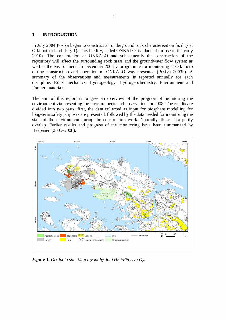
In July 2004 Posiva began to construct an underground rock characterisation facility at
Olkiluoto Island (Fig. 1). This facility, called ONKALO, is planned for use in the early
2010s. The construction of ONKALO and subsequently the construction of the
repository will affect the surrounding rock mass and the groundwater flow system as
well as the environment. In December 2003, a programme for monitoring at Olkiluoto
during construction and operation of ONKALO was presented (Posiva 2003b). A
summary of the observations and measurements is reported annually for each
discipline: Rock mechanics, Hydrogeology, Hydrogeochemistry, Environment and
Foreign materials.
The aim of this report is to give an overview of the progress of monitoring the
environment via presenting the measurements and observations in 2008. The results are
divided into two parts: first, the data collected as input for biosphere modelling for
long-term safety purposes are presented, followed by the data needed for monitoring the
state of the environment during the construction work. Naturally, these data partly
overlap. Earlier results and progress of the monitoring have been summarised by
Haapanen (2005–2008).
Figure 1. Olkiluoto site. Map layout by Jani Helin/Posiva Oy.


2 MONITORING SYSTEM AND SCHEDULE
The environmental monitoring system is described in Posiva Report 2003-05 (Posiva
2003b). Refinements to the system have been done based on experiences, and reported
in the specific Working Reports, as well as in previous summary reports on
environmental monitoring (Haapanen 2005–2008). The current environmental
monitoring schedule is presented in Table 1. Further changes will be applied according
to experiences from modelling work and increasing knowledge of most important site
data. For example, in addition to the originally planned activities, in 2008 several
studies on fauna were carried out, some soil and vegetation transects running from land
to sea were established, a separate survey of water quality with automatic detectors was
carried out and zooplankton and organic carbon studies were started in the context of
sea monitoring. Concerning the intensively monitored forest plots (FIP), soil properties
and biomass and chemical composition of ground vegetation and organic layer were
studied in 2007–2008.
Part of the monitoring is performed by the company running the nuclear power plants
on the island, Teollisuuden Voima Oy (TVO). TVO's radionuclide sampling system is
comprehensively described by Ikonen (2003) and Roivainen (2005) and TVO's marine
environment monitoring system, for example, by Ikonen et al. (2003). Monitoring has
been carried out for varying periods of time depending on the sector: while some
monitoring activities (performed by TVO) originate from the 1970s, the repository-
related environmental monitoring of the Olkiluoto Island has only recently been
comprehensive.
Major points of the monitoring design as well as maps of monitoring locations are
mainly presented at the beginning of each Sub-section. A list of monitoring locations is
presented in Appendix A. More specific details of the comprehensive forest and mire
monitoring system are presented in Appendix C.
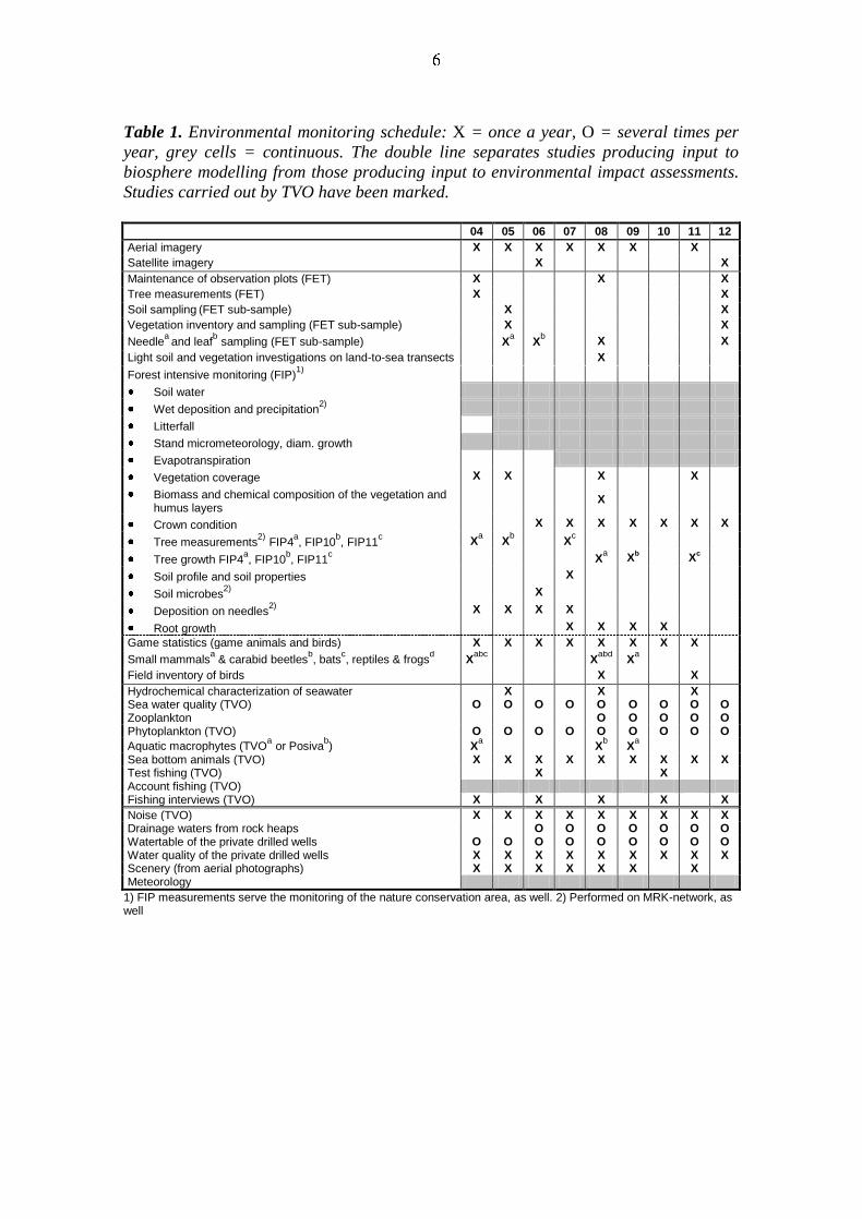
Table 1. Environmental monitoring schedule: X = once a year, O = several times per
year, grey cells = continuous. The double line separates studies producing input to
biosphere modelling from those producing input to environmental impact assessments.
Studies carried out by TVO have been marked.
04 05 06 07 08 09 10 11 12
Aerial imagery X X X X X X X
Satellite imagery X X
Maintenance of observation plots (FET) X X X
Tree measurements (FET) X X
Soil sampling (FET sub-sample) X X
Vegetation inventory and sampling (FET sub-sample) X X
Needlea
and leafb sampling (FET sub-sample) X
a X
b X X
Light soil and vegetation investigations on land-to-sea transects X
Forest intensive monitoring (FIP)1)
Soil water
Wet deposition and precipitation2)
Litterfall
Stand micrometeorology, diam. growth
Evapotranspiration
Vegetation coverage X X X X
Biomass and chemical composition of the vegetation and humus layers
X
Crown condition X X X X X X X
Tree measurements2)
FIP4a, FIP10
b, FIP11
c X
a X
b X
c
Tree growth FIP4a, FIP10
b, FIP11
c X
a X
b X
c
Soil profile and soil properties X
Soil microbes2)
X
Deposition on needles2)
X X X X
Root growth X X X X
Game statistics (game animals and birds) X X X X X X X X
Small mammalsa & carabid beetles
b, bats
c, reptiles & frogs
d X
abc X
abd X
a
Field inventory of birds X X
Hydrochemical characterization of seawater X X X Sea water quality (TVO) O O O O O O O O O Zooplankton O O O O O Phytoplankton (TVO) O O O O O O O O O
Aquatic macrophytes (TVOa or Posiva
b) X
a X
b X
a
Sea bottom animals (TVO) X X X X X X X X X Test fishing (TVO) X X Account fishing (TVO) Fishing interviews (TVO) X X X X X
Noise (TVO) X X X X X X X X X Drainage waters from rock heaps O O O O O O O Watertable of the private drilled wells O O O O O O O O O Water quality of the private drilled wells X X X X X X X X X Scenery (from aerial photographs) X X X X X X X Meteorology
1) FIP measurements serve the monitoring of the nature conservation area, as well. 2) Performed on MRK-network, as well
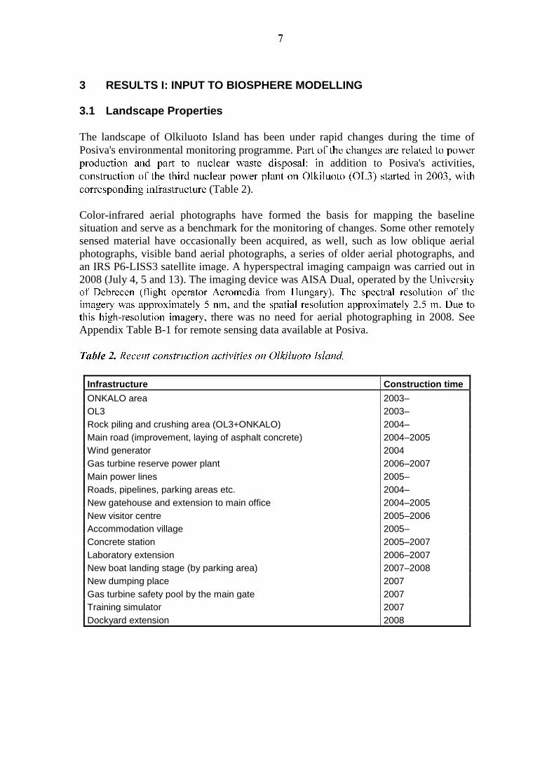
3 RESULTS I: INPUT TO BIOSPHERE MODELLING 3.1 Landscape Properties
The landscape of Olkiluoto Island has been under rapid changes during the time of
Posiva's environmental monitoring programme. P
n addition to Posiva's activities,
c
(Table 2).
Color-infrared aerial photographs have formed the basis for mapping the baseline
situation and serve as a benchmark for the monitoring of changes. Some other remotely
sensed material have occasionally been acquired, as well, such as low oblique aerial
photographs, visible band aerial photographs, a series of older aerial photographs, and
an IRS P6-LISS3 satellite image. A hyperspectral imaging campaign was carried out in
2008 (July 4, 5 and 13). The imaging device was AISA Dual, operated by the
here was no need for aerial photographing in 2008. See
Appendix Table B-1 for remote sensing data available at Posiva.
Infrastructure Construction time
ONKALO area 2003–
OL3 2003–
Rock piling and crushing area (OL3+ONKALO) 2004–
Main road (improvement, laying of asphalt concrete) 2004–2005
Wind generator 2004
Gas turbine reserve power plant 2006–2007
Main power lines 2005–
Roads, pipelines, parking areas etc. 2004–
New gatehouse and extension to main office 2004–2005
New visitor centre 2005–2006
Accommodation village 2005–
Concrete station 2005–2007
Laboratory extension 2006–2007
New boat landing stage (by parking area) 2007–2008
New dumping place 2007
Gas turbine safety pool by the main gate 2007
Training simulator 2007
Dockyard extension 2008
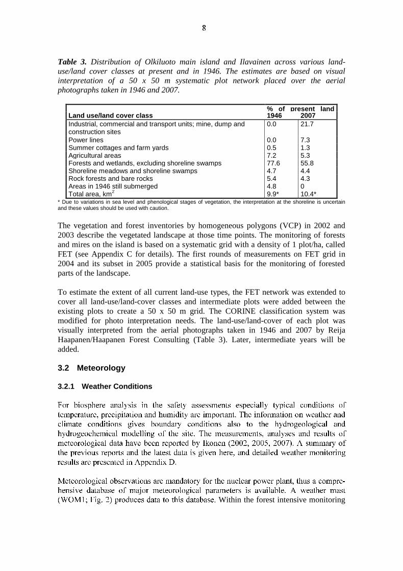
Table 3. Distribution of Olkiluoto main island and Ilavainen across various land-
use/land cover classes at present and in 1946. The estimates are based on visual
interpretation of a 50 x 50 m systematic plot network placed over the aerial
photographs taken in 1946 and 2007.
% of present land area Land use/land cover class 1946 2007
Industrial, commercial and transport units; mine, dump and construction sites
0.0 21.7
Power lines 0.0 7.3 Summer cottages and farm yards 0.5 1.3 Agricultural areas 7.2 5.3 Forests and wetlands, excluding shoreline swamps 77.6 55.8 Shoreline meadows and shoreline swamps 4.7 4.4 Rock forests and bare rocks 5.4 4.3 Areas in 1946 still submerged 4.8 0 Total area, km
2 9.9* 10.4*
* Due to variations in sea level and phenological stages of vegetation, the interpretation at the shoreline is uncertain and these values should be used with caution.
The vegetation and forest inventories by homogeneous polygons (VCP) in 2002 and
2003 describe the vegetated landscape at those time points. The monitoring of forests
and mires on the island is based on a systematic grid with a density of 1 plot/ha, called
FET (see Appendix C for details). The first rounds of measurements on FET grid in
2004 and its subset in 2005 provide a statistical basis for the monitoring of forested
parts of the landscape.
To estimate the extent of all current land-use types, the FET network was extended to
cover all land-use/land-cover classes and intermediate plots were added between the
existing plots to create a 50 x 50 m grid. The CORINE classification system was
modified for photo interpretation needs. The land-use/land-cover of each plot was
visually interpreted from the aerial photographs taken in 1946 and 2007 by Reija
Haapanen/Haapanen Forest Consulting (Table 3). Later, intermediate years will be
added.
3.2 Meteorology
3.2.1 Weather Conditions
Within the forest intensive monitoring
plots (FIP4, 10 and 11) meteorological measurements are recorded once an hour
(WOM2–4). The parameters are air temperature, minimum and maximum temperature
inside the crown layer and above the canopy (latter only on mast WOM2, which
reaches above the tree canopies), relative humidity, precipitation (1 m above ground
level), soil moisture content, and soil temperature. Photosynthetically active radiation
(PAR), solar radiation, air pressure, wind speed and its direction are measured only on
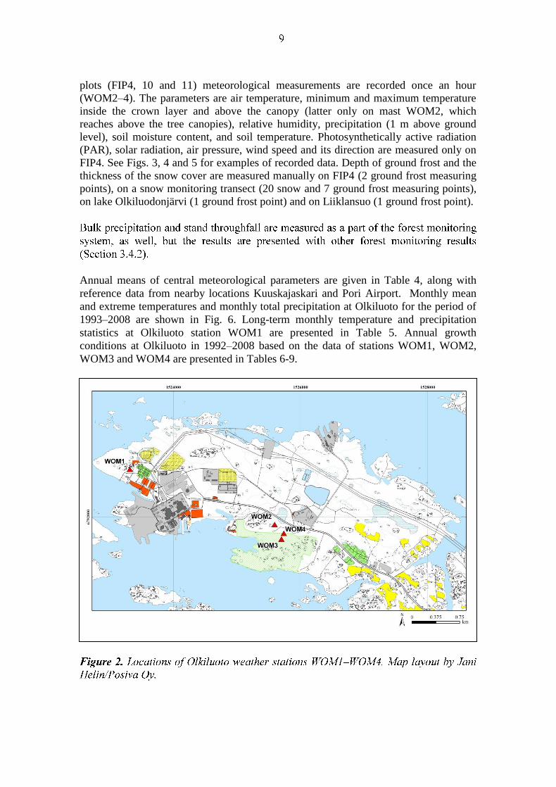
FIP4. See Figs. 3, 4 and 5 for examples of recorded data. Depth of ground frost and the
thickness of the snow cover are measured manually on FIP4 (2 ground frost measuring
points), on a snow monitoring transect (20 snow and 7 ground frost measuring points),
on lake Olkiluodonjärvi (1 ground frost point) and on Liiklansuo (1 ground frost point).
Annual means of central meteorological parameters are given in Table 4, along with
reference data from nearby locations Kuuskajaskari and Pori Airport. Monthly mean
and extreme temperatures and monthly total precipitation at Olkiluoto for the period of
1993–2008 are shown in Fig. 6. Long-term monthly temperature and precipitation
statistics at Olkiluoto station WOM1 are presented in Table 5. Annual growth
conditions at Olkiluoto in 1992–2008 based on the data of stations WOM1, WOM2,
WOM3 and WOM4 are presented in Tables 6-9.

Figure 4. Examples of data from meteorological measurements on FIP4, FIP10 and
FIP11: relative humidity at 2 m, %. Monthly averages between June 1, 2007 and
December 31, 2008.
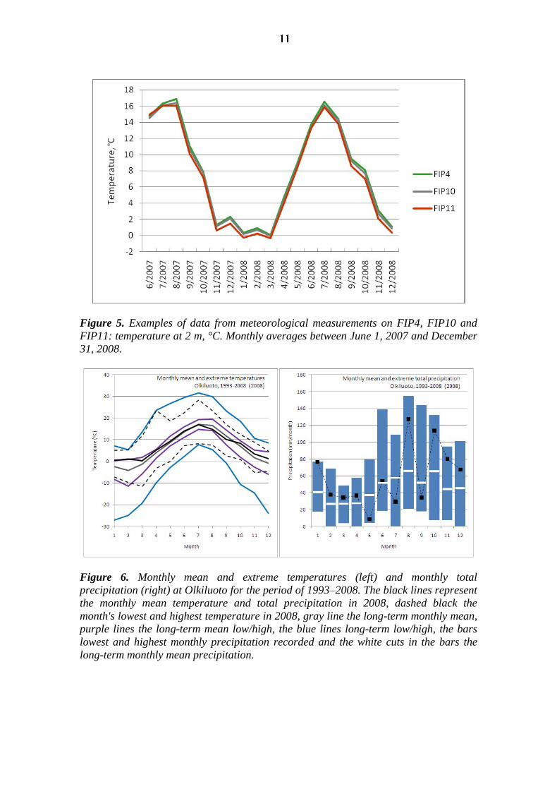
Figure 5. Examples of data from meteorological measurements on FIP4, FIP10 and
FIP11: temperature at 2 m, °C. Monthly averages between June 1, 2007 and December
31, 2008.
Figure 6. Monthly mean and extreme temperatures (left) and monthly total
precipitation (right) at Olkiluoto for the period of 1993–2008. The black lines represent
the monthly mean temperature and total precipitation in 2008, dashed black the
month's lowest and highest temperature in 2008, gray line the long-term monthly mean,
purple lines the long-term mean low/high, the blue lines long-term low/high, the bars
lowest and highest monthly precipitation recorded and the white cuts in the bars the
long-term monthly mean precipitation.
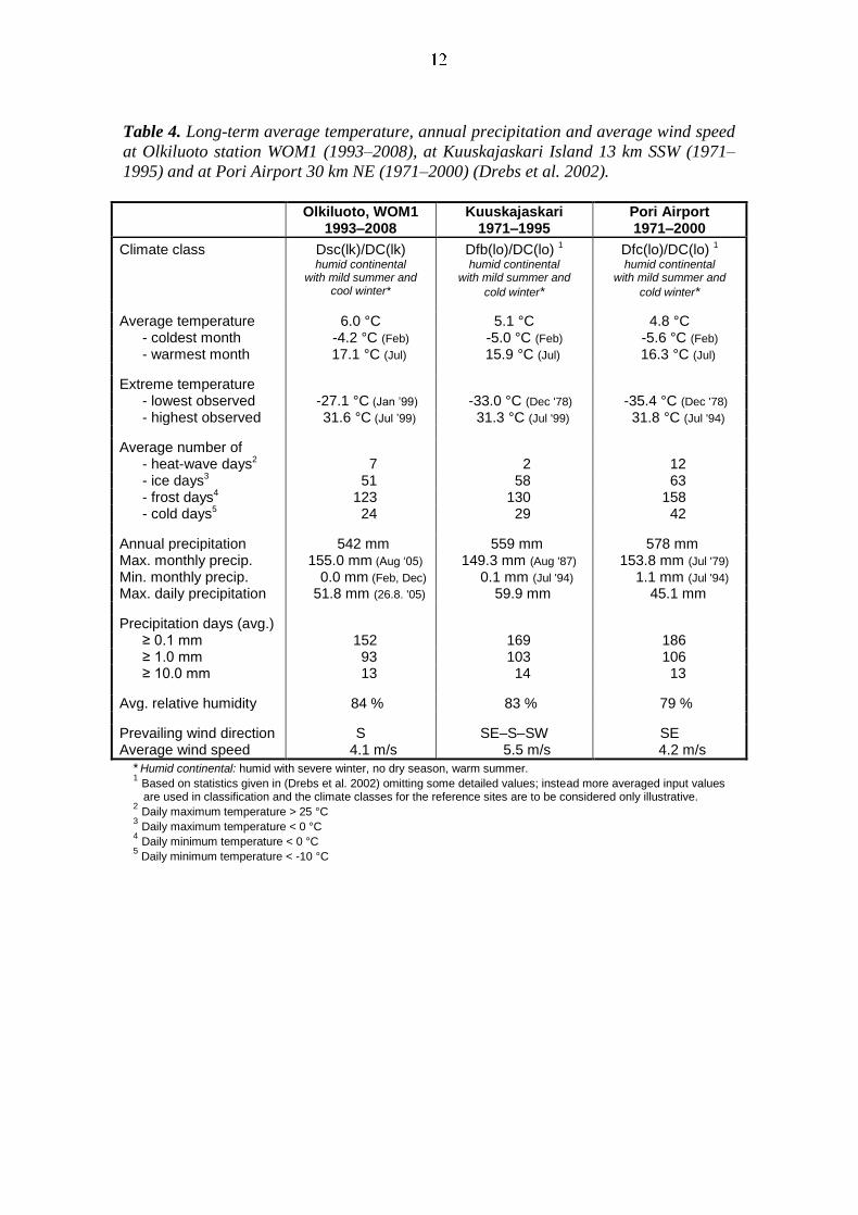
Table 4. Long-term average temperature, annual precipitation and average wind speed
at Olkiluoto station WOM1 (1993–2008), at Kuuskajaskari Island 13 km SSW (1971–
1995) and at Pori Airport 30 km NE (1971–2000) (Drebs et al. 2002).
Olkiluoto, WOM1
1993–2008 Kuuskajaskari
1971–1995 Pori Airport 1971–2000
Climate class Dsc(lk)/DC(lk) Dfb(lo)/DC(lo) 1 Dfc(lo)/DC(lo) 1 humid continental
with mild summer and cool winter*
humid continental with mild summer and
cold winter*
humid continental with mild summer and
cold winter*
Average temperature 6.0 °C 5.1 °C 4.8 °C - coldest month -4.2 °C (Feb) -5.0 °C (Feb) -5.6 °C (Feb) - warmest month 17.1 °C (Jul) 15.9 °C (Jul) 16.3 °C (Jul)
Extreme temperature - lowest observed -27.1 °C (Jan ’99) -33.0 °C (Dec '78) -35.4 °C (Dec '78) - highest observed 31.6 °C (Jul ’99) 31.3 °C (Jul '99) 31.8 °C (Jul '94)
Average number of - heat-wave days2 7 2 12 - ice days3 51 58 63 - frost days4 123 130 158 - cold days5 24 29 42
Annual precipitation 542 mm 559 mm 578 mm Max. monthly precip. 155.0 mm (Aug ‘05) 149.3 mm (Aug '87) 153.8 mm (Jul '79) Min. monthly precip. 0.0 mm (Feb, Dec) 0.1 mm (Jul '94) 1.1 mm (Jul '94) Max. daily precipitation 51.8 mm (26.8. '05) 59.9 mm 45.1 mm
Precipitation days (avg.) ≥ 0.1 mm 152 169 186 ≥ 1.0 mm 93 103 106 ≥ 10.0 mm 13 14 13
Avg. relative humidity 84 % 83 % 79 %
Prevailing wind direction S SE–S–SW SE Average wind speed 4.1 m/s 5.5 m/s 4.2 m/s
* Humid continental: humid with severe winter, no dry season, warm summer.
1 Based on statistics given in (Drebs et al. 2002) omitting some detailed values; instead more averaged input values are used in classification and the climate classes for the reference sites are to be considered only illustrative.
2 Daily maximum temperature > 25 °C
3 Daily maximum temperature < 0 °C
4 Daily minimum temperature < 0 °C
5 Daily minimum temperature < -10 °C
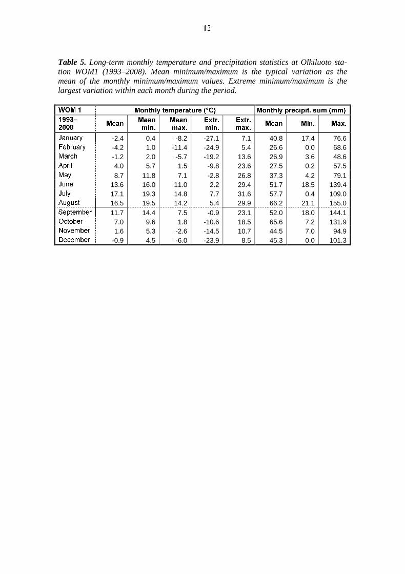
Table 5. Long-term monthly temperature and precipitation statistics at Olkiluoto sta-
tion WOM1 (1993–2008). Mean minimum/maximum is the typical variation as the
mean of the monthly minimum/maximum values. Extreme minimum/maximum is the
largest variation within each month during the period.
-2.4 0.4 -8.2 -27.1 7.1 40.8 17.4 76.6
-4.2 1.0 -11.4 -24.9 5.4 26.6 0.0 68.6
-1.2 2.0 -5.7 -19.2 13.6 26.9 3.6 48.6
4.0 5.7 1.5 -9.8 23.6 27.5 0.2 57.5
8.7 11.8 7.1 -2.8 26.8 37.3 4.2 79.1
13.6 16.0 11.0 2.2 29.4 51.7 18.5 139.4
17.1 19.3 14.8 7.7 31.6 57.7 0.4 109.0
16.5 19.5 14.2 5.4 29.9 66.2 21.1 155.0
11.7 14.4 7.5 -0.9 23.1 52.0 18.0 144.1
7.0 9.6 1.8 -10.6 18.5 65.6 7.2 131.9
1.6 5.3 -2.6 -14.5 10.7 44.5 7.0 94.9
-0.9 4.5 -6.0 -23.9 8.5 45.3 0.0 101.3
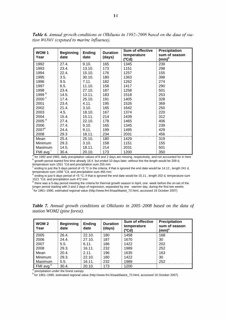
WOM 1 Year
Beginning date
Ending date
Duration (days)
Sum of effective temperature (ºCd)
Precipitation sum of season (mm)
a
1992 27.4. 9.10. 165 1345 239 1993 23.4. 13.10. 173 1151 298 1994 22.4. 15.10. 176 1257 155 1995 3.5. 30.10. 180 1363 398 1996 9.5. 7.11. 182 1262 274 1997 6.5. 11.10. 158 1417 290 1998 23.4. 27.10. 187 1258 501 1999
b 14.5. 13.11. 183 1518 253
2000 c 17.4. 25.10. 191 1405 328
2001 23.4. 4.11. 195 1526 369 2002 21.4. 3.10. 165 1642 250 2003 4.5. 18.10. 167 1374 220 2004 15.4. 15.11. 214 1439 312 2005
d 27.4. 22.10. 178 1465 406
2006 27.4. 9.10. 165 1345 239 2007
e 24.4. 9.11. 199 1495 429
2008 29.3 18.11. 234 2031 456
Mean 25.4. 25.10. 180 1429 319 Minimum 29.3. 3.10. 158 1151 155 Maximum 14.5. 18.11. 214 2031 501
FMI avg f 30.4. 20.10. 173 1200 350
a for 1992 and 1993, daily precipitation values of 8 and 2 days are missing, respectively, and not accounted for in here
b growth period started first time already 18.4. but ended 10 days later; without this the length would be 209 d,
temperature sum 1551 °Cd and precipitation sum 255 mm c ending to just the 5 days period of <5 °C in the criteria; if that is ignored the end date would be 14.12., length 241 d,
temperature sum 1458 °Cd, and precipitation sum 465 mm d ending to just 6 days period of <5 °C; if that is ignored the end date would be 15.11., length 202 d, temperature sum
1521 °Cd, and precipitation sum 472 mm e there was a 5-day period meeting the criteria for thermal growth season in April, one week before the on-set of the
longer period starting with 3 and 2 days of regression, separated by one warmer day, during the first two weeks f for 1961–1990, estimated regional value (http://www.fmi.fi/saa/tilastot_72.html, accessed 16 October 2007)
Table 7. Annual growth conditions at Olkiluoto in 2005–2008 based on the data of
station WOM2 (pine forest).
WOM 2 Year
Beginning date
Ending date
Duration (days)
Sum of effective temperature (ºCd)
Precipitation sum of season (mm)a
2005 26.4. 22.10. 180 1458 168 2006 24.4. 27.10. 187 1670 30 2007 5.5. 6.11. 186 1422 202 2008 29.3. 16.11. 232 1989 252
Mean 20.4. 2.11. 196 1635 163 Minimum 29.3. 22.10. 180 1422 30 Maximum 5.5. 16.11. 232 1989 252
FMI avg b 30.4. 20.10. 173 1200
a precipitation under the forest canopy
b for 1961–1990, estimated regional value (http://www.fmi.fi/saa/tilastot_72.html, accessed 16 October 2007)
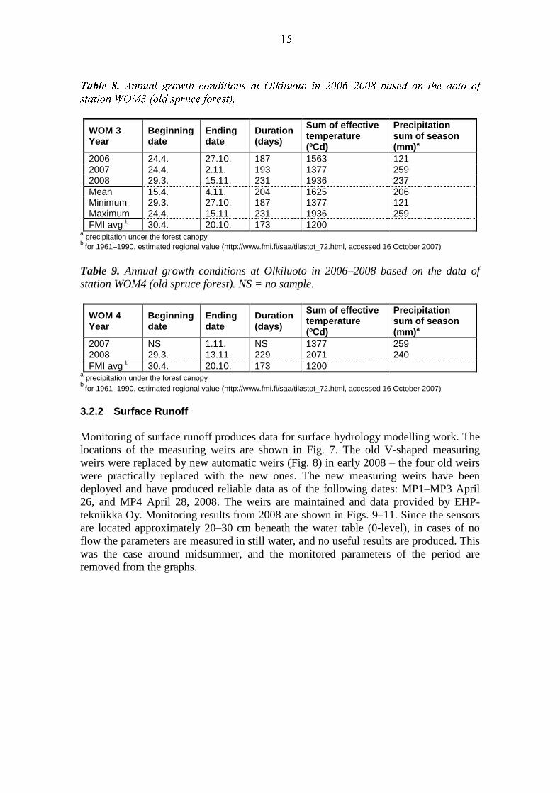
WOM 3 Year
Beginning date
Ending date
Duration (days)
Sum of effective temperature (ºCd)
Precipitation sum of season (mm)a
2006 24.4. 27.10. 187 1563 121 2007 24.4. 2.11. 193 1377 259 2008 29.3. 15.11. 231 1936 237
Mean 15.4. 4.11. 204 1625 206 Minimum 29.3. 27.10. 187 1377 121 Maximum 24.4. 15.11. 231 1936 259
FMI avg b 30.4. 20.10. 173 1200 a precipitation under the forest canopy
b for 1961–1990, estimated regional value (http://www.fmi.fi/saa/tilastot_72.html, accessed 16 October 2007)
Table 9. Annual growth conditions at Olkiluoto in 2006–2008 based on the data of
station WOM4 (old spruce forest). NS = no sample.
WOM 4 Year
Beginning date
Ending date
Duration (days)
Sum of effective temperature (ºCd)
Precipitation sum of season (mm)a
2007 NS 1.11. NS 1377 259 2008 29.3. 13.11. 229 2071 240
FMI avg b 30.4. 20.10. 173 1200 a precipitation under the forest canopy
b for 1961–1990, estimated regional value (http://www.fmi.fi/saa/tilastot_72.html, accessed 16 October 2007)
3.2.2 Surface Runoff
Monitoring of surface runoff produces data for surface hydrology modelling work. The
locations of the measuring weirs are shown in Fig. 7. The old V-shaped measuring
weirs were replaced by new automatic weirs (Fig. 8) in early 2008 – the four old weirs
were practically replaced with the new ones. The new measuring weirs have been
deployed and have produced reliable data as of the following dates: MP1–MP3 April
26, and MP4 April 28, 2008. The weirs are maintained and data provided by EHP-
tekniikka Oy. Monitoring results from 2008 are shown in Figs. 9–11. Since the sensors
are located approximately 20–30 cm beneath the water table (0-level), in cases of no
flow the parameters are measured in still water, and no useful results are produced. This
was the case around midsummer, and the monitored parameters of the period are
removed from the graphs.
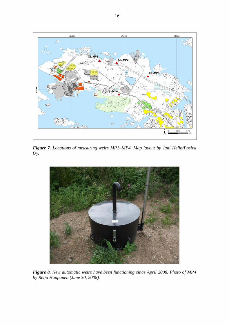
Figure 7. Locations of measuring weirs MP1–MP4. Map layout by Jani Helin/Posiva
Oy.
Figure 8. New automatic weirs have been functioning since April 2008. Photo of MP4
by Reija Haapanen (June 30, 2008).
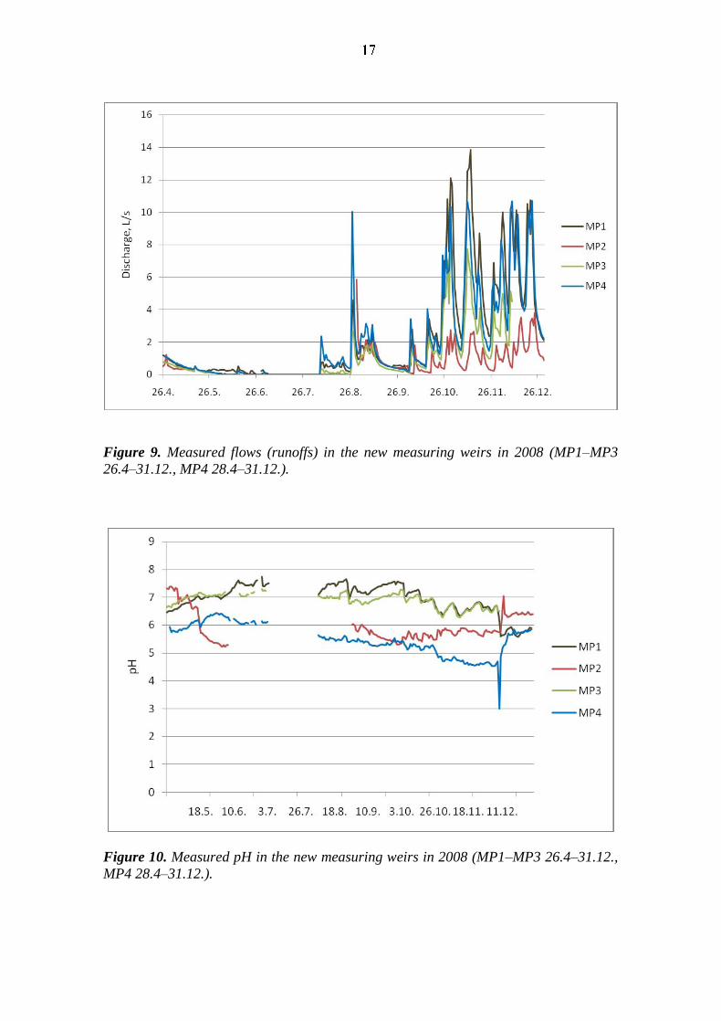
Figure 9. Measured flows (runoffs) in the new measuring weirs in 2008 (MP1–MP3
26.4–31.12., MP4 28.4–31.12.).
Figure 10. Measured pH in the new measuring weirs in 2008 (MP1–MP3 26.4–31.12.,
MP4 28.4–31.12.).
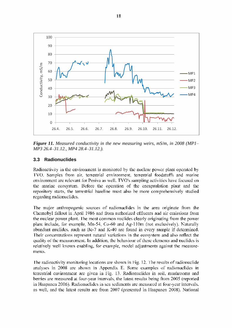
Figure 11. Measured conductivity in the new measuring weirs, mS/m, in 2008 (MP1–
MP3 26.4–31.12., MP4 28.4–31.12.).
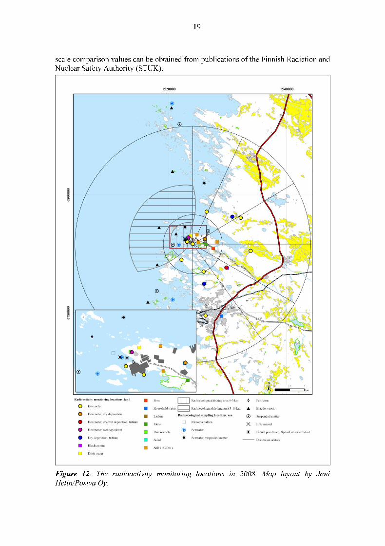
3.3 Radionuclides
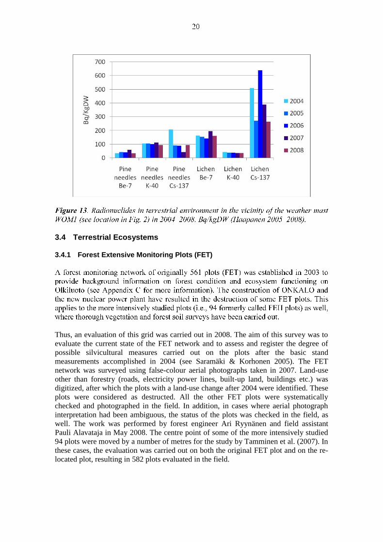
3.4 Terrestrial Ecosystems
3.4.1 Forest Extensive Monitoring Plots (FET)
Thus, an evaluation of this grid was carried out in 2008. The aim of this survey was to
evaluate the current state of the FET network and to assess and register the degree of
possible silvicultural measures carried out on the plots after the basic stand
measurements accomplished in 2004 (see Saramäki & Korhonen 2005). The FET
network was surveyed using false-colour aerial photographs taken in 2007. Land-use
other than forestry (roads, electricity power lines, built-up land, buildings etc.) was
digitized, after which the plots with a land-use change after 2004 were identified. These
plots were considered as destructed. All the other FET plots were systematically
checked and photographed in the field. In addition, in cases where aerial photograph
interpretation had been ambiguous, the status of the plots was checked in the field, as
well. The work was performed by forest engineer Ari Ryynänen and field assistant
Pauli Alavataja in May 2008. The centre point of some of the more intensively studied
94 plots were moved by a number of metres for the study by Tamminen et al. (2007). In
these cases, the evaluation was carried out on both the original FET plot and on the re-
located plot, resulting in 582 plots evaluated in the field.
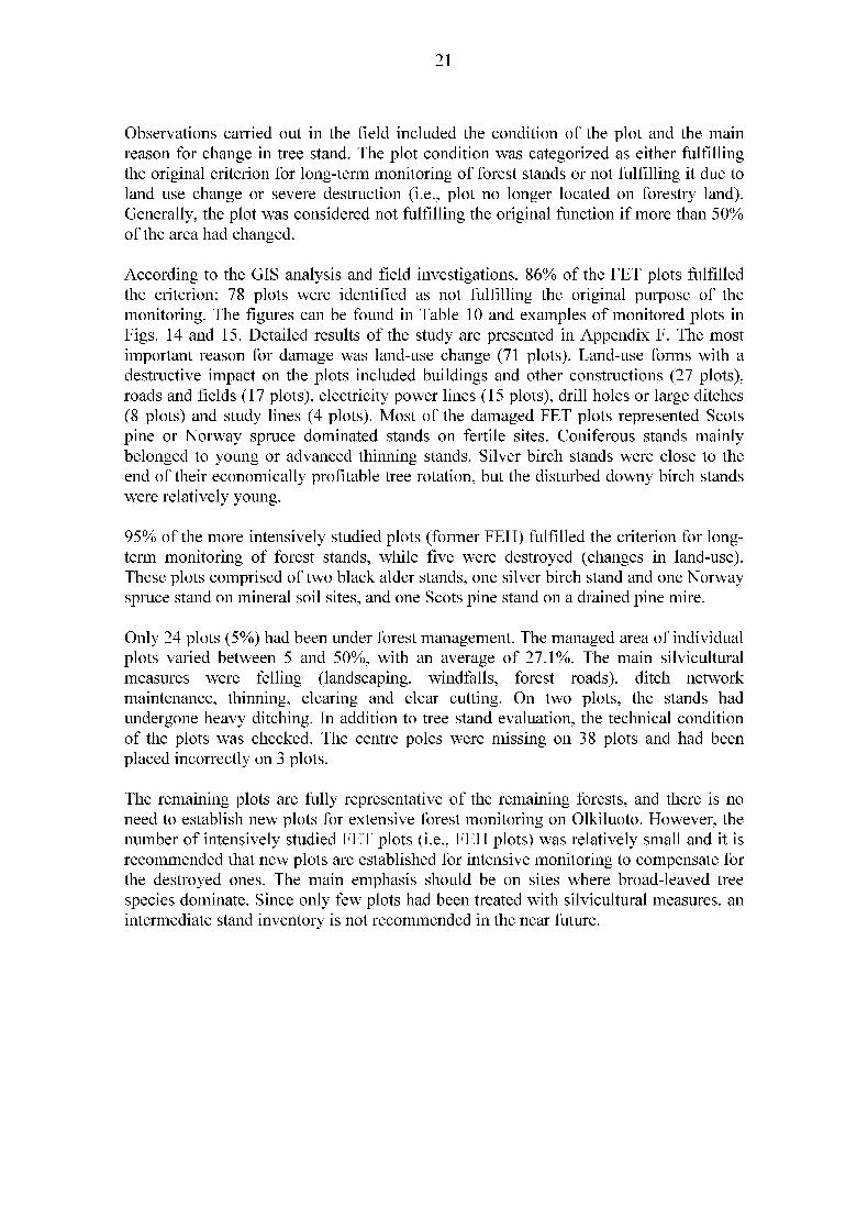
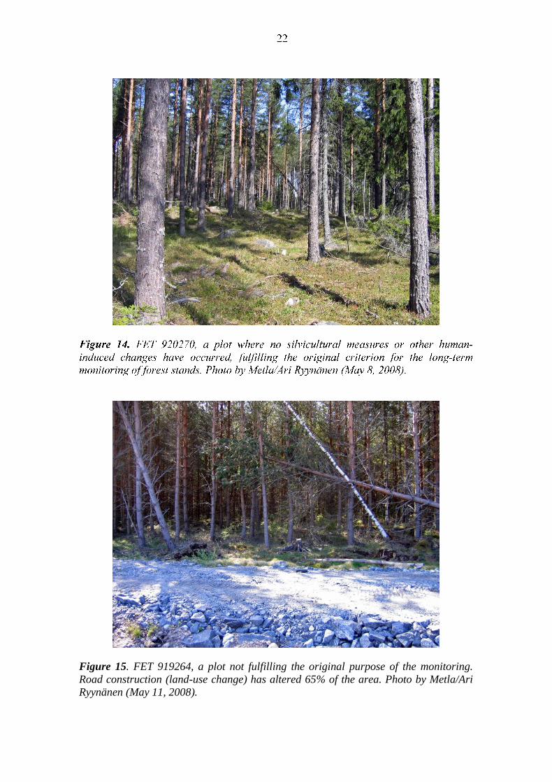
Figure 15. FET 919264, a plot not fulfilling the original purpose of the monitoring.
Road construction (land-use change) has altered 65% of the area. Photo by Metla/Ari
Ryynänen (May 11, 2008).
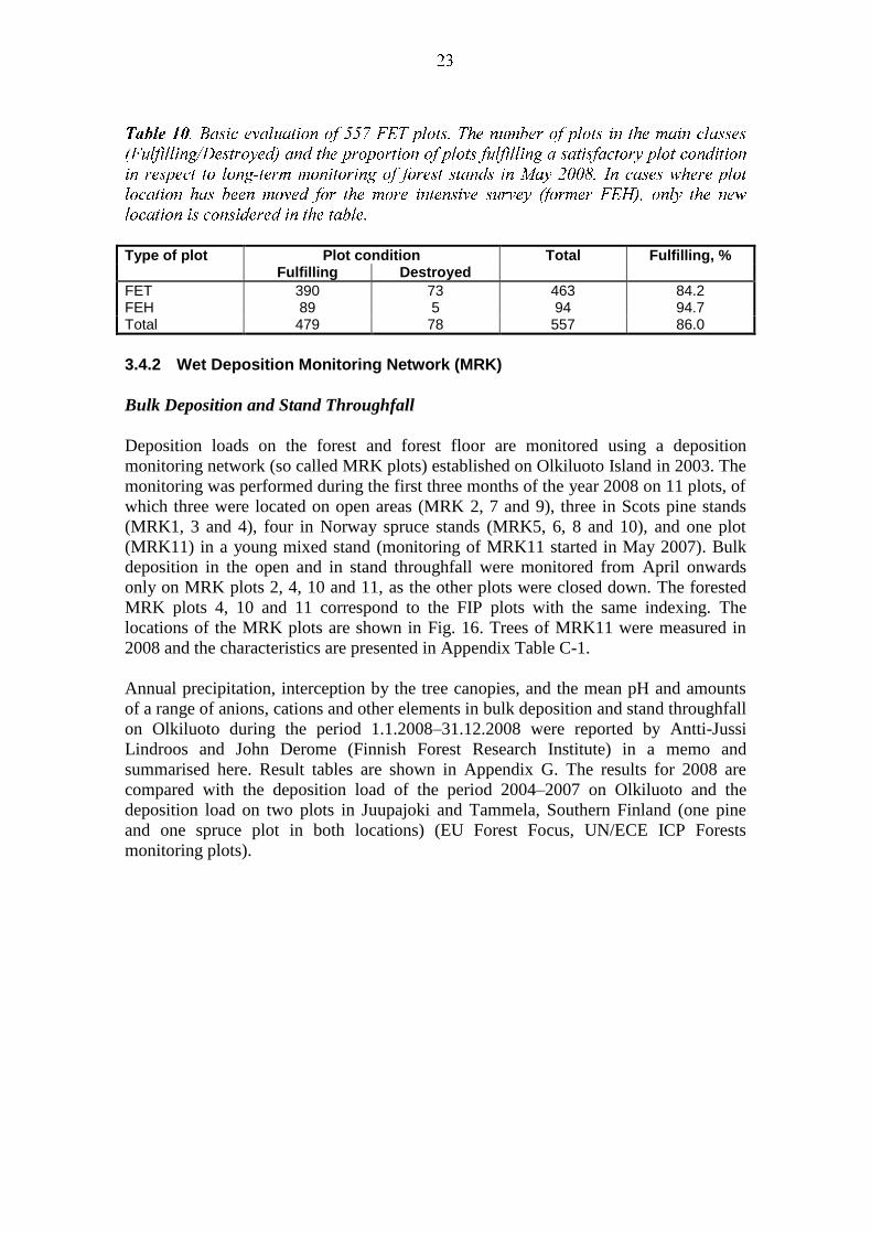
Type of plot Plot condition Total Fulfilling, % Fulfilling Destroyed
FET 390 73 463 84.2 FEH 89 5 94 94.7 Total 479 78 557 86.0
3.4.2 Wet Deposition Monitoring Network (MRK)
Bulk Deposition and Stand Throughfall
Deposition loads on the forest and forest floor are monitored using a deposition
monitoring network (so called MRK plots) established on Olkiluoto Island in 2003. The
monitoring was performed during the first three months of the year 2008 on 11 plots, of
which three were located on open areas (MRK 2, 7 and 9), three in Scots pine stands
(MRK1, 3 and 4), four in Norway spruce stands (MRK5, 6, 8 and 10), and one plot
(MRK11) in a young mixed stand (monitoring of MRK11 started in May 2007). Bulk
deposition in the open and in stand throughfall were monitored from April onwards
only on MRK plots 2, 4, 10 and 11, as the other plots were closed down. The forested
MRK plots 4, 10 and 11 correspond to the FIP plots with the same indexing. The
locations of the MRK plots are shown in Fig. 16. Trees of MRK11 were measured in
2008 and the characteristics are presented in Appendix Table C-1.
Annual precipitation, interception by the tree canopies, and the mean pH and amounts
of a range of anions, cations and other elements in bulk deposition and stand throughfall
on Olkiluoto during the period 1.1.2008–31.12.2008 were reported by Antti-Jussi
Lindroos and John Derome (Finnish Forest Research Institute) in a memo and
summarised here. Result tables are shown in Appendix G. The results for 2008 are
compared with the deposition load of the period 2004–2007 on Olkiluoto and the
deposition load on two plots in Juupajoki and Tammela, Southern Finland (one pine
and one spruce plot in both locations) (EU Forest Focus, UN/ECE ICP Forests
monitoring plots).

Figure 16. Location of MRK plots. Note that only four of them are used in wet
deposition monitoring from April 2008 onwards, but all forested locations (FIP11
excluded) are subject to needle sampling and analyses (see Section 4.1 later). "FIP"
stands for Forest Intensive monitoring Plot and FIPs contain MRKs with respective
index, e.g., FIP4=MRK4.
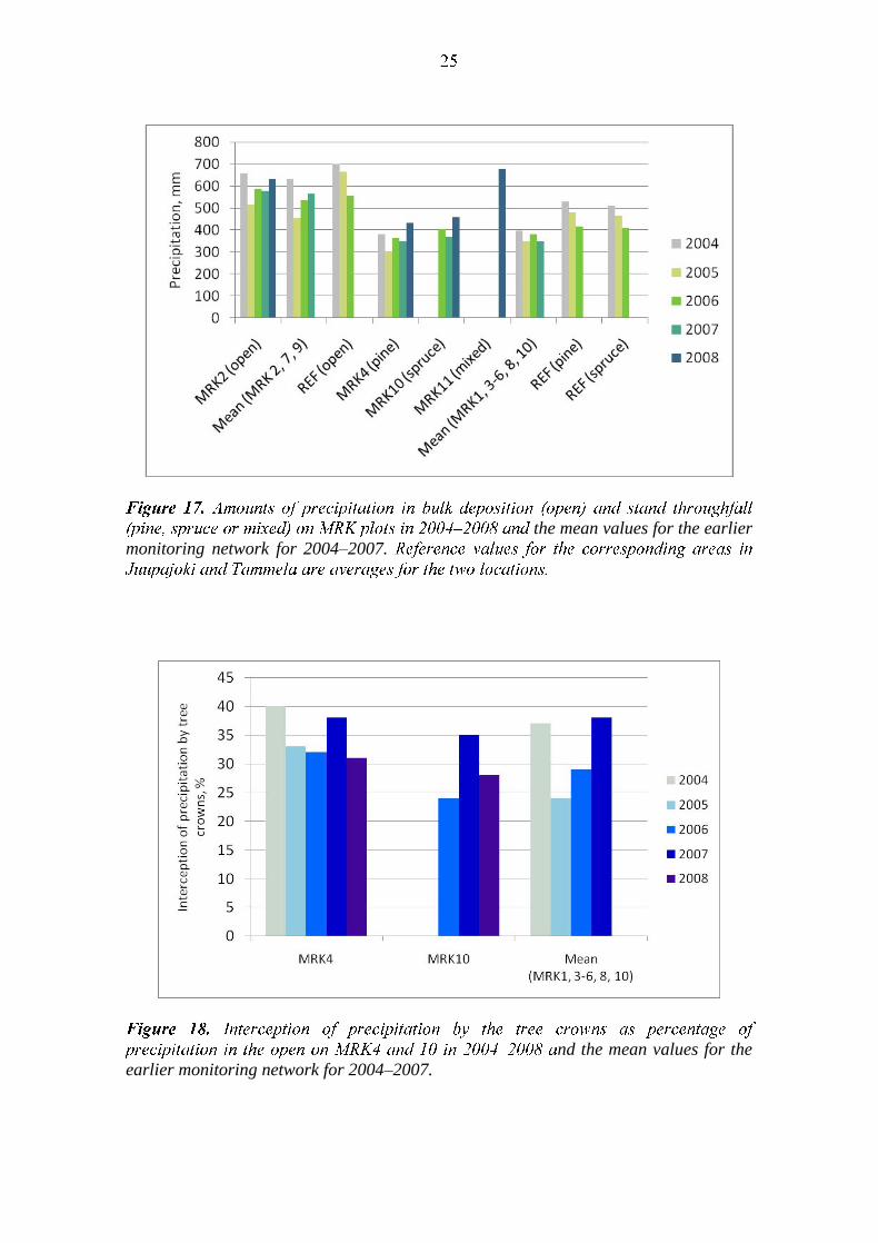
In 2008, the amount of precipitation on the open area (bulk deposition) plot MRK2 was
higher than during 2005–2007, but at a similar level as in 2004. This was partly due to
the high amounts of precipitation during the autumn months. The amounts of
precipitation in stand throughfall in 2008 on the Scots pine plot (MRK4) and the
Norway spruce plot (MRK10) were relatively similar and clearly lower than that
measured in bulk deposition in the open area (MRK2). This was also the case during
earlier years (Fig. 17, Table G-1). Although the canopy layer and forest structure have
an important effect on the amount of water reaching the forest floor in stand
throughfall, the amount of precipitation above the canopy (equivalent to the amount
measured in the open area) is the most important factor regulating the amount of water
passing to the forest floor in Finnish conditions. The effect of the tree canopy layer was
reflected in the interception values (precipitation in the open minus that in the stand)
and the values were relatively similar on the pine and spruce plots (Fig. 18, Table G-2).
The effect of the tree canopy on the amount of stand throughfall seemed to be
insignificant in the young stand (MRK11), because the amount of precipitation was
similar or even higher to that measured on MRK2 in the open area.
the mean values for the earlier
monitoring network for 2004–2007.
nd the mean values for the
earlier monitoring network for 2004–2007.
the mean values for the earlier monitoring network for
2004–2007.
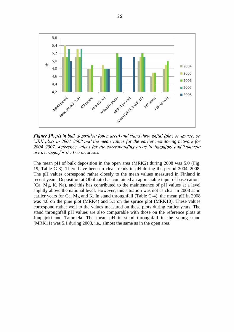
The mean pH of bulk deposition in the open area (MRK2) during 2008 was 5.0 (Fig.
19, Table G-3). There have been no clear trends in pH during the period 2004–2008.
The pH values correspond rather closely to the mean values measured in Finland in
recent years. Deposition at Olkiluoto has contained an appreciable input of base cations
(Ca, Mg, K, Na), and this has contributed to the maintenance of pH values at a level
slightly above the national level. However, this situation was not as clear in 2008 as in
earlier years for Ca, Mg and K. In stand throughfall (Table G-4), the mean pH in 2008
was 4.8 on the pine plot (MRK4) and 5.1 on the spruce plot (MRK10). These values
correspond rather well to the values measured on these plots during earlier years. The
stand throughfall pH values are also comparable with those on the reference plots at
Juupajoki and Tammela. The mean pH in stand throughfall in the young stand
(MRK11) was 5.1 during 2008, i.e., almost the same as in the open area.
the mean values for the earlier
monitoring network for 2004–2007.
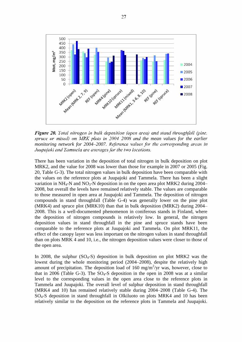
There has been variation in the deposition of total nitrogen in bulk deposition on plot
MRK2, and the value for 2008 was lower than those for example in 2007 or 2005 (Fig.
20, Table G-3). The total nitrogen values in bulk deposition have been comparable with
the values on the reference plots at Juupajoki and Tammela. There has been a slight
variation in NH4-N and NO3-N deposition in on the open area plot MRK2 during 2004–
2008, but overall the levels have remained relatively stable. The values are comparable
to those measured in open area at Juupajoki and Tammela. The deposition of nitrogen
compounds in stand throughfall (Table G-4) was generally lower on the pine plot
(MRK4) and spruce plot (MRK10) than that in bulk deposition (MRK2) during 2004–
2008. This is a well-documented phenomenon in coniferous stands in Finland, where
the deposition of nitrogen compounds is relatively low. In general, the nitrogen
deposition values in stand throughfall in the pine and spruce stands have been
comparable to the reference plots at Juupajoki and Tammela. On plot MRK11, the
effect of the canopy layer was less important on the nitrogen values in stand throughfall
than on plots MRK 4 and 10, i.e., the nitrogen deposition values were closer to those of
the open area.
In 2008, the sulphur (SO4-S) deposition in bulk deposition on plot MRK2 was the
lowest during the whole monitoring period (2004–2008), despite the relatively high
amount of precipitation. The deposition load of 160 mg/m2/yr was, however, close to
that in 2006 (Table G-3). The SO4-S deposition in the open in 2008 was at a similar
level to the corresponding values in the open area close to the reference plots in
Tammela and Juupajoki. The overall level of sulphur deposition in stand throughfall
(MRK4 and 10) has remained relatively stable during 2004–2008 (Table G-4). The
SO4-S deposition in stand throughfall in Olkiluoto on plots MRK4 and 10 has been
relatively similar to the deposition on the reference plots in Tammela and Juupajoki.

However, the stand throughfall deposition at the Tammela spruce plot has been clearly
higher than in Olkiluoto or Juupajoki. Sulphate deposition was clearly higher in stand
throughfall than in bulk deposition due to the wash-off of dry deposition from the tree
canopies. Sulphate deposition in stand throughfall is considered to rather well represent
the total deposition of sulphate from the atmosphere on forest ecosystems. In 2008, the
SO4-S deposition values in stand throughfall were very similar on plots MRK4 and 10
and higher than on plot MRK11 (young mixed stand).
The deposition of base cations (Ca, Mg, K) in bulk deposition on plot MRK2 in 2008
was somewhat higher or at a similar level compared with the situation on the reference
plots at Tammela and Juupajoki (Table G-3). Na deposition was higher than the
reference values. The deposition of base cations in bulk deposition and stand
throughfall has varied slightly during 2004–2008 (Table G-4). The relatively high
deposition of Cl (with associated Na) at Olkiluoto is due to the proximity of the sea,
which was also seen in the results for 2004–2008. The higher values for base cations
and chloride in stand throughfall are due to the leaching and wash-off of dry deposition
in the tree canopies.
The deposition of Al, Fe, Mn and Si in bulk precipitation and stand throughfall were
relatively similar in 2008 to the values in earlier years (Tables G-5 and G-6). The PO4
deposition was higher in 2008 than in earlier years both in bulk deposition (MRK2) and
in stand throughfall (MRK 4 and 10). Also the Cu and Zn deposition values in stand
throughfall were higher in 2008 than in earlier years on plot MRK4, but at the same
level as earlier on plots MRK2 and 10.
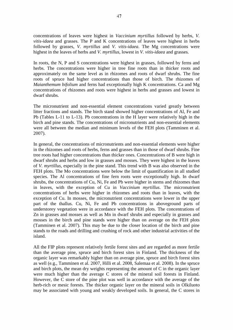
Needles
Spruce and pine needles have been collected annually from the same sample plots from
2003 to 2007 (wintertime, i.e., turn of 2003/04, 2004/2005 etc) in order to follow
changes in the foliar element concentrations. These dust deposition results are presented
in Section 4.1, but the analyses serve the biosphere modelling, as well. Result tables are
presented in Appendix H.
3.4.3 Forest Intensive Monitoring Plots (FIP)
Results of the soil solution monitoring in 2004–2008 were originally reported by John
Derome (Finnish Forest Research Institute) in a memo and are summarised below. The
result tables can be found in Appendix I.
On FIP4, the samples have been obtained on almost all sampling occasions during the
monitoring period (at ca. four week intervals). The suction-cup lysimeters provided
samples on seven sampling occasions from 24.5. to 7.11.2005, on five occasions from
23.5. to 2.11.2006, on 7 occasions from 29.5. to 12.11.2007 and on six occasions from
24.6.2008 to 10.11.2008. In July 2006, no samples were obtained because precipitation
was only 1.6 mm. On FIP10, the plate lysimeters installed at a depth of 5 cm yielded
samples only on two occasions in 2005 (5.8. and 6.9.), on five occasions in 2006 (from
19.6. to 2.11.), on all 7 sampling occasions in 2007 (from 29.5. to 12.11) and 2008
(from 24.6. to 10.11). There were considerable problems with the lysimeters in June–
July 2006 and May–June 2007 on this plot: the high water table made sampling almost
impossible because many of the sampling points were under water. On the new plot,
FIP11, the lysimeters were installed in autumn 2006, but the collection started on June
1, 2007, and the collection of percolation water samples covered the whole snow-free
period for the first time in 2008. The results obtained in 2007, or even in 2008 cannot
yet be considered to be fully representative of the site. The soil is always disturbed to
some extent during lysimeter installation. Furthermore, clear-cutting a few years
(approximately 10) earlier has resulted in the mineralisation of plant nutrients following
the removal of the original tree cover. Clear-cutting usually results in higher
temperatures in the organic layer (due to the absence of shading by the tree canopy),
which promotes the microbial activity and mineralisation. The cutting residues,
produced in connection with clear-cutting, also represent a considerable input of
mineral nutrients.
The amounts of percolation water passing down to a depth of 5 cm during the snow-free
period in FIP4 are presented in Fig. 21 and Table I-1. The proportion of percolation
water passing down to a depth of 5 cm on this plot varied between 15 to 23% of the
input to the forest floor (stand throughfall) during 2004–2008. Variation between the
individual years was not related to the total amount of stand throughfall during the soil
water collection period. However, the amounts of percolation water and throughfall
during the collection period were at their lowest in the same year (2006) and also at
their highest in the same year (2004). There was considerable variation in the amount of
percolation water between the sampling dates due primarily to the varying amounts of
stand throughfall. The amounts were especially low after snowmelt in the latter half of
May and the first half of June in 2004, and in July and August in 2006.
The amounts of percolation water passing down to a depth of 5 cm during the snow-free
period in FIP10 are presented in Fig. 22 and Table I-2. In 2005 the lysimeters did not
function correctly and the results for this year are only indicative. In 2006, when
sampling covered the whole snow-free period, the proportion of percolation water
passing down to a depth of 5 cm was ca. 7%. However, the actual amount was most
probably much higher because samples could not be obtained in June and early July
owing to the fact that the groundwater table/sea level was above the ground surface on
part of the plot. The water table was high in 2007, as well. In 2007, the proportion of
percolation water passing down to a depth of 5 cm was ca. 23%. On this plot the
proportion of percolation water has increased every year from 2005 to 2008,
presumably due to the fact that the problems with the lysimeters in 2005 and 2006 have
now been partly overcome and they are functioning correctly.
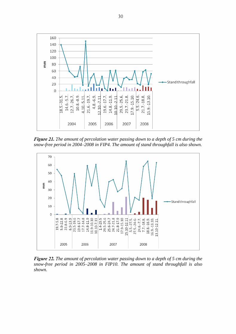
he amount of percolation water passing down to a depth of 5 cm during the
snow-free period in 2004–2008 in FIP4. The amount of stand throughfall is also shown.
he amount of percolation water passing down to a depth of 5 cm during the
snow-free period in 2005–2008 in FIP10. The amount of stand throughfall is also
shown.

Figure 23. The amount of percolation water passing down to a depth of 5 cm during the
snow-free period in 2008 in FIP11. The amount of stand throughfall is also shown. The
collection of percolation water started on this plot in spring 2007, but due to low values
(0.2–0.4 mm), the results of 2007 are not shown here.
The amounts of percolation water passing down to a depth of 5 cm during the snow-free
period in FIP11 are presented in Fig. 23 and Table I-3. The collection of percolation
water on this plot started on June 1, 2007. The amount of water passing down through
the organic layer on this plot in 2007 was extremely low, and in 2008 lower than that on
the other two plots, presumably due to the highly effective interception of rainwater and
strong rate of evapo-transpiration by the abundant ground vegetation and dense sapling
stand on this plot.
The chemical composition of the soil solution during the snow-free period in the plots
was compared with corresponding values in a Scots pine (FIP4, FIP11) or Norway
spruce (FIP10) stand growing on a site of similar fertility (Tammela, period 1998–2000,
depths of 5, 20 and 40 cm). However, since the plot FIP11 has been clear cut a few (ca.
10) years earlier, the results are not fully comparable with the middle-aged pure stand
used as an approximate reference site.
In FIP4, the pH of the soil solution clearly increased with increasing depth. The pH of
the soil solution at depths of 5, 20 and 30 cm remained relatively constant throughout
the 5-year monitoring period (Fig. 24, Table I-4). In contrast, there was a large variation
at a depth of 10 cm in 2006 and 2007. Otherwise the pH values at all depths were fully
comparable to a site of similar fertility at Tammela. In FIP10, The pH of the soil
solution at all depths in 2005 and 2006 was considerably higher than that in the
reference stand at Tammela, growing on a site of similar site type (Fig. 25, Table I-14).
However, the pH at 5 cm in 2007 had dropped to the value close to that of the reference
site. There was an extremely high increase in pH at 30 cm depth in 2008. The main
reason for this overall trend is that the soil at Olkiluoto is considerably younger than at
Tammela, and therefore contains much higher concentrations of base cations (Ca, Mg,
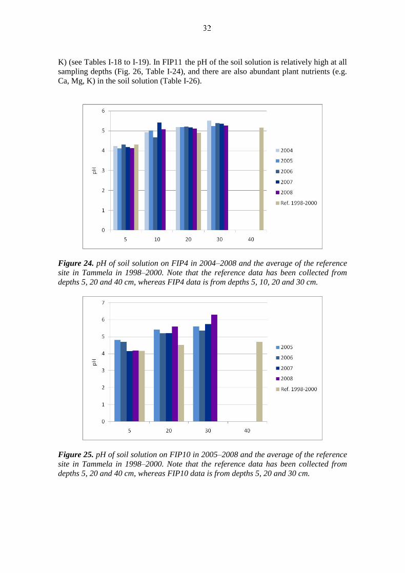
K) (see Tables I-18 to I-19). In FIP11 the pH of the soil solution is relatively high at all
sampling depths (Fig. 26, Table I-24), and there are also abundant plant nutrients (e.g.
Ca, Mg, K) in the soil solution (Table I-26).
Figure 24. pH of soil solution on FIP4 in 2004–2008 and the average of the reference
site in Tammela in 1998–2000. Note that the reference data has been collected from
depths 5, 20 and 40 cm, whereas FIP4 data is from depths 5, 10, 20 and 30 cm.
Figure 25. pH of soil solution on FIP10 in 2005–2008 and the average of the reference
site in Tammela in 1998–2000. Note that the reference data has been collected from
depths 5, 20 and 40 cm, whereas FIP10 data is from depths 5, 20 and 30 cm.
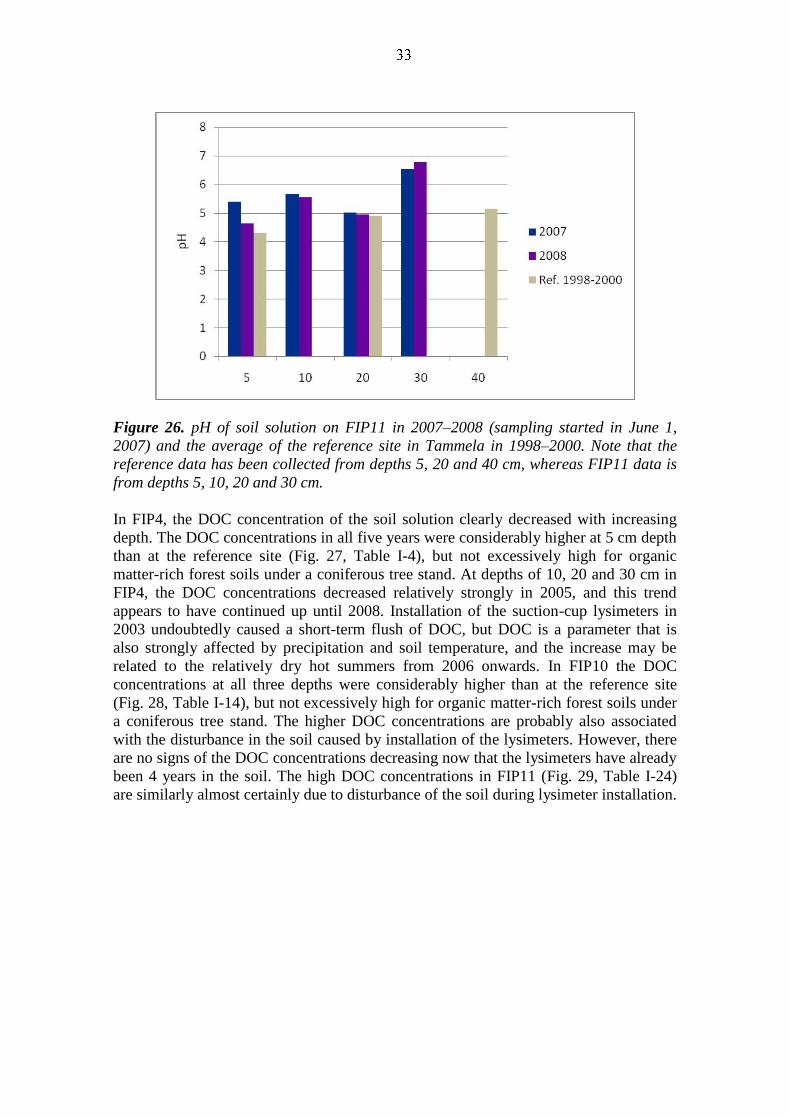
Figure 26. pH of soil solution on FIP11 in 2007–2008 (sampling started in June 1,
2007) and the average of the reference site in Tammela in 1998–2000. Note that the
reference data has been collected from depths 5, 20 and 40 cm, whereas FIP11 data is
from depths 5, 10, 20 and 30 cm.
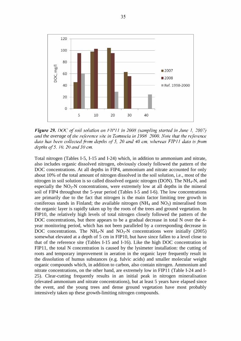
In FIP4, the DOC concentration of the soil solution clearly decreased with increasing
depth. The DOC concentrations in all five years were considerably higher at 5 cm depth
than at the reference site (Fig. 27, Table I-4), but not excessively high for organic
matter-rich forest soils under a coniferous tree stand. At depths of 10, 20 and 30 cm in
FIP4, the DOC concentrations decreased relatively strongly in 2005, and this trend
appears to have continued up until 2008. Installation of the suction-cup lysimeters in
2003 undoubtedly caused a short-term flush of DOC, but DOC is a parameter that is
also strongly affected by precipitation and soil temperature, and the increase may be
related to the relatively dry hot summers from 2006 onwards. In FIP10 the DOC
concentrations at all three depths were considerably higher than at the reference site
(Fig. 28, Table I-14), but not excessively high for organic matter-rich forest soils under
a coniferous tree stand. The higher DOC concentrations are probably also associated
with the disturbance in the soil caused by installation of the lysimeters. However, there
are no signs of the DOC concentrations decreasing now that the lysimeters have already
been 4 years in the soil. The high DOC concentrations in FIP11 (Fig. 29, Table I-24)
are similarly almost certainly due to disturbance of the soil during lysimeter installation.

the average of
the average of
the average of
Total nitrogen (Tables I-5, I-15 and I-24) which, in addition to ammonium and nitrate,
also includes organic dissolved nitrogen, obviously closely followed the pattern of the
DOC concentrations. At all depths in FIP4, ammonium and nitrate accounted for only
about 10% of the total amount of nitrogen dissolved in the soil solution, i.e., most of the
nitrogen in soil solution is so called dissolved organic nitrogen (DON). The NH4-N, and
especially the NO3-N concentrations, were extremely low at all depths in the mineral
soil of FIP4 throughout the 5-year period (Tables I-5 and I-6). The low concentrations
are primarily due to the fact that nitrogen is the main factor limiting tree growth in
coniferous stands in Finland; the available nitrogen (NH4 and NO3) mineralised from
the organic layer is rapidly taken up by the roots of the trees and ground vegetation. In
FIP10, the relatively high levels of total nitrogen closely followed the pattern of the
DOC concentrations, but there appears to be a gradual decrease in total N over the 4-
year monitoring period, which has not been paralleled by a corresponding decrease in
DOC concentrations. The NH4-N and NO3-N concentrations were initially (2005)
somewhat elevated at a depth of 5 cm in FIP10, but have since fallen to a level close to
that of the reference site (Tables I-15 and I-16). Like the high DOC concentration in
FIP11, the total N concentration is caused by the lysimeter installation: the cutting of
roots and temporary improvement in aeration in the organic layer frequently result in
the dissolution of humus substances (e.g. fulvic acids) and smaller molecular weight
organic compounds which, in addition to carbon, also contain nitrogen. Ammonium and
nitrate concentrations, on the other hand, are extremely low in FIP11 (Table I-24 and I-
25). Clear-cutting frequently results in an initial peak in nitrogen mineralisation
(elevated ammonium and nitrate concentrations), but at least 5 years have elapsed since
the event, and the young trees and dense ground vegetation have most probably
intensively taken up these growth-limiting nitrogen compounds.
In FIP4, sulphate concentrations at 5 cm depth (Table I-6) were considerably lower in
all five years than those at the reference site but relatively similar at other depths.
Sulphate concentrations of FIP10 were approximately the same as those for the
reference site at 5 cm depth (Table I-16). In both FIP4 and FIP10, there was a clear
increase in sulphate concentrations with increasing depth. Similar trends in the sulphate
concentration have been reported at all the ICP Forests Level II plots in Finland
(Derome et al. 2007).
Chloride concentrations were high at all depths throughout the monitoring period in
FIP4 and FIP10. Similarly in FIP11, Na and Cl concentrations are high, which is typical
of the area due to the close proximity of the Baltic Sea. Chloride concentrations at 5 cm
depth showed a considerable increase over the first three years in FIP4, but decreased in
2007 and 2008. Phosphate concentrations were extremely low in all five years in FIP4.
Phosphate concentrations were at approximately normal levels in FIP10. Phosphate
concentrations are very low in soil solution on most forested sites in Finland (Derome
et al. 2007). See Tables I-7, I-17 and I-25 for monitoring results.
The concentrations of the three important plant nutrients (Ca, Mg, K) were relatively
elevated in FIP4, especially in the mineral soil (10, 20 and 30 cm) at the start of the
monitoring period in 2004 (Tables I-8 and I-9). Since then, the concentrations in the
mineral soil have fallen and are now approaching the levels for the reference site. This
suggests that there has been a short-term flush of these nutrients following the
installation of the lysimeters (as for DOC). There was a clear peak in the K
concentration below the organic layer (at 5 cm depth) in 2006. The concentrations of
Na at all depths continued to be elevated, due to the proximity of the sea. In FIP10, the
concentrations of Ca, Mg and K were strongly elevated at all depths in the soil during
2005–2008 (Tables I-18 and I-19). The soil at the spruce plot is very young, and
weathering processes in the mineral soil will be relatively strong and release abundant
amounts of these three nutrients. The high concentrations of Na at all depths are due to
both the input from the sea and the weathering of minerals.
The concentrations of total Al at all depths in FIP4 were relatively similar in all five
years (Table I-10), and higher than the values for the reference site at depths of 10–30
cm. The concentration of Al3+
, which is a form of Al toxic to plant roots and
mycorrhizas, was still extremely low at 5 cm depth, but considerably higher at other
depths compared to the reference site. However, the concentrations are still much lower
than the widely accepted toxicity level of 2 mg/l. In FIP10, the total Al concentrations
were lower at 5 cm depth, but the Al3+
(Table I-20) and Mn concentrations (Table I-21)
were relatively similar to the reference values at all depths.
The Fe concentrations showed considerable year-to-year variation in FIP4 (Table I-11),
and remained higher at depths of 10–30 cm than at the reference site. The Si
concentrations at depths of 5 and 10 cm during 2005–2008 were considerably higher
than the corresponding values in 2004 (Table I-12), and higher than the corresponding
concentrations at the reference site. Similarly, in FIP10, the concentrations of Fe and Si
were strongly elevated at depths of 20 and 30 cm (Table I-22). The high silicon values
in FIP10 are undoubtedly due to the young age of the soil: silicon plays an important
role in soil-forming processes (podzolisation) under coniferous tree species. In FIP11,
elements associated with soil-forming processes (e.g. Al, Fe, Si) are present in
relatively high concentrations, but this is to be expected because the intensive uptake of
nutrients (and corresponding release of protons) by the roots of the young stand and
dense ground vegetation result in an increase in the dissolution of these elements
through the weathering of soil minerals (the overburden on Olkiluoto Island is very
young).
The Cu concentrations at all depths of FIP10 and at the reference site were below the
limit of quantification of the analytical instrument. The same was true for FIP4 and the
reference site, except the depth of 10 cm in 2005 in Olkiluoto (Table I-23). In FIP4 the
Zn concentrations were relatively constant, and higher than the reference values
throughout the monitoring period (Table I-13). In FIP10, the Zn concentrations were
also slightly higher than the reference (Table I-23). In FIP11 the manganese
concentrations are extremely low (Table I-28).
The concentrations of heavy metals at all depths in FIP4 were below the limit of
quantification during 2004–2008. In FIP10, nickel concentrations at 20 and 30 cm were
slightly elevated in 2005 and 2007. This is a relatively common finding in soils that
have developed from marine sediments. The Ni is derived from the bedrock in the
region and not a sign of pollution from industrial sources.

Table 11. Particle size distribution (µm) in the 10–60 cm soil layer by plot. Percentage
of the median particle size class is shown in boldface.
Cumulative percentage
Soil texture class Layer (cm) ≤2 ≤6 ≤20 ≤63 ≤200 ≤632
FIP4 10–30 0.5 1.7 4.0 9.7 24.0 58.9 sand
30–60 4.4 9.7 21.9 52.7 93.3 99.2 sandy loam
FIP10 10–30 2.0 5.1 10.4 21.4 38.3 71.3 loamy sand
30–60 1.0 2.1 4.8 16.3 62.7 96.1 loamy sand
FIP11 10–30 11.9 27.2 40.6 44.8 49.3 65.6 sandy loam
30–60 32.1 73.5 96.9 100.0 100.0 100.0 silty clay loam
Table 12. Mean thickness (cm) of the organic layer by organic layer type.
Organic layer type Mor Moder Peat Mull-like peat Total cm n cm n cm n cm n cm n
FIP4 4.4 44 6.0 1 4.4 45 FIP10 7.5 15 10.7 30 9.6 45 FIP11 6.7 17 9.2 6 12.0 1 7.5 24
1
PEAT 19.1 15 152
13*8 = 24 sub-samples from the upland site
23*5 = 15 sub-samples from the peatland site
–

–

stands. N = 6 soil cores (Helmisaari et al. 2009).
Scots pine and Norway spruce fine roots were mostly in the upper 15 cm soil layer,
whereas the depth distribution of birch fine roots was more superficial. Site fertility and
stoniness clearly affected the depthwise fine root distribution. The proportion of finest
roots (< 1 mm in diameter) out of the total biomass of fine roots was 55±11% in the
organic layer and 0–30 cm mineral soil layer. The biomass of understorey fine roots
was highest in the young birch stand FIP11. The mass of dead roots and rhizomes was
less than 10% of all roots and rhizomes in all stands. Most of the understorey fine roots
and rhizomes were in the organic layer in the conifer stands FIP4 and FIP10, and in
deeper soil layers in FIP11, probably because birch roots were mostly in the upper 0–5
cm. The share of the finest roots increased in the deeper soil layers (Helmisaari et al.
2009).
Mean ectomycorrhizal short root tip frequency (number of fine roots < 1 mm in
diameter/mg) was 7.4±2.8 for birch, 3.5±1.2 for pine and 3.7±0.7 for spruce. There
were no clear differences in the root tip frequency between soil layers. The EcM root tip
number per m2
in the upper 20 cm was 806,559±370,411/m2 for birch, 384 494±76,583
/m2 for pine and 1,027,960±564,909/m
2 for spruce (Helmisaari et al. 2009).
The installed root monitoring tubes were photographed; altogether 3,392 images were
taken during the growing season. The field vegetation around the tubes was recorded on
August 14 2008. The fine roots were analysed for their length and mean diameter by
manual tracing on digital images. Images were viewed as a time sequence, and the dates
of appearance and disappearance were recorded. Fine root elongation and longevity will
be reported later, as all fine roots born in the growing season 2008 continue to live in
the growing season 2009 (Helmisaari et al. 2009).
0
100
200
300
400
500
Birch Pine Spruce
Live < 2 mm
Dead < 2 mm
FIP4 FIP10 FIP11
Species Roots Root tips Roots
Root tips Roots
Root tips
Birch
0.23 (±0.02)
0.22 (±0.02)
Pine 0.35
(±0.03) 0.34
(±0.04)
Spruce
0.28 (±0.04)
0.27 (±0.04)
Dwarf shrubs 0.22
(±0.07) 0.21
(±0.05) 0.19
(±0.03) 0.17
(±0.03) 0.22
(±0.06) 0.21
(±0.06)
Grasses and herbs 0.18
(±0.08) 0.14
(±0.07) 0.22
(±0.03) 0.21
(±0.02) 0.18
(±0.01) 0.18
(±0.01)
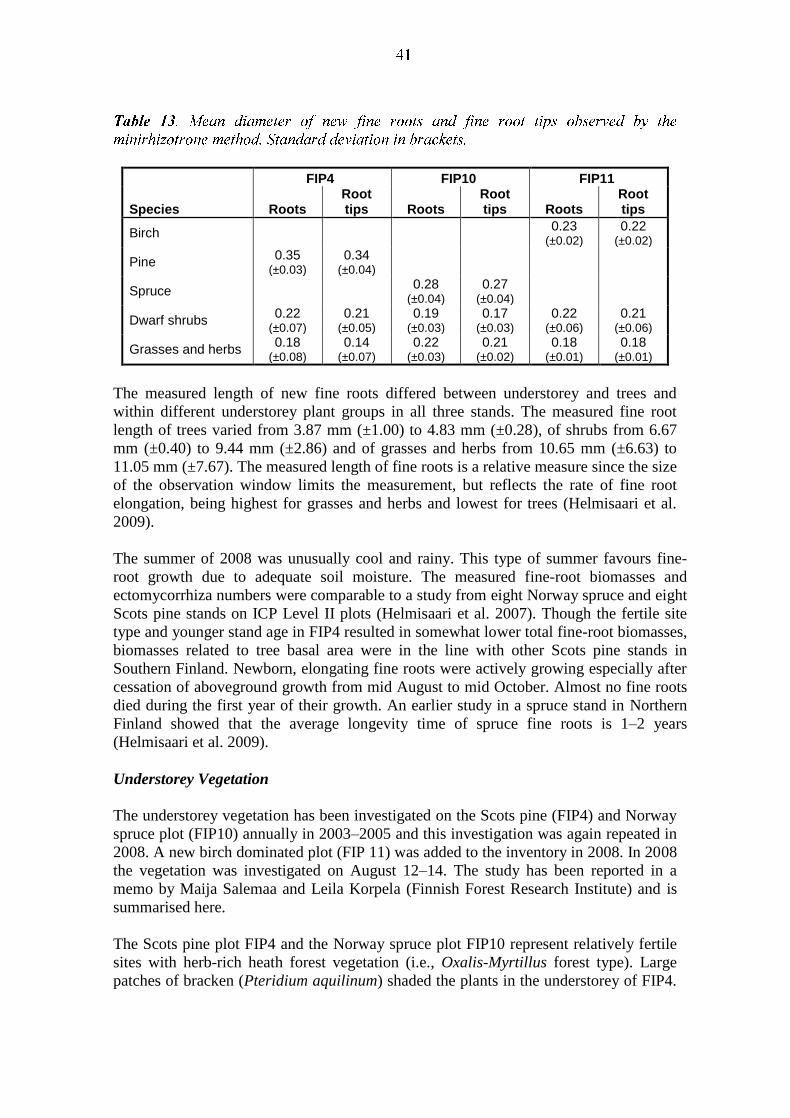
The measured length of new fine roots differed between understorey and trees and
within different understorey plant groups in all three stands. The measured fine root
length of trees varied from 3.87 mm (±1.00) to 4.83 mm (±0.28), of shrubs from 6.67
mm (±0.40) to 9.44 mm (±2.86) and of grasses and herbs from 10.65 mm (±6.63) to
11.05 mm (±7.67). The measured length of fine roots is a relative measure since the size
of the observation window limits the measurement, but reflects the rate of fine root
elongation, being highest for grasses and herbs and lowest for trees (Helmisaari et al.
2009).
The summer of 2008 was unusually cool and rainy. This type of summer favours fine-
root growth due to adequate soil moisture. The measured fine-root biomasses and
ectomycorrhiza numbers were comparable to a study from eight Norway spruce and eight
Scots pine stands on ICP Level II plots (Helmisaari et al. 2007). Though the fertile site
type and younger stand age in FIP4 resulted in somewhat lower total fine-root biomasses,
biomasses related to tree basal area were in the line with other Scots pine stands in
Southern Finland. Newborn, elongating fine roots were actively growing especially after
cessation of aboveground growth from mid August to mid October. Almost no fine roots
died during the first year of their growth. An earlier study in a spruce stand in Northern
Finland showed that the average longevity time of spruce fine roots is 1–2 years
(Helmisaari et al. 2009).
Understorey Vegetation
The understorey vegetation has been investigated on the Scots pine (FIP4) and Norway
spruce plot (FIP10) annually in 2003–2005 and this investigation was again repeated in
2008. A new birch dominated plot (FIP 11) was added to the inventory in 2008. In 2008
the vegetation was investigated on August 12–14. The study has been reported in a
memo by Maija Salemaa and Leila Korpela (Finnish Forest Research Institute) and is
summarised here.
The Scots pine plot FIP4 and the Norway spruce plot FIP10 represent relatively fertile
sites with herb-rich heath forest vegetation (i.e., Oxalis-Myrtillus forest type). Large
patches of bracken (Pteridium aquilinum) shaded the plants in the understorey of FIP4.
Grasses (Deschampsia flexuosa) grew in sunny openings. The number of vascular plant
species found in the shrub and field layers remained very stable in 2003–2008. The
number of moss species decreased slightly during the study period. There was variation
in the total cover of the field layer in the study years, mainly due to the decreased cover
of bracken in 2004. The cover of woody species has increased by about 10% units. The
cover of mosses has slightly decreased, but that of needle litter on the ground increased.
Browsing of elks has had an impact on the understorey vegetation. Forest road
construction in the vicinity has affected the illumination and moisture conditions in
FIP4.
The spruce plot FIP10 is relatively old, and a substantial amount of dead wood is lying
on the forest floor. The decomposing leaf litter of deciduous trees and coarse wood
debris offer suitable growing substrates for bryophyte and lichen species. Altogether 59
species were found in 2008. The total cover of the vascular plants has decreased from
42–45% in 2003–2005 to 24% in 2008. The cover of woody species has slightly
increased, whereas that of herbs and grasses has significantly decreased. The biggest
change was in the common wood sorrel (Oxalis acetosella), which decreased from 15%
in 2005 to 5% in 2008. This thin-leaved perennial herb suffers from draught and all
kinds of physical disturbances. The effects of the dry summer in 2006 may still be seen;
also, tree uprooting may have caused disturbance in the micro habitats of the species.
The birch dominated plot FIP11 is located on a rocky site and the vegetation
represented partly mesic heath forest vegetation (i.e. Myrtillus type) and partly herb-
rich heath vegetation. The plot was very dense and represented a young succession
phase. The average height of the birches was 2.7 m and their crowns covered 70–90%
of the area. The average cover of spruce (Picea abies) in the shrub layer was 2–3 %.
The most abundant vascular species in the field layer were a dwarf shrub Vaccinium
vitis-idaea, grasses Deschampsia flexuosa and Calamagrostis epigejos. Many herb,
grass and sedge species indicate that the site is fertile. A total of 66 species were found.
The open bedrock area in the middle of the sub-plot formed a dry and sunny
microhabitat rich in grass species.
The species as well the means and standard deviations of the cover percentage during
the study period 2003–2005 and 2008 are presented in Appendix K. The number of
species is shown in Fig. 31 and the cover percentages of vascular plants and needle
litter in Figs. 32 and 33, respectively.
Species occurrence has shown slight changes on the intensive spruce and pine
monitoring plots during 2003–2008. The number of vascular plant species has been
very similar across the years, but the number of bryophytes and lichens has varied. This
is partly dependent on the number of samples taken for microscopic identification. The
cover of woody species has slightly increased on both the spruce and pine plots,
indicating suitable weather conditions for the growth of dwarf shrubs. The cover of
herbs and grasses has been unchanged on the pine plot. On the other hand, the cover of
herbs has decreased significantly on the spruce plot from 2005 to 2008. In addition to
the dry summer of 2006, natural fluctuations may explain the changes. The change in
the cover of bryophytes often reflects the moisture condition and the amount of needle
litter. In addition to the anthropogenic impacts, the normal variation in weather

conditions and the shedding of needle litter on the ground affect the cover of plants. In
2004 the inventory was carried out in the middle of July, when the plants may not have
reached their maximum biomass. Weather conditions explain most of the annual
variation.

Biomass and Chemical Composition of the Vegetation and Humus Layers
A study on biomass and chemical composition of the vegetation and humus layers on
the intensive forest monitoring plots was conducted by Maija Salemaa and Leila
Korpela of the Finnish Forest Research Institute on August 13 and 14, 2008. The results
are summarised below, and tables of detailed data are presented in Appendix L.
The organic layer was sorted into forest floor litter (L horizon), fermentation horizon (F
horizon), humus (H horizon) and pieces of dead wood inside the humus layer. The
amount of aboveground litter (L layer) was higher in the spruce and birch stands than in
the pine stand (Table L-1), and relatively similar to that of the mesic forest intensive
monitoring spruce plots in Tammela and Punkaharju. The litter layer biomass of the
pine stand corresponded well with that of the sub-xeric pine plot of Juupajoki in
southern boreal region (Hilli et al. 2008). Woody litter formed the largest fraction of the
L layer in all the stands. Needle litter was abundant in the coniferous stands and dead
plant material and shed birch leaves in the birch stand. The average thickness of the
total organic layer was highest in the birch stand (9.8±0.50 cm); that of the spruce stand
was 8.1±0.5 cm and that of the pine stand 6.7±0.4 cm. The amount of organic matter
per area unit corresponded to the thickness of the organic layer. The average dry weight
of the total organic layer was higher in the birch (13,649 g/m2) and spruce (12,247
g/m2) stands than in the pine stand (4,366 g/m
2). The organic matter content was low in
the humus (H layer) of the pine stand. The amount of dead wood inside the organic
layer varied from 332 to 412 g/m2 in the stands.
The most abundant species groups in the aboveground vegetation were mosses in the
spruce stand, Vaccinium myrtillus in the pine stand and Vaccinium vitis-idaea in the
birch stand (Fig. 34). Grasses were relatively abundant on the pine and birch stands and
ferns were present on the spruce and pine stands. All stands had some lower herbs but
their biomass was low (Tables L-2–L-4). The total aboveground biomass was highest in
the birch stand and lowest in the spruce stand. The belowground biomass of the
vascular plant species (mosses excluded) was at least two times as high as the
aboveground biomass (Fig. 34). The results of the annual aboveground biomass
production analysis of the functional plant species groups in the understorey vegetation,
as expected. The production of aboveground biomass was highest in the youngest birch
stand plot with grasses and dwarf shrubs (Table L-5). This was in accordance with the
average biomass of the mesic and sub-xeric forests of whole country. The low amount
of the aboveground biomass on the old spruce stand corresponded to the mean amount
of aboveground biomass of herb-rich and mesic forest sites of the whole country
(Ilvesniemi et al. 2009). Mosses constitute the largest proportion (60%) of the annual
growth in the spruce stand, shrubs and grasses were significant in the pine and birch
stands. In addition, ferns showed a relatively substantial growth in the pine stand.
The total tree root biomass in the organic layer was highest in the spruce stand FIP10
(942 g/m2) and lowest in the pine stand FIP4 (100 g/m
2) (Table L-1). This was partly
due the fact that most pine fine roots were not separated from the humus layer. The
proportion of the fine roots (diameter < 2 mm) was low compared to the biomass of
thicker wooden roots. In the organic layer of the spruce stand, the belowground biomass
of the understorey plants was low compared to that of tree roots. In the pine stand, the
proportions were reversed, and in the birch stand the amounts of understorey and birch
root biomasses were similar.
The carbon and macronutrient concentrations of the organic layer were slightly higher
in the spruce stand than in the other stands, which indicates more fertile growing
conditions (Table L-6). The C/N ratio was highest in the F layer of the pine stand. There
were no significant differences in the macronutrient concentrations between the stands.
The spruce and birch stands had slightly higher concentrations than the pine stand.
Concentrations of N, P, K, Ca and Mg were higher in the F than in H layers, but the
opposite was true for S (Table L-5). Needle and leaf litter and dead plant material had
higher macronutrient concentrations than wood debris. On the grounds of N
concentration and C/N ratio the Olkiluoto FIP plots represent higher soil fertility than
the average Finnish forest sites (e.g., Salemaa et al. 2008) and also belong to the more
fertile sites among the plots studied on Olkiluoto (see Tamminen et al. 2007).

0
50
100
150
200
250
300
350
400
450
500
Spruce Pine Birch
Ab
ove
gro
un
d b
iom
ass: d
.w. g
/m 2
Mosses
Grasses
Ferns
Low herbs
Vacc myrt
Vacc viti
0
50
100
150
200
250
300
350
400
450
500
Be
low
gro
un
d b
iom
ass: d
.w. g
/m 2
Grasses
Ferns
Low herbs
Vacc myrt
Vacc viti
Figure 34. The mean (and standard error) aboveground living biomass (top graph) and
belowground total (living and dead) biomass (lower graph) g/m2 of the functional plant
species groups of the understorey vegetation. Only the upper part of mosses is included
into the aboveground biomass. Site fertility and tree stand volume decrease from left to
right.
The C concentrations of dwarf shrubs (50–53%) were slightly higher than those of the
other species groups (46–51%) (Tables L-8 to L-10). P concentrations of vascular
plants were highest in the birch stand. The macronutrient concentrations increased
towards the younger plant parts in dwarf shrubs and the upper parts in mosses (Tables
L-8 to L-10). In dwarf shrubs, the concentrations were higher in leaves than in stems,
and lowest in rhizomes and roots, with some exceptions. In general, the N, S and Ca
concentrations of leaves were highest in Vaccinium myrtillus followed by herbs, V.
vitis-idaea and grasses. The P and K concentrations of leaves were highest in herbs
followed by grasses, V. myrtillus and V. vitis-idaea. The Mg concentrations were
highest in the leaves of herbs and V. myrtillus, lowest in V. vitis-idaea and grasses.
In roots, the N, P and S concentrations were highest in grasses, followed by ferns and
herbs. The concentrations were higher in tree fine roots than in thicker roots and
approximately on the same level as in rhizomes and roots of dwarf shrubs. The fine
roots of spruce had higher concentrations than those of birch. The rhizomes of
Maianthemum bifolium and ferns had exceptionally high K concentrations. Ca and Mg
concentrations of rhizomes and roots were highest in herbs and grasses and lowest in
dwarf shrubs.
The micronutrient and non-essential element concentrations varied greatly between
litter fractions and stands. The birch stand showed higher concentrations of Al, Fe and
Pb (Tables L-11 to L-13). Pb concentrations in the H layer were relatively high in the
birch and pine stands. The concentrations of micronutrients and non-essential elements
were all between the median and minimum levels of the FEH plots (Tamminen et al.
2007).
In general, the concentrations of micronutrients and non-essential elements were higher
in the rhizomes and roots of herbs, ferns and grasses than in those of dwarf shrubs. Fine
tree roots had higher concentrations than thicker ones. Concentrations of B were high in
dwarf shrubs and herbs and low in grasses and mosses. They were highest in the leaves
of V. myrtillus, especially in the pine stand. This trend with B was also observed in the
FEH plots. The Mo concentrations were below the limit of quantification in all studied
species. The Al concentrations of fine fern roots were exceptionally high. In dwarf
shrubs, the concentrations of Cu, Ni, Fe and Pb were higher in stems and rhizomes than
in leaves, with the exception of Cu in Vaccinium myrtillus. The micronutrient
concentrations of herbs were higher in rhizomes and roots than in leaves, with the
exception of Cu. In mosses, the micronutrient concentrations were lower in the upper
part of the thallus. Cu, Ni, Fe and Pb concentrations in aboveground parts of
understorey vegetation were in accordance with the FEH plots. The concentrations of
Zn in grasses and mosses as well as Mn in dwarf shrubs and especially in grasses and
mosses in the birch and pine stands were higher than on average on the FEH plots
(Tamminen et al. 2007). This may be due to the closer location of the birch and pine
stands to the roads and drilling and crushing of rock and other industrial activities of the
island.
All the FIP plots represent relatively fertile forest sites and are regarded as more fertile
than the average pine, spruce and birch forest sites in Finland. The thickness of the
organic layer was remarkably higher than on average pine, spruce and birch forest sites
as well (e.g., Tamminen et al. 2007, Hilli et al. 2008, Salemaa et al. 2008). In the spruce
and birch plots, the mean dry weights representing the amount of C in the organic layer
were much higher than the average C stores of the mineral soil forests in Finland.
However, the C store of the pine plot was well in accordance with the average of the
herb-rich or mesic forests. The thicker organic layer on the mineral soils in Olkiluoto
may be associated with young and weakly developed soils. In general, the C stores in

the organic layer on mineral soils have been found to be highest in the Southwestern
part of Finland (Ilvesniemi et al. 2009, Tamminen et al. 2007). The C and nutrient
concentrations of tree roots followed those of dwarf shrubs and were in accordance with
the site fertility. There were no large differences between the stands in the C and
nutrient concentrations of the understorey vegetation, but the differences between
functional plant groups were clear. The carbon concentrations of dwarf-shrubs were
slightly higher than those of other species groups, and for example in evergreen leaves
of Vaccinium vitis-idaea higher than in the deciduous leaves of V. myrtillus. The C
concentrations of the understorey vegetation were in accordance with the previous
study of FEH plots. Overall, the mean nutrient concentrations of all the functional plant
groups were quite well in accordance with the herb-rich and mesic forests of Olkiluoto
FEH plots (Tamminen et al. 2007).
Litterfall
Litterfall collection was started on the plot FIP4 in summer 2004 and on the plot FIP10
in spring 2005. The results for 2004–2005 have been summarised by Haapanen (2007–
08). In 2007, the plot FIP11 was included in the monitoring programme. The results for
the litterfall biomass and element concentrations in the three FIP plots for 2006–2007
have been reported by Pasi Rautio and Lasse Aro (Finnish Forest Research Institute)
and are summarised here. The analysis results for the years 2006–2007 are presented in
Appendix M.
Annual total litterfall production (also without branches) was somewhat smaller in 2006
than in 2007 in both pine (FIP4) and spruce (FIP10) plots (Fig. 35, Table M-1). As a
reference Ukonmaanaho et al. (2008) reported litterfall production of 226 g/m2 for
Scots pine and 350 g/ m2 for Norway spruce in 13 Finnish ICP Forest plots (mainly in
Southern Finland) during 1996–2003. In FIP11 (young deciduous stand) the mass of
litterfall production was much lower than in FIP4 and FIP10 (Table M-1).
Element concentrations (aluminium, boron, calcium, chromium, copper, iron,
potassium, magnesium, manganese, nickel, phosphorus, sulphur, zinc, nitrogen and
carbon) in different litter fractions are presented in Tables M-2 to M-9. Concentrations
of cadmium, molybdenum and lead were in most cases below the limit of
quantification, hence not reported. The most notable differences between the plots are
those of Al and N concentrations. The concentration of Al is commonly higher in living
pine needles than in spruce needles and this can be seen also in the Al concentration of
litterfall in pine plot (FIP4) vs. that of spruce plot (FIP10) (Fig. 36). Highest N
concentrations were detected in leaves (Fig. 37). Highest N concentrations in leaves
occurred during summer (i.e. non-senescent leaves) but also senescent leaves contained
approximately as much N as green pine needles.

Figure 35. Litterfall biomass on the FIP plots in 2006 and 2007, g/m2.
Figure 36. Average aluminum concentration (mg/kg) of all six litter fractions on FIP
plots in 2006 and 2007.
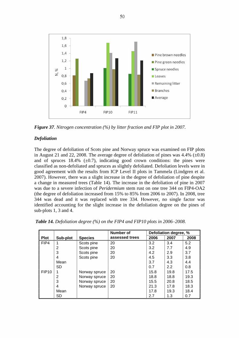
Figure 37. Nitrogen concentration (%) by litter fraction and FIP plot in 2007.
Defoliation
The degree of defoliation of Scots pine and Norway spruce was examined on FIP plots
in August 21 and 22, 2008. The average degree of defoliation of pines was 4.4% (±0.8)
and of spruces 18.4% (±0.7), indicating good crown conditions: the pines were
classified as non-defoliated and spruces as slightly defoliated. Defoliation levels were in
good agreement with the results from ICP Level II plots in Tammela (Lindgren et al.
2007). However, there was a slight increase in the degree of defoliation of pine despite
a change in measured trees (Table 14). The increase in the defoliation of pine in 2007
was due to a severe infection of Peridermium stem rust on one tree 344 on FIP4-OA2
(the degree of defoliation increased from 15% to 85% from 2006 to 2007). In 2008, tree
344 was dead and it was replaced with tree 334. However, no single factor was
identified accounting for the slight increase in the defoliation degree on the pines of
sub-plots 1, 3 and 4.
Table 14. Defoliation degree (%) on the FIP4 and FIP10 plots in 2006–2008.
Sub-plot Species
Number of assessed trees
Defoliation degree, %
Plot 2006 2007 2008
FIP4 1 Scots pine 20 3.2 3.4 5.2
2 Scots pine 20 3.2 7.7 4.9
3 Scots pine 20 4.2 2.9 3.7
4 Scots pine 20 4.5 3.3 3.8
Mean 3.7 4.3 4.4
SD 0.7 2.2 0.8
FIP10 1 Norway spruce 20 15.8 19.8 17.5
2 Norway spruce 20 18.8 18.8 19.3
3 Norway spruce 20 15.5 20.8 18.5
4 Norway spruce 20 21.3 17.8 18.3
Mean 17.8 19.3 18.4
SD 2.7 1.3 0.7
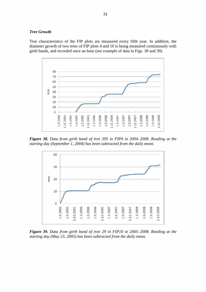
Tree Growth
Tree characteristics of the FIP plots are measured every fifth year. In addition, the
diameter growth of two trees of FIP plots 4 and 10 is being measured continuously with
girth bands, and recorded once an hour (see example of data in Figs. 38 and 39).
Figure 38. Data from girth band of tree 395 in FIP4 in 2004–2008. Reading at the
starting day (September 1, 2004) has been subtracted from the daily mean.
Figure 39. Data from girth band of tree 29 in FIP10 in 2005–2008. Reading at the
starting day (May 23, 2005) has been subtracted from the daily mean.
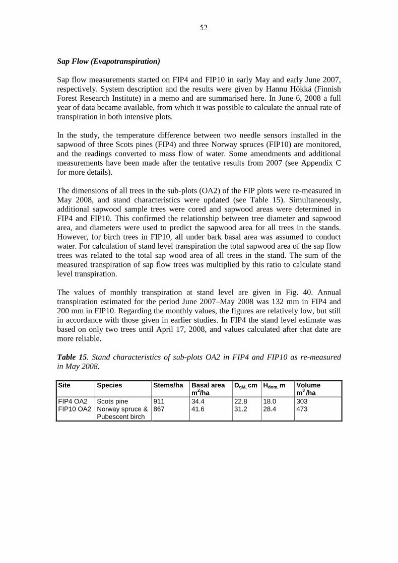
Sap Flow (Evapotranspiration)
Sap flow measurements started on FIP4 and FIP10 in early May and early June 2007,
respectively. System description and the results were given by Hannu Hökkä (Finnish
Forest Research Institute) in a memo and are summarised here. In June 6, 2008 a full
year of data became available, from which it was possible to calculate the annual rate of
transpiration in both intensive plots.
In the study, the temperature difference between two needle sensors installed in the
sapwood of three Scots pines (FIP4) and three Norway spruces (FIP10) are monitored,
and the readings converted to mass flow of water. Some amendments and additional
measurements have been made after the tentative results from 2007 (see Appendix C
for more details).
The dimensions of all trees in the sub-plots (OA2) of the FIP plots were re-measured in
May 2008, and stand characteristics were updated (see Table 15). Simultaneously,
additional sapwood sample trees were cored and sapwood areas were determined in
FIP4 and FIP10. This confirmed the relationship between tree diameter and sapwood
area, and diameters were used to predict the sapwood area for all trees in the stands.
However, for birch trees in FIP10, all under bark basal area was assumed to conduct
water. For calculation of stand level transpiration the total sapwood area of the sap flow
trees was related to the total sap wood area of all trees in the stand. The sum of the
measured transpiration of sap flow trees was multiplied by this ratio to calculate stand
level transpiration.
The values of monthly transpiration at stand level are given in Fig. 40. Annual
transpiration estimated for the period June 2007–May 2008 was 132 mm in FIP4 and
200 mm in FIP10. Regarding the monthly values, the figures are relatively low, but still
in accordance with those given in earlier studies. In FIP4 the stand level estimate was
based on only two trees until April 17, 2008, and values calculated after that date are
more reliable.
Table 15. Stand characteristics of sub-plots OA2 in FIP4 and FIP10 as re-measured
in May 2008.
Site Species Stems/ha Basal area m
2/ha
DgM, cm Hdom, m Volume m
3 /ha
FIP4 OA2 Scots pine 911 34.4 22.8 18.0 303 FIP10 OA2 Norway spruce &
Pubescent birch 867 41.6 31.2 28.4 473
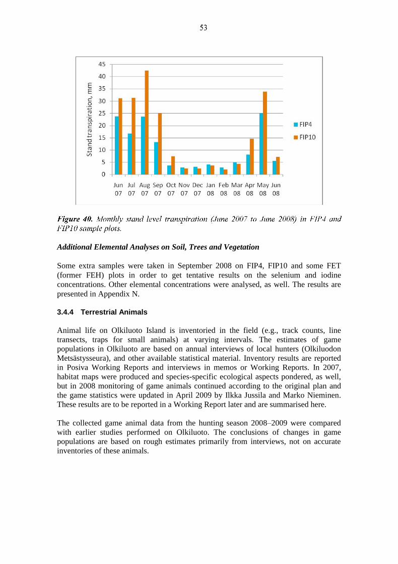
Additional Elemental Analyses on Soil, Trees and Vegetation
Some extra samples were taken in September 2008 on FIP4, FIP10 and some FET
(former FEH) plots in order to get tentative results on the selenium and iodine
concentrations. Other elemental concentrations were analysed, as well. The results are
presented in Appendix N.
3.4.4 Terrestrial Animals
Animal life on Olkiluoto Island is inventoried in the field (e.g., track counts, line
transects, traps for small animals) at varying intervals. The estimates of game
populations in Olkiluoto are based on annual interviews of local hunters (Olkiluodon
Metsästysseura), and other available statistical material. Inventory results are reported
in Posiva Working Reports and interviews in memos or Working Reports. In 2007,
habitat maps were produced and species-specific ecological aspects pondered, as well,
but in 2008 monitoring of game animals continued according to the original plan and
the game statistics were updated in April 2009 by Ilkka Jussila and Marko Nieminen.
These results are to be reported in a Working Report later and are summarised here.
The collected game animal data from the hunting season 2008–2009 were compared
with earlier studies performed on Olkiluoto. The conclusions of changes in game
populations are based on rough estimates primarily from interviews, not on accurate
inventories of these animals.
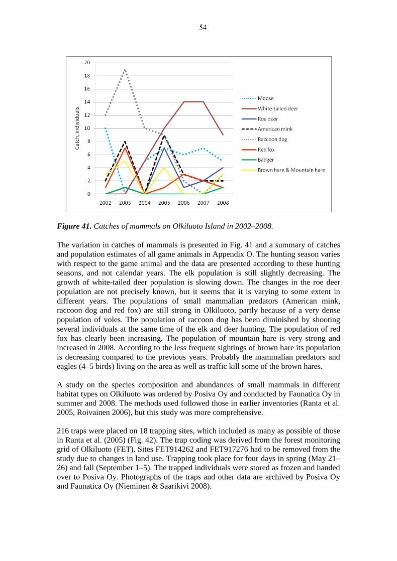
Figure 41. Catches of mammals on Olkiluoto Island in 2002–2008.
The variation in catches of mammals is presented in Fig. 41 and a summary of catches
and population estimates of all game animals in Appendix O. The hunting season varies
with respect to the game animal and the data are presented according to these hunting
seasons, and not calendar years. The elk population is still slightly decreasing. The
growth of white-tailed deer population is slowing down. The changes in the roe deer
population are not precisely known, but it seems that it is varying to some extent in
different years. The populations of small mammalian predators (American mink,
raccoon dog and red fox) are still strong in Olkiluoto, partly because of a very dense
population of voles. The population of raccoon dog has been diminished by shooting
several individuals at the same time of the elk and deer hunting. The population of red
fox has clearly been increasing. The population of mountain hare is very strong and
increased in 2008. According to the less frequent sightings of brown hare its population
is decreasing compared to the previous years. Probably the mammalian predators and
eagles (4–5 birds) living on the area as well as traffic kill some of the brown hares.
A study on the species composition and abundances of small mammals in different
habitat types on Olkiluoto was ordered by Posiva Oy and conducted by Faunatica Oy in
summer and 2008. The methods used followed those in earlier inventories (Ranta et al.
2005, Roivainen 2006), but this study was more comprehensive.
216 traps were placed on 18 trapping sites, which included as many as possible of those
in Ranta et al. (2005) (Fig. 42). The trap coding was derived from the forest monitoring
grid of Olkiluoto (FET). Sites FET914262 and FET917276 had to be removed from the
study due to changes in land use. Trapping took place for four days in spring (May 21–
26) and fall (September 1–5). The trapped individuals were stored as frozen and handed
over to Posiva Oy. Photographs of the traps and other data are archived by Posiva Oy
and Faunatica Oy (Nieminen & Saarikivi 2008).
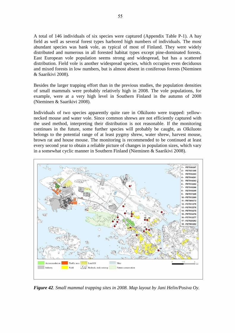
A total of 146 individuals of six species were captured (Appendix Table P-1). A hay
field as well as several forest types harbored high numbers of individuals. The most
abundant species was bank vole, as typical of most of Finland. They were widely
distributed and numerous in all forested habitat types except pine-dominated forests.
East European vole population seems strong and widespread, but has a scattered
distribution. Field vole is another widespread species, which occupies even deciduous
and mixed forests in low numbers, but is almost absent in coniferous forests (Nieminen
& Saarikivi 2008).
Besides the larger trapping effort than in the previous studies, the population densities
of small mammals were probably relatively high in 2008. The vole populations, for
example, were at a very high level in Southern Finland in the autumn of 2008
(Nieminen & Saarikivi 2008).
Individuals of two species apparently quite rare in Olkiluoto were trapped: yellow-
necked mouse and water vole. Since common shrews are not efficiently captured with
the used method, interpreting their distribution is not reasonable. If the monitoring
continues in the future, some further species will probably be caught, as Olkiluoto
belongs to the potential range of at least pygmy shrew, water shrew, harvest mouse,
brown rat and house mouse. The monitoring is recommended to be continued at least
every second year to obtain a reliable picture of changes in population sizes, which vary
in a somewhat cyclic manner in Southern Finland (Nieminen & Saarikivi 2008).
Figure 42. Small mammal trapping sites in 2008. Map layout by Jani Helin/Posiva Oy.
Birds
A study of birds in Olkiluoto was made in summer 2008 (Yrjölä 2009), repeating the
study conducted in 1997 (Yrjölä 1997). However, it was complemented with two new
line transect routes and six new waterfowl counting points for the eastern region, and
now covered the whole island. The line transect study was carried out on June 3–4. The
location of the transect lines is shown in Fig. 43. Transect lines 1–6 were counted
already in 1997, but line 1 was slightly longer then, for part of it is now under the
construction site of Olkiluoto 3. Results of line transect census for landbirds are
presented in Table Q-1.
Altogether, there were 1,429 observations covering 65 species (Yrjölä 2009). Chaffinch
and willow warbler are clearly the predominant species. Compared to 1997, the density
of chaffinch has slightly increased, whereas that of the willow warbler decreased. The
same tendency has been shown in national censuses. Species that can tolerate human
activity have increased, among them robin, great tit, blackbird, wheatear and pied
wagtail (e.g., Yrjölä 2007). Compared to 1997, there was a dramatic increase in the
redbacked shrike. This might be due to suitable biotopes in the vicinity of the power
stations and power lines. This migratory bird has in some places declined over the last
decades, but has experienced rather large annual fluctuations (e.g., Väisänen et al. 1998,
Yrjölä 2007).
Species common to spruce and wildwood forests have faced the greatest decline, for
example bullfinch, green sandpiper and willow tit. Of the game birds, black grouse has
clearly declined. This has happened over the last two decades elsewhere in Finland as
well (Helle & Wikman 2008). The declining of spruce forest species is probably due to
the alteration of the forest terrain in Olkiluoto. Forest fragmentation has probably had
an increasing effect on the species that favour open tracts (e.g., chaffinch, common
whitethroat and blue tit) (Yrjölä 2009).
A waterfowl census was made on May 5, 6 and 20, 2008. The counting spots were in
the same locations as in 1997, except that the spot by the construction site of Olkiluoto
3 power plant had to be moved slightly. Six new observation spots were established.
The census spots and the census sectors approximately covering them are presented in
Fig. 44. The results of the checkpoint census for waterfowl are presented in Appendix
Table Q-2 (Yrjölä 2009).
23 species of waterfowl were interpreted as nesting pairs. A few species were observed,
but not interpreted as nesting. The number and pairs of waterfowl and gulls has
increased. The most abundant species are common eider, mewgull, goldeneye and great
crested grebe. Common tern, mallard, greylag goose and common coot and have clearly
increased. The same trend has been seen in other parts of Southern Finland (e.g.,
Väisänen et al. 1998, Yrjölä 2007). Though the species that have increased in
population are clearly more numerous than those that have declined compared to 1997,
the species in the outer archipelago, such as the common eider and velvet scoter, have
declined. Red-breasted merganser, common redshank and black-headed gull have
clearly declined as well. The bird populations in the Finnish archipelago have declined
for long (Hilden 1995, Yrjölä 2009).

Figure 43. Landbird census transects in 2008. Map layout by Jani Helin/Posiva Oy.
Figure 44. Waterfowl counting sectors in 2008. Map layout by Jani Helin/Posiva Oy.
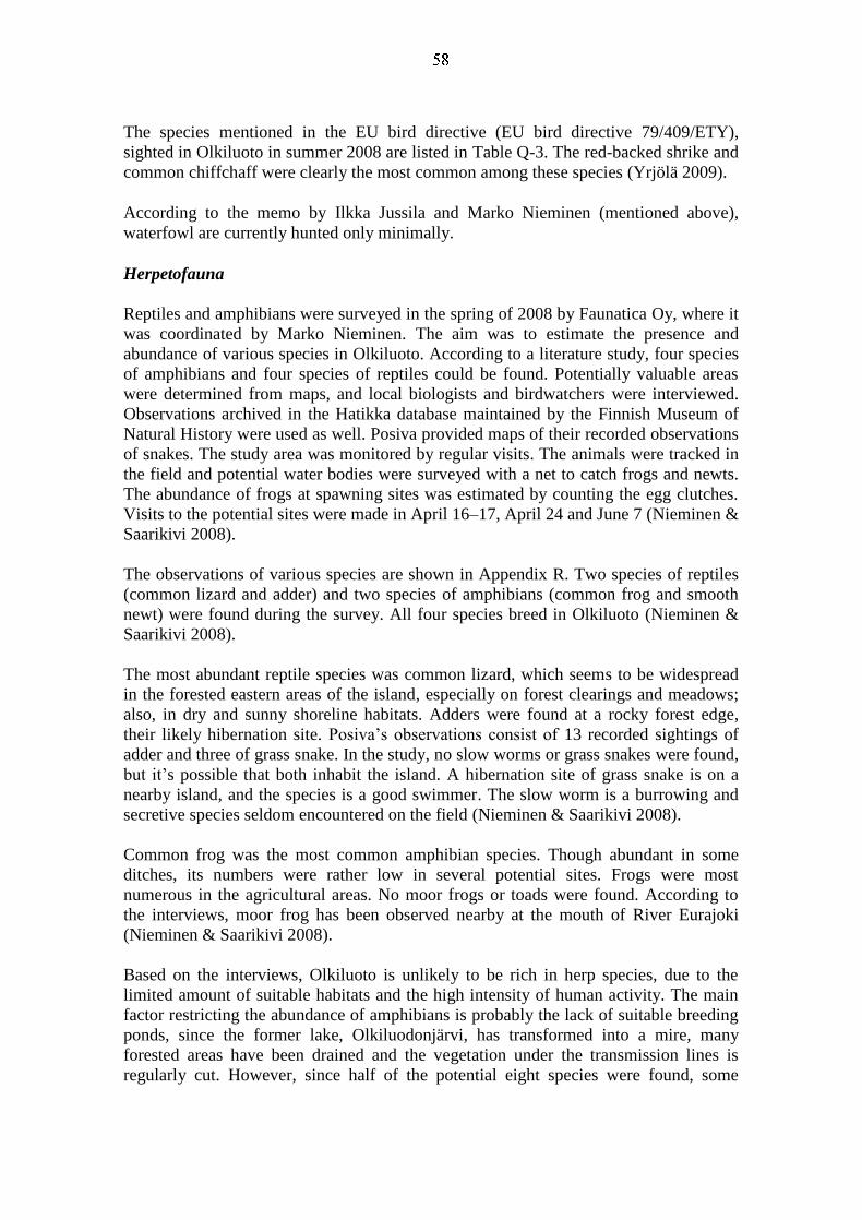
The species mentioned in the EU bird directive (EU bird directive 79/409/ETY),
sighted in Olkiluoto in summer 2008 are listed in Table Q-3. The red-backed shrike and
common chiffchaff were clearly the most common among these species (Yrjölä 2009).
According to the memo by Ilkka Jussila and Marko Nieminen (mentioned above),
waterfowl are currently hunted only minimally.
Herpetofauna
Reptiles and amphibians were surveyed in the spring of 2008 by Faunatica Oy, where it
was coordinated by Marko Nieminen. The aim was to estimate the presence and
abundance of various species in Olkiluoto. According to a literature study, four species
of amphibians and four species of reptiles could be found. Potentially valuable areas
were determined from maps, and local biologists and birdwatchers were interviewed.
Observations archived in the Hatikka database maintained by the Finnish Museum of
Natural History were used as well. Posiva provided maps of their recorded observations
of snakes. The study area was monitored by regular visits. The animals were tracked in
the field and potential water bodies were surveyed with a net to catch frogs and newts.
The abundance of frogs at spawning sites was estimated by counting the egg clutches.
Visits to the potential sites were made in April 16–17, April 24 and June 7 (Nieminen &
Saarikivi 2008).
The observations of various species are shown in Appendix R. Two species of reptiles
(common lizard and adder) and two species of amphibians (common frog and smooth
newt) were found during the survey. All four species breed in Olkiluoto (Nieminen &
Saarikivi 2008).
The most abundant reptile species was common lizard, which seems to be widespread
in the forested eastern areas of the island, especially on forest clearings and meadows;
also, in dry and sunny shoreline habitats. Adders were found at a rocky forest edge,
their likely hibernation site. Posiva’s observations consist of 13 recorded sightings of
adder and three of grass snake. In the study, no slow worms or grass snakes were found,
but it’s possible that both inhabit the island. A hibernation site of grass snake is on a
nearby island, and the species is a good swimmer. The slow worm is a burrowing and
secretive species seldom encountered on the field (Nieminen & Saarikivi 2008).
Common frog was the most common amphibian species. Though abundant in some
ditches, its numbers were rather low in several potential sites. Frogs were most
numerous in the agricultural areas. No moor frogs or toads were found. According to
the interviews, moor frog has been observed nearby at the mouth of River Eurajoki
(Nieminen & Saarikivi 2008).
Based on the interviews, Olkiluoto is unlikely to be rich in herp species, due to the
limited amount of suitable habitats and the high intensity of human activity. The main
factor restricting the abundance of amphibians is probably the lack of suitable breeding
ponds, since the former lake, Olkiluodonjärvi, has transformed into a mire, many
forested areas have been drained and the vegetation under the transmission lines is
regularly cut. However, since half of the potential eight species were found, some

suitable habitats exist. Most individuals were observed in the eastern parts of the island
(Nieminen & Saarikivi 2008).
Ground Beetles and Ants
The study on ground beetles and ants was carried out in summer 2008 by
Environmental Research Yrjölä ltd. The research goal was to clarify the species
composition on Olkiluoto and to collect samples for further examination by Posiva.
Other species of insects and spiders that were detected were also preserved for further
examination. Out of the 2005 survey (Ranta et al. 2005), four of the test sectors were
used in this research. The results cannot be directly compared with this earlier ground
beetle study in the area, as it was limited in the species and numbers of individual
specimens. (Santaharju et al. 2009).
Pitfall traps were located in different biotopes, nine in each spot within the FET
observation area employed in monitoring forests (Figs 46 and 47). The traps were
installed in the ground in June and August. At minimum, the species was identified to
the family level of ground beetles and to the species or species pairs of ants (Santaharju
et al. 2009).
The species found represented quite a usual range for Southern Finland. No rare or
endangered species were detected. The number of individual ants appeared to be higher
in biotopes dominated by conifers but as far as the amount of species was concerned,
the dispersion between different biotopes was great (Santaharju et al. 2009).
Regarding the ground beetles, the amounts of species and individuals were higher in
open field and meadow habitats. The large Carabus hortensis together with
Pterostichus niger and Patrobus atrorufus make up the majority of the ground beetle
communities in Olkiluoto, both in numbers and in weight (Santaharju et al. 2009).
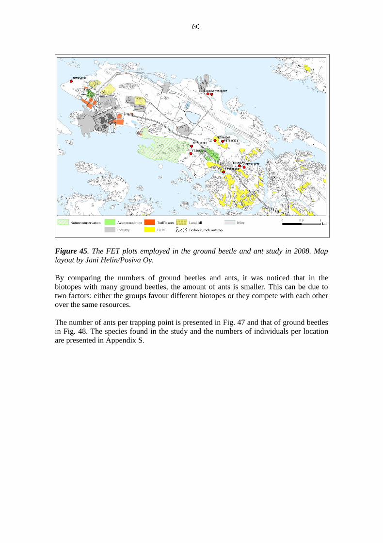
Figure 45. The FET plots employed in the ground beetle and ant study in 2008. Map
layout by Jani Helin/Posiva Oy.
By comparing the numbers of ground beetles and ants, it was noticed that in the
biotopes with many ground beetles, the amount of ants is smaller. This can be due to
two factors: either the groups favour different biotopes or they compete with each other
over the same resources.
The number of ants per trapping point is presented in Fig. 47 and that of ground beetles
in Fig. 48. The species found in the study and the numbers of individuals per location
are presented in Appendix S.
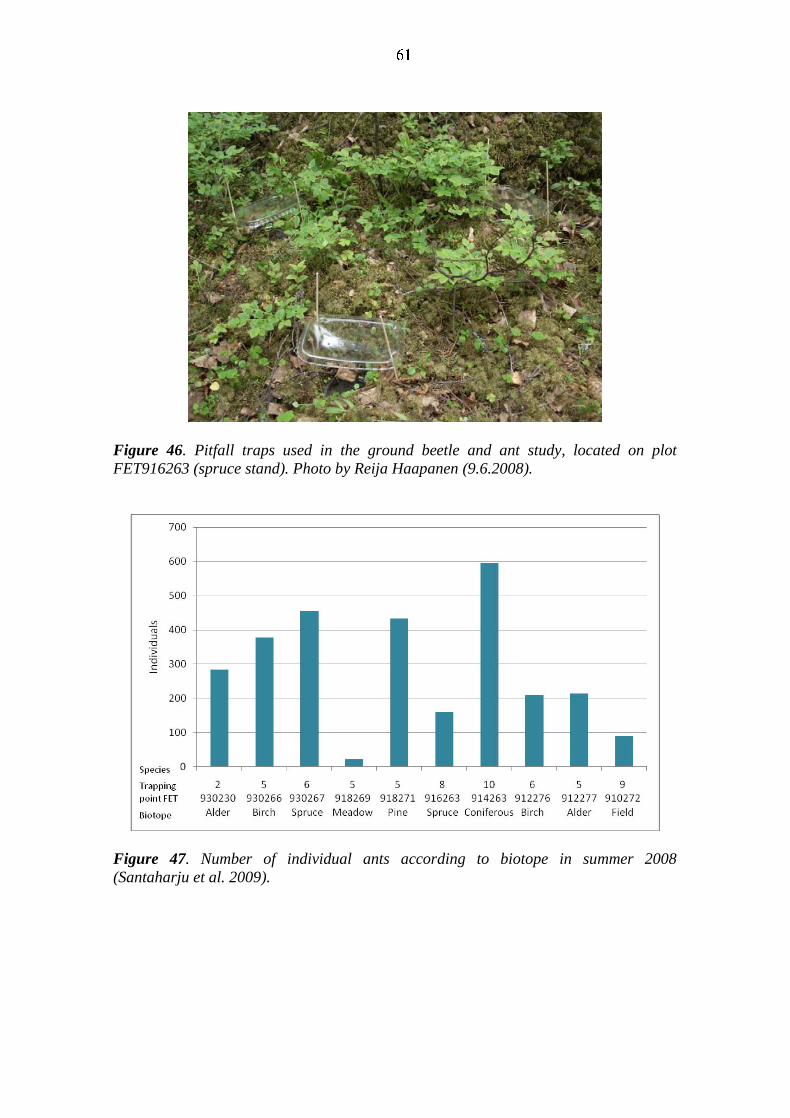
Figure 46. Pitfall traps used in the ground beetle and ant study, located on plot
FET916263 (spruce stand). Photo by Reija Haapanen (9.6.2008).
Figure 47. Number of individual ants according to biotope in summer 2008
(Santaharju et al. 2009).
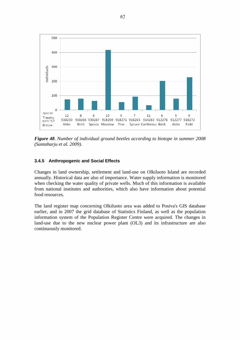
Figure 48. Number of individual ground beetles according to biotope in summer 2008
(Santaharju et al. 2009).
3.4.5 Anthropogenic and Social Effects
Changes in land ownership, settlement and land-use on Olkiluoto Island are recorded
annually. Historical data are also of importance. Water supply information is monitored
when checking the water quality of private wells. Much of this information is available
from national institutes and authorities, which also have information about potential
food resources.
The land register map concerning Olkiluoto area was added to Posiva's GIS database
earlier, and in 2007 the grid database of Statistics Finland, as well as the population
information system of the Population Register Centre were acquired. The changes in
land-use due to the new nuclear power plant (OL3) and its infrastructure are also
continuously monitored.
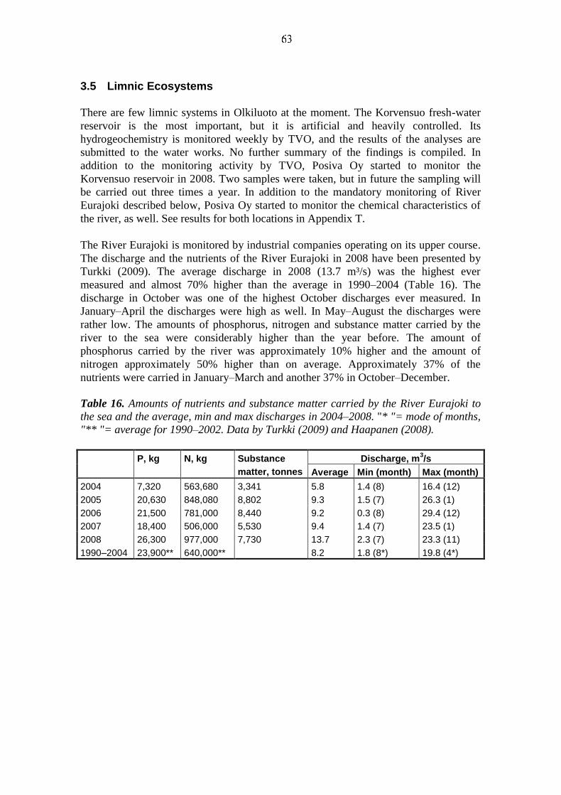
3.5 Limnic Ecosystems
There are few limnic systems in Olkiluoto at the moment. The Korvensuo fresh-water
reservoir is the most important, but it is artificial and heavily controlled. Its
hydrogeochemistry is monitored weekly by TVO, and the results of the analyses are
submitted to the water works. No further summary of the findings is compiled. In
addition to the monitoring activity by TVO, Posiva Oy started to monitor the
Korvensuo reservoir in 2008. Two samples were taken, but in future the sampling will
be carried out three times a year. In addition to the mandatory monitoring of River
Eurajoki described below, Posiva Oy started to monitor the chemical characteristics of
the river, as well. See results for both locations in Appendix T.
The River Eurajoki is monitored by industrial companies operating on its upper course.
The discharge and the nutrients of the River Eurajoki in 2008 have been presented by
Turkki (2009). The average discharge in 2008 (13.7 m³/s) was the highest ever
measured and almost 70% higher than the average in 1990–2004 (Table 16). The
discharge in October was one of the highest October discharges ever measured. In
January–April the discharges were high as well. In May–August the discharges were
rather low. The amounts of phosphorus, nitrogen and substance matter carried by the
river to the sea were considerably higher than the year before. The amount of
phosphorus carried by the river was approximately 10% higher and the amount of
nitrogen approximately 50% higher than on average. Approximately 37% of the
nutrients were carried in January–March and another 37% in October–December.
Table 16. Amounts of nutrients and substance matter carried by the River Eurajoki to
the sea and the average, min and max discharges in 2004–2008. "* "= mode of months,
"** "= average for 1990–2002. Data by Turkki (2009) and Haapanen (2008).
P, kg N, kg Substance
matter, tonnes
Discharge, m3/s
Average Min (month) Max (month)
2004 7,320 563,680 3,341 5.8 1.4 (8) 16.4 (12)
2005 20,630 848,080 8,802 9.3 1.5 (7) 26.3 (1)
2006 21,500 781,000 8,440 9.2 0.3 (8) 29.4 (12)
2007 18,400 506,000 5,530 9.4 1.4 (7) 23.5 (1)
2008 26,300 977,000 7,730 13.7 2.3 (7) 23.3 (11)
1990–2004 23,900** 640,000** 8.2 1.8 (8*) 19.8 (4*)
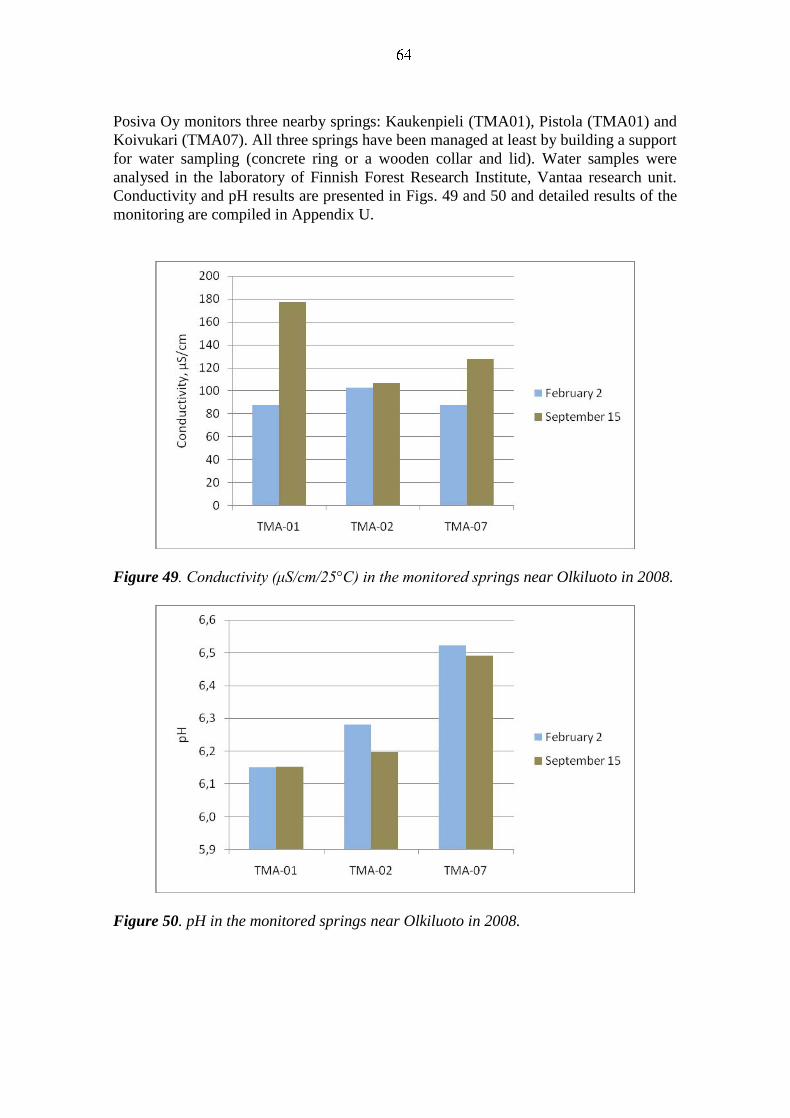
Posiva Oy monitors three nearby springs: Kaukenpieli (TMA01), Pistola (TMA01) and
Koivukari (TMA07). All three springs have been managed at least by building a support
for water sampling (concrete ring or a wooden collar and lid). Water samples were
analysed in the laboratory of Finnish Forest Research Institute, Vantaa research unit.
Conductivity and pH results are presented in Figs. 49 and 50 and detailed results of the
monitoring are compiled in Appendix U.
Figure 49. Conductivity (μS/cm/25°C) in the monitored springs near Olkiluoto in 2008.
Figure 50. pH in the monitored springs near Olkiluoto in 2008.
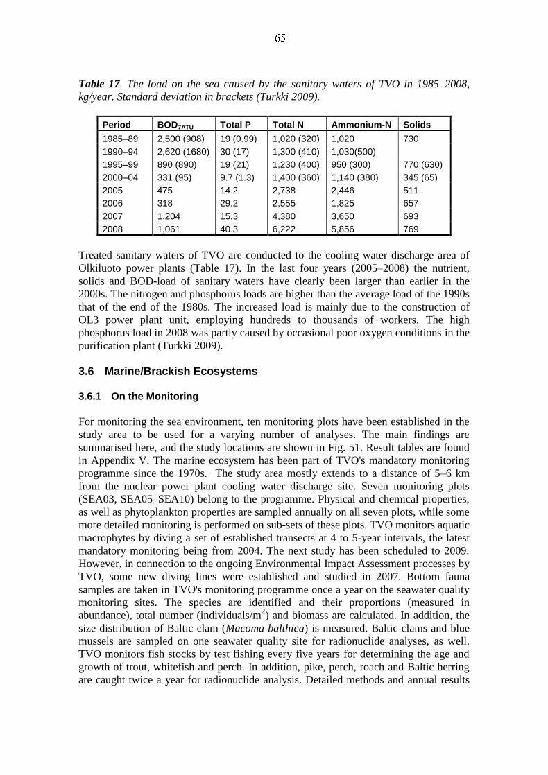
Table 17. The load on the sea caused by the sanitary waters of TVO in 1985–2008,
kg/year. Standard deviation in brackets (Turkki 2009).
Period BOD7ATU Total P Total N Ammonium-N Solids
1985–89 2,500 (908) 19 (0.99) 1,020 (320) 1,020 730
1990–94 2,620 (1680) 30 (17) 1,300 (410) 1,030(500)
1995–99 890 (890) 19 (21) 1,230 (400) 950 (300) 770 (630)
2000–04 331 (95) 9.7 (1.3) 1,400 (360) 1,140 (380) 345 (65)
2005 475 14.2 2,738 2,446 511
2006 318 29.2 2,555 1,825 657
2007 1,204 15.3 4,380 3,650 693
2008 1,061 40.3 6,222 5,856 769
Treated sanitary waters of TVO are conducted to the cooling water discharge area of
Olkiluoto power plants (Table 17). In the last four years (2005–2008) the nutrient,
solids and BOD-load of sanitary waters have clearly been larger than earlier in the
2000s. The nitrogen and phosphorus loads are higher than the average load of the 1990s
that of the end of the 1980s. The increased load is mainly due to the construction of
OL3 power plant unit, employing hundreds to thousands of workers. The high
phosphorus load in 2008 was partly caused by occasional poor oxygen conditions in the
purification plant (Turkki 2009).
3.6 Marine/Brackish Ecosystems
3.6.1 On the Monitoring
For monitoring the sea environment, ten monitoring plots have been established in the
study area to be used for a varying number of analyses. The main findings are
summarised here, and the study locations are shown in Fig. 51. Result tables are found
in Appendix V. The marine ecosystem has been part of TVO's mandatory monitoring
programme since the 1970s. The study area mostly extends to a distance of 5–6 km
from the nuclear power plant cooling water discharge site. Seven monitoring plots
(SEA03, SEA05–SEA10) belong to the programme. Physical and chemical properties,
as well as phytoplankton properties are sampled annually on all seven plots, while some
more detailed monitoring is performed on sub-sets of these plots. TVO monitors aquatic
macrophytes by diving a set of established transects at 4 to 5-year intervals, the latest
mandatory monitoring being from 2004. The next study has been scheduled to 2009.
However, in connection to the ongoing Environmental Impact Assessment processes by
TVO, some new diving lines were established and studied in 2007. Bottom fauna
samples are taken in TVO's monitoring programme once a year on the seawater quality
monitoring sites. The species are identified and their proportions (measured in
abundance), total number (individuals/m2) and biomass are calculated. In addition, the
size distribution of Baltic clam (Macoma balthica) is measured. Baltic clams and blue
mussels are sampled on one seawater quality site for radionuclide analyses, as well.
TVO monitors fish stocks by test fishing every five years for determining the age and
growth of trout, whitefish and perch. In addition, pike, perch, roach and Baltic herring
are caught twice a year for radionuclide analysis. Detailed methods and annual results
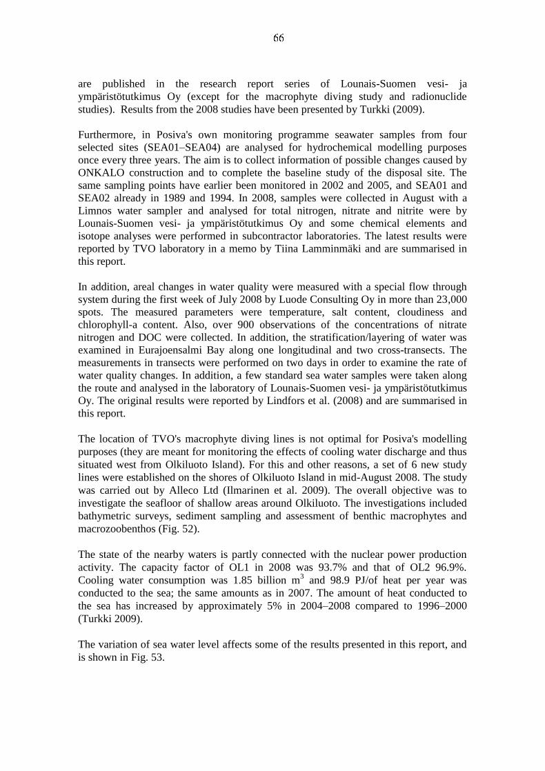
are published in the research report series of Lounais-Suomen vesi- ja
ympäristötutkimus Oy (except for the macrophyte diving study and radionuclide
studies). Results from the 2008 studies have been presented by Turkki (2009).
Furthermore, in Posiva's own monitoring programme seawater samples from four
selected sites (SEA01–SEA04) are analysed for hydrochemical modelling purposes
once every three years. The aim is to collect information of possible changes caused by
ONKALO construction and to complete the baseline study of the disposal site. The
same sampling points have earlier been monitored in 2002 and 2005, and SEA01 and
SEA02 already in 1989 and 1994. In 2008, samples were collected in August with a
Limnos water sampler and analysed for total nitrogen, nitrate and nitrite were by
Lounais-Suomen vesi- ja ympäristötutkimus Oy and some chemical elements and
isotope analyses were performed in subcontractor laboratories. The latest results were
reported by TVO laboratory in a memo by Tiina Lamminmäki and are summarised in
this report.
In addition, areal changes in water quality were measured with a special flow through
system during the first week of July 2008 by Luode Consulting Oy in more than 23,000
spots. The measured parameters were temperature, salt content, cloudiness and
chlorophyll-a content. Also, over 900 observations of the concentrations of nitrate
nitrogen and DOC were collected. In addition, the stratification/layering of water was
examined in Eurajoensalmi Bay along one longitudinal and two cross-transects. The
measurements in transects were performed on two days in order to examine the rate of
water quality changes. In addition, a few standard sea water samples were taken along
the route and analysed in the laboratory of Lounais-Suomen vesi- ja ympäristötutkimus
Oy. The original results were reported by Lindfors et al. (2008) and are summarised in
this report.
The location of TVO's macrophyte diving lines is not optimal for Posiva's modelling
purposes (they are meant for monitoring the effects of cooling water discharge and thus
situated west from Olkiluoto Island). For this and other reasons, a set of 6 new study
lines were established on the shores of Olkiluoto Island in mid-August 2008. The study
was carried out by Alleco Ltd (Ilmarinen et al. 2009). The overall objective was to
investigate the seafloor of shallow areas around Olkiluoto. The investigations included
bathymetric surveys, sediment sampling and assessment of benthic macrophytes and
macrozoobenthos (Fig. 52).
The state of the nearby waters is partly connected with the nuclear power production
activity. The capacity factor of OL1 in 2008 was 93.7% and that of OL2 96.9%.
Cooling water consumption was 1.85 billion m3 and 98.9 PJ/of heat per year was
conducted to the sea; the same amounts as in 2007. The amount of heat conducted to
the sea has increased by approximately 5% in 2004–2008 compared to 1996–2000
(Turkki 2009).
The variation of sea water level affects some of the results presented in this report, and
is shown in Fig. 53.
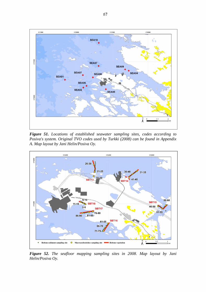
Figure 51. Locations of established seawater sampling sites, codes according to
Posiva's system. Original TVO codes used by Turkki (2008) can be found in Appendix
A. Map layout by Jani Helin/Posiva Oy.
Figure 52. The seafloor mapping sampling sites in 2008. Map layout by Jani
Helin/Posiva Oy.
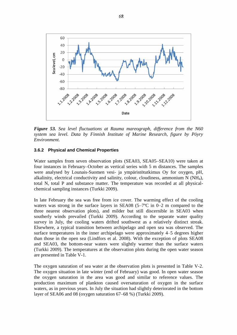
Figure 53. Sea level fluctuations at Rauma mareograph, difference from the N60
system sea level. Data by Finnish Institute of Marine Research, figure by Pöyry
Environment. 3.6.2 Physical and Chemical Properties
Water samples from seven observation plots (SEA03, SEA05–SEA10) were taken at
four instances in February–October as vertical series with 5 m distances. The samples
were analysed by Lounais-Suomen vesi- ja ympäristötutkimus Oy for oxygen, pH,
alkalinity, electrical conductivity and salinity, colour, cloudiness, ammonium N (NH4),
total N, total P and substance matter. The temperature was recorded at all physical-
chemical sampling instances (Turkki 2009).
In late February the sea was free from ice cover. The warming effect of the cooling
waters was strong in the surface layers in SEA08 (5–7ºC in 0–2 m compared to the
three nearest observation plots), and milder but still discernible in SEA03 when
southerly winds prevailed (Turkki 2009). According to the separate water quality
survey in July, the cooling waters drifted southwest as a relatively distinct streak.
Elsewhere, a typical transition between archipelago and open sea was observed. The
surface temperatures in the inner archipelago were approximately 4–5 degrees higher
than those in the open sea (Lindfors et al. 2008). With the exception of plots SEA08
and SEA03, the bottom-near waters were slightly warmer than the surface waters
(Turkki 2009). The temperatures at the observation plots during the open water season
are presented in Table V-1.
The oxygen saturation of sea water at the observation plots is presented in Table V-2.
The oxygen situation in late winter (end of February) was good. In open water season
the oxygen saturation in the area was good and similar to reference values. The
production maximum of plankton caused oversaturation of oxygen in the surface
waters, as in previous years. In July the situation had slightly deteriorated in the bottom
layer of SEA06 and 08 (oxygen saturation 67–68 %) (Turkki 2009).
According to the water quality survey in July, a strong gradient is discernible in the salt
content in Eurajoensalmi Bay. Impacts of river water were discernable up to 7–9 km
from the river mouth. The strongest transition took place approximately 2–5 km from
the river mouth. The highest measured salt contents were approximately 5.6 ‰
(Lindfors et al. 2008).
The opacity of water (visible depth) varied from 2.8 m in SEA09 to 4.9 m in SEA10.
The opacity was better than at the end of the 1990s and similar to the beginning of the
1990s (Turkki 2009; Fig. 54).
Wintertime N concentrations varied between 380–770 μg/l (Table V-3). In SEA09, the
values were clearly higher than elsewhere. SEA10 could not be reached for sampling.
The N concentrations were 13–14% higher than the average values since 2000, and
higher than the values in the reference sites. The reference concentration in Pyhäranta
was 300μg/l in 2004–2008, and in Rauma 250 μg/l (in 2007). The concentrations of
total N in the study locations were between 250–500 μg/l during the open water season.
They were at the same level as in 1998–2007 on average, except in SEA09, where the
open water season average was approximately 45% higher than the long time average.
The background concentration in coastal waters of the Bothnian Sea (data from
Pyhäranta reference site) was 280 μg/l in 2000–2008. The ammonium N concentrations
were relatively small, on average 4–17 μg/l during the open water season. In May the
amounts were under the detectable level. The highest value, 100 μg/l, was in SEA09 in
October. In the production layer, the total N concentrations varied between 230–740
μg/l during the growing season, similar to the average (Turkki 2009). According to the
water quality survey in July, the highest observed contents of nitrate nitrogen (300–400
μg/l) were in the delta area of River Eurajoki and by the coast of Rauma. The
concentrations of dissolved organic carbon varied between 4 and 8 mg/l (Lindfors et al.
2008).
In winter (February) the average P concentrations of water columns were between 27–
43 μg/l (Table V-4), and clearly higher than the average of 2000s. The P concentrations
were higher than the background concentration in coastal waters of the Bothnian Sea
measured at Pyhäranta, which was 19 μg/l in 2004–2007 and 16 μg/l in 2008. The
wintertime P concentrations increased significantly between 1979 and 2002. After some
fluctuation in the 2000s and a lower value in 2007, in 2008 the concentrations were the
highest of the monitoring period. The average P concentrations during the open water
season have showed periodic, irregular fluctuation. In 2008, the values (13–26 μg/l)
were generally lower than the long-time average (Fig. 55), except in SEA09 in October,
where the value was approximately 80% above the 1998–2007 average (Turkki 2009).
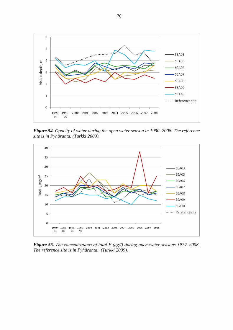
Figure 54. Opacity of water during the open water season in 1990–2008. The reference
site is in Pyhäranta. (Turkki 2009).
Figure 55. The concentrations of total P (μg/l) during open water seasons 1979–2008.
The reference site is in Pyhäranta. (Turkki 2009).
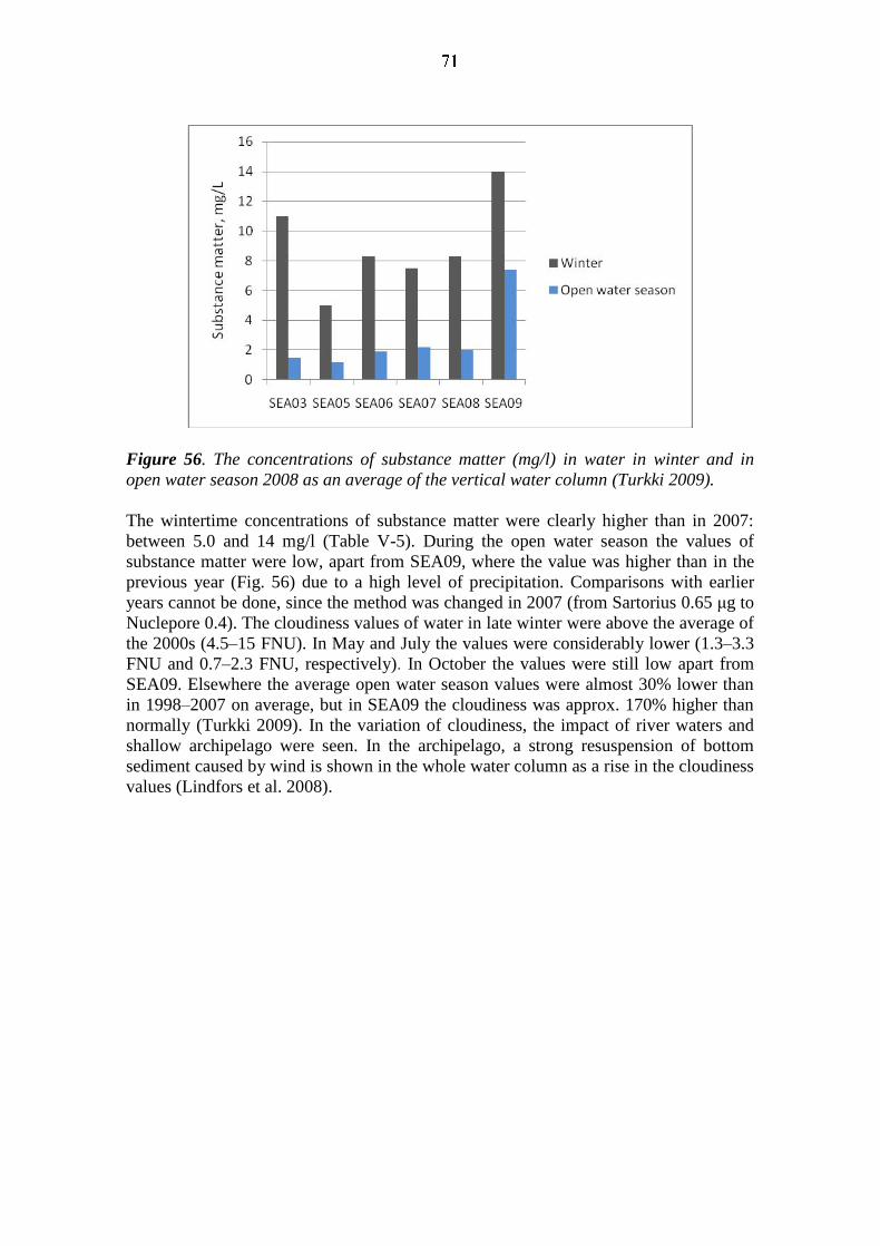
Figure 56. The concentrations of substance matter (mg/l) in water in winter and in
open water season 2008 as an average of the vertical water column (Turkki 2009).
The wintertime concentrations of substance matter were clearly higher than in 2007:
between 5.0 and 14 mg/l (Table V-5). During the open water season the values of
substance matter were low, apart from SEA09, where the value was higher than in the
previous year (Fig. 56) due to a high level of precipitation. Comparisons with earlier
years cannot be done, since the method was changed in 2007 (from Sartorius 0.65 μg to
Nuclepore 0.4). The cloudiness values of water in late winter were above the average of
the 2000s (4.5–15 FNU). In May and July the values were considerably lower (1.3–3.3
FNU and 0.7–2.3 FNU, respectively). In October the values were still low apart from
SEA09. Elsewhere the average open water season values were almost 30% lower than
in 1998–2007 on average, but in SEA09 the cloudiness was approx. 170% higher than
normally (Turkki 2009). In the variation of cloudiness, the impact of river waters and
shallow archipelago were seen. In the archipelago, a strong resuspension of bottom
sediment caused by wind is shown in the whole water column as a rise in the cloudiness
values (Lindfors et al. 2008).
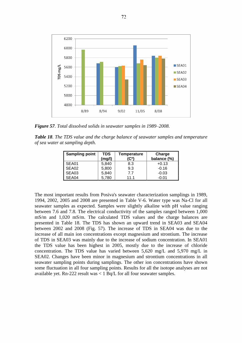
Figure 57. Total dissolved solids in seawater samples in 1989–2008.
Table 18. The TDS value and the charge balance of seawater samples and temperature
of sea water at sampling depth.
Sampling point TDS (mg/l)
Temperature (Cº)
Charge balance (%)
SEA01 5,840 8.3 +0.13 SEA02 5,800 9.3 -0.16 SEA03 5,840 7.7 -0.03 SEA04 5,780 11.1 -0.01
The most important results from Posiva's seawater characterization samplings in 1989,
1994, 2002, 2005 and 2008 are presented in Table V-6. Water type was Na-Cl for all
seawater samples as expected. Samples were slightly alkaline with pH value ranging
between 7.6 and 7.8. The electrical conductivity of the samples ranged between 1,000
mS/m and 1,020 mS/m. The calculated TDS values and the charge balances are
presented in Table 18. The TDS has shown an upward trend in SEA03 and SEA04
between 2002 and 2008 (Fig. 57). The increase of TDS in SEA04 was due to the
increase of all main ion concentrations except magnesium and strontium. The increase
of TDS in SEA03 was mainly due to the increase of sodium concentration. In SEA01
the TDS value has been highest in 2005, mostly due to the increase of chloride
concentration. The TDS value has varied between 5,620 mg/L and 5,970 mg/L in
SEA02. Changes have been minor in magnesium and strontium concentrations in all
seawater sampling points during samplings. The other ion concentrations have shown
some fluctuation in all four sampling points. Results for all the isotope analyses are not
available yet. Rn-222 result was < 1 Bq/L for all four seawater samples.
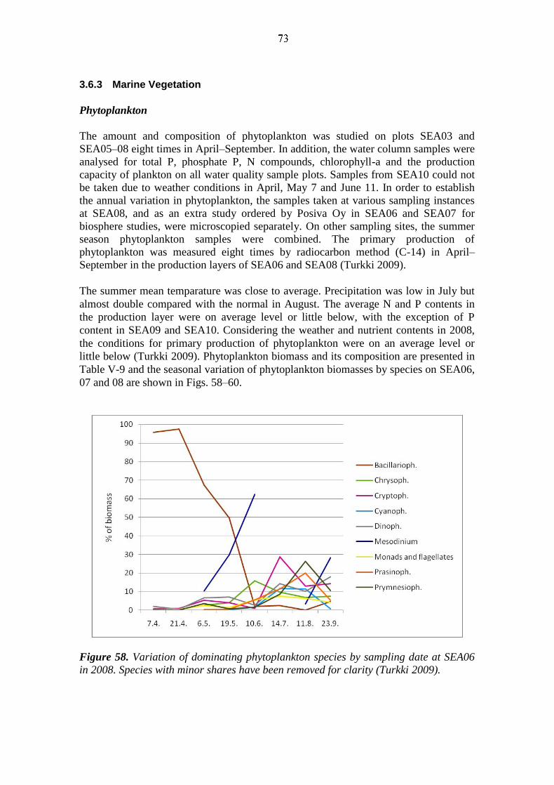
3.6.3 Marine Vegetation
Phytoplankton
The amount and composition of phytoplankton was studied on plots SEA03 and
SEA05–08 eight times in April–September. In addition, the water column samples were
analysed for total P, phosphate P, N compounds, chlorophyll-a and the production
capacity of plankton on all water quality sample plots. Samples from SEA10 could not
be taken due to weather conditions in April, May 7 and June 11. In order to establish
the annual variation in phytoplankton, the samples taken at various sampling instances
at SEA08, and as an extra study ordered by Posiva Oy in SEA06 and SEA07 for
biosphere studies, were microscopied separately. On other sampling sites, the summer
season phytoplankton samples were combined. The primary production of
phytoplankton was measured eight times by radiocarbon method (C-14) in April–
September in the production layers of SEA06 and SEA08 (Turkki 2009).
The summer mean temparature was close to average. Precipitation was low in July but
almost double compared with the normal in August. The average N and P contents in
the production layer were on average level or little below, with the exception of P
content in SEA09 and SEA10. Considering the weather and nutrient contents in 2008,
the conditions for primary production of phytoplankton were on an average level or
little below (Turkki 2009). Phytoplankton biomass and its composition are presented in
Table V-9 and the seasonal variation of phytoplankton biomasses by species on SEA06,
07 and 08 are shown in Figs. 58–60.
Figure 58. Variation of dominating phytoplankton species by sampling date at SEA06
in 2008. Species with minor shares have been removed for clarity (Turkki 2009).
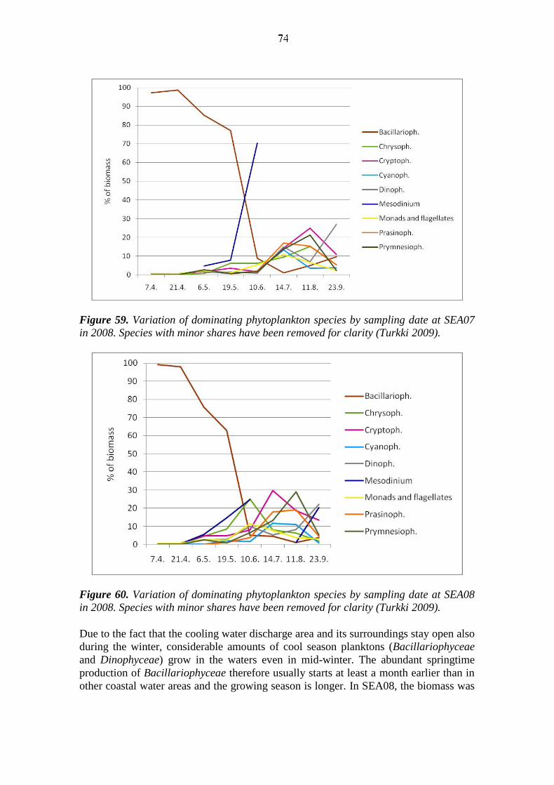
Figure 59. Variation of dominating phytoplankton species by sampling date at SEA07
in 2008. Species with minor shares have been removed for clarity (Turkki 2009).
Figure 60. Variation of dominating phytoplankton species by sampling date at SEA08
in 2008. Species with minor shares have been removed for clarity (Turkki 2009).
Due to the fact that the cooling water discharge area and its surroundings stay open also
during the winter, considerable amounts of cool season planktons (Bacillariophyceae
and Dinophyceae) grow in the waters even in mid-winter. The abundant springtime
production of Bacillariophyceae therefore usually starts at least a month earlier than in
other coastal water areas and the growing season is longer. In SEA08, the biomass was
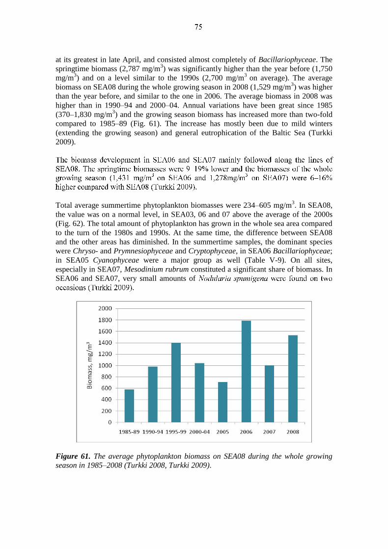
at its greatest in late April, and consisted almost completely of Bacillariophyceae. The
springtime biomass (2,787 mg/m3) was significantly higher than the year before (1,750
mg/m3) and on a level similar to the 1990s (2,700 mg/m
3 on average). The average
biomass on SEA08 during the whole growing season in 2008 (1,529 mg/m3) was higher
than the year before, and similar to the one in 2006. The average biomass in 2008 was
higher than in 1990–94 and 2000–04. Annual variations have been great since 1985
(370–1,830 mg/m3) and the growing season biomass has increased more than two-fold
compared to 1985–89 (Fig. 61). The increase has mostly been due to mild winters
(extending the growing season) and general eutrophication of the Baltic Sea (Turkki
2009).
Total average summertime phytoplankton biomasses were 234–605 mg/m3. In SEA08,
the value was on a normal level, in SEA03, 06 and 07 above the average of the 2000s
(Fig. 62). The total amount of phytoplankton has grown in the whole sea area compared
to the turn of the 1980s and 1990s. At the same time, the difference between SEA08
and the other areas has diminished. In the summertime samples, the dominant species
were Chryso- and Prymnesiophyceae and Cryptophyceae, in SEA06 Bacillariophyceae;
in SEA05 Cyanophyceae were a major group as well (Table V-9). On all sites,
especially in SEA07, Mesodinium rubrum constituted a significant share of biomass. In
SEA06 and SEA07, very small amounts of
Figure 61. The average phytoplankton biomass on SEA08 during the whole growing
season in 1985–2008 (Turkki 2008, Turkki 2009).
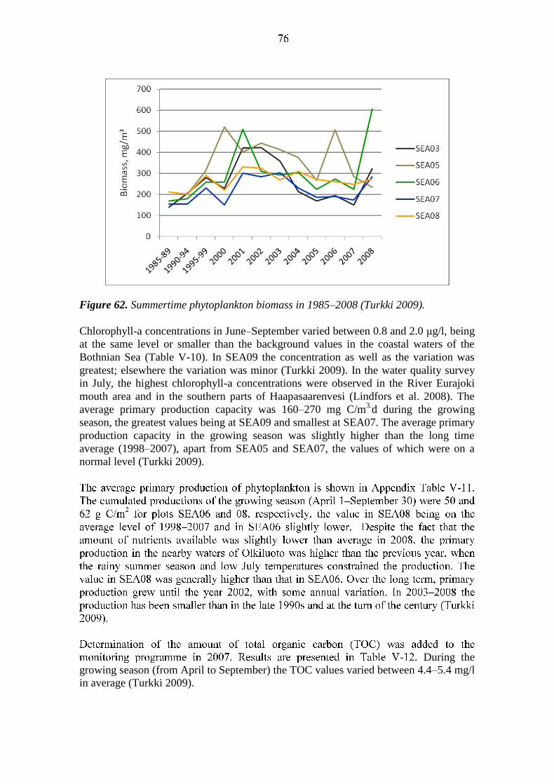
Figure 62. Summertime phytoplankton biomass in 1985–2008 (Turkki 2009).
Chlorophyll-a concentrations in June–September varied between 0.8 and 2.0 μg/l, being
at the same level or smaller than the background values in the coastal waters of the
Bothnian Sea (Table V-10). In SEA09 the concentration as well as the variation was
greatest; elsewhere the variation was minor (Turkki 2009). In the water quality survey
in July, the highest chlorophyll-a concentrations were observed in the River Eurajoki
mouth area and in the southern parts of Haapasaarenvesi (Lindfors et al. 2008). The
average primary production capacity was 160–270 mg C/m3.d during the growing
season, the greatest values being at SEA09 and smallest at SEA07. The average primary
production capacity in the growing season was slightly higher than the long time
average (1998–2007), apart from SEA05 and SEA07, the values of which were on a
normal level (Turkki 2009).
During the
growing season (from April to September) the TOC values varied between 4.4–5.4 mg/l
in average (Turkki 2009).

Zooplankton
The zooplankton research, ordered by Posiva, was made by Lounais-Suomen vesi- ja
ympäristötutkimus Oy. The study location was SEA08, in the cooling water discharge
area. The samples were collected from an 8 m high water column as a vertical series
with half meter distances, with a Limnos-type tube sampler. The samples were collected
on April 4, May 20, June 11, July 15 and August 12; a sampling was planned for
September as well, but was not carried out. In this research, both mesozooplankton
(0.2–2 mm, consisting of large rotifers, Cladocerans, copepods) and microzooplankton
(rotifers of 20–200 μm) were examined. The biomass of zooplankton (mg C/m3) and the
number of individuals per cubic meter were calculated. Considering the annual
dynamics of zooplankton, temperature and salinity are the most important factors.
(Turkki 2009).
According to the study, the zooplankton carbon biomass level in SEA08 (24 mg C/m3
on average) was higher than the average level of the long time series of zooplankton
observations in the Bothnian Sea converted to carbon biomass (converted fresh weight
12 mg C/m3), but lower than for example the carbon biomass level of the monitoring
data from the coasts of Helsinki. However, these data cannot be directly compared. In
the zooplankton samples, altogether 23 taxons were found in 2008, of which 12 taxons
of rotifers, 6 Cladocera species and 5 copepods (3 Calanoida and 2 Cyclopoida
copepods). The maximum carbon biomass was 44 mg C/m3 on July 15 and the average
carbon biomass of the sampling period was 24 mg C/m3. The maximum numbers of
individuals occurred in July and August, with over 80,000 individuals/m3. The average
number of individuals in the whole sampling period was 58,000/m3
(Turkki 2009).
Rotifers accounted for approximately 45% of the individuals and 14% of the biomass in
the study period. Their numbers were at their highest in August (38,000 individuals/m3)
and May (34,000/m3). The biomass level of rotifers was not high, except for the early
spring due to the low amount of crustaceans. In the whole sampling period, the most
common species were Synchaeta baltica, Keratella quadrata and Keratella cochlearis
(Turkki 2009).
Bosmina longispina maritima was the most important species of Cladocera. Its average
share of the total zooplankton biomass was 19% (5 mg C/m3). Podon polyphemoides
dominated the sample of early summer (June 11), when its share of total zooplankton
biomass was 42% (12 mg C/m3). The amounts of other Cladocerans were minor.
Regarding the whole period, the share of Cladocerans was a third (35%) of total
biomass and 17% of the total number of individuals (Turkki 2009).
Three Calanoida copepods were found: Acartia bifilosa, Eurytemora affinis and Temora
longicornis. The amounts of Acartia sp. and Eurytemora affinis increased in the mid-
and late summer samples. Regarding the whole period, the biomass and number of
individuals of Acartia sp. and E. affinis was at the same level. The share of Calanoida
copepods was 50% of the total zooplankton biomass and 36% of the number of
individuals. Cyclopoida copepods were of minor significance. Regarding other groups,
a small amount of nauplii larvae of Balanus improvisus was found. In addition, veliger
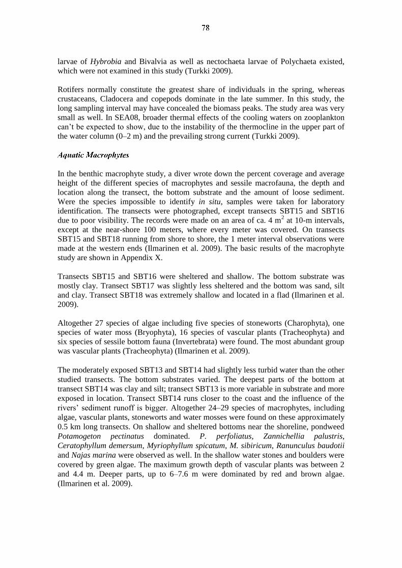
larvae of Hybrobia and Bivalvia as well as nectochaeta larvae of Polychaeta existed,
which were not examined in this study (Turkki 2009).
Rotifers normally constitute the greatest share of individuals in the spring, whereas
crustaceans, Cladocera and copepods dominate in the late summer. In this study, the
long sampling interval may have concealed the biomass peaks. The study area was very
small as well. In SEA08, broader thermal effects of the cooling waters on zooplankton
can’t be expected to show, due to the instability of the thermocline in the upper part of
the water column (0–2 m) and the prevailing strong current (Turkki 2009).
In the benthic macrophyte study, a diver wrote down the percent coverage and average
height of the different species of macrophytes and sessile macrofauna, the depth and
location along the transect, the bottom substrate and the amount of loose sediment.
Were the species impossible to identify in situ, samples were taken for laboratory
identification. The transects were photographed, except transects SBT15 and SBT16
due to poor visibility. The records were made on an area of ca. 4 m2 at 10-m intervals,
except at the near-shore 100 meters, where every meter was covered. On transects
SBT15 and SBT18 running from shore to shore, the 1 meter interval observations were
made at the western ends (Ilmarinen et al. 2009). The basic results of the macrophyte
study are shown in Appendix X.
Transects SBT15 and SBT16 were sheltered and shallow. The bottom substrate was
mostly clay. Transect SBT17 was slightly less sheltered and the bottom was sand, silt
and clay. Transect SBT18 was extremely shallow and located in a flad (Ilmarinen et al.
2009).
Altogether 27 species of algae including five species of stoneworts (Charophyta), one
species of water moss (Bryophyta), 16 species of vascular plants (Tracheophyta) and
six species of sessile bottom fauna (Invertebrata) were found. The most abundant group
was vascular plants (Tracheophyta) (Ilmarinen et al. 2009).
The moderately exposed SBT13 and SBT14 had slightly less turbid water than the other
studied transects. The bottom substrates varied. The deepest parts of the bottom at
transect SBT14 was clay and silt; transect SBT13 is more variable in substrate and more
exposed in location. Transect SBT14 runs closer to the coast and the influence of the
rivers’ sediment runoff is bigger. Altogether 24–29 species of macrophytes, including
algae, vascular plants, stoneworts and water mosses were found on these approximately
0.5 km long transects. On shallow and sheltered bottoms near the shoreline, pondweed
Potamogeton pectinatus dominated. P. perfoliatus, Zannichellia palustris,
Ceratophyllum demersum, Myriophyllum spicatum, M. sibiricum, Ranunculus baudotii
and Najas marina were observed as well. In the shallow water stones and boulders were
covered by green algae. The maximum growth depth of vascular plants was between 2
and 4.4 m. Deeper parts, up to 6–7.6 m were dominated by red and brown algae.
(Ilmarinen et al. 2009).
The species composition of the transect located in Flutanperä Bay (SBT18) was typical
for a flad: green algae (Vaucheria sp.), stoneworts (Chara aspera and Chara canescens)
and pondweed (Potamogeton pectinatus) were the most common species. Zannichellia
sp., Myriophyllum spicatum, Lemna trisulca and Najas marina appeared in some
places. Furthermore, club rush (Schoenoplectus tabernaemontani) and reed (Phragmites
australis) formed small stands along the transect. Altogether 13 species of macrophytes,
including algae, vascular plants and stoneworts, and three species of sessile
invertebrates were found on the transect. The most abundant groups of
macrozoobenthos were Gastropoda, Coleoptera and Chironomidae. Especially the
species Chironomus f. l. plumosus, which was only found at this transect, indicates high
eutrophication (Ilmarinen et al. 2009).
The extent of the reed colonies were recorded
at selected locations along the margin of the colony using a GPS device, and
observations were also made of the bottom type and water depth. The surveyed routes
were photographed as well, allowing delineation of the reed polygons from aerial
photographs. The results will be reported in
3.6.4 Marine Fauna
Bottom Fauna
Bottom fauna were inventoried in the mandatory monitoring programme of the power
plant on September 23 and 24, 2008 on plots.
Last year, only
o this year’s samples leaked as well and should be
treated as only approximate (Turkki 2009).
The number of s was in SEA08 and
the smallest in SEA09. The number of individuals varied between 2,843 and 4,527
individuals/m²
between 23 and 230 g/m²
the North-American polychaete
The average number of species, density and biomass were somewhat higher in 2008
than in 2007 (Turkki 2009). The numbers of species, individuals and biomass in 2008
by bottom type are presented in Table V-13. Since the sampling has often failed in hard
bottoms, time series figures (63 and 64) are presented for soft bottoms only.
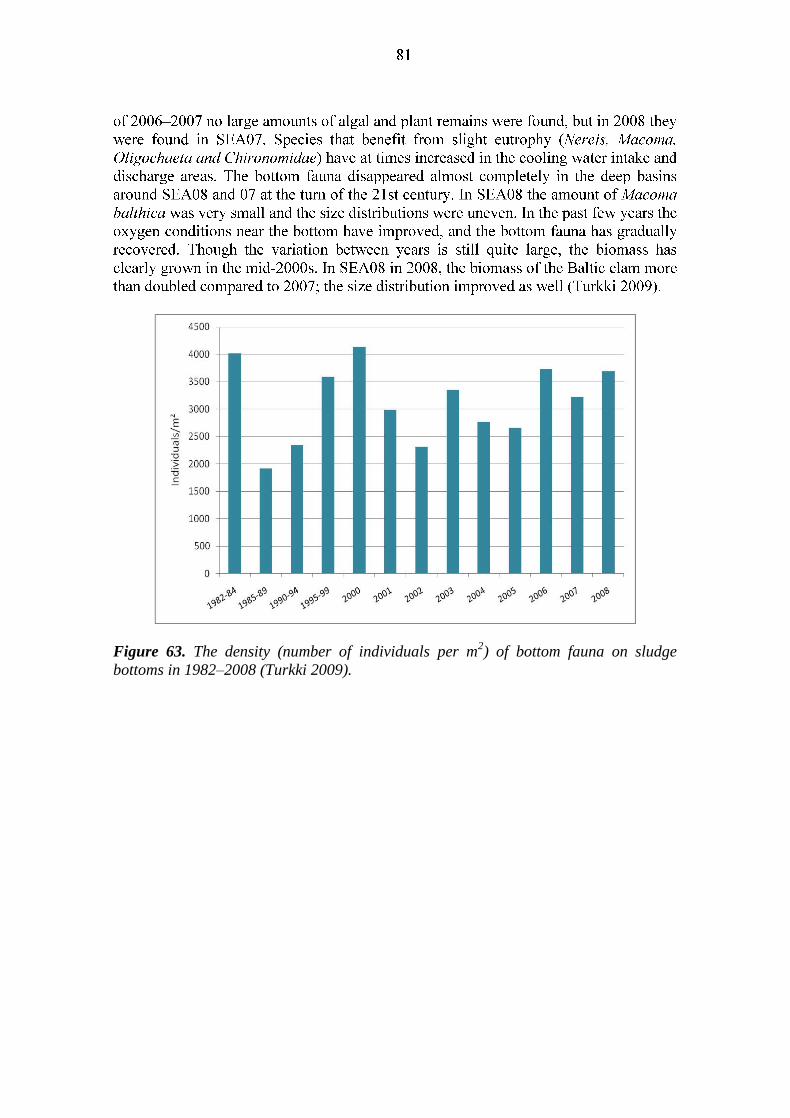
Figure 63. The density (number of individuals per m2) of bottom fauna on sludge
bottoms in 1982–2008 (Turkki 2009).
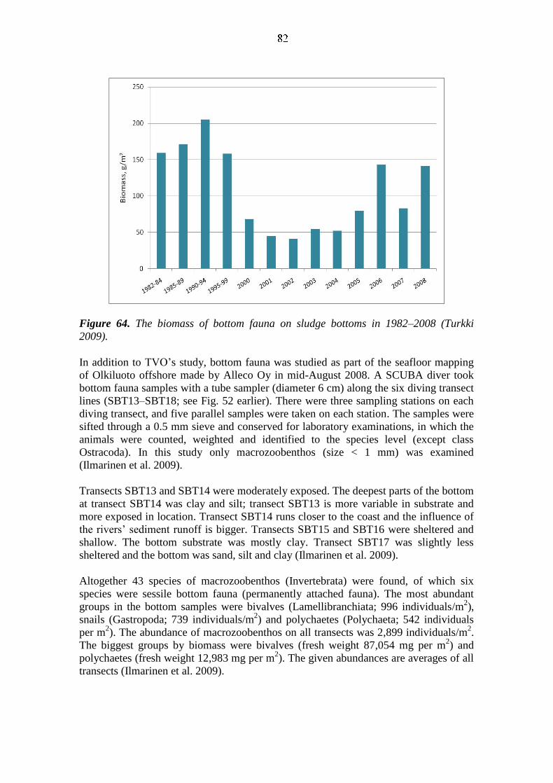
Figure 64. The biomass of bottom fauna on sludge bottoms in 1982–2008 (Turkki
2009).
In addition to TVO’s study, bottom fauna was studied as part of the seafloor mapping
of Olkiluoto offshore made by Alleco Oy in mid-August 2008. A SCUBA diver took
bottom fauna samples with a tube sampler (diameter 6 cm) along the six diving transect
lines (SBT13–SBT18; see Fig. 52 earlier). There were three sampling stations on each
diving transect, and five parallel samples were taken on each station. The samples were
sifted through a 0.5 mm sieve and conserved for laboratory examinations, in which the
animals were counted, weighted and identified to the species level (except class
Ostracoda). In this study only macrozoobenthos (size < 1 mm) was examined
(Ilmarinen et al. 2009).
Transects SBT13 and SBT14 were moderately exposed. The deepest parts of the bottom
at transect SBT14 was clay and silt; transect SBT13 is more variable in substrate and
more exposed in location. Transect SBT14 runs closer to the coast and the influence of
the rivers’ sediment runoff is bigger. Transects SBT15 and SBT16 were sheltered and
shallow. The bottom substrate was mostly clay. Transect SBT17 was slightly less
sheltered and the bottom was sand, silt and clay (Ilmarinen et al. 2009).
Altogether 43 species of macrozoobenthos (Invertebrata) were found, of which six
species were sessile bottom fauna (permanently attached fauna). The most abundant
groups in the bottom samples were bivalves (Lamellibranchiata; 996 individuals/m2),
snails (Gastropoda; 739 individuals/m2) and polychaetes (Polychaeta; 542 individuals
per m2). The abundance of macrozoobenthos on all transects was 2,899 individuals/m
2.
The biggest groups by biomass were bivalves (fresh weight 87,054 mg per m2) and
polychaetes (fresh weight 12,983 mg per m2). The given abundances are averages of all
transects (Ilmarinen et al. 2009).

SBT17 had the highest density of macrozoobenthos and a very high biodiversity with
species from 20 taxonomic groups (Figs. 65 and 66). The two other sheltered and
shallow soft bottom transects (SBT15 and 18) had also high diversity, but much lower
densities. The highest biomasses of individuals on transects SBT13, 14 and 17 were due
to the high abundance of Macoma baltica. Macoma baltica was also found at the clay
bottom transects SBT15 and 16. At transects SBT13, 14 and 17 Oligochaeta were
found, which are more common in clear water. These transects had slightly less turbid
water than the other transects. The biomass of Polychaeta Marenzelleria (arctia) was
high at transects SBT15 and SBT16. This species can tolerate low oxygen levels.
(Ilmarinen et al. 2009). For more details, see Appendix W.
Transect SBT18 was extremely shallow and located in a flad. The species composition
was typical for an enclosed bay in a land uplift region that still receives sea water
regularly. High biomass of Chironomidae were found at the transect; especially the
species Chironomus f. l. plumosus, which was only found at this transect, indicates high
eutrophication (Ilmarinen et al. 2009).
Figure 65. Macrozoobenthos individuals in sampling stations (Ilmarinen et al. 2009).
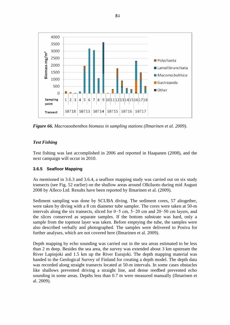
Figure 66. Macrozoobenthos biomass in sampling stations (Ilmarinen et al. 2009).
Test Fishing
Test fishing was last accomplished in 2006 and reported in Haapanen (2008), and the
next campaign will occur in 2010.
3.6.5 Seafloor Mapping
As mentioned in 3.6.3 and 3.6.4, a seafloor mapping study was carried out on six study
transects (see Fig. 52 earlier) on the shallow areas around Olkiluoto during mid August
2008 by Alleco Ltd. Results have been reported by Ilmarinen et al. (2009).
Sediment sampling was done by SCUBA diving. The sediment cores, 57 altogether,
were taken by diving with a 8 cm diameter tube sampler. The cores were taken at 50-m
intervals along the six transects, sliced for 0−5 cm, 5−20 cm and 20−50 cm layers, and
the slices conserved as separate samples. If the bottom substrate was hard, only a
sample from the topmost layer was taken. Before emptying the tube, the samples were
also described verbally and photographed. The samples were delivered to Posiva for
further analyses, which are not covered here (Ilmarinen et al. 2009).
Depth mapping by echo sounding was carried out in the sea areas estimated to be less
than 2 m deep. Besides the sea area, the survey was extended about 3 km upstream the
River Lapinjoki and 1.5 km up the River Eurajoki. The depth mapping material was
handed to the Geological Survey of Finland for creating a depth model. The depth data
was recorded along straight transects located at 50-m intervals. In some cases obstacles
like shallows prevented driving a straight line, and dense reedbed prevented echo
sounding in some areas. Depths less than 0.7 m were measured manually (Ilmarinen et
al. 2009).

The measured depths in the bathymetric survey were mostly over two metres, for the
area of the survey was determined from a nautical chart, where the depth data for the
shallow areas outside ship and boat lanes is inaccurate. The rivers are much deeper than
their mouth areas. The unmapped areas in the sheltered parts of the archipelago were
reedbeds (Phragmites australis) that couldn’t be penetrated during the survey. The reed
areas appeared to be less than one metre deep (Ilmarinen et al. 2009).
The study area showed a great variation in environmental conditions. Olkiluoto stands
between an almost open sea and the extremely sheltered river mouth area of Lapinjoki.
The moderately exposed north side and sheltered south side transects had plant and
animal communities quite typical to the archipelagos at the eastern side of Gulf of
Bothnia (Ilmarinen et al. 2009).
3.6.6 Anthropogenic and Social Effects
As part of the nuclear power plant's monitoring programme, fishing activities are
followed up by interviewing fishermen every other year. In addition, five fishermen
carry out continuous account fishing. Reporting of most recent results will be available
in summer 2009 and summarised in next version of this report.
3.7 Historical and Future Properties
For the Biosphere description 2009 report (Haapanen et al. 2009), a review was
prepared of the historical land use, evolution of settlement and history of agriculture
and forestry in the Satakunta region. Existing regional histories were used, as well as
maps acquired by the Vuojoki digitizing project. See the report for more information.
A GIS

4 RESULTS II: INPUT TO ENVIRONMENTAL IMPACT ASSESSMENTS 4.1 Air Quality
The results were reported in 2009 in a memo by the Finnish Forest Research Institute
(Lasse Aro, Arja Ylinen and Pasi Rautio) and are summarised here. Result tables can be
found in Appendix H.

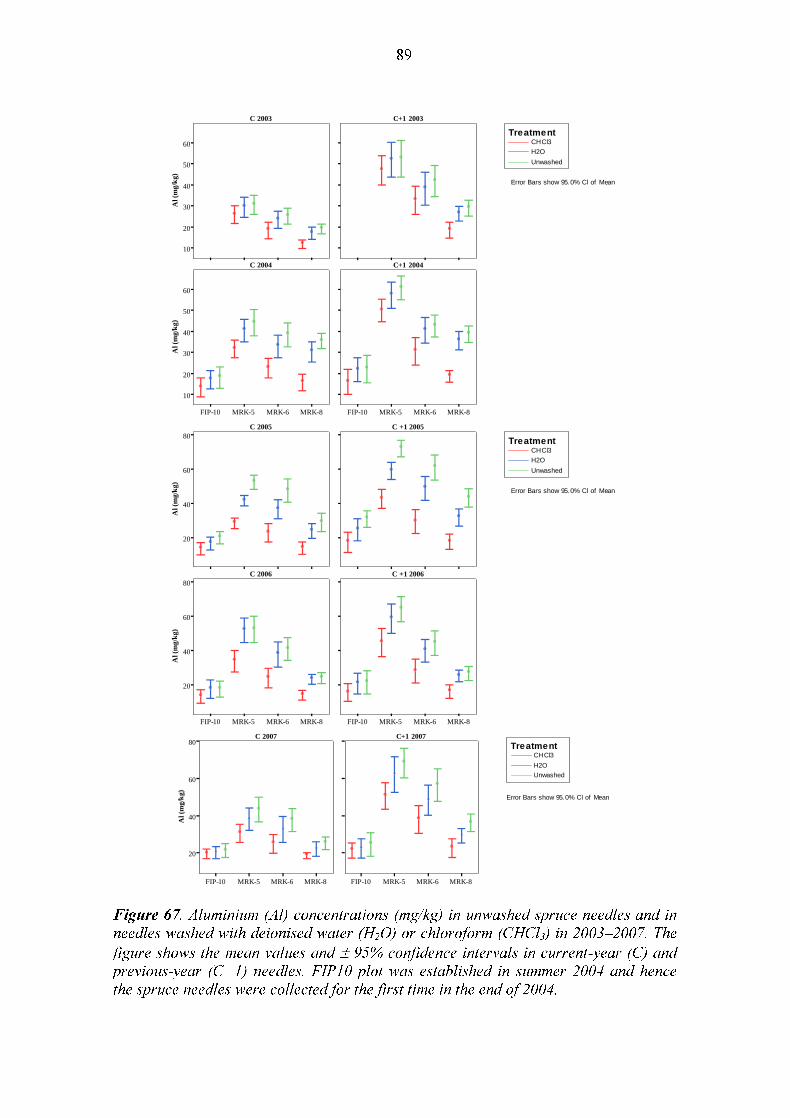
CHCl3
H2O
Unwashed
Treatment
Error Bars show 95.0% Cl of Mean
10
20
30
40
50
60
Al (m
g/k
g)
C 2003 C+1 2003
C 2004 C+1 2004
FIP-10 MRK-5 MRK-6 MRK-8
10
20
30
40
50
60
Al (m
g/k
g)
FIP-10 MRK-5 MRK-6 MRK-8
CHCl3
H2O
Unwashed
Treatment
Error Bars show 95.0% Cl of Mean
20
40
60
80
Al (m
g/k
g)
C 2005 C +1 2005
C 2006 C +1 2006
FIP-10 MRK-5 MRK-6 MRK-8
20
40
60
80
Al (m
g/k
g)
FIP-10 MRK-5 MRK-6 MRK-8
C 2007 C+1 2007
CHCl3
H2O
Unwashed
Treatment
Error Bars show 95.0% Cl of Mean
FIP-10 MRK-5 MRK-6 MRK-8
20
40
60
80
Al
(mg
/kg)
FIP-10 MRK-5 MRK-6 MRK-8

CHCl3
H2O
Unwashed
Treatment
Error Bars show 95.0% Cl of Mean
200
300
400
500
Al (m
g/k
g)
C 2003 C+1 2003
C 2004 C+1 2004
FIP-4 MRK-1 MRK-3
200
300
400
500
Al (m
g/k
g)
FIP-4 MRK-1 MRK-3
C 2005 C +1 2005
C 2006 C +1 2006
CHCl3
H2O
Unwashed
Treatment
Error Bars show 95.0% Cl of Mean
200
300
400
500
600
Al (m
g/k
g)
FIP-4 MRK-1 MRK-3
200
300
400
500
600
Al (m
g/k
g)
FIP-4 MRK-1 MRK-3
CHCl3
H2O
Unwashed
Treatment
Error Bars show 95.0% Cl of Mean
FIP-4 MRK-1 MRK-3
200
300
400
500
600
Al (m
g/k
g)
C 2007 C+1 2007
FIP-4 MRK-1 MRK-3
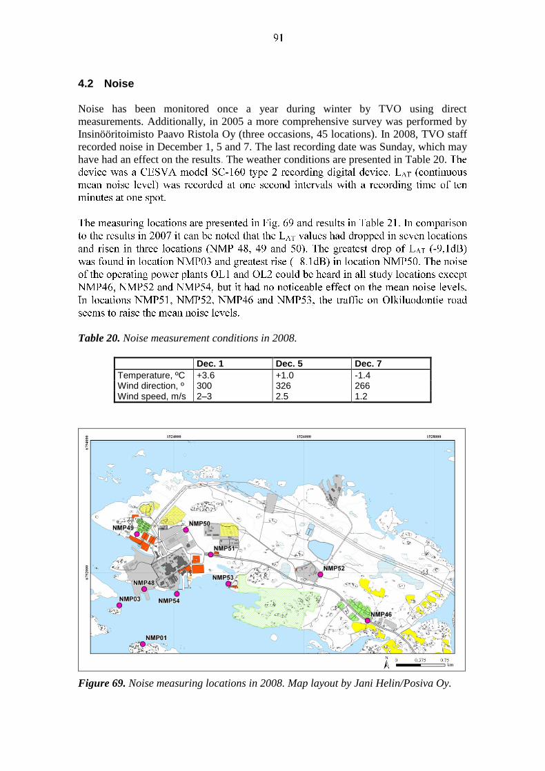
4.2 Noise
Noise has been monitored once a year during winter by TVO using direct
measurements. Additionally, in 2005 a more comprehensive survey was performed by
Insinööritoimisto Paavo Ristola Oy (three occasions, 45 locations). In 2008, TVO staff
recorded noise in December 1, 5 and 7. The last recording date was Sunday, which may
have had an effect on the results. The weather conditions are presented in Table 20.
Table 20. Noise measurement conditions in 2008.
Dec. 1 Dec. 5 Dec. 7
Temperature, ºC +3.6 +1.0 -1.4 Wind direction, º 300 326 266 Wind speed, m/s 2–3 2.5 1.2
Figure 69. Noise measuring locations in 2008. Map layout by Jani Helin/Posiva Oy.

Table 21. Noise levels (LAT , dB). In 2008 measurements occurred on December 1, 5*
and 7**.
Location 2007 2008
NMP01 44.2 36.6**
NMP03 47.2 38.1**
NMP46 52.7 49.4
NMP48 55.3 61.9*
NMP49 44.9 53.0
NMP50 49.2 55.1
NMP51 65.4 57.4
NMP52 54.3 50.0
NMP53 43.3 41.0
NMP54 46.9 46.5*
4.3 Water Quality
As stated above, TVO monitors seawater quality, nutrient and chemical loading and the
River Eurajoki is monitored by companies operating on its upper course. Results for the
quality, nutrient load and chemical loading of seawater are presented in Sub-section 3.6
and the results for the River Eurajoki in Sub-section 3.5. Surface runoff was first treated
in last year’s report, and is presented in connection to weather (Sub-section 3.2.2).
4.3.1 Drainage Water from Rock Heaps
Drainage water from rock heaps is sampled in observation wells or ditches three times
per year. Samples are analysed for heavy metals, amount of suspended solids and other
basic parameters. Monitoring of the ditch running by the rock piling and crushing areas
was started in autumn 2006. The results are compared with results from nearby multi-
level piezometer (OL-EP5). The results have been presented by TVO laboratory (Tiina
Lamminmäki) in a memo and are summarised here (r
–
In 2008, three samples were collected from OL-EP5 and one additional sample in
January 2009. From the ditch near OL-EP5 only two samples were collected in 2008;
due to lack of water, no sample could be taken in July and in January 2009 the ditch
was frozen. The analysis results between April 2008–January 2009, together with the
calculated TDS values and the charge balances are presented in Tables Y-1 and Y-2.
Figs. 70 and 71 show TDS and pH values during the full monitoring period.
In the samples taken between April 2008–January 2009, the water of OL-EP5 was
slightly alkaline with pH value ranging from 7.6–8.0, whereas the water of sample from
the nearby ditch was slightly acidic with pH values of 6.2 and 6.4. Conductivity ranged
from 78 mS/m to 250 mS/m in OL-EP5 and from 64 mS/m to 140 mS/m in the ditch.
The water type varied OL-EP5, whereas the water type in the ditch was Ca-Na-Mg-SO4
in both samplings. The waters were fresh (TDS < 1,000 mg/L), except in September
2008, when the waters were brackish (1,000 mg/L < TDS < 10,000 mg/L).
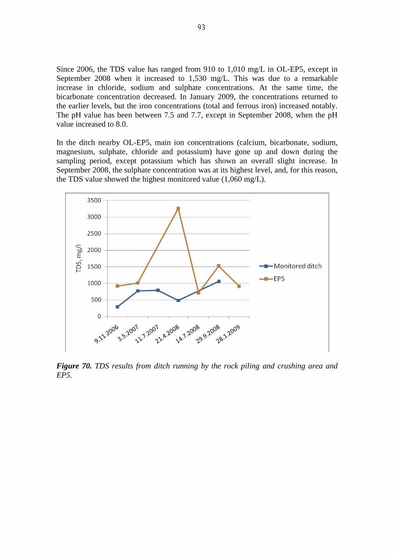
Since 2006, the TDS value has ranged from 910 to 1,010 mg/L in OL-EP5, except in
September 2008 when it increased to 1,530 mg/L. This was due to a remarkable
increase in chloride, sodium and sulphate concentrations. At the same time, the
bicarbonate concentration decreased. In January 2009, the concentrations returned to
the earlier levels, but the iron concentrations (total and ferrous iron) increased notably.
The pH value has been between 7.5 and 7.7, except in September 2008, when the pH
value increased to 8.0.
In the ditch nearby OL-EP5, main ion concentrations (calcium, bicarbonate, sodium,
magnesium, sulphate, chloride and potassium) have gone up and down during the
sampling period, except potassium which has shown an overall slight increase. In
September 2008, the sulphate concentration was at its highest level, and, for this reason,
the TDS value showed the highest monitored value (1,060 mg/L).
Figure 70. TDS results from ditch running by the rock piling and crushing area and
EP5.

Figure 71. pH results from ditch running by the rock piling and crushing area and
EP5.
4.3.2 Private Drilled Wells
The private drilled wells in active use have been chosen for monitoring the water table,
chemical composition and radon content. Originally there were four such wells, but
well DWH4 was no longer in use in 2007 and was removed from the program. Each
well is sampled once a year for chemical composition and radon content; in 2008 the
samples were taken on different days in each well, due problems with analysing
laboratory.
In 2008, the private well water tables were measured in April, June and August, except
for DWH3, which was measured in August. No water table measurements were taken in
late autumn in any of the wells. The results are presented in Fig. 72. Reference data
from three shallow wells in bedrock (PP) not affected by ONKALO are given as well.
PP values show water level above the sea level, whereas the DWH measurements give
difference to the top of the well. The fluctuation of private wells generally follows that
of reference data and no unexplained changes or effects from ONKALO were observed.
The low level in well DWH1 in late 2006 was due to heavy consumption just before the
measurement.
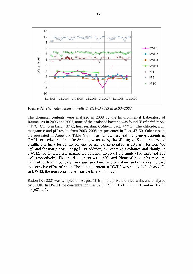
Figure 72. The water tables in wells DWH1–DWH3 in 2003–2008.
The chemical contents were analysed in 2008 by the Environmental Laboratory of
Rauma. As in 2006 and 2007, none of the analysed bacteria was found (Escherichia coli
+44ºC, Coliform bact. +37ºC, heat resistant Coliform bact. +44ºC). The chloride, iron,
manganese and pH results from 2003–2008 are presented in Figs. 47–50. Other results
are presented in Appendix Table Y-3.
Radon (Rn-222) was sampled on August 18 from the private drilled wells and analysed
by STUK. In DWH1 the concentration was 82 (
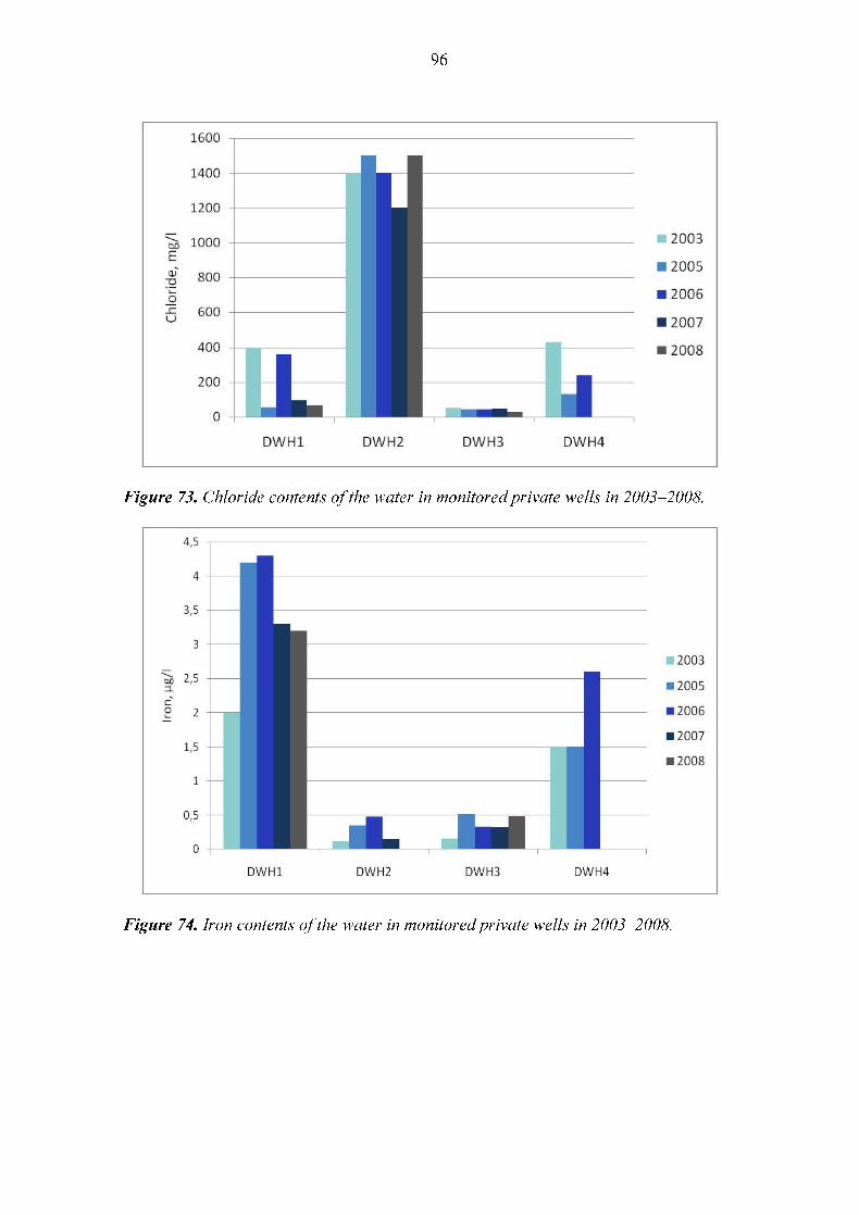
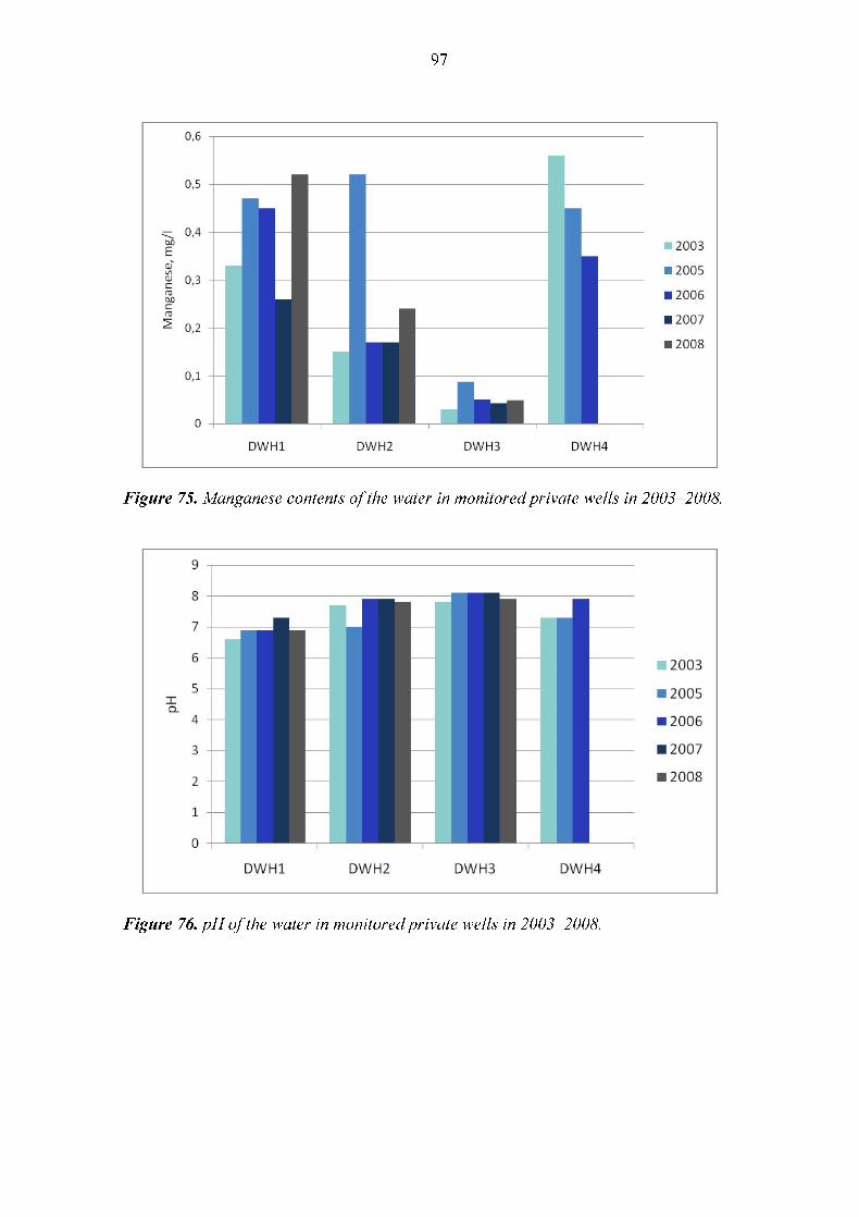
4.4 Overburden
The current monitoring data for nutrients, radionuclides and other substances in soil
have been presented in the modelling input (Sub-sections 3.3 and 3.4).
4.5 Flora and Fauna
A nature survey that covers the island is considered adequate for the environmental
impact evaluations with respect to flora and fauna. However, the FET and especially its
sub-sample will provide much more detailed vegetation information.
On the southern part of the island, there is a conservation area of old forest, which has
later been included in the Natura 2000 programme. The construction of ONKALO
could affect vegetation within this area through a change in groundwater level. The
vegetation sub-plots of the FIP system are also used to monitor these potential effects.
The flora and fauna studies have been presented in Sub-section 3.4.
4.6 Landscape, Land-Use and Traffic
A log of observations on landscape and land-use is to be maintained. For this frequently
taken aerial images are of great value, as well as digital photos taken on the ground. The
acquisition of aerial imagery has been presented in Sub-section 3.1. Ground-based
photographs were taken of the assessed FET plots in May 2008 (Sub-section 3.4) and
they serve as a baseline for the situation in 2008.
Baseline landscape and land-use of the vegetated areas have been documented in the
vegetation inventory (Miettinen & Haapanen 2002) and in the forest inventory by
compartments (Rautio et al. 2004). A statistical description of the forest and mire
regions is available in the FET inventory results (Saramäki & Korhonen 2005). The
new 50 x 50 m photo interpretation grid presented in Sub-section 3.1 is employed in
land-use change detection.
The potential of picking berries can be assessed on the basis of forest inventories,
national databases and knowledge of forest habitats.
Traffic conditions and changes in traffic levels are studied by means of single surveys
as needed during the construction of ONKALO. The ongoing construction of the OL3
nuclear power plant, however, has a much greater effect on traffic.
4.7 Supplementary Environmental Information
Supplementary environmental information outside Posiva's current scope, reported
within other site characterization disciplines or acquired by specific campaigns beyond
the actual monitoring programme, is taken into consideration as needed. Sources of this
information include TVO's monitoring programme (parts not considered here), the
future monitoring programme of the power plant for safeguard purposes, as well as
environmental studies carried out at the regional, national or international level by
authorities, research institutes, etc., and topical surveys for biosphere modelling, for
example.
In 2007, a vegetation mapping was done in association with a Natura assessment in the
northern parts of the Natura 2000 area. The study was presented in last year’s report.
The evaluation report of environmental impacts regarding the expanding of TVO’s
nuclear power plants with a fourth unit was completed in February 2008. A
supplementary report was delivered to the Ministry of employment and the economy in
August 2008 by TVO. In summer 2008, TVO started the Natura assessment in
accordance with the nature conservation act regarding possible impacts of the OL4
project on the Natura area in Rauma archipelago. Relating to the Natura assessment,
vegetation is surveyed by diving and video shooting in the sea areas of Rauma
archipelago in 2008 and 2009. The diving analyses were extended to the hard bottoms
in the central- and southern parts of the Natura area (e.g., on the western side of
Aikomaa and Nurmes as well as on the shores of Kylmä Santakari and Iso Pihlavakari
islands).
A survey was commissioned by TVO to investigate (during spring–early autumn 2008)
the occurrence of larvae of freshwater hydroid (Cordylophora caspia) in the sea water
system of Olkiluoto power plant in order to focus prevention measures.

5 SUMMARY
This report presents the annual environmental monitoring results for the year 2008. The
monitoring system is described in the Posiva Report 2003-05. The construction of
ONKALO underground rock characterization facility was started in July 2004 by
Posiva. Part of the measurements is targeted for monitoring the effects of this
construction work. Most, however, are meant for producing input for biosphere
modelling for long-term safety purposes. Many of the studies, especially those
concentrated on the sea ecosystem, have been running since the 1970s within TVO's
mandatory monitoring programme. Some of the monitoring is continuous, some is
performed annually and some is carried out in campaigns at intervals of 1–10 years.
The monitoring was accomplished as planned in 2008, but with amendments: several
studies on fauna were carried out, some soil and vegetation transects running from land
to sea were established, a separate survey of water quality with automatic detectors was
carried out and zooplankton and organic carbon studies were started in the context of
sea monitoring. First full year cycle of evapotranspiration on FIP4 and FIP10 was
available in summer 2008. Results from root investigation, soil profiles description and
soil, organic layer and ground vegetation samples taken on FIP plots were available for
the first time, as well. Reporting of weather monitoring has now been transferred to this
Working Report solely.
In the studies that have already produced repetitive data, no drastic changes were
observed in 2008, as were also the cases in 2004–2007. The proximity of sea and dust
produced during construction activities is seen in the soil solution and deposition
results. The animal and bird life on the island remains rich and typical of a coastal
region. However, in the middle of the island and the surroundings of the power stations,
the birdlife has undergone a change during the last decade. The game catches vary
according to hunting pressure and natural variation in populations. The mammalian
fauna on the island is very typical of coastal areas in Southwestern Finland. Olkiluoto is
generally not very favourable for most amphibians and reptiles. The captured
invertebrates represented rather common ones in Southern Finland.
Phytoplankton biomasses and primary production were higher than in 2007. The
biomasses have grown in the whole monitored sea area compared with the turn of 1980s
and 1990s and the differences between the cooling water discharge site and other
locations have diminished. Marine bottom fauna has suffered on the observation sites
closest to the cooling water discharge site, but in 2004–2008 the populations have
somewhat recovered. The new transect study concerned bottom fauna, aquatic
macrophytes and seafloor properties on the aquatic parts of the transects, and it
succeeded to catch varying bottom types and degrees of shelter and produced valuable
data for monitoring and modelling.
The water quality of the three monitored private drilled wells was poor, as in previous
years. The water level fluctuation follows that of reference sites (shallow wells in
bedrock not affected by ONKALO). The ditch water from rock piling and crushing area
was slightly acidic. Main ion concentrations have fluctuated during the monitoring

period. Noise readings in late 2008 varied between 36.6 and 61.9 dB. Industrial
activities, along with traffic, have an effect on the average noise levels.
REFERENCES
Derome, J. Lindroos, A-J. & Derome, K. 2007. Soil percolation water quality during
2001-2004 on 11 Level II plots. In: Merilä, P., Kilponen, T. & Derome, J. (eds.). Forest
Condition Monitoring in Finland – National report 2002–2005. Working Papers of the
Finnish Forest Research Institute 45. pp. 93–98.
Haapanen, R. 2005. Results of Monitoring at Olkiluoto in 2004. Environment. Posiva
Oy, Working Report 2005-31. 127 p. http://www.posiva.fi/
Haapanen, R. 2006. Results of Monitoring at Olkiluoto in 2005. Environment. Posiva
Oy, Working Report 2006-68. 99 p. http://www.posiva.fi/
Haapanen, R. 2007. Results of Monitoring at Olkiluoto in 2006. Environment. Posiva
Oy, Working Report 2007-52. 111 p. http://www.posiva.fi/
Haapanen, R. 2008. Results of Monitoring at Olkiluoto in 2007. Environment. Posiva
Oy, Working Report 2008-25. 111 p. http://www.posiva.fi/
Haapanen, R., Aro, L., Ilvesniemi, H., Kareinen, T., Kirkkala, T., Lahdenperä A-M.,
Mykrä, S., Turkki, H. & Ikonen, A. 2007. Olkiluoto Biosphere description 2006. Posiva
Oy, Report 2007-02. 181 p. http://www.posiva.fi/
Haapanen, R., Aro, L., Helin, J., Hjerpe, T., Ikonen, A., Kirkkala, T., Koivunen, S.,
Lahdenperä A-M., Puhakka, L., Rinne, M. & Salo, T. 2009. Olkiluoto Biosphere
Description 2009. Posiva Oy, Report. In press. 414 p.
Helle, P. & Wikman, M. 2008. Metsäkanalinnut syksyllä 2007 (In Finnish: Grouses in
autumn 2007.) In: Wikman, M. (ed.) Riistakannat 2007. Riista- ja kalatalousselvityksiä
5/2008.
Helmisaari, H-S., Derome, J., Nöjd, P. & Kukkola, M. 2007. Fine root biomass in
relation to site and stand characteristics in Norway spruce and Scots pine stands. Tree
Physiology. Vol. 27, no. 10, p. 1493–1504.
Helmisaari, H-S., Sah, S. & Aro, L. 2009. Fine roots on the intensive forest ecosystem
monitoring plots on Olkiluoto Island in 2008. Posiva Oy, Working Report 2009. In
preparation.
Hilden, O., Ulfvens, J., Pahtamaa, T. & Hästbacka, H. 1995. Changes in the archipelago
bird populations of the Finnish Quark, Gulf of Bothnia, from 1957–60 to 1990–91.
Ornis Fennica Vol. 72, no 3, p. 115–126.
Huhta, A-P. & Korpela, L. 2006. Permanent vegetation quadrats on Olkiluoto Island.
Establishment and results from the first inventory. Posiva Oy, Working Report 2006-
33. 76 p. http://www.posiva.fi/
Ikonen, A.T.K. 2002. Meteorological data of Olkiluoto in period of 1992–2001. Posiva
Oy, Working Report 2002-44. 26 p.
Ikonen, A.T.K. 2003. Environmental Radioactivity Data of Olkiluoto in 1984–2001.
Posiva Oy, Working Report 2003-14.
Ikonen, A.T.K. 2005. Meteorological data of Olkiluoto in period of 2002–2004. Posiva
Oy, Working Report 2005-35. 53 p. http://www.posiva.fi/
Ikonen, A.T.K. 2006. Posiva Biosphere Assessment: Revised structure and status 2006.
Posiva Oy, Report 2006-07. 132 p. http://www.posiva.fi/
Ikonen, A.T.K. 2007. Meteorological data and update of climate statistics of Olkiluoto,
2005–2006. Posiva Oy, Working Report 2007-86. 72 p.
Ikonen, A.T.K., Kaapu, J., Lehtonen, K., Mattila, J., Räisänen, R., Sauvonsaari, J. &
Turkki, H. 2003. Environment studies in the Olkiluoto area. Posiva Oy, Working
Report 2003-15. 114 p. http://www.posiva.fi/
Ilmarinen, K., Leinikki, J. & Oulasvirta, P. 2009. Seafloor mapping at Olkiluoto,
western coast of Finland. Posiva Oy, Working Report 2009-12. 48 p.
http://www.posiva.fi/
Järvinen, O. & Väisänen, R. A. 1983. Correction coefficients for line transect censuses
of breeding birds. Ornis Fennica Vol. 60, no 4, p. 97–104.
Jussila, I. & Nieminen, M. 2009. Game statistics for the Island of Olkiluoto in 2008–
2009. Posiva Oy, Working Report. In preparation.
Koskimies, P. & Väisänen, R. A. 1988. Linnustonseurannan havainnointiohjeet (In
Finnish: Observation guidelines for bird inventory). Helsingin yliopiston eläinmuseo,
Helsinki.
Lahdenperä, A-M., Palmén, J. & Hellä, P. 2005. Summary of Overburden Studies at
Olkiluoto with an Emphasis on Geosphere-Biosphere Interface. Posiva Oy, Working
Report 2005-11. 85 p. http://www.posiva.fi/
Lindfors, A., Huttunen, O. & Mykkänen, J. Vedenlaadun alueellinen jakauma
Olkiluodon edustalla heinäkuussa 2008. (In Finnish with an English abstract: Areal
Changes in Water Quality in Olkiluoto Area in July 2008). Posiva Oy, Working Report
2008-86. 33 p. http://www.posiva.fi/
Lindgren, M., Nevalainen, S. & Pouttu, A. 2007. Crown condition on the Level II
network 2001–2004. In: Merilä, P., Kilponen, T. & Derome, J. (eds.). Forest Condition
Monitoring in Finland. National report 2002–2005. Working Papers of the Finnish
Forest Research Institute 45, p. 41–45.
Miettinen, T. & Haapanen, R. 2002. Vegetation Types on Olkiluoto Island. Posiva Oy,
Working Report 2002-54. 54 p.
Mäkiaho, J-P. 2005. Development of Shoreline and Topography in the Olkiluoto Area,
Western Finland, 2000 BP–8000 AP. Posiva Oy, Working Report 2005-70. 47 p.
http://www.posiva.fi/
Nieminen, M. & Saarikivi, J. 2008. Herpetofauna and small mammals on the island of
Olkiluoto in 2008. Posiva Oy, Working Report 2008-91. 39 p. http://www.posiva.fi/
Posiva 2003a. Baseline conditions at Olkiluoto. Posiva Oy. Posiva Report 2003-02. 127
p.
Posiva 2003b. Programme of monitoring at Olkiluoto during construction and operation
of the ONKALO. Posiva Oy. Posiva Report 2003-05. 92 p http://www.posiva.fi/
Potila, H., Sarjala, T., & Aro, L. 2007. Dissolved nitrogen transformations and
microbial community structure in the organic layer of forest soils in Olkiluoto in 2006.
Posiva Oy, Working Report 2007-08. http://www.posiva.fi/
Ranta, P., Pöyri, V. & Vihervaara, P. 2005. Small mammal, bat and carabid beetle
inventories and update of game statistics for the Olkiluoto site in 2004. Posiva Oy,
Working Report 2005-19. 22 p. http://www.posiva.fi/
Rantataro, J. 2001. Acoustic-seismic research in the sea area near Olkiluoto in the year
2000 (In Finnish with an English abstract). Posiva Oy, Working Report 2002-19.
Rantataro, J. 2002. The estimation of sedimentary rock covered areas as well as
supplementary interpretation of acoustic-seismic research in Olkiluoto area (In Finnish
with an English abstract). Posiva Oy, Working Report 2002-38.
Rantataro, J. & Kaskela, A. 2009. Acoustic seismic studies in the sea area close to
Olkiluoto, 2008. Posiva Oy, Working Report 2009. In preparation.
Rautio, P., Latvajärvi, H., Jokela, A. & Kangas-Korhonen, P. 2004. Forest resources on
Olkiluoto Island. Posiva Oy, Working Report 2004-35. 109 p.
Roivainen, P. 2005. Environmental radioactivity data of Olkiluoto in 1977–1983 and
2002–2003. Posiva Oy, Working Report 2005-26. 121 p. http://www.posiva.fi/
Roivainen, P. 2006. Stable elements and radionuclides in shoreline alder stands at
Olkiluoto in 2005. Posiva Working Report 2006-70. 103 p. http://www.posiva.fi/
Santaharju, J., Helminen, S-L. & Yrjölä, R. 2009. Eurajoki Olkiluoto study on species
of ground beetles and ants 2008. Posiva Oy, Working Report 2009-18. 28 p.
Saramäki, J. & Korhonen, K. 2005. State of the Forests on Olkiluoto in 2004.
Comparisons between Olkiluoto and the rest of Southwest Finland. Posiva Oy, Working
Report 2005-39. 79 p. http://www.posiva.fi/
Tamminen, P., Aro, L. & Salemaa, M. 2007. Forest soil survey and mapping of
vegetation nutrition on Olkiluoto Island. Results from the first inventory on FEH plots.
Posiva Oy, Working Report 2007-78. 110 p. http://www.posiva.fi/
Turkki, H. 2009. Olkiluodon lähivesien fysikaalis-kemiallinen ja biologinen
tarkkailututkimus. Vuosiraportti 2008. (In Finnish: The physiochemical and biological
monitoring of nearby waters of Olkiluoto. Annual report 2008.) Lounais-Suomen vesi-
ja ympäristötutkimus Oy. Nro 114-09-340. 126 p.
Väisänen, R. A., Koskimies, P. & Lammi, E. 1998. Muuttuva pesimälinnusto (In
Finnish: Changing breeding bird populations). Helsinki, Otava. 567 p.
Vakkilainen, P. 1986. Haihdunta. (In Finnish: Evaporation). In: Mustonen, S. (ed.)
Sovellettu hydrologia (Applied hydrology). Vesiyhdistys r.y., 64–79.
Yrjölä, R. 2007. Vuosaaren satamahankkeen linnustonseuranta 2007 (In Finnish: Bird
inventory of the Vuosaari harbour project). Helsingin kaupungin ympäristökeskuksen
julkaisuja 4/2007. 68 p.
Yrjölä, R. 2009. Eurajoki Olkiluoto birdlife survey 2008. Posiva Oy, Working Report
2009-14. 76 p.
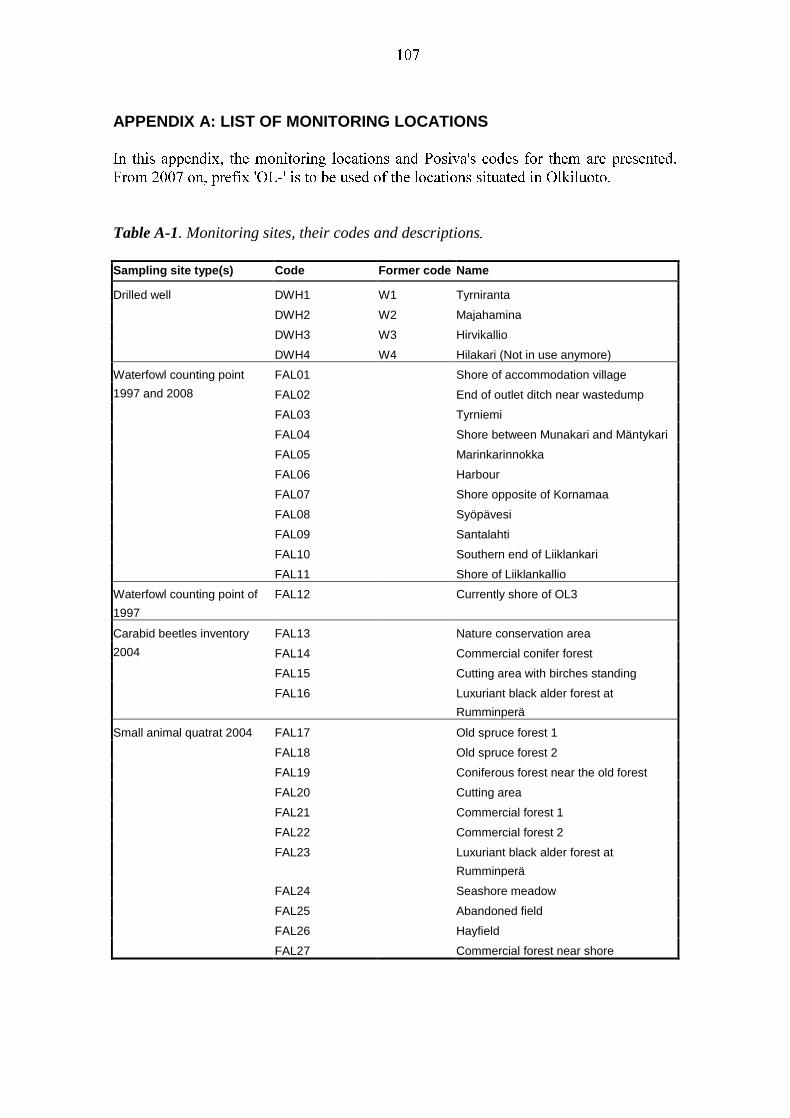
APPENDIX A: LIST OF MONITORING LOCATIONS
Table A-1. Monitoring sites, their codes and descriptions
Sampling site type(s) Code Former code Name
Drilled well DWH1 W1 Tyrniranta
DWH2 W2 Majahamina
DWH3 W3 Hirvikallio
DWH4 W4 Hilakari (Not in use anymore)
Waterfowl counting point
1997 and 2008
FAL01 Shore of accommodation village
FAL02 End of outlet ditch near wastedump
FAL03 Tyrniemi
FAL04 Shore between Munakari and Mäntykari
FAL05 Marinkarinnokka
FAL06 Harbour
FAL07 Shore opposite of Kornamaa
FAL08 Syöpävesi
FAL09 Santalahti
FAL10 Southern end of Liiklankari
FAL11 Shore of Liiklankallio
Waterfowl counting point of
1997
FAL12 Currently shore of OL3
Carabid beetles inventory
2004
FAL13 Nature conservation area
FAL14 Commercial conifer forest
FAL15 Cutting area with birches standing
FAL16 Luxuriant black alder forest at
Rumminperä
Small animal quatrat 2004 FAL17 Old spruce forest 1
FAL18 Old spruce forest 2
FAL19 Coniferous forest near the old forest
FAL20 Cutting area
FAL21 Commercial forest 1
FAL22 Commercial forest 2
FAL23 Luxuriant black alder forest at
Rumminperä
FAL24 Seashore meadow
FAL25 Abandoned field
FAL26 Hayfield
FAL27 Commercial forest near shore
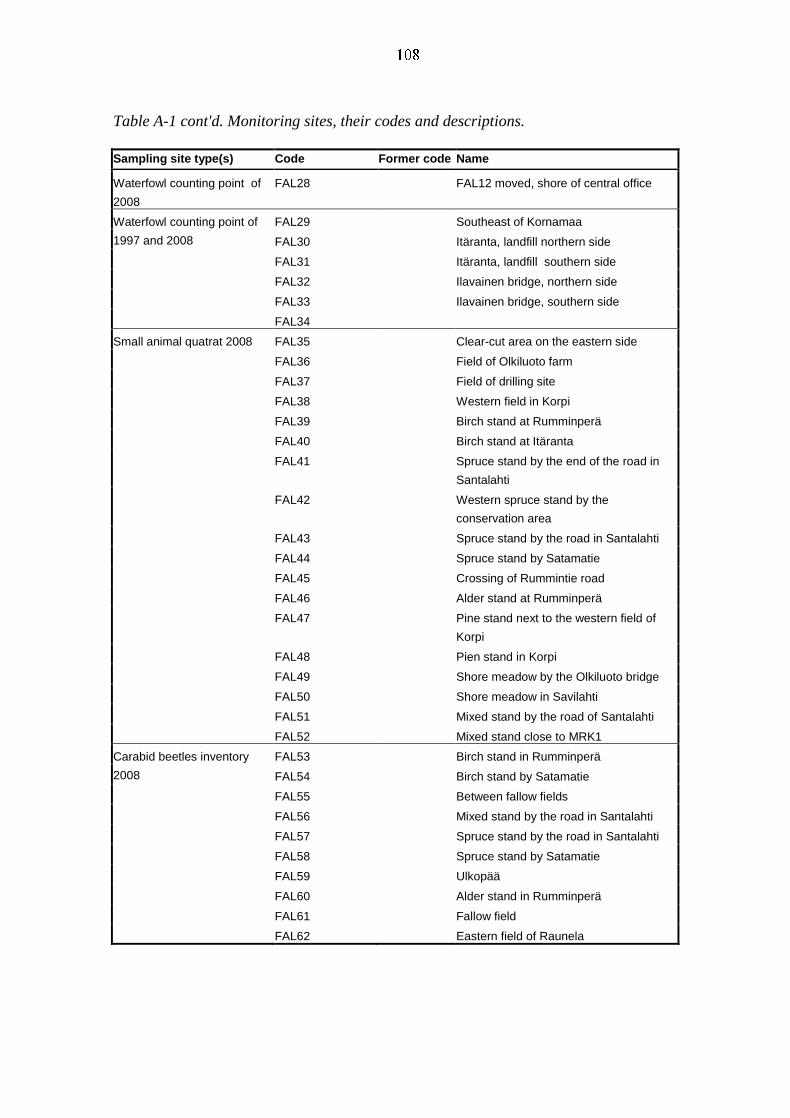
Table A-1 cont'd. Monitoring sites, their codes and descriptions.
Sampling site type(s) Code Former code Name
Waterfowl counting point of
2008
FAL28 FAL12 moved, shore of central office
Waterfowl counting point of
1997 and 2008
FAL29 Southeast of Kornamaa
FAL30 Itäranta, landfill northern side
FAL31 Itäranta, landfill southern side
FAL32 Ilavainen bridge, northern side
FAL33 Ilavainen bridge, southern side
FAL34
Small animal quatrat 2008 FAL35 Clear-cut area on the eastern side
FAL36 Field of Olkiluoto farm
FAL37 Field of drilling site
FAL38 Western field in Korpi
FAL39 Birch stand at Rumminperä
FAL40 Birch stand at Itäranta
FAL41 Spruce stand by the end of the road in
Santalahti
FAL42 Western spruce stand by the
conservation area
FAL43 Spruce stand by the road in Santalahti
FAL44 Spruce stand by Satamatie
FAL45 Crossing of Rummintie road
FAL46 Alder stand at Rumminperä
FAL47 Pine stand next to the western field of
Korpi
FAL48 Pien stand in Korpi
FAL49 Shore meadow by the Olkiluoto bridge
FAL50 Shore meadow in Savilahti
FAL51 Mixed stand by the road of Santalahti
FAL52 Mixed stand close to MRK1
Carabid beetles inventory
2008
FAL53 Birch stand in Rumminperä
FAL54 Birch stand by Satamatie
FAL55 Between fallow fields
FAL56 Mixed stand by the road in Santalahti
FAL57 Spruce stand by the road in Santalahti
FAL58 Spruce stand by Satamatie
FAL59 Ulkopää
FAL60 Alder stand in Rumminperä
FAL61 Fallow field
FAL62 Eastern field of Raunela
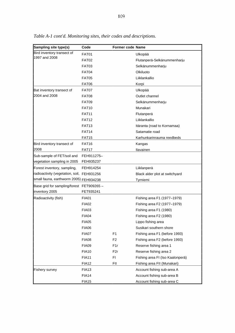
Table A-1 cont'd. Monitoring sites, their codes and descriptions.
Sampling site type(s) Code Former code Name
Bird inventory transect of
1997 and 2008 FAT01 Ulkopää
FAT02 Flutanperä-Selkänummenharju
FAT03 Selkänummenharju
FAT04 Olkiluoto
FAT05 Liiklankallio
FAT06 Korpi
Bat inventory transect of
2004 and 2008
FAT07 Ulkopää
FAT08 Outlet channel
FAT09 Selkänummenharju
FAT10 Munakari
FAT11 Flutanperä
FAT12 Liiklankallio
FAT13 Itäranta (road to Kornamaa)
FAT14 Satamatie road
FAT15 Karhunkarinrauma reedbeds
Bird inventory transect of
2008
FAT16 Kangas
FAT17 Ilavainen
Sub-sample of FET/soil and
vegetation sampling in 2005
FEH911275–
FEH935237
Forest inventory, sampling,
radioactivity (vegetation, soil,
small fauna, earthworm 2005)
FEH914254 Liiklanperä
FEH931256 Black alder plot at switchyard
FEH934238 Tyrniemi
Base grid for sampling/forest
inventory 2005
FET909265 –
FET935241
Radioactivity (fish) FIA01 Fishing area F1 (1977–1979)
FIA02 Fishing area F2 (1977–1979)
FIA03 Fishing area F1 (1980)
FIA04 Fishing area F2 (1980)
FIA05 Lippo fishing area
FIA06 Susikari southern shore
FIA07 F1 Fishing area F1 (before 1993)
FIA08 F2 Fishing area F2 (before 1993)
FIA09 F1r Reserve fishing area 1
FIA10 F2r Reserve fishing area 2
FIA11 FI Fishing area FI (Iso Kaalonperä)
FIA12 FII Fishing area FII (Munakari)
Fishery survey FIA13 Account fishing sub-area A
FIA14 Account fishing sub-area B
FIA15 Account fishing sub-area C
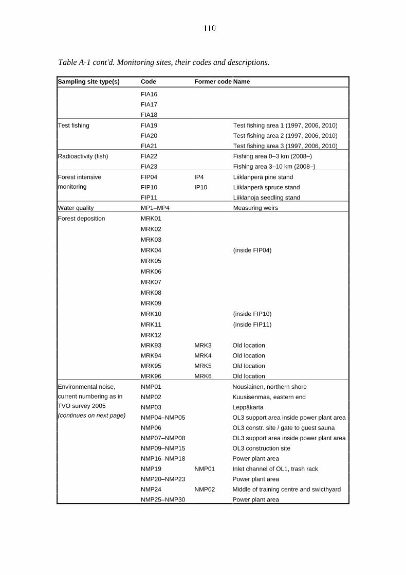
Table A-1 cont'd. Monitoring sites, their codes and descriptions.
Sampling site type(s) Code Former code Name
FIA16
FIA17
FIA18
Test fishing FIA19 Test fishing area 1 (1997, 2006, 2010)
FIA20 Test fishing area 2 (1997, 2006, 2010)
FIA21 Test fishing area 3 (1997, 2006, 2010)
Radioactivity (fish) FIA22 Fishing area 0–3 km (2008–)
FIA23 Fishing area 3–10 km (2008–)
Forest intensive
monitoring
FIP04 IP4 Liiklanperä pine stand
FIP10 IP10 Liiklanperä spruce stand
FIP11 Liiklanoja seedling stand
Water quality MP1–MP4 Measuring weirs
Forest deposition MRK01
MRK02
MRK03
MRK04 (inside FIP04)
MRK05
MRK06
MRK07
MRK08
MRK09
MRK10 (inside FIP10)
MRK11 (inside FIP11)
MRK12
MRK93 MRK3 Old location
MRK94 MRK4 Old location
MRK95 MRK5 Old location
MRK96 MRK6 Old location
Environmental noise,
current numbering as in
TVO survey 2005
(continues on next page)
NMP01 Nousiainen, northern shore
NMP02 Kuusisenmaa, eastern end
NMP03 Leppäkarta
NMP04–NMP05 OL3 support area inside power plant area
NMP06 OL3 constr. site / gate to guest sauna
NMP07–NMP08 OL3 support area inside power plant area
NMP09–NMP15 OL3 construction site
NMP16–NMP18 Power plant area
NMP19 NMP01 Inlet channel of OL1, trash rack
NMP20–NMP23 Power plant area
NMP24 NMP02 Middle of training centre and swicthyard
NMP25–NMP30 Power plant area
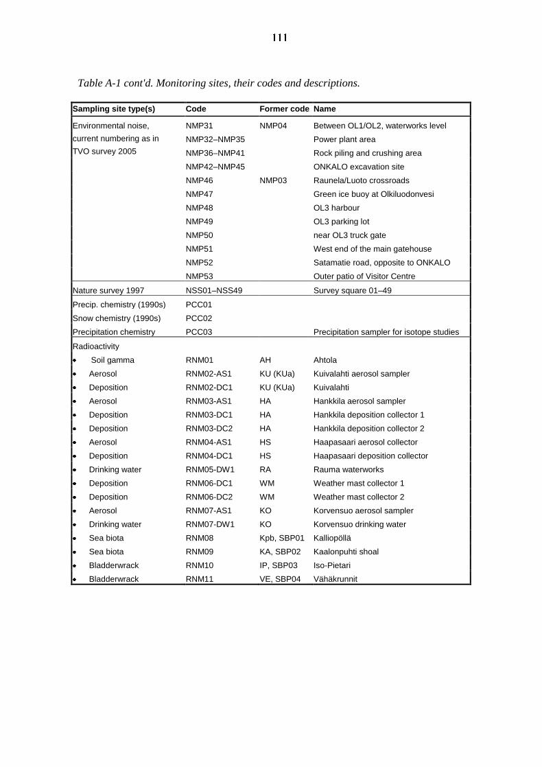
Table A-1 cont'd. Monitoring sites, their codes and descriptions.
Sampling site type(s) Code Former code Name
Environmental noise,
current numbering as in
TVO survey 2005
NMP31 NMP04 Between OL1/OL2, waterworks level
NMP32–NMP35 Power plant area
NMP36–NMP41 Rock piling and crushing area
NMP42–NMP45 ONKALO excavation site
NMP46 NMP03 Raunela/Luoto crossroads
NMP47 Green ice buoy at Olkiluodonvesi
NMP48 OL3 harbour
NMP49 OL3 parking lot
NMP50 near OL3 truck gate
NMP51 West end of the main gatehouse
NMP52 Satamatie road, opposite to ONKALO
NMP53 Outer patio of Visitor Centre
Nature survey 1997 NSS01–NSS49 Survey square 01–49
Precip. chemistry (1990s) PCC01
Snow chemistry (1990s) PCC02
Precipitation chemistry PCC03 Precipitation sampler for isotope studies
Radioactivity
Soil gamma RNM01 AH Ahtola
Aerosol RNM02-AS1 KU (KUa) Kuivalahti aerosol sampler
Deposition RNM02-DC1 KU (KUa) Kuivalahti
Aerosol RNM03-AS1 HA Hankkila aerosol sampler
Deposition RNM03-DC1 HA Hankkila deposition collector 1
Deposition RNM03-DC2 HA Hankkila deposition collector 2
Aerosol RNM04-AS1 HS Haapasaari aerosol collector
Deposition RNM04-DC1 HS Haapasaari deposition collector
Drinking water RNM05-DW1 RA Rauma waterworks
Deposition RNM06-DC1 WM Weather mast collector 1
Deposition RNM06-DC2 WM Weather mast collector 2
Aerosol RNM07-AS1 KO Korvensuo aerosol sampler
Drinking water RNM07-DW1 KO Korvensuo drinking water
Sea biota RNM08 Kpb, SBP01 Kalliopöllä
Sea biota RNM09 KA, SBP02 Kaalonpuhti shoal
Bladderwrack RNM10 IP, SBP03 Iso-Pietari
Bladderwrack RNM11 VE, SBP04 Vähäkrunnit
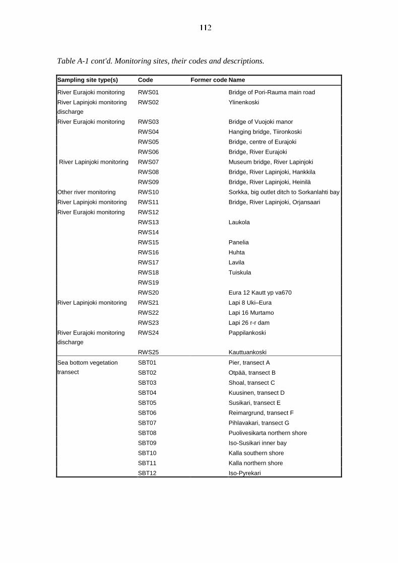
Table A-1 cont'd. Monitoring sites, their codes and descriptions.
Sampling site type(s) Code Former code Name
River Eurajoki monitoring RWS01 Bridge of Pori-Rauma main road
River Lapinjoki monitoring
discharge
RWS02 Ylinenkoski
River Eurajoki monitoring RWS03 Bridge of Vuojoki manor
RWS04 Hanging bridge, Tiironkoski
RWS05 Bridge, centre of Eurajoki
RWS06 Bridge, River Eurajoki
River Lapinjoki monitoring RWS07 Museum bridge, River Lapinjoki
RWS08 Bridge, River Lapinjoki, Hankkila
RWS09 Bridge, River Lapinjoki, Heinilä
Other river monitoring RWS10 Sorkka, big outlet ditch to Sorkanlahti bay
River Lapinjoki monitoring RWS11 Bridge, River Lapinjoki, Orjansaari
River Eurajoki monitoring RWS12
RWS13 Laukola
RWS14
RWS15 Panelia
RWS16 Huhta
RWS17 Lavila
RWS18 Tuiskula
RWS19
RWS20 Eura 12 Kautt yp va670
River Lapinjoki monitoring RWS21 Lapi 8 Uki–Eura
RWS22 Lapi 16 Murtamo
RWS23 Lapi 26 r-r dam
River Eurajoki monitoring
discharge
RWS24 Pappilankoski
RWS25 Kauttuankoski
Sea bottom vegetation
transect
SBT01 Pier, transect A
SBT02 Otpää, transect B
SBT03 Shoal, transect C
SBT04 Kuusinen, transect D
SBT05 Susikari, transect E
SBT06 Reimargrund, transect F
SBT07 Pihlavakari, transect G
SBT08 Puolivesikarta northern shore
SBT09 Iso-Susikari inner bay
SBT10 Kalla southern shore
SBT11 Kalla northern shore
SBT12 Iso-Pyrekari
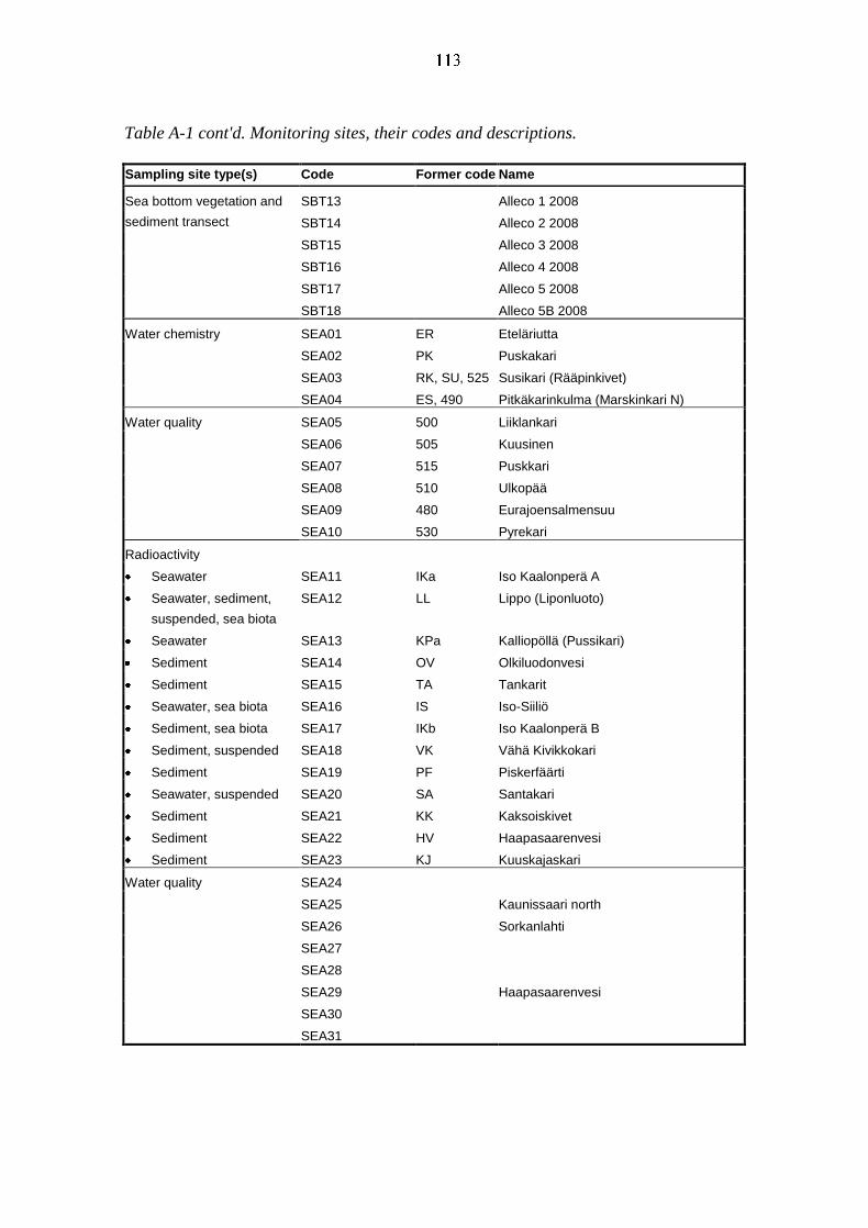
Table A-1 cont'd. Monitoring sites, their codes and descriptions.
Sampling site type(s) Code Former code Name
Sea bottom vegetation and
sediment transect
SBT13 Alleco 1 2008
SBT14 Alleco 2 2008
SBT15 Alleco 3 2008
SBT16 Alleco 4 2008
SBT17 Alleco 5 2008
SBT18 Alleco 5B 2008
Water chemistry SEA01 ER Eteläriutta
SEA02 PK Puskakari
SEA03 RK, SU, 525 Susikari (Rääpinkivet)
SEA04 ES, 490 Pitkäkarinkulma (Marskinkari N)
Water quality SEA05 500 Liiklankari
SEA06 505 Kuusinen
SEA07 515 Puskkari
SEA08 510 Ulkopää
SEA09 480 Eurajoensalmensuu
SEA10 530 Pyrekari
Radioactivity
Seawater SEA11 IKa Iso Kaalonperä A
Seawater, sediment,
suspended, sea biota
SEA12 LL Lippo (Liponluoto)
Seawater SEA13 KPa Kalliopöllä (Pussikari)
Sediment SEA14 OV Olkiluodonvesi
Sediment SEA15 TA Tankarit
Seawater, sea biota SEA16 IS Iso-Siiliö
Sediment, sea biota SEA17 IKb Iso Kaalonperä B
Sediment, suspended SEA18 VK Vähä Kivikkokari
Sediment SEA19 PF Piskerfäärti
Seawater, suspended SEA20 SA Santakari
Sediment SEA21 KK Kaksoiskivet
Sediment SEA22 HV Haapasaarenvesi
Sediment SEA23 KJ Kuuskajaskari
Water quality SEA24
SEA25 Kaunissaari north
SEA26 Sorkanlahti
SEA27
SEA28
SEA29 Haapasaarenvesi
SEA30
SEA31
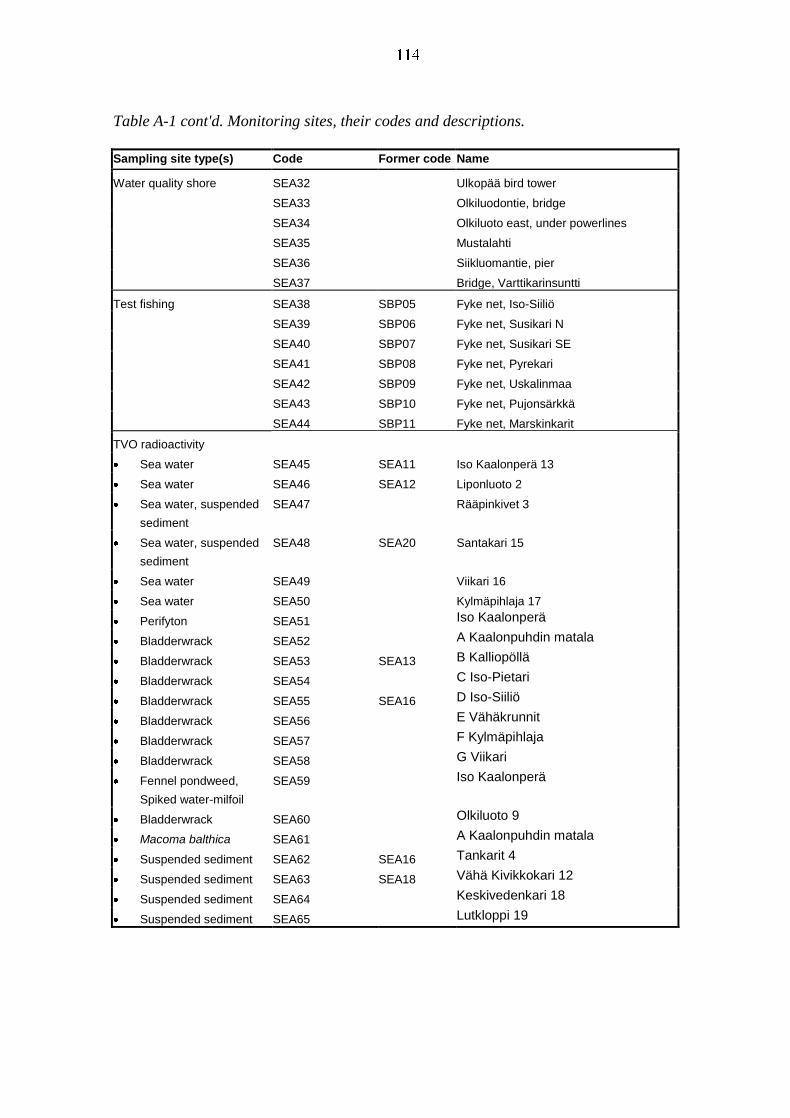
Table A-1 cont'd. Monitoring sites, their codes and descriptions.
Sampling site type(s) Code Former code Name
Water quality shore SEA32 Ulkopää bird tower
SEA33 Olkiluodontie, bridge
SEA34 Olkiluoto east, under powerlines
SEA35 Mustalahti
SEA36 Siikluomantie, pier
SEA37 Bridge, Varttikarinsuntti
Test fishing SEA38 SBP05 Fyke net, Iso-Siiliö
SEA39 SBP06 Fyke net, Susikari N
SEA40 SBP07 Fyke net, Susikari SE
SEA41 SBP08 Fyke net, Pyrekari
SEA42 SBP09 Fyke net, Uskalinmaa
SEA43 SBP10 Fyke net, Pujonsärkkä
SEA44 SBP11 Fyke net, Marskinkarit
TVO radioactivity
Sea water SEA45 SEA11 Iso Kaalonperä 13
Sea water SEA46 SEA12 Liponluoto 2
Sea water, suspended
sediment
SEA47 Rääpinkivet 3
Sea water, suspended
sediment
SEA48 SEA20 Santakari 15
Sea water SEA49 Viikari 16
Sea water SEA50 Kylmäpihlaja 17
Perifyton SEA51 Iso Kaalonperä
Bladderwrack SEA52 A Kaalonpuhdin matala
Bladderwrack SEA53 SEA13 B Kalliopöllä
Bladderwrack SEA54 C Iso-Pietari
Bladderwrack SEA55 SEA16 D Iso-Siiliö
Bladderwrack SEA56 E Vähäkrunnit
Bladderwrack SEA57 F Kylmäpihlaja
Bladderwrack SEA58 G Viikari
Fennel pondweed,
Spiked water-milfoil
SEA59 Iso Kaalonperä
Bladderwrack SEA60 Olkiluoto 9
Macoma balthica SEA61 A Kaalonpuhdin matala
Suspended sediment SEA62 SEA16 Tankarit 4
Suspended sediment SEA63 SEA18 Vähä Kivikkokari 12
Suspended sediment SEA64 Keskivedenkari 18
Suspended sediment SEA65 Lutkloppi 19
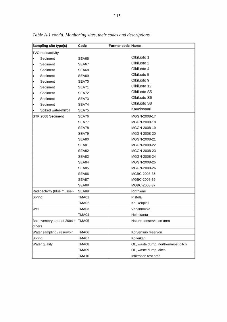
Table A-1 cont'd. Monitoring sites, their codes and descriptions.
Sampling site type(s) Code Former code Name
TVO radioactivity
Sediment SEA66 Olkiluoto 1
Sediment SEA67 Olkiluoto 2
Sediment SEA68 Olkiluoto 4
Sediment SEA69 Olkiluoto 5
Sediment SEA70 Olkiluoto 9
Sediment SEA71 Olkiluoto 12
Sediment SEA72 Olkiluoto S5
Sediment SEA73 Olkiluoto S6
Sediment SEA74 Olkiluoto S8
Spiked water-milfoil SEA75 Kaunissaari
GTK 2008 Sediment SEA76 MGGN-2008-17
SEA77 MGGN-2008-18
SEA78 MGGN-2008-19
SEA79 MGGN-2008-20
SEA80 MGGN-2008-21
SEA81 MGGN-2008-22
SEA82 MGGN-2008-23
SEA83 MGGN-2008-24
SEA84 MGGN-2008-25
SEA85 MGGN-2008-26
SEA86 MGBC-2008-35
SEA87 MGBC-2008-36
SEA88 MGBC-2008-37
Radioactivity (blue mussel) SEA89 Rihtniemi
Spring TMA01 Pistola
TMA02 Kaukenpieli
Well TMA03 Varvinnokka
TMA04 Helmiranta
Bat inventory area of 2004 +
others
TMA05 Nature conservation area
Water sampling / reservoir TMA06 Korvensuo reservoir
Spring TMA07 Koivukari
Water quality TMA08 OL, waste dump, northernmost ditch
TMA09 OL, waste dump, ditch
TMA10 Infiltration test area
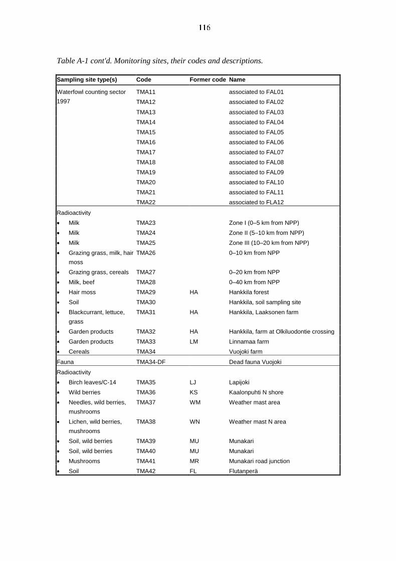
Table A-1 cont'd. Monitoring sites, their codes and descriptions.
Sampling site type(s) Code Former code Name
Waterfowl counting sector
1997
TMA11 associated to FAL01
TMA12 associated to FAL02
TMA13 associated to FAL03
TMA14 associated to FAL04
TMA15 associated to FAL05
TMA16 associated to FAL06
TMA17 associated to FAL07
TMA18 associated to FAL08
TMA19 associated to FAL09
TMA20 associated to FAL10
TMA21 associated to FAL11
TMA22 associated to FLA12
Radioactivity
Milk TMA23 Zone I (0–5 km from NPP)
Milk TMA24 Zone II (5–10 km from NPP)
Milk TMA25 Zone III (10–20 km from NPP)
Grazing grass, milk, hair
moss
TMA26 0–10 km from NPP
Grazing grass, cereals TMA27 0–20 km from NPP
Milk, beef TMA28 0–40 km from NPP
Hair moss TMA29 HA Hankkila forest
Soil TMA30 Hankkila, soil sampling site
Blackcurrant, lettuce,
grass
TMA31 HA Hankkila, Laaksonen farm
Garden products TMA32 HA Hankkila, farm at Olkiluodontie crossing
Garden products TMA33 LM Linnamaa farm
Cereals TMA34 Vuojoki farm
Fauna TMA34-DF Dead fauna Vuojoki
Radioactivity
Birch leaves/C-14 TMA35 LJ Lapijoki
Wild berries TMA36 KS Kaalonpuhti N shore
Needles, wild berries,
mushrooms
TMA37 WM Weather mast area
Lichen, wild berries,
mushrooms
TMA38 WN Weather mast N area
Soil, wild berries TMA39 MU Munakari
Soil, wild berries TMA40 MU Munakari
Mushrooms TMA41 MR Munakari road junction
Soil TMA42 FL Flutanperä
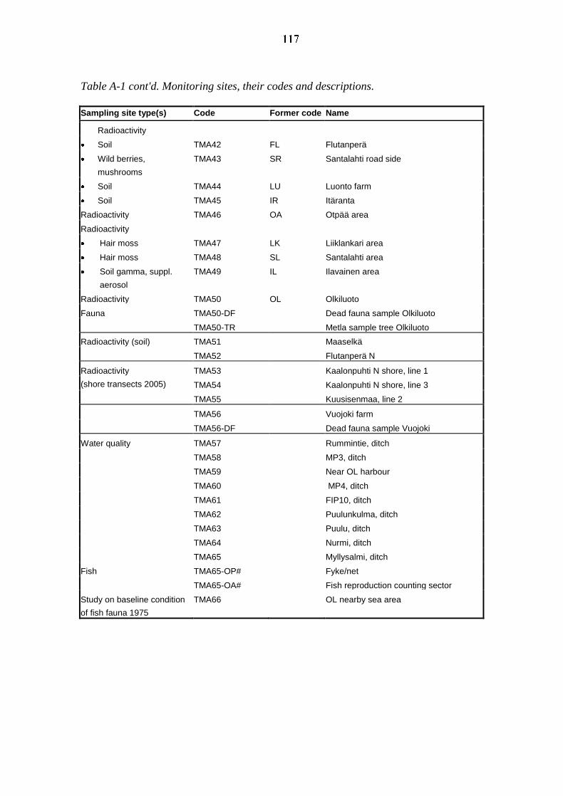
Table A-1 cont'd. Monitoring sites, their codes and descriptions.
Sampling site type(s) Code Former code Name
Radioactivity
Soil TMA42 FL Flutanperä
Wild berries,
mushrooms
TMA43 SR Santalahti road side
Soil TMA44 LU Luonto farm
Soil TMA45 IR Itäranta
Radioactivity TMA46 OA Otpää area
Radioactivity
Hair moss TMA47 LK Liiklankari area
Hair moss TMA48 SL Santalahti area
Soil gamma, suppl.
aerosol
TMA49 IL Ilavainen area
Radioactivity TMA50 OL Olkiluoto
Fauna TMA50-DF Dead fauna sample Olkiluoto
TMA50-TR Metla sample tree Olkiluoto
Radioactivity (soil) TMA51 Maaselkä
TMA52 Flutanperä N
Radioactivity
(shore transects 2005)
TMA53 Kaalonpuhti N shore, line 1
TMA54 Kaalonpuhti N shore, line 3
TMA55 Kuusisenmaa, line 2
TMA56 Vuojoki farm
TMA56-DF Dead fauna sample Vuojoki
Water quality TMA57 Rummintie, ditch
TMA58 MP3, ditch
TMA59 Near OL harbour
TMA60 MP4, ditch
TMA61 FIP10, ditch
TMA62 Puulunkulma, ditch
TMA63 Puulu, ditch
TMA64 Nurmi, ditch
TMA65 Myllysalmi, ditch
Fish TMA65-OP# Fyke/net
TMA65-OA# Fish reproduction counting sector
Study on baseline condition
of fish fauna 1975
TMA66 OL nearby sea area
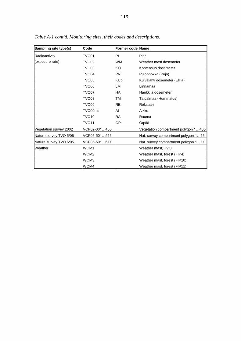
Table A-1 cont'd. Monitoring sites, their codes and descriptions.
Sampling site type(s) Code Former code Name
Radioactivity
(exposure rate)
TVO01 PI Pier
TVO02 WM Weather mast dosemeter
TVO03 KO Korvensuo dosemeter
TVO04 PN Pujonnokka (Pujo)
TVO05 KUb Kuivalahti dosemeter (Ellilä)
TVO06 LM Linnamaa
TVO07 HA Hankkila dosemeter
TVO08 TM Taipalmaa (Hummatus)
TVO09 RE Reksaari
TVO09old AI Aikko
TVO10 RA Rauma
TVO11 OP Otpää
Vegetation survey 2002 VCP02-001…435 Vegetation compartment polygon 1…435
Nature survey TVO 5/05 VCP05-501…513 Nat. survey compartment polygon 1…13
Nature survey TVO 6/05 VCP05-601…611 Nat. survey compartment polygon 1…11
Weather WOM1 Weather mast, TVO
WOM2 Weather mast, forest (FIP4)
WOM3 Weather mast, forest (FIP10)
WOM4 Weather mast, forest (FIP11)
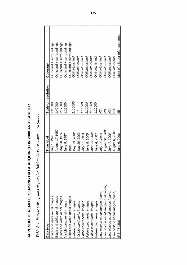
AP
PE
ND
IX B
: R
EM
OT
E S
EN
SIN
G D
AT
A A
CQ
UIR
ED
IN
20
08
AN
D E
AR
LIE
R
Data
typ
e
Tim
e lab
el
Scale
or
reso
luti
on
C
ov
era
ge
Bla
ck a
nd w
hite a
eria
l im
ages
July
1, 1
946
1:2
0000
O
L Isla
nd +
surr
oun
din
gs
Bla
ck a
nd w
hite a
eria
l im
ages
Aug
ust 17,1
957
1:4
2000
O
L Isla
nd +
surr
oun
din
gs
Bla
ck a
nd w
hite a
eria
l im
ages
Ma
y 1
0,
19
74
1:1
7500
O
L Isla
nd +
surr
oun
din
gs
Vis
ible
ba
nd a
eri
al im
ages
June 9
, 19
87
1:1
8600
O
L Isla
nd +
surr
oun
din
gs
Bla
ck a
nd w
hite a
eria
l im
ages
1995
OL Isla
nd +
surr
oun
din
gs
Fals
e-c
olo
ur
aeri
al im
ag
es
May 2
3,
20
02
1: 10
000
O
lkilu
oto
isla
nd
Vis
ible
ba
nd a
eri
al im
ages
May 1
0,
20
03
??
O
lkilu
oto
isla
nd
Fals
e-c
olo
ur
aeri
al im
ag
es
July
16,
200
4
1:1
0000
O
lkilu
oto
isla
nd
Fals
e-c
olo
ur
aeri
al im
ag
es
June 8
, 20
05
1:1
0000
O
lkilu
oto
isla
nd
Fals
e-c
olo
ur
aeri
al im
ag
es
June 1
7,
2006
1:1
0000
O
lkilu
oto
isla
nd
Fals
e-c
olo
ur
aeri
al im
ages
June 4
, 20
07
1:1
0000
O
lkilu
oto
isla
nd
Low
obliq
ue a
eria
l im
ages (
pla
ne)
July
16,
200
4
N/A
O
lkilu
oto
isla
nd
Low
obliq
ue a
eria
l im
ages (
helic
opte
r)
Aug
ust 31,
20
05
N
/A
Olk
iluoto
isla
nd
Low
obliq
ue
aeria
l im
ages (
pla
ne)
June 7
, 20
06
N
/A
Olk
iluoto
isla
nd
Lo
w o
bliq
ue a
eria
l im
ages (
pla
ne)
Aug
ust 6,
200
7
N/A
O
lkilu
oto
isla
nd
IRS
P6-L
ISS
June 6
, 20
06
25 m
M
ost of
a larg
er
refe
rence a
rea

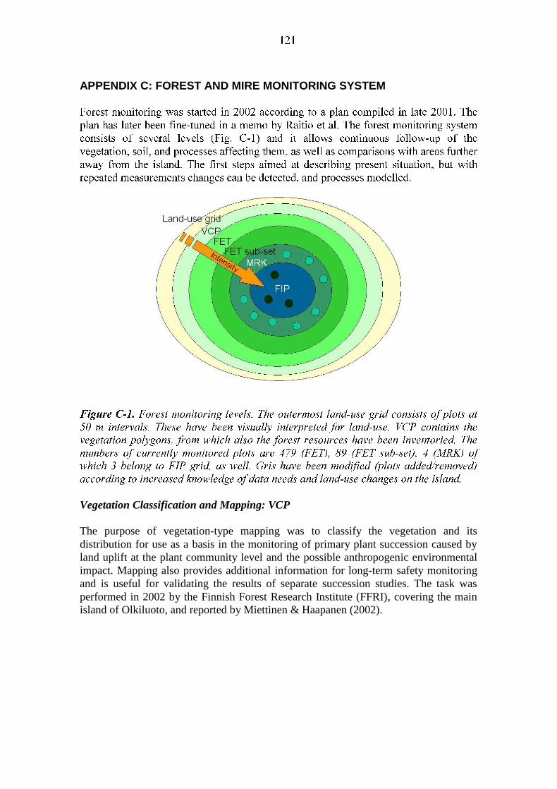
APPENDIX C: FOREST AND MIRE MONITORING SYSTEM
Vegetation Classification and Mapping: VCP
The purpose of vegetation-type mapping was to classify the vegetation and its
distribution for use as a basis in the monitoring of primary plant succession caused by
land uplift at the plant community level and the possible anthropogenic environmental
impact. Mapping also provides additional information for long-term safety monitoring
and is useful for validating the results of separate succession studies. The task was
performed in 2002 by the Finnish Forest Research Institute (FFRI), covering the main
island of Olkiluoto, and reported by Miettinen & Haapanen (2002).
Forest Inventory by VCP Units
The forest inventory by vegetation polygons, together with vegetation mapping,
provides a basis for the division of the area into homogeneous parts and facilitates
optimal targeting of intensive monitoring measurements. At the same time, it also
serves forestry in the Olkiluoto area by providing up-to-date information for the
planning of silvicultural treatment. The vegetation/tree map allows monitoring of
changes in the vegetated landscape. The inventory by forest compartments was
performed in 2003 by the FFRI, and the results have been reported by Rautio et al.
(2004).
Forest Extensive Monitoring Plots: FET
FET grid (Fig. C-2) was established in autumn 2003 by locating originally 561 plots
with the help of GPS and marking them out with a pole at the centre. The main purpose
of this grid is to describe the biomass, to monitor the changes in it and the damage
manifesting itself in tree stands. Furthermore, the FET grid provides a flexible
intercoordinated framework for other studies.
Field measurement of tree stand variables along FET plots is based on the use of three
concentric circular sample plots of a fixed radius: the inclusion area varies according to
the breast height diameter of the trees. The guidelines for inventorying the forests and
mires are in accordance with the National Forest Inventory of Finland, with the
exception of the actual layout of the plot, modified to better fit the purposes of Posiva.
A comprehensive measurement of forest parameters is to be carried out at intervals of
about 10 years (started in 2004; Saramäki & Korhonen 2005), but a lighter inventory
will be performed more often.
Part of the FET plots have been selected for further studies (Fig. C-2). Originally, 94
such plots were established. In these plots the vegetation is inventoried and the soil,
needles and vegetation are sampled at intervals of 5–10 years in order to describe soil
properties, vegetation composition and nutrient concentrations of plants and trees. The
vegetation inventory and sampling was performed for the first time in 2005 by the FFRI
(Huhta & Korpela 2006). Samples from mineral soil, peat, needles and understorey
vegetation were collected in 2005 by the FFRI and analysed during 2005–2006
(Tamminen et al. 2007).
Some of the plots have gone through significant changes in land-use since their
establishment, and a study of their condition was carried out in 2008. According to the
study, 78 of a total of 557 examined plots had changed and are no longer fulfilling the
original purpose of the monitoring. The study is described in more detail in Section
3.4.1.

Figure C-2. Forest monitoring locations in 2008. Map layout by Jani Helin/Posiva Oy.
Bulk Deposition and Stand Throughfall: MRK
Monitoring of bulk deposition and stand throughfall was started in Olkiluoto in June
2003 within a plot network called MRK (Fig. C-2). The sampling is now concentrated
on 4 plots (Table C-1) located at varying distances from the dust-producing activities:
excavation of ONKALO and rock piling and crushing.
Two of the original plots had to be moved because of felling activities on the plots and
new plots (MRK5 and MRK6) were established on August 25, 2003. The location of
the open area plot MRK2 was changed at the end of 2007 (monitoring started in week
50), and this new plot was denoted as MRK12. However, due to problems in collectors,
the location was again reverted to MRK2 in March, 2008.
MRK plots 1, 3, and 5–9 were closed down in spring 2008: it was seen that the needle
wash studies catch the dust effects more effectively, and a smaller network would be
enough to monitor the concentrations in wet deposition. Thus, bulk deposition in the
open and in stand throughfall were monitored from April 2008 onwards only on MRK
plots 2, 4, 10 and 11.
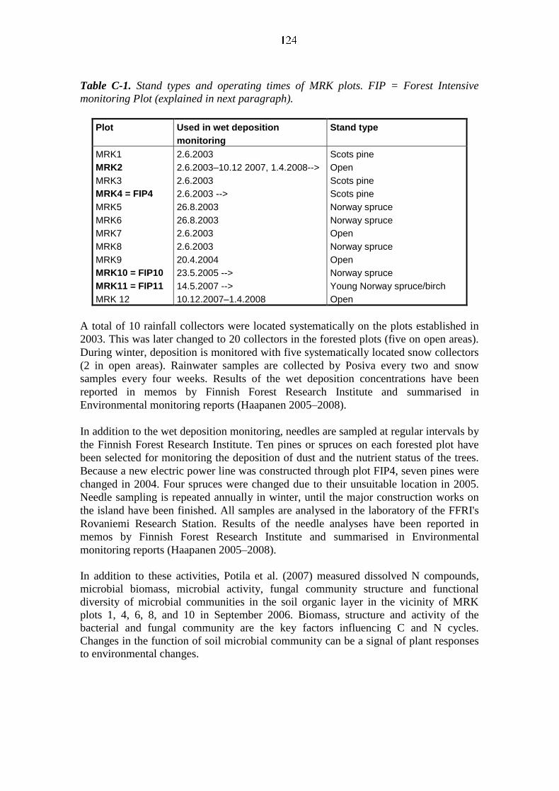
Table C-1. Stand types and operating times of MRK plots. FIP = Forest Intensive
monitoring Plot (explained in next paragraph).
Plot Used in wet deposition
monitoring
Stand type
MRK1
MRK2
MRK3
MRK4 = FIP4
MRK5
MRK6
MRK7
MRK8
MRK9
MRK10 = FIP10
MRK11 = FIP11
MRK 12
2.6.2003
2.6.2003–10.12 2007, 1.4.2008-->
2.6.2003
2.6.2003 -->
26.8.2003
26.8.2003
2.6.2003
2.6.2003
20.4.2004
23.5.2005 -->
14.5.2007 -->
10.12.2007–1.4.2008
Scots pine
Open
Scots pine
Scots pine
Norway spruce
Norway spruce
Open
Norway spruce
Open
Norway spruce
Young Norway spruce/birch
Open
A total of 10 rainfall collectors were located systematically on the plots established in
2003. This was later changed to 20 collectors in the forested plots (five on open areas).
During winter, deposition is monitored with five systematically located snow collectors
(2 in open areas). Rainwater samples are collected by Posiva every two and snow
samples every four weeks. Results of the wet deposition concentrations have been
reported in memos by Finnish Forest Research Institute and summarised in
Environmental monitoring reports (Haapanen 2005–2008).
In addition to the wet deposition monitoring, needles are sampled at regular intervals by
the Finnish Forest Research Institute. Ten pines or spruces on each forested plot have
been selected for monitoring the deposition of dust and the nutrient status of the trees.
Because a new electric power line was constructed through plot FIP4, seven pines were
changed in 2004. Four spruces were changed due to their unsuitable location in 2005.
Needle sampling is repeated annually in winter, until the major construction works on
the island have been finished. All samples are analysed in the laboratory of the FFRI's
Rovaniemi Research Station. Results of the needle analyses have been reported in
memos by Finnish Forest Research Institute and summarised in Environmental
monitoring reports (Haapanen 2005–2008).
In addition to these activities, Potila et al. (2007) measured dissolved N compounds,
microbial biomass, microbial activity, fungal community structure and functional
diversity of microbial communities in the soil organic layer in the vicinity of MRK
plots 1, 4, 6, 8, and 10 in September 2006. Biomass, structure and activity of the
bacterial and fungal community are the key factors influencing C and N cycles.
Changes in the function of soil microbial community can be a signal of plant responses
to environmental changes.
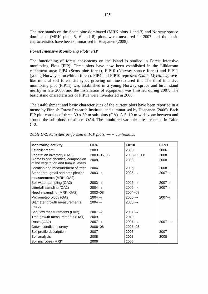
The tree stands on the Scots pine dominated (MRK plots 1 and 3) and Norway spruce
dominated (MRK plots 5, 6 and 8) plots were measured in 2007 and the basic
characteristics have been summarised in Haapanen (2008).
Forest Intensive Monitoring Plots: FIP
The functioning of forest ecosystems on the island is studied in Forest Intensive
monitoring Plots (FIP). Three plots have now been established in the Liiklansuo
catchment area: FIP4 (Scots pine forest), FIP10 (Norway spruce forest) and FIP11
(young Norway spruce/birch forest). FIP4 and FIP10 represent Oxalis-Myrtillus/grove-
like mineral soil forest site types growing on fine-textured till. The third intensive
monitoring plot (FIP11) was established in a young Norway spruce and birch stand
nearby in late 2006, and the installation of equipment was finished during 2007. The
basic stand characteristics of FIP11 were inventoried in 2008.
The establishment and basic characteristics of the current plots have been reported in a
memo by Finnish Forest Research Institute, and summarised by Haapanen (2006). Each
FIP plot consists of three 30 x 30 m sub-plots (OA). A 5–10 m wide zone between and
around the sub-plots constitutes OA4. The monitored variables are presented in Table
C-2.
Table C-2. Activities performed at FIP plots. → = continuous.
Monitoring activity FIP4 FIP10 FIP11
Establishment 2003 2003 2006
Vegetation inventory (OA3) 2003–05, 08 2003–05, 08 2008 Biomass and chemical composition of the vegetation and humus layers
2008 2008 2008
Location and measurement of trees 2004 2005 2008
Stand throughfall and precipitation
measurements (MRK, OA2)
2003 → 2005 → 2007→
Soil water sampling (OA2) 2003 → 2005 → 2007→
Litterfall sampling (OA2) 2004 → 2005 → 2007→
Needle sampling (MRK, OA2) 2003–08 2004–08
Micrometeorology (OA2) 2004 → 2005 → 2007→
Diameter growth measurements
(OA2)
2004 → 2005 →
Sap flow measurements (OA2) 2007 → 2007 →
Tree growth measurements (OA1) 2009 2010
Roots (OA2) 2007 → 2007 → 2007 →
Crown condition survey 2006–08 2006–08 -
Soil profile description 2007 2007 2007
Soil analysis 2008 2008 2008
Soil microbes (MRK) 2006 2006

Location and Measurement of Trees The trees on the Scots pine plot (FIP4) were measured in 2004 and on the Norway
spruce plot (FIP10) in 2005. The data can be found in Haapanen 2008. The trees
growing on the plot with the young mixed stand (FIP11) were measured in June 2008
and the results are presented in Table C-3.
Table C-3. The basic stand characteristics of plot FIP11 in June 2–4, 2008. Data
originally from the Finnish Forest Research Institute.
Su
b-p
lot
Tre
e s
pecie
s
Ste
ms/h
a
Basal
are
a w
ith
bark
, m
2/h
a
Mean
dia
mete
r
weig
hte
d w
ith
basal
are
a, c
m
Mean
he
igh
t
(ari
thm
eti
ca
l), m
Do
min
an
t h
eig
ht
(100/h
a),
m
Cro
wn
lim
it, m
Ste
m v
olu
me
wit
h b
ark
, m
3/h
a
1 Scots pine 0.0 0.0 - - - - 0.0
1 Norway spruce 1150.4 1.9 5.9 4.9 5.8 0.4 5.8
1 Silver birch 4778.8 2.7 4.0 5.3 6.3 1.3 8.6
1 Downy birch 11238.9 4.1 3.5 4.9 6.0 1.1 12.9
1 Total 17168.1 8.8 4.2 5.0 5.8 1.1 27.4
2 Scots pine 0.0 0.0 - - - - 0.0
2 Norway spruce 1415.9 0.7 4.2 4.0 5.4 0.3 2.3
2 Silver birch 6548.7 2.0 2.8 4.3 5.0 1.2 5.8
2 Downy birch 34778.8 2.3 1.4 2.9 4.6 0.9 8.7
2 Total 42743.4 5.0 2.4 3.4 5.5 1.0 16.8
3 Scots pine 88.5 0.0 1.2 1.4 1.4 0.1 0.0
3 Norway spruce 531.0 0.3 3.8 3.0 3.3 0.3 0.9
3 Silver birch 5480.7 1.8 3.0 4.4 6.4 1.2 5.6
3 Downy birch 8407.1 0.7 1.6 3.2 4.4 1.0 2.6
3 Total 14867.3 2.9 2.7 4.0 5.0 1.0 9.0
Soil Solution
Changes in the chemical composition of rainfall are being followed as the water first
passes down through the tree canopy, and then down the soil profile in the form of soil
solution. Soil solution gives information of soil formation processes, the effects of air
pollution and other stress factors on soil properties. The concentrations of individual
ions and the amount of water passing down through the soil are being monitored
continuously during the snow-free period in sub-plot OA2 of each FIP. Two sampling
techniques are being used (Table C-4): plate lysimeters (installed immediately below
the organic layer) and suction-cup lysimeters (installed at different depths, primarily in
the mineral soil). The soil in FIP4 is extremely stony, and the tension lysimeters were
therefore installed at depths of 10, 20 and 30 cm, instead of 20 and 40 cm as originally
planned.
In addition to the chemical composition, also the amount of percolation water is being
monitored using the plate lysimeters located at a depth of 5 cm. The collection period
for the first time that percolation water is collected following snowmelt starts in the
spring when the ground is no longer frozen. The amount of water percolating down to
different depths in the soil is determined by a number of factors:
1) The amount of water falling on the forest floor as rain or snow. In a tree
stand, this is the amount of stand throughfall.
2) Some of the water in stand throughfall is lost from the snow cover during
the winter through evaporation directly from the snow surface. This can be
especially high during spring when, even though the air temperature is
below freezing point, solar radiation causes the sublimation of ice directly
into water vapour that is released into the atmosphere.
3) Some of the water (as snow) falling on the forest floor is lost during
snowmelt in the form of horizontal runoff out of the stand. This can be
considerable if the ground immediately below the melting snow cover is still
frozen, thus preventing the water from passing down into the soil.
4) During the period extending from spring to autumn, a variable proportion of
the water falling onto the forest floor is recycled back into the atmosphere
though the uptake of water by the tree stand and ground vegetation (as
evapo-transpiration). The plate lysimeters are located below the organic
layer, which is the layer in the soil that contains the highest proportion of
plant roots.
5) Some of the water (as rain) that collects on the surface of the ground
vegetation during the snowfree period may evaporate directly into the
atmosphere, especially during warm periods.
6) During the summer especially, the intensity (amount) of stand throughfall
strongly affects the amount of percolation water: high precipitation events
result in more percolation water owing to the proportionally smaller amount
of water lost through evapo-transpiration.
In addition to the abovementioned natural factors, there are also technical problems
during the snowmelt period: the capacity (volume) of the bottles used to collect the
water samples may not always be sufficient to hold all the water running out of the plate
lysimeters. Under such conditions, the amount of percolation water will be
underestimated. On plot FIP10 there are also problems in the spring with an excessively
high water table and inundation by sea water; the plot is located only a few meters
above sea level.
Posiva's field personnel collect the samples and the chemical analyses are carried out in
the laboratory of the Finnish Forest Research Institute, Rovaniemi Research Station.
Monitoring of soil solution started in FIP4 on October 20, 2003, in FIP10 on May 24,
2005 and in FIP11 on June 1, 2007. The results are reported annually in a memo and
have been summarised in Haapanen (2005–2008).
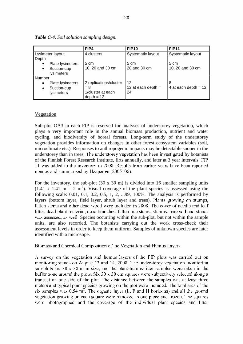
Table C-4. Soil solution sampling design.
FIP4 FIP10 FIP11
Lysimeter layout 4 clusters Systematic layout Systematic layout Depth
Plate lysimeters
Suction-cup lysimeters
5 cm 10, 20 and 30 cm
5 cm 20 and 30 cm
5 cm 10, 20 and 30 cm
Number
Plate lysimeters
Suction-cup lysimeters
2 replications/cluster = 8 1/cluster at each depth = 12
12 12 at each depth = 24
8 4 at each depth = 12
Vegetation
Sub-plot OA3 in each FIP is reserved for analyses of understorey vegetation, which
plays a very important role in the annual biomass production, nutrient and water
cycling, and biodiversity of boreal forests. Long-term study of the understorey
vegetation provides information on changes in other forest ecosystem variables (soil,
microclimate etc.). Responses to anthropogenic impacts may be detectable sooner in the
understorey than in trees. by botanists
of the Finnish Forest Research Institute, firts annually, and later at 3 year intervals
For the inventory, the sub-plot (30 x 30 m) is divided into 16 smaller sampling units
(1.41 x 1.41 m = 2 m2). Visual coverage of the plant species is assessed using the
following scale: 0.01, 0.1, 0.2, 0.5, 1, 2, ...99, 100%. The analysis is performed by
layers (bottom layer, field layer, shrub layer and trees).
Species occurring within the sub-plot, but not within the sample
units, are also recorded. The botanists carrying out the work cross-check their
assessment levels in order to keep them uniform. Samples of unknown species are later
identified with a microsope.
- Organic layer: divided into different horizons (L, F and H); pieces of dead
wood inside the humus layer as a separate class
- Understorey vegetation: separation by individual plant species and further by
plant compartments
- Tree roots: divided into fine roots (diameter < 2 mm) and thicker woody
roots.
Litterfall Sampling
The amount and chemical composition of litterfall in the stands is monitored using 12
litterfall collectors located on sub-plot OA2. Litterfall collection was started on the plot
FIP4 in summer 2004 and on the plot FIP10 in spring 2005. These results have been
presented in Haapanen (2007–2008). In 2006, litterfall collection was started April 25
and in 2007 on May 8 on these two plots. The young deciduous stand FIP11 was added
to the program on May 28, 2007.
Litterfall was collected using 12 litterfall traps (UN/ECE 2004) located systematically
on the plots. The litterfall collectors are funnel-shaped traps with a catch area of 0.5 m2
placed about 1.5 m above ground level. Since the last collection date is on early-late
November the mass of first collection in May represents the litterfall of the whole
winter.
Until 2006, the collected litter was divided into 5 different fractions: 1=pine brown
needles, 2=pine green needles, 3=spruce needles, 4=leaves and 5=remaining litter. In
2007 a new fraction (6=branches) was included in the monitoring programme. Branches
were collected using 12 branch traps, developed in Finnish Forest Research Institute to
collect branch litter that is missed by the funnel type litterfall traps used in the ICP
Forests programme (UN/ECE 2004) to collect mainly foliage litter. The branch traps
are of similar size than the funnel traps (0.5 m2) and positioned close to each funnel
trap.
Element concentrations were determined if there was enough material in a given litter
fraction to allow homogenization (grinding) and microwave digestion in acid preceding
chemical analysis.
Defoliation
Sap Flow (Evapotranspiration)
- -
-
-
Tree Growth
Tree characteristics will be measured every fifth year. In addition, the diameter growth
of two trees on sub-plot OA2 of FIP4 and FIP10 is being measured continuously with
girth bands (from 2007 on).
Soil Profile Description and Soil Analysis
Soil profile description and soil sampling took place on the FIP plots on May 22–24,
2007 with the method used by Tamminen et al. (2007) on the sub-sample of FET plots,
the only exception being the sampling pit locations: samples were collected on three
sides of OA2 of the FIP plots. Three composite samples were collected for each of the
soil layers. On the mineral soil sites, samples were taken from the organic layer and 0–
10, 10–30 and 50–60 cm mineral soil layers. On FIP11 only two sides could be sampled
according to the instructions for mineral soil sampling. The peat sampling procedure
was applied on the third side of FIP11-OA2: three replicates of the peat profile were
sampled in five separate sampling pits. The peat samples were taken on August 28,
2007.
were carried out in 2008.
Root Investigations
Initiation of the root investigation took place on May 22–24, 2007. Plastic root
tubes were installed in both vertical and horizontal positions on OA2 sub-plots of the
FIP plots. The root tubes have a diameter of 6 cm and a length of 1 m. The total number
of root tubes installed was 18. When the filming of the tubes started in June 2008, five
tubes had to be left out due to too small diameter; thus, 13 tubes are examined.

Stand Micrometeorology
Stand meteorological measurements are recorded once an hour in OA2. The parameters
are air temperature, minimum and maximum temperature inside the crown layer and
above the canopy, relative humidity, precipitation (1 m above ground level), soil
moisture content, and soil temperature. Depth of ground frost and the thickness of the
snow cover are measured manually on FIP4. Photosynthetically active radiation (PAR),
solar radiation, air pressure, wind speed and its direction are measured only on FIP4.
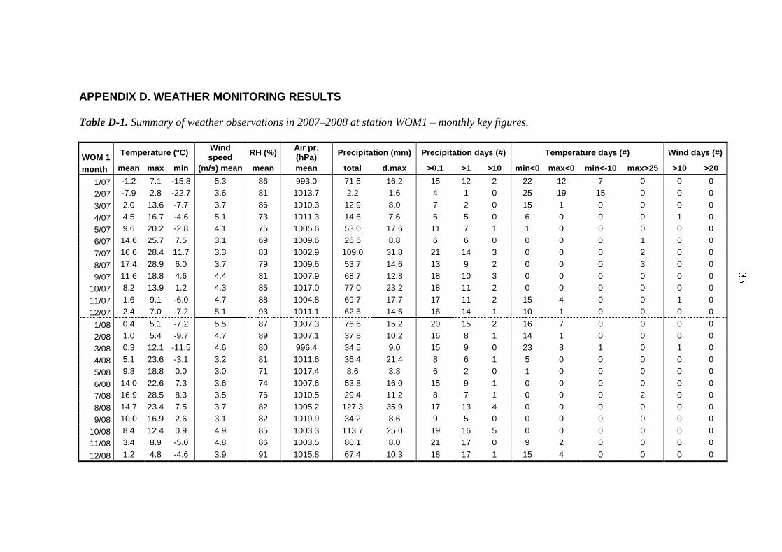
APPENDIX D. WEATHER MONITORING RESULTS
Table D-1. Summary of weather observations in 2007–2008 at station WOM1 – monthly key figures.
WOM 1 Temperature (°C)
Wind speed
RH (%) Air pr. (hPa)
Precipitation (mm) Precipitation days (#) Temperature days (#) Wind days (#)
month mean max min (m/s) mean mean mean total d.max >0.1 >1 >10 min<0 max<0 min<-10 max>25 >10 >20
1/07 -1.2 7.1 -15.8 5.3 86 993.0 71.5 16.2 15 12 2 22 12 7 0 0 0
2/07 -7.9 2.8 -22.7 3.6 81 1013.7 2.2 1.6 4 1 0 25 19 15 0 0 0
3/07 2.0 13.6 -7.7 3.7 86 1010.3 12.9 8.0 7 2 0 15 1 0 0 0 0
4/07 4.5 16.7 -4.6 5.1 73 1011.3 14.6 7.6 6 5 0 6 0 0 0 1 0
5/07 9.6 20.2 -2.8 4.1 75 1005.6 53.0 17.6 11 7 1 1 0 0 0 0 0
6/07 14.6 25.7 7.5 3.1 69 1009.6 26.6 8.8 6 6 0 0 0 0 1 0 0
7/07 16.6 28.4 11.7 3.3 83 1002.9 109.0 31.8 21 14 3 0 0 0 2 0 0
8/07 17.4 28.9 6.0 3.7 79 1009.6 53.7 14.6 13 9 2 0 0 0 3 0 0
9/07 11.6 18.8 4.6 4.4 81 1007.9 68.7 12.8 18 10 3 0 0 0 0 0 0
10/07 8.2 13.9 1.2 4.3 85 1017.0 77.0 23.2 18 11 2 0 0 0 0 0 0
11/07 1.6 9.1 -6.0 4.7 88 1004.8 69.7 17.7 17 11 2 15 4 0 0 1 0
12/07 2.4 7.0 -7.2 5.1 93 1011.1 62.5 14.6 16 14 1 10 1 0 0 0 0
1/08 0.4 5.1 -7.2 5.5 87 1007.3 76.6 15.2 20 15 2 16 7 0 0 0 0
2/08 1.0 5.4 -9.7 4.7 89 1007.1 37.8 10.2 16 8 1 14 1 0 0 0 0
3/08 0.3 12.1 -11.5 4.6 80 996.4 34.5 9.0 15 9 0 23 8 1 0 1 0
4/08 5.1 23.6 -3.1 3.2 81 1011.6 36.4 21.4 8 6 1 5 0 0 0 0 0
5/08 9.3 18.8 0.0 3.0 71 1017.4 8.6 3.8 6 2 0 1 0 0 0 0 0
6/08 14.0 22.6 7.3 3.6 74 1007.6 53.8 16.0 15 9 1 0 0 0 0 0 0
7/08 16.9 28.5 8.3 3.5 76 1010.5 29.4 11.2 8 7 1 0 0 0 2 0 0
8/08 14.7 23.4 7.5 3.7 82 1005.2 127.3 35.9 17 13 4 0 0 0 0 0 0
9/08 10.0 16.9 2.6 3.1 82 1019.9 34.2 8.6 9 5 0 0 0 0 0 0 0
10/08 8.4 12.4 0.9 4.9 85 1003.3 113.7 25.0 19 16 5 0 0 0 0 0 0
11/08 3.4 8.9 -5.0 4.8 86 1003.5 80.1 8.0 21 17 0 9 2 0 0 0 0
12/08 1.2 4.8 -4.6 3.9 91 1015.8 67.4 10.3 18 17 1 15 4 0 0 0 0
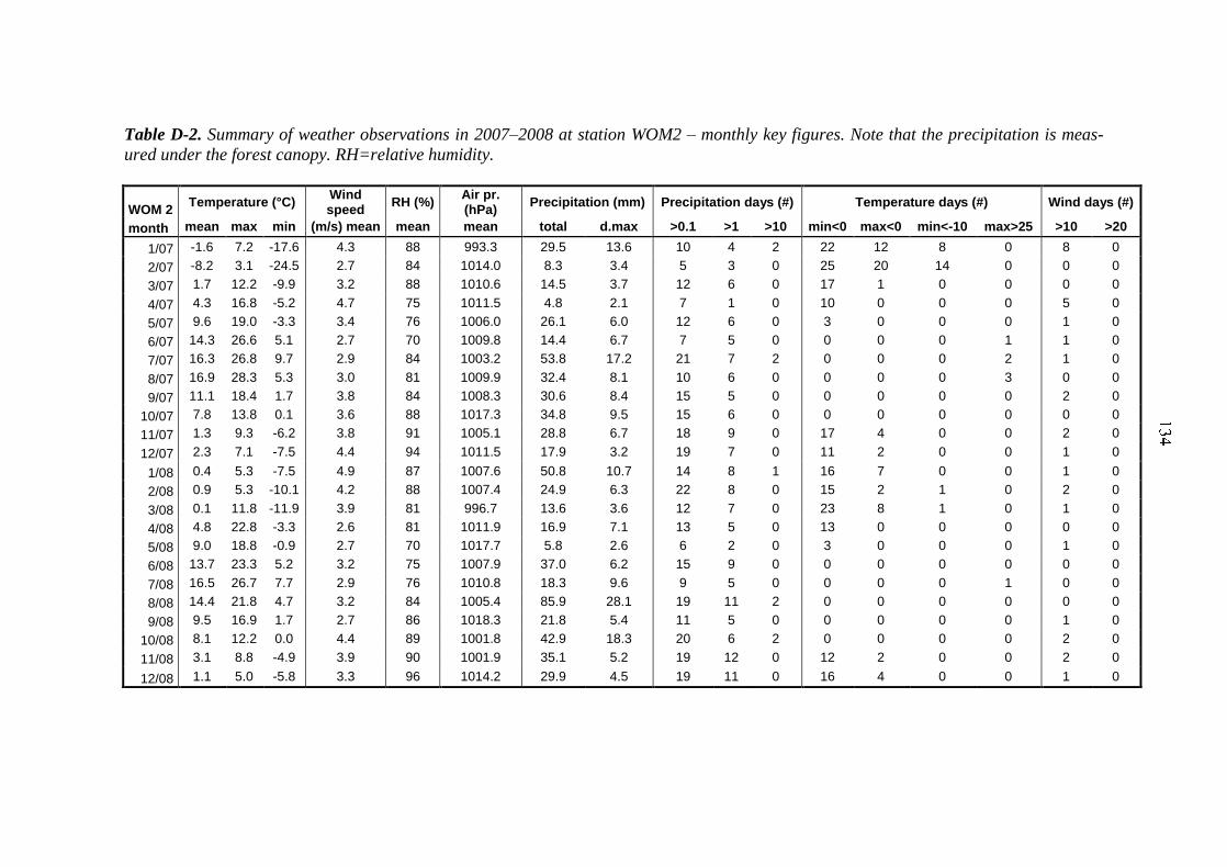
Table D-2. Summary of weather observations in 2007–2008 at station WOM2 – monthly key figures. Note that the precipitation is meas-
ured under the forest canopy. RH=relative humidity.
WOM 2 Temperature (°C)
Wind speed
RH (%) Air pr. (hPa)
Precipitation (mm) Precipitation days (#) Temperature days (#) Wind days (#)
month mean max min (m/s) mean mean mean total d.max >0.1 >1 >10 min<0 max<0 min<-10 max>25 >10 >20
1/07 -1.6 7.2 -17.6 4.3 88 993.3 29.5 13.6 10 4 2 22 12 8 0 8 0
2/07 -8.2 3.1 -24.5 2.7 84 1014.0 8.3 3.4 5 3 0 25 20 14 0 0 0
3/07 1.7 12.2 -9.9 3.2 88 1010.6 14.5 3.7 12 6 0 17 1 0 0 0 0
4/07 4.3 16.8 -5.2 4.7 75 1011.5 4.8 2.1 7 1 0 10 0 0 0 5 0
5/07 9.6 19.0 -3.3 3.4 76 1006.0 26.1 6.0 12 6 0 3 0 0 0 1 0
6/07 14.3 26.6 5.1 2.7 70 1009.8 14.4 6.7 7 5 0 0 0 0 1 1 0
7/07 16.3 26.8 9.7 2.9 84 1003.2 53.8 17.2 21 7 2 0 0 0 2 1 0
8/07 16.9 28.3 5.3 3.0 81 1009.9 32.4 8.1 10 6 0 0 0 0 3 0 0
9/07 11.1 18.4 1.7 3.8 84 1008.3 30.6 8.4 15 5 0 0 0 0 0 2 0
10/07 7.8 13.8 0.1 3.6 88 1017.3 34.8 9.5 15 6 0 0 0 0 0 0 0
11/07 1.3 9.3 -6.2 3.8 91 1005.1 28.8 6.7 18 9 0 17 4 0 0 2 0
12/07 2.3 7.1 -7.5 4.4 94 1011.5 17.9 3.2 19 7 0 11 2 0 0 1 0
1/08 0.4 5.3 -7.5 4.9 87 1007.6 50.8 10.7 14 8 1 16 7 0 0 1 0
2/08 0.9 5.3 -10.1 4.2 88 1007.4 24.9 6.3 22 8 0 15 2 1 0 2 0
3/08 0.1 11.8 -11.9 3.9 81 996.7 13.6 3.6 12 7 0 23 8 1 0 1 0
4/08 4.8 22.8 -3.3 2.6 81 1011.9 16.9 7.1 13 5 0 13 0 0 0 0 0
5/08 9.0 18.8 -0.9 2.7 70 1017.7 5.8 2.6 6 2 0 3 0 0 0 1 0
6/08 13.7 23.3 5.2 3.2 75 1007.9 37.0 6.2 15 9 0 0 0 0 0 0 0
7/08 16.5 26.7 7.7 2.9 76 1010.8 18.3 9.6 9 5 0 0 0 0 1 0 0
8/08 14.4 21.8 4.7 3.2 84 1005.4 85.9 28.1 19 11 2 0 0 0 0 0 0
9/08 9.5 16.9 1.7 2.7 86 1018.3 21.8 5.4 11 5 0 0 0 0 0 1 0
10/08 8.1 12.2 0.0 4.4 89 1001.8 42.9 18.3 20 6 2 0 0 0 0 2 0
11/08 3.1 8.8 -4.9 3.9 90 1001.9 35.1 5.2 19 12 0 12 2 0 0 2 0
12/08 1.1 5.0 -5.8 3.3 96 1014.2 29.9 4.5 19 11 0 16 4 0 0 1 0
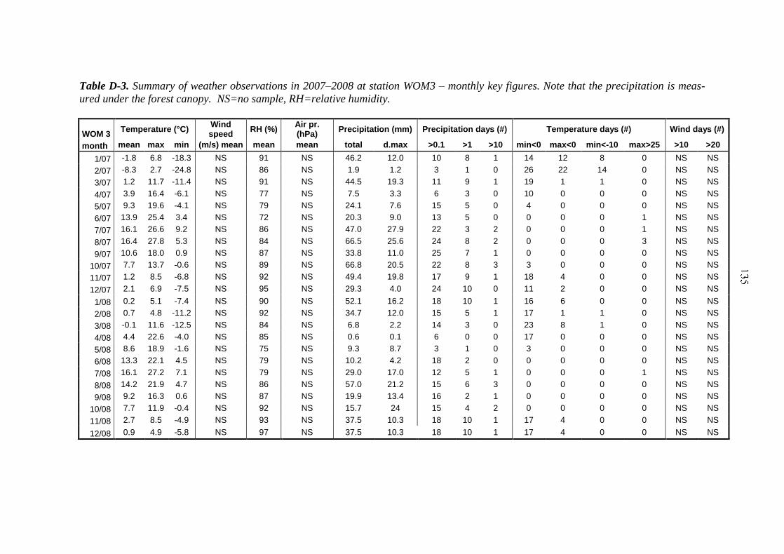
Table D-3. Summary of weather observations in 2007–2008 at station WOM3 – monthly key figures. Note that the precipitation is meas-
ured under the forest canopy. NS=no sample, RH=relative humidity.
WOM 3 Temperature (°C)
Wind speed
RH (%) Air pr. (hPa)
Precipitation (mm) Precipitation days (#) Temperature days (#) Wind days (#)
month mean max min (m/s) mean mean mean total d.max >0.1 >1 >10 min<0 max<0 min<-10 max>25 >10 >20
1/07 -1.8 6.8 -18.3 NS 91 NS 46.2 12.0 10 8 1 14 12 8 0 NS NS
2/07 -8.3 2.7 -24.8 NS 86 NS 1.9 1.2 3 1 0 26 22 14 0 NS NS
3/07 1.2 11.7 -11.4 NS 91 NS 44.5 19.3 11 9 1 19 1 1 0 NS NS
4/07 3.9 16.4 -6.1 NS 77 NS 7.5 3.3 6 3 0 10 0 0 0 NS NS
5/07 9.3 19.6 -4.1 NS 79 NS 24.1 7.6 15 5 0 4 0 0 0 NS NS
6/07 13.9 25.4 3.4 NS 72 NS 20.3 9.0 13 5 0 0 0 0 1 NS NS
7/07 16.1 26.6 9.2 NS 86 NS 47.0 27.9 22 3 2 0 0 0 1 NS NS
8/07 16.4 27.8 5.3 NS 84 NS 66.5 25.6 24 8 2 0 0 0 3 NS NS
9/07 10.6 18.0 0.9 NS 87 NS 33.8 11.0 25 7 1 0 0 0 0 NS NS
10/07 7.7 13.7 -0.6 NS 89 NS 66.8 20.5 22 8 3 3 0 0 0 NS NS
11/07 1.2 8.5 -6.8 NS 92 NS 49.4 19.8 17 9 1 18 4 0 0 NS NS
12/07 2.1 6.9 -7.5 NS 95 NS 29.3 4.0 24 10 0 11 2 0 0 NS NS
1/08 0.2 5.1 -7.4 NS 90 NS 52.1 16.2 18 10 1 16 6 0 0 NS NS
2/08 0.7 4.8 -11.2 NS 92 NS 34.7 12.0 15 5 1 17 1 1 0 NS NS
3/08 -0.1 11.6 -12.5 NS 84 NS 6.8 2.2 14 3 0 23 8 1 0 NS NS
4/08 4.4 22.6 -4.0 NS 85 NS 0.6 0.1 6 0 0 17 0 0 0 NS NS
5/08 8.6 18.9 -1.6 NS 75 NS 9.3 8.7 3 1 0 3 0 0 0 NS NS
6/08 13.3 22.1 4.5 NS 79 NS 10.2 4.2 18 2 0 0 0 0 0 NS NS
7/08 16.1 27.2 7.1 NS 79 NS 29.0 17.0 12 5 1 0 0 0 1 NS NS
8/08 14.2 21.9 4.7 NS 86 NS 57.0 21.2 15 6 3 0 0 0 0 NS NS
9/08 9.2 16.3 0.6 NS 87 NS 19.9 13.4 16 2 1 0 0 0 0 NS NS
10/08 7.7 11.9 -0.4 NS 92 NS 15.7 24 15 4 2 0 0 0 0 NS NS
11/08 2.7 8.5 -4.9 NS 93 NS 37.5 10.3 18 10 1 17 4 0 0 NS NS
12/08 0.9 4.9 -5.8 NS 97 NS 37.5 10.3 18 10 1 17 4 0 0 NS NS
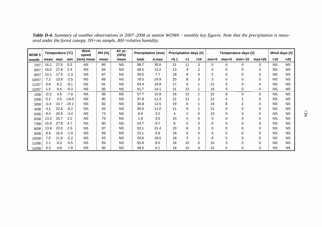
Table D-4. Summary of weather observations in 2007–2008 at station WOM4 – monthly key figures. Note that the precipitation is meas-
ured under the forest canopy. NS=no sample, RH=relative humidity.
WOM 3 Temperature (°C)
Wind speed
RH (%) Air pr. (hPa)
Precipitation (mm) Precipitation days (#) Temperature days (#) Wind days (#)
month mean max min (m/s) mean mean mean total d.max >0.1 >1 >10 min<0 max<0 min<-10 max>25 >10 >20
7/07 16.1 27.6 5.5 NS 85 NS 98.7 35.6 21 11 3 0 0 0 3 NS NS
8/07 16.0 27.8 2.4 NS 84 NS 49.5 13.2 13 9 2 0 0 0 4 NS NS
9/07 10.1 17.5 -1.3 NS 87 NS 29.5 7.7 18 9 0 2 0 0 0 NS NS
10/07 7.2 13.8 -2.5 NS 89 NS 78.5 24.9 20 8 3 3 0 0 0 NS NS
11/07 0.6 8.2 -9.1 NS 91 NS 54.4 19.8 17 9 1 21 5 0 0 NS NS
12/07 1.5 6.6 -9.3 NS 95 NS 61.7 14.1 21 13 1 16 3 0 0 NS NS
1/08 -0.3 4.5 -7.9 NS 89 NS 57.7 10.9 16 13 2 22 8 0 0 NS NS
2/08 0.2 4.5 -14.0 NS 90 NS 37.8 11.3 21 11 1 22 4 1 0 NS NS
3/08 -0.4 10.7 -15.1 NS 82 NS 30.8 12.5 19 6 1 24 8 2 0 NS NS
4/08 4.1 22.8 -6.2 NS 83 NS 30.6 11.0 11 8 1 21 0 0 0 NS NS
5/08 8.4 20.8 -3.4 NS 73 NS 6.9 3.2 4 2 0 10 0 0 0 NS NS
6/08 13.2 23.7 2.2 NS 79 NS 1.8 0.5 10 0 0 0 0 0 0 NS NS
7/08 15.9 27.9 4.7 NS 80 NS 24.7 9.7 8 5 0 0 0 0 3 NS NS
8/08 13.8 22.0 2.0 NS 87 NS 92.1 31.4 20 8 3 0 0 0 0 NS NS
9/08 8.6 16.4 -1.0 NS 89 NS 23.1 6.6 18 5 0 4 0 0 0 NS NS
10/08 7.0 11.6 -2.2 NS 93 NS 29.6 18.0 18 3 1 6 0 0 0 NS NS
11/08 2.1 8.3 -5.5 NS 93 NS 55.8 8.5 18 15 0 15 3 0 0 NS NS
12/08 0.3 4.8 -7.8 NS 96 NS 48.6 6.1 18 15 0 22 5 0 0 NS NS
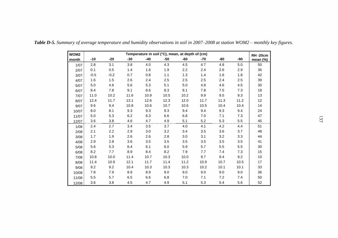
Table D-5. Summary of average temperature and humidity observations in soil in 2007–2008 at station WOM2 – monthly key figures.
WOM2 Temperature in soil (°C), mean, at depth of (cm) RH -20cm mean (%) month -10 -20 -30 -40 -50 -60 -70 -80 -90
1/07 2.8 3.1 3.8 4.0 4.3 4.5 4.7 4.8 5.0 50
2/07 0.1 0.5 1.4 1.6 1.9 2.2 2.4 2.6 2.9 36
3/07 -0.5 -0.2 0.7 0.8 1.1 1.3 1.4 1.6 1.8 42
4/07 1.6 1.5 2.6 2.4 2.5 2.5 2.5 2.4 2.5 39
5/07 5.0 4.6 5.6 5.3 5.1 5.0 4.8 4.6 4.5 30
6/07 8.4 7.8 9.1 8.6 8.3 8.1 7.8 7.5 7.3 18
7/07 11.0 10.2 11.6 10.9 10.5 10.2 9.9 9.5 9.3 13
8/07 12.4 11.7 13.1 12.6 12.3 12.0 11.7 11.3 11.2 12
9/07 9.6 9.4 10.8 10.6 10.7 10.6 10.5 10.4 10.4 14
10/07 8.0 8.1 9.3 9.3 9.3 9.4 9.4 9.3 9.4 24
11/07 5.0 5.3 6.2 6.3 6.6 6.8 7.0 7.1 7.3 47
12/07 3.6 3.8 4.6 4.7 4.9 5.1 5.2 5.3 5.5 45
1/08 2.4 2.7 3.4 3.5 3.7 4.0 4.1 4.2 4.4 51
2/08 2.1 2.2 2.9 3.0 3.2 3.4 3.5 3.6 3.7 48
3/08 1.7 1.9 2.6 2.6 2.8 3.0 3.1 3.2 3.3 44
4/08 2.9 2.8 3.6 3.5 3.5 3.5 3.5 3.5 3.5 41
5/08 5.6 5.3 6.4 6.1 6.0 5.9 5.7 5.5 5.5 30
6/08 8.2 7.7 8.9 8.4 8.2 7.9 7.7 7.4 7.3 15
7/08 10.8 10.0 11.4 10.7 10.3 10.0 9.7 9.4 9.2 10
8/08 11.4 10.9 12.1 11.7 11.4 11.2 10.9 10.7 10.5 17
9/08 9.2 9.2 10.4 10.3 10.3 10.3 10.2 10.1 10.1 33
10/08 7.8 7.9 8.9 8.9 9.0 9.0 9.0 9.0 9.0 36
11/08 5.5 5.7 6.5 6.6 6.8 7.0 7.1 7.2 7.4 50
12/08 3.6 3.8 4.5 4.7 4.9 5.1 5.3 5.4 5.6 52
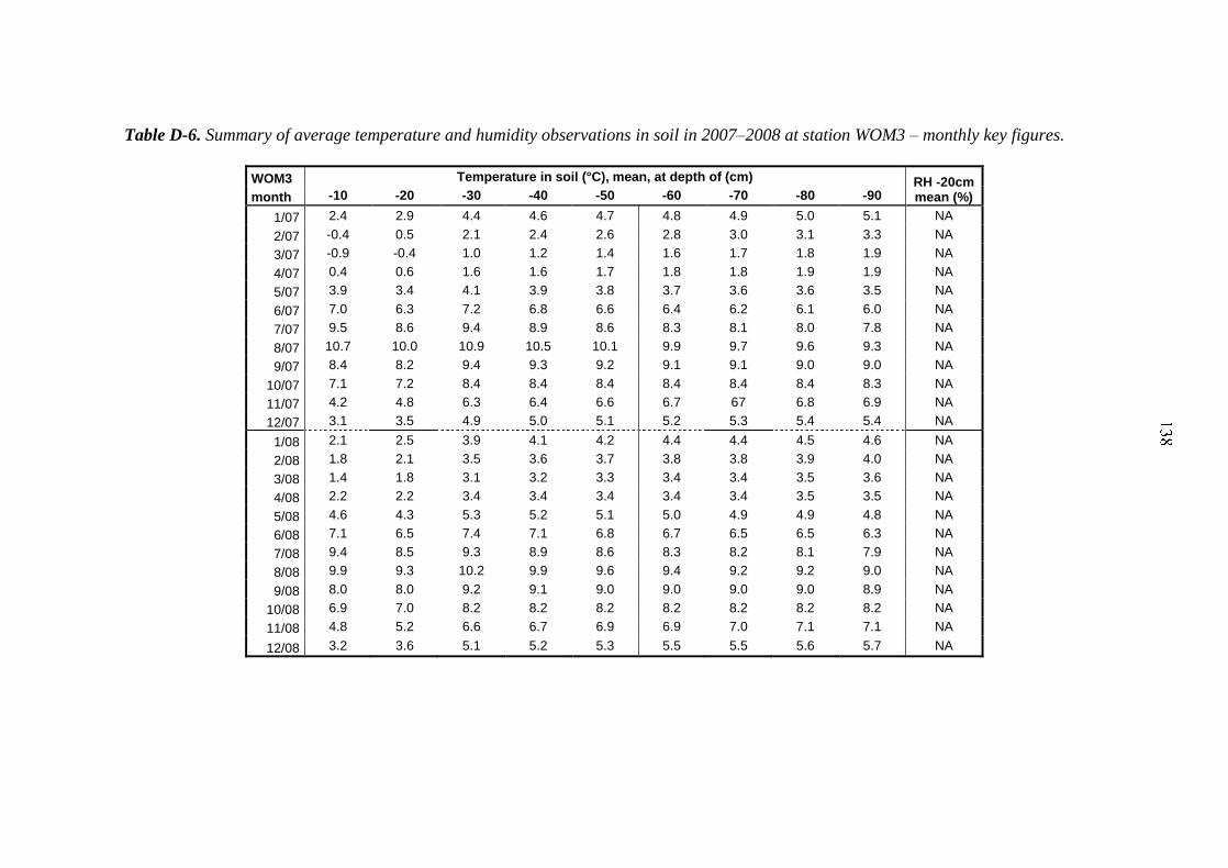
Table D-6. Summary of average temperature and humidity observations in soil in 2007–2008 at station WOM3 – monthly key figures.
WOM3 Temperature in soil (°C), mean, at depth of (cm) RH -20cm mean (%) month -10 -20 -30 -40 -50 -60 -70 -80 -90
1/07 2.4 2.9 4.4 4.6 4.7 4.8 4.9 5.0 5.1 NA
2/07 -0.4 0.5 2.1 2.4 2.6 2.8 3.0 3.1 3.3 NA
3/07 -0.9 -0.4 1.0 1.2 1.4 1.6 1.7 1.8 1.9 NA
4/07 0.4 0.6 1.6 1.6 1.7 1.8 1.8 1.9 1.9 NA
5/07 3.9 3.4 4.1 3.9 3.8 3.7 3.6 3.6 3.5 NA
6/07 7.0 6.3 7.2 6.8 6.6 6.4 6.2 6.1 6.0 NA
7/07 9.5 8.6 9.4 8.9 8.6 8.3 8.1 8.0 7.8 NA
8/07 10.7 10.0 10.9 10.5 10.1 9.9 9.7 9.6 9.3 NA
9/07 8.4 8.2 9.4 9.3 9.2 9.1 9.1 9.0 9.0 NA
10/07 7.1 7.2 8.4 8.4 8.4 8.4 8.4 8.4 8.3 NA
11/07 4.2 4.8 6.3 6.4 6.6 6.7 67 6.8 6.9 NA
12/07 3.1 3.5 4.9 5.0 5.1 5.2 5.3 5.4 5.4 NA
1/08 2.1 2.5 3.9 4.1 4.2 4.4 4.4 4.5 4.6 NA
2/08 1.8 2.1 3.5 3.6 3.7 3.8 3.8 3.9 4.0 NA
3/08 1.4 1.8 3.1 3.2 3.3 3.4 3.4 3.5 3.6 NA
4/08 2.2 2.2 3.4 3.4 3.4 3.4 3.4 3.5 3.5 NA
5/08 4.6 4.3 5.3 5.2 5.1 5.0 4.9 4.9 4.8 NA
6/08 7.1 6.5 7.4 7.1 6.8 6.7 6.5 6.5 6.3 NA
7/08 9.4 8.5 9.3 8.9 8.6 8.3 8.2 8.1 7.9 NA
8/08 9.9 9.3 10.2 9.9 9.6 9.4 9.2 9.2 9.0 NA
9/08 8.0 8.0 9.2 9.1 9.0 9.0 9.0 9.0 8.9 NA
10/08 6.9 7.0 8.2 8.2 8.2 8.2 8.2 8.2 8.2 NA
11/08 4.8 5.2 6.6 6.7 6.9 6.9 7.0 7.1 7.1 NA
12/08 3.2 3.6 5.1 5.2 5.3 5.5 5.5 5.6 5.7 NA
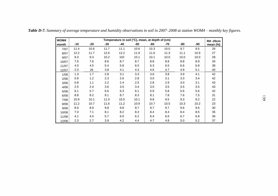
Table D-7. Summary of average temperature and humidity observations in soil in 2007–2008 at station WOM4 – monthly key figures.
WOM4 Temperature in soil (°C), mean, at depth of (cm) RH -20cm mean (%) month -10 -20 -30 -40 -50 -60 -70 -80 -90
7/07 11.4 10.6 11.7 11.1 10.6 10.3 10.0 9.7 9.5 26
8/07 12.2 11.7 12.6 12.2 11.9 11.6 11.3 11.1 10.9 27
9/07 9.3 9.3 10.2 102 10.1 10.1 10.0 10.0 10.0 28
10/07 7.5 7.6 8.6 8.7 8.7 8.8 8.8 8.8 8.9 34
11/07 4.0 4.5 5.4 5.8 6.0 6.3 6.5 6.6 6.8 38
12/07 2.3 26 3.8 4.1 4.3 4.6 4.7 4.9 5.1 40
1/08 1.3 1.7 2.8 3.1 3.3 3.6 3.8 3.9 4.1 42
2/08 0.9 1.2 2.3 2.6 2.8 3.0 3.1 3.3 3.4 42
3/08 0.8 1.1 2.2 2.4 2.5 2.8 2.9 3.0 3.1 43
4/08 2.5 2.4 3.6 3.5 3.4 3.5 3.5 3.5 3.5 43
5/08 6.1 5.7 6.6 6.3 6.1 5.9 5.8 5.6 5.6 42
6/08 8.8 8.2 9.1 8.7 8.3 8.1 7.8 7.6 7.5 31
7/08 10.9 10.1 11.0 10.5 10.1 9.8 9.5 9.3 9.2 22
8/08 11.2 10.7 11.6 11.2 10.9 10.7 10.5 10.3 10.2 23
9/08 8.9 8.9 9.8 9.8 9.7 9.7 9.7 9.6 9.6 30
10/08 7.0 7.1 8.1 8.2 8.3 8.4 8.4 8.4 8.5 35
11/08 4.1 4.5 5.7 6.0 6.2 6.4 6.6 6.7 6.8 36
12/08 2.3 2.7 3.9 4.2 4.4 4.7 4.8 5.0 5.2 37

Table D-8. Summary of extreme temperatures and relative humidity observations in soil in 2007–2008 at station WOM2 – monthly key
figures.
WOM2 Temperature in soil (°C), MINIMUM , at depth of (cm) Temperature in soil (°C), MAXIMUM , at depth of (cm) RH -20cm
month -10 -20 -30 -40 -50 -60 -70 -80 -90 -10 -20 -30 -40 -50 -60 -70 -80 -90 min max
1/07 0.9 1.3 2.0 2.3 2.6 2.9 3.2 3.4 3.7 4.2 4.3 5.1 5.2 5.3 5.5 5.6 5.6 5.8 42 55
2/07 -0.9 -0.3 0.6 0.9 1.2 1.5 1.7 1.9 2.1 1.1 1.4 2.1 2.3 2.6 2.9 3.2 3.4 3.7 24 42
3/07 -0.8 -0.3 0.6 0.7 1.0 1.2 1.3 1.5 1.7 0.0 0.1 1.0 1.0 1.2 1.5 1.7 1.9 2.1 25 59
4/07 -0.1 0.0 1.0 1.0 1.2 1.4 1.5 1.5 1.7 4.0 3.4 4.4 4.0 3.9 3.8 3.7 3.6 3.6 34 49
5/07 2.6 2.7 3.7 3.6 3.6 3.6 3.6 3.5 3.5 8.1 7.2 8.5 7.8 7.5 7.1 6.8 6.4 6.2 26 34
6/07 7.4 7.0 8.3 7.8 7.5 7.1 6.8 6.4 6.2 9.8 8.8 10.1 9.5 9.1 8.8 8.5 8.2 8.1 11 29
7/07 9.5 8.8 10.1 9.4 9.1 8.8 8.5 8.2 8.1 12.0 11.1 12.4 11.8 11.4 11.1 10.7 10.4 10.2 10 23
8/07 9.6 9.8 11.5 11.4 11.3 11.0 10.7 10.4 10.2 14.1 13.1 14.2 13.5 13.1 12.7 12.3 11.9 11.7 9 22
9/07 8.7 8.7 10.1 10.1 10.2 10.2 10.1 10.0 10.0 10.3 9.9 11.5 11.4 11.4 11.4 11.3 11.2 11.1 10 23
10/07 6.8 7.1 8.3 8.4 8.5 8.6 8.6 8.6 8.7 10.0 9.6 10.9 10.6 10.6 10.5 10.3 10.2 10.2 20 60
11/07 3.4 3.8 4.6 4.8 5.2 5.5 5.7 5.9 6.1 7.3 7.4 8.5 8.5 8.6 8.7 8.7 8.6 8.7 39 60
12/07 3.1 3.5 4.3 4.5 4.7 4.9 5.0 5.1 5.2 4.2 4.3 5.1 5.1 5.3 5.5 5.7 5.9 6.1 38 57
1/08 1.8 2.1 2.8 3.0 3.3 3.6 3.7 3.8 4.0 3.6 3.8 4.6 4.7 4.9 5.0 5.1 5.2 5.3 44 57
2/08 1.5 1.8 2.4 2.6 2.8 3.0 3.1 3.2 3.4 2.6 2.7 3.4 3.4 3.5 3.7 3.7 3.8 4.0 40 57
3/08 0.8 1.1 1.7 1.9 2.1 2.3 2.5 2.6 2.8 2.5 2.5 3.2 3.2 3.3 3.4 3.4 3.4 3.6 38 55
4/08 1.6 1.4 2.2 2.1 2.3 2.4 2.5 2.6 2.8 5.5 4.8 5.7 5.2 5.0 4.8 4.6 4.4 4.4 35 54
5/08 4.8 4.8 5.7 5.2 2.0 4.8 4.6 4.4 4.4 7.1 6.4 7.5 6.9 6.7 6.6 6.4 6.2 6.1 21 35
6/08 6.6 6.3 7.4 7.0 6.7 6.6 6.4 6.2 6.1 9.7 8.8 10.2 9.5 9.2 8.9 8.6 8.4 8.2 11 22
7/08 9.2 8.8 10.2 9.5 9.2 8.9 8.6 8.4 8.2 12.4 11.3 12.5 11.7 11.3 11.0 10.6 10.3 10.1 9 17
8/08 10.2 10.0 11.3 11.1 10.9 10.7 10.5 10.2 10.1 12.3 11.6 12.7 12.2 11.9 11.7 11.4 11.1 10.9 9 57
9/08 8.2 8.4 9.5 9.5 9.6 9.6 9.6 9.5 9.5 10.7 10.4 11.8 11.5 11.4 11.3 11.1 10.9 10.8 25 39
10/08 6.7 6.9 7.9 7.9 8.1 8.3 8.3 8.4 8.5 8.4 8.4 9.5 9.5 9.6 9.6 9.6 9.5 9.5 24 58
11/08 4.0 4.3 5.0 5.2 5.5 5.8 5.9 6.1 6.3 6.7 6.9 7.9 7.9 8.1 8.3 8.3 8.4 8.5 42 59
12/08 2.8 3.1 3.8 3.9 4.2 4.4 4.5 4.7 4.9 4.6 4.7 5.5 5.5 5.7 5.9 6.0 6.1 6.3 45 58
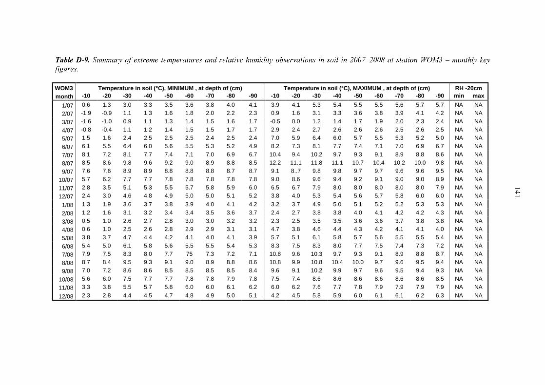
WOM3 Temperature in soil (°C), MINIMUM , at depth of (cm) Temperature in soil (°C), MAXIMUM , at depth of (cm) RH -20cm
month -10 -20 -30 -40 -50 -60 -70 -80 -90 -10 -20 -30 -40 -50 -60 -70 -80 -90 min max
1/07 0.6 1.3 3.0 3.3 3.5 3.6 3.8 4.0 4.1 3.9 4.1 5.3 5.4 5.5 5.5 5.6 5.7 5.7 NA NA
2/07 -1.9 -0.9 1.1 1.3 1.6 1.8 2.0 2.2 2.3 0.9 1.6 3.1 3.3 3.6 3.8 3.9 4.1 4.2 NA NA
3/07 -1.6 -1.0 0.9 1.1 1.3 1.4 1.5 1.6 1.7 -0.5 0.0 1.2 1.4 1.7 1.9 2.0 2.3 2.4 NA NA
4/07 -0.8 -0.4 1.1 1.2 1.4 1.5 1.5 1.7 1.7 2.9 2.4 2.7 2.6 2.6 2.6 2.5 2.6 2.5 NA NA
5/07 1.5 1.6 2.4 2.5 2.5 2.5 2.4 2.5 2.4 7.0 5.9 6.4 6.0 5.7 5.5 5.3 5.2 5.0 NA NA
6/07 6.1 5.5 6.4 6.0 5.6 5.5 5.3 5.2 4.9 8.2 7.3 8.1 7.7 7.4 7.1 7.0 6.9 6.7 NA NA
7/07 8.1 7.2 8.1 7.7 7.4 7.1 7.0 6.9 6.7 10.4 9.4 10.2 9.7 9.3 9.1 8.9 8.8 8.6 NA NA
8/07 8.5 8.6 9.8 9.6 9.2 9.0 8.9 8.8 8.5 12.2 11.1 11.8 11.1 10.7 10.4 10.2 10.0 9.8 NA NA
9/07 7.6 7.6 8.9 8.9 8.8 8.8 8.8 8.7 8.7 9.1 8..7 9.8 9.8 9.7 9.7 9.6 9.6 9.5 NA NA
10/07 5.7 6.2 7.7 7.7 7.8 7.8 7.8 7.8 7.8 9.0 8.6 9.6 9.4 9.2 9.1 9.0 9.0 8.9 NA NA
11/07 2.8 3.5 5.1 5.3 5.5 5.7 5.8 5.9 6.0 6.5 6.7 7.9 8.0 8.0 8.0 8.0 8.0 7.9 NA NA
12/07 2.4 3.0 4.6 4.8 4.9 5.0 5.0 5.1 5.2 3.8 4.0 5.3 5.4 5.6 5.7 5.8 6.0 6.0 NA NA
1/08 1.3 1.9 3.6 3.7 3.8 3.9 4.0 4.1 4.2 3.2 3.7 4.9 5.0 5.1 5.2 5.2 5.3 5.3 NA NA
2/08 1.2 1.6 3.1 3.2 3.4 3.4 3.5 3.6 3.7 2.4 2.7 3.8 3.8 4.0 4.1 4.2 4.2 4.3 NA NA
3/08 0.5 1.0 2.6 2.7 2.8 3.0 3.0 3.2 3.2 2.3 2.5 3.5 3.5 3.6 3.6 3.7 3.8 3.8 NA NA
4/08 0.6 1.0 2.5 2.6 2.8 2.9 2.9 3.1 3.1 4.7 3.8 4.6 4.4 4.3 4.2 4.1 4.1 4.0 NA NA
5/08 3.8 3.7 4.7 4.4 4.2 4.1 4.0 4.1 3.9 5.7 5.1 6.1 5.8 5.7 5.6 5.5 5.5 5.4 NA NA
6/08 5.4 5.0 6.1 5.8 5.6 5.5 5.5 5.4 5.3 8.3 7.5 8.3 8.0 7.7 7.5 7.4 7.3 7.2 NA NA
7/08 7.9 7.5 8.3 8.0 7.7 75 7.3 7.2 7.1 10.8 9.6 10.3 9.7 9.3 9.1 8.9 8.8 8.7 NA NA
8/08 8.7 8.4 9.5 9.3 9.1 9.0 8.9 8.8 8.6 10.8 9.9 10.8 10.4 10.0 9.7 9.6 9.5 9.4 NA NA
9/08 7.0 7.2 8.6 8.6 8.5 8.5 8.5 8.5 8.4 9.6 9.1 10.2 9.9 9.7 9.6 9.5 9.4 9.3 NA NA
10/08 5.6 6.0 7.5 7.7 7.7 7.8 7.8 7.9 7.8 7.5 7.4 8.6 8.6 8.6 8.6 8.6 8.6 8.5 NA NA
11/08 3.3 3.8 5.5 5.7 5.8 6.0 6.0 6.1 6.2 6.0 6.2 7.6 7.7 7.8 7.9 7.9 7.9 7.9 NA NA
12/08 2.3 2.8 4.4 4.5 4.7 4.8 4.9 5.0 5.1 4.2 4.5 5.8 5.9 6.0 6.1 6.1 6.2 6.3 NA NA
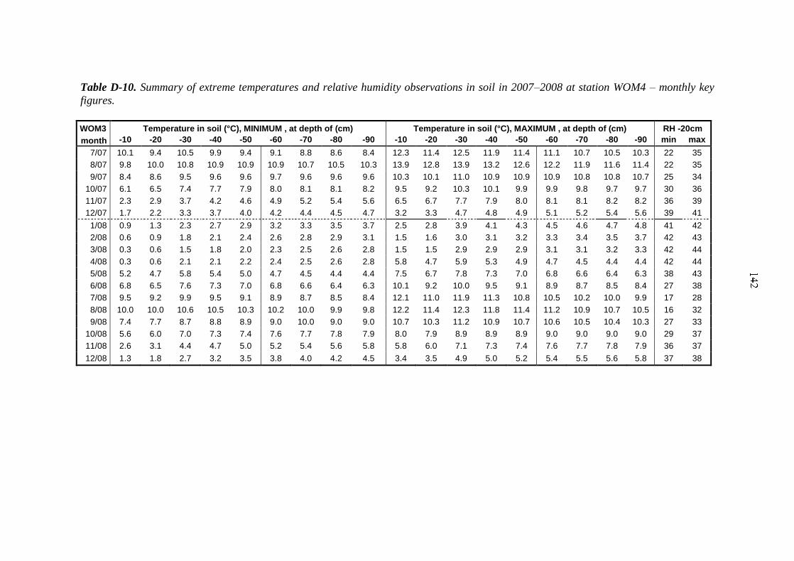
Table D-10. Summary of extreme temperatures and relative humidity observations in soil in 2007–2008 at station WOM4 – monthly key
figures.
WOM3 Temperature in soil (°C), MINIMUM , at depth of (cm) Temperature in soil (°C), MAXIMUM , at depth of (cm) RH -20cm
month -10 -20 -30 -40 -50 -60 -70 -80 -90 -10 -20 -30 -40 -50 -60 -70 -80 -90 min max
7/07 10.1 9.4 10.5 9.9 9.4 9.1 8.8 8.6 8.4 12.3 11.4 12.5 11.9 11.4 11.1 10.7 10.5 10.3 22 35
8/07 9.8 10.0 10.8 10.9 10.9 10.9 10.7 10.5 10.3 13.9 12.8 13.9 13.2 12.6 12.2 11.9 11.6 11.4 22 35
9/07 8.4 8.6 9.5 9.6 9.6 9.7 9.6 9.6 9.6 10.3 10.1 11.0 10.9 10.9 10.9 10.8 10.8 10.7 25 34
10/07 6.1 6.5 7.4 7.7 7.9 8.0 8.1 8.1 8.2 9.5 9.2 10.3 10.1 9.9 9.9 9.8 9.7 9.7 30 36
11/07 2.3 2.9 3.7 4.2 4.6 4.9 5.2 5.4 5.6 6.5 6.7 7.7 7.9 8.0 8.1 8.1 8.2 8.2 36 39
12/07 1.7 2.2 3.3 3.7 4.0 4.2 4.4 4.5 4.7 3.2 3.3 4.7 4.8 4.9 5.1 5.2 5.4 5.6 39 41
1/08 0.9 1.3 2.3 2.7 2.9 3.2 3.3 3.5 3.7 2.5 2.8 3.9 4.1 4.3 4.5 4.6 4.7 4.8 41 42
2/08 0.6 0.9 1.8 2.1 2.4 2.6 2.8 2.9 3.1 1.5 1.6 3.0 3.1 3.2 3.3 3.4 3.5 3.7 42 43
3/08 0.3 0.6 1.5 1.8 2.0 2.3 2.5 2.6 2.8 1.5 1.5 2.9 2.9 2.9 3.1 3.1 3.2 3.3 42 44
4/08 0.3 0.6 2.1 2.1 2.2 2.4 2.5 2.6 2.8 5.8 4.7 5.9 5.3 4.9 4.7 4.5 4.4 4.4 42 44
5/08 5.2 4.7 5.8 5.4 5.0 4.7 4.5 4.4 4.4 7.5 6.7 7.8 7.3 7.0 6.8 6.6 6.4 6.3 38 43
6/08 6.8 6.5 7.6 7.3 7.0 6.8 6.6 6.4 6.3 10.1 9.2 10.0 9.5 9.1 8.9 8.7 8.5 8.4 27 38
7/08 9.5 9.2 9.9 9.5 9.1 8.9 8.7 8.5 8.4 12.1 11.0 11.9 11.3 10.8 10.5 10.2 10.0 9.9 17 28
8/08 10.0 10.0 10.6 10.5 10.3 10.2 10.0 9.9 9.8 12.2 11.4 12.3 11.8 11.4 11.2 10.9 10.7 10.5 16 32
9/08 7.4 7.7 8.7 8.8 8.9 9.0 10.0 9.0 9.0 10.7 10.3 11.2 10.9 10.7 10.6 10.5 10.4 10.3 27 33
10/08 5.6 6.0 7.0 7.3 7.4 7.6 7.7 7.8 7.9 8.0 7.9 8.9 8.9 8.9 9.0 9.0 9.0 9.0 29 37
11/08 2.6 3.1 4.4 4.7 5.0 5.2 5.4 5.6 5.8 5.8 6.0 7.1 7.3 7.4 7.6 7.7 7.8 7.9 36 37
12/08 1.3 1.8 2.7 3.2 3.5 3.8 4.0 4.2 4.5 3.4 3.5 4.9 5.0 5.2 5.4 5.5 5.6 5.8 37 38
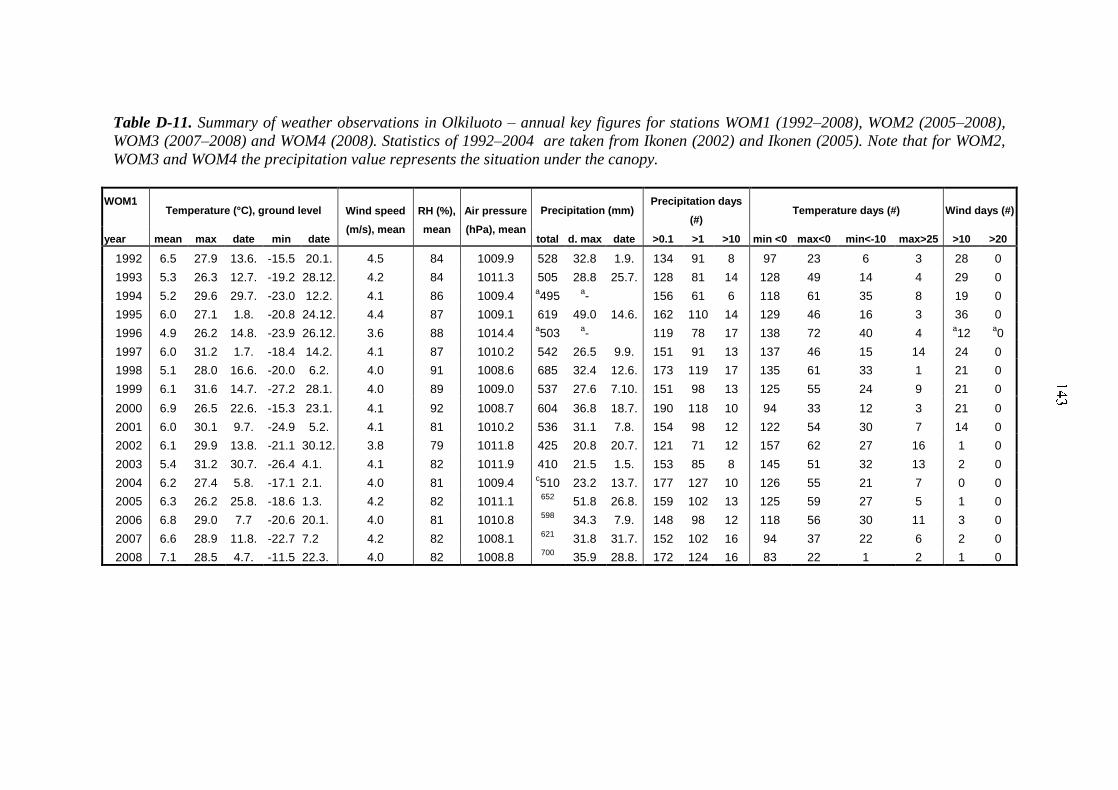
Table D-11. Summary of weather observations in Olkiluoto – annual key figures for stations WOM1 (1992–2008), WOM2 (2005–2008),
WOM3 (2007–2008) and WOM4 (2008). Statistics of 1992–2004 are taken from Ikonen (2002) and Ikonen (2005). Note that for WOM2,
WOM3 and WOM4 the precipitation value represents the situation under the canopy.
WOM1 Temperature (°C), ground level Wind speed
(m/s), mean
RH (%),
mean
Air pressure
(hPa), mean
Precipitation (mm) Precipitation days
(#) Temperature days (#) Wind days (#)
year mean max date min date total d. max date >0.1 >1 >10 min <0 max<0 min<-10 max>25 >10 >20
1992 6.5 27.9 13.6. -15.5 20.1. 4.5 84 1009.9 528 32.8 1.9. 134 91 8 97 23 6 3 28 0
1993 5.3 26.3 12.7. -19.2 28.12. 4.2 84 1011.3 505 28.8 25.7. 128 81 14 128 49 14 4 29 0
1994 5.2 29.6 29.7. -23.0 12.2. 4.1 86 1009.4 a495
a- 156 61 6 118 61 35 8 19 0
1995 6.0 27.1 1.8. -20.8 24.12. 4.4 87 1009.1 619 49.0 14.6. 162 110 14 129 46 16 3 36 0
1996 4.9 26.2 14.8. -23.9 26.12. 3.6 88 1014.4 a503
a- 119 78 17 138 72 40 4
a12
a0
1997 6.0 31.2 1.7. -18.4 14.2. 4.1 87 1010.2 542 26.5 9.9. 151 91 13 137 46 15 14 24 0
1998 5.1 28.0 16.6. -20.0 6.2. 4.0 91 1008.6 685 32.4 12.6. 173 119 17 135 61 33 1 21 0
1999 6.1 31.6 14.7. -27.2 28.1. 4.0 89 1009.0 537 27.6 7.10. 151 98 13 125 55 24 9 21 0
2000 6.9 26.5 22.6. -15.3 23.1. 4.1 92 1008.7 604 36.8 18.7. 190 118 10 94 33 12 3 21 0
2001 6.0 30.1 9.7. -24.9 5.2. 4.1 81 1010.2 536 31.1 7.8. 154 98 12 122 54 30 7 14 0
2002 6.1 29.9 13.8. -21.1 30.12. 3.8 79 1011.8 425 20.8 20.7. 121 71 12 157 62 27 16 1 0
2003 5.4 31.2 30.7. -26.4 4.1. 4.1 82 1011.9 410 21.5 1.5. 153 85 8 145 51 32 13 2 0
2004 6.2 27.4 5.8. -17.1 2.1. 4.0 81 1009.4 c510 23.2 13.7. 177 127 10 126 55 21 7 0 0
2005 6.3 26.2 25.8. -18.6 1.3. 4.2 82 1011.1 652
51.8 26.8. 159 102 13 125 59 27 5 1 0
2006 6.8 29.0 7.7 -20.6 20.1. 4.0 81 1010.8 598
34.3 7.9. 148 98 12 118 56 30 11 3 0
2007 6.6 28.9 11.8. -22.7 7.2 4.2 82 1008.1 621
31.8 31.7. 152 102 16 94 37 22 6 2 0
2008 7.1 28.5 4.7. -11.5 22.3. 4.0 82 1008.8 700
35.9 28.8. 172 124 16 83 22 1 2 1 0
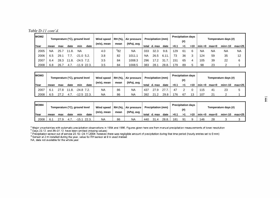
Table D-11 cont’d.
WOM2 Temperature (°C), ground level Wind speed
(m/s), mean
RH (%),
mean
Air pressure
(hPa), avg
Precipitation (mm) Precipitation days
(#) Temperature days (#)
Year mean max date min date total d. max date >0.1 >1 >10 min <0 max<0 min<-10 max>25
2005 NA 25.7 11.8. NA 4.0 d82 NA 333 32.3 9.8. 129 61 6 NA NA NA NA
2006 6.5 29.1 7.7. -21.0 5.2. 3.8 82 1011.1 NA 26.5 6.11. 73 36 3 124 59 35 12
2007 6.4 28.3 11.8. -24.5 7.2. 3.5 84 1008.3 296 17.2 31.7. 151 65 4 105 39 22 6
2008 6.8 26.7 4.7. -11.9 22.3. 3.5 84 1008.5 383 28.1 28.8. 179 89 5 98 23 2 1
WOM3 Temperature (°C), ground level Wind speed
(m/s), mean
RH (%),
mean
Air pressure
(hPa), avg
Precipitation (mm) Precipitation days
(#) Temperature days (#)
Year mean max date min date total d. max date >0.1 >1 >10 min <0 max<0 min<-10 max>25
2007 6.1 27.8 11.8. -24.8 7.2. NA 86 NA 437 27.9 27.7. 47 2 0 115 41 23 5
2008 6.5 27.2 4.7. -12.5 22.3. NA 86 NA 392 21.2 29.8 176 67 13 107 21 2 1
WOM4 Temperature (°C), ground level Wind speed
(m/s), mean
RH (%),
mean
Air pressure
(hPa), avg
Precipitation (mm) Precipitation days
(#) Temperature days (#)
Year mean max date min date total d. max date >0.1 >1 >10 min <0 max<0 min<-10 max>25
2008 6.1 27.9 4.7. -15.1 22.3. NA 86 NA 440 31.4 28.8. 181 91 9 146 28 3 3

Table D-12. Arithmetic mean snow thickness by terrain types in winters of 2007/2008
and 2008/2009. Number of observation points in brackets.
Date Open land/ wetland (2)
Pine forest (7)
Spruce forest (3)
Deciduous forest (8)
Overall mean (20)
2007/2008 8.1. 6.0 4.4 3.3 5.4 4.8 15.1. 0.0 0.0 0.0 0.0 0.0 22.1. 0.0 0.0 0.0 0.0 0.0 29.1. 0.0 0.0 0.0 0.0 0.0 5.2. 3.5 3.0 0.0 4.8 3.3 12.2. 0.0 0.0 0.0 0.0 0.0 19.2. 0.0 0.0 0.0 0.0 0.0 26.2. 0.0 0.0 0.0 0.0 0.0 4.3. 6.0 5.0 2.3 6.8 5.4 11.3. 0.0 0.0 0.0 0.0 0.0 17.3. 0.0 0.0 0.0 0.0 0.0 25.3. 2.0 1.7 1.0 2.1 1.8 1.4. 0.0 0.0 0.0 0.0 0.0
mean 1.3 1.1 0.5 1.5 1.2 max. of means
6.0 5.0 3.3 6.8 5.4
min. of means
0.0 0.0 0.0 0.0 0.0
2008/2009 27.11. 10.0 6.3 1.7 7.0 6.3 4.12. 0.0 0.0 0.0 0.0 0.0 11.12. 0.0 0.0 0.0 0.0 0.0 18.12. 0.0 0.0 0.0 0.0 0.0 23.12. 0.0 0.0 0.0 0.0 0.0 30.12. 0.0 0.0 0.0 0.0 0.0 8.1. 6.0 4.0 3.3 6.0 4.9 15.1. 0.0 0.0 0.0 0.0 0.0 22.1. 0.5 0.4 0.0 0.4 0.4 29.1. 9.0 6.6 4.3 8.4 7.2 5.2. 6.5 4.9 3.3 6.8 5.6 12.2. 5.5 5.0 3.0 6.4 5.3 19.2. 10.5 9.4 6.0 12.1 10.1 26.2. 14.0 11.9 7.7 13.8 12.2 5.3. 13.0 12.0 7.0 13.1 11.8 12.3. 20.0 17.0 13.0 19.0 17.5 19.3. 13.0 10.7 8.3 12.6 11.4 26.3. 9.5 9.6 5.7 11.3 9.7 2.4. 0.0 4.7 0.0 2.8 2.8 8.4. 0.0 0.0 0.0 0.0 0.0
mean 5.9 5.1 3.2 6.0 5.2 max. of means
20.0 17.0 13.0 19.0 17.5
min. of means
0.0 0.0 0.0 0.0 0.0
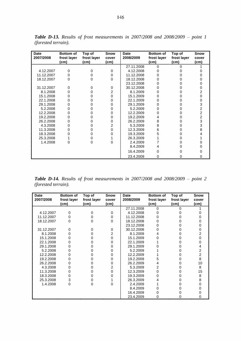
Table D-13. Results of frost measurements in 2007/2008 and 2008/2009 – point 1
(forested terrain).
Date 2007/2008
Bottom of frost layer (cm)
Top of frost layer (cm)
Snow cover (cm)
Date 2008/2009
Bottom of frost layer (cm)
Top of frost layer (cm)
Snow cover (cm)
27.11.2008 0 0 1 4.12.2007 0 0 0 4.12.2008 0 0 0
11.12.2007 0 0 0 11.12.2008 0 0 0 18.12.2007 0 0 0 18.12.2008 0 0 0
23.12.2008 0 0 0 31.12.2007 0 0 0 30.12.2008 0 0 0
8.1.2008 0 0 2 8.1.2009 0 0 2 15.1.2008 0 0 0 15.1.2009 0 0 0 22.1.2008 0 0 0 22.1.2009 0 0 0 29.1.2008 0 0 0 29.1.2009 0 0 3
5.2.2008 0 0 0 5.2.2009 0 0 2 12.2.2008 0 0 0 12.2.2009 0 0 2 19.2.2008 0 0 0 19.2.2009 4 0 2 26.2.2008 0 0 0 26.2.2009 8 0 3
4.3.2008 0 0 2 5.3.2009 8 0 3 11.3.2008 0 0 0 12.3.2009 6 0 8 18.3.2008 0 0 0 19.3.2009 5 0 4 25.3.2008 1 0 1 26.3.2009 1 0 1
1.4.2008 0 0 0 2.4.2009 7 0 0 8.4.2009 4 0 0
16.4.2009 0 0 0
23.4.2009 0 0 0
Table D-14. Results of frost measurements in 2007/2008 and 2008/2009 – point 2
(forested terrain).
Date 2007/2008
Bottom of frost layer (cm)
Top of frost layer (cm)
Snow cover (cm)
Date 2008/2009
Bottom of frost layer (cm)
Top of frost layer (cm)
Snow cover (cm)
27.11.2008 0 0 1 4.12.2007 0 0 0 4.12.2008 0 0 0
11.12.2007 0 0 0 11.12.2008 0 0 0 18.12.2007 0 0 0 18.12.2008 0 0 0
23.12.2008 0 0 0 31.12.2007 0 0 0 30.12.2008 0 0 0
8.1.2008 0 0 2 8.1.2009 4 0 2 15.1.2008 0 0 0 15.1.2009 0 0 0 22.1.2008 0 0 0 22.1.2009 1 0 0 29.1.2008 0 0 0 29.1.2009 0 0 4
5.2.2008 0 0 0 5.2.2009 1 0 2 12.2.2008 0 0 0 12.2.2009 1 0 2 19.2.2008 0 0 0 19.2.2009 5 0 8 26.2.2008 0 0 0 26.2.2009 4 0 10
4.3.2008 0 0 2 5.3.2009 2 0 8 11.3.2008 0 0 0 12.3.2009 0 0 15 18.3.2008 0 0 0 19.3.2009 0 0 8 25.3.2008 3 0 1 26.3.2009 4 0 8
1.4.2008 0 0 0 2.4.2009 1 0 0 8.4.2009 0 0 0 16.4.2009 0 0 0 23.4.2009 0 0 0
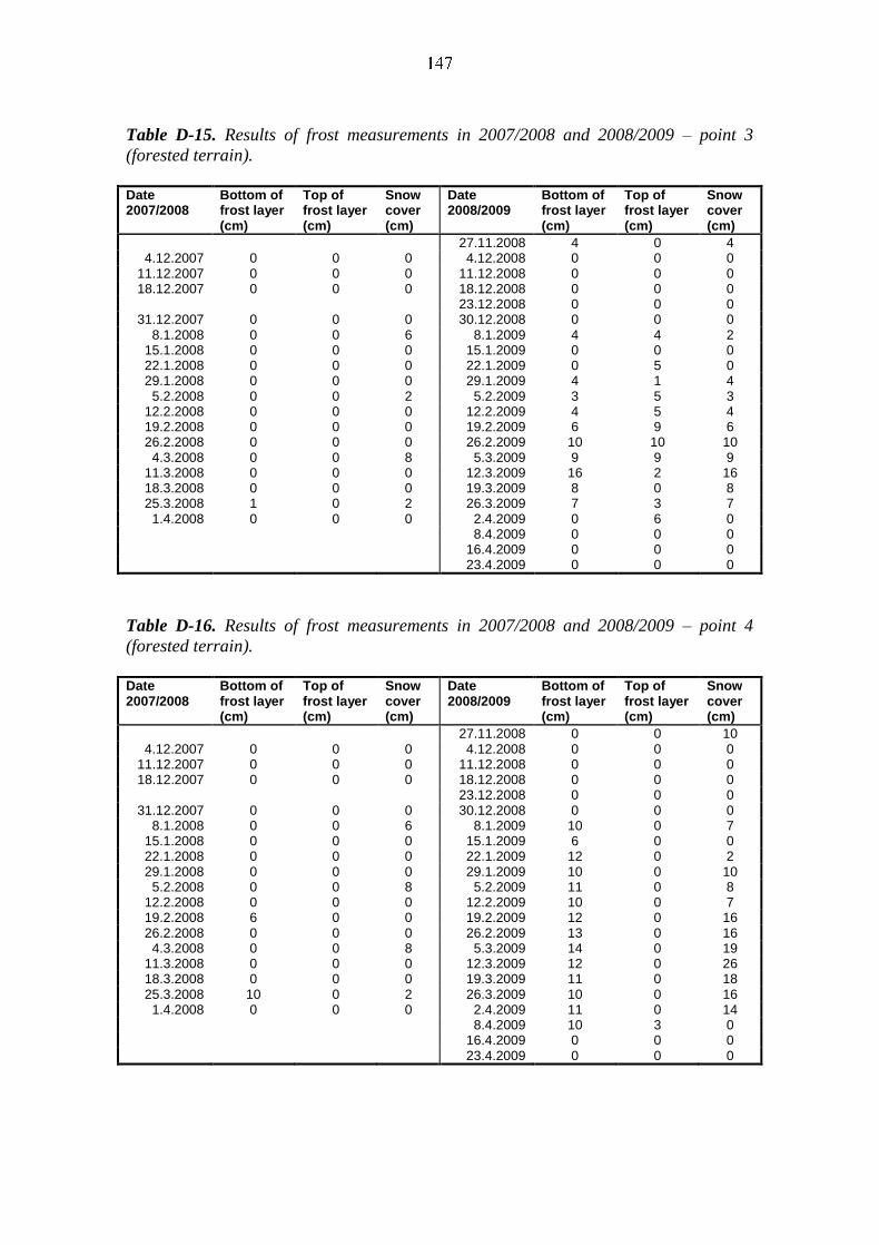
Table D-15. Results of frost measurements in 2007/2008 and 2008/2009 – point 3
(forested terrain). Date 2007/2008
Bottom of frost layer (cm)
Top of frost layer (cm)
Snow cover (cm)
Date 2008/2009
Bottom of frost layer (cm)
Top of frost layer (cm)
Snow cover (cm)
27.11.2008 4 0 4 4.12.2007 0 0 0 4.12.2008 0 0 0
11.12.2007 0 0 0 11.12.2008 0 0 0 18.12.2007 0 0 0 18.12.2008 0 0 0
23.12.2008 0 0 0 31.12.2007 0 0 0 30.12.2008 0 0 0
8.1.2008 0 0 6 8.1.2009 4 4 2 15.1.2008 0 0 0 15.1.2009 0 0 0 22.1.2008 0 0 0 22.1.2009 0 5 0 29.1.2008 0 0 0 29.1.2009 4 1 4
5.2.2008 0 0 2 5.2.2009 3 5 3 12.2.2008 0 0 0 12.2.2009 4 5 4 19.2.2008 0 0 0 19.2.2009 6 9 6 26.2.2008 0 0 0 26.2.2009 10 10 10
4.3.2008 0 0 8 5.3.2009 9 9 9 11.3.2008 0 0 0 12.3.2009 16 2 16 18.3.2008 0 0 0 19.3.2009 8 0 8 25.3.2008 1 0 2 26.3.2009 7 3 7
1.4.2008 0 0 0 2.4.2009 0 6 0 8.4.2009 0 0 0 16.4.2009 0 0 0 23.4.2009 0 0 0
Table D-16. Results of frost measurements in 2007/2008 and 2008/2009 – point 4
(forested terrain). Date 2007/2008
Bottom of frost layer (cm)
Top of frost layer (cm)
Snow cover (cm)
Date 2008/2009
Bottom of frost layer (cm)
Top of frost layer (cm)
Snow cover (cm)
27.11.2008 0 0 10 4.12.2007 0 0 0 4.12.2008 0 0 0
11.12.2007 0 0 0 11.12.2008 0 0 0 18.12.2007 0 0 0 18.12.2008 0 0 0
23.12.2008 0 0 0 31.12.2007 0 0 0 30.12.2008 0 0 0
8.1.2008 0 0 6 8.1.2009 10 0 7 15.1.2008 0 0 0 15.1.2009 6 0 0 22.1.2008 0 0 0 22.1.2009 12 0 2 29.1.2008 0 0 0 29.1.2009 10 0 10
5.2.2008 0 0 8 5.2.2009 11 0 8 12.2.2008 0 0 0 12.2.2009 10 0 7 19.2.2008 6 0 0 19.2.2009 12 0 16 26.2.2008 0 0 0 26.2.2009 13 0 16
4.3.2008 0 0 8 5.3.2009 14 0 19 11.3.2008 0 0 0 12.3.2009 12 0 26 18.3.2008 0 0 0 19.3.2009 11 0 18 25.3.2008 10 0 2 26.3.2009 10 0 16
1.4.2008 0 0 0 2.4.2009 11 0 14 8.4.2009 10 3 0 16.4.2009 0 0 0 23.4.2009 0 0 0
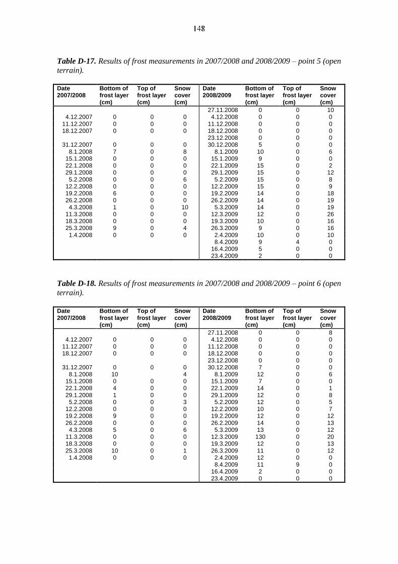
Table D-17. Results of frost measurements in 2007/2008 and 2008/2009 – point 5 (open
terrain). Date 2007/2008
Bottom of frost layer (cm)
Top of frost layer (cm)
Snow cover (cm)
Date 2008/2009
Bottom of frost layer (cm)
Top of frost layer (cm)
Snow cover (cm)
27.11.2008 0 0 10 4.12.2007 0 0 0 4.12.2008 0 0 0
11.12.2007 0 0 0 11.12.2008 0 0 0 18.12.2007 0 0 0 18.12.2008 0 0 0
23.12.2008 0 0 0 31.12.2007 0 0 0 30.12.2008 5 0 0
8.1.2008 7 0 8 8.1.2009 10 0 6 15.1.2008 0 0 0 15.1.2009 9 0 0 22.1.2008 0 0 0 22.1.2009 15 0 2 29.1.2008 0 0 0 29.1.2009 15 0 12
5.2.2008 0 0 6 5.2.2009 15 0 8 12.2.2008 0 0 0 12.2.2009 15 0 9 19.2.2008 6 0 0 19.2.2009 14 0 18 26.2.2008 0 0 0 26.2.2009 14 0 19
4.3.2008 1 0 10 5.3.2009 14 0 19 11.3.2008 0 0 0 12.3.2009 12 0 26 18.3.2008 0 0 0 19.3.2009 10 0 16 25.3.2008 9 0 4 26.3.2009 9 0 16
1.4.2008 0 0 0 2.4.2009 10 0 10 8.4.2009 9 4 0 16.4.2009 5 0 0 23.4.2009 2 0 0
Table D-18. Results of frost measurements in 2007/2008 and 2008/2009 – point 6 (open
terrain).
Date 2007/2008
Bottom of frost layer (cm)
Top of frost layer (cm)
Snow cover (cm)
Date 2008/2009
Bottom of frost layer (cm)
Top of frost layer (cm)
Snow cover (cm)
27.11.2008 0 0 8 4.12.2007 0 0 0 4.12.2008 0 0 0
11.12.2007 0 0 0 11.12.2008 0 0 0 18.12.2007 0 0 0 18.12.2008 0 0 0
23.12.2008 0 0 0 31.12.2007 0 0 0 30.12.2008 7 0 0
8.1.2008 10 4 8.1.2009 12 0 6 15.1.2008 0 0 0 15.1.2009 7 0 0 22.1.2008 4 0 0 22.1.2009 14 0 1 29.1.2008 1 0 0 29.1.2009 12 0 8
5.2.2008 0 0 3 5.2.2009 12 0 5 12.2.2008 0 0 0 12.2.2009 10 0 7 19.2.2008 9 0 0 19.2.2009 12 0 12 26.2.2008 0 0 0 26.2.2009 14 0 13
4.3.2008 5 0 6 5.3.2009 13 0 12 11.3.2008 0 0 0 12.3.2009 130 0 20 18.3.2008 0 0 0 19.3.2009 12 0 13 25.3.2008 10 0 1 26.3.2009 11 0 12
1.4.2008 0 0 0 2.4.2009 12 0 0 8.4.2009 11 9 0 16.4.2009 2 0 0 23.4.2009 0 0 0
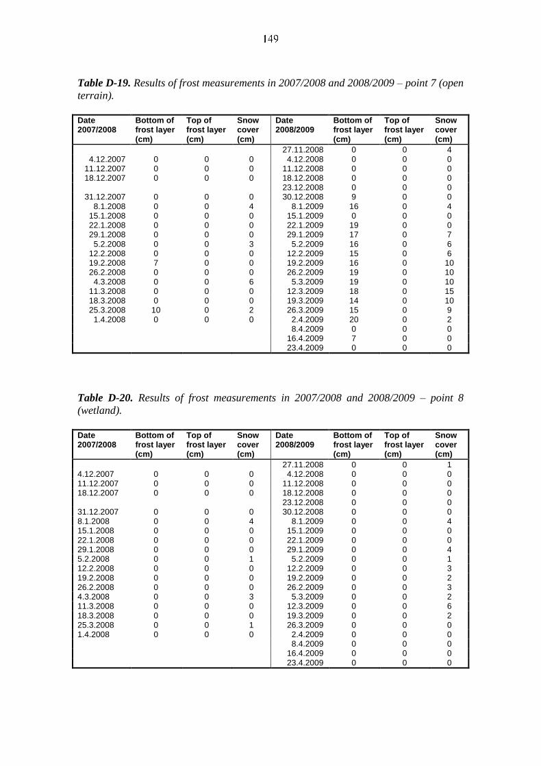
Table D-19. Results of frost measurements in 2007/2008 and 2008/2009 – point 7 (open
terrain).
Date 2007/2008
Bottom of frost layer (cm)
Top of frost layer (cm)
Snow cover (cm)
Date 2008/2009
Bottom of frost layer (cm)
Top of frost layer (cm)
Snow cover (cm)
27.11.2008 0 0 4 4.12.2007 0 0 0 4.12.2008 0 0 0
11.12.2007 0 0 0 11.12.2008 0 0 0 18.12.2007 0 0 0 18.12.2008 0 0 0
23.12.2008 0 0 0 31.12.2007 0 0 0 30.12.2008 9 0 0
8.1.2008 0 0 4 8.1.2009 16 0 4 15.1.2008 0 0 0 15.1.2009 0 0 0 22.1.2008 0 0 0 22.1.2009 19 0 0 29.1.2008 0 0 0 29.1.2009 17 0 7
5.2.2008 0 0 3 5.2.2009 16 0 6 12.2.2008 0 0 0 12.2.2009 15 0 6 19.2.2008 7 0 0 19.2.2009 16 0 10 26.2.2008 0 0 0 26.2.2009 19 0 10
4.3.2008 0 0 6 5.3.2009 19 0 10 11.3.2008 0 0 0 12.3.2009 18 0 15 18.3.2008 0 0 0 19.3.2009 14 0 10 25.3.2008 10 0 2 26.3.2009 15 0 9
1.4.2008 0 0 0 2.4.2009 20 0 2 8.4.2009 0 0 0 16.4.2009 7 0 0 23.4.2009 0 0 0
Table D-20. Results of frost measurements in 2007/2008 and 2008/2009 – point 8
(wetland).
Date 2007/2008
Bottom of frost layer (cm)
Top of frost layer (cm)
Snow cover (cm)
Date 2008/2009
Bottom of frost layer (cm)
Top of frost layer (cm)
Snow cover (cm)
27.11.2008 0 0 1 4.12.2007 0 0 0 4.12.2008 0 0 0 11.12.2007 0 0 0 11.12.2008 0 0 0 18.12.2007 0 0 0 18.12.2008 0 0 0 23.12.2008 0 0 0 31.12.2007 0 0 0 30.12.2008 0 0 0 8.1.2008 0 0 4 8.1.2009 0 0 4 15.1.2008 0 0 0 15.1.2009 0 0 0 22.1.2008 0 0 0 22.1.2009 0 0 0 29.1.2008 0 0 0 29.1.2009 0 0 4 5.2.2008 0 0 1 5.2.2009 0 0 1 12.2.2008 0 0 0 12.2.2009 0 0 3 19.2.2008 0 0 0 19.2.2009 0 0 2 26.2.2008 0 0 0 26.2.2009 0 0 3 4.3.2008 0 0 3 5.3.2009 0 0 2 11.3.2008 0 0 0 12.3.2009 0 0 6 18.3.2008 0 0 0 19.3.2009 0 0 2 25.3.2008 0 0 1 26.3.2009 0 0 0 1.4.2008 0 0 0 2.4.2009 0 0 0 8.4.2009 0 0 0 16.4.2009 0 0 0 23.4.2009 0 0 0
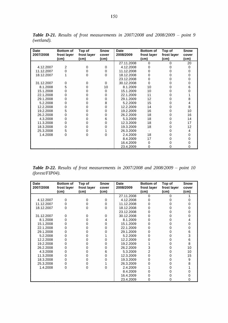
Table D-21. Results of frost measurements in 2007/2008 and 2008/2009 – point 9
(wetland).
Date 2007/2008
Bottom of frost layer (cm)
Top of frost layer (cm)
Snow cover (cm)
Date 2008/2009
Bottom of frost layer (cm)
Top of frost layer (cm)
Snow cover (cm)
27.11.2008 0 0 20 4.12.2007 2 0 0 4.12.2008 0 0 0
11.12.2007 0 0 0 11.12.2008 0 0 0 18.12.2007 1 0 0 18.12.2008 0 0 0
23.12.2008 0 0 0 31.12.2007 0 0 0 30.12.2008 0 0 0
8.1.2008 5 0 10 8.1.2009 10 0 6 15.1.2008 0 0 0 15.1.2009 10 0 0 22.1.2008 0 0 0 22.1.2009 11 0 1 29.1.2008 0 0 0 29.1.2009 12 0 8
5.2.2008 0 0 8 5.2.2009 15 0 4 12.2.2008 0 0 0 12.2.2009 14 0 8 19.2.2008 5 0 0 19.2.2009 16 0 10 26.2.2008 0 0 0 26.2.2009 18 0 16
4.3.2008 0 0 6 5.3.2009 18 0 14 11.3.2008 0 0 0 12.3.2009 18 0 17 18.3.2008 0 0 0 19.3.2009 18 0 12 25.3.2008 5 0 1 26.3.2009 - 0 4
1.4.2008 0 0 0 2.4.2009 18 0 0 8.4.2009 17 0 0 16.4.2009 0 0 0 23.4.2009 0 0 0
Table D-22. Results of frost measurements in 2007/2008 and 2008/2009 – point 10
(forest/FIP04).
Date 2007/2008
Bottom of frost layer (cm)
Top of frost layer (cm)
Snow cover (cm)
Date 2008/2009
Bottom of frost layer (cm)
Top of frost layer (cm)
Snow cover (cm)
27.11.2008 0 0 1 4.12.2007 0 0 0 4.12.2008 0 0 0
11.12.2007 0 0 0 11.12.2008 0 0 0 18.12.2007 0 0 0 18.12.2008 0 0 0
23.12.2008 0 0 0 31.12.2007 0 0 0 30.12.2008 0 0 0
8.1.2008 0 0 4 8.1.2009 0 0 4 15.1.2008 0 0 0 15.1.2009 0 0 0 22.1.2008 0 0 0 22.1.2009 0 0 0 29.1.2008 0 0 0 29.1.2009 0 0 6
5.2.2008 0 0 1 5.2.2009 0 0 3 12.2.2008 0 0 0 12.2.2009 0 0 6 19.2.2008 0 0 0 19.2.2009 1 0 8 26.2.2008 0 0 0 26.2.2009 3 0 10
4.3.2008 0 0 6 5.3.2009 2 0 10 11.3.2008 0 0 0 12.3.2009 0 0 15 18.3.2008 0 0 0 19.3.2009 0 0 9 25.3.2008 0 0 1 26.3.2009 0 0 8
1.4.2008 0 0 0 2.4.2009 1 0 1 8.4.2009 0 0 0 16.4.2009 0 0 0 23.4.2009 0 0 0

Table D-23. Results of frost measurements in 2007/2008 and 2008/2009 – point 11
(forest/FIP04).
Date 2007/2008
Bottom of frost layer (cm)
Top of frost layer (cm)
Snow cover (cm)
Date 2008/2009
Bottom of frost layer (cm)
Top of frost layer (cm)
Snow cover (cm)
27.11.2008 0 0 1 4.12.2007 0 0 0 4.12.2008 0 0 0
11.12.2007 0 0 0 11.12.2008 0 0 0 18.12.2007 0 0 0 18.12.2008 0 0 0
23.12.2008 0 0 0 31.12.2007 0 0 0 30.12.2008 0 0 0
8.1.2008 0 0 4 8.1.2009 2 0 2 15.1.2008 0 0 0 15.1.2009 0 0 0 22.1.2008 0 0 0 22.1.2009 4 0 0 29.1.2008 0 0 0 29.1.2009 0 0 6
5.2.2008 0 0 1 5.2.2009 0 0 2 12.2.2008 0 0 0 12.2.2009 0 0 2 19.2.2008 0 0 0 19.2.2009 0 0 5 26.2.2008 0 0 0 26.2.2009 6 0 7
4.3.2008 0 0 6 5.3.2009 5 0 6 11.3.2008 0 0 0 12.3.2009 2 0 10 18.3.2008 0 0 0 19.3.2009 0 0 6 25.3.2008 4 0 1 26.3.2009 5 0 4
2.4.2009 5 0 0 8.4.2009 0 0 0 16.4.2009 0 0 0 23.4.2009 0 0 0


APPENDIX E: RESULTS FROM RADIONUCLIDE MONITORING IN 2008
Results from the radionuclide monitoring from the year 2008 are presented in this
Appendix. In the data tables the uncertainty of the measurement is shown in the column
on the right-hand side of the activity concentration as a percentage of the concentration.
The uncertainties reported do not include the uncertainty arising out of the sampling
method and practice. For sampling periods longer than one day, the starting and ending
dates are reported. Activity concentrations are decay-corrected to correspond with the
middle of the sampling period. The dates have been printed as day.month notations, e.g.
1.3. is March 1. For sampling periods started in 2007 or ended in 2009 the year is also
given: 1.3.09. Measurement results below the minimum detectable activity (MDA) are
marked with the symbol < in the tables. Lost and contaminated samples are indicated.
Cells marked with symbol - = substance not measured. In addition to the results
presented in Tables, a ditch water sample from the dumping site was taken in Nov 18,
with K-40 620 Bq/m3 (s.d. 12) and Cs-137 1.39 Bq/m
3 (s.d. 18).
Table E-1. Radionuclides in deposition in 2008, Bq/m2, Tritium (H-3) deposition Bq/l.
Location Start date End date Be-7 ±% Cs-137 ±% H-3 ±% Sr-90 ±%
RNM02-DC1 1.1. 26.3. 176 6 0.34 30 - -
26.3. 25.6. 180 6 0.52 16 - -
25.6. 24.9. 360 14 0.31 24 - -
27.9. 30.12. 320 10 0.23 28 - -
RNM03-DC1 1.1. 26.3. 172 10 0.25 28 <4 -
26.3. 25.6. 207 10 0.92 12 <2 -
25.6. 24.9. 310 10 1.10 12 1.7 50 -
27.9. 30.12. 400 6 0.27 32 <21 -
RNM04-DC1 1.1. 26.3. 185 6 0.26 24 - -
26.3. 25.6. 166 10 0.58 16 - -
25.6. 24.9. 274 10 0.33 22 - -
27.9. 30.12. 310 8 0.25 24 - -
RNM06-DC1 1.1. 30.1. 75 10 0.083 12 <4 -
30.1. 27.2. 54 10 0.085 14 <4 -
1.3. 26.3. 60 14 0.087 14 <4 -
26.3. 29.4. 27.8 8 0.059 16 4.4 24 -
30.4. 28.5. 24.2 10 0.19 12 4.5 24 -
28.5. 25.6. 67 14 0.57 12 3.0 32 -
25.6. 30.7. 88 10 0.30 12 1.70 52 -
30.7. 27.8. 114 14 0.27 12 2.60 36 -
27.8. 24.9. 97 6 0.14 8 3.0 32 -
27.9. 29.10. 98 10 0.75 12 2.202 44 -
29.10. 26.11. 89 10 0.16 12 2.503 40 -
26.11. 30.12. 85 10 0.18 12 <2 -
1.1. 30.12. - - - 0.104 14 1 13.11.
2 13.10.
3 12.11.
4 13.12.
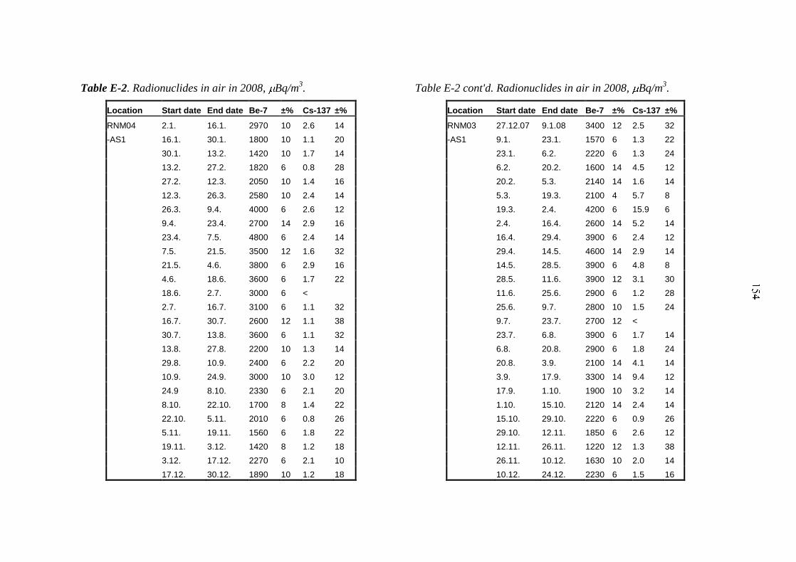
Table E-2. Radionuclides in air in 2008, Bq/m3.
Location Start date End date Be-7 ±% Cs-137 ±%
RNM04 2.1. 16.1. 2970 10 2.6 14
-AS1 16.1. 30.1. 1800 10 1.1 20
30.1. 13.2. 1420 10 1.7 14
13.2. 27.2. 1820 6 0.8 28
27.2. 12.3. 2050 10 1.4 16
12.3. 26.3. 2580 10 2.4 14
26.3. 9.4. 4000 6 2.6 12
9.4. 23.4. 2700 14 2.9 16
23.4. 7.5. 4800 6 2.4 14
7.5. 21.5. 3500 12 1.6 32
21.5. 4.6. 3800 6 2.9 16
4.6. 18.6. 3600 6 1.7 22
18.6. 2.7. 3000 6 <
2.7. 16.7. 3100 6 1.1 32
16.7. 30.7. 2600 12 1.1 38
30.7. 13.8. 3600 6 1.1 32
13.8. 27.8. 2200 10 1.3 14
29.8. 10.9. 2400 6 2.2 20
10.9. 24.9. 3000 10 3.0 12
24.9 8.10. 2330 6 2.1 20
8.10. 22.10. 1700 8 1.4 22
22.10. 5.11. 2010 6 0.8 26
5.11. 19.11. 1560 6 1.8 22
19.11. 3.12. 1420 8 1.2 18
3.12. 17.12. 2270 6 2.1 10
17.12. 30.12. 1890 10 1.2 18
Table E-2 cont'd. Radionuclides in air in 2008, Bq/m3.
Location Start date End date Be-7 ±% Cs-137 ±%
RNM03 27.12.07 9.1.08 3400 12 2.5 32
-AS1 9.1. 23.1. 1570 6 1.3 22
23.1. 6.2. 2220 6 1.3 24
6.2. 20.2. 1600 14 4.5 12
20.2. 5.3. 2140 14 1.6 14
5.3. 19.3. 2100 4 5.7 8
19.3. 2.4. 4200 6 15.9 6
2.4. 16.4. 2600 14 5.2 14
16.4. 29.4. 3900 6 2.4 12
29.4. 14.5. 4600 14 2.9 14
14.5. 28.5. 3900 6 4.8 8
28.5. 11.6. 3900 12 3.1 30
11.6. 25.6. 2900 6 1.2 28
25.6. 9.7. 2800 10 1.5 24
9.7. 23.7. 2700 12 <
23.7. 6.8. 3900 6 1.7 14
6.8. 20.8. 2900 6 1.8 24
20.8. 3.9. 2100 14 4.1 14
3.9. 17.9. 3300 14 9.4 12
17.9. 1.10. 1900 10 3.2 14
1.10. 15.10. 2120 14 2.4 14
15.10. 29.10. 2220 6 0.9 26
29.10. 12.11. 1850 6 2.6 12
12.11. 26.11. 1220 12 1.3 38
26.11. 10.12. 1630 10 2.0 14
10.12. 24.12. 2230 6 1.5 16
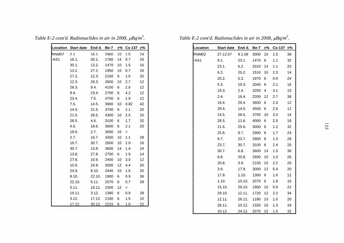
Table E-2 cont'd. Radionuclides in air in 2008, Bq/m3.
Location Start date End d. Be-7 ±% Cs-137 ±%
RNM07 2.1. 16.1. 2960 10 1.5 24
-AS1 16.1. 30.1. 1760 14 0.7 26
30.1. 13.2. 1470 10 1.5 16
13.2. 27.2. 1950 10 0.7 26
27.2. 12.3. 2160 6 1.0 20
12.3. 26.3. 2600 10 2.7 12
26.3. 9.4. 4100 6 2.0 12
9.4. 23.4. 2700 6 4.2 12
23.4. 7.5. 4700 6 1.9 12
7.5. 14.5. 3900 10 0.82 42
14.5. 21.5. 3700 6 2.1 20
21.5. 28.5. 4300 10 2.5 20
28.5. 4.6. 3100 6 1.7 32
4.6. 18.6. 3600 6 2.1 20
18.6. 2.7. 3000 10 <
2.7. 16.7. 3300 10 1.1 28
16.7. 30.7. 2600 10 1.0 16
30.7. 13.8. 3600 14 1.4 24
13.8. 27.8. 2700 6 1.9 14
27.8. 10.9. 2400 10 3.0 12
10.9. 24.9. 3000 12 4.4 20
24.9. 8.10. 2440 10 1.5 20
8.10. 22.10. 1900 6 0.9 36
22.10. 5.11. 2070 6 0.7 28
5.11. 19.11. 1500 12 <
19.11. 3.12. 1380 6 0.9 28
3.12. 17.12. 2180 6 1.5 10
17.12. 30.12. 2210 6 1.0 22
Table E-2 cont'd. Radionuclides in air in 2008, Bq/m3.
Location Start date End d. Be-7 ±% Cs-137 ±%
RNM02 27.12.07 9.1.08 3000 10 1.5 38
-AS1 9.1. 23.1. 1470 6 1.1 32
23.1. 6.2. 2010 14 1.1 20
6.2. 20.2. 1510 10 2.3 14
20.2. 5.3. 1970 6 0.9 24
5.3. 19.3. 2040 6 2.1 16
19.3. 2.4. 3200 4 3.1 10
2.4. 16.4. 2200 12 2.7 38
16.4. 29.4. 3600 6 2.4 12
29.4. 14.5. 4500 6 2.6 12
14.5. 28.5. 3700 10 3.3 14
28.5. 11.6. 4000 6 2.5 18
11.6. 25.6. 3000 6 1.2 32
25.6. 9.7. 2900 6 1.7 24
9.7. 23.7. 2800 6 1.3 28
23.7. 30.7. 3100 6 2.4 20
30.7. 6.8. 3600 14 1.5 36
6.8. 20.8. 2600 10 1.0 26
20.8. 3.9. 2100 10 2.2 20
3.9. 17.9. 3000 12 5.4 20
17.9. 1.10. 1300 6 1.6 12
1.10. 15.10. 2070 6 1.8 16
15.10. 29.10. 1900 10 0.9 22
29.10. 12.11. 1720 12 2.2 34
12.11. 26.11. 1180 10 1.0 20
26.11. 10.12. 1320 10 1.3 18
10.12. 24.12. 2070 12 1.5 32
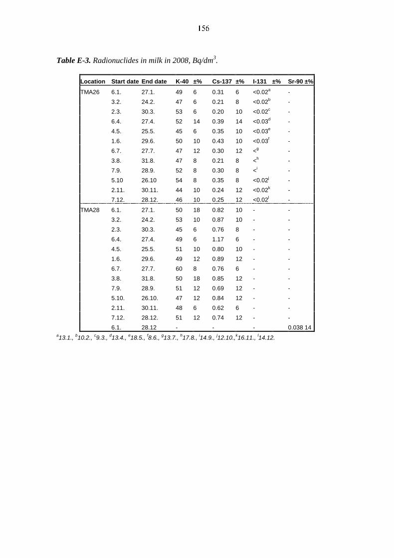
Table E-3. Radionuclides in milk in 2008, Bq/dm3.
Location Start date End date K-40 ±% Cs-137 ±% I-131 ±% Sr-90 ±%
TMA26 6.1. 27.1. 49 6 0.31 6 <0.02a -
3.2. 24.2. 47 6 0.21 8 <0.02b -
2.3. 30.3. 53 6 0.20 10 <0.02c -
6.4. 27.4. 52 14 0.39 14 <0.03d -
4.5. 25.5. 45 6 0.35 10 <0.03e -
1.6. 29.6. 50 10 0.43 10 <0.03f -
6.7. 27.7. 47 12 0.30 12 <g -
3.8. 31.8. 47 8 0.21 8 <h -
7.9. 28.9. 52 8 0.30 8 <i -
5.10 26.10 54 8 0.35 8 <0.02j -
2.11. 30.11. 44 10 0.24 12 <0.02k -
7.12. 28.12. 46 10 0.25 12 <0.02l -
TMA28 6.1. 27.1. 50 18 0.82 10 - -
3.2. 24.2. 53 10 0.87 10 - -
2.3. 30.3. 45 6 0.76 8 - -
6.4. 27.4. 49 6 1.17 6 - -
4.5. 25.5. 51 10 0.80 10 - -
1.6. 29.6. 49 12 0.89 12 - -
6.7. 27.7. 60 8 0.76 6 - -
3.8. 31.8. 50 18 0.85 12 - -
7.9. 28.9. 51 12 0.69 12 - -
5.10. 26.10. 47 12 0.84 12 - -
2.11. 30.11. 48 6 0.62 6 - -
7.12. 28.12. 51 12 0.74 12 - -
6.1. 28.12 - - - 0.038 14
a13.1.,
b10.2.,
c9.3.,
d13.4.,
e18.5.,
f8.6.,
g13.7.,
h17.8.,
i14.9.,
j12.10.,
k16.11.,
l14.12.

Table E-4. Radionuclides in food in 2008, Bq/kgDW.
Type Location Sampling date K-40 ±% Cs-137 ±% C-14 ±%
Beef TMA28 3.5. 85 6 0.68 7 -
9.10. 86 6 0.51 10 -
Wheat TMA27 31.8. 139 6 < 75 18
Table E-5. Radionuclides in drinking water in 2008, Bq/m3, H-3 Bq/l.
Location Sampling date H-3 ±% Sr-90 ±% K-40 ±% Cs-137 ±%
RNM05-DW1 8.1. <4 5.9 10 87 20 6.8 12
10.4. <2 - 94 12 3.8 12
2.7. < - 72 12 2.74 18
20.10. <2 6.3 a 12 111 10 3.5 12
RNM07-DW1 8.1. <4 5.8 10 115 12 4.7 12
10.4. <2 - 84 12 2.33 14
2.7. 1.60 54 - 78 12 2.87 14
20.10. <2 6.3 a 12 82 12 3.7 12
a 10.4.-20.10.
Table E-6. Radionuclides in terrestrial environment in 2008, Bq/kgDW.
Type Location
Sampl.
date
Be-7 ±% K-40 ±% Cs-134 ±% Cs-137 ±% C-14 ±% Sr-90 ±%
Pine
needles
TMA37 15.7. 35 14 94 12 < 95 12 104 12 -
Reference site a 12.8. 29.2 16 129 12 < 0.88 28 113 12 -
Reindeer
lichen
TMA38 17.7. 161 12 37 14 0.17 38 265 10 - -
Reference site b 7.10. 350 8 38 10 320 8 - -
Birch leaf TMA37 15.7. - 108 12 -
Reference site a 12.8. - 111 16 -
Lettuce TMA32 18.7. 51 14 2000 6 < 1.79 22 - -
22.8. 169 12 2050 12 < 3.1 12 - -
Common
haircap
TMA50 23.7. 340 10 250 8 < 142 8 - 2.80 16
Fern TMA49 17.7. 45 30 540 12 < 990 10 - -
Reference site a 12.8. 132 12 450 12 < 89 12 - -
Moss Reference site c 15.10. 750 8 275 8 201 8 - 3.9 10
Grazing
grass
TMA26 25.6. 21 14 620 8 0.36 58 144 18 -
TMA26 8.9. 226 8 900 8 < 2.81 12 - -
Black-
currant
TMA32 12.8. 2.18 16 96 18 < 0.15 14 - -
a Samples collected from Lohja. b Samples collected from Nummela c Samples collected from Espoo.

Table E-7. Radionuclides in fish in 2008, Bq/kgFW.
Species Location Start date End date K-40 ±% Co-60 ±% Cs-137 ±% Sr-90 ±%
Perch FIA11 9.5. 24.5. 106 10 0.094 28 24.1 8 -
FIA12 23.5. 26.5. 94 10 < 22.1 10 -
Pike FIA11 26.5.. 30.5. 122 8 < 14.0 8 -
FIA22 23.9. 8.19. 120 8 - 12.0 8 -
FIA12 15.5. 23.5. 114 12 < 14.7 12 -
FIA23 12.9. 16.9. 124 10 - 20.1 10 -
Baltic
herring
FIA12 3.6. 116 10 < 6.0 10 -
FIA23 19.9. 110 8 - 6.7 6 0.042 14
Bream FIA11 9.5. 112 10 < 5.8 8 -
FIA22 12.9. 8.10. 111 12 - 5.3 12 -
FIA12 10.5. 15.5. 104 10 < 4.5 10 -
FIA23 12.9. 16.9. 113 12 - 4.5 12 -
Table E-8. Radionuclides in seawater in 2008, Bq/m3, except for H-3, Bq/l.
Location Sampl. date H-3 ±% Sr-90 ±% K-40 ±% Cs-137 ±%
SEA11 11.3. 9.6 16 8.6 12 1920 6 37 6
15.5. 69 6 8.4 10 2190 12 47 12
17.7. <4 10.1 12 2050 6 41 6
18.11. <2 8.8 14 2060 6 39 8
SEA12 13.5. 10.6 14 - 1920 12 41 12
20.11. <2 - 2040 12 39 12
SEA03 15.5. 5.1 22 - 1920 6 40 6
19.11. <2 - 1960 8 41 10
SEA20 14.5. <2 - 1770 12 37 14
20.11. <2 - 1890 12 41 14
SEA46 13.5. <2 - 1960 12 45 14
20.11. <2 - 1990 12 41 12
SEA49 14.5. <2 7.9 10 1830 6 39 6
20.11. <2 9.3 14 2110 6 45 8
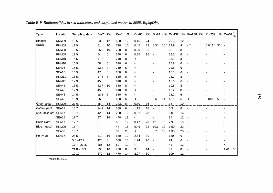
Table E-9. Radionuclides in sea indicators and suspended matter in 2008, Bq/kgDW.
Type Location Sampling date Be-7 ±% K-40 ±% Co-60 ±% Sr-90 ± % Cs-137 ±% Pu-238 ±% Pu-239 ±% Mn-54 ±
%
Bladder-
wrack
RNM09 13.5. 23.9 12 630 12 0.45 24 - 29.5 12 - - -
RNM09 17.9. 61 10 720 10 0.45 32 8.5 a 16
a 24.9 8 <
a 0.042
a 36
a -
RNM08 15.5. 25.3 10 790 8 0.30 36 - 32 8 - - -
RNM08 17.9. 64 6 540 6 0.35 16 - 19.5 6 - - -
RNM10 14.5. 17.8 8 710 8 < - 21.9 8 - - -
RNM10 16.9. 58 6 690 6 < - 17.9 6 - - -
SEA16 15.5. 13.8 8 719 6 < - 21.5 6 - - -
SEA16 16.9. 47 8 660 8 < - 16.3 6 - - -
RNM11 15.5. 17.5 8 810 8 < - 24.3 8 - - -
RNM11 17.9. 45 8 610 8 < - 16.6 6 - - -
SEA45 13.5. 22.7 10 650 8 < - 19.8 8 - - -
SEA45 17.9. 45 8 610 8 < - 15.2 8 - - -
SEA48 14.5. 18.6 8 630 6 < - 22.2 6 - - -
SEA48 16.9. 56 6 620 6 < 6.6 14 18.1 6 < 0.043 56 -
Green alga RNM09 27.6. 45 14 2430 8 0.80 36 - 33 10 - - -
Potam. pect. SEA17 15.7. 24.7 14 380 6 1.13 18 - 6.3 8 - - <
Myr. spicatum SEA17 16.7. 42 14 228 12 0.52 28 - 5.0 14 - - <
SEA25 17.7. 87 16 440 18 < - 37 12 - - <
Baltic clam SEA17 17.7. - 63 12 0.47 20 12.9 12 7.9 10 - - -
Blue mussel RNM09 15.7. - 44 16 0.49 32 10.1 12 1.50 22 - - -
SEA89 16.7. - 37 20 < 8.7 12 1.33 28 - - -
Perifyton SEA17 25.5. 119 16 540 12 2.64 30 - 150 6 - - -
5.6 –17.7. 420 8 530 10 1.74 26 - 74 6 - - <
17.7 –21.8. 285 12 80 12 < - 41 12 - - <
21.8 –18.9. 590 10 730 8 3.3 14 - 81 8 - - 1.41 30
19.10. 570 12 470 14 2.97 30 109 12
a results for 16.9.

Table E-9 cont'd. Radionuclides in sea indicators and suspended matter in 2008, Bq/kgDW.
Type Location Sampling date Be-7 ±% K-40 ±% Co-60 ±% Cs-137 ±% Pu-238 ±% Pu-239 ±%
Suspended
matter
SEA03 21.11.07 –10.4.08 390 8 700 6 0.86 32 300 6 - -
SEA03 10.4–4.6. 215 8 570 6 < 194 6 - -
SEA03 21.8–19.11. 640 8 780 10 1.86 20 310 6 - -
SEA03 21.11.07–19.11.08 - - - - < 0.70 24
SEA20 20.11.07 – 10.4.08 310 8 750 6 < 310 6 - -
SEA20 9.4 – 3.6. 200 8 620 10 < 227 6 - -
SEA20 3.6 – 20.8. 440 14 790 14 < 267 12 - -
SEA20 21.8–20.11. 440 6 680 6 < 274 6 - -
SEA15 20.11.07 – 10.4.08 320 8 760 8 < 330 6 - -
SEA15 10.4 – 3.6. 235 10 590 12 < 229 10 - -
SEA15 3.6– 21.8. 370 10 710 10 1.45 26 292 10 - -
SEA15 21.8–20.11. 390 12 710 12 2.02 20 275 10 - -
SEA18 21.11.07 – 10.4.08 470 14 740 18 1.84 18 360 10 - -
SEA18 10.4 – 4.6. 152 8 390 6 1.06 28 171 6 - -
SEA18 4.6– 21.8. 282 26 670 20 < 293 14 - -
SEA18 21.8–19.11. 620 14 670 14 0.99 32 320 10 - -
SEA50 9.4– 3.6. 166 16 570 16 < 193 12 - -
SEA50 3.6 – 20.8. 203 24 750 16 < 273 12 - -
SEA50 20.8–20.11. 520 10 700 12 < 281 10 -
SEA50 9.4–20.11. - - - - < 0.65 22
SEA47 9.4 – 4.6. 291 12 490 12 < 173 10 - -
SEA47 4.6 – 21.8. 460 8 710 10 < 294 6 - -
SEA47 21.8–20.11. 700 8 750 10 < 277 6 - -
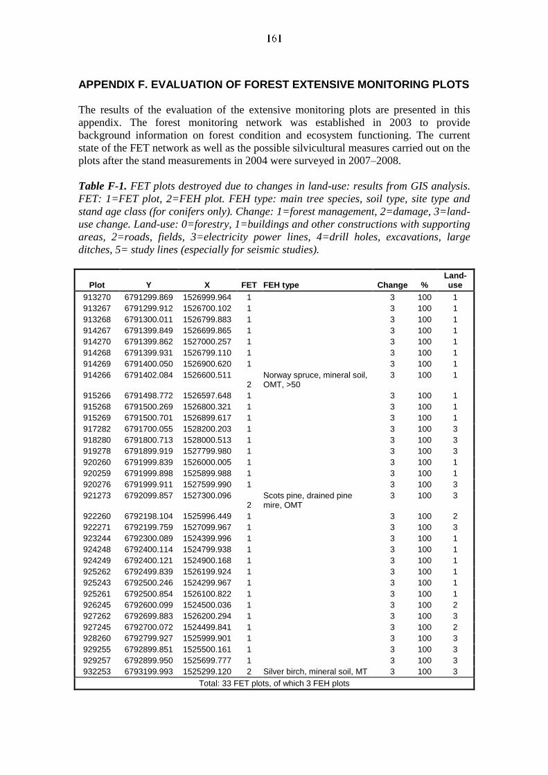
APPENDIX F. EVALUATION OF FOREST EXTENSIVE MONITORING PLOTS
The results of the evaluation of the extensive monitoring plots are presented in this
appendix. The forest monitoring network was established in 2003 to provide
background information on forest condition and ecosystem functioning. The current
state of the FET network as well as the possible silvicultural measures carried out on the
plots after the stand measurements in 2004 were surveyed in 2007–2008.
Table F-1. FET plots destroyed due to changes in land-use: results from GIS analysis.
FET: 1=FET plot, 2=FEH plot. FEH type: main tree species, soil type, site type and
stand age class (for conifers only). Change: 1=forest management, 2=damage, 3=land-
use change. Land-use: 0=forestry, 1=buildings and other constructions with supporting
areas, 2=roads, fields, 3=electricity power lines, 4=drill holes, excavations, large
ditches, 5= study lines (especially for seismic studies).
Plot Y X FET FEH type Change % Land-use
913270 6791299.869 1526999.964 1 3 100 1
913267 6791299.912 1526700.102 1 3 100 1
913268 6791300.011 1526799.883 1 3 100 1
914267 6791399.849 1526699.865 1 3 100 1
914270 6791399.862 1527000.257 1 3 100 1
914268 6791399.931 1526799.110 1 3 100 1
914269 6791400.050 1526900.620 1 3 100 1
914266 6791402.084 1526600.511 2
Norway spruce, mineral soil, OMT, >50
3 100 1
915266 6791498.772 1526597.648 1 3 100 1
915268 6791500.269 1526800.321 1 3 100 1
915269 6791500.701 1526899.617 1 3 100 1
917282 6791700.055 1528200.203 1 3 100 3
918280 6791800.713 1528000.513 1 3 100 3
919278 6791899.919 1527799.980 1 3 100 3
920260 6791999.839 1526000.005 1 3 100 1
920259 6791999.898 1525899.988 1 3 100 1
920276 6791999.911 1527599.990 1 3 100 3
921273 6792099.857 1527300.096 2
Scots pine, drained pine mire, OMT
3 100 3
922260 6792198.104 1525996.449 1 3 100 2
922271 6792199.759 1527099.967 1 3 100 3
923244 6792300.089 1524399.996 1 3 100 1
924248 6792400.114 1524799.938 1 3 100 1
924249 6792400.121 1524900.168 1 3 100 1
925262 6792499.839 1526199.924 1 3 100 1
925243 6792500.246 1524299.967 1 3 100 1
925261 6792500.854 1526100.822 1 3 100 1
926245 6792600.099 1524500.036 1 3 100 2
927262 6792699.883 1526200.294 1 3 100 3
927245 6792700.072 1524499.841 1 3 100 2
928260 6792799.927 1525999.901 1 3 100 3
929255 6792899.851 1525500.161 1 3 100 3
929257 6792899.950 1525699.777 1 3 100 3
932253 6793199.993 1525299.120 2 Silver birch, mineral soil, MT 3 100 3
Total: 33 FET plots, of which 3 FEH plots
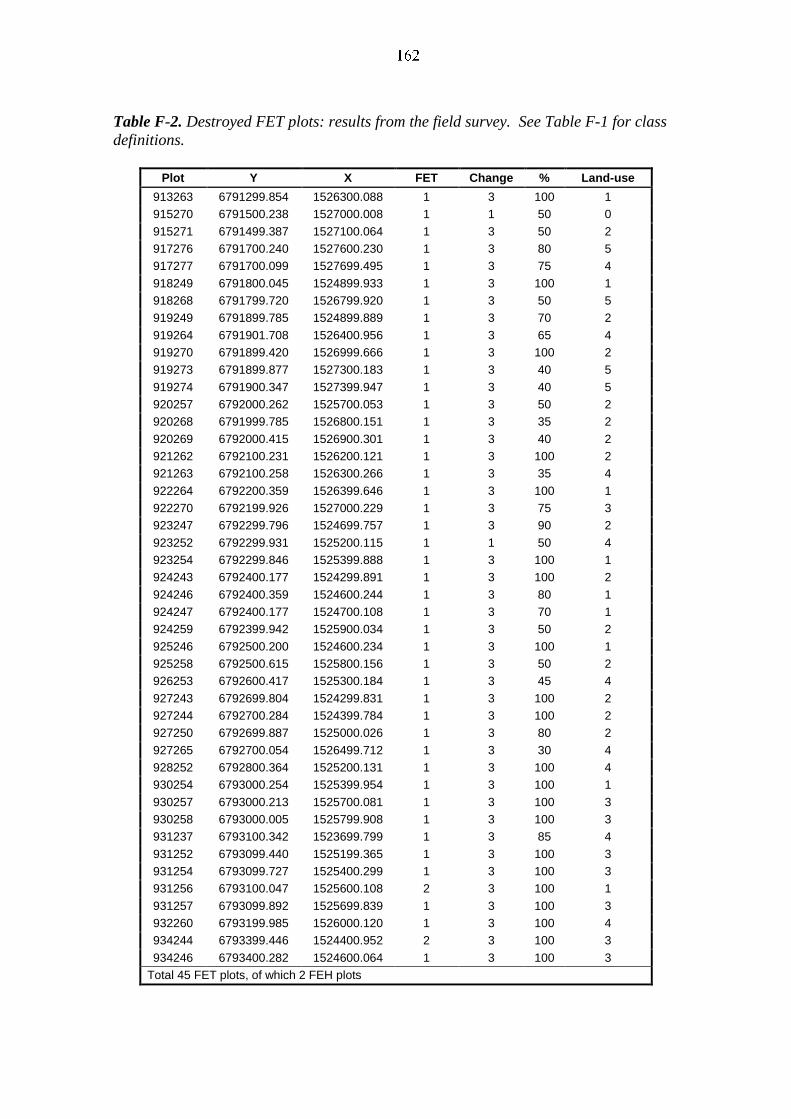
Table F-2. Destroyed FET plots: results from the field survey. See Table F-1 for class
definitions.
Plot Y X FET Change % Land-use
913263 6791299.854 1526300.088 1 3 100 1
915270 6791500.238 1527000.008 1 1 50 0
915271 6791499.387 1527100.064 1 3 50 2
917276 6791700.240 1527600.230 1 3 80 5
917277 6791700.099 1527699.495 1 3 75 4
918249 6791800.045 1524899.933 1 3 100 1
918268 6791799.720 1526799.920 1 3 50 5
919249 6791899.785 1524899.889 1 3 70 2
919264 6791901.708 1526400.956 1 3 65 4
919270 6791899.420 1526999.666 1 3 100 2
919273 6791899.877 1527300.183 1 3 40 5
919274 6791900.347 1527399.947 1 3 40 5
920257 6792000.262 1525700.053 1 3 50 2
920268 6791999.785 1526800.151 1 3 35 2
920269 6792000.415 1526900.301 1 3 40 2
921262 6792100.231 1526200.121 1 3 100 2
921263 6792100.258 1526300.266 1 3 35 4
922264 6792200.359 1526399.646 1 3 100 1
922270 6792199.926 1527000.229 1 3 75 3
923247 6792299.796 1524699.757 1 3 90 2
923252 6792299.931 1525200.115 1 1 50 4
923254 6792299.846 1525399.888 1 3 100 1
924243 6792400.177 1524299.891 1 3 100 2
924246 6792400.359 1524600.244 1 3 80 1
924247 6792400.177 1524700.108 1 3 70 1
924259 6792399.942 1525900.034 1 3 50 2
925246 6792500.200 1524600.234 1 3 100 1
925258 6792500.615 1525800.156 1 3 50 2
926253 6792600.417 1525300.184 1 3 45 4
927243 6792699.804 1524299.831 1 3 100 2
927244 6792700.284 1524399.784 1 3 100 2
927250 6792699.887 1525000.026 1 3 80 2
927265 6792700.054 1526499.712 1 3 30 4
928252 6792800.364 1525200.131 1 3 100 4
930254 6793000.254 1525399.954 1 3 100 1
930257 6793000.213 1525700.081 1 3 100 3
930258 6793000.005 1525799.908 1 3 100 3
931237 6793100.342 1523699.799 1 3 85 4
931252 6793099.440 1525199.365 1 3 100 3
931254 6793099.727 1525400.299 1 3 100 3
931256 6793100.047 1525600.108 2 3 100 1
931257 6793099.892 1525699.839 1 3 100 3
932260 6793199.985 1526000.120 1 3 100 4
934244 6793399.446 1524400.952 2 3 100 3
934246 6793400.282 1524600.064 1 3 100 3
Total 45 FET plots, of which 2 FEH plots
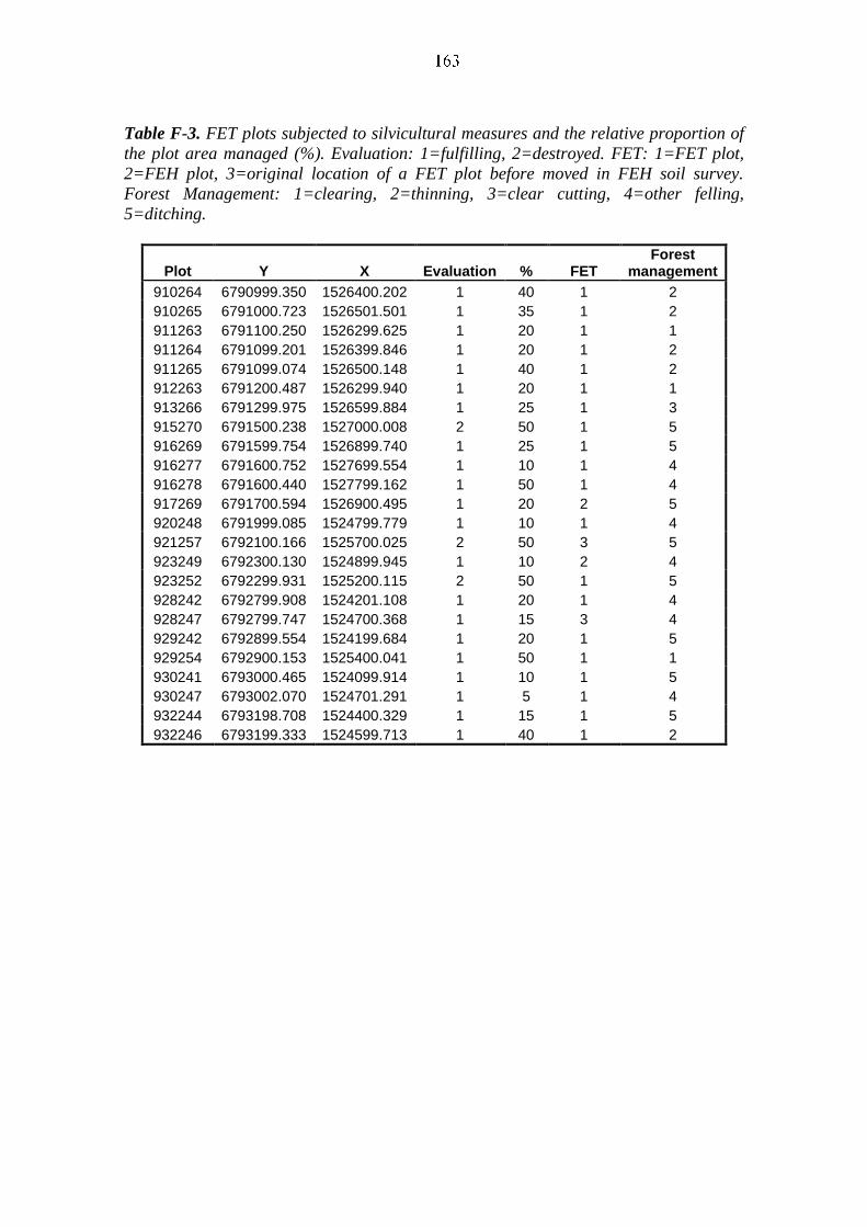
Table F-3. FET plots subjected to silvicultural measures and the relative proportion of
the plot area managed (%). Evaluation: 1=fulfilling, 2=destroyed. FET: 1=FET plot,
2=FEH plot, 3=original location of a FET plot before moved in FEH soil survey.
Forest Management: 1=clearing, 2=thinning, 3=clear cutting, 4=other felling,
5=ditching.
Plot Y X Evaluation % FET Forest
management
910264 6790999.350 1526400.202 1 40 1 2
910265 6791000.723 1526501.501 1 35 1 2
911263 6791100.250 1526299.625 1 20 1 1
911264 6791099.201 1526399.846 1 20 1 2
911265 6791099.074 1526500.148 1 40 1 2
912263 6791200.487 1526299.940 1 20 1 1
913266 6791299.975 1526599.884 1 25 1 3
915270 6791500.238 1527000.008 2 50 1 5
916269 6791599.754 1526899.740 1 25 1 5
916277 6791600.752 1527699.554 1 10 1 4
916278 6791600.440 1527799.162 1 50 1 4
917269 6791700.594 1526900.495 1 20 2 5
920248 6791999.085 1524799.779 1 10 1 4
921257 6792100.166 1525700.025 2 50 3 5
923249 6792300.130 1524899.945 1 10 2 4
923252 6792299.931 1525200.115 2 50 1 5
928242 6792799.908 1524201.108 1 20 1 4
928247 6792799.747 1524700.368 1 15 3 4
929242 6792899.554 1524199.684 1 20 1 5
929254 6792900.153 1525400.041 1 50 1 1
930241 6793000.465 1524099.914 1 10 1 5
930247 6793002.070 1524701.291 1 5 1 4
932244 6793198.708 1524400.329 1 15 1 5
932246 6793199.333 1524599.713 1 40 1 2


APPENDIX G. BULK DEPOSITION AND STAND THROUGHFALL MONITORING RESULTS IN 2004–2008
In this Appendix the annual bulk precipitation and stand throughfall results for the
MRK plots are given for the years 2004–2008. Original data has been presented in a
memo by Antti-Jussi Lindroos, John Derome and Lasse Aro (Finnish Forest Research
Institute). Precipitation collection on MRK9 was started on 20.4.2004, on MRK10 on
23.5.2005 and on MRK11 on 14.4.2007. Reference values for Forest Focus/ICP Forests
plots at Juupajoki and Tammela are given for comparison when possible.
Table G-1. Annual precipitation in the open (MRK2) and annual stand throughfall
(MRK4, MRK10 and MRK11) in 2004–2008. For comparison, the mean values for the
earlier monitoring network are presented for the years 2004–2007. NM = no
measurements covering the whole year.
Annual precipitation (mm)
Plot 2004 2005 2006 2007 2008
Open area (bulk deposition)
MRK2 659 517 586 579 631
Mean (MRK 2, 7, 9) 632 455 535 564
Stand throughfall
MRK4 (FIP4) 381 303 364 348 433
MRK10 (FIP10) NM NM 404 368 457
MRK11 NM NM NM NM 679
Mean (MRK 1, 3–6, 8, 10) 398 347 380 350
Table G-2. Interception of precipitation by the tree canopies during 2004–2008.
Interception was calculated as: (annual precipitation in the open – stand throughfall) /
(annual precipitation in the open) x 100, and expressed as %. NM = no measurements
covering the whole year.
Year MRK4 MRK10 Mean (MRK 1, 3–6, 8, 10)
2004 40 NM 37
2005 33 NM 24
2006 32 24 29
2007 38 35 38
2008 31 28
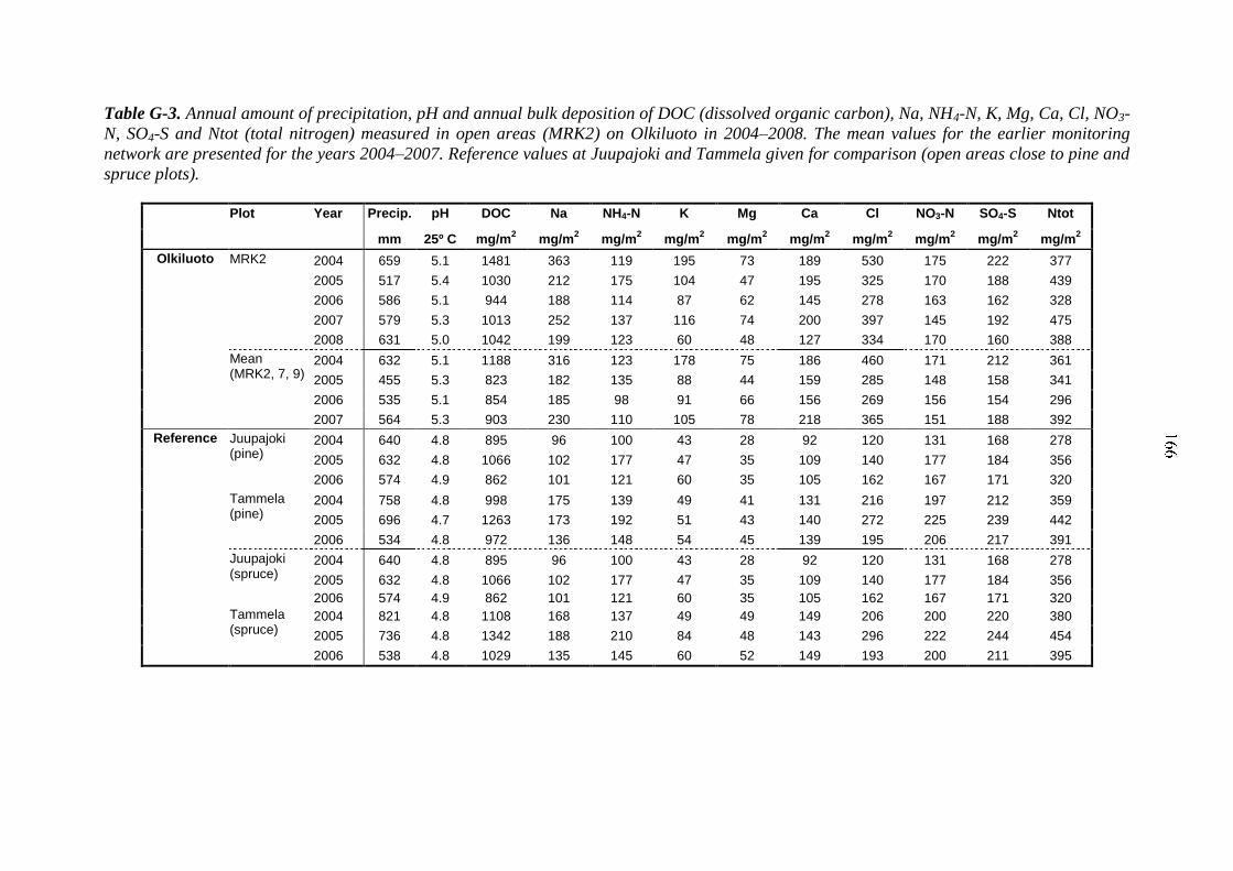
Table G-3. Annual amount of precipitation, pH and annual bulk deposition of DOC (dissolved organic carbon), Na, NH4-N, K, Mg, Ca, Cl, NO3-
N, SO4-S and Ntot (total nitrogen) measured in open areas (MRK2) on Olkiluoto in 2004–2008. The mean values for the earlier monitoring
network are presented for the years 2004–2007. Reference values at Juupajoki and Tammela given for comparison (open areas close to pine and
spruce plots).
Plot Year Precip. pH DOC Na NH4-N K Mg Ca Cl NO3-N SO4-S Ntot
mm 25º C mg/m2 mg/m
2 mg/m
2 mg/m
2 mg/m
2 mg/m
2 mg/m
2 mg/m
2 mg/m
2 mg/m
2
Olkiluoto MRK2 2004 659 5.1 1481 363 119 195 73 189 530 175 222 377
2005 517 5.4 1030 212 175 104 47 195 325 170 188 439
2006 586 5.1 944 188 114 87 62 145 278 163 162 328
2007 579 5.3 1013 252 137 116 74 200 397 145 192 475
2008 631 5.0 1042 199 123 60 48 127 334 170 160 388
Mean (MRK2, 7, 9)
2004 632 5.1 1188 316 123 178 75 186 460 171 212 361
2005 455 5.3 823 182 135 88 44 159 285 148 158 341
2006 535 5.1 854 185 98 91 66 156 269 156 154 296
2007 564 5.3 903 230 110 105 78 218 365 151 188 392
Reference Juupajoki (pine)
2004 640 4.8 895 96 100 43 28 92 120 131 168 278
2005 632 4.8 1066 102 177 47 35 109 140 177 184 356
2006 574 4.9 862 101 121 60 35 105 162 167 171 320
Tammela (pine)
2004 758 4.8 998 175 139 49 41 131 216 197 212 359
2005 696 4.7 1263 173 192 51 43 140 272 225 239 442
2006 534 4.8 972 136 148 54 45 139 195 206 217 391
Juupajoki (spruce)
2004 640 4.8 895 96 100 43 28 92 120 131 168 278
2005 632 4.8 1066 102 177 47 35 109 140 177 184 356
2006 574 4.9 862 101 121 60 35 105 162 167 171 320
Tammela (spruce)
2004 821 4.8 1108 168 137 49 49 149 206 200 220 380
2005 736 4.8 1342 188 210 84 48 143 296 222 244 454
2006 538 4.8 1029 135 145 60 52 149 193 200 211 395
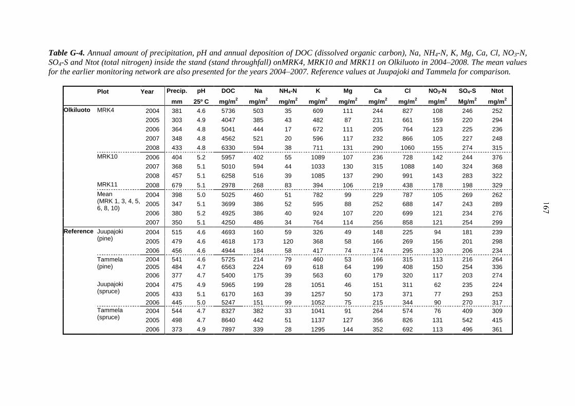
Table G-4. Annual amount of precipitation, pH and annual deposition of DOC (dissolved organic carbon), Na, NH4-N, K, Mg, Ca, Cl, NO3-N,
SO4-S and Ntot (total nitrogen) inside the stand (stand throughfall) onMRK4, MRK10 and MRK11 on Olkiluoto in 2004–2008. The mean values
for the earlier monitoring network are also presented for the years 2004–2007. Reference values at Juupajoki and Tammela for comparison.
Plot Year Precip. pH DOC Na NH4-N K Mg Ca Cl NO3-N SO4-S Ntot
mm 25º C mg/m2 mg/m
2 mg/m
2 mg/m
2 mg/m
2 mg/m
2 mg/m
2 mg/m
2 Mg/m
2 mg/m
2
Olkiluoto MRK4 2004 381 4.6 5736 503 35 609 111 244 827 108 246 252
2005 303 4.9 4047 385 43 482 87 231 661 159 220 294
2006 364 4.8 5041 444 17 672 111 205 764 123 225 236
2007 348 4.8 4562 521 20 596 117 232 866 105 227 248
2008 433 4.8 6330 594 38 711 131 290 1060 155 274 315
MRK10 2006 404 5.2 5957 402 55 1089 107 236 728 142 244 376
2007 368 5.1 5010 594 44 1033 130 315 1088 140 324 368
2008 457 5.1 6258 516 39 1085 137 290 991 143 283 322
MRK11 2008 679 5.1 2978 268 83 394 106 219 438 178 198 329
Mean (MRK 1, 3, 4, 5, 6, 8, 10)
2004 398 5.0 5025 460 51 782 99 229 787 105 269 262
2005 347 5.1 3699 386 52 595 88 252 688 147 243 289
2006 380 5.2 4925 386 40 924 107 220 699 121 234 276
2007 350 5.1 4250 486 34 764 114 256 858 121 254 299
Reference Juupajoki (pine)
2004 515 4.6 4693 160 59 326 49 148 225 94 181 239
2005 479 4.6 4618 173 120 368 58 166 269 156 201 298
2006 456 4.6 4944 184 58 417 74 174 295 130 206 234
Tammela (pine)
2004 541 4.6 5725 214 79 460 53 166 315 113 216 264
2005 484 4.7 6563 224 69 618 64 199 408 150 254 336
2006 377 4.7 5400 175 39 563 60 179 320 117 203 274
Juupajoki (spruce)
2004 475 4.9 5965 199 28 1051 46 151 311 62 235 224
2005 433 5.1 6170 163 39 1257 50 173 371 77 293 253
2006 445 5.0 5247 151 99 1052 75 215 344 90 270 317
Tammela (spruce)
2004 544 4.7 8327 382 33 1041 91 264 574 76 409 309
2005 498 4.7 8640 442 51 1137 127 356 826 131 542 415
2006 373 4.9 7897 339 28 1295 144 352 692 113 496 361

Table G-5. Annual bulk deposition of PO4-P, Al, Fe, Mn, Cu, Zn and Si in open area
(MRK2) on Olkiluoto in 2004–2008. The mean values for the earlier monitoring
network are presented for the years 2004–2007.
Plot Year PO4-P Al Fe Mn Cu Zn Si
mg/m2 mg/m
2 mg/m
2 mg/m
2 mg/m
2 mg/m
2 mg/m
2
MRK2 2004 18 32 10 6 11 9 16
2005 18 25 10 4 8 5 14
2006 8 30 7 2 9 6 14
2007 27 29 6 2 9 7 13
2008 49 15 6 3 4 7 9
Mean (MRK2,
7, 9) 2004 15 31 8 4 10 8 15
2005 12 23 8 3 7 5 13
2006 7 27 6 2 9 6 13
2007 18 28 6 2 9 8 14
Table G-6. Annual bulk deposition of PO4-P, Al, Fe, Mn, Cu, Zn and Si inside the stand
(stand throughfall) in MRK4, MRK10 and MRK11 on Olkiluoto in 2004–2008. The
mean values for the earlier monitoring network are presented for the years 2004–2007.
Plot Year PO4-P Al Fe Mn Cu Zn Si
mg/m2 mg/m
2 mg/m
2 mg/m
2 mg/m
2 mg/m
2 mg/m
2
MRK4 2004 7 19 9 29 6 9 26
2005 6 19 11 20 5 6 29
2006 5 21 9 23 6 8 27
2007 9 18 7 22 6 8 25
2008 28 23 12 34 21 17 28
MRK10 2006 17 20 10 20 6 10 27
2007 15 18 10 22 6 9 31
2008 30 17 13 22 5 12 35
MRK11 2008 44 18 7 8 6 15 24
Mean
(MRK 1, 3, 4, 5, 6, 8, 10)
2004 28 20 12 32 6 10 33
2005 15 19 13 27 6 6 34
2006 28 20 12 28 6 9 33
2007 20 18 12 27 6 9 34
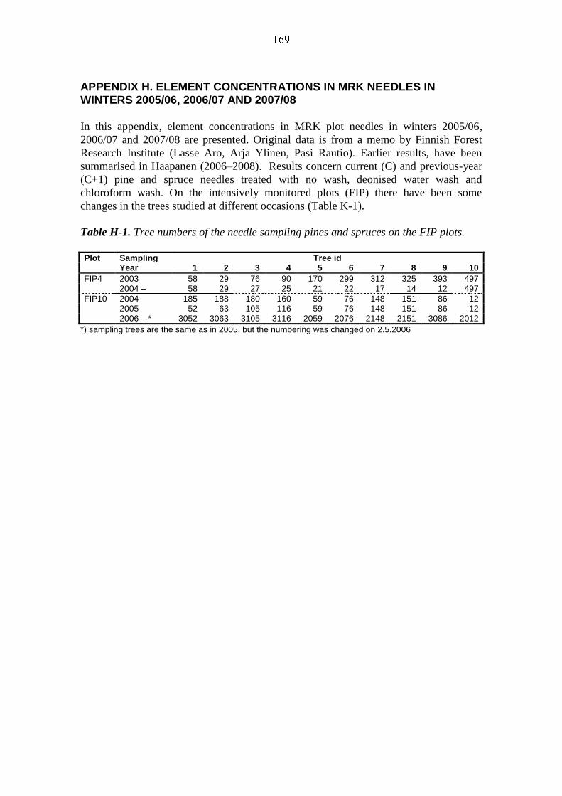
APPENDIX H. ELEMENT CONCENTRATIONS IN MRK NEEDLES IN WINTERS 2005/06, 2006/07 AND 2007/08
In this appendix, element concentrations in MRK plot needles in winters 2005/06,
2006/07 and 2007/08 are presented. Original data is from a memo by Finnish Forest
Research Institute (Lasse Aro, Arja Ylinen, Pasi Rautio). Earlier results, have been
summarised in Haapanen (2006–2008). Results concern current (C) and previous-year
(C+1) pine and spruce needles treated with no wash, deonised water wash and
chloroform wash. On the intensively monitored plots (FIP) there have been some
changes in the trees studied at different occasions (Table K-1).
Table H-1. Tree numbers of the needle sampling pines and spruces on the FIP plots.
Plot Sampling Tree id Year 1 2 3 4 5 6 7 8 9 10
FIP4 2003 58 29 76 90 170 299 312 325 393 497 2004 – 58 29 27 25 21 22 17 14 12 497
FIP10 2004 185 188 180 160 59 76 148 151 86 12 2005 52 63 105 116 59 76 148 151 86 12 2006 – * 3052 3063 3105 3116 2059 2076 2148 2151 3086 2012
*) sampling trees are the same as in 2005, but the numbering was changed on 2.5.2006
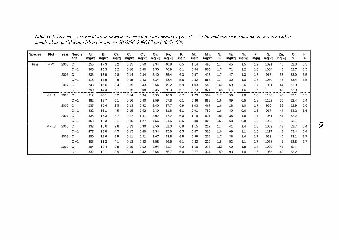
Species
Plot
Year
Needle age
Al , mg/kg
B, mg/kg
Ca, mg/g
Cd, mg/kg
Cr, mg/kg
Cu, mg/kg
Fe, mg/kg
K, mg/g
Mg, mg/g
Mn, mg/kg
N, %
Na, mg/kg
Ni, mg/kg
P, mg/g
S, mg/kg
Zn, mg/kg
C, %
H, %
Pine FIP4 2005 C 255 17.3 3.2 0.15 0.50 2.34 40.8 6.5 1.14 498 1.7 45 1.5 1.9 1021 40 52.3 6.5
C +1 365 15.3 5.2 0.18 0.80 2.50 70.9 6.1 0.84 805 1.7 71 1.2 1.8 1064 48 52.7 6.5
2006 C 235 13.9 2.8 0.14 0.34 2.40 35.4 6.3 0.97 473 1.7 47 1.3 1.8 968 38 53.0 6.5
C +1 318 12.6 4.6 0.15 0.43 2.34 48.4 5.8 0.82 665 1.7 80 1.0 1.7 1050 42 53.4 6.5
2007 C 243 15.6 3.4 0.15 2.43 2.54 49.2 5.9 1.03 583 1.62 69 2.6 1.7 1021 44 52.9
C+1 290 14.4 5.1 0.15 2.08 2.35 60.3 5.7 0.73 821 1.66 116 1.6 1.6 1102 48 52.9
MRK1 2005 C 312 20.1 3.2 0.14 0.34 2.35 46.6 6.7 1.23 584 1.7 56 1.0 1.8 1100 45 52.1 6.5
C +1 482 18.7 5.1 0.16 0.40 2.59 67.8 6.1 0.86 888 1.6 89 0.5 1.8 1102 50 52.4 6.4
2006 C 237 15.4 2.5 0.13 0.52 2.40 37.7 6.9 1.03 467 1.6 28 1.0 1.7 956 38 52.9 6.6
C +1 332 16.1 4.5 0.15 0.52 2.49 51.8 6.1 0.91 789 1.6 40 0.6 1.6 967 44 53.2 6.6
2007 C 335 17.3 3.7 0.17 1.41 2.02 47.2 6.0 1.19 671 1.54 38 1.6 1.7 1051 51 52.2
C+1 358 16.3 5.1 0.15 1.27 1.56 64.5 5.5 0.80 903 1.56 68 0.8 1.6 1093 52 53.1
MRK3 2005 C 332 15.6 2.8 0.13 0.30 2.56 51.0 6.8 1.15 227 1.7 41 1.4 1.8 1069 42 52.7 6.4
C +1 477 13.8 4.5 0.15 0.49 2.54 95.8 6.5 0.87 328 1.6 69 1.1 1.8 1117 43 53.4 6.4
2006 C 280 12.6 2.5 0.11 0.31 2.67 48.5 6.5 0.99 232 1.7 36 1.4 1.7 998 40 53.1 6.7
C +1 403 11.3 4.1 0.13 0.42 2.58 66.5 6.1 0.82 322 1.6 52 1.1 1.7 1058 41 53.8 6.7
2007 C 294 13.4 2.8 0.15 0.52 2.94 53.7 6.2 1.10 275 1.56 60 1.8 1.7 1000 45 5.4
C+1 332 12.1 3.9 0.14 0.42 2.64 76.7 6.0 0.77 334 1.59 93 1.0 1.6 1065 42 53.2
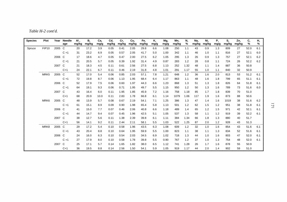
Table H-2 cont'd.
Species
Plot
Year
Needle age
Al , mg/kg
B, mg/kg
Ca, mg/g
Cd, mg/kg
Cr, mg/kg
Cu, mg/kg
Fe, mg/kg
K, mg/g
Mg, mg/g
Mn, mg/kg
N, %
Na, mg/kg
Ni, mg/kg
P, mg/g
S, mg/kg
Zn, mg/kg
C, %
H, %
Spruce FIP10 2005 C 20 17.2 3.9 0.05 0.41 2.05 29.8 6.6 1.08 250 1.1 43 0.9 1.3 809 27 52.0 6.1
C +1 31 23.2 6.9 0.05 0.57 2.05 41.7 5.0 1.00 342 1.1 46 1.0 1.1 816 27 52.1 6.0
2006 C 17 18.6 4.7 0.05 0.47 2.00 27.5 6.2 1.05 295 1.3 26 0.9 1.3 757 27 52.1 6.2
C +1 21 20.5 5.7 0.05 0.39 1.92 31.4 4.9 0.87 283 1.2 28 0.8 1.1 724 26 52.2 6.2
2007 C 21 18.3 4.5 0.11 0.61 2.56 27.5 6.8 1.13 252 1.32 48 1.1 1.4 887 36 50.8
C+1 24 22.1 6.7 0.11 0.46 2.19 31.8 4.8 1.01 291 1.17 55 1.0 1.1 840 32 50.9
MRK5 2005 C 52 17.0 5.4 0.06 0.85 2.03 57.1 7.8 1.21 648 1.2 36 1.6 2.0 813 53 51.2 6.1
C +1 72 19.8 8.7 0.06 1.13 1.95 68.4 6.4 1.17 863 1.1 48 1.6 1.8 799 65 51.1 6.1
2006 C 52 17.9 7.5 0.06 0.60 1.97 44.3 6.6 1.23 868 1.3 51 1.3 1.8 826 64 51.8 6.1
C +1 64 19.1 9.3 0.06 0.71 1.95 49.7 5.5 1.15 950 1.2 50 1.3 1.6 789 73 51.6 6.0
2007 C 43 16.4 6.0 0.11 1.95 1.85 45.9 7.2 1.16 758 1.18 85 1.7 1.8 839 70 51.0
C+1 68 20.9 10.0 0.11 2.83 1.78 66.8 6.1 1.14 1079 1.06 117 1.9 1.6 873 88 50.6
MRK6 2005 C 48 13.9 5.7 0.08 0.67 2.19 54.1 7.1 1.25 386 1.3 47 1.4 1.6 1019 38 51.6 6.2
C +1 61 15.1 8.9 0.09 0.90 1.98 65.4 5.8 1.13 501 1.2 62 1.5 1.2 951 38 51.8 6.1
2006 C 41 15.0 7.7 0.07 0.46 2.06 40.8 6.6 1.18 489 1.4 65 1.2 1.5 971 42 52.1 6.1
C +1 44 14.7 9.4 0.07 0.45 1.96 42.5 5.1 1.05 537 1.3 58 1.1 1.2 919 39 52.2 6.1
2007 C 38 12.7 5.6 0.11 1.38 2.39 39.8 6.1 1.11 384 1.34 66 1.8 1.3 880 40 51.7
C+1 56 14.1 9.2 0.11 2.44 2.11 58.1 5.5 1.03 522 1.25 87 2.0 1.2 928 43 51.3
MRK8 2005 C 29 17.2 5.4 0.10 0.58 1.96 43.5 6.3 1.08 609 1.2 32 1.0 1.6 854 43 51.6 6.1
C +1 43 20.4 8.8 0.10 0.64 1.95 59.9 5.5 1.00 823 1.1 38 1.1 1.3 834 52 51.6 6.1
2006 C 24 16.0 6.3 0.10 0.54 2.03 34.5 6.9 1.02 718 1.3 44 1.0 1.6 803 47 52.0 6.1
C +1 27 17.9 8.0 0.10 0.58 1.78 39.8 5.5 0.90 767 1.2 37 1.0 1.3 754 48 52.0 6.1
2007 C 25 17.1 5.7 0.14 1.65 1.82 38.0 6.5 1.12 741 1.28 26 1.7 1.6 878 55 50.9
C+1 36 19.5 8.8 0.14 2.56 1.50 54.1 5.9 1.05 919 1.17 44 2.0 1.4 902 59 51.0

Table H-3. Element concentrations in current (C) and previous-year (C+1) pine and spruce needles (washed with deionised water) on the
wet deposition sample plots on Olkiluoto Island in winters 2005/06, 2006/07 and 2007/2008.
Species
Plot
Year
Needle age
Al , mg/kg
B, mg/kg
Ca, mg/g
Cd, mg/kg
Cr, mg/kg
Cu, mg/kg
Fe, mg/kg
K, mg/g
Mg, mg/g
Mn, mg/kg
N, %
Na, mg/kg
Ni, mg/kg
P, mg/g
S, mg/kg
Zn, mg/kg
C, %
H, %
Pine FIP4 2005 C 247 16.9 3.1 0.15 0.39 2.42 35.6 6.6 1.14 469 1.7 48 1.5 1.8 1001 39 52.1 6.5
C +1 359 15.3 5.3 0.17 0.56 2.36 58.3 6.0 0.84 806 1.7 70 1.0 1.8 1074 49 52.9 6.5
2006 C 231 14.2 2.8 0.14 0.16 2.43 31.7 6.5 0.97 454 1.7 54 1.2 1.8 964 38 53.2 6.4
C +1 315 12.0 4.6 0.16 0.20 2.26 43.9 5.8 0.82 634 1.7 84 0.8 1.7 1044 41 53.5 6.5
2007 C 237 15.0 3.6 0.16 4.33 2.48 59.1 5.8 1.00 596 1.59 71 3.0 1.7 1015 44 52.3
C+1 280 14.5 5.0 0.15 3.65 2.09 62.2 5.7 0.76 797 1.63 115 2.1 1.6 1083 49 52.4
MRK1 2005 C 309 20.1 3.2 0.14 0.41 2.35 43.3 6.7 1.24 581 1.7 53 0.9 1.9 1096 45 52.2 6.4
C +1 474 18.9 5.0 0.16 0.58 2.51 60.8 6.2 0.85 877 1.6 87 0.6 1.8 1093 49 52.6 6.4
2006 C 235 15.4 2.5 0.13 0.19 2.36 31.7 6.8 1.03 469 1.6 25 0.9 1.7 945 37 53.2 6.6
C +1 332 16.5 4.5 0.15 0.26 2.36 43.8 6.0 0.89 799 1.5 39 0.5 1.6 960 44 53.3 6.6
2007 C 331 17.1 3.8 0.17 4.09 2.04 60.5 5.9 1.20 690 1.51 36 2.9 1.7 1038 50 52.0
C+1 349 16.2 5.2 0.16 3.68 1.49 78.7 5.4 0.80 912 1.54 67 2.0 1.6 1072 51 53.0
MRK3 2005 C 323 15.4 2.8 0.12 0.55 2.51 43.7 6.7 1.16 226 1.7 42 1.5 1.8 1063 42 52.7 6.5
C +1 466 13.7 4.5 0.14 0.91 2.45 76.6 6.5 0.86 333 1.6 69 1.2 1.8 1115 43 53.4 6.5
2006 C 266 12.2 2.5 0.12 0.20 2.58 38.1 6.5 0.97 223 1.6 35 1.3 1.7 971 39 53.2 6.6
C +1 386 10.8 4.0 0.13 0.24 2.44 54.0 6.1 0.83 304 1.6 59 1.0 1.6 1034 39 53.8 6.6
2007 C 283 13.2 2.8 0.14 3.25 2.89 63.7 6.2 1.10 274 1.52 55 2.8 1.7 992 44 52.1
C+1 321 12.1 3.9 0.14 3.05 2.63 84.1 6.0 0.76 334 1.58 94 1.9 1.6 1055 42 53.0
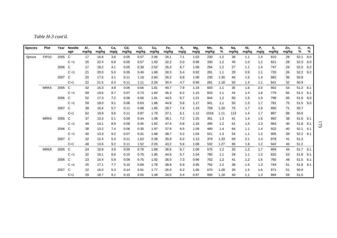
Table H-3 cont'd.
Species
Plot
Year
Needle age
Al , mg/kg
B, mg/kg
Ca, mg/g
Cd, mg/kg
Cr, mg/kg
Cu, mg/kg
Fe, mg/kg
K, mg/g
Mg, mg/g
Mn, mg/kg
N, %
Na, mg/kg
Ni, mg/kg
P, mg/g
S, mg/kg
Zn, mg/kg
C, %
H, %
Spruce FIP10 2005 C 17 16.6 3.6 0.05 0.57 2.06 26.1 7.1 1.03 230 1.2 36 1.1 1.4 810 28 52.1 6.0
C +1 25 22.4 6.8 0.05 0.57 1.93 32.2 5.0 0.98 330 1.2 40 1.0 1.1 821 28 52.3 6.0
2006 C 17 18.2 4.1 0.05 0.39 2.02 26.3 6.7 1.09 294 1.2 27 1.1 1.4 747 29 52.0 6.2
C +1 21 20.0 5.0 0.05 0.40 1.88 30.3 5.4 0.92 281 1.1 29 0.9 1.1 720 26 52.2 6.2
2007 C 20 17.5 4.1 0.11 1.16 2.60 26.2 6.8 1.08 235 1.30 46 1.5 1.4 882 36 50.8
C+1 22 21.5 6.4 0.11 1.11 2.26 30.4 4.7 0.99 281 1.18 50 1.4 1.1 841 32 50.9
MRK5 2005 C 42 16.3 4.8 0.06 0.66 1.81 40.7 7.9 1.19 603 1.1 35 1.6 2.0 802 53 51.2 6.1
C +1 59 19.6 8.7 0.07 0.73 1.84 46.3 6.2 1.15 833 1.1 44 1.4 1.8 779 65 51.2 6.1
2006 C 52 17.3 7.2 0.06 0.66 1.91 44.5 6.7 1.21 844 1.2 50 1.5 1.9 798 65 51.6 6.0
C +1 59 18.0 9.1 0.06 0.63 1.88 44.8 5.6 1.17 941 1.1 50 1.3 1.7 781 75 51.5 6.0
2007 C 38 16.4 5.7 0.11 0.98 1.85 28.7 7.4 1.19 758 1.20 75 1.7 1.9 850 71 50.7
C+1 62 19.8 9.6 0.11 0.87 1.79 37.1 6.1 1.12 1016 1.11 113 1.4 1.7 887 89 50.6
MRK6 2005 C 37 13.3 5.1 0.09 0.44 1.98 38.1 7.2 1.25 351 1.3 41 1.4 1.6 992 38 51.6 6.1
C +1 49 14.1 8.9 0.08 0.45 1.92 47.4 5.8 1.16 495 1.2 61 1.4 1.3 963 40 51.8 6.1
2006 C 38 13.2 7.4 0.06 0.30 1.97 37.9 6.5 1.09 480 1.4 64 1.1 1.4 922 40 52.1 6.1
C +1 40 13.3 9.2 0.07 0.31 1.88 38.7 5.2 1.04 521 1.3 54 1.1 1.2 905 39 52.2 6.1
2007 C 32 12.4 5.3 0.11 1.62 2.38 35.9 6.2 1.13 379 1.33 59 2.1 1.4 878 41 51.3
C+1 48 13.6 9.2 0.11 1.52 2.05 43.2 5.6 1.08 532 1.27 85 1.8 1.2 942 45 51.2
MRK8 2005 C 24 16.8 4.9 0.09 0.78 1.89 36.6 6.7 1.06 575 1.2 26 1.2 1.7 859 44 51.7 6.1
C +1 32 19.1 8.6 0.10 0.75 1.85 44.6 5.7 1.04 780 1.1 29 1.1 1.3 832 53 51.8 6.1
2006 C 23 15.4 5.9 0.09 0.75 1.92 36.0 7.3 0.96 702 1.2 41 1.2 1.6 760 48 51.5 6.1
C +1 25 17.1 7.7 0.10 0.69 1.78 38.8 5.9 0.95 792 1.2 38 1.5 1.3 744 51 51.8 6.1
2007 C 22 16.0 5.3 0.14 0.91 1.77 26.9 6.2 1.06 670 1.28 26 1.5 1.6 871 51 50.9
C+1 29 18.7 9.1 0.15 0.55 1.48 34.0 5.4 0.97 895 1.18 40 1.1 1.3 894 59 51.0

Species Plot
Year
Needle age
Al , mg/kg
B, mg/kg
Ca, mg/g
Cd, mg/kg
Cr, mg/kg
Cu, mg/kg
Fe, mg/kg
K, mg/g
Mg, mg/g
Mn, mg/kg
N, %
Na, mg/kg
Ni, mg/kg
P, mg/g
S, mg/kg
Zn, mg/kg
C, %
H, %
Pine FIP4 2005 C 232 16.7 3.2 0.15 0.57 2.3 29.1 6.4 1.1 463 1.7 39 1.5 1.8 973 39 51.5 6.5
C +1 338 15.3 5.3 0.17 0.62 2.2 43.1 5.9 0.8 802 1.7 66 1.0 1.8 1047 48 52.2 6.5
2006 C 234 14.4 3.0 0.14 0.14 2.3 27.6 6.4 1.0 482 1.7 54 1.2 1.8 985 39 52.5 6.4
C +1 307 12.2 4.6 0.16 0.17 2.3 32.3 5.8 0.8 648 1.7 77 0.9 1.8 1049 42 53.0 6.4
2007 C 250 14.9 3.7 0.16 0.94 2.44 32.0 6.0 0.96 599 1.61 83 1.5 1.7 1026 44 51.6
C+1 258 15.1 4.8 0.16 0.78 2.05 34.1 5.7 0.80 767 1.64 105 1.2 1.7 1090 48 51.8
MRK
1 2005 C 295 19.8 3.2 0.14 0.32 2.3 34.6 6.6 1.2 559 1.7 48 0.8 1.8 1071 45 51.5 6.4
C +1 446 18.6 5.2 0.15 0.40 2.4 44.4 5.9 0.8 878 1.6 78 0.5 1.8 1069 49 52.0 6.5
2006 C 240 15.5 2.6 0.13 0.51 2.4 30.1 6.9 1.0 502 1.6 25 1.0 1.7 958 38 52.6 6.5
C +1 315 16.8 4.4 0.16 0.51 2.4 34.5 6.2 0.9 767 1.6 33 0.6 1.6 957 43 52.8 6.5
2007 C 321 16.9 3.9 0.19 3.51 1.92 48.1 5.8 1.19 691 1.55 33 2.7 1.7 1034 51 51.3
C+1 340 16.3 5.2 0.16 4.06 1.45 65.9 5.4 0.78 913 1.55 66 2.2 1.6 1072 51 52.3
MRK
3 2005 C 307 15.3 2.8 0.12 0.43 2.5 34.6 6.7 1.1 219 1.6 37 1.5 1.8 1032 42 51.9 6.4
C +1 431 13.5 4.4 0.13 0.49 2.1 51.2 6.2 0.8 336 1.6 61 1.0 1.7 1064 42 53.6 6.4
2006 C 259 12.2 2.5 0.11 0.49 2.5 33.1 6.4 1.0 226 1.6 32 1.5 1.7 970 39 52.6 6.5
C +1 375 10.7 4.1 0.13 0.50 2.3 41.9 6.1 0.8 326 1.6 55 1.1 1.7 1039 40 53.2 6.6
2007 C 275 13.2 2.8 0.16 3.02 2.88 47.1 6.1 1.07 268 1.52 55 3.0 1.7 982 45 51.6
C+1 310 12.0 4.0 0.13 3.62 2.60 63.0 5.8 0.76 341 1.58 88 2.4 1.6 1047 43 52.1
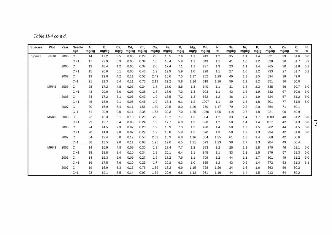
Table H-4 cont'd.
Species
Plot
Year
Needle age
Al, mg/kg
B, mg/kg
Ca, mg/g
Cd, mg/kg
Cr, mg/kg
Cu, mg/kg
Fe, mg/kg
K, mg/g
Mg, mg/g
Mn, mg/kg
N, %
Na, mg/kg
Ni, mg/kg
P, mg/g
S, mg/kg
Zn, mg/kg
C, %
H, %
Spruce FIP10 2005 C 14 17.2 3.5 0.05 0.29 2.0 16.5 7.6 1.1 243 1.2 35 1.1 1.4 821 29 51.6 6.0
C +1 17 22.9 6.3 0.05 0.34 1.8 18.4 5.9 1.1 349 1.1 41 1.0 1.2 828 30 51.7 5.9
2006 C 13 18.4 4.2 0.05 0.37 2.0 17.4 7.1 1.1 297 1.3 23 1.1 1.4 765 30 51.6 6.2
C +1 15 20.6 5.1 0.05 0.46 1.9 19.9 5.9 1.0 298 1.1 27 1.0 1.2 733 27 51.7 6.2
2007 C 19 19.0 4.2 0.11 0.53 2.49 18.6 7.5 1.17 262 1.29 46 1.3 1.5 894 38 49.9
C+1 21 22.3 6.4 0.11 0.75 2.13 22.2 5.8 1.14 318 1.16 59 1.2 1.2 851 36 50.0
MRK5 2005 C 28 17.2 4.8 0.06 0.34 1.8 18.0 8.6 1.3 640 1.1 31 1.8 2.2 835 56 50.7 6.0
C +1 43 20.0 8.0 0.06 0.38 1.8 18.6 7.3 1.3 903 1.1 43 1.5 1.9 832 67 50.6 6.0
2006 C 34 17.2 7.1 0.06 0.43 1.9 17.5 7.2 1.3 882 1.2 46 1.4 1.9 824 67 51.2 6.0
C +1 45 18.9 9.1 0.06 0.46 1.9 18.4 6.1 1.2 1007 1.1 49 1.3 1.8 801 77 51.0 6.0
2007 C 30 16.9 5.4 0.11 1.56 1.89 22.5 8.0 1.20 750 1.17 79 2.3 2.0 864 71 50.1
C+1 51 20.9 9.0 0.11 2.35 1.68 30.3 7.0 1.25 1066 1.05 118 2.7 1.8 921 90 49.9
MRK6 2005 C 23 13.3 5.1 0.10 0.20 2.0 15.2 7.7 1.3 384 1.2 33 1.4 1.7 1000 40 51.2 6.0
C +1 29 13.7 8.4 0.08 0.24 1.9 17.7 6.8 1.3 528 1.2 58 1.4 1.4 1011 42 51.3 6.0
2006 C 24 14.5 7.3 0.07 0.20 1.9 15.9 7.3 1.2 498 1.4 58 1.2 1.5 962 44 51.5 6.0
C +1 28 14.0 9.0 0.07 0.22 1.9 16.8 5.9 1.2 570 1.3 58 1.2 1.3 934 42 51.6 6.0
2007 C 34 12.4 5.0 0.12 0.53 2.63 16.9 6.8 1.16 384 1.25 61 1.8 1.4 868 42 50.6
C+1 38 13.5 9.0 0.11 0.68 1.95 19.0 6.5 1.21 573 1.23 98 1.7 1.3 984 49 50.4
MRK8 2005 C 14 16.9 4.8 0.09 0.30 1.8 18.4 7.7 1.2 593 1.2 25 1.1 1.8 870 46 51.1 6.0
C +1 18 18.8 8.4 0.10 0.34 1.8 20.1 6.4 1.1 845 1.1 33 1.1 1.5 876 57 51.3 6.0
2006 C 14 15.3 5.6 0.09 0.27 1.9 17.2 7.6 1.1 709 1.2 44 1.1 1.7 801 49 51.2 6.0
C +1 16 17.5 7.6 0.10 0.29 1.7 20.2 6.3 1.0 835 1.2 43 0.9 1.4 772 53 51.3 6.1
2007 C 19 16.9 5.3 0.13 0.76 1.69 18.2 6.9 1.15 728 1.26 24 1.6 1.6 863 56 50.2
C+1 23 19.1 8.5 0.14 0.97 1.39 20.6 6.6 1.13 961 1.16 44 1.4 1.5 913 64 50.2
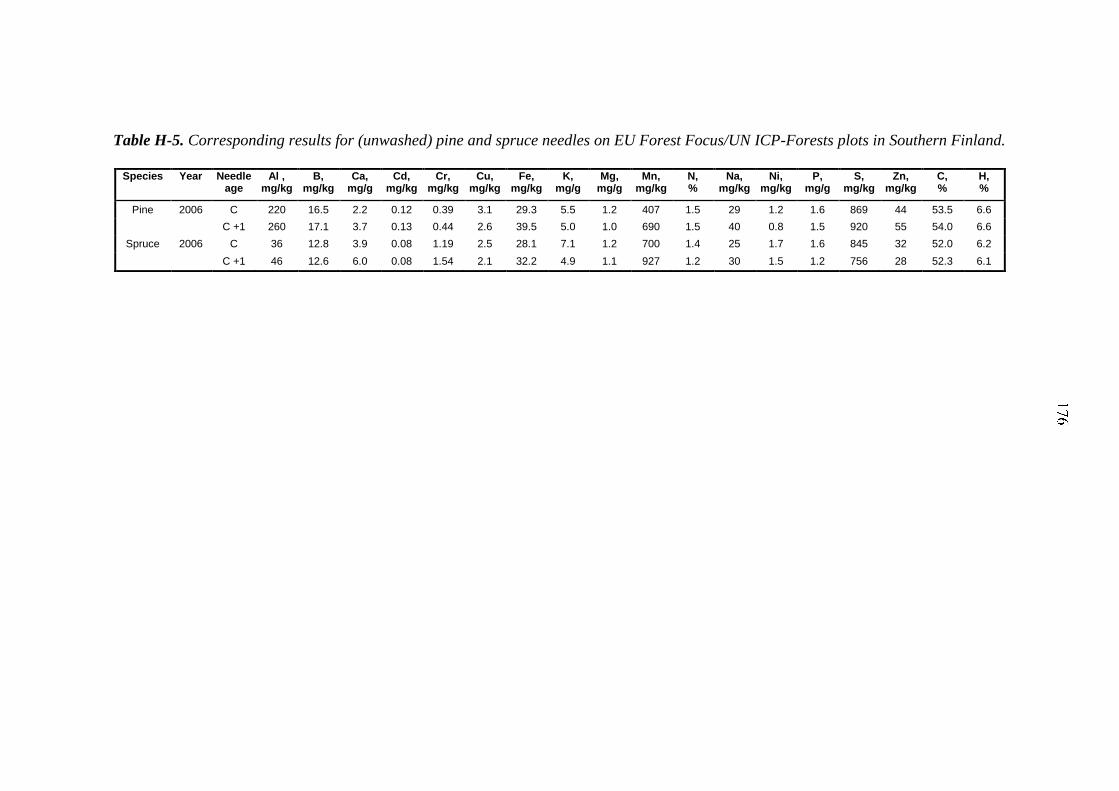
Table H-5. Corresponding results for (unwashed) pine and spruce needles on EU Forest Focus/UN ICP-Forests plots in Southern Finland.
Species
Year
Needle age
Al , mg/kg
B, mg/kg
Ca, mg/g
Cd, mg/kg
Cr, mg/kg
Cu, mg/kg
Fe, mg/kg
K, mg/g
Mg, mg/g
Mn, mg/kg
N, %
Na, mg/kg
Ni, mg/kg
P, mg/g
S, mg/kg
Zn, mg/kg
C, %
H, %
Pine 2006 C 220 16.5 2.2 0.12 0.39 3.1 29.3 5.5 1.2 407 1.5 29 1.2 1.6 869 44 53.5 6.6
C +1 260 17.1 3.7 0.13 0.44 2.6 39.5 5.0 1.0 690 1.5 40 0.8 1.5 920 55 54.0 6.6
Spruce 2006 C 36 12.8 3.9 0.08 1.19 2.5 28.1 7.1 1.2 700 1.4 25 1.7 1.6 845 32 52.0 6.2
C +1 46 12.6 6.0 0.08 1.54 2.1 32.2 4.9 1.1 927 1.2 30 1.5 1.2 756 28 52.3 6.1
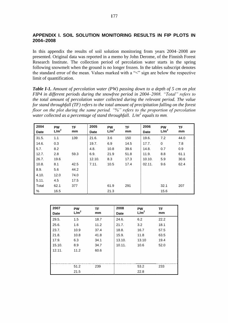
APPENDIX I. SOIL SOLUTION MONITORING RESULTS IN FIP PLOTS IN 2004–2008
In this appendix the results of soil solution monitoring from years 2004–2008 are
presented. Original data was reported in a memo by John Derome, of the Finnish Forest
Research Institute. The collection period of percolation water starts in the spring
following snowmelt when the ground is no longer frozen. In the tables subscript denotes
the standard error of the mean. Values marked with a “<” sign are below the respective
limit of quantification.
Table I-1. Amount of percolation water (PW) passing down to a depth of 5 cm on plot
FIP4 in different periods during the snowfree period in 2004–2008. “Total” refers to
the total amount of percolation water collected during the relevant period. The value
for stand throughfall (TF) refers to the total amount of precipitation falling on the forest
floor on the plot during the same period. “%” refers to the proportion of percolation
water collected as a percentage of stand throughfall. L/m2 equals to mm.
2004 PW L/m
2
TF mm
2005 PW L/m
2
TF mm
2006 PW L/m
2
TF mm Date Date Date
31.5. 1.1 139 21.6. 3.6 150 19.6. 7.2 44.0
14.6. 0.3 19.7. 6.9 14.5 17.7. 0 7.8
5.7. 8.2 4.8. 10.8 39.6 14.8. 0.7 0.9
12.7. 2.8 59.3 6.9. 21.9 51.8 11.9. 8.8 61.1
26.7. 19.6 12.10. 8.3 17.3 10.10. 5.9 30.6
10.8. 8.1 42.5 7.11. 10.5 17.4 02.11. 9.6 62.4
8.9. 5.6 44.2
4.10. 12.0 74.0
5.11. 4.5 17.5
Total 62.1 377 61.9 291 32.1 207
% 16.5 21.3 15.6
2007 PW L/m
2
TF mm
2008 PW L/m
2
TF mm Date Date
29.5. 1.5 18.7 24.6. 6.2 22.2
25.6. 1.6 11.2 21.7. 3.2 18.1
23.7. 10.9 37.4 18.8. 16.7 57.5
21.8. 10.8 41.8 15.9. 11.8 63.5
17.9. 6.3 34.1 13.10. 13.10 19.4
15.10. 8.9 34.7 10.11. 10.6 52.0
12.11. 11.2 60.6
51.2 239 53.2 233
21.5 22.8

Table I-2. Amount of percolation water passing down to a depth of 5 cm on plot FIP10
in different periods during the snowfree period in 2005–2008. See Table I-1 for
explanations.
2005 PW L/m
2
TF mm
2006 PW L/m
2
TF mm
2007 PW L/m
2
TF mm
2008 PW L/m
2
TF mm Date Date Date Date
5.8. 0.8 54.9 19.06. 0 49.8 29.5. 0.2 18.1 27.5. 0.3 3.0 22.8. 0.1 47.4 17.07. 0 7.5 25.6. 0.8 9.1 24.6. 1.5 21.0 6.9. 1.2 14.8. 0.3 1.6 24.7. 1.9 39.9 7.7. 3.2 17.5 13.9. 0.04 1.9 11.9. 7.4 59.4 21.8. 15.3 42.5 18.8. 20.4 58.4 10.10. 2.0 34.8 17.9. 4.6 27.9 16.9. 18.1 64.8 7.11. 5.7 60.9 15.10. 8.7 31.7 13.10 8.2 19.4 12.11. 21.6 64.9 12.11. 16.9 63.1
Total 2.2 377 15.4 215 53.1 234.1 68.6 247.2 % 0.6 7.1 22.7 27.8
Table I-3. Amount of percolation water passing down to a depth of 5 cm on plot FIP11
in different periods during the snowfree period in 2007–2008. See Table I-1 for
explanations.
2007 PW L/m
2
TF mm
2008 PW L/m
2
TF mm Date Date
1.6. 24.6. 7.2 30.9 23.7. 0.4 60.7 21.7. 3.3 29.8 21.8. 0.3 64.7 19.8. 20.5 83.6 17.9. 0.4 56.0 15.9. 13.8 78.1 15.10. 0.2 51.3 13.10. 5.9 30.6 12.11. 0.2 90.2 11.11. 8.4 90.3
Total 1.5 322.9 59.2 343.3 0.5 17.3
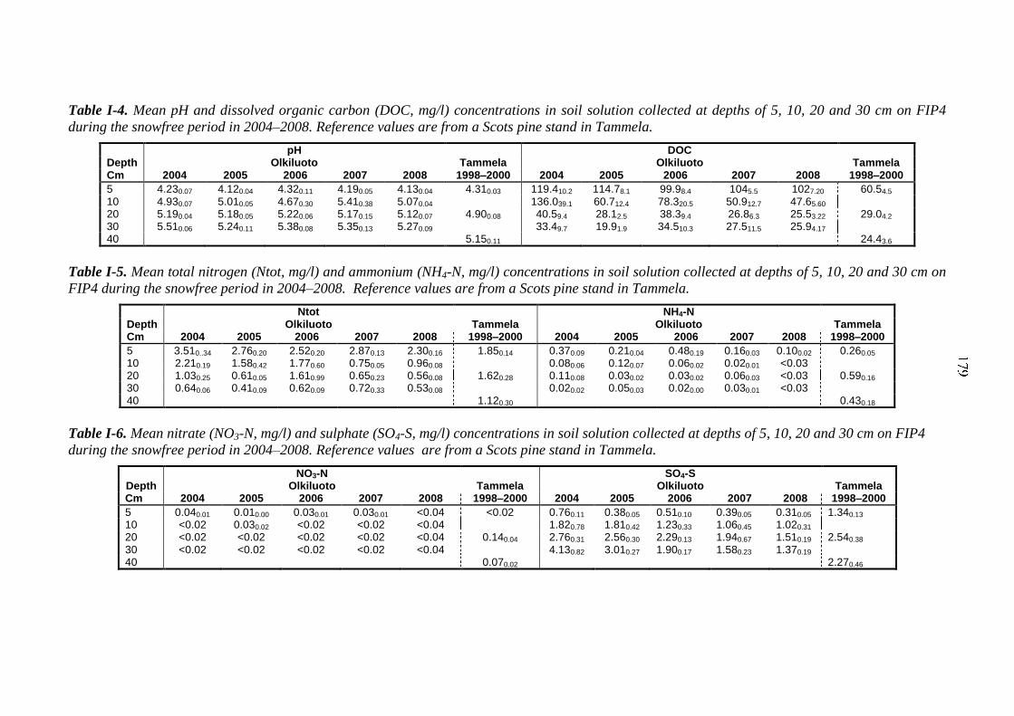
Table I-4. Mean pH and dissolved organic carbon (DOC, mg/l) concentrations in soil solution collected at depths of 5, 10, 20 and 30 cm on FIP4
during the snowfree period in 2004–2008. Reference values are from a Scots pine stand in Tammela.
pH DOC Depth Olkiluoto Tammela Olkiluoto Tammela Cm 2004 2005 2006 2007 2008 1998–2000 2004 2005 2006 2007 2008 1998–2000
5 4.230.07 4.120.04 4.320.11 4.190.05 4.130.04 4.310.03 119.410.2 114.78.1 99.98.4 1045.5 1027.20 60.54.5 10 4.930.07 5.010.05 4.670.30 5.410.38 5.070.04 136.039.1 60.712.4 78.320.5 50.912.7 47.65.60 20 5.190.04 5.180.05 5.220.06 5.170.15 5.120.07 4.900.08 40.59.4 28.12.5 38.39.4 26.86.3 25.53.22 29.04.2 30 5.510.06 5.240.11 5.380.08 5.350.13 5.270.09 33.49.7 19.91.9 34.510.3 27.511.5 25.94.17 40 5.150.11 24.43.6
Table I-5. Mean total nitrogen (Ntot, mg/l) and ammonium (NH4-N, mg/l) concentrations in soil solution collected at depths of 5, 10, 20 and 30 cm on
FIP4 during the snowfree period in 2004–2008. Reference values are from a Scots pine stand in Tammela.
Ntot NH4-N Depth Olkiluoto Tammela Olkiluoto Tammela Cm 2004 2005 2006 2007 2008 1998–2000 2004 2005 2006 2007 2008 1998–2000
5 3.510..34 2.760.20 2.520.20 2.870.13 2.300.16 1.850.14 0.370.09 0.210.04 0.480.19 0.160.03 0.100.02 0.260.05 10 2.210.19 1.580.42 1.770.60 0.750.05 0.960.08 0.080.06 0.120.07 0.060.02 0.020.01 <0.03 20 1.030.25 0.610.05 1.610.99 0.650.23 0.560.08 1.620.28 0.110.08 0.030.02 0.030.02 0.060.03 <0.03 0.590.16 30 0.640.06 0.410.09 0.620.09 0.720.33 0.530.08 0.020.02 0.050.03 0.020.00 0.030.01 <0.03 40 1.120.30 0.430.18
Table I-6. Mean nitrate (NO3-N, mg/l) and sulphate (SO4-S, mg/l) concentrations in soil solution collected at depths of 5, 10, 20 and 30 cm on FIP4
during the snowfree period in 2004–2008. Reference values are from a Scots pine stand in Tammela.
NO3-N SO4-S Depth Olkiluoto Tammela Olkiluoto Tammela Cm 2004 2005 2006 2007 2008 1998–2000 2004 2005 2006 2007 2008 1998–2000
5 0.040.01 0.010.00 0.030.01 0.030.01 <0.04 <0.02 0.760.11 0.380.05 0.510.10 0.390.05 0.310.05 1.340.13 10 <0.02 0.030.02 <0.02 <0.02 <0.04 1.820.78 1.810.42 1.230.33 1.060.45 1.020.31 20 <0.02 <0.02 <0.02 <0.02 <0.04 0.140.04 2.760.31 2.560.30 2.290.13 1.940.67 1.510.19 2.540.38 30 <0.02 <0.02 <0.02 <0.02 <0.04 4.130.82 3.010.27 1.900.17 1.580.23 1.370.19 40 0.070.02 2.270.46
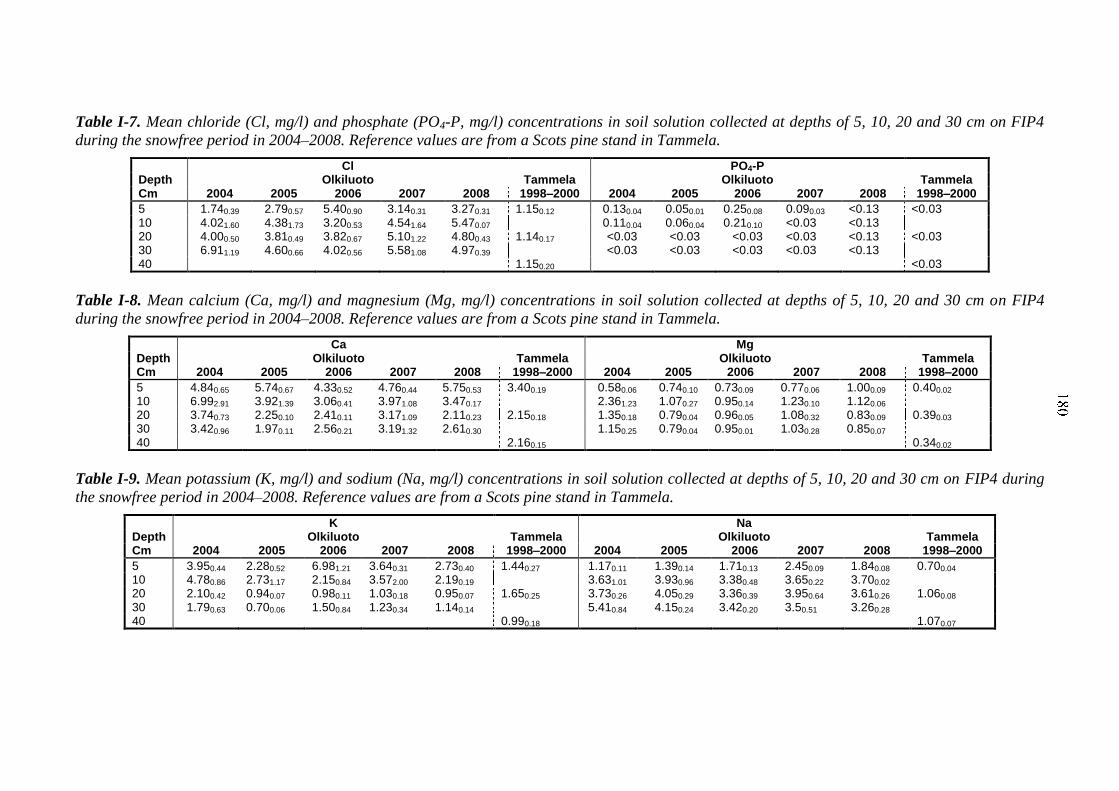
Table I-7. Mean chloride (Cl, mg/l) and phosphate (PO4-P, mg/l) concentrations in soil solution collected at depths of 5, 10, 20 and 30 cm on FIP4
during the snowfree period in 2004–2008. Reference values are from a Scots pine stand in Tammela.
Cl PO4-P Depth Cm
Olkiluoto Tammela Olkiluoto Tammela 2004 2005 2006 2007 2008 1998–2000 2004 2005 2006 2007 2008 1998–2000
5 1.740.39 2.790.57 5.400.90 3.140.31 3.270.31 1.150.12 0.130.04 0.050.01 0.250.08 0.090.03 <0.13 <0.03 10 4.021.60 4.381.73 3.200.53 4.541.64 5.470.07 0.110.04 0.060.04 0.210.10 <0.03 <0.13 20 4.000.50 3.810.49 3.820.67 5.101.22 4.800.43 1.140.17 <0.03 <0.03 <0.03 <0.03 <0.13 <0.03 30 6.911.19 4.600.66 4.020.56 5.581.08 4.970.39 <0.03 <0.03 <0.03 <0.03 <0.13 40 1.150.20 <0.03
Table I-8. Mean calcium (Ca, mg/l) and magnesium (Mg, mg/l) concentrations in soil solution collected at depths of 5, 10, 20 and 30 cm on FIP4
during the snowfree period in 2004–2008. Reference values are from a Scots pine stand in Tammela.
Ca Mg Depth Olkiluoto Tammela Olkiluoto Tammela Cm 2004 2005 2006 2007 2008 1998–2000 2004 2005 2006 2007 2008 1998–2000
5 4.840.65 5.740.67 4.330.52 4.760.44 5.750.53 3.400.19 0.580.06 0.740.10 0.730.09 0.770.06 1.000.09 0.400.02 10 6.992.91 3.921.39 3.060.41 3.971.08 3.470.17 2.361.23 1.070.27 0.950.14 1.230.10 1.120.06 20 3.740.73 2.250.10 2.410.11 3.171.09 2.110.23 2.150.18 1.350.18 0.790.04 0.960.05 1.080.32 0.830.09 0.390.03 30 3.420.96 1.970.11 2.560.21 3.191.32 2.610.30 1.150.25 0.790.04 0.950.01 1.030.28 0.850.07 40 2.160.15 0.340.02
Table I-9. Mean potassium (K, mg/l) and sodium (Na, mg/l) concentrations in soil solution collected at depths of 5, 10, 20 and 30 cm on FIP4 during
the snowfree period in 2004–2008. Reference values are from a Scots pine stand in Tammela.
K Na Depth Olkiluoto Tammela Olkiluoto Tammela Cm 2004 2005 2006 2007 2008 1998–2000 2004 2005 2006 2007 2008 1998–2000
5 3.950.44 2.280.52 6.981.21 3.640.31 2.730.40 1.440.27 1.170.11 1.390.14 1.710.13 2.450.09 1.840.08 0.700.04 10 4.780.86 2.731.17 2.150.84 3.572.00 2.190.19 3.631.01 3.930.96 3.380.48 3.650.22 3.700.02 20 2.100.42 0.940.07 0.980.11 1.030.18 0.950.07 1.650.25 3.730.26 4.050.29 3.360.39 3.950.64 3.610.26 1.060.08 30 1.790.63 0.700.06 1.500.84 1.230.34 1.140.14 5.410.84 4.150.24 3.420.20 3.50.51 3.260.28 40 0.990.18 1.070.07
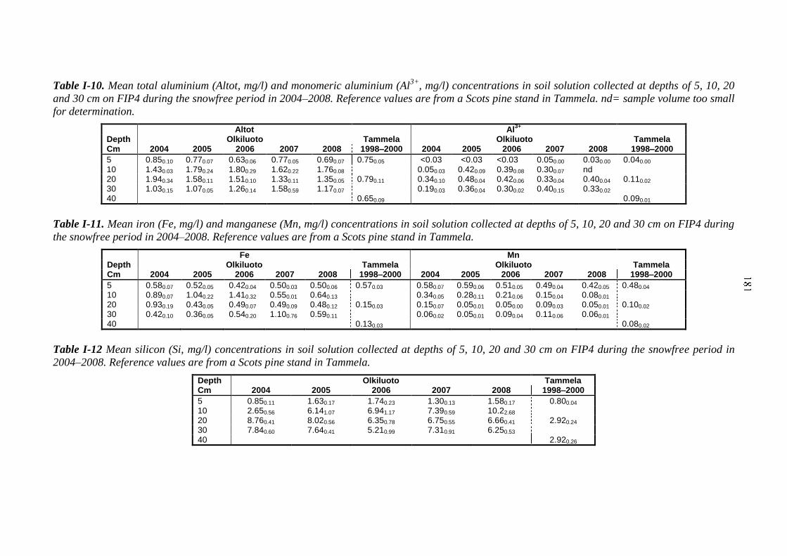
Table I-10. Mean total aluminium (Altot, mg/l) and monomeric aluminium (Al3+
, mg/l) concentrations in soil solution collected at depths of 5, 10, 20
and 30 cm on FIP4 during the snowfree period in 2004–2008. Reference values are from a Scots pine stand in Tammela. nd= sample volume too small
for determination.
Altot Al3+
Depth Olkiluoto Tammela Olkiluoto Tammela Cm 2004 2005 2006 2007 2008 1998–2000 2004 2005 2006 2007 2008 1998–2000
5 0.850.10 0.770.07 0.630.06 0.770.05 0.690.07 0.750.05 <0.03 <0.03 <0.03 0.050.00 0.030.00 0.040.00 10 1.430.03 1.790.24 1.800.29 1.620.22 1.760.08 0.050.03 0.420.09 0.390.08 0.300.07 nd 20 1.940.34 1.580.11 1.510.10 1.330.11 1.350.05 0.790.11 0.340.10 0.480.04 0.420.06 0.330.04 0.400.04 0.110.02 30 1.030.15 1.070.05 1.260.14 1.580.59 1.170.07 0.190.03 0.360.04 0.300.02 0.400.15 0.330.02 40 0.650.09 0.090.01
Table I-11. Mean iron (Fe, mg/l) and manganese (Mn, mg/l) concentrations in soil solution collected at depths of 5, 10, 20 and 30 cm on FIP4 during
the snowfree period in 2004–2008. Reference values are from a Scots pine stand in Tammela.
Fe Mn Depth Olkiluoto Tammela Olkiluoto Tammela Cm 2004 2005 2006 2007 2008 1998–2000 2004 2005 2006 2007 2008 1998–2000
5 0.580.07 0.520.05 0.420.04 0.500.03 0.500.06 0.570.03 0.580.07 0.590.06 0.510.05 0.490.04 0.420.05 0.480.04 10 0.890.07 1.040.22 1.410.32 0.550.01 0.640.13 0.340.05 0.280.11 0.210.06 0.150.04 0.080.01 20 0.930.19 0.430.05 0.490.07 0.490.09 0.480.12 0.150.03 0.150.07 0.050.01 0.050.00 0.090.03 0.050.01 0.100.02 30 0.420.10 0.360.05 0.540.20 1.100.76 0.590.11 0.060.02 0.050.01 0.090.04 0.110.06 0.060.01 40 0.130.03 0.080.02
Table I-12 Mean silicon (Si, mg/l) concentrations in soil solution collected at depths of 5, 10, 20 and 30 cm on FIP4 during the snowfree period in
2004–2008. Reference values are from a Scots pine stand in Tammela.
Depth Olkiluoto Tammela Cm 2004 2005 2006 2007 2008 1998–2000
5 0.850.11 1.630.17 1.740.23 1.300.13 1.580.17 0.800.04 10 2.650.56 6.141.07 6.941.17 7.390.59 10.22.68 20 8.760.41 8.020.56 6.350.78 6.750.55 6.660.41 2.920.24 30 7.840.60 7.640.41 5.210.99 7.310.91 6.250.53 40 2.920.26
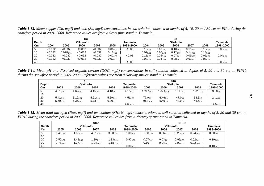
Table I-13. Mean copper (Cu, mg/l) and zinc (Zn, mg/l) concentrations in soil solution collected at depths of 5, 10, 20 and 30 cm on FIP4 during the
snowfree period in 2004–2008. Reference values are from a Scots pine stand in Tammela.
Cu Zn Depth Olkiluoto Tammela Olkiluoto Tammela Cm 2004 2005 2006 2007 2008 1998–2000 2004 2005 2006 2007 2008 1998–2000
5 <0.032 <0.032 <0.032 <0.032 0.010.00 <0.03 0.130.01 0.100.01 0.100.01 0.110.00 0.100.01 0.060.00 10 <0.032 0.0280.01 <0.032 <0.032 0.110.02 0.090.01 0.100.02 0.120.03 0.140.05 0.130.01 20 <0.032 <0.032 <0.032 <0.032 0.020.00 <0.03 0.110.02 0.050.00 0.070.01 0.090.03 0.060.01 0.040.01 30 <0.032 <0.032 <0.032 <0.032 0.020.00 0.080.02 0.040.00 0.080.02 0.070.01 0.050.01 40 <0.03 0.030.01
Table I-14. Mean pH and dissolved organic carbon (DOC, mg/l) concentrations in soil solution collected at depths of 5, 20 and 30 cm on FIP10
during the snowfree period in 2005–2008. Reference values are from a Norway spruce stand in Tammela.
pH DOC Depth Olkiluoto Tammela Olkiluoto Tammela Cm 2005 2006 2007 2008 1998–2000 2005 2006 2007 2008 1998–2000
5 4.810.35 4.690.19 4.150.06 4.180.04 4.160.02 129.736.7 125.414.4 131.86.9 122.57.1 33.01.8 10 20 5.410.12 5.190.21 5.210.15 5.590.11 4.510.03 77.06.9 60.62.9 47.04.6 53.53.0 24.14.6 30 5.600.19 5.360.25 5.730.12 6.300.11 59.814.9 50.95.9 48.92.4 46.54.4 40 4.690.03 4.50.2
Table I-15. Mean total nitrogen (Ntot, mg/l) and ammonium (NH4-N, mg/l) concentrations in soil solution collected at depths of 5, 20 and 30 cm on
FIP10 during the snowfree period in 2005–2008. Reference values are from a Norway spruce stand in Tammela.
Ntot NH4-N Depth Olkiluoto Tammela Olkiluoto Tammela Cm 2005 2006 2007 2008 1998–2000 2005 2006 2007 2008 1998–2000
5 6.401.64 4.860.60 4.310.29 3.880.26 1.080.08 1.680.39 0.360.12 0.280.04 0.240.02 0.300.06 10 20 2.520.51 1.480.03 1.290.11 1.330.09 0.970.30 0.070.02 0.030.01 0.020.00 0.020.01 0.190.05 30 1.780.75 1.370.17 1.240.09 1.180.15 0.100.22 0.040.01 0.020.00 0.020.00 40 0.300.02 0.100.01
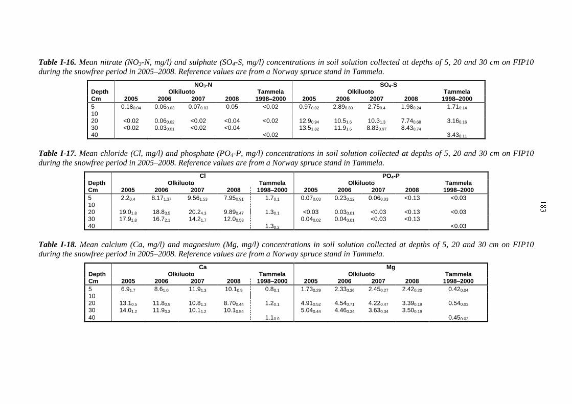
Table I-16. Mean nitrate (NO3-N, mg/l) and sulphate (SO4-S, mg/l) concentrations in soil solution collected at depths of 5, 20 and 30 cm on FIP10
during the snowfree period in 2005–2008. Reference values are from a Norway spruce stand in Tammela.
NO3-N SO4-S Depth Olkiluoto Tammela Olkiluoto Tammela Cm 2005 2006 2007 2008 1998–2000 2005 2006 2007 2008 1998–2000
5 0.180.04 0.060.03 0.070.03 0.05 <0.02 0.970.02 2.890.80 2.750.4 1.980.24 1.710.14 10 20 <0.02 0.060.02 <0.02 <0.04 <0.02 12.90.94 10.51.6 10.31.3 7.740.68 3.160.16 30 <0.02 0.030.01 <0.02 <0.04 13.51.82 11.91.6 8.830.97 8.430.74 40 <0.02 3.430.11
Table I-17. Mean chloride (Cl, mg/l) and phosphate (PO4-P, mg/l) concentrations in soil solution collected at depths of 5, 20 and 30 cm on FIP10
during the snowfree period in 2005–2008. Reference values are from a Norway spruce stand in Tammela.
Cl PO4-P Depth Olkiluoto Tammela Olkiluoto Tammela Cm 2005 2006 2007 2008 1998–2000 2005 2006 2007 2008 1998–2000
5 2.20.4 8.171.37 9.561.53 7.950.91 1.70.1 0.070.03 0.230.12 0.060.03 <0.13 <0.03 10 20 19.01.8 18.83.5 20.24.3 9.890.47 1.30.1 <0.03 0.030.01 <0.03 <0.13 <0.03 30 17.91.8 16.72.1 14.21.7 12.00.58 0.040.02 0.040.01 <0.03 <0.13 40 1.30.2 <0.03
Table I-18. Mean calcium (Ca, mg/l) and magnesium (Mg, mg/l) concentrations in soil solution collected at depths of 5, 20 and 30 cm on FIP10
during the snowfree period in 2005–2008. Reference values are from a Norway spruce stand in Tammela.
Ca Mg Depth Olkiluoto Tammela Olkiluoto Tammela Cm 2005 2006 2007 2008 1998–2000 2005 2006 2007 2008 1998–2000
5 6.91.7 8.61.0 11.91.3 10.10.9 0.80.1 1.730.29 2.330.36 2.450.27 2.420.20 0.420.04 10 20 13.10.5 11.80.9 10.81.3 8.700.44 1.20.1 4.910.52 4.540.71 4.220.47 3.390.19 0.540.03 30 14.01.2 11.90.3 10.11.2 10.10.54 5.040.44 4.460.34 3.630.34 3.500.19
40 1.10.0 0.450.02
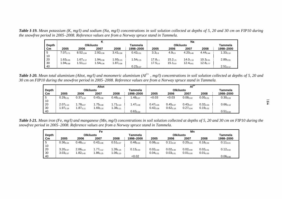
Table I-19. Mean potassium (K, mg/l) and sodium (Na, mg/l) concentrations in soil solution collected at depths of 5, 20 and 30 cm on FIP10 during
the snowfree period in 2005–2008. Reference values are from a Norway spruce stand in Tammela.
K Na Depth Olkiluoto Tammela Olkiluoto Tammela Cm 2005 2006 2007 2008 1998–2000 2005 2006 2007 2008 1998–2000
5 7.070.71 8.521.84 2.920.36 3.410.58 0.420.51 3.30.8 4.90.9 4.200.46 4.440.44 1.330.10 10 20 1.630.05 1.670.12 1.940.36 1.930.15 1.540.15 17.81.1 15.21.5 14.01.10 10.30.51 2.890.55 30 1.940.58 1.510.07 1.540.36 1.870.06 17.51.6 15.10.9 12.40.61 12.80.77 40 0.230.07 2.510.12
Table I-20. Mean total aluminium (Altot, mg/l) and monomeric aluminium (Al3+
, mg/l) concentrations in soil solution collected at depths of 5, 20 and
30 cm on FIP10 during the snowfree period in 2005–2008. Reference values are from a Norway spruce stand in Tammela.
Altot Al3+
Depth Olkiluoto Tammela Olkiluoto Tammela Cm 2005 2006 2007 2008 1998–2000 2005 2006 2007 2008 1998–2000
5 0.290.01 0.370.10 0.430.06 0.480.06 1.480.07 <0.03 <0.03 0.080.02 0.050.01 0.300.03 10 20 2.070.13 1.780.07 1.750.08 1.710.10 1.470.09 0.470.05 0.450.07 0.430.07 0.320.03 0.660.10 30 1.970.19 1.870.11 1.690.10 1.380.11 0.420.06 0.620.16 0.270.04 0.190.02 40 0.630.04 0.510.04
Table I-21. Mean iron (Fe, mg/l) and manganese (Mn, mg/l) concentrations in soil solution collected at depths of 5, 20 and 30 cm on FIP10 during the
snowfree period in 2005–2008. Reference values are from a Norway spruce stand in Tammela.
Fe Mn Depth Olkiluoto Tammela Olkiluoto Tammela Cm 2005 2006 2007 2008 1998–2000 2005 2006 2007 2008 1998–2000
5 0.360.04 0.480.14 0.420.08 0.510.07 0.480.03 0.080.03 0.110.02 0.200.03 0.180.03 0.110.01 10 20 3.200.57 2.060.19 1.770.12 1.390.15 0.130.03 0.020.00 0.020.00 0.020.00 0.020.01 0.120.02 30 3.030.57 1.820.40 1.860.25 1.060.10 0.040.01 0.030.01 0.010.00 0.010.00 40 <0.02 0.060.08
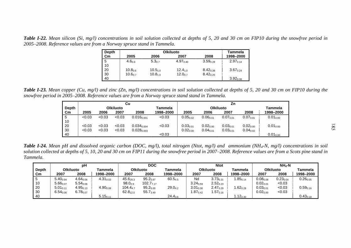
Table I-22. Mean silicon (Si, mg/l) concentrations in soil solution collected at depths of 5, 20 and 30 cm on FIP10 during the snowfree period in
2005–2008. Reference values are from a Norway spruce stand in Tammela.
Depth Cm
Olkiluoto Tammela 2005 2006 2007 2008 1998–2000
5 4.60.6 5.30.7 4.970.40 3.590.28 2.970.14 10 20 10.80.6 10.51.0 12.41.0 8.420.38 3.670.24 30 10.60.7 10.81.0 12.00.7 8.420.20 40 3.920.08
Table I-23. Mean copper (Cu, mg/l) and zinc (Zn, mg/l) concentrations in soil solution collected at depths of 5, 20 and 30 cm on FIP10 during the
snowfree period in 2005–2008. Reference values are from a Norway spruce stand stand in Tammela.
Cu Zn Depth Olkiluoto Tammela Olkiluoto Tammela Cm 2005 2006 2007 2008 1998–2000 2005 2006 2007 2008 1998–2000
5 <0.03 <0.03 <0.03 0.0160.001 <0.03 0.050.02 0.060.01 0.070.01 0.070.01 0.010.00 10 20 <0.03 <0.03 <0.03 0.0340.004 <0.03 0.030.01 0.020.00 0.030.01 0.020.00 0.010.00 30 <0.03 <0.03 <0.03 0.0280.003 0.020.00 0.040.01 0.030.01 0.040.02 40 <0.03 0.010.00
Table I-24. Mean pH and dissolved organic carbon (DOC, mg/l), total nitrogen (Ntot, mg/l) and ammonium (NH4-N, mg/l) concentrations in soil
solution collected at depths of 5, 10, 20 and 30 cm on FIP11 during the snowfree period in 2007–2008. Reference values are from a Scots pine stand in
Tammela.
pH DOC Ntot NH4-N Depth Olkiluoto Tammela Olkiluoto Tammela Olkiluoto Tammela Olkiluoto Tammela Cm 2007 2008 1998–2000 2007 2008 1998–2000 2007 2008 1998–2000 2007 2008 1998–2000
5 5.400.94 4.640.06 4.310.03 45.629.3 95.25.97 60.54.5 Nd 3.730.31 1.850.14 0.080.08 0.230.04 0.260.05 10 5.660.07 5.540.06 98.02.9 102.77.17 3.240.59 2.520.23 0.020.01 <0.03 20 5.010.11 4.950.13 4.900.08 104.44.7 95.25.00 29.04.2 3.010.30 2.470.29 1.620.28 0.030.01 <0.03 0.590.16 30 6.540.06 6.780.07 62.812.0 55.73.49 1.870.42 1.570.16 0.020.00 <0.03 40 5.150.11 24.43.6 1.120.30 0.430.18
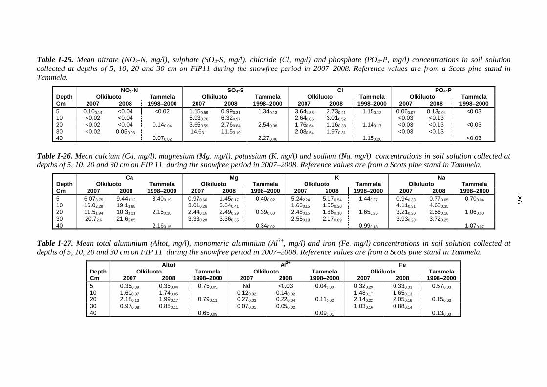
Table I-25. Mean nitrate (NO3-N, mg/l), sulphate (SO4-S, mg/l), chloride (Cl, mg/l) and phosphate (PO4-P, mg/l) concentrations in soil solution
collected at depths of 5, 10, 20 and 30 cm on FIP11 during the snowfree period in 2007–2008. Reference values are from a Scots pine stand in
Tammela.
NO3-N SO4-S Cl PO4-P Depth Olkiluoto Tammela Olkiluoto Tammela Olkiluoto Tammela Olkiluoto Tammela Cm 2007 2008 1998–2000 2007 2008 1998–2000 2007 2008 1998–2000 2007 2008 1998–2000
5 0.100.14 <0.04 <0.02 1.150.59 0.990.31 1.340.13 3.641.88 2.730.41 1.150.12 0.060.07 0.130.04 <0.03 10 <0.02 <0.04 5.930.70 6.320.97 2.640.86 3.010.52 <0.03 <0.13 20 <0.02 <0.04 0.140.04 3.650.59 2.760.84 2.540.38 1.760.64 1.160.38 1.140.17 <0.03 <0.13 <0.03 30 <0.02 0.050.03 14.63.1 11.53.19 2.080.54 1.970.31 <0.03 <0.13 40 0.070.02 2.270.46 1.150.20 <0.03
Table I-26. Mean calcium (Ca, mg/l), magnesium (Mg, mg/l), potassium (K, mg/l) and sodium (Na, mg/l) concentrations in soil solution collected at
depths of 5, 10, 20 and 30 cm on FIP 11 during the snowfree period in 2007–2008. Reference values are from a Scots pine stand in Tammela.
Ca Mg K Na Depth Olkiluoto Tammela Olkiluoto Tammela Olkiluoto Tammela Olkiluoto Tammela Cm 2007 2008 1998–2000 2007 2008 1998–2000 2007 2008 1998–2000 2007 2008 1998–2000
5 6.073.75 9.441.12 3.400.19 0.970.66 1.450.17 0.400.02 5.242.24 5.170.54 1.440.27 0.940.33 0.770.05 0.700.04 10 16.02.28 19.11.88 3.010.26 3.840.41 1.630.15 1.550.20 4.110.31 4.680.35 20 11.51.94 10.31.21 2.150.18 2.440.16 2.490.29 0.390.03 2.480.15 1.860.10 1.650.25 3.210.20 2.560.18 1.060.08 30 20.72.6 21.62.85 3.330.28 3.360.35 2.550.19 2.170.09 3.930.28 3.720.25 40 2.160.15 0.340.02 0.990.18 1.070.07
Table I-27. Mean total aluminium (Altot, mg/l), monomeric aluminium (Al3+
, mg/l) and iron (Fe, mg/l) concentrations in soil solution collected at
depths of 5, 10, 20 and 30 cm on FIP 11 during the snowfree period in 2007–2008. Reference values are from a Scots pine stand in Tammela.
Altot Al3+
Fe Depth Olkiluoto Tammela Olkiluoto Tammela Olkiluoto Tammela Cm 2007 2008 1998–2000 2007 2008 1998–2000 2007 2008 1998–2000
5 0.350.39 0.350.04 0.750.05 Nd <0.03 0.040.00 0.320.29 0.330.03 0.570.03 10 1.600.07 1.740.05 0.120.02 0.140.02 1.480.17 1.650.13 20 2.180.13 1.990.17 0.790.11 0.270.03 0.220.04 0.110.02 2.140.22 2.050.16 0.150.03 30 0.970.08 0.850.11 0.070.01 0.050.02 1.030.16 0.880.14 40 0.650.09 0.090.01 0.130.03
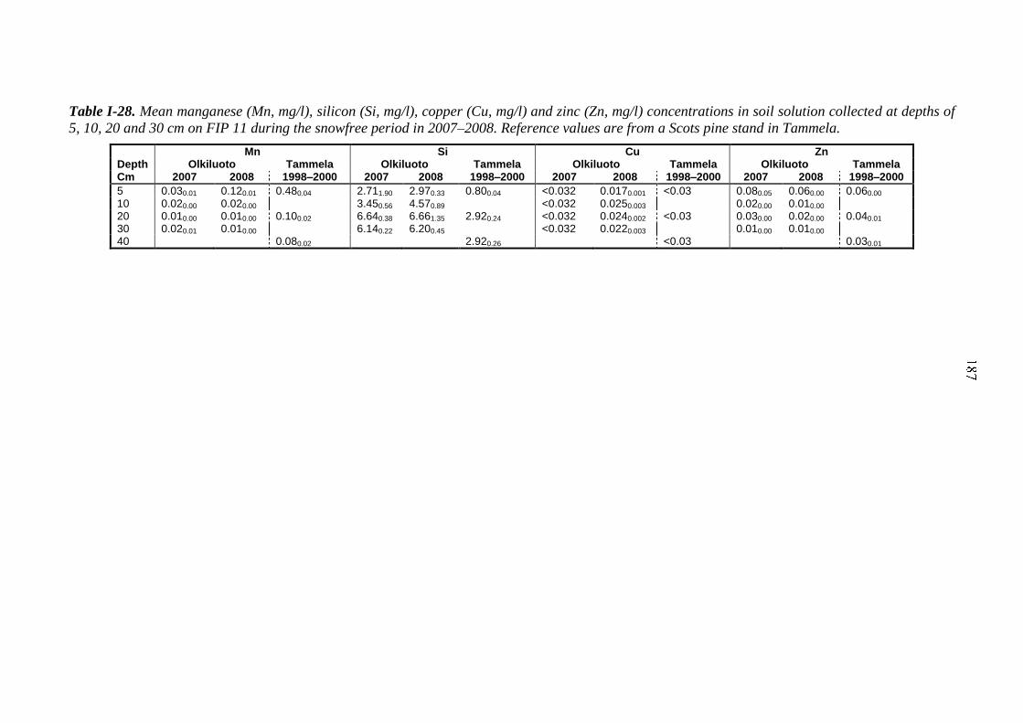
Table I-28. Mean manganese (Mn, mg/l), silicon (Si, mg/l), copper (Cu, mg/l) and zinc (Zn, mg/l) concentrations in soil solution collected at depths of
5, 10, 20 and 30 cm on FIP 11 during the snowfree period in 2007–2008. Reference values are from a Scots pine stand in Tammela.
Mn Si Cu Zn Depth Olkiluoto Tammela Olkiluoto Tammela Olkiluoto Tammela Olkiluoto Tammela Cm 2007 2008 1998–2000 2007 2008 1998–2000 2007 2008 1998–2000 2007 2008 1998–2000
5 0.030.01 0.120.01 0.480.04 2.711.90 2.970.33 0.800.04 <0.032 0.0170.001 <0.03 0.080.05 0.060.00 0.060.00 10 0.020.00 0.020.00 3.450.56 4.570.89 <0.032 0.0250.003 0.020.00 0.010.00 20 0.010.00 0.010.00 0.100.02 6.640.38 6.661.35 2.920.24 <0.032 0.0240.002 <0.03 0.030.00 0.020.00 0.040.01 30 0.020.01 0.010.00 6.140.22 6.200.45 <0.032 0.0220.003 0.010.00 0.010.00 40 0.080.02 2.920.26 <0.03 0.030.01

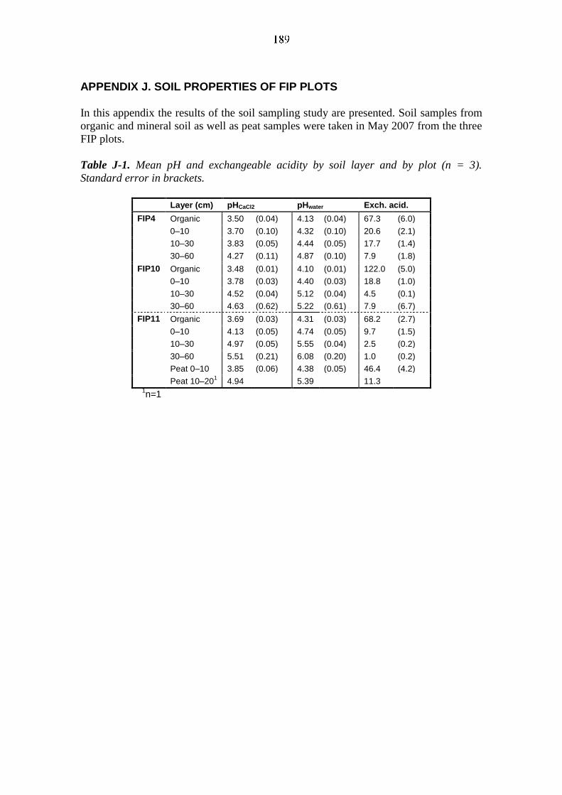
APPENDIX J. SOIL PROPERTIES OF FIP PLOTS
In this appendix the results of the soil sampling study are presented. Soil samples from
organic and mineral soil as well as peat samples were taken in May 2007 from the three
FIP plots.
Table J-1. Mean pH and exchangeable acidity by soil layer and by plot (n = 3).
Standard error in brackets.
Layer (cm) pHCaCl2 pHwater Exch. acid.
FIP4 Organic 3.50 (0.04) 4.13 (0.04) 67.3 (6.0)
0–10 3.70 (0.10) 4.32 (0.10) 20.6 (2.1)
10–30 3.83 (0.05) 4.44 (0.05) 17.7 (1.4)
30–60 4.27 (0.11) 4.87 (0.10) 7.9 (1.8)
FIP10 Organic 3.48 (0.01) 4.10 (0.01) 122.0 (5.0)
0–10 3.78 (0.03) 4.40 (0.03) 18.8 (1.0)
10–30 4.52 (0.04) 5.12 (0.04) 4.5 (0.1)
30–60 4.63 (0.62) 5.22 (0.61) 7.9 (6.7)
FIP11 Organic 3.69 (0.03) 4.31 (0.03) 68.2 (2.7)
0–10 4.13 (0.05) 4.74 (0.05) 9.7 (1.5)
10–30 4.97 (0.05) 5.55 (0.04) 2.5 (0.2)
30–60 5.51 (0.21) 6.08 (0.20) 1.0 (0.2)
Peat 0–10 3.85 (0.06) 4.38 (0.05) 46.4 (4.2)
Peat 10–201 4.94 5.39 11.3
1n=1
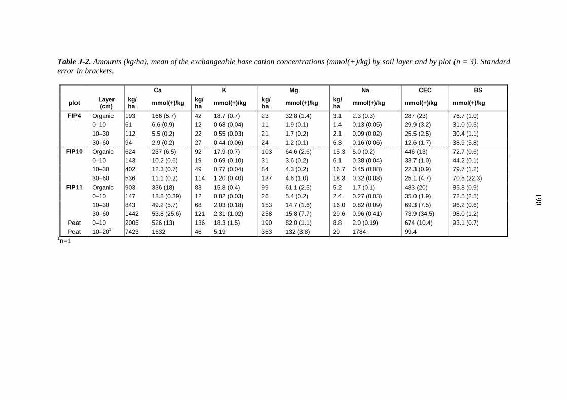
Table J-2. Amounts (kg/ha), mean of the exchangeable base cation concentrations (mmol(+)/kg) by soil layer and by plot (n = 3). Standard
error in brackets.
Layer (cm)
Ca K Mg Na CEC BS
plot kg/ ha
mmol(+)/kg kg/ ha
mmol(+)/kg kg/ ha
mmol(+)/kg kg/ ha
mmol(+)/kg mmol(+)/kg mmol(+)/kg
FIP4 Organic 193 166 (5.7) 42 18.7 (0.7) 23 32.8 (1.4) 3.1 2.3 (0.3) 287 (23) 76.7 (1.0)
0–10 61 6.6 (0.9) 12 0.68 (0.04) 11 1.9 (0.1) 1.4 0.13 (0.05) 29.9 (3.2) 31.0 (0.5)
10–30 112 5.5 (0.2) 22 0.55 (0.03) 21 1.7 (0.2) 2.1 0.09 (0.02) 25.5 (2.5) 30.4 (1.1)
30–60 94 2.9 (0.2) 27 0.44 (0.06) 24 1.2 (0.1) 6.3 0.16 (0.06) 12.6 (1.7) 38.9 (5.8)
FIP10 Organic 624 237 (6.5) 92 17.9 (0.7) 103 64.6 (2.6) 15.3 5.0 (0.2) 446 (13) 72.7 (0.6)
0–10 143 10.2 (0.6) 19 0.69 (0.10) 31 3.6 (0.2) 6.1 0.38 (0.04) 33.7 (1.0) 44.2 (0.1)
10–30 402 12.3 (0.7) 49 0.77 (0.04) 84 4.3 (0.2) 16.7 0.45 (0.08) 22.3 (0.9) 79.7 (1.2)
30–60 536 11.1 (0.2) 114 1.20 (0.40) 137 4.6 (1.0) 18.3 0.32 (0.03) 25.1 (4.7) 70.5 (22.3)
FIP11 Organic 903 336 (18) 83 15.8 (0.4) 99 61.1 (2.5) 5.2 1.7 (0.1) 483 (20) 85.8 (0.9)
0–10 147 18.8 (0.39) 12 0.82 (0.03) 26 5.4 (0.2) 2.4 0.27 (0.03) 35.0 (1.9) 72.5 (2.5)
10–30 843 49.2 (5.7) 68 2.03 (0.18) 153 14.7 (1.6) 16.0 0.82 (0.09) 69.3 (7.5) 96.2 (0.6)
30–60 1442 53.8 (25.6) 121 2.31 (1.02) 258 15.8 (7.7) 29.6 0.96 (0.41) 73.9 (34.5) 98.0 (1.2)
Peat 0–10 2005 526 (13) 136 18.3 (1.5) 190 82.0 (1.1) 8.8 2.0 (0.19) 674 (10.4) 93.1 (0.7)
Peat 10–201 7423 1632 46 5.19 363 132 (3.8) 20 1784 99.4
1n=1
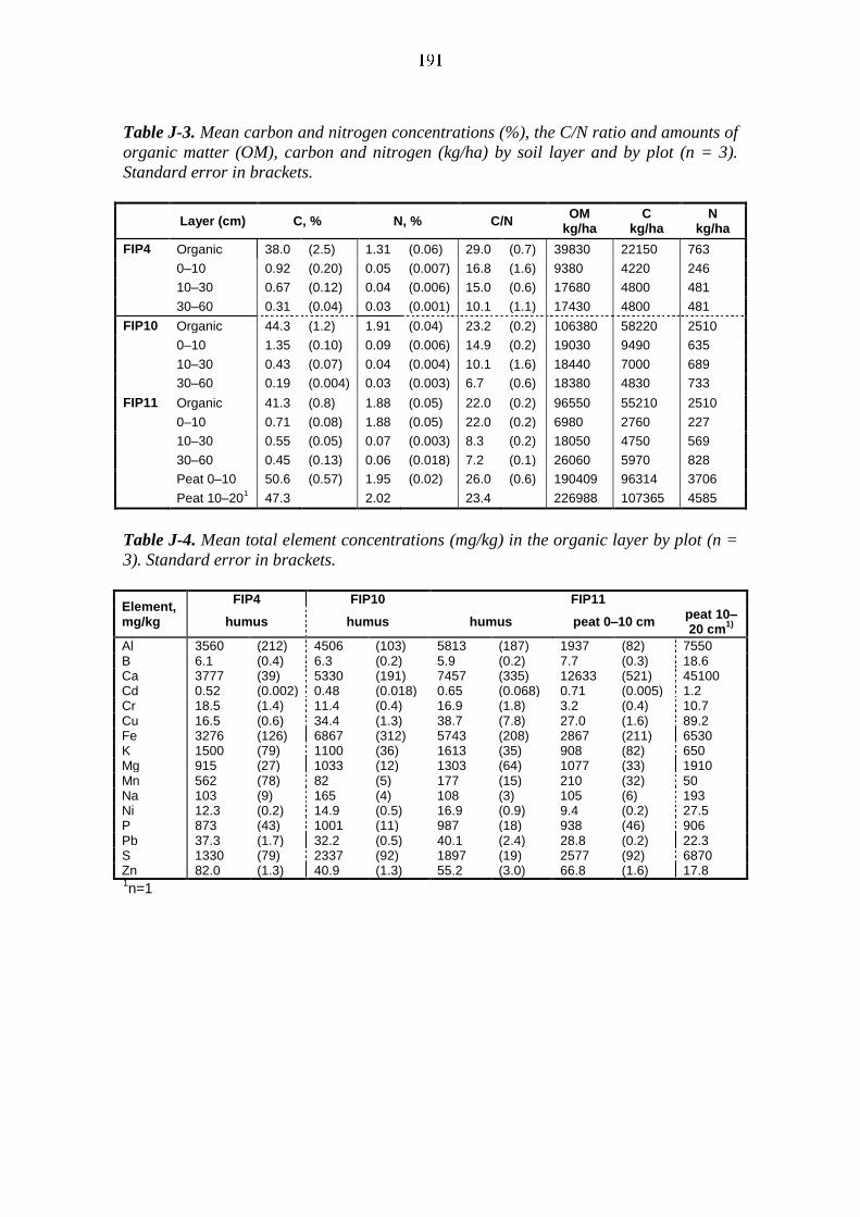
Table J-3. Mean carbon and nitrogen concentrations (%), the C/N ratio and amounts of
organic matter (OM), carbon and nitrogen (kg/ha) by soil layer and by plot (n = 3).
Standard error in brackets.
Layer (cm) C, % N, % C/N OM
kg/ha C
kg/ha N
kg/ha
FIP4 Organic 38.0 (2.5) 1.31 (0.06) 29.0 (0.7) 39830 22150 763
0–10 0.92 (0.20) 0.05 (0.007) 16.8 (1.6) 9380 4220 246
10–30 0.67 (0.12) 0.04 (0.006) 15.0 (0.6) 17680 4800 481
30–60 0.31 (0.04) 0.03 (0.001) 10.1 (1.1) 17430 4800 481
FIP10 Organic 44.3 (1.2) 1.91 (0.04) 23.2 (0.2) 106380 58220 2510
0–10 1.35 (0.10) 0.09 (0.006) 14.9 (0.2) 19030 9490 635
10–30 0.43 (0.07) 0.04 (0.004) 10.1 (1.6) 18440 7000 689
30–60 0.19 (0.004) 0.03 (0.003) 6.7 (0.6) 18380 4830 733
FIP11 Organic 41.3 (0.8) 1.88 (0.05) 22.0 (0.2) 96550 55210 2510
0–10 0.71 (0.08) 1.88 (0.05) 22.0 (0.2) 6980 2760 227
10–30 0.55 (0.05) 0.07 (0.003) 8.3 (0.2) 18050 4750 569
30–60 0.45 (0.13) 0.06 (0.018) 7.2 (0.1) 26060 5970 828
Peat 0–10 50.6 (0.57) 1.95 (0.02) 26.0 (0.6) 190409 96314 3706
Peat 10–201 47.3 2.02 23.4 226988 107365 4585
Table J-4. Mean total element concentrations (mg/kg) in the organic layer by plot (n =
3). Standard error in brackets.
Element, mg/kg
FIP4 FIP10 FIP11
humus humus humus peat 0–10 cm peat 10–20 cm
1)
Al 3560 (212) 4506 (103) 5813 (187) 1937 (82) 7550 B 6.1 (0.4) 6.3 (0.2) 5.9 (0.2) 7.7 (0.3) 18.6 Ca 3777 (39) 5330 (191) 7457 (335) 12633 (521) 45100 Cd 0.52 (0.002) 0.48 (0.018) 0.65 (0.068) 0.71 (0.005) 1.2 Cr 18.5 (1.4) 11.4 (0.4) 16.9 (1.8) 3.2 (0.4) 10.7 Cu 16.5 (0.6) 34.4 (1.3) 38.7 (7.8) 27.0 (1.6) 89.2 Fe 3276 (126) 6867 (312) 5743 (208) 2867 (211) 6530 K 1500 (79) 1100 (36) 1613 (35) 908 (82) 650 Mg 915 (27) 1033 (12) 1303 (64) 1077 (33) 1910 Mn 562 (78) 82 (5) 177 (15) 210 (32) 50 Na 103 (9) 165 (4) 108 (3) 105 (6) 193 Ni 12.3 (0.2) 14.9 (0.5) 16.9 (0.9) 9.4 (0.2) 27.5 P 873 (43) 1001 (11) 987 (18) 938 (46) 906 Pb 37.3 (1.7) 32.2 (0.5) 40.1 (2.4) 28.8 (0.2) 22.3 S 1330 (79) 2337 (92) 1897 (19) 2577 (92) 6870 Zn 82.0 (1.3) 40.9 (1.3) 55.2 (3.0) 66.8 (1.6) 17.8 1n=1
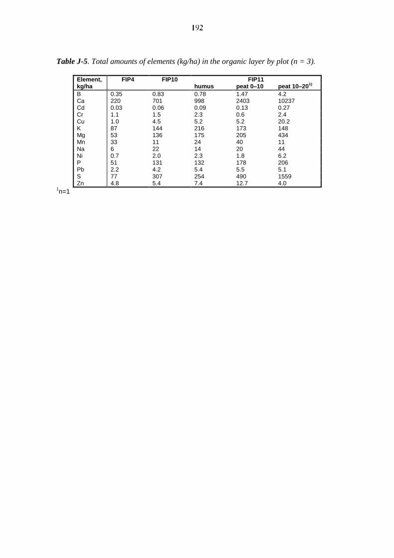
Table J-5. Total amounts of elements (kg/ha) in the organic layer by plot (n = 3).
Element, kg/ha
FIP4 FIP10 FIP11 humus peat 0–10 peat 10–20
1)
B 0.35 0.83 0.78 1.47 4.2 Ca 220 701 998 2403 10237 Cd 0.03 0.06 0.09 0.13 0.27 Cr 1.1 1.5 2.3 0.6 2.4 Cu 1.0 4.5 5.2 5.2 20.2 K 87 144 216 173 148 Mg 53 136 175 205 434 Mn 33 11 24 40 11 Na 6 22 14 20 44 Ni 0.7 2.0 2.3 1.8 6.2 P 51 131 132 178 206 Pb 2.2 4.2 5.4 5.5 5.1 S 77 307 254 490 1559 Zn 4.8 5.4 7.4 12.7 4.0
1n=1

APPENDIX K. UNDERSTOREY VEGETATION SURVEY RESULTS 2003–2005 AND 2008
In this appendix, the results of the understorey vegetation survey are presented. The
main aims of the monitoring are to characterize the current state of forest vegetation on
the three intensive forest monitoring plots FIP4, FIP10 and FIP11 on Olkiluoto Island,
and to detect temporal changes in the vegetation in relation to natural and anthropogenic
environmental factors. The survey has been conducted on Olkiluoto in 2003–2005 and
in 2008. Plots FIP4 and FIP10 have been examined throughout the whole period,
whereas plot FIP11 was surveyed for the first time in 2008.
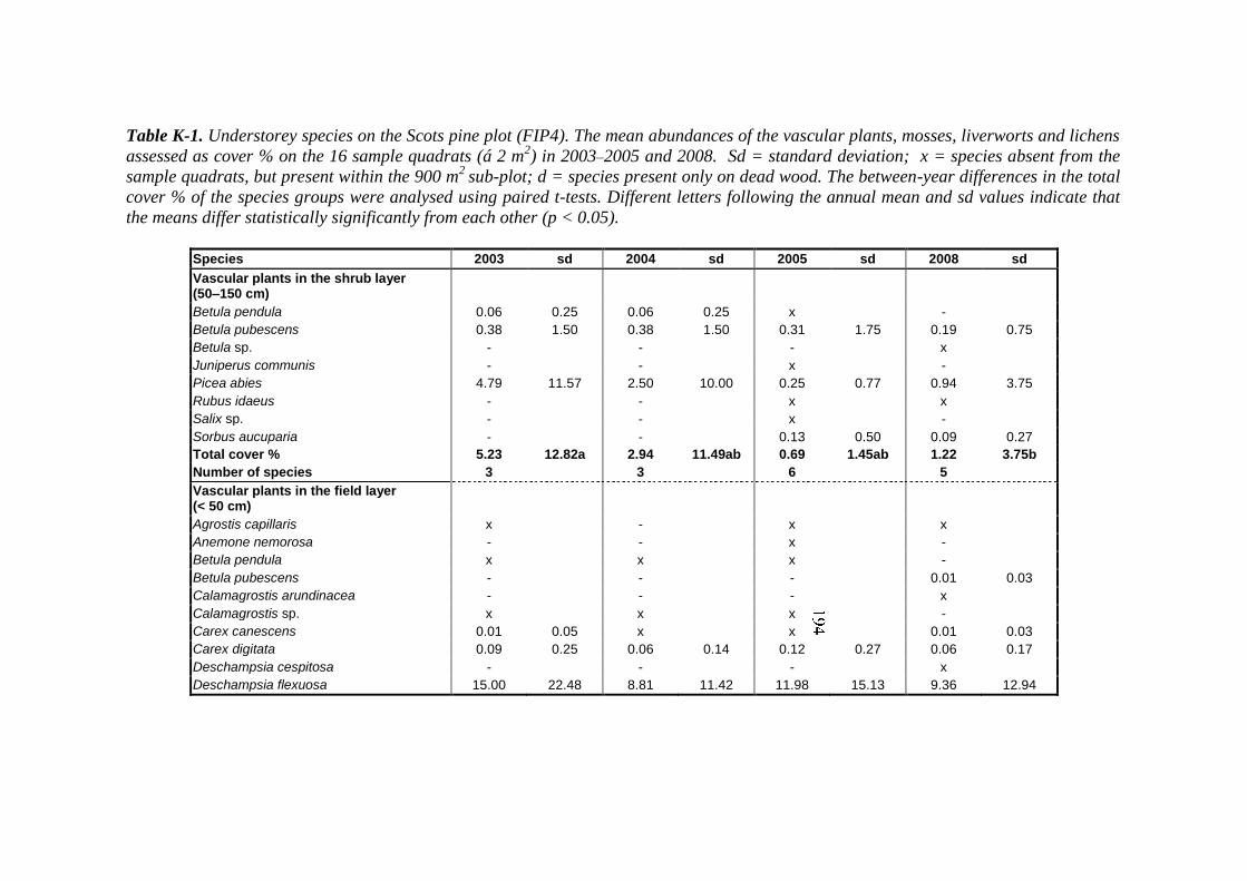
Table K-1. Understorey species on the Scots pine plot (FIP4). The mean abundances of the vascular plants, mosses, liverworts and lichens
assessed as cover % on the 16 sample quadrats (á 2 m2) in 2003–2005 and 2008. Sd = standard deviation; x = species absent from the
sample quadrats, but present within the 900 m2
sub-plot; d = species present only on dead wood. The between-year differences in the total
cover % of the species groups were analysed using paired t-tests. Different letters following the annual mean and sd values indicate that
the means differ statistically significantly from each other (p < 0.05).
Species 2003 sd 2004 sd 2005 sd 2008 sd
Vascular plants in the shrub layer (50–150 cm)
Betula pendula 0.06 0.25 0.06 0.25 x -
Betula pubescens 0.38 1.50 0.38 1.50 0.31 1.75 0.19 0.75
Betula sp. - - - x
Juniperus communis - - x -
Picea abies 4.79 11.57 2.50 10.00 0.25 0.77 0.94 3.75
Rubus idaeus - - x x
Salix sp. - - x -
Sorbus aucuparia - - 0.13 0.50 0.09 0.27
Total cover % 5.23 12.82a 2.94 11.49ab 0.69 1.45ab 1.22 3.75b
Number of species 3 3 6 5
Vascular plants in the field layer (< 50 cm)
Agrostis capillaris x - x x
Anemone nemorosa - - x -
Betula pendula x x x -
Betula pubescens - - - 0.01 0.03
Calamagrostis arundinacea - - - x
Calamagrostis sp. x x x -
Carex canescens 0.01 0.05 x x 0.01 0.03
Carex digitata 0.09 0.25 0.06 0.14 0.12 0.27 0.06 0.17
Deschampsia cespitosa - - - x
Deschampsia flexuosa 15.00 22.48 8.81 11.42 11.98 15.13 9.36 12.94
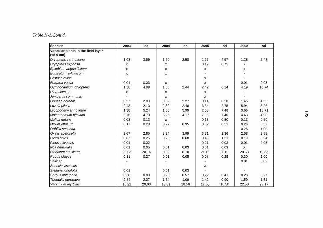
Table K-1.Cont'd.
Species 2003 sd 2004 sd 2005 sd 2008 sd
Vascular plants in the field layer (<5 0 cm)
Dryopteris carthusiana 1.63 3.59 1.20 2.58 1.67 4.57 1.28 2.48
Dryopteris expansa x x 0.19 0.75 x
Epilobium angustifolium x x x x
Equisetum sylvaticum x x - -
Festuca ovina - - x -
Fragaria vesca 0.01 0.03 x x 0.01 0.03
Gymnocarpium dryopteris 1.58 4.99 1.03 2.44 2.42 6.24 4.19 10.74
Hieracium sp. x x x -
Juniperus communis - x x -
Linnaea borealis 0.57 2.00 0.69 2.27 0.14 0.50 1.45 4.53
Luzula pilosa 2.43 2.13 2.32 2.48 3.54 2.75 5.94 5.26
Lycopodium annotinum 1.38 5.24 1.56 5.99 2.03 7.48 3.66 13.71
Maianthemum bifolium 5.76 4.73 5.25 4.17 7.06 7.40 4.43 4.98
Melica nutans 0.03 0.13 x 0.13 0.50 0.13 0.50
Milium effusum 0.17 0.28 0.22 0.35 0.32 0.51 0.26 0.57
Orthilia secunda - - - 0.25 1.00
Oxalis acetosella 2.67 2.85 3.24 3.99 3.31 2.36 2.58 2.88
Picea abies 0.07 0.25 0.25 0.68 0.45 1.31 0.19 0.54
Pinus sylvestris 0.01 0.02 - 0.01 0.03 0.01 0.05
Poa nemoralis 0.01 0.05 0.01 0.03 0.01 0.03 X
Pteridium aquilinum 20.03 20.14 8.82 8.10 21.19 20.61 20.63 19.83
Rubus idaeus 0.11 0.27 0.01 0.05 0.08 0.25 0.30 1.00
Salix sp. - - - 0.01 0.02
Senecio viscosus - - X -
Stellaria longifolia 0.01 0.01 0.03 - -
Sorbus aucuparia 0.38 0.89 0.26 0.57 0.22 0.41 0.28 0.77
Trientalis europaea 2.34 2.27 1.34 1.09 1.42 0.90 1.59 1.51
Vaccinium myrtillus 16.22 20.03 13.81 18.56 12.00 16.50 22.50 23.17
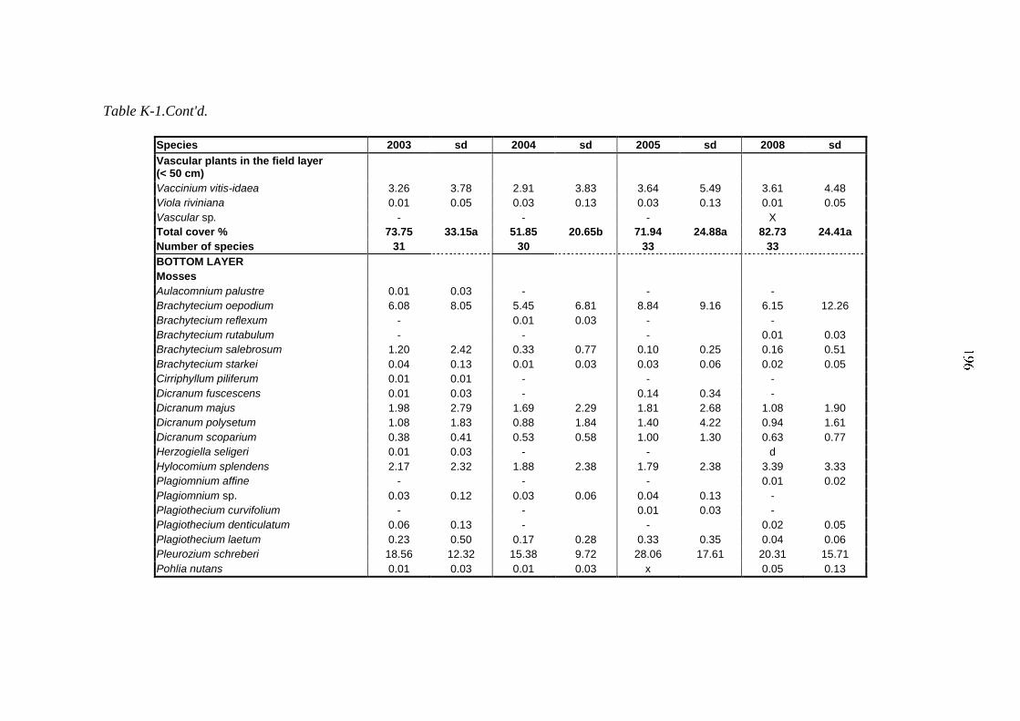
Table K-1.Cont'd.
Species 2003 sd 2004 sd 2005 sd 2008 sd
Vascular plants in the field layer (< 50 cm)
Vaccinium vitis-idaea 3.26 3.78 2.91 3.83 3.64 5.49 3.61 4.48
Viola riviniana 0.01 0.05 0.03 0.13 0.03 0.13 0.01 0.05
Vascular sp. - - - X
Total cover % 73.75 33.15a 51.85 20.65b 71.94 24.88a 82.73 24.41a
Number of species 31 30 33 33
BOTTOM LAYER
Mosses
Aulacomnium palustre 0.01 0.03 - - -
Brachytecium oepodium 6.08 8.05 5.45 6.81 8.84 9.16 6.15 12.26
Brachytecium reflexum - 0.01 0.03 - -
Brachytecium rutabulum - - - 0.01 0.03
Brachytecium salebrosum 1.20 2.42 0.33 0.77 0.10 0.25 0.16 0.51
Brachytecium starkei 0.04 0.13 0.01 0.03 0.03 0.06 0.02 0.05
Cirriphyllum piliferum 0.01 0.01 - - -
Dicranum fuscescens 0.01 0.03 - 0.14 0.34 -
Dicranum majus 1.98 2.79 1.69 2.29 1.81 2.68 1.08 1.90
Dicranum polysetum 1.08 1.83 0.88 1.84 1.40 4.22 0.94 1.61
Dicranum scoparium 0.38 0.41 0.53 0.58 1.00 1.30 0.63 0.77
Herzogiella seligeri 0.01 0.03 - - d
Hylocomium splendens 2.17 2.32 1.88 2.38 1.79 2.38 3.39 3.33
Plagiomnium affine - - - 0.01 0.02
Plagiomnium sp. 0.03 0.12 0.03 0.06 0.04 0.13 -
Plagiothecium curvifolium - - 0.01 0.03 -
Plagiothecium denticulatum 0.06 0.13 - - 0.02 0.05
Plagiothecium laetum 0.23 0.50 0.17 0.28 0.33 0.35 0.04 0.06
Pleurozium schreberi 18.56 12.32 15.38 9.72 28.06 17.61 20.31 15.71
Pohlia nutans 0.01 0.03 0.01 0.03 x 0.05 0.13
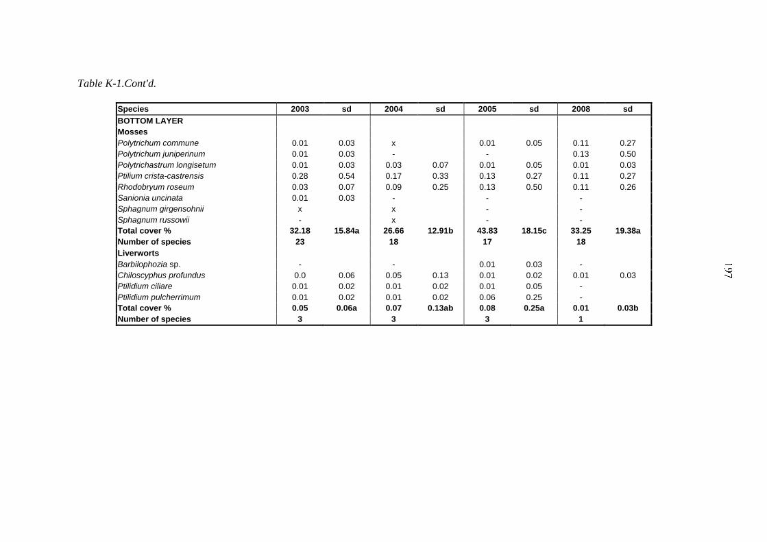
Table K-1.Cont'd.
Species 2003 sd 2004 sd 2005 sd 2008 sd
BOTTOM LAYER
Mosses
Polytrichum commune 0.01 0.03 x 0.01 0.05 0.11 0.27
Polytrichum juniperinum 0.01 0.03 - - 0.13 0.50
Polytrichastrum longisetum 0.01 0.03 0.03 0.07 0.01 0.05 0.01 0.03
Ptilium crista-castrensis 0.28 0.54 0.17 0.33 0.13 0.27 0.11 0.27
Rhodobryum roseum 0.03 0.07 0.09 0.25 0.13 0.50 0.11 0.26
Sanionia uncinata 0.01 0.03 - - -
Sphagnum girgensohnii x x - -
Sphagnum russowii - x - -
Total cover % 32.18 15.84a 26.66 12.91b 43.83 18.15c 33.25 19.38a
Number of species 23 18 17 18
Liverworts
Barbilophozia sp. - - 0.01 0.03 -
Chiloscyphus profundus 0.0 0.06 0.05 0.13 0.01 0.02 0.01 0.03
Ptilidium ciliare 0.01 0.02 0.01 0.02 0.01 0.05 -
Ptilidium pulcherrimum 0.01 0.02 0.01 0.02 0.06 0.25 -
Total cover % 0.05 0.06a 0.07 0.13ab 0.08 0.25a 0.01 0.03b
Number of species 3 3 3 1
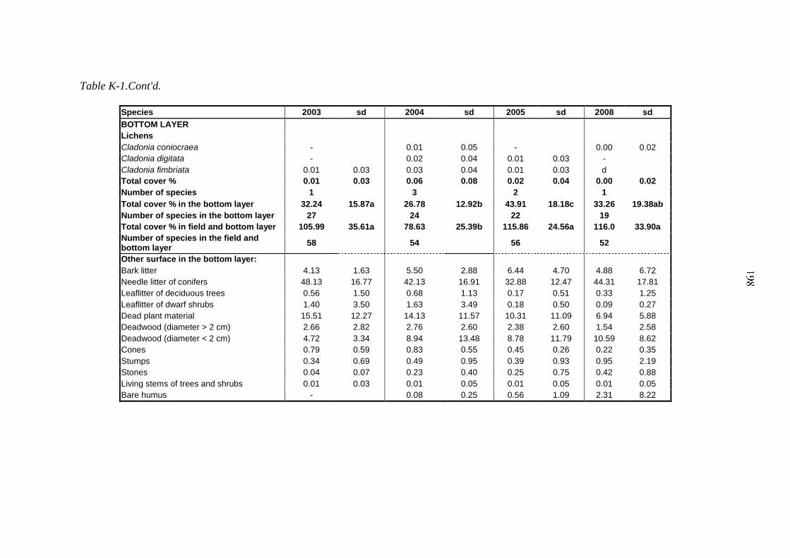
Table K-1.Cont'd.
Species 2003 sd 2004 sd 2005 sd 2008 sd
BOTTOM LAYER
Lichens
Cladonia coniocraea - 0.01 0.05 - 0.00 0.02
Cladonia digitata - 0.02 0.04 0.01 0.03 -
Cladonia fimbriata 0.01 0.03 0.03 0.04 0.01 0.03 d
Total cover % 0.01 0.03 0.06 0.08 0.02 0.04 0.00 0.02
Number of species 1 3 2 1
Total cover % in the bottom layer 32.24 15.87a 26.78 12.92b 43.91 18.18c 33.26 19.38ab
Number of species in the bottom layer 27 24 22 19
Total cover % in field and bottom layer 105.99 35.61a 78.63 25.39b 115.86 24.56a 116.0 33.90a
Number of species in the field and bottom layer
58 54 56 52
Other surface in the bottom layer:
Bark litter 4.13 1.63 5.50 2.88 6.44 4.70 4.88 6.72
Needle litter of conifers 48.13 16.77 42.13 16.91 32.88 12.47 44.31 17.81
Leaflitter of deciduous trees 0.56 1.50 0.68 1.13 0.17 0.51 0.33 1.25
Leaflitter of dwarf shrubs 1.40 3.50 1.63 3.49 0.18 0.50 0.09 0.27
Dead plant material 15.51 12.27 14.13 11.57 10.31 11.09 6.94 5.88
Deadwood (diameter > 2 cm) 2.66 2.82 2.76 2.60 2.38 2.60 1.54 2.58
Deadwood (diameter < 2 cm) 4.72 3.34 8.94 13.48 8.78 11.79 10.59 8.62
Cones 0.79 0.59 0.83 0.55 0.45 0.26 0.22 0.35
Stumps 0.34 0.69 0.49 0.95 0.39 0.93 0.95 2.19
Stones 0.04 0.07 0.23 0.40 0.25 0.75 0.42 0.88
Living stems of trees and shrubs 0.01 0.03 0.01 0.05 0.01 0.05 0.01 0.05
Bare humus - 0.08 0.25 0.56 1.09 2.31 8.22
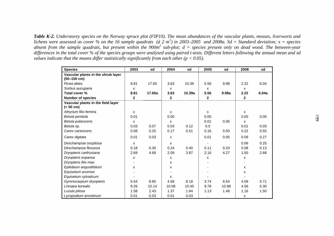
Table K-2. Understorey species on the Norway spruce plot (FIP10). The mean abundances of the vascular plants, mosses, liverworts and
lichens were assessed as cover % on the 16 sample quadrats (á 2 m2) in 2003–2005 and 2008a. Sd = Standard deviation; x = species
absent from the sample quadrats, but present within the 900m2 sub-plot; d = species present only on dead wood. The between-year
differences in the total cover % of the species groups were analysed using paired t-tests. Different letters following the annual mean and sd
values indicate that the means differ statistically significantly from each other (p < 0.05).
Species 2003 sd 2004 sd 2005 sd 2008 sd
Vascular plants in the shrub layer (50–150 cm)
Picea abies 8.81 17.65 3.63 10.39 5.56 9.98 2.22 6.04
Sorbus aucuparia x x x x
Total cover % 8.81 17.65a 3.63 10.39a 5.56 9.98a 2.22 6.04a
Number of species 2 2 2 2
Vascular plants in the field layer (< 50 cm)
Athyrium filix-femina x x x x
Betula pendula 0.01 0.00 0.00 0.00 0.00
Betula pubescens x x 0.01 0.05 x
Betula sp. 0.03 0.07 0.03 0.12 0.0 0.01 0.03
Carex canescens 0.08 0.25 0.17 0.51 0.16 0.50 0.22 0.55
Carex digitata 0.01 0.03 x 0.01 0.05 0.09 0.27
Deschampsia cespitosa x x - 0.06 0.25
Deschampsia flexuosa 0.18 0.30 0.24 0.40 0.11 0.20 0.08 0.13
Dryopteris carthusiana 2.69 4.69 2.09 3.87 2.16 4.27 1.50 2.68
Dryopteris expansa x x x x
Dryopteris filix-mas - x - -
Epilobium angustifolium x x - x
Equisetum arvense - - - x
Equisetum sylvaticum - x - -
Gymnocarpium dryopteris 5.54 8.85 4.58 8.18 3.74 6.54 4.09 5.71
Linnaea borealis 9.26 10.14 10.08 10.45 9.78 10.98 4.56 5.30
Luzula pilosa 1.58 2.43 1.37 1.84 1.13 1.48 1.16 1.50
Lycopodium annotinum 0.01 0.03 0.01 0.03 . x
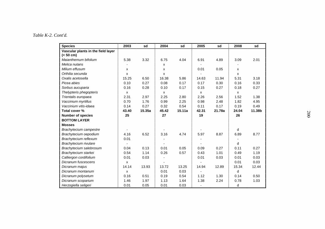
Table K-2. Cont'd.
Species 2003 sd 2004 sd 2005 sd 2008 sd
Vascular plants in the field layer (< 50 cm)
Maianthemum bifolium 5.38 3.32 6.75 4.04 6.91 4.89 3.09 2.01
Melica nutans - x - -
Milium effusum x x 0.01 0.05 x
Orthilia secunda x x - x
Oxalis acetosella 15.25 6.50 16.38 5.86 14.63 11.94 5.31 3.18
Picea abies 0.10 0.27 0.08 0.17 0.17 0.30 0.16 0.33
Sorbus aucuparia 0.16 0.28 0.10 0.17 0.15 0.27 0.18 0.27
Thelypteris phegopteris x x x x
Trientalis europaea 2.31 2.97 2.25 2.80 2.26 2.56 1.52 1.38
Vaccinium myrtillus 0.70 1.76 0.99 2.25 0.98 2.48 1.82 4.95
Vaccinium vitis-idaea 0.14 0.27 0.32 0.54 0.11 0.17 0.19 0.49
Total cover % 43.40 15.35a 45.42 15.11a 42.31 21.78a 24.04 11.38b
Number of species 25 27 19 26
BOTTOM LAYER
Mosses
Brachytecium campestre - - - d
Brachytecium oepodium 4.16 6.52 3.16 4.74 5.97 8.87 6.89 8.77
Brachytecium reflexum 0.01 - - -
Brachytecium rivulare - - - d
Brachytecium salebrosum 0.04 0.13 0.01 0.05 0.09 0.27 0.11 0.27
Brachytecium starkei 0.54 1.14 0.26 0.57 0.43 1.01 0.49 1.19
Calliergon cordifolium 0.01 0.03 - 0.01 0.03 0.01 0.03
Dicranum fuscescens x - - 0.01 0.03
Dicranum majus 14.14 13.93 13.72 13.25 14.94 12.89 15.34 12.44
Dicranum montanum x 0.01 0.03 - d
Dicranum polysetum 0.16 0.51 0.19 0.54 1.12 1.30 0.14 0.50
Dicranum scoparium 1.46 1.97 1.13 1.64 1.38 2.24 0.78 1.03
Herzogiella seligeri 0.01 0.05 0.01 0.03 - d
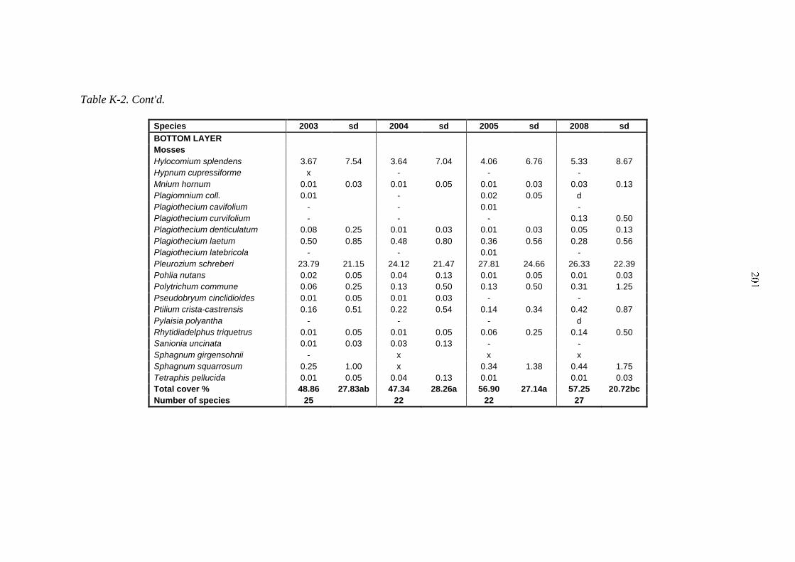
Table K-2. Cont'd.
Species 2003 sd 2004 sd 2005 sd 2008 sd
BOTTOM LAYER
Mosses
Hylocomium splendens 3.67 7.54 3.64 7.04 4.06 6.76 5.33 8.67
Hypnum cupressiforme x - - -
Mnium hornum 0.01 0.03 0.01 0.05 0.01 0.03 0.03 0.13
Plagiomnium coll. 0.01 - 0.02 0.05 d
Plagiothecium cavifolium - - 0.01 -
Plagiothecium curvifolium - - - 0.13 0.50
Plagiothecium denticulatum 0.08 0.25 0.01 0.03 0.01 0.03 0.05 0.13
Plagiothecium laetum 0.50 0.85 0.48 0.80 0.36 0.56 0.28 0.56
Plagiothecium latebricola - - 0.01 -
Pleurozium schreberi 23.79 21.15 24.12 21.47 27.81 24.66 26.33 22.39
Pohlia nutans 0.02 0.05 0.04 0.13 0.01 0.05 0.01 0.03
Polytrichum commune 0.06 0.25 0.13 0.50 0.13 0.50 0.31 1.25
Pseudobryum cinclidioides 0.01 0.05 0.01 0.03 - -
Ptilium crista-castrensis 0.16 0.51 0.22 0.54 0.14 0.34 0.42 0.87
Pylaisia polyantha - - - d
Rhytidiadelphus triquetrus 0.01 0.05 0.01 0.05 0.06 0.25 0.14 0.50
Sanionia uncinata 0.01 0.03 0.03 0.13 - -
Sphagnum girgensohnii - x x x
Sphagnum squarrosum 0.25 1.00 x 0.34 1.38 0.44 1.75
Tetraphis pellucida 0.01 0.05 0.04 0.13 0.01 0.01 0.03
Total cover % 48.86 27.83ab 47.34 28.26a 56.90 27.14a 57.25 20.72bc
Number of species 25 22 22 27
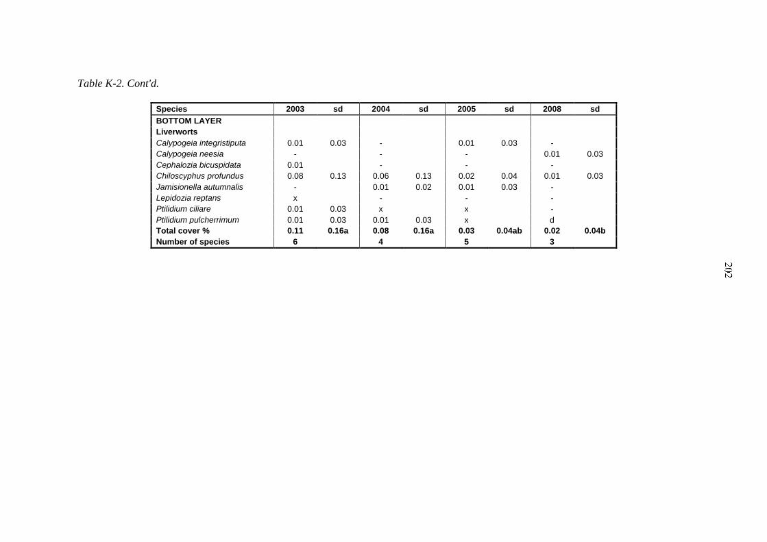
Table K-2. Cont'd.
Species 2003 sd 2004 sd 2005 sd 2008 sd
BOTTOM LAYER
Liverworts
Calypogeia integristiputa 0.01 0.03 - 0.01 0.03 -
Calypogeia neesia - - - 0.01 0.03
Cephalozia bicuspidata 0.01 - - -
Chiloscyphus profundus 0.08 0.13 0.06 0.13 0.02 0.04 0.01 0.03
Jamisionella autumnalis - 0.01 0.02 0.01 0.03 -
Lepidozia reptans x - - -
Ptilidium ciliare 0.01 0.03 x x -
Ptilidium pulcherrimum 0.01 0.03 0.01 0.03 x d
Total cover % 0.11 0.16a 0.08 0.16a 0.03 0.04ab 0.02 0.04b
Number of species 6 4 5 3
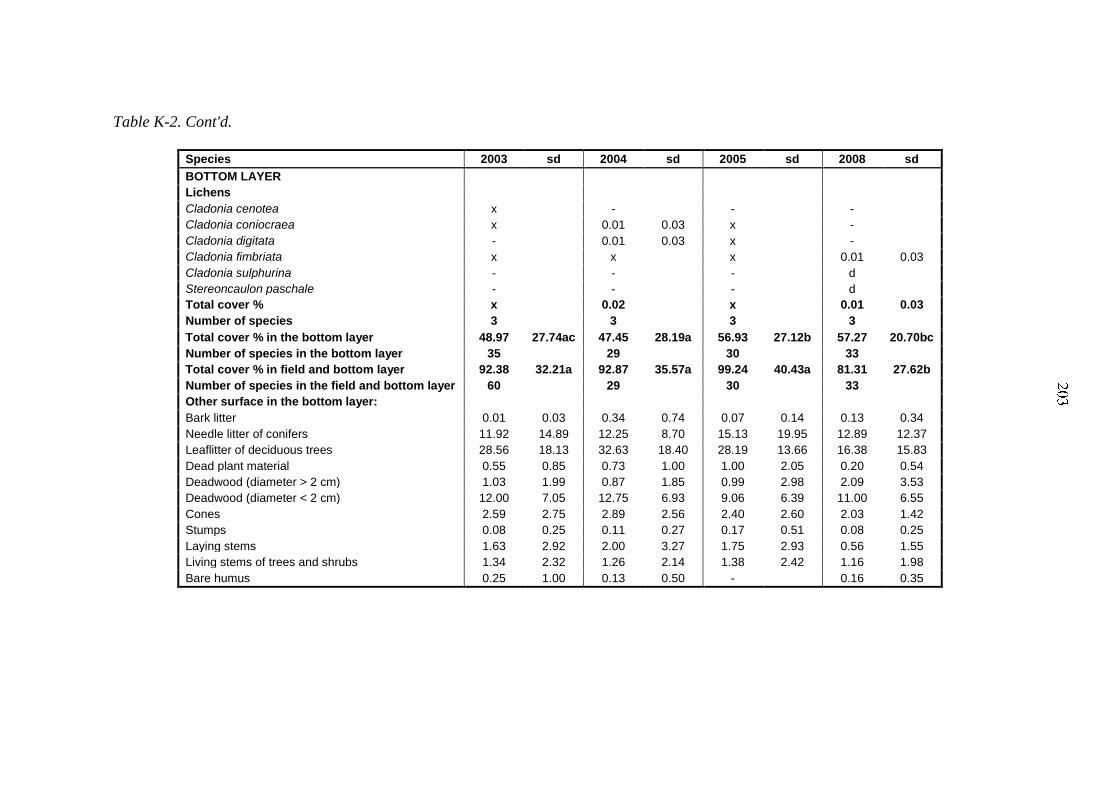
Table K-2. Cont'd.
Species 2003 sd 2004 sd 2005 sd 2008 sd
BOTTOM LAYER
Lichens
Cladonia cenotea x - - -
Cladonia coniocraea x 0.01 0.03 x -
Cladonia digitata - 0.01 0.03 x -
Cladonia fimbriata x x x 0.01 0.03
Cladonia sulphurina - - - d
Stereoncaulon paschale - - - d
Total cover % x 0.02 x 0.01 0.03
Number of species 3 3 3 3
Total cover % in the bottom layer 48.97 27.74ac 47.45 28.19a 56.93 27.12b 57.27 20.70bc
Number of species in the bottom layer 35 29 30 33
Total cover % in field and bottom layer 92.38 32.21a 92.87 35.57a 99.24 40.43a 81.31 27.62b
Number of species in the field and bottom layer 60 29 30 33
Other surface in the bottom layer:
Bark litter 0.01 0.03 0.34 0.74 0.07 0.14 0.13 0.34
Needle litter of conifers 11.92 14.89 12.25 8.70 15.13 19.95 12.89 12.37
Leaflitter of deciduous trees 28.56 18.13 32.63 18.40 28.19 13.66 16.38 15.83
Dead plant material 0.55 0.85 0.73 1.00 1.00 2.05 0.20 0.54
Deadwood (diameter > 2 cm) 1.03 1.99 0.87 1.85 0.99 2.98 2.09 3.53
Deadwood (diameter < 2 cm) 12.00 7.05 12.75 6.93 9.06 6.39 11.00 6.55
Cones 2.59 2.75 2.89 2.56 2.40 2.60 2.03 1.42
Stumps 0.08 0.25 0.11 0.27 0.17 0.51 0.08 0.25
Laying stems 1.63 2.92 2.00 3.27 1.75 2.93 0.56 1.55
Living stems of trees and shrubs 1.34 2.32 1.26 2.14 1.38 2.42 1.16 1.98
Bare humus 0.25 1.00 0.13 0.50 - 0.16 0.35
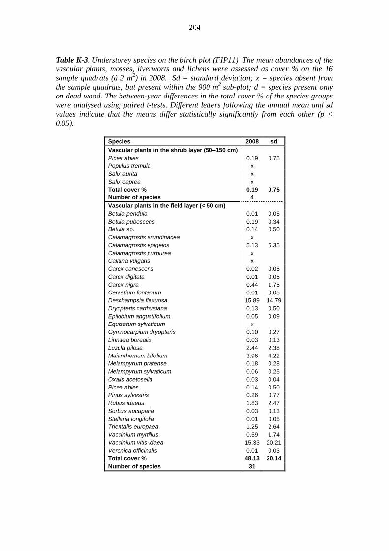
Table K-3. Understorey species on the birch plot (FIP11). The mean abundances of the
vascular plants, mosses, liverworts and lichens were assessed as cover % on the 16
sample quadrats (á 2 m2) in 2008. Sd = standard deviation; x = species absent from
the sample quadrats, but present within the 900 m2
sub-plot; d = species present only
on dead wood. The between-year differences in the total cover % of the species groups
were analysed using paired t-tests. Different letters following the annual mean and sd
values indicate that the means differ statistically significantly from each other (p <
0.05).
Species 2008 sd
Vascular plants in the shrub layer (50–150 cm)
Picea abies 0.19 0.75
Populus tremula x
Salix aurita x
Salix caprea x
Total cover % 0.19 0.75
Number of species 4
Vascular plants in the field layer (< 50 cm)
Betula pendula 0.01 0.05
Betula pubescens 0.19 0.34
Betula sp. 0.14 0.50
Calamagrostis arundinacea x
Calamagrostis epigejos 5.13 6.35
Calamagrostis purpurea x
Calluna vulgaris x
Carex canescens 0.02 0.05
Carex digitata 0.01 0.05
Carex nigra 0.44 1.75
Cerastium fontanum 0.01 0.05
Deschampsia flexuosa 15.89 14.79
Dryopteris carthusiana 0.13 0.50
Epilobium angustifolium 0.05 0.09
Equisetum sylvaticum x
Gymnocarpium dryopteris 0.10 0.27
Linnaea borealis 0.03 0.13
Luzula pilosa 2.44 2.38
Maianthemum bifolium 3.96 4.22
Melampyrum pratense 0.18 0.28
Melampyrum sylvaticum 0.06 0.25
Oxalis acetosella 0.03 0.04
Picea abies 0.14 0.50
Pinus sylvestris 0.26 0.77
Rubus idaeus 1.83 2.47
Sorbus aucuparia 0.03 0.13
Stellaria longifolia 0.01 0.05
Trientalis europaea 1.25 2.64
Vaccinium myrtillus 0.59 1.74
Vaccinium vitis-idaea 15.33 20.21
Veronica officinalis 0.01 0.03
Total cover % 48.13 20.14
Number of species 31
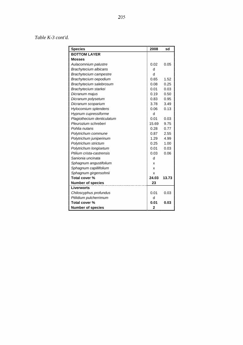
Table K-3 cont'd.
Species 2008 sd
BOTTOM LAYER
Mosses
Aulacomnium palustre 0.02 0.05
Brachytecium albicans d
Brachytecium campestre d
Brachytecium oepodium 0.65 1.52
Brachytecium salebrosum 0.08 0.25
Brachytecium starkei 0.01 0.03
Dicranum majus 0.19 0.50
Dicranum polysetum 0.83 0.95
Dicranum scoparium 3.78 3.49
Hylocomium splendens 0.06 0.13
Hypnum cupressiforme d
Plagiothecium denticulatum 0.01 0.03
Pleurozium schreberi 15.69 9.75
Pohlia nutans 0.28 0.77
Polytrichum commune 0.87 2.55
Polytrichum juniperinum 1.29 4.99
Polytrichum strictum 0.25 1.00
Polytrichum longisetum 0.01 0.03
Ptilium crista-castrensis 0.03 0.06
Sanionia uncinata d
Sphagnum angustifolium x
Sphagnum capillifolium x
Sphagnum girgensohnii x
Total cover % 24.03 13.73
Number of species 23
Liverworts
Chiloscyphus profundus 0.01 0.03
Ptilidium pulcherrimum d
Total cover % 0.01 0.03
Number of species 2
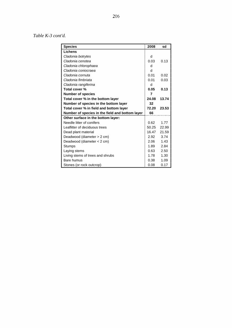
Table K-3 cont'd.
Species 2008 sd
Lichens
Cladonia botrytes d
Cladonia cenotea 0.03 0.13
Cladonia chlorophaea d
Cladonia coniocraea d
Cladonia cornuta 0.01 0.02
Cladonia fimbriata 0.01 0.03
Cladonia rangiferina d
Total cover % 0.05 0.13
Number of species 7
Total cover % in the bottom layer 24.08 13.74
Number of species in the bottom layer 32
Total cover % in field and bottom layer 72.20 23.53
Number of species in the field and bottom layer 66
Other surface in the bottom layer:
Needle litter of conifers 0.62 1.77
Leaflitter of deciduous trees 50.25 22.99
Dead plant material 16.47 21.59
Deadwood (diameter > 2 cm) 2.92 3.74
Deadwood (diameter < 2 cm) 2.06 1.43
Stumps 1.89 2.84
Laying stems 0.63 2.50
Living stems of trees and shrubs 1.78 1.30
Bare humus 0.38 1.09
Stones (or rock outcrop) 0.08 0.17
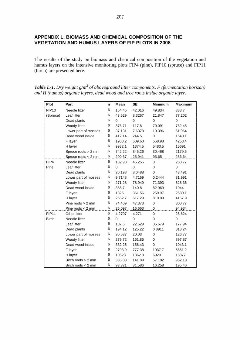
APPENDIX L. BIOMASS AND CHEMICAL COMPOSITION OF THE VEGETATION AND HUMUS LAYERS OF FIP PLOTS IN 2008
The results of the study on biomass and chemical composition of the vegetation and
humus layers on the intensive monitoring plots FIP4 (pine), FIP10 (spruce) and FIP11
(birch) are presented here.
Table L-1. Dry weight g/m2 of aboveground litter components, F (fermentation horizon)
and H (humus) organic layers, dead wood and tree roots inside organic layer.
Plot Part n Mean SE Minimum Maximum
FIP10 Needle litter 6 154.45 42.016 49.834 338.7
(Spruce) Leaf litter 6 43.629 8.3267 21.847 77.202
Dead plants 6 0 0 0 0
Woody litter 6 376.71 117.8 70.091 762.45
Lower part of mosses 6 37.131 7.6378 10.396 61.964
Dead wood inside 6 412.14 244.5 0 1540.1
F layer 6 1903.2 509.63 568.98 4253.4
H layer 6 9932.1 1374.5 5483.5 15691
Spruce roots > 2 mm 6 742.22 345.26 30.468 2179.5
Spruce roots < 2 mm 6 200.37 25.941 95.65 286.64
FIP4 Needle litter 6 132.98 45.256 0 288.77
Pine Leaf litter 6 0 0 0 0
Dead plants 6 20.198 8.0488 0 43.491
Lower part of mosses 6 9.7148 4.7169 0.2444 31.991
Woody litter 6 271.28 78.949 71.393 628.36
Dead wood inside 6 388.7 140.8 82.969 1044
F layer 6 1325 361.56 259.97 2680.1
H layer 6 2652.7 517.29 810.09 4157.9
Pine roots > 2 mm 6 74.409 47.373 0 300.77
Pine roots < 2 mm 6 25.097 16.663 0 94.934
FIP11 Other litter 6 4.2707 4.271 0 25.624
Birch Needle litter 6 0 0 0 0
Leaf litter 6 107.6 22.629 35.679 177.94
Dead plants 6 194.12 125.22 0.8911 813.24
Lower part of mosses 6 30.537 20.03 0 126.77
Woody litter 6 279.72 161.86 0 897.87
Dead wood inside 6 332.25 156.43 0 1043.1
F layer 6 2793.9 777.38 1037.7 5661.2
H layer 6 10523 1362.8 6929 15877
Birch roots > 2 mm 6 335.03 141.89 57.102 962.13
Birch roots < 2 mm 6 93.321 31.586 16.258 195.46
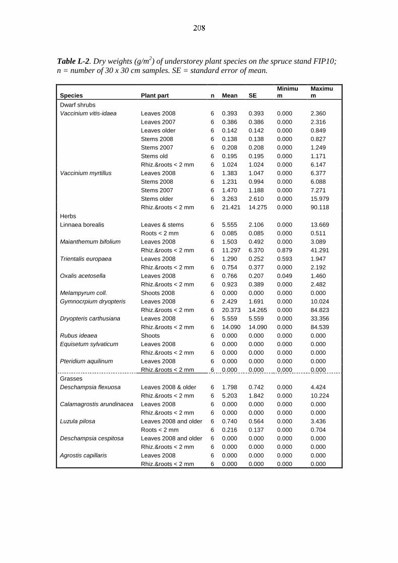
Table L-2. Dry weights (g/m2) of understorey plant species on the spruce stand FIP10;
n = number of 30 x 30 cm samples. SE = standard error of mean.
Species Plant part n Mean SE Minimum
Maximum
Dwarf shrubs
Vaccinium vitis-idaea Leaves 2008 6 0.393 0.393 0.000 2.360
Leaves 2007 6 0.386 0.386 0.000 2.316
Leaves older 6 0.142 0.142 0.000 0.849
Stems 2008 6 0.138 0.138 0.000 0.827
Stems 2007 6 0.208 0.208 0.000 1.249
Stems old 6 0.195 0.195 0.000 1.171
Rhiz.&roots < 2 mm 6 1.024 1.024 0.000 6.147
Vaccinium myrtillus Leaves 2008 6 1.383 1.047 0.000 6.377
Stems 2008 6 1.231 0.994 0.000 6.088
Stems 2007 6 1.470 1.188 0.000 7.271
Stems older 6 3.263 2.610 0.000 15.979
Rhiz.&roots < 2 mm 6 21.421 14.275 0.000 90.118
Herbs
Linnaea borealis Leaves & stems 6 5.555 2.106 0.000 13.669
Roots < 2 mm 6 0.085 0.085 0.000 0.511
Maianthemum bifolium Leaves 2008 6 1.503 0.492 0.000 3.089
Rhiz.&roots < 2 mm 6 11.297 6.370 0.879 41.291
Trientalis europaea Leaves 2008 6 1.290 0.252 0.593 1.947
Rhiz.&roots < 2 mm 6 0.754 0.377 0.000 2.192
Oxalis acetosella Leaves 2008 6 0.766 0.207 0.049 1.460
Rhiz.&roots < 2 mm 6 0.923 0.389 0.000 2.482
Melampyrum coll. Shoots 2008 6 0.000 0.000 0.000 0.000
Gymnocrpium dryopteris Leaves 2008 6 2.429 1.691 0.000 10.024
Rhiz.&roots < 2 mm 6 20.373 14.265 0.000 84.823
Dryopteris carthusiana Leaves 2008 6 5.559 5.559 0.000 33.356
Rhiz.&roots < 2 mm 6 14.090 14.090 0.000 84.539
Rubus ideaea Shoots 6 0.000 0.000 0.000 0.000
Equisetum sylvaticum Leaves 2008 6 0.000 0.000 0.000 0.000
Rhiz.&roots < 2 mm 6 0.000 0.000 0.000 0.000
Pteridium aquilinum Leaves 2008 6 0.000 0.000 0.000 0.000
Rhiz.&roots < 2 mm 6 0.000 0.000 0.000 0.000
Grasses
Deschampsia flexuosa Leaves 2008 & older 6 1.798 0.742 0.000 4.424
Rhiz.&roots < 2 mm 6 5.203 1.842 0.000 10.224
Calamagrostis arundinacea Leaves 2008 6 0.000 0.000 0.000 0.000
Rhiz.&roots < 2 mm 6 0.000 0.000 0.000 0.000
Luzula pilosa Leaves 2008 and older 6 0.740 0.564 0.000 3.436
Roots < 2 mm 6 0.216 0.137 0.000 0.704
Deschampsia cespitosa Leaves 2008 and older 6 0.000 0.000 0.000 0.000
Rhiz.&roots < 2 mm 6 0.000 0.000 0.000 0.000
Agrostis capillaris Leaves 2008 6 0.000 0.000 0.000 0.000
Rhiz.&roots < 2 mm 6 0.000 0.000 0.000 0.000
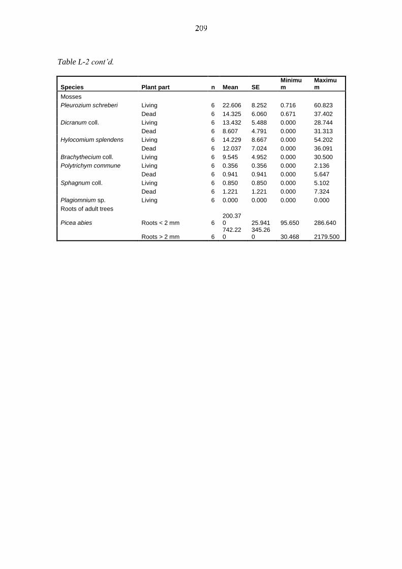
Table L-2 cont’d.
Species Plant part n Mean SE Minimum
Maximum
Mosses
Pleurozium schreberi Living 6 22.606 8.252 0.716 60.823
Dead 6 14.325 6.060 0.671 37.402
Dicranum coll. Living 6 13.432 5.488 0.000 28.744
Dead 6 8.607 4.791 0.000 31.313
Hylocomium splendens Living 6 14.229 8.667 0.000 54.202
Dead 6 12.037 7.024 0.000 36.091
Brachythecium coll. Living 6 9.545 4.952 0.000 30.500
Polytrichym commune Living 6 0.356 0.356 0.000 2.136
Dead 6 0.941 0.941 0.000 5.647
Sphagnum coll. Living 6 0.850 0.850 0.000 5.102
Dead 6 1.221 1.221 0.000 7.324
Plagiomnium sp. Living 6 0.000 0.000 0.000 0.000
Roots of adult trees
Picea abies Roots < 2 mm 6 200.370 25.941 95.650 286.640
Roots > 2 mm 6 742.220
345.260 30.468 2179.500
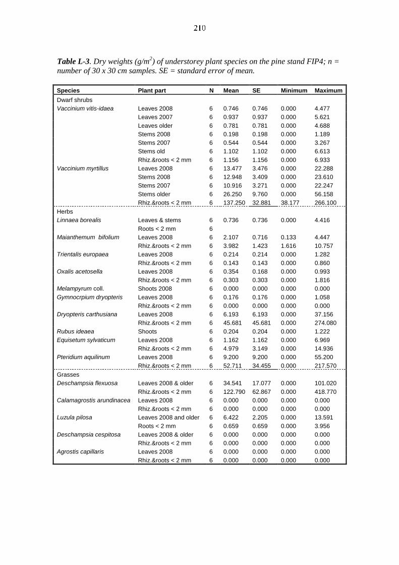
Table L-3. Dry weights (g/m2) of understorey plant species on the pine stand FIP4; n =
number of 30 x 30 cm samples. SE = standard error of mean.
Species Plant part N Mean SE Minimum Maximum
Dwarf shrubs
Vaccinium vitis-idaea Leaves 2008 6 0.746 0.746 0.000 4.477
Leaves 2007 6 0.937 0.937 0.000 5.621
Leaves older 6 0.781 0.781 0.000 4.688
Stems 2008 6 0.198 0.198 0.000 1.189
Stems 2007 6 0.544 0.544 0.000 3.267
Stems old 6 1.102 1.102 0.000 6.613
Rhiz.&roots < 2 mm 6 1.156 1.156 0.000 6.933
Vaccinium myrtillus Leaves 2008 6 13.477 3.476 0.000 22.288
Stems 2008 6 12.948 3.409 0.000 23.610
Stems 2007 6 10.916 3.271 0.000 22.247
Stems older 6 26.250 9.760 0.000 56.158
Rhiz.&roots < 2 mm 6 137.250 32.881 38.177 266.100
Herbs
Linnaea borealis Leaves & stems 6 0.736 0.736 0.000 4.416
Roots < 2 mm 6
Maianthemum bifolium Leaves 2008 6 2.107 0.716 0.133 4.447
Rhiz.&roots < 2 mm 6 3.982 1.423 1.616 10.757
Trientalis europaea Leaves 2008 6 0.214 0.214 0.000 1.282
Rhiz.&roots < 2 mm 6 0.143 0.143 0.000 0.860
Oxalis acetosella Leaves 2008 6 0.354 0.168 0.000 0.993
Rhiz.&roots < 2 mm 6 0.303 0.303 0.000 1.816
Melampyrum coll. Shoots 2008 6 0.000 0.000 0.000 0.000
Gymnocrpium dryopteris Leaves 2008 6 0.176 0.176 0.000 1.058
Rhiz.&roots < 2 mm 6 0.000 0.000 0.000 0.000
Dryopteris carthusiana Leaves 2008 6 6.193 6.193 0.000 37.156
Rhiz.&roots < 2 mm 6 45.681 45.681 0.000 274.080
Rubus ideaea Shoots 6 0.204 0.204 0.000 1.222
Equisetum sylvaticum Leaves 2008 6 1.162 1.162 0.000 6.969
Rhiz.&roots < 2 mm 6 4.979 3.149 0.000 14.936
Pteridium aquilinum Leaves 2008 6 9.200 9.200 0.000 55.200
Rhiz.&roots < 2 mm 6 52.711 34.455 0.000 217.570
Grasses
Deschampsia flexuosa Leaves 2008 & older 6 34.541 17.077 0.000 101.020
Rhiz.&roots < 2 mm 6 122.790 62.867 0.000 418.770
Calamagrostis arundinacea Leaves 2008 6 0.000 0.000 0.000 0.000
Rhiz.&roots < 2 mm 6 0.000 0.000 0.000 0.000
Luzula pilosa Leaves 2008 and older 6 6.422 2.205 0.000 13.591
Roots < 2 mm 6 0.659 0.659 0.000 3.956
Deschampsia cespitosa Leaves 2008 & older 6 0.000 0.000 0.000 0.000
Rhiz.&roots < 2 mm 6 0.000 0.000 0.000 0.000
Agrostis capillaris Leaves 2008 6 0.000 0.000 0.000 0.000
Rhiz.&roots < 2 mm 6 0.000 0.000 0.000 0.000
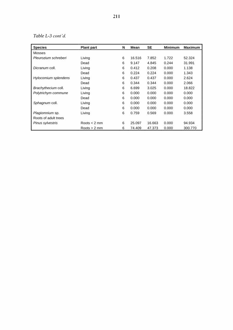
Table L-3 cont’d.
Species Plant part N Mean SE Minimum Maximum
Mosses
Pleurozium schreberi Living 6 16.516 7.852 1.722 52.324
Dead 6 9.147 4.845 0.244 31.991
Dicranum coll. Living 6 0.412 0.208 0.000 1.138
Dead 6 0.224 0.224 0.000 1.343
Hylocomium splendens Living 6 0.437 0.437 0.000 2.624
Dead 6 0.344 0.344 0.000 2.066
Brachythecium coll. Living 6 6.699 3.025 0.000 18.822
Polytrichym commune Living 6 0.000 0.000 0.000 0.000
Dead 6 0.000 0.000 0.000 0.000
Sphagnum coll. Living 6 0.000 0.000 0.000 0.000
Dead 6 0.000 0.000 0.000 0.000
Plagiomnium sp. Living 6 0.759 0.569 0.000 3.558
Roots of adult trees
Pinus sylvestris Roots < 2 mm 6 25.097 16.663 0.000 94.934
Roots > 2 mm 6 74.409 47.373 0.000 300.770

Table L-4. Dry weights (g/m2) of understorey plant species on the birch stand FIP11; n
= number of 30 x 30 cm samples. SE = standard error of mean.
Species Plant part n Mean SE Minimum Maximum
Dwarf shrubs
Vaccinium vitis-idaea Leaves 2008 6 20.191 5.624 0.000 30.999
Leaves 2007 6 10.696 3.149 0.000 19.136
Leaves older 6 3.662 1.969 0.000 11.910
Stems 2008 6 7.288 2.251 0.000 13.247
Stems 2007 6 12.292 4.063 0.000 26.647
Stems old 6 21.563 6.613 0.000 38.549
Rhiz.&roots < 2 mm 6 113.590 40.644 0.000 254.000
Vaccinium myrtillus Leaves 2008 6 2.106 1.434 0.000 8.380
Stems 2008 6 5.178 3.418 0.000 19.324
Stems 2007 6 7.047 4.884 0.000 28.880
Stems older 6 9.249 6.545 0.000 39.113
Rhiz.&roots < 2 mm 6 8.534 6.235 0.000 37.691
Herbs
Linnaea borealis Leaves & stems 6 0.000 0.000 0.000 0.000
Roots < 2 mm 6 0.000 0.000 0.000 0.000
Maianthemum bifolium Leaves 2008 6 2.995 1.322 0.000 9.024
Rhiz.&roots < 2 mm 6 14.299 6.755 0.836 47.069
Trientalis europaea Leaves 2008 6 0.487 0.234 0.000 1.558
Rhiz.&roots < 2 mm 6 1.937 0.875 0.000 5.143
Oxalis acetosella Leaves 2008 6 0.000 0.000 0.000 0.000
Rhiz.&roots < 2 mm 6 0.000 0.000 0.000 0.000
Melampyrum coll. Shoots 2008 6 0.232 0.232 0.000 1.391
Gymnocrpium dryopteris Leaves 2008 6 0.000 0.000 0.000 0.000
Rhiz.&roots < 2 mm 6 0.000 0.000 0.000 0.000
Dryopteris carthusiana Leaves 2008 6 0.000 0.000 0.000 0.000
Rhiz.&roots < 2 mm 6 0.000 0.000 0.000 0.000
Rubus ideaea Shoots 6 0.000 0.000 0.000 0.000
Equisetum sylvaticum Leaves 2008 6 0.000 0.000 0.000 0.000
Rhiz.&roots < 2 mm 6 0.000 0.000 0.000 0.000
Pteridium aquilinum Leaves 2008 6 0.000 0.000 0.000 0.000
Rhiz.&roots < 2 mm 6 0.000 0.000 0.000 0.000
Grasses
Deschampsia flexuosa Leaves 2008 & older 6 21.991 9.285 0.000 64.080
Rhiz.&roots < 2 mm 6 200.570 73.212 0.000 446.110
Calamagrostis arundinacea Leaves 2008 6 16.704 12.069 0.000 74.578
Rhiz.&roots < 2 mm 6 71.897 42.393 0.000 243.240
Luzula pilosa Leaves 2008 & older 6 1.402 0.923 0.000 5.902
Roots < 2 mm 6 0.953 0.659 0.000 4.180
Deschampsia cespitosa Leaves 2008 and older 6 0.067 0.067 0.000 0.400
Rhiz.&roots < 2 mm 6 0.169 0.169 0.000 1.013
Agrostis capillaris Leaves 2008 6 0.000 0.000 0.000 0.000
Rhiz.&roots < 2 mm 6 0.000 0.000 0.000 0.000
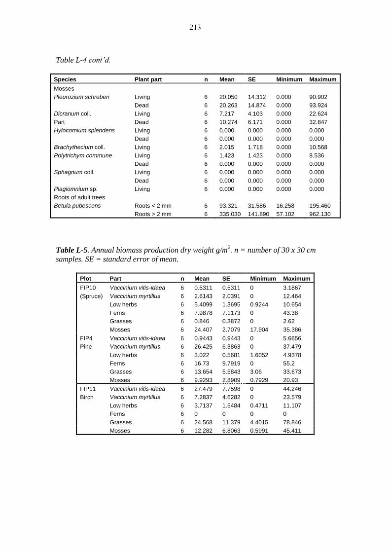
Table L-4 cont’d.
Species Plant part n Mean SE Minimum Maximum
Mosses
Pleurozium schreberi Living 6 20.050 14.312 0.000 90.902
Dead 6 20.263 14.874 0.000 93.924
Dicranum coll. Living 6 7.217 4.103 0.000 22.624
Part Dead 6 10.274 6.171 0.000 32.847
Hylocomium splendens Living 6 0.000 0.000 0.000 0.000
Dead 6 0.000 0.000 0.000 0.000
Brachythecium coll. Living 6 2.015 1.718 0.000 10.568
Polytrichym commune Living 6 1.423 1.423 0.000 8.536
Dead 6 0.000 0.000 0.000 0.000
Sphagnum coll. Living 6 0.000 0.000 0.000 0.000
Dead 6 0.000 0.000 0.000 0.000
Plagiomnium sp. Living 6 0.000 0.000 0.000 0.000
Roots of adult trees
Betula pubescens Roots < 2 mm 6 93.321 31.586 16.258 195.460
Roots > 2 mm 6 335.030 141.890 57.102 962.130
Table L-5. Annual biomass production dry weight g/m2. n = number of 30 x 30 cm
samples. SE = standard error of mean.
Plot Part n Mean SE Minimum Maximum
FIP10 Vaccinium vitis-idaea 6 0.5311 0.5311 0 3.1867
(Spruce) Vaccinium myrtillus 6 2.6143 2.0391 0 12.464
Low herbs 6 5.4099 1.3695 0.9244 10.654
Ferns 6 7.9878 7.1173 0 43.38
Grasses 6 0.846 0.3872 0 2.62
Mosses 6 24.407 2.7079 17.904 35.386
FIP4 Vaccinium vitis-idaea 6 0.9443 0.9443 0 5.6656
Pine Vaccinium myrtillus 6 26.425 6.3863 0 37.479
Low herbs 6 3.022 0.5681 1.6052 4.9378
Ferns 6 16.73 9.7919 0 55.2
Grasses 6 13.654 5.5843 3.06 33.673
Mosses 6 9.9293 2.8909 0.7929 20.93
FIP11 Vaccinium vitis-idaea 6 27.479 7.7598 0 44.246
Birch Vaccinium myrtillus 6 7.2837 4.6282 0 23.579
Low herbs 6 3.7137 1.5484 0.4711 11.107
Ferns 6 0 0 0 0
Grasses 6 24.568 11.379 4.4015 78.846
Mosses 6 12.282 6.8063 0.5991 45.411
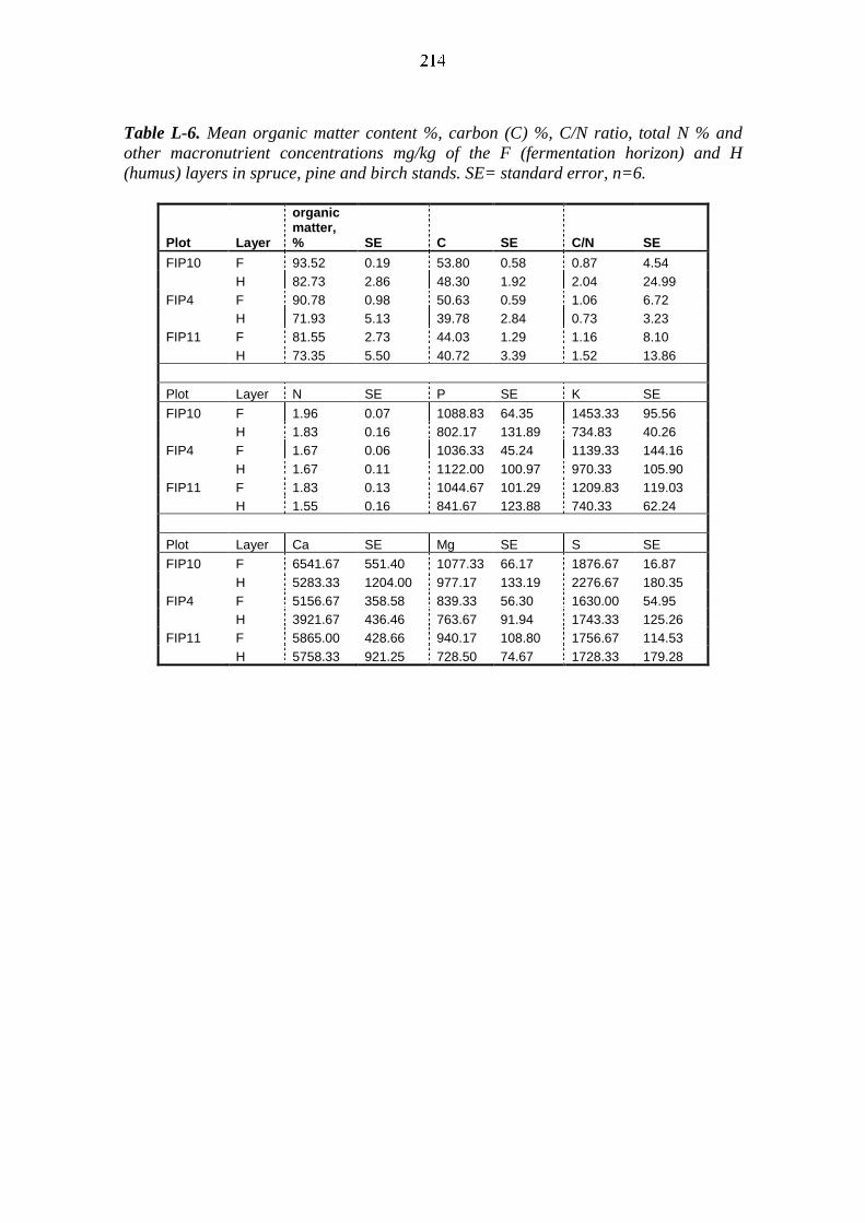
Table L-6. Mean organic matter content %, carbon (C) %, C/N ratio, total N % and
other macronutrient concentrations mg/kg of the F (fermentation horizon) and H
(humus) layers in spruce, pine and birch stands. SE= standard error, n=6.
Plot Layer
organic matter, % SE C SE C/N SE
FIP10 F 93.52 0.19 53.80 0.58 0.87 4.54
H 82.73 2.86 48.30 1.92 2.04 24.99
FIP4 F 90.78 0.98 50.63 0.59 1.06 6.72
H 71.93 5.13 39.78 2.84 0.73 3.23
FIP11 F 81.55 2.73 44.03 1.29 1.16 8.10
H 73.35 5.50 40.72 3.39 1.52 13.86
Plot Layer N SE P SE K SE
FIP10 F 1.96 0.07 1088.83 64.35 1453.33 95.56
H 1.83 0.16 802.17 131.89 734.83 40.26
FIP4 F 1.67 0.06 1036.33 45.24 1139.33 144.16
H 1.67 0.11 1122.00 100.97 970.33 105.90
FIP11 F 1.83 0.13 1044.67 101.29 1209.83 119.03
H 1.55 0.16 841.67 123.88 740.33 62.24
Plot Layer Ca SE Mg SE S SE
FIP10 F 6541.67 551.40 1077.33 66.17 1876.67 16.87
H 5283.33 1204.00 977.17 133.19 2276.67 180.35
FIP4 F 5156.67 358.58 839.33 56.30 1630.00 54.95
H 3921.67 436.46 763.67 91.94 1743.33 125.26
FIP11 F 5865.00 428.66 940.17 108.80 1756.67 114.53
H 5758.33 921.25 728.50 74.67 1728.33 179.28
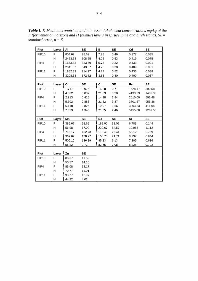
Table L-7. Mean micronutrient and non-essential element concentrations mg/kg of the
F (fermentation horizon) and H (humus) layers in spruce, pine and birch stands. SE=
standard error, n = 6.
Plot Layer Al SE B SE Cd SE
FIP10 F 804.67 98.62 7.98 0.46 0.277 0.035
H 2463.33 808.65 4.02 0.53 0.419 0.075
FIP4 F 1653.33 333.59 5.75 0.32 0.433 0.021
H 2841.67 643.37 4.28 0.38 0.489 0.031
FIP11 F 1882.33 214.27 4.77 0.52 0.436 0.038
H 3208.33 672.82 3.53 0.40 0.400 0.037
Plot Layer Cr SE Cu SE Fe SE
FIP10 F 1.717 0.076 15.88 0.71 1428.17 392.58
H 4.502 0.837 21.83 3.28 4133.33 1402.33
FIP4 F 2.913 0.415 14.98 2.84 2010.00 501.48
H 5.602 0.888 21.52 3.87 3701.67 955.36
FIP11 F 5.118 0.826 19.07 1.56 3003.33 411.04
H 7.353 1.346 21.55 2.46 5455.00 1269.58
Plot Layer Mn SE Na SE Ni SE
FIP10 F 385.67 98.69 182.00 32.02 6.783 0.144
H 56.98 17.00 220.67 54.57 10.063 1.112
FIP4 F 718.17 152.73 113.40 25.41 5.912 0.769
H 367.67 138.27 106.75 21.71 8.237 0.944
FIP11 F 506.10 136.89 85.83 6.13 7.205 0.616
H 58.22 9.72 83.65 7.08 8.228 0.702
Plot Layer Zn SE
FIP10 F 88.37 11.59
H 50.57 14.10
FIP4 F 85.08 13.17
H 70.77 11.01
FIP11 F 93.77 12.97
H 44.32 4.02
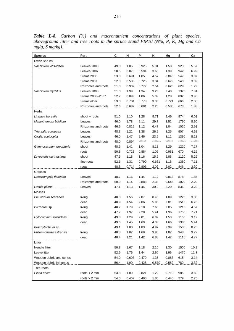
Table L-8. Carbon (%) and macronutrient concentrations of plant species,
aboveground litter and tree roots in the spruce stand FIP10 (N%, P, K, Mg and Ca
mg/g, S mg/kg).
Species Part C N P K Mg S Ca
Dwarf shrubs
Vaccinium vitis-idaea Leaves 2008 49.8 1.06 0.925 5.31 1.58 923 5.57
Leaves 2007 50.5 0.875 0.594 3.60 1.39 942 6.99
Stems 2008 53.3 0.691 1.05 4.57 0.846 547 3.07
Stems 2007 52.3 0.586 0.725 3.34 0.679 548 3.02
Rhizomes and roots 51.3 0.902 0.777 2.54 0.626 629 1.79
Vaccinium myrtillus Leaves 2008 51.0 1.99 1.34 9.23 2.40 1320 7.81
Stems 2008–2007 52.7 0.899 1.06 5.39 1.28 892 3.96
Stems older 53.0 0.704 0.773 3.36 0.721 666 2.06
Rhizomes and roots 52.6 0.687 0.681 2.26 0.530 673 1.88
Herbs
Linnaea borealis shoot + roots 51.0 1.10 1.28 8.71 2.49 874 6.01
Maianthemum bifolium Leaves 46.0 1.78 2.11 29.7 3.51 1790 8.50
Rhizomes and roots 46.6 0.819 1.12 6.47 1.04 1020 2.91
Trientalis europaea Leaves 48.3 1.21 1.38 26.2 3.25 907 4.62
Oxalis acetocella Leaves 46.0 1.47 2.46 23.5 3.11 1390 8.12
Rhizomes and roots 48.0 0.894 ****** ******* ****** ****** ******
Gymnocarpium dryopteris shoot 48.6 1.41 1.04 8.13 3.29 1220 7.17
roots 50.8 0.728 0.884 1.09 0.981 670 4.15
Dryopteris carthusiana shoot 47.5 1.18 1.16 15.9 5.88 1120 5.29
fine roots 52.5 1.31 0.790 0.681 1.18 1380 7.11
roots 48.8 0.714 0.806 2.02 2.02 846 3.30
Grasses
Deschampsia flexuosa Leaves 48.7 1.16 1.44 11.2 0.813 878 1.85
Rhizomes and roots 50.9 1.14 0.888 2.38 0.646 1020 2.20
Luzula pilosa Leaves 47.1 1.13 1.44 30.0 2.20 836 3.23
Mosses
Pleurozium schreberi living 48.8 1.56 2.07 8.40 1.89 1220 3.83
dead 48.9 1.54 2.06 5.96 2.01 1510 6.76
Dicranum sp. living 48.7 1.79 2.10 7.68 2.05 1210 4.57
dead 47.7 1.97 2.20 5.41 1.96 1750 7.71
Hylocomium splendens living 49.3 1.29 2.01 6.82 1.53 1150 3.12
dead 49.6 1.45 1.69 4.33 1.66 1380 5.44
Brachytechium sp. 49.1 1.80 1.83 4.97 2.39 1500 8.75
Ptilium crista-castrensis living 48.3 1.02 1.68 9.96 1.82 948 3.27
dead 48.4 1.21 1.42 6.88 1.42 1110 4.77
Litter
Needle litter 50.8 1.67 1.18 2.10 1.30 1500 10.2
Leave litter 52.9 1.76 1.44 2.60 1.95 1470 11.8
Wooden debris and cones 54.0 0.693 0.470 1.35 0.863 615 3.14
Wooden debris in humus 56.4 1.00 0.428 0.570 0.562 780 3.32
Tree roots
Picea abies roots < 2 mm 53.8 1.09 0.821 1.22 0.719 985 3.60
roots > 2 mm 54.3 0.467 0.490 1.85 0.445 379 2.75

Table L-9. Carbon and macronutrient concentrations of plant species, aboveground
litter and tree roots in the pine stand FIP4 (N%, P, K, Mg and Ca mg/g, S mg/kg).
Species Part C N P K Mg S Ca
Dwarf shrubs
Vaccinium vitis-idaea Leaves 2008 53.2 1.06 0.972 5.47 1.49 886 4.57
Leaves 2007 52.7 0.869 0.610 4.15 1.30 991 5.94
Leaves older ****** ****** 0.558 2.88 1.57 806 5.55
Stems 2008 ****** ****** 1.07 4.75 0.829 553 3.55
Stems 2007 51.3 0.547 0.631 3.25 0.497 454 3.46
Stems older ****** ****** 0.616 2.80 0.580 489 2.72
Rhizomes and roots ****** ****** 0.569 1.83 0.421 534 1.74
Vaccinium myrtillus Leaves 2008 51.0 1.79 1.04 8.03 2.04 1370 7.39
Stems 2008 52.7 1.16 0.937 5.08 1.11 900 3.86
Stems 2007 52.2 0.864 0.688 4.09 0.849 779 3.27
Stems older 51.3 0.650 0.543 2.97 0.621 660 1.73
Rhizomes and roots 51.3 0.749 0.561 2.30 0.471 886 1.48
Dwarf shrub Rhizomes and roots 52.0 0.559 0.637 2.40 0.488 751 1.44
Herbs
Maianthemum bifolium Leaves 46.5 1.39 1.01 16.8 2.59 1050 6.22
Rhizomes and roots 48.0 1.12 0.904 4.22 0.924 871 3.57
Dryopteris carthusiana shoot 48.0 1.16 0.815 16.9 4.57 907 4.39
fine roots < 2 mm 52.0 1.34 0.951 2.43 1.08 1300 3.50
roots > 2 mm 49.4 1.02 0.739 6.33 2.51 1060 3.29
Pteridium aquilinum shoot 46.9 1.23 1.09 20.3 1.76 884 3.54
fine roots < 2 mm 50.7 1.20 0.908 1.92 1.09 1250 3.39
roots > 2 mm 48.4 0.406 0.455 7.28 1.54 533 1.56
Grasses
Deschampsia flexuosa Leaves 48.2 1.71 1.37 12.1 0.873 982 1.81
Rhizomes and roots 50.7 1.60 0.824 1.25 0.494 1160 3.27
Luzula pilosa Leaves 48.5 1.57 1.30 17.4 1.99 1010 4.10
Mosses
Pleurozium schreberi living 48.3 1.94 2.25 9.26 1.72 1340 3.94
dead 47.6 1.66 1.70 4.75 1.66 1330 6.14
Hylocomium splendens living ****** ****** 2.50 10.2 1.54 1380 3.10
dead ****** ****** 1.60 4.39 1.34 1380 4.48
Brachytechium sp. 47.6 2.49 2.01 6.37 1.95 1720 6.34
Litter
Needle litter 54.3 1.20 0.944 1.90 0.900 1090 6.72
Plant litter 49.9 1.53 1.11 2.23 1.81 1300 5.76
Wooden debris 52.7 0.552 0.350 0.792 0.452 483 2.32
Wooden debris in humus 52.3 0.632 0.365 0.574 0.424 586 2.44
Tree roots
Pinus sylvestris roots >2 mm 50.9 0.474 0.446 2.31 0.625 641 1.14
roots <2 mm 51.8 1.57 0.966 0.450 0.708 1600 5.92
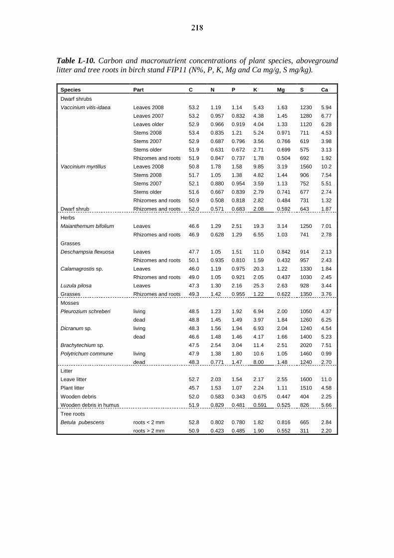
Table L-10. Carbon and macronutrient concentrations of plant species, aboveground
litter and tree roots in birch stand FIP11 (N%, P, K, Mg and Ca mg/g, S mg/kg).
Species Part C N P K Mg S Ca
Dwarf shrubs
Vaccinium vitis-idaea Leaves 2008 53.2 1.19 1.14 5.43 1.63 1230 5.94
Leaves 2007 53.2 0.957 0.832 4.38 1.45 1280 6.77
Leaves older 52.9 0.966 0.919 4.04 1.33 1120 6.28
Stems 2008 53.4 0.835 1.21 5.24 0.971 711 4.53
Stems 2007 52.9 0.687 0.796 3.56 0.766 619 3.98
Stems older 51.9 0.631 0.672 2.71 0.699 575 3.13
Rhizomes and roots 51.9 0.847 0.737 1.78 0.504 692 1.92
Vaccinium myrtillus Leaves 2008 50.8 1.78 1.58 9.85 3.19 1560 10.2
Stems 2008 51.7 1.05 1.38 4.82 1.44 906 7.54
Stems 2007 52.1 0.880 0.954 3.59 1.13 752 5.51
Stems older 51.6 0.667 0.839 2.79 0.741 677 2.74
Rhizomes and roots 50.9 0.508 0.818 2.82 0.484 731 1.32
Dwarf shrub Rhizomes and roots 52.0 0.571 0.683 2.08 0.592 643 1.87
Herbs
Maianthemum bifolium Leaves 46.6 1.29 2.51 19.3 3.14 1250 7.01
Rhizomes and roots 46.9 0.628 1.29 6.55 1.03 741 2.78
Grasses
Deschampsia flexuosa Leaves 47.7 1.05 1.51 11.0 0.842 914 2.13
Rhizomes and roots 50.1 0.935 0.810 1.59 0.432 957 2.43
Calamagrostis sp. Leaves 46.0 1.19 0.975 20.3 1.22 1330 1.84
Rhizomes and roots 49.0 1.05 0.921 2.05 0.437 1030 2.45
Luzula pilosa Leaves 47.3 1.30 2.16 25.3 2.63 928 3.44
Grasses Rhizomes and roots 49.3 1.42 0.955 1.22 0.622 1350 3.76
Mosses
Pleurozium schreberi living 48.5 1.23 1.92 6.94 2.00 1050 4.37
dead 48.8 1.45 1.49 3.97 1.84 1260 6.25
Dicranum sp. living 48.3 1.56 1.94 6.93 2.04 1240 4.54
dead 46.6 1.48 1.46 4.17 1.66 1400 5.23
Brachytechium sp. 47.5 2.54 3.04 11.4 2.51 2020 7.51
Polytrichum commune living 47.9 1.38 1.80 10.6 1.05 1460 0.99
dead 48.3 0.771 1.47 8.00 1.48 1240 2.70
Litter
Leave litter 52.7 2.03 1.54 2.17 2.55 1600 11.0
Plant litter 45.7 1.53 1.07 2.24 1.11 1510 4.58
Wooden debris 52.0 0.583 0.343 0.675 0.447 404 2.25
Wooden debris in humus 51.9 0.829 0.481 0.591 0.525 826 5.66
Tree roots
Betula pubescens roots < 2 mm 52.8 0.802 0.780 1.82 0.816 665 2.84
roots > 2 mm 50.9 0.423 0.485 1.90 0.552 311 2.20

Table L-11. Micronutrient and non-essential element concentrations (mg/kg) of plant species, aboveground litter and tree roots in the
spruce stand FIP10.
Species Part B Cu Zn Mn Ni Fe Cd Cr Pb Al Mo Na
Dwarf shrubs
Vaccinium vitis-idaea Leaves 2008 12.5 2.87 26.9 929 0.592 31.7 0.400 <2.40 60.6 <1.60 29.3
Leaves 2007 11.6 1.97 34.2 1490 0.876 45.0 0.522 <2.53 94.7 <1.68 30.3
Stems 2008 9.88 4.82 23.5 613 0.806 40.3 <2.57 49.3 <1.72 66.2
Stems 2007 7.66 3.69 28.6 906 0.761 58.5 0.201 0.417 <2.15 75.5 <1.44 73.7
Rhizomes and roots 6.50 4.57 30.5 429 1.65 79.7 0.211 0.508 <2.11 93.4 <1.41 106
Vaccinium myrtillus Leaves 2008 33.0 7.03 39.1 2810 1.51 98.6 0.918 <2.75 116 <1.84 111
Stems 2008–2007 11.5 6.41 41.5 2710 0.692 40.6 0.705 <1.92 81.7 <1.28 75.7
Stems older 6.53 1.96 40.0 1490 1.02 40.8 0.120 0.735 <1.81 71.7 <1.20 81.9
Rhizomes and roots 6.18 5.58 34.2 437 1.68 87.7 0.222 0.710 3.66 76.9 <1.11 62.0
Herbs
Linnaea borealis shoot + roots 15.1 5.83 70.0 648 2.57 201 0.126 1.31 2.17 115 <1.14 187
Maianthemum bifolium Leaves 22.3 4.07 33.5 499 1.69 101 0.685 0.946 <1.87 41.7 <1.25 66.3
Rhizomes and roots 9.36 25.8 56.7 150 2.03 160 0.533 0.876 3.83 87.9 <1.27 140
Trientalis europaea Leaves 17.1 2.87 22.4 425 1.65 134 <0.108 1.09 <1.62 64.9 <1.08 75.0
Oxalis acetocella Leaves 32.9 3.90 29.4 462 0.893 57.5 <0.165 0.810 <2.48 <26.5 <1.65 82.6
Rhizomes and roots ****** ****** ****** ****** ****** ******* ****** ****** ****** ****** ****** ******
Gymnocarpium dryopteris shoot 17.3 6.11 60.8 362 2.84 404 0.203 1.44 3.37 211 <1.19 132
roots 6.51 8.81 34.1 122 8.51 469 0.374 3.59 41.1 367 <1.17 49.9
Dryopteris carthusiana shoot 19.8 3.11 28.5 661 1.44 50.8 0.301 0.534 <1.67 20.6 <1.11 160
fine roots 7.83 26.5 28.1 54.0 6.46 3950 0.253 2.32 16.0 1100 <1.15 247
roots 14.2 7.40 27.9 75.9 2.72 731 0.156 0.468 6.00 250 <1.11 167
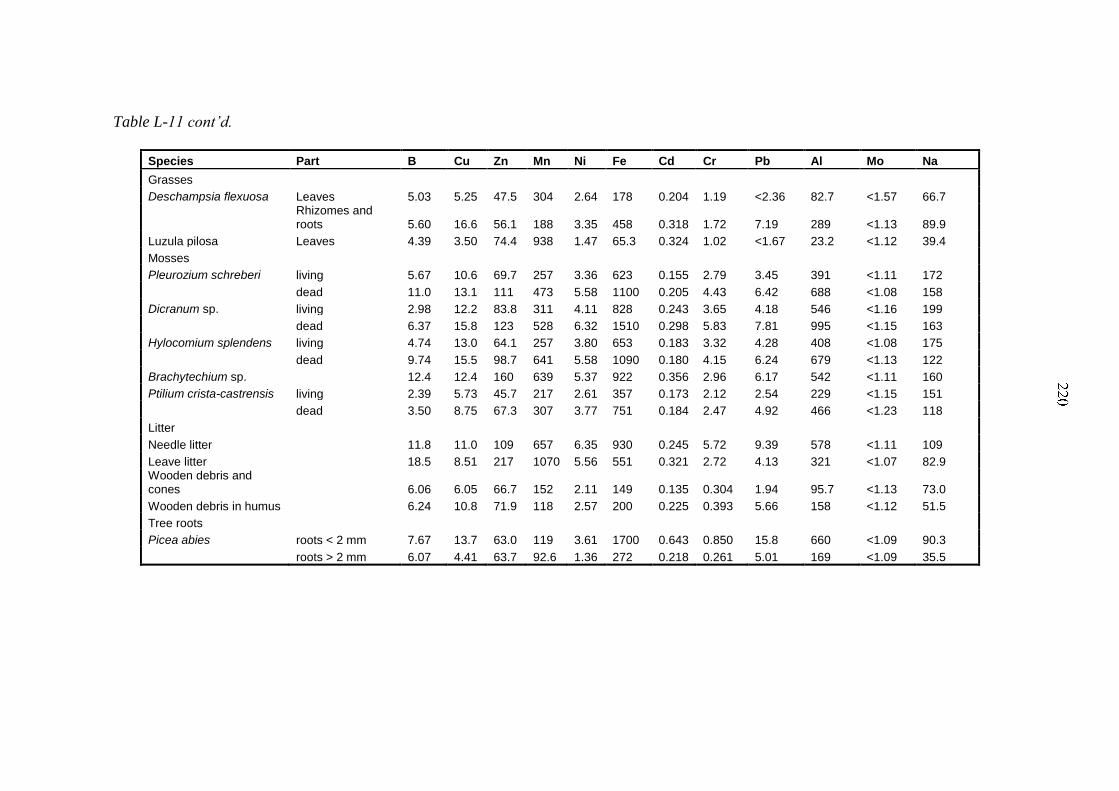
Table L-11 cont’d.
Species Part B Cu Zn Mn Ni Fe Cd Cr Pb Al Mo Na
Grasses
Deschampsia flexuosa Leaves 5.03 5.25 47.5 304 2.64 178 0.204 1.19 <2.36 82.7 <1.57 66.7
Rhizomes and roots 5.60 16.6 56.1 188 3.35 458 0.318 1.72 7.19 289 <1.13 89.9
Luzula pilosa Leaves 4.39 3.50 74.4 938 1.47 65.3 0.324 1.02 <1.67 23.2 <1.12 39.4
Mosses
Pleurozium schreberi living 5.67 10.6 69.7 257 3.36 623 0.155 2.79 3.45 391 <1.11 172
dead 11.0 13.1 111 473 5.58 1100 0.205 4.43 6.42 688 <1.08 158
Dicranum sp. living 2.98 12.2 83.8 311 4.11 828 0.243 3.65 4.18 546 <1.16 199
dead 6.37 15.8 123 528 6.32 1510 0.298 5.83 7.81 995 <1.15 163
Hylocomium splendens living 4.74 13.0 64.1 257 3.80 653 0.183 3.32 4.28 408 <1.08 175
dead 9.74 15.5 98.7 641 5.58 1090 0.180 4.15 6.24 679 <1.13 122
Brachytechium sp. 12.4 12.4 160 639 5.37 922 0.356 2.96 6.17 542 <1.11 160
Ptilium crista-castrensis living 2.39 5.73 45.7 217 2.61 357 0.173 2.12 2.54 229 <1.15 151
dead 3.50 8.75 67.3 307 3.77 751 0.184 2.47 4.92 466 <1.23 118
Litter
Needle litter 11.8 11.0 109 657 6.35 930 0.245 5.72 9.39 578 <1.11 109
Leave litter 18.5 8.51 217 1070 5.56 551 0.321 2.72 4.13 321 <1.07 82.9 Wooden debris and cones 6.06 6.05 66.7 152 2.11 149 0.135 0.304 1.94 95.7 <1.13 73.0
Wooden debris in humus 6.24 10.8 71.9 118 2.57 200 0.225 0.393 5.66 158 <1.12 51.5
Tree roots
Picea abies roots < 2 mm 7.67 13.7 63.0 119 3.61 1700 0.643 0.850 15.8 660 <1.09 90.3
roots > 2 mm 6.07 4.41 63.7 92.6 1.36 272 0.218 0.261 5.01 169 <1.09 35.5

Table L-12. Micronutrient and non-essential element concentrations (mg/kg) of plant species, aboveground litter and tree roots in the pine
stand FIP4.
Species Part B Cu Zn Mn Ni Fe Cd Cr Pb Al Mo Na
Dwarf shrubs
Vaccinium vitis-idaea Leaves 2008 11.5 2.43 28.0 1410 1.33 44.3 - 1.82 <2.66 94.9 <1.77 27.6
Leaves 2007 8.84 1.88 35.0 1980 1.39 55.8 - 2.25 <2.64 174 <1.76 29.7
Leaves older 8.37 2.58 28.1 1490 <0.497 23.0 - - <3.73 103 <2.48 53.9
Stems 2008 10.4 2.94 23.8 1000 1.61 50.5 - 2.29 <1.73 68.1 <1.15 33.6
Stems 2007 7.04 2.32 20.4 1010 0.635 60.9 - 0.657 <1.64 81.3 <1.09 41.8
Stems older 7.56 4.27 22.5 900 0.536 115 - - <2.60 128 <1.73 43.1
Rhizomes and roots 6.46 5.70 19.0 432 0.622 65.9 - - <2.66 123 <1.78 27.5
Vaccinium myrtillus Leaves 2008 22.4 5.23 12.7 3620 0.948 70.7 - 0.764 <1.97 155 <1.32 44.6
Stems 2008 12.5 5.47 30.2 2460 0.474 39.6 - 0.463 <1.62 97.0 <1.08 37.7
Stems 2007 9.65 4.69 37.1 2160 0.475 43.0 0.162 0.508 <1.62 146 <1.08 60.0
Stems older 6.59 1.44 32.5 1320 0.669 95.1 0.216 3.71 <1.62 132 <1.08 64.9
Rhizomes and roots 5.08 5.38 33.8 759 1.68 255 0.347 0.975 10.1 272 <1.08 49.0
Dwarf shrub Rhizomes and roots 4.97 8.63 21.9 419 1.09 138 0.268 0.696 5.16 192 <1.07 80.7
Herbs
Maianthemum bifolium Leaves 16.2 3.25 26.1 524 1.52 91.6 0.549 0.457 <1.96 50.2 <1.31 32.7
Rhizomes and roots 9.42 17.0 56.2 218 2.79 249 0.506 1.58 5.58 212 <1.10 157
Dryopteris carthusiana shoot 18.3 1.36 63.5 1360 1.75 66.4 0.685 0.424 <1.63 40.9 <1.09 36.5
fine roots < 2 mm 6.01 8.08 54.0 1030 5.28 730 0.479 2.23 18.8 759 <1.09 106
roots > 2 mm 15.1 2.47 58.9 1120 3.05 137 0.380 0.391 2.71 122 <1.09 152
Pteridium aquilinum shoot 9.95 3.78 19.6 193 1.54 44.2 <0.112 0.526 <1.68 20.0 <1.12 47.1
fine roots < 2 mm 4.70 19.6 44.4 174 8.90 2320 0.709 2.41 33.0 1890 <1.09 158
roots > 2 mm 5.13 3.64 18.8 103 1.82 71.2 <0.115 <0.230 5.66 125 <1.15 64.8

Table L-12 cont’d.
Species Part B Cu Zn Mn Ni Fe Cd Cr Pb Al Mo Na
Grasses
Deschampsia flexuosa Leaves 4.52 4.52 41.7 593 3.00 234 0.132 1.76 <1.65 145 <1.10 48.2
Rhizomes and roots 3.78 19.7 57.9 396 4.48 832 0.413 3.59 9.39 696 <1.12 112
Luzula pilosa Leaves 6.02 2.51 104 1440 1.73 158 0.638 1.09 <1.65 95.7 <1.10 58.7
Mosses
Pleurozium schreberi living 4.28 9.35 58.5 912 4.07 946 0.229 4.66 3.43 684 <1.09 148
dead 6.20 8.72 78.4 1430 5.65 1810 0.346 6.65 5.69 1340 <1.08 155
Hylocomium splendens living 3.49 12.8 48.4 580 2.24 484 <0.266 1.33 <3.99 329 <2.66 181
dead 5.24 12.0 65.6 1150 5.24 1540 0.303 4.32 5.81 1060 <1.21 123
Brachytechium sp. 7.31 9.75 127 1490 5.94 1520 0.464 6.35 5.44 1070 <1.08 140
Litter
Needle litter 11.3 4.69 63.8 1030 2.76 470 0.310 1.94 2.09 573 <1.07 87.1
Plant litter 13.2 6.63 79.1 1130 3.97 538 0.515 2.15 3.10 373 <1.14 102
Wooden debris 4.03 5.48 26.5 218 1.66 425 0.170 0.748 2.62 424 <1.13 62.7 Wooden debris in humus 3.23 6.08 26.8 163 1.90 322 0.198 0.466 5.00 350 <1.17 77.6
Tree roots
Pinus sylvestris roots > 2 mm 4.65 3.73 14.2 79.1 0.510 122 0.245 0.330 2.71 139 <1.06 48.8
roots < 2 mm 5.58 47.4 62.3 416 5.31 1130 0.569 1.90 21.5 968 <1.07 118
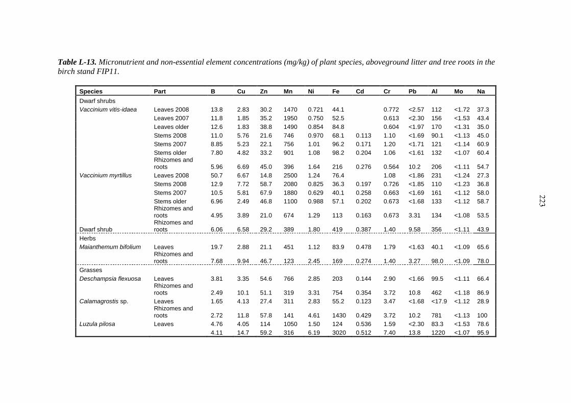
Table L-13. Micronutrient and non-essential element concentrations (mg/kg) of plant species, aboveground litter and tree roots in the
birch stand FIP11.
Species Part B Cu Zn Mn Ni Fe Cd Cr Pb Al Mo Na
Dwarf shrubs
Vaccinium vitis-idaea Leaves 2008 13.8 2.83 30.2 1470 0.721 44.1 0.772 <2.57 112 <1.72 37.3
Leaves 2007 11.8 1.85 35.2 1950 0.750 52.5 0.613 <2.30 156 <1.53 43.4
Leaves older 12.6 1.83 38.8 1490 0.854 84.8 0.604 <1.97 170 <1.31 35.0
Stems 2008 11.0 5.76 21.6 746 0.970 68.1 0.113 1.10 <1.69 90.1 <1.13 45.0
Stems 2007 8.85 5.23 22.1 756 1.01 96.2 0.171 1.20 <1.71 121 <1.14 60.9
Stems older 7.80 4.82 33.2 901 1.08 98.2 0.204 1.06 <1.61 132 <1.07 60.4
Rhizomes and roots 5.96 6.69 45.0 396 1.64 216 0.276 0.564 10.2 206 <1.11 54.7
Vaccinium myrtillus Leaves 2008 50.7 6.67 14.8 2500 1.24 76.4 1.08 <1.86 231 <1.24 27.3
Stems 2008 12.9 7.72 58.7 2080 0.825 36.3 0.197 0.726 <1.85 110 <1.23 36.8
Stems 2007 10.5 5.81 67.9 1880 0.629 40.1 0.258 0.663 <1.69 161 <1.12 58.0
Stems older 6.96 2.49 46.8 1100 0.988 57.1 0.202 0.673 <1.68 133 <1.12 58.7
Rhizomes and roots 4.95 3.89 21.0 674 1.29 113 0.163 0.673 3.31 134 <1.08 53.5
Dwarf shrub Rhizomes and roots 6.06 6.58 29.2 389 1.80 419 0.387 1.40 9.58 356 <1.11 43.9
Herbs
Maianthemum bifolium Leaves 19.7 2.88 21.1 451 1.12 83.9 0.478 1.79 <1.63 40.1 <1.09 65.6
Rhizomes and roots 7.68 9.94 46.7 123 2.45 169 0.274 1.40 3.27 98.0 <1.09 78.0
Grasses
Deschampsia flexuosa Leaves 3.81 3.35 54.6 766 2.85 203 0.144 2.90 <1.66 99.5 <1.11 66.4
Rhizomes and roots 2.49 10.1 51.1 319 3.31 754 0.354 3.72 10.8 462 <1.18 86.9
Calamagrostis sp. Leaves 1.65 4.13 27.4 311 2.83 55.2 0.123 3.47 <1.68 <17.9 <1.12 28.9
Rhizomes and roots 2.72 11.8 57.8 141 4.61 1430 0.429 3.72 10.2 781 <1.13 100
Luzula pilosa Leaves 4.76 4.05 114 1050 1.50 124 0.536 1.59 <2.30 83.3 <1.53 78.6
4.11 14.7 59.2 316 6.19 3020 0.512 7.40 13.8 1220 <1.07 95.9
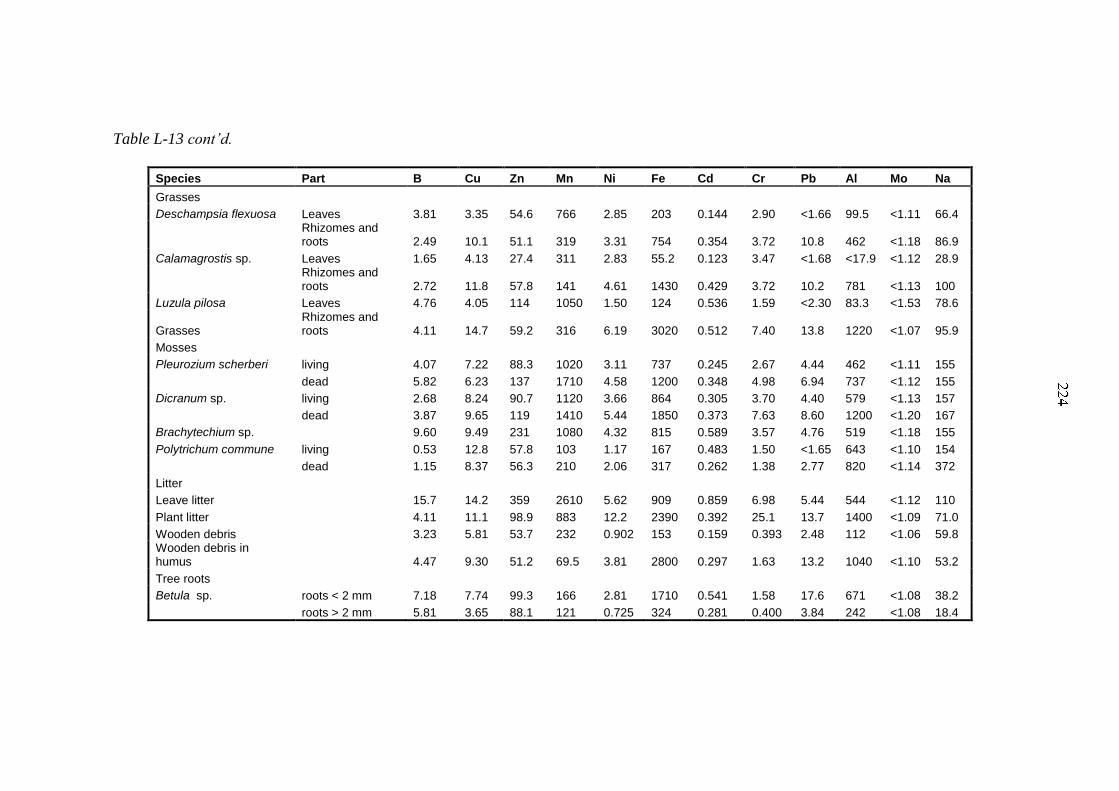
Table L-13 cont’d.
Species Part B Cu Zn Mn Ni Fe Cd Cr Pb Al Mo Na
Grasses
Deschampsia flexuosa Leaves 3.81 3.35 54.6 766 2.85 203 0.144 2.90 <1.66 99.5 <1.11 66.4
Rhizomes and roots 2.49 10.1 51.1 319 3.31 754 0.354 3.72 10.8 462 <1.18 86.9
Calamagrostis sp. Leaves 1.65 4.13 27.4 311 2.83 55.2 0.123 3.47 <1.68 <17.9 <1.12 28.9
Rhizomes and roots 2.72 11.8 57.8 141 4.61 1430 0.429 3.72 10.2 781 <1.13 100
Luzula pilosa Leaves 4.76 4.05 114 1050 1.50 124 0.536 1.59 <2.30 83.3 <1.53 78.6
Grasses Rhizomes and roots 4.11 14.7 59.2 316 6.19 3020 0.512 7.40 13.8 1220 <1.07 95.9
Mosses
Pleurozium scherberi living 4.07 7.22 88.3 1020 3.11 737 0.245 2.67 4.44 462 <1.11 155
dead 5.82 6.23 137 1710 4.58 1200 0.348 4.98 6.94 737 <1.12 155
Dicranum sp. living 2.68 8.24 90.7 1120 3.66 864 0.305 3.70 4.40 579 <1.13 157
dead 3.87 9.65 119 1410 5.44 1850 0.373 7.63 8.60 1200 <1.20 167
Brachytechium sp. 9.60 9.49 231 1080 4.32 815 0.589 3.57 4.76 519 <1.18 155
Polytrichum commune living 0.53 12.8 57.8 103 1.17 167 0.483 1.50 <1.65 643 <1.10 154
dead 1.15 8.37 56.3 210 2.06 317 0.262 1.38 2.77 820 <1.14 372
Litter
Leave litter 15.7 14.2 359 2610 5.62 909 0.859 6.98 5.44 544 <1.12 110
Plant litter 4.11 11.1 98.9 883 12.2 2390 0.392 25.1 13.7 1400 <1.09 71.0
Wooden debris 3.23 5.81 53.7 232 0.902 153 0.159 0.393 2.48 112 <1.06 59.8 Wooden debris in humus 4.47 9.30 51.2 69.5 3.81 2800 0.297 1.63 13.2 1040 <1.10 53.2
Tree roots
Betula sp. roots < 2 mm 7.18 7.74 99.3 166 2.81 1710 0.541 1.58 17.6 671 <1.08 38.2
roots > 2 mm 5.81 3.65 88.1 121 0.725 324 0.281 0.400 3.84 242 <1.08 18.4

APPENDIX M. CHEMICAL CHARACTERISTICS OF LITTERFALL IN FIP PLOTS IN 2006–2007 In this appendix the characteristics of litterfall on FIP4 FIP10 and FIP11 in 2006–2007 are
presented (original data by Pasi Rautio and Lasse Aro, FFRI). Concentrations of cadmium,
molybdenum and lead were in most cases below the limit of quantification, and are not
reported here.
Table M-1. Litterfall production (g/m2) on the FIP plots by sampling occasions (date) and
litter fraction in 2006 and 2007. Litter fractions: 1= pine brown needles, 2= pine green
needles, 3= spruce needles, 4= leaves, 5= remaining litter, 6= branches.
Plot Year Date Litter fraction Total 1 2 3 4 5 6
FIP4 2006 25.4. 7.76 3.99 0.54 27.42 39.71
23.5. 1.77 2.16 0.29 5.80 10.01
26.6. 8.03 0.77 0.46 23.14 32.41
17.7. 14.39 3.28 44.32 61.99
14.8. 7.13 0.84 0.11 10.59 18.68
11.9. 99.45 11.61 0.68 0.07 25.33 137.15
9.10. 104.05 1.70 0.03 10.11 115.89
2.11. 12.85 0.45 0.41 0.02 7.39 21.13
Total 255.44 24.80 2.53 0.09 154.11 436.96
2007 8.5. 42.51 18.24 2.98 0.09 64.70 101.96 230.47
29.5. 2.80 1.32 12.51 0.82 17.44
25.6. 9.25 3.28 1.50 45.11 15.21 74.34
23.7. 14.57 2.93 76.19 1.78 95.47
21.8. 22.95 9.37 0.11 37.55 8.01 77.99
17.9. 75.28 5.28 0.11 0.14 28.03 4.10 112.94
1.10. 47.49 0.48 0.02 0.25 4.27 0.07 52.58
20.10. 76.15 1.27 0.26 0.07 5.01 0.87 83.62
12.11. 8.23 0.74 0.24 13.54 0.80 23.56
Total 299.22 42.90 5.22 0.55 286.91 133.62 768.42
FIP10 2006 25.4. 0.03 47.00 1.09 24.23 72.35
23.5. 33.46 0.13 14.61 48.20
26.6. 0.04 16.94 0.13 15.77 32.87
17.7. 9.42 0.38 5.79 15.60
14.8. 3.89 0.94 7.95 12.78
11.9. 0.04 0.03 6.52 2.60 25.35 34.53
9.10. 2.74 8.04 9.06 19.84
2.11. 0.03 6.07 9.47 2.95 18.52
Total 0.09 0.06 126.05 22.77 105.71 254.69
2007 8.5. 0.04 0.03 85.76 12.02 62.45 70.35 230.64
29.5. 10.67 0.09 6.01 4.76 21.53
25.6. 10.40 0.77 7.39 4.54 23.11
24.7. 0.01 6.05 1.14 8.76 2.22 18.19
21.8. 6.42 2.41 10.37 4.36 23.55
17.9. 6.39 9.31 19.13 5.49 40.33
1.10. 0.00 1.48 14.00 1.98 0.72 18.19
30.10. 0.04 18.34 20.35 6.99 1.50 47.22
12.11. 0.06 10.67 0.77 15.11 9.40 36.00
Total 0.15 0.03 156.17 60.87 138.18 103.35 458.76
FIP11 2007 28.5. 0.26 0.22 1.86 0.34 2.68
25.6. 0.08 0.36 1.53 0.32 2.29
23.7. 0.11 1.89 0.87 0.15 3.02
21.8. 0.13 7.91 2.66 1.28 11.98
17.9. 0.05 0.04 0.13 13.49 1.26 0.10 15.06
1.10. 0.02 14.81 0.30 0.01 15.13
29.10 0.03 0.17 17.82 0.34 18.36
12.11. 0.06 0.19 0.48 0.45 1.27 2.45
Total 0.14 0.04 1.09 56.97 9.26 3.46 70.96

Table M-2. Aluminium and boron concentrations (mg/kg) in the six fractions of litterfall
on the FIP plots during 2006 and 2007. Litter fractions: 1= pine brown needles, 2=
pine green needles, 3= spruce needles, 4= leaves, 5= remaining litter, 6= branches.
Aluminium, mg/kg Boron, mg/kg
Litter fraction Litter fraction
Plot Year Date 1 2 3 4 5 6 1 2 3 4 5 6
FIP4 2006 25.4. 652 472 1760 10.2 13.8 4.85
23.5. 452 363 840 15.5 15.7 7.79
26.6. 380 297 542 16.1 14.5 10.4
17.7. 323 197 295 13.9 15.5 8.28
14.8. 295 187 445 15.2 15.9 7.69
11.9. 308 264 682 15.5 12.7 6.29
9.10. 331 244 683 18.1 12.7 7.91
2.11. 308 209 436 13.5 12.9 7.4
2007 8.5. 513 376 229 639 314 12 12.2 20.1 6.29 5.22
29.5. 365 305 596 364 14.3 14 6.36 10.6
25.6. 318 258 258 336 13.2 12 6.79 6.94
23.7. 282 199 256 414 12.8 14.7 3.88 6.55
21.8. 286 198 427 449 13.6 14.5 4.34 7.1
17.9. 291 257 456 412 16.3 13.3 4.97 8.13
1.10. 292 240 622 15.8 13.5 5.31
20.10. 311 255 705 335 14 14.5 7.4 6.63
12.11. 322 246 362 402 14.7 14.8 3.68 10
FIP10 2006 25.4. 79.7 436 771 21.4 22.1 9.41
23.5. 58 457 25.4 10.6
26.6. 38.3 295 20.7 11.6
17.7. 33.3 31.3 333 19.3 21.6 13.1
14.8. 36.6 30.6 306 18.7 26 14.9
11.9. 53.6 96.2 517 20.3 27 10.4
9.10. 52.9 73.9 385 21 45 12.4
2.11. 43.5 43.8 249 23.8 40 14.5
2007 8.5. 301 534 249 48.3 25.3 8.47 9.89 24.2
29.5. 74.1 538 235 21.6 11.2 10.2
25.6. 39 87.1 515 57.2 22.7 20.8 12.1 14
24.7. 65.9 207 970 154 18.6 25 7.51 9.76
21.8. 52 231 917 180 21 30.7 9.55 10.9
17.9. 42.2 57.7 430 235 21.5 37.8 9.09 10.5
1.10. 54.2 37 806 200 24.3 49.1 17.9 9.34
30.10. 49.2 78.7 403 243 26 52.1 13 10.6
12.11. 47.3 116 266 159 24.2 32.6 5.59 13.7
FIP11 2007 28.5. 66.6 301 19.6 11.1
25.6. 73.7 602 19 11.6
23.7. 60.3 671 21.7 9.51
21.8. 56.3 254 54.4 29.7 12.3 13.4
17.9. 53 482 32.3 13.8
1.10. 29.3 233 37.6 21.5
29.10 47.1 35.8
12.11. 115 516 46.7 25.4 5.92 12.6
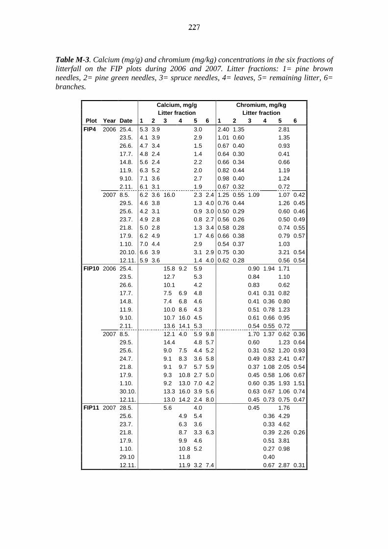
Table M-3. Calcium (mg/g) and chromium (mg/kg) concentrations in the six fractions of
litterfall on the FIP plots during 2006 and 2007. Litter fractions: 1= pine brown
needles, 2= pine green needles, 3= spruce needles, 4= leaves, 5= remaining litter, 6=
branches.
Calcium, mg/g Chromium, mg/kg
Litter fraction Litter fraction
Plot Year Date 1 2 3 4 5 6 1 2 3 4 5 6
FIP4 2006 25.4. 5.3 3.9 3.0 2.40 1.35 2.81
23.5. 4.1 3.9 2.9 1.01 0.60 1.35
26.6. 4.7 3.4 1.5 0.67 0.40 0.93
17.7. 4.8 2.4 1.4 0.64 0.30 0.41
14.8. 5.6 2.4 2.2 0.66 0.34 0.66
11.9. 6.3 5.2 2.0 0.82 0.44 1.19
9.10. 7.1 3.6 2.7 0.98 0.40 1.24
2.11. 6.1 3.1 1.9 0.67 0.32 0.72
2007 8.5. 6.2 3.6 16.0 2.3 2.4 1.25 0.55 1.09 1.07 0.42
29.5. 4.6 3.8 1.3 4.0 0.76 0.44 1.26 0.45
25.6. 4.2 3.1 0.9 3.0 0.50 0.29 0.60 0.46
23.7. 4.9 2.8 0.8 2.7 0.56 0.26 0.50 0.49
21.8. 5.0 2.8 1.3 3.4 0.58 0.28 0.74 0.55
17.9. 6.2 4.9 1.7 4.6 0.66 0.38 0.79 0.57
1.10. 7.0 4.4 2.9 0.54 0.37 1.03
20.10. 6.6 3.9 3.1 2.9 0.75 0.30 3.21 0.54
12.11. 5.9 3.6 1.4 4.0 0.62 0.28 0.56 0.54
FIP10 2006 25.4. 15.8 9.2 5.9 0.90 1.94 1.71
23.5. 12.7 5.3 0.84 1.10
26.6. 10.1 4.2 0.83 0.62
17.7. 7.5 6.9 4.8 0.41 0.31 0.82
14.8. 7.4 6.8 4.6 0.41 0.36 0.80
11.9. 10.0 8.6 4.3 0.51 0.78 1.23
9.10. 10.7 16.0 4.5 0.61 0.66 0.95
2.11. 13.6 14.1 5.3 0.54 0.55 0.72
2007 8.5. 12.1 4.0 5.9 9.8 1.70 1.37 0.62 0.36
29.5. 14.4 4.8 5.7 0.60 1.23 0.64
25.6. 9.0 7.5 4.4 5.2 0.31 0.52 1.20 0.93
24.7. 9.1 8.3 3.6 5.8 0.49 0.83 2.41 0.47
21.8. 9.1 9.7 5.7 5.9 0.37 1.08 2.05 0.54
17.9. 9.3 10.8 2.7 5.0 0.45 0.58 1.06 0.67
1.10. 9.2 13.0 7.0 4.2 0.60 0.35 1.93 1.51
30.10. 13.3 16.0 3.9 5.6 0.63 0.67 1.06 0.74
12.11. 13.0 14.2 2.4 8.0 0.45 0.73 0.75 0.47
FIP11 2007 28.5. 5.6 4.0 0.45 1.76
25.6. 4.9 5.4 0.36 4.29
23.7. 6.3 3.6 0.33 4.62
21.8. 8.7 3.3 6.3 0.39 2.26 0.26
17.9. 9.9 4.6 0.51 3.81
1.10. 10.8 5.2 0.27 0.98
29.10 11.8 0.40
12.11. 11.9 3.2 7.4 0.67 2.87 0.31
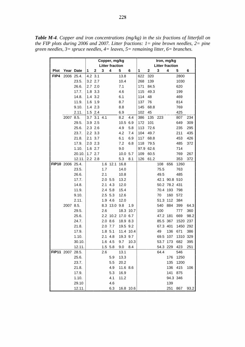
Table M-4. Copper and iron concentrations (mg/kg) in the six fractions of litterfall on
the FIP plots during 2006 and 2007. Litter fractions: 1= pine brown needles, 2= pine
green needles, 3= spruce needles, 4= leaves, 5= remaining litter, 6= branches.
Copper, mg/kg Iron, mg/kg
Litter fraction Litter fraction
Plot Year Date 1 2 3 4 5 6 1 2 3 4 5 6
FIP4 2006 25.4. 4.2 3.1 13.8 622 320 2800
23.5. 3.2 2.7 10.4 268 139 1030
26.6. 2.7 2.0 7.1 171 84.5 620
17.7. 1.8 3.3 4.6 115 49.3 199
14.8. 1.4 3.2 6.1 114 48 469
11.9. 1.6 1.9 8.7 137 76 814
9.10. 1.4 2.3 8.8 145 68.8 769
2.11. 1.5 2.4 6.9 102 45 425
2007 8.5. 3.7 3.1 4.1 8.2 4.4 386 135 223 807 234
29.5. 3.9 2.5 10.5 6.9 172 101 649 309
25.6. 2.3 2.6 4.9 5.8 113 72.6 235 295
23.7. 2.2 3.3 4.2 7.4 104 49.7 211 435
21.8. 2.1 3.7 6.1 6.9 117 68.8 453 426
17.9. 2.0 2.3 7.2 6.8 118 79.5 485 372
1.10. 1.6 2.7 9.0 97.9 62.6 714
20.10. 1.7 2.7 10.0 5.7 109 60.5 769 267
12.11. 2.2 2.8 5.3 8.1 126 61.2 353 372
FIP10 2006 25.4. 1.6 12.1 16.8 108 656 1260
23.5. 1.7 14.0 75.5 763
26.6. 2.1 10.8 49.5 485
17.7. 2.0 5.5 13.2 42.1 90.8 510
14.8. 2.1 4.3 12.0 50.2 78.2 431
11.9. 2.4 5.8 15.4 70.4 193 798
9.10. 2.5 5.3 12.6 70 160 572
2.11. 1.9 4.6 12.0 51.3 112 384
2007 8.5. 8.3 13.0 9.8 1.9 540 884 399 64.3
29.5. 2.6 18.3 10.7 100 777 360
25.6. 2.2 10.2 17.0 6.7 47.2 181 669 98.2
24.7. 2.0 8.6 18.9 8.3 85.5 367 1520 237
21.8. 2.0 7.7 19.5 9.2 67.3 401 1450 292
17.9. 1.8 5.1 11.4 10.4 49 136 671 386
1.10. 2.1 4.8 19.3 9.7 69.5 107 1310 329
30.10. 1.6 4.5 9.7 10.3 53.7 173 682 395
12.11. 1.5 5.8 9.0 8.4 54.3 229 423 251
FIP11 2007 28.5. 2.6 13.1 64.4 546
25.6. 5.9 13.3 176 1250
23.7. 5.5 20.2 135 1200
21.8. 4.9 11.6 8.6 136 415 106
17.9. 5.3 16.9 141 875
1.10. 4.1 11.2 94.3 346
29.10 4.6 139
12.11. 6.3 16.8 10.6 251 867 93.2
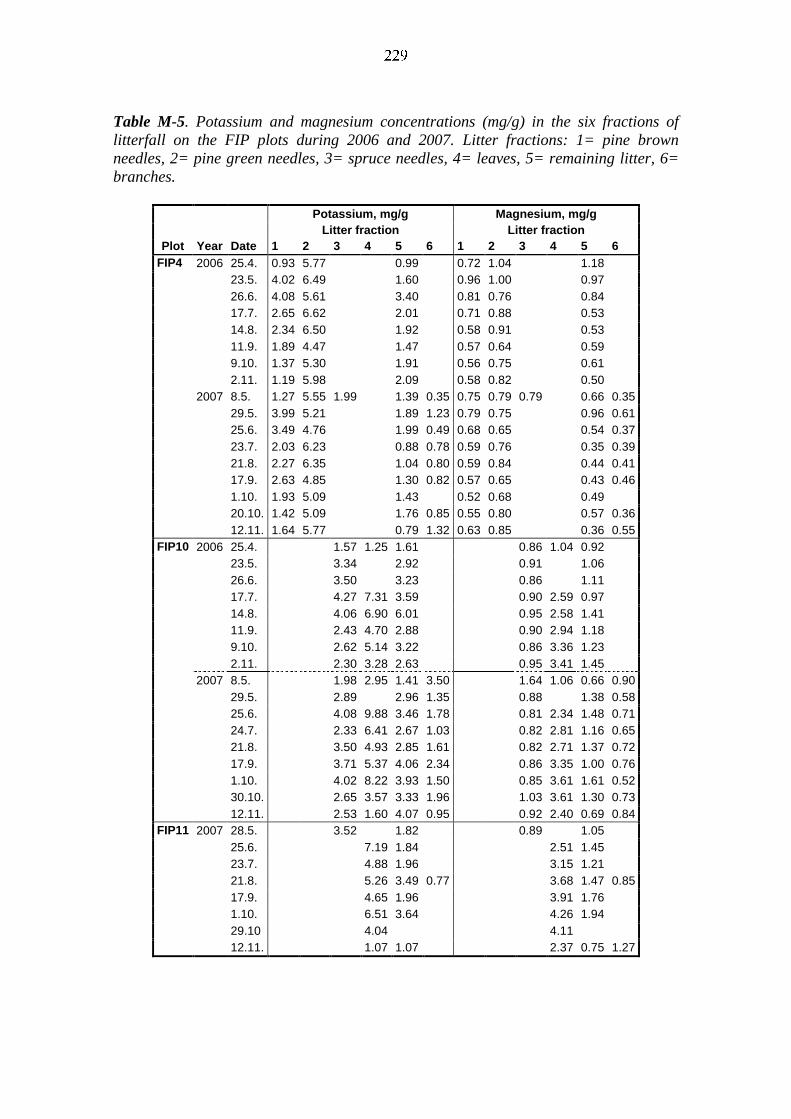
Table M-5. Potassium and magnesium concentrations (mg/g) in the six fractions of
litterfall on the FIP plots during 2006 and 2007. Litter fractions: 1= pine brown
needles, 2= pine green needles, 3= spruce needles, 4= leaves, 5= remaining litter, 6=
branches.
Potassium, mg/g Magnesium, mg/g
Litter fraction Litter fraction
Plot Year Date 1 2 3 4 5 6 1 2 3 4 5 6
FIP4 2006 25.4. 0.93 5.77 0.99 0.72 1.04 1.18
23.5. 4.02 6.49 1.60 0.96 1.00 0.97
26.6. 4.08 5.61 3.40 0.81 0.76 0.84
17.7. 2.65 6.62 2.01 0.71 0.88 0.53
14.8. 2.34 6.50 1.92 0.58 0.91 0.53
11.9. 1.89 4.47 1.47 0.57 0.64 0.59
9.10. 1.37 5.30 1.91 0.56 0.75 0.61
2.11. 1.19 5.98 2.09 0.58 0.82 0.50
2007 8.5. 1.27 5.55 1.99 1.39 0.35 0.75 0.79 0.79 0.66 0.35
29.5. 3.99 5.21 1.89 1.23 0.79 0.75 0.96 0.61
25.6. 3.49 4.76 1.99 0.49 0.68 0.65 0.54 0.37
23.7. 2.03 6.23 0.88 0.78 0.59 0.76 0.35 0.39
21.8. 2.27 6.35 1.04 0.80 0.59 0.84 0.44 0.41
17.9. 2.63 4.85 1.30 0.82 0.57 0.65 0.43 0.46
1.10. 1.93 5.09 1.43 0.52 0.68 0.49
20.10. 1.42 5.09 1.76 0.85 0.55 0.80 0.57 0.36
12.11. 1.64 5.77 0.79 1.32 0.63 0.85 0.36 0.55
FIP10 2006 25.4. 1.57 1.25 1.61 0.86 1.04 0.92
23.5. 3.34 2.92 0.91 1.06
26.6. 3.50 3.23 0.86 1.11
17.7. 4.27 7.31 3.59 0.90 2.59 0.97
14.8. 4.06 6.90 6.01 0.95 2.58 1.41
11.9. 2.43 4.70 2.88 0.90 2.94 1.18
9.10. 2.62 5.14 3.22 0.86 3.36 1.23
2.11. 2.30 3.28 2.63 0.95 3.41 1.45
2007 8.5. 1.98 2.95 1.41 3.50 1.64 1.06 0.66 0.90
29.5. 2.89 2.96 1.35 0.88 1.38 0.58
25.6. 4.08 9.88 3.46 1.78 0.81 2.34 1.48 0.71
24.7. 2.33 6.41 2.67 1.03 0.82 2.81 1.16 0.65
21.8. 3.50 4.93 2.85 1.61 0.82 2.71 1.37 0.72
17.9. 3.71 5.37 4.06 2.34 0.86 3.35 1.00 0.76
1.10. 4.02 8.22 3.93 1.50 0.85 3.61 1.61 0.52
30.10. 2.65 3.57 3.33 1.96 1.03 3.61 1.30 0.73
12.11. 2.53 1.60 4.07 0.95 0.92 2.40 0.69 0.84
FIP11 2007 28.5. 3.52 1.82 0.89 1.05
25.6. 7.19 1.84 2.51 1.45
23.7. 4.88 1.96 3.15 1.21
21.8. 5.26 3.49 0.77 3.68 1.47 0.85
17.9. 4.65 1.96 3.91 1.76
1.10. 6.51 3.64 4.26 1.94
29.10 4.04 4.11
12.11. 1.07 1.07 2.37 0.75 1.27
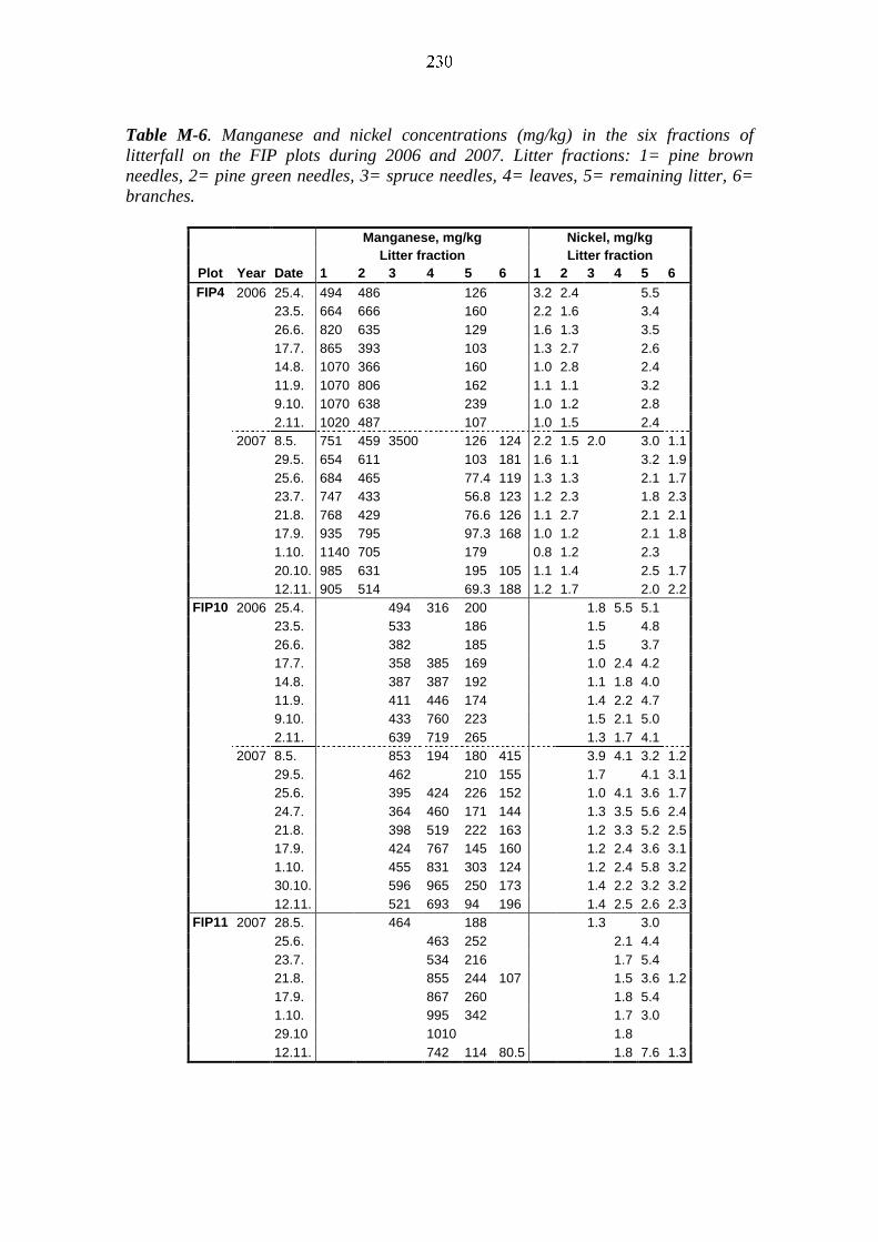
Table M-6. Manganese and nickel concentrations (mg/kg) in the six fractions of
litterfall on the FIP plots during 2006 and 2007. Litter fractions: 1= pine brown
needles, 2= pine green needles, 3= spruce needles, 4= leaves, 5= remaining litter, 6=
branches.
Manganese, mg/kg Nickel, mg/kg
Litter fraction Litter fraction
Plot Year Date 1 2 3 4 5 6 1 2 3 4 5 6
FIP4 2006 25.4. 494 486 126 3.2 2.4 5.5
23.5. 664 666 160 2.2 1.6 3.4
26.6. 820 635 129 1.6 1.3 3.5
17.7. 865 393 103 1.3 2.7 2.6
14.8. 1070 366 160 1.0 2.8 2.4
11.9. 1070 806 162 1.1 1.1 3.2
9.10. 1070 638 239 1.0 1.2 2.8
2.11. 1020 487 107 1.0 1.5 2.4
2007 8.5. 751 459 3500 126 124 2.2 1.5 2.0 3.0 1.1
29.5. 654 611 103 181 1.6 1.1 3.2 1.9
25.6. 684 465 77.4 119 1.3 1.3 2.1 1.7
23.7. 747 433 56.8 123 1.2 2.3 1.8 2.3
21.8. 768 429 76.6 126 1.1 2.7 2.1 2.1
17.9. 935 795 97.3 168 1.0 1.2 2.1 1.8
1.10. 1140 705 179 0.8 1.2 2.3
20.10. 985 631 195 105 1.1 1.4 2.5 1.7
12.11. 905 514 69.3 188 1.2 1.7 2.0 2.2
FIP10 2006 25.4. 494 316 200 1.8 5.5 5.1
23.5. 533 186 1.5 4.8
26.6. 382 185 1.5 3.7
17.7. 358 385 169 1.0 2.4 4.2
14.8. 387 387 192 1.1 1.8 4.0
11.9. 411 446 174 1.4 2.2 4.7
9.10. 433 760 223 1.5 2.1 5.0
2.11. 639 719 265 1.3 1.7 4.1
2007 8.5. 853 194 180 415 3.9 4.1 3.2 1.2
29.5. 462 210 155 1.7 4.1 3.1
25.6. 395 424 226 152 1.0 4.1 3.6 1.7
24.7. 364 460 171 144 1.3 3.5 5.6 2.4
21.8. 398 519 222 163 1.2 3.3 5.2 2.5
17.9. 424 767 145 160 1.2 2.4 3.6 3.1
1.10. 455 831 303 124 1.2 2.4 5.8 3.2
30.10. 596 965 250 173 1.4 2.2 3.2 3.2
12.11. 521 693 94 196 1.4 2.5 2.6 2.3
FIP11 2007 28.5. 464 188 1.3 3.0
25.6. 463 252 2.1 4.4
23.7. 534 216 1.7 5.4
21.8. 855 244 107 1.5 3.6 1.2
17.9. 867 260 1.8 5.4
1.10. 995 342 1.7 3.0
29.10 1010 1.8
12.11. 742 114 80.5 1.8 7.6 1.3
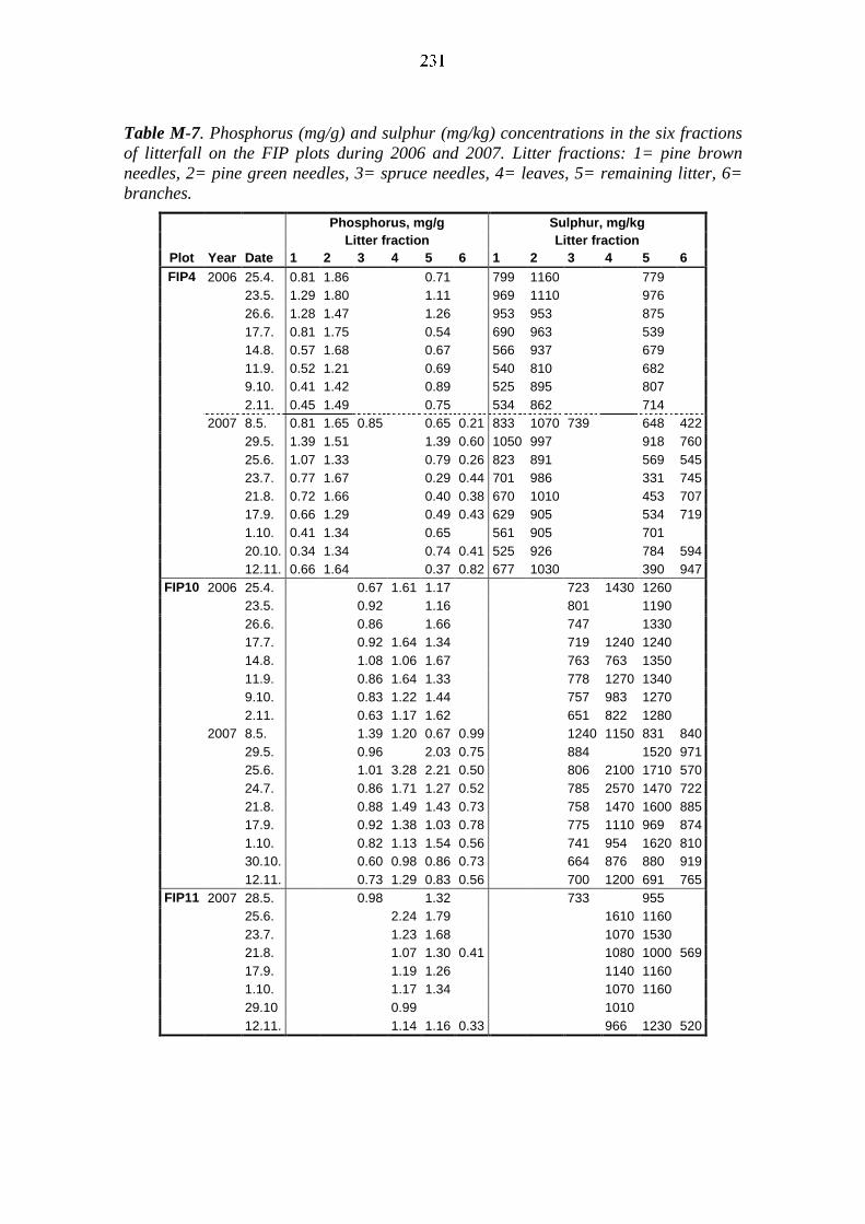
Table M-7. Phosphorus (mg/g) and sulphur (mg/kg) concentrations in the six fractions
of litterfall on the FIP plots during 2006 and 2007. Litter fractions: 1= pine brown
needles, 2= pine green needles, 3= spruce needles, 4= leaves, 5= remaining litter, 6=
branches.
Phosphorus, mg/g Sulphur, mg/kg
Litter fraction Litter fraction
Plot Year Date 1 2 3 4 5 6 1 2 3 4 5 6
FIP4 2006 25.4. 0.81 1.86 0.71 799 1160 779
23.5. 1.29 1.80 1.11 969 1110 976
26.6. 1.28 1.47 1.26 953 953 875
17.7. 0.81 1.75 0.54 690 963 539
14.8. 0.57 1.68 0.67 566 937 679
11.9. 0.52 1.21 0.69 540 810 682
9.10. 0.41 1.42 0.89 525 895 807
2.11. 0.45 1.49 0.75 534 862 714
2007 8.5. 0.81 1.65 0.85 0.65 0.21 833 1070 739 648 422
29.5. 1.39 1.51 1.39 0.60 1050 997 918 760
25.6. 1.07 1.33 0.79 0.26 823 891 569 545
23.7. 0.77 1.67 0.29 0.44 701 986 331 745
21.8. 0.72 1.66 0.40 0.38 670 1010 453 707
17.9. 0.66 1.29 0.49 0.43 629 905 534 719
1.10. 0.41 1.34 0.65 561 905 701
20.10. 0.34 1.34 0.74 0.41 525 926 784 594
12.11. 0.66 1.64 0.37 0.82 677 1030 390 947
FIP10 2006 25.4. 0.67 1.61 1.17 723 1430 1260
23.5. 0.92 1.16 801 1190
26.6. 0.86 1.66 747 1330
17.7. 0.92 1.64 1.34 719 1240 1240
14.8. 1.08 1.06 1.67 763 763 1350
11.9. 0.86 1.64 1.33 778 1270 1340
9.10. 0.83 1.22 1.44 757 983 1270
2.11. 0.63 1.17 1.62 651 822 1280
2007 8.5. 1.39 1.20 0.67 0.99 1240 1150 831 840
29.5. 0.96 2.03 0.75 884 1520 971
25.6. 1.01 3.28 2.21 0.50 806 2100 1710 570
24.7. 0.86 1.71 1.27 0.52 785 2570 1470 722
21.8. 0.88 1.49 1.43 0.73 758 1470 1600 885
17.9. 0.92 1.38 1.03 0.78 775 1110 969 874
1.10. 0.82 1.13 1.54 0.56 741 954 1620 810
30.10. 0.60 0.98 0.86 0.73 664 876 880 919
12.11. 0.73 1.29 0.83 0.56 700 1200 691 765
FIP11 2007 28.5. 0.98 1.32 733 955
25.6. 2.24 1.79 1610 1160
23.7. 1.23 1.68 1070 1530
21.8. 1.07 1.30 0.41 1080 1000 569
17.9. 1.19 1.26 1140 1160
1.10. 1.17 1.34 1070 1160
29.10 0.99 1010
12.11. 1.14 1.16 0.33 966 1230 520
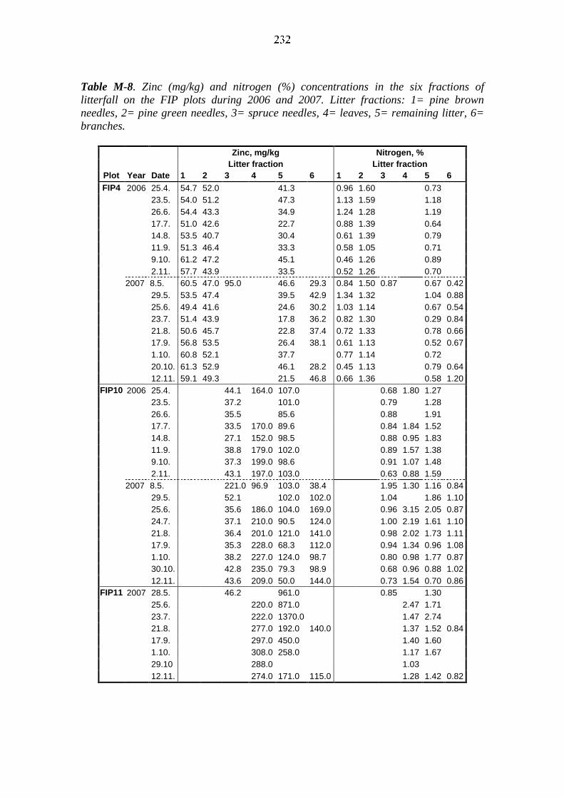
Table M-8. Zinc (mg/kg) and nitrogen (%) concentrations in the six fractions of
litterfall on the FIP plots during 2006 and 2007. Litter fractions: 1= pine brown
needles, 2= pine green needles, 3= spruce needles, 4= leaves, 5= remaining litter, 6=
branches.
Zinc, mg/kg Nitrogen, %
Litter fraction Litter fraction
Plot Year Date 1 2 3 4 5 6 1 2 3 4 5 6
FIP4 2006 25.4. 54.7 52.0 41.3 0.96 1.60 0.73
23.5. 54.0 51.2 47.3 1.13 1.59 1.18
26.6. 54.4 43.3 34.9 1.24 1.28 1.19
17.7. 51.0 42.6 22.7 0.88 1.39 0.64
14.8. 53.5 40.7 30.4 0.61 1.39 0.79
11.9. 51.3 46.4 33.3 0.58 1.05 0.71
9.10. 61.2 47.2 45.1 0.46 1.26 0.89
2.11. 57.7 43.9 33.5 0.52 1.26 0.70
2007 8.5. 60.5 47.0 95.0 46.6 29.3 0.84 1.50 0.87 0.67 0.42
29.5. 53.5 47.4 39.5 42.9 1.34 1.32 1.04 0.88
25.6. 49.4 41.6 24.6 30.2 1.03 1.14 0.67 0.54
23.7. 51.4 43.9 17.8 36.2 0.82 1.30 0.29 0.84
21.8. 50.6 45.7 22.8 37.4 0.72 1.33 0.78 0.66
17.9. 56.8 53.5 26.4 38.1 0.61 1.13 0.52 0.67
1.10. 60.8 52.1 37.7 0.77 1.14 0.72
20.10. 61.3 52.9 46.1 28.2 0.45 1.13 0.79 0.64
12.11. 59.1 49.3 21.5 46.8 0.66 1.36 0.58 1.20
FIP10 2006 25.4. 44.1 164.0 107.0 0.68 1.80 1.27
23.5. 37.2 101.0 0.79 1.28
26.6. 35.5 85.6 0.88 1.91
17.7. 33.5 170.0 89.6 0.84 1.84 1.52
14.8. 27.1 152.0 98.5 0.88 0.95 1.83
11.9. 38.8 179.0 102.0 0.89 1.57 1.38
9.10. 37.3 199.0 98.6 0.91 1.07 1.48
2.11. 43.1 197.0 103.0 0.63 0.88 1.59
2007 8.5. 221.0 96.9 103.0 38.4 1.95 1.30 1.16 0.84
29.5. 52.1 102.0 102.0 1.04 1.86 1.10
25.6. 35.6 186.0 104.0 169.0 0.96 3.15 2.05 0.87
24.7. 37.1 210.0 90.5 124.0 1.00 2.19 1.61 1.10
21.8. 36.4 201.0 121.0 141.0 0.98 2.02 1.73 1.11
17.9. 35.3 228.0 68.3 112.0 0.94 1.34 0.96 1.08
1.10. 38.2 227.0 124.0 98.7 0.80 0.98 1.77 0.87
30.10. 42.8 235.0 79.3 98.9 0.68 0.96 0.88 1.02
12.11. 43.6 209.0 50.0 144.0 0.73 1.54 0.70 0.86
FIP11 2007 28.5. 46.2 961.0 0.85 1.30
25.6. 220.0 871.0 2.47 1.71
23.7. 222.0 1370.0 1.47 2.74
21.8. 277.0 192.0 140.0 1.37 1.52 0.84
17.9. 297.0 450.0 1.40 1.60
1.10. 308.0 258.0 1.17 1.67
29.10 288.0 1.03
12.11. 274.0 171.0 115.0 1.28 1.42 0.82
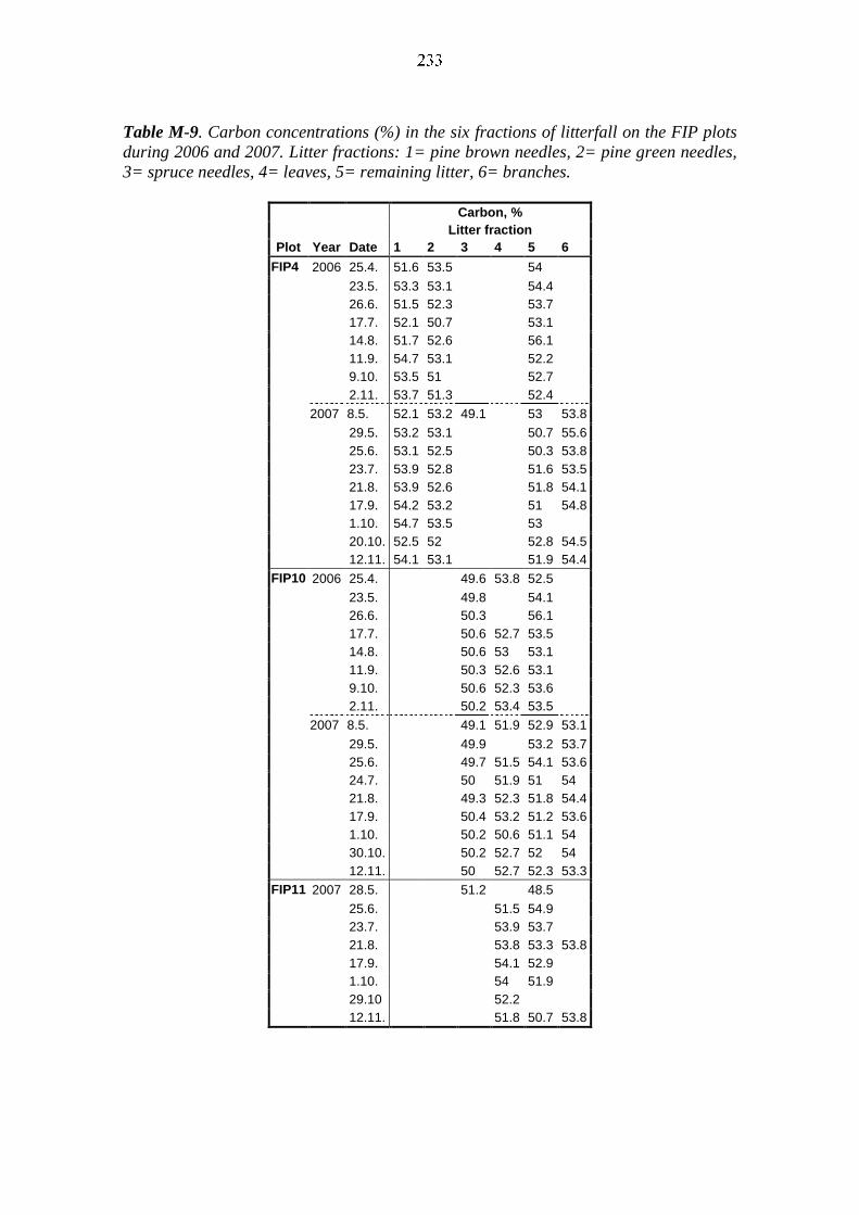
Table M-9. Carbon concentrations (%) in the six fractions of litterfall on the FIP plots
during 2006 and 2007. Litter fractions: 1= pine brown needles, 2= pine green needles,
3= spruce needles, 4= leaves, 5= remaining litter, 6= branches.
Carbon, %
Litter fraction
Plot Year Date 1 2 3 4 5 6
FIP4 2006 25.4. 51.6 53.5 54
23.5. 53.3 53.1 54.4
26.6. 51.5 52.3 53.7
17.7. 52.1 50.7 53.1
14.8. 51.7 52.6 56.1
11.9. 54.7 53.1 52.2
9.10. 53.5 51 52.7
2.11. 53.7 51.3 52.4
2007 8.5. 52.1 53.2 49.1 53 53.8
29.5. 53.2 53.1 50.7 55.6
25.6. 53.1 52.5 50.3 53.8
23.7. 53.9 52.8 51.6 53.5
21.8. 53.9 52.6 51.8 54.1
17.9. 54.2 53.2 51 54.8
1.10. 54.7 53.5 53
20.10. 52.5 52 52.8 54.5
12.11. 54.1 53.1 51.9 54.4
FIP10 2006 25.4. 49.6 53.8 52.5
23.5. 49.8 54.1
26.6. 50.3 56.1
17.7. 50.6 52.7 53.5
14.8. 50.6 53 53.1
11.9. 50.3 52.6 53.1
9.10. 50.6 52.3 53.6
2.11. 50.2 53.4 53.5
2007 8.5. 49.1 51.9 52.9 53.1
29.5. 49.9 53.2 53.7
25.6. 49.7 51.5 54.1 53.6
24.7. 50 51.9 51 54
21.8. 49.3 52.3 51.8 54.4
17.9. 50.4 53.2 51.2 53.6
1.10. 50.2 50.6 51.1 54
30.10. 50.2 52.7 52 54
12.11. 50 52.7 52.3 53.3
FIP11 2007 28.5. 51.2 48.5
25.6. 51.5 54.9
23.7. 53.9 53.7
21.8. 53.8 53.3 53.8
17.9. 54.1 52.9
1.10. 54 51.9
29.10 52.2
12.11. 51.8 50.7 53.8

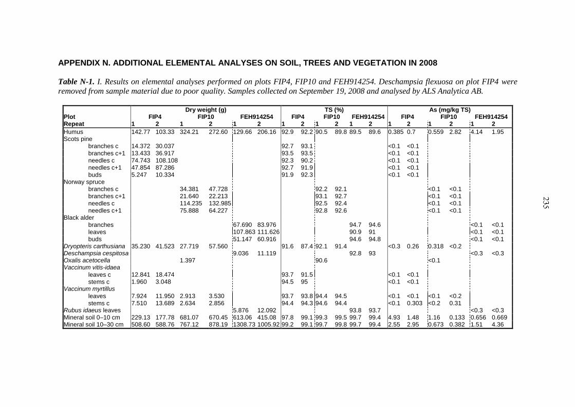
APPENDIX N. ADDITIONAL ELEMENTAL ANALYSES ON SOIL, TREES AND VEGETATION IN 2008
Table N-1. I. Results on elemental analyses performed on plots FIP4, FIP10 and FEH914254. Deschampsia flexuosa on plot FIP4 were
removed from sample material due to poor quality. Samples collected on September 19, 2008 and analysed by ALS Analytica AB.
Dry weight (g) TS (%) As (mg/kg TS) Plot FIP4 FIP10 FEH914254 FIP4 FIP10 FEH914254 FIP4 FIP10 FEH914254 Repeat 1 2 1 2 1 2 1 2 1 2 1 2 1 2 1 2 1 2
Humus 142.77 103.33 324.21 272.60 129.66 206.16 92.9 92.2 90.5 89.8 89.5 89.6 0.385 0.7 0.559 2.82 4.14 1.95 Scots pine
branches c 14.372 30.037 92.7 93.1 <0.1 <0.1
branches c+1 13.433 36.917 93.5 93.5 <0.1 <0.1
needles c 74.743 108.108 92.3 90.2 <0.1 <0.1 needles c+1 47.854 87.286 92.7 91.9 <0.1 <0.1
buds 5.247 10.334 91.9 92.3 <0.1 <0.1 Norway spruce
branches c 34.381 47.728 92.2 92.1 <0.1 <0.1 branches c+1 21.640 22.213 93.1 92.7 <0.1 <0.1
needles c 114.235 132.985 92.5 92.4 <0.1 <0.1
needles c+1 75.888 64.227 92.8 92.6 <0.1 <0.1 Black alder
branches 67.690 83.976 94.7 94.6 <0.1 <0.1
leaves 107.863 111.626 90.9 91 <0.1 <0.1
buds 51.147 60.916 94.6 94.8 <0.1 <0.1 Dryopteris carthusiana 35.230 41.523 27.719 57.560 91.6 87.4 92.1 91.4 <0.3 0.26 0.318 <0.2 Deschampsia cespitosa 9.036 11.119 92.8 93 <0.3 <0.3 Oxalis acetocella 1.397 90.6 <0.1 Vaccinum vitis-idaea
leaves c 12.841 18.474 93.7 91.5 <0.1 <0.1
stems c 1.960 3.048 94.5 95 <0.1 <0.1 Vaccinum myrtillus
leaves 7.924 11.950 2.913 3.530 93.7 93.8 94.4 94.5 <0.1 <0.1 <0.1 <0.2
stems c 7.510 13.689 2.634 2.856 94.4 94.3 94.6 94.4 <0.1 0.303 <0.2 0.31 Rubus idaeus leaves 5.876 12.092 93.8 93.7 <0.3 <0.3 Mineral soil 0–10 cm 229.13 177.78 681.07 670.45 613.06 415.08 97.8 99.1 99.3 99.5 99.7 99.4 4.93 1.48 1.16 0.133 0.656 0.669 Mineral soil 10–30 cm 508.60 588.76 767.12 878.19 1308.73 1005.92 99.2 99.1 99.7 99.8 99.7 99.4 2.55 2.95 0.673 0.382 1.51 4.36
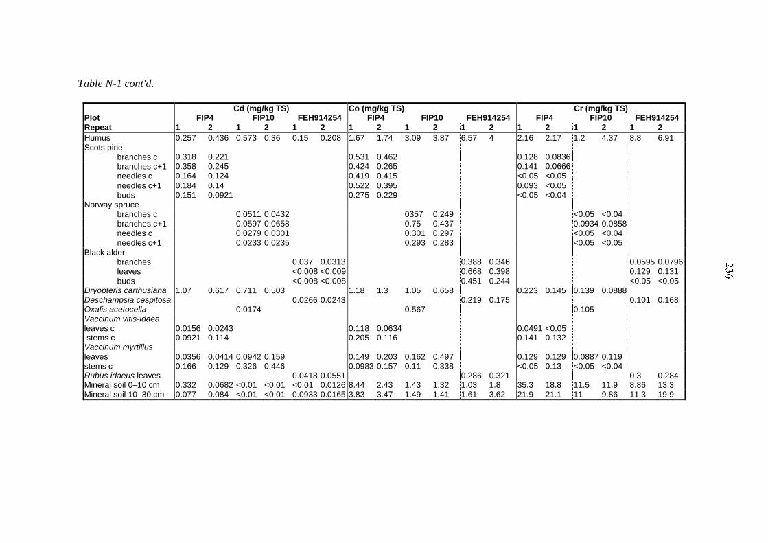
Table N-1 cont'd.
Cd (mg/kg TS) Co (mg/kg TS) Cr (mg/kg TS) Plot FIP4 FIP10 FEH914254 FIP4 FIP10 FEH914254 FIP4 FIP10 FEH914254 Repeat 1 2 1 2 1 2 1 2 1 2 1 2 1 2 1 2 1 2
Humus 0.257 0.436 0.573 0.36 0.15 0.208 1.67 1.74 3.09 3.87 6.57 4 2.16 2.17 1.2 4.37 8.8 6.91 Scots pine
branches c 0.318 0.221 0.531 0.462 0.128 0.0836
branches c+1 0.358 0.245 0.424 0.265 0.141 0.0666
needles c 0.164 0.124 0.419 0.415 <0.05 <0.05
needles c+1 0.184 0.14 0.522 0.395 0.093 <0.05
buds 0.151 0.0921 0.275 0.229 <0.05 <0.04 Norway spruce
branches c 0.0511 0.0432 0357 0.249 <0.05 <0.04
branches c+1 0.0597 0.0658 0.75 0.437 0.0934 0.0858
needles c 0.0279 0.0301 0.301 0.297 <0.05 <0.04
needles c+1 0.0233 0.0235 0.293 0.283 <0.05 <0.05
Black alder branches 0.037 0.0313 0.388 0.346 0.0595 0.0796
leaves <0.008 <0.009 0.668 0.398 0.129 0.131
buds <0.008 <0.008 0.451 0.244 <0.05 <0.05 Dryopteris carthusiana 1.07 0.617 0.711 0.503 1.18 1.3 1.05 0.658 0.223 0.145 0.139 0.0888 Deschampsia cespitosa 0.0266 0.0243 0.219 0.175 0.101 0.168 Oxalis acetocella 0.0174 0.567 0.105 Vaccinum vitis-idaea leaves c 0.0156 0.0243 0.118 0.0634 0.0491 <0.05 stems c 0.0921 0.114 0.205 0.116 0.141 0.132 Vaccinum myrtillus leaves 0.0356 0.0414 0.0942 0.159 0.149 0.203 0.162 0.497 0.129 0.129 0.0887 0.119 stems c 0.166 0.129 0.326 0.446 0.0983 0.157 0.11 0.338 <0.05 0.13 <0.05 <0.04 Rubus idaeus leaves 0.0418 0.0551 0.286 0.321 0.3 0.284 Mineral soil 0–10 cm 0.332 0.0682 <0.01 <0.01 <0.01 0.0126 8.44 2.43 1.43 1.32 1.03 1.8 35.3 18.8 11.5 11.9 8.86 13.3 Mineral soil 10–30 cm 0.077 0.084 <0.01 <0.01 0.0933 0.0165 3.83 3.47 1.49 1.41 1.61 3.62 21.9 21.1 11 9.86 11.3 19.9

Table N-1 cont'd.
Cu (mg/kg TS) Hg (kg/mg TS) Mn (mg/kg TS) Plot FIP4 FIP10 FEH914254 FIP4 FIP10 FEH914254 FIP4 FIP10 FEH914254 Repeat 1 2 1 2 1 2 1 2 1 2 1 2 1 2 1 2 1 2
Humus 12.8 14.7 21.4 44.1 63.3 57.3 0.192 0.217 0.32 0.339 0.147 0.106 1130 1200 153 17.5 56.6 38.5 Scots pine
branches c 3.88 4.85 <0.02 <0.01 187 136
branches c+1 4.53 4.36 <0.01 <0.02 191 189
needles c 2.7 3.35 <0.02 <0.02 499 467
needles c+1 2.71 2.46 0.0256 0.0277 895 730
buds 3.24 4.26 <0.02 <0.01 165 136 Norway spruce
branches c 3.81 4.09 <0.02 <0.01 156 129
branches c+1 4.32 6.5 <0.02 <0.01 153 141
needles c 2.11 2.29 <0.02 <0.01 252 244
needles c+1 1.75 2.05 0.0233 0.0243 278 302
Black alder branches 12.3 9.24 <0.02 <0.02 156 109
leaves 13.2 10.7 0.0213 0.0301 269 121
buds 17.5 13.5 <0.02 <0.02 112 60.3 Dryopteris carthusiana 6.99 6.06 4.8 5.56 0.0612 0.0585 0.0575 0.0591 3510 1920 1800 1220 Deschampsia cespitosa 8.59 6.36 0.0182 0.0214 116 67.9 Oxalis acetocella 3.53 0.0187 515 Vaccinum vitis-idaea
leaves c 3.31 3.38 <0.02 <0.02 2100 1890
stems c 5.02 3.89 <0.02 <0.02 1340 943 Vaccinum myrtillus
leaves 5.31 4.8 5.09 5.93 0.0178 0.0215 0.0261 0.0214 8740 3910 2040 2880
stems c 5.33 6.11 5.9 6.69 <0.02 <0.02 <0.02 <0.01 2850 2330 1790 2020 Rubus idaeus leaves 9.11 7.96 0.0317 0.0253 194 235 Mineral soil 0–10 cm 38 6.85 2.52 3.33 3.11 5.87 1.103 <0.04 <0.04 <0.04 <0.04 <0.04 Mineral soil 10–30 cm 6.42 7.52 2.25 2.65 4.56 8.58 <0.04 <0.04 <0.04 <0.04 <0.04 <0.04
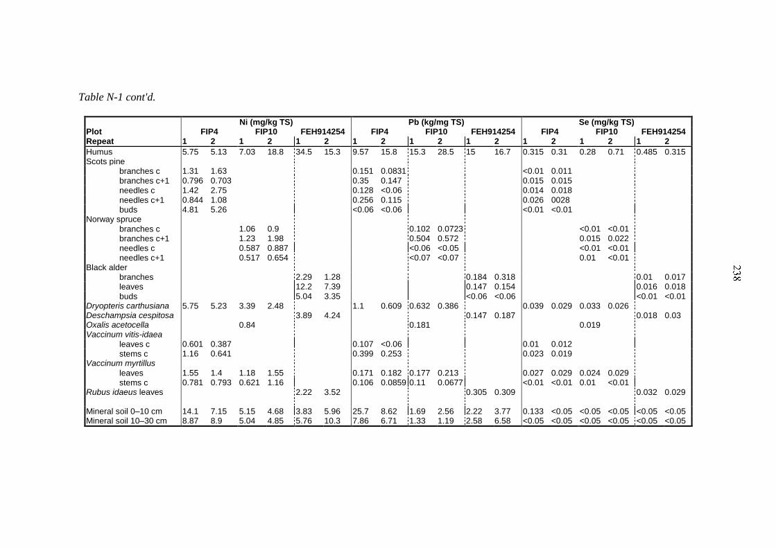
Table N-1 cont'd.
Ni (mg/kg TS) Pb (kg/mg TS) Se (mg/kg TS) Plot FIP4 FIP10 FEH914254 FIP4 FIP10 FEH914254 FIP4 FIP10 FEH914254 Repeat 1 2 1 2 1 2 1 2 1 2 1 2 1 2 1 2 1 2
Humus 5.75 5.13 7.03 18.8 34.5 15.3 9.57 15.8 15.3 28.5 15 16.7 0.315 0.31 0.28 0.71 0.485 0.315 Scots pine
branches c 1.31 1.63 0.151 0.0831 <0.01 0.011
branches c+1 0.796 0.703 0.35 0.147 0.015 0.015
needles c 1.42 2.75 0.128 <0.06 0.014 0.018
needles c+1 0.844 1.08 0.256 0.115 0.026 0028
buds 4.81 5.26 <0.06 <0.06 <0.01 <0.01 Norway spruce
branches c 1.06 0.9 0.102 0.0723 <0.01 <0.01
branches c+1 1.23 1.98 0.504 0.572 0.015 0.022
needles c 0.587 0.887 <0.06 <0.05 <0.01 <0.01
needles c+1 0.517 0.654 <0.07 <0.07 0.01 <0.01
Black alder branches 2.29 1.28 0.184 0.318 0.01 0.017
leaves 12.2 7.39 0.147 0.154 0.016 0.018
buds 5.04 3.35 <0.06 <0.06 <0.01 <0.01 Dryopteris carthusiana 5.75 5.23 3.39 2.48 1.1 0.609 0.632 0.386 0.039 0.029 0.033 0.026 Deschampsia cespitosa 3.89 4.24 0.147 0.187 0.018 0.03 Oxalis acetocella 0.84 0.181 0.019 Vaccinum vitis-idaea
leaves c 0.601 0.387 0.107 <0.06 0.01 0.012
stems c 1.16 0.641 0.399 0.253 0.023 0.019 Vaccinum myrtillus
leaves 1.55 1.4 1.18 1.55 0.171 0.182 0.177 0.213 0.027 0.029 0.024 0.029
stems c 0.781 0.793 0.621 1.16 0.106 0.0859 0.11 0.0677 <0.01 <0.01 0.01 <0.01 Rubus idaeus leaves
2.22 3.52 0.305 0.309 0.032 0.029
Mineral soil 0–10 cm 14.1 7.15 5.15 4.68 3.83 5.96 25.7 8.62 1.69 2.56 2.22 3.77 0.133 <0.05 <0.05 <0.05 <0.05 <0.05 Mineral soil 10–30 cm 8.87 8.9 5.04 4.85 5.76 10.3 7.86 6.71 1.33 1.19 2.58 6.58 <0.05 <0.05 <0.05 <0.05 <0.05 <0.05

Table N-1 cont'd.
Zn (mg/kg TS) I (kg/mg TS) V (mg/kg TS) Plot FIP4 FIP10 FEH914254 FIP4 FIP10 FEH914254 FIP4 FIP10 FEH914254 Repeat 1 2 1 2 1 2 1 2 1 2 1 2
Humus 85 55.5 67.4 20 17.5 21 2.39 2.72 3.91 8.51 6.83 5.15 Scots pine
branches c 35.5 28.1 0.14 0.12
branches c+1 30.8 25.1 0.16 0.09
needles c 31 41.6 0.14 0.11
needles c+1 42.9 44.1 0.2 0.16
buds 24.9 27.4 <0.05 0.08 Norway spruce
branches c 47.6 41 0.1 0.08
branches c+1 73 69.4 0.15 0.21
needles c 35.3 36.3 0.13 0.11
needles c+1 29.9 32.5 0.12 0.1
Black alder branches 42.8 31.6 0.16 0.21
leaves 34.8 29.1 0.648 0.618
buds 28.4 23.4 <0.05 0.1 Dryopteris carthusiana 217 149 120 91.2 0.53 0.418 0.312 0.415 Deschampsia cespitosa 17.8 20 0.372 0.374 Oxalis acetocella 20.6 0.361 Vaccinum vitis-idaea
leaves c 21.7 24.3 0.13 0.15
stems c 21 19.1 0.13 0.13 Vaccinum myrtillus
leaves 13.9 11.6 19.4 17.7 0.293 0.288 0.311 0.305
stems c 44.2 31.3 52.5 37 0.06 0.08 0.06 0.05 Rubus idaeus 29.1 22.5 0.822 0.642 Mineral soil 0–10 cm 89.6 27.3 12.2 12.5 12.5 15.9 4.6 <2 2.87 <2 <2 2.22 40.8 21.5 13.5 10.9 8.02 11.2 Mineral soil 10–30 cm 37.7 30.5 13.2 14.1 14.1 28.8 <2 <2 <2 <2 <2 <2 16 21.7 9.58 8.52 11.1 20.3

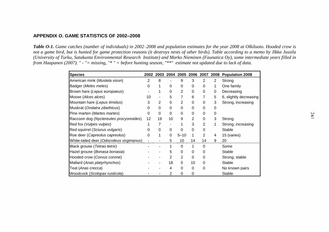
APPENDIX O. GAME STATISTICS OF 2002–2008
Table O-1. Game catches (number of individuals) in 2002–2008 and population estimates for the year 2008 at Olkiluoto. Hooded crow is
not a game bird, but is hunted for game protection reasons (it destroys nests of other birds). Table according to a memo by Ilkka Jussila
(University of Turku, Satakunta Environmental Research Institute) and Marko Nieminen (Faunatica Oy), some intermediate years filled in
from Haapanen (2007). " - "= missing, "* " = before hunting season, "**" estimate not updated due to lack of data.
Species 2002 2003 2004 2005 2006 2007 2008 Population 2008
American mink (Mustela vison) 2 8 - 9 3 2 2 Strong
Badger (Meles meles) 0 1 0 0 0 0 1 One family
Brown hare (Lepus europaeus) - 1 0 2 0 0 0 Decreasing
Moose (Alces alces) 10 - 5 7 6 7 5 6, slightly decreasing
Mountain hare (Lepus timidus) 3 2 0 2 0 0 3 Strong, increasing
Muskrat (Ondatra zibethicus) 0 0 0 0 0 0 0
Pine marten (Martes martes) 0 0 0 0 0 0 0
Raccoon dog (Nyctereutes procyonoides) 12 19 10 9 2 0 3 Strong
Red fox (Vulpes vulpes) 1 7 - 1 3 2 1 Strong, increasing
Red squirrel (Sciurus vulgaris) 0 0 0 0 0 0 Stable
Roe deer (Capreolus capreolus) 0 1 0 5–10 1 2 4 15 (varies)
White-tailed deer (Odocoileus virginianus) - - 5 10 14 14 9 20
Black grouse (Tetrao tetrix) - - 1 0 1 0 Some
Hazel grouse (Bonasa bonasia) - - 5 0 0 0 Stable
Hooded crow (Corvus corone) - - 2 2 0 0 Strong, stable
Mallard (Anas platyrhynchos) - - 18 5 10 0 Stable
Teal (Anas crecca) - - 4 0 0 0 No known pairs
Woodcock (Scolopax rusticola) - - 2 0 0 Stable

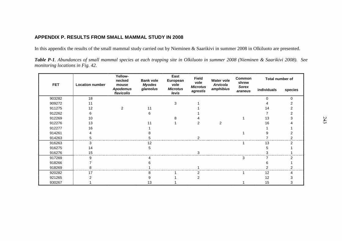
APPENDIX P. RESULTS FROM SMALL MAMMAL STUDY IN 2008 In this appendix the results of the small mammal study carried out by Nieminen & Saarikivi in summer 2008 in Olkiluoto are presented.
Table P-1. Abundances of small mammal species at each trapping site in Olkiluoto in summer 2008 (Nieminen & Saarikivi 2008). See
monitoring locations in Fig. 42.
FET Location number
Yellow-necked mouse
Apodemus flavicolis
Bank vole Myodes
glareolus
East European
vole Microtus
levis
Field vole
Microtus agrestis
Water vole Arvicola
amphibius
Common shrew Sorex
araneus
Total number of
individuals species
903282 18 0 0
909272 11 3 1 4 2
911275 12 2 11 1 14 2
912262 6 6 1 7 2
912269 10 8 4 1 13 3
912276 13 11 1 2 2 16 4
912277 16 1 1 1
914261 4 8 1 9 2
914263 5 5 2 7 2
916263 3 12 1 13 2
916275 14 5 5 1
916276 15 3 3 1
917269 9 4 3 7 2
918266 7 6 6 1
918269 8 1 1 2 2
920282 17 8 1 2 1 12 4
921265 2 9 1 2 12 3
930267 1 13 1 1 15 3

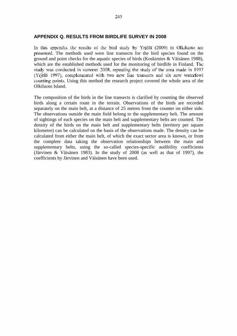
APPENDIX Q. RESULTS FROM BIRDLIFE SURVEY IN 2008
The methods used were line transects for the bird species found on the
ground and point checks for the aquatic species of birds (Koskimies & Väisänen 1988),
which are the established methods used for the monitoring of birdlife in Finland.
Using this method the research project covered the whole area of the
Olkiluoto Island.
The composition of the birds in the line transects is clarified by counting the observed
birds along a certain route in the terrain. Observations of the birds are recorded
separately on the main belt, at a distance of 25 metres from the counter on either side.
The observations outside the main field belong to the supplementary belt. The amount
of sightings of each species on the main belt and supplementary belts are counted. The
density of the birds on the main belt and supplementary belts (territory per square
kilometre) can be calculated on the basis of the observations made. The density can be
calculated from either the main belt, of which the exact sector area is known, or from
the complete data taking the observation relationships between the main and
supplementary belts, using the so-called species-specific audibility coefficients
(Järvinen & Väisänen 1983). In the study of 2008 (as well as that of 1997), the
coefficients by Järvinen and Väisänen have been used.

Table Q-1. Results of line transect census for landbirds of summer 2008 (Yrjölä 2009). D = species belongs to protected species mentioned
in the appendix 1 of the EU bird directive, VU = species according to the Finnish national classification for endangered species
(vulnerable), NT = species to be monitored in the Finnish classification as near endangered. See monitoring locations in Fig. 43.
Name Scientific name Main belt Supplementary
belt Total Density
(pairs/km2)
Grey heron Ardea cinerea 2 2 0.075
Common buzzard Buteo buteo 2 2 0.313
Hazel grouse D Bonasa bonasia 1 3 4 2.236
Black grouse D, NT Tetrao tetrix 1 1 0.140
Common crane D Grus grus 2 2 0.027
Little ringed plover Charadrius dubius 1 2 3 0.808
Common redshank Tringa totanus 1 1 2 0.155
Green sandpiper Tringa ochropus 1 1 0.138
Common sandpiper Actitis hypoleucos 3 3 0.505
Wood pigeon Columba palumbus 6 17 23 1.213
Eurasian cuckoo NT Cuculus canorus 5 5 0.147
Tawny owl Strix aluco 1 1 0.301
Common swift Apus apus 1 1 0.029
Eurasian wryneck VU Jynx torquilla 1 1 0.088
Black woodpecker D Drycopus martius 2 5 7 0.237
Great spotted woodpecker Denrocopos major 3 10 13 2.415
Lesser spotted woodpecker VU Denrocopos minor 1 1 0.201
Barn swallow Hirundo rustica 3 8 11 1.159
House martin Delichon urbica 10 10 1.491
Tree pipit Anthus trivialis 4 21 25 3.778
Pied wagtail Motacilla alba 13 6 20 5.786
Winter wren Troglodytes troglodytes 1 3 4 0.773
Hedge accentor Prunella modularis 4 10 14 2.074

Table Q-1 cont'd.
Name Scientific name Main belt
Supplementary belt Total
Density (pairs/km
2)
Robin Erithacus rubecula 9 36 45 10.205
Thrush nightingale Luscinia luscinia 5 5 0.394
Common redstart Phoenicurus phoenicurus 1 1 0.133
Norhern wheatear NT Oenanthe oenanthe 4 2 6 1.892
Blackbird Turdus merula 13 30 43 6.890
Fieldfare Turdus pilaris 1 7 8 1.629
Song thrush Turdus philomelos 4 30 34 4.555
Redwing Turdus iliacus 8 16 25 4.626
Sedge warbler Acrocephalus schoenopaenus
1 4 5 4.626
Blyth’s reed warbler Acrocephalus dumetorum 2 2 0.441
Marsh warbler Acrocephalus palustris 1 1 0.412
Icterine warbler Hippolais icterina 1 4 5 1.252
Lesser whitethroat Sylvia curruca 8 14 22 4.348
Common whitethroat Sylvia communis 6 12 18 3.649
Garden warbler Sylvia borin 5 36 41 5.743
Blackap Sylvia atricapilla 5 20 25 4.057
Common chiffchaff VU Phylloscopus collybita 3 9 12 1.390
Willow warbler Phylloscopus trochilus 64 202 266 39.774
Goldcrest Regulus regulus 5 18 23 6.858
Spotted flycatcher Muscicapa striata 14 5 19 6.948
Red breasted flycatcher D, NT Ficedula parva 1 1 0.249
Pied flycatcher Ficedula hypoleuca 2 15 17 3.573
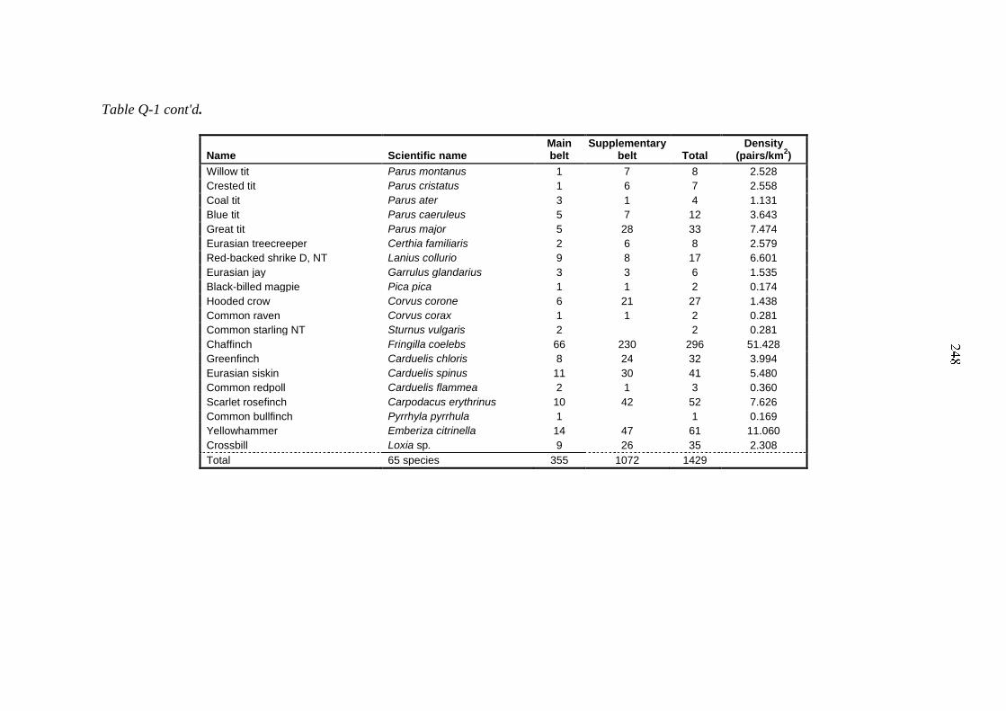
Table Q-1 cont'd.
Name Scientific name Main belt
Supplementary belt Total
Density (pairs/km
2)
Willow tit Parus montanus 1 7 8 2.528
Crested tit Parus cristatus 1 6 7 2.558
Coal tit Parus ater 3 1 4 1.131
Blue tit Parus caeruleus 5 7 12 3.643
Great tit Parus major 5 28 33 7.474
Eurasian treecreeper Certhia familiaris 2 6 8 2.579
Red-backed shrike D, NT Lanius collurio 9 8 17 6.601
Eurasian jay Garrulus glandarius 3 3 6 1.535
Black-billed magpie Pica pica 1 1 2 0.174
Hooded crow Corvus corone 6 21 27 1.438
Common raven Corvus corax 1 1 2 0.281
Common starling NT Sturnus vulgaris 2 2 0.281
Chaffinch Fringilla coelebs 66 230 296 51.428
Greenfinch Carduelis chloris 8 24 32 3.994
Eurasian siskin Carduelis spinus 11 30 41 5.480
Common redpoll Carduelis flammea 2 1 3 0.360
Scarlet rosefinch Carpodacus erythrinus 10 42 52 7.626
Common bullfinch Pyrrhyla pyrrhula 1 1 0.169
Yellowhammer Emberiza citrinella 14 47 61 11.060
Crossbill Loxia sp. 9 26 35 2.308
Total 65 species 355 1072 1429
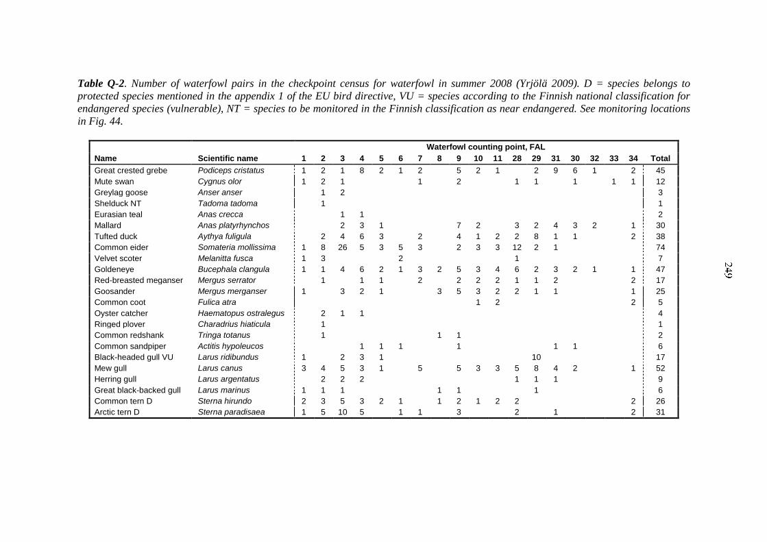
Table Q-2. Number of waterfowl pairs in the checkpoint census for waterfowl in summer 2008 (Yrjölä 2009). D = species belongs to
protected species mentioned in the appendix 1 of the EU bird directive, VU = species according to the Finnish national classification for
endangered species (vulnerable), NT = species to be monitored in the Finnish classification as near endangered. See monitoring locations
in Fig. 44.
Name Scientific name
Waterfowl counting point, FAL
1 2 3 4 5 6 7 8 9 10 11 28 29 31 30 32 33 34 Total
Great crested grebe Podiceps cristatus 1 2 1 8 2 1 2 5 2 1 2 9 6 1 2 45
Mute swan Cygnus olor 1 2 1 1 2 1 1 1 1 1 12
Greylag goose Anser anser 1 2 3
Shelduck NT Tadoma tadoma 1 1
Eurasian teal Anas crecca 1 1 2
Mallard Anas platyrhynchos 2 3 1 7 2 3 2 4 3 2 1 30
Tufted duck Aythya fuligula 2 4 6 3 2 4 1 2 2 8 1 1 2 38
Common eider Somateria mollissima 1 8 26 5 3 5 3 2 3 3 12 2 1 74
Velvet scoter Melanitta fusca 1 3 2 1 7
Goldeneye Bucephala clangula 1 1 4 6 2 1 3 2 5 3 4 6 2 3 2 1 1 47
Red-breasted meganser Mergus serrator 1 1 1 2 2 2 2 1 1 2 2 17
Goosander Mergus merganser 1 3 2 1 3 5 3 2 2 1 1 1 25
Common coot Fulica atra 1 2 2 5
Oyster catcher Haematopus ostralegus 2 1 1 4
Ringed plover Charadrius hiaticula 1 1
Common redshank Tringa totanus 1 1 1 2
Common sandpiper Actitis hypoleucos 1 1 1 1 1 1 6
Black-headed gull VU Larus ridibundus 1 2 3 1 10 17
Mew gull Larus canus 3 4 5 3 1 5 5 3 3 5 8 4 2 1 52
Herring gull Larus argentatus 2 2 2 1 1 1 9
Great black-backed gull Larus marinus 1 1 1 1 1 1 6
Common tern D Sterna hirundo 2 3 5 3 2 1 1 2 1 2 2 2 26
Arctic tern D Sterna paradisaea 1 5 10 5 1 1 3 2 1 2 31
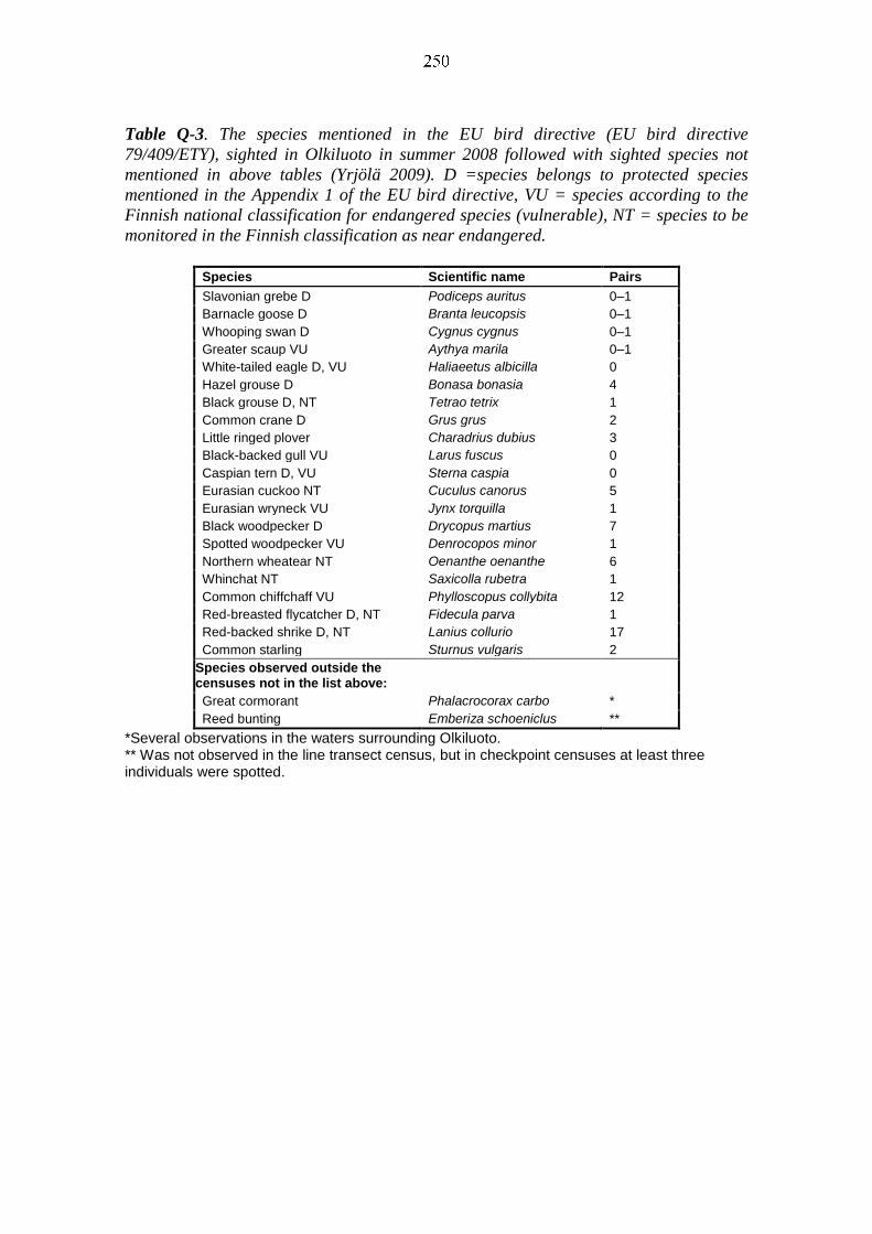
Table Q-3. The species mentioned in the EU bird directive (EU bird directive
79/409/ETY), sighted in Olkiluoto in summer 2008 followed with sighted species not
mentioned in above tables (Yrjölä 2009). D =species belongs to protected species
mentioned in the Appendix 1 of the EU bird directive, VU = species according to the
Finnish national classification for endangered species (vulnerable), NT = species to be
monitored in the Finnish classification as near endangered.
Species Scientific name Pairs
Slavonian grebe D Podiceps auritus 0–1
Barnacle goose D Branta leucopsis 0–1
Whooping swan D Cygnus cygnus 0–1
Greater scaup VU Aythya marila 0–1
White-tailed eagle D, VU Haliaeetus albicilla 0
Hazel grouse D Bonasa bonasia 4
Black grouse D, NT Tetrao tetrix 1
Common crane D Grus grus 2
Little ringed plover Charadrius dubius 3
Black-backed gull VU Larus fuscus 0
Caspian tern D, VU Sterna caspia 0
Eurasian cuckoo NT Cuculus canorus 5
Eurasian wryneck VU Jynx torquilla 1
Black woodpecker D Drycopus martius 7
Spotted woodpecker VU Denrocopos minor 1
Northern wheatear NT Oenanthe oenanthe 6
Whinchat NT Saxicolla rubetra 1
Common chiffchaff VU Phylloscopus collybita 12
Red-breasted flycatcher D, NT Fidecula parva 1
Red-backed shrike D, NT Lanius collurio 17
Common starling Sturnus vulgaris 2
Species observed outside the censuses not in the list above:
Great cormorant Phalacrocorax carbo *
Reed bunting Emberiza schoeniclus **
*Several observations in the waters surrounding Olkiluoto. ** Was not observed in the line transect census, but in checkpoint censuses at least three individuals were spotted.

APPENDIX R. RESULTS FROM HERPETOFAUNA SURVEY IN 2008
Reptiles and amphibians were surveyed on Olkiluoto in spring 2008. The aim of the
inventory was to determine the species composition and to estimate thei abundances of
different species in various habitat types on the island. The results of the study are
presented here.
Table R-1. Amphibian observations in Olkiluoto in 2008 (Nieminen & Saarikivi 2008).
Species Date No. of egg
clutches Coordinates (YKJ) Notes
Common frog Rana temporaria
16.4. 39 6803946 3205941 Field edge
21 6803887 3205858 Field edge
1 6803325 3205381 In ditch
17.4. 10 6804584 3204450 In ditch
1 6804538 3204376 In ditch
12 6804285 3204863 New heaping area
3 6804267 3204907 New heaping area
5 6804257 3204946 New heaping area
4 6804420 3205428 In pond
5 6805510 3204714 In pond
2
6804003 3206093 In ditch, under transmission line
24.4. 8 6806106 3202018 In pond
7 6805638 3202118 In ditch
21 6804965 3204845 In ditch
8 6804719 3205220 In pond
1 6803183 3205107 Field edge
Smooth newt Triturus vulgaris
17.4. 6803946 3205941 Field edge
6803887 3205858 Field edge
6803325 3205381 In ditch
24.4. 6803750 3203174 In reeds
6805998 3202077 In pond
6806098 3201987 In pond
Table R-2. Reptile observations in Olkiluoto in 2008 (Nieminen & Saarikivi 2008).
Species Date Observations Notes
Adder Vipera berus
16.4. 1 Possible overwintering site
17.4. 1 Crossed a road
24.4. 1 Young male
Common lizard Zootoca vivipara
16.4. 10 One on open rock at forest edge, one near adder site
17.4. 14 Several on reedbed, in meadow and on clearcut, one at the edge of reeds
24.4 4 Along a road, under transmission line and at forest edge
7.6. 3

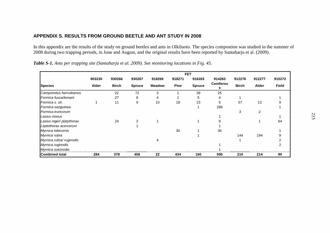
APPENDIX S. RESULTS FROM GROUND BEETLE AND ANT STUDY IN 2008
In this appendix are the results of the study on ground beetles and ants in Olkiluoto. The species compostion was studied in the summer of
2008 during two trapping periods, in June and August, and the original results have been reported by Santaharju et al. (2009).
Table S-1. Ants per trapping site (Santaharju et al. 2009). See monitoring locations in Fig. 45.
FET
903230 930266 930267 918269 918271 916263 914263 912276 912277 910272
Species Alder Birch Spruce Meadow Pine Spruce Coniferou
s Birch Alder Field
Camponotus herculeanus 22 72 3 1 39 25
Formica fusca/lemani 27 8 4 1 5 4 1 1
Formica s. str. 1 11 9 10 18 23 5 57 13 9
Formica sanguinea 1 286 1
Formica truncorum 3 2
Lasius mixtus 1 1
Lasius niger/ platythorax 24 2 1 1 9 1 64
Leptothorax acervorum 1 1
Myrnica lobicornis 30 1 36 1
Myrnica rubra 1 144 194 9
Myrnica rubra/ ruginodis 4 1 2
Myrnica ruginodis 1 2
Myrnica sulcinodis 1
Combined total 284 378 456 22 434 160 595 210 214 90
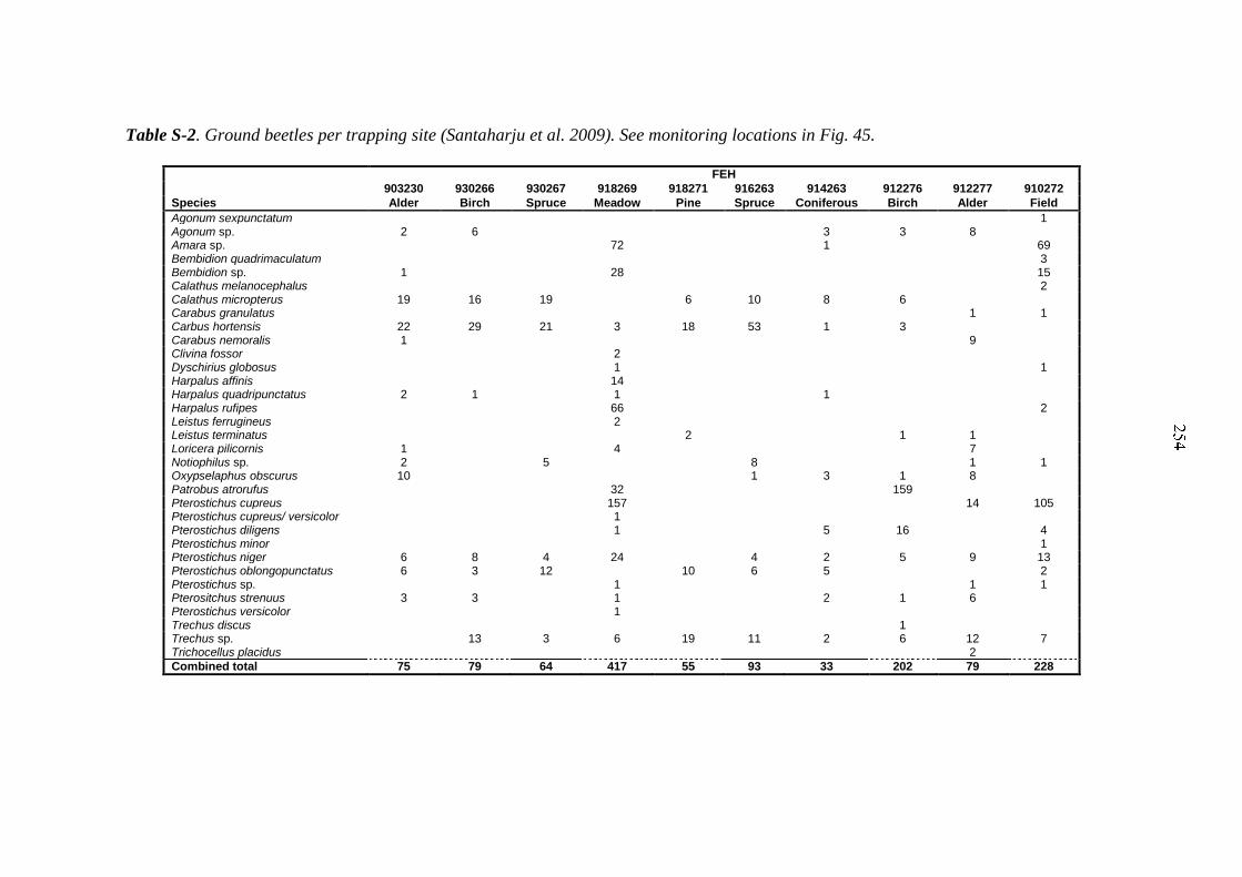
Table S-2. Ground beetles per trapping site (Santaharju et al. 2009). See monitoring locations in Fig. 45.
Species
FEH
903230 930266 930267 918269 918271 916263 914263 912276 912277 910272
Alder Birch Spruce Meadow Pine Spruce Coniferous Birch Alder Field
Agonum sexpunctatum 1 Agonum sp. 2 6 3 3 8 Amara sp. 72 1 69 Bembidion quadrimaculatum 3 Bembidion sp. 1 28 15 Calathus melanocephalus 2 Calathus micropterus 19 16 19 6 10 8 6 Carabus granulatus 1 1 Carbus hortensis 22 29 21 3 18 53 1 3 Carabus nemoralis 1 9 Clivina fossor 2 Dyschirius globosus 1 1 Harpalus affinis 14 Harpalus quadripunctatus 2 1 1 1 Harpalus rufipes 66 2 Leistus ferrugineus 2 Leistus terminatus 2 1 1 Loricera pilicornis 1 4 7 Notiophilus sp. 2 5 8 1 1 Oxypselaphus obscurus 10 1 3 1 8 Patrobus atrorufus 32 159 Pterostichus cupreus 157 14 105 Pterostichus cupreus/ versicolor 1 Pterostichus diligens 1 5 16 4 Pterostichus minor 1 Pterostichus niger 6 8 4 24 4 2 5 9 13 Pterostichus oblongopunctatus 6 3 12 10 6 5 2 Pterostichus sp. 1 1 1 Pterositchus strenuus 3 3 1 2 1 6 Pterostichus versicolor 1 Trechus discus 1 Trechus sp. 13 3 6 19 11 2 6 12 7 Trichocellus placidus 2
Combined total 75 79 64 417 55 93 33 202 79 228
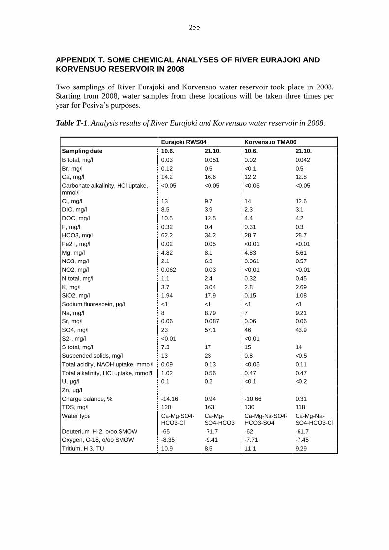
APPENDIX T. SOME CHEMICAL ANALYSES OF RIVER EURAJOKI AND KORVENSUO RESERVOIR IN 2008
Two samplings of River Eurajoki and Korvensuo water reservoir took place in 2008.
Starting from 2008, water samples from these locations will be taken three times per
year for Posiva’s purposes.
Table T-1. Analysis results of River Eurajoki and Korvensuo water reservoir in 2008.
Eurajoki RWS04 Korvensuo TMA06
Sampling date 10.6. 21.10. 10.6. 21.10.
B total, mg/l 0.03 0.051 0.02 0.042
Br, mg/l 0.12 0.5 <0.1 0.5
Ca, mg/l 14.2 16.6 12.2 12.8
Carbonate alkalinity, HCl uptake, mmol/l
<0.05 <0.05 <0.05 <0.05
Cl, mg/l 13 9.7 14 12.6
DIC, mg/l 8.5 3.9 2.3 3.1
DOC, mg/l 10.5 12.5 4.4 4.2
F, mg/l 0.32 0.4 0.31 0.3
HCO3, mg/l 62.2 34.2 28.7 28.7
Fe2+, mg/l 0.02 0.05 <0.01 <0.01
Mg, mg/l 4.82 8.1 4.83 5.61
NO3, mg/l 2.1 6.3 0.061 0.57
NO2, mg/l 0.062 0.03 <0.01 <0.01
N total, mg/l 1.1 2.4 0.32 0.45
K, mg/l 3.7 3.04 2.8 2.69
SiO2, mg/l 1.94 17.9 0.15 1.08
Sodium fluorescein, μg/l <1 <1 <1 <1
Na, mg/l 8 8.79 7 9.21
Sr, mg/l 0.06 0.087 0.06 0.06
SO4, mg/l 23 57.1 46 43.9
S2-, mg/l <0.01 <0.01
S total, mg/l 7.3 17 15 14
Suspended solids, mg/l 13 23 0.8 <0.5
Total acidity, NAOH uptake, mmol/l 0.09 0.13 <0.05 0.11
Total alkalinity, HCl uptake, mmol/l 1.02 0.56 0.47 0.47
U, μg/l 0.1 0.2 <0.1 <0.2
Zn, μg/l
Charge balance, % -14.16 0.94 -10.66 0.31
TDS, mg/l 120 163 130 118
Water type Ca-Mg-SO4-HCO3-Cl
Ca-Mg-SO4-HCO3
Ca-Mg-Na-SO4-HCO3-SO4
Ca-Mg-Na-SO4-HCO3-Cl
Deuterium, H-2, o/oo SMOW -65 -71.7 -62 -61.7
Oxygen, O-18, o/oo SMOW -8.35 -9.41 -7.71 -7.45
Tritium, H-3, TU 10.9 8.5 11.1 9.29

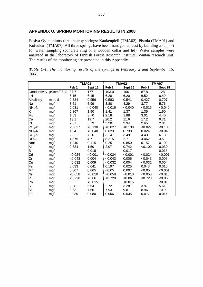
APPENDIX U. SPRING MONITORING RESULTS IN 2008 Posiva Oy monitors three nearby springs: Kaukenpieli (TMA02), Pistola (TMA01) and
Koivukari (TMA07). All three springs have been managed at least by building a support
for water sampling (concrete ring or a wooden collar and lid). Water samples were
analysed in the laboratory of Finnish Forest Research Institute, Vantaa research unit.
The results of the monitoring are presented in this Appendix.
Table U-1. The monitoring results of the springs in February 2 and September 15,
2008.
TMA01 TMA02 TMA07 Feb 2 Sept 15 Feb 2 Sept 15 Feb 2 Sept 15
Conductivity µS/cm/25°C 87.7 177 103.0 106 87.8 128 pH 6.15 6.15 6.28 6.20 6.52 6.49 Alkalinity mmol/l 0.334 0.956 0.583 0.541 0.427 0.707 Na mg/l 3.61 5.99 3.80 4.29 3.77 5.76 NH4-N mg/l 0.031 <0.040 <0.016 <0.040 <0.016 <0.040 K mg/l 0.867 1.90 1.41 1.37 1.35 1.90 Mg mg/l 1.53 3.70 2.18 1.88 3.01 4.40 Ca mg/l 13.1 19.7 20.2 11.6 17.2 9.71 Cl mg/l 2.57 5.79 3.20 2.34 2.65 2.84 PO4-P mg/l <0.027 <0.130 <0.027 <0.130 <0.027 <0.130 NO3-N mg/l 1.24 <0.040 0.023 0.738 0.024 <0.040 SO4-S mg/l 2.52 7.26 3.14 3.49 4.43 6.13 DOC mg/l 4.875 4.7 8.215 2.7 4.462 3.5 Ntot mg/l 1.340 0.115 0.251 0.850 0.157 0.102 Al mg/l 0.834 1.50 2.07 0.742 <0.100 0.030 B mg/l 0.018 0.017 0.018 Cd mg/l <0.024 <0.001 <0.024 <0.001 <0.024 <0.001 Cr mg/l <0.043 0.004 <0.043 0.005 <0.043 0.005 Cu mg/l <0.032 0.009 <0.032 0.004 <0.032 0.004 Fe mg/l 0.033 0.041 0.197 0.025 0.043 0.016 Mn mg/l 0.007 0.065 <0.05 0.007 <0.05 <0.001 Ni mg/l <0.058 <0.010 <0.058 <0.010 <0.058 <0.010 P mg/l <0.720 <0.06 <0.720 <0.06 <0.720 <0.06 Pb mg/l <0.015 <0.015 <0.015 S mg/l 2.28 6.64 2.72 3.28 3.97 5.61 Si mg/l 8.63 7.66 7.93 9.81 8.96 10.9 Zn mg/l 0.039 0.080 0.056 0.035 0.017 0.014

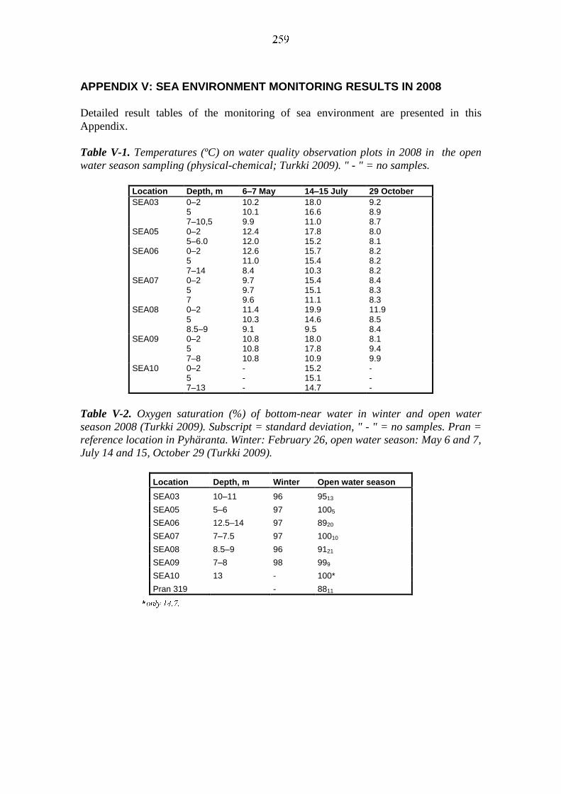
APPENDIX V: SEA ENVIRONMENT MONITORING RESULTS IN 2008
Detailed result tables of the monitoring of sea environment are presented in this
Appendix.
Table V-1. Temperatures (ºC) on water quality observation plots in 2008 in the open
water season sampling (physical-chemical; Turkki 2009). " - " = no samples.
Location Depth, m 6–7 May 14–15 July 29 October
SEA03 0–2 5 7–10,5
10.2 10.1 9.9
18.0 16.6 11.0
9.2 8.9 8.7
SEA05 0–2 5–6.0
12.4 12.0
17.8 15.2
8.0 8.1
SEA06
0–2 5 7–14
12.6 11.0 8.4
15.7 15.4 10.3
8.2 8.2 8.2
SEA07
0–2 5 7
9.7 9.7 9.6
15.4 15.1 11.1
8.4 8.3 8.3
SEA08
0–2 5 8.5–9
11.4 10.3 9.1
19.9 14.6 9.5
11.9 8.5 8.4
SEA09
0–2 5 7–8
10.8 10.8 10.8
18.0 17.8 10.9
8.1 9.4 9.9
SEA10
0–2 5 7–13
- - -
15.2 15.1 14.7
- - -
Table V-2. Oxygen saturation (%) of bottom-near water in winter and open water
season 2008 (Turkki 2009). Subscript = standard deviation, " - " = no samples. Pran =
reference location in Pyhäranta. Winter: February 26, open water season: May 6 and 7,
July 14 and 15, October 29 (Turkki 2009).
Location Depth, m Winter Open water season
SEA03 10–11 96 9513
SEA05 5–6 97 1005
SEA06 12.5–14 97 8920
SEA07 7–7.5 97 10010
SEA08 8.5–9 96 9121
SEA09 7–8 98 999
SEA10 13 - 100*
Pran 319 - 8811
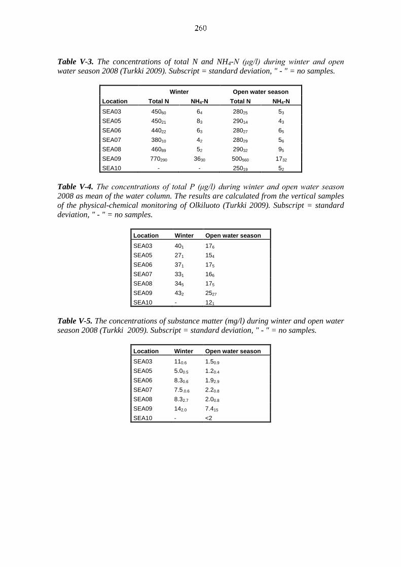
Table V-3. The concentrations of total N and NH4-N (μg/l) during winter and open
water season 2008 (Turkki 2009). Subscript = standard deviation, " - " = no samples.
Winter Open water season
Location Total N NH4-N Total N NH4-N
SEA03 45060 64 28025 53
SEA05 45021 83 29014 43
SEA06 44022 63 28027 65
SEA07 38010 42 28029 56
SEA08 46089 52 29032 95
SEA09 770290 3630 500560 1732
SEA10 - - 25019 52
Table V-4. The concentrations of total P (μg/l) during winter and open water season
2008 as mean of the water column. The results are calculated from the vertical samples
of the physical-chemical monitoring of Olkiluoto (Turkki 2009). Subscript = standard
deviation, " - " = no samples.
Location Winter Open water season
SEA03 401 176
SEA05 271 154
SEA06 371 175
SEA07 331 166
SEA08 345 175
SEA09 432 2527
SEA10 - 121
Table V-5. The concentrations of substance matter (mg/l) during winter and open water
season 2008 (Turkki 2009). Subscript = standard deviation, " - " = no samples.
Location Winter Open water season
SEA03 110.6 1.50.9
SEA05 5.00.5 1.20.4
SEA06 8.30.6 1.92.9
SEA07 7.5.0.6 2.20.8
SEA08 8.32.7 2.00.8
SEA09 142.0 7.415
SEA10 - <2

Table V-6. Results from Posiva's seawater characterization samplings in 1989, 1994,
2002, 2005 and 2008. All units mg/L.
SEA01 SEA02 SEA03 SEA04
month /year
8 /94
9 /02
11 /05
8 /08
8 /89
8 /94
9 /02
11 /05
8 /08
9 /02
11 /05
8 /08
9 /02
11 /05
8 /08
TDS 5680 5600 6060 5840 5970 5710 5620 5680 5800 5630 5760 5840 5340 5640 5780
Bromide 10 8.6 10 11 12 10 8.9 10 11 9.1 10 12 8.6 10 11
Chloride 3020 3050 3390 3150 3250 3030 3010 3120 3130 3010 3170 3150 2910 3080 3120
Sulphate 460 440 440 460 501 440 450 440 460 440 450 470 430 440 460
Potassium 65 59 61 62 61 66 59 59 62 59 60 63 55 58 62
Calcium 84 89 97 94 91 80 90 93 98 90 93 98 85 92 97
Magnesium 219 220 220 200 227 218 220 210 200 210 210 200 210 200 200
Sodium 1740 1650 1750 1780 1730 1780 1700 1660 1750 1730 1680 1770 1610 1660 1750
Strontium 1.2 1.3 1.4 1.3 - 1.2 1.3 1.2 1.3 1.3 1.3 1.3 1.2 1.2 1.2
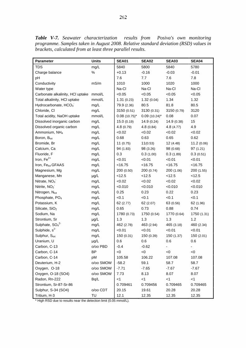
Table V-7. Seawater characterization results from Posiva's own monitoring
programme. Samples taken in August 2008. Relative standard deviation (RSD) values in
brackets, calculated from at least three parallel results.
Parameter Units SEA01 SEA02 SEA03 SEA04
TDS mg/L 5840 5800 5840 5780
Charge balance % +0.13 -0.16 -0.03 -0.01
pH 7.6 7.7 7.6 7.8
Conductivity mS/m 1010 1000 1020 1000
Water type Na-Cl Na-Cl Na-Cl Na-Cl
Carbonate alkalinity, HCl uptake mmol/L <0.05 <0.05 <0.05 <0.05
Total alkalinity, HCl uptake mmol/L 1.31 (0.23) 1.32 (0.04) 1.34 1.32
Hydrocarbonate, HCO3- mg/L 79.9 (2.36) 80.5 81.8 80.5
Chloride, Cl mg/L 3150 (0.51) 3130 (0.31) 3150 (0.79) 3120
Total acidity, NaOH uptake mmol/L 0.08 (10.75)* 0.09 (10.24)* 0.08 0.07
Dissolved inorganic carbon mg/L 15.0 (0.19) 14.9 (0.24) 14.9 (0.38) 15
Dissolved organic carbon mg/L 4.8 (0.79) 4.8 (0.84) 4.8 (4.77) 4.9
Ammonium, NH4 mg/L <0.02 <0.02 <0.02 <0.02
Boron, Btot mg/L 0.68 0.63 0.65 0.62
Bromide, Br mg/L 11 (0.75) 11(0.53) 12 (4.48) 11.2 (0.06)
Calcium, Ca mg/L 94 (1.83) 98 (3.26) 98 (0.68) 97 (1.21)
Fluoride, F mg/L 0.3 0.3 (1.00) 0.3 (1.89) 0.3 (0.51)
Iron, Fe2+
mg/L <0.01 <0.01 <0.01 <0.01
Iron, Fetot GFAAS mg/L <16.75 <16.75 <16.75 <16.75
Magnesium, Mg mg/L 200 (0.50) 200 (0.74) 200 (1.06) 200 (1.55)
Manganese, Mn μg/L <12.5 <12.5 <12.5 <12.5
Nitrate, NO3- mg/L <0.02 <0.02 <0.02 <0.02
Nitrite, NO2- mg/L <0.010 <0.010 <0.010 <0.010
Nitrogen, Ntot mg/L 0.25 0.23 0.22 0.23
Phosphate, PO4 mg/L <0.1 <0.1 <0.1 <0.1
Potassium, K mg/L 62 (2.77) 62 (2.07) 63 (0.56) 62 (1.96)
Silicate, SiO2 mg/L 0.65 0.73 0.88 0.74
Sodium, Na mg/L 1780 (0.73) 1750 (0.54) 1770 (0.64) 1750 (1.31)
Strontium, Sr μg/L 1.3 1.3 1.3 1.2
Sulphate, SO42-
mg/L 462 (2.78) 463 (2.94) 465 (3.18) 460 (2.34)
Sulphide, s2-
mg/L <0.01 <0.01 <0.01 <0.01
Sulphur, Stot mg/L 150 (0.31) 150 (0.39) 150 (1.37) 150 (2.01)
Uranium, U μg/L 0.6 0.6 0.6 0.6
Carbon, C-13 o/oo PBD -0.4 -0.62 - -
Carbon, C-14 BP <0 <0 <0 <0
Carbon, C-14 pM 105.58 106.22 107.08 107.08
Deuterium, H-2 o/oo SMOW -58.2 59.1 58.7 58.7
Oxygen, O-18 o/oo SMOW -7.71 -7.65 -7.67 -7.67
Oxygen, O-18 (SO4) o/oo SMOW 7.73 8.13 8.07 8.07
Radon, Rn-222 Bq/L <1 <1 <1 <1
Strontium, Sr-87-Sr-86 0.709461 0.709456 0.709465 0.709465
Sulphur, S-34 (SO4) o/oo CDT 20.15 19.61 20.28 20.28
Tritium, H-3 TU 12.1 12.35 12.35 12.35
* High RSD due to results near the detection limit (0.05 mmol/L).
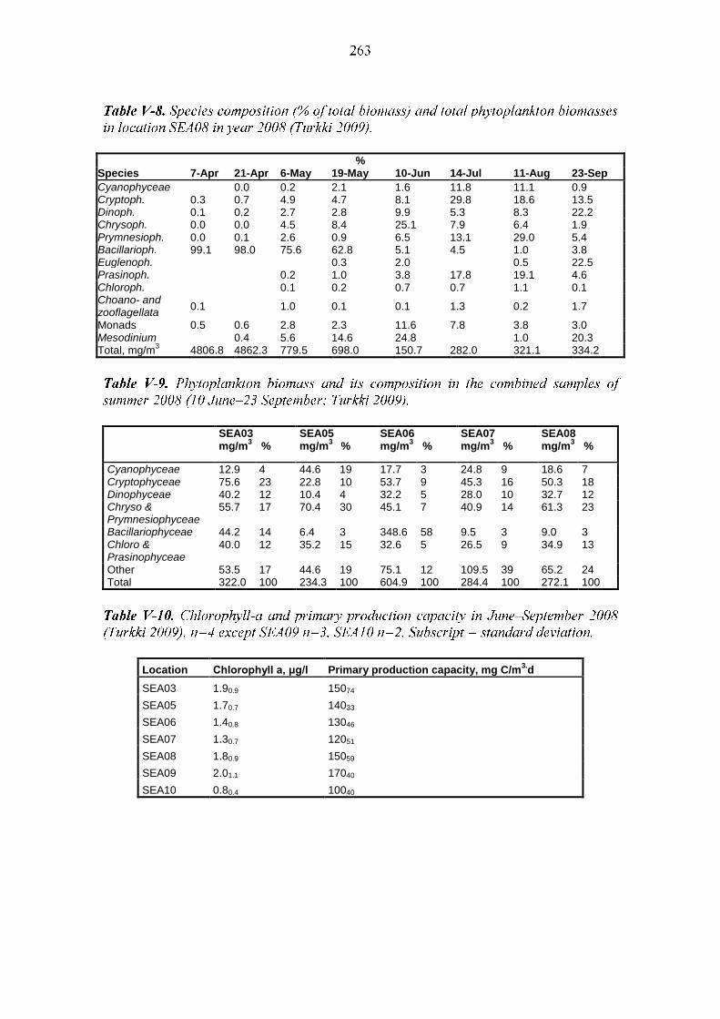
% Species 7-Apr 21-Apr 6-May 19-May 10-Jun 14-Jul 11-Aug 23-Sep
Cyanophyceae 0.0 0.2 2.1 1.6 11.8 11.1 0.9 Cryptoph. 0.3 0.7 4.9 4.7 8.1 29.8 18.6 13.5 Dinoph. 0.1 0.2 2.7 2.8 9.9 5.3 8.3 22.2 Chrysoph. 0.0 0.0 4.5 8.4 25.1 7.9 6.4 1.9 Prymnesioph. 0.0 0.1 2.6 0.9 6.5 13.1 29.0 5.4 Bacillarioph. 99.1 98.0 75.6 62.8 5.1 4.5 1.0 3.8 Euglenoph. 0.3 2.0 0.5 22.5 Prasinoph. 0.2 1.0 3.8 17.8 19.1 4.6 Chloroph. 0.1 0.2 0.7 0.7 1.1 0.1 Choano- and zooflagellata
0.1 1.0 0.1 0.1 1.3 0.2 1.7
Monads 0.5 0.6 2.8 2.3 11.6 7.8 3.8 3.0 Mesodinium 0.4 5.6 14.6 24.8 1.0 20.3 Total, mg/m
3 4806.8 4862.3 779.5 698.0 150.7 282.0 321.1 334.2
SEA03 mg/m
3 %
SEA05 mg/m
3 %
SEA06 mg/m
3 %
SEA07 mg/m
3 %
SEA08 mg/m
3 %
Cyanophyceae 12.9 4 44.6 19 17.7 3 24.8 9 18.6 7 Cryptophyceae 75.6 23 22.8 10 53.7 9 45.3 16 50.3 18 Dinophyceae 40.2 12 10.4 4 32.2 5 28.0 10 32.7 12 Chryso & Prymnesiophyceae
55.7 17 70.4 30 45.1 7 40.9 14 61.3 23
Bacillariophyceae 44.2 14 6.4 3 348.6 58 9.5 3 9.0 3 Chloro & Prasinophyceae
40.0 12 35.2 15 32.6 5 26.5 9 34.9 13
Other 53.5 17 44.6 19 75.1 12 109.5 39 65.2 24 Total 322.0 100 234.3 100 604.9 100 284.4 100 272.1 100
Location Chlorophyll a, μg/l Primary production capacity, mg C/m3.d
SEA03 1.90.9 15074
SEA05 1.70.7 14033
SEA06 1.40.8 13046
SEA07 1.30.7 12051
SEA08 1.80.9 15059
SEA09 2.01.1 17040
SEA10 0.80.4 10040
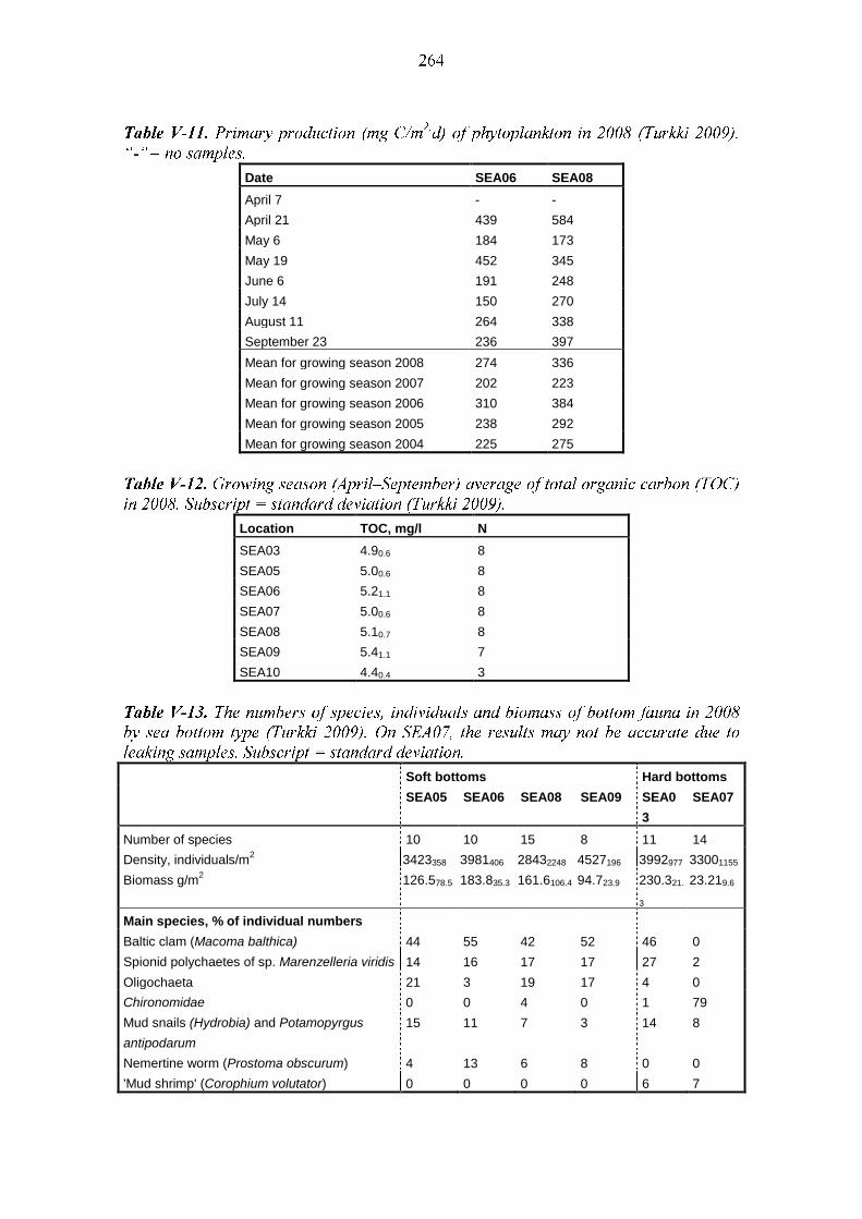
Date SEA06 SEA08
April 7 - -
April 21 439 584
May 6 184 173
May 19 452 345
June 6 191 248
July 14 150 270
August 11 264 338
September 23 236 397
Mean for growing season 2008 274 336
Mean for growing season 2007 202 223
Mean for growing season 2006 310 384
Mean for growing season 2005 238 292
Mean for growing season 2004 225 275
Location TOC, mg/l N
SEA03 4.90.6 8
SEA05 5.00.6 8
SEA06 5.21.1 8
SEA07 5.00.6 8
SEA08 5.10.7 8
SEA09 5.41.1 7
SEA10 4.40.4 3
Soft bottoms Hard bottoms
SEA05 SEA06 SEA08 SEA09 SEA0
3
SEA07
Number of species 10 10 15 8 11 14
Density, individuals/m2 3423358 3981406 28432248 4527196 3992977 33001155
Biomass g/m2 126.578.5 183.835.3 161.6106.4 94.723.9 230.321.
3
23.219.6
Main species, % of individual numbers
Baltic clam (Macoma balthica) 44 55 42 52 46 0
Spionid polychaetes of sp. Marenzelleria viridis 14 16 17 17 27 2
Oligochaeta 21 3 19 17 4 0
Chironomidae 0 0 4 0 1 79
Mud snails (Hydrobia) and Potamopyrgus
antipodarum
15 11
7
3
14
8
Nemertine worm (Prostoma obscurum) 4 13 6 8 0 0
'Mud shrimp' (Corophium volutator) 0 0 0 0 6 7
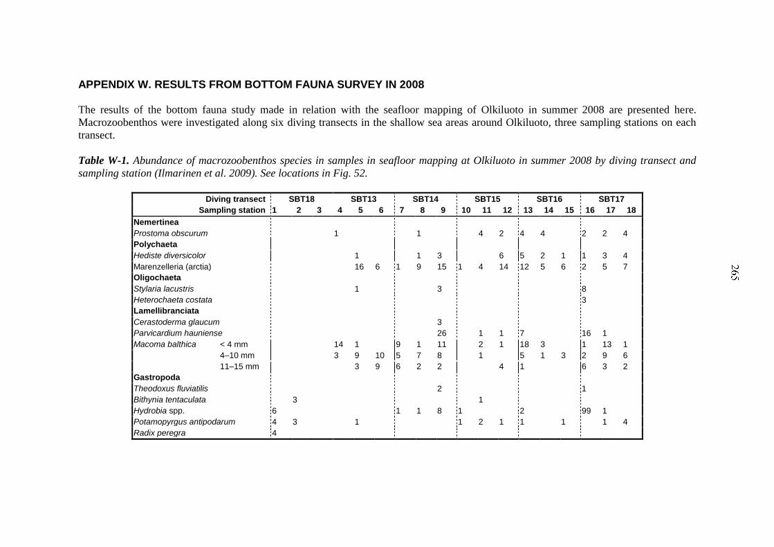
APPENDIX W. RESULTS FROM BOTTOM FAUNA SURVEY IN 2008
The results of the bottom fauna study made in relation with the seafloor mapping of Olkiluoto in summer 2008 are presented here.
Macrozoobenthos were investigated along six diving transects in the shallow sea areas around Olkiluoto, three sampling stations on each
transect.
Table W-1. Abundance of macrozoobenthos species in samples in seafloor mapping at Olkiluoto in summer 2008 by diving transect and
sampling station (Ilmarinen et al. 2009). See locations in Fig. 52.
Diving transect SBT18 SBT13 SBT14 SBT15 SBT16 SBT17
Sampling station 1 2 3 4 5 6 7 8 9 10 11 12 13 14 15 16 17 18
Nemertinea
Prostoma obscurum 1 1 4 2 4 4 2 2 4
Polychaeta
Hediste diversicolor 1 1 3 6 5 2 1 1 3 4
Marenzelleria (arctia) 16 6 1 9 15 1 4 14 12 5 6 2 5 7
Oligochaeta
Stylaria lacustris 1 3 8
Heterochaeta costata 3
Lamellibranciata
Cerastoderma glaucum 3
Parvicardium hauniense 26 1 1 7 16 1
Macoma balthica < 4 mm 14 1 9 1 11 2 1 18 3 1 13 1
4–10 mm 3 9 10 5 7 8 1 5 1 3 2 9 6
11–15 mm 3 9 6 2 2 4 1 6 3 2
Gastropoda
Theodoxus fluviatilis 2 1
Bithynia tentaculata 3 1
Hydrobia spp. 6 1 1 8 1 2 99 1
Potamopyrgus antipodarum 4 3 1 1 2 1 1 1 1 4
Radix peregra 4
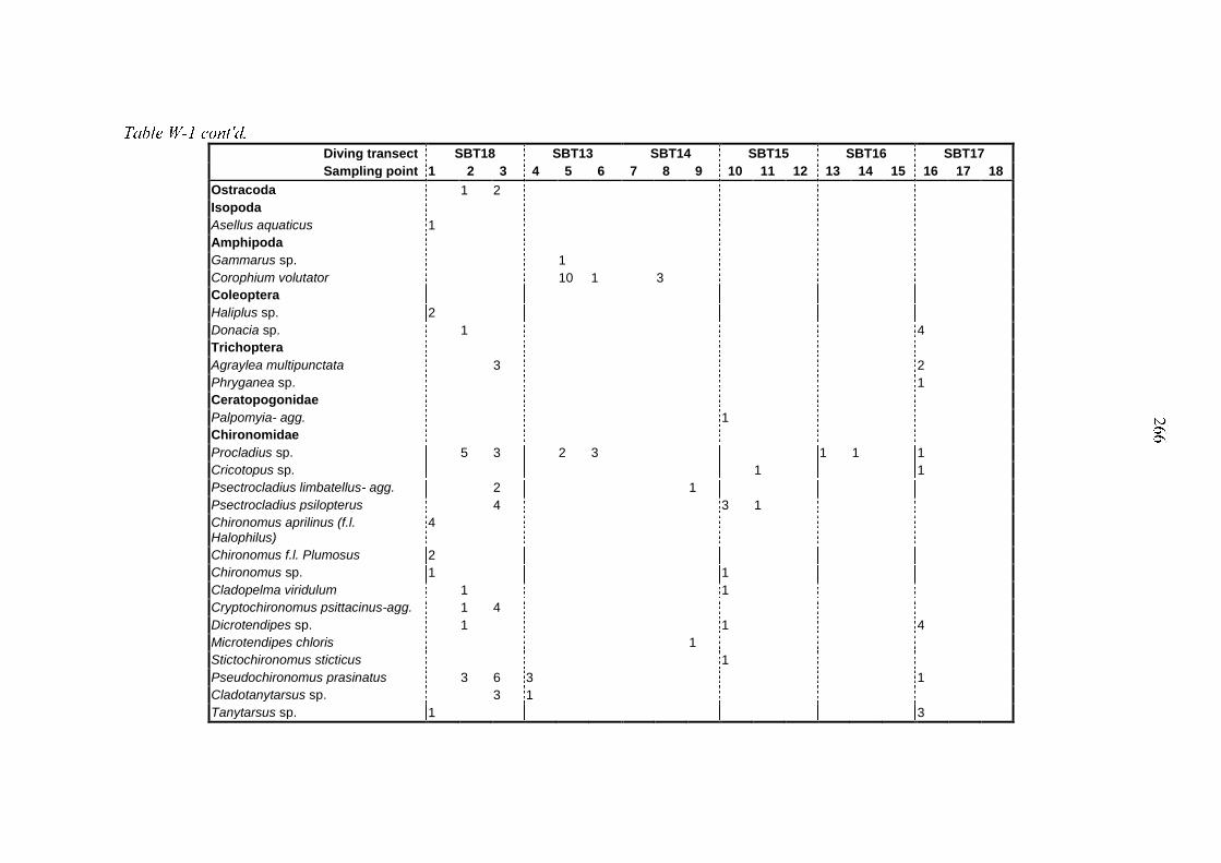
Diving transect SBT18 SBT13 SBT14 SBT15 SBT16 SBT17
Sampling point 1 2 3 4 5 6 7 8 9 10 11 12 13 14 15 16 17 18
Ostracoda 1 2
Isopoda
Asellus aquaticus 1
Amphipoda
Gammarus sp. 1
Corophium volutator 10 1 3
Coleoptera
Haliplus sp. 2
Donacia sp. 1 4
Trichoptera
Agraylea multipunctata 3 2
Phryganea sp. 1
Ceratopogonidae
Palpomyia- agg. 1
Chironomidae
Procladius sp. 5 3 2 3 1 1 1
Cricotopus sp. 1 1
Psectrocladius limbatellus- agg. 2 1
Psectrocladius psilopterus 4 3 1
Chironomus aprilinus (f.l. Halophilus)
4
Chironomus f.l. Plumosus 2
Chironomus sp. 1 1
Cladopelma viridulum 1 1
Cryptochironomus psittacinus-agg. 1 4
Dicrotendipes sp. 1 1 4
Microtendipes chloris 1
Stictochironomus sticticus 1
Pseudochironomus prasinatus 3 6 3 1
Cladotanytarsus sp. 3 1
Tanytarsus sp. 1 3
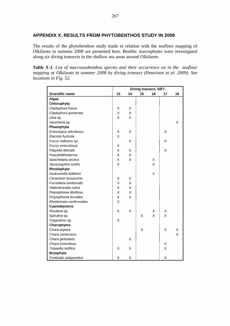
APPENDIX X. RESULTS FROM PHYTOBENTHOS STUDY IN 2008
The results of the phytobenthon study made in relation with the seafloor mapping of
Olkiluoto in summer 2008 are presented here. Benthic macrophytes were investigated
along six diving transects in the shallow sea areas around Olkiluoto.
Table X-1. List of macrozoobenthos species and their occurrence on in the seafloor
mapping at Olkiluoto in summer 2008 by diving transect (Ilmarinen et al. 2009). See
locations in Fig. 52.
Scientific name
Diving transect, SBT:
13 14 15 16 17 18
Algae
Chlorophyta
Cladophora fracta X X
Cladophora gomerata X X
Ulva sp. X X
Vaucheria sp. X
Phaeophyta
Ectocarpus siliculosus X X X
Elacista fucicola X
Fucus radicans sp. X X
Fucus vesiculosus X
Pilayella littoralis X X X
Pseudolithoderma X X
Spachelaria arctica X X X
Stictyosiphon tortilis X X
Rhodophyta
Audouinella leibleinii X
Ceramium tenuicorne X X
Furcellaria lumbricalis X X
Hildenbrandia rubra X X
Polysiphonia fibrillosa X X
Polysiphonia fucoides X X
Rhodomela confervoides X
Cyanobacteria
Rivularia sp. X X X X
Spirulina sp. X X X
Tolypothrix sp. X
Charophytes
Chara aspera X X X
Chara canescens X
Chara globularis X
Chara tomentosa X
Tolypella nidifica X X X
Bryophyta
Fontinalis antipyretica X X X

Table X-1 cont'd.
Scientific name
Diving transect, SBT:
13 14 15 16 17 18
Tracheophyta
Callitriche hermaphroditica X X X
Ceratophyllum demersum X X
Lemna trisulca X X X X
Myriophyllum sibiricum X X X X
Myriophyllum spicatum X X X X X X
Najas marina X X X X
Phragmites australis X X
Potamogeton pectinatus X X X X X X
Potamogeton perfoliatus X X X X
Ranunculus baudotii X X
Ranunculus circinatus X
Ruppia maritima X
Schoenoplectus tabernaemontani X
Zannichellia major
Zannichellia palustris X X X X X
Zannichellia pedicellata X
Number of macrophyte species per transect
29 24 7 10 19 13
Invertebrata
Balanus improvisus X X X
Cerastoderma glaucum X X X
Electra crustulenta X X X X
Ephydatia fluviatilis X X
Laomedea loveni X X
Mytilus edulis X X

APPENDIX Y. WATER QUALITY MONITORING RESULTS IN 2008
In this Appendix detailed results of water quality analyses are presented. Drainage water
from rock heaps is sampled in observation wells or ditches three times per year. The
results are compared with results from nearby multi-level piezometer (EP5). The results
have been presented by TVO laboratory (Tiina Lamminmäki) in a memo. The chemical
contents of three private wells in Olkiluoto are analysed annually.
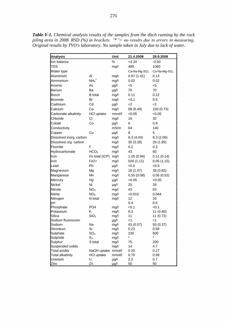
Table Y-1. Chemical analysis results of the samples from the ditch running by the rock
piling area in 2008. RSD (%) in brackets. ”*”= no results due to errors in measuring.
Original results by TVO's laboratory. No sample taken in July due to lack of water.
Analysis Unit 21.4.2008 29.9.2008
Ion balance % +4.34 -0.50
TDS mg/l 480 1060
Water type Ca-Na-Mg-SO4 Ca-Na-Mg-SO4
Aluminium Al mg/l 0.97 (1.41) 0.13
Ammonium NH4+ mg/l 0.02 0.02
Arsenic As µg/l <5 <5
Barium Ba µg/l 70 70
Boron B total mg/l 0.11 0.22
Bromide Br mg/l <0.1 0.5
Cadmium Cd µg/l <2 <2
Calcium Ca mg/l 68 (0.49) 150 (0.73)
Carbonate alkalinity HCl uptake mmol/l <0.05 <0.05
Chloride Cl mg/l 16 32
Cobalt Co µg/l 6 0.9
Conductivity mS/m 64 140
Copper Cu µg/l 8 5
Dissolved inorg. carbon mg/l 8.3 (4.04) 8.3 (2.06)
Dissolved org. carbon mg/l 35 (3.28) 26 (1.85)
Fluoride F mg/l 0.2 0.3
Hydrocarbonate HCO3 mg/l 43 60
Iron Fe total (ICP) mg/l 1.25 (0.94) 0.11 (0.14)
Iron Fe2+ mg/l 026 (1.11) 0.05 (1.15)
Lead Pb µg/l <0.5 <0.5
Magnesium Mg mg/l 18 (1.07) 38 (0.82)
Manganese Mn mg/l 0.55 (0.08) 0.06 (0.52)
Mercury Hg µg/l <0.05 <0.05
Nickel Ni µg/l 25 28
Nitrate NO3 mg/l 43 63
Nitrite NO2 mg/l <0.010 0.044
Nitrogen N total mg/l 12 16
pH 6.4 6.6
Phosphate PO4 mg/l <0.1 <0.1
Potassium K mg/l 8.3 11 (0.40)
Silica SiO2 mg/l 11 11 (0.72)
Sodium fluorescein µg/l <1 <1
Sodium Na mg/l 43 (0.57) 93 (0.37)
Strontium Sr mg/l 0.23 0.58
Sulphate SO4 mg/l 230 600
Sulphide S2- mg/l * *
Sulphur S total mg/l 75 200
Suspended solids mg/l 14 4.7
Total acidity NaOH uptake mmol/l 0.25 0.17
Total alkalinity HCl uptake mmol/l 0.70 0.99
Uranium U µg/l 2.2 0.7
Zinc Zn µg/l 50 50
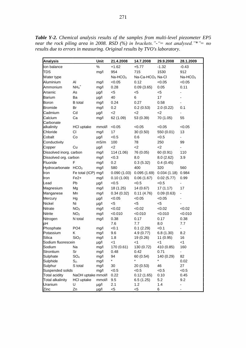
Table Y-2. Chemical analysis results of the samples from multi-level piezometer EP5
near the rock piling area in 2008. RSD (%) in brackets.”-“= not analysed.”*”= no
results due to errors in measuring. Original results by TVO's laboratory.
Analysis Unit 21.4.2008 14.7.2008 29.9.2008 28.1.2009
Ion balance % +1.62 +5.77 -1.32 -0.43
TDS mg/l 954 715 1530 912
Water type Na-HCO3 Na-Ca-HCO3 Na-Cl Na-HCO3
Aluminium Al mg/l <0.05 0.12 <0.05 <0.05
Ammonium NH4+ mg/l 0.28 0.09 (3.65) 0.05 0.11
Arsenic As µg/l <5 <5 <5 -
Barium Ba µg/l 40 6 17 -
Boron B total mg/l 0.24 0.27 0.58 -
Bromide Br mg/l 0.2 0.2 (0.53) 2.0 (0.22) 0.1
Cadmium Cd µg/l <2 <2 <2 -
Calcium Ca mg/l 62 (1.09) 53 (0.39) 70 (1.05) 55
Carbonate alkalinity HCl uptake mmol/l <0.05 <0.05 <0.05 <0.05
Chloride Cl mg/l 17 30 (0.50) 550 (0.01) 13
Cobalt Co µg/l <0.5 0.6 <0.5 -
Conductivity mS/m 100 78 250 99
Copper Cu µg/l <2 <2 <2 -
Dissolved inorg. carbon mg/l 114 (1.06) 76 (0.05) 60 (0.91) 110
Dissolved org. carbon mg/l <0.3 8.0 8.0 (2.62) 3.9
Fluoride F mg/l 0.2 0.3 (5.32) 0.4 (0.45)
Hydrocarbonate HCO3 mg/l 580 400 320 560
Iron Fe total (ICP) mg/l 0.090 (1.03) 0.095 (1.69) 0.034 (1.18) 0.984
Iron Fe2+ mg/l 0.10 (1.00) 0.06 (1.67) 0.02 (5.77) 0.99
Lead Pb µg/l <0.5 <0.5 <0.5 -
Magnesium Mg mg/l 18 (1.25) 14 (0.67) 17 (1.17) 17
Manganese Mn mg/l 0.34 (0.32) 0.11 (4.76) 0.09 (0.63) -
Mercury Hg µg/l <0.05 <0.05 <0.05 -
Nickel Ni µg/l <5 <5 <5 -
Nitrate NO3 mg/l <0.02 <0.02 <0.02 <0.02
Nitrite NO2 mg/l <0.010 <0.010 <0.010 <0.010
Nitrogen N total mg/l 0.38 0.17 0.17 0.38
pH 7.6 7.7 8.0 7.7
Phosphate PO4 mg/l <0.1 0.1 (2.29) <0.1 -
Potassium K mg/l 9.6 4.9 (0.77) 6.8 (1.30) 8.2
Silica SiO2 mg/l 1.8 19 (0.26) 11 (0.95) 16
Sodium fluorescein µg/l <1 <1 <1 <1
Sodium Na mg/l 170 (0.61) 130 (0.72) 410 (0.85) 160
Strontium Sr mg/l 0.48 0.42 0.71 -
Sulphate SO4 mg/l 94 60 (0.54) 140 (0.29) 82
Sulphide S2- mg/l * * * 0.02
Sulphur S total mg/l 30 20 (0.53) 46 27
Suspended solids mg/l <0.5 <0.5 <0.5 <0.5
Total acidity NaOH uptake mmol/l 0.22 0.12 (1.65) 0.10 0.45
Total alkalinity HCl uptake mmol/l 9.5 6.5 (1.25) 5.2 9.2
Uranium U µg/l 2.1 1.2
1.4 -
Zinc Zn µg/l <5 <5 6 -
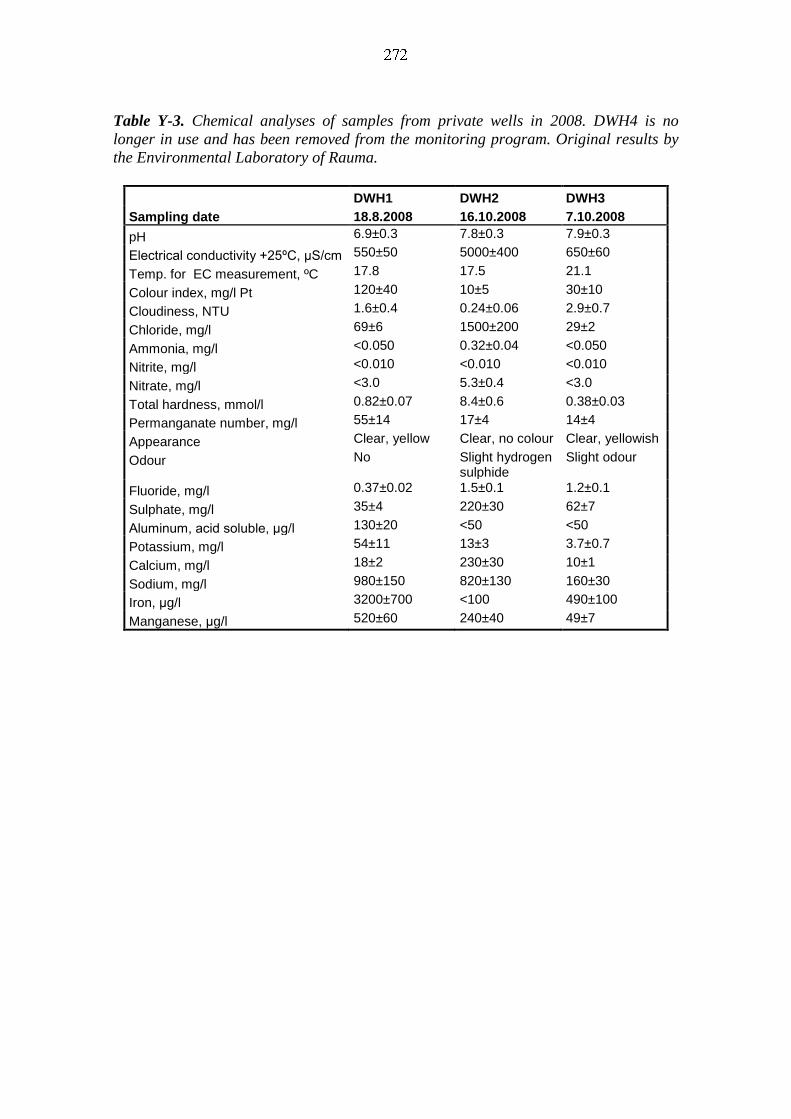
Table Y-3. Chemical analyses of samples from private wells in 2008. DWH4 is no
longer in use and has been removed from the monitoring program. Original results by
the Environmental Laboratory of Rauma.
DWH1 DWH2 DWH3
Sampling date 18.8.2008 16.10.2008 7.10.2008
pH 6.9±0.3 7.8±0.3 7.9±0.3
Electrical conductivity +25ºC, μS/cm 550±50 5000±400 650±60
Temp. for EC measurement, ºC 17.8 17.5 21.1
Colour index, mg/l Pt 120±40 10±5 30±10
Cloudiness, NTU 1.6±0.4 0.24±0.06 2.9±0.7
Chloride, mg/l 69±6 1500±200 29±2
Ammonia, mg/l <0.050 0.32±0.04 <0.050
Nitrite, mg/l <0.010 <0.010 <0.010
Nitrate, mg/l <3.0 5.3±0.4 <3.0
Total hardness, mmol/l 0.82±0.07 8.4±0.6 0.38±0.03
Permanganate number, mg/l 55±14 17±4 14±4
Appearance Clear, yellow Clear, no colour Clear, yellowish
Odour No Slight hydrogen sulphide
Slight odour
Fluoride, mg/l 0.37±0.02 1.5±0.1 1.2±0.1
Sulphate, mg/l 35±4 220±30 62±7
Aluminum, acid soluble, μg/l 130±20 <50 <50
Potassium, mg/l 54±11 13±3 3.7±0.7
Calcium, mg/l 18±2 230±30 10±1
Sodium, mg/l 980±150 820±130 160±30
Iron, μg/l 3200±700 <100 490±100
Manganese, μg/l 520±60 240±40 49±7
Related Documents