Restarting and error estimation in polynomial and extended Krylov subspace methods for the approximation of matrix functions Dissertation Bergische Universit¨ at Wuppertal Fakult¨ at f¨ ur Mathematik und Naturwissenschaften eingereicht von Marcel Schweitzer, M. Sc. zur Erlangung des Grades eines Doktors der Naturwissenschaften Betreut durch Prof. Dr. Andreas Frommer und Dr. Stefan G¨ uttel Angefertigt in der Zeit vom 01.12.2011 – 22.10.2015 Wuppertal, 22.10.2015

Welcome message from author
This document is posted to help you gain knowledge. Please leave a comment to let me know what you think about it! Share it to your friends and learn new things together.
Transcript
Restarting and error estimation inpolynomial and extended Krylov
subspace methods for theapproximation of matrix functions
Dissertation
Bergische Universitat Wuppertal
Fakultat fur Mathematik und Naturwissenschaften
eingereicht von
Marcel Schweitzer, M. Sc.zur Erlangung des Grades eines Doktors der Naturwissenschaften
Betreut durch Prof. Dr. Andreas Frommer und Dr. Stefan Guttel
Angefertigt in der Zeit vom
01.12.2011 – 22.10.2015
Wuppertal, 22.10.2015

Die Dissertation kann wie folgt zitiert werden:
urn:nbn:de:hbz:468-20160212-112106-7[http://nbn-resolving.de/urn/resolver.pl?urn=urn%3Anbn%3Ade%3Ahbz%3A468-20160212-112106-7]

ACKNOWLEDGMENTS
I wish to thank Prof. Dr. Andreas Frommer for giving me the opportunity towrite this thesis, for his support while doing so, and for raising my interest innumerical linear algebra in the first place.
I also wish to thank Dr. Stefan Guttel for his support and for two very nice andfruitful stays in Manchester, and Prof. Dr. Bruno Lang and Prof. Dr. Birgit Jacobfor agreeing to be members of my examination board.
In addition, I would like to thank all those people around me who accompaniedme on my path to finishing this thesis and somehow managed to survive myeveryday madness. Among these people, a very, very special “Thank you” goesto Sonja, as without her support and patience it would have been impossible forme to accomplish all this.
I

CONTENTS
Acknowledgments I
Contents III
1 Introduction 1
2 Review of basic material 5
2.1 Functions of matrices . . . . . . . . . . . . . . . . . . . . . . . . . 6
2.2 Stieltjes functions . . . . . . . . . . . . . . . . . . . . . . . . . . . 9
2.3 Krylov subspace methods for f(A)b . . . . . . . . . . . . . . . . . 18
2.4 The special case f(z) = z−1 . . . . . . . . . . . . . . . . . . . . . 26
2.5 Numerical quadrature . . . . . . . . . . . . . . . . . . . . . . . . 35
2.6 Model problems . . . . . . . . . . . . . . . . . . . . . . . . . . . . 43
3 An integral representation for the error in Arnoldi’s method 51
3.1 Error representation via divided differences . . . . . . . . . . . . . 51
3.2 Integral representation of the error function . . . . . . . . . . . . 53
III
CONTENTS
4 Implementation of a quadrature-based restarted Arnoldi method 61
4.1 Previously known restart approaches . . . . . . . . . . . . . . . . 61
4.2 Restarts based on numerical quadrature . . . . . . . . . . . . . . 65
4.3 Choice of quadrature rules and connection to Pade approximation 70
4.4 Numerical experiments . . . . . . . . . . . . . . . . . . . . . . . . 78
5 Convergence of restarted Krylov subspace methods 87
5.1 Known convergence results . . . . . . . . . . . . . . . . . . . . . . 87
5.2 Convergence of restarted Arnoldi for Stieltjes functions . . . . . . 89
5.3 Limitations for non-Hermitian matrices . . . . . . . . . . . . . . . 97
5.4 The restarted harmonic Arnoldi method . . . . . . . . . . . . . . 99
5.5 Convergence of restarted harmonic Arnoldi for Stieltjes functions . 101
5.6 Convergence of restarted FOM for linear systems . . . . . . . . . 107
5.7 Numerical experiments . . . . . . . . . . . . . . . . . . . . . . . . 115
6 Error estimates in Krylov methods 121
6.1 Relation between Gauss quadrature and the Lanczos process . . . 122
6.2 Bounds and estimates for bilinear forms uHh(A)v . . . . . . . . . 124
6.3 Error bounds for Stieltjes functions of positive definite matrices . 125
6.4 Computing error bounds with low computational cost . . . . . . . 129
6.5 Extension to non-Hermitian matrices . . . . . . . . . . . . . . . . 134
6.6 Numerical experiments . . . . . . . . . . . . . . . . . . . . . . . . 139
7 Error estimates in extended Krylov methods 153
7.1 Extended Krylov subspaces . . . . . . . . . . . . . . . . . . . . . 154
7.2 Integral representation of the error in extended Krylov methods . 157
7.3 Restart recovery in extended Krylov methods . . . . . . . . . . . 167
7.4 Numerical experiments . . . . . . . . . . . . . . . . . . . . . . . . 174
8 Conclusions & Outlook 179
IV

CONTENTS
List of Figures 183
List of Tables 185
List of Algorithms 186
List of Notations 187
Bibliography 188
V

CHAPTER 1
INTRODUCTION
Given a matrix A ∈ Cn×n, a vector b ∈ C
n and a sufficiently smooth functionf defined on spec(A), an increasingly important task in many areas of numericallinear algebra and scientific computing is the computation of
f(A)b, (1.1)
the action of the matrix function f(A) on the vector b. Important examplesof matrix functions include the matrix exponential f(A) = eA which is used,e.g., in exponential integrators for the solution of differential equations [88–90]and in network analysis [49], the matrix sign function f(A) = sign(A) whichhas important applications in lattice quantum chromodynamics [18, 48], or the(inverse) fractional powers f(A) = A±α for α ∈ (0, 1) which are, e.g., used infractional differential equations [23] and statistical sampling [93].
The presumably most widely known special case of the computation of a matrixfunction times a vector is the solution of a linear system of equations, i.e., thecomputation of x ∈ C
n such that
Ax = b, (1.2)
which corresponds to evaluating (1.1) with f(A) = A−1.
While both (1.1) and its special case (1.2) are often solved by the same or veryclosely related iterative methods, specifically Krylov subspace methods [37,67,88,98,114], the special structure of (1.2) and the simple nature of the function f(A) =A−1 allow for many theoretical and algorithmic simplifications and advantageswhich are not available in the more general case of an arbitrary function f .
1
1 Introduction
The main goal of this thesis is to fill some of these gaps by transferring or gener-alizing techniques and results which are well-known in the linear system case tothe case of more general matrix functions. Many of the results of this thesis dealwith the class of so-called Stieltjes functions [14, 15, 83] (but are in some casesalso applicable to broader classes of functions) which can be characterized by aRiemann–Stieltjes integral representation of the form
f(z) =
∞∫
0
1
z + tdµ(t), z ∈ C \ R−
0 , (1.3)
where µ is a nonnegative, monotonically increasing function defined on R+0 . Sub-
stituting the matrix A for z in (1.3) and applying this matrix function to a vectorb yields
f(A)b =
∞∫
0
(A+ tI)−1b dµ(t), (1.4)
which already reveals the intimate relation between Stieltjes matrix functions and(shifted) linear systems. This connection is the main building block of most ofthe ideas employed in this thesis.
There are two main concepts investigated in this thesis. On the one hand, weconsider restarting of Krylov subspace methods, a technique well-known in thelinear system context for methods such as GMRES [116] or FOM [113] for limitingmemory requirements of these methods. On the other hand, we deal with theefficient computation of error bounds and estimates, which is of special importancein case of the approximation of matrix functions, because in contrast to the linearsystem case, no quantity like a residual is available to easily monitor the progressof the method.
The remainder of this thesis is organized as follows. In Chapter 2, basic materialnecessary for making this thesis self-contained is presented. We begin with theprecise definition and important properties of matrix functions in general andStieltjes functions in particular. This is followed by a review of Krylov subspacemethods, both for matrix functions and for the special case of linear systems, anda short overview of numerical quadrature rules (Gauss quadrature, in particular)which will be extensively used in the computational methods presented in thisthesis for evaluating integral representations of matrix functions such as (1.4). Inaddition, we introduce a few model problems which will be used throughout thethesis for illustrating the developed results by numerical experiments. In Chap-ter 3, we derive an integral representation for the error f(A)b − fm of the iteratefm produced by m steps of a Krylov subspace method. This representation con-stitutes the common basis for the restart approach and the error estimates in thelater chapters of the thesis. In Chapter 4 we first give an overview of the restart
2
approaches for Krylov subspace methods for f(A)b available in the literatureso far. Afterwards, we investigate the possibility of using the error representa-tion from the previous chapter for a new implementation of the restart approachand comment on the differences and advantages in comparison to existing meth-ods. We already published the resulting method in [58]. Chapter 5 deals withconvergence of restarted Krylov subspace methods for the approximation of ma-trix functions. After reviewing the few previously known convergence results, weprove convergence of the restarted Arnoldi method for f a Stieltjes function andA Hermitian positive definite (for all restart lengths). In addition, we proposea variation of Arnoldi’s method based on interpolation in harmonic Ritz valueswhich allows to prove convergence for a larger class of matrices, the so-called pos-itive real matrices. We published these results in [57]. We conclude the chapterby investigating the linear system case and presenting results on the convergencebehavior of restarted FOM and restarted GMRES. We presented some of these re-sults (partially in a weaker form) already in the technical report [119]. Chapter 6deals with the estimation and bounding of the norm of the error ‖f(A)b−fm‖2 inKrylov subspace methods by making use of the error representation from Chap-ter 3 combined with techniques developed in [72–74] for error estimation in theiterative solution of linear systems. As these error bounds rely on the relationbetween the Lanczos process and Gauss quadrature, evaluating the integral rep-resentation of the error in this context gives rise to a nested quadrature approachwith an inner and an outer quadrature rule. Special care is devoted to the task ofcombining inner and outer quadrature rules in such a way that (in certain situa-tions, e.g., for Hermitian positive definite matrices A and f a Stieltjes function)the error estimates are guaranteed to be upper or lower bounds for the exact errornorm. In addition, we show how it is possible to compute these error bounds withnegligible computational cost, which is independent both of the matrix dimensionand the number of iterations performed in the Krylov subspace method, when Ais Hermitian positive definite, or at least independent of the matrix dimensionfor non-Hermitian A. Most of the results from this chapter (those applying toStieltjes functions) can also be found in our preprint [63]. In Chapter 7, resultssimilar to the ones from Chapter 6 are presented in the context of extended Krylovsubspace methods [38, 99, 124, 125]. These subspaces are built not only by usingpowers of the matrix A but also powers of A−1. Thus, they result in rational ap-proximations to f(A)b instead of polynomial approximations, therefore makingthe situation slightly more involved to analyze. We demonstrate how to transferthe techniques from the previous chapter to this situation, comment on the pos-sibility to also use rational Gauss quadrature rules for computing error estimatesand investigate in which situations one can still expect to obtain lower and upperbounds for the error. In Chapter 8, the results of this thesis are summarized andconcluding remarks and topics for future research are given.
3

CHAPTER 2
REVIEW OF BASIC MATERIAL
In this chapter, we introduce and review the basic terminology and classical resultson which the remainder of this thesis is based. We begin by presenting differentpossible definitions for matrix functions f(A) and important properties whichdirectly follow from these definitions in Section 2.1. In Section 2.2 we reviewthe definition of the Riemann–Stieltjes integral and use it to define the classof Stieltjes functions. These are the functions which we will mostly investigatethroughout the remainder of the thesis, as their special structure gives rise toa lot of computational and theoretical advantages. We present some examplesof Stieltjes functions and give an overview of classical results from the literaturewhich will become useful in later chapters. Next, Krylov subspace methods forapproximating f(A)b are described in Section 2.3. We do not only cover thecase of approximating a general matrix function f but also present some of thesimplifications and theoretical results arising when f(z) = z−1 in Section 2.4,i.e., when the solution of a linear system Ax = b is approximated. These resultswill later become beneficial when we investigate the intimate relation between thesolution of shifted linear systems and approximating certain functions of matrices.In Section 2.5, we give a short overview of numerical quadrature rules, witha special emphasis on Gauss quadrature. Gauss quadrature will be importantin two ways in this thesis. First, we will often work with (Riemann–Stieltjes)integral representations of functions for which no closed form is known, so thatthe integrals have to be evaluated numerically, and second, we will use the strongrelation between Gauss quadrature and the Lanczos process for computing errorestimates and error bounds in (extended) Krylov subspace methods in Chapter 6and Chapter 7. In the final section of this chapter, we introduce different modelproblems which involve the approximation of a matrix function times a vector
5
2 Review of basic material
and which will be used as benchmarks at various places throughout this thesis toillustrate and evaluate the developed methods and results.
2.1 Functions of matrices
In this section, we review the definition of a matrix function f(A) and basicproperties of matrix functions which we will use throughout this thesis. Mostof our presentation, including the three classical (and, if applicable, equivalent)definitions of a matrix function, mainly follows [85, Chapter 1], with additionalmaterial and inspiration drawn from [64, 71, 91]. We focus solely on theory ofmatrix functions in this section, deferring computational and algorithmic issuesto Section 2.3.
Each of the three definitions of a matrix function presented in the following hasdifferent advantages in different situations and most notably provides differentangles of insight concerning the nature and behavior of matrix functions.
Throughout the remainder of this section, we use the following notation. Wedenote the spectrum of A by spec(A) = λ1, . . . , λs, where λ1, . . . , λs are thedistinct eigenvalues of A. In addition, we denote by ni the index of the eigenvalueλi, i.e., the size of the largest Jordan block Jk(λi) corresponding to λi in the Jordancanonical form A = WJW−1, where J = diag(J1(λi1), . . . , Jp(λip)) with Jordanblocks
Jk(λik) =
λik 1
λik. . .. . . 1
λik
∈ C
mk×mk .
Recall that one eigenvalue may correspond to more than one Jordan block of A.We say that a function f is defined on the spectrum of A if the values
f (j)(λi), j = 0, . . . , ni − 1, i = 1, . . . , s (2.1)
all exist. If this requirement is fulfilled, the matrix function f(A) in the sense ofthe following definition is well-defined.
Definition 2.1. Let A ∈ Cn×n with Jordan canonical form A = WJW−1 and
let f be defined on the spectrum of A. Then
f(A) := Wf(J)W−1 := W diag(f(J1(λi1)), . . . , f(Jp(λip))
)W−1, (2.2)
6
2.1 Functions of matrices
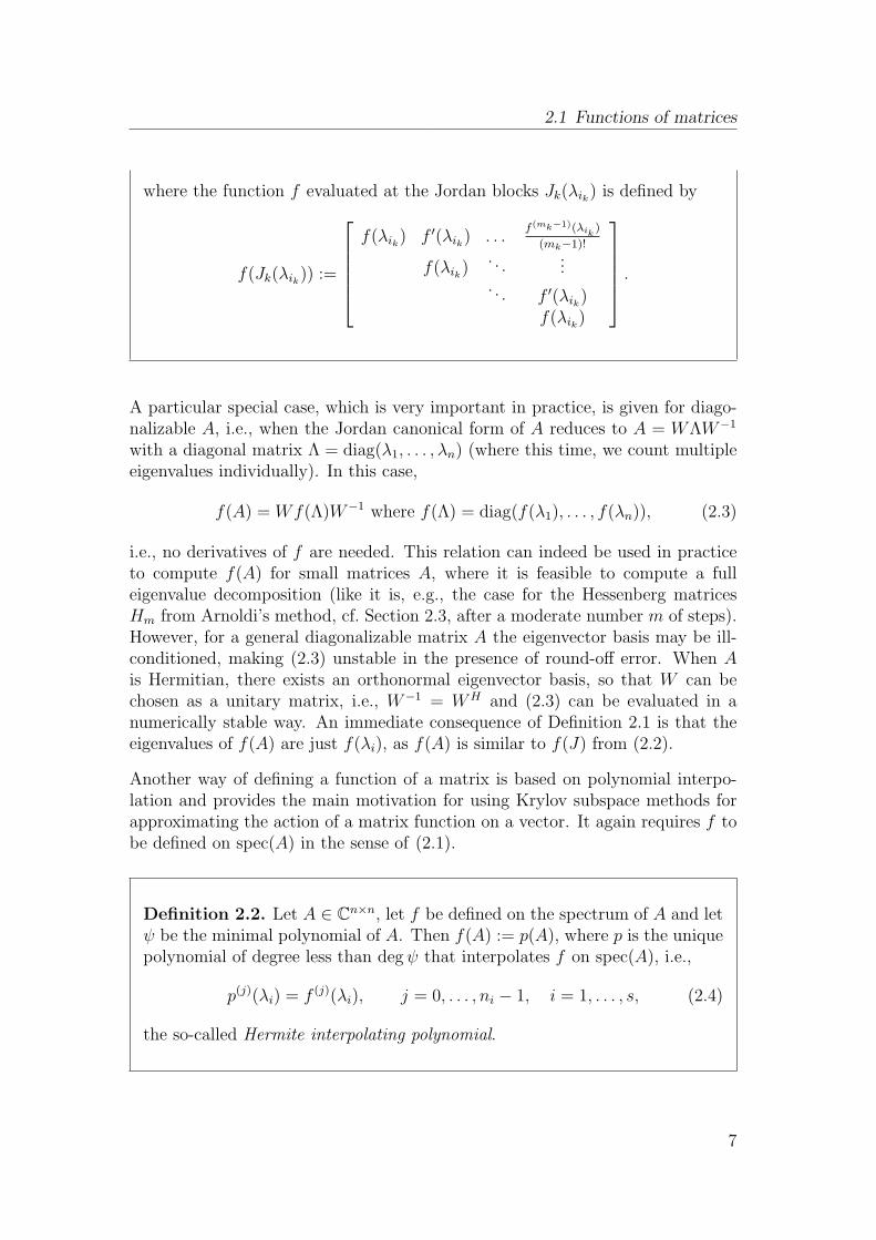
where the function f evaluated at the Jordan blocks Jk(λik) is defined by
f(Jk(λik)) :=
f(λik) f ′(λik) . . .f (mk−1)(λik
)
(mk−1)!
f(λik). . .
.... . . f ′(λik)
f(λik)
.
A particular special case, which is very important in practice, is given for diago-nalizable A, i.e., when the Jordan canonical form of A reduces to A = WΛW−1
with a diagonal matrix Λ = diag(λ1, . . . , λn) (where this time, we count multipleeigenvalues individually). In this case,
f(A) = Wf(Λ)W−1 where f(Λ) = diag(f(λ1), . . . , f(λn)), (2.3)
i.e., no derivatives of f are needed. This relation can indeed be used in practiceto compute f(A) for small matrices A, where it is feasible to compute a fulleigenvalue decomposition (like it is, e.g., the case for the Hessenberg matricesHm from Arnoldi’s method, cf. Section 2.3, after a moderate number m of steps).However, for a general diagonalizable matrix A the eigenvector basis may be ill-conditioned, making (2.3) unstable in the presence of round-off error. When Ais Hermitian, there exists an orthonormal eigenvector basis, so that W can bechosen as a unitary matrix, i.e., W−1 = WH and (2.3) can be evaluated in anumerically stable way. An immediate consequence of Definition 2.1 is that theeigenvalues of f(A) are just f(λi), as f(A) is similar to f(J) from (2.2).
Another way of defining a function of a matrix is based on polynomial interpo-lation and provides the main motivation for using Krylov subspace methods forapproximating the action of a matrix function on a vector. It again requires f tobe defined on spec(A) in the sense of (2.1).
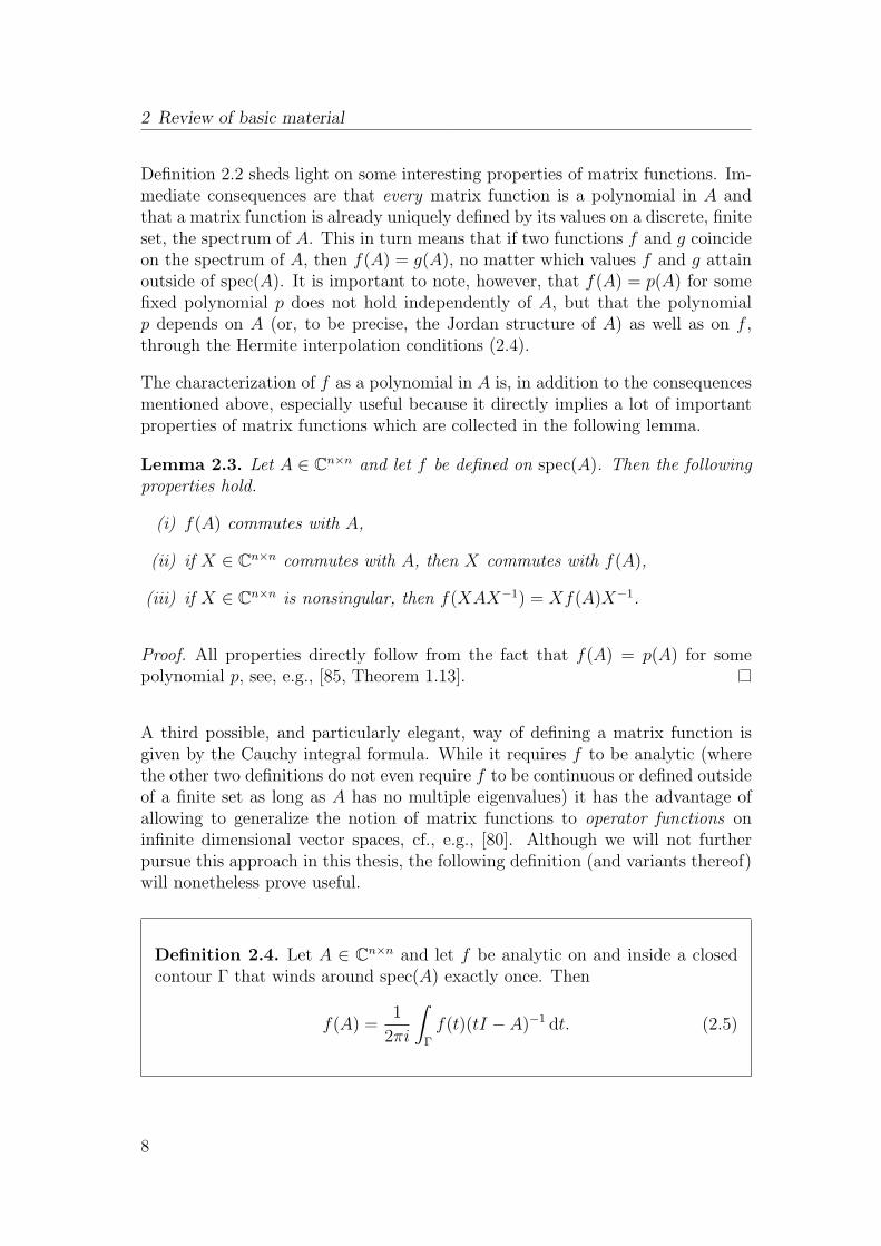
Definition 2.2. Let A ∈ Cn×n, let f be defined on the spectrum of A and let
ψ be the minimal polynomial of A. Then f(A) := p(A), where p is the uniquepolynomial of degree less than degψ that interpolates f on spec(A), i.e.,
p(j)(λi) = f (j)(λi), j = 0, . . . , ni − 1, i = 1, . . . , s, (2.4)
the so-called Hermite interpolating polynomial.
7
2 Review of basic material
Definition 2.2 sheds light on some interesting properties of matrix functions. Im-mediate consequences are that every matrix function is a polynomial in A andthat a matrix function is already uniquely defined by its values on a discrete, finiteset, the spectrum of A. This in turn means that if two functions f and g coincideon the spectrum of A, then f(A) = g(A), no matter which values f and g attainoutside of spec(A). It is important to note, however, that f(A) = p(A) for somefixed polynomial p does not hold independently of A, but that the polynomialp depends on A (or, to be precise, the Jordan structure of A) as well as on f ,through the Hermite interpolation conditions (2.4).
The characterization of f as a polynomial in A is, in addition to the consequencesmentioned above, especially useful because it directly implies a lot of importantproperties of matrix functions which are collected in the following lemma.
Lemma 2.3. Let A ∈ Cn×n and let f be defined on spec(A). Then the following
properties hold.
(i) f(A) commutes with A,
(ii) if X ∈ Cn×n commutes with A, then X commutes with f(A),
(iii) if X ∈ Cn×n is nonsingular, then f(XAX−1) = Xf(A)X−1.
Proof. All properties directly follow from the fact that f(A) = p(A) for somepolynomial p, see, e.g., [85, Theorem 1.13].
A third possible, and particularly elegant, way of defining a matrix function isgiven by the Cauchy integral formula. While it requires f to be analytic (wherethe other two definitions do not even require f to be continuous or defined outsideof a finite set as long as A has no multiple eigenvalues) it has the advantage ofallowing to generalize the notion of matrix functions to operator functions oninfinite dimensional vector spaces, cf., e.g., [80]. Although we will not furtherpursue this approach in this thesis, the following definition (and variants thereof)will nonetheless prove useful.
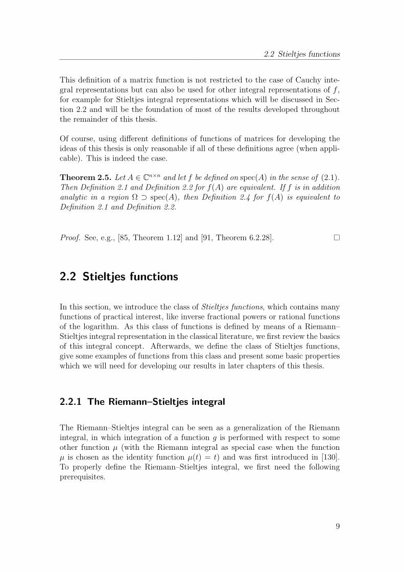
Definition 2.4. Let A ∈ Cn×n and let f be analytic on and inside a closed
contour Γ that winds around spec(A) exactly once. Then
f(A) =1
2πi
∫
Γ
f(t)(tI − A)−1 dt. (2.5)
8
2.2 Stieltjes functions
This definition of a matrix function is not restricted to the case of Cauchy inte-gral representations but can also be used for other integral representations of f ,for example for Stieltjes integral representations which will be discussed in Sec-tion 2.2 and will be the foundation of most of the results developed throughoutthe remainder of this thesis.
Of course, using different definitions of functions of matrices for developing theideas of this thesis is only reasonable if all of these definitions agree (when appli-cable). This is indeed the case.
Theorem 2.5. Let A ∈ Cn×n and let f be defined on spec(A) in the sense of (2.1).
Then Definition 2.1 and Definition 2.2 for f(A) are equivalent. If f is in additionanalytic in a region Ω ⊃ spec(A), then Definition 2.4 for f(A) is equivalent toDefinition 2.1 and Definition 2.2.
Proof. See, e.g., [85, Theorem 1.12] and [91, Theorem 6.2.28].
2.2 Stieltjes functions
In this section, we introduce the class of Stieltjes functions, which contains manyfunctions of practical interest, like inverse fractional powers or rational functionsof the logarithm. As this class of functions is defined by means of a Riemann–Stieltjes integral representation in the classical literature, we first review the basicsof this integral concept. Afterwards, we define the class of Stieltjes functions,give some examples of functions from this class and present some basic propertieswhich we will need for developing our results in later chapters of this thesis.
2.2.1 The Riemann–Stieltjes integral
The Riemann–Stieltjes integral can be seen as a generalization of the Riemannintegral, in which integration of a function g is performed with respect to someother function µ (with the Riemann integral as special case when the functionµ is chosen as the identity function µ(t) = t) and was first introduced in [130].To properly define the Riemann–Stieltjes integral, we first need the followingprerequisites.
9
2 Review of basic material
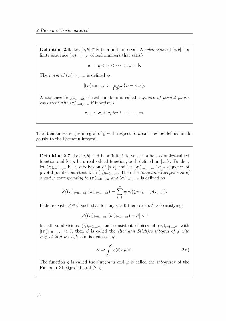
Definition 2.6. Let [a, b] ⊂ R be a finite interval. A subdivision of [a, b] is afinite sequence (τi)i=0,...,m of real numbers that satisfy
a = τ0 < τ1 < · · · < τm = b.
The norm of (τi)i=1,...,m is defined as
|(τi)i=0,...,m| := max1≤i≤m
τi − τi−1.
A sequence (σi)i=1,...,m of real numbers is called sequence of pivotal pointsconsistent with (τi)i=0,...,m if it satisfies
τi−1 ≤ σi ≤ τi for i = 1, . . . ,m.
The Riemann–Stieltjes integral of g with respect to µ can now be defined analo-gously to the Riemann integral.
Definition 2.7. Let [a, b] ⊂ R be a finite interval, let g be a complex-valuedfunction and let µ be a real-valued function, both defined on [a, b]. Further,let (τi)i=0,...,m be a subdivision of [a, b] and let (σi)i=1,...,m be a sequence ofpivotal points consistent with (τi)i=0,...,m. Then the Riemann–Stieltjes sum ofg and µ corresponding to (τi)i=0,...,m and (σi)i=1,...,m is defined as
S((τi)i=0,...,m, (σi)i=1,...,m
)=
m∑
i=1
g(σi)(µ(τi)− µ(τi−1)
).
If there exists S ∈ C such that for any ε > 0 there exists δ > 0 satisfying
∣∣S((τi)i=0,...,m, (σi)i=1,...,m
)− S
∣∣ < ε
for all subdivisions (τi)i=0,...,m and consistent choices of (σi)i=1,...,m with|(τi)i=0,...,m| < δ, then S is called the Riemann–Stieltjes integral of g withrespect to µ on [a, b] and is denoted by
S =:
∫ b
a
g(t) dµ(t). (2.6)
The function g is called the integrand and µ is called the integrator of theRiemann–Stieltjes integral (2.6).
10
2.2 Stieltjes functions
Note that for µ(t) = t (or µ(t) = t + c for some constant c ∈ R), Definition 2.7reduces to the definition of the ordinary Riemann integral. Another connectionbetween Riemann and Riemann–Stieltjes integrals is given by the following, clas-sical result.
Lemma 2.8. Let [a, b] ⊂ R be a finite interval, let g be continuous on [a, b] andlet µ be continuously differentiable on [a, b]. Then
∫ b
a
g(t) dµ(t) =
∫ b
a
g(t)µ′(t) dt.
Proof. See [121, Theorem 9.55b].
For a continuously differentiable integrator µ, the Riemann–Stieltjes integral thusreduces to an ordinary Riemann integral.
Example 2.9. A special case of a Riemann–Stieltjes integral correspondingto a nondifferentiable integrator is given when µ is a step function with jumpsof size µ1, . . . , µℓ at the points t1, . . . , tℓ, i.e.,
µ(t) =
0 a ≤ t ≤ t1
µ1 t1 < t ≤ t2
µ1 + µ2 t2 < t ≤ t3...
...
µ1 + · · ·+ µℓ tℓ < t ≤ b.
In this case, the Riemann–Stieltjes integral of a continuous function g reducesto a finite sum, cf. [83, Section 12.9, Example 3],
∫ b
a
g(t) dµ(t) =ℓ∑
i=1
g(ti)µi.
This observation will later prove useful for establishing a connection betweenrational functions in partial fraction form and Stieltjes functions, cf. Exam-ple 2.14.
We proceed by collecting some basic, easy to prove properties of the Riemann–Stieltjes integral which mostly generalize well-known properties of the Riemannintegral.
11
2 Review of basic material
Proposition 2.10. Let [a, b] ⊂ R be a finite interval, let g, g1, g2 be complex-valued functions on [a, b] and let µ, µ1, µ2 be real-valued functions on [a, b]. Then
(i) The Riemann–Stieltjes integral is linear in the integrand, i.e.,
∫ b
a
g1(t) + g2(t) dµ(t) =
∫ b
a
g1(t) dµ(t) +
∫ b
a
g2(t) dµ(t), (2.7)
and, for a constant c ∈ C,
∫ b
a
cg(t) dµ(t) = c
∫ b
a
g(t) dµ(t). (2.8)
(ii) The Riemann–Stieltjes integral is linear in the integrator, i.e.,
∫ b
a
g(t) d(µ1(t) + µ2(t)) =
∫ b
a
g(t) dµ1(t) +
∫ b
a
g(t) dµ2(t), (2.9)
and, for a constant c ∈ R,
∫ b
a
g(t) d(cµ(t)) = c
∫ b
a
g(t) dµ(t). (2.10)
(iii) For a < c < b it holds
∫ b
a
g(t) dµ(t) =
∫ c
a
g(t) dµ(t) +
∫ b
c
g(t) dµ(t) (2.11)
provided that all integrals in (2.11) exist.
(iv) If µ is monotonically increasing on [a, b], then
∫ b
a
dµ(t) :=
∫ b
a
1 dµ(t) = µ(b)− µ(a).
(v) If µ is monotonically increasing on [a, b] and g1, g2 are real-valued withg1(t) ≤ g2(t) for all t ∈ [a, b], then
∫ b
a
g1(t) dµ(t) ≤∫ b
a
g2(t) dµ(t).
Proof. See [26, Theorem 5.1.5], [108, Section VIII.6] and [121, Section 9.55c].
12
2.2 Stieltjes functions
Note that in assertion (i) and (ii) of Proposition 2.10, the existence of the inte-grals on the right-hand sides of equations (2.7), (2.8), (2.9) and (2.10) imply theexistence of the integrals on the left-hand sides.
Just as for Riemann integrals, improper Riemann–Stieltjes integrals may be de-fined.
Definition 2.11. Let a ∈ R, let g be a continuous, complex-valued functionand let µ be a real-valued function on [a,∞). Then the improper Riemann–Stieltjes integral of g with respect to µ on [a,∞) is defined as
∫ ∞
a
g(t) dµ(t) := limb→∞
∫ b
a
g(t) dµ(t),
provided that the limit exists.
There is a wide variety of results on assumptions necessary for the existence of(proper and improper) Riemann–Stieltjes integrals; see, e.g., [108, 121]. We willnot go into detail on this in general rather important topic, as we are primarilyinterested in Stieltjes integrals with integrand g(t) = 1
z+tfor z ∈ C \ R−
0 , forwhich the question of existence is easier to analyze than in the general case;cf. Section 2.2.2.
Before proceeding, we state one additional result which will prove useful for esti-mating error norms when investigating the convergence behavior of Krylov sub-space methods for Stieltjes matrix functions.
Lemma 2.12. Let a ∈ R, let g : [a,∞) −→ Cn be a vector-valued function, i.e.,
g(t) = [g1(t), g2(t), . . . , gn(t)]T
with gi : [a,∞) −→ C. Further, let µ be real-valued and monotonically increasingon [a,∞), such that all integrals
∫ ∞
a
gi(t) dµ(t)
exist and let || · ‖ be a norm on Cn. Then
∥∥∥∥∫ ∞
a
g(t) dµ(t)
∥∥∥∥ ≤∫ ∞
a
‖g(t)‖ dµ(t), (2.12)
where the integral on the left-hand side of (2.12) is understood component-wise.
13
2 Review of basic material
Proof. Let b > a, let T (j) = (τ(j)i )i=0,...,mj
be a sequence of subdivisions of [a, b]
with |T (j)| → 0 for j → ∞ and let Σ(j) = (σ(j)i )i=1,...,mj
be a sequence of con-sistent sequences of pivotal points. We define the vector-valued analogue to theRiemann–Stieltjes sum from Definition 2.7 as
S(T (j),Σ(j)) =
mj∑
i=1
[g1(σ
(j)i ), . . . , gn(σ
(j)i )]T (
µ(τ(j)i )− µ(τ (j)i−1)
),
i.e., the pivotal points are inserted into each individual component gi of g. Then,by applying Definition 2.7 to each component individually, we have
limj→∞
S(T (j),Σ(j)) =
∫ b
a
g(t) dµ(t), (2.13)
We further have for any j
‖S(T (j),Σ(j))‖ =
∥∥∥∥∥
mj∑
i=1
g(σ(j)i )(µ(τ
(j)i )− µ(τ (j)i−1)
)∥∥∥∥∥
≤mj∑
i=1
∥∥∥g(σ(j)i )(µ(τ
(j)i )− µ(τ (j)i−1)
)∥∥∥
=
mj∑
i=1
‖g(σ(j)i )‖
(µ(τ
(j)i )− µ(τ (j)i−1)
), (2.14)
where the inequality holds due to the triangle inequality and the last equalityholds because µ is monotonically increasing on [a, b]. By taking the norm on bothsides of (2.13) and inserting (2.14), we obtain
∥∥∥∥∫ b
a
g(t) dµ(t)
∥∥∥∥ =
∥∥∥∥ limj→∞S(T (j),Σ(j))
∥∥∥∥ =
∫ b
a
‖g(t)‖ dµ(t). (2.15)
By taking the limit b → ∞ inside the norm on the left-hand side of (2.15) andusing the fact that ‖ · ‖ is continuous, we obtain the desired result.
We remark that we do not make any statement about the existence of the integralon the right-hand side of (2.12), in the sense that if the integral is infinite, theninfinity is taken as (trivial) upper bound for the left-hand side. At all places wherewe use the result of Lemma 2.12 in this thesis, we will individually investigatewhether this integral is finite, as we do not need any general result about thefiniteness of such integrals.
We will now turn our attention to the class of Stieltjes functions which are definedby means of a Riemann–Stieltjes integral of the resolvent function g(t) = 1
z+t.
14
2.2 Stieltjes functions
2.2.2 The Stieltjes cone
We first define the class of Stieltjes functions.
Definition 2.13. Let µ be a monotonically increasing, real-valued functionon R
+0 such that ∫ ∞
0
1
1 + tdµ(t) <∞, (2.16)
and let a ≥ 0. Then the function f : C \ R−0 −→ C defined via
f(z) = a+
∫ ∞
0
1
z + tdµ(t) (2.17)
is called Stieltjes function corresponding to µ. The function µ is also calledgenerating function of f .
Note that the condition (2.16) imposed on µ is sufficient for f being defined (andholomorphic) in all z ∈ C \ R−
0 . The set of all Stieltjes functions forms a convexcone, i.e., it is closed under addition and under multiplication by nonnegativescalars. For both properties, see, e.g., [14, Section 3]. From now on we will,without loss of generality, always assume a = 0 in (2.17).
Before discussing useful properties of Stieltjes functions, we first list a few exam-ples of important functions belonging to this class.
Example 2.14. The following functions are Stieltjes functions.
(i) The function f(z) = z−1, generated by the step function
µ(t) =
0 t = 0,
1 t > 0.
(ii) Rational functions in partial fraction form with poles on the negativereal axis,
f(z) =ℓ∑
i=0
µi
z + ti,
15
2 Review of basic material
generated by the step function
µ(t) =
0 0 ≤ t ≤ t1
µ1 t1 < t ≤ t2
µ1 + µ2 t2 < t ≤ t3...
...
µ1 + · · ·+ µℓ tℓ < t
with ti ≥ 0, µi > 0, i = 1, . . . , ℓ.
(iii) The function f(z) = z−α for α ∈ (0, 1), because
z−α =sin(απ)
π
∫ ∞
0
t−α
z + tdt. (2.18)
(iv) The function f(z) = log(1 + z)/z, because
log(1 + z)
z=
∫ ∞
1
t−1
z + tdt. (2.19)
Note that the functions in Example 2.14(iii) and (iv) correspond to continuouslydifferentiable generating functions µ, so that they can be written as ordinaryRiemann integrals by Lemma 2.8. For further examples of Stieltjes functionsand proofs that the above functions indeed are Stieltjes functions in the sense ofDefinition 2.13, see, e.g., [14, 15, 55,83,130].
The following lemma gives a representation of the derivative of Stieltjes functionswhich will be useful for some results on error bounds in this thesis.
Lemma 2.15. Let f be a Stieltjes function with generating function µ. Then fis infinitely many times continuously differentiable on C \ R−
0 and
f (k)(z) = (−1)kk!∫ ∞
0
1
(z + t)k+1dµ(t) for all k ∈ N0.
Proof. See, e.g., [14, Section 3].
The class of Stieltjes functions is very closely related to the class of completelymonotonic functions defined in the following.
16
2.2 Stieltjes functions
Definition 2.16. A function f : R+ −→ R is called completely monotonic ifit is infinitely many times continuously differentiable and satisfies
(−1)kf (k)(z) ≥ 0 for k ∈ N0 and z ∈ R+.
The following result establishes the connection between Stieltjes functions andcompletely monotonic functions and gives another easy to prove but useful prop-erty of completely monotonic functions, see, e.g., [5, 14].
Proposition 2.17.
(i) Every Stieltjes function (or more precisely, its restriction to the positive realaxis) is a completely monotonic function.
(ii) Let f1, f2 be completely monotonic functions. Then f1 · f2 is a completelymonotonic function.
Proof. Part (i) directly follows from Lemma 2.15 and Proposition 2.10(v) andpart (ii) is a direct consequence of the Leibniz rule for product differentiation.
We mention in passing that the set of Stieltjes functions is a proper subset ofthe class of completely monotonic functions, i.e., not every completely mono-tonic function is a Stieltjes function, as the following example, taken from [14],illustrates.
Example 2.18. Consider the function f(z) = 1/(z(1 + z2)). One easilyverifies that f is completely monotonic, but it has poles at z = ±i, so that itcannot be a Stieltjes function.
The class of Stieltjes functions is of particular interest in our setting as the integralrepresentation (2.17) directly transfers to the case of matrix functions, similar tothe Cauchy integral representation (2.5) of analytic functions. For f a Stieltjesfunction with generating function µ and A ∈ C
n×n with spec(A) ⊆ C \ R−0 , we
directly have
f(A) =
∫ ∞
0
(A+ tI)−1 dµ(t)
17
2 Review of basic material
and thus
f(A)b =
∫ ∞
0
(A+ tI)−1b dµ(t). (2.20)
According to (2.20), f(A)b for f a Stieltjes function can be interpreted as theintegral over the solutions x (t) of the shifted linear systems
(A+ tI)x (t) = b
for t ≥ 0. This relation between the action of Stieltjes matrix functions on a vectorand shifted linear systems with positive shifts is one of the building blocks of theresults developed in this thesis. In particular, it allows to also establish a relationbetween Krylov subspace methods for approximating matrix functions and Krylovsubspace methods for the approximate solution of linear systems. This in turnallows to transfer theoretical results from the latter (which are understood farbetter) to the former and will be the basis of the convergence analysis presentedin Chapter 5. We continue by investigating Krylov subspace methods in detail inthe next section.
2.3 Krylov subspace methods for f (A)b
While Section 2.1 dealt with matrix functions f(A), for the remainder of thisthesis we will not focus on the computation of the matrix function f(A) itself,but rather on the action of f(A) on some vector b ∈ C
n, i.e.,
f(A)b. (2.21)
For techniques and algorithms related to the computation of f(A) (for small andpossibly dense matrices A), we refer to, e.g., [32,85,86] and the references therein.
One of the main computational difficulties when numerically evaluating (2.21) isthat f(A) is in general a full matrix, even when A is sparse or structured, withthe one exception from this rule being that f(A) is (block-)diagonal when A is(block-)diagonal. We just mention for the sake of completeness that when A isblock upper (or lower) triangular, f(A) will also inherit this property, but theupper (or lower) triangle will in general be completely filled, resulting in a matrixwith O(n2) nonzero entries, so that we consider this as a dense matrix in oursetting. Therefore, even for moderate values of n, it may not even be possible tostore the matrix f(A), such that the naive approach of first computing f(A) andthen multiplying it to b is infeasible, notwithstanding the high computationalcost.
Therefore, one typically tries to approximate the vector f(A)b directly by someiterative method. By far the most popular and most widely-used methods forthis task belong to the class of Krylov subspace methods (or related classes likeextended and general rational Krylov subspace methods).
18
2.3 Krylov subspace methods for f(A)b
2.3.1 The Arnoldi/Lanczos approximation for f(A)b
We begin our exposition with the basic definition of a Krylov subspace corre-sponding to a matrix A and a vector b, which is central to most of the results ofthis thesis.
Definition 2.19. Let A ∈ Cn×n and let b ∈ C
n. The mth Krylov subspacewith respect to A and b is defined as
Km(A, b) = pm−1(A)b : pm−1 ∈ Πm−1, (2.22)
where Πm−1 denotes the set of all polynomials of degree at most m− 1.
The idea of searching for an approximation to f(A)b in a Krylov subspaceKm(A, b) is quite obvious in light of Definition 2.2, as each matrix function isa polynomial (of degree at most n− 1) in A, so that f(A)b ∈ Kn(A, b). Approx-imations from Krylov subspaces of dimension m < n can thus be interpreted asreplacing the polynomial p from Definition 2.2 by another polynomial of lowerdegree. Before proceeding, we summarize some basic properties of Km(A, b).
Proposition 2.20. Let A ∈ Cn×n and let b ∈ C
n. In addition, let m∗ be thesmallest integer such that there exists a polynomial pm∗ ∈ Πm∗ which satisfiespm∗(A)b = 0. Then
(i) Km(A, b) ⊆ Km+1(A, b) for all m ≥ 1,
(ii) Km∗(A, b) is invariant under A, and Km(A, b) = Km∗(A, b) for all m ≥ m∗,
(iii) dimKm(A, b) = minm,m∗.
Proof. Part (i) is directly obvious from (2.22). For part (ii), see, e.g., [115, Propo-sition 6.1] and for part (iii), see, e.g., [115, Proposition 6.2].
Property (i) from Proposition 2.20 means that Krylov subspaces are nested, andtogether with Property (iii) it follows that, as long as m < m∗, if v1, . . . , vm isa basis of Km(A, b), then there exists vm+1 ∈ Km+1(A, b) \ Km(A, b) such thatv1, . . . , vm+1 is a basis of Km+1(A, b).
This observation allows to iteratively construct a basis of the Krylov subspaceKm(A, b) by starting with a basis of K1(A, b) = spanb and adding one basis
19
2 Review of basic material
vector at a time. The most obvious choice for a basis of Km(A, b) is the Krylovbasis
b, Ab, A2b, . . . , Am−1b,
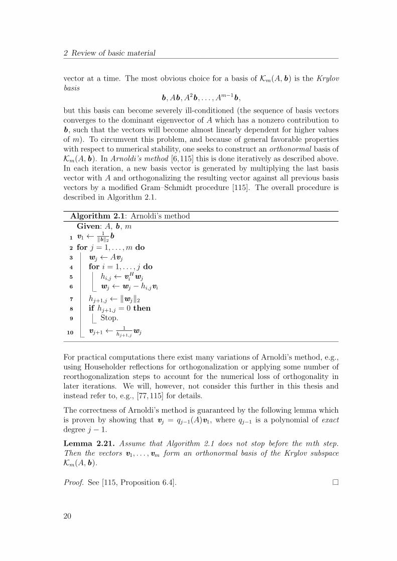
but this basis can become severely ill-conditioned (the sequence of basis vectorsconverges to the dominant eigenvector of A which has a nonzero contribution tob, such that the vectors will become almost linearly dependent for higher valuesof m). To circumvent this problem, and because of general favorable propertieswith respect to numerical stability, one seeks to construct an orthonormal basis ofKm(A, b). In Arnoldi’s method [6,115] this is done iteratively as described above.In each iteration, a new basis vector is generated by multiplying the last basisvector with A and orthogonalizing the resulting vector against all previous basisvectors by a modified Gram–Schmidt procedure [115]. The overall procedure isdescribed in Algorithm 2.1.
Algorithm 2.1: Arnoldi’s method
Given: A, b, mv1 ← 1
‖b‖2b1
for j = 1, . . . ,m do2
wj ← Avj3
for i = 1, . . . , j do4
hi,j ← vHi wj5
wj ← wj − hi,jvi6
hj+1,j ← ‖wj‖27
if hj+1,j = 0 then8
Stop.9
vj+1 ← 1hj+1,j
wj10
For practical computations there exist many variations of Arnoldi’s method, e.g.,using Householder reflections for orthogonalization or applying some number ofreorthogonalization steps to account for the numerical loss of orthogonality inlater iterations. We will, however, not consider this further in this thesis andinstead refer to, e.g., [77, 115] for details.
The correctness of Arnoldi’s method is guaranteed by the following lemma whichis proven by showing that vj = qj−1(A)v1, where qj−1 is a polynomial of exactdegree j − 1.
Lemma 2.21. Assume that Algorithm 2.1 does not stop before the mth step.Then the vectors v1, . . . , vm form an orthonormal basis of the Krylov subspaceKm(A, b).
Proof. See [115, Proposition 6.4].
20
2.3 Krylov subspace methods for f(A)b
If the condition hj+1,j = 0 is fulfilled in line 8 of Algorithm 2.1, the algorithmbreaks down. The following lemma assures that in this case the Krylov subspaceKj(A, b) has reached the maximum possible dimension and is invariant under A.
Lemma 2.22. Arnoldi’s method breaks down at step j if and only if j = m∗ (withm∗ as defined in Proposition 2.20). In this case, Kj(A, b) is invariant under A.
Proof. See [115, Proposition 6.6].
Collecting the orthonormal basis vectors computed by Algorithm 2.1 in a matrixVm = [v1, . . . , vm] ∈ C
n×m and the orthogonalization coefficients in an unreducedupper Hessenberg matrix Hm = [hi,j]i,j=1,...,m ∈ C
m×m yields the Arnoldi decom-position
AVm = VmHm + hm+1,mvm+1eHm (2.23)
where em ∈ Cm denotes the mth canonical unit vector. The following result
guarantees that the Arnoldi decomposition (2.23) is essentially unique, which willbe useful in Chapter 6 and 7, where we compute decompositions of the form (2.23)by other means than by applying Algorithm 2.1 and can still be sure to obtainthe same result.
Lemma 2.23. Let A ∈ Cn×n and let [V, v ] ∈ C
n×(m+1) have orthonormal columns.If there exist an upper Hessenberg matrix H ∈ C
m×m and a scalar h ∈ C suchthat
AV = V H + hveHm
is fulfilled, then V = VmD and H = DHHmD, where D ∈ Cm×m is a unitary
diagonal matrix and Hm and Vm are the matrices from the Arnoldi decomposi-tion (2.23) corresponding to the Krylov subspace Km(A, v1), where v1 is the firstcolumn of V . In particular, if all subdiagonal entries of H are real and positive,then V = Vm and H = Hm.
Proof. See [129, Chapter 5, Theorem 1.3].
By multiplying both sides of the relation (2.23) by V Hm and exploiting the orthog-
onality of the vi, i = 1, . . . ,m+ 1, one finds
V Hm AVm = Hm, (2.24)
showing that Hm can be interpreted as the (orthogonal) projection of A ontothe Krylov subspace Km(A, b). The identity (2.24) also allows to easily provethat substantial algorithmic and computational simplifications are possible inArnoldi’s method when the matrix A is Hermitian. By (2.24) it directly followsthat Hm is Hermitian whenever A is Hermitian, and because Hm is in additionupper Hessenberg by construction, it must be tridiagonal in this case. This in turn
21
2 Review of basic material
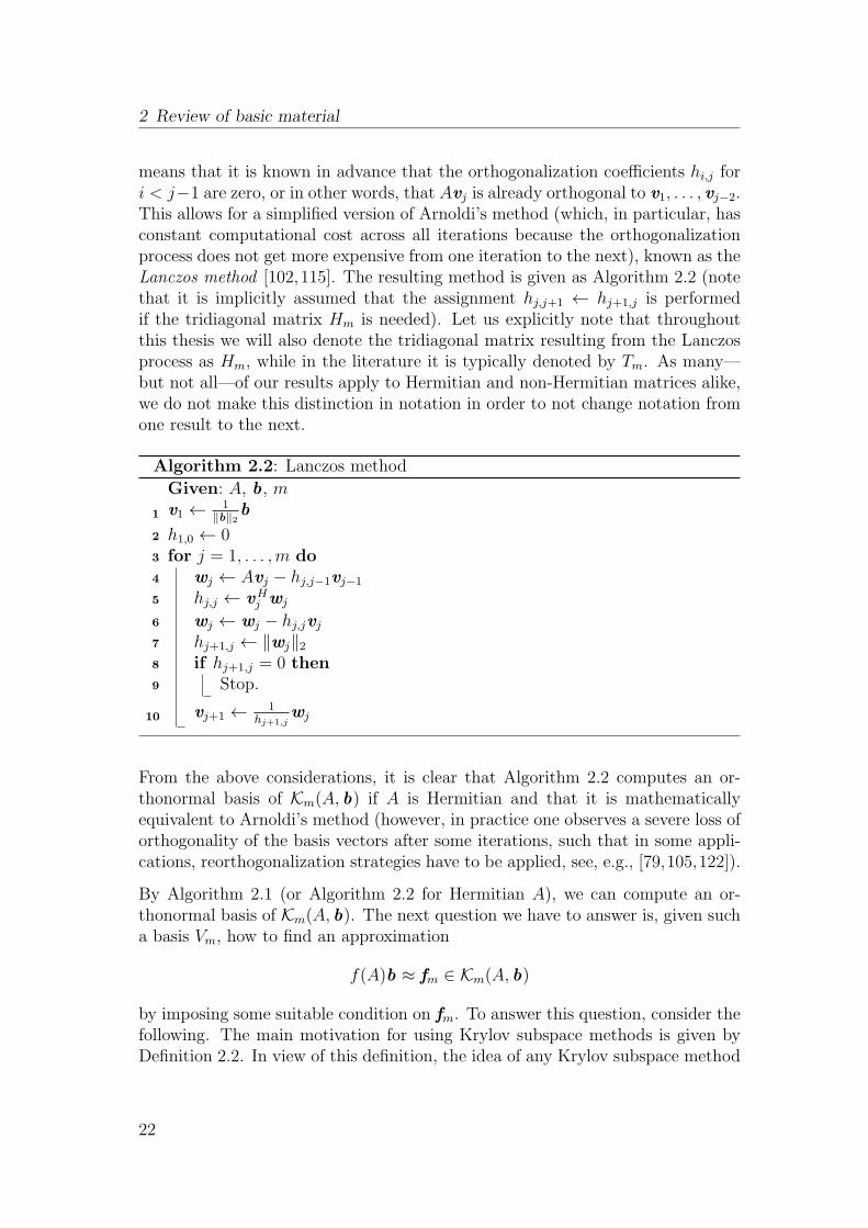
means that it is known in advance that the orthogonalization coefficients hi,j fori < j−1 are zero, or in other words, that Avj is already orthogonal to v1, . . . , vj−2.This allows for a simplified version of Arnoldi’s method (which, in particular, hasconstant computational cost across all iterations because the orthogonalizationprocess does not get more expensive from one iteration to the next), known as theLanczos method [102,115]. The resulting method is given as Algorithm 2.2 (notethat it is implicitly assumed that the assignment hj,j+1 ← hj+1,j is performedif the tridiagonal matrix Hm is needed). Let us explicitly note that throughoutthis thesis we will also denote the tridiagonal matrix resulting from the Lanczosprocess as Hm, while in the literature it is typically denoted by Tm. As many—but not all—of our results apply to Hermitian and non-Hermitian matrices alike,we do not make this distinction in notation in order to not change notation fromone result to the next.
Algorithm 2.2: Lanczos method
Given: A, b, mv1 ← 1
‖b‖2b1
h1,0 ← 02
for j = 1, . . . ,m do3
wj ← Avj − hj,j−1vj−14
hj,j ← vHj wj5
wj ← wj − hj,jvj6
hj+1,j ← ‖wj‖27
if hj+1,j = 0 then8
Stop.9
vj+1 ← 1hj+1,j
wj10
From the above considerations, it is clear that Algorithm 2.2 computes an or-thonormal basis of Km(A, b) if A is Hermitian and that it is mathematicallyequivalent to Arnoldi’s method (however, in practice one observes a severe loss oforthogonality of the basis vectors after some iterations, such that in some appli-cations, reorthogonalization strategies have to be applied, see, e.g., [79,105,122]).
By Algorithm 2.1 (or Algorithm 2.2 for Hermitian A), we can compute an or-thonormal basis of Km(A, b). The next question we have to answer is, given sucha basis Vm, how to find an approximation
f(A)b ≈ fm ∈ Km(A, b)
by imposing some suitable condition on fm. To answer this question, consider thefollowing. The main motivation for using Krylov subspace methods is given byDefinition 2.2. In view of this definition, the idea of any Krylov subspace method
22
2.3 Krylov subspace methods for f(A)b
can be summarized as approximating the polynomial p from Definition 2.2 (whichmay be of degree up to n−1) by a polynomial of smaller degreem−1. We can thusrephrase the above question as how to choose a polynomial pm−1 ∈ Πm−1, suchthat pm−1(A)b ≈ p(A)b. A straightforward approach, considering the fact that pinterpolates f at spec(A), is to choose pm−1 as a polynomial which interpolatesf at m suitably chosen points. One such choice are the eigenvalues of Hm, theso-called Ritz values corresponding to Km(A, b). The following, classical resultrelates the Ritz values to eigenvalues of A, thus giving a first motivation for whyone can consider them to be sensible interpolation points.
Proposition 2.24. Let Hm be the upper Hessenberg matrix from the Arnoldidecomposition (2.23) corresponding to Km(A, b) and let spec(Hm) = θ1, . . . , θm.Then
θi ∈ W(A) for i = 1, . . . ,m,
where
W(A) :=
vHAv
vHv: v 6= 0
denotes the field of values of A. If, in addition, Km(A, b) is A-invariant, i.e.,AKm(A, b) ⊆ Km(A, b), then
θi ∈ spec(A) for i = 1, . . . ,m.
Proof. The first part of the assertion follows directly from the relation Hm =V Hm AVm and the fact that Vm has orthonormal columns. The second part of the
statement follows, e.g., directly from [129, Chapter 4, Theorem 4.1].
Proposition 2.24 guarantees that the Ritz values corresponding to Km(A, b) arealways related to some kind of spectral information of A as they lie in its field ofvalues (which reduces to the spectral interval [λmin, λmax] in the Hermitian case),and that they even become exact eigenvalues of A once the Krylov subspacereaches its maximum possible dimension. Of course, Km(A, b) will in general notbecome A-invariant in practical computations, where one uses only small valuesof m, but the result at least shows that there is a relation between Ritz values andeigenvalues of A. In case that A is Hermitian, one can show further results on thebehavior of the Ritz values (which can be more or less arbitrary in the general,non-Hermitian case) before Km(A, b) becomes A-invariant, e.g., that “outliers” atthe left or right end of the spectrum are well approximated first, cf., e.g., [101,134].
In addition to the reasoning stated above, choosing pm−1 as the polynomial whichinterpolates f at the Ritz values corresponding to Km(A, b) has the additionaladvantage that pm−1(A)b is readily available without needing to explicitly com-pute pm−1 (the numerical computation of high-degree interpolating polynomialscan become highly unstable [131]). The precise result is stated in the followinglemma, first proven in [47] and [114].
23
2 Review of basic material
Lemma 2.25. Let A ∈ Cn×n and let b ∈ C
n. Let Vm, Hm fulfill the relation (2.23)and let
fm = Vmf(VHm AVm)V
Hm b = ‖b‖2Vmf(Hm)e1. (2.25)
Then
fm = pm−1(A)b,
where pm−1 ∈ Πm−1 is the unique polynomial interpolating f at the eigenvalues ofHm in the Hermite sense, provided that f is defined on spec(Hm).
Proof. See, e.g., [85, Theorem 13.5].
The approximation defined by (2.25) is commonly referred to as Arnoldi (orLanczos) approximation to f(A)b and is the standard choice for an approxi-mation from the Krylov subspace Km(A, b). Another possible motivation forusing (2.25), without even considering the interpolating polynomial characteriza-tion, is that (2.25) is a projection of the original problem (2.21) onto the smallerspace Km(A, b). Of course, for (2.25) to be well-defined, f(Hm) must exist, i.e.,f must be defined on spec(Hm). For this, it is not sufficient that f(A) is defined,as the following example illustrates.
Example 2.26. Consider the symmetric indefinite matrix
A =
[1 00 −1
],
the vector b = [1, 1]H and the function f(z) = z−1. As spec(A) = −1, 1,the matrix function f(A) = A−1 is well-defined and we have f(A)b =A−1b = [1,−1]H . However, one step of the Lanczos method computesv1 = [1/
√2, 1/√2]H and w1 = Av1 = [1/
√2,−1/
√2]H , which is already
orthogonal to v1, so that h1,1 = vH1 w1 = 0 and thus H1 = 0. Therefore,
f1 = ‖b‖2V1f(H1)e1 is not defined.
Example 2.26 motivates, amongst other reasons we will come across in later partsof this thesis, that it may under some circumstances be reasonable to extractother approximations than the Arnoldi approximation (2.25) from a given Krylovsubspace. The following result from [48] is a generalization of Lemma 2.25 whichshows that the polynomial interpolation characterization also holds when Hm
in (2.25) is replaced by a suitable rank-one modification.
24
2.3 Krylov subspace methods for f(A)b
Lemma 2.27. Let A ∈ Cn×n and let b ∈ C
n. Let Vm, Hm fulfill the rela-tion (2.23), let z ∈ C
n and let
fm = ‖b‖2Vmf(Hm + z eHm )e1. (2.26)
Then
fm = pm−1(A)b,
where pm−1 ∈ Πm−1 is the unique polynomial interpolating f at the eigenvalues ofHm + z eH
m in the Hermite sense, provided that f is defined on spec(Hm + z eHm ).
Proof. See [48, Lemma 3 and Corollary 4].
Before we proceed, we give some further comments on the advantages and disad-vantages of the Arnoldi approximation (and the related approximations (2.26)).An important advantageous feature of Arnoldi’s method for matrix functions isthat (at least in exact arithmetic), finite termination is guaranteed as long asall approximations are defined. By Lemma 2.22, the method breaks down afterm steps if and only if Km(A, b) is invariant under A. This in turn means thatf(A)b = p(A)b is already contained in Km(A, b) and the projection (2.25) willyield the exact value of f(A)b (therefore, such a breakdown is sometimes alsoreferred to as a lucky breakdown). However, using Arnoldi’s method for matrixfunctions also has several disadvantages. As already illustrated by Example 2.26,the Arnoldi approximations need not exist even when f(A)b is defined. Other dis-advantages are mainly of practical, computational nature. For evaluating (2.25),one needs to store the whole Arnoldi basis Vm. As the Arnoldi vectors will ingeneral be full vectors, this means storing a dense n ×m matrix. As A is oftenvery large and sparse in practical applications, n will frequently be large. In thiscase, the number m of steps that can be performed is often limited by the avail-able memory and may not be large enough to compute an approximation of thedesired accuracy. In addition, even if the available memory does not limit thenumber of steps that can be performed, the evaluation of f(Hm)e1, the action offunction of a matrix of size m ×m on a vector, becomes increasingly expensivewith growing number of iterations. If the number of iterations necessary to reacha sufficiently accurate approximation lies in the order of magnitude of n, eval-uating f(Hm)e1 may be about as difficult as evaluating f(A)b itself, which canmake the method infeasible for some problems. There are different approachesfor overcoming these difficulties. On the one hand, restarting techniques are pro-posed, in which a certain (small) number m of steps is performed, fm is computedby (2.25) and then, in a new Arnoldi iteration, one tries to approximate theremaining error f(A)b − fm. This technique is more often studied and betterunderstood in the context of linear systems, see, e.g., [56, 115, 116, 123] and wewill at this point not go into detail concerning this topic. Chapter 4 is devoted
25
2 Review of basic material
to restarting techniques, containing a review of existing approaches from the lit-erature and new developments and extensions of these approaches. The otherestablished approach for overcoming the disadvantages of the Arnoldi approxima-tion is using other subspaces than Krylov subspaces Km(A, b) which (hopefully)have better approximation properties, in the sense that a smaller dimension mis needed to reach an accurate enough approximation. Popular choices for thesericher subspaces are rational Krylov subspaces and, as a special case of the former,extended Krylov subspaces. We discuss extended Krylov subspace methods andtheir properties in Chapter 7, for further details and the treatment of general ra-tional Krylov subspaces, we refer to, e.g., [38,80,81,94–96,99] and the referencestherein.
2.4 The special case f (z) = z−1
Krylov subspace methods are frequently used for the solution of linear systems,i.e., the special case of (2.21) with f(z) = z−1. As we will exploit the relationbetween the approximation of Stieltjes matrix functions by the Arnoldi approxi-mation (2.25) and the solution of linear systems at several points throughout thisthesis, we will briefly cover some of the basic terminology and results arising inthis setting in the following. We do not in any way strive for completeness, espe-cially as there is a broad variety of Krylov subspace methods for linear systemslike, e.g., BiCGStab [128,138] or QMR [52], to name just two, which do not havea direct connection to the Arnoldi approximation (2.25). They are therefore notof relevance for the developments of this thesis, although some of them are widelyused in practical applications.
The method arising when the Arnoldi approximation (2.25) is applied to the linearsystem
Ax = b ⇔ x = A−1b,
i.e, the computation of the approximation
xm = ‖b‖2VmH−1m e1, (2.27)
where Vm, Hm are the matrices resulting from Arnoldi’s method for A and b, isknown as the full orthogonalization method (FOM) [113, 115] for linear systems.Note that when solving linear systems by a Krylov subspace method, it is commonpractice to provide the method with an initial guess x0. In this case, one onlyneeds to approximate the remaining error x ∗ − x0 of the initial guess. Thefollowing well-known result (which we state as a proposition despite its simplenature, as it will be used extensively throughout this thesis) gives an easy way todo so.
26
2.4 The special case f(z) = z−1
Proposition 2.28. Let A ∈ Cn×n, let b ∈ C
n and let x ∗ be the solution of thelinear system Ax = b. Further, let x0 ∈ C
n and define the residual r0 = b−Ax0.Then the error e0 = x ∗ − x0 satisfies the residual equation
Ae0 = r0. (2.28)
Proof. A direct computation yields A(x ∗−x0) = Ax ∗−Ax0 = b−Ax0 = r0.
According to Proposition 2.28, one can compute the residual r0 = b − Ax0 andthen find an Arnoldi approximation for A−1r0, the solution of the residual equa-tion (2.28), i.e., one generates iterates in the affine Krylov subspace
x0 +Km(A, r0).
The following result gives an explicit expression for the residual generated byapplying m steps of FOM to the linear system Ax = b.
Proposition 2.29. Let A ∈ Cn×n, b,x0 ∈ C
n and let xm be the approximationfrom m steps of FOM (with initial guess x0) applied to the linear system Ax = b.Then the residual rm = b − Axm satisfies
rm = −hm+1,meHmymvm+1, (2.29)
where ym = ‖r0‖2H−1m e1, with Hm, hm+1,m and vm+1 from the Arnoldi decompo-
sition (2.23). Thus, its Euclidean norm is given by
‖rm‖2 = hm+1,m|eHmym|. (2.30)
Proof. See, e.g., [115, Proposition 6.7].
By recalling the definition of ym in (2.30), we see that the Euclidean norm of theFOM residual can be found by computing the bottom left entry of the inverse ofHm, a relation which we will (implicitly and explicitly) exploit in later chapters.An important implication of Proposition 2.28, besides allowing to provide Krylovsubspace methods for linear systems with an initial guess, is the possibility torestart them easily. After some number m of steps of FOM (or any other Krylovsubspace method for Ax = b), one computes the residual rm = b −Axm and canthen approximately solve the residual equation Aem = rm by m further steps ofthe same method, obtaining an approximation em for the error em = x ∗ − xm.By an additive correction x
(2)m = xm + em one then (hopefully) obtains a better
approximation for x ∗. This procedure can then again be applied to the newresidual equation corresponding to x
(2)m and so on, yielding after k restart cycles
x (k+1)m = x (k)
m + e (k)m with e (k)
m = ‖r (k−1)m ‖2V (k)
m (H(k)m )−1e1, (2.31)
27
2 Review of basic material
where r(k−1)m = b − Ax
(k−1)m is the residual of the iterate from the (k − 1)st
cycle. This way, all quantities computed in the previous cycles of the method(in particular the matrices V
(i)m and H
(i)m for i = 1, . . . , k − 1) can be discarded,
thus avoiding the growing storage requirements and computational cost which isassociated with the unrestarted FOM approximation (2.27). We give a sketch ofthe resulting method (without going into detail on possible stopping criteria) inAlgorithm 2.3, it is discussed in detail in [113, 115]. Another method for whichrestarting is frequently used in practice is GMRES [116].
Algorithm 2.3: Restarted full orthogonalization method
Given: A, b, m, x0
r0 ← b − Ax01
β ← ‖r0‖22
v1 ← 1βr03
tol reached← 04
while tol reached = 0 do5
Compute Vm, Hm by Algorithm 2.1 applied to A, r0.6
ym ← βH−1m e17
xm ← x0 + Vmym8
if target accuracy reached then9
tol reached← 110
x0 ← xm11
r0 ← −hm+1,meHmymvm+112
β ← ‖r0‖213
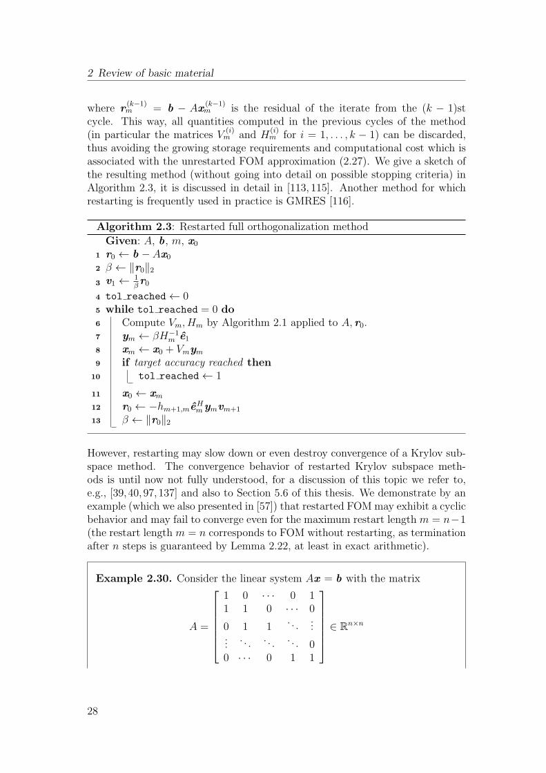
However, restarting may slow down or even destroy convergence of a Krylov sub-space method. The convergence behavior of restarted Krylov subspace meth-ods is until now not fully understood, for a discussion of this topic we refer to,e.g., [39, 40, 97, 137] and also to Section 5.6 of this thesis. We demonstrate by anexample (which we also presented in [57]) that restarted FOM may exhibit a cyclicbehavior and may fail to converge even for the maximum restart length m = n−1(the restart length m = n corresponds to FOM without restarting, as terminationafter n steps is guaranteed by Lemma 2.22, at least in exact arithmetic).
Example 2.30. Consider the linear system Ax = b with the matrix
A =
1 0 · · · 0 11 1 0 · · · 0
0 1 1. . .
......
. . . . . . . . . 00 · · · 0 1 1
∈ R
n×n
28
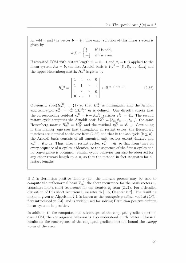
2.4 The special case f(z) = z−1
for odd n and the vector b = e1. The exact solution of this linear system isgiven by
x (i) =
12
if i is odd,
−12
if i is even.
If restarted FOM with restart length m = n− 1 and x0 = 0 is applied to thelinear system Ax = b, the first Arnoldi basis is V
(1)m = [e1, e2, . . . , en−1] and
the upper Hessenberg matrix H(1)m is given by
H(1)m =
1 0 · · · 0
1 1. . .
......
. . . . . . 00 · · · 1 1
∈ R
(n−1)×(n−1). (2.32)
Obviously, spec(H(1)m ) = 1 so that H
(1)m is nonsingular and the Arnoldi
approximation x(1)m = V
(1)m (H
(1)m )−1e1 is defined. One directly checks that
the corresponding residual r(1)m = b − Ax (1)
m satisfies r(1)m = en. The second
restart cycle computes the Arnoldi basis V(2)m = [en, e1, . . . , en−2], the same
Hessenberg matrix H(2)m = H
(1)m and the residual r
(2)m = en−1. Continuing
in this manner, one sees that throughout all restart cycles, the Hessenbergmatrices are identical to the one from (2.32) and that in the kth cycle (k ≤ n),the Arnoldi basis consists of all canonical unit vectors except en+1−k, and
r(k)m = en+1−k. Thus, after n restart cycles, r
(n)m = e1, so that from there on
every sequence of n cycles is identical to the sequence of the first n cycles andno convergence is obtained. Similar cyclic behavior can also be observed forany other restart length m < n, so that the method in fact stagnates for allrestart lengths.
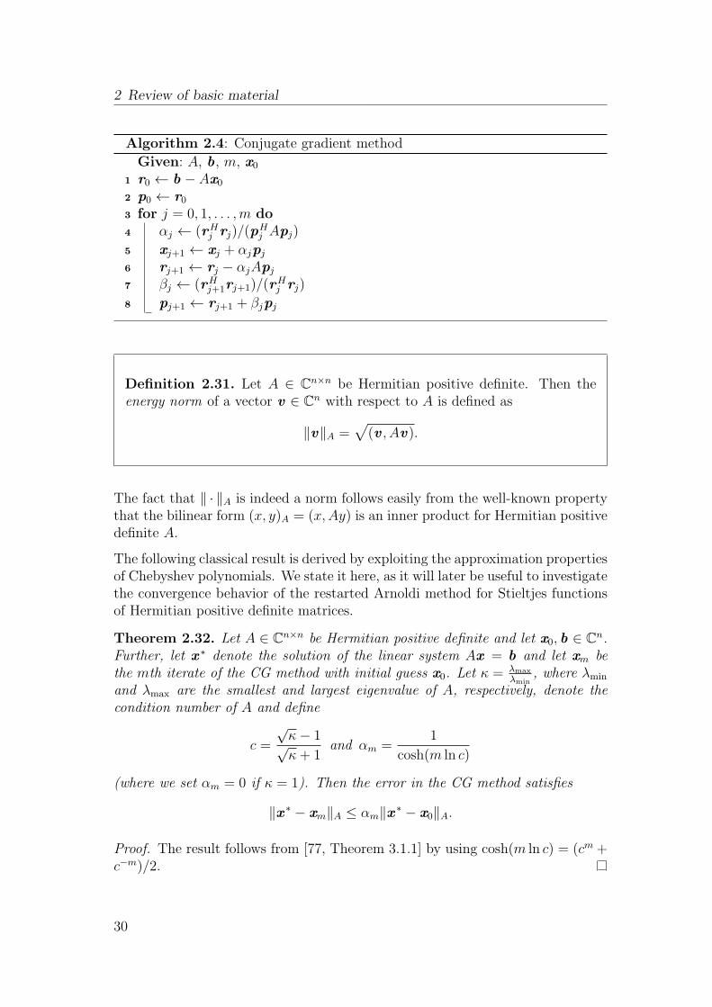
If A is Hermitian positive definite (i.e., the Lanczos process may be used tocompute the orthonormal basis Vm), the short recurrence for the basis vectors vjtranslates into a short recurrence for the iterates xj from (2.27). For a detailedderivation of this short recurrence, we refer to [115, Chapter 6.7]. The resultingmethod, given as Algorithm 2.4, is known as the conjugate gradient method (CG),first introduced in [84], and is widely used for solving Hermitian positive definitelinear systems in practice.
In addition to the computational advantages of the conjugate gradient methodover FOM, the convergence behavior is also understood much better. Classicalresults on the convergence of the conjugate gradient method bound the energynorm of the error.
29
2 Review of basic material
Algorithm 2.4: Conjugate gradient method
Given: A, b, m, x0
r0 ← b − Ax01
p0 ← r02
for j = 0, 1, . . . ,m do3
αj ← (rHj rj)/(p
Hj Apj)4
xj+1 ← xj + αjpj5
rj+1 ← rj − αjApj6
βj ← (rHj+1rj+1)/(r
Hj rj)7
pj+1 ← rj+1 + βjpj8
Definition 2.31. Let A ∈ Cn×n be Hermitian positive definite. Then the
energy norm of a vector v ∈ Cn with respect to A is defined as
‖v‖A =√
(v , Av).
The fact that ‖ · ‖A is indeed a norm follows easily from the well-known propertythat the bilinear form (x, y)A = (x,Ay) is an inner product for Hermitian positivedefinite A.
The following classical result is derived by exploiting the approximation propertiesof Chebyshev polynomials. We state it here, as it will later be useful to investigatethe convergence behavior of the restarted Arnoldi method for Stieltjes functionsof Hermitian positive definite matrices.
Theorem 2.32. Let A ∈ Cn×n be Hermitian positive definite and let x0, b ∈ C
n.Further, let x ∗ denote the solution of the linear system Ax = b and let xm bethe mth iterate of the CG method with initial guess x0. Let κ = λmax
λmin, where λmin
and λmax are the smallest and largest eigenvalue of A, respectively, denote thecondition number of A and define
c =
√κ− 1√κ+ 1
and αm =1
cosh(m ln c)
(where we set αm = 0 if κ = 1). Then the error in the CG method satisfies
‖x ∗ − xm‖A ≤ αm‖x ∗ − x0‖A.
Proof. The result follows from [77, Theorem 3.1.1] by using cosh(m ln c) = (cm +c−m)/2.
30
2.4 The special case f(z) = z−1
Another important Krylov subspace method, which is typically the method ofchoice for solving large, sparse, non-Hermitian linear systems in practical ap-plications, is GMRES [116]. GMRES differs from FOM (or CG in the Hermi-tian case) in the way the approximation is extracted from the affine Krylov sub-space x0 + Km(A, r0). The GMRES iterate xG
m is chosen such that the residualrGm = b−AxG
m is minimal among all possible approximations from x0+Km(A, r0).Defining the extended Hessenberg matrix
Hm =
[Hm
hm+1,meHm
]∈ C
(m+1)×m,
every approximation of the form xm = x0 + Vmym fulfills
b − Axm = r0 − AVmym = Vm(‖r0‖2e1 −Hmym)
so that
‖b − Axm‖2 =∥∥‖r0‖2e1 −Hmym
∥∥2.
This shows that the mth GMRES iterate, i.e., the vector which minimizes theresidual norm among all approximations from x0 + Km(A, r0), can be computedas
xGm = x0 + Vmy
Gm, (2.33)
where yGm solves the linear least squares problem
∥∥‖r0‖2e1 −Hmy∥∥2→ min . (2.34)
Interestingly, one can show that the GMRES approximation (2.33) also has aconnection to polynomial interpolation, albeit in different interpolation nodes,the so-called harmonic Ritz values.
Definition 2.33. The harmonic Ritz values of A ∈ Cn×n with respect to a
subspace U ⊆ Cn are those numbers ϑ ∈ C for which there exists x ∈ U , x 6=
0 such thatAx − ϑx ⊥ AU .
Although Definition 2.33 allows to define harmonic Ritz values corresponding toan arbitrary subspace U , we will in the following restrict ourselves to the caseU = Km(A, r0), as these are the harmonic Ritz values relevant in the context ofGMRES.
31
2 Review of basic material
Lemma 2.34. Let A ∈ Cn×n, let b ∈ C
n and let xGm be the GMRES approximation
(with initial guess x0) defined by (2.33) and (2.34). Then
xGm = x0 + pm−1(A)r0,
where pm−1 is the unique polynomial of degree at most m − 1 which interpolatesf(z) = z−1 in the harmonic Ritz values of A with respect to Km(A, r0).
Proof. See, e.g., [76, Theorem 5.1] and [111, Section 5].
Lemma 2.34 allows us to derive another characterization of the GMRES approx-imation, based on the result of Lemma 2.27. To do so, we need the followingauxiliary result.
Proposition 2.35. Consider the Arnoldi decomposition (2.23). The harmonicRitz values of A with respect to Km(A, r0) are the eigenvalues of the matrix
Hm = Hm +(hm+1,mH
−1m em
)eHm , (2.35)
provided that Hm is nonsingular.
Proof. See [111, Section 7.1].
Lemma 2.27 and 2.34 together with Proposition 2.35 now allow us to concludethat the GMRES approximation can also be characterized as
xGm = x0 + ‖r0‖2Vm
(Hm +
(hm+1,mH
−1m em
)eHm
)−1e1. (2.36)
It is not advisable to use this representation for practical computations due topossible numerical instabilities, and in addition due to the fact that (2.36) is notdefined when Hm is singular, while the computation of xG
m via (2.33) and (2.34)is always possible. Nonetheless, the relation (2.36) will later allow us to derive amethod for the approximation of Stieltjes matrix functions f(A) times a vectorb which reduces to GMRES in the case f(z) = z−1 and has some favorabletheoretical properties; cf. Section 5.4 and 5.5.
Next, we give a result from [42] on the reduction of the residual norm in theGMRES method for the class of positive real matrices.
Theorem 2.36. Let A ∈ Cn×n be positive real, i.e., ℜ(vHAv) > 0 for all v ∈
Cn, v 6= 0 and let b ∈ C
n. Define the quantities
δ := min
∣∣∣∣vHAv
vHv
∣∣∣∣ : v ∈ Cn, v 6= 0
, (2.37)
δ′ := min
∣∣∣∣vHA−1v
vHv
∣∣∣∣ : v ∈ Cn, v 6= 0
. (2.38)
32
2.4 The special case f(z) = z−1
Then the residual rGm corresponding to the GMRES iterate xG
m defined by (2.33)and (2.34) with initial guess x0 satisfies
‖rGm‖2 ≤
(1− δδ′
)m/2‖r0‖2. (2.39)
Proof. See, e.g., [42, Corollary 6.2].
Note that the quantities δ and δ′ from (2.37) and (2.38) are positive if A ispositive real (as in this case, A−1 is positive real as well, see [91, Chapter 1]) andsatisfy δδ′ ≤ 1, see, e.g., [42, Section 6]. In particular, one can directly concludefrom (2.39) that the restarted GMRES iteration for Ax = b always converges tothe solution x ∗ if A is positive real.
Corollary 2.37. Let the assumptions of Theorem 2.36 hold, let (xGm)(k) denote
the iterate obtained by k cycles of restarted GMRES with restart length m andinitial guess x0 and let (rG
m)(k) be the corresponding residual. Then
‖(rGm)(k)‖2 ≤
(1− δδ′
)km/2‖r0‖2. (2.40)
In particular, the restarted GMRES method converges to the exact solution x ∗ ofAx = b, because the right-hand side of (2.40) goes to zero for k →∞.
Proof. Equation (2.40) directly follows from Theorem 2.36 by noting that he kthcycle of restarted GMRES can be interpreted as performing m steps of GMRESwith initial guess (xG
m)(k−1). As 0 < δδ′ ≤ 1, we have |1 − δδ′| ≤ 1, so that theright-hand side of (2.40) goes to zero for k →∞.
2.4.1 Krylov subspace methods for shifted linear systems
Another important aspect central to many results of this thesis is the behavior ofKrylov subspace methods for shifted linear systems of the form
(A+ tI)x (t) = b, (2.41)
i.e., families of systems with the same right-hand side and with the system ma-trices differing only by multiples of the identity matrix. By (2.20), these systemshave a strong relation to Stieltjes matrix functions. The following result concern-ing Krylov subspaces for these systems holds.
Proposition 2.38. Let A ∈ Cn×n, let b ∈ C
n and let t ∈ C. Then
(i) Km(A, b) = Km(A+ tI, b) for all m > 0,
33
2 Review of basic material
(ii) Algorithm 2.1 applied to A+ tI and b computes the Arnoldi decomposition
(A+ tI)Vm = Vm(Hm + tI) + hm+1,mvm+1eHm ,
where Vm and Hm are the matrices from the Arnoldi decomposition (2.23)for A and b,
(iii) the mth FOM approximation xm(t) for the linear system (A + tI)x (t) = b
with initial guess x0(t) = 0 is given by
xm(t) = ‖b‖2Vm(Hm + tI)−1e1.
Proof. Assertion (i) directly follows by investigating the structure of powers ofthe shifted matrix A+ tI. Part (ii) can be concluded by inspecting the operationsin Arnoldi’s method, Algorithm 2.1. Part (iii) then follows directly from (ii).
The assertions of Proposition 2.38 have been observed several times and for dif-ferent Krylov subspace methods, see, e.g., [54, 62, 123]. These observations aretypically used to implement methods which are capable of solving several shiftedlinear systems at once, while only needing to compute a single approximationsubspace. This corresponds to only performing only a single matrix-vector multi-plication per iteration, independent of the number of shifted systems to be solved,cf., e.g., [54, 62, 123].
A topic to which special care has to be devoted when dealing with the simultane-ous solution of shifted linear systems is restarting. In the first cycle of a Krylovsubspace method for a family of systems of the form (2.41), the same Krylovsubspace can be constructed for all shifted systems (at least if all methods arestarted with initial guess x0(t) = 0) due to the fact that all systems have thesame right-hand side b. This need not be the case after restarting the method,as then one attempts to approximately solve the shifted residual equations
(A+ tI)em(t) = rm(t),
where rm(t) = b − (A + tI)xm(t), to compute an approximation for the errorem(t) := x ∗(t)− xm(t) of the current iterate. Of course, it suffices that the right-hand sides of the two systems be collinear (instead of equal) for Proposition 2.38to hold. Therefore, it is again possible to use the same Krylov subspace for allshifted systems if all residuals rm(t) are collinear. For the full orthogonalizationmethod, this is indeed the case, as by Proposition 2.29, the mth FOM residual iscollinear to the (m+ 1)st Arnoldi basis vector. Due to the shift invariance of theArnoldi method stated by Proposition 2.38(ii), this basis vector vm+1 is the samefor all systems, independent of the shift t. Thus, all shifted FOM residuals arecollinear to vm+1 and one can compute the restarted shifted FOM approximations
34
2.5 Numerical quadrature
of the second cycle (or later cycles) from one Krylov subspace for all systems again;see [123] for an in-depth treatment of the resulting method.
The GMRES method, however, does in general not produce collinear residu-als, so that one cannot just compute GMRES approximations for systems of theform (2.41) with different shifts t and then use only one approximation spaceagain after restarting. In [56], a variant of restarted GMRES for shifted linearsystems has been proposed which overcomes these issues as follows: Only theapproximate solution for one of the systems (the so-called seed system) is com-puted as a standard GMRES iterate as defined by (2.33) and (2.34), and thenthe approximations for the other systems are computed in a way that enforcescollinearity to the residual of the seed system. This way, the iterates for theother systems are no true GMRES iterates (and therefore, e.g., do not have theresidual norm minimization property) but restarting with one Krylov subspacefor all systems is again possible. We do not go into detail concerning this topichere, as the precise construction is not of importance in our context. Theoreticalresults concerning the “shifted” GMRES method from [56] will be addressed inChapter 5, where they are transferred to a method for approximating Stieltjesmatrix functions.
2.5 Numerical quadrature
When dealing with integrals of functions for which no antiderivative is knownor available in a numerical computation, one instead has to approximate theintegral numerically by what is typically called a quadrature rule. As integralrepresentations of functions for which no closed form is available will appear atmany places throughout this thesis, due to the integral representation of the errorin Arnoldi’s method to be introduced in Chapter 3, quadrature rules are of vitalimportance for making the methods and results presented in this thesis feasiblefor numerical computations. We therefore briefly review the basic concepts of(mostly Gauss) quadrature, following the presentation in [33] and [74]. Otherreferences for a basic treatment of quadrature rules include [46, 100, 131] (albeitsometimes in a slightly different setting than here).
We consider only quadrature rules on finite intervals in the following. For infiniteintervals of integration, one either applies a suitable variable transformation whichmaps the interval of integration to a finite one or uses quadrature rules specificallydesigned for infinite intervals; see, e.g., [33, Chapter 3] or [68]. As we will pursuethe first approach and comment on the choices of variable transformations indepth in Section 4.3, where they are actually applied in our setting, we do not gointo detail concerning infinite intervals of integration here.
35
2 Review of basic material
Gauss quadrature rules are typically introduced with respect to a nonnegativeweight function w(t) ≥ 0 in the literature. We will use a slightly more generalapproach in the following definition of quadrature rules, in the sense that weintroduce Gauss rules for Riemann–Stieltjes integrals corresponding to a mono-tonically increasing function µ. By Lemma 2.8, if µ is differentiable, this can alsobe interpreted as an integral corresponding to the nonnegative weight functionw = µ′. When dealing with quadrature rules other than Gauss rules in the fol-lowing, we will tacitly assume that µ(t) = t, i.e, we are in the case of Riemannintegrals.
Definition 2.39. Let [a, b] be a finite interval, let µ : [a, b] −→ R be mono-tonically increasing and let g : [a, b] −→ C be any function such that theintegral ∫ b
a
g(t) dµ(t) (2.42)
exists and has a finite value. An ℓ-point quadrature rule for µ on [a, b] is thengiven by a set of weights ωi ∈ C, i = 1, . . . , ℓ and a set of nodes ti ∈ [a, b], i =1, . . . , ℓ such that
ℓ∑
i=1
ωig(ti),
approximates (2.42).
Two of the simplest quadrature rules are the compound midpoint rule and thecompound trapezoidal rule. The compound midpoint rule is defined as
Mℓ(g) =b− aℓ
ℓ∑
i=1
g
(a+
(i− 1
2
)b− aℓ
), (2.43)
i.e., all weights are equal to b−aℓ
and the quadrature nodes are chosen as thecenters of a subdivision of [a, b] into ℓ intervals of equal length. The compoundtrapezoidal rule is given by
Tℓ(g) =b− a2ℓ
(g(a) + g(b)
)+b− aℓ
ℓ−1∑
i=1
g
(a+ i
b− aℓ
), (2.44)
i.e., the nodes are chosen equispaced in [a, b], this time including the endpoints,and the weights are chosen to be b−a
2ℓat the endpoints and b−a
ℓfor the interior
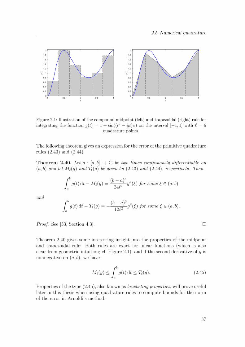
nodes. An illustration of these simple rules (also called primitive rules) is givenin Figure 2.1.
36
2.5 Numerical quadrature
t-1 -0.5 0 0.5 1
g(t
)
0
0.2
0.4
0.6
0.8
1
1.2
1.4
1.6
1.8
2
t-1 -0.5 0 0.5 1
g(t
)
0
0.2
0.4
0.6
0.8
1
1.2
1.4
1.6
1.8
2
Figure 2.1: Illustration of the compound midpoint (left) and trapezoidal (right) rule forintegrating the function g(t) = 1 + sin((t2 − 1
2 t)π) on the interval [−1, 1] with ℓ = 6quadrature points.
The following theorem gives an expression for the error of the primitive quadraturerules (2.43) and (2.44).
Theorem 2.40. Let g : [a, b] → C be two times continuously differentiable on(a, b) and let Mℓ(g) and Tℓ(g) be given by (2.43) and (2.44), respectively. Then
∫ b
a
g(t) dt−Mℓ(g) =(b− a)324ℓ2
g′′(ξ) for some ξ ∈ (a, b)
and ∫ b
a
g(t) dt− Tℓ(g) = −(b− a)312ℓ2
g′′(ξ) for some ξ ∈ (a, b).
Proof. See [33, Section 4.3].
Theorem 2.40 gives some interesting insight into the properties of the midpointand trapezoidal rule: Both rules are exact for linear functions (which is alsoclear from geometric intuition; cf. Figure 2.1), and if the second derivative of g isnonnegative on (a, b), we have
Mℓ(g) ≤∫ b
a
g(t) dt ≤ Tℓ(g). (2.45)
Properties of the type (2.45), also known as bracketing properties, will prove usefullater in this thesis when using quadrature rules to compute bounds for the normof the error in Arnoldi’s method.
37
2 Review of basic material
The primitive quadrature rules introduced so far are in general only exact forlinear functions, i.e., polynomials of degree up to 1. As a quadrature rule, accord-ing to Definition 2.39, is defined by 2ℓ parameters, ℓ weights and ℓ nodes, it isa natural consideration to try to construct quadrature rules which are exact forpolynomials of degree up to 2ℓ−1. Quadrature rules of this type are called Gaussquadrature rules.
Definition 2.41. Let [a, b] be a finite interval and let µ : [a, b] −→ R bemonotonically increasing. An ℓ-point quadrature rule for µ on [a, b] definedby (ωi, ti), i = 1, . . . , ℓ is called Gauss quadrature rule if it satisfies
∫ b
a
p2ℓ−1(t) dµ(t) =ℓ∑
i=1
ωip2ℓ−1(ti) for all p2ℓ−1 ∈ Π2ℓ−1. (2.46)
The existence of rules which satisfy (2.46) is closely related to orthonormal polyno-mials. Note that a function µ which is nonnegative and monotonically increasingon [a, b] induces a (not necessarily positive definite) inner product on polynomialsp, q ∈ Πk via
(p, q) =
∫ b
a
p(t)q(t) dµ(t). (2.47)
Sequences of polynomials which are orthonormal with respect to this inner prod-uct play an important role in numerical quadrature.
Definition 2.42. A sequence of polynomials pi, i = 0, 1, . . . is called orthonor-mal with respect to the inner product (2.47) if deg pi = i and
(pi, pj) =
1 if i = j,
0 otherwise.
One can show that for a nonnegative, monotonically increasing function µ thereexists a unique sequence of orthonormal polynomials if the inner product (2.47)is positive definite, see, e.g., [69] (more precisely, if (2.47) fulfills (p, q) > 0 forall 0 6= p, q ∈ Πk but not for p, q ∈ Πℓ for any ℓ > k, then there exists a finitesequence of k + 1 orthonormal polynomials). We will in the following for ease ofpresentation restrict ourselves to the case that (2.47) is positive definite, which is
38
2.5 Numerical quadrature
always fulfilled in the applications in this thesis. The following, central theoremstates that orthonormal polynomials always obey a three-term recurrence.
Theorem 2.43. Let µ be a nonnegative, monotonically increasing function on[a, b] such that the inner product (2.47) is positive definite. Define
p−1 ≡ 0 and p0 ≡ 1/
(∫ b
a
dµ(t)
)1/2
.
Then there exist coefficients ai, bi, i = 0, 1, 2, . . . such that the sequence pi, i =0, 1, . . . defined by
bipi(t) = (t− ai−1)pi−1(t)− bi−1pi−2(t), i = 1, 2, . . . (2.48)
is the unique sequence of orthonormal polynomials corresponding to the innerproduct (2.47).
Proof. See [69, Theorem 1.27 and 1.29].
We just note at this point that the three-term recurrence (2.48) satisfied byorthonormal polynomials is very similar to the three-term recurrence relationsatisfied by the Krylov basis vectors generated by the Lanczos process, Algo-rithm 2.2, for Hermitian A. Together with the intimate relation between theLanczos/Arnoldi method and polynomials in A, this allows to also relate theLanczos process to orthonormal polynomials and thus Gauss quadrature. Thistopic will be covered in depth in Section 6.1.
The relation between orthonormal polynomials and Gauss quadrature rules isgiven by the following result.
Theorem 2.44. Let µ be a nonnegative, monotonically increasing function on[a, b] such that the inner product (2.47) is positive definite and let pi, i = 0, 1, . . . ,be the sequence of orthonormal polynomials corresponding to µ and [a, b]. Then
(i) The roots ti, i = 1, . . . , ℓ of pℓ(t) are real, simple and lie in (a, b) for allℓ ≥ 1.
(ii) The quadrature rule defined by the nodes ti, i = 1, . . . , ℓ and the weights
ωi = −kℓ+1
kℓ
1
pℓ+1(ti)p′ℓ(ti), i = 1, . . . , ℓ (2.49)
where kℓ, kℓ+1 are the leading coefficients of pℓ and pℓ+1, respectively, is anℓ-point Gauss quadrature rule (which we denote by Gµ
ℓ (·) in the following).In addition, the weights ωi from (2.49) are all positive.
39
2 Review of basic material
Proof. Part (i) is, e.g., shown in [74, Theorem 2.14]. For part (ii), see, e.g., [33,Section 2.7]
Theorem 2.44 states that there always exists a Gauss quadrature rule for a giveninterval [a, b] and nonnegative, monotonically increasing function µ if the innerproduct (2.47) is positive definite. In [100] is is shown that there exist no ℓ-pointquadrature rules which integrate all polynomials of degree up to 2ℓ exactly, suchthat Gauss quadrature rules are optimal in this sense.
The representation of the nodes and weights of a Gauss rule given by Theorem 2.44is often not well-suited for numerical computations. In [75], based on [143], adifferent approach was proposed, which we briefly mention here as it will be ofimportance in Chapter 6 and 7 of this thesis. Assuming we know the coefficientsai, bi in (2.48), we can rewrite the three-term recurrence in matrix notation as
tp(t) = Tℓp(t) + bℓpℓ(t)eℓ, (2.50)
where Tℓ is the tridiagonal matrix defined by
Tℓ =
a1 b1
b1 a2 b2. . . . . . . . .
bℓ−1 aℓ−1 bℓ−1
bℓ aℓ
(2.51)
andp(t) = [p0(t), p1(t), . . . , pℓ−1(t)]
T .
The nodes ti, i = 1, . . . , ℓ of the ℓ-point Gauss quadrature rule are the zeros ofpℓ(t), so that inserting one of these nodes as t in (2.50) yields
tip(ti) = Tℓp(ti),
showing that ti is an eigenvalue of Tℓ with corresponding eigenvector p(ti). Thus,the nodes of Gauss quadrature rules can be computed by solving a symmetrictridiagonal eigenvalue problem. One can further show that the correspondingweights are the squares of the first entries of the eigenvectors p(ti) by using theso-called Christoffel–Darboux identity [74, Theorem 2.11], as proven, e.g., in [143].This approach gives a more stable way of computing the nodes and weights ofGauss quadrature rules. We refer the reader to [74,75] for an in-depth treatmentof this approach and its implications for the structure and properties of Gaussrules.
Next, we give two examples of practically relevant Gauss quadrature rules, whichwe will also use in the computations presented in this thesis.
40
2.5 Numerical quadrature
Example 2.45.
(i) The orthonormal polynomials corresponding to the function µ(t) = t onthe interval [−1, 1] are the Legendre polynomials given by the three-termrecurrence
p0 ≡ 1, p1(t) = t, (i+1)pi+1(t) = (2i+1)tpi(t)−ipi−1(t), i = 1, 2, . . . .
The resulting quadrature rules are called Gauss–Legendre rules.
(ii) The orthonormal polynomials corresponding to the Jacobi weight func-tion w(t) = (1 − t)α(1 + t)β with α, β > −1 on the interval [−1, 1] arethe Jacobi polynomials
pi(t) =1
2i
i∑
j=0
(i+ α
j
)(i+ β
i− j
)(t− 1)i−j(t+ 1)j, i = 0, 1, . . . .
The associated quadrature rules are called Gauss–Jacobi rules. In thespecial case α = β = −1
2, the weight function simplifies to w(t) =
(1− t2)−1/2 and the resulting quadrature rule is called Gauss–Chebyshevrule.
Note that we introduced Gauss–Jacobi quadrature with respect to a weight func-tion in Example 2.45(ii) as this is the classical approach from the literature. Keepin mind that the integral with respect to the weight function can also be inter-preted as a Riemann–Stieltjes integral.
For a sufficiently smooth function g, the error of a Gauss quadrature rule canagain, similarly to the primitive quadrature rules, be expressed in terms of aderivative of g evaluated at some point in (a, b).
Theorem 2.46. Let µ be a nonnegative, monotonically increasing function on[a, b], let g be 2ℓ times continuously differentiable on (a, b) and let Gµ
ℓ (g) denotethe corresponding ℓ-point Gauss quadrature rule. Then there exists ξ ∈ (a, b) suchthat ∫ b
a
g(t) dµ(t)−Gµℓ (g) = cG
g(2ℓ)(ξ)
(2ℓ)!,
with the constant
cG =
∫ b
a
pℓ(t)2 dµ(t),
where pℓ is the ℓth orthonormal polynomial corresponding to µ and [a, b].
41
2 Review of basic material
Proof. See, e.g., [69, Corollary to Theorem 1.48].
By Theorem 2.46, if g(2ℓ) ≥ 0 on (a, b), an ℓ-point Gauss quadrature rule willalways give a lower bound for the exact value of the approximated integral. Forcertain applications (cf. Chapter 6 and 7) it is of value to have a bracketingproperty for Gauss rules, similar to the property (2.45) for the midpoint andtrapezoidal rule. This is possible by considering quadrature rules in which onequadrature node is fixed a priori.
In principle, it is possible to fix any number of quadrature nodes at arbitrarypoints in [a, b], but we will for brevity only consider the case in which one quadra-ture node is fixed to be at a, the left endpoint of the integration interval, asthis is all that is needed in the remainder of this thesis. Rules of this kind withℓ+1 nodes, which are exact for polynomials of degree up to 2ℓ are called Gauss–Radau rules. The nodes and weights of a Gauss–Radau quadrature rule can alsobe computed by solving a symmetric tridiagonal matrix eigenvalue problem as forordinary Gauss rules, where the matrix Tℓ+1 is modified in such a way that oneof its eigenvalues is prescribed to be a. Without going into detail, we denote theresulting quadrature rule by GRµ
ℓ+1(·). For its error, the following theorem holds.
Theorem 2.47. Let µ be a nonnegative, monotonically increasing function on[a, b], let g be 2ℓ + 1 times continuously differentiable on (a, b) and let GRµ
ℓ+1(g)denote the corresponding (ℓ+1)-point Gauss–Radau quadrature rule with one nodefixed at a. Then there exists ξ ∈ (a, b) such that
∫ b
a
g(t) dµ(t)−GRµℓ+1(g) = cGR
g(2ℓ+1)(ξ)
(2ℓ+ 1)!,
with the constant
cGR =
∫ b
a
pℓ(t)2(t− a) dµ(t),
where pℓ is the ℓth orthonormal polynomial corresponding to µ defined via
dµ(t) = (t− a) dµ(t)
on [a, b].
Proof. See, e.g., [69, Theorem 3.3].
According to Theorem 2.46 and 2.47, we have the following version of the brack-eting property for functions g which are 2ℓ + 1 times continuously differentiableand satisfy g(2ℓ) ≥ 0 and g(2ℓ+1) ≤ 0 on (a, b):
Gµℓ (g) ≤
∫ b
a
g(t) dµ(t) ≤ GRµℓ+1(g). (2.52)
42
2.6 Model problems
We end this section by pointing out that for the class of Stieltjes functions (ormore generally completely monotonic functions), the following important resultdirectly follows from (2.52).
Corollary 2.48. Let µ be a nonnegative, monotonically increasing function on[a, b] and let g be a completely monotonic function, cf. Definition 2.16. Then for
all ℓ, ℓ ≥ 1 we have
Gµℓ (g) ≤
∫ b
a
g(t) dµ(t) ≤ GRµ
ℓ(g), (2.53)
i.e., the Gauss and Gauss–Radau rules for∫ b
ag(t) dµ(t) always yield lower and
upper bounds for the exact value of the integral, respectively, independently of thenumber of quadrature nodes.
2.6 Model problems
In this section we introduce various model problems from practical applicationswhich will be used to demonstrate and gauge the various features of the differentmethods and results presented in this thesis in a realistic setting. All test caseswill be considered at various places throughout this thesis. Note that some willbe encountered more frequently than others, as not all methods and error boundsare applicable to all of the model problems (depending, e.g., on Hermiticity ordefiniteness of the resulting matrices).
2.6.1 Three-dimensional heat equation
The first model problem we consider is a standard test case which is frequentlyused for testing Krylov subspace methods for the matrix exponential; see, e.g., [3,43,67]. We consider the initial boundary value problem with homogeneous Dirich-let boundary conditions (note that here and in the following, we use the nonstan-dard notation θ instead of t for the time parameter to avoid confusion with theintegration variable in the integral representations of matrix functions or the shiftin families of shifted linear systems)
∂u
∂θ−∆u = 0 on (0, 1)3 × (0, T ),
u(x, θ) = 0 on ∂(0, 1)3 for all θ ∈ [0, T ], (2.54)
u(x, 0) = u0(x) for all x ∈ (0, 1)3,
43
2 Review of basic material
where u0(x) is a function describing the initial conditions and ∆ denotes theLaplace operator defined by
∆u =∂2u
∂x21+∂2u
∂x22+∂2u
∂x23. (2.55)
The system (2.54) describes the evolution of a heat distribution in the unit cubeover a time interval (0, T ), starting from an initial distribution u0 at time 0.Discretizing (2.55) by the standard seven-point finite difference stencil with N+2equispaced grid points in each spatial direction, the system (2.54) reduces to alinear initial value ODE problem
du(θ)
dθ= Au(θ), for θ ∈ (0, T ) (2.56)
u(0) = u0,
where A ∈ RN3×N3
is Hermitian negative definite and u0 contains the values ofthe function u0(x) at the grid points. In our experiments, we choose N = 50,resulting in a matrix of dimension 125,000 which can be written as
A = A1D ⊗ I ⊗ I + I ⊗ A1D ⊗ I + I ⊗ I ⊗ A1D,
where A1D is the tridiagonal matrix
A1D = (N + 1)2
−2 1
1 −2 . . .. . . . . . 1
1 −2
∈ R
N×N .
The solution of the ODE system (2.56) is then given by
u(θ) = eθAu0, (2.57)
i.e., the evaluation of the solution u at some point in time amounts to evaluatingthe action of a matrix exponential function on the vector of initial conditions. Inour experiments, we approximate u(θ) at θ = 0.1 starting with a homogeneousinitial heat distribution u0 = 1 .
2.6.2 Three-dimensional convection diffusion equation
Our next model problem, taken from [43, 107], again deals with a PDE initialboundary value problem, which this time leads to a non-Hermitian matrix A. We
44
2.6 Model problems
investigate the system
∂u
∂θ−∆u+ τ1
∂u
∂x1+ τ2
∂u
∂x2= 0 on (0, 1)3 × (0, T ),
u(x, θ) = 0 on ∂(0, 1)3 for all θ ∈ [0, T ], (2.58)
u(x, 0) = u0(x) for all x ∈ (0, 1)3.
Again discretizing the Laplace operator by seven-point finite differences on a gridwith N +2 points in each spatial direction and using centralized finite differences(on the same grid) for the first-order derivatives, we find, as in Section 2.6.1, alinear ODE system of the form (2.56), where this time the matrix A ∈ R
N3×N3is
non-Hermitian and given by
A = A1D ⊗ I ⊗ I + I ⊗ C2 ⊗ I + I ⊗ I ⊗ C1 (2.59)
with N ×N matrices
Ci = (N + 1)2
−2 1− νi1 + νi −2 . . .
. . . . . . 1− νi1 + νi −2
, i = 1, 2
where νi =τi
2(N+1). Of course, the solution of the linear ODE system can again
be represented by a matrix exponential applied to the vector of initial conditionsas in (2.57) with the matrix A from (2.59). For our experiments we choose theparameters N = 50 and θ = 2 · 10−3 and convection coefficients τ1 = 4080, τ2 =2040, resulting in ν1 = 40, ν2 = 20, which leads to a highly non-Hermitian matrixA. The (discretized) initial conditions are again given by u0 = 1 .
2.6.3 Three-dimensional wave equation
In this model problem, which is, e.g., considered in [38], we aim to approximate afunction different from the matrix exponential. We consider solving the followinginitial boundary value problem for the three-dimensional wave equation on theunit cube and an infinite time interval
−∆u− ∂2u
∂θ2= 0 on (0, 1)3 × R
+
u(x, θ) = 0 on ∂(0, 1)3 for all θ ∈ R+0 , (2.60)
u(x, 0) = u0(x) for all x ∈ (0, 1)3.
45
2 Review of basic material
Discretizing the Laplace operator in the same way as in Section 2.6.1 and 2.6.2leads to the system
d2u(θ)
dθ2= Au(θ), for θ ∈ R
+
u(0) = u0,
where the matrix A is Hermitian positive definite in this case, as the sign of theLaplace operator and the sign of the time derivative are the same in (2.60), asopposed to (2.54) and (2.58). The solution of this system is given as
u(θ) = e−θ√Au0.
We rewrite this as
u(θ) = (Af(A) + I)u0, (2.61)
with the function
f(z) =e−θ
√z − 1
z. (2.62)
The formulation (2.61) has the advantage that the function f from (2.62) has theintegral representation
f(z) = −∫ ∞
0
1
z + t
sin(θ√t)
πtdt, (2.63)
which makes many of the methods and results developed in the following appli-cable in this situation. We stress, however, that the function f from (2.62) is nota Stieltjes function as the corresponding generating function is not monotonicallyincreasing. As in Section 2.6.1, we choose N = 50, θ = 0.1 and initial conditionsu0 = 1 in our computations.
2.6.4 Neuberger overlap operator in lattice QCD
The next problem we consider is from quantum chromodynamics (QCD), anarea of Theoretical Physics which studies the strong interaction between quarksand gluons. In lattice QCD, this theory is simulated on a four-dimensionalspace-time lattice (where we, for ease of notation, denote the grid points byx = (x0, x1, x2, x3), i.e., we do not distinguish space and time coordinates nota-tionwise). For introducing the basics of this model problem, we follow the de-scriptions in [20,117]. The most important relation for describing the interactionof quarks and gluons is the Dirac equation [35]
(D +m)ψ(x) = η(x), (2.64)
46
2.6 Model problems
where m is a scalar parameter, ψ and η represent quark fields and D is the Diracoperator defined by
D =3∑
i=0
γi ⊗(∂
∂xi+ Ai
)(2.65)
where the matrices Ai(x) ∈ C3×3 are elements of the Lie algebra su(3) of the
special unitary group SU(3) and the matrices γi ∈ C4×4, i = 0, . . . , 3 are gener-
ators of the Clifford algebra Cℓ4(C). From the above description it is clear thatthe quark field ψ(x) at a point x in space-time is a vector with 12 components(corresponding to three colors and four spins). For computer simulations, theDirac equation (2.64) is discretized on an Nt × N3
s grid (called the lattice fromhere on) with uniform lattice spacing a and Nt and Ns denoting the number oflattice points in the time dimension and each of the three spatial dimensions,respectively. We consider the Wilson discretization [144] with periodic bound-ary conditions in the following, in which the covariant derivatives in (2.65) arereplaced by centralized covariant finite differences (and a stabilization term isadded), resulting in the discretized operator
(DWφ)(x) =m0 + 4
aφ(x)− 1
2a
3∑
i=0
((I4 − γi)⊗ Ui(x)
)φ(x+ aei)
− 1
2a
3∑
i=0
((I4 + γi)⊗ UH
i (x− aei))φ(x− aei) (2.66)
where the mass parameter m0 determines the quark mass, and the matricesUi(x) ∈ C
3×3 (the so-called gauge links) are elements of the Lie group SU(3).Consistent with the periodic boundary conditions, terms of the form x − aeiare to be understood on a torus, i.e., the boundaries of the lattice are “gluedtogether”.
A set of gauge links Ui(x) for all grid points x is also referred to as a configuration.
The Wilson–Dirac operator (2.66) fulfills the so-called Γ5-symmetry
(Γ5DW )H = Γ5DW
with the Hermitian, unitary matrix
Γ5 = INtN3s⊗ γ0γ1γ2γ3 ⊗ I3; (2.67)
see, e.g., [60]. For the simulation of some physical observables it is important thatthe discretized operator fulfills a (lattice variant of) the so-called chiral symmetry,which amounts to fulfilling the Ginsparg–Wilson relation [70]
Γ5D +DΓ5 = aDΓ5D (2.68)
47
2 Review of basic material
with Γ5 from (2.67). Unfortunately, the Wilson–Dirac operator does not fulfillthis relation and is thus not suited for all simulations of interest. In [109], theNeuberger overlap operator
DN = ρI + Γ5 sign(Γ5DW ), where ρ > 1, (2.69)
which fulfills the relation (2.68), was introduced. In simulations involving the Neu-berger overlap operator (2.69), one has to solve linear systems with DN . As DN isnot explicitly available (it is not feasible to explicitly form sign(Γ5DW ) for realisticgrid sizes) one typically uses Krylov subspace methods which only need to applymatrix vector products with DN . Still, in each iteration of a Krylov subspacemethod, this amounts to approximating the action of the matrix sign function (ofa Hermitian matrix) on the latest Krylov basis vector, i.e., sign(Γ5DW )vi.
The matrix sign function can be represented by the identity
sign(A) = A(A2)−1/2, (2.70)
involving the Stieltjes function f(z) = z−1/2 (cf. Example 2.14), see, e.g., [31,48], which is the representation typically used in computational practice. Inour experiments we approximate the action of the matrix sign function involvedin (2.69), using the formulation (2.70), on a vector for a discretization on an 8×83lattice, thus yielding a matrix of dimension 12 · 84 = 49,152.
A further modification of the situation described above arises in the presence ofa nonzero chemical potential ν. In this case, the links in time direction in theWilson–Dirac operator change, and the discretization changes from (2.66) to
(DνWφ)(x) =
m0 + 4
aφ(x)− 1
2a
3∑
i=1
((I4 − γi)⊗ Ui(x)
)φ(x+ aei)
− 1
2a
3∑
i=1
((I4 + γi)⊗ UH
i (x− aei))φ(x− aei)
− 1
2aeν((I4 − γi)⊗ Ui(x)
)φ(x+ aei)
− 1
2ae−ν((I4 + γi)⊗ UH
i (x− aei))φ(x− aei), (2.71)
which agrees with (2.66) for chemical potential ν = 0. For ν 6= 0, the operatorDν
W from (2.71) is not Γ5-symmetric, such that the solution of systems with theoverlap operator (2.69) now involves approximating the matrix sign function (orinverse square root) of a non-Hermitian matrix. We also report experiments forthis case, using the same 8 × 83 configuration as before, but adding a chemicalpotential ν = 1/20, which is a physically reasonable value, given the temperatureT (a quantity from statistical physics) used for generating the configuration.
48
2.6 Model problems
2.6.5 Sampling from Gaussian Markov random fields
The last model problem we consider is taken from [93, 126] and arises from thestatistical application of sampling from a Gaussian Markov random field. Givena set of n points si ∈ R
d, i = 1, . . . , n, one defines a Gaussian random variablexi, i = 1, . . . , n at each point. The vector x of these random variables is called aGaussian Markov random field. The so-called precision matrix A ∈ R
n×n of thepoints si (with respect to two parameters δ, φ) is given by
aij =
1 + φ
∑nk=1,k 6=i χ
δij if i = j,
−φχδij otherwise,
(2.72)
where χδ is given by
χδij =
1 if ‖si − sj‖2 < δ,
0 otherwise.
The matrix A from (2.72) is obviously Hermitian and diagonally dominant. Bythe Gersgorin disk theorem (see, e.g., [136]), all eigenvalues λ of A fulfill λ ≥ 1,so that A is positive definite. In addition, as all row sums of A are 1, the vector1 fulfills A1 = 1 , showing that A must have an eigenvalue λ = 1 (as 1 is aneigenvector to this eigenvalue). A sample from the Gaussian Markov random fieldx can be obtained by computing A−1/2z , where z is a vector of independently andidentically distributed standard normal random variables; see [92, 127]. For ourexperiments, we simulate n = 50,000 points in the unit square (0, 1)× (0, 1) andchoose the parameters φ = 3, δ = 0.01, which results in a sparse, unstructuredmatrix A ∈ R
50,000×50,000 with spec(A) ⊆ [1, 109.6] and 830,626 nonzero entries.We are therefore, like for the Neuberger overlap operator at zero chemical poten-tial, in the situation of approximating a Stieltjes function of a Hermitian positivedefinite matrix. The vector z is generated by the Matlab function randn. Forapplications of Gaussian Markov random fields, see, e.g., [28, 112].
49

CHAPTER 3
AN INTEGRAL REPRESENTATION FOR THE
ERROR IN ARNOLDI’S METHOD
In this chapter we consider representations for the error of the iterate fm producedby m steps of Arnoldi’s method for f(A)b. These error representations form thebasis for both the restarting approaches discussed in Chapter 4 and 5 as wellas the computation of error bounds (mostly in unrestarted methods) which areinvestigated in Chapter 6 and 7. We begin by discussing previously known errorrepresentations from the literature in Section 3.1. In Section 3.2 we proceed byderiving new integral representations for the error for different classes of functionsrepresentable by contour integrals over resolvent functions. Important classesof functions to which our results apply are Stieltjes functions and holomorphicfunctions represented by the Cauchy integral formula.
3.1 Error representation via divided differences
In the special case f(z) = z−1, i.e., when solving a linear system, a simple errorrepresentation is given by the residual equation (2.28). This equation can berewritten as
e0 = A−1r0 = f(A)r0,
showing that the error is representable as the action of the matrix function f(A)on the vector r0. For general matrix functions, a similar result does unfortunatelynot hold. However, it is possible to represent the error of the restarted Arnoldiapproximation as the action of a matrix function different from f based on di-vided differences (see, e.g., [34]), as the following result from [43] shows. It is
51
3 An integral representation for the error in Arnoldi’s method
originally stated for Arnoldi-like decompositions, which are decompositions of theform (2.23) without the requirement that the columns of Vm are orthonormal. Aswe do not need this more general concept for the results of this thesis, we statethe result in terms of standard Arnoldi decompositions.
Theorem 3.1. Given A ∈ Cn×n, let b ∈ C
n, let Vm and Hm satisfy the Arnoldirelation (2.23) corresponding to A and b and let wm(z) =
∏mi=1(z − θi) be the
nodal polynomial associated with the Ritz values θ1, . . . , θm, i.e., the eigenvaluesof Hm. Then the error of the Arnoldi approximation fm from (2.25) is given by
f(A)b − fm = ‖b‖2γm[Dwmf ](A)vm+1 =: em(A)vm+1, (3.1)
where [Dwmf ] denotes the mth divided difference of f with respect to the interpo-
lation nodes θ1, . . . , θm, and γm =∏m
i=1 hi+1,i.
Proof. See [43, Theorem 2.6].
We note that an error representation based on mth order divided differences wasindependently found in [132].
From a theoretical point of view, Theorem 3.1 gives an answer to the questionhow the error after m steps of Arnoldi’s method can be represented as the actionof a matrix function on a vector again. However, it is not feasible for practicalcomputations due to the well-known fact that the numerical evaluation of high-order divided differences is prone to instabilities, especially when interpolationnodes are close to each other, thereby causing subtractive cancellations and verysmall denominators in the divided difference table. This fact especially leads toproblems when attempting to implement a restart approach based on this errorfunction, as for Hermitian A it is known that the Ritz values of all restart cycleswill asymptotically appear as a two-cyclic sequence [3], so that the interpolationnodes will form 2m clusters and the evaluation of the error function using (3.1)will necessarily become unstable.
Based on the results from [43], a different representation for the error in Arnoldi’smethod, which is also based on divided differences, was developed in [93] forHermitian A.
Theorem 3.2. Let the assumptions of Theorem 3.1 hold and let A ∈ Cn×n be
Hermitian. Let Wm be a unitary matrix whose columns are eigenvectors of Hm,and define αi = eH
mWmei and βi = eH1 Wmei, i = 1, . . . ,m. Then
f(A)b − fm = ‖b‖2hm+1,mg(A)vm+1
with
g(z) =m∑
i=1
αiβi[Dwif ](z), where wi(z) = (z − θi).
52
3.2 Integral representation of the error function
Proof. See [93, Theorem 2.1].
On first sight, one could expect the error representation given in Theorem 3.2to be more stable in finite precision arithmetic than the one from Theorem 3.1as it only involves first-order divided differences. However, as was stated in [93]and is also confirmed by our numerical experiments presented in Chapter 4, therepresentation is still unstable and therefore not usable in practice, especially incases where the requirements on accuracy and reliability are high.
3.2 Integral representation of the error function
As explained in the previous section, the error representations considered in theliterature so far are numerically infeasible (e.g., for implementing a restartedArnoldi method) due to the need of evaluating divided differences. In this section,we derive integral representations for the error of the Arnoldi approximation fordifferent classes of functions. Our results presented in this chapter have beenpublished in [57–59]. We begin by investigating “Cauchy-type” integrals.
Due to the intimate relation between Arnoldi’s method and polynomial interpo-lation, cf. Lemma 2.25 and Lemma 2.27, we first give an integral representationfor interpolating polynomials of functions of Cauchy-type.
Lemma 3.3. Let Ω ⊂ C be a region and let f : Ω→ C be analytic, with integralrepresentation
f(z) =
∫
Γ
g(t)
t− z dt, z ∈ Ω, (3.2)
with a path Γ ⊂ C \ Ω and a function g : Γ → C. The Hermite interpolatingpolynomial pm−1 of f with interpolation nodes θ1, . . . , θm ⊂ Ω is given as
pm−1(z) =
∫
Γ
(1− wm(z)
wm(t)
)g(t)
t− z dt, (3.3)
where wm(z) =∏m
i=1(z − θi), provided that the integral in (3.3) exists.
Proof. Observe that for fixed t, the function 1− wm(z)/wm(t) is a polynomial ofdegree m in z with a root at t. Therefore it contains a linear factor t− z, showingthat (1 − wm(z)/wm(t))/(t − z) is a polynomial of degree m − 1 in z, and so isthe whole right-hand side of (3.3). By definition of wm we have
pm−1(θi) =
∫
Γ
(1− wm(θi)
wm(t)
)g(t)
t− θidt =
∫
Γ
g(t)
t− θidt = f(θi)
53
3 An integral representation for the error in Arnoldi’s method
for i = 1, . . . ,m, showing that the interpolation conditions for f are satisfied. Inthe case of coalescent interpolation nodes θi, we also demand that certain deriva-tives of f are interpolated by pm−1. Assume that θi = θj for i < j, which thenamounts to the interpolation condition p′m−1(θi) = f ′(θi). For ε > 0, define thesequence of interpolating polynomials pεm−1(z) corresponding to the interpolationnodes θ1, . . . , θj−1, θi+ε, θj+1, . . . , θm, which are pairwise distinct for ε sufficientlysmall (assuming for simplicity that no other interpolation nodes than θi and θjcoincide). Due to the fact that interpolating polynomials depend analytically onthe interpolation nodes and because f is analytic in Ω, we have that
f ′(θi) = limε→0
f(θi + ε)− f(θi)ε
= limε→0
pεm−1(θi + ε)− pεm−1(θi)
ε= p′(θi).
For more than two coincident interpolation nodes and higher derivatives, theresult follows analogously.
Lemma 3.3 does not assert the existence of the integral on the right-hand sideof (3.3). Since f(z) is assumed to be representable by the integral (3.2), theintegral in (3.3) exists if and only if the integral
∫
Γ
1
wm(t)
g(t)
t− z dt, (3.4)
exists. At this point we just caution the reader to be aware of this fact andpostpone a discussion of sufficient conditions guaranteeing the existence of (3.4)to the end of this section. In the following we derive an integral representationfor the error of the Arnoldi approximation to f(A)b under the assumption thatall necessary integrals exists.
Theorem 3.4. Let Ω ⊂ C be a region, let f have an integral representationas in Lemma 3.3 with Γ ⊂ C \ Ω, and let A ∈ C
n×n with spec(A) ⊂ Ω andb ∈ C
n be given. Denote by fm the mth Arnoldi approximation (2.25) to f(A)bwith spec(Hm) = θ1, . . . , θm ⊂ Ω. Then, provided that the integral (3.4) withwm(t) =
∏mi=1(t− θi) exists,
f(A)b − fm = ‖b‖2γm∫
Γ
g(t)
wm(t)(tI − A)−1vm+1 dt =: em(A)vm+1, (3.5)
where γm =∏m
i=1 hi+1,i.
54
3.2 Integral representation of the error function
Proof. Let pm−1 denote the interpolating polynomial of f with respect to theinterpolation nodes θ1, . . . , θm. By subtracting pm−1 from f and using the repre-sentations (3.2) and (3.3) we have
f(z)− pm−1(z) =
∫
Γ
wm(z)
wm(t)
g(t)
t− z dt. (3.6)
Substituting A for z in (3.6), post-multiplying by b, and noting that pm−1(A)b =fm by Lemma 2.25 then leads to
f(A)b − fm =
∫
Γ
g(t)
wm(t)(tI − A)−1wm(A)b dt.
The assertion follows from the fact that wm(A)b = ‖b‖2γmvm+1, see [111, Corol-lary 2.1]. Note that in the result from [111] only symmetric matrices A areconsidered, but the result and its proof also apply to non-Hermitian A in exactlythe same way.
The most prominent examples of functions with a representation of the form (3.2)are holomorphic functions given by the Cauchy integral formula
f(z) =1
2πi
∫
Γ
f(t)
t− z dt,
where Γ is a path that winds around z exactly once. In this case, g(t) = 12πif(t)
in (3.2). Our more general approach allows to also consider other classes offunctions, like, e.g., Stieltjes functions generated by a differentiable function µ,where g(t) = µ′(t) (after performing a simple variable transformation t → −t);cf. Lemma 2.8.
It is also possible to derive a result similar to the one of Theorem 3.4 for generalStieltjes functions corresponding to a possibly nondifferentiable measure. We omita proof of this result, as it is almost identical to the one of Theorem 3.4.
Theorem 3.5. Let A ∈ Cn×n, let b ∈ C
n and let f be a Stieltjes function of theform (3.15). Assume that spec(A) ⊂ C \ R−
0 and denote by fm the mth Arnoldiapproximation (2.25) to f(A)b. Assume that spec(Hm) = θ1, . . . , θm satisfiesspec(Hm) ⊂ C \ R−
0 and define
em(z) = (−1)m+1‖b‖2γm∫ ∞
0
1
wm(t)
1
z + tdµ(t), z ∈ C \ R−
0 , (3.7)
where wm(t) =∏m
i=1(t+ θi) and γm =∏m
i=1 hi+1,i. Then
f(A)b − fm = em(A)vm+1, (3.8)
where vm+1 is the (m+ 1)st Arnoldi vector.
55
3 An integral representation for the error in Arnoldi’s method
Some functions of practical interest, like, e.g., f(z) = zα for α ∈ (0, 1), including
the square root as the most important special case, or f(z) = log(1 + z), do not
have an integral representation (3.2) but can be written as f(z) = zf(z), wheref is of the form (3.2). In this case, the result of Theorem 3.4 does not directlyapply. One could possibly overcome this problem by using the fact that
f(A)b = Af(A)b = f(A)b, where b = Ab
and then apply Arnoldi’s method to A and b. However, this approach has thedisadvantage that ‖b‖2 may be significantly larger than ‖b‖2 (by a factor of up to‖A‖2) which may result in larger absolute errors of the Arnoldi approximations.
Therefore, one should try to work with f directly. Fortunately, it is possible tomodify the result from Theorem 3.4 to accommodate for such functions.
Corollary 3.6. Let the assumptions of Theorem 3.4 hold and let f(z) = zf(z).
Denote by fm the mth Arnoldi approximation (2.25) to f(A)b. Then
f(A)b − fm = ‖b‖2γmA∫
Γ
g(t)
wm(t)(tI −A)−1vm+1 dt−hm+1,m
(eHmf(Hm)e1
)vm+1,
(3.9)provided that the integral in (3.9) exists.
Proof. By (2.25) we have
fm = Vmf(Hm)e1 = VmHmf(Hm)e1. (3.10)
Inserting the Arnoldi decomposition (2.23) into 3.10 gives
fm = AVmf(Hm)e1 − hm+1,m
(eHmf(Hm)e1
)vm+1. (3.11)
By subtracting (3.11) from f(A)b we arrive at
f(A)b − fm = A (f(A)b − Vmf(Hm)e1)− hm+1,m
(eHmf(Hm)e1
)vm+1. (3.12)
The assertion now follows by applying Theorem 3.4 to the first term on the right-hand side of (3.12).
Corollary 3.6 can easily be generalized to functions of the form f(z) = zℓf(z) byrepeated application of (2.23). We just state the result only for zf(z) for the sakeof notational simplicity and because it appears to be the most important case inpractice. Ignoring for a moment the term
−hm+1,m
(eHmf(Hm)e1
)vm+1 (3.13)
56
3.2 Integral representation of the error function
in (3.9), we observe that the error function on the right-hand side of (3.9) is of a
similar form as the original function f(z) = zf(z), in the sense that it is of theform zem(z), where em(z) denotes the error function for f(z) from (3.5). The re-maining term (3.13) in the error representation can be explicitly evaluated along
with fm from (3.10) at almost no cost because all necessary quantities are read-ily available. Doing this corresponds to the “corrected” Arnoldi approximationintroduced in [114] in the context of approximating so-called ϕ-functions.
Of course, the above discussion and the result of Corollary 3.6 also apply togeneral Stieltjes functions in light of Theorem 3.5, but we refrain from restatingit for this case, as the necessary modifications are obvious.
In the remainder of this section, we will investigate sufficient conditions for guar-anteeing the existence of the integrals appearing in Theorem 3.4 and 3.5. As atool, we need a result from classical analysis, the Abel–Dirichlet test for improperintegrals.
Theorem 3.7. Let h1(t) be piecewise continuously differentiable on every interval[t0, 0] ⊂ R
−0 and suppose h1(t)→ 0 as t→ −∞, while h′1(t) is absolutely integrable
on R−0 . Moreover, let h2(t) be piecewise continuous on every interval [t0, 0] ⊂ R
−0
and suppose
|H2(t)| ≤ C for t ∈ R−0 , where H2(t) =
∫ 0
t
h2(ζ) dζ (3.14)
with C independent of t ∈ R−0 . Then the integral
∫ 0
−∞ h1(t)h2(t) dt exists and isfinite.
Proof. See [121, Theorem 11.23a].
Using this result, we can prove the existence of the integral (3.4) for two importantclasses of functions.
Proposition 3.8. Assume that f, g, Ω, and Γ in (3.2) satisfy one of the twofollowing conditions:
(i) f is holomorphic in a region Ω′ ⊃ Ω, and Γ ⊂ Ω′ is a closed contour windingaround each z ∈ Ω exactly once, such that by the Cauchy integral formula
f(z) =1
2πi
∫
Γ
f(t)
t− z dt,
i.e., g(t) = 12πif(t) in (3.2).
57
3 An integral representation for the error in Arnoldi’s method
(ii) Γ = R−0 , Ω = C \ R−
0 and f is of the form
f(z) =
0∫
−∞
g(t)
t− z dt, z ∈ C \ R−0 (3.15)
where g(t) is a function which is piecewise continuous on every interval[t0, 0] ⊂ R
−0 .
Moreover, assume that wm(t) =∏m
i=1(t− θi) with θi ∈ Ω, i = 1, . . . ,m. Then theintegral ∫
Γ
1
wm(t)
g(t)
t− z dt
exists for all z ∈ Ω.
Proof. Part (i) is trivial, since in this case the function 1wm(t)
g(t)t−z
is continuouson the closed contour Γ for all z ∈ Ω. We note in passing that in this casethe integral representation (3.3) of the interpolating polynomial is a well-knownclassical result, cf., e.g., [140]. The proof for part (ii) is a bit more involved. Wedefine the auxiliary functions
h1(t) =1
wm(t), h2(t) =
g(t)
t− z .
For z ∈ C \ R−0 the function h2(t) is piecewise continuous on every finite subinter-
val of R−0 and the condition (3.14) from Theorem 3.7 is fulfilled with C = |f(z)|.
Since all roots of wm(t) lie outside of Γ = R−0 by assumption and the degree of
the denominator of h′1(t) exceeds the degree of the numerator by at least two, h′1is absolutely integrable over Γ. All other conditions on h1 from Theorem 3.7 areobviously fulfilled, so that the integral (3.4) exists. This concludes the proof ofthe proposition.
Proposition 3.8 guarantees the existence of the error function for Stieltjes func-tions generated by a differentiable function µ in a very general setting (i.e., aslong as no Ritz value lies on the negative real axis, a case in which f(Hm) isnot defined). For general Stieltjes functions (3.15), we can at least guarantee theexistence of the error function (3.7) if all Ritz values are real and positive, as itis, e.g., the case when the matrix A is Hermitian positive definite. In this case,the conditions spec(A) ⊂ C \ R−
0 and spec(Hm) ⊂ C \ R−0 are always fulfilled. In
addition, the nodal polynomial∏m
i=1wm(t) = (t + θi) is positive for t ≥ 0, andthus is 1/wm(t), so that there exists a constant α > 0 such that 1/wm(t) ≤ α
1+t
for t ≥ 0. Using this fact together with the condition (2.16) imposed on µ we find
µ(t) :=
∫ t
0
1
wm(τ)dµ(τ) ≤ α
∫ t
0
1
1 + τdµ(τ) <∞ (3.16)
58
3.2 Integral representation of the error function
for all t ≥ 0. Since
dµ(t) =1
wm(t)dµ(t),
this yields the following proposition.
Proposition 3.9. Let A ∈ Cn×n be Hermitian positive definite, let b ∈ C
n andlet f be a Stieltjes function of the form (3.15). Then the error function em(z)from (3.7) is a scalar multiple of another Stieltjes function,
em(z) = (−1)m+1‖b‖2γm∫ ∞
0
1
z + tdµ(t),
generated by the function µ from (3.16). In particular, the integral on the right-hand side of (3.7) exists and is finite.
We note that the conditions given here for the existence of the integrals in theerror function representation are sufficient, but not necessary and the integralsmay exist under much weaker conditions.
59

CHAPTER 4
IMPLEMENTATION OF A QUADRATURE-BASED
RESTARTED ARNOLDI METHOD
This chapter deals with the development of an efficient and numerically stablerestarted Arnoldi method for functions with integral representation, based on theerror function representation from Chapter 3. We first recapitulate the previouslyproposed restart procedures for Krylov subspace methods for matrix functionsfrom the literature in Section 4.1 before presenting our new method based onadaptive quadrature in Section 4.2. Section 4.3 is devoted to specifics aboutthe choice of quadrature rule for some important functions. In addition, wepresent results which reveal that these quadrature rules correspond to certainPade approximants in case of the Stieltjes functions f(z) = z−α and f(z) =log(1+z)/z. Numerical experiments demonstrating the efficiency and stability ofthe proposed restart procedure in comparison to other approaches for the modelproblems from Section 2.6 are reported in Section 4.4.
4.1 Previously known restart approaches
Several approaches for restarting Arnoldi’s method have been proposed in the lit-erature so far. The simplest and most straightforward ones are based on the errorfunction representations from Theorem 3.1 and Theorem 3.2, which directly allow(at least in exact arithmetic) to perform restarts like in the linear system case,with the only difference being that the function f is replaced by the error functionem after restarting; see [93, 132]. In Algorithm 4.1, we summarize a generic ver-sion of such a restarted Arnoldi method (with constant restart length m) without
going into detail on how the error function e(k−1)m in line 4 is determined. This
61
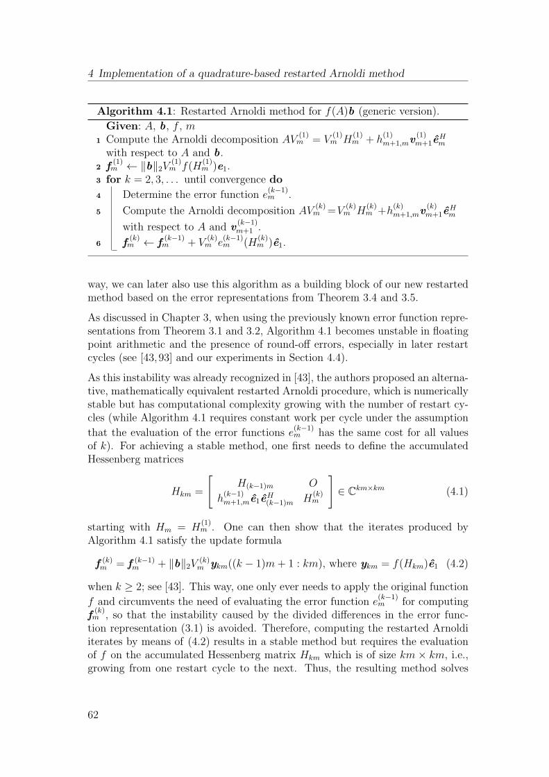
4 Implementation of a quadrature-based restarted Arnoldi method
Algorithm 4.1: Restarted Arnoldi method for f(A)b (generic version).
Given: A, b, f , mCompute the Arnoldi decomposition AV
(1)m = V
(1)m H
(1)m + h
(1)m+1,mv
(1)m+1e
Hm1
with respect to A and b.f(1)m ← ‖b‖2V (1)
m f(H(1)m )e1.2
for k = 2, 3, . . . until convergence do3
Determine the error function e(k−1)m .4
Compute the Arnoldi decomposition AV(k)m =V
(k)m H
(k)m +h
(k)m+1,mv
(k)m+1e
Hm5
with respect to A and v(k−1)m+1 .
f(k)m ← f
(k−1)m + V
(k)m e
(k−1)m (H
(k)m )e1.6
way, we can later also use this algorithm as a building block of our new restartedmethod based on the error representations from Theorem 3.4 and 3.5.
As discussed in Chapter 3, when using the previously known error function repre-sentations from Theorem 3.1 and 3.2, Algorithm 4.1 becomes unstable in floatingpoint arithmetic and the presence of round-off errors, especially in later restartcycles (see [43, 93] and our experiments in Section 4.4).
As this instability was already recognized in [43], the authors proposed an alterna-tive, mathematically equivalent restarted Arnoldi procedure, which is numericallystable but has computational complexity growing with the number of restart cy-cles (while Algorithm 4.1 requires constant work per cycle under the assumption
that the evaluation of the error functions e(k−1)m has the same cost for all values
of k). For achieving a stable method, one first needs to define the accumulatedHessenberg matrices
Hkm =
[H(k−1)m O
h(k−1)m+1,me1e
H(k−1)m H
(k)m
]∈ C
km×km (4.1)
starting with Hm = H(1)m . One can then show that the iterates produced by
Algorithm 4.1 satisfy the update formula
f (k)m = f (k−1)
m + ‖b‖2V (k)m ykm((k − 1)m+ 1 : km), where ykm = f(Hkm)e1 (4.2)
when k ≥ 2; see [43]. This way, one only ever needs to apply the original function
f and circumvents the need of evaluating the error function e(k−1)m for computing
f(k)m , so that the instability caused by the divided differences in the error func-tion representation (3.1) is avoided. Therefore, computing the restarted Arnoldiiterates by means of (4.2) results in a stable method but requires the evaluationof f on the accumulated Hessenberg matrix Hkm which is of size km × km, i.e.,growing from one restart cycle to the next. Thus, the resulting method solves
62
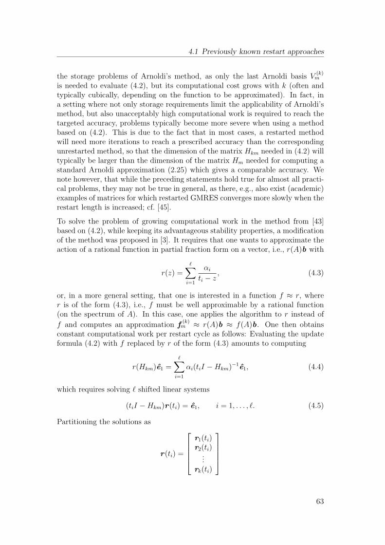
4.1 Previously known restart approaches
the storage problems of Arnoldi’s method, as only the last Arnoldi basis V(k)m
is needed to evaluate (4.2), but its computational cost grows with k (often andtypically cubically, depending on the function to be approximated). In fact, ina setting where not only storage requirements limit the applicability of Arnoldi’smethod, but also unacceptably high computational work is required to reach thetargeted accuracy, problems typically become more severe when using a methodbased on (4.2). This is due to the fact that in most cases, a restarted methodwill need more iterations to reach a prescribed accuracy than the correspondingunrestarted method, so that the dimension of the matrix Hkm needed in (4.2) willtypically be larger than the dimension of the matrix Hm needed for computing astandard Arnoldi approximation (2.25) which gives a comparable accuracy. Wenote however, that while the preceding statements hold true for almost all practi-cal problems, they may not be true in general, as there, e.g., also exist (academic)examples of matrices for which restarted GMRES converges more slowly when therestart length is increased; cf. [45].
To solve the problem of growing computational work in the method from [43]based on (4.2), while keeping its advantageous stability properties, a modificationof the method was proposed in [3]. It requires that one wants to approximate theaction of a rational function in partial fraction form on a vector, i.e., r(A)b with
r(z) =ℓ∑
i=1
αi
ti − z, (4.3)
or, in a more general setting, that one is interested in a function f ≈ r, wherer is of the form (4.3), i.e., f must be well approximable by a rational function(on the spectrum of A). In this case, one applies the algorithm to r instead of
f and computes an approximation f(k)m ≈ r(A)b ≈ f(A)b. One then obtains
constant computational work per restart cycle as follows: Evaluating the updateformula (4.2) with f replaced by r of the form (4.3) amounts to computing
r(Hkm)e1 =ℓ∑
i=1
αi(tiI −Hkm)−1e1, (4.4)
which requires solving ℓ shifted linear systems
(tiI −Hkm)r(ti) = e1, i = 1, . . . , ℓ. (4.5)
Partitioning the solutions as
r(ti) =
r1(ti)r2(ti)
...rk(ti)
63
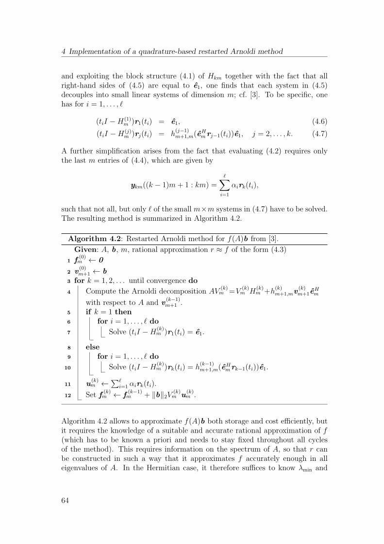
4 Implementation of a quadrature-based restarted Arnoldi method
and exploiting the block structure (4.1) of Hkm together with the fact that allright-hand sides of (4.5) are equal to e1, one finds that each system in (4.5)decouples into small linear systems of dimension m; cf. [3]. To be specific, onehas for i = 1, . . . , ℓ
(tiI −H(1)m )r1(ti) = e1, (4.6)
(tiI −H(j)m )rj(ti) = h
(j−1)m+1,m(e
Hmrj−1(ti))e1, j = 2, . . . , k. (4.7)
A further simplification arises from the fact that evaluating (4.2) requires onlythe last m entries of (4.4), which are given by
ykm((k − 1)m+ 1 : km) =ℓ∑
i=1
αirk(ti),
such that not all, but only ℓ of the small m×m systems in (4.7) have to be solved.The resulting method is summarized in Algorithm 4.2.
Algorithm 4.2: Restarted Arnoldi method for f(A)b from [3].
Given: A, b, m, rational approximation r ≈ f of the form (4.3)
f(0)m ← 01
v(0)m+1 ← b2
for k = 1, 2, . . . until convergence do3
Compute the Arnoldi decomposition AV(k)m =V
(k)m H
(k)m +h
(k)m+1,mv
(k)m+1e
Hm4
with respect to A and v(k−1)m+1 .
if k = 1 then5
for i = 1, . . . , ℓ do6
Solve (tiI −H(k)m )r1(ti) = e1.7
else8
for i = 1, . . . , ℓ do9
Solve (tiI −H(k)m )rk(ti) = h
(k−1)m+1,m(e
Hmrk−1(ti))e1.10
u(k)m ←∑ℓ
i=1 αirk(ti).11
Set f(k)m ← f
(k−1)m + ‖b‖2V (k)
m u(k)m .12
Algorithm 4.2 allows to approximate f(A)b both storage and cost efficiently, butit requires the knowledge of a suitable and accurate rational approximation of f(which has to be known a priori and needs to stay fixed throughout all cyclesof the method). This requires information on the spectrum of A, so that r canbe constructed in such a way that it approximates f accurately enough in alleigenvalues of A. In the Hermitian case, it therefore suffices to know λmin and
64
4.2 Restarts based on numerical quadrature
λmax, the smallest and largest eigenvalue of A, respectively, and to construct ras a good approximation on [λmin, λmax]. In the non-Hermitian case, however,it is far more complicated to find a suitable region which contains spec(A) andto construct an accurate rational approximation on such a general region, whichis no interval on the real line. In addition, Ritz values may appear anywherein the field of values W(A) of A, such that it may be necessary that f be wellapproximated on an even larger set. Another limitation to the applicability ofthe approach from [3] is that for certain functions, no simple to construct rationalapproximations which give a certain accuracy may be known, even for “simple”spectral regions.
Thus, while the method from [3] has very advantageous properties when applicable(e.g., for approximating the exponential of a Hermitian negative definite matrix),it is no black-box method in general, as it often requires spectral information onA and it is only feasible for a rather narrow class of functions. Therefore, in thenext section, by combining the error representations from Chapter 3 with numer-ical quadrature, we introduce another implementation of the restarted Arnoldimethod, which inherits the stability properties and constant computational costper cycle from Algorithm 4.2 and is applicable to a broad class of functions with-out requiring spectral information.
To end this section, we mention that Algorithm 4.2 is mathematically equivalentto restarted FOM for the shifted linear systems
(tiI − A)x (ti) = b, (4.8)
a method introduced in [123], with the only difference being that the approximatesolutions of the individual systems (4.8) do not need to be computed or storedexplicitly, as one is only interested in the approximation to r(A)b ≈ f(A)b. Asimilar point of view was recently discussed in [17], where this approach was usedto save computational work when solving families of shifted (block) linear systemshaving their origin in a partial fraction expansion (4.3) of a rational function.
4.2 Restarts based on numerical quadrature
In this section, we describe how to use the integral representation of the Arnoldierror for deriving a numerically stable version of Algorithm 4.1. The key obser-vation for achieving stability in this context is that the numerical evaluation ofintegrals is much more stable than the numerical evaluation of difference quotients(and thus, e.g., the computation of divided differences), see, e.g., [41], where thisis discussed in the context of the numerical solution of differential equations.
65
4 Implementation of a quadrature-based restarted Arnoldi method
To be able to use the error function representations from Theorem 3.4 and 3.5in Algorithm 4.1, we require not only an integral representation for the approx-imation fm obtained by m steps of Arnoldi’s method, but also for the restartedapproximations f
(k)m . Fortunately, recursively replacing f by e
(1)m , e
(2)m , . . . in the
statements of the theorems directly gives rise to such a representation. We sum-marize this result in the following corollary.
Corollary 4.1. Let the assumptions of Theorem 3.4 hold and let f(k)m be the
restarted Arnoldi approximation to f(A)b after k restart cycles of Algorithm 4.1.
Denote by w(j)m the nodal polynomial of the jth restart cycle, i.e., the monic poly-
nomial of degree m with its roots given by the eigenvalues of H(j)m , and assume
that all these roots do not lie on Γ and let γ(j)m =
∏mi=1 h
(j)i+1,i. Then the error of
f(k)m satisfies
f(A)b − f (k)m = ‖b‖2
(k∏
j=1
γ(j)m
)∫
Γ
g(t)∏k
j=1w(j)m (t)
(tI − A)−1v(k)m+1 dt (4.9)
=: e(k)m (A)v(k)m+1,
provided that the integral (3.4), with wm(t) =∏k
j=1w(j)m (t), exists.
In the same way, if f is a Stieltjes function (3.15), we have a representation ofthe form
f(A)b − f (k)m = e(k)m (A)v
(k)m+1, (4.10)
where
e(k)m (z) = (−1)k(m+1)‖b‖2(
k∏
j=1
γ(j)m
)∫ ∞
0
1∏k
j=1w(j)m (t)
1
z + tdµ(t). (4.11)
Instead of recursively inserting the error functions into Theorem 3.4, one alsofinds these results directly by using the fact that f
(k)m = pkm−1(A)b, where pkm−1
is the polynomial of degree km − 1 that interpolates f on spec(Hkm), with Hkm
from (4.1), see [43], and reproducing the proof of Theorem 3.4 for this case. Notethat the existence of the integrals in (4.9) and (4.11) can of course be guaranteedunder the same assumptions as in Proposition 3.8 and 3.9, respectively.
With Corollary 4.1, we are in a position to formulate our new, quadrature-basedrestarted Arnoldi method. It mainly consists of using the error function rep-resentation (4.9) or (4.11) in Algorithm 4.1 and approximating e
(k−1)m (A)b by a
(suitably chosen) quadrature rule, as it is in general not possible to evaluate (4.9)or (4.11) exactly. As we do not know a priori how many quadrature nodes arenecessary to approximate the error functions with sufficient accuracy (as even theerror functions themselves are not known in advance) and as this number may
66
4.2 Restarts based on numerical quadrature
vary from one cycle to the next, we use a simple form of adaptive quadrature.Of course one can also use more sophisticated techniques than what is describedin the following, as in general all forms of adaptive quadrature are suitable, butwe found that this simple approach was sufficient in our setting, as the efficientevaluation of quadrature rules is not the bottleneck of the method.
At each restart cycle, we choose two sets of ℓ and ℓ := ⌊√2 · ℓ⌋ quadrature nodes
and weights, and approximate e(k−1)m (H
(k)m )e1 by quadrature of these two different
orders. If the norm of the difference between the two resulting approximationsu
(k)m and u
(k)m is smaller than a prescribed tolerance tol, the approximation u
(k)m of
higher order is accepted, otherwise we increase the number of quadrature points byanother factor of
√2 and continue this way until the desired accuracy is reached.
This approach has two advantages. First (and obviously), if the initially chosennumber of quadrature points is too small to reach the prescribed accuracy, it au-tomatically increases the number as much as it is needed in the current cycle. Onthe other hand, the approach does in the same way allow to decrease the num-ber of quadrature points, if fewer points suffice to obtain the required tolerance.Therefore, if in a restart cycle the number of quadrature points is not increased,we decrease the number of quadrature points for the next cycle by a factor of√2 and first test whether this lower number is already sufficient. This way, later
restart cycles may indeed be less expensive than earlier cycles in our method. Wego into more detail concerning this topic in the numerical experiments reportedin Section 4.4. The resulting method is given as Algorithm 4.3 and was firstintroduced in [58], an implementation being provided in [59].
On first sight, one may assume that our approach may at one point be more proneto numerical instability than the one from [3], as it requires the evaluation of thenodal polynomial wm(t) which is of (possibly very high) degree m. However, notethat
γmwm(t)
= hm+1,meHm (tIm −Hm)
−1e1, (4.12)
see, e.g., [115], so that the necessary scalar quantities can be computed by solvinga shifted linear system of dimension m which can be done in a stable way. An-other technique for reliably evaluating wm(t) in factored form is to use a suitablereordering of its zeros while computing the product. These approaches togetherwith the numerical experiments reported in Section 4.4 suggest that our methodis indeed numerically stable.
We proceed by further commenting on the relation between Algorithm 4.3 andAlgorithm 4.2, the approach from [3], as this is the only other approach fromthe literature which also guarantees constant work per cycle as well as numericalstability. A further similarity of the two approaches is revealed by noting thatan arbitrary quadrature rule with nodes ti and weights ωi for approximating the
67
4 Implementation of a quadrature-based restarted Arnoldi method
Algorithm 4.3: Quadrature-based restarted Arnoldi method for f(A)b.
Given: A, b, f , m, tolCompute the Arnoldi decomposition AV
(1)m = V
(1)m H
(1)m + h
(1)m+1,mv
(1)m+1e
Hm1
with respect to A and b.f(1)m ← ‖b‖2V (1)
m f(H(1)m )e12
ℓ← 8, ℓ← round(√2 · ℓ)3
for k = 2, 3, . . . until convergence do4
Compute the Arnoldi decomposition AV(k)m =V
(k)m H
(k)m +h
(k)m+1,mv
(k)m+1e
Hm5
with respect to A and v(k−1)m+1 .
Choose sets (ti, ωi)i=1,...,ℓ, (ti, ωi)i=1,...,ℓ of quadrature nodes/weights.6
accurate ← false7
refined ← false8
while accurate = false do9
Compute u(k)m ≈ e
(k−1)m (H
(k)m )e1 by quadrature of order ℓ.10
Compute u(k)m ≈ e
(k−1)m (H
(k)m )e1 by quadrature of order ℓ.11
if ‖u (k)m − u
(k)m ‖2 < tol then12
accurate ← true.13
else14
ℓ← ℓ15
ℓ← round(√2 · ℓ)16
refined ← true.17
f(k)m ← f
(k−1)m + ‖b‖2V (k)
m u(k)m .18
if refined = false then19
ℓ← ℓ20
ℓ← round(ℓ/√2)21
error function em(z) from (3.5) gives rise to an approximation of the form
em(z) = ‖b‖2γmℓ∑
i=1
ωig(ti)
wm(ti)
1
ti − z(4.13)
which clearly is a rational approximation (of type (ℓ−1/ℓ)) for em(z). Therefore,in a sense, both methods rely on using rational approximations for the errorfunctions. In fact, we can show that under a few assumptions, both approachesare equivalent (at least assuming exact arithmetic). The precise result is givenin the following lemma, where we refer to Algorithm 4.1 (using quadrature toevaluate the integral representation of the error) instead of Algorithm 4.3 to makeclear that a non-adaptive approach is applied, in which the quadrature nodes and
68
4.2 Restarts based on numerical quadrature
weights are chosen a priori.
Lemma 4.2. Let the quadrature nodes ti and weights ωi in (4.13) be fixed through-out all restart cycles in Algorithm 4.1. Let Algorithm 4.2 utilize a rational ap-proximation in partial fraction form (4.3) with poles ti and weights αi = ωig(ti).Assume that this quadrature formula is also used to evaluate f in the first restartcycle of Algorithm 4.1. Then both algorithms produce the same approximationsf(k)m at each restart cycle k ≥ 1.
Proof. From (4.6) and (4.13) (with wm ≡ 1 in the first restart cycle) it immedi-ately follows that both algorithms produce the same first Arnoldi approximation
f (1)m = ‖b‖2V (1)
m
ℓ∑
i=1
ωig(ti)(tiI −H(1)m )−1e1.
In subsequent restart cycles k ≥ 2 of Algorithm 4.1, using the error functionrepresentation (4.13), the approximations are computed as
f (k)m = f (k−1)
m + ‖b‖2V (k)m
ℓ∑
i=1
ωig(ti)∏k−1
j=1 γ(j)m
∏k−1j=1 w
(j)m (ti)
(tiI −H(k)m )−1e1. (4.14)
From (4.7) we find rk(ti) = h(k−1)m+1,m(e
Hmrk−1(ti))(tiI −H(k)
m )−1e1. Repeated appli-cation of (4.12) yields
h(k−1)m+1,m(e
Hmrk−1(ti)) =
∏k−1j=1 γ
(j)m
∏k−1j=1 w
(j)m (ti)
,
so that (4.14) is equivalent to
f (k)m = f (k−1)
m + ‖b‖2V (k)m
ℓ∑
i=1
ωig(ti)rk(ti),
which is precisely the update formula of Algorithm 4.2 when αi = ωig(ti).
In light of Lemma 4.2, one may ask which advantages our new approach gives incomparison to the one from [3]. To answer this question, we stress again that theresult of Lemma 4.2 only holds in the very specific case that the quadrature ruleis fixed once and for all before starting the method. While it is indeed necessaryto fix the rational approximation in the approach from [3] in the beginning, thisis not the case for our method. In addition, as long as the integration pathΓ does not depend on the spectrum of A (which is, e.g., the case for Stieltjesfunctions), we need no additional information for the choice of quadrature rule,
69
4 Implementation of a quadrature-based restarted Arnoldi method
in contrast to bounds for the spectral region necessary for constructing a rationalapproximation. Even in cases where the path Γ depends on spec(A), like it is, e.g.,the case when approximating the matrix exponential, one can in many cases easilyconstruct sufficiently accurate rational approximations by exploiting informationobtained from Ritz values. This is not possible in Algorithm 4.2, as the rationalapproximation has to be chosen a priori and needs to stay fixed throughout allcycles, so that the spectral information available from the matrices H
(j)m cannot
be exploited in any way. We go into detail concerning this topic in Section 4.3.Another advantage is the potential for adaptivity not only for guaranteeing thatthe prescribed accuracy is reached, but also for not investing more computationalwork than necessary in later restart cycles and therefore in some cases makingthe method even more efficient.
We just briefly mention here that it is also possible to combine our quadrature-based restart approach with the deflated restarting technique from [44] in astraightforward way. This technique is also included in our implementation [59]of the restarted Arnoldi method, but we do not give the details for this here andrefer to [58] for numerical experiments illustrating the behavior of the resultingmethod.
An important point influencing the performance of our method which we have notyet discussed in detail is the choice of quadrature rules for evaluating the errorfunction e
(k−1)m . While in principle, we can use any convergent quadrature rule in
our adaptive algorithm, making it a black-box method, there are natural choicesof quadrature rules for certain functions which allow to improve the performanceof the method even further and also reveal interesting theoretical connections tocertain types of optimal rational approximants. This is the topic of the nextsection.
4.3 Choice of quadrature rules and connection to
Pade approximation
In this section, we will exemplarily go into more detail concerning the choiceof quadrature rules for three different functions, namely the Stieltjes functionsf(z) = z−α, α ∈ (0, 1) and f(z) = log(1 + z)/z, and the exponential functionf(z) = ez. As stated at the end of the last section, if the path of integration isknown (as, e.g., for Stieltjes functions) using any of the convergent quadraturerules presented in Section 2.5 is in principle possible, but there are often bet-ter choices available when exploiting specific properties of the function at hand.Concerning the exponential function, the path Γ is not known in advance if no
70
4.3 Choice of quadrature rules and connection to Pade approximation
spectral information on A is available, as it is typically the case when A is non-Hermitian (in the Hermitian negative definite case, Hankel contours that enclosethe negative real axis are suitable integration paths) and we will also commenton how to adaptively construct a suitable contour in this case.
As it turns out that certain choices of quadrature rules for Stieltjes functionscorrespond to certain (optimal) rational approximants of these functions, the so-called Pade approximants [8–10, 53, 110], we review the basic definition of theseapproximants before proceeding.
Definition 4.3. Let f be a function and let m ≥ 0, ℓ ≥ 1 be given. An (m/ℓ)Pade approximant of f with expansion point a is a rational function
rm,ℓ(z) =pm(z)
qℓ(z)where deg pm ≤ m, deg qℓ ≤ ℓ,
such that
dj
dzjf(z)
∣∣∣∣z=a
=dj
dzjrm,ℓ(z)
∣∣∣∣z=a
for j = 0, . . . ,m+ ℓ. (4.15)
We note that, by a classical result from [53,110], if an (m/ℓ) Pade approximant toa function f exists, then it is unique, so that we will in the following refer to rm,ℓ asthe (m/ℓ) Pade approximant of f at a. We also note that there exist other (moregeneral) definitions of Pade approximants, cf. [8], which agree with Definition 4.3when both are applicable, but use other matching conditions than (4.15). As thisis not of importance in our situation, we do not go into detail concerning thistopic.
We begin by considering quadrature rules for the integral representation (2.18)of the inverse fractional powers f(z) = z−α, α ∈ (0, 1). In this Stieltjes represen-tation, the integration interval Γ = R
+0 is known a priori but infinite. Instead of
using a quadrature rule for infinite intervals, one can also apply a suitable variabletransformation.
Lemma 4.4. Let z ∈ C \ R−0 and α ∈ (0, 1). Then for all β > 0
z−α =2β1−α sin(απ)
π
∫ 1
−1
(1− x)α−1(1 + x)−α
β(1 + x) + z(1− x) dx. (4.16)
71
4 Implementation of a quadrature-based restarted Arnoldi method
Proof. We apply the variable transformation t = β 1+x1−x
to (2.18). Noting thatdtdx
= 2β(1−x)2
and integrating by substitution, we find
z−α =sin(απ)
π
∫ 1
−1
(β 1+x
1−x
)−α
β 1+x1−x
+ z· 2β
(1− x)2 dx
=2β1−α sin(απ)
π
∫ 1
−1
(1− x)α(1 + x)−α
β(1 + x)(1− x) + z(1− x)2 dx,
from which the assertion follows.
The integrand in (4.16) has singularities at both endpoints −1 and 1. However,these singularities are contained only in the numerator, which exactly correspondsto the (α−1,−α) Jacobi weight function; cf. Example 2.45. Therefore, we can useGauss–Jacobi quadrature to resolve it exactly. The remaining integrand has nosingularities as long as z ∈ C\R−
0 (for z ∈ R−0 , the original integral representation
also has a singularity). The following result reveals a connection between Gauss–Jacobi quadrature for (4.16) and Pade approximants.
Lemma 4.5. Let β > 0 and let xi and ωi, i = 1, . . . , ℓ be the nodes and weightsof the ℓ-point (α− 1,−α) Gauss–Jacobi quadrature rule on [−1, 1]. Then
rℓ−1,ℓ(z) =2β1−α sin(απ)
π
ℓ∑
i=1
ωi
β(1 + xi) + z(1− xi)(4.17)
is the (ℓ− 1/ℓ) Pade approximant of z−α, α ∈ (0, 1), with expansion point β.
Proof. Note that (4.17) clearly is a rational function of type (ℓ − 1/ℓ) in partialfraction form. Therefore we only have to verify the Pade matching conditions
dj
dzjz−α
∣∣∣∣z=β
=dj
dzjrℓ−1,ℓ(z)
∣∣∣∣z=β
for j = 0, . . . , 2ℓ− 1.
The derivatives of rℓ−1,ℓ(z) are given by
dj
dzjrℓ−1,ℓ(z) = −
2β1−α sin(απ)
π
ℓ∑
i=1
(−1)j j! · (1− xi)j · ωi
(β(1 + xi) + z(1− xi))j+1. (4.18)
For z = β all denominators in (4.18) become independent of xi and we arrive at
dj
dzjrℓ−1,ℓ(z)
∣∣∣∣z=β
= −2β1−α sin(απ)
π
ℓ∑
i=1
(−1)j j! · (1− xi)j · ωi
(2β)j+1.
72
4.3 Choice of quadrature rules and connection to Pade approximation
As Gauss–Jacobi quadrature with ℓ nodes is exact for polynomials up to degree2ℓ− 1, we have the relation
dj
dzjrℓ−1,ℓ(z)
∣∣∣∣z=β
=2β1−αj! · sin(απ)
(2β)j+1π(−1)j
∫ 1
−1
(1− x)j(1− x)α−1(1 + x)−α dx.
for j = 0, . . . , 2ℓ− 1. Differentiating the right-hand side of (4.16) and evaluatingat β gives the same result, which completes the proof.
We note that it is known that the rational functions generated by certain Gaussquadrature rules coincide with certain Pade approximants, see, e.g., [4, 21], butthe precise result of Lemma 4.5 was not given in this explicit form before to thebest of our knowledge. As the approximation quality of Pade approximants istypically highest close to the expansion point, it seems reasonable to choose thetransformation parameter β such that the eigenvalues of A are clustered aroundit. A straightforward choice therefore is the arithmetic mean of the eigenvaluesof A, which is readily available as trace(A)/n. Other, more sophisticated choicesof β are of course possible in our setting due to the availability of Ritz valueinformation, but we observed in our experiments that this has no large influenceon the overall behavior of the method, especially as the cost of evaluating thequadrature rules in Algorithm 4.3 is typically negligible compared to the cost ofmatrix vector products and orthogonalization.
In Algorithm 4.3, the quadrature formula is of course not applied to evaluate f ,but instead to evaluate the error functions e
(k−1)m , for which the quadrature rule for
the transformed integral does not correspond to a Pade approximant, but can stillbe expected to yield good approximations. Applying the same variable transfor-mation as in Lemma 4.4 to the integral representation of the error function (3.7)corresponding to z−α results in the transformed integral
(−1)m+12 sin(απ)β1−α‖b‖2γmπ
∫ 1
−1
1
wm(β1+x1−x
)
(1− x)α−1(1 + x)−α
β(1 + x) + z(1− x) dx. (4.19)
The integrand again has singularities at both endpoints of the interval of integra-tion which can be resolved exactly by Gauss–Jacobi quadrature, but the reciprocalof the nodal polynomial introduces m additional singularities. Obviously, the sin-gularities of the reciprocal of wm prior to the variable transformation are exactlythe Ritz values with switched sign. As the variable transformation bijectivelymaps R+
0 to [−1, 1], the transformed integrand therefore has a singularity in theintegration interval if and only if there is a Ritz value on the negative real axis.As all Ritz values lie in the field of valuesW(A) of A, a sufficient condition for theintegrand in (4.19) having no singularities in the interval of integration is that thefield of values of A is disjoint from the negative real axis. This is, e.g., the case,when A is Hermitian positive definite, or, more generally, when A is positive real.
73
4 Implementation of a quadrature-based restarted Arnoldi method
If these conditions on A are not fulfilled it may well happen that Algorithm 4.3generates Ritz values on the negative real axis. This is, however, no shortcomingof our method, but rather a general problem. None of the restart approaches willwork in this case, as the function z−α and therefore also the error functions arenot defined on the branch-cut along R
−0 .
Another Stieltjes function for which a similar analysis as for z−α can be performedis f(z) = log(1 + z)/z with the integral representation (2.19). We again begin bytransforming the infinite integration interval to a finite one.
Lemma 4.6. Let z ∈ C \ (−∞,−1]. Then
log(1 + z)
z=
∫ 1
−1
1
z(1− x) + 2dx. (4.20)
Proof. We apply the transformation t = 2/(1− x), which satisfies dtdx
= 2(1−x)2
, to
(2.19). Integrating by substitution gives
log(1 + z)
z=
∫ 1
−1
1−x2
21−x
+ z· 2
(1− x)2 dx
=
∫ 1
−1
12
1−x+ z· 1
1− x dx,
which proves the lemma.
When using Gauss–Legendre quadrature for approximating the integral (4.20),we again find a connection to Pade approximants.
Lemma 4.7. Let xi and ωi, i = 1, . . . , ℓ be the nodes and weights of the ℓ-pointGauss–Legendre quadrature rule on [−1, 1]. Then
rℓ−1,ℓ(z) =ℓ∑
i=1
ωi
z(1− xi) + 2
is the (ℓ− 1/ℓ) Pade approximant of log(1 + z)/z with expansion point 0.
Proof. The proof proceeds analogously to the proof of Lemma 4.5 by noting thatℓ-point Gauss–Legendre quadrature is exact for polynomials of degree up to 2ℓ−1,and using the formula
dj
dzjrℓ−1,ℓ(z) =
ℓ∑
i=1
(−1)j j! · (1− xi)j · ωi
(z(1− xi) + 2)j+1
for the derivatives of rℓ−1,ℓ(z).
74
4.3 Choice of quadrature rules and connection to Pade approximation
In contrast to Lemma 4.5, the result of Lemma 4.7 does not allow to freely choosethe expansion point of the Pade approximant. Instead, it is always fixed at theorigin. As already mentioned in the discussion after Lemma 4.5, the method doesnot behave very sensitively with respect to the expansion point anyway, so thatwe can expect the method to work efficiently also in cases where the matrix Ahas eigenvalues far away from the origin. Apart from this minor difference, mostof the discussion for z−α also applies in the case of log(1 + z)/z with obviousmodifications, so that we refrain from restating this here.
The last function we discuss in detail in this section is the exponential function,f(z) = ez. We use the Cauchy integral representation
ez =1
2πi
∫
Γ
et
t− z dt (4.21)
where Γ is a closed contour in the extended complex plane winding around zexactly once, which directly translates into an integral representation for thematrix exponential
eA =1
2πi
∫
Γ
et (tI − A)−1 dt,
where Γ now has to wind around spec(A) exactly once; cf. Definition 2.4. Animportant special case arises when A is Hermitian negative semi-definite, i.e., itseigenvalues lie in R
−0 . It was shown in [135, 141, 142] that the trapezoidal rule
on suitably chosen parabolic, hyperbolic or cotangent Hankel contours (so-calledTalbot contours, introduced in [133]) gives very good approximation results forthe exponential function on the negative real axis (and thus also for the matrixexponential of Hermitian negative semi-definite matrices). Therefore, these con-tours seem well suited to be used in Algorithm 4.3 in this case. In the following,we only discuss parabolic contours, as the results are very similar for all threetypes of contours in our setting.
The optimized parabolic contour proposed in [135] is given as
γ(ζ) = ℓ(0.1309− 0.1194ζ2 + 0.25iζ) (4.22)
and the ℓ-point trapezoidal rule applied to (4.21) on the contour (4.22) gives aconvergence rate of O(2.85−ℓ). The resulting contour for different values of ℓ isgiven in Figure 4.1. While in the experiments reported in [135] at most ℓ = 32quadrature nodes were necessary to approximate the exponential function on R
−0
to machine precision, the situation is different in the context of our restartedArnoldi method. On the one hand, we are not interested in approximating theexponential itself, but rather the error function (3.5) and on the other hand, weare not only interested in achieving a high accuracy on R
−0 , but, when A is non-
Hermitian with field of values in the left half-plane, in a larger region of the lefthalf-plane which contains all Ritz values. Because of these two reasons, higher
75
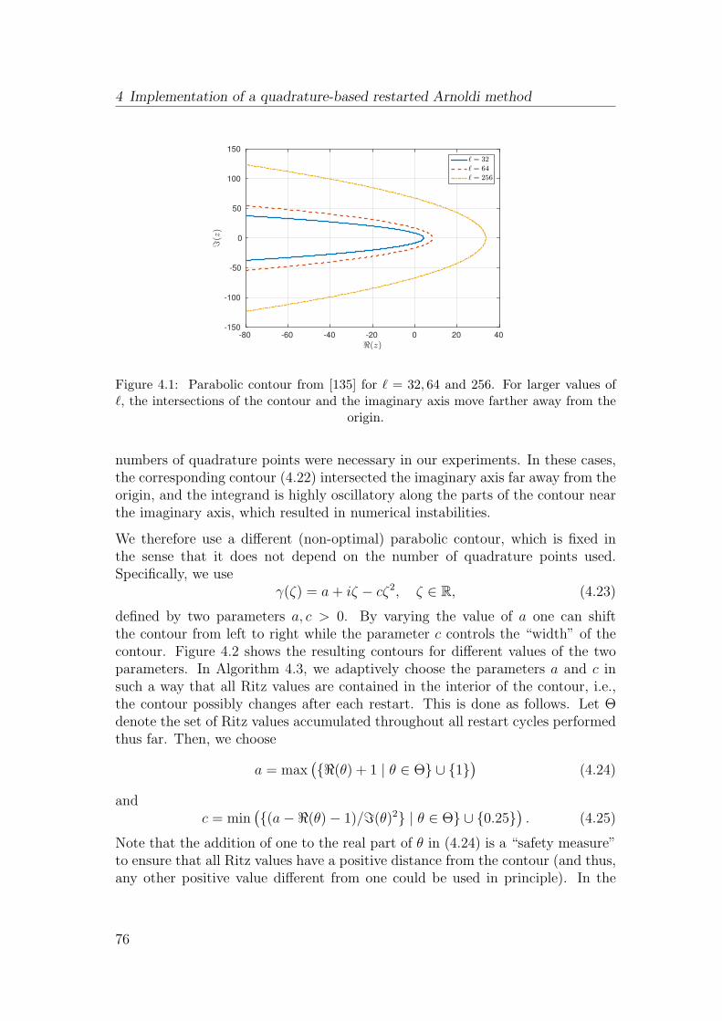
4 Implementation of a quadrature-based restarted Arnoldi method
<(z)-80 -60 -40 -20 0 20 40
=(z)
-150
-100
-50
0
50
100
150
` = 32
` = 64
` = 256
Figure 4.1: Parabolic contour from [135] for ℓ = 32, 64 and 256. For larger values ofℓ, the intersections of the contour and the imaginary axis move farther away from the
origin.
numbers of quadrature points were necessary in our experiments. In these cases,the corresponding contour (4.22) intersected the imaginary axis far away from theorigin, and the integrand is highly oscillatory along the parts of the contour nearthe imaginary axis, which resulted in numerical instabilities.
We therefore use a different (non-optimal) parabolic contour, which is fixed inthe sense that it does not depend on the number of quadrature points used.Specifically, we use
γ(ζ) = a+ iζ − cζ2, ζ ∈ R, (4.23)
defined by two parameters a, c > 0. By varying the value of a one can shiftthe contour from left to right while the parameter c controls the “width” of thecontour. Figure 4.2 shows the resulting contours for different values of the twoparameters. In Algorithm 4.3, we adaptively choose the parameters a and c insuch a way that all Ritz values are contained in the interior of the contour, i.e.,the contour possibly changes after each restart. This is done as follows. Let Θdenote the set of Ritz values accumulated throughout all restart cycles performedthus far. Then, we choose
a = max(ℜ(θ) + 1 | θ ∈ Θ ∪ 1
)(4.24)
andc = min
((a−ℜ(θ)− 1)/ℑ(θ)2 | θ ∈ Θ ∪ 0.25
). (4.25)
Note that the addition of one to the real part of θ in (4.24) is a “safety measure”to ensure that all Ritz values have a positive distance from the contour (and thus,any other positive value different from one could be used in principle). In the
76
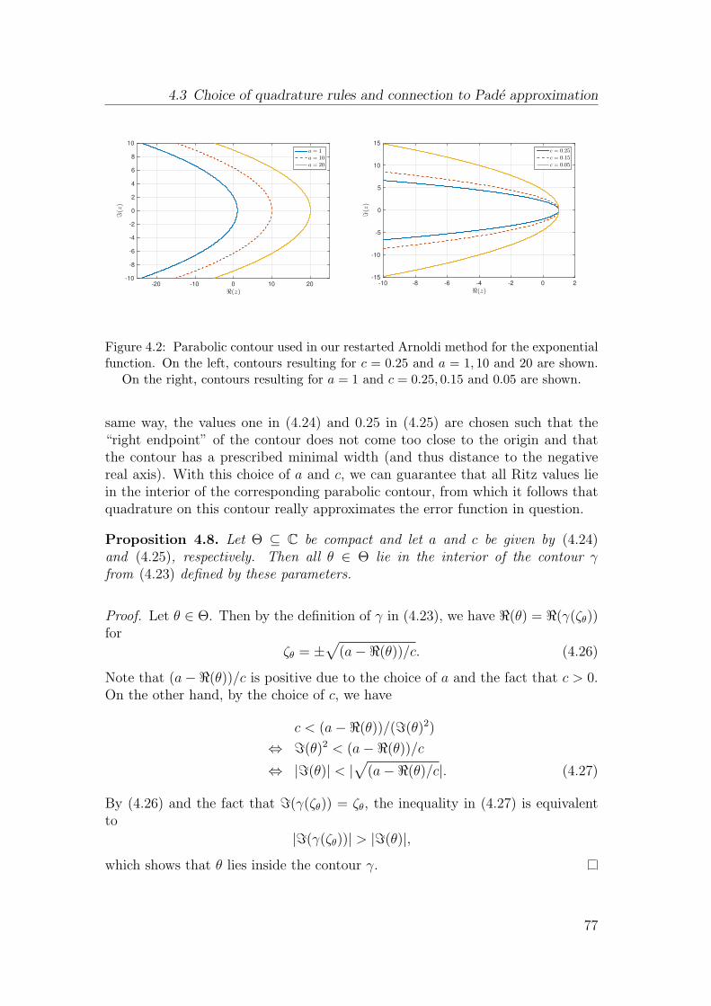
4.3 Choice of quadrature rules and connection to Pade approximation
<(z)-20 -10 0 10 20
=(z)
-10
-8
-6
-4
-2
0
2
4
6
8
10
a = 1
a = 10
a = 20
<(z)-10 -8 -6 -4 -2 0 2
=(z)
-15
-10
-5
0
5
10
15
c = 0:25
c = 0:15
c = 0:05
Figure 4.2: Parabolic contour used in our restarted Arnoldi method for the exponentialfunction. On the left, contours resulting for c = 0.25 and a = 1, 10 and 20 are shown.
On the right, contours resulting for a = 1 and c = 0.25, 0.15 and 0.05 are shown.
same way, the values one in (4.24) and 0.25 in (4.25) are chosen such that the“right endpoint” of the contour does not come too close to the origin and thatthe contour has a prescribed minimal width (and thus distance to the negativereal axis). With this choice of a and c, we can guarantee that all Ritz values liein the interior of the corresponding parabolic contour, from which it follows thatquadrature on this contour really approximates the error function in question.
Proposition 4.8. Let Θ ⊆ C be compact and let a and c be given by (4.24)and (4.25), respectively. Then all θ ∈ Θ lie in the interior of the contour γfrom (4.23) defined by these parameters.
Proof. Let θ ∈ Θ. Then by the definition of γ in (4.23), we have ℜ(θ) = ℜ(γ(ζθ))for
ζθ = ±√
(a−ℜ(θ))/c. (4.26)
Note that (a−ℜ(θ))/c is positive due to the choice of a and the fact that c > 0.On the other hand, by the choice of c, we have
c < (a−ℜ(θ))/(ℑ(θ)2)⇔ ℑ(θ)2 < (a−ℜ(θ))/c⇔ |ℑ(θ)| < |
√(a−ℜ(θ)/c|. (4.27)
By (4.26) and the fact that ℑ(γ(ζθ)) = ζθ, the inequality in (4.27) is equivalentto
|ℑ(γ(ζθ))| > |ℑ(θ)|,which shows that θ lies inside the contour γ.
77
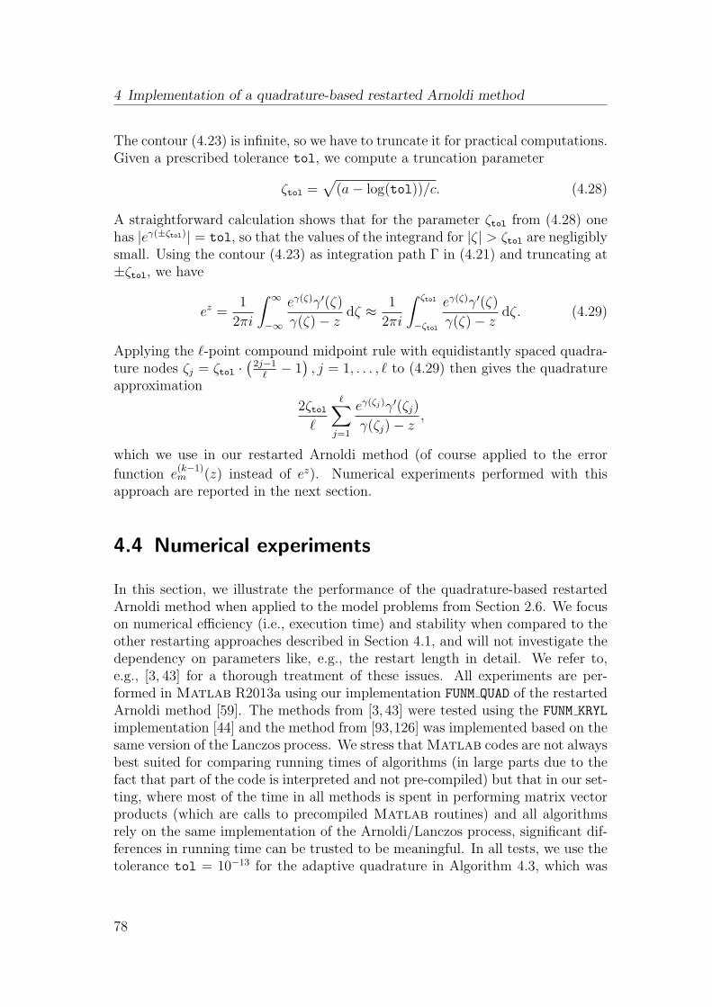
4 Implementation of a quadrature-based restarted Arnoldi method
The contour (4.23) is infinite, so we have to truncate it for practical computations.Given a prescribed tolerance tol, we compute a truncation parameter
ζtol =√
(a− log(tol))/c. (4.28)
A straightforward calculation shows that for the parameter ζtol from (4.28) onehas |eγ(±ζtol)| = tol, so that the values of the integrand for |ζ| > ζtol are negligiblysmall. Using the contour (4.23) as integration path Γ in (4.21) and truncating at±ζtol, we have
ez =1
2πi
∫ ∞
−∞
eγ(ζ)γ′(ζ)
γ(ζ)− z dζ ≈ 1
2πi
∫ ζtol
−ζtol
eγ(ζ)γ′(ζ)
γ(ζ)− z dζ. (4.29)
Applying the ℓ-point compound midpoint rule with equidistantly spaced quadra-ture nodes ζj = ζtol ·
(2j−1ℓ− 1), j = 1, . . . , ℓ to (4.29) then gives the quadrature
approximation
2ζtolℓ
ℓ∑
j=1
eγ(ζj)γ′(ζj)
γ(ζj)− z,
which we use in our restarted Arnoldi method (of course applied to the error
function e(k−1)m (z) instead of ez). Numerical experiments performed with this
approach are reported in the next section.
4.4 Numerical experiments
In this section, we illustrate the performance of the quadrature-based restartedArnoldi method when applied to the model problems from Section 2.6. We focuson numerical efficiency (i.e., execution time) and stability when compared to theother restarting approaches described in Section 4.1, and will not investigate thedependency on parameters like, e.g., the restart length in detail. We refer to,e.g., [3, 43] for a thorough treatment of these issues. All experiments are per-formed in Matlab R2013a using our implementation FUNM QUAD of the restartedArnoldi method [59]. The methods from [3, 43] were tested using the FUNM KRYL
implementation [44] and the method from [93,126] was implemented based on thesame version of the Lanczos process. We stress thatMatlab codes are not alwaysbest suited for comparing running times of algorithms (in large parts due to thefact that part of the code is interpreted and not pre-compiled) but that in our set-ting, where most of the time in all methods is spent in performing matrix vectorproducts (which are calls to precompiled Matlab routines) and all algorithmsrely on the same implementation of the Arnoldi/Lanczos process, significant dif-ferences in running time can be trusted to be meaningful. In all tests, we use thetolerance tol = 10−13 for the adaptive quadrature in Algorithm 4.3, which was
78
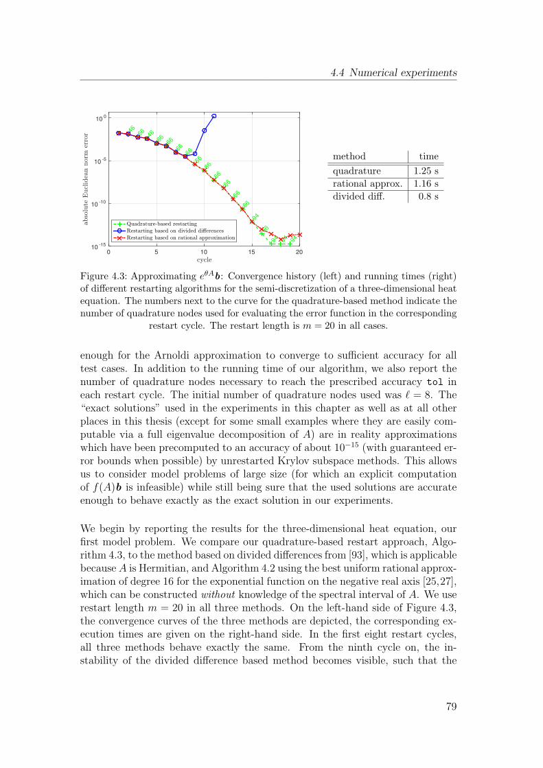
4.4 Numerical experiments
cycle0 5 10 15 20
abso
lute
Eucl
idea
nnorm
erro
r
10-15
10-10
10-5
100
46
66
46
66
66
66
66
66
66
66
66
66
66
94
66
94 9
494
Quadrature-based restarting
Restarting based on divided di,erences
Restarting based on rational approximation
method time
quadrature 1.25 s
rational approx. 1.16 s
divided diff. 0.8 s
Figure 4.3: Approximating eθAb: Convergence history (left) and running times (right)of different restarting algorithms for the semi-discretization of a three-dimensional heatequation. The numbers next to the curve for the quadrature-based method indicate thenumber of quadrature nodes used for evaluating the error function in the corresponding
restart cycle. The restart length is m = 20 in all cases.
enough for the Arnoldi approximation to converge to sufficient accuracy for alltest cases. In addition to the running time of our algorithm, we also report thenumber of quadrature nodes necessary to reach the prescribed accuracy tol ineach restart cycle. The initial number of quadrature nodes used was ℓ = 8. The“exact solutions” used in the experiments in this chapter as well as at all otherplaces in this thesis (except for some small examples where they are easily com-putable via a full eigenvalue decomposition of A) are in reality approximationswhich have been precomputed to an accuracy of about 10−15 (with guaranteed er-ror bounds when possible) by unrestarted Krylov subspace methods. This allowsus to consider model problems of large size (for which an explicit computationof f(A)b is infeasible) while still being sure that the used solutions are accurateenough to behave exactly as the exact solution in our experiments.
We begin by reporting the results for the three-dimensional heat equation, ourfirst model problem. We compare our quadrature-based restart approach, Algo-rithm 4.3, to the method based on divided differences from [93], which is applicablebecause A is Hermitian, and Algorithm 4.2 using the best uniform rational approx-imation of degree 16 for the exponential function on the negative real axis [25,27],which can be constructed without knowledge of the spectral interval of A. We userestart length m = 20 in all three methods. On the left-hand side of Figure 4.3,the convergence curves of the three methods are depicted, the corresponding ex-ecution times are given on the right-hand side. In the first eight restart cycles,all three methods behave exactly the same. From the ninth cycle on, the in-stability of the divided difference based method becomes visible, such that the
79
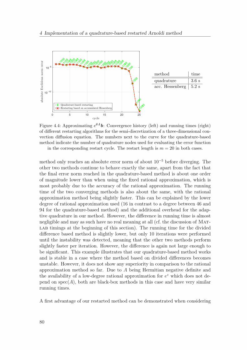
4 Implementation of a quadrature-based restarted Arnoldi method
cycle0 5 10 15 20 25
abso
lute
Eucl
idea
nnorm
erro
r
10-10
10-5
1088
1088
1088
1088
1088
1088
1088
1088
1088
1088
1088
1088
1088
10881088
1088
1088
1088
1088
1088
768
1088
1088
1088Quadrature-based restarting
Restarting based on accumulated Hessenberg
method time
quadrature 3.6 s
acc. Hessenberg 5.2 s
Figure 4.4: Approximating eθAb: Convergence history (left) and running times (right)of different restarting algorithms for the semi-discretization of a three-dimensional con-vection diffusion equation. The numbers next to the curve for the quadrature-basedmethod indicate the number of quadrature nodes used for evaluating the error function
in the corresponding restart cycle. The restart length is m = 20 in both cases.
method only reaches an absolute error norm of about 10−5 before diverging. Theother two methods continue to behave exactly the same, apart from the fact thatthe final error norm reached in the quadrature-based method is about one orderof magnitude lower than when using the fixed rational approximation, which ismost probably due to the accuracy of the rational approximation. The runningtime of the two converging methods is also about the same, with the rationalapproximation method being slightly faster. This can be explained by the lowerdegree of rational approximation used (16 in contrast to a degree between 46 and94 for the quadrature-based method) and the additional overhead for the adap-tive quadrature in our method. However, the difference in running time is almostnegligible and may as such have no real meaning at all (cf. the discussion of Mat-
lab timings at the beginning of this section). The running time for the divideddifference based method is slightly lower, but only 10 iterations were performeduntil the instability was detected, meaning that the other two methods performslightly faster per iteration. However, the difference is again not large enough tobe significant. This example illustrates that our quadrature-based method worksand is stable in a case where the method based on divided differences becomesunstable. However, it does not show any superiority in comparison to the rationalapproximation method so far. Due to A being Hermitian negative definite andthe availability of a low-degree rational approximation for ez which does not de-pend on spec(A), both are black-box methods in this case and have very similarrunning times.
A first advantage of our restarted method can be demonstrated when considering
80
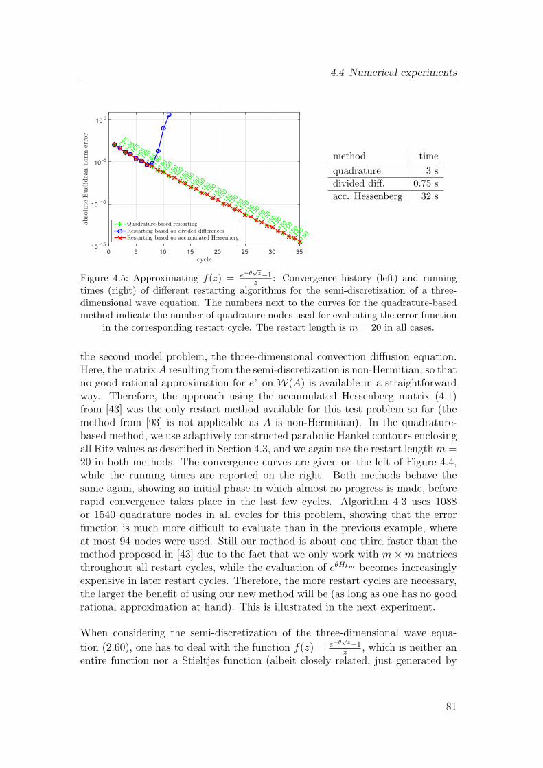
4.4 Numerical experiments
cycle0 5 10 15 20 25 30 35
abso
lute
Eucl
idea
nnorm
erro
r
10-15
10-10
10-5
100
225
195
165
165
165
165
150
150
150
150
150
150
150
150
150
150
150
150
150
150
150
150
150
150
150
150
150
150
150
150
150
150
150
150
Quadrature-based restarting
Restarting based on divided di,erences
Restarting based on accumulated Hessenberg
method time
quadrature 3 s
divided diff. 0.75 s
acc. Hessenberg 32 s
Figure 4.5: Approximating f(z) = e−θ√z−1
z : Convergence history (left) and runningtimes (right) of different restarting algorithms for the semi-discretization of a three-dimensional wave equation. The numbers next to the curves for the quadrature-basedmethod indicate the number of quadrature nodes used for evaluating the error function
in the corresponding restart cycle. The restart length is m = 20 in all cases.
the second model problem, the three-dimensional convection diffusion equation.Here, the matrix A resulting from the semi-discretization is non-Hermitian, so thatno good rational approximation for ez on W(A) is available in a straightforwardway. Therefore, the approach using the accumulated Hessenberg matrix (4.1)from [43] was the only restart method available for this test problem so far (themethod from [93] is not applicable as A is non-Hermitian). In the quadrature-based method, we use adaptively constructed parabolic Hankel contours enclosingall Ritz values as described in Section 4.3, and we again use the restart lengthm =20 in both methods. The convergence curves are given on the left of Figure 4.4,while the running times are reported on the right. Both methods behave thesame again, showing an initial phase in which almost no progress is made, beforerapid convergence takes place in the last few cycles. Algorithm 4.3 uses 1088or 1540 quadrature nodes in all cycles for this problem, showing that the errorfunction is much more difficult to evaluate than in the previous example, whereat most 94 nodes were used. Still our method is about one third faster than themethod proposed in [43] due to the fact that we only work with m×m matricesthroughout all restart cycles, while the evaluation of eθHkm becomes increasinglyexpensive in later restart cycles. Therefore, the more restart cycles are necessary,the larger the benefit of using our new method will be (as long as one has no goodrational approximation at hand). This is illustrated in the next experiment.
When considering the semi-discretization of the three-dimensional wave equa-
tion (2.60), one has to deal with the function f(z) = e−θ√
z−1z
, which is neither anentire function nor a Stieltjes function (albeit closely related, just generated by
81
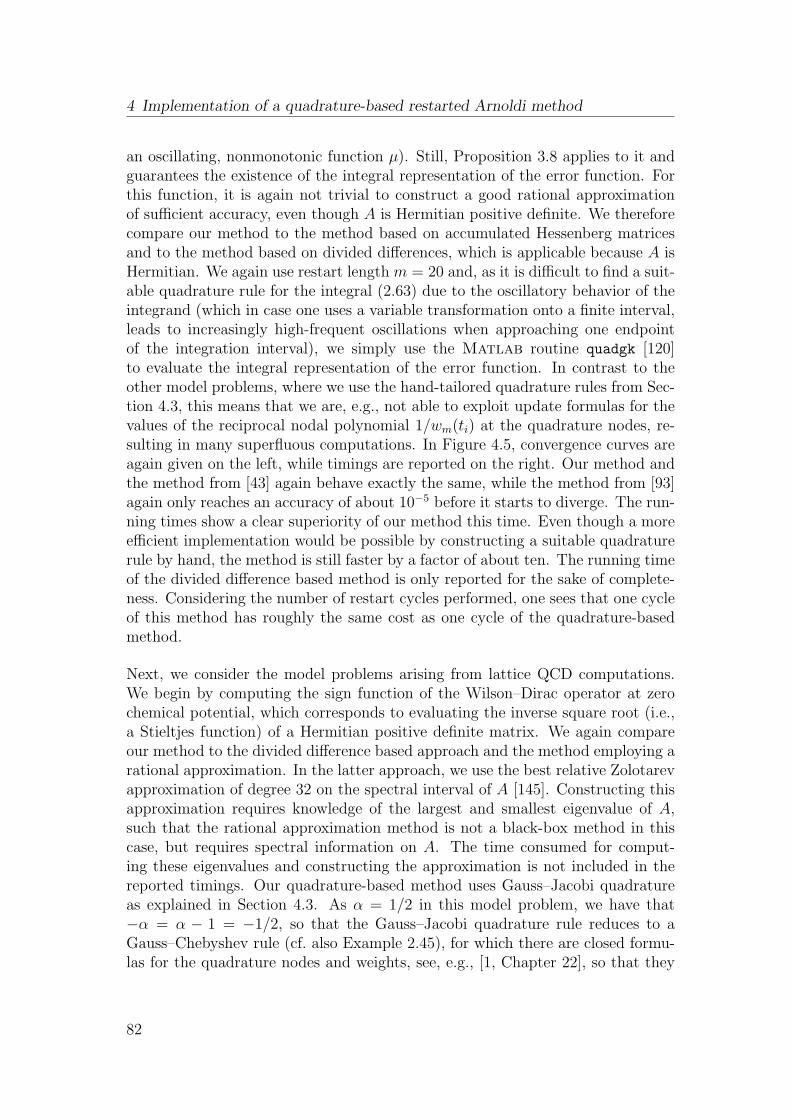
4 Implementation of a quadrature-based restarted Arnoldi method
an oscillating, nonmonotonic function µ). Still, Proposition 3.8 applies to it andguarantees the existence of the integral representation of the error function. Forthis function, it is again not trivial to construct a good rational approximationof sufficient accuracy, even though A is Hermitian positive definite. We thereforecompare our method to the method based on accumulated Hessenberg matricesand to the method based on divided differences, which is applicable because A isHermitian. We again use restart length m = 20 and, as it is difficult to find a suit-able quadrature rule for the integral (2.63) due to the oscillatory behavior of theintegrand (which in case one uses a variable transformation onto a finite interval,leads to increasingly high-frequent oscillations when approaching one endpointof the integration interval), we simply use the Matlab routine quadgk [120]to evaluate the integral representation of the error function. In contrast to theother model problems, where we use the hand-tailored quadrature rules from Sec-tion 4.3, this means that we are, e.g., not able to exploit update formulas for thevalues of the reciprocal nodal polynomial 1/wm(ti) at the quadrature nodes, re-sulting in many superfluous computations. In Figure 4.5, convergence curves areagain given on the left, while timings are reported on the right. Our method andthe method from [43] again behave exactly the same, while the method from [93]again only reaches an accuracy of about 10−5 before it starts to diverge. The run-ning times show a clear superiority of our method this time. Even though a moreefficient implementation would be possible by constructing a suitable quadraturerule by hand, the method is still faster by a factor of about ten. The running timeof the divided difference based method is only reported for the sake of complete-ness. Considering the number of restart cycles performed, one sees that one cycleof this method has roughly the same cost as one cycle of the quadrature-basedmethod.
Next, we consider the model problems arising from lattice QCD computations.We begin by computing the sign function of the Wilson–Dirac operator at zerochemical potential, which corresponds to evaluating the inverse square root (i.e.,a Stieltjes function) of a Hermitian positive definite matrix. We again compareour method to the divided difference based approach and the method employing arational approximation. In the latter approach, we use the best relative Zolotarevapproximation of degree 32 on the spectral interval of A [145]. Constructing thisapproximation requires knowledge of the largest and smallest eigenvalue of A,such that the rational approximation method is not a black-box method in thiscase, but requires spectral information on A. The time consumed for comput-ing these eigenvalues and constructing the approximation is not included in thereported timings. Our quadrature-based method uses Gauss–Jacobi quadratureas explained in Section 4.3. As α = 1/2 in this model problem, we have that−α = α − 1 = −1/2, so that the Gauss–Jacobi quadrature rule reduces to aGauss–Chebyshev rule (cf. also Example 2.45), for which there are closed formu-las for the quadrature nodes and weights, see, e.g., [1, Chapter 22], so that they
82
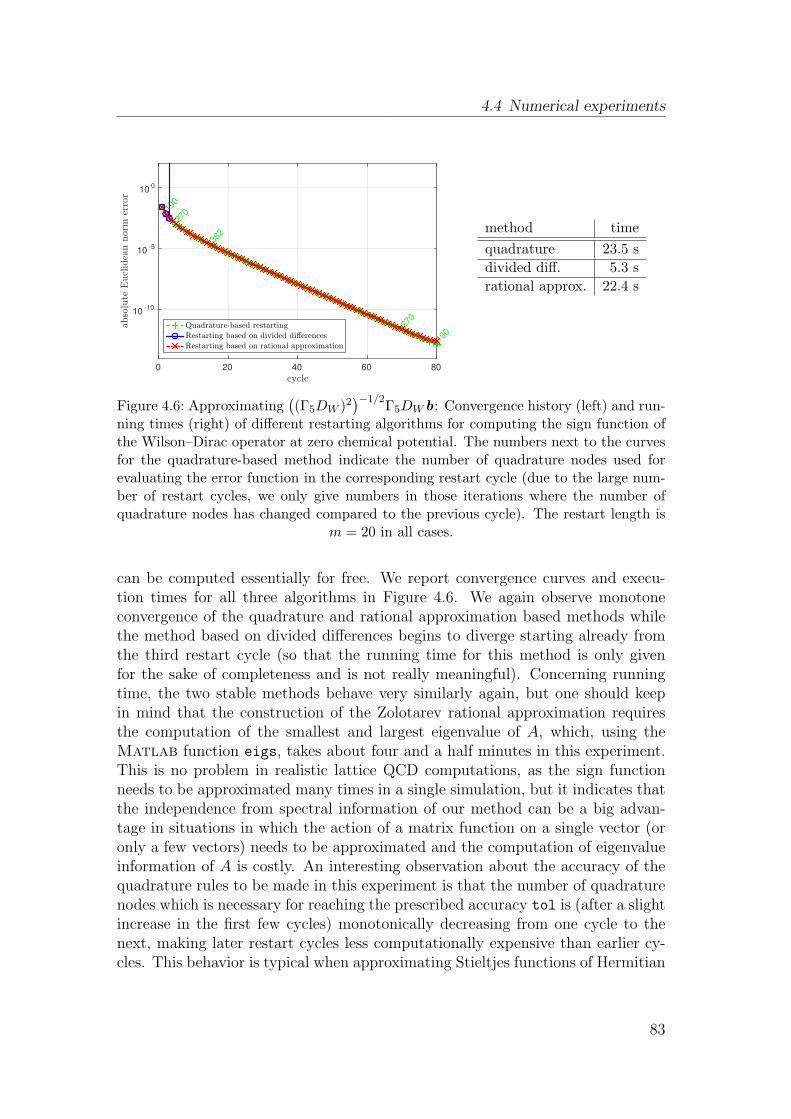
4.4 Numerical experiments
cycle0 20 40 60 80
abso
lute
Eucl
idea
nnorm
erro
r
10-10
10-5
100
190
270
382
270
190
Quadrature-based restarting
Restarting based on divided di,erences
Restarting based on rational approximation
method time
quadrature 23.5 s
divided diff. 5.3 s
rational approx. 22.4 s
Figure 4.6: Approximating((Γ5DW )2
)−1/2Γ5DWb: Convergence history (left) and run-
ning times (right) of different restarting algorithms for computing the sign function ofthe Wilson–Dirac operator at zero chemical potential. The numbers next to the curvesfor the quadrature-based method indicate the number of quadrature nodes used forevaluating the error function in the corresponding restart cycle (due to the large num-ber of restart cycles, we only give numbers in those iterations where the number ofquadrature nodes has changed compared to the previous cycle). The restart length is
m = 20 in all cases.
can be computed essentially for free. We report convergence curves and execu-tion times for all three algorithms in Figure 4.6. We again observe monotoneconvergence of the quadrature and rational approximation based methods whilethe method based on divided differences begins to diverge starting already fromthe third restart cycle (so that the running time for this method is only givenfor the sake of completeness and is not really meaningful). Concerning runningtime, the two stable methods behave very similarly again, but one should keepin mind that the construction of the Zolotarev rational approximation requiresthe computation of the smallest and largest eigenvalue of A, which, using theMatlab function eigs, takes about four and a half minutes in this experiment.This is no problem in realistic lattice QCD computations, as the sign functionneeds to be approximated many times in a single simulation, but it indicates thatthe independence from spectral information of our method can be a big advan-tage in situations in which the action of a matrix function on a single vector (oronly a few vectors) needs to be approximated and the computation of eigenvalueinformation of A is costly. An interesting observation about the accuracy of thequadrature rules to be made in this experiment is that the number of quadraturenodes which is necessary for reaching the prescribed accuracy tol is (after a slightincrease in the first few cycles) monotonically decreasing from one cycle to thenext, making later restart cycles less computationally expensive than earlier cy-cles. This behavior is typical when approximating Stieltjes functions of Hermitian
83
4 Implementation of a quadrature-based restarted Arnoldi method
cycle0 10 20 30 40 50 60 70
abso
lute
Eucl
idea
nnorm
erro
r
10-15
10-10
10-5
100
190
270
382
270
190
Quadrature-based restarting
Restarting based on accumulated Hessenberg
method time
quadrature 34.5 s
acc. Hessenberg 804 s
Figure 4.7: Approximating((Γ5DW )2
)−1/2Γ5DWb: Convergence history (left) and run-
ning times (right) of different restarting algorithms for computing the sign function ofthe Wilson–Dirac operator at nonzero chemical potential. The numbers next to thecurves for the quadrature-based method indicate the number of quadrature nodes usedfor evaluating the error function in the corresponding restart cycle (due to the largenumber of restart cycles, we only give numbers in those iterations where the number ofquadrature nodes has changed compared to the previous cycle). The restart length is
m = 20 in both cases.
positive definite matrices (see also the Gaussian Markov random field experimentlater in this section and the discussion in [58]) and can be explained as follows.The order of magnitude of the computed corrections becomes smaller and smallerthe longer the iteration goes on (see also the results on monotone convergencepresented in Chapter 5) so that the relative accuracy that is required to reach theabsolute accuracy tol is lower in later restart cycles. This is also in line with theerror function representation (3.7), where the integrand contains the reciprocal of∏k−1
j=1 w(j)m , a polynomial of degree (k − 1)m with roots in R
−0 in the kth restart
cycle. The higher the degree of this polynomial gets, the closer the integrand is tothe zero function (which still holds true after applying a variable transformation
as in Section 4.3, as some term involving the reciprocal of∏k−1
j=1 w(j)m is always
present).
Next, we turn our attention to the case of nonzero chemical potential, whichcorresponds to approximating the action of the inverse square root of a non-Hermitian matrix. Therefore, we cannot use the Zolotarev rational approximationhere (as it is not accurate enough for eigenvalues which do not lie close to thereal axis), and we thus compare our method to the approach of [43] again. Theresults of this experiment are given in Figure 4.7. The convergence behavior isvery similar to the one observed for the Neuberger operator at zero chemicalpotential, but the running times reported on the right-hand side of Figure 4.7
84
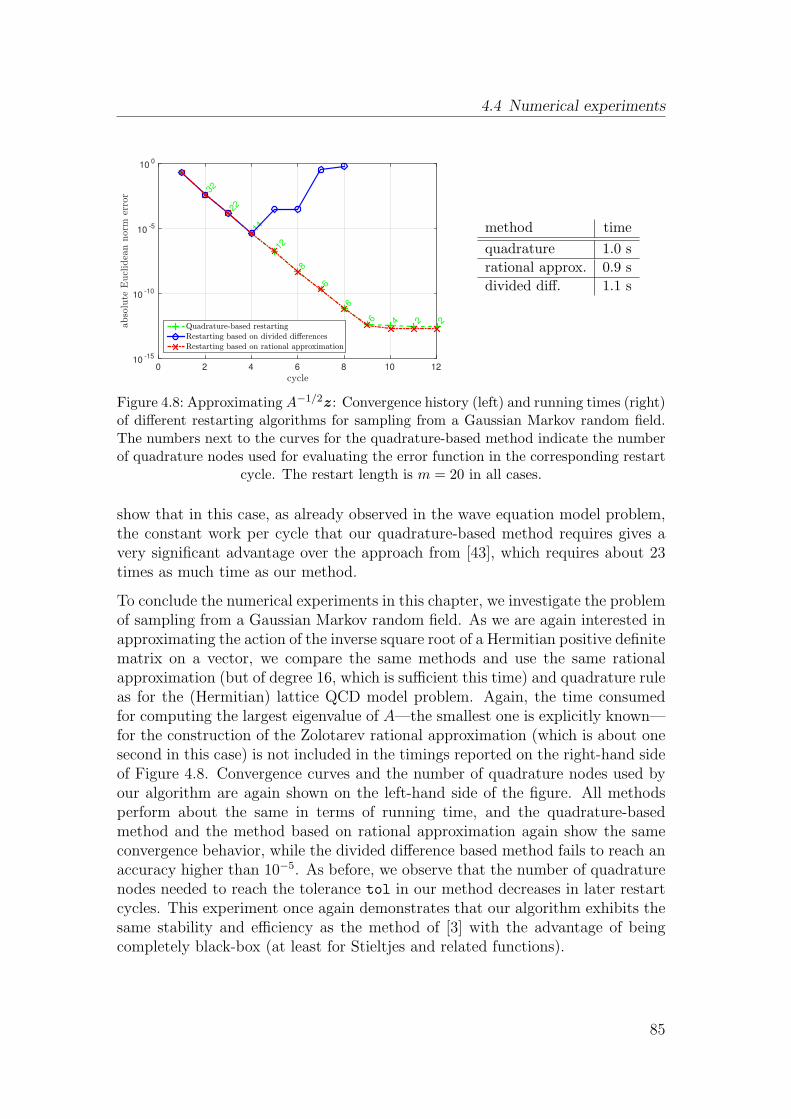
4.4 Numerical experiments
cycle0 2 4 6 8 10 12
abso
lute
Eucl
idea
nnorm
erro
r
10-15
10-10
10-5
100
32
22
14
12
8
6
6
6 4 2 2Quadrature-based restarting
Restarting based on divided di,erences
Restarting based on rational approximation
method time
quadrature 1.0 s
rational approx. 0.9 s
divided diff. 1.1 s
Figure 4.8: Approximating A−1/2z : Convergence history (left) and running times (right)of different restarting algorithms for sampling from a Gaussian Markov random field.The numbers next to the curves for the quadrature-based method indicate the numberof quadrature nodes used for evaluating the error function in the corresponding restart
cycle. The restart length is m = 20 in all cases.
show that in this case, as already observed in the wave equation model problem,the constant work per cycle that our quadrature-based method requires gives avery significant advantage over the approach from [43], which requires about 23times as much time as our method.
To conclude the numerical experiments in this chapter, we investigate the problemof sampling from a Gaussian Markov random field. As we are again interested inapproximating the action of the inverse square root of a Hermitian positive definitematrix on a vector, we compare the same methods and use the same rationalapproximation (but of degree 16, which is sufficient this time) and quadrature ruleas for the (Hermitian) lattice QCD model problem. Again, the time consumedfor computing the largest eigenvalue of A—the smallest one is explicitly known—for the construction of the Zolotarev rational approximation (which is about onesecond in this case) is not included in the timings reported on the right-hand sideof Figure 4.8. Convergence curves and the number of quadrature nodes used byour algorithm are again shown on the left-hand side of the figure. All methodsperform about the same in terms of running time, and the quadrature-basedmethod and the method based on rational approximation again show the sameconvergence behavior, while the divided difference based method fails to reach anaccuracy higher than 10−5. As before, we observe that the number of quadraturenodes needed to reach the tolerance tol in our method decreases in later restartcycles. This experiment once again demonstrates that our algorithm exhibits thesame stability and efficiency as the method of [3] with the advantage of beingcompletely black-box (at least for Stieltjes and related functions).
85

CHAPTER 5
CONVERGENCE OF RESTARTED KRYLOV
SUBSPACE METHODS
In this chapter we investigate the convergence behavior of the restarted Arnoldimethod introduced in Chapter 4. We begin by shortly reviewing the few exist-ing convergence results for restarted Krylov subspace methods for approximatingf(A)b in Section 5.1 before developing a new approach for the convergence anal-ysis of the restarted Arnoldi method for Stieltjes functions of Hermitian positivedefinite matrices in Section 5.2. In Section 5.3 we briefly comment on limitationsof the applicability of our theory in case of non-Hermitian matrices and use thisas a motivation for proposing a slight modification of Arnoldi’s method in Sec-tion 5.4 for which we can extend our convergence analysis to the class of positivereal matrices in Section 5.5. In Section 5.6 we give some results on a relatedtopic, namely the arbitrary convergence behavior of Krylov subspace methodsfor non-Hermitian linear systems. We conclude the chapter by presenting somenumerical experiments which illustrate the quality of the developed convergencebounds in Section 5.7.
5.1 Known convergence results
We begin by presenting previously known convergence results for restarted Krylovsubspace methods for matrix functions. The one case in which convergence of therestarted Arnoldi method is well understood is when f is an entire function oforder one; cf. [19].
87
5 Convergence of restarted Krylov subspace methods
Definition 5.1. The function f is called entire of order one if it is analyticin all z ∈ C and
lim supr→∞
log(log(M(r)))
log r= 1,
where M(r) = max|z|=r |f(z)|.
The most prominent example of an entire function of order one is the exponentialf(z) = ez as clearly
log(log(M(r)))
log r= 1 for all r > 0
in this case. A convergence analysis for the restarted Arnoldi method for entirefunctions of order one was given in [43].
Theorem 5.2. Let A ∈ Cn×n, let b ∈ C
n, let f be an entire function of orderone and denote by f
(k)m the approximation to f(A)b resulting from k cycles of the
restarted Arnoldi method with restart length m. Then there exist constants C andγ independent of m and k such that
‖f(A)b − f (k)m ‖2 ≤ C
γkm−1
(km− 1)!‖b‖2 for all k ≥ 1.
Proof. See [43, Theorem 4.2 and Corollary 4.3].
In particular, Theorem 5.2 guarantees that the restarted Arnoldi method con-verges superlinearly to f(A)b for all restart lengthsm when f is an entire functionof order one. The proof of this result relies on convergence results for polynomi-als of best uniform approximation to entire functions of order one; see [50]. Assimilar results from approximation theory are not available for larger classes offunctions (especially not for functions with singularities, such as Stieltjes func-tions), it seems difficult to generalize or extend the result of Theorem 5.2 to otherfunctions.
There is one other known result from the literature, given in [2], which guaranteeslinear convergence of the restarted Arnoldi method and is applicable to a class offunctions which contains the Stieltjes functions, but it is restricted to the case ofrestart length m = 1. This can be interpreted as a generalization of the methodof steepest descent for matrix functions, but is seldom used in practice.
88
5.2 Convergence of restarted Arnoldi for Stieltjes functions
Theorem 5.3. Let A ∈ Cn×n be Hermitian positive definite, let b ∈ C
n, and letλmin and λmax denote the smallest and largest eigenvalue of A, respectively. Let fbe a function analytic in (C \ R)∪ [λmin, λmax]. Then the restarted Arnoldi methodwith restart length m = 1 converges to f(A)b with asymptotic convergence factorat least
λmax − λmin
|ζ − λmax|+ |ζ − λmin|,
where ζ is a singularity of f which is closest to [λmin, λmax].
Proof. See [2, Corollary 5.5].
The technique of proof used to derive this result in [2] is different from the oneused to prove Theorem 5.2 in [43]. It relies on the fact, also proved in [2], that thesequence of Ritz values generated by the restarted Arnoldi method with m = 1asymptotically alternates between only two values θ1 and θ2, which allows toasymptotically characterize the corresponding Arnoldi approximations as result-ing from a simple interpolation process with only two nodes, a situation analyzed,e.g., in [140]. While it holds true for larger restart lengths m that the sequence ofRitz values generated by the restarted Arnoldi method asymptotically alternatesbetween two sets of m values, there are several other tools used in the proof ofTheorem 5.3 for which a generalization to m > 1 is currently unknown, so that atleast no straightforward generalization of the result of Theorem 5.3 is available.
In the next section, we therefore derive convergence results for Stieltjes matrixfunctions and arbitrary restart length m ≥ 1 using a different technique whichexploits the intimate relation between the restarted Arnoldi method for f(A)band restarted FOM for shifted linear systems.
5.2 Convergence of restarted Arnoldi for Stieltjes
functions
In this section, we prove convergence of the restarted Arnoldi method for Stieltjesfunctions of Hermitian positive definite matrices. We already published theseresults in [57]. We begin by pointing out a different interpretation of the errorfunction representation (3.8) which is crucial for the following analysis. In thefollowing, let xm(t) denote the mth FOM iterate (2.27) for the shifted linearsystem
(A+ tI)x (t) = b (5.1)
with initial guess x0(t) = 0. We assume from here on that t ≥ 0 and spec(A) ⊂C \ R−
0 , so that each shifted matrix A + tI is nonsingular and therefore each
89
5 Convergence of restarted Krylov subspace methods
system (5.1) has a unique solution x ∗(t). The residuals rm(t) = b− (A+ tI)xm(t)corresponding to the FOM iterates xm(t) then satisfy
rm(t) =(−1)m+1‖b‖2γm
wm(t)vm+1. (5.2)
with wm(t) =∏m
i=1(t+ θi) and γm =∏m
i=1 hi+1,i, which is merely a rewritten andshifted version of the representation (2.29) for the FOM residual.
Now consider the mth Arnoldi approximation fm for f a Stieltjes function (3.15),which can be rewritten as
fm = ‖b‖2Vmf(Hm)e1 =
∫ ∞
0
‖b‖2Vm(Hm + tI)−1e1 dµ(t) =
∫ ∞
0
xm(t) dµ(t).
(5.3)Combining the error representation (3.7) for f(A)b−fm with (5.2) similarly gives
f(A)b − fm = em(A)vm+1 =
∫ ∞
0
(A+ tI)−1rm(t) dµ(t) =
∫ ∞
0
em(t) dµ(t), (5.4)
where em(t) = x ∗(t)− xm(t) is the error of the mth FOM iterate for the system(A + tI)x (t) = b. We note that a similar result is known for analytic functionsusing the Cauchy integral representation and was observed, e.g., in [44, 88, 114].Equations (5.3) and (5.4) allow to interprete performing Arnoldi’s method forf(A)b as implicitly applying FOM to the shifted linear systems (5.1) for all valuest ≥ 0 and integrating the corresponding approximations when f is a Stieltjesfunction. Consequently, the error of the Arnoldi approximation fm is the integralover the errors for all these linear systems.
Although (5.4) already reveals the relation between approximating f(A)b byArnoldi’s method and the solution of shifted linear systems by FOM, we needto generalize this representation to the case of the respective restarted methodsto be able to use it in our convergence analysis. To do so, we follow a simi-lar analysis of the restarted Arnoldi approximation in case of analytic functionsrepresented by the Cauchy integral formula performed in [44]. Recalling the defi-nition (2.31) of the restarted FOM approximation and applying this to the shiftedlinear systems (5.1), we have
x (k+1)m (t) = x (k)
m (t) + e (k)m (t) with e (k)
m (t) = ‖b‖2V (k)m (H(k)
m + tI)−1e1. (5.5)
Inductively applying (5.2) to (5.5), we find that the residuals of the restartedshifted FOM iterates satisfy
r (k)m (t) = (−1)k(m+1)‖b‖2
∏kj=1 γ
(j)m
∏kj=1w
(j)m (t)
v(k)m+1. (5.6)
90
5.2 Convergence of restarted Arnoldi for Stieltjes functions
Using (4.10) and (4.11) together with (5.6) then gives the representation
e(k)m (A)v(k)m+1 =
∫ ∞
0
(A+ tI)−1r (k)m (t) dµ(t) =
∫ ∞
0
e (k)m (t) dµ(t). (5.7)
for the error of the restarted Arnoldi approximation. This representation will bethe basis of our convergence analysis, as it allows to transfer known results on thelinear system errors e
(k)m (t) to the matrix function setting.
For the remainder of this section, we restrict ourselves to Hermitian positivedefinite matrices A, as FOM reduces to the conjugate gradient method in thiscase and we can use Theorem 2.32 for bounding the norm of the right-hand sideof (5.7). The following results are therefore based on convergence results forrestarted CG, a method which one would under normal circumstances not usein practice, as the unrestarted CG method, Algorithm 2.4, only needs constantstorage and computational work per iteration and restarting therefore has nobenefit. It is nonetheless a convergent method and therefore suited for buildingthe basis of the analysis to come.
Before proceeding, we summarize a few obvious but important facts about theshifted linear systems (5.1).
Proposition 5.4. Let A ∈ Cn×n be Hermitian positive definite and let λmin and
λmax denote its smallest and largest eigenvalue respectively. Then
1. the matrix A+ tI is Hermitian positive definite for all t ≥ 0,
2. the condition number of A+ tI is κ(t) = λmax+tλmin+t
.
With these prerequisites we are now in a position to derive a first bound for the(energy) norm of the error of f
(k)m .
Lemma 5.5. Let A ∈ Cn×n be Hermitian positive definite, let b ∈ C
n, let f be aStieltjes function of the form (3.15) and let f
(k)m be the approximation to f(A)b
from k cycles of the restarted Arnoldi method with restart length m. Let λmin andλmax denote the smallest and largest eigenvalue of A, respectively, and define thefunctions
κ(t) =λmax + t
λmin + t, c(t) =
√κ(t)− 1√κ(t) + 1
, and αm(t) =1
cosh(m ln c(t)). (5.8)
The energy norm of the error of f(k)m is then bounded by
‖f(A)b − f (k)m ‖A ≤ ‖b‖2
√λmax
∫ ∞
0
αm(t)k
√λmin + t ·
√λmax + t
dµ(t). (5.9)
91
5 Convergence of restarted Krylov subspace methods
Proof. We first note that at this stage we allow ∞ as a value for the integral onthe right-hand side of (5.9). Its finiteness and convergence to zero for k → ∞will be discussed at a later point. By using (5.7), we can write
f(A)b − f (k)m =
∫ ∞
0
e (k)m (t) dµ(t), (5.10)
where e(k)m (t) denotes the error of the approximation x
(k)m (t) from k cycles of
restarted CG with restart length m for the shifted linear system (A+tI)x (t) = b.Taking the energy norm on both sides of (5.10) and using Lemma 2.12 gives
‖f(A)b − f (k)m ‖A ≤
∫ ∞
0
‖e (k)m (t)‖A dµ(t)
≤∫ ∞
0
√λmax√
λmax + t‖e (k)
m (t)‖A+tI dµ(t),
where we used that ‖v‖A ≤√λmax/(λmax + t)‖v‖A+tI holds for all t ≥ 0 since
vH(A+tI)v = vHAv+tvHv and vHAv ≤ λmaxvHv . According to Proposition 5.4
we can now apply Theorem 2.32 for the shifted matrices A + tI, where αm(t)from (5.8) is exactly the factor from the CG convergence bound for A+ tI. Usingthe fact that the kth cycle of restarted CG can be interpreted as performingm iterations of CG with the approximation x
(k−1)m (t) from the previous cycle as
initial guess, we obtain
‖f(A)b − f (k)m ‖A ≤
√λmax
∫ ∞
0
αm(t)√λmax + t
‖x ∗(t)− x (k−1)m (t)‖A+tI dµ(t)
=√λmax
∫ ∞
0
αm(t)√λmax + t
‖e (k−1)m (t)‖A+tI dµ(t),
with αm(t) from (5.8). Repeatedly applying the CG estimate for all t throughoutall restart cycles and using the fact that the initial guess of the first restart cycleis x0(t) = 0 for all t, we conclude that
‖f(A)b − f (k)m ‖A ≤
√λmax
∫ ∞
0
αm(t)k
√λmax + t
‖x ∗(t)‖A+tI dµ(t). (5.11)
As x ∗(t) = (A+ tI)−1b, a straightforward calculation shows that
‖x ∗(t)‖A+tI ≤‖b‖2√λmin + t
. (5.12)
Inserting (5.12) into (5.11) completes the proof.
As mentioned at the beginning of the proof of Lemma 5.5, it is not immediatelyclear whether the integral on the right-hand side of (5.9) has a finite value. There-fore, this upper bound by itself is of no great use. Using the following result onthe monotonicity of the function αm(t) from (5.8) will allow us to derive an upperbound which is finite and goes to zero as k →∞.
92
5.2 Convergence of restarted Arnoldi for Stieltjes functions
Proposition 5.6. The function αm(t) from (5.8) is monotonically decreasing onR
+0 .
Proof. As a function of t ∈ R+0 , κ from (5.8) decreases monotonically from κ(0) to
1, c increases monotonically from c(κ(0)) to 1 as a function of κ ∈ [κ(0),∞), andαm increases monotonically as a function of c ∈ [c(κ(0)), 1). Altogether, thus, αm
decreases monotonically as a function of t.
We continue with the main result of this section.
Theorem 5.7. Let A ∈ Cn×n be Hermitian positive definite, let b ∈ C
n, let f bea Stieltjes function of the form (3.15), and let f
(k)m be the approximation from k
cycles of Arnoldi’s method with restart length m. Further, let αm(t) be defined asin (5.8) and let t0 ≥ 0 be the left endpoint of the support of µ. The energy norm
of the error of f(k)m can then be bounded as
‖f(A)b − f (k)m ‖A ≤ Cαm(t0)
k, (5.13)
whereC = ‖b‖2
√λmax · f
(√λminλmax
)(5.14)
is a constant independent of m and k, and 0 ≤ αm(t0) < 1. In particular, therestarted Arnoldi method converges for all restart lengths m ≥ 1.
Proof. We begin by using Lemma 5.5 and Proposition 5.6 to estimate
‖f(A)b − f (k)m ‖A ≤ ‖b‖2
√λmax
∫ ∞
0
αm(t)k
√λmin + t ·
√λmax + t
dµ(t)
≤ ‖b‖2αm(t0)k√λmax
∫ ∞
0
1√λmin + t ·
√λmax + t
dµ(t).(5.15)
Due to the inequality
√λminλmax ≤
1
2(λmin + λmax)
for the geometric and arithmetic mean, we have√λmin + t ·
√λmax + t =
√λminλmax + (λmin + λmax)t+ t2
≥√λminλmax + 2
√λminλmaxt+ t2
=√λminλmax + t.
Therefore,1√
λmin + t ·√λmax + t
≤ 1√λminλmax + t
. (5.16)
93
5 Convergence of restarted Krylov subspace methods
Inserting (5.16) into (5.15), we obtain
‖f(A)b − f (k)m ‖A ≤ ‖b‖2αm(t0)
k√λmax
∫ ∞
0
1√λminλmax + t
dµ(t). (5.17)
The integral on the right-hand side of (5.17) is f(√λminλmax), which completes
the proof.
Theorem 5.7 proves that the restarted Arnoldi method for Hermitian positivedefinite A and f a Stieltjes function converges to f(A)b for all restart lengthsm ≥ 1. This qualitative statement does of course not depend on the norm inwhich the error is measured, but as one is typically interested in the Euclideannorm of the error when approximating matrix functions, we give another errorbound for this norm before proceeding.
Of course, as long as one only uses the equivalence of norms on Cn, only the
constant in front of the convergence factor αm(t0) changes when switching fromone norm to another.
Corollary 5.8. Let the assumptions of Theorem 5.7 hold. The Euclidean normof the error of f
(k)m can then be bounded as
‖f(A)b − f (k)m ‖2 ≤ Cαm(t0)
k,
whereC = ‖b‖2
√κ(0)f(
√λminλmax).
Proof. For all v ∈ Cn one has ‖v‖2 ≤ 1
λmin‖v‖A. Inserting this into (5.13) and
noting that κ(0) = λmax/λmin concludes the proof.
It is interesting to investigate two special cases of the bound (5.13), namely the“extremal” cases of restart length m = 1 and restart length m = n (i.e., theunrestarted Arnoldi method). For the case m = 1, the convergence factor is givenby
α1(t0) =1
cosh(ln c(t0)). (5.18)
Using the definition of the hyperbolic cosine and the definition of c(t) from (5.8),we find
cosh(ln c(t0)) =1
2
(eln c(t0) + e− ln c(t0)
)
=1
2
(c(t0) +
1
c(t0)
)
=1
2· 2κ(t0) + 2
κ(t0)− 1. (5.19)
94
5.2 Convergence of restarted Arnoldi for Stieltjes functions
Inserting (5.19) into (5.18) together with the definition of κ(t) then gives
α1(t0) =λmax − λmin
λmax + λmin + 2t0=
λmax − λmin
| − t0 − λmax|+ | − t0 − λmin|.
For f a Stieltjes function and A Hermitian positive definite, the singularity of fclosest to [λmin, λmax] is clearly ζ = −t0, so that we exactly recover the asymptoticconvergence factor from Theorem 5.3. This is indeed interesting as two completelydifferent techniques of proof were used to derive these results.
The other special case of our bound which we study in more detail is the un-restarted Arnoldi method. Of course, due to the finite termination property ofArnoldi’s method (cf. Section 2.3), the method will (at least in exact arithmetic)terminate after at most n steps. It is still interesting to have an estimate for theenergy norm of the error throughout the iterations of the method. The modifica-tion necessary to obtain a bound for the Euclidean norm is obvious, so we foregostating it here.
Corollary 5.9. Let the assumptions of Theorem 5.7 hold and let fm be the ap-proximation to f(A)b after m iterations of the unrestarted Arnoldi method. Theenergy norm of the error of fm can then be bounded as
‖f(A)b − fm‖A ≤ Cαm(t0), (5.20)
where C is the constant from (5.14).
Proof. The result directly follows by taking k = 1 in Theorem 5.7.
Ignoring the constant factor C, the bound (5.20) is the same bound as the stan-dard bound for the energy norm of the error in the CG method for the shiftedsystem (A + t0I)x (t0) = b, cf. Theorem 2.32. This is not necessarily a surprise,as the discussion so far already revealed that convergence of Arnoldi’s methodfor Hermitian positive definite A is closely tied to convergence of CG for shiftedlinear systems. As the shifted matrices become more and more well-conditionedfor growing t (cf. also the proof of Proposition 5.6), the system with smallest shiftt0 is the worst-conditioned of all systems and can therefore be expected to be theone dominating the convergence behavior of the method.
We stress here that all bounds presented so far, in particular (5.20), do not takeinto account superlinear convergence effects observed in later iterations of CG dueto spectral adaption; see [7,12,13]. For the restarted Arnoldi method, this is notreally relevant in practical situations, as these effects typically only take placein the unrestarted method or if the restart length m is rather large comparedto the matrix size n, a fact which we will further comment on in the numericalexperiments reported in Section 5.7. Later in this chapter, in Theorem 5.21, we
95
5 Convergence of restarted Krylov subspace methods
also present a result which accounts for superlinear convergence effects, but needstechniques of proof which are different from the ones used so far.
In the numerical experiments reported in Section 4.4, we observed that the (Eu-clidean) norm of the error was monotonically decreasing in cases where we approx-imated a Stieltjes function of a Hermitian positive definite matrix. While The-orem 5.7 guarantees that the norm of the error in the restarted Arnoldi methodconverges to zero for all restart lengths, it does not make any statements aboutmonotonicity. The following result from [55] (see also [36]) guarantees mono-tone convergence of the standard, unrestarted Arnoldi method for approximatingStieltjes matrix functions.
Theorem 5.10. Let A ∈ Cn×n be Hermitian positive definite, let b ∈ C
n, let fbe a Stieltjes function, and let fm denote the approximation for f(A)b obtainedby m iterations of Arnoldi’s method. Then
‖f(A)b − fm+1‖2 ≤ ‖f(A)b − fm‖2 for all m ≥ 1,
i.e., the Euclidean norm of the error decreases monotonically.
We already have all tools at hand to easily transfer the result of Theorem 5.10 tothe restarted case.
Corollary 5.11. Under the assumptions of Theorem 5.10, the approximationsf(k)m obtained via the restarted Arnoldi method satisfy
‖f(A)b − f (k+1)m ‖2 ≤ ‖f(A)b − f (k)
m ‖2 for all k ≥ 1.
Proof. The approximation f(k+1)m from the (k+ 1)st Arnoldi cycle can be written
asf (k+1)m = f (k)
m + d (k)m ,
where d(k)m is the approximation obtained by applyingm steps of Arnoldi’s method
for approximating e(k)m (A)v
(k)m+1. As the error function e
(k)m (z) is again a (multiple
of a) Stieltjes function according to Proposition 3.9, we can apply Theorem 5.10and find the desired result.
Another obvious extension of the results presented so far is the transfer to func-tions of the type f(z) = zf(z) for f a Stieltjes function, as already considered inCorollary 3.6. Using the error representation from Corollary 3.6, we can easilyderive an error bound similar to the one from Theorem 5.7 for the restarted cor-rected Arnoldi approximation. Note that this bound is not sharp and does notreflect the advantage of directly working with f as mentioned in the discussionpreceding Corollary 3.6.
96
5.3 Limitations for non-Hermitian matrices
Theorem 5.12. Let A ∈ Cn×n be Hermitian positive definite, let b ∈ C
n and letf(z) = zf(z) where f is a Stieltjes function as in (3.15). Let f
(k)m be the corrected
approximation from k cycles of the restarted Arnoldi method with restart lengthm for f(A)b, i.e.,
f (k)m = f (k)
m + h(k)m+1,m
(eHme
(k−1)m (H(k)
m )e1)v(k)m+1,
where f(k)m denotes the Arnoldi approximation for the error e
(k−1)m (A)v
(k−1)m+1 =
Ae(k−1)m (A)v
(k−1)m+1 = f(A)b − f
(k−1)m (starting with f
(0)m = 0, i.e., e
(0)m (z) = f(z)).
Further, let αm(t) be defined as in (5.8), and let t0 ≥ 0 be the left endpoint of thesupport of µ. Then
‖f(A)b − f (k)m ‖A ≤ λmaxCαm(t0)
k
and‖f(A)b − f (k)
m ‖2 ≤ λmaxCαm(t0)k,
where C and C are the constants from Theorem 5.7 and Corollary 5.8, respec-tively. In particular, the restarted corrected Arnoldi method for f(z) = zf(z)converges for all restart lengths m ≥ 1.
5.3 Limitations for non-Hermitian matrices
In the last section, we proved convergence of the restarted Arnoldi method forStieltjes functions of Hermitian matrices. A natural question is of course whetherthese results are generalizable to larger classes of matrices. To this end, we firstnote that it is sensible to require the field of values W(A) of A to lie in the righthalf-plane (i.e., that A is positive real), as any convergence proof must guaranteethat W(A) ∩ R
−0 = ∅, as otherwise it can happen that a Ritz value occurs on
R−0 and the restarted Arnoldi approximations are not even defined. Therefore,
a reasonable choice for the next larger class of matrices (containing the class ofHermitian positive definite matrices), are normal matrices with field of values inthe right half-plane. One can, however, construct matrices which belong to thisclass but for which the restarted Arnoldi method fails to converge, showing thata generalization of Theorem 5.7 seems impossible for (meaningful) larger classesof matrices. We illustrate this by investigating the matrix
A =
α 0 · · · 0 11 α 0 · · · 0
0 1 α. . .
......
. . . . . . . . . 00 · · · 0 1 α
∈ R
n×n, (5.21)
97
5 Convergence of restarted Krylov subspace methods
where n is odd and α ∈ R is a real parameter. Some properties of this matrix aresummarized in Proposition 5.13.
Proposition 5.13. Let A be the matrix from (5.21) where n is odd and α ∈ R isarbitrary. Then
(i) A is normal and
(ii) the eigenvalues of A are λk = α + e2πik/n, k = 1, . . . , n.
Proof. A straightforward calculation shows that
AHA =
2α α 0 · · · 0 α
α 2α α. . . · · · 0
0 α 2α. . . . . .
......
. . . . . . . . . . . . 0
0. . . . . . . . . 2α α
α 0 · · · 0 α 2α
= AAH
so that A is normal. For part (ii), we observe that the characteristic polynomialof A is given by
χA(λ) = (λ− α)n − 1,
such that its roots λk must be nth roots of unity shifted by α. This proves theresult.
Example 5.14. Consider a matrix A of the form (5.21) where n = 21 andα = 0.995. According to Proposition 5.13(i), A is normal, such that W(A) isthe convex hull of its eigenvalues, which by Proposition 5.13 are the nth rootsof unity shifted by α. The smallest real part among e2πik/21, k = 1, . . . , 21is cos(22π/21) > −0.995, such that the real parts of all eigenvalues of A arepositive and W(A) lies in the right half-plane.
When approximating the action of the Stieltjes matrix function A−1/2 on thefirst canonical unit vector e1 with the restarted Arnoldi method with restartlength m = 10, we observe that the method diverges (after a short initialphase in which the norm of the error is reduced), cf. Figure 5.1.
A thorough explanation of the behavior observed in Example 5.14 will be given inSection 5.6, in which the possible convergence curves of restarted Krylov subspacemethods for linear systems with matrices with sparsity pattern as in (5.21) are
98
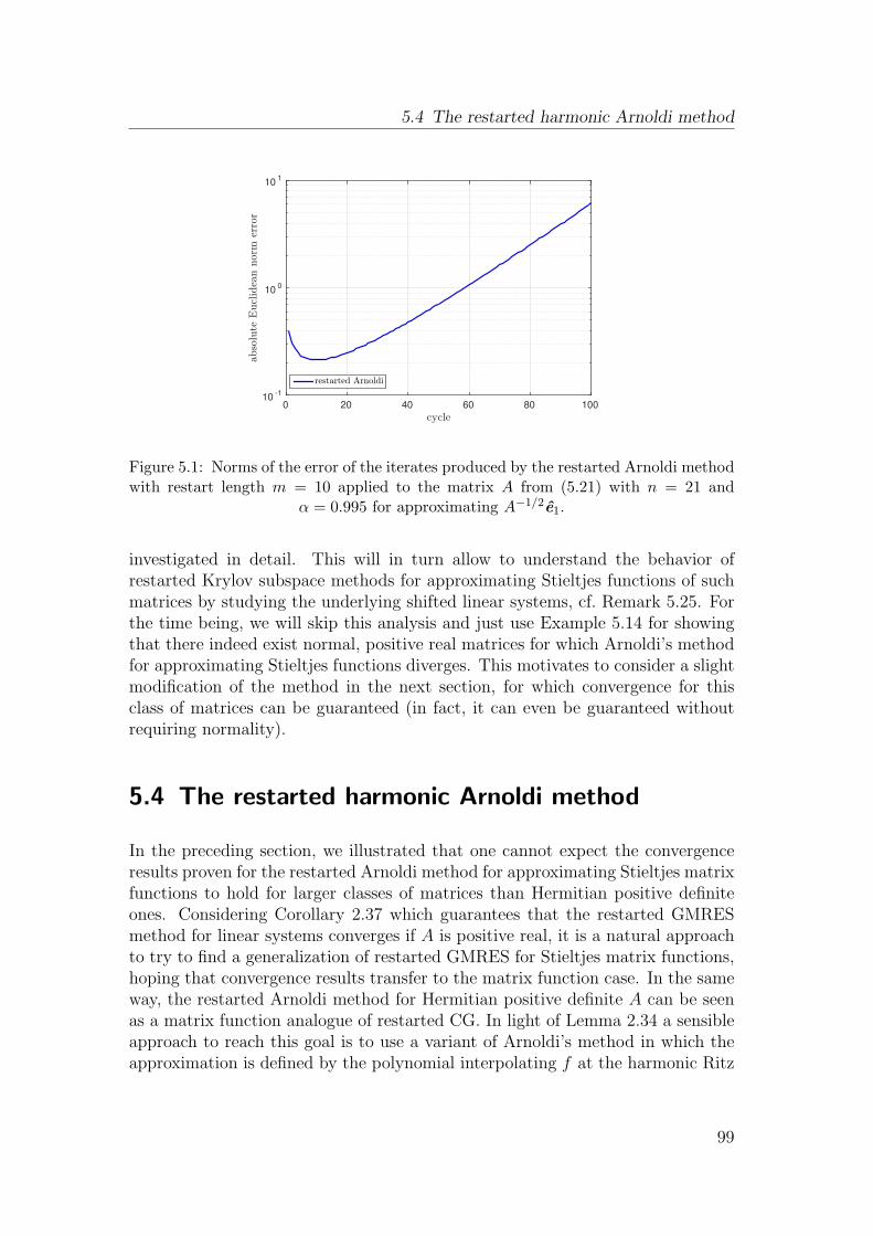
5.4 The restarted harmonic Arnoldi method
cycle0 20 40 60 80 100
abso
lute
Eucl
idea
nnorm
erro
r
10-1
100
101
restarted Arnoldi
Figure 5.1: Norms of the error of the iterates produced by the restarted Arnoldi methodwith restart length m = 10 applied to the matrix A from (5.21) with n = 21 and
α = 0.995 for approximating A−1/2e1.
investigated in detail. This will in turn allow to understand the behavior ofrestarted Krylov subspace methods for approximating Stieltjes functions of suchmatrices by studying the underlying shifted linear systems, cf. Remark 5.25. Forthe time being, we will skip this analysis and just use Example 5.14 for showingthat there indeed exist normal, positive real matrices for which Arnoldi’s methodfor approximating Stieltjes functions diverges. This motivates to consider a slightmodification of the method in the next section, for which convergence for thisclass of matrices can be guaranteed (in fact, it can even be guaranteed withoutrequiring normality).
5.4 The restarted harmonic Arnoldi method
In the preceding section, we illustrated that one cannot expect the convergenceresults proven for the restarted Arnoldi method for approximating Stieltjes matrixfunctions to hold for larger classes of matrices than Hermitian positive definiteones. Considering Corollary 2.37 which guarantees that the restarted GMRESmethod for linear systems converges if A is positive real, it is a natural approachto try to find a generalization of restarted GMRES for Stieltjes matrix functions,hoping that convergence results transfer to the matrix function case. In the sameway, the restarted Arnoldi method for Hermitian positive definite A can be seenas a matrix function analogue of restarted CG. In light of Lemma 2.34 a sensibleapproach to reach this goal is to use a variant of Arnoldi’s method in which theapproximation is defined by the polynomial interpolating f at the harmonic Ritz
99
5 Convergence of restarted Krylov subspace methods
values corresponding to the Krylov subspace Km(A, b) instead of the standardRitz values. The resulting approximation, which we will call (restarted) harmonicArnoldi approximation here and in the following, was already considered in thecontext of approximating matrix functions (albeit in unrestarted methods onlyand without presenting a convergence analysis) in [48, 87]. Our analysis of thismethod in the restarted context presented in this and the subsequent section wasalready published in [57].
By combining Lemma 2.27 and Proposition 2.35, it is immediately clear that theharmonic Arnoldi approximation for f(A)b can be computed as
fm = ‖b‖2Vmf(Hm + (hm+1,mH
−1m em)e
Hm
)e1 = ‖b‖2Vmf(Hm)e1, (5.22)
provided thatHm is nonsingular. When f is a Stieltjes function of the form (3.15),the harmonic Arnoldi approximation (5.22) can be rewritten as
fm =
∫ ∞
0
‖b‖2Vm(Hm + tI)−1e1 dµ(t) =:
∫ ∞
0
xm(t) dµ(t). (5.23)
We note straightaway, to avoid confusion, that while xm(0) is the mth GMRESiterate for the system Ax = b, the other vectors xm(t) for t > 0 are not theGMRES iterates for (A+ tI)x (t) = b. This is due to the fact that the eigenvalues
of Hm+ tI are not the harmonic Ritz values of A+ tI corresponding to Km(A, b).We will in the following show that this does not hinder a convergence analysisfor the resulting method, and reveal connections to the shifted GMRES methodfrom [56]. The following result shows that the residuals corresponding to thevectors xm(t) are collinear.
Lemma 5.15. Let A ∈ Cn×n, let b ∈ C
n and let Vm, Hm be the matrices from theArnoldi decomposition (2.23) for A and b and let Hm be defined as in (2.35) andxm(t) as in (5.23). For f(z) = z−1, let qHm,()−1 be the polynomial interpolating f
at spec(Hm), and let pm(z) = 1− zqHm,()−1(z). Then
rm(t) := b − (A+ tI)xm(t) = ηm(t)rm(0),
where
ηm(t) =1
pm(−t), rm(0) = pm(A)b. (5.24)
Proof. Let qHm+tI,()−1(z) interpolate f(z) = z−1 at spec(Hm+ tI) = ϑ1, . . . , ϑmin the Hermite sense. Then, by Lemma 2.27, we have xm(t) = qHm+tI,()−1(A+tI)b.Define the polynomial
pm,t(z) = 1− zqHm+tI,()−1(z)
100
5.5 Convergence of restarted harmonic Arnoldi for Stieltjes functions
of exact degree m, which satisfies pm,t(0) = 1. Then rm(t) = pm,t(A+ tI)b. Dueto
pm,t(ϑi + t) = 1− (ϑi + t) · 1
ϑi + t= 0,
the polynomial pm,t interpolates the zero function at spec(Hm+tI). In particular,we have
pm,0(z) =m∏
i=1
(1− z
ϑi
)
and
pm,t(z) =m∏
i=1
(1− z
ϑi + t
)=
1
pm,0(−t)pm,0(z − t). (5.25)
The last equality in (5.25) holds because the polynomial on the right-hand sidehas the same zeros as pm,t and attains the value 1 at z = 0. We thus find
rm(t) = pm,t(A+ tI)b =1
pm,0(−t)pm,0(A) = ηm(t)pm,0(A)b = ηm(t)rm(0),
which proves the assertion of the lemma.
The result of Lemma 5.15 shows that the residuals of the iterates xm(t) arecollinear to the residual produced by GMRES for the system Ax = b. This al-ready suggests to conjecture that there is a connection between the iterates xm(t)generated by the shifted GMRES method from [56], which was briefly describedin Section 2.4.1, as there the residuals of the shifted systems are also enforcedto be collinear to the GMRES residual of the seed system. By comparing thecollinearity factor ηm(t) given in (5.24) with the one from [56], one discovers thatthey are indeed the same (if the seed system is chosen as the system with shiftt = 0), and that thus also the approximations xm(t) are the same (as long as Ais nonsingular, as then the residual uniquely determines the approximation dueto the residual equation). Besides being an interesting observation, this is alsouseful because it allows to determine the approximations xm(t) in the way pro-
posed in [56] without needing to form the matrix Hm, which could in some cases
lead to numerical instabilities. We keep this in mind while still using Hm in thefollowing to avoid unnecessary notational overhead.
5.5 Convergence of restarted harmonic Arnoldi for
Stieltjes functions
In this section, we show how to transfer results on the convergence of restarted,shifted GMRES for positive real matrices A to the restarted harmonic Arnoldiapproximation.
101
5 Convergence of restarted Krylov subspace methods
Proceeding similarly to (5.4), this time for the error representation (5.23), andusing the result of Lemma 5.15, the error of the harmonic Arnoldi approximationcan be written as
f(A)b − fm =
∫ ∞
0
(A+ tI)−1rm(t) dµ(t) =
∫ ∞
0
ηm(t)(A+ tI)−1 dµ(t) · rm(0)
with ηm(t) from (5.24). We thus have f(A)b − fm = em(A)rm(0) with the errorfunction
em(z) =
∫ ∞
0
ηm(t)
z + tdµ(t).
We will show that the residual collinearity factors ηm(t) are bounded from aboveby 1. This is similar to the analysis performed in [56] for proving that the iteratesof the restarted shifted GMRES method are convergent for A positive real.
Lemma 5.16. Let A ∈ Cn×n be positive real and let ηm(t) be defined as in (5.24).
Then
|ηm(t)| ≤(
1
1 + tρ
)m
≤ 1, (5.26)
where
ρ := min
ℜ(vHA−1v
vHv
): v ∈ C
n, v 6= 0
. (5.27)
Proof. From the definition of ηm(t) in Lemma 5.15 we have
ηm(t) =1∏m
i=1(1 +tϑi),
with ϑi being the harmonic Ritz values of A with respect to Km(A, b). Sincethe harmonic Ritz values of A are the inverses of the Ritz values of A−1 withrespect to AKm(A, b), see [111], we have ϑ−1
i = (wHi A
−1wi)/(wHi wi) for some
vector wi ∈ Cn and thus ℜ(ϑ−1
i ) ≥ ρ. Therefore, for any t ≥ 0 we have, usingthat ℜ(ϑi) ≥ 0, i = 1, . . . ,m,
|1 + tϑ−1i | ≥ 1 + tℜ(ϑ−1
i ) ≥ 1 + tρ for i = 1, . . . ,m,
which gives (5.26).
The natural choice of norm for bounding the error of a Krylov subspace methodfor non-Hermitian positive real A is the energy norm induced by the matrix AHA(which is Hermitian positive definite when A is positive real), as most knownresults bound the Euclidean norm of the residual (see, e.g., Theorem 2.36) andwe have
‖r‖2 =√rHr =
√(Ae)H(Ae) = ‖e‖AHA.
102
5.5 Convergence of restarted harmonic Arnoldi for Stieltjes functions
In the proof of Lemma 5.5, we used the relation between the energy norms inducedby the Hermitian positive definite matrices A and A+ tI, and in the following weneed a similar result for the norms induced by AHA and (A + tI)H(A + tI). Asthe situation is a little bit more involved to analyze, we state the precise resultin a separate lemma.
Lemma 5.17. Let A ∈ Cn×n be positive real.
(i) For all v ∈ Cn and t ≥ 0 we have
‖v‖2AHA ≤1
ν−1maxt
2 + 2ρt+ 1‖v‖2(A+tI)H(A+tI) , (5.28)
where ρ is defined in (5.27) and
νmax := max
(Av)H(Av)
vHv: v ∈ C
n, v 6= 0
= ‖A‖22. (5.29)
(ii) For t ≥ 0 we have
1
ν−1maxt
2 + 2ρt+ 1≤ νmax
(t+ ρνmax)2. (5.30)
Proof. For part (i) we expand
‖v‖2(A+tI)H(A+tI) = ‖v‖2AHA + 2tℜ(vHAHv) + t2‖v‖22 .
The inequality now follows from ‖v‖22 ≥ 1νmax‖v‖2AHA and
ℜ(vHAHv)/(vHAHAv) = ℜ(wHA−1w)/(wHw) ≥ ρ, where Av = w .
The inequality in part (ii) is equivalent to (t + ρνmax)2 ≤ t2 + 2ρνmaxt + νmax,
i.e., to ρ2νmax ≤ 1, which can be established as follows. Let v be the normalizedeigenvector of (AAH)−1 corresponding to the smallest eigenvalue, which is 1/νmax.Then, by the Cauchy–Schwarz inequality,
ρ ≤ |vHA−1v | ≤ ‖v‖2 · ‖A−1v‖2 =√
vH(AAH)−1v =1
ν1/2max
,
which concludes the proof of the lemma.
With these prerequisites, we are in a position to prove the following theoremon the convergence of the restarted harmonic Arnoldi method for positive realmatrices.
103
5 Convergence of restarted Krylov subspace methods
Theorem 5.18. Let A ∈ Cn×n be positive real, let b ∈ C
n, let f be a Stieltjesfunction of the form (3.15), and let f
(k)m be the approximation from k cycles of
the restarted harmonic Arnoldi method with restart length m. Further, let ρ be asdefined in (5.27) and let δ, δ′ be defined as in (2.37) and (2.38), respectively. Fort ≥ 0 define
αm(t) :=
(√1− δδ′1 + tρ
)m
.
Let t0 ≥ 0 be the left endpoint of the support of µ. Then the AHA-energy norm ofthe error of f
(k)m satisfies
‖f(A)b − f (k)m ‖AHA ≤ ‖r (k)
m (0)‖2∫ ∞
0
(1 + tρ)−mk
√ν−1maxt
2 + 2ρt+ 1dµ(t) (5.31)
≤ ‖b‖2∫ ∞
0
αm(t)k
√ν−1maxt
2 + 2ρt+ 1dµ(t) (5.32)
≤ Cαm(t0)k, (5.33)
where 0 ≤ αm(t0) < 1 and
C = ‖b‖2√νmaxf(ρνmax) (5.34)
with νmax defined as in (5.29). In particular, the restarted harmonic Arnoldimethod converges for all restart lengths m ≥ 1.
Proof. As the proof is very similar to that of Lemma 5.5 and Theorem 5.7 weonly give a sketch. Using an upper index, as before, to distinguish the quantitiesbelonging to different restart cycles we have
f(A)b − f (k)m =
∫ ∞
0
e (k)m (t) dµ(t) =
∫ ∞
0
(A+ tI)−1r (k)m (t) dµ(t).
Using Lemma 5.17(i) together with the equality ‖e (k)m (t)‖(A+tI)H(A+tI) = ‖r (k)
m (t)‖2and the collinearity of these residuals as stated in Lemma 5.15, one obtains
‖f(A)b − f (k)m ‖AHA ≤
∫ ∞
0
|η(1)m (t) · · · η(k)m (t)|√ν−1maxt
2 + 2ρt+ 1‖r (k)
m (0)‖2 dµ(t).
Inequality (5.31) now follows by bounding each factor |η(j)m (t)| via (5.26). The
second relation (5.32) is obtained by using the bound for ‖r (k)m (0)‖2 from Theo-
rem 2.36. To get (5.33) and (5.34) one then uses the fact that αm(t) is monoton-ically decreasing as a function of t and the bound (5.30).
104
5.5 Convergence of restarted harmonic Arnoldi for Stieltjes functions
We just note that it is of course again possible to replace the bound (5.33) forthe AHA-energy norm by a bound for the Euclidean norm of the error by suitablymodifying the constant C, similarly to what we have done for the convergencebounds in the standard restarted Arnoldi method. We do not give the detailshere, as this is completely analogous. Convergence for functions of the typef(z) = zf(z) for f a Stieltjes function, i.e., an analogue to Theorem 5.12 forthe restarted harmonic Arnoldi method is also possible, again using exactly thesame tools as before, so that we omit it here and just state that the restarted(corrected) harmonic Arnoldi method also converges for functions of this typewhen A is positive real.
Theorem 5.18 guarantees the convergence of the restarted harmonic Arnoldimethod for all restart lengths m, but we give an additional result, which givesa little more insight into the behavior of the method in comparison to restartedGMRES, as it gives an in a sense more immediate relation.
Corollary 5.19. Let the assumptions of Theorem 5.18 hold. Then
‖f(A)b − f (k)m ‖AHA ≤ C1‖r (k)
m (0)‖2, (5.35)
where C1 =√νmaxf(ρνmax).
Proof. We insert the relation (1 + tρ) ≥ 1 for all t ≥ 0 into (5.31), which yields
‖f(A)b − f (k)m ‖AHA ≤ ‖r (k)
m (0)‖2∫ ∞
0
1√ν−1maxt
2 + 2ρt+ 1dµ(t).
The assertion of the corollary then follows by applying (5.30).
Corollary 5.19 is especially interesting in the context of superlinear convergenceof the GMRES method, see, e.g., [106, 139]. In this setting, the statement ofthe corollary can be rephrased as: If (restarted) GMRES for the positive reallinear system Ax = b exhibits superlinear convergence behavior, then so doesthe (restarted) harmonic Arnoldi method for approximating f(A)b when f is aStieltjes function.
We revisit Example 5.14, in which the standard restarted Arnoldi method failedto converge for a (normal) positive real matrix A. In Figure 5.2, we give the con-vergence curves of the restarted Arnoldi and restarted harmonic Arnoldi methodfor the same problem (and with the same parameters) as considered in Exam-ple 5.14. As predicted by Theorem 5.18, we observe that the restarted harmonicArnoldi method converges linearly to f(A)b.
105
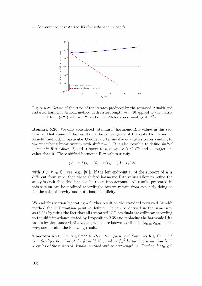
5 Convergence of restarted Krylov subspace methods
cycle0 20 40 60 80 100
abso
lute
Eucl
idea
nnorm
erro
r
10-10
10-8
10-6
10-4
10-2
100
102
restarted Arnoldi
restarted harmonic Arnoldi
Figure 5.2: Norms of the error of the iterates produced by the restarted Arnoldi andrestarted harmonic Arnoldi method with restart length m = 10 applied to the matrix
A from (5.21) with n = 21 and α = 0.995 for approximating A−1/2e1.
Remark 5.20. We only considered “standard” harmonic Ritz values in this sec-tion, so that some of the results on the convergence of the restarted harmonicArnoldi method, in particular Corollary 5.19, involve quantities corresponding tothe underlying linear system with shift t = 0. It is also possible to define shiftedharmonic Ritz values ϑi with respect to a subspace U ⊆ C
n and a “target” t0other than 0. These shifted harmonic Ritz values satisfy
(A+ t0I)xi − (ϑi + t0)xi ⊥ (A+ t0I)U
with 0 6= xi ∈ Cn, see, e.g., [87]. If the left endpoint t0 of the support of µ is
different from zero, then these shifted harmonic Ritz values allow to refine theanalysis such that this fact can be taken into account. All results presented inthis section can be modified accordingly, but we refrain from explicitly doing sofor the sake of brevity and notational simplicity.
We end this section by stating a further result on the standard restarted Arnoldimethod for A Hermitian positive definite. It can be derived in the same wayas (5.35) by using the fact that all (restarted) CG residuals are collinear accordingto the shift invariance stated by Proposition 2.38 and replacing the harmonic Ritzvalues by the standard Ritz values, which are known to all lie in [λmin, λmax]. Thisway, one obtains the following result.
Theorem 5.21. Let A ∈ Cn×n be Hermitian positive definite, let b ∈ C
n, let fbe a Stieltjes function of the form (3.15), and let f
(k)m be the approximation from
k cycles of the restarted Arnoldi method with restart length m. Further, let t0 ≥ 0
106
5.6 Convergence of restarted FOM for linear systems
be the left endpoint of the support of µ. The A2-energy norm of the error of f(k)m
can then be bounded as
‖f(A)b − f (k)m ‖A2 ≤ C‖r (k)
m (t0)‖2, (5.36)
where ‖r (k)m (t0)‖2 is the Euclidean norm of the residual of the (restarted) CG
iterate for the system (A+ t0I)x (t0) = b and
C = λmaxf(√
λmax
).
Consequently,
‖f(A)b − f (k)m ‖A ≤
C√λmin
‖r (k)m (t0)‖2. (5.37)
Again, this result essentially states that we can expect the restarted Arnoldimethod to exhibit superlinear convergence behavior whenever restarted CG forthe system (A+ t0I)x = b converges superlinearly [12,13]. Therefore, this resultis, just as Corollary 5.19, especially interesting in the unrestarted case (or forrestart lengths which are very large in relation to n, which are seldom used inpractice), as one typically observes superlinear convergence only in these cases;cf. also the experiments reported in Section 5.7. We just briefly remark that, whileall other results stated in this chapter for Hermitian positive definite matrices usethe energy norm corresponding to A, it is natural to initially arrive at an estimatein the energy norm corresponding to A2 in (5.36), as the proof relies on the relation
‖r (k)m (t)‖2 = ‖e (k)
m (t)‖A2 .
5.6 Convergence of restarted FOM for linear
systems
In this section, we give a few results concerning the convergence behavior ofrestarted FOM (and restarted GMRES) for the solution of non-Hermitian linearsystems. This topic is only remotely related to the other results presented in thissection (in the sense that f(z) = z−1 is also a special case of a Stieltjes function)and can be regarded as a by-product of investigating matrices like the one fromExample 5.14. The results in this section are also presented in [119].
As already illustrated, e.g., by Example 2.30, the restarted full orthogonalizationmethod can stagnate at some point, without ever reaching the desired solutionA−1b, even in exact arithmetic. Approximately solving a linear system with thematrix from Example 5.14 and the right-hand side e1 with restarted FOM wouldlead to a sequence of residual norms which exhibit a similar exponential growth
107
5 Convergence of restarted Krylov subspace methods
as the one depicted for the error norms for approximating A−1/2b in Figure 5.1.What kinds of behavior restarted FOM can exhibit under which circumstances isan issue that is not fully understood by now apart from the Hermitian positivedefinite case, when restarted FOM reduces to restarted CG, which is known toconverge to A−1b; cf. also Section 5.2. The asymptotic speed of convergence inthe Hermitian positive definite case is closely tied to spectral information of A,e.g., the smallest and largest eigenvalue for estimates like in Theorem 2.32, orinformation on clusters formed by the eigenvalues and outliers from the spectrumfor a more intricate analysis. This could lead one to believe that eigenvalueinformation can also be used to gain insight into the behavior of FOM in thenon-Hermitian case. We will show that this is not true and that restarted FOMcan attain any behavior completely independent of the spectrum of A. Resultsof this type are known for (restarted) GMRES, see, e.g., [39, 78, 137]. The resultfrom [78] essentially states that unrestarted GMRES can generate any prescribed,monotonically decreasing sequence of residual norms for a matrix which has anydesired eigenvalues. In [39], a refined result of this type is presented, in which alsothe Ritz values in each iteration can be freely prescribed. In [137], a similar resultis presented for restarted GMRES, where the residual norms at the end of eachrestart cycle can be prescribed for the first ⌊ n
m⌋ iterations (where m is the restart
length), again for a matrix with any desired eigenvalues. A more general result,allowing to prescribe the residual norms also in the iterations within each cycle(and with the possibility to additionally prescribe all Ritz values) was recentlygiven in [40].
We present similar results for restarted FOM, where the residual norm in eachiteration can be prescribed for the first n iterations (at most). Towards the end ofthis section, we will further comment on the relation and differences of our resultsfor FOM in comparison to the ones for GMRES.
To make notation not overly complicated, we will, in contrast to most of theother parts of this thesis, number the residuals consecutively, i.e., r1, . . . , rm arethe iterates from the first restart cycle, rm+1, . . . , r2m are the iterates from thesecond restart cycle and so on.
Theorem 5.22. Let m,n, q ∈ N with m ≤ n − 1 and q ≤ n, let r1, . . . , rq ∈ R+0
be given with r1, . . . , rq−1 > 0 and rq ≥ 0 and let µ1, . . . , µn ∈ C\0. Then thereexist a matrix A ∈ C
n×n with spec(A) = µ1, . . . µn and vectors b,x0 ∈ Cn such
that the residuals r1, . . . , rq generated by q steps of restarted FOM with restartlength m for Ax = b with initial guess x0 satisfy
‖rj‖2 = rj for j = 1, . . . , q.
The proof of Theorem 5.22 is quite lengthy and will require a few auxiliary results
108
5.6 Convergence of restarted FOM for linear systems
which are given next. We investigate matrices of the form
A(d , s) =
d1 0 · · · 0 sns1 d2 0 · · · 0
0 s2. . . . . .
......
. . . . . . dn−1 00 · · · 0 sn−1 dn
(5.38)
defined by two vectors d , s ∈ Cn in the following (note that the matrices from
Example 2.30 and 5.14 are both special cases of (5.38)).
For the sake of simplicity we assume that q = n and rn > 0 in Theorem 5.22.This is no essential restriction, as we will point out at the end of the proof ofTheorem 5.22. We first examine the results of applying Arnoldi’s method toA(d , s) and a (multiple of a) canonical unit vector.
Proposition 5.23. Let A(d , s) ∈ Cn×n be of the form (5.38), let m ≤ n − 1,
ξ0 ∈ C with |ξ0| = 1, and let c > 0. Let x0, b ∈ Cn be given such that the residual
r0 = b−Ax0 satisfies r0 = ξ0cei. Then the basis Vj+1 generated by j ≤ m steps ofArnoldi’s method, Algorithm 2.1, for A(d , s) and b with initial guess x0 is givenby
Vj+1 = [ξ0ei, ξ1ei+1, . . . , ξj ei+j] (5.39)
(where, like everywhere in the following, for ease of notation, the indices are to
be understood cyclically, i.e., en+1 := e1, en+2 := e2, . . . ) with ξk =si+k−1ξk−1
|si+k−1| , k =
1, . . . , j. The corresponding upper Hessenberg matrix is given by
Hj =
di 0 · · · 0 0|si| di+1 0 · · · 0
0 |si+1| . . . . . ....
.... . . . . . di+j−2 0
0 · · · 0 |si+j−2| di+j−1
, hj+1,j = |si+j−1|. (5.40)
Proof. One verifies by a direct computation that Vj+1 and Hj, hj+1,j from (5.39)and (5.40), respectively, satisfy the Arnoldi relation (2.23) for A(d , s). The as-sertion then follows from the essential uniqueness of the Arnoldi decomposition,see Lemma 2.23, because all subdiagonal entries of Hj are real and positive.
Given the orthonormal basis and Hessenberg matrix resulting from Arnoldi’smethod, we can easily give an explicit expression for the residuals generated byapplying FOM to the linear system A(d , s)x = b. Using Proposition 5.23, oneobtains the following result.
109
5 Convergence of restarted Krylov subspace methods
Proposition 5.24. Let the assumptions of Proposition 5.23 hold. Then the resid-ual generated by j ≤ m steps of FOM is given by
rj = (−1)jξjc|si · si+1 · · · si+j−1|di · di+1 · · · di+j−1
ei+j.
In particular,
‖rj‖2 =∣∣∣∣si+j−1
di+j−1
∣∣∣∣ · ‖rj−1‖2.
Proof. The FOM residual satisfies rj = −hj+1,j‖r0‖2(eHj H
−1j e1
)vj+1 according
to Proposition 2.29. In our setting we have
‖r0‖2 = c, hj+1,j = |si+j−1|, vj+1 = ξj ei+j,
and the lower left entry eHj H
−1j e1 of H
−1j is (−1)j−1 |si+1|···|si+j−2|
di+1···di+j−1due to the simple,
bidiagonal structure of Hj. Putting these quantities together proves the proposi-tion.
When applying restarted FOM with restart length m to the linear system
A(d , s)x = e1
with initial guess x0 = 0 it is now easy to use Proposition 5.24 to choose someof the coefficients in d and s in such a way that the prescribed residual normsr1, . . . , rm are generated. More precisely, one just needs to choose the first mentries of the coefficient vectors d , s such that they satisfy
sj =rjrj−1
dj, j = 1, . . . ,m (5.41)
(where we set r0 = 1) to produce the desired residual norm sequence. Assumingthat d1, . . . , dm are already fixed to arbitrary nonzero values, it is always possibleto choose s1, . . . , sm in such a way that (5.41) is satisfied. After restarting, thesituation is very similar. After the first m steps of FOM, the residual is, accordingto Proposition 5.24, given by
rm = (−1)mξm|s1 · s2 · · · sm|d1 · d2 · · · dm
em+1.
Therefore, using the new initial guess xm after restarting, we are again in a situa-tion in which the assumptions of Proposition 5.24 are fulfilled, with c = | s1···sm
d1···dm | =rm. From this, it is immediately clear that choosing the next m values in d ands (analogously to (5.41)) such that
sj =rjrj−1
dj, j = m+ 1, . . . ,min2m,n
110
5.6 Convergence of restarted FOM for linear systems
is fulfilled will produce the desired residual norms rm+1, . . . , rmin2m,n in the nextcycle of restarted FOM (or in the first n−m iterations of this cycle, if 2m > n).By continuing this construction, one can prescribe residual norms for furtheriterations until all values in s are fixed (i.e., for n iterations).
We assumed that the coefficients in d are already fixed to some arbitrary nonzerovalues. We will now show how to fix them in such a way that the matrix A(d , s)has any desired (nonzero) eigenvalues µ1, . . . , µn. One immediately sees that thecharacteristic polynomial of A(d , s) is given by
χA(d ,s)(λ) = (λ− d1) · · · (λ− dn)− s1 · · · sn. (5.42)
Assuming that the matrix A(d , s) produces the desired sequence of residualnorms, we can eliminate the dependency of χA(d ,s) on the values s1, . . . , sn. Mul-tiplying all equations in (5.41) (and its counterparts from later restart cycles), wefind the relation
s1 · · · sn = rn · d1 · · · dn. (5.43)
Inserting this into (5.42), we can rewrite the characteristic polynomial as
χA(d ,s)(λ) = (λ− d1) · · · (λ− dn)− rn · d1 · · · dn. (5.44)
There exist coefficients β0, . . . , βn−1 ∈ C such that the values µ1, . . . , µn are theroots of the corresponding monic polynomial, i.e.,
(λ− µ1) · · · (λ− µn) = λn + βn−1λn−1 + · · ·+ β1λ+ β0. (5.45)
Note that the following construction breaks down if rn = (−1)n (which can ofcourse only happen for even n, as rn ≥ 0). However, we may assume that rn 6=(−1)n without loss of generality. This can be seen as follows. If rn = (−1)n, wecan choose an arbitrary value α /∈ 0, 1, replace all values ri by αri and start theFOM iteration with right-hand side 1
αe1, which will produce the same sequence
of residual norms.
We now choose the values d1, . . . , dn such that they are the n roots of the poly-nomial
λn + βn−1λn−1 + · · · β1λ+ β0 with β0 =
β01 + (−1)n+1rn
.
These exist due to the fundamental theorem of algebra. With this choice of theroots di it obviously holds
(−1)nd1 · · · dn = β0. (5.46)
Inserting this into the characteristic polynomial (5.44), we find
χA(d ,s)(λ) = λn + βn−1λn−1 + · · ·+ β1λ+ β0 − rn · d1 · · · dn
= λn + βn−1λn−1 + · · ·+ β1λ+ β0 + (−1)n+1rnβ0
= λn + βn−1λn−1 + · · ·+ β1λ+ (1 + (−1)n+1rn)β0
= λn + βn−1λn−1 + · · ·+ β1λ+ β0,
111
5 Convergence of restarted Krylov subspace methods
showing that A(d , s) has the desired eigenvalues according to (5.45). Equa-
tion (5.46) together with the fact that β0 6= 0 (because β0 = µ1 · · ·µn 6= 0)implies that all entries of d are nonzero, such that all Hessenberg matrices (5.40)are nonsingular and all restarted Arnoldi approximations are therefore defined.This proves Theorem 5.22 in case that q = n and rn > 0. If q < n, we can usethe same construction as above and just fix the “unused” coefficients sq+1, . . . , snin such a way that (5.43) still holds (where rn is of course replaced by rq), so thissituation does not cause any difficulties. Now consider the case that rq = 0. Thisimplies sq = 0 and the characteristic polynomial (5.42) of A(d , s) is thereforegiven by
χA(d ,s)(λ) = (λ− d1) · · · (λ− dn),showing that the eigenvalues of A(d , s) are just the entries of d in this situation.Therefore, the eigenvalues of A(d , s) can again freely be prescribed through thechoice of the coefficients in d . If q 6= n, the coefficients sq+1, . . . , sn can attain anyvalues (e.g., all zero) as FOM terminates after finding the exact solution in theqth iteration in this case, and they are therefore of no importance. This concludesthe proof of Theorem 5.22.
An interesting observation concerning the construction from the proof of Theo-rem 5.22 is the following. The result only allows to prescribe the residual normsfor the first n iterations of restarted FOM, but due to the simple nature of thematrices A(d , s) we have full information on the residual norms in later itera-tions (exceeding n). Consider using FOM with restart length m for the linearsystem A(d , s)x = e1 with initial guess x0 = 0 again (where we assume thatA(d , s) was constructed with q = n and rn > 0). As the residual generated aftern iterations is again a multiple of a canonical unit vector, Proposition 5.24 stillapplies in this situation. One thus finds that the residuals in iterations exceedingn satisfy
‖rn+j‖2 =rj mod n
rj−1 mod n
‖rn+j−1‖2, (5.47)
i.e., the ratios of consecutive residuals are repeated cyclically. This full informa-tion on the behavior of the method in “later” iterations is a feature that distin-guishes our construction from the one in [40,137] for restarted GMRES, in whichno information at all is available on the behavior of the method after more thann iterations (or more than ⌊ n
m⌋ restart cycles).
Remark 5.25. The insight gained from the proof of Theorem 5.22 allows tobetter explain the behavior observed when trying to approximate the inversesquare root in Example 5.14, cf. also Figure 5.1, which can be interpreted asimplicitly solving shifted linear systems with A. In the first few restart cycles,the error norm actually decreases, as the (implicitly computed) iterates for theunderlying linear systems belonging to large shifts converge. Divergence onlytakes place for systems belonging to some interval [0, t′] close to the origin, and
112
5.6 Convergence of restarted FOM for linear systems
once the systems belonging to larger shifts are converged, the divergence for theother systems slowly becomes visible.
Another observation one can make about our construction is that it applies inalmost the same way to unrestarted FOM (in fact, the method behaves exactlythe same for all choices of restart length m ≤ n − 1), apart from the fact thatunrestarted FOM must terminate with the exact solution at the nth step. Thisgives the following result.
Corollary 5.26. Let n ∈ N, 1 ≤ q ≤ n, r1, . . . , rq−1 ∈ R+, rq = 0 and let
µ1, . . . , µn ∈ C \ 0. Then there exist a matrix A ∈ Cn×n with spec(A) =
µ1, . . . µn and vectors b,x0 ∈ Cn such that the residuals rj generated by j steps
of FOM for Ax = b with initial guess x0 satisfy
‖rj‖2 = rj for j = 1, . . . , q.
The proof of Corollary 5.26 is almost identical to the one of Theorem 5.22 apartfrom the fact that rn must be the zero vector due to the finite termination propertyof unrestarted FOM.
We now discuss the relation between our results for (restarted) FOM and resultson (restarted) GMRES from [39, 40, 78, 137]. The FOM residual norm and theGMRES residual norm are not independent of each other, but fulfill the followingrelation (where rF
j and rGj denote the residual generated by m steps of FOM and
GMRES, respectively)
‖rFj ‖2 =
‖rGj ‖2√
1− (‖rGj ‖2/‖rG
j−1‖2)2, (5.48)
see, e.g., [29, 30], or [22, 104] for other relations between FOM and GMRES. Re-lation (5.48) allows to prove Corollary 5.26 directly as a corollary of the resultsfrom [39, 78] by constructing a matrix A and a vector b such that GMRES gen-erates the sequence
rGj :=rFj√
1 + (rFj /rGj−1)
2with rG0 = 1.
of residual norms, where rFj are the FOM residual norms to be prescribed. Byvirtue of (5.48), A and b will then produce the desired FOM residual norms. Theresult of Theorem 5.22, however, can not be derived in such a simple way fromthe older GMRES result of [137], as this result does not allow the residual normat each iteration to be prescribed, but only from the more recent analysis of [40].
113
5 Convergence of restarted Krylov subspace methods
The other way around, our result can be used to construct A and b in such a waythat they produce an arbitrary admissible convergence curve in restarted GMRESwhere the norm after each iteration can be prescribed. The only limitation inthis case is that our construction does not allow for stagnation in GMRES, asstagnation from step j to step j + 1 in GMRES corresponds to the (j + 1)stFOM iterate not being defined; see [22]. This would require the value dj+1 to bezero, which is not possible in our construction. Therefore, we can conclude thatone can construct a matrix A and a vector b with arbitrary nonzero eigenvalueswhich produce any strictly monotonically decreasing sequence of residual normsin restarted GMRES, which gives an alternative proof for a result slightly weakerthan what was recently presented in [40].
Another result concerning restarted GMRES is given in the following. It is relatedto an open question from the conclusions section of [137], where the authors askwhether it is possible to give bounds on the residual norms generated by restartedGMRES based on eigenvalue information once the iteration number exceeds n.As our approach provides information on the residual norms also in these lateriterations, cf. (5.47), we can negatively answer this question (for both FOM andGMRES). For FOM, this is directly obvious from (5.47), for GMRES we give theprecise result (and its rather technical proof) in the following.
Simply put, the following theorem states that restarted GMRES can, indepen-dently of the eigenvalues of A, converge arbitrarily slowly for any number k (pos-sibly larger than n) of iterations, in the sense that the norm of the residual isreduced only by a prescribed margin which can be chosen arbitrarily close tozero.
Theorem 5.27. Let n,m, k ∈ N, m ≤ n − 1, let µ1, . . . , µn ∈ C \ 0 and let0 ≤ δ < 1. Then there exist a matrix A ∈ C
n×n with spec(A) = µ1, . . . µnand vectors x0, b ∈ C
n such that the residual rGk = b − AxG
k generated by kiterations of restarted GMRES with restart length m for Ax = b with initialguess x0 satisfies
‖rGk ‖2/‖rG
0 ‖2 ≥ δ.
Proof. According to Theorem 5.22 there exist a matrix A ∈ Cn×n with eigenvalues
µ1, . . . , µn and vectors b,x0 ∈ Cn such that the residuals rF
j produced by the firstn iterations of restarted FOM with restart length m fulfill
‖rFj ‖2 = ρj with ρ =
δ1/k
(1− δ2/k)1/2 for j = 1, . . . , n. (5.49)
Due to (5.47), we then have that (5.49) also holds for j > n. We rephrase thisrelation as
‖rFj−1‖2 =
1
ρ‖rF
j ‖2 for all j ∈ N. (5.50)
114
5.7 Numerical experiments
By relation (5.48), we have that two consecutive residual norms generated byrestarted GMRES for A, b and x0 fulfill
‖rGj ‖2
‖rGj−1‖2
=‖rF
j ‖2‖rG
j−1‖2√
1 + (‖rFj ‖2/‖rG
j−1‖2)2
=‖rF
j ‖2√‖rG
j−1‖22 + ‖rFj ‖22
=‖rF
j ‖2√‖rF
j−1‖22√1+(‖rF
j−1‖2/‖rGj−2‖2)2
+ ‖rFj ‖22
≥ ‖rFj ‖2√
‖rFj−1‖22 + ‖rF
j ‖22. (5.51)
Inserting (5.50) into the right-hand side of (5.51), we find
‖rGj ‖2
‖rGj−1‖2
≥ ‖rFj ‖2√
1ρ2‖rF
j ‖22 + ‖rFj ‖22
=1√1ρ2
+ 1. (5.52)
Repeated application of (5.52) for all j ≤ k yields
‖rGk ‖2/‖rG
0 ‖2 =(‖rG
k ‖2/‖rGk−1‖2
)· · ·(‖rG
1 ‖2/‖rG0 ‖2
)≥ 1(
1ρ2
+ 1)k/2 . (5.53)
The result follows from (5.53) by noting that ( 1ρ2
+ 1)k/2 = 1δ.
5.7 Numerical experiments
In this section we report a few experiments which illustrate the convergence the-ory developed in this chapter. As the results are more of theoretical importanceand the proven error bounds cannot be expected to be sharp, we mainly use sim-ple, academic examples involving (block) diagonal matrices instead of the modelproblems from Section 2.6, as these best allow to discuss the influence of, e.g., theeigenvalue distribution of the matrix on the quality of the error bounds. Again, allexperiments are performed in Matlab using the implementation FUNM QUAD [59]of the restarted Arnoldi method (and a modification thereof for the restartedharmonic Arnoldi method). Most of the experiments in this section have alreadybeen presented in the same or a similar form in [57].
115
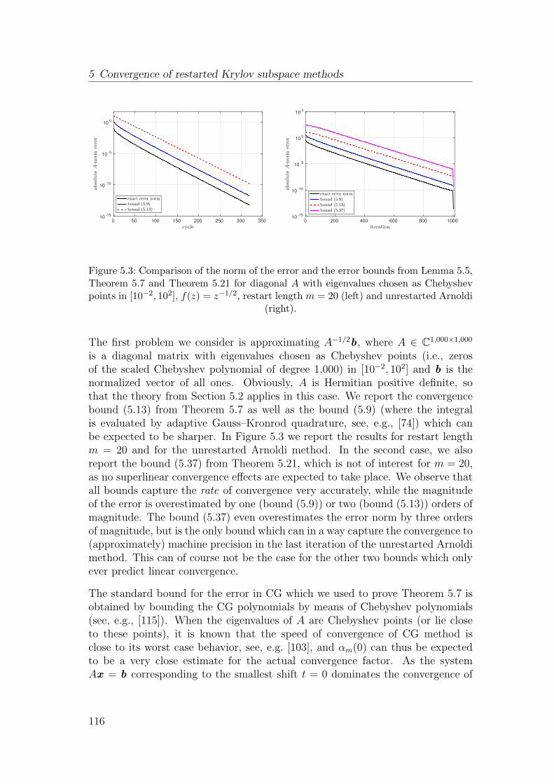
5 Convergence of restarted Krylov subspace methods
cycle0 50 100 150 200 250 300 350
abso
lute
A-n
orm
erro
r
10-15
10-10
10-5
100
exact error norm
bound (5.9)
bound (5.13)
iteration0 200 400 600 800 1000
abso
lute
A-n
orm
erro
r
10-15
10-10
10-5
100
105
exact error norm
bound (5.9)
bound (5.13)
bound (5.37)
Figure 5.3: Comparison of the norm of the error and the error bounds from Lemma 5.5,Theorem 5.7 and Theorem 5.21 for diagonal A with eigenvalues chosen as Chebyshevpoints in [10−2, 102], f(z) = z−1/2, restart length m = 20 (left) and unrestarted Arnoldi
(right).
The first problem we consider is approximating A−1/2b, where A ∈ C1,000×1,000
is a diagonal matrix with eigenvalues chosen as Chebyshev points (i.e., zerosof the scaled Chebyshev polynomial of degree 1,000) in [10−2, 102] and b is thenormalized vector of all ones. Obviously, A is Hermitian positive definite, sothat the theory from Section 5.2 applies in this case. We report the convergencebound (5.13) from Theorem 5.7 as well as the bound (5.9) (where the integralis evaluated by adaptive Gauss–Kronrod quadrature, see, e.g., [74]) which canbe expected to be sharper. In Figure 5.3 we report the results for restart lengthm = 20 and for the unrestarted Arnoldi method. In the second case, we alsoreport the bound (5.37) from Theorem 5.21, which is not of interest for m = 20,as no superlinear convergence effects are expected to take place. We observe thatall bounds capture the rate of convergence very accurately, while the magnitudeof the error is overestimated by one (bound (5.9)) or two (bound (5.13)) orders ofmagnitude. The bound (5.37) even overestimates the error norm by three ordersof magnitude, but is the only bound which can in a way capture the convergence to(approximately) machine precision in the last iteration of the unrestarted Arnoldimethod. This can of course not be the case for the other two bounds which onlyever predict linear convergence.
The standard bound for the error in CG which we used to prove Theorem 5.7 isobtained by bounding the CG polynomials by means of Chebyshev polynomials(see, e.g., [115]). When the eigenvalues of A are Chebyshev points (or lie closeto these points), it is known that the speed of convergence of CG method isclose to its worst case behavior, see, e.g. [103], and αm(0) can thus be expectedto be a very close estimate for the actual convergence factor. As the systemAx = b corresponding to the smallest shift t = 0 dominates the convergence of
116
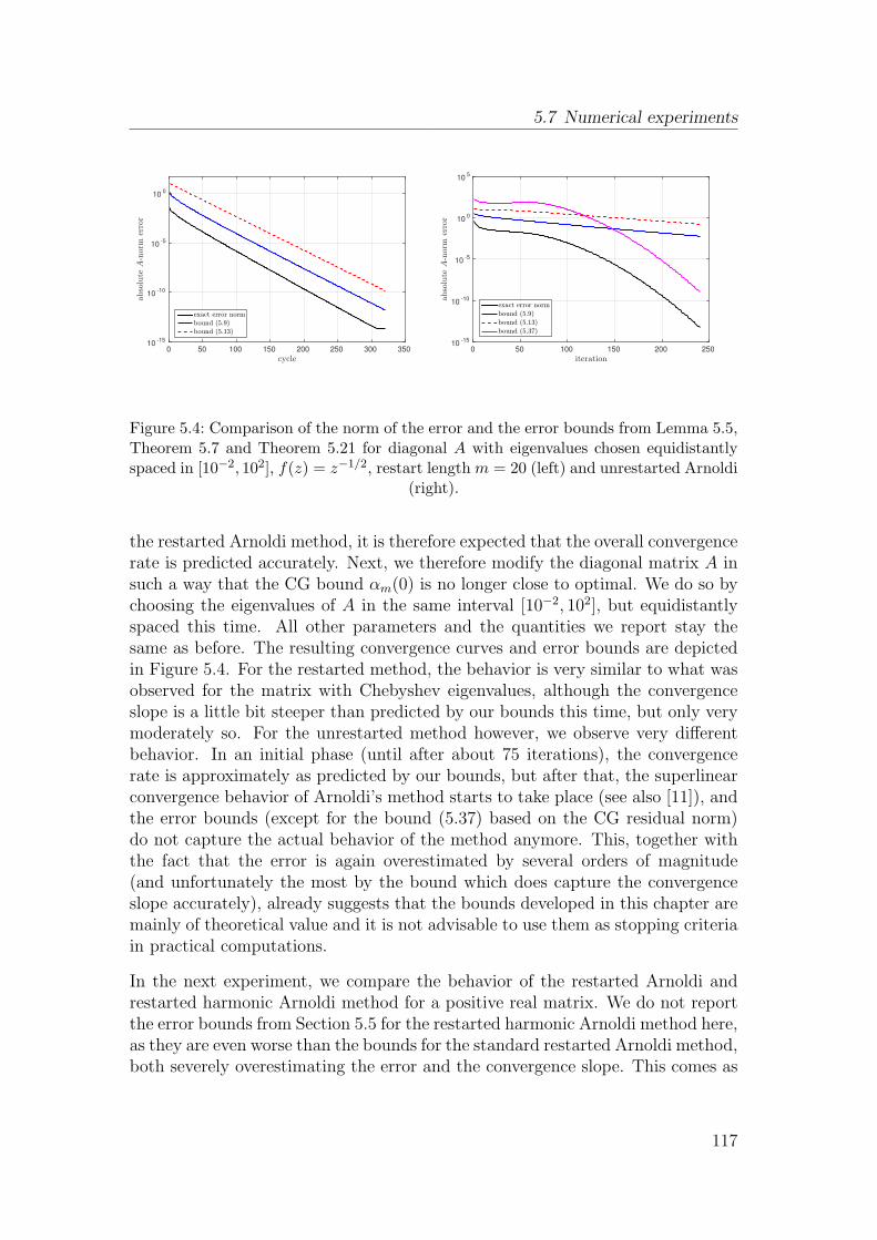
5.7 Numerical experiments
cycle0 50 100 150 200 250 300 350
abso
lute
A-n
orm
erro
r
10-15
10-10
10-5
100
exact error norm
bound (5.9)
bound (5.13)
iteration0 50 100 150 200 250
abso
lute
A-n
orm
erro
r
10-15
10-10
10-5
100
105
exact error norm
bound (5.9)
bound (5.13)
bound (5.37)
Figure 5.4: Comparison of the norm of the error and the error bounds from Lemma 5.5,Theorem 5.7 and Theorem 5.21 for diagonal A with eigenvalues chosen equidistantlyspaced in [10−2, 102], f(z) = z−1/2, restart length m = 20 (left) and unrestarted Arnoldi
(right).
the restarted Arnoldi method, it is therefore expected that the overall convergencerate is predicted accurately. Next, we therefore modify the diagonal matrix A insuch a way that the CG bound αm(0) is no longer close to optimal. We do so bychoosing the eigenvalues of A in the same interval [10−2, 102], but equidistantlyspaced this time. All other parameters and the quantities we report stay thesame as before. The resulting convergence curves and error bounds are depictedin Figure 5.4. For the restarted method, the behavior is very similar to what wasobserved for the matrix with Chebyshev eigenvalues, although the convergenceslope is a little bit steeper than predicted by our bounds this time, but only verymoderately so. For the unrestarted method however, we observe very differentbehavior. In an initial phase (until after about 75 iterations), the convergencerate is approximately as predicted by our bounds, but after that, the superlinearconvergence behavior of Arnoldi’s method starts to take place (see also [11]), andthe error bounds (except for the bound (5.37) based on the CG residual norm)do not capture the actual behavior of the method anymore. This, together withthe fact that the error is again overestimated by several orders of magnitude(and unfortunately the most by the bound which does capture the convergenceslope accurately), already suggests that the bounds developed in this chapter aremainly of theoretical value and it is not advisable to use them as stopping criteriain practical computations.
In the next experiment, we compare the behavior of the restarted Arnoldi andrestarted harmonic Arnoldi method for a positive real matrix. We do not reportthe error bounds from Section 5.5 for the restarted harmonic Arnoldi method here,as they are even worse than the bounds for the standard restarted Arnoldi method,both severely overestimating the error and the convergence slope. This comes as
117
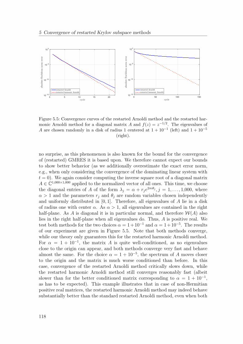
5 Convergence of restarted Krylov subspace methods
cycle0 5 10 15 20
abso
lute
Eucl
idea
nnorm
erro
r
10-15
10-10
10-5
100
restarted Arnoldi
restarted harmonic Arnoldi
cycle0 50 100 150
abso
lute
Eucl
idea
nnorm
erro
r
10-15
10-10
10-5
100
restarted Arnoldi
restarted harmonic Arnoldi
Figure 5.5: Convergence curves of the restarted Arnoldi method and the restarted har-monic Arnoldi method for a diagonal matrix A and f(z) = z−1/2. The eigenvalues ofA are chosen randomly in a disk of radius 1 centered at 1 + 10−1 (left) and 1 + 10−5
(right).
no surprise, as this phenomenon is also known for the bound for the convergenceof (restarted) GMRES it is based upon. We therefore cannot expect our boundsto show better behavior (as we additionally overestimate the exact error norm,e.g., when only considering the convergence of the dominating linear system witht = 0). We again consider computing the inverse square root of a diagonal matrixA ∈ C
1,000×1,000 applied to the normalized vector of all ones. This time, we choosethe diagonal entries of A of the form λj = α + rje
2πiθj , j = 1, . . . , 1,000, whereα > 1 and the parameters rj and θj are random variables chosen independentlyand uniformly distributed in [0, 1]. Therefore, all eigenvalues of A lie in a diskof radius one with center α. As α > 1, all eigenvalues are contained in the righthalf-plane. As A is diagonal it is in particular normal, and therefore W(A) alsolies in the right half-plane when all eigenvalues do. Thus, A is positive real. Wetest both methods for the two choices α = 1+10−1 and α = 1+10−5. The resultsof our experiment are given in Figure 5.5. Note that both methods converge,while our theory only guarantees this for the restarted harmonic Arnoldi method.For α = 1 + 10−1, the matrix A is quite well-conditioned, as no eigenvaluesclose to the origin can appear, and both methods converge very fast and behavealmost the same. For the choice α = 1 + 10−5, the spectrum of A moves closerto the origin and the matrix is much worse conditioned than before. In thiscase, convergence of the restarted Arnoldi method critically slows down, whilethe restarted harmonic Arnoldi method still converges reasonably fast (albeitslower than for the better conditioned matrix corresponding to α = 1 + 10−1,as has to be expected). This example illustrates that in case of non-Hermitianpositive real matrices, the restarted harmonic Arnoldi method may indeed behavesubstantially better than the standard restarted Arnoldi method, even when both
118
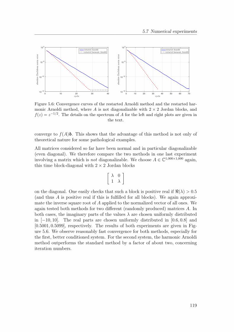
5.7 Numerical experiments
cycle0 10 20 30 40
abso
lute
Eucl
idea
nnorm
erro
r
10-15
10-10
10-5
100
restarted Arnoldi
restarted harmonic Arnoldi
cycle0 10 20 30 40 50 60 70
abso
lute
Eucl
idea
nnorm
erro
r
10-15
10-10
10-5
100
restarted Arnoldi
restarted harmonic Arnoldi
Figure 5.6: Convergence curves of the restarted Arnoldi method and the restarted har-monic Arnoldi method, where A is not diagonalizable with 2 × 2 Jordan blocks, andf(z) = z−1/2. The details on the spectrum of A for the left and right plots are given in
the text.
converge to f(A)b. This shows that the advantage of this method is not only oftheoretical nature for some pathological examples.
All matrices considered so far have been normal and in particular diagonalizable(even diagonal). We therefore compare the two methods in one last experimentinvolving a matrix which is not diagonalizable. We choose A ∈ C
1,000×1,000 again,this time block-diagonal with 2× 2 Jordan blocks
[λ 01 λ
]
on the diagonal. One easily checks that such a block is positive real if ℜ(λ) > 0.5(and thus A is positive real if this is fulfilled for all blocks). We again approxi-mate the inverse square root of A applied to the normalized vector of all ones. Weagain tested both methods for two different (randomly produced) matrices A. Inboth cases, the imaginary parts of the values λ are chosen uniformly distributedin [−10, 10]. The real parts are chosen uniformly distributed in [0.6, 0.8] and[0.5001, 0.5099], respectively. The results of both experiments are given in Fig-ure 5.6. We observe reasonably fast convergence for both methods, especially forthe first, better conditioned system. For the second system, the harmonic Arnoldimethod outperforms the standard method by a factor of about two, concerningiteration numbers.
119

CHAPTER 6
ERROR ESTIMATES IN KRYLOV METHODS
In Chapter 5 we have shown how to derive a priori error bounds for Arnoldi’smethod for Stieltjes matrix functions. However, as the numerical experimentsin Section 5.7 reveal (and as can be expected from similar experience with theerror bounds for linear systems our results are based upon), these bounds tend toseverely overestimate the order of magnitude of the error and (depending on theeigenvalue distribution of the matrix A) may also wrongly predict the convergenceslope. Therefore, they are not feasible for use as stopping criteria for iterativemethods in most practical situations, as this would typically lead to a relativelyhigh number of unnecessary Arnoldi iterations which are performed in spite ofthe error norm already being well below the desired tolerance. Therefore, wenow show how to compute error estimates during Arnoldi’s method which bettercapture the actual behavior of the error (and can be shown to be lower andupper bounds for the exact error norm in certain situations) and are thereforebetter suited as stopping criteria. In [65,66], approaches for computing such errorestimates (or bounds) for matrix function computations have been presented, butthe results given there only apply to rational functions in partial fraction form(another approach for rational functions, which we investigate in more detaillater in this chapter is presented in [61]). Therefore, it is of interest to constructsuch error bounds for more general classes of matrix functions. The boundswe present here for this purpose are largely based on the close relation betweenGauss quadrature and the Lanczos process, see [72–74], which we briefly reviewin Section 6.1. In Section 6.2, we describe how this relation can be used tocompute error bounds for bilinear forms uHh(A)v defined by a matrix functionh(A). By rewriting the error norm in Arnoldi’s method for Stieltjes functions assuch a bilinear form, we show how these techniques can be used for boundingthe Arnoldi error norm in Section 6.3. As the naive application of this approach
121
6 Error estimates in Krylov methods
leads to very high additional computational cost for the computation of the errorbounds (multiple additional matrix-vector products per Arnoldi iteration), wedescribe how to compute the bounds with cost independent of the matrix size nand iteration number m in Section 6.4. In Section 6.5 we briefly describe howthe techniques from the previous sections can be transferred to non-Hermitianmatrices (and functions which are not Stieltjes functions, like, e.g., the matrixexponential) although in this case one obtains only estimates for the error (insteadof bounds) in general, and the cost for the computation of these bounds growswith the number m of iterations in Arnoldi’s method (but is still independentof the matrix size n). In Section 6.6, we apply the developed techniques to themodel problems from Section 2.6 to illustrate the quality of our error estimatesand investigate their dependence on certain parameters.
The results presented in this section related to Stieltjes functions are submittedfor publication; see [63].
6.1 Relation between Gauss quadrature and the
Lanczos process
In this section we briefly review the connection between Gauss quadrature andthe Lanczos process. For this, consider the sequence of Lanczos polynomials, i.e.,the polynomials pk−1 with
pk−1(A)v1 = vk and deg pk−1 = k − 1. (6.1)
One can show that these polynomials form an orthonormal set with respect to aninner product depending on spec(A). For ease of presentation, we assume thatall eigenvalues of A are distinct in the following. We will, however, briefly touchon the necessary modifications in case that A has multiple eigenvalues right afterthe statement of the central Theorem 6.1.
Theorem 6.1. Let A ∈ Cn×n be Hermitian with eigenvalue decomposition A =
QΛQH and let pk−1, k = 1, 2, . . . be the Lanczos polynomials (6.1). Define thefunction
α(t) =
0, if t < λ1,∑ij=1 |v(j)|2, if λi ≤ t < λi+1,∑nj=1 |v(j)|2, if λn ≤ t,
(6.2)
where λmin = λ1 < λ2 < · · · < λn = λmax denote the (sorted) eigenvalues of Aand v = QHv1. Then the polynomials pk−1 are orthonormal with respect to the
122
6.1 Relation between Gauss quadrature and the Lanczos process
inner product
(p, q)α =
∫ b
a
p(t)q(t)dα(t)
= vHp(A)Hq(A)v , (6.3)
where a ≤ λmin and b ≥ λmax.
Proof. See [74, Theorem 4.2].
Remark 6.2. In case that the eigenvalues of A are not pairwise distinct, thenotation in Theorem 6.1 has to be adapted as follows. Denoting by λ1 < · · · < λnthe distinct eigenvalues, there exist corresponding eigenvectors vj and coefficientsηj, j = 1, . . . , n such that
v1 =n∑
j=1
ηj vj,
as A is Hermitian positive definite and thus, in particular, its eigenvectors forma basis of Cn. The step function α from (6.2) is then changed to
α(t) =
0, if t < λ1,∑ij=1 |ηj|2, if λi ≤ t < λi+1,∑nj=1 |ηj|2, if λn < t,
and all results presented in the following apply in a straightforward way.
Theorem 6.1 states that the Lanczos process generates a (finite) sequence of or-thonormal polynomials with respect to the inner product (6.3) defined via thefunction α. In practical situations, α is not known explicitly, as it requires knowl-edge of all eigenvalues and eigenvectors of A. Interestingly, by using the Lanczosprocess, it is possible to find Gauss quadrature rules corresponding to [a, b] andα without the explicit knowledge of α. The following theorem is derived byexploiting the relationship between Gauss quadrature and the eigenvalues andeigenvectors of tridiagonal matrices, see Section 2.5.
Theorem 6.3. Let A ∈ Cn×n be Hermitian positive definite with smallest and
largest eigenvalue λmin and λmax, respectively, let a ≤ λmin and b ≥ λmax, letv1 ∈ C
n with ‖v1‖2 = 1, let h be a function defined on [a, b] and let α be definedas in (6.2). Let tℓ, ωℓ, ℓ = 1, . . . , k be the nodes and weights of the k-point Gaussquadrature rule for approximating
∫ b
a
h(t)dα(t). (6.4)
123
6 Error estimates in Krylov methods
Thenk∑
ℓ=1
ωℓh(tℓ) = eH1 h(Hk)e1, (6.5)
where Hk is the tridiagonal matrix obtained by k steps of the Lanczos process,Algorithm 2.2, applied to A and v1.
Proof. See [74, Theorem 6.6]
In the same way, the (k+ 1)-point Gauss–Radau quadrature rule (with one node
fixed at λmin) can be evaluated as eH1 h(Hk+1)e1, with the modified tridiagonal
matrix
Hk+1 =
[Hk hk+1,kek
hk+1,keHk d(k)
], where d = h2k+1,k(Hk − λminI)
−1ek; (6.6)
see [74].
By Theorem 6.3, we can evaluate a Gauss quadrature rule for the function hwithout even explicitly computing the nodes and weights of the correspondingrule, by evaluating h on a tridiagonal matrix. In the next section we will showwhy and how bilinear forms uHh(A)v can be interpreted as Riemann–Stieltjesintegrals of the form (6.4).
6.2 Bounds and estimates for bilinear forms
uHh(A)v
Let A ∈ Cn×n be Hermitian positive definite with smallest and largest eigenvalue
λmin and λmax, respectively, let [a, b] with a ≤ λmin and b ≥ λmax and let h be afunction defined on [a, b] as before. Given vectors u , v ∈ C
n, we are interested inapproximating the bilinear form uHh(A)v . To do so, we mainly follow the pre-sentation in [74, Chapter 7]. With q1, . . . , qn denoting an orthonormal eigenbasisof A, we decompose u and v as
u =n∑
i=1
βiqi and v =n∑
i=1
ηiqi.
Inserting this relation into uHh(A)v and using the eigendecomposition A =QΛQH , we find
uHh(A)v = uHQh(Λ)QHv = βHh(Λ)η =n∑
i=1
βiηih(λi). (6.7)
124
6.3 Error bounds for Stieltjes functions of positive definite matrices
The sum on the right-hand side of (6.7) can be interpreted as a Riemann–Stieltjesintegral ∫ b
a
h(t) dα(t)
with respect to a piecewise constant step function α (cf. also Example 2.9) givenby
α(t) =
0, if t < λ1,∑ij=1 βjηj, if λi ≤ t < λi+1,∑nj=1 βjηj, if λn ≤ t.
In case of a quadratic form vHh(A)v , i.e., u = v in (6.7), the function α simplifiesto
α(t) =
0, if t < λ1,∑ij=1 |ηj|2, if λi ≤ t < λi+1,∑nj=1 |ηj|2, if λn ≤ t.
(6.8)
If we use v as starting vector for the Lanczos process (for notational simplicityassuming that ‖v‖2 = 1), we have η = v in Theorem 6.1, and the step functionα from (6.8) coincides with α from (6.2). In other words, the quadratic formvHh(A)v can be interpreted as a Riemann–Stieltjes integral with respect to thefunction α for which the Lanczos polynomials form an orthonormal sequence.Therefore, the corresponding Gauss quadrature rule (6.5) from Theorem 6.3 (or
the Gauss–Radau rule obtained from replacing Hk by Hk+1) is a natural choicefor approximating it. A simple way of approximating quadratic forms vHh(A)vis therefore as follows. First, normalize v if necessary, yielding v1. Performm steps of Algorithm 2.2 to obtain the tridiagonal matrix Hk (and modify thismatrix according to (6.6) if Gauss–Radau quadrature is to be used), and thenevaluate (6.5) to obtain an estimate corresponding to a k-point Gauss rule (or(k+1)-point Gauss–Radau rule). In the next section, we will show that the normof the error in Arnoldi’s method can be expressed as a quadratic form, so thatthe results from this and the preceding section apply in this case. Afterwards,in Section 6.4, we will show how to modify the simple approach described aboveso that it does not require k additional multiplications with A for performing asecondary Lanczos process.
6.3 Error bounds for Stieltjes functions of positive
definite matrices
We begin this section by giving a straightforward characterization of the errornorm in Arnoldi’s method for Stieltjes matrix functions.
125
6 Error estimates in Krylov methods
Lemma 6.4. Let A ∈ Cn×n be Hermitian positive definite, let b ∈ C
n, let f bea Stieltjes function of the form (3.15) and let fm be the approximation for f(A)bobtained from m steps of Arnoldi’s method. Then
‖f(A)b − fm‖22 = ‖b‖22γ2mvHm+1em(A)
2vm+1, (6.9)
where em(z) is given by
em(z) =
∫ ∞
0
1
z + tdµ(t) with dµ(t) =
1
wm(t)dµ(t) (6.10)
and γm, wm are as defined in Theorem 3.5.
Proof. By Theorem 3.5 and Proposition 3.9 we have the representation
f(A)b − fm = (−1)m+1‖b‖2γm∫ ∞
0
(A+ tI)−1 dµ(t)vm+1 (6.11)
for the error in Arnoldi’s method. Taking (squared) norms in (6.11) gives
‖f(A)b − fm‖22 = (‖b‖2γmem(A)vm+1)H (‖b‖2γmem(A)vm+1)
= ‖b‖22γ2mvHm+1em(A)
H em(A)vm+1
= ‖b‖22γ2mvHm+1em(A)
2vm+1,
where the last equality holds because em(A) is Hermitian if A is Hermitian.
The representation (6.9) of the Arnoldi error norm as a quadratic form allowsto use Gauss (and Gauss–Radau) quadrature in the sense of (6.5) to computeapproximations for it. In our situation, i.e., f a Stieltjes function and A Hermitianpositive definite, we can prove that the approximations obtained this way are lowerand upper bounds for the exact norm of the error.
Theorem 6.5. Let A ∈ Cn×n be Hermitian positive definite, let b ∈ C
n, let fbe a Stieltjes function of the form (3.15) and let fm be the mth Arnoldi approxi-
mation (2.25) to f(A)b. Denote by H(2)k the tridiagonal matrix resulting from k
steps of the Lanczos process applied to A and vm+1 and by H(2)k+1 the modification
of H(2)k according to (6.6). Then
‖b‖22γ2meH1 em
(H
(2)k
)2e1 ≤ ‖f(A)b − fm‖22 ≤ ‖b‖22γ2meH
1 em
(H
(2)k+1
)2e1, (6.12)
where em(z) is the error function given in (6.10) and γm is as defined in Theo-rem 3.5.
126
6.3 Error bounds for Stieltjes functions of positive definite matrices
Proof. By Theorem 6.3, the quantity eH1 em
(H
(2)k
)2e1 corresponds to a k-point
Gauss quadrature rule for the Riemann–Stieltjes integral∫ b
a
em(z)2 dα(z),
where α is given by (6.2). In the same way eH1 em
(H
(2)k+1
)2e1 corresponds to a
(k + 1)-point Gauss–Radau rule. As em(z) is a Stieltjes function by Proposi-tion 3.9, and thus, according to Proposition 2.17(i), completely monotonic, em(z)
2
is also completely monotonic by Proposition 2.17(ii), although it is not a Stielt-jes function in general. The bracketing property (2.53) from Corollary 2.48 thengives the desired result.
Theorem 6.5 suggests a simple way of computing error bounds for the Arnoldiapproximation to f(A)b, albeit one that is hardly feasible in practice. Directlyevaluating the leftmost and rightmost expression in (6.12) to bound the error inthemth step of Arnoldi’s method demands an additional k matrix vector productsfor computing H
(2)k . Therefore, the computation of the error bounds requires the
same amount of computational work as advancing the Arnoldi iteration from stepm to step m + k. This is an unacceptably high cost, especially if one wants tocompute error bounds in each iteration of Arnoldi’s method to monitor at whatpoint the desired accuracy is reached. How this can be circumvented will be thetopic of Section 6.4. Prior to that, we address another issue that arises when tryingto use (6.12) for computing error bounds. The function em(z) is not available in anexplicit closed form, so that it has to be evaluated, e.g, by numerical quadrature,just as in the implementation of the restarted Arnoldi method in Chapter 4. Whilein Chapter 4 we were mainly interested in using a convergent quadrature rulewhich gives an accurate enough representation of the error to be approximated,this time it is also important to know whether these approximations give loweror upper bounds for the exact value of the integral, because otherwise one cannotbe sure that the approximations computed for the quantities on the left andright of (6.12) are still bounds (rather than only estimates) for the error. In thefollowing we show that it suffices to choose a quadrature rule that gives lower (orupper) bounds for the value of em(z) in the scalar case, because this property willcarry over to the matrix case. Note that this result is not as trivial as it mayappear at first sight, as it relies on the fact that A (and thus Hk) is Hermitianpositive definite and does in general not hold in the non-Hermitian case.
Proposition 6.6. Let the assumptions of Theorem 3.4 hold and let H ∈ Cm×m
be any Hermitian positive definite matrix. Further, let tℓ, ωℓ ∈ R, ℓ = 1, . . . , k bethe nodes and weights of a quadrature rule for which
k∑
ℓ=1
ωℓ
z + tℓ≤ em(z) for z ∈ R
+. (6.13)
127
6 Error estimates in Krylov methods
Then
eH1
(k∑
ℓ=1
ωℓ(H + tℓI)−1
)2
e1 ≤ eH1 em(H)2e1.
The result holds analogously for quadrature rules which give upper bounds. Inparticular, the result applies to the matrices H
(2)k and H
(2)k+1 from Theorem 6.5.
Proof. Using the spectral decomposition H = UDUH with unitary U and diago-nal D and defining the shorthand notation u = UH e1, we have
eH1
(k∑
ℓ=1
ωℓ(H + tℓI)−1
)2
e1 = uH
(k∑
ℓ=1
ωℓ(D + tℓI)−1
)2
u
=m∑
i=1
|ui|2(
k∑
ℓ=1
ωℓ
dii + tℓ
)2
. (6.14)
Using (6.13) we can bound the right-hand side of (6.14) by
m∑
i=1
|ui|2(
k∑
ℓ=1
ωℓ
dii + tℓ
)2
≤m∑
i=1
|ui|2em(dii)2 = uH em(D)2u = eH1 em(H)2e1,
which concludes the proof for lower bounds. The modifications necessary forproving the result for upper bounds are straightforward. The matrix H
(2)k is
obviously Hermitian positive definite, as A is Hermitian positive definite andH
(2)k = V HAV for a matrix V of full (column) rank. For H
(2)k+1, note that the
modification (6.6) again results in a Hermitian matrix. As its eigenvalues are thenodes of a Gauss–Radau quadrature rule, they are known to lie in [λmin, λmax](when the fixed quadrature node a is chosen such that a ≤ λmin or a ≥ λmax,
which is the case in our setting), see, e.g., [69]. Therefore, H(2)k+1 is also a Hermitian
positive definite matrix and the result of the proposition applies.
We note that while the result of Proposition 6.6 is important in the sense that itguarantees that it is possible to really compute lower and upper bounds for theerror in Arnoldi’s method by properly combining two rules that each give a lower(or upper) bound in (6.12), the numerical experiments reported in Section 6.6show that the error in the inner quadrature rule, i.e., the rule for approximatingem(z), is typically negligible compared to the error of the outer Gauss quadraturerule used to approximate the bilinear form (6.9) for reasonable choices of param-eters, so that in most situations, the computed quantities can still be trusted tobe bounds for the error norm, even when no special care is devoted to choosingthe inner quadrature rule properly.
128
6.4 Computing error bounds with low computational cost
We end this section by commenting on the relation of the results presented hereto the results from [61]. In [61], an approach very similar to what is presentedhere is established for linear systems and, building on this, for rational functionsin partial fraction form (with poles on the negative real axis). These rationalfunctions belong to the class of Stieltjes functions, cf. also Example 2.14, and thetechniques presented in this thesis and in [61] in fact lead to exactly the sameresults in this case. Instead of using the results from this chapter, one couldalso apply the approach of [61] to other functions by first approximating f bya suitable rational function r ≈ f and then working with r for computing errorestimates (similar to Algorithm 4.2 from [3], where one replaces f by a rationalfunction to allow restarting). Using our approach, however, has the advantagethat it circumvents the (potentially costly or complicated) a priori constructionof a rational approximation for f and just works with f directly. In addition,when one is interested in computing guaranteed error bounds in the first place,one typically wants these to bound the error corresponding to f(A)b. Using theapproach from [61] would only yield bounds for the error corresponding to r(A)b.As long as one does not have information on the sign of the remainder term in therational approximation (and, in general, the remainder will change sign on theinterval [λmin, λmax]), one can therefore not relate these bounds to f(A)b directly.Therefore, our approach, while similar in spirit to what was done in [61], hasadditional advantages which warrant its closer investigation in this thesis.
6.4 Computing error bounds with low
computational cost
In this section, we show how to compute the quantities from (6.12) with com-putational cost independent of the number m of iterations performed thus far inArnoldi’s method and the dimension n of the matrix A, thus making it feasible toevaluate the resulting bounds in each iteration of Arnoldi’s method for monitoringprogress of the method. The main idea to reach this goal relies on the fact thatwe only need to know the tridiagonal matrix H
(2)k resulting from applying k steps
of Algorithm 2.2 to A and vm+1, but not the corresponding Arnoldi basis vectors.The tridiagonal matrix can be computed efficiently, as stated by the followingtheorem from [61]. We state the result in its original form here, as this is all weneed right now. We will present several more general versions of it in Section 6.5and Chapter 7, but giving the lengthy proofs of the more general versions herewould deviate from the main topic of this section.
Theorem 6.7. Let A ∈ Cn×n be Hermitian positive definite, let v1 ∈ C
n and letHm+k+1 be the tridiagonal matrix resulting from m + k + 1 steps of the Lanczosprocess for A and v1. Let k = minm, k and denote by H the lower right (k +
129
6 Error estimates in Krylov methods
k + 1) × (k + k + 1) sub-block of Hm+k+1. Further, let H denote the tridiagonal
matrix resulting from k steps of the Lanczos process applied to H and ek+1. Then
H = H(2)k , where H
(2)k denotes the matrix resulting from k iterations of the Lanczos
process for A and vm+1.
Proof. See [61, Theorem 4.1].
Theorem 6.7 states that the matrix H(2)k can be computed by performing k steps
of a secondary Lanczos process with a tridiagonal matrix of size at most (2k +1)× (2k + 1), i.e., with computational cost O(k2), independent of the size of theoriginal matrix. The price one pays for this reduction in computational complexityis that the error bounds for stepm are not available immediately when performingthis step, but only later at step m + k + 1 (if Gauss quadrature with k nodes isused for computing the bounds). Therefore, there is a trade-off between accuracyof the error bound (which implies a higher number k of quadrature nodes) andtimely availability of the bounds (which implies using as few nodes as possible).We further comment on this trade-off when investigating the dependency of themethod on the number of quadrature nodes used in the numerical experimentsreported in Section 6.6.
Apart from H(2)k , the computation of the error bounds by (6.12) requires one to be
able to evaluate em and thus the nodal polynomial wm(t), at least at the quadra-ture nodes used for approximating em. As wm(t) is a polynomial of degree m, anaive approach of evaluating it at each of the ℓ quadrature nodes used in the innerquadrature rule would require O(mℓ) arithmetic operations (notwithstanding thefact that the explicit formula for wm(t) requires computing the eigenvalues of Hm
in the first place), so that the cost of evaluating em would grow with the itera-tion number m. In addition, this approach could potentially become numericallyunstable for larger values of m. We can circumvent this problem by choosingthe quadrature nodes ti, i = 1, . . . , ℓ in advance and fixing them throughout alliterations, as 1/wm(ti) can be updated from 1/wm−1(ti) with computational costO(1) as follows. By exploiting the relation (4.12) (adapted to our situation, i.e.,replacing tI −Hm by Hm + tI), one immediately sees that 1/wm(t) is a multipleof the bottom left entry of the inverse of the shifted matrix Hm + tI. As Hm isHermitian and tridiagonal (and so are its shifted versions), one can easily give arecurrence relation for this entry. When performing Gaussian elimination to solve
(Hm + tiI)zm(ti) = e1, (6.15)
with Lm denoting the resulting lower triangular matrix and um the vector onwhich the same elimination steps have been performed (starting from e1), oneobviously has
Lm =
[Lm−1 ∗∗ ∗
]and um =
[um−1
∗
],
130
6.4 Computing error bounds with low computational cost
with ∗ denoting unknown quantities. The quantities with lower index m − 1result from the elimination for the system (6.15) from the previous Arnoldi step.Therefore, the last entry of the solution of (6.15) can be constructed when thetwo quantities ℓm−1,m−1 and um−1(m−1) are kept track of from the last iteration.One then has
um(m) = um−1(m− 1) · hm+1,m
ℓm,m
where ℓm,m = (hm,m + ti)−h2m+1,m
ℓm−1,m−1
,
so that all quantities necessary for computing 1/wm(ti) from (4.12) with costO(1) are available. We note that this approach in a way corresponds to what isdone in certain formulations of the (shifted) CG algorithm, see, e.g., [61,62,115],with the difference that the necessary quantities do not arise naturally during thecomputations in our case, as we are only implicitly working with shifted linearsystems. This approach only requires to store 2(k + 1) scalar values for eachquadrature point ti (as one needs to be able to retrieve the values from iterationmin iteration m+k+1 for computing the retrospective error bound), thus resultingin overall additional computational cost of order O(ℓ) and storage cost of orderO(kℓ), which is negligible in comparison to the computational cost and storagerequirements of Algorithm 2.2 for reasonable values of k and ℓ. The requirementthat the nodes for the inner quadrature rule have to be fixed in advance andcannot be changed during the execution of the algorithm (otherwise, one needsto recompute the values 1/wm(ti) from scratch for all new quadrature nodes,resulting in a cost of O(mℓ)) is not a big disadvantage. One generally does notneed a very high number ℓ of inner quadrature nodes to obtain an approximationerror in the same order of magnitude as the one of the outer quadrature rule;see also the results presented in Section 6.6. In addition, even the recomputationof all values with cost O(mℓ) is in general affordable should it really becomenecessary.
Algorithm 6.1 summarizes our approach of computing retrospective error boundsin the Lanczos method for f(A)b. The iteration stops once the upper bound ofthe error lies below the specified tolerance and the current iterate fm is formedand returned (even though the error bound corresponds to the iterate m − k −1, we know by Theorem 5.10 that the (Euclidean) error norm of the Arnoldiapproximations is monotonically decreasing for Hermitian positive definite A, sothat the error norm of fm will also lie below the specified tolerance and will ingeneral be smaller than the one of fm−k−1). In order to not make the notationoverly complicated we assume that the quantities di and ρi which keep track of thevalues necessary to retrieve the values of 1/wm(ti) are stored as full size vectors,although it suffices to keep the values from the last k + 1 iterations in an actualimplementation. Algorithm 6.1 is given in such a way that it only terminateswhen the desired tolerance is reached. It is of course possible to also specify anupper bound mmax for the number of iterations to be performed.
131
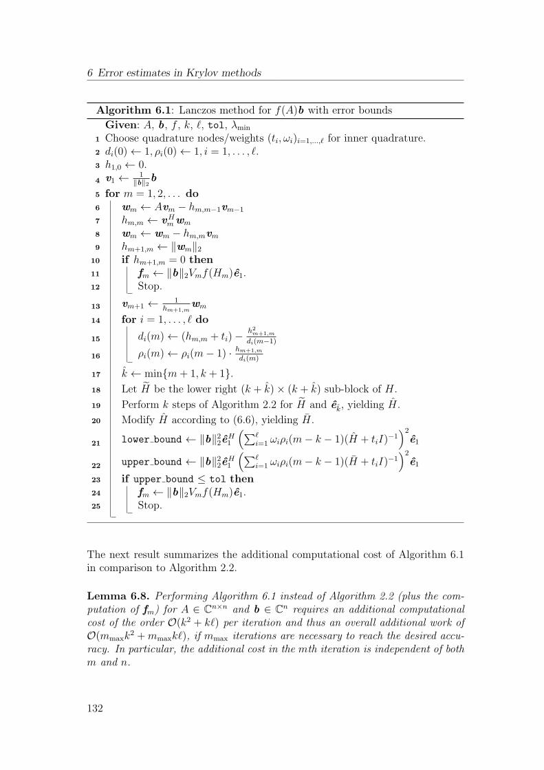
6 Error estimates in Krylov methods
Algorithm 6.1: Lanczos method for f(A)b with error bounds
Given: A, b, f , k, ℓ, tol, λmin
Choose quadrature nodes/weights (ti, ωi)i=1,...,ℓ for inner quadrature.1
di(0)← 1, ρi(0)← 1, i = 1, . . . , ℓ.2
h1,0 ← 0.3
v1 ← 1‖b‖2b4
for m = 1, 2, . . . do5
wm ← Avm − hm,m−1vm−16
hm,m ← vHmwm7
wm ← wm − hm,mvm8
hm+1,m ← ‖wm‖29
if hm+1,m = 0 then10
fm ← ‖b‖2Vmf(Hm)e1.11
Stop.12
vm+1 ← 1hm+1,m
wm13
for i = 1, . . . , ℓ do14
di(m)← (hm,m + ti)− h2m+1,m
di(m−1)15
ρi(m)← ρi(m− 1) · hm+1,m
di(m)16
k ← minm+ 1, k + 1.17
Let H be the lower right (k + k)× (k + k) sub-block of H.18
Perform k steps of Algorithm 2.2 for H and ek, yielding H.19
Modify H according to (6.6), yielding H.20
lower bound ← ‖b‖22eH1
(∑ℓi=1 ωiρi(m− k − 1)(H + tiI)
−1)2e121
upper bound ← ‖b‖22eH1
(∑ℓi=1 ωiρi(m− k − 1)(H + tiI)
−1)2e122
if upper bound ≤ tol then23
fm ← ‖b‖2Vmf(Hm)e1.24
Stop.25
The next result summarizes the additional computational cost of Algorithm 6.1in comparison to Algorithm 2.2.
Lemma 6.8. Performing Algorithm 6.1 instead of Algorithm 2.2 (plus the com-putation of fm) for A ∈ C
n×n and b ∈ Cn requires an additional computational
cost of the order O(k2 + kℓ) per iteration and thus an overall additional work ofO(mmaxk
2 +mmaxkℓ), if mmax iterations are necessary to reach the desired accu-racy. In particular, the additional cost in the mth iteration is independent of bothm and n.
132
6.4 Computing error bounds with low computational cost
Proof. The initializations in line 1 and 2 of Algorithm 6.1 have cost O(ℓ), assum-ing that the nodes and weights of the quadrature rule are available and do not needto be computed by a separate algorithm. Line 3–13 (ignoring the computation offm in line 11) exactly correspond to the Lanczos process given in Algorithm 2.2.The for loop in line 14–16 has computational cost O(ℓ), as the update formulasfor di and ρi only require a fixed number of scalar operations. Line 17 has costO(1). Line 18 has cost O(k) and line 19 has cost O(k2), as H is tridiagonal andmatrix vector products with it therefore have cost O(k). Line 20 again has cost
O(k) for solving the linear system with H. The computation of the lower andupper bounds in line 21 and 22, respectively, requires O(kℓ) operations. Addingup the cost of all individual lines and noting that O(ℓ),O(k) ⊂ O(kℓ) gives thedesired result.
Lemma 6.8 shows that the cost of computing error bounds for the Arnoldi ap-proximation for Hermitian positive definite A by Algorithm 6.1 is independentof n. If n is large and k and ℓ are small in comparison, the additional cost iscompletely negligible. In the numerical experiments reported in Section 6.6 wedemonstrate that values of k between 5 and 20 and values of ℓ below 100 are typi-cally sufficient to compute accurate error bounds, also for large matrix dimensionn. Although it is rather difficult to make any precise statement on the accuracyof the computed error bounds, one can of course expect their quality to dependon κ(A), the condition number of the matrix A. Therefore, for large κ(A), highervalues of k and ℓ might be necessary to obtain satisfactory results.
We conclude this section by briefly commenting on the situation when using arestarted Arnoldi method (like, e.g., the one from Chapter 4) instead of the fullArnoldi method. In this case, one cannot use the Lanczos restart recovery fromTheorem 6.7 to compute error bounds for all iterations of the method, but onlyfor those iterations for which the next k+1 iterations belong to the same restartcycle, because the construction from Theorem 6.7 requires the tridiagonal matrixresulting from k + 1 further steps of the Lanczos method and the result does nothold any longer if one restarts the method in between. Therefore, ifm denotes therestart length, we can only compute error bounds for the first m−k−1 iterationsof each cycle by the approach described before. However, in the restarted case,one is not that reliant on error bounds as for the full Arnoldi method, as onealready computes error estimates in a natural way: In each restart cycle, one aimsto approximate the error of the iterate from the last restart cycle. Therefore,assuming that the method computes sufficiently accurate approximations, thenorm of the additive correction computed in cycle j can be interpreted as anestimate for the norm of the error of the iterate from cycle j − 1 and thus givesa first hint at the progress of the method. However, if one just uses the approachfrom Chapter 4 to compute a correction for f
(j−1)m and then computes its norm,
one has no guarantee that the resulting value is an upper or lower bound for the
133
6 Error estimates in Krylov methods
error norm or that it is a sufficiently accurate approximation at all. To obtainbounds, at least for the iterate computed at the end of the last restart cycle,we can use the result of Theorem 6.5 directly, without need for restart recovery.When restarting the Arnoldi method, we perform the Lanczos process in thenext, jth restart cycle with the matrix A and the vector v
(j−1)m+1 . This is exactly
what is needed for computing the tridiagonal matrix used in (6.12). While in thefull Arnoldi method, using Theorem 6.5 directly means many additional matrixvector multiplications which do not advance the primary iteration, we are now ina situation where the matrix vector multiplications performed by the next cycleof the primary Lanczos process and those needed for the computation of the errorbounds are exactly the same. Therefore, if we compute the values on the left- andright-hand side of (6.12) at the end of restart cycle j (with restart length m), thiscorresponds to an approximation of the norm of the error after cycle j − 1 by anm-point Gauss and (m+ 1)-point Gauss–Radau rule, respectively. This can alsobe interpreted the other way around: One performs k iterations of a secondaryLanczos process to bound the error of the current iterate. If the bound shows thatthe iterate does not yet fulfill the accuracy requirement, the iterations performedin the secondary method are not “lost”, but can be used to begin the next restartcycle. We will also give some examples for the bounds obtained this way in thenumerical experiments reported in Section 6.6.
6.5 Extension to non-Hermitian matrices
In this section, we will briefly sketch how it is possibly to transfer the basic tech-niques used in the previous sections also to the case of non-Hermitian matrices.Most of the theoretical results concerning, e.g., the sign of the error in the in-ner and outer quadrature rules, do not hold any longer in this case so that onecannot obtain guaranteed lower or upper bounds for the error in general. Thebasis for being able to also use a similar approach in the non-Hermitian case isgiven in [24, 51], where it is shown that Arnoldi’s method can also be related toquadrature rules, similar to what was done for the Lanczos process in Section 6.1.In this context, one investigates bilinear forms
(h1, h2)A,v = vHh1(A)Hh2(A)v (6.16)
induced by A and v for functions h1, h2 defined on spec(A). When the functionsh1 and h2 are both analytic in a neighborhood of spec(A), one can use the Cauchyintegral formula (as in Definition 2.4) to rewrite (6.16) as a double integral alonga path Γ that winds around spec(A) exactly once
(h1, h2)A,v =1
4π2
∫
Γ
∫
Γ
h1(z1)h2(z2)vH(z1I −AH)−1(z2I −A)−1v dz1 dz2. (6.17)
134
6.5 Extension to non-Hermitian matrices
Using the quantities from the Arnoldi decomposition (2.23) to approximate (6.16),i.e.,
vHh1(A)Hh2(A)v ≈ ‖v‖22eH
1 h1(Hk)Hh2(Hk)e1 (6.18)
can then be interpreted as a k-point quadrature rule for (6.17). One can alsoshow that the polynomials pi defining the Arnoldi basis vectors are orthonormalwith respect to the bilinear form (6.16), i.e.,
(pi, pj)A,v =
1 if i = j,
0 otherwise.
From this, one can prove that the resulting k-point quadrature rules are exact for(h1, h2) ∈Wk−1, where
Wk−1 = (Πk−1 ⊕ Πk) ∪ (Πk ⊕ Πk−1);
see [24]. We do not go into detail concerning the theoretical analysis of the re-sulting quadrature rules, as most of this theory is not important or not applicablefor the developments presented in this section (one can, e.g., show that undersome conditions, these Arnoldi quadrature rules give upper or lower bounds forthe bilinear form (6.16), see [24], but these conditions are not fulfilled or cannoteasily be verified in our setting).
In this manner, one can use the upper Hessenberg matrix Hk resulting from ksteps of Arnoldi’s method applied to A and vm+1 to compute error estimates forthe mth Arnoldi approximation to f(A)b, where f is a Stieltjes function, just asin the Hermitian case, by setting h1 = h2 = em in (6.18). However, the key forbeing able to do so with affordable additional computational cost in the Hermitiancase was given by Theorem 6.7, which allows to perform the secondary Lanczosprocess on a (2k+1)× (2k+1) matrix instead of an n×n matrix. Unfortunately,the result given in [61] holds only in the Hermitian case and has to be modifiedaccordingly in case of non-Hermitian A. Its proof, however, is almost the sameas for the original result from [61].
Theorem 6.9. Let A ∈ Cn×n be Hermitian positive definite, let v1 ∈ C
n and letHm+k+1 be the upper Hessenberg matrix resulting from m+k+1 steps of Arnoldi’smethod for A and v1. Further, let H denote the upper Hessenberg matrix resultingfrom k steps of Arnoldi’s method applied to Hm+k+1 and em+1. Then H = H
(2)k ,
where H(2)k denotes the matrix resulting from k iterations of Arnoldi’s method for
A and vm+1.
Proof. Let the Arnoldi decomposition arising from k steps of Arnoldi’s methodfor A and vm+1 be given as
AVk = VkH(2)k + h
(2)k+1,kvk+1e
Hk . (6.19)
135
6 Error estimates in Krylov methods
As vm+1 ∈ Km+1(A, v1), we obviously have that
Kk+1(A, vm+1) ⊆ Km+k+1(A, v1).
Therefore, the basis vectors v1, . . . , vk+1 generated by Arnoldi’s method for A andvm+1 all lie in Km+k+1(A, v1) and can thus be written as linear combinations ofthe basis vectors v1, . . . , vm+k+1, i.e.,
[Vk, vk+1] = Vm+k+1[Qk, qk+1] (6.20)
for some matrix [Qk, qk+1] ∈ C(m+k+1)×(k+1). As [Vk, vk+1] and Vm+k+1 both have
orthonormal columns, [Qk, qk+1] must have orthonormal columns as well. Insert-ing (6.20) into the Arnoldi decomposition (6.19) gives
AVm+k+1Qk = Vm+k+1QkH(2)k + h
(2)k+1,kVm+k+1qk+1e
Hk . (6.21)
Left-multiplying both sides of (6.21) by the orthogonal projector Vm+k+1VHm+k+1
onto the space Km+k+1(A, v1) gives
Vm+k+1VHm+k+1AVm+k+1Qk = Vm+k+1QkH
(2)k + h
(2)k+1,kVm+k+1qk+1e
Hk .
which by (2.24) simplifies to
Vm+k+1Hm+k+1Qk = Vm+k+1QkH(2)k + h
(2)k+1,kVm+k+1qk+1e
Hk .
Noting that Vm+k+1 has full (column) rank, this implies
Hm+k+1Qk = QkH(2)k + h
(2)k+1,kqk+1e
Hk . (6.22)
Due to Lemma 2.23 and the fact that all subdiagonal entries of H(2)k are positive
(as it was computed by Arnoldi’s method), it follows that (6.22) is the Arnoldidecomposition corresponding to Hm+k+1 and q1. As v1 = vm+1, we have thatq1 = em+1, which proves the result.
Theorem 6.7 can directly be derived from Theorem 6.9 by noting that in theHermitian case, large parts of the coefficients in Qk from (6.20) are zero due tothe tridiagonal structure of Hm+k+1, thus allowing to only use a small part ofthe tridiagonal matrix for the computations, see [61]. As this is not the case inpresence of a non-Hermitian matrix A, it is not possible to only use a small sub-block of Hm+k+1 for retrieving the matrix H
(2)k . This in turn means that, while we
can circumvent additional multiplications with A, we cannot avoid multiplicationswith Hm+k+1, a matrix growing from one iteration to the next. Apart fromthis fact, the approach of Algorithm 6.1 can be used in the same way as inthe Hermitian case (replacing the Lanczos process by Arnoldi’s method and thecomputation of the bounds in line 21 and 22 by a quadrature-based approximation
136
6.5 Extension to non-Hermitian matrices
for (6.18)) and replacing the recurrence relations for the entries of the inverse ofshifted versions of Hm with the explicit computation of these values, as the simpleupdate formulas do not hold any longer, because Hm is not tridiagonal. We justbriefly mention here that it is still possible to obtain the necessary quantities ina more efficient way by applying successive rotations, similar to what is done inGMRES for cheaply computing the residual norm, see, e.g., [116]. This does not,however, change the overall cost of the algorithm, at least in O-sense, cf. also theproof of Lemma 6.10, so that we do not go into detail concerning this here. Theresulting method is given in Algorithm 6.2.
Algorithm 6.2: Arnoldi’s method for f(A)b with error estimate
Given: A, b, f , k, ℓ, tolChoose quadrature nodes/weights (ti, ωi)i=1,...,ℓ for inner quadrature.1
v1 ← 1‖b‖2b2
for m = 1, 2, . . . do3
wm ← Avm4
for i = 1, . . . ,m do5
hi,m ← vHi wm6
wm ← wm − hi,mvi7
hm+1,m ← ‖wm‖28
if hm+1,m = 0 then9
fm ← ‖b‖2Vmf(Hm)e1.10
Stop.11
vm+1 ← 1hm+1,m
wm12
for i = 1, . . . , ℓ do13
ρi(m)← hm+1,meHm (Hm + tI)−1e114
if m ≥ k + 1 then15
Perform k steps of Algorithm 2.1 for H and em−k, yielding H.16
estimate←‖b‖22eH1
∑ℓi=1|ωiρi(m−k−1)|2(H+ tiI)
−H(H+ tiI)−1e117
if estimate ≤ tol then18
fm ← ‖b‖2Vmf(Hm)e1.19
Stop.20
Note that, in contrast to Algorithm 6.1, Algorithm 6.2 does not guarantee thatthe exact error norm of the iterate fm lies below the prescribed tolerance tol
upon termination. We note that the results of the numerical experiments inSection 6.6 suggest that the error estimates are rather accurate and reliable inmany situations, at least for Stieltjes functions. It can, however, be useful toinclude a “safety factor” ε < 1 in the computations and run Algorithm 6.2 with thetolerance ε·tol instead of tol if it is important that the prescribed tolerance is not
137
6 Error estimates in Krylov methods
only approximately reached. The additional cost of Algorithm 6.2 in comparisonto the standard Arnoldi method without computation of error estimates is givenin the next lemma.
Lemma 6.10. Performing Algorithm 6.2 instead of Algorithm 2.1 (plus the com-putation of fm) for A ∈ C
n×n and b ∈ Cn requires an additional computational
cost of the order O(m2(k+ℓ)+kℓ) in the mth iteration and thus O(m3max(k+ℓ)+
mmaxkℓ), if mmax iterations are performed in total. In particular, the additionalcost per iteration is independent of n, but not of m.
Proof. The proof is very similar to the one of Lemma 6.8, with the followingdifferences. The secondary Arnoldi method for step m now has a cost of O(m2k),as each multiplication with Hm+k+1 has cost O(m2) since the upper triangle ofthis matrix is in general dense (and we assume k ∈ O(m)). The solution of eachlinear system in line 14 has cost O(m2) due to the Hessenberg structure of Hm,which results in O(m2ℓ) for all systems.
According to Lemma 6.10, the cost of computing error estimates in Algorithm 6.2grows with the number of iterations performed. Therefore, if a large number mof iterations is necessary, the cost of computing the estimates may become pro-hibitively large. On the other hand, the cost of the orthogonalization in Arnoldi’smethod also grows from one iteration to the next and is in fact of order O(mn).For k fixed (independently of m and n), we have that O(m2k) ⊂ O(mn), sothat the cost of Algorithm 6.2 (ignoring the matrix vector multiplication) is stillnot dominated by the cost of computing the error estimates, at least in O-sense.Nonetheless, computing the error estimates is more costly than in the Hermitiancase so that computing error estimates in the non-Hermitian case seems partic-ularly attractive in situations where only a low number of very costly iterationsis necessary for reaching the desired accuracy, as it is, e.g., typically the case inextended Krylov methods. Extending the results of this chapter to these relatediterative methods is the topic of Chapter 7.
In analogy to what was discussed at the end of Section 6.4, we again mentionthat the possibility of restart recovery is not given for all iterations in case oneuses a restarted Arnoldi method. One can, however, again use the norm of theapproximation computed at the end of each cycle as an estimate of the error norm.In contrast to the Hermitian positive definite case, there is no provable benefitof specifically using estimates computed by quadrature rules instead of just using‖e (k)
m ‖2, as for both alternatives, one does not have any information on the signof the remainder or the quality of the estimate. We therefore just mention thishere briefly, but will not further investigate it in the numerical experiments inSection 6.6.
138
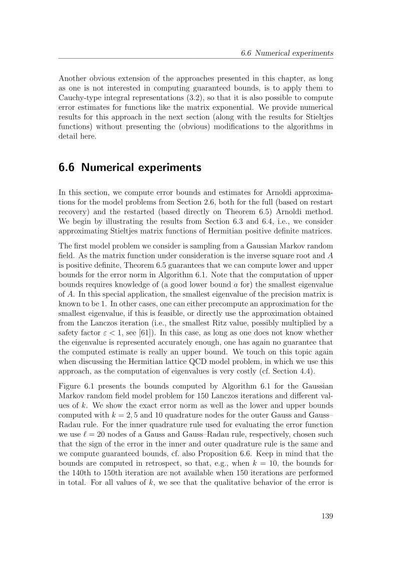
6.6 Numerical experiments
Another obvious extension of the approaches presented in this chapter, as longas one is not interested in computing guaranteed bounds, is to apply them toCauchy-type integral representations (3.2), so that it is also possible to computeerror estimates for functions like the matrix exponential. We provide numericalresults for this approach in the next section (along with the results for Stieltjesfunctions) without presenting the (obvious) modifications to the algorithms indetail here.
6.6 Numerical experiments
In this section, we compute error bounds and estimates for Arnoldi approxima-tions for the model problems from Section 2.6, both for the full (based on restartrecovery) and the restarted (based directly on Theorem 6.5) Arnoldi method.We begin by illustrating the results from Section 6.3 and 6.4, i.e., we considerapproximating Stieltjes matrix functions of Hermitian positive definite matrices.
The first model problem we consider is sampling from a Gaussian Markov randomfield. As the matrix function under consideration is the inverse square root and Ais positive definite, Theorem 6.5 guarantees that we can compute lower and upperbounds for the error norm in Algorithm 6.1. Note that the computation of upperbounds requires knowledge of (a good lower bound a for) the smallest eigenvalueof A. In this special application, the smallest eigenvalue of the precision matrix isknown to be 1. In other cases, one can either precompute an approximation for thesmallest eigenvalue, if this is feasible, or directly use the approximation obtainedfrom the Lanczos iteration (i.e., the smallest Ritz value, possibly multiplied by asafety factor ε < 1, see [61]). In this case, as long as one does not know whetherthe eigenvalue is represented accurately enough, one has again no guarantee thatthe computed estimate is really an upper bound. We touch on this topic againwhen discussing the Hermitian lattice QCD model problem, in which we use thisapproach, as the computation of eigenvalues is very costly (cf. Section 4.4).
Figure 6.1 presents the bounds computed by Algorithm 6.1 for the GaussianMarkov random field model problem for 150 Lanczos iterations and different val-ues of k. We show the exact error norm as well as the lower and upper boundscomputed with k = 2, 5 and 10 quadrature nodes for the outer Gauss and Gauss–Radau rule. For the inner quadrature rule used for evaluating the error functionwe use ℓ = 20 nodes of a Gauss and Gauss–Radau rule, respectively, chosen suchthat the sign of the error in the inner and outer quadrature rule is the same andwe compute guaranteed bounds, cf. also Proposition 6.6. Keep in mind that thebounds are computed in retrospect, so that, e.g., when k = 10, the bounds forthe 140th to 150th iteration are not available when 150 iterations are performedin total. For all values of k, we see that the qualitative behavior of the error is
139
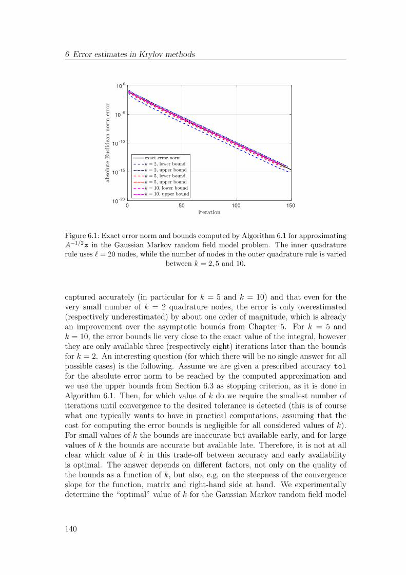
6 Error estimates in Krylov methods
iteration0 50 100 150
abso
lute
Eucl
idea
nnorm
erro
r
10-20
10-15
10-10
10-5
100
exact error norm
k = 2, lower bound
k = 2, upper bound
k = 5, lower bound
k = 5, upper bound
k = 10, lower bound
k = 10, upper bound
Figure 6.1: Exact error norm and bounds computed by Algorithm 6.1 for approximatingA−1/2z in the Gaussian Markov random field model problem. The inner quadraturerule uses ℓ = 20 nodes, while the number of nodes in the outer quadrature rule is varied
between k = 2, 5 and 10.
captured accurately (in particular for k = 5 and k = 10) and that even for thevery small number of k = 2 quadrature nodes, the error is only overestimated(respectively underestimated) by about one order of magnitude, which is alreadyan improvement over the asymptotic bounds from Chapter 5. For k = 5 andk = 10, the error bounds lie very close to the exact value of the integral, howeverthey are only available three (respectively eight) iterations later than the boundsfor k = 2. An interesting question (for which there will be no single answer for allpossible cases) is the following. Assume we are given a prescribed accuracy tol
for the absolute error norm to be reached by the computed approximation andwe use the upper bounds from Section 6.3 as stopping criterion, as it is done inAlgorithm 6.1. Then, for which value of k do we require the smallest number ofiterations until convergence to the desired tolerance is detected (this is of coursewhat one typically wants to have in practical computations, assuming that thecost for computing the error bounds is negligible for all considered values of k).For small values of k the bounds are inaccurate but available early, and for largevalues of k the bounds are accurate but available late. Therefore, it is not at allclear which value of k in this trade-off between accuracy and early availabilityis optimal. The answer depends on different factors, not only on the quality ofthe bounds as a function of k, but also, e.g, on the steepness of the convergenceslope for the function, matrix and right-hand side at hand. We experimentallydetermine the “optimal” value of k for the Gaussian Markov random field model
140
6.6 Numerical experiments
ℓ ratio lower bound ratio upper bound
5 1.01 1.0310 1.003 1.00220 1.00004 1.00001
Table 6.1: Maximum ratio of the bounds computed by Algorithm 6.1 for the valuesℓ = 5, 10, 20 of inner quadratures nodes and the bounds computed for ℓ = 50 for the
Gaussian Markov random field model problem and k = 5.
problem, when trying to reach an accuracy of tol = 10−9. For k = 2, the it-eration would have been terminated after 92 iterations, just as with k = 5. Fork = 10, one would require 96 iterations before detecting convergence to the de-sired tolerance, so that this value, despite the very high accuracy of the computedbounds, would result in four unnecessary Lanczos iterations in comparison to thelower values of k (which may seem surprising because the bounds for k = 2 lookquite more inaccurate than those for the other values at first glance). Anotherinteresting question is how to choose the value ℓ of inner quadrature nodes, espe-cially considering the fact that this number has to be set to a pre-chosen value ifone wants to avoid superfluous computations. Our experiments revealed that thecomputed error bounds are not very sensitive with respect to the value of ℓ, to theextent that the differences in the resulting bounds are not visible to the eye in therespective convergence graphs. We therefore give the results of our experiments,this time fixing k = 5 and varying ℓ = 5, 10, 20 and 50 in form of a table whichreports the maximal ratio between the bounds computed for ℓ = 5, 10, 20 and themost accurate value computed for ℓ = 50. These ratios are given in Table 6.1 andshow that the resulting bounds are almost the same for all values, in particularwhen considering that even a difference of a factor of two in the resulting boundswould be acceptable in most cases. Therefore, and in addition keeping in mindthat the cost of Algorithm 6.1 depends only mildly on ℓ (cf. Lemma 6.8), one maychoose some not too low number, like, e.g., ℓ = 20 or 50 and will most probablyobtain satisfactory results. There exist cases, however, in which the error func-tion is harder to approximate and the computed bounds are more sensitive withrespect to the number ℓ of inner quadrature nodes as well. It might therefore beadvisable to use a simple form of adaptive quadrature again as a safety measure.This is similar to what is done in our quadrature-based restarted Arnoldi method,Algorithm 4.3, albeit in a “relaxed form” (as one only wants to recompute thevalues of the nodal polynomial at the quadrature points if it is really necessary,to avoid computational cost depending on the iteration number m). A straight-forward approach is to use two quadrature rules of different order again, but toreject the result only if the two computed approximations differ by a factor ofmore than two, e.g. This way, one can still detect whether the inner approxima-
141
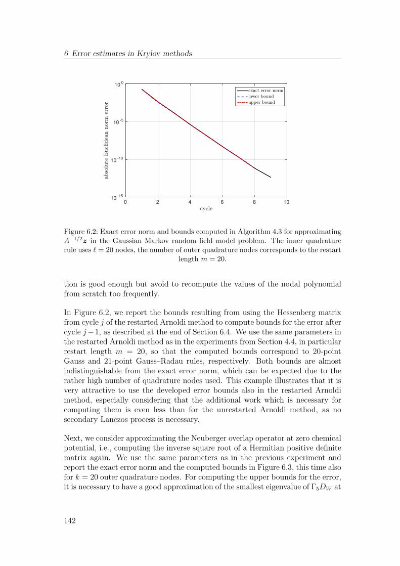
6 Error estimates in Krylov methods
cycle0 2 4 6 8 10
abso
lute
Eucl
idea
nnorm
erro
r
10-15
10-10
10-5
100
exact error norm
lower bound
upper bound
Figure 6.2: Exact error norm and bounds computed in Algorithm 4.3 for approximatingA−1/2z in the Gaussian Markov random field model problem. The inner quadraturerule uses ℓ = 20 nodes, the number of outer quadrature nodes corresponds to the restart
length m = 20.
tion is good enough but avoid to recompute the values of the nodal polynomialfrom scratch too frequently.
In Figure 6.2, we report the bounds resulting from using the Hessenberg matrixfrom cycle j of the restarted Arnoldi method to compute bounds for the error aftercycle j−1, as described at the end of Section 6.4. We use the same parameters inthe restarted Arnoldi method as in the experiments from Section 4.4, in particularrestart length m = 20, so that the computed bounds correspond to 20-pointGauss and 21-point Gauss–Radau rules, respectively. Both bounds are almostindistinguishable from the exact error norm, which can be expected due to therather high number of quadrature nodes used. This example illustrates that it isvery attractive to use the developed error bounds also in the restarted Arnoldimethod, especially considering that the additional work which is necessary forcomputing them is even less than for the unrestarted Arnoldi method, as nosecondary Lanczos process is necessary.
Next, we consider approximating the Neuberger overlap operator at zero chemicalpotential, i.e., computing the inverse square root of a Hermitian positive definitematrix again. We use the same parameters as in the previous experiment andreport the exact error norm and the computed bounds in Figure 6.3, this time alsofor k = 20 outer quadrature nodes. For computing the upper bounds for the error,it is necessary to have a good approximation of the smallest eigenvalue of Γ5DW at
142
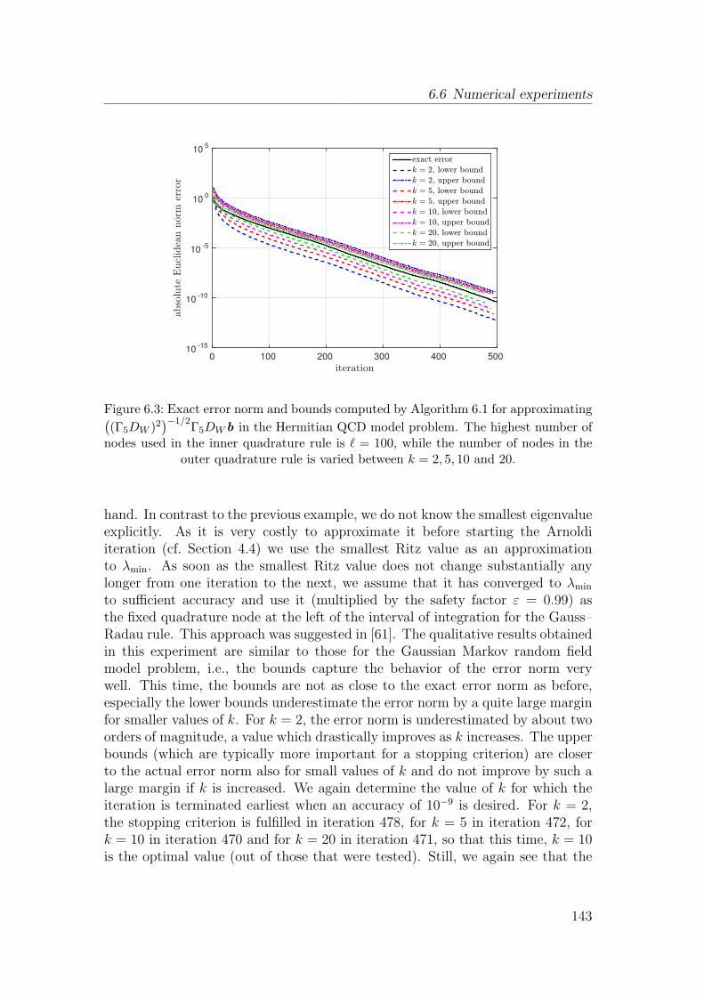
6.6 Numerical experiments
iteration0 100 200 300 400 500
abso
lute
Eucl
idea
nnorm
erro
r
10-15
10-10
10-5
100
105
exact error
k = 2, lower bound
k = 2, upper bound
k = 5, lower bound
k = 5, upper bound
k = 10, lower bound
k = 10, upper bound
k = 20, lower bound
k = 20, upper bound
Figure 6.3: Exact error norm and bounds computed by Algorithm 6.1 for approximating((Γ5DW )2
)−1/2Γ5DWb in the Hermitian QCD model problem. The highest number of
nodes used in the inner quadrature rule is ℓ = 100, while the number of nodes in theouter quadrature rule is varied between k = 2, 5, 10 and 20.
hand. In contrast to the previous example, we do not know the smallest eigenvalueexplicitly. As it is very costly to approximate it before starting the Arnoldiiteration (cf. Section 4.4) we use the smallest Ritz value as an approximationto λmin. As soon as the smallest Ritz value does not change substantially anylonger from one iteration to the next, we assume that it has converged to λmin
to sufficient accuracy and use it (multiplied by the safety factor ε = 0.99) asthe fixed quadrature node at the left of the interval of integration for the Gauss–Radau rule. This approach was suggested in [61]. The qualitative results obtainedin this experiment are similar to those for the Gaussian Markov random fieldmodel problem, i.e., the bounds capture the behavior of the error norm verywell. This time, the bounds are not as close to the exact error norm as before,especially the lower bounds underestimate the error norm by a quite large marginfor smaller values of k. For k = 2, the error norm is underestimated by about twoorders of magnitude, a value which drastically improves as k increases. The upperbounds (which are typically more important for a stopping criterion) are closerto the actual error norm also for small values of k and do not improve by such alarge margin if k is increased. We again determine the value of k for which theiteration is terminated earliest when an accuracy of 10−9 is desired. For k = 2,the stopping criterion is fulfilled in iteration 478, for k = 5 in iteration 472, fork = 10 in iteration 470 and for k = 20 in iteration 471, so that this time, k = 10is the optimal value (out of those that were tested). Still, we again see that the
143
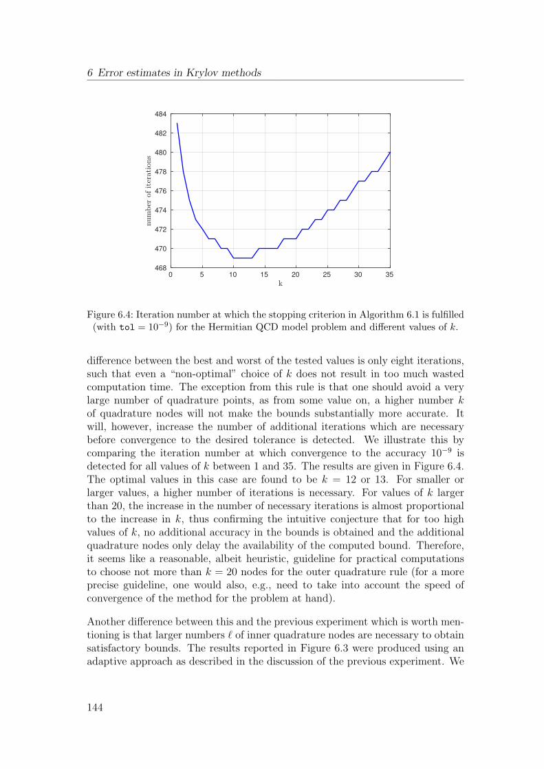
6 Error estimates in Krylov methods
k0 5 10 15 20 25 30 35
num
ber
ofiter
ations
468
470
472
474
476
478
480
482
484
Figure 6.4: Iteration number at which the stopping criterion in Algorithm 6.1 is fulfilled(with tol = 10−9) for the Hermitian QCD model problem and different values of k.
difference between the best and worst of the tested values is only eight iterations,such that even a “non-optimal” choice of k does not result in too much wastedcomputation time. The exception from this rule is that one should avoid a verylarge number of quadrature points, as from some value on, a higher number kof quadrature nodes will not make the bounds substantially more accurate. Itwill, however, increase the number of additional iterations which are necessarybefore convergence to the desired tolerance is detected. We illustrate this bycomparing the iteration number at which convergence to the accuracy 10−9 isdetected for all values of k between 1 and 35. The results are given in Figure 6.4.The optimal values in this case are found to be k = 12 or 13. For smaller orlarger values, a higher number of iterations is necessary. For values of k largerthan 20, the increase in the number of necessary iterations is almost proportionalto the increase in k, thus confirming the intuitive conjecture that for too highvalues of k, no additional accuracy in the bounds is obtained and the additionalquadrature nodes only delay the availability of the computed bound. Therefore,it seems like a reasonable, albeit heuristic, guideline for practical computationsto choose not more than k = 20 nodes for the outer quadrature rule (for a moreprecise guideline, one would also, e.g., need to take into account the speed ofconvergence of the method for the problem at hand).
Another difference between this and the previous experiment which is worth men-tioning is that larger numbers ℓ of inner quadrature nodes are necessary to obtainsatisfactory bounds. The results reported in Figure 6.3 were produced using anadaptive approach as described in the discussion of the previous experiment. We
144
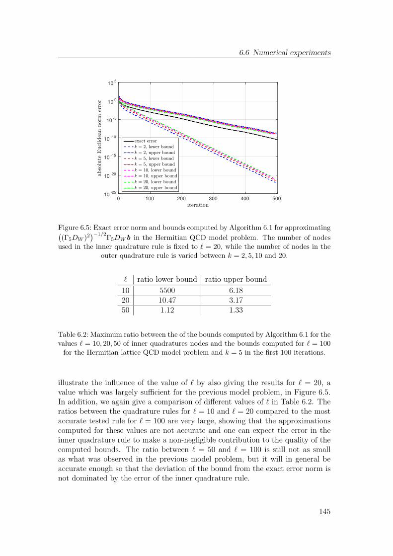
6.6 Numerical experiments
iteration0 100 200 300 400 500
abso
lute
Eucl
idea
nnorm
erro
r
10-25
10-20
10-15
10-10
10-5
100
105
exact error
k = 2, lower bound
k = 2, upper bound
k = 5, lower bound
k = 5, upper bound
k = 10, lower bound
k = 10, upper bound
k = 20, lower bound
k = 20, upper bound
Figure 6.5: Exact error norm and bounds computed by Algorithm 6.1 for approximating((Γ5DW )2
)−1/2Γ5DWb in the Hermitian QCD model problem. The number of nodes
used in the inner quadrature rule is fixed to ℓ = 20, while the number of nodes in theouter quadrature rule is varied between k = 2, 5, 10 and 20.
ℓ ratio lower bound ratio upper bound
10 5500 6.1820 10.47 3.1750 1.12 1.33
Table 6.2: Maximum ratio between the of the bounds computed by Algorithm 6.1 for thevalues ℓ = 10, 20, 50 of inner quadratures nodes and the bounds computed for ℓ = 100for the Hermitian lattice QCD model problem and k = 5 in the first 100 iterations.
illustrate the influence of the value of ℓ by also giving the results for ℓ = 20, avalue which was largely sufficient for the previous model problem, in Figure 6.5.In addition, we again give a comparison of different values of ℓ in Table 6.2. Theratios between the quadrature rules for ℓ = 10 and ℓ = 20 compared to the mostaccurate tested rule for ℓ = 100 are very large, showing that the approximationscomputed for these values are not accurate and one can expect the error in theinner quadrature rule to make a non-negligible contribution to the quality of thecomputed bounds. The ratio between ℓ = 50 and ℓ = 100 is still not as smallas what was observed in the previous model problem, but it will in general beaccurate enough so that the deviation of the bound from the exact error norm isnot dominated by the error of the inner quadrature rule.
145
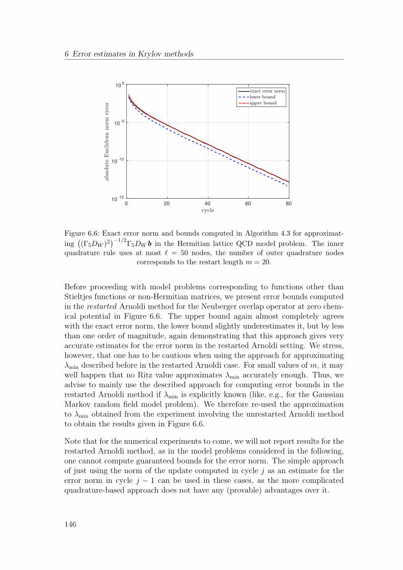
6 Error estimates in Krylov methods
cycle0 20 40 60 80
abso
lute
Eucl
idea
nnorm
erro
r
10-15
10-10
10-5
100
exact error norm
lower bound
upper bound
Figure 6.6: Exact error norm and bounds computed in Algorithm 4.3 for approximat-
ing((Γ5DW )2
)−1/2Γ5DWb in the Hermitian lattice QCD model problem. The inner
quadrature rule uses at most ℓ = 50 nodes, the number of outer quadrature nodescorresponds to the restart length m = 20.
Before proceeding with model problems corresponding to functions other thanStieltjes functions or non-Hermitian matrices, we present error bounds computedin the restarted Arnoldi method for the Neuberger overlap operator at zero chem-ical potential in Figure 6.6. The upper bound again almost completely agreeswith the exact error norm, the lower bound slightly underestimates it, but by lessthan one order of magnitude, again demonstrating that this approach gives veryaccurate estimates for the error norm in the restarted Arnoldi setting. We stress,however, that one has to be cautious when using the approach for approximatingλmin described before in the restarted Arnoldi case. For small values of m, it maywell happen that no Ritz value approximates λmin accurately enough. Thus, weadvise to mainly use the described approach for computing error bounds in therestarted Arnoldi method if λmin is explicitly known (like, e.g., for the GaussianMarkov random field model problem). We therefore re-used the approximationto λmin obtained from the experiment involving the unrestarted Arnoldi methodto obtain the results given in Figure 6.6.
Note that for the numerical experiments to come, we will not report results for therestarted Arnoldi method, as in the model problems considered in the following,one cannot compute guaranteed bounds for the error norm. The simple approachof just using the norm of the update computed in cycle j as an estimate for theerror norm in cycle j − 1 can be used in these cases, as the more complicatedquadrature-based approach does not have any (provable) advantages over it.
146
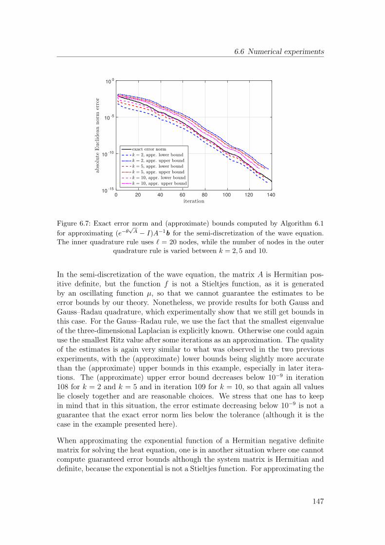
6.6 Numerical experiments
iteration0 20 40 60 80 100 120 140
abso
lute
Eucl
idea
nnorm
erro
r
10-15
10-10
10-5
100
exact error norm
k = 2, appr. lower bound
k = 2, appr. upper bound
k = 5, appr. lower bound
k = 5, appr. upper bound
k = 10, appr. lower bound
k = 10, appr. upper bound
Figure 6.7: Exact error norm and (approximate) bounds computed by Algorithm 6.1
for approximating (e−θ√A − I)A−1b for the semi-discretization of the wave equation.
The inner quadrature rule uses ℓ = 20 nodes, while the number of nodes in the outerquadrature rule is varied between k = 2, 5 and 10.
In the semi-discretization of the wave equation, the matrix A is Hermitian pos-itive definite, but the function f is not a Stieltjes function, as it is generatedby an oscillating function µ, so that we cannot guarantee the estimates to beerror bounds by our theory. Nonetheless, we provide results for both Gauss andGauss–Radau quadrature, which experimentally show that we still get bounds inthis case. For the Gauss–Radau rule, we use the fact that the smallest eigenvalueof the three-dimensional Laplacian is explicitly known. Otherwise one could againuse the smallest Ritz value after some iterations as an approximation. The qualityof the estimates is again very similar to what was observed in the two previousexperiments, with the (approximate) lower bounds being slightly more accuratethan the (approximate) upper bounds in this example, especially in later itera-tions. The (approximate) upper error bound decreases below 10−9 in iteration108 for k = 2 and k = 5 and in iteration 109 for k = 10, so that again all valueslie closely together and are reasonable choices. We stress that one has to keepin mind that in this situation, the error estimate decreasing below 10−9 is not aguarantee that the exact error norm lies below the tolerance (although it is thecase in the example presented here).
When approximating the exponential function of a Hermitian negative definitematrix for solving the heat equation, one is in another situation where one cannotcompute guaranteed error bounds although the system matrix is Hermitian anddefinite, because the exponential is not a Stieltjes function. For approximating the
147
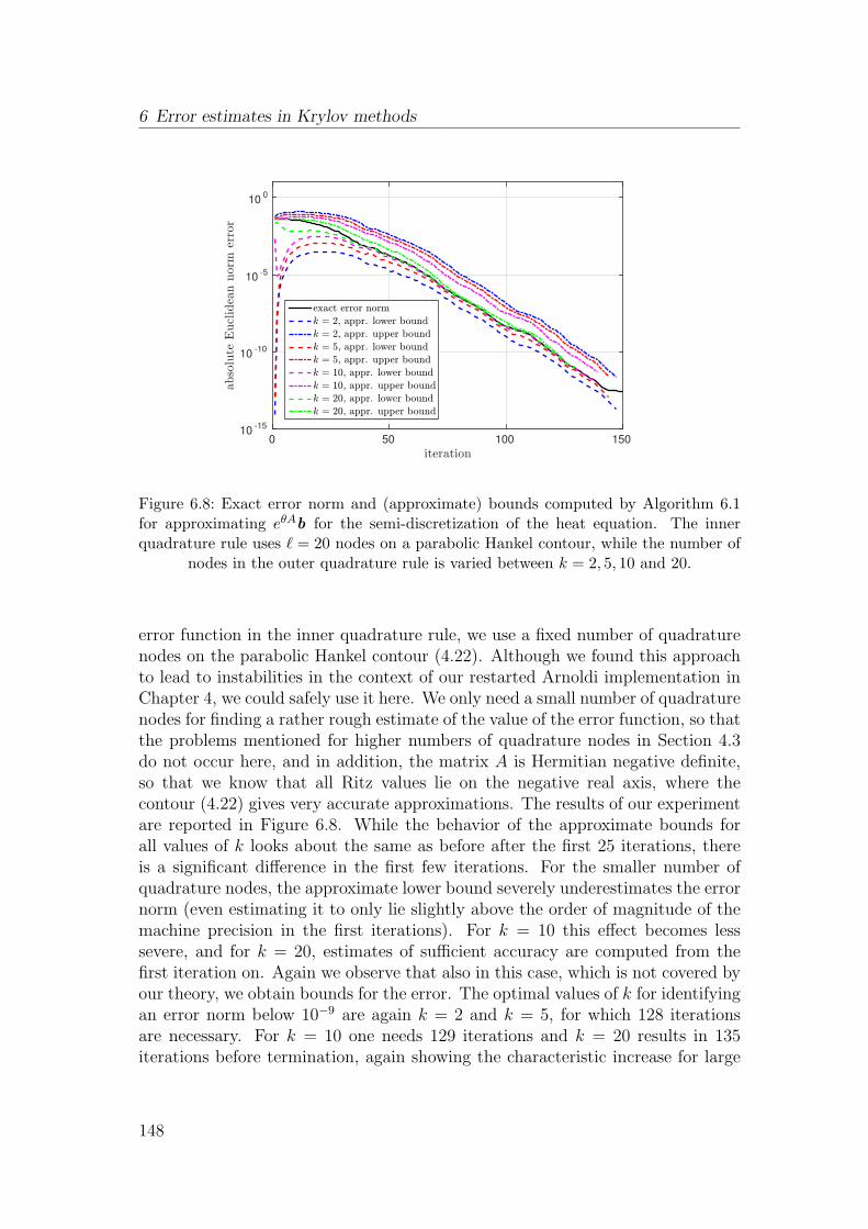
6 Error estimates in Krylov methods
iteration0 50 100 150
abso
lute
Eucl
idea
nnorm
erro
r
10-15
10-10
10-5
100
exact error norm
k = 2, appr. lower bound
k = 2, appr. upper bound
k = 5, appr. lower bound
k = 5, appr. upper bound
k = 10, appr. lower bound
k = 10, appr. upper bound
k = 20, appr. lower bound
k = 20, appr. upper bound
Figure 6.8: Exact error norm and (approximate) bounds computed by Algorithm 6.1for approximating eθAb for the semi-discretization of the heat equation. The innerquadrature rule uses ℓ = 20 nodes on a parabolic Hankel contour, while the number of
nodes in the outer quadrature rule is varied between k = 2, 5, 10 and 20.
error function in the inner quadrature rule, we use a fixed number of quadraturenodes on the parabolic Hankel contour (4.22). Although we found this approachto lead to instabilities in the context of our restarted Arnoldi implementation inChapter 4, we could safely use it here. We only need a small number of quadraturenodes for finding a rather rough estimate of the value of the error function, so thatthe problems mentioned for higher numbers of quadrature nodes in Section 4.3do not occur here, and in addition, the matrix A is Hermitian negative definite,so that we know that all Ritz values lie on the negative real axis, where thecontour (4.22) gives very accurate approximations. The results of our experimentare reported in Figure 6.8. While the behavior of the approximate bounds forall values of k looks about the same as before after the first 25 iterations, thereis a significant difference in the first few iterations. For the smaller number ofquadrature nodes, the approximate lower bound severely underestimates the errornorm (even estimating it to only lie slightly above the order of magnitude of themachine precision in the first iterations). For k = 10 this effect becomes lesssevere, and for k = 20, estimates of sufficient accuracy are computed from thefirst iteration on. Again we observe that also in this case, which is not covered byour theory, we obtain bounds for the error. The optimal values of k for identifyingan error norm below 10−9 are again k = 2 and k = 5, for which 128 iterationsare necessary. For k = 10 one needs 129 iterations and k = 20 results in 135iterations before termination, again showing the characteristic increase for large
148
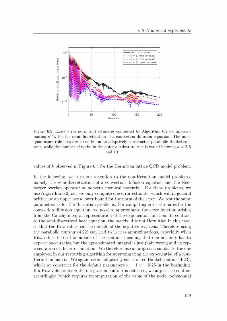
6.6 Numerical experiments
iteration0 50 100 150 200
abso
lute
Eucl
idea
nnorm
erro
r
10-10
10-5
100 exact error norm
k = 2, error estimate
k = 5, error estimate
k = 10, error estimate
Figure 6.9: Exact error norm and estimates computed by Algorithm 6.2 for approxi-mating eθAb for the semi-discretization of a convection diffusion equation. The innerquadrature rule uses ℓ = 20 nodes on an adaptively constructed parabolic Hankel con-tour, while the number of nodes in the outer quadrature rule is varied between k = 2, 5
and 10.
values of k observed in Figure 6.4 for the Hermitian lattice QCD model problem.
In the following, we turn our attention to the non-Hermitian model problems,namely the semi-discretization of a convection diffusion equation and the Neu-berger overlap operator at nonzero chemical potential. For these problems, weuse Algorithm 6.2, i.e., we only compute one error estimate, which will in generalneither be an upper nor a lower bound for the norm of the error. We test the sameparameters as for the Hermitian problems. For computing error estimates for theconvection diffusion equation, we need to approximate the error function arisingfrom the Cauchy integral representation of the exponential function. In contrastto the semi-discretized heat equation, the matrix A is not Hermitian in this case,so that the Ritz values can lie outside of the negative real axis. Therefore usingthe parabolic contour (4.22) can lead to useless approximations, especially whenRitz values lie on the outside of the contour, meaning that one not only has toexpect inaccuracies, but the approximated integral is just plain wrong and no rep-resentation of the error function. We therefore use an approach similar to the oneemployed in our restarting algorithm for approximating the exponential of a non-Hermitian matrix. We again use an adaptively constructed Hankel contour (4.23),which we construct for the default parameters a = 1, c = 0.25 in the beginning.If a Ritz value outside the integration contour is detected, we adjust the contouraccordingly (which requires recomputation of the value of the nodal polynomial
149
6 Error estimates in Krylov methods
at all quadrature points, but as already reasoned earlier, the computational costfor doing this is negligible compared to the other parts of the algorithm in mostcases). We note that this approach requires explicitly computing the Ritz valuesin each iteration which increases the additional cost of Algorithm 6.2. This maymake this approach prohibitively expensive in cases where the required numberm of iterations is large (which is, however, a situation in which one typicallyshould avoid using the standard Arnoldi method and instead turn to restarted orrational Krylov methods). The results of our experiment are given in Figure 6.9.In this example, the convergence of the Arnoldi approximations to f(A)b is notmonotone and the error estimates inherit the oscillating behavior of the exact er-ror. In the first about 50 iterations, the oscillations in the error norm are heavilyamplified in the error estimates, making them not reliable here. After the 50th it-eration, the oscillations in the error estimates become less strong and lie in aboutthe same order of magnitude as the oscillations in the exact error norm. However,the norm of the error is underestimated by about two to three orders of magnitudebetween the 70th and 100th iteration. Interestingly, the error estimate computedfor k = 5 is more accurate for this model problem than the estimate for k = 10.While the estimates give an idea on how the error behaves, especially in later it-erations, this experiment also illustrates the danger of using the estimates as solestopping criteria in the non-Hermitian case (or more generally in any situationin which one has no guarantee that the computed estimates are upper bounds).When demanding an accuracy of, e.g., 10−9, a stopping criterion based on theestimates produced by Algorithm 6.2 would already stop after a few iterations, oreven if one would ignore the largely oscillating error estimates computed in theinitial phase, after about 70 iterations, at a point where the exact error is far awayfrom reaching the demanded accuracy. We do therefore not recommend to use theerror estimates of Algorithm 6.2 as sole stopping criteria in practical situations.Even using a safety factor so that one only stops the iteration when the estimatelies several orders of magnitudes below the desired accuracy does not solve thisproblem. On the one hand this may result in a large number of unnecessary iter-ations, on the other hand, no matter how small the safety factor is chosen, therecan never be a guarantee that it suffices to reach the desired accuracy, as we haveno theoretical results at all on the quality of the computed error estimates. Thenext experiment, however, will show that there also exist situations in which theerror estimates from Algorithm 6.2 are of much better quality and do not alwaysshow the behavior observed for the “highly non-Hermitian” convection diffusionproblem (and the oscillating exponential function).
When approximating the action of the Neuberger operator at nonzero chemicalpotential, the error norm decreases much more smoothly than for the exponentialfunction in the semi-discretization of the convection diffusion equation, as can beseen from Figure 6.10. The error estimates behave in the same way as the exacterror norm, so that no oscillations like in the previous experiment are observed.
150
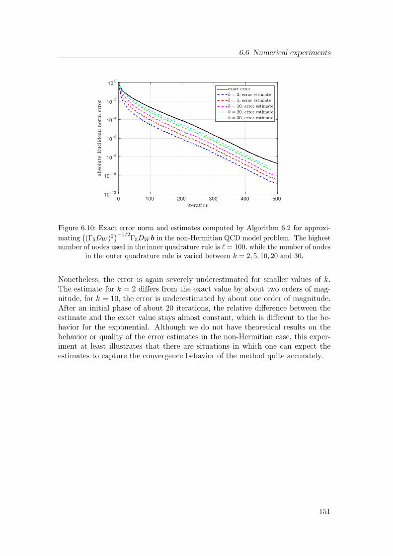
6.6 Numerical experiments
iteration0 100 200 300 400 500
abso
lute
Eucl
idea
nnorm
erro
r
10-12
10-10
10-8
10-6
10-4
10-2
100
exact error
k = 2, error estimate
k = 5, error estimate
k = 10, error estimate
k = 20, error estimate
k = 30, error estimate
Figure 6.10: Exact error norm and estimates computed by Algorithm 6.2 for approxi-
mating((Γ5DW )2
)−1/2Γ5DWb in the non-Hermitian QCD model problem. The highest
number of nodes used in the inner quadrature rule is ℓ = 100, while the number of nodesin the outer quadrature rule is varied between k = 2, 5, 10, 20 and 30.
Nonetheless, the error is again severely underestimated for smaller values of k.The estimate for k = 2 differs from the exact value by about two orders of mag-nitude, for k = 10, the error is underestimated by about one order of magnitude.After an initial phase of about 20 iterations, the relative difference between theestimate and the exact value stays almost constant, which is different to the be-havior for the exponential. Although we do not have theoretical results on thebehavior or quality of the error estimates in the non-Hermitian case, this exper-iment at least illustrates that there are situations in which one can expect theestimates to capture the convergence behavior of the method quite accurately.
151

CHAPTER 7
ERROR ESTIMATES IN EXTENDED KRYLOV
METHODS
In this chapter, we show how to transfer some of the techniques developed sofar to extended Krylov subspaces. These subspaces are constructed by not onlyapplying positive, but also negative powers of A to the vector b. This amountsto approximating f by a rational function (a Laurent polynomial, to be precise)instead of a polynomial. Of course, constructing a basis for these subspaces ismuch more costly than in the standard Krylov case and in return one hopes toobtain accurate approximations for much smaller subspace dimension (as oftenrational functions of rather small degree are much better suited for approximatinga given function than high-degree polynomials). Many of the properties of poly-nomial Krylov subspaces carry over to extended Krylov subspaces and we beginthis chapter by providing some basic material on these spaces and highlightingsimilarities and differences to the polynomial case in Section 7.1. Afterwards, inSection 7.2, we show how to transfer the integral representation for the error de-rived in Chapter 3 to approximations from extended Krylov spaces. This wouldin principle allow to use a restarting method similar to the one from Chapter 4 forextended Krylov subspace approximations. However, one typically uses extendedKrylov spaces only in situations where a low-dimensional approximation spacesuffices for achieving the desired accuracy, so that memory constraints seldombecome an issue and we do not go into detail on this topic and only mention inpassing that it would of course be possible to implement such a method. Instead,we focus on computing error estimates. To do so, we present a generalizationof Arnoldi/Lanczos restart recovery (Theorem 6.7 and 6.9) to extended Krylovspaces in section 7.3. We can then use these tools to compute estimates for theerror in extended Krylov subspace methods. We illustrate the quality of these
153
7 Error estimates in extended Krylov methods
estimates by performing numerical experiments on some of our model problemsin Section 7.4.
7.1 Extended Krylov subspaces
In the following, we introduce extended Krylov subspaces, which, in the con-text of approximating matrix functions, were first considered in [38] and furtherinvestigated in, e.g., [94–96,99].
The main idea of extended Krylov subspace methods (or also general rationalKrylov subspace methods, which we do not cover here) is that oftentimes whenusing rational functions for approximating a given function, the degree of the nu-merator and denominator necessary to reach a certain accuracy is substantiallysmaller than the degree of a polynomial exhibiting the same approximation qual-ity, see, e.g., [80]. Therefore it seems reasonable to use approximations to f(A)bwhich are characterized by an underlying rational approximant instead of a poly-nomial, especially when the behavior of f is difficult to capture by low-degreepolynomials. Different variants of general rational Krylov subspace methods arisethrough the choice of the poles of the rational functions, see, e.g., [80–82].
One simple, black-box choice of poles, which results in the so-called extendedKrylov subspaces, is to only choose the poles 0 and ∞ (often alternatingly), i.e.,building a Krylov subspace with respect to powers of A and A−1.
Definition 7.1. Let A ∈ Cn×n be nonsingular and let b ∈ C
n. Then the(k,m)th extended Krylov subspace with respect to A and b is
Ek,m(A, b) := A−kKk+m(A, b) = ℓk,m−1(A)b : ℓk,m−1 ∈ Lk,m−1,
whereLk,m−1 = spant−k, . . . , t−1, 1, t, t2, . . . , tm−1
denotes the space of Laurent polynomials of denominator degree at most kand numerator degree at most m− 1.
We begin our exposition by collecting some evident and useful properties anddifferent characterizations of extended Krylov subspaces. Results of this typehave also been observed in, e.g., [38, 95, 124].
Proposition 7.2. Let A ∈ Cn×n be nonsingular and let b ∈ C
n. Then
154
7.1 Extended Krylov subspaces
(i) Ek,m(A, b) ⊆ Ek+k0,m+m0(A, b) for all k0,m0 ≥ 0,
(ii) Ek,m(A, b) = Kk(A−1, A−1b) +Km(A, b) = Kk+m(A,A
−kb).
Proof. Property (i) directly follows from the definition of extended Krylov sub-spaces, similarly to the nestedness of polynomial Krylov subspaces. Both equali-ties in (ii) can be derived by using the representation
Ek,m(A, b) = spanA−kb, . . . , A−1b, b, Ab, A2b, . . . , Am−1b
and the definition of polynomial Krylov subspaces.
Property (i) from Proposition 7.2 is again a nestedness property, which holds forevery increase of the order of the subspace, be it an increase of the numeratordegree, the denominator degree, or both. Property (ii) relates extended Krylovsubspaces to polynomial Krylov spaces in two different ways. The first character-ization allows to write Ek,m(A, b) as the sum of two polynomial Krylov subspaces,one of them corresponding to A and one corresponding to A−1, while the secondone shows that Ek,m(A, b) is in fact a polynomial Krylov subspace correspondingto A, albeit with a different starting vector.
In the following we restrict ourselves to the case of k = m, sometimes calleddiagonal extended Krylov subspaces, to avoid unnecessary notational overhead.All results apply to general extended Krylov subspaces with k 6= m with obviousmodifications. A nested orthonormal basis for Em,m(A, b) can be computed bya method similar to Arnoldi’s method. There are, however, different ways togenerate the basis vectors. One way is to generate them sequentially, one-by-one,by alternatingly applying A and A−1 to the respective last basis vector. Anotherapproach, first introduced in [124], is to compute the basis in a “block-wise”fashion, two vectors at a time, by multiplying the last basis vector with A−1 andthe second to last basis vector with A. This way, odd-numbered basis vectorsadvance the basis corresponding to powers of A and even-numbered basis vectorsadvance the basis corresponding to powers of A−1. We will use the second, block-wise approach in this chapter, given in Algorithm 7.1.
The simple choice of poles in an extended Krylov subspace method gives rise toseveral theoretical and computational simplifications in contrast to general ratio-nal Krylov subspace methods. If it is feasible to solve the linear systems with A bya direct method, it is sufficient to compute an LU (or Cholesky) factorization [131]of A once and reuse it in each iteration of the method, while for varying poles onehas to compute a factorization for each of the poles used. Another advantage isthat for extended Krylov subspaces corresponding to a Hermitian matrix A it isagain possible to derive an analogue to the short-recurrence Lanczos process, theonly difference to the polynomial Lanczos algorithm being that the three-term
155
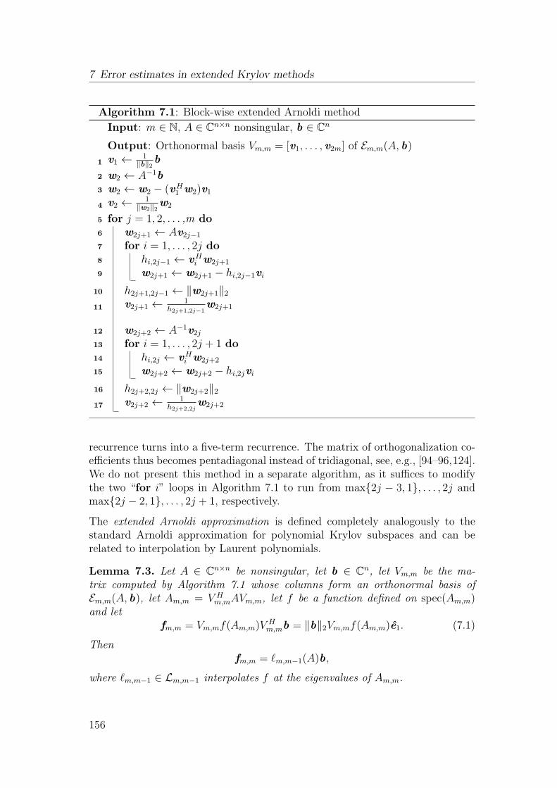
7 Error estimates in extended Krylov methods
Algorithm 7.1: Block-wise extended Arnoldi method
Input: m ∈ N, A ∈ Cn×n nonsingular, b ∈ C
n
Output: Orthonormal basis Vm,m = [v1, . . . , v2m] of Em,m(A, b)v1 ← 1
‖b‖2b1
w2 ← A−1b2
w2 ← w2 − (vH1 w2)v13
v2 ← 1‖w2‖2w24
for j = 1, 2, . . . ,m do5
w2j+1 ← Av2j−16
for i = 1, . . . , 2j do7
hi,2j−1 ← vHi w2j+18
w2j+1 ← w2j+1 − hi,2j−1vi9
h2j+1,2j−1 ← ‖w2j+1‖210
v2j+1 ← 1h2j+1,2j−1
w2j+111
w2j+2 ← A−1v2j12
for i = 1, . . . , 2j + 1 do13
hi,2j ← vHi w2j+214
w2j+2 ← w2j+2 − hi,2jvi15
h2j+2,2j ← ‖w2j+2‖216
v2j+2 ← 1h2j+2,2j
w2j+217
recurrence turns into a five-term recurrence. The matrix of orthogonalization co-efficients thus becomes pentadiagonal instead of tridiagonal, see, e.g., [94–96,124].We do not present this method in a separate algorithm, as it suffices to modifythe two “for i” loops in Algorithm 7.1 to run from max2j − 3, 1, . . . , 2j andmax2j − 2, 1, . . . , 2j + 1, respectively.
The extended Arnoldi approximation is defined completely analogously to thestandard Arnoldi approximation for polynomial Krylov subspaces and can berelated to interpolation by Laurent polynomials.
Lemma 7.3. Let A ∈ Cn×n be nonsingular, let b ∈ C
n, let Vm,m be the ma-trix computed by Algorithm 7.1 whose columns form an orthonormal basis ofEm,m(A, b), let Am,m = V H
m,mAVm,m, let f be a function defined on spec(Am,m)and let
fm,m = Vm,mf(Am,m)VHm,mb = ‖b‖2Vm,mf(Am,m)e1. (7.1)
Thenfm,m = ℓm,m−1(A)b,
where ℓm,m−1 ∈ Lm,m−1 interpolates f at the eigenvalues of Am,m.
156
7.2 Integral representation of the error in extended Krylov methods
Proof. The result follows, e.g., from the more general result of [80, Theorem 4.8]which gives a rational interpolation characterization for general rational Arnoldiapproximations, of which the extended Arnoldi approximation (7.1) is a specialcase (with minor modifications to account for the block-wise generation of thebasis vectors, which is not considered in [80]).
The projected matrix Am,m which is needed to evaluate the extended Arnoldiapproximation (7.1), in contrast to the polynomial Krylov case, does not coin-cide with the matrix of orthogonalization coefficients hi,j. However, when A isHermitian, one can show that it is pentadiagonal as well, and one can derive recur-sion formulas for the entries of Am,m based on the orthogonalization coefficientsfrom the extended Arnoldi method [94–96,118,124], so that it is not necessary toexplicitly compute the matrix as Am,m = V H
m,mAVm,m.
To conclude this section, we mention that the orthonormal basis Vm,m and thecompressed matrix Am,m fulfill the following extended Arnoldi relation
AVm,m = Vm,mAm,m + [v2m+1, v2m+2]τm,m[e2m−1, e2m]H , (7.2)
where τm,m = [v2m+1, v2m+2]HA[v2m−1, v2m] ∈ C
2×2, which is a natural analogueto the polynomial Arnoldi decomposition (2.23), see, e.g., [124].
7.2 Generalization of the integral representation of
the error to extended Krylov methods
In this section, we show how it is possible to generalize the error representationfrom Chapter 3 to the case of extended Krylov subspaces. For the sake of brevity,we restrict ourselves to the case of Stieltjes functions here and just mention inpassing that all results hold (with obvious modifications) for “Cauchy-type” in-tegral representations (3.2). There are again, like for polynomial Krylov spaces,two ways of deriving an integral representation for the error of extended Krylovapproximations of Stieltjes matrix functions. One approach is using the interpo-lation characterization from Lemma 7.3 to derive a representation similar to theone from Lemma 3.3 for the interpolating Laurent polynomials, the other one isusing the relation to shifted linear systems, as done in Chapter 5. We will coverboth approaches here for the following reasons. On the one hand, the integralrepresentation of the interpolating polynomial will allow to prove that it is againpossible to compute lower and upper bounds for the error in extended Krylovsubspace methods. On the other hand, working with extended Arnoldi approxi-mations for shifted linear systems, similarly to what was done at the beginning ofSection 5.2, allows to gain additional insight into the behavior of these methods
157
7 Error estimates in extended Krylov methods
for linear systems in general. At first sight, it may not seem reasonable at all touse extended Krylov methods for the solution of linear systems, as each iterationof such a method requires the application of A−1 to a vector, i.e., the solution ofa linear system. In fact, an extended Krylov subspace method for Ax = b wouldyield the exact solution x ∗ after just one step. However, if one has to solve a largenumber of shifted systems simultaneously, using an extended (or general rational)Krylov subspace method may become attractive, see, e.g., [81, 118, 125]. Clearly,if the total number of iterations in a rational Krylov subspace method needed forall systems to converge is lower than the number of systems to be solved, one hasalready gained something in terms of linear system solves. This gain can be evenlarger if one uses an extended Krylov subspace method, as this allows to re-usea single LU -decomposition in all iterations, making the subsequent linear sys-tem solves even cheaper. Therefore, investigating properties of extended Krylovmethods for (shifted) linear systems is of interest in its own right and also allowsto identify similarities and differences between polynomial and extended methodswhich are of interest for the applicability of our theory.
Lemma 3.3, which gave an integral representation for the interpolating polynomialof “Cauchy-type” functions, can easily be transferred to Laurent polynomials andStieltjes functions. In fact, this is again a slight modification of a classical resultfor analytic functions given in Cauchy integral representation, see, e.g., [140,Theorem VIII.2]
Lemma 7.4. Let f be a Stieltjes function of the form (3.15). The interpolatingLaurent polynomial ℓm,m−1 ∈ Lm,m−1 of f with interpolation nodes θ1, . . . , θ2m ⊂C \ R−
0 is given as
ℓm,m−1(z) =
∫ ∞
0
(1− w2m(−z)tm
w2m(t)(−z)m)
1
z + tdµ(t), (7.3)
where w2m(z) =∏2m
i=1(z + θi), provided that the integral in (7.3) exists.
Proof. The function 1 − w2m(−z)tm
w2m(t)(−z)mis a rational function in z with numerator
degree 2m and denominator degreem. Moreover, it has a root at −t, which meansthat its numerator must contain a linear factor z + t, showing that the integrandin (7.3) is a rational function in z with numerator degree 2m−1 and denominatordegree m. As the denominator is given by a multiple of (−z)m, it directly followsthat the integrand is a Laurent polynomial from Lm,m−1. Integration with respectto t does not change this, so that ℓm,m−1(z) from (7.3) is indeed a Laurentpolynomial of the required degrees. By definition of w2m(z) we have
ℓm,m−1(θi) =
∫ ∞
0
(1− w2m(−θi)tm
w2m(t)(−θi)m)
1
t+ θidµ(t) =
∫ ∞
0
1
t+ θidµ(t) = f(θi)
158
7.2 Integral representation of the error in extended Krylov methods
for i = 1, . . . , 2m, showing that the interpolation conditions for f are satisfied.The case of coinciding interpolation nodes θi can be treated in the same way asin the proof of Lemma 3.3.
Lemma 7.4 allows to easily derive a variant of Theorem 3.5 for extended Krylovsubspaces. We omit the proof of the following result, as it is completely analogousto the one of Theorem 3.5.
Theorem 7.5. Let A ∈ Cn×n be nonsingular, let b ∈ C
n and let f be a Stielt-jes function of the form (3.15). Assume that spec(A) ⊂ C \ R−
0 and denote byfm,m the (m,m)th extended Arnoldi approximation (7.1) to f(A)b. Assume thatspec(Am,m) = θ1, . . . , θ2m satisfies spec(Am,m) ⊂ C \ R−
0 and define
em,m(z) =
∫ ∞
0
tm
w2m(t)· (−z)
−mw2m(−z)z + t
dµ(t), z ∈ C \ R−0 , (7.4)
where w2m(z) =∏2m
i=1(z + θi). Then
f(A)b − fm,m = em,m(A)b. (7.5)
The result of Theorem 7.5 is stated in a slightly different way than the one ofTheorem 3.5 for polynomial Krylov spaces. While we could easily conclude thatwm(−A)b = (−1)m‖b‖2γmvm+1 in the polynomial case, such a relation is notreadily available for extended Krylov spaces, so that the term (−z)−mw2m(−z) isstill present in the error function representation given in (7.4). When investigatingextended Krylov subspace methods for shifted linear systems in the following, wewill show that a similar characterization of (−A)−mw2m(−A)b as for polynomialKrylov spaces is possible, allowing us to give a representation in which the errorfunction is applied to the extended Arnoldi basis vector v2m+1 instead of b.
Consider the shifted linear system
(A+ tI)x (t) = b (7.6)
and denote by
xm,m(t) = ‖b‖2Vm,m(Am,m + tI)−1e1 (7.7)
the extended Arnoldi approximation (7.1) for (7.6), computed from the extendedKrylov space Em,m(A, b). Note that extended Krylov subspaces are, in contrastto polynomial Krylov spaces, not shift invariant. It is still justified to computeapproximations for different shifts t from the subspace built with A, as at leastthe “polynomial part” is shift invariant and it still holds that
V Hm,m(A+ tI)Vm,m, = Am,m + tI,
159
7 Error estimates in extended Krylov methods
as a straightforward calculation shows. The shifted extended Arnoldi approxima-tions xm,m(t) from (7.7) are exactly the vectors implicitly generated for all t whenapproximating the action of a Stieltjes matrix function on a vector, as
fm,m =
∫ ∞
0
‖b‖2Vm,m(Am,m + tI)−1e1 dµ(t) =
∫ ∞
0
xm,m(t) dµ(t).
Representing f(A)b as the integral over the solutions x ∗(t) of (7.6) again, wethus find the representation
f(A)b − fm,m =
∫ ∞
0
x ∗(t)− xm,m(t) dµ(t) =
∫ ∞
0
em,m(t) dµ(t) (7.8)
for the error of the extended Arnoldi approximation fm,m, where
em,m(t) = x ∗(t)− xm,m(t)
denotes the error of the approximation (7.7). Using the fact that the errors em,m(t)fulfill (shifted versions) of the residual equation (2.28), we can rewrite (7.8) as
f(A)b − fm,m =
∫ ∞
0
(A+ tI)−1rm,m(t) dµ(t) (7.9)
where
rm,m(t) = b − (A+ tI)xm,m(t).
While it was obvious from Proposition 2.38(ii) in the polynomial Krylov case, itis not straightforwardly clear whether all residuals rm,m(t) of the shifted extendedArnoldi iterates are collinear, so that (7.9) can be interpreted as the action of amatrix function on a single vector. To prove that this is indeed the case (whichwill later allow us to relate the error representation (7.9) to (7.5)), we revisit theextended Arnoldi decomposition (7.2).
Proposition 7.6. Let xm,m(t) be the extended Arnoldi approximation (7.7) forthe shifted linear system (7.6) and let rm,m(t) = b − (A + tI)xm,m(t) be thecorresponding residual. Then
rm,m(t) = −‖b‖2[v2m+1, v2m+2]τm,m[e2m−1, e2m]H(Am,m + tI)−1e1 (7.10)
where τm,m = [v2m+1, v2m+2]HA[v2m−1, v2m].
Proof. By adding the term tVm,m on both sides of (7.2), we directly get
(A+ tI)Vm,m = Vm,m(Am,m + tI) + [v2m+1v2m+2]τm,m[e2m−1, e2m]H . (7.11)
160
7.2 Integral representation of the error in extended Krylov methods
Inserting (7.11) into the definition (7.7) of xm,m(t), we get
rm,m(t) = b − (A+ tI)(‖b‖2Vm,m(Am,m + tI)−1e1)
= b − ‖b‖2Vm,m(Am,m + tI)(Am,m + tI)−1e1
− ‖b‖2[v2m+1, v2m+2]τm,m[e2m−1, e2m]H(Am,m + tI)−1e1
= −‖b‖2[v2m+1, v2m+2]τm,m[e2m−1, e2m]H(Am,m + tI)−1e1,
where the last equality follows because ‖b‖2Vm,me1 = b.
The representation (7.10) of the shifted residuals rm,m(t) shows that they arelinear combinations of the two basis vectors v2m+1 and v2m+2. Carefully inspectingthe coefficient matrix τm,m however shows that only the vector v2m+1 contributesto the linear combination nontrivially.
Proposition 7.7. Let τm,m = [v2m+1, v2m+2]HA[v2m−1, v2m]. Then
τm,m(2, 1) = τm,m(2, 2) = 0. (7.12)
In particular, the shifted residuals rm,m(t) = b − (A+ tI)xm,m(t) satisfy
rm,m(t) = −‖b‖2[τm,m(1, 1)v2m+1, τm,m(1, 2)v2m+1][e2m−1, e2m]H(Am,m + tI)−1e1
(7.13)and are therefore collinear to the basis vector v2m+1.
Proof. From the definition of τm,m, we have τm,m(2, 1) = vH2m+2Av2m−1. Now
Av2m−1 ∈ AEm,m(A, b) ⊆ Em+1,m(A, b). This is exactly the space against whichv2m+2 is orthogonalized, so that v
H2m+2Av2m−1 = 0. Similarly, we have τm,m(2, 2) =
vH2m+2Av2m and Av2m ∈ AEm,m(A, b) ⊆ Em+1,m(A, b), so that the same argument
as above can be applied to show that τm,m(2, 2) is zero as well. This proves (7.12).Equation (7.13) then follows directly by inserting (7.12) into (7.10). Abbreviatingu := [e2m−1, e2m]
H(Am,m + tI)−1e1, the representation (7.13) becomes
rm,m(t) = −‖b‖2 (u(1)τm,m(1, 1) + u(2)τm,m(1, 2)) v2m+1, (7.14)
proving that all rm,m(t) are collinear to v2m+1. Note that the collinearity factorof course depends on t, which is not directly visible from (7.14), as u implicitlydepends on t.
The result of Proposition 7.7 shows that all shifted extended Arnoldi residuals areagain collinear to the next basis vector. Putting Proposition 7.6 and 7.7 in relationto Proposition 2.29, one sees that while the norm of the FOM residual dependsonly on the last entry of the first column of the inverse of the compressed matrixHm, the norm of the extended Arnoldi iterate depends on the last and second tolast entry of the first column of the inverse of Am,m (or shifted versions thereof).
161
7 Error estimates in extended Krylov methods
When A is Hermitian, Am,m + tI is pentadiagonal and it is again possible toderive efficient update formulas for the lower left entries of its inverse and thusthe norms of the shifted residuals, similarly to what was done in Section 6.4for the tridiagonal matrix from the Lanczos process, by thoroughly investigatingGaussian elimination for pentadiagonal matrices. We do not give the details ofthis rather technical matter here, but just mention that such recursion relations forthe residual norms in extended Krylov subspace methods which can be evaluatedwith cost O(1) per iteration have been presented in [118, Satz 4.4 & Satz 4.8].
Denoting the collinearity factor from (7.14) by ψm,m(t), we can rewrite (7.9) as
f(A)b − fm,m =
∫ ∞
0
ψm,m(t)(A+ tI)−1 dµ(t)v2m+1. (7.15)
Remark 7.8. Applying both (7.14) and (7.4)–(7.5) to the Stieltjes functionf(A) = (A+ tI)−1, we find
ψm,m(t)(A+ tI)−1v2m+1 =tm
w2m(t)(A+ tI)−1(−A)−mw2m(−A)b,
which shows that
ψm,m(t)v2m+1 =tm
w2m(t)(−A)−mw2m(−A)b,
i.e., that the nodal Laurent polynomial w2m(−z)(−z)m
evaluated in A maps b to a mul-tiple of the next basis vector v2m+1, just as in the polynomial Krylov case. Inparticular, we find
ψm,m(t) = c · tm
w2m(t), (7.16)
where c ∈ C is a constant independent of t, a relation which will be useful lateron.
With the representation (7.15) we made a first step towards being able to usean algorithm similar to Algorithm 6.1 for computing error estimates for the ex-tended Arnoldi approximation, as it gives rise to a natural analogue of Lemma 6.4,expressing the squared error norm as a quadratic form.
Lemma 7.9. Let A ∈ Cn×n be nonsingular, let b ∈ C
n, let f be a Stieltjesfunction of the form (3.15), and let fm,m be the extended Arnoldi approximationfor f(A)b. Then
‖f(A)b − fm,m‖22 = vH2m+1em,m(A)
H em,m(A)v2m+1, (7.17)
where em,m(z) is given by
em,m(z) =
∫ ∞
0
ψm,m(t)
z + tdµ(t). (7.18)
162
7.2 Integral representation of the error in extended Krylov methods
Proof. The proof is completely analogous to that of Lemma 6.4, just using theerror representation (7.15) and not exploiting Hermiticity of A.
Using relation (7.16), we can prove the following result for the error function (7.18)in the Hermitian positive definite case.
Theorem 7.10. Let the assumptions of Lemma 7.9 hold and let A be Hermitianpositive definite in addition. Then, the error function em,m(z) from (7.18) is amultiple of another Stieltjes function, i.e.,
em,m(z) = c ·∫ ∞
0
1
z + tdµ(t)
for a nonnegative, monotonically increasing function µ and a constant c ∈ C.
Proof. We proceed similarly to the polynomial Krylov case, where the error func-tion also was a multiple of a Stieltjes function. We define the function
µ(t) =
∫ t
0
τm
w2m(τ)dµ(τ), (7.19)
where w2m(τ) =∏2m
i=1(τ + θi) is again the nodal polynomial corresponding to theRitz values θ1, . . . , θ2m. As all Ritz values are positive when A is Hermitian posi-tive definite, the function τm/w2m(τ) is nonnegative on R
+0 . As µ is nonnegative
and monotonically increasing, the integral on the right-hand side of (7.19), andthus the function µ, is nonnegative for all t ≥ 0. Further, for t1 > t0 ≥ 0, we have
µ(t1) =
∫ t1
0
τm
w2m(τ)dµ(τ)
=
∫ t0
0
τm
w2m(τ)dµ(τ) +
∫ t1
t0
τm
w2m(τ)dµ(τ)
= µ(t0) +
∫ t1
t0
τm
w2m(τ)dµ(τ)
≥ µ(t0).
This shows that µ is nonnegative and monotonically increasing. To show that µgenerates a Stieltjes function, we have to check the condition (2.16), i.e., whether
∫ ∞
0
1
1 + tdµ(t) <∞.
For this, first note that (7.19) implies
dµ(t) =tm
w2m(t)dµ(t),
163
7 Error estimates in extended Krylov methods
and that the function tm/w2m(t) is bounded on R+0 by some constant d > 0, as
the degree of its denominator exceeds the degree of its numerator. Therefore, wehave∫ ∞
0
1
1 + tdµ(t) =
∫ ∞
0
1
1 + t
tm
w2m(t)dµ(t) ≤ d ·
∫ ∞
0
1
1 + tdµ(t) <∞, (7.20)
where the last inequality in (7.20) follows because µ satisfies the condition (2.16).Summarizing, we have shown that the function
∫ ∞
0
1
z + tdµ(t)
is a Stieltjes function. Inserting the relation (7.16) into the error function repre-sentation (7.18), we have that
em,m(z) = c ·∫ ∞
0
1
z + tdµ(t),
with the constant c from (7.16). This completes the proof of the theorem.
The result of Theorem 7.10 serves two purposes. On the one hand, it againguarantees that the integral in the error function representation (7.18) is alwaysfinite, and on the other hand, it shows that it is in principle also possible tocompute error bounds for extended Krylov subspace approximations by pairs ofGauss and Gauss–Radau quadrature rules when A is Hermitian positive definite.In this case, the error norm representation (7.17) becomes
‖f(A)b − fm,m‖22 = vH2m+1em,m(A)
2v2m+1,
and the function em,m(z)2 is completely monotonic, as it is the product of two
(multiples of) Stieltjes functions, just as in the polynomial Krylov case. We havetherefore just proven the following analogue to Theorem 6.5 for extended Krylovsubspace methods.
Theorem 7.11. Let A ∈ Cn×n be Hermitian positive definite, let b ∈ C
n, let fbe a Stieltjes function of the form (3.15), and let fm,m be the extended Arnoldiapproximation to f(A)b. Let v2m+1 be the (2m + 1)st extended Arnoldi basis
vector. Denote by H(2)k the tridiagonal matrix resulting from k steps of the Lanczos
process applied to A and v2m+1 and by H(2)k+1 the modification of H
(2)k according
to (6.6). Then
eH1 em,m
(H
(2)k
)2e1 ≤ ‖f(A)b − fm,m‖22 ≤ eH
1 em,m
(H
(2)k+1
)2e1, (7.21)
where em,m(z) is the error function from (7.18).
164
7.2 Integral representation of the error in extended Krylov methods
Just as in the polynomial Krylov case, we are of course again in the situationthat we are not able to exactly evaluate the error function em,m(z) but haveto use numerical quadrature instead. For computing guaranteed bounds for theextended Arnoldi error via (7.21), we thus also have to be careful about the signof the error in this inner quadrature rule. The result of Proposition 6.6 appliesin the extended case as well, so that it is sufficient to find a quadrature rulewhich computes lower or upper bounds for the scalar function g(t) = tm
w2m(t)1
z+t.
However, the integrand in this case is less well-behaved than in the polynomialKrylov case, where 1
wm(t)1
z+tis monotonically decreasing as a function of t on R
+0 .
This is not true in the extended Krylov case in general. Instead, the functiontm
w2m(t)has the value zero at t = 0, tends to zero for t → ∞, and has exactly
one local maximum in between. Noting that the value of the function is closelyrelated to the residual norms produced by the extended Krylov subspace methodfor linear systems, cf. Remark 7.8, this behavior is indeed quite natural: The linearsystem (7.6) corresponding to shift t = 0 is solved exactly in the very first step ofthe extended Arnoldi method (as one applies a multiplication with A−1), being inline with the function tm
w2m(t)attaining the value zero at t = 0. When increasing
the shift, the solutions of the corresponding shifted systems increasingly differfrom the solution for shift t = 0, so that they are harder to find for the methodand the residual norms increase. At some point, however, the better conditioningof the matrices A+ tI for large shifts t becomes noticeable and the method againfinds iterates with smaller residual norms as the systems become easier to solve(the point at which this change happens is exactly the local maximum of tm
w2m(t)
on R+0 ). An illustration of the function tm
w2m(t)1
z+twhich we need to approximate
by quadrature when computing error bounds in the extended Arnoldi method forthe Gaussian Markov random field model problem is given in Figure 7.1.
This structure of the integrand makes it much harder to find suitable integrationrules which provide lower and upper bounds, but as we already mentioned whendiscussing the polynomial Krylov case, the error in the inner quadrature rule istypically much smaller than the error in the outer quadrature rule, so that itseldom dominates the overall error and does in general not prevent the computedestimates from being bounds. This is also demonstrated in the numerical experi-ments presented in Section 7.4, but we stress that one has no guarantee for thisto be true.
To be able to generalize Algorithm 6.1 to the extended Arnoldi approximation bycomputing error norm estimates via Gauss quadrature for (7.17), we still need to
resolve one issue. We again need a way to find the matrix H(2)k from a secondary
Lanczos process without performing additional matrix vector multiplications withA, i.e., a result similar to that of Theorem 6.7. As the proofs of Theorem 6.7and 6.9 largely relied on the nestedness properties of Krylov subspaces, and theextended Krylov space Em,m(A, b) contains Km(A, b), we can expect a similar
165
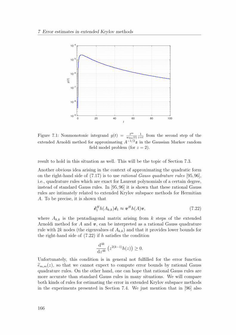
7 Error estimates in extended Krylov methods
t0 20 40 60 80 100
g(t
)
10-9
10-8
10-7
10-6
10-5
10-4
Figure 7.1: Nonmonotonic integrand g(t) = tm
w2m(t)1
z+t from the second step of the
extended Arnoldi method for approximating A−1/2z in the Gaussian Markov randomfield model problem (for z = 2).
result to hold in this situation as well. This will be the topic of Section 7.3.
Another obvious idea arising in the context of approximating the quadratic formon the right-hand side of (7.17) is to use rational Gauss quadrature rules [95,96],i.e., quadrature rules which are exact for Laurent polynomials of a certain degree,instead of standard Gauss rules. In [95, 96] it is shown that these rational Gaussrules are intimately related to extended Krylov subspace methods for HermitianA. To be precise, it is shown that
eH1 h(Ak,k)e1 ≈ vHh(A)v , (7.22)
where Ak,k is the pentadiagonal matrix arising from k steps of the extendedArnoldi method for A and v , can be interpreted as a rational Gauss quadraturerule with 2k nodes (the eigenvalues of Ak,k) and that it provides lower bounds forthe right-hand side of (7.22) if h satisfies the condition
d4k
dz4k(z2(k−1)h(z)
)≥ 0.
Unfortunately, this condition is in general not fulfilled for the error functionem,m(z), so that we cannot expect to compute error bounds by rational Gaussquadrature rules. On the other hand, one can hope that rational Gauss rules aremore accurate than standard Gauss rules in many situations. We will compareboth kinds of rules for estimating the error in extended Krylov subspace methodsin the experiments presented in Section 7.4. We just mention that in [96] also
166
7.3 Restart recovery in extended Krylov methods
rational Gauss–Radau rules are constructed, but we will not go into detail con-cerning this topic here, as the main use of these rules was to bracket vHh(A)v ,which is not possible for h = em,m as just explained.
Naively approximating (7.17) by a rational Gauss rule would not only require ad-ditional multiplications with A but also additional linear system solves. To avoidthis, we will also consider the possibility of using restart recovery for cheaply con-structing the matrix A
(2)k,k corresponding to a secondary extended Arnoldi method
for A and v2m+1 in the next section.
7.3 Restart recovery in extended Krylov methods
In this section we investigate how to compute error estimates with low computa-tional cost based on the representation (7.17) of the error norm in the extendedArnoldi method. We begin by proving a direct generalization of Theorem 6.9 tothe case of extended Krylov methods, which makes use of the fact that polynomialKrylov spaces are subspaces of (suitably chosen) extended Krylov spaces.
Theorem 7.12. Let the columns of Vm+k+1,m+k+1 be the orthonormal basis ofEm+k+1,m+k+1(A, v1) from m+k+1 steps of the extended Arnoldi method for A and
v1 and let Am+k+1,m+k+1 = V Hm+k+1,m+k+1AVm+k+1,m+k+1. Further, let H denote
the matrix resulting from k steps of Arnoldi’s method applied to Am+k+1,m+k+1 and
e2m+1. Then H = H(2)k , where H
(2)k denotes the matrix resulting from k iterations
of Arnoldi’s method for A and v2m+1.
Proof. The proof is completely analogous to the one of Theorem 6.9, using thefact that Kk+1(A, v2m+1) ⊆ Em+k+1,m+1(A, v1) ⊆ Em+k+1,m+k+1(A, v1) becausev2m+1 ∈ Em+1,m+1(A, v1). Therefore it is again possible to represent the Arnoldibasis vectors of Kk+1(A, v2m+1) in terms of the basis Vm+k+1,m+k+1 and proceed toconstruct an Arnoldi relation involving the corresponding coefficient matrix Qk
and the matrix Am+k+1,m+k+1.
The result of Theorem 7.12 shows that restart recovery similar to the polynomialKrylov case is possible in extended methods. The following proposition showsthat in the Hermitian case, it is again not necessary to perform the secondaryLanczos process with the full matrix Am+k+1,m+k+1, but only with a sub-block ofconstant size.
Proposition 7.13. Let the assumptions of Theorem 7.12 hold and let A be Her-mitian positive definite in addition. Then, k iterations of the Lanczos processapplied to the lower right (4k + 1) × (4k + 1) sub-block of Am+k+1,m+k+1 and
167
7 Error estimates in extended Krylov methods
e2k+1 produce the same matrix H(2)k as k iterations of the Lanczos process for
Am+k+1,m+k+1 and e2m+1.
Proof. The result can be proven by carefully investigating the nonzero structure ofthe matrix Am+k+1,m+k+1. The decomposition corresponding to k steps of Lanczosfor Am+k+1,m+k+1 and e2m+1 is given by
Am+k+1,m+k+1Vk = VkH(2)k + h
(2)k+1,kvk+1e
Hk . (7.23)
Given that Am+k+1,m+k+1 is pentadiagonal, H(2)k is tridiagonal and v1 = e2m+1 has
its only nonzero entry at position 2m + 1, by comparing nonzero structures, wefind that vj, j = 2, . . . , k has nonzero entries only in position 2m+1−2j, . . . , 2m+
1+2j. In particular, the rows 1, . . . , 2m−2k of Vk are all zero and do not make acontribution to (7.23) and we can thus omit the corresponding rows and columnsof Am+k+1,m+k+1. Given that the matrix is of size 2(m + k + 1) × 2(m + k + 1),the remaining lower right sub-block is thus of size (2(m+ k + 1)− (2m− 2k))×(2(m+ k + 1)− (2m− 2k)) = (4k + 1)× (4k + 1). In addition, omitting the first2m − 2k rows in e2m+1 ∈ R
2(m+k+1) results in e2k+1 ∈ R4k+1, thus proving the
assertion of the proposition.
We now have all the tools available to be able to use an extended Krylov subspaceanalogue to Algorithm 6.1. We do not give a detailed algorithm here, as it is just astraightforward adaption of the techniques from Algorithm 6.1 to Algorithm 7.1.
It is also possible to use restart recovery to construct the matrix A(2)k,k correspond-
ing to k steps of the extended Arnoldi method for A and v2m+1, instead of the
matrix H(2)k corresponding to standard Arnoldi, which can then be used for com-
puting error estimates based on rational Gauss quadrature via (7.22). Before wecan prove this, we need a few auxiliary results. First, we need to show that thematrix Bm,m = V H
m,mA−1Vm,m fulfills a relation similar to (7.2). A similar result
was shown in [96] (where the authors refer to the matrix Bm,m as the inverseprojection matrix ), but exclusively for the Hermitian case, and for a non-block-wise generation of the basis vectors, which leads to a slightly different nonzerostructure of Bm,m. We therefore give a sketch of the proof of the following resultwhich is adapted to our situation.
Lemma 7.14. Let A ∈ Cn×n be nonsingular, let b ∈ C
n and let the columnsof [Vm,m, v2m+1, v2m+2] be the orthonormal basis of Em,m(A, b) computed by Algo-rithm 7.1. Then the matrix Bm,m = V H
m,mA−1Vm,m satisfies
A−1Vm,m = Vm,mBm,m + [v2m+1, v2m+2]σm,m[e2m−1, e2m]H , (7.24)
where σm,m = [v2m+1, v2m+2]A−1[v2m−1, v2m].
168
7.3 Restart recovery in extended Krylov methods
Proof. For j ≤ 2(m − 1), we have vj ∈ Em−1,m−1(A, b) and thus A−1vj ∈Em,m(A, b). As v1, . . . , v2m form an orthonormal basis of Em,m(A, b), we canthus express A−1vj as
A−1vj =2m∑
i=1
(vHi A
−1vj)vi. (7.25)
Analogously, for 2m − 1 ≤ j ≤ 2m, we have that A−1vj ∈ Em+1,m+1(A, b) andthus
A−1vj =2m+2∑
i=1
(vHi A
−1vj)vi. (7.26)
Recasting (7.25) and (7.26) into matrix form proves the assertion.
Next, we investigate the nonzero structure of Am,m and Bm,m. This is again verysimilar to results already known for the Hermitian case [96, 124], and we refrainfrom giving a proof this time, as it is completely straightforward. One just needsto carefully examine which values of the form vH
i Avj or vHi A
−1vj are known tobe zero, because Avj or A−1vj lies in spanv1, . . . , vi−1, similarly to what wasdone in the proof of Proposition 7.7. By doing so, one finds that
Am,m =
α1,1 α1,2 α1,3 α1,4 α1,5 α1,6 α1,7 · · ·α2,1 α2,2 α2,3 α2,4 α2,5 α2,6 α2,7 · · ·α3,1 α3,2 α3,3 α3,4 α3,5 α3,6 α3,7 · · ·
α4,3 α4,4 α4,5 α4,6 α4,7 · · ·α5,3 α5,4 α5,5 α5,6 α5,7 · · ·
α6,5 α6,6 α6,7 · · ·α7,5 α7,6 α7,7 · · ·
.... . .
(7.27)
and
Bm,m =
β1,1 β1,2 β1,3 β1,4 β1,5 β1,6 β1,7 · · ·β2,1 β2,2 β2,3 β2,4 β2,5 β2,6 β2,7 · · ·
β3,2 β3,3 β3,4 β3,5 β3,6 β3,7 · · ·β4,2 β4,3 β4,4 β4,5 β4,6 β4,7 · · ·
β5,4 β5,5 β5,6 β5,7 · · ·β6,4 β6,5 β6,6 β6,7 · · ·
β7,6 β7,7 · · ·...
.... . .
. (7.28)
We are now in a position to prove a result which can be seen as an extendedKrylov analogue to Lemma 2.23. As Lemma 2.23 has a strong relation to theimplicit Q theorem, cf., e.g, [129, Chapter 2, Theorem 3.3], we can think of thefollowing result as an extended implicit Q theorem. We briefly mention here that
169
7 Error estimates in extended Krylov methods
a version of the implicit Q theorem for general rational Krylov subspaces wasrecently proven in [16]. However, the formulation of the theorem given in [16] isnot compatible with the block-wise generation of the extended Krylov subspace weuse. In addition, the notion of “essential uniqueness” used in [16] is weaker thanwhat we can use here, as extended Krylov subspaces allow for fewer additionaldegrees of freedom than general rational Krylov subspaces. We can thus formulatethe result in a more concise way, which is more reminiscent of the situation facedwhen dealing with polynomial Krylov spaces.
Theorem 7.15. Let A ∈ Cn×n be nonsingular. Assume there exist matrices
[Vm,m, v2m+1, v2m+2], [Vm,m, v2m+1, v2m+2] ∈ Cn×2(m+1) with orthonormal columns
and v1 = v1 as well as matrices Am,m, Am,m and Bm,m, Bm,m with nonzero struc-ture (7.27) and (7.28), respectively, and τm,m, τm,m, σm,m, σm,m ∈ C
2×2 such thatthe relations
AVm,m = Vm,mAm,m + [v2m+1, v2m+2]τm,m[e2m−1, e2m]H , (7.29)
A−1Vm,m = Vm,mBm,m + [v2m+1, v2m+2]σm,m[e2m−1, e2m]H , (7.30)
AVm,m = Vm,mAm,m + [v2m+1, v2m+2]τm,m[e2m−1, e2m]H , (7.31)
A−1Vm,m = Vm,mBm,m + [v2m+1, v2m+2]σm,m[e2m−1, e2m]H (7.32)
hold. Then Vm,m, Am,m, Bm,m are essentially equal to Vm,m, Am,m, Bm,m in thesense that there exists a unitary diagonal matrix Dm = diag(d1, . . . , dm) ∈ C
m×m
with d1 = 1 such that Vm,m = Vm,mDm, Am,m = DHmAm,mDm and Bm,m =
DHmBm,mDm.
Proof. The proof of the theorem, which is constructive, proceeds column by col-umn through the relations (7.29)–(7.32) and defines the values di according tothe assertion of the theorem. We begin by putting d1 = 1. We denote the entriesof Am,m, Am,m, Bm,m and Bm,m by αi,j, αi,j, βi,j and βi,j, respectively.
The first column of (7.30) reads (taking the nonzero structure (7.28) into account)
A−1v1 = β1,1v1 + β2,1v2,
which directly implies that β1,1 = vH1 A
−1v1 and β2,1 = vH2 A
−1v1. In the same way,
the first column of (7.32) implies β1,1 = vH1 A
−1v1. As v1 = v1 by assumption, we
thus have β1,1 = β1,1. Using this fact and rearranging the first columns of (7.30)and (7.32) gives
v2 = (A−1v1 − β1,1v1)/β2,1 and v2 = (A−1v1 − β1,1v1)/β2,1.
This directly shows thatv2 = β2,1/β2,1v2. (7.33)
170
7.3 Restart recovery in extended Krylov methods
Therefore, we set d2 = β2,1/β2,1. As ‖v2‖2 = ‖v2‖2 = 1 we have that |d2| = 1 as
well. Further, β2,1 = β2,1/d2 = d2β2,1.
Next, consider the first column of (7.29) and (7.31), again taking into account itsnonzero structure given in (7.27), i.e.,
Av1 = α1,1v1 + α2,1v2 + α3,1v3 and Av1 = α1,1v1 + α2,1v2 + α3,1v3, (7.34)
which, similarly to the above gives α1,1 = α1,1 = vH1 Av1 and α2,1 = vH
2 Av1.Using (7.33) together with the definition of d2, we further find
α2,1 = vH2 Av1 = d2α2,1.
Rearranging (7.34) gives
v3 = (Av1 − α1,1v1 − α2,1v2)/α3,1 and v3 = (Av1 − α1,1v1 − α2,1v2)/α3,1.
By inserting the relations α2,1 = d2α2,1, v2 = d2v2 and d2d2 = 1, we find
v3 = (Av1 − α1,1v1 − α2,1v2)/α3,1.
showing that v3 = α3,1/α3,1v3, so that we put d3 = α3,1/α3,1. With the samereasoning as for d2, we have |d3| = 1 and α3,1 = d3α3,1. Proceeding similarly withthe second column of (7.29) and (7.31), exploiting the fact that
v1 = d1v1, v2 = d2v2 and v3 = d3v3, (7.35)
direct calculations show that
α1,2 = d1d2α1,2, α2,2 = d2d2α2,2 = α2,2 and α3,2 = d3d2α3,2.
We have thus shown that, with the choices made for di so far, the first two columnsof DH
mAm,mDm and Am,m agree. We proceed with the second columns of (7.30)
and (7.32), which give βi,2 = vHi A
−1v2 and βi,2 = vHi A
−1v2 for i = 1, . . . , 4.Inserting the relations (7.35), as before, yields
β1,2 = d1d2β1,2, β2,2 = d2d2β2,2 = β2,2 and β3,2 = d3d2β3,2. (7.36)
We rearrange the second columns of (7.30) and (7.32) to give
v4 = (A−1v2 − β1,2v1 − β2,2v2 − β3,2v3)/β4,2
andv4 = (A−1v2 − β1,2v1 − β2,2v2 − β3,2v3)/β4,2. (7.37)
Using (7.35) and (7.36), we can rewrite (7.37) as
v4 = (d2A−1v2 − β1,2d2v1 − β2,2d2v2 − β3,2d2v3)/β4,2.
171
7 Error estimates in extended Krylov methods
Thus, v4 = d2β4,2/β4,2v4. Putting d4 = d2β4,2/β4,2, we have β4,2 = d4d2β4,2. Wehave thus also proven the relations from the assertion of the theorem for thefirst two columns of Bm,m and Bm,m. One can now continue in the same way asdemonstrated until here as there is always either one column of (7.29) and (7.31)or one column of (7.30) and (7.32) where the relation vi = divi has already beenshown for all but one of the pairs vi, vi appearing in the equation. This thenallows rearranging the equations such that they prove the assertion for the nextbasis vector. We refrain from explicitly presenting the inductive step here, as itis rather straightforward, but very technical and does not give any more insightthan what was presented up to this point.
With help of Theorem 7.15, we can now finally formulate the result needed forperforming extended restart recovery.
Theorem 7.16. Let A ∈ Cn×n and let the columns of Vm+k+2,m+k+2 be the or-
thonormal basis of Em+k+2,m+k+2(A, v1) from m + k + 2 steps of the extendedArnoldi method for A and v1 and let Am+k+2,m+k+2=V
Hm+k+2,m+k+2AVm+k+2,m+k+2
be nonsingular. Further, let Ak,k denote the matrix resulting from k steps of
the extended Arnoldi method applied to Am+k+2,m+k+2 and e2m+1. Then Ak,k =
DHkA
(2)k,kDk, where A
(2)k,k denotes the matrix resulting from k iterations of the ex-
tended Arnoldi method for A and v2m+1 and Dk is a unitary diagonal matrix withd1,1 = 1.
Proof. The proof proceeds similarly to the one of Theorem 6.9, with the differencethat we have to consider one additional “artificial” extended Arnoldi iteration inorder to find the relation for the inverse projection matrix at the end of the proof.In the remainder of the proof, we use the shorthand notation m = m+ k + 2.
Let the extended Arnoldi decomposition arising from k+ 1 steps of the extendedArnoldi method for A and v2m+1 be given as
AVk+1,k+1 = Vk+1,k+1A(2)k+1,k+1 + [v2k+3, v2k+4]τk+1,k+1[e2k+1, e2k+2]
H . (7.38)
As v2m+1 ∈ Em+1,m+1(A, v1), we obviously have that
Ek+2,k+2(A, v2m+1) ⊆ Em,m(A, v1).
Therefore, the basis vectors v1, . . . , v2k+4 generated by the extended Arnoldimethod for A and v2m+1 all lie in Em,m(A, v1) and can thus be written as lin-ear combinations of the basis vectors v1, . . . , v2m, i.e.,
[Vk+1,k+1, v2k+3, v2k+4] = Vm,m[Qk+1,k+1, q2k+3, q2k+4] (7.39)
for some matrix Qk+1,k+1 ∈ C2m×2(k+1). As [Vk+1,k+1, v2k+3, v2k+4] and Vm,m
both have orthonormal columns, [Qk+1,k+1, q2k+3, q2k+4] must have orthonormal
172
7.3 Restart recovery in extended Krylov methods
columns as well. Inserting (7.39) into the extended Arnoldi decomposition (7.38)gives
AVm,mQk+1,k+1=Vm,mQk+1,k+1A(2)k+1,k+1+Vm,m[q2k+3, q2k+4]τk+1,k+1[e2k+1, e2k+2]
H .
Left-multiplying both sides of this equation by Vm,mVHm,m, the orthogonal projector
onto the space Em,m(A, v1), and using
V Hm,mAVm,m = Am,m
allows to rewrite Vm,mAm,mQk+1,k+1 as
Vm,mQk+1,k+1A(2)k+1,k+1 + Vm,m[q2k+3, q2k+4]τk+1,k+1[e2k+1, e2k+2]
H .
Noting that Vm,m has full (column) rank, this implies
Am,mQk+1,k+1 = Qk+1,k+1A(2)k+1,k+1 + [q2k+3, q2k+4]τk+1,k+1[e2k+1, e2k+2]
H . (7.40)
Repeating the same line of argument starting from the relation (7.24), i.e.,
A−1Vk+1,k+1 = Vk+1,k+1B(2)k+1,k+1 + [v2k+3, v2k+4]σk+1,k+1[e2k+1, e2k+2]
H .
for the inverse projection matrix corresponding to Ek+1,k+1(A, v2m+1) shows thatwe additionally have
Bm,mQk+1,k+1 = Qk+1,k+1B(2)k+1,k+1 + [q2k+3, q2k+4]σk+1,k+1[e2k+1, e2k+2]
H . (7.41)
We further note that we have the following relation involving Am,m and Bm,m
(a similar statement is shown in [96]), found by left-multiplying (7.24) (with mreplaced by m) by V H
m,mA.
I = Am,mBm,m + V Hm,mA[v2m+1, v2m+2]σm,m[e2m−1, e2m]
H
which can be rearranged to
Bm,m = A−1m,m(I − V H
m,mA[v2m+1, v2m+2]σm,m[e2m−1, e2m]H), (7.42)
because Am,m is nonsingular by assumption. Inserting (7.42) into (7.41) anddiscarding the last two columns now finally gives
A−1m+k+1,m+k+1Qk,k = Qk,kB
(2)k,k + [q2k+1, q2k+2]σk,k[e2k−1, e2k]
H , (7.43)
where we use that, due to the nonzero structure of Qk+1,k+1, only the last twocolumns of V H
m,mA[v2m+1, v2m+2]σm,m[e2m−1, e2m]HQk+1,k+1 are nonzero. The re-
lations (7.40) (after also dropping the last two columns) and (7.43) now allow usto use Theorem 7.15 and prove the assertion by noting that q1 = e2m+1.
173
7 Error estimates in extended Krylov methods
Concerning the statement of Theorem 7.16, it is instructive to give some remarks.
Remark 7.17.
(i) While Theorem 7.16 does not guarantee that we exactly retrieve the matrix
A(2)k,k, but D
HkA
(2)k,kDk instead, this does not have an influence on estimates
computed for quadratic forms, as for any function h defined on spec(A(2)k,k)
we have
eH1 h(D
Hk A
(2)k,kDk)e1 = eH
1 DHk h(A
(2)k,k)Dke1 = eH
1 h(A(2)k,k)e1,
using the fact that Dke1 = e1 due to d1,1 = 1.
(ii) It is easily possible to derive a result analogous to Proposition 7.13 forTheorem 7.16. The proof follows in exactly the same way, as it only relieson properties of the basis vectors vi.
(iii) In the statement of Theorem 7.16, we assumed Am+k+2,m+k+2 to be non-singular. Cases in which this condition is always fulfilled are when A isHermitian positive definite, or more general, when A is positive real. Inother cases, it may well happen that Am+k+2,m+k+2 is singular. If this hap-pens, one can instead postpone the computation of error estimates to thenext step (if Am+k+3,m+k+3 happens to be nonsingular again) or just useestimates based on Gauss quadrature, which do not require the inversion ofAm+k+2,m+k+2.
We briefly summarize the results presented in this chapter before we proceedwith numerical experiments illustrating them in the next section. We showedthat it is possible to perform restart recovery in extended Krylov subspace meth-ods, with the possibility to generate either the Hessenberg matrix from a sec-ondary Arnoldi method or the block Hessenberg matrix from a secondary ex-tended Arnoldi method.
In the Hermitian positive definite case, we could further show that this restartrecovery can again be performed with matrices of constant size, so that the com-putation of error estimates is possible with cost independent of the matrix size anditeration number, and that the estimates from pairs of Gauss and Gauss–Radauquadrature form upper and lower bounds for the exact error norm.
7.4 Numerical experiments
In this section, we perform experiments for two of the model problems fromSection 2.6 to illustrate the quality of the error estimates for the extended Arnoldi
174
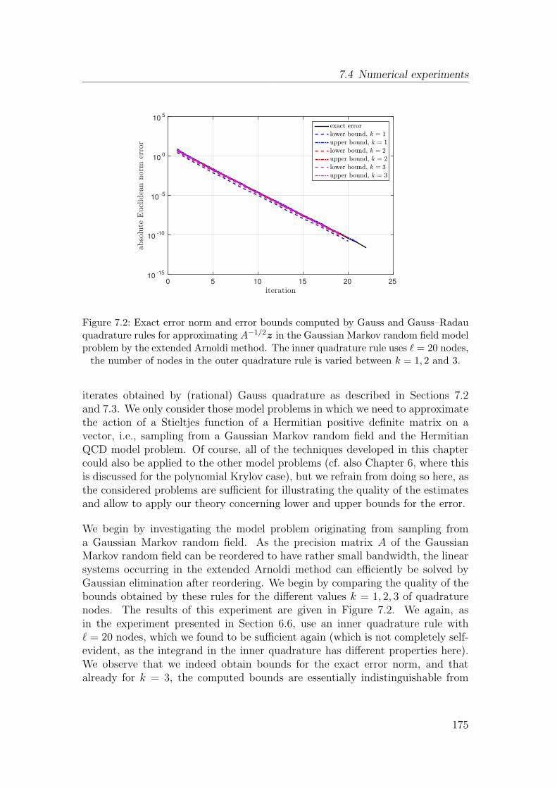
7.4 Numerical experiments
iteration0 5 10 15 20 25
abso
lute
Eucl
idea
nnorm
erro
r
10-15
10-10
10-5
100
105
exact error
lower bound, k = 1
upper bound, k = 1
lower bound, k = 2
upper bound, k = 2
lower bound, k = 3
upper bound, k = 3
Figure 7.2: Exact error norm and error bounds computed by Gauss and Gauss–Radauquadrature rules for approximating A−1/2z in the Gaussian Markov random field modelproblem by the extended Arnoldi method. The inner quadrature rule uses ℓ = 20 nodes,the number of nodes in the outer quadrature rule is varied between k = 1, 2 and 3.
iterates obtained by (rational) Gauss quadrature as described in Sections 7.2and 7.3. We only consider those model problems in which we need to approximatethe action of a Stieltjes function of a Hermitian positive definite matrix on avector, i.e., sampling from a Gaussian Markov random field and the HermitianQCD model problem. Of course, all of the techniques developed in this chaptercould also be applied to the other model problems (cf. also Chapter 6, where thisis discussed for the polynomial Krylov case), but we refrain from doing so here, asthe considered problems are sufficient for illustrating the quality of the estimatesand allow to apply our theory concerning lower and upper bounds for the error.
We begin by investigating the model problem originating from sampling froma Gaussian Markov random field. As the precision matrix A of the GaussianMarkov random field can be reordered to have rather small bandwidth, the linearsystems occurring in the extended Arnoldi method can efficiently be solved byGaussian elimination after reordering. We begin by comparing the quality of thebounds obtained by these rules for the different values k = 1, 2, 3 of quadraturenodes. The results of this experiment are given in Figure 7.2. We again, asin the experiment presented in Section 6.6, use an inner quadrature rule withℓ = 20 nodes, which we found to be sufficient again (which is not completely self-evident, as the integrand in the inner quadrature has different properties here).We observe that we indeed obtain bounds for the exact error norm, and thatalready for k = 3, the computed bounds are essentially indistinguishable from
175
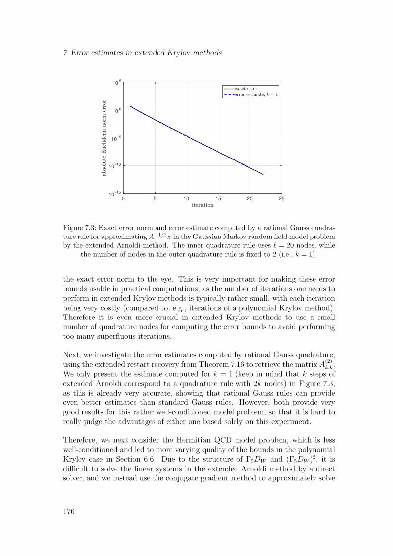
7 Error estimates in extended Krylov methods
iteration0 5 10 15 20 25
abso
lute
Eucl
idea
nnorm
erro
r
10-15
10-10
10-5
100
105
exact error
error estimate, k = 1
Figure 7.3: Exact error norm and error estimate computed by a rational Gauss quadra-ture rule for approximating A−1/2z in the Gaussian Markov random field model problemby the extended Arnoldi method. The inner quadrature rule uses ℓ = 20 nodes, while
the number of nodes in the outer quadrature rule is fixed to 2 (i.e., k = 1).
the exact error norm to the eye. This is very important for making these errorbounds usable in practical computations, as the number of iterations one needs toperform in extended Krylov methods is typically rather small, with each iterationbeing very costly (compared to, e.g., iterations of a polynomial Krylov method).Therefore it is even more crucial in extended Krylov methods to use a smallnumber of quadrature nodes for computing the error bounds to avoid performingtoo many superfluous iterations.
Next, we investigate the error estimates computed by rational Gauss quadrature,using the extended restart recovery from Theorem 7.16 to retrieve the matrix A
(2)k,k.
We only present the estimate computed for k = 1 (keep in mind that k steps ofextended Arnoldi correspond to a quadrature rule with 2k nodes) in Figure 7.3,as this is already very accurate, showing that rational Gauss rules can provideeven better estimates than standard Gauss rules. However, both provide verygood results for this rather well-conditioned model problem, so that it is hard toreally judge the advantages of either one based solely on this experiment.
Therefore, we next consider the Hermitian QCD model problem, which is lesswell-conditioned and led to more varying quality of the bounds in the polynomialKrylov case in Section 6.6. Due to the structure of Γ5DW and (Γ5DW )2, it isdifficult to solve the linear systems in the extended Arnoldi method by a directsolver, and we instead use the conjugate gradient method to approximately solve
176
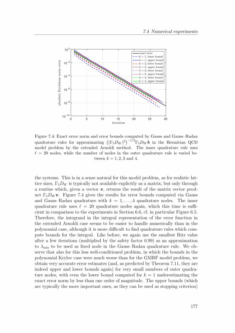
7.4 Numerical experiments
iteration0 5 10 15 20 25 30
abso
lute
Eucl
idea
nnorm
erro
r
10-10
10-8
10-6
10-4
10-2
100
exact error
k = 1, lower bound
k = 1, upper bound
k = 2, lower bound
k = 2, upper bound
k = 3, lower bound
k = 3, upper bound
k = 4, lower bound
k = 4, upper bound
Figure 7.4: Exact error norm and error bounds computed by Gauss and Gauss–Radau
quadrature rules for approximating((Γ5DW )2
)−1/2Γ5DWb in the Hermitian QCD
model problem by the extended Arnoldi method. The inner quadrature rule usesℓ = 20 nodes, while the number of nodes in the outer quadrature rule is varied be-
tween k = 1, 2, 3 and 4.
the systems. This is in a sense natural for this model problem, as for realistic lat-tice sizes, Γ5DW is typically not available explicitly as a matrix, but only througha routine which, given a vector v , returns the result of the matrix vector prod-uct Γ5DWv . Figure 7.4 gives the results for error bounds computed via Gaussand Gauss–Radau quadrature with k = 1, . . . , 4 quadrature nodes. The innerquadrature rule uses ℓ = 20 quadrature nodes again, which this time is suffi-cient in comparison to the experiments in Section 6.6, cf. in particular Figure 6.5.Therefore, the integrand in the integral representation of the error function inthe extended Arnoldi case seems to be easier to handle numerically than in thepolynomial case, although it is more difficult to find quadrature rules which com-pute bounds for the integral. Like before, we again use the smallest Ritz valueafter a few iterations (multiplied by the safety factor 0.99) as an approximationto λmin to be used as fixed node in the Gauss–Radau quadrature rule. We ob-serve that also for this less well-conditioned problem, in which the bounds in thepolynomial Krylov case were much worse than for the GMRF model problem, weobtain very accurate error estimates (and, as predicted by Theorem 7.11, they areindeed upper and lower bounds again) for very small numbers of outer quadra-ture nodes, with even the lower bound computed for k = 1 underestimating theexact error norm by less than one order of magnitude. The upper bounds (whichare typically the more important ones, as they can be used as stopping criterion)
177
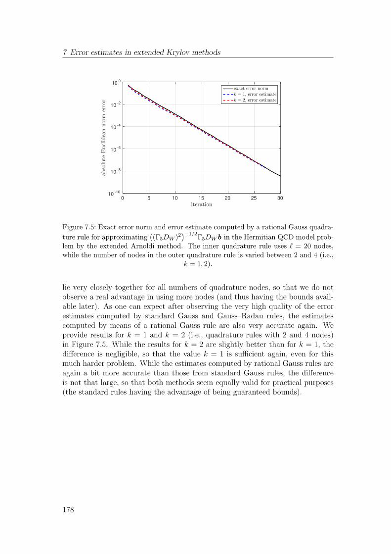
7 Error estimates in extended Krylov methods
iteration0 5 10 15 20 25 30
abso
lute
Eucl
idea
nnorm
erro
r
10-10
10-8
10-6
10-4
10-2
100
exact error norm
k = 1, error estimate
k = 2, error estimate
Figure 7.5: Exact error norm and error estimate computed by a rational Gauss quadra-
ture rule for approximating((Γ5DW )2
)−1/2Γ5DWb in the Hermitian QCD model prob-
lem by the extended Arnoldi method. The inner quadrature rule uses ℓ = 20 nodes,while the number of nodes in the outer quadrature rule is varied between 2 and 4 (i.e.,
k = 1, 2).
lie very closely together for all numbers of quadrature nodes, so that we do notobserve a real advantage in using more nodes (and thus having the bounds avail-able later). As one can expect after observing the very high quality of the errorestimates computed by standard Gauss and Gauss–Radau rules, the estimatescomputed by means of a rational Gauss rule are also very accurate again. Weprovide results for k = 1 and k = 2 (i.e., quadrature rules with 2 and 4 nodes)in Figure 7.5. While the results for k = 2 are slightly better than for k = 1, thedifference is negligible, so that the value k = 1 is sufficient again, even for thismuch harder problem. While the estimates computed by rational Gauss rules areagain a bit more accurate than those from standard Gauss rules, the differenceis not that large, so that both methods seem equally valid for practical purposes(the standard rules having the advantage of being guaranteed bounds).
178
CHAPTER 8
CONCLUSIONS & OUTLOOK
In this thesis, we presented several new results arising from a new integral rep-resentation of the error in Arnoldi’s method (and related methods such as theextended and harmonic Arnoldi method). This error representation allows toresolve some of the most prominent disadvantages from which Krylov subspacemethods for the approximation of matrix functions typically suffer.
In particular, we presented a quadrature-based restart approach for Arnoldi’smethod, which allows to overcome the memory constraints that often prevent asufficient number of iterations to be performed in the unrestarted case. The pre-sented method is, to our knowledge, the only restarted Krylov subspace methodfor f(A)b proposed so far which combines numerical stability and constant com-putational work per cycle and at the same time acts as a black-box solver for alarge class of functions.
Besides algorithmic questions concerning stability and efficient implementation,we presented a theoretical analysis of the convergence behavior of the restartedArnoldi method for the approximation of Stieltjes matrix functions using as toolsthe intimate relation between Stieltjes functions and shifted linear systems, allow-ing to generalize convergence results for the (shifted restarted) conjugate gradientmethod to our setting. The main result of this analysis was that the restartedArnoldi method converges to f(A)b for every restart lengthm ≥ 1 when A is Her-mitian positive definite. We also motivated that one cannot expect this result tobe generalizable to larger classes of matrices. As a by-product of this analysis, wepresented some results on the arbitrary convergence behavior of the restarted fullorthogonalization method and the restarted GMRES method for linear systems.To overcome the limitations just mentioned, we proposed using a slight variationof Arnoldi’s method, the restarted harmonic Arnoldi method (which reduces to
179
8 Conclusions & Outlook
restarted GMRES in the linear system case) for which we could prove convergencefor every restart length m ≥ 1 for the larger class of (possibly non-Hermitian)positive real matrices.
The other main application of our integral representation for the Arnoldi error wasthe efficient computation of error bounds and estimates using Gauss quadrature.In particular, we showed that it is possible to compute guaranteed error boundsarising from nested quadrature rules when f is a Stieltjes function and A is Her-mitian positive definite. These bounds can, e.g., be used as stopping criterion inArnoldi’s method. By making use of the so-called Lanczos restart recovery, wedemonstrated that the construction of these bounds can be incorporated into theLanczos method with computational cost independent of the dimension n of thematrix A and the iteration number m, such that they are available essentiallyfor free in cases where n is large. We also briefly sketched that it is possibleto transfer the error estimation approach to the case of non-Hermitian matricesand/or functions other than Stieltjes functions, although one has no guaranteethat one computes bounds in these cases and the cost of computing the estimatesincreases proportionally to the iteration number in Arnoldi’s method.
In the final chapter of this thesis, we showed how to transfer some of our resultsto extended Krylov subspace methods. For these methods, a similar integralrepresentation for the error as in the polynomial Krylov case exists and it istherefore possible to transfer most of the results of this thesis to this related classof methods. As restarting is not very relevant in the extended Krylov case (asone typically only uses extended Krylov methods if they converge to the desiredaccuracy in a small number of iterations), we mainly focused on the computationof error estimates. We showed that it is again possible to compute lower andupper bounds for the error norm in these methods by Gauss and Gauss–Radauquadrature when A is Hermitian positive definite. We also investigated the pos-sibility to use rational Gauss quadrature rules for error estimation, which led tovery accurate results but does not allow to compute guaranteed error bounds.
Topics for future research include a more thorough and in-depth treatment ofintegral representations for the error for extended and especially general rationalKrylov methods and the possibilities they offer. Another topic that could be cov-ered is a convergence analysis for (restarted or unrestarted) extended or rationalKrylov methods based on our error representation, which could maybe comple-ment other analysis approaches available in the literature so far which typicallyrely on other tools than the ones used in this thesis.
A further topic which seems very relevant and appealing, especially from a practi-tioner’s point of view, is the comparison of the efficiency of our restart approach toother techniques frequently used to overcome the memory limitations of Arnoldi’s
180

method. These techniques include, e.g., the already mentioned extended and ra-tional Krylov methods or the shifted conjugate gradient method applied to arational approximation of f in partial fraction form (when A is Hermitian pos-itive definite). As these methods all have (at least partially) the same goal butreach it in different ways, it is not at all clear whether one method is superior tothe others in general or whether this depends on some (and which) properties ofthe problem at hand. A comparison of this kind should include meaningful nu-merical experiments as well as theoretical evidence for the observed behavior andgive guidelines for deciding in which cases the presented methods should reallybe used in practice.
181

LIST OF FIGURES
2.1 Midpoint and trapezoidal rule . . . . . . . . . . . . . . . . . . . . 37
4.1 Parabolic contour from [135] . . . . . . . . . . . . . . . . . . . . . 76
4.2 Parabolic contour used in our restarted Arnoldi method . . . . . . 77
4.3 Restarting for negative discrete Laplace operator and f(z) = eθz . 79
4.4 Restarting for semi-discretization of a convection diffusion equationand f(z) = eθz . . . . . . . . . . . . . . . . . . . . . . . . . . . . . 80
4.5 Restarting for discrete Laplace operator and f(z) = e−θ√z−1
z. . . . 81
4.6 Restarting for Hermitian QCD model problem . . . . . . . . . . . 83
4.7 Restarting for non-Hermitian QCD model problem . . . . . . . . 84
4.8 Restarting for GMRF model problem . . . . . . . . . . . . . . . . 85
5.1 Divergence of restarted Arnoldi for a normal, positive real matrix 99
5.2 Convergence curves of restarted Arnoldi and restarted harmonicArnoldi for the matrix from Example 5.14 . . . . . . . . . . . . . 106
5.3 Convergence of (restarted) Arnoldi for diagonal Hpd matrix withChebyshev eigenvalues . . . . . . . . . . . . . . . . . . . . . . . . 116
5.4 Convergence of (restarted) Arnoldi for diagonal Hpd matrix withequidistantly spaced eigenvalues . . . . . . . . . . . . . . . . . . . 117
5.5 Convergence of restarted (harmonic) Arnoldi for diagonal positivereal matrix . . . . . . . . . . . . . . . . . . . . . . . . . . . . . . . 118
183
LIST OF FIGURES
5.6 Convergence of restarted (harmonic) Arnoldi for block diagonalJordan matrix . . . . . . . . . . . . . . . . . . . . . . . . . . . . . 119
6.1 Error bounds for GMRF model problem . . . . . . . . . . . . . . 140
6.2 Error bounds for restarted Arnoldi for GMRF model problem . . 142
6.3 Error bounds for Hermitian QCD model problem using at mostℓ = 100 inner quadrature nodes . . . . . . . . . . . . . . . . . . . 143
6.4 Comparison of iteration number for which convergence is detectedfor different k in the Hermitian QCD model problem . . . . . . . 144
6.5 Error bounds for Hermitian QCD model problem using ℓ = 20inner quadrature nodes . . . . . . . . . . . . . . . . . . . . . . . . 145
6.6 Error bounds for restarted Arnoldi for Hermitian QCD model prob-lem . . . . . . . . . . . . . . . . . . . . . . . . . . . . . . . . . . . 146
6.7 Approximate error bounds for discrete Laplace operator and f(z) =e−θ
√z−1
z. . . . . . . . . . . . . . . . . . . . . . . . . . . . . . . . . 147
6.8 Approximate error bounds for negative discrete Laplace operatorand f(z) = eθz . . . . . . . . . . . . . . . . . . . . . . . . . . . . . 148
6.9 Error estimates for semi-discretization of a convection diffusionequation and f(z) = eθz . . . . . . . . . . . . . . . . . . . . . . . 149
6.10 Error bounds for non-Hermitian QCDmodel problem using at mostℓ = 100 inner quadrature nodes . . . . . . . . . . . . . . . . . . . 151
7.1 Integrand in extended Arnoldi for the GMRF model problem . . . 166
7.2 Error bounds for extended Arnoldi and the GMRF model problem 175
7.3 Rational Gauss error estimates for the GMRF model problem . . 176
7.4 Error bounds for extended Arnoldi and the Hermitian QCD modelproblem . . . . . . . . . . . . . . . . . . . . . . . . . . . . . . . . 177
7.5 Rational Gauss error estimates for the Hermitian QCD model prob-lem . . . . . . . . . . . . . . . . . . . . . . . . . . . . . . . . . . . 178
184
LIST OF TABLES
6.1 Comparison of the bounds computed for different numbers ℓ ofinner quadrature nodes for the GMRF model problem . . . . . . . 141
6.2 Comparison of the bounds computed for different numbers ℓ ofinner quadrature nodes for the Hermitian QCD model problem . . 145
185
LIST OF ALGORITHMS
2.1 Arnoldi’s method . . . . . . . . . . . . . . . . . . . . . . . . . . . . 20
2.2 Lanczos method . . . . . . . . . . . . . . . . . . . . . . . . . . . . 22
2.3 Restarted full orthogonalization method . . . . . . . . . . . . . . . 28
2.4 Conjugate gradient method . . . . . . . . . . . . . . . . . . . . . . 30
4.1 Restarted Arnoldi method for f(A)b (generic version). . . . . . . . 62
4.2 Restarted Arnoldi method for f(A)b from [3]. . . . . . . . . . . . . 64
4.3 Quadrature-based restarted Arnoldi method for f(A)b. . . . . . . . 68
6.1 Lanczos method for f(A)b with error bounds . . . . . . . . . . . . 132
6.2 Arnoldi’s method for f(A)b with error estimate . . . . . . . . . . . 137
7.1 Block-wise extended Arnoldi method . . . . . . . . . . . . . . . . . 156
186
LIST OF NOTATIONS
Throughout this thesis, scalars are denoted by lower-case letters, matrices aredenoted by upper-case letters and vectors are denoted by lower-case, bold-faceletters. In addition, the following notations are used.
R the field of real numbersR
+ the positive real axis (0,∞)R
− the negative real axis (−∞, 0)R
+/−0 the positive/negative real axis including 0
C the field of complex numbersα the complex conjugate of the scalar α ∈ C
Kn the n-dimensional Euclidean vector space over the field K
Km×n the space of m× n matrices over the field K
vm a vector related to the mth iteration of an iterative method
v(k)m
a vector related to the mth iteration of the kth cycle of arestarted iterative method
v(i) the ith entry of the vector vv(i : j) the entries i, i+ 1, . . . , j of the vector v‖v‖2 the Euclidean norm of the vector v0 the vector of all zeros1 the vector of all onesI the identity matrixAH the complex adjoint of the matrix AA−1 the inverse of the nonsingular matrix Aaij the (i, j)th entry of the matrix AW(A) the field of values of the matrix Adiag(α1, . . . , αn) The diagonal matrix with diagonal entries α1, . . . , αn
diag(A1, . . . , An) The block-diagonal matrix with diagonal blocks A1, . . . , An
∆ the Laplace differential operator∂Ω the boundary of the domain ΩA⊗ B the Kronecker product of the matrices A and B
187
BIBLIOGRAPHY
[1] M. Abramowitz and I. A. Stegun, Handbook of Mathematical Func-tions: With Formulas, Graphs, and Mathematical Tables, Dover Publica-tions, New York, 1964.
[2] M. Afanasjew, M. Eiermann, O. G. Ernst, and S. Guttel, Ageneralization of the steepest descent method for matrix functions, Electron.Trans. Numer. Anal., 28 (2008), pp. 206–222.
[3] , Implementation of a restarted Krylov subspace method for the evalua-tion of matrix functions, Linear Algebra Appl., 429 (2008), pp. 2293–2314.
[4] G. D. Allen, C. K. Chui, W. R. Madych, F. J. Narcowich, and
P. W. Smith, Pade approximation and Gaussian quadrature, Bull. Aust.Math. Soc., 11 (1974), pp. 63–69.
[5] H. Alzer and C. Berg, Some classes of completely monotonic functions,Ann. Acad. Sci. Fenn., Math., 27 (2002), pp. 445–460.
[6] W. E. Arnoldi, The principle of minimized iteration in the solution ofthe matrix eigenvalue problem, Q. Appl. Math., 9 (1951), pp. 17–29.
[7] O. Axelsson and J. Karatson, Reaching the superlinear convergencephase of the CG method, J. Comput. Appl. Math., 260 (2014), pp. 244–257.
[8] G. A. Baker, The existence and convergence of subsequences of Padeapproximants, J. Math. Anal. Appl., 43 (1973), pp. 498–528.
[9] , Essentials of Pade Approximants, Academic Press, New York, 1975.
[10] G. A. Baker and P. Graves-Morris, Pade Approximants, 2nd edition,Cambridge University Press, Cambridge, 1996.
188
BIBLIOGRAPHY
[11] B. Beckermann and S. Guttel, Superlinear convergence of the rationalArnoldi method for the approximation of matrix functions, Numer. Math.,121 (2012), pp. 205–236.
[12] B. Beckermann and A. B. J. Kuijlaars, Superlinear convergence ofconjugate gradients, SIAM J. Numer. Anal., 39 (2001), pp. 300–329.
[13] , Superlinear CG convergence for special right-hand sides, Electron.Trans. Numer. Anal., 14 (2002), pp. 1–19.
[14] C. Berg, Stieltjes-Pick-Bernstein-Schoenberg and their connection to com-plete monotonicity, in Positive Definite Functions. From Schoenberg toSpace-Time Challenges, J. Mateu and E. Porcu, eds., Dept. of Mathematics,University Jaume I, Castellon de la Plana, Spain, 2008.
[15] C. Berg and G. Forst, Potential Theory on Locally Compact AbelianGroups, Springer, Berlin Heidelberg, 1975.
[16] M. Berljafa and S. Guttel, Generalized rational Krylov decomposi-tions with an application to rational approximation, SIAM J. Matrix Anal.Appl., 36 (2015), pp. 894–916.
[17] S. Birk, Deflated Shifted Block Krylov Subspace Methods for HermitianPositive Definite Matrices, PhD thesis, Bergische Universitat Wuppertal,2015.
[18] J. Bloch, A. Frommer, B. Lang, and T. Wettig, An iterative methodto compute the sign function of a non-Hermitian matrix and its applicationto the overlap Dirac operator at nonzero chemical potential, Comput. Phys.Commun., 177 (2007), pp. 933–943.
[19] R. P. Boas, Entire Functions, Academic Press, New York, 1954.
[20] J. Brannick, A. Frommer, K. Kahl, B. Leder, M. Rottmann, and
A. Strebel, Multigrid preconditioning for the overlap operator in latticeQCD, Numer. Math., (2015). to appear.
[21] C. Brezinski, From numerical quadrature to Pade approximation, Appl.Numer. Math., 60 (2010), pp. 1209–1220.
[22] P. Brown, A theoretical comparison of the Arnoldi and GMRES algo-rithms, SIAM J. Sci. Stat. Comput., 12 (1991), pp. 58–78.
[23] K. Burrage, N. Hale, and D. Kay, An efficient implicit FEM schemefor fractional-in-space reaction-diffusion equations, SIAM J. Sci. Comput.,34 (2012), pp. A2145–A2172.
[24] D. Calvetti, S. Kim, and L. Reichel, Quadrature rules based on theArnoldi process, SIAM J. Matrix Anal. Appl., 26 (2005), pp. 765–781.
189
BIBLIOGRAPHY
[25] A. J. Carpenter, A. Ruttan, and R. S. Varga, Extended numericalcomputations on the “1/9” conjecture in rational approximation theory, inRational Approximation and Interpolation, Proceedings, Tampa, Florida1983, Lecture Notes in Mathematics, vol. 1105, P. Graves-Morris, E. B.Saff, and R. S. Varga, eds., Springer, Berlin Heidelberg, 1984, pp. 383–411.
[26] M. Carter and B. van Brunt, The Lebesgue–Stieltjes Integral — APractical Introduction, Springer, New York, 2000.
[27] W. J. Cody, G. Meinardus, and R. S. Varga, Chebyshev rational ap-proximation to e−x in [0,+∞) and applications to heat-conduction problems,J. Approx. Theory, 2 (1969), pp. 50–65.
[28] N. A. C. Cressie, Statistics for Spatial Data, Wiley Series in Probabilityand Mathematical Statistics. John Wiley & Sons, New York, 1993.
[29] J. Cullum, Iterative methods for solving Ax = b, GMRES/FOM versusQMR/BiCG, Adv. Comput. Math., 6 (1996), pp. 1–24.
[30] J. Cullum and A. Greenbaum, Relations between Galerkin and norm-minimizing iterative methods for solving linear systems, SIAM J. MatrixAnal. Appl., 17 (1996), pp. 223–247.
[31] N. Cundy, J. van den Eshof, A. Frommer, S. Krieg, Th. Lippert,
and K. Schafer, Numerical methods for the QCD overlap operator: III.Nested iterations, Comput. Phys. Commun., 165 (2005), pp. 221–242.
[32] P. I. Davies and N. J. Higham, A Schur–Parlett algorithm for computingmatrix functions, SIAM J. Matrix Anal. Appl., 25 (2003), pp. 464–485.
[33] P. J. Davis and P. Rabinowitz, Methods of Numerical Integration, Aca-demic Press, New York, 1975.
[34] C. de Boor, Divided differences, Surv. Approx. Theory, 1 (2005), pp. 46–69.
[35] P. A. M. Dirac, The Principles of Quantum Mechanics, 4th edition, Ox-ford University Press, Oxford, 1958.
[36] V. Druskin, On monotonicity of the Lanczos approximation to the matrixexponential, Linear Algebra Appl., 429 (2008), pp. 1679–1683.
[37] V. Druskin and L. Knizhnerman, Two polynomial methods of calculat-ing functions of symmetric matrices, U.S.S.R. Comput. Math. Math. Phys.,29 (1989), pp. 112–121.
[38] V. Druskin and L. Knizhnerman, Extended Krylov subspaces: Approx-imation of the matrix square root and related functions, SIAM J. MatrixAnal. Appl., 19 (1998), pp. 755–771.
190
BIBLIOGRAPHY
[39] J. Duintjer Tebbens and G. Meurant, Any Ritz value behavior is pos-sible for Arnoldi and for GMRES, SIAM J. Matrix Anal. Appl., 33 (2012),pp. 958–978.
[40] , On the admissible convergence curves for restarted GMRES, tech.rep., Department of Computational Methods, Institute of Computer Sci-ence, Academy of Sciences of the Czech Republic, 2014.
[41] A. Dutt, L. Greengard, and V. Rokhlin, Spectral deferred correctionmethods for ordinary differential equations, BIT, 40 (2000), pp. 241–266.
[42] M. Eiermann and O. G. Ernst, Geometric aspects of the theory ofKrylov subspace methods, Acta Numerica, 10 (2001), pp. 251–312.
[43] M. Eiermann and O. G. Ernst, A restarted Krylov subspace methodfor the evaluation of matrix functions, SIAM J. Numer. Anal., 44 (2006),pp. 2481–2504.
[44] M. Eiermann, O. G. Ernst, and S. Guttel, Deflated restarting formatrix functions, SIAM J. Matrix Anal. Appl., 32 (2011), pp. 621–641.
[45] M. Embree, The tortoise and the hare restart GMRES, SIAM Rev., 45(2003), pp. 259–266.
[46] H. Engels, Numerical Quadrature and Cubature, Academic Press, London,1980.
[47] Th. Ericsson, Computing functions of matrices using Krylov subspacemethods, tech. rep., Chalmers University of Technology, Goteborg, Sweden,1990.
[48] J. van den Eshof, A. Frommer, Th. Lippert, K. Schilling, and
H. A. van der Vorst, Numerical methods for the QCD overlap operator.I. Sign-function and error bounds, Comput. Phys. Commun., 146 (2002),pp. 203–224.
[49] E. Estrada and D. J. Higham, Network properties revealed throughmatrix functions, SIAM Rev., 52 (2010), pp. 696–714.
[50] M. Freund and E. Gorlich, Polynomial approximation of an entirefunction and rate of growth of Taylor coefficients, Proc. Edinb. Math. Soc.,28 (1985), pp. 341–348.
[51] R. W. Freund and M. Hochbruck, Gauss quadrature associated withthe Arnoldi process and the Lanczos algorithm, in Linear Algebra for LargeScale and Real-Time Applications, M. S. Moonen, G. H. Golub, and B. L. R.De Moor, eds., Kluwer Academic Publishers, Dordrecht, 1993, pp. 377–380.
191
BIBLIOGRAPHY
[52] R. W. Freund and N. M. Nachtigal, QMR: a quasi-minimal resid-ual method for non-Hermitian linear systems, Numer. Math., 60 (1991),pp. 315–339.
[53] G. Frobenius, Ueber Relationen zwischen den Naherungsbruchen vonPotenzreihen, J. Reine Angew. Math., 90 (1881), pp. 1–17.
[54] A. Frommer, BiCGStab(ℓ) for families of shifted linear systems, Comput-ing, 70 (2003), pp. 87–109.
[55] , Monotone convergence of the Lanczos approximations to matrix func-tions of Hermitian matrices, Electron. Trans. Numer. Anal., 35 (2009),pp. 118–128.
[56] A. Frommer and U. Glassner, Restarted GMRES for shifted linearsystems, SIAM J. Sci. Comput., 19 (1998), pp. 15–26.
[57] A. Frommer, S. Guttel, and M. Schweitzer, Convergence ofrestarted Krylov subspace methods for Stieltjes functions of matrices, SIAMJ. Matrix Anal. Appl., 35 (2014), pp. 1602–1624.
[58] A. Frommer, S. Guttel, and M. Schweitzer, Efficient and stableArnoldi restarts for matrix functions based on quadrature, SIAM J. MatrixAnal. Appl., 35 (2014), pp. 661–683.
[59] A. Frommer, S. Guttel, and M. Schweitzer, FUNM QUAD: Animplementation of a stable, quadrature-based restarted Arnoldi methodfor matrix functions, tech. rep., Bergische Universitat Wuppertal, 2014.available at http://www.imacm.uni-wuppertal.de/fileadmin/imacm/
preprints/2014/imacm_14_04.pdf.
[60] A. Frommer, K. Kahl, S. Krieg, B. Leder, and M. Rottmann,Adaptive aggregation-based domain decomposition multigrid for the latticeWilson–Dirac operator, SIAM J. Sci. Comput., 36 (2014), pp. A1581–A1608.
[61] A. Frommer, K. Kahl, Th. Lippert, and H. Rittich, 2-norm errorbounds and estimates for Lanczos approximations to linear systems andrational matrix functions, SIAM J. Matrix Anal. Appl., 34 (2013), pp. 1046–1065.
[62] A. Frommer and P. Maass, Fast CG-based methods for Tikhonov–Phillips regularization, SIAM J. Sci. Comput., 20 (1999), pp. 1831–1850.
[63] A. Frommer and M. Schweitzer, Error bounds and estimatesfor Krylov subspace approximations of Stieltjes matrix functions,tech. rep., Bergische Universitat Wuppertal, 2015. available athttp://www.imacm.uni-wuppertal.de/fileadmin/imacm/preprints/
2015/imacm_15_21.pdf.
192
BIBLIOGRAPHY
[64] A. Frommer and V. Simoncini, Matrix functions, in Model Order Re-duction: Theory, Research Aspects and Applications, W. H. A. Schilders,H. A. van der Vorst, and J. Rommes, eds., Springer, Berlin Heidelberg,2008, pp. 275–303.
[65] , Stopping criteria for rational matrix functions of Hermitian and sym-metric matrices, SIAM J. Sci. Comput., 30 (2008), pp. 1387–1412.
[66] , Error bounds for Lanczos approximations of rational functions of ma-trices, in Numerical Validation in Current Hardware Architectures, A. Cuyt,W. Kramer, W. Luther, and P. Markstein, eds., Springer, Berlin Heidelberg,2009, pp. 203–216.
[67] E. Gallopoulos and Y. Saad, Efficient solution of parabolic equationsby Krylov approximation methods, SIAM J. Sci. Stat. Comput., 13 (1992),pp. 1236–1264.
[68] W. Gautschi, Quadrature formulae on half-infinite intervals, BIT, 31(1991), pp. 438–446.
[69] , Orthogonal Polynomials: Computation and Approximation, OxfordUniversity Press, Oxford, 2004.
[70] P. H. Ginsparg and K. G. Wilson, A remnant of chiral symmetry onthe lattice, Phys. Rev. D, 25 (1982), pp. 2649–2657.
[71] G. H. Golub and Ch. F. van Loan, Matrix Computations, 3rd edition,Johns Hopkins University Press, Baltimore and London, 1996.
[72] G. H. Golub and G. Meurant, Matrices, moments and quadrature, inNumerical Analysis 1993, D. F. Griffiths and G. A. Watson, eds., Essex,1994, Longman Scientific & Technical, pp. 105–156.
[73] , Matrices, moments and quadrature II; How to compute the norm ofthe error in iterative methods, BIT, 37 (1997), pp. 687–705.
[74] , Matrices, Moments and Quadrature with Applications, Princeton Uni-versity Press, Princeton and Oxford, 2010.
[75] G. H. Golub and J. H. Welsch, Calculation of Gauss quadrature rules,Math. Comput., 23 (1969), pp. 221–230+s1–s10.
[76] S. Goossens and D. Roose, Ritz and harmonic Ritz values and theconvergence of FOM and GMRES, Numer. Linear Algebra Appl., 6 (1999),pp. 281–293.
[77] A. Greenbaum, Iterative Methods for Solving Linear Systems, SIAM,Philadelphia, 1997.
193
BIBLIOGRAPHY
[78] A. Greenbaum, V. Ptak, and Z. Strakos, Any nonincreasing conver-gence curve is possible for GMRES, SIAM J. Matrix Anal. Appl., 17 (1996),pp. 465–469.
[79] A. Greenbaum and Z. Strakos, Predicting the behavior of finite preci-sion Lanczos and conjugate gradient computations, SIAM J. Matrix Anal.Appl., 13 (1992), pp. 121–137.
[80] S. Guttel, Rational Krylov Methods for Operator Functions, PhD the-sis, Fakultat fur Mathematik und Informatik der Technischen UniversitatBergakademie Freiberg, 2010.
[81] S. Guttel, Rational Krylov approximation of matrix functions: Numericalmethods and optimal pole selection, GAMM-Mitt., 36 (2013), pp. 8–31.
[82] S. Guttel and L. Knizhnerman, A black-box rational Arnoldi variantfor Cauchy–Stieltjes matrix functions, BIT, 53 (2013), pp. 595–616.
[83] P. Henrici, Applied and Computational Complex Analysis, Vol. 2, JohnWiley & Sons, New York, 1977.
[84] M. R. Hestenes and E. Stiefel, Methods of conjugate gradients forsolving linear systems, J. Res. Natl. Bur. Stand., 49 (1952), pp. 409–436.
[85] N. J. Higham, Functions of Matrices: Theory and Computation, SIAM,Philadelphia, 2008.
[86] N. J. Higham and A. H. Al-Mohy, Computing matrix functions, ActaNumerica, 19 (2010), pp. 159–208.
[87] M. Hochbruck and M. E. Hochstenbach, Subspace extraction formatrix functions, tech. rep., Case Western Reserve University, Departmentof Mathematics, Cleveland, 2005.
[88] M. Hochbruck and Ch. Lubich, On Krylov subspace approximationsto the matrix exponential operator, SIAM J. Numer. Anal., 34 (1997),pp. 1911–1925.
[89] M. Hochbruck, Ch. Lubich, and H. Selhofer, Exponential integra-tors for large systems of differential equations, SIAM J. Sci. Comput., 19(1998), pp. 1552–1574.
[90] M. Hochbruck and A. Ostermann, Exponential integrators, Acta Nu-merica, 19 (2010), pp. 209–286.
[91] R. A. Horn and Ch. R. Johnson, Topics in Matrix Analysis, CambridgeUniversity Press, Cambridge, 1991.
194
BIBLIOGRAPHY
[92] M. Ilic, I. W. Turner, and A. N. Pettitt, Bayesian computationsand efficient algorithms for computing functions of large, sparse matrices,ANZIAM J., 45 (2004), pp. C504–C518.
[93] M. Ilic, I. W. Turner, and D. P. Simpson, A restarted Lanczos ap-proximation to functions of a symmetric matrix, IMA J. Numer. Anal., 30(2010), pp. 1044–1061.
[94] C. Jagels and L. Reichel, The extended Krylov subspace method andorthogonal Laurent polynomials, Linear Algebra Appl., 431 (2009), pp. 441–458.
[95] , Recursion relations for the extended Krylov subspace method, LinearAlgebra Appl., 434 (2011), pp. 1716–1732.
[96] , The structure of matrices in rational Gauss quadrature, Math. Com-put., 82 (2013), pp. 2035–2060.
[97] W. Joubert, On the convergence behavior of the restarted GMRES al-gorithm for solving nonsymmetric linear systems, Numer. Linear AlgebraAppl., 1 (1994), pp. 427–447.
[98] L. Knizhnerman, Calculation of functions of unsymmetric matrices usingArnoldi’s method, Zh. Vychisl. Mat. Mat. Fiz., 31 (1991), pp. 1–9.
[99] L. Knizhnerman and V. Simoncini, A new investigation of the extendedKrylov subspace method for matrix function evaluations, Numer. Linear Al-gebra Appl., 17 (2010), pp. 615–638.
[100] A. R. Krommer and Ch. W. Ueberhuber, Computational Integration,SIAM, Philadelphia, 1998.
[101] A. B. J. Kuijlaars, Which eigenvalues are found by the Lanczos method?,SIAM J. Matrix Anal. Appl., 22 (2000), pp. 306–321.
[102] C. Lanczos, An iteration method for the solution of the eigenvalue problemof linear differential and integral operators, J. Res. Natl. Stand., 45 (1950),pp. 255–282.
[103] R. C. Li, Sharpness in rates of convergence for CG and symmetric Lanczosmethods, tech. rep., University of Kentucky, 2005.
[104] G. Meurant, On the residual norm in FOM and GMRES, SIAM J. MatrixAnal. Appl., 32 (2011), pp. 394–411.
[105] G. Meurant and Z. Strakos, The Lanczos and conjugate gradient algo-rithms in finite precision arithmetic, Acta Numerica, 15 (2006), pp. 471–542.
195
BIBLIOGRAPHY
[106] I. Moret, A note on the superlinear convergence of GMRES, SIAM J.Numer. Anal., 34 (1997), pp. 513–516.
[107] I. Moret and P. Novati, An interpolatory approximation of the ma-trix exponential based on Faber polynomials, J. Comput. Appl. Math., 131(2001), pp. 361–380.
[108] I. P. Natanson, Theorie der Funktionen einer reellen Veranderlichen,Akademie-Verlag, Berlin, 1975.
[109] H. Neuberger, Exactly massless quarks on the lattice, Phys. Lett., B, 417(1998), pp. 141–144.
[110] H. Pade, Sur la representation approchee d’une fonction par des fractionsrationelles, Ann. Sci. Ec. Norm. Super. (3), 9 (1892), pp. 3–93.
[111] C. C. Paige, B. N. Parlett, and H. A. van der Vorst, Approxi-mate solutions and eigenvalue bounds from Krylov subspaces, Numer. LinearAlgebra Appl., 2 (1995), pp. 115–133.
[112] A. N. Pettitt, I. S. Weir, and A. G. Hart, A conditional autore-gressive Gaussian process for irregularly spaced multivariate data with ap-plication to modelling large sets of binary data, Stat. Comput., 12 (2002),pp. 353–367.
[113] Y. Saad, Krylov subspace methods for solving large unsymmetric linearsystems, Math. Comput., 37 (1981), pp. 105–126.
[114] Y. Saad, Analysis of some Krylov subspace approximations to the matrixexponential operator, SIAM J. Numer. Anal., 29 (1992), pp. 209–228.
[115] , Iterative Methods for Sparse Linear Systems, 2nd edition, SIAM,Philadelphia, 2000.
[116] Y. Saad and M. Schultz, GMRES: A generalized minimal residual algo-rithm for solving nonsymmetric linear systems, SIAM J. Sci. Stat. Comput.,7 (1986), pp. 856–869.
[117] K. Schafer, Krylov subspace methods for shifted unitary matrices andeigenvalue deflation applied to the Neuberger Operator and the matrix signfunction, PhD thesis, Bergische Universitat Wuppertal, 2008.
[118] M. Schweitzer, Erweiterte Krylow-Unterraume fur Familien geshifteterSysteme, Bachelor’s thesis, Bergische Universitat Wuppertal, 2009.
[119] , Any cycle-convergence curve is possible for restarted FOM,tech. rep., Bergische Universtitat Wuppertal, 2014. available athttp://www.imacm.uni-wuppertal.de/fileadmin/imacm/preprints/
2014/imacm_14_19.pdf.
196
BIBLIOGRAPHY
[120] L. F. Shampine, Vectorized adaptive quadrature in MATLAB, J. Comput.Appl. Math., 211 (2008), pp. 131–140.
[121] G. E. Shilov, Elementary Real and Complex Analysis, MIT Press, Cam-bridge, 1973.
[122] H. D. Simon, Analysis of the symmetric Lanczos algorithm with reorthog-onalization methods, Linear Algebra Appl., 61 (1984), pp. 101–131.
[123] V. Simoncini, Restarted full orthogonalization method for shifted linearsystems, BIT, 43 (2003), pp. 459–466.
[124] , A new iterative method for solving large-scale Lyapunov matrix equa-tions, SIAM J. Sci. Comput., 29 (2007), pp. 1268–1288.
[125] , Extended Krylov subspace for parameter dependent systems, Appl.Numer. Math., 60 (2010), pp. 550–560.
[126] D. P. Simpson, Krylov subspace methods for approximating functions ofsymmetric positive definite matrices with applications to applied statisticsand anomalous diffusion, PhD thesis, Queensland University of Technology,2008.
[127] D. P. Simpson, I. W. Turner, and A. N. Pettitt, Fast samplingfrom a Gaussian Markov random field using Krylov subspace approaches,tech. rep., Queensland University of Technology, 2008.
[128] G. L. G. Sleijpen and D. R. Fokkema, BiCGstab(l) for linear equa-tions involving matrices with complex spectrum, Electron. Trans. Numer.Anal., 1 (1993), pp. 11–32.
[129] G. W. Stewart, Matrix Algorithms Volume II: Eigensystems, SIAM,Philadelphia, 2001.
[130] Th. J. Stieltjes, Recherches sur les fractions continues, Toulouse Ann.,8 (1894), pp. J1–J122.
[131] J. Stoer and R. Bulirsch, Introduction to Numerical Analysis, 3rdedition, Springer, New York, 2002.
[132] H. Tal-Ezer, On restart and error estimation for Krylov approximationof w = f(A)v, SIAM J. Sci. Comput., 29 (2007), pp. 2426–2441.
[133] A. Talbot, The accurate numerical inversion of Laplace transforms, J.Inst. Math. Appl., 23 (1979), pp. 97–120.
[134] L. N. Trefethen and D. Bau, Numerical Linear Algebra, SIAM,Philadelphia, 2000.
197
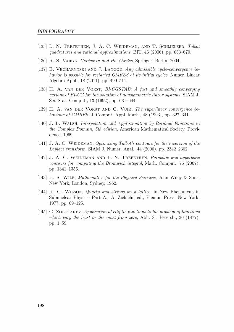
BIBLIOGRAPHY
[135] L. N. Trefethen, J. A. C. Weideman, and T. Schmelzer, Talbotquadratures and rational approximations, BIT, 46 (2006), pp. 653–670.
[136] R. S. Varga, Gersgorin and His Circles, Springer, Berlin, 2004.
[137] E. Vecharynski and J. Langou, Any admissible cycle-convergence be-havior is possible for restarted GMRES at its initial cycles, Numer. LinearAlgebra Appl., 18 (2011), pp. 499–511.
[138] H. A. van der Vorst, BI-CGSTAB: A fast and smoothly convergingvariant of BI-CG for the solution of nonsymmetric linear systems, SIAM J.Sci. Stat. Comput., 13 (1992), pp. 631–644.
[139] H. A. van der Vorst and C. Vuik, The superlinear convergence be-haviour of GMRES, J. Comput. Appl. Math., 48 (1993), pp. 327–341.
[140] J. L. Walsh, Interpolation and Approximation by Rational Functions inthe Complex Domain, 5th edition, American Mathematical Society, Provi-dence, 1969.
[141] J. A. C. Weideman, Optimizing Talbot’s contours for the inversion of theLaplace transform, SIAM J. Numer. Anal., 44 (2006), pp. 2342–2362.
[142] J. A. C. Weideman and L. N. Trefethen, Parabolic and hyperboliccontours for computing the Bromwich integral, Math. Comput., 76 (2007),pp. 1341–1356.
[143] H. S. Wilf, Mathematics for the Physical Sciences, John Wiley & Sons,New York, London, Sydney, 1962.
[144] K. G. Wilson, Quarks and strings on a lattice, in New Phenomena inSubnuclear Physics. Part A., A. Zichichi, ed., Plenum Press, New York,1977, pp. 69–125.
[145] G. Zolotarev, Application of elliptic functions to the problem of functionswhich vary the least or the most from zero, Abh. St. Petersb., 30 (1877),pp. 1–59.
198
Related Documents