responses to reviewer 1 - De Gruyter

1

RESPONSES TO REVIEWER 1 We thank the reviewer for excellent comments. They have caused a major change in the way we think about this problem.

Before getting into our response, let us first explain why this response took so long. There was disagreement amongst the co-authors about the existence of profit-shifting. Further analysis of the original data, following on suggestions the reviewers made, caused some -- but not of all of us -- to change our minds. As a result, this paper has gone through 3 major revisions, each time expanding the original dataset to include more data. As a result of the intensive, ultimately unsuccessful, search for profit-shifting, all of the co-authors became convinced that there is no evidence for profit-shifting in the Chinese data.

Our response proceeds as follows: • We address criticisms of the reviewer about our use of the effective tax rate variable

(EATR), particularly with respect to concerns about endogeneity. We will present evidence that the Chinese tax system is a flat tax rate with very few exceptions. This minimizes the margin for behavioral responses affecting EATR.

• We present the evidence that caused us to conclude that there is no basis for believing that profit-shifting is a problem with Chinese MNCs.

• We then respond to the reviewer’s remaining comments. We would like to have the opportunity to revise our study and resubmit to the journal, this

time with the conclusion that there is no evidence of profit-shifting in China. We feel that we have come to this conclusion through a rigorous analysis of the data, spurred by the comments from the reviewers. Given the lack of existing analyses of this important question, we believe our study makes an important contribution to the literature.

ADDRESSING CRITICISM ABOUT THE EATR VARIABLE 1. Comment: “The central tax measure used in the study is an effective average tax

rate (EATR). This EATR is, however, defined as a backward looking rate (actual tax payments divided by profits). It is argued that EM&W use an EATR as well. The EATR in EM&W is a so-called forward-looking measure, which defines the average tax burden of a hypothetical investment project in the tradition of King and Fullerton (1984) who suggest an effective marginal tax rate and Devereux and Griffith (1998) who suggest an effective average tax rate.”

Comment: “The reference to Devereux and Griffith (2003) is wrong. Their study

analyzes the above-mentioned forward-looking EATRs.” Response: We agree that we have mischaracterized EM&W/Devereux and Griffith’s

measure of average tax rates. The revised manuscript will make it clear that these studies use a measure of forward-looking average tax rates, while ours is backward-looking.

2. Comment: “The backward-looking EATR is not only endogenously determined (it

reflects a large number of behavioral responses to tax incentives), it also does not capture tax incentive which arise from tax law. This is very problematic and I do

2

not see how you solve that problem as there is no information on variation in statutory tax incentives within China.”

Comment: “As I said, the backward-looking EATR is the result of numerous

endogenous choices, and the interpretation of a marginal change thereof, in a ceteris paribus analysis, is not really possible.”

Comment: “In your approach, you distinguish between the two groups, based on investment. The backward-looking measure makes interpretation of the coefficients impossible: a higher ex-post effective tax payment reduces investment expenditure.”

Response: We apologize for not being clearer about the Chinese tax system and why

we believe the backward-looking EATR that we use, while not ideal, is sufficient to identify underlying statutory tax rates. Because this is such an important issue -- perhaps the key concern of the reviewers -- our response is rather detailed. It consists of two parts. First, we give details regarding the Chinese tax system and argue that the backward-looking, effective average tax rate that we use is an unbiased measure of the firm’s relevant statutory tax rate, free of behavioral responses. Second, we present new evidence of profit-shifting that causes us to change our conclusion.

Define EATR as:

(1) 𝐸𝐸𝐸𝐸 = 𝑇𝑇𝑇𝑇𝑇 𝑃𝑇𝑃𝑃𝑅𝑇𝑅𝑅𝑅𝑅𝑇𝑃 𝑃𝑅𝑅𝑃𝑃𝑅𝑇

.

In a complex corporate tax system like that in the US, EATR will be a function of Reported Profits. For example, federal corporate income taxes in the US are calculated according to a tiered tax rate schedule. Changes in profits can place the firm in a different tax bracket, affecting the EATR. In addition, there is a complex system of deductions, credits, and deferrals all of which can encourage behavioral responses to different tax rates. In this kind of system, the concerns of the reviewers would be completely justified, as profit-shifting would affect EATRs.

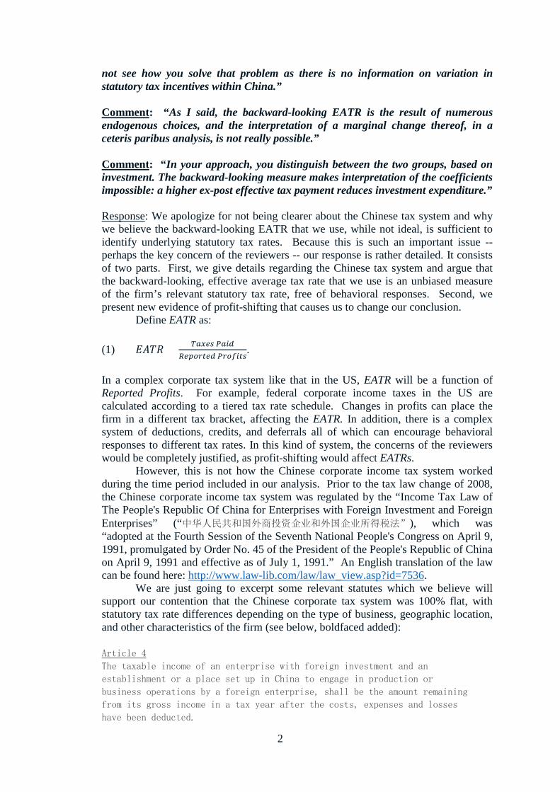
However, this is not how the Chinese corporate income tax system worked during the time period included in our analysis. Prior to the tax law change of 2008, the Chinese corporate income tax system was regulated by the “Income Tax Law of The People's Republic Of China for Enterprises with Foreign Investment and Foreign Enterprises” (“中华人民共和国外商投资企业和外国企业所得税法”), which was “adopted at the Fourth Session of the Seventh National People's Congress on April 9, 1991, promulgated by Order No. 45 of the President of the People's Republic of China on April 9, 1991 and effective as of July 1, 1991.” An English translation of the law can be found here: http://www.law-lib.com/law/law_view.asp?id=7536.

We are just going to excerpt some relevant statutes which we believe will support our contention that the Chinese corporate tax system was 100% flat, with statutory tax rate differences depending on the type of business, geographic location, and other characteristics of the firm (see below, boldfaced added):

Article 4

The taxable income of an enterprise with foreign investment and an

establishment or a place set up in China to engage in production or

business operations by a foreign enterprise, shall be the amount remaining

from its gross income in a tax year after the costs, expenses and losses

have been deducted.

3

Article 5

The income tax on enterprises with foreign investment and the income tax

which shall be paid by foreign enterprises on the income of their

establishments or places set up in China to engage in production or

business operations shall be computed on the taxable income at the rate of

thirty percent, and local income tax shall be computed on the taxable

income at the rate of three percent.

Article 7

The income tax on enterprises with foreign investment established in

Special Economic Zones, foreign enterprises which have establishments or

places in Special Economic Zones engaged in production or business

operations, and on enterprises with foreign investment of a production

nature in Economic and Technological Development Zones, shall be levied at

the reduced rate of fifteen percent.

The income tax on enterprises with foreign investment of a production

nature established in coastal economic open zones or in the old urban

districts of cities where the Special Economic Zones or the Economic and

Technological Development Zones are located, shall be levied at the

reduced rate of twenty-four percent.

The income tax on enterprises with foreign investment in coastal economic

open zones, in the old urban districts of cities where the Special

Economic Zones or the Economic and Technological Development Zones are

located or in other regions defined by the State Council, within the scope

of energy, communications, harbour, wharf or other projects encouraged by

the State, may be levied at the reduced rate of fifteen percent. The

specific measures shall be drawn up by the State Council.

Article 8

Any enterprise with foreign investment of a production nature scheduled to

operate for a period of not less than ten years shall, from the year

beginning to make profit, be exempted from income tax in the first and

second years and allowed a fifty percent reduction in the third to fifth

years. However, the exemption from or reduction of income tax on

enterprises with foreign investment engaged in the exploitation of

resources such as petroleum, natural gas, rare metals, and precious metals

shall be regulated separately by the State Council. More detail is provided in the web link above.

This is the tax law that regulated corporate income taxation in China for FIE’s until China passed a new Corporate Income Tax Law in 2007 that went into effect on January 1, 2008 (An and Tan, 2014). Accordingly, we can rewrite Equation (1) as follows:

(2) 𝐸𝐸𝐸𝐸 = 𝑇𝑇𝑇𝑇𝑇 𝑃𝑇𝑃𝑃

𝑅𝑇𝑅𝑅𝑅𝑅𝑇𝑃 𝑃𝑅𝑅𝑃𝑃𝑅𝑇= 𝑅𝑇𝑅𝑅𝑅𝑅𝑇𝑃 𝑃𝑅𝑅𝑃𝑃𝑅𝑇 × 𝑆𝑅𝑇𝑅𝑆𝑅𝑅𝑅𝑆 𝑇𝑇𝑇 𝑅𝑇𝑅𝑇

𝑅𝑇𝑅𝑅𝑅𝑅𝑇𝑃 𝑃𝑅𝑅𝑃𝑃𝑅𝑇

= 𝑆𝑆𝑆𝑆𝑆𝑆𝑆𝑆𝑆 𝐸𝑆𝑇 𝐸𝑆𝑆𝑅.

4

From Equation (2) it can be seen that the ratio of Taxes Paid to Reported Profits is a measure of the statutory tax rate faced by the firm. While profit-shifting will affect the amount of profits reported by the firm, it will not affect the ratio of Taxes Paid to Reported Profits. If we are given the opportunity to revise and resubmit our manuscript, we will be sure to emphasize this crucial element of the Chinese corporate tax system.

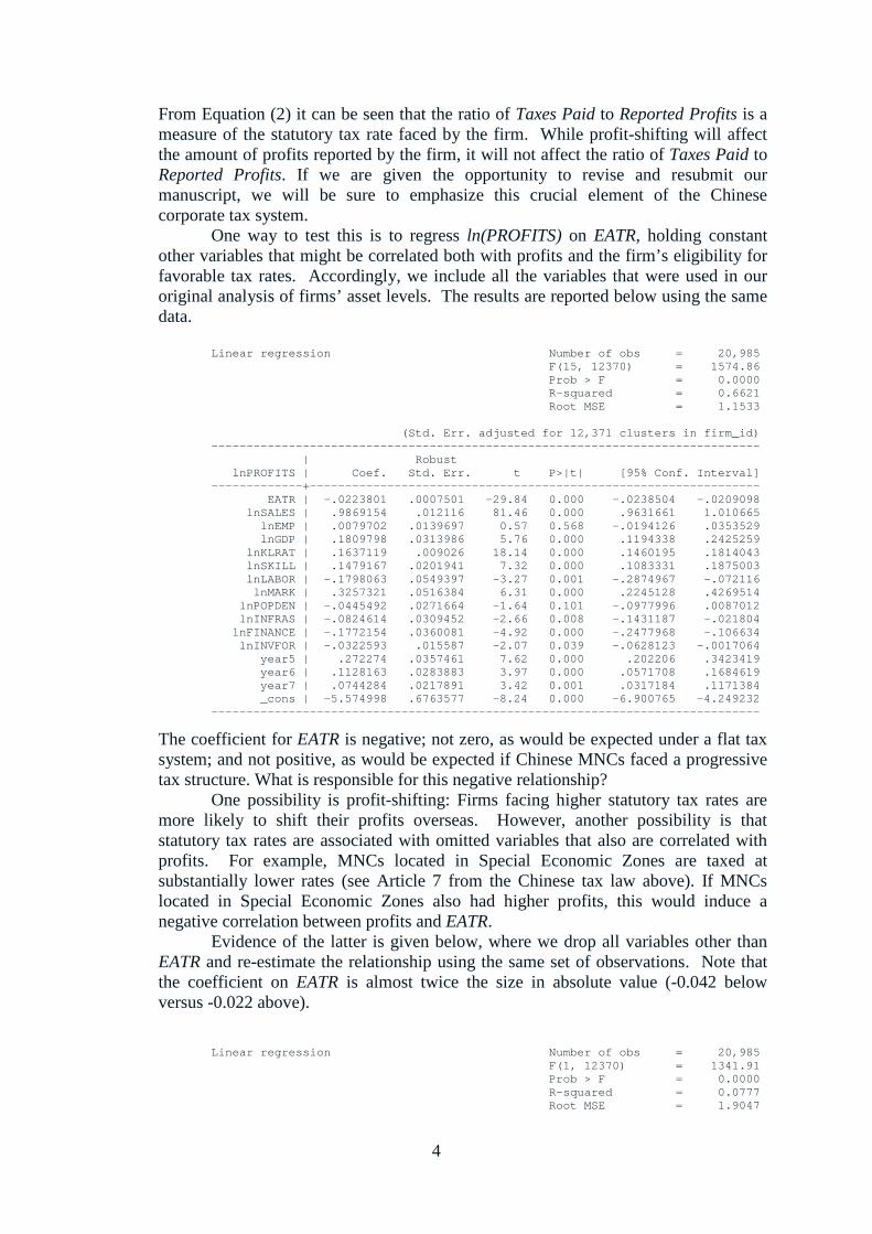
One way to test this is to regress ln(PROFITS) on EATR, holding constant other variables that might be correlated both with profits and the firm’s eligibility for favorable tax rates. Accordingly, we include all the variables that were used in our original analysis of firms’ asset levels. The results are reported below using the same data.

Linear regression Number of obs = 20,985 F(15, 12370) = 1574.86 Prob > F = 0.0000 R-squared = 0.6621 Root MSE = 1.1533 (Std. Err. adjusted for 12,371 clusters in firm_id) ------------------------------------------------------------------------------ | Robust lnPROFITS | Coef. Std. Err. t P>|t| [95% Conf. Interval] -------------+---------------------------------------------------------------- EATR | -.0223801 .0007501 -29.84 0.000 -.0238504 -.0209098 lnSALES | .9869154 .012116 81.46 0.000 .9631661 1.010665 lnEMP | .0079702 .0139697 0.57 0.568 -.0194126 .0353529 lnGDP | .1809798 .0313986 5.76 0.000 .1194338 .2425259 lnKLRAT | .1637119 .009026 18.14 0.000 .1460195 .1814043 lnSKILL | .1479167 .0201941 7.32 0.000 .1083331 .1875003 lnLABOR | -.1798063 .0549397 -3.27 0.001 -.2874967 -.072116 lnMARK | .3257321 .0516384 6.31 0.000 .2245128 .4269514 lnPOPDEN | -.0445492 .0271664 -1.64 0.101 -.0977996 .0087012 lnINFRAS | -.0824614 .0309452 -2.66 0.008 -.1431187 -.021804 lnFINANCE | -.1772154 .0360081 -4.92 0.000 -.2477968 -.106634 lnINVFOR | -.0322593 .015587 -2.07 0.039 -.0628123 -.0017064 year5 | .272274 .0357461 7.62 0.000 .202206 .3423419 year6 | .1128163 .0283883 3.97 0.000 .0571708 .1684619 year7 | .0744284 .0217891 3.42 0.001 .0317184 .1171384 _cons | -5.574998 .6763577 -8.24 0.000 -6.900765 -4.249232 ------------------------------------------------------------------------------

The coefficient for EATR is negative; not zero, as would be expected under a flat tax system; and not positive, as would be expected if Chinese MNCs faced a progressive tax structure. What is responsible for this negative relationship?

One possibility is profit-shifting: Firms facing higher statutory tax rates are more likely to shift their profits overseas. However, another possibility is that statutory tax rates are associated with omitted variables that also are correlated with profits. For example, MNCs located in Special Economic Zones are taxed at substantially lower rates (see Article 7 from the Chinese tax law above). If MNCs located in Special Economic Zones also had higher profits, this would induce a negative correlation between profits and EATR.

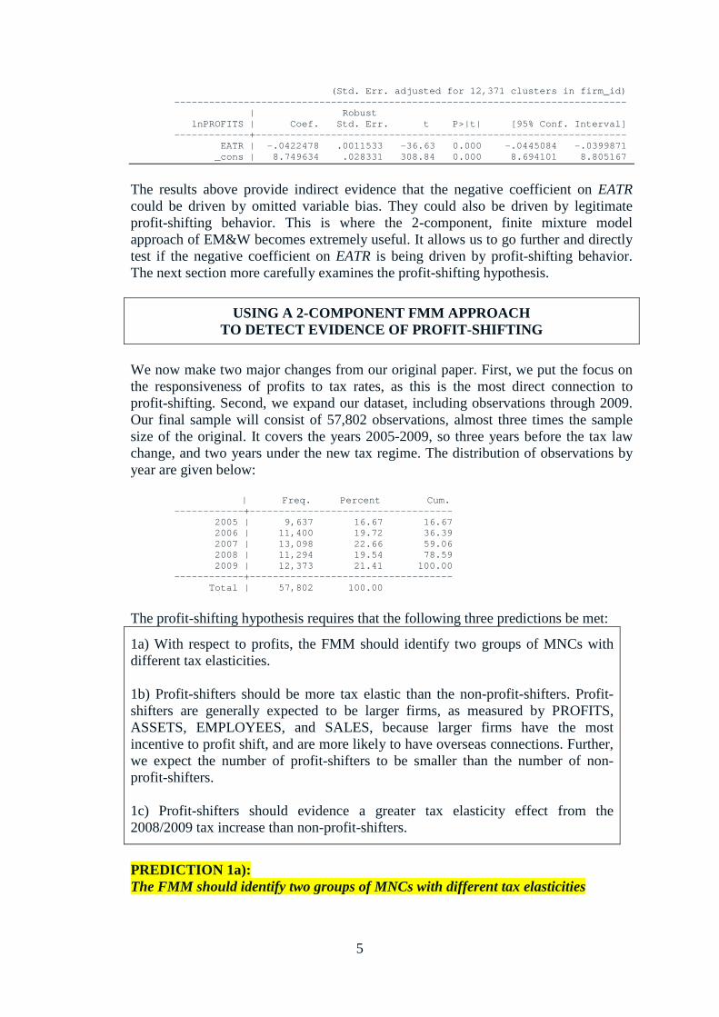
Evidence of the latter is given below, where we drop all variables other than EATR and re-estimate the relationship using the same set of observations. Note that the coefficient on EATR is almost twice the size in absolute value (-0.042 below versus -0.022 above).

Linear regression Number of obs = 20,985 F(1, 12370) = 1341.91 Prob > F = 0.0000 R-squared = 0.0777 Root MSE = 1.9047

5

(Std. Err. adjusted for 12,371 clusters in firm_id) ------------------------------------------------------------------------------ | Robust lnPROFITS | Coef. Std. Err. t P>|t| [95% Conf. Interval] -------------+---------------------------------------------------------------- EATR | -.0422478 .0011533 -36.63 0.000 -.0445084 -.0399871 _cons | 8.749634 .028331 308.84 0.000 8.694101 8.805167

The results above provide indirect evidence that the negative coefficient on EATR could be driven by omitted variable bias. They could also be driven by legitimate profit-shifting behavior. This is where the 2-component, finite mixture model approach of EM&W becomes extremely useful. It allows us to go further and directly test if the negative coefficient on EATR is being driven by profit-shifting behavior. The next section more carefully examines the profit-shifting hypothesis.

USING A 2-COMPONENT FMM APPROACH

TO DETECT EVIDENCE OF PROFIT-SHIFTING

We now make two major changes from our original paper. First, we put the focus on the responsiveness of profits to tax rates, as this is the most direct connection to profit-shifting. Second, we expand our dataset, including observations through 2009. Our final sample will consist of 57,802 observations, almost three times the sample size of the original. It covers the years 2005-2009, so three years before the tax law change, and two years under the new tax regime. The distribution of observations by year are given below:

| Freq. Percent Cum. ------------+----------------------------------- 2005 | 9,637 16.67 16.67 2006 | 11,400 19.72 36.39 2007 | 13,098 22.66 59.06 2008 | 11,294 19.54 78.59 2009 | 12,373 21.41 100.00 ------------+----------------------------------- Total | 57,802 100.00

The profit-shifting hypothesis requires that the following three predictions be met:

1a) With respect to profits, the FMM should identify two groups of MNCs with different tax elasticities.

1b) Profit-shifters should be more tax elastic than the non-profit-shifters. Profit-shifters are generally expected to be larger firms, as measured by PROFITS, ASSETS, EMPLOYEES, and SALES, because larger firms have the most incentive to profit shift, and are more likely to have overseas connections. Further, we expect the number of profit-shifters to be smaller than the number of non-profit-shifters.

1c) Profit-shifters should evidence a greater tax elasticity effect from the 2008/2009 tax increase than non-profit-shifters.

PREDICTION 1a): The FMM should identify two groups of MNCs with different tax elasticities

6

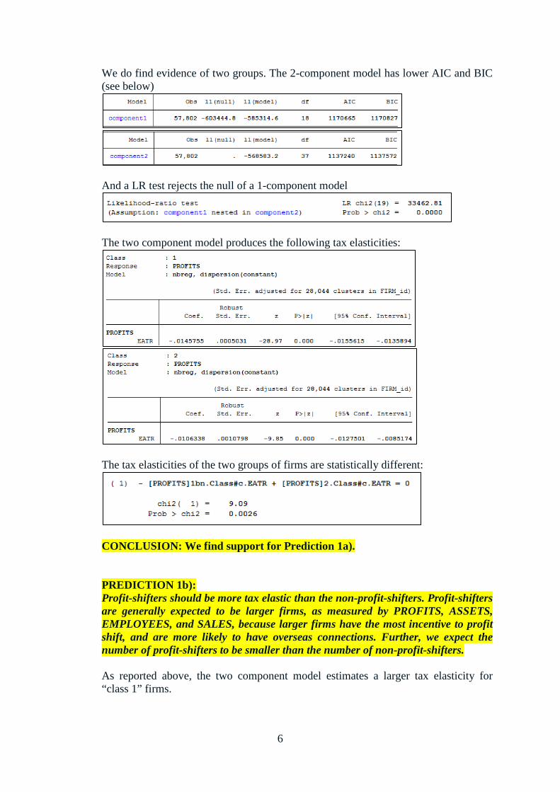
We do find evidence of two groups. The 2-component model has lower AIC and BIC (see below)

And a LR test rejects the null of a 1-component model

The two component model produces the following tax elasticities:

The tax elasticities of the two groups of firms are statistically different:

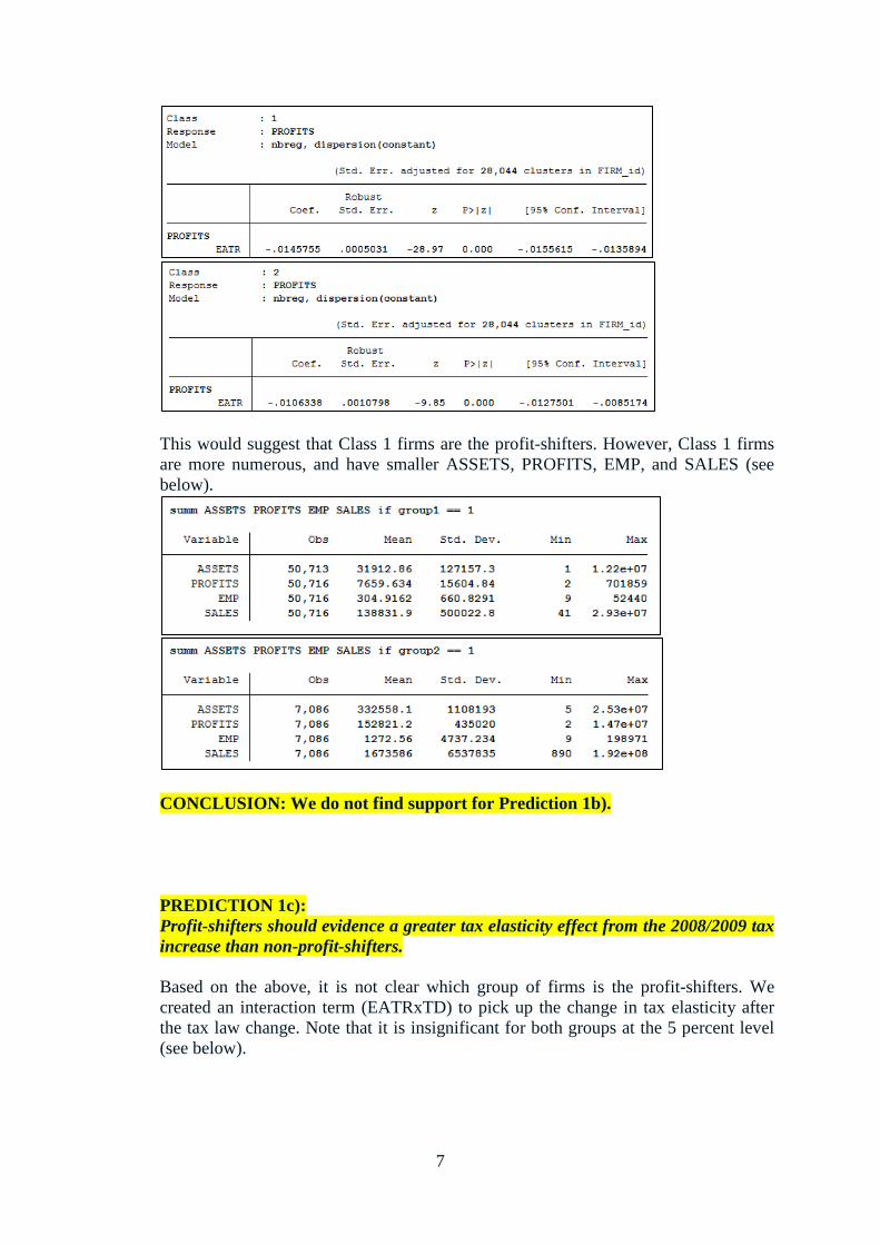
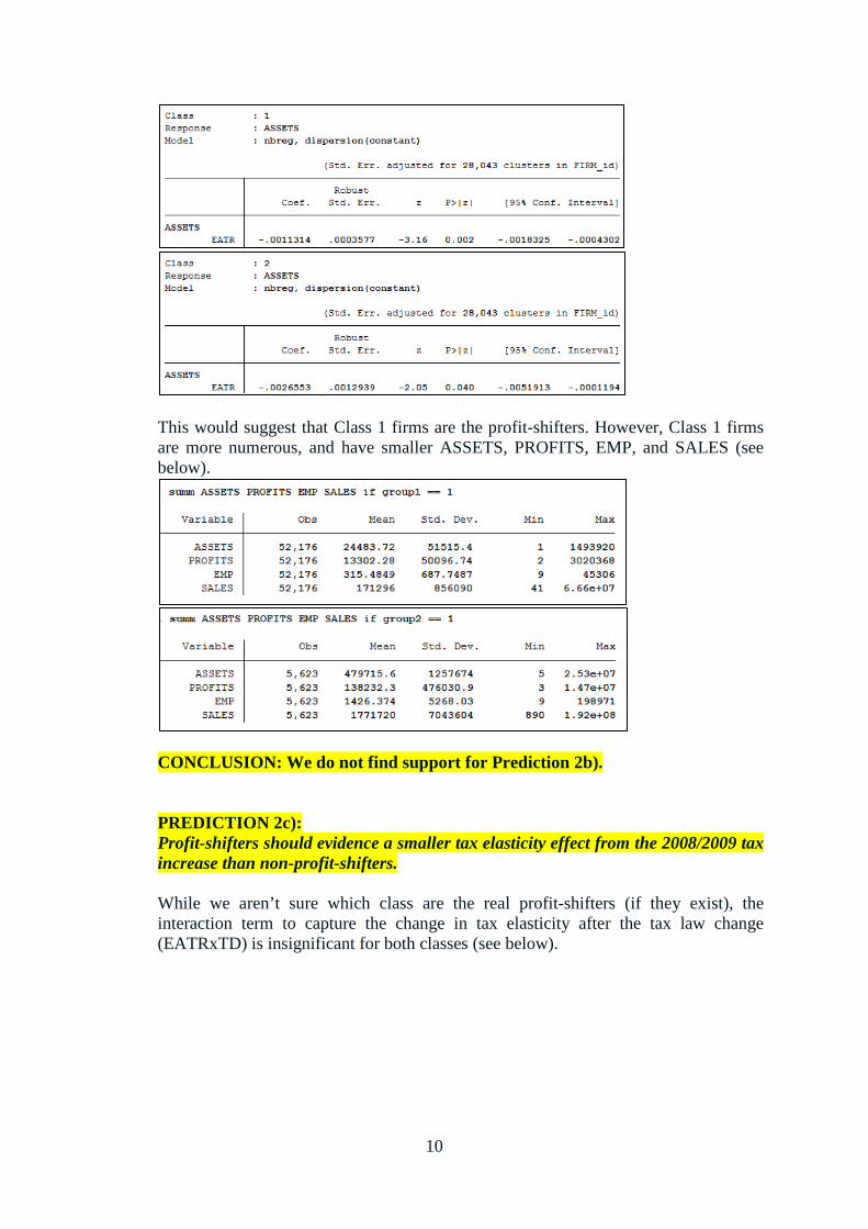
CONCLUSION: We find support for Prediction 1a). PREDICTION 1b): Profit-shifters should be more tax elastic than the non-profit-shifters. Profit-shifters are generally expected to be larger firms, as measured by PROFITS, ASSETS, EMPLOYEES, and SALES, because larger firms have the most incentive to profit shift, and are more likely to have overseas connections. Further, we expect the number of profit-shifters to be smaller than the number of non-profit-shifters. As reported above, the two component model estimates a larger tax elasticity for “class 1” firms.

7

This would suggest that Class 1 firms are the profit-shifters. However, Class 1 firms are more numerous, and have smaller ASSETS, PROFITS, EMP, and SALES (see below).

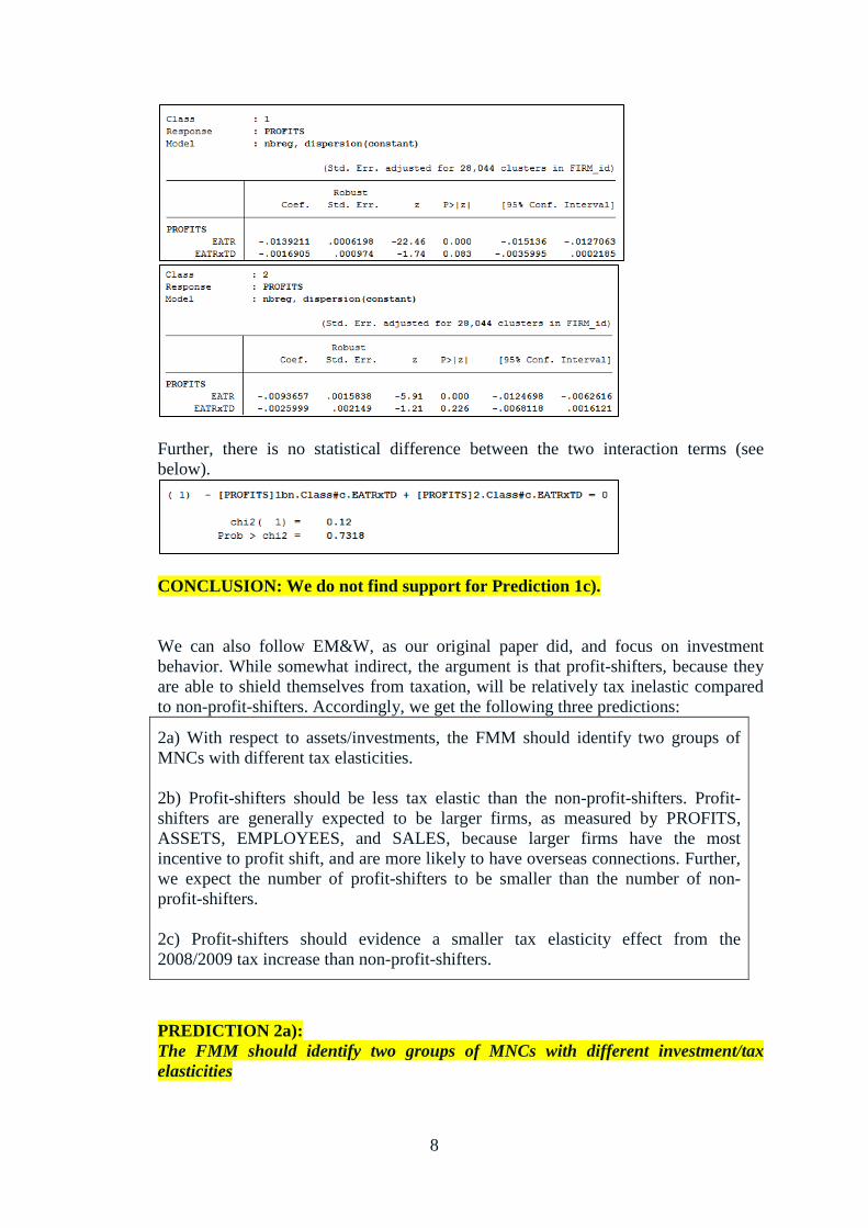
CONCLUSION: We do not find support for Prediction 1b). PREDICTION 1c): Profit-shifters should evidence a greater tax elasticity effect from the 2008/2009 tax increase than non-profit-shifters. Based on the above, it is not clear which group of firms is the profit-shifters. We created an interaction term (EATRxTD) to pick up the change in tax elasticity after the tax law change. Note that it is insignificant for both groups at the 5 percent level (see below).

8

Further, there is no statistical difference between the two interaction terms (see below).

CONCLUSION: We do not find support for Prediction 1c).

We can also follow EM&W, as our original paper did, and focus on investment

behavior. While somewhat indirect, the argument is that profit-shifters, because they are able to shield themselves from taxation, will be relatively tax inelastic compared to non-profit-shifters. Accordingly, we get the following three predictions:

2a) With respect to assets/investments, the FMM should identify two groups of MNCs with different tax elasticities.

2b) Profit-shifters should be less tax elastic than the non-profit-shifters. Profit-shifters are generally expected to be larger firms, as measured by PROFITS, ASSETS, EMPLOYEES, and SALES, because larger firms have the most incentive to profit shift, and are more likely to have overseas connections. Further, we expect the number of profit-shifters to be smaller than the number of non-profit-shifters.

2c) Profit-shifters should evidence a smaller tax elasticity effect from the 2008/2009 tax increase than non-profit-shifters.

PREDICTION 2a): The FMM should identify two groups of MNCs with different investment/tax elasticities

9

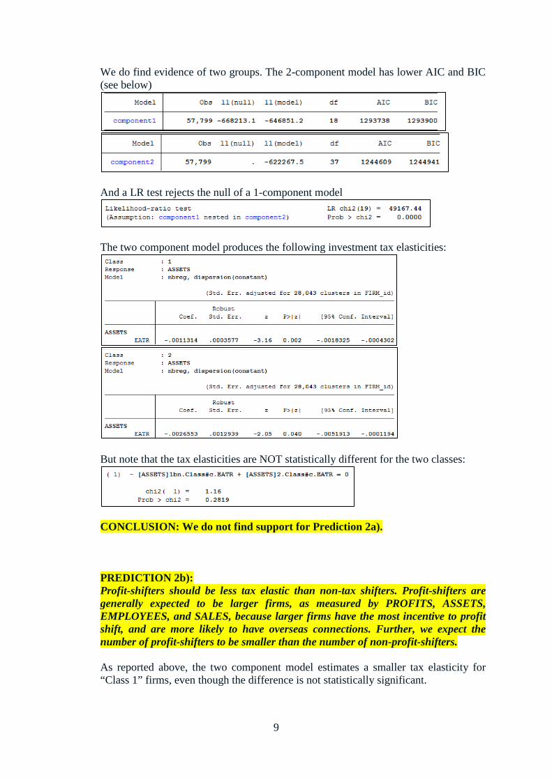
We do find evidence of two groups. The 2-component model has lower AIC and BIC (see below)

And a LR test rejects the null of a 1-component model

The two component model produces the following investment tax elasticities:

But note that the tax elasticities are NOT statistically different for the two classes:

CONCLUSION: We do not find support for Prediction 2a). PREDICTION 2b): Profit-shifters should be less tax elastic than non-tax shifters. Profit-shifters are generally expected to be larger firms, as measured by PROFITS, ASSETS, EMPLOYEES, and SALES, because larger firms have the most incentive to profit shift, and are more likely to have overseas connections. Further, we expect the number of profit-shifters to be smaller than the number of non-profit-shifters. As reported above, the two component model estimates a smaller tax elasticity for “Class 1” firms, even though the difference is not statistically significant.

10

This would suggest that Class 1 firms are the profit-shifters. However, Class 1 firms are more numerous, and have smaller ASSETS, PROFITS, EMP, and SALES (see below).

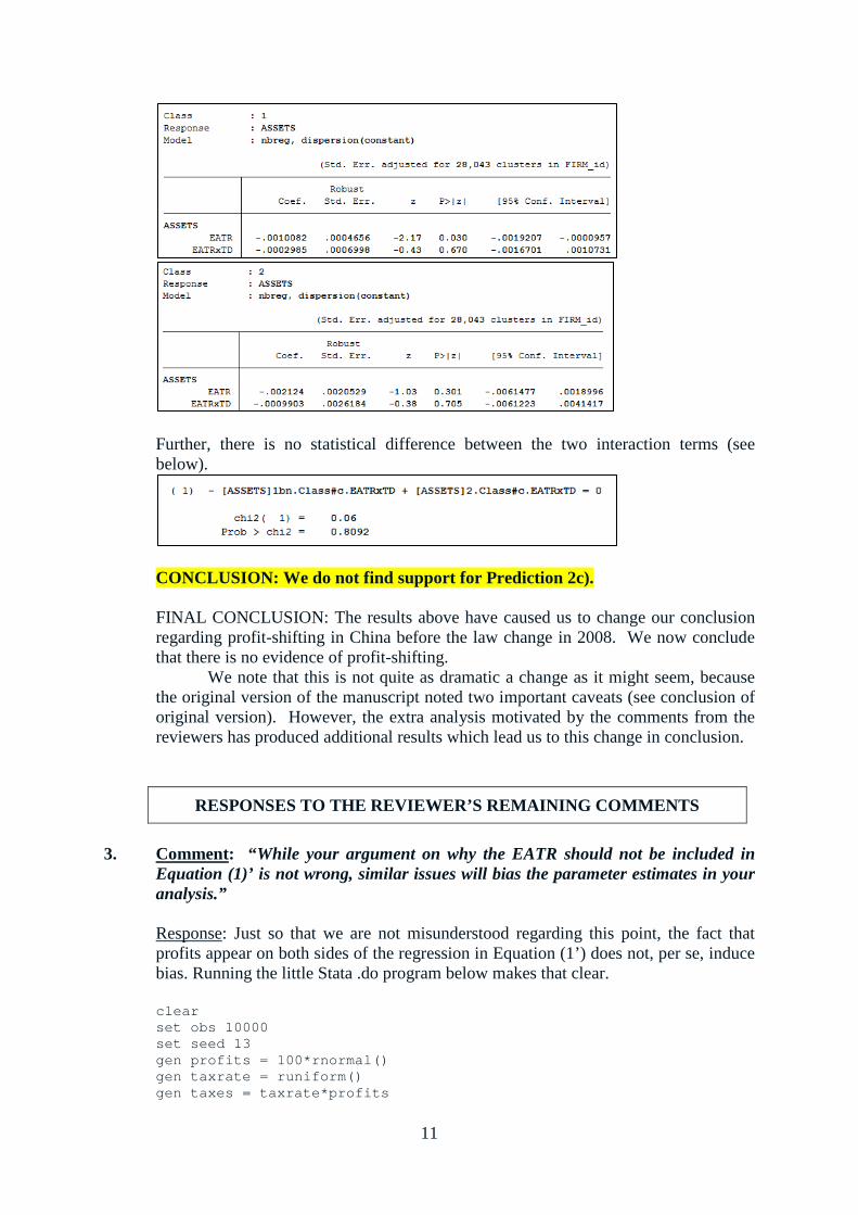
CONCLUSION: We do not find support for Prediction 2b). PREDICTION 2c): Profit-shifters should evidence a smaller tax elasticity effect from the 2008/2009 tax increase than non-profit-shifters. While we aren’t sure which class are the real profit-shifters (if they exist), the interaction term to capture the change in tax elasticity after the tax law change (EATRxTD) is insignificant for both classes (see below).

11

Further, there is no statistical difference between the two interaction terms (see below).

CONCLUSION: We do not find support for Prediction 2c). FINAL CONCLUSION: The results above have caused us to change our conclusion

regarding profit-shifting in China before the law change in 2008. We now conclude that there is no evidence of profit-shifting.

We note that this is not quite as dramatic a change as it might seem, because the original version of the manuscript noted two important caveats (see conclusion of original version). However, the extra analysis motivated by the comments from the reviewers has produced additional results which lead us to this change in conclusion.

RESPONSES TO THE REVIEWER’S REMAINING COMMENTS 3. Comment: “While your argument on why the EATR should not be included in

Equation (1)’ is not wrong, similar issues will bias the parameter estimates in your analysis.”

Response: Just so that we are not misunderstood regarding this point, the fact that profits appear on both sides of the regression in Equation (1’) does not, per se, induce bias. Running the little Stata .do program below makes that clear.

clear set obs 10000 set seed 13 gen profits = 100*rnormal() gen taxrate = runiform() gen taxes = taxrate*profits

12

// Clearly, taxes/profits = taxrate drop if profits<0 gen lnprofits = ln(profits) regress lnprofits taxrate

The core problem is distinguishing between profit-shifting (i.e., EATR increases, PROFITS decrease in response) and omitted variable bias related both to profits and the statutory tax rate facing the firm. As discussed above, the 2-component, finite mixture model approach gives us a way of circumventing this identification problem.

4. Comment: “The point you make about why using the finite mixture improves on

examining profits as dependent variable is based on flawed arguments. With the finite mixture, you investigate investment responses and not profit shifting behavior; though the latter determines investment responses.”

Response: We agree with the reviewer. Our dismissal of using profits as another

indicator of profit-shifting was incorrect. In hindsight, we were a little caught up with trying to replicate EM&W’s approach to the problem. The analysis we present in the preceding section corrects this by focusing on the responsiveness of profits to tax rates. If we are allowed to submit a revised manuscript, we will present the evidence using both profits and investments to show that there is no identifiable evidence of profit-shifting. We thank the reviewer for pushing us to think through these issues more carefully.

5. Comment: “All formulas provided on the econometric approach do not have a

time index. But the data presented is panel data. Are there any time effects in the estimation? (the EM&W also models unobserved heterogeneity at the level of foreign affiliates).”

Response: The original results included year dummies to address time effects, as do

the results above using the expanded dataset. We are still concerned about the few number of observations per firm, even in the expanded dataset: on average, there are only about two observations per firm. However, if we are permitted to submit a revised version of our manuscript, we will control for firm heterogeneity in the same manner as EM&W as a robustness check.

6. Comment: “To make a clear statement about whether the two groups respond

differently to tax incentives, the equality of the two coefficients has to be formally tested. It does not look like the hypothesis of equality of the two tax parameters can be rejected.”

Response: We agree. The analysis we present in the preceding section tests for equality in the respective tax coefficients. As a result, and in combination with the new evidence we have uncovered, we have now changed our conclusion regarding the existing of profit-shifting. We thank the reviewer for encouraging us to test for this.

13

Minor comments: 7. Comment: “I would remove Figure 1; the information provided therein can briefly

be summarized in the text.”

Response: A revised version of the manuscript will remove Figure 1. 8. Comment: “Given the not very detailed discussion of the actual estimation

approach, I think that Equations (1) and (1)’ take up too much room and should be removed. The finite mixture can be motivated in a more straightforward way.”

Response: We agree with the reviewer. A revised version of the manuscript will drop Equations (1) and (1’).

9. Comment: “EM&W do not hypothesize that shifters have higher levels of debt (as

is claimed on page 8); they might have. The debt variable is used to distinguish between the two groups (to determine \pi).”

Response: Here is what EM&W say about debt on page 6 of their paper:

A revised version of our manuscript will more carefully explain how EM&W use debt

as an indicator of profit-shifting behavior of firms. 10. Comment: “What does negative Debt of -0.52 mean? (Descriptive Statistics)”

Response: It’s a coding error in the Chinese data. There were very few negative Debt values in the original data set. The results were unaffected by dropping these. All the regression results above using the expanded number of observations now restrict observations to having non-negative values of Debt.

11. Comment: “Are observations from Year 2006 dropped from the sample? (Table

1)”

Response: Some of the explanatory variables were missing observations from certain years, and this caused those observations to be dropped. This is not a problem with the updated version of the data we use above, at least for 2006, though it is a problem for the years preceding 2005. Unfortunately, we were unable to get an explanation for why the earlier vintage had observations for these years, but the later vintage did not.

12. Comment: “The paper lacks a clear discussion of why the two groups should differ

in the assets (the dependent variable)”

14

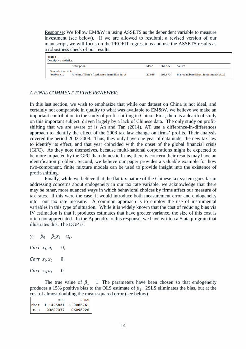
Response: We follow EM&W in using ASSETS as the dependent variable to measure investment (see below). If we are allowed to resubmit a revised version of our manuscript, we will focus on the PROFIT regressions and use the ASSETS results as a robustness check of our results.

A FINAL COMMENT TO THE REVIEWER: In this last section, we wish to emphasize that while our dataset on China is not ideal, and certainly not comparable in quality to what was available to EM&W, we believe we make an important contribution to the study of profit-shifting in China. First, there is a dearth of study on this important subject, driven largely by a lack of Chinese data. The only study on profit-shifting that we are aware of is An and Tan (2014). AT use a difference-in-differences approach to identify the effect of the 2008 tax law change on firms’ profits. Their analysis covered the period 2002-2008. Thus, they only have one year of data under the new tax law to identify its effect, and that year coincided with the onset of the global financial crisis (GFC). As they note themselves, because multi-national corporations might be expected to be more impacted by the GFC than domestic firms, there is concern their results may have an identification problem. Second, we believe our paper provides a valuable example for how two-component, finite mixture models can be used to provide insight into the existence of profit-shifting.

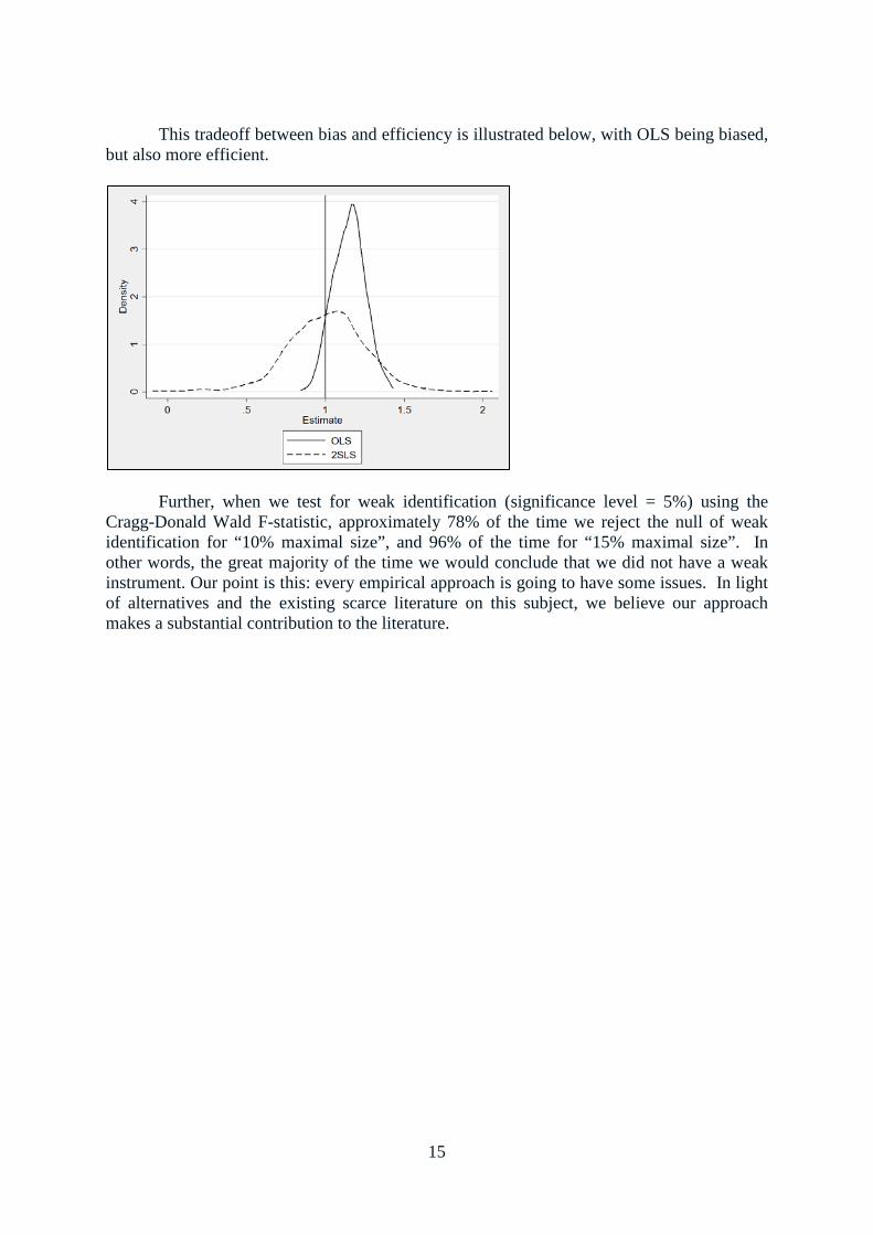
Finally, while we believe that the flat tax nature of the Chinese tax system goes far in addressing concerns about endogeneity in our tax rate variable, we acknowledge that there may be other, more nuanced ways in which behavioral choices by firms affect our measure of tax rates. If this were the case, it would introduce both measurement error and endogeneity into our tax rate measure. A common approach is to employ the use of instrumental variables in this type of situation. While it is widely known that the cost of reducing bias via IV estimation is that it produces estimates that have greater variance, the size of this cost is often not appreciated. In the Appendix to this response, we have written a Stata program that illustrates this. The DGP is: 𝑆𝑃 = 𝛽0 + 𝛽1𝑇𝑃 + 𝑆𝑃, 𝐶𝑆𝑆𝑆(𝑇𝑃, 𝑆𝑃) > 0, 𝐶𝑆𝑆𝑆(𝑧𝑃, 𝑇𝑃) > 0, 𝐶𝑆𝑆𝑆(𝑧𝑃,𝑆𝑃) = 0. The true value of 𝛽1 = 1. The parameters have been chosen so that endogeneity produces a 15% positive bias to the OLS estimate of 𝛽1. 2SLS eliminates the bias, but at the cost of almost doubling the mean-squared error (see below).

15

This tradeoff between bias and efficiency is illustrated below, with OLS being biased, but also more efficient.

Further, when we test for weak identification (significance level = 5%) using the Cragg-Donald Wald F-statistic, approximately 78% of the time we reject the null of weak identification for “10% maximal size”, and 96% of the time for “15% maximal size”. In other words, the great majority of the time we would conclude that we did not have a weak instrument. Our point is this: every empirical approach is going to have some issues. In light of alternatives and the existing scarce literature on this subject, we believe our approach makes a substantial contribution to the literature.

16

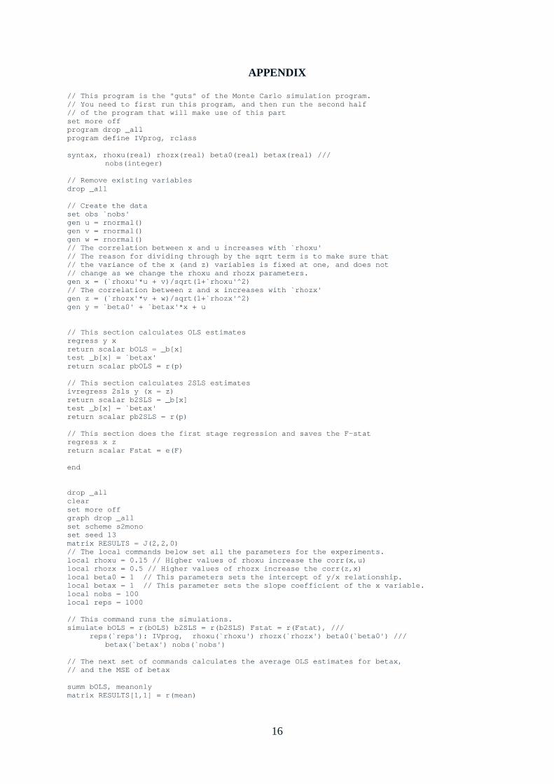
APPENDIX

// This program is the "guts" of the Monte Carlo simulation program. // You need to first run this program, and then run the second half // of the program that will make use of this part set more off program drop _all program define IVprog, rclass syntax, rhoxu(real) rhozx(real) beta0(real) betax(real) /// nobs(integer) // Remove existing variables drop _all // Create the data set obs `nobs' gen u = rnormal() gen v = rnormal() gen w = rnormal() // The correlation between x and u increases with `rhoxu' // The reason for dividing through by the sqrt term is to make sure that // the variance of the x (and z) variables is fixed at one, and does not // change as we change the rhoxu and rhozx parameters. gen x = (`rhoxu'*u + v)/sqrt(1+`rhoxu'^2) // The correlation between z and x increases with `rhozx' gen z = (`rhozx'*v + w)/sqrt(1+`rhozx'^2) gen y = `beta0' + `betax'*x + u // This section calculates OLS estimates regress y x return scalar bOLS = _b[x] test _b[x] = `betax' return scalar pbOLS = r(p) // This section calculates 2SLS estimates ivregress 2sls y (x = z) return scalar b2SLS = _b[x] test _b[x] = `betax' return scalar pb2SLS = r(p) // This section does the first stage regression and saves the F-stat regress x z return scalar Fstat = e(F) end drop _all clear set more off graph drop _all set scheme s2mono set seed 13 matrix RESULTS = J(2,2,0) // The local commands below set all the parameters for the experiments. local rhoxu = 0.15 // Higher values of rhoxu increase the corr(x,u) local rhozx = 0.5 // Higher values of rhozx increase the corr(z,x) local beta0 = 1 // This parameters sets the intercept of y/x relationship. local betax = 1 // This parameter sets the slope coefficient of the x variable. local nobs = 100 local reps = 1000 // This command runs the simulations. simulate bOLS = r(bOLS) b2SLS = r(b2SLS) Fstat = r(Fstat), /// reps(`reps'): IVprog, rhoxu(`rhoxu') rhozx(`rhozx') beta0(`beta0') /// betax(`betax') nobs(`nobs') // The next set of commands calculates the average OLS estimates for betax, // and the MSE of betax summ bOLS, meanonly matrix RESULTS[1,1] = r(mean)

17

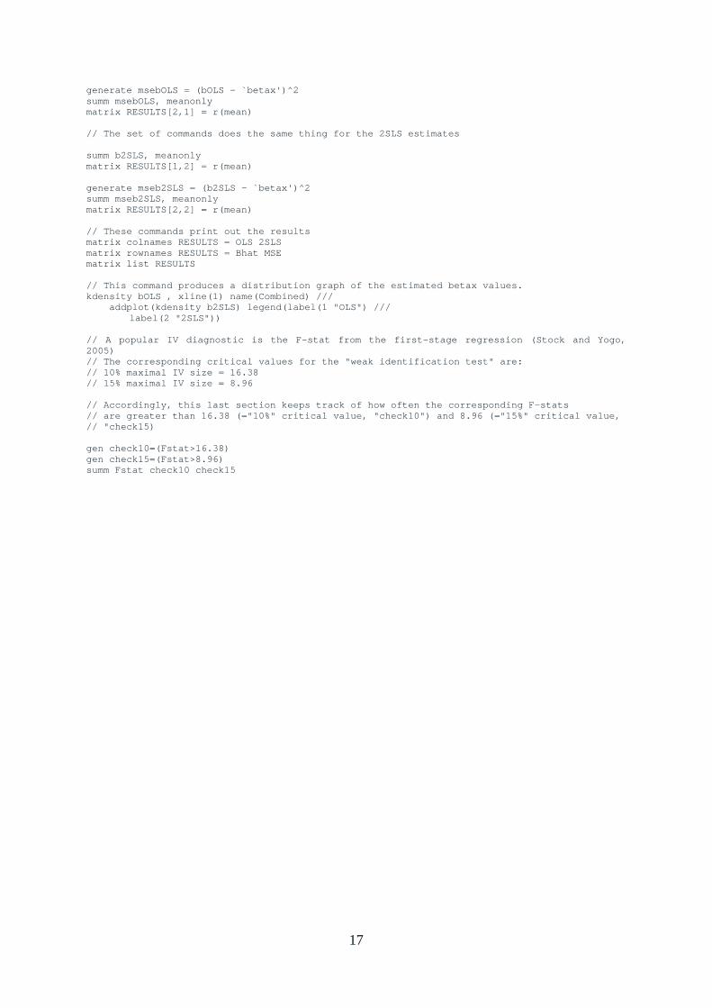
generate msebOLS = (bOLS - `betax')^2 summ msebOLS, meanonly matrix RESULTS[2,1] = r(mean) // The set of commands does the same thing for the 2SLS estimates summ b2SLS, meanonly matrix RESULTS[1,2] = r(mean) generate mseb2SLS = (b2SLS - `betax')^2 summ mseb2SLS, meanonly matrix RESULTS[2,2] = r(mean) // These commands print out the results matrix colnames RESULTS = OLS 2SLS matrix rownames RESULTS = Bhat MSE matrix list RESULTS // This command produces a distribution graph of the estimated betax values. kdensity bOLS , xline(1) name(Combined) /// addplot(kdensity b2SLS) legend(label(1 "OLS") /// label(2 "2SLS")) // A popular IV diagnostic is the F-stat from the first-stage regression (Stock and Yogo, 2005) // The corresponding critical values for the "weak identification test" are: // 10% maximal IV size = 16.38 // 15% maximal IV size = 8.96 // Accordingly, this last section keeps track of how often the corresponding F-stats // are greater than 16.38 (="10%" critical value, "check10") and 8.96 (="15%" critical value, // "check15) gen check10=(Fstat>16.38) gen check15=(Fstat>8.96) summ Fstat check10 check15