Responses of the atmospheric concentration of radon-222 to ... · realistically interpreting the evolution of air masses or planetary boundary layer. ... the changing ambient air

BOREAL ENVIRONMENT RESEARCH 21: 299–318 © 2016ISSN 1239-6095 (print) ISSN 1797-2469 (online) Helsinki 2016

Editor in charge of this article: Hannele Korhonen

Responses of the atmospheric concentration of radon-222 to the vertical mixing and spatial transportation

Xuemeng Chen1)*, Jussi Paatero2), Veli-Matti Kerminen1), Laura Riuttanen1), Juha Hatakka2), Veijo Hiltunen1), Pauli Paasonen1), Anne Hirsikko2), Alessandro Franchin1), Hanna E. Manninen1), Tuukka Petäjä1), Yrjö Viisanen2) and Markku Kulmala1)

1) Department of Physics, P.O. Box 64, FI-00014 University of Helsinki, Finland (*corresponding author’s e-mail: [email protected])

2) Finnish Meteorological Institute, P.O. Box 503, FI-00101 Helsinki, Finland

Received 28 April 2015, final version received 10 Nov. 2015, accepted 11 Nov. 2015

Chen X., Paatero J., Kerminen V.-M., Riuttanen L., Hatakka J., Hiltunen V., Paasonen P., Hirsikko A., Franchin A., Manninen H.E., Petäjä T., Viisanen Y. & Kulmala M. 2016: Responses of the atmospheric concentration of radon-222 to the vertical mixing and spatial transportation. Boreal Env. Res. 21: 299–318.

Radon-222 (222Rn) has traditionally been used as an atmospheric tracer for studying air masses and planetary boundary-layer evolution. However, there are various factors that influence its atmospheric concentration. Therefore, we investigated the variability of the atmospheric radon concentration in response to the vertical air mixing and spatial trans-port in a boreal forest environment in northern Europe. Long-term 222Rn data collected at the SMEAR II station in southern Finland during 2000–2006 were analysed along with meteorological data, mixing layer height retrievals and air-mass back trajectory informa-tion. The daily mean atmospheric radon concentration followed a log-normal distribution within the range < 0.1–11 Bq m–3, with the geometric mean of 2.5 Bq m–3 and a geometric standard deviation of 1.7 Bq m–3. In spring, summer, autumn and winter, the daily mean concentrations were 1.7, 2.7, 2.8 and 2.7 Bq m–3, respectively. The low, spring radon con-centration was especially attributed to the joint effect of enhanced vertical mixing due to the increasing solar irradiance and inhibited local emissions due to snow thawing. The lowest atmospheric radon concentration was observed with northwesterly winds and high radon concentrations with southeasterly winds, which were associated with the marine and continental origins of air masses, respectively. The atmospheric radon concentration was in general inversely proportional to the mixing layer height. However, the ambient tempera-ture and small-scale turbulent mixing were observed to disturb this relationship. The evo-lution of turbulence within the mixing layer was expected to be a key explanation for the delay in the response of the atmospheric radon concentration to the changes in the mixing layer thickness. Radon is a valuable naturally-occurring tracer for studying boundary layer mixing processes and transport patterns, especially when the mixing layer is fully devel-oped. However, complementing information, provided by understanding the variability of the atmospheric radon concentration, is of high necessity to be taken into consideration for realistically interpreting the evolution of air masses or planetary boundary layer.

300 Chen et al. • BOREAL ENV. RES. Vol. 21

Introduction

Radon-222 (222Rn) is a radioactive noble gas with a half-life of about 3.8 days, which is naturally exhaled from soil into the atmosphere (e.g. Pal et al. 2015). It originates from the spontaneous decay series of 238U in the Earth’s crust. Owing to the long half-life, monatomic radon gas can migrate through the soil and enter the atmosphere before lost in the radioactive decay. The con-centration of radon in the atmosphere is directly related to the exhalation rate of radon from soils (Escobar et al. 1999). This exhalation process is affected by several factors, including the concen-tration of its parent nuclide (radium-226), inter-nal structure of radium-containing mineral grain, soil type, moisture and temperature; and also the changing ambient air pressure has influences on the exhalation rate (Clements and Wilkening 1974, Stranden et al. 1984, Schery 1989, Mark-kanen and Arvela 1992, Nazaroff 1992, Ashok et al. 2011). Typically, radon is formed from radium decay inside the mineral grains of soil, and there-fore, it has to first escape into pores in between the grains before being transported to the atmos-phere by diffusion and convection (Porstendörfer 1994). The transport mechanisms of radon from soil to the atmosphere have been elucidated by Nazaroff (1992).

The dynamics of the planetary boundary layer (PBL) has crucial effects on the surface-atmosphere exchanges of energy, moisture, momentum and pollutants (Seidel et al. 2010, Behrendt et al. 2011, Pal and Devara 2012, Lac et al. 2013, McGrath-Spangler and Den-ning 2013, Lee et al. 2015). Therefore, the atmospheric concentration of radon is inevita-bly dependent on the vertical mixing through transport and changes in a dispersion volume in the PBL. According to Stull (1998), the PBL has a well-defined structure in high-pressure regions over land, which evolves with time: a very turbulent daytime mixed layer dies out after sunset, forming a residual layer and a relatively stable nocturnal boundary layer. Mixing due to turbulence can, to some extent, take place in the nocturnal boundary layer (Stull 1998). There is an increasing number of observational studies showing that boundary layer mixing can have distinct characteristics in different environments

(e.g. Barlow et al. 2011, Schween et al. 2014, Vakkari et al. 2015). Accordingly, a mixing layer (ML) is preferably used to denote the layer with complete or incomplete mixing process in the PBL (Beyrich 1997, Seibert et al. 1999).

Owing to the facts that radon is chemi-cally inert and its removal from the atmos-phere depends only on the radioactive decay process, radon has long been regarded as a useful tracer in studying the vertical mixing in the ML (Jacobi and André 1963, Guedalia et al. 1980, Kritz 1983, Sesana et al. 2003, Grossi et al. 2012, Pal 2014). Pal et al. (2015) stud-ied the variability of the atmospheric boundary layer using radon and recently Griffiths et al. (2013) reported the use of radon data to improve the determination of the ML height from lidar backscatter profiles. Radon is also the favoured choice for testing and developing climate and chemical transport models (Jocab and Prather 1990, Forster et al. 2007, Zhang et al. 2008), as reviewed by Zahorowski et al. (2004). Several applications involving radon as the atmospheric tracer have also been summarised by Williams et al. (2011). However, these studies were mostly based on relatively short-term study periods var-ying from a few weeks to a year, and therefore, they lack long-term statistical reliability on the diurnal and seasonal variability of the atmos-pheric radon concentration in responses to verti-cal and spatial mixings. If a biased observation on the intrinsic features in the variability of the atmospheric radon concentration were made, the scarcity would probably be propagated into the subsequent applications. Hence, data sets based on long-term comprehensive measurements are essential.

In this paper, we analysed the variability of the atmospheric radon concentration in response to the vertical mixing and spatial transport of air at the SMEAR II station (61°51Ń, 24°17É, 181 m a.s.l.) in a boreal forest environment at Hyytiälä of southern Finland (see Hari and Kul-mala 2005). The investigation was based on data sets of radon and meteorological variables col-lected during 2000–2006. Mixing-layer height estimates and back-trajectory calculations were used to assist the interpretation of the ambient data. The main goal of this study was, by using long-term data sets with aids of meteorological

BOREAL ENV. RES. Vol. 21 • Responses of radon-222 to the vertical mixing and spatial transportation 301

data, modelled mixing layer height and trajec-tory statistics, to elucidate how the mixing layer development and air mass motions affect the observed variability in the atmospheric radon concentration in the boreal forest environment of northern Europe.

Material and methods

The radon measurement at the SMEAR II sta-tion was deployed by the Finnish Meteorologi-cal Institute (FMI) and has been integrated into the long-term measurement system of the sta-tion. The atmospheric concentration of 222Rn was resolved from the measurement of beta activ-ity on atmospheric aerosol particles by a radon monitor. The meteorological data on wind and air temperature were obtained from mast measure-ments. The mast at the SMEAR II station had a height of 73 m, and continuous measurements during 2000–2006 were carried out at seven heights. The mast was later extended to 127 m and three more measurement heights were added. The air temperature data were taken from 4.2 m and 67.2 m, and the data on wind speed and wind direction from 8.4 m of the mast measurements. For a thorough investigation of the relation between the variations in the atmospheric radon concentration and vertical and spatial mixing, also the mixing layer (ML) height obtained from the European Centre for Medium-Range Weather Forecasts (ECMWF) Meteorological Archival and Retrieval System (MARS) and trajectory information calculated from the FLEXible TRA-jectories (FLEXTRA) model (Stohl et al. 1995) were analysed in this work. The data are pre-sented for UTC + 2.

Radon measurement

The radon measurements were carried out by a filter-based radon monitor and the design details of the instrument are described in Paatero et al. (1994). Here, we briefly present the meas-urement procedures and focus on resolving the atmospheric concentration of 222Rn from recorded count rates. The inlet of this monitor is kept at 6 m above the ground. The device

comprises primarily a pair of cylindrical Geiger-Müller counters housed in lead shields for beta particle detection and a mass flow meter for measuring the air stream. Both counters have an effective time of 4 h for sample collec-tion, and while one of the counters is sampling, the other one is closed for the radioactivity on the filter to decay. The airflow contains aerosol particles carrying daughter nuclides of radon. While passing through the device, these aerosol particles are collected on the filter wrapping the effective counter. The beta particles released from them are registered cumulatively in 10-min intervals. For the geometric configuration of this device, counting efficiencies of 0.96% and 4.3% are achieved for beta emissions from 214Pb and 214Bi, respectively. A rough estimation of the 1-σ counting statistics is ±20% for a presumed stable 222Rn concentration of 1 Bq m–3.

A full cycle of each counter takes 8 h before being effective for the next collection period. Ideally, counts in either counter drop to the base level at the end of the 8-h period, provided that the activity comes solely from the short-lived radon progeny, i.e. daughter nuclides of 222Rn. In practice, however, long-lived radioactivity in the air may affect measurements. This long-lived radioactivity is comprised mainly of 220Rn progeny and, to a lesser extent, of artificial radionuclides (for example, 137Cs from nuclear tests and accidents, e.g. Chernobyl). The long-lived radioactivity can elevate the base level for the next collection period. These contributions were excluded in this study by subtracting the base level from the beta activity registered in the concerned collection period. If the back-ground activity at the beginning of an 8-h cycle was lower than that at the end of this cycle, it indicates that the long-lived radioactivity came from the first 4-h collection period during this cycle. The base level was, therefore, determined by a linear interpolation between the activities recorded at the beginning and at the end of an 8-h cycle for 4 h. Otherwise, the base level was obtained from a linear interpolation over 8 h.

The atmospheric concentration of 222Rn can be approximated by the concentration (C) of 218Po in the atmosphere, which is resolvable from the registered activity according to the following equation (Paatero et al. 1994):


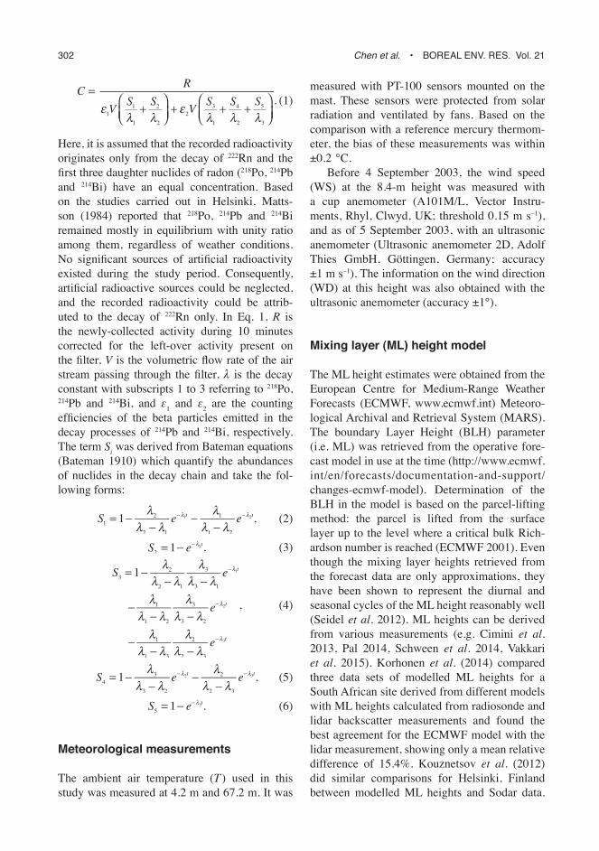
. (1)

Here, it is assumed that the recorded radioactivity originates only from the decay of 222Rn and the first three daughter nuclides of radon (218Po, 214Pb and 214Bi) have an equal concentration. Based on the studies carried out in Helsinki, Matts-son (1984) reported that 218Po, 214Pb and 214Bi remained mostly in equilibrium with unity ratio among them, regardless of weather conditions. No significant sources of artificial radioactivity existed during the study period. Consequently, artificial radioactive sources could be neglected, and the recorded radioactivity could be attrib-uted to the decay of 222Rn only. In Eq. 1, R is the newly-collected activity during 10 minutes corrected for the left-over activity present on the filter, V is the volumetric flow rate of the air stream passing through the filter, λ is the decay constant with subscripts 1 to 3 referring to 218Po, 214Pb and 214Bi, and ε1 and ε2 are the counting efficiencies of the beta particles emitted in the decay processes of 214Pb and 214Bi, respectively. The term Si was derived from Bateman equations (Bateman 1910) which quantify the abundances of nuclides in the decay chain and take the fol-lowing forms:

, (2)

, (3)

, (4)

, (5)

. (6)

Meteorological measurements

The ambient air temperature (T ) used in this study was measured at 4.2 m and 67.2 m. It was

measured with PT-100 sensors mounted on the mast. These sensors were protected from solar radiation and ventilated by fans. Based on the comparison with a reference mercury thermom-eter, the bias of these measurements was within ±0.2 °C.

Before 4 September 2003, the wind speed (WS) at the 8.4-m height was measured with a cup anemometer (A101M/L, Vector Instru-ments, Rhyl, Clwyd, UK; threshold 0.15 m s–1), and as of 5 September 2003, with an ultrasonic anemometer (Ultrasonic anemometer 2D, Adolf Thies GmbH, Gottingen, Germany; accuracy ±1 m s–1). The information on the wind direction (WD) at this height was also obtained with the ultrasonic anemometer (accuracy ±1°).

Mixing layer (ML) height model

The ML height estimates were obtained from the European Centre for Medium-Range Weather Forecasts (ECMWF, www.ecmwf.int) Meteoro-logical Archival and Retrieval System (MARS). The boundary Layer Height (BLH) parameter (i.e. ML) was retrieved from the operative fore-cast model in use at the time (http://www.ecmwf.int/en/forecasts/documentation-and-support/changes-ecmwf-model). Determination of the BLH in the model is based on the parcel-lifting method: the parcel is lifted from the surface layer up to the level where a critical bulk Rich-ardson number is reached (ECMWF 2001). Even though the mixing layer heights retrieved from the forecast data are only approximations, they have been shown to represent the diurnal and seasonal cycles of the ML height reasonably well (Seidel et al. 2012). ML heights can be derived from various measurements (e.g. Cimini et al. 2013, Pal 2014, Schween et al. 2014, Vakkari et al. 2015). Korhonen et al. (2014) compared three data sets of modelled ML heights for a South African site derived from different models with ML heights calculated from radiosonde and lidar backscatter measurements and found the best agreement for the ECMWF model with the lidar measurement, showing only a mean relative difference of 15.4%. Kouznetsov et al. (2012) did similar comparisons for Helsinki, Finland between modelled ML heights and Sodar data.


Although the ECMFW ML heights did not show the best agreement with the measurement among tested models, the measured and ECMWF ML heights were found comparable.

FLEXTRA trajectory and data analysis

Air mass back trajectories arriving at Hyyt-iälä on the 950-hPa pressure level were calcu-lated with the FLEXTRA kinematic trajectory model (ver. 3.3) (Stohl et al. 1995). For this study, 120-h back trajectories were calculated in 3-h intervals. Analysed meteorological fields from the European Centre for Medium-Range Weather Forecasts (ECMWF) numerical weather forecast model were used as a model input.

The trajectory data were analysed based on the method proposed by Riuttanen et al. (2013), which takes into account the horizontal uncer-tainties associated with the atmospheric trans-port model used for generating the air mass trajectories. By comparing the distance between receptor cells and calculated trajectory with the distance being travelled along the trajectory to the measurement site, weighing factors were assigned to the receptor cells. According to Stohl and Seibert (1998), the horizontal uncertainty in the trajectory calculated from the FLEXTRA model, with the analysed meteorological field input from the ECMWF numerical weather fore-cast model, is less than 20% of the travel dis-tance after 120-h travel time. Similar horizontal bias has also been reported for the computed trajectories when compared with manned bal-loon tracks (Baumann and Stohl 1997). Accord-ingly, if an adjacent cell (cell 1 in Fig. 1) fell in between 10% and 20% of the travelling distance by the trajectory (d ) before reaching the SMEAR II station, it was given a weighing factor of 0.3 (‘near’ case), and if the distance between the cell (cell 2) and the trajectory was shorter than d2, it received a weighing factor of 0.7 (‘close’ case). Cells outside the 20% boundary were assumed to receive no influence from the contents carried by the air mass travelling along the trajectory.

Because the resolved radon concentration was log-normally distributed (Fig. 2), the geo-metric mean value of the weighed concentrations accumulated in each cell was used to construct

the concentration field following Eq. 7, which was then normalised by the median values of the data set in this study to generate a relative con-centration field.

, (7)

where, i and j are the indices for the geographi-cal coordinates of a receptor cell, n is the index of the trajectory, and w represents the weighing factor, with k and l indicting the ‘close’ and ‘near’ cases, respectively. According to Riut-tanen et al. (2013), Eq. 7 is applicable only when the number of trajectory hits within each cell grid is greater than 10.

Mass balance analysis of the evolution of radon concentration with time and ML height

A mass balance approach, based on the Eulerian box model (Seinfeld and Pandis 2006), can be written to depict the temporal evolution of the atmospheric radon concentration with time by presuming that an equilibrium state is always established in the ML right after any change in

cell 1

cell 2

d

d1 d2

SMEAR II

Fig. 1. A schematic demonstration of the trajectory analysis. Here d1 = 0.2 ¥ d and d2 = 0.1 ¥ d, where d represents the distance being travelled by the trajectory before reaching the SMEAR II station.


the system. The atmospheric radon concentra-tion in this equilibrium state is expressed as Ceq. Furthermore, the distribution of radon in the ML is assumed to be homogeneous and therefore Ceq equals to the concentration derived from the measurement.

When the studied column is narrow enough, the horizontal transport of radon into the con-cerned volume can be roughly cancelled by the out-going fraction carried out by air masses from the volume. When averages of long-term data are considered, the effect of the horizontal transport on the column concentration can also be neglected, because the motion of air masses is not restricted into a single direction.

The primary source of radon is due to exhala-tion. Radon typically vanishes within the volume by spontaneous decay. The application of a mass balance approach is straightforward when this volume is constant. In the atmosphere, the ML depth changes with time, typically being low during night and early morning hours followed by a growth after sunrise with the maximum reached in the afternoon (e.g. Schween et al. 2014, Pal et al. 2015). When the ML expands, air above the ML containing radon gas (with concentration marked as C0) gets mixed into the volume, which dilutes the radon content in it, yet being an additional source of radon. C0, how-ever, becomes equal to Ceq, once the maximum mixing depth is reached. As a result, the balance equation can be written as:

dCeq/dt = Exhalation + Dilutiuon + Decay, (8)

where the exhalation term can be expressed as the exhalation rate (ExR) over the ML height (H), ExR/H. By assuming that the radon con-centration in the ML is in equilibrium, the decay term can be written as

dCeq/dtDecay = –λCeq, (9)

where λ is the decay constant of 222Rn. The dilu-tion term has two different forms depending on the dynamics of the ML: for ML expansion,

, (10)

and for ML shrinking, as C0 = Ceq,

dCeq/dtDilution = 0. (11)

According to Eq. 10, the change rate of radon concentration is related to the expansion rate of the ML. This relationship has been illustrated by Pal et al. (2015), showing that the faster the ML grows, the faster radon concentration decreases.

Results and discussion

General patterns in the atmospheric radon concentration

At the SMEAR II station, daily mean atmos-pheric concentrations of 222Rn ranged between < 0.1 and 11 Bq m–3 (the lower end of this range is restricted by the detection limit of the radon

CRn (Bq m–3)0.1 1 10

Per

cent

age

0

0.02

0.04

0.06

0.08

0.1

0.12

0.14

0.16

y = 0.1537exp{–[(logx – 0.5084)/0.9612]2}R2 = 0.983

Fig. 2. Statistical distri-bution of the daily mean atmospheric radon con-centration, CRn, for 2000–2006 with a log-normal fit-ting (solid line).


monitor) during the years 2000–2006. They fol-lowed a log-normal distribution with a geometric mean of 2.5 Bq m–3 and a geometric standard deviation of 1.7 Bq m–3 (Fig. 2). The geometric mean of the daily mean radon concentration in each year fell in between 2.3 and 2.6 Bq m–3, implying little inter-annual variability. A similar distribution pattern was also observed in daily medians of radon concentration, the geometric mean of which, however, got a slightly smaller

value of 2.3 Bq m–3 with a geometric standard deviation of 1.8 Bq m–3.

For the years 2000–2006, both the hourly medians for monthly periods and the daily medi-ans on the day-of-year basis of the atmospheric radon concentration varied roughly between 1 and 5 Bq m–3 (Figs. 3 and 4). Similar to obser-vations by Pal et al. (2015) in central Europe, a clear diurnal cycle in the atmospheric radon concentration, with a maximum in the early

Month1 2 3 4 5 6 7 8 9 10 11 12

Tim

e (U

TC +

2)

123456789

101112131415161718192021222324

1

1.5

2

2.5

3

3.5

4

4.5

5

5.5

CR

n (B

q m

–3)

Fig. 3. Patterns in the hourly-median atmos-pheric radon concentration (CRn) in different months in 2000–2006. First, hourly medians were calculated for the whole measure-ment period from the 10-minute measurement data. From these data, median values for each month as a vector of hour of the day were then cal-culated.

Day of year1 60 120 180 240 300 360

0

1

2

3

4

5

6

CR

n (B

q m

–3)

Fig. 4. Seasonal variation in the daily median atmospheric radon concentration (CRn) on the day-of-year basis for the years 2000–2006. First, hourly medians were calculated for the whole measurement period from the 10-minute measurement data. From these data, a median value for each day of the year was calculated.


morning and minimum in the afternoon, was found for March–October. During these months, the average length of a period within a day with a low atmospheric radon concentration first increased until the end of May, after which an opposite behaviour was seen until September. During the other months, the atmospheric radon concentration showed little diurnal variation. The high radon concentration observed between midnight and 9:00 (UTC + 2) in the morning in late summer can be ascribed to the increase in local emission due to the optimal combination of the temperature and soil moisture condition for radon exhalation, together with the frequent occurrence of nocturnal inversion.

As for the seasonal cycle (Fig. 4), a relatively high median radon concentration was found in winter. A decline in the daily median radon con-centration during the spring lasted until April. Thereafter, a recovery of concentration prevailed during the summer. The median radon concen-tration fluctuated around a relatively high level throughout the rest of the year, even though a slight decrease was seen in autumn. This obser-vation is comparable to the pattern shown by Mattsson (1970), who also reported that 214Bi, the short-lived progeny of 222Rn, possessed a con-centration in the range of about 25–125 pCi m–3 (1–5 Bq m–3) in Finland. A joint effect of soil moisture and mixing layer development, which will be discussed later in the text, resulted in the

minimum median radon concentration observed in April. The high atmospheric concentration of radon in autumn and winter was typically related to the persistent surface inversion.

Clear diurnal cycles in the median radon concentration based on the 10-min data were identifiable in all seasons, with the exception of winter (Fig. 5a). The largest amplitude in the diurnal variation was observed in the summer (June–August), with the maximum median radon concentration at around 06:00 and minimum at around 16:00. Comparable daily mean atmos-pheric concentrations of 222Rn were observed in summer (2.7 Bq m–3), autumn (September–November, 2.8 Bq m–3) and winter (December–February, 2.7 Bq m–3), whereas the concentra-tion was clearly lower in spring (March–May, 1.7 Bq m–3). Our findings are similar to the results obtained for a French site (Pal et al. 2015), where, however, no obvious low radon concentration was observed in spring and more pronounced diurnal variation was observed in autumn as compared with the patterns in other seasons.

Vertical mixing, horizontal transportation and local emissions affect atmospheric radon concentration. In summer, autumn and winter, the dilution due to vertical mixing, contribution from horizontal transportation and changes in local emissions were assumed to maintain the atmospheric radon concentration around a rela-

Time (UTC + 2)00 02 04 06 08 10 12 14 16 18 20 22 00

1

1.5

2

2.5

3

3.5

4

4.5a b

Spring Summer Autumn WinterTime (UTC + 2)

00 02 04 06 08 10 12 14 16 18 20 22 00

Mod

elle

d m

ixin

g la

yer h

eigh

t (m

)

0

200

400

600

800

1000

1200

1400

1600

1800

CR

n (B

q m

–3)

Fig. 5. Diurnal variations in different seasons in (a) median radon concentrations (CRn) in 10-min resolution for the years 2000–2006, and (b) modelled mixing layer heights processed as hourly medians for the years 2003–2006. The seasons are: spring (March–May), summer (June–August), autumn (September–November) and winter (December–February).


tive stable median level (Fig. 5a). However, the dilution effect of vertical mixing and the reduc-tion in local radon exhalation due to water block-age from snow thawing are especially prominent in spring, consequently leading to a remarkably low atmospheric concentration of radon..

The response of the atmospheric radon concentration to the development of ML

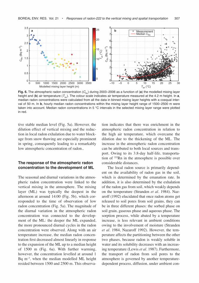
The seasonal and diurnal variations in the atmos-pheric radon concentration were linked to the vertical mixing in the atmosphere. The mixing layer (ML) was typically the deepest in the afternoon at around 14:00 (Fig. 5b), which cor-responded to the time of observation of low radon concentration (Fig. 5a). The magnitude of the diurnal variation in the atmospheric radon concentration was connected to the develop-ment of the ML: the deeper the ML expanded, the more pronounced diurnal cycles in the radon concentration were observed. Along with an air temperature increase, the median radon concen-tration first decreased almost linearly in response to the expansion of the ML up to a median height of 1500 m (Fig. 6a). With further warming, however, the concentration levelled at around 1 Bq m–3, when the median modelled ML height resided between 1500 and 2500 m. This observa-

tion indicates that there was enrichment in the atmospheric radon concentration in relation to the high air temperature, which overcame the dilution due to the thickening of the ML. The increase in the atmospheric radon concentration can be attributed to both local sources and trans-port. Owing to its 3.8-day half-life, transporta-tion of 222Rn in the atmosphere is possible over considerable distances.

The local radon source is primarily depend-ent on the availability of radon gas in the soil, which is determined by the emanation rate. In addition, it is also determined by the exhalation of the radon gas from soil, which weakly depends on the temperature (Stranden et al. 1984). Naz-aroff (1992) elucidated that once radon atoms get released to soil pores from soil grains, they can be in three different phases: the sorbed phase on soil grain, gaseous phase and aqueous phase. The sorption process, while abated by a temperature increase, is less relevant in ambient conditions owing to the involvement of moisture (Stranden et al. 1984, Nazaroff 1992). However, the tem-perature affects the partitioning between the other two phases, because radon is weakly soluble in water and its solubility decreases with an increas-ing temperature (Lewis et al. 1987). Furthermore, the transport of radon from soil pores to the atmosphere is governed by another temperature-dependent process, diffusion, under ambient con-

Fig. 6. The atmospheric radon concentration (CRn) during 2003–2006 as a function of (a) the modelled mixing layer height and (b) air temperature (TAir). The colour scale indicates air temperature measured at the 4.2 m height. In a, median radon concentrations were calculated from all the data in binned mixing layer heights with a coequal inter-val of 50 m. In b, hourly median radon concentrations within the mixing layer height range of 1500–2500 m were taken into account. Median radon concentrations in 5 °C intervals in the selected mixing layer range were plotted in red.

Modelled mixing layer height (m)0 500 1000 1500 2000 2500 3000 3500

0

0.5

1

1.5

2

2.5

3

3.5

T air

(°C

)

Tair (°C)

0

5

10

15

20

25

–10 –5 0 5 10 15 20 25 300

1

2

3

4

5

6

7

8ba Measurement

Median CRn

CR

n (B

q m

–3)

CR

n (B

q m

–3)


ditions (Nazaroff 1992). Accordingly, an increase in the air temperature heats the surface layer of the soil, which subsequently contributes to the growth in atmospheric radon concentration by reducing the solubility of radon in moisture con-tained in soil pores and enhancing the diffusion of the radon gas through the soil.

Compared with the temperature, the moisture has been shown to have a stronger influence on radon exhalation (Stranden et al. 1984, Nazaroff 1992). Typically the moisture plays opposite roles in affecting radon emanation and diffusion. The moisture reduces significantly the diffusion coefficient of radon in soil (Nazaroff 1992), whereas it enhances the emanation of radon from soil grains to soil pores (Markkanen and Arvela 1992), possibly due to the lower recoil range of radon in water than that in air (Nazaroff 1992). The overall effect of these two processes is that the maximum exhalation rate of radon appears at an optimal moisture concentration depending on the soil type, as shown by Stranden et al. (1984). The high soil moisture content during the snow-thawing period hindered radon exhalation, which contributed to the occurrence of the minimum radon concentration in April (Figs. 3–4). Yet, an over-dry condition brings no incentive either. Therefore, the ground-water level has been coherently found as an indicator of radon exhala-tion (Mattsson 1970). During warm periods, the surface air dries up the topsoil, which favours the diffusive transport of radon through the ground surface to the atmosphere, yet possibly without disrupting the radon emanation from ores con-taining the parent nuclides of radon. As a con-sequence, the plateau in Fig. 6a was most likely caused, in addition to the transported source, by the combination of the opposite effects of enhanced radon exhalation from soil and vertical dilution in the atmosphere. This means that the effect of the intensified radon exhalation result-ing from increasing air temperature was coun-terbalanced by the enhanced dilution as the ML height grew from 1500 m to 2500 m (Fig. 6a). In support of this, an exponential relationship was identified between air temperature and atmos-pheric radon concentration within the ML height range between 1500 and 2500 m based on hourly data (Fig. 6b). Such an increase in the atmos-pheric radon concentration with an increasing

air temperature was also evident beyond this ML range, when air temperature was above 5 °C.

For the ML height higher than about 2500 m, the median radon concentration tended to decrease further with an increasing ML height, and the median air temperature dropped from about 15 °C to slightly below 10 °C (Fig. 6a). Days with such a thick ML and moderate air temperature occurred typically in late spring and early summer.

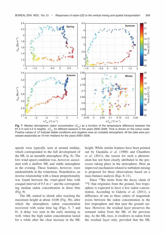
We observed clear diurnal patterns in the median radon concentration as a function of the temperature difference between the 67.2 m and 4.2 m heights in spring, summer and autumn (Fig. 7). Apart from the winter season, a stable layer near the surface with a positive temperature difference (inversion) was observed during the night, which lasted the longest in summer, fol-lowed by spring and autumn. The positive tem-perature difference was prominent in winter, yet no clear pattern in the evolution of this param-eter with time could be identified in relation to the atmospheric radon concentration during this season. During other seasons, the median radon concentration increased over the night when the positive temperature inversion prevailed, and ultimately led to the maximum median radon concentration at around 06:00 in the morning (Fig. 5a). Hereafter, the enhanced vertical mixing due to expanding ML after sunrise diminished the temperature inversion. Eventually, a reduc-tion in the median radon concentration occurred in the unstable atmosphere when the dilution became predominant on average. This process was intensified along with the further develop-ment of the ML until the maximum depth was reached at around 14:00, when the median radon concentration nearly dropped to its minimum. Thereafter, especially in summer and autumn following some latency, a slow increase in the median radon concentration emerged along with the gradual shrinkage of the ML.

The effect of wind on the atmospheric radon concentration

Wind affects the observed variability in the con-centrations of trace components in the atmos-phere (e.g. Pal et al. 2014). High median wind


speeds were typically seen at around midday, which corresponded to the full development of the ML in an unstable atmosphere (Fig. 8). The low-wind-speed condition was, however, associ-ated with a shallow ML and stable atmosphere in the evening. These features, however, were unidentifiable in the wintertime. Nonetheless, an inverse relationship with a linear proportionality was found between the wind-speed bins with coequal interval of 0.5 m s–1 and the correspond-ing median radon concentration in these bins (Fig. 9).

The ML started to shrink after reaching the maximum height at about 14:00 (Fig. 5b), after which the atmospheric radon concentration recovered with some time lag (Figs. 5, 7 and 8). A delay was seen in the early morning as well, when the high radon concentration lasted for a while after the clear increase in the ML

height. While similar features have been pointed out by Guedalia et al. (1980) and Chambers et al. (2011), the reason for such a phenom-enon has not been clearly attributed to the pro-cesses taking place in the atmosphere. Here an improved mechanism related to turbulent mixing is proposed for these observations based on a mass balance analysis (Eqs. 8–11).

Since 222Rn stems from the decay chain of 238U that originates from the ground, free tropo-sphere is expected to have a low radon concen-tration. According to Galeriu et al. (2011), a difference of one to three orders of magnitude exists between the radon concentration in the free troposphere and that near the ground sur-face. However, the residual layer preserves the remnant radon from the ML of the previous day. As the ML rises, it swallows in radon from the residual layer only, provided that the ML

–2 –1.5 –1 –0.5 0 0.5 11

1.2

1.4

1.6

1.8

2

2.2

2.4

Tim

e (U

TC +

2)

Spring

00

03

06

09

12

15

18

21

00

–1.5 –1 –0.5 0 0.5 1 1.5 21.5

2

2.5

3

3.5

4

4.5Summer

–4 –3 –2 –1 0 12.2

2.4

2.6

2.8

3

3.2

3.4

Tim

e (U

TC +

2)

Autumn

00

03

06

09

12

15

18

21

00

ΔTair (°C m–1) ΔTair (°C m–1)

CR

n (B

q m

–3)

CR

n (B

q m

–3)

–0.05 0 0.05 0.1 0.15 0.2 0.252.5

2.55

2.6

2.65

2.7

2.75

2.8

2.85Winter

Fig. 7. Median atmospheric radon concentration (CRn) as a function of the temperature difference between the 67.2 m and 4.2 m heights, ∆TAir, for different seasons in the years 2000–2006. Time is shown on the colour scale. Positive values of ∆T indicate stable conditions and negative ones an unstable atmosphere. All the data were pro-cessed seasonally as 10-min medians for the years 2000–2006.


height does not exceed that of the previous day. Otherwise, the nearly radon-free air from the free troposphere would significantly reduce the radon concentration in the ML. An example of the behaviours of the dilution and decay terms in the mass balance for the radon in the ML (Eqs. 8–11) is present in Fig. 10. This analysis was carried out using the median radon concentration and the median modelled ML height of the diur-nal data from the summers of 2000–2006. As the ML typically is deepest in summer (McGrath-Spangler and Denning 2013) and tends to deepen towards the end of summer (Leventidou et al. 2013), the air from the free troposphere has the greater effect on the dilution at this time of the year. In addition, the sum of the dilution and decay terms should be negative, since there is another source, the exhalation term, in the

0 500 1000 15001

1.2

1.4

1.6

1.8

2

2.2

2.4Spring

15

12

18

9

21

63

0

Win

d sp

eed

(m s

–1)

Win

d sp

eed

(m s

–1)

Win

d sp

eed

(m s

–1)

0.6

0.7

0.8

0.9

1

1.1

1.2

1.3

1.4

Modelled mixing layer height (m)

0 500 1000 1500 20001.5

2

2.5

3

3.5

4

4.5Summer

15

12

18

9

21

63

0

ΔT > 0 ΔT < 0

0.5

0.6

0.7

0.8

0.9

1

1.1

Modelled mixing layer height (m)400 500 600 700 800

2.2

2.4

2.6

2.8

3

3.2

3.4Autumn

15

1218

9

21

6

0

3

0.75

0.8

0.85

0.9

0.95

1

1.05

CR

n (B

q m

–3)

CR

n (B

q m

–3)

CR

n (B

q m

–3)

CR

n (B

q m

–3)

380 400 420 440 460 480 5002.5

2.55

2.6

2.65

2.7

2.75

2.8

2.85Winter

15

18

12

21

0

3

9

6

0.734

0.735

0.736

0.737

0.738

0.739

0.74

Win

d sp

eed

(m s

–1)

Fig. 8. Median atmospheric radon concentration (2000–2006), CRn, as function of the modelled mixing layer height (2003–2006) during the four seasons. The colour scale indicates the median wind speed (2000–2006). The filled black triangles indicate the observation time in 3-h intervals. The circles correspond to the positive (negative) temperature difference between the heights 67.2 m and 4.2 m. All the data were processed seasonally as 10-min medians.

Wind speed (m s–1)0 1 2 3 4 5

0

0.5

1

1.5

2

2.5

3y = –0.57x + 2.83R = –0.993

CR

n (B

q m

–3)

Fig. 9. The relation between the median atmospheric radon concentration (CRn) and median wind speed measured at the 8.4 m height for the years 2000–2006. Median radon concentrations were calculated in wind-speed bins with a coequal interval of 0.5 m s–1.


balance equation. Accordingly, the atmospheric radon concentration above the ML, when assum-ing C0 to be constant, should be smaller than 0.0627 Bq m–3. The position and shape of the curves in Fig. 10 are insensitive to small varia-tions in C0.

The relatively-stable nocturnal bound-ary layer had a depth slightly below 200 m in summer (Fig. 5b). At around 04:30 in the morn-ing, the ML started to expand and the atmos-pheric radon concentration reached its maximum (Fig. 5a). An increase in the ML height reduces the exhalation term in Eq. 8. In addition, the sum of the dilution and decay terms possessed negative values, even though this sum exhib-ited an exponential increase with an increase in the ML height (Fig. 10). Thus, in principle, the atmospheric radon concentration should drop simultaneously, which however, showed a delay by about 2 h. This observation could be related to the low turbulence in summer before 06:30 (Fig. 8): the solar radiation induced shear-driven turbulence in the top layer of the ML first and the gradual transport of this mixing to the measure-ment level retarded the instantaneous decrease in radon concentration. Using six years of data, Lapworth (2006) showed, that the downward transportation of turbulence is primarily responsi-ble for warming up the surface layer. The surface

heating enables the transition from shear-driven to convective mixing in the morning, but the warming of the surface layer comes mostly from the entrainment above due to the mechanical tur-bulence (Angevine 2001). The end of the morn-ing transition occurs typically at the maximum extension rate of the ML depth, which is the onset of ML growth after the stable boundary layer is eroded (Pal et al. 2012, Pal et al. 2013), when the dilution effect on atmospheric radon concentra-tion due to vertical mixing becomes pronounced. As for the shrinkage of the ML, the dilution term was zero, i.e. exhalation was the only source term in the mass balance equation. The turbulence was gradually discharged in the beginning of the ML thinning (Fig. 8) and such decay in turbulence is typically initialised in the top layer of the ML (Darbieu et al. 2014). Correspondingly, only a gentle increase in the median radon concentra-tion was observed (Fig. 5a). When the turbulence diminished, the accumulation of radon became predominant near the ground surface and a clear recovery in the atmospheric radon concentration eventually emerged after 19:00 (Fig. 5a). Once such a relatively stable condition was encoun-tered, especially in spring and summer, the accu-mulation of radon near the ground surface contin-ued until turbulence was introduced again in the following morning.

Modelled boundary layer height (m)0 200 400 600 800 1000 1200 1400 1600 1800

dCeq

/dt [

dilu

tion

+ de

cay]

(x 1

0–4 B

q m

–3 s

–1)

–8

–6

–4

–2

0

C0 = 0.0627 Bq m–3

dCeq /dt [decay] (x 10

–6 Bq m

–3 s–1)

–7

–6

–5

–4

–3Fig. 10. The contribution of the dilution and decay terms in Eq. 8. The dilu-tion term for the period of ML expansion was determined by assuming a constant radon concen-tration of 0.0627 Bq m–3 in the air above the ML. The change rate of atmos-pheric radon concentra-tion during ML expansion is shown in blue on the left-hand-side axis and that during ML shrinkage in red on the right-hand-side axis. The analysis was carried out under the assumption of a homo-geneous distribution of radon through the mixing layer.


Apart from the convective transport of radon gas in the ML, the advective motion of air masses brings also variations in the atmospheric radon concentration. As 222Rn has a half-life of 3.8 days, sources originating far away from the SMEAR II station may be detected at this site after a long journey guided by the movement of air masses in the atmosphere.

The lowest median radon concentrations at the SMEAR II station were typically observed when the wind blew from the northwest regard-less of the wind speed. Such winds are expected to bring air masses of marine origins to the measurement site (Fig. 11). Because the role of the oceans as a radon source is negligible, these

marine air masses, which originate typically from the Atlantic Ocean, carry only small amounts of radon, resulting in the observation of the lowest radon concentration. Relatively high median radon concentrations, especially in spring and summer, were observed with the lowest median wind speeds from the northeast. This phenom-enon might be ascribed to situations, where under certain combinations of the locations of high and low pressure systems, air masses arriving at the SMEAR II station from the northeast actually originate from continental areas of eastern Europe or Russia rather than from marine regions. In the springtime, high median radon concentra-tions generally span over the wind directions of

Win

d S

peed

(m s

–1)

0.1

0.2

0.3

0.4

0.5

0.6

0.7

0.8

0.9

1

1.1

1.2

1.3

0.5 1 1.5 2 2.5

30

210

60

240

90270

120

300

150

330

180

0

North

South

EastWest

Spring

1 2 3 4

30

210

60

240

90270

120

300

150

330

180

0

North

South

EastWest

(Bq m–3)(Bq m–3)

Summer

1 2 3 4 5

30

210

60

240

90270

120

300

150

330

180

0North

South

EastWest

Autumn

(Bq m–3)

1 2 3 4 5

30

210

60

240

90270

120

300

150

330

180

0

North

South

EastWest

Winter

(Bq m–3)

Fig. 11. Variations in the median atmospheric radon concentration, expressed as the distance form the origin, in relation to the wind direction and speed measured at the 8.4-m height in different seasons of the years 2003–2006. The median wind speed is shown on the colour scale. Radon concentration and wind speed data were processed as medians over 30° sectors of wind direction.


30°–180°, with the maximum found with south-easterly winds associated with the continental air masses. Such a pattern existed in summer as well, however, with the maximum observed with both southeasterly and northeasterly winds. Although high median radon concentrations were also asso-ciated with southeasterly winds in autumn and winter seasons, in contrast to the warmer seasons, median radon concentrations remained at rela-tively low levels when the wind came from the northeast. The southwesterly winds were strong-est in all seasons, but brought, on average, only moderate amounts of radon, possibly due to the mixing in of clean marine air masses from the Atlantic Ocean, because air masses coming to Finland from the west have more mid-latitude weather system activity than air masses coming from the east (Hoskins and Hodges 2002, Sinclair et al. 2012).

Trajectory analysis

The highest wind speed was measured between 12:00 and 15:00 (Fig. 8). In order to minimise the perturbation from local radon sources, radon data in this time window were used in the trajectory analysis. Overall, the relative concentration (see Fig. 12) suggested that the high radon relative concentration came substantially from the south-east. This observation aligns with the outcomes obtained from the exploration of the atmospheric radon concentration in relation to winds (Fig. 11) and also agrees with the results for 210Pb, a daughter nuclide of 222Rn, shown by Paatero and Hatakka (2000) based on samples collected at Sodankylä station (67°22Ń, 26°39É) in Fin-land. Riuttanen et al. (2013) showed that the potential source areas of aerosol particles located in the eastern Europe and Russia, which coincide with the hotspots depicted in Fig. 12 for radon, indicating the consistency in air mass transport. According to Wilkening and Clements (1975), the exhalation rate of 222Rn over ocean is less than 2% of that over the continental areas. Oce-anic air masses, therefore, share practically no contribution to the observed atmospheric radon concentration at the SMEAR II station whereas air masses passed over continental land take part in the transportation of radon gas originating

from locations other than the measurement site. Consequently, in the annual trajectory statistics, hotspots of radon were observed over the con-tinent in the southeast (Fig. 12). Besides, high relative concentration of radon was identified on the southern coast of Finland around Helsinki, coincident with the pattern shown by Szegvary et al. (2009) and the high concentration regions shown on the indoor radon map published by the Finnish Radiation and Nuclear Safety Authority (STUK 2014) and on the European indoor radon map (Tollefsen et al. 2014).

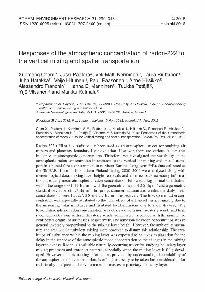
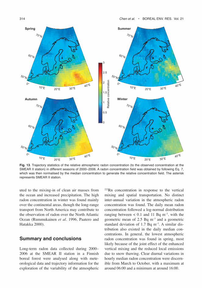
The transport pattern of radon, however, showed distinct seasonal features (Fig. 13). The continental air masses from the southeast brought especially large portion of radon to the SMEAR II station in spring and autumn, com-pared with the other two seasons. Sources of radon could be seen in northern Sweden all year round except in autumn. With the exception of winter, southern Sweden and Norway typically had slightly higher radon concentrations. An interesting spot was found for summer in south-ern Norway near the border with Sweden, which was probably due to the dilution by marine air masses over the surrounding regions. This region has been reported to have relatively high indoor radon concentrations (Tollefsen et al. 2014). The low concentration region over the continental Europe in the summer could also be attrib-

0° 10°E 20°E 30°E

40°E

50°E

60°E

70°E

Rel

ativ

e co

ncen

tratio

n

0

0.5

1

1.5

2

2.5

3

Fig. 12. Trajectory statistics of the relative atmospheric radon concentration (to the observed concentration at SMEAR II station) over 2000–2006. A radon concen-tration field was obtained by following Eq. 7, which was then normalised by the median concentration to generate the relative concentration field. The asterisk represents the SMEAR II station.


uted to the mixing-in of clean air masses from the ocean and increased precipitation. The high radon concentration in winter was found mainly over the continental areas, though the long-range transport from North America may contribute to the observation of radon over the North Atlantic Ocean (Rummukainen et al. 1996, Paatero and Hatakka 2000).

Summary and conclusions

Long-term radon data collected during 2000–2006 at the SMEAR II station in a Finnish boreal forest were analysed along with mete-orological data and trajectory information for the exploration of the variability of the atmospheric

222Rn concentration in response to the vertical mixing and spatial transportation. No distinct inter-annual variation in the atmospheric radon concentration was found. The daily mean radon concentration followed a log-normal distribution ranging between < 0.1 and 11 Bq m–3, with the geometric mean of 2.5 Bq m–3 and a geometric standard deviation of 1.7 Bq m–3. A similar dis-tribution also existed in the daily median con-centrations. In general, the lowest atmospheric radon concentration was found in spring, most likely because of the joint effect of the enhanced vertical mixing and the reduced local emissions due to snow thawing. Clear diurnal variations in hourly median radon concentration were discern-ible from March to October, with a maximum at around 06:00 and a minimum at around 16:00.

0° 10°E 20°E 30°E

40°E

50°N

60°N

70°N

Spring

0° 10°E 20°E 30°E

40°E

50°N°N

60°N

70°N

Summer

Rel

ativ

e co

ncen

tratio

n

0

0.5

1

1.5

2

2.5

3

0° 10°E 20°E 30°E

40°E

50°N

60°N

70°N

Autumn

0° 10°E 20°E 30°E

40°E

50°N

60°N

70°N

Winter

Fig. 13. Trajectory statistics of the relative atmospheric radon concentration (to the observed concentration at the SMEAR II station) in different seasons of 2000–2006. A radon concentration field was obtained by following Eq. 7, which was then normalised by the median concentration to generate the relative concentration field. The asterisk represents SMEAR II station.


In general, the median radon concentration was inversely related to the depth of the mixing layer (ML) height. However, a plateau was observed for the ML heights between 1500 and 2500 m, which coincided with an increased air temperature. This situation resulted from both the enhanced radon exhalation from soil due to the increasing temperature and the promoted dilution as the consequence of the thickening of the ML. During the winter months, the 222Rn concentration was relatively high with very little diurnal variation. Radon was accumulated near the surface as a consequence of the absence of solar radiation and subsequently reduced verti-cal mixing of the air. Later in the spring the concentration level decreased, when the mixing was intensified as the amount of solar radia-tion increased. The minimum concentrations was observed in the late spring when daytime con-vective movements of the air diluted the radon content of the air to a bigger volume and the flux of radon from the ground to the atmosphere was at its seasonal minimum due to the high moisture content in the soil due to snow thawing. In the late summer, the diurnal variation of atmospheric radon concentration was at its maximum due to frequent nocturnal surface inversions and the simultaneous high radon flux from the ground to the atmosphere. The latter factor, in turn, is related to the low soil moisture content, espe-cially in the surface layer.

The lowest radon concentration was related to clean marine air masses arriving at the SMEAR II station from the northwest, and high radon concentrations were typically found during southeasterly winds of continental origins. These observations were confirmed by the trajectory analysis. A reduction in the atmospheric radon concentration was observed in response to the intensification of wind speed. In addition, the downward transportation of turbulence from the top of the ML layer in the early morning led to a delayed response in the atmospheric radon concentration to the expansion of the ML. Simi-larly, the discharge of residual turbulence in the shrinking ML retarded the immediate recovery of the atmospheric radon concentration.

The features in the variability of the atmos-pheric radon concentration found here in relation to the development of the mixing volume and

the spatial transportation are important charac-teristics of radon in the atmosphere. In general, the variation in atmospheric radon concentra-tion can capture the vertical mixing height well. However, as shown in this paper, the changes in atmospheric radon concentration do not instantly follow the start of ML growth and shrinkage. This information is of paramount importance when determining the ML height or parameteris-ing the PBL mixing processes from radon data. In addition, our results imply that radon is a suitable candidate for studying the evolution of the turbulence during morning and evening tran-sitions in the boundary mixing processes. Nev-ertheless, it is also crucial to take into account the effect of the horizontal transportation on the atmospheric radon concentration. Wind either potentially carries more radon to the site or dilutes locally-emitted atmospheric radon. Such information can be typically obtained by study-ing the trajectories of air masses arriving at the measurement site, without which biases may be introduced when comparing similar verti-cal mixing processes of different days by using radon. Moreover, as an inert and long-lived gas, radon is useful in evaluating transport models, which can be applied to other trace compo-nents or pollutants in the atmosphere. Yet, to improve the accuracy of the transport pattern, it is important to be cautious about the variations in atmospheric radon concentration introduced by the boundary layer dynamics along the air-mass trajectories.

Acknowledgements: This study was supported by the Acad-emy of Finland Centre of Excellence (projects 272041 and 1118615). The authors acknowledge the funding provided by the CRAICC (Cryosphere–atmosphere interactions in a changing Arctic climate) project within the Nordforsk Top-level Research Initiative Programme ‘Interaction between climate change and the cryosphere. This study also received funding from the European Union’s Horizon 2020 Research and Innovation Programme (grant no. 654109) as well as the European Union Seventh Framework Programme (FP7/2007-2013) (grant no. 262254). Valuable communica-tions and suggestions from Dr. Aki Virkkula were thankfully appreciated.

References

Angevine W.M. 2001. Observations of the morning transition


of the convective boundary layer. Bound.-Layer Meteor. 101: 209–227.

Ashok G.V., Nagaiah N., Shiva Prasad N.G. & Ambika M.R. 2011. Study of radon exhalation rate from soil, Banga-lore, south India. Radiat. Protect. Environ. 34: 235–239.

Barlow J.F., Dunbar T.M., Nemitz E.G., Wood C.R., Gal-lagher M.W., Davies F., O’Connor E. & Harrison R.M. 2011. Boundary layer dynamics over London, UK, as observed using Doppler lidar during REPARTEE-II. Atmos. Chem. Phys. 11: 2111–2125.

Bateman H. 1910. Ther solution of a system of differential equations occurring in the theory of radio-active trans-formations. Proceedings of the Cambridge Philosophical Society, Mathematical and Physical Sciences 15: 423.

Baumann K. & Stohl A. 1997. Validation of a long-range tra-jectory model using gas balloon tracks from the Gordon Bennett Cup 95. J. Appl. Meteorol. 36: 711–720.

Behrendt A., Pal S., Wulfmeyer V., Valdebenito B.Á.M. & Lammel G. 2011. A novel approach for the charac-terization of transport and optical properties of aerosol particles near sources — Part I: Measurement of particle backscatter coefficient maps with a scanning UV lidar. Atmos. Environ. 45: 2795–2802.

Beyrich F. 1997. Mixing height estimation from sodar data — a critical discussion. Atmos. Environ. 31: 3941–3953.

Chambers S., Williams A.G., Zahorowski W., Griffiths A. & Crawford J. 2011. Separating remote fetch and local mixing influences on vertical radon measurements in the lower atmosphere. Tellus 63B: 843–859.

Clements W.E. & Wilkening M.H. 1974. Atmospheric pres-sure effects on 222Rn transport across the earth–air inter-face. J. Geophys. Res. 79: 5025–5029.

Darbieu C., Lohou F., Lothon M., Vilà-Guerau de Arellano J., Couvreux F., Durand P., Pino D., G. Patton E., Nilsson E., Blay-Carreras E. & Gioli B. 2014. Turbulence vertical structure of the boundary layer during the afternoon tran-sition. Atmos. Chem. Phys. Discuss. 14: 32491–32533.

ECMWF 2001. Newsletter No. 90. Shinfield Park, Reading, UK.

Escobar V.G., Tomé F.V. & Lozano J.C. 1999. Procedures for the determination of 222Rn exhalation and effective 226Ra activity in soil samples. Appl. Radiat. Isot. 50: 1039–1047.

Forster C., Stohl A. & Seibert P. 2007. Parameterization of convective transport in a lagrangian particle dispersion model and its evaluation. J. Appl. Meteor. Climatol. 46: 403–422.

Galeriu D., Melintescu A., Stochioiu A., Nicolae D. & Balin I. 2011. Radon, as a tracer for mixing height dynamics — an overview and rado perspectives. Rom. Rep. Phys. 63: 115–127.

Griffiths A.D., Parkes S.D., Chambers S.D., McCabe M.F. & Williams A.G. 2013. Improved mixing height monitor-ing through a combination of lidar and radon measure-ments. Atmos. Meas. Tech. 6: 207–218.

Grossi C., Arnold D., Adame J.A., López-Coto I., Bolívar J.P., de la Morena B.A. & Vargas A. 2012. Atmospheric 222Rn concentration and source term at El Arenosillo 100 m meteorological tower in southwest Spain. Radiat. Meas. 47: 149–162.

Guedalia D., Ntsila A., Druilhet A. & Fontan J. 1980. Moni-toring of the atmospheric stability above an urban and suburban site using sodar and radon measurements. J. Appl. Meteorol. 19: 839–848.

Hari P. & Kulmala M. 2005. Station for measuring ecosys-tem-atmosphere relations (SMEAR II). Boreal Env. Res. 10: 315–322.

Hoskins B.J. & Hodges K.I. 2002. New perspectives on the northern hemisphere winter storm tracks. J. Atmos. Sci. 59: 1041–1061.

Jacobi W. & André K. 1963. The vertical distribution of radon 222, radon 220 and their decay products in the atmosphere. J. Geophys. Res. 68: 3799–3814.

Jocab D.J. & Prather M.J. 1990. Radon-222 as a test of con-vective transport in a general circulation model. Tellus 42B: 118–134.

Korhonen K., Giannakaki E., Mielonen T., Pfüller A., Laakso L., Vakkari V., Baars H., Engelmann R., Beukes J.P., Van Zyl P.G., Ramandh A., Ntsangwane L., Josipovic M., Tiitta P., Fourie G., Ngwana I., Chiloane K. & Komp-pula M. 2014. Atmospheric boundary layer top height in South Africa: measurements with lidar and radiosonde compared to three atmospheric models. Atmos. Chem. Phys. 14: 4263–4278.

Kouznetsov R., Wood C., Sofiev M., Soares J., Karppinen A. & Fortelius C. 2012. Sodar verification of boundary-layer height schemes for the output of meteorologi-cal models. In: 16th International Symposium for the Advancement of Boundary-Layer Remote Sensing, 5–8 June 2012, Boulder, Colorado, Steering Committee of the 16th International Symposium for the Advancement of Boundary-Layer Remote Sensing, pp. 138–141. [Also available at http://www.esrl.noaa.gov/psd/events/2012/isars/pdf/isars2012-abstractVolume.pdf].

Kritz M.A. 1983. Use of long-lived radon daughters as indi-cators of exchange between the free troposphere and the marine boundary layer. J. Geophys. Res. 88: 8569–8573.

Lac C., Donnelly R.P., Masson V., Pal S., Riette S., Donier S., Queguiner S., Tanguy G., Ammoura L. & Xueref-Remy I. 2013. CO2 dispersion modelling over Paris region within the CO2-MEGAPARIS project. Atmos. Chem. Phys. 13: 4941–4961.

Lapworth A. 2006. The morning transition of the nocturnal boundary layer. Bound.-Layer Meteor. 119: 501–526.

Lee T.R., De Wekker S.F.J., Pal S., Andrews A.E. & Kofler J. 2015. Meteorological controls on the diurnal variability of carbon monoxide mixing ratio at a mountaintop moni-toring site in the Appalachian Mountains. Tellus 67B, 25659, doi:10.3402/tellusb.v67.25659.

Leventidou E., Zanis P., Balis D., Giannakaki E., Pytharoulis I. & Amiridis V. 2013. Factors affecting the compari-sons of planetary boundary layer height retrievals from CALIPSO, ECMWF and radiosondes over Thessaloniki, Greece. Atmos. Environ. 74: 360–366.

Lewis C., Hopke P.K. & Stukelt J.J. 1987. Solubility of radon in selected perfluorocarbon compounds and water Ind. Eng. Chem. Res. 26: 356–359.

Markkanen M. & Arvela H. 1992. Radon emanation from soils. Radiat. Prot. Dosim. 45: 269–272.

Mattsson R. 1970. Seasonal variations of short-lived radon


progeny, 210Pb and 210Po in ground level air in Finland. J. Geophys. Res. 75: 1741–1744.

Mattsson R. 1984. Observations of radioactivity 1982. Finn-ish Meteorological Institue, Helsinki.

McGrath-Spangler E.L. & Denning A.S. 2013. Global sea-sonal variations of midday planetary boundary layer depth from CALIPSO space-borne LIDAR. J. Geophys. Res. Atmos. 118: 1226–1233.

Nazaroff W.W. 1992. Radon transport from soil to air. Rev. Geophys. 30: 137–160.

Paatero J. & Hatakka J. 2000. Source areas of airborne 7Be and 210Pb measured in northern Finland. Health Phys. 79: 691–696.

Paatero J., Hatakka J., Mattsson R. & Lehtinen I. 1994. A comprehensive station for monitoring atmospheric radioactivity. Radiat. Prot. Dosim. 54: 33–39.

Pal S. 2014. Monitoring depth of shallow atmospheric boundary layer to complement LiDAR measurements affected by partial overlap. Remote Sens. 6: 8468–8493.

Pal S. & Devara P.C.S. 2012. A wavelet-based spectral analysis of long-term time series of optical properties of aerosols obtained by lidar and radiometer measurements over an urban station in western India. J. Atmos. Sol.-Terr. Phy. 84–85: 75–87.

Pal S., Haeffelin M. & Batchvarova E. 2013. Exploring a geophysical process-based attribution technique for the determination of the atmospheric boundary layer depth using aerosol lidar and near-surface meteoro-logical measurements. J. Geophys. Res. Atmos. 118: 9277–9295.

Pal S., Lee T.R., Phelps S. & De Wekker S.F. 2014. Impact of atmospheric boundary layer depth variability and wind reversal on the diurnal variability of aerosol concentra-tion at a valley site. Sci. Total. Environ. 496: 424–434.

Pal S., Lopez M., Schmidt M., Ramonet M., Gibert F., Xueref-Remy I. & Ciais P. 2015. Investigation of the atmospheric boundary layer depth variability and its impact on the 222Rn concentration at a rural site in France. J. Geophys. Res. Atmos. 120: 623–643.

Pal S., Xueref-Remy I., Ammoura L., Chazette P., Gibert F., Royer P., Dieudonné E., Dupont J.C., Haeffelin M., Lac C., Lopez M., Morille Y. & Ravetta F. 2012. Spatio-temporal variability of the atmospheric boundary layer depth over the Paris agglomeration: an assessment of the impact of the urban heat island intensity. Atmos. Envi-ron. 63: 261–275.

Porstendörfer J. 1994. Properties and behaviour of radon and thoron and their decay products in the air. J. Aerosol Sci. 25: 219–263.

Riuttanen L., Hulkkonen M., Dal Maso M., Junninen H. & Kulmala M. 2013. Trajectory analysis of atmospheric transport of fine particles, SO2, NOx and O3 to the SMEAR II station in Finland in 1996–2008. Atmos. Chem. Phys. 13: 2153–2164.

Rummukainen M., Laurila T. & Kivi R. 1996. Yearly cycle of lower tropospheric ozone at the arctic circle. Atmos. Environ. 30: 1875–1885.

Schery S.D. 1989. The flux of radon and thoron from Aus-tralian soils. J. Geophys. Res. 94: 8567–8576.

Schween J.H., Hirsikko A., Löhnert U. & Crewell S. 2014.

Mixing-layer height retrieval with ceilometer and Dop-pler lidar: from case studies to long-term assessment. Atmos. Meas. Tech. 7: 3685–3704.

Seibert P., Beyrich F., Gryning S.-E., Joffre S., Rasmussen A. & Tercier P. 1999. Review and intercomparison of operational methods for the determination of the mixing height. Atmos. Environ. 34: 1001–1027.

Seidel D.J., Ao C.O. & Li K. 2010. Estimating climato-logical planetary boundary layer heights from radi-osonde observations: comparison of methods and uncertainty analysis. J. Geophys. Res. 115: D16113, doi:10.1029/2009JD013680.

Seidel D.J., Zhang Y., Beljaars A., Golaz J.-C., Jacobson A.R. & Medeiros B. 2012. Climatology of the plan-etary boundary layer over the continental United States and Europe. J. Geophys. Res. Atmos. 117, D17106, doi:10.1029/2012JD018143.

Seinfeld J.H. & Pandis S.N. 2006. Atmospheric chemistry and physics from air pollution to climate change, 2nd ed. John Wiley & Sons, Inc., Hoboken, NJ.

Sesana L., Caprioli E. & Marcazzan G.M. 2003. Long period study of outdoor radon concentration in Milan and cor-relation between its temporal variations and dispersion properties of atmosphere. J. Environ. Radioact. 65: 147–160.

Sinclair V.A., Niemelä S. & Leskinen M. 2012. Structure of a narrow cold front in the boundary layer: observa-tions versus model simulation. Mon. Weather Rev. 140: 2497–2519.

Stohl A. & Seibert P. 1998. Accuracy of trajectories as deter-mined from the conservation of meteorological tracers. Q. J. R. Meteorol. Soc. 124: 1465–1484.

Stohl A., Wotawa G., Seibert P. & Kromp-Kolb H. 1995. Interpolation errors in wind fields as a function of spatial and temporal resolution and their impact on different types of kinematic trajectories. J. Appl. Meteorol. 34: 2149–2165.

Stranden E., Kolstad A.K. & Lind B. 1984. The influence of moisture and temperature on radon exhalation. Radiat. Prot. Dosim. 7: 55–58.

STUK 2014. Surveillance of environmental radiation in Fin-land. Annual report 2013. STUK, Helsinki.

Stull R.B. 1998. An introduction to boundary layer meteorol-ogy. Kluwer Academic Publishers, Dordrecht, Boston, London.

Szegvary T., Conen F. & Ciais P. 2009. European 222Rn inventory for applied atmospheric studies. Atmos. Envi-ron. 43: 1536–1539.

Tollefsen T., Cinelli G., Bossew P., Gruber V. & De Cort M. 2014. From the European indoor radon map towards an atlas of natural radiation. Radiat. Prot. Dosim. 162: 129–134.

Vakkari V., O’Connor E.J., Nisantzi A., Mamouri R.E. & Hadjimitsis D.G. 2015. Low-level mixing height detec-tion in coastal locations with a scanning Doppler lidar. Atmos. Meas. Tech. 8: 1875–1885.

Wilkening M.H. & Clements W.E. 1975. Radon 222 from the ocean surface. J. Geophys. Res. 80: 3828–3830.

Williams A.G., Zahorowski W., Chambers S., Griffiths A., Hacker J.M., Element A. & Werczynski S. 2011. The


vertical distribution of radon in clear and cloudy daytime terrestrial boundary layers. J. Atmos. Sci. 68: 155–174.

Zahorowski W., Chambers S.D. & Henderson-Sellers A. 2004. Ground based radon-222 observations and their application to atmospheric studies. J. Environ. Radioact.

76: 3–33.Zhang K., Wan H., Zhang M. & Wang B. 2008. Evaluation of

the atmospheric transport in a GCM using radon meas-urements: sensitivity to cumulus convection parameteri-zation. Atmos. Chem. Phys. 8: 2811–2832.

Responses of the atmospheric concentration of radon-222 to ... · realistically interpreting the evolution of air masses or planetary boundary layer. ... the changing ambient air

Documents