Response of Freshwater Flux and Sea Surface Salinity to Variability of the Atlantic Warm Pool

Response of Freshwater Flux and Sea Surface Salinity to Variability of theAtlantic Warm Pool

CHUNZAI WANG

NOAA/Atlantic Oceanographic and Meteorological Laboratory, Miami, Florida

LIPING ZHANG

Cooperative Institute for Marine and Atmospheric Studies, University of Miami, and NOAA/Atlantic Oceanographic

and Meteorological Laboratory, Miami, Florida, and Physical Oceanography Laboratory,

Ocean University of China, Qingdao, China

SANG-KI LEE

Cooperative Institute for Marine and Atmospheric Studies, University of Miami, and NOAA/Atlantic

Oceanographic and Meteorological Laboratory, Miami, Florida

(Manuscript received 16 May 2012, in final form 10 August 2012)

ABSTRACT

The response of freshwater flux and sea surface salinity (SSS) to the Atlantic warm pool (AWP) variations

from seasonal to multidecadal time scales is investigated by using various reanalysis products and observa-

tions. All of the datasets show a consistent response for all time scales: A large (small) AWP is associated with

a local freshwater gain (loss) to the ocean, less (more) moisture transport across Central America, and a local

low (high) SSS. The moisture budget analysis demonstrates that the freshwater change is dominated by the

atmospheric mean circulation dynamics, while the effect of thermodynamics is of secondary importance.

Further decomposition points out that the contribution of the mean circulation dynamics primarily arises

from its divergent part, which mainly reflects the wind divergent change in the low level as a result of SST

change. In association with a large (small) AWP, warmer (colder) than normal SST over the tropical North

Atlantic can induce anomalous low-level convergence (divergence), which favors anomalous ascent (decent)

and thus generates more (less) precipitation. On the other hand, a large (small) AWP weakens (strengthens)

the trade wind and its associated westward moisture transport to the eastern North Pacific across Central

America, which also favors more (less) moisture residing in the Atlantic and hence more (less) precipitation.

The results imply that variability of freshwater flux and ocean salinity in the North Atlantic associated with

the AWP may have the potential to affect the Atlantic meridional overturning circulation.

1. Introduction

The Atlantic warm pool (AWP), defined by the sea

surface temperature (SST) warmer than 28.58C (Wang

and Enfield 2001), comprises the Intra-America Seas

(IAS) (i.e., the Gulf of Mexico and the Caribbean) and

the western tropical North Atlantic (TNA). Unlike the

Indo-Pacific warm pool, which straddles the equator, the

AWP is entirely north of the equator and is sandwiched

between North and South America and between the

tropical North Pacific and Atlantic Ocean. The AWP

has a large seasonal cycle. In addition to the seasonal cy-

cle, the AWP shows variability on both interannual and

multidecadal time scales as well as a long-term warming

trend (Wang et al. 2008a), with largeAWPs being almost

three times larger than small ones (Wang and Enfield

2003).

Wang et al. (2006) demonstrated that summer rainfall

in the Caribbean, Mexico, and the eastern subtropical

Atlantic is largely associated with the AWP variability

by using a blend of satellite estimates and rain gauge data.

Based on the National Center for Atmospheric Research

atmospheric model, Wang et al. (2007, 2008b) further

Corresponding author address:Dr. ChunzaiWang, NOAA/Atlantic

Oceanographic and Meteorological Laboratory, 4301 Rickenbacker

Causeway, Miami, FL 33149.

E-mail: [email protected]

15 FEBRUARY 2013 WANG ET AL . 1249

DOI: 10.1175/JCLI-D-12-00284.1

� 2013 American Meteorological Society

showed that the variability of the AWP not only modu-

lates local precipitation but also affects moisture export

across Central America to the eastern North Pacific.

A large (small) AWP can induce an anomalous ascent

(decent) flow and thus leads to a significant response of

an increased (decreased) rainfall in the AWP region.

Meanwhile, a large (small) AWP weakens (strengthens)

the summertime Caribbean low-level jet (CLLJ) (Wang

2007; Wang and Lee 2007) and the associated westward

moisture transport, which is also in favor of generating

an increased (a decreased) precipitation in the TNA.

However, how evaporation, precipitation, moisture

transport and salinity varywith theAWP is poorly known

and understood, particularly in long-term observations.

The freshwater variation can lead to a salinification or

freshening of the subtropical North Atlantic Ocean,

which is subsequently carried by the wind-driven ocean

circulation (Thorpe et al. 2001; Vellinga and Wu 2004;

Yin et al. 2006; Krebs and Timmermann 2007) to high

latitudes where water cools and sinks. In this way, net

freshwater flux and its corresponding salinity change over

the AWP may have the potential to affect deep-water

formation and the Atlantic meridional overturning cir-

culation (Zaucker and Broecker 1992; Broecker 1997;

Romanova et al. 2004). The purpose of the present paper

is to present a quantitative evaluation of the net fresh-

water flux changes in response to the AWP variation.

Since the local salinity response is not only determined by

precipitation but also by evaporation, we thus assess the

net freshwater flux of evaporation minus precipitation

(EmP) associated with the AWP variability. Using sev-

eral reanalysis products and observations, we examine

the physical mechanisms of the net freshwater change

associatedwith theAWPvariation on various time scales.

Additionally, we also give a quantitative evaluation of

the moisture transport across Central America from the

Atlantic to the Pacific associatedwith theAWPvariability.

The paper is organized as follows. In the following

section, we describe the datasets and methods that are

used in this study. Section 3 shows the seasonal cycle of

the freshwater flux, associated physical mechanisms,

moisture transport, and sea surface salinity (SSS) in the

AWP region. Sections 4 and 5 document these variations

on interannual and multidecadal time scales. Finally,

section 6 gives a summary and discussion.

2. Datasets and methodology

a. Datasets

Several atmospheric reanalysis datasets are used in

this study. The first one is the National Centers for En-

vironmental Prediction (NCEP)–National Center for

Atmospheric Research (NCAR) reanalysis field on

a 2.58 3 2.58 latitude–longitude horizontal grid (Kalnay

et al. 1996). The data consist of daily fields from 1948 to

2010. The second dataset is from the 40-yr European

Centre for Medium-Range Weather Forecasts Re-

Analysis (ERA-40) (Gibson et al. 1997), which spans

from 1958 to 2001 and also has a horizontal resolution of

2.58 3 2.58. Another dataset is the Twentieth Century

Reanalysis version 2 (20CRv2), which contains the es-

timate of global tropospheric variability spanning from

1871 to 2010 at a 6-hourly interval and with a spatial

resolution of 28 3 28 (Compo et al. 2011). In addition,

the global objectively analyzed air–sea fluxes (OAFlux)

product (Yu and Weller 2007) is also used to examine

the evaporation change associated with the AWP. We

also use the Global Precipitation Climatology Project

(GPCP) (Adler et al. 2003) that is similar to the Climate

Prediction Center (CPC) Merged Analysis of Precipi-

tation (CMAP) (Xie and Arkin 1997). The GPCP da-

taset blends satellite estimates and rain gauge data on a

2.58 3 2.58 grid from January 1979 to 2010.

Three ocean reanalysis products are also used in this

study: the Simple Ocean Data Assimilation (SODA)

(Carton and Giese 2008), the German Estimating the

Circulation and Climate of the Ocean (GECCO) (Kohl

et al. 2006), and the Geophysical Fluid Dynamics Lab-

oratory (GFDL) (Rosati et al. 2004). The SODAuses an

ocean general circulation model to assimilate available

temperature and salinity observations. The product is

a gridded dataset of oceanic variables with monthly

values and a 0.58 3 0.58 horizontal resolution and 40

vertical levels. The version 2.2.4 of the SODA is used,

with the time covering from 1871 to 2008. The GECCO

is also amonthly product from 1952 to 2001, with a 18 3 18horizontal resolution and 23 vertical levels. The GFDL

ocean reanalysis product is from 1960 to 2004, with a 18 318 resolution (enhanced to 1/38 3 1/38 in the tropics be-

tween 308S and 308N) and 50 vertical levels. Additionally,

the objectively analyzed temperature and salinity version

6.7 (Ishii et al. 2006) at 24 levels in the upper ocean of

1500 m from 1945 to 2010 is also used to study the salinity

variability associated with the AWP variation. The anal-

ysis is based on the World Ocean Database/World Ocean

Atlas 2005 (WOA05), the global temperature–salinity

in the tropical Pacific from Institut de Recherche pour

le Developpement (IRD)/France, and the Centennial

in situ Observation Based Estimates (COBE) sea sur-

face temperature. The Ishii et al. analysis also includes

the Argo profiling buoy data in the final several years

and the XBT depth bias correction. Finally, we use the

global gridded Argo data from Katsumata and Yoshinari

(2010), which has a 18 3 18 horizontal resolution and

spans from 2001 to 2010.

1250 JOURNAL OF CL IMATE VOLUME 26

b. Moisture budget

Following Peixoto andOort (1992) and Trenberth and

Guillemot (1995), we can write the vertically integrated

moisture equation as

(E2P)5›W

›t1$ �

�g21

ðps

0(Uq) dp

�, (1)

where W5 (1/g)Ð ps0 q dp is the column-integrated water

vapor of the atmosphere; q, U, ps, E, and P are specific

humidity, horizontal velocity, surface pressure, evapo-

ration, and precipitation, respectively. In this paper,

E2P is represented byEmP. The second integral on the

rhs of Eq. (1) describes the divergence of water vapor

horizontal flux. Integrating Eq. (1) over the globe, the

divergence term becomes zero. Apparently, any varia-

tion in the global-mean water vapor results from an

imbalance between global-mean evaporation and pre-

cipitation. When time averages of Eq. (1) are taken for

a month, the divergence of water vapor flux can be di-

vided into the mean and transient eddy components in

the form of

(E2P)5›W

›t1$ �

�g21

ðps

0(Uq) dp

�

1$ ��g21

ðps

0(U0q0) dp

�

[›W

›t1 divQM 1 divQE . (2)

The overbar indicates monthly mean and the prime

represents departure from the monthly mean (by

transient eddies). Here divQM represents the moisture

flux divergence contributed from the mean (monthly to

longer time scales) and divQE is the contribution from

transient eddies (submonthly time scales). The water

vapor flux divergence can be further broken into

the contributions that depend mostly on the mass di-

vergence in the lower atmosphere and horizontal ad-

vection by the wind. Thus, Eq. (2) can be decomposed

into

(E2P)’›W

›t1

1

g

ðps

0(q$ �U) dp

11

g

ðps

0(U � $q) dp1 1

g

ðps

0$ � (U0q0) dp . (3)

Note that in Eq. (3) we have neglected the term of

(qsUs � $ps)/g since this term (involved surface quanti-

ties) is very small based on our calculation (also see

Seager et al. 2010).

We further examine the monthly change by denoting

d(�)5 (�)2 (�)C , (4)

where (�) indicates each term of Eq. (3) at every month

and (�)C indicates the long-term annual-mean value.

Then, Eq. (3) can be approximated as

d(E2P)’ d

�›W

›t

�1

1

g

ðps

0d(q$ �U) dp1

1

g

ðps

0d(U � $q) dp1 1

g

ðps

0$ � d(U0q0) dp

5 d

�›W

›t

�1

1

g

ðps

0(dq$ �UC 1 qC$ � dU1 dU � $qC 1UC � $dq) dp1 1

g

ðps

0$ � d(U0q0) dp . (5)

Following Seager et al. (2010), terms in Eq. (5) involving

change in q but no change in U (i.e., UC) are referred to

as thermodynamic contributors to the change in column-

integrated water vapor, and terms involving change in U

but no change in q (i.e., qC) are referred to as dynamic

contributors. Note that the nonlinear term [Ð pso $ � (dqdU) dp]

that is the product of changes in both time-mean specific

humidity and flow is neglected because of its small mag-

nitude. Briefly, the thermodynamic contributions are in

the form of

dTH51

g

ðps

0(dq$ �UC 1UC � $dq) dp[ dTHD 1 dTHA

(6)

and the dynamic contributions are

dMCD51

g

ðps

0(qC$ � dU1 dU � $qC) dp

[ dMCDD 1 dMCDA . (7)

In Eqs. (6) and (7), we can further decompose the

thermodynamic and dynamic contributions into terms

due to the flow divergence (subscript D) and the ad-

vection of moisture (subscript A),

dTHD 51

g

ðps

0(dq$ �UC) dp , (8)


dTHA51

g

ðps

0(UC � $dq) dp , (9)

dMCDD 51

g

ðps

0(qC$ � dU) dp , (10)

dMCDA51

g

ðps

0(dU � $qC) dp . (11)

All terms in these equations are obtained with the

originally daily or monthly data and then are averaged

to climatological seasonal cycle and summer (fall) mean

time series to focus on various time-scale variations.

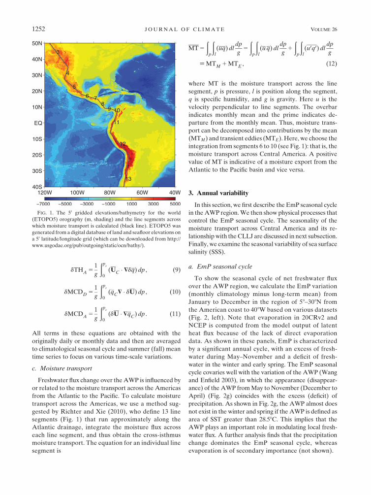
c. Moisture transport

Freshwater flux change over theAWP is influenced by

or related to the moisture transport across the Americas

from the Atlantic to the Pacific. To calculate moisture

transport across the Americas, we use a method sug-

gested by Richter and Xie (2010), who define 13 line

segments (Fig. 1) that run approximately along the

Atlantic drainage, integrate the moisture flux across

each line segment, and thus obtain the cross-isthmus

moisture transport. The equation for an individual line

segment is

MT5

ðp

ðl(uq) dl

dp

g5

ðp

ðl(uq) dl

dp

g1

ðp

ðl(u0q0) dl

dp

g

[MTM 1MTE , (12)

where MT is the moisture transport across the line

segment, p is pressure, l is position along the segment,

q is specific humidity, and g is gravity. Here u is the

velocity perpendicular to line segments. The overbar

indicates monthly mean and the prime indicates de-

parture from the monthly mean. Thus, moisture trans-

port can be decomposed into contributions by the mean

(MTM) and transient eddies (MTE). Here, we choose the

integration from segments 6 to 10 (see Fig. 1): that is, the

moisture transport across Central America. A positive

value of MT is indicative of a moisture export from the

Atlantic to the Pacific basin and vice versa.

3. Annual variability

In this section, we first describe the EmP seasonal cycle

in theAWP region.We then show physical processes that

control the EmP seasonal cycle. The seasonality of the

moisture transport across Central America and its re-

lationshipwith theCLLJ are discussed in next subsection.

Finally, we examine the seasonal variability of sea surface

salinity (SSS).

a. EmP seasonal cycle

To show the seasonal cycle of net freshwater flux

over the AWP region, we calculate the EmP variation

(monthly climatology minus long-term mean) from

January to December in the region of 58–308N from

the American coast to 408W based on various datasets

(Fig. 2, left). Note that evaporation in 20CRv2 and

NCEP is computed from the model output of latent

heat flux because of the lack of direct evaporation

data. As shown in these panels, EmP is characterized

by a significant annual cycle, with an excess of fresh-

water during May–November and a deficit of fresh-

water in the winter and early spring. The EmP seasonal

cycle covaries well with the variation of the AWP (Wang

and Enfield 2003), in which the appearance (disappear-

ance) of the AWP fromMay to November (December to

April) (Fig. 2g) coincides with the excess (deficit) of

precipitation. As shown in Fig. 2g, the AWP almost does

not exist in the winter and spring if the AWP is defined as

area of SST greater than 28.58C. This implies that the

AWP plays an important role in modulating local fresh-

water flux. A further analysis finds that the precipitation

change dominates the EmP seasonal cycle, whereas

evaporation is of secondary importance (not shown).

FIG. 1. The 50 gridded elevations/bathymetry for the world

(ETOPO5) orography (m, shading) and the line segments across

which moisture transport is calculated (black line). ETOPO5 was

generated froma digital database of land and seafloor elevations on

a 50 latitude/longitude grid (which can be downloaded from http://

www.usgodae.org/pub/outgoing/static/ocn/bathy/).


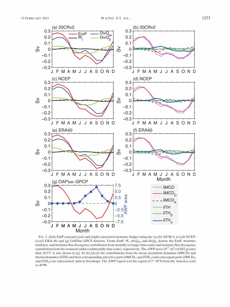
FIG. 2. (left) EmP seasonal cycle and (right) associated moisture budget using the (a),(b) 20CRv2; (c),(d) NCEP;

(e),(f) ERA-40; and (g) OAFlux–GPCP datasets. Terms EmP, Wt, divQM, and divQE denote the EmP, moisture

tendency, andmoisture flux divergence contribution frommonthly to longer time scales andmoisture flux divergence

contribution from the transient eddies (submonthly time scale), respectively. TheAWP area (1012 m2) of SST greater

than 28.58C is also shown in (g). In (b),(d),(f) the contributions from the mean circulation dynamics (dMCD) and

thermodynamics (dTH) and their corresponding advective parts (dMCDA and dTHA) and convergent parts (dMCDD

and dTHD) are represented: units in Sverdrups. The AWP region is in the region of 58–308N from the America coast

to 408W.


In general, the EmP annual cycle agrees well among

four different datasets of 20CRv2, NCEP, ERA-40, and

OAFlux–GPCP. However, some discrepancies still exist.

Net freshwater flux calculated from the OAFlux–GPCP

precipitation displays an EmP ridge in July, which in turn

leads to a weak semiannual feature of EmP. 20CRv2 is a

reanalysis dataset that can best reproduce this phenom-

enon. The EmP ridge in July is predominated by the

precipitation (not shown), which is closely related to the

well-known phenomenon of the midsummer drought that

is more obvious in the regions of Central America and

SouthMexico (e.g., Magana et al. 1999;Mapes et al. 2005).

b. Processes controlling EmP seasonal cycle

Next, we address how the EmP seasonal cycle is

formed or what physical processes controlling the EmP

seasonal cycle are. The left panels of Fig. 2 show EmP,

the moisture tendency (›W/›t), and the moisture flux

divergence contributed from themonthlymean (divQM)

and from the transient eddies (divQE). It is seen that the

EmP seasonal cycle in the AWP region can be largely

accounted for by divQM, including moistening in the

summer and fall and drying in the winter and spring,

while the contribution from moisture tendency is neg-

ligible. Given the smallness of moisture tendency, this

term is ignored in later discussions. In addition, we find

that divQE also presents an annual cycle, which is almost

in phase with EmP. The contribution from the transient

eddies is significant in the summer [June–August (JJA)],

but with a smaller magnitude than the mean term of

divQM in all other seasons. This is not surprising since

the AWP resides over the tropics where atmospheric

response to the ocean is primarily linear and baroclinic

and the transient eddy is not very active.

As derived in section 2, the change of divQM can be

further separated into the thermodynamics contribution

(dTH) and the contribution from the mean circulation

dynamics (dMCD). The right panels of Fig. 2 show that

a large portion of the EmP change can be explained by

the mean circulation dynamics of dMCD, whereas the

thermodynamics contribution of dTH is much smaller.

The dTH can be further decomposed into the effect of

the change in humidity gradient when the advective

wind is fixed at the climatological mean (dTHA) and the

effect of the change in humidity with a fixed climato-

logical divergent wind (dTHD) [see Eqs. (8) and (9)]. It

can be found that dTH is primarily determined by dTHA,

while the contribution from dTHD is negligible. Figure 2

shows that dTHA is characterized by a net freshwater

loss from the ocean in January–July and vice versa in

August–December.

The mean circulation dynamics of dMCD is domi-

nated by dMCDD which represents the effect of change

in thewind divergencewith a fixed humidity as can be seen

inEq. (10). Clearly, the positive value ofEmP in thewinter

and early spring (when the AWP disappears) is balanced

by an increase in low-level wind divergence, which disfa-

vors precipitation and corresponds to a weakening of the

ascent over the AWP region. The opposite is true during

the summer and fall when theAWPappears. These results

are consistent with previous modeling studies (e.g., Wang

et al. 2008b) in which atmospheric response to a large

(small) AWP is featured by an anomalous convergence

(divergence) in the low level and an upward (a downward)

vertical velocity—a classic Gill’s pattern response to the

tropical heating (Gill 1980).

The other component of dMCDA is of secondary im-

portance to the EmP change. Differing from other terms,

dMCDA shows a semiannual feature, with a drying effect

during the winter and summer and a moistening effect

during the other seasons. This is also the determining

factor to cause a weak semiannual variability of EmP in

20CRv2 dataset shown in Fig. 2a. In NCEP and ERA-40,

the contribution from dMCDD is too strong to recognize

the role of dMCDA, so that a semiannual variability of

EmP does not seem to clearly show. It is expected that

dMCDA is largely associated with the wind change since

the humidity gradient is fixed as shown in Eq. (11). Over

the AWP region, the maximum of easterly zonal wind at

925 hPa occurs in the Caribbean region, which is called

the Caribbean low-level jet. As shown by Wang (2007),

the CLLJ varies semiannually, with two maxima in the

summer and winter and twominima in the fall and spring.

It is interesting to find that the semiannual feature in

dMCDA is consistent with the variation of the CLLJ. This

suggests that the CLLJ and the associated moisture

transport may be closely related to the EmP variation,

which will be examined in the following section. Wang

(2007) further pointed out that the strength of theCLLJ is

closely linked with the meridional SST gradient that is

largely fluctuated with the AWP. Therefore, from the

dynamical point of view, theAWP can not only induce an

anomalous wind divergence to modulate EmP but also

modulate EmP by changing SST gradient to induce

moisture advection by anomalous wind. Additionally,

from the thermodynamical point of view, the AWP can

modulate local EmP by changing humidity advection by

the anomalous humidity gradient and by changing the

water vapor content to affect the moisture divergence.

In summary, the EmP seasonal cycle associated with

the AWP is dominated by the AWP-modulated mean

circulation dynamics (dMCD), whereas the thermody-

namics contribution (dTH) plays a much smaller role.

Furthermore, the large contribution of the mean circu-

lation dynamics is primarily due to the wind divergence

change (dMCDD).


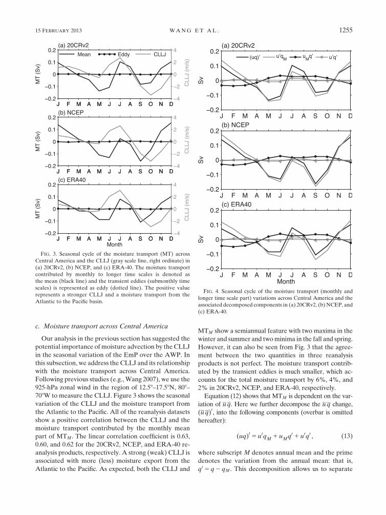
c. Moisture transport across Central America

Our analysis in the previous section has suggested the

potential importance ofmoisture advection by the CLLJ

in the seasonal variation of the EmP over the AWP. In

this subsection, we address the CLLJ and its relationship

with the moisture transport across Central America.

Following previous studies (e.g., Wang 2007), we use the

925-hPa zonal wind in the region of 12.58–17.58N, 808–708W to measure the CLLJ. Figure 3 shows the seasonal

variation of the CLLJ and the moisture transport from

the Atlantic to the Pacific. All of the reanalysis datasets

show a positive correlation between the CLLJ and the

moisture transport contributed by the monthly mean

part of MTM. The linear correlation coefficient is 0.63,

0.60, and 0.62 for the 20CRv2, NCEP, and ERA-40 re-

analysis products, respectively. A strong (weak) CLLJ is

associated with more (less) moisture export from the

Atlantic to the Pacific. As expected, both the CLLJ and

MTM show a semiannual feature with two maxima in the

winter and summer and twominima in the fall and spring.

However, it can also be seen from Fig. 3 that the agree-

ment between the two quantities in three reanalysis

products is not perfect. The moisture transport contrib-

uted by the transient eddies is much smaller, which ac-

counts for the total moisture transport by 6%, 4%, and

2% in 20CRv2, NCEP, and ERA-40, respectively.

Equation (12) shows that MTM is dependent on the var-

iation of uq. Here we further decompose the uq change,

(uq)0, into the following components (overbar is omitted

hereafter):

(uq)0 5u0qM 1 uMq01 u0q0 , (13)

where subscript M denotes annual mean and the prime

denotes the variation from the annual mean: that is,

q0 5 q2 qM. This decomposition allows us to separate

FIG. 3. Seasonal cycle of the moisture transport (MT) across

Central America and the CLLJ (gray scale line, right ordinate) in

(a) 20CRv2, (b) NCEP, and (c) ERA-40. The moisture transport

contributed by monthly to longer time scales is denoted as

the mean (black line) and the transient eddies (submonthly time

scales) is represented as eddy (dotted line). The positive value

represents a stronger CLLJ and a moisture transport from the

Atlantic to the Pacific basin.

FIG. 4. Seasonal cycle of the moisture transport (monthly and

longer time scale part) variations across Central America and the

associated decomposed components in (a) 20CRv2, (b) NCEP, and

(c) ERA-40.


the effects of humidity and wind changes (Fig. 4). All of

the three reanalysis products show that moisture trans-

port from the Atlantic to the Pacific is primarily de-

termined by the wind change, whereas the contribution

by the humidity change is small. The nonlinear term of

u0q0 is very small and can be ignored. A comparison of

Figs. 3 and 4 shows that the CLLJ and u0qM are in phase,

again suggesting that the CLLJ is important for the

moisture transport across Central America. In spite of

small amplitude, the humidity change can still make

contribution to the moisture transport. The contribution

by the humidity change (uMq0) is an increase (decrease)

of moisture transport during the summer and fall (winter

and spring) as a result of the appearance (disappear-

ance) of the AWP.

We have shown a link among the AWP, EmP in the

AWP region, and the moisture transport across Central

America. In association with the appearance (disap-

pearance) of the AWP, less (more) moisture is exported

from the Atlantic to the Pacific and more (less) pre-

cipitation occurs in the AWP region. This is because

a large (small) AWP induces a low-level wind conver-

gence (divergence), which favors (disfavors) local pre-

cipitation on one hand and also increases (decreases) the

low-level westerly anomaly that decreases (increases)

the moisture transport from the Atlantic to the Pacific

on the other hand. However, there is an exception in

July when precipitation is less (Fig. 2) and more mois-

ture is transported across Central America (Figs. 3, 4)

when the AWP is developed. This exception may result

from the midsummer drought, the CLLJ variation, and

the intrusion of the North Atlantic subtropical high.

Finally, we note that the magnitudes of the moisture

transport across Central America and EmP over the

AWP are comparable on a seasonal time scale, implying

that both of them can have a potential to affect ocean

salinity (see next subsection) and then the Atlantic

meridional overturning circulation (AMOC).

d. Seasonal cycle of sea surface salinity

The AWP-modulated EmP and moisture transport

across Central America can ultimately affect ocean sa-

linity, especially sea surface salinity. Figure 5 shows the

seasonal SSS cycle averaged over the AWP region. As

expected, SSS is small (large) during the summer and fall

(winter and spring) when theAWPappears (disappears)

and the EmP and moisture transport across Central

America are small (large). However, we have to keep in

mind that the seasonal cycle of mixed layer salinity also

depends on salinity advection, especially in the eastern

part of the AWP where horizontal salinity advection

is very important (Foltz and McPhaden 2008). All of

the datasets of the direct observations and reanalysis

products capture the seasonality of SSS in the AWP

region, although the details is different. The SODA re-

analysis product shares great similarity with the Argo

observation, albeit with a smoother curve due to the

relatively coarse resolution. This provides us a confi-

dence to use SODA for analyzing the long-term vari-

ability of SSS in the following sections. SSS seasonality

in GECCO and Ishii et al. seems to be overestimated,

while the GFDL reanalysis tends to underestimate the

SSS seasonal cycle over the AWP region.

4. Interannual variability

The freshwater flux in the AWP region also has sig-

nificant interannual fluctuations. In this section, we ex-

amine and show the freshwater variability associated

with the AWP, its associated mechanisms, moisture

transport across Central America, and SSS on inter-

annual time scales.

a. EmP variability

We first compute the AWP index as the anomalies of

the area of SST warmer than 28.58C divided by the cli-

matological AWP area (Wang et al. 2006, 2008a), as

shown in Fig. 6a. The interannual AWP variability

(Fig. 6b) is obtained by performing an 8-yr high-frequency

filter to the detrended AWP index. We identify a warm

pool 25% larger (smaller) than the climatological area

as a large (small) warm pool; otherwise, the warm pool is

classified as normal or neutral. Given that the AWP

almost does not exist during winter and spring based on

the definition of SST warmer than 28.58C, we attempt to

highlight the EmP anomalies associated with the AWP

in summer (JJA) and fall [September–November (SON)].

The composites of the EmP anomalies for the large AWP

(LAWP) and small AWP (SAWP) are shown in Fig. 7.

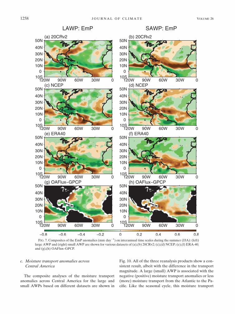
All of the datasets show a similar pattern during JJA.

The entire TNA experiences a reduced EmP when the

AWP is large, with maximum values located in the

FIG. 5. Seasonal cycle of SSS over the AWP region based on

various datasets of SODA, GECCO, GFDL, and Argo observa-

tions and WOA05 data developed by Ishii et al. (2006).


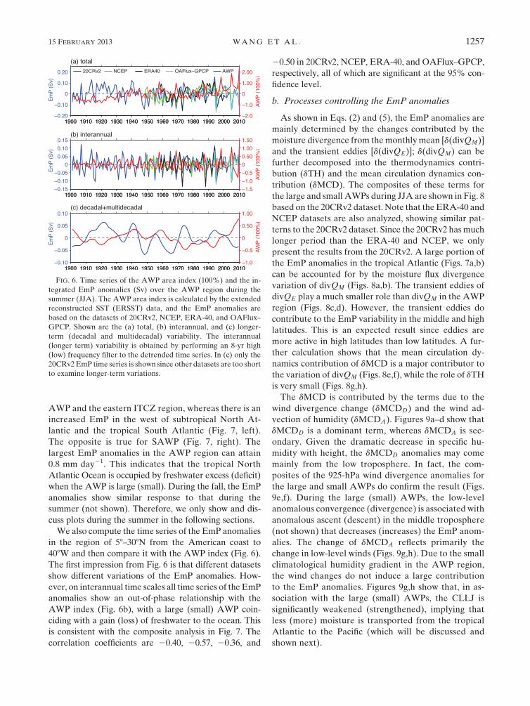
AWP and the eastern ITCZ region, whereas there is an

increased EmP in the west of subtropical North At-

lantic and the tropical South Atlantic (Fig. 7, left).

The opposite is true for SAWP (Fig. 7, right). The

largest EmP anomalies in the AWP region can attain

0.8 mm day21. This indicates that the tropical North

Atlantic Ocean is occupied by freshwater excess (deficit)

when the AWP is large (small). During the fall, the EmP

anomalies show similar response to that during the

summer (not shown). Therefore, we only show and dis-

cuss plots during the summer in the following sections.

We also compute the time series of the EmP anomalies

in the region of 58–308N from the American coast to

408W and then compare it with the AWP index (Fig. 6).

The first impression from Fig. 6 is that different datasets

show different variations of the EmP anomalies. How-

ever, on interannual time scales all time series of the EmP

anomalies show an out-of-phase relationship with the

AWP index (Fig. 6b), with a large (small) AWP coin-

ciding with a gain (loss) of freshwater to the ocean. This

is consistent with the composite analysis in Fig. 7. The

correlation coefficients are 20.40, 20.57, 20.36, and

20.50 in 20CRv2, NCEP, ERA-40, and OAFlux–GPCP,

respectively, all of which are significant at the 95% con-

fidence level.

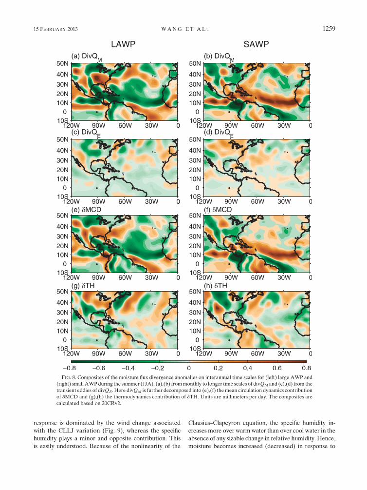
b. Processes controlling the EmP anomalies

As shown in Eqs. (2) and (5), the EmP anomalies are

mainly determined by the changes contributed by the

moisture divergence from themonthlymean [d(divQM)]

and the transient eddies [d(divQE)]; d(divQM) can be

further decomposed into the thermodynamics contri-

bution (dTH) and the mean circulation dynamics con-

tribution (dMCD). The composites of these terms for

the large and small AWPs during JJA are shown in Fig. 8

based on the 20CRv2 dataset. Note that theERA-40 and

NCEP datasets are also analyzed, showing similar pat-

terns to the 20CRv2 dataset. Since the 20CRv2 hasmuch

longer period than the ERA-40 and NCEP, we only

present the results from the 20CRv2. A large portion of

the EmP anomalies in the tropical Atlantic (Figs. 7a,b)

can be accounted for by the moisture flux divergence

variation of divQM (Figs. 8a,b). The transient eddies of

divQE play a much smaller role than divQM in the AWP

region (Figs. 8c,d). However, the transient eddies do

contribute to the EmP variability in the middle and high

latitudes. This is an expected result since eddies are

more active in high latitudes than low latitudes. A fur-

ther calculation shows that the mean circulation dy-

namics contribution of dMCD is a major contributor to

the variation of divQM (Figs. 8e,f), while the role of dTH

is very small (Figs. 8g,h).

The dMCD is contributed by the terms due to the

wind divergence change (dMCDD) and the wind ad-

vection of humidity (dMCDA). Figures 9a–d show that

dMCDD is a dominant term, whereas dMCDA is sec-

ondary. Given the dramatic decrease in specific hu-

midity with height, the dMCDD anomalies may come

mainly from the low troposphere. In fact, the com-

posites of the 925-hPa wind divergence anomalies for

the large and small AWPs do confirm the result (Figs.

9e,f). During the large (small) AWPs, the low-level

anomalous convergence (divergence) is associated with

anomalous ascent (descent) in the middle troposphere

(not shown) that decreases (increases) the EmP anom-

alies. The change of dMCDA reflects primarily the

change in low-level winds (Figs. 9g,h). Due to the small

climatological humidity gradient in the AWP region,

the wind changes do not induce a large contribution

to the EmP anomalies. Figures 9g,h show that, in as-

sociation with the large (small) AWPs, the CLLJ is

significantly weakened (strengthened), implying that

less (more) moisture is transported from the tropical

Atlantic to the Pacific (which will be discussed and

shown next).

FIG. 6. Time series of the AWP area index (100%) and the in-

tegrated EmP anomalies (Sv) over the AWP region during the

summer (JJA). The AWP area index is calculated by the extended

reconstructed SST (ERSST) data, and the EmP anomalies are

based on the datasets of 20CRv2, NCEP, ERA-40, and OAFlux–

GPCP. Shown are the (a) total, (b) interannual, and (c) longer-

term (decadal and multidecadal) variability. The interannual

(longer term) variability is obtained by performing an 8-yr high

(low) frequency filter to the detrended time series. In (c) only the

20CRv2EmP time series is shown since other datasets are too short

to examine longer-term variations.


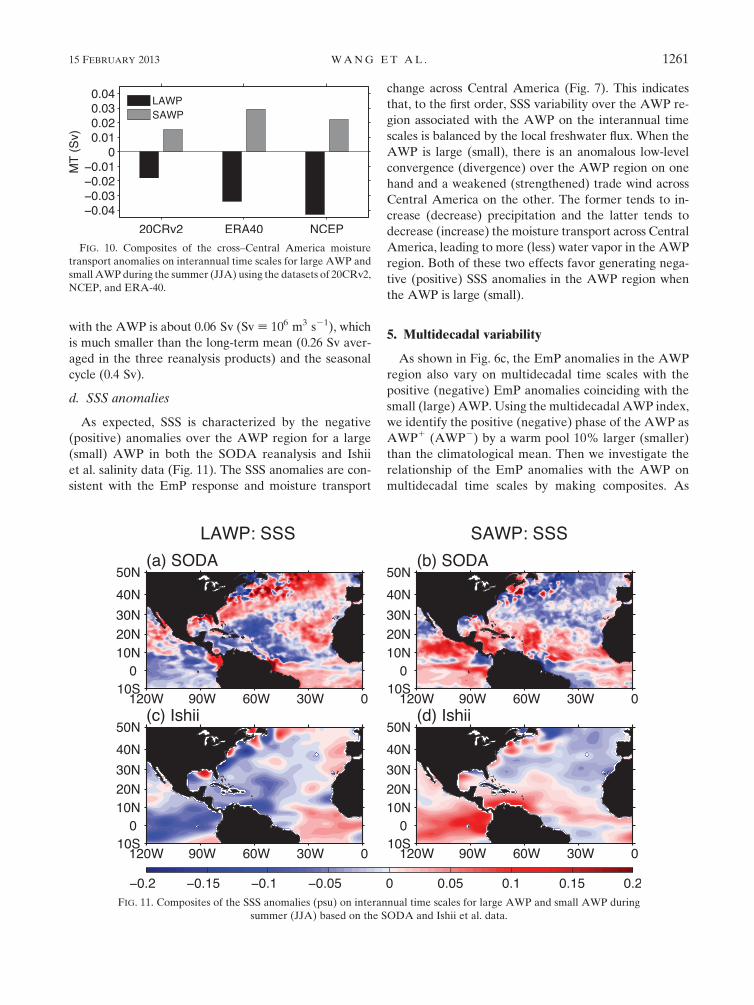
c. Moisture transport anomalies acrossCentral America

The composite analyses of the moisture transport

anomalies across Central America for the large and

small AWPs based on different datasets are shown in

Fig. 10. All of the three reanalysis products show a con-

sistent result, albeit with the difference in the transport

magnitude. A large (small) AWP is associated with the

negative (positive) moisture transport anomalies or less

(more) moisture transport from the Atlantic to the Pa-

cific. Like the seasonal cycle, this moisture transport

FIG. 7. Composites of the EmP anomalies (mm day21) on interannual time scales during the summer (JJA): (left)

large AWP and (right) small AWP are shown for various datasets of (a),(b) 20CRv2; (c),(d) NCEP; (e),(f) ERA-40;

and (g),(h) OAFlux–GPCP.


response is dominated by the wind change associated

with the CLLJ variation (Fig. 9), whereas the specific

humidity plays a minor and opposite contribution. This

is easily understood. Because of the nonlinearity of the

Clausius–Clapeyron equation, the specific humidity in-

creases more over warmwater than over cool water in the

absence of any sizable change in relative humidity.Hence,

moisture becomes increased (decreased) in response to

FIG. 8. Composites of the moisture flux divergence anomalies on interannual time scales for (left) large AWP and

(right) smallAWPduring the summer (JJA): (a),(b) frommonthly to longer time scales of divQM and (c),(d) from the

transient eddies of divQE. Here divQM is further decomposed into (e),(f) themean circulation dynamics contribution

of dMCD and (g),(h) the thermodynamics contribution of dTH. Units are millimeters per day. The composites are

calculated based on 20CRv2.


a large (small) AWP, which in turn favors more (less)

moisture transported to the Pacific. However, the specific

humidity response cannot be overwhelmed by the role of

wind change, which tends to reduce (increase) the easterly

wind and thus generate a weakened (strengthened) mois-

ture transport acrossCentralAmerica during a large (small)

AWP. Note that the magnitude (peak-to-peak variation)

of interannual moisture transport anomalies associated

FIG. 9. Composites of the moisture change (mm day21), calculated based on 20CRv2, due to mean circulation

dynamics on interannual time scales for (left) large AWP and (right) small AWP during the summer (JJA). The

contribution by (a),(b) the wind divergent change and (c),(d) the advection of moisture by the wind change are

shown. Composites of the 925-hPa (e),(f) wind divergence and (g),(h) wind anomalies are also shown.


with the AWP is about 0.06 Sv (Sv[ 106 m3 s21), which

is much smaller than the long-term mean (0.26 Sv aver-

aged in the three reanalysis products) and the seasonal

cycle (0.4 Sv).

d. SSS anomalies

As expected, SSS is characterized by the negative

(positive) anomalies over the AWP region for a large

(small) AWP in both the SODA reanalysis and Ishii

et al. salinity data (Fig. 11). The SSS anomalies are con-

sistent with the EmP response and moisture transport

change across Central America (Fig. 7). This indicates

that, to the first order, SSS variability over the AWP re-

gion associated with the AWP on the interannual time

scales is balanced by the local freshwater flux. When the

AWP is large (small), there is an anomalous low-level

convergence (divergence) over the AWP region on one

hand and a weakened (strengthened) trade wind across

Central America on the other. The former tends to in-

crease (decrease) precipitation and the latter tends to

decrease (increase) the moisture transport across Central

America, leading to more (less) water vapor in the AWP

region. Both of these two effects favor generating nega-

tive (positive) SSS anomalies in the AWP region when

the AWP is large (small).

5. Multidecadal variability

As shown in Fig. 6c, the EmP anomalies in the AWP

region also vary on multidecadal time scales with the

positive (negative) EmP anomalies coinciding with the

small (large) AWP. Using the multidecadal AWP index,

we identify the positive (negative) phase of the AWP as

AWP1 (AWP2) by a warm pool 10% larger (smaller)

than the climatological mean. Then we investigate the

relationship of the EmP anomalies with the AWP on

multidecadal time scales by making composites. As

FIG. 10. Composites of the cross–Central America moisture

transport anomalies on interannual time scales for large AWP and

small AWPduring the summer (JJA) using the datasets of 20CRv2,

NCEP, and ERA-40.

FIG. 11. Composites of the SSS anomalies (psu) on interannual time scales for large AWP and small AWP during

summer (JJA) based on the SODA and Ishii et al. data.


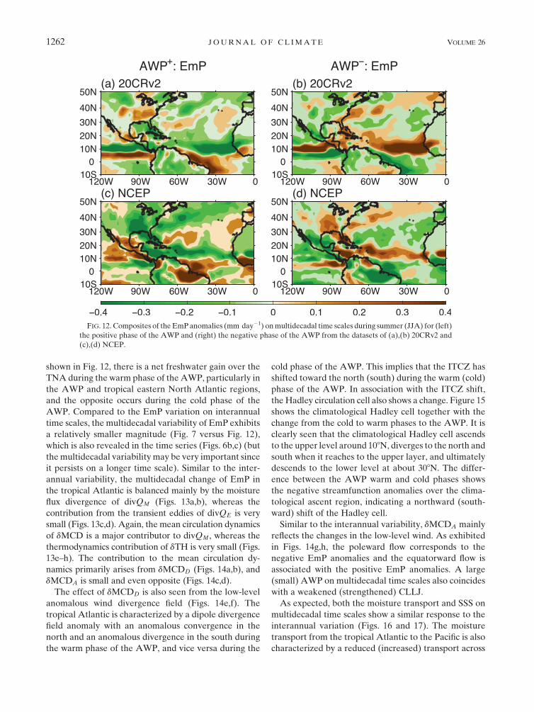
shown in Fig. 12, there is a net freshwater gain over the

TNA during the warm phase of theAWP, particularly in

the AWP and tropical eastern North Atlantic regions,

and the opposite occurs during the cold phase of the

AWP. Compared to the EmP variation on interannual

time scales, the multidecadal variability of EmP exhibits

a relatively smaller magnitude (Fig. 7 versus Fig. 12),

which is also revealed in the time series (Figs. 6b,c) (but

themultidecadal variability may be very important since

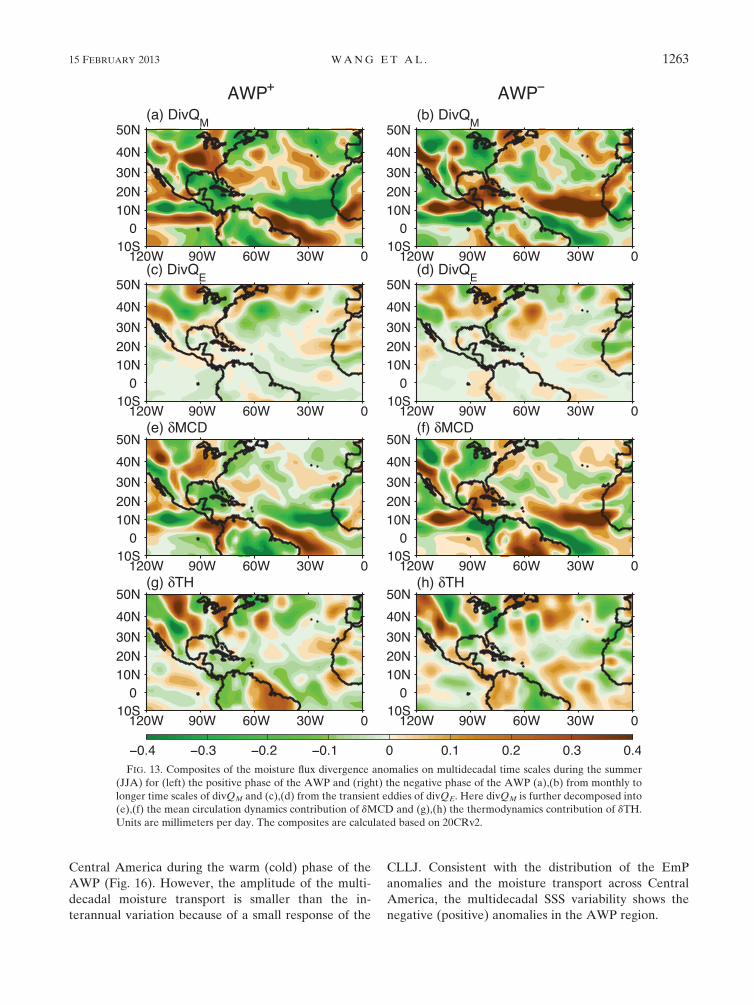
it persists on a longer time scale). Similar to the inter-

annual variability, the multidecadal change of EmP in

the tropical Atlantic is balanced mainly by the moisture

flux divergence of divQM (Figs. 13a,b), whereas the

contribution from the transient eddies of divQE is very

small (Figs. 13c,d). Again, the mean circulation dynamics

of dMCD is a major contributor to divQM, whereas the

thermodynamics contribution of dTH is very small (Figs.

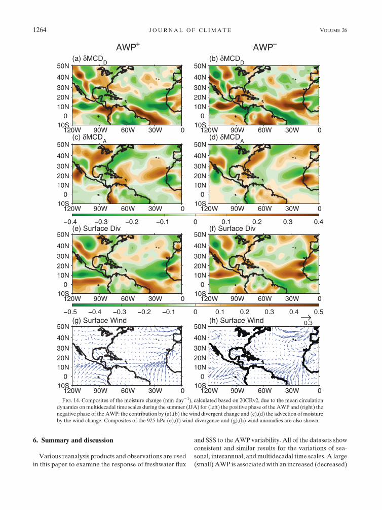
13e–h). The contribution to the mean circulation dy-

namics primarily arises from dMCDD (Figs. 14a,b), and

dMCDA is small and even opposite (Figs. 14c,d).

The effect of dMCDD is also seen from the low-level

anomalous wind divergence field (Figs. 14e,f). The

tropical Atlantic is characterized by a dipole divergence

field anomaly with an anomalous convergence in the

north and an anomalous divergence in the south during

the warm phase of the AWP, and vice versa during the

cold phase of the AWP. This implies that the ITCZ has

shifted toward the north (south) during the warm (cold)

phase of the AWP. In association with the ITCZ shift,

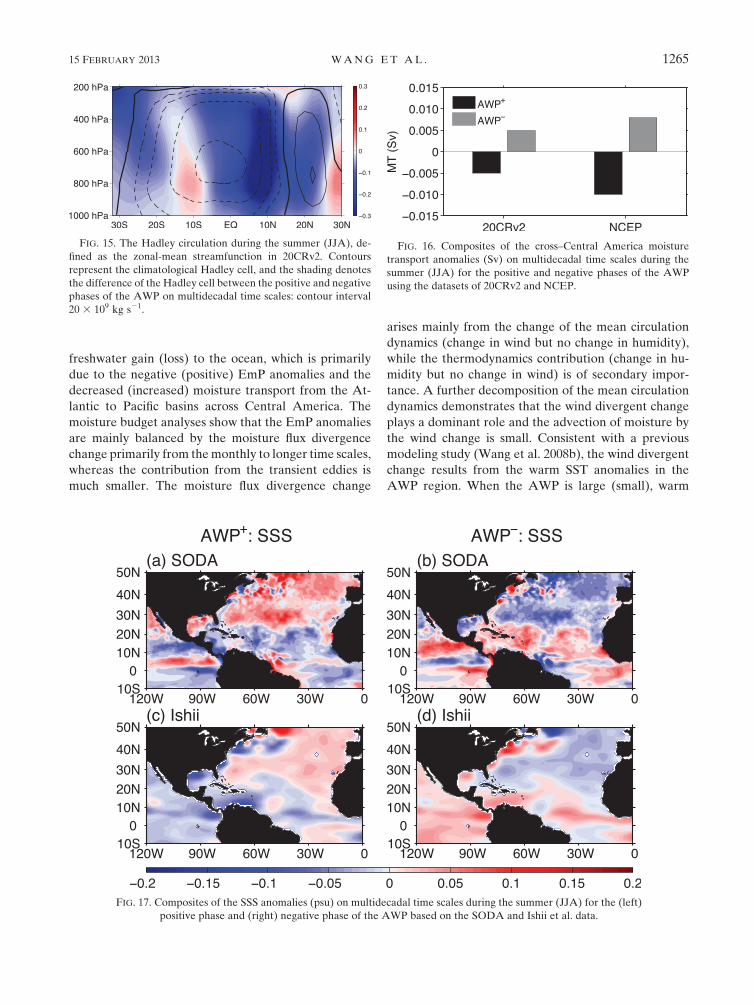
the Hadley circulation cell also shows a change. Figure 15

shows the climatological Hadley cell together with the

change from the cold to warm phases to the AWP. It is

clearly seen that the climatological Hadley cell ascends

to the upper level around 108N, diverges to the north and

south when it reaches to the upper layer, and ultimately

descends to the lower level at about 308N. The differ-

ence between the AWP warm and cold phases shows

the negative streamfunction anomalies over the clima-

tological ascent region, indicating a northward (south-

ward) shift of the Hadley cell.

Similar to the interannual variability, dMCDA mainly

reflects the changes in the low-level wind. As exhibited

in Figs. 14g,h, the poleward flow corresponds to the

negative EmP anomalies and the equatorward flow is

associated with the positive EmP anomalies. A large

(small) AWP on multidecadal time scales also coincides

with a weakened (strengthened) CLLJ.

As expected, both the moisture transport and SSS on

multidecadal time scales show a similar response to the

interannual variation (Figs. 16 and 17). The moisture

transport from the tropical Atlantic to the Pacific is also

characterized by a reduced (increased) transport across

FIG. 12. Composites of the EmP anomalies (mm day21) onmultidecadal time scales during summer (JJA) for (left)

the positive phase of the AWP and (right) the negative phase of the AWP from the datasets of (a),(b) 20CRv2 and

(c),(d) NCEP.


Central America during the warm (cold) phase of the

AWP (Fig. 16). However, the amplitude of the multi-

decadal moisture transport is smaller than the in-

terannual variation because of a small response of the

CLLJ. Consistent with the distribution of the EmP

anomalies and the moisture transport across Central

America, the multidecadal SSS variability shows the

negative (positive) anomalies in the AWP region.

FIG. 13. Composites of the moisture flux divergence anomalies on multidecadal time scales during the summer

(JJA) for (left) the positive phase of the AWP and (right) the negative phase of the AWP (a),(b) from monthly to

longer time scales of divQM and (c),(d) from the transient eddies of divQE. Here divQM is further decomposed into

(e),(f) the mean circulation dynamics contribution of dMCD and (g),(h) the thermodynamics contribution of dTH.

Units are millimeters per day. The composites are calculated based on 20CRv2.


6. Summary and discussion

Various reanalysis products and observations are used

in this paper to examine the response of freshwater flux

and SSS to the AWP variability. All of the datasets show

consistent and similar results for the variations of sea-

sonal, interannual, andmultidecadal time scales. A large

(small)AWP is associated with an increased (decreased)

FIG. 14. Composites of the moisture change (mm day21), calculated based on 20CRv2, due to the mean circulation

dynamics onmultidecadal time scales during the summer (JJA) for (left) the positive phase of the AWP and (right) the

negative phase of theAWP: the contribution by (a),(b) the wind divergent change and (c),(d) the advection ofmoisture

by the wind change. Composites of the 925-hPa (e),(f) wind divergence and (g),(h) wind anomalies are also shown.


freshwater gain (loss) to the ocean, which is primarily

due to the negative (positive) EmP anomalies and the

decreased (increased) moisture transport from the At-

lantic to Pacific basins across Central America. The

moisture budget analyses show that the EmP anomalies

are mainly balanced by the moisture flux divergence

change primarily from themonthly to longer time scales,

whereas the contribution from the transient eddies is

much smaller. The moisture flux divergence change

arises mainly from the change of the mean circulation

dynamics (change in wind but no change in humidity),

while the thermodynamics contribution (change in hu-

midity but no change in wind) is of secondary impor-

tance. A further decomposition of the mean circulation

dynamics demonstrates that the wind divergent change

plays a dominant role and the advection of moisture by

the wind change is small. Consistent with a previous

modeling study (Wang et al. 2008b), the wind divergent

change results from the warm SST anomalies in the

AWP region. When the AWP is large (small), warm

FIG. 15. The Hadley circulation during the summer (JJA), de-

fined as the zonal-mean streamfunction in 20CRv2. Contours

represent the climatological Hadley cell, and the shading denotes

the difference of the Hadley cell between the positive and negative

phases of the AWP on multidecadal time scales: contour interval

20 3 109 kg s21.

FIG. 16. Composites of the cross–Central America moisture

transport anomalies (Sv) on multidecadal time scales during the

summer (JJA) for the positive and negative phases of the AWP

using the datasets of 20CRv2 and NCEP.

FIG. 17. Composites of the SSS anomalies (psu) on multidecadal time scales during the summer (JJA) for the (left)

positive phase and (right) negative phase of the AWP based on the SODA and Ishii et al. data.


(cold) SST over the AWP region induces an anomalous

convergence (divergence) in the low level according to

the Gill (1980) theory, which induces an anomalous as-

cent (descent) motion and thus generates an increased

(decreased) precipitation. Meanwhile, the divergent

circulation change is associated with the north–south

shift of the ITCZ, leading to an anomalous precipitation

band over the tropical Atlantic.

On the other hand, a large (small) AWP is also asso-

ciated with a weakening (strengthening) of the CLLJ

and the westerly (easterly) anomalies across Central

America. The wind change reduces (enhances) the mois-

ture transport from the Atlantic to the Pacific, which in

turn leads to more (less) moisture residing in the AWP

region and, thus, generating more (less) local precipita-

tion. Both local EmP and moisture transport changes can

affect the ocean salinity ultimately. As expected, SSS

variability associated with the AWP is characterized by

the negative (positive) SSS anomaly response to a large

(small) AWP.

Although the features and processes of the freshwater

variations in theAWPare similar on seasonal, interannual,

and multidecadal time scales, their magnitudes are quite

different. The range or amplitude (peak-to-peak varia-

tion) of the AWP-modulated seasonality of the EmP

anomalies has the largest value, reaching 0.6 Sv. The

magnitude of interannual variability of EmP associated

with the AWP in the summer is ;0.2 Sv, while the

multidecadal variability has a smaller amplitude that can

reach 0.15 Sv. Similarly, the moisture transport across

Central America associated with the AWP has the

largest magnitude in the seasonal cycle, which can reach

0.4 Sv. However, the cross–Central American moisture

transport exhibits a smaller amplitude change in the

summer on the interannual and multidecadal time scales,

with amplitude about 0.06 Sv and 0.02 Sv, respectively.

As a result, SSS has the largest amplitude in the sea-

sonal cycle (0.6 psu); however, it only has 0.4 and

0.2 psu fluctuations on interannual and multidecadal

time scales, respectively.

The results suggest a potential interaction between

the AWP and the Atlantic meridional overturning cir-

culation (AMOC) through the freshwater and salinity

response. On one hand, as the AMOC weakens, its

northward heat transport is reduced; thus, the North

Atlantic cools and theAWP becomes small. On the other

hand, a small AWP decreases rainfall in the TNA and

increases the cross–Central American moisture export to

the eastern North Pacific. Both of these factors tend to

increase salinity in the tropical North Atlantic Ocean.

Advected northward by the wind-driven ocean circula-

tion (Thorpe et al. 2001; Vellinga andWu 2004; Yin et al.

2006; Krebs and Timmermann 2007), the positive salinity

anomalies may increase the upper-ocean density in the

deep-water formation regions and thus strengthen the

AMOC. Therefore, the AWP seems to play a negative

feedback role that acts to restore the AMOC after it is

weakened or shut down. This hypothesis needs to be

tested and confirmed by using numerical model experi-

ments. In particular, model experiments should address

whether the AWP-related freshwater flux and the mois-

ture export across Central America to the eastern Pacific

are of significance for the strength of the AMOC, if the

persistence of the anomaly is on a longer time scale (e.g.,

on the order of decades).

Acknowledgments. We thank Greg Foltz for serving as

AOML’s internal reviewer and two anonymous reviewers

for their comments and suggestions. This work was sup-

ported by grants from National Oceanic and Atmospheric

Administration/Climate Program Office, the base funding

of NOAA/Atlantic Oceanographic and Meteorological

Laboratory (AOML). The findings and conclusions in this

report are those of the author(s) and do not necessarily

represent the views of the funding agency.

REFERENCES

Adler, R. F., and Coauthors, 2003: The version-2 Global Pre-

cipitation Climatology Project (GPCP) monthly precipitation

analysis (1979–present). J. Hydrometeor., 4, 1147–1167.

Broecker, W. S., 1997: Thermohaline circulation, the Achilles heel

of our climate system: Will man-made CO2 upset the current

balance? Science, 278, 1582–1588.

Carton, J. A., and B. S. Giese, 2008: A reanalysis of ocean climate

using Simple Ocean Data Assimilation (SODA). Mon. Wea.

Rev., 136, 2999–3017.Compo, G. P., and Coauthors, 2011: The Twentieth Century Re-

analysis project. Quart. J. Roy. Meteor. Soc., 137, 1–28.

Foltz, G. R., and M. J. McPhaden, 2008: Seasonal mixed layer sa-

linity balance of the tropical North Atlantic Ocean. J. Geo-

phys. Res., 113, C02013, doi:10.1029/2007JC004178.

Gibson, J. K., P. Kallberg, S. Uppala, A. Nomura, A. Hernandez,

and E. Serrano, 1997: ERAdescription. ECMWFRe-Analysis

Project Rep. 1, 71 pp.

Gill, A. E., 1980: Some simple solutions for heat-induced tropical

circulation. Quart. J. Roy. Meteor. Soc., 106, 447–462.

Ishii, M., M. Kimoto, K. Sakamoto, and S. I. Iwasaki, 2006: Steric

sea level changes estimated from historical ocean subsurface

temperature and salinity analyses. J. Oceanogr., 62, 155–170.

Kalnay, E., and Coauthors, 1996: The NCEP/NCAR 40-Year Re-

analysis Project. Bull. Amer. Meteor. Soc., 77, 437–471.Katsumata, K., and H. Yoshinari, 2010: Uncertainties in global

mapping of Argo drift data at the parking level. J. Oceanogr.,

66, 553–569.

Kohl, A., D. Dommenget, K. Ueyoshi, and D. Stammer, 2006: The

global ECCO 1952 to 2001 ocean synthesis. ECCOTech. Rep.

40, 44 pp. [Available online at http://www.ecco-group.org/

ecco1/report/report_40.pdf.]

Krebs,U., andA. Timmermann, 2007: Tropical air–sea interactions

accelerate the recovery of theAtlantic meridional overturning

circulation after a major shutdown. J. Climate, 20, 4940–4956.


Magana, V., J. A. Amador, and S. Medina, 1999: The midsummer

drought over Mexico and Central America. J. Climate, 12,

1577–1588.

Mapes, B. E., P. Liu, and N. Buenning, 2005: Indian monsoon onset

and the Americas midsummer drought: Out-of-equilibrium

response to smooth seasonal forcing. J. Climate, 18, 1109–1115.

Peixoto, J. P., and A. H. Oort, 1992: Physics of Climate.American

Institute of Physics, 520 pp.

Richter, I., and S.-P. Xie, 2010: Moisture transport from the At-

lantic to the Pacific basin and its response to North Atlantic

cooling and global warming. Climate Dyn., 35, 551–566.

Romanova, V., M. Prange, and G. Lohmann, 2004: Stability of the

glacial thermohaline circulation and its dependence on the

background hydrological cycle. Climate Dyn., 22, 527–538.

Rosati, A., M. Harrison, A. Wittenberg, and S. Zhang, 2004:

NOAA/GFDL ocean data assimilation activities. Proc.

CLIVAR Workshop on Ocean Reanalysis, NCAR, Boulder,

CO, 25–26.

Seager, R., N. Naik, and G. A. Vecchi, 2010: Thermodynamic and

dynamic mechanisms for large-scale changes in the hydro-

logical cycle in response to global warming. J. Climate, 23,

4651–4668.

Thorpe, R. B., J. M. Gregory, T. C. Johns, R. A.Wood, and J. F. B.

Mitchell, 2001: Mechanisms determining the Atlantic ther-

mohaline circulation response to greenhouse gas forcing in

a non-flux-adjusted coupled climate model. J. Climate, 14,3102–3116.

Trenberth, K. E., and C. J. Guillemot, 1995: Evaluation of the

global atmospheric moisture budget as seen from analyses.

J. Climate, 8, 2255–2272.Vellinga, M., and P. Wu, 2004: Low-latitude freshwater influences

on centennial variability of the Atlantic thermohaline circu-

lation. J. Climate, 17, 4498–4511.

Wang, C., 2007: Variability of the Caribbean low-level jet and its

relations to climate. Climate Dyn., 29, 411–422.

——, and D. B. Enfield, 2001: The tropical Western Hemisphere

warm pool. Geophys. Res. Lett., 28, 1635–1638.

——, and ——, 2003: A further study of the tropical Western

Hemisphere warm pool. J. Climate, 16, 1476–1493.——, and S.-K. Lee, 2007: Atlantic warm pool, Caribbean low-level

jet, and their potential impact on Atlantic hurricanes. Geo-

phys. Res. Lett., 34, L02703, doi:10.1029/2006GL028579.

——, D. B. Enfield, S.-K. Lee, and C.W. Landsea, 2006: Influences

of the Atlantic warm pool on Western Hemisphere summer

rainfall and Atlantic hurricanes. J. Climate, 19, 3011–3028.

——, S.-K. Lee, and D. B. Enfield, 2007: Impact of the Atlantic

warm pool on the summer climate of the Western Hemi-

sphere. J. Climate, 20, 5021–5040.

——, ——, and ——, 2008a: Atlantic warm pool acting as a link

between Atlantic multidecadal oscillation and Atlantic tropi-

cal cyclone activity.Geochem. Geophys. Geosyst., 9,Q05V03,

doi:10.1029/2007GC001809.

——, ——, and ——, 2008b: Climate response to anomalously

large and small Atlantic warm pools during the summer.

J. Climate, 21, 2437–2450.

Xie, P., and P. A. Arkin, 1997: Global precipitation: A 17-year

monthly analysis based on gauge observations, satellite esti-

mates, and numericalmodel outputs.Bull. Amer.Meteor. Soc.,

78, 2539–2558.

Yin, J., M. E. Schlesinger, N. G. Andronova, S. Malyshev, and

B. Li, 2006: Is a shutdown of the thermohaline circulation ir-

reversible? J. Geophys. Res., 111, D12104, doi:10.1029/

2005JD006562.

Yu, L., and R. A. Weller, 2007: Objectively analyzed air–sea heat

flux for the global ice-free oceans (1981–2005). Bull. Amer.

Meteor. Soc., 88, 527–539.

Zaucker, F., and W. S. Broecker, 1992: The influence of atmo-

spheric moisture transport on the fresh water balance of the

Atlantic drainage basin: General circulation model simula-

tions and observations. J. Geophys. Res., 97, 2765–2773.


Response of Freshwater Flux and Sea Surface Salinity to Variability of the Atlantic Warm Pool

Documents