Resource-constrained multi-project scheduling with activity and time flexibility Viktoria A. Hauder a,b,c,* , Andreas Beham a,c , Sebastian Raggl a,c , Sophie N. Parragh b , Michael Affenzeller c,d a Josef Ressel Center for Adaptive Optimization in Dynamic Environments, University of Applied Sciences Upper Austria, Hagenberg b Institute of Production and Logistics Management, Johannes Kepler University, Linz, Austria c Heuristic and Evolutionary Algorithms Laboratory, University of Applied Sciences Upper Austria, Hagenberg d Institute of Formal Models and Verification, Johannes Kepler University, Linz, Austria Abstract Project scheduling in manufacturing environments often requires flexibility in terms of the selection and the exact length of alternative production activi- ties. Moreover, the simultaneous scheduling of multiple lots is mandatory in many production planning applications. To meet these requirements, a new resource-constrained project scheduling problem (RCPSP) is introduced where both decisions (activity flexibility and time flexibility) are integrated. Besides the minimization of makespan, two new alternative objectives are presented: maximization of balanced length of selected activities (time balance) and maxi- mization of balanced resource utilization (resource balance). New mixed integer and constraint programming (CP) models are proposed for the developed inte- grated flexible project scheduling problem. Benchmark instances on an already existing flexible RCPSP and the newly developed problem are solved to opti- mality. The real-world applicability of the suggested CP models is shown by additionally solving a large industry case. Keywords: Multi-project scheduling, activity and time flexibility, constraint programming, manufacturing * Corresponding author email address: [email protected] The financial support by the Austrian Federal Ministry for Digital and Economic Affairs and the National Foundation for Research, Technology and Development, and the Christian Doppler Research Association is gratefully acknowledged. The work described in this paper was also done within the project Logistics Optimization in the Steel Industry (LOISI) #855325 within the funding program Smart Mobility 2015 organized by the Austrian Re- search Promotion Agency (FFG) and funded by the Governments of Styria and Upper Austria. Former working title: “On constraint programming for a new flexible project schedul- ing problem with resource constraints”. Preprint submitted to Computers and Industrial Engineering 2 July 2020 (accepted 13 September 2020) arXiv:1902.09244v2 [cs.AI] 23 Oct 2020

Welcome message from author
This document is posted to help you gain knowledge. Please leave a comment to let me know what you think about it! Share it to your friends and learn new things together.
Transcript
Resource-constrained multi-project schedulingwith activity and time flexibility
Viktoria A. Haudera,b,c,∗, Andreas Behama,c, Sebastian Raggla,c,Sophie N. Parraghb, Michael Affenzellerc,d
aJosef Ressel Center for Adaptive Optimization in Dynamic Environments,University of Applied Sciences Upper Austria, Hagenberg
bInstitute of Production and Logistics Management,Johannes Kepler University, Linz, Austria
cHeuristic and Evolutionary Algorithms Laboratory,University of Applied Sciences Upper Austria, Hagenberg
dInstitute of Formal Models and Verification, Johannes Kepler University, Linz, Austria
Abstract
Project scheduling in manufacturing environments often requires flexibility interms of the selection and the exact length of alternative production activi-ties. Moreover, the simultaneous scheduling of multiple lots is mandatory inmany production planning applications. To meet these requirements, a newresource-constrained project scheduling problem (RCPSP) is introduced whereboth decisions (activity flexibility and time flexibility) are integrated. Besidesthe minimization of makespan, two new alternative objectives are presented:maximization of balanced length of selected activities (time balance) and maxi-mization of balanced resource utilization (resource balance). New mixed integerand constraint programming (CP) models are proposed for the developed inte-grated flexible project scheduling problem. Benchmark instances on an alreadyexisting flexible RCPSP and the newly developed problem are solved to opti-mality. The real-world applicability of the suggested CP models is shown byadditionally solving a large industry case.
Keywords: Multi-project scheduling, activity and time flexibility, constraintprogramming, manufacturing
∗Corresponding author email address: [email protected]
The financial support by the Austrian Federal Ministry for Digital and Economic Affairsand the National Foundation for Research, Technology and Development, and the ChristianDoppler Research Association is gratefully acknowledged. The work described in this paperwas also done within the project Logistics Optimization in the Steel Industry (LOISI)#855325 within the funding program Smart Mobility 2015 organized by the Austrian Re-search Promotion Agency (FFG) and funded by the Governments of Styria and Upper Austria.
Former working title: “On constraint programming for a new flexible project schedul-ing problem with resource constraints”.
Preprint submitted to Computers and Industrial Engineering 2 July 2020 (accepted 13 September 2020)
arX
iv:1
902.
0924
4v2
[cs
.AI]
23
Oct
202
0
1. Introduction and motivation
Project scheduling is an essential operational planning area in different busi-
ness sectors where precedences between activities and the access to limited re-
sources have to be taken into account. Besides a large number of applications
such as research and development or software development, one important exam-
ple is the scheduling of manufacturing activities (Artigues et al., 2013). The un-
derlying optimization problem is the well-known NP-hard resource-constrained
project scheduling problem (RCPSP), characterizing a project where all in-
cluded activities have to be scheduled in such a way that resource constraints,
processing times, and precedence relations are respected. The most common
objective is the minimization of the makespan (Hartmann & Briskorn, 2010).
In a manufacturing context, decision-makers sometimes have the flexibil-
ity to choose between different manufacturing activities or decide on the exact
length of them. Precisely these flexibility descriptions motivate the RCPSP
presented in this work, faced by many different manufacturing industries. For
the production of multiple lots (=jobs), there are several alternative produc-
tion activities per lot. Due to existing technological requirements, alternative
activities are aggregated to a number of alternative routes per lot. For every
lot, one production route has to be selected, an individual delivery date has to
be considered and early delivery is not permitted. Besides machines or man-
power, also typical logistics renewable resources such as vehicles or intermediate
storages (buffers) have to be considered since they are strongly limited in many
factories. Every activity of every lot demands at least one scarce resource, e.g.
a transporting, storaging or machining activity. Due to the consideration of
all existing resources, all activities of one lot have to be sequenced directly one
after another. This means that idle times between the activities within one lot
are not allowed, since they would result in a temporary ficticious disappearance
of the production lot. E.g., if the machining activity of lot 1 is finished, the
next one in the precedence relationship, e.g. the storaging activity of lot 1 has
to start immediately. However, routes (multiple activities) of different lots can
be scheduled in parallel, competing for the available production resources. E.g.,
the storaging activity of lot 2 can start before the storaging activity of lot 1 is
completed. Moreover, different lots use different production activities and the
sequence of utilized resources is not identical for all lots. With special regard to
logistics activities such as storaging, minimum and maximum allowed processing
times are specified for activities. Thus, processing times are of variable length,
1
i.e. the start and the end time per activity have to be decided during the opti-
mization process (time flexibility). As a result, the treated problem integrates
the two major decisions of activity selection and processing time determination.
In addition, we introduce two new objective functions: maximization of bal-
anced length of activity processing times (time balance), and maximization of
balanced resource utilization (resource balance).
The described production process may be found in various production in-
dustries. Three different examples the authors know from several cooperations
with production managers are the steel-, the food-, and the glass processing
industry, to name just a few. The production of steel slabs is typically pro-
cessed lot-wise and includes several logistics activities, e.g. a storaging activity
between necessary cooling, reheating or transporting activities. Moreover, in
many steel plants a minimum and maximum allowed processing time is given as
it does not influence the quality of such a product whether the storaging activity
of one lot is performed for one hour or two days in a slabyard. Furthermore,
this time flexibility gives production managers an often demanded additional
degree of freedom in their production planning possibilities. The same holds for
the glass processing industry where e.g. transporting and storaging activities
are necessary in the production process.
In the very different food processing industry, similar patterns can be found.
Industrial bakeries for example typically prescribe a minimum purchase quantity
for business customers to be able to carry out a lot-wise production. Further-
more, besides recipes for which precise time specifications have to be met, for
other ones the production activities are allowed to vary up to one hour or even
more, e.g. the cooling down of hot baked goods. For deep-frozen baked goods,
there is an even higher time flexibility: the baked good has to be at least stored
in a freezer for a certain amount of time but can be stored up to weeks or even
longer if necessary. The same examples also apply to forbidden early deliveries.
There are business customers who do not give their door keys to carriers for
security reasons, and therefore only allow deliveries beginning at their opening
hours. Some steel and glass industry customers (e.g. automobile industry) also
do not accept early delivery, overall resulting in deliveries without earliness.
Furthermore, objective functions directly or indirectly influence financial
burdens of companies, e.g. balancing the working time of all employees increases
the acceptance of work schedules and balancing resource allocation avoids idle
resources (Matl et al., 2017; Rieck et al., 2012). However, to the best of our
knowledge, time balancing purposes concerning activities have not been consid-
2
ered yet in the scientific literature on RCPSP. For balancing resource utilization
over time, resources are weighted by introducing costs (Li et al., 2018; Neumann
& Zimmermann, 1999) although in many companies, there are often several
equivalent resources (e.g. two deep freezing facilities of an industrial bakery or
two slab yards of a steel manufacturer) with the only goal of avoiding uneven
utilizations. Therefore, the two above presented new objectives are introduced.
The described choices between various alternative activities are known as
flexible project scheduling (Beck & Fox, 2000; Tao & Dong, 2017). Related to
this, Tao & Dong (2017) present the RCPSP with alternative activity chains
(RCPSP-AC) and develop a simulated annealing algorithm for solving it. They
describe that more efficient solution methods should be investigated for the
RCPSP-AC in order to tackle related real-world problems. Moreover, they point
out the necessity of an officially available benchmark set for the RCPSP-AC.
Motivated by these suggestions, the new problem extensions described above,
and the success of constraint programming (CP) for solving scheduling prob-
lems (Laborie et al., 2018; Schnell & Hartl, 2017), we develop and solve mixed
integer programming (MIP) and CP models for the RCPSP-AC, its new multi-
project version (RCMPSP-AC), and a new version featuring multiple projects
as well as time flexibility. The latter we denote resource-constrained multi-
project scheduling problem with alternative activity chains and time flexibility
(RCMPSP-ACTF). To be more precise, the contribution of this work is fivefold:
• A new resource-constrained multi-project scheduling problem with alter-
native activity chains and time flexibility (RCMPSP-ACTF) is introduced
and a related MIP model is proposed. It is based on the work of Tao &
Dong (2017) who consider alternative activity chains in a single-project
environment without time flexibility.
• Two new objective functions aiming at well-balanced solutions are pre-
sented.
• CP solution models are developed for the RCPSP-AC, its multi-project
version, and the RCMPSP-ACTF.
• MIP and CP modeling approaches are compared on newly generated
benchmark data sets, illustrating the advantage of using our new CP mod-
els: all benchmarks of the RCPSP-AC and many instances of the newly
presented problems are solved to optimality.
• With the CP based models, a large industry case with more than 600
activities is solved to optimality and the impact of using the proposed
alternative objective functions is evaluated.
3
The remainder of this paper is organized as follows. Section 2 gives an extensive
review of related literature. The developed problem formulation is introduced
in Section 3, while Section 4 provides a detailed description of the created con-
straint programming solution approach. In Section 5, the computational results
for the generated benchmark data and the real-world case study are discussed.
Finally, Section 6 gives concluding remarks and suggestions for further research.
2. Literature overview
The scheduling of manufacturing activities has been extensively investigated
in the last decades since its efficient management is of high relevance in prac-
tice (Russell & Taghipour, 2019). One area of such scheduling problems are
flexible manufacturing systems (FMS), considering flexibility within the pro-
duction process (B lazewicz et al., 2019). Examples for FMS are flexible job
shops (FJS), flexible or hybrid flow shops (FFS) or resource-constrained FMS.
FJS and FFS typically consider machines as resources. In FJS, different jobs
can consist of different activities (=operations) which can be performed on al-
ternative machines (Rajabinasab & Mansour, 2011). In FFS, all jobs consist
of the same activities but they can also be executed on alternative machines
(Ruiz & Vazquez-Rodrıguez, 2010). For the FJS and FFS, only one job can be
handled at a time by each resource, there are no precedence constraints between
the jobs and storage capacities (buffers) are assumed to be unlimited (unlimited
idle times between activities are allowed) or zero (no idle times are allowed since
there is no capacity) (B lazewicz et al., 2019). However, as described in Section
1, in the production environments considered in this work the production activ-
ities require additional resources with limited capacities such as storage areas.
They all have capacities (i.e. no idle times between activities within one job
are allowed since the capacities are modeled by activities that demand them;
idle times between different jobs are allowed), and multiple activities and jobs
can be handled at a time by each resource. Moreover, there are alternative
activities for every job, all of them are in a precedence relationship and they
have flexible processing times, overall resulting in a resource-constrained FMS
which corresponds to a flexible RCPSP (B lazewicz et al., 2019) where several
scheduling issues have to be newly mastered together.
The RCPSP is a well-researched topic, creating a schedule with starting
times for all activities. Basically, there are fixed processing times, activity de-
mands for limited resources, and precedence relations between all activities,
4
typically represented by acyclic activity-on-node (AON) networks (Hans et al.,
2007; Johnson & Garey, 1979). Besides the standard objective of makespan
minimization, also a wide variety of alternative objectives has been studied. An
example that is also tackled in this work is resource leveling, where varying
resource utilization over time is minimized (Li et al., 2018). One of the many
extensions which is examined in this work is related to time, considering an addi-
tional flexibility or a limitation of processing times (Artigues, 2017). Examples
related to time extensions are idle times (Allahverdi, 2016), uncertain activ-
ity durations (Moradi et al., 2019), flexible resource usage durations (Naber &
Kolisch, 2014), generalized precedence relations (GPR) (Schnell & Hartl, 2016),
and setup times (Vanhoucke & Coelho, 2019).
A great variety of exact and heuristic solution methods has already been in-
vestigated. As the detailed presentation of algorithmic methods and the many
existing extensions of the RCPSP is outside the scope of this work, the subse-
quent review is limited to flexible and multi-project scheduling and constraint
programming. The interested reader is referred to the works of Artigues et al.
(2013); B lazewicz et al. (2019); Hartmann & Briskorn (2010); Schwindt et al.
(2015) and Weglarz (2012) for an additional comprehensive examination.
2.1. Flexible and multi-project resource-constrained project scheduling
Flexible project scheduling as a generalization of the RCPSP has proven to
be also NP-hard (Blazewicz et al., 1983; Tao & Dong, 2017). It deals with the
selection of the best out of multiple alternative activities (Beck & Fox, 2000;
Burgelman & Vanhoucke, 2018). Already Pritsker (1966) has shown that besides
so-called AND nodes which imply the selection of all successor nodes, also OR
nodes can be introduced. OR nodes allow flexibility, as one out of multiple ex-
isting successor nodes is chosen. Johannes (2005) proofed that the minimization
of weighted completion times under consideration of OR precedence constraints
is already NP-hard with one single resource. Capek et al. (2012) considered
an RCPSP with alternative process plans for wire harnesses production. They
proposed an integer linear programming (ILP) model and a heuristic algorithm
for real-world applicability. Kellenbrink & Helber (2015) examined an aircraft
turnaround process and proposed a genetic algorithm (GA) for the optimiza-
tion of the developed flexible project structure. Vanhoucke & Coelho (2016)
considered bidirectional relations besides AND/OR ones. They developed a sat-
isfiability approach and showed its competitiveness on well-known benchmark
datasets. Tao & Dong (2017) studied an AND/OR network under considera-
5
tion of alternative activity chains (RCPSP-AC), which builds the base for the
development of our problem formulations. They showed that their RCPSP-AC
is a generalization of the multi-mode RCPSP (MRCPSP) and proposed a sim-
ulated annealing procedure. Tao & Dong (2018) extended the RCPSP-AC by
integrating it into a bi-objective MRCPSP. They solved the new problem with
a hybrid metaheuristic, consisting of a tabu search procedure and the NSGA II
and compared it with the solutions generated with an exact solver. Tao et al.
(2018) introduced an RCPSP with hierarchical alternatives and stochastic ac-
tivity durations and proposed a metaheuristic framework consisting of sample
average approximation and an evolutionary algorithm. Burgelman & Vanhoucke
(2018) presented a new flexible MRCPSP under maximization of weighted alter-
native execution modes and proposed different ILP formulations. Servranckx &
Vanhoucke (2019b) proposed an RCPSP with alternative subgraphs and solved
it with a tabu search. Moreover, they extended the problem by introducing
different strategies for the consideration of uncertainty for this new problem
(Servranckx & Vanhoucke, 2019a). Birjandi et al. (2019) introduced a new non-
linear MIP model for an RCPSP with multiple routes (RCPSP-MR) and solved
it with a hybrid metaheuristic based on particle swarm optimization (PSO) and
a GA. Birjandi & Mousavi (2019) presented a fuzzy extension of the RCPSP-
MR with flexible activities under uncertain conditions and proposed a hybrid
approach consisting of distribution rules, PSO and a GA.
The resource-constrained multi-project scheduling problem (RCMPSP) as
another generalization of the RCPSP considers a set of multiple projects l ∈{1, ..., L} and activities j ∈ Nl = {1, ..., n + 1} per project (Hartmann &
Briskorn, 2010; Lova et al., 2000). There are two possible ways for the represen-
tation of this multi-project variant. Through the single-project (SP) approach,
all projects are cumulated into an AON network with one common dummy
source and sink node (Lova & Tormos, 2001). Pritsker et al. (1969) were the
first to suggest an additional sink node per project for the consideration of a
due date per project within the SP approach. With the multi-project (MP)
approach, source and sink nodes for every project are considered, and the con-
necting elements are commonly shared resources. A recent example is the one of
Asta et al. (2016) who worked on a multi-mode RCMPSP under consideration
of the SP and the MP approach and proposed a combination of monte-carlo and
hyper-heuristic methods. Chakrabortty et al. (2017) suggested an evolutionary
local search method based on priority rules for the MP approach. An already
existing example for a manufacturing application of an SP approach for the
6
RCMPSP is the work of Voß & Witt (2007). They modeled a hybrid flow shop
scheduling problem as a multi-mode RCMPSP. Stages with variable capacities,
waiting times between stages and renewable resources were considered. All ex-
isting stages must be traversed and different resources must be used. In their
work, every machine only processed one job at a time, production routes were
identical for every job and processing times were fixed. The objectives were the
minimization of weighted tardiness and a maximized resource utilization. They
applied dispatching rules for solving large real-world instances.
2.2. Scheduling and constraint programming
Constraint programming is a powerful optimization technique especially for
combinatorial problems and thus, also for scheduling and real-world problems
(Baptiste et al., 2012). Bockmayr & Hooker (2005) presented the general func-
tionality of CP. They showed similarities of CP and MIP methods such as the
generation of branching trees. One dissimilarity is constraint propagation, which
is part of CP and removes all values from domains, which cannot take part in any
feasible solution. CP has already been efficiently applied to different domains
such as the deficiency problem (Altinakar et al., 2016), project driven manufac-
turing (Banaszak et al., 2009), ship scheduling and inventory management (Goel
et al., 2015), operating theatres (Wang et al., 2015), resource-constrained FMS
(Novas & Henning, 2014), and the RCPSP (Liess & Michelon, 2008). Recent
works also showed the compatibility of the CP methodology with the RCPSP.
Schnell & Hartl (2016, 2017) developed and analyzed exact algorithms, Boolean
Satisfiability Solving and CP approaches for the MRCPSP with GPR and pre-
sented new best solutions. Kreter et al. (2017) developed new CP models and a
special propagator for the RCPSP with general temporal constraints and calen-
dar constraints and provided optimal solutions for all benchmarks sets. Kreter
et al. (2018) developed new MIP and CP models for resource availability cost
problems and solved all open benchmarks to optimality.
2.3. Identified research gap
Considering the described literature, the presented scheduling problem in
Section 1 can be modeled as a resource-constrained multi-project scheduling
problem since precedence relations, limited renewable resources and multiple
lots (projects) have to be taken into account. Moreover, flexibility concerning
activity selection like in Tao & Dong (2017) and activity processing times has
to be incorporated. To the best of our knowledge, the integration of multiple
7
projects and flexible processing times has not been considered yet in an RCPSP
context. As the already described work of Tao & Dong (2017) on the RCPSP-
AC builds the base for the development of our work, we call our new problem
the resource-constrained multi-project scheduling problem with alternative ac-
tivity chains and time flexibility (RCMPSP-ACTF). Two new objectives for the
RCMPSP-ACTF, minimizing different processing time buffers and peak usages
of resources are introduced and the necessary additional constraints are pre-
sented. CP models are developed for the RCPSP-AC, its new multi-project
extension (RCMPSP-AC) and the new RCMPSP-ACTF and they are tested
on newly generated benchmark data. The developed models also provide deci-
sion support for a steel industry company partner, illustrated by the presented
real-world case study in this work.
3. Problem definition
In this section, the MIP formulations for the new RCMPSP-ACTF are pre-
sented. Section 3.1 provides basic assumptions and necessary notations, includ-
ing an exemplarily AON network that is used to model the introduced problem.
In Sections 3.2 - 3.4, we formally define the RCMPSP-ACTF and the two new
objectives alongside the necessary constraints for time and resource balance.
3.1. Notations
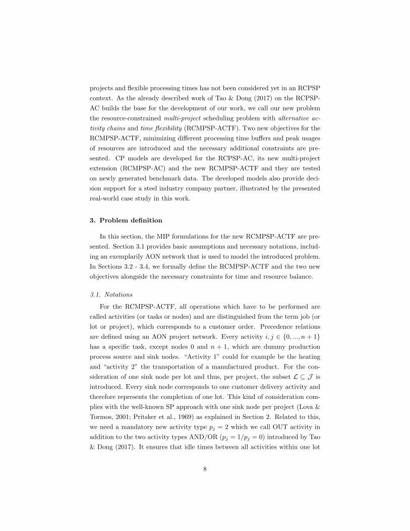
For the RCMPSP-ACTF, all operations which have to be performed are
called activities (or tasks or nodes) and are distinguished from the term job (or
lot or project), which corresponds to a customer order. Precedence relations
are defined using an AON project network. Every activity i, j ∈ {0, ..., n + 1}has a specific task, except nodes 0 and n + 1, which are dummy production
process source and sink nodes. “Activity 1” could for example be the heating
and “activity 2” the transportation of a manufactured product. For the con-
sideration of one sink node per lot and thus, per project, the subset L ⊆ J is
introduced. Every sink node corresponds to one customer delivery activity and
therefore represents the completion of one lot. This kind of consideration com-
plies with the well-known SP approach with one sink node per project (Lova &
Tormos, 2001; Pritsker et al., 1969) as explained in Section 2. Related to this,
we need a mandatory new activity type pj = 2 which we call OUT activity in
addition to the two activity types AND/OR (pj = 1/pj = 0) introduced by Tao
& Dong (2017). It ensures that idle times between all activities within one lot
8
2
4
8
1110
0
14
1
7
OR activityLegend:
AND activity
minimum | maximum allowed processing time of activity j
demand of activity j of resource r
a7|b
7
c7r
a8|b
8
c8r
a9|b
9
c9r
a11|b
11
c11r
a12|b
12
c12r
a10|b
10
c10r
a4|b
4
c4r
a5|b
5
c5r
a2|b
2
c2r
a3|b
3
c3r
a13|b
13
c13r
a1|b
1
c1r
a6|b
6
c6r
OUT activity
3
5
6
9
12
13
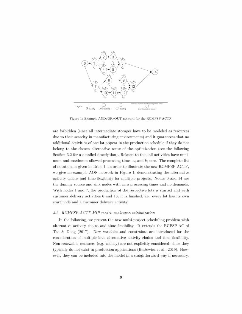
Figure 1: Example AND/OR/OUT network for the RCMPSP-ACTF.
are forbidden (since all intermediate storages have to be modeled as resources
due to their scarcity in manufacturing environments) and it guarantees that no
additional activities of one lot appear in the production schedule if they do not
belong to the chosen alternative route of the optimization (see the following
Section 3.2 for a detailed description). Related to this, all activities have mini-
mum and maximum allowed processing times ai and bi now. The complete list
of notations is given in Table 1. In order to illustrate the new RCMPSP-ACTF,
we give an example AON network in Figure 1, demonstrating the alternative
activity chains and time flexibility for multiple projects. Nodes 0 and 14 are
the dummy source and sink nodes with zero processing times and no demands.
With nodes 1 and 7, the production of the respective lots is started and with
customer delivery activities 6 and 13, it is finished, i.e. every lot has its own
start node and a customer delivery activity.
3.2. RCMPSP-ACTF MIP model: makespan minimization
In the following, we present the new multi-project scheduling problem with
alternative activity chains and time flexibility. It extends the RCPSP-AC of
Tao & Dong (2017). New variables and constraints are introduced for the
consideration of multiple lots, alternative activity chains and time flexibility.
Non-renewable resources (e.g. money) are not explicitly considered, since they
typically do not exist in production applications (B lazewicz et al., 2019). How-
ever, they can be included into the model in a staightforward way if necessary.
9
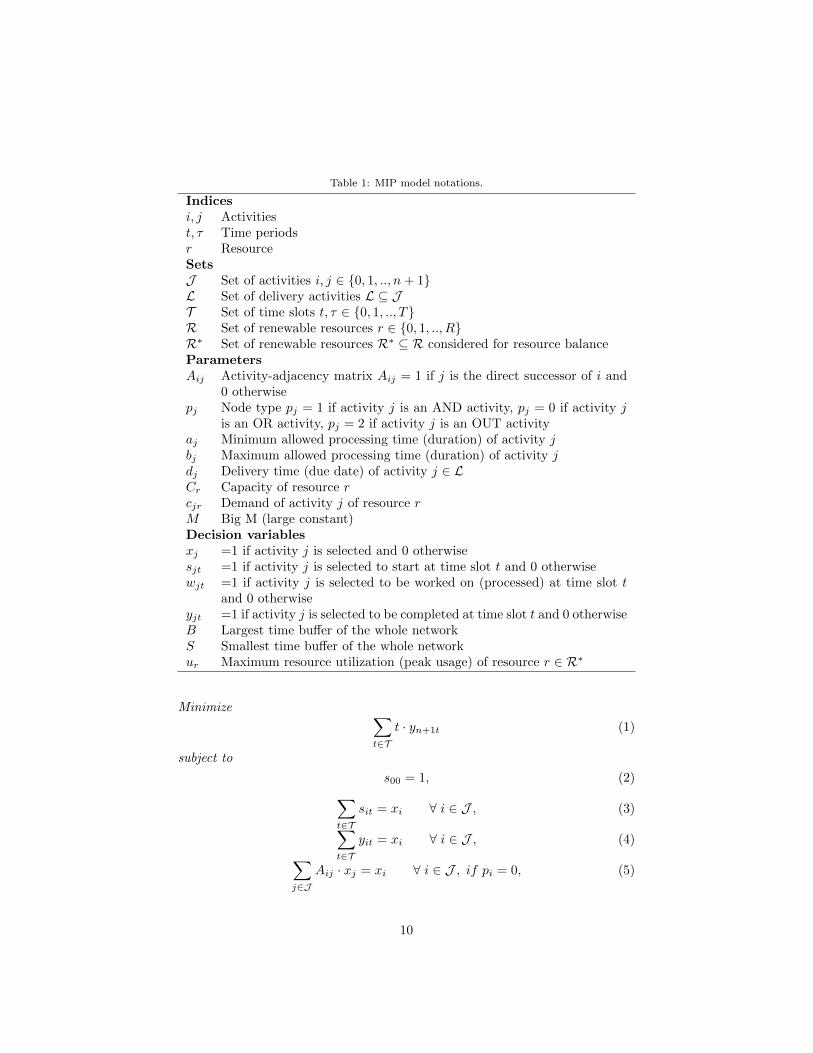
Table 1: MIP model notations.
Indicesi, j Activitiest, τ Time periodsr ResourceSetsJ Set of activities i, j ∈ {0, 1, .., n+ 1}L Set of delivery activities L ⊆ JT Set of time slots t, τ ∈ {0, 1, .., T}R Set of renewable resources r ∈ {0, 1, .., R}R∗ Set of renewable resources R∗ ⊆ R considered for resource balanceParametersAij Activity-adjacency matrix Aij = 1 if j is the direct successor of i and
0 otherwisepj Node type pj = 1 if activity j is an AND activity, pj = 0 if activity j
is an OR activity, pj = 2 if activity j is an OUT activityaj Minimum allowed processing time (duration) of activity jbj Maximum allowed processing time (duration) of activity jdj Delivery time (due date) of activity j ∈ LCr Capacity of resource rcjr Demand of activity j of resource rM Big M (large constant)Decision variablesxj =1 if activity j is selected and 0 otherwisesjt =1 if activity j is selected to start at time slot t and 0 otherwisewjt =1 if activity j is selected to be worked on (processed) at time slot t
and 0 otherwiseyjt =1 if activity j is selected to be completed at time slot t and 0 otherwiseB Largest time buffer of the whole networkS Smallest time buffer of the whole networkur Maximum resource utilization (peak usage) of resource r ∈ R∗
Minimize ∑t∈T
t · yn+1t (1)
subject to
s00 = 1, (2)∑t∈T
sit = xi ∀ i ∈ J , (3)∑t∈T
yit = xi ∀ i ∈ J , (4)∑j∈J
Aij · xj = xi ∀ i ∈ J , if pi = 0, (5)
10
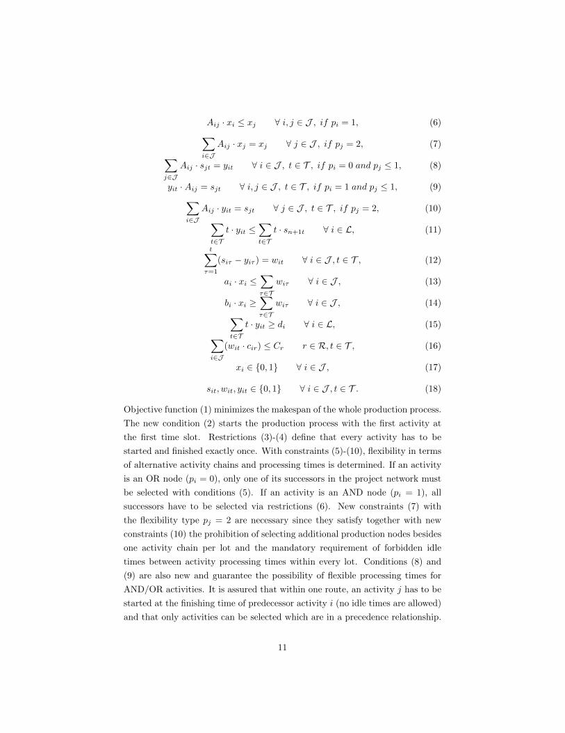
Aij · xi ≤ xj ∀ i, j ∈ J , if pi = 1, (6)∑i∈J
Aij · xj = xj ∀ j ∈ J , if pj = 2, (7)∑j∈J
Aij · sjt = yit ∀ i ∈ J , t ∈ T , if pi = 0 and pj ≤ 1, (8)
yit ·Aij = sjt ∀ i, j ∈ J , t ∈ T , if pi = 1 and pj ≤ 1, (9)∑i∈J
Aij · yit = sjt ∀ j ∈ J , t ∈ T , if pj = 2, (10)∑t∈T
t · yit ≤∑t∈T
t · sn+1t ∀ i ∈ L, (11)
t∑τ=1
(siτ − yiτ ) = wit ∀ i ∈ J , t ∈ T , (12)
ai · xi ≤∑τ∈T
wiτ ∀ i ∈ J , (13)
bi · xi ≥∑τ∈T
wiτ ∀ i ∈ J , (14)∑t∈T
t · yit ≥ di ∀ i ∈ L, (15)∑i∈J
(wit · cir) ≤ Cr r ∈ R, t ∈ T , (16)
xi ∈ {0, 1} ∀ i ∈ J , (17)
sit, wit, yit ∈ {0, 1} ∀ i ∈ J , t ∈ T . (18)
Objective function (1) minimizes the makespan of the whole production process.
The new condition (2) starts the production process with the first activity at
the first time slot. Restrictions (3)-(4) define that every activity has to be
started and finished exactly once. With constraints (5)-(10), flexibility in terms
of alternative activity chains and processing times is determined. If an activity
is an OR node (pi = 0), only one of its successors in the project network must
be selected with conditions (5). If an activity is an AND node (pi = 1), all
successors have to be selected via restrictions (6). New constraints (7) with
the flexibility type pj = 2 are necessary since they satisfy together with new
constraints (10) the prohibition of selecting additional production nodes besides
one activity chain per lot and the mandatory requirement of forbidden idle
times between activity processing times within every lot. Conditions (8) and
(9) are also new and guarantee the possibility of flexible processing times for
AND/OR activities. It is assured that within one route, an activity j has to be
started at the finishing time of predecessor activity i (no idle times are allowed)
and that only activities can be selected which are in a precedence relationship.
11
New constraints (11) ensure that all lots have to be finished before the whole
project (production process) can be finished. With the new restrictions (12)
it is guaranteed that every time slot t which is used for the processing of one
activity i has to be between its decided start and end time. New conditions (13)-
(14) ensure that the flexible processing time for every activity complies with its
defined minimum and maximum allowed processing times. The new constraints
(15) make sure that the production of one lot cannot be finished earlier than its
delivery time and thus that tardiness is allowed but earliness is not. Conditions
(16) represent the capacity restrictions for all renewable resources. Constraints
(17)-(18) define all decision variables as Boolean ones.
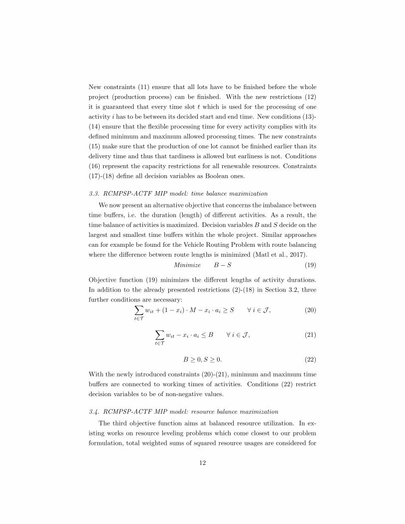
3.3. RCMPSP-ACTF MIP model: time balance maximization
We now present an alternative objective that concerns the imbalance between
time buffers, i.e. the duration (length) of different activities. As a result, the
time balance of activities is maximized. Decision variables B and S decide on the
largest and smallest time buffers within the whole project. Similar approaches
can for example be found for the Vehicle Routing Problem with route balancing
where the difference between route lengths is minimized (Matl et al., 2017).
Minimize B − S (19)
Objective function (19) minimizes the different lengths of activity durations.
In addition to the already presented restrictions (2)-(18) in Section 3.2, three
further conditions are necessary:∑t∈T
wit + (1− xi) ·M − xi · ai ≥ S ∀ i ∈ J , (20)
∑t∈T
wit − xi · ai ≤ B ∀ i ∈ J , (21)
B ≥ 0, S ≥ 0. (22)
With the newly introduced constraints (20)-(21), minimum and maximum time
buffers are connected to working times of activities. Conditions (22) restrict
decision variables to be of non-negative values.
3.4. RCMPSP-ACTF MIP model: resource balance maximization
The third objective function aims at balanced resource utilization. In ex-
isting works on resource leveling problems which come closest to our problem
formulation, total weighted sums of squared resource usages are considered for
12
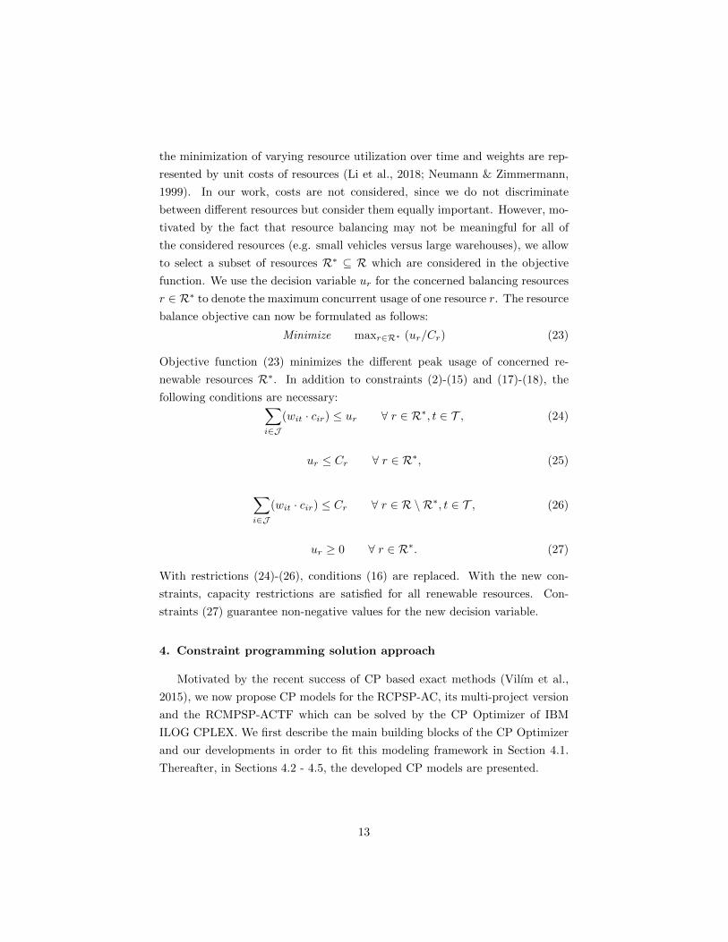
the minimization of varying resource utilization over time and weights are rep-
resented by unit costs of resources (Li et al., 2018; Neumann & Zimmermann,
1999). In our work, costs are not considered, since we do not discriminate
between different resources but consider them equally important. However, mo-
tivated by the fact that resource balancing may not be meaningful for all of
the considered resources (e.g. small vehicles versus large warehouses), we allow
to select a subset of resources R∗ ⊆ R which are considered in the objective
function. We use the decision variable ur for the concerned balancing resources
r ∈ R∗ to denote the maximum concurrent usage of one resource r. The resource
balance objective can now be formulated as follows:
Minimize maxr∈R∗ (ur/Cr) (23)
Objective function (23) minimizes the different peak usage of concerned re-
newable resources R∗. In addition to constraints (2)-(15) and (17)-(18), the
following conditions are necessary:∑i∈J
(wit · cir) ≤ ur ∀ r ∈ R∗, t ∈ T , (24)
ur ≤ Cr ∀ r ∈ R∗, (25)
∑i∈J
(wit · cir) ≤ Cr ∀ r ∈ R \ R∗, t ∈ T , (26)
ur ≥ 0 ∀ r ∈ R∗. (27)
With restrictions (24)-(26), conditions (16) are replaced. With the new con-
straints, capacity restrictions are satisfied for all renewable resources. Con-
straints (27) guarantee non-negative values for the new decision variable.
4. Constraint programming solution approach
Motivated by the recent success of CP based exact methods (Vilım et al.,
2015), we now propose CP models for the RCPSP-AC, its multi-project version
and the RCMPSP-ACTF which can be solved by the CP Optimizer of IBM
ILOG CPLEX. We first describe the main building blocks of the CP Optimizer
and our developments in order to fit this modeling framework in Section 4.1.
Thereafter, in Sections 4.2 - 4.5, the developed CP models are presented.
13
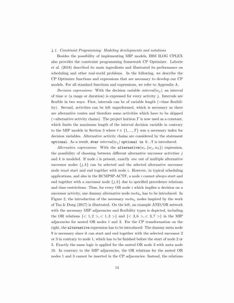
4.1. Constraint Programming: Modeling developments and notations
Besides the possibility of implementing MIP models, IBM ILOG CPLEX
also provides the constraint programming framework CP Optimizer. Laborie
et al. (2018) described its main ingredients and illustrated its performance on
scheduling and other real-world problems. In the following, we describe the
CP Optimizer functions and expressions that are necessary to develop our CP
models. For all standard functions and expressions, we refer to Appendix A.
Decision expressions: With the decision variable interval(wj), an interval
of time w (a range or duration) is expressed for every activity j. Intervals are
flexible in two ways: First, intervals can be of variable length (=time flexibil-
ity). Second, activities can be left unperformed, which is necessary as there
are alternative routes and therefore some activities which have to be skipped
(=alternative activity chains). The project horizon T is now used as a constant,
which limits the maximum length of the interval decision variable in contrary
to the MIP models in Section 3 where t ∈ {1, ..., T} was a necessary index for
decision variables. Alternative activity chains are considered by the statement
optional. As a result, dvar interval(wj) optional in 0..T is introduced.
Alternative expressions: With the alternative(wi, {wj , wk}) expression,
the possibility of choosing between different alternative successor activities j
and k is modeled. If node i is present, exactly one out of multiple alternative
successor nodes {j, k} can be selected and the selected alternative successor
node must start and end together with node i. However, in typical scheduling
applications, and also in the RCMPSP-ACTF, a node i cannot always start and
end together with a successor node {j, k} due to specified precedence relations
and time restrictions. Thus, for every OR node i which implies a decision on a
successor activity, one dummy alternative node metaa has to be introduced. In
Figure 2, the introduction of the necessary metaa nodes inspired by the work
of Tao & Dong (2017) is illustrated. On the left, an example AND/OR network
with the necessary MIP adjacencies and flexibility types is depicted, including
the OR relations {< 1, 2 >,< 1, 3 >} and {< 3, 6 >,< 3, 7 >} in the MIP
adjacencies for nested OR nodes 1 and 3. For the CP transformation on the
right, the alternative expression has to be introduced: The dummy meta node
9 is necessary since it can start and end together with the selected successor 2
or 3 in contrary to node 1, which has to be finished before the start of node 2 or
3. Exactly the same logic is applied for the nested OR node 3 with meta node
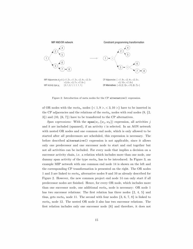
10. In contrary to the MIP adjacencies, the OR relations for the nested OR
nodes 1 and 3 cannot be inserted in the CP adjacencies: Instead, the relations
14
CP Adjacencies { <1, 9>, <2, 4>, <2, 5>,
<3, 10>, <7, 8>}
CP Alternatives { <9, {2, 3}>, <10, {6, 7}> }
11
2
5
4
3
7 8
10
9
616
17 18
12
15
14
1
3
Constraint programming transformationMIP AND/OR network
MIP Adjacencies Aij=1 { <1, 2>, <1, 3>, <2, 4>, <2, 5>
<3, 6>, <3, 7>, <7, 8> }
MIP Activity type pi [ 0, 1, 0, 1, 1, 1, 1, 1 ]
Figure 2: Introduction of meta nodes for the CP alternative() expression.
of OR nodes with the metaa nodes {< 1, 9 >,< 3, 10 >} have to be inserted in
the CP adjacencies and the relations of the metaa nodes with real nodes (9, {2,
3}) and (10, {6, 7}) have to be transferred to the CP alternatives.
Span expressions: With the span(wi, {wj , wk}) expression, all activities j
and k are included (spanned), if an activity i is selected. In an AON network
with nested OR nodes and one common end node, which is only allowed to be
started after all predecessors are scheduled, this expression is necessary. The
before described alternative() expression is not applicable, since it allows
only one predecessor and one successor node to start and end together but
not all activities can be included. For every node that implies a decision on a
successor activity chain, i.e. a relation which includes more than one node, one
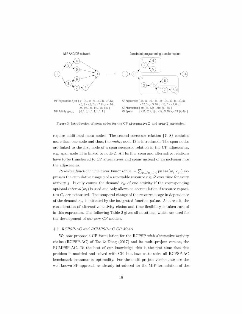
dummy span activity of the type metas has to be introduced. In Figure 3, an
example MIP network with one common end node 14 is shown on the left and
the corresponding CP transformation is presented on the right. The OR nodes
1 and 3 are linked to metaa alternative nodes 9 and 10 as already described for
Figure 2. However, the new common project end node 14 can only start if all
predecessor nodes are finished. Hence, for every OR node, which includes more
than one successor node, one additional metas node is necessary: OR node 1
has two successor relations: The first relation has three nodes {2, 4, 5} and
thus, gets metas node 11. The second with four nodes {3, 6, 7, 8} is linked to
metas node 12. The nested OR node 3 also has two successor relations. The
first relation includes only one successor node {6} and therefore, it does not
15
16
17 18
12
15
14
1141
3
MIP AND/OR network
MIP Adjacencies Aij=1 { <1, 2>, <1, 3>, <2, 4>, <2, 5>,
<3, 6>, <3, 7>, <7, 8>, <4, 14>,
<5, 14>, <6, 14>, <8, 14> }
MIP Activity type pi [ 0, 1, 0, 1, 1, 1, 1, 1, 1 ]
CP Adjacencies { <1, 9>, <9, 14>, <11, 2>, <2, 4>, <2, 5>,
<12, 3>, <3, 10>, <13, 7>, <7, 8>, }
CP Alternatives { <9, {11, 12}>, <10, {6, 13}> }
CP Spans { <11, {2, 4, 5}>, <12, {3, 10}>, <13, {7, 8}> }
11
2
5
4 11
3
7 8
10
12
13
9 114
6
Constraint programming transformation
Figure 3: Introduction of meta nodes for the CP alternative() and span() expression.
require additional meta nodes. The second successor relation {7, 8} contains
more than one node and thus, the metas node 13 is introduced. The span nodes
are linked to the first node of a span successor relation in the CP adjacencies,
e.g. span node 11 is linked to node 2. All further span and alternative relations
have to be transferred to CP alternatives and spans instead of an inclusion into
the adjacencies.
Resource function: The cumulFunction qr =∑j∈J :cjr≥0 pulse(wj , cjr) ex-
presses the cumulative usage q of a renewable resource r ∈ R over time for every
activity j. It only counts the demand cjr of one activity if the corresponding
optional interval(wj) is used and only allows an accumulation if resource capaci-
ties Cr are exhausted. The temporal change of the resource usage in dependence
of the demand cjr is initiated by the integrated function pulse. As a result, the
consideration of alternative activity chains and time flexibility is taken care of
in this expression. The following Table 2 gives all notations, which are used for
the development of our new CP models.
4.2. RCPSP-AC and RCMPSP-AC CP Model
We now propose a CP formulation for the RCPSP with alternative activity
chains (RCPSP-AC) of Tao & Dong (2017) and its multi-project version, the
RCMPSP-AC. To the best of our knowledge, this is the first time that this
problem is modeled and solved with CP. It allows us to solve all RCPSP-AC
benchmark instances to optimality. For the multi-project version, we use the
well-known SP approach as already introduced for the MIP formulation of the
16
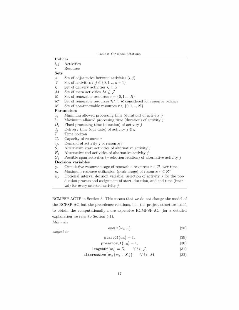
Table 2: CP model notations.
Indicesi, j Activitiesr ResourceSetsA Set of adjacencies between activities (i, j)J Set of activities i, j ∈ {0, 1, .., n+ 1}L Set of delivery activities L ⊆ JM Set of meta activities M⊆ JR Set of renewable resources r ∈ {0, 1, .., R}R∗ Set of renewable resources R∗ ⊆ R considered for resource balanceN Set of non-renewable resources r ∈ {0, 1, .., N}Parametersaj Minimum allowed processing time (duration) of activity jbj Maximum allowed processing time (duration) of activity jDj Fixed processing time (duration) of activity jdj Delivery time (due date) of activity j ∈ LT Time horizonCr Capacity of resource rcjr Demand of activity j of resource rSj Alternative start activities of alternative activity jEj Alternative end activities of alternative activity jGj Possible span activities (=selection relation) of alternative activity jDecision variablesqr Cumulative resource usage of renewable resources r ∈ R over timeur Maximum resource utilization (peak usage) of resource r ∈ R∗wj Optional interval decision variable: selection of activity j for the pro-
duction process and assignment of start, duration, and end time (inter-val) for every selected activity j
RCMPSP-ACTF in Section 3. This means that we do not change the model of
the RCPSP-AC but the precedence relations, i.e. the project structure itself,
to obtain the computationally more expensive RCMPSP-AC (for a detailed
explanation we refer to Section 5.1).
Minimize
endOf(wn+1
)(28)
subject to
startOf(w0
)= 1, (29)
presenceOf(w0
)= 1, (30)
lengthOf(wi)
= Di ∀ i ∈ J , (31)
alternative(wi, {wa ∈ Si}
)∀ i ∈M, (32)
17
span(wi, {ws ∈ Gi}
)∀ i ∈M, (33)
endBeforeStart(wi, wj
)∀ i, j ∈ A, (34)
presenceOf(wi)
= presenceOf(wj), ∀ i, j ∈ A, (35)
qr ≤ Cr ∀ r ∈ R, (36)∑j∈J\M
presenceOf(wj)· cjr ≤ Cr ∀ r ∈ N . (37)
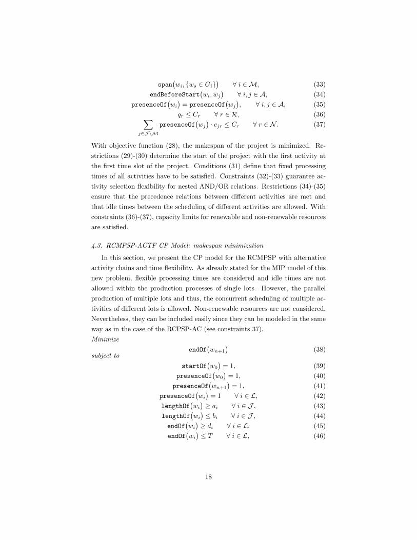
With objective function (28), the makespan of the project is minimized. Re-
strictions (29)-(30) determine the start of the project with the first activity at
the first time slot of the project. Conditions (31) define that fixed processing
times of all activities have to be satisfied. Constraints (32)-(33) guarantee ac-
tivity selection flexibility for nested AND/OR relations. Restrictions (34)-(35)
ensure that the precedence relations between different activities are met and
that idle times between the scheduling of different activities are allowed. With
constraints (36)-(37), capacity limits for renewable and non-renewable resources
are satisfied.
4.3. RCMPSP-ACTF CP Model: makespan minimization
In this section, we present the CP model for the RCMPSP with alternative
activity chains and time flexibility. As already stated for the MIP model of this
new problem, flexible processing times are considered and idle times are not
allowed within the production processes of single lots. However, the parallel
production of multiple lots and thus, the concurrent scheduling of multiple ac-
tivities of different lots is allowed. Non-renewable resources are not considered.
Nevertheless, they can be included easily since they can be modeled in the same
way as in the case of the RCPSP-AC (see constraints 37).
Minimize
endOf(wn+1
)(38)
subject to
startOf(w0
)= 1, (39)
presenceOf(w0
)= 1, (40)
presenceOf(wn+1
)= 1, (41)
presenceOf(wi)
= 1 ∀ i ∈ L, (42)
lengthOf(wi)≥ ai ∀ i ∈ J , (43)
lengthOf(wi)≤ bi ∀ i ∈ J , (44)
endOf(wi)≥ di ∀ i ∈ L, (45)
endOf(wi)≤ T ∀ i ∈ L, (46)
18
alternative(wi, {wa ∈ Si}
)∀ i ∈M, (47)
endAtStart(wi, wa
)∀ i ∈M, a ∈ Ei, (48)
endBeforeStart(wi, wn+1
)∀ i, j ∈ L, (49)
endAtStart(wi, wj
)∀ i, j ∈ A, (50)
presenceOf(wi)
= presenceOf(wj)
∀ i, j ∈ A, (51)
qr ≤ Cr ∀ r ∈ R. (52)
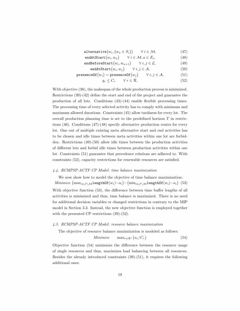
With objective (38), the makespan of the whole production process is minimized.
Restrictions (39)-(42) define the start and end of the project and guarantee the
production of all lots. Conditions (43)-(44) enable flexible processing times.
The processing time of every selected activity has to comply with minimum and
maximum allowed durations. Constraints (45) allow tardiness for every lot. The
overall production planning time is set to the predefined horizon T in restric-
tions (46). Conditions (47)-(48) specify alternative production routes for every
lot. One out of multiple existing meta alternative start and end activities has
to be chosen and idle times between meta activities within one lot are forbid-
den. Restrictions (49)-(50) allow idle times between the production activities
of different lots and forbid idle times between production activities within one
lot. Constraints (51) guarantee that precedence relations are adhered to. With
constraints (52), capacity restrictions for renewable resources are satisfied.
4.4. RCMPSP-ACTF CP Model: time balance maximization
We now show how to model the objective of time balance maximization:
Minimize(maxi∈J\MlengthOf(wi)−ai
)−(mini∈J\MlengthOf(wi)−ai
)(53)
With objective function (53), the difference between time buffer lengths of all
activities is minimized and thus, time balance is maximized. There is no need
for additional decision variables or changed restrictions in contrary to the MIP
model in Section 3.3. Instead, the new objective function is employed together
with the presented CP restrictions (39)-(52).
4.5. RCMPSP-ACTF CP Model: resource balance maximization
The objective of resource balance maximization is modeled as follows:
Minimize maxr∈R∗(ur/Cr
)(54)
Objective function (54) minimizes the difference between the resource usage
of single resources and thus, maximizes load balancing between all resources.
Besides the already introduced constraints (39)-(51), it requires the following
additional ones:
19
qr ≤ ur ∀ r ∈ R∗, (55)
ur ≤ Cr ∀ r ∈ R∗, (56)
qr ≤ Cr ∀ r ∈ R \ R∗. (57)
The new restrictions (55)-(57) replace constraints (52). They restrict the peak
usage of all concerned resources to the defined capacity limits.
5. Computational experiments
The MIP and CP models are implemented in OPL and the CPLEX 12.9.0
MIP solver and CP Optimizer are used to solve them. All experiments are
carried out on a virtual machine Intel(R) Xeon(R) CPU E5-2660 v4, 2.00GHz
with 28 logical processors, Microsoft Windows 10 Education. Since Tao & Dong
(2017) introduce a limit of 3.600 seconds for their runs and we derive results
for benchmark instances generated as described in their work, we use the same
limit for our optimization runs. We first describe the test design in Section 5.1
and then present and discuss the obtained results for the benchmark sets and
the industry case study in Sections 5.2-5.4.
5.1. Instance generation
For the RCPSP-AC, we base our single-project instances on the information
given in Tao & Dong (2017), since their employed instances are not available
and they describe the necessity of an officially available benchmark set in their
work. However, they fully present one instance in their work, consisting of a
project structure with J = 30 nodes in total and including five nested OR
nodes. Following Tao & Dong (2017), to obtain five instance groups with 15
instances each, this project structure is multiplied by 2, 3, 4 and 5, resulting
in instance groups with 30, 60, 90, 120, and 150 nodes besides two additional
dummy nodes for each instance (start and end node). As described in their
work, processing times and demands for all resources are randomly generated.
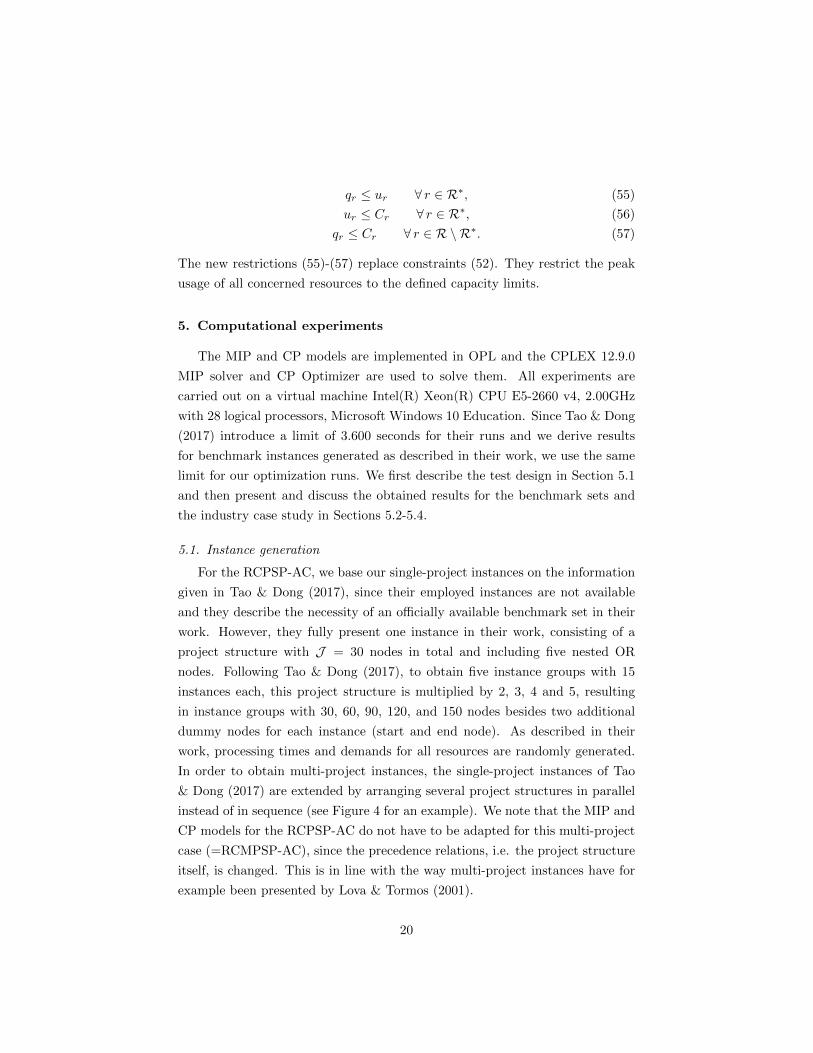
In order to obtain multi-project instances, the single-project instances of Tao
& Dong (2017) are extended by arranging several project structures in parallel
instead of in sequence (see Figure 4 for an example). We note that the MIP and
CP models for the RCPSP-AC do not have to be adapted for this multi-project
case (=RCMPSP-AC), since the precedence relations, i.e. the project structure
itself, is changed. This is in line with the way multi-project instances have for
example been presented by Lova & Tormos (2001).
20
0
J = 30
J = 30
Multi-project case
J = 30 J = 30 61
Single-project case
0
61
Figure 4: Benchmark instance generation for the RCPSP-AC and the RCMPSP-AC.
The instances for the RCMPSP-ACTF are inspired by the project network
data obtained from cooperations with the manufacturing industries described in
Section 1. This network consists of activities such as production (0), cooling (1),
processing (2), relocation (3), storaging (4), vehicle relocation (5) and delivery
(6). Activities (0) and (3) have a fixed duration, all other activities have variable
processing times with minimum and maximum allowed durations. Each lot
starts at (0) and ends at (6) via one alternative route. The customer orders are
connected to related alternative routes, which may involve different activities at
various locations. We use three different lot sizes |L| ∈ {10, 50, 100}. All lots are
sampled from existing customer orders. Processing times, resource capacities
with related resource factors {0.25, 0.50, 0.75, 1.00} and the resource strength
are defined based on Kolisch et al. (1995). Resource demands are equal to one
for the real-world situation and only one out of all existing resources is required
by each activity. We use an additional, different demand pattern where the
demands and the amount of required resources are defined randomly to be able
to validate the real-world situation. As a result, we have two demand patterns
real-world (rw) and random (rand). With the 3 lot sizes, the 2 demand patterns
and the 4 resource strengths, we have 24 instance groups. For each group
we generate 5 instances with varying random seed, which results in a total of
120 instances. The whole data generation procedure is presented in detail in
Appendix B.
For all instances, we note that we limit the large constant M (“Big M”) in
the MIP models to the maximum allowed project duration T in order to support
better relaxations and integer solvability and a less required computation time
(Camm et al., 1990).
21
5.2. RCPSP-AC and RCMPSP-AC: Optimization results
In Table 3, we provide the results for the CP and the MIP models on the
generated single-project instances for the RCPSP-AC of Tao & Dong (2017)
and the multi-project instances for the RCMPSP-AC. Each entry is an average
value across 15 instances per data set. The first column gives the instance size.
In columns 2-6, CP solutions are presented: The second column provides the
best bound and the best solution is found in the third column. In the fourth
column, the runtime is shown in seconds, followed by the number of instances
for which an optimal solution was found and the number of instances for which
a feasible solution was found in columns 5 and 6. Bold letters indicate the
optimal solution. Columns 7-11, where MIP solutions are shown, follow the
same logic as columns 2-6. We note that in order to validate our optimization
results for the RCPSP-AC, we implemented the MIP model presented by Tao
& Dong (2017) and tested it with the benchmark instance J = 30 which they
presented in their paper. Since we had to add and change several constraints
of their MIP model to obtain the same results as presented in their paper for
this instance, we provide the modified MIP model in Appendix C. The detailed
results for every examined benchmark instance are given in Appendix D.
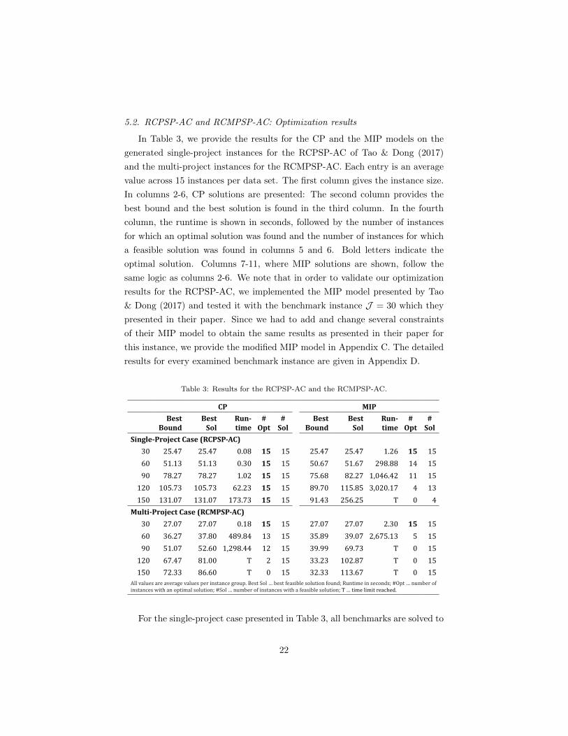
Table 3: Results for the RCPSP-AC and the RCMPSP-AC.
CP MIP
Best
Bound
Best
Sol
Run-
time
#
Opt
#
Sol
Best
Bound
Best
Sol
Run-
time
#
Opt
#
Sol
Single-Project Case (RCPSP-AC)
30 25.47 25.47 0.08 15 15 25.47 25.47 1.26 15 15
60 51.13 51.13 0.30 15 15 50.67 51.67 298.88 14 15
90 78.27 78.27 1.02 15 15 75.68 82.27 1,046.42 11 15
120 105.73 105.73 62.23 15 15 89.70 115.85 3,020.17 4 13
150 131.07 131.07 173.73 15 15 91.43 256.25 T 0 4
Multi-Project Case (RCMPSP-AC)
30 27.07 27.07 0.18 15 15 27.07 27.07 2.30 15 15
60 36.27 37.80 489.84 13 15 35.89 39.07 2,675.13 5 15
90 51.07 52.60 1,298.44 12 15 39.99 69.73 T 0 15
120 67.47 81.00 T 2 15 33.23 102.87 T 0 15
150 72.33 86.60 T 0 15 32.33 113.67 T 0 15
All values are average values per instance group. Best Sol … best feasible solution found; Runtime in seconds; #Opt … number of
instances with an optimal solution; #Sol … number of instances with a feasible solution; T … time limit reached.
For the single-project case presented in Table 3, all benchmarks are solved to
22
optimality by using the CP model but not when using the MIP model. The CP
approach provides optimal solutions to dimensions of increasing difficulty with
very little effort while in case of the MIP model the solver struggles to solve
instances with more than 90 nodes within the allotted runtime. The results also
show that the CP Optimizer solves instances of size 150 in less time on average
than the MIP solver for dimension 60.
Given these results, we have generated additional new multi-project in-
stances which are computationally more challenging. For this new RCMPSP-AC
case, the CP and the MIP solver struggle to solve problems of increasing size to
optimality. Although they both get feasible solutions for all problem instances,
the CP Optimizer finds better bounds and better solutions on average than
the MIP solver. Interestingly, for the MIP solver, finding feasible solutions for
multi-project instances appears to be easier than for single-project instances.
Nevertheless, proving their optimality is considerably more difficult.
As explained in Section 5.1, benchmarks are generated equal to the descrip-
tion of Tao & Dong (2017) with the only difference of a parallel project structure
for the multi-project case. This means that the same resource capacities are used
for the multi-project case where a lot more activities have to be scheduled in
parallel than in the single-project case of Tao & Dong (2017). Thus, the re-
source strength, which is an indicator of instance hardness (Kolisch et al., 1995)
is much higher.
5.3. RCMPSP-ACTF: Optimization results
In Table 4, we present the optimization results for the benchmark data
generated for the RCMPSP-ACTF. They follow the same logic as the results
for the RCPSP-AC and RCMPSP-AC shown in Table 3 with the only difference
that in the second column now the respective demand patterns (real-world and
random) are given in addition. The detailed results for every examined instance
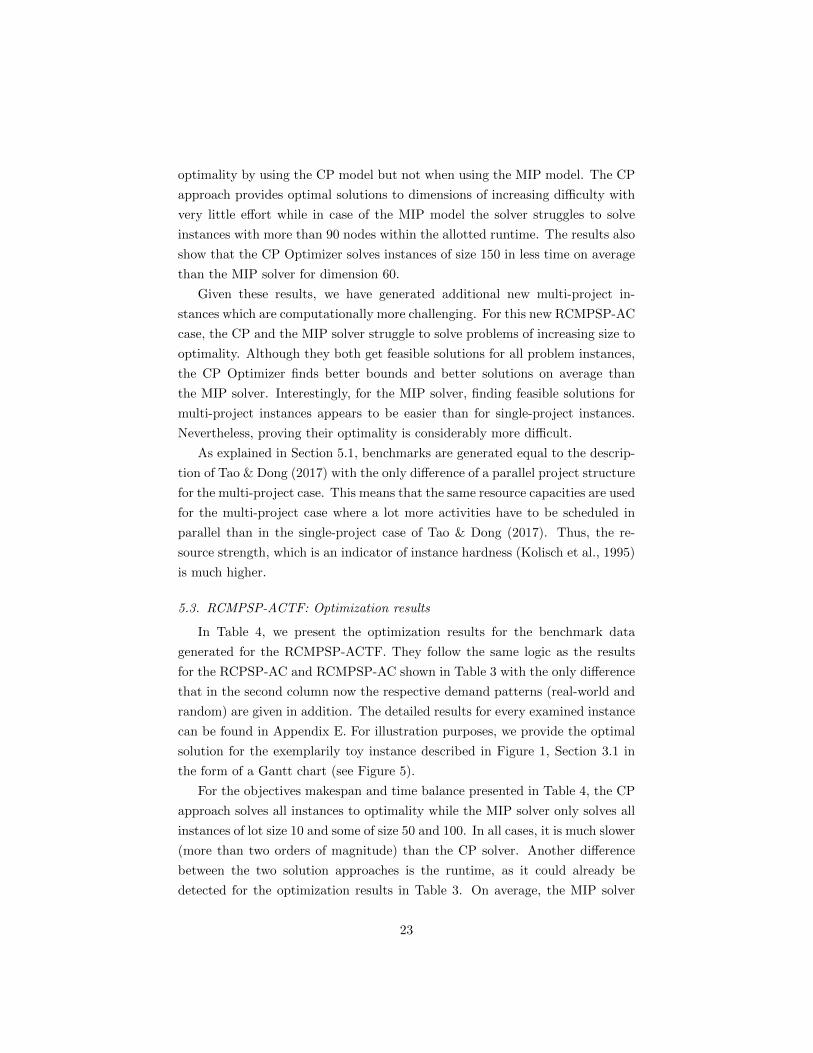
can be found in Appendix E. For illustration purposes, we provide the optimal
solution for the exemplarily toy instance described in Figure 1, Section 3.1 in
the form of a Gantt chart (see Figure 5).
For the objectives makespan and time balance presented in Table 4, the CP
approach solves all instances to optimality while the MIP solver only solves all
instances of lot size 10 and some of size 50 and 100. In all cases, it is much slower
(more than two orders of magnitude) than the CP solver. Another difference
between the two solution approaches is the runtime, as it could already be
detected for the optimization results in Table 3. On average, the MIP solver
23
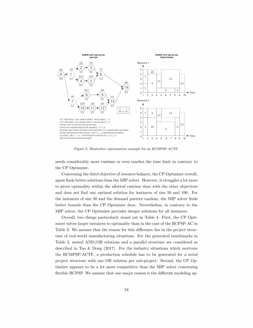
- Lot 1: Start activity 1, end (=delivery) activity 6 with due date d6
= 9
- Lot 2: Start activity 7, end (=delivery) activity 13 with due date d13
= 10
- Activities 0 and 14 are dummy start and end nodes
- There are two renewable resources with capacities C1= 5; C
2=6
- All activities have minimum and maximum processing times ( aj | b
j ) depicted above the activities
and they have demands for both resources 1 and 2 ( cj1
; cj2
) depicted below the activities,
e.g. activity 1 with a1 = 1 | b
1 = 8 and demands for resources are c
11=2; c
12= 4
(Note: All input data are randomly generated)
2
4
8
1110
0
14
1
7
1|6
3;2
2|11
1;3
3|8
2;1
1|8
3;3
1|9
4;2
2|10
1;4
2|12
4;2
1|10
1;3
2|4
1;2
1|9
2;1
1|1
4;5
1|8
2;4
1|13
5
6
9
12
13
1;4
0|0
0;0
0|0
0;0
ORAND OUT
RCMPSP-ACTF with two lots:
Input data
1 2 3 4 5 6 7 8 9 10
Time
6
5
4
3
2
1
0
Resource 2
1
7
10
411
5
12
136
1 2 3 4 5 6 7 8 9 10
Time
5
4
3
2
1
0
Resource 1
1
7
4
10
11
5
12
13
6
RCMPSP-ACTF with two lots:
Optimal Solution
Figure 5: Illustrative optimization example for an RCMPSP-ACTF.
needs considerably more runtime or even reaches the time limit in contrary to
the CP Optimizer.
Concerning the third objective of resource balance, the CP Optimizer overall,
again finds better solutions than the MIP solver. However, it struggles a lot more
to prove optimality within the allotted runtime than with the other objectives
and does not find any optimal solution for instances of size 50 and 100. For
the instances of size 50 and the demand pattern random, the MIP solver finds
better bounds than the CP Optimizer does. Nevertheless, in contrary to the
MIP solver, the CP Optimizer provides integer solutions for all instances.
Overall, two things particularly stand out in Table 4. First, the CP Opti-
mizer solves larger instances to optimality than in the case of the RCPSP-AC in
Table 3. We assume that the reason for this difference lies in the project struc-
ture of real-world manufacturing situations. For the generated benchmarks in
Table 3, nested AND/OR relations and a parallel structure are considered as
described in Tao & Dong (2017). For the industry situations which motivate
the RCMPSP-ACTF, a production schedule has to be generated for a serial
project structure with one OR relation per sub-project. Second, the CP Op-
timizer appears to be a lot more competitive than the MIP solver concerning
flexible RCPSP. We assume that one major reason is the different modeling ap-
24
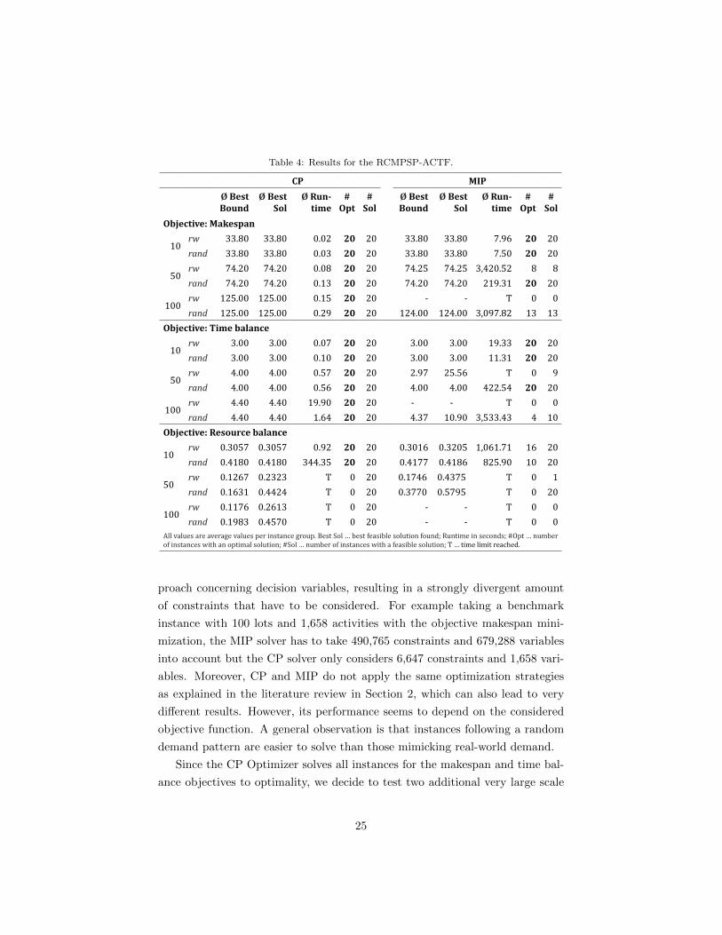
Table 4: Results for the RCMPSP-ACTF.
CP MIP
Ø Best
Bound
Ø Best
Sol
Ø Run-
time
#
Opt
#
Sol
Ø Best
Bound
Ø Best
Sol
Ø Run-
time
#
Opt
#
Sol
Objective: Makespan
10rw 33.80 33.80 0.02 20 20 33.80 33.80 7.96 20 20
rand 33.80 33.80 0.03 20 20 33.80 33.80 7.50 20 20
50rw 74.20 74.20 0.08 20 20 74.25 74.25 3,420.52 8 8
rand 74.20 74.20 0.13 20 20 74.20 74.20 219.31 20 20
100rw 125.00 125.00 0.15 20 20 - - T 0 0
rand 125.00 125.00 0.29 20 20 124.00 124.00 3,097.82 13 13
Objective: Time balance
10rw 3.00 3.00 0.07 20 20 3.00 3.00 19.33 20 20
rand 3.00 3.00 0.10 20 20 3.00 3.00 11.31 20 20
50rw 4.00 4.00 0.57 20 20 2.97 25.56 T 0 9
rand 4.00 4.00 0.56 20 20 4.00 4.00 422.54 20 20
100rw 4.40 4.40 19.90 20 20 - - T 0 0
rand 4.40 4.40 1.64 20 20 4.37 10.90 3,533.43 4 10
Objective: Resource balance
10rw 0.3057 0.3057 0.92 20 20 0.3016 0.3205 1,061.71 16 20
rand 0.4180 0.4180 344.35 20 20 0.4177 0.4186 825.90 10 20
50rw 0.1267 0.2323 T 0 20 0.1746 0.4375 T 0 1
rand 0.1631 0.4424 T 0 20 0.3770 0.5795 T 0 20
100rw 0.1176 0.2613 T 0 20 - - T 0 0
rand 0.1983 0.4570 T 0 20 - - T 0 0
All values are average values per instance group. Best Sol … best feasible solution found; Runtime in seconds; #Opt … number
of instances with an optimal solution; #Sol … number of instances with a feasible solution; T … time limit reached.
proach concerning decision variables, resulting in a strongly divergent amount
of constraints that have to be considered. For example taking a benchmark
instance with 100 lots and 1,658 activities with the objective makespan mini-
mization, the MIP solver has to take 490,765 constraints and 679,288 variables
into account but the CP solver only considers 6,647 constraints and 1,658 vari-
ables. Moreover, CP and MIP do not apply the same optimization strategies
as explained in the literature review in Section 2, which can also lead to very
different results. However, its performance seems to depend on the considered
objective function. A general observation is that instances following a random
demand pattern are easier to solve than those mimicking real-world demand.
Since the CP Optimizer solves all instances for the makespan and time bal-
ance objectives to optimality, we decide to test two additional very large scale
25
instances with l=1,000 and l=10,000 lots. With the makespan objective, op-
timal solutions are available for both instances in 21.76 and 315.61 seconds.
However, with the time balance objective, optimality can only be proven for
l=1,000 in 364.05 seconds; for l=10,000 a gap of 58,54% is left after the allowed
runtime of one hour. Although the time balance objective cannot compete with
the makespan for the largest instance, our results show that CP works far better
for interval-related objectives (especially the makespan) than for the resource
balance objective on the tested benchmarks.
5.4. Industry case study
In the following, we present our results of a case study for a globally operating
steel producer. The considered products are steel slabs, which are large and
bulky artefacts cast out of different sorts of metal. The manufacturer requires
an optimized schedule starting with predefined continuous casting programs and
ending with customer deliveries. The objective of this study is threefold: We
evaluate our proposed models in terms of satisfying all constraints, providing
optimal solutions and giving insights into the impact of the respective objectives
on processing time lengths and resource utilizations. The manufacturer requests
a maximum runtime of 1 hour. The reason is that the optimization results serve
as a management decision support, which has to be available at short notice for a
large-scale instance size. Since up to now, the operational production planning
of the company is partially triggered manually or with spreadsheet software,
unfortunately, we cannot compare our results with existing schedules. As it
is not possible to publish the whole real-world data instance with the detailed
project structure, we give the following company-released information.
The continuous casting plan for the following 2.5 hours has to be taken into
account for the optimization, i.e. all customer orders (=lots), which are cast
in the next 2.5 hours have to be included in the scheduling plan. However, the
overall planning horizon, which has to be considered for the optimization is 3
days (and not 2.5 hours), since the delivery dates for the produced lots vary up
to 3 days. This inclusion of the whole production cycle is also necessary since
the company wants to generate new production schedules in this make-to-order
environment as often as demanded for the already mentioned management de-
cision support, as it is for example also explained in Voß & Witt (2007). The
steel producer asks for a minute-by-minute planning, resulting in a total plan-
ning horizon of T =4,088 minutes. Our partner produces L=50 lots with related
556 activities. Whereas 21 lots have three route alternatives, 23 have two and six
26
lots have to follow a fixed route. Some production activities have fixed process-
ing times, such as automated handover activities. For other activities, strongly
varying minimum (ai) and maximum allowed processing times (bi) are defined
by the steel producer, e.g. having a storaging activity with ai=24 and bi=506
minutes. The manufacturer has eight renewable resources with very different
capacities Cr = [10; 10; 30; 10; 50; 240; 220; 80], since vehicles, a cooling bed
and an automated handover resource with a much lower capacity than large
warehouses, cooling and warming boxes are included. For some production re-
sources such as the automated handover resource, concurrent use is not possible,
i.e., it is always fully used by a maximum of one activity. Other resources such
as warehouses have high and not fully utilized capacities. The company only
considers their two conventional warehouses r ∈ {6, 8} as appropriate for load
balancing purposes R∗ ⊆ R. All other resources have very different technical
purposes, i.e. they are not considered since e.g. a load balancing between a
handover and a vehicle resource would not make sense for the company.
With the presented MIP models, it is not possible to generate a feasible
solution within the allowed runtime. We assume that the major reason is the
time index t for the time-related decision variables together with the very long
planning horizon of T =4,088 minutes, since preliminary tests with a very low
(unrealistic) time horizon provide at least a feastible solution. Thus, all pre-
sented results are obtained by means of the CP Optimizer.
For the CP optimization, 50 additional dummy meta nodes which are nec-
essary for the route selection and 1 dummy start and 1 dummy end node are
added, resulting in a total of J=608 activities (for the MIP optimization only
1 dummy start and 1 dummy end node were added). Nevertheless, all three
CP models are solved to optimality within seconds, as shown in Table 5, where
the following information is provided for each run: the optimization runtime,
the makespan of the obtained solution, the time buffer and the peak usage of
resources 6 and 8 (R6 and R8). The optimal makespan is achieved with all
three objectives. The reason for this equality is that the due date of the last
lot is reached without any tardiness by all three objectives. However, the goal
of balancing the peak usages of resources R∗ is much better reached with the
resource balance objective than with the others. The same result applies to the
time balance objective: the aim of the company to distribute processing times
in such a way that buffer time variations are minimized is far better reached
with this objective in contrary to the other ones. A related closer examination
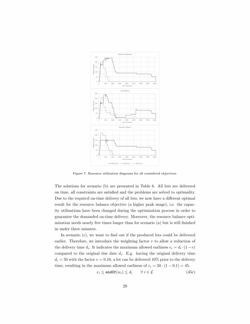
of the time buffer and peak usage variations is depicted in Figures 6-7.
27
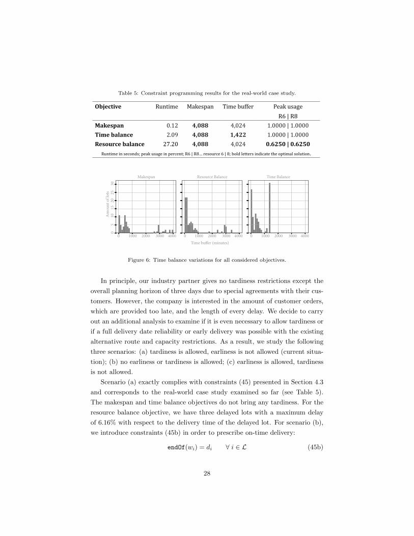
Table 5: Constraint programming results for the real-world case study.
Objective Runtime Makespan Time buffer Peak usage
R6 | R8
Makespan 0.12 4,088 4,024 1.0000 | 1.0000
Time balance 2.09 4,088 1,422 1.0000 | 1.0000
Resource balance 27.20 4,088 4,024 0.6250 | 0.6250
Runtime in seconds; peak usage in percent; R6 | R8… resource 6 | 8; bold letters indicate the optimal solution.
Makespan Resource Balance Time Balance
A
mou
nt o
f lot
s 0
5
10
15
20
2
5
30
0 1000 2000 3000 4000 0 1000 2000 3000 4000 0 1000 2000 3000 4000Time buffer (minutes)
Figure 6: Time balance variations for all considered objectives.
In principle, our industry partner gives no tardiness restrictions except the
overall planning horizon of three days due to special agreements with their cus-
tomers. However, the company is interested in the amount of customer orders,
which are provided too late, and the length of every delay. We decide to carry
out an additional analysis to examine if it is even necessary to allow tardiness or
if a full delivery date reliability or early delivery was possible with the existing
alternative route and capacity restrictions. As a result, we study the following
three scenarios: (a) tardiness is allowed, earliness is not allowed (current situa-
tion); (b) no earliness or tardiness is allowed; (c) earliness is allowed, tardiness
is not allowed.
Scenario (a) exactly complies with constraints (45) presented in Section 4.3
and corresponds to the real-world case study examined so far (see Table 5).
The makespan and time balance objectives do not bring any tardiness. For the
resource balance objective, we have three delayed lots with a maximum delay
of 6.16% with respect to the delivery time of the delayed lot. For scenario (b),
we introduce constraints (45b) in order to prescribe on-time delivery:
endOf(wi) = di ∀ i ∈ L (45b)
28
0
50
100
150
200
250
0 500 1000 1500 2000 2500 3000 3500 4000
Uti
lize
d C
ap
aci
ty
Time (minutes)
Resource Balance
Resource 6 Resource 7 Resource 8
0
50
100
150
200
250
0 500 1000 1500 2000 2500 3000 3500 4000
Uti
lize
d C
ap
aci
ty
Time (minutes)
Time Balance
0
50
100
150
200
250
0 500 1000 1500 2000 2500 3000 3500 4000
Uti
lize
d C
ap
aci
ty
Time (minutes)
Objective Makespan
Figure 7: Resource utilization diagrams for all considered objectives.
The solutions for scenario (b) are presented in Table 6. All lots are delivered
on time, all constraints are satisfied and the problems are solved to optimality.
Due to the required on-time delivery of all lots, we now have a different optimal
result for the resource balance objective (a higher peak usage), i.e. the capac-
ity utilizations have been changed during the optimization process in order to
guarantee the demanded on-time delivery. Moreover, the resource balance opti-
mization needs nearly five times longer than for scenario (a) but is still finished
in under three minutes.
In scenario (c), we want to find out if the produced lots could be delivered
earlier. Therefore, we introduce the weighting factor v to allow a reduction of
the delivery time di. It indicates the maximum allowed earliness ei = di · (1−v)
compared to the original due date di. E.g. having the original delivery time
di = 50 with the factor v = 0.10, a lot can be delivered 10% prior to the delivery
time, resulting in the maximum allowed earliness of ei = 50 · (1− 0.1) = 45.
ei ≤ endOf(wi) ≤ di ∀ i ∈ L (45c)
29
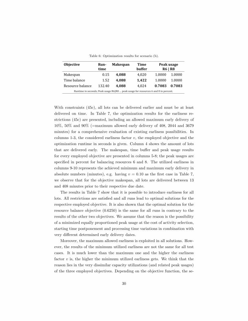
Table 6: Optimization results for scenario (b).
Objective Run-
time
Makespan Time
buffer
Peak usage
R6 | R8
Makespan 0.15 4,088 4,020 1.0000 1.0000
Time balance 1.52 4,088 1,422 1.0000 1.0000
Resource balance 132.40 4,088 4,024 0.7083 0.7083
Runtime in seconds; Peak usage R6|R8 … peak usage for resources 6 and 8 in percent.
With constraints (45c), all lots can be delivered earlier and must be at least
delivered on time. In Table 7, the optimization results for the earliness re-
strictions (45c) are presented, including an allowed maximum early delivery of
10%, 50% and 90% (=maximum allowed early delivery of 408, 2044 and 3679
minutes) for a comprehensive evaluation of existing earliness possibilities. In
columns 1-3, the considered earliness factor v, the employed objective and the
optimization runtime in seconds is given. Column 4 shows the amount of lots
that are delivered early. The makespan, time buffer and peak usage results
for every employed objective are presented in columns 5-8; the peak usages are
specified in percent for balancing resources 6 and 8. The utilized earliness in
columns 9-10 represents the achieved minimum and maximum early delivery in
absolute numbers (minutes), e.g. having v = 0.10 as the first case in Table 7,
we observe that for the objective makespan, all lots are delivered between 13
and 408 minutes prior to their respective due date.
The results in Table 7 show that it is possible to introduce earliness for all
lots. All restrictions are satisfied and all runs lead to optimal solutions for the
respective employed objective. It is also shown that the optimal solution for the
resource balance objective (0.6250) is the same for all runs in contrary to the
results of the other two objectives. We assume that the reason is the possibility
of a minimized equally proportioned peak usage at the cost of activity selection,
starting time postponement and processing time variations in combination with
very different determined early delivery dates.
Moreover, the maximum allowed earliness is exploited in all solutions. How-
ever, the results of the minimum utilized earliness are not the same for all test
cases. It is much lower than the maximum one and the higher the earliness
factor v is, the higher the minimum utilized earliness gets. We think that the
reason lies in the very dissimilar capacity utilizations (and related peak usages)
of the three employed objectives. Depending on the objective function, the se-
30
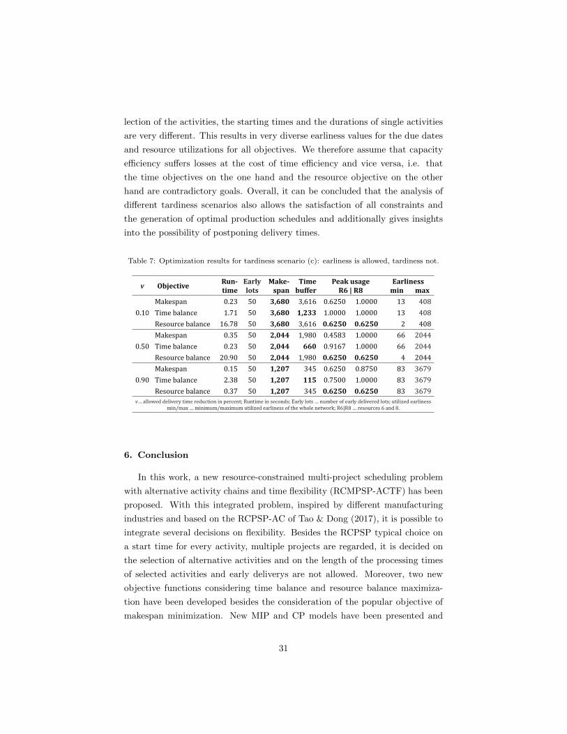
lection of the activities, the starting times and the durations of single activities
are very different. This results in very diverse earliness values for the due dates
and resource utilizations for all objectives. We therefore assume that capacity
efficiency suffers losses at the cost of time efficiency and vice versa, i.e. that
the time objectives on the one hand and the resource objective on the other
hand are contradictory goals. Overall, it can be concluded that the analysis of
different tardiness scenarios also allows the satisfaction of all constraints and
the generation of optimal production schedules and additionally gives insights
into the possibility of postponing delivery times.
Table 7: Optimization results for tardiness scenario (c): earliness is allowed, tardiness not.
v ObjectiveRun-
time
Early
lots
Make-
span
Time
buffer
Peak usage
R6 | R8
Earliness
min max
0.10
Makespan 0.23 50 3,680 3,616 0.6250 1.0000 13 408
Time balance 1.71 50 3,680 1,233 1.0000 1.0000 13 408
Resource balance 16.78 50 3,680 3,616 0.6250 0.6250 2 408
0.50
Makespan 0.35 50 2,044 1,980 0.4583 1.0000 66 2044
Time balance 0.23 50 2,044 660 0.9167 1.0000 66 2044
Resource balance 20.90 50 2,044 1,980 0.6250 0.6250 4 2044
0.90
Makespan 0.15 50 1,207 345 0.6250 0.8750 83 3679
Time balance 2.38 50 1,207 115 0.7500 1.0000 83 3679
Resource balance 0.37 50 1,207 345 0.6250 0.6250 83 3679
v… allowed delivery time reduction in percent; Runtime in seconds; Early lots … number of early delivered lots; utilized earliness
min/max … minimum/maximum utilized earliness of the whole network; R6|R8 … resources 6 and 8.
6. Conclusion
In this work, a new resource-constrained multi-project scheduling problem
with alternative activity chains and time flexibility (RCMPSP-ACTF) has been
proposed. With this integrated problem, inspired by different manufacturing
industries and based on the RCPSP-AC of Tao & Dong (2017), it is possible to
integrate several decisions on flexibility. Besides the RCPSP typical choice on
a start time for every activity, multiple projects are regarded, it is decided on
the selection of alternative activities and on the length of the processing times
of selected activities and early deliverys are not allowed. Moreover, two new
objective functions considering time balance and resource balance maximiza-
tion have been developed besides the consideration of the popular objective of
makespan minimization. New MIP and CP models have been presented and
31
in a comprehensive numerical study, the strong potential of our developed CP
approach has been demonstrated in terms of solution quality and runtime: we
solve all benchmarks for the RCPSP-AC to optimality and therefore provide an
additional set where the computationally more expensive multi-project environ-
ment is considered. Moreover, many instances of the newly developed problem
and the industry case are solved to optimality.
Future research will address several topics concerning the advancement of
flexibility in a scheduling context. First, new methods, which provide better
solutions for the multi-project RCPSP-AC and the RCMPSP-ACTF maximiz-
ing resource balance, should be addressed. Second, the mutual influence of the
investigated three objectives should be examined in a multi-objective context.
Third, an additional consideration of the MP approach for the new problem
and a comparison to the established SP approach would be an interesting topic
of investigation. Moreover, the robustness of the achieved optimization results
with regard to disruptive incidents, such as the sudden breakdown of resources,
can significantly influence the competitiveness of organizations. In order to
meet this challenge, disturbance variables and related methods to obtain robust
solutions should be investigated.
References
Allahverdi, A. (2016). A survey of scheduling problems with no-wait in process.European Journal of Operational Research, 255 , 665–686. doi:10.1016/j.ejor.2016.05.036.
Altinakar, S., Caporossi, G., & Hertz, A. (2016). A comparison of integer andconstraint programming models for the deficiency problem. Computers &Operations Research, 68 , 89–96. doi:10.1016/j.cor.2015.10.016.
Artigues, C. (2017). On the strength of time-indexed formulations for theresource-constrained project scheduling problem. Operations Research Let-ters, 45 , 154–159. doi:10.1016/j.orl.2017.02.001.
Artigues, C., Demassey, S., & Neron, E. (2013). Resource-constrained projectscheduling: models, algorithms, extensions and applications. John Wiley &Sons.
Asta, S., Karapetyan, D., Kheiri, A., Ozcan, E., & Parkes, A. J. (2016). Com-bining monte-carlo and hyper-heuristic methods for the multi-mode resource-constrained multi-project scheduling problem. Information Sciences, 373 ,476–498. doi:10.1016/j.ins.2016.09.010.
32
Banaszak, Z., Zaremba, M., & Muszynski, W. (2009). Constraint program-ming for project-driven manufacturing. International Journal of ProductionEconomics, 120 , 463–475. doi:10.1016/j.ijpe.2008.12.016.
Baptiste, P., Le Pape, C., & Nuijten, W. (2012). Constraint-based scheduling:applying constraint programming to scheduling problems volume 39. SpringerScience & Business Media. doi:10.1007/978-1-4615-1479-4.
Beck, J. C., & Fox, M. S. (2000). Constraint-directed techniques for schedul-ing alternative activities. Artificial Intelligence, 121 , 211–250. doi:10.1016/S0004-3702(00)00035-7.
Birjandi, A., & Mousavi, S. M. (2019). Fuzzy resource-constrained projectscheduling with multiple routes: A heuristic solution. Automation in Con-struction, 100 , 84–102. doi:10.1016/j.autcon.2018.11.029.
Birjandi, A., Mousavi, S. M., Hajirezaie, M., & Vahdani, B. (2019). Optimizingand solving project scheduling problem for flexible networks with multipleroutes in production environments. Journal of Quality Engineering and Pro-duction Optimization, 4 , 175–196.
B lazewicz, J., Ecker, K. H., Pesch, E., Schmidt, G., Sterna, M., & Weglarz, J.(2019). Handbook on Scheduling: From Theory to Practice. Springer.
Blazewicz, J., Lenstra, J. K., & Kan, A. R. (1983). Scheduling subject toresource constraints: classification and complexity. Discrete applied mathe-matics, 5 , 11–24. doi:10.1016/0166-218X(83)90012-4.
Bockmayr, A., & Hooker, J. N. (2005). Constraint programming. Handbooksin Operations Research and Management Science, 12 , 559–600. doi:10.1016/S0927-0507(05)12010-6.
Burgelman, J., & Vanhoucke, M. (2018). Maximising the weighted number of ac-tivity execution modes in project planning. European Journal of OperationalResearch, 270 , 999–1013. doi:10.1016/j.ejor.2018.04.035.
Camm, J. D., Raturi, A. S., & Tsubakitani, S. (1990). Cutting big m down tosize. Interfaces, 20 , 61–66. doi:10.1287/inte.20.5.61.
Capek, R., Sucha, P., & Hanzalek, Z. (2012). Production scheduling with alter-native process plans. European Journal of Operational Research, 217 , 300–311. doi:10.1016/j.ejor.2011.09.018.
Chakrabortty, R. K., Sarker, R. A., & Essam, D. L. (2017). Resource constrainedmulti-project scheduling: A priority rule based evolutionary local searchapproach. In Intelligent and Evolutionary Systems (pp. 75–86). Springer.doi:10.1007/978-3-319-49049-6.
33
Goel, V., Slusky, M., van Hoeve, W.-J., Furman, K. C., & Shao, Y. (2015).Constraint programming for lng ship scheduling and inventory management.European Journal of Operational Research, 241 , 662–673. doi:10.1016/j.ejor.2014.09.048.
Hans, E. W., Herroelen, W., Leus, R., & Wullink, G. (2007). A hierarchicalapproach to multi-project planning under uncertainty. Omega, 35 , 563–577.doi:10.1016/j.omega.2005.10.004.
Hartmann, S., & Briskorn, D. (2010). A survey of variants and extensions ofthe resource-constrained project scheduling problem. European Journal ofoperational research, 207 , 1–14. doi:10.1016/j.ejor.2009.11.005.
Johannes, B. (2005). On the complexity of scheduling unit-time jobs withor-precedence constraints. Operations research letters, 33 , 587–596. doi:10.1016/j.orl.2004.11.009.
Johnson, D. S., & Garey, M. R. (1979). Computers and intractability: A guideto the theory of NP-completeness. WH Freeman. doi:10.1137/1024022.
Kellenbrink, C., & Helber, S. (2015). Scheduling resource-constrained projectswith a flexible project structure. European Journal of Operational Research,246 , 379–391. doi:10.1016/j.ejor.2015.05.003.
Kolisch, R., Sprecher, A., & Drexl, A. (1995). Characterization and genera-tion of a general class of resource-constrained project scheduling problems.Management science, 41 , 1693–1703. doi:10.1287/mnsc.41.10.1693.
Kreter, S., Schutt, A., & Stuckey, P. J. (2017). Using constraint program-ming for solving rcpsp/max-cal. Constraints, 22 , 432–462. doi:10.1007/s10601-016-9266-6.
Kreter, S., Schutt, A., Stuckey, P. J., & Zimmermann, J. (2018). Mixed-integerlinear programming and constraint programming formulations for solving re-source availability cost problems. European Journal of Operational Research,266 , 472–486. doi:10.1016/j.ejor.2017.10.014.
Laborie, P., Rogerie, J., Shaw, P., & Vilım, P. (2018). Ibm ilog cp optimizer forscheduling. Constraints, 23 , 210–250. doi:10.1007/s10601-018-9281-x.
Li, H., Xiong, L., Liu, Y., & Li, H. (2018). An effective genetic algorithmfor the resource levelling problem with generalised precedence relations. In-ternational Journal of Production Research, 56 , 2054–2075. doi:10.1080/00207543.2017.1355120.
Liess, O., & Michelon, P. (2008). A constraint programming approach for theresource-constrained project scheduling problem. Annals of Operations Re-search, 157 , 25–36. doi:10.1007/s10479-007-0188-y.
34
Lova, A., Maroto, C., & Tormos, P. (2000). A multicriteria heuristic method toimprove resource allocation in multiproject scheduling. European Journal ofOperational Research, 127 , 408–424. doi:10.1016/S0377-2217(99)00490-7.
Lova, A., & Tormos, P. (2001). Analysis of scheduling schemes and heuristicrules performance in resource-constrained multiproject scheduling. Annals ofOperations Research, 102 , 263–286. doi:10.1023/A:1010966401888.
Matl, P., Hartl, R. F., & Vidal, T. (2017). Workload equity in vehicle rout-ing problems: A survey and analysis. Transportation Science, 52 , 239–260.doi:10.1287/trsc.2017.0744.
Moradi, M., Hafezalkotob, A., & Ghezavati, V. (2019). Robust resource-constrained project scheduling problem of the project’s subcontractors in acooperative environment under uncertainty: Social complex construction casestudy. Computers & Industrial Engineering , 133 , 19–28. doi:10.1016/j.cie.2019.04.046.
Naber, A., & Kolisch, R. (2014). Mip models for resource-constrained projectscheduling with flexible resource profiles. European Journal of OperationalResearch, 239 , 335–348. doi:10.1016/j.ejor.2014.05.036.
Neumann, K., & Zimmermann, J. (1999). Resource levelling for projects withschedule-dependent time windows. European Journal of Operational Re-search, 117 , 591–605. doi:10.1016/S0377-2217(98)00272-0.
Novas, J. M., & Henning, G. P. (2014). Integrated scheduling of resource-constrained flexible manufacturing systems using constraint programming.Expert Systems with Applications, 41 , 2286–2299. doi:10.1016/j.eswa.2013.09.026.
Pritsker, A. A. B. (1966). Gert-graphical evaluation and review technique, .
Pritsker, A. A. B., Waiters, L. J., & Wolfe, P. M. (1969). Multiproject schedul-ing with limited resources: A zero-one programming approach. Managementscience, 16 , 93–108. doi:10.1287/mnsc.16.1.93.
Rajabinasab, A., & Mansour, S. (2011). Dynamic flexible job shop schedulingwith alternative process plans: an agent-based approach. The InternationalJournal of Advanced Manufacturing Technology , 54 , 1091–1107.
Rieck, J., Zimmermann, J., & Gather, T. (2012). Mixed-integer linear pro-gramming for resource leveling problems. European Journal of OperationalResearch, 221 , 27–37. doi:10.1016/j.ejor.2012.03.003.
Ruiz, R., & Vazquez-Rodrıguez, J. A. (2010). The hybrid flow shop schedulingproblem. European journal of operational research, 205 , 1–18.
35
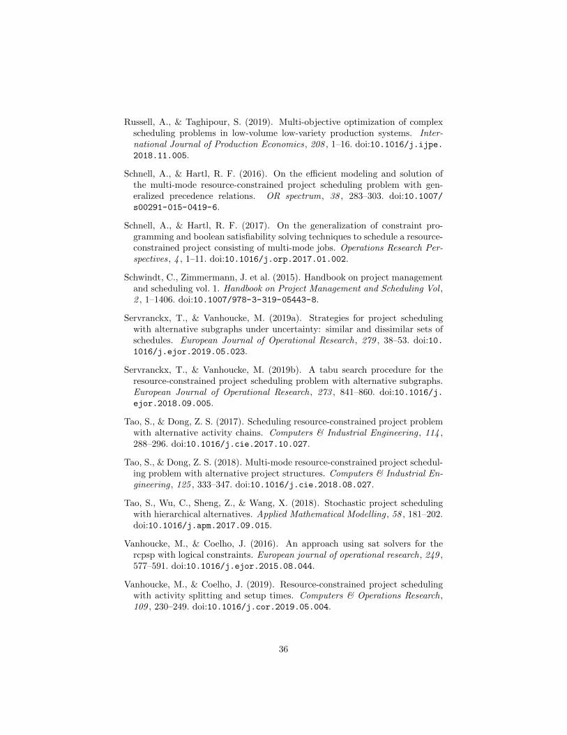
Russell, A., & Taghipour, S. (2019). Multi-objective optimization of complexscheduling problems in low-volume low-variety production systems. Inter-national Journal of Production Economics, 208 , 1–16. doi:10.1016/j.ijpe.2018.11.005.
Schnell, A., & Hartl, R. F. (2016). On the efficient modeling and solution ofthe multi-mode resource-constrained project scheduling problem with gen-eralized precedence relations. OR spectrum, 38 , 283–303. doi:10.1007/s00291-015-0419-6.
Schnell, A., & Hartl, R. F. (2017). On the generalization of constraint pro-gramming and boolean satisfiability solving techniques to schedule a resource-constrained project consisting of multi-mode jobs. Operations Research Per-spectives, 4 , 1–11. doi:10.1016/j.orp.2017.01.002.
Schwindt, C., Zimmermann, J. et al. (2015). Handbook on project managementand scheduling vol. 1. Handbook on Project Management and Scheduling Vol ,2 , 1–1406. doi:10.1007/978-3-319-05443-8.
Servranckx, T., & Vanhoucke, M. (2019a). Strategies for project schedulingwith alternative subgraphs under uncertainty: similar and dissimilar sets ofschedules. European Journal of Operational Research, 279 , 38–53. doi:10.1016/j.ejor.2019.05.023.
Servranckx, T., & Vanhoucke, M. (2019b). A tabu search procedure for theresource-constrained project scheduling problem with alternative subgraphs.European Journal of Operational Research, 273 , 841–860. doi:10.1016/j.ejor.2018.09.005.
Tao, S., & Dong, Z. S. (2017). Scheduling resource-constrained project problemwith alternative activity chains. Computers & Industrial Engineering , 114 ,288–296. doi:10.1016/j.cie.2017.10.027.
Tao, S., & Dong, Z. S. (2018). Multi-mode resource-constrained project schedul-ing problem with alternative project structures. Computers & Industrial En-gineering , 125 , 333–347. doi:10.1016/j.cie.2018.08.027.
Tao, S., Wu, C., Sheng, Z., & Wang, X. (2018). Stochastic project schedulingwith hierarchical alternatives. Applied Mathematical Modelling , 58 , 181–202.doi:10.1016/j.apm.2017.09.015.
Vanhoucke, M., & Coelho, J. (2016). An approach using sat solvers for thercpsp with logical constraints. European journal of operational research, 249 ,577–591. doi:10.1016/j.ejor.2015.08.044.
Vanhoucke, M., & Coelho, J. (2019). Resource-constrained project schedulingwith activity splitting and setup times. Computers & Operations Research,109 , 230–249. doi:10.1016/j.cor.2019.05.004.
36
Vilım, P., Laborie, P., & Shaw, P. (2015). Failure-directed search for constraint-based scheduling. In International Conference on AI and OR Techniques inConstriant Programming for Combinatorial Optimization Problems (pp. 437–453). Springer.
Voß, S., & Witt, A. (2007). Hybrid flow shop scheduling as a multi-modemulti-project scheduling problem with batching requirements: A real-worldapplication. International journal of production economics, 105 , 445–458.doi:10.1016/j.ijpe.2004.05.029.
Wang, T., Meskens, N., & Duvivier, D. (2015). Scheduling operating theatres:Mixed integer programming vs. constraint programming. European Journalof Operational Research, 247 , 401–413. doi:10.1016/j.ejor.2015.06.008.
Weglarz, J. (2012). Project scheduling: recent models, algorithms and ap-plications volume 14. Springer Science & Business Media. doi:10.1007/978-1-4615-5533-9.
37
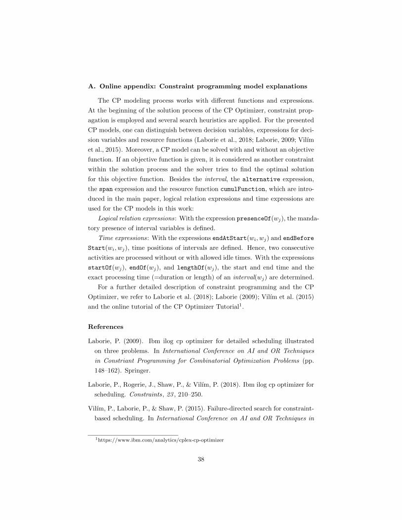
A. Online appendix: Constraint programming model explanations
The CP modeling process works with different functions and expressions.
At the beginning of the solution process of the CP Optimizer, constraint prop-
agation is employed and several search heuristics are applied. For the presented
CP models, one can distinguish between decision variables, expressions for deci-
sion variables and resource functions (Laborie et al., 2018; Laborie, 2009; Vilım
et al., 2015). Moreover, a CP model can be solved with and without an objective
function. If an objective function is given, it is considered as another constraint
within the solution process and the solver tries to find the optimal solution
for this objective function. Besides the interval, the alternative expression,
the span expression and the resource function cumulFunction, which are intro-
duced in the main paper, logical relation expressions and time expressions are
used for the CP models in this work:
Logical relation expressions: With the expression presenceOf(wj), the manda-
tory presence of interval variables is defined.
Time expressions: With the expressions endAtStart(wi, wj) and endBefore
Start(wi, wj), time positions of intervals are defined. Hence, two consecutive
activities are processed without or with allowed idle times. With the expressions
startOf(wj), endOf(wj), and lengthOf(wj), the start and end time and the
exact processing time (=duration or length) of an interval(wj) are determined.
For a further detailed description of constraint programming and the CP
Optimizer, we refer to Laborie et al. (2018); Laborie (2009); Vilım et al. (2015)
and the online tutorial of the CP Optimizer Tutorial1.
References
Laborie, P. (2009). Ibm ilog cp optimizer for detailed scheduling illustrated
on three problems. In International Conference on AI and OR Techniques
in Constriant Programming for Combinatorial Optimization Problems (pp.
148–162). Springer.
Laborie, P., Rogerie, J., Shaw, P., & Vilım, P. (2018). Ibm ilog cp optimizer for
scheduling. Constraints, 23 , 210–250.
Vilım, P., Laborie, P., & Shaw, P. (2015). Failure-directed search for constraint-
based scheduling. In International Conference on AI and OR Techniques in
1https://www.ibm.com/analytics/cplex-cp-optimizer
38

Constriant Programming for Combinatorial Optimization Problems (pp. 437–
453). Springer.
39
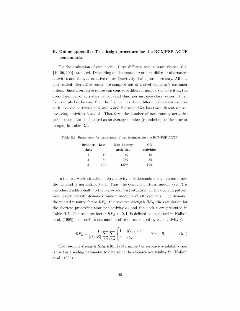
B. Online appendix: Test design procedure for the RCMPSP-ACTF
benchmarks
For the evaluation of our models, three different test instance classes |L ∈{10, 50, 100}| are used. Depending on the customer orders, different alternative
activities and thus, alternative routes (=activity chains) are necessary. All lots
and related alternative routes are sampled out of a steel company’s customer
orders. Since alternative routes can consist of different numbers of activities, the
overall number of activities per lot (and thus, per instance class) varies. It can
for example be the case that the first lot has three different alternative routes
with involved activities 3, 4, and 5 and the second lot has two different routes,
involving activities 3 and 5. Therefore, the number of non-dummy activities
per instance class is depicted as an average number (rounded up to the nearest
integer) in Table B.1.
Table B.1: Parameters for test classes of test instances for the RCMPSP-ACTF.
Instance
class
Lots Non-dummy
activities
OR
activities
1 10 162 10
2 50 797 50
3 100 1,593 100
In the real-world situation, every activity only demands a single resource and
the demand is normalized to 1. Thus, the demand pattern random (rand) is
introduced additionally to the real-world (rw) situation. In the demand pattern
rand, every activity demands random amounts of all resources. The demand,
the related resource factor RFR, the resource strength RSR, the calculation for
the shortest processing time per activity aj and the slack s are presented in
Table B.2. The resource factor RFR ∈ [0, 1] is defined as explained in Kolisch
et al. (1995). It describes the number of resources r used by each activity j:
RFR =1
|J |1
|R|∑j∈J
∑r∈R
1, if cjr > 0
0, else∀ r ∈ R (b.1)
The resource strength RSR ∈ [0, 1] determines the resource availability and
is used as a scaling parameter to determine the resource availability Cr (Kolisch
et al., 1995).
40
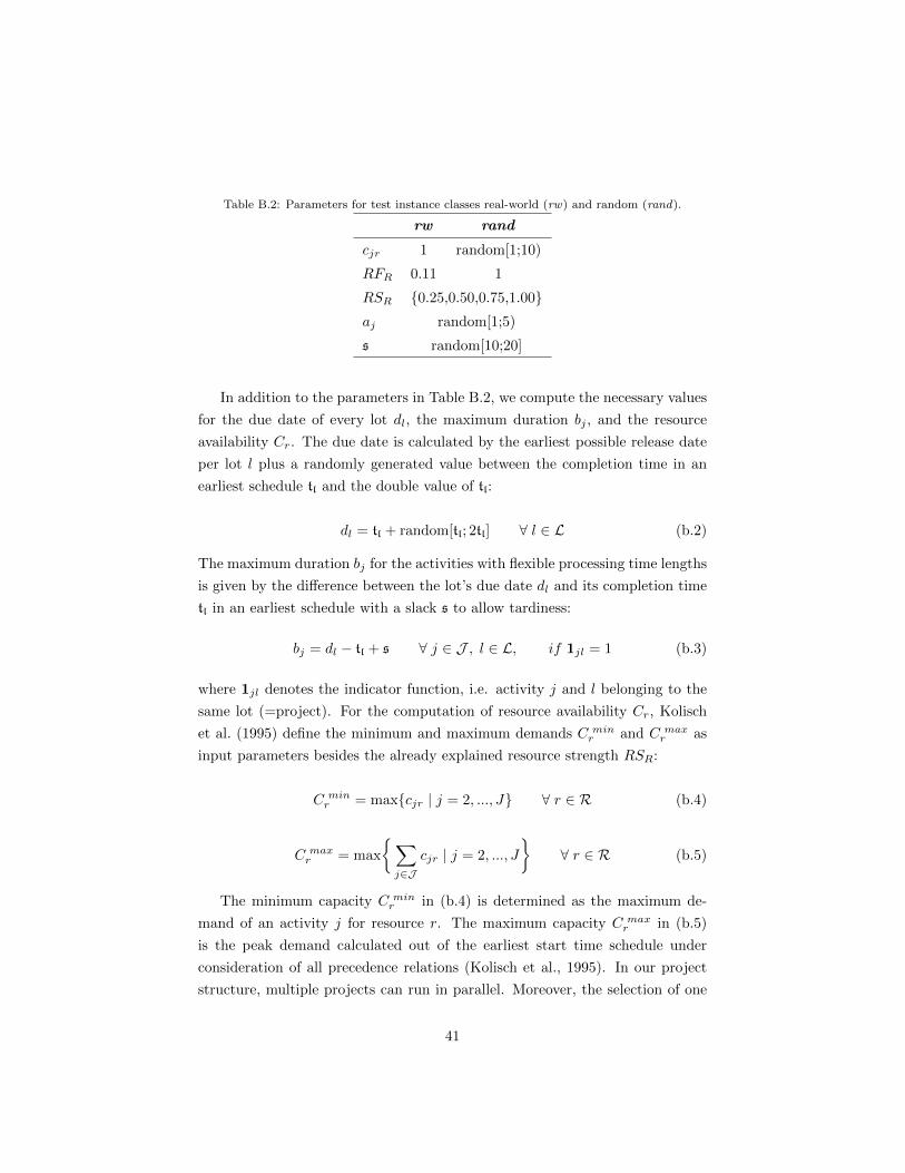
Table B.2: Parameters for test instance classes real-world (rw) and random (rand).
rw rand
cjr 1 random[1;10)
RFR 0.11 1
RSR {0.25,0.50,0.75,1.00}aj random[1;5)
s random[10;20]
In addition to the parameters in Table B.2, we compute the necessary values
for the due date of every lot dl, the maximum duration bj , and the resource
availability Cr. The due date is calculated by the earliest possible release date
per lot l plus a randomly generated value between the completion time in an
earliest schedule tl and the double value of tl:
dl = tl + random[tl; 2tl] ∀ l ∈ L (b.2)
The maximum duration bj for the activities with flexible processing time lengths
is given by the difference between the lot’s due date dl and its completion time
tl in an earliest schedule with a slack s to allow tardiness:
bj = dl − tl + s ∀ j ∈ J , l ∈ L, if 1jl = 1 (b.3)
where 1jl denotes the indicator function, i.e. activity j and l belonging to the
same lot (=project). For the computation of resource availability Cr, Kolisch
et al. (1995) define the minimum and maximum demands C minr and C max
r as
input parameters besides the already explained resource strength RSR:
C minr = max{cjr | j = 2, ..., J} ∀ r ∈ R (b.4)
C maxr = max
{∑j∈J
cjr | j = 2, ..., J
}∀ r ∈ R (b.5)
The minimum capacity C minr in (b.4) is determined as the maximum de-
mand of an activity j for resource r. The maximum capacity C maxr in (b.5)
is the peak demand calculated out of the earliest start time schedule under
consideration of all precedence relations (Kolisch et al., 1995). In our project
structure, multiple projects can run in parallel. Moreover, the selection of one
41
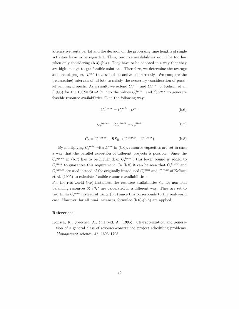
alternative route per lot and the decision on the processing time lengths of single
activities have to be regarded. Thus, resource availabilities would be too low
when only considering (b.3)-(b.4). They have to be adapted in a way that they
are high enough to get feasible solutions. Therefore, we determine the average
amount of projects Lpar that would be active concurrently. We compare the
[release;due) intervals of all lots to satisfy the necessary consideration of paral-
lel running projects. As a result, we extend C minr and C max
r of Kolisch et al.
(1995) for the RCMPSP-ACTF to the values C lowerr and C upper
r to generate
feasible resource availabilities Cr in the following way:
C lowerr = C min
r · Lpar (b.6)
C upperr = C lower
r + C maxr (b.7)
Cr = C lowerr +RSR · (C upper
r − C lowerr ) (b.8)
By multiplying C minr with Lpar in (b.6), resource capacities are set in such
a way that the parallel execution of different projects is possible. Since the
C upperr in (b.7) has to be higher than C lower
r , this lower bound is added to
C maxr to guarantee this requirement. In (b.8) it can be seen that C lower
r and
C upperr are used instead of the originally introduced C min
r and C maxr of Kolisch
et al. (1995) to calculate feasible resource availabilities.
For the real-world (rw) instances, the resource availabilities Cr for non-load
balancing resources R \ R∗ are calculated in a different way. They are set to
two times C minr instead of using (b.8) since this corresponds to the real-world
case. However, for all rand instances, formulae (b.6)-(b.8) are applied.
References
Kolisch, R., Sprecher, A., & Drexl, A. (1995). Characterization and genera-
tion of a general class of resource-constrained project scheduling problems.
Management science, 41 , 1693–1703.
42
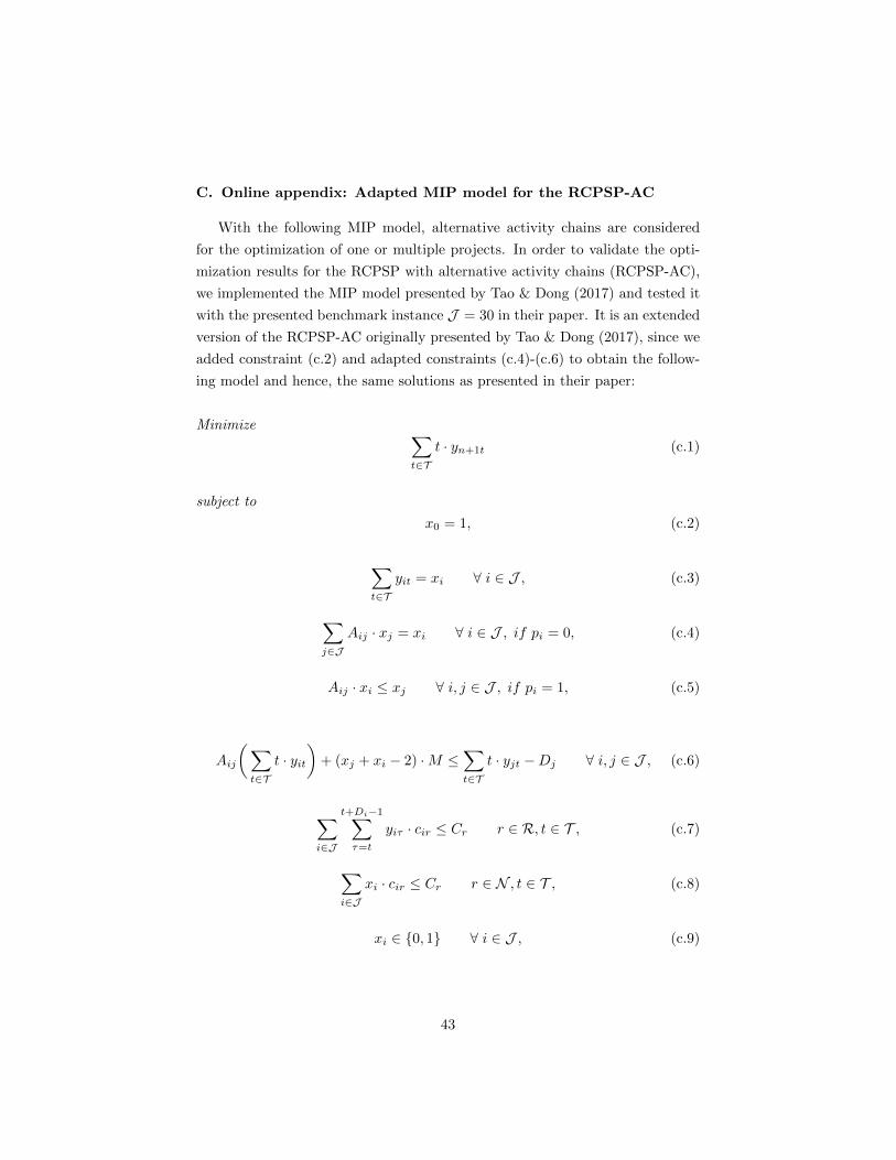
C. Online appendix: Adapted MIP model for the RCPSP-AC
With the following MIP model, alternative activity chains are considered
for the optimization of one or multiple projects. In order to validate the opti-
mization results for the RCPSP with alternative activity chains (RCPSP-AC),
we implemented the MIP model presented by Tao & Dong (2017) and tested it
with the presented benchmark instance J = 30 in their paper. It is an extended
version of the RCPSP-AC originally presented by Tao & Dong (2017), since we
added constraint (c.2) and adapted constraints (c.4)-(c.6) to obtain the follow-
ing model and hence, the same solutions as presented in their paper:
Minimize ∑t∈T
t · yn+1t (c.1)
subject to
x0 = 1, (c.2)
∑t∈T
yit = xi ∀ i ∈ J , (c.3)
∑j∈J
Aij · xj = xi ∀ i ∈ J , if pi = 0, (c.4)
Aij · xi ≤ xj ∀ i, j ∈ J , if pi = 1, (c.5)
Aij
(∑t∈T
t · yit)
+ (xj + xi − 2) ·M ≤∑t∈T
t · yjt −Dj ∀ i, j ∈ J , (c.6)
∑i∈J
t+Di−1∑τ=t
yiτ · cir ≤ Cr r ∈ R, t ∈ T , (c.7)
∑i∈J
xi · cir ≤ Cr r ∈ N , t ∈ T , (c.8)
xi ∈ {0, 1} ∀ i ∈ J , (c.9)
43
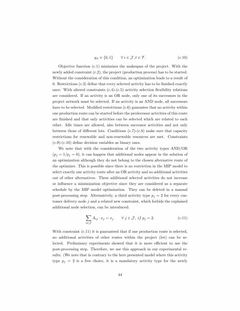
yit ∈ {0, 1} ∀ i ∈ J , t ∈ T . (c.10)
Objective function (c.1) minimizes the makespan of the project. With the
newly added constraint (c.2), the project (production process) has to be started.
Without the consideration of this condition, an optimization leads to a result of
0. Restrictions (c.3) define that every selected activity has to be finished exactly
once. With altered constraints (c.4)-(c.5) activity selection flexibility relations
are considered. If an activity is an OR node, only one of its successors in the
project network must be selected. If an activity is an AND node, all successors
have to be selected. Modified restrictions (c.6) guarantee that no activity within
one production route can be started before the predecessor activities of this route
are finished and that only activities can be selected which are related to each
other. Idle times are allowed, also between successor activities and not only
between those of different lots. Conditions (c.7)-(c.8) make sure that capacity
restrictions for renewable and non-renewable resources are met. Constraints
(c.9)-(c.10) define decision variables as binary ones.
We note that with the consideration of the two activity types AND/OR
(pj = 1/pj = 0), it can happen that additional nodes appear in the solution of
an optimization although they do not belong to the chosen alternative route of
the optimizer. This is possible since there is no restriction in the MIP model to
select exactly one activity route after an OR activity and no additional activities
out of other alternatives. These additional selected activities do not increase
or influence a minimization objective since they are considered as a separate
schedule by the MIP model optimization. They can be deleted in a manual
post-processing step. Alternatively, a third activity type pj = 2 for every cus-
tomer delivery node j and a related new constraint, which forbids the explained
additional node selection, can be introduced:∑i∈J
Aij · xj = xj ∀ j ∈ J , if pj = 2. (c.11)
With constraint (c.11) it is guaranteed that if one production route is selected,
no additional activities of other routes within the project (lot) can be se-
lected. Preliminary experiments showed that it is more efficient to use the
post-processing step. Therefore, we use this approach in our experimental re-
sults. (We note that in contrary to the here presented model where this activity
type pj = 2 is a free choice, it is a mandatory activity type for the newly
44
presented RCMPSP-ACTF in this work as explained in Section 3.1.)
References
Tao, S., & Dong, Z. S. (2017). Scheduling resource-constrained project problem
with alternative activity chains. Computers & Industrial Engineering , 114 ,
288–296. doi:10.1016/j.cie.2017.10.027.
45
D. Online appendix: Optimization results for the RCPSP-AC and
the RCMPSP-AC
On the following pages, we present the detailed examination of all designed
benchmark instances for the resource-constrained project scheduling problem
with alternative activity chains (RCPSP-AC) and its multi-project version, the
RCMPSP-AC. The columns in Table D.1 give (1) the name of every instance, (2)
the solver (MIP or CP) which has been applied, (3) the project-scheduling type,
i.e. if it is a single- (RCPSP-AC) or a multi-project(RCMPSP-AC) instance,
(4) the considered amount of nodes, (5) an identification number from 1-10
per project and node case, (6) the best objective value found, (7) the best
bound found, and (8) the runtime in seconds. Bold letters represent the optimal
solution.
46
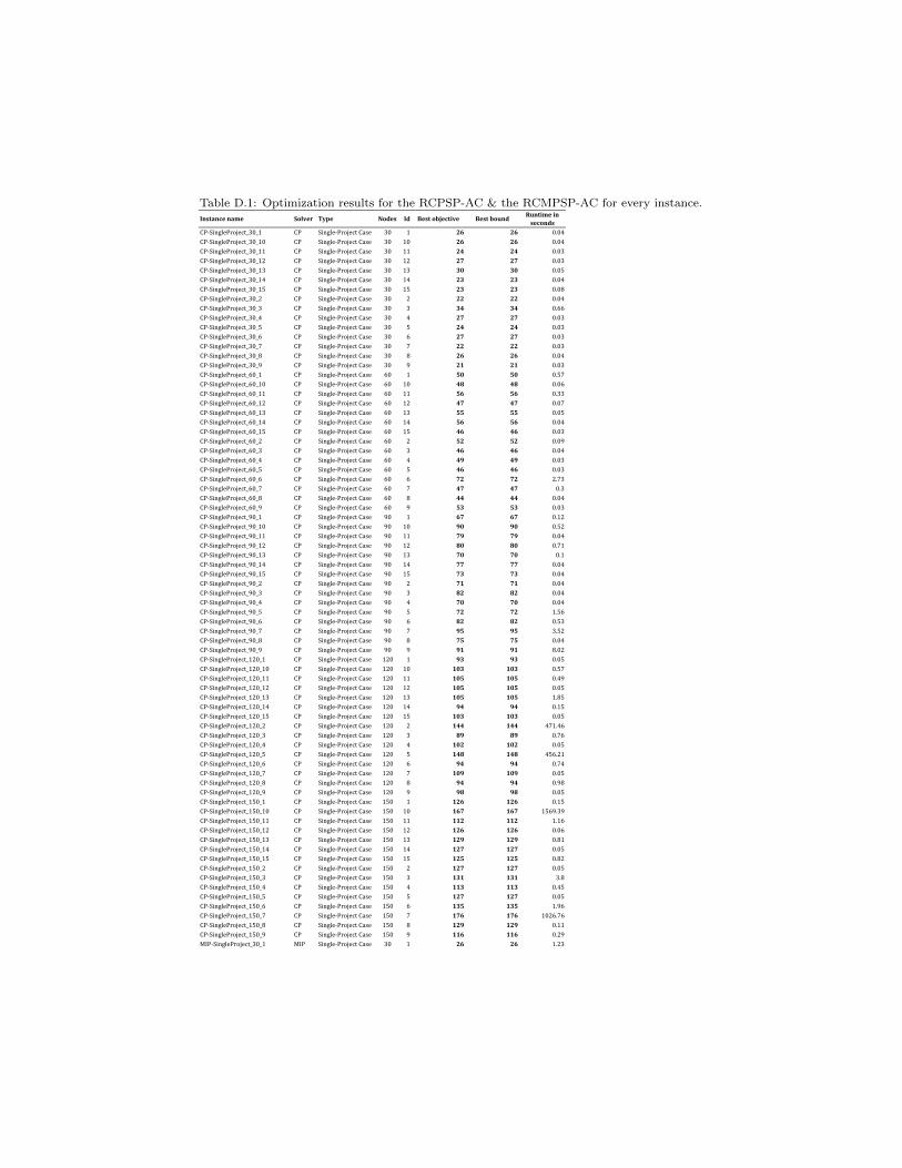
Instance name Solver Type Nodes Id Best objective Best boundRuntime in
seconds
CP-SingleProject_30_1 CP Single-Project Case 30 1 26 26 0.04
CP-SingleProject_30_10 CP Single-Project Case 30 10 26 26 0.04
CP-SingleProject_30_11 CP Single-Project Case 30 11 24 24 0.03
CP-SingleProject_30_12 CP Single-Project Case 30 12 27 27 0.03
CP-SingleProject_30_13 CP Single-Project Case 30 13 30 30 0.05
CP-SingleProject_30_14 CP Single-Project Case 30 14 23 23 0.04
CP-SingleProject_30_15 CP Single-Project Case 30 15 23 23 0.08
CP-SingleProject_30_2 CP Single-Project Case 30 2 22 22 0.04
CP-SingleProject_30_3 CP Single-Project Case 30 3 34 34 0.66
CP-SingleProject_30_4 CP Single-Project Case 30 4 27 27 0.03
CP-SingleProject_30_5 CP Single-Project Case 30 5 24 24 0.03
CP-SingleProject_30_6 CP Single-Project Case 30 6 27 27 0.03
CP-SingleProject_30_7 CP Single-Project Case 30 7 22 22 0.03
CP-SingleProject_30_8 CP Single-Project Case 30 8 26 26 0.04
CP-SingleProject_30_9 CP Single-Project Case 30 9 21 21 0.03
CP-SingleProject_60_1 CP Single-Project Case 60 1 50 50 0.57
CP-SingleProject_60_10 CP Single-Project Case 60 10 48 48 0.06
CP-SingleProject_60_11 CP Single-Project Case 60 11 56 56 0.33
CP-SingleProject_60_12 CP Single-Project Case 60 12 47 47 0.07
CP-SingleProject_60_13 CP Single-Project Case 60 13 55 55 0.05
CP-SingleProject_60_14 CP Single-Project Case 60 14 56 56 0.04
CP-SingleProject_60_15 CP Single-Project Case 60 15 46 46 0.03
CP-SingleProject_60_2 CP Single-Project Case 60 2 52 52 0.09
CP-SingleProject_60_3 CP Single-Project Case 60 3 46 46 0.04
CP-SingleProject_60_4 CP Single-Project Case 60 4 49 49 0.03
CP-SingleProject_60_5 CP Single-Project Case 60 5 46 46 0.03
CP-SingleProject_60_6 CP Single-Project Case 60 6 72 72 2.73
CP-SingleProject_60_7 CP Single-Project Case 60 7 47 47 0.3
CP-SingleProject_60_8 CP Single-Project Case 60 8 44 44 0.04
CP-SingleProject_60_9 CP Single-Project Case 60 9 53 53 0.03
CP-SingleProject_90_1 CP Single-Project Case 90 1 67 67 0.12
CP-SingleProject_90_10 CP Single-Project Case 90 10 90 90 0.52
CP-SingleProject_90_11 CP Single-Project Case 90 11 79 79 0.04
CP-SingleProject_90_12 CP Single-Project Case 90 12 80 80 0.71
CP-SingleProject_90_13 CP Single-Project Case 90 13 70 70 0.1
CP-SingleProject_90_14 CP Single-Project Case 90 14 77 77 0.04
CP-SingleProject_90_15 CP Single-Project Case 90 15 73 73 0.04
CP-SingleProject_90_2 CP Single-Project Case 90 2 71 71 0.04
CP-SingleProject_90_3 CP Single-Project Case 90 3 82 82 0.04
CP-SingleProject_90_4 CP Single-Project Case 90 4 70 70 0.04
CP-SingleProject_90_5 CP Single-Project Case 90 5 72 72 1.56
CP-SingleProject_90_6 CP Single-Project Case 90 6 82 82 0.53
CP-SingleProject_90_7 CP Single-Project Case 90 7 95 95 3.52
CP-SingleProject_90_8 CP Single-Project Case 90 8 75 75 0.04
CP-SingleProject_90_9 CP Single-Project Case 90 9 91 91 8.02
CP-SingleProject_120_1 CP Single-Project Case 120 1 93 93 0.05
CP-SingleProject_120_10 CP Single-Project Case 120 10 103 103 0.57
CP-SingleProject_120_11 CP Single-Project Case 120 11 105 105 0.49
CP-SingleProject_120_12 CP Single-Project Case 120 12 105 105 0.05
CP-SingleProject_120_13 CP Single-Project Case 120 13 105 105 1.85
CP-SingleProject_120_14 CP Single-Project Case 120 14 94 94 0.15
CP-SingleProject_120_15 CP Single-Project Case 120 15 103 103 0.05
CP-SingleProject_120_2 CP Single-Project Case 120 2 144 144 471.46
CP-SingleProject_120_3 CP Single-Project Case 120 3 89 89 0.76
CP-SingleProject_120_4 CP Single-Project Case 120 4 102 102 0.05
CP-SingleProject_120_5 CP Single-Project Case 120 5 148 148 456.21
CP-SingleProject_120_6 CP Single-Project Case 120 6 94 94 0.74
CP-SingleProject_120_7 CP Single-Project Case 120 7 109 109 0.05
CP-SingleProject_120_8 CP Single-Project Case 120 8 94 94 0.98
CP-SingleProject_120_9 CP Single-Project Case 120 9 98 98 0.05
CP-SingleProject_150_1 CP Single-Project Case 150 1 126 126 0.15
CP-SingleProject_150_10 CP Single-Project Case 150 10 167 167 1569.39
CP-SingleProject_150_11 CP Single-Project Case 150 11 112 112 1.16
CP-SingleProject_150_12 CP Single-Project Case 150 12 126 126 0.06
CP-SingleProject_150_13 CP Single-Project Case 150 13 129 129 0.81
CP-SingleProject_150_14 CP Single-Project Case 150 14 127 127 0.05
CP-SingleProject_150_15 CP Single-Project Case 150 15 125 125 0.82
CP-SingleProject_150_2 CP Single-Project Case 150 2 127 127 0.05
CP-SingleProject_150_3 CP Single-Project Case 150 3 131 131 3.8
CP-SingleProject_150_4 CP Single-Project Case 150 4 113 113 0.45
CP-SingleProject_150_5 CP Single-Project Case 150 5 127 127 0.05
CP-SingleProject_150_6 CP Single-Project Case 150 6 135 135 1.96
CP-SingleProject_150_7 CP Single-Project Case 150 7 176 176 1026.76
CP-SingleProject_150_8 CP Single-Project Case 150 8 129 129 0.11
CP-SingleProject_150_9 CP Single-Project Case 150 9 116 116 0.29
MIP-SingleProject_30_1 MIP Single-Project Case 30 1 26 26 1.23
Table D.1: Optimization results for the RCPSP-AC & the RCMPSP-AC for every instance.
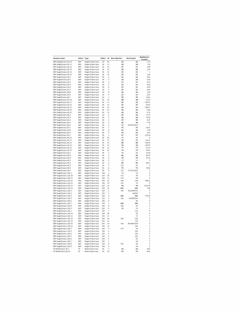
Instance name Solver Type Nodes Id Best objective Best boundRuntime in
seconds
MIP-SingleProject_30_10 MIP Single-Project Case 30 10 26 26 1.74
MIP-SingleProject_30_11 MIP Single-Project Case 30 11 24 24 0.5
MIP-SingleProject_30_12 MIP Single-Project Case 30 12 27 27 1.08
MIP-SingleProject_30_13 MIP Single-Project Case 30 13 30 30 1.92
MIP-SingleProject_30_14 MIP Single-Project Case 30 14 23 23 1
MIP-SingleProject_30_15 MIP Single-Project Case 30 15 23 23 1.66
MIP-SingleProject_30_2 MIP Single-Project Case 30 2 22 22 0.61
MIP-SingleProject_30_3 MIP Single-Project Case 30 3 34 34 4.78
MIP-SingleProject_30_4 MIP Single-Project Case 30 4 27 27 0.41
MIP-SingleProject_30_5 MIP Single-Project Case 30 5 24 24 0.63
MIP-SingleProject_30_6 MIP Single-Project Case 30 6 27 27 0.78
MIP-SingleProject_30_7 MIP Single-Project Case 30 7 22 22 0.69
MIP-SingleProject_30_8 MIP Single-Project Case 30 8 26 26 1.39
MIP-SingleProject_30_9 MIP Single-Project Case 30 9 21 21 0.55
MIP-SingleProject_60_1 MIP Single-Project Case 60 1 50 50 14.01
MIP-SingleProject_60_10 MIP Single-Project Case 60 10 48 48 13.16
MIP-SingleProject_60_11 MIP Single-Project Case 60 11 56 56 339.67
MIP-SingleProject_60_12 MIP Single-Project Case 60 12 47 47 40.47
MIP-SingleProject_60_13 MIP Single-Project Case 60 13 55 55 364.67
MIP-SingleProject_60_14 MIP Single-Project Case 60 14 56 56 9.66
MIP-SingleProject_60_15 MIP Single-Project Case 60 15 46 46 6.72
MIP-SingleProject_60_2 MIP Single-Project Case 60 2 52 52 11.77
MIP-SingleProject_60_3 MIP Single-Project Case 60 3 46 46 11.09
MIP-SingleProject_60_4 MIP Single-Project Case 60 4 49 49 6.47
MIP-SingleProject_60_5 MIP Single-Project Case 60 5 46 46 5.78
MIP-SingleProject_60_6 MIP Single-Project Case 60 6 80 65.09730234 T
MIP-SingleProject_60_7 MIP Single-Project Case 60 7 47 47 33.41
MIP-SingleProject_60_8 MIP Single-Project Case 60 8 44 44 7.36
MIP-SingleProject_60_9 MIP Single-Project Case 60 9 53 53 14.2
MIP-SingleProject_90_1 MIP Single-Project Case 90 1 67 67 213.34
MIP-SingleProject_90_10 MIP Single-Project Case 90 10 99 83 T
MIP-SingleProject_90_11 MIP Single-Project Case 90 11 79 79 64.75
MIP-SingleProject_90_12 MIP Single-Project Case 90 12 80 80 160.44
MIP-SingleProject_90_13 MIP Single-Project Case 90 13 70 70 159.97
MIP-SingleProject_90_14 MIP Single-Project Case 90 14 77 77 41.19
MIP-SingleProject_90_15 MIP Single-Project Case 90 15 73 73 39.75
MIP-SingleProject_90_2 MIP Single-Project Case 90 2 71 71 31.98
MIP-SingleProject_90_3 MIP Single-Project Case 90 3 82 82 49.47
MIP-SingleProject_90_4 MIP Single-Project Case 90 4 70 70 76.72
MIP-SingleProject_90_5 MIP Single-Project Case 90 5 73 72 T
MIP-SingleProject_90_6 MIP Single-Project Case 90 6 82 82 381.5
MIP-SingleProject_90_7 MIP Single-Project Case 90 7 114 81 T
MIP-SingleProject_90_8 MIP Single-Project Case 90 8 75 75 73.81
MIP-SingleProject_90_9 MIP Single-Project Case 90 9 122 73.13231487 T
MIP-SingleProject_120_1 MIP Single-Project Case 120 1 93 92 T
MIP-SingleProject_120_10 MIP Single-Project Case 120 10 112 99 T
MIP-SingleProject_120_11 MIP Single-Project Case 120 11 113 90 T
MIP-SingleProject_120_12 MIP Single-Project Case 120 12 106 104 3601.2
MIP-SingleProject_120_13 MIP Single-Project Case 120 13 131 75 T
MIP-SingleProject_120_14 MIP Single-Project Case 120 14 94 94 1123.39
MIP-SingleProject_120_15 MIP Single-Project Case 120 15 103 103 768
MIP-SingleProject_120_2 MIP Single-Project Case 120 2 156 56.22509767 T
MIP-SingleProject_120_3 MIP Single-Project Case 120 3 86.002 T
MIP-SingleProject_120_4 MIP Single-Project Case 120 4 102 102 772.05
MIP-SingleProject_120_5 MIP Single-Project Case 120 5 183 69.3007463 T
MIP-SingleProject_120_6 MIP Single-Project Case 120 6 82 T
MIP-SingleProject_120_7 MIP Single-Project Case 120 7 109 109 T
MIP-SingleProject_120_8 MIP Single-Project Case 120 8 106 87 T
MIP-SingleProject_120_9 MIP Single-Project Case 120 9 98 97 T
MIP-SingleProject_150_1 MIP Single-Project Case 150 1 126 T
MIP-SingleProject_150_10 MIP Single-Project Case 150 10 50 T
MIP-SingleProject_150_11 MIP Single-Project Case 150 11 74 T
MIP-SingleProject_150_12 MIP Single-Project Case 150 12 326 104 T
MIP-SingleProject_150_13 MIP Single-Project Case 150 13 120 T
MIP-SingleProject_150_14 MIP Single-Project Case 150 14 130 86.38461539 T
MIP-SingleProject_150_15 MIP Single-Project Case 150 15 104 T
MIP-SingleProject_150_2 MIP Single-Project Case 150 2 214 94 T
MIP-SingleProject_150_3 MIP Single-Project Case 150 3 102 T
MIP-SingleProject_150_4 MIP Single-Project Case 150 4 104 T
MIP-SingleProject_150_5 MIP Single-Project Case 150 5 102 T
MIP-SingleProject_150_6 MIP Single-Project Case 150 6 82 T
MIP-SingleProject_150_7 MIP Single-Project Case 150 7 44 T
MIP-SingleProject_150_8 MIP Single-Project Case 150 8 355 89 T
MIP-SingleProject_150_9 MIP Single-Project Case 150 9 90 T
CP-MultiProject_30_1 CP Multi-Project Case 30 1 26 26 0.03
CP-MultiProject_30_10 CP Multi-Project Case 30 10 23 23 0.03
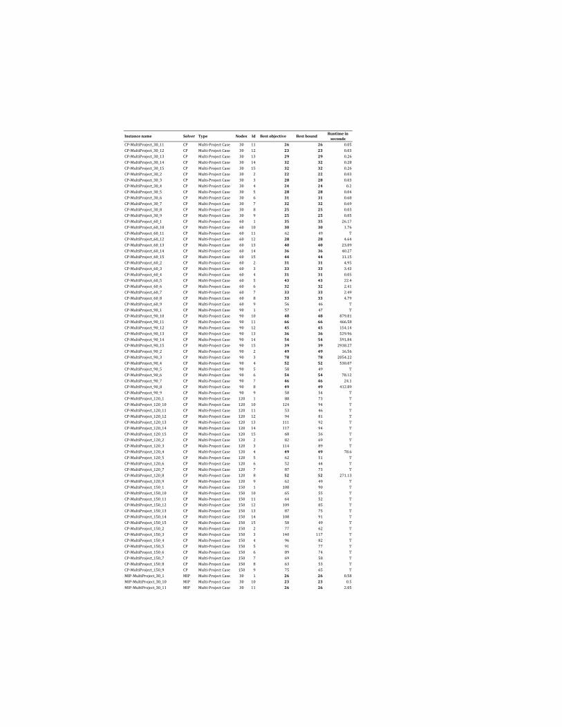
Instance name Solver Type Nodes Id Best objective Best boundRuntime in
seconds
CP-MultiProject_30_11 CP Multi-Project Case 30 11 26 26 0.05
CP-MultiProject_30_12 CP Multi-Project Case 30 12 23 23 0.03
CP-MultiProject_30_13 CP Multi-Project Case 30 13 29 29 0.26
CP-MultiProject_30_14 CP Multi-Project Case 30 14 32 32 0.28
CP-MultiProject_30_15 CP Multi-Project Case 30 15 32 32 0.26
CP-MultiProject_30_2 CP Multi-Project Case 30 2 22 22 0.03
CP-MultiProject_30_3 CP Multi-Project Case 30 3 28 28 0.03
CP-MultiProject_30_4 CP Multi-Project Case 30 4 24 24 0.2
CP-MultiProject_30_5 CP Multi-Project Case 30 5 28 28 0.04
CP-MultiProject_30_6 CP Multi-Project Case 30 6 31 31 0.68
CP-MultiProject_30_7 CP Multi-Project Case 30 7 32 32 0.69
CP-MultiProject_30_8 CP Multi-Project Case 30 8 25 25 0.03
CP-MultiProject_30_9 CP Multi-Project Case 30 9 25 25 0.05
CP-MultiProject_60_1 CP Multi-Project Case 60 1 35 35 26.17
CP-MultiProject_60_10 CP Multi-Project Case 60 10 30 30 1.76
CP-MultiProject_60_11 CP Multi-Project Case 60 11 62 49 T
CP-MultiProject_60_12 CP Multi-Project Case 60 12 28 28 4.64
CP-MultiProject_60_13 CP Multi-Project Case 60 13 40 40 23.09
CP-MultiProject_60_14 CP Multi-Project Case 60 14 36 36 40.27
CP-MultiProject_60_15 CP Multi-Project Case 60 15 44 44 11.15
CP-MultiProject_60_2 CP Multi-Project Case 60 2 31 31 4.95
CP-MultiProject_60_3 CP Multi-Project Case 60 3 33 33 3.43
CP-MultiProject_60_4 CP Multi-Project Case 60 4 31 31 0.05
CP-MultiProject_60_5 CP Multi-Project Case 60 5 43 43 22.4
CP-MultiProject_60_6 CP Multi-Project Case 60 6 32 32 2.41
CP-MultiProject_60_7 CP Multi-Project Case 60 7 33 33 2.49
CP-MultiProject_60_8 CP Multi-Project Case 60 8 33 33 4.79
CP-MultiProject_60_9 CP Multi-Project Case 60 9 56 46 T
CP-MultiProject_90_1 CP Multi-Project Case 90 1 57 47 T
CP-MultiProject_90_10 CP Multi-Project Case 90 10 48 48 879.81
CP-MultiProject_90_11 CP Multi-Project Case 90 11 66 66 466.58
CP-MultiProject_90_12 CP Multi-Project Case 90 12 45 45 154.14
CP-MultiProject_90_13 CP Multi-Project Case 90 13 36 36 529.96
CP-MultiProject_90_14 CP Multi-Project Case 90 14 54 54 591.84
CP-MultiProject_90_15 CP Multi-Project Case 90 15 39 39 2938.27
CP-MultiProject_90_2 CP Multi-Project Case 90 2 49 49 16.56
CP-MultiProject_90_3 CP Multi-Project Case 90 3 78 78 2054.22
CP-MultiProject_90_4 CP Multi-Project Case 90 4 52 52 530.07
CP-MultiProject_90_5 CP Multi-Project Case 90 5 58 49 T
CP-MultiProject_90_6 CP Multi-Project Case 90 6 54 54 78.12
CP-MultiProject_90_7 CP Multi-Project Case 90 7 46 46 24.1
CP-MultiProject_90_8 CP Multi-Project Case 90 8 49 49 412.89
CP-MultiProject_90_9 CP Multi-Project Case 90 9 58 54 T
CP-MultiProject_120_1 CP Multi-Project Case 120 1 88 73 T
CP-MultiProject_120_10 CP Multi-Project Case 120 10 124 94 T
CP-MultiProject_120_11 CP Multi-Project Case 120 11 53 46 T
CP-MultiProject_120_12 CP Multi-Project Case 120 12 94 81 T
CP-MultiProject_120_13 CP Multi-Project Case 120 13 111 92 T
CP-MultiProject_120_14 CP Multi-Project Case 120 14 117 94 T
CP-MultiProject_120_15 CP Multi-Project Case 120 15 68 56 T
CP-MultiProject_120_2 CP Multi-Project Case 120 2 82 69 T
CP-MultiProject_120_3 CP Multi-Project Case 120 3 114 89 T
CP-MultiProject_120_4 CP Multi-Project Case 120 4 49 49 78.6
CP-MultiProject_120_5 CP Multi-Project Case 120 5 62 51 T
CP-MultiProject_120_6 CP Multi-Project Case 120 6 52 44 T
CP-MultiProject_120_7 CP Multi-Project Case 120 7 87 73 T
CP-MultiProject_120_8 CP Multi-Project Case 120 8 52 52 271.13
CP-MultiProject_120_9 CP Multi-Project Case 120 9 62 49 T
CP-MultiProject_150_1 CP Multi-Project Case 150 1 108 90 T
CP-MultiProject_150_10 CP Multi-Project Case 150 10 65 55 T
CP-MultiProject_150_11 CP Multi-Project Case 150 11 64 52 T
CP-MultiProject_150_12 CP Multi-Project Case 150 12 109 85 T
CP-MultiProject_150_13 CP Multi-Project Case 150 13 87 75 T
CP-MultiProject_150_14 CP Multi-Project Case 150 14 108 91 T
CP-MultiProject_150_15 CP Multi-Project Case 150 15 58 49 T
CP-MultiProject_150_2 CP Multi-Project Case 150 2 77 62 T
CP-MultiProject_150_3 CP Multi-Project Case 150 3 140 117 T
CP-MultiProject_150_4 CP Multi-Project Case 150 4 96 82 T
CP-MultiProject_150_5 CP Multi-Project Case 150 5 91 77 T
CP-MultiProject_150_6 CP Multi-Project Case 150 6 89 74 T
CP-MultiProject_150_7 CP Multi-Project Case 150 7 69 58 T
CP-MultiProject_150_8 CP Multi-Project Case 150 8 63 53 T
CP-MultiProject_150_9 CP Multi-Project Case 150 9 75 65 T
MIP-MultiProject_30_1 MIP Multi-Project Case 30 1 26 26 0.58
MIP-MultiProject_30_10 MIP Multi-Project Case 30 10 23 23 0.5
MIP-MultiProject_30_11 MIP Multi-Project Case 30 11 26 26 2.05
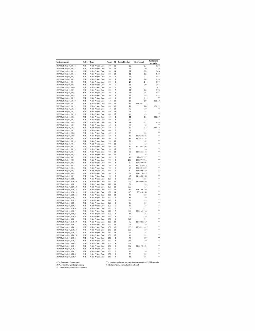
Instance name Solver Type Nodes Id Best objective Best boundRuntime in
seconds
MIP-MultiProject_30_12 MIP Multi-Project Case 30 12 23 23 0.59
MIP-MultiProject_30_13 MIP Multi-Project Case 30 13 29 29 2.19
MIP-MultiProject_30_14 MIP Multi-Project Case 30 14 32 32 9.86
MIP-MultiProject_30_15 MIP Multi-Project Case 30 15 32 32 5.48
MIP-MultiProject_30_2 MIP Multi-Project Case 30 2 22 22 0.61
MIP-MultiProject_30_3 MIP Multi-Project Case 30 3 28 28 1.16
MIP-MultiProject_30_4 MIP Multi-Project Case 30 4 24 24 1.77
MIP-MultiProject_30_5 MIP Multi-Project Case 30 5 28 28 2.03
MIP-MultiProject_30_6 MIP Multi-Project Case 30 6 31 31 1.7
MIP-MultiProject_30_7 MIP Multi-Project Case 30 7 32 32 3.78
MIP-MultiProject_30_8 MIP Multi-Project Case 30 8 25 25 0.83
MIP-MultiProject_30_9 MIP Multi-Project Case 30 9 25 25 1.33
MIP-MultiProject_60_1 MIP Multi-Project Case 60 1 35 34 T
MIP-MultiProject_60_10 MIP Multi-Project Case 60 10 30 30 131.69
MIP-MultiProject_60_11 MIP Multi-Project Case 60 11 68 52.05493117 T
MIP-MultiProject_60_12 MIP Multi-Project Case 60 12 28 28 650.92
MIP-MultiProject_60_13 MIP Multi-Project Case 60 13 43 38 T
MIP-MultiProject_60_14 MIP Multi-Project Case 60 14 36 35 T
MIP-MultiProject_60_15 MIP Multi-Project Case 60 15 46 43 T
MIP-MultiProject_60_2 MIP Multi-Project Case 60 2 31 31 832.27
MIP-MultiProject_60_3 MIP Multi-Project Case 60 3 33 32 T
MIP-MultiProject_60_4 MIP Multi-Project Case 60 4 31 31 6.58
MIP-MultiProject_60_5 MIP Multi-Project Case 60 5 46 42 T
MIP-MultiProject_60_6 MIP Multi-Project Case 60 6 32 32 2484.52
MIP-MultiProject_60_7 MIP Multi-Project Case 60 7 34 33 T
MIP-MultiProject_60_8 MIP Multi-Project Case 60 8 33 32 T
MIP-MultiProject_60_9 MIP Multi-Project Case 60 9 60 45.29245876 T
MIP-MultiProject_90_1 MIP Multi-Project Case 90 1 64 42.28875354 T
MIP-MultiProject_90_10 MIP Multi-Project Case 90 10 53 42 T
MIP-MultiProject_90_11 MIP Multi-Project Case 90 11 77 42 T
MIP-MultiProject_90_12 MIP Multi-Project Case 90 12 49 36.37645594 T
MIP-MultiProject_90_13 MIP Multi-Project Case 90 13 38 36 T
MIP-MultiProject_90_14 MIP Multi-Project Case 90 14 68 41.00336215 T
MIP-MultiProject_90_15 MIP Multi-Project Case 90 15 42 36 T
MIP-MultiProject_90_2 MIP Multi-Project Case 90 2 60 37.0675747 T
MIP-MultiProject_90_3 MIP Multi-Project Case 90 3 233 49.55991856 T
MIP-MultiProject_90_4 MIP Multi-Project Case 90 4 57 38.65460085 T
MIP-MultiProject_90_5 MIP Multi-Project Case 90 5 69 43.95874473 T
MIP-MultiProject_90_6 MIP Multi-Project Case 90 6 63 39.83051839 T
MIP-MultiProject_90_7 MIP Multi-Project Case 90 7 52 36.05089349 T
MIP-MultiProject_90_8 MIP Multi-Project Case 90 8 54 37.64176625 T
MIP-MultiProject_90_9 MIP Multi-Project Case 90 9 67 41.46633183 T
MIP-MultiProject_120_1 MIP Multi-Project Case 120 1 118 35 T
MIP-MultiProject_120_10 MIP Multi-Project Case 120 10 175 33.59646636 T
MIP-MultiProject_120_11 MIP Multi-Project Case 120 11 58 30 T
MIP-MultiProject_120_12 MIP Multi-Project Case 120 12 132 33 T
MIP-MultiProject_120_13 MIP Multi-Project Case 120 13 149 46.02206268 T
MIP-MultiProject_120_14 MIP Multi-Project Case 120 14 165 35.5618358 T
MIP-MultiProject_120_15 MIP Multi-Project Case 120 15 76 30 T
MIP-MultiProject_120_2 MIP Multi-Project Case 120 2 99 30 T
MIP-MultiProject_120_3 MIP Multi-Project Case 120 3 150 39 T
MIP-MultiProject_120_4 MIP Multi-Project Case 120 4 53 30 T
MIP-MultiProject_120_5 MIP Multi-Project Case 120 5 69 35 T
MIP-MultiProject_120_6 MIP Multi-Project Case 120 6 56 27 T
MIP-MultiProject_120_7 MIP Multi-Project Case 120 7 110 39.22162996 T
MIP-MultiProject_120_8 MIP Multi-Project Case 120 8 58 26 T
MIP-MultiProject_120_9 MIP Multi-Project Case 120 9 75 29 T
MIP-MultiProject_150_1 MIP Multi-Project Case 150 1 161 31 T
MIP-MultiProject_150_10 MIP Multi-Project Case 150 10 73 33.11055313 T
MIP-MultiProject_150_11 MIP Multi-Project Case 150 11 71 29 T
MIP-MultiProject_150_12 MIP Multi-Project Case 150 12 135 37.56741542 T
MIP-MultiProject_150_13 MIP Multi-Project Case 150 13 128 30 T
MIP-MultiProject_150_14 MIP Multi-Project Case 150 14 134 35 T
MIP-MultiProject_150_15 MIP Multi-Project Case 150 15 66 32 T
MIP-MultiProject_150_2 MIP Multi-Project Case 150 2 98 37 T
MIP-MultiProject_150_3 MIP Multi-Project Case 150 3 248 29 T
MIP-MultiProject_150_4 MIP Multi-Project Case 150 4 126 32 T
MIP-MultiProject_150_5 MIP Multi-Project Case 150 5 112 31.32498581 T
MIP-MultiProject_150_6 MIP Multi-Project Case 150 6 114 33 T
MIP-MultiProject_150_7 MIP Multi-Project Case 150 7 81 28 T
MIP-MultiProject_150_8 MIP Multi-Project Case 150 8 73 32 T
MIP-MultiProject_150_9 MIP Multi-Project Case 150 9 85 35 T
CP … Constraint Programming T … Maximum allowed computation time exploited (3.600 seconds)
MIP … Mixed Integer Programming bold characters … optimal solution found
Id … Identification number of instance
E. Online appendix: Optimization results for the RCMPSP-ACTF
On the following pages, we present the detailed examination of all designed
benchmark instances for the newly developed resource-constrained multi-project
scheduling problem with alternative activity chains and time flexibility (RCMPSP-
ACTF). The columns in Table E.1 give (1) the name of every instance, (2) the
solver (MIP or CP) which has been applied, (3) the considered amount of nodes,
(4) the demand patterns real-world (rw) or random (rand), (5) an identification
number from 1-5 per project and node case, (6) the considered objective func-
tion, (7) the best objective value found, (8) the best bound found, and (9) the
runtime in seconds. Bold letters represent the optimal solution.
51
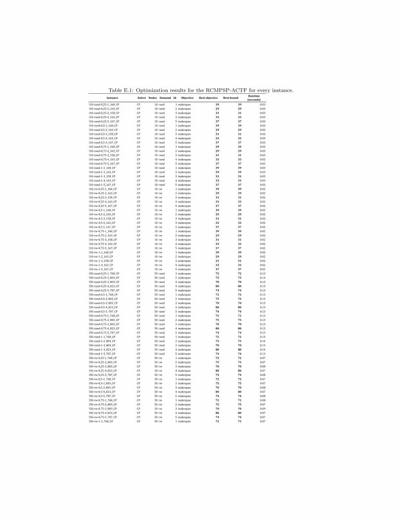
Instance Solver Nodes Demand Id Objective Best objective Best boundRuntime
(seconds)
l10-rand-0,25-1_160_CP CP 10 rand 1 makespan 39 39 0.03
l10-rand-0,25-2_163_CP CP 10 rand 2 makespan 29 29 0.03
l10-rand-0,25-3_158_CP CP 10 rand 3 makespan 31 31 0.03
l10-rand-0,25-4_163_CP CP 10 rand 4 makespan 33 33 0.03
l10-rand-0,25-5_167_CP CP 10 rand 5 makespan 37 37 0.03
l10-rand-0,5-1_160_CP CP 10 rand 1 makespan 39 39 0.03
l10-rand-0,5-2_163_CP CP 10 rand 2 makespan 29 29 0.03
l10-rand-0,5-3_158_CP CP 10 rand 3 makespan 31 31 0.03
l10-rand-0,5-4_163_CP CP 10 rand 4 makespan 33 33 0.03
l10-rand-0,5-5_167_CP CP 10 rand 5 makespan 37 37 0.03
l10-rand-0,75-1_160_CP CP 10 rand 1 makespan 39 39 0.03
l10-rand-0,75-2_163_CP CP 10 rand 2 makespan 29 29 0.03
l10-rand-0,75-3_158_CP CP 10 rand 3 makespan 31 31 0.03
l10-rand-0,75-4_163_CP CP 10 rand 4 makespan 33 33 0.03
l10-rand-0,75-5_167_CP CP 10 rand 5 makespan 37 37 0.03
l10-rand-1-1_160_CP CP 10 rand 1 makespan 39 39 0.03
l10-rand-1-2_163_CP CP 10 rand 2 makespan 29 29 0.03
l10-rand-1-3_158_CP CP 10 rand 3 makespan 31 31 0.03
l10-rand-1-4_163_CP CP 10 rand 4 makespan 33 33 0.03
l10-rand-1-5_167_CP CP 10 rand 5 makespan 37 37 0.03
l10-rw-0,25-1_160_CP CP 10 rw 1 makespan 39 39 0.02
l10-rw-0,25-2_163_CP CP 10 rw 2 makespan 29 29 0.02
l10-rw-0,25-3_158_CP CP 10 rw 3 makespan 31 31 0.02
l10-rw-0,25-4_163_CP CP 10 rw 4 makespan 33 33 0.02
l10-rw-0,25-5_167_CP CP 10 rw 5 makespan 37 37 0.02
l10-rw-0,5-1_160_CP CP 10 rw 1 makespan 39 39 0.02
l10-rw-0,5-2_163_CP CP 10 rw 2 makespan 29 29 0.02
l10-rw-0,5-3_158_CP CP 10 rw 3 makespan 31 31 0.02
l10-rw-0,5-4_163_CP CP 10 rw 4 makespan 33 33 0.02
l10-rw-0,5-5_167_CP CP 10 rw 5 makespan 37 37 0.02
l10-rw-0,75-1_160_CP CP 10 rw 1 makespan 39 39 0.02
l10-rw-0,75-2_163_CP CP 10 rw 2 makespan 29 29 0.02
l10-rw-0,75-3_158_CP CP 10 rw 3 makespan 31 31 0.02
l10-rw-0,75-4_163_CP CP 10 rw 4 makespan 33 33 0.02
l10-rw-0,75-5_167_CP CP 10 rw 5 makespan 37 37 0.02
l10-rw-1-1_160_CP CP 10 rw 1 makespan 39 39 0.02
l10-rw-1-2_163_CP CP 10 rw 2 makespan 29 29 0.02
l10-rw-1-3_158_CP CP 10 rw 3 makespan 31 31 0.02
l10-rw-1-4_163_CP CP 10 rw 4 makespan 33 33 0.02
l10-rw-1-5_167_CP CP 10 rw 5 makespan 37 37 0.02
l50-rand-0,25-1_768_CP CP 50 rand 1 makespan 72 72 0.13
l50-rand-0,25-2_803_CP CP 50 rand 2 makespan 75 75 0.14
l50-rand-0,25-3_803_CP CP 50 rand 3 makespan 70 70 0.13
l50-rand-0,25-4_823_CP CP 50 rand 4 makespan 80 80 0.13
l50-rand-0,25-5_787_CP CP 50 rand 5 makespan 74 74 0.13
l50-rand-0,5-1_768_CP CP 50 rand 1 makespan 72 72 0.13
l50-rand-0,5-2_803_CP CP 50 rand 2 makespan 75 75 0.13
l50-rand-0,5-3_803_CP CP 50 rand 3 makespan 70 70 0.13
l50-rand-0,5-4_823_CP CP 50 rand 4 makespan 80 80 0.13
l50-rand-0,5-5_787_CP CP 50 rand 5 makespan 74 74 0.13
l50-rand-0,75-1_768_CP CP 50 rand 1 makespan 72 72 0.13
l50-rand-0,75-2_803_CP CP 50 rand 2 makespan 75 75 0.13
l50-rand-0,75-3_803_CP CP 50 rand 3 makespan 70 70 0.13
l50-rand-0,75-4_823_CP CP 50 rand 4 makespan 80 80 0.13
l50-rand-0,75-5_787_CP CP 50 rand 5 makespan 74 74 0.13
l50-rand-1-1_768_CP CP 50 rand 1 makespan 72 72 0.13
l50-rand-1-2_803_CP CP 50 rand 2 makespan 75 75 0.14
l50-rand-1-3_803_CP CP 50 rand 3 makespan 70 70 0.13
l50-rand-1-4_823_CP CP 50 rand 4 makespan 80 80 0.14
l50-rand-1-5_787_CP CP 50 rand 5 makespan 74 74 0.13
l50-rw-0,25-1_768_CP CP 50 rw 1 makespan 72 72 0.07
l50-rw-0,25-2_803_CP CP 50 rw 2 makespan 75 75 0.07
l50-rw-0,25-3_803_CP CP 50 rw 3 makespan 70 70 0.08
l50-rw-0,25-4_823_CP CP 50 rw 4 makespan 80 80 0.07
l50-rw-0,25-5_787_CP CP 50 rw 5 makespan 74 74 0.08
l50-rw-0,5-1_768_CP CP 50 rw 1 makespan 72 72 0.07
l50-rw-0,5-2_803_CP CP 50 rw 2 makespan 75 75 0.07
l50-rw-0,5-3_803_CP CP 50 rw 3 makespan 70 70 0.08
l50-rw-0,5-4_823_CP CP 50 rw 4 makespan 80 80 0.07
l50-rw-0,5-5_787_CP CP 50 rw 5 makespan 74 74 0.08
l50-rw-0,75-1_768_CP CP 50 rw 1 makespan 72 72 0.08
l50-rw-0,75-2_803_CP CP 50 rw 2 makespan 75 75 0.07
l50-rw-0,75-3_803_CP CP 50 rw 3 makespan 70 70 0.09
l50-rw-0,75-4_823_CP CP 50 rw 4 makespan 80 80 0.07
l50-rw-0,75-5_787_CP CP 50 rw 5 makespan 74 74 0.07
l50-rw-1-1_768_CP CP 50 rw 1 makespan 72 72 0.07
Table E.1: Optimization results for the RCMPSP-ACTF for every instance.
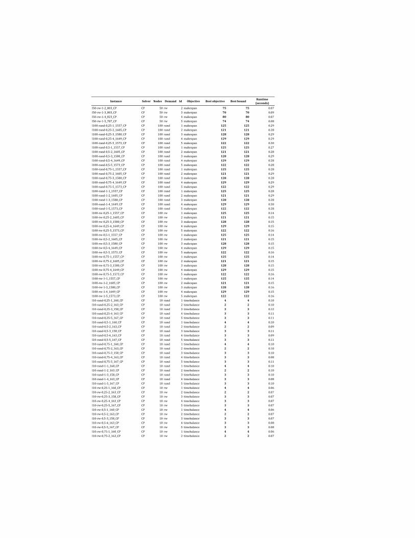
Instance Solver Nodes Demand Id Objective Best objective Best boundRuntime
(seconds)
l50-rw-1-2_803_CP CP 50 rw 2 makespan 75 75 0.07
l50-rw-1-3_803_CP CP 50 rw 3 makespan 70 70 0.09
l50-rw-1-4_823_CP CP 50 rw 4 makespan 80 80 0.07
l50-rw-1-5_787_CP CP 50 rw 5 makespan 74 74 0.08
l100-rand-0,25-1_1557_CP CP 100 rand 1 makespan 125 125 0.29
l100-rand-0,25-2_1605_CP CP 100 rand 2 makespan 121 121 0.28
l100-rand-0,25-3_1580_CP CP 100 rand 3 makespan 128 128 0.29
l100-rand-0,25-4_1649_CP CP 100 rand 4 makespan 129 129 0.29
l100-rand-0,25-5_1573_CP CP 100 rand 5 makespan 122 122 0.30
l100-rand-0,5-1_1557_CP CP 100 rand 1 makespan 125 125 0.27
l100-rand-0,5-2_1605_CP CP 100 rand 2 makespan 121 121 0.28
l100-rand-0,5-3_1580_CP CP 100 rand 3 makespan 128 128 0.29
l100-rand-0,5-4_1649_CP CP 100 rand 4 makespan 129 129 0.28
l100-rand-0,5-5_1573_CP CP 100 rand 5 makespan 122 122 0.28
l100-rand-0,75-1_1557_CP CP 100 rand 1 makespan 125 125 0.28
l100-rand-0,75-2_1605_CP CP 100 rand 2 makespan 121 121 0.29
l100-rand-0,75-3_1580_CP CP 100 rand 3 makespan 128 128 0.28
l100-rand-0,75-4_1649_CP CP 100 rand 4 makespan 129 129 0.29
l100-rand-0,75-5_1573_CP CP 100 rand 5 makespan 122 122 0.29
l100-rand-1-1_1557_CP CP 100 rand 1 makespan 125 125 0.28
l100-rand-1-2_1605_CP CP 100 rand 2 makespan 121 121 0.29
l100-rand-1-3_1580_CP CP 100 rand 3 makespan 128 128 0.28
l100-rand-1-4_1649_CP CP 100 rand 4 makespan 129 129 0.30
l100-rand-1-5_1573_CP CP 100 rand 5 makespan 122 122 0.28
l100-rw-0,25-1_1557_CP CP 100 rw 1 makespan 125 125 0.14
l100-rw-0,25-2_1605_CP CP 100 rw 2 makespan 121 121 0.15
l100-rw-0,25-3_1580_CP CP 100 rw 3 makespan 128 128 0.15
l100-rw-0,25-4_1649_CP CP 100 rw 4 makespan 129 129 0.15
l100-rw-0,25-5_1573_CP CP 100 rw 5 makespan 122 122 0.16
l100-rw-0,5-1_1557_CP CP 100 rw 1 makespan 125 125 0.14
l100-rw-0,5-2_1605_CP CP 100 rw 2 makespan 121 121 0.15
l100-rw-0,5-3_1580_CP CP 100 rw 3 makespan 128 128 0.15
l100-rw-0,5-4_1649_CP CP 100 rw 4 makespan 129 129 0.15
l100-rw-0,5-5_1573_CP CP 100 rw 5 makespan 122 122 0.16
l100-rw-0,75-1_1557_CP CP 100 rw 1 makespan 125 125 0.14
l100-rw-0,75-2_1605_CP CP 100 rw 2 makespan 121 121 0.15
l100-rw-0,75-3_1580_CP CP 100 rw 3 makespan 128 128 0.15
l100-rw-0,75-4_1649_CP CP 100 rw 4 makespan 129 129 0.15
l100-rw-0,75-5_1573_CP CP 100 rw 5 makespan 122 122 0.16
l100-rw-1-1_1557_CP CP 100 rw 1 makespan 125 125 0.14
l100-rw-1-2_1605_CP CP 100 rw 2 makespan 121 121 0.15
l100-rw-1-3_1580_CP CP 100 rw 3 makespan 128 128 0.16
l100-rw-1-4_1649_CP CP 100 rw 4 makespan 129 129 0.15
l100-rw-1-5_1573_CP CP 100 rw 5 makespan 122 122 0.16
l10-rand-0,25-1_160_CP CP 10 rand 1 timebalance 4 4 0.10
l10-rand-0,25-2_163_CP CP 10 rand 2 timebalance 2 2 0.10
l10-rand-0,25-3_158_CP CP 10 rand 3 timebalance 3 3 0.12
l10-rand-0,25-4_163_CP CP 10 rand 4 timebalance 3 3 0.11
l10-rand-0,25-5_167_CP CP 10 rand 5 timebalance 3 3 0.11
l10-rand-0,5-1_160_CP CP 10 rand 1 timebalance 4 4 0.10
l10-rand-0,5-2_163_CP CP 10 rand 2 timebalance 2 2 0.09
l10-rand-0,5-3_158_CP CP 10 rand 3 timebalance 3 3 0.11
l10-rand-0,5-4_163_CP CP 10 rand 4 timebalance 3 3 0.09
l10-rand-0,5-5_167_CP CP 10 rand 5 timebalance 3 3 0.11
l10-rand-0,75-1_160_CP CP 10 rand 1 timebalance 4 4 0.10
l10-rand-0,75-2_163_CP CP 10 rand 2 timebalance 2 2 0.10
l10-rand-0,75-3_158_CP CP 10 rand 3 timebalance 3 3 0.10
l10-rand-0,75-4_163_CP CP 10 rand 4 timebalance 3 3 0.08
l10-rand-0,75-5_167_CP CP 10 rand 5 timebalance 3 3 0.11
l10-rand-1-1_160_CP CP 10 rand 1 timebalance 4 4 0.10
l10-rand-1-2_163_CP CP 10 rand 2 timebalance 2 2 0.10
l10-rand-1-3_158_CP CP 10 rand 3 timebalance 3 3 0.10
l10-rand-1-4_163_CP CP 10 rand 4 timebalance 3 3 0.08
l10-rand-1-5_167_CP CP 10 rand 5 timebalance 3 3 0.10
l10-rw-0,25-1_160_CP CP 10 rw 1 timebalance 4 4 0.06
l10-rw-0,25-2_163_CP CP 10 rw 2 timebalance 2 2 0.07
l10-rw-0,25-3_158_CP CP 10 rw 3 timebalance 3 3 0.07
l10-rw-0,25-4_163_CP CP 10 rw 4 timebalance 3 3 0.07
l10-rw-0,25-5_167_CP CP 10 rw 5 timebalance 3 3 0.07
l10-rw-0,5-1_160_CP CP 10 rw 1 timebalance 4 4 0.06
l10-rw-0,5-2_163_CP CP 10 rw 2 timebalance 2 2 0.07
l10-rw-0,5-3_158_CP CP 10 rw 3 timebalance 3 3 0.07
l10-rw-0,5-4_163_CP CP 10 rw 4 timebalance 3 3 0.08
l10-rw-0,5-5_167_CP CP 10 rw 5 timebalance 3 3 0.08
l10-rw-0,75-1_160_CP CP 10 rw 1 timebalance 4 4 0.06
l10-rw-0,75-2_163_CP CP 10 rw 2 timebalance 2 2 0.07
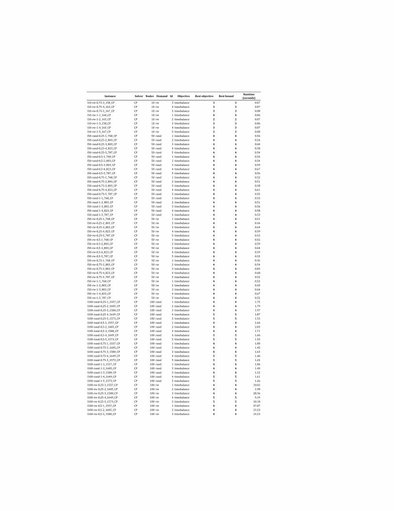
Instance Solver Nodes Demand Id Objective Best objective Best boundRuntime
(seconds)
l10-rw-0,75-3_158_CP CP 10 rw 3 timebalance 3 3 0.07
l10-rw-0,75-4_163_CP CP 10 rw 4 timebalance 3 3 0.07
l10-rw-0,75-5_167_CP CP 10 rw 5 timebalance 3 3 0.08
l10-rw-1-1_160_CP CP 10 rw 1 timebalance 4 4 0.06
l10-rw-1-2_163_CP CP 10 rw 2 timebalance 2 2 0.07
l10-rw-1-3_158_CP CP 10 rw 3 timebalance 3 3 0.06
l10-rw-1-4_163_CP CP 10 rw 4 timebalance 3 3 0.07
l10-rw-1-5_167_CP CP 10 rw 5 timebalance 3 3 0.08
l50-rand-0,25-1_768_CP CP 50 rand 1 timebalance 4 4 0.56
l50-rand-0,25-2_803_CP CP 50 rand 2 timebalance 4 4 0.54
l50-rand-0,25-3_803_CP CP 50 rand 3 timebalance 4 4 0.60
l50-rand-0,25-4_823_CP CP 50 rand 4 timebalance 4 4 0.58
l50-rand-0,25-5_787_CP CP 50 rand 5 timebalance 4 4 0.54
l50-rand-0,5-1_768_CP CP 50 rand 1 timebalance 4 4 0.54
l50-rand-0,5-2_803_CP CP 50 rand 2 timebalance 4 4 0.54
l50-rand-0,5-3_803_CP CP 50 rand 3 timebalance 4 4 0.59
l50-rand-0,5-4_823_CP CP 50 rand 4 timebalance 4 4 0.67
l50-rand-0,5-5_787_CP CP 50 rand 5 timebalance 4 4 0.56
l50-rand-0,75-1_768_CP CP 50 rand 1 timebalance 4 4 0.52
l50-rand-0,75-2_803_CP CP 50 rand 2 timebalance 4 4 0.51
l50-rand-0,75-3_803_CP CP 50 rand 3 timebalance 4 4 0.58
l50-rand-0,75-4_823_CP CP 50 rand 4 timebalance 4 4 0.61
l50-rand-0,75-5_787_CP CP 50 rand 5 timebalance 4 4 0.55
l50-rand-1-1_768_CP CP 50 rand 1 timebalance 4 4 0.53
l50-rand-1-2_803_CP CP 50 rand 2 timebalance 4 4 0.51
l50-rand-1-3_803_CP CP 50 rand 3 timebalance 4 4 0.56
l50-rand-1-4_823_CP CP 50 rand 4 timebalance 4 4 0.58
l50-rand-1-5_787_CP CP 50 rand 5 timebalance 4 4 0.53
l50-rw-0,25-1_768_CP CP 50 rw 1 timebalance 4 4 0.51
l50-rw-0,25-2_803_CP CP 50 rw 2 timebalance 4 4 0.44
l50-rw-0,25-3_803_CP CP 50 rw 3 timebalance 4 4 0.64
l50-rw-0,25-4_823_CP CP 50 rw 4 timebalance 4 4 0.59
l50-rw-0,25-5_787_CP CP 50 rw 5 timebalance 4 4 0.53
l50-rw-0,5-1_768_CP CP 50 rw 1 timebalance 4 4 0.52
l50-rw-0,5-2_803_CP CP 50 rw 2 timebalance 4 4 0.59
l50-rw-0,5-3_803_CP CP 50 rw 3 timebalance 4 4 0.64
l50-rw-0,5-4_823_CP CP 50 rw 4 timebalance 4 4 0.59
l50-rw-0,5-5_787_CP CP 50 rw 5 timebalance 4 4 0.53
l50-rw-0,75-1_768_CP CP 50 rw 1 timebalance 4 4 0.45
l50-rw-0,75-2_803_CP CP 50 rw 2 timebalance 4 4 0.54
l50-rw-0,75-3_803_CP CP 50 rw 3 timebalance 4 4 0.83
l50-rw-0,75-4_823_CP CP 50 rw 4 timebalance 4 4 0.68
l50-rw-0,75-5_787_CP CP 50 rw 5 timebalance 4 4 0.52
l50-rw-1-1_768_CP CP 50 rw 1 timebalance 4 4 0.52
l50-rw-1-2_803_CP CP 50 rw 2 timebalance 4 4 0.43
l50-rw-1-3_803_CP CP 50 rw 3 timebalance 4 4 0.64
l50-rw-1-4_823_CP CP 50 rw 4 timebalance 4 4 0.67
l50-rw-1-5_787_CP CP 50 rw 5 timebalance 4 4 0.52
l100-rand-0,25-1_1557_CP CP 100 rand 1 timebalance 4 4 1.75
l100-rand-0,25-2_1605_CP CP 100 rand 2 timebalance 4 4 1.79
l100-rand-0,25-3_1580_CP CP 100 rand 3 timebalance 4 4 1.97
l100-rand-0,25-4_1649_CP CP 100 rand 4 timebalance 5 5 1.87
l100-rand-0,25-5_1573_CP CP 100 rand 5 timebalance 5 5 1.55
l100-rand-0,5-1_1557_CP CP 100 rand 1 timebalance 4 4 1.66
l100-rand-0,5-2_1605_CP CP 100 rand 2 timebalance 4 4 2.03
l100-rand-0,5-3_1580_CP CP 100 rand 3 timebalance 4 4 1.71
l100-rand-0,5-4_1649_CP CP 100 rand 4 timebalance 5 5 1.66
l100-rand-0,5-5_1573_CP CP 100 rand 5 timebalance 5 5 1.55
l100-rand-0,75-1_1557_CP CP 100 rand 1 timebalance 4 4 1.80
l100-rand-0,75-2_1605_CP CP 100 rand 2 timebalance 4 4 1.45
l100-rand-0,75-3_1580_CP CP 100 rand 3 timebalance 4 4 1.63
l100-rand-0,75-4_1649_CP CP 100 rand 4 timebalance 5 5 1.46
l100-rand-0,75-5_1573_CP CP 100 rand 5 timebalance 5 5 1.24
l100-rand-1-1_1557_CP CP 100 rand 1 timebalance 4 4 1.86
l100-rand-1-2_1605_CP CP 100 rand 2 timebalance 4 4 1.49
l100-rand-1-3_1580_CP CP 100 rand 3 timebalance 4 4 1.52
l100-rand-1-4_1649_CP CP 100 rand 4 timebalance 5 5 1.61
l100-rand-1-5_1573_CP CP 100 rand 5 timebalance 5 5 1.26
l100-rw-0,25-1_1557_CP CP 100 rw 1 timebalance 4 4 10.02
l100-rw-0,25-2_1605_CP CP 100 rw 2 timebalance 4 4 1.98
l100-rw-0,25-3_1580_CP CP 100 rw 3 timebalance 4 4 28.36
l100-rw-0,25-4_1649_CP CP 100 rw 4 timebalance 5 5 5.19
l100-rw-0,25-5_1573_CP CP 100 rw 5 timebalance 5 5 10.18
l100-rw-0,5-1_1557_CP CP 100 rw 1 timebalance 4 4 47.87
l100-rw-0,5-2_1605_CP CP 100 rw 2 timebalance 4 4 15.53
l100-rw-0,5-3_1580_CP CP 100 rw 3 timebalance 4 4 14.23
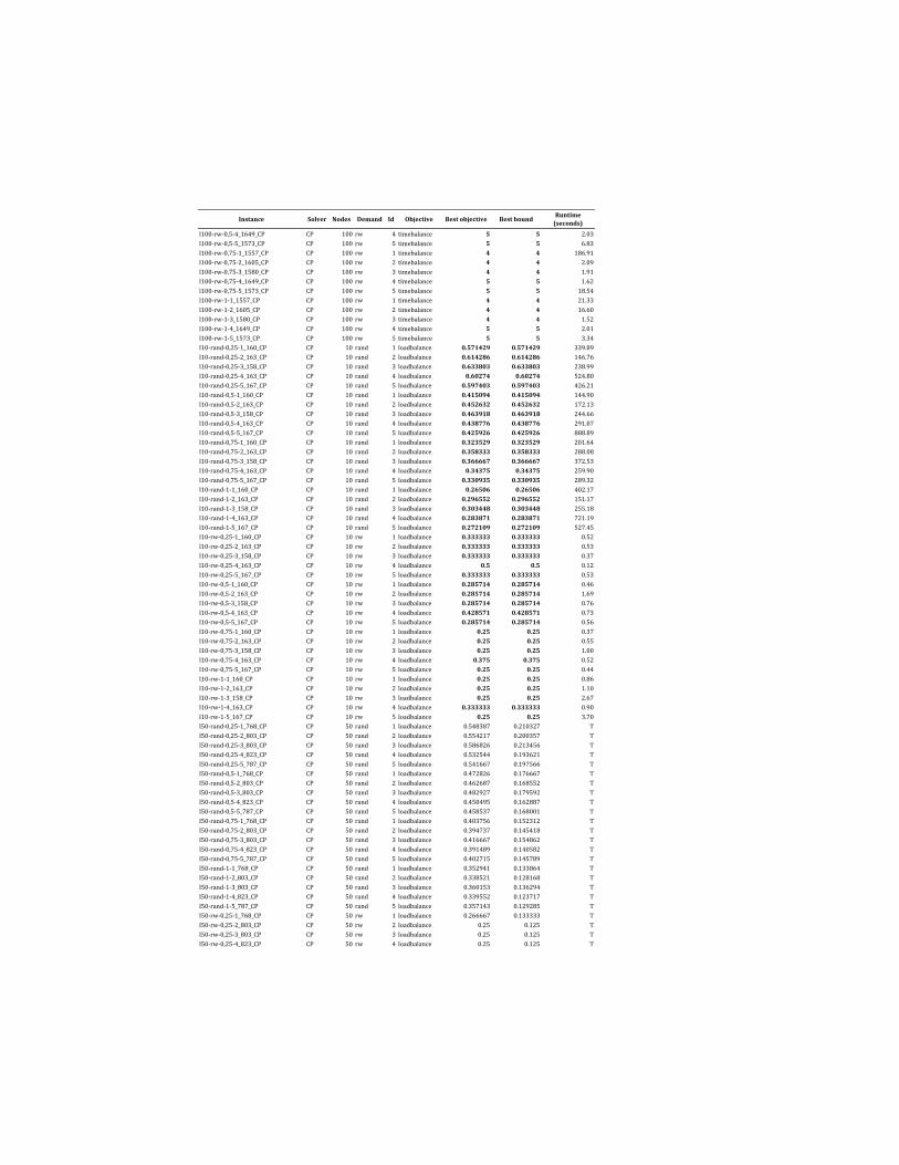
Instance Solver Nodes Demand Id Objective Best objective Best boundRuntime
(seconds)
l100-rw-0,5-4_1649_CP CP 100 rw 4 timebalance 5 5 2.03
l100-rw-0,5-5_1573_CP CP 100 rw 5 timebalance 5 5 6.83
l100-rw-0,75-1_1557_CP CP 100 rw 1 timebalance 4 4 186.91
l100-rw-0,75-2_1605_CP CP 100 rw 2 timebalance 4 4 2.09
l100-rw-0,75-3_1580_CP CP 100 rw 3 timebalance 4 4 1.91
l100-rw-0,75-4_1649_CP CP 100 rw 4 timebalance 5 5 1.62
l100-rw-0,75-5_1573_CP CP 100 rw 5 timebalance 5 5 18.54
l100-rw-1-1_1557_CP CP 100 rw 1 timebalance 4 4 21.33
l100-rw-1-2_1605_CP CP 100 rw 2 timebalance 4 4 16.60
l100-rw-1-3_1580_CP CP 100 rw 3 timebalance 4 4 1.52
l100-rw-1-4_1649_CP CP 100 rw 4 timebalance 5 5 2.01
l100-rw-1-5_1573_CP CP 100 rw 5 timebalance 5 5 3.34
l10-rand-0,25-1_160_CP CP 10 rand 1 loadbalance 0.571429 0.571429 339.89
l10-rand-0,25-2_163_CP CP 10 rand 2 loadbalance 0.614286 0.614286 146.76
l10-rand-0,25-3_158_CP CP 10 rand 3 loadbalance 0.633803 0.633803 238.99
l10-rand-0,25-4_163_CP CP 10 rand 4 loadbalance 0.60274 0.60274 524.80
l10-rand-0,25-5_167_CP CP 10 rand 5 loadbalance 0.597403 0.597403 426.21
l10-rand-0,5-1_160_CP CP 10 rand 1 loadbalance 0.415094 0.415094 144.90
l10-rand-0,5-2_163_CP CP 10 rand 2 loadbalance 0.452632 0.452632 172.13
l10-rand-0,5-3_158_CP CP 10 rand 3 loadbalance 0.463918 0.463918 244.66
l10-rand-0,5-4_163_CP CP 10 rand 4 loadbalance 0.438776 0.438776 291.07
l10-rand-0,5-5_167_CP CP 10 rand 5 loadbalance 0.425926 0.425926 888.89
l10-rand-0,75-1_160_CP CP 10 rand 1 loadbalance 0.323529 0.323529 201.64
l10-rand-0,75-2_163_CP CP 10 rand 2 loadbalance 0.358333 0.358333 288.08
l10-rand-0,75-3_158_CP CP 10 rand 3 loadbalance 0.366667 0.366667 372.53
l10-rand-0,75-4_163_CP CP 10 rand 4 loadbalance 0.34375 0.34375 259.90
l10-rand-0,75-5_167_CP CP 10 rand 5 loadbalance 0.330935 0.330935 289.32
l10-rand-1-1_160_CP CP 10 rand 1 loadbalance 0.26506 0.26506 402.17
l10-rand-1-2_163_CP CP 10 rand 2 loadbalance 0.296552 0.296552 151.17
l10-rand-1-3_158_CP CP 10 rand 3 loadbalance 0.303448 0.303448 255.18
l10-rand-1-4_163_CP CP 10 rand 4 loadbalance 0.283871 0.283871 721.19
l10-rand-1-5_167_CP CP 10 rand 5 loadbalance 0.272109 0.272109 527.45
l10-rw-0,25-1_160_CP CP 10 rw 1 loadbalance 0.333333 0.333333 0.52
l10-rw-0,25-2_163_CP CP 10 rw 2 loadbalance 0.333333 0.333333 0.53
l10-rw-0,25-3_158_CP CP 10 rw 3 loadbalance 0.333333 0.333333 0.37
l10-rw-0,25-4_163_CP CP 10 rw 4 loadbalance 0.5 0.5 0.12
l10-rw-0,25-5_167_CP CP 10 rw 5 loadbalance 0.333333 0.333333 0.53
l10-rw-0,5-1_160_CP CP 10 rw 1 loadbalance 0.285714 0.285714 0.46
l10-rw-0,5-2_163_CP CP 10 rw 2 loadbalance 0.285714 0.285714 1.69
l10-rw-0,5-3_158_CP CP 10 rw 3 loadbalance 0.285714 0.285714 0.76
l10-rw-0,5-4_163_CP CP 10 rw 4 loadbalance 0.428571 0.428571 0.73
l10-rw-0,5-5_167_CP CP 10 rw 5 loadbalance 0.285714 0.285714 0.56
l10-rw-0,75-1_160_CP CP 10 rw 1 loadbalance 0.25 0.25 0.37
l10-rw-0,75-2_163_CP CP 10 rw 2 loadbalance 0.25 0.25 0.55
l10-rw-0,75-3_158_CP CP 10 rw 3 loadbalance 0.25 0.25 1.00
l10-rw-0,75-4_163_CP CP 10 rw 4 loadbalance 0.375 0.375 0.52
l10-rw-0,75-5_167_CP CP 10 rw 5 loadbalance 0.25 0.25 0.44
l10-rw-1-1_160_CP CP 10 rw 1 loadbalance 0.25 0.25 0.86
l10-rw-1-2_163_CP CP 10 rw 2 loadbalance 0.25 0.25 1.10
l10-rw-1-3_158_CP CP 10 rw 3 loadbalance 0.25 0.25 2.67
l10-rw-1-4_163_CP CP 10 rw 4 loadbalance 0.333333 0.333333 0.90
l10-rw-1-5_167_CP CP 10 rw 5 loadbalance 0.25 0.25 3.70
l50-rand-0,25-1_768_CP CP 50 rand 1 loadbalance 0.548387 0.210327 T
l50-rand-0,25-2_803_CP CP 50 rand 2 loadbalance 0.554217 0.200357 T
l50-rand-0,25-3_803_CP CP 50 rand 3 loadbalance 0.586826 0.213456 T
l50-rand-0,25-4_823_CP CP 50 rand 4 loadbalance 0.532544 0.193621 T
l50-rand-0,25-5_787_CP CP 50 rand 5 loadbalance 0.541667 0.197566 T
l50-rand-0,5-1_768_CP CP 50 rand 1 loadbalance 0.472826 0.176667 T
l50-rand-0,5-2_803_CP CP 50 rand 2 loadbalance 0.462687 0.168552 T
l50-rand-0,5-3_803_CP CP 50 rand 3 loadbalance 0.482927 0.179592 T
l50-rand-0,5-4_823_CP CP 50 rand 4 loadbalance 0.450495 0.162887 T
l50-rand-0,5-5_787_CP CP 50 rand 5 loadbalance 0.458537 0.168001 T
l50-rand-0,75-1_768_CP CP 50 rand 1 loadbalance 0.403756 0.152312 T
l50-rand-0,75-2_803_CP CP 50 rand 2 loadbalance 0.394737 0.145418 T
l50-rand-0,75-3_803_CP CP 50 rand 3 loadbalance 0.416667 0.154862 T
l50-rand-0,75-4_823_CP CP 50 rand 4 loadbalance 0.391489 0.140582 T
l50-rand-0,75-5_787_CP CP 50 rand 5 loadbalance 0.402715 0.145789 T
l50-rand-1-1_768_CP CP 50 rand 1 loadbalance 0.352941 0.133864 T
l50-rand-1-2_803_CP CP 50 rand 2 loadbalance 0.338521 0.128168 T
l50-rand-1-3_803_CP CP 50 rand 3 loadbalance 0.360153 0.136294 T
l50-rand-1-4_823_CP CP 50 rand 4 loadbalance 0.339552 0.123717 T
l50-rand-1-5_787_CP CP 50 rand 5 loadbalance 0.357143 0.129285 T
l50-rw-0,25-1_768_CP CP 50 rw 1 loadbalance 0.266667 0.133333 T
l50-rw-0,25-2_803_CP CP 50 rw 2 loadbalance 0.25 0.125 T
l50-rw-0,25-3_803_CP CP 50 rw 3 loadbalance 0.25 0.125 T
l50-rw-0,25-4_823_CP CP 50 rw 4 loadbalance 0.25 0.125 T
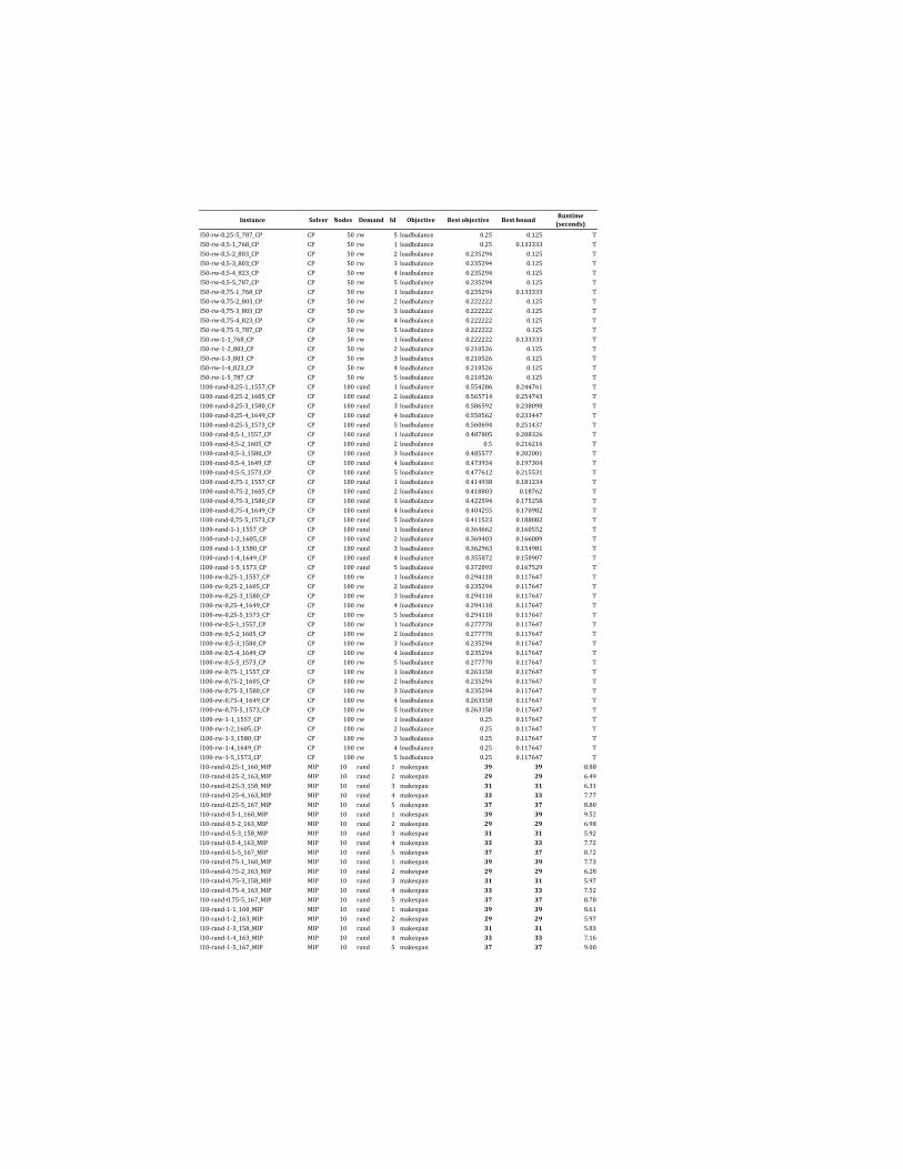
Instance Solver Nodes Demand Id Objective Best objective Best boundRuntime
(seconds)
l50-rw-0,25-5_787_CP CP 50 rw 5 loadbalance 0.25 0.125 T
l50-rw-0,5-1_768_CP CP 50 rw 1 loadbalance 0.25 0.133333 T
l50-rw-0,5-2_803_CP CP 50 rw 2 loadbalance 0.235294 0.125 T
l50-rw-0,5-3_803_CP CP 50 rw 3 loadbalance 0.235294 0.125 T
l50-rw-0,5-4_823_CP CP 50 rw 4 loadbalance 0.235294 0.125 T
l50-rw-0,5-5_787_CP CP 50 rw 5 loadbalance 0.235294 0.125 T
l50-rw-0,75-1_768_CP CP 50 rw 1 loadbalance 0.235294 0.133333 T
l50-rw-0,75-2_803_CP CP 50 rw 2 loadbalance 0.222222 0.125 T
l50-rw-0,75-3_803_CP CP 50 rw 3 loadbalance 0.222222 0.125 T
l50-rw-0,75-4_823_CP CP 50 rw 4 loadbalance 0.222222 0.125 T
l50-rw-0,75-5_787_CP CP 50 rw 5 loadbalance 0.222222 0.125 T
l50-rw-1-1_768_CP CP 50 rw 1 loadbalance 0.222222 0.133333 T
l50-rw-1-2_803_CP CP 50 rw 2 loadbalance 0.210526 0.125 T
l50-rw-1-3_803_CP CP 50 rw 3 loadbalance 0.210526 0.125 T
l50-rw-1-4_823_CP CP 50 rw 4 loadbalance 0.210526 0.125 T
l50-rw-1-5_787_CP CP 50 rw 5 loadbalance 0.210526 0.125 T
l100-rand-0,25-1_1557_CP CP 100 rand 1 loadbalance 0.554286 0.244761 T
l100-rand-0,25-2_1605_CP CP 100 rand 2 loadbalance 0.565714 0.254743 T
l100-rand-0,25-3_1580_CP CP 100 rand 3 loadbalance 0.586592 0.238098 T
l100-rand-0,25-4_1649_CP CP 100 rand 4 loadbalance 0.550562 0.233447 T
l100-rand-0,25-5_1573_CP CP 100 rand 5 loadbalance 0.560694 0.251437 T
l100-rand-0,5-1_1557_CP CP 100 rand 1 loadbalance 0.487805 0.208326 T
l100-rand-0,5-2_1605_CP CP 100 rand 2 loadbalance 0.5 0.216216 T
l100-rand-0,5-3_1580_CP CP 100 rand 3 loadbalance 0.485577 0.202001 T
l100-rand-0,5-4_1649_CP CP 100 rand 4 loadbalance 0.473934 0.197304 T
l100-rand-0,5-5_1573_CP CP 100 rand 5 loadbalance 0.477612 0.215531 T
l100-rand-0,75-1_1557_CP CP 100 rand 1 loadbalance 0.414938 0.181234 T
l100-rand-0,75-2_1605_CP CP 100 rand 2 loadbalance 0.418803 0.18762 T
l100-rand-0,75-3_1580_CP CP 100 rand 3 loadbalance 0.422594 0.175258 T
l100-rand-0,75-4_1649_CP CP 100 rand 4 loadbalance 0.404255 0.170982 T
l100-rand-0,75-5_1573_CP CP 100 rand 5 loadbalance 0.411523 0.188082 T
l100-rand-1-1_1557_CP CP 100 rand 1 loadbalance 0.364662 0.160552 T
l100-rand-1-2_1605_CP CP 100 rand 2 loadbalance 0.369403 0.166089 T
l100-rand-1-3_1580_CP CP 100 rand 3 loadbalance 0.362963 0.154981 T
l100-rand-1-4_1649_CP CP 100 rand 4 loadbalance 0.355072 0.150907 T
l100-rand-1-5_1573_CP CP 100 rand 5 loadbalance 0.372093 0.167529 T
l100-rw-0,25-1_1557_CP CP 100 rw 1 loadbalance 0.294118 0.117647 T
l100-rw-0,25-2_1605_CP CP 100 rw 2 loadbalance 0.235294 0.117647 T
l100-rw-0,25-3_1580_CP CP 100 rw 3 loadbalance 0.294118 0.117647 T
l100-rw-0,25-4_1649_CP CP 100 rw 4 loadbalance 0.294118 0.117647 T
l100-rw-0,25-5_1573_CP CP 100 rw 5 loadbalance 0.294118 0.117647 T
l100-rw-0,5-1_1557_CP CP 100 rw 1 loadbalance 0.277778 0.117647 T
l100-rw-0,5-2_1605_CP CP 100 rw 2 loadbalance 0.277778 0.117647 T
l100-rw-0,5-3_1580_CP CP 100 rw 3 loadbalance 0.235294 0.117647 T
l100-rw-0,5-4_1649_CP CP 100 rw 4 loadbalance 0.235294 0.117647 T
l100-rw-0,5-5_1573_CP CP 100 rw 5 loadbalance 0.277778 0.117647 T
l100-rw-0,75-1_1557_CP CP 100 rw 1 loadbalance 0.263158 0.117647 T
l100-rw-0,75-2_1605_CP CP 100 rw 2 loadbalance 0.235294 0.117647 T
l100-rw-0,75-3_1580_CP CP 100 rw 3 loadbalance 0.235294 0.117647 T
l100-rw-0,75-4_1649_CP CP 100 rw 4 loadbalance 0.263158 0.117647 T
l100-rw-0,75-5_1573_CP CP 100 rw 5 loadbalance 0.263158 0.117647 T
l100-rw-1-1_1557_CP CP 100 rw 1 loadbalance 0.25 0.117647 T
l100-rw-1-2_1605_CP CP 100 rw 2 loadbalance 0.25 0.117647 T
l100-rw-1-3_1580_CP CP 100 rw 3 loadbalance 0.25 0.117647 T
l100-rw-1-4_1649_CP CP 100 rw 4 loadbalance 0.25 0.117647 T
l100-rw-1-5_1573_CP CP 100 rw 5 loadbalance 0.25 0.117647 T
l10-rand-0.25-1_160_MIP MIP 10 rand 1 makespan 39 39 8.88
l10-rand-0.25-2_163_MIP MIP 10 rand 2 makespan 29 29 6.49
l10-rand-0.25-3_158_MIP MIP 10 rand 3 makespan 31 31 6.31
l10-rand-0.25-4_163_MIP MIP 10 rand 4 makespan 33 33 7.77
l10-rand-0.25-5_167_MIP MIP 10 rand 5 makespan 37 37 8.80
l10-rand-0.5-1_160_MIP MIP 10 rand 1 makespan 39 39 9.52
l10-rand-0.5-2_163_MIP MIP 10 rand 2 makespan 29 29 6.98
l10-rand-0.5-3_158_MIP MIP 10 rand 3 makespan 31 31 5.92
l10-rand-0.5-4_163_MIP MIP 10 rand 4 makespan 33 33 7.72
l10-rand-0.5-5_167_MIP MIP 10 rand 5 makespan 37 37 8.72
l10-rand-0.75-1_160_MIP MIP 10 rand 1 makespan 39 39 7.73
l10-rand-0.75-2_163_MIP MIP 10 rand 2 makespan 29 29 6.28
l10-rand-0.75-3_158_MIP MIP 10 rand 3 makespan 31 31 5.97
l10-rand-0.75-4_163_MIP MIP 10 rand 4 makespan 33 33 7.52
l10-rand-0.75-5_167_MIP MIP 10 rand 5 makespan 37 37 8.78
l10-rand-1-1_160_MIP MIP 10 rand 1 makespan 39 39 8.61
l10-rand-1-2_163_MIP MIP 10 rand 2 makespan 29 29 5.97
l10-rand-1-3_158_MIP MIP 10 rand 3 makespan 31 31 5.83
l10-rand-1-4_163_MIP MIP 10 rand 4 makespan 33 33 7.16
l10-rand-1-5_167_MIP MIP 10 rand 5 makespan 37 37 9.00
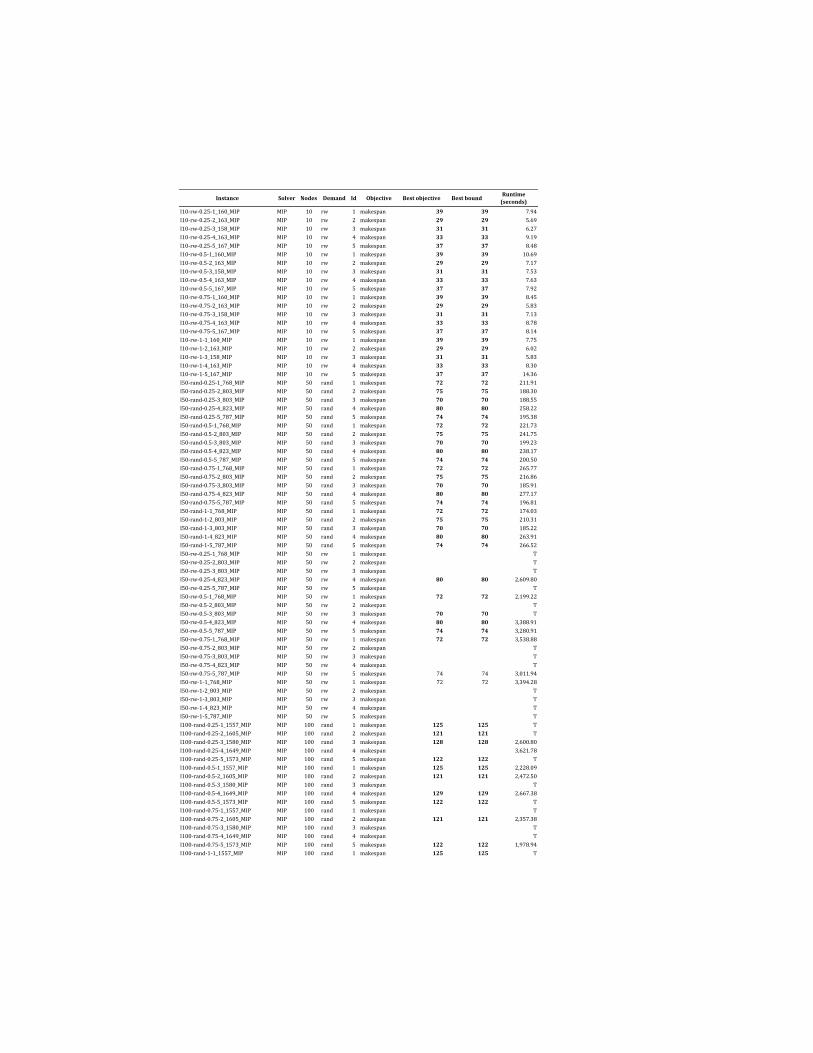
Instance Solver Nodes Demand Id Objective Best objective Best boundRuntime
(seconds)
l10-rw-0.25-1_160_MIP MIP 10 rw 1 makespan 39 39 7.94
l10-rw-0.25-2_163_MIP MIP 10 rw 2 makespan 29 29 5.69
l10-rw-0.25-3_158_MIP MIP 10 rw 3 makespan 31 31 6.27
l10-rw-0.25-4_163_MIP MIP 10 rw 4 makespan 33 33 9.19
l10-rw-0.25-5_167_MIP MIP 10 rw 5 makespan 37 37 8.48
l10-rw-0.5-1_160_MIP MIP 10 rw 1 makespan 39 39 10.69
l10-rw-0.5-2_163_MIP MIP 10 rw 2 makespan 29 29 7.17
l10-rw-0.5-3_158_MIP MIP 10 rw 3 makespan 31 31 7.53
l10-rw-0.5-4_163_MIP MIP 10 rw 4 makespan 33 33 7.63
l10-rw-0.5-5_167_MIP MIP 10 rw 5 makespan 37 37 7.92
l10-rw-0.75-1_160_MIP MIP 10 rw 1 makespan 39 39 8.45
l10-rw-0.75-2_163_MIP MIP 10 rw 2 makespan 29 29 5.83
l10-rw-0.75-3_158_MIP MIP 10 rw 3 makespan 31 31 7.13
l10-rw-0.75-4_163_MIP MIP 10 rw 4 makespan 33 33 8.78
l10-rw-0.75-5_167_MIP MIP 10 rw 5 makespan 37 37 8.14
l10-rw-1-1_160_MIP MIP 10 rw 1 makespan 39 39 7.75
l10-rw-1-2_163_MIP MIP 10 rw 2 makespan 29 29 6.02
l10-rw-1-3_158_MIP MIP 10 rw 3 makespan 31 31 5.83
l10-rw-1-4_163_MIP MIP 10 rw 4 makespan 33 33 8.30
l10-rw-1-5_167_MIP MIP 10 rw 5 makespan 37 37 14.36
l50-rand-0.25-1_768_MIP MIP 50 rand 1 makespan 72 72 211.91
l50-rand-0.25-2_803_MIP MIP 50 rand 2 makespan 75 75 188.30
l50-rand-0.25-3_803_MIP MIP 50 rand 3 makespan 70 70 188.55
l50-rand-0.25-4_823_MIP MIP 50 rand 4 makespan 80 80 258.22
l50-rand-0.25-5_787_MIP MIP 50 rand 5 makespan 74 74 195.38
l50-rand-0.5-1_768_MIP MIP 50 rand 1 makespan 72 72 221.73
l50-rand-0.5-2_803_MIP MIP 50 rand 2 makespan 75 75 241.75
l50-rand-0.5-3_803_MIP MIP 50 rand 3 makespan 70 70 199.23
l50-rand-0.5-4_823_MIP MIP 50 rand 4 makespan 80 80 238.17
l50-rand-0.5-5_787_MIP MIP 50 rand 5 makespan 74 74 200.50
l50-rand-0.75-1_768_MIP MIP 50 rand 1 makespan 72 72 265.77
l50-rand-0.75-2_803_MIP MIP 50 rand 2 makespan 75 75 216.86
l50-rand-0.75-3_803_MIP MIP 50 rand 3 makespan 70 70 185.91
l50-rand-0.75-4_823_MIP MIP 50 rand 4 makespan 80 80 277.17
l50-rand-0.75-5_787_MIP MIP 50 rand 5 makespan 74 74 196.81
l50-rand-1-1_768_MIP MIP 50 rand 1 makespan 72 72 174.03
l50-rand-1-2_803_MIP MIP 50 rand 2 makespan 75 75 210.31
l50-rand-1-3_803_MIP MIP 50 rand 3 makespan 70 70 185.22
l50-rand-1-4_823_MIP MIP 50 rand 4 makespan 80 80 263.91
l50-rand-1-5_787_MIP MIP 50 rand 5 makespan 74 74 266.52
l50-rw-0.25-1_768_MIP MIP 50 rw 1 makespan T
l50-rw-0.25-2_803_MIP MIP 50 rw 2 makespan T
l50-rw-0.25-3_803_MIP MIP 50 rw 3 makespan T
l50-rw-0.25-4_823_MIP MIP 50 rw 4 makespan 80 80 2,609.80
l50-rw-0.25-5_787_MIP MIP 50 rw 5 makespan T
l50-rw-0.5-1_768_MIP MIP 50 rw 1 makespan 72 72 2,199.22
l50-rw-0.5-2_803_MIP MIP 50 rw 2 makespan T
l50-rw-0.5-3_803_MIP MIP 50 rw 3 makespan 70 70 T
l50-rw-0.5-4_823_MIP MIP 50 rw 4 makespan 80 80 3,388.91
l50-rw-0.5-5_787_MIP MIP 50 rw 5 makespan 74 74 3,280.91
l50-rw-0.75-1_768_MIP MIP 50 rw 1 makespan 72 72 3,538.88
l50-rw-0.75-2_803_MIP MIP 50 rw 2 makespan T
l50-rw-0.75-3_803_MIP MIP 50 rw 3 makespan T
l50-rw-0.75-4_823_MIP MIP 50 rw 4 makespan T
l50-rw-0.75-5_787_MIP MIP 50 rw 5 makespan 74 74 3,011.94
l50-rw-1-1_768_MIP MIP 50 rw 1 makespan 72 72 3,394.28
l50-rw-1-2_803_MIP MIP 50 rw 2 makespan T
l50-rw-1-3_803_MIP MIP 50 rw 3 makespan T
l50-rw-1-4_823_MIP MIP 50 rw 4 makespan T
l50-rw-1-5_787_MIP MIP 50 rw 5 makespan T
l100-rand-0.25-1_1557_MIP MIP 100 rand 1 makespan 125 125 T
l100-rand-0.25-2_1605_MIP MIP 100 rand 2 makespan 121 121 T
l100-rand-0.25-3_1580_MIP MIP 100 rand 3 makespan 128 128 2,600.80
l100-rand-0.25-4_1649_MIP MIP 100 rand 4 makespan 3,621.78
l100-rand-0.25-5_1573_MIP MIP 100 rand 5 makespan 122 122 T
l100-rand-0.5-1_1557_MIP MIP 100 rand 1 makespan 125 125 2,228.09
l100-rand-0.5-2_1605_MIP MIP 100 rand 2 makespan 121 121 2,472.50
l100-rand-0.5-3_1580_MIP MIP 100 rand 3 makespan T
l100-rand-0.5-4_1649_MIP MIP 100 rand 4 makespan 129 129 2,667.38
l100-rand-0.5-5_1573_MIP MIP 100 rand 5 makespan 122 122 T
l100-rand-0.75-1_1557_MIP MIP 100 rand 1 makespan T
l100-rand-0.75-2_1605_MIP MIP 100 rand 2 makespan 121 121 2,357.38
l100-rand-0.75-3_1580_MIP MIP 100 rand 3 makespan T
l100-rand-0.75-4_1649_MIP MIP 100 rand 4 makespan T
l100-rand-0.75-5_1573_MIP MIP 100 rand 5 makespan 122 122 1,978.94
l100-rand-1-1_1557_MIP MIP 100 rand 1 makespan 125 125 T
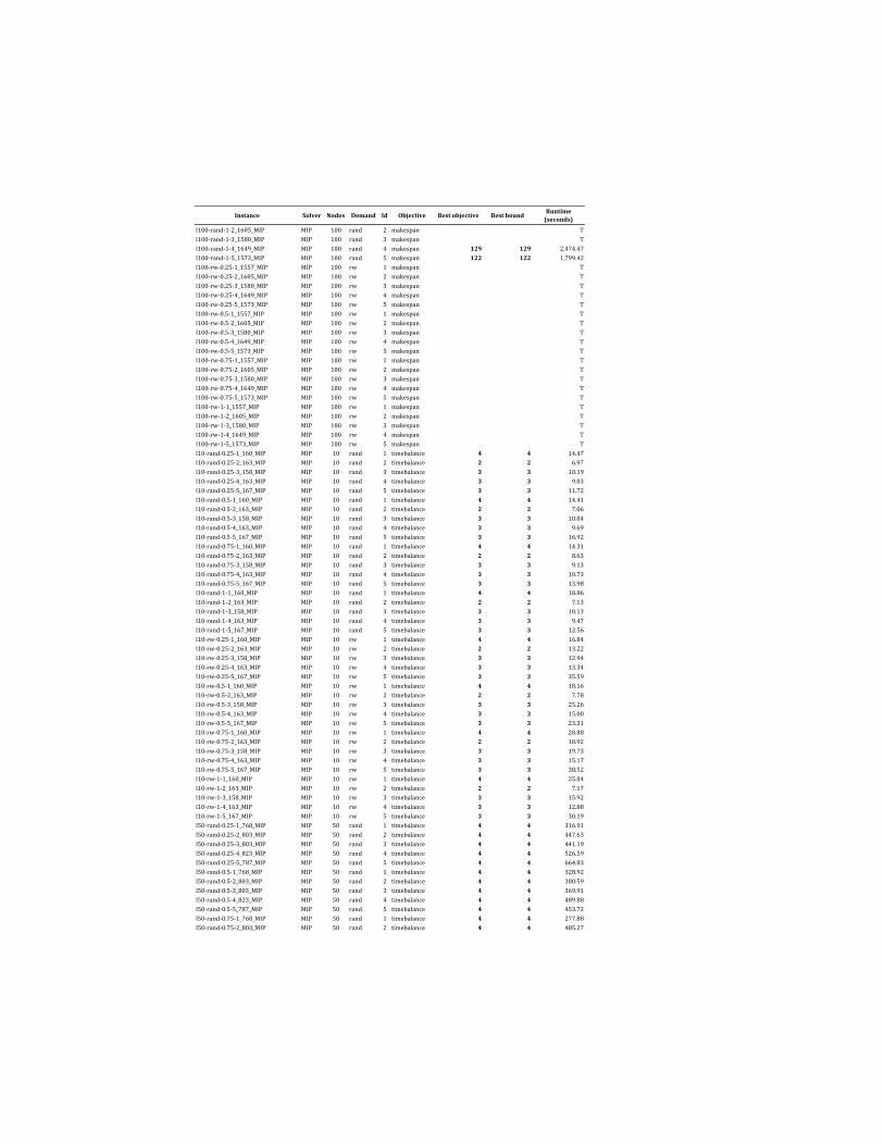
Instance Solver Nodes Demand Id Objective Best objective Best boundRuntime
(seconds)
l100-rand-1-2_1605_MIP MIP 100 rand 2 makespan T
l100-rand-1-3_1580_MIP MIP 100 rand 3 makespan T
l100-rand-1-4_1649_MIP MIP 100 rand 4 makespan 129 129 2,474.47
l100-rand-1-5_1573_MIP MIP 100 rand 5 makespan 122 122 1,799.42
l100-rw-0.25-1_1557_MIP MIP 100 rw 1 makespan T
l100-rw-0.25-2_1605_MIP MIP 100 rw 2 makespan T
l100-rw-0.25-3_1580_MIP MIP 100 rw 3 makespan T
l100-rw-0.25-4_1649_MIP MIP 100 rw 4 makespan T
l100-rw-0.25-5_1573_MIP MIP 100 rw 5 makespan T
l100-rw-0.5-1_1557_MIP MIP 100 rw 1 makespan T
l100-rw-0.5-2_1605_MIP MIP 100 rw 2 makespan T
l100-rw-0.5-3_1580_MIP MIP 100 rw 3 makespan T
l100-rw-0.5-4_1649_MIP MIP 100 rw 4 makespan T
l100-rw-0.5-5_1573_MIP MIP 100 rw 5 makespan T
l100-rw-0.75-1_1557_MIP MIP 100 rw 1 makespan T
l100-rw-0.75-2_1605_MIP MIP 100 rw 2 makespan T
l100-rw-0.75-3_1580_MIP MIP 100 rw 3 makespan T
l100-rw-0.75-4_1649_MIP MIP 100 rw 4 makespan T
l100-rw-0.75-5_1573_MIP MIP 100 rw 5 makespan T
l100-rw-1-1_1557_MIP MIP 100 rw 1 makespan T
l100-rw-1-2_1605_MIP MIP 100 rw 2 makespan T
l100-rw-1-3_1580_MIP MIP 100 rw 3 makespan T
l100-rw-1-4_1649_MIP MIP 100 rw 4 makespan T
l100-rw-1-5_1573_MIP MIP 100 rw 5 makespan T
l10-rand-0.25-1_160_MIP MIP 10 rand 1 timebalance 4 4 14.47
l10-rand-0.25-2_163_MIP MIP 10 rand 2 timebalance 2 2 6.97
l10-rand-0.25-3_158_MIP MIP 10 rand 3 timebalance 3 3 10.19
l10-rand-0.25-4_163_MIP MIP 10 rand 4 timebalance 3 3 9.03
l10-rand-0.25-5_167_MIP MIP 10 rand 5 timebalance 3 3 11.72
l10-rand-0.5-1_160_MIP MIP 10 rand 1 timebalance 4 4 14.41
l10-rand-0.5-2_163_MIP MIP 10 rand 2 timebalance 2 2 7.06
l10-rand-0.5-3_158_MIP MIP 10 rand 3 timebalance 3 3 10.84
l10-rand-0.5-4_163_MIP MIP 10 rand 4 timebalance 3 3 9.69
l10-rand-0.5-5_167_MIP MIP 10 rand 5 timebalance 3 3 16.92
l10-rand-0.75-1_160_MIP MIP 10 rand 1 timebalance 4 4 14.31
l10-rand-0.75-2_163_MIP MIP 10 rand 2 timebalance 2 2 8.63
l10-rand-0.75-3_158_MIP MIP 10 rand 3 timebalance 3 3 9.13
l10-rand-0.75-4_163_MIP MIP 10 rand 4 timebalance 3 3 10.73
l10-rand-0.75-5_167_MIP MIP 10 rand 5 timebalance 3 3 13.98
l10-rand-1-1_160_MIP MIP 10 rand 1 timebalance 4 4 18.86
l10-rand-1-2_163_MIP MIP 10 rand 2 timebalance 2 2 7.13
l10-rand-1-3_158_MIP MIP 10 rand 3 timebalance 3 3 10.13
l10-rand-1-4_163_MIP MIP 10 rand 4 timebalance 3 3 9.47
l10-rand-1-5_167_MIP MIP 10 rand 5 timebalance 3 3 12.56
l10-rw-0.25-1_160_MIP MIP 10 rw 1 timebalance 4 4 16.84
l10-rw-0.25-2_163_MIP MIP 10 rw 2 timebalance 2 2 13.22
l10-rw-0.25-3_158_MIP MIP 10 rw 3 timebalance 3 3 12.94
l10-rw-0.25-4_163_MIP MIP 10 rw 4 timebalance 3 3 13.34
l10-rw-0.25-5_167_MIP MIP 10 rw 5 timebalance 3 3 35.59
l10-rw-0.5-1_160_MIP MIP 10 rw 1 timebalance 4 4 18.16
l10-rw-0.5-2_163_MIP MIP 10 rw 2 timebalance 2 2 7.78
l10-rw-0.5-3_158_MIP MIP 10 rw 3 timebalance 3 3 25.26
l10-rw-0.5-4_163_MIP MIP 10 rw 4 timebalance 3 3 15.00
l10-rw-0.5-5_167_MIP MIP 10 rw 5 timebalance 3 3 23.31
l10-rw-0.75-1_160_MIP MIP 10 rw 1 timebalance 4 4 28.88
l10-rw-0.75-2_163_MIP MIP 10 rw 2 timebalance 2 2 10.92
l10-rw-0.75-3_158_MIP MIP 10 rw 3 timebalance 3 3 19.73
l10-rw-0.75-4_163_MIP MIP 10 rw 4 timebalance 3 3 15.17
l10-rw-0.75-5_167_MIP MIP 10 rw 5 timebalance 3 3 38.52
l10-rw-1-1_160_MIP MIP 10 rw 1 timebalance 4 4 25.84
l10-rw-1-2_163_MIP MIP 10 rw 2 timebalance 2 2 7.17
l10-rw-1-3_158_MIP MIP 10 rw 3 timebalance 3 3 15.92
l10-rw-1-4_163_MIP MIP 10 rw 4 timebalance 3 3 12.88
l10-rw-1-5_167_MIP MIP 10 rw 5 timebalance 3 3 30.19
l50-rand-0.25-1_768_MIP MIP 50 rand 1 timebalance 4 4 316.91
l50-rand-0.25-2_803_MIP MIP 50 rand 2 timebalance 4 4 447.63
l50-rand-0.25-3_803_MIP MIP 50 rand 3 timebalance 4 4 441.19
l50-rand-0.25-4_823_MIP MIP 50 rand 4 timebalance 4 4 526.59
l50-rand-0.25-5_787_MIP MIP 50 rand 5 timebalance 4 4 664.83
l50-rand-0.5-1_768_MIP MIP 50 rand 1 timebalance 4 4 328.92
l50-rand-0.5-2_803_MIP MIP 50 rand 2 timebalance 4 4 380.59
l50-rand-0.5-3_803_MIP MIP 50 rand 3 timebalance 4 4 369.91
l50-rand-0.5-4_823_MIP MIP 50 rand 4 timebalance 4 4 489.88
l50-rand-0.5-5_787_MIP MIP 50 rand 5 timebalance 4 4 453.72
l50-rand-0.75-1_768_MIP MIP 50 rand 1 timebalance 4 4 277.88
l50-rand-0.75-2_803_MIP MIP 50 rand 2 timebalance 4 4 485.27
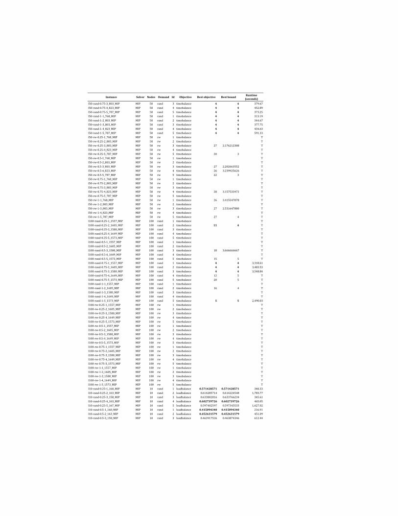
Instance Solver Nodes Demand Id Objective Best objective Best boundRuntime
(seconds)
l50-rand-0.75-3_803_MIP MIP 50 rand 3 timebalance 4 4 379.67
l50-rand-0.75-4_823_MIP MIP 50 rand 4 timebalance 4 4 452.89
l50-rand-0.75-5_787_MIP MIP 50 rand 5 timebalance 4 4 373.25
l50-rand-1-1_768_MIP MIP 50 rand 1 timebalance 4 4 313.19
l50-rand-1-2_803_MIP MIP 50 rand 2 timebalance 4 4 344.67
l50-rand-1-3_803_MIP MIP 50 rand 3 timebalance 4 4 377.75
l50-rand-1-4_823_MIP MIP 50 rand 4 timebalance 4 4 434.63
l50-rand-1-5_787_MIP MIP 50 rand 5 timebalance 4 4 591.33
l50-rw-0.25-1_768_MIP MIP 50 rw 1 timebalance T
l50-rw-0.25-2_803_MIP MIP 50 rw 2 timebalance T
l50-rw-0.25-3_803_MIP MIP 50 rw 3 timebalance 27 2.176212308 T
l50-rw-0.25-4_823_MIP MIP 50 rw 4 timebalance T
l50-rw-0.25-5_787_MIP MIP 50 rw 5 timebalance 20 3 T
l50-rw-0.5-1_768_MIP MIP 50 rw 1 timebalance T
l50-rw-0.5-2_803_MIP MIP 50 rw 2 timebalance T
l50-rw-0.5-3_803_MIP MIP 50 rw 3 timebalance 27 2.202663552 T
l50-rw-0.5-4_823_MIP MIP 50 rw 4 timebalance 26 3.239925626 T
l50-rw-0.5-5_787_MIP MIP 50 rw 5 timebalance 22 3 T
l50-rw-0.75-1_768_MIP MIP 50 rw 1 timebalance T
l50-rw-0.75-2_803_MIP MIP 50 rw 2 timebalance T
l50-rw-0.75-3_803_MIP MIP 50 rw 3 timebalance T
l50-rw-0.75-4_823_MIP MIP 50 rw 4 timebalance 28 3.157533472 T
l50-rw-0.75-5_787_MIP MIP 50 rw 5 timebalance T
l50-rw-1-1_768_MIP MIP 50 rw 1 timebalance 26 3.415547878 T
l50-rw-1-2_803_MIP MIP 50 rw 2 timebalance T
l50-rw-1-3_803_MIP MIP 50 rw 3 timebalance 27 2.531647880 T
l50-rw-1-4_823_MIP MIP 50 rw 4 timebalance T
l50-rw-1-5_787_MIP MIP 50 rw 5 timebalance 27 4 T
l100-rand-0.25-1_1557_MIP MIP 100 rand 1 timebalance T
l100-rand-0.25-2_1605_MIP MIP 100 rand 2 timebalance 11 4 T
l100-rand-0.25-3_1580_MIP MIP 100 rand 3 timebalance T
l100-rand-0.25-4_1649_MIP MIP 100 rand 4 timebalance T
l100-rand-0.25-5_1573_MIP MIP 100 rand 5 timebalance T
l100-rand-0.5-1_1557_MIP MIP 100 rand 1 timebalance T
l100-rand-0.5-2_1605_MIP MIP 100 rand 2 timebalance T
l100-rand-0.5-3_1580_MIP MIP 100 rand 3 timebalance 18 3.666666667 T
l100-rand-0.5-4_1649_MIP MIP 100 rand 4 timebalance T
l100-rand-0.5-5_1573_MIP MIP 100 rand 5 timebalance 15 5 T
l100-rand-0.75-1_1557_MIP MIP 100 rand 1 timebalance 4 4 3,318.61
l100-rand-0.75-2_1605_MIP MIP 100 rand 2 timebalance 4 4 3,483.53
l100-rand-0.75-3_1580_MIP MIP 100 rand 3 timebalance 4 4 3,548.84
l100-rand-0.75-4_1649_MIP MIP 100 rand 4 timebalance 12 5 T
l100-rand-0.75-5_1573_MIP MIP 100 rand 5 timebalance 20 5 T
l100-rand-1-1_1557_MIP MIP 100 rand 1 timebalance T
l100-rand-1-2_1605_MIP MIP 100 rand 2 timebalance 16 4 T
l100-rand-1-3_1580_MIP MIP 100 rand 3 timebalance T
l100-rand-1-4_1649_MIP MIP 100 rand 4 timebalance T
l100-rand-1-5_1573_MIP MIP 100 rand 5 timebalance 5 5 2,490.03
l100-rw-0.25-1_1557_MIP MIP 100 rw 1 timebalance T
l100-rw-0.25-2_1605_MIP MIP 100 rw 2 timebalance T
l100-rw-0.25-3_1580_MIP MIP 100 rw 3 timebalance T
l100-rw-0.25-4_1649_MIP MIP 100 rw 4 timebalance T
l100-rw-0.25-5_1573_MIP MIP 100 rw 5 timebalance T
l100-rw-0.5-1_1557_MIP MIP 100 rw 1 timebalance T
l100-rw-0.5-2_1605_MIP MIP 100 rw 2 timebalance T
l100-rw-0.5-3_1580_MIP MIP 100 rw 3 timebalance T
l100-rw-0.5-4_1649_MIP MIP 100 rw 4 timebalance T
l100-rw-0.5-5_1573_MIP MIP 100 rw 5 timebalance T
l100-rw-0.75-1_1557_MIP MIP 100 rw 1 timebalance T
l100-rw-0.75-2_1605_MIP MIP 100 rw 2 timebalance T
l100-rw-0.75-3_1580_MIP MIP 100 rw 3 timebalance T
l100-rw-0.75-4_1649_MIP MIP 100 rw 4 timebalance T
l100-rw-0.75-5_1573_MIP MIP 100 rw 5 timebalance T
l100-rw-1-1_1557_MIP MIP 100 rw 1 timebalance T
l100-rw-1-2_1605_MIP MIP 100 rw 2 timebalance T
l100-rw-1-3_1580_MIP MIP 100 rw 3 timebalance T
l100-rw-1-4_1649_MIP MIP 100 rw 4 timebalance T
l100-rw-1-5_1573_MIP MIP 100 rw 5 timebalance T
l10-rand-0.25-1_160_MIP MIP 10 rand 1 loadbalance 0.571428571 0.571428571 348.33
l10-rand-0.25-2_163_MIP MIP 10 rand 2 loadbalance 0.614285714 0.614224548 1,783.77
l10-rand-0.25-3_158_MIP MIP 10 rand 3 loadbalance 0.633802816 0.633766234 345.61
l10-rand-0.25-4_163_MIP MIP 10 rand 4 loadbalance 0.602739726 0.602739726 465.05
l10-rand-0.25-5_167_MIP MIP 10 rand 5 loadbalance 0.597402597 0.597343533 1,627.02
l10-rand-0.5-1_160_MIP MIP 10 rand 1 loadbalance 0.415094340 0.415094340 216.91
l10-rand-0.5-2_163_MIP MIP 10 rand 2 loadbalance 0.452631579 0.452631579 451.09
l10-rand-0.5-3_158_MIP MIP 10 rand 3 loadbalance 0.463917526 0.463874346 612.44
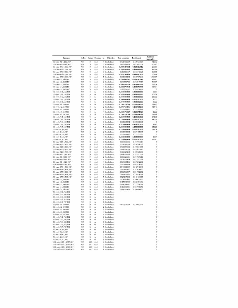
Instance Solver Nodes Demand Id Objective Best objective Best boundRuntime
(seconds)
l10-rand-0.5-4_163_MIP MIP 10 rand 4 loadbalance 0.438775509 0.438731857 710.13
l10-rand-0.5-5_167_MIP MIP 10 rand 5 loadbalance 0.425925926 0.425883568 1,307.42
l10-rand-0.75-1_160_MIP MIP 10 rand 1 loadbalance 0.323529412 0.323529412 206.56
l10-rand-0.75-2_163_MIP MIP 10 rand 2 loadbalance 0.358333333 0.358333333 470.44
l10-rand-0.75-3_158_MIP MIP 10 rand 3 loadbalance 0.366666667 0.366643321 196.05
l10-rand-0.75-4_163_MIP MIP 10 rand 4 loadbalance 0.343750000 0.343750000 703.00
l10-rand-0.75-5_167_MIP MIP 10 rand 5 loadbalance 0.330935252 0.330919296 1,499.09
l10-rand-1-1_160_MIP MIP 10 rand 1 loadbalance 0.265060241 0.265060241 471.81
l10-rand-1-2_163_MIP MIP 10 rand 2 loadbalance 0.296551724 0.296549919 793.09
l10-rand-1-3_158_MIP MIP 10 rand 3 loadbalance 0.303448276 0.303448276 287.36
l10-rand-1-4_163_MIP MIP 10 rand 4 loadbalance 0.283870968 0.283870968 420.34
l10-rand-1-5_167_MIP MIP 10 rand 5 loadbalance 0.283950617 0.265930870 T
l10-rw-0.25-1_160_MIP MIP 10 rw 1 loadbalance 0.333333333 0.333333333 66.06
l10-rw-0.25-2_163_MIP MIP 10 rw 2 loadbalance 0.333333333 0.333333333 909.58
l10-rw-0.25-3_158_MIP MIP 10 rw 3 loadbalance 0.333333333 0.333333333 236.63
l10-rw-0.25-4_163_MIP MIP 10 rw 4 loadbalance 0.500000000 0.500000000 10.73
l10-rw-0.25-5_167_MIP MIP 10 rw 5 loadbalance 0.333333333 0.333333333 36.23
l10-rw-0.5-1_160_MIP MIP 10 rw 1 loadbalance 0.285714286 0.285714286 574.05
l10-rw-0.5-2_163_MIP MIP 10 rw 2 loadbalance 0.285714286 0.285714286 414.41
l10-rw-0.5-3_158_MIP MIP 10 rw 3 loadbalance 0.333333332 0.253145849 T
l10-rw-0.5-4_163_MIP MIP 10 rw 4 loadbalance 0.428571429 0.428571429 12.23
l10-rw-0.5-5_167_MIP MIP 10 rw 5 loadbalance 0.285714286 0.285714286 118.80
l10-rw-0.75-1_160_MIP MIP 10 rw 1 loadbalance 0.250000000 0.250000000 171.38
l10-rw-0.75-2_163_MIP MIP 10 rw 2 loadbalance 0.250000000 0.250000000 440.59
l10-rw-0.75-3_158_MIP MIP 10 rw 3 loadbalance 0.333333332 0.250000000 T
l10-rw-0.75-4_163_MIP MIP 10 rw 4 loadbalance 0.375000000 0.375000000 15.63
l10-rw-0.75-5_167_MIP MIP 10 rw 5 loadbalance 0.250000000 0.250000000 142.28
l10-rw-1-1_160_MIP MIP 10 rw 1 loadbalance 0.250000000 0.250000000 1,713.78
l10-rw-1-2_163_MIP MIP 10 rw 2 loadbalance 0.333333332 0.229477187 T
l10-rw-1-3_158_MIP MIP 10 rw 3 loadbalance 0.333333332 0.222222222 T
l10-rw-1-4_163_MIP MIP 10 rw 4 loadbalance 0.333333333 0.333333333 12.39
l10-rw-1-5_167_MIP MIP 10 rw 5 loadbalance 0.250000000 0.250000000 1,937.67
l50-rand-0.25-1_768_MIP MIP 50 rand 1 loadbalance 0.834394904 0.471791014 T
l50-rand-0.25-2_803_MIP MIP 50 rand 2 loadbalance 0.728915663 0.470106371 T
l50-rand-0.25-3_803_MIP MIP 50 rand 3 loadbalance 0.760479042 0.490834855 T
l50-rand-0.25-4_823_MIP MIP 50 rand 4 loadbalance 0.668639053 0.435022617 T
l50-rand-0.25-5_787_MIP MIP 50 rand 5 loadbalance 0.676829268 0.480128353 T
l50-rand-0.5-1_768_MIP MIP 50 rand 1 loadbalance 0.494565216 0.397511769 T
l50-rand-0.5-2_803_MIP MIP 50 rand 2 loadbalance 0.566326531 0.394969311 T
l50-rand-0.5-3_803_MIP MIP 50 rand 3 loadbalance 0.678571429 0.412551739 T
l50-rand-0.5-4_823_MIP MIP 50 rand 4 loadbalance 0.534653465 0.369292271 T
l50-rand-0.5-5_787_MIP MIP 50 rand 5 loadbalance 0.557213930 0.403976181 T
l50-rand-0.75-1_768_MIP MIP 50 rand 1 loadbalance 0.544600939 0.342940348 T
l50-rand-0.75-2_803_MIP MIP 50 rand 2 loadbalance 0.551111111 0.343028677 T
l50-rand-0.75-3_803_MIP MIP 50 rand 3 loadbalance 0.536796537 0.354972202 T
l50-rand-0.75-4_823_MIP MIP 50 rand 4 loadbalance 0.463302752 0.318438736 T
l50-rand-0.75-5_787_MIP MIP 50 rand 5 loadbalance 0.529147982 0.348461875 T
l50-rand-1-1_768_MIP MIP 50 rand 1 loadbalance 0.578512397 0.300623027 T
l50-rand-1-2_803_MIP MIP 50 rand 2 loadbalance 0.477443609 0.302171606 T
l50-rand-1-3_803_MIP MIP 50 rand 3 loadbalance 0.498084291 0.313358764 T
l50-rand-1-4_823_MIP MIP 50 rand 4 loadbalance 0.426294821 0.281793250 T
l50-rand-1-5_787_MIP MIP 50 rand 5 loadbalance 0.484962406 0.308868437 T
l50-rw-0.25-1_768_MIP MIP 50 rw 1 loadbalance T
l50-rw-0.25-2_803_MIP MIP 50 rw 2 loadbalance T
l50-rw-0.25-3_803_MIP MIP 50 rw 3 loadbalance T
l50-rw-0.25-4_823_MIP MIP 50 rw 4 loadbalance T
l50-rw-0.25-5_787_MIP MIP 50 rw 5 loadbalance T
l50-rw-0.5-1_768_MIP MIP 50 rw 1 loadbalance 0.437500000 0.174603175 T
l50-rw-0.5-2_803_MIP MIP 50 rw 2 loadbalance T
l50-rw-0.5-3_803_MIP MIP 50 rw 3 loadbalance T
l50-rw-0.5-4_823_MIP MIP 50 rw 4 loadbalance T
l50-rw-0.5-5_787_MIP MIP 50 rw 5 loadbalance T
l50-rw-0.75-1_768_MIP MIP 50 rw 1 loadbalance T
l50-rw-0.75-2_803_MIP MIP 50 rw 2 loadbalance T
l50-rw-0.75-3_803_MIP MIP 50 rw 3 loadbalance T
l50-rw-0.75-4_823_MIP MIP 50 rw 4 loadbalance T
l50-rw-0.75-5_787_MIP MIP 50 rw 5 loadbalance T
l50-rw-1-1_768_MIP MIP 50 rw 1 loadbalance T
l50-rw-1-2_803_MIP MIP 50 rw 2 loadbalance T
l50-rw-1-3_803_MIP MIP 50 rw 3 loadbalance T
l50-rw-1-4_823_MIP MIP 50 rw 4 loadbalance T
l50-rw-1-5_787_MIP MIP 50 rw 5 loadbalance T
l100-rand-0.25-1_1557_MIP MIP 100 rand 1 loadbalance T
l100-rand-0.25-2_1605_MIP MIP 100 rand 2 loadbalance T
l100-rand-0.25-3_1580_MIP MIP 100 rand 3 loadbalance T
l100-rand-0.25-4_1649_MIP MIP 100 rand 4 loadbalance T
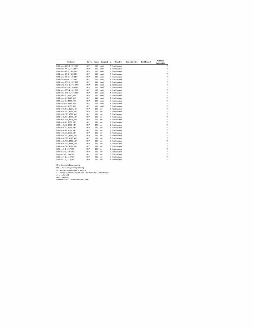
Instance Solver Nodes Demand Id Objective Best objective Best boundRuntime
(seconds)
l100-rand-0.25-5_1573_MIP MIP 100 rand 5 loadbalance T
l100-rand-0.5-1_1557_MIP MIP 100 rand 1 loadbalance T
l100-rand-0.5-2_1605_MIP MIP 100 rand 2 loadbalance T
l100-rand-0.5-3_1580_MIP MIP 100 rand 3 loadbalance T
l100-rand-0.5-4_1649_MIP MIP 100 rand 4 loadbalance T
l100-rand-0.5-5_1573_MIP MIP 100 rand 5 loadbalance T
l100-rand-0.75-1_1557_MIP MIP 100 rand 1 loadbalance T
l100-rand-0.75-2_1605_MIP MIP 100 rand 2 loadbalance T
l100-rand-0.75-3_1580_MIP MIP 100 rand 3 loadbalance T
l100-rand-0.75-4_1649_MIP MIP 100 rand 4 loadbalance T
l100-rand-0.75-5_1573_MIP MIP 100 rand 5 loadbalance T
l100-rand-1-1_1557_MIP MIP 100 rand 1 loadbalance T
l100-rand-1-2_1605_MIP MIP 100 rand 2 loadbalance T
l100-rand-1-3_1580_MIP MIP 100 rand 3 loadbalance T
l100-rand-1-4_1649_MIP MIP 100 rand 4 loadbalance T
l100-rand-1-5_1573_MIP MIP 100 rand 5 loadbalance T
l100-rw-0.25-1_1557_MIP MIP 100 rw 1 loadbalance T
l100-rw-0.25-2_1605_MIP MIP 100 rw 2 loadbalance T
l100-rw-0.25-3_1580_MIP MIP 100 rw 3 loadbalance T
l100-rw-0.25-4_1649_MIP MIP 100 rw 4 loadbalance T
l100-rw-0.25-5_1573_MIP MIP 100 rw 5 loadbalance T
l100-rw-0.5-1_1557_MIP MIP 100 rw 1 loadbalance T
l100-rw-0.5-2_1605_MIP MIP 100 rw 2 loadbalance T
l100-rw-0.5-3_1580_MIP MIP 100 rw 3 loadbalance T
l100-rw-0.5-4_1649_MIP MIP 100 rw 4 loadbalance T
l100-rw-0.5-5_1573_MIP MIP 100 rw 5 loadbalance T
l100-rw-0.75-1_1557_MIP MIP 100 rw 1 loadbalance T
l100-rw-0.75-2_1605_MIP MIP 100 rw 2 loadbalance T
l100-rw-0.75-3_1580_MIP MIP 100 rw 3 loadbalance T
l100-rw-0.75-4_1649_MIP MIP 100 rw 4 loadbalance T
l100-rw-0.75-5_1573_MIP MIP 100 rw 5 loadbalance T
l100-rw-1-1_1557_MIP MIP 100 rw 1 loadbalance T
l100-rw-1-2_1605_MIP MIP 100 rw 2 loadbalance T
l100-rw-1-3_1580_MIP MIP 100 rw 3 loadbalance T
l100-rw-1-4_1649_MIP MIP 100 rw 4 loadbalance T
l100-rw-1-5_1573_MIP MIP 100 rw 5 loadbalance T
CP … Constraint Programming
MIP … Mixed Integer Programming
Id … Identification number of instance
T … Maximum allowed computation time exploited (3.600 seconds)
rw … real world
rand … random
bold characters … optimal solution found
Related Documents