RESOURCE ALLOCATION IN COMPUTER NETWORKS joão taveira araújo @jta

Welcome message from author
This document is posted to help you gain knowledge. Please leave a comment to let me know what you think about it! Share it to your friends and learn new things together.
Transcript

RESOURCE ALLOCATION
IN COMPUTER NETWORKS
joão taveira araújo@jta

A S S U M P T I O N

A S S U M P T I O N

How do you share a network?

TCP


“How do you share a network?”

TCP

TCPan answer (maybe)

“How do you share a network?”
the question

A S S U M P T I O N
given an answer

A S S U M P T I O N
given an answer
can’t fully understand

A S S U M P T I O N
given an answer
never worked through question
can’t fully understand

T H I S T A L K
‘62
‘74
‘88
‘07

T H I S T A L K
‘62
‘74
‘88
‘07
different interpretations of the same question

T H I S T A L K
‘62
‘74
‘88
‘07
foundational papers

O B J E C T I V E S

O B J E C T I V E S
how did we get here

O B J E C T I V E S
how did we get here
what assumptions

at what cost
O B J E C T I V E S
how did we get here
what assumptions

T H I S T A L K

Let us consider the synthesis of a communication network which will allow several hundred major communications stations to talk with one another after an enemy attack. As a criterion of survivability we elect to use the percentage of stations both surviving the physical attack and remaining in electrical connection with the largest single group of surviving stations. This criterion is chosen as a conservative measure of the ability of the surviving stations to operate together as a coherent entity after the attack. This means that small groups of stations isolated from the single largest group are considered to be ineffective.
Although one can draw a wide variety of networks, they all factor into two components: centralized (or star) and distributed (or grid or mesh) (see Fig. 1).
The centralized network is obviously vulnerable as destruction of a single central node destroys communication between the end stations. In practice, a mixture of star and mesh components is used to form communications networks. For example, type (b) in Fig. 1 shows the hierarchical structure of a set of stars connected in the form of a larger star with an
Paul Baran‘62 On Distributed Communications Networks
I N T RO D U C T I O N
“Let us consider the synthesis of
a communication network which
will allow several hundred major
communications stations to talk
with one another after an enemy
attack.”

Paul Baran‘62 On Distributed Communications Networks

capacity and the switching flexibility to allow transmission between any ith station and any jth station, provided a path can be drawn from the ith to the jth station.
Starting with a network composed of an array of stations connected as in Fig. 3, an assigned percentage of nodes and links is destroyed. If, after this operation, it is still possible to draw a line to connect the ith station to the jth station, the ith and jth stations are said to be connected.
Node Destruction
Figure 4 indicates network performance as a function of the probability of destruction for each separate node. If the expected "noise" was destruction caused by conventional hardware failure, the failures would be randomly distributed through the network. But, if the disturbance were caused by enemy attack, the possible "worst cases" must be considered.
To bisect a 32-link network requires direction of 288 weapons each with a probability of kill, pk = 0.5, or 160 with a pk = 0.7, to produce over an 0.9 probability of successfully bisecting the network. If hidden alternative command is allowed, then the largest single group would still have an expected value of almost 50 per cent of the initial stations surviving intact. If this raid misjudges complete availability of weapons, or complete knowledge of all links in the cross section, or the effects of the weapons against each and every link, the raid fails. The high risk of such raids against highly parallel structures causes examination of alternative attack policies. Consider the following uniform raid example. Assume that 2,000 weapons are deployed against a 1000-station
Paul Baran‘62 On Distributed Communications Networks
E X A M I N AT I O N O F A D I S T R I B U T E D N E T WO R K

capacity and the switching flexibility to allow transmission between any ith station and any jth station, provided a path can be drawn from the ith to the jth station.
Starting with a network composed of an array of stations connected as in Fig. 3, an assigned percentage of nodes and links is destroyed. If, after this operation, it is still possible to draw a line to connect the ith station to the jth station, the ith and jth stations are said to be connected.
Node Destruction
Figure 4 indicates network performance as a function of the probability of destruction for each separate node. If the expected "noise" was destruction caused by conventional hardware failure, the failures would be randomly distributed through the network. But, if the disturbance were caused by enemy attack, the possible "worst cases" must be considered.
To bisect a 32-link network requires direction of 288 weapons each with a probability of kill, pk = 0.5, or 160 with a pk = 0.7, to produce over an 0.9 probability of successfully bisecting the network. If hidden alternative command is allowed, then the largest single group would still have an expected value of almost 50 per cent of the initial stations surviving intact. If this raid misjudges complete availability of weapons, or complete knowledge of all links in the cross section, or the effects of the weapons against each and every link, the raid fails. The high risk of such raids against highly parallel structures causes examination of alternative attack policies. Consider the following uniform raid example. Assume that 2,000 weapons are deployed against a 1000-station
“(…) destruction caused by
conventional hardware failure,
the failures would be randomly
distributed through the network.
But, if the disturbance were
caused by enemy attack, the
possible "worst cases" must be
considered.”
Paul Baran‘62 On Distributed Communications Networks
E X A M I N AT I O N O F A D I S T R I B U T E D N E T WO R K

the ith station to the jth station, the ith and jth stations are said to be connected.
Node Destruction
Figure 4 indicates network performance as a function of the probability of destruction for each separate node. If the expected "noise" was destruction caused by conventional hardware failure, the failures would be randomly distributed through the network. But, if the disturbance were caused by enemy attack, the possible "worst cases" must be considered.
To bisect a 32-link network requires direction of 288 weapons each with a probability of kill, pk = 0.5, or 160 with a pk = 0.7, to produce over an 0.9 probability of successfully bisecting the network. If hidden alternative command is allowed, then the largest single group would still have an expected value of almost 50 per cent of the initial stations surviving intact. If this raid misjudges complete availability of weapons, or complete knowledge of all links in the cross section, or the effects of the weapons against each and every link, the raid fails. The high risk of such raids against highly parallel structures causes examination of alternative attack policies. Consider the following uniform raid example. Assume that 2,000 weapons are deployed against a 1000-station network. The stations are so spaced that destruction of two stations with a single weapon is unlikely. Divide the 2,000 weapons into two equal 1000-weapon salvos. Assume any probability of destruction of a single node from a single weapon less than 1.0; for example, 0.5. Each weapon on the first salvo has a 0.5 probability of destroying its target. But, each weapon of the second salvo has only a 0.25 probability, since one-half the targets have already
Paul Baran‘62 On Distributed Communications Networks
E X A M I N AT I O N O F A D I S T R I B U T E D N E T WO R K
“To bisect a 32-link network requires
direction of 288 weapons each with
a probability of kill, pk = 0.5, or 160
with a pk = 0.7, to produce over an
0.9 probability of successfully
bisecting the network.”
the ith station to the jth station, the ith and jth stations are said to be connected.
Node Destruction
Figure 4 indicates network performance as a function of the probability of destruction for each separate node. If the expected "noise" was destruction caused by conventional hardware failure, the failures would be randomly distributed through the network. But, if the disturbance were caused by enemy attack, the possible "worst cases" must be considered.
To bisect a 32-link network requires direction of 288 weapons each with a probability of kill, pk = 0.5, or 160 with a pk = 0.7, to produce over an 0.9 probability of successfully bisecting the network. If hidden alternative command is allowed, then the largest single group would still have an expected value of almost 50 per cent of the initial stations surviving intact. If this raid misjudges complete availability of weapons, or complete knowledge of all links in the cross section, or the effects of the weapons against each and every link, the raid fails. The high risk of such raids against highly parallel structures causes examination of alternative attack policies. Consider the following uniform raid example. Assume that 2,000 weapons are deployed against a 1000-station network. The stations are so spaced that destruction of two stations with a single weapon is unlikely. Divide the 2,000 weapons into two equal 1000-weapon salvos. Assume any probability of destruction of a single node from a single weapon less than 1.0; for example, 0.5. Each weapon on the first salvo has a 0.5 probability of destroying its target. But, each weapon of the second salvo has only a 0.25 probability, since one-half the targets have already
Paul Baran‘62 On Distributed Communications Networks
E X A M I N AT I O N O F A D I S T R I B U T E D N E T WO R K

mode is also used for levels six and eight.[1]
Each node and link in the array of Fig. 2 has the capacity and the switching flexibility to allow transmission between any ith station and any jth station, provided a path can be drawn from the ith to the jth station.
Starting with a network composed of an array of stations connected as in Fig. 3, an assigned percentage of nodes and links is destroyed. If, after this operation, it is still possible to draw a line to connect the ith station to the jth station, the ith and jth stations are said to be connected.
Node Destruction
Figure 4 indicates network performance as a function of the probability of destruction for each separate node. If the expected "noise" was destruction caused by conventional hardware failure, the failures would be randomly distributed through the network. But, if the disturbance were caused by enemy attack, the possible "worst cases" must be considered.
To bisect a 32-link network requires direction of 288 weapons each with a probability of kill, pk = 0.5, or 160 with a pk = 0.7, to produce over an 0.9 probability of successfully bisecting the network. If hidden alternative command is allowed, then the largest single group would still have an expected value of almost 50 per cent of the initial stations surviving intact. If this raid misjudges complete availability of weapons, or complete knowledge of all links in the cross section, or the effects of the weapons against each and every link, the raid fails. The high risk of such raids against highly parallel structures causes
Paul Baran‘62 On Distributed Communications Networks
E X A M I N AT I O N O F A D I S T R I B U T E D N E T WO R K

4. First, extremely survivable networks can be built using a moderately low redundancy of connectivity level. Redundancy levels on the order of only three permit withstanding extremely heavy level attacks with negligible additional loss to communications. Secondly, the survivability curves have sharp break-points. A network of this type will withstand an increasing attack level until a certain point is reached, beyond which the network rapidly deteriorates. Thus, the optimum degree of redundancy can be chosen as a function of the expected level of attack. Further redundancy buys little. The redundancy level required to survive even very heavy attacks is not great--on the order of only three or four times that of the minimum span network.
Link Destruction
In the previous example we have examined network performance as a function of the destruction of the nodes (which are better targets than links). We shall now re-examine the same network, but using unreliable links. In particular, we want to know how unreliable the links may be without further degrading the performance of the network.
Figure 5 shows the results for the case of perfect nodes; only the links fail. There is little system degradation caused even using extremely unreliable links--on the order of 50 per cent down-time--assuming all nodes are working.
Combination Link and Node Destruction
The worst case is the composite effect of failures of both the links and the nodes. Figure 6 shows the effect of link failure upon a network having 40 per
Paul Baran‘62 On Distributed Communications Networks
E X A M I N AT I O N O F A D I S T R I B U T E D N E T WO R K

Link Destruction
In the previous example we have examined network performance as a function of the destruction of the nodes (which are better targets than links). We shall now re-examine the same network, but using unreliable links. In particular, we want to know how unreliable the links may be without further degrading the performance of the network.
Figure 5 shows the results for the case of perfect nodes; only the links fail. There is little system degradation caused even using extremely unreliable links--on the order of 50 per cent down-time--assuming all nodes are working.
Combination Link and Node Destruction
The worst case is the composite effect of failures of both the links and the nodes. Figure 6 shows the effect of link failure upon a network having 40 per cent of its nodes destroyed. It appears that what would today be regarded as an unreliable link can be used in a distributed network almost as effectively as perfectly reliable links. Figure 7 examines the result of 100 trial cases in order to estimate the probability density distribution of system performance for a mixture of node and link failures. This is the distribution of cases for 20 per cent nodal damage and 35 per cent link damage.
Paul Baran‘62 On Distributed Communications Networks
E X A M I N AT I O N O F A D I S T R I B U T E D N E T WO R K


We will soon be living in an era in which we cannot guarantee survivability of any single point. However, we can stil l design systems in which system destruction requires the enemy to pay the price of destroying n of n stations. If n is made sufficiently large, it can be shown that highly survivable system structures can be built - even in the thermonuclear era. In order to build such networks and systems we will have to use a large number of elements. We are interested in knowing how inexpensive these elements may be and still permit the system to operate reliably. There is a strong relationship between element cost and element reliability. To design a system that must anticipate a worst-case destruction of both enemy attack and normal system failures, one can combine the failures expected by enemy attack together with the failures caused by normal reliability problems, provided the enemy does not know which elements are inoperative. Our future systems design problem is that of building very reliable systems out of the described set of unreliable e l ements a t lowest cos t . In choos ing the communications links of the future, digital links appear increasingly attractive by permitting low-cost switching and low-cost links. For example, if "perfect
Paul Baran‘62 On Distributed Communications Networks
O N A F U T U R E S Y S T E M D E V E L O P M E N T
“(…) highly survivable system
structures can be built - even in
the thermonuclear era.”

We will soon be living in an era in which we cannot guarantee survivability of any single point. However, we can stil l design systems in which system destruction requires the enemy to pay the price of destroying n of n stations. If n is made sufficiently large, it can be shown that highly survivable system structures can be built - even in the thermonuclear era. In order to build such networks and systems we will have to use a large number of elements. We are interested in knowing how inexpensive these elements may be and still permit the system to operate reliably. There is a strong relationship between element cost and element reliability. To design a system that must anticipate a worst-case destruction of both enemy attack and normal system failures, one can combine the failures expected by enemy attack together with the failures caused by normal reliability problems, provided the enemy does not know which elements are inoperative. Our future systems design problem is that of building very reliable systems out of the described set of unreliable e l ements a t lowest cos t . In choos ing the communications links of the future, digital links appear increasingly attractive by permitting low-cost switching and low-cost links. For example, if "perfect
Paul Baran‘62 On Distributed Communications Networks
O N A F U T U R E S Y S T E M D E V E L O P M E N T
“(…) have to use a large number
of elements. We are interested
in knowing how inexpensive
these elements may be”

high data rate links in emergencies.[2]
Satellites
The problem of building a reliable network using satellites is somewhat similar to that of building a communications network with unreliable links. When a satellite is overhead, the link is operative. When a satellite is not overhead, the link is out of service. Thus, such links are highly compatible with the type of system to be described.
Variable Data Rate Links
In a conventional circuit switched system each of the tandem links requires matched transmission bandwidths. In order to make fullest use of a digital link, the post-error-removal data rate would have to vary, as it is a function of noise level. The problem then is to build a communication network made up of links of variable data rate to use the communication resource most efficiently.
Variable Data Rate Users
We can view both the links and the entry point nodes of a multiple-user all-digital communications system as elements operating at an ever changing data rate. From instant to instant the demand for transmission will vary.
We would like to take advantage of the average demand over all users instead of having to allocate a full peak demand channel to each. Bits can become a common denominator of loading for economic charging of customers. We would like to efficiently
Paul Baran‘62 On Distributed Communications Networks
O N A F U T U R E S Y S T E M D E V E L O P M E N T

of system to be described.
Variable Data Rate Links
In a conventional circuit switched system each of the tandem links requires matched transmission bandwidths. In order to make fullest use of a digital link, the post-error-removal data rate would have to vary, as it is a function of noise level. The problem then is to build a communication network made up of links of variable data rate to use the communication resource most efficiently.
Variable Data Rate Users
We can view both the links and the entry point nodes of a multiple-user all-digital communications system as elements operating at an ever changing data rate. From instant to instant the demand for transmission will vary.
We would like to take advantage of the average demand over all users instead of having to allocate a full peak demand channel to each. Bits can become a common denominator of loading for economic charging of customers. We would like to efficiently hand le both those user s who make h igh l y intermittent bit demands on the network, and those who make long-term continuous, low bit demands.
Common User
In communications, as in transportation, it is more economical for many users to share a common resource rather than each to build his own system--particularly when supplying intermittent or occasional service. This intermittency of service is
Paul Baran‘62 On Distributed Communications Networks
O N A F U T U R E S Y S T E M D E V E L O P M E N T

Variable Data Rate Users
We can view both the links and the entry point nodes of a multiple-user all-digital communications system as elements operating at an ever changing data rate. From instant to instant the demand for transmission will vary.
We would like to take advantage of the average demand over all users instead of having to allocate a full peak demand channel to each. Bits can become a common denominator of loading for economic charging of customers. We would like to efficiently hand le both those user s who make h igh l y intermittent bit demands on the network, and those who make long-term continuous, low bit demands.
Common User
In communications, as in transportation, it is more economical for many users to share a common resource rather than each to build his own system--particularly when supplying intermittent or occasional service. This intermittency of service is highly characteristic of digital communication requirements. Therefore, we would like to consider the interconnection, one day, of many all-digital links to provide a resource optimized for the handling of data for many potential intermittent users--a new common-user system.
Figure 9 demonstrates the basic notion. A wide mixture of different digital transmission links is combined to form a common resource divided among many potent ia l u ser s . But , each o f these communications links could possibly have a different data rate. Therefore, we shall next consider how links
Paul Baran‘62 On Distributed Communications Networks
O N A F U T U R E S Y S T E M D E V E L O P M E N T
“more economical to share a
common (…) resource optimized
for the handling of data”

common-user system.
Figure 9 demonstrates the basic notion. A wide mixture of different digital transmission links is combined to form a common resource divided among many potent ia l u ser s . But , each o f these communications links could possibly have a different data rate. Therefore, we shall next consider how links of different data rates may be interconnected.
Standard Message Block
Present common carrier communications networks, used for digital transmission, use links and concepts originally designed for another purpose--voice. These systems are built around a frequency division multiplexing link-to-link interface standard. The standard between links is that of data rate. Time division multiplexing appears so natural to data transmission that we might wish to consider an alternative approach--a standardized message block as a network interface standard. While a standardized message block is common in many computer-communications applications, no serious attempt has ever been made to use it as a universal standard. A universally standardized message block would be composed of perhaps 1024 bits. Most of the message block would be reserved for whatever type data is to be transmitted, while the remainder would contain housekeeping information such as error detection and routing data, as in Fig. 10.
As we move to the future, there appears to be an increasing need for a standardized message block for all-digital communications networks. As data rates increase, the velocity of propagation over long links becomes an increasingly important consideration.[3]
Paul Baran‘62 On Distributed Communications Networks
O N A F U T U R E S Y S T E M D E V E L O P M E N T
“Time division multiplexing
appears so natural to data that
we might wish to consider an
alternative approach - a
standardized message block”

Telecommunications textbooks arrive at a fire according to a Poisson distribution

“How do you share a network?”

priority marking(defense contractor)


IP type of service field


Act I AN EXERCISE TO THE READER

A R P A N E T

Act II Scientific Positivism


A protocol that supports the sharing of resources that exist in different packet switching networks is presented. The protocol provides for variation in individual network packet sizes, transmission failures, sequencing, flow control, end-to-end error checking, and the creation and destruction of logical process-to-process connections. Some implementation issues are considered, and problems such as internetwork routing, accounting, and timeouts are exposed.
In the last few years considerable effort has been expended on the design and implementation of packet switching networks [1]-[7],[14],[17]. A principle reason for developing such networks has been to facilitate the sharing of computer resources. A packet communication network includes a transportation mechanism for delivering data between computers or between computers and terminals. To make the data meaningful, computer and terminals share a common protocol (i.e, a set of agreed upon conventions). Several protocols have already been developed for this purpose [8]-[12],[16]. However, these protocols have addressed only the problem of communication on the
Vinton G. Cerf and Robert E. Kahn‘74 A Protocol for Packet Network Intercommunication
A B S T R AC T
I N T RO D U C T I O N
A protocol that supports the sharing of resources that exist in different packet switching networks is presented. The protocol provides for variation in individual network packet sizes, transmission failures, sequencing, flow control, end-to-end error checking, and the creation and destruction of logical process-to-process connections. Some implementation issues are considered, and problems such as internetwork routing, accounting, and timeouts are exposed.

In the last few years considerable effort has been expended on the design and implementation of packet switching networks [1]-[7],[14],[17]. A principle reason for developing such networks has been to facilitate the sharing of computer resources. A packet communication network includes a transportation mechanism for delivering data between computers or between computers and terminals. To make the data meaningful, computer and terminals share a common protocol (i.e, a set of agreed upon conventions). Several protocols have already been developed for this purpose [8]-[12],[16]. However, these protocols have addressed only the problem of communication on the
Vinton G. Cerf and Robert E. Kahn‘74 A Protocol for Packet Network Intercommunication
A B S T R AC T
I N T RO D U C T I O N
“A protocol that supports the
sharing of resources that exist in
different packet switching
networks is presented.”
A protocol that supports the sharing of resources that exist in different packet switching networks is presented. The protocol provides for variation in individual network packet sizes, transmission failures, sequencing, flow control, end-to-end error checking, and the creation and destruction of logical process-to-process connections. Some implementation issues are considered, and problems such as internetwork routing, accounting, and timeouts are exposed.

A protocol that supports the sharing of resources that exist in different packet switching networks is presented. The protocol provides for variation in individual network packet sizes, transmission failures, sequencing, flow control, end-to-end error checking, and the creation and destruction of logical process-to-process connections. Some implementation issues are considered, and problems such as internetwork routing, accounting, and timeouts are exposed.
In the last few years considerable effort has been expended on the design and implementation of packet switching networks [1]-[7],[14],[17]. A principle reason for developing such networks has been to facilitate the sharing of computer resources. A packet communication network includes a transportation mechanism for delivering data between computers or between computers and terminals. To make the data meaningful, computer and terminals share a common protocol (i.e, a set of agreed upon conventions). Several protocols have already been developed for this purpose [8]-[12],[16]. However, these protocols have addressed only the problem of communication on the
Vinton G. Cerf and Robert E. Kahn‘74 A Protocol for Packet Network Intercommunication
A B S T R AC T
I N T RO D U C T I O N
packet fragmentation
transmission failures
sequencing
flow control
error checking
connection setup

\
N
W GATEWAY GATEWAY
Fig. 2. Three networks interconnected by two GATEWAYS.
(may be null) b- Internetwork Header
LOCAL HEADER SOURCE DESTINATION SEQUENCE NO. BYTE COUNTIFLAG FIELD\ TEXT ICHECKSUM
Fig. 3. Internetwork packet format (fields not shown to scale).
worlc header, is illustrated in Fig. 3 . The source and desti- nation entries uniforndy and uniquely identify the address of every HOST in the composite network. Addressing is a subject of considerable complexity which is discussed in greater detail in the next section. Thenext two entries in the header provide a sequence number and a byte count that may be used to properly sequence the packets upon delivery to the dest'ination and may also enable the GATEWAYS to detect fault conditions affecting the packet. The flag field is used to convey specific control information and is discussed in the sect.ion on retransmission and duplicate detection later. The remainder of the packet consists of text for delivery to the destination and a trailing check sum used for end-to-end software verification. The GATEWAY does not modify the text and merely forwards the check sum along without computing or recomputing it.
Each nct\r-orlr may need to augment the packet format before i t can pass t'hrough the individual netu-ork. We havc indicated a local header in the figure which is prefixed to the beginning of the packet. This local header is intro- duced nlcrely t'o illustrate the concept of embedding an intcrnetworlc packet in the format of the individual net#- work through which the packet must pass. It will ob- viously vary in its exact form from network to network and may even be unnecessary in some cases. Although not explicitly indicated in the figure, i t is also possiblc that a local trailer may be appended to the end of the packet.
Unless all transnlitted packets are legislatively re- stricted to be small enough to be accepted by cvcry in- dividual network, the GATEWAY may be forced to split a packet int,o two or more smaller packets. This action is called fragmentation and must be done in such a way that the destination is able to piece togcthcr the fragmcntcd packet. It is clear that the internct\vorl; header format imposes a minimum packet size which all networks must carry (obviously all networks will want to carry packets larger than this minimum). We believe the long rangc growth and development of internctworl; com- munication would be seriously inhibited by specifying how much larger than the minimum a paclcct sizc can bc, for tjhc follo\\-ing reasons.
1) If a maximum permitted packet size is specified then i t bccomos impossible to completely isolate the internal
packet size parameters of one network from the internal packet size parameters of all other networks.
2 ) It would be very difficult to increase the maximum permitted packet size in response to new technology (e.g., large memory systems, higher data rate communication facilities, etc.) since this would require the agreement and then implen-rentation by all participating networks.
3 ) Associative addressing and pa.clcet encryption may require the size of a particular pa'ckct to cxpand during transit for incorporation of new information.
Provision for fragmentation (regardless of where i t is performed) permits packet sixc variations to be handled on an individual network basis without global admin- istration and also permits HOSTS and processes to be insulated from changes in the pa,ckct sizes permitted in any networks through which their data must pass.
If fragmentation must be done, i t appears best to do it upon entering the nest netu-orlc at the GAPEWAY since only t.his GATEWAY (and not the other netLvorlcs) must be awarc of the int.ernal packet size parameters which made the fragmentation necessary.
If a GATEWAY fragnwnts an incoming packet into t'T1-o or more paclcet,s, they must eventually be passed along to the destination HOST as fragnxnts or reassembled for the HOST. It is conceivable that one might desire the GArrEwAY to perform the rea.ssenlbly to simplify the task of the desti- nation HOST (or process) and/or to take advantage of a larger packet size. We take the position tJhat GATEWAYS
should not perform this function since GATEWAY re- assen-rbly can lead to serious buffering problems, potential deadlocks, the necessity for all fragments of a packet to pass through the same GArrEwA>r, and increased dclay in transmission. Furthermore, i t is not sufficient for the
may also have to fragment a paclxt for transmission. Thus the destination HOST must be prepared to do this task.
Let us now turn briefly to the somewhat unusual ac- counting effect 11-hich arises when a packet may be frag- mented by one or more GATEWAYS. We assume, for simplicity, that each network initially charges a fixed rate per paclrct transmitted, regardless of distancc, and if one network can handle a larger packet size t lml another, i t charges a proportionally larger price per paclcct. We also assume tha t a subsequent increase in any network's packet size docs not result in additional cost per packet to its users. The charge to a uscr thus remains basically constant through any net which must fragmcnt a packet. The unusual cffcct occurs when a paclcct is fragmented into smaller packets which must individually pass through a subsequent nctxvork with a larger packet size than the original unfragmented packet. We expect that most net- works \vi11 naturally selech packet sizes close to one anot'her, but in any case, an increase in packet size in one net, even when it causes fragmentation, will not increase the cost of transnlission and may actually decrease it. I n the event that any other packet charging policies (than
GATEWAYS to provide this function since the final GATEWAY
Vinton G. Cerf and Robert E. Kahn‘74 A Protocol for Packet Network Intercommunication
643 IEEE TRANSACTIONS ON COMMUNICATIOKS, MAY 197'
byte identification-sequence number
First Message
(SEQ = k)
Fig. 7. Assignment of sequence numbers.
LH = Local Header IH = InternetwolX Header
CK = Checksum PH = Process Header
Fig. 5 . Creation of segments and packets from messages.
32 32 16 16 En
Source Port DertinatianIPort Wmdow ACK Text (Field sizes in bits1 ,+JPlOLIIl Hed..LJ Fig. 6. Segment format (process header and text).
segment is extracted from the message by the source TCP and formatted for internetwork transmission, the relative location of the first byte of segment text is used as the sequence number for the packet. The byte count field in the internetwork header accounts for all the text in-the segment (but docs not include the check-sum bytes or t'he bytes in either internetxork or process header). We emphasize that the sequence number associated with a given packet is unique only to the pair of ports that are communicating (see Fig. 7). Arriving packets are ex- amined to determine for which port they are intended. The sequence numbers on each arriving packet are then used to determine the relative location of the packet text in the messages under reconstruction. We note that this allows the exact position of the data in the reconstructed message to be determined even n-hen pieces 'are still missing.
Every segment produced by a source TCP is packaged in a single internetwork packet and a check sum is com- puted over the text and process header associated with the segment.
The splitting of messages into segments by the TCP and the potential splitting of segments into smaller pieces by GATEWAYS creates the necessity for indic,ating to- the destination TCP when the end of a segment (ES) has arrived and when the end of a message (EM) has arrived. The flag field of the internetwork header is used for this purpose (see Fig. S) .
The ES flag is set by the source TCP each time it prc- pares a segment for transmission. If it should happen that the message is completely contained in the segment, then the EM flag would also be set. The EM flag is also set on the last segment of a message, if the message could not be contained in one segment, These two flags are used by the destination TCP, respectively, to discover the presence of a check sum for a given segment and to discover that a complete message has arrived.
The ES and EM flags in the internetwork header are known to the GATEWAY and are of special importance when packets must be split apart for propagation through the next local network. We illustrate their use with an ex- ample in Fig. 9.
The original message -4 in Fig. 9 is shown split into two segments A and Az and formatted' by the TC1' into a pair
16 bits
Y E S M S
N L
_ . . E E R
I l l I L End of Message when set = 1
End of Segment when set = 1 Release Use of ProcessIPort when set=l Synchronize to Packet Sequence Number when set = 1
Fig. 8. Internetwork header flag field.
- 1000 bytes . 100 101 102 . . .
I TEXT OFMESSAGE A
SEQ CT ES EM 500 2
SRC CK TEXT 0 PH 1 500 100 DST
1- internetwork header --+ segment 1 split by source TCP . -.
SEQ CT ES EM 500 2
SRC CK TEXT 1 PH 1 500 600 DST
250 2
SRC packet A1 TEXT 0 / PH 0 250 100 DST
~~~ ~
split by GATEWAY
SRC packet A12 CK TEXT 0 PH 1 250 350 DST
SRC TEXT packet AZ1 0 PH 0 250 600 DST
SRC packet A22 CK TEXT 1 PH 1 250 850 DST
Fig. 9. Message splitting and packet splitting.
of internetwork packets. Packets A1 and A2 have the ES bits set, and A2 has its En1 bit set as well. Whe packet A1 passes through the GATEWAY, it is split into t w pieces: packet A 11 for which neither EM nor ES bits a1 xt , and packet A12 whose ES bit is set. Similarly, packt A , is split such that the first piece, packet A21, has neithe bit set, but packet A22 has both bits set. The scyuenc number field (SEQ) and the byte count field (CT) of eac packet is modified by the GATEWAY to properly identif the t'ext bytes of each packet. The GATEWAY need on1 cxamine the internetmork header to do fragmentation.
The destination TCP, upon reassembling segment 9 will detect the ES flag and will verify the check sum knows is contained in packet iz12. Upon rcceipt of pack( A z 2 , assuming all other packets have arrived, the dest nation TCP detects that it has reassembled a complel message and can now advise the destination process of il rcceipt,:

\
N
W GATEWAY GATEWAY
Fig. 2. Three networks interconnected by two GATEWAYS.
(may be null) b- Internetwork Header
LOCAL HEADER SOURCE DESTINATION SEQUENCE NO. BYTE COUNTIFLAG FIELD\ TEXT ICHECKSUM
Fig. 3. Internetwork packet format (fields not shown to scale).
worlc header, is illustrated in Fig. 3 . The source and desti- nation entries uniforndy and uniquely identify the address of every HOST in the composite network. Addressing is a subject of considerable complexity which is discussed in greater detail in the next section. Thenext two entries in the header provide a sequence number and a byte count that may be used to properly sequence the packets upon delivery to the dest'ination and may also enable the GATEWAYS to detect fault conditions affecting the packet. The flag field is used to convey specific control information and is discussed in the sect.ion on retransmission and duplicate detection later. The remainder of the packet consists of text for delivery to the destination and a trailing check sum used for end-to-end software verification. The GATEWAY does not modify the text and merely forwards the check sum along without computing or recomputing it.
Each nct\r-orlr may need to augment the packet format before i t can pass t'hrough the individual netu-ork. We havc indicated a local header in the figure which is prefixed to the beginning of the packet. This local header is intro- duced nlcrely t'o illustrate the concept of embedding an intcrnetworlc packet in the format of the individual net#- work through which the packet must pass. It will ob- viously vary in its exact form from network to network and may even be unnecessary in some cases. Although not explicitly indicated in the figure, i t is also possiblc that a local trailer may be appended to the end of the packet.
Unless all transnlitted packets are legislatively re- stricted to be small enough to be accepted by cvcry in- dividual network, the GATEWAY may be forced to split a packet int,o two or more smaller packets. This action is called fragmentation and must be done in such a way that the destination is able to piece togcthcr the fragmcntcd packet. It is clear that the internct\vorl; header format imposes a minimum packet size which all networks must carry (obviously all networks will want to carry packets larger than this minimum). We believe the long rangc growth and development of internctworl; com- munication would be seriously inhibited by specifying how much larger than the minimum a paclcct sizc can bc, for tjhc follo\\-ing reasons.
1) If a maximum permitted packet size is specified then i t bccomos impossible to completely isolate the internal
packet size parameters of one network from the internal packet size parameters of all other networks.
2 ) It would be very difficult to increase the maximum permitted packet size in response to new technology (e.g., large memory systems, higher data rate communication facilities, etc.) since this would require the agreement and then implen-rentation by all participating networks.
3 ) Associative addressing and pa.clcet encryption may require the size of a particular pa'ckct to cxpand during transit for incorporation of new information.
Provision for fragmentation (regardless of where i t is performed) permits packet sixc variations to be handled on an individual network basis without global admin- istration and also permits HOSTS and processes to be insulated from changes in the pa,ckct sizes permitted in any networks through which their data must pass.
If fragmentation must be done, i t appears best to do it upon entering the nest netu-orlc at the GAPEWAY since only t.his GATEWAY (and not the other netLvorlcs) must be awarc of the int.ernal packet size parameters which made the fragmentation necessary.
If a GATEWAY fragnwnts an incoming packet into t'T1-o or more paclcet,s, they must eventually be passed along to the destination HOST as fragnxnts or reassembled for the HOST. It is conceivable that one might desire the GArrEwAY to perform the rea.ssenlbly to simplify the task of the desti- nation HOST (or process) and/or to take advantage of a larger packet size. We take the position tJhat GATEWAYS
should not perform this function since GATEWAY re- assen-rbly can lead to serious buffering problems, potential deadlocks, the necessity for all fragments of a packet to pass through the same GArrEwA>r, and increased dclay in transmission. Furthermore, i t is not sufficient for the
may also have to fragment a paclxt for transmission. Thus the destination HOST must be prepared to do this task.
Let us now turn briefly to the somewhat unusual ac- counting effect 11-hich arises when a packet may be frag- mented by one or more GATEWAYS. We assume, for simplicity, that each network initially charges a fixed rate per paclrct transmitted, regardless of distancc, and if one network can handle a larger packet size t lml another, i t charges a proportionally larger price per paclcct. We also assume tha t a subsequent increase in any network's packet size docs not result in additional cost per packet to its users. The charge to a uscr thus remains basically constant through any net which must fragmcnt a packet. The unusual cffcct occurs when a paclcct is fragmented into smaller packets which must individually pass through a subsequent nctxvork with a larger packet size than the original unfragmented packet. We expect that most net- works \vi11 naturally selech packet sizes close to one anot'her, but in any case, an increase in packet size in one net, even when it causes fragmentation, will not increase the cost of transnlission and may actually decrease it. I n the event that any other packet charging policies (than
GATEWAYS to provide this function since the final GATEWAY
Vinton G. Cerf and Robert E. Kahn‘74 A Protocol for Packet Network Intercommunication643 IEEE TRANSACTIONS ON COMMUNICATIOKS, MAY 197'
byte identification-sequence number
First Message
(SEQ = k)
Fig. 7. Assignment of sequence numbers.
LH = Local Header IH = InternetwolX Header
CK = Checksum PH = Process Header
Fig. 5 . Creation of segments and packets from messages.
32 32 16 16 En
Source Port DertinatianIPort Wmdow ACK Text (Field sizes in bits1 ,+JPlOLIIl Hed..LJ Fig. 6. Segment format (process header and text).
segment is extracted from the message by the source TCP and formatted for internetwork transmission, the relative location of the first byte of segment text is used as the sequence number for the packet. The byte count field in the internetwork header accounts for all the text in-the segment (but docs not include the check-sum bytes or t'he bytes in either internetxork or process header). We emphasize that the sequence number associated with a given packet is unique only to the pair of ports that are communicating (see Fig. 7). Arriving packets are ex- amined to determine for which port they are intended. The sequence numbers on each arriving packet are then used to determine the relative location of the packet text in the messages under reconstruction. We note that this allows the exact position of the data in the reconstructed message to be determined even n-hen pieces 'are still missing.
Every segment produced by a source TCP is packaged in a single internetwork packet and a check sum is com- puted over the text and process header associated with the segment.
The splitting of messages into segments by the TCP and the potential splitting of segments into smaller pieces by GATEWAYS creates the necessity for indic,ating to- the destination TCP when the end of a segment (ES) has arrived and when the end of a message (EM) has arrived. The flag field of the internetwork header is used for this purpose (see Fig. S) .
The ES flag is set by the source TCP each time it prc- pares a segment for transmission. If it should happen that the message is completely contained in the segment, then the EM flag would also be set. The EM flag is also set on the last segment of a message, if the message could not be contained in one segment, These two flags are used by the destination TCP, respectively, to discover the presence of a check sum for a given segment and to discover that a complete message has arrived.
The ES and EM flags in the internetwork header are known to the GATEWAY and are of special importance when packets must be split apart for propagation through the next local network. We illustrate their use with an ex- ample in Fig. 9.
The original message -4 in Fig. 9 is shown split into two segments A and Az and formatted' by the TC1' into a pair
16 bits
Y E S M S
N L
_ . . E E R
I l l I L End of Message when set = 1
End of Segment when set = 1 Release Use of ProcessIPort when set=l Synchronize to Packet Sequence Number when set = 1
Fig. 8. Internetwork header flag field.
- 1000 bytes . 100 101 102 . . .
I TEXT OFMESSAGE A
SEQ CT ES EM 500 2
SRC CK TEXT 0 PH 1 500 100 DST
1- internetwork header --+ segment 1 split by source TCP . -.
SEQ CT ES EM 500 2
SRC CK TEXT 1 PH 1 500 600 DST
250 2
SRC packet A1 TEXT 0 / PH 0 250 100 DST
~~~ ~
split by GATEWAY
SRC packet A12 CK TEXT 0 PH 1 250 350 DST
SRC TEXT packet AZ1 0 PH 0 250 600 DST
SRC packet A22 CK TEXT 1 PH 1 250 850 DST
Fig. 9. Message splitting and packet splitting.
of internetwork packets. Packets A1 and A2 have the ES bits set, and A2 has its En1 bit set as well. Whe packet A1 passes through the GATEWAY, it is split into t w pieces: packet A 11 for which neither EM nor ES bits a1 xt , and packet A12 whose ES bit is set. Similarly, packt A , is split such that the first piece, packet A21, has neithe bit set, but packet A22 has both bits set. The scyuenc number field (SEQ) and the byte count field (CT) of eac packet is modified by the GATEWAY to properly identif the t'ext bytes of each packet. The GATEWAY need on1 cxamine the internetmork header to do fragmentation.
The destination TCP, upon reassembling segment 9 will detect the ES flag and will verify the check sum knows is contained in packet iz12. Upon rcceipt of pack( A z 2 , assuming all other packets have arrived, the dest nation TCP detects that it has reassembled a complel message and can now advise the destination process of il rcceipt,:
643 IEEE TRANSACTIONS ON COMMUNICATIOKS, MAY 197'
byte identification-sequence number
First Message
(SEQ = k)
Fig. 7. Assignment of sequence numbers.
LH = Local Header IH = InternetwolX Header
CK = Checksum PH = Process Header
Fig. 5 . Creation of segments and packets from messages.
32 32 16 16 En
Source Port DertinatianIPort Wmdow ACK Text (Field sizes in bits1 ,+JPlOLIIl Hed..LJ Fig. 6. Segment format (process header and text).
segment is extracted from the message by the source TCP and formatted for internetwork transmission, the relative location of the first byte of segment text is used as the sequence number for the packet. The byte count field in the internetwork header accounts for all the text in-the segment (but docs not include the check-sum bytes or t'he bytes in either internetxork or process header). We emphasize that the sequence number associated with a given packet is unique only to the pair of ports that are communicating (see Fig. 7). Arriving packets are ex- amined to determine for which port they are intended. The sequence numbers on each arriving packet are then used to determine the relative location of the packet text in the messages under reconstruction. We note that this allows the exact position of the data in the reconstructed message to be determined even n-hen pieces 'are still missing.
Every segment produced by a source TCP is packaged in a single internetwork packet and a check sum is com- puted over the text and process header associated with the segment.
The splitting of messages into segments by the TCP and the potential splitting of segments into smaller pieces by GATEWAYS creates the necessity for indic,ating to- the destination TCP when the end of a segment (ES) has arrived and when the end of a message (EM) has arrived. The flag field of the internetwork header is used for this purpose (see Fig. S) .
The ES flag is set by the source TCP each time it prc- pares a segment for transmission. If it should happen that the message is completely contained in the segment, then the EM flag would also be set. The EM flag is also set on the last segment of a message, if the message could not be contained in one segment, These two flags are used by the destination TCP, respectively, to discover the presence of a check sum for a given segment and to discover that a complete message has arrived.
The ES and EM flags in the internetwork header are known to the GATEWAY and are of special importance when packets must be split apart for propagation through the next local network. We illustrate their use with an ex- ample in Fig. 9.
The original message -4 in Fig. 9 is shown split into two segments A and Az and formatted' by the TC1' into a pair
16 bits
Y E S M S
N L
_ . . E E R
I l l I L End of Message when set = 1
End of Segment when set = 1 Release Use of ProcessIPort when set=l Synchronize to Packet Sequence Number when set = 1
Fig. 8. Internetwork header flag field.
- 1000 bytes . 100 101 102 . . .
I TEXT OFMESSAGE A
SEQ CT ES EM 500 2
SRC CK TEXT 0 PH 1 500 100 DST
1- internetwork header --+ segment 1 split by source TCP . -.
SEQ CT ES EM 500 2
SRC CK TEXT 1 PH 1 500 600 DST
250 2
SRC packet A1 TEXT 0 / PH 0 250 100 DST
~~~ ~
split by GATEWAY
SRC packet A12 CK TEXT 0 PH 1 250 350 DST
SRC TEXT packet AZ1 0 PH 0 250 600 DST
SRC packet A22 CK TEXT 1 PH 1 250 850 DST
Fig. 9. Message splitting and packet splitting.
of internetwork packets. Packets A1 and A2 have the ES bits set, and A2 has its En1 bit set as well. Whe packet A1 passes through the GATEWAY, it is split into t w pieces: packet A 11 for which neither EM nor ES bits a1 xt , and packet A12 whose ES bit is set. Similarly, packt A , is split such that the first piece, packet A21, has neithe bit set, but packet A22 has both bits set. The scyuenc number field (SEQ) and the byte count field (CT) of eac packet is modified by the GATEWAY to properly identif the t'ext bytes of each packet. The GATEWAY need on1 cxamine the internetmork header to do fragmentation.
The destination TCP, upon reassembling segment 9 will detect the ES flag and will verify the check sum knows is contained in packet iz12. Upon rcceipt of pack( A z 2 , assuming all other packets have arrived, the dest nation TCP detects that it has reassembled a complel message and can now advise the destination process of il rcceipt,:
wat?!?

SEQ and SYN in internetwork header

SEQ and SYN in internetwork header
if there’s an internetwork header, and a process header, what the hell is TCP?

We suppose that processes wish to communicate in ful l duplex with their correspondents using unbounded but finite length messages. A single character might constitute the text of a message from a process to a terminal or vice versa. An entire page of characters might constitute the text of a message from a file to a process. A data stream (e.g. a continuously generated bit string) can be represented as a sequence of finite length messages.
Within a HOST we assume that existence of a transmission control program (TCP) which handles the transmission and acceptance of messages on behalf of the processes it serves. The TCP is in turn served by one or more packet switches connected to the HOST in which the TCP resides. Processes that want to communicate present messages to the TCP for transmission, and TCP’s deliver incoming messages to the appropriate destination processes.
We allow the TCP to break up messages into segments because the destination may restrict the amount of data that may arrive, because the local network may limit the maximum transmissin size, or because the TCP may need to share its resources among many processes concurrently. Furthermore, we constrain the length of a segment to an integral number of 8-bit bytes. This uniformity is most helpful in simplifying the software needed with HOST machines of different natural word lengths.
Provision at the process level can be made for padding a message that is not an integral number of
Vinton G. Cerf and Robert E. Kahn‘74 A Protocol for Packet Network Intercommunication
P RO C E S S L E V E L C O M M U N I C AT I O N
“Within a HOST we assume the
existence of a transmission
control program (TCP) which
handles transmission”

TCP is a userspace networking stack
SEQ and SYN in internetwork header

No transmission can be 100 percent reliable. We propose a timeout and positive acknowledgement mechanism which will allow TCP’s to recover from packet losses from one HOST to another. A TCP t ransmit s packets and wa i t s for rep l i e s (acknowledgements) that are carried in the reverse packet stream. If no acknowledgement for a particular packet is received, the TCP will retransmit. It i s our expectat ion that the HOST leve l retransmission mechanism, which is described in the following paragraphs, will not be called upon very often in practice. Evidence already exists that individual networks can be effectively constructed without this feature. However, the inclusion of a HOST retransmission capability makes it possible to recover from occasional network problems and allows a wide range of HOST protocol strategies to be incorporated. We envision it will occasionally be invoked to a l low HOST accommodation to infrequent overdemands for limited buffer resources, and otherwise not used much.
Any retransmission policy requires some means by which the receiver can detect duplicate arrivals. Even
Vinton G. Cerf and Robert E. Kahn‘74 A Protocol for Packet Network Intercommunication
R E T R A N S M I S S I O N A N D D U P L I C AT E D E T E C T I O N
“No transmission can be 100
percent reliable.”
“retransmission (…) will not be
called upon very often in
practice. Evidence already exists
that individual networks can be
effectively constructed without
this feature.”

TCP is a userspace networking stack
SEQ and SYN in internetwork header
retransmissions are pathological

a wide range of HOST protocol strategies to be incorporated. We envision it will occasionally be invoked to a l low HOST accommodation to infrequent overdemands for limited buffer resources, and otherwise not used much.
Any retransmission policy requires some means by which the receiver can detect duplicate arrivals. Even if an infinite number of distinct packet sequence numbers were available, the receiver would still have the problem of knowing how long to remember previously received packets in order to detect duplicates. Matters are complicated by the fact that only a finite number of distinct sequence numbers are in fact available, and if they are reused, the receiver must be ab le to d i s t ingu i sh between ne w transmissions and retransmissions.
A window strategy, similar to that used by the French CYCLADES system (voie virtuelle transmission mode [8]) and the ARPANET very distant HOST connection [18]), is proposed here (see Fig. 10). Suppose that the sequence number field in the internetwork header permits sequence numbers to range from 0 to n − 1. We assume that the sender will not transmit more than w bytes without receiving an acknowledgment. The w bytes serve as the window (see Fig. 11). Clearly, w must be less than n. The rules for sender and receiver are as follows.
Sender: Let L be the sequence number associated with the left window edge.
1) The sender transmits bytes from segments whose text lies between L and up to L + w − 1.
2) On timeout (duration unspecified), the sender
Vinton G. Cerf and Robert E. Kahn‘74 A Protocol for Packet Network Intercommunication
R E T R A N S M I S S I O N A N D D U P L I C AT E D E T E C T I O N
CRRF AND KAHX: PACKET NETWORK INTERCOMMUNICATION 643
RETRANSMISSION AND DUPLICATE DETECTION
No transmission can be 100 percent reliable. We propose a timeout and positive acknowledgment mecha- nism which will allow TCP’s to recover from packet losses from one HOST to another. A TCP transmits packets and waits for replies (acknowledgements) that are carried in the reverse packet stream. If no acknowledgment for a particular packet is received, the TCP will retransmit. It is our expectation that the HOST level retransmission mechanism, which is described in the following para- graphs, will not be called upon very often in practice. Evidence already exists2 that individual networks can be effectively constructed without this feature. However, the inclusion of a HOST retransmission capability makes i t possible to recover from occasional network problems and allows a wide range of HOST protocol strategies to be in- corporated. We envision it will occasionally be invoked to allow HOST accommodation to infrequent overdemands for limited buffer resources, and otherwise not used much.
Any retransmission policy requires some means by which the receiver can detect duplicate arrivals. Even if an infinite number of distinct packet sequence numbers were available, the receiver mould still have the problem of knowing how long to remember previously received packets in order to detect duplicates. Matters are compli- cated by the fact that only a finite number of distinct sequence numbers are in fact available, and if they are reused, the receiver must be able to distinguish between new transmissions and retransmissions.
A window strategy, similar to that used by the French CYCLADES system (voie virtuelle transmission mode [SI) and the ARPANET very distant HOST connection [lS], is proposed here (see Fig. 10).
Suppose that the sequence number field in the inter- network header permits sequence numbers to range from 0 to n - 1. We assume that the sender will not transmit more than w bytes without receiving an acknowledgment. The w bytes serve as the window (see Fig. 11). Clearly, w must be less than n. The rules for sender and receiver are as follows.
Sender: Let L be the sequence number associated with the left window edge.
1) The sender transmits bytes from segments whose text lies between L and up to L + w - 1.
2 ) On timeout (duration unspecified), the sender retransmits unacknowledged bytes.
3) On receipt of acknowledgment consisting of the receiver’s current left window edge, the sender’s, left window edge is advanced over the aclrnowledged bytes (advancing the right window edge implicitly).
Receiver: 1) Arriving packets yhose sequence numbers coincide
with the receiver’s current left window edge are acknowl- edged by sending to the source the next sequence number
Left Window Edge I
0 n- 1 a+w- 1 a
1- window -4 I< packet sequence number space -1
Fig. 10. The window concept.
Source Address
I Address Destination I
6 7
8 9
10
Next Read Position
End Read Position
Timeout
Fig. 11. Conceptual TCB format.
expected. This effectively acknowledges bytes in between. The left window edge is advanced to the next sequence number expected.
2) Packets arriving with a sequence number to the left of the window edge (or, in fact, outside of the window) are discarded, and the current left window edge is returned as acknowledgment.
3) Packets whose sequence numbers lie within the receiver’s window but do not coinicide with the receiver’s left window edge are optionally kept or discarded, but are not acknowledged. This is the case when packets arrive out of order.
We make some observations on this strategy. First, all computations with sequence numbers and window edges must be made modulo n (e.g., byte 0 follows byte n - 1). Second, w must be less than n/Y; otherwise a retrans- mission may appear to the receiver to be a new trans- mission in the case that the receiver has accepted a window’s worth of incoming packcts, but all acknowledg- ments havc been lost. Third, the receiver can either save or discard arriving packets whose !sequence numbers do not coincide with the receiver’s left window. Thus, in the simplest implementation, the receiver need not buffer more than one packet per message stream if space is critical. Fourth, multiple packets can be aclrnowledgcd simultaneously. Fifth, the receiver is able to deliver messages to processes in their proper order as a natural result of the reassembly mechanism. Sixth, when dupli- cates arc detected, the acknowledgment method used naturally works to rcsynchronizc scndcr and receiver. Furthermore, if the rcccivcr accepts packets whose sequcnce numbcrs lie within the current window but
The ARPANET is one such example. required that a retransmission not appear to be a new transmission. Actually n/2 is merely a convenient number to use; it is only

broken into two 300-byte packets.
On retransmission, the same packet might be broken into three 200-byte packets going through a different HOST. Since each byte has a sequence number, there is no confusion at the receiving TCP. We leave for later the issue of initially synchronizing the sender and receiver left window edges and the window size.
Every segment that arrives at the destination TCP is ultimately acknowlegded by returning the sequence number of the next segment which must be passed to the process (it may not yet have arrived).
Earlier we described the use of a sequence number space and window to aid in duplicate detection. Acknowledgments are carried in the process header (see Fig. 6) and along with them there is provision for a “suggested window” which the receiver can use to control the flow of data from the sender. This is intended to be the main component of the process flow control mechanism. The receiver is free to vary the window size according to any algorithm it desires so long as the window size never exceeds half the sequence number space.
This flow control mechanism is exceedingly powerful and flexible and does not suffer from synchronization troubles that may be encountered by incremental buffer allocation schemes [9], [10]. However, it relies heavily on an effective retransmission strategy. The receiver can reduce the window even while packets are en route from the sender whose window is presently larger. The net effect of this reduction will be that the receiver may discard incoming packets (they may be outside the window) and reiterate the current window size along with a current window
Vinton G. Cerf and Robert E. Kahn‘74 A Protocol for Packet Network Intercommunication
CRRF AND KAHX: PACKET NETWORK INTERCOMMUNICATION 643
RETRANSMISSION AND DUPLICATE DETECTION
No transmission can be 100 percent reliable. We propose a timeout and positive acknowledgment mecha- nism which will allow TCP’s to recover from packet losses from one HOST to another. A TCP transmits packets and waits for replies (acknowledgements) that are carried in the reverse packet stream. If no acknowledgment for a particular packet is received, the TCP will retransmit. It is our expectation that the HOST level retransmission mechanism, which is described in the following para- graphs, will not be called upon very often in practice. Evidence already exists2 that individual networks can be effectively constructed without this feature. However, the inclusion of a HOST retransmission capability makes i t possible to recover from occasional network problems and allows a wide range of HOST protocol strategies to be in- corporated. We envision it will occasionally be invoked to allow HOST accommodation to infrequent overdemands for limited buffer resources, and otherwise not used much.
Any retransmission policy requires some means by which the receiver can detect duplicate arrivals. Even if an infinite number of distinct packet sequence numbers were available, the receiver mould still have the problem of knowing how long to remember previously received packets in order to detect duplicates. Matters are compli- cated by the fact that only a finite number of distinct sequence numbers are in fact available, and if they are reused, the receiver must be able to distinguish between new transmissions and retransmissions.
A window strategy, similar to that used by the French CYCLADES system (voie virtuelle transmission mode [SI) and the ARPANET very distant HOST connection [lS], is proposed here (see Fig. 10).
Suppose that the sequence number field in the inter- network header permits sequence numbers to range from 0 to n - 1. We assume that the sender will not transmit more than w bytes without receiving an acknowledgment. The w bytes serve as the window (see Fig. 11). Clearly, w must be less than n. The rules for sender and receiver are as follows.
Sender: Let L be the sequence number associated with the left window edge.
1) The sender transmits bytes from segments whose text lies between L and up to L + w - 1.
2 ) On timeout (duration unspecified), the sender retransmits unacknowledged bytes.
3) On receipt of acknowledgment consisting of the receiver’s current left window edge, the sender’s, left window edge is advanced over the aclrnowledged bytes (advancing the right window edge implicitly).
Receiver: 1) Arriving packets yhose sequence numbers coincide
with the receiver’s current left window edge are acknowl- edged by sending to the source the next sequence number
Left Window Edge I
0 n- 1 a+w- 1 a
1- window -4 I< packet sequence number space -1
Fig. 10. The window concept.
Source Address
I Address Destination I
6 7
8 9
10
Next Read Position
End Read Position
Timeout
Fig. 11. Conceptual TCB format.
expected. This effectively acknowledges bytes in between. The left window edge is advanced to the next sequence number expected.
2) Packets arriving with a sequence number to the left of the window edge (or, in fact, outside of the window) are discarded, and the current left window edge is returned as acknowledgment.
3) Packets whose sequence numbers lie within the receiver’s window but do not coinicide with the receiver’s left window edge are optionally kept or discarded, but are not acknowledged. This is the case when packets arrive out of order.
We make some observations on this strategy. First, all computations with sequence numbers and window edges must be made modulo n (e.g., byte 0 follows byte n - 1). Second, w must be less than n/Y; otherwise a retrans- mission may appear to the receiver to be a new trans- mission in the case that the receiver has accepted a window’s worth of incoming packcts, but all acknowledg- ments havc been lost. Third, the receiver can either save or discard arriving packets whose !sequence numbers do not coincide with the receiver’s left window. Thus, in the simplest implementation, the receiver need not buffer more than one packet per message stream if space is critical. Fourth, multiple packets can be aclrnowledgcd simultaneously. Fifth, the receiver is able to deliver messages to processes in their proper order as a natural result of the reassembly mechanism. Sixth, when dupli- cates arc detected, the acknowledgment method used naturally works to rcsynchronizc scndcr and receiver. Furthermore, if the rcccivcr accepts packets whose sequcnce numbcrs lie within the current window but
The ARPANET is one such example. required that a retransmission not appear to be a new transmission. Actually n/2 is merely a convenient number to use; it is only
“a ‘suggested window’ which
the receiver can use to control
the flow of data from the sender.
This is intended to be the main
component of the process flow
control mechanism.”
F L OW C O N T RO L

TCP is a userspace networking stack
SEQ and SYN in internetwork header
retransmissions are pathological
the resource is the host

TCP is a userspace networking stack
SEQ and SYN in internetwork header
retransmissions are pathological
the resource is the host
no UDP

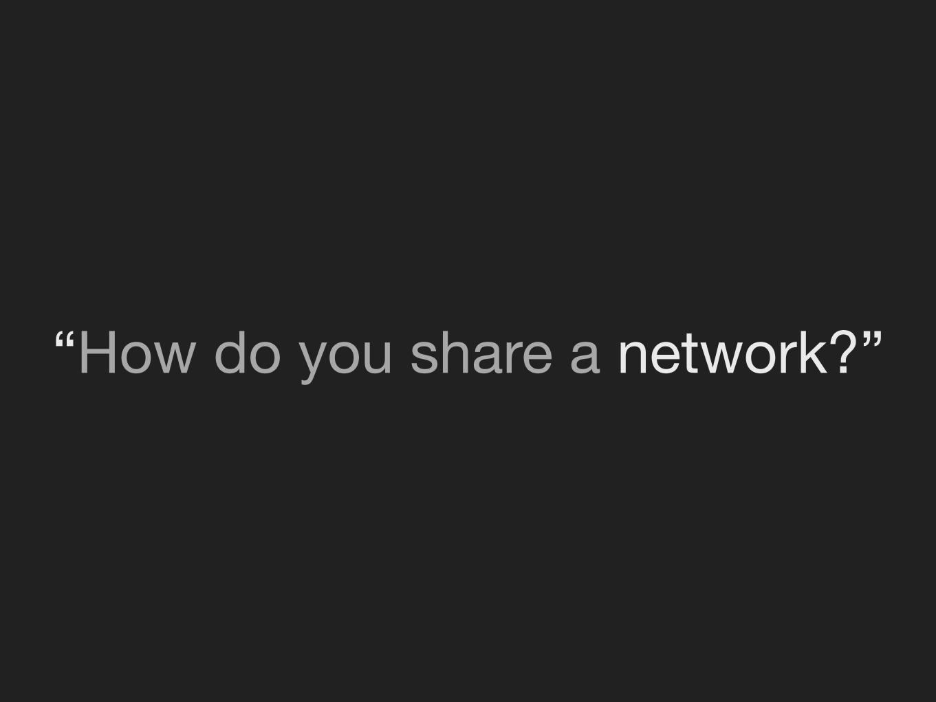
“How do you share a network?”

flow control(systems engineer)
x.25
flow control
diagnostics
connection setup
hop-by-hop reliability

Act II Scientific Positivism

Act III HARSH, BITTER REALITY

The authors wish to thank a number of colleagues for helpful comments during early discussions of international network protocols, especially R. Metcalfe, R. Scantlebury, D. Walden, and H. Zimmerman; D. Davies and L. Pouzin who constructively commented on the fragmentation and accounting issues; and S. Crocker who commented on the creation and destruction of associations.
Vinton G. Cerf and Robert E. Kahn‘74 A Protocol for Packet Network Intercommunication
AC K N OW L E D G E M E N T S
“The authors wish to thank (…)
especially R. Metcalfe (…)”

BOB METCALFE

what if instead of all this…

what if instead of all this…
x.25
flow control
diagnostics
connection setup
hop-by-hop reliability

what if instead of all this…
x.25
flow control
diagnostics
connection setup
hop-by-hop reliability
???
…i did nothing?

ethernet


R F C 1 2 9 6
1981 1982 1983 1984 1985 1986 1987
30,000
0
5000
10,000
15,000
20,000
25,000
Year
Numb
er of
hosts

In October of '86, the Internet had the first of what became a series of 'congestion collapses'. During this period, the data throughput from LBL to UC Berkeley (sites separated by 400 yards and three IMP hops) dropped from 32 Kbps to 40 bps. Mike Karels and I were fascinated by this sudden factor-of-thousand drop in bandwidth and embarked on an investigation of why things had gotten so bad. We wondered, in particular, if the 4.3BSD (Berkeley UNIX) TCP was mis-behaving or if it could be tuned to work better under abysmal network conditions. The answer to both of these questions was "yes".
Since that time, we have put seven new algorithms into the 4BSDTCP:(i) round-trip-time variance estimation(ii) exponential retransmit timer backoff(iii) slow-start(iv) more aggressive receiver ack policy(v) dynamic window sizing on congestion(vi) Karn's clamped retransmit backoff(vii) fast retransmitOur measurements and the reports of beta testers suggest that the final product is fairly good at dealing
Van Jacobson‘88 Congestion Avoidance and Control

“In October of '86, the Internet
had the first of what became a
series of 'congestion collapses’.
(…) were fascinated by this
sudden factor-of-thousand drop
in bandwidth and embarked on
an investigation of why things
had gotten so bad.”
In October of '86, the Internet had the first of what became a series of 'congestion collapses'. During this period, the data throughput from LBL to UC Berkeley (sites separated by 400 yards and three IMP hops) dropped from 32 Kbps to 40 bps. Mike Karels and I were fascinated by this sudden factor-of-thousand drop in bandwidth and embarked on an investigation of why things had gotten so bad. We wondered, in particular, if the 4.3BSD (Berkeley UNIX) TCP was mis-behaving or if it could be tuned to work better under abysmal network conditions. The answer to both of these questions was "yes".
Since that time, we have put seven new algorithms into the 4BSDTCP:(i) round-trip-time variance estimation(ii) exponential retransmit timer backoff(iii) slow-start(iv) more aggressive receiver ack policy(v) dynamic window sizing on congestion(vi) Karn's clamped retransmit backoff(vii) fast retransmitOur measurements and the reports of beta testers suggest that the final product is fairly good at dealing
Van Jacobson‘88 Congestion Avoidance and Control

Van Jacobson‘88 Congestion Avoidance and Control
o
Z o~
g ~ 69 o 0. o
o
?* d,
..y':":" o /
.,,"
e ~
0 2 4 6 8 10
Send Time (sec)
Trace data of the start of a TCP conversat ion be tween t w o Sun 3/50s runn ing Sun os 3.5 (the 4.3BSD TCP). The two Suns were on different Ethemets connected by IP gateways driving a 230.4 Kbs point-to-point l ink (essentially the setup shown in fig. 7). Each dot is a 512 data-byte packet. The x-axis is the time the packet was sent. The y-axis is the sequence number in the packet header. Thus a vertical array of dots indicate back-to-back packets and two dots with the same y but different x indicate a retransmit. 'Desirable' behavior on this graph would be a relatively smooth line of clots extending diagonally from the lower left to the upper right. The slope of this line would equal the available bandwidth. Nothing in this trace resembles desirable behavior. The dashed line shows the 20 KBps bandwidth available for this connection. Only 35% of this bandwidth was used; the rest was wasted on retransmits. Almost everything is retransmitted at ]east once and data from 54 to 58 KB is sent five times.
Figure 3: Startup behavior of TCP without Slow-start
that R and the variation in R increase quickly with load. If the load is p (the ratio of average arrival rate to average departure rate), R and aR scale like (1 - p ) - l . To make this concrete, if the network is running at 75% of capacity, as the Arpanet was in last April 's collapse, one should expect round-trip-time to vary by a factor of sixteen (±2~).
The TCP protocol specification, [RFC793], suggests estimating mean round trip time via the low-pass filter
R = c~R + ( 1 - ~ )M
where R is the average RTT estimate, M is a round trip time measurement from the most recently acked data packet, and c~ is a filter gain constant with a suggested value of 0.9. Once the R estimate is updated, the re- transmit t imeout interval, rto, for the next packet sent is set to fiR.
The parameter fl accounts for RTT variation (see [Cla82], section 5). The suggested fl = 2 can adapt to loads of at most 30%. Above this point, a connection will respond to load increases by retransmitt ing packets that have only been delayed in transit. This forces the network to do useless work, wasting bandwid th on du- plicates of packets that will be delivered, at a time when it's known to be having trouble with useful work. I.e., this is the network equivalent of pouring gasoline on a fire.
We developed a cheap method for estimating vari- ation (see appendix A) 3 and the resulting retransmit timer essentially eliminates spurious retransmissions.
3 We are far from the first to recognize that t ransport needs to esti- mate both mean and variation. See, for example, [Edg83]. But we do think our estimator is simpler than most.
ACM SIGCOMM - 1 6 1 - Computer Communicat ion Review
what if instead of all this…

Van Jacobson‘88 Congestion Avoidance and Control
o
Z o~
g ~ 69 o 0. o
o
?* d,
..y':":" o /
.,,"
e ~
0 2 4 6 8 10
Send Time (sec)
Trace data of the start of a TCP conversat ion be tween t w o Sun 3/50s runn ing Sun os 3.5 (the 4.3BSD TCP). The two Suns were on different Ethemets connected by IP gateways driving a 230.4 Kbs point-to-point l ink (essentially the setup shown in fig. 7). Each dot is a 512 data-byte packet. The x-axis is the time the packet was sent. The y-axis is the sequence number in the packet header. Thus a vertical array of dots indicate back-to-back packets and two dots with the same y but different x indicate a retransmit. 'Desirable' behavior on this graph would be a relatively smooth line of clots extending diagonally from the lower left to the upper right. The slope of this line would equal the available bandwidth. Nothing in this trace resembles desirable behavior. The dashed line shows the 20 KBps bandwidth available for this connection. Only 35% of this bandwidth was used; the rest was wasted on retransmits. Almost everything is retransmitted at ]east once and data from 54 to 58 KB is sent five times.
Figure 3: Startup behavior of TCP without Slow-start
that R and the variation in R increase quickly with load. If the load is p (the ratio of average arrival rate to average departure rate), R and aR scale like (1 - p ) - l . To make this concrete, if the network is running at 75% of capacity, as the Arpanet was in last April 's collapse, one should expect round-trip-time to vary by a factor of sixteen (±2~).
The TCP protocol specification, [RFC793], suggests estimating mean round trip time via the low-pass filter
R = c~R + ( 1 - ~ )M
where R is the average RTT estimate, M is a round trip time measurement from the most recently acked data packet, and c~ is a filter gain constant with a suggested value of 0.9. Once the R estimate is updated, the re- transmit t imeout interval, rto, for the next packet sent is set to fiR.
The parameter fl accounts for RTT variation (see [Cla82], section 5). The suggested fl = 2 can adapt to loads of at most 30%. Above this point, a connection will respond to load increases by retransmitt ing packets that have only been delayed in transit. This forces the network to do useless work, wasting bandwid th on du- plicates of packets that will be delivered, at a time when it's known to be having trouble with useful work. I.e., this is the network equivalent of pouring gasoline on a fire.
We developed a cheap method for estimating vari- ation (see appendix A) 3 and the resulting retransmit timer essentially eliminates spurious retransmissions.
3 We are far from the first to recognize that t ransport needs to esti- mate both mean and variation. See, for example, [Edg83]. But we do think our estimator is simpler than most.
ACM SIGCOMM - 1 6 1 - Computer Communicat ion Review
what if instead of all this…aggravating
retransmissions

(vii) fast retransmitOur measurements and the reports of beta testers suggest that the final product is fairly good at dealing with congested conditions on the Internet.This paper is a brief description of (i) - (v) and the rationale behind them. (vi) is an algorithm recently developed by Phil Karn of Bell Communications Research, described in [KP87]. (vii) is described in a soon-to-be-published RFC.
Algorithms (i) - (v) spring from one observation: The flow on a TCP connection (or ISO TP-4 or Xerox NS SPP connection) should obey a 'conservation of packets' principle. And, if this principle were obeyed, congestion collapse would become the exception rather than the rule. Thus congestion control involves finding places that violate conservation and fixing them.
By 'conservation of packets' I mean that for a connection 'in equilibrium', i.e., running stably with a full window of data in transit, the packet flow is what a physicist would call 'conservative': A new packet isn't put into the network until an old packet leaves. The physics of flow predicts that systems with this property should be robust in the face of congestion. Observation of the Internet suggests that it was not particularly robust. Why the discrepancy?
There are only three ways for packet conservation to fail:
1. The connection doesn't get to equilibrium, or2. A sender injects a new packet before an old packet has exited, or3. The equilibrium can't be reached because of resource limits along the path.
Van Jacobson‘88 Congestion Avoidance and Control
“(…) should obey a
‘conservation of packets’
principle”

(vii) fast retransmitOur measurements and the reports of beta testers suggest that the final product is fairly good at dealing with congested conditions on the Internet.This paper is a brief description of (i) - (v) and the rationale behind them. (vi) is an algorithm recently developed by Phil Karn of Bell Communications Research, described in [KP87]. (vii) is described in a soon-to-be-published RFC.
Algorithms (i) - (v) spring from one observation: The flow on a TCP connection (or ISO TP-4 or Xerox NS SPP connection) should obey a 'conservation of packets' principle. And, if this principle were obeyed, congestion collapse would become the exception rather than the rule. Thus congestion control involves finding places that violate conservation and fixing them.
By 'conservation of packets' I mean that for a connection 'in equilibrium', i.e., running stably with a full window of data in transit, the packet flow is what a physicist would call 'conservative': A new packet isn't put into the network until an old packet leaves. The physics of flow predicts that systems with this property should be robust in the face of congestion. Observation of the Internet suggests that it was not particularly robust. Why the discrepancy?
There are only three ways for packet conservation to fail:
1. The connection doesn't get to equilibrium, or2. A sender injects a new packet before an old packet has exited, or3. The equilibrium can't be reached because of resource limits along the path.
“(…) for a connection 'in
equilibrium', (…) the packet flow
is what a physicist would call
'conservative': A new packet
isn't put into the network until an
old packet leaves.”
Van Jacobson‘88 Congestion Avoidance and Control
“(…) should obey a
‘conservation of packets’
principle”

Van Jacobson‘88 Congestion Avoidance and Control
slow start

Van Jacobson‘88 Congestion Avoidance and Control
congestion avoidance

Van Jacobson‘88 Congestion Avoidance and Control
..' . f"J /
o _ ..."' ,,# . . .......'"'"" 0 / " 8
o
, / f y / f j , f , . • v o
8 0 -
~" j,Z ZZf "''ff "
o . , , , , , 2 4 6 8 10
Send Time (sec)
Same conditions as the previous figure (same time of day, same Suns, same network path, same buffer and window sizes), except the machines were running the 4.3+TCP with slow-start. No bandwidth is wasted on retransmits but two seconds is spent on the slow-start so the effective bandwidth of this part of the trace is 16 KBps - - two times better than figure 3. (This is slightly misleading: Unlike the previous figure, the slope of the trace is 20 KBps and the effect of the 2 second offset decreases as the trace lengthens. E.g., if this trace had run a minute, the effective bandwidth would have been 19 KBps. The effective bandwidth without slow-start stays at 7 KBps no matter how long the trace.)
Figure 4: Startup behavior of TCP with Slow-start
A pleasant side effect of estimating ~ rather than using a fixed value is that low load as well as high load per- formance improves, particularly over high delay paths such as satellite links (figures 5 and 6).
Another timer mistake is in the backoff after a re- transmit: If a packet has to be retransmitted more than once, h o w should the retransmits be spaced? Only one scheme will work, exponential backoff, but proving this is abi t involved. 4 To finesse a proof, note that a ne twork is, to a very good approximation, a linear system. That is, it is composed of elements that behave like linear op- erators m integrators, delays, gain stages, etc. Linear
4 An in-progress paper attempts a proof. If an IP gateway is viewed as a 'shared resource with fixed capacity', it bears a remarkable resem- blance to the 'ether' in an Ethernet. The retransmit backoff problem is essentially the same as showing that no backoff'slower' than an expo- nential will guarantee stability on an Ethernet. Unfortunately, in the- ory even exponential backoff won't guarantee stability (see [Aid87]). Fortunately, in practise we don't have to deal with the theorist's infi- nite user population and exponential is "good enough".
system theory says that if a system is stable, the stability is exponential. This suggests that an unstable system (a ne twork subject to r andom load shocks and prone to congestive collapse s ) can be stabilized by adding some exponential damping (exponential timer backoff) to its pr imary excitation (senders, traffic sources).
3 Adapting to the path: congestion avoidance
If the timers are in good shape, it is possible to state with some confidence that a t imeout indicates a lost packet and not a broken timer. At this point, something can be done about (3). Packets get lost for two reasons: they
s The phrase congestion collapse (describing a positive feedback in- stability due to poor retransmit timers) is again the coinage of John Nagle, this time from [Nag84].
ACM S IGCOMM - 1 6 2 - Computer Communicat ion Review
o
Z o~
g ~ 69 o 0. o
o
?* d,
..y':":" o /
.,,"
e ~
0 2 4 6 8 10
Send Time (sec)
Trace data of the start of a TCP conversat ion be tween t w o Sun 3/50s runn ing Sun os 3.5 (the 4.3BSD TCP). The two Suns were on different Ethemets connected by IP gateways driving a 230.4 Kbs point-to-point l ink (essentially the setup shown in fig. 7). Each dot is a 512 data-byte packet. The x-axis is the time the packet was sent. The y-axis is the sequence number in the packet header. Thus a vertical array of dots indicate back-to-back packets and two dots with the same y but different x indicate a retransmit. 'Desirable' behavior on this graph would be a relatively smooth line of clots extending diagonally from the lower left to the upper right. The slope of this line would equal the available bandwidth. Nothing in this trace resembles desirable behavior. The dashed line shows the 20 KBps bandwidth available for this connection. Only 35% of this bandwidth was used; the rest was wasted on retransmits. Almost everything is retransmitted at ]east once and data from 54 to 58 KB is sent five times.
Figure 3: Startup behavior of TCP without Slow-start
that R and the variation in R increase quickly with load. If the load is p (the ratio of average arrival rate to average departure rate), R and aR scale like (1 - p ) - l . To make this concrete, if the network is running at 75% of capacity, as the Arpanet was in last April 's collapse, one should expect round-trip-time to vary by a factor of sixteen (±2~).
The TCP protocol specification, [RFC793], suggests estimating mean round trip time via the low-pass filter
R = c~R + ( 1 - ~ )M
where R is the average RTT estimate, M is a round trip time measurement from the most recently acked data packet, and c~ is a filter gain constant with a suggested value of 0.9. Once the R estimate is updated, the re- transmit t imeout interval, rto, for the next packet sent is set to fiR.
The parameter fl accounts for RTT variation (see [Cla82], section 5). The suggested fl = 2 can adapt to loads of at most 30%. Above this point, a connection will respond to load increases by retransmitt ing packets that have only been delayed in transit. This forces the network to do useless work, wasting bandwid th on du- plicates of packets that will be delivered, at a time when it's known to be having trouble with useful work. I.e., this is the network equivalent of pouring gasoline on a fire.
We developed a cheap method for estimating vari- ation (see appendix A) 3 and the resulting retransmit timer essentially eliminates spurious retransmissions.
3 We are far from the first to recognize that t ransport needs to esti- mate both mean and variation. See, for example, [Edg83]. But we do think our estimator is simpler than most.
ACM SIGCOMM - 1 6 1 - Computer Communicat ion Review

C O N G E S T I O N C O N T R O L
fix RTT estimator
slow start (slower than flow control)
congestion avoidance

Act IV

Van Jacobson‘88 Congestion Avoidance and Controlis costly. But an exponential, almost regardless of its time constant, increases so quickly that overestimates are inevitable.
Without justification, I'll state that the best increase policy is to make small, constant changes to the window size:
On no congestion:
W~ = W~_~ + ~ (~ << Wmo=)
where W,.,,a= is the pipesize (the delay-bandwidth prod- uct of the path minus protocol overhead - - i.e., the largest sensible window for the unloaded path). This is the additive increase / multiplicative decrease policy suggested in [JRC87] and the policy we've implemented in TCP. The only difference between the two implemen- tations is the choice of constants for d and u. We used 0.5 and I for reasons partially explained in appendix C. A more complete analysis is in yet another in-progress paper.
The preceding has probably made the congestion control algorithm sound hairy but it's not. Like slow- start, it's three lines of code:
• On any timeout, set cwnd to half the current win- dow size (this is the multiplicative decrease).
• On each ack for new data, increase cwnd by 1/cwnd (this is the additive increase). 10
• When sending, send the minimum of the re- ceiver's advertised window and cwnd.
Note that this algorithm is only congestion avoidance, it doesn't include the previously described slow-start. Since the packet loss that signals congestion will re- sult in a re-start, it will almost certainly be necessary
we have to be sure that during the non-equilibrium window adjust- ment, our control policy allows the gateway enough free bandwidth to dissipate queues that inevitably form due to path testing and traf- fic fluctuations. By an argument similar to the one used to show exponential timer backoff is necessary, it's possible to show that an exponential (multiplicative) window increase policy will be 'faster' than the dissipation time for some traffic mix and, thus, leads to an unbounded growth of the bottleneck queue.
10 This increment rule may be less than obvious. We want to in- crease the window by at most one packet over a time interval of length R (the round trip time). To make the algorithm "self-clocked', it's better to increment by a small amount on each ack rather than by a large amount at the end of the interval. (Assuming, of course, that the sender has effective silly window avoidance (see [Cla82], section 3) and doesn't attempt to send packet fragments because of the frac- tionally sized window.) A window of size cwnd packets will generate at most cwnd acks in one R. Thus an increment of 1/cwnd per ack will increase the window by at most one packet in one R. In TCP, windows and packet sizes are in bytes so the increment translates to maxseg*maxseg/cwnd where maxseg is the maximum segment size and cwnd is expressed in bytes, not packets.
to slow-start in addition to the above. But, because both congestion avoidance and slow-start are triggered by a timeout and both manipulate the congestion win- dow, they are frequently confused. They are actually in- dependent algorithms with completely different objec- tives. To emphasize the difference, the two algorithms have been presented separately even though in prac- tise they should be implemented together. Appendix B describes a combined slow-start/congestion avoidance algorithm. 11
Figures 7 through 12 show the behavior of TCP con- nections with and without congestion avoidance. Al- though the test conditions (e.g., 16 KB windows) were deliberately chosen to stimulate congestion, the test sce- nario isn't far from common practice: The Arpanet IMP end-to-end protocol allows at most eight packets in transit between any pair of gateways. The default 4.3BSD window size is eight packets (4 KB). Thus si- multaneous conversations between, say, any two hosts at Berkeley and any two hosts at MIT would exceed the buffer capacity of the UCB-MIT IMP path and would lead 12 to the behavior shown in the following figures.
4 F u t u r e w o r k : t h e g a t e w a y s i d e o f c o n g e s t i o n c o n t r o l
While algorithms at the transport endpoints can insure the network capacity isn't exceeded, they cannot insure
11We have also developed a rate-based variant of the congestion avoidance algorithm to apply to connectiontess traffic (e.g., domain server queries, RPC requests). Remembering that the goal of the in- crease and decrease policies is bandwidth adjustment, and that 'time' (the controlled parameter in a rate-based scheme) appears in the de- nominator of bandwidth, the algorithm follows immediately: The multiplicative decrease remains a multiplicative decrease (e.g., dou- ble the interval between packets). But subtracting a constant amount from interval does not result in an additive increase in bandwidth. This approach has been tried, e.g., [Kli87] and [PP87], and appears to oscillate badly. To see why, note that for an inter-packet interval / and decrement c, the bandwidth change of a decrease-interval-by- constant policy is
1 1 7 --+ [ - c
a non-linear, and destablizing, increase. An update policy that does result in a linear increase of bandwidth
over time is Odi-- I
a + l i -1 where I i is the interval between sends when the i th packet is sent and c~ is the desired rate of increase in packets per packet/sec.
We have simulated the above algori thm and i t appears to perform well. To test the predictions of that simulation against reality, we have a cooperative project with Sun Microsystems to prototype RPC dynamic congestion control algorithms using NFS as a test-bed (since NFS is known to have congestion problems yet it would be desirable to have it work over the same range of networks as TCP).
12 did lead.
ACM SIGCOMM -165- Computer Communication Review
u = 1
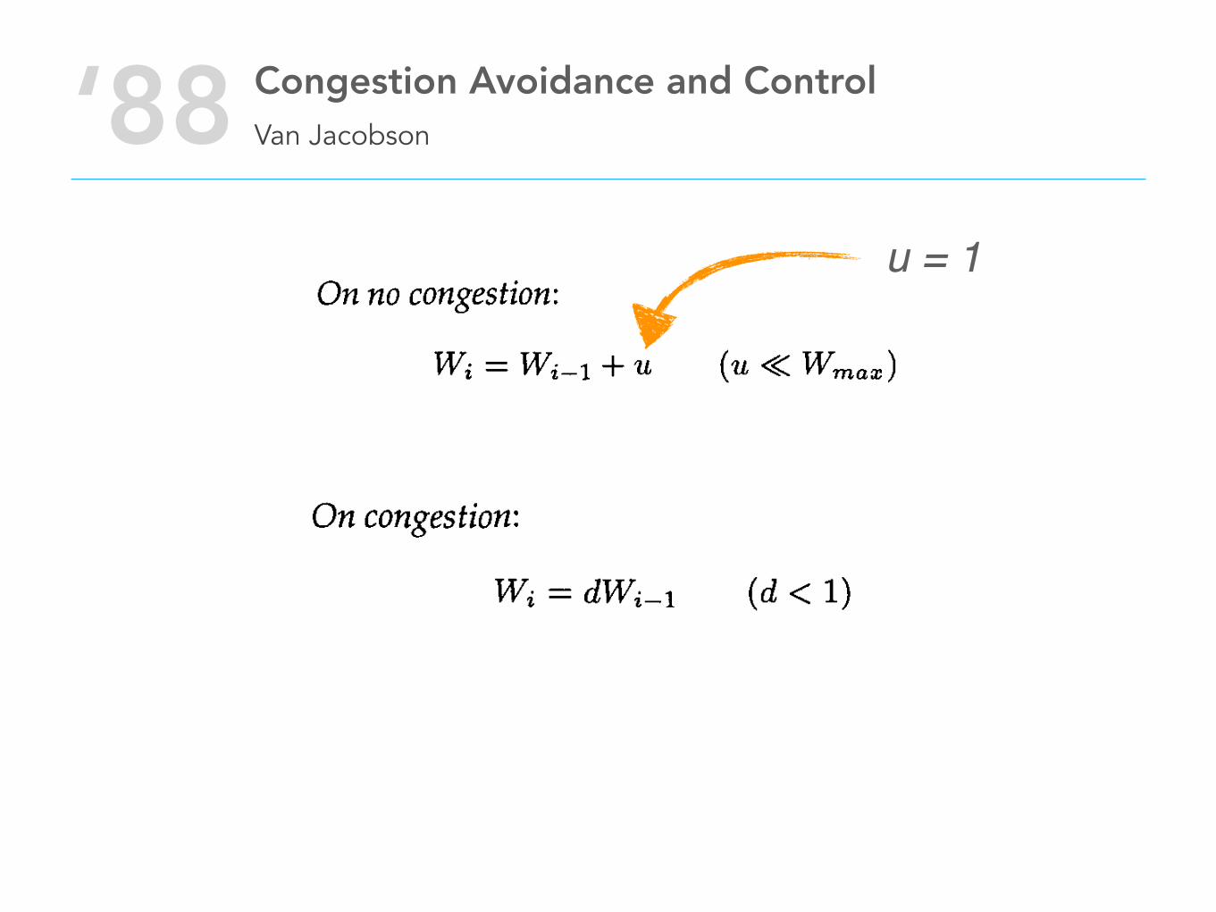
Van Jacobson‘88 Congestion Avoidance and Control
o
,¢
. i . : i i i : ..: ~ : .." ...../i : . , .
.. ~: i • f'." ~" :" ," i-y" D
I T I I I I I I I I 10 20 30 40 50 60 70 80 90 1 O0 110
Packet
Same data as above but the solid line shows a retransmit timer computed according to the algorithm in appendix A.
Figure 6: Performance of a Mean+Variance retransmit timer
retransmits): Li = N + 7Li-1
(These are the first two terms in a Taylor series expan- sion of L(t) . There is reason to believe one might even- tually need a three term, second order model , bu t not until the Internet has g rown substantially.)
When the ne twork is congested, 7 mus t be large and the queue lengths will start increasing exponentially, s The system will stabilize only if the traffic sources throt- tle back at least as quickly as the queues are growing. Since a source controls load in a window-based proto- col by adjusting the size of the window, W , we end up with the sender policy
On congestion:
Wi = dWi_l (d < 1)
I.e., a mult ipl icat ive decrease of the w indow size (which becomes an exponential decrease over t ime if the con- gestion persists).
If there 's no congestion, 7 mus t be near zero and the load approximate ly constant. The ne twork announces, via a d ropped packet, w hen demand is excessive bu t says nothing if a connect ion is using less than its fair
SI.e., the system behaves like Li ,.~ 7Li -1 , a difference equation with the solution
Ln = 7n Lo which goes exponentially to infinity for any 7 > 1.
share (since the ne twork is stateless, it cannot know this). Thus a connect ion has to increase its bandwid th utilization to find out the current limit. E.g., you could have been sharing the path wi th someone else and con- verged to a w ind ow that gives you each half the avail- able bandwidth . If she shuts down, 50% of the band- width will be wasted unless you r w i n d o w size is in- creased. What should the increase policy be?
The first thought is to use a symmetric , multiplica- tive increase, possibly with a longer t ime constant, Wi = bWi-1, 1 < b <_ 1/d. This is a mistake. The result will oscillate wildly and, on the average, deliver poor throughput . There is an analytic reason for this bu t it's tedious to derive. It has to do wi th that fact that it is easy to drive the net into saturation bu t ha rd for the net to recover (what [Kle76], chap. 2.1, calls the rush-hour effect). 9 Thus overest imating the available bandwid th
9In fig. 1, note that the 'pipesize' is 16 packets, 8 in each path, but the sender is using a window of 22 packets. The six excess packets will form a queue at the entry to the bottleneck and that queue cannot shrink, even though the sender carefully clocks out packets at the bottleneck link rate. This stable queue is another, unfortunate, aspect of conservation: The queue would shrink only if the gateway could move packets into the skinny pipe faster than the sender dumped packets into the fat pipe. But the system tunes itself so each time the gateway pulls a packet off the front of its queue, the sender lays a new packet on the end.
A gateway needs excess output capacity (i.e., p < 1) to dissipate a queue and the clearing time will scale like (1 - p)-2 ([Kle76], chap. 2 is an excellent discussion of this). Since at equilibrium our trans- port connection 'wants' to run the bottleneck link at 100% (p = 1),
ACM SIGCOMM -164- Computer Communication Review
is costly. But an exponential, almost regardless of its time constant, increases so quickly that overestimates are inevitable.
Without justification, I'll state that the best increase policy is to make small, constant changes to the window size:
On no congestion:
W~ = W~_~ + ~ (~ << Wmo=)
where W,.,,a= is the pipesize (the delay-bandwidth prod- uct of the path minus protocol overhead - - i.e., the largest sensible window for the unloaded path). This is the additive increase / multiplicative decrease policy suggested in [JRC87] and the policy we've implemented in TCP. The only difference between the two implemen- tations is the choice of constants for d and u. We used 0.5 and I for reasons partially explained in appendix C. A more complete analysis is in yet another in-progress paper.
The preceding has probably made the congestion control algorithm sound hairy but it's not. Like slow- start, it's three lines of code:
• On any timeout, set cwnd to half the current win- dow size (this is the multiplicative decrease).
• On each ack for new data, increase cwnd by 1/cwnd (this is the additive increase). 10
• When sending, send the minimum of the re- ceiver's advertised window and cwnd.
Note that this algorithm is only congestion avoidance, it doesn't include the previously described slow-start. Since the packet loss that signals congestion will re- sult in a re-start, it will almost certainly be necessary
we have to be sure that during the non-equilibrium window adjust- ment, our control policy allows the gateway enough free bandwidth to dissipate queues that inevitably form due to path testing and traf- fic fluctuations. By an argument similar to the one used to show exponential timer backoff is necessary, it's possible to show that an exponential (multiplicative) window increase policy will be 'faster' than the dissipation time for some traffic mix and, thus, leads to an unbounded growth of the bottleneck queue.
10 This increment rule may be less than obvious. We want to in- crease the window by at most one packet over a time interval of length R (the round trip time). To make the algorithm "self-clocked', it's better to increment by a small amount on each ack rather than by a large amount at the end of the interval. (Assuming, of course, that the sender has effective silly window avoidance (see [Cla82], section 3) and doesn't attempt to send packet fragments because of the frac- tionally sized window.) A window of size cwnd packets will generate at most cwnd acks in one R. Thus an increment of 1/cwnd per ack will increase the window by at most one packet in one R. In TCP, windows and packet sizes are in bytes so the increment translates to maxseg*maxseg/cwnd where maxseg is the maximum segment size and cwnd is expressed in bytes, not packets.
to slow-start in addition to the above. But, because both congestion avoidance and slow-start are triggered by a timeout and both manipulate the congestion win- dow, they are frequently confused. They are actually in- dependent algorithms with completely different objec- tives. To emphasize the difference, the two algorithms have been presented separately even though in prac- tise they should be implemented together. Appendix B describes a combined slow-start/congestion avoidance algorithm. 11
Figures 7 through 12 show the behavior of TCP con- nections with and without congestion avoidance. Al- though the test conditions (e.g., 16 KB windows) were deliberately chosen to stimulate congestion, the test sce- nario isn't far from common practice: The Arpanet IMP end-to-end protocol allows at most eight packets in transit between any pair of gateways. The default 4.3BSD window size is eight packets (4 KB). Thus si- multaneous conversations between, say, any two hosts at Berkeley and any two hosts at MIT would exceed the buffer capacity of the UCB-MIT IMP path and would lead 12 to the behavior shown in the following figures.
4 F u t u r e w o r k : t h e g a t e w a y s i d e o f c o n g e s t i o n c o n t r o l
While algorithms at the transport endpoints can insure the network capacity isn't exceeded, they cannot insure
11We have also developed a rate-based variant of the congestion avoidance algorithm to apply to connectiontess traffic (e.g., domain server queries, RPC requests). Remembering that the goal of the in- crease and decrease policies is bandwidth adjustment, and that 'time' (the controlled parameter in a rate-based scheme) appears in the de- nominator of bandwidth, the algorithm follows immediately: The multiplicative decrease remains a multiplicative decrease (e.g., dou- ble the interval between packets). But subtracting a constant amount from interval does not result in an additive increase in bandwidth. This approach has been tried, e.g., [Kli87] and [PP87], and appears to oscillate badly. To see why, note that for an inter-packet interval / and decrement c, the bandwidth change of a decrease-interval-by- constant policy is
1 1 7 --+ [ - c
a non-linear, and destablizing, increase. An update policy that does result in a linear increase of bandwidth
over time is Odi-- I
a + l i -1 where I i is the interval between sends when the i th packet is sent and c~ is the desired rate of increase in packets per packet/sec.
We have simulated the above algori thm and i t appears to perform well. To test the predictions of that simulation against reality, we have a cooperative project with Sun Microsystems to prototype RPC dynamic congestion control algorithms using NFS as a test-bed (since NFS is known to have congestion problems yet it would be desirable to have it work over the same range of networks as TCP).
12 did lead.
ACM SIGCOMM -165- Computer Communication Review
u = 1
d = 0.5

is costly. But an exponential, almost regardless of its time constant, increases so quickly that overestimates are inevitable.
Without justification, I'll state that the best increase policy is to make small, constant changes to the window size:
On no congestion:
W~ = W~_~ + ~ (~ << Wmo=)
where W,.,,a= is the pipesize (the delay-bandwidth prod- uct of the path minus protocol overhead - - i.e., the largest sensible window for the unloaded path). This is the additive increase / multiplicative decrease policy suggested in [JRC87] and the policy we've implemented in TCP. The only difference between the two implemen- tations is the choice of constants for d and u. We used 0.5 and I for reasons partially explained in appendix C. A more complete analysis is in yet another in-progress paper.
The preceding has probably made the congestion control algorithm sound hairy but it's not. Like slow- start, it's three lines of code:
• On any timeout, set cwnd to half the current win- dow size (this is the multiplicative decrease).
• On each ack for new data, increase cwnd by 1/cwnd (this is the additive increase). 10
• When sending, send the minimum of the re- ceiver's advertised window and cwnd.
Note that this algorithm is only congestion avoidance, it doesn't include the previously described slow-start. Since the packet loss that signals congestion will re- sult in a re-start, it will almost certainly be necessary
we have to be sure that during the non-equilibrium window adjust- ment, our control policy allows the gateway enough free bandwidth to dissipate queues that inevitably form due to path testing and traf- fic fluctuations. By an argument similar to the one used to show exponential timer backoff is necessary, it's possible to show that an exponential (multiplicative) window increase policy will be 'faster' than the dissipation time for some traffic mix and, thus, leads to an unbounded growth of the bottleneck queue.
10 This increment rule may be less than obvious. We want to in- crease the window by at most one packet over a time interval of length R (the round trip time). To make the algorithm "self-clocked', it's better to increment by a small amount on each ack rather than by a large amount at the end of the interval. (Assuming, of course, that the sender has effective silly window avoidance (see [Cla82], section 3) and doesn't attempt to send packet fragments because of the frac- tionally sized window.) A window of size cwnd packets will generate at most cwnd acks in one R. Thus an increment of 1/cwnd per ack will increase the window by at most one packet in one R. In TCP, windows and packet sizes are in bytes so the increment translates to maxseg*maxseg/cwnd where maxseg is the maximum segment size and cwnd is expressed in bytes, not packets.
to slow-start in addition to the above. But, because both congestion avoidance and slow-start are triggered by a timeout and both manipulate the congestion win- dow, they are frequently confused. They are actually in- dependent algorithms with completely different objec- tives. To emphasize the difference, the two algorithms have been presented separately even though in prac- tise they should be implemented together. Appendix B describes a combined slow-start/congestion avoidance algorithm. 11
Figures 7 through 12 show the behavior of TCP con- nections with and without congestion avoidance. Al- though the test conditions (e.g., 16 KB windows) were deliberately chosen to stimulate congestion, the test sce- nario isn't far from common practice: The Arpanet IMP end-to-end protocol allows at most eight packets in transit between any pair of gateways. The default 4.3BSD window size is eight packets (4 KB). Thus si- multaneous conversations between, say, any two hosts at Berkeley and any two hosts at MIT would exceed the buffer capacity of the UCB-MIT IMP path and would lead 12 to the behavior shown in the following figures.
4 F u t u r e w o r k : t h e g a t e w a y s i d e o f c o n g e s t i o n c o n t r o l
While algorithms at the transport endpoints can insure the network capacity isn't exceeded, they cannot insure
11We have also developed a rate-based variant of the congestion avoidance algorithm to apply to connectiontess traffic (e.g., domain server queries, RPC requests). Remembering that the goal of the in- crease and decrease policies is bandwidth adjustment, and that 'time' (the controlled parameter in a rate-based scheme) appears in the de- nominator of bandwidth, the algorithm follows immediately: The multiplicative decrease remains a multiplicative decrease (e.g., dou- ble the interval between packets). But subtracting a constant amount from interval does not result in an additive increase in bandwidth. This approach has been tried, e.g., [Kli87] and [PP87], and appears to oscillate badly. To see why, note that for an inter-packet interval / and decrement c, the bandwidth change of a decrease-interval-by- constant policy is
1 1 7 --+ [ - c
a non-linear, and destablizing, increase. An update policy that does result in a linear increase of bandwidth
over time is Odi-- I
a + l i -1 where I i is the interval between sends when the i th packet is sent and c~ is the desired rate of increase in packets per packet/sec.
We have simulated the above algori thm and i t appears to perform well. To test the predictions of that simulation against reality, we have a cooperative project with Sun Microsystems to prototype RPC dynamic congestion control algorithms using NFS as a test-bed (since NFS is known to have congestion problems yet it would be desirable to have it work over the same range of networks as TCP).
12 did lead.
ACM SIGCOMM -165- Computer Communication Review
The first thought is to use a symmetric, multiplicative increase, possibly with a longer time constant, Wi = bWi-1, 1 < b <1/d. This is a mistake. The result will oscillate wildly and, on the average, deliver poor throughput. There is an analytic reason for this but it's tedious to derive. It has to do with that fact that it is easy to drive the net into saturation but hard for the net to recover (what [Kle76], chap. 2.1, calls the rush-hour effect).9 Thus overestimating the available bandwidth is costly. But an exponential, almost regardless of its time constant, increases so quickly that overestimates are inevitable.
Without justification, I'll state that the best increase policy is to make small, constant changes to the window size:
Van Jacobson‘88 Congestion Avoidance and Control
A DA P T I N G T O T H E PAT H : C O N G E S T I O N AV O I DA N C E

is costly. But an exponential, almost regardless of its time constant, increases so quickly that overestimates are inevitable.
Without justification, I'll state that the best increase policy is to make small, constant changes to the window size:
On no congestion:
W~ = W~_~ + ~ (~ << Wmo=)
where W,.,,a= is the pipesize (the delay-bandwidth prod- uct of the path minus protocol overhead - - i.e., the largest sensible window for the unloaded path). This is the additive increase / multiplicative decrease policy suggested in [JRC87] and the policy we've implemented in TCP. The only difference between the two implemen- tations is the choice of constants for d and u. We used 0.5 and I for reasons partially explained in appendix C. A more complete analysis is in yet another in-progress paper.
The preceding has probably made the congestion control algorithm sound hairy but it's not. Like slow- start, it's three lines of code:
• On any timeout, set cwnd to half the current win- dow size (this is the multiplicative decrease).
• On each ack for new data, increase cwnd by 1/cwnd (this is the additive increase). 10
• When sending, send the minimum of the re- ceiver's advertised window and cwnd.
Note that this algorithm is only congestion avoidance, it doesn't include the previously described slow-start. Since the packet loss that signals congestion will re- sult in a re-start, it will almost certainly be necessary
we have to be sure that during the non-equilibrium window adjust- ment, our control policy allows the gateway enough free bandwidth to dissipate queues that inevitably form due to path testing and traf- fic fluctuations. By an argument similar to the one used to show exponential timer backoff is necessary, it's possible to show that an exponential (multiplicative) window increase policy will be 'faster' than the dissipation time for some traffic mix and, thus, leads to an unbounded growth of the bottleneck queue.
10 This increment rule may be less than obvious. We want to in- crease the window by at most one packet over a time interval of length R (the round trip time). To make the algorithm "self-clocked', it's better to increment by a small amount on each ack rather than by a large amount at the end of the interval. (Assuming, of course, that the sender has effective silly window avoidance (see [Cla82], section 3) and doesn't attempt to send packet fragments because of the frac- tionally sized window.) A window of size cwnd packets will generate at most cwnd acks in one R. Thus an increment of 1/cwnd per ack will increase the window by at most one packet in one R. In TCP, windows and packet sizes are in bytes so the increment translates to maxseg*maxseg/cwnd where maxseg is the maximum segment size and cwnd is expressed in bytes, not packets.
to slow-start in addition to the above. But, because both congestion avoidance and slow-start are triggered by a timeout and both manipulate the congestion win- dow, they are frequently confused. They are actually in- dependent algorithms with completely different objec- tives. To emphasize the difference, the two algorithms have been presented separately even though in prac- tise they should be implemented together. Appendix B describes a combined slow-start/congestion avoidance algorithm. 11
Figures 7 through 12 show the behavior of TCP con- nections with and without congestion avoidance. Al- though the test conditions (e.g., 16 KB windows) were deliberately chosen to stimulate congestion, the test sce- nario isn't far from common practice: The Arpanet IMP end-to-end protocol allows at most eight packets in transit between any pair of gateways. The default 4.3BSD window size is eight packets (4 KB). Thus si- multaneous conversations between, say, any two hosts at Berkeley and any two hosts at MIT would exceed the buffer capacity of the UCB-MIT IMP path and would lead 12 to the behavior shown in the following figures.
4 F u t u r e w o r k : t h e g a t e w a y s i d e o f c o n g e s t i o n c o n t r o l
While algorithms at the transport endpoints can insure the network capacity isn't exceeded, they cannot insure
11We have also developed a rate-based variant of the congestion avoidance algorithm to apply to connectiontess traffic (e.g., domain server queries, RPC requests). Remembering that the goal of the in- crease and decrease policies is bandwidth adjustment, and that 'time' (the controlled parameter in a rate-based scheme) appears in the de- nominator of bandwidth, the algorithm follows immediately: The multiplicative decrease remains a multiplicative decrease (e.g., dou- ble the interval between packets). But subtracting a constant amount from interval does not result in an additive increase in bandwidth. This approach has been tried, e.g., [Kli87] and [PP87], and appears to oscillate badly. To see why, note that for an inter-packet interval / and decrement c, the bandwidth change of a decrease-interval-by- constant policy is
1 1 7 --+ [ - c
a non-linear, and destablizing, increase. An update policy that does result in a linear increase of bandwidth
over time is Odi-- I
a + l i -1 where I i is the interval between sends when the i th packet is sent and c~ is the desired rate of increase in packets per packet/sec.
We have simulated the above algori thm and i t appears to perform well. To test the predictions of that simulation against reality, we have a cooperative project with Sun Microsystems to prototype RPC dynamic congestion control algorithms using NFS as a test-bed (since NFS is known to have congestion problems yet it would be desirable to have it work over the same range of networks as TCP).
12 did lead.
ACM SIGCOMM -165- Computer Communication Review
The first thought is to use a symmetric, multiplicative increase, possibly with a longer time constant, Wi = bWi-1, 1 < b <1/d. This is a mistake. The result will oscillate wildly and, on the average, deliver poor throughput. There is an analytic reason for this but it's tedious to derive. It has to do with that fact that it is easy to drive the net into saturation but hard for the net to recover (what [Kle76], chap. 2.1, calls the rush-hour effect).9 Thus overestimating the available bandwidth is costly. But an exponential, almost regardless of its time constant, increases so quickly that overestimates are inevitable.
Without justification, I'll state that the best increase policy is to make small, constant changes to the window size:
Van Jacobson‘88 Congestion Avoidance and Control
“There is an analytic reason for
this but it's tedious to derive.”
“Without justification, I’ll state
that the best increase policy
(…)”
A DA P T I N G T O T H E PAT H : C O N G E S T I O N AV O I DA N C E

A reason for using 1⁄2 as the decrease term, as op- posed to the 7/8 in [JRC87], was the following handwaving: When a packet is dropped, you're either starting (or restarting after a drop) or steady-state sending. If you're starting, you know that half the current window size 'worked', i.e., that a window's worth of packets were exchanged with no drops (slow-start guarantees this). Thus on congestion you set the window to the largest size that you know works then slowly increase the size. If the connection is steady-state running and a packet is dropped, it's probably because a new connection started up and took some of your bandwidth. We usually run our nets with p < 0.5 so it's probable that there are now exactly two conversations sharing the bandwidth. I.e., you should reduce your window by half because the bandwidth available to you has been reduced by half. And, if there are more than two conversations sharing the bandwidth, halving your window is conservative - and being conservative at high traffic intensities is probably wise.
Although a factor of two change in window size seems a large performance penalty, in system terms the cost is negligible: Currently, packets are dropped
Van Jacobson‘88 Congestion Avoidance and Control
W I N D OW A D J U S T M E N T P O L I C Y

A reason for using 1⁄2 as the decrease term, as op- posed to the 7/8 in [JRC87], was the following handwaving: When a packet is dropped, you're either starting (or restarting after a drop) or steady-state sending. If you're starting, you know that half the current window size 'worked', i.e., that a window's worth of packets were exchanged with no drops (slow-start guarantees this). Thus on congestion you set the window to the largest size that you know works then slowly increase the size. If the connection is steady-state running and a packet is dropped, it's probably because a new connection started up and took some of your bandwidth. We usually run our nets with p < 0.5 so it's probable that there are now exactly two conversations sharing the bandwidth. I.e., you should reduce your window by half because the bandwidth available to you has been reduced by half. And, if there are more than two conversations sharing the bandwidth, halving your window is conservative - and being conservative at high traffic intensities is probably wise.
Although a factor of two change in window size seems a large performance penalty, in system terms the cost is negligible: Currently, packets are dropped
Van Jacobson‘88 Congestion Avoidance and Control
“A reason for using 1/2 as the
decrease term (…) was the
following handwaving (…)”
W I N D OW A D J U S T M E N T P O L I C Y

nets with p < 0.5 so it's probable that there are now exactly two conversations sharing the bandwidth. I.e., you should reduce your window by half because the bandwidth available to you has been reduced by half. And, if there are more than two conversations sharing the bandwidth, halving your window is conservative - and being conservative at high traffic intensities is probably wise.
Although a factor of two change in window size seems a large performance penalty, in system terms the cost is negligible: Currently, packets are dropped only when a large queue has formed. Even with an [ISO86] 'congestion experienced' bit to force senders to reduce their windows, we're stuck with the queue because the bottleneck is running at 100% utilization with no excess bandwidth available to dissipate the queue. If a packet is tossed, some sender shuts up for two RTT, exactly the time needed to empty the queue. If that sender restarts with the correct window size, the queue won't reform. Thus the delay has been reduced to minimum without the system losing any bottleneck bandwidth.
The 1 packet increase has less justification than the 0.5 decrease. In fact, it's almost certainly too large. If the algorithm converges to a window size of w, there are O(w2) packets between drops with an additive increase policy. We were shooting for an average drop rate of < 1% and found that on the Arpanet (the worst case of the four networks we tested), windows converged to 8-12 packets. This yields I packet increments for a 1% average drop rate.
Van Jacobson‘88 Congestion Avoidance and Control
“A reason for using 1/2 as the
decrease term (…) was the
following handwaving (…)”
“The 1-packet increase has less
justification than the 0.5
decrease. In fact, it's almost
certainly too large.”
W I N D OW A D J U S T M E N T P O L I C Y

“How do you share a network?”

packet conservation principle(physicist)

flow rate fairness(sharing buffer space)

3 0 Y E A R S
improve detection of congestion
improve RTT estimation
faster window adaptation
enforce flow rate fairness

This paper is deliberately destructive. It sets out to destroy an ideology that is blocking progress - the idea that fairness between multiplexed packet traffic can be achieved by controlling relative flow rates alone. Flow rate fairness was the goal behind fair resource allocation in widely deployed protocols like weighted fair queuing (WFQ), TCP congestion control and TCP-friendly rate control [8, 1, 11]. But it is actually just unsubstantiated dogma to say that equal flow rates are fair. This is why resource allocation and accountability keep reappearing on ever y l i st of requirements for the Internet architecture (e.g. [2]), but never get solved. Obscured by this broken idea, we wouldn’t know a good solution from a bad one.
Controlling relative flow rates alone is a completely impractical way of going about the problem. To be realistic for large-scale Internet deployment, relative flow rates should be the outcome of another fairness mechanism, not the mechanism itself. That other mechanism should share out the ‘cost’ of one user’s actions on others—how much each user’s transfers restrict other transfers, given capacity constraints.
Bob Briscoe‘07 Flow Rate Fairness: Dismantling A Religion
I N T RO D U C T I O N

This paper is deliberately destructive. It sets out to destroy an ideology that is blocking progress - the idea that fairness between multiplexed packet traffic can be achieved by controlling relative flow rates alone. Flow rate fairness was the goal behind fair resource allocation in widely deployed protocols like weighted fair queuing (WFQ), TCP congestion control and TCP-friendly rate control [8, 1, 11]. But it is actually just unsubstantiated dogma to say that equal flow rates are fair. This is why resource allocation and accountability keep reappearing on ever y l i st of requirements for the Internet architecture (e.g. [2]), but never get solved. Obscured by this broken idea, we wouldn’t know a good solution from a bad one.
Controlling relative flow rates alone is a completely impractical way of going about the problem. To be realistic for large-scale Internet deployment, relative flow rates should be the outcome of another fairness mechanism, not the mechanism itself. That other mechanism should share out the ‘cost’ of one user’s actions on others—how much each user’s transfers restrict other transfers, given capacity constraints.
Bob Briscoe‘07 Flow Rate Fairness: Dismantling A Religion
“This paper is deliberately
destructive.”
I N T RO D U C T I O N

flow rate fairness

flow rate fairness
shares the wrong thing
rate

x2(t)
x1(t)bit rate
S H A R I N G W H A T ?
x1(t) = x2(t)

S H A R I N G B E N E F I T S ?
u1(x)
u2(x)
utility function
u1(t) > u2(t)

S H A R I N G C O S T S ?

S H A R I N G C O S T S ?

S H A R I N G C O S T S ?
the marginal cost of bandwidth is 0

S H A R I N G C O S T S ?
the marginal cost of bandwidth is 0
sunk cost

S H A R I N G C O S T S ?
the marginal cost of bandwidth is 0
sunk cost
ephemeral commodity

S H A R I N G C O S T S ?
c1(t)
c2(t)

S H A R I N G C O S T S ?
c1(t)
c2(t)
x2(t) > x1(t)higher rate

S H A R I N G C O S T S ?
c1(t)
c2(t)
x2(t) > x1(t)higher rate
c1(t) = c2(t)same cost

So in networking, the cost of one flow’s behaviour depends on the congestion volume it causes which is the product of its instantaneous flow rate and congestion on its path, integrated over time. For instance, if two users are sending at 200kbps and 300kbps into a 450kbps line for 0.5s, congestion is (200 + 300 − 450)/(200 + 300) = 10% so the congestion volume each causes is 200k × 10% × 0.5 = 10kb and 15kb respectively.
So cost depends not only on flow rate, but on congestion as well. Typically congestion might be in the fractions of a percent but it varies from zero to tens of percent. So, flow rate can never alone serve as a measure of cost.
To summarise so far, flow rate is a hopelessly incorrect proxy both for benefit and for cost. Even if the intent was to equalise benefits, equalising flow rates wouldn’t achieve it. Even if the intent was to equalise costs, equalising flow rates wouldn’t achieve it.
But actually a realistic resource allocation mechanism only needs to concern itself with costs. If we set aside political economy for a moment and use pure microeconomics, we can use a competitive market to arbitrate fairness, which handles the benefits side, as we shall now explain. Then once we have a feasible, scalable system that at least implements one defined form of fairness, we will show how to build other forms of fairness within that.
In life, as long as people cover the cost of their actions, it is generally considered fair enough. If one person enjoys a hot shower more than their
Bob Briscoe‘07 Flow Rate Fairness: Dismantling A Religion
C O S T, N O T B E N E F I T

So in networking, the cost of one flow’s behaviour depends on the congestion volume it causes which is the product of its instantaneous flow rate and congestion on its path, integrated over time. For instance, if two users are sending at 200kbps and 300kbps into a 450kbps line for 0.5s, congestion is (200 + 300 − 450)/(200 + 300) = 10% so the congestion volume each causes is 200k × 10% × 0.5 = 10kb and 15kb respectively.
So cost depends not only on flow rate, but on congestion as well. Typically congestion might be in the fractions of a percent but it varies from zero to tens of percent. So, flow rate can never alone serve as a measure of cost.
To summarise so far, flow rate is a hopelessly incorrect proxy both for benefit and for cost. Even if the intent was to equalise benefits, equalising flow rates wouldn’t achieve it. Even if the intent was to equalise costs, equalising flow rates wouldn’t achieve it.
But actually a realistic resource allocation mechanism only needs to concern itself with costs. If we set aside political economy for a moment and use pure microeconomics, we can use a competitive market to arbitrate fairness, which handles the benefits side, as we shall now explain. Then once we have a feasible, scalable system that at least implements one defined form of fairness, we will show how to build other forms of fairness within that.
In life, as long as people cover the cost of their actions, it is generally considered fair enough. If one person enjoys a hot shower more than their
Bob Briscoe‘07 Flow Rate Fairness: Dismantling A Religion
“(…) flow rate is a hopelessly
incorrect proxy both for benefit and
for cost. Even if the intent was to
equalise benefits, equalising flow
rates wouldn’t achieve it. Even if
the intent was to equalise costs,
equalising flow rates wouldn’t
achieve it.”
C O S T, N O T B E N E F I T

flow rate fairness
shares the wrong thing
rate

flow rate fairness
shares the wrong thing
flow
amongst the wrong entity

x2(t)
x1(t)bit rate
S H A R I N G A M O N G S T W H A T ?
x1(t) = x2(t)

x2(t)
x1(t)bit rate
x1(t) = x2(t) = x3(t)x3(t)
x2(t) + x3(t) > x1(t)
S H A R I N G A M O N G S T W H A T ?

x2(t)
x1(t)bit rate
x1(t) = x2(t) = x3(t) = x4(t)
x3(t)
x2(t) + x3(t) + x4(t) > x1(t)
S H A R I N G A M O N G S T W H A T ?
x4(t)

fairness is not a question of technical function—any allocation ‘works’. But getting it hopelessly wrong badly skews the outcome of conflicts between the vested interests of real businesses and real people. But isn’t it a basic article of faith that multiple views of fairness should be able to co-exist, the choice depending on policy? Absolutely correct—and we shall return to how this can be done later. But that doesn’t mean we have to give the time of day to any random idea of fairness.
Fair allocation of rates between flows isn’t based on any respected definition of fairness from philosophy or the social sciences. It has just gradually become the way things are done in networking. But it’s actually self-referential dogma. Or put more bluntly, bonkers.
We expect to be fair to people, groups of people, institutions, companies - things the security community would call ‘principals’. But a flow is merely an information transfer between two applications. Where does the argument come from that information transfers should have equal rights? It’s equivalent to claiming food rations are fair because the boxes are all the same size, irrespective of how many boxes each person gets or how often they get them.
Because flows don’t deserve rights in real life, it is not surprising that two loopholes the size of barn doors appear when trying to allocate rate fairly to flows in a nonco-operative environment. If at every instant a resource is shared among the flows competing for a share, any realworld entity can gain by i) creating more flows than anyone else, and ii) keeping them going longer than anyone else.
Bob Briscoe‘07 Flow Rate Fairness: Dismantling A Religion
I N T RO D U C T I O N
“It’s equivalent to claiming food
rations are fair because the boxes
are all the same size, irrespective of
how many boxes each person gets
or how often they get them.”

flow rate fairness
shares the wrong thing
flow
amongst the wrong entity

flow rate
shares the wrong thing
fairness
amongst the wrong entity
non-sequitur

Whether the prevailing notion of flow rate fairness has been the root cause or not, there will certainly be no solution until the networking community gets its head out of the sand and understands how unrealistic its view is, and how important this issue is. Certainly fairness is not a question of technical function—any allocation ‘works’. But getting it hopelessly wrong badly skews the outcome of conflicts between the vested interests of real businesses and real people. But isn’t it a basic article of faith that multiple views of fairness should be able to co-exist, the choice depending on policy? Absolutely correct—and we shall return to how this can be done later. But that doesn’t mean we have to give the time of day to any random idea of fairness.
Fair allocation of rates between flows isn’t based on any respected definition of fairness from philosophy or the social sciences. It has just gradually become the way things are done in networking. But it’s actually self-referential dogma. Or put more bluntly, bonkers.
We expect to be fair to people, groups of people, institutions, companies - things the security community would call ‘principals’. But a flow is merely an information transfer between two applications. Where does the argument come from that information transfers should have equal rights? It’s equivalent to claiming food rations are fair because the boxes are all the same size, irrespective of how many boxes each person gets or how often they get them.
Because flows don’t deserve rights in real life, it is not surprising that two loopholes the size of barn doors appear when trying to allocate rate fairly to flows in a
Bob Briscoe‘07 Flow Rate Fairness: Dismantling A Religion
I N T RO D U C T I O N
“Fair allocation of rates between
flows isn’t based on any respected
definition of fairness from
philosophy or the social sciences. It
has just gradually become the way
things are done in networking.”

This paper is deliberately destructive. It sets out to destroy an ideology that is blocking progress - the idea that fairness between multiplexed packet traffic can be achieved by controlling relative flow rates alone. Flow rate fairness was the goal behind fair resource allocation in widely deployed protocols like weighted fair queuing (WFQ), TCP congestion control and TCP-friendly rate control [8, 1, 11]. But it is actually just unsubstantiated dogma to say that equal flow rates are fair. This is why resource allocation and accountability keep reappearing on ever y l i st of requirements for the Internet architecture (e.g. [2]), but never get solved. Obscured by this broken idea, we wouldn’t know a good solution from a bad one.
Controlling relative flow rates alone is a completely impractical way of going about the problem. To be realistic for large-scale Internet deployment, relative flow rates should be the outcome of another fairness mechanism, not the mechanism itself. That other mechanism should share out the ‘cost’ of one user’s actions on others—how much each user’s transfers restrict other transfers, given capacity constraints. Then flow rates will depend on a deeper level of fairness that has so far remained unnamed in the literature, but is best termed ‘cost fairness’.
It really is only the idea of flow rate fairness that needs dest roy ing—near l y ever yth ing we ’ve engineered can remain. The Internet architecture needs some minor additions, but otherwise it is
Bob Briscoe‘07 Flow Rate Fairness: Dismantling A Religion
I N T RO D U C T I O N
“Obscured by this broken idea, we
wouldn’t know a good solution
from a bad one.”

what would fair look like?

C O S T F A I R
the cost is congestion

The benefit of a data transfer can be assumed to increase with flow rate, but the shape and size of the function relating the two (the utility function) is unknown, subjective and private to each user. Flow rate itself is an extremely inadequate measure for comparing benefits: user benefit per bit rate might be ten orders of magnitude different for different types of flow (e.g. SMS and video). So different applications might derive completely different benefits from equal flow rates and equal benefits might be derived from very different flow rates.
Turning to the cost of a data transfer across a network, flow rate alone is not the measure of that either. Cost is also dependent on the level of congestion on the path. This is counter-intuitive for some people so we shall explain a little further. Once a network has been provisioned at a certain size, it doesn’t cost a network operator any more whether a user sends more data or not. But if the network becomes congested, each user restricts every other user, which can be interpreted as a cost to all - an externality in economic terms. For any level of congestion, Kelly showed [20] that the system is optimal if the blame for congestion is attributed among all the users causing it, in proportion to their bit rates. That’s exactly what routers are designed to do anyway. During congestion, a queue randomly distributes the losses so all flows see about the same loss (or ECN marking) rate; if a flow has twice the bit rate of another it should see twice the losses. In this respect random early detection (RED [12]) is slightly f a i re r than drop ta i l , but to a fir s t o rder approximation they both meet this criterion.
So in networking, the cost of one flow’s behaviour depends on the congestion volume it causes which is
Bob Briscoe‘07 Flow Rate Fairness: Dismantling A Religion
C O S T, N O T B E N E F I T

The benefit of a data transfer can be assumed to increase with flow rate, but the shape and size of the function relating the two (the utility function) is unknown, subjective and private to each user. Flow rate itself is an extremely inadequate measure for comparing benefits: user benefit per bit rate might be ten orders of magnitude different for different types of flow (e.g. SMS and video). So different applications might derive completely different benefits from equal flow rates and equal benefits might be derived from very different flow rates.
Turning to the cost of a data transfer across a network, flow rate alone is not the measure of that either. Cost is also dependent on the level of congestion on the path. This is counter-intuitive for some people so we shall explain a little further. Once a network has been provisioned at a certain size, it doesn’t cost a network operator any more whether a user sends more data or not. But if the network becomes congested, each user restricts every other user, which can be interpreted as a cost to all - an externality in economic terms. For any level of congestion, Kelly showed [20] that the system is optimal if the blame for congestion is attributed among all the users causing it, in proportion to their bit rates. That’s exactly what routers are designed to do anyway. During congestion, a queue randomly distributes the losses so all flows see about the same loss (or ECN marking) rate; if a flow has twice the bit rate of another it should see twice the losses. In this respect random early detection (RED [12]) is slightly f a i re r than drop ta i l , but to a fir s t o rder approximation they both meet this criterion.
So in networking, the cost of one flow’s behaviour depends on the congestion volume it causes which is
Bob Briscoe‘07 Flow Rate Fairness: Dismantling A Religion
“(…) if the network becomes
congested, each user restricts every
other user, which can be
interpreted as a cost to all - an
externality in economic terms.”
C O S T, N O T B E N E F I T


time
rate
V O L U M E C A P P I N G

time
rate
V O L U M E C A P P I N G

time
rate
V O L U M E C A P P I N G not much faster

time
rate
V O L U M E C A P P I N G not much faster
waste


time
rate
R A T E L I M I T I N G
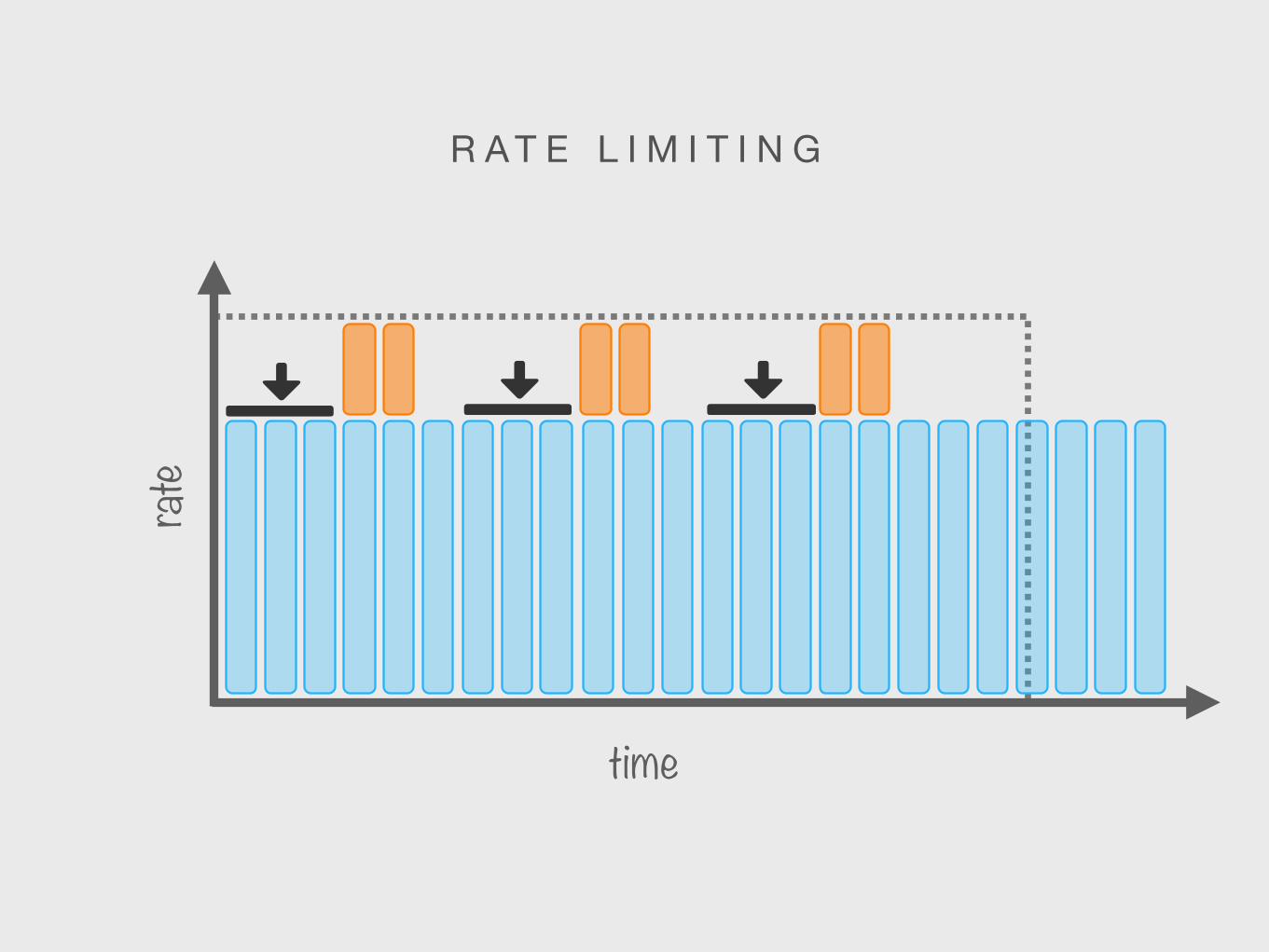
time
rate
R A T E L I M I T I N G

time
rate
R A T E L I M I T I N Gmuch slower

time
rate
R A T E L I M I T I N Gmuch slowerwaste

C O S T F A I R N E S S
c2(t)
c1(t)
congestion rate
reflects cost
integrates correctly
verifiable acrossnetwork borders

time
rate
W E I G H T E D C O S T

time
rate
W E I G H T E D C O S T


causes disproportionate congestion

causes disproportionate congestion
“protect customers” / demand more money

causes disproportionate congestion
“protect customers” / demand more money
“not fair”

ahead of time but set a logical limit above which congestion marking starts. Such operators continually receive information on how much real demand there is for capacity while collecting revenue to repay their investments. Such congestion marking controls demand wi thout r i sk o f ac tua l conges t ion deteriorating service.
Once a cost is assigned to congestion that equates to the cost of alleviating it, users will only cause congestion if they want extra capacity enough to be willing to pay its cost. Of course, there will be no need to be too precise about that rule. Perhaps some people might be allowed to get more than they pay for and others less. Perhaps some people will be prepared to pay for what others get, and so on. But, in a system the size of the Internet, there has to be be some handle to arbitrate how much cost some users cause to others. Flow rate fairness comes nowhere near being up to the job. It just isn’t realistic to create a system the size of the Internet and define fairness within the system without reference to fairness outside the system — in the real world where everyone grudgingly accepts that fairness usually means “you get what you pay for”.
Note that we use the phrase “you get what you pay for” not just “you pay for what you get”. In Kelly’s original formulation, users had to pay for the congestion they caused, which was unlikely to be taken up commercially. But the reason we are revitalising Kelly’s work is that recent advances (§4.3.2) should allow ISPs to keep their popular flat fee pricing packages by aiming to ensure that users cannot cause more congestion costs than their flat fee pays for.
Bob Briscoe‘07 Flow Rate Fairness: Dismantling A Religion
C O S T, N O T B E N E F I T

ahead of time but set a logical limit above which congestion marking starts. Such operators continually receive information on how much real demand there is for capacity while collecting revenue to repay their investments. Such congestion marking controls demand wi thout r i sk o f ac tua l conges t ion deteriorating service.
Once a cost is assigned to congestion that equates to the cost of alleviating it, users will only cause congestion if they want extra capacity enough to be willing to pay its cost. Of course, there will be no need to be too precise about that rule. Perhaps some people might be allowed to get more than they pay for and others less. Perhaps some people will be prepared to pay for what others get, and so on. But, in a system the size of the Internet, there has to be be some handle to arbitrate how much cost some users cause to others. Flow rate fairness comes nowhere near being up to the job. It just isn’t realistic to create a system the size of the Internet and define fairness within the system without reference to fairness outside the system — in the real world where everyone grudgingly accepts that fairness usually means “you get what you pay for”.
Note that we use the phrase “you get what you pay for” not just “you pay for what you get”. In Kelly’s original formulation, users had to pay for the congestion they caused, which was unlikely to be taken up commercially. But the reason we are revitalising Kelly’s work is that recent advances (§4.3.2) should allow ISPs to keep their popular flat fee pricing packages by aiming to ensure that users cannot cause more congestion costs than their flat fee pays for.
Bob Briscoe‘07 Flow Rate Fairness: Dismantling A Religion
“It just isn’t realistic to create a
system the size of the Internet and
define fairness within the system
without reference to fairness
outside the system”
C O S T, N O T B E N E F I T

“How do you share a network?”

cost(economist)

H O W M A N Y W O R K A R O U N D S ?
“TCP is bad with small flows”
batch and re-use connections
open parallel connections
artificial limits in multitenancy


we still have no idea
2 0 1 6

we know what we have is wrong
we still have no idea
2 0 1 6

we know what we have is wrong
not broken enough to fix
we still have no idea
2 0 1 6


End
Related Documents