Resolving the Controversy over the Core Radius of 47 Tucanae (NGC 104)1,2

arX

iv:a

stro

-ph/

0005

192v

1 9

May

200

0

Resolving the Controversy Over the Core Radius of 47 Tucanae (NGC 104)1,2

Justin H. Howell and Puragra Guhathakurta3

UCO/Lick Observatory, Department of Astronomy & Astrophysics,

University of California, Santa Cruz, California 95064, USA

Email: [email protected], [email protected]

and

Ronald L. Gilliland

Space Telescope Science Institute, 3700 San Martin Drive,

Baltimore, Maryland 21218, USA

Email: [email protected]

ABSTRACT

This paper investigates the discrepancy between recent measurements of the density

profile of the globular cluster 47 Tucanae that have used Hubble Space Telescope data

sets. A large core radius would support the long-held view that 47 Tuc is a relaxed

cluster, while a small core radius may indicate that it is in a post–core-collapse phase or

possibly even on the verge of core collapse, as suggested by a variety of unusual objects

— millisecond pulsars, X-ray sources, high velocity stars — observed in the core of

the cluster. Guhathakurta et al. (1992) used pre-refurbishment Wide Field/Planetary

Camera 1 (WFPC1) V -band images to derive rcore = 23′′ ± 2′′. Calzetti et al. (1993)

suggested that the density profile is instead a superposition of two King profiles, one

with a small, 8′′ core radius and the other with a 25′′ core radius, based on U -band

Faint Object Camera (FOC) images. More recently, De Marchi et al. (1996) have used

deep WFPC1 U -band images to derive rcore = 12′′ ± 2′′. The cluster centers used in

these studies are in agreement with one another; differences in the adopted centers

are not the cause of the discrepancy. Our independent analysis of the data used by

De Marchi et al. reaches the following conclusions:

(1) De Marchi et al.’s rcore ∼ 12′′ value is spuriously low, a result of radially-varying

bias in the star counts in a magnitude limited sample — photometric errors and

a steeply rising stellar luminosity function cause more stars to scatter across the

1Based on observations with the NASA/ESA Hubble Space Telescope, obtained at the Space Telescope Science

Institute, which is operated by the Association of Universities for Research in Astronomy, Inc., under NASA contract

NAS5-26555.

2Lick Observatory Bulletin No. 139X.

3Alfred P. Sloan Research Fellow

– 2 –

limiting magnitude into the sample than out of it, especially near the cluster

center where crowding effects are most severe.

(2) Changing the limiting magnitude to the main sequence turnoff, away from the

steep part of the luminosity function, partially alleviates the problem and results

in rcore = 18′′.

(3) Combining such a limiting magnitude with accurate photometry derived from

point-spread-function fitting, instead of the less accurate aperture photometry

employed by De Marchi et al., results in a reliable measurement of the density

profile which is well fit by rcore = 22′′ ± 2′′.

The Calzetti et al. FOC-based density profile measurement is also likely to have been

biased by a poor choice of limiting magnitude and large radially varying photometric

errors associated with aperture photometry. Archival Wide Field Planetary Camera 2

(WFPC2) data are used to derive a star list with a higher degree of completeness,

greater photometric accuracy, and wider areal coverage than the WFPC1 and FOC

data sets; the WFPC2-based density profile supports the above conclusions, yielding

rcore = 24.′′0 ± 1.′′9.

Subject headings: globular clusters: individual (47 Tucanae, NGC 104) — globular

clusters: general — methods: data analysis — techniques: photometric

1. Introduction

Globular clusters are excellent laboratories for studying the dynamics of a stellar system.

The high density of stars near their centers results in frequent interactions—e.g., single star-single

star, single star-binary, and binary-binary. Such interactions redistribute energy throughout the

cluster and drive its global evolution on the so-called “two-body relaxation” timescale. This

can sometimes be comparable to the typical orbital period of stars near the cluster center, and

significantly shorter than the cluster age, implying that dynamical evolution is important. The

orbital period or crossing/dynamical time is related to the core radius (the characteristic length

scale associated with the inner density profile) and the velocity dispersion of the cluster. It is

customary to characterize the radial distribution of various stellar populations in terms of the core

radius (cf. Rasio 2000).

The inner stellar density profile of a globular cluster is suggestive of its evolutionary state

(Hut 1996). Most clusters are characterized by constant density cores, well fit by models based

on a relaxed, Maxwellian distribution function of stars out to the limiting (tidal) radius (King

1966a). On the other hand, about twenty percent of all globular clusters appear to have undergone

catastrophic gravothermal collapse as a result of runaway energy loss from the core due to

two-body relaxation (Djorgovski & King 1986; see the recent review in Meylan & Heggie 1997).

– 3 –

Even these post–core-collapse (PCC) clusters, however, are not expected to develop central

singularities as heating by binaries will drive a “quasi-steady post-collapse” stage followed by

gravothermal oscillations. Theoretical modeling suggests that clusters in the post-collapse phase

should have core radii in the range rcore ∼ 0.01 – 0.04rh (Goodman 1987; Gao et al. 1991) or even

as large as rcore ∼ 0.09rh (Vesperini & Chernoff 1994), where rh is the half-mass radius. These

calculations are based on a single-mass stellar population; models with a realistic stellar mass

function could yield a larger core radius.

The globular cluster 47 Tucanae has been studied extensively, and has long been considered a

prototypical relaxed globular cluster (King 1985) with a large core radius: rcore ∼ 25′′ (Djorgovski

& King 1984). Recent observations of a variety of exotic objects, such as millisecond pulsars

(Robinson et al. 1995), X-ray sources (Hertz & Grindlay 1983; Hasinger, Johnston, & Verbunt

1994), and nine stars whose velocities differ from the cluster mean by ∼> 30 km s−1 (Gebhardt

et al. 1995), have raised the possibility that 47 Tuc may be approaching core collapse. The

half-light (or half-mass) radius of 47 Tuc is rh = 174′′ (Trager, Djorgovski, & King 1993), so if

it has undergone core collapse it should have a core radius in the range 1.′′7 to 16′′ (following

Goodman 1987; Gao et al. 1991; Vesperini & Chernoff 1994). Two recent determinations of the

core radius of 47 Tuc fall within the upper end of this range, as discussed in § 2 below. Moreover,

Gebhardt & Fischer (1995) have constructed nonparametric dynamical models based on the

surface brightness and velocity dispersion profiles, and conclude that the mass profile of 47 Tuc is

as centrally concentrated as that of M15. The density profile slope of 47 Tuc beyond 2′ is found

to be similar to that seen in Fokker-Planck simulations of PCC clusters (Cohn 1980).

Ground-based studies typically use integrated surface brightness measurements to determine a

cluster’s density profile (cf. Djorgovski & King 1984). A substantial fraction of the optical light of

a cluster comes from a handful of the brightest red giant branch (RGB) stars so that the effective

Poisson error associated with integrated light measurements is large. This kind of “sampling”

error makes the measured density profile noisy, and any error in the center determination tends to

bias the measured core radius towards large values. Hubble Space Telescope (HST ) images, even

with the aberrated pre-refurbishment point spread function (PSF), offer the advantage of resolving

individual stars down to the main sequence turnoff even in the cluster core (Guhathakurta et al.

1992, hereafter GYSB). Star counts are more representative of the stellar mass density than the

integrated light, and the effective Poisson errors are smaller (King 1966b). It is preferable to work

at short wavelengths (e.g., the U band) where the brightest RGB stars are suppressed relative

to the more numerous, bluer faint subgiants: this reduces sampling effects in integrated light

measurements and increases the degree of faint star completeness (most notably in the vicinity of

bright giants) for star count measurements (Calzetti et al. 1993; De Marchi et al. 1996, hereafter

DPSGB).

This paper focuses on the question: What is the core radius of 47 Tuc as defined by the radial

distribution of evolved stars? It examines recent measurements of the density profile of 47 Tuc

that appear to be in disagreement with one another. In particular, the HST Wide Field/Planetary

– 4 –

Camera 1 (WFPC1) data set analyzed by DPSGB is reanalyzed here using somewhat different

photometric techniques; our results and those of DPSGB are compared to archival Wide Field

Planetary Camera 2 (WFPC2) data. The background of the core radius controversy is given in

§ 2. In § 3, the available 47 Tuc data sets and the methodologies of this paper and DPSGB are

discussed. In § 4 the photometric errors associated with each method are examined, demonstrating

that the aperture photometry technique of DPSGB produces a radially-varying bias in the star

counts used to measure rcore. Core radius calculations are presented in § 5 along with tests which

show that the core radius discrepancy can be explained in terms of the star count bias in the

DPSGB study. The conclusions of this paper are presented in § 6.

2. The Controversy to Date

The first HST-based core radius for 47 Tuc was derived from F555W images obtained with

the WFPC1 instrument operated in Planetary Camera mode4 (GYSB): rcore = 23′′ ± 2′′, in good

agreement with earlier ground-based measurements (cf. Harris & Racine 1979). Shortly thereafter,

Calzetti et al. (1993) analyzed an independent set of pre-refurbishment HST Faint Object Camera

(FOC) ultraviolet data, and obtained results that were in conflict with previous work. They

pointed out that the cluster center determined from the ground was significantly in error, biased

by a few bright giant stars. More surprisingly, they derived a cluster density profile that did not

resemble a King profile, but was instead fit by a superposition of two King profiles with core radii

of 25′′ and 8′′, suggesting that 47 Tuc is on the verge of core collapse.

The cause of the discrepancy between these density profile measurements remained unclear

for the next few years, and so did the true nature of 47 Tuc’s density profile. The center derived

by Calzetti et al. (1993) is ∼ 6′′ from the earlier ground-based estimate (Auriere & Ortolani 1988),

but only 1.′′4 from GYSB’s estimate which is well within the formal errors. When Calzetti et al.’s

FOC ultraviolet image-based cluster centroid estimate is used in conjunction with the GYSB

F555W data set, the resulting density profile is marginally smoother than the profile obtained

using GYSB’s center estimate, possibly indicating that the former center estimate is more accurate

(see § 1), but the best-fit core radius is ∼> 20′′ in both cases (Guhathakurta et al. 1993). Two

possible sources of discrepancy in density profile measurements are ruled out:

(1) Detailed image simulations show that the sample of faint RGB/subgiant stars used by GYSB

is nearly complete and, in particular, the degree of incompleteness does not vary appreciably

with radius.

(2) If there were a bluer-inward radial gradient in the mean color of faint RGB/subgiant stars,

this would result in a difference between the density profiles derived from ultraviolet versus

4All Wide Field/Planetary Camera 1 (WFPC1) data sets referred to in this paper were obtained in Planetary

Camera mode.

– 5 –

visual-band images. However, a star-by-star match between the Calzetti et al. and GYSB

data sets reveals no such (F342W − F555W) color gradient in 47 Tuc.

More recently, DPSGB used an F336W image from the deep WFPC1 data set of Gilliland

et al. (1995) to revise the cluster center derived by Calzetti et al. (1993) and measure a core radius

of rcore = 12′′ ± 2′′, arguing that neither the Calzetti et al. (1993) composite King profile nor the

traditional large core radius fit the data. This 12′′ core radius is within a factor of two or three of

the range of theoretical estimates for the core radius of a PCC cluster with 47 Tuc’s rh. DPSGB

argued that this is suggestive that 47 Tuc may be approaching core collapse as Calzetti et al.

(1993) had proposed.

3. Data and Photometric Techniques

There are two HST imaging data sets analyzed in this paper: (1) pre-refurbishment WFPC1

data described by Gilliland et al. (1995), consisting of a very deep F336W image (∼ 99 × 1000 s)

with excellent sub-pixel dithering and shorter F439W and F555W exposures (160 s and 60 s,

respectively); and (2) archival WFPC2 data from program GO-6095 (PI: S. G. Djorgovski),

consisting of F218W (4 × 800 s), F439W (2 × 50 s), and F555W (7 s) images. The deep WFPC1

data set combines the advantages of ultraviolet imaging (as used by Calzetti et al. 1993) with a

wider field of view (equivalent to that used by GYSB), and is significantly deeper than all previous

47 Tuc data sets. The great improvement in PSF quality in the WFPC2 data set relative to

the deep WFPC1 data set more than compensates for the shorter exposure times, resulting in a

higher degree of completeness and about a factor of two smaller photometric errors (Guhathakurta

et al., in preparation). Moreover, the larger field of view of WFPC2 (150′′ × 150′′ with the PC

quadrant being partially filled, extending to r ∼ 100′′) compared to WFPC1 (68′′ × 68′′, extending

to r ∼ 55′′) makes it better for density profile measurements.

Since this work and DPSGB use the same deep WFPC1 data set, it is important to examine

and compare the stellar photometry techniques used in the two studies. This paper uses standard

PSF-fitting photometry techniques based on daophot ii (Stetson 1992). These techniques are

described in detail in GYSB and Yanny et al. (1994), with minor modifications to adapt them to

the doubly-oversampled combined F336W WFPC1 image constructed from the sub-pixel dithered

exposures (Gilliland et al. 1995; Edmonds et al. 1996). The main steps in the technique are

outlined here. A preliminary star list is derived by applying daophot’s find routine to the deep

WFPC1 F336W image. For each of the four CCDs, a set of bright, unsaturated, and relatively

isolated stars are used to construct a PSF template, which is allowed to vary quadratically with

position. This template is then fit to all stars on the image using the preliminary star list. The

neighbors of the PSF template stars are subtracted, and the process is iterated a few times.

Stars too faint to be detected in the initial find run are then added based on inspection of the

PSF-subtracted frames. The process of PSF template building and fitting is iterated a few more

– 6 –

times, and the final star list is fit. The magnitudes returned by daophot’s PSF-fitting routine

allstar are converted to total instrumental magnitudes by using the PSF template stars to

determine a spatially-dependent aperture correction. The resulting photometry in the F336W,

F439W, and F555W bands is converted to the Johnson UBV system through an empirical fit

to ground-based data from Auriere et al. (1994). A similar set of techniques is applied to the

WFPC2 data set (cf. Guhathakurta et al. 1996) to derive an independent star list for which the

instrumental F218W, F439W, and F555W magnitudes are converted to Johnson U , B, and V

magnitudes, respectively.

DPSGB uses a ‘core aperture photometry’ technique defined in De Marchi et al. (1993). PSF

peaks are identified on the deep WFPC1 F336W image and aperture photometry is carried out

using a small aperture comparable to the size of the PSF core (hence the term ‘core aperture

photometry’) and a sky annulus of roughly twice that radius. An aperture correction factor is

applied to convert the resulting aperture magnitudes to total magnitudes, compensating for the

portion of the PSF that lies outside the aperture and for the fact that the sky annulus includes

light from the star in question. This method is hereafter referred to as aperture photometry. The

sample of Calzetti et al. (1993) is analyzed using the same aperture photometry technique on the

same crowded field. While § 4 makes a specific comparison of our results to DPSGB because they

share a common data set, the conclusions are expected to apply to Calzetti et al.’s rcore analysis as

well. Neighbor contamination affects aperture photometry to a much greater degree than it affects

PSF-fitting photometry. Since aperture photometry is based on the total flux within the aperture,

the contribution of neighboring stars is a direct source of photometric bias. Neighbors have a

somewhat smaller effect on the sky measurement since the latter is estimated from the mode.

There are three sets of stellar U magnitudes discussed in this study. The photometry from this

work using the deep WFPC1 data set is referred to as U ≡ UWFPC1 (this paper); the photometry

presented by DPSGB based on the same data set is referred to as UD ≡ UWFPC1 (DPSGB) − 0.39

(see § 4.1), where UWFPC1(DPSGB) is identical to the quantity m336 in that paper. Photometry

from the archival WFPC2 data set is referred to as UWFPC2. The WFPC2 PSF is much sharper

than that of WFPC1, resulting in more accurate photometry; thus the WFPC2 data set is used

to define the ‘true’ stellar magnitudes of the stars identified on both the WFPC1 and WFPC2

images. For each star in the WFPC1 and WFPC2 data sets, the positional offset in arcseconds,

∆α and ∆δ (relative to reference star ‘E’ in the 47 Tuc core; GYSB), is determined using the

IRAF task metric (Gilmozzi, Ewald, & Kinney 1995) which uses pointing information based on

the HST Guide Star Catalog.

4. Photometric Error and its Effect on Star Counts

– 7 –

4.1. Star-by-Star Comparison

In order to compare the performance of the two photometric techniques described above,

the input star lists used in the two studies are examined. If, for example, one list systematically

misses stars in the crowded central region of the cluster, then this will result in differences in

the measured core radii. The star finding/PSF-fitting iterations described above yield a set of

14801 stars identified on the deep WFPC1 F336W image. A star list kindly provided by Guido

De Marchi gives the positions and magnitudes of 14979 stars from the same image as reduced

by DPSGB. The bright stars in these two star lists match with an rms positional difference of

one-third of one PC pixel, σ = 0.′′016. The entire matched star list contains 12372 stars with

positions agreeing to within 3σ (1 PC pixel) between the two input star lists. It should be noted

that 141 stars appear twice on the star list from DPSGB. The majority of the ∼ 2500 unmatched

stars fall below the main sequence turnoff and thus are not used to calculate rcore. An inspection of

the unmatched stars suggests that many such stars from the DPSGB list may be spurious, as they

tend to lie in the wings of bright stars, while unmatched stars from this work tend to be faint stars

barely visible on the image. The fraction of evolved stars (defined to be those with U < 18.11)

that remain unmatched in each sample is quite small: 217 from this paper and 246 from DPSGB

out of a total of > 4000 evolved stars. Comparison of our (DPSGB’s) WFPC1 photometry to

WFPC2 photometry of these unmatched stars indicates that 10% (40%) of the unmatched stars

are main sequence stars scattered to brighter magnitudes as a result of photometric error. As

expected, the unmatched stars are such a small fraction of the total that they have a negligible

effect on the rcore estimate (§ 5). We conclude that the set of stars used in the rcore analysis is

basically the same for our study and that of DPSGB; the sample differences are too small to

explain the vastly different conclusions about rcore.

Establishing a common photometric system is the next step in comparing the photometry

derived from the two data reduction techniques. This paper converts instrumental magnitudes

to standard Johnson UBV magnitudes empirically as described in § 3 above. DPSGB uses

m336 ≡ UWFPC1 (DPSGB) throughout, referring to instrumental magnitudes “converted to the

WF/PC ground system”. A star-by-star comparison between the two data sets indicates that a

constant offset of −0.39 mag applied to UWFPC1 (DPSGB) brings the majority of stars into good

agreement with our measured U magnitude. The quantity UD will hereafter be used in place of

UWFPC1 (DPSGB) − 0.39.

To examine the variation of photometric scatter with radius, the WFPC1 magnitude (U or

UD) of each star is compared to its ‘true’ magnitude, UWFPC2. The top and bottom panels of

Fig. 1 plot (UWFPC2 − U) and (UWFPC2 − UD), respectively, versus UWFPC2. Only stars whose

(∆α, ∆δ) positions match to within 0.′′1 between the WFPC1 and WFPC2 data sets are used. The

matched WFPC1 sample is divided at the median radius for stars with U < 18.11, rmed = 21.′′54.

The r < rmed (inner) subsamples are plotted in the left panels and the r > rmed (outer) subsamples

are plotted in the right panels. The small number of points in the outer subsamples results

from the limited overlap between the WFPC1 and WFPC2 fields of view away from the core of

– 8 –

the cluster. There are systematic differences between the WFPC1 photometry and the WFPC2

photometry: U and UD are systematically too faint for bright red giants and too bright for main

sequence turnoff stars; these are caused by errors in the conversion to Johnson U magnitudes for

the WFPC1 data set (§ 4.2).

The U vs. UWFPC2 scatter is similar for inner and outer samples while the scatter increases

dramatically toward smaller radii for UD vs. UWFPC2. Moreover, DPSGB’s photometry of turnoff

stars has a larger scatter than that of this work at all radii. While the standard deviation and mean

value of ∆U [≡ (UWFPC2 − U) or (UWFPC2 − UD)] are indicative of the overall rms photometric

scatter and mean bias, respectively, it is instructive to examine the full distribution of ∆U values.

Stars in the interval 17.8 < UWFPC2 < 19.8 are used to construct cumulative distributions of

∆U . The cumulative distributions using DPSGB’s photometry show a long, asymmetric tail of

large (UWFPC2 − UD), while the distributions using the photometry from this study are quite

symmetrical and narrow, implying lower scatter and little or no bias. More quantitatively, the

∆U values corresponding to the 95th percentile of the distribution are: +0.5, +0.5 (this study:

inner and outer subsamples, respectively); +1.2, +0.75 (DPSGB: inner and outer subsamples,

respectively).

The conclusion to be drawn from this subsection is that the star lists used in the two

studies are effectively identical, but photometric accuracy is not. DPSGB’s photometry shows a

systematically greater photometric error, and a bias in the sense that stars are more likely to be

measured as brighter than they truly are than fainter. More importantly, this error and bias are

greatest near the cluster center.

4.2. Color-Magnitude Diagrams

Color-magnitude diagrams (CMDs; Fig. 2) provide an alternate perspective on the nature

of photometric error in the WFPC1 U -band data set, complementary to the discussion in the

previous subsection. As described below, the CMDs also help to highlight a discrepancy between

the WFPC1 and WFPC2 U -band photometric calibration. The CMDs combine B and V

magnitudes, obtained via PSF-fitting, with each of the WFPC1 U magnitudes under examination:

our PSF-fitting photometry and DPSGB’s aperture photometry. The B vs. U − V and B vs.

UD − V CMDs (left and right, respectively) are presented for stars in the inner and outer halves

of the matched star sample (upper and lower, respectively). The B vs. U − V diagrams use

U lim = 18.11, while the B vs. UD − V diagrams use U limD

= 17.71. Limiting magnitudes will be

discussed in detail in § 4.3.

The use of the CMD as a diagnostic tool is best illustrated through stars with the most

extreme photometric errors. A plot of U − UD vs. UWFPC2 is used to identify ‘outliers’ with

U − UD > +3σ, where σ is calculated in running bins of width 0.5 mag in UWFPC2 (open squares

in Fig. 2); the U − UD distribution is skewed towards positive values such that very few stars

– 9 –

Fig. 1.— Difference between WFPC1 and WFPC2 U -band stellar photometry as a function of

WFPC2 magnitude using the PSF-fitting method (this work: upper panels) and the aperture

photometry method (DPSGB: lower panels). The left panels show the inner sample of stars with

r < 21.′′54, while the right panels show the outer sample of stars with r > 21.′′54. The smaller number

of stars in the outer samples is due to the limited overlap between the WFPC1 and WFPC2 fields

of view away from the cluster center. The limiting magnitude used in core radius calculation is

indicated by the solid lines: U lim = 18.11 (upper panels) and U limD

= 17.71 (lower panels). Dashed

lines show UWFPC2 = 18.11 and UWFPC2 = 17.71 (upper and lower, respectively). The DPSGB

aperture photometry displays a larger scatter than the PSF-fitting photometry used in this work,

and the scatter increases towards the cluster center. The mismatch between WFPC1 and WFPC2

photometry, most noticeable at the bright end and near the turnoff, is a result of systematic error

in the WFPC1 to Johnson U magnitude conversion.

– 10 –

Fig. 2.— Color-magnitude diagrams for the inner (top panels) and outer (bottom panels) WFPC1

subsamples, using U -band photometry from this work (U : left) and DPSGB (UD: right), combined

with B- and V -band photometry derived from PSF-fitting. The limiting magnitude is U lim = 18.11

for this work, and U limD

= 17.71 for DPSGB. Squares represent stars which are > +3σ outliers

in a U − UD scatter plot (their number is indicated in parentheses in each panel). These outliers

tend to have bluer UD − V colors than the main CMD features, but their U − V colors are not

similarly biased, indicating that they are outliers because of photometric scatter/bias in UD. The

solid line is the median color of stars derived from WFPC2 photometry. The disagreement between

WFPC2 photometry and both sets of WFPC1 photometry, most pronounced for bright red giants

and turnoff stars, is caused by systematic error in the WFPC1 to Johnson U calibration.

– 11 –

have U − UD < −3σ. The open squares in B vs. UD − V diagrams generally lie on or beyond

the blue fringe of the subgiant branch and RGB defined by the rest of the points. By contrast,

the vast majority of the open squares in the B vs. U − V diagrams are distributed evenly about

the underlying subgiant and red giant branches, with only a few points near the red edge. This

indicates that outliers in the U −UD distribution are predominantly the result of the measured UD

value being systematically too bright. As expected, the greater degree of crowding causes outliers

in the inner subsample to display larger deviations in the CMD than those in the outer subsample.

Moreover, the width of the RGB appears to be slightly greater in UD − V than in U − V .

The solid lines show the median color of stars from the WFPC2 sample in 0.1 mag bins. The

discrepancy between WFPC2 and WFPC1 photometry for both this study and DPSGB is worst

for the reddest stars (bright RGB) and for the bluest stars (turnoff), and in opposite senses. This

results from error in the Johnson U calibration for the WFPC1 data set, which has been improved

for the WFPC2 data set. Both data sets have been empirically transformed to the Johnson system

using the ground-based data of Auriere et al. (1994). However, the larger field of view of WFPC2

includes stars farther from the cluster center and thus less affected by crowding in Auriere et al.’s

data. The WFPC2 ridge line is in good agreement with Auriere et al.’s photometry, which should

be accurate outside the crowded cluster core.

4.3. Luminosity Function

In this subsection, we examine the stellar luminosity function of 47 Tuc. This is a key

element in understanding the bias in star counts in a magnitude-limited sample that results from

photometric error (scatter and bias), and therefore in understanding the difference in core radius

estimates between DPSGB and GYSB. The U -band stellar luminosity functions for the inner and

outer samples are shown in the left and right panels of Fig. 3, respectively. Data points represent

the full U -band sample from this paper, the dot-dashed line is the DPSGB UD sample excluding

the 141 duplicate stars, and the solid line is the WFPC2 sample for UWFPC2 ≤ 19, normalized

to match the WFPC1 luminosity functions. The WFPC2 luminosity functions shown in the two

panels are identical except for the normalization, and are based on the full star list derived from

the entire WFPC2 field of view. Since this study relies only on post–main-sequence stars which

are not expected to be affected by mass segregation, we have chosen to combine the entire WFPC2

sample into a single luminosity function; a full study of mass segregation will be presented in

Guhathakurta et al. (in preparation).

In order to isolate a sample of post–main-sequence stars, the U magnitude of the main

sequence turnoff is determined using a sample of turnoff stars identified in a WFPC2 V vs. B − V

CMD. The mean UWFPC2 magnitude of these stars is adopted as the limiting magnitude for the

deep WFPC1 data set analyzed in this paper: U lim = 18.11. On the other hand, DPSGB used

mlim336 ≡ U lim

WFPC1(DPSGB) = 18.1 which corresponds to U lim

D= 17.71. Vertical lines are drawn at

U = 18.11 and U = 17.71 in Fig. 3; these correspond to the diagonal lines in Fig. 1. Note that

– 12 –

Fig. 3.— Stellar U -band luminosity functions for the inner (left) and outer (right) subsamples.

Points with error bars are based on PSF-fitting photometry derived from a deep WFPC1 image

(this work), the dot-dashed line is based on aperture photometry on the same deep WFPC1 data set

(DPSGB), and the bold solid line is derived from archival WFPC2 data. The WFPC2 luminosity

function is the same in both panels, with different empirical normalizations to match the inner and

outer WFPC1 luminosity functions. The solid vertical line at U = 18.11 and the dashed line at

U = 17.71 mark the limiting magnitudes used in this work and by DPSGB, respectively.

– 13 –

the magnitude cut used by DSPGB falls on a steep part of the luminosity function. The next

subsection quantifies the consequences of choosing a limiting magnitude on a steep part of the

luminosity function.

Of the three samples, WFPC2 photometry produces the sharpest luminosity function. The

luminosity function derived from this study’s WFPC1 photometry has a somewhat more gradual

rise from the RGB to the main sequence turnoff than the WFPC2 luminosity function as a result

of its larger photometric errors. The DPSGB luminosity functions, particularly their inner sample,

have the most gradual transition between the RGB and turnoff, indicating the largest photometric

errors. There are significant differences between the WFPC2 luminosity function and those derived

from the deep WFPC1 data (our study and DPSGB) most notably at the bright end and near the

turnoff; these are a result of systematic error in the conversion to Johnson U for the WFPC1 data

set (§ 4.2).

4.4. Discussion of Errors and “Limiting Magnitude Bias”

The above diagnostics (§§ 4.1–4.3) complement one another by providing somewhat different

perspectives on the photometric error in the various data sets. The ∆U plots indicate the

photometric scatter as a function of radius for each of the deep WFPC1 photometry sets, but

only under the assumption that UWFPC2 is the true magnitude of the star. While it is possible in

principle to compare the three data sets to empirically determine the photometric error in each,

the strongly non-gaussian error distributions make this impractical. Instead, the CMD diagnostic

described in § 4.2 clearly demonstrates that there are large photometric errors associated with the

UD photometry but not with U , and this conclusion is independent of the accuracy of UWFPC2.

A skeptic may wonder if there are systematic errors generic to the PSF-fitting method that

‘cancel’ each other in the B vs. U − V CMD or in the U vs. UWFPC2 comparison causing the

PSF-fitting magnitudes to appear more accurate than they actually are. A related question is:

How accurate is UWFPC2? The luminosity function diagnostic is useful in this regard, despite the

mismatches caused by errors in the WFPC1 Johnson U conversion. Figure 3 clearly shows that

the most prominent features (e.g., the steep rise at the subgiant branch, the peak at the main

sequence turnoff) are sharpest for WFPC2 photometry, slightly smoothed out by photometric

errors for our deep WFPC1 photometry, and even more smoothed out (larger photometric errors)

in the case of the DPSGB data.

Photometric errors associated with the aperture photometry technique result in a significant,

radially-varying bias in the star counts; we hereafter refer to this as “limiting magnitude bias”.

The limiting magnitude used by DPSGB is on a steep part of the luminosity function where many

stars which are slightly fainter than the limiting magnitude scatter into the sample while relatively

few stars scatter out of the sample. Limiting magnitude bias is exacerbated by the asymmetry in

the distribution of photometric errors (photometric bias; see § 4.1) and by the fact that the errors

– 14 –

(scatter and bias) tend to increase towards the fainter magnitudes. Since aperture photometry

errors increase with stellar crowding towards the cluster center, so does the degree of limiting

magnitude bias.

The differential limiting magnitude bias between inner and outer subsamples may be

quantified as follows. Since the bounding radius of the inner sample, rmed, was chosen to be the

median radius of stars in the matched sample with U < 18.11, the inner to outer star count ratio

is expected to be unity. It is not surprising that N(r < rmed)/N(r > rmed) = 1.02 ± 0.03 for stars

from this study with U < 18.11. By contrast, stars with UD < 17.71 from the DPSGB sample

have N(r < rmed)/N(r > rmed) = 1.42 ± 0.06. The latter ratio is significantly greater than unity,

indicating radially-varying limiting magnitude bias in the DPSGB sample.

Alternatively, the limiting magnitude bias for each WFPC1 sample can be quantified

with respect to the ‘true’ WFPC2 photometry. The diagonal lines in Fig. 1 correspond

to U = U lim (upper panels) and UD = U limD

(lower panels). The vertical dashed lines

indicate UWFPC2 = U lim (upper panels) and UWFPC2 = U limD

(lower panels). The ratios

N(U < U lim)/N(UWFPC2 < U lim) are 1.54 ± 0.06 and 1.34 ± 0.15 for inner and outer subsamples,

respectively, while N(UD < U limD

)/N(UWFPC2 < U limD

) are 2.32± 0.14 and 1.09± 0.22 for inner and

outer subsamples, respectively. These ratios are greater than unity because errors in the WFPC1

Johnson U conversion cause the main sequence magnitudes to be systematically too bright (§ 4.2;

Fig. 1). Each ratio indicates the number of stars selected in a sample relative to the corresponding

true (WFPC2-based) number of stars satisfying the selection criterion. For the photometry from

this work, the excess relative to unity is similar in the inner and outer subsamples, so the derived

core radius should not be greatly affected. DPSGB’s photometry results in a large and significant

excess of stars selected in the inner subsample, but not in the outer subsample. This radial

variation has a substantial impact on the core radius measurement (§ 5). The large difference

between the inner and outer DPSGB ratios is a direct result of the increased scatter and bias in

their photometry at small radii.

5. Core Radius Calculations

The effect of limiting magnitude bias on the measurement of the core radius is explored in

this section. A one-parameter surface density profile of the form:

σ(r) =σ0

[1 + (r/rcore)2](1)

is used to make maximum likelihood fits to various magnitude-limited samples of evolved stars to

determine rcore, while the normalization constant σ0 is constrained by the total number of stars in

each sample. Calculations are performed using both GYSB’s estimate of the cluster center:

αJ2000 = 00h24m05s.87

δJ2000 = −72◦04′57.′′8 (2)

– 15 –

and DPSGB’s center estimate:

αJ2000 = 00h24m05s.29

δJ2000 = −72◦04′56.′′3 . (3)

The two center estimates agree to within the quoted uncertainty of ∼ 1.′′0–1.′′3 in each estimate.

Unless otherwise stated, all core radius estimates in this paper are based on the GYSB center.

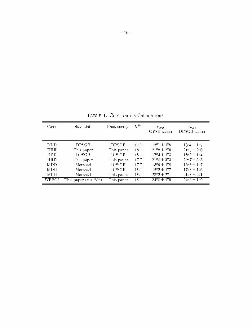
Table 1 contains a summary of the core radius measurements. The three letters identifying

each calculation indicate the source of: (1) the star list (D for DPSGB, H for this work, M for

the matched sample); (2) the photometry (D or H); and (3) the limiting magnitude (D or H).

For direct comparison with DPSGB’s rcore measurement, the 141 duplicate stars are included

in their star list. The result of the maximum likelihood fit (case DDD) is rcore = 13.′′7 ± 1.′′8,

in agreement with the DPSGB value of rcore = 12.′′2 ± 2.′′1 derived using radial binning and a

least-squares fit. A maximum likelihood fit to the evolved star sample from this paper (case HHH)

gives rcore = 21.′′8± 2.′′0. Applying a limiting magnitude of U limD

= 18.11 instead of U limD

= 17.71 to

DPSGB’s star list and photometry results in a core radius of 17.′′4 ± 1.′′5 (case DDH). The change

in derived core radius from 13.′′7 to 17.′′4 is a direct result of the change in limiting magnitude and

is independent of whether the 141 duplicate stars are included. Using the star list and photometry

from this study but choosing DPSGB’s limiting magnitude U lim = 17.71 gives rcore = 21.′′0 ± 3.′′3

(case HHD). Thus, the large scatter/bias in DPSGB’s photometry and their increase towards the

crowded cluster center, combined with a poor choice of limiting magnitude, are responsible for the

spuriously low core radius estimate.

Table 1 also shows that the measured rcore is independent of whether the star list from this

study, DPSGB’s star list, or the matched star list is used. The dependence of the derived rcore

on limiting magnitude and photometric technique is roughly the same for all three lists. Likewise

the choice of cluster center has little effect on the derived rcore: although core radii based on the

DPSGB center tend to be ≈ 0.′′5 smaller than those based on GYSB’s center, this difference is less

than the uncertainty in an individual measurement.

The WFPC2 data set provides a consistency check on the core radius of 47 Tuc. For all stars

derived from the archival WFPC2 data set with UWFPC2 < 18.11, the same maximum likelihood

algorithm used above yields rcore = 23.′′1 ± 1.′′7. An independent sample of 7044 turnoff stars with

17 ∼< V < 18 drawn from the WFPC2 V vs. B − V CMD (avoiding potential blend artifacts that

may have scattered to brighter magnitudes) results in rcore = 23.′′3 ± 1.′′2. While these turnoff

stars are fainter on average than the evolved stars used in earlier density profile studies, they

are expected to have roughly the same mass as red giants so that mass segregation effects are

unlikely to be important. A third calculation truncates the UWFPC2 < 18.11 sample at r ∼ 85′′ as

a precaution against inter-CCD edge effects caused by vignetting near the ridges of the pyramid

mirror. A core radius of rcore = 24.′′0± 1.′′9 (case WFPC2 in Table 1) is derived from this truncated

sample. It is reassuring that these WFPC2 rcore measurements are consistent with GYSB, earlier

– 16 –

Table 1. Core Radius Cal ulationsCase Star List Photometry U lim r ore r oreGYSB enter DPSGB enterDDD DPSGB DPSGB 17:71 13:007� 1:008 13:004� 1:007HHH This paper This paper 18.11 21:008� 2:000 21:005� 2:000DDH DPSGB DPSGB 18:11 17:004� 1:005 16:008� 1:004HHD This paper This paper 17.71 21:000� 3:003 20:007� 3:003MDD Mat hed DPSGB 17:71 13:009� 1:008 13:005� 1:007MDH Mat hed DPSGB 18:11 18:002� 1:007 17:008� 1:006MHH Mat hed This paper 18:11 22:002� 2:001 21:008� 2:001WFPC2 This paper (r < 8500) This paper 18:11 24:000� 1:009 24:005� 1:009

– 17 –

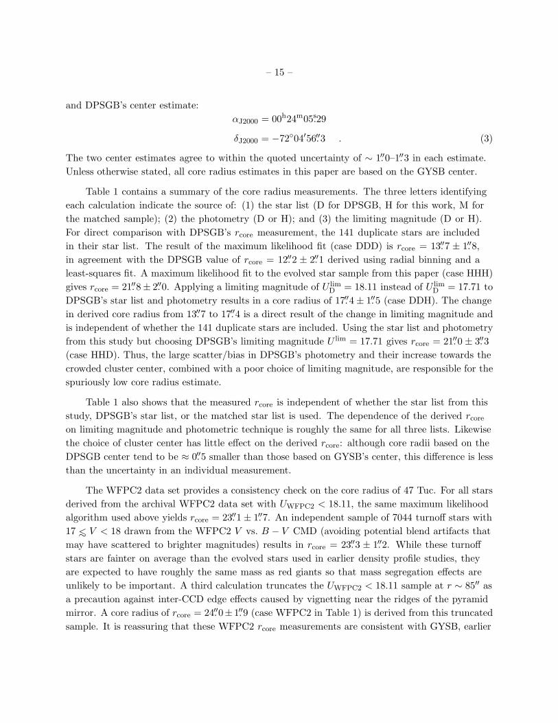
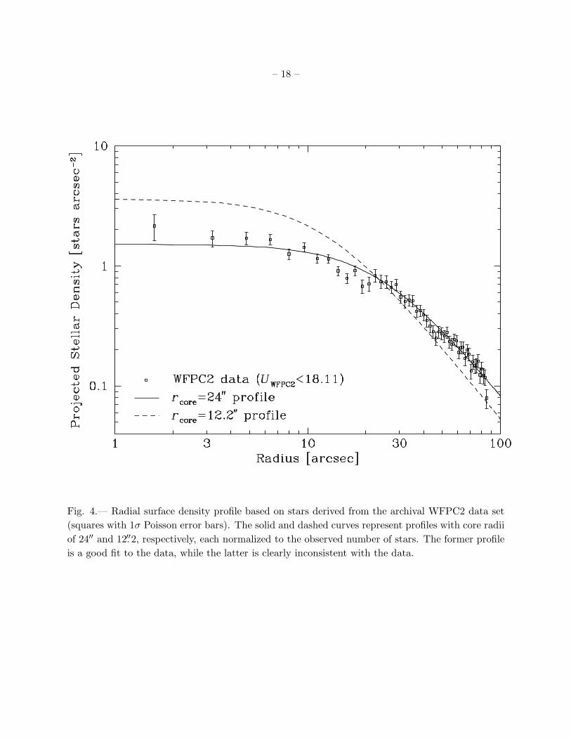
ground-based measurements, and the HHH and MHH calculations above. Figure 4 shows the

radial surface density profile of the WFPC2 truncated sample. Also shown are an rcore = 24.′′0

profile (solid line) and an rcore = 12.′′2 profile (dashed line); the latter is clearly inconsistent

with the data. These profiles have been normalized to the total observed number of stars in the

plot. Figure 5 shows the cumulative radial distributions of the MHH sample (left panel) and the

truncated WFPC2 sample (right panel). Also shown are profiles for the best fitting core radii

(dotted lines) and for core radii that differ from the best fit value by ±1σ (dashed lines).

As an alternative to the maximum likelihood technique, we conduct Kolmogorov-Smirnov

tests between the star count samples and the fitting function in Eq. (1). The MHH sample

of 4504 stars (Table 1) and the truncated WFPC2 sample of 3963 stars are used to construct

cumulative radial distributions (Fig. 5). One-sided Kolmogorov-Smirnov tests indicate that the

MHH data differ from the rcore = 22′′ fitting function by an amount that would be exceeded by

chance 26% of the time. Similarly, the truncated WFPC2 data differ from an rcore = 24′′ profile by

an amount that would be exceeded by chance 33% of the time. Thus, the functional form adopted

here provides an adequate fit to the star count data.

As a final check on the rcore calculations, one can test whether the degree of limiting

magnitude bias (§ 4) for a given sample is sufficient to explain the core radius derived for it. Using

the photometry of DPSGB and their sample of stars with UD < U limD

(case DDD in Table 1), the

inner to outer star count ratio is N(r < rmed)/N(r > rmed) = 1.42± 0.06. Integrating a 14′′ profile

(comparable to the maximum likelihood fit for this sample) over the area of the WFPC1 field

of view predicts an inner to outer ratio of 1.49 consistent with the directly measured star count

ratio. On the other hand, integration of the 22′′ profile that best fits the star list and PSF-fitting

photometry used in this paper (case HHH in Table 1) yields an inner to outer ratio of 1.05; this is

comparable to the directly measured star count ratio of 1.02 ± 0.03.

6. Conclusions

This paper presents estimates of the density profile of the globular cluster 47 Tuc based

on three samples of stars (star list and photometry) derived independently from Hubble Space

Telescope WFPC1 and WFPC2 images. Apparent discrepancies amongst the core radius

measurements published by Guhathakurta et al. (1992), De Marchi et al. (1996), and Calzetti

et al. (1993) are investigated. Our conclusion is that there is severe, radially-varying bias in

the magnitude-limited star counts used by De Marchi et al. and Calzetti et al., and this causes

their core radius estimates to be spuriously low (rcore ∼ 14′′) relative to other determinations

(rcore ∼ 23′′). This “limiting magnitude bias” is a result of large photometric scatter/bias

associated with the application of their aperture photometry method to the crowded central

regions of the cluster, coupled with a choice of limiting magnitude near the steep part of the

stellar luminosity function. In general, such a choice of limiting magnitude is dangerous; even with

symmetric errors the resulting sample will be contaminated by large numbers of stars just fainter

– 18 –

Fig. 4.— Radial surface density profile based on stars derived from the archival WFPC2 data set

(squares with 1σ Poisson error bars). The solid and dashed curves represent profiles with core radii

of 24′′ and 12.′′2, respectively, each normalized to the observed number of stars. The former profile

is a good fit to the data, while the latter is clearly inconsistent with the data.

– 19 –

Fig. 5.— Cumulative radial distribution of the matched deep WFPC1 and truncated WFPC2

samples (solid lines, left and right panels, respectively). Best fit model profiles with rcore = 22′′

and rcore = 24′′ are indicated by dotted lines in the left and right panels, respectively; the dashed

lines indicate model profiles with rcore values that are ±1σ removed from the best fit value. The

shapes of the WFPC1 and WFPC2 cumulative distributions are different because of the difference

in geometry between the two data sets and because of the r ∼ 85′′ truncation of the WFPC2 data

set.

– 20 –

than the cutoff. Any radial variation in the magnitude of the errors will cause the degree of this

contamination to vary, resulting in an incorrect determination of the radial density profile.

Combining De Marchi et al.’s photometry with a limiting magnitude near the main sequence

turnoff at the peak of the luminosity function reduces, but does not eliminate, the discrepancy

(rcore ∼ 18′′); the radial variations in DPSGB’s photometry (larger photometric scatter/bias at

small radii) have a significant effect on the derived core radius even with an optimal choice of

limiting magnitude. A more accurate PSF-fitting method is used in this paper to indepedently

derive two sets of stellar photometry, one from the deep WFPC1 data analyzed by De Marchi

et al. and the other from an archival WFPC2 data set. The core radii derived using these

two photometry sets are independent of the choice of limiting magnitude and star list, and are

consistent with each other and with previous ground-based and HST work: rcore ∼ 23′′ (cf. Harris

& Racine 1979; Djorgovski & King 1984; Guhathakurta et al. 1992).

The best fit core radius for the surface density distribution of evolved stars in 47 Tuc is about

15% of the cluster half-mass radius (rh = 174′′). This is significantly larger than the range of

(rcore/rh) values found in numerical simulations of post–core-collapse clusters: 0.01–0.04 (Cohn

1980; Goodman 1987; Gao et al. 1991). It should be noted however that the surface brightness

profile is not a perfect discriminant between a relaxed and post–core-collapse cluster, and it is

advisable to combine it with velocity dispersion data (Gebhardt & Fischer 1995).

We are grateful to Guido De Marchi for making stellar photometry tables available to us in

electronic form, and to Randi Cohen for help in the early phase of this project. We would like to

thank Fernando Camilo, Paulo Freire, Karl Gebhardt, and Fred Rasio for helpful discussions, and

the referees, especially Tad Pryor, for several useful suggestions.

– 21 –

REFERENCES

Auriere, M., Lauzeral, C., & Koch Miramond, L. 1994, in Frontiers of Space and Ground-Based

Astronomy, edited by W. Wamsteker, M. S. Longair, and Y. Kondo (Kluwer Academic

Publishers), p. 633

Auriere, M., & Ortolani, S. 1988, A&A, 204, 106

Calzetti, D., De Marchi, G., Paresce, F., & Shara, M. 1993, ApJ, 402, L1

Cohn, H. 1980, ApJ, 242, 765

De Marchi, G., Paresce, F., & Ferraro, F. R. 1993, ApJS, 85, 293

De Marchi, G., Paresce, F., Stratta, M. G., Gilliland, R. L., & Bohlin, R. C. 1996, ApJ, 468, L51

(DPSGB)

Djorgovski, S. G., & King, I. R. 1984, ApJ, 277, L49

Djorgovski, S. G., & King, I. R. 1986, ApJ, 305, L61

Edmonds, P. D., Gilliland, R. L., Guhathakurta, P., Petro, L., Saha, A., & Shara, M. M. 1996,

ApJ, 468, 241

Gao, B., Goodman, J., Cohn, H., & Murphy, B. 1991, ApJ, 370, 567

Gebhardt, K., & Fischer, P. 1995, AJ, 109, 209

Gebhardt, K., Pryor, C., Williams, T. B., & Hesser, J. E. 1995, AJ, 110, 1699

Gilliland, R. L., Edmonds, P. D., Petro, L., Saha, A., & Shara, M. M. 1995, ApJ, 447, 191

Gilmozzi, R., Ewald, S. P., & Kinney, E. K. 1995, The Geometric Distortion Correction for the

WFPC Cameras (WFPC2 Instrum. Sci. Rep. 95-02) (Baltimore: STScI)

Goodman, J. 1987, ApJ, 313, 576

Guhathakurta, P., Yanny, B., Schneider, D. P., & Bahcall, J. N. 1992, AJ, 104, 1790 (GYSB)

Guhathakurta, P., Yanny, B., Schneider, D. P., & Bahcall, J. N. 1993, in Blue Stragglers, edited

by R. A. Saffer (San Francisco: ASP Conf. Series No. 53), p. 60

Guhathakurta, P., Yanny, B., Schneider, D. P., & Bahcall, J. N. 1996, AJ, 111, 267

Harris, W. E., & Racine, R. 1979, ARA&A, 17, 241

Hasinger, G., Johnston, H., & Verbunt, F. 1994, A&A, 288, 466

Hertz, P., & Grindlay, J. 1983, ApJ, 272, 105

– 22 –

Hut, P. 1996, in Dynamical Evolution of Star Clusters–Confrontation of Theory and Observations,

edited by P. Hut and J. Makino (Dordrecht: Kluwer), p. 121

King, I. R. 1966a, AJ, 71, 64

King, I. R. 1966b, AJ, 71, 276

King, I. R. 1985, Scientific American, 252, 78

Meylan, G., & Heggie, D. C. 1997, A&A Rev., 8, 1

Phillips, A. C., Forbes, D. A., Bershady, M. A., Illingworth, G. D., & Koo, D. C. 1994, AJ, 107,

1904

Rasio, F. A. 2000, in Pulsar Astronomy—2000 and Beyond, edited by M. Kramer, N. Wex, and

R. Wielebinski (San Francisco: ASP Conf. Series No. 202), p. 589

Robinson, C., Lyne, A. G., Manchester, R. N., Bailes, M., D’Amico, N., & Johnston, S. 1995,

MNRAS, 274, 547

Stetson, P. B. 1992, in Astronomical Data Analysis Software, edited by D. M. Worrall,

C. Biemesderfer, and J. Barnes (San Francisco: ASP Conf. Series No. 25), p. 297

Trager, S. C., Djorgovski, S. G., & King, I. R. 1993, in Structure and Dynamics of Globular

Clusters, edited by S. G. Djorgovski and G. Meylan (San Francisco: ASP Conf. Series No.

50), p. 347

Vesperini, E., & Chernoff, D. F. 1994, ApJ, 431, 231

Yanny, B., Guhathakurta, P., Bahcall, J. N., & Scheider, D. P. 1994, AJ, 107, 1745

This preprint was prepared with the AAS LATEX macros v4.0.