AD-A269 730 NAVAL POSTGRADUATE SCHOOL Monterey, California DTIC THESIS Q 'ELECTE SEP23 1993 1 Eu RESOLUTION IN RADAR MAPPING by Michael D. Anderson March 1993 Thesis Advisor: Gurnam S. Gill Approved for public release; distribution is unlimited 93-22036 2,) 2 0 IP

Welcome message from author
This document is posted to help you gain knowledge. Please leave a comment to let me know what you think about it! Share it to your friends and learn new things together.
Transcript

AD-A269 730
NAVAL POSTGRADUATE SCHOOLMonterey, California
DTICTHESIS Q 'ELECTESEP23 1993 1
EuRESOLUTION IN RADAR MAPPING
by
Michael D. Anderson
March 1993
Thesis Advisor: Gurnam S. Gill
Approved for public release; distribution is unlimited
93-22036
2,) 2 0 IP

Form ApprovedREPORT DOCUMENTATION PAGE oMB No o07o oaBPublic reDoring burden for thi coltec'tion of information ,s •,lmeted To AJeraJe I ov e e•r.psne nclu.ling Ire lime for re,.ewng in$1r l . (e1 .r' e..,$ oat, W•0"d•galhrefng and maintaining the data needed, and comrlleit n and reute.rn, the collec"0o, Of o nforlo tatron Send comments reqarding th,, burden est-n te 01 4n. -Are, au•oe of ¶.colltecon of informatiOn, including suggestions for reducng this ourden to vash,nglon Hesouar e'.. ,Se.,.ces 0Orectoraie for informat•on Opera:ton% And fooD~cc, , i5 r eefwnDaws nHghway, Sute 1204, Arlngton, VA 22202-4302 and O the Orffce of Managemet and Budget Paperwofk Reduction Project (0704-.083) iti.Wr-9r10,
2O0503
1. AGENCY USE ONLY (Leave blank) 2, REPORT DATE 3. REPORT TYPE AND DATES COVERED
March 1993 I Master's Thesis4. TITLE AND SUBTITLE S. FUNDING NUMBERS
Resolution in Radar Mapping
6. AUTHOR(S)
Michael D. Anderson
7. PERFORMING ORGANIZATION NAME(S) AND ADDRESS(ES) 8. PERFORMING ORGANIZATION
Naval Postgraduate School REPORT NUMBER
Monterey, CA 93943-5000
9. SPONSORING/MONITORING AGENCY NAME(S) AND ADDRESS(ES) 10. SPONSORING/MONITORINGAGENCY REPUHT NUMBER
11. SUPPLEMENTARYNOTES The views expressed in this thesis are those of the
author and do not reflect the official policy or position of theDepartment of Defense or the US Government.
12a. DISTRIBUTION /AVAILABILITY STATEMENT 12b. DISTRIBUTION CODE
Approved for public release; distribution isunlimited
13.ABSTRACT(Maximum200words) Signal processing has led to great performancegains in radar mapping. The most critical feature of these systems iscell size, which determines resolution. Cell size is defined by rangeresolution and azimuth resolution.
Range resolution is improved through pulse compression. Phase offrequency modulation of a waveform yields increased bandwidth and shorter effective pulse width without reducing total signal energy. Severalfamilies of codes are vestigated emphasizing matched filter outputand doppler tolerance
Azimuth resolution is improved through beam sharpening. Severalbeam sharpening techniques are illustrated with radar images providedby Hughes Aircraft. Range bin output plots demonstrate the effective-ness of these techniques.
With these techniques, "near-SARI' quality output can be obtainedfrom real beam mapping radars allowing the real-time and all aspectcapabilities of real beam systems to be more fully employed intactical missions.14. SUBJECT TERMS 15. NUMBER OF PAGES90Resolution; Pulse Compression; Beam Sharpening; PC
Radar Mapping 16, PRICE CODE
17. SECURITY CLASSIFICATION 18. SECURITY CLASSIFICATION 19. SECURITY CLASSIFICATION 20. LIMITAT"'4 Or O85TRACTOF REPORT OF THIS PAGE OF ABSTRACT
UNCLAS UNCLAS UNCLAS ULNSN 7540-01-280-5500 Standard Form 298 (Rev 2-89)
i~sroi vAS i 139-18

Approved for public release; distribution is unlimited
RESOLUTION IN RADAR MAPPING
by
i.-hael D. AndersonLieutenant, United States Navy
B.S.E.E., United States Naval Academy, 1987
Submitted in partial fulfillment of therequirements for the degree of
MASTER OF SCIENCE IN ELECTRICAL ENGINEERING
from the
NAVAL POSTGRADUATE SCHOOLMarch 1993
Author: A/ 22Y 4k -Mic D. Anderson
Approved by: "Gurnam S. Gill, Thesis Advisor
7"4C. 1ýDavid C. Jenft, Second Reader
Michael A. Morgan, ChairmanDepartment of Electrical and Computer Engineering
ii

ABSTRACT
Signal processing has led to great performance gains in radar mapping. The
most critical feature of these systems is cell size, which determines resolution. Cell
size is defined by range resolution and azimuth resolution.
Range resolution is improved through pulse compression. Phase or frequency
modulation of a waveform yields increased bandwidth and shorter effective pulse
width without reducing total signal energy. Several families of codes are investigated
emphasizing matched filter output and doppler tolerance.
Azimuth resolution is improved through beam sharpening. Several beam
sharpening techniques are illustrated with radar images provided by Hughes Aircraft.
Range bin output plots demonstrate the effectiveness of these techniques.
With these techniques, "near-SAR" quality output can be obtained from real
beam mapping radars allowing the real-time and all aspect capabilities of real beam
systems to be more fully employed in tactical missions.
Accesitro For
NTIS CRA&IDTIC TAB
U. announced LI
Justification .. .............
By ....................
Dist, ibution I
Availability CodesS' Avail and I or
Dist Special
DTIC QUALITY INSPECTIMiii.

TABLE OF CONTENTS
1. INTRODUCTION 1
A. RADAR MAPPING 1
B. CELL SIZE AND RESOLUTION 4
11. RANGE RESOLUTION 9
A. WAVEFORM SELECTION 9
B. LINEAR FREQUENCY MODULATION 12
C. PSEUDO-RANDOM BINARY CODES 12
1. Barker Codes 14
2. Compound Barker Codes 15
3. Minimum Peak Sidelobe Codes 18
4. Complementary Codes 18
D. POLYPHASE CODES 24
1. Frank Codes 24
2. PI Code 26
3. P2 Code 26
4. P3 Code 29
5. P4 Code 29
111. AZIMUTH RESOLUTION 33
A. BEAM SHARPENING TECHNIQUES 33
1. Combination of Sum and Difference Channels 34
2. Monopulse Beam Sharpening 36
.3. Inverse Filtering 36
iv

4. Maximum Entropy 38
5. Hughes Advanced Discrimination Technique (HADT) 39
B. IMAGE ENHANCEMENT 43
1. Histogram Flattening 43
2. Edge Detection 43
3. Line (boundary) Detection 46
4. Thresholding and Centroiding 46
5. Median Filter 47
IV. CONCLUSIONS AND RECOMMENDATIONS 52
APPENDIX MATCHED FILTER OUTPUT AND THE AMBIGUITY DIAGRAM 61
A. THE AMBIGUITY DIAGRAM 61
1. Development 61
2. Usage 62
3. Types 63
B. AMBIGUITY DIAGRAM PLOTTING PROGRAM 66
LIST OF REFERENCES 82
INITIAL DISTRIBUTION LIST 83
v

ACKNOWLEDGMENTS
I wish to express my gratitude to Dr. Gurnam Gill who endeavors to take the "black magic" out
of radar engineering.
I am deeply indebted to Tom Kennedy, T.D. (Buzz) Elliot, Dr. Kapriel Krikorian and Kurt
Tarhan of Hughes Aircraft who went well out of their way to provide materials, documentation and
explanations of the "black magic" they are building into radar systems.
Many thanks to Paul for his teamwork these past two years and to GrisweUl for his
encouragement.
Special thanks to my wife, Karen, for her support and for putting up with me through the
process.
vi

I. INTRODUCTION
The evolution of radar has reached a new stage. Like many other areas of technical
development, software is now driving innovation and providing new levels of performance. Digital
signal processing has permeated every aspect of radar, from the shape of the transmitted pulse to
the type of return display. One application which has greatly benefitted from signal processing
advances is radar mapping.
A. RADAR MAPPING
One of the primary advantages of radar mapping is all-weather capability. Clouds, fog and haze
generally do not limit system capability. In addition, radar mapping can be done day or night.
Finally, both the angle and direction of illumination are controllable. For these reasons, radar
mapping is invaluable in environmental mapping as well as tactical surveillance. Airborne radars are
able to fill a number of mission roles through mapping.
Navigation is one of the roles for radar mapping. Numerous applications exist to fil this role.
Terrain following involves vertical scanning with horizon information fed directly to flight control to
allow extreme low altitude approach. Terrain avoidance is similar, but incorporates horizontal
sweeps to avoid obstacles. TERCOM, or terrain contour mapping, is used to guide a platform over
a timed preprogrammed ground trajectory. This mode assumes a known contour map. Radar map-
matching involves guiding a platform over a pre-designated course over previously mapped terrain,
as the Tomahawk TIAM cruise missile does. Either real-beam or SAR mapping can be used for
this function.
In air-to-ground applications, weapon delivery can be entirely dependent on radar mapping. All
weather attack capability is demonstrated in the scenario of Figure 1. [1] In this case, a SAR
processing system is demonstrated. A first SAR map gives the system operator an overview of the
attack area. By designating a point with a cursor, a second finer-detail image is mapped of the
1

immediate target area. By marking the precise target with a cursor, the operator initializes a
sequence in which the system provides steering guidance to the target and controls weapon release
In the air-to-ground battle, radar mapping also proves invaluable in reconnaissance and
surveillance. The ability to distinguish and localize targets from stand-off distance provides a great
advantage to friendly ground forces. Long-range targeting data and advance warnLý, of large troop
movements can provide the margin of victory in battle. Finally, radar mapping can also be quite
useful in the area of battle damage assessment.
For several of these mission roles, SAR mapping has been the method of choice. With recent
developments in real-beam mapping, however, real beam is expanding its role in warfare. The value
of real beam mapping was demonstrated in Operation Desert Storm. A vital mission of the U.S. Air
Force and other allied air assets was the location and destruction of both fixed and mobile ground-
to-ground missile or Scud launchers. This became a high-priority cat and mouse game as efforts to
protect Israel and Saudi Arabia from missile attack required searching great expanses of desert for
relatively small targets. In effect, this mission resembled the proverbial search for a needle in a
haystack. While Synthetic Aperature Radar (SAR) could provide the necessary resolution to detect
these launchers, the time required for processing of th- data would slow the searches considerably.
With its all-aspect real time capability, real beam systems could search a much greater area in less
time. This is critical when dealing with mobile targets and quick response tactics.
2

f
J -2
Figure 1. Radar target detection, localization and targeting
3

As envisioned, a real beam system would perform rapid sweeps of the desert and localize
potential targets and areas of interest. A SAR system would then be employed to provide greater
detail and targeting information. In this way, limited assets could be best employed to meet the
threat as quickly as possible.
B. CELL SIZE AND RESOLUTION
As alluded to above, the effectiveness of radar mapping is, to a large extent, dependeat on
system cell size at operational range. Cell or "pixel" size is defined as a rectangle whose sides are
the system range and azimuth resolution distances. Driving the choice of cell size are considerations
such as object size, processing requirements, interpretation requirements and, of course, cost. A
demonstration of the effects of cell size is presented in Figures 2 and 3. [1) In this figure, all
portions of the shape were assumed to reflect equally with full cells lighter in the correspording map
and partially full cells darker according to the strength of the return. In actuality, several mappings
from different aspects with different frequencies and polarizations would have to be combined to
generate this quality return. Obviously, with smaller cell size, detection and localization of small
objects is improved as well as discrimination of detail in larger objects or areas. Table 1 [1] provides
typical cell size requirements for square mapping of common map features.
In general, it is easier to achieve fine range resolution than fine azimuth resolution. Resolution
in range is approximately 492 feet per microsecond of pulse width. In order to improve range
resolution beyond this figure, all that needs to be done is to reduce the pulse width of the system.
As will be discussed in Chapter II, when there are limits to the physical reduction of pulse width,
pulse compression can be used to achieve additional improvement in resolution. The matched filter
and ambiguity diagram, as presented and implemented in Appendices A and B, will be used to
illustrate several techniques. However, the more significant limitation for real beam systems has
always been the azimuth resolution.
4

C)
I IZ
0
V)LL1
__ __a_
Figue 2 Siulatd rsoltionof ellsizeequl t 1/5objct ize
50

:7 <
"'41 .C
CL
4 0~
cc
I .
V _ -. 0
S" 0
----------- i
LA. _._ I3
Figure 3. Simulated resolution of cell size equal to 1/20 object size.
6

TABLE 1CELL SIZE REQUIREMiNTS
Features to be Resolved Cell Size
Coastlines, large cities, outlines of mountains 500 ft
Major highways, variations in fields 60-100 ft
"Road map" details: city streets, large buildings, 30-50 ftsmall airfields
Vehicles, houses, small buildings 5-10 ft
Azimuth resolution of a standard system is roughly the 3 dB beamwidth of the antenna times
the range. At five nautical miles, a 16 foot array operating in X ba ,d has an azimuth resolution of
approximately 200 feet. To recognize the shape of even large objects at long distance, the military
has had to resort to SAR. Since the beamwidth varies proportionally with wavelength and inversely
with antenna length, to improve resolution, it is necessary to operate at shorter wavelengths or with
larger antennas. There are limits on choice of wavelength and antenna size. Limitations on
machining tolerance and phase alignment make the construction of large antennas a difficult task.
Airframe requirements complicate this task even further. Improvements in signal processing,
however, have advarxced to the point that *near SAR" quality images can be obtained from real beam
systems. This is especially true for point reflectors. Chapter III will present a discussion of azimuth
resolution and several beam sharpening techniques. These techniques will include actual beam
sharpening algotithns as well as image enhancement techniques which are applied after initial beam
sharpening. The comparative performance of these techniques will be demonstrated by the quality
of through a set of images obtained through the application of algorithms developed by the
Advanced Systems Division of Hughes Aircraft Company.
As these techniques are further developed and refined, real beam radar mapping will
undoubtedly be applied to a great many situations which require SAR systems today. With faster
7

scan time, all aspect capability and good resolution, real beam systems can provide a great advantage
in tactical operations.
8

II. RANGE RESOLUTION
A. WAVEFORM SELECTION
Long operational range and fine range resolution are two of the primary design considerations
in a mapping radar. These apparently contradictory goals are achieved by proper selection of radar
waveform. The radar waveform is defined by its carrier frequency, pulse repetition frequency
(PRF), pulse width and intrapulse modulation. The tradeoffs involved in the selection of waveform
parameters are described in this section.
The selection of carrier frequency is an important first step in waveform design. The
propagation characteristics of radar change rapidly in the microwave region. Nathanson [21 provides
the following guidance. Attenuation due to rain (in dB) is proportional to f2-8 and backscatter from
rain and small particles varies as e" dB over most of this region. Ionospheric effects also vary with
frequency and are of concern at frequencies below 3 GHz, while polar operations are affected by
aurora backscatter below 2 GHz. Table 2 [1] defines the radar frequency bands and common
usages. The carrier frequency also has implications for azimuth resolution, though this will be
discussed at greater length in the next chapter.
Once the operating frequency has been chosen, the next issue to be considered is the selection
of pulse repetition frequency (PRF). The most widely used method of range measurement is pulse
delay ranging. It is simple, avoids the problem of transmitter leakage noise, provides easy range
measurement, and is extremely accurate. With this form of operation, however, great care must be
taken when selecting the PRF. The choice of PRF is crucial because it determines to what extent
the ranges and doppler frequencies observed by the radar will be ambiguous.
The returns from objects separated by the system unambiguous range are received
simultaneously. The echoes from a target, therefore, must compete with ground return not only
9

from the target's own range but from every range that is separated from it by a whole multiple of
the unambiguous range. Any overlapping of the return profiles can result in target echoes and
ground clutter passing through the same doppler filter, even though the true doppler frequencies of
the target and clutter are quite different. This becomes a significant problem if the received
frequency is less than the width of the true doppler profile, as it must often be to reduce range
ambiguities. Reducing the PRF causes the mainlobe clutter to occupy a large portion of the receiver
passband. As the percentage of the passband occupied by the mainlobe clutter increases, it becomes
difficult to reject clutter on the basis of doppler frequency without rejecting a large percentage of the
target echoes as well. The lower the PRF, the more severe this effect becomes. With ground
clutter being widely dispersed, range and doppler ambiguities greatly compound the problem of
isolating target echoes.
Once the decision regarding PRF has been resolved, the designer's attention turns to the
selection of pulse width. Ideally, to achieve both long detection range and fine range resolution, a
system should transmit extremely narrow pulses of exceptionally high peak power. Since there are
limitations on the amount of peak power which can be transmitted, to obtain long range at PRFs
low enough for pulse delay ranging, fairly wide pulses must be transmitted. Pulse length determines
the range resolution. To improve range resolution, a designer must shorten the pulse width. As
pulse length is decreased, however, so is the total energy contained in the pulse. Eventually, a point
is reached where further energy decrease in the signal is unacceptable due to detection
requirements. With transmitter peak power and receiver sensitivity improvements coming slowly,
and only at great cost, a clear limit seemed to exist in the detection-range resolution tradeoff. In
search of a way around these limits, it was found that the limits on range resolution can be
circumvented by coding successive increments of the transmitted pulse with phase or frequency
modulation. This led to the development of linear frequency-modulation pulse compression.
10
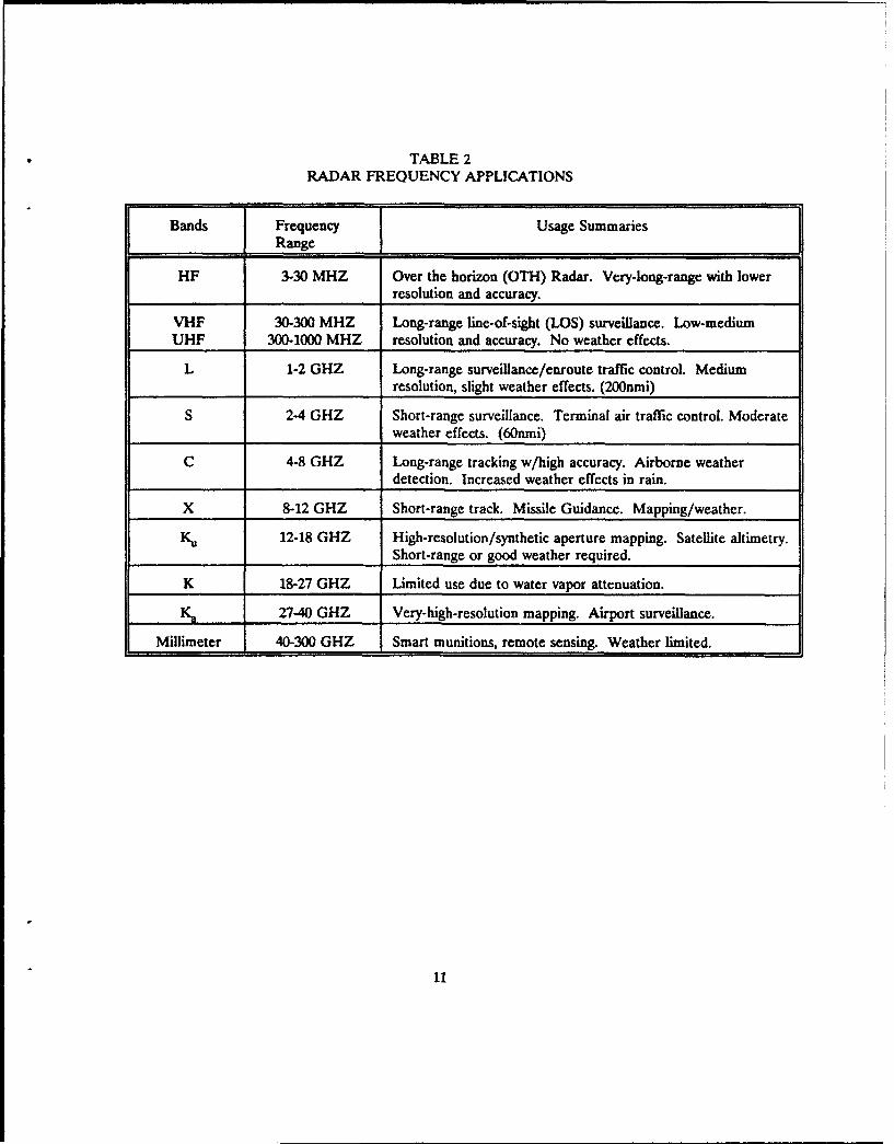
TABLE 2RADAR FREQUENCY APPLICATIONS
Bands Frequency Usage SummariesRange
HF 3-30 MHZ Over the horizon (OTH) Radar. Very-long-range with lowerresolution and accuracy.
VHF 30-300 MHZ Long-range line-of-sight (LOS) surveillance. Low-mediumUHF 300-1000 MHZ resolution and accuracy. No weather effects.
L 1-2 GHZ Long-range surveillance/enroute traffic control. Mediumresolution, slight weather effects. (200nmi)
S 2-4 GHZ Short-range surveillance. Terminal air traffic control. Moderateweather effects. (60nmi)
C 4-8 GHZ Long-range tracking w/high accuracy. Airborne weatherdetection. Increased weather effects in rain.
X 8-12 GHZ Short-range track. Missile Guidance. Mapping/weather.
K. 12-18 GHZ High-resolution/synthetic aperture mapping. Satellite altimetry.Short-range or good weather required.
K 18-27 GHZ Limited use due to water vapor attenuation.
K, 27-40 GHZ Very-high-resolution mapping. Airport surveillance.
Millimeter 40-300 GHZ Smart munitions, remote sensing. Weather limited.
11

If a matched filter is used, the sensitivity of a radar receiver depends only on the total energy
contained in the signal. The time distribution of the energy is unimportant. Within the constraints
set by frequency and PRF selection, resolution then becomes the determining factor in the form of
the transmitted energy. The single measure which best expresses the range resolution properties of
a signal is the effective bandwidth. Long duration and high bandwidth are not incompatible if a
signal contains rapid or irregular structure changes such as in pulse compression. Three types of
pulse compression will be discussed in this chapter, linear frequency modulation, pseudo-random
binary coding and pseudo-random polyphase coding.
B. LINEAR FREQUENCY MODULATION
Linear frequency modulation (LFM), also known as "chirp," is the result of increasing or
decreasing the radio frequency of a transmitted signal at a constant rate throughout each pulse. This
form of pulse compression enables very large compression ratios, and is simple to implement. There
is a slight ambiguity between range and doppler using this method. A positive doppler shift will
cause the signal to leave the filter sooner. The radar system can not distinguish between a target at
a slightly closer range and one with a positive doppler shift at a slightly farther range.
To resolve a LFM signal, it is passed through a linear filter with a frequency change equal to the
inverse of the pulse width. This must occur over a time equal to the compressed pulse width. The
pulse compression ratio (PCR) achieved is equal to the ratio of the transmitted pulse width to the
compressed pulse width. This is also equal to the pulse width times the frequency change which is
known as the "time-bandwidth product."
C. PSEUDO-RANDOM BINARY CODES
In many applications, digital implementation of pulse compression is preferred over analog.
There are many advantages to digital implementation, including:
12

- freedom from ringing due to impedance mismatches/analog filters
- reproducible response
- high peak-to-sidelobe ratios without weighting
- change bandwidth by changing clock frequency
- change the waveform and PCR by controlling the number of time samples and by digitallyswitching the matched filter
. compatibility with MTI and other signal processing.
Despite the advantages of digital implementation, significant limitations still exist due to range
sidelobes. Range sidelobes exist due to the sin(x)/x shape of the energy spectrum of the
uncompressed pulse. As the uncompressed pulse passes through the filter, the higher frequency
spectral sidelobes travel faster than the main lobe frequencies, and the lower frequency sidelobes
travel slower. The spectral shape of the energy then is reflected in the shape of the compressed
pulse amplitude vs time plot. This has an effect similar to antenna sidelobes. Range sidelobes imply
wasted energy and can result in false targets. Amplitude weighting, such as the use of Hamming
window, can be used to minimize the sidelobes. This weighting, however, often has the effect of
broadening the compressed pulse width or "main lobe" of the energy form.
The binary coding is actually a phase reversal of 0 or 180 degrees impressed upon the carrier
signal. These phase sequences are usually represented by a series of + 1 and -1. The resulting
signal is wideband with bandwidth equivalent to twice the code clock rate. The range resolution of
these codes is determined by the transmitted chip width. A chip is defined as one coded segment of
the transmitted pulse.
The following are several of the more popular binary phase coding sequences. Most are easily
implemented and display good autocorrelation characteristics. This class of waveform, however,
does suffer from significant doppler phase shift limitations.
13

1. Barker Codes
These are a select number of pseudo-random codes which come close to the desirable feature
of zero range sidelobes. With these sequences, the sidelobes of the compressed pulse are limited to
the amplitude of the uncompressed individual segment, while the main lobe amplitude is multiplied
by the number of bits in the code. Matched filter outputs for these sequences have normalized
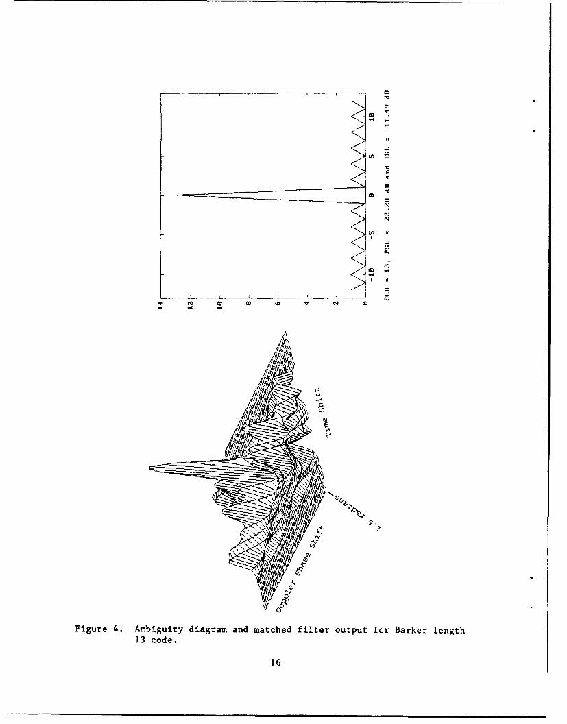
range sidelobes of only 1/L2 relative to the mainlobe. The primary drawback of these codes is that
the longest known code is only 13 bits long. It has been proven that no other examples of these
codes exist for odd lengths, and no even codes for lengths less than 6084. While it has not been
proven, it is probable that no others exist at all. The known Barker codes, along with their known
autocorrelation peak sidelobes and integrated sidelobes are given in Table 3. [21 The limitation to
length 13 is serious, since it does not allow complete decoupling between average power and
resolution. A second drawback is that the matched filter output of these waveforms degrades rapidly
with doppler shift. Large sidelobes result in the autocorrelation and appear as spikes other than at
the origin in the ambiguity diagram. This effect is demonstrated in Figure 4 which shows the
matched filter output without doppler shift and the ambiguity diagram for a Barker 13 sequence.
TABLE 3THE KNOWN BARKER CODES
Length Code Elements PSL, dB ISL, dB
1 +
2 + -, + + -6.0 -3.0
3 + +- -9.5 -6.5
4 + + - +, + + - -12.0 -6.0
5 + + +- + -14.0 -8.0
7 + ++ -- + - -16.9 -9.1
11 + + +--- ++++ -- +- -20.8 -10.8
13 + + + + +--+ +-+-+ .22.3 -11.5
14

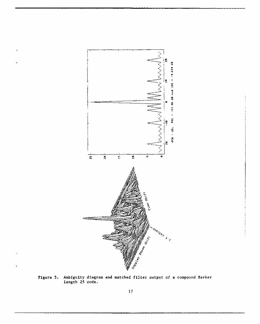
2. Compound Barker Codes
One attempt to circumvent the length limitation of the Barker codes is known as compound
Barker codes. This coding process can best be described through the use of the example below:
Barker length 4: + + + sidelobe level -12.0dB
Barker length 3: = > (+ +-) (+ +-) (+ +-) (+ +-) sidelobe level - 9.5dB
Compound Barker length 12: + +- + +- -- + ++- sidelobe level - 9.5dB
Each bit of one sequence represents either a true or inverted replication of the second sequence.
The resulting length and pulse compression ratio is equal to the product of the two original code
lengths. While the range sidelobes will no longer be equal in amplitude, the main lobe to sidelobe
amplitude ratio will be equal to the lowest original code used. Figure 5 provides the matched filter
output and ambiguity diagram for Complementary Barker length 25 (5 in 5). This figure
demonstrates that these longer codes are very sensitive to doppler phase shift.
15
C.P
&0ý 1.1
IQ0-
I:)
Figre . Abigitydiaramandmathedfiler utpt fr Brke legt
13 code
16N
A -T
0.,
,N*
Figure 5. Ambiguity diagram and matched filter output of a compound Barker
length 25 code.
17
3. Minimum Peak Sidelobe (MPS) Codes
Another effort has been the compilation of the minimum sidelobe codes. These are simply
the binary sequences which attain the lowest PSL for given lengths. Table 4 [2] gives the MPS codes
for lengths 14 through 48. These codes were discovered by an exhaustive search of all possibilities.
Figure 6 gives the matched filter outputs and ambiguity diagrams for the MPS code length 5 (a
Barker) and a nonideal code of the same length for comparison. Note the higher peak sidelobes in
the non-optimal code.
4. Complementary Codes
There are four known kernels of complementary code. A kernel is a basic length of code
which cannot be shortened by inverting standard generation procedures. The known kernels are
given in Table 5 [31 below. CorrespondL:- sidelobes produced by the A and B sequences have
opposite phases. By alternately modulating successive pulses and switching the matched filter,
sidelobes are canceled upon integration of successive pulses.
Longer sequences can be built up by "chaining' to form what is known as composite
complementary sequences. Chained codes have sidelobes greater than a single code, but these
cancel upon integration of an even numbers of pulses. The topic of complementary codes and their
ambiguity diagrams were explored in Akita [3]. Figures 7 and 8, from this source, present an
example of matched filter output and the corresponding ambiguity diagram for a complementary
sequence of length 10,
18

TABLE 4MINIMUM PEAK SIDELOBE (MPS) CODES
Sample codeLength Number PSL ISL, dB (octal)
7 1 1 -9.19 0478 16 2 -6.02 2279 20 2 -5.28 327
10 10 2 -5.85 054711 1 1 -10.83 1107
12 32 2 -8.57 465713 1 1 -11.49 1263714 18 2 -7.12 1220315 26 2 -6.89 1405316 20 2 -6.60 064167
17 8 2 -6.55 07351318 4 2 -8.12 31036519 2 2 -6.88 133561720 6 2 -7.21 121403321 6 2 -8.12 5535603
22 756 3 -7.93 0346653723 1021 3 -7.50 1617651124 1716 3 -9.03 3112774325 2 2 -8.51 11124034726 484 3 -8.76 21600533127 774 3 -9.93 22673560728 4 2 -8.94 107421045529 561 3 -8.31 262250034730 172 3 -8&82 430522201731 502 3 -8.56 05222306017
32 844 3 -8.52 0017132531433 278 3 -9.30 3145245417734 102 3 -9.49 14637741512535 222 3 -8.79 00074552546336 322 3 -8.38 146122404076
37 110 3 -8.44 025641166763638 34 3 -9.19 000741512514639 60 3 -8.06 114650276747440 114 3 -8.70 0210436703513241 30 3 -8.75 03435224401544
42 8 3 -9.41 0421075607226443 24 3 -8.29 00026625314703444 30 3 -7.98 01773166262532745 8 3 -8.18 05274146155576646 2 1 -8.12 0074031736662526
47 2 3 -8.53 015151764121461048 8 3 -7.87 0526554171447763
19

4F
(a)
0
(b)
Figure 6. a) Ambiguity diagram for the MPS length 5 code(+4-+)b) Ambiguity diagram for a non-optimal code of length
5 ( 4 - )
20

TABLE 5THE KNOWN COMPLEMENTARY KERNELS
ILENGTH SEQUENCE
2 A = {-1,-4}B = {-1,+1}
10 A = {-1,+1,+1,-1,+1,-1,+1,+1,+1,-1)B = {-1,+ 1,+i,+1,+ 1,+ 1,+ 1,-1,-1,+1i}
10 A = {+I,-1+1,-1,+1,+1,+1,+1,-1,-1}B = {+1,+I,+1,+1,-1,+1,+1,-1,-1,+1}
26 A = {+I,-I,+I,+I,-I,-I,+I,-I,-I,-I,-I,+I,-I,+ 1,-1,-1,-1,-1, + 1, + 1,-1,-I,-I, + 1,-1, + 1)
B = {-1, + 1,,-1,-,+ 1, + 1,-1, + 1, + 1, + 1, + 1,-1,-i,
The complementary codes, like all binary phase codes, are limited by doppler sensitivity. Any
doppler shifts encountered must be small, or pulse widths must be short, since it is the total phase
shift across the pulse which matters. Excessive phase shift across the waveform will result in serious
degradation of the amplitude vs. time plot.
21

I,C
t
--. ..... . .. .
-I 8 -6 -4 -2 a 2 a to 1
time
4J 4
S
20
-2 I
-lB -8 - -4 -2 0 2 4 6 8 18
+ime
Figure 7. Matched filter output of complementary length 10 kernels;sequence A, sequence B and summation.
22

k
Figure 8. Amibiguity diagram of complementary length 10 kernel.
23

C. POLYPHASE CODES
Polyphase codes are another class of pseudo-random sequences. With these codes, the bits can
consist of any number of different harmonically related phases, rather than only 0 or 180 degrees.
Several such codes are available, with some of the more common ones described below.
1. Frank Codes
The Frank codes are a series of inphase and quadrature (I) samples taken at the Nyquist
rate of a "step-chirp" waveform. The formation of the code is demonstrated by Figure 9. [41 To
generate this code, P phase increments are defined by dividing 360/P. P groups of P segments are
then generated according to the following procedure:
The first phase of each group is 0. The phases of the remaining segments in each group
increase in increments of
Ae =(G-1)*(P-1)YO (2.1)
where
G is the group number and
( is the basic increment.
The resulting code is given by
e(ij) = (2n/N)(i-1)(j-1) (2.2)
For example:
P=4:
Group 1: segment 1=0, segment 2=0, segment 3=0, segment 4=0
Group 2: segment 1=0, segment 2=(360/4)(1)(1)=90, segment
3 = (360/4)(1)(2) = 180, etc.
The resulting code is shown at the bottom of Figure 9.
24

12,
I0 •
8,
a
44
to
2,
TCI 4
I STEP Cti•ak
-[ _ F24Tc
T , 4 T I
S~0 0 190 iso 27 0i
rc -- -FRANuk- POLYPHASE COE
Figure 9. Derivation of Frank code from a step-chirp waveform.
25

For a given number of segments, a Frank code provides the same pulse compression ratio as
a binary phase code and the same peak to sidelobe ratio as a Barker code. Yet, by using more
phases (increasing P), the codes can be made any length. As P is increased, however, the size of the
fundamental phase increment decreases, making performance more sensitive to externally introduced
phase shifts and imposing more severe restrictions on uncompressed pulse width and maximum
doppler shift. This is demonstrated in Figures 10 and 11 showing degradation of the ambiguity
diagrams for increasing length Frank codes. Another limitation of the Frank codes is that the
largest phase change between elements occurs at the center of the sequence. Because of this,
receiver bandwidth limitations have especially significant effects on the center peak to sidelobe ratio.
2. P1 Code
To alleviate the problems of bandwidth limitation present in the Frank codes, the code groups
representing the j frequencies were rearranged in time order of transmission. This placed the lowest
amount of phase increment in the center to preserve the main lobe. This led to the creation of the
P1 code given by
O (ij) = -(ir/N)[N-(2j-1)][(j-1)N + (i-1)J (2.3)
When N is odd, the P1 code is simply the Frank code rearranged to have conjugate symmetry
around the DC term. The autocorrelation functions of the two codes are nearly identical, but the P1
has no bandwidth limitations.
3. P2 Code
The P2 code is given by
O(ij) = (Qx/2)[(N-1)/N]-(ir/N)(i-1)) (N + 1-2j} (2.4)
It has an autocorrelation function nearly identical in magnitude to both the Frank and P1 codes, and
has no bandwidth limitations. The difference is that P2 is real as opposed to complex
26

Figure 10. Frank codes of P-3 (length 9) and P-4 (length 16).
27

Figure 11. Frank codes of P-5 (length 25) and P-7 (length 49).
28

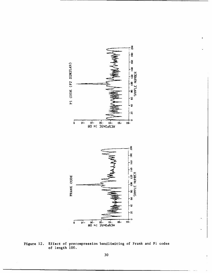
because it is symmetrical. Figure 12 [41 demonstrates the improved bandwidth tolerance of both P1
and P2 over the Frank codes. In this example, bandlimited results show a 6 db improvement in peak
sidelobe level for P1 over Frank code. Both P1 and P2 still remain fairly doppler intolerant,
however. This is a characteristic of the analog step chirp waveform from which both, along with the
Frank code, are derived.
4. P3 Code
Since the linear chirp waveform is much more tolerant of doppler than the step chirp, the P3
code was developed from it. The code is written as
e(i) = % (i1) 2/p as (i) varies from 1 to p (2.5)
In this equation p represents the pulse compression ratio. The resulting waveform is just as doppler
tolerant as the analog linear chirp, but suffers from the same bandwidth limitations as the Frank
codes. Figure 13 demonstrates the improved doppler tolerances of the P3 code. While the unshifted
matched filter output shows the Frank to have a superior peak-to-sidelobe ratio by 4 db, the doppler
shifted signals clearly show the superiority of P3. Of particular note is the elimination of grating
lobes and preservation of the image lobe.
5. P4 Code
A waveform both doppler tolerant and not bandwidth limited resulted from rearranging the P3
code. The resulting code is known as P4 and is written ase(i) = [ic (i-1) 2/p ]-% (i-1). Figure 14 [41
demonstrates the bandwidth limitation improvement of P4 over P3.
29
CD
0
CL
= -Jir
i ".....
a or- or- oS- oIý- OS- O9-90 NI 2SNOdS38
z
gO NI 3SNOJSd
Figure 12. Effect of precompression bandlimiting of Frank and P1 codes
of length 100.
30

WI
0 W
Cj 0
g 9
OP NI 3SNOdS3M V311:1 90 NI 3SNO$S3W W3fLj
00 NI 3MNOdSUM 3l111 90 NI MSNOdS3U Wt311t
Figure 13. a) and b) are Frank and P3 code matched filter outputs for
length 100. c) and d) show matched filter outputs for the
doppler phase shifted case.31

CO
0o
•0NI 3SNOdS-4ý
S• -Sz
oi- - o- o- O0- 09-90 NI 3SN0d£&•
Figure 14. Bandlimited matched filter outputs for P3 and P4 codes length 100.
32
0 m

I11. AZIMUTH RESOLUTION
With pulse compression providing a means of achieving good detection range and fine range
resolution, the largest remaining constraint in a mapping radar is azimuth resolution. As mentioned
in the introduction, in an unprocessed real beam system, azimuth resolution is determined by the
antenna beamwidth. While beamwidth control is adequate for target detecticn, prohibitively large
antennas result for the narrow beams required to determine detailed characteristics such as the
number, size or separation of targets. The need for information of this sort led to the development
of synthetic aperature radar.
Unfortunately SAR systems also have limitations. These systems are unable to map at nose
aspect, are expensive, and are hardware dependent, Most importantly, they are comparatively slow
in mapping due to the extensive amount of signal processing required. These limitations have led to
renewed efforts to improve the angular resolution of real beam systems. These efforts are referred
to as real beam sharpening.
A. BEAM SHARPENING TECHNIQUES
Beam sharpening reflects two areas of effort: actual beam sharpening algorithms, and image
enhancement techniques which are applied after initial beam sharpening. While some
implementations will combine some of both, they will be presented individually in this paper.
These techniques enhance angular designation accuracy in all aspect scenarios. Further, real-
time post-processing is possible to accomilish this without extending the radar frame time. Even
while implementing these additional processors, real beam systems can map a 60 degree swath in
just 1-2 seconds.
Techniques already in use on the F-15E provide a 2-1 enhancement in designation accuracy.
Test results of new techniques being developed at Hughes Aircraft promise beam sharpening of 6:1
33

with 6 dB SNR and up to 25:1 for a 20 dB SNR return. These estimates are based on isolated
corner reflector return. The following pages will provide a brief introduction into a number of these
techniques.
1. Combination of Sum and Difference Channels
Useful for resolving point targets, this method was developed at Hughes Aircraft and is
currently implemented in the F-1SE. Figure 15 [5) demonstrates the concept. The boresight null in
the difference (D) channel pattern forms a sharp peak when combined with the sum (S) channel
pattern. A weighting factor (K) controls the beam sharpening ratios. A value of (K) equal to .75 is
common. The output (So) is given by
Sc = ISI - KIDI (3.1)
This technique can also be applied using sum and synthetic difference channels. If difference
channel information is not available, synthetic difference channel data may be generated through the
use of anti-symmetric weights. The difference channel data (D) is generated as shown below.
Dj = E(1-k) wk S,+k (3.2)
where wk is a suitable set of anti-symmetric weights, (j) is the radar pulse index, and Sj+k is the sum
channel data for each pulse and set of weights. The optimum weights (wk) to maximize the gain
slope of the synthetic difference pattern vary as
wk.t dG(9)/dO (3.3)
where:
G(9) = antenna azimuth gain
e = k(scan rate)/PRF
The sum and synthetic difference channel data are then combined as for the previous case.
34

T-k
U)U
DI
JI
:1 1
Figure 15. Combination of sum and difference channels resulting in
attenuation of response away from boresight.
35

2. Monopulse Beam Sharpening
Also used for point targets, this technique uses sum and difference channels to form an
azimuth discriminant on the I/0 data for each return in each range bin. The discriminant (a) for
each pulse (j) is given by
a = k Re((S" .D,)/(S" .Sj)) (3.4)
where k is a scaling factor given by 1/(discriminant slope)(angular bin spacing), Sj is the sum
channel data for each pulse and Dj is the difference channel data for each pulse. Re is the real
operator and * denotes complex conjugation. This discriminant value gives the distance of each
scatterer from the center of the range bin. As the scatterer enters the beam, each subsequent pulse
will show the scatterer moving closer to the center as the beam scans across it. Eventually, the
discriminant will reach zero, cause a sign change and move out of the beam. Once the discriminant
is formed for a pulse and range bin, the value of the discriminant assigns the return to one of the
azimuth bins which each range bin is divided into. The magnitude of the sum channel data is what
is actually stored in the bin. With each pulse, data is continually added to the bins. Upon
completion of the scan, the accumulated sum of the contents of each bin is displayed thereby
localizing scatterers.
Synthetic monopulse beam sharpening is also possible. It involves the sum channel and
synthetic difference channel. The synthetic difference channel is formed as previously described, and
is then applied as in regular monopulse beam sharpening.
3. Inverse Filtering
In a large class of imaging systems, spatial degradation can be modeled by a linear-shift-
invariant impulse response and additive noise. In these cases, restoration can be accomplished
through linear filtering. This is illustrated as part of an algorithm in Figure 16. 16] The image
degradation is modeled by a system with a particular transfer function HD(Xy). Noise N(xy) is
36

z0
0..+ cn
w w
U.U.
U- 0
tCiVN
40
Figre 6.Coninousimge esoraio moel
370

added to the signal resulting in the observed image field F0 (xy). After passing through a
restoration filter, an approximation to the original image field F is obtained.
Inverse filtering reflects the earliest attempts towards image restoration. In this process, the
transfer function of the degrading system is inverted to yield a restored image. One application of
this technique is the modeling of low-resolution data as tie convolution of high resolution data with
a known spatial antenna pattern. With a known transfer function for the antenna and a good
estimate of the mean square of the observed data, the mean square of the high-resolution signal can
be reconstructed through appropriate deconvolution techniques. This assumes that the original and
observed data are random processes. If source noise is present, however, an additive reconstruction
error will result. This error can be quite large at spatial frequencies for which the spatial image
degradation transfer function is small (typically, at high spatial frequencies). This impairs the quality
of high detail regions of an image. Proposals have been made to reduce susceptibility to noise. One
method involves using a restoration filter with a transfer function which is multiplied by a unit step
function over the areas where the image spectrum is expected to exceed the noise spectrum, and is
zero everywhere else. This strikes a compromise between noise suppression and loss of high-
frequency image detail. Other filter implementations, such as the Wiener filter and its variations,
provide better performance in the presence of noise.
4. Maximum Entropy
Maximum entropy is a nonlinear technique which can be used to resolve closely spaced signals.
It is an extension of inverse filtering which incorporates linear prediction to better resolve an image
scene. The technique is applied to magnitude data in each range bin. As scatterers enter the beam,
they cause predictable transients due to the roll-off of the antenna beam shape. A Fourier
transform of the data is then taken and scaled to remove the effect of the antenna pattern. This
results in a set of autocorrelation coefficients. A set of predictive linear equations is applied and
solved to further resolve the data which has been corrected for actual antenna length and generate a
38

second set of coefficients. A second Fourier transform is then performed, this time on the
coefficients. The resulting transform is related to image intensity with the poles of the coefficients
denoting the scatterers.
5. Hughes Advanced Discrimination Technique (HADI)
Further work has been done in this field by personnel at Hughes Aircraft Advanced Systems
Group. While much of their work is proprietary in nature and cannot be discussed in detail, the
following figures show the improvement in resolution which can be achieved with today's signal
processing.
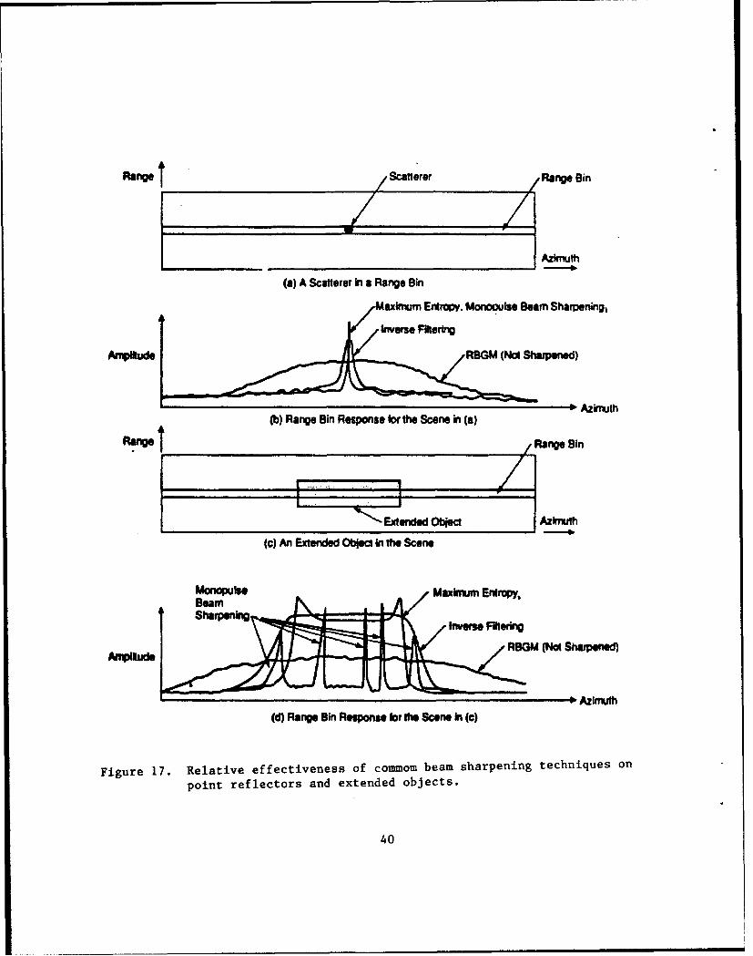
Figure 17 15] provides a comparison of the various beam sharpening techniques for both point
and extended targets. Note that for point targets, the maximum entropy, monopulse beam
sharpening and HADT methods provide excellent results. For extended targets, the maximum
entropy and HADT work well with the exception of some peaking in the return just before roll-off.
A Hughes modified inverse filter has also attained good results on extended targets. (Figure 18 [5]
shows the real return of an air-to-ground radar with a 2.5 degree bearnwidth mapping two corner
reflectors spaced three degrees apart.) Even though the separation is greater than the 3 dB beam
width, the objects are indistinguishable in the raw return. In the HADT processed response,
however, the targets are readily distinguished. Figure 19 [5] provides a comparison of SAR results,
unprocessed real beam return and sharpened real beam ground mapping (RBGM) return. While
targets in the unprocessed real beam image appear as smears due to the wide beam width sweeping
across them, the HADT sharpened image reveals the SAR processed image in clarity.
39
Range /Scatterer , Range Bin
Azkmth
(a) A Scafterer in a Range Bin
Maximum Entropy. Monooulse Beam Sharpening,
b Azimuth(b) Range Bin Response for the Scene in (a)
Range Range Bin
Extended Objet Azimuth
(c) An Extended Object in the Scene
BMonopul Maxinwum Entropy,
An•tudeBGM (No Sned)
SAzk•uh(d) Range Bin Response for the Scene In (c)
Figure 17. Relative effectiveness of commom beam sharpening techniques on
point reflectors and extended objects.
40

*0
CLn
.,. ..........SJ g
CM
CU3
CY
00
* Cm.. .. . . . . . . .............................. ..-
0 • • ......•--, r • I..........
*0
(59p) opnv•.uBh
Figure 18. Raw and processed range bin return of corner reflectors.
41

E E0OL
EmCO
xc 5
CD
E
tmo
42-
00o C/
Figure 19. Comparison of.SAR, unprocessed real beam and
sharpened real beam displays.
42

B. IMAGE ENHANCEMENT
Once the beam sharpening techniques discussed above have been applied, image processing can
further improve the output and generate more accurate and useful information. In order to
implement these techniques, a high throughput processor is required such as the APG-70, APG-73
or Hughes CIP. Several image processing techniques which have been widely implemented are
presented below.
1. Histogram Flattening
In many images, detail in the darker regions is imperceptible. Signal processing is required to
alter brightness or improve contrast. One method which works well is histogram modification. Both
adaptive and non-adaptive histogram modification techniques exist. In principle, these techniques
involve rescaling the image to some desired form. A common method of scaling is to find the
average value of the histogram and normalize quantized bands of pixels against it. By allowing fewer
levels of quantization, higher contrast of features is obtained. This process, however, does result in
an increase in quantization error.
2. Edge Detection
A common task in radar mapping is to determine the extent and position of extended targets
such as airfields and roads. One method of performing this task is through the detection of
luminescent edges or discontinuities between reasonably smooth regions. The only digital images
which exhibit step edges are artificially generated test patterns and images. Due to low.pass filtering
prior to digitization, any digital image resulting from optical or radar images of real scenes will have
reduced edge slopes. For this reason, additional processing is required to identify and localize the
boundaries of any extended objects.
One of the primary methods of edge detection is differential detection. This can take the
form of either first order derivative or second order derivative processing. In the first order case,
some form of spatial first order differentiation is performed, with the resulting edge gradient being
43

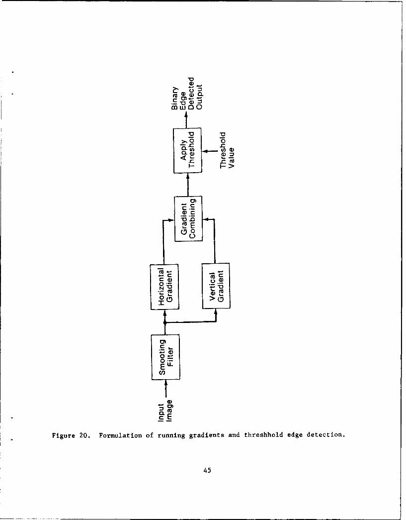
compared to a threshold value. A gradient above threshold denotes the presence of a boundary.
This process is demonstrated in Figure 20. [71
The simplest method of generating gradients is to compute the running difference of pixel
magnitude along rows and columns. Diagonal gradients can be obtained by forming a running
difference of diagonal pixel pairs. The running difference technique is highly susceptible to small
fluctuations in object luminance. Object boundaries are also not well defined. Modifications do
exist to better define edge locations. One such method which has provided good results is to simply
take the pixel differences separated by a null. Luminance fluctuation problems have been limited
through the use of weighted averages and moving windows. Larger windows improve the detection
of edges in high noise environments, but the computational requirements increase rapidly with size.
A sample C language program to perform first order derivative edge detection is presented in
Embree [7]. This program uses convolution smoothing and vertical edge detection with a 3X3
moving window called Sobel detection.
In second order derivative processing, a change in the polarity of the second derivative
signifies an edge. One implementation utilizes the Laplacian which is zero if the intensity is constant
or changing linearly. A greater rate of change will result in a sign change at the point of inflection.
The location of the zero crossing signifies the assigned location of the edge. A shortcoming of the
Laplacian is that it produces a fairly noisy result. Extraneous edge points are often introduced, and
especially strong responses result from corner reflectors.
An alternate implementation is to first estimate the edge direction. The second order
derivative is then taken along the edge. The difficulty in this method lies in estimating the edge
direction. First order detection techniques are sometimes used for this purpose.
A second method of edge detection is model fitting. This involves fitting the observed data in
a region of pixels to matrix mappings of possible edge types. Once a close fit is found, an edge is
deemed to exist and the region of pixels is assigned the properties of the model selected. In this
44
:3•j~ 4-'a ) CIL
Ca) o
0
0-Q
o, I - H>
a) C
cE
Figure 20. Formulation of running gradients and threshhold edge detection.
45

method, the match is made if the mean square error is below a threshold value. The model fitting
method requires much more computation than the derivative detection methods.
Pratt [6] provides an excellent comparison of these methods with several implementations of
each. The implementations are evaluated with respect to three criteria. The first, good detection,
refers to the ability of the system to detect edges without undue false detections. The selection of
threshold mirrors the tradeoffs of probability of detection (Pd) and probability of false alarm (Pf) in
target detection. The second, good localization, refers to the edge being designated as close to edge
center as possible. The third, single response, states that only one peak above threshold should exist
for each edge crossing.
3. Line (boundary) Detection
Similar techniques are used in the detection and refining of image lines. A line can be
modeled as a series of closely spaced parallel edges. Weighted averages and model fitting for
orientation are often used to limit susceptibility to noise.
4. Thresholding and Centroiding
This technique can detect and localize point scatterers as well as determine the extent of large
objects. Thresholds are determined by local noise estimates. An m out of n detection scheme is
employed to separate 'ioint reflectors from extended objects. If greater than m cells in an n cell
window exceed the threshold, then an extended object is determined to exist in the space. If fewer
than m threshold crossings exist, then a centroiding algorithm is applied at the peak crossing. This
algorithm estimates the location and amplitude of the point object and designates it to the
appropriate cell. The rest of the window is then replaced by the local background. Au estimate of
the location for a point scatterer is obtained by summing the weighted amplitudes of each cell and
dividing by an unweighted sum.
46
5. Median Filter
Noise can exist in one of two forms. It can be contained in a separate portion of the
frequency spectrum from the signal, or it can coexist with the signal across the spectrum of interest.
In the first instance, linear filtering can be quite effective. In the second case, filtering to remove
noise will also degrade the signal. An example of the second type of noise is "salt and pepper" noise.
It often results from A/D converter problems or digital transmission errors. These bit errors result
in impulses in an otherwise smooth sequence. Linear filtering to remove these "specks" in an image
can result in blurred images and loss of high frequency information. An effective method of
removing this noise is median filtering.
Embree [71 describes median filtering as a simple four step process:
1) A window of contiguous data is selected for each output point. Thiswindow can be reflected as adjacent time samples in a sequence, or asneighboring pixels in an image.
2) The data is sorted by signal value, from high to low.
3) The central value is selected as the median.
4) This median value is used as the filter output.
The advantage of this process is that sharp edges are preserved and not blurred as in averaging
filters. A twist to this process is conditional median filtering. This technique avoids unnecessary
corruption of the signal while maintaining the impulse removal capability of the previous fdter. The
process is as follows:
1) Select window.
2) Sort data from high to low.
3) Determine median.
4) The output of the filter is the median if the absolute value of thedifference between the median and input is above a chosen threshold.
Otherwise, the input is pas, -d through as the output.
47

Median filtering is highly dependent on the type of sort used. In image processing, max or
min values are often used to alter shrink or grow bright areas in an image. This is known as erosion
or dilation. Selection of output can also be used to control contrast.
Figures 21 and 22 [71 show the effect of median and conditional median filtering. These plots
are the result of the program MEDIAN which is shown in Embree [7]. The "flat topping" evident in
the figure is the result of median filtering a cosine wave. This is unwanted when filtering sinusoidal
signals, but is acceptable for image row and column processing. It should be noted that the amount
of "flat topping" is reduced through the use of conditional median filtering.
Richards (81 demonstrates a further usage of median filtering to enhance noncoherent radar
data. The algorithm diagrammed in Figure 23a 18] shows the combined usage of median and inverse
filtering. A median filter is used to segment real air-to-ground radar data into two classes, potential
point targets and background. The separation of the data overcomes the contradictory processing
goals of targets and background, namely to enhance target spikes while smoothing background
clutter. Once separated, the two classes of data are passed through deconvolution filters. This
inverse filtering removes the known spatial antenna pattern from the data to yield a high resolution
image. The resulting data is then recombined to yield an improved return. A lower order median
filter is also used as the background component constraint in Figure 23a. [81 This was done to
further control clutter spikes and ringing in the background which would otherwise be accentuated
by the far lower diagrams. Figure 23b [8] shows the effect of this process on millimeter-wave data.
Notice that the target response is sharpened in each case while the background has been noticeably
smoothed.
48

1.30-
S0.00-
-1.30
-. 0.0.0 25'.00 50.00 75-00 100.00Sample Number
I.NIX
a1.10
cn_
1.06.00 25.00 50.00 75.00 100.00
Sample Number
(b)
Figure 21. Median filtering with sort lengths of 3 and 9 threshhold = 0.
49

1.30.
CA.
w 0.00-
0n
-1.30- f0.00 25.00 50.00 M500 100.00
Sample Number
(a)
"B /7- 1 . 0 -1 1
0.60 25.'00 50.00 75.00 100.00Sample Number
(b)
Figure 22. Conditional median filtering with sort lengths 3, threshhold
.1, and sort length 9, threshhold .2.
50

(a)
KUW O MW
'0 023SAMPLE SA
CO
(b)
Figure 23. An inverse filtering process utilizing median filtering (a),sampled data and filtered results shown below (b).
51

IV. CONCLUSIONS AND RECOMMENDATIONS
While the various methods of beam sharpening have been treated separately in this paper, in
practice their implementation is often combined. This was demonstrated in the discussion of inverse
filtering and the example from Richards [81 in which used median filters in the deconvolution
process. In one Hughes system, the Hughes Advanced Discrimination Technique is used to detect
the location of point scatterers, a modified inverse filter sharpens extended objects, median filtering
is used to reduce impulse noise, edge detection algorithms are employed to identify roads and
runways, and histogram flattening is implemented to improve image contrast and emphasize low
contrast detail. When used in a system with high pulse compression, small mapping cells and
improved resolution are obtained.
Through the combined usage of these techniques, beam sharpening ratios of 6:1 can be achieved
for isolated corner reflectors with a 6 dB signal-to-noise ratio (SNR). With a 20 dB SNR, a 25:1
beam sharpening ratio can be achieved for corner reflectors and a 13:1 improvement for extended
objects 15]. To illustrate the value of this capability, the following example will compare SAR and
sharpened real beam resolutions for a fictional scenario.
Assuming operation at 12 GHz, the border of X and K. bands, the system wavelength will equal
.082 feet. If antenna length is assumed to be 10 feet, then the azimuth resolutions can be easily
calculated. Stimson [1] gives the azimuth resolution of a SAR system as one half the physical
antenna length. A comparison of resolution for real beam, sharpened real beam and SAR systems is
shown in Table 6. From the unsharpened real beam results, it is not hard to see why these systems
have been limited in application. The sharpened real beam columns, however, demonstrate "near
SAR" quality. These examples do assume corner reflectors. The beam sharpening results for
extended objects would only be approximately half as good.
52

TABLE 6COMPARISON OF SAR AND REAL BEAM RESOLUTIONS
RANGE SAR UNSHARPENED SHARPENED SHARPENED(in nmi) RESOLUTION REAL BEAM REAL BEAM (6 REAL BEAM
dB) (20dB)
50 5ft 2,461 ft 410 ft 98 ft
20 5ft 984 ft 164 ft 39 ft
10 I 5ft 492 ft 82 ft 20 ft
This level of improvement implies great potential for future mapping radars. Referring back to
Table 1 on page 7, with a 20 dB SNR highways can be mapped to over 50 miles. "Road map" level
of detail is available to over 20 miles. Taking into consideration that Scud launchers and other
tactical targets are much larger than standard vehicles and are very well represented by corner
reflectors, Table 6 demonstrates the capability to perform the mission proposed in the introduction
of high-speed search and target localization. Further, these results were obtained by processing
magnitude data only. In future efforts, these techniques may yield even better results through the
processing of 10 data.
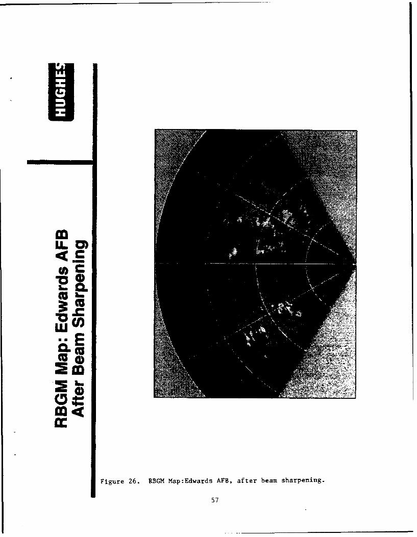
Figures 24 through 29, provided by Hughes, demonstrate the effectiveness the techniques
discussed in this paper. These figures provide a visual comparison of the results of these techniques
and SAR imaging. This data was collected by an F-15 in tests on another project. Efforts and
equipment dedicated to mapping in future tests may also yield further improved results.
Resolution in range is equally impressive. As mentioned in Chapter II, bandwidth is the best
determinant of performance. Since the 3dB bandwidth of a pulse is approximately the inverse of the
pulse width, fine range resolution implies the need for high bandwidth. Continuing improvements in
system bandwidth performance make it easier to achieve small cell size.
Continuing efforts to increase signal bandwidth and improve azimuth resolution yield numerous
opportunities for further research. Of particular interest in the future will be continuing efforts to
53

improve the extended object capability of mapping systems. Image processing can play a great role
in this effort. With stand-off weapons and associated tactics evolving at an extraordinary rate, radar
mapping will have a large role to play in any future conflicts.
54

Un
"0
IL
i.
maEm
Figure 24. SAR Map:Edwards AFB.
55

LL~
CC Im
Figure 25. RBGM Map:Edwards AFB, before beam sharpening.
56
cc
0LC
Fiue2.RBLMpEwad Fafe emshreigNI57

0
L_
O0goE
C)o
(1)
Cl)
Figure 27. SAR Map:Corner Reflectors, Rosamond Dry Lake.
58
C|

0
0
Figure 28. RLBGM Map:Corner Reflectors, before beam sharpening.
59

CL4g)
am.
0
Ecc
Figure 29. REGH Map:Corner Reflectors, after beam sharpening.
60

APPENDIX
MATCHED FILTER OUTPUT AND THE AMBIGUITY DIAGRAM
A. THE AMBIGUITY DIAGRAM
One of the primary tools which will be used to evaluate these coding schemes is the ambiguity
diagram. The ambiguity diagram represents the response of a matched filter to a waveform, and its
doppler shifted versions, reflected from a pce. t scatterer.
1. Development
The output of a matched filter can be represented as the cross correlation between a
transmitted signal and the received signal. Neglecting noise, Skolnick 19] presents this as
f Sr(t)S-(t-TR')dt (A.1)
where
S(t) is the transmitted signal
Sr(t) is the received signal.
TR' is the estimate of the time delay
The transmitted and received signals are assumed to be of the form
S(t) = u(t)eJ2wff (A.2)
Sr(t) = u(t-T)ed2i(1+fd)(t-T) (A.3)
where
f is the carrier frequency
fd is the doppler shift
T is the time delay
61

Substituting these representations into (A.1) and simplifying by setting T=O, f=0 and -
TR'=TR, the output of the matched filter becomes
X(TR,fd) = fu(t)u'(t + TR)eJ2 i- fdt (A.4)
where
u(t) is the complex modulation function
lu(t)J is the envelope of the real signal
With this representation, a positive fd denotes a closing #arget while a positive TR denotes a
target beyond the reference delay. The ambiguity function is the magnitude of this equation
squared.
The ambiguity diagram has a number of important properties as mentioned earlier. Several
include:
IX(TR,fd)1 2= IX(0,0)1 2=(2E)2 maximum value (A.5)
I X(-TR,-fd) 12 = I X(TR,fd) t 2 symmetry (A.6)
ff IX(TR,fd)I 2dTRdfd= (2E) 2 constant tctal volume (A.7)
Eq. (A.7) is known as the waveform uncertainty principle and illustrates the problems and
tradeoffs associated with waveform selection.
2. Usage
While the ambiguity diagram is of limited use as a practical design tool, it is helpful in
examining the limitations and utilities of particular classes of radar waveforms. By studying the
ambiguity diagram for a particular waveform, judgements can be made regarding its suitability for
various applications.
Wavcforms are selected to satisfy five major requirements. These are:
1) detection, 2) measurement accuracy, 3) resolution, 4) ambiguity and 5) clutter rejection. All of
these characteristics can be visually evaluated using the ambiguity diagram. The ambiguity diagram
62

allows the user to intuitively evaluate waveforms at a glance. General characteristics are presented
clearly without intensive mathematical formulation, as demonstrated below.
1) Detection is independent of the transmitted waveform and depends only on the level ofenergy which exceeds a chosen threshold at the origin. The maximum value of the ambiguityfunction occurs at the origin with a value of (2E)2. The threshold must be set below this value,but high enough to avoid any secondary peaks.
2) Range accuracy is dependent ca transmitted bandwidth (B) and doppler accuracy isdependent on the pulse width. Tae effects of these elements on the ambiguity function areshown in Figure 30. [91 Time delay (range) and frequency (doppler shift) are plotted on thehorizontal axes with the ambiguity function magnitude plotted on the vertical axis. As will alsobe shown later, the volume under the ambiguity diagram remains constant. This is known as theradar waveform uncertainty law. Care must be taken in attempting to compress the diagramalong either the range or frequency axis. (The waveform uncertainty principle forces a trade-offbetween range and doppler accuracy. Since the volume under the ambiguity function mustremain constant, efforts to compress the diagram along one axis may result in a spreading of thediagram along the other.
3) Resolution is closely related to measurement accuracy. A waveform with good resolution willalways have good accuracy. A waveform with good accuracy, however, may not have goodresolution due to the presence of sidelobes. Waveform resolution is displayed as twooverlapping ambiguity diagrams displaced by the range and Doppler spacing of the targets.While waveforms with narrow spikes may provide excellent accuracy and resolution in the mainpeak, they may also have large sidelobes. Sidelobes from a large target or ground clutter maycontain enough energy to overpower a smaller target's central peak.
4) As alluded to above, peaks other than at the origin yield ambiguity in the measurement ofrange and doppler. Decisions with regard to pulse train length and PRF can be quicklyevaluated by observing the presence and height of secondary peaks with respect to the mainpeak.
5) Clutter rejection ability is visualized by insuring ambiguity function peaks do not exist indoppler or range bins with high clutter.
3. Types
There are five major classes of waveforms which give rise to three types of ambiguity
diagrams. These types are the "knife edge", "bed of spikes" and "thumbtack". These are
demonstrated in Figures 30. [9]
The "knife edge", or "ridge", diagram is obtained from a single pulse of sine wave. Linear
frequency modulation rotates this ridge through the fd,T plane.
63

tx( r. fd)1
Ix( x*,'d'd
PKnfe edge (ridge)
T - signoI duration
8 = signal bandwidth
• Ix•,• f)l•2
T huntOCk
Bed of spikes
Figure 30. The ambiguity diagram, ideal approximation and three major classes.
64

The "bed of spikes" results from a periodic train of pulses. The form of each of the spikes is
dependent upon the waveform of the individual pulses. This is representative of pulse-Doppler and
MTI systems.
The "thumbtack" ambiguity diagram results from noise or pseudonoise codes. These codes
include Pseudorandom, Barker and Polyphase codes. This thumbtack usually exists on a large
pedestal of range-Doppler sidelobes which can be quite significant.
65

B. AMBIGUITY DIAGRAM PLOTTING PROGRAM
01
= ambigUus Michael D. Anderson =
%= A menu driven plotting program to draw ambiguity= diagrams for various pulse compression code families. -
= AmbigUus is the main, calling menu subroutines and == performing the mesh plot.
clearclgCODE= [];
intro t (Calls subroutine to provide instructions)waveform t (Calls subroutine to route user through menus.
% Menu programs implement selected codes andt return for phase incrementation and plotting)
% (Scale the ambiguity diagram by selecting max reach of thedoppler axis.)
s=input('Enter max doppler phase shift across the pulse in
radians: ')
l=length(CODE);
for k=l:50; % (Implement the iterative phasestep=(s*2)/(50-1); % shift across the code for eachshift=(-s)+(k-l)*step; % increment along the doppler
% axis.)
for j=l:l;v(j)=shift*j+CODE(j);
end
ua=i*CODE;va=i*v;ub=exp(ua); k (Digitalizes the phase code values)vb=exp(va); t (Digitalizes the shifted phase code)output=xcorr(ub,vb); * (Performs the autocorrelation)x=abs(output); t (The matched filter output)X=x.A2; * (The ambiguity function is theA(k,:)=X; % square of the filter function)
endmesh(A) t (Plots the 3-D ambiguity diagram)
66

%
= intro Michael D. Anderson
%= Greets users and instructs them of the purposeS= and usage of the program.
clcecho on
Welcome to the program ambigUus. This program will enable%
%! you to view the ambiguity diagram for a number of your favorite0
% waveforms.0
%k The ambiguity diagram is a 3-D plot showing the response of0
% a matched filter receiver to reflections from point scatterers.%
k Range and frequency shifts are read along the horizontal axes,0
% as the matched filter response is plotted along the vertical6%
% axis.001 This plot can be used to evaluate the critical properties%
% of detection, range and doppler accuracy, range and doppler%
% resolution, range and doppler ambiguity, and clutter rejection.%
16 (press any key to continue)echo off
pause;end
67

t waveform Michael D. Anderson
A menu program allowing the user to select which= waveform to implement.
clgclc
echo on% Two major classifications of radar waveforms are pseudo-
% random binary codes and polyphase codes. Both can be modeled%
% with this program.0
Pseudo-random binary codes consist of Barker, Compound0-k Barker and Complementary codes.%
Polyphase codes consist of Frank codes and the P-series
% codes. These are digital representations of LFM and step-chirp0
% waveforms.0
% 1) Barker code% 2) Compound Barker code
3) Pseudorandom code4) Polyphase code5) Frank code
% 6) P1 code% 7) P2 code! 8) P3 code% 9) P4 code% 0) quit program
echo offn=input('Select the waveform type to process: ');
if n==lbarkform
elseif n==2compound
elseif n==3randform
elseif n==4polyform
elseif n==5frnkform
68

elseif n==6plf orm
elseif n.=7p2 form
elseif n==8p3f arm
elseif n==9p4f arm
elsedeath
end
69

%
t barkform Michael D. Anderson
SAllows user to select code length to plot and loadsthe vector CODE with the code phases.
%
clearclc
echo on
% The Barker codes are a special set of binary phase codes0
t which yield equal sidelobes after passage through a matched
% filter. These codes have pulse compression ratios equal to0
t their length. The (+) and (-) in the sequences represent0
% phase shifts of zero and pi radians. The known Barker codes%
% are as follows:%
selection code # code sequence%1 2A
% 2 2B ++% 3 3 ++-% 4 4A ++-+% 5 4B +++-% 6 5 +++-+0% 7 7% 8 11+ --
9 13 .............
echo off
n=input('Enter your choice, selection # ');if n=l,
CODE=[O pi);elseif n==2,
CODE=[O 0];elseif n==3,
CODE=[0 0 pil;elseif n==4,
CODE=[0 0 pi 0];elseif n==5,
CODE=[O 0 0 pi];elseif n==6,
CODE=[0 0 0 pi 01;
70

elseif n==7,CODE=[0 0 0 pi pi 0 pi];
elseif n==8,CODE=[0 0 0 pi pi pi 0 pi pi 0 pi];
elseif n==9,CODE=[0 0 0 0 0 pi pi 0 0 pi 0 pi 0];
endend
71

= compound Michael D. Anderson
%= Allows user to select inner and outer codes to generate= compound barker codes. Originated from "combined.m"
with Capt. Paul Ohrt, RCA for EC 4970, 1992.
clear
BARKER2 =[0, pi];BARKER3= [0,0,pi];BARKER4=[0,0,pi,0];BARKER5= [0, 0, 0,pi, 0]BARKER7=[0,0,0,pi,pi,0,pi];BARKER11=[0,0,0,pi,pi,pi,0,pi,pi,0,pi];BARKER13= [0, 0,0,0, 0,pi,pi, 0, 0,pi, 0,pi, 0];
clcecho on
This subroutine generates Compound Barker codes.
% The known Barker codes have lengths of n= 2,3,4,5,7,11 or 130
% You need to choose the length of the inner Barker code, "I"
% and outer Barker code, "n". The length will be m*n and the
% PSL will be at the level of the shortest Barker code used.
echo offm=input('ENTER the # of the inner Barker Code to use, m =n=input('ENTER the # of the outer Barker Code to use, n =
%ý Set selected inner Barker Code
if m==2in_CODE=BARKER2;
elseif m==3in_CODE=BARKER3;
elseif m==4in CODE=BARKER4;
elseif m==5in CODE=BARKER5;
elseif m==7in_CODE=BARKER7;
elseif m==l1in_CODE=BARKER11;
elseif m==13in_CODE=BARKER13;
else
72

compound % starts sub program over if improper "Im" entered
end
Set selected outer Barker Code
if n==2out CODE=BARKER2;
elseif n==3out CODE=BARKER3;
elseif n==4out CODE=BARKER4;
elseif n==5outCODE=BARKER5;
elseif n==7outCODE=BARKER7;
elseif n==l1out CODE=BARKER11;
elseif n==13outCODE=BARKER13;
elsecompound % starts sub program over if improper "n" entered
end
% Take Cosine of phase changes and develop "rm in n" BARKER CODE
incos=cos(in CODE);out_cos=cos(outCODE);
CODE=[);
for count=l:nINC=out cos(count).*in cos;CODE=[CODE, INC);
end
CODE=acos(CODE);end
73

randform Michael D. Anderson =
9 5 Allows user to select code length to plot for a% = polyphase code using shift register implementation. -
= Program originated from "random.m" developed with% = Capt. Paul Ohrt RCA for EC4970, 1992.%
clearclc
echo onWhen a large pulse compression ratio is required,
% pseudorandom codes are often used. These approximate noise0
% modulated signals with "thumbtack" ambiguity functions and0
% excellent range and doppler resolution.
A commmon method of generating these codes is the modulo 2
% adder or exclusive-OR gate shift register decribed in Skolnik%t ch 11. That method is used here. The only restrictions are0
k that the initial conditions of the register can not all be zeroI;% (or the output will si.mply be a sequence of zeros), and that (p)8
% can not equal (q) (both shift inputs can not be taken from the% n% same bit). The length of the resulting code will be z -1.0
o (hit any key to continue)
echo off
pause;clc
n=input('ENTER the length of the shift register (# of bits): ');p=input('ENTER the first feedback bit: # ');q=input('ENTER the second feedback bit: # ');
echo on%_
% To enter your initial conditions, simply enter a string of
% ones and zeros.%
74

% ex. Shift register length 7. Initial conditions 1001100%
echo off
IC=0;
flag=1;while flag=l
IC=input('Enter your string of length [n]: ');if length(IC)=n,
flag=0end
end
CODE=[IC]; % initial start point
MLS=2An-.1; % maximal length sequence
for count = (n+l) :MLS
XOR=CODE(p) ICODE(q); % OR function from Matlab
if CODE (p) &CODE (q) ==l;XOR=0; % to ensure XOR conditions met
elseXOR=XOR;
end
CODE=[XOR,CODE]; % update code values from shift
end
CODE=acos (CODE);
end
75

= polyform Michael D. Anderson
'I' Allows user to select code length to plot for a simpleIi polyphase sequence and loads the CODE vector. Program*= originated from polyphas.m with Capt. Paul Ohrt RCA0= for EC 4970, 1992.
clearclc
echo on% This subroutine implements a POLYPHASE coding% sequence. The POLYPHASE code developed here is a sequence% between 0 and pi in n increments.% You must specify how many increments are to be used.0
echo off
n=input('ENTER the # of increments the Code is to use. n =
% (Generate polyphase vector)
k=0: (n-l); % (increment vector)phi=pi.vk.A2./n;CODE=cos(phi)+i.*sin(phi);
end
76

= frnkform Michael D. Anderson =9- ==
% = Allows user to select length of a frank code and loads == the vector CODE with the code phases. From "frank.m"= generated in 1992 for EC 4970.
clearclc
echo on%1 This subroutine implements Frank Coding. It is equal to0
% Barker coding in PSL, but is not limited in length.
Frank coding is a step-wise approximation of a60
% linear FM or "chirp" code. To use this coding scheme,
* enter the number of phase subdivisions N. The PCR0% will be N squared.0
echo off
N=input('N =step 2*pi/N;
for k = 1:Nfor j = 1:N
count - (k-l)*N + j;% Generate the Frank Code Matrixx(count) = (k-l)*(j-l); % Store in vector form
endend
stepx = step*x; % combine the Frank Code Matrix with the actual% phase increment to generate the phase sampling
CODE=cos(stepx)+j.*sin(stepx);
end
77

= piform Michael D. Anderson =09 ==
%6 = Allows user to select code length for P1 code and loads =% = the vector CODE with the code phases. Derived from
= frnkform.m 1992.
clearclc
echo onThis subroutine implements Pi coding, a Frank code
0
W rearranged to avoid bandwidth limitations. The ambiguity0
% diagram will be almost identical to the Frank code since both%
% are derived from the same waveform.0
% Enter the number of phase subdivisions N.0
echo off
N=input('N = N);step = pi/N;
for k = 1:Nfor j = 1:N
count = (k-l)*N + j;x(count) = ((j-l)*N+(k-l));x(count) = x(count)*(N-(2*j-l));
endend
stepx = (-l)*step*x;
CODE=cos(stepx)+j.*sin(stepx);
end
78

p2form, Michael D. Anderson =16
%= Allows user to select code length for P2 and loads =%= the vector CODE with the code phases.
clearclc
echo onThis subroutine implements P2 coding. P2 coding
% is a real vice complex version of PI. Results should
% be indistinguishable from Frank and P1 codes.0
% Enter the number of phase subdivisions N.0
echo off
N=input('Nstep = (pi/2)*((N-1)/N);
for k 1:Nfor j = 1:N
count = (k-l)*N + j;x(count) = step- (pi/N)*(k-1);x(count) = x(count)*(N+l-2*j);
endend
CODE=cos (x) +j .*sin (x);
end
79

= p3form Michael D. Anderson =6
%= Allows user to select code length for P3 and loads0= the vector CODE with the code phases.
clearclc
echo on%- This subroutine implements P3 coding. This code0
% is derived from a linear chirp rather than the step0
% chirp as the Frank, P1 and P2 codes. Because of this,0
% it will show the bette_ . doppler tolerance of the linear0
% frequency modulated (LFM) signal.01
echo off
N=input('N =
step = pi/N;
for j = 1:Nx(j) = (j-1)A2;
end
stepx = step*x;
CODE=cos(stepx)+j.*sin(stepx);
end
80
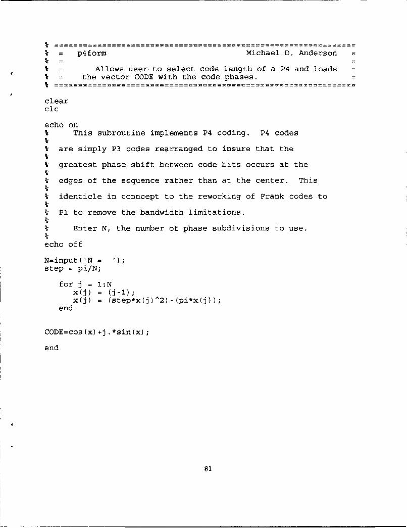
= p4form Michael D. Anderson =
%~ = Allows user to select code length of a P4 and loads =
%= the vector CODE with the code phases.
clearclc
echo onThis subroutine implements P4 coding. P4 codes0
% are simply P3 codes rearranged to insure that the%
% greatest phase shift between code bits occurs at the
% edges of the sequence rather than at the center. This%
% identicle in conncept to the reworking of Frank codes to%
% P1 to remove the bandwidth limitations.%
%- Enter N, the number of phase subdivisions to use.o
echo off
N=input('N = );step = pi/N;
for j = I:Nx(j) = (j-1);x(j) = (step*x(j)A2)-(pi*x(j));
end
CODE=cos(x)+j.*sin(x);
end
81

LIST OF REFERENCES
1. Stimson, G.W., "Introduction to Airborne Radar," Hughes Aircraft Co., El Segundo, CA, 1983.
2. Nathanson, F.E., Radar Design Principles, second ed., McGraw-Hill, Inc. NY, 1991.
3. Akita, R.M. "An Investigation of the Narrow-band and Wide-band Ambiguity Functions forComplementary Codes," Master's Thesis, Naval Postgraduate School, Monterey, CA, 1968.
4. Lewis, L. and Kretchmer, F.F. Jr., "New Polyphase Pulse Compression Waveforms andImplementation Techniques," Advances in Radar Techniques, ed. J. Clarke Peter Peregrinus Ltd.,London, UK., 1985. pp. 496-500.
5. Unpublished presentation materials, Hughes Aircraft Advanced Systems.
6. Pratt, W. K., Digital Image Processing, John Wiley & Sons, Inc., NY, 1991.
7. Embree, P.M. and Kimble, B., C Language Algorithms for Digital Signal Processing, PrenticeHall, Englewood Cliffs, NJ., 1991.
8. Richard, MA., Morris, C.E. and Haynes, M.H., "Iterative Enhancement of Noncoherent RadarData," Proceedings 1986 IEEE International Conference on Acoustics, Speech and SignalProcessing, April 1986.
9. Skolnick, M.L., Introduction to Radar Systems, McGraw-Hill Publishing Co., NY, 1980.
82
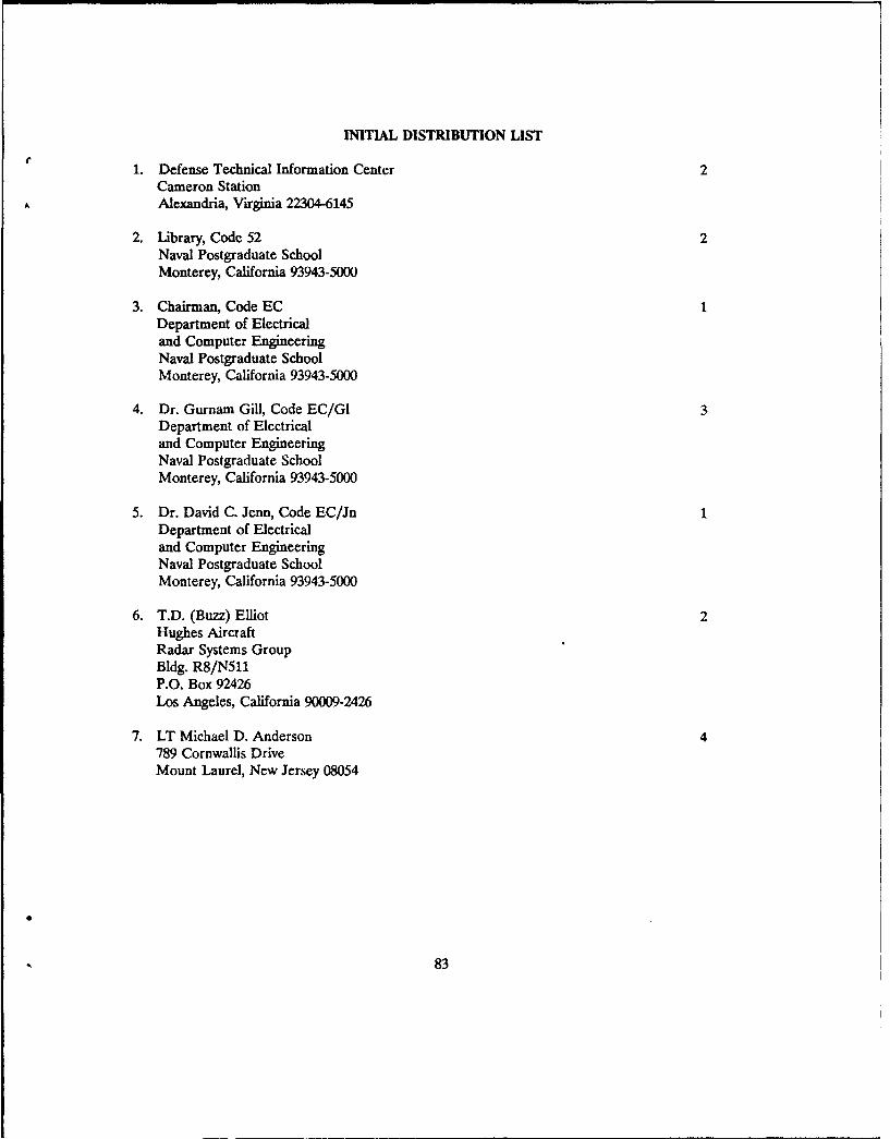
INITIAL DISTRIBUTION LIST
1. Defense Technical Information Center 2Cameron StationAlexandria, Virginia 22304-6145
2. Library, Code 52 2Naval Postgraduate SchoolMonterey, California 93943-5000
3. Chairman, Code ECDepartment of Electricaland Computer EngineeringNaval Postgraduate SchoolMonterey, California 93943-5000
4. Dr. Gurnam Gill, Code EC/GI 3Department of Electricaland Computer EngineeringNaval Postgraduate SchoolMonterey, California 93943-5000
5. Dr. David C. Jenm, Code EC/JnDepartment of Electricaland Computer EngineeringNaval Postgraduate SchoolMonterey, California 93943-5000
6. T.D. (Buzz) Elliot 2Hughes AircraftRadar Systems GroupBldg. R8/N511P.O. Box 92426Los Angeles, California 90009-2426
7. LT Michael D. Anderson 4789 Cornwallis DriveMount Laurel, New Jersey 08054
83
Related Documents