RESIDUAL-BASED VARIATIONAL MULTISCALE MODELS FOR THE LARGE EDDY SIMULATION OF COMPRESSIBLE AND INCOMPRESSIBLE TURBULENT FLOWS By Jianfeng Liu A Thesis Submitted to the Graduate Faculty of Rensselaer Polytechnic Institute in Partial Fulfillment of the Requirements for the Degree of DOCTOR OF PHILOSOPHY Major Subject: MECHANICAL ENGINEERING Approved by the Examining Committee: Prof. Assad A. Oberai, Thesis Adviser Prof. Mark S. Shephard, Member Prof. Donald A. Drew, Member Prof. Onkar Sahni, Member Rensselaer Polytechnic Institute Troy, New York July 2012 (For Graduation August 2012)

Welcome message from author
This document is posted to help you gain knowledge. Please leave a comment to let me know what you think about it! Share it to your friends and learn new things together.
Transcript
RESIDUAL-BASED VARIATIONAL MULTISCALEMODELS FOR THE LARGE EDDY SIMULATION OF
COMPRESSIBLE AND INCOMPRESSIBLETURBULENT FLOWS
By
Jianfeng Liu
A Thesis Submitted to the Graduate
Faculty of Rensselaer Polytechnic Institute
in Partial Fulfillment of the
Requirements for the Degree of
DOCTOR OF PHILOSOPHY
Major Subject: MECHANICAL ENGINEERING
Approved by theExamining Committee:
Prof. Assad A. Oberai, Thesis Adviser
Prof. Mark S. Shephard, Member
Prof. Donald A. Drew, Member
Prof. Onkar Sahni, Member
Rensselaer Polytechnic InstituteTroy, New York
July 2012(For Graduation August 2012)

c© Copyright 2012
by
Jianfeng Liu
All Rights Reserved
ii

CONTENTS
LIST OF TABLES . . . . . . . . . . . . . . . . . . . . . . . . . . . . . . . . . vi
LIST OF FIGURES . . . . . . . . . . . . . . . . . . . . . . . . . . . . . . . . vii
DEDICATION . . . . . . . . . . . . . . . . . . . . . . . . . . . . . . . . . . . xix
ACKNOWLEDGEMENT . . . . . . . . . . . . . . . . . . . . . . . . . . . . . xx
ABSTRACT . . . . . . . . . . . . . . . . . . . . . . . . . . . . . . . . . . . . xxi
1. Introduction . . . . . . . . . . . . . . . . . . . . . . . . . . . . . . . . . . . 1
1.1 Turbulent Flows . . . . . . . . . . . . . . . . . . . . . . . . . . . . . . 1
1.2 Approaches to Studying Turbulence . . . . . . . . . . . . . . . . . . . 2
1.3 Numerical Simulation of Turbulent Flows . . . . . . . . . . . . . . . . 4
1.3.1 Direct Numerical Simulation (DNS) . . . . . . . . . . . . . . . 4
1.3.2 Large-Eddy Simulation (LES) . . . . . . . . . . . . . . . . . . 5
1.3.3 Reynolds-averaged Navier-Stokes (RANS) Equations . . . . . 5
1.4 LES of Turbulent Flows . . . . . . . . . . . . . . . . . . . . . . . . . 6
1.4.1 LES of Incompressible Flows . . . . . . . . . . . . . . . . . . . 6
1.4.2 LES of Compressible Flows . . . . . . . . . . . . . . . . . . . 8
1.5 Residual based Variational Multiscale (RBVM) Formulation . . . . . 9
1.6 Residual based Eddy Viscosity (RBEV) Model . . . . . . . . . . . . . 10
1.7 Description of Chapters . . . . . . . . . . . . . . . . . . . . . . . . . 12
2. Residual Based Methods for Large Eddy Simulation of Turbulent Flows . . 13
2.1 Residual-based variational multiscale formulation (RBVM) . . . . . . 15
2.2 A mixed model based on residual based variational multiscale formu-lation (MM1) . . . . . . . . . . . . . . . . . . . . . . . . . . . . . . . 20
2.2.1 Weak Form of MM1 . . . . . . . . . . . . . . . . . . . . . . . 21
2.2.2 Analysis of mechanical energy for the RBVM formulation . . . 23
2.2.3 Derivation of the dynamic calculation for C0, C1 and Prt. . . . 26
2.3 Residual based eddy viscosity model (RBEV) . . . . . . . . . . . . . 30
2.3.1 Weak form of the RBEV model . . . . . . . . . . . . . . . . . 30
2.3.2 Estimate of the RBEV parameter C . . . . . . . . . . . . . . 32
2.4 A purely residual based mixed model (MM2) . . . . . . . . . . . . . . 34
iii

3. Large-Eddy Simulation of Compressible Homogeneous Isotropic TurbulentFlows . . . . . . . . . . . . . . . . . . . . . . . . . . . . . . . . . . . . . . . 37
3.1 Introduction . . . . . . . . . . . . . . . . . . . . . . . . . . . . . . . . 37
3.2 LES models . . . . . . . . . . . . . . . . . . . . . . . . . . . . . . . . 38
3.2.1 Weak form of LES models . . . . . . . . . . . . . . . . . . . . 38
3.2.2 Unresolved scales and stabilization parameter τ . . . . . . . . 40
3.2.3 Specialization to a Fourier spectral basis . . . . . . . . . . . . 41
3.3 Homogeneous Isotropic Turbulence (HIT) . . . . . . . . . . . . . . . . 44
3.4 Numerical Results for RBVM and MM1 . . . . . . . . . . . . . . . . 50
3.4.1 Low Reynolds Number Case . . . . . . . . . . . . . . . . . . . 50
3.4.2 Study of the effects of varying χ . . . . . . . . . . . . . . . . . 57
3.4.3 Study of the effects of varying Ma . . . . . . . . . . . . . . . 62
3.4.4 High Reynolds Number Case . . . . . . . . . . . . . . . . . . . 66
3.4.5 Summary . . . . . . . . . . . . . . . . . . . . . . . . . . . . . 74
3.5 Numerical Results for the RBEV model . . . . . . . . . . . . . . . . . 75
3.5.1 Low Reynolds Number Case . . . . . . . . . . . . . . . . . . . 75
3.5.2 High Reynolds Number Case . . . . . . . . . . . . . . . . . . . 87
3.6 Numerical Results for the MM2 Model . . . . . . . . . . . . . . . . . 98
3.6.1 Low Reynolds Number Case . . . . . . . . . . . . . . . . . . . 98
3.6.2 High Reynolds Number Case . . . . . . . . . . . . . . . . . . . 109
3.7 The RBEV and MM2 Models with Cτ = 0.5 . . . . . . . . . . . . . . 120
3.7.1 Low Reynolds Number Case . . . . . . . . . . . . . . . . . . . 120
3.7.2 High Reynolds Number Case . . . . . . . . . . . . . . . . . . . 125
3.8 Chapter Summary . . . . . . . . . . . . . . . . . . . . . . . . . . . . 131
4. Residual-Based Models Applied to Incompressible Turbulent Channel Flow 133
4.1 Introduction . . . . . . . . . . . . . . . . . . . . . . . . . . . . . . . . 133
4.2 Residual-based models . . . . . . . . . . . . . . . . . . . . . . . . . . 134
4.2.1 Weak form for FEM . . . . . . . . . . . . . . . . . . . . . . . 134
4.2.2 Unresolved scales and stabilization parameter τ . . . . . . . . 135
4.3 Turbulent Channel Flow . . . . . . . . . . . . . . . . . . . . . . . . . 136
4.3.1 Wall shear stress . . . . . . . . . . . . . . . . . . . . . . . . . 138
4.3.2 Wall units . . . . . . . . . . . . . . . . . . . . . . . . . . . . . 140
4.3.3 Law of the wall and regions and layers near the wall . . . . . . 141
iv

4.4 Numerical Simulation . . . . . . . . . . . . . . . . . . . . . . . . . . . 144
4.4.1 Reτ = 395 . . . . . . . . . . . . . . . . . . . . . . . . . . . . . 148
4.4.1.1 RBEV . . . . . . . . . . . . . . . . . . . . . . . . . 148
4.4.1.2 MM2 . . . . . . . . . . . . . . . . . . . . . . . . . . 168
4.4.2 Reτ = 590 . . . . . . . . . . . . . . . . . . . . . . . . . . . . . 184
4.4.2.1 RBEV . . . . . . . . . . . . . . . . . . . . . . . . . . 184
4.4.2.2 MM2 . . . . . . . . . . . . . . . . . . . . . . . . . . 189
4.5 Chapter summary . . . . . . . . . . . . . . . . . . . . . . . . . . . . . 194
5. Conclusion . . . . . . . . . . . . . . . . . . . . . . . . . . . . . . . . . . . . 196
REFERENCES . . . . . . . . . . . . . . . . . . . . . . . . . . . . . . . . . . . 199
v

LIST OF TABLES
2.1 A concise description of all models based on the terms appearing inEquation (2.22). . . . . . . . . . . . . . . . . . . . . . . . . . . . . . . . 26
3.1 Parameters for the decay of homogeneous compressible turbulence. . . . 51
4.1 Physical parameters for the channel flow problem. . . . . . . . . . . . . 147
4.2 Numerical parameters for the channel flow problem. . . . . . . . . . . 147
vi

LIST OF FIGURES
3.1 Sketch of energy spectrum. . . . . . . . . . . . . . . . . . . . . . . . . . 49
3.2 Time history of turbulent kinetic energy of the incompressible velocitycomponent for the Reλ = 65.5 case on a 323 grid with χ = 0.4 andMa = 0.488. A comparison of the DSYE, RBVM, MM1, and no modelcases. . . . . . . . . . . . . . . . . . . . . . . . . . . . . . . . . . . . . 52
3.3 Time history of turbulent kinetic energy of the compressible velocitycomponent for the Reλ = 65.5 case on a 323 grid with χ = 0.4 andMa = 0.488. A comparison of the DSYE, RBVM, MM1, and no modelcases. . . . . . . . . . . . . . . . . . . . . . . . . . . . . . . . . . . . . . 52
3.4 Energy spectrum of the incompressible velocity component for the Reλ =65.5 case on a 323 grid with χ = 0.4 and Ma = 0.488 at t/Te ≈ 3. Acomparison of the DSYE, RBVM, MM1, and no model cases. . . . . . . 54
3.5 Energy spectrum of the compressible velocity component for the Reλ =65.5 case on a 323 grid with χ = 0.4 and Ma = 0.488 at t/Te ≈ 3. Acomparison of the DSYE, RBVM, MM1, and no model cases. . . . . . . 54
3.6 Energy spectrum of the incompressible velocity component for the Reλ =65.5 case on a 323 grid with χ = 0.4 and Ma = 0.488 at t/Te ≈ 6. Acomparison of the DSYE, RBVM, MM1, and no model cases. . . . . . . 55
3.7 Energy spectrum of the compressible velocity component for the Reλ =65.5 case on a 323 grid with χ = 0.4 and Ma = 0.488 at t/Te ≈ 6. Acomparison of the DSYE, RBVM, MM1, and no model cases. . . . . . . 55
3.8 Density spectrum for the Reλ = 65.5 case on a 323 grid with χ = 0.4and Ma = 0.488 at t/Te ≈ 6. A comparison of the DSYE, RBVM,MM1, and no model cases. . . . . . . . . . . . . . . . . . . . . . . . . . 56
3.9 Pressure spectrum for the Reλ = 65.5 case on a 323 grid with χ = 0.4and Ma = 0.488 at t/Te ≈ 6. A comparison of the DSYE, RBVM,MM1, and no model cases. . . . . . . . . . . . . . . . . . . . . . . . . . 56
3.10 Time history of root-mean-square of density for the Reλ = 65.5 case ona 323 grid with χ = 0.4 and Ma = 0.488. A comparison of the DSYE,RBVM, MM1, and no model cases. . . . . . . . . . . . . . . . . . . . . 57
3.11 Time history of the Smagorinsky coefficient C0 for the Reλ = 65.5 caseon a 323 grid with Ma = 0.488. A comparison of the DSYE and MM1cases. . . . . . . . . . . . . . . . . . . . . . . . . . . . . . . . . . . . . . 58
vii

3.12 Time history of the Smagorinsky coefficient C1 for the Reλ = 65.5 caseon a 323 grid with Ma = 0.488. A comparison of the DSYE and MM1cases. . . . . . . . . . . . . . . . . . . . . . . . . . . . . . . . . . . . . . 59
3.13 Time history of Prt for the Reλ = 65.5 case on a 323 grid with Ma =0.488. A comparison of the DSYE and MM1 cases. . . . . . . . . . . . . 59
3.14 Energy spectrum of the incompressible velocity component for the Reλ =65.5 case on a 323 grid with χ = 0.2 and Ma = 0.488 at t/Te ≈ 6. Acomparison of the DSYE, RBVM, MM1, and no model cases. . . . . . . 60
3.15 Energy spectrum of the compressible velocity component for the Reλ =65.5 case on a 323 grid with χ = 0.2 and Ma = 0.488 at t/Te ≈ 6. Acomparison of the DSYE, RBVM, MM1, and no model cases. . . . . . . 61
3.16 Energy spectrum of the incompressible velocity component for the Reλ =65.5 case on a 323 grid with χ = 0.6 and Ma = 0.488 at t/Te ≈ 6. Acomparison of the DSYE, RBVM, MM1, and no model cases. . . . . . . 61
3.17 Energy spectrum of the compressible velocity component for the Reλ =65.5 case on a 323 grid with χ = 0.6 and Ma = 0.488 at t/Te ≈ 6. Acomparison of the DSYE, RBVM, MM1, and no model cases. . . . . . . 62
3.18 Energy spectrum of the incompressible velocity component for the Reλ =65.5 case on a 323 grid with χ = 0.4 and Ma = 0.300 at t/Te ≈ 6. Acomparison of the DSYE, RBVM, MM1, and no model cases. . . . . . . 63
3.19 Energy spectrum of the compressible velocity component for the Reλ =65.5 case on a 323 grid with χ = 0.4 and Ma = 0.300 at t/Te ≈ 6. Acomparison of the DSYE, RBVM, MM1, and no model cases. . . . . . . 64
3.20 Energy spectrum of the incompressible velocity component for the Reλ =65.5 case on a 323 grid with χ = 0.4 and Ma = 0.700 at t/Te ≈ 6. Acomparison of the DSYE, RBVM, MM1, and no model cases. . . . . . . 64
3.21 Energy spectrum of the compressible velocity component for the Reλ =65.5 case on a 323 grid with χ = 0.4 and Ma = 0.700 at t/Te ≈ 6. Acomparison of the DSYE, RBVM, MM1, and no model cases. . . . . . . 65
3.22 Time history of the Smagorinsky coefficient C0 for the Reλ = 65.5 caseon a 323 grid with χ = 0.4. A comparison of the DSYE and MM1 cases. 65
3.23 Energy spectrum of the incompressible velocity component for the Reλ =121.0 case on a 323 grid with χ = 0.4 and Ma = 0.488 at t/Te ≈ 3. Acomparison of the DSYE, RBVM, MM1, and no model cases. . . . . . . 67
viii
3.24 Energy spectrum of the incompressible velocity component for the Reλ =121.0 case on a 323 grid with χ = 0.4 and Ma = 0.488 at t/Te ≈ 6. Acomparison of the DSYE, RBVM, MM1, and no model cases. . . . . . . 67
3.25 Energy spectrum of the compressible velocity component for the Reλ =121.0 case on a 323 grid with χ = 0.4 and Ma = 0.488 at t/Te ≈ 3. Acomparison of the DSYE, RBVM, MM1, and no model cases. . . . . . . 68
3.26 Energy spectrum of the compressible velocity component for the Reλ =121.0 case on a 323 grid with χ = 0.4 and Ma = 0.488 at t/Te ≈ 6. Acomparison of the DSYE, RBVM, MM1, and no model cases. . . . . . . 68
3.27 Time history of turbulent kinetic energy of the incompressible velocitycomponent for the Reλ = 121.0 case on a 643 grid with χ = 0.4 andMa = 0.488. A comparison of the DSYE, RBVM, MM1, and no modelcases. . . . . . . . . . . . . . . . . . . . . . . . . . . . . . . . . . . . . . 69
3.28 Time history of turbulent kinetic energy of the compressible velocitycomponent for the Reλ = 121.0 case on a 643 grid with χ = 0.4 andMa = 0.488. A comparison of the DSYE, RBVM, MM1, and no modelcases. . . . . . . . . . . . . . . . . . . . . . . . . . . . . . . . . . . . . . 70
3.29 Time history of root-mean-square of density for the Reλ = 121.0 caseon a 643 grid with χ = 0.4 and Ma = 0.488. A comparison of theDSYE, RBVM, MM1, and no model cases. . . . . . . . . . . . . . . . . 70
3.30 Energy spectrum of the incompressible velocity component for the Reλ =121.0 case on a 643 grid with χ = 0.4 and Ma = 0.488 at t/Te ≈ 3. Acomparison of the DSYE, RBVM, MM1, and no model cases. . . . . . . 71
3.31 Energy spectrum of the compressible velocity component for the Reλ =121.0 case on a 643 grid with χ = 0.4 and Ma = 0.488 at t/Te ≈ 3. Acomparison of the DSYE, RBVM, MM1, and no model cases. . . . . . . 72
3.32 Energy spectrum of the incompressible velocity component for the Reλ =121.0 case on a 643 grid with χ = 0.4 and Ma = 0.488 at t/Te ≈ 6. Acomparison of the DSYE, RBVM, MM1, and no model cases. . . . . . . 72
3.33 Energy spectrum of the compressible velocity component for the Reλ =121.0 case on a 643 grid with χ = 0.4 and Ma = 0.488 at t/Te ≈ 6. Acomparison of the DSYE, RBVM, MM1, and no model cases. . . . . . . 73
3.34 Density spectrum for the Reλ = 121.0 case on a 643 grid with χ = 0.4and Ma = 0.488 at t/Te ≈ 6. A comparison of the DSYE, RBVM,MM1, and no model cases. . . . . . . . . . . . . . . . . . . . . . . . . . 73
ix
3.35 Pressure spectrum for the Reλ = 121.0 case on a 643 grid with χ = 0.4and Ma = 0.488 at t/Te ≈ 6. A comparison of the DSYE, RBVM,MM1, and no model cases. . . . . . . . . . . . . . . . . . . . . . . . . . 74
3.36 Time history of turbulent kinetic energy for the Reλ = 65.5 case on a323 grid. A comparison of the dynamic and static SYE, RBEV, and nomodel cases. . . . . . . . . . . . . . . . . . . . . . . . . . . . . . . . . . 77
3.37 Time history of root-mean-square of density and temperature for theReλ = 65.5 case on a 323 grid. A comparison of the dynamic and staticSYE, RBEV, and no model cases. . . . . . . . . . . . . . . . . . . . . . 78
3.38 Energy spectrum of the total velocity for the Reλ = 65.5 case on a 323
grid. A comparison of the dynamic and static SYE, RBEV, and nomodel cases. . . . . . . . . . . . . . . . . . . . . . . . . . . . . . . . . . 78
3.39 Energy spectrum of solenoidal and dilatational velocity for the Reλ =65.5 case on a 323 grid. A comparison of the dynamic and static SYE,RBEV, and no model cases. . . . . . . . . . . . . . . . . . . . . . . . . 79
3.40 Spectrum of density, pressure and temperature for the Reλ = 65.5 caseon a 323 grid. A comparison of the dynamic and static SYE, RBEV,and no model cases. . . . . . . . . . . . . . . . . . . . . . . . . . . . . . 80
3.41 Time history of eddy viscosity for the Reλ = 65.5 case on a 323 grid. Acomparison of the dynamic and static SYE and RBEV cases. . . . . . 81
3.42 Time history of average eddy viscosity for the Reλ = 65.5 case on a 323
grid. A comparison of the dynamic and static SYE and RBEV cases. . 82
3.43 Time history of turbulent kinetic energy for the Reλ = 65.5 case on a643 grid. A comparison of the dynamic and static SYE, RBEV, and nomodel cases. . . . . . . . . . . . . . . . . . . . . . . . . . . . . . . . . . 83
3.44 Time history of root-mean-square of density and temperature for theReλ = 65.5 case on a 643 grid. A comparison of the dynamic and staticSYE, RBEV, and no model cases. . . . . . . . . . . . . . . . . . . . . . 84
3.45 Energy spectrum of the total velocity for the Reλ = 65.5 case on a 643
grid. A comparison of the dynamic and static SYE, RBEV, and nomodel cases. . . . . . . . . . . . . . . . . . . . . . . . . . . . . . . . . . 84
3.46 Energy spectrum of solenoidal and dilatational velocity for the Reλ =65.5 case on a 643 grid. A comparison of the dynamic and static SYE,RBEV, and no model cases. . . . . . . . . . . . . . . . . . . . . . . . . 85
x

3.47 Spectrum of density, pressure and temperature for the Reλ = 65.5 caseon a 643 grid. A comparison of the dynamic and static SYE, RBEV,and no model cases. . . . . . . . . . . . . . . . . . . . . . . . . . . . . . 86
3.48 Time history of average eddy viscosity for the Reλ = 65.5 case on a 643
grid. A comparison of the dynamic and static SYE and RBEV cases. . 87
3.49 Time history of turbulent kinetic energy for the Reλ = 117.1 case on a323 grid. A comparison of the dynamic and static SYE, RBEV, and nomodel cases. . . . . . . . . . . . . . . . . . . . . . . . . . . . . . . . . . 89
3.50 Time history of root-mean-square of density and temperature for theReλ = 117.1 case on a 323 grid. A comparison of the dynamic and staticSYE, RBEV, and no model cases. . . . . . . . . . . . . . . . . . . . . . 90
3.51 Energy spectrum of the total velocity for the Reλ = 117.1 case on a323 grid. A comparison of the dynamic and static SYE, RBEV, and nomodel cases. . . . . . . . . . . . . . . . . . . . . . . . . . . . . . . . . . 90
3.52 Energy spectrum of solenoidal and dilatational velocity for the Reλ =117.1 case on a 323 grid. A comparison of the dynamic and static SYE,RBEV, and no model cases. . . . . . . . . . . . . . . . . . . . . . . . . 91
3.53 Spectrum of density, pressure and temperature for the Reλ = 117.1 caseon a 323 grid. A comparison of the dynamic and static SYE, RBEV,and no model cases. . . . . . . . . . . . . . . . . . . . . . . . . . . . . . 92
3.54 Time history of average eddy viscosity for the Reλ = 117.1 case on a323 grid. A comparison of the dynamic and static SYE and RBEV cases. 93
3.55 Time history of turbulent kinetic energy for the Reλ = 117.1 case on a643 grid. A comparison of the dynamic and static SYE, RBEV, and nomodel cases. . . . . . . . . . . . . . . . . . . . . . . . . . . . . . . . . . 94
3.56 Time history of root-mean-square of density and temperature for theReλ = 117.1 case on a 643 grid. A comparison of the dynamic and staticSYE, RBEV, and no model cases. . . . . . . . . . . . . . . . . . . . . . 95
3.57 Energy spectrum of the total velocity for the Reλ = 117.1 case on a643 grid. A comparison of the dynamic and static SYE, RBEV, and nomodel cases. . . . . . . . . . . . . . . . . . . . . . . . . . . . . . . . . . 95
3.58 Energy spectrum of solenoidal and dilatational velocity for the Reλ =117.1 case on a 643 grid. A comparison of the dynamic and static SYE,RBEV, and no model cases. . . . . . . . . . . . . . . . . . . . . . . . . 96
xi

3.59 Spectrum of density, pressure and temperature for the Reλ = 117.1 caseon a 643 grid. A comparison of the dynamic and static SYE, RBEV,and no model cases. . . . . . . . . . . . . . . . . . . . . . . . . . . . . . 97
3.60 Time history of average eddy viscosity for the Reλ = 117.1 case on a643 grid. A comparison of the dynamic and static SYE and RBEV cases. 98
3.61 Time history of turbulent kinetic energy for the Reλ = 65.5 case on a643 grid. A comparison of the dynamic SYE, RBEV, RBVM, MM2 andno model cases. . . . . . . . . . . . . . . . . . . . . . . . . . . . . . . . 100
3.62 Time history of root-mean-square of density and temperature for theReλ = 65.5 case on a 643 grid. A comparison of the dynamic SYE,RBEV, RBVM, MM2 and no model cases. . . . . . . . . . . . . . . . . 101
3.63 Energy spectrum of the total velocity for the Reλ = 65.5 case on a 643
grid. A comparison of the dynamic SYE, RBEV, RBVM, MM2 and nomodel cases. . . . . . . . . . . . . . . . . . . . . . . . . . . . . . . . . . 101
3.64 Energy spectrum of solenoidal and dilatational velocity for the Reλ =65.5 case on a 643 grid. A comparison of the dynamic SYE, RBEV,RBVM, MM2 and no model cases. . . . . . . . . . . . . . . . . . . . . . 102
3.65 Spectrum of density, pressure and temperature for the Reλ = 65.5 caseon a 643 grid. A comparison of the dynamic SYE, RBEV, RBVM, MM2and no model cases. . . . . . . . . . . . . . . . . . . . . . . . . . . . . . 103
3.66 Time history of average eddy viscosity for the Reλ = 65.5 case on a 643
grid. A comparison of the dynamic SYE, RBEV, MM2 cases. . . . . . 104
3.67 Time history of turbulent kinetic energy for the Reλ = 65.5 case on a643 grid. A comparison of the dynamic SYE, RBEV, RBVM, MM2 andno model cases. . . . . . . . . . . . . . . . . . . . . . . . . . . . . . . . 105
3.68 Time history of root-mean-square of density and temperature for theReλ = 65.5 case on a 643 grid. A comparison of the dynamic SYE,RBEV, RBVM, MM2 and no model cases. . . . . . . . . . . . . . . . . 106
3.69 Energy spectrum of the total velocity for the Reλ = 65.5 case on a 643
grid. A comparison of the dynamic SYE, RBEV, RBVM, MM2 and nomodel cases. . . . . . . . . . . . . . . . . . . . . . . . . . . . . . . . . . 106
3.70 Energy spectrum of solenoidal and dilatational velocity for the Reλ =65.5 case on a 643 grid. A comparison of the dynamic SYE, RBEV,RBVM, MM2 and no model cases. . . . . . . . . . . . . . . . . . . . . . 107
xii

3.71 Spectrum of density, pressure and temperature for the Reλ = 65.5 caseon a 643 grid. A comparison of the dynamic SYE, RBEV, RBVM, MM2and no model cases. . . . . . . . . . . . . . . . . . . . . . . . . . . . . . 108
3.72 Time history of average eddy viscosity for the Reλ = 65.5 case on a 643
grid. A comparison of the dynamic SYE, RBEV, MM2 cases. . . . . . 109
3.73 Time history of turbulent kinetic energy for the Reλ = 117.1 case ona 323 grid. A comparison of the dynamic SYE, RBEV, RBVM, MM2and no model cases. . . . . . . . . . . . . . . . . . . . . . . . . . . . . 111
3.74 Time history of root-mean-square of density and temperature for theReλ = 117.1 case on a 323 grid. A comparison of the dynamic SYE,RBEV, RBVM, MM2 and no model cases. . . . . . . . . . . . . . . . . 112
3.75 Energy spectrum of the total velocity for the Reλ = 117.1 case on a 323
grid. A comparison of the dynamic SYE, RBEV, RBVM, MM2 and nomodel cases. . . . . . . . . . . . . . . . . . . . . . . . . . . . . . . . . . 112
3.76 Energy spectrum of solenoidal and dilatational velocity for the Reλ =117.1 case on a 323 grid. A comparison of the dynamic SYE, RBEV,RBVM, MM2 and no model cases. . . . . . . . . . . . . . . . . . . . . . 113
3.77 Spectrum of density, pressure and temperature for the Reλ = 117.1 caseon a 323 grid. A comparison of the dynamic SYE, RBEV, RBVM, MM2and no model cases. . . . . . . . . . . . . . . . . . . . . . . . . . . . . . 114
3.78 Time history of average eddy viscosity for the Reλ = 117.1 case on a323 grid. A comparison of the dynamic SYE, RBEV, MM2 cases. . . . 115
3.79 Time history of turbulent kinetic energy for the Reλ = 117.1 case ona 643 grid. A comparison of the dynamic SYE, RBEV, RBVM, MM2and no model cases. . . . . . . . . . . . . . . . . . . . . . . . . . . . . 116
3.80 Time history of root-mean-square of density and temperature for theReλ = 117.1 case on a 643 grid. A comparison of the dynamic SYE,RBEV, RBVM, MM2 and no model cases. . . . . . . . . . . . . . . . . 117
3.81 Energy spectrum of the total velocity for the Reλ = 117.1 case on a 643
grid. A comparison of the dynamic SYE, RBEV, RBVM, MM2 and nomodel cases. . . . . . . . . . . . . . . . . . . . . . . . . . . . . . . . . . 117
3.82 Energy spectrum of solenoidal and dilatational velocity for the Reλ =117.1 case on a 643 grid. A comparison of the dynamic SYE, RBEV,RBVM, MM2 and no model cases. . . . . . . . . . . . . . . . . . . . . . 118
xiii
3.83 Spectrum of density, pressure and temperature for the Reλ = 117.1 caseon a 643 grid. A comparison of the dynamic SYE, RBEV, RBVM, MM2and no model cases. . . . . . . . . . . . . . . . . . . . . . . . . . . . . . 119
3.84 Time history of average eddy viscosity for the Reλ = 117.1 case on a643 grid. A comparison of the dynamic SYE, RBEV, MM2 cases. . . . 120
3.85 Time history of turbulent kinetic energy for the Reλ = 65.5 case on a323 grid. A comparison of the dynamic SYE, RBEV, RBVM, MM2 andno model cases, with Cτ = 0.5. . . . . . . . . . . . . . . . . . . . . . . 121
3.86 Time history of root-mean-square of density and temperature for theReλ = 65.5 case on a 323 grid. A comparison of the dynamic SYE,RBEV, RBVM, MM2 and no model cases, with Cτ = 0.5. . . . . . . . 122
3.87 Energy spectrum of the total velocity for the Reλ = 65.5 case on a 323
grid. A comparison of the dynamic SYE, RBEV, RBVM, MM2 and nomodel cases, with Cτ = 0.5. . . . . . . . . . . . . . . . . . . . . . . . . . 123
3.88 Energy spectrum of solenoidal and dilatational velocity for the Reλ =65.5 case on a 323 grid. A comparison of the dynamic SYE, RBEV,RBVM, MM2 and no model cases, with Cτ = 0.5. . . . . . . . . . . . . 124
3.89 Spectrum of density, pressure and temperature for the Reλ = 65.5 caseon a 323 grid. A comparison of the dynamic SYE, RBEV, RBVM, MM2and no model cases, with Cτ = 0.5. . . . . . . . . . . . . . . . . . . . . 125
3.90 Time history of turbulent kinetic energy for the Reλ = 117.1 case ona 323 grid. A comparison of the dynamic SYE, RBEV, RBVM, MM2and no model cases, with Cτ = 0.5. . . . . . . . . . . . . . . . . . . . . 127
3.91 Time history of root-mean-square of density and temperature for theReλ = 117.1 case on a 323 grid. A comparison of the dynamic SYE,RBEV, RBVM, MM2 and no model cases, with Cτ = 0.5. . . . . . . . 128
3.92 Energy spectrum of the total velocity for the Reλ = 117.1 case on a 323
grid. A comparison of the dynamic SYE, RBEV, RBVM, MM2 and nomodel cases, with Cτ = 0.5. . . . . . . . . . . . . . . . . . . . . . . . . . 128
3.93 Energy spectrum of solenoidal and dilatational velocity for the Reλ =117.1 case on a 323 grid. A comparison of the dynamic SYE, RBEV,RBVM, MM2 and no model cases, with Cτ = 0.5. . . . . . . . . . . . . 129
3.94 Spectrum of density, pressure and temperature for the Reλ = 117.1 caseon a 323 grid. A comparison of the dynamic SYE, RBEV, RBVM, MM2and no model cases, with Cτ = 0.5. . . . . . . . . . . . . . . . . . . . . 130
4.1 Sketch of channel flow. . . . . . . . . . . . . . . . . . . . . . . . . . . . 137
xiv

4.2 Mean velocity profiles in fully developed turbulent channel flow mea-sured by Wei and Willmarth (1989): ©, Re0 = 2, 970; ¤, Re0 = 14, 914;M, Re0 = 22, 776; O, Re0 = 39, 582; the solid line represent the log-law. 143
4.3 Computational domain for LES of turbulent channel flow. . . . . . . . 145
4.4 323 mesh for turbulent channel flow. . . . . . . . . . . . . . . . . . . . 147
4.5 Average streamwise velocity for the Reτ = 395 case on a 323 mesh withdt = 0.050 and C1 = 3. A comparison of the Dynamic Smagorinsky,RBEV and no model cases. . . . . . . . . . . . . . . . . . . . . . . . . . 149
4.6 Average streamwise velocity in wall coordinates for the Reτ = 395 caseon a 323 mesh with dt = 0.050 and C1 = 3. A comparison of theDynamic Smagorinsky, RBEV and no model cases. . . . . . . . . . . . . 150
4.7 Average pressure for the Reτ = 395 case on a 323 mesh with dt = 0.050and C1 = 3. A comparison of the Dynamic Smagorinsky, RBEV andno model cases. . . . . . . . . . . . . . . . . . . . . . . . . . . . . . . . 150
4.8 RMS of velocity fluctuations in wall coordinates for the Reτ = 395 caseon a 323 mesh with dt = 0.050 and C1 = 3. A comparison of theDynamic Smagorinsky, RBEV and no model cases. . . . . . . . . . . . . 151
4.9 Average value of the eddy viscosity, stabilization parameter and residualof the momentum equation for the Reτ = 395 case on a 323 mesh withdt = 0.050 and C1 = 3. Values for RBEV model. . . . . . . . . . . . . . 152
4.10 Average streamwise velocity for the Reτ = 395 case wtih C1 = 3. Acomparison of the RBEV model on 323 and 643 meshes with dt = 0.025and dt = 0.050. . . . . . . . . . . . . . . . . . . . . . . . . . . . . . . . 154
4.11 Average streamwise velocity in wall coordinates for the Reτ = 395 casewtih C1 = 3. A comparison of the RBEV model on 323 and 643 mesheswith dt = 0.025 and dt = 0.050. . . . . . . . . . . . . . . . . . . . . . . 154
4.12 Average pressure for for the Reτ = 395 case wtih C1 = 3. A comparisonof the RBEV model on 323 and 643 meshes with dt = 0.025 and dt =0.050. . . . . . . . . . . . . . . . . . . . . . . . . . . . . . . . . . . . . 155
4.13 RMS of velocity fluctuations in wall coordinates for the Reτ = 395 casewtih C1 = 3. A comparison of the RBEV model on 323 and 643 mesheswith dt = 0.025 and dt = 0.050. . . . . . . . . . . . . . . . . . . . . . . 156
4.14 Average value of the eddy viscosity, stabilization parameter and residualof the momentum equation for the Reτ = 395 case wtih C1 = 3. Acomparison of the RBEV model on 323 and 643 meshes with dt = 0.025and dt = 0.050. . . . . . . . . . . . . . . . . . . . . . . . . . . . . . . . 157
xv

4.15 Average streamwise velocity for the Reτ = 395 case on a 323 mesh withdt = 0.050. A comparison of the RBEV model with C1 = 1, 2, 3, 12, 72. . 159
4.16 Average streamwise velocity in wall coordinatesfor the Reτ = 395 caseon a 323 mesh with dt = 0.050. A comparison of the RBEV model withC1 = 1, 2, 3, 12, 72. . . . . . . . . . . . . . . . . . . . . . . . . . . . . . . 160
4.17 Average pressure for the Reτ = 395 case on a 323 mesh with dt = 0.050.A comparison of the RBEV model with C1 = 1, 2, 3, 12, 72. . . . . . . . 160
4.18 RMS of velocity fluctuations in wall coordinates for the Reτ = 395 caseon a 323 mesh with dt = 0.050. A comparison of the RBEV model withC1 = 1, 2, 3, 12, 72. . . . . . . . . . . . . . . . . . . . . . . . . . . . . . . 161
4.19 Average value of the eddy viscosity, stabilization parameter and residualof the momentum equation for the Reτ = 395 case on a 323 mesh withdt = 0.050. A comparison of the RBEV model with C1 = 1, 2, 3, 12, 72. . 162
4.20 Average streamwise velocity for the Reτ = 395 case on a 643 mesh withdt = 0.050. A comparison of the RBEV model with C1 = 1, 3, 6, 12. . . 164
4.21 Average streamwise velocity in wall coordinates for the Reτ = 395 caseon a 643 mesh with dt = 0.050. A comparison of the RBEV model withC1 = 1, 3, 6, 12. . . . . . . . . . . . . . . . . . . . . . . . . . . . . . . . . 164
4.22 Average pressure for the Reτ = 395 case on a 643 mesh with dt = 0.050.A comparison of the RBEV model with C1 = 1, 3, 6, 12. . . . . . . . . . 165
4.23 RMS of velocity fluctuations in wall coordinates for the Reτ = 395 caseon a 643 mesh with dt = 0.050. A comparison of the RBEV model withC1 = 1, 3, 6, 12. . . . . . . . . . . . . . . . . . . . . . . . . . . . . . . . . 166
4.24 Average value of the eddy viscosity, stabilization parameter and residualof the momentum equation for the Reτ = 395 case on a 643 mesh withdt = 0.050. A comparison of the RBEV model with C1 = 1, 3, 6, 12. . . 167
4.25 Average streamwise velocity for the Reτ = 395 case on a 323 mesh withdt = 0.050 and C1 = 3. A comparison of the RBEV, RBVM, and MM2cases. . . . . . . . . . . . . . . . . . . . . . . . . . . . . . . . . . . . . . 170
4.26 Average streamwise velocity in wall coordinates for the Reτ = 395 caseon a 323 mesh with dt = 0.050 and C1 = 3. A comparison of the RBEV,RBVM, and MM2 cases. . . . . . . . . . . . . . . . . . . . . . . . . . . 170
4.27 Average pressure for the Reτ = 395 case on a 323 mesh with dt = 0.050and C1 = 3. A comparison of the RBEV, RBVM, and MM2 cases. . . . 171
xvi

4.28 RMS of velocity fluctuations in wall coordinates for the Reτ = 395 caseon a 323 mesh with dt = 0.050 and C1 = 3. A comparison of the RBEV,RBVM, and MM2 cases. . . . . . . . . . . . . . . . . . . . . . . . . . . 172
4.29 Average value of the eddy viscosity, stabilization parameter and residualof the momentum equation for the Reτ = 395 case on a 323 mesh withdt = 0.050 and C1 = 3. A comparison of the RBEV, and MM2 cases. . . 173
4.30 Average streamwise velocity for the Reτ = 395 case on a 323 mesh withdt = 0.050 and C1 = 12. A comparison of the RBEV, RBVM, andMM2 cases. . . . . . . . . . . . . . . . . . . . . . . . . . . . . . . . . . 175
4.31 Average streamwise velocity in wall coordinates for the Reτ = 395 caseon a 323 mesh with dt = 0.050 and C1 = 12. A comparison of theRBEV, RBVM, and MM2 cases. . . . . . . . . . . . . . . . . . . . . . . 175
4.32 Average pressure for the Reτ = 395 case on a 323 mesh with dt = 0.050and C1 = 12. A comparison of the RBEV, RBVM, and MM2 cases. . . 176
4.33 RMS of velocity fluctuations in wall coordinates for the Reτ = 395 caseon a 323 mesh with dt = 0.050 and C1 = 12. A comparison of theRBEV, RBVM, and MM2 cases. . . . . . . . . . . . . . . . . . . . . . . 177
4.34 Average value of the eddy viscosity, stabilization parameter and residualof the momentum equation for the Reτ = 395 case on a 323 mesh withdt = 0.050 and C1 = 12. A comparison of the RBEV, and MM2 cases. . 178
4.35 Average streamwise velocity for the Reτ = 395 case on a 643 mesh withdt = 0.050 and C1 = 12. A comparison of the RBEV, RBVM, andMM2 cases. . . . . . . . . . . . . . . . . . . . . . . . . . . . . . . . . . 180
4.36 Average streamwise velocity in wall coordinates for the Reτ = 395 caseon a 643 mesh with dt = 0.050 and C1 = 12. A comparison of theRBEV, RBVM, and MM2 cases. . . . . . . . . . . . . . . . . . . . . . . 180
4.37 Average pressure for the Reτ = 395 case on a 643 mesh with dt = 0.050and C1 = 12. A comparison of the RBEV, RBVM, and MM2 cases. . . 181
4.38 RMS of velocity fluctuations in wall coordinates for the Reτ = 395 caseon a 643 mesh with dt = 0.050 and C1 = 12. A comparison of theRBEV, RBVM, and MM2 cases. . . . . . . . . . . . . . . . . . . . . . . 182
4.39 Average value of the eddy viscosity, stabilization parameter and residualof the momentum equation for the Reτ = 395 case on a 643 mesh withdt = 0.050 and C1 = 12. A comparison of the RBEV, and MM2 cases. . 183
4.40 Average streamwise velocity for the Reτ = 590 case on a 643 mesh withdt = 0.025. A comparison of C1 = 1, 3, 12 for the RBEV model. . . . . . 185
xvii

4.41 Average streamwise velocity in wall coordinates for the Reτ = 590 caseon a 643 mesh with dt = 0.025. A comparison of C1 = 1, 3, 12 for theRBEV model. . . . . . . . . . . . . . . . . . . . . . . . . . . . . . . . . 185
4.42 Average pressure for the Reτ = 590 case on a 643 mesh with dt = 0.025.A comparison of C1 = 1, 3, 12 for the RBEV model. . . . . . . . . . . . 186
4.43 RMS of velocity fluctuations in wall coordinates for the Reτ = 590 caseon a 643 element mesh with dt = 0.025. A comparison of C1 = 1, 3, 12for the RBEV model. . . . . . . . . . . . . . . . . . . . . . . . . . . . . 187
4.44 Average value of the eddy viscosity, stabilization parameter and residualof the momentum equation for the Reτ = 590 case on a 643 elementmesh with dt = 0.025. A comparison of C1 = 1, 3, 12 for the RBEVmodel. . . . . . . . . . . . . . . . . . . . . . . . . . . . . . . . . . . . . 188
4.45 Average streamwise velocity for the Reτ = 590 case on a 643 mesh withdt = 0.025 and C1 = 12. A comparison of the RBEV, RBVM, andMM2 cases. . . . . . . . . . . . . . . . . . . . . . . . . . . . . . . . . . 190
4.46 Average streamwise velocity in wall coordinates for the Reτ = 590 caseon a 643 mesh with dt = 0.025 and C1 = 12. A comparison of theRBEV, RBVM, and MM2 cases. . . . . . . . . . . . . . . . . . . . . . . 190
4.47 Average pressure for the Reτ = 590 case on a 643 mesh with dt = 0.025and C1 = 12. A comparison of the RBEV, RBVM, and MM2 cases. . . 191
4.48 RMS of velocity fluctuations in wall coordinates for the Reτ = 590 caseon a 643 element mesh with dt = 0.025 and C1 = 12. A comparison ofthe RBEV, RBVM, and MM2 cases. . . . . . . . . . . . . . . . . . . . . 192
4.49 Average value of the eddy viscosity, stabilization parameter and residualof the momentum equation for the Reτ = 590 case on a 643 elementmesh with dt = 0.025 and C1 = 12. A comparison of the RBEV, andMM2 cases. . . . . . . . . . . . . . . . . . . . . . . . . . . . . . . . . . 193
xviii

DEDICATION
I gratefully dedicate my dissertation to my family members. A special feeling of
gratitude to my loving parents, Xiujun Liu and Lijuan Zhang, for their nurturing,
endless love, support and encouragement. Thank you for always pushing me and
guiding me.
I also dedicate my dissertation to my girl friend, Boyang Zhang, for her pa-
tience, tolerance and understanding.
Finally, I’d like to dedicate my dissertation and give special thanks to my
dissertation advisor Professor Assad Oberai, who is also my friend, for his encour-
agement and patience throughout the entire doctorate program.
xix

ACKNOWLEDGEMENT
This dissertation would not have been possible without the guidance and the
help of many individuals who in one way or another contributed and extended their
valuable assistance in the preparation and completion of this work.
Foremost, I would like to express my sincere gratitude to my advisor and friend
Professor Assad Oberai for his constantly generous support of my Ph.D study and
research. His patience, knowledge, motivation and enthusiasm guided me in all
the time of research and writing of this thesis. His incredible dedication to my
professional and technical growth has been the key factor in my completion of this
thesis.
Special thanks to the rest of my committee: Professor Mark Shephard, Profes-
sor Donald Drew, and Professor Onkar Sahni, for their encouragement, instructive
suggestions, insightful comments, and their willingness to serve on my committee.
I would also like to thank Professor Lucy Zhang for her serving on my committee
for a while.
I wish to extend my warmest thanks to my fellow groupmates in RPI for their
support: Zhen Wang, Sevan Goenezen, Jayanth Jagular, Yixiao Zhang, David Son-
dak, Jingsen Ma, Elizabete Rodrigues Ferreira and Jean-Francois Dord. I would also
like to thank my dear friends who share enjoyable times together: Boyang Zhang,
Xingshi Wang, Chu Wang, Yi Chen, Qiukai Lu, Lijuan Zhang, Fan Zhang, Tie Xie,
Zhi Li, Yanheng Li, Weijing Wang, Frank Yong, James Young, Chayut Napombe-
jara, Michel Rasquin and James Jiang. I appreciate their help and friendship. These
acknowledgements would not be complete without thanking the staffs at RPI, who
have helped me in various aspects.
Last but not the least, I would like to thank my parents: Xiujun Liu and
Lijuan Zhang, for giving birth to me and supporting me spiritually throughout my
life.
xx

ABSTRACT
In the large-eddy simulation (LES) for turbulent flows, the large scale unsteady
turbulent motions which are affected by the flow geometry, are directly solved, while
the effects of the small scale motions which have a universal character are modeled.
Compared with direct numerical simulation (DNS), the huge computational cost for
solving the small-scale motions in high Reynolds number flows is avoided in LES.
In the variational multiscale (VMS) formulation of LES, the starting point
for deriving models is the weak or the variational statement of conservation laws,
whereas in the traditional filter-based LES formulation it is the strong form of these
equations. In the residual-based variational multiscale (RBVM) formulation, the
basic idea is to split the solution and weighting function spaces into coarse and fine
scale partitions. Splitting the weighting functions in this way yields two sets of
coupled equations: one for the coarse, or the resolved, scales and another for the
fine, or the unresolved, scales. The equations for the fine scales are observed to
be driven by the residual of the coarse scale solution projected onto the fine scale
space. These equations are solved approximately and the solution is substituted in
the equations for the coarse scales. In this way the effect of the unresolved scales
on the resolved scales is modeled.
In this thesis we develop and test several LES models that are based on the
RBVM formulation. These include:
1. The RBVM model, which is extended to compressible flows for the first time.
2. A new mixed model for compressible flows comprised of the RBVM model
and the traditional Smagorinsky-type eddy viscosity model. In this model the
RBVM term is used to model the cross-stresses and the eddy viscosity is used
to model the Reynolds stresses.
3. A new residual-based eddy viscosity (RBEV) model for incompressible and
xxi

compressible flows that displays a “dynamic” behavior without the need to
evaluate any dynamic parameters, thus making it easy to implement.
4. A purely residual-based mixed model comprised of the RBVM model for the
cross-stresses and the RBEV model for the Reynolds stresses, that is relatively
easy to implement.
All these models are tested in modeling the decay of compressible homogeneous
isotropic turbulence using a Fourier-spectral basis. The RBVM, the RBEV and the
purely residual based mixed model are also tested in predicting the statistics of
an incompressible turbulent channel flow using the finite element method. It is
found that in general, the new residual-based models outperform the traditional
eddy viscosity models.
xxii

CHAPTER 1
Introduction
1.1 Turbulent Flows
Turbulent flows are a common phenomena in nature. They are observed when
a ship travels on the surface of the ocean, in the water coming out of a pipe, and in
the wake of a racing car. The notion of a turbulent flow was recorded more than 500
years [1]. However it was not until about 100 years ago, the scientists and engineers
begin to investigate and understand the turbulent flows in detail [2].
In 1883 Osborne Reynolds reported a very famous and important experiment
in the history of turbulence [2]. In this experiment dye was steadily injected at the
centerline of a long pipe carrying flowing water. Reynolds observed that, depending
on the speed of the water, the dye in the pipe showed different behavior. When the
speed was small, the dye appeared as a straight line at the center of the pipe. When
the speed was increased, the straight line became curved line. When the speed was
farther increased beyond a certain threshold value, the dye mixed with the water,
and it was difficult to tell the dye from the surrounding water. Further it appeared
that it would be impossible to predict the behavior of this flow. At this point the
flow is said to be turbulent. By changing the speed of the water and the pipe di-
ameter, or even replacing the water with an other fluid material, the transition to
turbulence was always observed at a fixed parameter.
Later this experiment was summarized by the single non-dimensional param-
eter, which is called the Reynolds number Re. The Reynolds number is defined
as
Re = UL/ν, (1.1)
where U is characteristic velocity and L is characteristic length scale of the flow,
and ν is the kinematic viscosity of the fluid. The Reynolds number denotes the
1
2
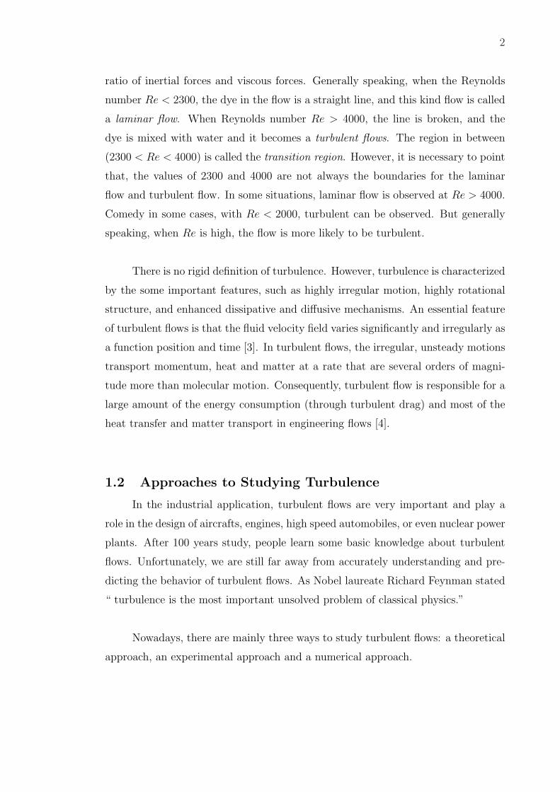
ratio of inertial forces and viscous forces. Generally speaking, when the Reynolds
number Re < 2300, the dye in the flow is a straight line, and this kind flow is called
a laminar flow. When Reynolds number Re > 4000, the line is broken, and the
dye is mixed with water and it becomes a turbulent flows. The region in between
(2300 < Re < 4000) is called the transition region. However, it is necessary to point
that, the values of 2300 and 4000 are not always the boundaries for the laminar
flow and turbulent flow. In some situations, laminar flow is observed at Re > 4000.
Comedy in some cases, with Re < 2000, turbulent can be observed. But generally
speaking, when Re is high, the flow is more likely to be turbulent.
There is no rigid definition of turbulence. However, turbulence is characterized
by the some important features, such as highly irregular motion, highly rotational
structure, and enhanced dissipative and diffusive mechanisms. An essential feature
of turbulent flows is that the fluid velocity field varies significantly and irregularly as
a function position and time [3]. In turbulent flows, the irregular, unsteady motions
transport momentum, heat and matter at a rate that are several orders of magni-
tude more than molecular motion. Consequently, turbulent flow is responsible for a
large amount of the energy consumption (through turbulent drag) and most of the
heat transfer and matter transport in engineering flows [4].
1.2 Approaches to Studying Turbulence
In the industrial application, turbulent flows are very important and play a
role in the design of aircrafts, engines, high speed automobiles, or even nuclear power
plants. After 100 years study, people learn some basic knowledge about turbulent
flows. Unfortunately, we are still far away from accurately understanding and pre-
dicting the behavior of turbulent flows. As Nobel laureate Richard Feynman stated
“ turbulence is the most important unsolved problem of classical physics.”
Nowadays, there are mainly three ways to study turbulent flows: a theoretical
approach, an experimental approach and a numerical approach.

3
The theoretical study of turbulent flows is based on the Navier-Stokes (NS)
equations. However, because of the unsteady, irregular, random and chaotic charac-
teristic of turbulence, it is very difficult to solve these partial differential equations
analytically for most practical situations. It is especially true when we know that
these equations can lead to chaotic solutions. Currently, the theoretical understand-
ing of turbulent flow is mostly based on statistical studies. The Russian mathemati-
cian Andrey Kolmogorov proposed the first statistical theory of turbulence, based
on the hypothesis of energy cascade [5, 6, 7]. This theory is usually referred as the
K41 theory and we will utilize this theory in Chapter 3. One important conclusion
of the K41 theory is that, turbulent flows contain eddies of different length scales.
Kinetic energy is transferred from larger eddies to smaller ones. Although the hy-
pothesis leads to a simple expression for how energy is distributed among eddies of
different sizes, it does not provide a tool which can be used to predict the behavior
of complicated flows in an industrial setting.
Experimental study of turbulence is another approach to understanding tur-
bulence. Wind tunnels provide useful information for aerodynamic studies. A lot
of important experimental data has come from wind tunnels. On one hand, these
results can be used to validate some theories, and on the other hand, they can be
used to develop more accurate and higher fidelity models. However, experimental
study of turbulence is not an easy task. For example, turbulence usually occurs at
high speeds or large spatial scale. Often it is not easy or cheap to achieve these
high speeds or large spatial scale. For example it is very difficult to realize experi-
ments that study atmospheric boundary layers or supersonic flows. Even for some
industrial applications such as the testing of new designs for cars and airplanes, such
experiments can become very expensive, because the design process usually requires
several cycles.
The numerical simulation of turbulent flows, which is a part of computational
fluid dynamics (CFD), is the “ third approach ” in the study turbulent flows. The

4
numerical simulation is very new compared to the experimental approach which has
been around from the seventeenth century, and theoretical approach which started
in the eighteenth century. The numerical simulation requires two important ingre-
dients: a high-speed digital computer and the development of accurate numerical
algorithms. Numerical simulation can be thought of as a connection between ex-
perimental and theoretical studies of turbulent flows. By solving the NS equations
numerically, we can develop an understanding of some behaviors observed in exper-
iments. In addition to this, numerical simulation can replace experiments in cases
where it is impossible to perform the experiment or it is too expensive.
1.3 Numerical Simulation of Turbulent Flows
According to the K41 theory, in turbulent flows kinetic energy is transferred
from larger length scales to smaller length scales. Based on this idea, the eddies
in turbulent flows can be divided into three categories based on their length scales.
Integral length scales are the largest scales. These eddies obtain energy from the
mean flow and also from each other. Kolmogorov length scales are the smallest
scales. In this range, the energy input from nonlinear interactions and the energy
lost from dissipation due to viscous effect balance each other. Eddies in the inertial
subrange are between the largest and the smallest scales. They pass the energy from
the largest to the smallest length scale without dissipating it.
There are several important numerical methods available to simulate turbu-
lent flows. There are the direct numerical simulation (DNS), large-eddy simulation
(LES), and Reynolds-averaged Navier-Stokes (RANS) equations. The research pre-
sented in this proposal is dedicated to LES. To assess the performance of LES
models, their results will be compared to DNS results obtained on much finer grids.
In the following paragraphs we present a brief introduction to DNS, LES and RANS.
1.3.1 Direct Numerical Simulation (DNS)
In DNS we solve the Navier-Stokes equations without any model term. All
the scales of motion are resolved. It is the simplest approach and it could provide

5
unbeatable accuracy. The drawback of DNS is the very large computational cost.
In order to simulate all the scales, the computational domain has to be large enough
to contain the largest eddies, and the grid spacing has to be small enough to capture
the smallest eddies. The cost increases rapidly with the Reynolds number (approx-
imately as Re3). The DNS approach was not widely used before 1970s because of
the lack of computer power. Even now, DNS has been only applied to turbulent
flows with low or moderate Reynolds numbers.
1.3.2 Large-Eddy Simulation (LES)
As discussed in previous subsection, the computational cost of DNS is high,
and it increases rapidly with the Reynolds number, so that DNS is not usually
applied to high Reynolds number flows. LES has be developed to tackle this problem.
In turbulent flows, the larger-scale motions are affected by the flow geometry and
are not universal, while the smaller scales have a universal character. Further, most
of the energy is contained in the large scales but most of the computational cost
is spent in solving the small scales. So the basic idea of LES is that the larger-
scale motions are computed explicitly, and the influence of the smaller scales is
represented by simple models. Thus, compared with DNS, the vast computational
cost of explicitly representing the small-scale motions is avoided.
1.3.3 Reynolds-averaged Navier-Stokes (RANS) Equations
Besides DNS and LES, the Reynolds-averaged Navier-Stokes (RANS) equa-
tions are also used to model turbulent flows. These equations are the ensemble-
averaged equations of motion for fluid flow. Reynolds decomposition is used for
RANS, so an instantaneous quantity is decomposed into its ensemble-averaged and
fluctuating values. The same averaging procedure is applied to the NS equations.
RANS equations contains the averaged variables and terms that depend on the fluc-
tuating variables. The terms containing the fluctuating variables must be modeled,
and they must be expressed only in terms of the averaged quantities. This expres-
sions is called model terms. Some models include the Spalart-Allmaras, k−ω, k−ε,
and SST models which add additional equations to bring closure to the RANS equa-
tions. Compared to LES, the RANS have smaller computational cost, but they do
6
not provide instantaneous quantities and good estimation for fluctuation.
1.4 LES of Turbulent Flows
In this section, we will introduce large eddy simulation of turbulent flows with
more details. LES of incompressible and compressible flows are described separately,
but we should keep in mind that they share the same basic idea. In order to simulate
the effect of the small scales, Smagorinsky model [8] is introduced for incompressible
flows and Smagorinsky-Yoshizawa -eddy-diffusivity (SYE) model [9] for compressible
flows. Smagorinsky model model is the simplest model [3] and is widely used for
LES. Especially, we will use a dynamic version of SYE model in this thesis as a LES
model for compressible flows in some sections. And the Smagorinsky model is used
as comparison case in some other sections.
1.4.1 LES of Incompressible Flows
In DNS, the velocity field u(x, t) contains all the length scales. In LES, in
order to split the velocity field into a large scale (coarse scale) velocity field and
a small scale (fine scale) velocity field, a low-pass filtering operation is introduced.
The general filtering operation is defined by
∫G(r, x)dr = 1, (1.2)
the filtered velocity field Uh(x, t) is determined by
u(x, t) =
∫G(r, x)u(x− r, t)dr, (1.3)
and the residual field is defined by
u′(x, t) ≡ u(x, t)− u(x, t), (1.4)

7
The incompressible Navier-Stokes equations are
∂ui
∂xi
= 0, (1.5)
∂ui
∂t+
∂
∂xj
(uiuj) = −1
ρ
∂p
∂xi
+∂σij
∂xj
. (1.6)
In the equations above ui is the velocity field, p is the pressure, ρ is the fixed
density, σij is the viscous stress tensor. We apply the filtering operation to the
Navier Stokes equations and arrive at
∂ui
∂xi
= 0, (1.7)
∂ui
∂t+
∂
∂xj
(uiuj) = −1
ρ
∂p
∂xi
+∂σij
∂xj
+∂τSGS
ij
∂xj
, (1.8)
where
τSGSij = uiuj − uiuj. (1.9)
is the subgrid stress (SGS) tensor. In order to close the equations for the filtered
velocity, a model for the subgrid stress tensor τSGSij is needed. The simplest model
is the Smagorinsky model [8], which also forms the basis for several of the more
advanced models, such as dynamic Smagorinsky model [10], the the mixed Bardina
model [11], and the mixed Clark model [12].
The Smagorinsky model is expressed as a linear eddy-viscosity model
τSGSij = −2νtSij, (1.10)
It relates subgrid stress τSGSij to the filtered rate of strain Sij, through νr(x, t), which
is the eddy viscosity, modeled as
νt = (Cs∆)2|S|, (1.11)
where S is the characteristic filtered rate of strain, 4 is the filter width, and Cs is
the Smagorinsky coefficient. We note that Cs = 0.1 is a preferred value for free-shear

8
flows and for channel flow.
1.4.2 LES of Compressible Flows
In compressible flows, it is convenient to use Favre filtering to avoid the intro-
duction of subgrid-scale terms in the equation of conservation of mass. Favre (or
density-averaged) quantities [13] are defined as f ≡ (ρf)h/ρh. Applying this filter
to the compressible Navier Stokes equations yields two subgrid quantities:
τSGSkl = ρukul − ukul), (1.12)
qSGSk = ρ(ukT − ukT ). (1.13)
In the equations above T is the temperature, τSGSkl is the subgrid scale stress
tensor and qSGSk is the subgrid scale heat flux, which appears in the filtered energy
equation. Both these terms need to modeled in terms of the filtered variables. The
simplest model is based on eddy diffusivity concept and is due to Samgorinsky and
Yoshizawa [9]. It is given by
τSGSkl = −2C0ρ∆2|S|(Sh
kl − 1
3Sh
mmδkl) +2
3C1ρ∆2|S|2δkl, (1.14)
qSGSk = − ρCs∆
2|S|PrT
∂T
∂xk
. (1.15)
In the equations above S is the filtered rate of strain, C0 is the Smagorinsky pa-
rameter that goes to model the deviatoric component of the subgrid stress, C1 is
the model attached to the dilatational component of subgrid stress, and PrT is the
turbulent Prandtl number. All these three parameters need to be specified in order
to use this model.
In contrast to all the models described in the previous page, the research in this
thesis does not use spatial filters to derive LES equations. Rather it uses projection
operators applied to the variational formulation of the Navier-Stokes equations.
This approach is based on the Variational Multiscale formulation (VMS) [14] and is

9
described in the following section.
1.5 Residual based Variational Multiscale (RBVM) Formu-
lation
In large eddy simulation (LES) the large scales of fluid motion are explicitly
resolved while the effect of the fine scales on the large scales is modeled using terms
that depend solely on the large scale variables. In filter-based LES this scale separa-
tion is achieved through the application of spatial filters that tend to smooth a given
field variable. In contrast to this in the variational multiscale (VMS) formulation
the scale separation is achieved through projection operators [14]. In addition in
the VMS formulation the starting point for deriving LES models is the weak or the
variational statement of conservation laws, whereas in the filter-based LES formu-
lation it is the strong form of these equations.
In the residual-based variational multiscale (RBVM) formulation [15, 16] the
basic idea is to split the solution and weighting function spaces into coarse and fine
scale partitions. Splitting the weighting functions in this way yields two sets of cou-
pled equations: one for the coarse scales and another for the fine, or the unresolved,
scales. The equations for the fine scales are observed to be driven by the residual
of the coarse scale solution projected onto the fine scale space. Hence the name the
“residual-based” VMS formulation. These equations for the unresolved scales are
solved approximately and the solution is substituted in the equations for the coarse
scales. In this way the effect of the fine or the unresolved scales on the coarse scales
is modeled.
Thus far the RBVM formulation has been applied to incompressible turbulent
flows [15, 17]. In this context in [18, 19] it was observed that while the RBVM
formulation accurately modeled the cross-stress terms (uu′) it did not at all model
the Reynolds stress terms (u′u′). To remedy this a mixed model was proposed that
appended to the RBVM terms a Smagorinsky eddy viscosity model [8] in order to
capture the effect of the Reynolds stresses. The value of the Smagorinsky parame-
10
ter in this model was determined dynamically, while accounting for the dissipation
induced by the RBVM terms. In tests of the decay of incompressible homogeneous
turbulence it was observed that the mixed model was more accurate than the RBVM
and the dynamic Smagorinsky models.
In this thesis we aim to extend these ideas to compressible turbulent flows.
First, we consider the extension of the RBVM formulation to compressible flows.
Thereafter motivated by the shortcomings of this model in the incompressible case
we consider a mixed version of this model (which is referred as the MM1 model)
where we add the Smagorinsky, Yoshizawa [9], and eddy diffusivity terms to model
the Reynolds components of the deviatoric subgrid stresses, the dilatational sub-
grid stresses and the subgrid heat flux vector, respectively [10]. Through a simple
analysis of the subgrid mechanical energy and through the dynamic approach we
conclude that out of these the RBVM formulation requires a model only for the
deviatoric component of the Reynolds stresses. The other significant subgrid quan-
tities are adequately represented within the RBVM formulation. Thus the mixed
RBVM formulation for compressible flows contains only one additional term when
compared with the RBVM formulation, which is the deviatroic Smagorinsky model.
1.6 Residual based Eddy Viscosity (RBEV) Model
In LES the large scale fluctuations are resolved and the effect of the fine scale
fluctuations on the large scales is modeled through terms that depend only on the
large scales. Over the years several LES models have been developed, and a majority
of these, to some extent the commonly used ones, are based on the concept of an
eddy viscosity. This idea is motivated by direct analogy with a molecular viscosity.
Just as the molecular viscosity represents momentum transfer through fluctuations
of the atomistic particles, the turbulent eddy viscosity represents momentum trans-
fer through fluctuating continuum fluid velocity.
The Smagorinsky model is the most popular eddy viscosity based LES model.

11
In this model the eddy viscosity is taken to be proportional to a local rate of strain
and a representative length scale, often set to a measure of the grid size. Despite
its popularity, this model has its drawbacks. In particular, it has been recognized
that it must be modified in space and time whenever the turbulence is decaying or
damped in some spatial regions (close to a wall, for example). The most effective
way to accomplish this is to employ the so-called dynamic approach based on the
Germano identity. In this approach the subgrid stresses on the computational grid
and on a test-filter scale are considered. The difference between these two, which
can be explicitly determined once scale similarity is invoked, is used to estimate the
magnitude of the Smagorinsky eddy viscosity. This approach, which has been widely
used, has been successful in simulating complex flows. However, it is cumbersome
in that (1) it requires the use of at least one additional filter and (2) it involves
averaging, either in space, or time, or along material trajectories in order to achieve
a smoothly varying eddy viscosity. The dynamic approach may be thought of as a
way of repairing a glaring drawback of the Smagorinsky model. That is, it does not
vanish when the flow field is devoid of any fluctuations. In that sense it is inconsis-
tent.
In this thesis we present a new eddy viscosity model that is inherently consis-
tent and circumvents the use of a dynamic approach. Our model is based on ideas
derived from the variational multiscale (VMS) formulation. Within this approach
an equation for the fine scales is derived from the original variational formulation
for the Navier Stokes equations. This equation is then approximated to obtain an
explicit, approximate expression for the fine scales. In this expression it is observed
that the fine scales are driven by the residual of the coarse scales. Thus when the
coarse scales are accurate, the residual vanishes, as do the fine scales. We recognize
that once an expression for the fine scales is obtained (albeit an approximate one),
it may be used to estimate the viscosity induced by these scales on the coarse scales.
In analogy to the molecular viscosity we may assume that the turbulent, or eddy,
viscosity is proportional to the magnitude of the fine scale velocity times a length
scale which plays the role of the mean free path. In the context of LES it makes

12
sense to select this length scale to be proportional to the grid size. As a result
we have νT ∼ |u′|h. We dub this model the residual-based eddy viscosity (RBEV)
model.
Further, motivated by the mixed model (MM1) based on the RBVM model
and the dynamics Smagorinsky model, a purely residual-based mixed model (MM2)
based on the RBEV model and the RBVM model is also proposed.
1.7 Description of Chapters
The layout of this thesis is as follows. In Chapter 2, four residual-based models
for large eddy simulation of turbulent flows are derived for both incompressible
and compressible flows. They are the residual-based variational multiscale model
(RBVM), the mixed model (MM1) based on the RBVM model and the dynamic
Smagorinsky-Yoshizawa-eddy diffusivity (DSYE) model, the residual-based eddy
viscosity model(RBEV), and the purely residual based mixed model (MM2) based
on the RBVM and RBEV models. In Chapter 3, we test the performance of the
new LES models in predicting the decay of compressible, homogeneous, isotropic
turbulence (HIT) in regimes where shocklets are known to exist within Fourier-
spectral method. In Chapter 4, we test the RBEV model and the MM2 model
on the incompressible fully developed turbulent channel flows within finite element
method. Conclusions will be drawn in Chapter 5.
CHAPTER 2
Residual Based Methods for Large Eddy Simulation of
Turbulent Flows
In the residual-based variational multiscale (RBVM) formulation [15, 16] the
basic idea is to split the solution and weighting function spaces into coarse and fine
scale partitions. Splitting the weighting functions in this way yields two sets of cou-
pled equations: one for the coarse scales and another for the fine, or the unresolved,
scales. The equations for the fine scales are observed to be driven by the residual
of the coarse scale solution projected onto the fine scale space. Hence the name the
“residual-based” VMS formulation. These equations for the unresolved scales are
solved approximately and the solution is substituted in the equations for the coarse
scales. In this way the effect of the fine or the unresolved scales on the coarse scales
is modeled.
Thus far the RBVM formulation has been applied to incompressible turbulent
flows [15, 17]. In this context in [18, 19] it was observed that while the RBVM
formulation accurately modeled the cross-stress terms (uu′ terms) it did not at all
model the Reynolds stress terms (u′u′). To remedy this a mixed model was pro-
posed that appended to the RBVM terms a Smagorinsky eddy viscosity model [8]
in order to capture the effect of the Reynolds stresses. The value of the Smagorin-
sky parameter in this model was determined dynamically, while accounting for the
dissipation induced by the RBVM terms. In tests of the decay of incompressible
homogeneous turbulence it was observed that the mixed model was more accurate
than the RBVM and the dynamic Smagorinsky models.
In this chapter, we aim to extend the ideas of RBVM formulation to compress-
ible turbulent flows. Thereafter motivated by the shortcomings of this model in the
incompressible case we consider a mixed version of this model (MM1) where we add
the Smagorinsky, Yoshizawa [9], and eddy diffusivity terms to model the Reynolds
13
14
components of the deviatoric subgrid stresses, the dilatational subgrid stresses and
the subgrid heat flux vector, respectively [10]. Through a simple analysis of the
subgrid mechanical energy and through the results of the dynamic approach we
conclude that out of these the RBVM formulation requires a model only for the
deviatoric component of the Reynolds stresses. The other significant subgrid quan-
tities are adequately represented within the RBVM formulation. Thus the mixed
RBVM formulation (MM1) for compressible flows contains only one additional term
when compared with the RBVM formulation, which is the deviatroic Smagorinsky
model.
Second, we present a new eddy viscosity model that is inherently consistent
and circumvents the use of a dynamic approach. Our model is based on ideas derived
from the variational multiscale (VMS) formulation. Within an explicit, approximate
expression for the fine scales is derived. In this expression it is observed that the fine
scales are driven by the residual of the coarse scales. Thus when the coarse scales
are accurate, the residual vanishes, as do the fine scales. We recognize that once an
expression for the fine scales is obtained (albeit an approximate one), it may be used
to estimate the viscosity induced by these scales on the coarse scales. In analogy
to the molecular viscosity we may assume that the turbulent, or eddy, viscosity is
proportional to the magnitude of the fine scale velocity times a length scale which
plays the role of the mean free path. In the context of LES it makes sense to select
this length scale to be proportional to the grid size. As a result we have νT ∼ |u′|h.
We dub this model the residual-based eddy viscosity (RBEV) model. This RBEV
model can be applied to both incompressible and compressible flows.
Finally, a purely residual based mixed model (MM2) based on the RBVM and
RBEV models for incompressible and compressible flows is introduced.
The layout of the remainder of this chapter is as follows. In Section 2.1, we
provide a concise derivation of the RBVM method applied to a generic partial differ-
ential equation for both incompressible and compressible turbulent flows. In Section
15
2.2, a mixed model (MM1) based on the RBVM and the dynamic Smagorinsky-
Yoshizawa-eddy diffusivity (DSYE) model is proposed for compressible turbulent
flow. In Section 2.3, a residual based eddy viscosity model is proposed for both in-
compressible and compressible turbulent flows. In Section 2.4, purely residual based
mixed model (MM2), that combines the RBVM and RBEV models, is proposed for
both incompressible and compressible turbulent flows. This model is simpler to im-
plement than MM1 in that it does not rely on a dynamic procedure to determine
its parameters.
2.1 Residual-based variational multiscale formulation (RBVM)
In this section, the RBVM formulation of LES for the incompressible and
compressible Navier-Stokes equations is developed. For a detailed derivation of
the RBVM approach for the incompressible Navier-Stokes equations the reader is
referred to [15].
The strong form of the incompressible Navier–Stokes equations in dimension-
less variables is given by
∇ · u = 0, (2.1)
ρ∂u
∂t+ ρ∇ · (u⊗ u) = −∇p +
1
Re∇2u + f , (2.2)
where ρ = 1, Re is the Reynolds number.
The strong form of the compressible Navier–Stokes equations in dimensionless
variables is given by
∂ρ
∂t+∇ ·m = 0, (2.3)
∂m
∂t+∇ · (m⊗m
ρ) = −∇p +
1
Re∇ · σ + f , (2.4)
∂p
∂t+∇ · (up) + (γ − 1)p∇ · u =
(γ − 1)
ReΦ +
1
M2∞PrRe∇ · (µ∇T ), (2.5)
16
where the viscous stress tensor σ is given in terms of the rate of strain S by
σ = 2µ(S − 1
3tr(S)I), (2.6)
and the viscous dissipation Φ is given by
Φ = σ : S. (2.7)
The system is closed with an equation of state
γM2∞p = ρT. (2.8)
Further, the dynamic viscosity is expressed in terms of the local temperature
using,
µ = T 0.76. (2.9)
This problem is posed on a spatial domain Ω and in the time interval ]0, T [
with given initial condition data and boundary conditions. In the above equations, ρ
is the density, u is the velocity, m = ρu is the momentum, p is the thermal pressure,
T is temperature, M∞ is the free-stream Mach number, γ is the adiabatic index,
Pr is the Prandtl number, Re is the Reynolds number and f is a forcing function.
The density, velocity, temperature and viscosity are scaled by their reference values
while the pressure is scaled by the product of the reference density and the square
of the reference velocity. The Reynolds number is based on the reference values of
the velocity, length, viscosity and density. For the homogeneous turbulence problem
considered in this paper, the flow is assumed to be periodic with a period 2π in each
coordinate direction. The values of the physical parameters are provided in Chapter
3.
Note that one can write Equations (2.1) and (2.2), Equations (2.3) − (2.5)
concisely as
LU = F , (2.10)

17
where U = [u, p]T are the unknowns with F = [f , 0]T for the incompressible case
and U = [ρ, m, p]T are the unknowns with F = [0, f , 0]T for the compressible case.
L represents the differential operator associated with the Navier-Stokes equations.
The weak form of Equation 2.10 is given by: Find U ∈ V such that
A(W , U ) = (W , F ) ∀W ∈ V . (2.11)
Here A(·, ·) is a semi-linear form that is linear in its first slot, (·, ·) denotes the L2
inner product, and W is the weighting function. For the incompressible case it is
given by W = [w, q]T and for the compressible case it is given by W = [r, w, q]T . Vis the space of trial solutions and weighting functions. In this presentation we have
chosen the same space for both trial solutions and weighting functions in order to
keep the presentation simple.
The semi-linear form of incompressible case is given by
A(W , U ) ≡ (w, u,t)− (∇w, u⊗ u)
− (∇ ·w, p) +2
Re(∇Sw,∇Su) + (q,∇ · u).
(2.12)
Here ∇S = (∇+∇T )/2 is the symmetric gradient operator.
The semi-linear form of compressible case is given by
A(W , U ) ≡ (r, ρ,t)− (∇r, m)
+ (w, m,t)− (∇w,m⊗m
ρ)
− (∇ ·w, p) +1
Re(∇w, σ)
+ (q, p,t)− (∇q, up)− (1− γ)(q, p∇ · u)
− (γ − 1)
Re(q, Φ) +
1
M2∞PrRe(∇q, µ∇T ).
(2.13)
The weak form is posed using the infinite dimensional function space V . In
18
practice this space is approximated by its finite-dimensional counterpart Vh ⊂ V .
In the residual-based variational multiscale formulation the goal is to construct a
finite dimensional problem whose solution is equal to PhU , where Ph : V → Vh is
a projection operator that defines the desired or optimal solution. If the range of
Ph is all of Vh then it is possible to split V = Vh ⊕ V ′ which implies that for every
V ∈ V there is a unique decomposition V = V h + V ′, where V h = PhV ∈ Vh
and V ′ = P′V ∈ V ′. The space V ′ ≡ V ∈ V|PhV = 0, and P′ = I − Ph where I
is the identity operator. Using this decomposition in Equation (2.11) for both the
weighting functions and the trial solutions we arrive at a set of coupled equations.
Find Uh ∈ Vh and U ′ ∈ V ′, such that
A(W h, Uh + U ′) = (W h, F ) ∀W h ∈ Vh, (2.14)
A(W ′, Uh + U ′) = (W ′, F ) ∀W ′ ∈ V ′. (2.15)
The idea is to solve for U ′ in terms of Uh and F analytically using the fine scale
equation (Equation (2.15)), and substitute the expression for U ′ into the coarse-
scale equation (Equation (2.14)), which is to be solved numerically. By doing this
one would have introduced in the coarse scale equation the effect of the fine or
subgrid scales.
To derive an expression for U ′ we subtract A(W ′, Uh) from both sides of
Equation (2.15),
A(W ′, Uh + U ′)− A(W ′, Uh) = −A(W ′, Uh) + (W ′, F )
= −(W ′,LUh − F ), (2.16)
where we have performed integration by parts on the first term on the right hand
side of the first line of Equation (2.16). For general functions in H1(Ω) the quantity
LUh must be interpreted in the sense of distributions. Note that this equation for
U ′ is driven by the coarse-scale residual R(Uh) ≡ LUh − F . Further, when the
coarse-scale residual is zero its solution is given by U ′ = 0. The formal solution of
Equation (2.16) may be written as
19
U ′ = F ′(R(Uh); Uh). (2.17)
This implies that the fine scales are a functional of the residual of the coarse scales
and are parameterized by the coarse scales. Thus they depend on the entire history
of the coarse scales and their residual. A short-time approximation that does away
with all the history effects and replaces the differential operator in Equation (2.16)
by an algebraic operator is given by
U ′ ≈ −P′τ (Uh) P′TR(Uh). (2.18)
Here P′T : Vh∗ → V∗ is the transpose of P′, where the spaces Vh∗ and V∗are
dual of Vh and V , respectively, with respect to the L2 duality pairing [20]. Further,
τ is a matrix that depends on Uh. The operator τ is selected to approximate the
Green’s operator for the fine-scale problem, and can be thought of as a double inte-
gral of the Green’s operator.
In moving from Equation (2.17) to Equation (2.18) instead of solving a very
complicated equation for the fine scales, a gross approximation is made. In particular
it is assumed that the fine scales are equal to the residual of the coarse scales,
which represent the rate of unbalance for the coarse scale representation of a given
conservation variable, times the characteristic time scale. In the advective limit
this time scale is the time it takes to advect the fine scale scales across a typical
grid size, and in the diffusive limit it is the time it takes for them to diffuse. The
precise definition of τ is presented in Chapter 3 and Chapter 4 when the models
are implementd. For a discussion on this the reader is referred to [14, 15] . The
approximation for U ′ above differs from that in [15] in the inclusion of the projectors
P′ and P′T . We believe that these projectors are necessary in order to maintain a
formal consistency between the exaction equation for the fine scales Equation (2.16)
and its approximation Equation (2.18). In particular the operator P′T ensures that
any component of the residual that is not “sensed” by a function in V ′ does not
20
contribute to the fine scales, and the operator P′ ensures that the approximation
for the fine scales belongs to V ′. In this regard the approximation above is closer to
the orthogonal sub-scales method of Codina [16].
Using this expression in Equation (2.14) we arrive at the equation for the
residual-based variational multiscale (RBVM) formulation: Find Uh ∈ Vh, such
that
A(W h, Uh − P′τ P′TR(Uh)) = (W h, F ) ∀W h ∈ Vh. (2.19)
Remark: The space for U ′ , that is V ′, is infinite dimensional. However,
in practice this space must also be approximated with a finite dimensional space.
Furthermore it must be selected such that the cost of computing U ′ in this space
does not overwhelm the total computational costs. In our application, where we
have used Fourier modes, the coarse scale space is comprised of all modes with
wavenumber less than or equal to the cutoff wavenumber kh, and the fine scale
space is comprised of all modes with wavenumber greater than kh but less than or
equal to 3kh/2. This choice is motivated by tests (not shown here) that have shown
that using a fine scale space that is larger than this does not significantly alter the
results. Thus in order to minimize the computational effort we select the smallest
possible space for U ′. We note that the ratio of memory costs for the RBVM model
to the no-model case scales as α3, where α > 1 is the ratio of the cutoff wavenumber
for the fine scales to the coarse scales. The ratio of flops per time-step also scales
with the same power of α. Therefore it is imperative that α be kept small in order
for the RBVM formulation to be competitive.
2.2 A mixed model based on residual based variational mul-
tiscale formulation (MM1)
In [19], for incompressible flows the authors demonstrated that while the
RBVM model works well for the cross-stress term it does not introduce an ade-
quate model for the Reynolds stress term. Subsequent analysis has revealed that
the RBVM approximation for the fine scales produces a reasonable estimate for their

21
magnitude [21, 22]. Thus the reason why the Reynolds stresses are not accurately
represented is not because their magnitude is underestimated, rather it is that they
are uncorrelated with the large-scale rate of strain tensor. A likely explanation for
this is the exclusion of the history effects in the approximation for the fine scales
which prevents these correlations from evolving. With this in mind they appended to
the RBVM model the dynamic Smagorinsky model in order to model the Reynolds
stress.
2.2.1 Weak Form of MM1
We will first review the mixed model based on RBVM formulation for incom-
pressible flows presented in [19]. Then we extend this model to compressible flows.
We label this model as MM1, for mixed model 1, in anticipation of another mixed
model that is proposed in Section 2.4.
Incompressible flows
In [19], based on the results of their a-priori analysis, the authors conclude
that the RBVM model captures the cross-stresses reasonably well but does not
accurately model the Reynolds stress term. On the other hand, it appears that the
Reynolds stress term may be well represented by a simple eddy viscosity. Motivated
by these observations they propose a mixed model where they append to the RBVM
formulation the Smagorinsky eddy viscosity term. In this model the variational
multiscale term models the cross-stress contribution, while the Smagorinsky term
models the Reynolds stress contribution.
Thus the weak or variational formulation of the new mixed model of incom-
pressible flows is given by: Find Uh ∈ Vh, such that
A(W h, Uh + U ′) +
(∇Swh, 2(csh)2|Sh|Sh)
= (W h, F ) ∀W h ∈ Vh,(2.20)
Here cs is the Smagorinsky parameter and Sh is the rate of strain. When
utilizing a Fourier-spectral discretization while specifying Ph to the H1 projection

22
this expression simplifies to: Find Uh ∈ Vh, such that
A(W h, Uh
)+
(∇Swh, 2(csh)2|Sh|Sh)
− (∇wh, uh ⊗ u′ + u′ ⊗ uh + u′ ⊗ u′)
= (W h, F ) ∀W h ∈ Vh,
(2.21)
where uh ⊗ u′ and u′ ⊗ uh are cross-stress term and u′ ⊗ u′ is the Reynolds
stress term. A variant of the proposed mixed model is obtained by discarding the
contribution from the RBVM model to the Reynolds stress. That is by neglecting
the u′⊗u′ term in Equation (2.21). This is a reasonable proposition since as shown
in [19], the Reynolds stress term is not modeled accurately by this term. Instead it
is well represented by the Smagorinsky term.
Compressible flows
We follow the same approach and propose, the following mixed model for
compressible flows: Find Uh ∈ Vh, such that
A(W h, Uh + U ′)
+(∇wh, 2C0h
2ρh|Sh|Shdev −
2
3C1h
2ρh|Sh|2I)
+(∇qh,
C0
PrtγM2∞h2ρh|Sh|∇T h
)
= (W h, F ) ∀W h ∈ Vh,
(2.22)
where A(·, ·) is defined in Equation (2.13), Sh is the rate of strain computed the
velocity field uh ≡ mh/ρh, the subscript dev denotes its deviatoric component and
T h ≡ γM2∞ph/ρh. From the definitions of uh and T h we note that these correspond
to the so-called Favre-averaged variables in traditional LES nomenclature.
Comparing with Equation (2.19), we note that two new terms have been added.
The first term models the deviatoric and dilatational components of the subgrid
scale stress tensor and the second term models the subgrid heat flux vector. For the

23
deviatoric component of the subgrid stress we have utilized the Smagorinsky eddy
viscosity model [8], for the dilatational component we have utilized Yoshizawa’s
model [9], and for the subgrid heat flux vector we have utilized an eddy diffusivity
type model. In a typical LES the first term is employed to represent both the
cross and Reynolds stress components of the subgrid stress, whereas in our mixed
model it is added to represent the missing Reynolds stress. In the following section
we demonstrate that the RBVM model by itself introduces a reasonable expression
for the dilatational Reynolds stress component. Based on this analysis we do not
include an eddy viscosity model for the dilatational component of subgrid stress
(that is C1 = 0). Further in Section 4 we note that the dynamic procedure yields a
negative value for Pr−1t which is clipped to zero. Thus in effect in the mixed model
C1 = Pr−1t = 0 and the only non-zero term corresponds to C0, that is a model for
the deviatoric subgrid stresses.
2.2.2 Analysis of mechanical energy for the RBVM formulation
In this section we derive a mechanical energy identity for the RBVM formula-
tion for compressible flow. We split the total rate transfer of mechanical energy due
to the subgrid scales into a dilatational and deviatoric component. For the devia-
toric component, in earlier studies of incompressible flows it has been shown that
the RBVM model is unable to model the Reynolds stress term, and for this purpose
a mixed model is necessary. For the dilatational component, we demonstrate that
the RBVM model introduces a cross and a Reynolds-stress term, where the latter
is similar to the Yoshizawa model. As a result no additional model is required for
the dilatational component of the stress tensor.
We begin by noting that Equation (2.22) contains all the models considered
in the manuscript. In particular when U ′ = 0 and C1 = C0 = 0, it represents the
Galerkin method, or the DNS case; when only U ′ = 0 it reduces to the Smagorinsky-
Yoshizawa model; when C1 = C0 = 0, it reduces to the RBVM model; when all terms
are active it represents the mixed model.

24
Setting W h = [0, uh, 0]T in this equation for the Galerkin method we arrive
at mechanical energy identity:
d
dt
(1
2
∫
Ω
ρh|uh|2dx)
=
≡εhGal︷ ︸︸ ︷
−∫
Ω
|uh|22
(ρh
,t +∇ · (ρhuh))dx−
∫
Ω
Sh : σht dx, (2.23)
where σht = −ph1 + 1
Reσh is the total Cauchy stress tensor. This equation states
that the rate of change of kinetic energy is determined by the dissipation induced
by the molecular stresses and a term that depends on the residual of the continuity
equation. We combine these two contributions into a term denoted by εhGal.
Next we consider Equation (2.22) written for the Smagorinsky-Yoshizawa
model and set W h = [0, uh, 0]T to arrive at the mechanical energy identity for
this model:
d
dt
(1
2
∫
Ω
ρh|uh|2dx)
= εhGal (2.24)
−2C0h2
∫
Ω
ρh|Sh||Shdev|2dx
+2
3C1h
2
∫
Ω
ρh|Sh|2(∇ · uh)dx,
where Shdev denotes the deviatoric part of Sh. From this equation we conclude that
the deviatoric contribution to the rate of change of kinetic energy is negative and
thus this term always dissipates resolved kinetic energy. On the other hand, the
dilatational contribution can either add or remove kinetic energy. When ∇·uh < 0,
that is we have a flow where resolved scales are undergoing a compression, this term
is negative and as a result the resolved scales loose kinetic energy. The situation is
reversed in the case of an expansion.
Finally we consider Equation (2.22) written for the RBVM model and set
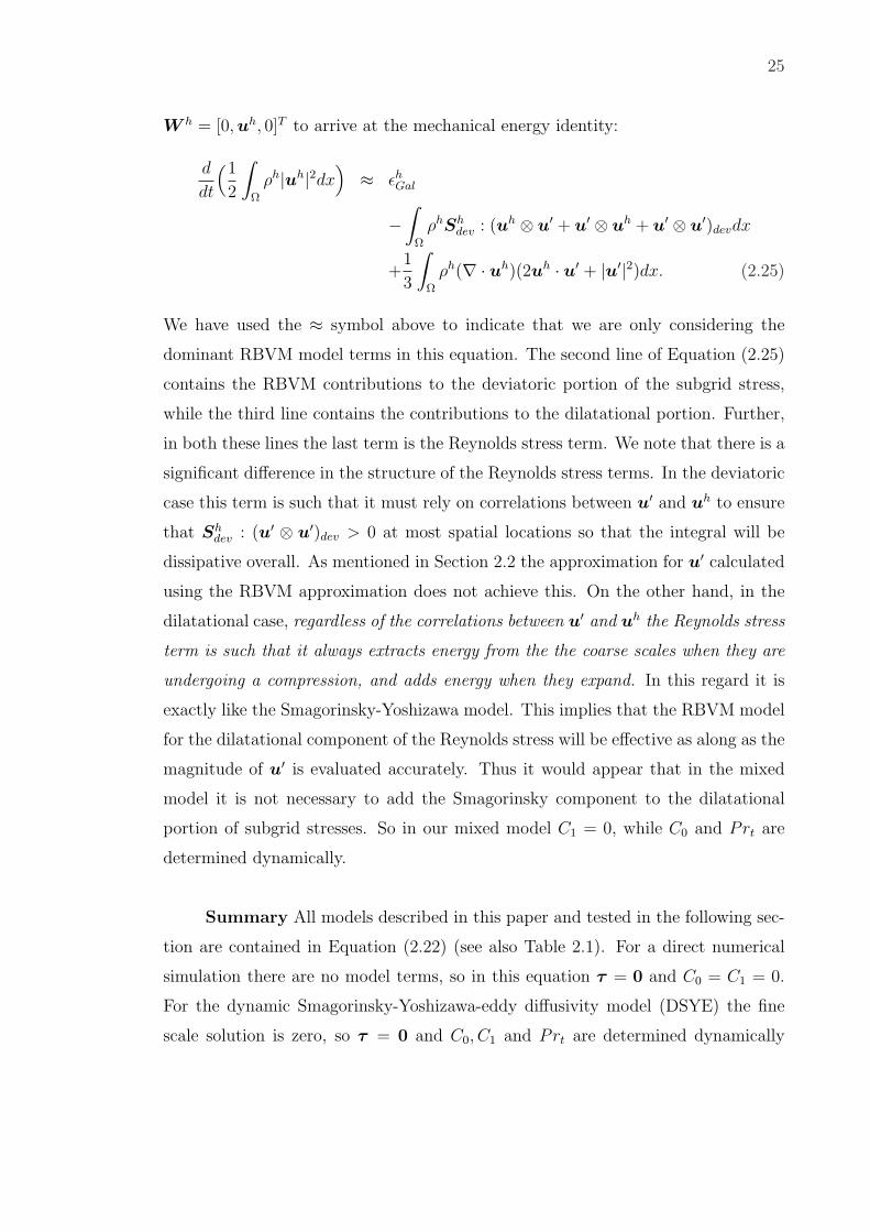
25
W h = [0, uh, 0]T to arrive at the mechanical energy identity:
d
dt
(1
2
∫
Ω
ρh|uh|2dx)
≈ εhGal
−∫
Ω
ρhShdev : (uh ⊗ u′ + u′ ⊗ uh + u′ ⊗ u′)devdx
+1
3
∫
Ω
ρh(∇ · uh)(2uh · u′ + |u′|2)dx. (2.25)
We have used the ≈ symbol above to indicate that we are only considering the
dominant RBVM model terms in this equation. The second line of Equation (2.25)
contains the RBVM contributions to the deviatoric portion of the subgrid stress,
while the third line contains the contributions to the dilatational portion. Further,
in both these lines the last term is the Reynolds stress term. We note that there is a
significant difference in the structure of the Reynolds stress terms. In the deviatoric
case this term is such that it must rely on correlations between u′ and uh to ensure
that Shdev : (u′ ⊗ u′)dev > 0 at most spatial locations so that the integral will be
dissipative overall. As mentioned in Section 2.2 the approximation for u′ calculated
using the RBVM approximation does not achieve this. On the other hand, in the
dilatational case, regardless of the correlations between u′ and uh the Reynolds stress
term is such that it always extracts energy from the the coarse scales when they are
undergoing a compression, and adds energy when they expand. In this regard it is
exactly like the Smagorinsky-Yoshizawa model. This implies that the RBVM model
for the dilatational component of the Reynolds stress will be effective as along as the
magnitude of u′ is evaluated accurately. Thus it would appear that in the mixed
model it is not necessary to add the Smagorinsky component to the dilatational
portion of subgrid stresses. So in our mixed model C1 = 0, while C0 and Prt are
determined dynamically.
Summary All models described in this paper and tested in the following sec-
tion are contained in Equation (2.22) (see also Table 2.1). For a direct numerical
simulation there are no model terms, so in this equation τ = 0 and C0 = C1 = 0.
For the dynamic Smagorinsky-Yoshizawa-eddy diffusivity model (DSYE) the fine
scale solution is zero, so τ = 0 and C0, C1 and Prt are determined dynamically

26
Table 2.1: A concise description of all models based on the terms appear-ing in Equation (2.22).
Terms No Model Smagorinsky-Yoshizawa RBVM MM1τ 0 0 X XC0 0 X 0 XC1 0 X 0 0
Pr−1t 0 X 0 0
using the variational counterpart of the Germano identity [23, 24] (see Section 2.2.3
below). For the residual based variational multiscale model (RBVM) the fine scales
are active, that is τ 6= 0 while C0 = C1 = 0. For the mixed model the fine scales
are active τ 6= 0, C1 = 0, while C0 and Prt are determined dynamically. In our
simulation of the decay of compressible turbulence using the mixed model we have
found that dynamic procedure almost always yields negative values for Prt, indicat-
ing that RBVM model alone introduces adequate dissipation in the energy equation.
In order to avoid unstable solutions we set Pr−1t = 0 whenever this happens. The
net result is that in the mixed model the only active term is Smagorinsky model for
the deviatoric component of the subgrid stress.
Remark We note that our mixed model is similar to other mixed models,
including the scale-similarity model [11, 25, 26, 27] and the tensor-diffusivity model
[28, 29] in that it contains distinct models for the cross-stress term and the Reynolds
stress term. However, the form of the model term for the cross stress in our model
is distinct from other mixed models.
2.2.3 Derivation of the dynamic calculation for C0, C1 and Prt.
In this section we describe the dynamic procedure we have used to determine
the unknown parameters in the LES models. We have utilized the variational coun-
terpart of the Germano identity described in [23, 24].
DSYE model
The equations for this model are given by Equation (2.22) with U ′ = 0. In this
equation, in order to focus on the momentum equations we select W h = [0, wh, 0],

27
to arrive at
(wh, mh,t)− (∇wh,
mh ⊗mh
ρh)− (∇ ·wh, ph) +
1
Re(∇wh, σh)
+
(∇wh, 2C0ρ
hh2|Sh|Shdev −
2
3C1ρ
hh2|Sh|2I)
= 0 ∀wh.
(2.26)
In the equations above h = π/kh, where kh is the cutoff wavenumber. The equations
for the same model used in a coarser discretization with the finite dimensional space
VH ⊂ Vh are given by
(wH , mH,t )− (∇wH ,
mH ⊗mH
ρH)− (∇ ·wH , pH) +
1
Re(∇wH , σH)
+
(∇wH , 2C0ρ
HH2|SH |SHdev −
2
3C1ρ
HH2|SH |2I)
= 0 ∀wH .
(2.27)
where H = π/kH , where kH is the cutoff wavenumber at the H-scale. In this study
we have selected kH = kh/2. Since VH ⊂ Vh, we replace wh with wH in Equation
(2.26), and subtract the resulting equation from Equation (2.27) to arrive at
(∇wH ,
mh ⊗mh
ρh− mH ⊗mH
ρH
)=
−2C0
(∇wH , ρHH2|SH |Sh
dev − ρhh2|Sh|Shdev
)
+2
3C1
(∇wH , ρHH2|SH |2I − ρhh2|Sh|2I
)∀wH .
(2.28)
In arriving the this equation we have set
(wH , mH,t −mh
,t) = 0,
(∇ ·wH , pH − ph) = 0,
(∇wH , σH − σh) = 0,
(2.29)
the first two relations above hold exactly for a Fourier-spectral spatial discretization,
while the last is an assumption.
In Equation (2.28) we select ∇wH = SHdev, and recognize that (Sdev, I) = 0,

28
to arrive at
(SH
dev,mh ⊗mh
ρh− mH ⊗mH
ρH
)=
−2C0(SHdev, ρ
HH2|SH |SHdev − ρhh2|Sh|Sh
dev),
(2.30)
which yields the final expression for C0,
C0 = −1
2
(SH
dev,mh ⊗mh
ρh− mH ⊗mH
ρH
)
(SH
dev, ρHH2|SH |SH
dev − ρhh2|Sh|Shdev
) . (2.31)
In order to determine C1 we select ∇wH = I in Equation (2.28), to arrive at
(1, tr
(mh ⊗mh
ρh− mH ⊗mH
ρH
))=
2C1(1, ρHH2|SH |2 − ρhh2|Sh|2),
(2.32)
which yields
C1 =1
2
(1, tr
(mh ⊗mh
ρh− mH ⊗mH
ρH
))
(1, ρHH2|SH |2 − ρhh2|Sh|2) . (2.33)
In order to determine the turbulent Prandtl number in Equation (2.22), we choose
W h = [0, 0, qh] to get
(qh, ph,t)− (∇qh, uhph)− (1− γ)(qh, ph∇ · uh)
− (γ − 1)
Re(qh, Φh) +
1
M2∞PrRe(∇qh, µh∇T h)
+(∇qh,
C0
PrtγM2∞h2ρh|Sh|∇T h
)= 0 ∀qh.
(2.34)

29
Similarly at the H−scale we arrive at
(qH , pH,t )− (∇qH , uHpH)− (1− γ)(qH , pH∇ · uH)
− (γ − 1)
Re(qH , ΦH) +
1
M2∞PrRe(∇qH , µH∇TH)
+(∇qH ,
C0
PrtγM2∞H2ρH |SH |∇TH
)= 0 ∀qH .
(2.35)
Since VH ⊂ Vh, we may replace qh with qH in (2.34) and subtract the result from
Equation (2.35) to arrive at
(∇qH ,
mhph
ρh− mHpH
ρH
)=
C0
PrtγM2∞
(∇qH , h2ρh|Sh|∇T h −H2ρH |SH |∇TH
)∀qH .
(2.36)
Where we have made use of
(qH , pH,t − ph
,t) = 0,
(qH , pH∇ · uH − ph∇ · uh) = 0,
(qH , ΦH − Φh) = 0,
(∇qH , µH∇TH − µh∇T h) = 0.
(2.37)
The first relation above holds exactly for a Fourier-spectral spatial discretization,
while the others are assumed. We let ∇qH = ∇TH , in Equation (2.36) and arrive
at
(∇TH ,
mhph
ρh− mHpH
ρH
)=
C0
PrtγM2∞
(∇TH , h2ρh|Sh|∇T h −H2ρH |SH |∇TH
).
(2.38)

30
This equation yields
Prt =C0
γM2∞
(∇TH , h2ρh|Sh|∇T h −H2ρH |SH |∇TH
)
(∇TH ,
mhph
ρh− mHpH
ρH
) . (2.39)
Mixed model
The procedure in this case is the same as for the DYSE model, except in
Equation (2.22) U ′ 6= 0. In particular we get
C0 = −1
2
(SH
dev,(mh+m′)⊗(mh+m′)
ρh+ρ′ − (mH+m′′)⊗(mH+m′′)ρH+ρ′′
)
(SH
dev, ρHH2|SH |SH
dev − ρhh2|Sh|Shdev
) , (2.40)
and
Prt =C0
γM2∞
(∇TH , h2ρh|Sh|∇T h −H2ρH |SH |∇ TH
)
(∇TH , (mh+m′)(ph+p′)
ρh+ρ′ − (mH+m′′)(pH+p′′)ρH+ρ′′
) . (2.41)
Where ρ′, m′ and p′ are the fine scale variables at the h-scale and ρ′′, m′′ and p′′
are the variables at the H-scale.
Remark: In the DSYE model, C0, C1 and Prt are calculated dynamically,
while in the mixed model only C0 and Prt are using dynamic valure and C1 = 0 as
it should has no contribution.
2.3 Residual based eddy viscosity model (RBEV)
2.3.1 Weak form of the RBEV model
An approximate solution to the weak form of Navier Stokes Equations (2.1) −(2.2) and Equations (2.3) − (2.5) is obtained by approximating the infinite dimen-
sional space V with a finite dimensional Vh ⊂ V . The equation for the approximate
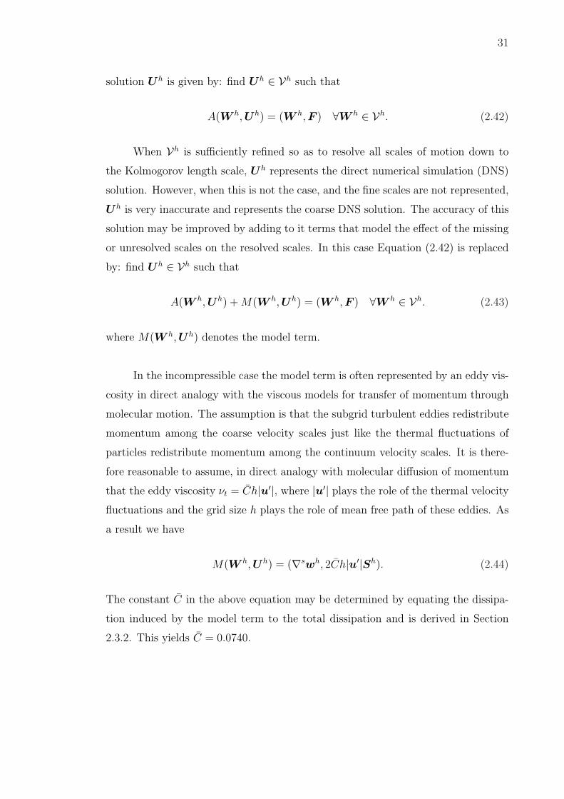
31
solution Uh is given by: find Uh ∈ Vh such that
A(W h, Uh) = (W h, F ) ∀W h ∈ Vh. (2.42)
When Vh is sufficiently refined so as to resolve all scales of motion down to
the Kolmogorov length scale, Uh represents the direct numerical simulation (DNS)
solution. However, when this is not the case, and the fine scales are not represented,
Uh is very inaccurate and represents the coarse DNS solution. The accuracy of this
solution may be improved by adding to it terms that model the effect of the missing
or unresolved scales on the resolved scales. In this case Equation (2.42) is replaced
by: find Uh ∈ Vh such that
A(W h, Uh) + M(W h, Uh) = (W h, F ) ∀W h ∈ Vh. (2.43)
where M(W h, Uh) denotes the model term.
In the incompressible case the model term is often represented by an eddy vis-
cosity in direct analogy with the viscous models for transfer of momentum through
molecular motion. The assumption is that the subgrid turbulent eddies redistribute
momentum among the coarse velocity scales just like the thermal fluctuations of
particles redistribute momentum among the continuum velocity scales. It is there-
fore reasonable to assume, in direct analogy with molecular diffusion of momentum
that the eddy viscosity νt = Ch|u′|, where |u′| plays the role of the thermal velocity
fluctuations and the grid size h plays the role of mean free path of these eddies. As
a result we have
M(W h, Uh) = (∇swh, 2Ch|u′|Sh). (2.44)
The constant C in the above equation may be determined by equating the dissipa-
tion induced by the model term to the total dissipation and is derived in Section
2.3.2. This yields C = 0.0740.

32
For turbulent flows where compressibility is important, following Yoshizawa,
the fine scale fluctuations introduce two other terms. As a result we propose
M(W h, Uh) = 2C(∇swh, ρhh|u′|Shdev)
− 1
3(∇ ·wh, ρh|u′|2) +
C
PrtγM2∞(∇qh, ρhh|u′|∇T h).
(2.45)
In the equation above Prt = 0.5 is the turbulent Prandtl number assumed to
be constant.
In the expressions above there is no undetermined parameter, however we
have made use of u′, the fine scale velocity field, which is obviously not known in a
coarse scale simulation. However, tt may be evaluated using the VMS formulation
as described in Section 2.1.
2.3.2 Estimate of the RBEV parameter C
In this subsection, we determine the value of RBEV parameter C. The con-
stant C is determined by equating the dissipation induced by the model term to
the total dissipation. The idea is similar as the derivation of static Smagorinsky
parameter cs [30]. The derivation presented in this section is based on homogeneous
isotropic turbulence, and uses the knowledge of Kolmogorov spectrum described in
Section 3.3.
The RBEV model can be viewed in two parts. First, the linear eddy-viscosity
model
τij = −2νtShij, (2.46)
is used to relate the residual stress to the filtered rate of strain. The coefficient of
proportionality νt is the eddy viscosity of the residual motions. Second, the eddy
viscosity is modeled as
νt = Ch|u′|, (2.47)

33
where the grid size is defined as h = π/kh and kh is the cutoff wavenumber. Ac-
cording to the eddy-viscosity model, the rate of transfer of energy to the residual
motions or the dissipation ε is
ε = −τijShij. (2.48)
In addition, we need the Kolmogorov spectrum, it is shown as
E(k) = CKε2/3k−5/3, (2.49)
where CK is the Kolmogorov constant. Using Equations (2.46) and (2.49) in Equa-
tion (2.48), we get,
ε = 2νtShijS
hij, (2.50)
because
ShijS
hij =
∫ kh
0
k2E(k)dk, (2.51)
so
ε = 2νt
∫ kh
0
k2E(k)dk, (2.52)
with Equation (2.47), Equation (2.52) becomes
ε = 2Ch|u′|∫ kh
0
k2E(k)dk, (2.53)
with
|u′| = |u′iu′i|1/2 =(2
∫ ∞
kh
E(k)dk)1/2
, (2.54)
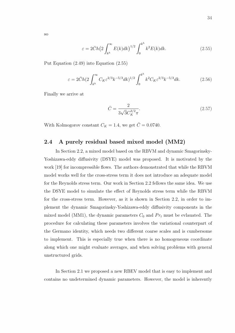
34
so
ε = 2Ch(2
∫ ∞
kh
E(k)dk)1/2
∫ kh
0
k2E(k)dk. (2.55)
Put Equation (2.49) into Equation (2.55)
ε = 2Ch(2
∫ ∞
kh
CKε2/3k−5/3dk)1/2
∫ kh
0
k2CKε2/3k−5/3dk. (2.56)
Finally we arrive at
C =2
3√
3C3/2K π
. (2.57)
With Kolmogorov constant CK = 1.4, we get C = 0.0740.
2.4 A purely residual based mixed model (MM2)
In Section 2.2, a mixed model based on the RBVM and dynamic Smagorinsky-
Yoshizawa-eddy diffusivity (DSYE) model was proposed. It is motivated by the
work [19] for incompressible flows. The authors demonstrated that while the RBVM
model works well for the cross-stress term it does not introduce an adequate model
for the Reynolds stress term. Our work in Section 2.2 fellows the same idea. We use
the DSYE model to simulate the effect of Reynolds stress term while the RBVM
for the cross-stress term. However, as it is shown in Section 2.2, in order to im-
plement the dynamic Smagorinsky-Yoshizawa-eddy diffusivity components in the
mixed model (MM1), the dynamic parameters C0 and Prt must be evlauated. The
procedure for calculating these parameters involves the variational counterpart of
the Germano identity, which needs two different coarse scales and is cumbersome
to implement. This is especially true when there is no homogeneous coordinate
along which one might evaluate averages, and when solving problems with general
unstructured grids.
In Section 2.1 we proposed a new RBEV model that is easy to implement and
contains no undetermined dynamic parameters. However, the model is inherently
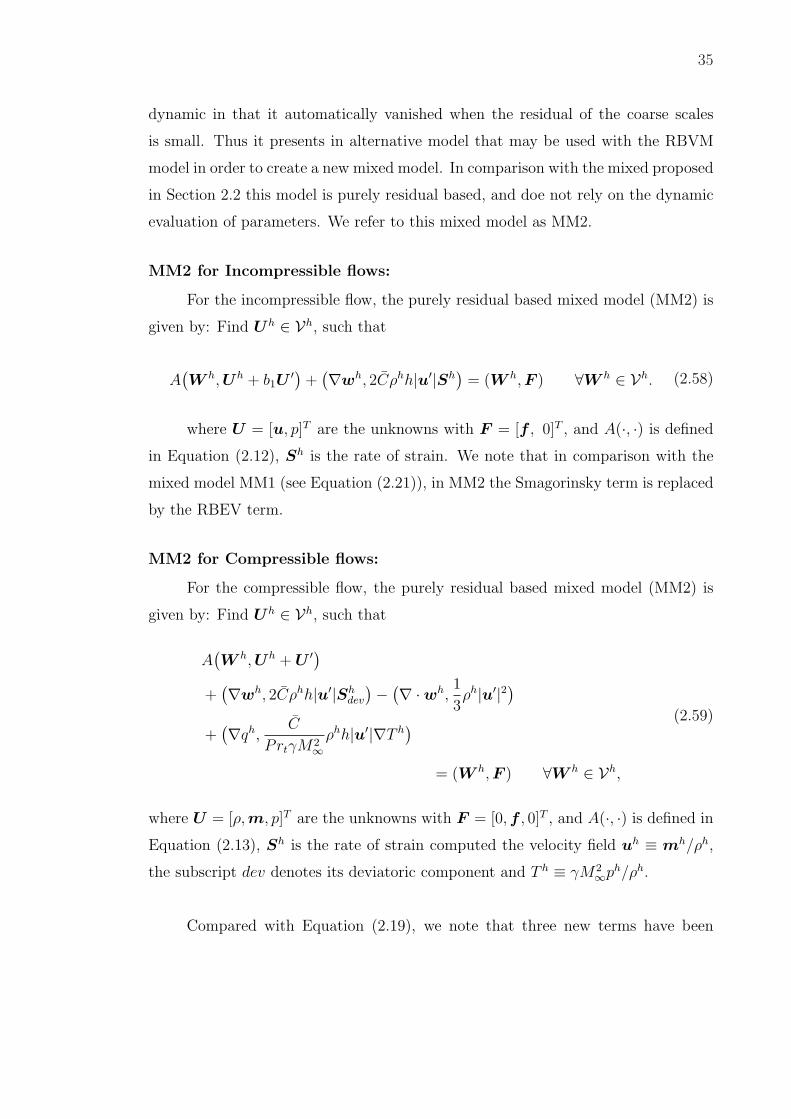
35
dynamic in that it automatically vanished when the residual of the coarse scales
is small. Thus it presents in alternative model that may be used with the RBVM
model in order to create a new mixed model. In comparison with the mixed proposed
in Section 2.2 this model is purely residual based, and doe not rely on the dynamic
evaluation of parameters. We refer to this mixed model as MM2.
MM2 for Incompressible flows:
For the incompressible flow, the purely residual based mixed model (MM2) is
given by: Find Uh ∈ Vh, such that
A(W h, Uh + b1U
′) +(∇wh, 2Cρhh|u′|Sh
)= (W h, F ) ∀W h ∈ Vh. (2.58)
where U = [u, p]T are the unknowns with F = [f , 0]T , and A(·, ·) is defined
in Equation (2.12), Sh is the rate of strain. We note that in comparison with the
mixed model MM1 (see Equation (2.21)), in MM2 the Smagorinsky term is replaced
by the RBEV term.
MM2 for Compressible flows:
For the compressible flow, the purely residual based mixed model (MM2) is
given by: Find Uh ∈ Vh, such that
A(W h, Uh + U ′)
+(∇wh, 2Cρhh|u′|Sh
dev
)− (∇ ·wh,1
3ρh|u′|2)
+(∇qh,
C
PrtγM2∞ρhh|u′|∇T h
)
= (W h, F ) ∀W h ∈ Vh,
(2.59)
where U = [ρ, m, p]T are the unknowns with F = [0, f , 0]T , and A(·, ·) is defined in
Equation (2.13), Sh is the rate of strain computed the velocity field uh ≡ mh/ρh,
the subscript dev denotes its deviatoric component and T h ≡ γM2∞ph/ρh.
Compared with Equation (2.19), we note that three new terms have been
36
added. The first two term models the deviatoric and dilatational components of the
subgrid scale stress tensor and the third term models the subgrid heat flux vector.
In comparison with the mixed model MM1, we note that the Smagorinsky and the
eddy diffusivity term have been replaced by their RBEV counterparts. We note that
we do not need a RBEV term for the diltational component of the residual stresses
because the RBVM formulation already provides this (see the discussion in Section
2.2.2).
Remark We note that our mixed model is similar to other mixed models,
including the scale-similarity model [11, 25, 26, 27] and the tensor-diffusivity model
[28, 29] in that it contains distinct models for the cross-stress term and the Reynolds
stress term. However, the form of the model term for the cross stress in our model
is distinct from other mixed models. In addition, this purely residual based mixed
model (MM2) is much easier for the implementation than the mixed model based
on dynamic Smagorinsky model (MM1).

CHAPTER 3
Large-Eddy Simulation of Compressible Homogeneous
Isotropic Turbulent Flows
3.1 Introduction
In this chapter, we test the performance of the four LES models developed in
Chapter 2 for compressible turbulent flows within a Fourier-spectral method method.
They are
• the residual-based variational multiscale (RBVM) model
• the mixed model based on RBVM (MM1)
• the residual-based eddy viscosity (RBEV) model
• the purely-residual based mixed model (MM2)
We will test the performance of these LES models in predicting the decay
of compressible, homogeneous, isotropic turbulence in regimes where shocklets are
known to exist. The LES models will be tested with Taylor micro-scale Reynolds
numbers of Reλ ≈ 65 and Reλ ≈ 120 on 323 and 643 grids.
The layout of this chapter is as follows. In Section 3.2, we specialize the
weak form of the models developed in Chapter 2 to a spectral method that utilizes
Fourier basis functions. The precise definition for the unresolved scales, and well
as the parameters τ is also provided. Homogeneous Isotropic Turbulence (HIT) is
introduced in Section 3.3 to understand the behavior of turbulent flows. In Section
3.4, we apply the RBVM model and the MM1 model to decay of compressible
Portions of this chapter previously appeared as: J. Liu, and A. A. Oberai, “The residual-basedvariational multiscale formulation for the large eddy simulation of compressible flows, ” Comput.Methods Appl. Mech. Eng., accepted, 2012.
37

38
turbulent flows. In Section 3.5, the RBEV model and the MM2 model will be
applied to to study the same flows. Conclusions are drawn in Section 3.6.
3.2 LES models
In Chapter 2, we have introduced and developed the residual based variational
multiscale model (RBVM), a mixed model based on RBVM (MM1), the residual
based eddy viscosity model (RBEV) and the purely residual based mixed model
(MM2). In this chapter we will apply these LES models to study the decay of com-
pressible homogeneous isotropic turbulent flows by using a Fourier-spectral method.
3.2.1 Weak form of LES models
RBVM and MM1 models:
The weak form of the RBVM and MM1 models is given by Equation (2.22) in
Chapter 2. It is repeated here for convenience: Find Uh ∈ Vh, such that
A(W h, Uh + U ′)
+(∇wh, 2C0h
2ρh|Sh|Shdev
)− (∇wh,2
3C1h
2ρh|Sh|2I)
+(∇qh,
C0
PrtγM2∞h2ρh|Sh|∇T h
)
= (W h, F ) ∀W h ∈ Vh,
(3.1)
In Equation (3.1), C0, C1 and Prt−1 are three parameters and U ′ is given by
Equation (2.18). This equation contains the following LES models within it:
• With C0 = C1 = Prt−1 = 0 and τ = 0, we arrive at the direct numerical
simulation (DNS).
• With C0 = C1 = Prt−1 = 0, but τ 6= 0, we arrive at the residual based
variational multiscale model (RBVM).
• With C0, C1 and Prt−1 are determined dynamically, and τ = 0, we arrive at
the dynamic Smagorinsky-Yoshizawa-eddy diffusivity model (DSYE).

39
• With C0, C1 and Prt−1 are kept at a fixed value, and τ = 0, we arrive at the
static Smagorinsky-Yoshizawa-eddy diffusivity model (SSYE).
• With C0 and Prt−1 are determined dynamically, C1 = 0 and τ 6= 0 we arrive
at mixed model based on RBVM and DSYE (MM1).
RBEV and MM2 models:
The weak from for the RBEV and the MM2 models is given by Equation (2.59)
in Chapter 2. It is repeated here for convenience:
Find Uh ∈ Vh, such that
A(W h, Uh + b1U
′)
+(∇wh, 2Cρhh|u′|Sh
dev
)− (∇ ·wh, b21
3ρh|u′|2)
+(∇qh,
C
PrtγM2∞ρhh|u′|∇T h
)
= (W h, F ) ∀W h ∈ Vh,
(3.2)
In Equation (3.2), b1, b2 are parameters. This equation contains the following LES
models within it:
• With b1 = b2 = C = 0, we arrive at the direct numerical simulation (DNS).
• With b2 = C = 0, but b1 6= 0, we arrive at the residual based variational
multiscale model (RBVM).
• With b2 6= 0 and C 6= 0 but b1 = 0, we arrive at the residual based eddy
viscosity model (RBEV).
• With b1 6= 0 and C 6= 0 while b2 = 0, we arrive at the purely residual based
mixed model (MM2).

40
3.2.2 Unresolved scales and stabilization parameter τ
The unresolved scales U ′ = [ρ′, m′, p′] that appear in Equations (3.1) and (3.2)
are determined by
U ′ ≈ −P′τ (Uh) P′TR(Uh), (3.3)
where P′ is a projection operator that maps an element of V to V ′ and R(Uh) ≡LUh−F is the coarse-scale residual. For other details, please refer to the discussion
in Section 2.
The coarse-scale residual R(Uh) = (Rρ,Rm,Rp)T is given by
Rρ =∂ρh
∂t+∇ ·mh, (3.4)
Rm =∂mh
∂t+∇ · (m
h ⊗mh
ρh) +∇ph − 1
Re∇ · σh − f , (3.5)
Rp =∂ph
∂t+∇ · (uhph)− (γ − 1)ph∇ · uh − (γ − 1)
ReΦh
− 1
M2∞PrRe∇ · (µh∇T h). (3.6)
We assume a diagonal form for the matrix τ , that is τ = diag(τc, τm, τm, τm, τe).
Each of τc, τm and τe represents a combination of an advective and a diffusive time-
scale associated with differential operator for the fine scales. Our definition for τ
for the compressible Navier-Stokes equations is motivated by the work of [15, 31].
The τ ’s are given by
τc = Cτ
[(λ)2
]−1/2
,
τm = Cτ
[(λ)2 +
(4
h2
< µh >
< ρh > Re
)2 ]−1/2
,
τe = Cτ
[(λ)2 +
(4
h2
γ < µh >
< ρh > PrRe
)2 ]−1/2
,
(3.7)
41
with
1
λe=
1− e−Ma
λe1
+e−Ma
λe2
, (3.8)
(λe1)
2 =4
h2< |uh|2 > (1 + 2Ma−2 + Ma−1
√4 + Ma−2), (3.9)
(λe2)
2 =4
h2< |uh|2 >, (3.10)
where h = πkh is the grid size, u = mh
ρh , < · > denotes the spatial average of
a quantity, Ma =√
< |uh|2 >/ < ch > is the turbulent Mach number, and
ch = (T h)1/2/M∞ is the local speed of sound. Cτ is constant, which is either 1
or 1/2. In the equation above λ is the reciprocal of the characteristic advective time
scale. It is a combination of a time scale that is appropriate for the low-Mach num-
ber limit λ2 and another that is appropriate for the high Mach number limit, λ1. In
this case λ can be thought of as a doubly-asymptotic approximation of the two. We
note that a similar approximation was proposed in [31], however it underestimated
the value of λ in the compressible limit.
3.2.3 Specialization to a Fourier spectral basis
We will apply the RBVM model, the MM1 model, the RBEV model and the
MM2 model to simulate the decay of homogeneous isotropic turbulence of compress-
ible flows. We assume that Ω = ]0, 2π[3 and the density, velocity and pressure fields
satisfy periodic boundary conditions. We propose to simulate this problem using the
Fourier-spectral method. In this case the space of functions Vh are approximated
by a Fourier-spectral basis. Fourier modes with |k| < kh are used to define Vh. We
note that these basis functions have the special property that they are orthogonal
to each other in all Hm inner-products. In addition, we define the projector Ph to
be the H1 projection and due to the orthogonality of the Fourier modes this is the
low-pass sharp cut-off filter in wavenumber space. Then P′ is the high-pass, sharp
cutoff filter in wavenumber space.
As a result of this, the expression for the fine scale variables U ′ = [ρ′, m, p′]T
42
simplify to:
ρ′ = 0, (3.11)
m′ = −P′τmP′T (∇ · (m
h ⊗mh
ρh)− 1
Re∇ · σh
), (3.12)
p′ = −P′τeP′T (∇ · (uhph)− (γ − 1)ph∇ · uh − (γ − 1)
ReΦh
− 1
M2∞PrRe∇ · (µh∇T h)
). (3.13)
Further, the equations for all the LES models derived in the previous section
simplify to
∂ρh
∂t+ ik · mh = 0, (3.14)
∂mh
∂t+ ik · m⊗m
ρ+ ikph =
ik · σRe
+ ik · 2 ρhνtShdev −
ik
3ρhu2
rms, (3.15)
∂ph
∂t+ ik · up + (γ − 1)p∇ · u =
(γ − 1)
Reσ : S +
ik
M2∞· (
µ(T )∇T
PrRe+
ρhνt∇T h
γPrt
), (3.16)
where the hat denotes the Fourier coefficient of a variable corresponding to a wavenum-
ber k. In addition ρ = ρh + ρ′, m = mh + m′, p = ph + p′, u = m/ρ, uh = mh/ρh,
T = γM2∞p/ρ, T h = γM2
∞ph/ρh, S and Sh are the symmetric gradients of u and
uh respectively, and σ = µ(T )Sdev.
All the models to be tested in this can be obtained by defining νt and urms as
follows:
1. For no model (DNS), νt = urms = 0 and ρ′ = m′ = p′ = 0.
2. For the static Smagorinsky-Yoshizawa eddy viscosity model (Static SYE), νt =
C20h
2|Sh| and u2rms = 2C1h
2|Sh|2, where C0 = 0.1, 0.16, C1 = 0.020 and
Prt = 0.5, and ρ′ = m′ = p′ = 0.

43
3. For the dynamic Smagorinsky-Yoshizawa eddy viscosity model (DSYE), νt =
C20h
2|Sh| and u2rms = 2C1h
2|Sh|2, where C0, C1 and Prt are determined dy-
namically, and ρ′ = m′ = p′ = 0.
4. For the residual based variational multiscale model (RBVM), νt = urms = 0,
ρ′, m′ and p′ are given by Equations (3.11)-(3.13).
5. For the MM1 model, νt = C20h
2|Sh| and u2rms = 0, where C0 and Prt are
determined dynamically, and ρ′, m′ and p′ are given by Equations (3.11)-
(3.13).
6. For the residual based eddy viscosity model (RBEV) νt = Ch|u′| and urms =
|u′|, where u′ is given by u′ = m′ρh with m′ given by Equation (3.12), C =
0.0740 and Prt = 0.5. However, in all the other terms ρ′ = m′ = p′ = 0.
7. For the MM2 model, νt = Ch|u′| and urms = |u′|, where u′ is given by
u′ = m′ρh , C = 0.0740 and Prt = 0.5. ρ′, m′ and p′ are given by Equations
(3.11)-(3.13).

44
3.3 Homogeneous Isotropic Turbulence (HIT)
The concept of using statistical methods for the analysis of turbulent flows
was introduced by G. I. Taylor in the 1930s. These methods include using studying
structure functions and their Fourier transforms in order to understand turbulent
flows. As mentioned in Chapter 1, in 1941 the Russian statistician Kolmogorov pub-
lished three papers [5, 6, 7] on the statistical theories of turbulence, which is known
as the K41 theory. His theory provides a prediction of the structure functions and
their Fourier transforms for of a homogeneous isotropic turbulent flow. Kolmogorov
demonstrated that even though the velocity of a homogeneous isotropic turbulent
flow fluctuates in an unpredictable manner, the energy spectrum (how much kinetic
energy is present on average at a particular length scale) is predictable.
Homogeneous isotropic turbulence
Homogeneous isotropic turbulence is the simplest and most fundamental tur-
bulent flow. If all the statistics of turbulence are invariant under a shift in position,
the field u(x, t) is homogeneous. If the field is also statistically invariant under
rotations and reflections of the coordinate system, then it is isotropic. If the flow
field is statistically invariant under all translations, rotations and reflections of the
coordinate system, it is said to be homogeneous isotropic turbulence (HIT).
It should be pointed out that, the HIT is an idealization and never happens
in nature. Fortunately, HIT can be realized in the lab to help study the theory of
HIT. It can be approximately generated in a wind or water tunnel by let a uniform
fluid stream that passes through a uniform metal grid. Once the fluid passes the
metal grid, there is no production of turbulent kinetic energy, the turbulence decays
downstream of the grid. The downstream distance to the grid can be interpreted
as psuedo-time. In this way is the decay of homogeneous isotropic turbulence is
experimentally realized. However, the turbulence from this method is relatively
homogeneous in planes normal to the mean flow, and it is not fully isotropic. Another
approach has been to use fans. In [32], eight synthetic jet actuators on the corners
of a cubic chamber are used to create energetic turbulence, and HIT without a mean
flow was realized in a small region at the center of the chamber.
45
Fourier modes
In order to show a clear picture of the energy cascade, we will examine the
Navier-Stokes equations in wavenumber space. In this subsection we will apply
Fourier modes to the Navier-Stokes equations for homogeneous turbulence in which
the mean velocity is zero.
The Fourier series representation of the turbulent velocity field in 3D is
u(x, t) =∑
k
eik·xu(k, t), (3.17)
where k is the wavenumber, eik·x is the Fourier modes and uj(k, t) are the Fourier
coefficients of velocity, which are defined as
uj(k, t) = Fkuj(x, t), (3.18)
the operator Fk determines the coefficient for the Fourier mode with wavenum-
ber k. It is defined as
Fkg(x) =1
L3
∫ L
0
∫ L
0
∫ L
0
g(x)e−ik·xdx1dx2dx3 = g(k). (3.19)
The Fourier operator transfers variables from spatial space u(x, t) to wavenum-
ber space u(k, t).
Turbulent kinetic energy (TKE) in spectral space
The total kinetic energy E can be written with a spatial average,
E =1
2< u2
i >=1
2
1
V
∫ ∫ ∫ui(x)ui(x)dx, (3.20)
where V is the volume. The angle brackets represent an spatial average.
According to the mathematics of Fourier transform, the total kinetic energy
can be written as
E =1
2
∫ ∫ ∫u(k) · u∗(k)dk =
∫ ∫ ∫E(k)dk, (3.21)

46
where E(k) is defined as the kinetic energy of the Fourier mode with wavenum-
ber k,
E(k) =1
2u(k) · u∗(k), (3.22)
where u∗(k) is the conjugate of u(k). E(k) contains directional information.
In an isotropic velocity fields the spectrum does not depend on directions. Usually,
we want to know the energy at a particular scale k = |k| without any interest in
its direction. To find E(k), we integrate over the spherical shell of radius k (in
3-dimensions),
E =
∫ ∫ ∫E(k)dk =
∫ ∞
0
E(k)dk. (3.23)
As the mean velocity is zero, so the kinetic energy E is equal to turbulent
kinetic energy K. Then we get the turbulent kinetic energy K,
K =
∫ ∞
0
E(k)dk, (3.24)
the dissipation ε can be defined based on the energy spectrum as,
ε =
∫ ∞
0
2νk2E(k)dk, (3.25)
where ν is the kinematic viscosity.
The Taylor-scale Reynolds number Reλ is often used to characterize HIT,
which is defined based on K and ε as
Reλ =(20
3
K2
εν
). (3.26)
Energy cascade
Turbulence can be considered to be composed of eddies of different sizes. Ed-
dies with characteristic size ` have a characteristic velocity u(`) and characteristic
timescale τ(`) = `/u(`). The eddies in the largest size range are characterized by
the lengthscale `0 which is comparable to the flow scale L, and their characteristic
velocity u0 is on the order of the r.m.s. turbulence intensity which is comparable to

47
characteristic velocity U of the HIT.
The large eddies are usually unstable and they break up into smaller eddies.
In this way kinetic energy contained in large eddies is transferred to smaller eddies.
These smaller eddies have a similar break-up process, and transfer their energy to
even smaller eddies. The procedure of kinetic energy transfer from large eddies to
small eddies is the energy cascade. Energy cascade continues until the Reynolds
number Re(`) = u(`)/` is sufficiently small that the eddy motion is stable, and
molecular viscosity is effective in dissipating the kinetic energy. Then kinetic energy
is converted into heat, and lost to the environment. This procedure is called dissi-
pation.
The Kolmogorov hypotheses and Characteristic scales of turbulence
The K41 theory contains three hypotheses, and among other things it can de-
termine the size of the smallest eddies that are responsible for dissipating the energy
in the energy cascade. First, it is useful to introduce a lengthscale `EI ≈ 16`0, which
is used to separate the anisotropic large eddies ` > `EI and the isotropic small eddies
` < `EI . The three Kolmogorov hypotheses are as following [3]:
Kolmogorov’s hypothesis of local isotropy: At sufficiently high Reynolds
number, the small-scale turbulent motions (` ¿ `0) are statistically isotropic.
Kolmogorov’s first similarity hypothesis: In every turbulent flow at suf-
ficiently high Reynolds number, the statistics of the small-scale motions (` < `EI)
have a universal form that is uniquely determined by ν and ε.
Given the two parameters ν and ε, the characteristic length, velocity, and time
scales for the smallest eddies can be determined. These are the Kolmogorov scales:
η = (ν3/ε)1/4,
uη = (εν)1/4,
τη = (ν/ε)1/2.
(3.27)
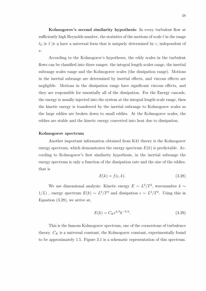
48
Kolmogorov’s second similarity hypothesis: In every turbulent flow at
sufficiently high Reynolds number, the statistics of the motions of scale ` in the range
`0 À ` À η have a universal form that is uniquely determined by ε, independent of
ν.
According to the Kolmogorov’s hypotheses, the eddy scales in the turbulent
flows can be classified into three ranges: the integral length scales range, the inertial
subrange scales range and the Kolmogorov scales (the dissipation range). Motions
in the inertial subrange are determined by inertial effects, and viscous effects are
negligible. Motions in the dissipation range have significant viscous effects, and
they are responsible for essentially all of the dissipation. For the Energy cascade,
the energy is usually injected into the system at the integral length scale range, then
the kinetic energy is transferred by the inertial subrange to Kolmogorov scales as
the large eddies are broken down to small eddies. At the Kolmogorov scales, the
eddies are stable and the kinetic energy converted into heat due to dissipation.
Kolmogorov spectrum
Another important information obtained from K41 theory is the Kolmogorov
energy spectrum, which demonstrates the energy spectrum E(k) is predictable. Ac-
cording to Kolmogorov’s first similarity hypothesis, in the inertial subrange the
energy spectrum is only a function of the dissipation rate and the size of the eddies.
that is
E(k) = f(ε, k). (3.28)
We use dimensional analysis: Kinetic energy E ∼ L2/T 2, wavenumber k ∼1/L) , energy spectrum E(k) ∼ L3/T 2 and dissipation ε ∼ L2/T 3. Using this in
Equation (3.28), we arrive at,
E(k) = CKε2/3k−5/3. (3.29)
This is the famous Kolmogorov spectrum, one of the cornerstone of turbulence
theory. CK is a universal constant, the Kolmogorov constant, experimentally found
to be approximately 1.5. Figure 3.1 is a schematic representation of this spectrum.

49
00
log(k)
log(E(k))
Inertial subrange scales
Kolmogorovlengthscales
Energy Flow
Integral length scales
Figure 3.1: Sketch of energy spectrum.

50
3.4 Numerical Results for RBVM and MM1
In this section we present results using the RBVM, the mixed RBVM and the
dynamic Smagorinsky-Yoshizawa-eddy diffusivity (DSYE) model with a spectral
basis. All variables are represented using a Fourier basis with a cut-off wave number
denoted by kh. The test problem corresponds to a DNS simulation of the decay of
homogeneous turbulence for a compressible fluid computed in [33]. In particular we
focus on the D9 case described in that paper with Ω =]0, 2π[3. In order to validate
our implementation of the compressible Navier-Stokes equations we compute our
own DNS results and compare with the results presented in [33] and achieve good
agreement. The physical parameters associated with the cases we have considered
are listed in Table 3.1. They include the initial spectrum for the turbulent kinetic
energy E(k, 0), the initial total kinetic energy q2/2, the free stream Mach number
M∞, the turbulent Mach number, Ma, the Reynolds number Re and the ratio
of initial compressible to total kinetic energy χ. We assume that there are no
fluctuations in the initial values of the thermodynamic quantities, namely pressure,
density and the temperature. We choose Prandtl number Pr = 0.7 and the adiabatic
index for air to be γ = 1.4.
3.4.1 Low Reynolds Number Case
For compressible flows the velocity field is comprised of solenoidal (incompress-
ible) and dilatational (compressible) components, us and uc respectively. For the
case of isotropic turbulence in Fourier space the Helmholtz decomposition is unique
and is given by
uc = [(k · u)/k2]k, (3.30)
us = u− uc . (3.31)
Let Ks and Kc denote the turbulent kinetic energy from the solenoidal and
dilatational velocity components, respectively. We define χ = Kc/(Kc + Ks) as the
ratio of compressible kinetic energy to the total kinetic energy.
The turbulent Mach number Ma =√
< |uh|2 >/ < ch >, where < · >

51
Table 3.1: Parameters for the decay of homogeneous compressible tur-bulence.
E(k, 0) q2
2M∞ Ma Re χ
0.011k4e−2( k4 )
2
1.3235 0.184 -0.430 0.300-0.700 376 0.2-0.6
represents the spatial average and c is the local speed of sound. We approxi-
mate the turbulent Mach number with the root-mean-square Mach number Ma ≈√< |uh|2 > /ch2, which is easier to evaluate.
These parameters lead to the development of local, weak shocks, referred to
as shocklets close to the regions where the local Mach number exceeds unity. As
pointed out in [33] this happens when ∇ · u obtains a large negative value corre-
sponding to the deceleration of a supersonic flow to a subsonic flow. During the
decay of turbulence the local Mach number varies in the range Ma ∼ 0.1 − 0.7,
and the Taylor microscale Reynolds number, Reλ = O(27 − 65). We refer this low
Reynolds number test as Case Reλ = 65.5.
We solve the Navier Stokes equations on a grid with N3 points and compute all
integrals on a (3N/2)3 grid. We note that even for the DNS simulation this does not
de-alias all the terms, but does guarantee the accurate computation of predominantly
quadratic terms. For the DNS simulation N = 256 and for the LES simulations
N = 32. For the LES calculations we use the truncated velocity field obtained from
the DNS at t/Te = 1.2, where Te = 0.667 is the eddy turn-over time [33], as the initial
condition. We compare the performance of the models from t/Te = 1.2 ∼ 7.0, which
corresponds to a Taylor micro-scale Reynolds number of Reλ = 65.5 ∼ 27.4. For
time integration we use the fourth-order Runge-Kutta algorithm, and we evaluate
all terms explicitly. The details of the numerical algorithm can be found in [34].
For all the LES models in this section, Cτ = 0.5. For more details, the readers are
referred to [35].

52
1 2 3 4 5 6 70
0.1
0.2
0.3
0.4
0.5
0.6
t/Te
KS
DSYERBVMMM1No ModelDNS
Figure 3.2: Time history of turbulent kinetic energy of the incompress-
ible velocity component for the Reλ = 65.5 case on a 323 grid
with χ = 0.4 and Ma = 0.488. A comparison of the DSYE,
RBVM, MM1, and no model cases.
1 2 3 4 5 6 70
0.02
0.04
0.06
0.08
0.1
0.12
0.14
0.16
0.18
0.2
t/Te
KC
DSYERBVMMM1No ModelDNS
Figure 3.3: Time history of turbulent kinetic energy of the compressible
velocity component for the Reλ = 65.5 case on a 323 grid with
χ = 0.4 and Ma = 0.488. A comparison of the DSYE, RBVM,
MM1, and no model cases.

53
Figures 3.2 and 3.3 show the turbulent kinetic energy in the incompressible
and compressible velocity components, respectively, as a function of time. We ob-
serve that the no model case overpredicts these quantities. In Figure 3.2, for the
incompressible turbulent kinetic energy, the RBVM model is most accurate followed
by the mixed model, followed by the DSYE model which is clearly too dissipative.
The RBVM model slightly overpredicts the kinetic energy while the mixed model
underpredicts it. The evolution of the compressible component of the kinetic energy
is shown in Figure 3.3 and all three LES models perform well. Here the mixed
model is the most accurate followed closely by the RBVM model, which slightly
overpredicts the kinetic energy. The DSYE model is once again overly dissipative.
This behavior is explained by examining the incompressible and compressible
energy spectra at t/Te ≈ 3.0 in Figures 3.4 and 3.5 and at t/Te ≈ 6.0 in Figures 3.6
and 3.7.
From the figure for the incompressible spectra at t/Te ≈ 3.0 (Figure 3.4) we
observe that the no-model case displays a pile-up of energy at high wavenumbers. All
the LES models are quite accurate at low-to-mid wavenumbers, while the RBVM is
the most accurate at high wavenumbers, followed by the mixed model. At t/Te ≈ 6.0
(Figure 3.6) the mixed model is the most accurate at the mid-to-high wavenumbers
whereas the RBVM model is most accurate at low wavenumbers. In either case the
DSYE model is the least accurate.
For the compressible spectra in Figures 3.5 and 3.7 we observe that the energy
pile-up in the no-model case is not as large as in the incompressible case thereby
indicating that the compressible component of the subgrid model plays a smaller
role. All the LES models appear to perform quite well with the RBVM and the
mixed models being the most accurate at high wavenumbers. The same conclusions
can be drawn for the density and pressure spectra at time t/Te ≈ 6.0, shown in
Figures 3.8 and 3.9, respectively. The evolution of the root-mean-square (rms)
density is shown in Figure 3.10. Once again the DSYE model is observed to lead to
smaller rms values while the RBVM and the mixed model are more accurate.

54
100
101
10−2
k
ES
DSYERBVMMM1No ModelDNS
Figure 3.4: Energy spectrum of the incompressible velocity component
for the Reλ = 65.5 case on a 323 grid with χ = 0.4 and Ma =
0.488 at t/Te ≈ 3. A comparison of the DSYE, RBVM, MM1,
and no model cases.
100
101
10−3
10−2
k
EC
DSYERBVMMM1No ModelDNS
Figure 3.5: Energy spectrum of the compressible velocity component for
the Reλ = 65.5 case on a 323 grid with χ = 0.4 and Ma = 0.488
at t/Te ≈ 3. A comparison of the DSYE, RBVM, MM1, and
no model cases.
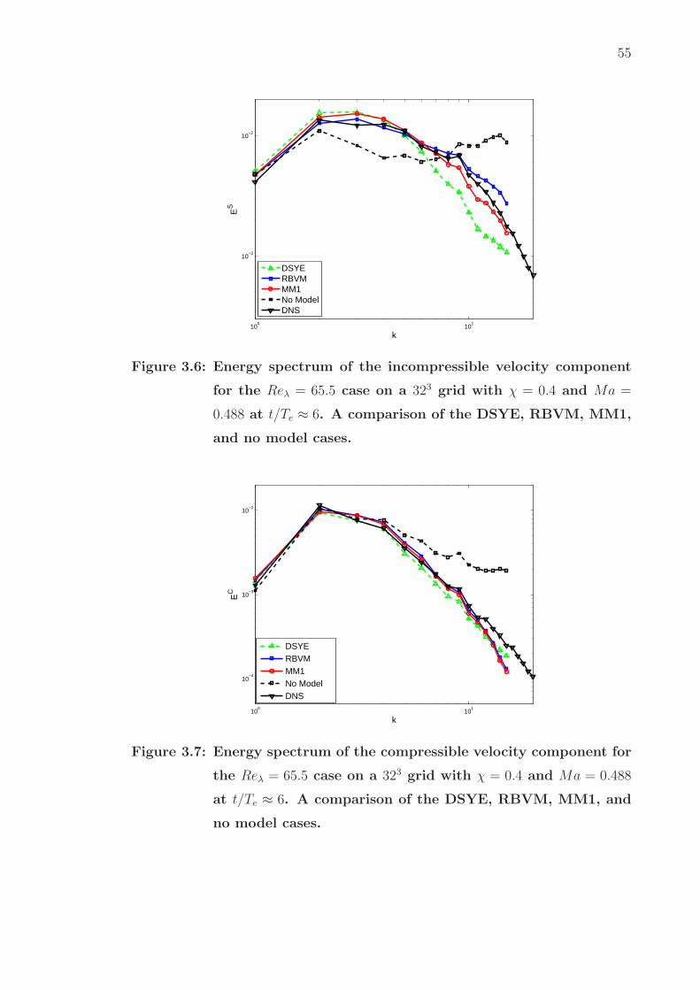
55
100
101
10−3
10−2
k
ES
DSYERBVMMM1No ModelDNS
Figure 3.6: Energy spectrum of the incompressible velocity component
for the Reλ = 65.5 case on a 323 grid with χ = 0.4 and Ma =
0.488 at t/Te ≈ 6. A comparison of the DSYE, RBVM, MM1,
and no model cases.
100
101
10−4
10−3
10−2
k
EC
DSYERBVMMM1No ModelDNS
Figure 3.7: Energy spectrum of the compressible velocity component for
the Reλ = 65.5 case on a 323 grid with χ = 0.4 and Ma = 0.488
at t/Te ≈ 6. A comparison of the DSYE, RBVM, MM1, and
no model cases.

56
100
101
10−4
10−3
k
Eρ
DSYERBVMMM1No ModelDNS
Figure 3.8: Density spectrum for the Reλ = 65.5 case on a 323 grid with
χ = 0.4 and Ma = 0.488 at t/Te ≈ 6. A comparison of the
DSYE, RBVM, MM1, and no model cases.
100
101
10−3
10−2
10−1
k
Ep
DSYERBVMMixedNo ModelDNS
Figure 3.9: Pressure spectrum for the Reλ = 65.5 case on a 323 grid with
χ = 0.4 and Ma = 0.488 at t/Te ≈ 6. A comparison of the
DSYE, RBVM, MM1, and no model cases.

57
1 2 3 4 5 6 70.06
0.08
0.1
0.12
0.14
0.16
0.18
0.2
t/Te
ρ rms
DSYERBVMMM1No ModelDNS
Figure 3.10: Time history of root-mean-square of density for the Reλ =
65.5 case on a 323 grid with χ = 0.4 and Ma = 0.488. A com-
parison of the DSYE, RBVM, MM1, and no model cases.
We have also performed these simulations with kh = 32 (not shown here). We
observe the same trends however the differences between all the models are much
smaller.
3.4.2 Study of the effects of varying χ
In this section we examine the effect of varying the initial fraction of the
compressible turbulent kinetic energy. In particular we select χ = 0.2 and χ = 0.6
to add to the χ = 0.4 case described in the previous section. The Mach number
Ma = 0.488 is unchanged.
When χ is small a greater proportion of the total initial kinetic energy is
incompressible. As a result a larger contribution from the deviatoric component of
the subgrid stress is required. The dynamic Smagorinsky and mixed models respond
to this by increasing the value of the model parameters with decreasing values of χ.
This is seen in Figure 3.11, where we have plotted value of the deviatoric parameter
C0 as a function of time. We observe that with increasing time all parameters
tend to smaller values because of the natural decay in the turbulence intensity. We
also note that the value of C0 for the mixed model is consistently smaller than the

58
dynamic Smagorinsky model, indicating that the dynamic procedure is accounting
for the additional dissipation generated by the RBVM component of the mixed
model. With increasing value of χ the ratio of the average value of C0 for the mixed
model to the corresponding value for the dynamic Smagorinsky model appears to
decreasing, indicating that for large values of χ the mixed model is tending toward
the RBVM model.
For completeness the variation of the other dynamic parameters that is C1
and Pr−1t as a function of time is shown in Figures 3.12 and 3.13, respectively. The
value of C1 in the mixed model is selected to be zero as discussed in Section 2.2.
The value of Pr−1t for the mixed model is also zero because the dynamic procedure
yields a negative value which is ignored.
1 2 3 4 5 6 7
0
0.005
0.01
0.015
0.02
0.025
0.03
t/Te
C0
DSYE χ =0.2MM1 χ= 0.2DSYE χ =0.4MM1 χ=0.4DSYE χ =0.6MM1 χ =0.6
Figure 3.11: Time history of the Smagorinsky coefficient C0 for the Reλ =
65.5 case on a 323 grid with Ma = 0.488. A comparison of the
DSYE and MM1 cases.

59
1 2 3 4 5 6 7
0
0.05
0.1
t/Te
C1
DSYE χ=0.2MM1 χ=0.2DSYE χ=0.4MM1 χ=0.4DSYE χ=0.6MM1 χ=0.6
Figure 3.12: Time history of the Smagorinsky coefficient C1 for the Reλ =
65.5 case on a 323 grid with Ma = 0.488. A comparison of the
DSYE and MM1 cases.
1 2 3 4 5 6 7
0
0.5
1
1.5
2
2.5
3
3.5
4
t/Te
γ M
∞2/P
r t
DSYE χ =0.2MM1 χ=0.2DSYE χ =0.4MM1 χ=0.4DSYE χ =0.6MM1 χ=0.6
Figure 3.13: Time history of Prt for the Reλ = 65.5 case on a 323 grid with
Ma = 0.488. A comparison of the DSYE and MM1 cases.
In Figure 3.14 we have plotted the spectrum for the incompressible velocity

60
component for different models for χ = 0.2 and t/Te ≈ 6. We note that RBVM
model is the most accurate for low wavenumbers whereas the mixed model is the
most accurate for high wavenumbers. The DSYE model is too dissipative. The
spectrum for the compressible component is shown in Figure 3.15. All models are
very accurate for small wavenumbers whereas the RBVM and the mixed model are
slightly more accurate for high wavenumbers.
In Figure 3.16 we have plotted the spectrum for the incompressible velocity
component for different models for χ = 0.6 and t/Te ≈ 6. We note that RBVM
model is the most accurate overall followed by the mixed model. The DSYE model
continues to be too dissipative. The spectrum for the compressible component is
shown in Figure 3.17. Here all the models are very accurate for the entire range of
wavenumbers.
100
101
10−3
10−2
k
ES
DSYERBVMMM1No ModelDNS
Figure 3.14: Energy spectrum of the incompressible velocity component
for the Reλ = 65.5 case on a 323 grid with χ = 0.2 and Ma =
0.488 at t/Te ≈ 6. A comparison of the DSYE, RBVM, MM1,
and no model cases.

61
100
101
10−4
10−3
10−2
k
EC
DSYERBVMMM1No ModelDNS
Figure 3.15: Energy spectrum of the compressible velocity component for
the Reλ = 65.5 case on a 323 grid with χ = 0.2 and Ma = 0.488
at t/Te ≈ 6. A comparison of the DSYE, RBVM, MM1, and
no model cases.
100
101
10−3
10−2
k
ES
DSYERBVMMM1No ModelDNS
Figure 3.16: Energy spectrum of the incompressible velocity component
for the Reλ = 65.5 case on a 323 grid with χ = 0.6 and Ma =
0.488 at t/Te ≈ 6. A comparison of the DSYE, RBVM, MM1,
and no model cases.
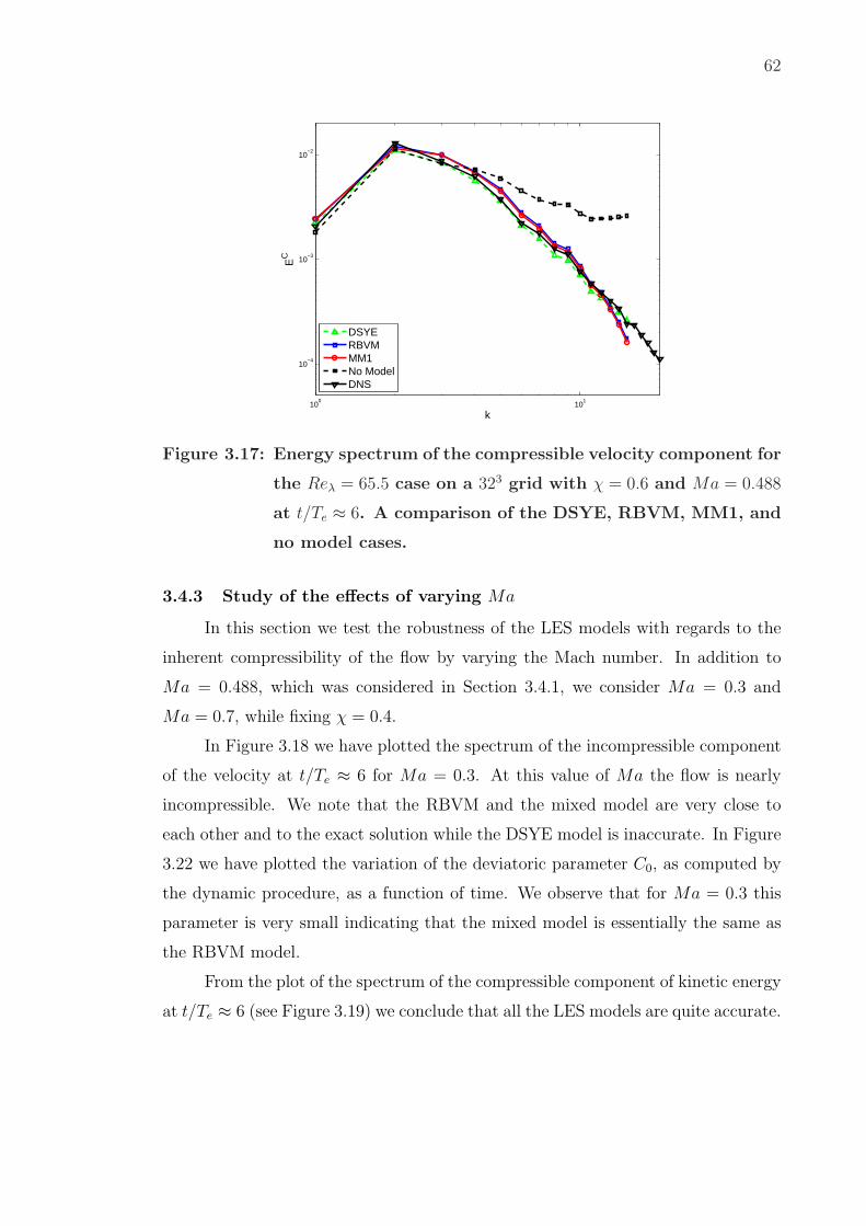
62
100
101
10−4
10−3
10−2
k
EC
DSYERBVMMM1No ModelDNS
Figure 3.17: Energy spectrum of the compressible velocity component for
the Reλ = 65.5 case on a 323 grid with χ = 0.6 and Ma = 0.488
at t/Te ≈ 6. A comparison of the DSYE, RBVM, MM1, and
no model cases.
3.4.3 Study of the effects of varying Ma
In this section we test the robustness of the LES models with regards to the
inherent compressibility of the flow by varying the Mach number. In addition to
Ma = 0.488, which was considered in Section 3.4.1, we consider Ma = 0.3 and
Ma = 0.7, while fixing χ = 0.4.
In Figure 3.18 we have plotted the spectrum of the incompressible component
of the velocity at t/Te ≈ 6 for Ma = 0.3. At this value of Ma the flow is nearly
incompressible. We note that the RBVM and the mixed model are very close to
each other and to the exact solution while the DSYE model is inaccurate. In Figure
3.22 we have plotted the variation of the deviatoric parameter C0, as computed by
the dynamic procedure, as a function of time. We observe that for Ma = 0.3 this
parameter is very small indicating that the mixed model is essentially the same as
the RBVM model.
From the plot of the spectrum of the compressible component of kinetic energy
at t/Te ≈ 6 (see Figure 3.19) we conclude that all the LES models are quite accurate.

63
In Figure 3.20 we have plotted the spectrum of the incompressible component
of the velocity at t/Te ≈ 6 for Ma = 0.7. At this high Mach number we expect the
compressible effects to be more pronounced and we would also expect the formation
relatively strong local shocks. From the plot we observe that the RBVM model is
most accurate in this case followed by the mixed model. The latter is somewhere
between the RBVM and the DSYE model. This may be understood by observing
the variation of C0 for these two models with time (see Figure 3.22). We note that
the value of C0 for the mixed model is higher than it was for Ma = 0.3, indicating
that its performance will be closer to that of the DSYE model in this case.
From the plot of the spectrum of the compressible component of the velocity
we observe that the RBVM and the mixed models are very accurate while the DSYE
model underestimates the spectrum.
100
101
10−3
10−2
k
ES
DSYERBVMMM1No ModelDNS
Figure 3.18: Energy spectrum of the incompressible velocity component
for the Reλ = 65.5 case on a 323 grid with χ = 0.4 and Ma =
0.300 at t/Te ≈ 6. A comparison of the DSYE, RBVM, MM1,
and no model cases.

64
100
101
10−4
10−3
10−2
k
EC
DSYERBVMMM1No ModelDNS
Figure 3.19: Energy spectrum of the compressible velocity component for
the Reλ = 65.5 case on a 323 grid with χ = 0.4 and Ma = 0.300
at t/Te ≈ 6. A comparison of the DSYE, RBVM, MM1, and
no model cases.
100
101
10−3
10−2
k
ES
DSYERBVMMM1No ModelDNS
Figure 3.20: Energy spectrum of the incompressible velocity component
for the Reλ = 65.5 case on a 323 grid with χ = 0.4 and Ma =
0.700 at t/Te ≈ 6. A comparison of the DSYE, RBVM, MM1,
and no model cases.
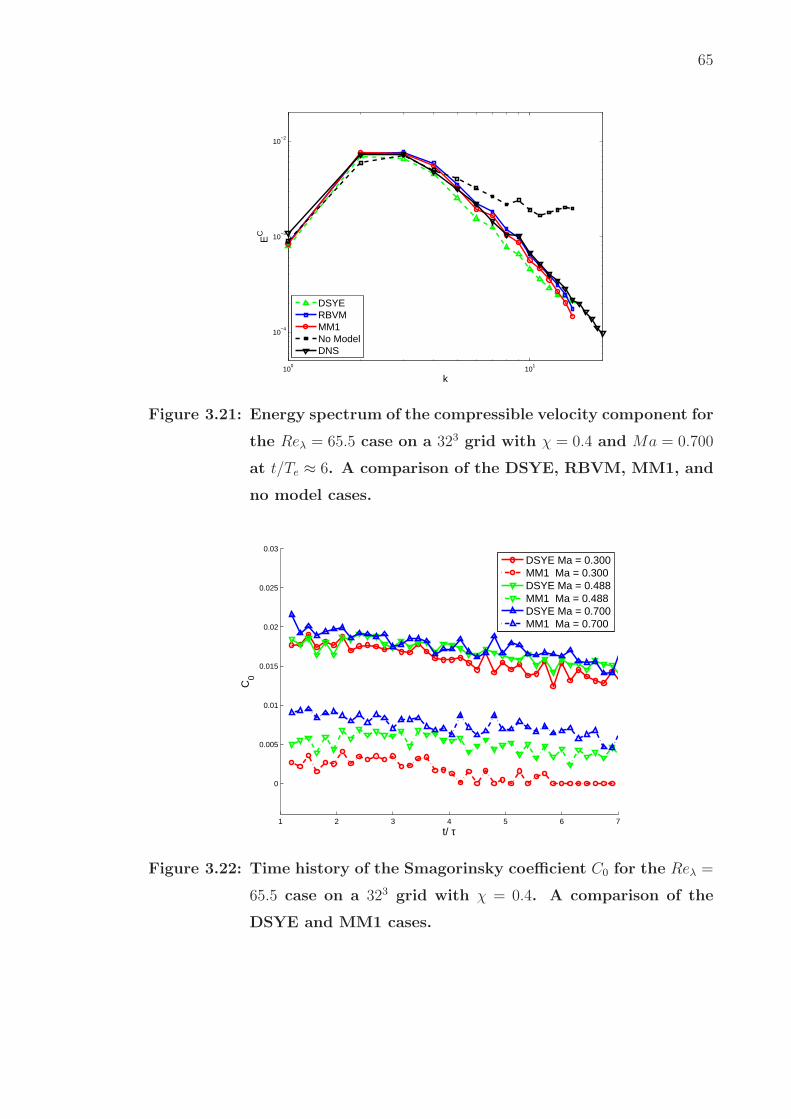
65
100
101
10−4
10−3
10−2
k
EC
DSYERBVMMM1No ModelDNS
Figure 3.21: Energy spectrum of the compressible velocity component for
the Reλ = 65.5 case on a 323 grid with χ = 0.4 and Ma = 0.700
at t/Te ≈ 6. A comparison of the DSYE, RBVM, MM1, and
no model cases.
1 2 3 4 5 6 7
0
0.005
0.01
0.015
0.02
0.025
0.03
t/ τ
C0
DSYE Ma = 0.300MM1 Ma = 0.300DSYE Ma = 0.488MM1 Ma = 0.488DSYE Ma = 0.700MM1 Ma = 0.700
Figure 3.22: Time history of the Smagorinsky coefficient C0 for the Reλ =
65.5 case on a 323 grid with χ = 0.4. A comparison of the
DSYE and MM1 cases.
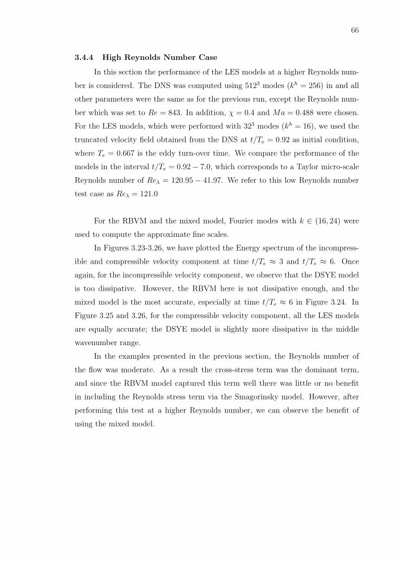
66
3.4.4 High Reynolds Number Case
In this section the performance of the LES models at a higher Reynolds num-
ber is considered. The DNS was computed using 5123 modes (kh = 256) in and all
other parameters were the same as for the previous run, except the Reynolds num-
ber which was set to Re = 843. In addition, χ = 0.4 and Ma = 0.488 were chosen.
For the LES models, which were performed with 323 modes (kh = 16), we used the
truncated velocity field obtained from the DNS at t/Te = 0.92 as initial condition,
where Te = 0.667 is the eddy turn-over time. We compare the performance of the
models in the interval t/Te = 0.92− 7.0, which corresponds to a Taylor micro-scale
Reynolds number of Reλ = 120.95 − 41.97. We refer to this low Reynolds number
test case as Reλ = 121.0
For the RBVM and the mixed model, Fourier modes with k ∈ (16, 24) were
used to compute the approximate fine scales.
In Figures 3.23-3.26, we have plotted the Energy spectrum of the incompress-
ible and compressible velocity component at time t/Te ≈ 3 and t/Te ≈ 6. Once
again, for the incompressible velocity component, we observe that the DSYE model
is too dissipative. However, the RBVM here is not dissipative enough, and the
mixed model is the most accurate, especially at time t/Te ≈ 6 in Figure 3.24. In
Figure 3.25 and 3.26, for the compressible velocity component, all the LES models
are equally accurate; the DSYE model is slightly more dissipative in the middle
wavenumber range.
In the examples presented in the previous section, the Reynolds number of
the flow was moderate. As a result the cross-stress term was the dominant term,
and since the RBVM model captured this term well there was little or no benefit
in including the Reynolds stress term via the Smagorinsky model. However, after
performing this test at a higher Reynolds number, we can observe the benefit of
using the mixed model.
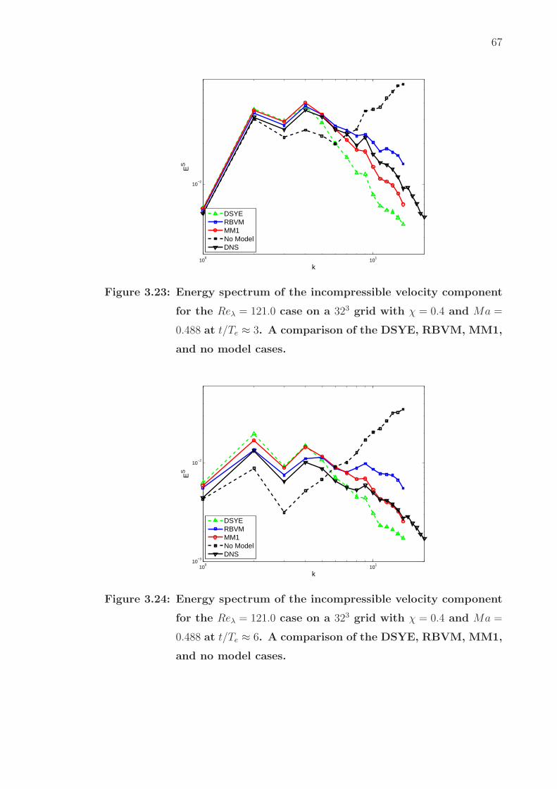
67
100
101
10−2
k
ES
DSYERBVMMM1No ModelDNS
Figure 3.23: Energy spectrum of the incompressible velocity component
for the Reλ = 121.0 case on a 323 grid with χ = 0.4 and Ma =
0.488 at t/Te ≈ 3. A comparison of the DSYE, RBVM, MM1,
and no model cases.
100
101
10−3
10−2
k
ES
DSYERBVMMM1No ModelDNS
Figure 3.24: Energy spectrum of the incompressible velocity component
for the Reλ = 121.0 case on a 323 grid with χ = 0.4 and Ma =
0.488 at t/Te ≈ 6. A comparison of the DSYE, RBVM, MM1,
and no model cases.
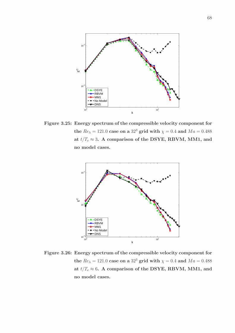
68
100
101
10−3
10−2
k
EC
DSYERBVMMM1No ModelDNS
Figure 3.25: Energy spectrum of the compressible velocity component for
the Reλ = 121.0 case on a 323 grid with χ = 0.4 and Ma = 0.488
at t/Te ≈ 3. A comparison of the DSYE, RBVM, MM1, and
no model cases.
100
101
10−4
10−3
10−2
k
EC
DSYERBVMMM1No ModelDNS
Figure 3.26: Energy spectrum of the compressible velocity component for
the Reλ = 121.0 case on a 323 grid with χ = 0.4 and Ma = 0.488
at t/Te ≈ 6. A comparison of the DSYE, RBVM, MM1, and
no model cases.

69
We now consider the “convergence” of the LES models by computing the LES
solution with 643 modes. The solution at t/τ ≈ 1 was used as an initial condition for
the LES runs which were performed with 643 modes (kh = 64). For the RBVM and
the mixed model modes with k ∈ (64, 96) were used to computer the approximate
fine scales.
1 2 3 4 5 6 70
0.1
0.2
0.3
0.4
0.5
0.6
0.7
t/Te
KS
DSYERBVMMM1No ModelDNS
Figure 3.27: Time history of turbulent kinetic energy of the incompress-
ible velocity component for the Reλ = 121.0 case on a 643 grid
with χ = 0.4 and Ma = 0.488. A comparison of the DSYE,
RBVM, MM1, and no model cases.

70
1 2 3 4 5 6 70
0.02
0.04
0.06
0.08
0.1
0.12
0.14
0.16
0.18
0.2
t/Te
KC
DSYERBVMMM1No ModelDNS
Figure 3.28: Time history of turbulent kinetic energy of the compressible
velocity component for the Reλ = 121.0 case on a 643 grid with
χ = 0.4 and Ma = 0.488. A comparison of the DSYE, RBVM,
MM1, and no model cases.
1 2 3 4 5 6 70.06
0.08
0.1
0.12
0.14
0.16
0.18
0.2
t/Te
ρ rms
DSYERBVMMM1No ModelDNS
Figure 3.29: Time history of root-mean-square of density for the Reλ =
121.0 case on a 643 grid with χ = 0.4 and Ma = 0.488. A com-
parison of the DSYE, RBVM, MM1, and no model cases.
In Figures 3.27 - 3.29, we have plotted the evolution of the resolved turbulent

71
kinetic energies and density rms as a function of time. Once again it is observed
that the DSYE model is too dissipative which RBVM and the mixed model works
very well. Both the RBVM and mixed model have good agreement with DNS result.
In Figures 3.30 - 3.33, the energy spectrum of the incompressible and compressible
velocity components are given at t/Te ≈ 3 and t/Te ≈ 6. Once again we observe
that the DSYE model is too dissipative at high wavenumbers for the incompressible
velocity component. The RBVM model is very close to DNS. The performance of
the mixed model is between the DSYE and RBVM model. For the compressible
velocity component, both the RBVM and the mixed models perform very well,
while the DSYE model overpredicts the spectrum near the cut-off wavenumber.
The spectrum of density and pressure are shown in Figures 3.34 - 3.35. Here all
the models are very accurate, however the DSYE model is not as accurate as the
RBVM and the mixed model.
100
101
10−3
10−2
k
ES
DSYERBVMMM1No ModelDNS
Figure 3.30: Energy spectrum of the incompressible velocity component
for the Reλ = 121.0 case on a 643 grid with χ = 0.4 and Ma =
0.488 at t/Te ≈ 3. A comparison of the DSYE, RBVM, MM1,
and no model cases.

72
100
101
10−4
10−3
10−2
k
EC
DSYERBVMMM1No ModelDNS
Figure 3.31: Energy spectrum of the compressible velocity component for
the Reλ = 121.0 case on a 643 grid with χ = 0.4 and Ma = 0.488
at t/Te ≈ 3. A comparison of the DSYE, RBVM, MM1, and
no model cases.
100
101
10−3
10−2
k
ES
DSYERBVMMM1No ModelDNS
Figure 3.32: Energy spectrum of the incompressible velocity component
for the Reλ = 121.0 case on a 643 grid with χ = 0.4 and Ma =
0.488 at t/Te ≈ 6. A comparison of the DSYE, RBVM, MM1,
and no model cases.
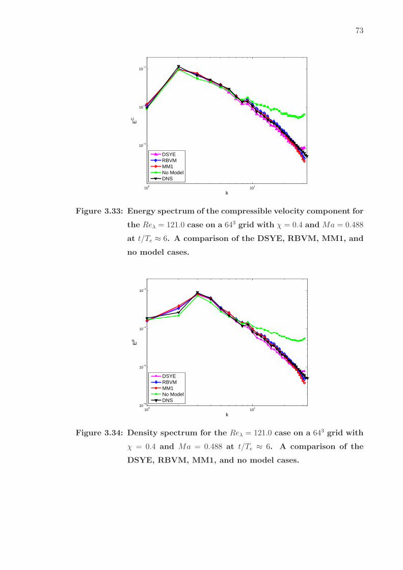
73
100
101
10−4
10−3
10−2
k
EC
DSYERBVMMM1No ModelDNS
Figure 3.33: Energy spectrum of the compressible velocity component for
the Reλ = 121.0 case on a 643 grid with χ = 0.4 and Ma = 0.488
at t/Te ≈ 6. A comparison of the DSYE, RBVM, MM1, and
no model cases.
100
101
10−6
10−5
10−4
10−3
k
Eρ
DSYERBVMMM1No ModelDNS
Figure 3.34: Density spectrum for the Reλ = 121.0 case on a 643 grid with
χ = 0.4 and Ma = 0.488 at t/Te ≈ 6. A comparison of the
DSYE, RBVM, MM1, and no model cases.

74
100
101
10−4
10−3
10−2
10−1
k
Ep
DSYERBVMMM1No ModelDNS
Figure 3.35: Pressure spectrum for the Reλ = 121.0 case on a 643 grid
with χ = 0.4 and Ma = 0.488 at t/Te ≈ 6. A comparison of the
DSYE, RBVM, MM1, and no model cases.
3.4.5 Summary
We have developed and implemented the residual-based variational multiscale
(RBVM) model for compressible turbulent flows. Motivated by earlier results for
incompressible flows we have also considered a mixed version of this model wherein
Smagorinsky, Yoshizawa and eddy-diffusivity terms are added in order to better
model the Reynolds stress contributions. Through energy analysis of the mixed
model (performed in Chapter 2) we have demonstrated that the Yoshizawa model is
redundant because the RBVM model itself introduces a viable Reynolds stress term
for the dilatational component of subgrid stresses. In addition, from the dynamic
procedure we have found that the eddy-diffusivity term in the energy equation is not
required for the mixed RBVM model. As a result the mixed RBVM model contains
only one term in addition to the RBVM model. This term models the Reynolds
stress component of the deviatoric part of subgrid stresses and is represented by a
Smagorinsky-type model.
We have tested the performance of the RBVM, the mixed and the dynamic
Smagorinsky-Yoshizawa-eddy diffusivity (DSYE) models in predicting the decay

75
of compressible, homogeneous, isotropic turbulence in regimes where shocklets are
known to exist. We have varied the level of compressibility of the flow by varying
the initial proportion of turbulent kinetic energy and by varying the Mach number.
In all cases we have found that RBVM and the mixed models are equally accurate
and perform significantly better than the DSYE model. We have also found that for
the mixed model the variational counterpart of the Germano identity automatically
accounts for the dissipation produced by the RBVM terms and produces smaller
Smagorinsky parameter when compared to the dynamic Smagorinsky model.
3.5 Numerical Results for the RBEV model
In this section we present results using the RBEV model. The models are
tested in decaying homogeneous isotropic turbulent flows which are described in
Section 3.4. However, in this section, we just test the cases with Ma = 0.488 and
χ = 0.40. We still test the models with different Reynolds numbers and different
grids (323 and 643). The RBEV model is compared with dynamic Smagorinsky-
Yoshizawa-eddy diffusivity (DSYE) model, and the static Smagorinsky-Yoshizawa-
eddy diffusivity (SSYE) model with coefficient Cs = 0.10 and Cs = 0.16. For all the
LES models in this section, Cτ = 1.0 for the stabilization parameter τ . The intent
of the results presented in this section is to test the performance of the RBEV model
as a stand-alone eddy viscosity model.
3.5.1 Low Reynolds Number Case
In the low Reynolds Numbers case, Re = 376 and DNS is performed with
2563 mesh and time step dt = 0.001. For the LES calculations we use the truncated
velocity field obtained from the DNS at t/Te = 1.2, where Te = 0.667 as the initial
condition. We compare the performance of the models from t/Te = 1.2 ∼ 7.0, which
corresponds to a Taylor micro-scale Reynolds number of Reλ = 65.5 ∼ 27.4. Both
323 and 643 meshes are considered for LES simulation with dt = 0.005. We refer
this low Reynolds number test case as Reλ = 65.5

76
In Figures 3.36 - 3.42 we present results for the low Reynolds number case on
a 323 mesh.
In Figure 3.36, the time history of the turbulent kinetic energies (TKE) is
plotted for all the models. We observe that overall the RBEV model is the most
accurate followed by the static SYE model with Cs = 0.10, the DSYE model and
then the static SYE model with Cs = 0.16. In Figure 3.37, the time history of
root-mean-square (RMS) of density and temperature are shown. Both the RBEV
and the static SYE model with Cs = 0.10 are very close to the DNS result, while
the DSYE model and the static SYE model with Cs = 0.16 are too dissipative.
In Figure 3.38 we have plotted the spectra of the total TKE at t/Te = 3 and
t/Te = 6. We observe that the RBEV and the static SYE(0.10) are the most accurate
while the other two models are overly dissipative. This observation also holds for
the incompressible spectra shown in Figure 3.39. However, for the compressible
spectra we observe that all the models about equally accurate. Figure 3.40 shows
the spectrum of density, pressure and temperature at t/Te = 6. Here too, the RBEV
and the static SYE(0.10) perform better.
In Figure 3.41, we show the time history of the eddy viscosity of different mod-
els at four points given by the coordinates (0, 0, 0), (L/4, L/4, L/4) ,(L/2, L/2, L/2)
and (0, L/4, L/2). We observe that all viscosities vary widely in time but generally
decrease with time. The values of the RBEV and the SSYE(0.10) models and of
the DSYE and SSYE(0.16) are similar. The same trends are also seen in the values
of the average values of viscosities shown in Figure 3.42. These plots explain why
the performance of the RBEV and the SSYE(0.10) models and the the DSYE and
SSYE(0.16) models is similar. They also explain why the results for the latter are
more dissipative.
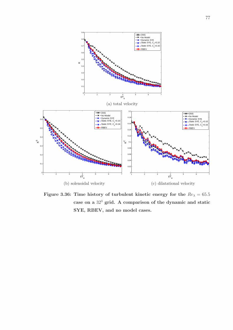
77
1 2 3 4 5 6 70
0.1
0.2
0.3
0.4
0.5
0.6
0.7
0.8
0.9
t/Te
K
DNSNo ModelDynamic SYEStatic SYE, C
s=0.10
Static SYE, Cs=0.16
RBEV
(a) total velocity
1 2 3 4 5 6 70
0.1
0.2
0.3
0.4
0.5
0.6
t/Te
KS
DNSNo ModelDynamic SYEStatic SYE, C
s=0.10
Static SYE, Cs=0.16
RBEV
(b) solenoidal velocity
1 2 3 4 5 6 70
0.02
0.04
0.06
0.08
0.1
0.12
0.14
0.16
0.18
0.2
t/Te
KC
DNSNo ModelDynamic SYEStatic SYE, C
s=0.10
Static SYE, Cs=0.16
RBEV
(c) dilatational velocity
Figure 3.36: Time history of turbulent kinetic energy for the Reλ = 65.5
case on a 323 grid. A comparison of the dynamic and static
SYE, RBEV, and no model cases.

78
1.5 2 2.5 3 3.5 4 4.5 5 5.5 6 6.5 7
0.06
0.08
0.1
0.12
0.14
0.16
0.18
t/Te
ρ rms
DNSNo ModelDynamic SYEStatic SYE, C
s=0.10
Static SYE, Cs=0.16
RBEV
(a) density
1.5 2 2.5 3 3.5 4 4.5 5 5.5 6 6.5 70.02
0.025
0.03
0.035
0.04
0.045
0.05
0.055
0.06
0.065
0.07
t/Te
Trm
s
DNSNo ModelDynamic SYEStatic SYE, C
s=0.10
Static SYE, Cs=0.16
RBEV
(b) temperature
Figure 3.37: Time history of root-mean-square of density and tempera-
ture for the Reλ = 65.5 case on a 323 grid. A comparison of
the dynamic and static SYE, RBEV, and no model cases.
100
101
10−2
k
E
DNSNo ModelDynamic SYEStatic SYE, C
s=0.10
Static SYE, Cs=0.16
RBEV
(a) total velocity, t/Te = 3
100
101
10−3
10−2
k
E
DNSNo ModelDynamic SYEStatic SYE, C
s=0.10
Static SYE, Cs=0.16
RBEV
(b) total velocity, t/Te = 6
Figure 3.38: Energy spectrum of the total velocity for the Reλ = 65.5 case
on a 323 grid. A comparison of the dynamic and static SYE,
RBEV, and no model cases.

79
100
101
10−2
k
ES
DNSNo ModelDynamic SYEStatic SYE, C
s=0.10
Static SYE, Cs=0.16
RBEV
(a) solenoidal velocity, t/Te = 3
100
101
10−3
10−2
k
ES
DNSNo ModelDynamic SYEStatic SYE, C
s=0.10
Static SYE, Cs=0.16
RBEV
(b) solenoidal velocity, t/Te = 6
100
101
10−3
10−2
k
EC
DNSNo ModelDynamic SYEStatic SYE, C
s=0.10
Static SYE, Cs=0.16
RBEV
(c) dilatational velocity, t/Te = 3
100
101
10−4
10−3
10−2
k
EC
DNSNo ModelDynamic SYEStatic SYE, C
s=0.10
Static SYE, Cs=0.16
RBEV
(d) dilatational velocity, t/Te = 6
Figure 3.39: Energy spectrum of solenoidal and dilatational velocity for
the Reλ = 65.5 case on a 323 grid. A comparison of the
dynamic and static SYE, RBEV, and no model cases.

80
100
101
10−4
10−3
k
Eρ
DNSNo ModelDynamic SYEStatic SYE, C
s=0.10
Static SYE, Cs=0.16
RBEV
(a) density, t/Te = 6
100
101
10−3
10−2
10−1
k
Ep
DNSNo ModelDynamic SYEStatic SYE, C
s=0.10
Static SYE, Cs=0.16
RBEV
(b) pressure, t/Te = 6
100
101
10−6
10−5
10−4
k
ET
DNSNo ModelDynamic SYEStatic SYE, C
s=0.10
Static SYE, Cs=0.16
RBEV
(c) temperature, t/Te = 6
Figure 3.40: Spectrum of density, pressure and temperature for the Reλ =
65.5 case on a 323 grid. A comparison of the dynamic and
static SYE, RBEV, and no model cases.

81
1 2 3 4 5 6 7 80
0.001
0.002
0.003
0.004
0.005
0.006
0.007
0.008
0.009
0.01
t/Te
ν t
Dynamic SYE νt
Static SYE νt, C
s=0.10
Static SYE νt, C
s=0.16
RBEV νt
(a) point (0, 0, 0)
1 2 3 4 5 6 7 80
0.002
0.004
0.006
0.008
0.01
0.012
t/Te
ν t
Dynamic SYE νt
Static SYE νt, C
s=0.10
Static SYE νt, C
s=0.16
RBEV νt
(b) point (L/4, L/4, L/4)
1 2 3 4 5 6 7 80
0.002
0.004
0.006
0.008
0.01
0.012
t/Te
ν t
Dynamic SYE νt
Static SYE νt, C
s=0.10
Static SYE νt, C
s=0.16
RBEV νt
(c) point (L/2, L/2, L/2)
1 2 3 4 5 6 7 80
0.002
0.004
0.006
0.008
0.01
0.012
t/Te
ν t
Dynamic SYE νt
Static SYE νt, C
s=0.10
Static SYE νt, C
s=0.16
RBEV νt
(d) point (0, L/4, L/2)
Figure 3.41: Time history of eddy viscosity for the Reλ = 65.5 case on a
323 grid. A comparison of the dynamic and static SYE and
RBEV cases.

82
1 2 3 4 5 6 7 80
1
2
3
4
5
6
7
8x 10
−3
t/Te
νt
Dynamic SYE νt
Static SYE νt, C
s=0.10
Static SYE νt, C
s=0.16
RBEV νt
Figure 3.42: Time history of average eddy viscosity for the Reλ = 65.5
case on a 323 grid. A comparison of the dynamic and static
SYE and RBEV cases.
We now consider the same problem but on a fine mesh of 643 modes. In Figure
3.43 we have plotted the evolution of kinetic energies as a function of time. We now
observe that the RBEV, DSYE, and SSYE(0.10) models are all very accurate while
the SSYE(0.16) model is less so. The same observations hold for the time-history
of the RMS of density and temperature shown in Figure 3.44.
In the spectra of the total velocity (Figure 3.45) and incompressible velocity
(Figure 3.46(a) and (b)), RBEV is most accurate followed by DSYE and SSYE(0.1),
and then SSYE(0.16). For the compressible velocity spectra (shown in Figure 3.46(c)
and (d)), the DSYE and the SSYE(0.1) are the most accurate followed by the RBEV
and the SSYE(0.16) models. The spectra for density, temperature and pressure
(Figure 3.47) all show the same trends.
The average eddy viscosity as a function of time for all the models is shown in
Figure 3.48. We observe that the values for the DSYE and SSYE(0.1) is very close,
while that of SSYE(0.16) is higher and that of RBEV is smaller. This explains why
the RBEV is the least dissipative, followed by the DSYE and SSYE(0.1), and then
the SSYE(0.16) models.
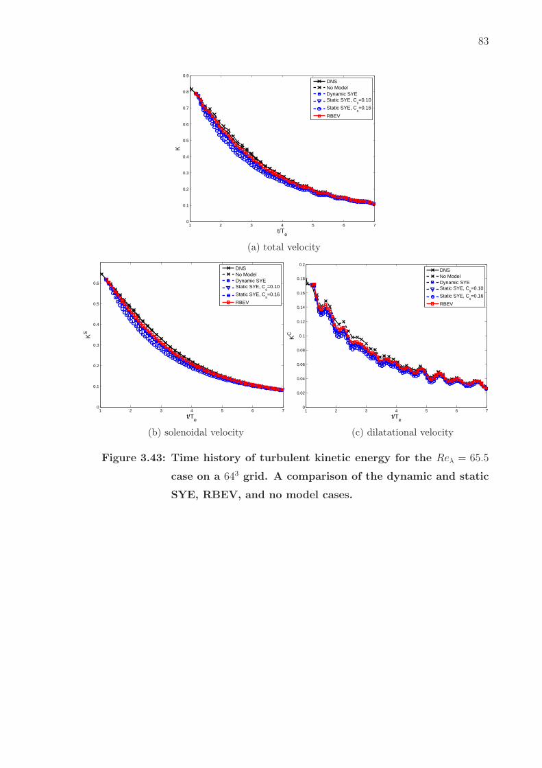
83
1 2 3 4 5 6 70
0.1
0.2
0.3
0.4
0.5
0.6
0.7
0.8
0.9
t/Te
K
DNSNo ModelDynamic SYEStatic SYE, C
s=0.10
Static SYE, Cs=0.16
RBEV
(a) total velocity
1 2 3 4 5 6 70
0.1
0.2
0.3
0.4
0.5
0.6
t/Te
KS
DNSNo ModelDynamic SYEStatic SYE, C
s=0.10
Static SYE, Cs=0.16
RBEV
(b) solenoidal velocity
1 2 3 4 5 6 70
0.02
0.04
0.06
0.08
0.1
0.12
0.14
0.16
0.18
0.2
t/Te
KC
DNSNo ModelDynamic SYEStatic SYE, C
s=0.10
Static SYE, Cs=0.16
RBEV
(c) dilatational velocity
Figure 3.43: Time history of turbulent kinetic energy for the Reλ = 65.5
case on a 643 grid. A comparison of the dynamic and static
SYE, RBEV, and no model cases.
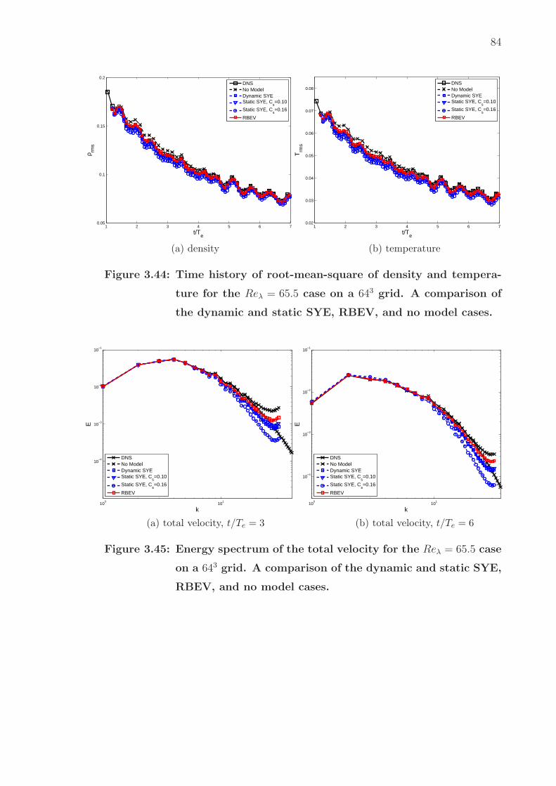
84
1 2 3 4 5 6 70.05
0.1
0.15
0.2
t/Te
ρ rms
DNSNo ModelDynamic SYEStatic SYE, C
s=0.10
Static SYE, Cs=0.16
RBEV
(a) density
1 2 3 4 5 6 70.02
0.03
0.04
0.05
0.06
0.07
0.08
t/Te
Trm
s
DNSNo ModelDynamic SYEStatic SYE, C
s=0.10
Static SYE, Cs=0.16
RBEV
(b) temperature
Figure 3.44: Time history of root-mean-square of density and tempera-
ture for the Reλ = 65.5 case on a 643 grid. A comparison of
the dynamic and static SYE, RBEV, and no model cases.
100
101
10−4
10−3
10−2
10−1
k
E
DNSNo ModelDynamic SYEStatic SYE, C
s=0.10
Static SYE, Cs=0.16
RBEV
(a) total velocity, t/Te = 3
100
101
10−4
10−3
10−2
10−1
k
E
DNSNo ModelDynamic SYEStatic SYE, C
s=0.10
Static SYE, Cs=0.16
RBEV
(b) total velocity, t/Te = 6
Figure 3.45: Energy spectrum of the total velocity for the Reλ = 65.5 case
on a 643 grid. A comparison of the dynamic and static SYE,
RBEV, and no model cases.

85
100
101
10−4
10−3
10−2
10−1
k
ES
DNSNo ModelDynamic SYEStatic SYE, C
s=0.10
Static SYE, Cs=0.16
RBEV
(a) solenoidal velocity, t/Te = 3
100
101
10−4
10−3
10−2
10−1
k
ES
DNSNo ModelDynamic SYEStatic SYE, C
s=0.10
Static SYE, Cs=0.16
RBEV
(b) solenoidal velocity, t/Te = 6
100
101
10−4
10−3
10−2
k
EC
DNSNo ModelDynamic SYEStatic SYE, C
s=0.10
Static SYE, Cs=0.16
RBEV
(c) dilatational velocity, t/Te = 3
100
101
10−5
10−4
10−3
10−2
k
EC
DNSNo ModelDynamic SYEStatic SYE, C
s=0.10
Static SYE, Cs=0.16
RBEV
(d) dilatational velocity, t/Te = 6
Figure 3.46: Energy spectrum of solenoidal and dilatational velocity for
the Reλ = 65.5 case on a 643 grid. A comparison of the
dynamic and static SYE, RBEV, and no model cases.
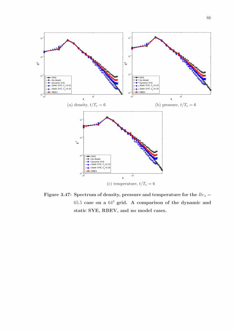
86
100
101
10−6
10−5
10−4
10−3
k
Eρ
DNSNo ModelDynamic SYEStatic SYE, C
s=0.10
Static SYE, Cs=0.16
RBEV
(a) density, t/Te = 6
100
101
10−4
10−3
10−2
10−1
k
Ep
DNSNo ModelDynamic SYEStatic SYE, C
s=0.10
Static SYE, Cs=0.16
RBEV
(b) pressure, t/Te = 6
100
101
10−7
10−6
10−5
10−4
k
ET
DNSNo ModelDynamic SYEStatic SYE, C
s=0.10
Static SYE, Cs=0.16
RBEV
(c) temperature, t/Te = 6
Figure 3.47: Spectrum of density, pressure and temperature for the Reλ =
65.5 case on a 643 grid. A comparison of the dynamic and
static SYE, RBEV, and no model cases.

87
1 2 3 4 5 6 7 80
0.5
1
1.5
2
2.5x 10
−3
t/Te
ν t
Dynamic SYE νt
Static SYE νt, C
s=0.10
Static SYE νt, C
s=0.16
RBEV νt
Figure 3.48: Time history of average eddy viscosity for the Reλ = 65.5
case on a 643 grid. A comparison of the dynamic and static
SYE and RBEV cases.
3.5.2 High Reynolds Number Case
In the high Reynolds Numbers case, Re = 843.79. For the LES calculations
we use the truncated velocity field obtained from the DNS at t/Te = 1.05, where
Te = 0.667 at the initial condition. For the DNS, the mesh is 5123 with dt = 0.0005.
We compare the performance of the models from t/Te = 1.05 ∼ 7.0, which corre-
sponds to a Taylor micro-scale Reynolds number of Reλ = 117.1 ∼ 40.9. Both 323
and 643 meshes are considered for LES simulation with dt = 0.005. We refer this
test case as Reλ = 117.1. Figures 3.49 - 3.60 contain the plots for this case.
First we consider the results for the 323 case. The plots for the variation
of turbulent kinetic energies and RMS values (Figures 3.49 and 3.50, respectively)
indicate that RBEV model and the SSYE(0.10) model are the equally accurate
followed by the DSYE and SSYE(0.16) models.
The spectra for the total kinetic energy (Figure 3.51) and the incompressible
kinetic energy (Figure 3.52(a) and (b)) reveal that the RBEV and the SSYE(0.10)
models are the most accurate followed by the DSYE and the SSYE(0.16) models.

88
In the spectra for the compressible kinetic energy (Figure 3.52(c) and (d)), no LES
model is particularly good. The DSYE and the SSYE(0.16) models are too dissipa-
tive with the RBEV and the SSYE(0.10) models are not dissipative enough.
In the spectra of the density, pressure and temperature (Figure 3.53), we
observe that the RBEV and SSYE(0.10) models are once the most accurate. How-
ever, now they behave differently: while the RBEV model underpredicts at large
wavenumber, the SSYE(0.10) model overpredicts.
Figure 3.54 shows the spatial average of eddy viscosity as function of time.
The RBEV and the SSYE(0.10) models, and the DSYE and the SSYE(0.16) have
similar values, which would explain their similar performances.

89
1 2 3 4 5 6 70
0.1
0.2
0.3
0.4
0.5
0.6
0.7
0.8
0.9
t/Te
K
DNSNo ModelDynamic SYEStatic SYE, C
s=0.10
Static SYE, Cs=0.16
RBEV
(a) total velocity
1 2 3 4 5 6 70
0.1
0.2
0.3
0.4
0.5
0.6
t/Te
KS
DNSNo ModelDynamic SYEStatic SYE, C
s=0.10
Static SYE, Cs=0.16
RBEV
(b) solenoidal velocity
1 2 3 4 5 6 70
0.02
0.04
0.06
0.08
0.1
0.12
0.14
0.16
0.18
0.2
t/Te
KC
DNSNo ModelDynamic SYEStatic SYE, C
s=0.10
Static SYE, Cs=0.16
RBEV
(c) dilatational velocity
Figure 3.49: Time history of turbulent kinetic energy for the Reλ = 117.1
case on a 323 grid. A comparison of the dynamic and static
SYE, RBEV, and no model cases.

90
1 2 3 4 5 6 70.05
0.1
0.15
0.2
t/Te
ρ rms
DNSNo ModelDynamic SYEStatic SYE, C
s=0.10
Static SYE, Cs=0.16
RBEV
(a) density
1 2 3 4 5 6 70.02
0.03
0.04
0.05
0.06
0.07
0.08
t/Te
Trm
s
DNSNo ModelDynamic SYEStatic SYE, C
s=0.10
Static SYE, Cs=0.16
New model
(b) temperature
Figure 3.50: Time history of root-mean-square of density and tempera-
ture for the Reλ = 117.1 case on a 323 grid. A comparison of
the dynamic and static SYE, RBEV, and no model cases.
100
101
10−2
10−1
k
E
DNSNo ModelDynamic SYEStatic SYE, C
s=0.10
Static SYE, Cs=0.16
RBEV
(a) total velocity, t/Te = 3
100
101
10−3
10−2
10−1
k
E
DNSNo ModelDynamic SYEStatic SYE, C
s=0.10
Static SYE, Cs=0.16
RBEV
(b) total velocity, t/Te = 6
Figure 3.51: Energy spectrum of the total velocity for the Reλ = 117.1
case on a 323 grid. A comparison of the dynamic and static
SYE, RBEV, and no model cases.

91
100
101
10−2
10−1
k
ES
DNSNo ModelDynamic SYEStatic SYE, C
s=0.10
Static SYE, Cs=0.16
RBEV
(a) solenoidal velocity, t/Te = 3
100
101
10−4
10−3
10−2
10−1
k
ES
DNSNo ModelDynamic SYEStatic SYE, C
s=0.10
Static SYE, Cs=0.16
RBEV
(b) solenoidal velocity, t/Te = 6
100
101
10−3
10−2
k
EC
DNSNo ModelDynamic SYEStatic SYE, C
s=0.10
Static SYE, Cs=0.16
RBEV
(c) dilatational velocity, t/Te = 3
100
101
10−4
10−3
10−2
k
EC
DNSNo ModelDynamic SYEStatic SYE, C
s=0.10
Static SYE, Cs=0.16
RBEV
(d) dilatational velocity, t/Te = 6
Figure 3.52: Energy spectrum of solenoidal and dilatational velocity for
the Reλ = 117.1 case on a 323 grid. A comparison of the
dynamic and static SYE, RBEV, and no model cases.

92
100
101
10−5
10−4
10−3
k
Eρ
DNSNo ModelDynamic SYEStatic SYE, C
s=0.10
Static SYE, Cs=0.16
RBEV
(a) density, t/Te = 6
100
101
10−3
10−2
10−1
k
Ep
DNSNo ModelDynamic SYEStatic SYE, C
s=0.10
Static SYE, Cs=0.16
RBEV
(b) pressure, t/Te = 6
100
101
10−6
10−5
10−4
k
ET
DNSNo ModelDynamic SYEStatic SYE, C
s=0.10
Static SYE, Cs=0.16
RBEV
(c) temperature, t/Te = 6
Figure 3.53: Spectrum of density, pressure and temperature for the Reλ =
117.1 case on a 323 grid. A comparison of the dynamic and
static SYE, RBEV, and no model cases.

93
1 2 3 4 5 6 7 80
1
2
3
4
5
6
7
8
9x 10
−3
t/Te
ν t
Dynamic SYE νt
Static SYE νt, C
s=0.10
Static SYE νt, C
s=0.16
RBEV νt
Figure 3.54: Time history of average eddy viscosity for the Reλ = 117.1
case on a 323 grid. A comparison of the dynamic and static
SYE and RBEV cases.
Figures 3.55 - 3.60 are the results for high Reynolds number, Reλ = 117.1
case, on a 643 mesh.
In Figure 3.55 we have plotted the evolution of kinetic energies as a function
of time. For the total and incompressible component, we observe that the RBEV is
the most accurate followed by DSYE and SSYE(0.1), and then SSYE(0.16). For the
compressible component the same trend is seen even though all models appear to
perform well. The same trend is observed in the evolution of rms values of density
and temperature (see Figure 3.56).
In the plots for the spectra for the total and incompressible kinetic energy
we observe that the RBEV model is the most accurate followed by SSYE(0.10),
DSYE, and SSYE(0.16) (see Figures 3.57 and 3.58). In the spectra of the com-
pressible kinetic energy we observe that the DSYE is most accurate, followed by the
SSYE(0.10) model, the RBEV model and the SSYE(0.16) model. In this case the
SSYE(0.10) and RBEV models are not dissipative enough while the SSYE(0.16) is
too dissipative. The same trends are seen in the spectra for the density, pressure
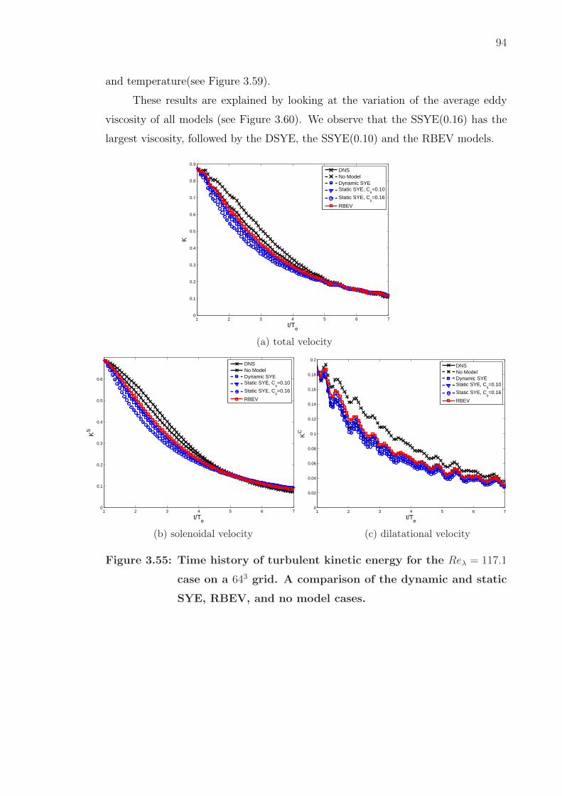
94
and temperature(see Figure 3.59).
These results are explained by looking at the variation of the average eddy
viscosity of all models (see Figure 3.60). We observe that the SSYE(0.16) has the
largest viscosity, followed by the DSYE, the SSYE(0.10) and the RBEV models.
1 2 3 4 5 6 70
0.1
0.2
0.3
0.4
0.5
0.6
0.7
0.8
0.9
t/Te
K
DNSNo ModelDynamic SYEStatic SYE, C
s=0.10
Static SYE, Cs=0.16
RBEV
(a) total velocity
1 2 3 4 5 6 70
0.1
0.2
0.3
0.4
0.5
0.6
t/Te
KS
DNSNo ModelDynamic SYEStatic SYE, C
s=0.10
Static SYE, Cs=0.16
RBEV
(b) solenoidal velocity
1 2 3 4 5 6 70
0.02
0.04
0.06
0.08
0.1
0.12
0.14
0.16
0.18
0.2
t/Te
KC
DNSNo ModelDynamic SYEStatic SYE, C
s=0.10
Static SYE, Cs=0.16
RBEV
(c) dilatational velocity
Figure 3.55: Time history of turbulent kinetic energy for the Reλ = 117.1
case on a 643 grid. A comparison of the dynamic and static
SYE, RBEV, and no model cases.

95
1 2 3 4 5 6 70.05
0.1
0.15
0.2
t/Te
ρ rms
DNSNo ModelDynamic SYEStatic SYE, C
s=0.10
Static SYE, Cs=0.16
RBEV
(a) density
1 2 3 4 5 6 70.02
0.03
0.04
0.05
0.06
0.07
0.08
t/Te
Trm
s
DNSNo ModelDynamic SYEStatic SYE, C
s=0.10
Static SYE, Cs=0.16
RBEV
(b) temperature
Figure 3.56: Time history of root-mean-square of density and tempera-
ture for the Reλ = 117.1 case on a 643 grid. A comparison of
the dynamic and static SYE, RBEV, and no model cases.
100
101
10−3
10−2
10−1
k
E
DNSNo ModelDynamic SYEStatic SYE, C
s=0.10
Static SYE, Cs=0.16
RBEV
(a) total velocity, t/Te = 3
100
101
10−4
10−3
10−2
k
E
DNSNo ModelDynamic SYEStatic SYE, C
s=0.10
Static SYE, Cs=0.16
RBEV
(b) total velocity, t/Te = 6
Figure 3.57: Energy spectrum of the total velocity for the Reλ = 117.1
case on a 643 grid. A comparison of the dynamic and static
SYE, RBEV, and no model cases.

96
100
101
10−3
10−2
10−1
k
ES
DNSNo ModelDynamic SYEStatic SYE, C
s=0.10
Static SYE, Cs=0.16
RBEV
(a) solenoidal velocity, t/Te = 3
100
101
10−4
10−3
10−2
k
ES
DNSNo ModelDynamic SYEStatic SYE, C
s=0.10
Static SYE, Cs=0.16
RBEV
(b) solenoidal velocity, t/Te = 6
100
101
10−4
10−3
10−2
k
EC
DNSNo ModelDynamic SYEStatic SYE, C
s=0.10
Static SYE, Cs=0.16
RBEV
(c) dilatational velocity, t/Te = 3
100
101
10−4
10−3
10−2
k
EC
DNSNo ModelDynamic SYEStatic SYE, C
s=0.10
Static SYE, Cs=0.16
RBEV
(d) dilatational velocity, t/Te = 6
Figure 3.58: Energy spectrum of solenoidal and dilatational velocity for
the Reλ = 117.1 case on a 643 grid. A comparison of the
dynamic and static SYE, RBEV, and no model cases.

97
100
101
10−6
10−5
10−4
10−3
k
Eρ
DNSNo ModelDynamic SYEStatic SYE, C
s=0.10
Static SYE, Cs=0.16
RBEV
(a) density, t/Te = 6
100
101
10−4
10−3
10−2
10−1
k
Ep
DNSNo ModelDynamic SYEStatic SYE, C
s=0.10
Static SYE, Cs=0.16
RBEV
(b) pressure, t/Te = 6
100
101
10−6
10−5
10−4
k
ET
DNSNo ModelDynamic SYEStatic SYE, C
s=0.10
Static SYE, Cs=0.16
RBEV
(c) temperature, t/Te = 6
Figure 3.59: Spectrum of density, pressure and temperature for the Reλ =
117.1 case on a 643 grid. A comparison of the dynamic and
static SYE, RBEV, and no model cases.

98
1 2 3 4 5 6 7 80
0.5
1
1.5
2
2.5
3x 10
−3
t/Te
ν t
Dynamic SYE νt
Static SYE νt, C
s=0.10
Static SYE νt, C
s=0.16
RBEV νt
Figure 3.60: Time history of average eddy viscosity for the Reλ = 117.1
case on a 643 grid. A comparison of the dynamic and static
SYE and RBEV cases.
3.6 Numerical Results for the MM2 Model
In this section we present the results of the purely residual-based mixed model
(MM2). The models are tested in the same decaying homogeneous isotropic turbu-
lent flows as that for the RBEV model in the previous section. The MM2 model
is compared with the RBVM model, the RBEV model and the DSYE model. We
remind the reader that the MM2 model is an additive combination of the RBVM
and RBEV models. We test the models with different Reynolds numbers and dif-
ferent grids (323 and 643). For all the LES models in this section, Cτ = 1.0 in the
definition for the stabilization parameter τ .
3.6.1 Low Reynolds Number Case
The parameters for this flow are the same as the low Reynolds number case
described in the previous section.
In Figures 3.61 - 3.66 we present results for the low Reynolds number case on a
323 mesh. In Figure 3.61, the time history of the turbulent kinetic energies is plotted

99
for all the models. For the total and incompressible component, we observe that the
RBVM model is the most accurate followed by the RBEV and MM2 models, and
then the DSYE model. For the compressible component, the RBVM model is the
most accurate followed by MM2 and RBEV, and then DSYE. In Figure 3.62, the
time history of RMS of density and temperature are shown. Both the RBEV and
RBVM models are very close to the DNS result, followed by the MM2 model. The
DSYE model is too dissipative.
In Figure 3.63, we have plotted the spectra of the total TKE at t/Te = 3 and
t/Te = 6. We observe that RBVM mode is the most accurate while the MM2 model
is slightly more dissipative and the RBEV model displays a slight pile-up on energy
at large wavenumbers. DSYE is the least accurate and is too dissipative. This
observation also holds for the incompressible spectra shown in Figure 3.64(a) and
(b). However, for the compressible spectra in Figure 3.64(c) and (d), we observe
that the RBEV model and the DSYE model are better than the RBVM and MM2
models. The last two are too dissipative.
Figure 3.65 shows the spectra of density, pressure and temperature at t/Te = 6.
For the density and pressure, the RBEV model and the DSYE model are more
accurate than the RBVM and MM2 models. The latter two are too dissipative. For
the temperature, the RBVM model is the best, followed the RBEV model and the
DSYE model. The MM2 model is still too dissipative.
The average values of viscosities as a function of time are shown in Figure
3.66. We observe that the eddy viscosity from the RBEV component in the mixed
model is smaller than that in the pure RBEV model. This is because the RBVM
component in mixed model also adds some dissipation to the simulation, so the
effect of eddy viscosity from RBEV component is reduced. It shows that the RBEV
model behaves like a dynamic model, as it adjusts to the overall dissipation in the
system.
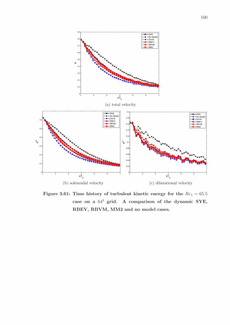
100
1 2 3 4 5 6 70
0.1
0.2
0.3
0.4
0.5
0.6
0.7
0.8
0.9
t/Te
K
DNSNo ModelDSYERBEVRBVMMM2
(a) total velocity
1 2 3 4 5 6 70
0.1
0.2
0.3
0.4
0.5
0.6
t/Te
KS
DNSNo ModelDSYERBEVRBVMMM2
(b) solenoidal velocity
1 2 3 4 5 6 70
0.02
0.04
0.06
0.08
0.1
0.12
0.14
0.16
0.18
0.2
t/Te
KC
DNSNo ModelDSYERBEVRBVMMM2
(c) dilatational velocity
Figure 3.61: Time history of turbulent kinetic energy for the Reλ = 65.5
case on a 643 grid. A comparison of the dynamic SYE,
RBEV, RBVM, MM2 and no model cases.

101
1.5 2 2.5 3 3.5 4 4.5 5 5.5 6 6.5 7
0.06
0.08
0.1
0.12
0.14
0.16
0.18
t/Te
ρ rms
DNSNo ModelDSYERBEVRBVMMM2
(a) density
1.5 2 2.5 3 3.5 4 4.5 5 5.5 6 6.5 70.02
0.025
0.03
0.035
0.04
0.045
0.05
0.055
0.06
0.065
0.07
t/Te
Trm
s
DNSNo ModelDSYERBEVRBVMMM2
(b) temperature
Figure 3.62: Time history of root-mean-square of density and tempera-
ture for the Reλ = 65.5 case on a 643 grid. A comparison
of the dynamic SYE, RBEV, RBVM, MM2 and no model
cases.
100
101
10−2
k
E
DNSNo ModelDSYERBEVRBVMMM2
(a) total velocity, t/Te = 3
100
101
10−3
10−2
k
E
DNSNo ModelDSYERBEVRBVMMM2
(b) total velocity, t/Te = 6
Figure 3.63: Energy spectrum of the total velocity for the Reλ = 65.5 case
on a 643 grid. A comparison of the dynamic SYE, RBEV,
RBVM, MM2 and no model cases.

102
100
101
10−2
k
ES
DNSNo ModelDSYERBEVRBVMMM2
(a) solenoidal velocity, t/Te = 3
100
101
10−3
10−2
k
ES
DNSNo ModelDSYERBEVRBVMMM2
(b) solenoidal velocity, t/Te = 6
100
101
10−4
10−3
10−2
k
EC
DNSNo ModelDSYERBEVRBVMMM2
(c) dilatational velocity, t/Te = 3
100
101
10−4
10−3
10−2
k
EC
DNSNo ModelDSYERBEVRBVMMM2
(d) dilatational velocity, t/Te = 6
Figure 3.64: Energy spectrum of solenoidal and dilatational velocity for
the Reλ = 65.5 case on a 643 grid. A comparison of the
dynamic SYE, RBEV, RBVM, MM2 and no model cases.

103
100
101
10−6
10−5
10−4
10−3
k
Eρ
DNSNo ModelDSYERBEVRBVMMM2
(a) density, t/Te = 6
100
101
10−4
10−3
10−2
10−1
k
Ep
DNSNo ModelDSYERBEVRBVMMM2
(b) pressure, t/Te = 6
100
101
10−6
10−5
10−4
k
ET
DNSNo ModelDSYERBEVRBVMMM2
(c) temperature, t/Te = 6
Figure 3.65: Spectrum of density, pressure and temperature for the Reλ =
65.5 case on a 643 grid. A comparison of the dynamic SYE,
RBEV, RBVM, MM2 and no model cases.

104
1 2 3 4 5 6 7 80
1
2
3
4
5
6x 10
−3
t/Te
νt
DSYE νt
RBEV νt
MM2 νt
Figure 3.66: Time history of average eddy viscosity for the Reλ = 65.5 case
on a 643 grid. A comparison of the dynamic SYE, RBEV,
MM2 cases.
We now consider the same problem but on a finer mesh of 643 modes. In
Figures 3.67 - 3.72 we present the results for this test.
In Figure 3.67, the time history of the turbulent kinetic energies is plotted for
all the models. We now observe that the RBEV, RBVM, and MM2 models are all
very accurate while the DSYE model is less so. The same observations hold for the
time-history of the RMS of density and temperature shown in Figure 3.68.
In the spectra of the total velocity (Figure 3.69) and incompressible veloc-
ity (Figure 3.70(a) and (b)), the RBVM and the MM2 models are most accurate
followed by the RBEV model. The DSYE model is a little dissipative. For the
compressible velocity spectra (shown in Figure 3.70(c) and (d)), the DSYE model is
the most accurate followed by the RBEV model. The RBVM and MM2 models are
slightly overly dissipative in the high wavenumber range. The spectra for density,
temperature and pressure (Figure 3.71) all show the same trends.
The average values of viscosities as a function of time is shown in Figure 3.72.
We still observe that the eddy viscosity of RBEV component in the mixed model is
smaller than that in the pure RBEV model. Once again this points to the apparent
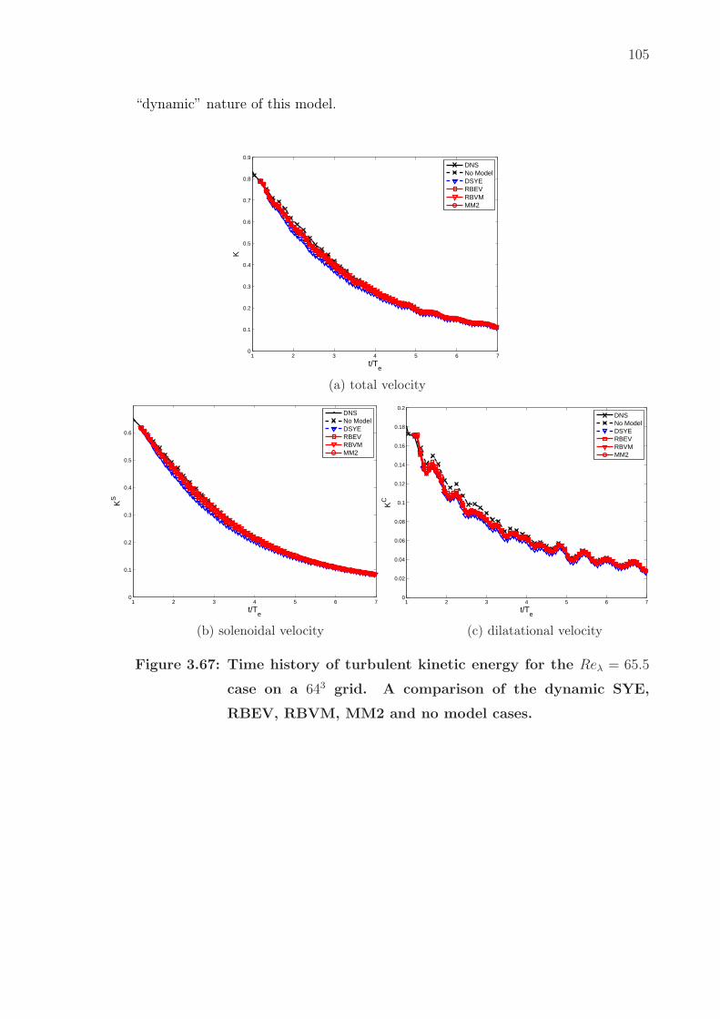
105
“dynamic” nature of this model.
1 2 3 4 5 6 70
0.1
0.2
0.3
0.4
0.5
0.6
0.7
0.8
0.9
t/Te
K
DNSNo ModelDSYERBEVRBVMMM2
(a) total velocity
1 2 3 4 5 6 70
0.1
0.2
0.3
0.4
0.5
0.6
t/Te
KS
DNSNo ModelDSYERBEVRBVMMM2
(b) solenoidal velocity
1 2 3 4 5 6 70
0.02
0.04
0.06
0.08
0.1
0.12
0.14
0.16
0.18
0.2
t/Te
KC
DNSNo ModelDSYERBEVRBVMMM2
(c) dilatational velocity
Figure 3.67: Time history of turbulent kinetic energy for the Reλ = 65.5
case on a 643 grid. A comparison of the dynamic SYE,
RBEV, RBVM, MM2 and no model cases.

106
1 2 3 4 5 6 70.05
0.1
0.15
0.2
t/Te
ρ rms
DNSNo ModelDSYERBEVRBVMMM2
(a) density
1 2 3 4 5 6 70.02
0.03
0.04
0.05
0.06
0.07
0.08
t/Te
Trm
s
DNSNo ModelDSYERBEVRBVMMM2
(b) temperature
Figure 3.68: Time history of root-mean-square of density and tempera-
ture for the Reλ = 65.5 case on a 643 grid. A comparison
of the dynamic SYE, RBEV, RBVM, MM2 and no model
cases.
100
101
10−4
10−3
10−2
10−1
k
E
DNSNo ModelDSYERBEVRBVMMM2
(a) total velocity, t/Te = 3
100
101
10−4
10−3
10−2
10−1
k
E
DNSNo ModelDSYERBEVRBVMMM2
(b) total velocity, t/Te = 6
Figure 3.69: Energy spectrum of the total velocity for the Reλ = 65.5 case
on a 643 grid. A comparison of the dynamic SYE, RBEV,
RBVM, MM2 and no model cases.

107
100
101
10−4
10−3
10−2
10−1
k
ES
DNSNo ModelDSYERBEVRBVMMM2
(a) solenoidal velocity, t/Te = 3
100
101
10−4
10−3
10−2
10−1
k
ES
DNSNo ModelDSYERBEVRBVMMM2
(b) solenoidal velocity, t/Te = 6
100
101
10−4
10−3
10−2
k
EC
DNSNo ModelDSYERBEVRBVMMM2
(c) dilatational velocity, t/Te = 3
100
101
10−5
10−4
10−3
10−2
k
EC
DNSNo ModelDSYERBEVRBVMMM2
(d) dilatational velocity, t/Te = 6
Figure 3.70: Energy spectrum of solenoidal and dilatational velocity for
the Reλ = 65.5 case on a 643 grid. A comparison of the
dynamic SYE, RBEV, RBVM, MM2 and no model cases.
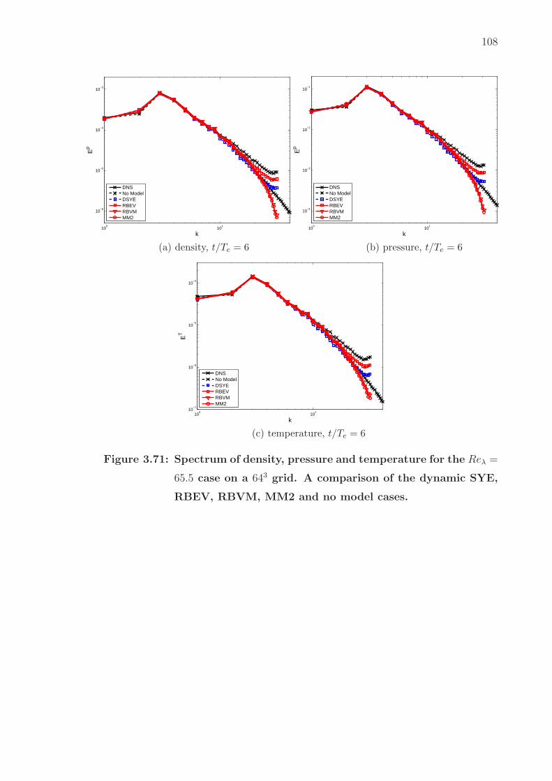
108
100
101
10−6
10−5
10−4
10−3
k
Eρ
DNSNo ModelDSYERBEVRBVMMM2
(a) density, t/Te = 6
100
101
10−4
10−3
10−2
10−1
k
Ep
DNSNo ModelDSYERBEVRBVMMM2
(b) pressure, t/Te = 6
100
101
10−7
10−6
10−5
10−4
k
ET
DNSNo ModelDSYERBEVRBVMMM2
(c) temperature, t/Te = 6
Figure 3.71: Spectrum of density, pressure and temperature for the Reλ =
65.5 case on a 643 grid. A comparison of the dynamic SYE,
RBEV, RBVM, MM2 and no model cases.
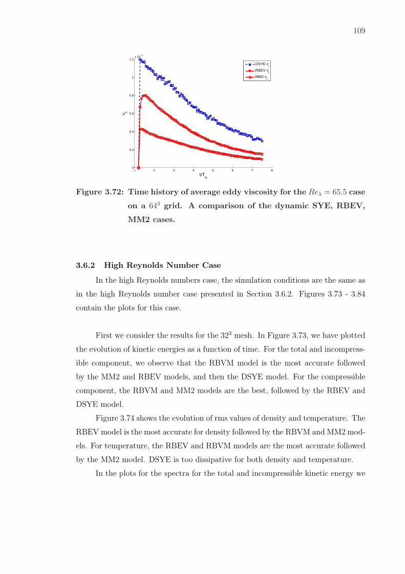
109
1 2 3 4 5 6 7 80
0.2
0.4
0.6
0.8
1
1.2x 10
−3
t/Te
ν t
DSYE νt
RBEV νt
MM2 νt
Figure 3.72: Time history of average eddy viscosity for the Reλ = 65.5 case
on a 643 grid. A comparison of the dynamic SYE, RBEV,
MM2 cases.
3.6.2 High Reynolds Number Case
In the high Reynolds numbers case, the simulation conditions are the same as
in the high Reynolds number case presented in Section 3.6.2. Figures 3.73 - 3.84
contain the plots for this case.
First we consider the results for the 323 mesh. In Figure 3.73, we have plotted
the evolution of kinetic energies as a function of time. For the total and incompress-
ible component, we observe that the RBVM model is the most accurate followed
by the MM2 and RBEV models, and then the DSYE model. For the compressible
component, the RBVM and MM2 models are the best, followed by the RBEV and
DSYE model.
Figure 3.74 shows the evolution of rms values of density and temperature. The
RBEV model is the most accurate for density followed by the RBVM and MM2 mod-
els. For temperature, the RBEV and RBVM models are the most accurate followed
by the MM2 model. DSYE is too dissipative for both density and temperature.
In the plots for the spectra for the total and incompressible kinetic energy we
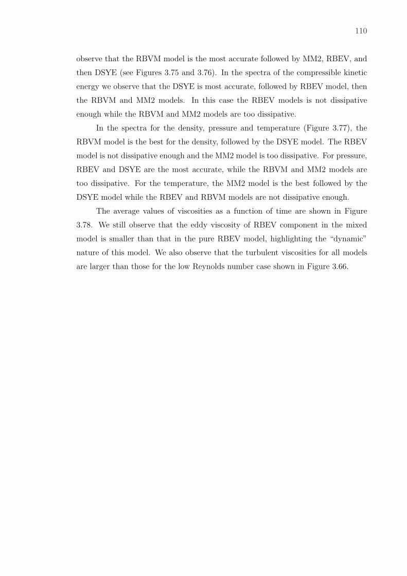
110
observe that the RBVM model is the most accurate followed by MM2, RBEV, and
then DSYE (see Figures 3.75 and 3.76). In the spectra of the compressible kinetic
energy we observe that the DSYE is most accurate, followed by RBEV model, then
the RBVM and MM2 models. In this case the RBEV models is not dissipative
enough while the RBVM and MM2 models are too dissipative.
In the spectra for the density, pressure and temperature (Figure 3.77), the
RBVM model is the best for the density, followed by the DSYE model. The RBEV
model is not dissipative enough and the MM2 model is too dissipative. For pressure,
RBEV and DSYE are the most accurate, while the RBVM and MM2 models are
too dissipative. For the temperature, the MM2 model is the best followed by the
DSYE model while the RBEV and RBVM models are not dissipative enough.
The average values of viscosities as a function of time are shown in Figure
3.78. We still observe that the eddy viscosity of RBEV component in the mixed
model is smaller than that in the pure RBEV model, highlighting the “dynamic”
nature of this model. We also observe that the turbulent viscosities for all models
are larger than those for the low Reynolds number case shown in Figure 3.66.
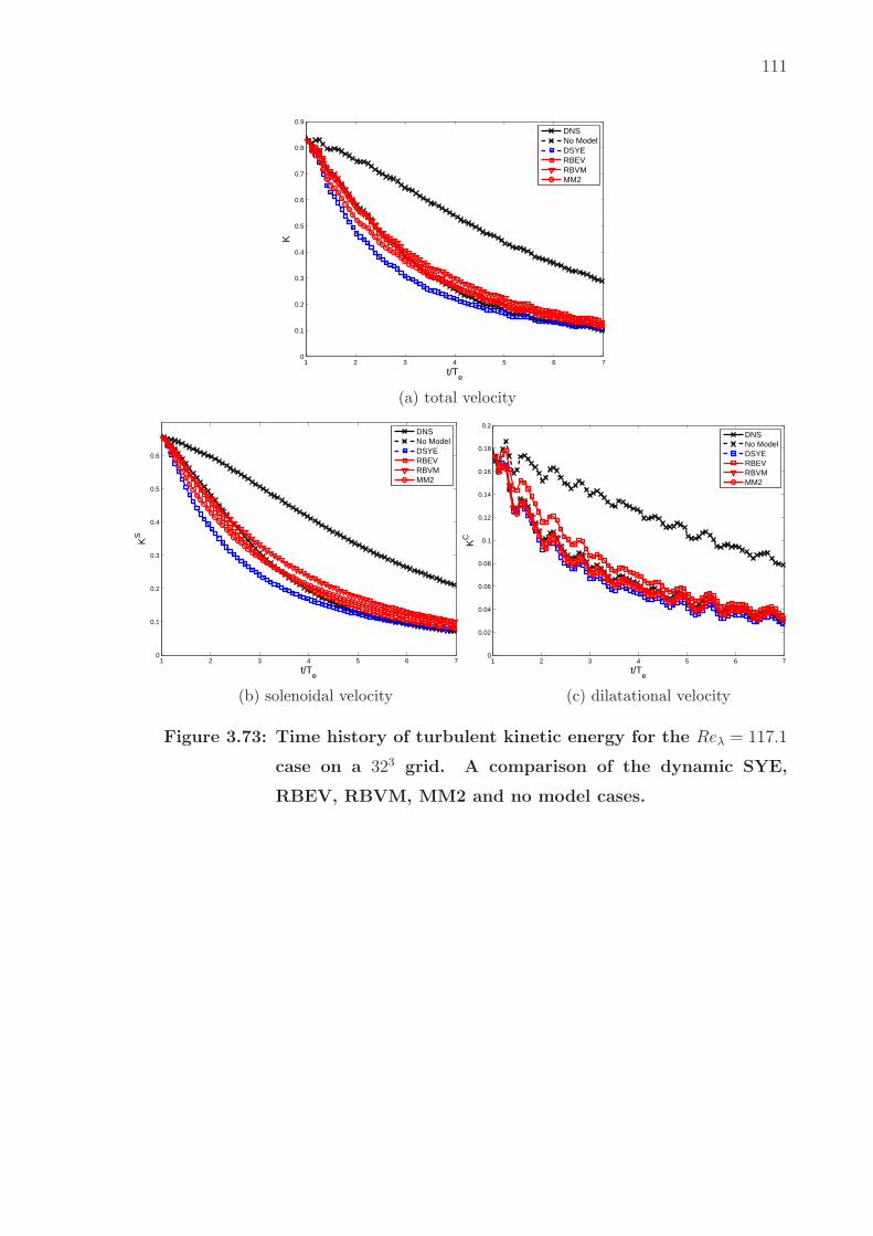
111
1 2 3 4 5 6 70
0.1
0.2
0.3
0.4
0.5
0.6
0.7
0.8
0.9
t/Te
K
DNSNo ModelDSYERBEVRBVMMM2
(a) total velocity
1 2 3 4 5 6 70
0.1
0.2
0.3
0.4
0.5
0.6
t/Te
KS
DNSNo ModelDSYERBEVRBVMMM2
(b) solenoidal velocity
1 2 3 4 5 6 70
0.02
0.04
0.06
0.08
0.1
0.12
0.14
0.16
0.18
0.2
t/Te
KC
DNSNo ModelDSYERBEVRBVMMM2
(c) dilatational velocity
Figure 3.73: Time history of turbulent kinetic energy for the Reλ = 117.1
case on a 323 grid. A comparison of the dynamic SYE,
RBEV, RBVM, MM2 and no model cases.
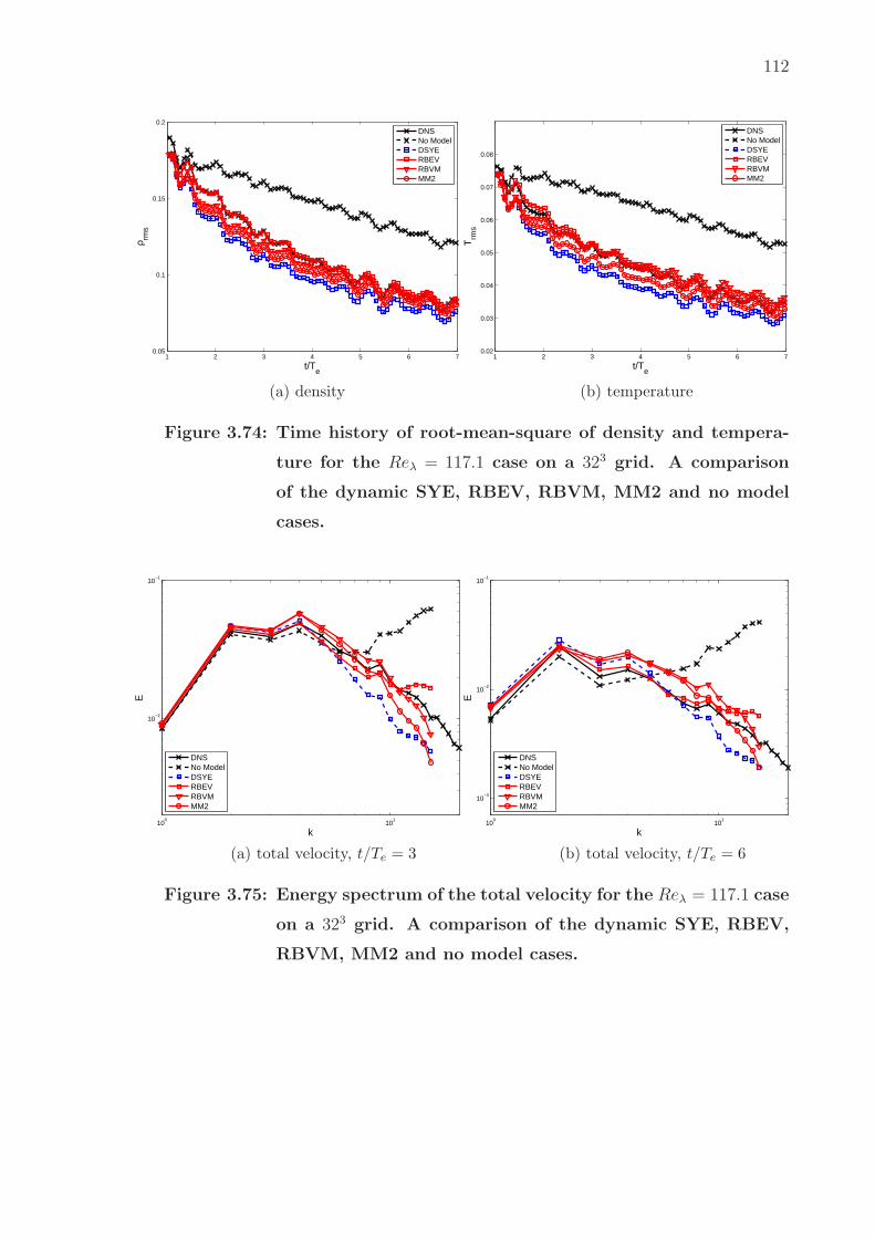
112
1 2 3 4 5 6 70.05
0.1
0.15
0.2
t/Te
ρ rms
DNSNo ModelDSYERBEVRBVMMM2
(a) density
1 2 3 4 5 6 70.02
0.03
0.04
0.05
0.06
0.07
0.08
t/Te
Trm
s
DNSNo ModelDSYERBEVRBVMMM2
(b) temperature
Figure 3.74: Time history of root-mean-square of density and tempera-
ture for the Reλ = 117.1 case on a 323 grid. A comparison
of the dynamic SYE, RBEV, RBVM, MM2 and no model
cases.
100
101
10−2
10−1
k
E
DNSNo ModelDSYERBEVRBVMMM2
(a) total velocity, t/Te = 3
100
101
10−3
10−2
10−1
k
E
DNSNo ModelDSYERBEVRBVMMM2
(b) total velocity, t/Te = 6
Figure 3.75: Energy spectrum of the total velocity for the Reλ = 117.1 case
on a 323 grid. A comparison of the dynamic SYE, RBEV,
RBVM, MM2 and no model cases.

113
100
101
10−2
10−1
k
ES
DNSNo ModelDSYERBEVRBVMMM2
(a) solenoidal velocity, t/Te = 3
100
101
10−4
10−3
10−2
10−1
k
ES
DNSNo ModelDSYERBEVRBVMMM2
(b) solenoidal velocity, t/Te = 6
100
101
10−4
10−3
10−2
k
EC
DNSNo ModelDSYERBEVRBVMMM2
(c) dilatational velocity, t/Te = 3
100
101
10−4
10−3
10−2
k
EC
DNSNo ModelDSYERBEVRBVMMM2
(d) dilatational velocity, t/Te = 6
Figure 3.76: Energy spectrum of solenoidal and dilatational velocity for
the Reλ = 117.1 case on a 323 grid. A comparison of the
dynamic SYE, RBEV, RBVM, MM2 and no model cases.
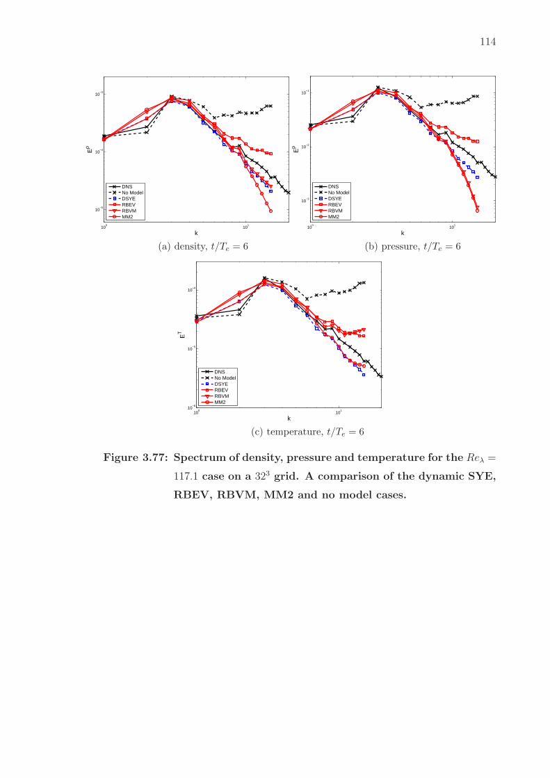
114
100
101
10−5
10−4
10−3
k
Eρ
DNSNo ModelDSYERBEVRBVMMM2
(a) density, t/Te = 6
100
101
10−3
10−2
10−1
k
Ep
DNSNo ModelDSYERBEVRBVMMM2
(b) pressure, t/Te = 6
100
101
10−6
10−5
10−4
k
ET
DNSNo ModelDSYERBEVRBVMMM2
(c) temperature, t/Te = 6
Figure 3.77: Spectrum of density, pressure and temperature for the Reλ =
117.1 case on a 323 grid. A comparison of the dynamic SYE,
RBEV, RBVM, MM2 and no model cases.

115
1 2 3 4 5 6 7 80
1
2
3
4
5
6
7x 10
−3
t/Te
ν t
DSYE νt
RBEV νt
MM2 νt
Figure 3.78: Time history of average eddy viscosity for the Reλ = 117.1
case on a 323 grid. A comparison of the dynamic SYE,
RBEV, MM2 cases.
In Figures 3.79 - 3.84 we plot the results for high Reynolds number case on a
finer, 643 mesh.
In Figure 3.79 we have plotted the evolution of kinetic energies as a function
of time. For the total and incompressible component, we observe that the RBEV,
RBVM and MM2 models are very accurate while the DSYE model is slightly dis-
sipative. We note that the MM2 model dissipates slightly more energy than what
is required while the RBEV is not dissipative enough. For the compressible com-
ponent, the RBVM and MM2 models are very accurate followed by the RBEV and
DSYE models. The same trend is observed in the evolution of rms values of density
and temperature (see Figure 3.80).
In the plots for the spectra for the total and incompressible kinetic energy,
we observe that the RBVM model is the most accurate followed by the MM2, and
RBEV models (see Figures 3.81 and 3.82), while the DSYE model is too dissipative.
In the spectra of the compressible kinetic energy we observe that the DSYE is most
accurate, followed by the RBEV model, then the RBVM and the MM2 models. In
this case the RBEV models is not dissipative enough while the RBVM and MM2

116
models are too dissipative. The same trends are seen in the spectra for the density,
pressure (see Figure 3.83). For temperature, the DSYE is most accurate, followed
by the RBVM and MM2 models, and then RBEV model.
The average values of viscosities as a function of time are shown in Figure
3.84. Once again the DSYE is the largest followed by the pure RBEV and then the
RBEV component of the MM2 model.
1 2 3 4 5 6 70
0.1
0.2
0.3
0.4
0.5
0.6
0.7
0.8
0.9
t/Te
K
DNS
No Model
DSYE
RBEV
RBVM
MM2
(a) total velocity
1 2 3 4 5 6 70
0.1
0.2
0.3
0.4
0.5
0.6
t/Te
Ks
DNSNo ModelDSYERBEVRBVMMM2
(b) solenoidal velocity
1 2 3 4 5 6 70
0.02
0.04
0.06
0.08
0.1
0.12
0.14
0.16
0.18
0.2
t/Te
Kc
DNSNo ModelDSYERBEVRBVMMM2
(c) dilatational velocity
Figure 3.79: Time history of turbulent kinetic energy for the Reλ = 117.1
case on a 643 grid. A comparison of the dynamic SYE,
RBEV, RBVM, MM2 and no model cases.

117
1 2 3 4 5 6 70.05
0.1
0.15
0.2
t/Te
ρ rms
DNSRBEVDSYERBEVRBVMMM2
(a) density
1 2 3 4 5 6 70.02
0.03
0.04
0.05
0.06
0.07
0.08
t/Te
Trm
s
DNSNo ModelDSYERBEVRBVMMM2
(b) temperature
Figure 3.80: Time history of root-mean-square of density and tempera-
ture for the Reλ = 117.1 case on a 643 grid. A comparison
of the dynamic SYE, RBEV, RBVM, MM2 and no model
cases.
100
101
10−3
10−2
10−1
k
E
DNSNo ModelDSYERBEVRBVMMM2
(a) total velocity, t/Te = 3
100
101
10−4
10−3
10−2
k
E
DNSNo ModelDSYERBEVRBVMMM2
(b) total velocity, t/Te = 6
Figure 3.81: Energy spectrum of the total velocity for the Reλ = 117.1 case
on a 643 grid. A comparison of the dynamic SYE, RBEV,
RBVM, MM2 and no model cases.

118
100
101
10−3
10−2
10−1
k
ES
DNSNo ModelDSYERBEVRBVMMM2
(a) solenoidal velocity, t/Te = 3
100
101
10−4
10−3
10−2
k
ES
DNSNo ModelDSYERBEVRBVMMM2
(b) solenoidal velocity, t/Te = 6
100
101
10−4
10−3
10−2
k
EC
DNSNo ModelDSYERBEVRBVMMM2
(c) dilatational velocity, t/Te = 3
100
101
10−4
10−3
10−2
k
EC
DNSNo ModelDSYERBEVRBVMMM2
(d) dilatational velocity, t/Te = 6
Figure 3.82: Energy spectrum of solenoidal and dilatational velocity for
the Reλ = 117.1 case on a 643 grid. A comparison of the
dynamic SYE, RBEV, RBVM, MM2 and no model cases.

119
100
101
10−6
10−5
10−4
10−3
k
Eρ
DNSNo ModelDSYERBEVRBVMMM2
(a) density, t/Te = 6
100
101
10−4
10−3
10−2
10−1
k
Ep
DNSNo ModelDSYERBEVRBVMMM2
(b) pressure, t/Te = 6
100
101
10−6
10−5
10−4
k
ET
DNSNo ModelDSYERBEVRBVMMM2
(c) temperature, t/Te = 6
Figure 3.83: Spectrum of density, pressure and temperature for the Reλ =
117.1 case on a 643 grid. A comparison of the dynamic SYE,
RBEV, RBVM, MM2 and no model cases.
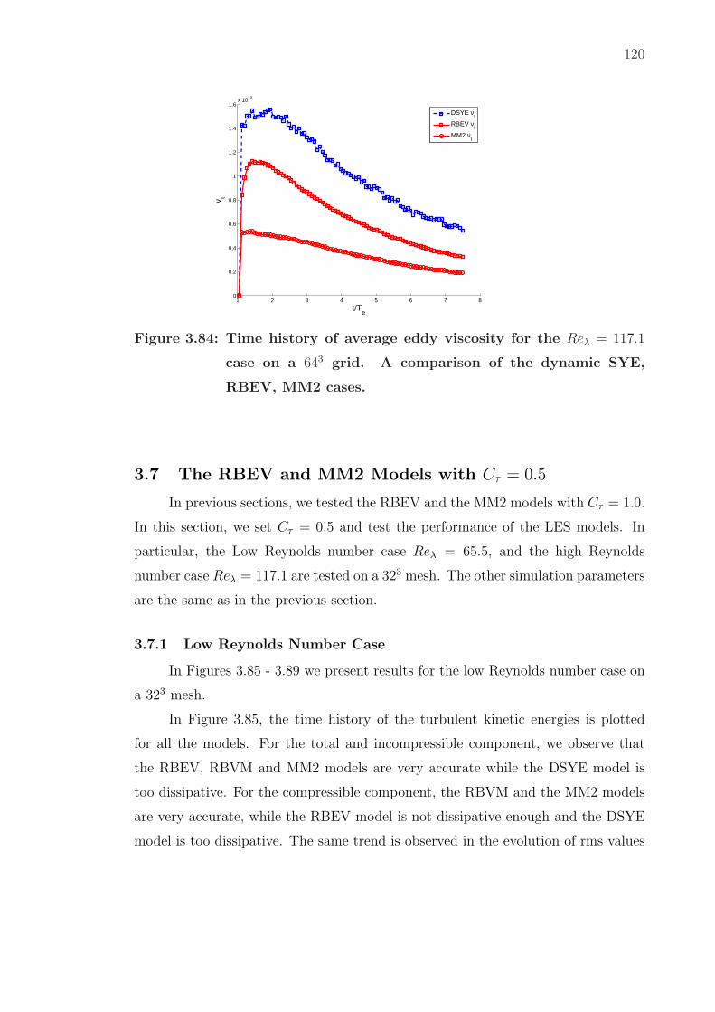
120
1 2 3 4 5 6 7 80
0.2
0.4
0.6
0.8
1
1.2
1.4
1.6x 10
−3
t/Te
ν t
DSYE νt
RBEV νt
MM2 νt
Figure 3.84: Time history of average eddy viscosity for the Reλ = 117.1
case on a 643 grid. A comparison of the dynamic SYE,
RBEV, MM2 cases.
3.7 The RBEV and MM2 Models with Cτ = 0.5
In previous sections, we tested the RBEV and the MM2 models with Cτ = 1.0.
In this section, we set Cτ = 0.5 and test the performance of the LES models. In
particular, the Low Reynolds number case Reλ = 65.5, and the high Reynolds
number case Reλ = 117.1 are tested on a 323 mesh. The other simulation parameters
are the same as in the previous section.
3.7.1 Low Reynolds Number Case
In Figures 3.85 - 3.89 we present results for the low Reynolds number case on
a 323 mesh.
In Figure 3.85, the time history of the turbulent kinetic energies is plotted
for all the models. For the total and incompressible component, we observe that
the RBEV, RBVM and MM2 models are very accurate while the DSYE model is
too dissipative. For the compressible component, the RBVM and the MM2 models
are very accurate, while the RBEV model is not dissipative enough and the DSYE
model is too dissipative. The same trend is observed in the evolution of rms values
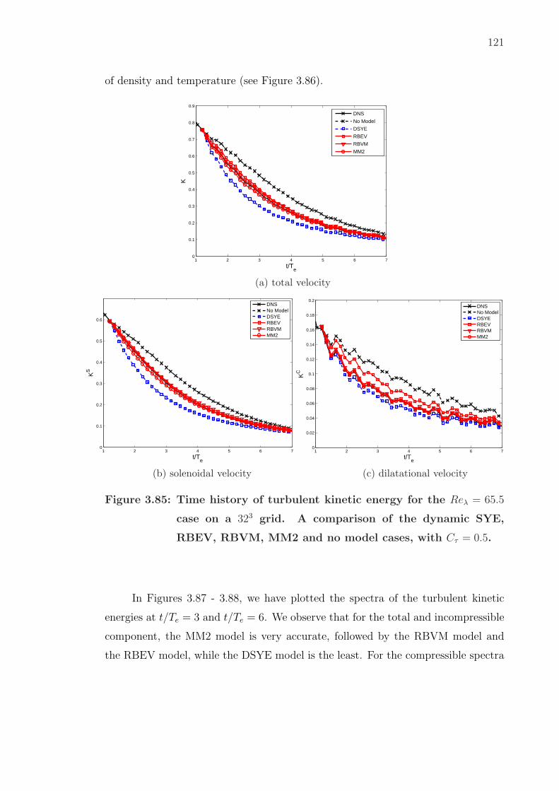
121
of density and temperature (see Figure 3.86).
1 2 3 4 5 6 70
0.1
0.2
0.3
0.4
0.5
0.6
0.7
0.8
0.9
t/Te
K
DNS
No Model
DSYE
RBEV
RBVM
MM2
(a) total velocity
1 2 3 4 5 6 70
0.1
0.2
0.3
0.4
0.5
0.6
t/Te
KS
DNSNo ModelDSYERBEVRBVMMM2
(b) solenoidal velocity
1 2 3 4 5 6 70
0.02
0.04
0.06
0.08
0.1
0.12
0.14
0.16
0.18
0.2
t/Te
KC
DNSNo ModelDSYERBEVRBVMMM2
(c) dilatational velocity
Figure 3.85: Time history of turbulent kinetic energy for the Reλ = 65.5
case on a 323 grid. A comparison of the dynamic SYE,
RBEV, RBVM, MM2 and no model cases, with Cτ = 0.5.
In Figures 3.87 - 3.88, we have plotted the spectra of the turbulent kinetic
energies at t/Te = 3 and t/Te = 6. We observe that for the total and incompressible
component, the MM2 model is very accurate, followed by the RBVM model and
the RBEV model, while the DSYE model is the least. For the compressible spectra

122
we observe that the RBVM, MM2 and DSYE models are about equally accurate,
while the RBEV model is not dissipative enough. Figure 3.89 shows the spectrum
of density, pressure and temperature at t/Te = 6. The RBVM, MM2 and DSYE
models are about equally accurate, while the RBEV model is not dissipative enough.
1.5 2 2.5 3 3.5 4 4.5 5 5.5 6 6.5 7
0.06
0.08
0.1
0.12
0.14
0.16
0.18
t/Te
ρ rms
DNSNo ModelDSYERBEVRBVMMM2
(a) density
1.5 2 2.5 3 3.5 4 4.5 5 5.5 6 6.5 70.02
0.025
0.03
0.035
0.04
0.045
0.05
0.055
0.06
0.065
0.07
t/Te
Trm
s
DNSNo ModelDSYERBEVRBVMMM2
(b) temperature
Figure 3.86: Time history of root-mean-square of density and tempera-
ture for the Reλ = 65.5 case on a 323 grid. A comparison
of the dynamic SYE, RBEV, RBVM, MM2 and no model
cases, with Cτ = 0.5.

123
100
101
10−2
k
E
DNSNo ModelDSYERBEVRBVMMM2
(a) total velocity, t/Te = 3
100
101
10−3
10−2
k
E
DNSNo ModelDSYERBEVRBVMMM2
(b) total velocity, t/Te = 6
Figure 3.87: Energy spectrum of the total velocity for the Reλ = 65.5 case
on a 323 grid. A comparison of the dynamic SYE, RBEV,
RBVM, MM2 and no model cases, with Cτ = 0.5.

124
100
101
10−2
k
ES
DNSNo ModelDSYERBEVRBVMMM2
(a) solenoidal velocity, t/Te = 3
100
101
10−3
10−2
k
ES
DNSNo ModelDSYERBEVRBVMMM2
(b) solenoidal velocity, t/Te = 6
100
101
10−4
10−3
10−2
k
EC
DNSNo ModelDSYERBEVRBVMMM2
(c) dilatational velocity, t/Te = 3
100
101
10−4
10−3
10−2
k
EC
DNSNo ModelDSYERBEVRBVMMM2
(d) dilatational velocity, t/Te = 6
Figure 3.88: Energy spectrum of solenoidal and dilatational velocity for
the Reλ = 65.5 case on a 323 grid. A comparison of the
dynamic SYE, RBEV, RBVM, MM2 and no model cases,
with Cτ = 0.5.
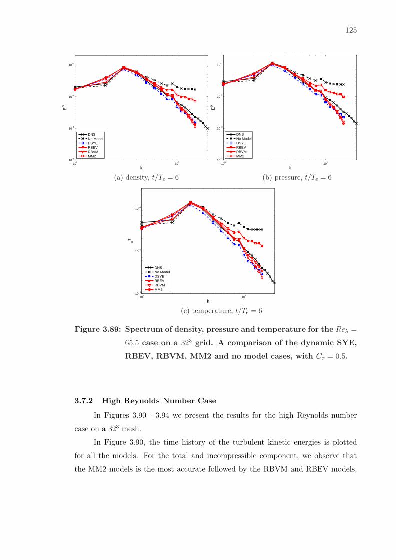
125
100
101
10−6
10−5
10−4
10−3
k
Eρ
DNSNo ModelDSYERBEVRBVMMM2
(a) density, t/Te = 6
100
101
10−4
10−3
10−2
10−1
k
Ep
DNSNo ModelDSYERBEVRBVMMM2
(b) pressure, t/Te = 6
100
101
10−6
10−5
10−4
k
ET
DNSNo ModelDSYERBEVRBVMMM2
(c) temperature, t/Te = 6
Figure 3.89: Spectrum of density, pressure and temperature for the Reλ =
65.5 case on a 323 grid. A comparison of the dynamic SYE,
RBEV, RBVM, MM2 and no model cases, with Cτ = 0.5.
3.7.2 High Reynolds Number Case
In Figures 3.90 - 3.94 we present the results for the high Reynolds number
case on a 323 mesh.
In Figure 3.90, the time history of the turbulent kinetic energies is plotted
for all the models. For the total and incompressible component, we observe that
the MM2 models is the most accurate followed by the RBVM and RBEV models,

126
and then the DSYE model . For the compressible component the RBVM and MM2
model are very accurate, while the RBEV model is not dissipative enough and
the DSYE model is slightly overly dissipative. The same trend is observed in the
evolution of rms values of density and temperature (see Figure 3.86).
In Figures 3.87 - 3.88, we have plotted the spectra of the turbulent kinetic
energies at t/Te = 3 and t/Te = 6. We observe that for the total and incompressible
component, the MM2 model is the most accurate, followed by the RBVM model,
and then the RBEV and DSYE model. The RBEV model is not dissipative enough
while the DSYE model is too dissipative. For the compressible spectra we observe
that the RBVM, MM2 and DSYE models are about equally accurate, while the
RBEV model is not dissipative enough. Figure 3.89 shows the spectrum of density,
pressure and temperature at t/Te = 6. For the density and pressure, the RBVM,
MM2 and DSYE models are about equally accurate, while the RBEV model is not
dissipative enough. For the temperature, the MM2 model is the most accurate,
followed by the RBVM and DSYE model, while the RBEV model is not dissipative
enough.

127
1 2 3 4 5 6 70
0.1
0.2
0.3
0.4
0.5
0.6
0.7
0.8
0.9
t/Te
K
DNS
No Model
DSYE
RBEV
RBVM
MM2
(a) total velocity
1 2 3 4 5 6 70
0.1
0.2
0.3
0.4
0.5
0.6
t/Te
Ks
DNSNo ModelDSYERBEVRBVMMM2
(b) solenoidal velocity
1 2 3 4 5 6 70
0.02
0.04
0.06
0.08
0.1
0.12
0.14
0.16
0.18
0.2
t/Te
Kc
DNSNo ModelDSYERBEVRBVMMM2
(c) dilatational velocity
Figure 3.90: Time history of turbulent kinetic energy for the Reλ = 117.1
case on a 323 grid. A comparison of the dynamic SYE,
RBEV, RBVM, MM2 and no model cases, with Cτ = 0.5.
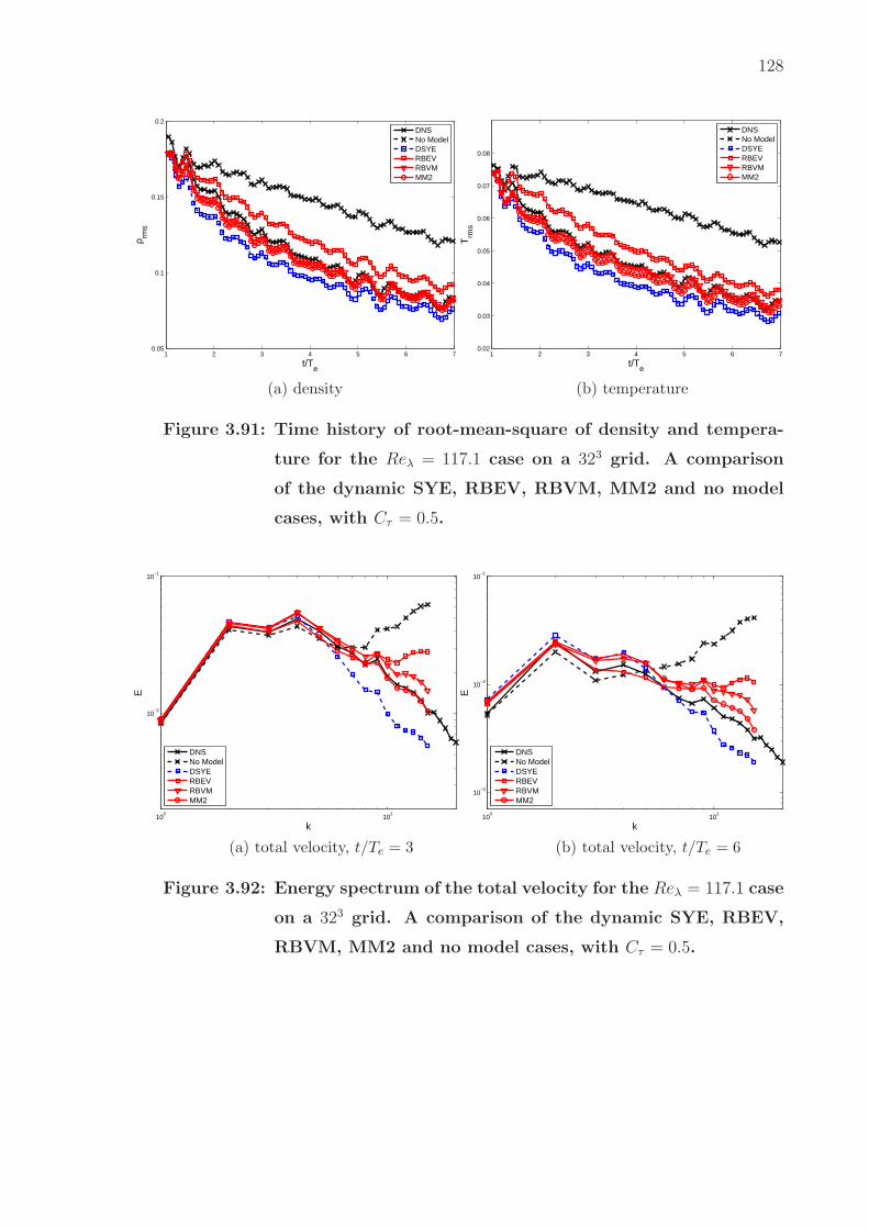
128
1 2 3 4 5 6 70.05
0.1
0.15
0.2
t/Te
ρ rms
DNSNo ModelDSYERBEVRBVMMM2
(a) density
1 2 3 4 5 6 70.02
0.03
0.04
0.05
0.06
0.07
0.08
t/Te
Trm
s
DNSNo ModelDSYERBEVRBVMMM2
(b) temperature
Figure 3.91: Time history of root-mean-square of density and tempera-
ture for the Reλ = 117.1 case on a 323 grid. A comparison
of the dynamic SYE, RBEV, RBVM, MM2 and no model
cases, with Cτ = 0.5.
100
101
10−2
10−1
k
E
DNSNo ModelDSYERBEVRBVMMM2
(a) total velocity, t/Te = 3
100
101
10−3
10−2
10−1
k
E
DNSNo ModelDSYERBEVRBVMMM2
(b) total velocity, t/Te = 6
Figure 3.92: Energy spectrum of the total velocity for the Reλ = 117.1 case
on a 323 grid. A comparison of the dynamic SYE, RBEV,
RBVM, MM2 and no model cases, with Cτ = 0.5.

129
100
101
10−2
10−1
k
ES
DNSNo ModelDSYERBEVRBVMMM2
(a) solenoidal velocity, t/Te = 3
100
101
10−4
10−3
10−2
10−1
k
ES
DNSNo ModelDSYERBEVRBVMMM2
(b) solenoidal velocity, t/Te = 6
100
101
10−4
10−3
10−2
k
EC
DNSNo ModelDSYERBEVRBVMMM2
(c) dilatational velocity, t/Te = 3
100
101
10−4
10−3
10−2
k
EC
DNSNo ModelDSYERBEVRBVMMM2
(d) dilatational velocity, t/Te = 6
Figure 3.93: Energy spectrum of solenoidal and dilatational velocity for
the Reλ = 117.1 case on a 323 grid. A comparison of the
dynamic SYE, RBEV, RBVM, MM2 and no model cases,
with Cτ = 0.5.

130
100
101
10−5
10−4
10−3
k
Eρ
DNSNo ModelDSYERBEVRBVMMM2
(a) density, t/Te = 6
100
101
10−3
10−2
10−1
k
Ep
DNSNo ModelDSYERBEVRBVMMM2
(b) pressure, t/Te = 6
100
101
10−6
10−5
10−4
k
ET
DNSNo ModelDSYERBEVRBVMMM2
(c) temperature, t/Te = 6
Figure 3.94: Spectrum of density, pressure and temperature for the Reλ =
117.1 case on a 323 grid. A comparison of the dynamic SYE,
RBEV, RBVM, MM2 and no model cases, with Cτ = 0.5.
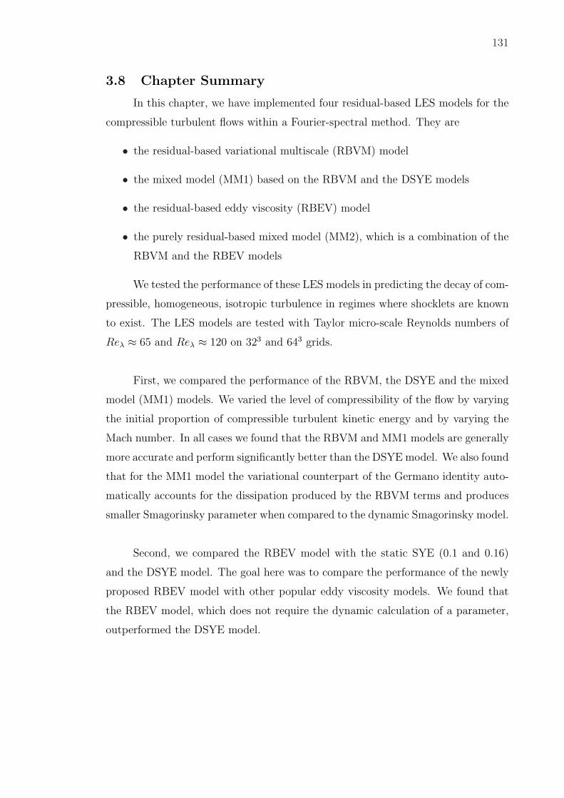
131
3.8 Chapter Summary
In this chapter, we have implemented four residual-based LES models for the
compressible turbulent flows within a Fourier-spectral method. They are
• the residual-based variational multiscale (RBVM) model
• the mixed model (MM1) based on the RBVM and the DSYE models
• the residual-based eddy viscosity (RBEV) model
• the purely residual-based mixed model (MM2), which is a combination of the
RBVM and the RBEV models
We tested the performance of these LES models in predicting the decay of com-
pressible, homogeneous, isotropic turbulence in regimes where shocklets are known
to exist. The LES models are tested with Taylor micro-scale Reynolds numbers of
Reλ ≈ 65 and Reλ ≈ 120 on 323 and 643 grids.
First, we compared the performance of the RBVM, the DSYE and the mixed
model (MM1) models. We varied the level of compressibility of the flow by varying
the initial proportion of compressible turbulent kinetic energy and by varying the
Mach number. In all cases we found that the RBVM and MM1 models are generally
more accurate and perform significantly better than the DSYE model. We also found
that for the MM1 model the variational counterpart of the Germano identity auto-
matically accounts for the dissipation produced by the RBVM terms and produces
smaller Smagorinsky parameter when compared to the dynamic Smagorinsky model.
Second, we compared the RBEV model with the static SYE (0.1 and 0.16)
and the DSYE model. The goal here was to compare the performance of the newly
proposed RBEV model with other popular eddy viscosity models. We found that
the RBEV model, which does not require the dynamic calculation of a parameter,
outperformed the DSYE model.
132
Third we have examined the performance of the new purely residual-based
mixed model (MM2). We have found that with the parameter Cτ = 1.0 it yields re-
sults that are overly dissipative, specially for the compressible quantities of interest.
However, it still outperforms the DSYE model (but not the RBVM model). With
Cτ = 0.5 the mixed model (MM2) is the most accurate model.
Our recommendation is therefore to use purely residual based mixed model
(MM2) with Cτ = 0.5. This model is accurate, easy too implement, as it involves
no dynamic procedure, and consistent, in that it vanished when the residual of the
coarse scales is small.
CHAPTER 4
Residual-Based Models Applied to Incompressible
Turbulent Channel Flow
4.1 Introduction
The residual-based eddy viscosity (RBEV) model and the purely residual-
based mixed model (MM2) have been applied to the decay of compressible homoge-
neous isotropic turbulence (HIT) in Chapter 3. Results show that the RBEV model
and the MM2 model match the DNS results well and better than the dynamic
Smagorinsky-Yoshizawa-eddy diffusivity (DSYE) model and static Smagorinsky-
Yoshizawa-eddy diffusivity (SSYE) model with the coefficient Cs = 0.16. In contrast
to HIT, most flows in nature are bounded by one or more solid surfaces. Fully de-
veloped channel flow is one of the simplest bounded flows and is a good test case
for new LES models. The residual-based variational multiscale (RBVM) model and
the mixed model (MM1) based on RBVM have been applied to incompressible tur-
bulent channel flow by Wang and Oberai. In this Chapter, we apply the RBEV
model and the MM2 model to the incompressible fully developed turbulent channel
flow with the finite element method (FEM). We do this for two reasons: (1) to test
the performance of these models for wall bounded flows and (2) to implement these
models in a finite element code, so that they can then be applied to modeling flows
in complex geometric configurations.
The layout of this chapter is as follows. In Section 4.1, we specialize the
weak form of the models developed in Chapter 2 to the finite element method.
The precise definition of the unresolved scales and the stabilization parameters τ
is also provided. In Section 4.2, the fully developed channel flow is introduced
to understand some important concepts and behavior of these turbulent flows. In
section 4.3, we apply the RBEV model and the MM2 model to study the fully
developed channel flow and compare their performance with each other as well as
the RBVM model and the dynamic Smagorinsky model. Conclusions are drawn in
133

134
Section 4.5.
4.2 Residual-based models
In Chapter 2, we have introduced and developed the residual-based eddy vis-
cosity model (RBEV) and the purely residual-based mixed model (MM2). In this
chapter we apply these LES models to incompressible turbulent channel flow by
using the finite element method.
4.2.1 Weak form for FEM
The weak form of the RBEV and MM2 models for incompressible flows is
given by Equation (2.58) in Chapter 2. It is repeated here for convenience:
Find Uh ∈ Vh, such that
A(W h, Uh + b1U
′) +(∇wh, 2νtS
h)
= (W h, F ) ∀W h ∈ Vh. (4.1)
where Uh = [uh, ph]T are the unknowns with F = [f , 0]T , and Sh is the rate
of strain. Further, νt = Ch|u′| is the eddy viscosity of the RBEV model. The
semi-linear form A(·, ·) in the incompressible case is given by,
A(W , U ) ≡ (w, u,t)− (∇w, u⊗ u)
− (∇ ·w, p) + 2ν(∇Sw,∇Su) + (q,∇ · u),(4.2)
and the fine scale solution is expressed in terms of the coarse scale residual as
U ′ ≈ −P′τ (Uh) P′TR(Uh). (4.3)
We note that in Equation (4.1) b1 is a parameter. By changing the values of
b1 and C, Equation (4.1) represents different models. When b1 = C = 0, we arrive
at DNS. When b1 = 0 and C = 0.0740, we arrive at the RBEV model. When b1 = 1
and C = 0, we arrive at the RBVM model. When b1 = 1 and C = 0.0740, we arrive
at the MM2 model.

135
After using Equation (4.3) in (4.1) we recognize that the fine scale variables
appear in all linear and non-linear terms of A(·, ·). We retain all the nonlinear terms.
However, for the linear terms, following [15] we ignore the time derivative and the
viscous terms (wh, u′,t) = 0 and 2ν(∇Swh,∇Su′) = 0 to arrive at:
The mixed model (MM2) is given as: Find Uh ∈ Vh, such that
A(W h, Uh)− b1(∇wh, uh ⊗ u′ + u′ ⊗ uh + u′ ⊗ u′) (4.4)
− b1(∇ · qh, u′)− (∇ ·wh, p′) +(∇wh, 2νtS
h)
= (wh, f).
In the equation above there should be a parameter b1 in front of the p′ term.
However, we have replaced this with 1 because without this term, the finite element
is unstable while using the same interpolation functions for uh and ph. So we need
this term for all models. We note that Equation (4.4) includes all the models tested
in this chapter, except the dynamic Smagorinsky model, which is described in [36].
In particular,
• With b1 = 0 and C = 0, we arrive at DNS, just with stabilization for pressure.
• With b1 = 1 and C = 0, we arrive at the RBVM model.
• With b1 = 0 and C = 0.0740, we arrive at the RBEV model.
• With b1 = 1 and C = 0.0740, we arrive at the mixed model (MM2).
4.2.2 Unresolved scales and stabilization parameter τ
In Equation (4.4) the unresolved scales U ′ is depend upon stabilization pa-
rameter τ and the coarse scale residual R(Uh). With τ and R(Uh), the fine scale
velocity and pressure are written as
u′ = −τMrM(uh, ph), (4.5)
p′ = −τCrC(uh). (4.6)
where τ = diag(τM , τM , τM , τC) is diagonal matrix, and following [15] the P′ and P′T
operators are replaced with the identity. The stabilization parameters for velocity

136
τM and pressure τC are defined as:
τM =1√
(2C1/∆t)2 + uigijuj + C2ν2gijgij
, (4.7)
τC =1
8C1
1
τM tr(gij). (4.8)
The constant C1 is obtained by considering the local gradient in element space-
time coordinate systems [37], and we will study the effect of different C1 value in the
following sections. The positive constant C2, which is derived from an element-wise
inverse estimate [38], is independent of the grid size, and in this chapter C2 = 36 is
fixed. The tensor gij = ξk,iξk,j is the covariant metric tensor, where ξi,j = ∂ξi/∂xj.
The stabilization parameter τM comes from the asymptotic scaling arguments in
[39] which are developed within stabilized finite methods [40, 41].
The coarse scale residual R = [rM(uh, ph), rC(uh)]T is given by
rM(uh, ph) = uh,t +∇ · (uh ⊗ uh) +∇ph − ν∇2uh − f , (4.9)
rC(uh) = ∇ · uh. (4.10)
For more discussions about this fine-scale approximation, the reader is referred
to [15].
4.3 Turbulent Channel Flow
In contrast to the homogeneous isotropic turbulence which is discussed in the
previous chapter, most flows in nature are bounded by one or more solid surfaces,
for example, a typical flow goes through pipes or ducts. In this thesis, we consider
one of the simplest of bounded flows: fully developed channel flow. In channel flows,
the mean velocity vector is parallel to the wall.
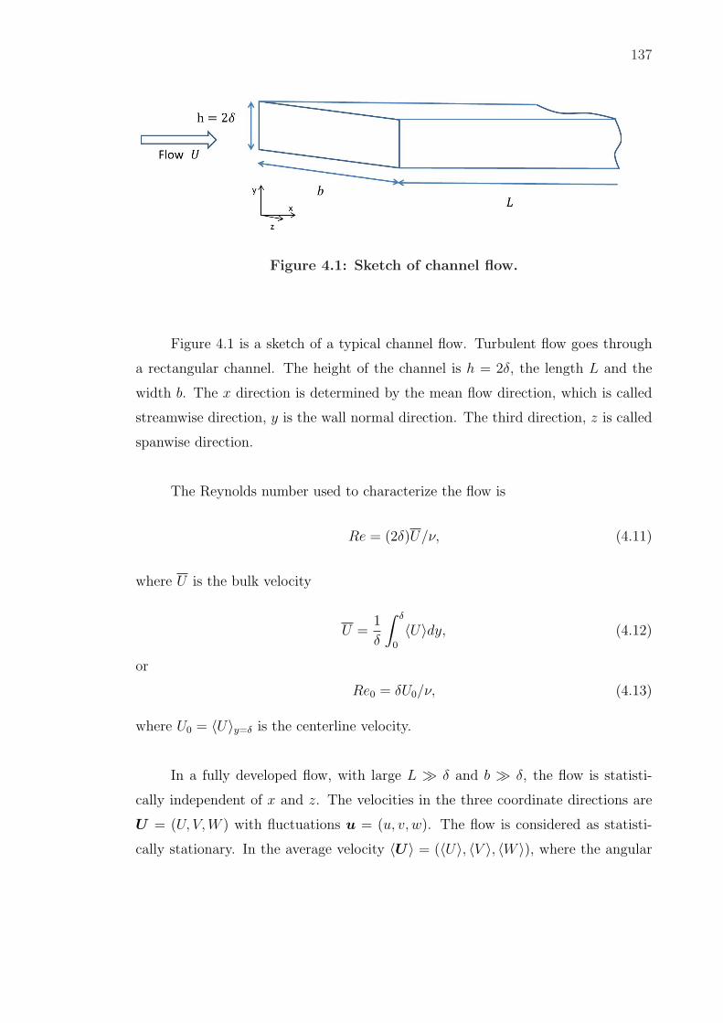
137
Figure 4.1: Sketch of channel flow.
Figure 4.1 is a sketch of a typical channel flow. Turbulent flow goes through
a rectangular channel. The height of the channel is h = 2δ, the length L and the
width b. The x direction is determined by the mean flow direction, which is called
streamwise direction, y is the wall normal direction. The third direction, z is called
spanwise direction.
The Reynolds number used to characterize the flow is
Re = (2δ)U/ν, (4.11)
where U is the bulk velocity
U =1
δ
∫ δ
0
〈U〉dy, (4.12)
or
Re0 = δU0/ν, (4.13)
where U0 = 〈U〉y=δ is the centerline velocity.
In a fully developed flow, with large L À δ and b À δ, the flow is statisti-
cally independent of x and z. The velocities in the three coordinate directions are
U = (U, V, W ) with fluctuations u = (u, v, w). The flow is considered as statisti-
cally stationary. In the average velocity 〈U〉 = (〈U〉, 〈V 〉, 〈W 〉), where the angular

138
brackets denote the average operator in directions and time, 〈V 〉 and 〈W 〉 are zero
and 〈U〉 depends only on the wall normal direction. Experiments also confirm the
natural expectation that the flow is statistically symmetric about the mid-plane
y = δ. The flow could be driven by the pressure gradient or body force. The pres-
sure gradient or body force is balanced by the surface force due to the wall shear
stress.
4.3.1 Wall shear stress
We assume the flow is driven by the pressure gradient and there is no body
force. Using the average operator on the continuity equation of NS equation, we get
the mean continuity equation,
〈Ui,i〉 = 0, (4.14)
with u = U − 〈U〉, we also get,
ui,i = 0, (4.15)
which means both the average velocity and the fluctuation velocity satisfy the con-
tinuity equation.
Using the average operator on the momentum equations, we get the mean-
momentum equations,
〈Uj〉〈Ui〉,j +1
ρ〈p〉,i − ν〈Ui〉,jj + 〈uiuj〉,j = 0. (4.16)
The y direction mean-momentum equation is
0 =d
dy〈v2〉+
1
ρ
∂〈p〉∂y
, (4.17)
with the boundary condition 〈v2〉y=0 = 0, integrates on y to
〈v2〉+ 〈p〉/ρ = pw(x)/ρ, (4.18)
where pw = 〈p(x, 0, 0)〉 is the mean pressure on the bottom wall. As 〈v2〉 is inde-

139
pendent of x, the mean pressure gradient in x direction is uniform:
∂〈p〉∂x
=dpw
dx. (4.19)
The x direction mean-momentum equation is
0 = νd2〈U〉dy2
− d
dy〈uv〉 − 1
ρ
∂〈p〉∂x
, (4.20)
and it can be rewritten asdτ
dy=
dpw
dx, (4.21)
where τ(y) is the total shear stress
τ = ρνd〈U〉dy
− ρ〈uv〉. (4.22)
For this flow there is no mean acceleration, so in Equation (4.21), the mean pres-
sure gradient in streamwise direction is balanced by the shear-stress gra-
dient in the wall normal direction.
Since τ is a function only of y, and pw is a function only of x (because pw
in defined only on the wall), so in Equation (4.21), both dτ/dy and dpw/dx are
constant. The solutions for τ(y) and dpw/dx can be written in terms of the wall
shear stress
τw = τ(0). (4.23)
Because τ(y) is antisymmetric about the mid-plane, so τ(δ) is zero, and at the top
wall the stress is τ(2δ) = −τw. Hence, the solution to Equation (4.21) is
τ(y) = τw(1− y
δ), (4.24)
and
−dpw
dx=
τw
δ. (4.25)
The total shear stress τ(y) in Equation 4.22 is the sum of the viscous stress

140
ρνd〈U〉/dy and the Reynolds stress −ρ〈uv〉. At the wall all the Reynolds stresses
are zero because the boundary condition U (x, t) = 0. As a result, the wall shear
stress is entirely due to the viscous contribution, so the wall shear stress is
τw = ρν(d〈U〉dy
)y=0. (4.26)
4.3.2 Wall units
With the wall shear stress τw, viscosity ν and density ρ, we define the viscous
scales, which are the appropriate scales for the near wall region. These are the
friction velocity
uτ =
√τw
ρ, (4.27)
and the viscous length-scale
δν = ν
√ρ
τw
=ν
uτ
. (4.28)
and the friction Reynolds number based on the viscous scales is defined by
Reτ =uτδ
ν=
δ
δν
. (4.29)
The distance from the wall measured in viscous lengths is denoted by
y+ =y
δν
=uτy
ν, (4.30)
similarly, in streamwise and spanwise direction
x+ =x
δν
=uτx
ν, (4.31)
z+ =z
δν
=uτz
ν. (4.32)
The velocity in wall unit u+(y+) defined by
u+ = 〈U〉/uτ . (4.33)
These variables are expressed in wall units.

141
4.3.3 Law of the wall and regions and layers near the wall
A fully developed channel flow is completely specified by ρ, ν, δ and dp/dx.
As uτ is a function of ρ, δ and dp/dx, in a fully developed channel flow, it can
also be completely specified by ρ, ν, δ and uτ . Two independent non-dimensional
parameters can be formed together with y, and they are y/δ and Reτ = uτδ/ν.
Since Reτ = (y/δν)/(y/δ) so the mean velocity 〈U〉 can be written as
〈U〉 = uτF (y
δν
,y
δ), (4.34)
where F is a universal non-dimensional function.
The mean velocity gradient is an important parameter in channel flows, be-
cause the viscous stress and the turbulent production are both determined by
d〈U〉/dy. So we to solve d〈U〉/dy instead of 〈U〉 , and we can write
d〈U〉dy
=uτ
yΦ(
y
δν
,y
δ), (4.35)
where Φ is an other universal non-dimensional function.
It is found that at high Reynolds number, when y/δ ¿ 1, there is an region
where the mean velocity is only determined by the viscous scales, and independent
of δ. This region is called inner layer. In the inner layer,
d〈U〉dy
=uτ
yΦ1(
y
δν
), (4.36)
where
Φ1(y
δν
) = limy/δ¿1
Φ(y
δν
,y
δ). (4.37)
With the velocity in wall unit u+(y+) defined by u+ = 〈U〉/uτ , Equation (4.36)
can be written asdu+
dy+=
1
y+Φ(y+). (4.38)
Equation (4.38) shows that the velocity in wall unit u+ is only a function of
the wall unit y+, and independent of uτ . This is the law of the wall :
u+ = Fw(y+), (4.39)

142
where
Fw(y+) =
∫ y+
0
1
y+Φ1(y
+)y+. (4.40)
The region with y+ < 50, is called the viscous wall region, where the viscous
contribution to the shear stress is important. When y+ < 5 within viscous wall
region, it is the viscous sublayer, where the Reynolds shear stress is negligible. One
important conclusion for this layer is Fw(y+) = y+ and this leads to u+ = y+.
When y+ > 30, y/δ < 0.3 , the viscosity can be neglect, and it is found that
Φ1 = 1/κ, where κ is a constant. Then u+ is solved as
u+ =1
κlny+ + B, (4.41)
where B = 5.2 is a constant, and κ = 0.41 is the Von Karman constant. This is the
log law for y+ > 30, and this region is called the log-law region. Figure 4.2 (cited
from [3]. ) shows that four different Reynolds numbers cases all match the log law
very well when y+ > 30.

143
Figure 4.2: Mean velocity profiles in fully developed turbulent channel
flow measured by Wei and Willmarth (1989): ©, Re0 = 2, 970;
¤, Re0 = 14, 914; M, Re0 = 22, 776; O, Re0 = 39, 582; the solid line
represent the log-law.
Here is a summary of the regions and layers that describe the near-wall flows.
When y/δ < 0.1 , we are in the inner layer, and in this layer, 〈U〉 determined
by uτ and y+, independent of U0 and δ. When y+ > 50 and y/δ ≤ 1, we are in
the outer layer, and in this layer direct effects of viscosity on 〈U〉 are negligible.
The region between inner and outer layers is the overlap region with y+ > 50 and
y/δ < 0.1.
In the inner layer, when y+ < 50 we are in the viscous wall region, and in this
region, the viscous contribution to the shear stress is significant. Especially when
y+ < 5 in the viscous wall region, we are in the viscous sublayer. In this layer, the
Reynolds shear stress is negligible compared with the viscous stress, and U+ = y+.
When y+ > 30 and y/δ < 0.3, we are in the Log-law region, where u+ = 1κlny+ +B.

144
The region between the viscous sublayer and the log-law region is the buffer layer
with 5 < y+ < 30. As the Reynolds number Re of the flow increases with δ changing,
the fraction of the channel occupied by the viscous wall region decreases, since δν/δ
varies as Re−1.
4.4 Numerical Simulation
All the LES models including the RBEV model , the RBVM model, dynamic
Smagorinsky model and the mixed model (MM2) are tested for turbulent chan-
nel flow. The computation domain is shown in Figure 4.3 and the dimensions in
streamwise, wall-normal, and spanwise directions of the computational domain are
Lx = 2π, Ly = 2h = 2, and Lz = 2π/3. We impose periodic boundary condition
to in the in streamwise and spanwise directions. It means the real dimensions in
streamwise and spanwise directions are infinity. Channel flow with Reτ = 395 and
Reτ = 590 are tested. The friction Reynolds number is defined as Reτ = uτh/ν,
where uτ is the friction velocity, h = 1 is the channel half-width and ν is the kine-
matic viscosity.
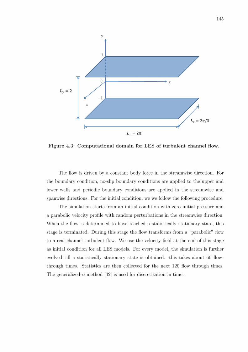
145
Figure 4.3: Computational domain for LES of turbulent channel flow.
The flow is driven by a constant body force in the streamwise direction. For
the boundary condition, no-slip boundary conditions are applied to the upper and
lower walls and periodic boundary conditions are applied in the streamwise and
spanwise directions. For the initial condition, we we follow the following procedure.
The simulation starts from an initial condition with zero initial pressure and
a parabolic velocity profile with random perturbations in the streamwise direction.
When the flow is determined to have reached a statistically stationary state, this
stage is terminated. During this stage the flow transforms from a “parabolic” flow
to a real channel turbulent flow. We use the velocity field at the end of this stage
as initial condition for all LES models. For every model, the simulation is further
evolved till a statistically stationary state is obtained. this takes about 60 flow-
through times. Statistics are then collected for the next 120 flow through times.
The generalized-α method [42] is used for discretization in time.

146
The parabolic velocity with random perturbations is given as
[U, V, W ] = [1.5 ∗ (1− y2) + 0.4 ∗ (r − 0.5), 0, 0], (4.42)
where y is the wall-normal coordinate and r is random variable in the range (−1, 1).
The simulations were performed using 323 and 643 finite elements. For both
meshes, we employ C0-continuous trilinear basis functions. The mesh is uniform
along the x and z directions and nonuniform along the wall normal direction. The
resolution in the wall normal direction is much finer at the wall in order to resolve
the boundary layer. Grid points in the y direction are clustered near the wall by
the following function:
yi =1
btanh
(ξitanh−1(b)
), (4.43)
where ξi is a set of uniformly spaced points in the interval [−1, 1]. The coefficient b
is a parameter that controls the strength of the clustering. The value of b is chosen
such that for the first point in the all-normal direction y+ < 1. Thus the first plane
of grid points off the wall is within the viscous sublayer. Figure 4.4 shows the 333
mesh.

147
Figure 4.4: 323 mesh for turbulent channel flow.
Table 4.1: Physical parameters for the channel flow problem.
Reτ Nom. Reτ Actual ν fb ρ dt
395 392.24 14.8384e− 5 33.87522076− 4 1.0 0.05 and 0.025
590 585.88 6.6508514e− 5 15.18351427e− 4 1.0 0.025
Table 4.2: Numerical parameters for the channel flow problem.
Reτ Nom. Nx ×Ny ×Nz 4x+ 4y+min 4y+
max 4z+ dt+
395 32× 32× 32 77.4 1.31 67.9 25.8 1.15 and 0.57
395 64× 64× 64 38.8 0.47 19.4 12.9 1.15 and 0.57
590 64× 64× 64 57.9 0.71 28.9 19.3 0.57
We perform the LES with a mesh of 323 and 643 finite elements, and compare
the performance of all the LES models with DNS results of [43]. The DNS results
were computed using a Chebychev-tau formulation in the wall normal direction and

148
a Fourier representation in the streamwise and spanwise directions, on a mesh of
256 × 193 × 192. Thus the DNS has 264 times as many points for 322 case and
35 times as many points for the 643 case. The new LES models are also compared
to SUPG stablized dynamic Smagorinsky model [36]. The physical and numerical
parameters we used are listed in Tables 4.1 and 4.2, respectively.
In the following subsections, we will first discuss the channel flow with Reτ =
395 and then the channel flow with Reτ = 590.
4.4.1 Reτ = 395
In this subsection we consider the performance of the RBEV, RBVM and MM2
models and also examine the effect of two important numerical parameters dt and
the constant C1 that appears in the definition of τm (see Equation (4.7)).
4.4.1.1 RBEV
Figure 4.5 - 4.9 are the results for the RBEV model on a 323 mesh with dt =
0.050 and C1 = 3. Figure 4.5 compares average streamwise velocities of different
models. It shows that the no model test underpredicts the average velocity, while the
Smagorinsky model overestimates the average velocity. The same conclusion can be
drawn from the semi-log plot for u+ in Figure 4.6 presented in wall coordinates. In
this plot we have also plotted the analytical solutions u+ = y+ and u+ = 1/κlny+ +
B, where κ = 0.41 and B = 5.5. We note that the DNS data matches these
analytical solutions well, as does the RBEV model. The no model test underpredicts
the velocity, while the Smagorinsky model overestimates the velocity.
Figure 4.7 compares the average pressures. Big oscillations are observed for
the for no model case, while the Smagorinsky model also overestimates the average
pressure. The RBEV model matches the DNS solution most accurately.
In Figure 4.8, we compare the fluctuations computed by the LES models with
their DNS counterparts. We note that all models overpredict the streamwise fluc-
tuations urms in (a) though the RBEV model is marginally more accurate than the
others. For the wall normal fluctuations, vrms in (b), the RBEV model is the most
accurate in the near wall region while the dynamic Smagorinsky model is the most

149
accurate in the center of the channel. For the spanwise fluctuations, wrms in (c),
the dynamic Smagorinsky model is more accurate than RBEV model, and both of
them overpredict the vlaue.
In Figure 4.9, the average values of the eddy viscosity, the stabilization pa-
rameter and the residual of the momentum equation are shown. In (a), the eddy
viscosity is near to zero close the wall and grows within the channel. It is remarkable
that it achieves this behavior without an explicit dynamic approach. We attribute
this behavior to the fact that RBEV model is inherently dynamic in that it is based
on the residual of the coarse scales which automatically vanishes in well-resolved
regions of the flow. In (b), the stabilization τ starts from almost 0 at the wall and
quickly reaches a constant value in the channel. In (c), the residual is reduced when
a small distance from the wall and then grows quickly for a very short distance.
Then it begins to reduce, and reaches the lowest point at the middle of the channel.
0 0.2 0.4 0.6 0.8 1 1.2 1.4−1
−0.8
−0.6
−0.4
−0.2
0
0.2
0.4
0.6
0.8
1
y/h
<u>
Moser et al
Dynamic SMG
No model
RBEV
Figure 4.5: Average streamwise velocity for the Reτ = 395 case on a 323
mesh with dt = 0.050 and C1 = 3. A comparison of the Dy-
namic Smagorinsky, RBEV and no model cases.
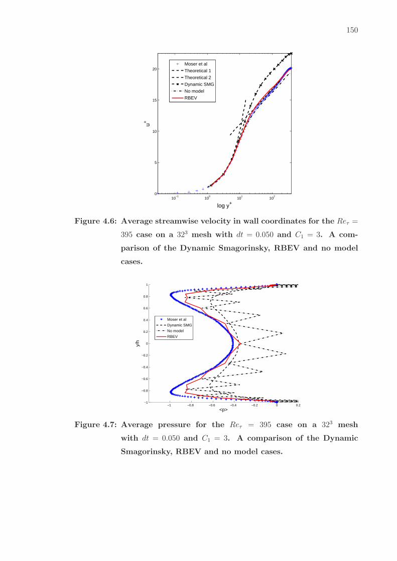
150
10−1
100
101
102
0
5
10
15
20
log y+
u+
Moser et al
Theoretical 1
Theoretical 2
Dynamic SMG
No model
RBEV
Figure 4.6: Average streamwise velocity in wall coordinates for the Reτ =
395 case on a 323 mesh with dt = 0.050 and C1 = 3. A com-
parison of the Dynamic Smagorinsky, RBEV and no model
cases.
−1 −0.8 −0.6 −0.4 −0.2 0 0.2−1
−0.8
−0.6
−0.4
−0.2
0
0.2
0.4
0.6
0.8
1
<p>
y/h
Moser et al
Dynamic SMG
No model
RBEV
Figure 4.7: Average pressure for the Reτ = 395 case on a 323 mesh
with dt = 0.050 and C1 = 3. A comparison of the Dynamic
Smagorinsky, RBEV and no model cases.

151
0 50 100 150 200 250 300 3500
0.5
1
1.5
2
2.5
3
3.5
4
y+
u rms
Moser et alDynamic SMGNo modelRBEV
(a) RMS of velocity fluctuations in streamwise direction
0 50 100 150 200 250 300 3500
0.2
0.4
0.6
0.8
1
1.2
y+
v rms
Moser et al
Dynamic SMG
No model
RBEV
(b) RMS of velocity fluctuations in wall normal direction
0 50 100 150 200 250 300 3500
0.2
0.4
0.6
0.8
1
1.2
1.4
1.6
y+
wrm
s
Moser et alDynamic SMGNo modelRBEV
(c) RMS of velocity fluctuations in spanwise direction
Figure 4.8: RMS of velocity fluctuations in wall coordinates for the
Reτ = 395 case on a 323 mesh with dt = 0.050 and C1 = 3.
A comparison of the Dynamic Smagorinsky, RBEV and no
model cases.
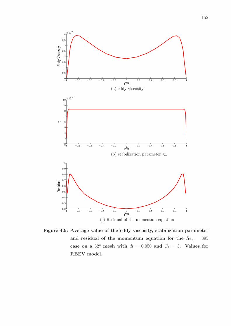
152
−1 −0.8 −0.6 −0.4 −0.2 0 0.2 0.4 0.6 0.8 10
0.5
1
1.5
2
2.5
3
3.5
4x 10
−5
y/h
Eddy
Vis
cosi
ty
(a) eddy viscosity
−1 −0.8 −0.6 −0.4 −0.2 0 0.2 0.4 0.6 0.8 12
3
4
5
6
7
8
9
10x 10
−3
y/h
τ
(b) stabilization parameter τm
−1 −0.8 −0.6 −0.4 −0.2 0 0.2 0.4 0.6 0.8 10.2
0.3
0.4
0.5
0.6
0.7
0.8
0.9
1
y/h
Res
idua
l
(c) Residual of the momentum equation
Figure 4.9: Average value of the eddy viscosity, stabilization parameter
and residual of the momentum equation for the Reτ = 395
case on a 323 mesh with dt = 0.050 and C1 = 3. Values for
RBEV model.

153
Mesh and time-step refinement
In the section, we study the effects of varying the time step and grid refinement
for the RBEV model with Reτ = 395. We consider dt = 0.025 and dt = 0.050 and
meshes of 32 and 64 elements which leads to four cases. The parameter C1 = 3 for
all cases.
Figure 4.10 compares average streamwise velocities of different models.. All
the RBEV models match the DNS solution very accurately, and some convergence
with grid refinement is observed. The same conclusion can be drawn from the semi-
log plot for u+ in Figure 4.11 presented in wall coordinates.
For the average pressure profile in Figure 4.12, the results on the 643 mesh are
better than on the 323 mesh. They are closer to the DNS result and are smoother.
In Figure 4.13, we compare the fluctuations computed by the LES models
with their DNS counterparts. We note that though all RBEV tests overpredict the
streamwise fluctuations urms near wall region in (a), the RBEV results on the 643
mesh are more accurate than the ones on a 323 mesh. The RBEV results on the
643 mesh also match DNS very well when y+ > 100. For the vrms in (b), all RBEV
tests overpredict in near wall region. The RBEV results on the 643 mesh are slightly
more accurate than the ones on the 323 mesh. For the spanwise fluctuations, wrms
in (c),the improvement in going from the coarse to the fine mesh is significant.
In Figure 4.9, the average values of the eddy viscosity, the stabilization pa-
rameter and the residual of the momentum equation are shown. In (a), we observe
that the RB eddy viscosity reduces with refinement in space and time. In that
sense it displays a “dynamic” behavior. We note that the stabilization parameter
in (b) appears to depend strongly on the time step and not the mesh size in most
of the domain. It is basically equal to dt/(2C1) in this region. Close to the wall the
mesh size is small enough so that this is not the case. Remarkably the coarse scale
residual (c) is about the same for all cases. This indicates that even with the 643
mesh the simulation is far from being fully resolved, and that the models still play
an important role.

154
0 0.2 0.4 0.6 0.8 1 1.2 1.4−1
−0.8
−0.6
−0.4
−0.2
0
0.2
0.4
0.6
0.8
1
y/h
<u>
Moser et al
RBEV: dt=0.025, 323
RBEV: dt=0.050, 323
RBEV: dt=0.025, 643
RBEV: dt=0.050, 643
Figure 4.10: Average streamwise velocity for the Reτ = 395 case wtih
C1 = 3. A comparison of the RBEV model on 323 and 643
meshes with dt = 0.025 and dt = 0.050.
10−1
100
101
102
0
5
10
15
20
log y+
u+
Moser et al
Theoretical 1
Theoretical 2
RBEV: dt=0.025, 323
RBEV: dt=0.050, 323
RBEV: dt=0.025, 643
RBEV: dt=0.050, 643
Figure 4.11: Average streamwise velocity in wall coordinates for the
Reτ = 395 case wtih C1 = 3. A comparison of the RBEV
model on 323 and 643 meshes with dt = 0.025 and dt = 0.050.

155
−1 −0.8 −0.6 −0.4 −0.2 0 0.2−1
−0.8
−0.6
−0.4
−0.2
0
0.2
0.4
0.6
0.8
1
<p>
y/h
Moser et al
RBEV: dt=0.025, 323
RBEV: dt=0.050, 323
RBEV: dt=0.025, 643
RBEV: dt=0.050, 643
Figure 4.12: Average pressure for for the Reτ = 395 case wtih C1 = 3. A
comparison of the RBEV model on 323 and 643 meshes with
dt = 0.025 and dt = 0.050.

156
0 50 100 150 200 250 300 3500
0.5
1
1.5
2
2.5
3
3.5
4
y+
u rms
Moser et al.
RBEV: dt=0.025, 323
RBEV: dt=0.050, 323
RBEV: dt=0.025, 643
RBEV: dt=0.050, 643
(a) RMS of velocity fluctuations in streamwise direction
0 50 100 150 200 250 300 3500
0.2
0.4
0.6
0.8
1
1.2
y+
v rms
Moser et al.
RBEV: dt=0.025, 323
RBEV: dt=0.050, 323
RBEV: dt=0.025, 643
RBEV: dt=0.050, 643
(b) RMS of velocity fluctuations in wall normal direction
0 50 100 150 200 250 300 3500
0.2
0.4
0.6
0.8
1
1.2
1.4
1.6
y+
wrm
s
Moser et al.
RBEV: dt=0.025, 323
RBEV: dt=0.050, 323
RBEV: dt=0.025, 643
RBEV: dt=0.050, 643
(c) RMS of velocity fluctuations in spanwise direction
Figure 4.13: RMS of velocity fluctuations in wall coordinates for the
Reτ = 395 case wtih C1 = 3. A comparison of the RBEV
model on 323 and 643 meshes with dt = 0.025 and dt = 0.050.

157
−1 −0.8 −0.6 −0.4 −0.2 0 0.2 0.4 0.6 0.8 10
0.5
1
1.5
2
2.5
3
3.5
4x 10
−5
y/h
Eddy
Vis
cosi
ty
RBEV: dt=0.025, 323
RBEV: dt=0.050, 323
RBEV: dt=0.025, 643
RBEV: dt=0.050, 643
(a) eddy viscosity
−1 −0.8 −0.6 −0.4 −0.2 0 0.2 0.4 0.6 0.8 10
1
2
3
4
5
6
7
8
9x 10
−3
y/h
τ
RBEV: dt=0.025, 323
RBEV: dt=0.050, 323
RBEV: dt=0.025, 643
RBEV: dt=0.050, 643
(b) stabilization parameter τm
−1 −0.8 −0.6 −0.4 −0.2 0 0.2 0.4 0.6 0.8 10.1
0.2
0.3
0.4
0.5
0.6
0.7
0.8
0.9
1
y/h
Res
idua
l
RBEV: dt=0.025, 323
RBEV: dt=0.050, 323
RBEV: dt=0.025, 643
RBEV: dt=0.050, 643
(c) Residual of the momentum equation
Figure 4.14: Average value of the eddy viscosity, stabilization parameter
and residual of the momentum equation for the Reτ = 395
case wtih C1 = 3. A comparison of the RBEV model on 323
and 643 meshes with dt = 0.025 and dt = 0.050.

158
Effect of varying C1
In the section, we examine the effect of varying C1 with dt = 0.050.
In Figures 4.15 - 4.19 we present the results for the RBEV model on the 322
mesh.
Figure 4.15 compares average streamwise velocities. We observe that the
RBEV model with C1 = 2 and C1 = 3 matches the DNS solution very accurately.
The RBEV models with C1 = 12 and C1 = 72 underpredicts the average velocity,
while the RBEV model with C1 = 1 overestimates the average velocity. The same
conclusion can be drawn from the semi-log plot for u+ in Figure 4.16 presented in
wall coordinates. The reason for this behavior is tied to the expression for the stabi-
lization parameter τm. We note that the viscosity is proportional to τm through the
expression for u′. Also, for the parameters considered in this problem, in most of the
domain, τm ∼ dt/(2C1). Thus as C1 is increased the turbulent viscosity decreases
(see Figure 4.19) and as a result the mean velocity also decreases.
In the average pressure profile in Figure 4.17, the RBEV model with C1 = 3
matches the DNS solution most accurately. The RBEV model with C1 = 1 and
C1 = 2 overestimate the average pressure. We observe that oscillations becomes
bigger if C1 is bigger. Once again this may be attributed to the reduction in the
turbulent viscosity with increasing C1.
In Figure 4.18, we compare the fluctuations computed by the LES models with
their DNS counterparts. We note that all RBEV tests overpredict the streamwise
fluctuations urms near wall region in (a). For the vrms in (b), the RBEV models
with C1 = 2 and C1 = 3 are the most accurate in the near wall region y+ < 50,
while the RBEV models with C1 = 12 and C1 = 72 overpredict in near wall region
and the RBEV model with C1 = 1 underpredicts. For the wrms in (c), the RBEV
model with C1 = 1 is most accurate. All the other RBEV results overpredict this
fluctuation.
In Figure 4.19, the average values of the eddy viscosity, the stabilization pa-
rameter and the residual of the momentum equation are shown. In (a), we observe
that the eddy viscosity decreases as C1 is increased. This is attributed to the de-

159
crease in the stabilization parameter shown in (b). The residual in (c) is about the
same for all cases.
0 0.2 0.4 0.6 0.8 1 1.2 1.4−1
−0.8
−0.6
−0.4
−0.2
0
0.2
0.4
0.6
0.8
1
y/h
<u>
Moser et al
Dynamic SMG
No modelRBEV: C
1=1
RBEV: C1=2
RBEV: C1=3
RBEV: C1=12
RBEV: C1=72
Figure 4.15: Average streamwise velocity for the Reτ = 395 case on a 323
mesh with dt = 0.050. A comparison of the RBEV model
with C1 = 1, 2, 3, 12, 72.

160
10−1
100
101
102
0
5
10
15
20
log y+
u+
Moser et al
Theoretical 1
Theoretical 2
Dynamic SMG
No modelRBEV: C
1=1
RBEV: C1=2
RBEV: C1=3
RBEV: C1=12
RBEV: C1=72
Figure 4.16: Average streamwise velocity in wall coordinatesfor the Reτ =
395 case on a 323 mesh with dt = 0.050. A comparison of the
RBEV model with C1 = 1, 2, 3, 12, 72.
−1 −0.8 −0.6 −0.4 −0.2 0 0.2−1
−0.8
−0.6
−0.4
−0.2
0
0.2
0.4
0.6
0.8
1
<p>
y/h
Moser et al
Dynamic SMG
No modelRBEV: C
1=1
RBEV: C1=2
RBEV: C1=3
RBEV: C1=12
RBEV: C1=72
Figure 4.17: Average pressure for the Reτ = 395 case on a 323 mesh with
dt = 0.050. A comparison of the RBEV model with C1 =
1, 2, 3, 12, 72.

161
0 50 100 150 200 250 300 3500
0.5
1
1.5
2
2.5
3
3.5
4
y+
u rms
Moser et al
Dynamic SMG
No model
RBEV: C1=1
RBEV: C1=2
RBEV: C1=3
RBEV: C1=12
RBEV: C1=72
(a) RMS of velocity fluctuations in streamwise direction
0 50 100 150 200 250 300 3500
0.2
0.4
0.6
0.8
1
1.2
y+
v rms
Moser et al
Dynamic SMG
No model
RBEV: C1=1
RBEV: C1=2
RBEV: C1=3
RBEV: C1=12
RBEV: C1=72
(b) RMS of velocity fluctuations in wall normal direction
0 50 100 150 200 250 300 3500
0.2
0.4
0.6
0.8
1
1.2
1.4
1.6
y+
wrm
s
Moser et al
Dynamic SMG
No model
RBEV: C1=1
RBEV: C1=2
RBEV: C1=3
RBEV: C1=12
RBEV: C1=72
(c) RMS of velocity fluctuations in spanwise direction
Figure 4.18: RMS of velocity fluctuations in wall coordinates for the
Reτ = 395 case on a 323 mesh with dt = 0.050. A compar-
ison of the RBEV model with C1 = 1, 2, 3, 12, 72.

162
−1 −0.8 −0.6 −0.4 −0.2 0 0.2 0.4 0.6 0.8 10
0.2
0.4
0.6
0.8
1
1.2x 10
−4
y/h
Eddy
Vis
cosi
ty
RBEV: C1=1
RBEV: C1=2
RBEV: C1=3
RBEV: C1=12
RBEV: C1=72
(a) eddy viscosity
−1 −0.8 −0.6 −0.4 −0.2 0 0.2 0.4 0.6 0.8 10
0.005
0.01
0.015
0.02
0.025
y/h
τ
RBEV: C1=1
RBEV: C1=2
RBEV: C1=3
RBEV: C1=12
RBEV: C1=72
(b) stabilization parameter τm
−1 −0.8 −0.6 −0.4 −0.2 0 0.2 0.4 0.6 0.8 1
0.2
0.4
0.6
0.8
1
1.2
1.4
1.6
y/h
Res
idua
l
RBEV: C1=1
RBEV: C1=2
RBEV: C1=3
RBEV: C1=12
RBEV: C1=72
(c) Residual of the momentum equation
Figure 4.19: Average value of the eddy viscosity, stabilization parameter
and residual of the momentum equation for the Reτ = 395
case on a 323 mesh with dt = 0.050. A comparison of the
RBEV model with C1 = 1, 2, 3, 12, 72.

163
For the 323 mesh it might be concluded that the values of C1 = 2, 3 produced
the most accurate results. We now test whether this hold for the 643 mesh. The
results are shown in Figures 4.20 - 4.24.
Figure 4.20 compares average streamwise velocities for different values of C1.
We observed that the RBEV model with C1 = 3 matches the DNS solution very
accurately. It shows that the RBEV model with C1 = 6 and C1 = 12 slightly un-
derpredicts the average velocity, while the RBEV model with C1 = 1 overestimates
the average velocity. The same conclusion can be drawn from the semi-log plot for
u+ in Figure 4.21 presented in wall coordinates. This behavior is consistent with
the values of the turbulent viscosities shown in Figure 4.24.
In the average pressure profile presented in Figure 4.22 we observe that the
larger values of C1 produce more accurate results. However, the results for C1 = 3,
though not the most accurate, is still acceptable. The result for C1 = 1 is clearly
wrong and needs to be explored some more.
In Figure 4.23, we compare the fluctuations computed by the LES models with
their DNS counterparts. The RBEV model with C1 = 1 is clearly incorrect. All the
other RBEV models overpredict the streamwise fluctuations urms near wall region
in (a), but are very accurate near the center of the channel. For the vrms in (b), the
RBEV model with C1 = 3 is the most accurate in the near wall region y+ < 50.
When y+ > 70, the dynamic Smagorinsky model is most accurate. For the wrms in
(c), the dynamic Smagorinsky model is most accurate, followed by the RBEV model
with C1 = 3.
In Figure 4.24, the average values of the eddy viscosity, the stabilization pa-
rameter and the residual of the momentum equation are shown. The RBEV model
with C1 = 1 performs unusually. If we ignore this case, in (a), we observe that the
eddy viscosity decreases as C1 is increased. The same conclusion can be drawn from
the stabilization parameter in (b). The residual in (c) is about the same for all cases.
In summary, for the 643 case also we conclude that the value of C1 = 3 provides
the most accurate results.

164
0 0.2 0.4 0.6 0.8 1 1.2 1.4−1
−0.8
−0.6
−0.4
−0.2
0
0.2
0.4
0.6
0.8
1
y/h
<u>
Moser et al
Dynamic SMG
No modelRBEV: C
1=1
RBEV: C1=3
RBEV: C1=6
RBEV: C1=12
Figure 4.20: Average streamwise velocity for the Reτ = 395 case on a 643
mesh with dt = 0.050. A comparison of the RBEV model
with C1 = 1, 3, 6, 12.
10−1
100
101
102
0
2
4
6
8
10
12
14
16
18
20
log y+
u+
Moser et al
Theoretical 1
Theoretical 2
Dynamic SMG
No modelRBEV: C
1=1
RBEV: C1=3
RBEV: C1=6
RBEV: C1=12
Figure 4.21: Average streamwise velocity in wall coordinates for the
Reτ = 395 case on a 643 mesh with dt = 0.050. A compar-
ison of the RBEV model with C1 = 1, 3, 6, 12.

165
−1 −0.8 −0.6 −0.4 −0.2 0 0.2−1
−0.8
−0.6
−0.4
−0.2
0
0.2
0.4
0.6
0.8
1
<p>
y/h
Moser et al
Dynamic SMG
No modelRBEV: C
1=1
RBEV: C1=3
RBEV: C1=6
RBEV: C1=12
Figure 4.22: Average pressure for the Reτ = 395 case on a 643 mesh with
dt = 0.050. A comparison of the RBEV model with C1 =
1, 3, 6, 12.
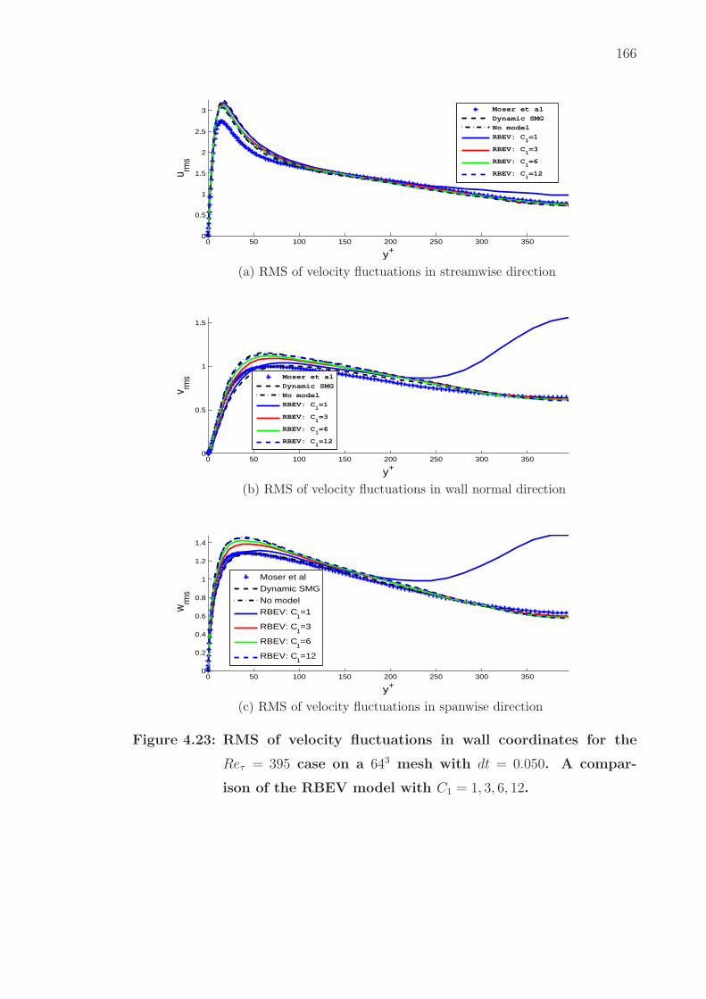
166
0 50 100 150 200 250 300 3500
0.5
1
1.5
2
2.5
3
y+
u rms
Moser et al
Dynamic SMG
No model
RBEV: C1=1
RBEV: C1=3
RBEV: C1=6
RBEV: C1=12
(a) RMS of velocity fluctuations in streamwise direction
0 50 100 150 200 250 300 3500
0.5
1
1.5
y+
v rms
Moser et al
Dynamic SMG
No model
RBEV: C1=1
RBEV: C1=3
RBEV: C1=6
RBEV: C1=12
(b) RMS of velocity fluctuations in wall normal direction
0 50 100 150 200 250 300 3500
0.2
0.4
0.6
0.8
1
1.2
1.4
y+
wrm
s
Moser et al
Dynamic SMG
No modelRBEV: C
1=1
RBEV: C1=3
RBEV: C1=6
RBEV: C1=12
(c) RMS of velocity fluctuations in spanwise direction
Figure 4.23: RMS of velocity fluctuations in wall coordinates for the
Reτ = 395 case on a 643 mesh with dt = 0.050. A compar-
ison of the RBEV model with C1 = 1, 3, 6, 12.

167
−1 −0.8 −0.6 −0.4 −0.2 0 0.2 0.4 0.6 0.8 10
0.5
1
1.5
2
2.5x 10
−4
y/h
Eddy
Vis
cosi
ty
RBEV: C1=1
RBEV: C1=3
RBEV: C1=6
RBEV: C1=12
(a) eddy viscosity
−1 −0.8 −0.6 −0.4 −0.2 0 0.2 0.4 0.6 0.8 10
0.005
0.01
0.015
0.02
0.025
y/h
τ
RBEV: C1=1
RBEV: C1=3
RBEV: C1=6
RBEV: C1=12
(b) stabilization parameter τm
−1 −0.8 −0.6 −0.4 −0.2 0 0.2 0.4 0.6 0.8 10
0.5
1
1.5
2
2.5
y/h
Res
idua
l
RBEV: C1=1
RBEV: C1=3
RBEV: C1=6
RBEV: C1=12
(c) Residual of the momentum equation
Figure 4.24: Average value of the eddy viscosity, stabilization parameter
and residual of the momentum equation for the Reτ = 395
case on a 643 mesh with dt = 0.050. A comparison of the
RBEV model with C1 = 1, 3, 6, 12.

168
4.4.1.2 MM2
In this section we present results for the purely residual-based mixed model
(MM2). First we consider its performance on the 323 mesh with C1 = 3 and
dt = 0.05. Not surprisingly, we find what with this value of C1 this model is too
viscous and leads to an over-prediction of the mean velocity. This is explained by
recognizing that with this value of C1 the RBEV model by itself produced enough
viscosity so as to yield an accurate mean velocity. In the MM2 model we are adding
to it the viscous contribution from the RBVM model, which clearly means that the
resulting model will be too viscous.
Thereafter, we set C1 = 12 and test the performance of this method on a 323
and a 643 mesh with dt = 0.0050 units. With this value of C1 it performs very well
and is competitive with the RBEV model with C1 = 3.
In Figures 4.25 - 4.29 we present results on the 323 mesh with C1 = 3.
In Figure 4.25 compares average streamwise velocities of different models. The
RBEV model matches the DNS most accurately. The RBVM and the MM2 models
overestimate the average velocity and they are very close to each other. All the
residual-based models are more accurate than the dynamic Smagorinsky model. The
same conclusion can be drawn from the semi-log plot for u+ in Figure 4.26 presented
in wall coordinates. Figure 4.27 compares the average pressure. The RBVM model
and the MM2 model overestimate the pressure profile. The pressure profile from the
RBVM model and the MM2 model are smoother than the RBEV model. All the
residual-based models are more accurate than the dynamic Smagorinsky model.
In Figure 4.28, we compare the fluctuations computed by the LES models
with their DNS counterparts. We note that all models overpredict the streamwise
fluctuations urms in (a), though the RBEV model is marginally more accurate than
the others. For the wall normal fluctuations, vrms in (b), the RBVM model and
the MM2 model are more accurate than the RBEV model in the whole channel,
and both of them are more accurate than dynamic Smagorinsky model around the
channel center. For the spanwise fluctuations, wrms in (c), the RBVM model and

169
the MM2 model are more accurate than the RBEV model, and both of them are
also more accurate dynamic Smagorinsky model near the channel center. In the
near wall region, the dynamic Smagorinsky model is most accurate, followed by the
MM2 model and the RBVM model, then the RBEV model.
In Figure 4.29, the average values of the eddy viscosity, the stabilization pa-
rameter and the residual of the momentum equation are shown. In (a), the eddy
viscosity in the MM2 model is smaller than that in the pure RBEV model. This
is reasonable because in the MM2 model the RBVM component also contributes to
the dissipation. So the contribution from of the RBEV component is reduced dy-
namically. In (b), the stabilization parameter τ is the same for both these models.
Finally, in (c), we observe that the residual from the MM2 model is smaller than
that for RBEV model, which is the reason why the eddy viscosity in MM2 model is
smaller than that of the pure RBEV model.
In summary we note that while the MM2 model produces reasonable results
with C1 = 3, it is not as good as the RBEV model alone. In general is too viscous.
This may be corrected by using a large value of C1, as shown in the next set of
results.

170
0 0.2 0.4 0.6 0.8 1 1.2 1.4−1
−0.8
−0.6
−0.4
−0.2
0
0.2
0.4
0.6
0.8
1
y/h
<u>
Moser et al
Dynamic SMG
No model
RBEV
RBVM
MM2
Figure 4.25: Average streamwise velocity for the Reτ = 395 case on a 323
mesh with dt = 0.050 and C1 = 3. A comparison of the RBEV,
RBVM, and MM2 cases.
10−1
100
101
102
0
5
10
15
20
log y+
u+
Moser et al
Theoretical 1
Theoretical 2
Dynamic SMG
No model
RBEV
RBVM
MM2
Figure 4.26: Average streamwise velocity in wall coordinates for the
Reτ = 395 case on a 323 mesh with dt = 0.050 and C1 = 3.
A comparison of the RBEV, RBVM, and MM2 cases.

171
−1 −0.8 −0.6 −0.4 −0.2 0 0.2−1
−0.8
−0.6
−0.4
−0.2
0
0.2
0.4
0.6
0.8
1
<p>
y/h
Moser et al
Dynamic SMG
No model
RBEV
RBVM
MM2
Figure 4.27: Average pressure for the Reτ = 395 case on a 323 mesh with
dt = 0.050 and C1 = 3. A comparison of the RBEV, RBVM,
and MM2 cases.

172
0 50 100 150 200 250 300 3500
0.5
1
1.5
2
2.5
3
3.5
4
y+
u rms
Moser et alDynamic SMGNo modelRBEVRBVMMM2
(a) RMS of velocity fluctuations in streamwise direction
0 50 100 150 200 250 300 3500
0.2
0.4
0.6
0.8
1
1.2
y+
v rms
Moser et al
Dynamic SMG
No model
RBEV
RBVM
MM2
(b) RMS of velocity fluctuations in wall normal direction
0 50 100 150 200 250 300 3500
0.2
0.4
0.6
0.8
1
1.2
1.4
1.6
y+
wrm
s
Moser et al
Dynamic SMG
No model
RBEV
RBVM
MM2
(c) RMS of velocity fluctuations in spanwise direction
Figure 4.28: RMS of velocity fluctuations in wall coordinates for the
Reτ = 395 case on a 323 mesh with dt = 0.050 and C1 = 3.
A comparison of the RBEV, RBVM, and MM2 cases.

173
−1 −0.8 −0.6 −0.4 −0.2 0 0.2 0.4 0.6 0.8 10
0.5
1
1.5
2
2.5
3
3.5
4x 10
−5
y/h
Eddy
Vis
cosi
ty
RBEV
MM2
(a) eddy viscosity
−1 −0.8 −0.6 −0.4 −0.2 0 0.2 0.4 0.6 0.8 12
3
4
5
6
7
8
9
10x 10
−3
y/h
τ
RBEV
MM2
(b) stabilization parameter τm
−1 −0.8 −0.6 −0.4 −0.2 0 0.2 0.4 0.6 0.8 10
0.1
0.2
0.3
0.4
0.5
0.6
0.7
0.8
0.9
y/h
Res
idua
l
RBEV
MM2
(c) Residual of the momentum equation
Figure 4.29: Average value of the eddy viscosity, stabilization parameter
and residual of the momentum equation for the Reτ = 395
case on a 323 mesh with dt = 0.050 and C1 = 3. A comparison
of the RBEV, and MM2 cases.

174
In Figures 4.30 - 4.34, we plot the results for LES models on a 323 mesh with
dt = 0.050 and C1 = 12.
Figure 4.30 compares average streamwise velocities of different models. The
RBVM model and the MM2 model match DNS most accurately. The RBEV model
underpredicts the profile. The same conclusion can be drawn from the semi-log
plot for u+ in Figure 4.31 presented in wall coordinates. Figure 4.31 compares the
average pressure. All of the three models have the similar performance while the
RBEV model has some oscillations.
In Figure 4.33, we compare the fluctuations computed by the LES models with
their DNS counterparts. We note that all the models overpredict the streamwise
fluctuations urms in (a) though the MM2 model is marginally more accurate than
the others. For the wall normal fluctuations, vrms in (b), the MM2 model and the
RBVM model are more accurate than the RBEV model. In the near wall region,
all the three models are more accurate than the dynamic Smagorinsky model. At
the center of the channel, the MM2 model and the RBVM model also match the
DNS results very accurately. For the spanwise fluctuations, wrms in (c), the MM2
model and the RBVM model are more accurate than the RBEV model. Overall the
dynamic Smagorinsky model is the most accurate.
In Figure 4.34, the average values of the eddy viscosity, the stabilization pa-
rameter and the residual of the momentum equation are shown. In (a), the eddy
viscosity in the MM2 model is smaller than that in the pure RBEV model. In (b),
the stabilization parameter τ are the same. In (c), the residual from the MM2 model
is smaller than that from the RBEV model, which also accounts for the smaller eddy
viscosity observed in (a).
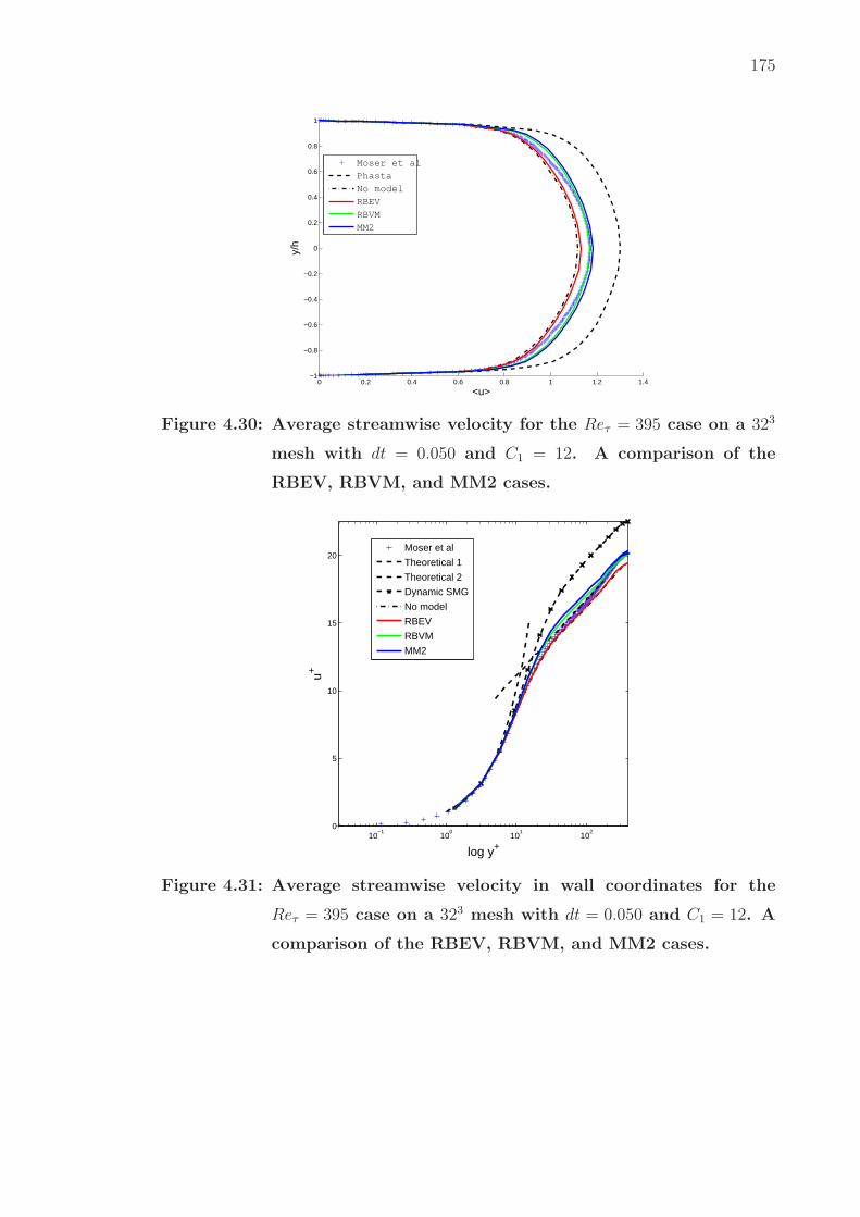
175
0 0.2 0.4 0.6 0.8 1 1.2 1.4−1
−0.8
−0.6
−0.4
−0.2
0
0.2
0.4
0.6
0.8
1
y/h
<u>
Moser et al
Phasta
No model
RBEV
RBVM
MM2
Figure 4.30: Average streamwise velocity for the Reτ = 395 case on a 323
mesh with dt = 0.050 and C1 = 12. A comparison of the
RBEV, RBVM, and MM2 cases.
10−1
100
101
102
0
5
10
15
20
log y+
u+
Moser et al
Theoretical 1
Theoretical 2
Dynamic SMG
No model
RBEV
RBVM
MM2
Figure 4.31: Average streamwise velocity in wall coordinates for the
Reτ = 395 case on a 323 mesh with dt = 0.050 and C1 = 12. A
comparison of the RBEV, RBVM, and MM2 cases.

176
−1 −0.8 −0.6 −0.4 −0.2 0 0.2−1
−0.8
−0.6
−0.4
−0.2
0
0.2
0.4
0.6
0.8
1
<p>
y/h
Moser et al
Dynamic SMG
No model
RBEV
RBVM
MM2
Figure 4.32: Average pressure for the Reτ = 395 case on a 323 mesh with
dt = 0.050 and C1 = 12. A comparison of the RBEV, RBVM,
and MM2 cases.
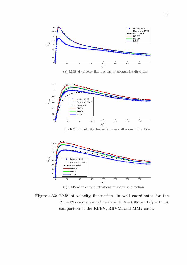
177
0 50 100 150 200 250 300 3500
0.5
1
1.5
2
2.5
3
3.5
4
y+
u rms
Moser et alDynamic SMGNo modelRBEVRBVMMM2
(a) RMS of velocity fluctuations in streamwise direction
0 50 100 150 200 250 300 3500
0.2
0.4
0.6
0.8
1
1.2
y+
v rms
Moser et al
Dynamic SMG
No model
RBEV
RBVM
MM2
(b) RMS of velocity fluctuations in wall normal direction
0 50 100 150 200 250 300 3500
0.2
0.4
0.6
0.8
1
1.2
1.4
1.6
y+
wrm
s
Moser et al
Dynamic SMG
No model
RBEV
RBVM
MM2
(c) RMS of velocity fluctuations in spanwise direction
Figure 4.33: RMS of velocity fluctuations in wall coordinates for the
Reτ = 395 case on a 323 mesh with dt = 0.050 and C1 = 12. A
comparison of the RBEV, RBVM, and MM2 cases.

178
−1 −0.8 −0.6 −0.4 −0.2 0 0.2 0.4 0.6 0.8 10
0.2
0.4
0.6
0.8
1
1.2x 10
−5
y/h
Eddy
Vis
cosi
ty
RBEV
MM2
(a) eddy viscosity
−1 −0.8 −0.6 −0.4 −0.2 0 0.2 0.4 0.6 0.8 11.7
1.8
1.9
2
2.1x 10
−3
y/h
τ
RBEV
MM2
(b) stabilization parameter τm
−1 −0.8 −0.6 −0.4 −0.2 0 0.2 0.4 0.6 0.8 10.1
0.2
0.3
0.4
0.5
0.6
0.7
0.8
0.9
1
1.1
y/h
Res
idua
l
RBEVMM2
(c) Residual of the momentum equation
Figure 4.34: Average value of the eddy viscosity, stabilization parameter
and residual of the momentum equation for the Reτ = 395
case on a 323 mesh with dt = 0.050 and C1 = 12. A comparison
of the RBEV, and MM2 cases.

179
From the result on the 323 mesh we conclude that for the RBVM and MM2
models the value of C1 = 12 produces the most accurate results. We now consider
this value for the 643 mesh. In Figures 4.35 - 4.39 we plot the results for LES models
on a 643 mesh with dt = 0.050 and C1 = 12.
Figure 4.35 compares average streamwise velocities of different models. We
observe that all the residual-based models are very accurate. The RBEV under-
estimates the velocity profile while the RBVM and MM2 models over estimate it
slightly. The same conclusion can be drawn from the semi-log plot for u+ in Figure
4.36 presented in wall coordinates. Figure 4.37 compares the average pressure. All
of the three residual-based models have the similar performance while the RBEV
model has some oscillations. Further, the RBEV model matches DNS most accu-
rately where the profile has a turn-over point while the RBVM and mixed model are
more accurate when pressure profile is more straight. All of them are more accurate
than the dynamic Smagorinsky model.
In Figure 4.38, we compare the fluctuations computed by the LES models
with their DNS counterparts. We note that all models overpredict the streamwise
fluctuations urms in (a) though the RBEV model is marginally more accurate than
the others. For the wall normal fluctuations, vrms in (b), the MM2 and RBVM
models are more accurate than the RBEV model. In the near wall region, all
three residual-based models are more accurate than dynamic Smagorinsky model
which underpredicts the fluctuations. For the spanwise fluctuations, wrms in (c),
the MM2 model and the RBVM model are more accurate than the RBEV model.
Near the center of the channel, all three residual-based models slightly underpredict
the fluctuations. The dynamic Smagorinsky model is the most accurate. .
In Figure 4.39, the average values of the eddy viscosity, the stabilization pa-
rameter and the residual of the momentum equation are shown. In (a), the eddy
viscosity in the MM2 model is smaller than in the pure RBEV model. In (b), we
observe that the stabilization parameter τ are the same for these models. In (c), we
note that the residual from the MM2 model is smaller than that from the RBEV
model leading to the difference in the eddy viscosity for these models.

180
0 0.2 0.4 0.6 0.8 1 1.2 1.4−1
−0.8
−0.6
−0.4
−0.2
0
0.2
0.4
0.6
0.8
1
y/h
<u>
Moser et al
Dynamic SMG
No model
RBEV
RBVM
MM2
Figure 4.35: Average streamwise velocity for the Reτ = 395 case on a 643
mesh with dt = 0.050 and C1 = 12. A comparison of the
RBEV, RBVM, and MM2 cases.
10−1
100
101
102
0
2
4
6
8
10
12
14
16
18
20
log y+
u+
Moser et al
Theoretical 1
Theoretical 2
Dynamic SMG
No model
RBEV
RBVM
MM2
Figure 4.36: Average streamwise velocity in wall coordinates for the
Reτ = 395 case on a 643 mesh with dt = 0.050 and C1 = 12. A
comparison of the RBEV, RBVM, and MM2 cases.
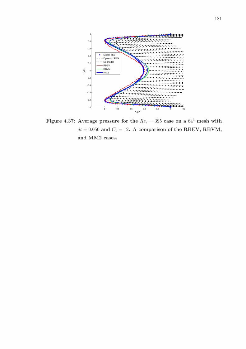
181
−1 −0.8 −0.6 −0.4 −0.2 0 0.2−1
−0.8
−0.6
−0.4
−0.2
0
0.2
0.4
0.6
0.8
1
<p>
y/h
Moser et al
Dynamic SMG
No model
RBEV
RBVM
MM2
Figure 4.37: Average pressure for the Reτ = 395 case on a 643 mesh with
dt = 0.050 and C1 = 12. A comparison of the RBEV, RBVM,
and MM2 cases.
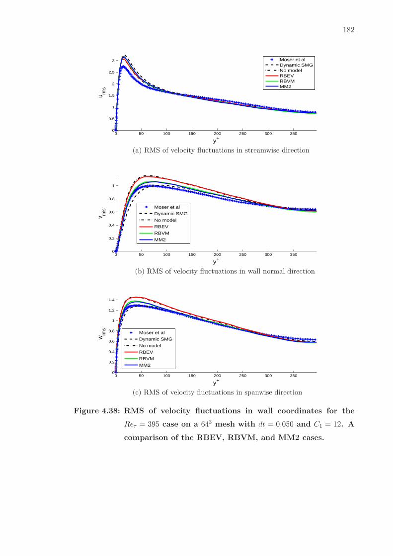
182
0 50 100 150 200 250 300 3500
0.5
1
1.5
2
2.5
3
y+
u rms
Moser et alDynamic SMGNo modelRBEVRBVMMM2
(a) RMS of velocity fluctuations in streamwise direction
0 50 100 150 200 250 300 3500
0.2
0.4
0.6
0.8
1
y+
v rms
Moser et al
Dynamic SMG
No model
RBEV
RBVM
MM2
(b) RMS of velocity fluctuations in wall normal direction
0 50 100 150 200 250 300 3500
0.2
0.4
0.6
0.8
1
1.2
1.4
y+
wrm
s
Moser et al
Dynamic SMG
No model
RBEV
RBVM
MM2
(c) RMS of velocity fluctuations in spanwise direction
Figure 4.38: RMS of velocity fluctuations in wall coordinates for the
Reτ = 395 case on a 643 mesh with dt = 0.050 and C1 = 12. A
comparison of the RBEV, RBVM, and MM2 cases.

183
−1 −0.8 −0.6 −0.4 −0.2 0 0.2 0.4 0.6 0.8 10
1
2
3
4
5
6
7x 10
−6
y/h
Eddy
Visc
osity
RBEV
MM2
(a) eddy viscosity
−1 −0.8 −0.6 −0.4 −0.2 0 0.2 0.4 0.6 0.8 10.4
0.6
0.8
1
1.2
1.4
1.6
1.8
2
2.2
x 10−3
y/h
τ
RBEV
MM2
(b) stabilization parameter τm
−1 −0.8 −0.6 −0.4 −0.2 0 0.2 0.4 0.6 0.8 10
0.1
0.2
0.3
0.4
0.5
0.6
0.7
0.8
0.9
1
y/h
Res
idua
l
RBEV
MM2
(c) Residual of the momentum equation
Figure 4.39: Average value of the eddy viscosity, stabilization parameter
and residual of the momentum equation for the Reτ = 395
case on a 643 mesh with dt = 0.050 and C1 = 12. A comparison
of the RBEV, and MM2 cases.

184
4.4.2 Reτ = 590
In this section we test the LES models at a higher Reynolds number of Reτ =
590. We only consider the 643 element mesh. First we consider the performance
of the RBEV model with C1 = 3, which provided the best results for the lower
Reynolds number case. We note that it continues to be very accurate at the higher
Reynolds number. Thereafter we examine the performance of the MM2 model at
C1 = 12, and observe that it too continues to be accurate at the higher Reynolds
number.
4.4.2.1 RBEV
In Figures 4.40 - 4.44 we plot the results for the RBEV model with Re = 590
on a 643 grid with dt = 0.025 and different value of C1 = 1, 3, 12.
Figure 4.40 compares results for the average streamwise velocity profile. The
RBEV model with C1 = 3 matches the DNS most accurately. The RBEV model
with C1 = 12 slightly underpredicts and the RBEV model with C1 = 1 slightly
overpredicts the average velocity. The same trends are observed in the semi-log
plot for u+ in Figure 4.41 presented in wall coordinates. Figure 4.40 compares
the average pressure. The RBEV models with C1 = 3 and C1 = 12 match the
DNS most accurately while the RBEV model with C1 = 1 slightly overpredicts the
average pressure.
In Figure 4.43, we compare the fluctuations computed by the LES models
with their DNS counterparts. We note that all models overpredict the streamwise
fluctuations urms in (a). For the wall normal fluctuations, vrms in (b), the RBVM
model with C1 = 1 is more accurate than the others. Near the center of the channel,
all three models are very good. The same conclusion can be drawn for the spanwise
fluctuations, wrms in (c).
In Figure 4.44, the average values of the eddy viscosity, the stabilization pa-
rameter and the residual of the momentum equation are shown. Once again we
observe that as C1 increases the eddy viscosity and the stabilization parameter de-
crease, while the residual remain relatively unchanged.

185
0 0.1 0.2 0.3 0.4 0.5 0.6 0.7 0.8 0.9−1
−0.8
−0.6
−0.4
−0.2
0
0.2
0.4
0.6
0.8
1
y/h
<u>
Moser et alRBEV: C
1=1
RBEV: C1=3
RBEV: C1=12
Figure 4.40: Average streamwise velocity for the Reτ = 590 case on a 643
mesh with dt = 0.025. A comparison of C1 = 1, 3, 12 for the
RBEV model.
10−1
100
101
102
0
2
4
6
8
10
12
14
16
18
20
log y+
u+
Moser et al
Theoretical 1
Theoretical 2RBEV: C
1=1
RBEV: C1=3
RBEV: C1=12
Figure 4.41: Average streamwise velocity in wall coordinates for the
Reτ = 590 case on a 643 mesh with dt = 0.025. A compar-
ison of C1 = 1, 3, 12 for the RBEV model.

186
−1 −0.8 −0.6 −0.4 −0.2 0 0.2−1
−0.8
−0.6
−0.4
−0.2
0
0.2
0.4
0.6
0.8
1
<u>
y/h
Moser et alRBEV: C
1=1
RBEV: C1=3
RBEV: C1=12
Figure 4.42: Average pressure for the Reτ = 590 case on a 643 mesh with
dt = 0.025. A comparison of C1 = 1, 3, 12 for the RBEV model.

187
0 100 200 300 400 5000
0.5
1
1.5
2
2.5
3
3.5
y+
u rms
Moser et alRBEV: C
1=1
RBEV: C1=3
RBEV: C1=12
(a) RMS of velocity fluctuations in streamwise direction
0 100 200 300 400 5000
0.2
0.4
0.6
0.8
1
1.2
y+
v rms
Moser et alRBEV: C
1=1
RBEV: C1=3
RBEV: C1=12
(b) RMS of velocity fluctuations in wall normal direction
0 100 200 300 400 5000
0.2
0.4
0.6
0.8
1
1.2
1.4
1.6
y+
wrm
s
Moser et alRBEV: C
1=1
RBEV: C1=3
RBEV: C1=12
(c) RMS of velocity fluctuations in spanwise direction
Figure 4.43: RMS of velocity fluctuations in wall coordinates for the
Reτ = 590 case on a 643 element mesh with dt = 0.025. A
comparison of C1 = 1, 3, 12 for the RBEV model.

188
−1 −0.8 −0.6 −0.4 −0.2 0 0.2 0.4 0.6 0.8 10
0.2
0.4
0.6
0.8
1
1.2
1.4
1.6
1.8
2x 10
−5
y/h
Eddy
Vis
cosi
ty
RBEV: C1=1
RBEV: C1=3
RBEV: C1=12
(a) eddy viscosity
−1 −0.8 −0.6 −0.4 −0.2 0 0.2 0.4 0.6 0.8 10
0.002
0.004
0.006
0.008
0.01
0.012
0.014
y/h
τ
RBEV: C1=1
RBEV: C1=3
RBEV: C1=12
(b) stabilization parameter τm
−1 −0.8 −0.6 −0.4 −0.2 0 0.2 0.4 0.6 0.8 10.1
0.2
0.3
0.4
0.5
0.6
0.7
0.8
y/h
Res
idua
l
RBEV: C1=1
RBEV: C1=3
RBEV: C1=12
(c) Residual of the momentum equation
Figure 4.44: Average value of the eddy viscosity, stabilization parameter
and residual of the momentum equation for the Reτ = 590
case on a 643 element mesh with dt = 0.025. A comparison of
C1 = 1, 3, 12 for the RBEV model.
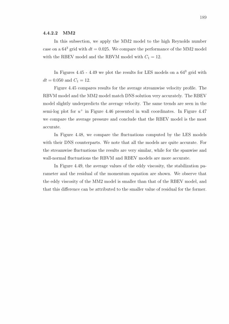
189
4.4.2.2 MM2
In this subsection, we apply the MM2 model to the high Reynolds number
case on a 643 grid with dt = 0.025. We compare the performance of the MM2 model
with the RBEV model and the RBVM model with C1 = 12.
In Figures 4.45 - 4.49 we plot the results for LES models on a 643 grid with
dt = 0.050 and C1 = 12.
Figure 4.45 compares results for the average streamwise velocity profile. The
RBVM model and the MM2 model match DNS solution very accurately. The RBEV
model slightly underpredicts the average velocity. The same trends are seen in the
semi-log plot for u+ in Figure 4.46 presented in wall coordinates. In Figure 4.47
we compare the average pressure and conclude that the RBEV model is the most
accurate.
In Figure 4.48, we compare the fluctuations computed by the LES models
with their DNS counterparts. We note that all the models are quite accurate. For
the streamwise fluctuations the results are very similar, while for the spanwise and
wall-normal fluctuations the RBVM and RBEV models are more accurate.
In Figure 4.49, the average values of the eddy viscosity, the stabilization pa-
rameter and the residual of the momentum equation are shown. We observe that
the eddy viscosity of the MM2 model is smaller than that of the RBEV model, and
that this difference can be attributed to the smaller value of residual for the former.

190
0 0.1 0.2 0.3 0.4 0.5 0.6 0.7 0.8 0.9−1
−0.8
−0.6
−0.4
−0.2
0
0.2
0.4
0.6
0.8
1
y/h
<u>
Moser et al
RBEV
RBVM
MM2
Figure 4.45: Average streamwise velocity for the Reτ = 590 case on a 643
mesh with dt = 0.025 and C1 = 12. A comparison of the
RBEV, RBVM, and MM2 cases.
10−1
100
101
102
0
2
4
6
8
10
12
14
16
18
20
log y+
u+
Moser et al
Theoretical 1
Theoretical 2
RBEV
RBVM
MM2
Figure 4.46: Average streamwise velocity in wall coordinates for the
Reτ = 590 case on a 643 mesh with dt = 0.025 and C1 = 12. A
comparison of the RBEV, RBVM, and MM2 cases.

191
−1 −0.8 −0.6 −0.4 −0.2 0 0.2−1
−0.8
−0.6
−0.4
−0.2
0
0.2
0.4
0.6
0.8
1
<p>
y/h
Moser et al
RBEV
RBVM
MM2
Figure 4.47: Average pressure for the Reτ = 590 case on a 643 mesh with
dt = 0.025 and C1 = 12. A comparison of the RBEV, RBVM,
and MM2 cases.
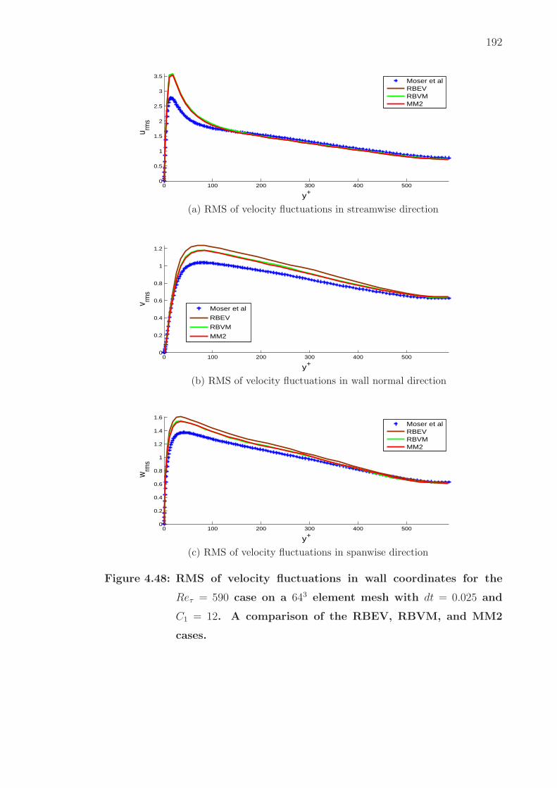
192
0 100 200 300 400 5000
0.5
1
1.5
2
2.5
3
3.5
y+
u rms
Moser et alRBEVRBVMMM2
(a) RMS of velocity fluctuations in streamwise direction
0 100 200 300 400 5000
0.2
0.4
0.6
0.8
1
1.2
y+
v rms
Moser et al
RBEV
RBVM
MM2
(b) RMS of velocity fluctuations in wall normal direction
0 100 200 300 400 5000
0.2
0.4
0.6
0.8
1
1.2
1.4
1.6
y+
wrm
s
Moser et alRBEVRBVMMM2
(c) RMS of velocity fluctuations in spanwise direction
Figure 4.48: RMS of velocity fluctuations in wall coordinates for the
Reτ = 590 case on a 643 element mesh with dt = 0.025 and
C1 = 12. A comparison of the RBEV, RBVM, and MM2
cases.
193
−1 −0.8 −0.6 −0.4 −0.2 0 0.2 0.4 0.6 0.8 10
0.2
0.4
0.6
0.8
1
1.2
1.4
1.6
1.8x 10
−6
y/h
Eddy
Vis
cosi
ty
RBEV
MM2
(a) eddy viscosity
−1 −0.8 −0.6 −0.4 −0.2 0 0.2 0.4 0.6 0.8 16.5
7
7.5
8
8.5
9
9.5
10
10.5x 10
−4
y/h
τ
RBEV
MM2
(b) stabilization parameter τm
−1 −0.8 −0.6 −0.4 −0.2 0 0.2 0.4 0.6 0.8 10
0.1
0.2
0.3
0.4
0.5
0.6
0.7
y/h
Res
idua
l
RBEV
MM2
(c) Residual of the momentum equation
Figure 4.49: Average value of the eddy viscosity, stabilization parameter
and residual of the momentum equation for the Reτ = 590
case on a 643 element mesh with dt = 0.025 and C1 = 12. A
comparison of the RBEV, and MM2 cases.

194
4.5 Chapter summary
In this chapter, we have implemented two residual-based LES models for in-
compressible turbulent flows within the finite element method. They are
• the residual-based eddy viscosity (RBEV) model
• the purely residual-based mixed model (MM2), which is a combination of the
RBVM and the RBEV models
We tested the performance of these LES models in predicting fully developed
turbulent channel flows. The LES models are tested on problems with friction
Reynolds numbers Reτ = 390, 590 on 323 and 643 grids.
First, we compared the performance of the RBEV and the dynamic Smagorin-
sky models. We found that the RBEV model is generally more accurate and per-
forms significantly better than the dynamic Smagorinsky model. We also note that
the performance of the RBEV model strongly depends on the value of C1, which is
a parameter within the stabilization parameter τm. With C1 = 3, the RBEV model
matches the DNS result very accurately for the average streamwise velocity and the
average pressure. We observe that the eddy viscosity of the RBEV model is near to
zero close the wall and grows within the channel. It is remarkable that it achieves
this behavior without an explicit dynamic approach. We attribute this behavior to
the fact that RBEV model is inherently dynamic in that it is based on the resid-
ual of the coarse scales which automatically vanishes in well-resolved regions of the
flow. We also observed that the eddy viscosity reduces with refinement in space and
time. In that sense it displays a “dynamic” behavior. The RBEV model is more
accurate and much easier to implement than the dynamic Smagorinsky model, and
it is found to be robust by examining the dependence of its performance on grid
size, the constant in the stabilization parameter, and the Reynolds number. We
conclude that the RBEV model represents a viable strategy for wall bounded flows.
Thereafter we examined the performance of the new purely residual-based
mixed model (MM2). We observed that the MM2 model with C1 = 12 performs

195
very accurately. It is competitive with the RBEV model with C1 = 3 and is more
accurate than dynamic Smagorinsky model. We also found that for the MM2 model
the eddy viscosity of the RBEV term automatically accounts for the dissipation pro-
duced by the RBVM terms and produces smaller eddy viscosity when compared to
the purely RBEV model. Since there is no dynamic evaluation of parameters within
this model, it is much easier to implement than the mixed model (MM1) based on
the RBVM and the dynamic Smagorinsky models. The performance of the MM2
model is found to be robust by examining its dependence on grid sizes, the constant
C1 in the stabilization parameter, and the Reynolds number.
Our recommendation is therefore to use the residual-based eddy viscosity
(RBEV) model with C1 = 3 and the purely residual based mixed model (MM2)
with C1 = 12 within finite element method. These models are accurate, easy to
implement, as they involve no dynamic procedure, and are consistent, in that the
eddy viscosity vanishes when the residual of the coarse scales is small.
CHAPTER 5
Conclusion
In this thesis we have developed and implemented several residual-based large
eddy simulation models for compressible and incompressible turbulent flows. Within
this framework our main accomplishments are:
(1) We have extended the residual-based variational multiscale formulation
(RBVM) to compressible turbulent flows. New definition of stabilization parameter
τ is proposed for compressible turbulent flows. We have tested the performance of
the RBVM model in predicting the decay of compressible, homogeneous, isotropic
turbulence (HIT) in regimes where shocklets are known to exist within Fourier-
spectral method. We varied the level of compressibility of the flow by varying the
initial proportion of compressible turbulent kinetic energy and by varying the Mach
number. In all cases we found that the RBVM model is generally more accurate and
performs better than the popular dynamic Smagorinsky-Yoshizawa-eddy-diffusivity
(DSYE) model.
(2) We have proposed and implemented a mixed model (MM1) based on the
RBVM and DSYE models. In the MM1 model, the RBVM terms account for cross
stresses while the DSYE terms account for Reynolds stresses. The MM1 model is
tested on the same compressible HIT as the RBVM model with varying the level
of compressibility of the flow. We have found that the MM1 model is generally
more accurate than the DSYE model. For low Reynolds number the MM1 model is
somewhat less accurate than the RBVM model, while for high Reynolds number it
is more accurate than the RBVM model. This is to be expected because Reynolds
stresses are important in high Reynolds number turbulent flows.
(3) We have developed and tested a new residual-based eddy viscosity model
(RBEV) that uses the RBVM formulation. In the RBEV model, the eddy viscosity
196

197
is defined as νt ∼ h|u′|, where h is the grid size and u′ is the fine scales velocity
fluctuation. The RBEV model is inherently dynamic because it is based on the
residual of the coarse scales which automatically vanishes in well-resolved regions
of the flow. In this way, the RBEV model requires no dynamic calculation of a
parameter, so it is much easier to implement than the dynamic Smagorinsky type
models.
The RBEV model is tested on the same compressible HIT as the RBVM and
MM1 models. We observed that the RBEV model is more accurate than the DSYE
model for the incompressible velocity component, while for the compressible velocity
component it is not dissipative enough. Compared to the DSYE model, the RBEV
model achieves similar accuracy but without a dynamic evlautation of parameters.
The RBEV model is also tested on the incompressible fully developed turbu-
lent channel flows within finite element method. The RBEV model is observed to
be more accurate and much easier to implement than dynamic Smagorinsky model.
We also observed that the eddy viscosity of the RBEV model is near to zero close
to the wall and grows within the channel. It is remarkable that it achieves this
behavior without an explicit dynamic approach. By examining the dependence of
the performance of this model on grid (spatial and temporal) size, constants that
appear within the stabilization parameter and the Reynolds number, the RBEV
model is found to be robust and it represents a viable strategy for simulating wall
bounded flows.
(4) Motivated by the MM1 model and the RBEV model above, we developed
and implemented a purely residual based mixed model (MM2) based on the RBVM
and RBEV models. In the MM2 model, the RBVM terms account for cross stresses
while the RBEV terms account for Reynolds stresses. The MM2 model is inherently
dynamic but does not involve the dynamic calculation of parameters, so it is much
easier to implement than the MM1 model.
The MM2 model is tested for the compressible HIT and it is observed to be
more accurate than the DSYE model. For low Reynolds number the MM2 model is
slightly less accurate than RBVM the model, while for high Reynolds number it is

198
more accurate than the RBVM model.
The MM2 model is also tested for the same incompressible channel turbulent
flows as the RBEV model. For a different set of constant values in the definition of
stabilization parameter the MM2 model is as accurate as the RBEV model, and is
more accurate than the dynamic Smagorinsky model. We also found that for the
MM2 model the eddy viscosity of the RBEV term automatically accounts for the
dissipation produced by the RBVM terms and produces smaller eddy viscosity when
compared to the pure RBEV model. The MM2 model is much easier to implement
than the MM1 model. By testing this model for a range of problem parameters we
conclude that it is robust, and it represents a viable strategy for simulating wall
bounded flows.
For future work, the RBVM, the RBEV and the MM2 models will be applied
to other problems, including flows with complex geometries and flows at very large
scales. These models will also be extended to magnetohydrodynamics (MHD) or
related areas.
REFERENCES
[1] J. P. Richter, The notebooks of Leonardo da Vinci. New York: Dover
Publications, 1970.
[2] O. Reynolds, “An experimental investigation of the circumstances which
determine whether the motion of water shall be direct or sinuous, and the law
of resistance in parallel channels,” Philosph. Trans. Roy. Soc. London, vol.
174, pp. 935–982, 1883.
[3] S. B. Pope, Turbulent flows. Cambridge, UK: Cambridge University Press,
2000.
[4] J. L. Lumley, Turbulence and turbulence modeling, research trends in fluid
dynamics. Woodbury, NY: API Press, 1996.
[5] A. N. Kolmogorov, “1941a: Dissipation of energy in locally isotropic
turbulence,” Doklady Akademiia Nauk SSSR, vol. 30, pp. 301–305, 1941.
[6] A. N. Kolmogorov, “1941b: The local structure of turbulence in
incompressible viscous uid for very large Reynolds numbers,” Doklady
Akademiia Nauk SSSR, vol. 31, pp. 538–540, 1941.
[7] A. N. Kolmogorov, “The equations of turbulent motion in an incompressible
fluid,” Izvestia Acad. Sci., USSR, vol. Phys. 6, pp. 56–58, 1942.
[8] J. Smagorinsky, “General circulation experiments with the primitive
equations. I. the basic experiment,” Mon. Weather Rev., vol. 91, pp. 99–164,
1963.
[9] A. Yoshizawa, “Statistical theory for compressible turbulent shear flows, with
the application to subgrid modeling,” Phys. Fluids, vol. 29, pp. 2152–2164,
2000.
199
200
[10] P. Moin, K. Squires, W. Cabot, and S. Lee, “A dynamic subgrid-scale model
for compressible turbulence and scalar transport,” Phys. Fluids A: Fluid,
vol. 3, pp. 2746–2757, 1991.
[11] J. Bardina, J. H. Ferziger, and W. C. Reynolds, “Improved subgrid-scale
models for large-eddy simulation,” in Amer. Inst. of Aeronautics and
Astronautics, Fluid and Plasma Dynamics Conf. 13th, vol. 1, Snowmass, CO,
1980, pp. 14–16.
[12] R. A. Clark, J. H. Ferziger, and W. C. Reynolds, “ Evaluation of subgrid-scale
models using an accurately simulated turbulent flow,” J. Fluid Mech, vol. 91,
pp. 1–16, 1979.
[13] A. Favre, “ Equations des gaz turbulents compressibles,” J. Mecanique, vol. 4,
pp. 361–390, 1965.
[14] T. J. R. Hughes, L. Mazzei, and K. E. Jansen, “Large Eddy Simulation and
the Variational Multiscale Method,” Comput. Vis. Sci., vol. 3, pp. 47–59,
2000.
[15] Y. Bazilevs, V. M. Calo, J. A. Cottrell, T. J. R. Hughes, A. Reali, and
G. Scovazzi, “Variational multiscale residual-based turbulence modeling for
large eddy simulation of incompressible flows,” Comput. Methods Appl. Mech.
Eng., vol. 197, no. 1-4, pp. 173–201, 2007.
[16] R. Codina, “Stabilized finite element approximation of transient
incompressible flows using orthogonal subscales,” Comput. Methods Appl.
Mech. Eng., vol. 191, no. 39-40, pp. 4295–4321, 2002.
[17] P. Gamnitzer, V. Gravemeier, and W. A. Wall, “Time-dependent subgrid
scales in residual-based large eddy simulation of turbulent channel flow,”
Comput. Methods Appl. Mech. Eng., vol. 199, no. 13-16, pp. 819–827, 2010.
[18] Z. Wang and A. A. Oberai, “Spectral analysis of the dissipation of the
residual-based variational multiscale method,” Comput. Methods Appl. Mech.
Eng., vol. 199, no. 13-16, pp. 810–818, 2010.

201
[19] Z. Wang and A. A. Oberai, “A mixed large eddy simulation model based on
the residual-based variational multiscale formulation,” Phys. Fluids, vol. 22,
pp. 075 107:1–9, 2010.
[20] T. J. R. Hughes and G. Sangalli, “Variational multiscale analysis: the
fine-scale green’s function, projection, optimization, localization, and
stabilized methods,” SIAM J. Numerical Anal., vol. 45(2), pp. 539–557, 2007.
[21] A. A. Oberai, J. Liu, D. Sondak, and T. J. R. Hughes, “A residual-based eddy
viscosity model for the les of turbulent flows,” Comput. Methods Appl. Mech.
Eng., submitted.
[22] D. Sondak and A. A. Oberai, “LES models for incompressible
magnetohydrodynamics derived from the variational multiscale formulation,”
Phys. Plasmas, submitted.
[23] A. A. Oberai and J. Wanderer, “Variational formulation of the Germano
identity for the Navier–Stokes equations,” J. Turbulence, vol. 6, no. 7, pp.
1–17, 2005.
[24] A. A. Oberai and J. Wanderer, “A dynamic multiscale viscosity method for
the spectral approximation of conservation laws,” Comput. Methods Appl.
Mech. Eng., vol. 195, no. 13-16, pp. 1778–1792, 2006.
[25] C. G. Speziale, G. Erlebacher, T. A. Zang, and M. Y. Hussaini, “The
subgrid-scale modeling of compressible turbulence,” Phys. Fluids, vol. 31, pp.
940–942, 1988.
[26] S. Liu, C. Meneveau, and J. Katz, “On the properties of similarity
subgrid-scale models as deduced from measurements in a turbulent jet,” J.
Fluid Mech., vol. 275(-1), pp. 83–119, 1994.
[27] B. Vreman, B. Geurts, and H. Kuerten, “ Subgrid-modeling in LES of
compressible flow,” Appl. Sci. Res., vol. 54, pp. 191–203, 1995.

202
[28] A. Leonard and G. S. Winckelmans, “A tensor-diffusivity subgrid model for
large-eddy simulation,” in Proc. Isaac Newton Institute Symposium /
ERCOFTAC Workshop. Norwell, MA: Kluwer Academic Publishers, 1999,
pp. 12–14.
[29] G. S. Winckelmans, A. A. Wray, O. V. Vasilyev, and H. Jeanmart,
“Explicit-filtering large-eddy simulation using the tensor-diffusivity model
supplemented by a dynamic Smagorinsky term,” Phys. Fluids, vol. 13, pp.
1385–1403, 2001.
[30] D. K. Lilly, “ A proposed modification of the Germano subgrid-scale closure
method,” Phys. Fluids, vol. A 4 (3), pp. 633–635, 1992.
[31] G. Hauke, “Simple stabilizing matrices for the computation of compressible
flows in primitive variables,” Comput. Methods Appl. Mech. Eng., vol. 190, no.
51-52, pp. 6881–6893, 2001.
[32] W. Hwang and J. K. Eaton, “Creating homogeneous and isotropic turbulence
without a mean flow,” Exp. Fluids, vol. 36, pp. 444–454, 2004.
[33] R. Samtaney, D. I. Pullin, and B. Kosovic, “Direct numerical simulation of
decaying compressible turbulence and shocklet statistics,” Phys. Fluids, vol.
13(5), pp. 1415–1430, 2001.
[34] C. Canuto, M. Y. Hussaini, A. Quarteroni, and T. A. Zang, Spectral methods
in fluid dynamics. New York City, NY: Springer, 1988.
[35] J. Liu and A. A. Oberai, “The residual-based variational multiscale
formulation for the large eddy simulation of compressible flows,” Comput.
Methods Appl. Mech. Eng., vol. accepted, 2012.
[36] M. Germano, U. Piomelli, P. Moin, and W. H. Cabot, “A dynamic
subgridscale eddy viscosity model,” Phys. Fluids, vol. A 3, pp. 1760–1765,
1991.
[37] F. Shakib, Finite element analysis of the compressible Euler and
Navier-Stokes equations. Stanford, CA: Stanford University, 1989.

203
[38] C. Johnson, Numerical solution of partial differential equations by the finite
element method. Cambridge, UK: Cambridge University Press, 1987.
[39] G. I. Barenblatt, Scaling, self-similarity, and intermediate asymptotics:
dimensional analysis and intermediate asymptotics. Cambridge, UK:
Cambridge University Press, 1987.
[40] T. J. R. Hughes and M. Mallet, “A new finite element formulation for
computational fluid dynamics: III. The generalized streamline operator for
multidimensional advective-diffusive systems,” Comput. Methods Appl. Mech.
Eng., vol. 58(3), pp. 305–328, 1986.
[41] F. Shakib, T. J. R. Hughes, and Z. Johan, “A new finite element formulation
for computational fluid dynamics: X. The compressible Euler and
Navier-Stokes equations,” Comput. Methods Appl. Mech. Eng., vol. 89(1-3),
pp. 141–219, 1991.
[42] K. E. Jansen, C. H. Whiting, and C. M. Hulbert, “Generalized- α method for
integrating the filtered Navier-Stokes equations with a stabilized finite element
method,” Comput. Methods Appl. Mech. Eng., vol. 190(3), pp. 305–319, 2000.
[43] R. D. Moser, J. Kim, and N. N. Mansour, “Direct numerical simulation of
turbulent channel flow up to Reτ = 590,” Phys. Fluids, vol. 11, pp. 943–945,
1999.
Related Documents