Residential NOx exposure in a 35-year cohort study. Changes of exposure, and comparison with back extrapolation for historical exposure assessment

Accepted Manuscript

Residential NOx exposure in a 35-year cohort study. Changes of exposure, andcomparison with back extrapolation for historical exposure assessment

Peter Molnár, Leo Stockfelt, Lars Barregard, Gerd Sallsten

PII: S1352-2310(15)30128-X

DOI: 10.1016/j.atmosenv.2015.05.055

Reference: AEA 13862

To appear in: Atmospheric Environment

Received Date: 5 February 2015

Revised Date: 22 May 2015

Accepted Date: 24 May 2015

Please cite this article as: Molnár, P., Stockfelt, L., Barregard, L., Sallsten, G., Residential NOx exposurein a 35-year cohort study. Changes of exposure, and comparison with back extrapolation for historicalexposure assessment, Atmospheric Environment (2015), doi: 10.1016/j.atmosenv.2015.05.055.

This is a PDF file of an unedited manuscript that has been accepted for publication. As a service toour customers we are providing this early version of the manuscript. The manuscript will undergocopyediting, typesetting, and review of the resulting proof before it is published in its final form. Pleasenote that during the production process errors may be discovered which could affect the content, and alllegal disclaimers that apply to the journal pertain.

MA

NU

SC

RIP

T

AC

CE

PTE

D

ACCEPTED MANUSCRIPT

MA

NU

SC

RIP

T

AC

CE

PTE

D

ACCEPTED MANUSCRIPT

1

Residential NOx exposure in a 35-year cohort study. Changes of exposure, and 1

comparison with back extrapolation for historical exposure assessment 2

Peter Molnár a*, Leo Stockfelt a, Lars Barregard a, Gerd Sallsten a 3

a Occupational and Environmental Medicine at University of Gothenburg, Sweden 4

* Corresponding author. [email protected] 5

6

ABSTRACT 7

In this study we aimed to investigate the effects on historical NOx estimates on time trends, 8

spatial distributions, exposure contrasts, the effect of relocation patterns and the effects of 9

back extrapolation. Historical levels of nitrogen oxides (NOx) from 1975 to 2009 were 10

modeled with high resolution in Gothenburg, Sweden, using historical emission databases and 11

Gaussian models. Yearly historical addresses were collected and geocoded from a population-12

based cohort of Swedish men from 1973 to 2007, with a total of 160 568 address years. Of 13

these addresses, 146 675 (91%) were within our modeled area and assigned a NOx level. 14

NOx levels decreased substantially from a maximum median level of 43.9 µg m-3 in 1983 to 15

16.6 µg m-3 in 2007, mainly due to lower emissions per vehicle km. There was a considerable 16

variability in concentrations within the cohort, with a ratio of 3.5 between the means in the 17

highest and lowest quartile. About 50% of the participants changed residential address during 18

the study, but the mean NOx exposure was not affected. About half of these moves resulted in 19

a positive or negative change in NOx exposure of >10 µg m-3, and thus changed the exposure 20

substantially. Back extrapolation of NOx levels using the time trend of a background 21

monitoring station worked well for 5 to 7 years back in time, but extrapolation more than ten 22

years back in time resulted in substantial scattering compared to the “true” dispersion models 23

for the corresponding years. These findings are important to take into account since accurate 24

exposure estimates are essential in long term epidemiological studies of health effects of air 25

pollution. 26

Keywords: air pollution, dispersion modeling, back extrapolation, NO2, GIS, time trends, 27

spatial distribution 28

29

MA

NU

SC

RIP

T

AC

CE

PTE

D

ACCEPTED MANUSCRIPT

2

1. INTRODUCTION 30

Long-term exposure to outdoor air pollution is associated with increased cardiopulmonary 31

morbidity and mortality (Brook et al., 2010; WHO, 2013). The initial well-known, long-term 32

studies of mortality are the US six-city study (Dockery et al., 1993) and the American Cancer 33

Society study (Pope et al., 1995), both of which used urban background stations in different 34

cities to estimate the population exposures. More recent studies have assigned individual 35

residential exposure using spatial models within cities, either dispersion models or land use 36

regression (LUR) models (Cesaroni G, 2013; Filleul et al., 2005; Hoek et al., 2013). 37

In population-based studies of long-term health effects, such as cohort studies, accurate 38

estimates of residential air pollution levels for many years (up to several decades) are needed 39

as well as a reasonable exposure contrast in the cohort. In many countries NOx levels from 40

road traffic have decreased in the past couple of decades due to preventive measures such as 41

catalytic converters. Residential exposure to air pollution will also be affected by changes in 42

population density, building of new roads, or changes in public transport. When a spatial 43

model is available, historical exposure levels are often assessed by scaling the spatial model 44

with yearly mean levels at a central monitoring station, assuming that the time trend is the 45

same at all addresses (Eeftens et al., 2011; Filleul et al., 2005; Gulliver et al., 2013). An 46

important issue then is how representative the urban station is, and whether its historical time 47

trend is representative of the whole city. Ideally, complete residential histories are collected 48

for all individuals studied. If this is not possible, then the question arises, how much do air 49

pollution levels typically change when people move within a city? 50

The aim of the present study was to use data on long-term residential exposure to NOx from 51

dispersion modeling over a 35-year period in a population-based cohort to answer the 52

following questions: 53

MA

NU

SC

RIP

T

AC

CE

PTE

D

ACCEPTED MANUSCRIPT

3

-What were the time trends, spatial distributions, and contrasts of the population’s residential 54

exposure to NOx? 55

- Did the participants’ relocation patterns affect the residential exposure? 56

-How accurately would a current model combined with back extrapolation predict historical 57

residential exposure? 58

59

2. MATERIALS AND METHODS 60

2.1. Setting 61

The city of Gothenburg is situated on the Swedish west coast (58’N 12’E) and is Sweden’s 62

second largest city, with a current population of 533 000 and another 430 000 inhabitants in 63

the greater Gothenburg area (data from Statistics Sweden, www.scb.se). The population in the 64

Gothenburg region has grown by 35% since the early 1970s. Gothenburg is an industrial city 65

with several large industries and has Scandinavia’s largest harbor. 66

67

2.2. Dispersion Modeling of NOx Levels 68

To model the nitrogen oxides (NOx) levels historical and current emission databases (EDBs) 69

administered by the city of Gothenburg were used, and calculations were done using the 70

Enviman AQPlanner (OPSIS AB, Furulund, Sweden) consisting of a Gaussian model, 71

AERMOD (US EPA). The EDBs contain information on emissions from around 6700 72

sources. Most of these sources are line sources corresponding to road traffic (approximately 73

5900) and shipping (approximately 100). Point sources (approximately 500) include industries 74

and larger energy and heat producers. Area sources included emissions from small-scale 75

heating and construction machinery. 76

Historical EDBs and dispersion models were constructed by the environmental office in 77

Gothenburg for the years 1975, 1983, 1990, 1997, 2004, and 2009, and the models were run 78

MA

NU

SC

RIP

T

AC

CE

PTE

D

ACCEPTED MANUSCRIPT

4

for these years. The EDB:s for the years 1975 and 1983 lacked full information on emissions 79

from industries and shipping, since it was not mandatory to report this at that time. These 80

sources were instead estimated based on later emission data and adjusted by reported 81

production data. But since emissions from industries and shipping were less than half of the 82

traffic emissions and, for most participants not close to their homes, the impact of this 83

uncertainty was minor. The total NOx emissions by source and the vehicle emission factors 84

used in the models are presented in Table 1. Concentrations of NOx were modeled as hourly 85

means using a spatial resolution of 50×50 m for the central parts of Gothenburg, covering an 86

area of 12.5×15 km (250×300 squares). These hourly means were aggregated to yearly means. 87

For the intervening years, each grid cell was linearly interpolated from the modeled years. 88

89

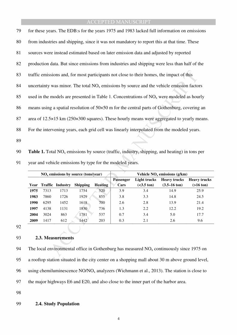
Table 1. Total NOx emissions by source (traffic, industry, shipping, and heating) in tons per 90

year and vehicle emissions by type for the modeled years. 91

NOx emissions by source (tons/year) Vehicle NOx emissions (g/km)

Year Traffic Industry Shipping Heating

Passenger

Cars

Light trucks

(<3.5 ton)

Heavy trucks

(3.5–16 ton)

Heavy trucks

(>16 ton)

1975 7313 1713 1754 520 3.9 3.4 14.9 25.9

1983 7860 1726 1929 855 3.8 3.3 14.8 24.5

1990 6295 1452 1618 700 2.6 2.8 13.9 21.4

1997 4138 1131 1830 736 1.3 2.2 12.2 19.2

2004 3024 863 1781 537 0.7 3.4 5.0 17.7

2009 1417 612 1442 203 0.3 2.1 2.6 9.6

92

2.3. Measurements 93

The local environmental office in Gothenburg has measured NOx continuously since 1975 on 94

a rooftop station situated in the city center on a shopping mall about 30 m above ground level, 95

using chemiluminescence NO/NOx analyzers (Wichmann et al., 2013). The station is close to 96

the major highways E6 and E20, and also close to the inner part of the harbor area. 97

98

2.4. Study Population 99

MA

NU

SC

RIP

T

AC

CE

PTE

D

ACCEPTED MANUSCRIPT

5

We estimated residential exposure to NOx, using the dispersion model mentioned above, in a 100

population-based cohort of men in Gothenburg. The population was that of the Primary 101

Prevention Study (PPS), consisting of 7494 men in Gothenburg, born 1915–1925, from a 102

random sample of 10 000 men (participation rate 75%). They were enrolled for medical 103

examination and identification of cardiovascular risk factors in 1970–1973 (Wilhelmsen et al., 104

1972). For all men participating in the screening, individual yearly addresses were retrieved 105

from 1970 to 2007 (or until death/emigration). For the years 1970–1978 addresses were 106

retrieved from the National Archives, and from 1978 and onward from Statistics Sweden. 107

A small number of recruited participants (n=50) died before the start of our study period 108

(1973) or had no address information in any register. Some had moved away from 109

Gothenburg prior to the study start. A flowchart of inclusion/exclusion of the cohort 110

participants from one year to the other is available in the electronic supplement (Fig. S1). 111

From Statistics Sweden we obtained information on the number of people living within 100-112

meter squares for the whole population of Gothenburg for the years 1975, 1990, and 2005. 113

This coarser geodata set was used to investigate whether our cohort participants were 114

representative of the whole population. 115

116

2.5. Geocoding of Addresses 117

Most addresses from Statistics Sweden were automatically geocoded, and the addresses from 118

the National Archives were geocoded by SWECO Position AB, Gothenburg, Sweden. The 119

geocoded coordinates used were at the entrance of the property for single houses, and for 120

apartment complexes with multiple entrances, each individual entranceway was used. This 121

gives a very high precision when using the 50-meter squares for the NOx modeling. For the 122

years 1973 and 1974 the NOx concentration levels for 1975 were used. 123

MA

NU

SC

RIP

T

AC

CE

PTE

D

ACCEPTED MANUSCRIPT

6

A number of addresses could not be geocoded automatically due to spelling errors, change of 124

street name over time, or insufficient information (e.g., post box address). These were 125

manually checked and corrected, if possible. In cases where buildings or roads had changed 126

addresses these were located and assigned coordinates using old city maps in the city 127

archives. In some cases the address information for certain years was inadequate, or located 128

outside the Gothenburg region, and no NOx levels could be assigned. The border of the 129

modeled area cut through some relatively populated areas. Using a model calculation for the 130

year 1990 covering a larger area, we were able to assign NOx exposure to some participants’ 131

addresses just outside the modeled area with a high degree of certainty. Participants living just 132

outside the border (about 200 m or less outside) were assigned an NOx value if the value of a 133

participant’s address just inside the main area differed by less than 0.2 µg m3 in the year 1990. 134

This resulted in about 6% more addresses with NOx values (8943 exposure years). 135

Over the whole study period, 1973 to 2007, 160 568 address years were geocoded. Out of 136

these address years, 146 675 were assigned a NOx value (91%). At the start of the study 6946 137

participants were still alive and residing in the Gothenburg area, and we could model 138

exposure for 6563 participants (94.5%). 139

140

2.6. Data Analysis 141

The geocoded data (addresses and modeled NOx levels) were imported into QGIS version 142

2.4.0-Chugiak (Quantum GIS Development Team, 2014) and overlay analyses were 143

performed using the function join attributes by location. Descriptive statistics for NOx were 144

calculated. Exposure contrasts (defined as the ratio between the 4th and 1st quartiles) were 145

calculated. Linear associations between continuous variables were assessed by the Pearson 146

correlation coefficient and the R2 value. To investigate whether relocation patterns affected 147

the exposure trends, we analyzed the differences between NOx exposure the first year at their 148

MA

NU

SC

RIP

T

AC

CE

PTE

D

ACCEPTED MANUSCRIPT

7

new address, and the same year at the old address (as if they had resided at the old address 149

another year). The mean difference was tested for the whole period and for three time periods 150

(1974–1983, 1984–1993, and 1994–2007), and for three different age groups (49–59, 60–69, 151

and 70–92) using the t-test. 152

153

3. RESULTS 154

Maps of the modeled NOx values and the distribution of the cohort members’ homes are 155

presented in Fig. 1 for three selected years, 1975, 1990, and 2004, representing an early year, 156

the middle of the study period, and a year at the end. In the electronic supplement (Fig. S2) a 157

descriptive map over different areas of Gothenburg (residential/industrial etc.) is available. 158

159

160

Fig. 1. Modeled NOx values for three selected years and locations of the participants 161

addresses (dark blue dots), illustrating the declining NOx trend over time and the diminishing 162

population in the cohort (1975 N=6283, 1990 N=4133, and 2004 N=1710). 163

164

3.1. Time Trends, Spatial Distribution and Exposure Contrast 165

The median levels of NOx at the participants’ homes increased in the beginning to the highest 166

level, 43.9 µg m-3, in 1983, and then declined to 16.6 µg m-3 in 2007 (Fig. 2). The median 167

NOx levels for the whole modeled area (global median) followed the same trend over time as 168

MA

NU

SC

RIP

T

AC

CE

PTE

D

ACCEPTED MANUSCRIPT

8

the levels at the residential addresses and were on average 74% of the median levels at the 169

participants’ residences (Fig. 2). The levels at the central monitoring station were always 170

higher than the median residential levels (see Fig. S3 in the supplement), but the temporal 171

correlation was high (rp=0.87). The yearly modeled concentration for the location of the 172

monitoring station also agreed well with the continuous measurements, (N=5, rp=0.98), 173

although the modeled concentrations were lower in the 2000s. 174

The median levels for the whole population for the years 1975, 1990, and 2004 (using the 175

population of 2005) were 37.7 µg m-3, 34.8 µg m-3, and 22.1 µg m-3, respectively (Fig. 2). The 176

corresponding median levels for the cohort for these years were 37.7 µg m-3, 32.6 µg m-3, and 177

20.7 µg m-3. 178

The changes in source emissions over time (Table 1, N=6 for each emission source) and 179

median exposures among the participants were highly correlated with the traffic and industry 180

emissions (rp=0.98 and 0.97, respectively) (Fig. S4 in the supplement). For shipping and 181

heating emissions, the correlations were lower, in the range of 0.6–0.7. For the long-range 182

contribution, data on NO2 from the rural background station Råö were available from 1982 183

(Sjöberg et al., 2013). The yearly mean levels of NO2 at this station decreased from around 10 184

µg m-3 in 1982 to about 5 µg m-3 in 2007 (see Fig. S5 in the supplement). The long-range 185

contribution of NO2 to the participants’ NOx levels was on average about 20%. 186

187

MA

NU

SC

RIP

T

AC

CE

PTE

D

ACCEPTED MANUSCRIPT

9

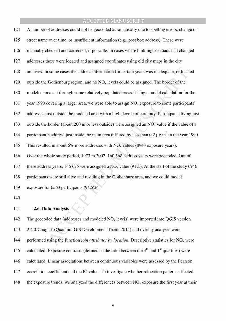
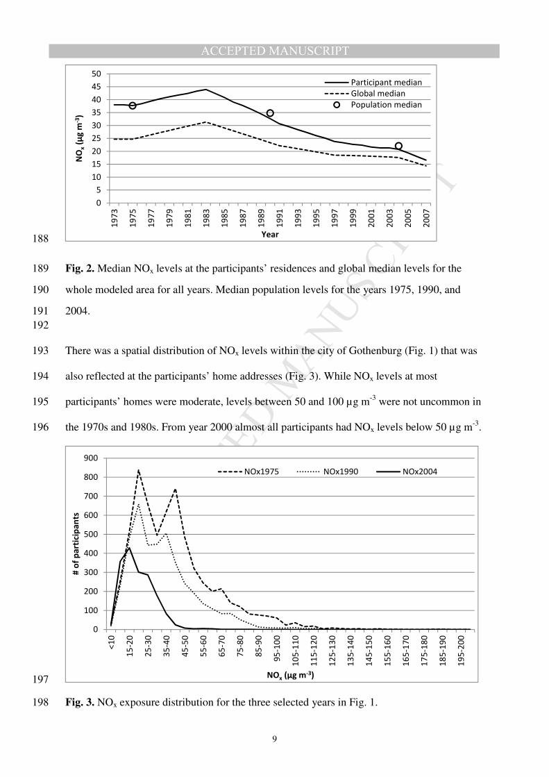
188

Fig. 2. Median NOx levels at the participants’ residences and global median levels for the 189

whole modeled area for all years. Median population levels for the years 1975, 1990, and 190

2004. 191

192

There was a spatial distribution of NOx levels within the city of Gothenburg (Fig. 1) that was 193

also reflected at the participants’ home addresses (Fig. 3). While NOx levels at most 194

participants’ homes were moderate, levels between 50 and 100 µg m-3 were not uncommon in 195

the 1970s and 1980s. From year 2000 almost all participants had NOx levels below 50 µg m-3. 196

197

Fig. 3. NOx exposure distribution for the three selected years in Fig. 1. 198

0

5

10

15

20

25

30

35

40

45

50

19

73

19

75

19

77

19

79

19

81

19

83

19

85

19

87

19

89

19

91

19

93

19

95

19

97

19

99

20

01

20

03

20

05

20

07

NO

x(µ

g m

-3)

Year

Participant median

Global median

Population median

0

100

200

300

400

500

600

700

800

900

<1

0

15

-20

25

-30

35

-40

45

-50

55

-60

65

-70

75

-80

85

-90

95

-10

0

10

5-1

10

11

5-1

20

12

5-1

30

13

5-1

40

14

5-1

50

15

5-1

60

16

5-1

70

17

5-1

80

18

5-1

90

19

5-2

00

# o

f p

art

icip

an

ts

NOx (µg m-3)

NOx1975 NOx1990 NOx2004

MA

NU

SC

RIP

T

AC

CE

PTE

D

ACCEPTED MANUSCRIPT

10

199

The distribution in exposure levels between those who were exposed to the highest NOx levels 200

and those exposed to the lowest can be expressed as the quartile contrast, that is, the mean in 201

the highest quartile divided by the mean in the lowest quartile (Q4/Q1). In this study, the 202

mean contrast was 3.5 (range 2.6–4.1), and fairly constant over time, with a slight decrease 203

from year 2000 (Fig. 4). The IQR range per year is also presented in Fig. 4, and the mean 204

value over the whole period was 22.8 µg m-3. Expressed in µg m-3 of NOx, the exposure 205

contrast was, however, much larger at the beginning of the period (50–60 µg m-3) than at the 206

end (20–30 µg m-3). The contrast between the 95th and the 5th percentile was on average 4.9 207

(range 3.1–5.7) and followed the same trend over time as the quartile contrast. 208

209

210

Fig. 4. Mean levels within the highest and lowest quartile (Q4 and Q1 respectively), inter 211

quartile range (IQR), and exposure contrast within the cohort. 212

213

3.2. Participant’s Relocation Patterns 214

Of all the 6946 participants, about 50% (3491) resided at the same address during the whole 215

study period, or until they died. About 30% moved once, 12% moved twice, and 7% moved 216

three or more times, giving a sum of 5703 changes of address. Among those who moved, 217

77.5% went from one address within the modeled area to another address within the modeled 218

MA

NU

SC

RIP

T

AC

CE

PTE

D

ACCEPTED MANUSCRIPT

11

area, 10.5% moved out of the modeled area, 5.4% moved into the modeled area, and 6.5% 219

moved from one location outside to another location outside of the modeled area. On average, 220

3.9% of the participants relocated each year (range 2%–7%). 221

Some participants moved from a high exposure area to a low exposure area and vice versa, 222

while some of the movements changed the exposure little. To investigate whether relocation 223

patterns affected the exposure trends, we analyzed the differences in NOx between the old 224

address the year after a participant moved and the NOx level the first year at their new 225

address. Participants relocating did not change the exposure systematically over time, mean 226

difference due to relocation 0.36 µg m-3 (95 % C.I. -0.43–1.16 µg m-3, P= 0,37), but 23% 227

moved to an address with at least 10 µg m-3 higher NOx level and 24% to an address with at 228

least 10 µg m-3 lower NOx level (Fig. 5). We found a statistical significant trend (p<0.001) 229

that more relocations were made into areas with higher NOx levels for the period 1984–1993 230

(mean difference 2.9 µg m-3, 95 % C.I. 2.3–4.6 µg m-3), while for the previous ten years, 231

moves were more often to cleaner areas, but non-significant, and the last period (1994–2007) 232

no clear trends were found. When analyzing relocation patterns by age groups instead, we 233

found a significant effect of relocations towards more polluted areas (p=0.008) for the age 234

group 70–92 with a mean difference of 1.41 µg m-3 (95 % C.I. 0.4–2.5 µg m-3), while for 235

younger ages the differences were small and non-significant. 236

237

MA

NU

SC

RIP

T

AC

CE

PTE

D

ACCEPTED MANUSCRIPT

12

238

Fig. 5. The effect on NOx exposure due to participant relocation: (a) A box and whiskers plot 239

with 5th and 95th percentiles shown as black dots for the old address and the new address, and 240

for the difference between old minus new address. (b) The frequency distribution of the NOx 241

differences. 242

243

3.3. Historical Dispersion Modeling vs Back Extrapolation 244

How far back in time is a spatial model valid? By using the dispersion model for the year 245

2009 and the time trend at the central monitoring station, the back-extrapolated NOx levels at 246

the participants’ homes were compared to the “true” levels for the previous modeled years, 247

2004, 1997, and 1975, with the participants’ correct addresses (Fig. 6). For the year 2004, the 248

back extrapolation fitted the dispersion model well (R2=0.98), with only a very slight 249

underestimation. For the year 1997, however, the underestimation increased, and the 250

scattering compared to the dispersion model increased (R2=0.69). Going further back in time, 251

the scattering increased more and for the year 1975; R2 was 0.60. If participant movement was 252

MA

NU

SC

RIP

T

AC

CE

PTE

D

ACCEPTED MANUSCRIPT

13

not taken into account (i.e., if the most recent known address was used for the whole time 253

period) the scattering increased even more (data not shown). 254

255

256

Fig. 6. Comparison of NOx levels between dispersion models for the years 2004, 1997, and 257

1975 and corresponding back extrapolation based on the dispersion model of 2009. 258

259

4. DISCUSSION 260

4.1. Time trends 261

The general reduction of NOx levels over time was highly correlated with all major sources of 262

emissions (Table 1) as well as the rural background levels. Even though the total traffic within 263

the city has increased by 60% during the study period, according to the Gothenburg traffic 264

office, the reduction in NOx levels at the participants’ homes over time was mainly achieved 265

by the 81% reduction in NOx emission from traffic. Also industry and heating emissions were 266

reduced substantially (64 and 67 % respectively), but their absolute contributions were 267

smaller. The NO2 reduction of about 50 % at the Råö background station from 1982 to 2007 268

also gave a small contribution, while the reduction in emissions from shipping (the second 269

largest source) was only minor (18%). Traffic planning in Gothenburg has also for the last 30 270

years been aimed at reducing traffic in the city center and in housing areas, and promoting 271

public transportation. Traffic has been directed to some major traffic routes (arterial links) 272

through and around the city. The only places with increased NOx within the city are along 273

MA

NU

SC

RIP

T

AC

CE

PTE

D

ACCEPTED MANUSCRIPT

14

some parts of these arterial links around and through the city, but these are not close to major 274

housing areas. Since the NOx concentrations over time among our participants were similar to 275

those for the whole population in the years 1975, 1990, and 2004, we consider that the 276

exposure levels and trends over time for the participants can be generalized to the whole 277

population. Similar trends of general reductions of NOx have been seen in several other cities, 278

such as London, Paris, Rome, and Stockholm (Carslaw et al., 2011). 279

280

4.2. Exposure Contrasts 281

A large difference (contrast) in exposure between participants is valuable in epidemiological 282

studies aimed at revealing possible differences in health outcomes (Nieuwenhuijsen, 2003; 283

Rappaport and Kupper, 2008). In our cohort, the contrast was relatively high over the years, 284

with an average ratio Q4/Q1 of 3.5, and was only reduced somewhat in the last ten years. A 285

stable contrast over time was also found in a study in the Netherlands (Eeftens et al., 2011). 286

The 95th to 5th percentile contrast in our study was on average 4.9 (range 3.1-5.7), over 5 for 287

the first 26 years and below 4 only in the last six years of the study. This can be compared to 288

the cities in the Expolis study (de Hoogh et al., 2014) where the mean 95th to 5th percentile 289

contrast for NO2 was 2.5 for the LUR models and 2.3 for the dispersion models. Notable in 290

the Expolis is that the highest contrasts were found in the Swedish cities Umeå (4.0 for the 291

LUR model) and Stockholm (5.5 for the dispersion model). 292

293

4.3. Participant’s Relocation Patterns 294

When participants move from one address to another, they can move to a location with higher 295

or lower air pollution levels than before, or to an address with similar levels. Participant 296

relocation can potentially influence the distribution of NOx exposure, depending on whether 297

they tend to move from the city center to suburban areas or vice versa. In this study, some 298

MA

NU

SC

RIP

T

AC

CE

PTE

D

ACCEPTED MANUSCRIPT

15

cohort members moved towards cleaner areas and some in the opposite direction, while most 299

changes due to relocation were moderate (Fig. 5). The relocation patterns did not change the 300

exposure for the whole study period, but when analyzing different time periods, we found a 301

statistical significant trend that more moves were made into areas with higher NOx levels for 302

the period 1984–1993. For the previous ten years, relocations were more often to cleaner 303

areas, but the difference was non-significant. For relocation patterns by age groups, we only 304

found a significant effect of relocations towards more polluted areas in the oldest age group, 305

70–92 years old. The tendencies in relocation patterns are in agreement of how people in 306

Sweden tended to move during those years, with a strong “green” movement around 1980, 307

and also that elderly people tend to move from single family homes in the suburbs to more 308

convenient apartments closer to services such as health care facilities (Altoff, 2014). These 309

patterns might be different in other parts of the world. It has been suggested that people who 310

increase their exposure to air pollution when changing residence run a higher risk than those 311

whose exposure is stable at the higher exposure level (Hart et al., 2013). In the present study 312

about half the population moved during the study period, and half of those who did so moved 313

to an address with at least somewhat higher NOx. 314

315

4.4. Dispersion Model and Model Accuracy 316

As mentioned earlier, there are several different methods available for estimating population 317

exposure. If a good quality emission database is available, dispersion models perform well 318

and are deemed as good as or better than other commonly used methods (Beelen et al., 2010). 319

When working with historical data, as in this retrospective cohort study, dispersion models 320

have an advantage over other models such as LUR models, when historical emission 321

databases are available, making it possible to estimate historical pollution levels with equally 322

good accuracy over time, as long as the emission database and meteorological data is of 323

MA

NU

SC

RIP

T

AC

CE

PTE

D

ACCEPTED MANUSCRIPT

16

sufficient quality. The LUR model, on the other hand, is based on repeated measurements 324

spread out over the area of interest during a specific year, and the influence of emission 325

sources, land use, population density, altitude, meteorology, and so forth are estimated 326

through a regression model. LUR model estimates are often comparable with dispersion 327

models for the year the LUR was created. A high correlation (rp=0.77) between LUR and 328

dispersion modeling was found in two French metropolitan areas (Sellier et al., 2014), while a 329

moderate agreement (r=0.55) was found in the Netherlands (Beelen et al., 2010). 330

In the present work, the dispersion model performed well when comparing the yearly mean 331

NOx values with the city’s official central monitoring station over the years (Fig. S1). In 1991 332

another monitoring station, Järntorget, was established, and in 1996 the Gårda station started. 333

Yearly mean values of NOx from these stations agree well with the modeled values as well 334

(data not shown). The good agreement between the city monitoring data and the model 335

estimates suggests that the dispersion model is valid for health effect studies in Gothenburg. 336

337

4.5. Historical Dispersion Models vs Back Extrapolation 338

From our results, back extrapolation based on a dispersion model for a recent year, adjusting 339

for long-term trends at an urban background station, showed high accuracy when going back 340

5 to 7 years, with only a very slight underestimation. However, when going further back in 341

time, the underestimation remained, and the scattering increased, suggesting that the historical 342

time trends at the urban background station were not valid for all areas within our modeled 343

area. The same results were found if we chose another modeled year than 2009 as the 344

baseline. The closest modeled years (back or forward 5 to 7 years in time) showed valid 345

results, but when going one step further (12 to 14 years) the scattering increased (data not 346

shown). Using results from a current model (dispersion or LUR) to estimate historical 347

exposures would create large uncertainties when going far back in time (e.g., 35 years in our 348

MA

NU

SC

RIP

T

AC

CE

PTE

D

ACCEPTED MANUSCRIPT

17

case). Our analysis was made using historically correct addresses for all years. If participant 349

relocation was not taken into account (i.e., if the most recent known address was used for the 350

whole time period) the scattering due to misclassification increased even more (data not 351

shown). In our cohort, about 50% of the participants moved at least once after inclusion at 50 352

years of age. Our results suggest that without historical spatial models and without correct 353

historical participant addresses, there is considerable risk for misclassification of the exposure 354

when exposure is extrapolated back in time. Similar risk for misclassification will occur if 355

forward extrapolation is used. 356

A few other studies have investigated back or forward extrapolation of models with measured 357

concentrations. In the Netherlands, Eeftens et al. (2011) tested two LUR models for NO2, the 358

TRAPCA study for the years 1999–2000 and the TRACHEA for 2007, with measured NO2 359

levels for the same periods. They found good model prediction between the respective LUR 360

models and the measured NO2 for the other period (R2=0.77 and R2=0.81, with back and 361

forwards extrapolation, respectively). In a study in the United Kingdom, Gulliver et al. (2013) 362

created LUR models for the years 2001 and 2009 and compared to NO2 measurements for the 363

years 2009, 2001, and 1991. They found that the LUR models predicted moderately well R2 364

values from 0.54 to 0.66 for 2001 and from 0.57 to 0.62 for 2009. The back extrapolation of 365

the 2009 model to 1991 yielded R2=0.55, the 2001 model to 1991 yielded R2=0.49, and the 366

2009 model to 2001 yielded R2=0.41. Thus, in the UK study the extrapolation 18 years back 367

in time managed to maintain the same level of prediction; however, going back from 2009 to 368

2001, the prediction was clearly reduced. This illustrates the built-in variability and 369

uncertainty between different years. Some years (even far back in time) might correlate well, 370

while another year might not be representative (or typical). 371

372

4.6. Strengths and Limitations 373

MA

NU

SC

RIP

T

AC

CE

PTE

D

ACCEPTED MANUSCRIPT

18

Some of the strengths in this study are a long study period (35 years), inclusion of historical 374

emission databases for several years covering the investigated period and the high spatial 375

resolution (50-meter squares), and long-term history of the residential addresses of the cohort 376

participants. Limitations include that, while the cohort was shown to be representative of the 377

whole population, the cohort included only men, and they were in a restricted age group (48–378

94 years). As well, there were data missing for those who moved out of the modeled area. 379

380

4.7. Conclusions 381

NOx levels decreased substantially (more than two-fold) over a 35-year period, mainly due to 382

lower emissions from road traffic, but also due to reductions of emissions from industries and 383

residential heating. There was a considerable spatial contrast with a ratio between the highest 384

and lowest quartile means of 3.5 on average. In the 2000s, the ratio was slightly lower, but 385

around three. About 50% of the participants relocated at least once during the study. There 386

was a statistical significant increase in exposure due to relocation between the years 1984-387

1993, and also in the age group 70–92 years old, but the mean levels did not change 388

systematically for the whole study period. Of these changes of residence, nearly 50% resulted 389

in a positive or negative change in NOx exposure of >10 µg m-3, which is important to take 390

into account in epidemiological studies. Back extrapolation at residential addresses using the 391

time trend of a background monitoring station worked well 5 to 7 years back in time, but 392

extrapolation more than ten years back in time resulted in substantial scattering. 393

We have shown that relocation patterns affect individual exposure estimates, even though the 394

cohort mean is unaffected, and that back extrapolation can create substantial errors in long 395

term studies if not handled properly. These findings are important to take into account in long 396

term epidemiological studies since accurate exposure estimates are essential for correct risk 397

assessments. 398

MA

NU

SC

RIP

T

AC

CE

PTE

D

ACCEPTED MANUSCRIPT

19

399

400

5. ACKNOWLEDGEMENTS 401

We thank Jan Brandberg and Erik Bäck at the environmental office in Gothenburg for 402

providing the emission data and the dispersion modeling. The personnel at the Gothenburg 403

city archives are acknowledged for the help in locating old addresses. This study was funded 404

by the Swedish Research Council for Health, Working Life and Welfare (FORTE, application 405

number 2008-0406). 406

407

6. REFERENCES 408

Altoff, K., 2014. Demografi och flyttmönster i Västra Götaland 1990-2012 (in Swedish), 409

English title: Demographics and migration patterns in Västra Götaland 1990-2012. 410

Beelen, R., Voogt, M., Duyzer, J., Zandveld, P., Hoek, G., 2010. Comparison of the 411

performances of land use regression modelling and dispersion modelling in estimating 412

small-scale variations in long-term air pollution concentrations in a Dutch urban area. 413

Atmos. Environ. 44, 4614-4621. 414

Brook, R.D., Rajagopalan, S., Pope, C.A., Brook, J.R., Bhatnagar, A., Diez-Roux, A.V., 415

Holguin, F., Hong, Y.L., Luepker, R.V., Mittleman, M.A., Peters, A., Siscovick, D., Smith, 416

S.C., Whitsel, L., Kaufman, J.D., Amer Heart Assoc Council, E., Council Kidney 417

Cardiovasc, D., Council Nutr Phys Activity, M., 2010. Particulate Matter Air Pollution and 418

Cardiovascular Disease An Update to the Scientific Statement From the American Heart 419

Association. Circulation 121, 2331-2378. 420

Carslaw, D., Beevers, S., E., W., Williams, M., Tate, J., Murrells, T., Stedman, J., Li, Y., 421

Grice, S., Kent, A., Tsagatakis, I., 2011. Trends in NOx and NO2 emissions and ambient 422

measurements in the UK. Department for Environment, Food and Rural Affairs, London. 423

MA

NU

SC

RIP

T

AC

CE

PTE

D

ACCEPTED MANUSCRIPT

20

Cesaroni G, B.C., Gariazzo C, Stafoggia M, Sozzi R, Davoli M, Forastiere F, 2013. Long-424

Term Exposure to Urban Air Pollution and Mortality in a Cohort of More than a Million 425

Adults in Rome. Environ. Health Perspect. 121, 324–331. 426

de Hoogh, K., Korek, M., Vienneau, D., Keuken, M., Kukkonen, J., Nieuwenhuijsen, M.J., 427

Badaloni, C., Beelen, R., Bolignano, A., Cesaroni, G., Pradas, M.C., Cyrys, J., Douros, J., 428

Eeftens, M., Forastiere, F., Forsberg, B., Fuks, K., Gehring, U., Gryparis, A., Gulliver, J., 429

Hansell, A.L., Hoffmann, B., Johansson, C., Jonkers, S., Kangas, L., Katsouyanni, K., 430

Künzli, N., Lanki, T., Memmesheimer, M., Moussiopoulos, N., Modig, L., Pershagen, G., 431

Probst-Hensch, N., Schindler, C., Schikowski, T., Sugiri, D., Teixidó, O., Tsai, M.-Y., Yli-432

Tuomi, T., Brunekreef, B., Hoek, G., Bellander, T., 2014. Comparing land use regression 433

and dispersion modelling to assess residential exposure to ambient air pollution for 434

epidemiological studies. Environ. Int. 73, 382-392. 435

Dockery, D.W., Pope, C.A., Xu, X., Spengler, J.D., Ware, J.H., Fay, M.E., Ferris, B.G., 436

Speizer, F.E., 1993. An Association between Air Pollution and Mortality in Six U.S. 437

Cities. N. Engl. J. Med. 329, 1753-1759. 438

Eeftens, M., Beelen, R., Fischer, P., Brunekreef, B., Meliefste, K., Hoek, G., 2011. Stability 439

of measured and modelled spatial contrasts in NO2 over time. Occup. Environ. Med. 68, 440

765-770. 441

Filleul, L., Rondeau, V., Vandentorren, S., Le Moual, N., Cantagrel, A., Annesi-Maesano, I., 442

Charpin, D., Declercq, C., Neukirch, F., Paris, C., Vervloet, D., Brochard, P., Tessier, J.F., 443

Kauffmann, F., Baldi, I., 2005. Twenty five year mortality and air pollution: results from 444

the French PAARC survey. Occup. Environ. Med. 62, 453-460. 445

Gulliver, J., de Hoogh, K., Hansell, A., Vienneau, D., 2013. Development and Back-446

Extrapolation of NO2 Land Use Regression Models for Historic Exposure Assessment in 447

Great Britain. Environ. Sci. Technol. 47, 7804-7811. 448

Hart, J.E., Rimm, E.B., Rexrode, K.M., Laden, F., 2013. Changes in Traffic Exposure and the 449

Risk of Incident Myocardial Infarction and All-Cause Mortality. Epidemiology 24, 734-450

742. 451

MA

NU

SC

RIP

T

AC

CE

PTE

D

ACCEPTED MANUSCRIPT

21

Hoek, G., Krishnan, R.M., Beelen, R., Peters, A., Ostro, B., Brunekreef, B., Kaufman, J.D., 452

2013. Long-term air pollution exposure and cardio- respiratory mortality: a review. 453

Environ. Health 12. 454

Nieuwenhuijsen, M.J., 2003. Exposure assessment in occupational and environmental 455

epidemiology. Oxford University Press, New York, United States. 456

Pope, C.A., Thun, M.J., Namboodiri, M.M., Dockery, D.W., Evans, J.S., Speizer, F.E., Heath, 457

C.W., 1995. PARTICULATE AIR-POLLUTION AS A PREDICTOR OF MORTALITY 458

IN A PROSPECTIVE-STUDY OF US ADULTS. Am. J. Respir. Crit. Care Med. 151, 459

669-674. 460

Quantum GIS Development Team, 2014. Quantum GIS Geographic Information System. 461

Open Source Geospatial Foundation Project. 462

Rappaport, S.M., Kupper, L.L., 2008. Quantitative Exposure Assessment. Stephen Rappaport, 463

El Cerrito, CA, USA. 464

Sellier, Y., Galineau, J., Hulin, A., Caini, F., Marquis, N., Navel, V., Bottagisi, S., Giorgis-465

Allemand, L., Jacquier, C., Slama, R., Lepeule, J., 2014. Health effects of ambient air 466

pollution: Do different methods for estimating exposure lead to different results? Environ. 467

Int. 66, 165-173. 468

Sjöberg, K., Pihl Karlsson, G., Svensson, A., Wängberg, I., Brorström-Lundén, E., Hansson, 469

K., Potter, A., Rehngren, E., Sjöblom, A., Areskoug, H., Kreuger, J., Södergren, H., 470

Andersson, C., Holmin Fridell, S., Andersson, S., 2013. Nationell Miljöövervakning - Luft. 471

Data t.o.m. 2011 (English title: National Environmental Monitoring - Air. Data up to 472

2011). IVL Swedish Environmental Research Institute. 473

WHO, 2013. Review of evidence on health aspects of air pollution – REVIHAAP Project, 474

Copenhagen, Denmark. 475

Wichmann, J., Rosengren, A., Sjoberg, K., Barregard, L., Sallsten, G., 2013. Association 476

between Ambient Temperature and Acute Myocardial Infarction Hospitalisations in 477

Gothenburg, Sweden: 1985-2010. PLoS One 8. 478

MA

NU

SC

RIP

T

AC

CE

PTE

D

ACCEPTED MANUSCRIPT

22

Wilhelmsen, L., Tibblin, G., Werkö, L., 1972. A primary preventive study in Gothenburg, 479

Sweden. Prev. Med. 1, 153-160. 480

481

MA

NU

SC

RIP

T

AC

CE

PTE

D

ACCEPTED MANUSCRIPT

Highlights

• Traffic intensity increased 1973 to 2007, but NOx levels decreased considerably

• Within city exposure contrast remained substantial over the whole period

• Changes of residences resulted in a change of >10 µg/m3 NOx in 50% of cases

• Back extrapolation 5-7 years yielded fairly accurate residential NOx estimates

• Back extrapolation more than 10 years greatly increased misclassification

MA

NU

SC

RIP

T

AC

CE

PTE

D

ACCEPTED MANUSCRIPT

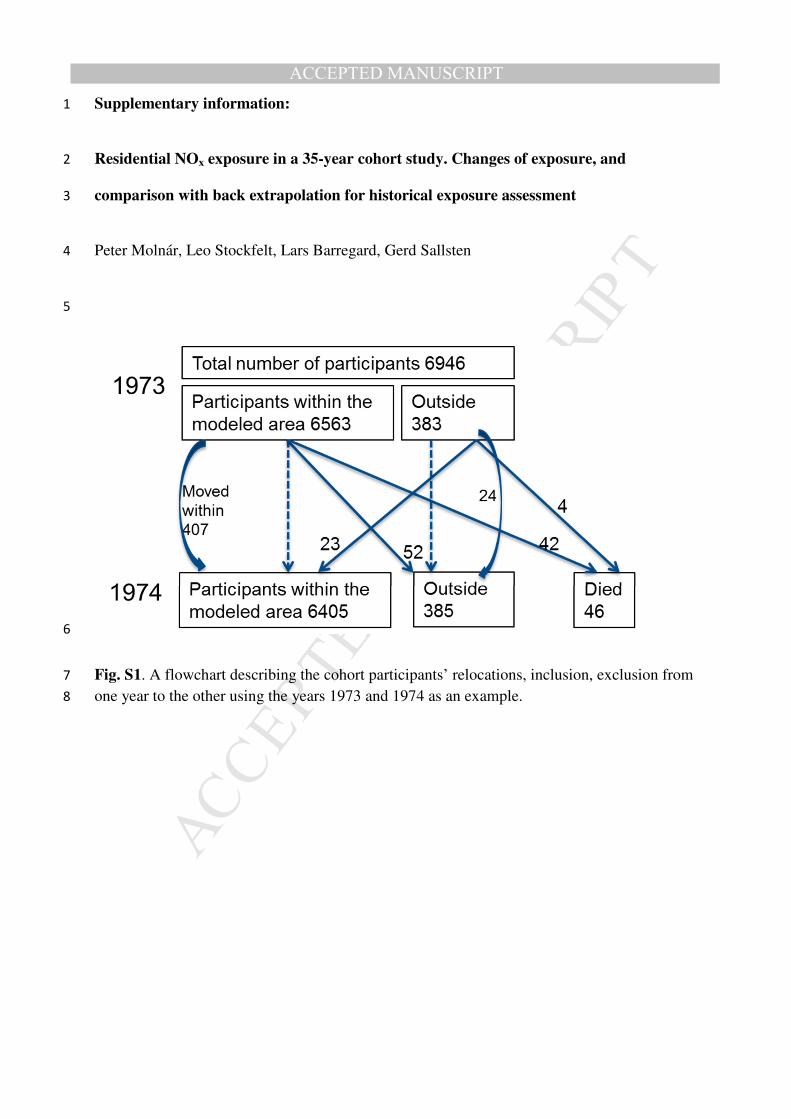
Supplementary information: 1

Residential NOx exposure in a 35-year cohort study. Changes of exposure, and 2

comparison with back extrapolation for historical exposure assessment 3

Peter Molnár, Leo Stockfelt, Lars Barregard, Gerd Sallsten 4

5

6

Fig. S1. A flowchart describing the cohort participants’ relocations, inclusion, exclusion from 7

one year to the other using the years 1973 and 1974 as an example. 8

MA

NU

SC

RIP

T

AC

CE

PTE

D

ACCEPTED MANUSCRIPT

9

10

Fig. S2. A descriptive map over Gothenburg. Grey areas are industrial, orange areas are residential areas, green areas are forests, light yellow areas are open 11

land (farm land, meadows etc.), and blue areas are water (ocean, lakes and rivers). The red buildings are public buildings (hospitals, university buildings, 12

libraries, sport venues etc.).13

MA

NU

SC

RIP

T

AC

CE

PTE

D

ACCEPTED MANUSCRIPT

14

Fig. S3. Measured yearly mean NOx levels at Gothenburg’s official rooftop station Femman 15

and the modeled levels recalculated to the same height (30 m), together with the mean levels 16

at the participants’ homes. 17

18

19

Fig. S4. Mean NOx exposure vs NOx emissions by source. 20

21

0

20

40

60

80

100

120

140

19

73

19

75

19

77

19

79

19

81

19

83

19

85

19

87

19

89

19

91

19

93

19

95

19

97

19

99

20

01

20

03

20

05

20

07

20

09

NO

x (

µg

/m3

)

Year

Femman modeled @30m

Femman Measured @30m

Participant Mean

R² = 0.9633

R² = 0.9504

R² = 0.3847

R² = 0.5027

0

1000

2000

3000

4000

5000

6000

7000

8000

9000

0 10 20 30 40 50

NO

xe

mis

sio

ns

by

so

urc

e (

ton

s /y

ea

r)

Mean exposure NOx (µg m-3)

Traffic

Industry

Shipping

Heating

MA

NU

SC

RIP

T

AC

CE

PTE

D

ACCEPTED MANUSCRIPT

22

Fig. S5. Time trends of rural background NO2 and participant mean NOx. 23

0

2

4

6

8

10

12

0

10

20

30

40

50

60

1975 1980 1985 1990 1995 2000 2005 2010 2015

NO

2a

t R

åö

(µ

g m

-3)

NO

xe

xp

osu

re (

µg

m-3

)

Year

Participant Mean

NO2 Råö