Residence Time Distribution of Mixing Based on Mathematical ...

The University of AkronIdeaExchange@UAkron

Honors Research Projects The Dr. Gary B. and Pamela S. Williams HonorsCollege

Spring 2018

Residence Time Distribution of Mixing Based onMathematical ModelingMichelle [email protected]

Please take a moment to share how this work helps you through this survey. Your feedback will beimportant as we plan further development of our repository.Follow this and additional works at: http://ideaexchange.uakron.edu/honors_research_projects

Part of the Other Chemical Engineering Commons

This Honors Research Project is brought to you for free and open access by The Dr. Gary B. and Pamela S. WilliamsHonors College at IdeaExchange@UAkron, the institutional repository of The University of Akron in Akron, Ohio,USA. It has been accepted for inclusion in Honors Research Projects by an authorized administrator ofIdeaExchange@UAkron. For more information, please contact [email protected], [email protected].

Recommended CitationAyers, Michelle, "Residence Time Distribution of Mixing Based on Mathematical Modeling" (2018). HonorsResearch Projects. 604.http://ideaexchange.uakron.edu/honors_research_projects/604

1

ResidenceTimeDistributionofMixingBasedonMathematicalModeling

MichelleAyers

Department of Chemical and Biomolecular Engineering

Honors Research Project

Submitted to

The Honors College

Approved: Accepted: ______________________ Date ________ __________________ Date _________ Honors Project Sponsor (signed) Department Head (signed) ______________________________ _______________________ Honors Project Sponsor (printed) Department Head (printed) ______________________ Date _______ __________________ Date ________ Reader (signed) Honors Faculty Advisor (signed) _________________________ _____________________________ Reader (printed) Honors Faculty Advisor (printed) ______________________ Date _______ __________________ Date _________ Reader (signed) Dean, Honors College _________________________________ Reader (printed)

2

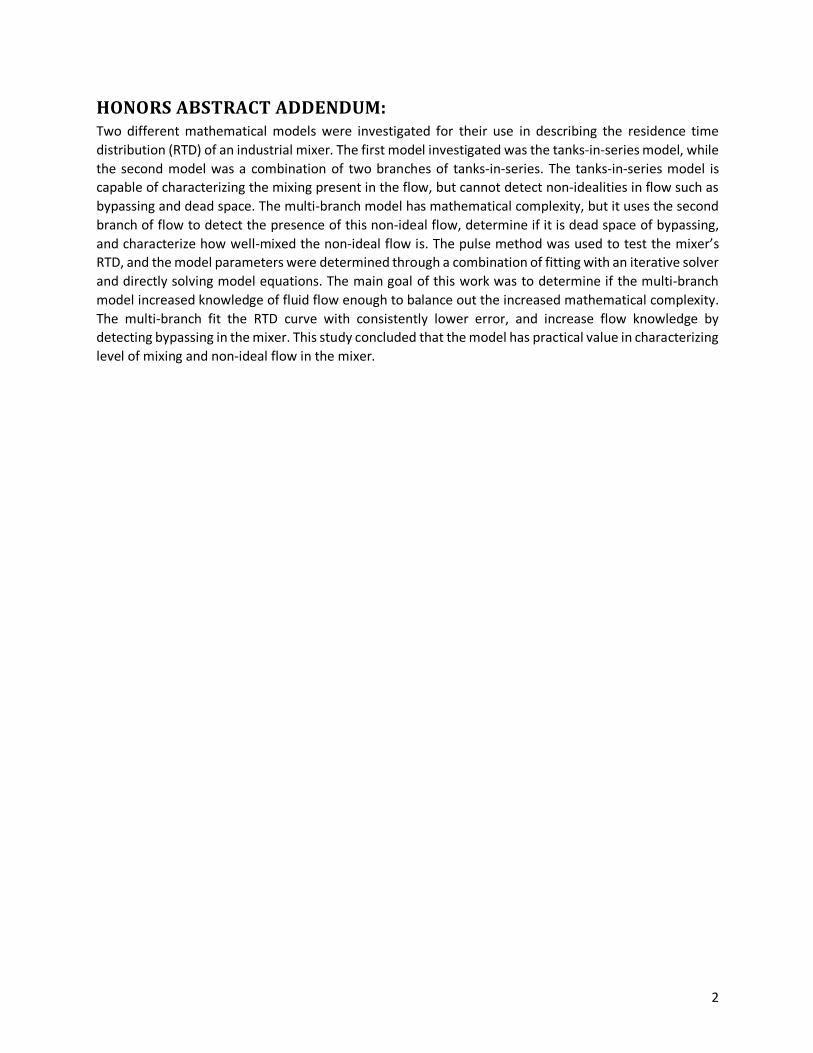
HONORSABSTRACTADDENDUM:Two different mathematical models were investigated for their use in describing the residence time distribution (RTD) of an industrial mixer. The first model investigated was the tanks-in-series model, while the second model was a combination of two branches of tanks-in-series. The tanks-in-series model is capable of characterizing the mixing present in the flow, but cannot detect non-idealities in flow such as bypassing and dead space. The multi-branch model has mathematical complexity, but it uses the second branch of flow to detect the presence of this non-ideal flow, determine if it is dead space of bypassing, and characterize how well-mixed the non-ideal flow is. The pulse method was used to test the mixer’s RTD, and the model parameters were determined through a combination of fitting with an iterative solver and directly solving model equations. The main goal of this work was to determine if the multi-branch model increased knowledge of fluid flow enough to balance out the increased mathematical complexity. The multi-branch fit the RTD curve with consistently lower error, and increase flow knowledge by detecting bypassing in the mixer. This study concluded that the model has practical value in characterizing level of mixing and non-ideal flow in the mixer.

3

CONTENTSExecutive Summary ................................................................................................................................. 4

Problem .......................................................................................................................................... 4

Results ............................................................................................................................................ 4

Conclusions ..................................................................................................................................... 4

Broader Implications ....................................................................................................................... 4

Recommendations .......................................................................................................................... 5

Introduction ............................................................................................................................................ 6

Background ............................................................................................................................................. 6

Experimental Methods .......................................................................................................................... 10

Data and Results ................................................................................................................................... 12

Test runs: ...................................................................................................................................... 12

Tanks-in-Series: ............................................................................................................................. 13

Multi-Branch Model Parameters:................................................................................................... 14

Analysis of Model Error: ................................................................................................................ 14

Discussion and Analysis ......................................................................................................................... 16

Conclusions and Recommendations ...................................................................................................... 17

References ............................................................................................................................................ 19

Appendix A: Flow Condition Testing ...................................................................................................... 20

Dye Injection Level Comparison: .................................................................................................... 20

RTD Graphs: .................................................................................................................................. 20

Tanks-in-Series Comparison: .......................................................................................................... 21

Multi-Branch Model Comparison: .................................................................................................. 22

Flow Rate Comparison: .................................................................................................................. 22

RTD Graphs: .................................................................................................................................. 23

Tanks in Series Results: .................................................................................................................. 24

Multi-Branch Model Results: ......................................................................................................... 24

Mixing Speed Comparison: ............................................................................................................ 25

RTD Charts: ................................................................................................................................... 25

Tanks-in-Series Results: ................................................................................................................. 26

Multi-Branch Model Results: ......................................................................................................... 28

4

EXECUTIVESUMMARYProblemResidence time distribution (RTD) is an important concept when describing flow in non-ideal reactors and vessels. RTD curves are valuable when sizing reactors and determining product quality when real vessels fail to reflect ideal flow assumptions. Often, the RTD of real vessels is modeled as combinations of ideal reactors to provide a mathematical way of describing the flow. One model often used is the tanks-in-series (TIS) model, which models vessels as n CSTRs in series. It is a single-parameter model and the parameter n can be easily solved analytically. It is able to describe the level of mixing in a vessel, but is unable to describe non-idealities in flow such as bypassing and dead space. The main parameters characterizing TIS results are the mean residence time, τm, the standard deviation, σ, and the number of tanks in series, n. Himmelblau and Bischoff proposed a model consisting of two branches in series in an effort to describe the presence of dead space or bypassing in a vessel as well as the level of mixing in the main flow and dead space or bypassing flow. The model has parameters for the number of tanks in series in each branch (n and m for the side branch and main branch, respectively), the ratio of residence time between the main branch and side branch (α), and the fraction of fluid to the non-ideal branch of flow (f). This makes the model complex mathematically, and requires it to be fitted with an iterative solver rather than being solved analytically. The purpose of this project was to investigate the use of this higher-parameter, multi-branch model and compare to the results for the TIS model to determine if the increase in mathematical complexity is worth it to better understand the flow behavior through an inline mixer.

ResultsA set of flow parameters were defined to test the mixer for repeatability and compare the level of error of the TIS and multi-branch models. The TIS results for the mixer showed a τm of 68.4±3.77 s, σ of 22.8±1.28 s and n of 9.16±1.52. The multi-branch model produced parameters α = 1.49±0.24, f = 0.280±0.074, n = 20.2±4.4, and m = 12.9±2.5. When comparing error qualitatively, the multi-branch model’s graph of residuals showed consistently lower magnitude of error with more random scatter in the error, indicating a better fit for non-linear models. Quantitatively, the error between the models was compared using the sum squared error (SSE), the mean squared error (MSE), and the integrated absolute error (IAE). The TIS model produced SSE, MSE, and IAE results of 5.22±2.37, 0.0129±0.00153, and 0.191±0.042. The multi-branch model produced SSE, MSE, and IAE of 0.456±0.148, 0.00116±0.00038, and 0.0618±0.0092.

ConclusionsUpon testing, the multi-branch model from Himmelblau and Bischoff showed consistently lower error from the experimental RTD results. The results for SSE and MSE were an order of magnitude smaller for the multi-branch model compared to the TIS model. The IAE result for the multi-branch model was about 70% smaller than the IAE for the TIS model. The TIS model also showed a higher number of tanks in series to describe the mixing seen in the main fluid in the vessel, with 28% of fluid bypassing the vessel at a residence time 49% faster than the main residence time. The amount of tanks in the bypassing branch of flow was 20.2, showing a high level of mixing in this bypassing flow. Overall, the multi-branch model showed that it was worth the increased mathematical complexity to better understand the flow behavior through the mixer tested.

BroaderImplicationsCompleting this project allowed me to gain proficiency in understanding residence time distribution, a topic not discussed in Chemical Reactions Engineering where it most applies. It has also helped me to develop a better understanding of the capabilities of Microsoft Excel’s solver and how to change the settings to avoid trivial solutions and ensure that the solved answer is a true, global minimum. This project

5

involved designing my own plan of experiments, experimental setup, and testing method, as this work had not been done much at the facility where the research was conducted. Leading this project has given me many opportunities to grow as both a leader and as an engineer. This project was the largest project I participated in during my time at Bridgestone Americas Center for Research and Technology, and as the project leader it was my largest individual project-related responsibility. Through leadership of this project, I gained experience in setting a project timeline and task list, and adapting this timeline as needed as the project progressed. I also had to learn how to balance attending to detail work and individual tasks while keeping my eye on all of the pieces in motion and seeing how it all comes together. Several important lessons this project has taught me include how to start a project with the end in mind; knowing the value of the project from the very beginning; and the importance of maintaining focus on the end goal when the course or direction of the project needed adapted to address new challenges. As a result of my work on this project part-time as part of my school work, I gained experience balancing school and work obligations, and connecting my school work to real-world, relevant information.

RecommendationsOne recommendation for further work is to test the residence time distribution of other pieces of equipment to further determine if the multi-branch model can be useful for varying flow systems. Although it showed increase in flow knowledge for the system tested using that model, it is important to investigate if this trend holds true for other pieces of equipment to validate the model’s overall worth. Another recommendation is to validate the RTD results obtained in this test using the step method of RTD testing. This type of testing is usually used to validate results obtained from the pulse method to ensure that they accurately represent the RTD of the equipment.

6

INTRODUCTIONResidence time distribution (RTD) is an important concept in reactions and process controls engineering. In process controls engineering, the RTD of a piece of equipment plays a roll in what transfer functions model the equipment’s responses to both disturbance and set point changes. This is essential in designing proper control systems. In reactions engineering, RTD can be used to size reactors, determine quality of product, and determine what type of flow is seen in a process vessel (e.g. CSTR vs. plug flow). RTD can also be used to diagnose problems in reactors and vessels such as the presence of dead space and bypassing in the fluid flow, both of which can effect reactor conversion. In the field of polymers, RTD has been studied for its relation to molecular weight distribution (MWD) in polymerization and functionalization reactions (Cozewith & Squire, 2000). In an effort to better understand how RTD can be used to diagnose and predict process behavior, the RTD of reactors is usually modeled as combinations of ideal reactors. Many models have been suggested to accomplish this. The most common single-parameter models used for tubular reactors are tanks-in-series and diffusion models. For stirred tanks, some single-parameters models include CSTR with dead space and CSTR with bypass. However, in many cases, higher parameter models are needed to fully understand the non-idealities of flow present, such as tanks-in-series with bypass or dead space. Levenspiel’s Chemical Reactions Engineering presents many combination models to represent non-ideal flow (1972). Unfortunately, there is frequently a trade-off when increasing model parameters between mathematical difficulty in solving and model accuracy. There is also difficulty in ensuring that the model still retains physical significance as parameters are increased. For this study, a multi-parameter model from Process Analysis and Simulation by Himmelblau and Bischoff (1968) was investigated to determine its ability to model the RTD of an industrial mixer by detecting dead space and bypassing while also characterizing the amount of mixing in the flow by determining the number of tanks-in-series the mixer reflects overall.

BACKGROUNDWhen studying fluid flow through a vessel, plug flow or perfect mixing is usually assumed for ease of calculation. However, many real systems do not follow these assumptions, which can make calculations based on these assumptions inaccurate. The concept of distribution of residence times in chemical reactors was first proposed by MacMullin and Weber in 1935 (Fogler, 2016), but did not become widely used until the early 1950’s. Around this time, P.V. Danckwerts made the concept of RTD more accessible by defining the distributions commonly used today, the exit age distribution function, E(t), and the cumulative distribution function, F(t) (1953). Typically, when talking about RTD, E(t) is considered the residence time distribution function. By definition, E(t)dt is defined as the fraction of fluid exiting the reactor that has spent between time t and t + dt inside the reactor (Fogler, 2016). One main way of testing for residence time distribution is called the pulse method. Using this method, a pulse of a tracer is injected at feed to a piece of equipment in as short of a time as possible. The concentration of tracer in the effluent, C(t), is then monitored over time and used to determine the E(t) curve using the following equation:

𝐸(𝑡) = &(')∫ &('))'*+

(1)

Once E(t) is obtained, F(t) can be obtained using the equation:

𝐹(𝑡) = ∫ 𝐸(𝑡)𝑑𝑡'. (2)

which is used to define the relationship between the exit age distribution and cumulative age distribution functions. Depending on testing method, one curve may be easier to obtain than another, and Equation (2) is used to translate between the two. In terms of analyzing the RTD of a piece of

7

equipment, either function can be used. For the purposes of this paper, the E(t) function is used to define the RTD.

When characterizing the RTD of a piece of equipment, the three main parameters used are the mean residence time, τm, the variance, σ2, and the skewness, S3, of the RTD curve. These are calculated from the first, second, and third moments of the RTD curve. The mean residence time, τm, is calculated using the following equation:

𝜏0 = ∫ '1('))'*+

∫ 1('))'*+

= ∫ 𝑡𝐸(𝑡)𝑑𝑡2. (3)

For ideal vessels with constant volumetric flow rate, ν, the mean residence time is equal to the nominal residence time, τm = τ = V/ν, where V is the vessel’s volume. The variance of the RTD curve, σ2, is calculated using the second moment of the curve:

𝜎4 = ∫ (𝑡 − 𝜏0)4𝐸(𝑡)𝑑𝑡2. (4)

The magnitude of this moment characterizes the spread of the distribution around the mean residence time, and is equal to the square of the standard deviation σ. The third moment of the RTD curve, S3, is called the skewness of the graph, and is calculated using the following equation:

𝑆7 = 89:/< ∫ (𝑡 − 𝜏0)7𝐸(𝑡)𝑑𝑡

2. (5)

The magnitude of this moment indicates how much the distribution is skewed in one direction or another from the mean residence time.

For ease of comparison, RTD analysis is usually done using a normalized RTD function rather than E(t). A dimensionless parameter θ is defined such that θ = 𝑡/𝜏, and a dimensionless function E(θ) is defined:

𝐸(θ) = 𝜏𝐸(𝑡) (6)

Using this normalized distribution function, flow performance for reactors and vessels of different sizes can be compared directly. For example, CSTR’s of different sizes may have vastly different E(t) curves but all the same E(θ) curves, indicating that they exhibit the same type of flow behavior.

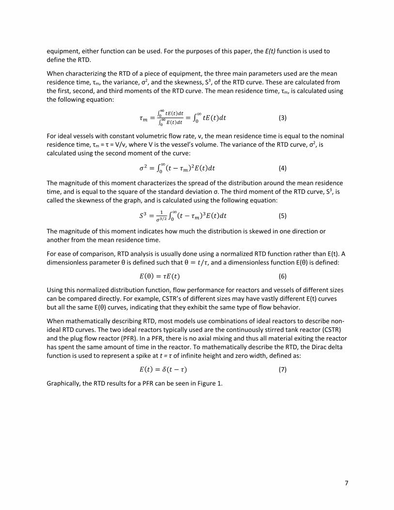
When mathematically describing RTD, most models use combinations of ideal reactors to describe non-ideal RTD curves. The two ideal reactors typically used are the continuously stirred tank reactor (CSTR) and the plug flow reactor (PFR). In a PFR, there is no axial mixing and thus all material exiting the reactor has spent the same amount of time in the reactor. To mathematically describe the RTD, the Dirac delta function is used to represent a spike at t = τ of infinite height and zero width, defined as:

𝐸(𝑡) = 𝛿(𝑡 − 𝜏) (7)

Graphically, the RTD results for a PFR can be seen in Figure 1.

8

Figure 1: E(t) and F(t) for an Ideal PFR (CITE FOGLER)

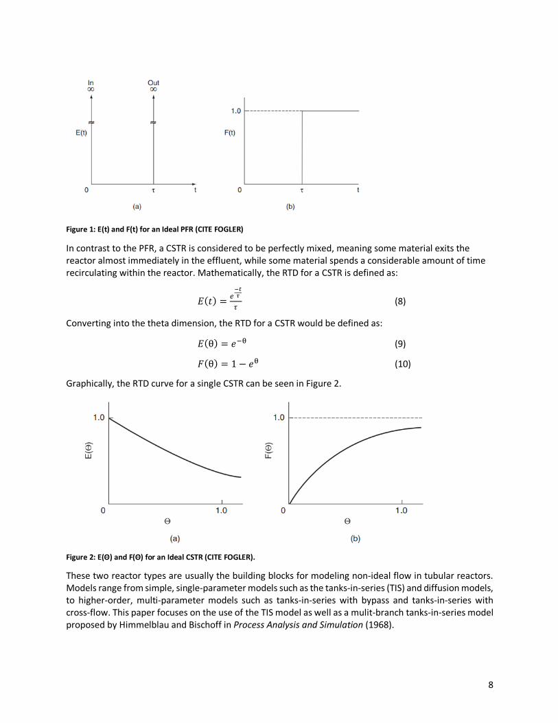
In contrast to the PFR, a CSTR is considered to be perfectly mixed, meaning some material exits the reactor almost immediately in the effluent, while some material spends a considerable amount of time recirculating within the reactor. Mathematically, the RTD for a CSTR is defined as:

𝐸(𝑡) = ?@AB

C (8)

Converting into the theta dimension, the RTD for a CSTR would be defined as:

𝐸(θ) = 𝑒EF (9)

𝐹(θ) = 1 − 𝑒F (10)

Graphically, the RTD curve for a single CSTR can be seen in Figure 2.

Figure 2: E(Θ) and F(Θ) for an Ideal CSTR (CITE FOGLER).

These two reactor types are usually the building blocks for modeling non-ideal flow in tubular reactors. Models range from simple, single-parameter models such as the tanks-in-series (TIS) and diffusion models, to higher-order, multi-parameter models such as tanks-in-series with bypass and tanks-in-series with cross-flow. This paper focuses on the use of the TIS model as well as a mulit-branch tanks-in-series model proposed by Himmelblau and Bischoff in Process Analysis and Simulation (1968).

9

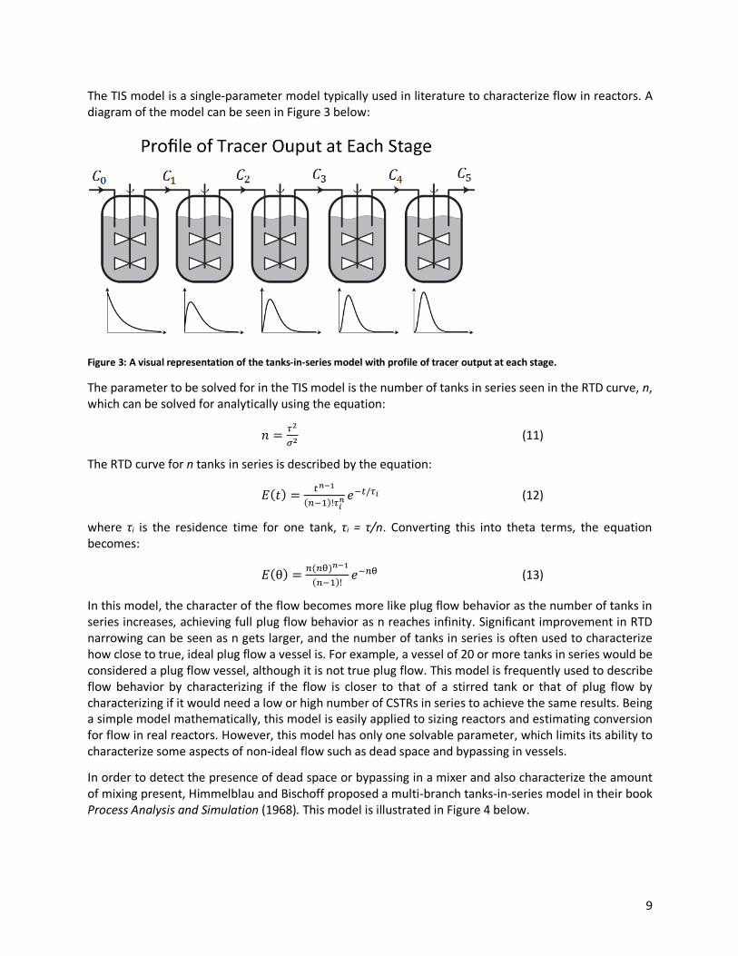
The TIS model is a single-parameter model typically used in literature to characterize flow in reactors. A diagram of the model can be seen in Figure 3 below:

Figure 3: A visual representation of the tanks-in-series model with profile of tracer output at each stage.

The parameter to be solved for in the TIS model is the number of tanks in series seen in the RTD curve, n, which can be solved for analytically using the equation:

𝑛 = C<

9< (11)

The RTD curve for n tanks in series is described by the equation:

𝐸(𝑡) = 'I@J

(KE8)!CMI 𝑒E'/CM (12)

where τi is the residence time for one tank, τi = τ/n. Converting this into theta terms, the equation becomes:

𝐸(θ) = K(KF)I@J

(KE8)!𝑒EKF (13)

In this model, the character of the flow becomes more like plug flow behavior as the number of tanks in series increases, achieving full plug flow behavior as n reaches infinity. Significant improvement in RTD narrowing can be seen as n gets larger, and the number of tanks in series is often used to characterize how close to true, ideal plug flow a vessel is. For example, a vessel of 20 or more tanks in series would be considered a plug flow vessel, although it is not true plug flow. This model is frequently used to describe flow behavior by characterizing if the flow is closer to that of a stirred tank or that of plug flow by characterizing if it would need a low or high number of CSTRs in series to achieve the same results. Being a simple model mathematically, this model is easily applied to sizing reactors and estimating conversion for flow in real reactors. However, this model has only one solvable parameter, which limits its ability to characterize some aspects of non-ideal flow such as dead space and bypassing in vessels.

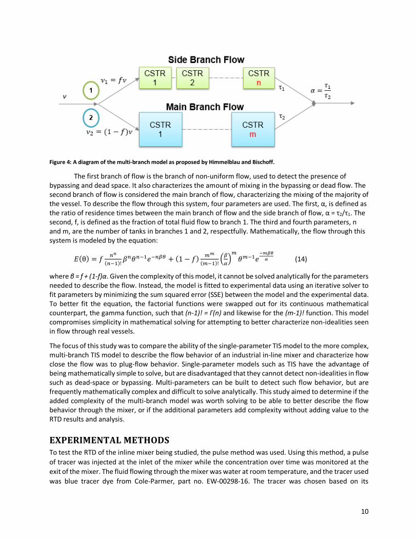
In order to detect the presence of dead space or bypassing in a mixer and also characterize the amount of mixing present, Himmelblau and Bischoff proposed a multi-branch tanks-in-series model in their book Process Analysis and Simulation (1968). This model is illustrated in Figure 4 below.

10

Figure 4: A diagram of the multi-branch model as proposed by Himmelblau and Bischoff.

The first branch of flow is the branch of non-uniform flow, used to detect the presence of bypassing and dead space. It also characterizes the amount of mixing in the bypassing or dead flow. The second branch of flow is considered the main branch of flow, characterizing the mixing of the majority of the vessel. To describe the flow through this system, four parameters are used. The first, α, is defined as the ratio of residence times between the main branch of flow and the side branch of flow, α = τ2/τ1. The second, f, is defined as the fraction of total fluid flow to branch 1. The third and fourth parameters, n and m, are the number of tanks in branches 1 and 2, respectfully. Mathematically, the flow through this system is modeled by the equation:

𝐸(θ) = 𝑓 KI

(KE8)!𝛽K𝜃KE8𝑒EKQR + (1 − 𝑓) 0T

(0E8)!UQVW0𝜃0E8𝑒

@TXYZ (14)

where β = f + (1-f)α. Given the complexity of this model, it cannot be solved analytically for the parameters needed to describe the flow. Instead, the model is fitted to experimental data using an iterative solver to fit parameters by minimizing the sum squared error (SSE) between the model and the experimental data. To better fit the equation, the factorial functions were swapped out for its continuous mathematical counterpart, the gamma function, such that (n-1)! = Γ(n) and likewise for the (m-1)! function. This model compromises simplicity in mathematical solving for attempting to better characterize non-idealities seen in flow through real vessels.

The focus of this study was to compare the ability of the single-parameter TIS model to the more complex, multi-branch TIS model to describe the flow behavior of an industrial in-line mixer and characterize how close the flow was to plug-flow behavior. Single-parameter models such as TIS have the advantage of being mathematically simple to solve, but are disadvantaged that they cannot detect non-idealities in flow such as dead-space or bypassing. Multi-parameters can be built to detect such flow behavior, but are frequently mathematically complex and difficult to solve analytically. This study aimed to determine if the added complexity of the multi-branch model was worth solving to be able to better describe the flow behavior through the mixer, or if the additional parameters add complexity without adding value to the RTD results and analysis.

EXPERIMENTALMETHODSTo test the RTD of the inline mixer being studied, the pulse method was used. Using this method, a pulse of tracer was injected at the inlet of the mixer while the concentration over time was monitored at the exit of the mixer. The fluid flowing through the mixer was water at room temperature, and the tracer used was blue tracer dye from Cole-Parmer, part no. EW-00298-16. The tracer was chosen based on its

11

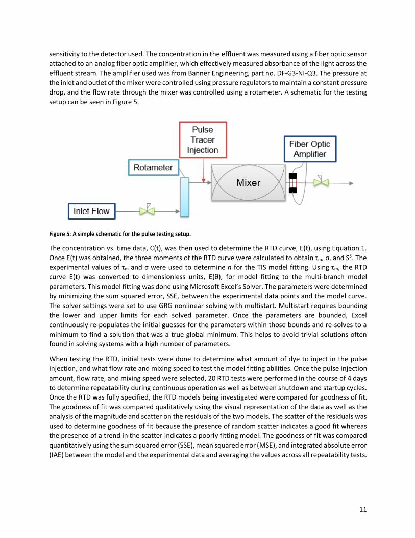
sensitivity to the detector used. The concentration in the effluent was measured using a fiber optic sensor attached to an analog fiber optic amplifier, which effectively measured absorbance of the light across the effluent stream. The amplifier used was from Banner Engineering, part no. DF-G3-NI-Q3. The pressure at the inlet and outlet of the mixer were controlled using pressure regulators to maintain a constant pressure drop, and the flow rate through the mixer was controlled using a rotameter. A schematic for the testing setup can be seen in Figure 5.

Figure 5: A simple schematic for the pulse testing setup.

The concentration vs. time data, C(t), was then used to determine the RTD curve, E(t), using Equation 1. Once E(t) was obtained, the three moments of the RTD curve were calculated to obtain τm, σ, and S3. The experimental values of τm and σ were used to determine n for the TIS model fitting. Using τm, the RTD curve E(t) was converted to dimensionless units, E(θ), for model fitting to the multi-branch model parameters. This model fitting was done using Microsoft Excel’s Solver. The parameters were determined by minimizing the sum squared error, SSE, between the experimental data points and the model curve. The solver settings were set to use GRG nonlinear solving with multistart. Multistart requires bounding the lower and upper limits for each solved parameter. Once the parameters are bounded, Excel continuously re-populates the initial guesses for the parameters within those bounds and re-solves to a minimum to find a solution that was a true global minimum. This helps to avoid trivial solutions often found in solving systems with a high number of parameters.

When testing the RTD, initial tests were done to determine what amount of dye to inject in the pulse injection, and what flow rate and mixing speed to test the model fitting abilities. Once the pulse injection amount, flow rate, and mixing speed were selected, 20 RTD tests were performed in the course of 4 days to determine repeatability during continuous operation as well as between shutdown and startup cycles. Once the RTD was fully specified, the RTD models being investigated were compared for goodness of fit. The goodness of fit was compared qualitatively using the visual representation of the data as well as the analysis of the magnitude and scatter on the residuals of the two models. The scatter of the residuals was used to determine goodness of fit because the presence of random scatter indicates a good fit whereas the presence of a trend in the scatter indicates a poorly fitting model. The goodness of fit was compared quantitatively using the sum squared error (SSE), mean squared error (MSE), and integrated absolute error (IAE) between the model and the experimental data and averaging the values across all repeatability tests.

12

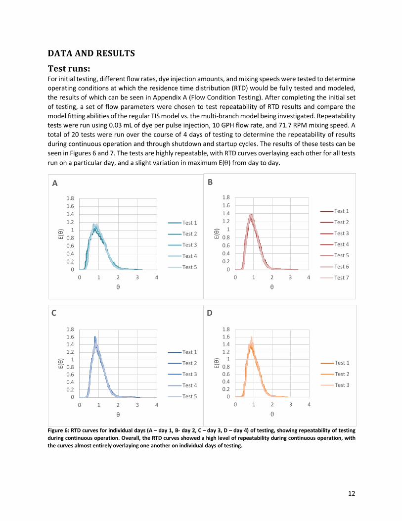
DATAANDRESULTSTestruns:For initial testing, different flow rates, dye injection amounts, and mixing speeds were tested to determine operating conditions at which the residence time distribution (RTD) would be fully tested and modeled, the results of which can be seen in Appendix A (Flow Condition Testing). After completing the initial set of testing, a set of flow parameters were chosen to test repeatability of RTD results and compare the model fitting abilities of the regular TIS model vs. the multi-branch model being investigated. Repeatability tests were run using 0.03 mL of dye per pulse injection, 10 GPH flow rate, and 71.7 RPM mixing speed. A total of 20 tests were run over the course of 4 days of testing to determine the repeatability of results during continuous operation and through shutdown and startup cycles. The results of these tests can be seen in Figures 6 and 7. The tests are highly repeatable, with RTD curves overlaying each other for all tests run on a particular day, and a slight variation in maximum E(q) from day to day.

Figure 6: RTD curves for individual days (A – day 1, B- day 2, C – day 3, D – day 4) of testing, showing repeatability of testing during continuous operation. Overall, the RTD curves showed a high level of repeatability during continuous operation, with the curves almost entirely overlaying one another on individual days of testing.

00.20.40.60.8

11.21.41.61.8

0 1 2 3 4

E(θ)

θ

A

Test 1

Test 2

Test 3

Test 4

Test 5 00.20.40.60.8

11.21.41.61.8

0 1 2 3 4

E(θ)

θ

B

Test 1

Test 2

Test 3

Test 4

Test 5

Test 6

Test 7

00.20.40.60.8

11.21.41.61.8

0 1 2 3 4

E(θ)

θ

C

Test 1

Test 2

Test 3

Test 4

Test 5 00.20.40.60.8

11.21.41.61.8

0 1 2 3 4

E(θ)

θ

D

Test 1

Test 2

Test 3

13

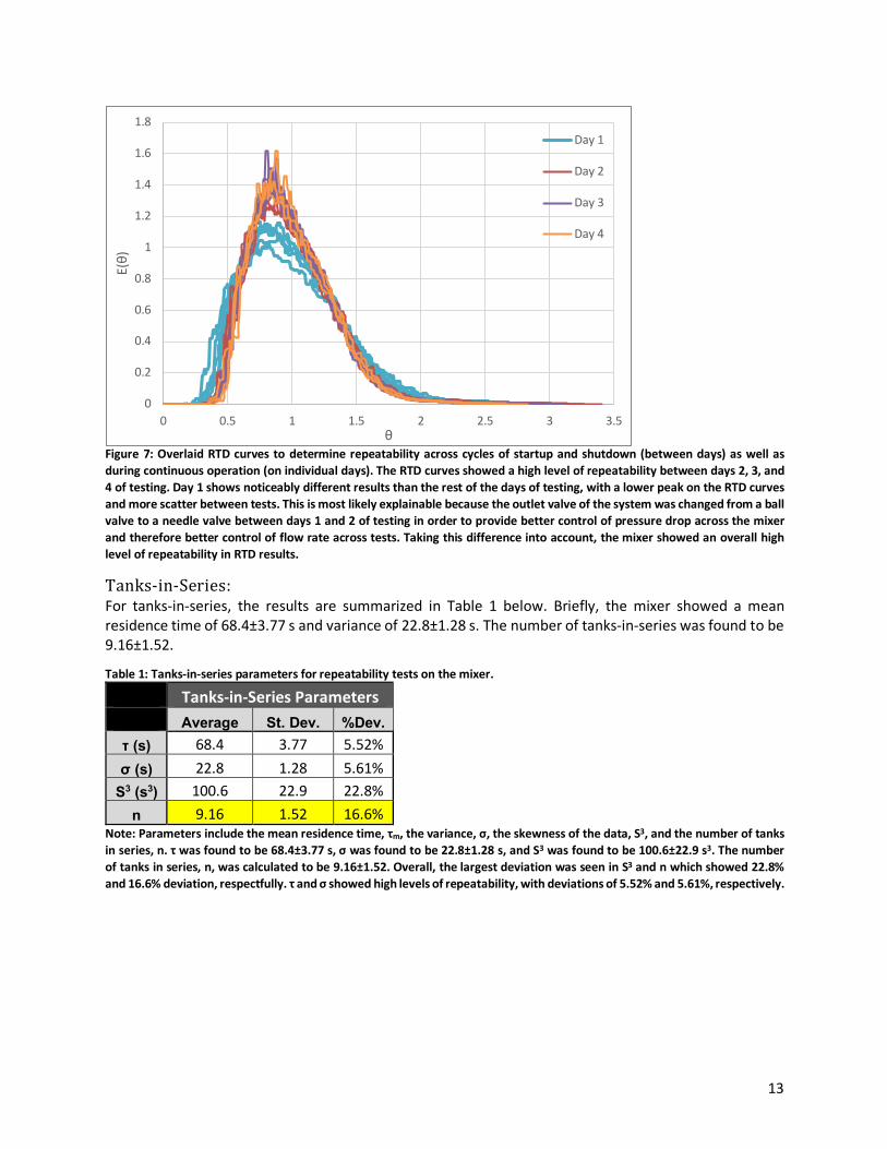
Figure 7: Overlaid RTD curves to determine repeatability across cycles of startup and shutdown (between days) as well as during continuous operation (on individual days). The RTD curves showed a high level of repeatability between days 2, 3, and 4 of testing. Day 1 shows noticeably different results than the rest of the days of testing, with a lower peak on the RTD curves and more scatter between tests. This is most likely explainable because the outlet valve of the system was changed from a ball valve to a needle valve between days 1 and 2 of testing in order to provide better control of pressure drop across the mixer and therefore better control of flow rate across tests. Taking this difference into account, the mixer showed an overall high level of repeatability in RTD results.

Tanks-in-Series:For tanks-in-series, the results are summarized in Table 1 below. Briefly, the mixer showed a mean residence time of 68.4±3.77 s and variance of 22.8±1.28 s. The number of tanks-in-series was found to be 9.16±1.52.

Table 1: Tanks-in-series parameters for repeatability tests on the mixer. Tanks-in-Series Parameters Average St. Dev. %Dev.

τ (s) 68.4 3.77 5.52% σ (s) 22.8 1.28 5.61%

S3 (s3) 100.6 22.9 22.8% n 9.16 1.52 16.6%

Note: Parameters include the mean residence time, τm, the variance, σ, the skewness of the data, S3, and the number of tanks in series, n. τ was found to be 68.4±3.77 s, σ was found to be 22.8±1.28 s, and S3 was found to be 100.6±22.9 s3. The number of tanks in series, n, was calculated to be 9.16±1.52. Overall, the largest deviation was seen in S3 and n which showed 22.8% and 16.6% deviation, respectfully. τ and σ showed high levels of repeatability, with deviations of 5.52% and 5.61%, respectively.

0

0.2

0.4

0.6

0.8

1

1.2

1.4

1.6

1.8

0 0.5 1 1.5 2 2.5 3 3.5

E(θ)

θ

Day 1

Day 2

Day 3

Day 4

14

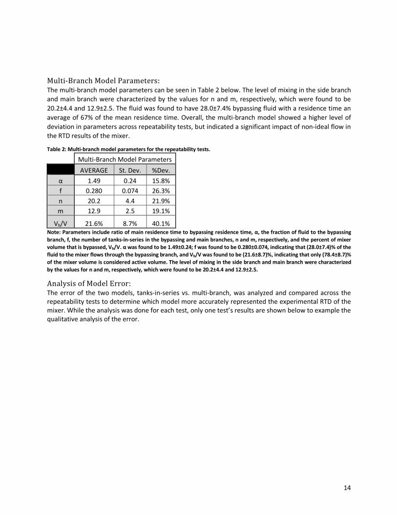
Multi-BranchModelParameters:The multi-branch model parameters can be seen in Table 2 below. The level of mixing in the side branch and main branch were characterized by the values for n and m, respectively, which were found to be 20.2±4.4 and 12.9±2.5. The fluid was found to have 28.0±7.4% bypassing fluid with a residence time an average of 67% of the mean residence time. Overall, the multi-branch model showed a higher level of deviation in parameters across repeatability tests, but indicated a significant impact of non-ideal flow in the RTD results of the mixer.

Table 2: Multi-branch model parameters for the repeatability tests.

Multi-Branch Model Parameters AVERAGE St. Dev. %Dev. α 1.49 0.24 15.8% f 0.280 0.074 26.3% n 20.2 4.4 21.9% m 12.9 2.5 19.1%

Vb/V 21.6% 8.7% 40.1% Note: Parameters include ratio of main residence time to bypassing residence time, α, the fraction of fluid to the bypassing branch, f, the number of tanks-in-series in the bypassing and main branches, n and m, respectively, and the percent of mixer volume that is bypassed, Vb/V. α was found to be 1.49±0.24; f was found to be 0.280±0.074, indicating that (28.0±7.4)% of the fluid to the mixer flows through the bypassing branch, and Vb/V was found to be (21.6±8.7)%, indicating that only (78.4±8.7)% of the mixer volume is considered active volume. The level of mixing in the side branch and main branch were characterized by the values for n and m, respectively, which were found to be 20.2±4.4 and 12.9±2.5.

AnalysisofModelError:The error of the two models, tanks-in-series vs. multi-branch, was analyzed and compared across the repeatability tests to determine which model more accurately represented the experimental RTD of the mixer. While the analysis was done for each test, only one test’s results are shown below to example the qualitative analysis of the error.

15

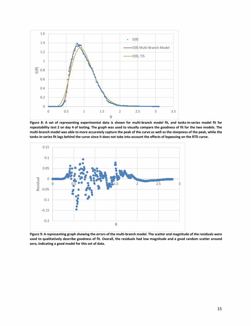
Figure 8: A set of representing experimental data is shown for multi-branch model fit, and tanks-in-series model fit for repeatability test 2 on day 4 of testing. The graph was used to visually compare the goodness of fit for the two models. The multi-branch model was able to more accurately capture the peak of the curve as well as the steepness of the peak, while the tanks-in-series fit lags behind the curve since it does not take into account the effects of bypassing on the RTD curve.

Figure 9: A representing graph showing the errors of the multi-branch model. The scatter and magnitude of the residuals were used to qualitatively describe goodness of fit. Overall, the residuals had low magnitude and a good random scatter around zero, indicating a good model for this set of data.

0

0.2

0.4

0.6

0.8

1

1.2

1.4

1.6

0 0.5 1 1.5 2 2.5 3 3.5

E(θ)

θ

E(θ)

E(θ) Multi-Branch Model

E(θ), TIS

-0.2

-0.15

-0.1

-0.05

0

0.05

0.1

0.15

0 0.5 1 1.5 2 2.5 3

Resid

ual

θ

16

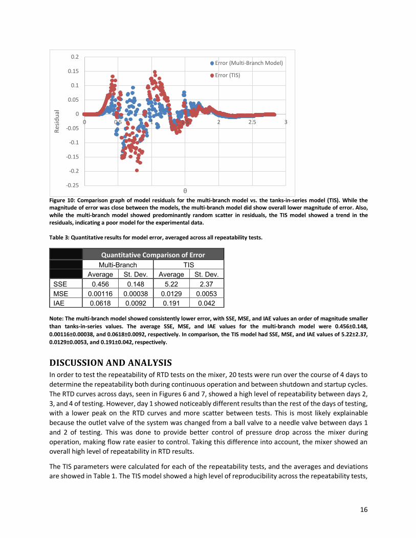
Figure 10: Comparison graph of model residuals for the multi-branch model vs. the tanks-in-series model (TIS). While the magnitude of error was close between the models, the multi-branch model did show overall lower magnitude of error. Also, while the multi-branch model showed predominantly random scatter in residuals, the TIS model showed a trend in the residuals, indicating a poor model for the experimental data. Table 3: Quantitative results for model error, averaged across all repeatability tests.

Note: The multi-branch model showed consistently lower error, with SSE, MSE, and IAE values an order of magnitude smaller than tanks-in-series values. The average SSE, MSE, and IAE values for the multi-branch model were 0.456±0.148, 0.00116±0.00038, and 0.0618±0.0092, respectively. In comparison, the TIS model had SSE, MSE, and IAE values of 5.22±2.37, 0.0129±0.0053, and 0.191±0.042, respectively.

DISCUSSIONANDANALYSISIn order to test the repeatability of RTD tests on the mixer, 20 tests were run over the course of 4 days to determine the repeatability both during continuous operation and between shutdown and startup cycles. The RTD curves across days, seen in Figures 6 and 7, showed a high level of repeatability between days 2, 3, and 4 of testing. However, day 1 showed noticeably different results than the rest of the days of testing, with a lower peak on the RTD curves and more scatter between tests. This is most likely explainable because the outlet valve of the system was changed from a ball valve to a needle valve between days 1 and 2 of testing. This was done to provide better control of pressure drop across the mixer during operation, making flow rate easier to control. Taking this difference into account, the mixer showed an overall high level of repeatability in RTD results.

The TIS parameters were calculated for each of the repeatability tests, and the averages and deviations are showed in Table 1. The TIS model showed a high level of reproducibility across the repeatability tests,

-0.25

-0.2

-0.15

-0.1

-0.05

0

0.05

0.1

0.15

0.2

0 0.5 1 1.5 2 2.5 3

Resid

ual

θ

Error (Multi-Branch Model)

Error (TIS)

Quantitative Comparison of Error Multi-Branch TIS Average St. Dev. Average St. Dev. SSE 0.456 0.148 5.22 2.37 MSE 0.00116 0.00038 0.0129 0.0053 IAE 0.0618 0.0092 0.191 0.042

17

with deviations ranging from 5.52-22.8%. The lowest amount of deviation is seen in the results for τ and σ, with standard deviations of 5.52% and 5.61% respectively. A higher deviation of 16.6% was seen in n, and the highest deviation of 22.8% was seen in the S3 value for the tests. The multi-branch model parameters were also calculated for each of the repeatability tests, and the averages and deviations are shown in Table 2 above. The multi-branch model showed higher levels of deviation between tests compared to the tanks-in-series model, with deviations ranging from 15.8-40.1%. The least amount of deviation, 15.8%, was seen in α. The parameters n and m had higher levels of deviation, 21.9%, and 19.1% respectively, while the highest level of deviation was seen in the parameter f, with 26.3% deviation. This higher level of deviation in parameters is most likely due to the higher number of parameters in the multi-branch model, which makes it abler to detect slight differences in experimental data when data fitting. A higher level of sensitivity can lead to a higher level of variance in data, as minor differences between tests are easier to detect. In addition, the multi-branch model is also a fitted model, as opposed to one that is solved analytically, which could produce greater variance. Fitted models are more subject to respond to the variance due to the scatter of data in the experimental data points they are directly fitted to.

In comparing the error between the two models, both qualitative and quantitative error analysis were used, as shown in Figures 9 and 10 and Table 3 above. For the quantitative error analysis, the multi-branch model had SSE, MSE, and IAE values of 0.456±0.148, 0.00116±0.00038, and 0.0618±0.0092, respectively. In comparison, the TIS model had SSE, MSE, and IAE values of 5.22±2.37, 0.0128±0.0053, and 0.191±0.042, respectively. The quantitative error analysis showed less calculated error for the multi-branch model across the board, with SSE and MSE values a full order of magnitude smaller than the tanks-in-series model. The qualitative error analysis showed a lower magnitude of error on the multi-branch model as well as a more random scatter of error. In comparison, the tanks-in-series model showed a higher magnitude of error as well as trend in the error values across the values of θ. When analyzing goodness of fit of nonlinear models, a trend in the error of the model is a sign of a poorly fitting model, usually one with too few or insignificant parameters. For example, most data can be fitted quite well with an extremely high order polynomial, but the graph of residuals would indicate that the model does not actually capture the trend of the experimental data by showing a trend in the residuals of the model.

There are many possible sources of error in this testing method. For one, error in calibration of the fiber optic sensor could have caused concentration measurements to be skewed during testing. This error was minimized by performing repeatability tests on concentration calibration to ensure that the concentrations consistently gave the same results and limiting the amount of dye injected to ensure the concentration stayed in the detector’s calibrated range. Another source of error was consistency of flow rate through the mixer, as it was controlled by a manual rotameter. This error was minimized by performing repeatability tests across the mixer to ensure the results weren’t affected by this error. A further source of error is a sloppy pulse injection, which can cause skewed RTD results. This error was minimized by using an instantaneous pulse injection with a needle injection port. The amount of dye injected was kept small enough to injected virtually instantaneously but large enough to be accurately measured.

CONCLUSIONSANDRECOMMENDATIONSIt was found that the multi-branch model showed a higher level of deviation in parameters during repeatability tests, but consistently lower levels of error from the experimental data, both qualitatively and quantitatively. The multi-branch model was also able to detect bypassing in the mixer, which the TIS model was unable to see. This indicates that although the multi-branch model is more difficult to fit experimentally, it is worth the mathematical complexity to be able to detect non-idealities present in the

18

flow when analyzing the RTD. The results of this study will be used to analyze reactor and mixer RTD results in the future, helping to experimentally diagnose ills such as dead space and bypassing in equipment.

One recommendation for further work is to test different pieces of equipment for residence time distribution, using this model, to clarify that this model is useful for varying flow systems. Although using this model with this system brought an increase in flow knowledge, it is important to investigate if this holds true for other systems. Another recommendation for further work is to validate the RTD results obtained in this experiment using the step method of RTD testing. RTD testing frequently involves using both methods to validate that the results obtained using either method accurately represent the RTD of the equipment. This further validation work would be required to ensure the model’s overall worth.

19

REFERENCESCozewith, C., & Squire, K. R. (2000, 06). Effect of Reactor Residence Time Distribution on Polymer

Functionalization Reactions. Chemical Engineering Science, 55(11), 2019-2029. doi:10.1016/s0009-2509(99)00479-0

Danckwerts, P. V. (1953, February). Continuous Flow Systems: Distribution of Residence Times. Chemical Engineering Science, 2(1), 1-13. Retrieved February 2018, from http://www.sciencedirect.com/science/article/pii/0009250953800011

Fogler, H. S. (2016). Elements of Chemical Reaction Engineering (5th ed.). Boston, MA: Prentice Hall.

Himmelblau, D. M., & Bischoff, K. B. (1968). Process Analysis and Simulation: Deterministic Systems. Austin: Wiley.

Levenspiel, O. (1972). Chemical Reaction Engineering (2nd ed.). New York: Wiley.

20

APPENDIXA:FLOWCONDITIONTESTINGFor initial testing, different flow rates, dye injection amounts, and mixing speeds were tested to determine operating conditions at which the RTD would be fully tested and modeled.

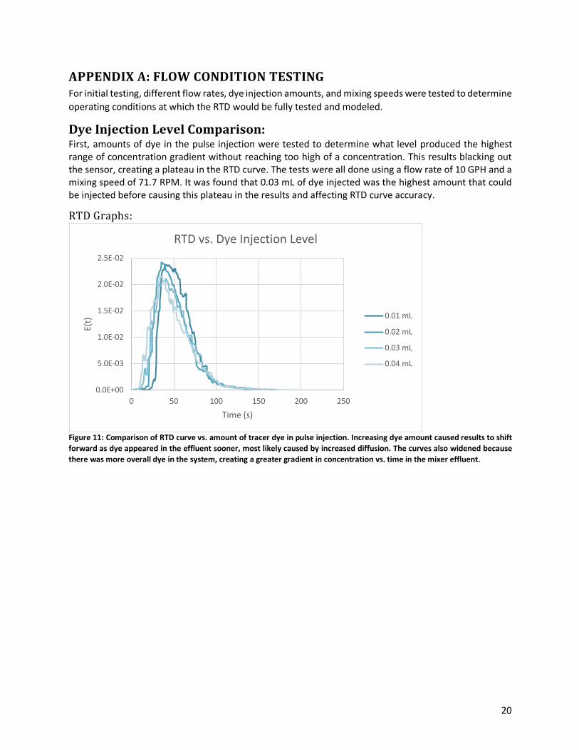
DyeInjectionLevelComparison:First, amounts of dye in the pulse injection were tested to determine what level produced the highest range of concentration gradient without reaching too high of a concentration. This results blacking out the sensor, creating a plateau in the RTD curve. The tests were all done using a flow rate of 10 GPH and a mixing speed of 71.7 RPM. It was found that 0.03 mL of dye injected was the highest amount that could be injected before causing this plateau in the results and affecting RTD curve accuracy.

RTDGraphs:

Figure 11: Comparison of RTD curve vs. amount of tracer dye in pulse injection. Increasing dye amount caused results to shift forward as dye appeared in the effluent sooner, most likely caused by increased diffusion. The curves also widened because there was more overall dye in the system, creating a greater gradient in concentration vs. time in the mixer effluent.

0.0E+00

5.0E-03

1.0E-02

1.5E-02

2.0E-02

2.5E-02

0 50 100 150 200 250

E(t)

Time (s)

RTD vs. Dye Injection Level

0.01 mL

0.02 mL

0.03 mL

0.04 mL

21

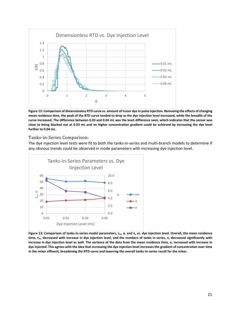
Figure 12: Comparison of dimensionless RTD curve vs. amount of tracer dye in pulse injection. Removing the effects of changing mean residence time, the peak of the RTD curve tended to drop as the dye injection level increased, while the breadth of the curve increased. The difference between 0.03 and 0.04 mL was the least difference seen, which indicates that the sensor was close to being blacked out at 0.03 mL and no higher concentration gradient could be achieved by increasing the dye level further to 0.04 mL.

Tanks-in-SeriesComparison:The dye injection level tests were fit to both the tanks-in-series and multi-branch models to determine if any obvious trends could be observed in mode parameters with increasing dye injection level.

Figure 13: Comparison of tanks-in-series model parameters, τm, σ, and n, vs. dye injection level. Overall, the mean residence time, τm, decreased with increase in dye injection level, and the numbers of tanks in series, n, decreased significantly with increase in dye injection level as well. The variance of the data from the mean residence time, σ, increased with increase in dye injected. This agrees with the idea that increasing the dye injection level increases the gradient of concentration over time in the mixer effluent, broadening the RTD curve and lowering the overall tanks-in-series result for the mixer.

0

0.2

0.4

0.6

0.8

1

1.2

1.4

0 1 2 3 4 5

E(θ)

θ

Dimensionless RTD vs. Dye Injection Level

0.01 mL

0.02 mL

0.03 mL

0.04 mL

0.0

2.0

4.0

6.0

8.0

10.0

0

10

20

30

40

50

60

0.01 0.02 0.03 0.04

n

τ m, σ

Dye Injection Level (mL)

Tanks-in-Series Parameters vs. Dye Iinjection Level

τm

σ

n

22

Tanks-In-Series Parameters 0.01 mL 0.02 mL 0.03 mL 0.04 mL

τm 55.7 50.8 51.5 48.9 σ 18.8 20.8 21.7 24.0 S3 105.1 130.3 106.3 158.4 n 8.74 5.95 5.64 4.14

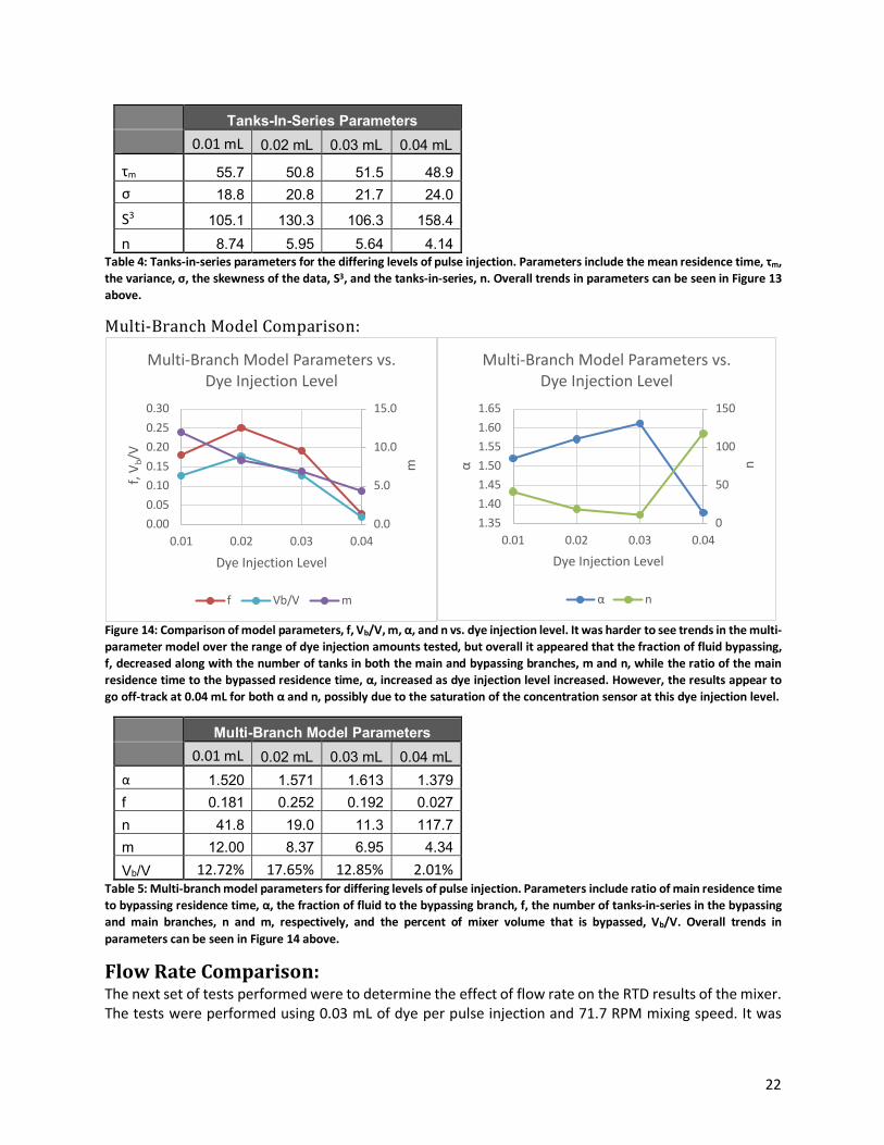
Table 4: Tanks-in-series parameters for the differing levels of pulse injection. Parameters include the mean residence time, τm, the variance, σ, the skewness of the data, S3, and the tanks-in-series, n. Overall trends in parameters can be seen in Figure 13 above.

Multi-BranchModelComparison:

Figure 14: Comparison of model parameters, f, Vb/V, m, α, and n vs. dye injection level. It was harder to see trends in the multi-parameter model over the range of dye injection amounts tested, but overall it appeared that the fraction of fluid bypassing, f, decreased along with the number of tanks in both the main and bypassing branches, m and n, while the ratio of the main residence time to the bypassed residence time, α, increased as dye injection level increased. However, the results appear to go off-track at 0.04 mL for both α and n, possibly due to the saturation of the concentration sensor at this dye injection level.

Multi-Branch Model Parameters 0.01 mL 0.02 mL 0.03 mL 0.04 mL α 1.520 1.571 1.613 1.379 f 0.181 0.252 0.192 0.027 n 41.8 19.0 11.3 117.7 m 12.00 8.37 6.95 4.34 Vb/V 12.72% 17.65% 12.85% 2.01%

Table 5: Multi-branch model parameters for differing levels of pulse injection. Parameters include ratio of main residence time to bypassing residence time, α, the fraction of fluid to the bypassing branch, f, the number of tanks-in-series in the bypassing and main branches, n and m, respectively, and the percent of mixer volume that is bypassed, Vb/V. Overall trends in parameters can be seen in Figure 14 above.

FlowRateComparison:The next set of tests performed were to determine the effect of flow rate on the RTD results of the mixer. The tests were performed using 0.03 mL of dye per pulse injection and 71.7 RPM mixing speed. It was

0.0

5.0

10.0

15.0

0.000.050.100.150.200.250.30

0.01 0.02 0.03 0.04

m

f, V b

/V

Dye Injection Level

Multi-Branch Model Parameters vs. Dye Injection Level

f Vb/V m

0

50

100

150

1.351.401.451.501.551.601.65

0.01 0.02 0.03 0.04

nα

Dye Injection Level

Multi-Branch Model Parameters vs. Dye Injection Level

α n

23

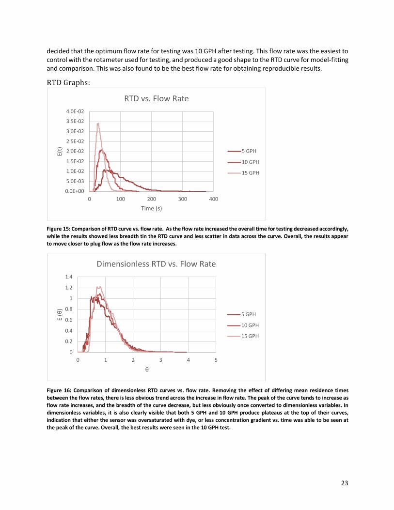
decided that the optimum flow rate for testing was 10 GPH after testing. This flow rate was the easiest to control with the rotameter used for testing, and produced a good shape to the RTD curve for model-fitting and comparison. This was also found to be the best flow rate for obtaining reproducible results.

RTDGraphs:

Figure 15: Comparison of RTD curve vs. flow rate. As the flow rate increased the overall time for testing decreased accordingly, while the results showed less breadth tin the RTD curve and less scatter in data across the curve. Overall, the results appear to move closer to plug flow as the flow rate increases.

Figure 16: Comparison of dimensionless RTD curves vs. flow rate. Removing the effect of differing mean residence times between the flow rates, there is less obvious trend across the increase in flow rate. The peak of the curve tends to increase as flow rate increases, and the breadth of the curve decrease, but less obviously once converted to dimensionless variables. In dimensionless variables, it is also clearly visible that both 5 GPH and 10 GPH produce plateaus at the top of their curves, indication that either the sensor was oversaturated with dye, or less concentration gradient vs. time was able to be seen at the peak of the curve. Overall, the best results were seen in the 10 GPH test.

0.0E+00

5.0E-03

1.0E-02

1.5E-02

2.0E-02

2.5E-02

3.0E-02

3.5E-02

4.0E-02

0 100 200 300 400

E(t)

Time (s)

RTD vs. Flow Rate

5 GPH

10 GPH

15 GPH

0

0.2

0.4

0.6

0.8

1

1.2

1.4

0 1 2 3 4 5

E (θ

)

θ

Dimensionless RTD vs. Flow Rate

5 GPH

10 GPH

15 GPH

24

TanksinSeriesResults:

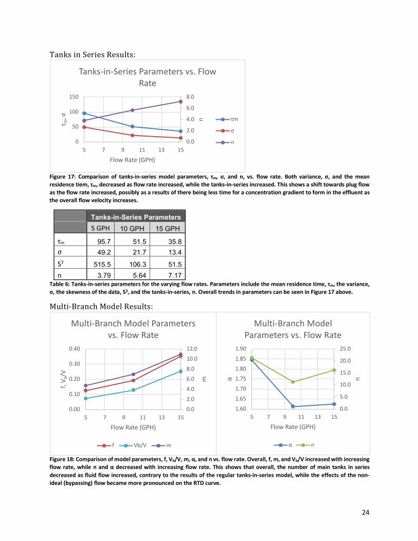
Figure 17: Comparison of tanks-in-series model parameters, τm, σ, and n, vs. flow rate. Both variance, σ, and the mean residence tiem, τm, decreased as flow rate increased, while the tanks-in-series increased. This shows a shift towards plug flow as the flow rate increased, possibly as a results of there being less time for a concentration gradient to form in the effluent as the overall flow velocity increases.

Tanks-in-Series Parameters 5 GPH 10 GPH 15 GPH

τm 95.7 51.5 35.8 σ 49.2 21.7 13.4 S3 515.5 106.3 51.5 n 3.79 5.64 7.17

Table 6: Tanks-in-series parameters for the varying flow rates. Parameters include the mean residence time, τm, the variance, σ, the skewness of the data, S3, and the tanks-in-series, n. Overall trends in parameters can be seen in Figure 17 above.

Multi-BranchModelResults:

Figure 18: Comparison of model parameters, f, Vb/V, m, α, and n vs. flow rate. Overall, f, m, and Vb/V increased with increasing flow rate, while n and α decreased with increasing flow rate. This shows that overall, the number of main tanks in series decreased as fluid flow increased, contrary to the results of the regular tanks-in-series model, while the effects of the non-ideal (bypassing) flow became more pronounced on the RTD curve.

0.0

2.0

4.0

6.0

8.0

0

50

100

150

5 7 9 11 13 15

n

τ m, σ

Flow Rate (GPH)

Tanks-in-Series Parameters vs. Flow Rate

τm

σ

n

0.0

2.04.0

6.08.0

10.012.0

0.00

0.10

0.20

0.30

0.40

5 7 9 11 13 15

m

f, V b

/V

Flow Rate (GPH)

Multi-Branch Model Parameters vs. Flow Rate

f Vb/V m

0.0

5.0

10.0

15.0

20.0

25.0

1.601.651.701.751.801.851.90

5 7 9 11 13 15

nα

Flow Rate (GPH)

Multi-Branch Model Parameters vs. Flow Rate

α n

25

Multi-Branch Model Parameters 5 GPH 10 GPH 15 GPH α 1.845 1.613 1.624 f 0.125 0.192 0.353 n 21.3 11.3 16.1 m 4.74 6.95 10.93 Vb/V 7.21% 12.85% 25.17%

Table 7: Multi-branch model parameters for differing flow rates. Parameters include ratio of main residence time to bypassing residence time, α, the fraction of fluid to the bypassing branch, f, the number of tanks-in-series in the bypassing and main branches, n and m, respectively, and the percent of mixer volume that is bypassed, Vb/V. Overall trends in parameters can be seen in Figure 18 above.

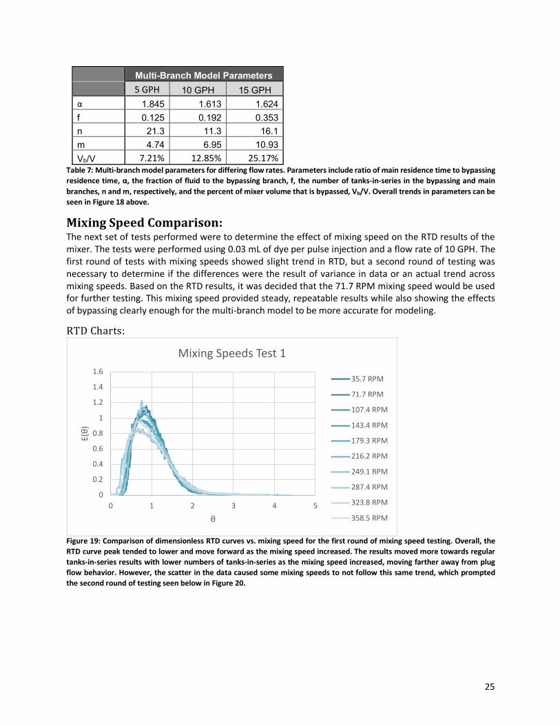
MixingSpeedComparison:The next set of tests performed were to determine the effect of mixing speed on the RTD results of the mixer. The tests were performed using 0.03 mL of dye per pulse injection and a flow rate of 10 GPH. The first round of tests with mixing speeds showed slight trend in RTD, but a second round of testing was necessary to determine if the differences were the result of variance in data or an actual trend across mixing speeds. Based on the RTD results, it was decided that the 71.7 RPM mixing speed would be used for further testing. This mixing speed provided steady, repeatable results while also showing the effects of bypassing clearly enough for the multi-branch model to be more accurate for modeling.

RTDCharts:

Figure 19: Comparison of dimensionless RTD curves vs. mixing speed for the first round of mixing speed testing. Overall, the RTD curve peak tended to lower and move forward as the mixing speed increased. The results moved more towards regular tanks-in-series results with lower numbers of tanks-in-series as the mixing speed increased, moving farther away from plug flow behavior. However, the scatter in the data caused some mixing speeds to not follow this same trend, which prompted the second round of testing seen below in Figure 20.

0

0.2

0.4

0.6

0.8

1

1.2

1.4

1.6

0 1 2 3 4 5

E(θ)

θ

Mixing Speeds Test 1

35.7 RPM

71.7 RPM

107.4 RPM

143.4 RPM

179.3 RPM

216.2 RPM

249.1 RPM

287.4 RPM

323.8 RPM

358.5 RPM

26

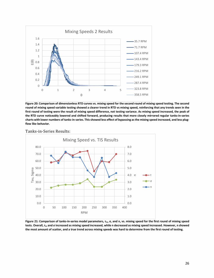
Figure 20: Comparison of dimensionless RTD curves vs. mixing speed for the second round of mixing speed testing. The second round of mixing speed variable testing showed a clearer trend in RTD vs mixing speed, reinforcing that any trends seen in the first round of testing were the result of mixing speed difference, not testing variance. As mixing speed increased, the peak of the RTD curve noticeably lowered and shifted forward, producing results that more closely mirrored regular tanks-in-series charts with lower numbers of tanks-in-series. This showed less effect of bypassing as the mixing speed increased, and less plug-flow like behavior.

Tanks-in-SeriesResults:

Figure 21: Comparison of tanks-in-series model parameters, τm, σ, and n, vs. mixing speed for the first round of mixing speed tests. Overall, τm and σ increased as mixing speed increased, while n decreased as mixing speed increased. However, n showed the most amount of scatter, and a true trend across mixing speeds was hard to determine from the first round of testing.

0

0.2

0.4

0.6

0.8

1

1.2

1.4

1.6

0 1 2 3 4 5

E(θ)

θ

Mixing Speeds 2 Results

35.7 RPM

71.7 RPM

107.4 RPM

143.4 RPM

179.3 RPM

216.2 RPM

249.1 RPM

287.4 RPM

323.8 RPM

358.5 RPM

0.0

1.0

2.0

3.0

4.0

5.0

6.0

7.0

8.0

0.0

10.0

20.0

30.0

40.0

50.0

60.0

70.0

80.0

0 50 100 150 200 250 300 350 400

n

Tau,

Sig

ma

RPM

Mixing Speed vs. TIS Results

τ

σ

n

27

Tanks-in-Series Parameters Mixing Speed (RPM)

35.70 71.70 107.40 143.40 179.30 216.2 249.1 287.4 323.8 358.5

τm 58.2 60.7 72.1 68.1 73.2 74.7 45.8 59.9 58.7 70.2 σ 22.3 25.4 26.6 26.6 28.6 34.5 23.6 23.5 30.2 33.8 S3 102.6 108.8 124.8 127.0 136.5 242.8 127.9 103.4 181.2 241.8 n 6.78 5.73 7.36 6.56 6.54 4.69 3.75 6.48 3.77 4.31

Table 8: Tanks-in-series parameters for the first round of testing of varying mixing speeds. Parameters include the mean residence time, τm, the variance, σ, the skewness of the data, S3, and the tanks-in-series, n. Overall trends in parameters can be seen in Figure 21 above.

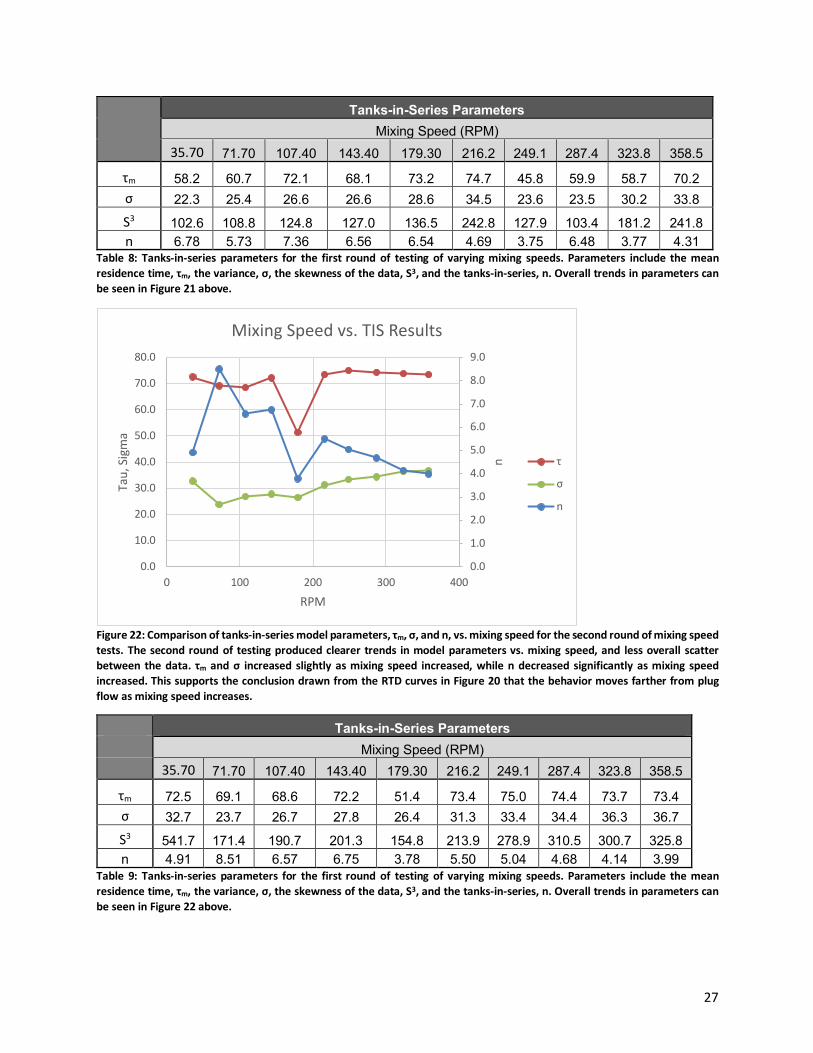
Figure 22: Comparison of tanks-in-series model parameters, τm, σ, and n, vs. mixing speed for the second round of mixing speed tests. The second round of testing produced clearer trends in model parameters vs. mixing speed, and less overall scatter between the data. τm and σ increased slightly as mixing speed increased, while n decreased significantly as mixing speed increased. This supports the conclusion drawn from the RTD curves in Figure 20 that the behavior moves farther from plug flow as mixing speed increases.

Tanks-in-Series Parameters Mixing Speed (RPM) 35.70 71.70 107.40 143.40 179.30 216.2 249.1 287.4 323.8 358.5

τm 72.5 69.1 68.6 72.2 51.4 73.4 75.0 74.4 73.7 73.4 σ 32.7 23.7 26.7 27.8 26.4 31.3 33.4 34.4 36.3 36.7 S3 541.7 171.4 190.7 201.3 154.8 213.9 278.9 310.5 300.7 325.8 n 4.91 8.51 6.57 6.75 3.78 5.50 5.04 4.68 4.14 3.99

Table 9: Tanks-in-series parameters for the first round of testing of varying mixing speeds. Parameters include the mean residence time, τm, the variance, σ, the skewness of the data, S3, and the tanks-in-series, n. Overall trends in parameters can be seen in Figure 22 above.

0.0

1.0

2.0

3.0

4.0

5.0

6.0

7.0

8.0

9.0

0.0

10.0

20.0

30.0

40.0

50.0

60.0

70.0

80.0

0 100 200 300 400

n

Tau,

Sig

ma

RPM

Mixing Speed vs. TIS Results

τ

σ

n

28

Multi-BranchModelResults:

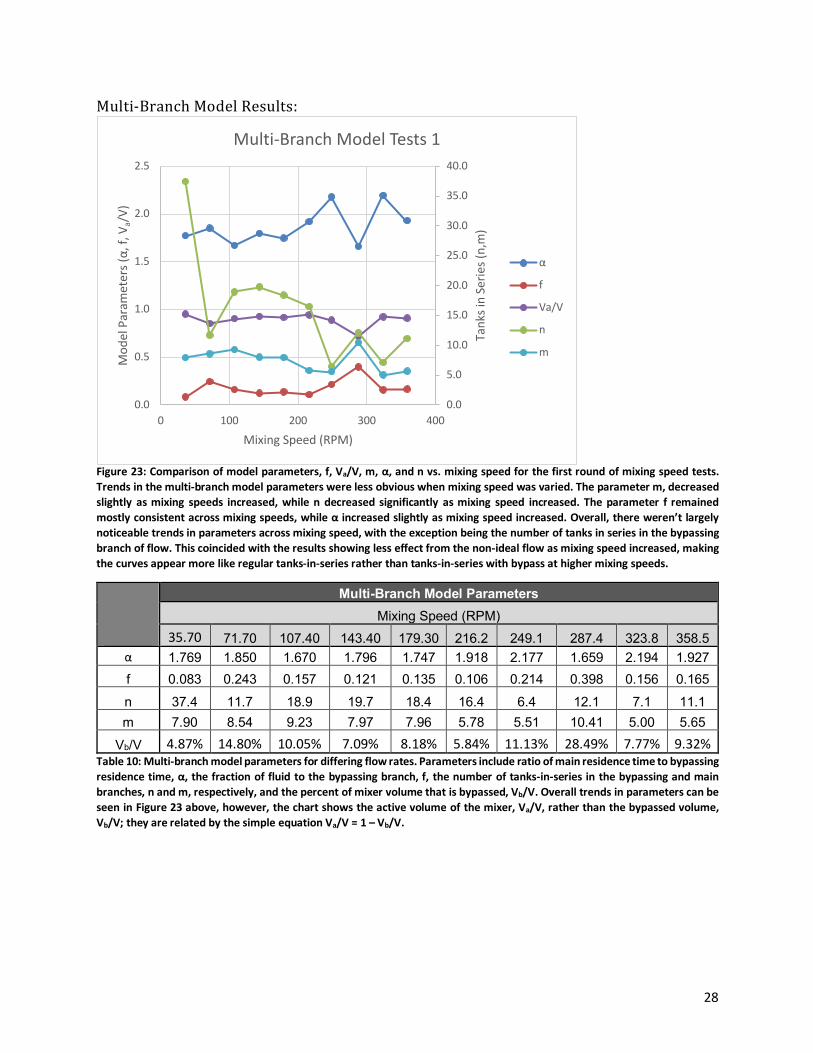
Figure 23: Comparison of model parameters, f, Va/V, m, α, and n vs. mixing speed for the first round of mixing speed tests. Trends in the multi-branch model parameters were less obvious when mixing speed was varied. The parameter m, decreased slightly as mixing speeds increased, while n decreased significantly as mixing speed increased. The parameter f remained mostly consistent across mixing speeds, while α increased slightly as mixing speed increased. Overall, there weren’t largely noticeable trends in parameters across mixing speed, with the exception being the number of tanks in series in the bypassing branch of flow. This coincided with the results showing less effect from the non-ideal flow as mixing speed increased, making the curves appear more like regular tanks-in-series rather than tanks-in-series with bypass at higher mixing speeds.

Multi-Branch Model Parameters Mixing Speed (RPM)

35.70 71.70 107.40 143.40 179.30 216.2 249.1 287.4 323.8 358.5 α 1.769 1.850 1.670 1.796 1.747 1.918 2.177 1.659 2.194 1.927 f 0.083 0.243 0.157 0.121 0.135 0.106 0.214 0.398 0.156 0.165 n 37.4 11.7 18.9 19.7 18.4 16.4 6.4 12.1 7.1 11.1 m 7.90 8.54 9.23 7.97 7.96 5.78 5.51 10.41 5.00 5.65

Vb/V 4.87% 14.80% 10.05% 7.09% 8.18% 5.84% 11.13% 28.49% 7.77% 9.32% Table 10: Multi-branch model parameters for differing flow rates. Parameters include ratio of main residence time to bypassing residence time, α, the fraction of fluid to the bypassing branch, f, the number of tanks-in-series in the bypassing and main branches, n and m, respectively, and the percent of mixer volume that is bypassed, Vb/V. Overall trends in parameters can be seen in Figure 23 above, however, the chart shows the active volume of the mixer, Va/V, rather than the bypassed volume, Vb/V; they are related by the simple equation Va/V = 1 – Vb/V.

0.0

5.0

10.0

15.0

20.0

25.0

30.0

35.0

40.0

0.0

0.5

1.0

1.5

2.0

2.5

0 100 200 300 400

Tank

s in

Serie

s (n,

m)

Mod

el P

aram

eter

s (α,

f, V

a/V)

Mixing Speed (RPM)

Multi-Branch Model Tests 1

α

f

Va/V

n

m

29

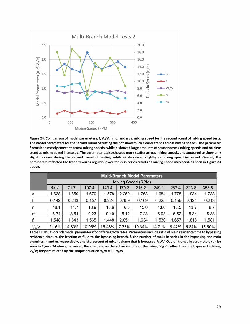
Figure 24: Comparison of model parameters, f, Va/V, m, α, and n vs. mixing speed for the second round of mixing speed tests. The model parameters for the second round of testing did not show much clearer trends across mixing speeds. The parameter f remained mostly constant across mixing speeds, while n showed large amounts of scatter across mixing speeds and no clear trend as mixing speed increased. The parameter α also showed more scatter across mixing speeds, and appeared to show only slight increase during the second round of testing, while m decreased slightly as mixing speed increased. Overall, the parameters reflected the trend towards regular, lower tanks-in-series results as mixing speed increased, as seen in Figure 23 above.

Multi-Branch Model Parameters Mixing Speed (RPM)

35.7 71.7 107.4 143.4 179.3 216.2 249.1 287.4 323.8 358.5 α 1.638 1.850 1.670 1.578 2.250 1.763 1.684 1.778 1.934 1.738 f 0.142 0.243 0.157 0.224 0.159 0.169 0.225 0.156 0.124 0.213 n 18.1 11.7 18.9 16.6 6.3 15.0 13.0 16.5 13.7 8.7 m 8.74 8.54 9.23 9.40 5.12 7.23 6.98 6.52 5.34 5.38 β 1.548 1.643 1.565 1.448 2.051 1.634 1.530 1.657 1.818 1.581 Vb/V 9.16% 14.80% 10.05% 15.48% 7.75% 10.34% 14.71% 9.42% 6.84% 13.50%

Table 11: Multi-branch model parameters for differing flow rates. Parameters include ratio of main residence time to bypassing residence time, α, the fraction of fluid to the bypassing branch, f, the number of tanks-in-series in the bypassing and main branches, n and m, respectively, and the percent of mixer volume that is bypassed, Vb/V. Overall trends in parameters can be seen in Figure 24 above, however, the chart shows the active volume of the mixer, Va/V, rather than the bypassed volume, Vb/V; they are related by the simple equation Va/V = 1 – Vb/V.

0.0

2.0

4.0

6.0

8.0

10.0

12.0

14.0

16.0

18.0

20.0

0.0

0.5

1.0

1.5

2.0

2.5

0 100 200 300 400

Tank

s in

Serie

s (n,

m)

Mod

el P

aram

eter

s (α,

f, V

a/V)

Mixing Speed (RPM)

Multi-Branch Model Tests 2

α

f

Va/V

n

m