Reshetov LA Survey and some new results on performance analysis of complex-valued parameter estimators

Contents lists available at ScienceDirect

Signal Processing

Signal Processing 111 (2015) 210–221

http://d0165-16

n Corrfax: þ3

E-mabeida3

journal homepage: www.elsevier.com/locate/sigpro

Survey and some new results on performance analysisof complex-valued parameter estimators

Jean Pierre Delmas a,n, Habti Abeida b

a Institut TELECOM, TELECOM SudParis, Département CITI, CNRS UMR 5157, 91011 Evry Cedex, Franceb Department of Electrical Engineering, University of Taif, Al-Haweiah 21974, Saudi Arabia

a r t i c l e i n f o

Article history:Received 24 October 2014Accepted 9 December 2014Available online 26 December 2014

Keywords:Circular (proper) and noncircular(improper) complex-valued signalsStatistical performance analysisCramer–Rao boundAsymptotically minimum variance boundSlepian–Bangs and Whittle formulas

x.doi.org/10.1016/j.sigpro.2014.12.00984/& 2014 Elsevier B.V. All rights reserved.

esponding author. Tel.: þ33 1 60 76 46 32;3 1 60 76 44 33.ail addresses: jean-pierre.delmas@[email protected] (H. Abeida).

a b s t r a c t

Recently, there has been an increased awareness that simplistic adaptation of perfor-mance analysis developed for random real-valued signals and parameters to the complexcase may be inadequate or may lead to intractable calculations. Unfortunately, manyfundamental statistical tools for handling complex-valued parameter estimators aremissing or scattered in the open literature. In this paper, we survey some known resultsand provide a rigorous and unified framework to study the statistical performance ofcomplex-valued parameter estimators with a particular attention paid to properness (i.e.,second order circularity), specifically referring to the second-order statistical properties.In particular, some new properties relative to the properness of the estimates, asympto-tically minimum variance bound and Whittle formulas are presented. A new look at therole of nuisance parameters is given, proving and illustrating that the noncircularGaussian distributions do not necessarily improve the Cramer–Rao bound (CRB) withrespect to the circular case. Efficiency of subspace-based complex-valued parameterestimators that are presented with a special emphasis is put on noisy linear mixture.

& 2014 Elsevier B.V. All rights reserved.

1. Introduction

Complex-valued random signals associated with complex-valued parameters play an increasingly important role inmany science and engineering problems, including those incommunications, radar, biomedicine, geophysics, oceanogra-phy, electromagnetics, and optics, among others (see, e.g., [1,2]and the references therein). But the usual way to analyze thestatistical performance of complex-valued parameter estima-tors is still often by splitting each complex parameter into itsreal and imaginary parts and treating them as separate realparameters [3,4]. Although this procedure is mathematically

s.eu (J.P. Delmas),

correct, it involves complicated expressions, lacking the engi-neering insight necessary for a lucid understanding of thevarious phenomena and for suggesting improved solutions.Unfortunately, many fundamental statistical tools for handlingcomplex-valued parameter estimators are missing or scat-tered in open literature (see, e.g., [5, Chapter 6] and thereferences therein).

In this paper, we provide a rigorous and unified frameworkto study the statistical performance of complex-valued para-meter estimators. As for all parameter estimation, an algo-rithm or an estimator extracts an approximation θ̂N of anunknown parameter θ from measurements ½xð1Þ;…; xðNÞ�.Here the measurements are characterized by a joint PDFpðxðnÞn ¼ 1;…;N; θ;αÞ where xðnÞACr , θ¼ ðθ1;…; θqÞT ACq isthe parameter of interest and α gathers all the other unknownparameters (nuisance parameters). There are two issues toconsider in performance analysis. The first one, which is

2 This is typically the case for the estimates derived from the methodof moments, where sN are the sample moments of xðnÞ. This is also the

J.P. Delmas, H. Abeida / Signal Processing 111 (2015) 210–221 211

treated in Section 2, consists in studying the performance of aparticular algorithm, principally to derive the asymptotic1

distribution, bias and covariance of θ̂N . In this section,particular attention is paid to properness (i.e., second-ordercircularity) of the asymptotic distribution of the parameterestimates where new properties are given. The second one isto establish a limit on the accuracy of any estimator belongingto a family of estimators. This is the subject of Sections 3 and4, respectively, dedicated to the Cramer–Rao and asymptoti-cally minimum variance bounds, where new extensions aregiven. A particular treatment of the noisy linear mixture isgiven in Section 5, where the efficiency of subspace-basedcomplex-valued parameter estimators is studied. Illustrationare given in Section 6 dedicated to blind identification ofcomplex SIMO channels and complex independent compo-nent analysis. Finally, Section 7 presents a conclusion.

The following notations are used throughout the paper.Matrices and vectors are represented by bold upper case andbold lower case characters, respectively. Vectors are bydefault in column orientation, while T, H, n and # standfor transpose, conjugate transpose, conjugate and Moore–Penrose inverse, respectively. oðϵÞ denotes a quantity suchthat limϵ-0oðϵÞ=ϵ¼ 0. Eð�Þ, Trð�Þ, Reð�Þ and Imð�Þ are theexpectation, trace, real and imaginary part operators,respectively. I is the identity matrix. vecð�Þ is the “vectoriza-tion” operator that turns a matrix into a vector by stackingthe columns of the matrix one below another which is usedin conjunction with the Kronecker product A � B as theblock matrix whose (i,j) block element is ai;jB and with thevec-permutation matrix K which transforms vecðCÞ tovecðCT Þ for any square matrix C. vð�Þ denotes the operatorobtained from vecð�Þ by eliminating all supradiagonal ele-ments of the matrix. ~a ¼ ðaT ; aHÞT and a ¼ ðReðaÞT ; ImðaÞT ÞTare, respectively, the augmented and the real-valued vectorassociated with complex-valued vector a.

2. Performance analysis

To study the asymptotic performance of an algorithm, itis fruitful to adopt a functional analysis that consists inrecognizing that the whole process of constructing theestimate θ̂N is equivalent to defining a functional relationlinking this estimate to the measurements fromwhich it isinferred. Note that this functional analysis first introducedin [6] has been presented in [7, Section 3.1] for the real-valued DOA parameter and can be considered as anextension of this one. As generally θ̂N are functions ofsome statistics sNACp deduced from ðxðnÞÞn ¼ 1;…;N , wehave the following mapping:

xðnÞð Þn ¼ 1;…;N⟼sN⟼gθ̂N : ð1Þ

The statistic sN is assumed to converge almost surely tosðθÞ ¼ EðsNÞ and θ is supposed identifiable from sðθÞ, sogenerally pZq. The functional dependence θ̂N ¼ gðsNÞ con-stitutes an extension of the mapping sðθÞ⟼θ in the

1 In general only the asymptotic distribution, bias and covariance canbe derived, either w.r.t. the number N of measurements, the size r or thesignal to noise ratio of the measurements. Hopefully, in practice theobtained results give good approximations for finite values of thesequantities.

neighborhood of sðθÞ. Each extension g specifies a particularalgorithm. The statistics sN may be sample moments,2

cumulants of xðnÞ or any specific statistics adapted to thedistribution of the measurements. For example, for the noisylinear mixtures (31), the orthogonal projectors associatedwith the sample estimates of the covariance, complementarycovariance3 or augmented covariance of xðnÞ have been usedfor subspace-based algorithms. In the specific case of inde-pendent identically distributed (IID) measurements xðnÞ,closed-form expressions ð1=NÞRs and ð1=NÞCs of the covar-iance E½ðsN�sÞðsN�sÞH� and complementary covarianceE½ðsN�sÞðsN�sÞT � matrices of sN (where s¼ sðθÞ for short)can be easily derived for sample moments or cumulants ofxðnÞ. For stationary measurements xðnÞ and associated sam-ple statistics sN , central limit theorems and standard theo-rems of continuity allow us to derive convergences indistribution w.r.t. the number N of the measurements (see,e.g., [9] for the second-order statistics sN), viz.,

ffiffiffiffiN

psN�sð Þ-L N Cð0;Rs;CsÞ; ð2Þ

where N Cðm;R;CÞ denotes the complex Gaussian distribu-tion with mean m, covariance R and complementary covar-iance C, defined as the distribution of a complex-valuedrandom variable z such that the associated scalar real-valuedrandom variable ~aH ~z is Gaussian distributed N Rðmz;RzÞ withmean mz ¼ ~aH ~m and covariance Rz ¼ ~aH R

CnCRn

� �~a for any

vector a of compatible dimension.Finally, note that this functional analysis (1) is not

always relevant for other distributions of ðxðnÞÞn ¼ 1;…;N .For example, if xðnÞ ¼ sðθ;nÞþeðnÞ where sðθ;nÞ is a non-linear deterministic function4 of θ and ðeðnÞÞn ¼ 1;…;N is thezero-mean IID, ðxðnÞÞn ¼ 1;…;N are independent, but notidentically distributed and the speed of convergence ofthe sequence of estimates θ̂N can depend on its compo-nent and be different from

ffiffiffiffiN

p.

For statistics sN satisfying (2) and for R-differentiablemapping g [10],

gðsNÞ ¼ gðsÞþDgðsN�sÞþDn;gðsN�sÞnþoðJsN�sJ Þ; ð3Þ

where Dg and Dn;g , q� p matrices, denote the R-derivative∂g=∂s and the conjugate R-derivative ∂g=∂sn of g at point s[11]. In practice, the matrices Dg and Dn;g are derived fromperturbation analysis where only the wide-linear term iskept. Furthermore, their derivations are simplified fromthe chain rule by decomposing the mapping g (i.e., thealgorithm) as successive simpler mappings.

It is proved in the Appendix that if ½Dg ;Dn;g�a0, thefollowing convergence in distribution holds:

ffiffiffiffiN

pðθ̂N�θÞ-L N Cð0;Rθ ;CθÞ ð4Þ

case for the maximum likelihood estimator for Gaussian distribution forwhich sN are first and second-order statistics.

3 Other names for complementary covariance matrix includepseudo-covariance matrix, conjugate covariance matrix and relationmatrix.

4 The celebrated noisy sinusoid case where sðθ;nÞ ¼ PKk ¼ 1 ake

ið2πnf k þϕkÞ

is such an example.

6 Note that R ~s characterizes the asymptotic second-order momentsof ~sN as

J.P. Delmas, H. Abeida / Signal Processing 111 (2015) 210–221212

with

Rθ ¼ ½Dg ;Dn;g �Rs Cs

Cn

s Rn

s

" #DH

g

DHn;g

24

35 and Cθ ¼ ½Dg;Dn;g �

Cs Rs

Rn

s Cn

s

" #DT

g

DTn;g

24

35:

ð5ÞFrom (5), we deduce that for g C-differentiable at point s,Dng ¼ 0, and the usual expressions

Rθ ¼DgRsDHg and Cθ ¼DgCsDT

g ð6Þ

are derived. Furthermore in this case θ̂N is asymptoticallyproper (i.e., Cθ ¼ 0) if and only if sN is asymptoticallyproper (i.e., Cs ¼ 0). We note that generally, if sN isasymptotically proper, θ̂N is not necessarily asymptoticallyproper. It becomes proper if Dn

g ¼ 0, i.e., if g is C-differenti-able at point s (gðsNÞ ¼ gðsÞþDgðsN�sÞþoðJsN�sJ Þ.Finally for real-valued θ, Dn

g ¼Dn;g and the asymptoticcovariance Rθ is given by

Rθ ¼ 2½DgRsDHg þReðDgCsDT

g Þ�: ð7Þ

Under additional regularity assumptions on g, thecovariance and the complementary covariance of θ̂N aregiven, respectively, by

E θ̂N�θ� �

ðθ̂N�θÞHh i

¼ 1NRθþo

1N

� �and

E θ̂N�θ� �

ðθ̂N�θÞTh i

¼ 1NCθþo

1N

� �: ð8Þ

Using a second-order expansion of gðsNÞ where g issupposed to be R-differentiable to the second-order [8],it is proved in the Appendix that the bias is given by theclosed-form expression not published in the open litera-ture:

E θ̂N� �

�θ¼ 12N

2TrðRsHð1Þg;1ÞþTrðCn

sHð2Þg;1ÞþTrðCsH

ð3Þg;1Þ

⋮2TrðRsHð1Þ

g;qÞþTrðCn

sHð2Þg;qÞþTrðCsHð3Þ

g;qÞ

2664

3775þo

1N

� �ð9Þ

where Hð1Þg;k, H

ð2Þg;k and Hð3Þ

g;k are the three Hessian matrices [5,

A2.3] ð∂=∂sÞ ∂gk=∂s� �H , ð∂=∂snÞ ∂gk=∂s

� �H and ð∂=∂sÞ ∂gk=∂s� �T

of the kth component gk of the function g at point s,respectively. We note that for g C-differentiable to the

second-order, the only nonzero Hessian is Hð3Þg;k, and (9)

reduces to its last termwhich is zero if sN is asymptoticallyproper. So for g C-differentiable to the second-order andsN asymptotically proper, θ̂N is asymptotically unbiased to

the first order.5 Finally, for real-valued θ, Hð3Þg;k ¼ ðHð2Þ

g;kÞn, Eq.(9) reduces to

E θ̂N� �

�θ¼ 12N

TrðR ~sH ~g ;1Þ⋮

TrðR ~sH ~g ;qÞ

264

375þo

1N

� �;

where

H ~g ;k ¼∂∂~s

∂g∂~s

� �H

¼Hð1Þ

g;k Hð2Þg;k

Hð2Þg;kn

Hð1Þg;kn

24

35

5 This contrasts with the real-valued case for which the bias on θ̂N isof order 1/N.

is the complex augmented Hessian matrix [5, A2.3] of thekth component of the function g at point s and

R ~s ¼Rs Cs

Cn

s Rn

s

" #

is the asymptotic augmented covariance6 of sN .We note that necessary mathematical conditions con-

cerning the remainder terms of these first- and second-order expansions are in the signal processing literaturenever checked as these conditions are very difficult toprove for the involved mappings sN ⟼

gθ̂N . For example,

the following necessary conditions are given in [12,Th. 4.2.2] for the second-order algorithms: (i) the mea-surements fxðnÞgn ¼ 1;…;N are independent with finiteeighth moments, (ii) the mapping sN ⟼

gθ̂N is four times

R-differentiable, (iii) the fourth derivative of this mappingand those of its square are bounded. These assumptionsthat do not depend on the distribution of the measure-ments are very strong, but fortunately (8) and (9) continueto hold in many cases in which these assumptions are notsatisfied, in particular for Gaussian distributed data (see,e.g., [12, Ex. 4.2.2]).

Finally, we note that if in practice all functions g, i.e.,algorithms are R-differentiable, only some of them areC-differentiable. Among them, when θ̂N are roots (e.g., forthe root MUSIC algorithms) or explicit solutions (e.g., forthe Cðk; qÞ formula [13] extended to the complex case [14])of polynomials equations whose coefficients are C-differ-entiable functions of the statistics sN , the algorithm g isC-differentiable. This is in contrast to the case where θ̂Nmaximizes a (real-valued) function depending on thestatistics sN , where g may be now only R-differentiable.This is the case for the subspace-based algorithms forestimating the SIMO and MIMO impulse responses.

3. Asymptotically minimum variance bound

To assess the performance of an algorithm based on aspecific statistic sN built from ðxðnÞÞn ¼ 1;…;N , it is interestingto compare the asymptotic covariance Rθ (5) and thecomplementary covariance Cθ (5) to an attainable lowerbound that depends on the statistic sN only. The asympto-tically minimum variance bound (AMVB) is such a bound.7

This bound is generally easy to derive in contrast to theCRB which depends on the distribution of the measure-ments that appears to be prohibitive to compute for non-Gaussian distributions, except in special cases. This bounduses only the statistical properties of the statistic sN andcan be used as a benchmark against which potentialestimates θ̂N ¼ gðsNÞ are tested. To extend the derivationsof Porat and Friedlander [15] concerning this AMVB tocomplex-valued measurements and parameters, threeadditional conditions than those introduced in Section 2

C~s ¼Cs Rs

Rn

s Cn

s

" #:

7 Also called asymptotically best consistent (ABC) estimators in [16].

J.P. Delmas, H. Abeida / Signal Processing 111 (2015) 210–221 213

must be satisfied. First, the mapping θ⟼sðθÞ must beR-differentiable. Second, the involved function g thatdefines the considered algorithm must be R-differentiable.And third, the asymptotic augmented covariance R ~s of sNmust be nonsingular. To satisfy this condition, the 2pcomponents of ~sN ¼def ½sTN ; sHN �T must be asymptotically line-arly independent random variables. Consequently, nocomponent of sN must be real-valued. If some componentsare real-valued, the redundancies in ~sN must be with-drawn (see, e.g., [17] for the second-order statistics).

Using the augmented representation, and following thesteps of the derivation of the AMVB for real-valued sN andθ̂N [15], it is proved in the Appendix that the augmentedcovariance matrix R ~θ of the asymptotic distribution of anestimate of θ given by an arbitrary consistent algorithm(characterized by the mapping g) based on the statistic sNis bounded below by ð ~DH

s R�1~s

~Ds�1:

Result 1.

R ~θ ¼Rθ Cθ

Cn

θ Rn

θ

" #¼ ~DgR ~s

~DHg ZAMVBsð ~θÞ ¼def ð ~D

Hs R

�1~s

~Ds�1

ð10Þ

with ~Dg ¼def DgDn

n;g

Dn;gDn

g

h iand ~Ds ¼def Ds

Dn

n;s

Dn;sDn

s

h iwhere Ds and Dn;s

denote the R-derivative and the conjugate R-derivative ofsðθÞ at point θ, respectively.

Using the partitioned matrix-inversion lemma in (10),Rθ is lower bounded as well. But an algorithm that attainsthis bound alone does not necessarily attain the AMVB (10)since Rθ does not provide a full second-order descriptionof a complex random variable; Cθ is also needed.

Furthermore, it is proved in the Appendix that thefollowing nonlinear least squares algorithm is an algo-rithm that attains the AMVB:

θ̂N ¼ arg minβ

½~sN� ~sðβÞ�HWN½~sN� ~sðβÞ�; ð11Þ

where ~sðβÞ ¼def ½sT ðβÞ; sHðβÞ�T and WN is an arbitrary consistentestimate of R�1

~s that satisfies WN ¼ R�1~s þoðJsN�sðθÞJ Þ.

For real-valued θ, Dn;g ¼Dg and the AMVB (10) reducesto

Rθ ¼ 2½DgRsDHg þReðDgCsDT

g Þ�ZAMVBsðθÞ ¼def DHs ;D

Ts

h iR�1

~s

Ds

Dn

s

" # !�1

:

An example of such a derivation is given in [17] for thesecond-order statistics applied to DOA estimation. Notethat in contrast to the Cramer–Rao bound (CRB) that isgenerally difficult to compute for nonGaussian distribu-tions, the AMVB that uses only the asymptotic second-order statistics of sN is much easier to derive.

4. Cramer–Rao bound

To simplify the notations, when the number N of measure-ments is fixed, these measurements are denoted by x andtheir PDF by pðx; θÞ, where throughout this section, θ denotesthe unknown parameter that gathers the parameter of inter-est and nuisance parameter.

4.1. General properties of the FIM

Many authors have extended the CRB to complex-valued measurements and parameters. Among them,Ref. [18] has derived this bound by imitating the proof inthe real case and Ref. [19] has used the one-to-onemappings ~x⟷x and ~θ⟷θ. Note that despite the CRBhas been well covered in the complex case, new contribu-tions continue to appear (see, e.g., [20]).

If θ̂ denotes an unbiased estimator of θ, the augmen-

ted covariance matrix of θ̂, R ~̂θ¼

Rθ̂ Cθ̂

Cn

θ̂ Rn

θ̂

" #, where

Rθ̂ ¼defE½ðθ̂�θÞðθ̂�θÞH� and Cθ̂ ¼

defE½ðθ̂�θÞðθ̂�θÞT �, is upperbounded by the inverse of the augmented Fisher informa-tion matrix (FIM):

J ~θ ¼Jθ Jn;θJnn;θ Jnθ

" #ð12Þ

assumed to be nonsingular [19, Theorem 1], [5, Result 6.3]:

R ~̂θZCRBð ~θÞ ¼def J�1

~θ : ð13Þ

where Jθ and Jn;θ are the complex FIM and the comple-mentary complex FIM, respectively, given under regularityconditions by

Jθ ¼ E∂ ln pðx; θÞ

∂θ

H ∂ ln pðx; θÞ∂θ

!¼ �E

∂∂θ

∂ ln pðx; θÞ∂θ

H !; ð14Þ

Jn;θ ¼ E∂ ln pðx; θÞ

∂θ

H ∂ ln pðx; θÞ∂θn

!¼ �E

∂∂θn

∂ ln pðx; θÞ∂θn

T !:

ð15ÞThe CRB (13) implies the following bound on the covar-iance matrix Rθ̂ of θ̂ [18]:

Rθ̂ ZðJθ� Jn;θJ�1θ Jn

n;θÞ�1ZJ�1θ : ð16Þ

If an unbiased estimator θ̂ attains this bound on Rθ̂ alone,

it does not imply that θ̂ attains the CRB (13), since alsoCθ̂ ¼ �ðJθ� Jn;θJ

�1θ Jn

n;θÞ�1Jn;θJn�1θ needs to hold (see also [19,

Corollary 1(a)]). Only if the complementary FIM Jn;θvanishes, then Rθ̂ ¼ J�1

θ implies that θ̂ attains the CRB (13).Note that (16) assumes that J ~θ is nonsingular, which is

not the case for real-valued parameters for which Jθ ¼ Jn;θ .In this case, the complex CRB is simply given by Rθ̂ Z J�1

θ .In the presence of nuisance parameters α (generally real-

valued), the complex CRB on the parameter of interest θ onlyis obtained similar to that in the real case. Using the one-to-

one mapping θα

h i⟷

~θα

h i, it is straightforward to prove the

following result not published in the open literature:In the case of nuisance parameter α, (13) and (16),

respectively, become

R ~̂θZCRBð ~θÞ ¼def ðJ ~θ � J ~θ ;αJ

�1α JH~θ ;αÞ�1Z J�1

~θ ; ð17Þ

Rθ̂ Z ½ðJ ~θ � J ~θ ;αJ�1α JH~θ ;αÞ�1�θ;θZ ðJθ�Jn;θJ

�1θ Jn

n;θÞ�1Z J�1θ ; ð18Þ

where ½��θ;θ denotes the q� q top-left submatrix of ½��, Jα isthe usual FIM w.r.t. the real-valued parameter α only,

J.P. Delmas, H. Abeida / Signal Processing 111 (2015) 210–221214

and J ~θ ;α ¼ Jθ;αJn;θ;α

h iwith

Jθ;α ¼ E∂ ln pðx; θ;αÞ

∂θ

H ∂ ln pðx; θ;αÞ∂α

!¼ �E

∂∂α

∂ ln pðx; θ;αÞ∂θ

H !

ð19Þ

Jn;θ;α ¼ E∂ ln pðx; θ;αÞ

∂θn

H ∂ ln pðx; θ;αÞ∂α

!¼ �E

∂∂α

∂ ln pðx; θ;αÞ∂θn

H !:

ð20Þ

4.2. Specific Gaussian case

4.2.1. Slepian–Bangs formulaFor complex Gaussian distributions, N Cðmx;Rx;CxÞ, the

Slepian–Bangs formula has been extended in [21] and[5, 6.3.5] for real and complex-valued parameters, respec-tively, where their elementwise FIM and the complemen-tary FIM have been given.8 Note that these matrices canalso be given by the following compact expressions:

Jθ ¼∂m ~x

∂θ

� �H

R�1~x

∂m ~x

∂θþ12DH

r ~x C�1nr ~x Dr ~x ; ð21Þ

Jn;θ ¼∂m ~x

∂θ

� �H

R�1~x

∂m ~x

∂θnþ12DH

r ~x C�1nr ~x Dn;r ~x ; ð22Þ

which gives

J ~θ ¼∂m ~x∂θ

� �H∂m ~x∂θn

� �H264

375R�1

~x∂m ~x

∂θ∂m ~x

∂θn

þ12

DHr ~x

DHn;r ~x

24

35R�1n

r ~x Dr ~x Dn;r ~x

� �; ð23Þ

where m ~x ¼ ðmTx ;m

Hx ÞT , R ~x ¼ Eðð ~x�m ~x Þð ~x�m ~x ÞHÞ with

~x ¼ ðxT ; xHÞT , Dr ~x and Dn;r ~x denote the R-derivative ∂r ~x=∂θand the conjugate R-derivative ∂r ~x=∂θn of r ~x ¼defvecðR ~x Þ,respectively, and where Rr ~x ¼ Rn

~x � R ~x is the covarianceof the asymptotic distribution of r ~x ;N ¼ vecðR ~x ;NÞ withR ~x ;N ¼def ð1=NÞPN

n ¼ 1 ~xðnÞ ~xHðnÞ.

4.2.2. Whittle formulaWhen xðnÞ is a real-valued stationary zero-mean Gaus-

sian multivariate process with spectrum Rxðf Þ that dep-ends on the real-valued parameter θ, the Whittle formula[22, Th. 9] gives the elements of the asymptotic FIMassociated with N sample values of xðnÞ. Thus thematrix-valued Cramer–Rao bound is given by

Rθ̂ ZJ�1θ where Jθ ¼

N2

Z þ1=2

�1=2DH

rx fð Þ R�n

x ðf Þ � R�1x ðf Þ

� �Drx fð Þ df ;

ð24Þwhere Rθ̂ is the covariance of any unbiased estimate of θbuilt from ðxðnÞÞn ¼ 1;…;N and Drx ðf Þ denotes the derivative∂rxðf Þ=∂θ of rxðf Þ ¼defvecðRxðf ÞÞ where Rxðf Þ is Hermitianstructured.

Using the one-to-one mappings ~xðnÞ⟷xðnÞ and ~θ⟷θ,it is proved in the Appendix the following extension of theWhittle formula:

8 Note that (21) and (22) are slightly different from the elementwiseexpressions [5, (6.65)] and [5, (6.66)] because the latter expressions areerroneous.

Result 2. Let xðnÞ be a complex-valued stationary zero-mean non necessarily circular, Gaussian multivariate pro-cess with spectrum Rxðf Þ and complementary spectrumCxðf Þ [5, Section 8.1] that both depend on the complex-valued parameter θ, the matrix-valued Cramer–Rao boundis given by

R ~̂θZJ�1

~θ with J ~θ ¼Jθ Jn;θJnn;θ Jnθ

" #is assumed to be nonsingular;

ð25Þand Jθ and Jn;θ are given, respectively, by

Jθ ¼N2

Z þ1=2

�1=2DH

r ~x fð Þ R�1n~x ðf Þ � R�1

~x ðf Þ� �

Dr ~x fð Þ df ; ð26Þ

Jn;θ ¼N2

Z þ1=2

�1=2DH

r ~x fð Þ R�1n~x ðf Þ � R�1

~x ðf Þ� �

Dn;r ~x fð Þ df ; ð27Þ

or more compactly, by

J ~θ ¼N2

Z þ1=2

�1=2

DHr ~x ðf Þ

DHrn; ~x ðf Þ

24

35R�n

~x fð Þ

� R�1~x fð Þ Dr ~x ðf Þ Drn; ~x ðf Þ

� �df ; ð28Þ

where Dr ~x ðf Þ and Dn;r ~x ðf Þ denote the R-derivative ∂r ~x ðf Þ=∂θand the conjugate R-derivative ∂r ~x ðf Þ=∂θn of r ~x ðf Þ ¼defvecðR ~x ðf ÞÞ, respectively, and R ~x ðf Þ is the spectrum of theaugmented process ~xðnÞ:

R ~x ðf Þ ¼Rxðf Þ Cxðf ÞCn

xð� f Þ Rn

xð� f Þ

" #;

with Rxðf Þ and Cxðf Þ the Fourier transforms of RxðkÞ ¼E½ðxðnÞxHðn�kÞ� and CxðkÞ ¼ E½ðxðnÞxT ðn�kÞ�, respectively,both characterizing the statistical properties of the randomprocess xðnÞ.

Note that for real-valued parameters, (25) reduces toRθ̂ ZJ�1

θ that was proved in [23] for deriving the CRB ofestimated delays in the context of complex-valued sta-tionary processes.

4.2.3. Circular to noncircular comparisonFor the Gaussian distribution characterized by (mx;Rx;CxÞ,

suppose now that the parameter θ is identifiable fromðmx;Rx) only. A question remains open (see [5, Section6.3.5]): Is J ~θ more positive definite if Cxa0 than if Cx ¼ 0?Or in other words, does the noncircular case generallyimprove the CRB of θ with respect to the circular case?Addressing generally this question from (21) and (22) seemsvery challenging. But formulating this question in the frame-work of measurements x¼ ðxðnÞÞn ¼ 1;…;N , where xðnÞ are IIDand where mx, Rx and Cx denote the mean, covariance andcomplementary covariance of xðnÞ, respectively, is mucheasier, as the AMVB based on the statistics that include boththe sample mean, sample covariance and sample comple-mentary covariance attains the CRB for the Gaussian distribu-tion, i.e.,

J�1~θ ¼ ð ~DH

s R�1~s

~DsÞ�1; ð29Þwhere J ~θ is associated with xðnÞ alone and where theaugmented statistics involved is ~sðθÞ ¼ ½mT

x ;mHx ; vec

T ðRxÞ;

J.P. Delmas, H. Abeida / Signal Processing 111 (2015) 210–221 215

vT ðCxÞ; vHðCxÞ�T in order to satisfy the three conditions of theAMVB (10). Using (29), it is proved in the Appendix:

Result 3. When the parameter θ of the Gaussian distribu-tion (characterized by (mx;Rx;CxÞ) of xðnÞ is identifiablefrom ðmx;Rx) only, noncircular Gaussian distributionsgenerally improve the CRB for θ with respect to thecircular case:

CRBmx ;Rx ;Cx ð ~θÞrCRBmx ;Rx ;0ð ~θÞ ð30Þwhere CRBmx ;Rx ;Cx ð ~θÞ and CRBmx ;Rx ;0ð ~θÞ denote the augmen-ted complex CRB (13) associated with noncircular andcircular Gaussian distribution, respectively.

In the presence of nuisance parameters α, the previousquestion is much more involved because the complemen-tary covariance matrix Cx can not only bear information onthe parameter of interest θ, but can also introduce addi-tional nuisance parameters. An example in which (30) isnot satisfied in the presence of nuisance parameters ispresented in Section 6. However in particular statisticalmodels, (30) can be extended as it is proved in the nextsection.

5. Noisy linear mixture

Consider the following model:

xðnÞ ¼AðθÞsðnÞþeðnÞACr n¼ 1;…;N; ð31Þwhere (i) sðnÞ and eðnÞ are independent zero-mean ran-dom variables, (ii) eðnÞ is circular with EðeðnÞeHðnÞÞ ¼ σ2e Iand sðnÞACp is either circular with EðsðnÞsHðnÞÞ ¼ Rs non-singular or noncircular with Eð~sðnÞ~sHðnÞÞ ¼ R ~s nonsingular,(iii) the useful parameter θACq is characterized by thesubspace generated by the columns of the full column rankr � p matrix AðθÞ with por. The nuisance parameters αgather here the terms ðRsÞi;j for 1r ir jrp and σ2e [resp.,the terms ðRsÞi;j and ðCsÞi;j for 1r ir jrp and σ2e] in thecircular [resp., noncircular] case.

5.1. CRB expressions

Using the direct approach introduced by [24] to con-centrate the CRB on the parameter θ, it is proved in theAppendix the following result not been published in theopen literature:

For the model (31) with assumptions (i)–(iii) whereðsðnÞÞn ¼ 1;…;N and ðeðnÞÞn ¼ 1;…;N are independent Gaussiandistributed random variables, the CRB for the real-valuedparameter alone θ ¼def ½ReT ðθÞ; ImT ðθÞ�T is given by

CRB θ� �¼ σ2e

2NRe

∂aH

∂θHT � Π?

A

� �∂a∂θ

� � �1

; ð32Þ

where a¼defvecðAÞ, Π?A ¼def I�AðAHAÞ�1AH is the ortho-

complement of the projection matrix on the columns ofA and H is given by the Hermitian matrices RsA

HR�1x ARs

and RsAH ;CsA

Th i

R�1~x

ARsAnCn

s

h iin the circular and noncircular

cases, respectively.We note that (32) extends the CRB compact expres-

sion [24, rel. (5)] given for the DOA modeling with scalar-sensors for one parameter per source, and encompa-sses DOA modeling with vector-sensors for an arbitrary

number of parameters per source and many other modelsas the SIMO and MIMO modelings.

Using the one-to-one mapping θ⟷ ~θ, the followingcompact expression of the augmented complex CRB (12)and (13) is proved in the Appendix.

Result 4. For the model (31) with assumptions (i)–(iii),where ðsðnÞÞn ¼ 1;…;N and ðeðnÞÞn ¼ 1;…;N are independentGaussian distributed random variables, we have

R ~̂θZCRBð ~θÞ; with CRBð ~θÞ ¼ J�1

~θ ¼Jθ Jn;θJnn;θ Jnθ

" #�1

; ð33Þ

where

Jθ ¼Nσ2e

∂a∂θ

� �H

HT � Π?A

� � ∂a∂θ

� �þ ∂a

∂θn

� �T

H � Π? T

A

� � ∂a∂θn

� �n" #

; ð34Þ

Jn;θ ¼Nσ2e

∂a∂θ

� �H

HT � Π?A

� � ∂a∂θn

� �þ ∂a

∂θn

� �T

H � Π? T

A

� � ∂a∂θ

� �n" #

:

ð35Þ

In the particular case where a is C-differentiable w.r.t. θ(e.g., for SIMO and MIMO channel modelings), ∂a=∂θn ¼ 0,and (34) and (35) reduce to

Jθ ¼Nσ2e

∂a∂θ

� �H

HT � Π?A

� � ∂a∂θ

� �and Jn;θ ¼ 0; ð36Þ

and the AMV estimator is asymptotically circular withRθ̂ ¼ J�1

θ , whatever the circularity properties of xðnÞ.Note that the closed-form expressions (32) and (34)–

(36) do not take into account the prior knowledge relativeto the sources because they have been derived without anyconstraint on Rs and Cs. But unfortunately, taking intoaccount these constraints leads to very intricate expres-sions (see, e.g., [25, Eq. (13)] for circular uncorrelatedsources for the DOA modeling). This point will be illu-strated in Section 6 with the SISO channel modeling.Furthermore, note that the condition A is full column rankwith por which is not necessary to identify the usefulparameter θ when specific a priori knowledge about thesources is available, see, e.g., [28] for real-valued or QPSKmodulations and [29] for offset linear modulations in SISOchannel modeling.

Finally comparing the circular to the noncircular cases,it is proved in the Appendix that the CRB for θ in thenoncircular case is upper bounded by the associatedasymptotic RB in the circular case. More precisely, for themodel (31) with assumptions (i)–(iii), where ðsðnÞÞn ¼ 1;…;N

and ðeðnÞÞn ¼ 1;…;N are independent Gaussian distributedrandom variables, we have

CRBRx ;Cx ð ~θÞrCRBRx ;0ð ~θÞ: ð37Þ

This result extends the CRB inequality proved in [21] forthe DOA parameters. Consequently, when the precisionon the parameter θ is important, it is preferable to usenoncircular sðkÞ signals (e.g., real-valued) than circularones, for example for blind SISO, SIMO and MIMO channelsidentification.

9 We have assumed h10 ¼ 1 to avoid any ambiguity for the definitionof the impulse response θ in the product AðθÞsðnÞ.

J.P. Delmas, H. Abeida / Signal Processing 111 (2015) 210–221216

5.2. Efficiency of subspace-based estimators

For the model (31) with assumptions (i)–(iii), many algo-rithms are consistent subspace-based, i.e., the estimates θ̂ areobtained by exploiting the orthogonality between a samplesubspace and a parameter-dependent subspace [26]. In otherwords, for circular xðnÞ, these algorithms satisfy the mapping(1) where the statistic sN is usually the orthogonal projectorΠRx ;N on noise (or signal) associated with the sample covar-iance Rx;N ¼ ð1=NÞPN

n ¼ 1 xðnÞxHðnÞ. To exploit the potentialnoncircularity of xðnÞ, the orthogonal projector ΠR ~x ;N asso-ciated with the sample augmented covariance R ~x ;N ¼ð1=NÞPN

n ¼ 1 ~xðnÞ ~xHðnÞ or the couple ðΠRx ;N ;ΠCx ;N) of ortho-gonal projectors (where ΠCx ;N is the orthogonal projectorassociated with Cx;N ¼ ð1=NÞPN

n ¼ 1 xðnÞxT ðnÞ) is used. Alth-ough, the asymptotic covariance Rs of the statistics vecðΠRx ;NÞ,vecðΠR ~x ;NÞ and vecðΠRx ;N ;ΠCx ;NÞ are singular, and thus do notsatisfy the third condition introduced in the beginning ofSection 3, the following result (not published in the openliterature) is proved in the Appendix:

For the model (31) with assumptions (i)–(iii), the AMVB(10) becomes

R ~θ ¼Rθ Cθ

Cn

θ Rn

θ

" #¼ ~DgR ~s

~DHg ZAMVBsð ~θÞ ¼def ð ~D

Hs R

#~s~Ds�1

ð38Þ

for sN ¼ vecðΠRx ;NÞ, vecðΠR ~x ;NÞ or vecðΠRx ;N ;ΠCx ;NÞ. Further-more, despite the lack of a one-to-one mapping betweenðΠRx ;N ;ΠCx ;NÞ and ΠR ~x ;N , contrary to the one-to-one map-ping ðRx;N ;Cx;NÞ⟷R ~x ;N , the AMVB based on the statisticsðΠRx ;N ;ΠCx ;NÞ and ΠR ~x ;N coincide. Note that the expressionof R ~s does not depend on the temporal covariance and thefourth-order moments of xðnÞ [21]. So, the asymptoticaugmented covariance R ~θ of an estimator of θ given byan arbitrary consistent subspace-based algorithm builtfrom ΠRx ;N , ΠR ~x ;N or ðΠRx ;N ;ΠCx ;NÞ depends on the distribu-tion of the time series xðnÞ through the second-ordermoments of xðnÞ only.

To evaluate the efficiency of these subspace-basedalgorithms, we consider now the particular case whereðsðnÞÞn ¼ 1;…;N and ðeðnÞÞn ¼ 1;…;N are independent Gaussiandistributed random variables. In this case, the followingresult is proved in the Appendix:

Result 5. For the model (31) with assumptions (i)–(iii),where ðsðnÞÞn ¼ 1;…;N and ðeðnÞÞn ¼ 1;…;N are independentGaussian distributed random variables, the AMVB (38)associated with the statistics ΠRx ;N [resp. ΠR ~x ;N orðΠRx ;N ;ΠCx ;NÞ] are equal to the normalized (with N¼1)CRB (33) associated with the circular [resp. noncircular]Gaussian distribution of xðnÞ:

AMVBsð ~θÞ ¼ CRBð ~θÞ ðwith N¼ 1Þ: ð39Þ

This result extends to arbitrary complex parametrization, aresult proved in [27] in the particular case of DOA model-ing with a single parameter per source. It proves theinterest of the subspace-based algorithms when no a prioriinformation is available on the distribution of the signalssðnÞ and eðnÞ.

Finally, using a whitening approach, the followingremark is proved in the Appendix:

Remark 1. All the Results of this section (rel. (32), Result4, rel. (37) and (38), and Result 5) can be extended to thecase where the noise eðnÞ is circular with EðeðnÞeHðnÞÞ ¼σ2eΣ where Σ is known positive definite, by replacing Π?

Aby ΠΣ ¼defΣ�1�Σ�1AðAHΣ�1AÞ�1AHΣ�1, which is no lon-ger a projection matrix.

6. Numerical illustration

In this section, we illustrate the results of Section 5 byconsidering the complex blind SIMO channel identificationand complex independent component analysis (ICA) mod-els. The blind SIMO channel identification data model canbe written as shown in (31) after collecting the Lþ1successive received sampled complex baseband signals atthe output of a 1� P SIMO FIR channel of order M where

AðθÞ ¼

h10 h11 ⋯ h1M⋮ ⋮ ⋮ ⋮hP0 hP1 ⋯ hPM

h10 h11 ⋯ h1M

⋮ ⋮ ⋮ ⋮⋮ ⋮ ⋮ ⋮hP0 hP

1 ⋯ hPM

0BBBBBBBBBBBB@

1CCCCCCCCCCCCAACPðLþ1Þ�ðLþMþ1Þ; with 9 h1

0 ¼ 1

with θ¼ ½h20;…;hP0;h11;…;hP

1;…;h1M ;…;hPM�T ACðMþ1ÞP�1

and where sðnÞ gathers LþMþ1 successive inputs. Tosatisfy the condition (iii) introduced in the beginning ofSection 5, L must satisfy PðLþ1Þ4LþMþ1 and the poly-nomials hðpÞðzÞ ¼ PM

k ¼ 0 hpkz

k, p¼ 1;…; P must not sharecommon zeros.

We consider here the particular case P ¼ L¼M¼ 2,where the input sðnÞ is a sequence of equiprobableindependent BPSK σseiϕs f�1; þ1g or QPSK σseiϕs f�1; þ1;� i; þ ig symbols. Consequently, Rs ¼ σ2s I for both inputs,but Cs ¼ σ2s e

2iϕs I for BPSK symbols and Cs ¼ 0 for QPSKsymbols.

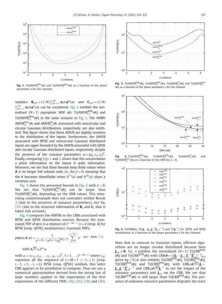
Fig. 1 exhibits the normalized (N¼1) asymptotic MSEðθÞ: Tr½AMVBBPSK

s ðθÞ� and Tr½AMVBQPSKs ðθÞ� associated with

the projector statistics, as a function of the phase β forthe channels hð1ÞðzÞ ¼ ð1�z�1

1;1 zÞð1�z�12;1 zÞ and hð2ÞðzÞ ¼

ð1�z�11;2 zÞð1�z�1

2;2 zÞ with z1;1 ¼ 0:8, z2;1 ¼ 1:25eiπ=4, z1;2 ¼0:8eiβ and z2;2 ¼ 1:25e� iπ=4, where σ2s =σ

2e ¼ 10 dB and

ϕs ¼ π=3. We note that here the AMV estimators areasymptotically circular because AðθÞ is C-differentiable. ForGaussian distributed inputs sðnÞ, these AMVBs are equal tothe associated CRBs (33) and (36) from Result 2. Fig. 1shows that the difference between Tr½AMVBBPSK

s ðθÞ� andTr½AMVBQPSK

s ðθÞ� is large enough, in particular for β appr-oaching 0 for which AðθÞ is close to be singular where θ isnot identifiable. This behavior is similar to the DOA model-ing for which the difference between these two AMVBs ismore prominent for low DOA separations [21].

When the structure information of Rs and Cs is used, two

new AMVBs (AMVBBPSKr;c ðθÞ and AMVBQPSK

r;c ðθÞ) based on the

0 1 2 3 4 5 6101

102

103

104

105

106

β (radians)

Tr(A

MV

B(θ

))

Fig. 1. Tr½AMVBBPSKs ðθÞ� and Tr½AMVBQPSK

s ðθÞ� as a function of the phaseparameter β for the channel.

0 1 2 3 4 5 6100

101

102

β (radians)

Tr(A

MV

B(θ

))

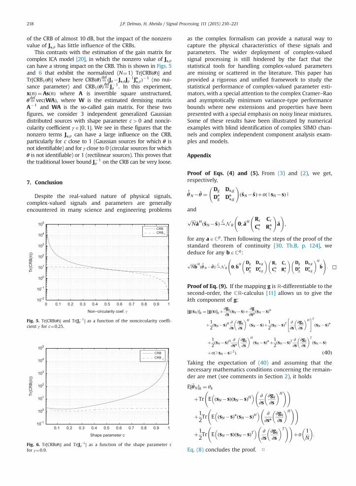
Fig. 2. Tr½AMVBBPSKr;c ðθÞ�, Tr½AMVBQPSK

r;c ðθÞ�, Tr½AMVBCGr;c ðθÞ� and Tr½AMVBNCG

r;c

ðθÞ� as a function of the phase parameter β for the channel.

0 5 10 15 20 25 30100

101

102

103

SNR (dB)

Tr(A

MV

B(θ

))

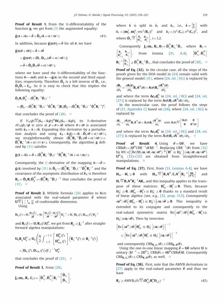
Fig. 3. Tr½AMVBBPSKr;c ðθÞ�, Tr½AMVBQPSK

r;c ðθÞ�, Tr½AMVBCGr;c ðθÞ� and

Tr½AMVBNCGr;c ðθÞ� as a function of the SNR for β¼ 0.

0 1 2 3 4 5 6100

101

102

β (radians)

CR

B(θ

)

Fig. 4. Tr½CRBðθÞ�, Tr½ðJθ�Jn;θJ�1θ Jn

n;θÞ�1� and Tr½J�1θ � for QPSK and BPSK

modulations as a function of the phase parameter β for the channel.

J.P. Delmas, H. Abeida / Signal Processing 111 (2015) 210–221 217

statistics Rx;N ¼ ð1=NÞPNn ¼ 1 xðnÞxHðnÞ and Cx;N ¼ ð1=NÞPN

n ¼ 1 xðnÞxT ðnÞ can be considered. Fig. 2 exhibits the nor-

malized (N¼1) asymptotic MSE ðθÞ: Tr½AMVBBPSKr;c ðθÞ� and

Tr½AMVBQPSKr;c ðθÞ� in the same scenario as Fig. 1. The AMBV

AMVBNCGr;c ðθÞ and AMVBCG

r;c ðθÞ associated with noncircular andcircular Gaussian distributions, respectively, are also exhib-ited. This figure shows that these AMVB are slightly sensitiveto the distribution of the inputs. Furthermore, the AMVBassociated with BPSK and noncircular Gaussian distributedinputs are upper bounded by the AMVB associated with QPSKand circular Gaussian distributed inputs, respectively, despitethe presence of the nuisance parameters α¼ ½ϕs; σs; σe�T .Finally, comparing Figs 1 and 2 shows that this uncorrelationa priori information on the inputs is quite informative.Moreover, we see that these bounds keep finite values whenA is no longer full column rank, i.e., for β¼ 0, meaning that

the θ becomes identifiable when hð1ÞðzÞ and hð2ÞðzÞ share acommon zero.

Fig. 3 shows the presented bounds in Fig. 2 with β¼ 0.We see that Tr½AMVBNCG

r;c ðθÞ� can be larger thanTr½AMVBCG

r;c ðθÞ�, depending on the SNR values. This inter-esting counterexample does not contradict neither Result3 (due to the presence of nuisance parameters), nor Eq.(33) (due to the structure information of Rs and Cs that istaken into account).

Fig. 4 compares the AMVBs to the CRBs associated withBPSK and QPSK distribution sources. Because the asso-ciated PDF of xðnÞ is a mixture of cLþMþ1 (c¼2 [resp. 4] forBPSK [resp. QPSK] modulations), Gaussian PDFs:

p x nð Þ; θ;αð Þ ¼ 1

cLþMþ1πPðLþ1Þσ2PðLþ1Þe

XcLþMþ 1

l ¼ 1

e� JxðnÞ�AðθÞsl J 2=σ2e

with sl ¼defσseiαsϵlwith ϵl ¼ ðϵ1;l; ϵ2;l;…; ϵLþMþ1;lÞT , l¼ 1;…; cLþMþ1 where ϵk;lrepresent all the sequence of LþMþ1 f�1; þ1g [resp.f�1; þ1; � i; þ ig] BPSK [resp. QPSK] symbols, this latterCRB appears to be prohibitive to compute. Thus we use anumerical approximation derived from the strong law oflarge numbers applied to the expectation of the firstexpressions of the different FIMs (14), (15), (19) and (20).

Note that in contrast to Gaussian inputs, efficient algo-rithms are no longer circular distributed because hereJn;θa0. Fig. 4 exhibits the normalized (N¼1) Tr½CRBBPSK

ðθÞ� and Tr½CRBQPSKðθÞ� with CRBðθÞ ¼ ½ðJ ~θ �J ~θ ;α J�1α JH~θ ;αÞ�1�θ;θ

given by (18).It also exhibits Tr½CRBBPSK1 ðθÞ�, Tr½CRBBPSK

2 ðθÞ�,Tr½CRBQPSK

1 ðθÞ� and Tr½CRBQPSK2 ðθÞ�, with CRB1ðθÞ ¼def ðJθ�

Jn;θJ�1θ Jn

n;θÞ�1 and CRB2ðθÞ ¼def J�1θ to see the impact of the

nuisance parameters and Jn;θ on the CRB. We see thatTr½CRBQPSKðθÞ� is still larger than Tr½CRBBPSKðθÞ�. The pre-sence of unknown nuisance parameters degrades the trace

J.P. Delmas, H. Abeida / Signal Processing 111 (2015) 210–221218

of the CRB of almost 10 dB, but the impact of the nonzerovalue of Jn;θ has little influence of the CRBs.

This contrasts with the estimation of the gain matrix forcomplex ICA model [20], in which the nonzero value of Jn;θcan have a strong impact on the CRB. This is shown in Figs. 5and 6 that exhibit the normalized (N¼1) Tr½CRBðθÞ� andTr½CRB1ðθÞ� where here CRBðθÞ ¼def ðJθ�Jn;θJ

�1θ Jn

n;θÞ�1 (no nui-sance parameter) and CRB1ðθÞ ¼def J�1

θ . In this experiment,xðnÞ ¼AsðnÞ where A is invertible square unstructured,θ¼def vecðWAÞ, where W is the estimated demixing matrixA�1 and WA is the so-called gain matrix. For these twofigures, we consider 3 independent generalized Gaussiandistributed sources with shape parameter c40 and noncir-cularity coefficient γA ½0;1�. We see in these figures that thenonzero terms Jn;θ can have a large influence on the CRB,particularly for c close to 1 (Gaussian sources for which θ isnot identifiable) and for γ close to 0 (circular sources for whichθ is not identifiable) or 1 (rectilinear sources). This proves thatthe traditional lower bound J�1

θ on the CRB can be very loose.

7. Conclusion

Despite the real-valued nature of physical signals,complex-valued signals and parameters are generallyencountered in many science and engineering problems

0 0.1 0.2 0.3 0.4 0.5 0.6 0.7 0.8 0.9 110−2

10−1

100

101

102

103

104

105

Non−circularity coef. γ

Tr(C

RB

(θ))

Fig. 5. Tr½CRBðθÞ� and Tr½J�1θ � as a function of the noncircularity coeffi-

cient γ for c¼0.25.

0.1 0.2 0.3 0.4 0.5 0.6 0.7 0.8 0.9 110−1

100

101

102

103

104

105

Shape parameter c

Tr(C

RB

(θ))

Fig. 6. Tr½CRBðθÞ� and Tr½J�1θ � as a function of the shape parameter c

for γ¼0.9.

as the complex formalism can provide a natural way tocapture the physical characteristics of these signals andparameters. The wider deployment of complex-valuedsignal processing is still hindered by the fact that thestatistical tools for handling complex-valued parametersare missing or scattered in the literature. This paper hasprovided a rigorous and unified framework to study thestatistical performance of complex-valued parameter esti-mators, with a special attention to the complex Cramer–Raoand asymptotically minimum variance-type performancebounds where new extensions and properties have beenpresented with a special emphasis on noisy linear mixtures.Some of these results have been illustrated by numericalexamples with blind identification of complex SIMO chan-nels and complex independent component analysis exam-ples and models.

Appendix

Proof of Eqs. (4) and (5). From (3) and (2), we get,respectively,

~̂θN� ~θ ¼Dg Dn;g

Dn

g Dn

n;g

!ð~sN� ~sÞþoðJsN�sÞJ

and

ffiffiffiffiN

p~aH ~sN� ~sð Þ-L N R 0; ~aH Rs Cs

Cn

s Rn

s

!~a

!;

for any aACp. Then following the steps of the proof of thestandard theorem of continuity [30, Th.B, p. 124], wededuce for any bACq:

ffiffiffiffiN

p~bHð ~̂θN� ~θÞ-L N R 0; ~b

H Dg Dn;g

Dn

g Dn

n;g

!Rs Cs

Cn

s Rn

s

!Dg Dn;g

Dn

g Dn

n;g

!H

~b

0@

1A: □

Proof of Eq. (9). If the mapping g is R-differentiable to thesecond-order, the CR-calculus [11] allows us to give thekth component of g:

½gðsNÞ�k ¼ ½gðsÞ�kþ∂gk∂s

sN�sð Þþ ∂g∂sn

ðsN�sÞn

þ12ðsN�sÞH ∂

∂s∂gk∂s

� �H

sN�sð Þþ12ðsN�sÞT ∂

∂s∂gk∂s

� �H" #T

ðsN�sÞn

þ12ðsN�sÞH ∂

∂sn∂gk∂s

� �H

ðsN�sÞnþ12ðsN�sÞT ∂

∂s∂gk∂s

� �T

sN�sð Þ

þoðJsN�sJ2Þ: ð40ÞTaking the expectation of (40) and assuming that thenecessary mathematics conditions concerning the remain-der are met (see comments in Section 2), it holds

E½θ̂N�k ¼ θk

þTr E ðsN�sÞðsN�sÞH� � ∂

∂s∂gk∂s

� �H ! !

þ12Tr E ðsN�sÞnðsN�sÞH

� � ∂∂sn

∂gk∂s

� �H ! !

þ12Tr E ðsN�sÞðsN�sÞT

� � ∂∂s

∂gk∂s

� �T ! !

þo1N

� �:

Eq. (8) concludes the proof. □

J.P. Delmas, H. Abeida / Signal Processing 111 (2015) 210–221 219

Proof of Result 1. From the R-differentiability of thefunction g, we get from (3) the augmented equality:

~gðsþδsÞ ¼ ~θþ ~Dgδ~sþoðJδsJ Þ: ð41Þ

In addition, because ~g½sðθÞ� ¼ ~θ for all θ, we have

~g½sðθþδθÞ� ¼ ~θþδ ~θ

¼ ~g½sðθÞþðDs;Dn;sÞδ ~θþoðJδθJ Þ�

¼ ~θþ ~Dg~Dsδ ~θþoðJδθJ Þ;

where we have used the R-differentiability of the func-tions θ⟼sðθÞ and s⟼gðsÞ in the second and third equal-ities, respectively. Therefore ~Dg is a left inverse of ~Ds, i.e.,~Dg

~Ds ¼ I2q. So it is easy to check that this implies thefollowing equality:

~DgR ~s~DHg �ð ~DH

s R�1~s

~Ds�1

¼ ½ ~Dg�ð ~DHs R

�1~s

~Ds�1 ~DHs R

�1~s �R ~s ½ ~Dg�ð ~DH

s R�1~s

~Ds�1 ~DHs R

�1~s �H ;

that concludes the proof of (10). □

If VNðβÞ ¼def ½~sN� ~sðβÞ�HWN½~sN� ~sðβÞ�, its R-derivative∂VNðβÞ=∂β is zero at β¼ θþδθ where θþδθ is associatedwith ~sN ¼ ~sþδ~s. Expanding this derivative by a perturba-tion analysis and using ~sN� ~sðβÞ ¼ δ~s� ~Dsδ ~θþoðJδθJ Þ,we straightforwardly obtain ð ~DH

s R�1~s

~DsÞδ ~θþoðJδθJ Þ ¼~DHs R

�1~s δ~sþoðJδJsJ Þ. Consequently, the algorithm g defi-

ned by (11) satisfies

~gð~sþδ~sÞ ¼ ~θþð ~DHs R

�1~s

~Ds�1 ~DHs R

�1~s δ~sþoðJδsÞJ Þ:

Consequently, the C-derivative of the mapping ~s⟼ ~θ ¼~gð~sÞ involved by (11) is ~Dg ¼ ð ~DH

s R�1~s

~Ds�1 ~DHs R

�1~s and the

covariance of the asymptotic distribution of ~θN is therefore

R ~θ ¼ ~DgR ~s~DHg ¼ ð ~DH

s R�1~s

~DsÞ�1 that concludes the proof of(11). □

Proof of Result 2. Whittle formula (24) applies to xðnÞassociated with the real-valued parameter θ whereU¼def 12 I

� iIIiI

� �of conformable dimension.

Using

Drx fð Þ ¼Ur∂r ~x ðf Þ∂θ

¼Ur∂r ~x ðf Þ∂θ

;∂r ~x ðf Þ∂θn

U�1

q ¼Ur Dr ~x ðf Þ;Dn;r ~x ðf Þ� �

U�1q

and Rx ðf Þ ¼UrR ~x ðf ÞUHr , we get from R ^θ

Z J�1θ after straight-

forward algebra manipulations:

UqR ~̂θUH

q ZUqN2

Z þ1=2

�1=2

DHr ~x ðf Þ

DHn;r ~x ðf Þ

24

35 R�n

x ðf Þ � R�1x ðf Þ

� �0@

� Dr ~x ðf Þ;Dn;r ~x ðf Þ� �

df ;��1UH

q ;

that concludes the proof of (25). □

Proof of Result 3. From (29),

J ~θ ðmx;Rx;CxÞ ¼ ~DHs1 ;

~DHs2

h iR�1

~s

~Ds1

~Ds2

" #;

where ~s is split in ~s1 and ~s2, i.e., ~s ¼ ~s1~s2

h iwith

~s1 ¼ ½mTx ;m

Hx ; vec

T ðRxÞ�T and ~s2 ¼ ½vT ðCxÞ; vHðCxÞ�T , and

where ~Dsi ¼def Dsi

Dn

n;si

Dn;siDn

si

, i¼1,2.

Consequently J ~θ ðmx;Rx;0Þ ¼ ~DHs1R

�1~s1

~Ds1 where R ~s ¼R ~s1RH

~s1;2

R ~s1;2R ~s2

. From lemma [31, A.4], ~D

Hs1 ;

~DHs2

h iR�1

~s~Ds1~Ds2

Z ~D

Hs1R

�1~s1

~Ds1 , that concludes the proof of (30). □

Proof of Eq. (32). In the circular case, all the steps of theproofs given for the DOA model in [24] remain valid withthe general model (31), where [24, rel. (16)] is replaced by

∂Rx

∂θk¼ ∂AðθÞ

∂θkRsA

H θð ÞþA θð ÞRs∂AHðθÞ∂θk

and where the term AckdHk in [24, rel. (18)] and [24, rel.

(27)] is replaced by the term AðθÞRs∂AHðθÞ=∂θk.In the noncircular case, the proof follows the steps

of [21, Appendix C] based on [24], where [24, rel. (16)] isreplaced by

∂R ~x

∂θk¼ ∂ ~AðθÞ

∂θkR ~s

~AHθð Þþ ~A θð ÞR ~s

∂ ~AHðθÞ∂θk

with ~A θð Þ ¼defAðθÞ 00 AnðθÞ

" #

and where the term AckdHk in [24, rel. (18)] and [24, rel.

(27)] is replaced by the term ~AðθÞR ~s∂ ~AHðθÞ=∂θk. □

Proof of Result 4. Using θ ¼U ~θ, we haveCRBð ~θÞ ¼ ½UHCRB�1ðθÞU��1. Replacing CRB�1ðθÞ from (32)by 8N=σ2e Re U ∂a=∂θ; ∂a=∂θn

� ���H HT � Π?

A

� �∂a=∂θ; ∂a=∂θn� �

UHÞ�, (33)–(35) are obtained from straightforwardmanipulations. □

Proof of Eq. (37). First, from [31, Lemma A.4], we have

Hnc�HcZ0 with Hnc ¼def RsAH ;CsA

Th i

R�1~x

ARsAnCn

s

h iand

Hc ¼defRsAHR�1

x ARs, and this inequality applies to the trans-

pose of these matrices: HTnc�HT

c Z0. Then, because

Π?A Z0, ðHT

nc�HTc Þ � Π?

A Z0 thanks to a standard resultof linear algebra (see, e.g., [32, prop. 11.5]. Consequently

∂aH=∂θ ðHTnc�HT

c Þ � Π?A Þ

� �∂a=∂θZ0. This inequality is

extended to its conjugate and consequently to the

real-valued symmetric matrix Re ∂aH=∂θ ðHTnc�HT

c ���

Π?A ÞÞ∂a=∂θÞ. Then by inversion

Re ∂aH=∂θ HTnc � Π?

A

� �∂a=∂θ

� �h i�1

r Re ∂aH=∂θ HTc � Π?

A

� �∂a=∂θ

� �h i�1

and consequently CRBRx ;Cx ðθÞrCRBRx ;0ðθÞ.Using the one-to-one linear mapping θ ¼U ~θ where U is

unitary (U�1 ¼ 2UH), CRBð ~θÞ ¼ 4UHCRBðθÞU. ConsequentlyCRBRx ;Cx ð ~θÞrCRBRx ;0ð ~θÞ, as well. □

Proof of Eq. (38). First, note that the AMVB derivations in[27] apply to the real-valued parameter θ and thus wehave

Rθ ZAMVBsðθÞ ¼def ðDHs;θR

#s Ds;θ Þ�1 ð42Þ

J.P. Delmas, H. Abeida / Signal Processing 111 (2015) 210–221220

where Ds;θ ¼defdsðθÞ=dθ which is related to the R-derivative

Ds ¼ ∂s=∂θ and the conjugate R-derivative Dn;s ¼ ∂s=∂θn of sby Ds;θ ¼ ½Ds;Dn;s�U�1. Using θ ¼U ~θ, Rθ ¼UR ~θU

H , (42) isequivalent to

R ~θ Z ½ðDs;Dn;sÞHR#s ðDs;Dn;sÞ��1:

Consider now the statistic sN ¼ vecðΠRx ;NÞ. Using the Her-mitian structure of ΠRx ;N , its asymptotic covariance Rs andcomplementary covariance Cs are related by

R ~s ¼Rs Cs

Cn

s Rn

s

" #¼ 2BKRsBH

K ;

where BK ¼def 1ffiffi2

p IK

� �satisfying BH

KBK ¼ I. Consequently

R#~s ¼ 1

2BKR#s B

HK from [32, Prop. 7.69]. This implies

~DHs R

#~s~Ds ¼

14

DHs DT

n;s

DHn;s DT

s

24

35 I

K

R#s I;K½ �

Ds Dn;s

Dn

n;s Dn

s

" #

¼ ðDs;Dn;sÞHR#s ðDs;Dn;sÞ; ð43Þ

where KDs ¼Dn

n;s and KDn;s ¼Dn

s (due to the Hermitian

structure of sN ¼ΠRx ;N and the relation ðds=dθÞn ¼ dsn=dθn

between R-derivatives) are used in the second equality. So(38) is proved for sN ¼ vecðΠRx ;NÞ. The proofs for vecðΠR ~x ;NÞand vecðΠRx ;N ;ΠCx ;NÞ are similar. Finally, note that AMVBderivations in [27], the AMVB based on ΠR ~x ;N and

ðΠRx ;N ;ΠCx ;NÞ coincide for θ, and thus for ~θ. □

Proof of Result 5. Consider the statistic sN ¼ vecðΠRx ;NÞwhose Moore–Penrose inverse of the covariance of itsasymptotic distribution is given from [27] by

R#s ¼ 1

σ2eðAnHnAT � Π?

A ÞþðΠ? T

A � AHAHÞh i

:

So from (43), ~DHs R

#~s~Ds is given by

~DHs R

#~s~Ds ¼ 1

σ2e

DHs

DHn;s

24

35 ðAnHnAT � Π?

A ÞþðΠ? T

A � AHAHÞh i

Ds;Dn;s� �

;

ð44Þwhose term (k,l) of the 1,1 block is written as

1σ2evecH

∂Π?A

∂θk

� �ðAnHnAT � Π?

A ÞþðΠ?n

A � AHAH� �

vec∂Π?

A

∂θl

� �: ð45Þ

Using vecH ∂Π?A =∂θk

� �¼ vecT ∂Π?A =∂θnk

� �T� �and the iden-

tity TrðABCDÞ ¼ vecT ðAT ÞðDT � BÞvecðCÞ, the term (45)becomes

1σ2eTr

∂Π?A

∂θnkΠ?

A∂Π?

A

∂θlAHAHþ∂Π?

A

∂θnkAHAH∂Π?

A

∂θlΠ?

A

� �

¼ 1σ2eTr AH∂Π?

A

∂θnk|fflfflfflffl{zfflfflfflffl}Π?A∂Π?

A

∂θlA|fflfflffl{zfflfflffl}Hþ∂Π?

A

∂θnkA|fflfflffl{zfflfflffl}HA

H∂Π?A

∂θl|fflfflfflffl{zfflfflfflffl}Π?A

0B@

1CA:

ð46ÞThen Π?

A A¼ 0 implying ð∂Π?A =∂θiÞAþΠ?

A ∂A=∂θi ¼ 0 andð∂Π?

A =∂θni ÞAþΠ?A ∂A=∂θni ¼ 0, i¼ k; l and using the relation

∂� =∂θi� �n ¼ ∂�n=∂θni , i¼ k; l between R-derivatives of Aand Π?

A , the term (46) is written as

1σ2eTr

∂A∂θk

� �H

Π?A∂A∂θl

Hþ ∂A∂θnk

� �T

Π? T

A∂A∂θnl

� �n

HT

!

¼ 1σ2evecT

∂A∂θk

� �n

HT � Π?A

� �vec

∂A∂θl

� �

þ 1σ2evecT

∂A∂θnk

� �H � Π? T

A

� �vec

∂A∂θnl

� �n

:

Consequently the block (1,1) of ~DHs R

#~s~Ds is given by

1σ2e

∂a∂θ

� �H

HT � Π?A

� � ∂a∂θ

� �þ 1σ2e

∂a∂θn

� �T

H � Π? T

A

� � ∂a∂θn

� �n

;

which is equal to the block Jθ of (34) for N¼1. Thederivation of the other three blocks of ~D

Hs R

#~s~Ds is obtained

following the same steps and (39) is proved for thestatistic sN ¼ vecðΠRx ;NÞ.Concerning the statistics sN ¼ vecðΠR ~x ;NÞ and sN ¼ vecðΠRx ;

N;ΠCx ;NÞ, the covariance Rs of their asymptotic distribution andthe associated Moore–Penrose inverse R#

s have been derivedin [27]. Following the same steps that for sN ¼ vecðΠRx ;NÞ, (39)is proved for these other two statistics. □

Proof of Remark 1. Using an arbitrary square root L of Σ,i.e., Σ¼ LLH , the model (31) becomes

xLðnÞ ¼defL�1xðnÞ ¼ALðθÞsðnÞþeLðnÞ ð47Þwith ALðθÞ ¼defL�1AðθÞ and eLðnÞ ¼defL�1eðnÞ. Consequently,the three conditions introduced in the beginning of Sec-tion 5 are still valid, and thus also all the results of thissection apply by replacing AðθÞ by L�1AðθÞ in expressions(32) and (34)–(36).Note that in these expressions, a and Π?

A becomeaL ¼ vecðL�1AÞ ¼ vecðL�1AIÞ ¼ ðI � L�1ÞvecðAÞ ¼ ðI � L�1Þa and Π?

AL¼ I�L�1AðAHΣ�1AÞ�1AHL�H , respectively. H is

invariant in the circular and noncircular cases as

RsAHL�HðL�1RxL�HÞ�1L�1ARs ¼H

and

½RsAHL�H ;CsA

TL�T � L�1RxL�H L�1CxL�T

L�nCn

xL�H L�nRn

xL�T

" #�1L�1ARs

L�nAnCn

s

" #

¼ ½RsAHL�H ;CsA

TL�T � LH

LT

" #Rx Cx

Cn

x Rn

x

" #�1

½L; Ln� L�1ARs

L�nAnCn

s

" #¼H;

using partitioned inverse identities (see, e.g., [32, Prop.14.11]).Consequently the term ∂a=∂θ

� �HðHT � Π?A Þ ∂a=∂θ� �

in theexpressions (32) and (34)–(36) becomes

∂aL∂θ

� �H

HT � Π?AL

� � ∂aL∂θ

� �

¼ ∂a∂θ

� �H

ðI � L�HÞðHT � Π?ALÞðI � L�1Þ|fflfflfflfflfflfflfflfflfflfflfflfflfflfflfflfflfflfflfflfflfflfflfflfflfflfflfflfflffl{zfflfflfflfflfflfflfflfflfflfflfflfflfflfflfflfflfflfflfflfflfflfflfflfflfflfflfflfflffl}

HT � ðL�HΠ?ALL� 1Þ

∂a∂θ

� �;

withL�HΠ?

ALL�1 ¼Σ�1�Σ�1AðAHΣ�1AÞ�1AHΣ�1 ¼defΠΣ . □

References

[1] T. Adali, P.J. Schreier, L.L. Scharf, Complex-valued signal processing:the proper way to deal with impropriety, IEEE Trans. Signal Process.59 (November (11)) (2011) 5101–5125.

[2] E. Ollila, V. Koivunen, H.V. Poor, Complex-valued signal processing -essential models, tools and statistics, in: Proceedings of InformationTheory and Applications Workshop, La Jolla, CA, 2011.

J.P. Delmas, H. Abeida / Signal Processing 111 (2015) 210–221 221

[3] A. Van Den Bos, Estimation of complex parameters, in: The 10th IFACSymposium, vol. 3, July 1994, pp. 495–499.

[4] T. Adalı, Complex-valued adaptive signal processing, in: AdaptiveSignal Processing—Next-Generation Solutions, John Wiley and Sons,New York, 2010.

[5] P. Schreier, L.L. Scharf, Statistical Signal Processing of Complex-Valued Data—The Theory of Improper and Noncircular Signals,Cambridge University Press, New York, 2010.

[6] J.P. Delmas, Asymptotic performance of second-order algorithms,IEEE Trans. Signal Process. 50 (January (1)) (2002) 49–57.

[7] J.P. Delmas, Performance bounds and statistical Analysis of DOAestimation, in: Academic Press Library in Signal Processing, vol. 3,1st edition, Array and Statistical Signal Processing, Elsevier, Oxford,UK, 2013.

[8] J.R. Magnus, H. Neudecker, Matrix Differential Calculus with Appli-cations in Statistics and Econometrics, Revised edition, John Wileyand Sons, UK, 1999.

[9] J.P. Delmas, H. Abeida, Asymptotic distribution of circularity coeffi-cients estimate of complex random variables, Signal Process. 89(December) (2009) 2311–2698.

[10] J. Eriksson, E. Ollila, V. Koivunen, Essential statistics and tools forcomplex random variables, IEEE Trans. Signal Process. 58 (October(10)) (2010) 5400–5408.

[11] K. Kreutz-Delgado, The Complex Gradient Operator and the CR-calculus, Cornell University Library, New York, 2007.

[12] E.L. Lehmann, Elements of Large-Sample Theory, Springer-Verlag,New-York, 1999.

[13] G.B. Giannakis, Cumulants: a powerful tool in signal processing,Proc. IEEE 75 (September (9)) (1987) 1333–1334.

[14] J.P. Delmas, Y. Meurisse, Extension of the matrix Bartlett's formula tothe third and fourth order and to noisy linear models with applica-tion to parameter estimation, IEEE Trans. Signal Process. 53 (August(8)) (2005) 2765–2776.

[15] B. Porat, B. Friedlander, Performance analysis of parameter estima-tion algorithms based on high-order moments, Int. J. Adapt. ControlSignal Process. 3 (1989) 191–229.

[16] P. Stoica, B. Friedlander, T. Söderström, An approximate maximumapproach to ARMA spectral estimation, in: Proceedings of theDecision and Control, Fort Lauderdale, 1985.

[17] J.P. Delmas, Asymptotically minimum variance second-order estima-tion for noncircular signals with application to DOA estimation, IEEETrans. Signal Process. 52 (May (5)) (2004) 1235–1241.

[18] A. Van Den Bos, A Cramer–Rao lower bound for complex para-meters, IEEE Trans. Signal Process. 42 (10) (1994) 2859.

[19] E. Ollila, V. Koivunen, J. Eriksson, On the Cramer-Rao bound for theconstrained and unconstrained complex parameters, in: Proceedingsof IEEE Sensor Array and Multichannel Signal Processing Workshop,Darmstadt, Germany, July 2008.

[20] B. Loesch, B. Yang, Cramer-Rao bound for circular and noncircularcomplex independent component analysis, IEEE Trans. Signal Pro-cess. 61 (January (2)) (2013) 365–379.

[21] J.P. Delmas, H. Abeida, Stochastic Cramer–Rao bound for noncircularsignals with application to DOA estimation, IEEE Trans. SignalProcess. 52 (November (11)) (2004) 3192–3199.

[22] P. Whittle, The analysis of multiple stationary time series, J. R. Stat.Soc. 15 (1953) 125–139.

[23] J.P. Delmas, Y. Meurisse, On the Cramer Rao bound and maximumlikelihood in passive time delay estimation for complex signals, in:Proceedings of ICASSP, Kyoto, Japan, March 2012.

[24] P. Stoica, A.G. Larsson, A.B. Gershman, The stochastic CRB for arrayprocessing: a textbook derivation, IEEE Signal Process. Lett. 8 (May)(2001) 148–150.

[25] M. Jansson, B. Goransson, B. Ottersten, A subspace method fordirection of arrival estimation of uncorrelated emitter signals, IEEETrans. Signal Process. 47 (April (4)) (1999) 945–956.

[26] J.F. Cardoso, E. Moulines, Invariance of subspace based estimator,IEEE Trans. Signal Process. 48 (September (9)) (2000) 2495–2505.

[27] H. Abeida, J.P. Delmas, Efficiency of subspace-based DOA estimators,Signal Process. 87 (September (9)) (2007) 2075–2084.

[28] J.P. Delmas, P. Comon, Y. Meurisse, Performance limits of alphabetdiversities for FIR SISO channel identification, IEEE Trans. SignalProcess. 57 (January (1)) (2009) 73–82.

[29] D. Darsena, G. Gelli, L. Paura, F. Verde, Subspace-based blind channelidentification of SISO-FIR systems with improper random inputs,Signal Process. 84 (2004) 2021–2039.

[30] R.J. Serfling, Approximation Theorems of Mathematical Statistics,John Wiley and Sons, New York, 1980.

[31] P. Stoica, A. Nehorai, Performance study of conditional and uncondi-tional direction of arrival estimation, IEEE Trans. ASSP 38 (October)(1990) 1783–1795.

[32] G.A.F. Seber, A Matrix Handbook for Statisticians, Wiley Series inProbability and Statistics, NJ, 2008.