Reshetov LA Statistical resolution limit for the multidimensional harmonic retrieval model: hypothesis test and Cramér-Rao Bound approaches

RESEARCH Open Access

Statistical resolution limit for themultidimensional harmonic retrieval model:hypothesis test and Cramér-Rao BoundapproachesMohammed Nabil El Korso*, Rémy Boyer, Alexandre Renaux and Sylvie Marcos

Abstract

The statistical resolution limit (SRL), which is defined as the minimal separation between parameters to allow acorrect resolvability, is an important statistical tool to quantify the ultimate performance for parametric estimationproblems. In this article, we generalize the concept of the SRL to the multidimensional SRL (MSRL) applied to themultidimensional harmonic retrieval model. In this article, we derive the SRL for the so-called multidimensionalharmonic retrieval model using a generalization of the previously introduced SRL concepts that we callmultidimensional SRL (MSRL). We first derive the MSRL using an hypothesis test approach. This statistical test isshown to be asymptotically an uniformly most powerful test which is the strongest optimality statement that onecould expect to obtain. Second, we link the proposed asymptotic MSRL based on the hypothesis test approach toa new extension of the SRL based on the Cramér-Rao Bound approach. Thus, a closed-form expression of theasymptotic MSRL is given and analyzed in the framework of the multidimensional harmonic retrieval model.Particularly, it is proved that the optimal MSRL is obtained for equi-powered sources and/or an equi-distributednumber of sensors on each multi-way array.

Keywords: Statistical resolution limit, Multidimensional harmonic retrieval, Performance analysis, Hypothesis test,Cramér-Rao bound, Parameter estimation, Multidimensional signal processing

IntroductionThe multidimensional harmonic retrieval problem is animportant topic which arises in several applications [1].The main reason is that the multidimensional harmonicretrieval model is able to handle a large class of applica-tions. For instance, the joint angle and carrier estimationin surveillance radar system [2,3], the underwater acous-tic multisource azimuth and elevation direction finding[4], the 3-D harmonic retrieval problem for wirelesschannel sounding [5,6] or the detection and localizationof multiple targets in a MIMO radar system [7,8].One can find many estimation schemes adapted to the

multidimensional harmonic retrieval estimation pro-blem, see, e.g., [1,2,4-7,9,10]. However, to the best of

our knowledge, no work has been done on the resolva-bility of such a multidimensional model.The resolvability of closely spaced signals, in terms of

parameter of interest, for a given scenario (e.g., for agiven signal-to-noise ratio (SNR), for a given number ofsnapshots and/or for a given number of sensors) is aformer and challenging problem which was recentlyupdated by Smith [11], Shahram and Milanfar [12], Liuand Nehorai [13], and Amar and Weiss [14]. More pre-cisely, the concept of statistical resolution limit (SRL), i.e., the minimum distance between two closely spacedsignalsa embedded in an additive noise that allows a cor-rect resolvability/parameter estimation, is rising in sev-eral applications (especially in problems such as radar,sonar, and spectral analysis [15].)The concept of the SRL was defined/used in several

manners [11-14,16-24], which could turn in it to a con-fusing concept. There exist essentially three approaches

* Correspondence: [email protected] des Signaux et Systèmes (L2S), Université Paris-Sud XI (UPS),CNRS, SUPELEC, 3 Rue Joliot Curie, Gif-Sur-Yvette 91192, France

El Korso et al. EURASIP Journal on Advances in Signal Processing 2011, 2011:12http://asp.eurasipjournals.com/content/2011/1/12

© 2011 El Korso et al; licensee Springer. This is an Open Access article distributed under the terms of the Creative CommonsAttribution License (http://creativecommons.org/licenses/by/2.0), which permits unrestricted use, distribution, and reproduction inany medium, provided the original work is properly cited.

mailto:[email protected]

http://creativecommons.org/licenses/by/2.0

to define/obtain the SRL. (i) The first is based on theconcept of mean null spectrum: assuming, e.g., that twosignals are parameterized by the frequencies f1 and f2,the Cox criterion [16] states that these sources areresolved, w.r.t. a given high-resolution estimation algo-rithm, if the mean null spectrum at each frequency f1and f2 is lower than the mean of the null spectrum at

the midpointf1 + f2

2. Another commonly used criterion,

also based on the concept of the mean null spectrum, isthe Sharman and Durrani criterion [17], which statesthat two sources are resolved if the second derivative of

the mean of the null spectrum at the midpointf1 + f2

2is

negative. It is clear that the SRL based on the mean nullspectrum is relevant to a specific high-resolution algo-rithm (for some applications of these criteria one cansee [16-19] and references therein.) (ii) The secondapproach is based on detection theory: the main idea isto use a hypothesis test to decide if one or two closelyspaced signals are present in the set of the observations.Then, the challenge herein is to link the minimumseparation, between two sources (e.g., in terms of fre-quencies) that is detectable at a given SNR, to the prob-ability of false alarm, Pfa and/or to the probability ofdetection Pd. In this spirit, Sharman and Milanfar [12]have considered the problem of distinguishing whetherthe observed signal contains one or two frequencies at agiven SNR using the generalized likelihood ratio test(GLRT). The authors have derived the SRL expressionsw.r.t. Pfa and Pd in the case of real received signals, andunequal and unknown amplitudes and phases. In [13],Liu and Nehorai have defined a statistical angular reso-lution limit using the asymptotic equivalence (in termsof number of observations) of the GLRT. The challengewas to determine the minimum angular separation, inthe case of complex received signals, which allows toresolve two sources knowing the direction of arrivals(DOAs) of one of them for a given Pfa and a given Pd.Recently, Amar and Weiss [14] have proposed to deter-mine the SRL of complex sinusoids with nearby fre-quencies using the Bayesian approach for a givencorrect decision probability. (iii) The third approach isbased on a estimation accuracy criteria independent ofthe estimation algorithm. Since the Cramér-Rao Bound(CRB) expresses a lower bound on the covariance matrixof any unbiased estimator, then it expresses also theultimate estimation accuracy [25,26]. Consequently, itcould be used to describe/obtain the SRL. In this con-text, one distinguishes two main criteria for the SRLbased on the CRB: (1) the first one was introduced byLee [20] and states that: two signals are said to be resol-vable w.r.t. the frequencies if the maximum standarddeviation is less than twice the difference between f1 and

f2. Assuming that the CRB is a tight bound (under mild/weak conditions), the standard deviation, σf̂1 and σf̂2, ofan unbiased estimator f̂ = [f̂1 f̂2]T is given by

√CRB(f1)

and√

CRB(f2), respectively. Consequently, the SRL isdefined, in the Lee criterion sense, as 2max{√

CRB(f1),√

CRB(f2)}. One can find some results and

applications in [20,21] where this criterion is used toderive a matrix-based expression (i.e., without analyticinversion of the Fisher information matrix) of the SRLfor the frequency estimates in the case of the condi-tional and unconditional signal source models. On theother hand, Dilaveroglu [22] has derived a closed-formexpression of the frequency resolution for the real andcomplex conditional signal source models. However,one can note that the coupling between the parameters,CRB(f1, f2) (i.e., the CRB for the cross parameters f1 andf2), is ignored by this latter criterion. (2) To extend this,Smith [11] has proposed the following criterion: two sig-nals are resolvable w.r.t. the frequencies if the differencebetween the frequencies, δf, is greater than the standarddeviation of the DOA difference estimation. Since, thestandard deviation can be approximated by the CRB,then, the SRL, in the Smith criterion sense, is defined asthe limit of δf for which δf <

√CRB(δf ) is achieved.

This means that, the SRL is obtained by solving the fol-lowing implicit equation

δ2f = CRB(δf ) = CRB(f1) + CRB(f2) − 2CRB(f1, f2).

In [11,23], Smith has derived the SRL for two closelyspaced sources in terms of DOA, each one modeled byone complex pole. In [24], Delmas and Abeida havederived the SRL based on the Smith criterion for DOAof discrete sources under QPSK, BPSK, and MSK modelassumptions. More recently, Kusuma and Goyal [27]have derived the SRL based on the Smith criterion insampling estimation problems involving a powersumseries.It is important to note that all the criteria listed before

take into account only one parameter of interest per sig-nal. Consequently, all the criteria listed before cannot beapplied to the aforementioned the multidimensionalharmonic model. To the best of our knowledge, noresults are available on the SRL for multiple parametersof interest per signal. The goal of this article is to fillthis lack by proposing and deriving the so-called MSRLfor the multidimensional harmonic retrieval model.More precisely, in this article, the MSRL for multiple

parameters of interest per signal using a hypothesis testis derived. This choice is motivated by the followingarguments: (i) the hypothesis test approach is not speci-fic to a certain high-resolution algorithm (unlike themean null spectrum approach), (ii) in this article, we


Page 2 of 14

link the asymptotic MSRL based on the hypothesis testapproach to a new extension of the MSRL based on theCRB approach. Furthermore, we show that the MSRLbased on the CRB approach is equivalent to the MSRLbased on the hypothesis test approach for a fixed couple(Pfa, Pd), and (iii) the hypothesis test is shown to beasymptotically an uniformly most powerful test which isthe strongest statement of optimality that one couldexpect to obtain [28].The article is organized as follows. We first begin by

introducing the multidimensional harmonic model, insection “Model setup”. Then, based on this model, weobtain the MSRL based on the hypothesis test and onthe CRB approach. The link between theses two MSRLsis also described in section “Determination of the MSRLfor two sources” followed by the derivation of the MSRLclosed-form expression, where, as a by product theexact closed-form expressions of the CRB for the multi-dimensional retrieval model is derived (note that to thebest of our knowledge, no exact closed-form expressionsof the CRB for such model is available in the literature).Furthermore, theoretical and numerical analyses aregiven in the same section. Finally, conclusions are given.

Glossary of notationThe following notations are used through the article.Column vectors, matrices, and multi-way arrays arerepresented by lower-case bold letters (a, ...), upper-casebold letters (A, ...) and bold calligraphic letters (A, ...),whereas

• ℝ and ℂ denote the body of real and complexvalues, respectively,• RD1×D2×···×DI and CD1×D2×···×DI denote the real andcomplex multi-way arrays (also called tensors) bodyof dimension D1 × D2 × ... ×DI, respectively,• j = the complex number

√−1.• IQ = the identity matrix of dimension Q,• 0Q1×Q2 = the Q1 × Q2 matrix filled by zeros,• [a]i = the ith element of the vector a,• [A]i1,i2 = the i1th row and the i2th column elementof the matrix A,• [A]i1,i2,...,iN = the (i1, i2, ..., iN)th entry of the multi-way array A,• [A]i,p:q = the row vector containing the (q - p + 1)elements [A]i,k, where k = p, ..., q,• [A]p:q,k = the column vector containing the (q - p +1) elements [A]i,k, where i = p, ..., q,• the derivative of vector a w.r.t. to vector b is

defined as follows:

[∂a∂b

]i,j

=∂[a]i

∂[b]j,

• AT = the transpose of the matrix A,• A* = the complex conjugate of the matrix A,

• AH = (A*)T,• tr {A} = the trace of the matrix A,• det {A} = the determinant of the matrix A,• ℜ{a} = the real part of the complex number a,• E{a} = the expectation of the random variable a,

• ||a||2 =1L

∑Lt=1 [a]2

t denotes the normalized norm

of the vector a (in which L is the size of a),• sgn (a) = 1 if a ≥ 0 and -1 otherwise.• diag(a) is the diagonal operator which forms adiagonal matrix containing the vector a on itsdiagonal,• vec(.) is the vec-operator stacking the columns of amatrix on top of each other,• ⊙ stands for the Hadamard product,• ⊗ stands for the Kronecker product,• ○ denotes the multi-way array outer-product(recall that for a given multi-way arraysA ∈ CA1×A2×···×AI and B ∈ CB1×B2×···×BJ, the result ofthe outer-product of A and B denoted by

CA1×···×AI×B1×···×BJ is given by[C]a1,...,aI,b1,...,bJ = [A ◦ B]a1,...,aI,b1,...,bJ = [A]a1,...,aI [B]b1,...,bJ ).

Model setupIn this section, we introduce the multidimensional har-monic retrieval model in the multi-way array form (alsoknown as tensor form [29]). Then, we use the PARAFAC(PARallel FACtor) decomposition to obtain a vectorform of the observation model. This vector form will beused to derive the closed-form expression of the MSRL.Let us consider a multidimensional harmonic model

consisting of the superposition of two harmonics eachone of dimension P contaminated by an additive noise.Thus, the observation model is given as follows[8,9,26,30-32]:

[Y(t)]n1,...,nP = [X (t)]n1,...,nP +[N (t)]n1,...,nP , t = 1, . . . , L, and np = 0, . . . , Np−1,ð1Þwhere Y(t), X (t), and N (t) denote the noisy observa-

tion, the noiseless observation, and the noise multi-wayarray at the tth snapshot, respectively. The number ofsnapshots and the number of sensors on each array aredenoted by L and (N1, ...,NP), respectively. The noiselessobservation multi-way array can be written as followsb

[26,30-32]:

[X (t)]n1 ,...,nP =2∑

m=1

sm(t)P∏

p=1

ejω(p)m np , (2)

where ω(p)m and sm(t) denote the mth frequency viewed

along the pth dimension or array and the mth complexsignal source, respectively. Furthermore, the signalsource is given by sm(t) = αm(t)ejφm(t) where am(t) and


Page 3 of 14

jm(t) denote the real positive amplitude and the phasefor the mth signal source at the tth snapshot,respectively.Since,

P∏p=1

ejω(p)m np =

[a(ω(1)

m ) ◦ a(ω(2)m ) ◦ · · · ◦ a(ω(P)

m )]

n1,n2,...,nP

,

where a(.) is a Vandermonde vector defined as

a(ω(p)m ) =

[1 ejω(p)

m · · · ej(Np − 1)ω(p)m

]T,

then, the multi-way array X (t) follows a PARAFACdecomposition [7,33]. Consequently, the noiseless obser-vation multi-way array can be rewritten as follows:

X (t) =2∑

m=1

sm(t)(a(ω(1)

m ) ◦ a(ω(2)m ) ◦ · · · ◦ a(ω(P)

m ))

. (3)

First, let us vectorize the noiseless observation asfollows:

vec(X (t)) =[[X (t)]0,0,...,0 · · · [X (t)]N1−1,0,··· ,0[X (t)]0,1,...,0 · · · [X (t)]N1−1,N2−1,...,NP−1

]T.ð4Þ

Thus, the full noise-free observation vector is given by

x =[vecT(X (1)) vecT(X (2)) · · · vecT(X (L))

]T.

Second, and in the same way, we define y, the noisyobservation vector, and n, the noise vector, by the con-catenation of the proper multi-way array’s entries, i.e.,

y =[vecT(Y(1)) vecT(Y(2)) · · · vecT(Y(L))

]T= x + n. (5)

Consequently, in the following, we will consider theobservation model in (5). Furthermore, the unknownparameter vector is given by

ξ =[ωTρT]T, (6)

where ω denotes the unknown parameter vector ofinterest, i.e., containing all the unknown frequencies

ω =[(ω(1))

T · · · (ω(P))T]T

,

in which

ω(p) =[ω

(p)1 ω

(p)2

]T. (7)

whereas r contains the unknown nuisance/unwantedparameters vector, i.e., characterizing the noise covar-iance matrix and/or amplitude and phase of each source(e.g., in the case of a covariance noise matrix equal toσ 2ILN1...NP

and unknown deterministic amplitudes andphases, the unknown nuisance/unwanted parametersvector r is given by r = [a1(1) ... a2(L)j1(1) ... j2(L)s2]T.

In the following, we conduct a hypothesis test formu-lation on the observation model (5) to derive our MSRLexpression in the case of two sources.

Determination of the MSRL for two sourcesHypothesis test formulationResolving two closely spaced sources, with respect totheir parameters of interest, can be formulated as a bin-ary hypothesis test [12-14] (for the special case of P =1). To determine the MSRL (i.e., P ≥ 1), let us considerthe hypothesis H0 which represents the case where thetwo emitted signal sources are combined into one signal,i.e., the two sources have the same parameters (thishypothesis is described by ∀p ∈ [1 . . . P], ω(p)

1 = ω(p)2 ),

whereas the hypothesis H1 embodies the situation wherethe two signals are resolvable (the latter hypothesis isdescribed by ∃p Î [1 ... P], such that ω

(p)1 �= ω

(p)2). Conse-

quently, one can formulate the hypothesis test, as a sim-ple one-sided binary hypothesis test as follows:{H0 : δ = 0,

H1 : δ > 0,(8)

where the parameter δ is the so-called MSRL whichindicates us in which hypothesis our observation modelbelongs. Thus, the question addressed below is how canwe define the MSRL δ such that all the P parameters ofinterest are taken into account? A natural idea is that δreflects a distance between the P parameters of interest.Let the MSRL denotes the l1 normc between two setscontaining the parameters of interest of each source(which is the naturally used norm, since in the mono-parameter frequency case that we extend here, the SRLis defined as δ = f1 - f2 [13,14,34]). Meaning that, if wedenote these sets as C1 and C2 where

Cm ={ω

(1)m , ω(2)

m , . . . , ω(P)m

}, m = 1,2, thus, δ can be

defined as

δ �P∑

p=1

∣∣∣ω(p)2 − ω

(p)1

∣∣∣ . (9)

First, note that the proposed MSRL describes well thehypothesis test (8) (i.e., δ = 0 means that the twoemitted signal sources are combined into one signal andδ ≠ 0 the two signals are resolvable). Second, since theMSRL δ is unknown, it is impossible to design an opti-mal detector in the Neyman-Pearson sense. Alterna-tively, the GLRT [28,35] is a well-known approachappropriate to solve such a problem. To conduct theGLRT on (8), one has to express the probability densityfunction (pdf) of (5) w.r.t. δ. Assuming (without loss ofgenerality) that ω

(1)1 > ω

(1)2, one can notice that ξ is

known if and only if δ and ϑ �[ω

(1)2 (ω(2))

T. . . (ω(P))

T]T


Page 4 of 14

are fixed (i.e., there is a one to one mapping between δ,ϑ, and ξ). Consequently, the pdf of (5) can be describedas p(y|δ,ϑ). Now, we are ready to conduct the GLRT forthis problem:

LG(y) =maxδ,ϑ1p(y|δ, ϑ1,H1)

maxϑ0p(y|ϑ0,H0)

=p(y|δ̂, ϑ̂1,H1)

p(y|ϑ̂0,H0)

H1

≷H0

ς ′,(10)

where δ̂, ϑ̂1, and ϑ̂0 denote the maximum likelihoodestimates (MLE) of δ under H1, the MLE of ϑ under H1

and the MLE of ϑ under H0, respectively, and where ς’denotes the test threshold. From (10), one obtains

TG(y) = Ln LG(y)H1

≶H0

ς = Lnς ′, (11)

in which Ln denotes the natural logarithm.

Asymptotic equivalence of the MSRLFinding the analytical expression of TG(y) in (11) is nottractable. This is mainly due to the fact that the deriva-tion of δ̂ is impossible since from (2) one obtains a mul-timodal likelihood function [36]. Consequently, in thefollowing, and as ind [13], we consider the asymptoticcase (in terms of the number of snapshots). In [35, eq(6C.1)], it has been proven that, for a large number ofsnapshots, the statistic TG(y) follows a chi-square pdfunder H0 and H1 given by

TG(y) ∼{

χ21 under H0,

χ ′21(κ ′(Pfa, Pd)) under H1,

(12)

where χ21 and χ ′2

1(κ ′(Pfa, Pd)) denote the central chi-square and the noncentral chi-square pdf with onedegree of freedom, respectively. Pfa and Pd are, respec-tively, the probability of false alarm and the probabilityof detection of the test (8). In the following, CRB(δ)denotes the CRB for the parameter δ where theunknown vector parameter is given by [δ ϑT]T. Conse-quently, assuming that CRB(δ) exists (under H0 andH1), is well defined (see section “MSRL closed-formexpression” for the necessarye and sufficient conditions)and is a tight bound (i.e., achievable under quite gen-eral/weak conditions [36,37]), thus the noncentral para-meter �’(Pfa, Pd) is given by [[35], p. 239]

κ ′(Pfa, Pd) = δ2(CRB(δ))−1. (13)

On the other hand, one can notice that the noncentralparameter �’(Pfa, Pd) can be determined numerically bythe choice of Pfa and Pd [13,28] as the solution of

Q−1χ2

1(Pfa) = Q−1

χ21 (κ ′(Pfa,Pd))

(Pd), (14)

in whichQ−1χ2

1(� ) andQ−1

χ ′21(κ ′(Pfa,Pd))

(� ) are the inverse

of the right tail of the χ21 and χ ′2

1(κ ′(Pfa, Pd)) pdf start-ing at the value ϖ. Finally, from (13) and (14) oneobtainsf

δ = κ(Pfa, Pd)√

CRB(δ), (15)

where√

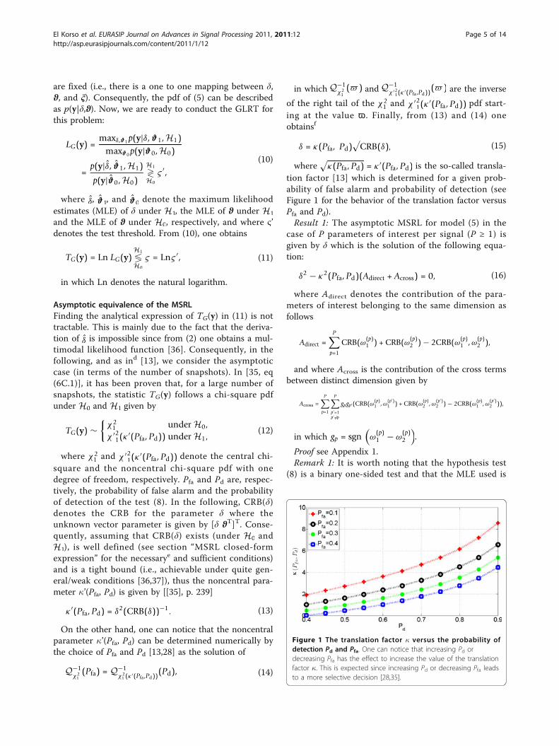
κ(Pfa, Pd) = κ ′(Pfa, Pd) is the so-called transla-tion factor [13] which is determined for a given prob-ability of false alarm and probability of detection (seeFigure 1 for the behavior of the translation factor versusPfa and Pd).Result 1: The asymptotic MSRL for model (5) in the

case of P parameters of interest per signal (P ≥ 1) isgiven by δ which is the solution of the following equa-tion:

δ2 − κ2(Pfa, Pd)(Adirect + Across) = 0, (16)

where Adirect denotes the contribution of the para-meters of interest belonging to the same dimension asfollows

Adirect =P∑

p=1

CRB(ω(p)1 ) + CRB(ω(p)

2 ) − 2CRB(ω(p)1 , ω(p)

2 ),

and where Across is the contribution of the cross termsbetween distinct dimension given by

Across =P∑

p=1

P∑p′=1p′ �=p

gpgp′(CRB(ω(p)1 , ω(p′)

1 ) + CRB(ω(p)2 , ω(p′)

2 ) − 2CRB(ω(p)1 , ω(p′)

2 )),

in which gp = sgn(ω

(p)1 − ω

(p)2

).

Proof see Appendix 1.Remark 1: It is worth noting that the hypothesis test

(8) is a binary one-sided test and that the MLE used is

Figure 1 The translation factor � versus the probability ofdetection Pd and Pfa. One can notice that increasing Pd ordecreasing Pfa has the effect to increase the value of the translationfactor �. This is expected since increasing Pd or decreasing Pfa leadsto a more selective decision [28,35].


Page 5 of 14

an unconstrained estimator. Thus, one can deduce thatthe GLRT, used to derive the asymptotic MSRL [13,35]:(i) is the asymptotically uniformly most powerful testamong all invariant statistical tests, and (ii) has anasymptotic constant false-alarm rate (CFAR). Which is,in the asymptotic case, considered as the strongest state-ment of optimality that one could expect to obtain [28].

• Existence of the MSRL: It is natural to assume thatthe CRB is a non-increasing (i.e., decreasing or con-stant) function on ℝ+ w.r.t. δ since it is more diffi-cult to estimate two closely spaced signals than twolargely-spaced ones. In the same time the left handside of (15) is a monotonically increasing function w.r.t. δ on ℝ+. Thus for a fixed couple (Pfa, Pd), thesolution of the implicit equation given by (15) alwaysexists. However, theoretically, there is no assurancethat the solution of equation (15) is unique.• Note that, in practical situation, the case whereCRB(δ) is not a function of δ is important since inthis case, CRB(δ) is constant w.r.t. δ and thus thesolution of (15) exists and is unique (see section“MSRL closed-form expression”).

In the following section, we study the explicit effect ofthis so-called translation factor.

The relationship between the MSRL based on the CRBand the hypothesis test approachesIn this section, we link the asymptotic MSRL (derivedusing the hypothesis test approach, see Result 1) to anew proposed extension of the SRL based on the Smithcriterion [11]. First, we recall that the Smith criteriondefines the SRL in the case of P = 1 only. Then, weextend this criterion to P ≥ 1 (i.e., the case of the multi-dimensional harmonic model). Finally, we link theMSRL based on the hypothesis test approach (see Result1) to the MSRL based on the CRB approach (i.e., theextended SRL based on the Smith criterion).The Smith criterion: Since the CRB expresses a lower

bound on the covariance matrix of any unbiased estima-tor, then it expresses also the ultimate estimation accu-racy. In this context, Smith proposed the followingcriterion for the case of two source signals parameter-ized each one by only one frequency [11]: two signalsare resolvable if the difference between their frequency,

δω(1) = ω(1)2 − ω

(1)1, is greater than the standard deviation

of the frequency difference estimation. Since, the stan-dard deviation can be approximated by the CRB, then,the SRL, in the Smith criterion sense, is defined as thelimit of δω(1) for which δω(1) <

√CRB(δω(1) ) is achieved.

This means that, the SRL is the solution of the followingimplicit equation

δ2ω(1) = CRB(δω(1) ).

The extension of the Smith criterion to the case of P ≥1: Based on the above framework, a straightforwardextension of the Smith criterion to the case of P ≥ 1 forthe multidimensional harmonic model is as follows: twomultidimensional harmonic retrieval signals are resolva-ble if the distance between C1 and C2, is greater thanthe standard deviation of the δCRB estimation. Conse-quently, assuming that the CRB exists and is welldefined, the MSRL δCRB is given as the solution of thefollowing implicit equation{

δ2CRB = CRB(δCRB)

s.t. δCRB =∑P

p=1 |ω(p)2 − ω

(P)1 |. (17)

Comparison and link between the MSRL based on theCRB approach and the MSRL based on the hypothesistest approach: The MSRL based on the hypothesis testapproach is given as the solution of{

δ = κ(Pfa, Pd)√

CRB(δ),

s.t. δ =∑P

p=1

∣∣∣ω(p)2 − ω

(p)1

∣∣∣ ,whereas the MSRL based on the CRB approach is

given as the solution of (17). Consequently, one has thefollowing result:Result 2: Upon to a translation factor, the asymptotic

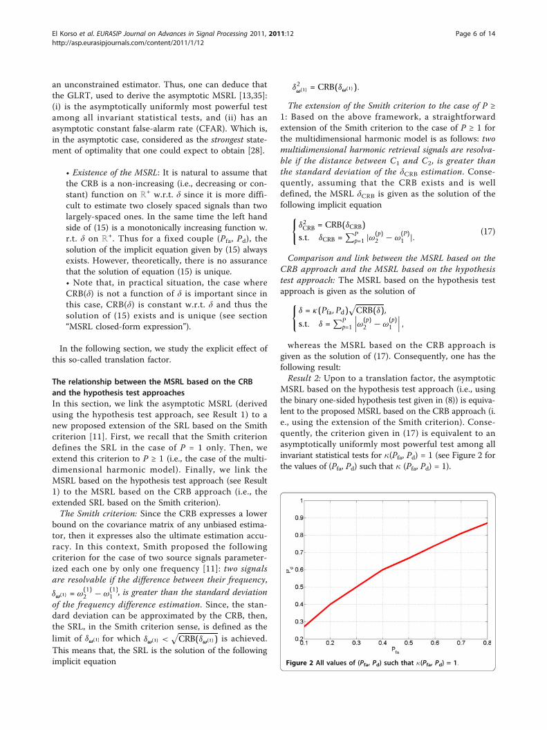
MSRL based on the hypothesis test approach (i.e., usingthe binary one-sided hypothesis test given in (8)) is equiva-lent to the proposed MSRL based on the CRB approach (i.e., using the extension of the Smith criterion). Conse-quently, the criterion given in (17) is equivalent to anasymptotically uniformly most powerful test among allinvariant statistical tests for �(Pfa, Pd) = 1 (see Figure 2 forthe values of (Pfa, Pd) such that � (Pfa, Pd) = 1).

Figure 2 All values of (Pfa, Pd) such that �(Pfa, Pd) = 1.


Page 6 of 14

The following section is dedicated to the analyticalcomputation of closed-form expression of the MSRL. Insection “Assumptions,” we introduce the assumptionsused to compute the MSRL in the case of a Gaussianrandom noise and orthogonal waveforms. Then, wederive non matrix closed-form expressions of the CRB(note that to the best of our knowledge, no closed-formexpressions of the CRB for such model is available inthe literature). In “MSRL derivation” and thanks tothese expressions, the MSRL wil be deduced using (16).Finally, the MSRL analysis is given.

MSRL closed-form expressionin section “Determination of the MSRL for two sources”we have defined the general model of the multidimen-sional harmonic model. To derive a closed-form expres-sion of the MSRL, we need more assumptions on thecovariance noise matrix and/or on the signal sources.

Assumptions• The noise is assumed to be a complex circularwhite Gaussian random process i.i.d. with zero-meanand unknown variance σ 2ILN1...NP.• We consider a multidimensional harmonic modeldue to the superposition of two harmonics each ofthem of dimension P ≥ 1. Furthermore, for sake ofsimplicity and clarity, the sources have beenassumed known and orthogonal (e.g., [7,38]). Inthis case, the unknown parameter vector is fixedand does not grow with the number of snapshots.Consequently, the CRB is an achievable bound[36].• Each parameter of interest w.r.t. to the first signal,

ω(p)1 p = 1 . . . P, can be as close as possible to the

parameter of interest w.r.t. to the second signal

ω(p)2 p = 1 . . . P, but not equal. This is not really a

restrictive assumption, since in most applications,having two or more identical parameters of interestis a zero probability event [[9], p. 53].

Under these assumptions, the joint probability densityfunction of the noisy observations y for a givenunknown deterministic parameter vector ξ is as follows:

p(y|ξ) =L∏

t=1

p(vec(Y(t))|ξ) =1

(πσ 2)LN e

−1σ 2 (y−x)

H(y−x)

,

where N =∏P

p=1 Np. The multidimensional harmonic

retrieval model with known sources is consideredherein, and thus, the parameter vector is given by

ξ =[ωTσ 2]T, (18)

where

ω =[(ω(1))

T · · · (ω(P))T]T

,

in which

ω(p) =[ω

(p)1 ω

(p)2

]T. (19)

CRB for the multidimensional harmonic model withorthogonal known signal sourcesThe Fisher information matrix (FIM) of the noisy obser-vations y w.r.t. a parameter vector ξ is given by [39]

FIM(ξ) = E

{∂ ln p(y|ξ)

∂ξ

(∂ ln p(y|ξ)

∂ξ

)H}

.

For a complex circular Gaussian observation model,the (ith, kth) element of the FIM for the parameter vec-tor ξ is given by [34]

[FIM(ξ)]i,k =LNσ 4

∂σ 2

∂[ξ ]i

∂σ 2

∂[ξ ]k+

2σ 2

{

∂xH

∂[ξ ]i

∂x∂[ξ ]k

}(i, k) = {1, . . . , 2P + 1}2.ð20Þ

Consequently, one can state the following lemma.Lemma 1: The FIM for the sum of two P-order har-

monic models with orthogonal known sources, has ablock diagonal structure and is given by

FIM(ξ) =2σ 2

[Fω 02P×1

01×2P ×]

, (21)

where, the (2P) × (2P) matrix Fω is also a block diago-nal matrix given by

Fω = LN(� ⊗ G), (22)

in which Δ = diag {||a1||2 ,||a2||

2} where

αm =[αm(1) ... αm(L)

]T for m ∈ {1, 2}, (23)

and

[G]k,l =

⎧⎪⎨⎪⎩

(2Nk − 1)(Nk − 1)6

for k = l,

(Nk − 1)(Nl − 1)2

for k �= l.

Proof see Appendix 2.After some calculation and using Lemma 1, one can

state the following result.Result 3: The closed-form expressions of the CRB for

the sum of two P-order harmonic models with orthogo-nal known signal sources are given by

CRB(ω(p)m ) =

6LNSNRm

Cp, m ∈ {1, 2}, (24)


Page 7 of 14

where SNRm =||αm||2

σ 2denotes the SNR of the mth

source and where

Cp =Np(1 − 3VP) + 3VP + 1

(Np + 1)(N2p − 1)

in which VP =1

1 + 3∑P

p=1Np−1Np+1

.

Furthermore, the cross-terms are given by

CRB(ω(p)m , ω(p′)

m′ ) =

⎧⎨⎩

0 for m �= m′,−6

LNSNRmC̃p,p′ for m = m′ and p �= p′, (25)

where

C̃p,p′ =3VP

(Np + 1)(Np′ + 1).

Proof see Appendix 3.

MSRL derivationUsing the previous result, one obtains the unique solu-tion of (16), thus, the MSRL for model (1) is given bythe following result:Result 4: The MSRL for the sum of P-order harmonic

models with orthogonal known signal sources, is givenby

δ =

√√√√√√√ 6LNESNR

⎛⎜⎜⎝

P∑p=1

Cp −P∑

p,p′=1p �=p′

gpgp′ C̃p,p′

⎞⎟⎟⎠ , (26)

where the so-called extended SNR is given by

ESNR =SNR1SNR2

SNR1 + SNR2.

Proof see Appendix 4.

Numerical analysisTaking advantage of the latter result, one can analyzethe MSRL given by (26):

• First, from Figure 3 note that the numerical solu-tion of the MSRL based on (12) is in good agree-ment with the analytical expression of the MSRL(23), which validate the closed-form expression givenin (23). On the other hand, one can notice that, forPd = 0.37 and Pfa = 0.1 the MSRL based on the CRBis exactly equal to the MSRL based on hypothesistest approach derived in the asymptotic case. Fromthe case Pd = 0.49 and Pfa = 0.3 or/and Pd = 0.32and Pfa = 0.1, one can notice the influence of thetranslation factor �(Pfa, Pd) on the MSRL.

• The MSRLg is O(

√1

ESNR) which is consistent with

some previous results for the case P = 1 (e.g.,[12,14,24]).• From (26) and for a large number of sensors N1 =N2 = ... = NP = N ≫ 1, one obtains a simple expres-sion

δ =

√12

LNP+1ESNRP

1 + 3P,

meaning that, the SRL is O(

√1

NP+1).

• Furthermore, since P ≥ 1, one has

(P + 1) (3P + 1)P(3P + 4)

< 1,

and consequently, the ratio between the MSRL of amultidimensional harmonic retrieval with P parametersof interest, denoted by δP and the MSRL of a multidi-mensional harmonic retrieval with P + 1 parameters ofinterest, denoted by δP+1, is given by

δP+1

δP=

√(P + 1)(3P + 1)

NP(3P + 4), (27)

meaning that the MSRL for P + 1 parameters of inter-est is less than the one for P parameters of interest (seeFigure 4). This, can be explained by the estimation addi-tional parameter and also by an increase of the receivednoisy data thanks to the additional dimension. Oneshould note that this property is proved theoreticallythanks to (27) using the assumption of an equal andlarge number of sensors. However, from Figure 4 wenotice that, in practice, this can be verified even for a

Figure 3 MSRL versus s2 for L = 100.


Page 8 of 14

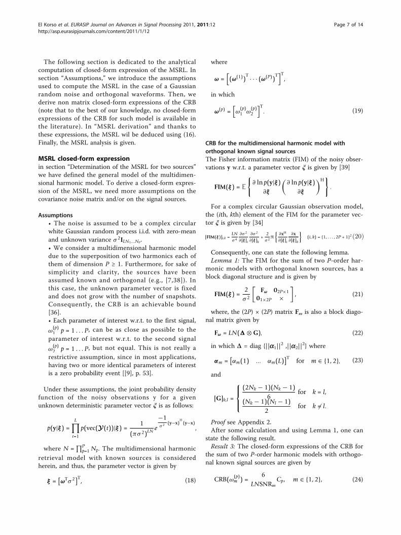
small number of sensors (e.g., in Figure 4 one has 3 ≤Np ≤ 5 for p = 3, ..., 6).

• Furthermore, since√4

LNP+1ESNR≤ δP < δP−1 < · · · < δ1

one can note that, the SRL is lower bounded by√4

LNP+1ESNR.

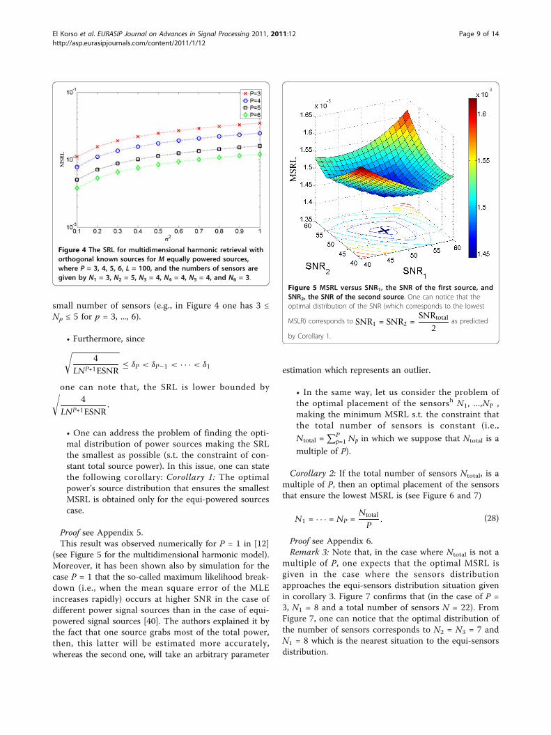
• One can address the problem of finding the opti-mal distribution of power sources making the SRLthe smallest as possible (s.t. the constraint of con-stant total source power). In this issue, one can statethe following corollary: Corollary 1: The optimalpower’s source distribution that ensures the smallestMSRL is obtained only for the equi-powered sourcescase.

Proof see Appendix 5.This result was observed numerically for P = 1 in [12]

(see Figure 5 for the multidimensional harmonic model).Moreover, it has been shown also by simulation for thecase P = 1 that the so-called maximum likelihood break-down (i.e., when the mean square error of the MLEincreases rapidly) occurs at higher SNR in the case ofdifferent power signal sources than in the case of equi-powered signal sources [40]. The authors explained it bythe fact that one source grabs most of the total power,then, this latter will be estimated more accurately,whereas the second one, will take an arbitrary parameter

estimation which represents an outlier.

• In the same way, let us consider the problem ofthe optimal placement of the sensorsh N1, ...,NP ,making the minimum MSRL s.t. the constraint thatthe total number of sensors is constant (i.e.,

Ntotal =∑P

p=1 Np in which we suppose that Ntotal is a

multiple of P).

Corollary 2: If the total number of sensors Ntotal, is amultiple of P, then an optimal placement of the sensorsthat ensure the lowest MSRL is (see Figure 6 and 7)

N1 = · · · = NP =Ntotal

P. (28)

Proof see Appendix 6.Remark 3: Note that, in the case where Ntotal is not a

multiple of P, one expects that the optimal MSRL isgiven in the case where the sensors distributionapproaches the equi-sensors distribution situation givenin corollary 3. Figure 7 confirms that (in the case of P =3, N1 = 8 and a total number of sensors N = 22). FromFigure 7, one can notice that the optimal distribution ofthe number of sensors corresponds to N2 = N3 = 7 andN1 = 8 which is the nearest situation to the equi-sensorsdistribution.

Figure 5 MSRL versus SNR1, the SNR of the first source, andSNR2, the SNR of the second source. One can notice that theoptimal distribution of the SNR (which corresponds to the lowest

MSLR) corresponds to SNR1 = SNR2 =SNRtotal

2as predicted

by Corollary 1.

Figure 4 The SRL for multidimensional harmonic retrieval withorthogonal known sources for M equally powered sources,where P = 3, 4, 5, 6, L = 100, and the numbers of sensors aregiven by N1 = 3, N2 = 5, N3 = 4, N4 = 4, N5 = 4, and N6 = 3.


Page 9 of 14

ConclusionIn this article, we have derived the MSRL for the multi-dimensional harmonic retrieval model. Toward this end,we have extended the concept of SRL to multiple para-meters of interest per signal. First, we have used ahypothesis test approach. The applied test is shown tobe asymptotically an uniformly most powerful testwhich is the strongest statement of optimality that onecould hope to obtain. Second, we have linked theasymptotic MSRL based on the hypothesis test approachto a new extension of the SRL based on the Cramér-Raobound approach. Using the Cramér-Rao bound and a

proper change of variable formula, closed-form expres-sion of the MSRL are given.Finally, note that the concept of the MSRL can be

used to optimize, for example, the waveform and/or thearray geometry for a specific problem.

Appendix 1The proof of Result 1Appendix 1.1: In this appendix, we derive the MSRLusing the l1 norm.From CRB(ξ) where ξ = [ωT rT]T in which

ω = [ω(1)1 ω

(1)2 ω

(2)1 ω

(2)2 · · · ω(P)

1 ω(P)2 ]T, one can deduce

CRB(

ξ) where

ξ = g(ξ) = [δ ϑT]T in which

ϑ � [ω(1)2 (ω(2))T · · · (ω(P))T]T. Thanks to the Jacobian

matrix given by

∂g(ξ)∂ξ

=

⎡⎣hT 0

A 00 I

⎤⎦ ,

where h = [g1g2 ... gP ]T ⊗ [1 - 1]T, in which

gp =∂δ

∂ω(p)1

= − ∂δ

∂ω(p)2

= sgn (ω(p)1 − ω

(p)2 ) and A = [0 I].

Using the change of variable formula

CRB(

ξ) =∂g(

ξ)

∂

ξ

CRB(ξ)

⎛⎝∂g(

ξ)

∂

ξ

⎞⎠

T

, (29)

one has

CRB(

ξ) =[

hTCRB(ω)h ×× I

].

Consequently, after some calculus, one obtains

CRB(δ) � [CRB(

ξ)]1,1 = hTCRB(ω)h

=2P∑p=1

2P∑p′=1

[h]p[h]p′ [CRB(ω)]p,p′

=P∑

p=1

P∑p′=1

gpgp′(

[CRB(ξ)]2p,2p′ + [CRB(ξ)]2p−1,2p′−1 − [CRB(ξ)]2p,2p′−1 − [CRB(ξ)]2p−1,2p′

)

� Adirect + Across,

ð30Þ

where

Adirect =∑P

p=1 CRB(ω(p)1 ) + CRB(ω(p)

2 ) − 2CRB(ω(p)1 , ω(p)

2 )

and where Across(k) =∑P

p=1

∑Pp′=1p′ �=p

gpgp′(

CRB(ω(p)1 , ω(p′)

1 ) + CRB(ω(p)2 , ω(p′)

2 ) − 2CRB(ω(p)1 , ω(p′)

2 ))

Finally using (30) one obtains (16)Appendix 1.2: In this part, we derive the MSRL using

the lk norm for a given integer k ≥ 1. The aim of thispart is to support the endnote a, which stays that usingthe l1 norm computing the MSRL using the l1 norm isfor the calculation convenience.Once again, from CRB(ξ), one can deduce CRB(

ξ k)where

ξ k = gk(ξ) = [δ(k) ϑT]T in which the distancebetween C1 and C2 using the lk norm is given by δ(k) ≜

Figure 7 The plot of the MSRL versus N2 in the case of P = 3,N1 = 8 and a total number of sensors N = 22.

Figure 6 The MSRL versus N1 and N2 in the case of P = 3 and atotal number of sensors Ntotal = 21. One can notice that theoptimal distribution of the number of sensors (which corresponds

to the lowest SLR) corresponds to N1 = N2 = N3 =Ntotal

3as

predicted by (28).


Page 10 of 14

k-norm distance(C1,C2) =(∑P

p=1 δkp

)1/kand where

ϑ � [ω(1)2 (ω(2))T . . . (ω(P))T]T. The Jacobian matrix is

given by

∂g(ξ)∂ξ

=

⎡⎣hT

k 0A 00 I

⎤⎦ ,

where hk = [1 - 1]T ⊗ [g1(k)g2(k) ... gP(k)]T, in which

gp(k) =∂δ(k)

∂ω(p)1

= −∂δ(k)

∂ω(p)2

and A = [0I]. Since |x|k can be

written as√

x2k. Thus, for × ≠ 0, one has

gp(k) =

∂

(∑Pp′=1

√(ω

(p′)1 − ω

(p′)2

)2k)1/k

∂ω(p)1

=1k

( p∑i=1

√(ω

(i)1 − ω

(i)2

)2k)1

k−1 ∂

√(ω

(i)1 − ω

(i)2

)2k

∂ω(i)1

= sgn(ω(p)1 − ω

(p)2 )

⎛⎝ P∑

p=1

√(ω

(p′)1 − ω

(p′)2

)2k

⎞⎠

1k

−1√(ω

(p)1 − ω

(p)2

)2(k−1)= sgn(ω(p)

1 − ω(p)2 )δ1−kδk−1

p .

ð31Þ

Again, using the change of variable formula (29), onehas

CRB(

ξ k) =[

hTkCRB(ω)hk ×

× I

].

Consequently, after some calculus, one obtains

CRB(δ(k)) � [CRB(

ξ k)]1,1

=P∑

p=1

P∑p′=1

gp(k)gp′ (k)([CRB(ξ)]2p,2p′ + [CRB(ξ)]2p−1,2p′−1 − [CRB(ξ)]2p,2p′−1 − [CRB(ξ)]2p−1,2p′ )

= (δ(k))2(1−k)(Adirect(k) + Across(k)),

ð32Þ

whereAdirect(k) =

∑Pp=1 δ

2(k−1)p

(CRB(ω(p)

1 ) + CRB(ω(p)2 ) − 2CRB(ω(p)

1 , ω(p)2 ))

and whereAcross(k) =

∑P

p=1

∑Pp′=1p′ �=p

δk−1p δk−1

p′ sgn(ω(p)1 −ω

(p)2 )sgn(ω(p′)

1 −ω(p′)2 )

(CRB(ω(p)

1 , ω(p′)1 ) + CRB(ω(p)

2 , ω(p′)2 ) − 2CRB(ω(p)

1 , ω(p′)2 )).

Consequently, note that resolving analytically theimplicit equation (32) w.r.t. δ(k) is intractable (asidefrom some special cases). Whereas, resolving analyticallythe implicit equation (30) can be tedious but feasible(see section “MSRL closed form expression”).Furthermore, denoting gp(1) = gp, Across(1) ≜ Across and

Adirect(1) ≜ Adirect and using (32) one obtains (16).

Appendix 2Proof of Lemma 1From (20) one can note the well-known property thatthe model signal parameters are decoupled from thenoise variance [42]. Consequently, the block-diagonalstructure in (21) is self-evident.Now, let us prove (22). From (4), one obtains

∂vec(X (t))

∂ω(p)m

= jsm(t)(a(ω(1)

m ) ⊗ a(ω(2)m ) ⊗ · · · ⊗ a’(ω(p)

m ) ⊗ · · · ⊗ a(ω(P)m ))

,

where

a’(ω(p)m ) =

[0 ejω(p)

m . . . (Np − 1)ej(Np−1)ω(p)m

]T.

Thus,

∂x

∂ω(p)m

= jsm ⊗(a(ω(1)

m ) ⊗ a(ω(2)m ) ⊗ · · · ⊗ a’(ω(p)

m ) ⊗ · · · ⊗ a(ω(P)m ))

,

where sm = [sm(1) ... sm(L)]T. Using the distributivity of

the Hermitian operator over the Kronecker product andthe mixed-product property of the Kronecker product[43] and assuming, without loss of generality that p’ <p,one obtains

(∂x

∂ω(p)m

)H ∂x

∂ω(p′)m

=(sHm, ⊗

[aH(ω(1)

m′ ) ⊗ aH(ω(2)m ) ⊗ · · · ⊗ a’H(ω(p′)

m ) ⊗ · · · ⊗ aH(ω(P)m′ )])

×(sm ⊗

[a(ω(1)

m ) ⊗ a(ω(2)m ) ⊗ · · · ⊗ a’(ω(p)

m ) ⊗ · · · ⊗ a(ω(P)m )])

= (sHm, sm) ⊗

(aH(ω(1)

m′ )a(ω(1)m ))

⊗ · · · ⊗(a’H(ω(p)

m′ )a(ω(p)m ))

⊗ . . .

. . . ⊗(aH(ω(p′)

m )a’(ω(p′)m′ ))

⊗ · · · ⊗(aH(ω(P)

m′ )a(ω(P)m ))

.

ð33Þ

On the other hand, one has

aH(ω(p)m )a(ω(p)

m ) = Np, (34)

whereas

aH(ω(p)m )a’(ω(p)

m ) =Np(Np − 1)

2and a’H(ω(p)

m )a’(ω(p)m ) =

Np(2Np − 1)(Np − 1)

6ð35Þ

Finally, assuming known orthogonal wavefronts [38] (i.e., sH

m, sm = 0) and replacing (35) and (34) into (33), oneobtains

(∂x

∂ω(p)m

)H∂x

∂ω(p′)m′

=

⎧⎪⎪⎪⎨⎪⎪⎪⎩

0 for m �= m′,

L||αm||2N(Np − 1)(Np′ − 1)

4for m = m′ and p �= p′,

L||αm||2N(2Np − 1)(Np − 1)

6for m = m′ and p = p′,

(36)

where am = [am (1) ... am (L)] for m Î {1, 2}: Conse-quently, using (36), Fω can be expressed as a block diag-onal matrix

Fω =[

J1 00 J2

], (37)

where each P × P block Jm is defined by

Jm = L||αm||2NG, (38)

where

G =

⎡⎢⎢⎢⎢⎢⎢⎢⎢⎣

(N1 − 1)(2N1 − 1)6

(N1 − 1)(N2 − 1)4

. . .(N1 − 1)(NP − 1)

4(N2 − 1)(N1 − 1)

4(N2 − 1)(2N2 − 1)

6. . .

(N2 − 1)(NP − 1)4

......

. . ....

(NP − 1)(N1 − 1)4

(N2P − 1)(N2 − 1)4

· · · (NP − 1)(2NP − 1)6

⎤⎥⎥⎥⎥⎥⎥⎥⎥⎦

.

Consequently, from (37) and (38) one obtains (22).


Page 11 of 14

Appendix 3Proof of Result 3Using (22) one obtains

CRB(ω) =σ 2

2F−1

ω =σ 2

2LN(�−1 ⊗ G−1) (39)

where �−1 = diag{

1||α1||2 ,

1||α2||2

}. In the following,

we give a closed-form expression of G-1. One can noticethat the matrix G has a particular structure such that itcan be rewritten as the sum of a diagonal matrix and ofa rank-one matrix: G = Q + ggT where

Q =1

12diag{ N2

1 − 1, . . . , N2P − 1} and γ =

12

[N1 − 1, . . . , NP − 1]T

Thanks to this particular structure, an analytical inverseof G can easily be obtained. Indeed, using the matrixinversion lemma

G−1 = (Q + γ γ T)−1

= Q−1 − Q−1γ γ TQ−1

1 + γ TQ−1γ.

(40)

A straightforward calculus leads to the followingresults,

Q−1γ γ TQ−1 = 36

⎡⎢⎢⎢⎢⎢⎢⎢⎢⎢⎣

1

(N1 + 1)2

1(N1 + 1)(N2 + 1)

· · · 1(N1 + 1)(NP + 1)

1(N2 + 1)(N1 + 1)

1

(N2 + 1)2 · · · 1(N2 + 1)(NP + 1)

......

. . ....

1(NP + 1)(N1 + 1)

1(NP + 1)(N2 + 1)

· · · 1

(NP + 1)2

⎤⎥⎥⎥⎥⎥⎥⎥⎥⎥⎦

, (41)

and

γ TQ−1γ = 3P∑

p=1

Np − 1

Np + 1. (42)

Consequently, replacing (41) and (42) into (40), oneobtains

[G−1]k,l =

⎧⎪⎪⎨⎪⎪⎩

12Np(1 − 3VP) + 3VP + 1

(Np + 1)(N2p − 1)

for k = l,

− 36VP

(Np + 1)(Np′ + 1)for k �= l,

(43)

where VP =(

1 + 3∑P

p=1Np − 1

Np + 1

)−1

. Finally, replacing

(43) into (39) one finishes the proof.

Appendix 4Proof of Result 4Using Results 1 and 3, one has

Adirect =P∑

p=1

(CRB(ω(p)

1 ) + CRB (ω(p)2 ))

=6σ 2

LN

(1

||α1||2 +1

||α2||2) P∑

p=1

Np(1 − 3VP) + 3VP + 1

(Np + 1)(N2p − 1)

,

(44)

and

Across =P∑

p=1

P∑p′=1p′ �=p

gpgp′(

CRB(ω(p)1 , ω(p′)

1 ) + CRB(ω(p)2 , ω(p′)

2 ))

= −6σ 2

LN

(1

||α1||2 +1

||α2||2) P∑

p,p′=1p �= p′

3gpgp′VP

(Np + 1)(Np′ + 1).

(45)

Consequently, replacing (44) and (45) into (16), onefinishes the proof.

Appendix 5Proof of Corollary 1In this appendix, we minimize the MSRL under the con-straint SNR1 + SNR2 = SNRtotal (where SNRtotal is a realfixed value). Since, the term

(∑P

p=1 Cp −∑Pp,p′=1p �=p′

gpgp′C̃p,p′ ) is independent from SNR1

and SNR2, minimizing δ is equivalent to minimizeG(SNR1, SNR2) where

G(SNR1, SNR2) = δ2 LN6

⎛⎜⎜⎝

P∑p=1

Cp −P∑

p,p′=1p �=p′

gpgp′ C̃p,p′

⎞⎟⎟⎠

−1

=SNR1 + SNR2

SNR1SNR2.

Using the method of Lagrange multipliers, the pro-blem is as follows:⎧⎨⎩

minSNR1,SNR2G(SNR1, SNR2)s.t.SNR1 + SNR2 = SNRtotal

Thus, the Lagrange function is given byF(SNR1, SNR2, λ) = G(SNR1, SNR2) + λ(SNR1 + SNR2 − SNRtotal)

where l denotes the so-called Lagrange multiplier. Asimple derivation leads to,

∂F(SNR1, SNR2)∂ SNR1

=−1

SNR21

+ λ = 0 (46)

∂F(SNR1, SNR2)∂ SNR2

=−1

SNR22

+ λ = 0 (47)

∂F(SNR1, SNR2)∂λ

= SNR1 + SNR2 − SNRtotal = 0. (48)

Consequently, from (46) and (47), one obtains SNR1 =

SNR1. Using (48), one obtains SNR1 = SNR2 =SNRtotal

2.

Using the constraint SNR1 + SNR2 = SNRtotal onededuces corollary 1.

Appendix 6Minimizing δ w.r.t. N1, ..., NP is equivalent to minimiz-

ing the function f (N) =∑P

p=1 Cp −∑Pp,p′=1p,�=p′

gpgp′ C̃p,p′,


Page 12 of 14

where N = [N1 ... NP]T. However, since the numbers of

sensors on each array, N1, ..., NP, are integers, the deri-vation of f(N) w.r.t. N is meaningless. Consequently, letus define the function �f (.) exactly as f (.) where the setof definition is ℝP instead of NP. Consequently,

f̄ (N̄)|N̄=N = f (N), where N̄ = [N̄1 . . . N̄P]T,

in which N̄1, ..., N̄P are real (continuous) variables.Using the method of Lagrange multipliers, the pro-

blem is as follows:{minN̄ f̄ (N̄)∑P

p=1 N̄p = N̄total

where N̄total is a real positive constant value. Thus, theLagrange function is given by

�(N̄, λ) = f̄ (N̄) + λ(∑P

p=1 N̄p − N̄total

)where l denotes

the Lagrange multiplier. For a sufficient number of sen-sors, the Lagrange function can be approximated by

�(N̄, λ) ≈P∑

p=1

N̄p(1 − 3V) + 3V + 1

N̄3p

−P∑

p,p′=1p �=p′

3gpgp′V

N̄p N̄p′+ λ

⎛⎝ P∑

p=1

N̄p − N̄total

⎞⎠

where V =1

1 + 3P. A simple derivation leads to,

∂�(N̄, λ)

∂N̄1=

3(V − 1)

N̄31

− 3V + 1

N̄41

+3V

N̄21

P∑p,p′=1p �=p′

gpgp′

N̄p′+ λ = 0

...

∂�(N̄, λ)

∂N̄P=

3(V − 1)

N̄3P

− 3V + 1

N̄4P

+3V

N̄2P

P∑p,p′=1p �=p′

gpgp′

N̄p′+ λ = 0

∂�(N̄, λ)∂λ

=P∑

p=1

N̄p − N̄total = 0.

This system of equations seems hard to solve. How-ever, an obvious solution is given by N̄1 = · · · = N̄P = N̄

and λ =3V + 1

N̄4− 3

V(Pν − 1) + V − 1

N̄3in which ν =

∑Pp,p′=1p �=p′

gpgp′.

Since,∑P

p=1 Np = N̄total, thus the trivial solution is given

by N̄1 = · · · = N̄P =N̄total

P. Consequently, if N̄total is a

multiple of P then, the solution of minimizing the func-tion f̄ (N̄) in ℝP coincides the solution of minimizing thefunction f(N) in NP. Thus, the optimal placement mini-

mizing the MSRL is N1 = · · · = NP =N̄total

P. This con-

clude the proof.

EndnotesaThe notion of distance and closely spaced signals used inthe following, is w.r.t. to the metric space (d, C), where d :

C × C ® ℝ in which d and C denote a metric and the setof the parameters of interest, respectively. bSee [2-9] forsome practical examples for the multidimensional harmo-nic retrieval model. cThis study can be straightforwardlyextended to other norms. The choice of the l1 is motivatedby its calculation convenience (see the derivation of Result1 and Appendix 1). Furthermore, since the MSRL is con-sidered to be small (this assumption can be argued by thefact that the high-resolution algorithms have asymptoti-cally an infinite resolving power [44]), thus all continuousp-norms are similar to (i.e., looks like) the l1 norm. Moreimportantly, in a finite dimensional vector space, all con-tinuous p-norms are equivalent [[45], p. 53], thus thechoice of a specific norm is free. dNote that, due to thespecific definition of the SRL in [13] (i.e., using the samenotation as in [13], δ = cos(uT

1u2))and the restrictiveassumption in [13] (u1 and u2 belong to the same plan),the SRL as defined in [13] cannot be used in the multidi-mensional harmonic context. eOne of the necessary condi-tions regardless the noise pdf is that ω

(p)1 �= ω

(p)2. Meaning

that each parameter of interest w.r.t. to the first signal ω(p)1

can be as close as possible to the parameter of interest w.r.t. to the second signal ω(p)

2, but not equal. This is not really

a restrictive assumptions, since in most applications, hav-ing two or more identical parameters of interest is a zeroprobability event [[9], p. 53]. fNote that applying (15) for P= 1 and for �(Pfa, Pd) = 1, one obtains the Smith criterion[11]. gWhere O(.) denotes the Landau notation [46]. hOneshould note, that we assumed a uniform linear multi-array, and the problem is to find the optimal distributionof the number of sensors on each array. The more generalcase, i.e., where the optimization problem considers thenon linearity of the multi-way array, is beyond the scopeof the problem addressed herein.

AbbreviationsCRB: Cramér-Rao Bound; DOAs: direction of arrivals; FIM: Fisher informationmatrix; GLRT: generalized likelihood ratio test; MLE: maximum likelihoodestimates; MSRL: multidimensional SRL; PARAFAC: PARallel FACtor; pdf:probability density function; SNR: signal-to-noise ratio; SRL: statisticalresolution limit.

AcknowledgementsThis project is funded by region Île de France and Digiteo Research Park.This work has been partially presented in communication [41].

Competing interestsThe authors declare that they have no competing interests.

Received: 10 November 2010 Accepted: 13 June 2011Published: 13 June 2011

References1. Jiang T, Sidiropoulos N, ten Berge J: Almost-sure identifiability of

multidimensional harmonic retrieval. IEEE Trans. Signal Processing 2001,49(9):1849-1859.


Page 13 of 14

2. Vanpoucke F: Algorithms and Architectures for Adaptive Array SignalProcessing Universiteit Leuven, Leuven, Belgium: Ph. D. dissertation; 1995.

3. Haardt M, Nossek J: 3-D unitary ESPRIT for joint 2-D angle and carrierestimation. Proc. of IEEE Int. Conf. Acoust., Speech, Signal Processing, Munich,Germany 1997, 1:255-258.

4. Wong K, Zoltowski M: Uni-vector-sensor ESPRIT for multisource azimuth,elevation, and polarization estimation. IEEE Trans. Antennas Propagat 1997,45(10):1467-1474.

5. Mokios K, Sidiropoulos N, Pesavento M, Mecklenbrauker C: On 3-Dharmonic retrieval for wireless channel sounding. in Proc. of IEEE Int. Conf.Acoust., Speech, Signal Processing, vol. 2, (Philadelphia, USA., 2004) pp. 89-92.

6. Schneider C, Trautwein U, Wirnitzer W, Thoma R: Performance verificationof MIMO concepts using multi-dimensional channel sounding. in Proc.EUSIPCO, Florence, Italy, Sep. 2006 .

7. Nion D, Sidiropoulos N: A PARAFAC-based technique for detection andlocalization of multiple targets in a MIMO radar system. in Proc. of IEEEInt. Conf. Acoust., Speech, Signal Processing, Taipei, Taiwan, 2009 .

8. Nion D, Sidiropoulos D: Tensor algebra and multi-dimensional harmonicretrieval in signal processing for MIMO radar. IEEE Trans. Signal Processingnov. 2010, 58:5693-5705.

9. Gershman A, Sidiropoulos N: Space-time processing for MIMOcommunications New York: Wiley; 2005,

10. Boyer R: Decoupled root-MUSIC algorithm for multidimensionalharmonic retrieval. in Proc. IEEE Int. Work. Signal Processing, WirelessCommunications, Recife, Brazil 2008, 16-20.

11. Smith ST: Statistical resolution limits and the complexified Cramér Raobound. IEEE Trans. Signal Processing 2005, 53:1597-1609.

12. Shahram M, Milanfar P: On the resolvability of sinusoids with nearbyfrequencies in the presence of noise. IEEE Trans. Signal Processing 2005,53(7):2579-2585.

13. Liu Z, Nehorai A: Statistical angular resolution limit for point sources. IEEETrans. Signal Processing 2007, 55(11):5521-5527.

14. Amar A, Weiss A: Fundamental limitations on the resolution ofdeterministic signals. IEEE Trans. Signal Processing 2008, 56(11):5309-5318.

15. VanTrees HL: In Detection, Estimation and Modulation Theory. Volume 1. NewYork: Wiley; 1968.

16. Cox H: Resolving power and sensitivity to mismatch of optimum arrayprocessors. J Acoust Soc Am 1973, 54(3):771-785.

17. Sharman K, Durrani T: Resolving power of signal subspace methods forfnite data lengths. in Proc. of IEEE Int. Conf. Acoust., Speech, SignalProcessing, Florida, USA 1995, 1501-1504.

18. Kaveh M, Barabell A: The statistical performance of the MUSIC and theminimum-norm algorithms in resolving plane waves in noise. Proc. ASSPWorkshop on Spectrum Estimation and Modeling 1986, 34(2):331-341.

19. Abeidam H, Delmas J-P: Statistical performance of MUSIC-like algorithmsin resolving noncircular sources. IEEE Trans. Signal Processing 2008,56(6):4317-4329.

20. Lee HB: The Cramér-Rao bound on frequency estimates of signalsclosely spaced in frequency. IEEE Trans. Signal Processing 1992,40(6):1507-1517.

21. The Cramér-Rao bound on frequency estimates of signals closely spacedin frequency (unconditional case). IEEE Trans. Signal Processing 1994,42(6):1569-1572.

22. Dilaveroglu E: Nonmatrix Cramér-Rao bound expressions for high-resolution frequency estimators. IEEE Trans. Signal Processing 1998,46(2):463-474.

23. Smith ST: Accuracy and resolution bounds for adaptive sensor arrayprocessing. Proceedings in the ninth IEEE SP Workshop on Statistical Signaland Array Processing 1998, 37-40.

24. Delmas J-P, Abeida H: Statistical resolution limits of DOA for discretesources. Proc. of IEEE Int. Conf. Acoust., Speech, Signal Processing, Toulouse,France 2006, 4:889-892.

25. Liu X, Sidiropoulos N: Cramér-Rao lower bounds for low-rankdecomposition of multidimensional arrays. IEEE Trans. Signal Processing2002, 49:2074-2086.

26. Boyer R: Deterministic asymptotic Cramér-Rao bound for themultidimensional harmonic model. Signal Processing 2008, 88:2869-2877.

27. Kusuma J, Goyal V: On the accuracy and resolution of powersum-basedsampling methods. IEEE Trans. Signal Processing 2009, 57(1):182-193.

28. Scharf LL: Statistical Signal Processing: Detection, Estimation, and Time SeriesAnalysis Reading: Addison Wesley; 1991.

29. Westin C: A Tensor Framework For Multidimensional Signal ProcessingCiteseer, 1994.

30. Haardt M, Nossek J: Simultaneous Schur decomposition of severalnonsymmetric matrices to achieve automatic pairing inmultidimensional harmonic retrieval problems. IEEE Trans. SignalProcessing 1998, 46(1):161-169.

31. Roemer F, Haardt M, Galdo GD: Higher order SVD based subspaceestimation to improve multi-dimensional parameter estimationalgorithms. in Proc. IEEE Int. Conf. Signals, Systems, and Computers Work2007.

32. Pesavento M, Mecklenbrauker C, Bohme J: Multidimensional rankreduction estimator for parametric MIMO channel models. EURASIPJournal on Applied Signal Processing 2004, 9:1354-1363.

33. Harshman R: Foundations of the PARAFAC procedure: Models and conditionsfor an “explanatory” multi-modal factor analysis. UCLA Working Papers inPhonetics 1970.

34. Stoica P, Moses R: Spectral Analysis of Signals NJ: Prentice Hall; 2005.35. Kay SM: In Fundamentals of Statistical Signal Processing: Detection Theory.

Volume 2. NJ: Prentice Hall; 1998.36. Ottersten B, Viberg M, Stoica P, Nehorai A: Exact and large sample

maximum likelihood techniques for parameter estimation and detectionin array processing. In Radar Array Processing. Volume ch 4. Edited by:Haykin S, Litva J, Shepherd TJ. Berlin: Springer-Verlag; 1993:99-151.

37. Renaux A, Forster P, Chaumette E, Larzabal P: On the high SNR conditionalmaximum-likelihood estimator full statistical characterization. IEEE Trans.Signal Processing 2006, 12(54):4840-4843.

38. Li J, Compton RT: Maximum likelihood angle estimation for signals withknown waveforms. IEEE Trans. Signal Processing 1993, 41:2850-2862.

39. Cramér H: Mathematical Methods of Statistics New York: PrincetonUniversity, Press; 1946.

40. Abramovich Y, Johnson B, Spencer N: Statistical nonidentifiability of closeemitters: Maximum-likelihood estimation breakdown. EUSIPCO, Glasgow,Scotland 2009.

41. El Korso MN, Boyer R, Renaux A, Marcos S: Statistical resolution limit formultiple signals and parameters of interest. in Proc. of IEEE Int. Conf.Acoust., Speech, Signal Processing, Dallas, TX, 2010

42. Kay SM: In Fundamentals of Statistical Signal Processing. Volume 1. NJ:Prentice Hall; 1993.

43. Petersen KB, Pedersen MS: The matrix cookbook [http://matrixcookbook.com], ver. nov. 14, 2008.

44. VanTrees HL: In Detection, Estimation and Modulation theory: Optimum ArrayProcessing. Volume 4. New York: Wiley; 2002.

45. Golub GH, Loan CFV: Matrix Computations London: Johns Hopkins; 1989.46. Cormen T, Leiserson C, Rivest R: Introduction to algorithms The MIT press;

1990.

doi:10.1186/1687-6180-2011-12Cite this article as: El Korso et al.: Statistical resolution limit for themultidimensional harmonic retrieval model: hypothesis test andCramér-Rao Bound approaches. EURASIP Journal on Advances in SignalProcessing 2011 2011:12.

Submit your manuscript to a journal and benefi t from:

7 Convenient online submission

7 Rigorous peer review

7 Immediate publication on acceptance

7 Open access: articles freely available online

7 High visibility within the fi eld

7 Retaining the copyright to your article

Submit your next manuscript at 7 springeropen.com


Page 14 of 14

http://matrixcookbook.com

http://matrixcookbook.com

http://www.springeropen.com/

http://www.springeropen.com/

Reshetov LA Statistical resolution limit for the multidimensional harmonic retrieval model: hypothesis test and Cramér-Rao Bound approaches

Documents