Reshaping data with the reshape package Hadley Wickham. http://had.co.nz/reshape September 2006 Contents 1 Introduction 2 2 Conceptual framework 3 3 Melting data 4 3.1 Melting data with id variables encoded in column names ................ 4 3.2 Melting arrays ....................................... 5 3.3 Missing values in molten data ............................... 6 4 Casting molten data 8 4.1 Basic use .......................................... 8 4.2 Aggregation ......................................... 12 4.3 Margins ........................................... 13 4.4 Returning multiple values ................................. 14 4.5 High-dimensional arrays .................................. 16 4.6 Lists ............................................. 18 5 Other convenience functions 20 5.1 Factors ............................................ 20 5.2 Data frames ......................................... 20 5.3 Miscellaneous ........................................ 21 6 Case studies 22 6.1 Investigating balance .................................... 22 6.2 Tables of means ....................................... 23 6.3 Investigating inter-rep reliability ............................. 24 7 Where to go next 25 1

Welcome message from author
This document is posted to help you gain knowledge. Please leave a comment to let me know what you think about it! Share it to your friends and learn new things together.
Transcript

Reshaping data with the reshape package
Hadley Wickham.http://had.co.nz/reshape
September 2006
Contents
1 Introduction 2
2 Conceptual framework 3
3 Melting data 43.1 Melting data with id variables encoded in column names . . . . . . . . . . . . . . . . 43.2 Melting arrays . . . . . . . . . . . . . . . . . . . . . . . . . . . . . . . . . . . . . . . 53.3 Missing values in molten data . . . . . . . . . . . . . . . . . . . . . . . . . . . . . . . 6
4 Casting molten data 84.1 Basic use . . . . . . . . . . . . . . . . . . . . . . . . . . . . . . . . . . . . . . . . . . 84.2 Aggregation . . . . . . . . . . . . . . . . . . . . . . . . . . . . . . . . . . . . . . . . . 124.3 Margins . . . . . . . . . . . . . . . . . . . . . . . . . . . . . . . . . . . . . . . . . . . 134.4 Returning multiple values . . . . . . . . . . . . . . . . . . . . . . . . . . . . . . . . . 144.5 High-dimensional arrays . . . . . . . . . . . . . . . . . . . . . . . . . . . . . . . . . . 164.6 Lists . . . . . . . . . . . . . . . . . . . . . . . . . . . . . . . . . . . . . . . . . . . . . 18
5 Other convenience functions 205.1 Factors . . . . . . . . . . . . . . . . . . . . . . . . . . . . . . . . . . . . . . . . . . . . 205.2 Data frames . . . . . . . . . . . . . . . . . . . . . . . . . . . . . . . . . . . . . . . . . 205.3 Miscellaneous . . . . . . . . . . . . . . . . . . . . . . . . . . . . . . . . . . . . . . . . 21
6 Case studies 226.1 Investigating balance . . . . . . . . . . . . . . . . . . . . . . . . . . . . . . . . . . . . 226.2 Tables of means . . . . . . . . . . . . . . . . . . . . . . . . . . . . . . . . . . . . . . . 236.3 Investigating inter-rep reliability . . . . . . . . . . . . . . . . . . . . . . . . . . . . . 24
7 Where to go next 25
1

1 Introduction
Reshaping data is a common task in practical data analysis, and it is usually tedious and unintuitive.Data often has multiple levels of grouping (nested treatments, split plot designs, or repeated
measurements) and typically requires investigation at multiple levels. For example, from a longterm clinical study we may be interested in investigating relationships over time, or between timesor patients or treatments. Performing these investigations fluently requires the data to be reshapedin different ways, but most software packages make it difficult to generalise these tasks and codeneeds to be written for each specific case.
While most practitioners are intuitively familiar with the idea of reshaping, it is useful define it alittle more formally. Data reshaping is easiest to define with respect to aggregation. Aggregation isa common and familiar task where data is reduced and rearranged into a smaller, more convenientform, with a concomitant reduction in the amount of information. One commonly used aggregationprocedure is Excel’s Pivot tables. Reshaping involves a similar rearrangement, but preserves alloriginal information; where aggregation reduces many cells in the original data set to one cell in thenew dataset, reshaping preserves a one-to-one connection. These ideas are expanded and formalisedin the next section.
In R, there are a number of general functions that can aggregate data, for example tapply, by andaggregate, and a function specifically for reshaping data, reshape. Each of these functions tendsto deal well with one or two specific scenarios, and each requires slightly different input arguments.In practice, careful thought is required to piece together the correct sequence of operations to getyour data into the form that you want. The reshape package overcomes these problems with ageneral conceptual framework that needs just two functions: melt and cast.
In this form it is difficult to investigate relationships between other facets of the data: betweensubjects, or treatments, or replicates. Reshaping the data allows us to explore these other relation-ships while still being able to use the familiar tools that operate on columns.
This document provides an introduction to the conceptual framework behind reshape with thetwo fundamental operations of melting and casting. I then provide a detailed description of meltand cast with plenty of examples. I discuss stamp, an extension of cast, and other useful functionsin the reshape package. Finally, I provide some case studies using reshape in real life examples.
2
2 Conceptual framework
To help us think about the many ways we might rearrange a data set it is useful to think aboutdata in a new way. Usually, we think about data in terms of a matrix or data frame, where wehave observations in the rows and variables in the columns. For the purposes of reshaping, we candivide the variables into two groups: identifier and measured variables.
1. Identifier, or id, variables identify the unit that measurements take place on. Id variables areusually discrete, and are typically fixed by design. In ANOVA notation (Yijk), id variablesare the indices on the variables (i, j, k).
2. Measured variables represent what is measured on that unit (Y ).
It is possible to take this abstraction a step further and say there are only id variables and a value,where the id variables also identify what measured variable the value represents. For example, wecould represent this data set, which has two id variables, subject and time,
subject time age weight height1 John Smith 1 33 90 22 Mary Smith 1 2
as:
subject time variable value1 John Smith 1 age 332 John Smith 1 weight 903 John Smith 1 height 24 Mary Smith 1 height 2
where each row represents one observation of one variable. This operation is called melting andproduces “molten” data. Compared to the original data set, it has a new id variable “variable”,and a new column “value”, which represents the value of that observation. We now have the datain a form in which there are only id variables and a value.
From this form, we can create new forms by specifying which variables should form the columnsand rows. In the original data frame, the “variable” id variable forms the columns, and all identifiersform the rows. We don’t have to specify all the original id variables in the new form. When wedon’t, the id variables no longer uniquely identify one row, and in this case we need a function thatreduces these many numbers to one. This is called an aggregation function.
The following section describes the melting operation in detail with an implementation in R.
3

3 Melting data
Melting a data frame is a little trickier in practice than it is in theory. This section describes thepractical use of the melt function in R.
The melt function needs to know which variables are measured and which are identifiers. Thisdistinction should be obvious from your design: if you fixed the value, it is an id variable. Ifyou don’t specify them explicitly, melt will assume that any factor or integer column is an idvariable. If you specify only one of measured and identifier variables, melt assumes that all theother variables are the other sort. For example, with the smiths dataset, which we used in theconceptual framework section, all the following calls have the same effect:
melt(smiths, id=c("subject","time"), measured=c("age","weight","height"))melt(smiths, id=c("subject","time"))melt(smiths, id=1:2)melt(smiths, measured=c("age","weight","height"))melt(smiths)
> melt(smiths)subject time variable value
1 John Smith 1 age 33.02 Mary Smith 1 age NA3 John Smith 1 weight 90.04 Mary Smith 1 weight NA5 John Smith 1 height 1.96 Mary Smith 1 height 1.5
Melt doesn’t make many assumptions about your measured and id variables: there can be anynumber, in any order, and the values within the columns can be in any order too. There is only oneassumption that melt makes: all measured values must be numeric. This is usually ok, because mostof the time measured variables are numeric, but unfortunately if you are working with categoricalor date measured variables, reshape isn’t going to be much help.
3.1 Melting data with id variables encoded in column names
A more complicated case is where the variable names contain information about more than onevariable. For example, here we have an experiment with two treatments (A and B) with datarecorded on two time points (1 and 2), and the column names represent both treatment and time.
> trial <- data.frame(id = factor(1:4), A1 = c(1, 2, 1, 2), A2 = c(2,+ 1, 2, 1), B1 = c(3, 3, 3, 3))> (trialm <- melt(trial))
id variable value1 1 A1 12 2 A1 2
4
3 3 A1 14 4 A1 25 1 A2 26 2 A2 17 3 A2 28 4 A2 19 1 B1 310 2 B1 311 3 B1 312 4 B1 3
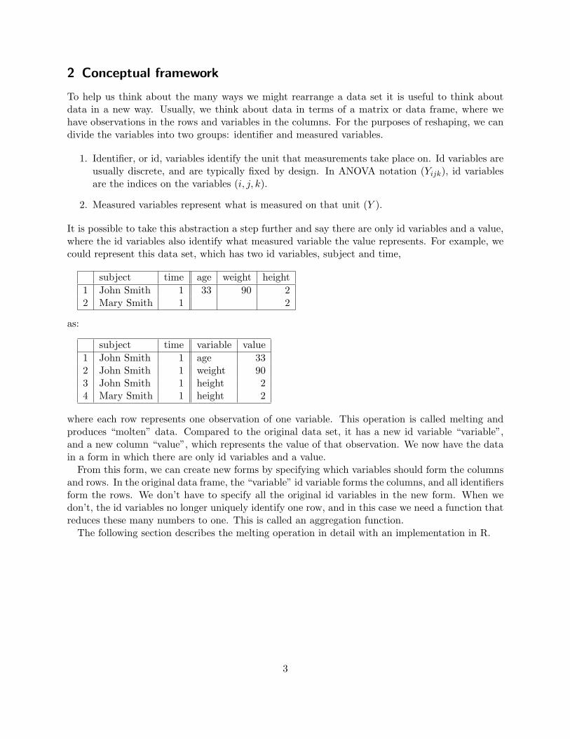
To fix this we need to create a time and treatment column after reshaping:
> (trialm <- cbind(trialm, colsplit(trialm$variable, names = c("treatment",+ "time"))))
id variable value treatment time1 1 A1 1 A 12 2 A1 2 A 13 3 A1 1 A 14 4 A1 2 A 15 1 A2 2 A 26 2 A2 1 A 27 3 A2 2 A 28 4 A2 1 A 29 1 B1 3 B 110 2 B1 3 B 111 3 B1 3 B 112 4 B1 3 B 1
I’m not aware of any general way to do this, so you may need to modify the code in colsplitdepending on your situation.
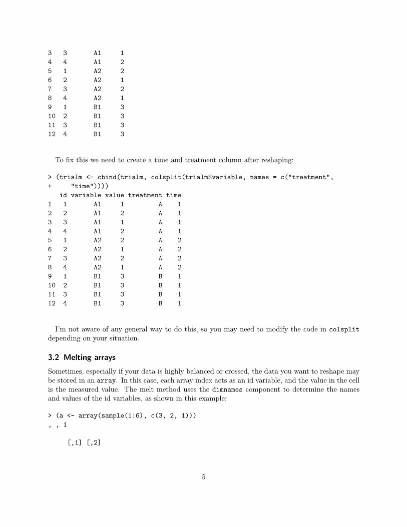
3.2 Melting arrays
Sometimes, especially if your data is highly balanced or crossed, the data you want to reshape maybe stored in an array. In this case, each array index acts as an id variable, and the value in the cellis the measured value. The melt method uses the dimnames component to determine the namesand values of the id variables, as shown in this example:
> (a <- array(sample(1:6), c(3, 2, 1))), , 1
[,1] [,2]
5
[1,] 5 6[2,] 3 4[3,] 1 2
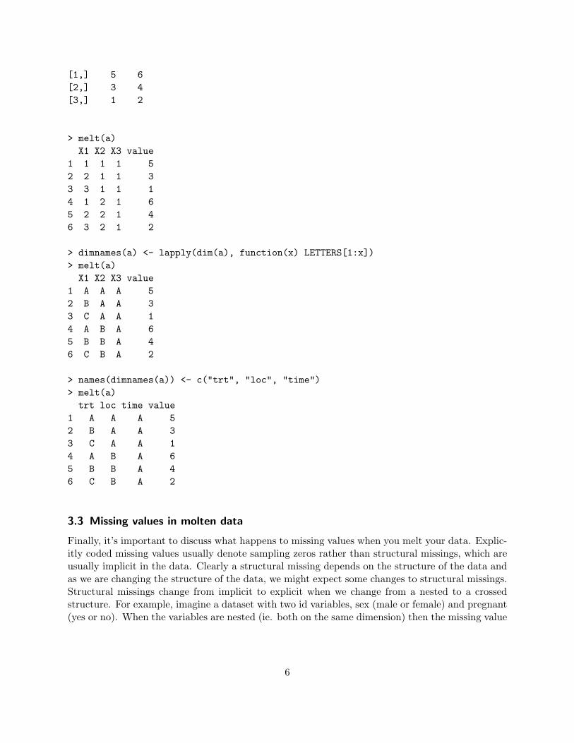
> melt(a)X1 X2 X3 value
1 1 1 1 52 2 1 1 33 3 1 1 14 1 2 1 65 2 2 1 46 3 2 1 2
> dimnames(a) <- lapply(dim(a), function(x) LETTERS[1:x])> melt(a)X1 X2 X3 value
1 A A A 52 B A A 33 C A A 14 A B A 65 B B A 46 C B A 2
> names(dimnames(a)) <- c("trt", "loc", "time")> melt(a)trt loc time value
1 A A A 52 B A A 33 C A A 14 A B A 65 B B A 46 C B A 2
3.3 Missing values in molten data
Finally, it’s important to discuss what happens to missing values when you melt your data. Explic-itly coded missing values usually denote sampling zeros rather than structural missings, which areusually implicit in the data. Clearly a structural missing depends on the structure of the data andas we are changing the structure of the data, we might expect some changes to structural missings.Structural missings change from implicit to explicit when we change from a nested to a crossedstructure. For example, imagine a dataset with two id variables, sex (male or female) and pregnant(yes or no). When the variables are nested (ie. both on the same dimension) then the missing value
6
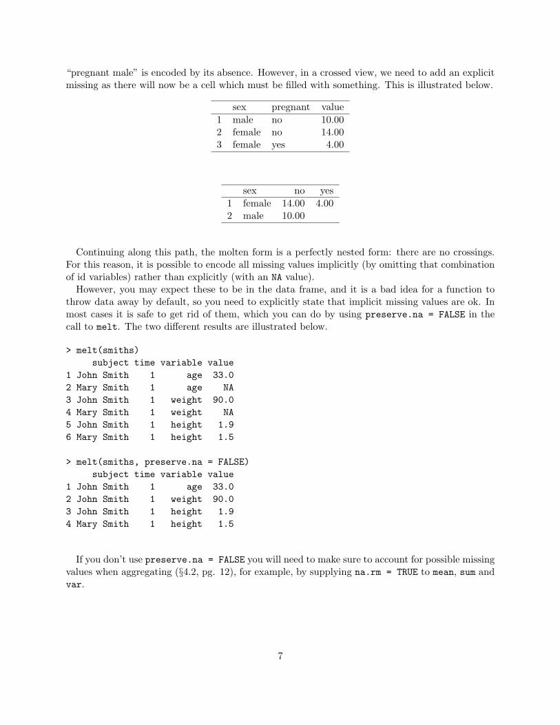
“pregnant male” is encoded by its absence. However, in a crossed view, we need to add an explicitmissing as there will now be a cell which must be filled with something. This is illustrated below.
sex pregnant value1 male no 10.002 female no 14.003 female yes 4.00
sex no yes1 female 14.00 4.002 male 10.00
Continuing along this path, the molten form is a perfectly nested form: there are no crossings.For this reason, it is possible to encode all missing values implicitly (by omitting that combinationof id variables) rather than explicitly (with an NA value).
However, you may expect these to be in the data frame, and it is a bad idea for a function tothrow data away by default, so you need to explicitly state that implicit missing values are ok. Inmost cases it is safe to get rid of them, which you can do by using preserve.na = FALSE in thecall to melt. The two different results are illustrated below.
> melt(smiths)subject time variable value
1 John Smith 1 age 33.02 Mary Smith 1 age NA3 John Smith 1 weight 90.04 Mary Smith 1 weight NA5 John Smith 1 height 1.96 Mary Smith 1 height 1.5
> melt(smiths, preserve.na = FALSE)subject time variable value
1 John Smith 1 age 33.02 John Smith 1 weight 90.03 John Smith 1 height 1.94 Mary Smith 1 height 1.5
If you don’t use preserve.na = FALSE you will need to make sure to account for possible missingvalues when aggregating (§4.2, pg. 12), for example, by supplying na.rm = TRUE to mean, sum andvar.
7

4 Casting molten data
Once you have your data in the molten form, you can use cast to create the form you want. Casthas two arguments that you will always supply:
• data: the molten data set to cast
• formula: the casting formula which describes the shape of the output format (if you omitthis argument, cast will return the data frame to its pre-molten form)
Most of this section explains the different casting formulas you can use. It also explains the useof the other optional arguments to cast:
• fun.aggregate: aggregation function to use (if necessary)
• margins: what marginal values should be computed
• subset: only operate on a subset of the original data.
4.1 Basic use
The casting formula has the following basic form: col var 1 + col var 2 ∼ row var 1 + row var 2.This describes which variables you want to appear in the columns and which in the rows. Thesevariables need to come from the molten data frame or be one of the following special variables:
• . corresponds to no variable, useful when creating formulas of the form . ∼ x or x ∼ .
• ... represents all variables not previously included in the casting formula. Including this inyour formula will guarantee that no aggregation occurs. There can be only one ... in a castformula.
• result variable is used when your aggregation formula returns multiple results. See §4.4,pg. 14 for more details.
The first set of examples illustrated reshaping: all the original variables are used. Each of thesereshapings changes which variable appears in the columns. The typical view of a data frame hasthe “variable” variable in the columns, but if we were interested in investigating the relationshipsbetween subjects or times, we might put those in the columns instead.
> cast(smithsm, time + subject ~ variable)time subject age weight height
1 1 John Smith 33 90 1.95 1 Mary Smith NA NA 1.5
> cast(smithsm, ... ~ variable)subject time age weight height
1 John Smith 1 33 90 1.95 Mary Smith 1 NA NA 1.5
8
> cast(smithsm, ... ~ subject)time variable John.Smith Mary.Smith
1 1 age 33.0 NA2 1 weight 90.0 NA3 1 height 1.9 1.5
> cast(smithsm, ... ~ time)subject variable X1
1 John Smith age 33.02 John Smith weight 90.03 John Smith height 1.94 Mary Smith height 1.5
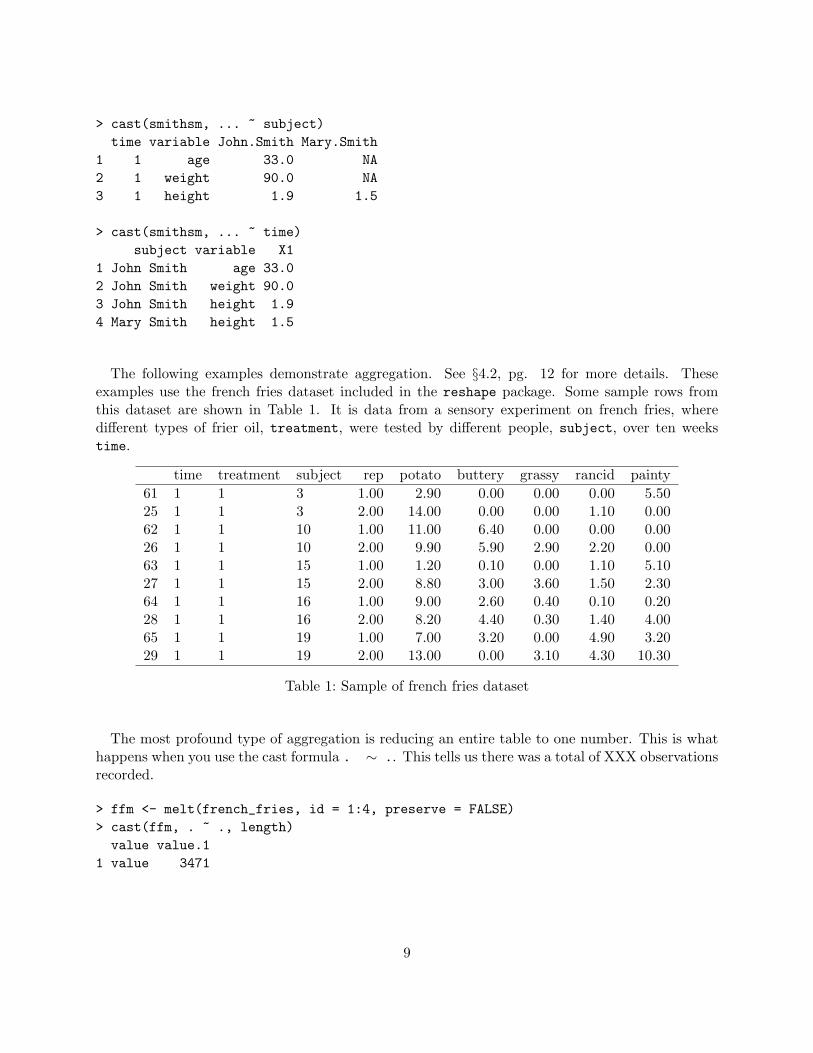
The following examples demonstrate aggregation. See §4.2, pg. 12 for more details. Theseexamples use the french fries dataset included in the reshape package. Some sample rows fromthis dataset are shown in Table 1. It is data from a sensory experiment on french fries, wheredifferent types of frier oil, treatment, were tested by different people, subject, over ten weekstime.
time treatment subject rep potato buttery grassy rancid painty61 1 1 3 1.00 2.90 0.00 0.00 0.00 5.5025 1 1 3 2.00 14.00 0.00 0.00 1.10 0.0062 1 1 10 1.00 11.00 6.40 0.00 0.00 0.0026 1 1 10 2.00 9.90 5.90 2.90 2.20 0.0063 1 1 15 1.00 1.20 0.10 0.00 1.10 5.1027 1 1 15 2.00 8.80 3.00 3.60 1.50 2.3064 1 1 16 1.00 9.00 2.60 0.40 0.10 0.2028 1 1 16 2.00 8.20 4.40 0.30 1.40 4.0065 1 1 19 1.00 7.00 3.20 0.00 4.90 3.2029 1 1 19 2.00 13.00 0.00 3.10 4.30 10.30
Table 1: Sample of french fries dataset
The most profound type of aggregation is reducing an entire table to one number. This is whathappens when you use the cast formula . ∼ .. This tells us there was a total of XXX observationsrecorded.
> ffm <- melt(french_fries, id = 1:4, preserve = FALSE)> cast(ffm, . ~ ., length)value value.1
1 value 3471
9
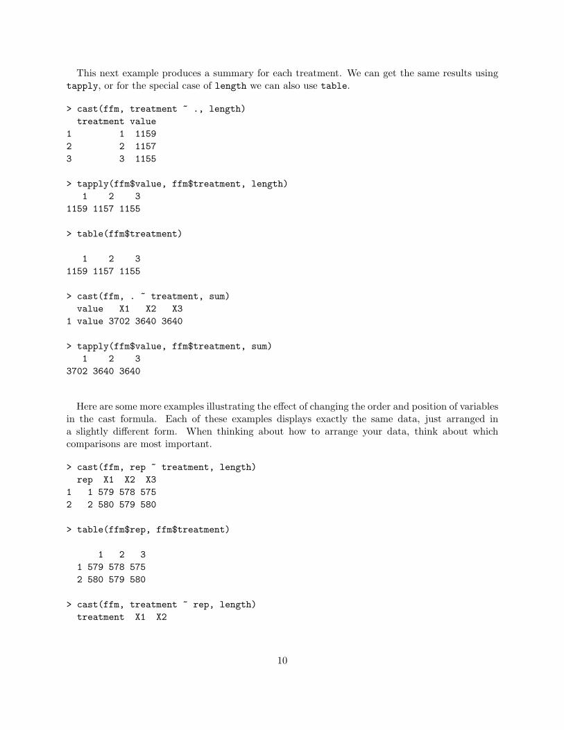
This next example produces a summary for each treatment. We can get the same results usingtapply, or for the special case of length we can also use table.
> cast(ffm, treatment ~ ., length)treatment value
1 1 11592 2 11573 3 1155
> tapply(ffm$value, ffm$treatment, length)1 2 3
1159 1157 1155
> table(ffm$treatment)
1 2 31159 1157 1155
> cast(ffm, . ~ treatment, sum)value X1 X2 X3
1 value 3702 3640 3640
> tapply(ffm$value, ffm$treatment, sum)1 2 3
3702 3640 3640
Here are some more examples illustrating the effect of changing the order and position of variablesin the cast formula. Each of these examples displays exactly the same data, just arranged ina slightly different form. When thinking about how to arrange your data, think about whichcomparisons are most important.
> cast(ffm, rep ~ treatment, length)rep X1 X2 X3
1 1 579 578 5752 2 580 579 580
> table(ffm$rep, ffm$treatment)
1 2 31 579 578 5752 580 579 580
> cast(ffm, treatment ~ rep, length)treatment X1 X2
10
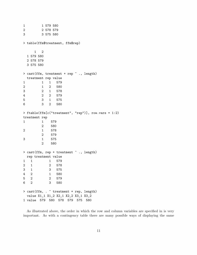
1 1 579 5802 2 578 5793 3 575 580
> table(ffm$treatment, ffm$rep)
1 21 579 5802 578 5793 575 580
> cast(ffm, treatment + rep ~ ., length)treatment rep value
1 1 1 5792 1 2 5803 2 1 5784 2 2 5795 3 1 5756 3 2 580
> ftable(ffm[c("treatment", "rep")], row.vars = 1:2)treatment rep1 1 579
2 5802 1 578
2 5793 1 575
2 580
> cast(ffm, rep + treatment ~ ., length)rep treatment value
1 1 1 5792 1 2 5783 1 3 5754 2 1 5805 2 2 5796 2 3 580
> cast(ffm, . ~ treatment + rep, length)value X1_1 X1_2 X2_1 X2_2 X3_1 X3_2
1 value 579 580 578 579 575 580
As illustrated above, the order in which the row and column variables are specified in is veryimportant. As with a contingency table there are many possible ways of displaying the same
11

variables, and the way they are organised reveals different patterns in the data. Variables specifiedfirst vary slowest, and those specified last vary fastest. Because comparisons are made most easilybetween adjacent cells, the variable you are most interested in should be specified last, and theearly variables should be thought of as conditioning variables. An additional constraint is thatdisplays have limited width but essentially infinite length, so variables with many levels must bespecified as row variables.
4.2 Aggregation
Whenever there are fewer cells in the cast form than there were in the original data format, anaggregation function is necessary. This formula reduces multiple cells into one, and is suppliedin the fun.aggregate argument, which defaults (with a warning) to length. Aggregation is avery common and useful operation and the case studies section (§6, pg. 22) contains many otherexamples of aggregation.
The aggregation function will be passed the vector of a values for one cell. It may take otherarguments, passed in through ... in cast. Here are a few examples:
> cast(ffm, . ~ treatment)Warning: Aggregation requires fun.aggregate: length used as defaultvalue X1 X2 X3
1 value 1159 1157 1155
> cast(ffm, . ~ treatment, function(x) length(x))value X1 X2 X3
1 value 1159 1157 1155
> cast(ffm, . ~ treatment, length)value X1 X2 X3
1 value 1159 1157 1155
> cast(ffm, . ~ treatment, sum)value X1 X2 X3
1 value 3702 3640 3640
> cast(ffm, . ~ treatment, mean)value X1 X2 X3
1 value 3.2 3.1 3.2
> cast(ffm, . ~ treatment, mean, trim = 0.1)value X1 X2 X3
1 value 2.6 2.5 2.6
12
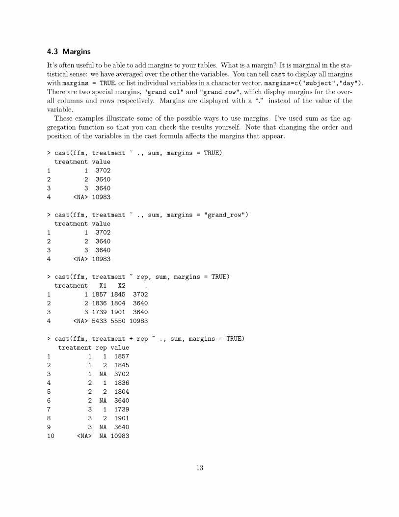
4.3 Margins
It’s often useful to be able to add margins to your tables. What is a margin? It is marginal in the sta-tistical sense: we have averaged over the other the variables. You can tell cast to display all marginswith margins = TRUE, or list individual variables in a character vector, margins=c("subject","day").There are two special margins, "grand col" and "grand row", which display margins for the over-all columns and rows respectively. Margins are displayed with a “.” instead of the value of thevariable.
These examples illustrate some of the possible ways to use margins. I’ve used sum as the ag-gregation function so that you can check the results yourself. Note that changing the order andposition of the variables in the cast formula affects the margins that appear.
> cast(ffm, treatment ~ ., sum, margins = TRUE)treatment value
1 1 37022 2 36403 3 36404 <NA> 10983
> cast(ffm, treatment ~ ., sum, margins = "grand_row")treatment value
1 1 37022 2 36403 3 36404 <NA> 10983
> cast(ffm, treatment ~ rep, sum, margins = TRUE)treatment X1 X2 .
1 1 1857 1845 37022 2 1836 1804 36403 3 1739 1901 36404 <NA> 5433 5550 10983
> cast(ffm, treatment + rep ~ ., sum, margins = TRUE)treatment rep value
1 1 1 18572 1 2 18453 1 NA 37024 2 1 18365 2 2 18046 2 NA 36407 3 1 17398 3 2 19019 3 NA 364010 <NA> NA 10983
13

> cast(ffm, treatment + rep ~ time, sum, margins = TRUE)treatment rep X1 X2 X3 X4 X5 X6 X7 X8 X9 X10 .
1 1 1 156 213 206 181 208 182 156 185 176 194 18572 1 2 216 195 194 154 204 185 158 216 122 201 18453 1 NA 373 408 400 335 412 366 314 402 298 396 37024 2 1 187 213 172 193 157 183 175 173 185 199 18365 2 2 168 157 186 187 173 215 172 189 145 212 18046 2 NA 355 370 358 380 330 398 347 362 330 411 36407 3 1 189 212 172 190 151 161 165 150 173 175 17398 3 2 217 180 199 192 183 192 218 175 164 182 19019 3 NA 406 392 372 382 334 353 384 325 337 357 364010 <NA> NA 1134 1170 1129 1097 1076 1117 1045 1088 965 1163 10983
> cast(ffm, treatment + rep ~ time, sum, margins = "treatment")treatment rep X1 X2 X3 X4 X5 X6 X7 X8 X9 X10
1 1 1 156 213 206 181 208 182 156 185 176 1942 1 2 216 195 194 154 204 185 158 216 122 2013 1 NA 373 408 400 335 412 366 314 402 298 3964 2 1 187 213 172 193 157 183 175 173 185 1995 2 2 168 157 186 187 173 215 172 189 145 2126 2 NA 355 370 358 380 330 398 347 362 330 4117 3 1 189 212 172 190 151 161 165 150 173 1758 3 2 217 180 199 192 183 192 218 175 164 1829 3 NA 406 392 372 382 334 353 384 325 337 357
> cast(ffm, rep + treatment ~ time, sum, margins = "rep")rep treatment X1 X2 X3 X4 X5 X6 X7 X8 X9 X10
1 1 1 156 213 206 181 208 182 156 185 176 1942 1 2 187 213 172 193 157 183 175 173 185 1993 1 3 189 212 172 190 151 161 165 150 173 1754 1 <NA> 532 637 550 564 515 526 497 509 534 5685 2 1 216 195 194 154 204 185 158 216 122 2016 2 2 168 157 186 187 173 215 172 189 145 2127 2 3 217 180 199 192 183 192 218 175 164 1828 2 <NA> 601 533 579 533 560 591 548 580 430 595
4.4 Returning multiple values
Occasionally it is useful to aggregate with a function that returns multiple values, e.g. range orsummary. This can be thought of as combining multiple casts each with an aggregation functionthat returns one variable. To display this we need to add an extra variable, result variable thatdifferentiates the multiple return values. By default, this new id variable will be shown as the last
14
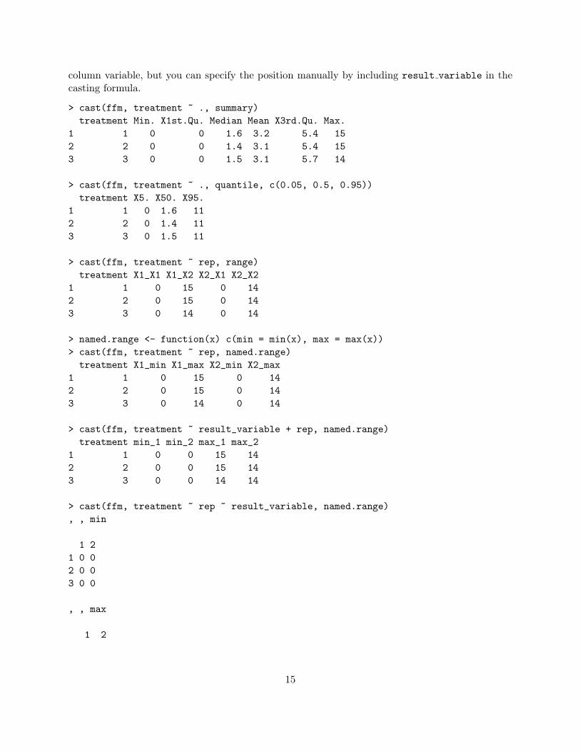
column variable, but you can specify the position manually by including result variable in thecasting formula.
> cast(ffm, treatment ~ ., summary)treatment Min. X1st.Qu. Median Mean X3rd.Qu. Max.
1 1 0 0 1.6 3.2 5.4 152 2 0 0 1.4 3.1 5.4 153 3 0 0 1.5 3.1 5.7 14
> cast(ffm, treatment ~ ., quantile, c(0.05, 0.5, 0.95))treatment X5. X50. X95.
1 1 0 1.6 112 2 0 1.4 113 3 0 1.5 11
> cast(ffm, treatment ~ rep, range)treatment X1_X1 X1_X2 X2_X1 X2_X2
1 1 0 15 0 142 2 0 15 0 143 3 0 14 0 14
> named.range <- function(x) c(min = min(x), max = max(x))> cast(ffm, treatment ~ rep, named.range)treatment X1_min X1_max X2_min X2_max
1 1 0 15 0 142 2 0 15 0 143 3 0 14 0 14
> cast(ffm, treatment ~ result_variable + rep, named.range)treatment min_1 min_2 max_1 max_2
1 1 0 0 15 142 2 0 0 15 143 3 0 0 14 14
> cast(ffm, treatment ~ rep ~ result_variable, named.range), , min
1 21 0 02 0 03 0 0
, , max
1 2
15
1 15 142 15 143 14 14
Returning multidimensional objects (eg. matrices or arrays) from an aggregation doesn’t cur-rently work very well. However, you can probably work around this deficiency by creating a high-Darray, and then using iapply.
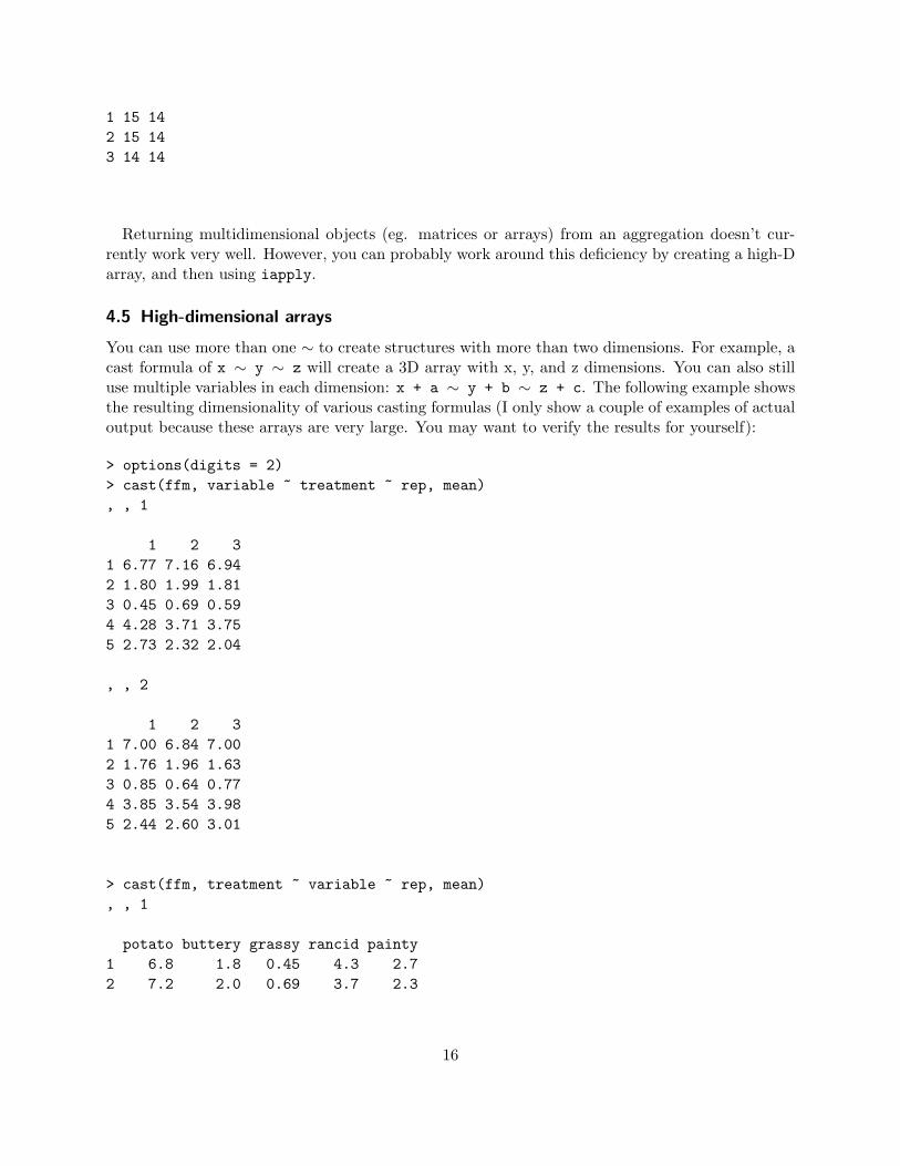
4.5 High-dimensional arrays
You can use more than one ∼ to create structures with more than two dimensions. For example, acast formula of x ∼ y ∼ z will create a 3D array with x, y, and z dimensions. You can also stilluse multiple variables in each dimension: x + a ∼ y + b ∼ z + c. The following example showsthe resulting dimensionality of various casting formulas (I only show a couple of examples of actualoutput because these arrays are very large. You may want to verify the results for yourself):
> options(digits = 2)> cast(ffm, variable ~ treatment ~ rep, mean), , 1
1 2 31 6.77 7.16 6.942 1.80 1.99 1.813 0.45 0.69 0.594 4.28 3.71 3.755 2.73 2.32 2.04
, , 2
1 2 31 7.00 6.84 7.002 1.76 1.96 1.633 0.85 0.64 0.774 3.85 3.54 3.985 2.44 2.60 3.01
> cast(ffm, treatment ~ variable ~ rep, mean), , 1
potato buttery grassy rancid painty1 6.8 1.8 0.45 4.3 2.72 7.2 2.0 0.69 3.7 2.3
16

3 6.9 1.8 0.59 3.8 2.0
, , 2
potato buttery grassy rancid painty1 7.0 1.8 0.85 3.8 2.42 6.8 2.0 0.64 3.5 2.63 7.0 1.6 0.77 4.0 3.0
> dim(cast(ffm, time ~ variable ~ treatment, mean))[1] 10 5 3
> dim(cast(ffm, time ~ variable ~ treatment + rep, mean))[1] 10 5 6
> dim(cast(ffm, time ~ variable ~ treatment ~ rep, mean))[1] 10 5 3 2
> dim(cast(ffm, time ~ variable ~ subject ~ treatment ~ rep))[1] 10 5 12 3 2
> dim(cast(ffm, time ~ variable ~ subject ~ treatment ~ result_variable,+ range))[1] 10 5 12 3 2
The high-dimensional array form is useful for sweeping out margins with sweep, or modifyingwith iapply. See the case studies for examples.
The ∼ operator is a type of crossing operator, as all combinations of the variables will appearin the output table. Compare this to the + operator, where only combinations that appear in thedata will appear in the output. For this reason, increasing the dimensionality of the output, i.e.using more ∼s, will generally increase the number of (structural) missings. This is illustrated inthe next example:
> sum(is.na(cast(ffm, ... ~ .)))[1] 0
> sum(is.na(cast(ffm, ... ~ rep)))[1] 9
> sum(is.na(cast(ffm, ... ~ subject)))[1] 129
> sum(is.na(cast(ffm, ... ~ time ~ subject ~ variable ~ rep)))
17
[1] 129
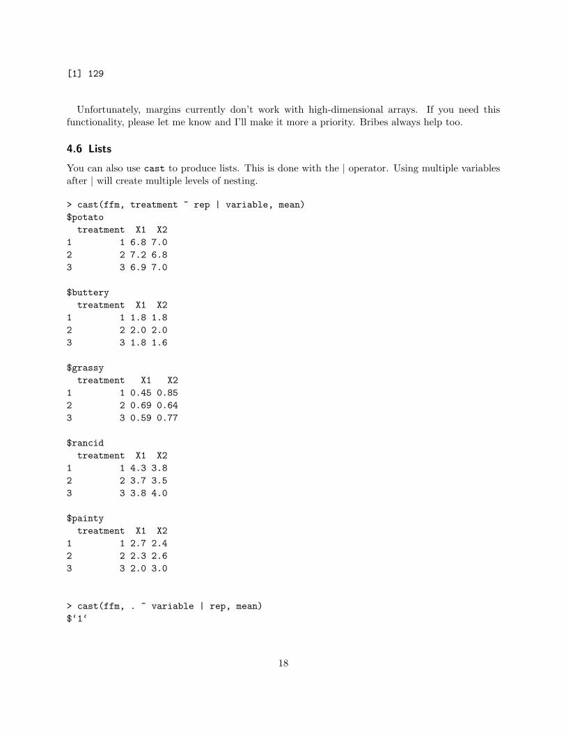
Unfortunately, margins currently don’t work with high-dimensional arrays. If you need thisfunctionality, please let me know and I’ll make it more a priority. Bribes always help too.
4.6 Lists
You can also use cast to produce lists. This is done with the | operator. Using multiple variablesafter | will create multiple levels of nesting.
> cast(ffm, treatment ~ rep | variable, mean)$potatotreatment X1 X2
1 1 6.8 7.02 2 7.2 6.83 3 6.9 7.0
$butterytreatment X1 X2
1 1 1.8 1.82 2 2.0 2.03 3 1.8 1.6
$grassytreatment X1 X2
1 1 0.45 0.852 2 0.69 0.643 3 0.59 0.77
$rancidtreatment X1 X2
1 1 4.3 3.82 2 3.7 3.53 3 3.8 4.0
$paintytreatment X1 X2
1 1 2.7 2.42 2 2.3 2.63 3 2.0 3.0
> cast(ffm, . ~ variable | rep, mean)$‘1‘
18
value potato buttery grassy rancid painty1 value 7 1.9 0.58 3.9 2.4
$‘2‘value potato buttery grassy rancid painty
1 value 7 1.8 0.75 3.8 2.7
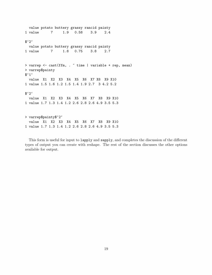
> varrep <- cast(ffm, . ~ time | variable + rep, mean)> varrep$painty$‘1‘value X1 X2 X3 X4 X5 X6 X7 X8 X9 X10
1 value 1.5 1.6 1.2 1.5 1.4 1.9 2.7 3 4.2 5.2
$‘2‘value X1 X2 X3 X4 X5 X6 X7 X8 X9 X10
1 value 1.7 1.3 1.4 1.2 2.6 2.8 2.6 4.9 3.5 5.3
> varrep$painty$‘2‘value X1 X2 X3 X4 X5 X6 X7 X8 X9 X10
1 value 1.7 1.3 1.4 1.2 2.6 2.8 2.6 4.9 3.5 5.3
This form is useful for input to lapply and sapply, and completes the discussion of the differenttypes of output you can create with reshape. The rest of the section discusses the other optionsavailable for output.
19
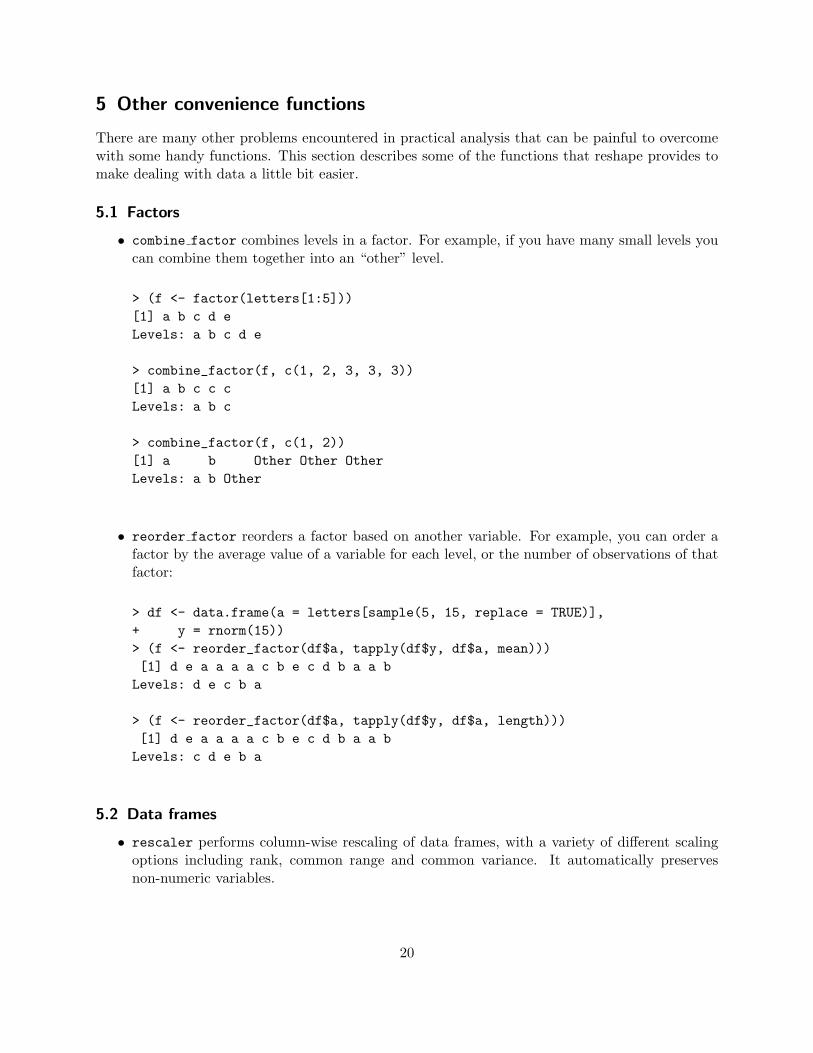
5 Other convenience functions
There are many other problems encountered in practical analysis that can be painful to overcomewith some handy functions. This section describes some of the functions that reshape provides tomake dealing with data a little bit easier.
5.1 Factors
• combine factor combines levels in a factor. For example, if you have many small levels youcan combine them together into an “other” level.
> (f <- factor(letters[1:5]))[1] a b c d eLevels: a b c d e
> combine_factor(f, c(1, 2, 3, 3, 3))[1] a b c c cLevels: a b c
> combine_factor(f, c(1, 2))[1] a b Other Other OtherLevels: a b Other
• reorder factor reorders a factor based on another variable. For example, you can order afactor by the average value of a variable for each level, or the number of observations of thatfactor:
> df <- data.frame(a = letters[sample(5, 15, replace = TRUE)],+ y = rnorm(15))> (f <- reorder_factor(df$a, tapply(df$y, df$a, mean)))[1] d e a a a a c b e c d b a a bLevels: d e c b a
> (f <- reorder_factor(df$a, tapply(df$y, df$a, length)))[1] d e a a a a c b e c d b a a bLevels: c d e b a
5.2 Data frames
• rescaler performs column-wise rescaling of data frames, with a variety of different scalingoptions including rank, common range and common variance. It automatically preservesnon-numeric variables.
20

• merge.all merges multiple data frames together, an extension of merge in base R. It assumesthat all columns with the same name should be equated.
• rbind.fill rbinds two data frames together, filling in any missing columns in the seconddata frame with missing values.
5.3 Miscellaneous
• round any allows you to round a number to any degree of accuracy, e.g. to the nearest 1, 10,or any other number.
> round_any(105, 10)[1] 100
> round_any(105, 4)[1] 104
> round_any(105, 4, ceiling)[1] 108
• iapply is an idempotent version of the apply function. This is useful when dealing withhigh-dimensional arrays as it will return the array in the same shape that you sent it. It alsosupports functions that return matrices or arrays in a sensible manner.
21
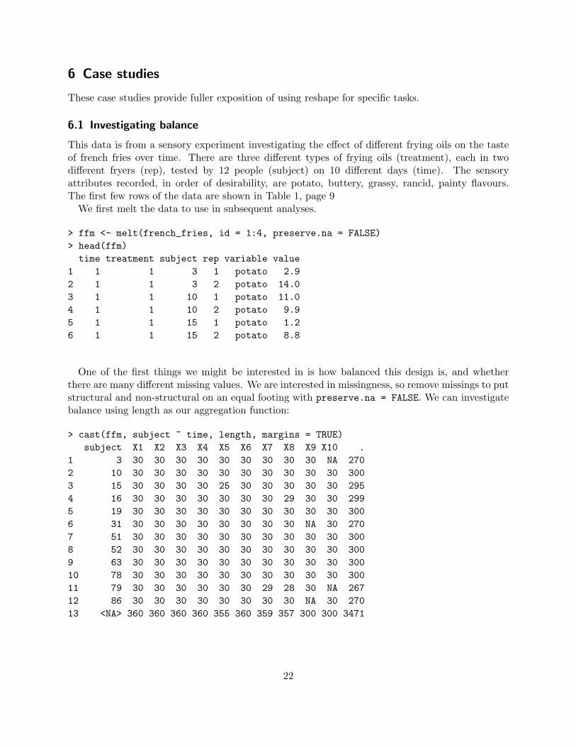
6 Case studies
These case studies provide fuller exposition of using reshape for specific tasks.
6.1 Investigating balance
This data is from a sensory experiment investigating the effect of different frying oils on the tasteof french fries over time. There are three different types of frying oils (treatment), each in twodifferent fryers (rep), tested by 12 people (subject) on 10 different days (time). The sensoryattributes recorded, in order of desirability, are potato, buttery, grassy, rancid, painty flavours.The first few rows of the data are shown in Table 1, page 9
We first melt the data to use in subsequent analyses.
> ffm <- melt(french_fries, id = 1:4, preserve.na = FALSE)> head(ffm)time treatment subject rep variable value
1 1 1 3 1 potato 2.92 1 1 3 2 potato 14.03 1 1 10 1 potato 11.04 1 1 10 2 potato 9.95 1 1 15 1 potato 1.26 1 1 15 2 potato 8.8
One of the first things we might be interested in is how balanced this design is, and whetherthere are many different missing values. We are interested in missingness, so remove missings to putstructural and non-structural on an equal footing with preserve.na = FALSE. We can investigatebalance using length as our aggregation function:
> cast(ffm, subject ~ time, length, margins = TRUE)subject X1 X2 X3 X4 X5 X6 X7 X8 X9 X10 .
1 3 30 30 30 30 30 30 30 30 30 NA 2702 10 30 30 30 30 30 30 30 30 30 30 3003 15 30 30 30 30 25 30 30 30 30 30 2954 16 30 30 30 30 30 30 30 29 30 30 2995 19 30 30 30 30 30 30 30 30 30 30 3006 31 30 30 30 30 30 30 30 30 NA 30 2707 51 30 30 30 30 30 30 30 30 30 30 3008 52 30 30 30 30 30 30 30 30 30 30 3009 63 30 30 30 30 30 30 30 30 30 30 30010 78 30 30 30 30 30 30 30 30 30 30 30011 79 30 30 30 30 30 30 29 28 30 NA 26712 86 30 30 30 30 30 30 30 30 NA 30 27013 <NA> 360 360 360 360 355 360 359 357 300 300 3471
22

Of course we can also use our own aggregation function. Each subject should have had 30observations at each time, so by displaying the difference we can more easily see where the data ismissing.
> cast(ffm, subject ~ time, function(x) 30 - length(x))subject X1 X2 X3 X4 X5 X6 X7 X8 X9 X10
1 3 0 0 0 0 0 0 0 0 0 NA2 10 0 0 0 0 0 0 0 0 0 03 15 0 0 0 0 5 0 0 0 0 04 16 0 0 0 0 0 0 0 1 0 05 19 0 0 0 0 0 0 0 0 0 06 31 0 0 0 0 0 0 0 0 NA 07 51 0 0 0 0 0 0 0 0 0 08 52 0 0 0 0 0 0 0 0 0 09 63 0 0 0 0 0 0 0 0 0 010 78 0 0 0 0 0 0 0 0 0 011 79 0 0 0 0 0 0 1 2 0 NA12 86 0 0 0 0 0 0 0 0 NA 0
We can also easily see the range of values that each variable takes:
> cast(ffm, variable ~ ., function(x) c(min = min(x), max = max(x)))variable min max
1 potato 0 152 buttery 0 113 grassy 0 114 rancid 0 155 painty 0 13
6.2 Tables of means
When creating these tables, it is a good idea to restrict the number of digits displayed. You cando this globally, by setting options(digits=2), or locally, by using round any.
Since the data is fairly well balanced, we can do some (crude) investigation as to the effects of thedifferent treatments. For example, we can calculate the overall means for each sensory attributefor each treatment:
> options(digits = 2)> cast(ffm, treatment ~ variable, mean, margins = c("grand_col",+ "grand_row"))treatment potato buttery grassy rancid painty .
1 1 6.9 1.8 0.65 4.1 2.6 3.22 2 7.0 2.0 0.66 3.6 2.5 3.1
23

3 3 7.0 1.7 0.68 3.9 2.5 3.24 <NA> 7.0 1.8 0.66 3.9 2.5 3.2
It doesn’t look like there is any effect of treatment. This can be confirmed using a more formalanalysis of variance.
6.3 Investigating inter-rep reliability
Since we have a repetition over treatments, we might be interested in how reliable each subject is:are the scores for the two reps highly correlated? We can explore this graphically by reshaping thedata and plotting the data. Our graphical tools work best when the things we want to compareare in different columns, so we’ll cast the data to have a column for each rep and then use qplotto plot rep 1 (X1) vs rep 2 (X2), with a separate plot for each variable.
> library(ggplot)> qplot(X1, X2, . ~ variable, data = cast(ffm, ... ~ rep))
0
5
10
15
0 5 10 150 5 10 150 5 10 150 5 10 150 5 10 15
variable: potato variable: buttery variable: grassy variable: rancid variable: painty●
●
●●
● ●
●
●
●
●
●
●
●
●
●
●
● ●
●
●●
●●
●
●●
●
●
●
●
●
●●
●
●●
●
●
●
● ●
●
●
●●
●
● ●
●
●
●
●
●
●
●
●●
●
●
●
●
●●
●
●
●
●
●
●
●
●
●
●
●
●
●
●
●
●●●
●
●
●●
●
●
●
●
●●
●
●
●
● ●
●
●
●
●
●
●●
●
●
●
●
●●
●
●
●
●
●
●
●
●
●
●
●
●
●●
●
●●
●
●
●
●
●
●
●
● ●
●
●
●
●●
●
●
●
●
●
●
●● ●
●
●
●●
●
●
●
●
●
●
●
●
●
●
●
●
●
●
●
●
●●
●
●
●
●
●
●
●●
●
●
●
●
●●
●●
●
●
●●
●
●
●●
●●
●●
●
●
●
●
●
●
●
●
●●
●
●
●
●
●
●
●
●
●
●
●
●
●
●
●
●
●
●
●
●
●
●
●
●
●
●
●
●
●
●
●
●
●
●
●
●
●
●
●
●
●
●
●●
●
●
●
●
●
●
●
●●
●
●
●
●
●
●
●
●
●
●
●
●
●
●
●
●
●
●
●
●
●
●
●
●
●
●
●●
●
●
●
●
●
●
●
●
●
●
●
●
●
●
●
●
●
●
●
●●
●
●
●
●
●
●
●
●
●
●
●
●
●
●
●
●
●
●
●
●
●
●●
●
●
●
●
●
●
●
●●
●
●
●
●
●
●
●
●
●●
●
●
●
●
●●
●
●●
●●
● ●●
●
●
●●
●●
● ●
●
●
●
●
●
●
●
●●
●
●
●
●
●
●
●
●
●
●
●
●
●
●
●●
●
●
●
●
●●
●
●
●
●●
●
●
●●
●
●
●
●
●
●
●
●
●●
● ●
●
●
●●
●
● ●
● ●
●
●
●
●
●●
●
●
●
●
●●
●
●
●
●
●
●
●
●
●● ●
●
●
●
●
● ●
●
●
●
●
●
●
●
●
●
●
●
●
●
●●
●
● ●
●
●●
●
●
●
●
●
●
●
●
●
●
● ●
●
●● ●
●
●
●
●
●
●
●
●
●●●●
●
●
●
●●
●●
●
●●
●
● ●
●
●
●
●
●
●
●●
●
● ●
●
●
●
●●
●
●
●
●●
●
●●
●
●
●
●
●
●
●
●
●
●
●
●
●
●
●
●●
●
●
●●
●
●●
●
●● ●●
●●
●
●
●
●●●●●
●●
●
●
●
●
●●
●●●●
●
●
●
●
●
●●
●
●●●
●●
●● ●
●●
●
●
●●
●● ●●
● ●●
●
●●
●
●
●
●●
●●
●
● ●
●
●●●●
●●
●●
●
●●
●●
●
●
●●
●
●●●●●
●
●●
●
●
●
●
●
●●
●●
●●●
● ●
●●
●
●
●
●
●
●
●
●
●
●●
●
●
●●●
●
●
●
●●●
●
●●
●
●
●●●
●
●
●●
●
●● ●
●
●
●
●
●
●
●
●
●●
●
●
●
●
●
●
●●
●
●
●
●
●
●
●
●
●● ●
●
● ●
●
●
●
●●
●●
●
●●●●
●
●
●●
●
●
●
●
●
●
●
● ●
●
●
●
●
●
●
●
●
●
●
●
●
●●
●
●●●
●
●●●
●●
●
●
●
●
●
●
●●
●
●
●
●
●●
●
●
●
●
●
●
●●
●●
●
●
●
●
●
●
●
●
●
●
●
●●
●●
●
●
●
●
●
●
●
●
●●
●●
●
●
●
●
●
●●
●
●
● ●●
●
●●
●
●
●
●
●●
●
●
●
●
● ●
●
●
●
●
●
●●
●
●
●
●●
●
● ●
●
●
●
●
●
●
●
●
●
●
●
●
●●
●
●
●●
●
●
●
●
●
●
●●
●
●
●
●
●●
●
●
●
●●
●●
●
●
●●
●
●
●
●
●●
●
●
●
●
●
●
●
●
●
●
● ●
●●●
●
●
●
●
●
●
●
●
●
●
●
●
●
●
●
●
●
●●
●
●
●●
●●
●
●
●
● ●
●
●
●●
●
●
●
●
●
● ●
●
●
●
●
●●
●
●
●
●
●
●
●
●
●
●
●
● ●
●●●
●
●
●
●
● ●●●
●
●
●
●
●
●
●
●
●●
●
●●
●
●
●●●
●
●
●
●
●
●
●
●●
●
●
●
●● ●●
●
●
●
●
●
●
●
●
●
●
●●
●●
●
●
●
●
●
●
●
●
●
●
●●
●
●●
●
●●
●●
●
●
●
●●
●
●
●
●
●
●
●
●
●
●
●
●
●
●
●●
●
●
●●
●
●
●
●
● ●
●● ●
●
●
●
●●
●
● ●
●
●
●
●
●
●
●
●
●●
●
●●●
●
●
●
●
●
●
●
●
●
●
●
●
●
●
●
●
●
●●
●
●
●
●
● ●
● ●
●
●
●
●
●
●
●
●
●
●
●
●
●
●
●
●
●
●
●
●
●
●
●
●
●
●
●
●
●
●
●●
●
●
●
●
●
●
●
●
●
●
●
●
●
●
X2
X1
This plot is not trivial to understand, as we are plotting two rather unusual variables. Each pointcorresponds to one measurement for a given subject, date and treatment. This gives a scatterplotfor each variable than can be used to assess the inter-rep relationship. The inter-rep correlationlooks strong for potatoey, weak for buttery and grassy, and particularly poor for painty.
If we wanted to explore the relationships between subjects or times or treatments we could followsimilar steps.
24

7 Where to go next
Now that you’ve read this introduction, you should be able to get started using the reshapepackage. You can find a quick reference and more examples in ?melt and ?cast. You can findsome additional information on the reshape website http://had.co.nz/reshape, including thelatest version of this document, as well as copies of presentations and papers related to reshape.
I would like to include more case studies of reshape in use. If you have an interesting example,or there is something you are struggling with please let me know: [email protected].
25
Related Documents