RESERVOIR STUDIES OF NEW MULTILATERAL WELL ARCHITECTURE A Thesis by MANOJ SARFARE Submitted to the Office of Graduate Studies of Texas A&M University in partial fulfillment of the requirements for the degree of MASTER OF SCIENCE May 2004 Major Subject: Petroleum Engineering brought to you by CORE View metadata, citation and similar papers at core.ac.uk provided by Texas A&M University

Welcome message from author
This document is posted to help you gain knowledge. Please leave a comment to let me know what you think about it! Share it to your friends and learn new things together.
Transcript
RESERVOIR STUDIES OF NEW MULTILATERAL WELL ARCHITECTURE
A Thesis
by
MANOJ SARFARE
Submitted to the Office of Graduate Studies of Texas A&M University
in partial fulfillment of the requirements for the degree of
MASTER OF SCIENCE
May 2004
Major Subject: Petroleum Engineering
brought to you by COREView metadata, citation and similar papers at core.ac.uk
provided by Texas A&M University

RESERVOIR STUDIES OF NEW MULTILATERAL WELL ARCHITECTURE
A Thesis
by
MANOJ SARFARE
Submitted to Texas A&M University
in partial fulfillment of the requirements for the degree of
MASTER OF SCIENCE
Approved as to style and content by:
_______________________________ Peter P. Valkó
(Chair of Committee)
_______________________________ J. Bryan Maggard
(Member)
_______________________________ Terry L. Kohutek
(Member)
_______________________________ Stephen A. Holditch
(Head of Department)
May 2004
Major Subject: Petroleum Engineering
iii
ABSTRACT
Reservoir Studies of New Multilateral Well Architecture. (May 2004)
Manoj Sarfare, B.E., Maharashtra Institute of Technology, India
Chair of Advisory Committee: Dr. Peter P. Valkó
Hydrocarbon recovery from conventional reservoirs is decreasing and the need to
produce oil cheaply from mature, marginal and unconventional reservoirs poses a big
challenge to the industry today. Multilateral well technology can provide innovative
solutions to these problems and prove to be the most likely tool to propel the industry in
the next century. In this research we propose a new multilateral well architecture for
more efficient and effective field drainage. We study the architecture from a reservoir
engineering point of view and analyze the effect of various design parameters such as
branch density and penetration extent of laterals on the performance of the proposed
architecture for homogeneous reservoirs. We also analyze the performance in case of
anisotropic reservoirs.
The numerical simulation results show that the multilateral wells usually help
improve the overall cumulative production from a reservoir as compared to conventional
wells. Also, they provide the added benefit of faster field drainage and present a more
attractive return on investment. In this thesis we also present the results for a
representative field case analysis. The rapidly changing Solution GOR contributed to
making the oil viscous, which reduced the problem to optimize the mother bore location.
In addition to these numerical studies we perform analytic studies to develop quick
estimates of the theoretical limits of Productivity Index of the proposed architecture. We
use known results from the literature to test their validity to estimate the upper and lower
bounds on productivity. The results show that current tools to determine the lower limit is
insufficient to predict performance.

iv
DEDICATION
To my beloved mom, dad, and brother, who have always helped and supported
me in all my endeavors.

v
ACKNOWLEDGEMENTS
I would like to take this opportunity to thank all those who helped and assisted me
in completing this thesis. First and foremost, I extend my deepest gratitude to Dr. Peter
Valkó, advisor and chair of my committee. His support, encouragement, and guidance
have been invaluable in the successful completion of this thesis. He has been most patient
and helpful all through my years as a graduate student at Texas A&M University.
I would like to thank Dr. Bryan Maggard for guiding me with my work. Also, I
would like to thank Dr. Terry Kohutek for serving on my committee.
Friends have been a great source of advice during these years. Deepak, Ashish,
Vivek, and Sandeep have provided a lot of tips towards writing the thesis and I sincerely
thank them for the same. Harshal, Kartik, and DC, along with the others have helped
make the long hours spent in the department quite enjoyable and pleasant. I have learnt
new things all along the process and I thank everyone for their support and advice.

vi
TABLE OF CONTENTS
Page
ABSTRACT……………………………………………………………………………...iii
DEDICATION....................................................................................................................iv
ACKNOWLEDGEMENTS……………………………………………………………….v
TABLE OF CONTENTS………………………………………………………………...vi
LIST OF FIGURES………………………………………………………………………ix
LIST OF TABLES…………………………………………………………………….......x
CHAPTER
I INTRODUCTION – RESERVOIR APPLICATIONS OF MULTILATERAL WELL TECHNOLOGY.......................................................................................... 1
1.1 Introduction ............................................................................................. 1 1.2 Statement of Problem............................................................................... 1 1.3 Multilateral Wells – An Overview ........................................................... 2
1.3.1 A Background of Multilateral Wells................................................ 2 1.3.2 Present State of Multilateral Wells .................................................. 3 1.3.3 The Future....................................................................................... 6
II NEW MULTILATERAL WELL ARCHITECTURE ........................................... 8
2.1 Description of the New Multi-lateral Well Architecture ........................... 8 2.2 Advantages of ML Wells ....................................................................... 10 2.3 Multilateral Well Model......................................................................... 10 2.4 Methodology and Procedure .................................................................. 12 2.5 Technical Indicator ................................................................................ 13
III ESTIMATION OF THEORETICAL UPPER AND LOWER LIMITS…………16
3.1 Motivation ............................................................................................. 16 3.2 Methodology ......................................................................................... 16 3.3 Upper Limit / Maximum Achievable PI ................................................. 19

vii
CHAPTER Page
3.3.1 Infinite Conductivity Fracture PI ................................................... 19 3.3.2 Application to ML Well Architecture ............................................ 20
3.4 Lower Limit for PI................................................................................. 21 3.4.1 Outline .......................................................................................... 21 3.4.2 Step 1 - Numerical Analysis of Actual ML Well with Single
Block Productivity ........................................................................ 22 3.4.3 Step 2 – Analysis of Analytic and Numeric Solution for Well- Defined Geometry......................................................................... 28 3.4.4 Discussion of Results .................................................................... 35
IV PRELIMINARY ANALYSIS OF PROPOSED ARCHITECTURE FOR SYNTHETIC CASES ……………………………………………………………36
4.1 Parameters to be Analyzed..................................................................... 36 4.2 Reservoir Geometry and Properties........................................................ 37 4.3 Simulation Cases ................................................................................... 37 4.4 Simulation Results ................................................................................. 38
4.4.1 Branch Density and Partial Penetration Effects.............................. 38 4.4.2 Permeability.................................................................................. 48 4.4.3 Grid Refinement............................................................................ 56
V FIELD CASE SIMULATION AND ANALYSIS……………………………….58
5.1 Data for El Furrial Field......................................................................... 58 5.2 Representative Unit................................................................................ 60 5.3 Base Case .............................................................................................. 65 5.4 ML Well Architecture and Simulation Cases ......................................... 65 5.5 Simulation Results ................................................................................. 67
VI CONCLUSIONS AND RECOMMENDATIONS………………………………74
6.1 Conclusions ........................................................................................... 74 6.2 Recommendations for Future Studies..................................................... 76
NOMENCLATURE……………………………………………………………………..77
REFERENCES…………………………………………………………………………..79

viii
APPENDIX A……………………………………………………………………………83
APPENDIX B……………………………………………………………………………88
VITA……………………………………………………………………………………..98

ix
LIST OF FIGURES
FIGURE Page
1.1 TAML classification of ML wells......................................................................... 4
2.1 New multilateral well architecture ........................................................................ 9
2.2 Multilateral well model used for numerical simulations...................................... 11
3.1 Rearranged form of a horizontal well architecture .............................................. 18
3.2 Infinite conductivity fracture in a rectangular geometry...................................... 19
3.3 Infinite laterals forming an infinite conductivity fracture in the vertical plane..... 20
3.4 Comparison of single block performance with the corresponding ML well structure ............................................................................................................ 28
3.5 Simplest single block structure with a 5:1 ratio between its sides........................ 29
3.6 Partially penetrating vertical well ....................................................................... 30
3.7 Comparison of results for isotropic case ............................................................. 33
3.8 Comparison of results for anisotropic case.......................................................... 34
4.1 A much lower bottomhole pressure is need when using fewer laterals, increasing the possibility of borehole collapse, sand production, water coning... 39 4.2 Productivity of the ML well architecture decreases significantly (by 50%) as we go from an isotropic reservoir to an anisotropic reservoir. ............................. 49 5.1 El Furrial field location ...................................................................................... 58
5.2 Structural model of El Furrial ............................................................................. 59
5.3 Variation of solution GOR with pressure ............................................................ 62
5.4 Variation of viscosity with pressure.................................................................... 63
5.5 Variation of solution GOR with depth ................................................................ 64
5.6 Variation of viscosity with depth ........................................................................ 65
5.7 General ML well architecture used for simulation .............................................. 66
x
LIST OF TABLES
TABLE Page
3.1 Single block productivity for an 8 lateral structure subset ................................... 24
3.2 Productivity of an 8 lateral structure................................................................... 25
3.3 Single block productivity of a 15 lateral subset................................................... 26
3.4 Productivity of a 15 lateral structure................................................................... 27
3.5 Dimensionless height for Cinco pseudo-skin data............................................... 30
3.6 Comparison of PI’s for isotropic case ................................................................. 32
3.7 Comparison of PI’s for anisotropic case ............................................................. 32
4.1 Base case reservoir properties............................................................................. 37
4.2 Summary of simulation results ........................................................................... 40
4.3 Productivity of a 60 lateral structure................................................................... 41
4.4 Productivity of a 30 lateral structure................................................................... 42
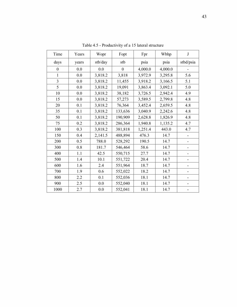
4.5 Productivity of a 15 lateral structure................................................................... 43
4.6 Productivity of a 4 lateral structure..................................................................... 44
4.7 Productivity of a 30 lateral structure with 45% penetration................................. 45
4.8 Productivity of a 4 lateral structure with 45% penetration in the reservoir........... 46
4.9 Productivity of a 2 lateral structure with 73 % penetration.................................. 47
4.10 Isotropic reservoir productivity with a 60 lateral structure ................................ 50
4.11 Isotropic reservoir productivity with a 30 lateral structure ................................ 51
4.12 Isotropic reservoir productivity with a 4 lateral structure .................................. 52
4.13 Anisotropic reservoir productivity with a 60 lateral structure............................ 53
4.14 Anisotropic reservoir productivity with a 30 lateral structure............................ 54

xi
TABLE Page
4.15 Anisotropic reservoir productivity with a 4 lateral structure.............................. 55
4.16 Results showing numerical consistency with grid refinement............................ 57
5.1 Reservoir characteristics of El Furrial................................................................. 59
5.2 El Furrial fluid PVT properties ........................................................................... 60
5.3 Solution GOR vs. depth...................................................................................... 61
5.4 Base case results (8 vertical wells)...................................................................... 68
5.5 Case A results .................................................................................................... 69
5.6 Case B results..................................................................................................... 70
5.7 Case C results..................................................................................................... 71
5.8 Case D results .................................................................................................... 72
5.9 Case E results ..................................................................................................... 73
1
CHAPTER I
INTRODUCTION – RESERVOIR APPLICATIONS OF MULTILATERAL
WELL TECHNOLOGY
1.1 Introduction
Since their introduction in the early part of the last decade, multilateral well systems
and their applications have developed rapidly1. They have been used in a myriad of
operating conditions varying from mature fields to forming an integral part of completely
new field development strategies. However under all the different operating arenas the
aim is to produce hydrocarbons as quickly and efficiently as possible. In doing so the
industry is faced by many challenges2, some of which are:
1. complex geologic conditions such as compartmentalized or stacked reservoirs
2. difficult reservoir conditions such as viscous fluids or tight formations
3. hostile environments such as deep water or frontier development sites
4. efficient and effective reservoir management and development plans
Innovative solutions are necessary to tackle the problems and challenges facing the
industry successfully. Multilateral well technology provides just such a solution. The
technology has been successfully applied in all the above areas and shows a dramatic
impact on the financial results of many, thus promising to be not just an evolutionary but
also a revolutionary technology in the oil field.
1.2 Statement of Problem
Multilateral well has the potential for improvement in the productivity of a
reservoir 3-5. Over the last decade multilateral well technology1 has been one of the most
rapidly evolving and widely utilized production technology both for new as well as
maturing reservoirs2, 6-7. Reservoir applications of multilateral wells have been discussed
and the need to identify and quantify the reservoir benefits of this technology has
_______________
This thesis follows the style of SPE Reservoir Evaluation and Engineering.
2
received attention. With applications anticipated from the deepwater to the arctic, from
heavy oil to gas condensate reservoirs and from small isolated lens8 to giant field
development – multilateral wells represent the leading edge in production technology.
Multilateral wells, used to develop fields in various locations3, are classified into
different forms or levels namely on the basis of the junction structure8. Hundreds of
highly specialized multilateral wells have been successfully drilled and completed. The
forum for Technical Advancement of Multilaterals (TAML) was created and a
multilateral classification matrix was developed to foster better understanding of
multilateral applications, capabilities and equipment. With the increasing maturity of
reservoirs and the need to produce oil cheaper and quicker, multilateral well technology
provides the industry with another tool to lower the cost of reserve development1.
However this technology is still not widely accepted in the industry essentially due to the
perceived high costs and the hesitation due to risks associated with implementing the
technique.
In this thesis we propose an entirely new and advanced multilateral well
architecture. It comprises a non-perforated horizontal mother bore with several laterals
connected to it in the horizontal plane. The uniqueness of this architecture lies in the
constructional and operational flexibility it affords for efficient reservoir drainage. We
endeavor to further the present database of knowledge and understanding of multilateral
wells with regards to reservoir engineering. To achieve this we study the parameters that
affect the overall productivity of the new well architecture under various operational
scenarios. While the final analysis with regards to feasibility of a technology depends
greatly upon economic evaluation, it is beyond the scope of this study.
1.3 Multilateral Wells – An Overview
1.3.1 A Background of Multilateral Wells
It is acknowledged that the father of multilateral (ML) wells is Alexander
Grigoryan9. In 1949, he developed an interest in the theoretical work of American
scientist L. Yuren, who maintained that increased production could be achieved by
increasing the diameter of the borehole in the productive zone of the formation.

3
Grigoryan took this theory a step further and proposed branching the borehole in the
productive zone to increase surface exposure.
He put this theory into practice in the former U.S.S.R. field called Bashkiria (now
known as Bashkortostan). His target in this field was an interval in the range of 10 to 60
m (33 to 197 ft) in thickness. He drilled to a depth of 575 m above the pay zone and then
drilled nine branches from the open borehole. Compared with the other wells in the field
this well was 1.5 times more expensive, but penetrated 5.5 times the pay thickness and
produced 17 times more oil each day. This unprecedented success inspired the Soviets to
drill an additional 110 ML wells.
1.3.2 Present State of Multilateral Wells
Inspite of the success of the early ML wells, they have not yet evolved to the
point of being the industry norm today. Like horizontal wells, ML well application is
justified through their economic viability. Defined as a single well with one or more
branches emanating from the main borehole, their aim is to improve production while
saving time and money. The complexity of ML wells ranges from simple to extremely
complex structures. According to the TAML classification ML wells are classified into 6
levels, shown in Figure 1.1, though they can be simply classified into two groups as:
• Wells that require pressure integrity at the junction
• Wells that do not require pressure integrity at the junction.
The characteristics of the various levels are10:
Level 1 - There is an openhole junction between the mainbore and the lateral.
Level 2 - The junction is constructed to be openhole extending from a cased and
cemented mainbore.

4
Level 3 - This is a slight modification of the Level 2 junction in that the lateral borehole
is drilled from a cased and cemented mainbore. However in addition a slotted liner or
screen is placed in the lateral and tied back to the mainbore through a hanger device.
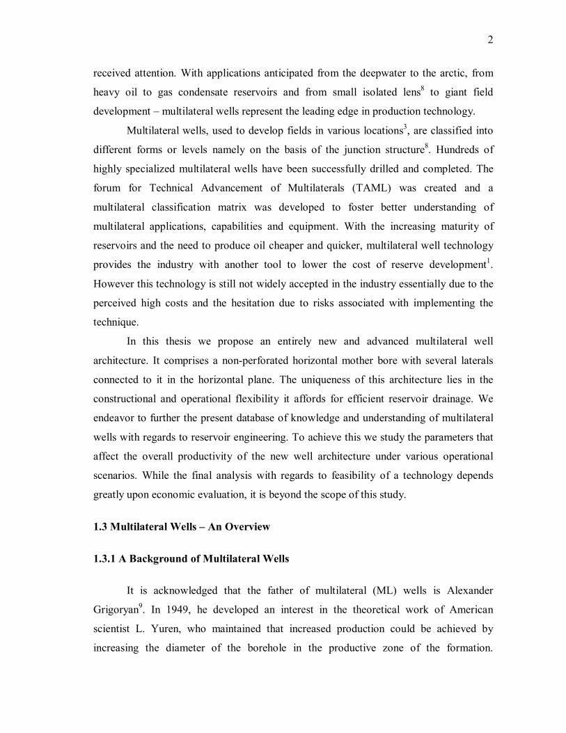
Figure 1.1 – TAML classification of ML wells10
Level 4 - The lateral borehole extends from a cased and cemented mainbore. The junction
is constructed such that a lateral liner is cemented back to the mainbore.
Level 5 - This junction is described as a pressure seal across the junction established by
the completion equipment. Packers and other seals may be used along with dual tubing
strings to obtain a three-way pressure seal.
5
Level 6 - This junction provides for a pressure seal established by the casing itself. It is
typically employed at the bottom of a casing string. After the casing and junction are
cemented into place the laterals are drilled and tied back to the junction with some
cemented lateral liner and hanger assembly.
ML wells with TAML junction levels 1 through 4 have been applied extensively
in the new and maturing reservoirs of all sectors of the North Sea3. A Level 4 ML well
has been successfully used in the Tern field in the North Sea. The Troll Olje field also in
the North Sea is another example where ML technology was found more appropriate than
conventional technologies11. Multilaterals have provided a means to optimize slot usage,
commercially develop lower-quality reserves in the Brent sequence and when applied
with complementary technologies of underbalanced drilling and intelligent well
completions help optimize field development
The economic benefits of ML wells compared to horizontal wells in water-drive
reservoirs in varying permeability fields has been investigated and found to have a better
net present value12. A level 6 junction was used to simulate the performance of ML wells.
Also when OOIP is lower the performance of a multilateral well is better than a
horizontal well. The use of ML technology improved the recovery factor by water
flooding in a mature oil field in Venezuela. The recovery factor, economic viability and
lowest operational activity were achieved for a ML development scheme compared to the
vertical well concept13. Level 4 ML technology in conjunction with intelligent systems
helped improve the recovery at Wytch Farm, UK14. This scheme not only helped to
recover the marginal reserves but also added new production at reduced risk. The
Mukhaizna field, south Oman contains 14-16° API oil in unconsolidated sand15. The
possibility of early water breakthrough posed further technical difficulties in producing
the heavy crude. However the use of dual lateral wells helped make the project a very
attractive investment opportunity.
Also studies have been performed to predict the performance of multilateral wells.
Larsen16 computes the productivity indices or skin values for arbitrary well
configurations in homogeneous reservoirs of constant thickness. Symmetry of the
reservoirs is an important requirement in this computational technique. Other models to
predict ML well performance assume the well to be divided into various segments and

6
computations are performed on each of these segments. Salas17 models the Well Index
factor for ML wells by accounting for competition effects of inflow performance and
interference effects of commingled production of branched wells. A transient model18 for
ML wells is developed that can be applied in commingled reservoirs. The model accounts
for crossflow between layers.
The ML wells applications mentioned above essentially address the various
challenges facing the industry mentioned earlier. The history of the last decade of ML
wells has helped establish the business driver for ML technology19. However inspite the
successful application of ML technology in the oilfield the industry is hesitant to accept
this technology in a big way. This inertia arises from the fact that the behavior of ML
wells is not completely understood and the difficulty to evaluate the potential benefits of
ML technology. The lack of willingness to adapt to it can be ascribed to the following
reasons:
1. Reliability
Despite the high technical and economic success of ML wells they are still
viewed to be associated with a great amount of risk. This perception exists though the
industry wide statistics suggest otherwise.
2. Value
Even the operators most experienced with ML technology are sometimes
hard pressed in identifying and quantifying the true value and return on
investment of these wells. This is partly due to the inability to perform effective
modeling and prediction of well performance and lateral contributions.
1.3.3 The Future
The future of ML wells is in harder-to-drill formations where the reservoirs
require selective completions, selective isolations and stimulation operations. They could
also be used in exploration wells, to mitigate geologic risks and navigate heterogeneous
reservoirs1. The future of the oil and gas business20 lies in unconventional reservoirs like
tight-gas sands, coalbed methane, heavy oil and gas shales. To be able to produce these

7
resources economically improved technology will be in greater demand. Many current
technologies like hydraulic fracturing, steam injection will definitely be applicable along
with improved reservoir characterization methods to reduce risk. But in addition to this
the ability to produce the resources to the surface will need the development of
multibranched well bores. Greater recoveries coupled with economic attractiveness will
definitely help improve the confidence of operators in this nascent technology.

8
CHAPTER II
NEW MULTILATERAL WELL ARCHITECTURE
2.1 Description of the New Multi-lateral Well Architecture
Consider a reservoir or a part of it that has a rectangular cross-section along its
depth. The new multilateral well architecture 21 consists of a horizontal well penetrating
almost the entire length of the reservoir along with branches from the horizontal in the
lateral direction. A vertical well is connected to one end, heel, of the horizontal well and
it acts as the point of vertical lift. The other end of the horizontal is the toe so that the
flow in the horizontal is from toe to heel. Hence there is only one vertical conduit acting
as the production string. The main horizontal section (collector well or mother bore) is
not perforated but contains several pre-prepared junctions. The diameter and completion
type of the vertical and the main horizontal sections are such that they maximize the pipe
flow capacity. The horizontal wellbore and the surrounding reservoir are completely
isolated. Once cemented the vertical and horizontal sections are not readily accessible
with well intervention tools. The junction equipment is placed during the drilling of the
main horizontal well and it is cemented together with the main horizontal section. The
pressure and structural integrity of these junctions is a critical requirement. However
unlike traditional multilateral wells this integrity is not compromised by additional
requirements such as potential capability of future well intervention, formation damage
control during drilling or ability to accept tools in a later phase.
Once the main horizontal well bore is drilled the other laterals are drilled from
one or more locations on the surface. The laterals are drilled in a direction perpendicular
to the main horizontal well. The feeder lateral is connected to the main mother bore at the
pre-prepared junction points. They are completed in a number of ways while focusing on
maximizing the inflow potential without compromising it by additional requirements. For
example relatively slim holes are acceptable as they are less capital intensive, not
prepared to accept tools at a later stage and might be completed open-hole or frac-packed
and hence disposable. Also the time schedule of feeder lateral drilling is very flexible and
can change depending upon further information collected from the field and on market
requirements.
9
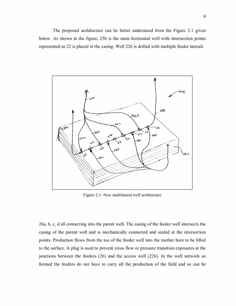
The proposed architecture can be better understood from the Figure 2.1 given
below. As shown in the figure, 25b is the main horizontal well with intersection points
represented as 22 is placed in the casing. Well 226 is drilled with multiple feeder laterals
Figure 2.1- New multilateral well architecture
26a, b, c, d all connecting into the parent well. The casing of the feeder well intersects the
casing of the parent well and is mechanically connected and sealed at the intersection
points. Production flows from the toe of the feeder well into the mother bore to be lifted
to the surface. A plug is used to prevent cross flow or pressure transition exposures at the
junctions between the feeders (26) and the access well (226). In the well network so
formed the feeders do not have to carry all the production of the field and so can be
10
smaller in diameter. The mother bore is a larger well bore so that it can handle the large
flow rates.
The proposed architecture is radically new as the collector well is not used for
lateral drilling or any well intervention in the laterals. Thus the continuity of production
is not jeopardized on account of any event in the laterals. In fact there is a separation of
two functions: one is to collect hydrocarbons from the reservoir as performed by the
laterals and the other is to conduct the hydrocarbons to the point of vertical lift and
ultimately to the surface.
2.2 Advantages of ML Wells
The various advantages of multilateral wells can be summarized as follows:
1. Reduction in well costs. This is due to the need to use fewer top-side and near
surface equipment for a single multilateral well as compared to a group of
conventional wells.
2. Mechanically sealed junctions with full casing integrity eliminate one of the main
failure point as compared to other multilateral designs
3. Improves sweep efficiency by delaying gas or water breakthrough.
4. Facilitates better drainage of heterogeneous reservoir systems.
5. Enhances production for difficult fluids.
6. Reduction of environmental footprint.
7. Increases the reservoir exposure.
8. Better connects the natural reservoir permeability
9. Greater exposure accelerates the production rate.
10. Accelerated production also allows for early production of secondary or marginal
reserves.
11. Reduced overall project costs improving the rate of return.
2.3 Multilateral Well Model
From a reservoir engineering point of view it is difficult to quantify various
advantages of the proposed multilateral well architecture. However it is possible to
investigate quantitatively 21 the productivity of the new well architecture through

11
numerical simulations. To simulate the proposed architecture the well bore structure is
modeled as a main horizontal wellbore fed by many parallel laterals. This structure is
shown in Figure 2.2. The reservoir essentially contains a vertical well bore that conducts
the fluids to the surface. From this vertical, a main horizontal section called mother bore
is drilled to penetrate the entire length of the reservoir in the direction of the largest
horizontal dimension. Now feeder laterals are connected to the mother bore at the pre-
prepared junction points. One lateral is drilled on either side of the mother bore so that
they form a network of alternately placed laterals. The laterals are perpendicular to the
mother bore and are in the direction of the smallest horizontal dimension.
Figure 2.2 – Multilateral well model used for numerical simulations
As shown in the figure depending upon the branch density, we can have all the
laterals drilled or any subset of it. In addition we can drill the laterals reaching the outer
boundary of the drainage volume (100% penetration) or we can assume a smaller
percentage of penetration. In the model the mother bore is not perforated and the feeder
laterals are perforated (or completed open hole) providing communication with the
reservoir. Formation damage in the vicinity of the laterals is neglected. This is because
the feeder laterals are drilled and completed with the requirement of minimum formation
damage made possible by lack of necessity to compromise for well integrity, larger hole
12
diameter, preparing for additional drilling activity, preparing for sophisticated completion
equipment. Also frictional pressure losses in the main horizontal section are neglected
due to its large diameter.
2.4 Methodology and Procedure
The first task in evaluating the performance of the suggested well architecture
would be to identify the types of reservoir applications for which the technology may be
used. From this point of view various parameters affecting the performance of
multilateral wells must be identified and analyzed. In this work we focus on the reservoir
engineering aspects, investigating such issues as the effect of branch density (number of
laterals) and the penetration of laterals (with respect to the lateral dimensions of the
reservoir). The main issue is the overall productivity of the well architecture as a complex
drainage tool.
The primary tool to do such investigations is reservoir simulation. However it is
also important to put the results into perspective, partly by comparing them to more
conventional drainage systems and partly by establishing theoretical limits. Such a
methodology ensures that no false anticipations are generated and a realistic evaluation
can be performed.
The obvious reservoir engineering approach to do this job is to establish a “base
case” and perform parametric studies. We perform simulations using Eclipse – one of the
most widely used reservoir simulators in the industry. The multilateral well model
discussed above forms the basis of these parametric studies. The lateral configurations
are changed as per the investigative needs.
Firstly the performance is investigated in a homogeneous reservoir model. In this
model, we build rectangular reservoir with the architecture proposed above. In all the
models we can have up to 60 laterals producing into the mother bore. Branch density and
penetration of laterals are the two basic parameters that most affect overall productivity.
Assume that a multilateral well must be designed to drain the net pay for a given
reservoir. The very first question that arises is: what should be the number of feeder
laterals drilled? The next issue is: how far should these laterals penetrate into the bulk of
the reservoir. While this decision will depend upon the cost of drilling and completion,

13
various additional factors such as hydrocarbons in place, reservoir structure, driving
mechanism and others will influence the final answer. Hence our strategy is to evaluate
the simplest assumptions through this preliminary analysis and consider the additional
details with particular reservoirs. Along with the homogeneous case we try to incorporate
heterogeneity in the model by using anisotropic reservoirs.
Secondly, representative cases will be set up for field data. Reservoir and fluid
data are used to prepare models wherein a part of the actual field is represented as the
rectangular reservoir we use in the preliminary analysis. The performance of the
multilateral well architecture will be compared with that of conventional vertical wells.
2.5 Technical Indicator
Cumulative production is one of the most important quantities considered while
making a decision about the feasibility of any field development theme. In addition to
cumulative production (in a certain amount of time) one should consider the actual
distribution of production in time. However both cumulative production and its
distribution in time both have only a limited information value, if we cannot compare it to
some ideal drainage structure or an existing well architecture.
The reservoir engineering concept of Productivity Index 22 (PI) is a quantity
which helps to put the various results into perspective. While traditionally this concept is
used mostly for a single well, its generalization is a valuable tool to evaluate complex
well architectures. Also it can be un-dimensionalized in a format that is representative not
only for a given reservoir-fluid system, but for a whole family of them.
Productivity index essentially describes a linear relationship between the
production rate and the driving force. For practical and theoretical purposes we select the
driving force as the drawdown pressure. The drawdown pressure is defined as the average
pressure in the reservoir minus the average pressure along the sink surface (i.e. the
wellbore pressure). The Productivity Index, denoted by J is given by,
wfres ppqJ−
= ……………………………………………………………………….. (2.1)
where resp is the average volumetric pressure in the reservoir and wfp is the wellbore
flowing pressure.
14
The value calculated from equation 1 in general is not constant in the transient
flow regime as J decreases with time. In the stabilized flow regime the PI is constant.
There are three main stabilized flow regimes:
Steady-state
The boundary at the top and bottom are no flow. A constant pressure is assumed
at the outer boundary of the reservoir in the lateral directions. In addition, wfp or the
production rate is kept constant. The steady-state is characterized by a non-changing
pressure distribution in the reservoir.
Pseudo-steady state
Again the boundary condition at the top and bottom are no flow. At the outer
boundary of the reservoir in the lateral directions we assume the same conditions: no flow
across the boundaries. Such an idealization is often called a volumetric reservoir. In
addition we keep constant total production rate. The pseudo-steady state represents the
long-time limiting behavior of the reservoir and is characterized by a constant change in
pressure with time everywhere in the reservoir. This implies that the shape of pressure
distribution in the reservoir is preserved during production though the reservoir is being
depleted at a uniform depletion rate. However such a regime cannot be maintained
forever, because the reservoir is depleted at a constant rate and hence the wellbore
pressure is also decreasing with a constant rate and will ultimately reach a physical limit
of zero pressure.
Boundary-dominated state
Once more the top and bottom boundaries are at no flow condition. At the outer
boundary of the reservoir in the lateral directions we assume no flow condition with a
constant wellbore pressure. The boundary-dominated state is the long-time limiting
behavior of the system and is characterized by a completely different pressure
distribution than the pseudo-steady state pressure distribution. Under boundary-
dominated flow the rate of depletion depends both upon the location as well as the time,
but the rate of change of depletion rate is a function of location only. At any particular

15
instant the depletion rate is such a function of location that the further the location from
the nearest wellbore larger is the depletion rate at that location. Such a flow regime
exhibits a continuously decreasing production rate and a similarly decreasing drawdown.
Though Productivity Index is a valuable technical indicator only factors like oil in
place and profit analysis will essentially determine the optimum Productivity Index to be
used. In practice, however it is observed that the increase in Productivity Index requires
investment but the relation between PI and cost increase is very stochastic in nature.
16
CHAPTER III
ESTIMATION OF THEORETICAL UPPER AND LOWER LIMITS
3.1 Motivation
The need to provide a theoretical framework for the simulation results obtained in
the later part of the research is a major driving force in performing the analytical work
presented in this chapter. A firm theoretical basis is necessary to put numerical results
into perspective and be confident of the results obtained in a new study. The architecture
studied in this thesis is unique and hitherto uninvestigated in the literature. Also the
currently available models to evaluate the productivity of a single ML well comprises
variables and effects that are not applicable in the cases we analyze and hence are not
suited to predict the performance accurately. Some of these variables are those of friction
effect in the flowline and crossflow between layers.
As mentioned earlier the PI is a very effective tool in analyzing well performance
and comparing different reservoir flow systems. Hence the objective of the material
presented in this chapter is to develop back of the envelope methods to obtain theoretical
limits of productivity index attainable by the advanced well architecture design.
3.2 Methodology
We aim to obtain a theoretical upper and lower limit for the productivity of the
proposed well architecture for some particular cases and to do so we use results available
in the literature to model the fluid flow in a ML well.
The concept of infinite fracture conductivity23 is used to establish the maximum
PI obtainable by the ML well architecture. The flow into the laterals penetrating the
smaller horizontal dimension of a reservoir is linear. This is similar to the linear flow into
an infinite conductivity fracture, which extends from the well bore to the lateral reservoir
boundaries in the vertical plane. An infinite conductivity fracture is characterized by
negligible pressure drop in the flow direction and hence represents the greatest
throughput of fluids as per the definition of PI. The flow is both linear as well as
perpendicular to the fracture and the laterals. In order to model the ML well as an infinite
conductivity fracture we assume infinite lateral branch density in the horizontal plane.

17
Since we neglect the frictional pressure drop in the laterals the fluids will be conveyed to
the mother bore instantly without any need to expend fluid energy to overcome resistance
to flow and thus maximize the productivity. We then turn the reservoir with infinite
laterals in the horizontal plane on one of its sides so that the laterals are in a vertical
plane. The maximum or the upper limit of productivity for the infinite laterals is obtained
when the pressure drop in the laterals is negligible and hence they can then be modeled as
an infinite conductivity fracture. We first present a rigorous derivation of the maximum
dimensionless PI ( dJ ) for an infinite conductivity fracture as presented by
Wattenbarger23 et al. This result ( maxdJ ) is then used to obtain the maximum PI for a
reservoir geometry used extensively in this research.
Again to estimate the theoretical lower limit of PI we use the known analytical
result24, which predicts the PI for a reservoir of arbitrary drainage area and shape and
given as,
+
=
srC
ABkhJ
wA2
4ln21
12.141
γµ
..………………………………………………. (3.1)
where,
k = Permeability, md
h = Reservoir depth, ft
B = Oil formation volume factor
µ = Viscosity, cp
A = Drainage Area, ft 2
γ = Euler’s Constant
AC = Dietz shape factor
wr = Well bore radius, ft
s = skin factor
The above equation is essentially derived for a vertical well operating at pseudo-
steady state. As in the case of determining the upper limit, we rotate the reservoir on one
of its sides so that all the laterals are in the vertical plane. With such a rearrangement we

18
can consider each lateral as a unique identity separated from the neighboring laterals in
the reservoir by an imaginary no flow boundary. Then each block containing one lateral
in the vertical plane surrounded by no flow boundaries on all sides can be assumed to
represent a partially penetrating vertical well. Such a rearrangement is shown in Figure
3.1 for a ML well containing 2 laterals in the horizontal plane. Any partially penetrating
well imparts a skin also known as the pseudo-skin factor. Cinco-Ley25 et al. has
published data for the skin effects of partially penetrating wells. The PI for a block
containing a partially penetrating vertical well can be determined using the known values
of Dietz’ shape factor and pseudo-skin as given by Cinco-Ley. We expect, from basic
reservoir engineering principles, that the sum of PI’s for each of the block should be
equal to the theoretical value of the least PI attainable by using the ML well architecture.
However modeling the worst case behavior by introducing a no flow boundary between
the laterals is not very intuitive and obvious.
Figure 3.1 – Rearranged form of a horizontal well architecture

19
3.3 Upper Limit / Maximum Achievable PI
3.3.1 Infinite Conductivity Fracture PI
The PI attainable for an infinite conductivity fracture has been obtained by
Watterbarger et al. In this section we present a rigorous derivation of the result for
pseudo-steady state behavior. As mentioned earlier the flow into an infinite conductivity
fracture is linear. Hence to model this physics of the phenomenon we use the linear
diffusivity equation and obtain its solution for pseudo-steady state which requires a no
flow outer boundary and constant rate inner boundary condition. The linear diffusivity
equation has been presented in fluid flow texts. Consider a hydraulically fractured well in
a rectangular geometry as shown in Figure 3.2. We use the equation as given below in
field units. A rigorous derivation of the result obtained in the literature has been provided
in the appendix.
fx
ey
ex
fx
ey
ex
Figure 3.2 – Infinite conductivity fracture in a rectangular geometry
20
The maximum PI attainable for the case of an infinite fracture is
=
f
e
CR
xy
B
khJ
62.141 πµ
…………………………………………………………… (3.2)
3.3.2 Application to ML Well Architecture
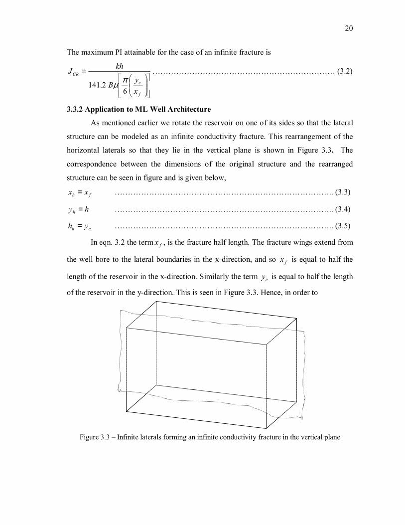
As mentioned earlier we rotate the reservoir on one of its sides so that the lateral
structure can be modeled as an infinite conductivity fracture. This rearrangement of the
horizontal laterals so that they lie in the vertical plane is shown in Figure 3.3. The
correspondence between the dimensions of the original structure and the rearranged
structure can be seen in figure and is given below,
fh xx = ……………………………………………………………………….. (3.3)
hyh = ……………………………………………………………………….. (3.4)
eh yh = ……………………………………………………………………….. (3.5)
In eqn. 3.2 the term fx , is the fracture half length. The fracture wings extend from
the well bore to the lateral boundaries in the x-direction, and so fx is equal to half the
length of the reservoir in the x-direction. Similarly the term ey is equal to half the length
of the reservoir in the y-direction. This is seen in Figure 3.3. Hence, in order to
Figure 3.3 – Infinite laterals forming an infinite conductivity fracture in the vertical plane
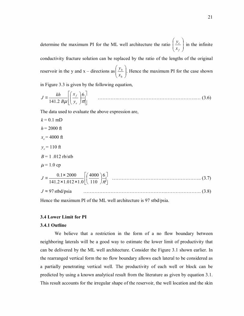
21
determine the maximum PI for the ML well architecture the ratio
f
e
xy
in the infinite
conductivity fracture solution can be replaced by the ratio of the lengths of the original
reservoir in the y and x – directions as
h
h
xy
. Hence the maximum PI for the case shown
in Figure 3.3 is given by the following equation,
=
πµ6
2.141 e
f
yx
BkhJ ………….………………………………………….… (3.6)
The data used to evaluate the above expression are,
k = 0.1 mD
h = 2000 ft
ex = 4000 ft
ey = 110 ft
B = 1 .012 rb/stb
µ = 1.0 cp
×××=
π6
1104000
0.1012.12.14120001.0J ……………………………………………….. (3.7)
stbd/psia 97≈J …………………………………………….…………………. (3.8)
Hence the maximum PI of the ML well architecture is 97 stbd/psia.
3.4 Lower Limit for PI
3.4.1 Outline
We believe that a restriction in the form of a no flow boundary between
neighboring laterals will be a good way to estimate the lower limit of productivity that
can be delivered by the ML well architecture. Consider the Figure 3.1 shown earlier. In
the rearranged vertical form the no flow boundary allows each lateral to be considered as
a partially penetrating vertical well. The productivity of each well or block can be
predicted by using a known analytical result from the literature as given by equation 3.1.
This result accounts for the irregular shape of the reservoir, the well location and the skin

22
due to a partially penetrating well. Reservoir engineering logic suggests that the sum of
the productivity of all the blocks should be equal to the productivity of the ML well
architecture. In fact the estimate by the analytical result should slightly under predict the
ML well productivity as the laterals will normally drain the reservoir more uniformly
than the set of partially penetrating vertical wells. However from the results shown in the
next section we see that the present analytical tool is inadequate to predict the
performance of ML wells as they more often than not tend to over-predict the PI in most
cases analyzed.
Ideally the analytical result should be compared with the numerical solution of
productivity for the reservoir geometry used. The reservoir considered is 4000 × 2000 ×
110 feet in the x, y and z directions respectively. Rearrangement of the reservoir causes
re-orientation of the dimensions in the y and z directions with the dimensions in the 3 co-
ordinate directions now being 4000 × 110 × 2000 feet. Data for pseudo-skin and Dietz
shape factor are not available for this geometry and hence we adopt a two step approach
to investigate the ability of the current analytic tool to predict performance.
3.4.2 Step 1 - Numerical Analysis of Actual ML Well with Single Block Productivity
The first step is essentially a validation of the reservoir engineering principle that
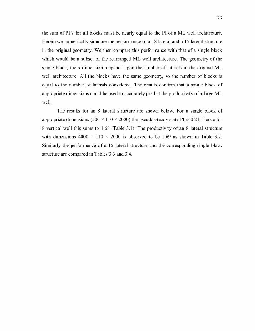
23
the sum of PI’s for all blocks must be nearly equal to the PI of a ML well architecture.
Herein we numerically simulate the performance of an 8 lateral and a 15 lateral structure
in the original geometry. We then compare this performance with that of a single block
which would be a subset of the rearranged ML well architecture. The geometry of the
single block, the x-dimension, depends upon the number of laterals in the original ML
well architecture. All the blocks have the same geometry, so the number of blocks is
equal to the number of laterals considered. The results confirm that a single block of
appropriate dimensions could be used to accurately predict the productivity of a large ML
well.
The results for an 8 lateral structure are shown below. For a single block of
appropriate dimensions (500 × 110 × 2000) the pseudo-steady state PI is 0.21. Hence for
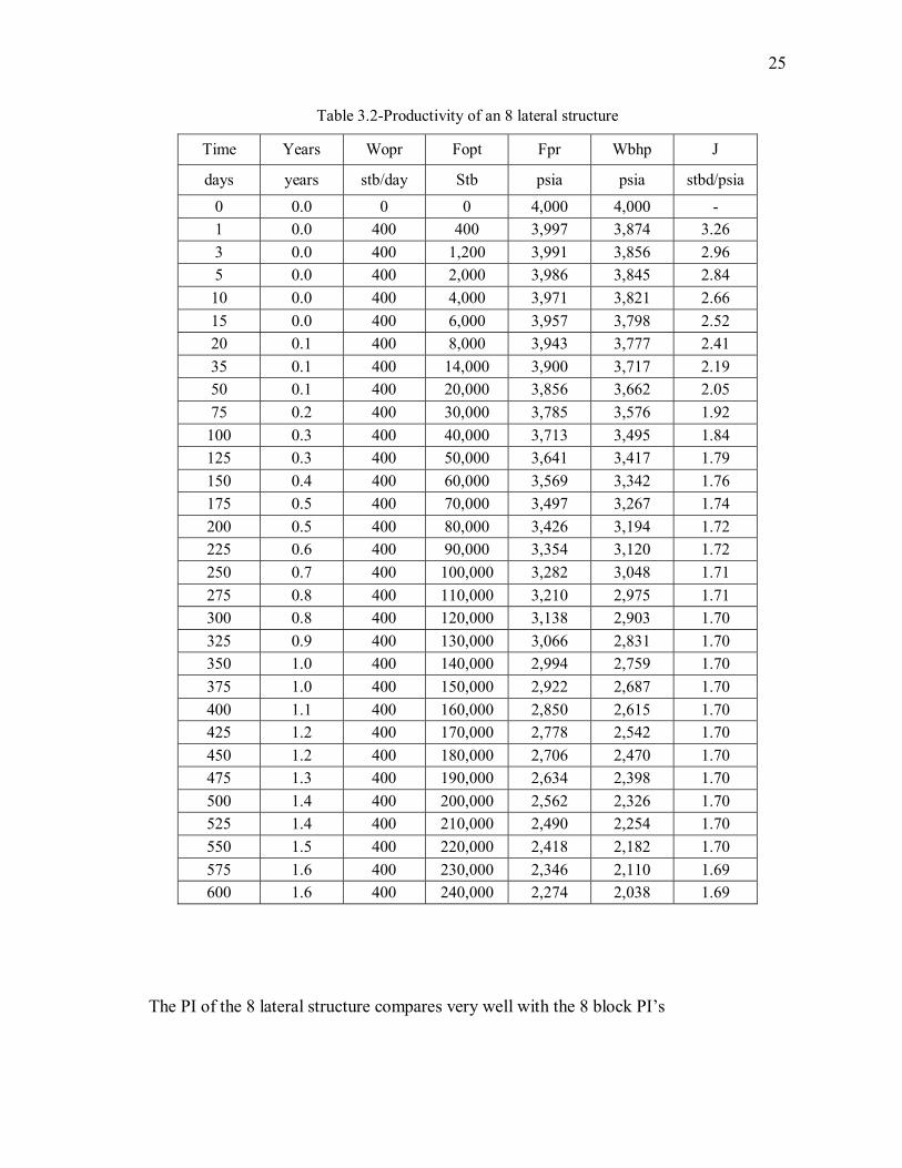
8 vertical well this sums to 1.68 (Table 3.1). The productivity of an 8 lateral structure
with dimensions 4000 × 110 × 2000 is observed to be 1.69 as shown in Table 3.2.
Similarly the performance of a 15 lateral structure and the corresponding single block
structure are compared in Tables 3.3 and 3.4.
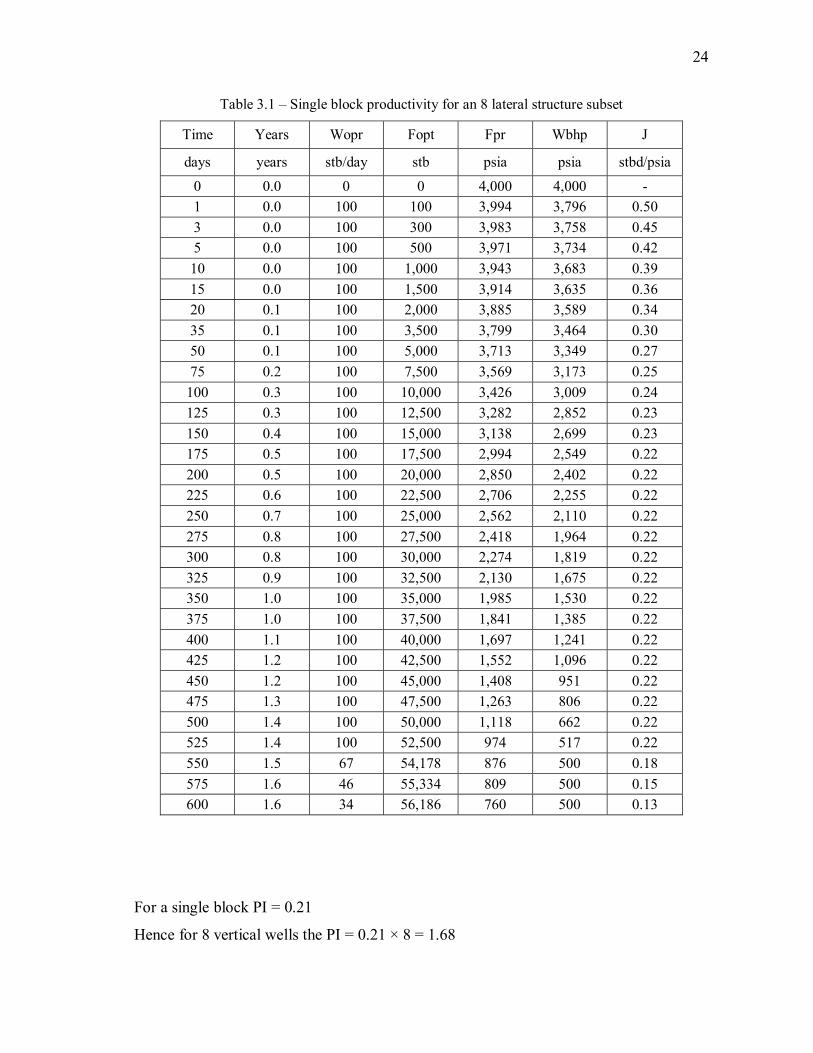
24
Table 3.1 – Single block productivity for an 8 lateral structure subset
Time Years Wopr Fopt Fpr Wbhp J
days years stb/day stb psia psia stbd/psia
0 0.0 0 0 4,000 4,000 - 1 0.0 100 100 3,994 3,796 0.50 3 0.0 100 300 3,983 3,758 0.45 5 0.0 100 500 3,971 3,734 0.42 10 0.0 100 1,000 3,943 3,683 0.39 15 0.0 100 1,500 3,914 3,635 0.36 20 0.1 100 2,000 3,885 3,589 0.34 35 0.1 100 3,500 3,799 3,464 0.30 50 0.1 100 5,000 3,713 3,349 0.27 75 0.2 100 7,500 3,569 3,173 0.25
100 0.3 100 10,000 3,426 3,009 0.24 125 0.3 100 12,500 3,282 2,852 0.23 150 0.4 100 15,000 3,138 2,699 0.23 175 0.5 100 17,500 2,994 2,549 0.22 200 0.5 100 20,000 2,850 2,402 0.22 225 0.6 100 22,500 2,706 2,255 0.22 250 0.7 100 25,000 2,562 2,110 0.22 275 0.8 100 27,500 2,418 1,964 0.22 300 0.8 100 30,000 2,274 1,819 0.22 325 0.9 100 32,500 2,130 1,675 0.22 350 1.0 100 35,000 1,985 1,530 0.22 375 1.0 100 37,500 1,841 1,385 0.22 400 1.1 100 40,000 1,697 1,241 0.22 425 1.2 100 42,500 1,552 1,096 0.22 450 1.2 100 45,000 1,408 951 0.22 475 1.3 100 47,500 1,263 806 0.22 500 1.4 100 50,000 1,118 662 0.22 525 1.4 100 52,500 974 517 0.22 550 1.5 67 54,178 876 500 0.18 575 1.6 46 55,334 809 500 0.15 600 1.6 34 56,186 760 500 0.13
For a single block PI = 0.21
Hence for 8 vertical wells the PI = 0.21 × 8 = 1.68
25
Table 3.2-Productivity of an 8 lateral structure
Time Years Wopr Fopt Fpr Wbhp J
days years stb/day Stb psia psia stbd/psia
0 0.0 0 0 4,000 4,000 - 1 0.0 400 400 3,997 3,874 3.26 3 0.0 400 1,200 3,991 3,856 2.96 5 0.0 400 2,000 3,986 3,845 2.84 10 0.0 400 4,000 3,971 3,821 2.66 15 0.0 400 6,000 3,957 3,798 2.52 20 0.1 400 8,000 3,943 3,777 2.41 35 0.1 400 14,000 3,900 3,717 2.19 50 0.1 400 20,000 3,856 3,662 2.05 75 0.2 400 30,000 3,785 3,576 1.92
100 0.3 400 40,000 3,713 3,495 1.84 125 0.3 400 50,000 3,641 3,417 1.79 150 0.4 400 60,000 3,569 3,342 1.76 175 0.5 400 70,000 3,497 3,267 1.74 200 0.5 400 80,000 3,426 3,194 1.72 225 0.6 400 90,000 3,354 3,120 1.72 250 0.7 400 100,000 3,282 3,048 1.71 275 0.8 400 110,000 3,210 2,975 1.71 300 0.8 400 120,000 3,138 2,903 1.70 325 0.9 400 130,000 3,066 2,831 1.70 350 1.0 400 140,000 2,994 2,759 1.70 375 1.0 400 150,000 2,922 2,687 1.70 400 1.1 400 160,000 2,850 2,615 1.70 425 1.2 400 170,000 2,778 2,542 1.70 450 1.2 400 180,000 2,706 2,470 1.70 475 1.3 400 190,000 2,634 2,398 1.70 500 1.4 400 200,000 2,562 2,326 1.70 525 1.4 400 210,000 2,490 2,254 1.70 550 1.5 400 220,000 2,418 2,182 1.70 575 1.6 400 230,000 2,346 2,110 1.69 600 1.6 400 240,000 2,274 2,038 1.69
The PI of the 8 lateral structure compares very well with the 8 block PI’s

26
Table 3.3 – Single block productivity of a 15 lateral subset
Time Years Wopr Fopt Fpr Wbhp J
days years stb/day stb psia psia stbd/pspia
0 0.0 0 0 4,000 4,000 1 0.0 50 50 3,995 3,876 0.42 3 0.0 50 150 3,984 3,850 0.37 5 0.0 50 250 3,973 3,829 0.35 10 0.0 50 500 3,946 3,782 0.30 15 0.0 50 750 3,919 3,737 0.27 20 0.1 50 1,000 3,892 3,694 0.25 35 0.1 50 1,750 3,812 3,578 0.21 50 0.1 50 2,500 3,731 3,471 0.19 75 0.2 50 3,750 3,596 3,309 0.17
100 0.3 50 5,000 3,462 3,157 0.16 125 0.3 50 6,250 3,327 3,011 0.16 150 0.4 50 7,500 3,192 2,870 0.16 175 0.5 50 8,750 3,057 2,730 0.15 200 0.5 50 10,000 2,922 2,593 0.15 225 0.6 50 11,250 2,787 2,456 0.15 250 0.7 50 12,500 2,652 2,320 0.15 275 0.8 50 13,750 2,517 2,184 0.15 300 0.8 50 15,000 2,382 2,048 0.15 325 0.9 50 16,250 2,247 1,913 0.15 350 1.0 50 17,500 2,112 1,777 0.15 375 1.0 50 18,750 1,976 1,642 0.15 400 1.1 50 20,000 1,841 1,506 0.15 425 1.2 50 21,250 1,706 1,371 0.15 450 1.2 50 22,500 1,570 1,235 0.15 475 1.3 50 23,750 1,435 1,100 0.15 500 1.4 50 25,000 1,299 964 0.15 525 1.4 50 26,250 1,164 828 0.15 550 1.5 50 27,500 1,028 693 0.15 575 1.6 50 28,750 892 557 0.15 600 1.6 36 29,649 795 500 0.12
Hence the productivity of 15 blocks = 0.15 × 15 = 2.25
27
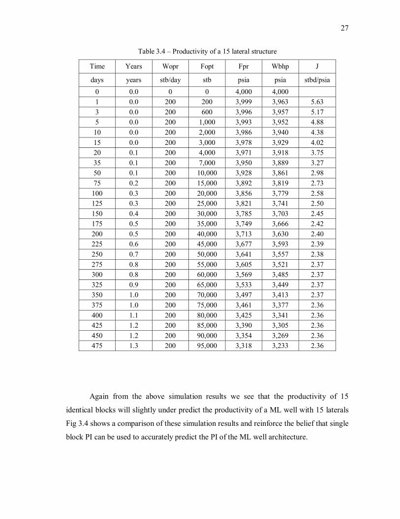
Table 3.4 – Productivity of a 15 lateral structure
Time Years Wopr Fopt Fpr Wbhp J
days years stb/day stb psia psia stbd/psia
0 0.0 0 0 4,000 4,000 1 0.0 200 200 3,999 3,963 5.63 3 0.0 200 600 3,996 3,957 5.17 5 0.0 200 1,000 3,993 3,952 4.88 10 0.0 200 2,000 3,986 3,940 4.38 15 0.0 200 3,000 3,978 3,929 4.02 20 0.1 200 4,000 3,971 3,918 3.75 35 0.1 200 7,000 3,950 3,889 3.27 50 0.1 200 10,000 3,928 3,861 2.98 75 0.2 200 15,000 3,892 3,819 2.73
100 0.3 200 20,000 3,856 3,779 2.58 125 0.3 200 25,000 3,821 3,741 2.50 150 0.4 200 30,000 3,785 3,703 2.45 175 0.5 200 35,000 3,749 3,666 2.42 200 0.5 200 40,000 3,713 3,630 2.40 225 0.6 200 45,000 3,677 3,593 2.39 250 0.7 200 50,000 3,641 3,557 2.38 275 0.8 200 55,000 3,605 3,521 2.37 300 0.8 200 60,000 3,569 3,485 2.37 325 0.9 200 65,000 3,533 3,449 2.37 350 1.0 200 70,000 3,497 3,413 2.37 375 1.0 200 75,000 3,461 3,377 2.36 400 1.1 200 80,000 3,425 3,341 2.36 425 1.2 200 85,000 3,390 3,305 2.36 450 1.2 200 90,000 3,354 3,269 2.36 475 1.3 200 95,000 3,318 3,233 2.36
Again from the above simulation results we see that the productivity of 15
identical blocks will slightly under predict the productivity of a ML well with 15 laterals
Fig 3.4 shows a comparison of these simulation results and reinforce the belief that single
block PI can be used to accurately predict the PI of the ML well architecture.

28
1.20
1.40
1.60
1.80
2.00
2.20
2.40
2.60
4 6 8 10 12 14 16
No of Blocks / Laterals
PI, s
tbd/
psi
8 blocks 8 laterals 15 blocks 15 laterals
Figure 3.4 – Comparison of single block performance with the corresponding ML well structure
3.4.3 Step 2 – Analysis of Analytic and Numeric Solution for Well-Defined
Geometry
In the second step the idea is to use the pseudo-skin and shape factor data
published in the literature to evaluate the PI of a single block and compare it to the
numerical solution of similar geometry containing a partially penetrating well. By doing
so we can observe the results and comment whether the current tools are good enough to
accurately predict the performance of a block which in turn predicts ML well
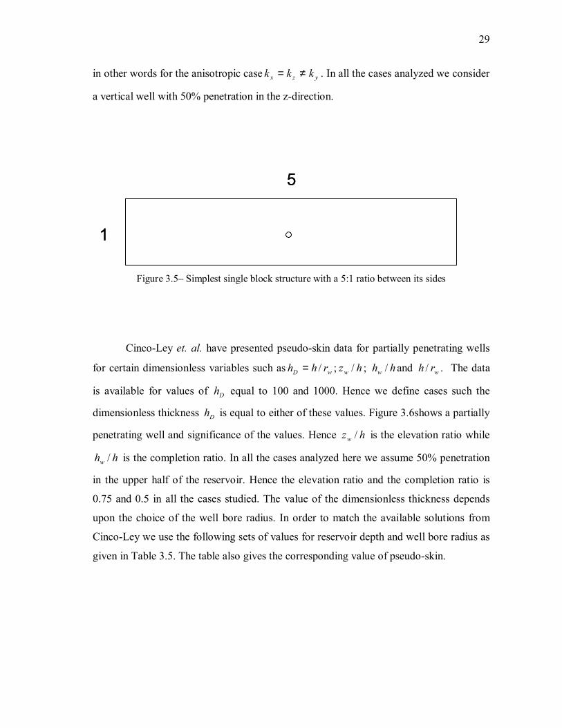
performance. Dietz shape factor 24 is available for an aspect ratio of 1:5 with the well in
the center. This geometry shown in Figure 3.5comes closest to the single block geometry
of an 8 lateral structure subset and hence we choose this ratio for our computations. The
dimensions used in the x and y directions are 500 ×100 feet with varying depths. We also
perform the comparison of analytic and numeric solutions for the isotropic and
anisotropic case. The anisotropy exits in the horizontal plane in the rearranged structure,
29
in other words for the anisotropic case yzx kkk ≠= . In all the cases analyzed we consider
a vertical well with 50% penetration in the z-direction.
5
1
5
1
Figure 3.5– Simplest single block structure with a 5:1 ratio between its sides
Cinco-Ley et. al. have presented pseudo-skin data for partially penetrating wells
for certain dimensionless variables such as wD rhh /= ; hzw / ; hhw / and wrh / . The data
is available for values of Dh equal to 100 and 1000. Hence we define cases such the
dimensionless thickness Dh is equal to either of these values. Figure 3.6shows a partially
penetrating well and significance of the values. Hence hzw / is the elevation ratio while
hhw / is the completion ratio. In all the cases analyzed here we assume 50% penetration
in the upper half of the reservoir. Hence the elevation ratio and the completion ratio is
0.75 and 0.5 in all the cases studied. The value of the dimensionless thickness depends
upon the choice of the well bore radius. In order to match the available solutions from
Cinco-Ley we use the following sets of values for reservoir depth and well bore radius as
given in Table 3.5. The table also gives the corresponding value of pseudo-skin.

30
wz
wr
wh
wh = Completion Thickness
wz = Elevation
wz
wr
wh
wz
wr
wh
wh = Completion Thickness
wz = Elevation
wh = Completion Thickness
wz = Elevation Figure 3.6– Partially penetrating vertical well
Table 3.5 – Dimensionless height for Cinco pseudo-skin data
Depth, ft Well bore Radius, ft Dh Skin, S
50 0.5 100 3.067
500 0.5 1000 5.467
1000 1 1000 5.467
1500 1.5 1000 5.467

31
Consider the first case when the depth is equal to 50 ft. The dimensions of the
block are 500 × 100 × 50 in the three co-ordinate directions. As in all the other cases the
drainage area to be used for the analytic solution is 500 × 100. For this drainage area with
the well in the center the Dietz shape factor is 2.36. For a given depth corresponding
values of well bore radius and skin are used. The equation used is,
+
=
srC
ABkhJ
wA2
4ln21
12.141
γµ
………………………………………………... (3.1)
Depending upon the permeability distribution in the reservoir the value of k will change
for a isotropic and anisotropic reservoir. For the rearranged structure the permeability
anisotropy exists in the x-y plane i.e. in the horizontal plane. For the purpose of this
calculation we have used yx kkk = in anisotropic cases. For the isotropic case we
assume the permeability to be equal to 1 in all directions.
Hence for a given reservoir configuration we have solutions for the isotropic as
well as the anisotropic case. A comparison of the analytic and numeric results is shown in
Table 3.6 for the isotropic case and Table 3.7 for the anisotropic case. These results are
then plotted to in Figure 3.7and Figure 3.8 to show the deviation in the results with
increasing depths.
32
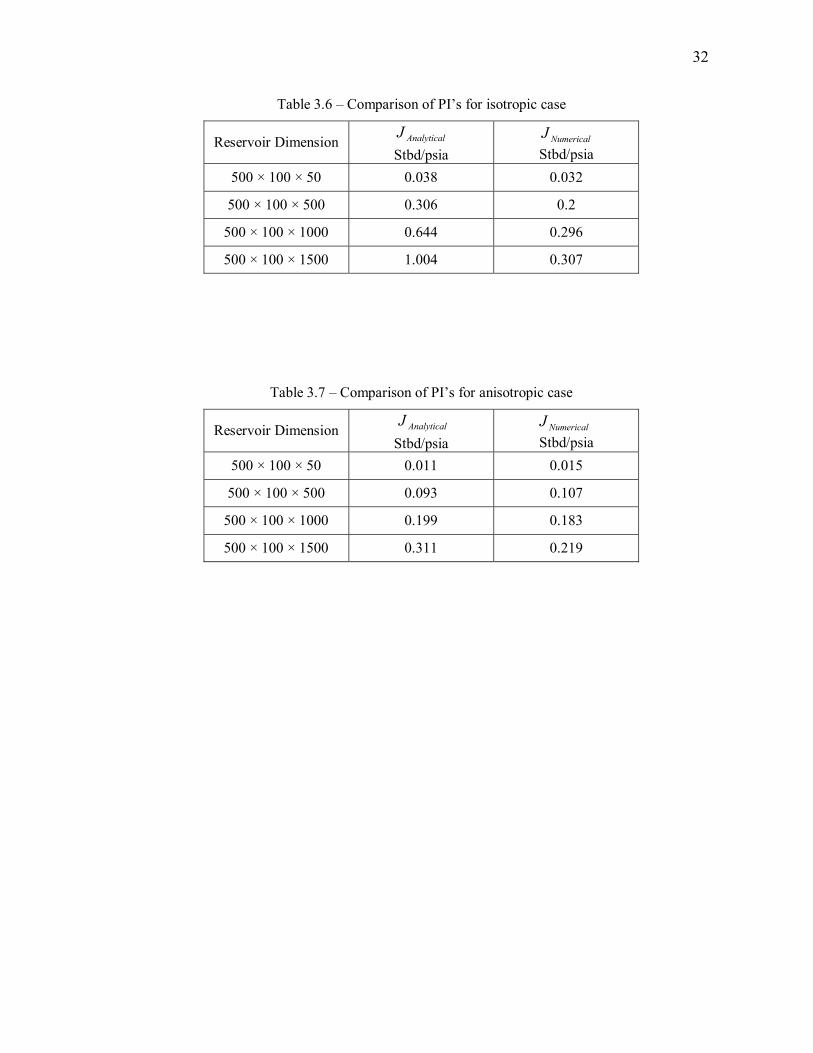
Table 3.6 – Comparison of PI’s for isotropic case
Reservoir Dimension AnalyticalJ Stbd/psia
NumericalJ Stbd/psia
500 × 100 × 50 0.038 0.032
500 × 100 × 500 0.306 0.2
500 × 100 × 1000 0.644 0.296
500 × 100 × 1500 1.004 0.307
Table 3.7 – Comparison of PI’s for anisotropic case
Reservoir Dimension AnalyticalJ Stbd/psia
NumericalJ Stbd/psia
500 × 100 × 50 0.011 0.015
500 × 100 × 500 0.093 0.107
500 × 100 × 1000 0.199 0.183
500 × 100 × 1500 0.311 0.219

33
Isotropic Case
0
500
1000
1500
2000
0 0.2 0.4 0.6 0.8 1 1.2
PI, stbd/psia
Dep
th, f
t
Analytical Numerical
Figure 3.7 – Comparison of results for isotropic case

34
Anisotropic
0
500
1000
1500
2000
0 0.05 0.1 0.15 0.2 0.25 0.3 0.35
PI, Stbd/psia
Dep
th, f
t
Analytical Numerical
Figure 3.8 – Comparison of results for anisotropic case

35
3.4.4 Discussion of Results
From the results we can clearly see that the present analytical tool is not very
effective in accurately predicting the productivity of a block containing a partially
penetrating well. The analytical solution compares reasonable well with the numerical
results at low depths. But at greater depths the analytical and numerical solutions diverge
for both the isotropic and anisotropic case.
36
CHAPTER IV
PRELIMINARY ANALYSIS OF PROPOSED ARCHITECTURE FOR
SYNTHETIC CASES
4.1 Parameters to be Analyzed
In this chapter we simulate synthetic cases to study the effect of various
parameters on the performance of ML wells. A base case is set up containing a ML well
architecture described earlier. Single phase flow of dry oil, which contains no dissolved
gases, is considered in this parametric analysis. The parameters we wish to investigate are
essentially related to the design of the architecture and primary reservoir properties that
affect the flow of the fluids in the reservoir.
Branch Density & Extent of Penetration – The cost of a ML well will depend
greatly upon the number of laterals to be drilled and extent of their penetration into the
bulk of the reservoir. Drilling any more laterals than absolutely necessary puts greater
burden on the cash flow. On the other hand fewer laterals might not utilize the full
benefits of the larger reservoir exposure offered by ML wells. It is expected that initially
adding a lateral to the structure will continuously add production but after a certain extent
the addition of each extra lateral will not significantly add to the total production. In such
a case the excess laterals become redundant. Also it might be beneficial to drill the
laterals only to a certain extent into the reservoir rather than all the way to the lateral
boundary. We wish to address such issues through this analysis. The aim in designing the
architecture is to drill an optimum number of laterals with an optimum penetration extent
so that the benefit to cost ratio of the well, which is nothing but the stock tank barrels of
oil produced per dollar spent, is maximized. Hence we choose branch density and
penetration extent as the investigative parameters at the outset.
Permeability Variations – The flow into the laterals will be normally linear and
perpendicular. The laterals are considered to be only in the horizontal direction and hence
the permeability in the z direction plays an important role in the inflow to the laterals. We
compare the effect of permeability variation for a given lateral structure.
37
4.2 Reservoir Geometry and Properties
A homogeneous rectangular reservoir is simulated. The dimensions of the
reservoir in the 3 co-ordinate directions are 2000 × 4000 × 110 respectively. The mother
bore is placed at the middle of the reservoir in the z-direction. While the laterals form an
alternating mesh of perforated slim holes connected to the mother bore. The base case
analyzed is anisotropic, so that the permeability in the horizontal and vertical direction is
not the same. A 21 × 62 × 11 grid is used. The other important input properties are shown
in the Table 4.1 below.
Table 4.1 – Base case reservoir properties
4.3 Simulation Cases
To analyze density effects of laterals we simulate a 60, 30, 15 and a 4 – lateral
structure for complete penetration from the mother bore to the lateral boundary. This is
followed by simulation for the lateral partial penetration assuming they penetrate out to
Grid Size 21 × 62 × 11
Reservoir Size 2000 × 4000 × 110
Permeability (mD) Anisotropic
yx kk = 1.00
zk 0.10
Porosity 0.3

38
an extent of 45% and 75% of lateral dimension. Finally to observe permeability effects
we simulate the base case assuming isotropic permeability in the reservoir.
4.4 Simulation Results
4.4.1 Branch Density and Partial Penetration Effects
A summary of some key results for branch density effects is given in Table 4.2.
From the table we see that the cumulative production for a structure with 60 laterals is
0.5520 MMSTB, while the cumulative production from a 4 - lateral structure is 0.5505
MMSTB. The difference of about 1500 STB indicates that the same reservoir can be
depleted to nearly the same extent by using much fewer laterals. In other words after a
certain number increasing the number of laterals does not increase the cumulative
production by a large amount. The only noticeable difference between using a very high
number of laterals as compared to using an optimum is in the time required to attain a
certain amount of cumulative production. For example the time to obtain 550,000 STB of
cumulative production from a 60 and a 4 lateral structure would be 287 days and 1000
days respectively.
In all the runs mentioned above the bottom hole flowing pressure was allowed to
fall to 14.7 psia. These cases were simulated again, but this time the bottom hole flowing
pressure is set to not decrease below 1000 psia. The corresponding results are tabulated in
Table 2 - B. Again the difference in cumulative for 60 and 4 laterals is very small and the
basic difference is in the time distribution of the production. The results of the simulation
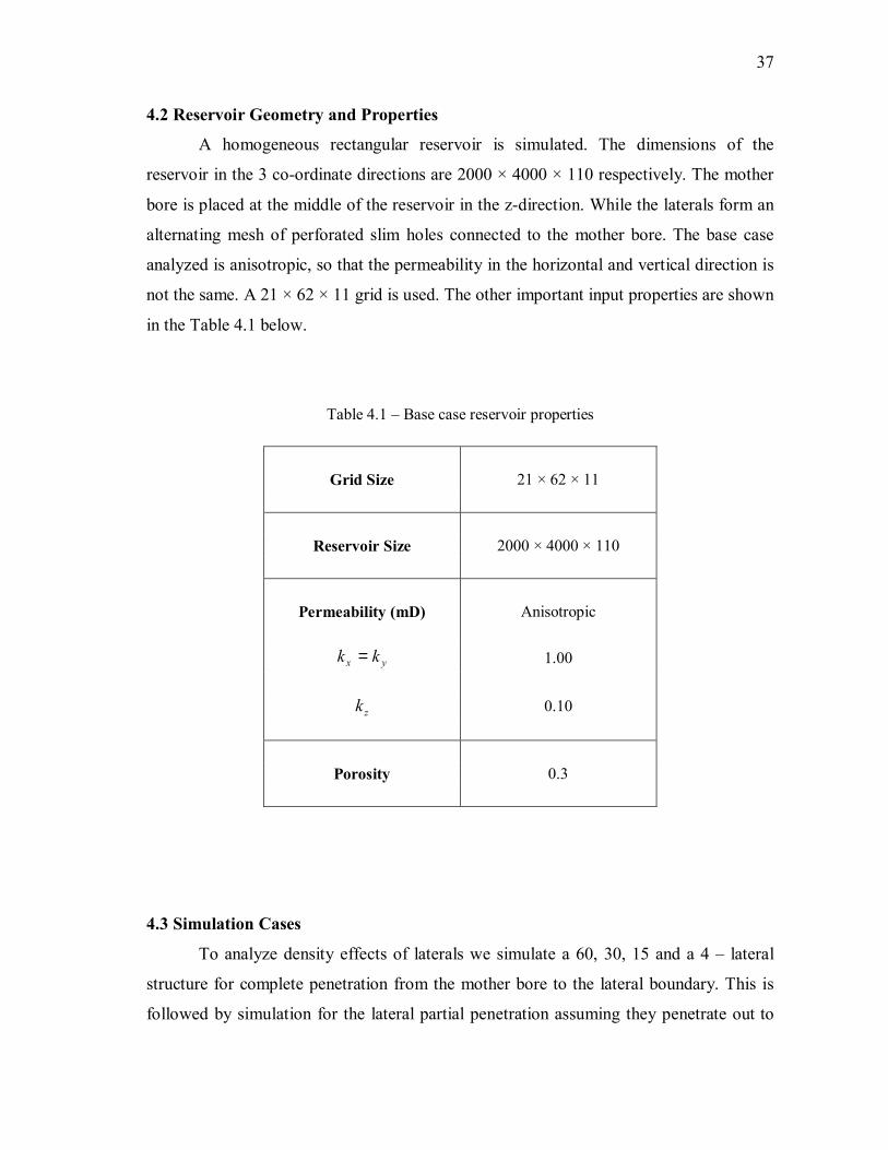
for the effect of density are shown in Tables 4.3 – 4.6. Figure 4.1 shows a variation in
bottomhole pressure with the number of laterals.
39
0
200
400
600
800
1000
1200
0 10 20 30 40 50 60 70
Number of Laterals
Bot
tom
hole
Pre
ssur
e, p
si
Figure 4.1 – A much lower bottomhole pressure is needed when using fewer laterals, increasing
the possibility of borehole collapse, sand production, water coning.
40
Table 4.2 - Summary of simulation results
Well Structure Cum Prod. Field Pressure BHP
(No. of Laterals) stb psia psia
[A] Base Case Runs
60 552,030 18 0
30 552,048 18 14.7
15 552,041 18 14.7 4 550,539 29 14.7
[B] Base Case Runs (BHP = 1000 PSIA)
60 416,055 1,003 0
30 416,049 1,003 0 4 414,971 1,011 1,000

41
Table 4.3 – Productivity of a 60 lateral structure
Time Years Wopr Fopt Fpr Wbhp J
days years stb/day stb psia psia stbd/psia
0.0 0.0 0.0 0.0 4000.0 4000.0 - 1.0 0.0 3818.2 3818.2 3972.5 3838.6 28.5 3.0 0.0 3818.2 11454.5 3917.8 3774.7 26.7 5.0 0.0 3818.2 19090.9 3863.0 3718.9 26.5
10.0 0.0 3818.2 38181.8 3726.1 3581.7 26.4 15.0 0.0 3818.2 57272.7 3589.1 3444.6 26.4 20.0 0.1 3818.2 76363.6 3452.0 3307.4 26.4 35.0 0.1 3818.2 133636.3 3040.4 2895.7 26.4 50.0 0.1 3818.2 190909.0 2628.3 2483.4 26.3 75.0 0.2 3818.2 286363.5 1940.4 1795.2 26.3 100.0 0.3 3818.2 381818.0 1251.1 1105.6 26.2 150.0 0.4 3086.5 536140.8 133.4 14.7 - 200.0 0.5 287.5 550515.1 29.1 14.7 - 300.0 0.8 14.4 551952.1 18.6 14.7 - 400.0 1.1 0.7 552024.4 18.1 14.7 - 500.0 1.4 0.1 552029.8 18.1 14.7 - 600.0 1.6 0.0 552030.1 18.1 14.7 - 700.0 1.9 0.0 552030.1 18.1 0.0 - 800.0 2.2 0.0 552030.1 18.1 0.0 - 900.0 2.5 0.0 552030.1 18.1 0.0 -
1000.0 2.7 0.0 552030.1 18.1 0.0 -
42
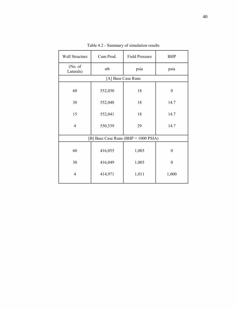
Table 4.4 – Productivity of a 30 lateral structure
Time Years Wopr Fopt Fpr Wbhp J
days years stb/day stb psia Psia stbd/psia
0 0.0 0.0 0 4,000.0 4,000.0 - 1 0.0 3,818.2 3,818 3,972.6 3,706.7 14.4 3 0.0 3,818.2 11,455 3,917.9 3,634.5 13.5 5 0.0 3,818.2 19,091 3,863.1 3,576.9 13.3 10 0.0 3,818.2 38,182 3,726.2 3,438.7 13.3 15 0.0 3,818.2 57,273 3,589.2 3,301.0 13.3 20 0.1 3,818.2 76,364 3,452.1 3,163.6 13.2 35 0.1 3,818.2 133,636 3,040.5 2,751.4 13.2 50 0.1 3,818.2 190,909 2,628.4 2,338.8 13.2 75 0.2 3,818.2 286,364 1,940.5 1,650.2 13.2
100 0.3 3,818.2 381,818 1,251.2 960.3 13.1 150 0.4 2,817.5 522,695 231.1 14.7 - 200 0.5 484.3 546,911 55.4 14.7 - 300 0.8 46.4 551,549 21.7 14.7 - 400 1.1 4.5 551,996 18.5 14.7 - 500 1.4 0.5 552,042 18.1 14.7 - 600 1.6 0.0 552,047 18.1 14.7 - 700 1.9 0.0 552,048 18.1 14.7 - 800 2.2 0.0 552,048 18.1 14.7 - 900 2.5 0.0 552,048 18.1 14.7 - 1000 2.7 0.0 552,048 18.1 14.7 -
43
Table 4.5 - Productivity of a 15 lateral structure
Time Years Wopr Fopt Fpr Wbhp J
days years stb/day stb psia psia stbd/psia
0 0.0 0.0 0 4,000.0 4,000.0 - 1 0.0 3,818.2 3,818 3,972.9 3,295.8 5.6 3 0.0 3,818.2 11,455 3,918.2 3,166.5 5.1 5 0.0 3,818.2 19,091 3,863.4 3,092.1 5.0 10 0.0 3,818.2 38,182 3,726.5 2,942.4 4.9 15 0.0 3,818.2 57,273 3,589.5 2,799.8 4.8 20 0.1 3,818.2 76,364 3,452.4 2,659.5 4.8 35 0.1 3,818.2 133,636 3,040.9 2,242.6 4.8 50 0.1 3,818.2 190,909 2,628.8 1,826.9 4.8 75 0.2 3,818.2 286,364 1,940.8 1,135.2 4.7
100 0.3 3,818.2 381,818 1,251.4 443.0 4.7 150 0.4 2,141.5 488,894 476.3 14.7 - 200 0.5 788.0 528,292 190.5 14.7 - 300 0.8 181.7 546,464 58.6 14.7 - 400 1.1 42.5 550,715 27.7 14.7 - 500 1.4 10.1 551,722 20.4 14.7 - 600 1.6 2.4 551,964 18.7 14.7 - 700 1.9 0.6 552,022 18.2 14.7 - 800 2.2 0.1 552,036 18.1 14.7 - 900 2.5 0.0 552,040 18.1 14.7 - 1000 2.7 0.0 552,041 18.1 14.7 -

44
Table 4.6 - Productivity of a 4 lateral structure
Time Years Wopr Fopt Fpr Wbhp J
days years stb/day stb psia psia stbd/psia
0 0.0 0.0 0 4,000.0 4,000.0 - 1 0.0 3,818.2 3,818 3,973.5 2,341.4 2.3 3 0.0 3,818.2 11,455 3,918.9 1,993.4 2.0 5 0.0 3,818.2 19,091 3,864.2 1,817.9 1.9 10 0.0 3,818.2 38,182 3,727.3 1,528.4 1.7 15 0.0 3,818.2 57,273 3,590.4 1,285.4 1.7 20 0.1 3,818.2 76,364 3,453.3 1,064.4 1.6 35 0.1 3,818.2 133,636 3,041.5 477.6 1.5 50 0.1 3,701.5 189,159 2,641.8 14.7 - 75 0.2 2,701.4 256,694 2,154.9 14.7 -
100 0.3 2,072.3 308,502 1,781.0 14.7 - 150 0.4 1,385.1 377,756 1,280.7 14.7 - 200 0.5 965.2 426,017 931.6 14.7 - 300 0.8 539.3 479,945 541.1 14.7 - 400 1.1 306.9 510,631 318.6 14.7 - 500 1.4 175.9 528,219 191.1 14.7 - 600 1.6 101.1 538,329 117.7 14.7 - 700 1.9 58.2 544,147 75.4 14.7 - 800 2.2 33.5 547,498 51.1 14.7 - 900 2.5 19.3 549,427 37.1 14.7 - 1000 2.7 11.1 550,539 29.1 14.7 -
Further results for partial penetration of laterals are shown in Tables 4.7 – 4.9. Here we
compare partial penetration effects using 2 to 30 - laterals. A comparison of results
shows that using 4 laterals produces just as well as 30 - laterals. However a comparison
of production from 4 and 2 - laterals indicates a significant difference in cumulative
production. This is observed even when the 4 - lateral structure penetrated to only 45%
while the 2 lateral structure penetrated to about 73%. Also the time taken to produce the
same amount of reservoir fluids is much less for the 4 – laterals case with 45%
penetration thus increasing the economy of operation.

45
Table 4.7- Productivity of a 30 lateral structure with 45% penetration
Time Years Wopr Fopt Fpr Wbhp J
days years stb/day stb psia psia stbd/psia
0 0.0 0.0 0 4,000 4,000 - 1 0.0 3,818.2 3,818 3,972 3,302 5.7 4 0.0 3,818.2 15,273 3,890 3,106 4.9 13 0.0 3,818.2 49,636 3,643 2,724 4.2 25 0.1 3,818.2 95,455 3,314 2,302 3.8 50 0.1 3,818.2 190,909 2,627 1,546 3.5 75 0.2 3,430.8 276,680 2,009 1,000 3.4
100 0.3 2,003.1 326,756 1,647 1,000 3.1 200 0.5 340.8 399,892 1,119 1,000 2.9 300 0.8 61.7 412,979 1,024 1,000 2.5 305 0.8 55.7 413,257 1,022 1,000 2.5 310 0.8 50.3 413,509 1,020 1,000 2.5 315 0.9 45.5 413,736 1,018 1,000 2.4 320 0.9 41.1 413,942 1,017 1,000 2.4 325 0.9 37.1 414,128 1,016 1,000 2.3
337.5 0.9 29.4 414,496 1,013 1,000 2.2 350 1.0 23.2 414,785 1,011 1,000 2.1 400 1.1 9.9 415,410 1,006 1,000 1.5 500 1.4 1.8 415,786 1,004 1,000 - 600 1.6 0.3 415,853 1,003 1,000 - 700 1.9 0.1 415,865 1,003 1,000 - 800 2.2 0.0 415,867 1,003 1,000 - 900 2.5 0.0 415,867 1,003 1,000 - 1000 2.7 0.0 415,867 1,003 1,000 -

46
Table 4.8 – Productivity of a 4 lateral structure with 45% penetration in the reservoir
Time Years Wopr Fopt Fpr Wbhp J
days years stb/day stb psia psia stbd/psia
0 0.0 0 0 4,000 4000 - 1 0.0 2,305 2,305 3,984 1000 0.77 3 0.0 1,953 6,211 3,956 1000 0.66 5 0.0 1,843 9,898 3,929 1000 0.63 10 0.0 1,716 18,478 3,868 1000 0.60 15 0.0 1,635 26,655 3,809 1000 0.58 50 0.1 1,353 76,606 3,450 1000 0.55
100 0.3 1,100 134,554 3,034 1000 0.54 200 0.5 746 221,247 2,409 1000 0.53 300 0.8 512 280,501 1,982 1000 0.52 400 1.1 354 321,376 1,687 1000 0.52 500 1.4 246 349,749 1,482 1000 0.51 600 1.6 172 369,529 1,339 1000 0.51 625 1.7 157 373,462 1,311 1000 0.51 650 1.8 144 377,059 1,284 1000 0.51 675 1.8 132 380,349 1,261 1000 0.50 700 1.9 120 383,359 1,239 1000 0.50 725 2.0 110 386,112 1,219 1000 0.50 750 2.1 101 388,631 1,201 1000 - 775 2.1 92 390,938 1,184 1000 - 800 2.2 84 393,047 1,169 1000 - 900 2.5 59 399,847 1,120 1000 - 1000 2.7 42 404,629 1,085 1000 -
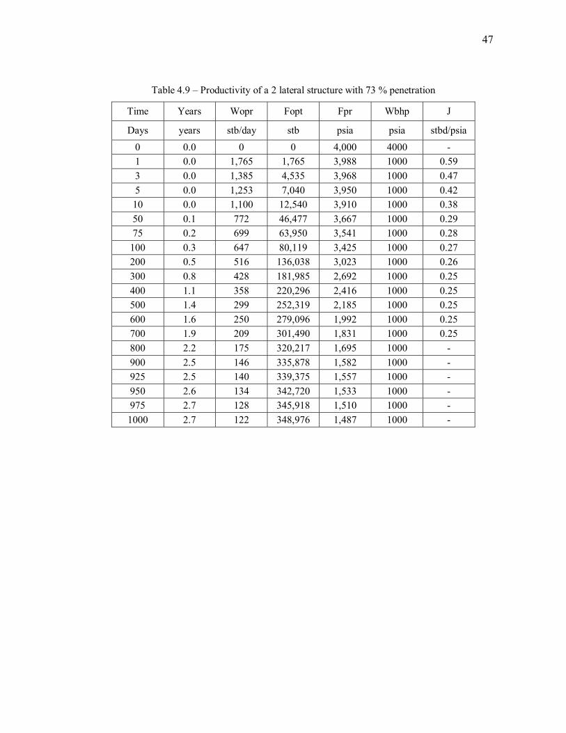
47
Table 4.9 – Productivity of a 2 lateral structure with 73 % penetration
Time Years Wopr Fopt Fpr Wbhp J
Days years stb/day stb psia psia stbd/psia
0 0.0 0 0 4,000 4000 - 1 0.0 1,765 1,765 3,988 1000 0.59 3 0.0 1,385 4,535 3,968 1000 0.47 5 0.0 1,253 7,040 3,950 1000 0.42 10 0.0 1,100 12,540 3,910 1000 0.38 50 0.1 772 46,477 3,667 1000 0.29 75 0.2 699 63,950 3,541 1000 0.28
100 0.3 647 80,119 3,425 1000 0.27 200 0.5 516 136,038 3,023 1000 0.26 300 0.8 428 181,985 2,692 1000 0.25 400 1.1 358 220,296 2,416 1000 0.25 500 1.4 299 252,319 2,185 1000 0.25 600 1.6 250 279,096 1,992 1000 0.25 700 1.9 209 301,490 1,831 1000 0.25 800 2.2 175 320,217 1,695 1000 - 900 2.5 146 335,878 1,582 1000 - 925 2.5 140 339,375 1,557 1000 - 950 2.6 134 342,720 1,533 1000 - 975 2.7 128 345,918 1,510 1000 - 1000 2.7 122 348,976 1,487 1000 -

48
4.4.2 Permeability
Permeability is perhaps the most important reservoir property that has a
significant effect on the performance of multilateral wells. This is amply noticeable from
the simulation results for isotropic and anisotropic reservoirs. The value of permeability
used for isotropic reservoirs is 1 md while for the anisotropic reservoir a h
vk
k ratio of
0.1 is used with a horizontal permeability of 1 md.
For both isotropic and anisotropic reservoirs the results show that as we decrease
the branch density by half the PI also decreases by more than half. For example from the
table we see that for an isotropic reservoir with a 60 – lateral structure the PI is 74
STBD/psia, while for a 30 – lateral structure the PI is 33 STBD/psia. This indicates a
reduction of more than 50% in the PI. This trend is also observed when we reduce the
branch density even further. Similar variation of results is also observed for an
anisotropic reservoir though a much lower PI is achieved for a vertical to horizontal
permeability ratio of 0.1.
The cumulative production from an isotropic reservoir is comparable for a
structure with 60 – laterals and with 4 – laterals. However for the h
vk
k ratio of 0.1 the
cumulative production from a 4 – lateral structure is only 0.3085 MMSTB while it is
0.3818 MMSTB for a 15 – lateral structure. This shows that for a large permeability
variation in the two directions the capacity to produce the fluids is lower and more time
will be required to produce the same amount. The results are shown in Tables 4.10 –
4.15.Comparison of the PI for the two cases is shown in Figure 4.2

49
0
10
20
30
40
50
60
70
80
0 10 20 30 40 50 60 70
Number of Laterals
PI, s
tbd/
psi
Isotropic case Anisotropic Case
Figure 4.2 – Productivity of the ML well architecture decreases significantly (by 50%) as we go
from an isotropic reservoir to an anisotropic reservoir

50
Table 4.10 – Isotropic reservoir productivity with a 60 lateral structure
Time Years Wopr Fopt Fpr Wbhp J
Days years stb/day stb psia psia stbd/psia
0 0.0 0 0 4,000 4,000 - 1 0.0 3,818 3,818 3,973 3,922 76.1 3 0.0 3,818 11,455 3,918 3,867 74.9 5 0.0 3,818 19,091 3,863 3,812 74.7 10 0.0 3,818 38,182 3,726 3,675 74.6 15 0.0 3,818 57,273 3,589 3,538 74.6 20 0.1 3,818 76,364 3,452 3,401 74.5 50 0.1 3,818 190,909 2,628 2,576 74.4
100 0.3 3,818 381,818 1,250 1,198 74.1 125 0.3 1,273 413,653 1,019 1,000 65.4 150 0.4 83 415,724 1,004 1,000 18.6 175 0.5 6 415,862 1,003 1,000 1.6 200 0.5 0 415,871 1,003 1,000 0.1 225 0.6 0 415,871 1,003 1,000 0.0 250 0.7 0 415,871 1,003 1,000 0.0 275 0.8 0 415,871 1,003 1,000 - 300 0.8 0 415,871 1,003 1,000 - 400 1.1 0 415,871 1,003 0 - 500 1.4 0 415,871 1,003 0 - 600 1.6 0 415,871 1,003 0 - 700 1.9 0 415,871 1,003 0 - 800 2.2 0 415,871 1,003 0 - 900 2.5 0 415,871 1,003 0 - 1000 2.7 0 415,871 1,003 0 -

51
Table 4.11 – Isotropic reservoir productivity with a 30 lateral structure
Time Years Wopr Fopt Fpr Wbhp J
Days years stb/day stb psia psia stbd/psia
0 0.0 0 0 4,000 4,000 - 1 0.0 3,818 3,818 3,973 3,867 36.0 3 0.0 3,818 11,455 3,918 3,807 34.4 5 0.0 3,818 19,091 3,863 3,751 34.0 10 0.0 3,818 38,182 3,726 3,613 33.8 15 0.0 3,818 57,273 3,589 3,476 33.7 20 0.1 3,818 76,364 3,452 3,338 33.6 35 0.1 3,818 133,636 3,040 2,926 33.6 50 0.1 3,818 190,909 2,628 2,514 33.5 75 0.2 3,818 286,364 1,939 1,825 33.5
100 0.3 3,818 381,818 1,250 1,135 33.4 125 0.3 1,171 411,100 1,038 1,000 30.9 150 0.4 163 415,181 1,008 1,000 19.4 175 0.5 24 415,769 1,004 1,000 5.7 200 0.5 4 415,858 1,003 1,000 1.0 300 0.8 0 415,871 1,003 1,000 0.0 400 1.1 0 415,871 1,003 1,000 0.0 500 1.4 0 415,871 1,003 0 - 600 1.6 0 415,871 1,003 0 - 700 1.9 0 415,871 1,003 0 - 800 2.2 0 415,871 1,003 0 - 900 2.5 0 415,871 1,003 0 - 1000 2.7 0 415,871 1,003 0 -

52
Table 4.12 – Isotropic reservoir productivity with a 4 lateral structure
Time Years Wopr Fopt Fpr Wbhp J
days years stb/day stb psia psia stbd/psia
0 0.0 0 0 4,000 4,000 - 1 0.0 3,818 3,818 3,973 3,055 4.16 3 0.0 3,818 11,455 3,918 2,756 3.29 5 0.0 3,818 19,091 3,863 2,558 2.93 10 0.0 3,818 38,182 3,726 2,233 2.56 15 0.0 3,818 57,273 3,589 1,981 2.37 20 0.1 3,818 76,364 3,452 1,768 2.27 35 0.1 3,818 133,636 3,040 1,245 2.13 50 0.1 3,358 184,013 2,677 1,000 2.00 75 0.2 2,317 241,934 2,260 1,000 1.84
100 0.3 1,680 283,929 1,957 1,000 1.76 125 0.3 1,241 314,952 1,733 1,000 1.69 150 0.4 927 338,128 1,566 1,000 1.64 175 0.5 699 355,606 1,439 1,000 1.59 200 0.5 531 368,891 1,343 1,000 1.55 300 0.8 190 397,722 1,135 1,000 1.41 400 1.1 74 408,512 1,057 1,000 1.29 500 1.4 30 412,815 1,026 1,000 1.16 600 1.6 13 414,631 1,013 1,000 1.02 700 1.9 5 415,377 1,007 1,000 0.73 800 2.2 2 415,681 1,005 1,000 0.43 900 2.5 1 415,804 1,004 1,000 0.21 1000 2.7 0 415,855 1,004 1,000 0.10
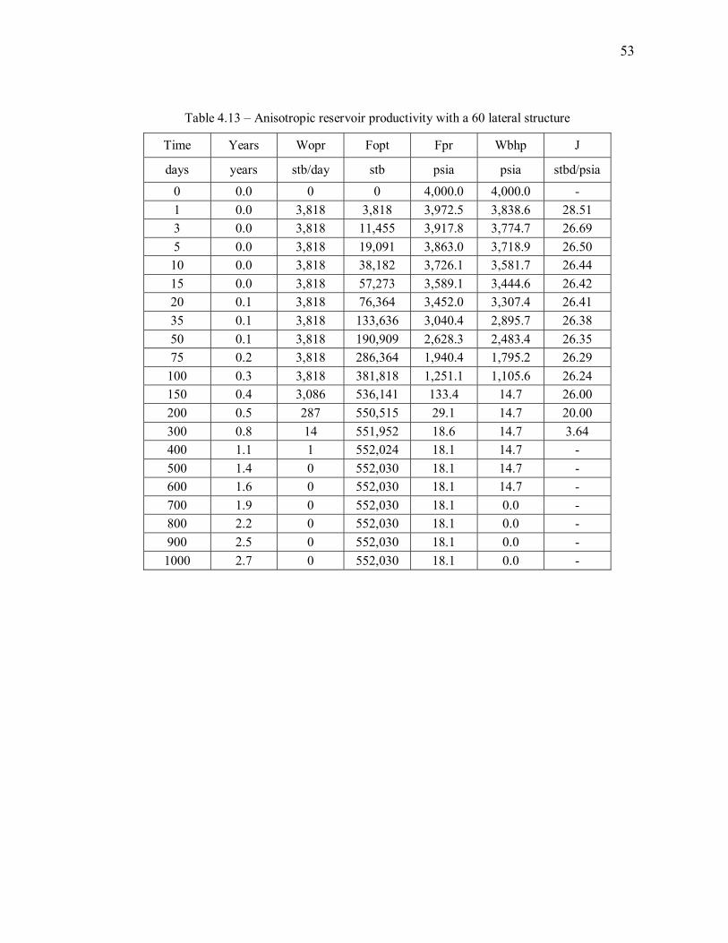
53
Table 4.13 – Anisotropic reservoir productivity with a 60 lateral structure
Time Years Wopr Fopt Fpr Wbhp J
days years stb/day stb psia psia stbd/psia
0 0.0 0 0 4,000.0 4,000.0 - 1 0.0 3,818 3,818 3,972.5 3,838.6 28.51 3 0.0 3,818 11,455 3,917.8 3,774.7 26.69 5 0.0 3,818 19,091 3,863.0 3,718.9 26.50 10 0.0 3,818 38,182 3,726.1 3,581.7 26.44 15 0.0 3,818 57,273 3,589.1 3,444.6 26.42 20 0.1 3,818 76,364 3,452.0 3,307.4 26.41 35 0.1 3,818 133,636 3,040.4 2,895.7 26.38 50 0.1 3,818 190,909 2,628.3 2,483.4 26.35 75 0.2 3,818 286,364 1,940.4 1,795.2 26.29
100 0.3 3,818 381,818 1,251.1 1,105.6 26.24 150 0.4 3,086 536,141 133.4 14.7 26.00 200 0.5 287 550,515 29.1 14.7 20.00 300 0.8 14 551,952 18.6 14.7 3.64 400 1.1 1 552,024 18.1 14.7 - 500 1.4 0 552,030 18.1 14.7 - 600 1.6 0 552,030 18.1 14.7 - 700 1.9 0 552,030 18.1 0.0 - 800 2.2 0 552,030 18.1 0.0 - 900 2.5 0 552,030 18.1 0.0 - 1000 2.7 0 552,030 18.1 0.0 -
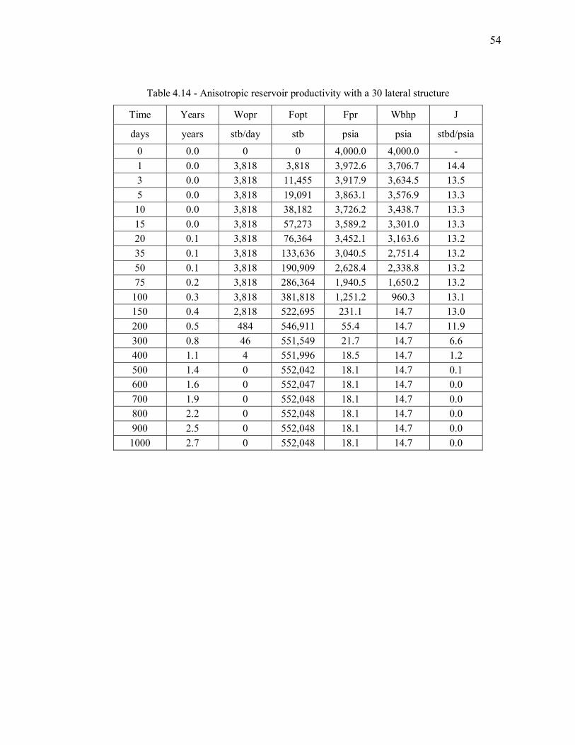
54
Table 4.14 - Anisotropic reservoir productivity with a 30 lateral structure
Time Years Wopr Fopt Fpr Wbhp J
days years stb/day stb psia psia stbd/psia
0 0.0 0 0 4,000.0 4,000.0 - 1 0.0 3,818 3,818 3,972.6 3,706.7 14.4 3 0.0 3,818 11,455 3,917.9 3,634.5 13.5 5 0.0 3,818 19,091 3,863.1 3,576.9 13.3 10 0.0 3,818 38,182 3,726.2 3,438.7 13.3 15 0.0 3,818 57,273 3,589.2 3,301.0 13.3 20 0.1 3,818 76,364 3,452.1 3,163.6 13.2 35 0.1 3,818 133,636 3,040.5 2,751.4 13.2 50 0.1 3,818 190,909 2,628.4 2,338.8 13.2 75 0.2 3,818 286,364 1,940.5 1,650.2 13.2
100 0.3 3,818 381,818 1,251.2 960.3 13.1 150 0.4 2,818 522,695 231.1 14.7 13.0 200 0.5 484 546,911 55.4 14.7 11.9 300 0.8 46 551,549 21.7 14.7 6.6 400 1.1 4 551,996 18.5 14.7 1.2 500 1.4 0 552,042 18.1 14.7 0.1 600 1.6 0 552,047 18.1 14.7 0.0 700 1.9 0 552,048 18.1 14.7 0.0 800 2.2 0 552,048 18.1 14.7 0.0 900 2.5 0 552,048 18.1 14.7 0.0 1000 2.7 0 552,048 18.1 14.7 0.0
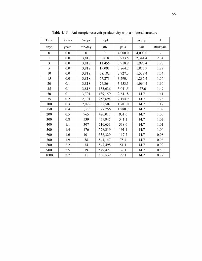
55
Table 4.15 – Anisotropic reservoir productivity with a 4 lateral structure
Time Years Wopr Fopt Fpr Wbhp J
days years stb/day stb psia psia stbd/psia
0 0.0 0 0 4,000.0 4,000.0 - 1 0.0 3,818 3,818 3,973.5 2,341.4 2.34 3 0.0 3,818 11,455 3,918.9 1,993.4 1.98 5 0.0 3,818 19,091 3,864.2 1,817.9 1.87 10 0.0 3,818 38,182 3,727.3 1,528.4 1.74 15 0.0 3,818 57,273 3,590.4 1,285.4 1.66 20 0.1 3,818 76,364 3,453.3 1,064.4 1.60 35 0.1 3,818 133,636 3,041.5 477.6 1.49 50 0.1 3,701 189,159 2,641.8 14.7 1.41 75 0.2 2,701 256,694 2,154.9 14.7 1.26
100 0.3 2,072 308,502 1,781.0 14.7 1.17 150 0.4 1,385 377,756 1,280.7 14.7 1.09 200 0.5 965 426,017 931.6 14.7 1.05 300 0.8 539 479,945 541.1 14.7 1.02 400 1.1 307 510,631 318.6 14.7 1.01 500 1.4 176 528,219 191.1 14.7 1.00 600 1.6 101 538,329 117.7 14.7 0.98 700 1.9 58 544,147 75.4 14.7 0.96 800 2.2 34 547,498 51.1 14.7 0.92 900 2.5 19 549,427 37.1 14.7 0.86 1000 2.7 11 550,539 29.1 14.7 0.77

56
4.4.3 Grid Refinement
The most common technique to establish the numerical accuracy of simulation results is
to perform grid refinement. The base case comprises a grid of 21 62 11. We have
refined the grid by a factor of 2 both in each of the directions X and Z, individually as
well as simultaneously, so that the biggest case simulated is 81 62 41. The results
shown in Table 4.16 are obtained for the case of 60 and 30 laterals only. Also only the
anisotropic reservoir case is refined to determine the accuracy. The following table
summaries the results of grid refinement. A comparison of the PI for the base case and
the refined cases indicates a good validation of the results obtained from the base case
simulations. As mentioned earlier these results are obtained for an anisotropic reservoir
with permeability in the three directions given as (1.0, 1.0, 0.1) md.

57
Table 4.16 – Results showing numerical consistency with grid refinement
Grid Number of Productivity
Structure Laterals Index, J
A. Base Case
60 26.2447 21 × 62 × 11
30 13.1281
B. Grid Refinement
Z - Direction:
60 23.9285 21 × 62 × 21
30 11.936
X - Direction:
60 23.5568 41 × 62 × 11
30 11.7413
X & Z - Direction:
60 23.6054 41 × 62 × 21
30 11.7428 60 23.429
81 × 62 × 41 30 11.6357
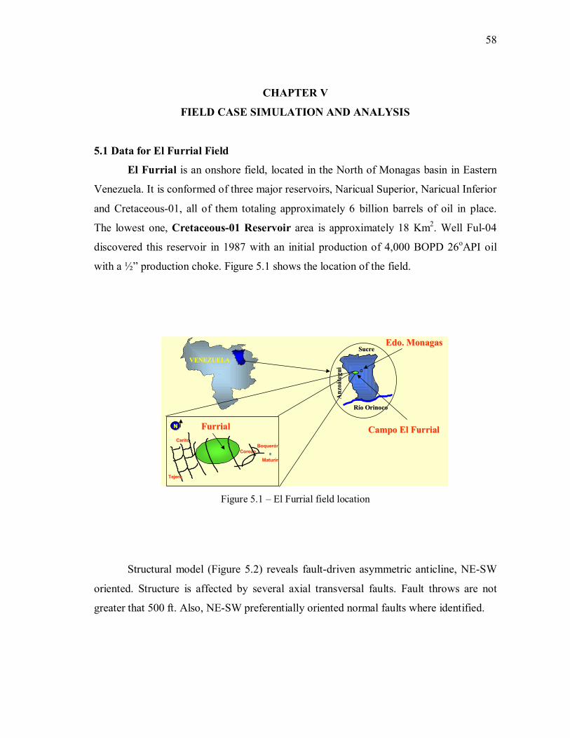
58
CHAPTER V
FIELD CASE SIMULATION AND ANALYSIS
5.1 Data for El Furrial Field
El Furrial is an onshore field, located in the North of Monagas basin in Eastern
Venezuela. It is conformed of three major reservoirs, Naricual Superior, Naricual Inferior
and Cretaceous-01, all of them totaling approximately 6 billion barrels of oil in place.
The lowest one, Cretaceous-01 Reservoir area is approximately 18 Km2. Well Ful-04
discovered this reservoir in 1987 with an initial production of 4,000 BOPD 26oAPI oil
with a ½” production choke. Figure 5.1 shows the location of the field.
Río OrinocoRío Orinoco
SucreSucreA
nzoá
tegu
iA
nzoá
tegu
i
Campo El FurrialCampo El Furrial
Edo. MonagasEdo. Monagas
FurrialFurrial
CorozoCorozoBoquerónBoquerón
MaturínMaturín
CaritoCarito
TejeroTejero
NN
VENEZUELAVENEZUELA
Figure 5.1 – El Furrial field location
Structural model (Figure 5.2) reveals fault-driven asymmetric anticline, NE-SW
oriented. Structure is affected by several axial transversal faults. Fault throws are not
greater that 500 ft. Also, NE-SW preferentially oriented normal faults where identified.

59
CRETACEO
NARICUALSUP/MED.
NARICUALINFERIOR
TOPE 16 API a -15800’ (FCO. NORTE)
SENO
F.M. CARAPITA
-15424’-15595’
-15398’ -15173’
-12704’
-13878’
TOPE 16 API a -14800 (FCO. SUR)
Figure 5.2 – Structural model of El Furrial
Fluid column characterization showed depth variations on thermodynamic and
chemical properties, associated to gravity drainage process of the heavy components of
the crude, which originated heavy crude formation and tar mat.
The main reservoir characteristics are summarized in Table 5.1
Table 5.1 – Reservoir characteristics of El Furrial
Porosity Net ht
(ft) Sw A
Bo
(rb/stb) µo (cp) k (md) pi(psia)
9-15% 200-800 19-24% 18 km2 1.5 0.5-0.6 10-80 11,200

60
5.2 Representative Unit
To simulate the field we will consider a representation of the Cretaceous
Reservoir that is simplified in many senses, but still contains the main formation
characteristics and basic fluid properties. Our goal is to make the reservoir model as
simple as possible, but capture all the major factors responsible for the performance
differences between traditional and the suggested advanced well architecture. In the
representative unit we assume ex = 20,000 ft; ey = 10,000 ft and h = 750 ft.
The permeability field is anisotropic. The two horizontal permeabilities are:
xk = 86.6 md
yk = 28.7 md
and the vertical permeability is
kz = 2.6 md
Note the large permeability contrast between horizontal and vertical.
The porosity is 0.12, providing the oil in place. The PVT properties of the fluids
are given in Table 5.2
Table 5.2 – El Furrial fluid PVT properties
P sR oB µ
Psia mcf/stb rb/stb Cp 500 0.054 1.045 7666 714 0.055 1.047 7366
1428 0.125 1.080 1251 2142 0.215 1.124 212 2857 0.335 1.185 36 3571 0.502 1.273 6 4285 0.753 1.409 1.04 4642 0.933 1.508 0.43 5000 1.172 1.640 0.17
Table 5.3 shows the variation of solution gas oil ratio with depth. It can be seen

61
from the data that gas volume decreases by a couple of order magnitudes within a few
1000 ft. Due to this rapid change the oil viscosity increases rapidly with depth.
Table 5.3 – Solution GOR vs. depth
Depth, ft sR (mcf/stb)
12000 1.145 14350 0.874 14646 0.747 14700 0.619 14800 0.538 14880 0.330 14960 0.244 15000 0.055 16500 0.055
Thus from the PVT and Solution GOR data we can see that there exist a very high
contrast in mobility in the reservoir. Figure 5.3 and 5.4 shows the change in Solution
GOR and Viscosity with pressure. The bar charts show the sharp change in properties
with decrease in pressure. The variation of solution GOR and viscosity with depth in the
reservoir is shown in Figures 5.5 and Figure 5.6 respectively.
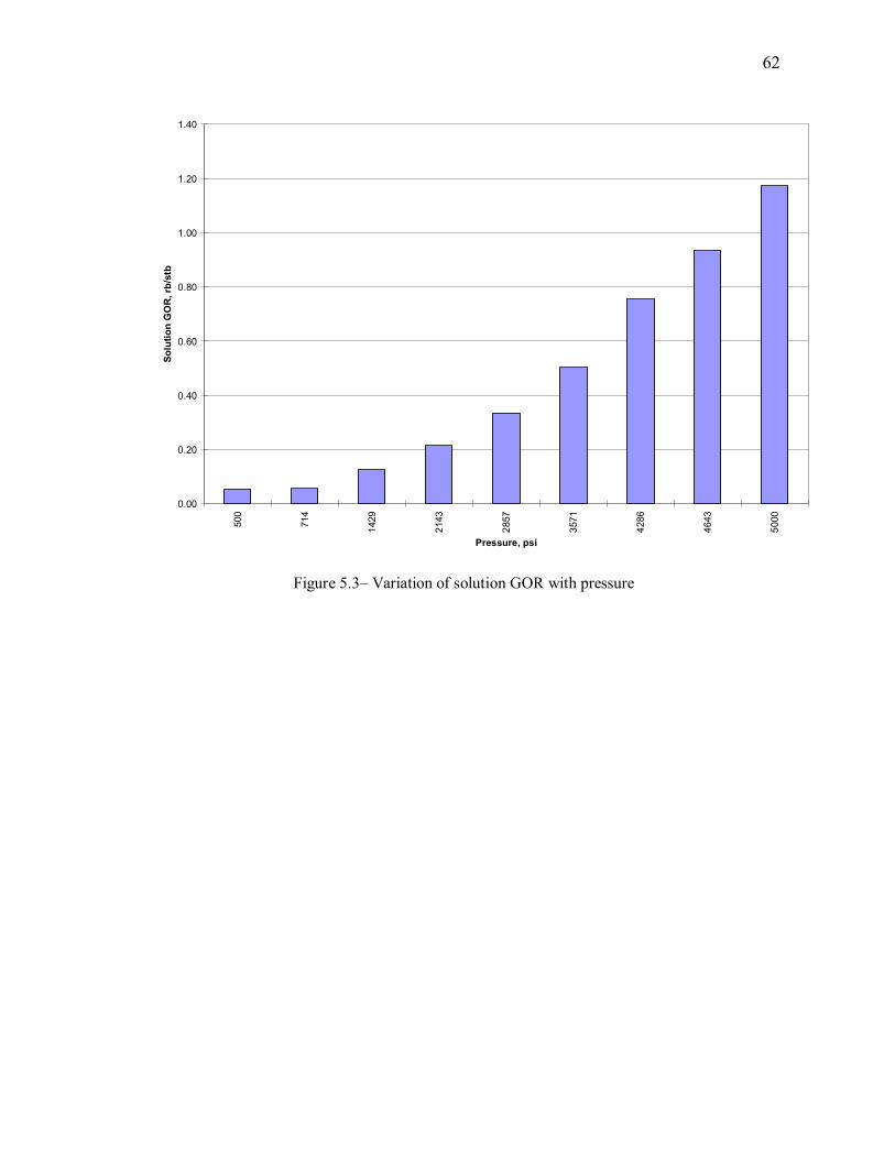
62
0.00
0.20
0.40
0.60
0.80
1.00
1.20
1.40
500
714
1429
2143
2857
3571
4286
4643
5000
Pressure, psi
Solu
tion
GO
R, r
b/st
b
Figure 5.3– Variation of solution GOR with pressure

63
0
1000
2000
3000
4000
5000
6000
7000
8000
9000
500
714
1429
2143
2857
3571
4286
4643
5000
Pressure,psia
Visc
osity
, cp
Figure 5.4– Variation of viscosity with pressure

64
Figure 5.5– Variation of solution GOR with depth
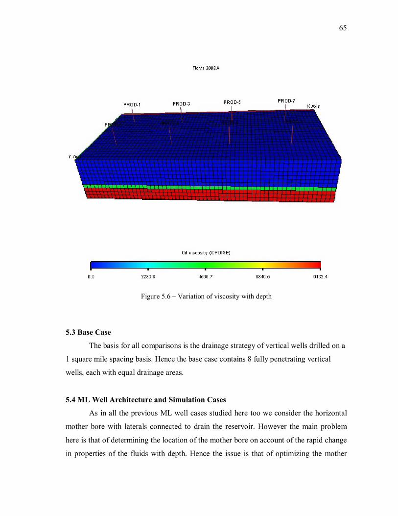
65
Figure 5.6 – Variation of viscosity with depth 5.3 Base Case
The basis for all comparisons is the drainage strategy of vertical wells drilled on a
1 square mile spacing basis. Hence the base case contains 8 fully penetrating vertical
wells, each with equal drainage areas.
5.4 ML Well Architecture and Simulation Cases
As in all the previous ML well cases studied here too we consider the horizontal
mother bore with laterals connected to drain the reservoir. However the main problem
here is that of determining the location of the mother bore on account of the rapid change
in properties of the fluids with depth. Hence the issue is that of optimizing the mother

66
bore lateral in addition to determining the optimum lateral density and penetration ratio.
We assume that the laterals are 100% penetrating when they extend from the mother bore
to the lateral boundary. Penetration ratio (the extent of penetration) is an important design
parameter to be neglected. Taking into account all of these variable the following cases
have been simulated. The cases designed are described as the location of the horizontal
mother bore, number of laterals and finally the penetration ratio.
Case A – Mother bore: 375 ft from top; 15 horizontal legs; Penetration: 100 %
Case B – Mother bore: 239 ft from top; 15 horizontal legs; Penetration: 100 %
Case C – Mother bore: 239 ft from top; 15 horizontal legs; Penetration: 67 %
Case D – Mother bore: 239 ft from top; 8 horizontal legs; Penetration: 100 %
Case E – Mother bore: 239 ft from top; 8 horizontal legs; penetration: 100 %
Figure 5.7 shows a general representation of the cases simulated
Figure 5.7 – General ML well architecture used for simulation

67
5.5 Simulation Results
The results of the simulation are presented in this section in Tables 5.4-5.9. The
time over which the simulation is run is three years. An example input data file for the
advanced well architecture case has been attached in the APPENDIX B for reference. For
the economic evaluation of the technology the cumulative production is an important
parameter.

68
Table 5.4 – Base case results (8 vertical wells)
Base Case: 8 Vertical wells Time Field Pr. W1 W1 cum W1 bhp ∆P Np Cum Gp Cum Days psia stbd MMstb psia psi MMstb Bscf
0 11,204 0 0.00 11,077 128 0.0 0.0 30 11,179 4,500 0.14 10,491 688 1.1 0.8 60 11,154 4,500 0.27 10,438 717 2.2 1.6 90 11,129 4,500 0.41 10,390 739 3.2 2.3
120 11,104 4,500 0.54 10,346 758 4.3 3.1 150 11,079 4,500 0.68 10,303 777 5.4 3.9 180 11,054 4,500 0.81 10,260 794 6.5 4.6 210 11,032 3,900 0.93 10,312 720 7.4 5.3 240 11,011 3,900 1.04 10,279 732 8.4 6.0 270 10,989 3,900 1.16 10,244 744 9.3 6.7 300 10,967 3,900 1.28 10,210 757 10.2 7.3 330 10,945 3,900 1.40 10,175 771 11.2 8.0 360 10,923 3,900 1.51 10,140 784 12.1 8.7 390 10,904 3,500 1.62 10,168 736 12.9 9.3 420 10,884 3,500 1.72 10,139 745 13.8 9.9 450 10,865 3,500 1.83 10,109 756 14.6 10.5 480 10,845 3,500 1.93 10,078 767 15.5 11.1 510 10,826 3,500 2.04 10,047 778 16.3 11.7 540 10,806 3,500 2.14 10,017 789 17.1 12.3 570 10,789 3,100 2.24 10,049 739 17.9 12.8 600 10,771 3,100 2.33 10,024 747 18.6 13.3 630 10,754 3,100 2.42 9,998 755 19.4 13.9 660 10,736 3,100 2.51 9,972 765 20.1 14.4 690 10,719 3,100 2.61 9,945 774 20.9 14.9 720 10,702 3,100 2.70 9,919 783 21.6 15.4 750 10,686 2,800 2.78 9,940 746 22.3 15.9 780 10,670 2,800 2.87 9,917 753 22.9 16.4 810 10,654 2,800 2.95 9,894 760 23.6 16.9 840 10,639 2,800 3.04 9,870 768 24.3 17.4 870 10,623 2,800 3.12 9,847 776 25.0 17.8 900 10,607 2,800 3.20 9,823 784 25.6 18.3 930 10,592 2,600 3.28 9,831 761 26.3 18.8 960 10,578 2,600 3.36 9,810 767 26.9 19.2 990 10,563 2,600 3.44 9,789 774 27.5 19.7 1020 10,549 2,600 3.52 9,767 781 28.1 20.1 1050 10,534 2,600 3.59 9,746 788 28.8 20.6 1080 10,519 2,600 3.67 9,724 795 29.4 21.0

69
Table 5.5 – Case A results
Case A - Motherbore 375 ft from top;15 horizontal laterals;100% Time Field Pr. W W cum W BHP ∆ P Np Cum Gp Cum Days psia Stbd MMstb psia psi MMstb Bscf
0 11,204 0 0.0 11,200 4.5 0.0 0.0 30 11,185 33,000 1.0 10,411 773.8 1.0 0.4 60 11,165 33,000 2.0 10,386 779.5 2.0 0.7 90 11,146 33,000 3.0 10,363 782.2 3.0 1.1 120 11,126 33,000 4.0 10,342 784.0 4.0 1.4 150 11,106 33,000 5.0 10,321 785.4 5.0 1.8 180 11,087 33,000 5.9 10,300 786.6 5.9 2.2 210 11,067 33,000 6.9 10,279 787.8 6.9 2.5 240 11,047 33,000 7.9 10,258 789.1 7.9 2.9 270 11,027 33,000 8.9 10,237 790.7 8.9 3.3 300 11,008 33,000 9.9 10,215 792.5 9.9 3.6 330 10,988 33,000 10.9 10,193 794.5 10.9 4.0 360 10,968 33,000 11.9 10,171 796.9 11.9 4.4 390 10,949 32,000 12.8 10,168 781.0 12.8 4.7 420 10,930 32,000 13.8 10,146 783.3 13.8 5.1 450 10,910 32,000 14.8 10,124 786.2 14.8 5.5 480 10,891 32,000 15.7 10,101 789.4 15.7 5.9 510 10,872 32,000 16.7 10,079 793.0 16.7 6.2 540 10,852 32,000 17.6 10,055 796.8 17.6 6.6 570 10,834 30,000 18.5 10,067 766.8 18.5 7.0 600 10,816 30,000 19.4 10,046 769.6 19.4 7.3 630 10,797 30,000 20.3 10,024 773.2 20.3 7.7 660 10,779 30,000 21.2 10,002 777.3 21.2 8.0 690 10,761 30,000 22.1 9,979 781.7 22.1 8.4 720 10,743 30,000 23.0 9,956 786.3 23.0 8.8 750 10,725 29,000 23.9 9,950 775.1 23.9 9.1 780 10,707 29,000 24.8 9,928 779.3 24.8 9.5 810 10,689 29,000 25.7 9,905 784.0 25.7 9.8 840 10,672 29,000 26.5 9,883 788.9 26.5 10.2 870 10,654 29,000 27.4 9,860 794.0 27.4 10.5 900 10,636 29,000 28.3 9,837 799.4 28.3 10.9 930 10,620 27,000 29.1 9,845 774.5 29.1 11.2 960 10,603 27,000 29.9 9,825 778.3 29.9 11.5 990 10,586 27,000 30.7 9,803 782.8 30.7 11.9
1020 10,570 27,000 31.5 9,782 787.7 31.5 12.2 1050 10,553 27,000 32.3 9,760 792.8 32.3 12.5 1080 10,536 27,000 33.1 9,738 798.0 33.1 12.9
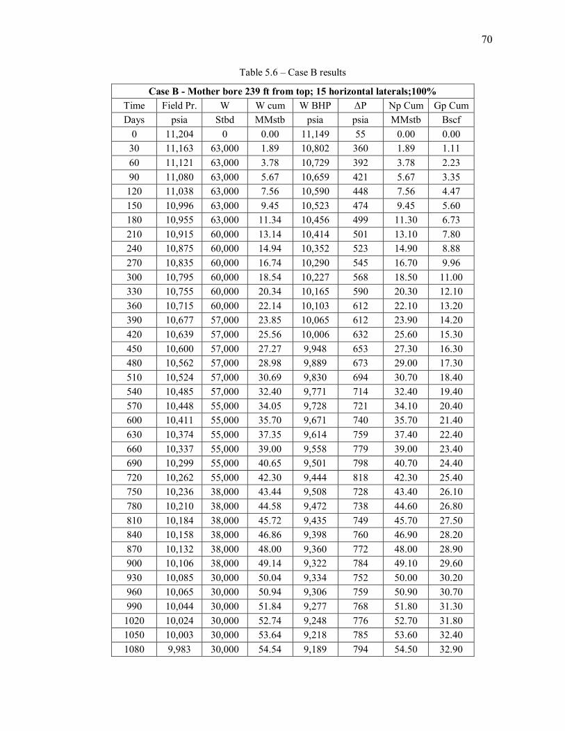
70
Table 5.6 – Case B results
Case B - Mother bore 239 ft from top; 15 horizontal laterals;100% Time Field Pr. W W cum W BHP ∆P Np Cum Gp Cum Days psia Stbd MMstb psia psia MMstb Bscf
0 11,204 0 0.00 11,149 55 0.00 0.00 30 11,163 63,000 1.89 10,802 360 1.89 1.11 60 11,121 63,000 3.78 10,729 392 3.78 2.23 90 11,080 63,000 5.67 10,659 421 5.67 3.35 120 11,038 63,000 7.56 10,590 448 7.56 4.47 150 10,996 63,000 9.45 10,523 474 9.45 5.60 180 10,955 63,000 11.34 10,456 499 11.30 6.73 210 10,915 60,000 13.14 10,414 501 13.10 7.80 240 10,875 60,000 14.94 10,352 523 14.90 8.88 270 10,835 60,000 16.74 10,290 545 16.70 9.96 300 10,795 60,000 18.54 10,227 568 18.50 11.00 330 10,755 60,000 20.34 10,165 590 20.30 12.10 360 10,715 60,000 22.14 10,103 612 22.10 13.20 390 10,677 57,000 23.85 10,065 612 23.90 14.20 420 10,639 57,000 25.56 10,006 632 25.60 15.30 450 10,600 57,000 27.27 9,948 653 27.30 16.30 480 10,562 57,000 28.98 9,889 673 29.00 17.30 510 10,524 57,000 30.69 9,830 694 30.70 18.40 540 10,485 57,000 32.40 9,771 714 32.40 19.40 570 10,448 55,000 34.05 9,728 721 34.10 20.40 600 10,411 55,000 35.70 9,671 740 35.70 21.40 630 10,374 55,000 37.35 9,614 759 37.40 22.40 660 10,337 55,000 39.00 9,558 779 39.00 23.40 690 10,299 55,000 40.65 9,501 798 40.70 24.40 720 10,262 55,000 42.30 9,444 818 42.30 25.40 750 10,236 38,000 43.44 9,508 728 43.40 26.10 780 10,210 38,000 44.58 9,472 738 44.60 26.80 810 10,184 38,000 45.72 9,435 749 45.70 27.50 840 10,158 38,000 46.86 9,398 760 46.90 28.20 870 10,132 38,000 48.00 9,360 772 48.00 28.90 900 10,106 38,000 49.14 9,322 784 49.10 29.60 930 10,085 30,000 50.04 9,334 752 50.00 30.20 960 10,065 30,000 50.94 9,306 759 50.90 30.70 990 10,044 30,000 51.84 9,277 768 51.80 31.30
1020 10,024 30,000 52.74 9,248 776 52.70 31.80 1050 10,003 30,000 53.64 9,218 785 53.60 32.40 1080 9,983 30,000 54.54 9,189 794 54.50 32.90
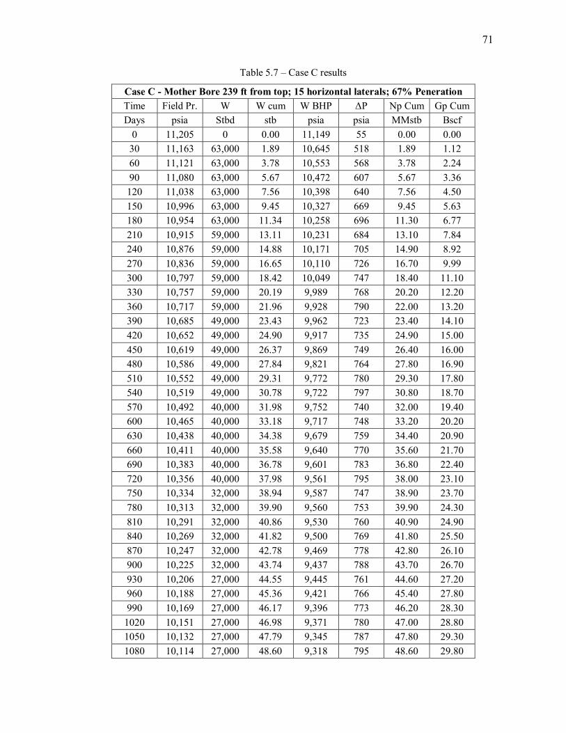
71
Table 5.7 – Case C results
Case C - Mother Bore 239 ft from top; 15 horizontal laterals; 67% Peneration Time Field Pr. W W cum W BHP ∆P Np Cum Gp Cum Days psia Stbd stb psia psia MMstb Bscf
0 11,205 0 0.00 11,149 55 0.00 0.00 30 11,163 63,000 1.89 10,645 518 1.89 1.12 60 11,121 63,000 3.78 10,553 568 3.78 2.24 90 11,080 63,000 5.67 10,472 607 5.67 3.36 120 11,038 63,000 7.56 10,398 640 7.56 4.50 150 10,996 63,000 9.45 10,327 669 9.45 5.63 180 10,954 63,000 11.34 10,258 696 11.30 6.77 210 10,915 59,000 13.11 10,231 684 13.10 7.84 240 10,876 59,000 14.88 10,171 705 14.90 8.92 270 10,836 59,000 16.65 10,110 726 16.70 9.99 300 10,797 59,000 18.42 10,049 747 18.40 11.10 330 10,757 59,000 20.19 9,989 768 20.20 12.20 360 10,717 59,000 21.96 9,928 790 22.00 13.20 390 10,685 49,000 23.43 9,962 723 23.40 14.10 420 10,652 49,000 24.90 9,917 735 24.90 15.00 450 10,619 49,000 26.37 9,869 749 26.40 16.00 480 10,586 49,000 27.84 9,821 764 27.80 16.90 510 10,552 49,000 29.31 9,772 780 29.30 17.80 540 10,519 49,000 30.78 9,722 797 30.80 18.70 570 10,492 40,000 31.98 9,752 740 32.00 19.40 600 10,465 40,000 33.18 9,717 748 33.20 20.20 630 10,438 40,000 34.38 9,679 759 34.40 20.90 660 10,411 40,000 35.58 9,640 770 35.60 21.70 690 10,383 40,000 36.78 9,601 783 36.80 22.40 720 10,356 40,000 37.98 9,561 795 38.00 23.10 750 10,334 32,000 38.94 9,587 747 38.90 23.70 780 10,313 32,000 39.90 9,560 753 39.90 24.30 810 10,291 32,000 40.86 9,530 760 40.90 24.90 840 10,269 32,000 41.82 9,500 769 41.80 25.50 870 10,247 32,000 42.78 9,469 778 42.80 26.10 900 10,225 32,000 43.74 9,437 788 43.70 26.70 930 10,206 27,000 44.55 9,445 761 44.60 27.20 960 10,188 27,000 45.36 9,421 766 45.40 27.80 990 10,169 27,000 46.17 9,396 773 46.20 28.30
1020 10,151 27,000 46.98 9,371 780 47.00 28.80 1050 10,132 27,000 47.79 9,345 787 47.80 29.30 1080 10,114 27,000 48.60 9,318 795 48.60 29.80

72
Table 5.8 – Case D results
Case D - Mother bore 239 ft from top; 8 horizontal laterals; 100% penetration Time Field Pr. W W cum W BHP ∆P Np Cum Gp Cum Days psia Stbd MMstb psia Psia MMstb Bscf
0 11,204 0 0.00 11,149 55 0.00 0.00 30 11,163 62,000 1.86 10,505 659 1.86 1.10 60 11,122 62,000 3.72 10,433 690 3.72 2.20 90 11,082 62,000 5.58 10,365 717 5.58 3.31 120 11,040 62,000 7.44 10,299 742 7.44 4.43 150 10,999 62,000 9.30 10,233 766 9.30 5.55 180 10,958 62,000 11.16 10,169 789 11.20 6.67 210 10,922 54,000 12.78 10,221 701 12.80 7.65 240 10,886 54,000 14.40 10,167 719 14.40 8.63 270 10,850 54,000 16.02 10,113 737 16.00 9.62 300 10,814 54,000 17.64 10,058 756 17.60 10.60 330 10,778 54,000 19.26 10,003 775 19.30 11.60 360 10,742 54,000 20.88 9,947 794 20.90 12.60 390 10,711 46,000 22.26 9,999 712 22.30 13.40 420 10,680 46,000 23.64 9,954 726 23.60 14.30 450 10,649 46,000 25.02 9,907 741 25.00 15.10 480 10,618 46,000 26.40 9,861 757 26.40 16.00 510 10,587 46,000 27.78 9,814 773 27.80 16.80 540 10,556 46,000 29.16 9,767 788 29.20 17.70 570 10,529 40,000 30.36 9,794 735 30.40 18.40 600 10,501 40,000 31.56 9,755 747 31.60 19.20 630 10,474 40,000 32.76 9,715 760 32.80 19.90 660 10,447 40,000 33.96 9,674 773 34.00 20.70 690 10,420 40,000 35.16 9,634 786 35.20 21.40 720 10,393 40,000 36.36 9,593 800 36.40 22.20 750 10,370 33,000 37.35 9,632 738 37.40 22.80 780 10,348 33,000 38.34 9,600 747 38.30 23.40 810 10,325 33,000 39.33 9,568 757 39.30 24.00 840 10,303 33,000 40.32 9,535 768 40.30 24.60 870 10,280 33,000 41.31 9,502 778 41.30 25.30 900 10,257 33,000 42.30 9,469 789 42.30 25.90 930 10,238 28,000 43.14 9,488 750 43.10 26.40 960 10,219 28,000 43.98 9,461 758 44.00 26.90 990 10,200 28,000 44.82 9,434 766 44.80 27.50
1020 10,180 28,000 45.66 9,406 774 45.70 28.00 1050 10,161 28,000 46.50 9,379 783 46.50 28.50 1080 10,142 28,000 47.34 9,351 791 47.30 29.00
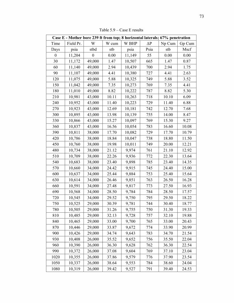
73
Table 5.9 – Case E results
Case E - Mother bore 239 ft from top; 8 horizontal laterals; 67% penetration Time Field Pr. W W cum W BHP ∆P Np Cum Gp Cum Days psia stbd stb psia Psia stb Mscf
0 11,204 0 0.00 11,149 55 0.00 0.00 30 11,172 49,000 1.47 10,507 665 1.47 0.87 60 11,140 49,000 2.94 10,439 700 2.94 1.75 90 11,107 49,000 4.41 10,380 727 4.41 2.63 120 11,075 49,000 5.88 10,325 749 5.88 3.52 150 11,042 49,000 7.35 10,273 769 7.35 4.41 180 11,010 49,000 8.82 10,222 787 8.82 5.30 210 10,981 43,000 10.11 10,263 718 10.10 6.09 240 10,952 43,000 11.40 10,223 729 11.40 6.88 270 10,923 43,000 12.69 10,181 742 12.70 7.68 300 10,895 43,000 13.98 10,139 755 14.00 8.47 330 10,866 43,000 15.27 10,097 769 15.30 9.27 360 10,837 43,000 16.56 10,054 783 16.60 10.08 390 10,811 38,000 17.70 10,082 729 17.70 10.79 420 10,786 38,000 18.84 10,047 738 18.80 11.50 450 10,760 38,000 19.98 10,011 749 20.00 12.21 480 10,734 38,000 21.12 9,974 761 21.10 12.92 510 10,709 38,000 22.26 9,936 772 22.30 13.64 540 10,683 38,000 23.40 9,898 785 23.40 14.35 570 10,660 34,000 24.42 9,915 745 24.40 15.00 600 10,637 34,000 25.44 9,884 753 25.40 15.64 630 10,614 34,000 26.46 9,851 763 26.50 16.28 660 10,591 34,000 27.48 9,817 773 27.50 16.93 690 10,568 34,000 28.50 9,784 784 28.50 17.57 720 10,545 34,000 29.52 9,750 795 29.50 18.22 750 10,525 29,000 30.39 9,781 744 30.40 18.77 780 10,505 29,000 31.26 9,755 750 31.30 19.33 810 10,485 29,000 32.13 9,728 757 32.10 19.88 840 10,465 29,000 33.00 9,700 765 33.00 20.43 870 10,446 29,000 33.87 9,672 774 33.90 20.99 900 10,426 29,000 34.74 9,643 783 34.70 21.54 930 10,408 26,000 35.52 9,652 756 35.50 22.04 960 10,390 26,000 36.30 9,628 762 36.30 22.54 990 10,372 26,000 37.08 9,604 769 37.10 23.04
1020 10,355 26,000 37.86 9,579 776 37.90 23.54 1050 10,337 26,000 38.64 9,553 784 38.60 24.04 1080 10,319 26,000 39.42 9,527 791 39.40 24.53

74
CHAPTER VI
CONCLUSIONS AND RECOMMENDATIONS
6.1 Conclusions
A new multilateral well architecture is proposed and investigated in this thesis. Its
performance is compared against conventional vertical wells in most cases, as this was
the original development plan used in the field. Initially parametric studies were
performed to evaluate and understand performance by using simple models. These
models were then applied to representative field cases and the numerical results analyzed.
Also simple methods to estimate productivity are used and tested for their applicability.
The following conclusions can be drawn from the study:
1. Simulations show that for the reservoir studied there exist an optimum number of
laterals that can be used to drain the reservoir efficiently. Increasing the laterals
after a certain number does not produce any significant difference in the
cumulative production from the reservoir. For most of the cases studied 4 laterals
were usually sufficient to drain the reservoir efficiently in a given period of time.
2. Parametric studies were performed by varying the lateral penetration. Initially
100% lateral penetration was assumed. However comparable production was
obtained even when the penetration was lowered to 50%.
3. A comparison of results shows that to maintain a given production rate at lower
branch densities much lower flowing bottom hole pressures are needed. The
resulting large pressure drawdowns could cause sand production, early water or
gas breakthrough or collapse of the slender laterals since they are completed open
hole. To avoid such catastrophes it would be a better idea to use more laterals
with lower penetration extents. This would present the added advantage of
marginal reserve development while lowering drilling cost per field compared to
conventional wells.

75
4. The numerical validation of parametric studies has been performed through a grid
refinement study. The results obtained are within permissible error limits.
5. Permeability is a very important variable affecting the performance of the ML
well architecture. For a given branch density the PI in the case of an isotropic
permeability distribution is almost always twice the PI for anisotropic
permeability variation in the reservoir. The reduced flow in the vertical direction
(direction of assumed anisotropy) is the most obvious reason for this reduced
productivity. However it is anticipated that better performance in anisotropic
reservoirs can be achieved by using deviated laterals. Hence deviated laterals
form the next direction of studies.
6. The field case studied showed that the reservoir fluid properties play a very
important role in fixing the ML well architecture. The nature of the fluids is such
that gas production causes the oil viscosity to rise quickly in the upper part. Hence
the most desirable location of the horizontal mother bore was in the upper region
of the reservoir. This essentially is indicative of the fact that a standard
architecture is not necessarily effective in all cases.
7. A simple method to evaluate the maximum PI achievable using the ML well
architecture is developed. Laterals have been modeled using the infinite
conductivity fracture concept to arrive at this estimate which also depends upon
the reservoir geometry.
8. The present analytical tool available to determine a lower limit for PI is unable to
predict the performance within acceptable limits of error. The estimate is highly
dependent upon the geometry and specifically the depth of the reservoir. At lower
depths usually deviation between predicted and calculated values is not very
large. However at large values of depth the departure between the two values is
large and the calculated PI seems to attain a certain maximum value. Such

76
behavior is not captured by the analytical tool which does not quite account for
the depth in the dimensionless PI.
6.2 Recommendations for Future Studies
The following recommendations can be made on the basis of the results and
conclusions:
1. The proposed architecture is a very effective tool to better produce oil and gas.
The cases analyzed were mostly homogeneous in nature.
2. The benefits of reduced cost per barrel of oil produced, greater reserve production
and improved environmental footprint make it a lucrative technology which
should be tested more in developing fields.
3. For heterogeneous cases a slightly modified architecture should be considered for
better performance.
4. Better performance prediction tools are necessary to fully appreciate the benefits
of this technology.
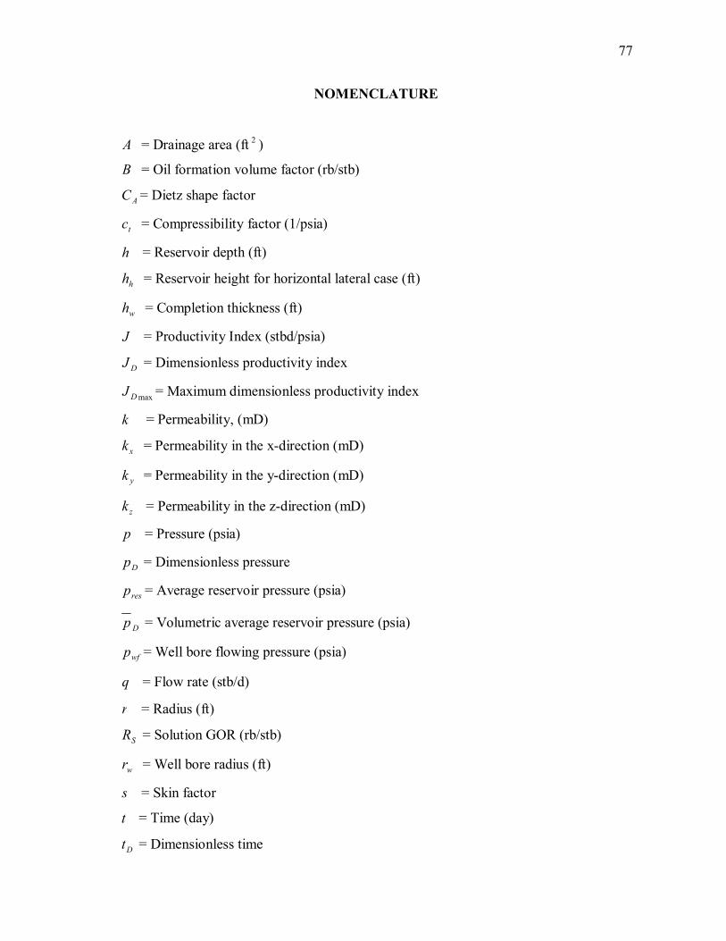
77
NOMENCLATURE
A = Drainage area (ft 2 )
B = Oil formation volume factor (rb/stb)
AC = Dietz shape factor
tc = Compressibility factor (1/psia)
h = Reservoir depth (ft)
hh = Reservoir height for horizontal lateral case (ft)
wh = Completion thickness (ft)
J = Productivity Index (stbd/psia)
DJ = Dimensionless productivity index
maxDJ = Maximum dimensionless productivity index
k = Permeability, (mD)
xk = Permeability in the x-direction (mD)
yk = Permeability in the y-direction (mD)
zk = Permeability in the z-direction (mD)
p = Pressure (psia)
Dp = Dimensionless pressure
resp = Average reservoir pressure (psia)
Dp = Volumetric average reservoir pressure (psia)
wfp = Well bore flowing pressure (psia)
q = Flow rate (stb/d)
r = Radius (ft)
SR = Solution GOR (rb/stb)
wr = Well bore radius (ft)
s = Skin factor
t = Time (day)
Dt = Dimensionless time
78
xfDt = Dimensionless time with respect to fx
eyDt = Dimensionless time with respect to ey
V = Reservoir pore volume (ft 3 )
ex = Length of rectangular reservoir in x-direction (ft)
fx = Fracture half length (ft)
hx = Reservoir x-dimension for horizontal lateral case (ft)
y = Length in y-direction (ft)
Dy = Dimensionless length in y-direction
ey = Length of rectangular reservoir in y-direction (ft)
hy = Reservoir y-dimension for horizontal lateral case (ft)
wz = Elevation (ft)
Greek Letters
φ = Porosity
γ = Euler’s constant, 1.78
µ = Viscosity, cp
79
REFERENCES
1. Oberkircher, J., Smith, R. and Thackwray, I.: “Boon or Bane? A Survey of the
First 10 Years of Modern Multilateral Wells,” paper SPE 84025 presented at the
2003 SPE Annual Technical Conference and Exhibition, Denver, Colorado, 5 – 8
October.
2. Oberkircher, J.: “Multilateral Technology as a Creative Reservoir Development
Strategy for New and Mature Fields Alike,” paper SPE 77826 presented at the
2002 SPE Asia Pacific Oil & Gas Conference and Exhibition, Melbourne,
Australia, 8-10 October.
3. Vullinghs, P. and Dech, J.A.: “Multilateral Well Utilization on the Increase,”
paper SPE 56954 presented at the 1999 Offshore Europe Conference, Aberdeen,
Scotland, 7-9 September.
4. Dittoe, S. R., Retnanto, A. and Economides, M. J.: “An Analysis of Reserves
Enhancement in Petroleum Reservoirs with Horizontal and Multilateral Wells”
paper SPE 37073 presented at the 1996 International Conference on Horizontal
Well Technology, Calgary, Canada, 18-20 November.
5. Retnanto. A., and Economides, M.J.: “Performance of Multiple Horizontal Wells
Laterals in Low-to-Medium Permeability Reservoirs,” paper SPE 29647
presented at the 1995 Western Regional Meeting, Bakersfield, California, 8-10
March.
6. Oberkircher, J.: “The Economic Viability of Multilateral Wells,” paper SPE
59202 presented at the 2000 IADC/SPE Drilling Conference, New Orleans,
Louisiana, 23-25 February.
7. Tantawi, I., Taylor, R. and Russell, R.: “The Successful Redevelopment of
Existing Well Using Multilateral Drilling Technique,” paper SPE 49477 presented

80
at the 1998 8th International Petroleum Exhibition and Conference, Abu Dhabi,
U.A.E., 11-14 October.
8. Mong, K., Al-Yami, H. and Lambe, S.: “The Application of Pressure Isolated
Multilateral Junction Improves Economics in Offshore Arabian Gulf,” paper SPE
77201 presented at the 2002 IADC/SPE Asia Pacific Drilling Technology,
Jakarta, Indonesia, 9-11 September.
9. “Horizontal and Multilateral Wells,” http://www.spe.org/spe/jsp/basic/0,,1104
_1714_1003974,00.html, 22 November 2003
10. Cavender, T., Roane, T.D. and Restarick, H.L. “Interfacing Fracturing and Sand
Control Completion Strategies into Multilateral Technology; Considerations and
Solutions,” paper SPE 80477 presented at the 2003 SPE Asia Pacific Oil and Gas
Conference and Exhibition, Jakarta, Indonesia, 15 – 17 April.
11. Berge, F., Hepburn, N., Bowling, J. and Gronas, T.: “A New Generation
Multilateral System for the Troll Olje Field – Development and Case History,”
paper SPE 71837 presented at the 2001 Offshore Europe Conference, Aberdeen,
Scotland, 4 – 7 September.
12. Rivera, N., Jensen, J.L., Spivey, J.P. and Jardon, M.: “Economic Comparisons of
Multilateral and Horizontal Wells in Water-Drive Reservoirs,” paper SPE 80927
presented at the 2003 SPE Production and Operations Symposium, Oklahoma
City, Oklahoma, 22 – 25 March.
13. Gutierrez, O.D., Romero, A.M., Carreno, Z., Garrido, M., Leon, A. and Mohtadi,
M.: “Using Multilateral Well Technology to Improve Recovery Factor by Water
Flooding in a Giant Oil Field in Venezuela Lagunilla Inferior (LL-03),” paper
SPE 78955 presented at the 2002 SPE International Thermal Operations and
81
Heavy Oil Symposium and International Horizontal Well Technology
Conference, Calgary, Alberta, Canada, 4 – 7 November.
14. Redlinger, T., Constantine, J., Makin, G. Brown, C., Cooke, D. et al.:
“Multilateral Technology Coupled with an Intelligent Completion System
Provides Increased Recovery in a Mature Field at BP Wytch Farm, UK,” paper
SPE/IADC 79887 presented at the 2003 SPE/IADC Drilling Conference,
Amsterdam, The Netherlands, 19 – 21 February.
15. Al-Azkawi, A, Taylor, G., Chadwick, R. and McGrain, B.: “Multilateral Wells
Improve Development of Heavy Crude Production in the Mukhaizna Field,
Sultanate of Oman,” paper SPE 79021 presented at the 2002 SPE International
Thermal Operations and Heavy Oil Symposium and International Horizontal Well
Technology Conference, Calgary, Alberta, Canada, 4 – 7 November.
16. Larsen, L.: “Productivity Computations for Multilateral, Branched and Other
Generalized and Extended Well Concepts,” paper SPE 36754 presented at the
1996 SPE Annual Technical Conference and Exhibition, Denver, Colorado, 6 – 9
October.
17. Salas, J.R., Clifford, P.J. and Jenkins, D.P.: “Multilateral Well Performance
Prediction,” paper SPE 35711 presented at the 1996 Western Regional Meeting,
Anchorage, Alaska, 22-24 May.
18. Yildiz, T.: “Long-Term Performance of Multilaterals in Commingled Reservoirs,”
paper SPE 78985 presented at the 2002 SPE International Thermal Operations
and Heavy Oil Symposium and International Horizontal Well Technology
Conference, Calgary, Alberta, Canada, 4 – 7 November.

82
19. Brister, R.: “Screening Variables for Multilateral Technology,” paper SPE 64698
presented at the 2000 SPE International Oil and Gas Conference, Beijing, China,
7 – 10 November.
20. Holditch. S.: “The Increasing Role of Unconventional Reservoirs in the Future of
Oil and Gas Business,” JPT (November 2003) 34.
21. Valko, P.P.: “Reservoir Applications of New Multilateral Field Drainage
Architectures and Related Technologies,” 2002, Report No. 2, Unpublished,
Texas A&M U., College Station, Texas.
22. Valko. P.P., Doublet, L.E. and Blasingame, T.A.: “Development and Application
of the Multi-Well Productivity Index (MPI),” SPEJ (March 2000)
23. Wattenbarger, R.A., El-Banbi, A.H., Villegas, M.E. and Maggard, J.B.:
“Production Analysis of Linear Flow into Fractured Tight Gas Wells,” paper SPE
39931 presented at the 1998 APE Rocky Mountain Regional Low Permeability
Reservoirs Symposium and Exhibition, Denver, Colorado, 5 – 8 April.
24. Economides, M.J., Hill, A.D. and Ehlig-Economides, C.: Petroleum Production
Systems, Prentice Hall, Inc., New Jersey (1994) 25.
25. Cinco-Ley, H., Ramey, H. J. and Miller, F.G.: “Pseudo-Skin Factors for Partially
Penetrating Directionally Drilled Wells,” paper SPE 5589 presented at the 1975
Annual Technical Conference and Exhibition, Dallas, Texas, 28 September – 1
October.
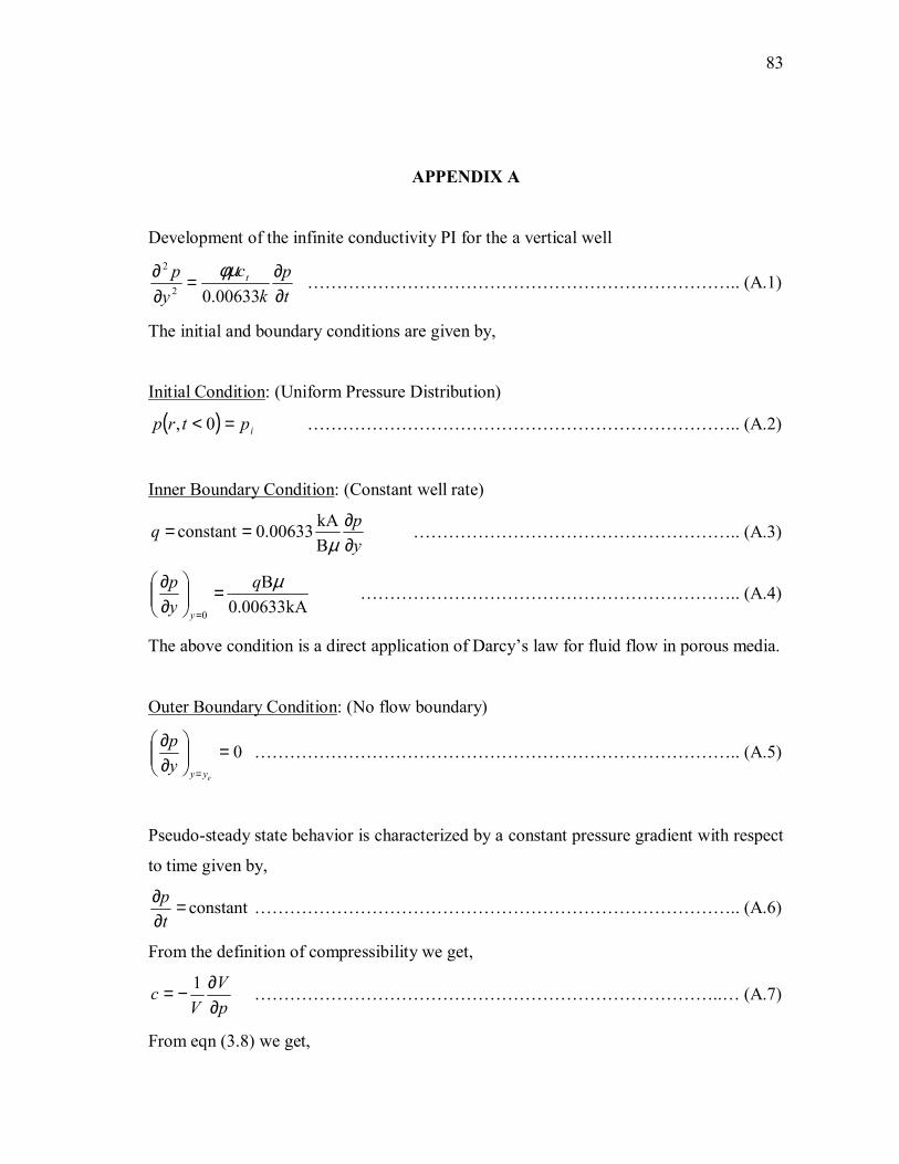
83
APPENDIX A
Development of the infinite conductivity PI for the a vertical well
tp
kc
yp t
∂∂=
∂∂
00633.02
2 φµ ……………………………………………………………….. (A.1)
The initial and boundary conditions are given by,
Initial Condition: (Uniform Pressure Distribution)
( ) iptrp =< 0, ……………………………………………………………….. (A.2)
Inner Boundary Condition: (Constant well rate)
ypq
∂∂==
µBkA0.00633constant ……………………………………………….. (A.3)
0.00633kAB
0
µqyp
y
=
∂∂
=
……………………………………………………….. (A.4)
The above condition is a direct application of Darcy’s law for fluid flow in porous media.
Outer Boundary Condition: (No flow boundary)
0=
∂∂
= eyyyp ……………………………………………………………………….. (A.5)
Pseudo-steady state behavior is characterized by a constant pressure gradient with respect
to time given by,
constant =∂∂
tp ……………………………………………………………………….. (A.6)
From the definition of compressibility we get,
pV
Vc
∂∂−= 1 ……………………………………………………………………..… (A.7)
From eqn (3.8) we get,

84
tV
cVtp
∂∂−=
∂∂ 1 ……………………………………………………………...... (A.8)
where,
AhV φ= ……………………………………………………………………….. (A.9)
Substituing eqn 3.11 into eqn. 3.10 gives,
AhcqB
tp
φ−=
∂∂ ……………………………………………………………..……….. (A.10)
The above equation obtained can also be used in terms of field units without applying any
conversion factor.
Substituting eqn 3.12 into eqn. 3.3 gives,
−=∂∂
AhcqB
kc
yp t
φφµ00633.02
2
……………………………………………………… (A.11)
The area of the rectangular geometry perpendicular to the flow is given as,
hxA f4= ……………………………………………………..……………….. (A.12)
Substituting eqn 3.14 into eqn. 3.13 gives,
( )hxkyqB
yp
fe 400633.02
2 µ−=∂∂ ……………………………………………………… (A.13)
In the above equation the flow rate q has units in Dft 3
which is converted to stock tank
barrel units. Also we multiply divide the above equation by π2 to obtain the diffusivity
equation in the form similar to the radial flow equation.
ef ykhxqB
yp µπ 2.141
22
2
−=∂∂ …....………………………………..……………….. (A.14)
To solve the diffusivity equation we convert it into dimensionless form using the
following dimensionless groups,
eD y
yy = …………………………………………………………………….... (A.15)
( )µqBppkh
p iD 2.141
−= ……………………………………………………………… (A.16)
2
00633.0
etD yc
kttφµ
= ……………………………………………………………… (A.17)
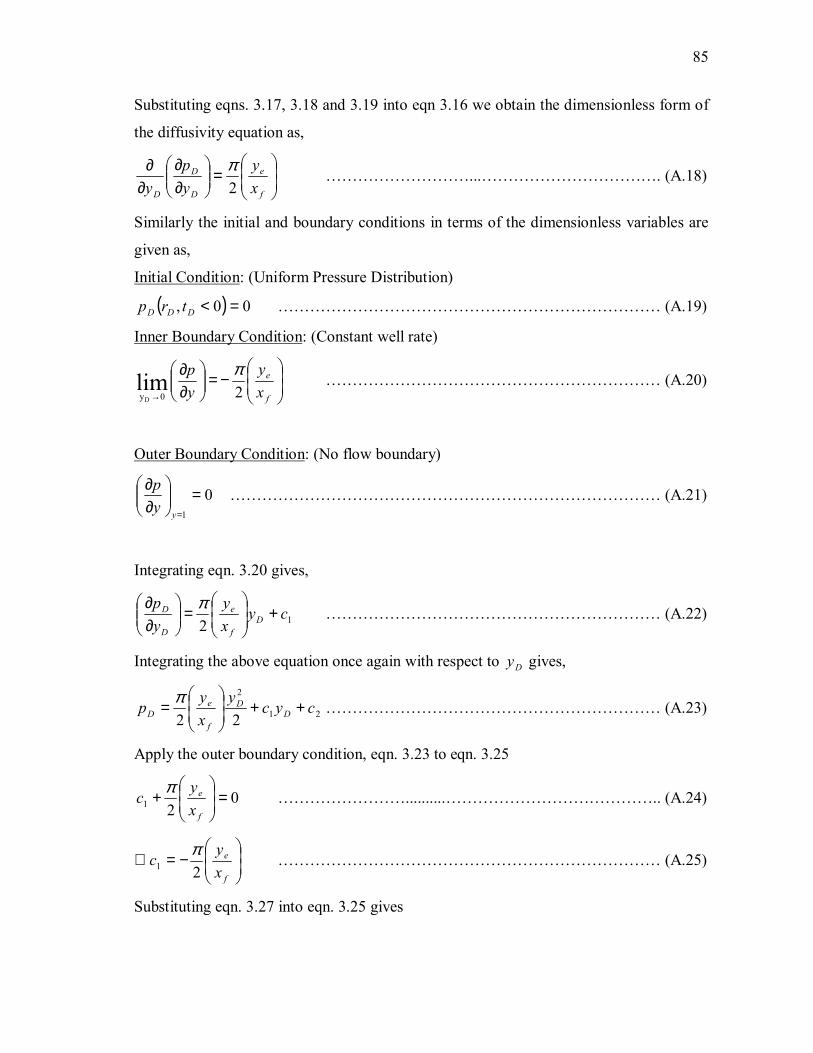
85
Substituting eqns. 3.17, 3.18 and 3.19 into eqn 3.16 we obtain the dimensionless form of
the diffusivity equation as,
=
∂∂
∂∂
f
e
D
D
D xy
yp
y 2π ………………………...……………………………. (A.18)
Similarly the initial and boundary conditions in terms of the dimensionless variables are
given as,
Initial Condition: (Uniform Pressure Distribution)
( ) 00, =<DDD trp ……………………………………………………………… (A.19)
Inner Boundary Condition: (Constant well rate)
−=
∂∂
→ f
e
xy
yp
2 lim
0yD
π ……………………………………………………… (A.20)
Outer Boundary Condition: (No flow boundary)
01
=
∂∂
=yyp ……………………………………………………………………… (A.21)
Integrating eqn. 3.20 gives,
12cy
xy
yp
Df
e
D
D +
=
∂∂ π ……………………………………………………… (A.22)
Integrating the above equation once again with respect to Dy gives,
21
2
22cyc
yxy
p DD
f
eD ++
= π ……………………………………………………… (A.23)
Apply the outer boundary condition, eqn. 3.23 to eqn. 3.25
021 =
+
f
e
xy
c π ……………………..........………………………………….. (A.24)
−=∴
f
e
xy
c21π ……………………………………………………………… (A.25)
Substituting eqn. 3.27 into eqn. 3.25 gives
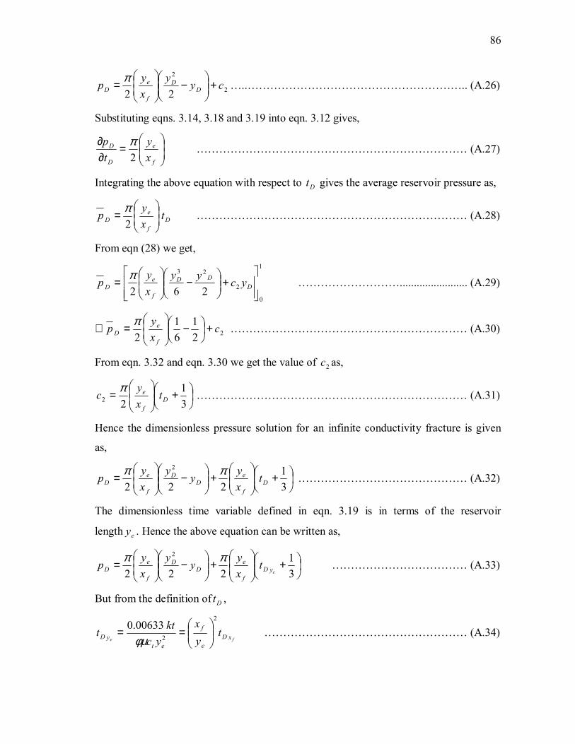
86
2
2
22cy
yxy
p DD
f
eD +
−
= π …..………………………………………………….. (A.26)
Substituting eqns. 3.14, 3.18 and 3.19 into eqn. 3.12 gives,
=
∂∂
f
e
D
D
xy
tp
2π ……………………………………………………………… (A.27)
Integrating the above equation with respect to Dt gives the average reservoir pressure as,
Df
eD t
xy
p
=
2π ……………………………………………………………… (A.28)
From eqn (28) we get, 1
0
2
23
262
+
−
= D
DD
f
eD ycyy
xy
p π ………………………........................ (A.29)
221
61
2c
xy
pf
eD +
−
=∴ π ……………………………………………………… (A.30)
From eqn. 3.32 and eqn. 3.30 we get the value of 2c as,
+
=
31
22 Df
e txy
c π ……………………………………………………………… (A.31)
Hence the dimensionless pressure solution for an infinite conductivity fracture is given
as,
+
+
−
=
31
222
2
Df
eD
D
f
eD t
xy
yy
xy
p ππ ……………………………………… (A.32)
The dimensionless time variable defined in eqn. 3.19 is in terms of the reservoir
length ey . Hence the above equation can be written as,
+
+
−
=
31
222
2
eyDf
eD
D
f
eD t
xy
yy
xy
p ππ ……………………………… (A.33)
But from the definition of Dt ,
fe xDe
f
etyD t
yx
ycktt
2
2
00633.0
==
φµ ……………………………………………… (A.34)

87
fe xDe
fyD
f
e tyx
txy
=
∴ ……………………………………………………… (A.35)
Hence the general solution for the dimensionless pressure is given as,
+
+
−
=
f
exD
e
fD
D
f
eD x
yt
yx
yy
xy
pf 6222
2 πππ ……………………………… (A.36)
The solution at the well bore with 0=Dy is given as,
+
=
f
exD
e
fDw x
yt
yx
pf 62
ππ ……………………………………………… (A.37)
The average reservoir pressure is obtained from eqn. 3.30 while the pressure at the well
bore is obtained from eqn. 3.39 by substituting into the definition for dimensionless
pressures and generating the corresponding pressures. These pressures are then used to
obtain the PI for constant rate condition as,
=
f
e
CR
xy
B
khJ
62.141 πµ
……………………………………………………… (A.38)
The general definition for PI in terms of the dimensionless PI is given as,
DCR JB
khJµ2.141
= ……………………………………………………………… (A.39)
Comparing eqns. 3.40 and 3.41 we obtain the maximum dimensionless PI as,
π6
max, =DJ ……………………………………………………………………… (A.40)

88
APPENDIX B
The following data file is used to simulate a case where 15 laterals penetrate the reservoir
at a depth of 365 ft from the top of the reservoir.
-- -- ------------------------------------------------------------------------------------------------ -- Office Simulation File - Multilateral Well Architecture is used to drain the field -- ------------------------------------------------------------------------------------------------ -- RUNSPEC TITLE VERSION 1 Jabillos - 62x21x11 START 30 'DEC' 1987 / FIELD GAS OIL WATER DISGAS SAVE 'UNFORMATTED' / MONITOR RSSPEC DIMENS -- NX NY NZ 62 21 11 / WELLDIMS -- MX CON/WELL GRPS WLL/GRP 1 671 1 1/ -- Maximum number of connections WSEGDIMS 1 723 63/ -- DIMENSION OF MULTISEGMENT WELL -------------------------------------------------------------------------------- GRID --------------------------------------------------------------------------------

89
EQUALS -- PROP VALUE IX1 IX2 JY1 JY2 KZ1 KZ2 'DX' 322.58 1 62 1 21 1 11 / 'DY' 476.19 1 62 1 21 1 11 / 'DZ' 68.18 1 62 1 21 1 11 / 'TOPS' 14500 1 62 1 21 1 1 / -- CRETACEOUS-01 RESSERVOIR , 750 FT 'PERMX' 86.6 1 62 1 21 1 11/ 'PERMY' 28.67 1 62 1 21 1 11/ 'PERMZ' 2.6 1 62 1 21 1 11/ 'PORO' .12 1 62 1 21 1 11/ / GRIDFILE 2 / INIT -------------------------------------------------------------------------------- EDIT -------------------------------------------------------------------------------- -------------------------------------------------------------------------------- PROPS -------------------------------------------------------------------------------- PMAX -- Maximum Simulation Pressure 11200 1* 1* 1* / DENSITY -- Fluid Densities at Surface Conditions -- sto wat gas (lbm/ft3) 54.637 62.4 0.068432 / ROCK -- Rock Properties 7000 3e-006 / PVCO -- Live Oil PVT Properties (Dissolved Gas) -- pbub Rs Bo vis coil cvis -- psia mcf/stb rb/stb cp 1/psi 1/psi 500 0.054 1.045 7666 1.5296e-005 2.022e-005 714.286 0.0558333 1.0474 7366.34 1.5296e-005 2.022e-005 1428.57 0.125625 1.08002 1251.99 1.5296e-005 2.022e-005 2142.86 0.215357 1.124 212.79 1.5296e-005 2.022e-005

90
2857.14 0.335 1.18504 36.166 1.5296e-005 2.022e-005 3571.43 0.5025 1.27335 6.1468 1.5296e-005 2.022e-005 4285.71 0.75375 1.4094 1.04472 1.5296e-005 2.022e-005 4642.86 0.933214 1.50811 0.430698 1.5296e-005 2.022e-005 5000 1.1725 1.64093 0.177561 1.5296e-005 2.022e-005 / PVZG -- Dry Gas PVT Properties (using Z-factors) -- press z-fac gas vis -- psia cp -- 290 / 500 0.922 0.03 1000 0.922 0.03 2000 0.893 0.03 3000 0.902 0.03 4000 0.935 0.03 5000 1 0.03 / PVTW -- Water PVT Properties -- p Bw cw vis cvis -- psia rb/stb 1/psi cp 1/psi 4789.7 1 3e-006 0.15 0 / ------------------------------------------------------------------------------- STONE1 -- SWFN -- Water Saturation Functions -- sw krw pcow 0.14 0 0 0.16 0.00025 0 0.2 0.00085 0 0.3 0.0083 0 0.4 0.035 0 0.5 0.049 0 0.6 0.106 0 0.64 0.134 0 0.7 0.19 0 0.8 0.32 0 0.9 0.493 0 1 1 0 /
91
-- Gas rel perm and cap pressure SGFN -- sg krg pcgo 0 0 0 0.05 8e-006 0 0.1 1e-005 0 0.2 0.0025 0 0.3 0.0133 0 0.4 0.0434 0 0.5 0.1082 0 0.6 0.2285 0 0.73 0.5107 0 0.86 1 0 / SOF3 -- Oil Saturation Functions -- Soil krow krog 0 0 0 0.1 0.01 0.0001 0.2 0.0194 0.0054 0.3 0.028 0.009 0.36 0.03 0.016 0.4 0.039 0.035 0.5 0.084 0.05 0.6 0.173 0.1 0.7 0.302 0.28 0.8 0.615 0.54 0.84 0.81 0.716 0.86 1 1 / ------------------------------------------------------------------------------- REGIONS ------------------------------------------------------------------------------- ------------------------------------------------------------------------------- SOLUTION ------------------------------------------------------------------------------- EQUIL -- Equilibration Data Specification 14875 11200 16250 0 13000 0 1 1 -20 / RSVD -- depth Rs (mcf/stb) 12000 1.14504 14350 0.874212 14646 0.7475 14700 0.619152

92
14800 0.538511 14880 0.330833 14960 0.244157 15000 0.0558333 16500 0.0558333 / -- Switch echo output off NOECHO DATUM 14875 / RPTSOL -- Initialisation Print Output 'FIP=2' 'EQUIL' 'VOIL' / ------------------------------------------------------------------------------- SUMMARY ------------------------------------------------------------------------------- RPTSMRY 1 / RPTONLY FPR WBHP / FOIP FOPR FWPR FGPR FOPT RUNSUM EXCEL SEPARATE

93
------------------------------------------------------------------------------- SCHEDULE ------------------------------------------------------------------------------- DRSDT 0.0003 1* / RPTRST BASIC=2 VISC / TUNING 1* 31 8* / 11* / 4* 31 5* / RPTSCHED 'RESTART=2' 'FIP=2' 'WELLS=4' 'CPU=1' 'TUNING' / WSEGITER --ITERMAX 50 / WELSPECS -- NAME GRP I J BHPDTH WELL1 'ESTE' 1 11 14875 'OIL' / / COMPDAT -- Well I J K K Flag ..... -- Name (up) (down) WELL1 1 11 4 4 'SHUT' 2* 3.00 3* X / WELL1 62 11 4 4 'SHUT' 2* 3.00 3* X / WELL1 3 11 4 4 OPEN 2* 0.3 3* Y / WELL1 3 10 4 4 OPEN 2* 0.3 3* Y / WELL1 3 9 4 4 OPEN 2* 0.3 3* Y / WELL1 3 8 4 4 OPEN 2* 0.3 3* Y / WELL1 3 7 4 4 OPEN 2* 0.3 3* Y / WELL1 3 6 4 4 OPEN 2* 0.3 3* Y / WELL1 7 11 4 4 OPEN 2* 0.3 3* Y / WELL1 7 12 4 4 OPEN 2* 0.3 3* Y / WELL1 7 13 4 4 OPEN 2* 0.3 3* Y / WELL1 7 14 4 4 OPEN 2* 0.3 3* Y / WELL1 7 15 4 4 OPEN 2* 0.3 3* Y / WELL1 7 16 4 4 OPEN 2* 0.3 3* Y / WELL1 11 11 4 4 OPEN 2* 0.3 3* Y /
94
WELL1 11 10 4 4 OPEN 2* 0.3 3* Y / WELL1 11 9 4 4 OPEN 2* 0.3 3* Y / WELL1 11 8 4 4 OPEN 2* 0.3 3* Y / WELL1 11 7 4 4 OPEN 2* 0.3 3* Y / WELL1 11 6 4 4 OPEN 2* 0.3 3* Y / WELL1 15 11 4 4 OPEN 2* 0.3 3* Y / WELL1 15 12 4 4 OPEN 2* 0.3 3* Y / WELL1 15 13 4 4 OPEN 2* 0.3 3* Y / WELL1 15 14 4 4 OPEN 2* 0.3 3* Y / WELL1 15 15 4 4 OPEN 2* 0.3 3* Y / WELL1 15 16 4 4 OPEN 2* 0.3 3* Y / WELL1 19 11 4 4 OPEN 2* 0.3 3* Y / WELL1 19 10 4 4 OPEN 2* 0.3 3* Y / WELL1 19 9 4 4 OPEN 2* 0.3 3* Y / WELL1 19 8 4 4 OPEN 2* 0.3 3* Y / WELL1 19 7 4 4 OPEN 2* 0.3 3* Y / WELL1 19 6 4 4 OPEN 2* 0.3 3* Y / WELL1 23 11 4 4 OPEN 2* 0.3 3* Y / WELL1 23 12 4 4 OPEN 2* 0.3 3* Y / WELL1 23 13 4 4 OPEN 2* 0.3 3* Y / WELL1 23 14 4 4 OPEN 2* 0.3 3* Y / WELL1 23 15 4 4 OPEN 2* 0.3 3* Y / WELL1 23 16 4 4 OPEN 2* 0.3 3* Y / WELL1 27 11 4 4 OPEN 2* 0.3 3* Y / WELL1 27 10 4 4 OPEN 2* 0.3 3* Y / WELL1 27 9 4 4 OPEN 2* 0.3 3* Y / WELL1 27 8 4 4 OPEN 2* 0.3 3* Y / WELL1 27 7 4 4 OPEN 2* 0.3 3* Y / WELL1 27 6 4 4 OPEN 2* 0.3 3* Y / WELL1 32 11 4 4 OPEN 2* 0.3 3* Y / WELL1 32 12 4 4 OPEN 2* 0.3 3* Y / WELL1 32 13 4 4 OPEN 2* 0.3 3* Y / WELL1 32 14 4 4 OPEN 2* 0.3 3* Y / WELL1 32 15 4 4 OPEN 2* 0.3 3* Y / WELL1 32 16 4 4 OPEN 2* 0.3 3* Y / WELL1 36 11 4 4 OPEN 2* 0.3 3* Y / WELL1 36 10 4 4 OPEN 2* 0.3 3* Y / WELL1 36 9 4 4 OPEN 2* 0.3 3* Y / WELL1 36 8 4 4 OPEN 2* 0.3 3* Y / WELL1 36 7 4 4 OPEN 2* 0.3 3* Y / WELL1 36 6 4 4 OPEN 2* 0.3 3* Y / WELL1 40 11 4 4 OPEN 2* 0.3 3* Y / WELL1 40 12 4 4 OPEN 2* 0.3 3* Y / WELL1 40 13 4 4 OPEN 2* 0.3 3* Y /
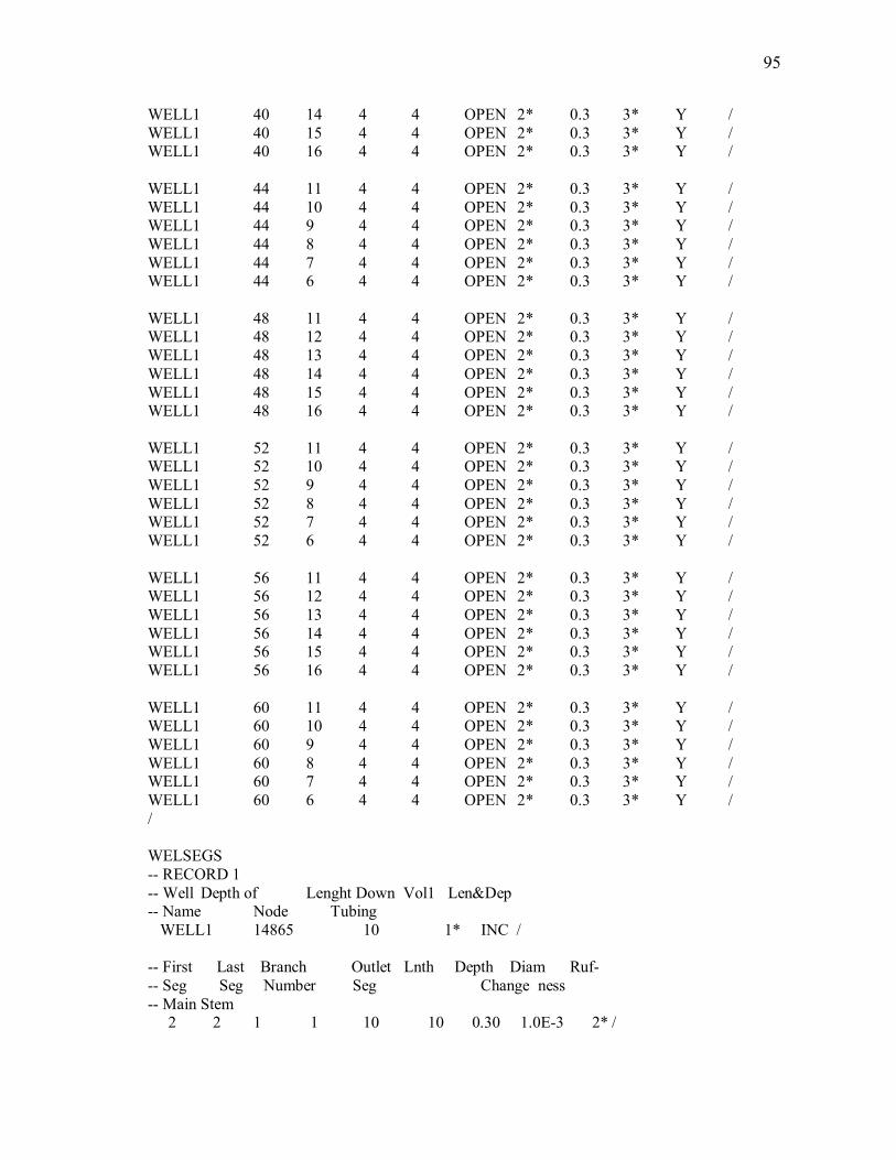
95
WELL1 40 14 4 4 OPEN 2* 0.3 3* Y / WELL1 40 15 4 4 OPEN 2* 0.3 3* Y / WELL1 40 16 4 4 OPEN 2* 0.3 3* Y / WELL1 44 11 4 4 OPEN 2* 0.3 3* Y / WELL1 44 10 4 4 OPEN 2* 0.3 3* Y / WELL1 44 9 4 4 OPEN 2* 0.3 3* Y / WELL1 44 8 4 4 OPEN 2* 0.3 3* Y / WELL1 44 7 4 4 OPEN 2* 0.3 3* Y / WELL1 44 6 4 4 OPEN 2* 0.3 3* Y / WELL1 48 11 4 4 OPEN 2* 0.3 3* Y / WELL1 48 12 4 4 OPEN 2* 0.3 3* Y / WELL1 48 13 4 4 OPEN 2* 0.3 3* Y / WELL1 48 14 4 4 OPEN 2* 0.3 3* Y / WELL1 48 15 4 4 OPEN 2* 0.3 3* Y / WELL1 48 16 4 4 OPEN 2* 0.3 3* Y / WELL1 52 11 4 4 OPEN 2* 0.3 3* Y / WELL1 52 10 4 4 OPEN 2* 0.3 3* Y / WELL1 52 9 4 4 OPEN 2* 0.3 3* Y / WELL1 52 8 4 4 OPEN 2* 0.3 3* Y / WELL1 52 7 4 4 OPEN 2* 0.3 3* Y / WELL1 52 6 4 4 OPEN 2* 0.3 3* Y / WELL1 56 11 4 4 OPEN 2* 0.3 3* Y / WELL1 56 12 4 4 OPEN 2* 0.3 3* Y / WELL1 56 13 4 4 OPEN 2* 0.3 3* Y / WELL1 56 14 4 4 OPEN 2* 0.3 3* Y / WELL1 56 15 4 4 OPEN 2* 0.3 3* Y / WELL1 56 16 4 4 OPEN 2* 0.3 3* Y / WELL1 60 11 4 4 OPEN 2* 0.3 3* Y / WELL1 60 10 4 4 OPEN 2* 0.3 3* Y / WELL1 60 9 4 4 OPEN 2* 0.3 3* Y / WELL1 60 8 4 4 OPEN 2* 0.3 3* Y / WELL1 60 7 4 4 OPEN 2* 0.3 3* Y / WELL1 60 6 4 4 OPEN 2* 0.3 3* Y / / WELSEGS -- RECORD 1 -- Well Depth of Lenght Down Vol1 Len&Dep -- Name Node Tubing WELL1 14865 10 1* INC / -- First Last Branch Outlet Lnth Depth Diam Ruf- -- Seg Seg Number Seg Change ness -- Main Stem 2 2 1 1 10 10 0.30 1.0E-3 2* /

96
3 63 2 2 322.58 0 3.00 1.0E-3 2* / 64 69 3 5 476.2 0 0.3 0.001 2* / 70 75 4 9 476.2 0 0.3 0.001 2* / 76 81 5 13 476.2 0 0.3 0.001 2* / 82 87 6 17 476.2 0 0.3 0.001 2* / 88 93 7 21 476.2 0 0.3 0.001 2* / 94 99 8 25 476.2 0 0.3 0.001 2* / 100 105 9 29 476.2 0 0.3 0.001 2* / 106 111 10 34 476.2 0 0.3 0.001 2* / 112 117 11 38 476.2 0 0.3 0.001 2* / 118 123 12 42 476.2 0 0.3 0.001 2* / 124 129 13 46 476.2 0 0.3 0.001 2* / 130 135 14 50 476.2 0 0.3 0.001 2* / 136 141 15 54 476.2 0 0.3 0.001 2* / 142 147 16 58 476.2 0 0.3 0.001 2* / 148 153 17 62 476.2 0 0.3 0.001 2* / / COMPSEGS -- Name WELL1 / -- I J K Brn Start End Dir End -- No Length Length Pent Range -- Main Horizontal branch 1 11 4 2 10.00 1* X 62 / 3 11 4 3 1* 1* Y 6 / 7 11 4 4 1* 1* Y 16 / 11 11 4 5 1* 1* Y 6 / 15 11 4 6 1* 1* Y 16 / 19 11 4 7 1* 1* Y 6 / 23 11 4 8 1* 1* Y 16 / 27 11 4 9 1* 1* Y 6 / 32 11 4 10 1* 1* Y 16 / 36 11 4 11 1* 1* Y 6 / 40 11 4 12 1* 1* Y 16 / 44 11 4 13 1* 1* Y 6 / 48 11 4 14 1* 1* Y 16 / 52 11 4 15 1* 1* Y 6 / 56 11 4 16 1* 1* Y 16 / 60 11 4 17 1* 1* Y 6 / / WCONPROD -- Name Flag Control Qoilmax Limits BHP WELL1 'OPEN' 'ORAT' 63000.00 / /

97
TSTEP 6*30 / WCONPROD -- Name Flag Control Qoilmax Limits BHP WELL1 'OPEN' 'ORAT' 59000.00 / / TSTEP 6*30 / WCONPROD -- Name Flag Control Qoilmax Limits BHP WELL1 'OPEN' 'ORAT' 49000.00 / / TSTEP 6*30 / WCONPROD -- Name Flag Control Qoilmax Limits BHP WELL1 'OPEN' 'ORAT' 40000.00 / / TSTEP 6*30 / WCONPROD -- Name Flag Control Qoilmax Limits BHP WELL1 'OPEN' 'ORAT' 32000.00 / / TSTEP 6*30 / WCONPROD -- Name Flag Control Qoilmax Limits BHP WELL1 'OPEN' 'ORAT' 27000.00 / / TSTEP 6*30 / END
98
VITA
Manoj Sarfare holds a B.E. degree in petrochemical engineering from
Maharashtra Institute of Technology, Pune, India. He worked with Dr. Peter Valkó as a
Research Assistant on the industry funded project on Reservoir Applications of
Advanced Multilateral Well Technology.
His current address: Texas A&M University
Attn.: Dr. Peter. P. Valkó
Harold Vance Department of Petroleum Engineering
3116 TAMU
College Station, TX 77843-3116
USA
Related Documents