RESERVOIR CHARACTERIZATION USING EXPERIMENTAL DESIGN AND RESPONSE SURFACE METHODOLOGY A Thesis by HARSHAL PARIKH Submitted to the Office of Graduate Studies of Texas A&M University in partial fulfillment of the requirements for the degree of MASTER OF SCIENCE August 2003 Major Subject: Petroleum Engineering

Welcome message from author
This document is posted to help you gain knowledge. Please leave a comment to let me know what you think about it! Share it to your friends and learn new things together.
Transcript
RESERVOIR CHARACTERIZATION USING
EXPERIMENTAL DESIGN AND RESPONSE SURFACE
METHODOLOGY
A Thesis
by
HARSHAL PARIKH
Submitted to the Office of Graduate Studies of Texas A&M University
in partial fulfillment of the requirements for the degree of
MASTER OF SCIENCE
August 2003
Major Subject: Petroleum Engineering
RESERVOIR CHARACTERIZATION USING
EXPERIMENTAL DESIGN AND RESPONSE SURFACE
METHODOLOGY
A Thesis
by
HARSHAL PARIKH
Submitted to the Office of Graduate Studies of Texas A&M University
in partial fulfillment of the requirements for the degree of
MASTER OF SCIENCE
Approved as to style and content by:
_______________________________ Akhil Datta-Gupta
(Chair of Committee)
_______________________________ W. John Lee
(Member)
_______________________________ Bani K. Mallick
(Member)
_______________________________ Hans C. Juvkam-Wold (Head of Department)
August 2003
Major Subject: Petroleum Engineering
iii
ABSTRACT
Reservoir Characterization Using Experimental Design and Response Surface
Methodology. (August 2003)
Harshal Parikh, B.S., Mumbai University Institute of Chemical Technology
Chair of Advisory Committee: Dr. Akhil Datta-Gupta
This research combines a statistical tool called experimental design/response surface
methodology with reservoir modeling and flow simulation for the purpose of reservoir
characterization. Very often, it requires large number of reservoir simulation runs for
identifying significant reservoir modeling parameters impacting flow response and for
history matching. Experimental design/response surface (ED/RS) is a statistical
technique, which allows a systematic approach for minimizing the number of simulation
runs to meet the two objectives mentioned above. This methodology may be applied to
synthetic and field cases using existing statistical software tools.
The application of ED/RS methodology for the purpose of reservoir characterization
has been applied for two different objectives. The first objective is to address the
uncertainties in the identification of the location and transmissibility of flow barriers in a
field in the Gulf of Mexico. This objective is achieved by setting up a simple full-
factorial design. The range of transmissibility of the barriers is selected using a Latin
Hypercube Sampling (LHS). An analysis of variance (ANOVA) gives the significance
of the location and transmissibility of barriers and comparison with decline-type curve
analysis which gives us the most likely scenarios of the location and transmissibility of
the flow barriers. The second objective is to identify significant geologic parameters in
object-based and pixel-based reservoir models. This study is applied on a synthetic
fluvial reservoir, whose characteristic feature is the presence of sinuous sand filled
channels within a background of floodplain shale. This particular study reveals the
impact of uncertainty in the reservoir modeling parameters on the flow performance.

iv
Box-Behnken design is used in this study to reduce the number of simulation runs along
with streamline simulation for flow modeling purposes.
In the first study, we find a good match between field data and that predicted from
streamline simulation based on the most likely scenario. This validates the use of ED to
get the most likely scenario for the location and transmissibility of flow barriers. It can
be concluded from the second study that ED/RS methodology is a powerful tool along
with a fast streamline simulator to screen large number of reservoir model realizations
for the purpose of studying the effect of uncertainty of geologic modeling parameters on
reservoir flow behavior.

v
DEDICATION
To my beloved parents, my brother, Niraj, and to my lovely fiancé, Sheetal, for their
love, care, and inspiration.

vi
ACKNOWLEDGMENTS
I would like to take this opportunity to express my deepest gratitude and appreciation to
the people who have given me their assistance throughout my studies and during the
preparation of this thesis. I would especially like to thank my advisor and committee
chair, Dr. Akhil Datta-Gupta, for his continuous encouragement, financial support, and
especially for his academic guidance.
I would like to thank Dr. W. John Lee and Dr. Bani K. Mallick for serving as
committee members, and I do very much acknowledge their friendliness, guidance and
helpful comments while working towards my graduation.
Finally, I want to thank my friends in the reservoir characterization group, Dr. Arun
Khargoria (now with Petrotel), Dr. Zhong He, Dr. Sang Heon Lee (now with
ChevronTexaco), Ichiro Osako, Hao Cheng, Ahmed Daoud and Nam Il for making my
graduate years very pleasant. The facilities and resources provided by the Harold Vance
Department of Petroleum Engineering, Texas A&M University, are gratefully
acknowledged. I thank Texas A&M University for educating me in various ways, and
for providing me with the very best education there is. I would like to take the
opportunity to thank the faculty and staff for helping me prepare for a life after
graduation.
I am going to remember these years of hard work with great pleasure. To all of you, I
appreciate what you have done to help me in my scholastic and professional growth. I
would like to thank you for providing me with a work environment that lends itself to
creativity and productivity, without too many financial concerns. Not everyone is so
fortunate. I know I still have much to learn, but with continued support and
encouragement from people like you I know I can accomplish a great deal.
Thank you very much.

vii
TABLE OF CONTENTS
Page
ABSTRACT…………………………………………………………………….…...… iii
DEDICATION………………………………………………….….…………….…….. v
ACKNOWLEDGMENTS…………………………………………….………….…. vi
TABLE OF CONTENTS…………………………………………….…………….… vii
LIST OF FIGURES…………………………………………………………………….. ix
LIST OF TABLES…………………………………………………………………... xi
CHAPTER
I INTRODUCTION - APPLICATION OF EXPERIMENTAL DESIGN/RESPONSE SURFACE METHODOLOGY IN RESERVOIR CHARACTERIZATION………………………… …………………………..... 1
1.1 Experimental Design and Response Surface....………….……........2 1.2 Identification of Most Likely Reservoir Scenario ..…………...…...5 1.3 Uncertainty Analysis of Reservoir Modeling Parameters ............ 7
II EVALUATING UNCERTAINTIES IN IDENTIFICATION OF LOCATION AND TRANSMISSIBILITY OF FLOW BARRIERS.. ..……….10
2.1 Well Drainage Volume …………..……………………………………11 2.1.1 Drainage Volume From Decline Type-Curve...……….11 2.1.2 Drainage Volume From Streamline 'Diffusive' Time of Flight…………...…………...………… …………...14 2.1.3 Drainage Volume Matching ……………………….….17
2.2 Quantifying Uncertainties via ED ………..……………………….20 2.2.1 Full Factorial Design and LHS ..........………...…….....20 2.2.2 Analysis of Variance…………………………………..22 2.2.3 Most Likely Scenario..……………………………......28
2.3 Discussion and Conclusions……………..……………….….............. 31
III IDENTIFICATION OF SIGNIFICANT RESERVOIR MODELING PARAMETERS IN FLOW RESPONSE……………………………… ………33
3.1 Box-Behnken Design ....................................................………………33 3.2 Streamline Simulation ………......................................……………... 35 3.3 Object-Based Model ............................................…...…..…………….38

viii
CHAPTER Page
3.3.1 Identification and Uncertainty Analysis ……….........44 3.3.2 Results and Conclusions......………………………......48
3.4 Pixel-Based Model ………..…………………………………………....49 3.4.1 Identification and Uncertainty Analysis……………… 52 3.4.2 Results and Conclusions.......………………………......57
3.5 Discussion............................……………..……………….…...58
IV CONCLUSIONS AND FUTURE WORK………..… ..……………………… 63
NOMENCLATURE………………………………………………………….………. 65
REFERENCES……………………………………………………………...……….. 67
APPENDIX A……………………………………………………………...……...….. 72
APPENDIX B……………………………………………………………...……...….. 74
VITA………………………………………………………………………...……...… 76

ix
LIST OF FIGURES FIGURE Page 1.1 Examples of designs for three factors…………………………………………..4
2.1 Well production rate and flow bottomhole pressure of the production well for the field case ............................................................................................ 10
2.2 Decline type-curve matching of production well. ........................................... 13 2.3 Decline type-curve matching of late-time data points..................................... 14 2.4 Permeability model of the field.. .................................................................... 16 2.5 Porosity model of the field............................................................................. 17 2.6 Permeability of layer 10 and potential flow barriers ....................................... 19 2.7 φ∗h*So of layer 10 and potential flow barriers ............................................... 19 2.8 Drainage volume matching for different south barrier locations ..................... 19 2.9 Calculated well bottomhole pressure vs. observed bottomhole pressure for the scenario of X2 and J=25........................................................................... 30 2.10 Calculated well bottomhole pressure vs. observed bottomhole pressure for the scenario of X7 and J=22........................................................................... 30 2.11 Calculated well bottomhole pressure vs. observed bottomhole pressure for the scenario of X6 and J=25........................................................................... 31 3.1 Plan and section view of conceptual model for fluvial facies: background of floodplain shale, sand–filled abandoned channel and levee border sand ..... 39 3.2 Areal view of some parameters used to define channel object: (a) angle for channel direction and deviation for actual channel center line and (b)
variable channel width with connection between channel cross section lines. 39 3.3 Cross section view of channel object defined by width, thickness, and relative position of maximum thickness. ........................................................ 40
x
FIGURE Page 3.4 Cross section through abandoned sand-filled channel and levee sand. Three
distance parameters (A), (B) and (C) are used to define size of levee sand.. ... 40 3.5 The synthetic reservoir case with an injector-producer in Quarter 5-spot
pattern. ......................................................................................................... 43 3.6 Plots at a particular experimental design point for object-based models: (a)
permeability field, (b) swept region at 5000 days, and (c) travel time plot...... 43 3.7 Response surface validation for object-based modeling parameters................ 46 3.8 Residuals v/s predicted sweep volume for object-based models. .................... 46 3.9 Response surfaces over the uncertainty range of object-based modeling
parameters. .................................................................................................... 47 3.10 Scenarios predicted by response surface in object-based models to give (a)
best sweep efficiency, and (b) worst sweep efficiency. .................................. 48 3.11 Plots at a particular experimental design point in pixel-based models: (a)
permeability field, (b) swept region at 5000 days, and (c) travel time plot...... 52 3.12 Response surface validation for pixel-based modeling parameters ................. 55 3.13 Residuals vs. predicted sweep efficiency for pixel-based models ................... 55 3.14 Response surfaces over the uncertainty range of pixel-based modeling
parameters. .................................................................................................... 56 3.15 Scenarios predicted by response surface in pixel-based models to give (a)
best sweep efficiency, and (b) worst sweep efficiency. .................................. 57 3.16 Response surfaces of sweep volume variances over the uncertainty range
of modeling parameters in object-based models................................................61 3.17 Scenarios predicted by response surface of variances in sweep volume for
object-based models to give (a) minimum sweep efficiency variance, and (b) maximum sweep efficiency variance.......................................................... 62

xi
LIST OF TABLES TABLE Page 1 Comparison of drainage volume for different locations of the south barrier..18 2 Comparison of drainage volume for different transmissibility multipliers
for the NW barrier ...................................................................................... 18 3 Factor ranges............................................................................................... 21 4 Equiprobable ranges for the south and northwest transmissibilities.............. 21 5 Transmissibility multipliers of the south and NW barriers obtained
using Latin Hypercube Sampling................................................................. 22 6 Experimental design set-up for drainage volume from streamline
simulation for different scenarios ................................................................ 22 7 Analysis of Variance (ANOVA).................................................................. 24 8 SNK test for transmissibility means............................................................. 26 9 SNK test for location means ........................................................................ 27 10 Tukey test for transmissibility means........................................................... 27 11 Tukey test for location means ...................................................................... 28 12 Drainage volume means over different transmissibility multipliers .............. 29 13 Drainage volume means over different locations for most likely
transmissibility multipliers .......................................................................... 29 14 Factor ranges and scaling for object-based models....................................... 42 15 Experimental design: object-based model.................................................... 42 16 Response surface coefficients: object-based models .................................... 45 17 Scenarios with highest and lowest sweep efficiency in object-based models......................................................................................................... 46 18 Factor ranges and scaling for pixel-based models ........................................ 51

xii
TABLE Page 19 Experimental design: pixel-based model...................................................... 51 20 Response surface coefficients: pixel based models ...................................... 54 21 Scenarios with highest and lowest sweep efficiency in pixel-based models.. 55 22 Scenarios with minimum and maximum variances in object-based models. . 60

1
CHAPTER I
INTRODUCTION - APPLICATION OF EXPERIMENTAL
DESIGN/RESPONSE SURFACE METHODOLOGY IN RESERVOIR
CHARACTERIZATION
Reservoir characterization is one of the most important phases in reservoir studies. A
reservoir model is first developed with static data using a particular type of reservoir
modeling technique. Geostatistical simulation is one example for deriving a realistic
reservoir description. However, the reservoir modeling parameters are highly uncertain.
This leads to an uncertain framework of the reservoir model. Uncertainty in the reservoir
model itself introduces an uncertainty in the flow simulation results. As a result it
becomes necessary to study the impact of uncertain geologic modeling parameters on the
flow performance. However, these kinds of studies typically require a large number of
simulation runs. This suggests that it would take too much time to get an accurate
description of the reservoir model, rendering the study unfeasible for quick decision
making. For that reason, this research proposes to combine flow simulation with a
statistical tool called experimental design and response surface methodology (ED/RS).
ED/RS reduces the number of simulation runs by intelligently choosing the
combinations of reservoir modeling/geologic parameters to change within their
uncertainty range.
ED/RS methodology has been previously used in reservoir characterization
applications including uncertainty modeling,1-5 sensitivity studies1,5 and history
matching.6-9 It has also been widely used in performance predictions within the oil
industry.10-16
One of the objectives of this thesis was to use experimental design to maximize the
information derived from the flow simulation of various geologic models. Previous
This thesis follows the style of the Journal of Petroleum Technology.
2
studies have been performed on models generated by pixel-based modeling techniques,
which essentially follow variogram-based geostatistical algorithms.1,3,5 Some studies
have also been performed on object-based models.2,4 This research attempts to assess
uncertainty in reservoir modeling parameters for both pixel-based and object-based
models under similar geologic settings. This gives an insight into which modeling
parameters are significant in both the modeling techniques and gives us a basis to
compare the modeling parameters of the two methods. It is shown that the channel
permeabilities and the sandstone ratio, which are common modeling parameters in both
the cases, have the most significant effect on flow simulation results. Another unique
feature of this study is the use of streamline simulation17 as the flow simulation
technique to get the reservoir performance response. This allows fast flow simulation of
multiple geologic realizations18, which is absolutely essential for carrying out such a
study requiring large number of simulation runs.
Another important objective was to use ED/RS methodology for history matching
purposes.6-9. The reservoir is a field case from the Gulf of Mexico. In this study, we
utilize ED/RS to identify the most likely location and transmissibility of flow barriers in
the reservoir by matching drainage volume from traditional type-curve analysis and from
a streamline approach using a diffusive time of flight concept. Then we address the
uncertainties in the identification procedure using an experimental design procedure.
This gives us the most likely scenario for the location and the transmissibility of the flow
barriers. We also compare the bottom hole pressure data with the simulation results. This
comparison shows a good match with the field data. This validates the streamline
approach used to get drainage volume and the identification of reservoir
compartmentalization.
1.1 Experimental Design and Response Surface
Numerical models are widely used in engineering and scientific studies. High
performance computers now solve these numerical models. As a result, experimenters
have increasingly turned to mathematical models to simulate complex systems. The
computer models (or codes) often have high-dimensional inputs, which can be scalars or
3
functions. The output may also be multivariate. In particular, it is common for the output
to be time-dependent function from which a number of summary responses are
extracted. Making a number of runs at various input configurations is what we call a
computer experiment. The design problem is the choice of inputs for efficient analysis of
data. Experimental design is an intelligent way to pick the choice of input combinations
for minimizing the number of computer model runs for the purpose of data analysis,
inversion problems and input uncertainty assessment. One way to carry the above tasks
on experimental design results is to build a response surface. A response surface is an
empirical fit of computed responses as a function of input parameters. Another way to do
input uncertainty assessment is to perform Analysis of Variance (ANOVA) on the
experimental design results.
In experimental design, several parameters are varied simultaneously according to a
predefined pattern. The technique gives the possibility of obtaining the same information
as the ‘one parameter at a time’ method with significantly fewer simulation runs, and to
obtain some understanding of the possible interactions between the parameters.
Experimental Design has been used in diverse areas such as aerospace,19 civil
engineering20,21 and electronics22 for analysis and optimization of complex, nonlinear
systems described by computer models.23 As mentioned previously many reservoir
engineering studies have used experimental design. For our purpose then, the computer
model is essentially a reservoir simulator. The input parameters are classified by our
knowledge and our ability to change them. For our cases, we have uncertain geologic or
modeling parameters, which can neither be measured accurately nor controlled.
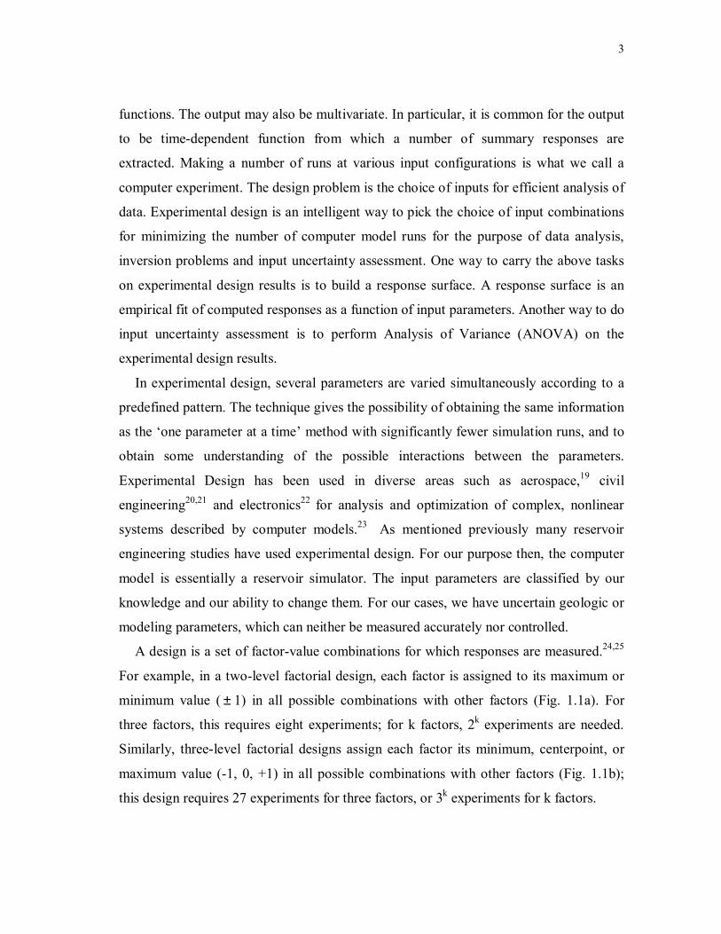
A design is a set of factor-value combinations for which responses are measured.24,25
For example, in a two-level factorial design, each factor is assigned to its maximum or
minimum value ( ± 1) in all possible combinations with other factors (Fig. 1.1a). For
three factors, this requires eight experiments; for k factors, 2k experiments are needed.
Similarly, three-level factorial designs assign each factor its minimum, centerpoint, or
maximum value (-1, 0, +1) in all possible combinations with other factors (Fig. 1.1b);
this design requires 27 experiments for three factors, or 3k experiments for k factors.
4
(a) (b) (c)(a) (b) (c)
Figure 1.1 – Examples of designs for three factors. (a) A two-level factorial requires eight experiments, (b) a three-level factorial design requires 27 experiments, and (c) a Box-Behnken design requires 15 experiments (including three replicates at the centerpoint).
From the above discussion it is clear that it would take a prohibitively large number
of experiments with an increase in the number of factors. Hence we use modified three-
level factorial designs, which reduce the number of experiments by confounding higher
order interactions. The reduction becomes more significant as the number of factor
increases. For the purpose of the first study, which is to identify the most likely scenario
for the location and transmissibility of flow barriers, we use a full factorial experimental
design since we have just two factors. Then we perform ANOVA on the flow simulation
results to analyze the experimental design. For the second study, which is to identify
significant geologic modeling parameters and to study their uncertainty impact on flow
behavior, we use a Box-Behnken26 design since we have four factors or geologic
modeling parameters. A Box-Behnken design requires less number of experiments as
compared to a full-factorial design. For example this design requires 15 experiments for
three factors, including three at the factor centerpoint (all factors assigned to their
centerpoint values) (Fig.1.1c). Centerpoint replicates make the design more nearly
orthogonal, which improves the precision of estimates of response surface coefficients.
Also, there is no simple formula relating the number of required experiments to the

5
number of factors for Box-Behnken designs. Using fast streamline simulation
technology on realizations within each scenario of the experimental design, we can get
the flow responses. These results allow us to build a response surface model which is an
empirical fit of the flow response as a function of the modeling parameters. A Box-
Behnken design would give us a second-degree polynomial response surface model.
Box-Behnken designs neither require nor depend on the prior specification of the model.
Also by including the centerpoint, Box-Behnken designs reduce estimation error for the
most likely responses. Analysis of the response surface model would then help to meet
our objectives.
1.2 Identification of Most Likely Reservoir Scenario
Reservoir compartmentalization can have a significant impact on the field development.
Pressure discontinuities and well production histories can provide important evidence of
reservoir compartmentalization in oil and gas reservoirs. The presence of faults or low-
permeability barriers produces poor fluid communication between the compartments.
This has a significant influence on the depletion performance of the wells. Previous
efforts on the study of compartmentalized reservoirs focussed primarily on the modeling
of production performance from compartmentalized systems. Such reservoirs have been
commonly modeled using material balance techniques, 27-30 although some models have
also taken into account transient flow within compartments.31, 32 All these models require
prior knowledge of reservoir compartmentalization and flow barriers. However, such
information may not be available, particularly in the early stages of field development
with limited geologic and well information. Therefore it is necessary to find a technique
to identify reservoir compartmentalization and flow barriers from well production,
particularly from primary production.
The approach to identify reservoir compartmentalization and flow barriers utilizes
streamline-based drainage volume computations during primary production. Firstly, a
decline type curve analysis of the primary production data is used to identify well
communications and estimate the drainage volume of individual wells. Second, starting
with a geological model the drainage volumes of each well are recomputed using a

6
streamline-based flow simulation. Reservoir compartmentalization and flow barriers are
then inferred through a matching of the streamline-based drainage volume with those
from the decline-curve analysis. The role of experimental design is useful in this
matching process.
Thus the basic principle involves reconciling reservoir drainage volumes derived from
decline curve analysis of primary production response with the drainage volumes
computed using a streamline model. The major steps are outlined below.
• Well drainage volume from decline-type curve analysis:
This step involves a conventional decline type-curve analysis whereby the field data
is plotted on a log-log plot of normalized production rate, q/∆P, versus a material
balance time, Np/q and then matched with the decline type curves.33-34 This matching
yields the drainage volume associated with the producing well. A deviation of the data
from the type curve can be indicative of a drainage volume change resulting from, for
example, a new well sharing the drainage volume of the existing well and also indicates
pressure communication between the two wells. The deviated data can be rescaled to
estimate the new drainage volume associated with each well.
• Well drainage volume from streamline simulation:
Streamline models can be utilized to compute drainage volumes during primary
depletion or compressible flow by utilizing the concept of a ‘diffusive’ time of flight.35
The ‘diffusive’ time of flight is associated with the propagation of a front of maximum
pressure drawdown or buildup associated with an impulse source/sink and can be used to
determine the drainage volumes in 3D heterogeneous media with multiple wells under
very general conditions.
• Drainage volume matching to infer the location of flow barriers:
This step reconciles the two drainage volumes for each well: one from decline type
curve analysis and other from streamline simulation using the geologic model.
Discrepancy between them can suggest the presence of flow barriers that are not
included in the geologic model. Different locations and transmissibilities of the flow
barriers will give different drainage volumes for the wells. The plausible choice of

7
locations and the transmissibilities are determined by matching the drainage volumes
from streamline simulation with those derived using decline type-curve analysis.
• Quantifying uncertainties via experimental design:
The locations and transmissibilities of flow barriers cannot be uniquely determined
without additional information. Thus, we carry out a statistical experimental design to
account for their variability and compute the corresponding changes in the drainage
volume from streamline simulation. The experimental design allows changing the barrier
locations and transmissibilities in a systematic way for matching the drainage volume.
Based on the drainage volume matching it is possible to get the most likely scenario for
the location and transmissibilities of flow barriers. The final step is to then compare the
plot of the observed with the calculated well bottomhole pressure (obtained by
performing streamline simulation on the most likely scenario). Also, to determine the
relative impact of the locations and transmissibilities of the flow barriers, an analysis of
variance (ANOVA) is performed on the experimental design results.
1.3 Uncertainty Analysis of Reservoir Modeling Parameters
Stochastic simulation techniques can be grouped into two main classes of object-based
and pixel-based techniques. Geological uncertainties are associated with each technique.
These uncertainties in the geological data for each technique are used to constrain the
reservoir models. To quantify the significance of a particular geologic factor in each
modeling method, an experimental design set-up is used. In this case, a Box-Behnken
design is used to get the factor combinations for each experiment.
Reservoir sweep efficiency is used as the response variable. The sweep volume
efficiency is obtained using streamline flow simulation. Streamline simulation is used
since it is faster than conventional finite-difference simulation and one can easily obtain
the swept volume for waterflood cases from streamline simulation computations. The
flow simulation result for each experiment helps to build a response surface. The
response surface quantifies the importance of a particular geologic factor on the response
variable and allows studying the impact of uncertainty in the geologic parameters on the
flow behavior of the reservoir. Note that the above procedure is performed on both
8
modeling methods. The response surfaces for the models from both the methods are then
used as a tool to compare the geologic factors from both the methods.
This study is applied on a synthetic fluvial reservoir, whose characteristic feature is
the presence of sinuous sand filled channels within a background of floodplain shale.
The reservoir models and the modeling parameters to be analyzed for each method are
described below:
• Object-based models
A hierarchical object-based modeling of complex fluvial facies is used to model this
synthetic reservoir.36 The task is carried out by FLUVSIM: a program for object-based
stochastic modeling of fluvial depositional systems.37
Within a layer, the distribution of channel complexes is modeled to honor well data.
Facies for each layer is specified for each well as the well data. In the model, three facies
are present. The first facies type is background floodplain shale, which is viewed as the
matrix within which the sand objects are embedded. The second facies type is channel
sand that fills sinuous abandoned channels. This facies is viewed as the best reservoir
quality due to the relatively high energy of deposition and consequent coarser grain. The
third facies type is levee sand formed along the channel margins. These sands are
considered to be poorer quality than the channel fill. For the object-based models the
effect of uncertainty of the following geologic modeling parameters is investigated:
1. Channel Dimensions
- Thickness
- Width/Thickness Ratio
2. Sandstone ratio
3. Channel Permeability
- Channel sand permeability
- Levee sand permeability
4. Channel Sinuosity
9
The ED/RS methodology would give which parameters from the above are significant
and how these parameters affect the volumetric sweep efficiency, which represents the
flow performance of the reservoir.
• Pixel-based models
Sequential Indicator Simulation (SIS) is used for the stochastic modeling of fluvial
depositional systems. The task is carried out by SISIM provided in GSLIB package. SIS
is one of the most popular pixel-based simulation methods and has been proven
effective in many case studies
The well data in this case are permeability values for each layer indicating the type of
facies for that layer. The type of facies considered here for each layer are similar to
those taken for object-based modeling. In this study the effect of uncertainty of the
following geologic modeling parameters is investigated:
1. Variogram range
- Major axis
- Minor axis
2. Sandstone Ratio/Sandstone pdf cut-off
3. Channel Permeability
- Channel sand permeability
- Levee sand permeability
4. Variogram parameters
- Nugget
- Sill
Again, the ED/RS methodology would give which parameters from the above are
significant and how these parameters affect the volumetric sweep efficiency, which
represents the flow performance of the reservoir.
After the above analysis, it is also interesting to compare the modeling parameters for
both the methods from the response surface results.

10
CHAPTER II
EVALUATING UNCERTAINTIES IN IDENTIFICATION OF LOCATION
AND TRANSMISSIBILITY OF FLOW BARRIERS
In this chapter, we discuss the application of experimental design in evaluating
uncertainties in identification of location and transmissibility of flow barriers. The
analysis is performed on a field example in Gulf of Mexico. It has a single well
producing under primary depletion. The production rate and flowing bottomhole
pressure are monthly averaged. In this chapter, the first part discusses the underlying
mathematical formulation behind the drainage volume calculations using the decline
type-curve analysis and the concept of streamline ‘diffusive’ time-of-flight and its
relationship with reservoir drainage volumes. The second part would discuss the use of
experimental design and analysis of variance to address the uncertainties in the
identification procedure.
0
500
1000
1500
2000
2500
3000
0 200 400 600 800 1000 1200Time, day
Oil
prod
. rat
e, S
TB/d
ay
2000
3000
4000
5000
6000
7000
8000W
ell b
otto
mho
le p
ress
ure,
psi
Oil rate
BHP observed
Figure 2.1 – Well production rate and flow bottomhole pressure of the production well
for the field case.

11
2.1 Well Drainage Volume
The analysis is performed on a field example in Gulf of Mexico. It has a single well
producing under primary depletion. The production rate and flowing bottomhole
pressure (Fig. 2.1) are monthly averaged.
2.1.1 Drainage Volume From Decline Type-Curve
Consider an unfractured well producing a slightly compressible liquid in a closed system
under pseudo-steady state flow conditions (boundary dominated flow). The following
relationship can be obtained between a normalized flow rate vs. a ‘material balance
time’: 33,34
tbcNB
Bb
ppq
psseoi
opss
wfi +=
− 1
1 (1)
where,
=
wAo
oopss rC
Aehk
Bb 2'4ln
212.141
γµ (2)
qN
t p= (3)
In dimensionless form Eq. (1) can be expressed as,
DdDd t
q+
=1
1 (4)
where,
12
wfiwAo
ooDd pp
qrCA
ehkBq
−
= 2'
4ln212.141
γµ (5)
During decline type curve analysis, a log-log plot of q/∆P versus t on type curves of
Ddq versus Ddt are overlaid. For our case, type curves have also been generated using
flow rate integral and flow rate integral derivative. A simultaneous match to all the three
type curves can reduce the subjectivity and personal bias during the matching process.33,
34 Once the match is obtained the drainage volume can be calculated as follows:
..
..
..
..
)()/(
)()(
PMDd
PMo
PMDd
PM
oi
o
qpq
tt
BBN ∆= (6)
where M.P. refers to match point value.
If there is aquifer support, the expansion of the aquifer can be incorporated into the
drainage volume calculations as follows,
e
a
o
wwpsd c
cBBNNN += (7)
where,
owwoofe
wfa
sscsccc
ccc
/)( ++=
+= (8)

13
0.01
0.1
1
10
100
0.001 0.01 0.1 1 10 100 1000
Dimensionless Material Balance Time, tDd,bar=NpDd/qDd
qDdqDdiqDdid
Dim
esio
nles
s D
eclin
e R
ate,
qDd
,
Rat
e In
tegr
al, q
Ddi,
and
Inte
gral
-Der
ivat
ive,
qD
did
Transient Flow Region
Boundary-Dominated Flow Region
reD=re/rwa=1.0E4
800
100200
3050 10
A Unfractured Well Centered in a Bounded Circular reservoir
0.1
1
10
1 10 100 1000 10000
Figure 2.2 – Decline type-curve matching of production well.
A deviation from the type-curve may occur if a new producing well shares the
original drainage volume of an existing well. Also, other factors such as multiphase flow
can result in a deviation from the type curve because water breakthrough and/or gas
production may significantly alter the mobility term and/or total compressibility.
Our aim is to identify reservoir compartmentalization and flow barriers using three
years of primary production response. Fig. 2.2 shows the decline type-curve matching.
The data follows the type curves pretty well. However the late-time data appears to
systematically fall above the type-curves and runs parallel to the type-curve. This
indicates a new pseudo-steady state. Such a trend may indicate an extension of the
drainage volume. In other words, it may suggest the presence of partially sealing flow
barriers that provide production and pressure support at later times via access to
additional reservoir volume (compartments). From the decline-curve matching, the
estimate of an initial drainage volume is 10.77 MMSTB, and an extended total drainage
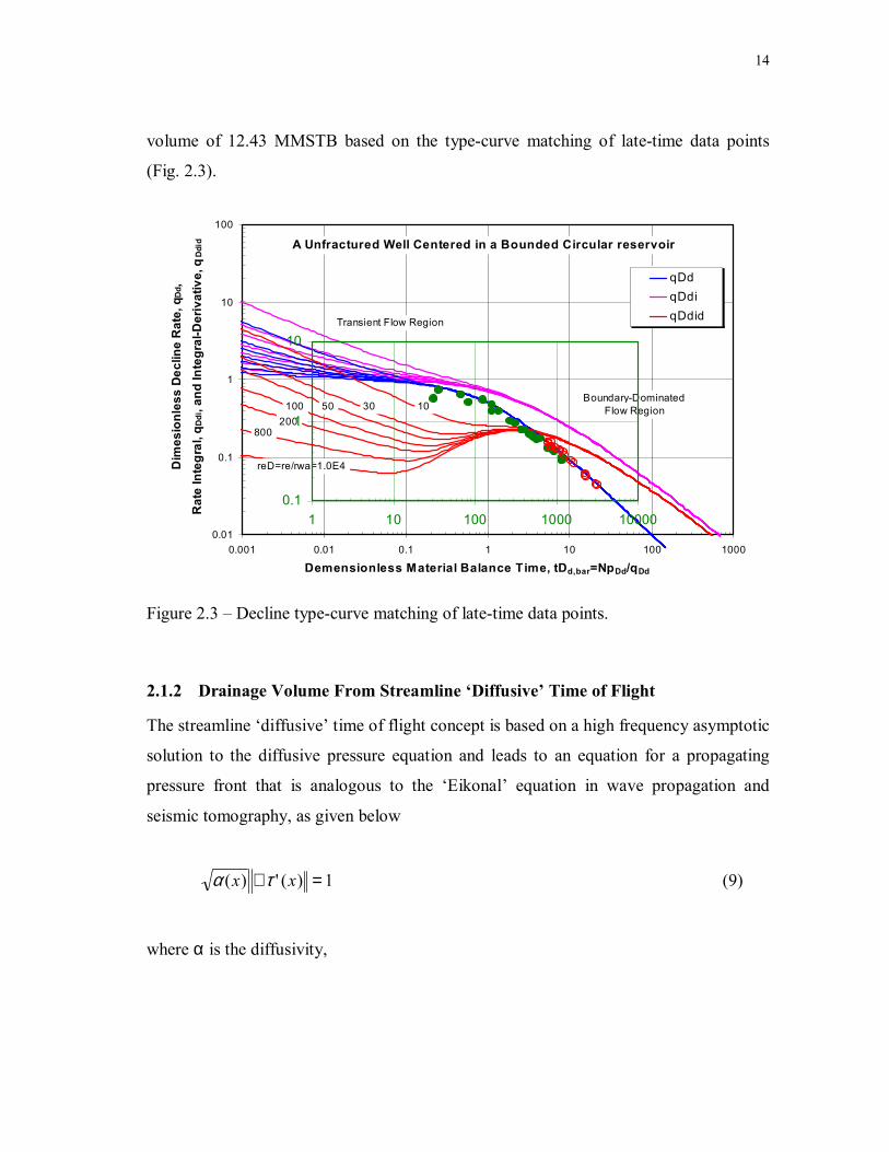
14
volume of 12.43 MMSTB based on the type-curve matching of late-time data points
(Fig. 2.3).
0.01
0.1
1
10
100
0.001 0.01 0.1 1 10 100 1000
Demensionless Material Balance Time, tDd,bar=NpDd/qDd
qDdqDdiqDdid
Dim
esio
nles
s D
eclin
e R
ate,
qDd
,
Rat
e In
tegr
al, q
Ddi,
and
Inte
gral
-Der
ivat
ive,
qDd
id
Transient Flow Region
Boundary-Dominated Flow Region
reD=re/rwa=1.0E4
800
100200
3050 10
A Unfractured Well Centered in a Bounded Circular reservoir
0.1
1
10
1 10 100 1000 10000
Figure 2.3 – Decline type-curve matching of late-time data points.
2.1.2 Drainage Volume From Streamline ‘Diffusive’ Time of Flight
The streamline ‘diffusive’ time of flight concept is based on a high frequency asymptotic
solution to the diffusive pressure equation and leads to an equation for a propagating
pressure front that is analogous to the ‘Eikonal’ equation in wave propagation and
seismic tomography, as given below
1)(')( =∇ xx τα (9)
where α is the diffusivity,

15
tcxxKxµφ
α)(
)()( = (10)
From Eq. 9, the pressure front propagates at a velocity given by the square root of
diffusivity. The Eikonal equation, being a hyperbolic equation, allows us to invoke
characteristic directions and streamlines for propagating fronts. In particular, we can
now define a ‘diffusive’ time of flight for compressible flow as follows,
∫=ψ α
τ)(
)('x
dsx (11)
where ψ refers to as streamline and s is the distance along the streamline. Note that the
‘diffusive’ time of flight has units of square root of time, which is consistent with the
scaling behavior of diffusive flow.
It is important to point out that for compressible flow, pathlines can be generated in
the same manner as in conventional streamline simulation using the Pollock algorithm.38
Fluid compressibility acts as a diffusive source (as opposed to a point source) and the
semi-analytic pathline construction applies under such conditions.
An important feature of the ‘diffusive’ time of flight is that it is related to the
propagation of a ‘pressure front’ of maximum drawdown or build up corresponding to an
impulse source or sink. This becomes apparent when we examine the time domain
solution to the 0th order asymptotic expansion for an impulse source in a three-
dimensional medium,39
−=
tx
txxAtP
4)('exp
2)(')()(
2
30τ
πτ (12)
16
At a fixed position, x, the pressure response, P(t), will be maximized when its
derivative is set equal to zero, which in turn results in the following relationship between
the observed time and the ‘diffusive’ time of flight
6)('2
maxxt τ= (13)
Therefore, the ‘diffusive’ time of flight is associated with the propagation of a front of
maximum drawdown or build up. The time at which the pressure response reaches a
maximum at a location for an impulse input can be defined as the transient pressure front
arrival time. In fact, this front location is closely related to the concept of drainage
volume and drainage radius during conventional well test and decline type curve
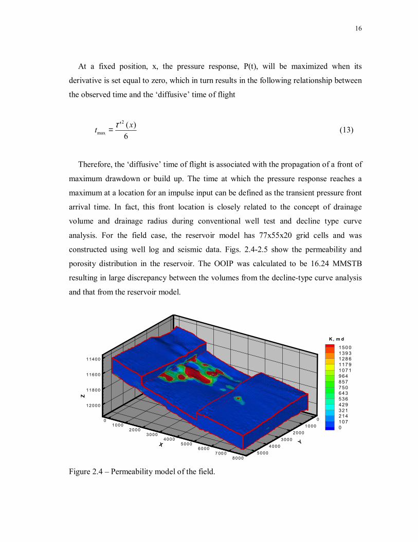
analysis. For the field case, the reservoir model has 77x55x20 grid cells and was
constructed using well log and seismic data. Figs. 2.4-2.5 show the permeability and
porosity distribution in the reservoir. The OOIP was calculated to be 16.24 MMSTB
resulting in large discrepancy between the volumes from the decline-type curve analysis
and that from the reservoir model.
1 1 4 0 0
1 1 6 0 0
1 1 8 0 0
1 2 0 0 0
Z
01 0 0 0
2 0 0 03 0 0 0
4 0 0 05 0 0 0
6 0 0 07 00 0
8 0 0 0
X
01 0 0 0
2 0 0 03 0 0 0
4 0 0 05 0 0 0
Y
150 0139 3128 6117 9107 19648577506435364293212141070
K , m d
Figure 2.4 – Permeability model of the field.

17
11400
11600
11800
12000
Z
01000
20003000
40005000
60007000
8000
X
01000
20003000
40005000
Y
0.350.320.300.270.250.220.200.170.150.120.100.070.050.020.00
Porosity
Figure 2.5 – Porosity model of the field.
2.1.3 Drainage Volume Matching
The large discrepancy between the drainage volume from the decline type-curve analysis
and that from the reservoir model indicates that a sealing flow barrier prevents the well
from draining the whole reservoir. Furthermore, based on the decline type-curve
analysis, there may also be a partially sealing flow barrier isolating a portion of the
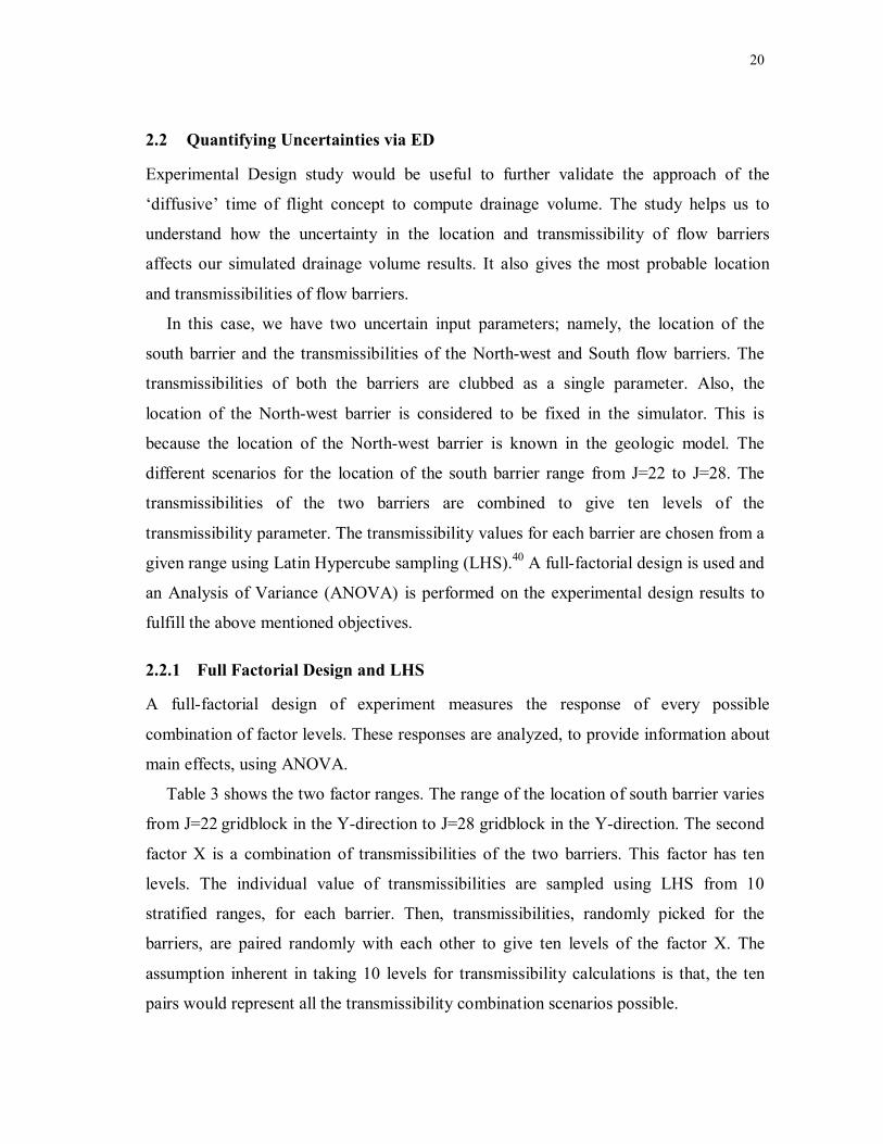
reservoir from the main reservoir. To locate the potential flow barriers, we examine the
distributions of permeability, porosity and oil-footage (φ∗h∗ So) in the reservoir model
for potential trends. Based on low permeability and oil-footage combined with
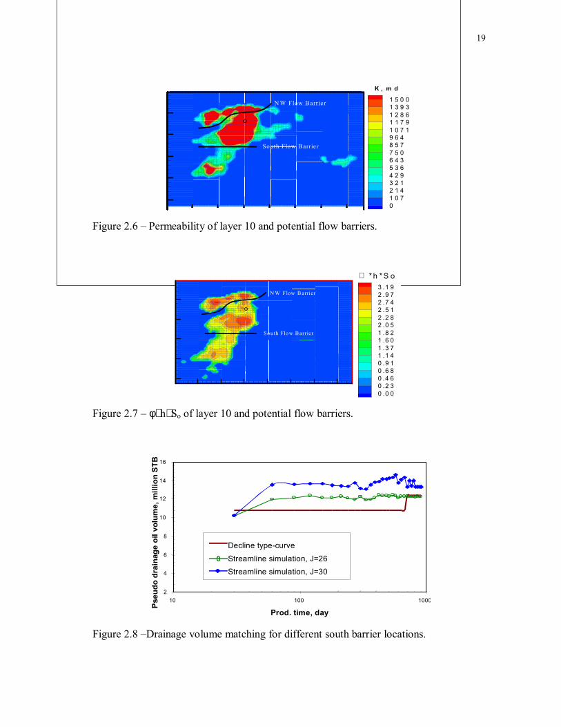
geological input, we place two flow barriers into the reservoir model (Figs. 2.6-2.7) – a
northwest barrier and a south barrier. We then proceed to investigate the impact of these
flow barriers on the drainage volume calculations using streamline simulation.
Several scenarios are investigated with respect to the location and transmissibilities
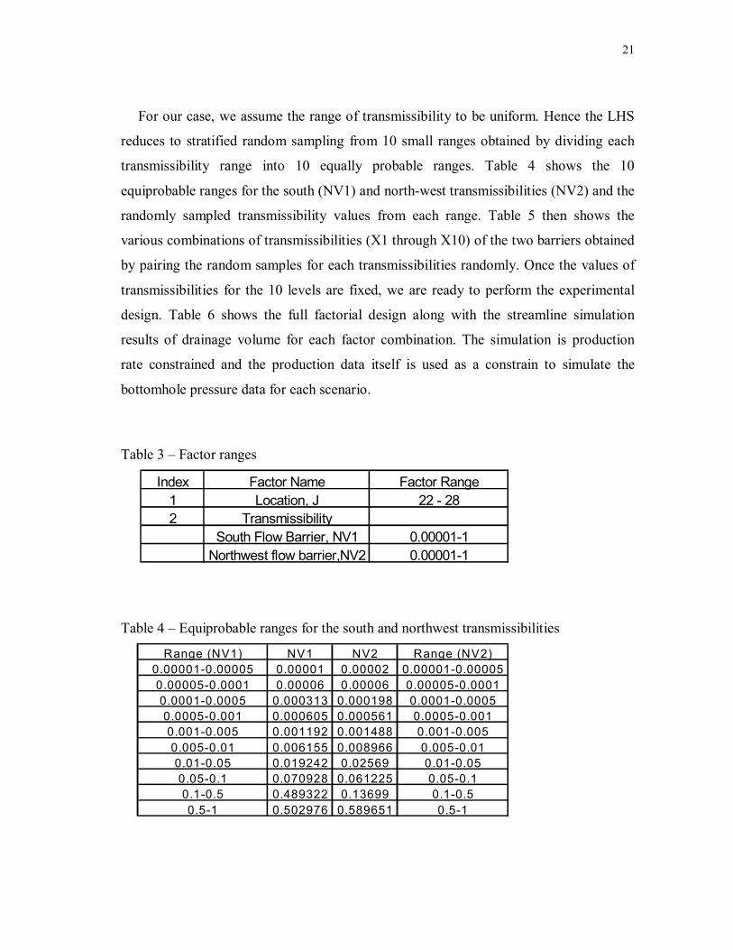
of flow barriers. To start with, we varied the location of the south barrier while assuming

18
both the barriers to be almost sealing. The results are shown in Table 1 and Fig. 2.8. We
then studied the sensitivity of the NW barrier transmissibility on the drainage volume.
The results are shown in Table 2.
Recognizing the non-uniqueness and uncertainty associated with our analysis, we
further investigate the barrier location and transmissibility via a statistical experimental
design.
Table 1 – Comparison of drainage volume for different locations of the south barrier
Case 1 No flow barrier /
South, J=30 0.0001NW 0.0001
South, J=28 0.0001NW 0.0001
South, J=26 0.0001NW 0.0001
10.2 ~ 12.4
10.3 ~ 14.6
10.4 ~ 12.8
Location Trans Multiplier
Case 3
Case 2
Case 4
10.77 ~ 12.43
18.2
Pseudo Drainage Oil Volume, Npsd, Million STB
Pseudo Drainage Oil Volume, Npsd, Million STB
Decline type-curveStreamline simulation
Table 2 – Comparison of drainage volume for different transmissibility multipliers for the NW barrier
South, J=26 0.0001NW 0.0001
South, J=26 0.0001NW 0.001
South, J=26 0.0001NW 0.01
South, J=26 0.0001NW 0.1
10.0~12.7
10.2 ~ 12.4
10.0~13.7
10.0~13.7
Pseudo Drainage Oil Volume, Npsd, Million STB
Pseudo Drainage Oil Volume, Npsd, Million STB
Location Trans Multiplier
Case 6
Case 6
Case 5
Case 4
Streamline simulation
10.77 ~ 12.43
Decline type-curve
19
N W Flow Barrier
South Flow Barrier
N W Flow Barrier
South Flow Barrier
1 5 0 01 3 9 31 2 8 61 1 7 91 0 7 19 6 48 5 77 5 06 4 35 3 64 2 93 2 12 1 41 0 70
K , m d
N W Flow Barrier
South Flow Barrier
N W Flow Barrier
South Flow Barrier
1 5 0 01 3 9 31 2 8 61 1 7 91 0 7 19 6 48 5 77 5 06 4 35 3 64 2 93 2 12 1 41 0 70
K , m d
Figure 2.6 – Permeability of layer 10 and potential flow barriers.
N W Flow B arrier
South Flow B arrier
3 .1 92 .9 72 .7 42 .5 12 .2 82 .0 51 .8 21 .6 01 .3 71 .1 40 .9 10 .6 80 .4 60 .2 30 .0 0
∅ * h * S o
N W Flow B arrier
South Flow B arrier
3 .1 92 .9 72 .7 42 .5 12 .2 82 .0 51 .8 21 .6 01 .3 71 .1 40 .9 10 .6 80 .4 60 .2 30 .0 0
∅ * h * S o
Figure 2.7 – φ∗h∗ So of layer 10 and potential flow barriers.
2
4
6
8
10
12
14
16
10 100 1000
Prod. time, day
Pseu
do d
rain
age
oil v
olum
e, m
illio
n ST
B
Decline type-curveStreamline simulation, J=26Streamline simulation, J=30
2
4
6
8
10
12
14
16
10 100 1000
Prod. time, day
Pseu
do d
rain
age
oil v
olum
e, m
illio
n ST
B
Decline type-curveStreamline simulation, J=26Streamline simulation, J=30
Figure 2.8 –Drainage volume matching for different south barrier locations.
20
2.2 Quantifying Uncertainties via ED
Experimental Design study would be useful to further validate the approach of the
‘diffusive’ time of flight concept to compute drainage volume. The study helps us to
understand how the uncertainty in the location and transmissibility of flow barriers
affects our simulated drainage volume results. It also gives the most probable location
and transmissibilities of flow barriers.
In this case, we have two uncertain input parameters; namely, the location of the
south barrier and the transmissibilities of the North-west and South flow barriers. The
transmissibilities of both the barriers are clubbed as a single parameter. Also, the
location of the North-west barrier is considered to be fixed in the simulator. This is
because the location of the North-west barrier is known in the geologic model. The
different scenarios for the location of the south barrier range from J=22 to J=28. The
transmissibilities of the two barriers are combined to give ten levels of the
transmissibility parameter. The transmissibility values for each barrier are chosen from a
given range using Latin Hypercube sampling (LHS).40 A full-factorial design is used and
an Analysis of Variance (ANOVA) is performed on the experimental design results to
fulfill the above mentioned objectives.
2.2.1 Full Factorial Design and LHS
A full-factorial design of experiment measures the response of every possible
combination of factor levels. These responses are analyzed, to provide information about
main effects, using ANOVA.
Table 3 shows the two factor ranges. The range of the location of south barrier varies
from J=22 gridblock in the Y-direction to J=28 gridblock in the Y-direction. The second
factor X is a combination of transmissibilities of the two barriers. This factor has ten
levels. The individual value of transmissibilities are sampled using LHS from 10
stratified ranges, for each barrier. Then, transmissibilities, randomly picked for the
barriers, are paired randomly with each other to give ten levels of the factor X. The
assumption inherent in taking 10 levels for transmissibility calculations is that, the ten
pairs would represent all the transmissibility combination scenarios possible.
21
For our case, we assume the range of transmissibility to be uniform. Hence the LHS
reduces to stratified random sampling from 10 small ranges obtained by dividing each
transmissibility range into 10 equally probable ranges. Table 4 shows the 10
equiprobable ranges for the south (NV1) and north-west transmissibilities (NV2) and the
randomly sampled transmissibility values from each range. Table 5 then shows the
various combinations of transmissibilities (X1 through X10) of the two barriers obtained
by pairing the random samples for each transmissibilities randomly. Once the values of
transmissibilities for the 10 levels are fixed, we are ready to perform the experimental
design. Table 6 shows the full factorial design along with the streamline simulation
results of drainage volume for each factor combination. The simulation is production
rate constrained and the production data itself is used as a constrain to simulate the
bottomhole pressure data for each scenario.
Table 3 – Factor ranges
Index Factor Name Factor Range1 Location, J 22 - 282 Transmissibility
South Flow Barrier, NV1 0.00001-1Northwest flow barrier,NV2 0.00001-1
Table 4 – Equiprobable ranges for the south and northwest transmissibilities
Range (NV1) NV1 NV2 Range (NV2)0.00001-0.00005 0.00001 0.00002 0.00001-0.000050.00005-0.0001 0.00006 0.00006 0.00005-0.00010.0001-0.0005 0.000313 0.000198 0.0001-0.00050.0005-0.001 0.000605 0.000561 0.0005-0.0010.001-0.005 0.001192 0.001488 0.001-0.0050.005-0.01 0.006155 0.008966 0.005-0.010.01-0.05 0.019242 0.02569 0.01-0.050.05-0.1 0.070928 0.061225 0.05-0.10.1-0.5 0.489322 0.13699 0.1-0.50.5-1 0.502976 0.589651 0.5-1

22
Table 5 – Transmissibility multipliers of the south and NW barriers obtained using Latin Hypercube Sampling
N o t e : N V 1 f o r N W b a r r i e r ; N V 2 f o r s o u t h b a r r i e r
N V 1 N V 20 . 0 0 0 0 1 0 . 5 8 9 6 5 X 10 . 0 0 0 3 1 0 . 0 2 5 6 9 X 20 . 0 7 0 9 3 0 . 1 3 6 9 9 X 30 . 0 0 6 1 6 0 . 0 0 0 0 2 X 40 . 0 1 9 2 4 0 . 0 0 0 5 6 X 50 . 0 0 1 1 9 0 . 0 0 0 0 6 X 60 . 4 8 9 3 2 0 . 0 0 0 2 X 70 . 0 0 0 6 0 . 0 6 1 2 2 X 8
0 . 0 0 0 0 6 0 . 0 0 8 9 7 X 90 . 5 0 2 9 8 0 . 0 0 1 4 9 X 1 0
Table 6 – Experimental design set-up for drainage volume from streamline simulation for different scenarios
X1 X2 X3 X4 X5 X6 X7 X8 X9 X10
J=22 16.92 16.89 18.19 11.24 12.45 10.57 10.81 17.02 16.51 15.72J=23 17.05 16.89 18.18 11.18 14.17 11.03 12.07 17.04 16.68 15.74J = 24 16.94 16.89 18.19 12.89 13.89 11.03 13.03 17.02 16.71 16.84J = 25 17.10 16.94 18.18 13.31 13.89 12.35 13.37 17.03 16.84 15.33J = 26 16.93 16.92 18.17 13.54 13.94 12.99 13.54 17.03 16.47 15.18J = 27 16.98 16.91 18.19 13.71 14.18 13.29 13.88 17.03 16.43 14.74J = 28 17.05 16.92 18.17 13.93 14.47 13.41 13.98 17.04 16.47 14.99
South Barrier Location Drainage Volume (Million STB)
2.2.2 Analysis of Variance
Based on the experimental design results, we performed an analysis of variance
(ANOVA) to examine the significance of the location of the south barrier and the
transmissibility of both the barriers on the computed drainage volume. The ANOVA also
included the SNK test and Tukey test.41. The following equations give the sum of
squares computed in the ANOVA

23
∑∑ −=i j
ij yySSY 2)( (14)
2
... )(∑ −=j
j yySSTrans j = 1,2,....10 (15)
2
... )(∑ −=i
i yySSLoc (16)
SSLocSSTransSSYSSError −−= (17)
DFSSErrorMSError
DFSSLocMSLoc
DFSSTransMSTrans === ,, (18)
where, i= number of the location factor and j= number of transmissibility factor and
yij= drainage volume at i location and j transmissibility, y =overall drainage volume,
..y = sum of drainage volume means
The test of equal transmissibility means, which indicates no transmissibility effects on
drainage volume, is a test of,
10.2.1. ... yyy === (19)
The test of equal location means, which indicates no location effects on drainage
volume, is a test of,
7.2.1. ... yyy === (20)
The test statistic for testing the above two null hypotheses is,
MSErrorMSLocF
MSErrorMSTransF == , (21)

24
which has F distribution with nine (10-1=9) degrees of freedom for MSTrans, six (7-
1=6) degrees of freedom for MSLoc and fifty-four (9x6=54) degrees of freedom for the
denominator MSError. The analysis of variance (ANOVA) is actually a hypothesis test
with the null hypothesis (Ho) that the factor (in our case, transmissibility or location) has
no effect on the simulator output (drainage volume in our case). The test statistic (F) in
an ANOVA is a Fisher distributed random variable with a certain number of degrees of
freedom. A large value on the observed test statistic (Fobs) indicate that the factor has no
effect. The Pr-significance value is defined as the probability of having a test statistic
that is at least large as the observed test statistic:
)|( trueishypothesisnullFFPP obs ⋅⋅⋅≥= (22)
A small Pr-value means that the probability of getting the observed test statistic,
given that the null hypothesis is true, is very unlikely. The null hypothesis is then
rejected, and we assume that the factor has an effect. That means that the lower the P-
significance value, the more significant is the difference amongst different factor level
mean responses, indicating that the effect for that particular factor is significant. Table 7
shows the ANOVA table for the experimental design. The table shows the P-significance
value for the null hypothesis test. From Table 7 it can be seen that transmissibility of
flow barriers have a significant effect on the drainage volume as compared to the
location of south barrier.
Table 7 – Analysis of Variance (ANOVA) S o u rc e D F T y p e I I I S S M e a n S q u a re F V a lu e P r
(S S ) (M S )T R A N S 9 2 9 6 .9 4 6 6 3 2 .9 9 4 1 7 9 .3 2 < .0 0 0 1
L O C A T IO N 6 7 .5 5 6 5 1 .2 5 9 4 3 .0 3 0 .0 1 2 6E rro r 5 4 2 2 .4 6 0 7 0 .4 1 5 9
S o u rc e D F T y p e I I I S S M e a n S q u a re F V a lu e P r (S S ) (M S )
T R A N S 9 2 9 6 .9 4 6 6 3 2 .9 9 4 1 7 9 .3 2 < .0 0 0 1L O C A T IO N 6 7 .5 5 6 5 1 .2 5 9 4 3 .0 3 0 .0 1 2 6
E rro r 5 4 2 2 .4 6 0 7 0 .4 1 5 9

25
When an ANOVA F test reveals significant differences among the each factor level
means (as it did in our case), it does not in any way indicate which means differ or the
magnitude of the difference. Thus, the detection of magnitude of difference between
factor or level means will require some kind of post-ANOVA analysis. SNK/Tukey tests
are two of the several mean separation procedures used in post-ANOVA analysis. The
following is the description of how a SNK and a Tukey test can be performed on
treatment means:
Student – Newman – Keuls (S-N-K) Procedure:
1) Divide the set of paired comparisons into subsets of order p. The S-N-K procedure
has a different critical value for each subset.
2) Specifically, the observed difference of each pair of means in the subset of order p is
compared to the critical difference given by
2/),,()()( vprspSNK d α= (23)
For p=1, 2.......7 (for comparing location means) and p=1,2.......10 (for comparing
transmissibility means)
Where, ),,( vpr α = studentized range value of order p
v = degrees of freedom on MSE
α = Experimentwise error rate
)( ds = Standard deviation
3) If the critical difference is less than the difference between 2 means, then those 2
means are said to be significantly different.
Tukey test:
1) The observed difference of any pair of means is compared to the Tukey’s critical
difference given by
2/),,()( vkrsTK d α= (24)

26
Where, ),,( vpr α = studentized range value of order p
k = number of means being compared
α = Experimentwise error rate
v = degrees of freedom on MSE
)( ds = Standard deviation
2) If the critical difference is less than the difference between 2 means, then those 2
means are said to be significantly different.
Table 8 – SNK test for transmissibility means α 0.05
Error Degrees of Freedom 54Error Mean Square 0.415939
Number of Means 2 3 4 5 6 7 8 9 10Critical Range 0.691162 0.830798 0.913830 0.972860 1.018503 1.055623 1.086843 1.113744 1.137348
Grouping Mean N TRANS
18.1814 7 X3
17.0300 7 X8
16.9957 7 X1
16.9086 7 X2
16.5871 7 X9
15.5057 7 X10
13.8557 7 X5
12.9543 7 X7
12.8286 7 X4
12.0957 7 X6
α 0.05Error Degrees of Freedom 54Error Mean Square 0.415939
Number of Means 2 3 4 5 6 7 8 9 10Critical Range 0.691162 0.830798 0.913830 0.972860 1.018503 1.055623 1.086843 1.113744 1.137348
α 0.05Error Degrees of Freedom 54Error Mean Square 0.415939
Number of Means 2 3 4 5 6 7 8 9 10Critical Range 0.691162 0.830798 0.913830 0.972860 1.018503 1.055623 1.086843 1.113744 1.137348
Grouping Mean N TRANS
18.1814 7 X3
17.0300 7 X8
16.9957 7 X1
16.9086 7 X2
16.5871 7 X9
15.5057 7 X10
13.8557 7 X5
12.9543 7 X7
12.8286 7 X4
12.0957 7 X6
Grouping Mean N TRANS
18.1814 7 X3
17.0300 7 X8
16.9957 7 X1
16.9086 7 X2
16.5871 7 X9
15.5057 7 X10
13.8557 7 X5
12.9543 7 X7
12.8286 7 X4
12.0957 7 X6
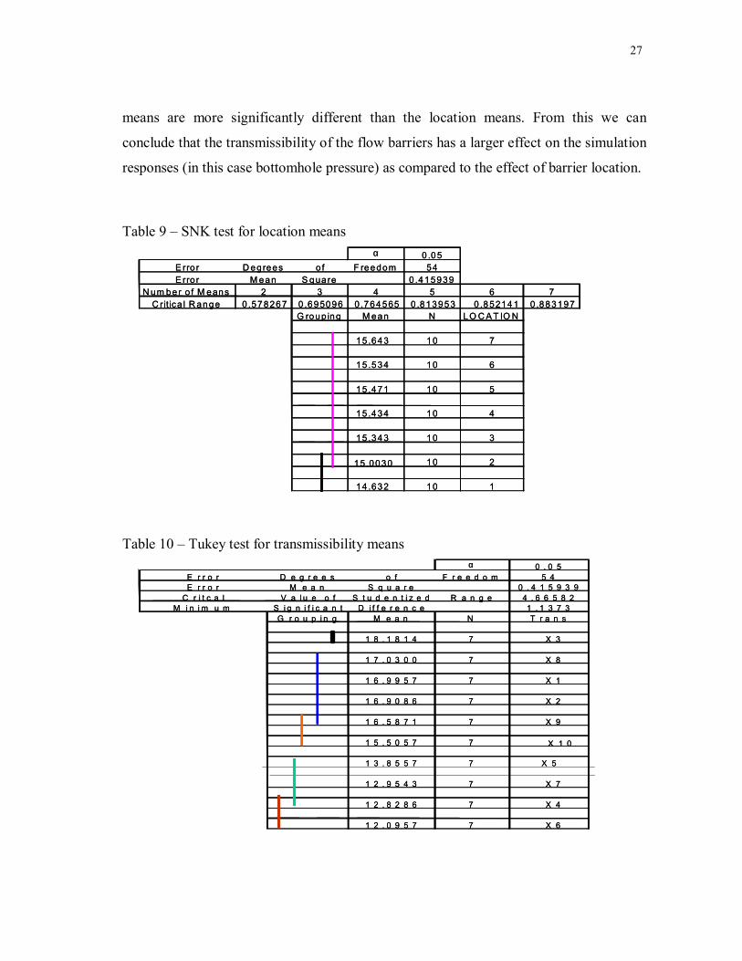
Table 8 shows the SNK test for transmissibility means and Table 9 shows the SNK test
for location means. Table 10 shows the Tukey test for transmissibility means and Table
11 shows Tukey test for location means. The grouping lines indicate the means that are
not significantly different. Both the post ANOVA analyses show that the transmissibility
27
means are more significantly different than the location means. From this we can
conclude that the transmissibility of the flow barriers has a larger effect on the simulation
responses (in this case bottomhole pressure) as compared to the effect of barrier location.
Table 9 – SNK test for location means α 0 .05
E rro r D egrees o f F reedom 54E rro r M ean S quare 0 .415939
N um ber o f M eans 2 3 4 5 6 7C ritica l R ange 0 .578267 0 .695096 0 .764565 0 .813953 0 .852141 0 .883197
G roup ing M ean N LO C A T IO N
15.643 10 7
15 .534 10 6
15 .471 10 5
15 .434 10 4
15 .343 10 3
15 .0030 10 2
14 .632 10 1
α 0 .05E rro r D egrees o f F reedom 54E rro r M ean S quare 0 .415939
N um ber o f M eans 2 3 4 5 6 7C ritica l R ange 0 .578267 0 .695096 0 .764565 0 .813953 0 .852141 0 .883197
G roup ing M ean N LO C A T IO N
15.643 10 7
15 .534 10 6
15 .471 10 5
15 .434 10 4
15 .343 10 3
15 .0030 10 2
14 .632 10 1
Table 10 – Tukey test for transmissibility means α 0 . 0 5
E r r o r D e g r e e s o f F r e e d o m 5 4E r r o r M e a n S q u a r e 0 . 4 1 5 9 3 9
C r i t c a l V a l u e o f S t u d e n t i z e d R a n g e 4 . 6 6 5 8 2M i n i m u m S i g n i f i c a n t D i f f e r e n c e 1 . 1 3 7 3
G r o u p i n g M e a n N T r a n s
1 8 . 1 8 1 4 7 X 3
1 7 . 0 3 0 0 7 X 8
1 6 . 9 9 5 7 7 X 1
1 6 . 9 0 8 6 7 X 2
1 6 . 5 8 7 1 7 X 9
1 5 . 5 0 5 7 7 X 1 0
1 3 . 8 5 5 7 7 X 5
1 2 . 9 5 4 3 7 X 7
1 2 . 8 2 8 6 7 X 4
1 2 . 0 9 5 7 7 X 6
α 0 . 0 5E r r o r D e g r e e s o f F r e e d o m 5 4E r r o r M e a n S q u a r e 0 . 4 1 5 9 3 9
C r i t c a l V a l u e o f S t u d e n t i z e d R a n g e 4 . 6 6 5 8 2M i n i m u m S i g n i f i c a n t D i f f e r e n c e 1 . 1 3 7 3
G r o u p i n g M e a n N T r a n s
1 8 . 1 8 1 4 7 X 3
1 7 . 0 3 0 0 7 X 8
1 6 . 9 9 5 7 7 X 1
1 6 . 9 0 8 6 7 X 2
1 6 . 5 8 7 1 7 X 9
1 5 . 5 0 5 7 7 X 1 0
1 3 . 8 5 5 7 7 X 5
1 2 . 9 5 4 3 7 X 7
1 2 . 8 2 8 6 7 X 4
1 2 . 0 9 5 7 7 X 6
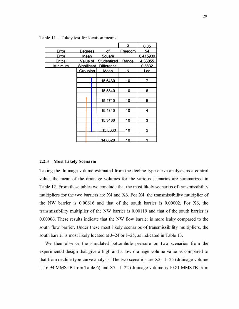
28
Table 11 – Tukey test for location means α 0.05
Error Degrees of Freedom 54Error Mean Square 0.415939
Critcal Value of Studentized Range 4.33055Minimum Significant Difference 0.8832
Grouping Mean N Loc
15.6430 10 7
15.5340 10 6
15.4710 10 5
15.4340 10 4
15.3430 10 3
15.0030 10 2
14.6320 10 1
α 0.05Error Degrees of Freedom 54Error Mean Square 0.415939
Critcal Value of Studentized Range 4.33055Minimum Significant Difference 0.8832
Grouping Mean N Loc
15.6430 10 7
15.5340 10 6
15.4710 10 5
15.4340 10 4
15.3430 10 3
15.0030 10 2
14.6320 10 1
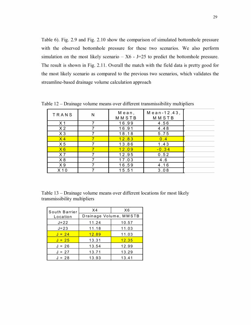
2.2.3 Most Likely Scenario
Taking the drainage volume estimated from the decline type-curve analysis as a control
value, the mean of the drainage volumes for the various scenarios are summarized in
Table 12. From these tables we conclude that the most likely scenarios of transmissibility
multipliers for the two barriers are X4 and X6. For X4, the transmissibility multiplier of
the NW barrier is 0.00616 and that of the south barrier is 0.00002. For X6, the
transmissibility multiplier of the NW barrier is 0.00119 and that of the south barrier is
0.00006. These results indicate that the NW flow barrier is more leaky compared to the
south flow barrier. Under these most likely scenarios of transmissibility multipliers, the
south barrier is most likely located at J=24 or J=25, as indicated in Table 13.
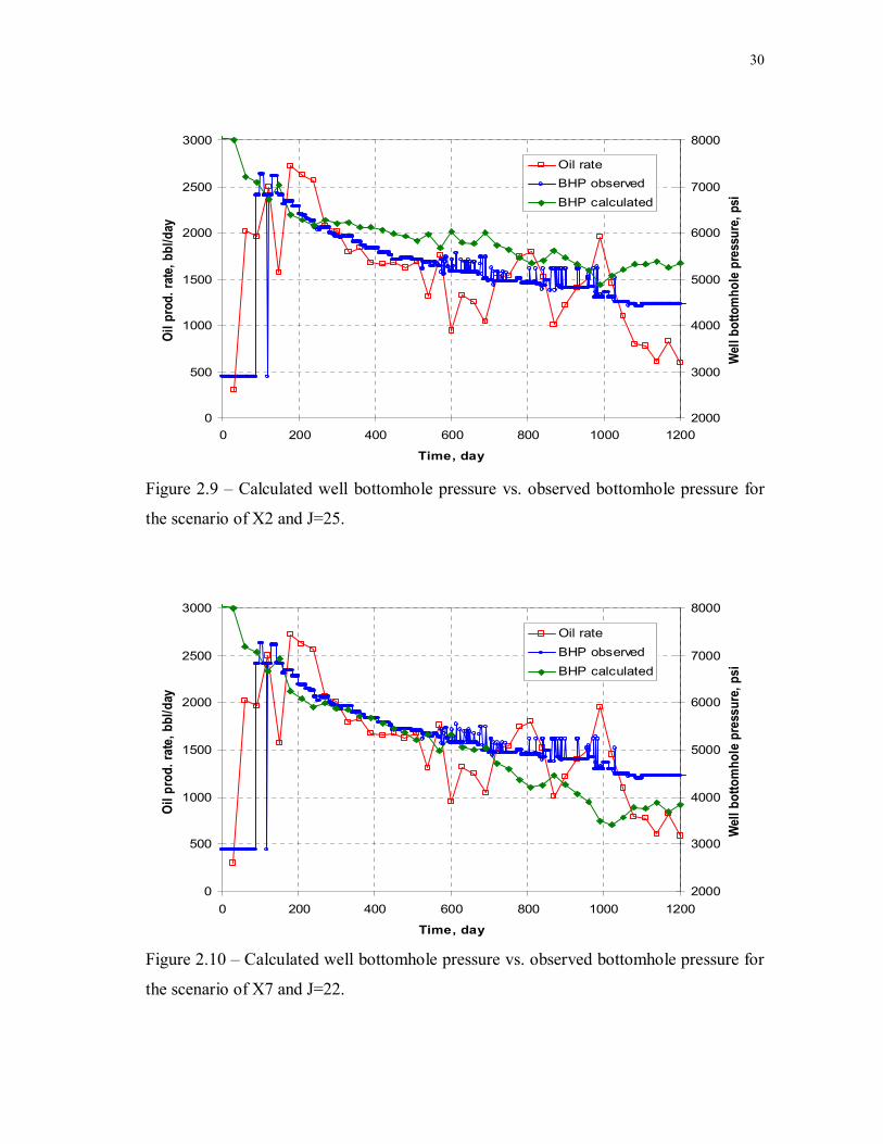
We then observe the simulated bottomhole pressure on two scenarios from the
experimental design that give a high and a low drainage volume value as compared to
that from decline type-curve analysis. The two scenarios are X2 - J=25 (drainage volume
is 16.94 MMSTB from Table 6) and X7 - J=22 (drainage volume is 10.81 MMSTB from
29
Table 6). Fig. 2.9 and Fig. 2.10 show the comparison of simulated bottomhole pressure
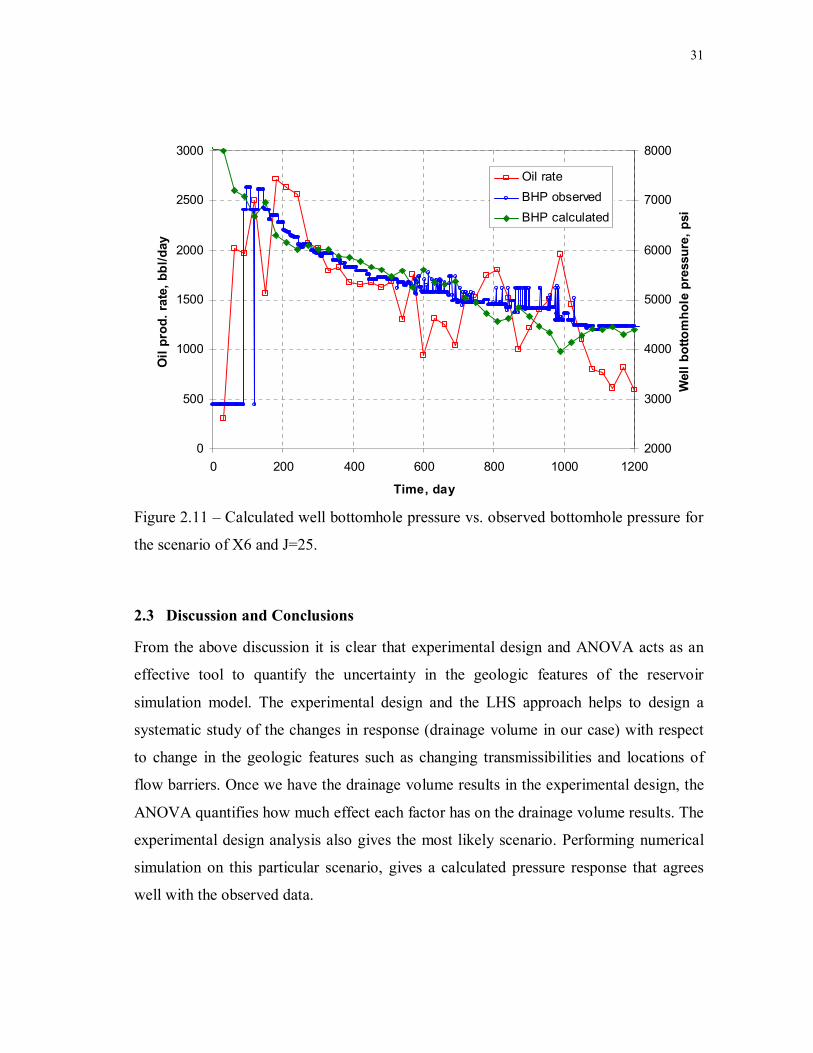
with the observed bottomhole pressure for these two scenarios. We also perform
simulation on the most likely scenario – X6 - J=25 to predict the bottomhole pressure.
The result is shown in Fig. 2.11. Overall the match with the field data is pretty good for
the most likely scenario as compared to the previous two scenarios, which validates the
streamline-based drainage volume calculation approach
Table 12 – Drainage volume means over different transmissibility multipliers
X 1 7 1 6 .9 9 4 .5 6X 2 7 1 6 .9 1 4 .4 8X 3 7 1 8 .1 8 5 .7 5X 4 7 1 2 .8 3 0 .4X 5 7 1 3 .8 6 1 .4 3X 6 7 1 2 .0 9 - 0 .3 4X 7 7 1 2 .9 5 0 .5 2X 8 7 1 7 .0 3 4 .6X 9 7 1 6 .5 9 4 .1 6
X 1 0 7 1 5 .5 1 3 .0 8
T R A N S M e a n , M M S T B
M e a n - 1 2 .4 3 , M M S T B
N
Table 13 – Drainage volume means over different locations for most likely transmissibility multipliers
X4 X6
J= 22 11 .24 10 .57J= 23 11 .18 11 .03
J = 24 12 .89 11 .03J = 25 13 .31 12 .35J = 26 13 .54 12 .99J = 27 13 .71 13 .29J = 28 13 .93 13 .41
S ou th B arr ie r Loca tion D ra in age Vo lum e, M M S TB
30
0
500
1000
1500
2000
2500
3000
0 200 400 600 800 1000 1200
Time, day
Oil p
rod.
rate,
bbl
/day
2000
3000
4000
5000
6000
7000
8000
Wel
l bot
tom
hole
pres
sure
, psi
Oil rateBHP observedBHP calculated
Figure 2.9 – Calculated well bottomhole pressure vs. observed bottomhole pressure for
the scenario of X2 and J=25.
0
500
1000
1500
2000
2500
3000
0 200 400 600 800 1000 1200
Time, day
Oil p
rod.
rate
, bbl
/day
2000
3000
4000
5000
6000
7000
8000
Wel
l bot
tom
hole
pre
ssur
e, p
si
Oil rateBHP observedBHP calculated
Figure 2.10 – Calculated well bottomhole pressure vs. observed bottomhole pressure for
the scenario of X7 and J=22.
31
0
500
1000
1500
2000
2500
3000
0 200 400 600 800 1000 1200
Time, day
Oil
prod
. rat
e, b
bl/d
ay
2000
3000
4000
5000
6000
7000
8000
Wel
l bot
tom
hole
pre
ssur
e, p
si
Oil rateBHP observedBHP calculated
Figure 2.11 – Calculated well bottomhole pressure vs. observed bottomhole pressure for
the scenario of X6 and J=25.
2.3 Discussion and Conclusions
From the above discussion it is clear that experimental design and ANOVA acts as an
effective tool to quantify the uncertainty in the geologic features of the reservoir
simulation model. The experimental design and the LHS approach helps to design a
systematic study of the changes in response (drainage volume in our case) with respect
to change in the geologic features such as changing transmissibilities and locations of
flow barriers. Once we have the drainage volume results in the experimental design, the
ANOVA quantifies how much effect each factor has on the drainage volume results. The
experimental design analysis also gives the most likely scenario. Performing numerical
simulation on this particular scenario, gives a calculated pressure response that agrees
well with the observed data.

32
The following conclusions from this study can be summarized as follows:
1. The transmissibiity of the North west/ South flow barrier has a greater effect on the
drainage volume than the location of the south barrier.
2. The Northwest flow barrier is more leaky than the South flow barrier.
3. The most likely position of the South barrier is at J=24 or J=25.
4. The order of magnitude of transmissibility multiplier for south barrier is 10-5 and the
order of magnitude of transmissibility multiplier for the Northwest barrier is 10-3.
33
CHAPTER III
IDENTIFICATION OF SIGNIFICANT RESERVOIR MODELING
PARAMETERS IN FLOW RESPONSE
The accuracy of flow performance predictions depends on the validity of the reservoir
model used for numerical simulation. In real life however, reservoir modeling
parameters required to build the reservoir models are highly uncertain. It is therefore
necessary to identify significant modeling parameters and study the impact of
uncertainty in these modeling parameters on the flow performance. Typically such a
study would require a large number of simulation runs, which take too much time. This
makes such study unfeasible for quick decision making. We propose to combine a fast
approximate simulation technique like streamline simulation with a statistical technique
called experimental design and response surface methodology. Experimental Design
reduces the number of simulation runs by carefully choosing the combinations of
geologic parameters to change. Streamline simulator quantifies the impact on the flow
response. In this case, we take the sweep efficiency as the response for waterflooded
reservoirs. This particular response variable is very fast to compute with streamline
simulation under the steady state pressure conditions we assume.
This chapter would first discuss the theory behind Box-Behnken designs in detail.
This is followed by fundamentals of streamline simulation and the method to compute
sweep efficiency. The next section discusses the method to identify significant modeling
parameters and to quantify the impact of their uncertainty on sweep efficiency in both
object and pixel-based modeling methods.
3.1 Box-Behnken Design
Box and Behnken (1960) developed a family of efficient three-level designs for fitting
second-order response surfaces. The class of designs is based on the construction of

34
balanced incomplete block designs. The Box-Behnken design is an efficient option for
factors with three evenly spaced levels.
Another important characteristic of the Box-Behnken design is that it is a spherical
design. Note, for example, in the Box-Behnken design shown in Fig. 1.1, all of the
points are so-called “edge points” (i.e., points that are on the edges of the cube); in this
case, all edge points are at a distance 2 from the design center. There are no factorial
or face points. The Box-Behnken design involves all edge points, but the entire cube is
not covered. In fact, there are no points on the corner of the cube or even at a distance
3 from the design center. The lack of coverage of the cube should not be viewed as a
reason not to use Box-Behnken. It is not meant to be a cuboidal design. However the use
of the Box-Behnken should be confined to situations in which one is not interested in
predicting response at the extremes, that is, at the corners of the cube. If three levels are
required and coverage of the cube is necessary, one should use a face center cube rather
than a Box-Behnken design. In our case, we assume that within the parameter range, the
most probable values lie near their center values. The extreme values of the parameters
are kind of unrealistic and we do not need accurate predictions at extreme values. For
that reason, we choose a Box-Behnken design over Face Center Cube.
The spherical nature of the Box-Behnken, combined with the fact that the designs are
rotatable or near rotatable, suggests that ample center runs should be used. In our
particular case since we have four parameters, use of 3-5 centerpoint or center runs are
recommended for Box-Behnken design.
Box-Behnken design is a second-order design. This means that the design results in a
second-order polynomial response surface model. The second-order response surface
model can be written as follows,
∑ ∑= =
++−+++ ++++++=k
i
k
iikkijkkkkjkjkjiijjj xbxxbxxbxxbxbbxy
1 1
22/)1(,12/)1(,312,211,,0, ...)(r) (25)
where,

35
y = response variable, subscripts: i= number of coefficient, j= number of response, k
= number of parameters, x = parameter value
The column vector of coefficients br
in the above equation are found by solving:
yXXXb rr][]}][{[ '1' −= (26)
where, [X] is a design matrix with the following:
row rank = number of design points
column rank = number of regressors
yr : column vector of observed responses
3.2 Streamline Simulation
The streamline approach provides a unique advantage in computing swept volumes
(which is the response parameter in this study) under the most general conditions. The
key underlying concept here is the streamline time-of-flight proposed by Datta-Gupta
and King.17 The swept volume being a fundamental quantity is expected to correlate
with recovery regardless of the displacement process.
The fundamental quantity in the streamline simulation is the time-of-flight which is
simply the travel time of a neutral tracer along the streamlines. The time of flight at a
particular gridblock with dimensions x, y and z can be defined as,
∫=udszyx φτ ),,( (27)
We can rewrite Eq.27 in a different form as follows
φτ =∆.u (28)
36
The velocity field for a general three-dimensional medium can be expressed in terms of
bi-streamfunctions ψ and χ as follows
χψ ∇×∇=ur (29)
A streamline is defined by the intersection of a constant value for ψ with a constant
value of χ .
Streamline techniques are based upon a coordinate transformation from the physical
space to the time of flight coordinates where all the streamlines can be treated straight
lines of varying lengths. This coordinate transformation is greatly facilitated by the fact
that the Jacobian of the coordinate transformation assumes an extraordinarily simple
form:
φτχψτχψτ =∇=∇×∇∇=∂∂ u
zyxr.).(
),,(),,( (30)
where we have utilized Eq. 28 and Eq. 29. Thus we have the following relationship
between the physical space and the time of flight coordinates following the flow
direction,
χψτφ ddddxdydz = (31)
It is now easy to see that the coordinate transformation also preserves pore volume, an
essential feature for computing volumetric sweep efficiency.
In three-dimensional flow, we can derive the following expressions for swept
volumes:

37
∫∫∫∫∫∫
−=
−=
)),((
)),,(()(
χψττθχψ
τθφ
tddd
zyxtdxdydztVswept (32)
where, θ is the Heaviside function and the integral represents the time of flight that are
less than the time of interest. Rather than evaluating such complex integrals in 3-D, the
swept volume can be obtained by examining the connectivity in the streamline time-of-
flight.
Eq. 32 can be interpreted as simply the connected areas or volumes for a given time-
of-flight. Eq. 32 can be approximated as follows
∫∑ −= )()()()( iii
swept qtdtV ψτθψτ (33)
where, θ is the Heaviside function, )( iq ψ is the volumetric flow rate assigned to the
streamline iψ and i is the number of streamline.
Consider a 3-D Cartesian array of face connected cells. We can define an indicator
variable at each cell based on the time-of-flight. For example, a cell is coded as
‘unswept’ if the time-of-flight at the analyzed cell is greater than the time of interest and
as ‘swept’ if it is less than or equal to the time of interest. Scanning through the 3-D
array and adding the pore volumes of the ‘swept’ cells we can obtain the swept volume
at the time of interest. We can then compute the swept volume efficiency by simply
dividing the total pore volume. Also, the accuracy of swept volume calculations will
deteriorate if the cell size becomes too large.
From the above discussion, it is clear that the swept volume is a good choice as a
measure of reservoir recovery for waterflood operations. It becomes easy to compute this
particular response variable quickly for multiple scenarios within the experimental
design.
38
3.3 Object-Based Model
For this particular study, we consider a fluvial reservoir whose characteristic feature is
the presence of sinuous sand-filled channels within a background of floodplain shale.
From a reservoir modeling perspective, it is convenient to view fluvial reservoirs with a
hierarchical classification scheme. This genetic hierarchy of heterogeneities may then be
quantitatively modeled by successive coordinate transformations and objects
representing lithofacies associations.36 Permeability models are constructed at the
appropriate scale using coordinate systems aligned with depositional continuity. For this
study, we will use a GSLIB-style program named FLUVSIM, which is a computer code
for such hierarchical object-based modeling, and uses simulated annealing and non-
random perturbation rules for conditioning to extensive well data.37
Fig. 3.1 illustrates the conceptual model for fluvial facies modeling. There are three
facies types, with the geometric specification of each chosen to mimic shapes idealized
from observations. The first facies type is background floodplain shale, which is viewed
as the matrix within which the reservoir quality or sand objects are embedded. The
second facies type is channel sand that fills sinuous abandoned channels. This facies is
viewed as the best reservoir quality due to the relatively high energy of deposition and
consequent coarser grain size. The sand-filled channels are geometrically defined by a
channel width, maximum thickness, and the relative position of the maximum thickness.
The third facies type is the levee sand formed along the channel margins. These sands
are considered to be poorer quality than the channel fill.
The parameters used to define an abandoned sand-filled channel are illustrated in
Figs. 3.2 and 3.3. The channels are defined by an orientation angle, the average
departure from the channel direction, the ‘wavelength’ or correlation length of that
average departure, thickness, thickness undulation (and correlation length),
width/thickness ratio, and width undulation. Each parameter may take a range of
possible values according to a triangular probability distribution. The channel center
line, width, and thickness are 1-D Gaussian fields along the channel direction coordinate.
Fig. 3.4 shows the geometric form adopted for the levee sand. The three distance
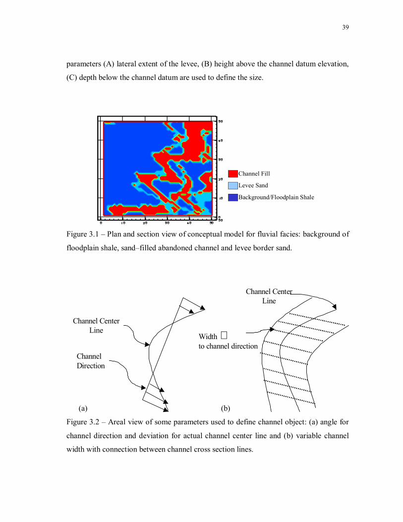
39
parameters (A) lateral extent of the levee, (B) height above the channel datum elevation,
(C) depth below the channel datum are used to define the size.
Channel Fill
Levee Sand
Background/Floodplain Shale
Figure 3.1 – Plan and section view of conceptual model for fluvial facies: background of
floodplain shale, sand–filled abandoned channel and levee border sand.
Channel CenterLine
Channel Direction
Width to channel direction
⊥
Channel CenterLine
Figure 3.2 – Areal view of some parameters used to define channel object: (a) angle for
channel direction and deviation for actual channel center line and (b) variable channel
width with connection between channel cross section lines.
(a) (b)

40
Width
Thickness
Position of maximumthickness
Figure 3.3 – Cross section view of channel object defined by width, thickness, and
relative position of maximum thickness.
Levee Sand Abandoned Sand-FilledChannel
A
C
Figure 3.4 – Cross section through abandoned sand-filled channel and levee sand. Three
distance parameters (A), (B) and (C) are used to define size of levee sand.
The modeling parameters selected for this study are as follows,
1. Channel Dimensions
- Thickness
- Width/Thickness Ratio
2. Sandstone ratio
3. Channel Permeability
- Channel sand permeability
- Levee sand permeability
B

41
4. Channel Sinuosity
The selection of the modeling parameters is largely subjective. It is important to use a
sound judgement while selecting modeling parameters. In this study, we assume the
above parameters to be largely uncertain and examine their impact on the flow
responses. Table 14 shows the factor ranges. The factor ranges are scaled from –1 to +1.
Factor combinations for the simulation models are specified by a 28 experiment Box-
Behnken design for the four-factor stochastic model sets. Flow simulation is performed
on five realizations at each design point for the stochastic permeability field. The
stochasticity in the object-based models comes from the random positioning of the
channels.
The synthetic reservoir model for this study (Fig. 3.5) is a 50x50x10-gridblock model
with an injector and producer in a Quarter 5-spot pattern. The size of each gridblock is
20x20x10 feet.
Table 15 shows the Box-Behnken experimental design for the object-based reservoir
scenarios. The first column indicates the experiment number and the next four columns
represent the levels of the four modeling parameters for each experiment. The sixth
column represents the mean swept volume efficiencies obtained by performing
streamline simulation on five stochastic realizations of each of the 28 scenarios. The
seventh column is the standard deviation of the sweep volume for each scenario. The
stochastic nature of each scenario is a result of random positioning of channels for a
particular scenario in an experiment. Figs. 3.6a, b and c show the permeability, swept
volume (at 5000 days) and travel time plot for a particular experiment. This scenario has
a high channel dimensions and low channel sinuosity. The travel time plot clearly shows
that the high permeability channel zones near the injector are swept almost
instantaneously. Similarly we can visualize similar plots for different scenarios to see
how our uncertainty in modeling parameters would effect the sweep and travel time plot
of the reservoir. Once the flow simulation results for all experiments are obtained we can
analyze the design with response surface methodology for identifying significant
parameters and for response uncertainty assessment.

42
Table 14 – Factor Ranges and Scaling for object-based models
LevelsVariable -1 0 1
ChanDimthickness (ft) 0.25--1 1--2 2--5
w/t ratio 15--25 25--75 80--100SandRatio 0.2 0.35 0.5ChanPet
Perm (md) (10,1) (100,10) (1000, 100)
Sinuosity (ft) 50 100 150
Table 15 – Experimental design: object-based model
Exp # ChannelDimen SandstoneRatioPetrophysical Sinuosity Vol.Sw Eff Std Deviation1 0 -1 0 -1 27.18% 8.10%2 -1 0 0 1 35.48% 3.12%3 1 0 0 -1 21.57% 8.97%4 -1 1 0 0 37.01% 3.15%5 0 1 1 0 43.66% 2.21%6 0 0 0 0 32.57% 2.04%7 0 0 0 0 30.59% 2.04%8 0 0 -1 1 50.65% 0.71%9 1 0 1 0 25.23% 4.15%10 -1 0 -1 0 55.05% 1.54%11 0 0 1 -1 29.12% 1.57%12 0 1 -1 0 52.59% 0.45%13 0 0 0 0 32.43% 0.86%14 -1 0 0 -1 38.22% 0.91%15 0 1 0 -1 41.58% 1.96%16 0 0 1 1 28.66% 0.54%17 0 -1 1 0 11.73% 1.58%18 1 0 0 1 30.04% 0.27%19 1 0 -1 0 33.47% 3.24%20 0 -1 0 1 35.31% 4.47%21 1 1 0 0 40.16% 1.32%22 -1 -1 0 0 26.00% 10.83%23 0 0 0 0 34.62% 0.82%24 1 -1 0 0 25.41% 1.81%25 0 1 0 1 44.15% 0.27%26 0 0 -1 -1 45.67% 3.96%27 -1 0 1 0 23.38% 1.85%28 0 -1 -1 0 43.86% 4.41%
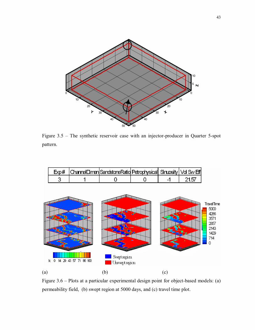
43
5
10
Z
0
10
20
30
40
50
X
0
10
20
30
40
50
Y
Figure 3.5 – The synthetic reservoir case with an injector-producer in Quarter 5-spot
pattern.
(a) (b) (c)
Figure 3.6 – Plots at a particular experimental design point for object-based models: (a)
permeability field, (b) swept region at 5000 days, and (c) travel time plot.

44
3.3.1 Identification and Uncertainty Analysis
The identification of significant reservoir modeling parameters is achieved by the
response surface methodology. The response surface can be directly obtained from the
flow responses in the experimental design. In this study, the form of the response surface
equation for the object-based model is a function of the modeling parameters.
SinuosityPetropropbSinuositySandstonebPetropropatioSandstoneRbSinuosityenChannelDimbPetropropenChannelDimbatioSandstoneR
enChannelDimbSinuositybPetropropb
atioSandstoneRbenChannelDimbSinuositybPetropropbatioSandstoneRbenChannelDimbbSweepEff
××+××+××+××+××+×
×+×+×+
×+×+×+
×+×+×+=
1413
12
1110
92
82
7
26
254
3210
)()(
)()(
(34)
Table 16 shows the response surface regression results obtained using statistical software
called EREGRESS. The first column indicates the coefficient that is computed and the
second column shows its value. The third column is the Pr-significant value. The Pr-
significant value cut-off for the factor to be significant is chosen as 0.005. This means
that the coefficients with Pr-significant value smaller than 0.005 are significant. The
fourth column shows the standard error in the estimation of a particular response surface
coefficient. The fifth and sixth columns show the –95% and +95% confidence values
respectively for a particular response surface coefficient. The highlighted rows show
coefficients for parameters that have a significant impact on the flow response. Before
using this response surface equation to predict sweep efficiency values over the whole
parameter range, we test this response surface model for the experimental design points,
for which we have the responses obtained from streamline simulation. Fig. 3.7 shows a
plot of predicted sweep efficiency v/s calculated sweep efficiency. The predicted sweep
efficiencies are the ones from the response surface model and the calculated sweep
efficiencies are the flow simulation results as shown in Table 15. The plot shows a very
high correlation coefficient (0.9427) validating the response surface model results.
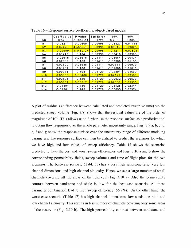
45
Table 16 – Response surface coefficients: object-based models
C o e ff v a lu e P v a lu e S td E rro r -95 % 95 %b 0 0 .3 26 8.10 6 e-11 0 .0 1 72 9 0 .2 8 8 0 .3 63b 1 -0 .03 2 7 1 0.00 6 00 0 .0 0 99 8 -0 .0 5 42 7 -0 .01 1 15b 2 0 .0 7 47 2 4.58 9 e-06 0 .0 0 99 8 0.05 3 15 0 .0 9 62 8b 3 -0 .09 9 5 9 1.84 5 e-07 0 .0 0 99 8 -0 .1 21 -0 .07 8 03b 4 0 .0 1 74 7 0 .1 0 4 0 .0 0 99 8 -0 .0 0 41 0 0 .0 3 90 3b 5 -0 .02 6 1 5 0.08 6 75 0 .0 1 41 1 -0 .0 5 66 4 0 .0 0 43 4b 6 0 .0 2 08 9 0 .1 6 3 0 .0 1 41 1 -0 .0 0 96 0 0 .0 5 13 8b 7 0 .0 3 89 0 0.01 6 35 0 .0 1 41 1 0.00 8 41 0 .0 6 93 9b 8 0 .0 1 96 1 0 .1 8 8 0 .0 1 41 1 -0 .0 1 08 8 0 .0 5 01 0b 9 0 .0 0 93 4 0 .5 9 8 0 .0 1 72 9 -0 .0 2 80 1 0 .0 4 66 9
b1 0 0 .0 5 85 6 0.00 4 86 0 .0 1 72 9 0.02 1 21 0 .0 9 59 1b1 1 0 .0 2 80 3 0 .1 2 9 0 .0 1 72 9 -0 .0 0 93 2 0 .0 6 53 7b1 2 0 .0 5 80 1 0.00 5 17 0 .0 1 72 9 0.02 0 66 0 .0 9 53 5b1 3 -0 .01 3 9 1 0 .4 3 6 0 .0 1 72 9 -0 .0 5 12 5 0 .0 2 34 4b1 4 -0 .01 3 6 1 0 .4 4 5 0 .0 1 72 9 -0 .0 5 09 5 0 .0 2 37 4
A plot of residuals (difference between calculated and predicted sweep volume) v/s the
predicted sweep volume (Fig. 3.8) shows that the residual values are of the order of
magnitude of 10-2. This allows us to further use the response surface as a predictive tool
to obtain flow responses over the whole parameter uncertainty range. Figs. 3.9 a, b, c, d,
e, f and g show the response surface over the uncertainty range of different modeling
parameters. The response surface can then be utilized to predict the scenarios for which
we have high and low values of sweep efficiency. Table 17 shows the scenarios
predicted to have the best and worst sweep efficiencies and Figs. 3.10 a and b show the
corresponding permeability fields, sweep volumes and time-of-flight plots for the two
scenarios. The best-case scenario (Table 17) has a very high sandstone ratio, very low
channel dimensions and high channel sinuosity. Hence we see a large number of small
channels covering all the areas of the reservoir (Fig. 3.10 a). Also the permeability
contrast between sandstone and shale is low for the best-case scenario. All these
parameter combination lead to high sweep efficiency (56.7%). On the other hand, the
worst-case scenario (Table 17) has high channel dimensions, low sandstone ratio and
low channel sinuosity. This results in less number of channels covering only some areas
of the reservoir (Fig. 3.10 b). The high permeability contrast between sandstone and
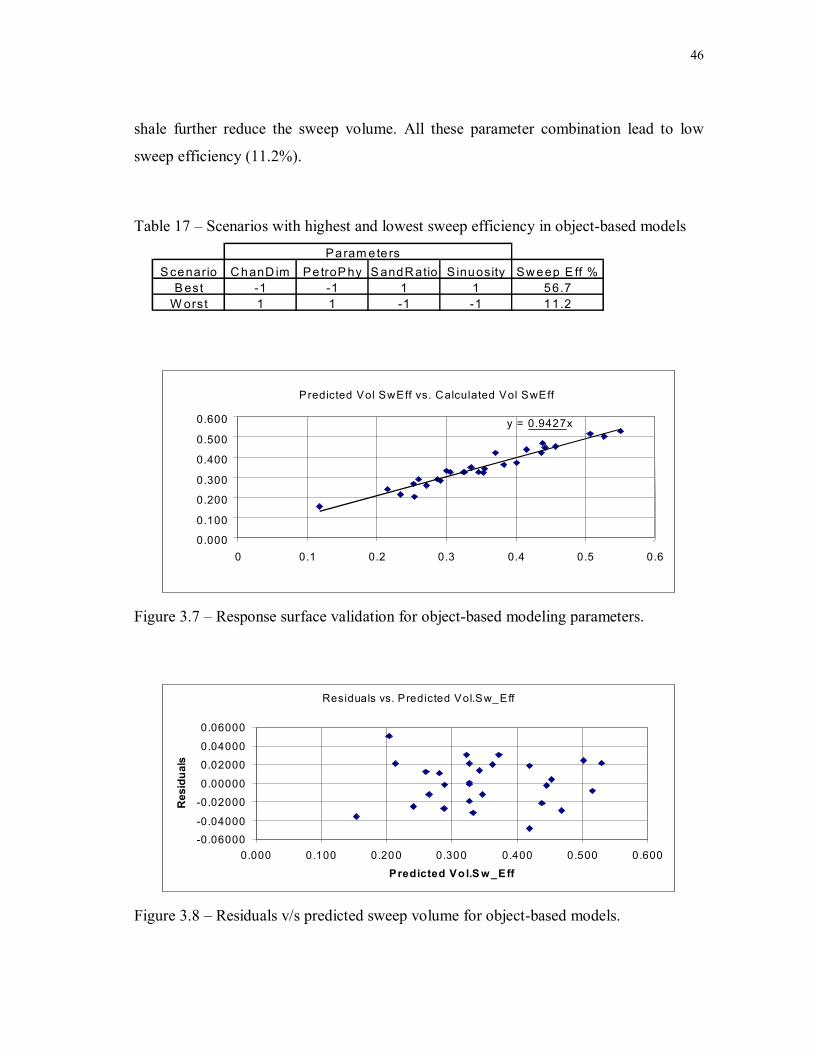
46
shale further reduce the sweep volume. All these parameter combination lead to low
sweep efficiency (11.2%).
Table 17 – Scenarios with highest and lowest sweep efficiency in object-based models Param eters
S cenario C hanD im PetroP hy S andR atio S inuosity Sw eep E ff %B est -1 -1 1 1 56.7
W orst 1 1 -1 -1 11.2
y = 0.9427x
0.000
0.100
0.200
0.300
0.400
0.500
0.600
0 0.1 0.2 0.3 0.4 0.5 0.6
Predicted Vol SwEff vs. Calculated Vol SwEff
Figure 3.7 – Response surface validation for object-based modeling parameters.
Residuals vs. P redicted Vol.Sw_Eff
-0.06000-0.04000
-0.02000
0.00000
0.02000
0.04000
0.06000
0.000 0.100 0.200 0.300 0.400 0.500 0.600Predicted Vol.S w_Eff
Res
idua
ls
Figure 3.8 – Residuals v/s predicted sweep volume for object-based models.

47
-1.0
-0.3
0.3
1.0
-1.0 -0
.6 -0.1 0.
3 0.8
0.00.10.20.30.4
0.5
0.6
Res
p1
Petrophysical ChannelDimen
0.5-0.60.4-0.50.3-0.40.2-0.30.1-0.20.0-0.1
-1.0 -0
.6 -0.1 0.
3 0.8
-1.0-0
.30.31.
0 0.0
0.1
0.2
0.3
0.4
0.5
Res
p1
SandstoneRatio
ChannelDimen
0.4-0.50.3-0.40.2-0.30.1-0.20.0-0.1
-1.0-0
.30.31.
0
-1.0
-0.6
-0.1
0.3
0.8
0.0
0.1
0.2
0.3
0.4
Resp
1
SinuosityChannelDimen
0.3-0.40.2-0.30.1-0.20.0-0.1
-1.0-0
.30.31.
0
-1.0
-0.6
-0.1
0.3
0.8
0.00.10.20.3
0.4
0.5
0.6
Resp
1
SandstoneRatio Petrophysical
0.5-0.60.4-0.50.3-0.40.2-0.30.1-0.20.0-0.1
-1.0-0
.30.31.
0
-1.0
-0.6
-0.1
0.3
0.8
0.00.10.20.30.40.5
0.6
Res
p1
SinuosityPetrophysical
0.5-0.60.4-0.50.3-0.40.2-0.30.1-0.20.0-0.1
-1.0 -0
.6 -0.1 0.
3 0.8
-1.0-0
.30.31.
0 0.0
0.1
0.2
0.3
0.4
0.5
Res
p1
SinuositySandstoneR
atio
0.4-0.50.3-0.40.2-0.30.1-0.20.0-0.1
a b
c d
e f
Resp 1Resp 1
Resp 1
Resp 1
Resp 1 Resp 1
Petrophysical Chan Dimen Chan Dimen Sandstone Ratio
Sinuosity Chan Dimen
Sandstone Ratio Petrophysical
Sinuosity Petrophysical
Sandstone Ratio
Sinuosity
Figure 3.9 – Response surfaces over the uncertainty range of object-based modeling
parameters.
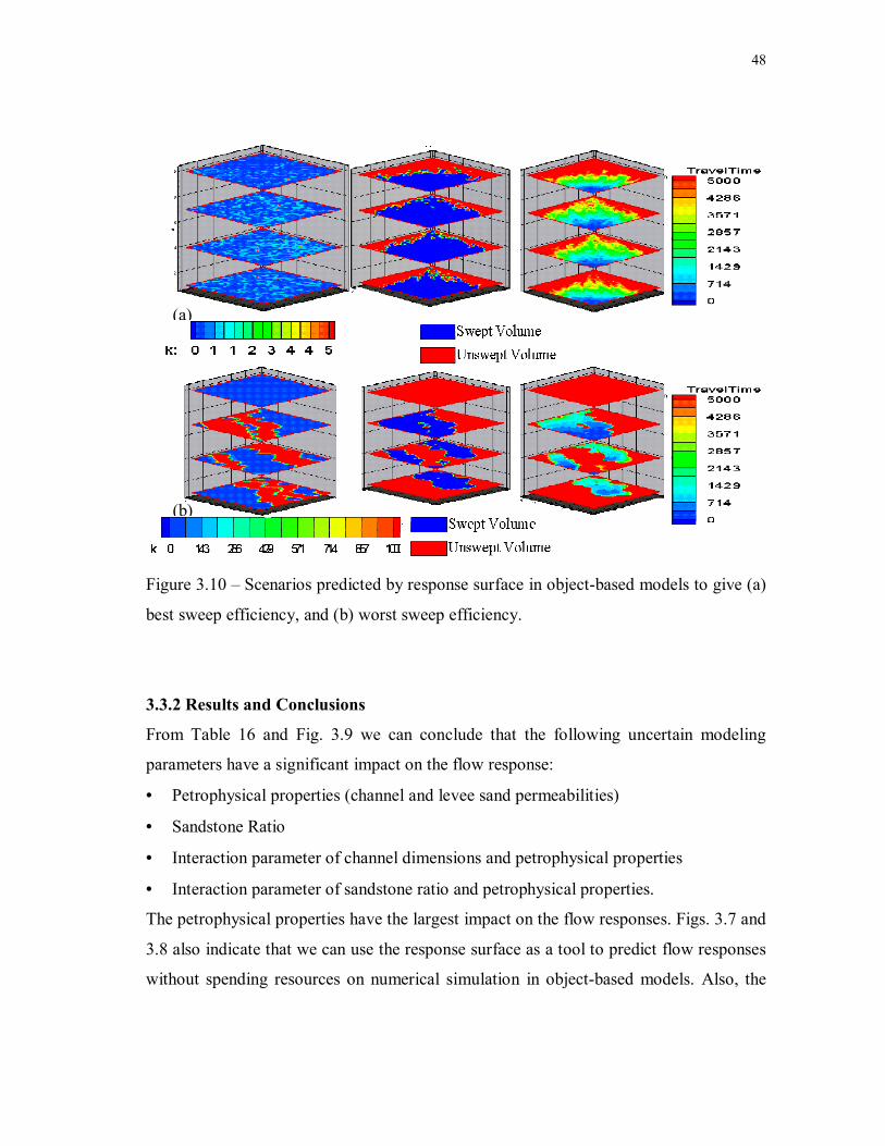
48
Figure 3.10 – Scenarios predicted by response surface in object-based models to give (a)
best sweep efficiency, and (b) worst sweep efficiency.
3.3.2 Results and Conclusions
From Table 16 and Fig. 3.9 we can conclude that the following uncertain modeling
parameters have a significant impact on the flow response:
• Petrophysical properties (channel and levee sand permeabilities)
• Sandstone Ratio
• Interaction parameter of channel dimensions and petrophysical properties
• Interaction parameter of sandstone ratio and petrophysical properties.
The petrophysical properties have the largest impact on the flow responses. Figs. 3.7 and
3.8 also indicate that we can use the response surface as a tool to predict flow responses
without spending resources on numerical simulation in object-based models. Also, the
(a)
(b)

49
response surfaces in Fig. 3.9 provide quick insights into flow response-parameter
relationships. It is also clear that the uncertainty in certain object-based modeling
parameters has a large impact on the flow responses. The response surface can predict
the scenarios for which we get the best and the worst flow response.
3.4 Pixel-Based Model
A similar synthetic fluvial reservoir which we modeled using object-based modeling
technique is now modeled using a pixel-based technique. We use sequential indicator
simulation (SIS) which is a pixel-based simulation algorithm that builds a categorical
image, pixel by pixel, by drawing from a non-parametric conditional distribution. Unlike
object-based models, for pixel-based algorithms, the resulting geometries (for each
category) tend to be noisy. However, conditioning to well data is not a problem in pixel-
based methods like SIS. We use an indicator simulation with three categories since we
have three facies similar to the ones in the reservoir model used in object-based
technique. For this particular study, we use the GSLIB sisim program.
For the single multiple indicator simulation the following sequence is adopted. The
indicator is defined by three categories, each category representing a particular facies.
Also the well data is represented as indicator data for each layer in the reservoir model.
We carry out a sequence of indicator krigings at each node, conditional to neighboring
well indicator data and previously simulated indicator values. This indicator kriging
requires the 3D variogram of the indicator variable. The parameters used to model this
indicator variogram (range, sill and nugget) can be highly uncertain. Geological
interpretation of the channel sizes usually helps us in evaluating the uncertainty of the
variogram range. The sum of sill and nugget is set to 1 and both the sill and nugget are
varied accordingly to study their impact on flow responses.
The modeling parameters selected for this study are as follows,
1. Variogram Range
- Major Axis
- Minor Axis

50
2. Sandstone ratio
3. Channel Permeability
- Channel sand permeability
- Levee sand permeability
4. Variogram Parameters
- Nugget
- Sill
The sandstone ratio is changed by changing the sandstone pdf cut off value, which
indicates the probability of sandstone facies in the reservoir model. The channel and
levee sand permeability range is the same as that in object-based models.
Table 18 shows the factor ranges. The factor ranges are scaled from –1 to +1. Factor
combinations for the simulation models are specified by a 28 experiment Box-Behnken
design for the four-factor stochastic model sets. Five realizations are run at each design
point for the stochastic permeability field.
The synthetic reservoir model for this study is a 50x50x10-gridblock model with an
injector and producer in a Quarter 5-spot pattern. The size of each gridblock is 20x20x10
feet. This reservoir is the same as used in object-based modeling.
Table 19 shows the Box-Behnken experimental design for the object-based reservoir
scenarios. The first column indicates the experiment number and the next four columns
represent the levels of the four modeling parameters for each experiment. The sixth
column represents the mean sweep volume efficiencies obtained by performing
streamline simulation on five stochastic realizations of each of the 28 scenarios. The
seventh column is the standard deviation of the sweep volume for each scenario.
Figs. 3.11 a, b and c show the permeability, swept volume (at 5000 days) and travel
time plot for a particular experiment. This scenario has a high variogram range and low
sandstone ratio. The travel time plot clearly shows that the high permeability channel
zones near the injector are swept almost instantaneously. Similarly we can visualize
similar plots for different scenarios to see how our uncertainty in modeling parameters
would affect the sweep and travel time plot of the reservoir. Once the flow simulation

51
results for all experiments are obtained we can analyze the design with response surface
methodology for identifying significant parameters and for response uncertainty
assessment.
Table 18 – Factor ranges and scaling for pixel-based models Parameter -1 0 1
Var iogram Rangea_hmax 100.00 500.00 1000.00a_hmin 10.00 50.00 100.00
Sanstone pdf cut-off 0.2 0.35 0.5C hanPet
Perm (10,1) (100,10) (1000, 100)
Var iogram nugget 0 0.4 0.8sill 1 0.6 0.2
Table 19 – Experimental design: pixel-based model Exp # Variogramrange pdfcutoff petrophysical Nugget&Sill Vol Sw.Eff Std Deviation
1 1 -1 0 0 24.01% 0.78%2 -1 0 -1 0 53.34% 1.27%3 0 0 -1 1 51.93% 0.67%4 0 1 1 0 44.56% 1.88%5 0 0 1 -1 10.57% 1.86%6 -1 0 0 1 31.01% 5.04%7 1 0 0 1 35.36% 0.79%8 0 0 0 0 30.94% 2.08%9 0 0 0 0 30.29% 2.41%
10 0 1 -1 0 50.53% 0.64%11 0 0 0 0 30.71% 2.64%12 0 0 1 1 12.56% 3.52%13 -1 0 0 -1 28.03% 4.84%14 1 0 -1 0 47.62% 1.06%15 1 0 1 0 17.42% 3.47%16 0 -1 -1 0 58.95% 0.76%17 -1 1 0 0 47.57% 0.34%18 0 -1 0 1 24.86% 3.04%19 -1 -1 0 0 25.13% 1.80%20 0 0 0 0 30.33% 1.72%21 0 -1 1 0 9.93% 1.68%22 0 -1 0 -1 12.98% 1.32%23 0 1 0 1 46.25% 5.36%24 0 1 0 -1 34.87% 1.23%25 0 0 -1 -1 40.62% 3.83%26 -1 0 1 0 24.77% 0.62%27 1 1 0 0 45.60% 0.53%28 1 0 0 -1 11.41% 1.17%
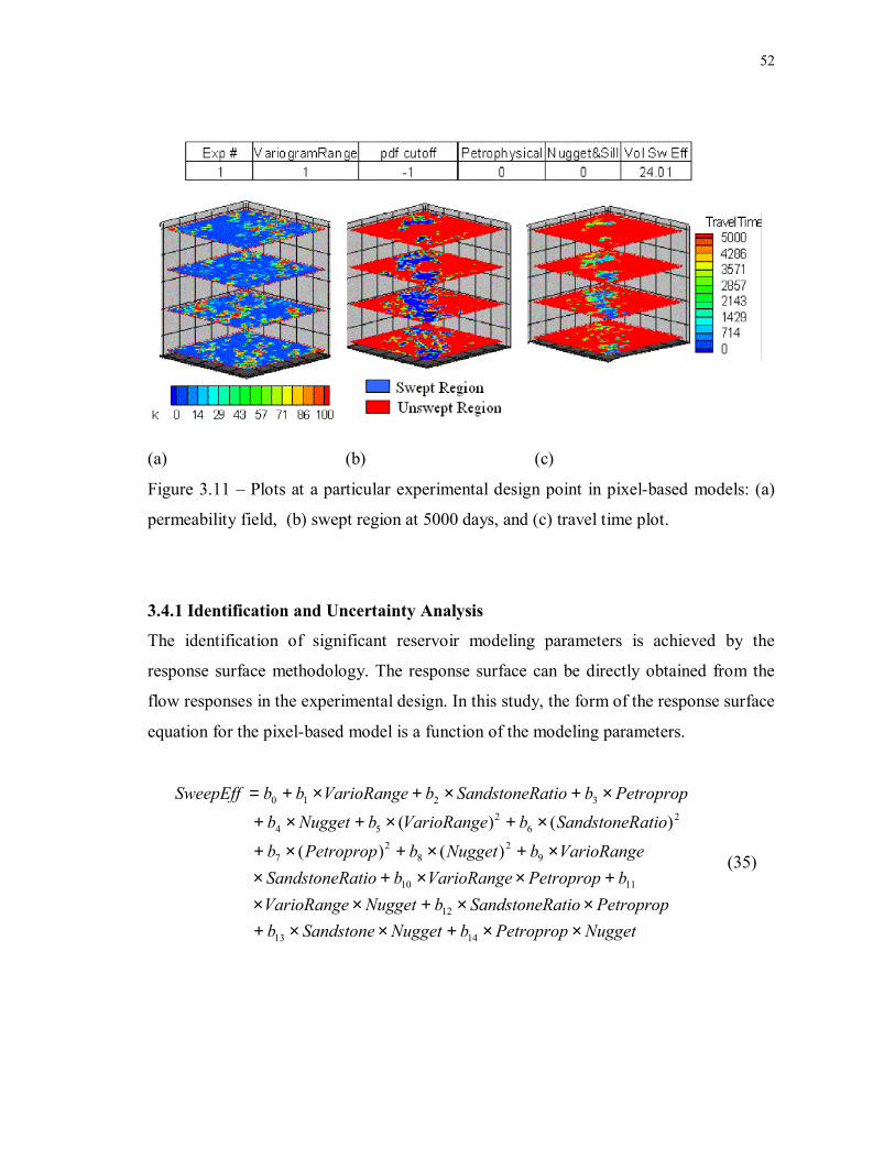
52
(a) (b) (c)
Figure 3.11 – Plots at a particular experimental design point in pixel-based models: (a)
permeability field, (b) swept region at 5000 days, and (c) travel time plot.
3.4.1 Identification and Uncertainty Analysis
The identification of significant reservoir modeling parameters is achieved by the
response surface methodology. The response surface can be directly obtained from the
flow responses in the experimental design. In this study, the form of the response surface
equation for the pixel-based model is a function of the modeling parameters.
NuggetPetropropbNuggetSandstonebPetropropatioSandstoneRbNuggetVarioRange
bPetropropVarioRangebatioSandstoneRVarioRangebNuggetbPetropropb
atioSandstoneRbVarioRangebNuggetbPetropropbatioSandstoneRbVarioRangebbSweepEff
××+××+××+××
+××+××+×+×+
×+×+×+
×+×+×+=
1413
12
1110
92
82
7
26
254
3210
)()(
)()(
(35)

53
Table 20 shows the response surface regression results obtained using a statistical
software called EREGRESS. The first column indicates the coefficient that is computed
and the second column shows its value. The third column is the Pr-significant value. The
Pr-significant value cut-off for the factor to be significant is chosen as 0.005. This means
that the coefficients with Pr-significant value smaller than 0.005 are significant. The
fourth column shows the standard error in the estimation of a particular response surface
coefficient. The fifth and sixth columns show the –95% and +95% confidence values
respectively for a particular response surface coefficient. The highlighted rows show
coefficients for parameters that have a significant impact on the flow response. Before
using this response surface equation to predict sweep efficiency values over the whole
parameter range, we test this response surface model for the experimental design points,
for which we have the responses obtained from streamline simulation. Fig. 3.12 shows a
plot of predicted sweep efficiency v/s calculated sweep efficiency. The predicted sweep
efficiencies are the ones from the response surface model and the calculated sweep
efficiencies are the flow simulation results as shown in Table 19. The plot shows a very
high correlation coefficient (0.9771) validating the response surface model results. A
plot of residuals (difference between calculated and predicted sweep volume) v/s the
predicted sweep volume (Fig. 3.13) shows that the residual values are of the order of
magnitude of 10-2. This allows us to further use the response surface as a predictive tool
to obtain flow responses over the whole parameter uncertainty range. This allows us to
further use the response surface as a predictive tool to obtain flow responses over the
whole parameter uncertainty range. Figs. 3.14. a, b, c, d, e, f and g show the response
surface over the uncertainty range of different modeling parameters.
The response surface can then be utilized to predict the scenarios for which we have high
and low values of sweep efficiency. Table 21 shows the scenarios predicted to have the
best and worst sweep efficiencies and Figs. 3.15 a and b show the corresponding
permeability fields, sweep volume and time-of-flight plot for the two scenarios. The best
case scenario (Table 21) has a very high sandstone ratio and very high variogram range.
Since the variogram range is directly proportional to the length of the channel, we see a
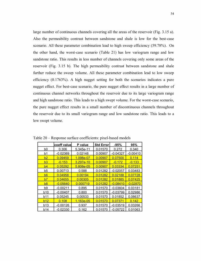
54
large number of continuous channels covering all the areas of the reservoir (Fig. 3.15 a).
Also the permeability contrast between sandstone and shale is low for the best-case
scenario. All these parameter combination lead to high sweep efficiency (59.78%). On
the other hand, the worst-case scenario (Table 21) has low variogram range and low
sandstone ratio. This results in less number of channels covering only some areas of the
reservoir (Fig. 3.15 b). The high permeability contrast between sandstone and shale
further reduce the sweep volume. All these parameter combination lead to low sweep
efficiency (0.1763%). A high nugget setting for both the scenarios indicates a pure
nugget effect. For best-case scenario, the pure nugget effect results in a large number of
continuous channel networks throughout the reservoir due to its large variogram range
and high sandstone ratio. This leads to a high swept volume. For the worst-case scenario,
the pure nugget effect results in a small number of discontinuous channels throughout
the reservoir due to its small variogram range and low sandstone ratio. This leads to a
low swept volume.
Table 20 – Response surface coefficients: pixel-based models
coeff value P value Std Error -95% 95%b0 0.306 5.345e-11 0.01570 0.272 0.340b1 -0.02369 0.02148 0.00907 -0.04327 -0.00410b2 0.09459 1.098e-07 0.00907 0.07500 0.114b3 -0.153 3.297e-10 0.00907 -0.172 -0.133b4 0.05292 5.808e-05 0.00907 0.03334 0.07251b5 0.00713 0.588 0.01282 -0.02057 0.03483b6 0.04958 0.00194 0.01282 0.02188 0.07728b7 0.04655 0.00305 0.01282 0.01885 0.07425b8 -0.05640 0.000719 0.01282 -0.08410 -0.02870b9 -0.00211 0.895 0.01570 -0.03604 0.03181b10 -0.00407 0.800 0.01570 -0.03799 0.02986b11 0.05245 0.00533 0.01570 0.01852 0.08637b12 0.108 1.163e-05 0.01570 0.07371 0.142b13 -0.00126 0.937 0.01570 -0.03519 0.03266b14 -0.02330 0.162 0.01570 -0.05722 0.01063

55
Table 21 – Scenarios with highest and lowest sweep efficiency in pixel-based models
ParametersScenario Nugget VarioRange SandRatio Petrophy Sweep Eff %
Best 1 1 1 -1 59.78Worst 1 -1 -1 1 0.1763
Predicted Vol SwEff vs. Calculated Vol SwEff
y = 0.9771x
0.0000.1000.2000.3000.4000.5000.6000.700
0 0.1 0.2 0.3 0.4 0.5 0.6 0.7
Figure 3.12 – Response surface validation for pixel-based modeling parameters.
Residuals vs. Predicted VolSwEff
-0.06000-0.04000
-0.020000.00000
0.020000.04000
0.06000
0.000 0.100 0.200 0.300 0.400 0.500 0.600
Predicted VolSwEff
Res
idua
ls
Figure 3.13 – Residuals vs. predicted sweep efficiency for pixel-based models.

56
-1.0 -0.6 -0.1 0.
3 0.8
-1.0
0.1 0.000.050.100.150.200.250.300.35
VolS
wEf
fVariogramrange
Nugget&Sill
0.3-0.40.3-0.30.2-0.30.2-0.20.1-0.20.1-0.10.0-0.1
-1.0-0
.30.31.
0
-1.0
-0.6
-0.1
0.3
0.8
0.0
0.1
0.2
0.3
0.4
0.5
VolS
wEf
f
pdfcutoffNugget&Sill
0.4-0.50.3-0.40.2-0.30.1-0.20.0-0.1
-1.0
-0.3
0.3
1.0
-1.0 -0
.6 -0.1 0.
3 0.8
0.00.10.20.30.40.5
0.6
VolS
wEf
f
petrophysical Nugget&Sill
0.5-0.60.4-0.50.3-0.40.2-0.30.1-0.20.0-0.1
-1.0 -0
.3 0.3 1.
0
-1.0-0
.6-0.10.
30.8
0.0
0.1
0.2
0.3
0.4
0.5
VolS
wEf
f
pdfcutoff
Variogramrange
0.4-0.50.3-0.40.2-0.30.1-0.20.0-0.1
-1.0
-0.3
0.3
1.0
-1.0 -0
.6 -0.1 0.
3 0.8
0.00.10.20.3
0.4
0.5
0.6
VolS
wEf
f
petrophysical Variogramrange
0.5-0.60.4-0.50.3-0.40.2-0.30.1-0.20.0-0.1
-1.0
-0.6
-0.1
0.3
0.8
-1.0 -0
.3 0.3 1.
00.00.10.20.3
0.4
0.5
0.6
VolS
wEf
f
petrophysical
pdfcutoff
0.5-0.60.4-0.50.3-0.40.2-0.30.1-0.20.0-0.1
(a) (b)
(c) (d)
(c) (e)
VolSwEffVolSwEff
VolSwEff VolSwEff
VolSwEffVolSwEff
Nugget & Sill
Variogram Range
pdf cutoffNugget & Sill
Petrophysical Nugget & Sill Variogram Range
pdf cutoff
Petrophysical Variogram Range Petrophysical
pdf cut off
Figure 3.14 – Response surfaces over the uncertainty range of pixel-based modeling
parameters.
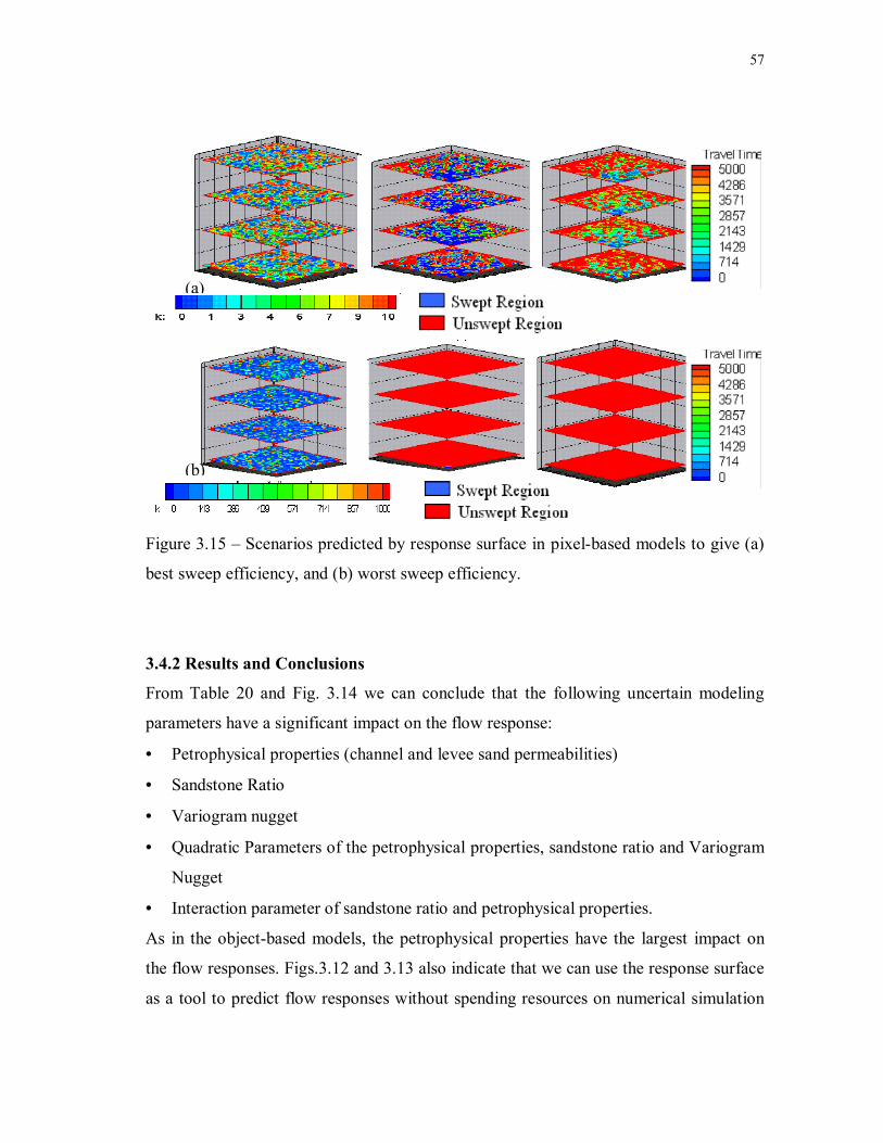
57
Figure 3.15 – Scenarios predicted by response surface in pixel-based models to give (a)
best sweep efficiency, and (b) worst sweep efficiency.
3.4.2 Results and Conclusions
From Table 20 and Fig. 3.14 we can conclude that the following uncertain modeling
parameters have a significant impact on the flow response:
• Petrophysical properties (channel and levee sand permeabilities)
• Sandstone Ratio
• Variogram nugget
• Quadratic Parameters of the petrophysical properties, sandstone ratio and Variogram
Nugget
• Interaction parameter of sandstone ratio and petrophysical properties.
As in the object-based models, the petrophysical properties have the largest impact on
the flow responses. Figs.3.12 and 3.13 also indicate that we can use the response surface
as a tool to predict flow responses without spending resources on numerical simulation
(a)
(b)
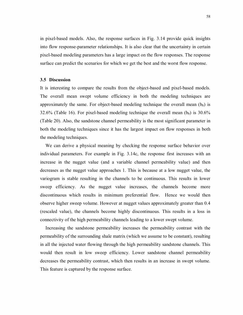
58
in pixel-based models. Also, the response surfaces in Fig. 3.14 provide quick insights
into flow response-parameter relationships. It is also clear that the uncertainty in certain
pixel-based modeling parameters has a large impact on the flow responses. The response
surface can predict the scenarios for which we get the best and the worst flow response.
3.5 Discussion
It is interesting to compare the results from the object-based and pixel-based models.
The overall mean swept volume efficiency in both the modeling techniques are
approximately the same. For object-based modeling technique the overall mean (b0) is
32.6% (Table 16). For pixel-based modeling technique the overall mean (b0) is 30.6%
(Table 20). Also, the sandstone channel permeability is the most significant parameter in
both the modeling techniques since it has the largest impact on flow responses in both
the modeling techniques.
We can derive a physical meaning by checking the response surface behavior over
individual parameters. For example in Fig. 3.14c, the response first increases with an
increase in the nugget value (and a variable channel permeability value) and then
decreases as the nugget value approaches 1. This is because at a low nugget value, the
variogram is stable resulting in the channels to be continuous. This results in lower
sweep efficiency. As the nugget value increases, the channels become more
discontinuous which results in minimum preferential flow. Hence we would then
observe higher sweep volume. However at nugget values approximately greater than 0.4
(rescaled value), the channels become highly discontinuous. This results in a loss in
connectivity of the high permeability channels leading to a lower swept volume.
Increasing the sandstone permeability increases the permeability contrast with the
permeability of the surrounding shale matrix (which we assume to be constant), resulting
in all the injected water flowing through the high permeability sandstone channels. This
would then result in low sweep efficiency. Lower sandstone channel permeability
decreases the permeability contrast, which then results in an increase in swept volume.
This feature is captured by the response surface.

59
The significance of interaction parameters, especially between sandstone ratio and
petrophysical properties, on flow responses indicates that flow behavior would change
with respect to sandstone ratio if the petrophysical properties are changed and vice-
versa. Another important significant interaction parameter is between channel
dimensions and petrophysical properties.
Another important aspect of this study is that we performed quick streamline
simulation on five different realizations within each scenario for both object and pixel-
based models. In theory, we can have infinite number of stochastic realizations. It is then
interesting to see the response surface of the variance of flow responses within each
scenario for object-based models. The variance in object-based model is due to its
stochastic nature, which comes from the random positioning of the channels for different
random numbers within a scenario. The variance for each scenario represents the
stochastic nature for that particular set of parameter values. Figs. 3.16. a, b, c, d, e and f
show the response surfaces for variance in swept volume with respect to the object-based
modeling parameters. This figure then gives a useful insight as to how the uncertainty in
modeling parameters affects the stochastic nature of the object-based modeling
technique. This exercise would be extremely useful to rank stochastic object-based
reservoir models that also have uncertain modeling parameter ranges. The response
surface can be optimized to get the modeling parameter values at which the variance due
to stochastic nature is the minimum. Hence, for object based models, we can have
parameter values at which the flow response is the best and worst (Table 17 and Fig.
3.10) and the parameter values at which the variance or standard deviation in sweep
volume due to stochastic nature is minimum and maximum (Table 22 and Figs. 3.17 a
and b). Figs. 3.17 a and b represent the permeability plots of scenarios with minimum
and maximum sweep volume variance respectively. Fig. 3.17 a. clearly shows a large
number of low sinuosity channels running through the whole reservoir. Since the
variance in swept volume comes from the random positioning of the channels, the
variance in swept volume for this permeability scenario would be negligible. Fig. 3.17 b.
shows very few low sinuosity channels running through the reservoir. This indicates that
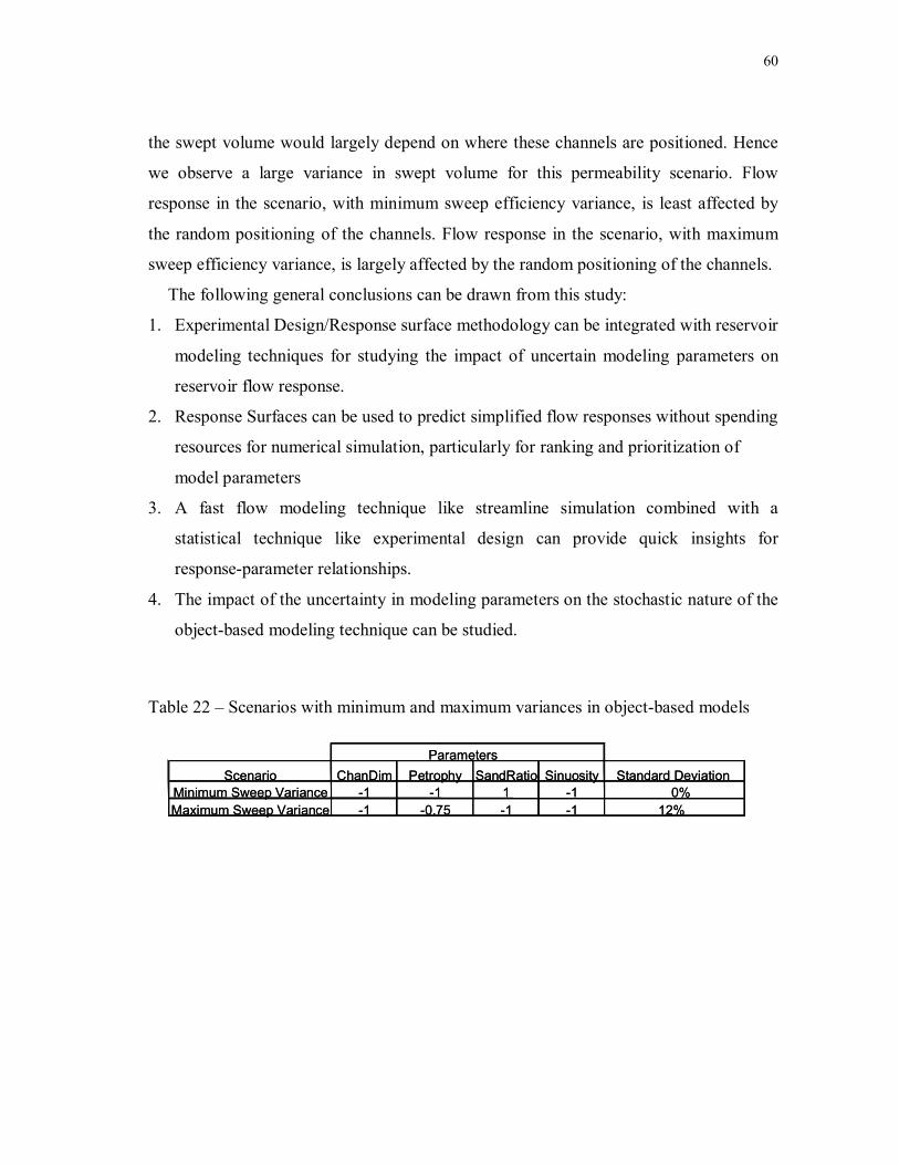
60
the swept volume would largely depend on where these channels are positioned. Hence
we observe a large variance in swept volume for this permeability scenario. Flow
response in the scenario, with minimum sweep efficiency variance, is least affected by
the random positioning of the channels. Flow response in the scenario, with maximum
sweep efficiency variance, is largely affected by the random positioning of the channels.
The following general conclusions can be drawn from this study:
1. Experimental Design/Response surface methodology can be integrated with reservoir
modeling techniques for studying the impact of uncertain modeling parameters on
reservoir flow response.
2. Response Surfaces can be used to predict simplified flow responses without spending
resources for numerical simulation, particularly for ranking and prioritization of
model parameters
3. A fast flow modeling technique like streamline simulation combined with a
statistical technique like experimental design can provide quick insights for
response-parameter relationships.
4. The impact of the uncertainty in modeling parameters on the stochastic nature of the
object-based modeling technique can be studied.
Table 22 – Scenarios with minimum and maximum variances in object-based models
ParametersScenario ChanDim Petrophy SandRatio Sinuosity Standard Deviation
Minimum Sweep Variance -1 -1 1 -1 0%Maximum Sweep Variance -1 -0.75 -1 -1 12%
ParametersScenario ChanDim Petrophy SandRatio Sinuosity Standard Deviation
Minimum Sweep Variance -1 -1 1 -1 0%Maximum Sweep Variance -1 -0.75 -1 -1 12%

61
-1.0
-0.6
-0.1
0.3
0.8
-1.0
-0.3
0.3
1.0
0.0000
0.0005
0.0010
0.0015
0.0020
Varia
nce
Petrophysical
ChannelDimen -1
.0-0.6-0.10.
30.8
-1.0
0.10.00000.00100.00200.00300.00400.00500.00600.00700.0080
Varia
nce
SandstoneRatio
ChannelDimen
-1.0 -0.6 -0.1 0.
3 0.8
-1.0
0.1 0.00000.00100.0020
0.0030
0.0040
0.0050
0.0060
Varia
nce
Sinuosity
ChannelDime
n
-1.0 -0
.3 0.3 1.
0
-1.0-0
.6-0.10.
30.8
0.00000.00050.00100.00150.00200.00250.00300.0035
Varia
nce
SandstoneRatio
Petrophysical
-1.0 -0
.3 0.3 1.
0
-1.0-0
.6-0.10.
30.8
0.0000
0.0005
0.0010
0.0015
0.0020
0.0025
Varia
nce
Sinuosity
Petrophysical -1.0-0
.6-0.10.
30.8 -1.0
-0.3
0.3
1.0
0.00000.00100.00200.00300.00400.00500.00600.0070
Varia
nce
Sinuosity
SandstoneRatio
0.0-0.00.0-0.00.0-0.00.0-0.00.0-0.00.0-0.00.0-0.0
(a) (b)
(c) (d)
(e) (f)
Variance Variance
VarianceVariance
Variance Variance
Chan Dim Petrophysical Sandstone
Ratio
Chan Dimen
Chan Dimen
SinuosityPetrophysical
Sandstone Ratio
Petrophysical Sinuosity
Sinuosity
Sandstone Ratio
Sandstone Ratio
Figure 3.16 – Response surfaces of sweep volume variances over the uncertainty range
of modeling parameters in object-based models.

62
Figure 3.17 – Scenarios predicted by response surface of variances in sweep volume for
object-based models to give (a) minimum sweep efficiency variance, and (b) maximum
sweep efficiency variance.

63
CHAPTER IV
CONCLUSIONS AND FUTURE WORK
This research successfully applied a statistical tool called experimental design and
response surface methodology for a reservoir characterization problem and for flow
uncertainty assessment.
In the first study, the drainage volumes, obtained from decline curve analysis and
‘diffusive’ time-of-flight concept, are matched via experimental design leading to two
conclusions which can be used for similar kind of studies:
• Experimental design can be successfully used to characterize barrier locations
and barrier transmissibility in different reservoirs
• The ‘diffusive’ time-of-flight approach to calculate drainage volume is further
validated by the experimental design.
Streamline-based drainage volume calculations in conjunction with conventional decline
type curve analysis can provide a powerful approach to identification of reservoir
compartmentalization and flow barriers during early stages of reservoir development.
This approach relies on inferring flow barriers and reservoir compartmentalization based
on a drainage volume matching. Thus, the results will be non-unique in general and will
require prior geologic knowledge or additional information to address such non-
uniqueness. The experimental design and Analysis of Variance quantifies this
uncertainty in the location and strength of the flow barriers
The second study successfully integrates experimental design/response surface
methodology with reservoir modeling and flow simulation to study the impact of
uncertain modeling parameters on the reservoir flow response. First, the study reveals
the modeling parameters that significantly affect flow response. The response surface
analysis then tells us how exactly the flow response behaves within the uncertainty range
of modeling parameters. Further study to optimize the response surface for the minimum
and maximum flow response, reveals the worst reservoir model and the best reservoir

64
model scenarios in terms of flow response. The worst reservoir model can be considered
as a pessimistic case for recovery predictions and the best reservoir model can be
considered as the optimistic case for the recovery predictions. Hence, one can obtain a
preliminary ranking of reservoir models based on the uncertainty in model parameters.
For the object-based models, we also analyze the response surface of the flow response
variance. This analysis gives us the scenarios that would show maximum and minimum
variability of flow response due to the random positioning of the high-permeability
channels. The above two analysis combined would then help us to identify scenarios
where the flow response might be favorable but also might be highly uncertain and
largely dependent on the positioning of channels. It could also help us identify scenarios
with a highly predictable flow response.
The future work would involve successful application of the experimental
design/response surface procedure on a field case. It would be interesting to see if the
response surface can predict the flow responses accurately for a complicated field case.
Another area of research would be the application of response surface methodology for
history matching purposes. Response surfaces can be used to compute sensitivities or
flow responses instead of the flow simulator, which can significantly reduce the
computation time for history matching large reservoirs.

65
NOMENCLATURE
DF =degrees of freedom
F =test statistic
MSError = experimental error mean squares
MSLoc = location mean squares
MSTrans = transmissibility mean squares
P =significance level
SSError = experimental error sum of squares
SSLoc = location sum of squares
SSTrans = transmissibility sum of squares
SSY = total sum of squares
A =drainage area
Bo =formation factor of oil
Ca =shape factor of drainage area
ce =effective compressibility
cf =rock compressibility
co =oil compressibility
cw =water compressibility
ct =total compressbility
h =formation thickeness
K =permeability of reservoir
Ko =effective permeability of oil
Np =cumulative production of well
pi =initial reservoir pressure
pwf =flow bottomhole pressure of well
q =production rate of well
qDd =dimensionless production rate
rD =dimensionless radius

66
rw’ =effecitive wellbore radius
s =distance along streamline
So =oil saturation
Sw =water saturation
tD =dimensionless time
t =material balance time
Ddt =dimensionless material balance time
φ =porosity
γ =Euler constant
tλ =total mobility
oµ =viscosity of oil
τ =time of flight
'τ =‘Diffusive’ time of flight
θ =Heaviside function
χψ , =bi-streamfunctions

67
REFERENCES
1. White, C.D., Willis, B.J., Narayanan, K. and Dutton, S.P.: “Identifying and
Estimating Significant Geologic Parameters With Experimental Design,” SPEJ,
(Sept 2001), 311-324.
2. Brandsaeter, I., Wist, H.T., Naess, A., Lia, O., Arntzen, J. et al.: “Ranking of
Stochastic Realizations of Complex Tidal Reservoirs Using Streamline Simulation
Criteria,” Petroleum Geoscience (2001) 7, S53-S63.
3. Manceau, E., Mezghani, M., Zabala-Mezghani, I. and Roggero, F.: “Combination of
Experimental Design and Joint Modeling Methods for Quantifying the Risk
Associated With Deterministic and Stochastic Uncertainties-An Integrated Test
Study,” paper SPE 71620 presented at the 2001 SPE Annual Technical Conference
and Exhibition, New Orleans, Louisiana, September 30-October 3.
4. Friedmann, F., Chawathe, A. and Larue, D.K.: “Assessing Uncertainty in
Channelized Reservoirs Using Experimental Designs,” paper SPE 71622 presented
at the 2001 SPE Annual Technical Conference and Exhibition, New Orleans,
Louisiana, September 30-October 3.
5. White, C.D. and Royer, S.A.: “Experimental Design as a Framework for Reservoir
Studies,” paper SPE 79676 presented at the 2003 SPE Reservoir Simulation
Symposium, Houston, Texas, February 3-5.
6. Parish, R.G., Calderbank, V.J., Watkins, A.J., Muggeridge, A.H., Goode, A.T. et al.:
“Effective History Matching: The Application of Advanced Software Techniques to
the History Matching Process,” paper SPE 25250 presented at the 1993 SPE
Reservoir Simulation Symposium, New Orleans, Louisiana, February 28-March 3.
7. Eide, A.L., Holden, L., Reiso, E. and Aanonsen, S.I.: “Automatic History Matching
by Use of Response Surface and Experimental Design,” paper presented at the 1994
IV European Conference on Mathematics of Oil Recovery, Roras, Norway, June 7-
10.
68
8. Zabala, I., Blanc, G., Collombier, D. and Mezghani, M.: “Use of Experimental
Design in Resolving Inverse Problems: Application to History Matching”, paper
presented at the 2000 VII European Conference on Mathematics of Oil Recovery,
Baveno, Italy, September 5-8.
9. Zabala, I.M. and Mezghani, M.: “Constraining Reservoir Facies Models to Dynamic
Data-Impact,” paper SPE 71335 presented at the 2001 SPE Annual Technical
Conference and Exhibition, New Orleans, Louisiana, September 30-October 3.
10. Damsleth, E., Hage, A. and Volden, R.: “Maximum Information at Minimum Cost:
A North Sea Field Development Study Using Experimental Design,” paper SPE
23139 presented at the 1991 Offshore Europe Conference, Aberdeen, Scotland,
September 3- 6.
11. Faidi, S.A., Ponting, D.K. and Eagling, T.L.: “Experimental Design in Interactive
Reservoir Simulation,” paper SPE 36005 presented at the 1996 Petroleum Computer
Conference, Dallas, Texas, June 2- 5.
12. Dejean, J.P. and Blanc, G.: “Managing Uncertainties on Production Predictions
Using Integrated Statistical Methods,” paper SPE 56696 presented at the 1999 SPE
Annual Technical Conference and Exhibition, Houston, Texas, October 3-6.
13. Venkataraman, R.: “Application of the Method of Experimental Design to Quantify
Uncertainty in Production Profiles,” paper SPE 59422 presented at the 2000 Asia
Pacific Conference on Integrated Modeling for Asset Management, Yokohama,
Japan, April 25-26.
14. Chewaroungroaj, J., Varela, O.J. and Lake, L.W.: “An Evaluation of Procedures to
Estimate Uncertainty in Hydrocarbon Recovery Predictions,” paper SPE 59449
presented at the 2000 Asia Pacific Conference on Integrated Modeling for Asset
Management, Yokohama, Japan, April 25-26.
15. Elk, J.F., Guerrera, L., Vijayan, K. and Gupta, R.: “Improved Uncertainty
Management in Field Development Studies Through the Application of the
Experimental Design Method to the Multiple Realizations Approach,” paper SPE

69
64462 presented at the 2000 SPE Annual Technical Conference and Exhibition,
Dallas, Texas, October 1-4.
16. Corre, B., Feraudy, V. and Vincent, G.: “Integrated Uncertainty Assessment for
Project Evaluation and Risk Analysis,” paper SPE 65205 presented at the 2000
European Petroleum Conference, Paris, France, October 24-25.
17. King, M.J. and Datta-Gupta, A.: “Streamline Simulation: A Current Perspective,” In
Situ (1998) 22, No.1, 91-140.
18. Idorobo, E.A., Choudhary, M.K. and Datta-Gupta, A.: “Swept Volume Calculations
and Ranking of Geostatistical Reservoir Models Using Streamline Simulation,”
paper SPE 65557 presented at the 2000 AAPG Western Regional Meeting, Long
Beach, California, June 19-23.
19. Zang, T.A. and Green, L.L.: “Multidisciplinary Design Optimization Techniques:
Implications and Opportunities for Fluid Dynamics Research,” paper AIAA-99-3708
presented at the 1999 30th AIAA Fluid Dynamics Conference, Norfolk, Virginia,
June 28-July 1.
20. Toropov, V.V. and Alvarez, L.F.: “Application of Genetic Programming and
Response Surface Methodology to Optimization and Inverse Problems,” paper
presented at the 1998 Inverse Problems in Engineering Mechanics, Nagano-shi,
Japan, March 24-27.
21. Rikards, R.: “Method of Identification of Elastic Properties of Laminates Based on
Experiment Design,” Composites: Part B (1999) 30, 279-289.
22. Bates, R. A., Buck, R.J., Riccomango, E. and Wynn, H.P.: “Experimental Design
and Observation for Large Systems,” J. of the Royal Statistical Society. (1996) 58,
No.1, 77-94.
23. Sacks, J., Welch, W.J., Mitchell, T.J. and Wynn, H.P.: “Design and Analysis of
Computer Experiments,” Statistical Science (1989) 4, No.4, 409-435.
24. Myers, R.H. and Montgomery, D.C.: Response Surface Methodology: Process and
Product Optimization Using Designed Experiments, Wiley, New York (1995), 700.

70
25. Box, G.E.P. and Draper, N.R.: Empirical Model Building and Response Surfaces,
Wiley, New York (1987), 699.
26. Box, G.E.P. and Behnken, D.W.: “Some New Three Level Designs for the Study of
Quantitative Variables,” Technometrics (1960) 2, No.4, 455.
27. Fox, M.J., Chedburn, A.C.S. and Stewart, G.: “Simple Characterization of
Communication Between Reservoir Regions,” paper SPE 18360 presented at the
1998 SPE European Petroleum Conference, London, UK, Oct. 16-19.
28. Ursin, J-R.: “Fault Block Modelling-An Alternative Simulation Tool for Strongly
Compartmentalized Gas Reservoirs,” JCPT, (Nov. 2001) 40, 42-49.
29. Hagort, J. and Hoogstra, R: “Numerical Solution of the Material Balance Equations
of Compartmented Gas Reservoir,” SPE Reservoir Eval. & Eng. (Aug 1999) 385.
30. Ehllg-Economides, C.A.: “Application for Multiphase Compartmentalized Material
Balance,” paper SPE 27999 presented at the Univ. Of Tulsa Centennial Petroleum
Engineering Symposium, Tulsa, OK, Aug. 29-31, 1994.
31. Stewart, G. And Whaballa, A.E.: “Pressure Behaviour of Compartmentalized
Reservoirs,” paper SPE 19779 presented at the 1989 SPE Annual Technical
Conference and Exhibition, San Antonio, Texas, Oct. 8-11.
32. Rahman, N.M.A. and Ambastha, A.K.: “Generalized 3D Analytical Model for
Transient Flow in Compartmentalized Reservoir,” SPEJ (Sept. 2001) 276.
33. Palacio, J.C. and Blasingame, T.A.: “Decline Curve Analysis Using Type Curves:
Analysis of Gas Well Production Data,” paper SPE 25909 presented at the 1993
Rocky Mountain Regional/Low Permeability Reservoir Symposium, Denver,
Colorado, April 12-14.
34. Doublet, L.E., Pande, P.K., McCollum, T.J. and Blasingame, T.A.: “Decline Curve
Analysis Using Type Curve-Analysis of Oil Well Production Using Material
Balance Time: Application to Field Case,” paper SPE 28688 presented at the 1994
SPE Petroleum Conference and Exhibition of Mexico, Veracruz, Mexico, Oct. 10-
13.

71
35. Kulkarni, K.N., Datta-Gupta, A. and Vasco, D.W.: “A Streamline Approach for
Integrating Transient Pressure Data Into High –Resolution Reservoir Models,” SPEJ
(September 2001) 273.
36. Deutsch, C.V and Wang, L.: “Hierarchical Object-based Stochastic Modeling of
Fluvial Reservoirs,” Mathematical Geology (1996) 28, No.7, 857.
37. Deutsch, C.V and Tran, T.T.: “FLUVSIM: A Program for Object-Based Stochastic
Modeling of Fluvial Depositional Systems,” Computers and Geosciences (2002) 28,
525.
38. Pollock, D.W.: “Semianalytical Computation of Pathlines for Finite-Difference
Models,” Groundwater (1988) 26, No.6, 743.
39. Virieux, J., Flores-Luna, C. and Gibert, D.: “Asymptotic Theory for Diffusive
Electromagnetic Imaging,” Geophys. J. Int. (1994) 119, 857
40. Imam, R. L and Conover, W.J.: “Small Sample Sensitivity Analysis Techniques for
Computer Models, With an Application to Risk Assessment,” Commun. Stat.- Theor.
Meth. (1980), 17, No.A9, 1749.
41. Lentner, B. and Bishop, T.: Experimental Design and Analysis, Valley Book
Company, Blacksburg, Virginia (1993), 90.

72
APPENDIX A
SAS INPUT TO PERFORM THE SNK AND TUKEY MEAN
SEPERATION TESTS
TITLE 'DRAINAGE VOLUME: 7 LOCATIONS'; CARDS; 1 1 16.92 1 2 17.05 1 3 16.94 1 4 17.10 1 5 16.93 1 6 16.98 1 7 17.05 2 1 16.89 2 2 16.89 2 3 16.89 2 4 16.94 2 5 16.92 2 6 16.91 2 7 16.92 3 1 18.19 3 2 18.18 3 3 18.19 3 4 18.18 3 5 18.17 3 6 18.19 3 7 18.17 4 1 11.24 4 2 11.18 4 3 12.89 4 4 13.31 4 5 13.54 4 6 13.71 4 7 13.93 5 1 12.45 5 2 14.17 5 3 13.89 5 4 13.89 5 5 13.94 5 6 14.18 5 7 14.47 6 1 10.57

73
6 2 11.03 6 3 11.03 6 4 12.35 6 5 12.99 6 6 13.29 6 7 13.41 7 1 10.81 7 2 12.07 7 3 13.03 7 4 13.37 7 5 13.54 7 6 13.88 7 7 13.98 8 1 17.02 8 2 17.04 8 3 17.02 8 4 17.03 8 5 17.03 8 6 17.03 8 7 17.04 9 1 16.51 9 2 16.68 9 3 16.71 9 4 16.84 9 5 16.47 9 6 16.43 9 7 16.47 10 1 15.72 10 2 15.74 10 3 16.84 10 4 15.33 10 5 15.18 10 6 14.74 10 7 14.99 PROC GLM; CLASS TRANS LOCATION; MODEL DRAIN=TRANS LOCATION/SS3; MEANS LOCATION; MEANS TRANS; MEANS TRANS/SNK TUKEY; MEANS LOCATION/SNK TUKEY;

74
APPENDIX B
RESPONSE SURFACE GENERATION USING EREGRESS
SOFTWARE Essential experimental design and regression software (EREGRESS)
• Initialize the macros Eed22.xla and Eer22.xla and open an EXCEL sheet
• Go to DOE (Design of Experiment) and select Design an Experiment.
• Select the number of factors, the number of responses, the type of response surface
design and finally the number of centerpoints
• Choose the Factor names, select the highest and lowest factor levels and choose units
each factor.
• Once the experimental design is set up completely with response values, perform
regression using Analyze Design. The following interface can be seen for pixel-
based regression:

75
• Select the parameter terms, quadratic terms and the interaction terms for the response
surface model and click on MAKE XLS button to generate an EXCEL sheet with
response surface results.

76
VITA
Harshal Parikh received his B.S. degree in chemical engineering from Mumbai
University Institute of Chemical Technology, India, in May 2000. His experience
includes working as a Graduate Research Assistant in the Reservoir Characterization
group with Dr.Akhil Datta-Gupta and an internship with Ambuja Cements Pvt.Ltd in the
field of process design and optimization.
His current address: 9200 N. Plaza Drive
Apt # 3109
Austin, Texas 78753
USA
Related Documents