ResearchSpace@UKZN - University of KwaZulu-Natal

iii

UNIVERSITY OF KWAZULU-NATAL

CHARACTERISATION OF TARO (COLOCASIA ESCULENTA (L) SCHOTT) IN SOUTH AFRICA: TOWARDS BREEDING AN

ORPHAN CROP

WILLEM STERNBERG JANSEN VAN RENSBURG 2017

iv

CHARACTERISATION OF TARO (COLOCASIA ESCULENTA (L) SCOTT) GERMPLASM

COLLECTIONS IN SOUTH AFRICA: TOWARDS BREEDING AN ORPHAN CROP

Willem Sternberg Jansen van Rensburg 209531252 MSc. (RAU)

Submitted in fulfilment of the requirements for the degree Doctor of Philosophy (PLANT BREEDING)

In the School of Agricultural, Earth and Environmental Sciences

College of Agriculture, Engineering and Science University of KwaZulu-Natal;

Pietermaritzburg Republic of South Africa

September 2017

v

DECLARATION I, Willem Jansen van Rensburg, declare that:

1. The research reported in this thesis, except where otherwise indicated, is my original work and has not been submitted for any degree or examination at any other university.

2. This thesis does not contain data, pictures, graphs or other information from other researchers, unless specifically acknowledged as being sourced from other persons.

3. This thesis does not contain other persons’ writing, unless acknowledged as being sourced from other researchers. Where other written sources have been quoted, then their words have been re-written and the information attributed to them has been referenced.

4. This study was funded by the European Union and the Department of Agriculture, Forestry and Fisheries

Signed __________________________ WS Jansen van Rensburg ____________________________ Professor AT Modi (Supervisor) __________________________ Dr P Shanahan (Co-Supervisor) __________________________ Dr MW Bairu (Co-Supervisor- ARC) _____________________________ Professor H Shimelis (Co-Supervisor)

vi

DEDICATION

This thesis is dedicated to my parents Koos and Ria Jansen van Rensburg

I would have been nothing without you

vii

ACKNOWLEDGEMENTS I want to give my sincere appreciation and gratitude to:

My supervisors, Prof AT Modi, Prof H Shimelis, Dr MW Bairu and Dr P Shanahan

for their very precious time, patience and guidance during the period of this study.

Dr V Lebot (CIRAD) and Dr A Ivancic (University of Maribor) for their advice and

inputs.

The Agricultural Research Council (ARC) for providing me with the opportunity

to conduct the study.

The European Union and the Department of Agriculture, Forestry and Fisheries

for providing financial support.

Ms Liesl Morey and Mr Frikkie Calitz Biometry Unit of ARC for guiding me with

statistical procedures and performing various analyses.

My colleagues, Dr Abe Shegro Gerrano, Ms Ria Greyling, Ms Lindiwe Khoza, Ms

Salome Lebelo and Ms Mpumi Skosana, for their assistance and support.

The Umbumbulu community members and the OSCA staff for their willingness

to assist in the trials.

Madison Davies for the English editing.

My sister Thia Fenton, Paul and the children for their support and looking after

the Khashmeri dachshunds when I visited the trials.

Roelene Pienaar Marx and Linda Joubert for their support.

Dr Pieter Hurter for the English editing, moral support and friendship.

The Khashmeri dachshunds that walk the journey with me. Some of them has

started the journey with me but were not able to walk with me the whole way.

New ones has joined during the journey. They all have kept me company and did

not complain about the late evenings.

My parents, Koos and Ria Jansen van Rensburg, for enabling me to study. You

were not able to assist me financially but your gift was more valuable than money

– you created an environment for me to study.

viii

General Abstract Amadumbe (Colocasia esculenta), better known as taro, is a traditional root crop widely

cultivated in the coastal areas of South Africa. Taro is showing potential for

commercialisation. However, very little is known about the genetic diversity, potential

and its introduction and movement in South Africa. This study was undertaken to

(1) determine the genetic diversity in the ARC taro germplasm collection using agro-

morphological characteristics and microsatellite markers, (2) to determine if it is

possibility to breed with local taro germplasm and (3) to determine the effect of four

different environments (Roodeplaat, Umbumbulu, Owen Sithole College of Agriculture

and Nelspruit) on ten agro-morphological characteristics of 29 taro landraces

Taro germplasm was collected in South Africa in order to build up a representative

collection. Germplasm was also imported from Nigeria and Vanuatu. The South African

taro germplasm, and selected introduced germplasm, were characterised using agro-

morphological descriptors and simple sequence repeat (SSR) markers. Limited variation

was observed between the South African accessions when agro-morphological

descriptors were used. Non-significant variations were observed for eight of the 30 agro-

morphological characteristics. The 86 accessions were grouped into three clusters each

containing 39, 20 and 27 accessions, respectively. The tested SSR primers revealed

polymorphisms for the South African germplasm collections. Primer Uq 84 was highly

polymorphic. The SSR markers grouped the accessions into five clusters with 33, 6, 5,

41 and 7 accessions in each of the clusters. All the dasheen type taro accessions were

clustered together. When grown under uniform conditions, a higher level of genetic

diversity in the South African germplasm was observed when molecular (SSR) analysis

was performed than with morphological characterisation. No correlation was detected

between the different clusters and geographic distribution, since accessions from the

same locality did not always cluster together. Conversely, accessions collected at

different sites were grouped together. There was also no clear correlation between the

ix

clustering pattern based on agro-morphology and SSRs. Thus, in order to obtain a more

complete characterisation, both molecular and morphological data should be used.

Although the results indicated that there is more diversity present in the local germplasm

than expected, the genetic base is still rather narrow, as reported in other African

countries.

Fourteen distinct taro genotypes were planted as breeding parents and grown in a

glasshouse. Flowering were induced with gibberellic acid (GA3). Crosses were

performed in various combinations; however, no offspring were obtained. This might be

due to the triploid nature of the South African germplasm. It might be useful to pollinate

diploid female parents with triploid male parents or use advanced breeding techniques,

like embryo rescue or polyploidization, to obtain offspring with the South African triploid

germplasm as one parent. The triploid male parents might produce balanced gametes

at low percentages, which can fertilize the diploid female parents.

Twenty-nine taro accessions were planted at three localities, representing different agro-

ecological zones. These localities were Umbumbulu (South of Durban - KZN), Owen

Sithole College of Agricultural (OSCA, Empangeni, KZN) and ARC - Vegetable and

Ornamental Plants (Roodeplaat, Pretoria). Different growth and yield related parameters

were measured. The data were subjected to analysis of variance (ANOVA) and additive

main effects and multiplicative interaction (AMMI) analyses. Significant GxE was

observed between locality and specific lines for mean leaf length, leaf width, leaf number,

plant height, number of suckers per plant, number of cormels harvested per plant, total

weight of the cormels harvested per plant and corm length. No significant interaction

between the genotype and the environment was observed for the canopy diameter and

corm breadth. From the AMMI model, it is clear that all the interactions are significant for

leaf length, leaf width, number of leaves on a single plant, plant height, number of

suckers, number of cormels harvested from a single plant and weight of cormels

x

harvested from a single plant. The AMMI model indicated that the main effects were

significant but not the interactions for canopy diameter. The AMMI model for the length

and width of the corms showed that the effect of environment was highly significant.

There is a strong positive correlation between the number of suckers and the number of

leaves (0.908), number of cormels (0.809) and canopy diameter (0.863) as well as

between the number of leaves and the canopy diameter (0.939) and between leaf width

and plant height (0.816). There is not a single genotype that can be identified as “the

best” genotype. This is due to the interaction between the environments and the

genotypes. Amzam174 and Thandizwe43 seem to be genotypes that are often regarded

as being in the top four. For the farmer, the total weight of the cormels harvested from a

plant will be the most important. Thandizwe43, Mabhida and Amzam174 seem to be

some of the better genotypes for the total weight and number of cormels harvested from

a single plant and can be promoted under South African taro producers. The local

accessions also perform better than introduced accessions. It is clear that some of the

introduced accessions do have the potential to be commercialised in South Africa.

The study indicate that there are genetic diversity that can be tapped into for breeding

of taro in South Africa. However, hand pollination techniques should be optimized.

Superior genotypes within each cluster in the dendrograms as well as Thandizwe43,

Mabhida and Amzam174 (identified by the AMMI analysis as high yielding) can be

identified and used as parents in a clonal selection and breeding programme.

Additionally, more diploid germplasm can be imported to widen the genetic base. The

choice of germplasm must be done with caution to obtain germplasm adapted to South

African climate and for acceptable for the South African consumers.

Key words: accessions, agro-ecological zones, agro-morphological characteristics,

local germplasm, polymorphism and taro

xi

TABLE OF CONTENTS General Abstract ............................................................................................... viii List of Tables ..................................................................................................... xiii List of Figures ..................................................................................................... xv Chapter 1: Literature Review ............................................................................. 1 1.1 Colocasia esculenta ....................................................................................... 1 1.1.1 Scientific classification ................................................................................. 1 1.1.2 Description .................................................................................................. 2 1.1.3 Growth and development ............................................................................ 7 1.1.4 Origin and geographic distribution ............................................................... 8 1.1.5 Utilization and nutritional value .................................................................... 9 1.1.6 Production and international trade ............................................................. 11 1.1.7 Diseases and pests ................................................................................... 12 1.1.8 Yield .......................................................................................................... 13 1.1.9 Colocasia esculenta in South Africa .......................................................... 14 1.2 Genetic diversity ........................................................................................... 15 1.2.1 Agro-morphological characterization ......................................................... 16 1.2.2 Isozymes .................................................................................................. 18 1.2.3 DNA markers ............................................................................................. 19 1.2.3.1 RAPDs ................................................................................................... 20 1.2.3.2 SSRs ...................................................................................................... 20 1.2.3.3 AFLPs .................................................................................................... 21 1.2.4 Karyotype analysis and cytogenetics ......................................................... 22 1.2.5 Correlation between the different methods ................................................ 22 1.2.6 Genetic diversity in Taro ............................................................................ 23 1.3 Breeding in Taro ........................................................................................... 25 1.4 Genotype x environmental interaction .......................................................... 30 1.4.1 Statistical methods to measure GxE interaction ......................................... 33 1.4.1.1 Regression ............................................................................................. 33 1.4.1.2 Analysis of variance ................................................................................ 35 1.4.1.3 Principal component analysis (PCA) ....................................................... 37 1.4.1.4 Additive main effects and multiplicative interaction (AMMI) ..................... 38 1.4.2 Genotype x environment interaction in Colocasia esculenta ...................... 40 1.5 Justification and study objectives ................................................................. 40 1.6 References ................................................................................................... 41 Chapter 2: Genetic diversity of Colocasia esculenta in South Africa assessed through morphological traits. .......................................................................... 52 2.1 Introduction ................................................................................................. 53 2.2 Material and methods ................................................................................... 55 2.2.1 ARC Roodeplaat germplasm collection ..................................................... 55 2.2.2 Genetic diversity studies ............................................................................ 56 2.2.2.1 Morphological descriptors: ...................................................................... 56 2.2.2.2 SSR markers: ......................................................................................... 57 2.3 Results ......................................................................................................... 59

xii

2.3.1 Morphological diversity .............................................................................. 59 2.3.2 Molecular analysis ..................................................................................... 67 2.4 Discussion .................................................................................................... 71 2.5 Conclusion ................................................................................................... 73 2.5 References ................................................................................................... 73 Chapter 3: Genetic improvement of Colocasia esculenta in South Africa assessed through SSR markers ...................................................................................... 78 3.1 Introduction .................................................................................................. 78 3.2 Materials and Methods ................................................................................. 80 3.3 Results and discussion ................................................................................. 82 3.4 Conclusions .................................................................................................. 86 3.5 References ................................................................................................... 86 Chapter 4: Genotype x environment interaction for C. esculenta in South Africa ...................................................................................................... 89 4.1 Introduction .................................................................................................. 90 4.2 Materials and methods: ................................................................................ 92 4.2.1 Planting material ........................................................................................ 92 4.2.2 Experimental layout ................................................................................... 92 4.2.3 Data collection and data analysis ............................................................. 95 4.3 Results ......................................................................................................... 97 4.3.1 Leaf length ................................................................................................ 97 4.3.2 Leaf width .................................................................................................. 98 4.3.3 Leaf number .............................................................................................. 99 4.3.4 Plant height ............................................................................................. 100 4.3.5 Canopy diameter ..................................................................................... 101 4.3.6 Number of suckers .................................................................................. 102 4.3.7 Number of cormels harvested from a single plant .................................... 103 4.3.8 Weight of cormels harvested from a single plant ..................................... 107 4.3.9 Corm length ............................................................................................. 110 4.3.10 Corm breadth ........................................................................................ 111 4.3.11 Summery of the ANOVA and AMMI results ........................................... 112 4.3.11 Correlation between variables ............................................................... 115 4.4 Discussion .................................................................................................. 117 4.5 References ................................................................................................. 118 Chapter 5: General conclusions .................................................................... 122 References ....................................................................................................... 126 Appendix 1: ARC taro Germplasm collection .................................................. 129 Appendix 2: Taro descriptors .......................................................................... 134 Appendix 3: ANOVA Tables ............................................................................ 135 Appendix 4: AMMI ANOVA tables .................................................................. 145 Appendix 5: AMMI biplots ............................................................................... 149 Appendix 6: Summary of the genotypes performance ..................................... 159

xiii

List of Tables

Table 1.1 Two factor mixed model (fixed genotypes; random environments) analysis for

g genotypes at e locations with r replicates per site ..................................................... 36

Table 2.1: Reaction cocktail for SSR analysis ............................................................. 58

Table 2.2: South African taro accessions grouped into three clusters. ........................ 65

Table 2.3: Distances between the central objects ....................................................... 66

Table 2.4: Variation accounted for by each principal component (PC) ........................ 66

Table 2.5: The correlation coefficients of each trait with respect to each principal

component .................................................................................................................. 66

Table 2.6: Accessions within the respective five clusters formed by SSR analysis..... 68

Table 2.7: Distances between the central objects for the five clusters formed by SSR

analysis ....................................................................................................................... 68

Table 3.1: Taro lines planted for cross hybridization ................................................... 80

Table 3.2: Hand pollinations done at ARC tp profuce taro seed .................................. 81

Table 4.1: Passport data on the collection sites of the genotypes included in the trials

.................................................................................................................................... 94

Table 4.2: ANOVA table for the mean number of cormels of 29 lines at three different

localities .................................................................................................................... 104

Table 4.3: The t-grouping for mean number of cormels harvested per plant in the different

localities. ................................................................................................................... 104

Table 4.4: The t-grouping for mean number of cormels for the different lines. ........... 104

Table 4.5: ANOVA table for AMMI model for the number of cormels harvested from the

single plant. ............................................................................................................... 105

Table 4.6: ANOVA table for the mean weight of cormels of 29 lines at three different

localities ................................................................................................................... 107

Table 4.7: The t-grouping for mean weight of cormels harvested per plant for the different

lines. ......................................................................................................................... 107

Table 4.8: The t-grouping for the mean weight of cormels harvested per plant for the

different lines ............................................................................................................. 108

Table 4.9: ANOVA table for AMMI model for the weight of the cormels harvested from a

single plant. ............................................................................................................... 110

Table 4.10: Summary of the four top genotypes in the three different localities as well as

overall taken from the ANOVA analysis. .................................................................... 113

Table 4.11: Summary of the four top genotypes in the three different localities as well as

overall taken from the AMMI analysis. ....................................................................... 113

xiv

Table 4.12: Summary of the best genotypes according to the ANOVA and the AMMI

analysis for each characteristic in each locality as well as the most stable and unstable

genotype for each characteristics. ............................................................................. 114

Table 4.13: The correlation between the variables. ................................................... 114

xv

List of Figures

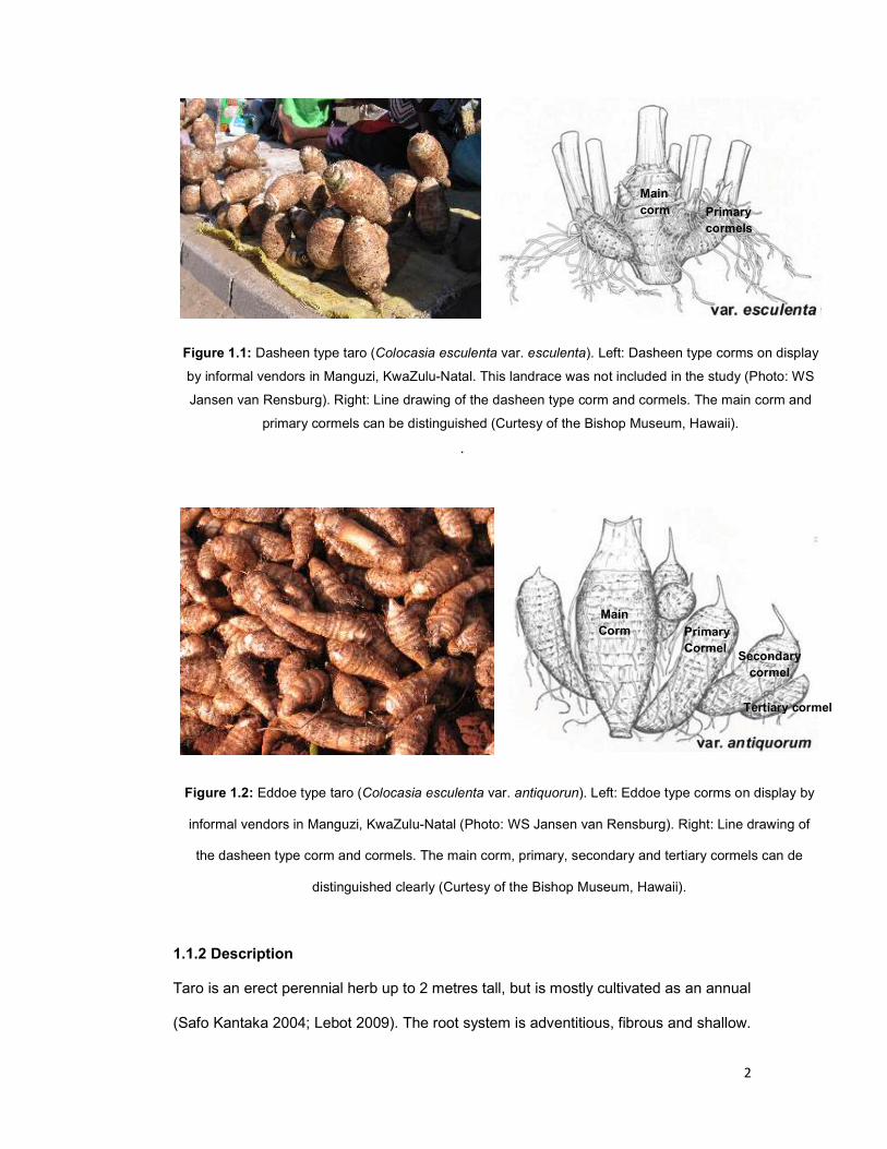
Figure 1.1: Dasheen type taro (Colocasia esculenta var esculenta). Dasheen type corms

on display by informal vendors in Manguzi, KwaZulu-Natal (left). Line drawing of the

dasheen type corm and cormels. ................................................................................... 2

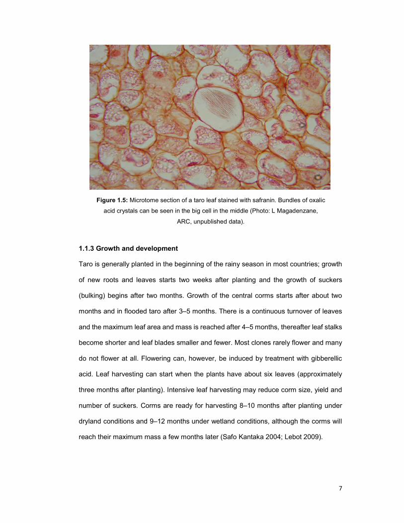
Figure 1.2: Eddoe type taro (Colocasia esculenta var antiquorun). Eddoe type cormels

on display by informal vendors in Chatsworth, KwaZulu-Natal (left). Line drawing of the

eddoe type corm and cormels. ...................................................................................... 2

Figure 1.3: A botanical drawing of a taro plant. The large peltate leaves and

inflorescences of the taro plant as well as the stolons and sucker can be seen ............. 4

Figure 1.4: The inflorescence of an amadumbe. ........................................................... 5

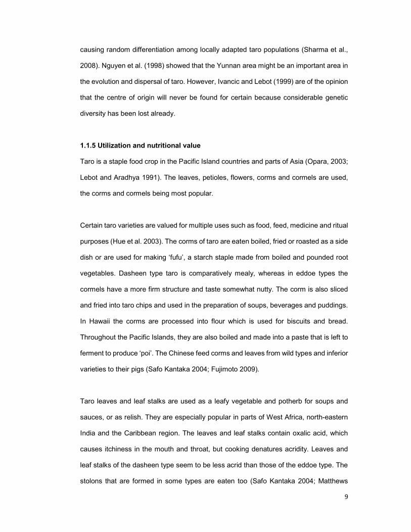
Figure 1.5: Bundles of oxalic acid crystals as seen in the big cell. ................................ 7

Figure 1.6: The taro inflorescence. The complete inflorescence from Cocoindia on the

left. The spathe in the inflorescence from a line 2-2 on the right was cut away to show

the female flowers ....................................................................................................... 27

Figure 1.7: Taro fruiting body with numerous berries. The colours vary from green to

yellow, orange and almost black.................................................................................. 28

Figure 1.8: The performance of two hypothetical genotypes in two hypothetical

environments, showing (a) no GE, (b) ‘quantitative’ GXE (without reversal of ranks) and

(c) “qualitative GXE (with reversal of rank – crossover type) ....................................... 32

Figure 1.9: A generalized interpretation of the genotypic pattern obtained when

genotypic regression coefficients are plotted against genotypic mean, adapted from

Finlay and Wilkinson (1963). ....................................................................................... 34

Figure 2.1: Distribution of collection localities for the South African C. esculenta

accessions .................................................................................................................. 56

Figure 2.2: Diversity in Vanuatu seedling accessions germinated at ARC VOP to

illustrate the variability in certain of the characteristics used in morphological

characterisation. .......................................................................................................... 60

Figure 2.3: Agglomerative hierarchical clustering (AHC) of 86 South African taro

accessions based on agro-morphological descriptors ................................................. 64

Figure 2.4: Agglomerative hierarchical clustering (AHC) of the South African taro

accessions based on polymorphic SSRs. .................................................................... 69

Figure 2.5: Biplot analysis of the polymorphic SSR loci. ............................................. 70

Figure 3.1: Floral tissue in leaves of taro plants observed in plants four weeks after

treatment with 500 ppm gibberellic acid. ...................................................................... 82

xvi

Figure 3.2: Flag leafs, the first indication of flowering. The plant on the left was treated

with gibberellic acid and the plant on right was a natural flowering clone from Vanuatu.

.................................................................................................................................... 82

Figure 3.3: The cluster of inflorescences. The inflorescences open in sequence. The

first youngest inflorescence is closest to the petiole. ................................................... 83

Figure 3.4: Detail of the infloresence. Male flowers in various stages can be seen on the

left. The female flowers can be seen on the right. White to cream sterile flowers can be

seen distributed between the green fertile flowers. ...................................................... 84

Figure 3.5: Cross section of the inflorescence. The sterile appendage can be seen at

the far left, followed by the male flowers, a band of sterile flowers and a band of female

flowers. Then the female flowers can be seen on the right. The fertile flowers are green

and the infertile flowers, or staminates, are white ........................................................ 84

Figure 3.6: A close up of the male (left) flowers and female (right) flowers. The green

fertile and the white sterile flowers can be seen clearly. .............................................. 85

Figure 3.7 Cross section of the inflorescence. ............................................................ 85

Figure 4.1: The distribution of the four trial sites. ........................................................ 93

Figure 4.2: The AMMI1 model for number of cormels, plotting the overall mean of each

line and locality against the first principal component (PC1) ...................................... 106

Figure 4.3: The AMMI1 model for weight of cormels harvested from a single plant,

plotting the overall mean of each line and locality against the first principal component

(PC1)......................................................................................................................... 109

Figure 4.4: The biplot showing the correlation between the different chatacteristics . 116

1

CHAPTER 1: LITERATURE REVIEW

1.1 Colocasia esculenta (L) Schott. (Taro, Amadumbe)

Amadumbe (Colocasia esculenta) is a popular starch crop in certain parts of South Africa

(Modi 2007, Mabhaudhi 2012). Amadumbe is the isiZulu vernacular for taro, dasheen,

eddoe, cocoyam or elephant as it is better known throughout the rest of the world (Safo

Kantaka 2004, Mabhaudhi 2012). It is a popular starch staple in tropical Africa, Asia,

Pacific Islands and Americas (Lebot 2009). Lebot reported that taro is still regarded as

an orphan crop, commonly cultivated in home gardens or in shifting agroforestry with

limited input. There are no commercial taro cultivars in South Africa and research on taro

is inadequate when compared with that of conventional root and tuber crops (Modi

2007).

1.1.1 Scientific classification

Colocasia esculenta (L.) Schott

Protologue: Schott & Endl., Melet. bot.: 18 (1832).

Family: Araceae

Chromosome number: 2n = 28, 42, 56 and x = 14

Synonyms: Colocasia antiquorum Schott (1832).

The genus Colocasia consist of eight species from tropical Asia and is classified in the

tribe Colocasieae, along with Alocasia. There are two variety-groups of taro, the

Dasheen Group which consists of a single large corm producing a few small cormels

(Figure 1.1) and the Eddoe Group (frequently classified as C. esculenta var. antiquorum

(Schott) F.T.Hubb. & Rehder) producing many cormels of varying size (Figure 1.2) (Safo

Kantaka 2004; Lebot 2009). Most taro landraces in South Africa belong to the Eddoe

Group.

2

Figure 1.1: Dasheen type taro (Colocasia esculenta var. esculenta). Left: Dasheen type corms on display

by informal vendors in Manguzi, KwaZulu-Natal. This landrace was not included in the study (Photo: WS

Jansen van Rensburg). Right: Line drawing of the dasheen type corm and cormels. The main corm and

primary cormels can be distinguished (Curtesy of the Bishop Museum, Hawaii).

.

Figure 1.2: Eddoe type taro (Colocasia esculenta var. antiquorun). Left: Eddoe type corms on display by

informal vendors in Manguzi, KwaZulu-Natal (Photo: WS Jansen van Rensburg). Right: Line drawing of

the dasheen type corm and cormels. The main corm, primary, secondary and tertiary cormels can de

distinguished clearly (Curtesy of the Bishop Museum, Hawaii).

1.1.2 Description

Taro is an erect perennial herb up to 2 metres tall, but is mostly cultivated as an annual

(Safo Kantaka 2004; Lebot 2009). The root system is adventitious, fibrous and shallow.

Main Corm Primary

Cormel Secondary

cormel

Tertiary cormel

Main corm Primary

cormels

3

The storage stem (corm) is usually brown and marked by a number of rings, it is

cylindrical or spherical in shape and may grow to be very large - up to 4 kg (Figure 1.1

and 1.2). The lateral buds give rise to cormels, suckers or stolons. The leaves are

arranged in a rosette and are simple and peltate (Figure 1.3). The petiole can be up to

1 m long, with distinct sheath. The leaf blades are cordate, up to 85 × 60 cm, entire,

glabrous, with three main veins and rounded lobes at the base (Safo Kantaka 2004;

Lebot 2009).

The inflorescence is a spadix tipped by a sterile appendage, surrounded by a spathe

and supported by a peduncle much shorter than leaf petioles (Figure 1.4). The individual

flowers are unisexual, small, and without a perianth. Male and female flowers appear on

the same spadix (inflorescence) separated by a band of sterile flowers. The male flowers

are on the upper part of the spadix - the stamens entirely fused, while the female flowers

are at the base of the spadix with a superior one-celled ovary that has an almost sessile

stigma. The fruit is a densely packed, many-seeded berry with up to 50 seeds. The

seeds are ovoid to ellipsoid, less than 2 mm long, with copious endosperm (Safo Kantaka

2004; Lebot 2009).

Wild and “domesticated” forms of taro occur. The main characteristics of wild C.

esculenta are long stolons; small, elongated corms; continuous growth; and a

predominantly high concentration of calcium oxalate (Figure 1.5) that is associated with

acridity (Lebot et al. 2004). Bradbury and Nixon (1998) noted that acridity can be

ascribed to an irritant on the raphides that cause a reaction after the raphides puncture

the soft skin and mucous membranes. The domesticated taro as well as intermediate

types can be either dasheen or eddoe type. These accessions could be hybrids between

the two types, or accessions that are difficult to classify because of the unusual shape

of their corms (Lebot et al. 2004).

4

Figure 1.3: A botanical drawing of a taro plant. The large peltate leaves and inflorescences

of the taro plant and the stolons and sucker can be seen (Curtis's Botanical Magazine v.120

[ser.3:v.50] 1894; https://ast.wikipedia.org/wiki/Colocasia_esculenta#/media/File:

Colocasia_esculenta_CBM.png accessed 20 July 2017)

5

Figure 1.4: The inflorescence of taro landrace Cocoindia. The yellow spadix is clearly visible.

The male flowers and sterile appendage can be seen but the base of the spadix encloses the

female flowers. The abaxial side of a peltate leaf with three main nerves can be seen behind

the inflorescences (Photo: WS Jansen van Rensburg).

In Asia and the Pacific region, dasheen cultivars are generally diploid and widely

distributed in the humid tropics, whereas eddoe cultivars are mostly triploids and are

found in subtropical to temperate areas (Matthews 2004). Dasheen is overwhelmingly

dominant in both the highlands and lowlands of Papua New Guinea. In Indonesia,

dasheen is generally dominant but eddoe occupies highland areas above 1000m (Lebot

et al. 2002). Taro is cultivated up to 2500 meters above sea level in tropical latitudes. In

6

China, dasheen is found in the southern regions because it needs higher temperatures

(Xu et al. 2001). In Ethiopia, dasheen is dominant in highland areas and eddoe in lowland

areas (Fujimoto 2009). Burkill (1985) and Fujimoto (2009) noted that the eddoe form is

in general ‘hardier’ than the dasheen form and can be grown under ‘drier and harsher’

conditions. In Asia and the Pacific region, the dasheen type is dominant and the eddoe

type is found in some temperate and tropical highland areas. In Africa most taro cultivars

are the eddoe type, this may be due to the generally drier African climate in comparison

to the climate of Asia and the Pacific region (Safo Kantanka 2004; Fujimoto 2009). Safo

Kantanka (2004) noted that eddoe types may have originated in China, where they then

spread to the Caribbean region, and then to Africa, indicating a recent introduction of

eddoe cultivars. Safo Kantanka (2004) did not speculate on how and when the taro

spread to Caribbean and Africa. However, according to Fujimoto (2009), the recent

introduction of eddoe cultivars cannot be the case in Ethiopia. Most taro cultivars in

Africa, both eddoe and dasheen types, presumably originate from ancient arrivals of

tropical Asia, with some later additions. Through time, a diversification of local cultivars

and domination of the eddoe type may have taken place, along with development of

different cultivation techniques (Fujimoto 2009). In South Africa both eddoe and dasheen

type landraces are cultivated in KwaZulu-Natal, however the eddoe type seems to be

the most preferred type (Mare 2009). Chaïr et al. (2016) noted that al the South African

landraces included in the study were triploid.

Taro is sometimes confused with tannia (Xanthosoma sagittifolium (L.Schott)) because

of its similar appearance. A ready distinction can be found in the junction of the leaf stalk

with the blade, in taro the leaf is peltate with the petiole attached near the centre of the

lower surface of the leaf rather than the margin, whereas in Xanthosoma the petiole is

attached on the leaf margin of the arrow shaped leaves (Safo Kantaka 2004).

7

Figure 1.5: Microtome section of a taro leaf stained with safranin. Bundles of oxalic

acid crystals can be seen in the big cell in the middle (Photo: L Magadenzane,

ARC, unpublished data).

1.1.3 Growth and development

Taro is generally planted in the beginning of the rainy season in most countries; growth

of new roots and leaves starts two weeks after planting and the growth of suckers

(bulking) begins after two months. Growth of the central corms starts after about two

months and in flooded taro after 3–5 months. There is a continuous turnover of leaves

and the maximum leaf area and mass is reached after 4–5 months, thereafter leaf stalks

become shorter and leaf blades smaller and fewer. Most clones rarely flower and many

do not flower at all. Flowering can, however, be induced by treatment with gibberellic

acid. Leaf harvesting can start when the plants have about six leaves (approximately

three months after planting). Intensive leaf harvesting may reduce corm size, yield and

number of suckers. Corms are ready for harvesting 8–10 months after planting under

dryland conditions and 9–12 months under wetland conditions, although the corms will

reach their maximum mass a few months later (Safo Kantaka 2004; Lebot 2009).

8

Taro is propagated vegetatively. It is sometimes difficult to keep planting material in a

healthy condition during the dry season or periods of drought. Essentially four types of

planting material are used; side suckers growing from the main corm, small

unmarketable cormels (60–150 g), corm pieces, and head setts or ‘huli’, i.e. the apical

1–2 cm of the main corm with 15–20 cm of the leaf stalks attached. In Ghana, planting

is mainly by use of either young suckers or mature setts cut from harvested corms.

Planting material must be taken from healthy plants (Safo Kantaka 2004; Lebot 2009).

1.1.4 Origin and geographic distribution

Taro is probably one of the oldest crops and has been grown for more than 10 000 years

in tropical Asia (Lebot 2009). It is believed that taro was domesticated in northern India,

but independent domestication in New Guinea has also been reported. Colocasia

esculenta occurs wild in tropical Asia, extending as far east as New Guinea and northern

Australia. A form with long stolons, which occurs throughout this region, has been

postulated as the ancestor of cultivated taro on the basis of ribosome-DNA analysis

(Safo Kantaka 2004). Eddoe types may have originated in China, from where they

spread to the Caribbean region, and then to Africa (Safo Kantaka 2004; Lebot 2009). It

was spread by human settlers eastward to New Guinea and the Pacific over 2000 years

ago, where it became one of the most important food plants economically and culturally

(Safo Kantaka 2004; Lebot 2009). Distribution to China, Egypt and East Africa also

occurred at least 2000 years ago. Taro was taken to West Africa from Egypt and East

Africa by the Arabs. It was introduced into Europe from Egypt. From Spain it was taken

to the New World and new introductions may have been made into West Africa from

tropical America. Presently, taro is grown in many tropical and subtropical areas around

the world for its corms, leaves and flowers (Safo Kantaka 2004; Lebot 2009:281).

There is an indication that when taro was introduced to a new area, only a small fraction

of genetic variability in heterogeneous taro populations was transferred, possibly

9

causing random differentiation among locally adapted taro populations (Sharma et al.,

2008). Nguyen et al. (1998) showed that the Yunnan area might be an important area in

the evolution and dispersal of taro. However, Ivancic and Lebot (1999) are of the opinion

that the centre of origin will never be found for certain because considerable genetic

diversity has been lost already.

1.1.5 Utilization and nutritional value

Taro is a staple food crop in the Pacific Island countries and parts of Asia (Opara, 2003;

Lebot and Aradhya 1991). The leaves, petioles, flowers, corms and cormels are used,

the corms and cormels being most popular.

Certain taro varieties are valued for multiple uses such as food, feed, medicine and ritual

purposes (Hue et al. 2003). The corms of taro are eaten boiled, fried or roasted as a side

dish or are used for making ‘fufu’, a starch staple made from boiled and pounded root

vegetables. Dasheen type taro is comparatively mealy, whereas in eddoe types the

cormels have a more firm structure and taste somewhat nutty. The corm is also sliced

and fried into taro chips and used in the preparation of soups, beverages and puddings.

In Hawaii the corms are processed into flour which is used for biscuits and bread.

Throughout the Pacific Islands, they are also boiled and made into a paste that is left to

ferment to produce ‘poi’. The Chinese feed corms and leaves from wild types and inferior

varieties to their pigs (Safo Kantaka 2004; Fujimoto 2009).

Taro leaves and leaf stalks are used as a leafy vegetable and potherb for soups and

sauces, or as relish. They are especially popular in parts of West Africa, north-eastern

India and the Caribbean region. The leaves and leaf stalks contain oxalic acid, which

causes itchiness in the mouth and throat, but cooking denatures acridity. Leaves and

leaf stalks of the dasheen type seem to be less acrid than those of the eddoe type. The

stolons that are formed in some types are eaten too (Safo Kantaka 2004; Matthews

10

2004). It’s reported that the flowers are consumed in China (Jianchu et al. 2001;

Matthews 2004) and Bangladesh (Paul et al. 2011). Taro leaves are also used as

temporary wrapping for small articles such as spices, herbal medicines, and wild honey

(Fujimoto 2009).

Taro corms, stolons and leaves are used as fodder for pigs (Safo Kantaka 2004; Hue et

al. 2003; Fujimoto 2009). Besides its nutritional value, taro is traditionally used as a

medicinal plant and provides bioactive compounds which act as immune stimulators

(Pereira et al. 2015). Taro is also used medicinally for headaches (Hue et al., 2003)

gastro-intestinal disorders and dental decay in children (Safo Kantaka 2004).

Taro corms are an excellent source of carbohydrates and potassium (Manner and

Taylor, 2010; Oke 1990). The nutritional content for taro corms varies between

genotypes (Guchait et al. 2008). Mare and Modi (20212) noted that planting date and

fertilizer. Furthermore, they also noted that interaction between temperature, packaging,

landrace (genotype) and sampling date influence reducing sugars during storage.

Mineral content plays a crucial role in consumers’ acceptance according to Champagne

et al. (2013). The digestibility of taro starch is very high and the starch grain is about ten

times smaller than a starch grain of potato, it is therefore suitable for people with

digestive problems. Taro is an excellent food for diabetics because the low glycemic

index facilitates slow release of glucose into the bloodstream (Manner and Taylor 2010).

Taro starch is hypoallergenic, making it useful for people allergic to cereals, it is even

used as substitute baby food for infants with milk sensitivity (Safo Kantaka 2004; Darkwa

and Darkwa 2013). Interaction between landrace (genotype), planting date and fertilizer

application influence starch content in corms (Mare and Modi 2012). They also noted

that the interaction of temperature, packaging, cultivar and sampling month influence

starch content. Taro flour has been reported to have been used in infant food formulae

and canned baby foods in the United States of America (Darkwa and Darkwa 2013).

11

Yellow fleshed taro contains higher levels of β-carotene than white flesh (Engelberger et

al. 2003). Taro is an ideal crop to help in combatting hunger and malnutrition die to the

highly digestible, low GI starch particles and the availability of germplasm with higher β-

carotene and flavonoids. However, the yields are relatively low and taro is more adapted

to tropical and sub-tropical climates. It creates an opportunity to breed for higher yields

and plants that are adapted to more arid conditions.

All parts of most cultivars are acrid, though the acridity in taro is not due to the calcium

oxalate raphides. Some irritant on the raphide surface caused the acridity, with the

raphides apparently functioning to carry the acridity factor (Paul et al. 1999). Cooking

the taro generally denatures the acridity (Manner and Taylor 2010).

1.1.6 Production and international trade

World production of taro increased from 4 487 124 tonnes in 1961 to 10 108 223 tonnes

in 2014 according to the FAO (2017). The area under production increased from 758 228

hectares to 1 455 508 hectares during the same period (FAO 2017). In 2014 Africa

produced 7 314 417 tonnes of taro. The biggest production was in Western Africa (4

798 185 tonnes), followed by Central Africa (1 966 283 tonnes), Eastern Africa

(427 116 tonnes) and Northern Africa (122 833 tonnes). Other areas that produced

significant amounts of taro in 2014 are Asia (225 9532 tonnes), Central America

(83 331 tonnes), Oceania (42 5247 tonnes) and Melanesia (38 5370 tonnes). Nigeria

specifically had the highest production of taro in 2014 with 3 273 000 tonnes produced

from 639 980 hectares. Nigeria is followed by China with a production of 1 884 987 from

97 601 hectares. Cameroon and Ghana followed with a production of 1 672 731 tonnes

and 1 299 000 tonnes respectively (FAO 2017). No production figures were available for

South Africa.

12

It is difficult to get exact producer price data, but the average producer price for a tonne

of taro was 975.17USD in 2014. The producer price varies from 186.6USD/tonne in

Egypt to 2 794.9 USD/tonne in Japan (FAO 2017).

In some regions of Asia and the Pacific, taro is being been gradually replaced by more

productive root crops such as tannia (Xanthosoma sagittifolium), cassava (Manihot

esculenta Crantz) and sweet potato (Ipomoea batatas (L.) Lam.). This is leading to the

genetic erosion of variability in taro (Safo Kantaka 2004; Caillon at al. 2006; Fujimoto

2009).

Taro corms and leaves, although common in local markets, are mostly grown for

subsistence and home consumption. Large-scale commercial production is not common.

Local consumption forms the greatest utilisation of taro produced on other continents

too. However, small amounts are exported to Europe and Australia for the immigrant

community. Trinidad and Tobago also import some taro (Safo Kantaka 2004).

1.1.7 Diseases and pests

Taro blight (Phytophthora colocasiae) is a major wetland taro disease, causing purple to

brown circular water-soaked lesions. It is the most devastating taro disease, particularly

in the Pacific region where it has caused considerable losses due to rot. Taro blight is

associated with high relative humidity. Several species of Pythium (P. adhaerens,

P. aphanidermatum, P. arrhenomanes, P. carolinianum, P. debaryanum, P. delicense,

P. graminicola, P. helicoides, P. irregular, P. middletonii, P. myriotylum, P. splendens,

P vexans and P ultimum) cause taro soft rot, with wilting and chlorosis of leaves.

Sclerotium rot caused by Sclerotium rolfsii is characterized by stunting of the plant,

rotting and formation of many spherical sclerotia on the corm. In both flooded and upland

taro, dark brown spots that appear in older leaves are caused by Cladosporium

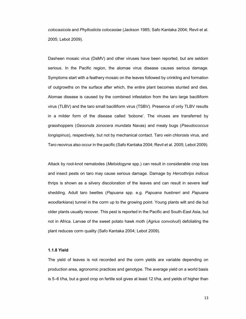
13

colocasicola and Phyllosticta colocasiae (Jackson 1985; Safo Kantaka 2004; Revil et al.

2005; Lebot 2009).

Dasheen mosaic virus (DsMV) and other viruses have been reported, but are seldom

serious. In the Pacific region, the alomae virus disease causes serious damage.

Symptoms start with a feathery mosaic on the leaves followed by crinkling and formation

of outgrowths on the surface after which, the entire plant becomes stunted and dies.

Alomae disease is caused by the combined infestation from the taro large bacilliform

virus (TLBV) and the taro small bacilliform virus (TSBV). Presence of only TLBV results

in a milder form of the disease called ‘bobone’. The viruses are transferred by

grasshoppers (Gesonula zonocera mundata Navas) and mealy bugs (Pseudococcus

longispinus), respectively, but not by mechanical contact. Taro vein chlorosis virus, and

Taro reovirus also occur in the pacific (Safo Kantaka 2004; Revil et al. 2005; Lebot 2009).

Attack by root-knot nematodes (Meloidogyne spp.) can result in considerable crop loss

and insect pests on taro may cause serious damage. Damage by Hercothrips indicus

thrips is shown as a silvery discoloration of the leaves and can result in severe leaf

shedding. Adult taro beetles (Papuana spp. e.g. Papuana huebneri and Papuana

woodlarkiana) tunnel in the corm up to the growing point. Young plants wilt and die but

older plants usually recover. This pest is reported in the Pacific and South-East Asia, but

not in Africa. Larvae of the sweet potato hawk moth (Agrius convolvuli) defoliating the

plant reduces corm quality (Safo Kantaka 2004; Lebot 2009).

1.1.8 Yield

The yield of leaves is not recorded and the corm yields are variable depending on

production area, agronomic practices and genotype. The average yield on a world basis

is 5–6 t/ha, but a good crop on fertile soil gives at least 12 t/ha, and yields of higher than

14

40 t/ha have been achieved in Hawaii (Safo Kantaka 2004). The average global yield

increases from 5.9 t/ha in 1961 to 6.9 t/ha in 2014 (FAO 2017).

At a regional level, the average yield during 2014 was 16.6 t/ha in Asia, 10.25 t/ha in

Central America, 9.7 t/ha in America, 9.6 t/a in the Caribbean, 8.2 t/ha in Melanesia,

7.8 t/ha in Oceania, 6.1 t/ha in South America, 5.8 t/ha in Africa and 5.1 t/ha in

Polynesia. Within Africa, the highest yields were reached in Northern Africa (34.82 t/ha),

followed by Central Africa (7.9588 t/ha) and Eastern and Western Africa (5.2 t/ha) (FAO

2017).

The highest yields, during 2014, were recorded in Egypt (34.8 t/a), Cyprus (26.1 t/a) and

mainland China (19.3 t/a). Although Nigeria is the biggest producer, the average yield in

Nigeria was only 5.1 t/a during 2014. In Ethiopia the yield can vary between 1.79 kg/m2

(1.26 kg/plant) and 1.00 kg/m2 (0.65 kg/plant) for the Highlands and lowlands

respectively (Fujimoto 2009). However, Lebot (2009) reported that yields of 60-110t/ha

have been recorded under traditional cropping systems. At the ARC Research Station,

Roodeplaat (South Africa) yields vary between 6 and 10 t/ha (Personal communication

Abe Shegro Gerrano). Mare (2012) noted that landrace, agronomic practices influence

the yield.

1.1.9 Colocasia esculenta in South Africa

Taro is being cultivated in South Arica for a long time, but no information exists on how

and when taro was introduced. Taro is cultivated in the subtropical eastern side of South

Africa. It is cultivated as far south as Bizana in coastal Eastern Cape Province, then

northwards on the coastal areas of KwaZulu-Natal and certain areas of Mpumalanga

and Limpopo Provinces (Modi 2004; Shange 2004). Subsistence and small scale

farmers in South Africa mostly cultivate taro for own use and trade on the informal market

(Figure 1.1 and 1.2) (Shange 2004). No improved cultivars exist but Mare (2006) farmers

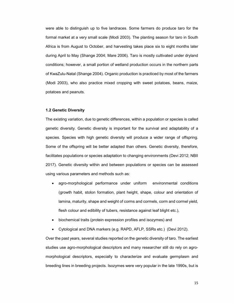
15

were able to distinguish up to five landraces. Some farmers do produce taro for the

formal market at a very small scale (Modi 2003). The planting season for taro in South

Africa is from August to October, and harvesting takes place six to eight months later

during April to May (Shange 2004; Mare 2006). Taro is mostly cultivated under dryland

conditions; however, a small portion of wetland production occurs in the northern parts

of KwaZulu-Natal (Shange 2004). Organic production is practiced by most of the farmers

(Modi 2003), who also practice mixed cropping with sweet potatoes, beans, maize,

potatoes and peanuts.

1.2 Genetic Diversity

The existing variation, due to genetic differences, within a population or species is called

genetic diversity. Genetic diversity is important for the survival and adaptability of a

species. Species with high genetic diversity will produce a wider range of offspring.

Some of the offspring will be better adapted than others. Genetic diversity, therefore,

facilitates populations or species adaptation to changing environments (Devi 2012; NBII

2017). Genetic diversity within and between populations or species can be assessed

using various parameters and methods such as:

agro-morphological performance under uniform environmental conditions

(growth habit, stolon formation, plant height, shape, colour and orientation of

lamina, maturity, shape and weight of corms and cormels, corm and cormel yield,

flesh colour and edibility of tubers, resistance against leaf blight etc.),

biochemical traits (protein expression profiles and isozymes) and

Cytological and DNA markers (e.g. RAPD, AFLP, SSRs etc.) (Devi 2012).

Over the past years, several studies reported on the genetic diversity of taro. The earliest

studies use agro-morphological descriptors and many researcher still do rely on agro-

morphological descriptors, especially to characterize and evaluate germplasm and

breeding lines in breeding projects. Isozymes were very popular in the late 1990s, but is

16

still being used because it is relatively easy and affordable. DNA based methods have

gained popularity lately because of the reproducibility and the relative large amounts of

data that can be generated.

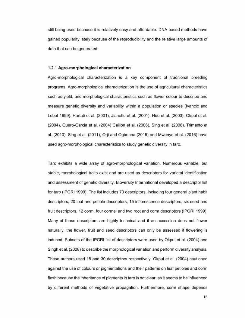
1.2.1 Agro-morphological characterization

Agro-morphological characterization is a key component of traditional breeding

programs. Agro-morphological characterization is the use of agricultural characteristics

such as yield, and morphological characteristics such as flower colour to describe and

measure genetic diversity and variability within a population or species (Ivancic and

Lebot 1999). Hartati et al. (2001), Jianchu et al. (2001), Hue et al. (2003), Okpul et al.

(2004), Quero-Garcia et al. (2004) Caillon et al. (2006), Sing et al. (2008), Trimanto et

al. (2010), Sing et al. (2011), Orji and Ogbonna (2015) and Mwenye et al. (2016) have

used agro-morphological characteristics to study genetic diversity in taro.

Taro exhibits a wide array of agro-morphological variation. Numerous variable, but

stable, morphological traits exist and are used as descriptors for varietal identification

and assessment of genetic diversity. Bioversity International developed a descriptor list

for taro (IPGRI 1999). The list includes 73 descriptors, including four general plant habit

descriptors, 20 leaf and petiole descriptors, 15 inflorescence descriptors, six seed and

fruit descriptors, 12 corm, four cormel and two root and corm descriptors (IPGRI 1999).

Many of these descriptors are highly technical and if an accession does not flower

naturally, the flower, fruit and seed descriptors can only be assessed if flowering is

induced. Subsets of the IPGRI list of descriptors were used by Okpul et al. (2004) and

Singh et al. (2008) to describe the morphological variation and perform diversity analysis.

These authors used 18 and 30 descriptors respectively. Okpul et al. (2004) cautioned

against the use of colours or pigmentations and their patterns on leaf petioles and corm

flesh because the inheritance of pigments in taro is not clear, as it seems to be influenced

by different methods of vegetative propagation. Furthermore, corm shape depends

17

strongly on location, environmental conditions, and plant age (Ivancic and Lebot, 1999).

Mare (2006) use ten qualitative morphological characteristics to characterise South

African taro landraces in KwaZulu-Natal with the help of farmers.

The number of descriptors used vary between the different studies. The IPGRI

descriptor list (IPGRI 1999) is time-consuming, but generate large amounts of data. The

condensed descriptor list used by Singh et al. (2008) has less characteristics, but were

still able to identify duplicates. The much shorter list used by Mare (2006) is easy to use

and include important consumer characteristics like taste, cooking time and sliminess.

Taro cultivars are vegetatively propagated, therefore, low intraspecific variability is

expected (Okpul et al. 2004). Nevertheless, Okpul et al. (2004) observed high

morphological variation in Papua New Guinea germplasm by using 18 agro-

morphological descriptors. This is in agreement with results of studies by Lebot et al.

(2000) and Godwin et al. (2001). According to Okpul et al (2004) this variability may be

attributed to sexual recombination, migration and mutation, with subsequent selection

by farmers in geographical isolation for adaptability under various agro-ecological

regimes and cropping systems and culinary and quality preferences.

Quero-Garcia et al. (2004) and Okpul et al. (2004) did not find any significant correlations

and patterns in Vanuatu taro germplasm diversity using morphological characteristics.

This may be because the characters used were too heterogeneous (passport, agronomic

and morphological characters), and generally not correlated. However, no clearly

differentiated groups were produced when working with agronomic and morphological

characters separately. Accessions with rare traits (i.e., orange corm colour) appeared

clearly isolated in the dendrograms (Quero-Garcia et al. 2004).

18

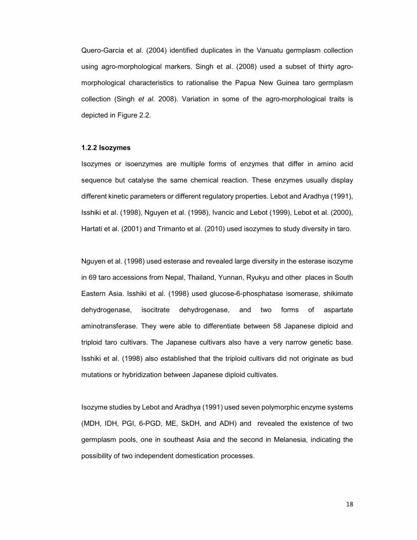
Quero-Garcia et al. (2004) identified duplicates in the Vanuatu germplasm collection

using agro-morphological markers. Singh et al. (2008) used a subset of thirty agro-

morphological characteristics to rationalise the Papua New Guinea taro germplasm

collection (Singh et al. 2008). Variation in some of the agro-morphological traits is

depicted in Figure 2.2.

1.2.2 Isozymes

Isozymes or isoenzymes are multiple forms of enzymes that differ in amino acid

sequence but catalyse the same chemical reaction. These enzymes usually display

different kinetic parameters or different regulatory properties. Lebot and Aradhya (1991),

Isshiki et al. (1998), Nguyen et al. (1998), Ivancic and Lebot (1999), Lebot et al. (2000),

Hartati et al. (2001) and Trimanto et al. (2010) used isozymes to study diversity in taro.

Nguyen et al. (1998) used esterase and revealed large diversity in the esterase isozyme

in 69 taro accessions from Nepal, Thailand, Yunnan, Ryukyu and other places in South

Eastern Asia. Isshiki et al. (1998) used glucose-6-phosphatase isomerase, shikimate

dehydrogenase, isocitrate dehydrogenase, and two forms of aspartate

aminotransferase. They were able to differentiate between 58 Japanese diploid and

triploid taro cultivars. The Japanese cultivars also have a very narrow genetic base.

Isshiki et al. (1998) also established that the triploid cultivars did not originate as bud

mutations or hybridization between Japanese diploid cultivates.

Isozyme studies by Lebot and Aradhya (1991) used seven polymorphic enzyme systems

(MDH, IDH, PGI, 6-PGD, ME, SkDH, and ADH) and revealed the existence of two

germplasm pools, one in southeast Asia and the second in Melanesia, indicating the

possibility of two independent domestication processes.

19

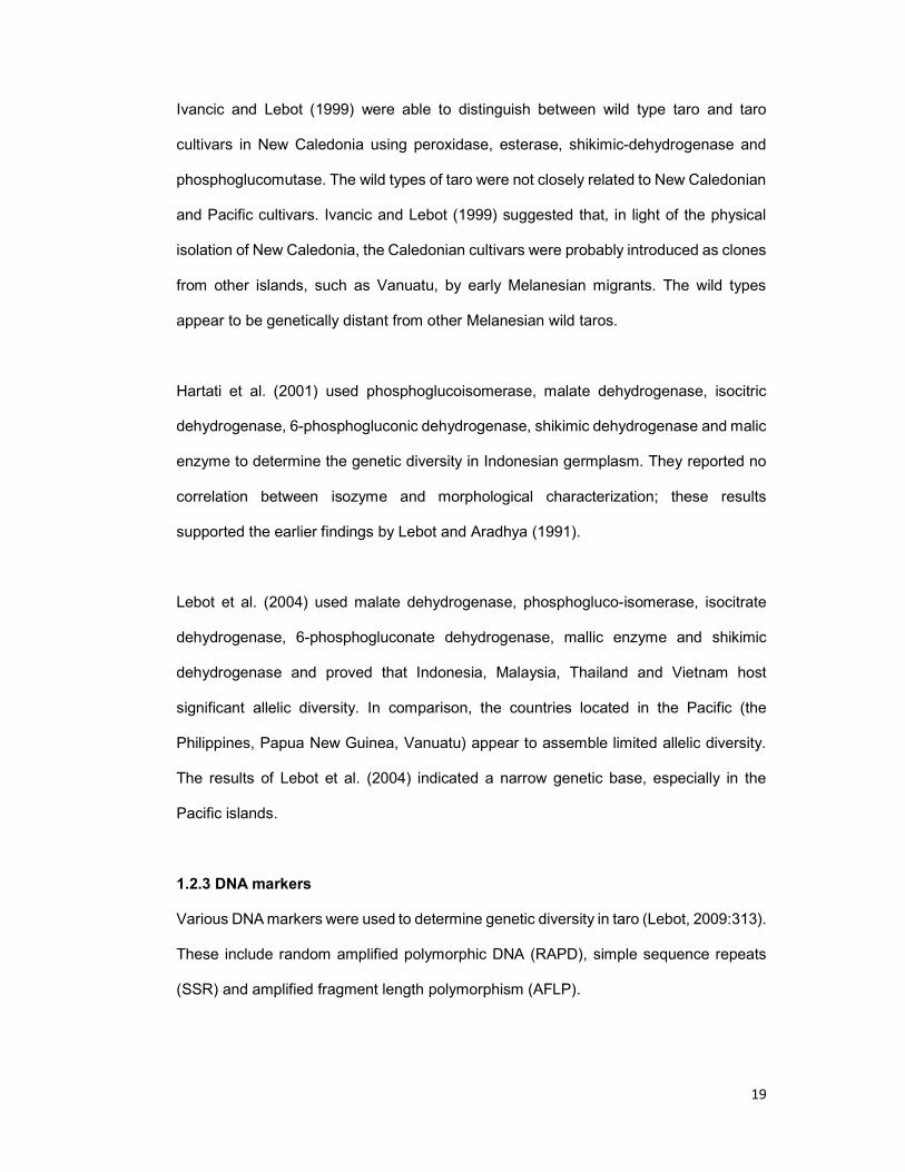
Ivancic and Lebot (1999) were able to distinguish between wild type taro and taro

cultivars in New Caledonia using peroxidase, esterase, shikimic-dehydrogenase and

phosphoglucomutase. The wild types of taro were not closely related to New Caledonian

and Pacific cultivars. Ivancic and Lebot (1999) suggested that, in light of the physical

isolation of New Caledonia, the Caledonian cultivars were probably introduced as clones

from other islands, such as Vanuatu, by early Melanesian migrants. The wild types

appear to be genetically distant from other Melanesian wild taros.

Hartati et al. (2001) used phosphoglucoisomerase, malate dehydrogenase, isocitric

dehydrogenase, 6-phosphogluconic dehydrogenase, shikimic dehydrogenase and malic

enzyme to determine the genetic diversity in Indonesian germplasm. They reported no

correlation between isozyme and morphological characterization; these results

supported the earlier findings by Lebot and Aradhya (1991).

Lebot et al. (2004) used malate dehydrogenase, phosphogluco-isomerase, isocitrate

dehydrogenase, 6-phosphogluconate dehydrogenase, mallic enzyme and shikimic

dehydrogenase and proved that Indonesia, Malaysia, Thailand and Vietnam host

significant allelic diversity. In comparison, the countries located in the Pacific (the

Philippines, Papua New Guinea, Vanuatu) appear to assemble limited allelic diversity.

The results of Lebot et al. (2004) indicated a narrow genetic base, especially in the

Pacific islands.

1.2.3 DNA markers

Various DNA markers were used to determine genetic diversity in taro (Lebot, 2009:313).

These include random amplified polymorphic DNA (RAPD), simple sequence repeats

(SSR) and amplified fragment length polymorphism (AFLP).

20

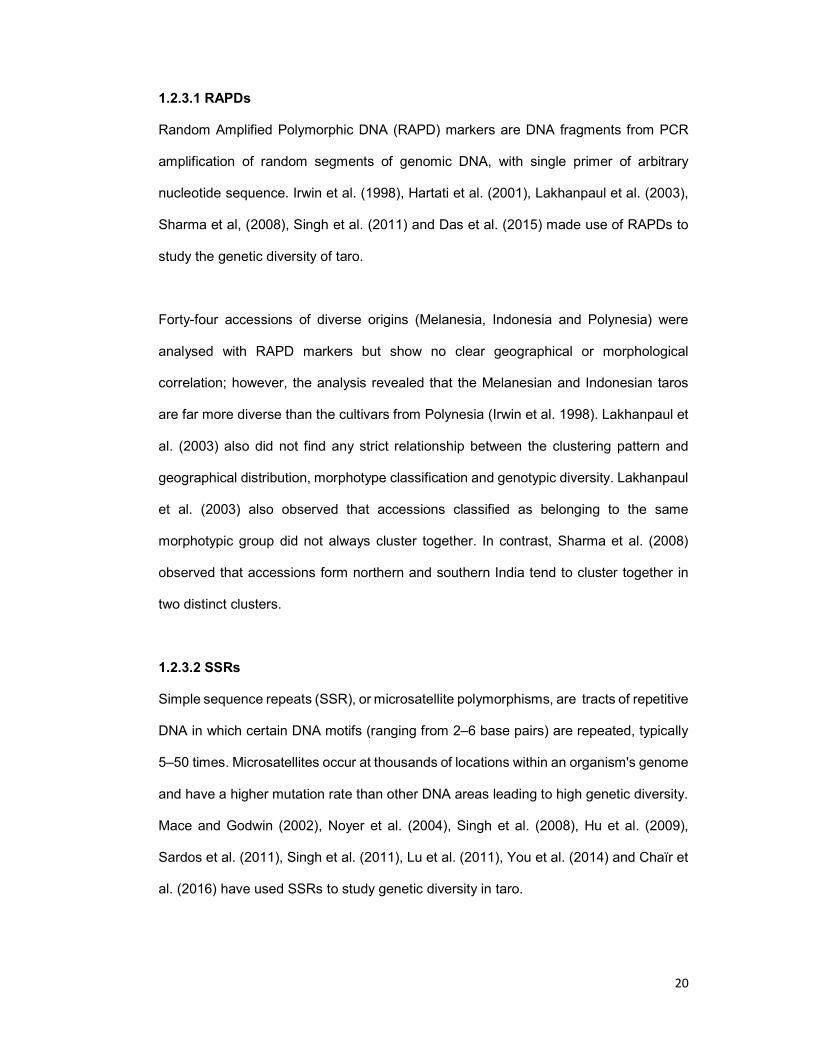
1.2.3.1 RAPDs

Random Amplified Polymorphic DNA (RAPD) markers are DNA fragments from PCR

amplification of random segments of genomic DNA, with single primer of arbitrary

nucleotide sequence. Irwin et al. (1998), Hartati et al. (2001), Lakhanpaul et al. (2003),

Sharma et al, (2008), Singh et al. (2011) and Das et al. (2015) made use of RAPDs to

study the genetic diversity of taro.

Forty-four accessions of diverse origins (Melanesia, Indonesia and Polynesia) were

analysed with RAPD markers but show no clear geographical or morphological

correlation; however, the analysis revealed that the Melanesian and Indonesian taros

are far more diverse than the cultivars from Polynesia (Irwin et al. 1998). Lakhanpaul et

al. (2003) also did not find any strict relationship between the clustering pattern and

geographical distribution, morphotype classification and genotypic diversity. Lakhanpaul

et al. (2003) also observed that accessions classified as belonging to the same

morphotypic group did not always cluster together. In contrast, Sharma et al. (2008)

observed that accessions form northern and southern India tend to cluster together in

two distinct clusters.

1.2.3.2 SSRs

Simple sequence repeats (SSR), or microsatellite polymorphisms, are tracts of repetitive

DNA in which certain DNA motifs (ranging from 2–6 base pairs) are repeated, typically

5–50 times. Microsatellites occur at thousands of locations within an organism's genome

and have a higher mutation rate than other DNA areas leading to high genetic diversity.

Mace and Godwin (2002), Noyer et al. (2004), Singh et al. (2008), Hu et al. (2009),

Sardos et al. (2011), Singh et al. (2011), Lu et al. (2011), You et al. (2014) and Chaïr et

al. (2016) have used SSRs to study genetic diversity in taro.

21

Microsatellite and SSR markers were tested on 17 accessions from several Pacific

countries (Mace and Godwin, 2002). They proved to be a valuable tool for the

identification of duplicates, although the geographical structure produced was not very

informative, probably due to the size of the sample and the low number of primers used.

You et al. (2014) also proved that SSR markers were able to distinguish between 68 taro

cultivars. Similarly, Quero-Garcia et al. (2006) did not reveal any clear geographical

structure and Caillon et al. (2006) observed that genetic diversity cultivated in one village

was equivalent to the overall genetic diversity cultivated within Vanuatu. In Vanuatu,

Sardos et al. (2011) distinguished between genotypes by SSRs and observed that

genetic clusters are mainly differentiated by rare alleles. In contrast to other researchers,

Sardos et al. (2011) did find a degree of correlation between geographical and present

social and genetic diversity. SSRs were able to discriminate between diploid and

tetraploid germplasm (Chaïr et al. 2016).

1.2.3.3 AFLPs

Amplified fragment length polymorphism (AFLP) use restriction enzymes to digest

genomic DNA with adaptors are then ligated to the sticky ends of the restriction

fragments. A subset of the restriction fragments is then amplified using primers

complementary to the adaptor sequence, the restriction site sequence and a few

nucleotides inside the restriction site fragments. Kreike et al. (2004), Quero-Garcia et al.

(2004), Lebot et al. (2004), Caillon et al. (2006), Sharma et al. (2008) and Mwenye et al.

(2016) used AFLPS to study diversity in C esculenta. Sharma et al. (2008) found that

Indian taro cultivars can be distinguished from each other using AFLPS. Quero-Garcia

et al. (2004) identified no duplicates with AFLP markers.

Kreike et al. (2004) used AFLP markers to study the diversity of a core sample of

accessions from seven different countries. Most accessions could be clearly

differentiated by using three primer pairs and few duplicates were identified.

22

Differentiation between Southeast Asian and Melanesian taros was obtained confirming

the isozyme results (Kreike et al. 2004). Kreike et al. (2004) also revealed that the

diversity among wild types was greater than that within the cultivated taro. Quero-Garcia

et al. (2004) used AFLP analysis in Vanuatu to validate a stratification methodology of

large germplasm collections. Quero-Garcia et al. (2004) demonstrate that AFLPs were

able to differentiate between all the accessions and no duplicates were identified, even

in geographically different but almost morphologically identical accessions. Quero-

Garcia et al. (2004) also reported that the AFLP variability did not show any geographic

pattern. Mwenye et al. (2016) noted low levels of diversity within Malawi, with correlation

between geographical location and diversity.

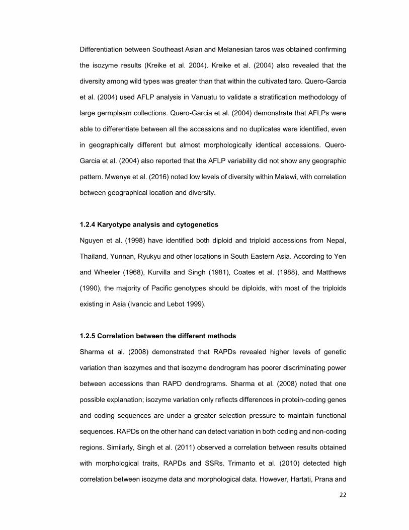
1.2.4 Karyotype analysis and cytogenetics

Nguyen et al. (1998) have identified both diploid and triploid accessions from Nepal,

Thailand, Yunnan, Ryukyu and other locations in South Eastern Asia. According to Yen

and Wheeler (1968), Kurvilla and Singh (1981), Coates et al. (1988), and Matthews

(1990), the majority of Pacific genotypes should be diploids, with most of the triploids

existing in Asia (Ivancic and Lebot 1999).

1.2.5 Correlation between the different methods

Sharma et al. (2008) demonstrated that RAPDs revealed higher levels of genetic

variation than isozymes and that isozyme dendrogram has poorer discriminating power

between accessions than RAPD dendrograms. Sharma et al. (2008) noted that one

possible explanation; isozyme variation only reflects differences in protein-coding genes

and coding sequences are under a greater selection pressure to maintain functional

sequences. RAPDs on the other hand can detect variation in both coding and non-coding

regions. Similarly, Singh et al. (2011) observed a correlation between results obtained

with morphological traits, RAPDs and SSRs. Trimanto et al. (2010) detected high

correlation between isozyme data and morphological data. However, Hartati, Prana and

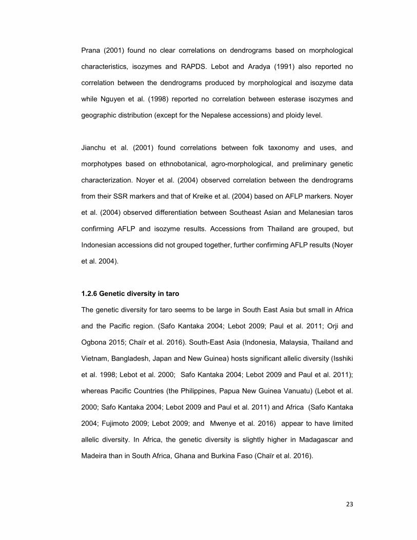
23

Prana (2001) found no clear correlations on dendrograms based on morphological

characteristics, isozymes and RAPDS. Lebot and Aradya (1991) also reported no

correlation between the dendrograms produced by morphological and isozyme data

while Nguyen et al. (1998) reported no correlation between esterase isozymes and

geographic distribution (except for the Nepalese accessions) and ploidy level.

Jianchu et al. (2001) found correlations between folk taxonomy and uses, and

morphotypes based on ethnobotanical, agro-morphological, and preliminary genetic

characterization. Noyer et al. (2004) observed correlation between the dendrograms

from their SSR markers and that of Kreike et al. (2004) based on AFLP markers. Noyer

et al. (2004) observed differentiation between Southeast Asian and Melanesian taros

confirming AFLP and isozyme results. Accessions from Thailand are grouped, but

Indonesian accessions did not grouped together, further confirming AFLP results (Noyer

et al. 2004).

1.2.6 Genetic diversity in taro

The genetic diversity for taro seems to be large in South East Asia but small in Africa

and the Pacific region. (Safo Kantaka 2004; Lebot 2009; Paul et al. 2011; Orji and

Ogbona 2015; Chaïr et al. 2016). South-East Asia (Indonesia, Malaysia, Thailand and

Vietnam, Bangladesh, Japan and New Guinea) hosts significant allelic diversity (Isshiki

et al. 1998; Lebot et al. 2000; Safo Kantaka 2004; Lebot 2009 and Paul et al. 2011);

whereas Pacific Countries (the Philippines, Papua New Guinea Vanuatu) (Lebot et al.

2000; Safo Kantaka 2004; Lebot 2009 and Paul et al. 2011) and Africa (Safo Kantaka

2004; Fujimoto 2009; Lebot 2009; and Mwenye et al. 2016) appear to have limited

allelic diversity. In Africa, the genetic diversity is slightly higher in Madagascar and

Madeira than in South Africa, Ghana and Burkina Faso (Chaïr et al. 2016).

24

Clonally propagated crops, like taro, tend to have a narrow genetic base. The wide

genetic diversity of taro in certain places can be attributed to the fact that certain taro

cultivars do flower and are cross pollinated by naturally occurring pollinators. Cross

compatibility between species occurs (even with wild types) and insect pollinators do

occur abundantly in certain areas (Hartari et al. 2001). Mare (2006) noted that there

might just be four taro landraces in central KwaZulu-Natal, South Africa in spite of the

taro’s long history in South Africa. This might be due to the fact that taro is vegetatively

propagated in South Africa. Flowering seldom occur and the known natural pollinators

do not occur in South Africa.

Ivancic and Lebot (1999), Hartati et al. (2001), Jianchu et al. (2001), Matsuda and

Nawata (2002), Hue et al. (2003), Kreike et al. (2004) Caillon et al. (2006) and other

authors observed no correlation between geographic distribution and diversity of taro.

However, Sharma et al. (2008) noted correlation between cluster analyses (but not

dendrograms) based on RAPDS and geographic distribution. They also traced evidence

of local natural selection. Sharma et al. (2008) reported high levels of diversity in Indian

taro collection and attributed the largest portion of the diversity to geographic isolation.

The low genetic diversity in Africa and the Pacific areas have certain implications on

breeding of taro in these areas. One of these is the introduction of germplasm from other

areas. These areas is also outside the centre of diversity of taro and incidences of natural

hybridization is low.

Very little is known about the genetic diversity of taro in South Africa. Mare (2006) noted

that local the farmers are able to distinguish between different landraces. Mabhaudhi

and Modi (2013) distinguished between three taro landraces using agro-morphological

characteristics and SSRs. More information is needed to understand the genetic

structure, of taro in South Africa, better

25

1.3 Breeding in Taro

There are three approaches to obtain improved cultivars of taro (Sivan and Liyanage

1993). The easiest is to collect and evaluate local germplasm in order to identify

promising lines to propagated and distributed. Alternatively, elite cultivars can be

imported from other countries to evaluate under local conditions, to identify cultivars

suitable for local conditions and markets. Lastly, controlled breeding can be used to

recombine characteristics in progeny that are evaluated against a set of predetermined

criteria (Sivan and Liyanage 1993).

The discovery of methods of flower induction in taro has greatly facilitated breeding (Safo

Kantaka 2004). One of the first breeding programmes was initiated in the early 1970’s in

the Solomon Islands to breed for taro leaf blight resistance (Patel et al. 1984, as cited

by Lebot 2009). This was followed by breeding programmes in Hawaii, Samoa, Papua

New Guinea (PNG), India, Philippines, Fiji and Vanuatu (Lebot 2009). There are taro

breeding programmes in Mauritius that used mutation breeding to identify taro blight

resistance (Seetohul et al. 2007). Lebot (2009) also noted that little was achieved in

these programmes due to the narrow genetic base of the breeding stock and the

introduction of “wild” germplasm that also introduced undesirable traits.

Most domesticated taro genotypes do not flower naturally (Del Peno 1990; Wilson 1990;

Lebot 2009). Wild types do flower more easily and the character can be bred into a

population (Lebot 2009). Lebot (2009) lists several possible ways to promote flowering

in taro and other aroids. These are treatment with gibberellic acid (0.3 – 0.5 g/ℓ), removal

of leaves (effective for Xanthosoma and Alocasia), heat and drought stress, and removal

of cormels and stolons. However, spraying the parental material with GA was considered

the most efficient and reliable method (Ivancic 1992 as cited by Iramu et al. 2009; Wilson

1990; Mukherjee et al. 2016). The first inflorescences appear from 60 to 90 days after

26

gibberellic acid application, depending on the clone and the growing conditions (Wilson

1990).

Plants produce a floral bract or flag leaf before the plant produces an inflorescence.

These bracts are produced by both natural and induced flowering (De la Pena 1990;

Wilson 1990; Lebot 2009). The first inflorescences usually appear within 1–3 weeks after

the flag leaf. Gibberellic acid induces deformities before the normal inflorescences.

These deformities include incomplete and patches of floral colour and texture on the

leaves. Gibberellic acid also stimulates plants to produce more suckers, more stolons,

elongated petioles, and branching corms (Wilson 1990).

Taro flowers are thermogenic. The flowers have a distinct odour when female flowers

are receptive (Wilson 1990). Taro flowers are protogynous, thus the female flowers

become receptive before the pollen is shed from the male flowers from the same

inflorescence (Mukherjee et al. 2016) however, Wilson (1990) noted that the female

flowers may be receptive on the same day as the pollen shed of the male flowers in the

some inflorescence or it may occur a day before or even after, depending on the location

and genotype. The two sides of the spathe enclosing the base of the inflorescence “crack

open” and the constricted part of the spathe becomes loose around the band of sterile

flowers (Wilson 1990) as the spathe of the inflorescence unfold slowly and enable

pollinators to enter. The majority of insects will remain inside the inflorescence until the

next morning when the inflorescence will be completely opened and the pollen released.

The odour will disappear but the same attraction will come from another inflorescence,

which will release pollen a day later (Lebot 2009). The crack closes after pollen shed

and the spathe becomes tight around the band of sterile flowers (Figure 1.6) (Wilson

1990).

27

Figure 1.6: The taro inflorescence. The complete inflorescence from Cocoindia on the left. The spathe in the inflorescence from a line 2-2 on the right was cut away to show the female

flowers (Photos: WS Jansen van Rensburg).

Pollination is done by various insects, wind or water, though insects are the main vectors

(Lebot 2009). Insects that pollinate taro naturally include Drosophilidae (mainly

Drosophila pisticola and D. stamenicola, in Papua New Guinea) (Lebot 2009), dipteran

flies, like Dacus dorsalis, in Malaysia, (Lebot 2009) and bees, small solitary wasps, small

Coleoptera insects, mosquitoes and ants (Lebot 2009) no natural pollinator was

observed in Africa. Wind pollination is significant for genotypes with open flowering and

a fully exposed male part of the spadix (Figure 1.6). Rain results mostly in self-fertilization

by washing pollen grains from the male part of the spadix to the female part (Lebot 2009).

Spathe covering female flowers

Constriction in spathe

Spathe

Sterile appendage

Male flowers

Band of sterile flowers

Sterile female flowers

Female flowers

Intact inflorescence

Spathe cut away from inflorescence

28

Figure 1.7: Taro fruiting body with numerous berries. The colours vary from green to yellow,

orange and almost black (Lebot 2011).

For controlled pollination, the stigma becomes receptive at the time when the

inflorescence emerges from the petiole sheath, about five days before the odour is

released or six days before pollen is shed, and remains in this condition for up to 10 days

(Okpul and Ivancic 1995). On sunny days in New Caledonia, pollen appeared before

08:00 in vigorous populations along rivers, but in drier places pollen could be seen after

10:00 (Ivancic and Lebot 1999). Ivancic and Lebot (1999) also found that pollen remain

viable for up to 18 days in New Caledonia. Asynchrony in flowering during artificial

hybridization can be overcome by cryostoring of pollen (Mukherjee et al. 2016).

The taro fruit is a cluster of densely packed berries (Figure 1.9). Each berry contains 1

to 10 seeds, but it may contain up to as many as 28 to 35 seeds (Wilson 1990; Iramu et

al., 2009). The fruits are ready to be harvested 30–35 days after fertilization. Taro seeds

29

are tiny, less than 2 mm long. When mature they are ovate in shape, hard, and

conspicuously ridged longitudinally. The seeds germinate in 7 to 14 days with no

apparent dormancy. Seeds can be stored for one year in a moderately cool and dry

room. They can remain viable for at least two years in a desiccator inside a refrigerator

(Wilson 1990). Dry winds and high temperatures often cause seed set failure (Lebot

2009; Mukherjee et al. 2016).

The aim of most taro breeding programmes is yield (Sivan and Liyanage 1993; Soulard

et al. 2016), quality (Sivan and Liyanage 1993; Iramu et al., 2009) and pest and disease

resistance (Sivan and Liyanage 1993; Iramu et al., 2009). Many taro breeders emphasis

yield in the early generations of taro breeding programmes according to Soulard et al.

(2016). Several specific characters were evaluated in a breeding programme. The most

important characteristics are plant characters (plant type, petiole colour), plant vigour,

sucker number (Sivan and Liyanage 1993), resistance to pests and diseases (viruses,

fungi, and insects) (Sivan and Liyanage 1993; Seetohul et al. 2007) maturity, marketable

and non-marketable yield, corm characters (shape, smoothness, colour of buds, basal

rings, petiole base and flesh) and eating quality (dry weight percentage, specific gravity,

taste) (Sivan and Liyanage 1993). According to Sivan and Liyanage (1993), it will take

six to ten years to release a taro cultivar using traditional breeding methods. Recently,

emphasis has also been placed on the nutrient composition of taro corms. Breeding is

done to increase the nutrient content (bio-fortification), or decrease the anti -nutrient

content of taro. These compounds are beta-carotene, anthocyanin antioxidants,

phenolic compounds and oxalates etc. (Guchhait 2008; Champagne et al. 2013).

The presence of stolons was found to be often associated with undesirable traits such

as poor corm shape, poor taste quality and acridity (Lebot et al. 2004). Heritability values

compared to narrow-sense heritabilities, suggest a possibility of using family selection in

the first cycles of a breeding programme (Lebot 2009). Orji and Ogbonna (2015) and

30

Soulard et al. (2016) found a strong indication that stolons, suckers and flowering are

under genetic control. Stolon production and the number of suckers are strongly

negatively correlated, while flowering and the number of inflorescences are not

correlated to any other traits (Soulard et al. 2016). Orji and Ogbonna (2015) noted that

plant girth was positively correlated to plant height but negatively correlated to the

number of suckers. The number of leaves and the number of suckers are also positively

correlated (Orji and Ogbonna 2015). Dry matter content was negatively correlated to

fresh weight (Quero-Garcia et al. 2006; Mulualem and WeldeMichael 2013; Soulard et

al. 2016). Quero-Garcia et al. (2009) found that mid-parent values were good predictions

for progeny means for number of suckers, corm width, and dry matter content.

Furthermore, the corm weight correlations were not significant and were remarkably

lower than for corm dimensions. Soulard et al. (2016) found that the number of stolons,

the number of suckers, fresh corm weight, and dry matter content were the most

heritable traits. They also noted a moderate to high genetic gain for most heritable traits

in early generation selections. Sugars, proteins and mineral content is negatively

correlated to starch content in the corms, whereas starch and dry matter content is

positively correlated (Lebot et al. 2011; Champagne et al. 2013). Cormel numbers and

dry matter percentages have high heritability values in Indian taro germplasm. The

number of cormels and dry matter percentages are positively correlated to tuber yield

per plant. Weight of cormels per plant has a direct effect on tuber yield and is an

important selection criterion to increase tuber yield per plant (Mukherjee et al. 2016).

1.4 Genotype by environmental interaction

Fox et al. (1997) defined genotype by environment interaction (GxE) as the differential

expression of a genotype across environments. A genotype is the result of the action

and interaction of those genes controlling a “character”. Environment refers to the

“conditions” under which the plants grow and these environments consist of a

combination of many biological, physical, and time factors which vary independently and

31

interact with each other. All these different factors have effects on the genotype to result

in the specific phenotype that is observed (Romagosa and Fox 1993; Fox et al, 1997).

GxE implies that even if all individual in a population were identical (with the same

genotypes), they would not necessarily express their genetic potential in the same way

with high variation in environmental conditions because genetic expression is a

stochastic process.

Different types of GxE can be distinguished if the relative mean performance of each

genotype in each environment is plotted against the environmental means (Figure 1.8).

The two genotypes may react similarly to different environments (Figure 1.8a), or the

two genotypes may react differently to the different environments. The ranking may stay

the same (Figure 1,6b) or the ranking may change, crossover type, (Figure 1.8c) when

two genotypes react differently to different environments. The type of GxE that has the

biggest implication for plant breeders is the crossover type (Figure 1.8 c), which involves

a change in rank order of the genotypes across environments. With crossover-interaction

a genotype or variety recommended for one environment will not necessarily be that

suited to another environment (Ramagosa and Fox 1993; Fox et al. 1997). The presence

of GxE interactions implies that the relative behaviour of genotypes in a trial depends

upon the particular environment in which they are being grown.

Becker (1981) cited by Fox et al. (1997) distinguishes two types of genetic stability:

biological or homeostatic stability, which refers to genotypes that maintain a constant

yield across environments; and agronomic stability, which refers to genotypes that yield

according to the productive potential of the test environments. If a genotype exhibits

32

Figure 1.8: The performance of two hypothetical genotypes in two hypothetical environments,

showing (a) no GxE interaction, (b) ‘quantitative’ GxE interaction (without reversal of ranks) and

(c) “qualitative GxE interaction (with reversal of rank – crossover type) (Adapted from

Romagosa and Fox 1993).

Environments

Per

form

ance

Genotype 1

Genotype 2

Environments

Per

form

anc

e

Genotype 1

Genotype 2

Environments

Per

form

anc

e

Genotype 1

Genotype 2

a

b

c

33

agronomic stability over a wide range of environments, the genotype is considered to

have a general or wide adaptability. In contrast, if a genotype exhibits agronomic stability

in a limited range of similar environments the genotype is considered to have a specific

or narrow adaptability (Fox et al., 1997).

1.4.1 Statistical methods to measure GxE interaction

Various methods are used to analyse GxE interactions. These methods vary from

analysis of variance (ANOVA) and regression, to non-parametric methods like pattern

analysis and multivariate techniques (Ramagosa and Fox 1993; p 387).

1.4.1.1 Regression

Regression analysis is a statistical process for estimating the relationships among

variables. Historically, regression was a popular statistical method to partition and

analyse interaction (Gauch 1992). A model to determine genotype stability by simple

linear regression was developed by Finlay and Wilkenson (1963). But even prior to

Finlay and Wilkenson, Yates and Cochran proposed a similar method in 1938 (Gauch

1992). Ramagosa and Fox (1993) stated that the Finlay and Wilkinson regression is the

most widely used (and, possibly misused) statistical technique in plant breeding.

Finlay and Wilkinson (1963) analysed the linear regression of the yield for each variety

on the mean yield of all varieties for each site in each season. The mean yield of all the

varieties at a specific site and season provides a numerical grading for sites and can be

useful in evaluating the site’s environment. The average yield of a large group of varieties

can describe a complex natural environment without defining or analysing the interacting

edaphic and seasonal factors (Finlay and Wilkinson 1963; Gauch 1992, p62).

34

Figure 1.9: A generalized interpretation of the genotypic pattern obtained when genotypic

regression coefficients are plotted against genotypic mean, adapted from Finlay and Wilkinson

(1963).

The regression coefficients of a variety can be plotted against the variety’s mean yield

(Finlay and Wilkinson 1963). The population mean would have a regression coefficient

of one. Regression coefficient for a variety in the order of 1.0 has an average stability

over all environments. These varieties will perform consistently above or below the

average for that environment, but their responses to changes in the environment will be

the same. If the mean yield is below average these varieties are poorly adapted to all

environments; if the mean yield is high, the variety is well adapted to all environments.

Regression coefficients significantly larger than one (a very steep slope) are specifically

adapted to high yielding/favourable environments and are sensitive to changes in

environment. These varieties react very positively (increase in yield) for a small positive

A

bove

1

Bel

ow 1

Specifically adapted to unfavourable environments

Specifically adapted to favourable environments

Poorly adapted to all

environments

Average stability

Well adapted to all environments

Below average stability

Above average stability

1

Genotypic mean yield

35

change in environment. These varieties will have a low yield in unfavourable

environments but will react positively to changes in environment and will yield above

average in favourable environments. Regression coefficients significantly smaller than

one (a flatter slope) are specifically adapted to low yielding/unfavourable environments.

These varieties “resist” environmental changes and respond very little to large changes

in environments; the varieties, as a result, have above average stability. They will have

a good yield in unfavourable environments, but because they are less sensitive to

environmental change, these varieties will still yield approximately the same at

favourable environments where other cultivars might out-yield them. The interpretation

of stability and adaptability by plotting the regression coefficient of a specific cultivar

against the mean yield of that cultivar is summarized in Figure 1.9. Regression is

effective to emphasize the trends of varietal responses in a range of environments

(Finlay and Wilkinson 1963; Gauch 1992).

1.4.1.2 Analysis of variance

ANOVA offers an additive model for two-way data tables and analyse the differences

between group means and their associated procedures (such as "variation" among and

between groups). In the ANOVA setting, the observed variance in a particular variable

is partitioned into components attributed to different sources of variation. The observed

yield (Yij) of a given genotype “i” in environment “j” is portioned into (a) an additive model

with three parameters, namely the grand mean µ, genotype deviation Gi, and

environment deviation Ej, (b) the non-additive residuals or interaction GEij and error eij

(Gauch, 1992, p 59).

The analysis of variance of a two-factor mixed model (fixed genotypes and random

environment) expresses the observed (Yij) mean yield of the ith genotype at the jth

environment as:

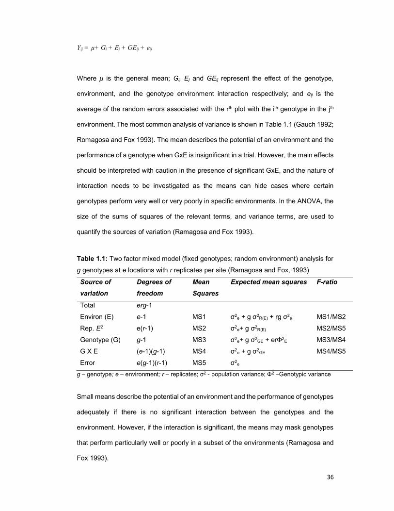
36

Yij = µ+ Gi + Ej + GEij + eij

Where µ is the general mean; Gi, Ej and GEij represent the effect of the genotype,

environment, and the genotype environment interaction respectively; and eij is the

average of the random errors associated with the rth plot with the ith genotype in the jth

environment. The most common analysis of variance is shown in Table 1.1 (Gauch 1992;

Romagosa and Fox 1993). The mean describes the potential of an environment and the

performance of a genotype when GxE is insignificant in a trial. However, the main effects

should be interpreted with caution in the presence of significant GxE, and the nature of

interaction needs to be investigated as the means can hide cases where certain

genotypes perform very well or very poorly in specific environments. In the ANOVA, the

size of the sums of squares of the relevant terms, and variance terms, are used to

quantify the sources of variation (Ramagosa and Fox 1993).

Table 1.1: Two factor mixed model (fixed genotypes; random environment) analysis for

g genotypes at e locations with r replicates per site (Ramagosa and Fox, 1993)

Source of

variation

Degrees of

freedom

Mean

Squares

Expected mean squares F-ratio

Total erg-1

Environ (E) e-1 MS1 σ2e + g σ2

R(E) + rg σ2e MS1/MS2

Rep. E2 e(r-1) MS2 σ2e+ g σ2

R(E) MS2/MS5

Genotype (G) g-1 MS3 σ2e+ g σ2

GE + erФ2E MS3/MS4

G X E (e-1)(g-1) MS4 σ2e + g σ2

GE MS4/MS5

Error e(g-1)(r-1) MS5 σ2e

g – genotype; e – environment; r – replicates; σ2 - population variance; Ф2 –Genotypic variance

Small means describe the potential of an environment and the performance of genotypes

adequately if there is no significant interaction between the genotypes and the

environment. However, if the interaction is significant, the means may mask genotypes

that perform particularly well or poorly in a subset of the environments (Ramagosa and

Fox 1993).

37

1.4.1.3 Principal Component Analysis (PCA)

Principal component analysis (PCA) offers a multiplicative model for analysis in contrast

to the additive model of ANOVA (Gauch 1992, p 69). In an additive model the effects of

individual factors are differentiated and added together to model the data, whereas in a

multiplicative model the joint effect of two or more causes is the product of their effects,

if they were acting alone. ANOVA analysis results in only one set of genotype and

environmental deviations, whereas PCA can give several sets of parameters (axes),

PC1, PC2, PC3………PCn. The PCA offers a series of models that result in one full

model (Gauch 1992, p 69-70).

PCA reduces the dimensionality of multivariate data and makes it possible to visualise it

in fewer dimensions (normally 2) in a series of biplots (Gauch 1992 p 71). The PCA

biplots have two types of points, genotype and environment; interpretation of the biplot

involves analysing the relationships amongst points of the same kind and the relationship

between points of different kinds. Amongst points of the same type, points that are close

to each other are similar and points that are far apart are dissimilar. When interpreting

different kinds of points, a genotype’s score can be multiplied with the environment’s

score to give the PCA models’ expected value for that genotype in that environment.

Scores near zero represent genotypes or environments with small variations (for the

specific characteristic), whereas genotypes or environments with large values (positive

or negative) have large variations. Expected values for a characteristic far above the

grand mean involve genotypes with large positive scores of the same sign, while

relatively small values for the characteristic involving large scores of opposite signs.

Genotypes with large positive scores grow very well in environments with a positive

score, but especially poorly in environments with a large negative score. The opposite

is also true; genotypes with a large negative score grow well in environments with a

negative score. Thus, the distribution of points on the PCA biplot can be used to interpret

38

and explain responses and interactions, and can be complimented by additional

knowledge of the environments and genotypes (Gauch 1992).

1.4.1.4 Additive main effects and multiplicative interaction (AMMI)

The additive main effects and multiplicative interaction, or AMMI, method combines the

standard ANOVA for the genotype and environment main effects with PCA. The AMMI

model separates the additive variance from the multiplicative (interaction) variance and

applies PCA to the interaction portion from the ANOVA analysis. The ANOVA partitions

the total variation into three orthogonal sources, namely genotype; environment and

genotype environment interactions. The AMMI then uses a PCA to partition the genotype

environment interactions into several orthogonal axes (interaction principle component

axes) that account more effectively for the interaction patterns (Shaffi et al 1992; Gauch

and Zobel 1996; p 85; Hill et al., 1997). Hill et al (1997) noted that the AMMI strips away

the additive effects of genotype and environment from the two-way genotype-

environment table and conducts a PCA on the residual.

The AMMI analysis generates a series of models, designated as AMMI0, AMMI1, AMM2,

AMMI3…. AMMIF depending on the number of axes retained. AMMI0 fits only additive

main effects of genotypes and environments, but retains no interaction principal

component axes (IPCA). AMMI1 fits the additive effects from AMMI0 plus the

interactions associated with the first principal component axis (IPCA1). AMMI2 fits the

interaction associated with IPCA2 and so on up to AMMIF, the full model that retains all

the axes (Hill et al., 1997).

The AMMI results can be plotted in a biplot that shows main and interaction for

genotypes and environments. The AMMI1 places the genotype and environment means

on the X axis and the respective eigenvectors on the Y axis. Genotypes and

environments that fall in a vertical line have similar means, and genotypes and

39

environments that fall on a horizontal line have similar interaction patterns. Genotypes

or environments with a large first principal component axis score have high interactions,

and those with values close to zero have small interactions. Polygons may be applied to

AMMI2 to show which genotype is the most successful in each environment (Gauch and

Zobel 1996; p 89, 90; Hill et al., 1997).

The AMMI equation is expressed thus:

Yger = µ + αg + βe + Σnλnϒgnσen + ρge + εger

Where:

Yger = observed yield or phenotype of genotype g in environment e for replicate r.

Additive parameters:

µ = grand mean

αg = deviation of the genotype

βe =deviation of the environment

Multiplicative parameters:

λn = singular value for the interaction principal component axis (IPCA) n

ϒgn = genotype Eigen vector for axis n

σen = environment Eigen vector

ρge = residuals

εger = error (Gauch and Zobel 1996; p86)

The AMMI method is used for three main purposes - model diagnosis, to clarify GxE

interactions, and to improve accuracy of estimates. AMMI is more appropriate in the

initial statistical analysis of yield trials, because it offers an analytical tool for diagnosing

models as subcases when these are better for a particular data set. AMMI is also used

to clarify GxE interactions. AMMI plots summarize patterns and relationships of

genotypes and environments. AMMI can also improve the accuracy of yield estimates

that are equivalent to increasing the number of replicates, thus reducing the costs of

trials by reducing the number of replications, or creating the opportunity to include more

varieties in the experiment. Additionally, it will improve the efficiency in selecting the best

genotypes (Crossa 1990).

40

AMMI has proven useful for understanding complex GxE interactions, as the results can

be plotted in a very informative biplot which shows both main and interaction effects for

both genotypes and environments. Additionally, AMMI can partition the data into a

pattern rich model and discard noise residual to gain accuracy (Gauch and Zobel 1996;

p85).

1.4.2 Genotype x environment interaction in Colocasia esculenta

Different taro types are found globally. Some types are adapted to paddy conditions,

others to upland conditions, while some even tolerate relatively long periods of drought.

Furthermore, some types are only adapted to coastal areas or higher altitudes (Lebot

2009).

Ivancic and Lebot (2000) found that none of the more than 2000 genotypes tested in

paddy conditions in Papua New Guinea were adapted to paddy growing, they noted that

it might be an indication of a narrow range of environmental adaptability. Okpul (2005)

tested seven taro elite lines, and a highly preferred control cultivar, ‘Numkoi’, in seven

diverse agro-ecological environments. There were significant differences in yield among

genotypes at six sites, and significant GxE interaction (Okpul 2005)

1.5 Justification and study objectives

Only taro landraces are used in South Africa and in Africa. No local genetically improved

material exists and taro genetically improved germplasm is imported from the various

breeding programs and the Secretariat of the Pacific Community (Suva, Fiji), that host

the largest aroid germplasm collection in the world. Literature indicate that the diversity

of taro is low in African countries. This also seems to be the case in South Arica

superficially; however, no information is available for South Africa. Worldwide, very little

is known about the influence of the environment on the performance of specific

41

landraces. The study intend to highlight certain aspects of the genetic improvement of

taro in South Africa. It will attempt to establish the genetic diversity of taro in South Africa.

The study will also attempt to generate diversity by means of hand pollinations. Finally,

the study will attempt to determine the influence of the environment on taro landraces.

The specific objectives of the study are:

To determine the genetic diversity in the ARC taro germplasm collection using

agro-morphological characteristics and microsatellite markers.

To determine if it is possibility to breed with local taro germplasm.

To determine the effect of four different environments (Roodeplaat, Umbumbulu,

Owen Sithole College of Agriculture and Nelspruit) on ten agro-morphological

characteristics of 29 taro landraces.

1.5 References

Bradbury JH and Nixon RW (1998) The acridity of raphides from the edible aroids.

Journal of the Science of Food and Agriculture 76: 608-616

Burkill HM (1985) The useful plants of west tropical Africa, 2nd edition. Royal Botanic

Gardens, Kew, UK

Caillon S, Quero-Garcia J, Lescure J-P and Lebot V (2006) Nature of taro (Colocasia

esculenta (L). Scott) genetic diversity in a Pacific island, Vanua Laa, Vanuatu.

Genetic Resources and Crop Evolution. 23:1273-1289

Chaïr H, Traore RE, Duval MF, Rivallan R, Mukherjee A, Aboagye LM, Van Rensburg

WJ, Andrianavalona V, Pinheiro De Carvalho MAA, Saborio F, Sri Prana M,

Komolong B, Lawac F and Lebot V (2016) Genetic Diversification and Dispersal

of Taro (Colocasia esculenta (L.) Schott). PLoS One 11(6):e0157712.

doi:10.1371

42

Champagne A, Legendre L and Lebot V (2013) Biofortification of taro (Colocasia

esculenta) through breeding for increased contents in carotenoids and

anthocyanins. Euphytica 194:125–136

Coates DJ, Yen DE, Gaffey PM (1988) Chromosome variation in Colocasia esculenta.

Implication for origin in the Pacific. Cytologia 53:551–560

Crossa J (1990) Statistical analysis of multilocation trials. Advances in Agronomy

44:55-86.

Darkwa S and Darkwa AA (2013) Taro “Colocasia esculenta”: It’s Utilization in Food

Products in Ghana. Journal of Food Processing and Technology 4:225

Das AB, Das A, Pradhan C and Naskar SK (2015) Genotypic variations of ten Indian

cultivars of Colocasia esculenta var. antiquorom Schott. evident by chromosomal

and RAPD markers, Caryologia, 68:44-54

De la Pena RS (1990) Development of new taro varieties through breeding. Research

extension series / Hawaii Institute of Tropical Agriculture and Human Resources.

pp 32-36

Devi AA (2012) Genetic Diversity Analysis in Taro Using Molecular Markers – An

Overview. Journal of Root Crops 3815-25

Engelberger L, Aalbersberg W, Ravi P, Bonnin E, Marks GC, Fitzgerald MH and Elymore

J (2003) Further analyses on Micronesian banana, taro, breadfruit and other

foods for provitamin A carotenoids and minerals. Journal of Food Composition

and Analysis 16:219-236

FAO. (2017) FAOSTAT database collections Food and Agriculture Organization of the

United Nations Rome URL: http://www fao org/faostat/en/#data/QC Access date:

3 January 2017

Finlay KW and Wilkinson GN (1963) The analysis of adaptation in a plant breeding

programme. Australian Journal of Agricultural Research 14: 742-754.

Fox PN, Crossa J and Romagosa I (1997) Multi-environment testing and genotype x

environment interaction. In: Statistical methods for Plant Variety Evaluation.

43

Edited by R. A. Kempton and P. N. Fox. Chapman and Hall, London ISBN 0

412 45750 3

Fujimoto T (2009) Taro (Colocasia esculenta [L] Schott) Cultivation in Vertical Wet-Dry

Environments: Farmers’ Techniques and Cultivar Diversity in South-western

Ethiopia. Economic Botany 63:152–166

Gauch Jr HG (1992) Statistical Analysis of Regional Yield Trails: AMMI Analysis of

Factorial Designs. Elsevier Science Publishers, Amsterdam, The Netherlands.

pp 278

Gauch Jr HG and Zobel RW (1996) AMMI analysis of a yield trial. In Genotype by

Environment Interaction, edited by Kang MS and Gauch Jr. HG CRC Press,

Boca Raton Florida, USA. (p 85-122)

Godwin IG, Mace ES and Nurzuhairawaity. 2001. Genotyping Pacific Island taro

(Colocasia esculenta (L.) Schott) germplasm. In Plant genotyping — the DNA

fingerprinting of plants. Edited by R. Henry. CAB International, Oxon, U.K. pp.

109–128.

Guchhait S, Bhattacharya A, Pal S, Mazumdar D, Chattopadhyay A and Das AK (2008)

Quality Evaluation of Cormels of New Germplasm of Taro. International Journal

of Vegetable Science 14:304-321

Hartati NS, Prana TK and Prana MS (2001) Comparative study on some Indonesian taro

(Colocasia esculenta (L.) Schott) samples using morphological characters,

RAPD markers and isozyme patterns. Annales Bogorienses 7(2):65-73

Hill J, Becker HC and Tigerstedt PMA (1998) Quantitative and Ecological Aspects of

Plant Breeding. Plant Breeding Series 4. Chapman and Hall, Londen, UK, pp

275

Hu K, Huang XF, Kev WD and Ding YI (2009) Characterization of 11 new microsatellite

loci in taro (Colocasia esculenta). Molecular Ecology Resources 9:582–584

Hue NN, Trinh LN, Han P, Sthapit B and Jarvis D (2003) Taro cultivar diversity in three

ecosites of North Vietnam. On-Farm Management of Agricultural Biodiversity in

Vietnam 58-62

44

IPGRI (1999) Descriptors for taro (Colocasia esculenta). International Plant Genetic

Resources Institute, Roe.

Iramu E, Wagih ME and Singh D (2009) Genetic hybridization among genotypes of Taro

(Colocasia esculanta) and recurrent selection for leaf blight resistance. Indian

Journal of Science and Technology 3(1):96-101

Irwin SVP. Kaufusi K, Banks R, de la Pena JJ and Cho J (1998) Molecular

characterization of taro (Colocasia esculenta) using RAPD markers. Euphytica

99:183-189

Isshiki S, Nakamura N, Tashiro Y and Miyazaki S (1998) Classification of the Cultivars

of Japanese Taro [Colocasia esculenta (L.) Schott] by Isozyme analysis. Journal

of the Japanese Society for Horticultural Science 67:521-525

Ivancic A and Lebot V (1999) Botany and genetics of New Caledonian wild Taro,

Colocasia esculenta. Pacific Science 53:273-285

Ivancic A and Lebot V (2000) Taro (Colocasia esculenta): Genetics and Breeding.

Collection ‘Repères’, CIRAD, Montpellier, France

Jackson GVH and Gerlach WWP (1985) Pythium rots of taro. Advisory leaflet (South

Pacific Commission) 20. Noumea, New Caledonia: South Pacific Commission.

Jianchu X, Yongping Y, Yongdong P, Ayad WG and Eyzaguirre P (2001) Genetic

Diversity in Taro (Colocasia esculenta Schott, Araceae) in China: An

Ethnobotanical and genetic Approach. Ecomomic Botany 55(1):14-31

Kreike CM, van Eck HJ and Lebot V (2004) Genetic diversity of taro, Colocasia esculenta

(L.) Schott, in Southeast Asia and the Pacific. Theoretical and Applied Genetics

109:761–768

Kuruvilla K M and Singh A (1981) Karyotypic and electrophoretic studies on taro and its

origin. Euphytica 30:405-413

Lakhanpaul S, Velayudhan KC, Bhat KV (2003) Analysis of genetic diversity in Indian

Colocasia esculenta(L.) Schott using random amplified polymorphic DNA

(RAPD) markers. Genet Resouces andr Crop Evolution 50:603–609

45

Lebot V (2009) Tropical Root and Tuber Crops: Cassava, Sweet Potato, Yams and

Aroids. CABI, Wallingford, UK. pp 413

Lebot V (2011) International Network for Edible Aroids. INEA Launching Meeting, Kuala

Lumpur, April 13-14th 2011, http://www.ediblearoids.org/LIBRARY.aspx

accessed 18 February 2018.

Lebot V and Aradhya KM (1991) Isozyme variation in taro (Colocasia esculenta (L)

Schott) from Asia and Oceania. Euphytica 56:55-66

Lebot V, Gunua T, Pardales JR, Prana MS, Thongjiem M, Viet NV and Yap TC (2004)

Characterisation of taro (Colocasia esculenta (L ) Schott) genetic resources

inSouth-east Asia and Oceania. Genetic Resources and Crop Evolution 51:381–

392

Lebot V, Hartati S, Hue NT, Viet NV, Nghia NH, Okpul T, Pardales J, Prana MS, Prana

TK, Thongjiem M, Krieke CM, Van Eck H, Yap TC, and Ivancic A (2002) Genetic

variation in taro (Colocasia esculenta) in South East Asia and Oceania. In:

Twelfth Symposium of the ISTRC. Potential of root crops for food and industrial

resources. Sept. 10–16, 2000, Tsukuba, Japan, pp. 523–534.

Lebot V, Malapa R, Bourrieau M (2011) Rapid estimation of taro quality by near infrared

spectroscopy. Journal of Agriculture and Food Chemistry 59:9327–9334

Lebot V, Prana MS, Kreike N, van Heck H, Pardales J, Okpul T, Gendua T, Thongjiem

M, Hue H, Viet N and Yap TC (2004) Characterisation of taro (Colocasia

esculenta (L.) Schott) genetic resources in Southeast Asia and Oceania. Genetic

Resources and Crop Evolution 51:381–392, 2004.

Lu Z, Li W, Yang Y and Hu X (2011) Isolation and characterization of 19 new

microsatellite loci in Colocasia esculenta (Araceae). American Journal of Botany

98(9):239-241

Mabhaudhi T (2012) Drought tolerance and water–use of selected South African

landraces of taro (Colocasia esculenta L. Schott) and Bambara groundnut

46

(vigna subterranea L. Verdc). PhD Thesis, University of KwaZulu-Natal,

Pietermaritzburg, pp 241

Mabhaudhi T and Modi AT (2013) Preliminary Assessment of Genetic Diversity in

Three Taro (Colocasia esculenta L. Schott) Landraces Using Agro-

morphological and SSR DNA Characterisation. Journal of Agricultural Science

and Technology B 3 (2013) 265-271

Mace ES and Godwin ID (2002) Development and characterization of polymorphic

microsatellite markers in taro (Colocasia esculenta). Genome 45:823–832

Manner HI and Taylor M (2010) Farm and Forestry Production and Marketing Profile

for Taro (Colocasia esculenta) In: Elevitch CR(ed) Specialty Crops for Pacific

Island Agroforestry. Permanent Agriculture Resources (PAR), Holualoa, Hawaii

http://agroforestry net/scps

Mare RM (2006) Phytotron and field performance of taro (Colocasia esculenta (L)

Schot) landraces from Umbumbulu. MSc Thesis, University of KwaZulu-Natal,

Pietermaritzburg. pp 132

Matsuda M and Nawata E (2002) Geographical distribution of ribosomal DNA variation

in taro, Colocasia esculenta (L.) Scott. In eastern Asia. Euphytica 128:165-127

Matthews PJ (1990) The origins, dispersal and domestication of taro. PhD. thesis,

Australian National University, Canberra.

Matthews PJ (2004) Genetic diversity in taro, and the preservation of culinary

knowledge. Ethnobotany Research and Applications 2:55-71

Modi AT (2003) What do subsistence farmers know about indigenous crops and

organic farming? Preliminary case in KwaZulu-Natal. Development Southern

Africa 20:673-682

Modi AT (2004) Short-Term preservation of maize landrace seed and taro propagules

using indigenous storage methods. South African Journal of Botany 7016-23

47

Modi AT (2007) Effect of indigenous storage method on performance of taro [Colocasia

esculenta (L ) Schott] under field conditions in a warm subtropical area. South

African Journal of Plant Soil 24:214–219

Mukherjee A, George J, Pillai R, Chakrabarti SK, Naskar SK, Patro R, Nayak S and

Lebot V (2016) Development of taro (Colocasia esculenta (L.) Schott) hybrids

overcoming its

Mulualem T, and WeldeMichael G (2013) Study on genotypic variability estimates and

interrelationship of agronomic traits for selection of taro (Colocasia esculenta (L.)

Schott) in Ethiopia. Sky Journal of Agriculture Research 2(11):154–158.

Mwenye O, Herselman L, Benesi I and Labuschagne M (2016) Genetic Relationships in

Malawian Cocoyam Measured by Morphological and DNA Markers. Crop

Science 56:1189-1198

NBII (2017), National Biological Information Infrastructure". Introduction to Genetic

Diversity. U.S. Geological. https://web.archive.org/web/20110225072641/

http://www.nbii.gov/portal/server.pt?open=512&objID=405&PageID=0&cached=

true&mode=2&userID=2:1-10. Accessed 3 January 2017

Nguyen VX, Yoshino H and Tahara M (1998) Phylogenetic Analysis of Taro (Colocasia

esculanta (L.) Scott) and Related Species based on Esterase Isozymes.

Scientific Reports of the Faculty of Agriculture Okayama University 87:133-139

Noyer JL, Billot C, Weber P, Brottier P, Quero-Garcia J and Lebot, V. 2004. Genetic

diversity of taro (Colocasia esculenta (L.) Schott) assessed by SSR markers. In:

Guarino L, Taylor M, Osborn T (eds) Third Taro Symposium. 21–23 May 2003.

Secretariat of the Pacific Community, Fiji, pp 174–180

Oke OL (1990) Roots, tubers, plantains and bananas in human nutrition. FAO Corporate

Documentary Repository Food and Agriculture Organization of the United

Nations, Rome, Italy

48

Okpul T (2005) Effect of variety site on corm yield, leaf blight resistance and culinary

quality of seven taro, Colocasia esculenta (L.) Schott, varieties in Papua New

Guinea. MSc. thesis, University of Technology, Lae, Papua New Guinea.

Okpul T and Ivancic A (1995) Study of stigma receptivity in intraspecific hybridization of

taro. Paper presented at the Taro Seminar held 26–30 June 1995 at the Papua

New Guinea University of Technology, Lae.

Okpul T, Singh, Gunna T and Wagih ME (2004) Assessment of diversity using agro-

morphological traits for selecting a core sample of Papua New Guinea taro

(Colocasia esculenta (L) Scott) collection. Genetic Resources and Crop

Evolution 51:671-678

Opara LU (2003) Edible aroids: Post-harvest operation. Massey University (FAO), New

Zealand, Palmerston North. Available at:http://www fao org/fileadmin/

user_upload/inpho/docs/ 31 March 2017

Orji KO and Ogbonna PE (2015) Morphological correlation analysis on some agronomic

traits of taro (Colocasia esculenta) in the plains of Nsukka, Nigeria. Journal of

Global Bioscience 4:1120-1126

Patel MZ, Saelea J and Jackson GVH (1984) Breeding strategies for controlling diseases

of taro in Solomon Islands. In: Proceedings of the Sixth Symposium of the

International Society for Tropical Root Crops 21–26 February 1983. CIP Lima

pp 143–149

Paul KK, Bari MA and Debnath SC (2011) Genetic variability of Colocasia esculenta (L.)

Schott. Bangladesh Journal of Botany. 40:185-188

Paull RE, Tang C-D, Gross K and Uruu G1 (1999) The nature of the taro acridity factor.

Postharvest Biology and Technology 16:71-78

Pereira PR, Silva JT, Verícimo MA, Paschoalin VMF and Teixeira G (2015) Crude extract

from taro (Colocasia esculenta) as a natural source of bioactive proteins able to

stimulate haematopoietic cells in two murine models. Journal of Functional Foods

18:333-343

49

Quero-Garcia J, Courtois B. Ivancic A, Letourmy P, Risterucci AM, Noyer JL, Feldmann

PH and Lebot V (2006) First genetic maps and QTL studies of yield traits of taro

(Colocasia esculenta (L.) Schott) Euphytica 51:187–199

Quero-Garcia J, Letourmy P, Ivancic A, Feldmann P, Courtois B, Noyer JL and Lebot V

(2009) Hybrid performance in taro (Colocasia esculenta) in relation to genetic

dissimilarity of parents. Theoretical and Applied Genetics 119:213–221

Quero-Garcia J, Noyer JL, Perrier X, Marchand JL and Lebot V (2004) A germplasm

stratification of taro (Colocasia esculenta) based on agro-morphological

descriptors, validation by AFLP markers. Euphytica 137:387–395

Ramagosa I and Fox PN (1993) Genotype by environmental interaction and

adaptation. In: Plant Breeding: Principals and Prospects. Edited by Hayward

MD, Chapman NO and Hall, London ISBN 0 412 43390 7

Revill PA, Jackson GVH, Hafner GJ, Yang I, Maino MK, Dowling ML, Devitt LC, Dale JL

and Harding RM (2005) Incidence and distribution of viruses of Taro (Colocasia

esculenta) in Pacific Island countries. Australasian Plant Pathology 34:327-331

Safo Kantaka O (2004) Colocasia esculenta (L.) Schott In: Grubben, G.J.H. and Denton,

O.A. (Editors). PROTA 2: Vegetables/Légumes. [CD-Rom]. PROTA,

Wageningen, Netherlands. pp668

Sardos J, Noyer J, Malapa R, Bouchet S and Lebot V (2011) Genetic diversity of taro

(Colocasia esculenta (L.) Schott) in Vanuatu (Oceania): an appraisal of the

distribution of allelic diversity (DAD) with SSR markers. Genetic Resources and

Crop Evolution 59:805-820.

Seetohul S, Puchooa D and Ranghoo-Sanmukhiya VM (2007) Genetic Improvement of

Taro (Colocasia esculenta var esculenta) through in-vitro mutagenesis.

University of Mauritos Research Journal 13A:79-89

Shaffi B, Mahler KA, Price WJ, and Auld DL (1992) Genotype x Environment

interaction effects on winter Rapeseed yield and oil content. Crop Science 32:

922-927.

50

Shange LP (2004) Taro (Colocasia esculenta (L) Scott) production by small scale

farmers in KwaZulu-Natal: Farmers practices and performance of propagule

types under wetland conditions. MSc Thesis. University of KwaZulu-Natal.

Pietermaritzburg

Sharma K, Mishra A K and Misra RS (2008) The genetic structure of taro: A comparison

of RAPD and isozyme markers. Plant Biotechnology Reports 2:191-198

Singh D, Mace ES, Godwin ID, Mathur PN, Okpul T, Taylor M, Hunter D, Kambuou R,

Ramanatha Rao V and Jackson G (2008) Assesment and rationalization of

genetic diversity of Papua New Guinea taro (Colocasia esculenta) using SSR

DNA fingerprinting. Genetic Resources and Crop Evolution 55:811-822

Singh S, Singh DR, Faseela F, Kumar N, Damodaran V and Srivastava RC (2011)

Diversity of 21 taro (Colocasia esculenta (L.) Schott) accessions of Andaman

Islands. Genetic Resources and Crop Evolution 59:821-829

Sivan P and Liyanage A de S (1993) Breeding and evaluation of taro (Colocasia

esculenta) for the South Pacific Region. Research extension series / Hawaii

Institute of Tropical Agriculture and Human Resources. Pp 5

Soulard L, Letourmy P, Cao T, Lawac F, Chair H and Lebot V (2016) Evaluation of

Vegetative Growth, Yield and Quality Related Traits in Taro (Colocasia esculenta

[L.] Schott). Crop Science 56:1-14

Sreekumari MT, Abraham K, Edison S and Unnikrishnan M (2004) Taro breeding in India

In: Guarino L, Taylor M and Osborn T (eds) Proceedings of the 3rd Taro

Symposium. Nadi, Fiji, Secretariat of the Pacific Community pp 202–207

Trimanto T, Sajidan S and Sugiyarto S (2010). Characterisation of taro (Colocasia

esculenta) based on morphological and isozymic patterns markers. Nusantara

BioScience 2:7-14

Wilson JE (1990) Taro Breeding. Agro-Facts. Crops IRETA Publication No. 3/89. Apia,

Western Samoa. pp 51

51

Xu J, Yang Y, Pu Y, Ayad WG and Eyzaguirre PB (2001) Genetic diversity in Taro

(Colocasia esculenta Schott Araceae) in China: An ethnobotanical and genetic

approach. Economic Botany 55:14-31

Yen DE and Wheeler JM (1968) Induction of taro into the Pacific: the indications of

chromosome numbers. Ethnology 7, 259–267.

You Y, Liu D, Liu H, Zheng X, Diao Y, Huang X and Hu Z (2014) Development and

characterisation of EST-SSR markers by transcriptome sequencing in taro

(Colocasia esculenta (L.) Schott). Molecular Breeding 35:134

DOI:10.1007/s11032-015-0307-4

52

Chapter 2: Genetic diversity of Colocasia esculenta in South Africa

Abstract

Amadumbe (Colocasia esculenta), better known as taro, is a traditional root crop in

coastal areas of South Africa. Taro is showing potential for commercialisation. However,

very little is known about the introduction and movement of taro in South Africa. More

information on the genetic diversity of taro is necessary before any genetic improvement

can be attempted. This study investigated the diversity within the Agriculture Research

Council (ARC) germplasm collection using agromorphological descriptors and simple

sequence repeat (SSR) markers,

Taro germplasm was collected in South Africa in order to build up a representative

collection with 77 local accessions as well as foreign accessions. Germplasm was also

imported from Nigeria and Vanuatu. The South African taro germplasm, as well as

selected imported germplasm, was characterised using key agro-morphological

descriptors as proposed by Singh et al (2008). Theas well as simple sequence repeats

(SSR) developed by Mace and Godwin (2002). Dendrograms were constructed using

UPGMA cluster analysis.

Very little variation was observed between the South African accessions using agro-

morphological descriptors. No variations were observed for eight of the 30 agro-

morphological characteristics. These eight characteristics are leaf blade colour

variegation, predominant position of leaf lamina surface, leaf main vein colour, leaf vein

pattern, petiole basal ring colour, type of leaf blade variegation, colour of leaf blade

variegation). The 86 accessions were grouped into three clusters. The three clusters

contained 39, 20 and 27 accessions respectively.

53

SSR primers revealed polymorphisms for the South African germplasm. Primer Uq 84

was highly polymorphic. The accessions grouped into five clusters with 33, 6, 5, 41 and

7 accessions in each of the clusters. All the dasheen type accessions clustered together.

A higher level of genetic diversity in the South African germplasm was observed when

molecular analysis was compared to with morphological characterisation. No correlation

was detected between the different clusters and geographic distribution, since

accessions from the same locality did not always cluster together, or conversely,

accessions collected at different sites were grouped together. There was also no clear

correlation between the clustering based on agro-morphology and SSRs. Thus in order

to obtain more complete characterisation, both molecular and morphological data should

be used. Although the results indicated that there is more diversity present in the local

germplasm than expected, the genetic base is still rather narrow, as is the case in other

African countries.

2.1 Introduction

The existing variation, due to genetic differences, within a population or species is called

genetic diversity. Genetic diversity is important for the survival and adaptability of

species. Species with high genetic diversity will produce a wider range of offspring.

Some of the offspring will better adapt than others. Genetic diversity, therefore, facilitates

populations or species adaptation to changing environments (Devi 2012; NBII 2017).

Genetic diversity within and between populations or species can be assessed using

various parameters and methods such as;

agro-morphological (growth habit, stolon formation, plant height, shape, colour

and orientation of lamina, maturity, shape and weight of corms and cormels, corm

and cormel yield, flesh colour and edibility of tubers, resistance against leaf blight

etc.),

biochemical (protein expression profiles and isozymes) and

54

molecular markers (DNA markers e.g. RAPD, AFLP, SSRs etc.) (Nybom 2004;

Devi 2012).

Taro exhibits a wide array of agro-morphological variation. Okpul et al. (2004) and Singh

et al. (2008) have developed concise descriptor lists for taro. The level of morphological

variability reported by authors vary. Okpul et al. (2004), Lebot et al. (2000) and Godwin

et al. (2001) observed high morphological variation in areas where there is natural sexual

recombination as well as exchange of germplasm.

Various DNA markers were used to determine genetic diversity in taro (Lebot, 2009).

These include random amplified polymorphic DNA (RAPD), simple sequence repeats

(SSR) and amplified fragment length polymorphism (AFLP). Simple sequence repeats

(SSR) or microsatellite polymorphisms have a higher mutation rate than other DNA

areas leading to high genetic diversity. Mace and Godwin (2002), Noyer et al. (2004),

Singh et al. (2008), Hu et al. (2009), Sardos et al. (2011), Singh et al. (2011), Lu et al.

(2011), You et al. (2014) and Chaïr et al. (2016) have used SSRs to study genetic

diversity in taro. They proved to be a valuable tool for the identification of duplicates

(Mace and Godwin, 2002). The SSRs did not reveal any clear geographical structure

(Mace and Godwin 2002; Quero-Garcia et al. 2006); however, Sardos et al. (2011) did

found a degree of correlation between geographical and present social and genetic

diversity and SSRs diversity. SSRs were able to discriminate between diploid and

tetraploid germplasm (Chaïr et al. 2016).

Higher levels of genetic diversity are reported for taro originating from South East Asia

than those originating from Africa and the Pacific region (Safo Kantaka 2004; Lebot

2009; Paul et al. 2011; Orji and Ogbona 2015; Chaïr et al. 2016). The highest allelic

diversity is observed in South-East Asia (Indonesia, Malaysia, Thailand and Vietnam,

Bangladesh, Japan and New Guinea) (Isshiki et al. 1998; Lebot et al. 2000; Safo

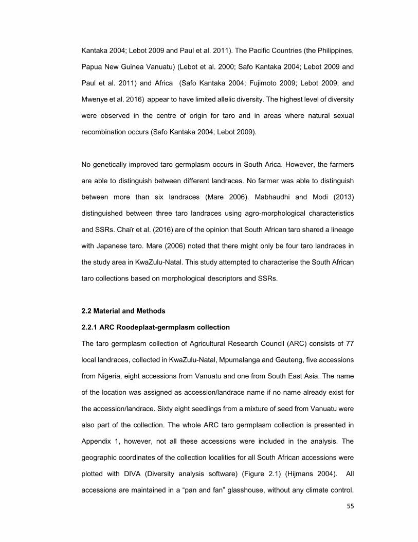
55

Kantaka 2004; Lebot 2009 and Paul et al. 2011). The Pacific Countries (the Philippines,

Papua New Guinea Vanuatu) (Lebot et al. 2000; Safo Kantaka 2004; Lebot 2009 and

Paul et al. 2011) and Africa (Safo Kantaka 2004; Fujimoto 2009; Lebot 2009; and

Mwenye et al. 2016) appear to have limited allelic diversity. The highest level of diversity

were observed in the centre of origin for taro and in areas where natural sexual

recombination occurs (Safo Kantaka 2004; Lebot 2009).

No genetically improved taro germplasm occurs in South Arica. However, the farmers

are able to distinguish between different landraces. No farmer was able to distinguish

between more than six landraces (Mare 2006). Mabhaudhi and Modi (2013)

distinguished between three taro landraces using agro-morphological characteristics

and SSRs. Chaïr et al. (2016) are of the opinion that South African taro shared a lineage

with Japanese taro. Mare (2006) noted that there might only be four taro landraces in

the study area in KwaZulu-Natal. This study attempted to characterise the South African

taro collections based on morphological descriptors and SSRs.

2.2 Material and Methods

2.2.1 ARC Roodeplaat-germplasm collection

The taro germplasm collection of Agricultural Research Council (ARC) consists of 77

local landraces, collected in KwaZulu-Natal, Mpumalanga and Gauteng, five accessions

from Nigeria, eight accessions from Vanuatu and one from South East Asia. The name

of the location was assigned as accession/landrace name if no name already exist for

the accession/landrace. Sixty eight seedlings from a mixture of seed from Vanuatu were

also part of the collection. The whole ARC taro germplasm collection is presented in

Appendix 1, however, not all these accessions were included in the analysis. The

geographic coordinates of the collection localities for all South African accessions were

plotted with DIVA (Diversity analysis software) (Figure 2.1) (Hijmans 2004). All

accessions are maintained in a “pan and fan” glasshouse, without any climate control,

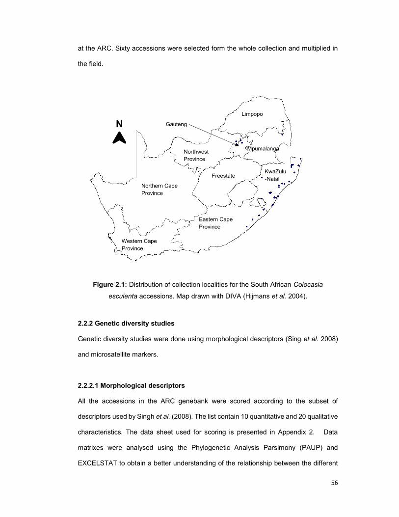
56

at the ARC. Sixty accessions were selected form the whole collection and multiplied in

the field.

Figure 2.1: Distribution of collection localities for the South African Colocasia

esculenta accessions. Map drawn with DIVA (Hijmans et al. 2004).

2.2.2 Genetic diversity studies

Genetic diversity studies were done using morphological descriptors (Sing et al. 2008)

and microsatellite markers.

2.2.2.1 Morphological descriptors

All the accessions in the ARC genebank were scored according to the subset of

descriptors used by Singh et al. (2008). The list contain 10 quantitative and 20 qualitative

characteristics. The data sheet used for scoring is presented in Appendix 2. Data

matrixes were analysed using the Phylogenetic Analysis Parsimony (PAUP) and

EXCELSTAT to obtain a better understanding of the relationship between the different

Eastern Cape Province

KwaZulu-Natal

Mpumalanga

Freestate

Limpopo

Gauteng

Northwest Province

Western Cape Province

Northern Cape Province

N

57

accessions. Cladograms are constructed using the Unweighted Pair Group Method with

Arithmetic mean (UPGMA) algorithm. The Dice dissimilarity index used was [2a/(2a + b

+ c))]. This method, first described by Sneath and Sokal (1973), used the concept of

minimal dissimilarity between two “neighboring” points and an ultrametric distance

(Sokal and Michener 1958; Sneath and Sokal 1973).

2.2.2.2 SSR markers:

Genomic DNA was isolated using the CTAB method (Edwards, Johnson and Thompson

1991). Two leaf discs were collected in a microfuge tube by punching the discs directly

into the tube, using the lid as a punch. A pinch of Carborundum was added and the leaf

material grounded thoroughly in the microfuge tube with a clean glass grinder. A 400 ml

warm (60°C) CTAB buffer was added to the grounded leaf mixture and incubated at

60°C (waterbath) for 30 minutes. Equal volume of chloroform:isoamylalcohol (24:1) was

then added and mixed (5 minutes) by inverting the tube several times. The mixture was

then centrifuged at 10 000 g for 10 minutes (Allegra X-22R, Bench Top, Beckman). The

supernatant was then carefully transferred into a clean microfuge tube and 0.6 volumes

of ice-cold isopropanol added to the supernatant. The mixture was gently mixed by

inversion and left at –20°C for 30 minutes. The mixture was centrifuged at 10 000 x g for

10 minutes and decanted to drain the isopropanol and retain the DNA pellet. The pellet

was washed using 70% ethanol followed by quick centrifugation to help the DNA pellet

seat at the bottom of the tube and drain the ethanol. The pellets were left to air dry. The

resulting pellets were re-suspended in 50 µl TE buffer. Concentration of the genomic

DNA was determined by fluorometer with a SEQUOIA-TURNER Model 450 digital

fluorometer. DNA concentration was adjusted at 10 ng/µl for all samples.

Six pairs SSR primer sets with forward and reverse sequence were chosen from those

published by Mace and Gordon (2002). The SSR primers used were Uq 55; Uq 73;

Uq 84; Uq 88, Uq 97; Uq 110; and Uq 115 . Polymerase chain reactions were run

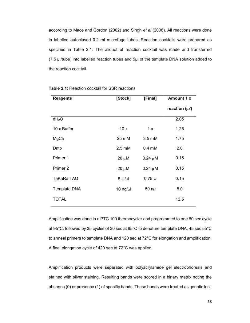
58

according to Mace and Gordon (2002) and Singh et al (2008). All reactions were done

in labelled autoclaved 0.2 ml microfuge tubes. Reaction cocktails were prepared as

specified in Table 2.1. The aliquot of reaction cocktail was made and transferred

(7.5 µl/tube) into labelled reaction tubes and 5µl of the template DNA solution added to

the reaction cocktail.

Table 2.1: Reaction cocktail for SSR reactions

Reagents [Stock] [Final] Amount 1 x

reaction ()

dH2O 2.05

10 x Buffer 10 x 1 x 1.25

MgCl2 25 mM 3.5 mM 1.75

Dntp 2.5 mM 0.4 mM 2.0

Primer 1 20 M 0.24 M 0.15

Primer 2 20 M 0.24 M 0.15

TaKaRa TAQ 5 U/l 0.75 U 0.15

Template DNA 10 ng/l 50 ng 5.0

TOTAL 12.5

Amplification was done in a PTC 100 thermocycler and programmed to one 60 sec cycle

at 95°C, followed by 35 cycles of 30 sec at 95°C to denature template DNA, 45 sec 55°C

to anneal primers to template DNA and 120 sec at 72°C for elongation and amplification.

A final elongation cycle of 420 sec at 72°C was applied.

Amplification products were separated with polyacrylamide gel electrophoresis and

stained with silver staining. Resulting bands were scored in a binary matrix noting the

absence (0) or presence (1) of specific bands. These bands were treated as genetic loci.

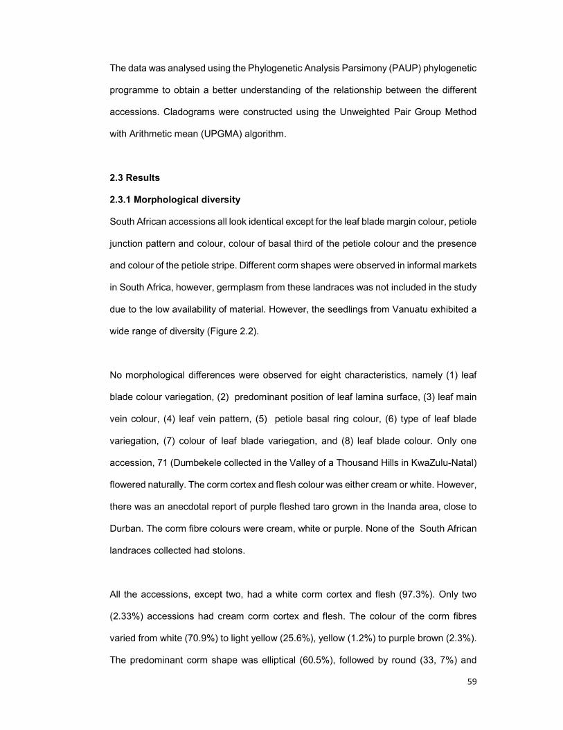
59

The data was analysed using the Phylogenetic Analysis Parsimony (PAUP) phylogenetic

programme to obtain a better understanding of the relationship between the different

accessions. Cladograms were constructed using the Unweighted Pair Group Method

with Arithmetic mean (UPGMA) algorithm.

2.3 Results

2.3.1 Morphological diversity

South African accessions all look identical except for the leaf blade margin colour, petiole

junction pattern and colour, colour of basal third of the petiole colour and the presence

and colour of the petiole stripe. Different corm shapes were observed in informal markets

in South Africa, however, germplasm from these landraces was not included in the study

due to the low availability of material. However, the seedlings from Vanuatu exhibited a

wide range of diversity (Figure 2.2).

No morphological differences were observed for eight characteristics, namely (1) leaf

blade colour variegation, (2) predominant position of leaf lamina surface, (3) leaf main

vein colour, (4) leaf vein pattern, (5) petiole basal ring colour, (6) type of leaf blade

variegation, (7) colour of leaf blade variegation, and (8) leaf blade colour. Only one

accession, 71 (Dumbekele collected in the Valley of a Thousand Hills in KwaZulu-Natal)

flowered naturally. The corm cortex and flesh colour was either cream or white. However,

there was an anecdotal report of purple fleshed taro grown in the Inanda area, close to

Durban. The corm fibre colours were cream, white or purple. None of the South African

landraces collected had stolons.

All the accessions, except two, had a white corm cortex and flesh (97.3%). Only two

(2.33%) accessions had cream corm cortex and flesh. The colour of the corm fibres

varied from white (70.9%) to light yellow (25.6%), yellow (1.2%) to purple brown (2.3%).

The predominant corm shape was elliptical (60.5%), followed by round (33, 7%) and

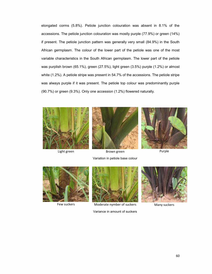
60

elongated corms (5.8%). Petiole junction colouration was absent in 8.1% of the

accessions. The petiole junction colouration was mostly purple (77.9%) or green (14%)

if present. The petiole junction pattern was generally very small (84.9%) in the South

African germplasm. The colour of the lower part of the petiole was one of the most

variable characteristics in the South African germplasm. The lower part of the petiole

was purplish brown (65.1%), green (27.5%), light green (3.5%) purple (1.2%) or almost

white (1.2%). A petiole stripe was present in 54.7% of the accessions. The petiole stripe

was always purple if it was present. The petiole top colour was predominantly purple

(90.7%) or green (9.3%). Only one accession (1.2%) flowered naturally.

Light green

Brown green

Purple

Variation in petiole base colour

Few suckers Moderate nymber of suckers Many suckers

Variance in amount of suckers

61

No stolons

Short stolons

Long stolons

Variation in length and number of stolons

Green

Green brown

Purple

Variation of variegation in petioles

Green shoulder

Light purple shoulder

Dark purple shoulder

Variation in petiole shoulder colour

All veins purpel

All veins green

Primary veins purple

Variation in colour of main veins

62

No colour in petiole junction Large petiole junction Petiole juction colour extend into the veins

Variation in colour and pattern of petiole junction on adaxial side of the leaf

Purple variegated

Green

Purple

Variation in leaf blade colour r

No waviness

Medium waviness

Very wavy

Variation in waviness of the leaf blade margin

Figure 2.2: Vanuatu seedling accessions germinated at ARC VOP to illustrate the variability in certain characteristics (WS Jansen van Rensburg).

Agglomerative hierarchical clustering (AHC) revealed that the 86 accessions were

grouped into three clusters (Figure 2.3 and Table 2.2). Cluster 1 contained 39

accessions (Table 2.2). It included accessions collected at Hluhluwe (all except 1),

63

Maphumulo, Warwick market, Willowvale, Creighton, Isiphingo (3), Umbumbulu (2),

Pietermaritzburg, Nelspruit, Manguzi, Mtwalume, Makatini and Pieter Maritz

(commercial farmer). The accessions in this group were collected in Mpumalanga,

KwaZulu-Natal (North central and South) and Eastern Cape. The presence of a purple

petiole stripe was unique to this group. Coco India, an accession from Nigeria, was also

included into this cluster.

Cluster 2 included 20 accessions (Table 2.2). Accessions were collected at Hluhluwe,

Maphumulo, Mkuze (all accessions collected at Mkuze), Makatini, Lusikisiki,

Umbumbulu, Jozini, Empangeni and Pietermaritzburg (from Prof. Albert Modi, UKZN).

Ukpong and Nigeria, two accessions from Nigeria, were also included in this cluster. All

the accessions, except for Ukpong and Nigeria, were collected in Northern and Central

KwaZulu-Natal and Eastern Cape. None of the accessions in this group had a purple-

brown lower petiole colour.

Cluster 3 consisted of 27 accessions (Table 2.2). The accessions were collected in

Jozini, Lusikisiki, Eshowe (3), Brits, Tshwane, Pietermaritzburg, Soshanguve,

Mtwalume, Maphumulo, and Dumkehle (Valley of a Thousand Hills), Ghana and an

accession from Nigeria that was also included belonged to this cluster. All the

accessions, excluding Ghana, were collected in the Northern, Central and Southern

KwaZulu-Natal and Gauteng. The lower petiole colour of all accessions in this group was

purple-brown. There was no obvious correlation between the origin of the accessions

and the clusters. The most important characteristics seemed to be the colouration of the

petiole.

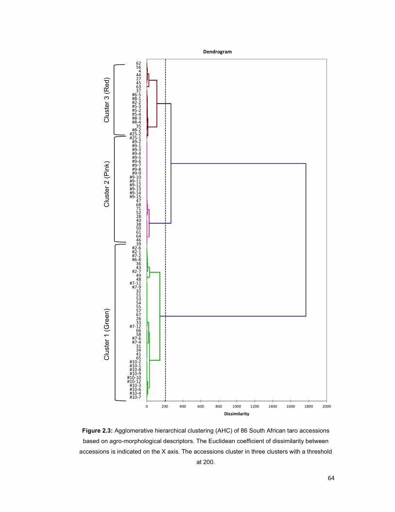
64

Figure 2.3: Agglomerative hierarchical clustering (AHC) of 86 South African taro accessions

based on agro-morphological descriptors. The Euclidean coefficient of dissimilarity between

accessions is indicated on the X axis. The accessions cluster in three clusters with a threshold

at 200.

#10-7#10-4#10-6#10-3

#10-12#10-10

#10-9#10-8#10-1#10-2

65413431

#7-4#7-6

5866

#7-12332667575554535132

#7-9#7-11

4849

#2-74336

#6-8#7-2#2-1#2-6

394664615038402852716847

#9-15#9-14#9-13#9-12#9-11#9-10

#9-9#9-8#9-7#9-6#9-5#9-4#9-3#9-1#9-2

#25-1#25-2

#8-235

#8-4#8-3#5-4#5-2#5-3#2-2#8-1#6-5

3763452744

45662

0 200 400 600 800 1000 1200 1400 1600 1800 2000

Dissimilarity

Dendrogram

Clu

ster

1 (

Gre

en)

Clu

ste

r 2

(Pin

k)C

lust

er

3 (

Re

d)

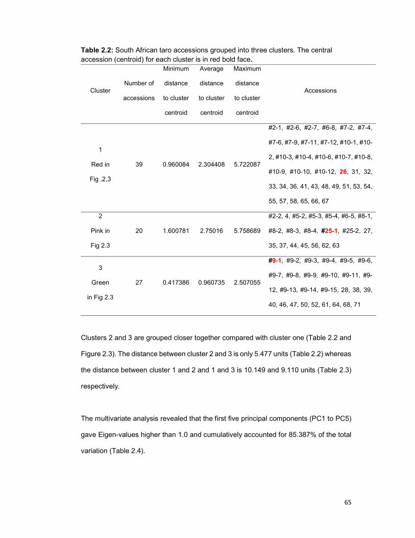
65

Table 2.2: South African taro accessions grouped into three clusters. The central accession (centroid) for each cluster is in red bold face.

Cluster Number of

accessions

Minimum

distance

to cluster

centroid

Average

distance

to cluster

centroid

Maximum

distance

to cluster

centroid

Accessions

1

Red in

Fig ,2,3

39 0.960084 2.304408 5.722087

#2-1, #2-6, #2-7, #6-8, #7-2, #7-4,

#7-6, #7-9, #7-11, #7-12, #10-1, #10-

2, #10-3, #10-4, #10-6, #10-7, #10-8,

#10-9, #10-10, #10-12, 26, 31, 32,

33, 34, 36, 41, 43, 48, 49, 51, 53, 54,

55, 57, 58, 65, 66, 67

2

Pink in

Fig 2.3

20 1.600781 2.75016 5.758689

#2-2, 4, #5-2, #5-3, #5-4, #6-5, #8-1,

#8-2, #8-3, #8-4, #25-1, #25-2, 27,

35, 37, 44, 45, 56, 62, 63

3

Green

in Fig 2.3

27 0.417386 0.960735 2.507055

#9-1, #9-2, #9-3, #9-4, #9-5, #9-6,

#9-7, #9-8, #9-9, #9-10, #9-11, #9-

12, #9-13, #9-14, #9-15, 28, 38, 39,

40, 46, 47, 50, 52, 61, 64, 68, 71

Clusters 2 and 3 are grouped closer together compared with cluster one (Table 2.2 and

Figure 2.3). The distance between cluster 2 and 3 is only 5.477 units (Table 2.2) whereas

the distance between cluster 1 and 2 and 1 and 3 is 10.149 and 9.110 units (Table 2.3)

respectively.

The multivariate analysis revealed that the first five principal components (PC1 to PC5)

gave Eigen-values higher than 1.0 and cumulatively accounted for 85.387% of the total

variation (Table 2.4).

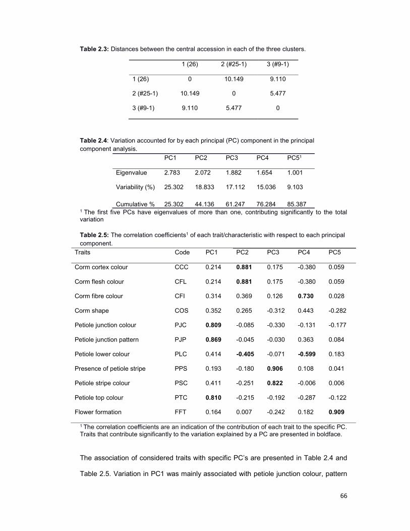
66

Table 2.3: Distances between the central accession in each of the three clusters.

1 (26) 2 (#25-1) 3 (#9-1)

1 (26) 0 10.149 9.110

2 (#25-1) 10.149 0 5.477

3 (#9-1) 9.110 5.477 0

Table 2.4: Variation accounted for by each principal (PC) component in the principal component analysis.

PC1 PC2 PC3 PC4 PC51

Eigenvalue 2.783 2.072 1.882 1.654 1.001

Variability (%) 25.302 18.833 17.112 15.036 9.103

Cumulative % 25.302 44.136 61.247 76.284 85.387 1 The first five PCs have eigenvalues of more than one, contributing significantly to the total variation Table 2.5: The correlation coefficients1 of each trait/characteristic with respect to each principal component.

Traits Code PC1 PC2 PC3 PC4 PC5

Corm cortex colour CCC 0.214 0.881 0.175 -0.380 0.059

Corm flesh colour CFL 0.214 0.881 0.175 -0.380 0.059

Corm fibre colour CFI 0.314 0.369 0.126 0.730 0.028

Corm shape COS 0.352 0.265 -0.312 0.443 -0.282

Petiole junction colour PJC 0.809 -0.085 -0.330 -0.131 -0.177

Petiole junction pattern PJP 0.869 -0.045 -0.030 0.363 0.084

Petiole lower colour PLC 0.414 -0.405 -0.071 -0.599 0.183

Presence of petiole stripe PPS 0.193 -0.180 0.906 0.108 0.041

Petiole stripe colour PSC 0.411 -0.251 0.822 -0.006 0.006

Petiole top colour PTC 0.810 -0.215 -0.192 -0.287 -0.122

Flower formation FFT 0.164 0.007 -0.242 0.182 0.909

1 The correlation coefficients are an indication of the contribution of each trait to the specific PC. Traits that contribute significantly to the variation explained by a PC are presented in boldface.

The association of considered traits with specific PC’s are presented in Table 2.4 and

Table 2.5. Variation in PC1 was mainly associated with petiole junction colour, pattern

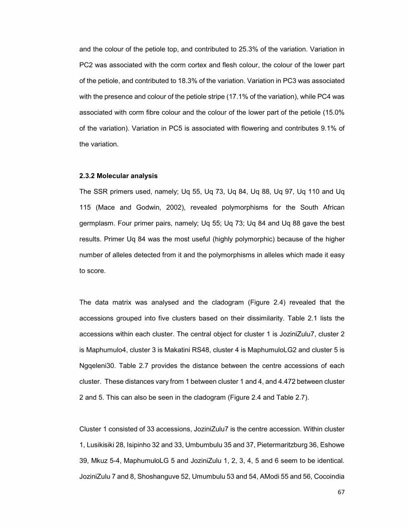
67

and the colour of the petiole top, and contributed to 25.3% of the variation. Variation in

PC2 was associated with the corm cortex and flesh colour, the colour of the lower part

of the petiole, and contributed to 18.3% of the variation. Variation in PC3 was associated

with the presence and colour of the petiole stripe (17.1% of the variation), while PC4 was

associated with corm fibre colour and the colour of the lower part of the petiole (15.0%

of the variation). Variation in PC5 is associated with flowering and contributes 9.1% of

the variation.

2.3.2 Molecular analysis

The SSR primers used, namely; Uq 55, Uq 73, Uq 84, Uq 88, Uq 97, Uq 110 and Uq

115 (Mace and Godwin, 2002), revealed polymorphisms for the South African

germplasm. Four primer pairs, namely; Uq 55; Uq 73; Uq 84 and Uq 88 gave the best

results. Primer Uq 84 was the most useful (highly polymorphic) because of the higher

number of alleles detected from it and the polymorphisms in alleles which made it easy

to score.

The data matrix was analysed and the cladogram (Figure 2.4) revealed that the

accessions grouped into five clusters based on their dissimilarity. Table 2.1 lists the

accessions within each cluster. The central object for cluster 1 is JoziniZulu7, cluster 2

is Maphumulo4, cluster 3 is Makatini RS48, cluster 4 is MaphumuloLG2 and cluster 5 is

Ngqeleni30. Table 2.7 provides the distance between the centre accessions of each

cluster. These distances vary from 1 between cluster 1 and 4, and 4.472 between cluster

2 and 5. This can also be seen in the cladogram (Figure 2.4 and Table 2.7).

Cluster 1 consisted of 33 accessions, JoziniZulu7 is the centre accession. Within cluster

1, Lusikisiki 28, Isipinho 32 and 33, Umbumbulu 35 and 37, Pietermaritzburg 36, Eshowe

39, Mkuz 5-4, MaphumuloLG 5 and JoziniZulu 1, 2, 3, 4, 5 and 6 seem to be identical.

JoziniZulu 7 and 8, Shoshanguve 52, Umumbulu 53 and 54, AModi 55 and 56, Cocoindia

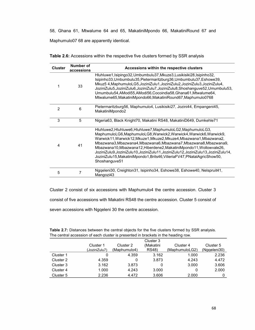
68

58, Ghana 61, Mtwalume 64 and 65, MakatiniMpondo 66, MakatiniRound 67 and

Maphumulo07 68 are apparently identical.

Table 2.6: Accessions within the respective five clusters formed by SSR analysis

Cluster Number of accessions

Accessions within the respective clusters

1

33

Hluhluwe1,Isipingo32,Umbumbulu37,Mkuze3,Lusikisiki28,Isipinho32, Isipinho33,Umbumbulu35,Pietermaritzburg36,Umbumbulu37,Eshowe39, Mkuz5 4,MaphumuloLG5,JoziniZulu1,JoziniZulu2,JoziniZulu3,JoziniZulu4, JoziniZulu5,JoziniZulu6,JoziniZulu7,JoziniZulu8,Shoshanguve52,Umumbulu53, Umumbulu54,AModi55,AModi56,Cocoindia58,Ghana61,Mtwalume64, Mtwalume65,MakatiniMpondo66,MakatiniRound67,Maphumulo0768

2

6

Pietermaritzburg56, Maphumulo4, Lusikisiki27, Jozini44, Empangeni45, MakatiniMpondo2

3

5

Nigeria63, Black Knight70, Makatini RS48, MakatiniD649, Dumkehle71

4

41

Hluhluwe2,Hluhluwe6,Hluhluwe7,MaphumuloLG2,MaphumuloLG3, MaphumuloLG6,MaphumuloLG8,Warwick2,Warwick4,Warwick6,Warwick9, Warwick11,Warwick12,Mkuze1,Mkuze2,Mkuze4,Mbazwana1,Mbazwana2, Mbazwana3,Mbazwana4,Mbazwana6,Mbazwana7,Mbazwana8,Mbazwana9, Mbazwana10,Mbazwana12,Hiberdene2,MakatiniMpondo11,Wollowvale26, JoziniZulu9,JoziniZulu10,JoziniZulu11,JoziniZulu12,JoziniZulu13,JoziniZulu14, JoziniZulu15,MakatiniMpondo1,Brits46,VilieriaFV47,PNatalAgricShow50, Shoshanguve51

5 7 Ngqeleni30, Creighton31, Isipinho34, Eshowe38, Eshowe40, Nelspruit41, Mangozi43

Cluster 2 consist of six accessions with Maphumulo4 the centre accession. Cluster 3

consist of five accessions with Makatini RS48 the centre accession. Cluster 5 consist of

seven accessions with Ngqeleni 30 the centre accession.

Table 2.7: Distances between the central objects for the five clusters formed by SSR analysis. The central accession of each cluster is presented in brackets in the heading row.

Cluster 1

(JoziniZulu7) Cluster 2

(Maphumulo4)

Cluster 3 (Makatini

RS48) Cluster 4

(MaphumuloLG2) Cluster 5

(Ngqeleni30) Cluster 1 0 4.359 3.162 1.000 2.236 Cluster 2 4.359 0 3.873 4.243 4.472 Cluster 3 3.162 3.873 0 3.000 3.606 Cluster 4 1.000 4.243 3.000 0 2.000 Cluster 5 2.236 4.472 3.606 2.000 0

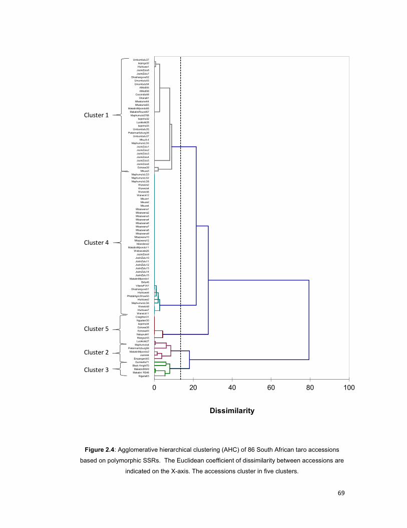
69

Figure 2.4: Agglomerative hierarchical clustering (AHC) of 86 South African taro accessions

based on polymorphic SSRs. The Euclidean coefficient of dissimilarity between accessions are

indicated on the X-axis. The accessions cluster in five clusters.

Nigeria63

Makatini RS48MakatiniD649

Black Knight70Dumkehle71

Empangeni45

Jozini44MakatiniMpondo2

Pietermaritzburg56Maphumulo4

Lusikisiki27Mangozi43Nelspruit41

Eshowe40Eshowe38

Isipinho34Ngqeleni30

Creighton31Warwick11Hluhluwe7

Warwick9MaphumuloLG6

Hluhluwe2PNatalAgricShow50

Hluhluwe6Shoshanguve51

VilieriaFV47

Brits46MakatiniMpondo1

JoziniZulu15JoziniZulu14

JoziniZulu13JoziniZulu12JoziniZulu11

JoziniZulu10JoziniZulu9

Wollowvale26MakatiniMpondo11

Hiberdene2Mbazwana12Mbazwana10

Mbazwana9Mbazwana8

Mbazwana7Mbazwana6

Mbazwana4Mbazwana3Mbazwana2

Mbazwana1Mkuze4

Mkuze2Mkuze1

Warwick12Warwick6Warwick4

Warwick2MaphumuloLG8

MaphumuloLG2MaphumuloLG3

Mkuze3Eshowe39

JoziniZulu6

JoziniZulu5JoziniZulu4

JoziniZulu3JoziniZulu2JoziniZulu1

MaphumuloLG5Mkuz5-4

Umbumbulu37Pietermaritzburg36

Umbumbulu35Isipinho33

Lusikisiki28

Isipinho32Maphumulo0768

MakatiniRound67MakatiniMpondo66

Mtwalume65Mtwalume64

Ghana61

Cocoindia58AModi56

AModi55Umumbulu54

Umumbulu53Shoshanguve52

JoziniZulu7

JoziniZulu8Hluhluwe1

Isipingo32Umbumbulu37

0 20 40 60 80 100

Dissimilarity

Cluster 1

Cluster 4

Cluster 3

Cluster 5

Cluster 2

70

Figure 2.5: Biplot analysis of the polymorphic SSR loci. Cluster 1 from the cladogram is represented in cyan (cluster1), cluster 2 is represented in dark blue (cluster 2), cluster 3 is

represented olive green (cluster3), cluster 4 is represented in red (cluster 4) and cluster 5 in teal (cluster 5). Cluster colours do not correspond to cluster colours in Figure 2.4.

Hluhluwe1

Isipingo32Umbumbulu37

Pietermaritzburg56Nigeria63

Black Knight70

Hluhluwe2

Hluhluwe6

Hluhluwe7

Maphumulo4

MaphumuloLG2MaphumuloLG3

MaphumuloLG6

MaphumuloLG8

Warwick2Warwick4Warwick6

Warwick9Warwick11

Warwick12Mkuze1Mkuze2

Mkuze3

Mkuze4Mbazwana1Mbazwana2Mbazwana3Mbazwana4Mbazwana6Mbazwana7Mbazwana8Mbazwana9Mbazwana10Mbazwana12Hiberdene2MakatiniMpondo11Wollowvale26

Lusikisiki27

Lusikisiki28

Ngqeleni30Creighton31

Isipinho32Isipinho33

Isipinho34

Umbumbulu35Pietermaritzburg36Umbumbulu37

Eshowe38

Eshowe39

Eshowe40

Nelspruit41

Mangozi43

Jozini44

Empangeni45

Mkuz5-4MaphumuloLG5JoziniZulu1JoziniZulu2JoziniZulu3JoziniZulu4JoziniZulu5JoziniZulu6JoziniZulu7

JoziniZulu8

JoziniZulu9JoziniZulu10JoziniZulu11JoziniZulu12

JoziniZulu13JoziniZulu14JoziniZulu15MakatiniMpondo1

MakatiniMpondo2

Brits46

VilieriaFV47

Makatini RS48MakatiniD649

PNatalAgricShow50Shoshanguve51

Shoshanguve52Umumbulu53Umumbulu54AModi55AModi56Cocoindia58Ghana61Mtwalume64Mtwalume65MakatiniMpondo66MakatiniRound67Maphumulo0768

Dumkehle71

-2

-1

0

1

2

3

4

5

6

7

8

0 2 4 6 8 10

F2

(4.

90

%)

Biplot (axes F1 and F2: 85.77 %)

71

Cluster 4 consist of 41 accessions with MaphumuloLG 2 the centre accession. All the

accessions in this cluster are closely related, but MaphumuloLG 8, Warwick 2, 4, 6 and

12, Mkuze 1, 2 and 4, Mbazwana 1, 2, 3, 4, 6, 7, 8, 9, 10 and 12, Hibberdene 2,

MakatiniMpondo 11, Willowvale 26, JoziniZulu 9, 10, 11, 12, 13, 14 and 15,

MakatiniMpondo 1, Brits 46, VilieriaFV 47, and Shoshanguve 51 are apparently identical.

This clustering included accessions collected in three different provinces of South Africa.

Accessions collected in Eshowe, Hluhluwe, Isipingo, Jozini, Lusiksiki, Makatini,

Maphumolo, Mkuze and Pietermaritzburg were grouped in different clusters. All the

accessions collected from Professor A Modi (University of KwaZulu-Natal), Mbazwana,

Mtwalume, Umbumbulu and Warwick grouped in the same cluster. The ornamental

accession, Black Knight, was placed in cluster 1 with other “edible accessions”. The

accessions from Nigeria grouped in two different clusters within the South African

accessions. All the accessions in cluster 3 are dasheen type.

The different accessions cluster together mostly according to the cladogram in a

principal component biplot (Figure 2.5.) The first principal component of the biplot

(Figure 2.5) explains the majority of the variation (80.87%). The second principal

component only describes an additional 4.9% of the variation.

2.3 Discussion

A higher level of genetic diversity in the South African germplasm was observed when

molecular analysis was performed than with morphological characterisation. No clear

pattern was observed in the clustering of accessions in the cladogram. No correlation

was detected between the different clusters and geographic distribution, since

accessions from the same locality did not always cluster together, while conversely,

accessions collected at different sites were grouped sometimes together. For example,

72

15 accessions were collected in Jozini (JoziniZulu type 1 to 15), and eight of these

grouped in Cluster 1 and the others in Cluster 4. Cluster 1 and 4 are closely related

according to the distances between the central accessions (Table 2). This absence of

correlation with geography was also reported by Ivancic and Lebot (1999) in New

Caledonia, Hartati et al. (2001) in Indonesia, Jianchu et al. (2001) in China, Matsuda and

Nawata (2002) in eastern Asia, Hue et al. (2003), Kreike et al. (2004) in southeast Asia

and the Pacific and Caillon et al. (2006) in Vanuatu.

Accessions that were almost identical on a molecular level were distinguished

morphologically. For example, on a molecular level, Cocoindia 58, AModi 55 and 56 and

Ghana 61 were identical; however, morphologically Cocoindia 58 is a more robust plant

growing to twice the size of the other three accessions. The primers used do not offer

definitive resolution of molecular differences between the genotypes. This indicated that

in order to obtain more complete characterisation, both molecular and morphological

data should be used. The cladograms clearly indicate that taro germplasm was

exchanged extensively between different areas. Discussion with various farmers during

fieldwork confirmed this, indicating that they obtained their planting material from other

provinces and that extensive exchange of material take place. Some farmers even

indicate getting planting material from Swaziland. There are also many accessions

identified within the clusters that most probably are duplications. These accessions

should be evaluated critically and to rationalise the number of accessions in the

collection.

Although the results indicated that there is more diversity present in the local germplasm

than expected when looking superciliously at the South African germplasm, the genetic

base is still rather narrow when considering the amount of duplicates indicted in the

analyses. This is also reported for other African countries such as Malawi (Mwenye et

al. 2016), Ghana and Burkina Faso (Chaïr et al. 2016). Several authors reported that the

73

genetic diversity for taro seems to be low in Africa (Safo Kantaka 2004; Lebot 2009; Paul

et al. 2011; Orji and Ogbona 2015; Chaïr et al. 2016).

2.4 Conclusion

South African taro still have a very narrow genetic base in spite of its long history South

Africa. Farmers have selected landraces adapted to local conditions over time, but no

diversity were introduced, except from neighbouring countries. The study shows that

although the genetic base is narrow, more diversity exists than expected. The

accessions were grouped in clusters, unfortunately no correlation exists between the

clusters resulting from the morphological characteristics and molecular characteristics.

Superior genotypes within each cluster can be used as parents and these superior

landraces can also multiplied and distributed to farmers. Possible duplicates are also

identified and the results can be used to rationalise the germplasm collection. In order

to implement a successful breeding programme, it might be necessary widen the genetic

base by importing germplasm. However, imported germplasm must be adapted to the

local climatic conditions and acceptable for the local climatic consumers. One

characteristic that showed low diversity in the South African germplasm is corm flesh

colour. Yellow and purple fleshed taro, that have higher levels of beta-carotene and

flavonoids respectively, can be imported for local evaluation.

2.5 References

Caillon S, Quero-Garcia J, Lescure J-P and Lebot V, (2006) Nature of taro (Colocasia

esculenta (L). Scott) genetic diversity in a Pacific island, Vanua Laa, Vanuatu.

Genetic Resources and Crop Evolution. 23:1273-1289

Chaïr H, Traore RE, Duval MF, Rivallan R, Mukherjee A, Aboagye LM, Van Rensburg

WJ, Andrianavalona V, Pinheiro De Carvalho MAA, Saborio F, Sri Prana M,

Komolong B, Lawac F and Lebot V (2016) Genetic Diversification and Dispersal

74

of Taro (Colocasia esculenta (L.) Schott). PLoS One 11(6):e0157712. doi:

10.1371

Devi AA (2012) Genetic Diversity Analysis in Taro Using Molecular Markers – An

Overview. Journal of Root Crops 3815-25

Edwards K, Johnstone C, Thompson C. (1991) A simple and rapid method for the

preparation of plant genomic DNA for PCR analysis. Nucleic Acids Research

25:1349

Fujimoto T (2009) Taro (Colocasia esculenta [L.] Schott) Cultivation in Vertical Wet-Dry

Environments: Farmers’ Techniques and Cultivar Diversity in Southwestern

Ethiopia. Economic Botany:63:152–166.

Godwin IG, Mace ES and Nurzuhairawaity. (2001) Genotyping Pacific Island taro

(Colocasia esculenta (L.) Schott) germplasm. In Plant genotyping — the DNA

fingerprinting of plants. Edited by R. Henry. CAB International, Oxon, U.K. pp.

109–128.

Hartati NS, Prana TK and Prana MS (2001) Comparative study on some Indonesian taro

(Colocasia esculenta (L.) Schott) samples using morphological characters,

RAPD markers and isozyme patterns. Annales Bogorienses 7(2):65-73

Hijmans RJ, Guarino L, Bussink C, Mathur P, Cruz M, Barrentes I, Rojas E. (2004) DIVA-

GIS. Version 7.5. A geographic information system for the analysis of species

distribution data. http://www. diva-gis. org/download Accessed 3 March 2014.

Hu K, Huang XF, Kev WD and Ding YI (2009) Characterization of 11 new microsatellite

loci in taro (Colocasia esculenta). Molecular Ecology Resources 9:582–584

Hue NN, Trinh LN, Han P, Sthapit B and Jarvis D (2003) Taro cultivar diversity in three

ecosites of North Vietnam. On-Farm Management of Agricultural Biodiversity in

Vietnam 58-62

Isshiki S, Nakamura N, Tashiro Y and Miyazaki S (1998) Classification of the Cultivars

of Japanese Taro [Colocasia esculenta (L.) Schott] by Isozyme analysis. Journal

of the Japanese Society for Horticultural Science 67:521-525

75

Ivancic A and Lebot V (1999) Botany and genetics of New Caledonian wild Taro,

Colocasia esculenta. Pacific Science 53:273-285

Jianchu X, Yongping Y, Yongdong P, Ayad WG and Eyzaguirre P (2001) Genetic

Diversity in Taro (Colocasia esculenta Schott, Araceae) in China: An

Ethnobotanical and genetic Approach. Ecomomic Botany 55(1):14-31

Krieke CM, van Eck HJ and Lebot V (2004) Genetic diversity of taro, Colocasia esculenta

(L.) Schott, in Southeast Asia and the Pacific. Theoretical and Applied Genetics

109:761–768

Lebot V (2009) Tropical Root and Tuber Crops: Cassava, Sweet Potato, Yams and

Aroids. CABI, Wallingford, UK. pp 413

Lu Z, Li W, Yang Y and Hu X (2011) Isolation and characterization of 19 new

microsatellite loci in Colocasia esculenta (Araceae). American Journal of Botany

98(9):239-241

Mabhaudhi T and Modi AT (2013) Preliminary Assessment of Genetic Diversity in

Three Taro (Colocasia esculenta L. Schott) Landraces Using Agro-

morphological and SSR DNA Characterisation. Journal of Agricultural Science

and Technology B 3 (2013):265-271

Mace ES and Godwin ID (2002) Development and characterization of polymorphic

microsatellite markers in taro (Colocasia esculenta). Genome 45:823–832

Mare RM (2006) Phytotron and field performance of taro (Colocasia esculenta (L)

Schot) landraces from Umbumbulu. MSc Thesis, University of KwaZulu-Natal,

Pietermaritzburg. pp 132

Matsuda M and Nawata E (2002) Geographical distribution of ribosomal DNA variation

in taro, Colocasia esculenta (L.) Scott. In eastern Asia. Euphytica 128:165-127

Mwenye O, Herselman L, Benesi I and Labuschagne M (2016) Genetic Relationships in

Malawian Cocoyam Measured by Morphological and DNA Markers. Crop

Science 56:1189-1198

76

NBII (2017), National Biological Information Infrastructure". Introduction to Genetic

Diversity. U.S. Geological. https://web.archive.org/web/20110225072641/

http://www.nbii.gov/portal/server.pt?open=512&objID=405&PageID=0&cached=

true&mode=2&userID=2:1-10. Accessed 3 January 2017

Noyer JL, Billot C, Weber P, Brottier P, Quero-Garcia J and Lebot, V. (2004) Genetic

diversity of taro (Colocasia esculenta (L.) Schott) assessed by SSR markers. In:

Guarino L, Taylor M, Osborn T (eds) Third Taro Symposium. 21–23 May 2003.

Secretariat of the Pacific Community, Fiji, pp 174–180

Nybom H (2004) Comparison of different nuclear DNA markers for estimating

intraspecific genetic diversity in plants. Molecular Ecology 13(5):1143–1155

Okpul T, Singh, Gunna T and Wagih ME (2004) Assessment of diversity using agro-

morphological traits for selecting a core sample of Papua New Guinea taro

(Colocasia esculenta (L) Scott) collection. Genetic Resources and Crop

Evolution 51:671-678

Orji KO and Ogbonna PE (2015) Morphological correlation analysis on some agronomic

traits of taro (Colocasia esculenta) in the plains of Nsukka, Nigeria. Journal of

Global Bioscience 4:1120-1126

Paul KK, Bari MA and Debnath SC (2011) Genetic variability of Colocasia esculenta (L.)

Schott. Bangladesh Journal of Botany. 40:185-188

Quero-Garcia J, Courtois B. Ivancic A, Letourmy P, Risterucci AM, Noyer JL, Feldmann

PH and Lebot V (2006) First genetic maps and QTL studies of yield traits of taro

(Colocasia esculenta (L.) Schott) Euphytica 51:187–199

Safo Kantaka O (2004) Colocasia esculenta (L.) Schott In: Grubben, G.J.H. and Denton,

O.A. (Editors). PROTA 2: Vegetables/Légumes. [CD-Rom]. PROTA,

Wageningen, Netherlands. pp668

Sardos J, Noyer J, Malapa R, Bouchet S and Lebot V (2011) Genetic diversity of taro

(Colocasia esculenta (L.) Schott) in Vanuatu (Oceania): an appraisal of the

77

distribution of allelic diversity (DAD) with SSR markers. Genetic Resources and

Crop Evolution 59:805-820.

Singh D, Mace ES, Godwin ID, Mathur PN, Okpul T, Taylor M, Hunter D, Kambuou R,

Ramanatha Rao V and Jackson G (2008) Assesment and rationalization of

genetic diversity of Papua New Guinea taro (Colocasia esculenta) using SSR

DNA fingerprinting. Genetic Resources and Crop Evolution 55:811-822

Singh S, Singh DR, Faseela F, Kumar N, Damodaran V and Srivastava RC (2011)

Diversity of 21 taro (Colocasia esculenta (L.) Schott) accessions of Andaman

Islands. Genetic Resources and Crop Evolution 59:821-829

Sneath PHA and Sokal RR (1973) Numerical Taxonomy, Freeman, San Francisco.

Sokal RR and Michener CP (1958) A statistical technique for evaluating systematic

relationships. University of Kansas Science Bulletin 38:1409–1438.

You Y, Liu D, Liu H, Zheng X, Diao Y, Huang X and Hu Z (2014) Development and

characterisation of EST-SSR markers by transcriptome sequencing in taro

(Colocasia esculenta (L.) Schoot). Moleular Breeding 35:134

DOI:10.1007/s11032-015-0307-4

78

Chapter 3: Genetic improvement of Colocasia esculenta in South Africa

Abstract

Taro (Colocasia esculenta), known colloquially as Amadumbe in South Africa, is a tuber

crop that is usually cultivated in the coastal and sub-tropical regions of South Africa. Taro

is typically produced by smallholder farmers and traded informally, No improved cultivars

exist in South Africa and farmers plant local landraces from material that has been

retained from the previous season or traded and exchanged from other regions. The

study aim to investigate to develop improved taro cultivars utilizing South African

germplasm.

Fourteen taro genotypes were planted in a pan and fan glasshouse to be utilized as

parents. GA3 was used to artificially induce flowering. Eighty-five male female

combination crossed were carried out. No offspring were obtained. This must be due to

the triploid nature of the South African germplasm. It might be useful to pollinate diploid

female parents with triploid male parents. The triploid male parents might produce

balanced gametes at low percentages, which can fertilize the diploid female parents.

3.1 Introduction

There are three approaches to obtain improved taro cultivars (Sivan and Liyanage 1993).

The easiest is to collect and evaluate local germplasm in order to identify promising lines

to propagated and distributed. Alternatively, elite cultivars can be imported from other

countries to evaluate under local conditions for suitability to local conditions and markets.

Lastly, controlled breeding can be used to recombine characteristics in progeny that are

evaluated against a set of predetermined criteria (Sivan and Liyanage 1993).

Most domesticated taro genotypes do not flower naturally (Del Peno 1990; Wilson 1990;

Lebot 2009). Wild types do flower more easily and the character can be bred into a

79

population (Lebot 2009). The discovery of methods to induce flowering in taro has greatly

facilitated breeding (Safo Kantaka 2004). One of the first breeding programmes was

initiated in the early 1970’s in the Solomon Islands to breed for taro leaf blight resistance

(Patel et al. 1984, as cited by Lebot 2009). This was followed by breeding programmes

in Hawaii, Samoa, Papua New Guinea (PNG), India, Philippines, Fiji and Vanuatu (Lebot

2009). There are taro breeding programmes in Mauritius that used mutation breeding to

identify taro blight resistance (Seetohul et al. 2007). Lebot (2009) also noted that little

was achieved in these programmes due to the narrow genetic base of the breeding stock

and the introduction of “wild” germplasm that also introduced undesirable traits.

The aim of most taro breeding programmes is yield (Sivan and Liyanage 1993; Soulard

et al. 2016), quality (Sivan and Liyanage 1993; Iramu et al., 2009) and pest and disease

resistance (Sivan and Liyanage 1993; Iramu et al., 2009). Many taro breeders emphasis

yield in the early generations of taro breeding programmes according to Soulard et al.

(2016). According to Sivan and Liyanage (1993) it will take six to ten years to release a

taro cultivar using traditional breeding methods. Modern biotechnology and molecular

breeding tools can speed up the breeding. Recently, emphasis has also been placed on

the nutrient composition of taro corms. Breeding is done to increase the nutrient content

(bio-fortification), or decrease the anti -nutrient content of taro. These compounds are

beta-carotene, anthocyanin antioxidants, phenolic compounds and oxalates etc.

(Guchhait 2008; Champagne et al. 2013).

No improved taro cultivars exist in South Africa and farmers use traditional landraces.

These landraces have been selected and maintained by local farmers over many years.

Very little extra diversity is available to the farmers. Mare (2006) reported that there might

only be four landraces present in KwaZulu-Natal. The objective of this study is to

investigate the possibility to do hand pollinations, using South African taro landraces.

80

3.2 Materials and Methods

Ten local lines (Table 3.1) were planted in 50 cm pots at ARC-Roodeplaat in a pan and

fan glasshouse. Ten plants of each of the fourteen plants were placed at random in a

pan and fan glasshouse. The pots were watered daily by filling the pot to the rim. The

lines were treated with 500 ppm gibberellic acid (Valent Biosciences). The gibberellic

acid was sprayed on the leaves and petioles of the young plants when the plants had

two mature leaves as described by Wilson (1990).

Table 3.1: Taro lines planted as parents (male or female) for cross hybridization.

Accession Province/State District Nearest Town/village

2-2 KwaZulu-Natal Hluhluwe Hluhluwe

4 KwaZulu-Natal Maphumulo Maphumulo

5-2 KwaZulu-Natal Mkuze Mkuze

6-8 KwaZulu-Natal Maphumulo Maphumulo

7-5 KwaZulu-Natal Durban Metro Durban

9-11 KwaZulu-Natal Jozini Jozini

10-3 KwaZulu-Natal Mbazwana Mbazwana

26 Eastern Province Mbhashe Willowvale

28 Eastern Province Ingquza Lusikisiki

40 KwaZulu-Natal Eshowe Eshowe

44 KwaZulu-Natal Umhlubuyalingana Jozini

50 KwaZulu-Natal Pietermaritzburg Pietermaritzburg

56 KwaZulu-Natal Pietermaritzburg Pietermaritzburg

66 KwaZulu-Natal Jozini Jozini

Hand pollinations was done as described by Wilson (1990) and Lebot (2009). Hand-

pollinations was done early in the mornings before 11:00. Inflorescences, to be used as

female, were emasculated by catting away the spadix with a sharp knife. The

emasculated inflorescence were covered with a muslin bag to prevent pollination by any

other pollen sources. The male section of the inflorescence were then removed and

discarded. Pollen were collected by removing the male part from inflorescence that have

already shed pollen. Pollen was then transfer to the female flowers using a small brush

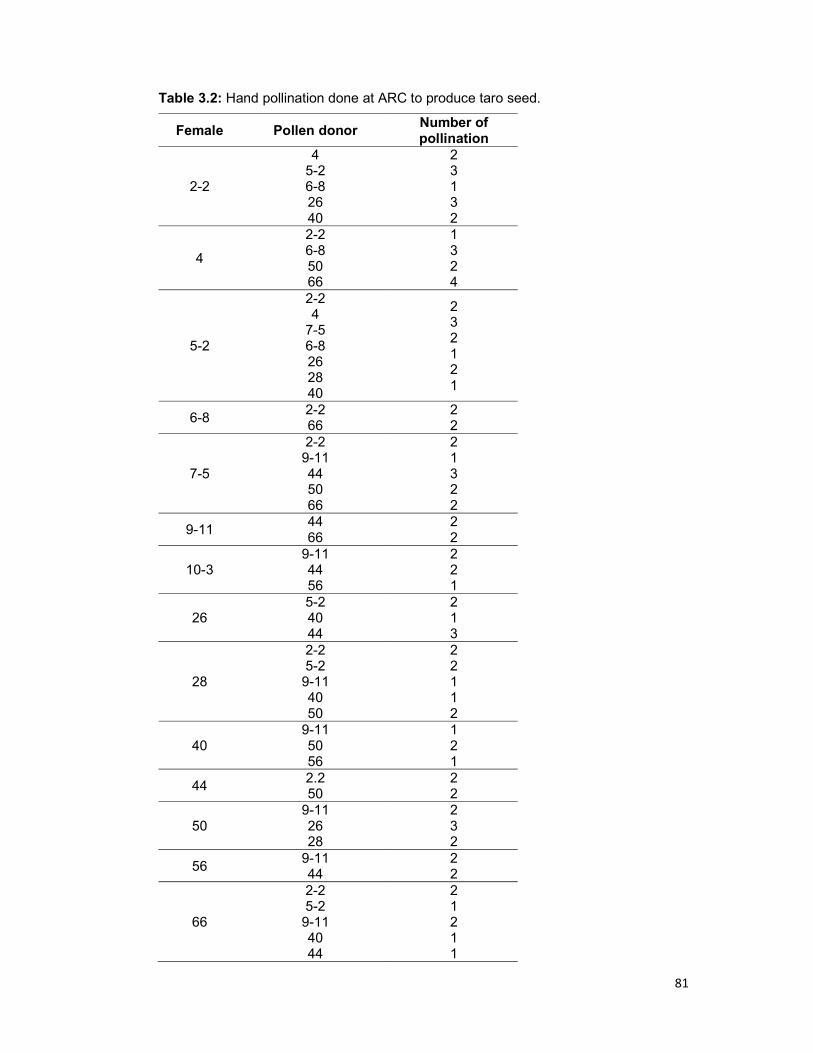
81

Table 3.2: Hand pollination done at ARC to produce taro seed.

Female Pollen donor Number of pollination

2-2

4 5-2 6-8 26 40

2 3 1 3 2

4

2-2 6-8 50 66

1 3 2 4

5-2

2-2 4

7-5 6-8 26 28 40

2 3 2 1 2 1

6-8 2-2 66

2 2

7-5

2-2 9-11 44 50 66

2 1 3 2 2

9-11 44 66

2 2

10-3 9-11 44 56

2 2 1

26 5-2 40 44

2 1 3

28

2-2 5-2

9-11 40 50

2 2 1 1 2

40 9-11 50 56

1 2 1

44 2.2 50

2 2

50 9-11 26 28

2 3 2

56 9-11 44

2 2

66

2-2 5-2

9-11 40 44

2 1 2 1 1

82

and the “female” inflorescence were covered again. The number of pollinations are

summarised in Table 3.2.

3.3 Results and Discussion

The only natural flowerings at ARC-Roodeplaat were observed in two dasheen lines.

However, the eddoe type is preferred for consumption in South Africa. All lines that were

treated with gibberellic acid flowered.

Figure 3.1: Floral tissue in leaves of taro plants observed in plants four weeks after treatment with

500ppm gibberellic acid on line 26 (Photos: WS Jansen van Rensburg).

Figure 3.2: Flag leaves, the first indication of flowering. The plant on the left (line 26) was treated with gibberellic acid and the plant on right was a natural flowering clone from Vanuatu (Photos:

WS Jansen van Rensburg). .

83

The first sign of the flowering was floral tissue that appeared in the leaves (Figure 3.1).

This varied from small patches of yellow flower tissue, to whole leaves that were

deformed and consisted of mostly floral tissue. The first flag leaves were visible four

weeks after the plants were treated with gibberellic acid (Figure 3.2). The first flowers

appeared two to four weeks later. The inflorescences appeared in clusters numbering

between three to ten (Figure 3.3). The inflorescences of one cluster did not all open at

the same time (Figure 3.3).

Figure 3.3: The cluster of inflorescences opening in sequence in

Cocoindia. The first youngest inflorescence is closest to the petiole

(Photos: WS Jansen van Rensburg).

All the inflorescences that developed were normal, and the male and female flowers

were easily distinguished (Figure 3.4. 3.5 and 3.6). Various numbers of sterile female

flowers were observed on an inflorescence. Flowering was therefore successfully

induced as describe by Wilson (1990), Lebot (2009), Amadi et al. (2015) and Mukherjee

et al. (2016). Some berries started to develop but aborted very soon due to no seed set

(Figure 3.7). All hand pollinations were unsuccessful. Lebot (2009) and Mukherjee et al.

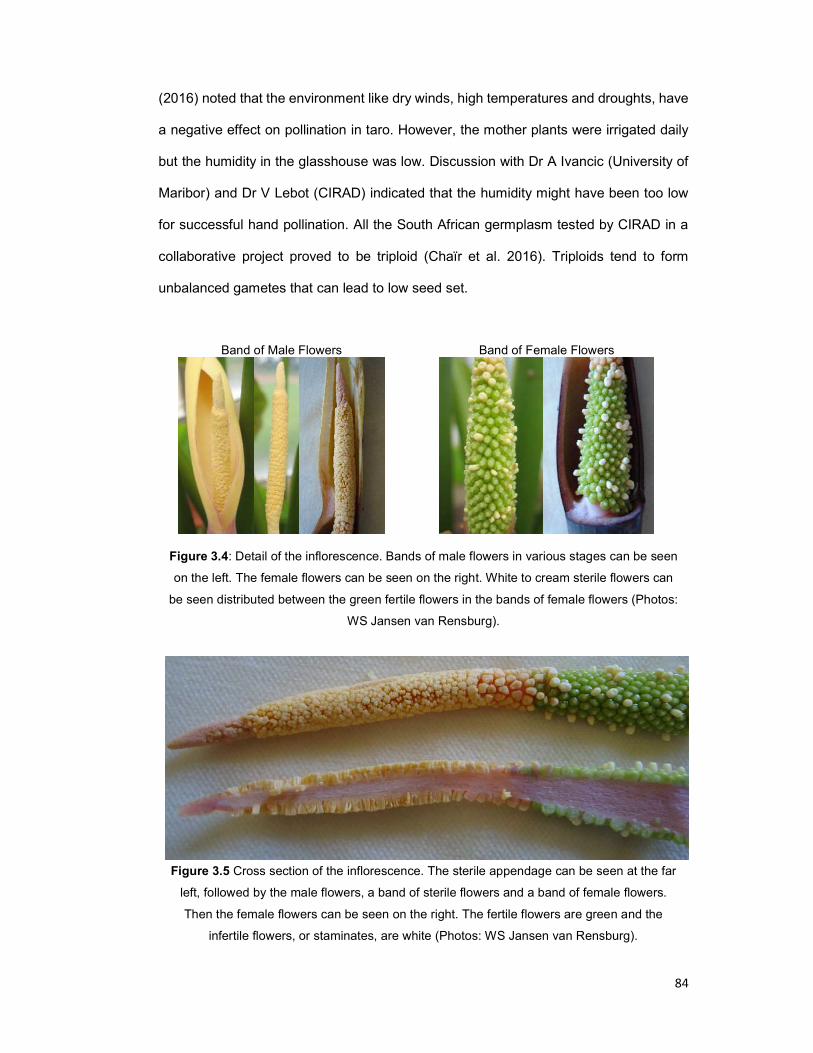
84

(2016) noted that the environment like dry winds, high temperatures and droughts, have

a negative effect on pollination in taro. However, the mother plants were irrigated daily

but the humidity in the glasshouse was low. Discussion with Dr A Ivancic (University of

Maribor) and Dr V Lebot (CIRAD) indicated that the humidity might have been too low

for successful hand pollination. All the South African germplasm tested by CIRAD in a

collaborative project proved to be triploid (Chaïr et al. 2016). Triploids tend to form

unbalanced gametes that can lead to low seed set.

Band of Male Flowers Band of Female Flowers

Figure 3.4: Detail of the inflorescence. Bands of male flowers in various stages can be seen

on the left. The female flowers can be seen on the right. White to cream sterile flowers can

be seen distributed between the green fertile flowers in the bands of female flowers (Photos:

WS Jansen van Rensburg).

Figure 3.5 Cross section of the inflorescence. The sterile appendage can be seen at the far

left, followed by the male flowers, a band of sterile flowers and a band of female flowers.

Then the female flowers can be seen on the right. The fertile flowers are green and the

infertile flowers, or staminates, are white (Photos: WS Jansen van Rensburg).

85

Male Flowers Female flowers

Figure 3.6: A close up of the male flowers (left) and female flowers (right). The green fertile female flowers can clearly be distinguished from the white sterile flowers on the lower part of

the inflorescence (Photos: WS Jansen van Rensburg)

Figure 3.7: Hand pollination of taro flowers. a). Inflorescence with the spadix partially

removed to show the position of the different parts of the inflorescence in relation to

the spadix. b. Emasculation of the inflorescence. The upper band of male flowers

completely cut off. c. The berries that start to develop after pollination. Unfertilised

berries will abort soon after this stage. (Photos: WS Jansen van Rensburg).

a b c

86

3.4 Conclusion

Flowering was successfully induced into South African landraces using established

technique that is used with success in all aroids (Mukherjee et al. 2016). However, no

offspring were produced. This may be due to unfavourable climatic conditions or to the

triploid nature of the germplasm. It is expected that triploids will have a very low

percentage of balanced gametes, making breeding with them very difficult. In future

breeding attempt, diploids will be used as the female parent with a South African triploid

as the male parents. Crossed between diploids should be included to confirm the

success of the pollination methodology. The assumption is that the possibility to

successfully create a balanced gamete will be higher because thousands of pollen grains

were formed during androgenises. A further study on the reproductive biology of the

specific taro accessions in the ARC germplasm collection will also help to identify

possible incompatibility mechanisms that prevent successful hybridization.

3.5 References

Amadi CO, Onyeka J, Chukwu GO, and Okoye BC (2015) Hybridization and Seed

Germination of Taro (Colocasia Esculenta) in Nigeria. Journal of Crop

Improvement 29:106–116

Chaïr H, Traore RE, Duval MF, Rivallan R, Mukherjee A, Aboagye LM, Van Rensburg

WJ, Andrianavalona V, Pinheiro De Carvalho MAA, Saborio F, Sri Prana M,

Komolong B, Lawac F and Lebot V (2016) Genetic Diversification and Dispersal

of Taro (Colocasia esculenta (L.) Schott). PLoS ONE

Champagne A, Legendre L and Lebot V (2013) Biofortification of taro (Colocasia

esculenta) through breeding for increased contents in carotenoids and

anthocyanins. Euphytica 194:125–136

87

De la Pena RS (1990) Development of new taro varieties through breeding. Research

extension series / Hawaii Institute of Tropical Agriculture and Human Resources.

pp 32-36

Guchhait S, Bhattacharya A, Pa lS, Mazumdar D, Chattopadhyay A and Das AK (2008)

Quality Evaluation of Cormels of New Germplasm of Taro, International Journal

of Vegetable Science, 14:4, 304-321

Iramu E, Wagih ME and Singh D (2009) Genetic hybridization among genotypes of Taro

(Colocasia esculanta) and recurrent selection for leaf blight resistance. Indian

Journal of Science and Technology 3(1):96-101

Lebot V (2009) Tropical Root and Tuber Crops: Cassava, Sweet Potato, Yams and

Aroids. CABI, Wallingford, UK. pp 413

Mare RM (2006) Phytotron and field performance of taro (Colocasia esculenta (L)

Schot) landraces from Umbumbulu. MSc Thesis, University of KwaZulu-Natal,

Pietermaritzburg. pp 132

Mukherjee A, George G, Pillai R, Chakrabarti SK, Naskar SK, Patro R., Nayak S and

Lebot V (2016) Development of taro (Colocasia esculenta (L.) Schott) hybrids

overcoming its asynchrony in flowering using cryostored pollen. Euphytica DOI

10.1007/s10681-016-1745-8

Safo Kantaka O (2004) Colocasia esculenta (L.) Schott In: Grubben, G.J.H. and Denton,

O.A. (Editors). PROTA 2: Vegetables/Légumes. [CD-Rom]. PROTA,

Wageningen, Netherlands

Seetohul S, Puchooa D and Ranghoo-Sanmukhiya VM (2007) Genetic Improvement of

Taro (Colocasia esculenta var esculenta) through in-vitro mutagenesis.

University of Mauritos Research Journal 13A:79-89

Sivan P and Liyanage A de S (1993) Breeding and evaluation of taro (Colocasia

esculenta) for the South Pacific Region. Research extension series / Hawaii

Institute of Tropical Agriculture and Human Resources. Pp 5

88

Soulard L, Letourmy P, Cao T, Lawac F, Chair H and Lebot V (2016) Evaluation of

Vegetative Growth, Yield and Quality Related Traits in Taro (Colocasia esculenta

[L.] Schott). Crop Science 56:1-14

Wilson JE (1990) Taro Breeding. Agro-Facts. Crops IRETA Publication No. 3/89. Apia,

Western Samoa. pp 51

89

Chapter 4: Genotype x Environment Interaction for Colocasia esculenta in South

Africa

Abstract

Taro (Colocasia esculenta), commonly known as Amadumbe in South Africa, is a starch

root crop that is traditionally cultivated in the coastal and sub-tropical regions of South

Africa. Smallholder farmers are the main taro producers. Taro is generally traded in the

informal market, however, taro has commercial potential. No improved cultivars exist

and farmers plant local landraces of material that they have retain from the previous

season. Furthermore, there is also very little information available on the influence of the

environment on specific genotypes of taro. The aim of this study is to investigate the

influence of different environments on selected taro landraces.

The Agricultural Research Council (ARC) has built up a taro germplasm collection that

comprises of local and foreign accessions. Twenty-nine of these accessions were

planted at three localities, representing different agro-ecological zones. These localities

were Umbumbulu (South of Durban), Owen Sithole College of Agricultural (OSCA,

Empangeni) and ARC - Vegetable and Ornamental Plants (Roodeplaat, Pretoria).

Different growth and yield related parameters were measured. The data were analysed

using analysis of variance (ANOVA) and additive main effects and multiplicative

interaction (AMMI) analyses.

Significant GxE observed were between locality and specific lines for mean leaf length,

leaf width, leaf number, plant height, number of suckers per plant, number of cormels

harvested per plant, total weight of the cormels harvested per plant and corm length. No

significant interaction between the genotype and the environment was observed for

canopy diameter and corm breadth. From the AMMI model, it was clear that all the

interactions were significant for leaf length, leaf width, number of leaves on a single plant,

90

plant height, number of suckers, number of cormels harvested from a single plant, weight

of cormels harvested from a single plant. The AMMI model indicated that the main effects

were significant but not the interactions with canopy diameter. The AMMI model for the

length and width of the corms showed that effect of environment was highly significant

but not effect of genotype.

There is a strong positive correlation between the number of suckers and the number of

leaves (0.908), number of cormels (0.809) and canopy diameter (0.863) as well as

between the number of leaves and the canopy diameter (0.939) and between leaf width

and plant height (0.816).

There is not a single genotype that can be identified as “the best” genotype. This is due

to the interaction between the environments and the genotypes. Amzam174 and

Thandizwe43 seem to be genotypes that are often regarded as being in the top four. For

the farmer, the total weight of the cormels harvested from a plant will be the most

important. Thandizwe43, Mabhida and Amzam174 seem to be some of the better

genotypes for the total weight and number of cormels harvested from a single plant. The

local accessions also perform better than the foreign accessions. It is clear that some of

the accessions do have the potential to be commercialised in South Africa based on

wide adaptability and good corm yield.

4.1 Introduction

Fox et al. (1997) defined genotype by environment interaction (GxE) as the differential

expression of a genotype across environments. Genotype refers to the expression of all

the genes and interaction of those genes controlling a “character” or “trait”. Environment

refers to the “external conditions” under which the plants grow. The environment consists

of a combination of many external biological, physical, and time factors which vary

independently or these external environmental factors can also interact with each other.

91

All these different external factors have an effect on the expression of the genotype to

result in the specific phenotype observed (Romagosa and Fox 1993; Fox et al. 1997).

GxE implies that the same genotypes may express their genetic potential in different

ways under different environmental conditions. Various methods are used to evaluate

GxE interactions. These methods vary from analysis of variance, regression to non-

parametric methods like pattern analysis and multivariate techniques (Ramagosa and

Fox 1993).

Two popular methods are the analysis of variance (ANOVA) and additive main effects

and multiplicative interaction (AMMI). AMMIs was used to investigate GxE in taro (Eze

et al. 201) and various other root and tuber crops like cassava (Dixon et al. 2002; Sholihin

2017), elephant foot jam (Kumar et al. 2014), potato (Steyn et al. 1993; Abalo et al. 2003;

Hassanpanah 2009; Gedif and Yigzaw 2014), sweet potato (Calisckan et al. 2007;

Kathabwalika et al. 2013) and yam (Egesi and Asiedu 2002; Otoo et al. 2006). Calisckan

et al. (2007) is of the opinion that AMMI is better for evaluation than joint regression to

evaluate GXE in sweet potato. Steyn et al (1993) noted that the AMMI graphical

presentation of the results, to display the stability of a genotype in different environments,

make interpretation of the data very easy. Egesi and Asiedu (2002) was able to select

superior yam selections with specific or broad adaptation with the help of AMMI analysis.

Very little research has been published on GxE in taro. Eze et al. (2016) investigated the

yield stability of eight taro genotypes across two locations in two years using AMMI and

Genotype and Genotype-by-Environment (GGE) biplot models. Sing et al. (2006) used

ANOVA to identify superior genotypes in a multi-location trials with six elite taro lines

from the third cycle of the Papua New breeding program. ReyesCastro et al. (2005)

investigated the performance of three purple cocoyam genotypes in four locations over

two years.

92

Okpul (2005), Sing et al, (2006) and Eze et al. (2016) noted that taro corm yield was

significantly affected by different environments, genotypes and by the interaction

between the genotype by environments. Sing et al (2006) note that the environment

influence TLB resistance. Lu et al. (2008) noted that environment has a significant

influence on starch quality in taro. Eze et al. (2016) noted that not a single genotype can

be identified as the best performer overall, but Sing et al. (2006) was able to identify a

genotype that is superior over environments.

Some types of taro are adapted to paddy conditions, others to upland conditions, while

some even tolerate relatively long periods of drought. Some are adapted to coastal areas

or higher altitudes only (Lebot 2009). However, there is a lack of information on the

influence of the environment on the expression of the genotypes. The aim of this study

was to investigate the influence of three different agro-ecological environments on

selected taro genotypes. The aim of the study is to establish the influence of three

different environments on selected taro genotypes.

4.2 Materials and Methods:

4.2.1 Planting material

Whole corms of 29 different accessions were selected from the ARC germplasm

collection. These accessions are described in Table 4.1. The genotypes include local

and selected accessions of foreign germplasm.

4.2.2 Experimental layout

Four multi-locational trials were planted in areas representing diverse agro-ecological

zones. These localities were Umbumbulu (South of Durban), Owen Sithole Agricultural

College (OSCA, Empangeni), Lowveld College of Agriculture (Nelspruit) and ARC -

Vegetable and Ornamental Plant Institute at Roodeplaat (Pretoria). The trial at

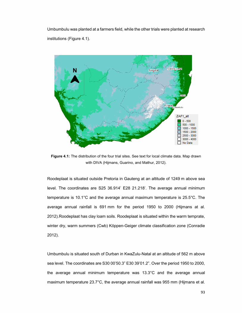
93

Umbumbulu was planted at a farmers field, while the other trials were planted at research

institutions (Figure 4.1).

Figure 4.1: The distribution of the four trial sites. See text for local climate data. Map drawn

with DIVA (Hijmans, Guarino, and Mathur, 2012).

Roodeplaat is situated outside Pretoria in Gauteng at an altitude of 1249 m above sea

level. The coordinates are S25 36.914’ E28 21.218’. The average annual minimum

temperature is 10.1°C and the average annual maximum temperature is 25.5°C. The

average annual rainfall is 691 mm for the period 1950 to 2000 (Hijmans at al.

2012).Roodeplaat has clay loam soils. Roodeplaat is situated within the warm temprate,

winter dry, warm summers (Cwb) Köppen-Geiger climate classification zone (Conradie

2012).

Umbumbulu is situated south of Durban in KwaZulu-Natal at an altitude of 562 m above

sea level. The coordinates are S30 00’50.3” E30 39’01.2”. Over the period 1950 to 2000,

the average annual minimum temperature was 13.3°C and the average annual

maximum temperature 23.7°C, the average annual rainfall was 955 mm (Hijmans et al.

N

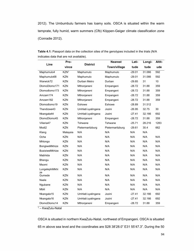
94

2012). The Umbumbulu farmers has loamy soils. OSCA is situated within the warm

temprate, fully humid, warm summers (Cfb) Köppen-Geiger climate classification zone

(Conradie 2012).

Table 4.1: Passport data on the collection sites of the genotypes included in the trials (N/A

indicates data that are not available).

Line Pro-

vince District

Nearest

Town/village

Lati-

tude

Longi-

tude

Altit-

ude

Maphumulo4 KZN1 Maphumulo Maphumulo -29.01 31.066 592

Maphumulo68 KZN Maphumulo Maphumulo -29.01 31.066 592

Warwick72 KZN Durban Metro Durban -29.85 31 10

DlomoDlomo171 KZN Mthonjaneni Empangeni -28.72 31.88 359

Dlomodlomo173 KZN Mthonjaneni Empangeni -28.72 31.88 359

Amzam174 KZN Mthonjaneni Empangeni -28.72 31.88 359

Amzam182 KZN Mthonjaneni Empangeni -28.72 31.88 359

Dlomodlomo19 KZN Eshowe Eshowe -28.89 31.512

Thandizwe43 KZN Umhlab’uyalingana Jozini -26.95 32.75 30

Nkangala44 KZN Umhlab’uyalingana Jozini -27.41 32.166 692

DlomoDlomo45 KZN Mthonjaneni Empangeni -28.72 31.88 359

Vilieria47 KZN Tshwane Tshwane -25.71 28.216 1283

Modi2 KZN Pietermaritzburg Pietermaritzburg -29.61 30.4 662

Klang Malaysia N/A N/A N/A N/A

Ocha KZN N/A N/A N/A N/A N/A

Mhlongo KZN N/A N/A N/A N/A N/A

BongiweMkhize KZN N/A N/A N/A N/A N/A

BusisiweMkhize KZN N/A N/A N/A N/A N/A

Mabhida KZN N/A N/A N/A N/A N/A

Bhengu KZN N/A N/A N/A N/A N/A

Msomi KZN N/A N/A N/A N/A N/A

LungelephiMkhize

KZN N/A N/A N/A N/A N/A

Gumede KZN N/A N/A N/A N/A N/A

Nxele KZN N/A N/A N/A N/A N/A

Ngubane KZN N/A N/A N/A N/A N/A

Mbili KZN N/A N/A N/A N/A N/A

Nkangala15 KZN Umhlab’uyalingana Jozini -27.41 32.166 692

Nkangala16 KZN Umhlab’uyalingana Jozini -27.41 32.166 692

DlomoDlomo14 KZN Mthonjaneni Empangeni -28.72 31.88 359

1 – KwaZulu-Natal

OSCA is situated in northern KwaZulu-Natal, northwest of Empangeni. OSCA is situated

65 m above sea level and the coordinates are S28 38’28.0” E31 55’47.3”. During the 50

95

year period from 1950 to 2000, the average annual minimum temperature was 16.6°C

and the average annual maximum temperature was 26.9°C. The average annual rainfall

was 1030 mm. (Hijmans et al. 2012). OSCA has clay loam soils. OSCA is situated within

the warm temprate, fully humid, hot summers (Cfa) Köppen-Geiger climate classification

zone (Conradie 2012).

The Lowveld College of Agriculture is situated in the Northern outskirts of Nelspruit in

Mpumalanga. It is situated 718 m above sea level. The coordinates are S 25 26’00.9”

E30 58’26.2”. The average annual minimum temperature was 13.5°C and the average

annual maximum temperature was 26.2°C. The average annual rainfall was 793mm

(Hijmans et al. 2012). The trial site is selected close to a little river and has clay soils.

Frost does occur occasionally. Lowveld College of Agriculture is situated within the warm

temprate, winter dry, hot summers (Cwa) Köppen-Geiger climate classification zone

(Conradie 2012).

The soil at all sites was prepared by mechanical ploughing followed by ridging. Ridging

was done mechanically with a “ridge maker”, except at Umbumbulu where it was done

by hand. The ridges were one meter apart and about 30 cm deep. Corms were planted

between the ridges and then covered.

The plants were planted in a randomised complete block design with three replicates.

Each plot consisted of three rows with five plants each (15 plants per plot). There was 1

m between the row spacing and 60 cm between the intra-row spacing. One cup well

decomposed (150 ml) of compost was added before planting, and no additional fertilizer

was added to the trials during the growth period, thus following the traditional planting

method. All trials were irrigated three times a week for about 2 to 3 hours, to supply 15

mm of water per irrigation, trials were not irrigated when it was raining. The Umbumbulu

96

trail was rain fed. Weeding was done manually. The trial at the Lowveld Agricultural

College was poorly maintained and was discarded from the analysis due to too many

missing plants.

4.2.3 Data collection and Data analysis

Date for the characterization were not taken for the whole ARC taro germplasm

collection, but only for the 30 accessions included in the multi-location trial. The following

measurements were taken from three plants in each plot after four months of growth

(Sing et al. 2008):

Emergence: All plants that did not emerged were counted. This parameter were mostly

used when yield were calculated.

Leaf length: The length of the first unfolded mature leaf was measured with a tape

measure. Measure was taken from the tip of the leaf, to the deepest point of the sinus.

Leaf width: width of the first unfolded mature leaf was measured with a tape measure

across the widest part of the leaf.

Number of suckers: The number of suckers around the main plant were counted. In

eddoe types, where it was difficult to recognise the main plant, the number of suckers

were counted and then one was deducted from the total number. The number of suckers

will correlate to the number of cormels.

Leaf number: All the mature leaves that were present on the main plant and suckers at

that specific time were counted,

Plant height: The height of the tallest leaf of the plant was measured from soil level,

Canopy diameter (Canopy cover): The diameter of the whole plant, main plant with all

suckers, was taken across the middle of the clump at the widest point.

Number of cormels: The total number of corms (dasheen type) or cormels (eddoe type)

that were harvested was counted.

Weight of cormels: The total weight of all the corms (dasheen type) or cormels (eddoe

type) harvested from one plant was determined.

97

Corm length: The average length of ten randomly selected corms (dasheen type) or

cormels (eddoe type).

Corm breadth: The average breadth of ten randomly selected corms (dasheen type) or

cormels (eddoe type) measured at its widest point.

A combined ANOVA was done for each of the characteristics across the localities using

Genstat 14. The ANOVA gave an indication of significant differences between genotypes

for the characteristics as well as GxE interactions. Further multivariate analysis (AMMI)

was done where significant GxE was detected. The AMMIs gave an indication of the

stability of the varieties for the different characteristics (Zobel et al., 1988). The AMMI

analysis provides a biplot of main effects and the first principle component scores of the

interactions (IPCA 1) of both genotypes and environments. The IPCA 1 score is on the

vertical axis and the mean yield on the horizontal. Genotypes or environments that

appear almost on a perpendicular line of the graph have similar means, while those that

fall almost on a horizontal line have similar interaction patterns (Crossa, 1990). High

PCA scores (either negative or positive as it is a relative value) indicate the specific

adaptation of a genotype to certain environments, alternatively, the more the IPCA score

approximates zero, the more stable the genotype is over all respective environments

(Crossa, 1990).

4.3 Results

All data sets were complete (261 observations) except for “Leaf length” and “Number of

suckers” where one outlier each was removed and two outliers were removed in “Corm

length”. The ANOVA tables that were directly linked to yield parameters are presented

in this chapter. All the other ANOVA tables are presented in Appendix 2. The AMMI,

ANOVA tables and biplots that are directly linked to yield parameters are presented in

this chapter. All the other AMMI ANOVA tables are presented in Appendix 4 and AMMI

biplots are presented in Appendix 5.

98

4.3.1 Leaf length

The ANOVA table for leaf length is presented in Appendix 2. Significant interaction was

observed between locality and specific lines for mean leaf length. On average, the leaves

in Umbumbulu were significantly shorter than the leaves in Roodeplaat and OSCA.

There were significant differences in mean leaf length between the different lines. The

mean leaf length varied from 34.388 cm for BongiweMkhize to 24.916 for Klang.

The ANOVA for the AMMI (Appendix 4) model for leaf length also showed that the main

effects and interactions were significant. IPCA1 explains 90.15% of the variation and

IPCA2 9.855%. IPCA1 was significant, but IPCA2 was not significant (f=0.9993). The

first four AMMI selections at OSCA were Mbili, BongiweMkhize, DlomoDlomo171, and

Nkangala16, respectively. The first four lines at Roodeplaat were Thandizwe43,

Ngubane, BongiweMkhize, and Gumede. The first four lines at Umbumbulu were

Thandizwe43, Gumede, DlomoDlomo45, and Ngubane. No lines were in the top four

lines in all three localities, but Thandizwe43, Ngubane, BongiweMkhize, and Gumede

were in the top four in two localities. Overall the top four lines were BongiweMkhize,

Mbili, Ngubane, and Thandizwe43. Thandizwe43 showed better stability than the other

three. Gumede, Nkangala44, Bhengu, Mabhida, DlomoDlomo45, and Thandizwe43

showed good stability and above average leaf length while Mhlongo, Modi2, Ocha,

Dlomodlomo173, Msomi and Amzam182 showed good stability but below average leaf

length. Maphumulo68 and Klang showed low stability and below average leaf length,

while Mbili also has low stability but above average leaf length (Appendix 5).

4.3.2 Leaf width

The ANOVA table for leaf width is presented in Appendix 3. The influence of genotype,

location, and the interaction between genotype and environment was significant. There

were significant differences between OSCA and the other two localities for mean leaf

99

width. Leaves were significantly wider in OSCA. The overall mean leaf width was

25.49cm. The mean leaf width varied from 34.00cm measured for Mbili in OSCA, to

15.77cm for Klang in OSCA (Data not shown). Mean leaf width also differed significantly

between lines. Ngubane has the widest leaves (28.79cm) and Klang has the narrowest

leaves (20.37 cm).

From the ANOVA table for the AMMI model, it is clear that all the main effects and

interactions are significant (Appendix 4). IPCA1 explains 78.25% of the variation and

IPCA2 21.75%. IPCA1 is significant, but IPCA2 is not significant (f=0.9065). It is

therefore meaningful to plot the AMMI1 biplot. The first four AMMI selections at

Umbumbulu and Roodeplaat were Mabhida, Ngubane, Gumede, and Bhengu. The first

four lines selected at OSCA were Mbili, Amzam174, Vilieria47, and Ngubane. Overall

Ngubane, Mbili, Mabhida and Amzam174 had the highest mean leaf width; however,

Mabhida and Amzam174 were less stable. Gumede, Nkangala15 Ngubane, and

Mabhida had good stability and above average leaf width. Nkangala44. Mhlongo,

Dlomodlomo173, Msomi, and DlomoDlomo45 showed good stability but below average

leaf width (Appendix 5).

4.3.3 Leaf number

The ANOVA for leaf number is presented in Appendix 3. The influence of genotype,

location and the interaction between genotype and environment was significant. All three

localities differed significantly for leaf number. The plants in OSCA had, on average,

more leaves than at Umbumbulu, but less leaves than at Roodeplaat. The mean number

of leaves per plant was 26.51. The highest mean number of leaves was 57.33 observed

for Amzam174 at Roodeplaat, while the lowest mean number of leaves was 6.67 for

DlomoDlomo1713 observed in Umbumbulu. The average number of leaves also differed

between the different lines. Amzam174 has the highest average number of leaves

(34.297) and Nxele the lowest average number of leaves (20.149).

100

From the ANOVA table (Appendix 5) for the AMMI model for the number of leaves on a

single plant, it is clear that the main effects and the interactions were significant. IPCA1

explains 63.56% of the variation and IPCA2 36.44%. IPCA1 was significant, but IPCA2

was not significant (f=0.3493). Therefore, only AMMI1 plots were drawn. According to

the AMMI, the four best lines at OSCA were Thandizwe43, BusisiweMkhize,

LungelephiMkhize, and Ngubane. The four best lines at Roodeplaat were Amzam174,

Thandizwe43, Nkangala15, and Amzam182. The four best lines at Umbumbulu were

Amzam174, Amzam182, Bhengu, and Nkangala15. No lines were in the top four at all

three localities but Amzam174, Thandizwe43, and Nkangala15 were under the top four

in two of the three localities, namely Roodeplaat and Umbumbulu. The overall four best

lines were Amzam174, Thandizwe43, Nkangala15, and Dlomodlomo19. Amzam174

showed a high degree of stability, while Thandizwe43 showed low stability. Bhengu,

Amzam182, Amzam174, and Nkangala15 showed a high degree of stability and above

average number of leaves, while Vilieria47 and DlomoDlomo171 also showed a high

degree of stability but below average number of leaves. LungelephiMkhize,

BusisiweMkhize, and Thandizwe43 showed a low degree of stability but above average

number of leaves, while Maphumulo4 showed low degree of stability and below average

number of leaves per plant (Appendix 5).

4.3.4 Plant height

The ANOVA table for plant height is presented in Appendix 3. The influence of locality

and genotype was highly significant, the interaction between the locality and the

genotype was significant but not as highly as the two factors individually (p=0.0547). The

height of the plants differed significantly between all three localities. The plant heights

differ significantly and the tallest plants were observed in OSCA, followed by Roodeplaat,

and then Unbumbulu. The overall mean for plant height was 73.55cm. The plant height

varied between103.44cm for BongiweMkhize in OSCA, to 51.33cm for Maphumulo68 in

101

OSCA. On average, the tallest plants were observed for Ngubane (85.63cm) and

shortest plants were Maphumulo68 (59.45cm).

The ANOVA table (Appendix 4) for AMMI model for plant height showed that the main

effects and interactions were significant. IPCA1 explains 79.22% of the variation and

IPCA2 20.78%. Only IPCA1 is significant and not IPCA2 (f=0.9397). AMM2 plots will

therefore not be meaningful. According to the AMMI, the four best lines in OSCA were

BongiweMkhize, Ngubane, Nkangala16, and Amzam174. The four best lines in

Roodeplaat were Amzam174, Ngubane, Thandizwe43, and Nkangala15 and the four

best lines in Umbumbulu were Amzam174, Thandizwe43, Ngubane and

DlomoDlomo14. Amzam174 and Ngubane were in the top four lines in all three localities

while Thandizwe43 was in the top four lines in two localities. Ngubane, Amzam174,

Thandizwe43, and BongiweMkhize had the best overall performance for plant height.

However, BongiweMkhize and Ngubane showed high levels of instability. The most

stable lines for plant height were Amzam182, Modi2, Mhlongo, and Dlomodlomo173, but

only Amzam182 showed above average plant height. The highest levels of instability

were observed in Maphumulo4, DlomoDlomo14, Maphumulo68, and BongiweMkhize.

BongiweMkhize was ranked fourth overall for plant height but was also the fourth least

stable line (Appendix 5).

4.3.5 Canopy diameter

The ANOVA table for canopy diameter is presented in Appendix 3. The influence of the

genotypes and environment was significant, but not the interaction between the

environment and the genotype (p=0.566) (Appendix 3).There were significant

differences in mean canopy diameter between the localities (Appendix 3).There were

also significant differences in mean canopy diameter between the lines (Appendix 3).

Thandizwe43 has the highest mean canopy diameter (86.630cm) and Maphumulo68 the

lowest canopy diameter (61.811cm). The overall mean canopy diameter was 74.98cm.

102

The canopy diameter varied between 113.89cm for Amzam182 at Roodeplaat, and

36.58cm for Maphumulo682 at OSCA.

The ANOVA table for the AMMI model indicated that the main affects were significant.

However, the interactions were not significant (f=0.4964). IPCA1 explains 62.92% of the

variation and IPCA2 37.08%. Neither IPCA1 (f=0.2289) or IPCA2 (f=0.7916) were

significant. The AMMI model for canopy diameter was therefore not important. An AMMI

biplot were drawn even though the model is not significant. According to the AMMI, the

four best lines in OSCA were Amzam174, Thandizwe43, Dlomodlomo19, and

BongiweMkhize in descending order. At Roodeplaat it was Thandizwe43, Nkangala44,

Amzam174, and Amzam182 in descending order, and in Umbumbulu it included

Nkangala44, Thandizwe43, Bhengu, and Amzam182. Thandizwe43 was in the four best

lines in all three localities, while Nkangala44, Amzam174, and Amzam182 were in the

top four in two localities. Overall, Thandizwe43, Amzam174, and Nkangala44 were the

top lines. Nkangala44 had the lowest performance but was more stable than the other

two. Maphumulo68 had the poorest performance and showed the least stability.

Amzam182, Mbili, and Mabhida showed good stability and above average yield.

4.3.6 Number of suckers

The ANOVA table for the number of suckers per plant is presented in Appendix 3. The

influence of environment, genotype and the interaction between environment and

genotype was significant. There were significant differences in the mean number of

suckers between the different localities, Roodeplaat had the highest mean number of

suckers per plant, followed by OSCA, and then Umbumbulu. There were also significant

differences between the lines for the mean number of suckers per plant. Amzam174

had the highest number of suckers (14.56) and Maphumulo68 the lowest (6.78). The

overall mean number of suckers per plant was 10.27. The mean number of suckers per

plant varied from 25.33 at Roodeplaat for Mbili, to 2.11 at Umbumbulu for Warwick72.

103

According to the ANOVA table (Appendix 4) for the AMMI model, for the number of

suckers per plant, the main effects were highly significant and the interaction was also

significant. IPCA1 explains 55.36% of the variation and IPCA2 44.64%. IPCA1 was

significant but IPCA2 was not (f=0.1279).

According to the AMMI, the four first lines at Umbumbulu were Amzam174, Nkangala44,

Amzam182, and Thandizwe43. The best four lines at and Roodeplaat were Amzam174,

Nkangala15, DlomoDlomo171, and Thandizwe43. Amzam174 and Thandizwe43 ranked

first and fourth respectively at all three localities. Overall, the four best lines were

Amzam174, Nkangala15, Thandizwe43, and DlomoDlomo171. Amzam182 and

Nkangala16 showed a very high degree of stability and above average number of

suckers. BongiweMkhize, LungelephiMkhize, Gumede, and Warwick72 also showed a

high degree of stability but below average number of suckers. DlomoDlomo171 and

Nkangala15 showed a high degree of instability and above average number of suckers,

while Maphumulo68 and Vilieria47 also showed high instability, but below average

number of suckers.

4.3.7 Number of cormels harvested from a single plant

The ANOVA table for the number of cormels harvested per plant is presented in Table

4.4 and Appendix 3. The influence of environment, genotype and the interaction between

environment and genotype was significant (Table 4.2). The mean number of cormels

harvested per plant differed significantly between the localities. The highest mean

number of corms per plant was harvested at Roodeplaat and lowest at Umbumbulu

(Table 4.3). Significant interactions were observed between the mean number of cormels

and locality (Table 4.4). The overall mean number of corms per plant was 22.17 corms.

The highest mean number of cormels observed was 62.67 for DlomoDlomo171 in

Roodeplaat and the lowest mean number of cormels were observed was 2.11 for Klang

in OSCA.

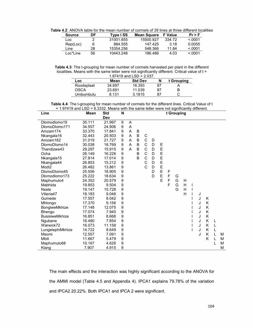
104

Table 4.2: ANOVA table for the mean number of cormels of 29 lines at three different localities Source DF Type I SS Mean Square F Value Pr > F Loc 2 31001.855 15500.927 334.72 <.0001 Rep(Loc) 6 884.555 147.425 3.18 0.0055 Line 28 15354.256 548.366 11.84 <.0001 Loc*Line 56 10443.248 186.486 4.03 <.0001

Table 4.3: The t-grouping for mean number of cormels harvested per plant in the different localities. Means with the same letter were not significantly different. Critical value of t =

1.97419 and LSD = 2.037. Loc Mean Std Dev N t Grouping Roodeplaat 34.697 16.393 87 A OSCA 23.691 11.039 87 B Umbumbulu 8.131 3.1815 87 C

Table 4.4: The t-grouping for mean number of cormels for the different lines. Critical Value of t

= 1.97419 and LSD = 6.3332. Means with the same letter were not significantly different. Line Mean Std

Dev N t Grouping

Dlomodlomo19 35.111 21.997 9 A DlomoDlomo171 34.557 24.906 9 A Amzam174 33.370 17.841 9 A B Nkangala16 32.443 20.503 9 A B C Amzam182 31.019 21.727 9 A B C D DlomoDlomo14 30.038 18.769 9 A B C D E Thandizwe43 29.297 15.915 9 A B C D E Ocha 28.149 16.226 9 B C D E Nkangala15 27.814 17.014 9 B C D E Nkangala44 26.853 15.212 9 C D E Modi2 26.482 13.861 9 C D E DlomoDlomo45 25.556 18.905 9 D E F Dlomodlomo173 25.222 18.634 9 D E F G Maphumulo4 24.352 20.579 9 E F G H Mabhida 19.853 9.504 9 F G H I Nxele 19.147 15.728 9 G H I Vilieria47 18.183 9.046 9 H I J Gumede 17.557 8.042 9 I J K Mhlongo 17.370 9.156 9 I J K BongiweMkhize 17.148 12.075 9 I J K Bhengu 17.074 7.940 9 I J K BusisiweMkhize 16.851 8.668 9 I J K Ngubane 16.480 7.854 9 I J K L Warwick72 16.073 11.158 9 I J K L LungelephiMkhize 14.722 8.649 9 I J K L Msomi 12.557 7.091 9 J K L M Mbili 11.667 5.479 9 K L M Maphumulo68 10.167 4.626 9 L M Klang 7.907 4.915 9 M

The main effects and the interaction was highly significant according to the ANOVA for

the AMMI model (Table 4.5 and Appendix 4). IPCA1 explains 79.78% of the variation

and IPCA2 20.22%. Both IPCA1 and IPCA 2 were significant.

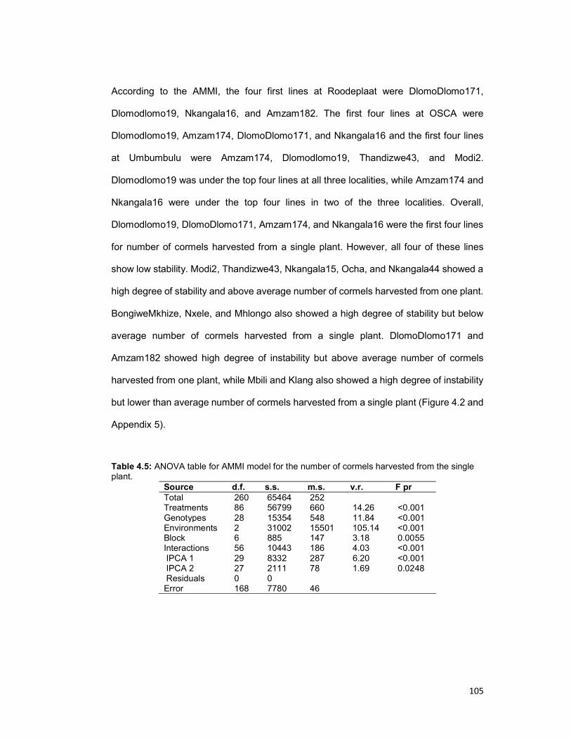
105

According to the AMMI, the four first lines at Roodeplaat were DlomoDlomo171,

Dlomodlomo19, Nkangala16, and Amzam182. The first four lines at OSCA were

Dlomodlomo19, Amzam174, DlomoDlomo171, and Nkangala16 and the first four lines

at Umbumbulu were Amzam174, Dlomodlomo19, Thandizwe43, and Modi2.

Dlomodlomo19 was under the top four lines at all three localities, while Amzam174 and

Nkangala16 were under the top four lines in two of the three localities. Overall,

Dlomodlomo19, DlomoDlomo171, Amzam174, and Nkangala16 were the first four lines

for number of cormels harvested from a single plant. However, all four of these lines

show low stability. Modi2, Thandizwe43, Nkangala15, Ocha, and Nkangala44 showed a

high degree of stability and above average number of cormels harvested from one plant.

BongiweMkhize, Nxele, and Mhlongo also showed a high degree of stability but below

average number of cormels harvested from a single plant. DlomoDlomo171 and

Amzam182 showed high degree of instability but above average number of cormels

harvested from one plant, while Mbili and Klang also showed a high degree of instability

but lower than average number of cormels harvested from a single plant (Figure 4.2 and

Appendix 5).

Table 4.5: ANOVA table for AMMI model for the number of cormels harvested from the single plant.

Source d.f. s.s. m.s. v.r. F pr Total 260 65464 252 Treatments 86 56799 660 14.26 <0.001 Genotypes 28 15354 548 11.84 <0.001 Environments 2 31002 15501 105.14 <0.001 Block 6 885 147 3.18 0.0055 Interactions 56 10443 186 4.03 <0.001 IPCA 1 29 8332 287 6.20 <0.001 IPCA 2 27 2111 78 1.69 0.0248 Residuals 0 0 Error 168 7780 46

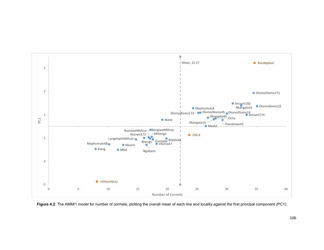
106

Figure 4.2: The AMMI1 model for number of cormels, plotting the overall mean of each line and locality against the first principal component (PC1).

Amzam174

Amzam182

Bhengu

BongiweMkhizeBusisiweMkhize

DlomoDlomo14

DlomoDlomo171

Dlomodlomo173

Dlomodlomo19

DlomoDlomo45

Gumede

Klang

LungelephiMkhize Mabhida

Maphumulo4

Maphumulo68

Mbili

Mhlongo

Modi2

Msomi

Ngubane

Nkangala15

Nkangala16

Nkangala44Nxele Ocha

Thandizwe43

Vilieria47

Warwick72 OSCA

Roodeplaat

Umbumbulu

Mean, 22.17

-5

-3

-1

1

3

5

0 5 10 15 20 25 30 35 40

PC1

Number of Cormels

107

4.3.8 Weight of cormels harvested from a single plant

The ANOVA table for the total weight of the cormels harvested per plant is presented in

table 4.6 and Appendix 3. The influence of environment, genotype and the interaction

between environment and genotype was significant (Table 4.6). The mean weight of

cormels harvested per plant was significantly lower in Umbumbulu than in Roodeplaat

and OSCA. There was no significant difference between Roodeplaat and OSCA (Table

4.7). The mean weight of cormels also differed significantly between lines (Table 4.8).

The highest mean weight was for Thandizwe43 (0.90kg) and the lowest was Klang

(0.3589). The overall mean weight of all the cormels harvested from one plant was

0.654kg. The mean weight of cormels harvest per plant varied from 1.44kg for Ngubane

in OSCA to 0.09g for Klang in OSCA.

Table 4.6: ANOVA table for the mean weight of cormels harvested from a single plant of 29 lines at three different localities

Source DF Type I SS Mean Square

F Value Pr > F

Loc 2 14.680 7.340 150.19 <.0001 Rep(Loc) 6 0.9764 0.162 3.33 0.0040 Line 28 3.3429 0.119 2.44 0.0003 Loc*Line 56 6.1053 0.109 2.23 <.0001 LocxLin 0 0.0000 . . .

Table 4.7: The t-grouping for mean weight of cormels harvested per plant in the different localities. Means with the same letter were not significantly different. Critical Value of t = 1.97419 and LSD = 0.0662

Loc Mean Std Dev N t Grouping Roodeplaat 0.84747 0.243 87 A OSCA 0.79644 0.381 87 A Umbumbulu 0.32080 0.108 87 B

The ANOVA table (Table 4.9 and Appendix 4) for AMMI model for the weight of the

cormels harvested from a single plant showed that the main effects and the interactions

were significant. IPCA1 explains 82.27% of the variation and IPCA2 17.73%. IPCA1 was

highly significant while IPCA2 was not significant (f=0.7209).

108

From the AMMI analysis, the four top lines at Roodeplaat were Amzam174, Mhlongo,

Maphumulo4, and Thandizwe43. The four top lines at Umbumbulu were Thandizwe43,

Mabhida, Amzam174, and Gumede. The four top lines at OSCA were Ngubane,

Thandizwe43, Mabhida, and Vilieria47. Thandizwe43 was under the top four lines in all

three localities while Mabhida, and Amzam174 were under the top four lines in two

localities. Thandizwe43, Mabhida, Amzam174, Ngubane were overall the top four lines.

Ngubane showed a very high degree of instability while Amzam174 showed a high

degree of stability. Nxele, Dlomodlomo19, Gumede, and BusisiweMkhize were the most

stable lines but Nxele had a below average weight for cormels harvested from a single

plant (yield). Ngubane, Klang, Vilieria47, and Mbili were the least stable lines.

Table 4.8: The t-grouping for mean weight of cormels harvested per plant for the different lines. Critical Value of t = 1.97419 and LSD = 0.2057. Means with the same letter were not significantly different.

Line Mean Std Dev N t Grouping Thandizwe43 0.9000 0.466 9 A Mabhida 0.8656 0.401 9 A B Amzam174 0.7867 0.343 9 A B C Ngubane 0.7833 0.512 9 A B C Gumede 0.7689 0.359 9 A B C D BusisiweMkhize 0.7478 0.494 9 A B C D E Mhlongo 0.7333 0.387 9 A B C D E Bhengu 0.7322 0.290 9 A B C D E Dlomodlomo19 0.6944 0.316 9 A B C D E Modi2 0.6878 0.335 9 B C D E LungelephiMkhize 0.6856 0.388 9 B C D E Ocha 0.6833 0.322 9 B C D E DlomoDlomo14 0.6622 0.361 9 B C D E Nkangala15 0.6533 0.364 9 C D E BongiweMkhize 0.6478 0.402 9 C D E Amzam182 0.6422 0.370 9 C D E Nkangala16 0.6256 0.283 9 C D E DlomoDlomo45 0.6200 0.348 9 C D E Nxele 0.6144 0.337 9 C D E Vilieria47 0.6111 0.368 9 C D E Mbili 0.6044 0.330 9 C D E F Warwick72 0.5944 0.399 9 C D E F DlomoDlomo171 0.5922 0.287 9 C D E F Nkangala44 0.5844 0.200 9 C D E F Maphumulo4 0.5833 0.367 9 C D E F Msomi 0.5756 0.324 9 D E F Dlomodlomo173 0.5522 0.406 9 E F G Maphumulo68 0.4011 0.217 9 F G Klang 0.3589 0.244 9 G

109

Figure 4.3: The AMMI1 model for weight of cormels harvested from a single plant, plotting the overall mean of each line and locality against the first principal

component (PC1).

Amzam174

Amzam182

Bhengu

BongiweMkhize

BusisiweMkhize

DlomoDlomo14

DlomoDlomo171

Dlomodlomo173Dlomodlomo19

DlomoDlomo45

Gumede

Klang

LungelephiMkhize

Mabhida

Maphumulo4Maphumulo68

Mbili

Mhlongo

Modi2

Msomi

Ngubane

Nkangala15

Nkangala16Nkangala44

NxeleOcha

Thandizwe43

Vilieria47

Warwick72

OSCA

Roodeplaat,

Umbumbulu

Mean, 0.6549

0.3 0.4 0.5 0.6 0.7 0.8 0.9-1

-0.8

-0.6

-0.4

-0.2

0

0.2

0.4

0.6

Weight of cormels harvested from single plant

PC1

110

Table 4.9: ANOVA table for AMMI model for the weight of the cormels harvested from a single plant.

Source d.f. s.s. m.s. v.r. F pr Total 260 33.315 0.1281 Treatments 86 24.128 0.2806 5.74 <0.001 Genotypes 28 3.343 0.1194 2.44 <0.001 Environments 2 14.680 7.3400 45.10 <0.001 Block 6 0.976 0.1627 3.33 0.0040 Interactions 56 6.105 0.1090 2.23 <0.001 IPCA 1 29 5.023 0.1732 3.54 <0.001 IPCA 2 27 1.083 0.0401 0.82 0.7209 Residuals 0 0.000 Error 168 8.211 0.0489

All these lines, except Ngubane, showed below average weight for cormels harvested

from a single plant. Ngubane showed the highest degree of instability but was ranked

overall fourth for weight of cormels harvested from a single plant (Figure 4.3 and

Appendix 5).

4.3.9 Corm length

The ANOVA table for corm length is presented in Appendix 3. The effect of locality was

highly significant but the effect of genotype (p=0.1885) was not, however, the interaction

between the genotype and the environment was significant (p=0.0368). The mean corm

length differed significantly between the different localities. There were also some

differences between lines for the mean corm length. The overall mean corm length was

67.63mm. The mean corm length varied between 103.20mm for LungelephiMkhize at

OSCA, and 41.43mm for Nkangala443 at Roodeplaat.

The ANOVA table (Appendix 4) for AMMI model for the length of the corms showed that

effect of environment was highly significant but not effect of genotype. IPCA1 explains

76.01% of the variation and IPCA2 23.99%. Only IPCA1 was significant while IPCA2

was not significant (f=0.8206). From the AMMI analysis, the four top lines at Umbumbulu

were Maphumulo68, LungelephiMkhize, Ngubane, and Ocha in descending order. The

four top lines at Roodeplaat were LungelephiMkhize, Maphumulo68, Ngubane, and

Ocha. The same four lines were identified at Roodeplaat and Umbumbulu, but the

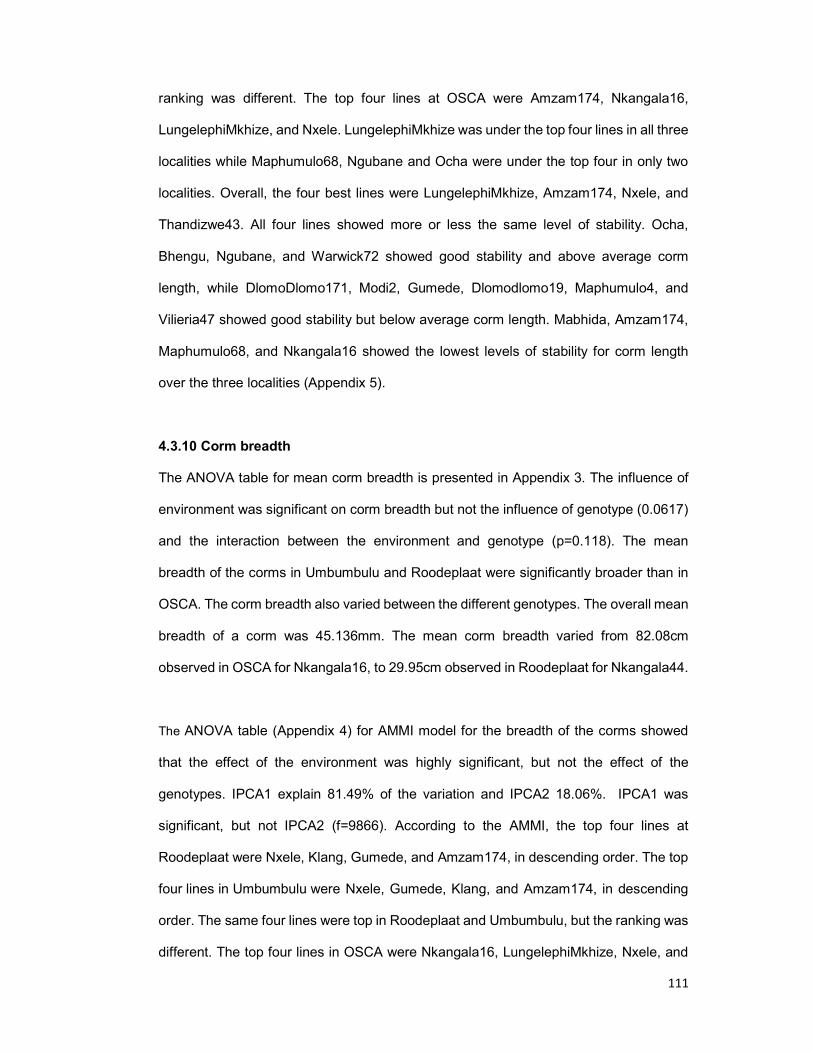
111

ranking was different. The top four lines at OSCA were Amzam174, Nkangala16,

LungelephiMkhize, and Nxele. LungelephiMkhize was under the top four lines in all three

localities while Maphumulo68, Ngubane and Ocha were under the top four in only two

localities. Overall, the four best lines were LungelephiMkhize, Amzam174, Nxele, and

Thandizwe43. All four lines showed more or less the same level of stability. Ocha,

Bhengu, Ngubane, and Warwick72 showed good stability and above average corm

length, while DlomoDlomo171, Modi2, Gumede, Dlomodlomo19, Maphumulo4, and

Vilieria47 showed good stability but below average corm length. Mabhida, Amzam174,

Maphumulo68, and Nkangala16 showed the lowest levels of stability for corm length

over the three localities (Appendix 5).

4.3.10 Corm breadth

The ANOVA table for mean corm breadth is presented in Appendix 3. The influence of

environment was significant on corm breadth but not the influence of genotype (0.0617)

and the interaction between the environment and genotype (p=0.118). The mean

breadth of the corms in Umbumbulu and Roodeplaat were significantly broader than in

OSCA. The corm breadth also varied between the different genotypes. The overall mean

breadth of a corm was 45.136mm. The mean corm breadth varied from 82.08cm

observed in OSCA for Nkangala16, to 29.95cm observed in Roodeplaat for Nkangala44.

The ANOVA table (Appendix 4) for AMMI model for the breadth of the corms showed

that the effect of the environment was highly significant, but not the effect of the

genotypes. IPCA1 explain 81.49% of the variation and IPCA2 18.06%. IPCA1 was

significant, but not IPCA2 (f=9866). According to the AMMI, the top four lines at

Roodeplaat were Nxele, Klang, Gumede, and Amzam174, in descending order. The top

four lines in Umbumbulu were Nxele, Gumede, Klang, and Amzam174, in descending

order. The same four lines were top in Roodeplaat and Umbumbulu, but the ranking was

different. The top four lines in OSCA were Nkangala16, LungelephiMkhize, Nxele, and

112

Amzam174, in descending order. Nxele and Amzam174 were under the top four lines in

all three localities, while Klang and Gumede were under the top four lines in two

localities. Overall the best genotypes were Nxele, Amzam174, Gumede, Nkangala16,

and LungelephiMkhize, but Nxele and Gumede showed more stability. Ngubane,

Bhengu, Warwick72, Dlomodlomo19, Gumede, and Thandizwe43 had good stability and

above average corm breadths. Modi2, Maphumulo4, Mbili, Mabhida, and

BusisiweMkhize had good stability but below average come breadths.

LungelephiMkhize, Msomi, Nkangala15 had above average corm breadth but showed

low stability. Klang showed low stability and a mean corm breadth below average,

although it was under the top four lines in Umbumbulu. Generally, lines were less stable

for corm breadths than corm length.

4.3.11 Summery of the ANOVA and AMMI results

The summary of the four best genotypes for each characteristic as determined by the

ANOVA (Table 4.10 and Appendix 6) and AMMI (Table 4.11 and Appendix 6) show that

there is not a single genotype that can be identified as “the best”. This is due to the

interaction between the environments and the genotypes. Eze et al. (2016) also noted

that the ranking of Nigerian taro cultivars differ between the environments. Amzam174

and Thandizwe43 seem to be genotypes that are often under the top four. For the farmer,

the total weight of the cormels harvested from a plant will be often the most important.

Consumer preference may sometimes play an important role in a farmer’s choice of

cultivar as well. Thandizwe43, Mabhida and Amzam174 seem to be some of the better

genotypes. Table 4.15 combines the best cultivars as indicated by the ANOVA and the

AMMI analysis. There is no clear line that can be identified as the best performer,

however Amzam174, DlomoDlomo45 and 19 and Thandizwe43 occur several times for

the yield related parameters. Egesi and Asiedu (2002) were also not able to identify one

single yam genotype that perform best over all the environments.

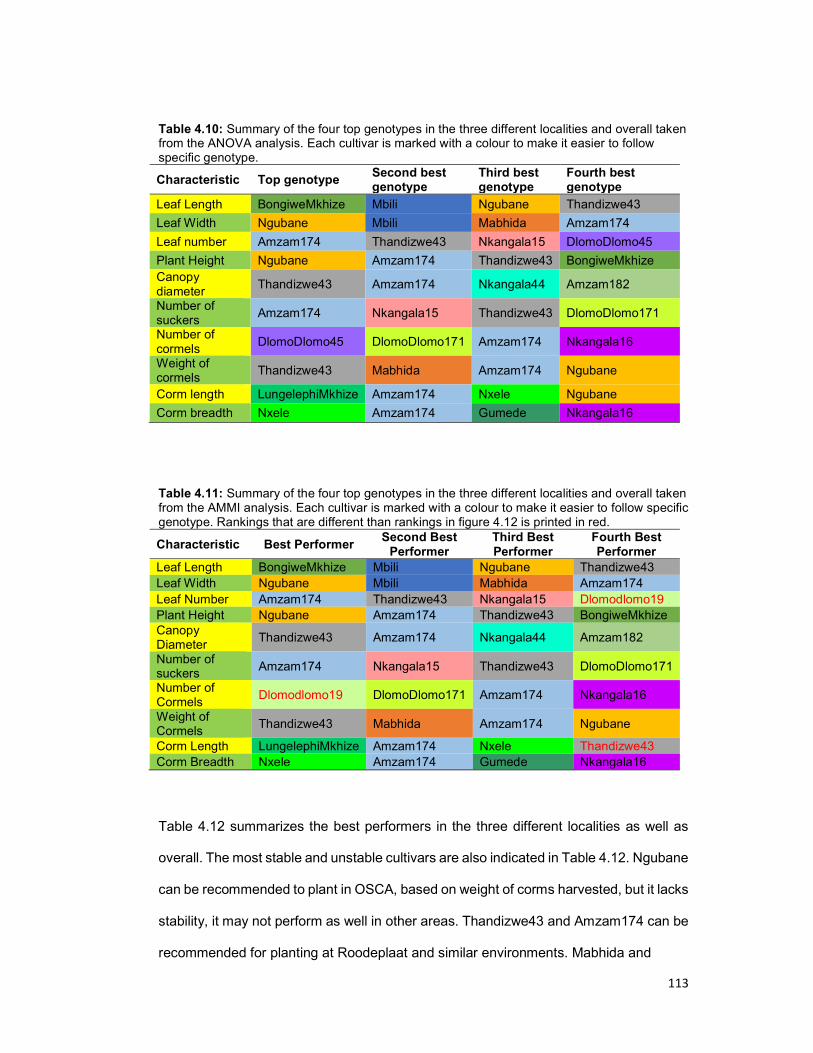
113

Table 4.10: Summary of the four top genotypes in the three different localities and overall taken from the ANOVA analysis. Each cultivar is marked with a colour to make it easier to follow specific genotype.

Characteristic Top genotype Second best genotype

Third best genotype

Fourth best genotype

Leaf Length BongiweMkhize Mbili Ngubane Thandizwe43

Leaf Width Ngubane Mbili Mabhida Amzam174

Leaf number Amzam174 Thandizwe43 Nkangala15 DlomoDlomo45

Plant Height Ngubane Amzam174 Thandizwe43 BongiweMkhize Canopy diameter

Thandizwe43 Amzam174 Nkangala44 Amzam182

Number of suckers

Amzam174 Nkangala15 Thandizwe43 DlomoDlomo171

Number of cormels

DlomoDlomo45 DlomoDlomo171 Amzam174 Nkangala16

Weight of cormels

Thandizwe43 Mabhida Amzam174 Ngubane

Corm length LungelephiMkhize Amzam174 Nxele Ngubane

Corm breadth Nxele Amzam174 Gumede Nkangala16

Table 4.11: Summary of the four top genotypes in the three different localities and overall taken from the AMMI analysis. Each cultivar is marked with a colour to make it easier to follow specific genotype. Rankings that are different than rankings in figure 4.12 is printed in red.

Characteristic Best Performer Second Best

Performer Third Best Performer

Fourth Best Performer

Leaf Length BongiweMkhize Mbili Ngubane Thandizwe43 Leaf Width Ngubane Mbili Mabhida Amzam174 Leaf Number Amzam174 Thandizwe43 Nkangala15 Dlomodlomo19 Plant Height Ngubane Amzam174 Thandizwe43 BongiweMkhize Canopy Diameter

Thandizwe43 Amzam174 Nkangala44 Amzam182

Number of suckers

Amzam174 Nkangala15 Thandizwe43 DlomoDlomo171

Number of Cormels

Dlomodlomo19 DlomoDlomo171 Amzam174 Nkangala16

Weight of Cormels

Thandizwe43 Mabhida Amzam174 Ngubane

Corm Length LungelephiMkhize Amzam174 Nxele Thandizwe43 Corm Breadth Nxele Amzam174 Gumede Nkangala16

Table 4.12 summarizes the best performers in the three different localities as well as

overall. The most stable and unstable cultivars are also indicated in Table 4.12. Ngubane

can be recommended to plant in OSCA, based on weight of corms harvested, but it lacks

stability, it may not perform as well in other areas. Thandizwe43 and Amzam174 can be

recommended for planting at Roodeplaat and similar environments. Mabhida and

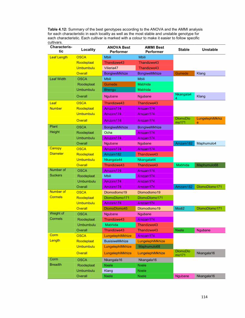
114

Table 4.12: Summary of the best genotypes according to the ANOVA and the AMMI analysis for each characteristic in each locality as well as the most stable and unstable genotype for each characteristic. Each cultivar is marked with a colour to make it easier to follow specific cultivars.

Characteris-tic Locality

ANOVA Best Performer

AMMI Best Performer

Stable Unstable

Leaf Length OSCA Mbili Mbili

Roodeplaat Thandizwe43 Thandizwe43

Umbumbulu Vilieria47 Thandizwe43

Overall BongiweMkhize BongiweMkhize Gumede Klang

Leaf Width OSCA Mbili Mbili

Roodeplaat Gumede Mabhida

Umbumbulu Bhengu Mabhida

Overall Ngubane Ngubane Nkangala44

Klang

Leaf OSCA Thandizwe43 Thandizwe43

Number Roodeplaat Amzam174 Amzam174 Umbumbulu Amzam174 Amzam174

Overall Amzam174 Amzam174 DlomoDlomo171

LungelephiMkhize

Plant OSCA BongiweMkhize BongiweMkhize Height Roodeplaat Ocha Amzam174 Umbumbulu Amzam174 Amzam174 Overall Ngubane Ngubane Amzam182 Maphumulo4

Canopy OSCA Amzam174 Amzam174 Diameter Roodeplaat Amzam182 Thandizwe43 Umbumbulu Nkangala44 Nkangala44 Overall Thandizwe43 Thandizwe43 Mabhida Maphumulo68

Number of OSCA Amzam174 Amzam174 Suckers Roodeplaat Mbili Amzam174 Umbumbulu Amzam174 Amzam174 Overall Amzam174 Amzam174 Amzam182 DlomoDlomo171

Number of OSCA Dlomodlomo19 Dlomodlomo19 Cormels Roodeplaat DlomoDlomo171 DlomoDlomo171 Umbumbulu Amzam174 Amzam174 Overall DlomoDlomo45 Dlomodlomo19 Modi2 DlomoDlomo171

Weight of OSCA Ngubane Ngubane Cormels Roodeplaat Thandizwe43 Amzam174 Umbumbulu Mabhida Thandizwe43 Overall Thandizwe43 Thandizwe43 Nxele Ngubane

Corm OSCA LungelephiMkhize Amzam174 Length Roodeplaat BusisiweMkhize LungelephiMkhize Umbumbulu LungelephiMkhize Maphumulo68

Overall LungelephiMkhize LungelephiMkhize DlomoDlomo171

Nkangala16

Corm OSCA Nkangala16 Nkangala16 Breadth Roodeplaat Nxele Nxele Umbumbulu Klang Nxele Overall Nxele Nxele Ngubane Nkangala16

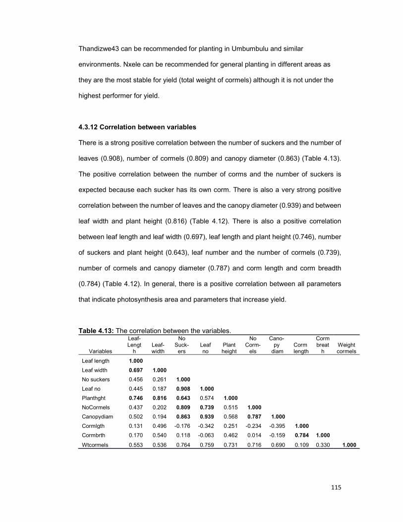
115

Thandizwe43 can be recommended for planting in Umbumbulu and similar

environments. Nxele can be recommended for general planting in different areas as

they are the most stable for yield (total weight of cormels) although it is not under the

highest performer for yield.

4.3.12 Correlation between variables

There is a strong positive correlation between the number of suckers and the number of

leaves (0.908), number of cormels (0.809) and canopy diameter (0.863) (Table 4.13).

The positive correlation between the number of corms and the number of suckers is

expected because each sucker has its own corm. There is also a very strong positive

correlation between the number of leaves and the canopy diameter (0.939) and between

leaf width and plant height (0.816) (Table 4.12). There is also a positive correlation

between leaf length and leaf width (0.697), leaf length and plant height (0.746), number

of suckers and plant height (0.643), leaf number and the number of cormels (0.739),

number of cormels and canopy diameter (0.787) and corm length and corm breadth

(0.784) (Table 4.12). In general, there is a positive correlation between all parameters

that indicate photosynthesis area and parameters that increase yield.

Table 4.13: The correlation between the variables.

Variables

Leaf- Lengt

h Leaf- width

No Suck-

ers Leaf no

Plant height

No Corm-

els

Cano-py

diam Corm

length

Corm breat

h Weight cormels

Leaf length 1.000

Leaf width 0.697 1.000

No suckers 0.456 0.261 1.000

Leaf no 0.445 0.187 0.908 1.000

Planthght 0.746 0.816 0.643 0.574 1.000

NoCormels 0.437 0.202 0.809 0.739 0.515 1.000

Canopydiam 0.502 0.194 0.863 0.939 0.568 0.787 1.000

Cormlgth 0.131 0.496 -0.176 -0.342 0.251 -0.234 -0.395 1.000

Cormbrth 0.170 0.540 0.118 -0.063 0.462 0.014 -0.159 0.784 1.000

Wtcormels 0.553 0.536 0.764 0.759 0.731 0.716 0.690 0.109 0.330 1.000

116

Figure 4.4: The biplot showing the correlation between the different characteristics.

There is a strong correlation on the biplot (Figure 4.4) between most of the

characteristics. The number of cormels and the number of suckers are highly correlated.

This is to be expected because each sucker is exists of a cormel and the leaves growing

from the cormel. The weight of the cormels harvested is strongly correlated to the

number of cormels. This give an indication that both these characteristics can be used

to select for high yielding eddoe type genotypes. Canopy diameter, plant height and leaf

number is to an extend correlated to characteristics related to yield like corm weight and

number. This indicate that the area of available to photosynthesis can influence yield.

Leaflength

Leafwidth

Nosuckers

Leafno

Planthght

NoCormels

Canopydiam

Cormlgth

Cormbrth

Wtcormels

-1

-0.75

-0.5

-0.25

0

0.25

0.5

0.75

1

-1 -0.75 -0.5 -0.25 0 0.25 0.5 0.75 1

F2 (1

6.33

%)

F1 (83.67 %)

Variables (axes F1 and F2: 100.00 %)

117

4.4 Discussion

The ANOVA showed that the environment had a significant influence on all the

characteristics except for the length and breadth of the cormels. This might be because

the cormels form continuously during the season (Lebot 2009) and therefore do not

mature at the same time. Furthermore, the secondary and tertiary cormels were also

harvested, the secondary and tertiary cormels vary in size and shape depending on

when and there they were initiated. Cormels of various sizes can be found at the same

time on a plant. The position where the cormel develop, influences the shape of the

cormel as well. Cormels that form lower on the mother corm must grow around the

cormels that have developed higher up on the mother corm. The influence of

environment was highly significant for all characteristics. These cormels will be more

elongated and curved. Significant interaction between environment and tuber yield were

noted in other tuberous crops like cassava (Dixon et al. 2002; Sholihin 2017), elephant

foot jam (Kumar et al. 2014), potato (Abalo et al. 2003; Hassanpanah 2009; Gedif and

Yigzaw 2014), sweet potato (Calisckan et al. 2007; Kathabwalika et al. 2013) and yam

(Egesi and R. Asiedu 2002; Otoo et al. 2006).

Ngubane can be recommended to plant in OSCA, based on weight of corms harvested,

but it lacks stability, it may not perform as well in other areas. Thandizwe43 and

Amzam174 can be recommended for planting at Roodeplaat and similar environments.

Mabhida and Thandizwe43 can be recommended for planting in Umbumbulu and similar

environments. Nxele can be recommended for general planting in different areas as they

are the most stable for yield (total weight of cormels) although it is not under the highest

performer for yield. Egesi and Asiedu (2002) and Kapinga et al. (2009) also identified

superior yam selections with specific or broad adaptation using AMMI analysis. The

ranking of the genotypes for specific trait was not consistent between environments. This

was also noted by Eze et al. (2016) in taro, (Osiru et al. 2009) in sweet potato.

118

The interaction between the environment and genotype was also significant for all

characteristics except the height of the plants, the canopy diameter, and corm breadth.

The interaction was highly significant to the number of cormels per plant and the weight

of the cormels harvested from a plant. These two characteristics are the major indicators

of yield. It is an indication that although these characteristics can be improved by

breeding, the environment must also be taken into account during evaluation. It will,

therefore, be advantageous to select for taro genotypes in different environments.

All the characteristics are positively correlated. There is a strong positive correlation

between the number of suckers and the number of leaves, number of cormels and

canopy diameter. There is also a positive correlation between leaf length and leaf width,

leaf length and plant height, number of suckers and plant height, leaf number and the

number of cormels, number of cormels and canopy diameter and corm length and corm

breadth. The positive correlation between the number of corms and the number of

suckers is expected because each sucker has its own corm. The weight of the cormels

harvested is strongly correlated to the number of cormels. This give an indication that

both these characteristics can be used to select for high yielding eddoe type genotypes.

4.5 References

Abalo G, Hakiza JJ, El-Bedewy R and Adipala E (2003) Genotype X Environment

Interaction Studies on Yields of Selected Potato Genotypes in Uganda. African

Crop Science Journal 11(1):9-15

Caliskan ME, Erturk E , Sogut T, Boydak E and Arioglu H (2007) Genotype ×

environment interaction and stability analysis of sweetpotato (Ipomoea batatas)

genotypes, New Zealand Journal of Crop and Horticultural Science, 35:1, 87-99,

DOI: 10.1080/01140670709510172

119

Conradie DCU (2012) South Africa’s Climatic Zones: Today, Tomorrow Future Trends

and Issues Impacting on the Built Environment, International Green Building

Conference and Exhibition, July 25-26, 2012, Sandton, South Africa

Crossa J (1990) Statistical analysis of multilocation trials. Advances in Agronomy 44:55-

86.

Dixon AGO, Ngeve JM and Nukenine EN (2002) Response of Cassava Genotypes oo

Four Biotic Constraints in Three Agro-Ecologies of Nigeria. African Crop

Egesi CN and Asiedu R (2002) Analysis of Yam Yields Using The Additive Main Effects

and Multiplicative Interaction (AMMI) Model. African Crop Science Journal

10(3)195-201

Eze CE, Nwofia GE and Onyeka J (2016) An Assessment of Taro Yield and Stability

Using AMMI and GGE Biplot Models. Journal of Experimental Agriculture

International 14(2): 1-9

Fox PN, Crossa J and Romagosa I (1997) Multi-environment testing and genotype x

environment interaction. In: Statistical methods for Plant Variety Evaluation.

Edited by R. A. Kempton and P. N. Fox. Chapman and Hall, London ISBN 0 412

45750 3

Gedif M and Yigzaw D (2014) Potato (Solanum tuberosum L.) Using a GGE Biplot

Method in Amhara Region, Ethiopia. Agricultural Sciences 5:239-249

Hassanpanah D (2009) Analysis of GxE Interaction by Using the Additive Main Effects

and Multiplicative Interaction in Potato Cultivars. International Journal of Plant

Breeding and Genetics 9:1-7

Hijmans RJ, Guarino L, and Mathur P (2012) DIVA-GIS Version 7.5, LizardTech, Inc.

and are the University of California, USA

Hill J, Becker HC and Tigerstedt PMA (1998) Quantitative and Ecological Aspects of

Plant Breeding. Plent Breeding Series 4. Chapman and Hall, Londen, UK, pp 275

Kathabwalika DM, Chilembwe EHC, Mwale VM, Kambewa D and Njoloma JP (2013)

Plant growth and yield stability of orange fleshed sweet potato (Ipomoea batatas)

120

genotypes in three agro-ecological zones of Malawi. International Research

Journal of Agricultural Science and Soil Science 3(11):383-392

Kumar S, Singh PK, Solankey SS and Singh BK (2014) Genotypic × environment

interaction and stability analysis for yield and quality components in elephant foot

yam [Amorphophallus paeoniifolius (Dennst) Nicolson]. African Journal of

Agricultural Research 9(7):707-712

Lebot V (2009) Tropical Root and Tuber Crops: Cassava, Sweet Potato, Yams and

Aroids. CABI, Wallingford, UK. pp 413

Lu TJ, Lin JH, Chen JC and Chang YU (2008) Characteristics of Taro (Colocasia

esculenta) Starches Planted in Different Seasons and Their Relations to the

Molecular Structure of Starch. Journal of Agricultural and Food Chemistry

56(6):2208–2215

Mwololo J, Muturi PW, Mburu MWK, Njeru RW, Kiarie N, Munyua JK, Ateka EM, Muinga

RW, Kapinga RE and Lemaga B (2009) Additive main effects and multiplicative

interaction analysis of genotype x environmental interaction among sweetpotato

genotypes. Journal of Animal and Plant Sciences 2(3):148-155

Okpul T (2005) Effect of variety site on corm yield, leaf blight resistance and culinary

quality of seven taro, Colocasia esculenta (L.) Schott, varieties in Papua New

Guinea. MSc. thesis, University of Technology, Lae, Papua New Guinea.

Osiru MO,Olanya OM, Adipala E, Kapinga R and Lemaga B (2009) Yield stability

analysis of Ipomoea batatus L. cultivars in diverse environments. Australian

Journal of Crop Science 3(4):213-220

Otoo E, Okonkwo CC and Asiedu R (2006) Stability studies of hybrid yam (Dioscorea

rotundata Poir.) genotypes in Ghana. Journal of Food, Agriculture and

Environment.4(1):234-238

ReyesCastro G, Nyman G and Ronnberg-Wastljung AC (2005) Agronomic performance

of three cocoyam (Xanthosoma violaceum Schott) genotypes grown in

Nicaragua. Euphytica 142: 265–272

121

Romagosa I and Fox PN (1993) Genotype by environmental interaction and adaptation.

In: Plant Breeding: Principals and Prospects. Edited by Hayward MD, Chapman

NO and Hall, London ISBN 0 412 43390 7

Sholihin S (2017) Productivity and stability of cassava promising clones based on the

fresh tuber yield in six months using AMMI and GGE biplot. International Journal

of Development and Sustainability 6(11):1675-1688

Singh D, Guaf J, Okpul T, Wiles G and Hunter D (2006) Taro (Colocasia esculenta)

variety release recommendations for Papua New Guinea based on multi-location

trials. New Zealand Journal of Crop and Horticultural Sciences 34:163-171

Steyn PJ, Visser AF, Smith MF and Schoeman JL (1993) AMMI analysis of potato

cultivar yield trials, South African Journal of Plant and Soil, 10(1): 28-34, DOI:

10.1080/02571862.1993.10634639

Zobel RW, Wright MJ and Gauch HG (1988) Statistical analysis of a yield trial. Agronomy

Journal. 80:388-393

122

Chapter 5: General Discussion

Amadumbe (Colocasia esculenta) is a popular starchy crop in certain parts of South

Africa (Modi 2007). Amadumbe is better known as taro; dasheen; eddoe; cocoyam or

elephant ear in other parts of the world (Safo Kantaka 2004). It is a popular starchy

staple in tropical Africa, Asia, Pacific Islands and Americas (Lebot 2009). However,

despite its wide distribution range, taro is still regarded as an orphan crop (Lebot 2009).

In South Africa, taro is mostly cultivated in the subtropical eastern coastal and lowland

areas. There are no commercial taro cultivars in South Africa and research on taro is

inadequate when compared with that of conventional root and tuber crops (Modi, 2007).

The present study has highlighted certain aspects of the diversity of taro present in South

Africa and its implication on breeding. The study attempted to establish the genetic

diversity of taro in South Africa, to generate diversity by means of hand pollinations and

to determine the influence of the environment on taro landraces.

The diversity of South African taro landraces were determined by agro-morphological

and SSR characterization. In the South African germplasm, a higher level of diversity

was revealed by molecular studies than what was revealed by morphological

characterisation. No clear clustering of accessions was observed in the cladogram for

both morphological and molecular studies. No correlation was detected between the

different clusters and geographic distribution; accessions from the same locality did not

always cluster together, or conversely, accessions collected at different sites were

grouped together. In other regions Ivancic and Lebot (1999), Hartati, et al. (2001),

Jianchu et al. (2001), Matsuda and Nawata (2002), Hue et al. (2003), Kreike, van Eck

and Lebot (2004) Caillon, et al. (2006) who detected little correlation between geographic

distribution and diversity of taro, and little correlation between dendrograms based on

molecular data and dendrograms based on morphological data. In some instances,

accessions that were almost identical on a molecular level were distinguishable

123

morphologically. Hartati et al. (2001) also found no clear correlations on dendrograms

based on morphological characteristics, isozymes and RAPDs, but Sing et al. (2011) did

observe a correlation between results obtained with morphological traits, RAPDs and

SSRs. Trimanto et al. (2010) also detected a significant correlation between isozyme

data and morphological data. A narrow genetic base is also reported for other African

countries such as Malawi (Mwenye et al. 2016), Ghana and Burkina Faso (Chaïr et al.

2016). Several authors reported that the genetic diversity for taro seems to be low in

Africa (Safo Kantaka 2004; Lebot 2009; Paul et al. 2011; Orji and Ogbona 2015; Chaïr

et al. 2016). Together, previous studies and the present results indicated that in order to

obtain more complete characterisation, a range of molecular and morphological data

should be considered. The present results clearly indicate that taro germplasm was

exchanged extensively between different areas. Discussions with various farmers

confirmed this as they indicated that they obtained their planting material from other

provinces. Farmers in Mtwalume (KwaZulu-Natal) indicated that they have obtained

planting material from relatives in Lusikisiki in the Eastern Cape. Farmers in Jozini

indicated that they have obtained planting material from Umbumbulu and the Natal South

Coast. However, there is no formal seed system and all these exchange is informal. The

present results indicated that there is more diversity present in the local germplasm than

expected, however, the genetic base is still rather narrow.

The study also attempt to create diversity within the South African taro germplasm.

Flowering was induced successfully in the South African germplasm; however, no

successful pollinations were obtained. The failure to get off spring might be due to

unfavourable conditions during pollination or to the ploidy level of the South African

landraces. Discussions with Dr A Ivancic (University of Maribor) and Dr V Lebot (CIRAD)

indicate that the humidity might be too low for successful hand pollinations. All the South

African germplasm tested by CIRAD in a collaborative project also proved to be triploid

(Chaïr et al. 2016). It is expected that triploids will have a very low percentage of

124

balanced gametes, making breeding with them very difficult. In future breeding attempt,

diploids will be used as the female parent with a South African triploid as the male

parents, this might increase the success of the pollinations. Crosses between diploids

should be included to confirm the success of the pollination methodology. A further study

on the reproductive biology of the specific taro accessions in the ARC germplasm

collection will also help to identify possible incompatibility mechanisms that prevent

successful hybridization.

The present study also intended to determine the influence of environment on the taro

landraces. The study showed clearly that environment had a significant influence on the

morphological expression in the South African taro germplasm. The exception was the

breath of the cormels. This might be because the cormels are forming continuously

during the season and therefore do not mature at the same time. The position where the

cormel develops influences the shape of the cormel as well. Cormels that form lower on

the mother corm must grow around the cormels that have developed higher up on the

mother corm.

The interaction between the environment and genotype was also significant for all

characteristics except for plant height and the canopy diameter. The interaction was

highly significant for characteristics related to yield such as the number of cormels per

plant and the weight of the cormels harvested from a plant. This indicate that the

environment should be taken into account when breeding for these characteristics.

No single genotype could be identified as “the best” by the ANOVAs or the AMMIs. This

showed that the environment influence the expression of genotypes in taro. Amzam174

and Thandizwe43 seem to be two genotypes that are often in the top four for all 10

characteristics. In terms of the total weight of cormels harvested from a plant

125

Thandizwe43, Mabhida and Amzam174 seem to be some of the better genotypes. When

the ANOVA and AMMI “best performing genotypes” were combined, no top performer

could be identified. However, Amzam174, DlomoDlomo45 and 19 and Thandizwe43

occur several times for the yield related parameters. Ngubane can be recommended to

plant in OSCA, but, because it lacks stability, it may not perform as well in other areas.

Thandizwe43 and Amzam174 can be recommended for planting at Roodeplaat and

similar environments. Mabhida and Thandizwe43 can be recommended for planting in

Umbumbulu and similar environments. Nxele can be recommended for general planting

in different areas as they are the most stable for yield (total weight of cormels) although

it is not under the highest performer for yield. Nqubane is better adapted to the Owen

Sitole College of Agriculture, in the northern KwaZulu-Natal environmental conditions.

The only foreign cultivar in the study, Klang, has low yields in all environments. Klang

had a much longer growing season than the local germplasm, and had not matured when

the other germplasm were harvested. Furthermore, Klang is a dasheen type cultivar.

The dasheen type is generally more popular warmer regions such as the Pacific Islands

and Indonesia, however, South African consumers do prefer eddoe type.

All the characteristics morphological are positively correlated. There are a strong positive

correlation between the number of suckers and the number of leaves, number of cormels

and canopy diameter. There was also a positive correlation between leaf length and leaf

width, leaf length and plant height, number of suckers and plant height, leaf number and

the number of cormels, number of cormels and canopy diameter and corm length and

corm breadth. The weight of the cormels harvested was strongly correlated to the

number of cormels. This gave an indication that both these characteristics could be used

to select for high-yielding eddoe type cultivars.

The results on the diversity studies indicate that there is diversity in the South African

taro landraces that can be exploited. It was also clear that the environment influence the

126

expression of various traits. There was no landrace identified that prove to be the best

performing over all environments, but there is high yielding landraces that proof to be

stable over environments. These landraces can be multiplied for the use by farmers and

can be included in future breeding attests. However, the inability to produce any

offspring from the hand pollinations hamper the creation of new diversity through hand

pollinations. Further investigation in the reproductive biology of taro in South Africa is

warranted.

To implement a successful breeding programme it is necessary to import more diploid

germplasm to widen the genetic base. However, choice of germplasm must be done with

caution to ensure that the imported germplasm is adapted to South African climate and

that it is acceptable for the South African consumers. Superior genotypes within each

cluster in the dendrograms can be identified and used as parents in a clonal selection

and breeding programme. If triploids within the South African germplasm are to be used

in further breeding, a diploid must be used as the female parent and a triploid can used

as the male parents. The assumption is that the change to get a balanced gamete is

much larger among the thousands of pollen grains produced. It is therefore necessary

to determine the ploidy of the South African germplasm. Further study on the

reproductive biology of specific taro accessions in the ARC germplasm collection will

also help to identify possible incompatibility mechanisms that prevent successful

breeding.

References

Caillon S, Quero-Garcia J, Lescure J-P and Lebot V, (2006) Nature of taro (Colocasia

esculenta (L). Scott) genetic diversity in a Pacific island, Vanua Laa, Vanuatu.

Genetic Resources and Crop Evolution. 23:1273-1289

Chaïr H, Traore RE, Duval MF, Rivallan R, Mukherjee A, Aboagye LM, Van Rensburg

WJ, Andrianavalona V, Pinheiro De Carvalho MAA, Saborio F, Sri Prana M,

127

Komolong B, Lawac F and Lebot V (2016) Genetic Diversification and Dispersal

of Taro (Colocasia esculenta (L.) Schott). PLoS ONE

Hartati NS, Prana TK and Prana MS (2001) Comparative study on some Indonesian taro

(Colocasia esculenta (L.) Schott) samples using morphological characters,

RAPD markers and isozyme patterns. Annales Bogorienses 7(2):65-73

Hue NN, Trinh LN, Han P, Sthapit B and Jarvis D (2003) Taro cultivar diversity in three

ecosites of North Vietnam. On-Farm Management of Agricultural Biodiversity in

Vietnam 58-62

Ivancic A and Lebot V (1999) Botany and genetics of New Caledonian wild Taro,

Colocasia esculenta. Pacific Science 53:273-285

Jianchu X, Yongping Y, Yongdong P, Ayad WG and Eyzaguirre P (2001) Genetic

Diversity in Taro (Colocasia esculenta Schott Araceae) in China: An

Ethnobotanical and genetic Approach. Ecomomic Botany 55:14-31

Keike CM, van Eck HJ and Lebot V (2004) Genetic diversity of taro, Colocasia esculenta

(L.) Schott, in Southeast Asia and the Pacific. Theoretical and Applied Genetics

109:761–768

Lebot V (2009) Tropical Root and Tuber Crops: Cassava, Sweet Potato, Yams and

Aroids. CABI, Wallingford, UK pp 413

Matsuda M and Nawata E (2002) Geographical distribution of ribosomal DNA variation

in taro, Colocasia esculenta (L.) Scott. In eastern Asia. Euphytica 128:165-127

Modi AT (2007) Effect of indigenous storage method on performance of taro [Colocasia

esculenta (L ) Schott] under field conditions in a warm subtropical area. South

African Journal of Plant Soil 24:214–219

Mwenye O, Herselman L, Benesi I and Labuschagne M (2016) Genetic Relationships in

Malawian Cocoyam Measured by Morphological and DNA Markers. Crop

Science 56:1189-1198

128

Orji KO and Ogbonna PE (2015) Morphological correlation analysis on some agronomic

traits of taro (Colocasia esculenta) in the plains of Nsukka, Nigeria. Journal of

Global Bioscience 4:1120-1126

Paul KK, Bari MA and Debnath SC (2011) Genetic variability of Colocasia esculenta

(L) Schott. Bangladesh Journal of Botany 40:185-188

Safo Kantaka O (2004) Colocasia esculenta (L.) Schott In: Grubben, G.J.H. and Denton,

O.A. (Editors). PROTA 2: Vegetables/Légumes. [CD-Rom]. PROTA,

Wageningen, Netherlands pages. pp668

Singh S, Singh DR, Faseela F, Kumar N, Damodaran V and Srivastava RC (2011)

Diversity of 21 taro (Colocasia esculenta (L.) Schott) accessions of Andaman

Islands. Genetic Resources and Crop Evolution 59:821-829

Trimanto, Sajidan and Sugiyarto. 2010. Characterisation of taro (Colocasia esculenta)

based on morphological and isozymic patterns markers. Nusantara Bioscience

2(1):7-14

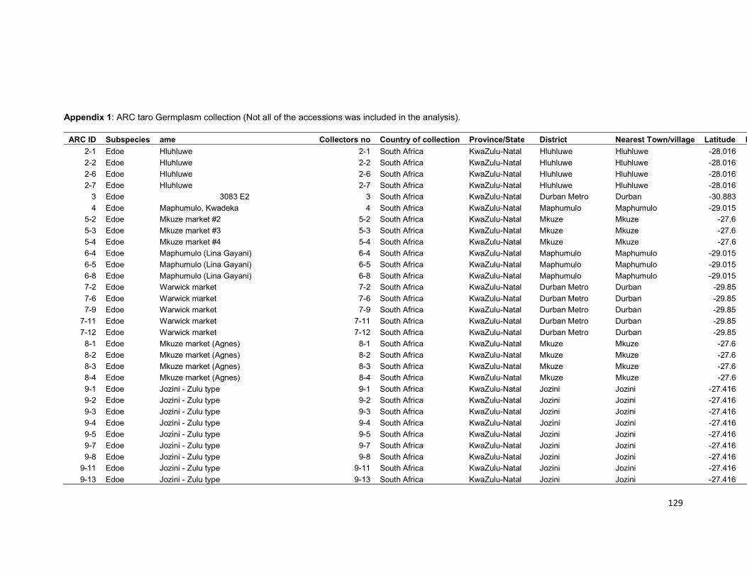
129

Appendix 1: ARC taro Germplasm collection (Not all of the accessions was included in the analysis).

ARC ID Subspecies ame Collectors no Country of collection Province/State District Nearest Town/village Latitude Longitude

2-1 Edoe Hluhluwe 2-1 South Africa KwaZulu-Natal Hluhluwe Hluhluwe -28.016

2-2 Edoe Hluhluwe 2-2 South Africa KwaZulu-Natal Hluhluwe Hluhluwe -28.016

2-6 Edoe Hluhluwe 2-6 South Africa KwaZulu-Natal Hluhluwe Hluhluwe -28.016

2-7 Edoe Hluhluwe 2-7 South Africa KwaZulu-Natal Hluhluwe Hluhluwe -28.016

3 Edoe 3083 E2 3 South Africa KwaZulu-Natal Durban Metro Durban -30.883

4 Edoe Maphumulo, Kwadeka 4 South Africa KwaZulu-Natal Maphumulo Maphumulo -29.015

5-2 Edoe Mkuze market #2 5-2 South Africa KwaZulu-Natal Mkuze Mkuze -27.6

5-3 Edoe Mkuze market #3 5-3 South Africa KwaZulu-Natal Mkuze Mkuze -27.6

5-4 Edoe Mkuze market #4 5-4 South Africa KwaZulu-Natal Mkuze Mkuze -27.6

6-4 Edoe Maphumulo (Lina Gayani) 6-4 South Africa KwaZulu-Natal Maphumulo Maphumulo -29.015

6-5 Edoe Maphumulo (Lina Gayani) 6-5 South Africa KwaZulu-Natal Maphumulo Maphumulo -29.015

6-8 Edoe Maphumulo (Lina Gayani) 6-8 South Africa KwaZulu-Natal Maphumulo Maphumulo -29.015

7-2 Edoe Warwick market 7-2 South Africa KwaZulu-Natal Durban Metro Durban -29.85

7-6 Edoe Warwick market 7-6 South Africa KwaZulu-Natal Durban Metro Durban -29.85

7-9 Edoe Warwick market 7-9 South Africa KwaZulu-Natal Durban Metro Durban -29.85

7-11 Edoe Warwick market 7-11 South Africa KwaZulu-Natal Durban Metro Durban -29.85

7-12 Edoe Warwick market 7-12 South Africa KwaZulu-Natal Durban Metro Durban -29.85

8-1 Edoe Mkuze market (Agnes) 8-1 South Africa KwaZulu-Natal Mkuze Mkuze -27.6

8-2 Edoe Mkuze market (Agnes) 8-2 South Africa KwaZulu-Natal Mkuze Mkuze -27.6

8-3 Edoe Mkuze market (Agnes) 8-3 South Africa KwaZulu-Natal Mkuze Mkuze -27.6

8-4 Edoe Mkuze market (Agnes) 8-4 South Africa KwaZulu-Natal Mkuze Mkuze -27.6

9-1 Edoe Jozini - Zulu type 9-1 South Africa KwaZulu-Natal Jozini Jozini -27.416

9-2 Edoe Jozini - Zulu type 9-2 South Africa KwaZulu-Natal Jozini Jozini -27.416

9-3 Edoe Jozini - Zulu type 9-3 South Africa KwaZulu-Natal Jozini Jozini -27.416

9-4 Edoe Jozini - Zulu type 9-4 South Africa KwaZulu-Natal Jozini Jozini -27.416

9-5 Edoe Jozini - Zulu type 9-5 South Africa KwaZulu-Natal Jozini Jozini -27.416

9-7 Edoe Jozini - Zulu type 9-7 South Africa KwaZulu-Natal Jozini Jozini -27.416

9-8 Edoe Jozini - Zulu type 9-8 South Africa KwaZulu-Natal Jozini Jozini -27.416

9-11 Edoe Jozini - Zulu type 9-11 South Africa KwaZulu-Natal Jozini Jozini -27.416

9-13 Edoe Jozini - Zulu type 9-13 South Africa KwaZulu-Natal Jozini Jozini -27.416

130

ARC ID Subspecies ame Collectors no Country of collection Province/State District Nearest Town/village Latitude Longitude

9-14 Edoe Jozini - Zulu type 9-14 South Africa KwaZulu-Natal Jozini Jozini -27.416

9-15 Edoe Jozini - Zulu type 9-15 South Africa KwaZulu-Natal Jozini Jozini -27.416

10-1 Edoe Mbazwana Market #2 10-1 South Africa KwaZulu-Natal Mbazwana Mbazwana -27.466

10-2 Edoe Mbazwana Market #3 10-2 South Africa KwaZulu-Natal Mbazwana Mbazwana -27.466

10-3 Edoe Mbazwana Market #4 10-3 South Africa KwaZulu-Natal Mbazwana Mbazwana -27.466

10-4 Edoe Mbazwana Market #5 10-4 South Africa KwaZulu-Natal Mbazwana Mbazwana -27.466

10-6 Edoe Mbazwana Market #7 10-6 South Africa KwaZulu-Natal Mbazwana Mbazwana -27.466

10-7 Edoe Mbazwana Market #8 10-7 South Africa KwaZulu-Natal Mbazwana Mbazwana -27.466

10-8 Edoe Mbazwana Market #9 10-8 South Africa KwaZulu-Natal Mbazwana Mbazwana -27.466

10-9 Edoe Mbazwana Market #10 10-9 South Africa KwaZulu-Natal Mbazwana Mbazwana -27.466

10-10 Edoe Mbazwana Market #11 10-10 South Africa KwaZulu-Natal Mbazwana Mbazwana -27.466

10-12 Edoe Mbazwana Market #12 10-12 South Africa KwaZulu-Natal Mbazwana Mbazwana -27.466

11 Edoe 59 in field multiplacation 11 South Africa KwaZulu-Natal 12 Edoe 70 in field multiplacation 12 South Africa KwaZulu-Natal 13 Edoe 1991 in field multiplacation 13 South Africa KwaZulu-Natal 14 Edoe 2053 in field multiplacation 14 South Africa KwaZulu-Natal 15 Edoe 2914 in field multiplacation 15 South Africa KwaZulu-Natal Umhlubuyalingana Jozini 16 Edoe 2919 in field multiplacation 16 South Africa KwaZulu-Natal Umhlubuyalingana Jozini

17-1 Edoe 3053 in field multiplacation 17-1 South Africa KwaZulu-Natal Mthonjaneni Empangeni 17-2 Edoe 3053Amzam in field multiplacation 17-2 South Africa KwaZulu-Natal Mthonjaneni Empangeni 17-3 Edoe 3053ex in field multiplacation 17-3 South Africa KwaZulu-Natal Mthonjaneni Empangeni 17-4 Edoe 3053/5118 Amzam 4 in field multiplacation 17-4 South Africa Unknown 18-1 Edoe 5118 in field multiplacation 18-1 South Africa KwaZulu-Natal 18-2 Edoe 5118 Amzam in field multiplacation 18-2 South Africa KwaZulu-Natal

19 Edoe 2053ex in field multiplacation 19 South Africa KwaZulu-Natal Mthonjaneni Empangeni 20 Edoe Ede Ocha in field multiplacation 20 South Africa KwaZulu-Natal

25-1 Edoe Makatini flats – Mpondo 25-1 South Africa KwaZulu-Natal Jozini Jozini -27.416

25-2 Edoe Makatini flats – Mpondo 25-2 South Africa KwaZulu-Natal Jozini Jozini -27.416

26 Edoe 1197 26 South Africa Eastern Province Mbhashe Willowvale -32.2097

27 Edoe 1329 27 South Africa Eastern Province Ingquza Lusikisiki -31.3378

28 Edoe 1338 28 South Africa Eastern Province Ingquza Lusikisiki -31.32

29 Edoe 1637 29 South Africa Eastern Province Mbizana Bizana -30.8803

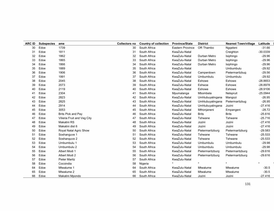
131

ARC ID Subspecies ame Collectors no Country of collection Province/State District Nearest Town/village Latitude Longitude

30 Edoe 1739 30 South Africa Eastern Province OR Thambo Ngqeleni -31.66

31 Edoe 1811 31 South Africa KwaZulu-Natal Creighton -30.0339

32 Edoe 1862 32 South Africa KwaZulu-Natal Durban Metro Isiphingo -29.96

33 Edoe 1865 33 South Africa KwaZulu-Natal Durban Metro Isiphingo -29.96

34 Edoe 1866 34 South Africa KwaZulu-Natal Durban Metro Isiphingo -29.96

35 Edoe 1889 35 South Africa KwaZulu-Natal Umbumbulu -29.92

36 Edoe 1906 36 South Africa KwaZulu-Natal Camperdown Pietermaritzbug -29.56

37 Edoe 1991 37 South Africa KwaZulu-Natal Umbumbulu Umbumbulu -29.92

38 Edoe 2045 38 South Africa KwaZulu-Natal Eshowe Eshowe -28.8653

39 Edoe 2073 39 South Africa KwaZulu-Natal Eshwoe Eshowe -28.8978

40 Edoe 2119 40 South Africa KwaZulu-Natal Eshowe Eshowe -28.9106

41 Edoe 2304 41 South Africa Mpumalanga Mbombela Nelspruit -25.0944

42 Edoe 2823 42 South Africa KwaZulu-Natal Umhlubuyalingana Mangozi -26.95

43 Edoe 2825 43 South Africa KwaZulu-Natal Umhlubuyalingana Pietermaritzbug -26.95

44 Edoe 2914 44 South Africa KwaZulu-Natal Umhlubuyalingana Jozini -27.416

45 Edoe 3053 45 South Africa KwaZulu-Natal Mthonjaneni Empangeni -28.72

46 Edoe Brits Pick and Pay 46 South Africa KwaZulu-Natal Brits Brits -25.616

47 Edoe Vilieria Fruit and Veg City 47 South Africa KwaZulu-Natal Tshwane Tshwane -25.716

48 Edoe Makatini RS 48 South Africa KwaZulu-Natal Jozini Jozini -27.416

49 Edoe Makatini dist 6 49 South Africa KwaZulu-Natal Jozini Jozini -27.416

50 Edoe Royal Natal Agric Show 50 South Africa KwaZulu-Natal Pietermaritzburg Pietermaritzburg -29.583

51 Edoe Soshanguve 1 51 South Africa KwaZulu-Natal Tshwane Tshwane -25.533

52 Edoe Soshanguve 2 52 South Africa KwaZulu-Natal Tshwane Tshwane -25.533

53 Edoe Umbumbulu 1 53 South Africa KwaZulu-Natal Umbumbulu Umbumbulu -29.98

54 Edoe Umbumbulu 2 54 South Africa KwaZulu-Natal Umbumbulu Umbumbulu -29.98

55 Edoe Albert Modi 1 55 South Africa KwaZulu-Natal Pietermaritzburg Pietermaritzburg -29.616

56 Edoe Albert Modi 2 56 South Africa KwaZulu-Natal Pietermaritzburg Pietermaritzburg -29.616

57 Edoe Pieter Maritz 57 South Africa KwaZulu-Natal 58 Edoe Cocoindia 58 Nigeria * * * * *

64 Edoe Mtwalume 1 64 South Africa KwaZulu-Natal Mtwalume Mtwalume -30.5

65 Edoe Mtwalume 2 65 South Africa KwaZulu-Natal Mtwalume Mtwalume -30.5

66 Edoe Makatini Mpondo 66 South Africa KwaZulu-Natal Jozini Jozini -27.416

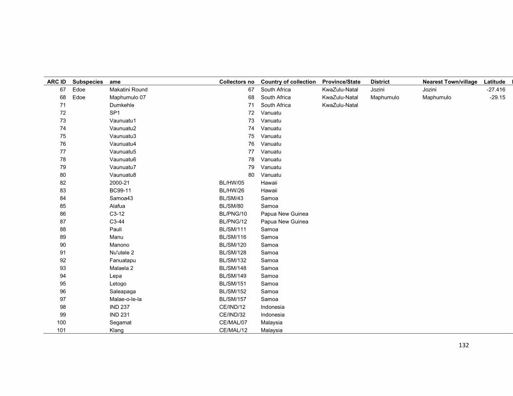
132

ARC ID Subspecies ame Collectors no Country of collection Province/State District Nearest Town/village Latitude Longitude

67 Edoe Makatini Round 67 South Africa KwaZulu-Natal Jozini Jozini -27.416

68 Edoe Maphumulo 07 68 South Africa KwaZulu-Natal Maphumulo Maphumulo -29.15

71 Dumkehle 71 South Africa KwaZulu-Natal 72 SP1 72 Vanuatu 73 Vaunuatu1 73 Vanuatu 74 Vaunuatu2 74 Vanuatu 75 Vaunuatu3 75 Vanuatu 76 Vaunuatu4 76 Vanuatu 77 Vaunuatu5 77 Vanuatu 78 Vaunuatu6 78 Vanuatu 79 Vaunuatu7 79 Vanuatu 80 Vaunuatu8 80 Vanuatu 82 2000-21 BL/HW/05 Hawaii 83 BC99-11 BL/HW/26 Hawaii 84 Samoa43 BL/SM/43 Samoa 85 Alafua BL/SM/80 Samoa 86 C3-12 BL/PNG/10 Papua New Guinea 87 C3-44 BL/PNG/12 Papua New Guinea 88 Pauli BL/SM/111 Samoa 89 Manu BL/SM/116 Samoa 90 Manono BL/SM/120 Samoa 91 Nu'utele 2 BL/SM/128 Samoa 92 Fanuatapu BL/SM/132 Samoa 93 Malaela 2 BL/SM/148 Samoa 94 Lepa BL/SM/149 Samoa 95 Letogo BL/SM/151 Samoa 96 Saleapaga BL/SM/152 Samoa 97 Malae-o-le-la BL/SM/157 Samoa 98 IND 237 CE/IND/12 Indonesia 99 IND 231 CE/IND/32 Indonesia

100 Segamat CE/MAL/07 Malaysia 101 Klang CE/MAL/12 Malaysia

133

ARC ID Subspecies ame Collectors no Country of collection Province/State District Nearest Town/village Latitude Longitude

102 Kluang CE/MAL/14 Malaysia 103 Edoe Srisamrong CE/THA/07 Thailand 104 Ta Daeng CE/THA/09 Thailand 105 Chom tim CE/VEN/01 Vietnam 106 Shogatsu-imo CA/JP/04 Japan 107 PE x PH15-6 BL/HW/08 Hawaii 108 Pa'akala BL/HW/37 Hawaii 109 C2-E3 BL/PNG/03 Papua New Guinea 110 C2-E11 BL/PNG/08 Papua New Guinea 111 C3-22 BL/PNG/11 Papua New Guinea 112 Samoana BL/SM/83 Samoa 113 Tolo-gataua BL/SM/104 Samoa 114 Sapapalii BL/SM/134 Samoa 115 Matautu BL/SM/136 Samoa 116 Vaimauga BL/SM/143 Samoa 117 Lalomanu BL/SM/158 Samoa 118 IND 155 CE/IND/06 Indonesia 119 IND 178 CE/IND/08 Indonesia 120 IND 225 CE/IND/10 Indonesia 121 Lamputara CE/IND/14 Indonesia 122 Apu CE/IND/20 Indonesia 123 IND 512 CE/IND/24 Indonesia 124 Manokwari CE/IND/31 Indonesia 125 Phuek CE/THA/01 Thailand 126 Surin CE/THA/02 Thailand 127 Tha-u-then CE/THA/19 Thailand 128 Boklua CE/THA/24 Thailand 129 Sangkom CE/THA/30 Thailand 130 Tsuronoko CA/JP/01 Japan 131 Miyako CA/JP/03 Japan

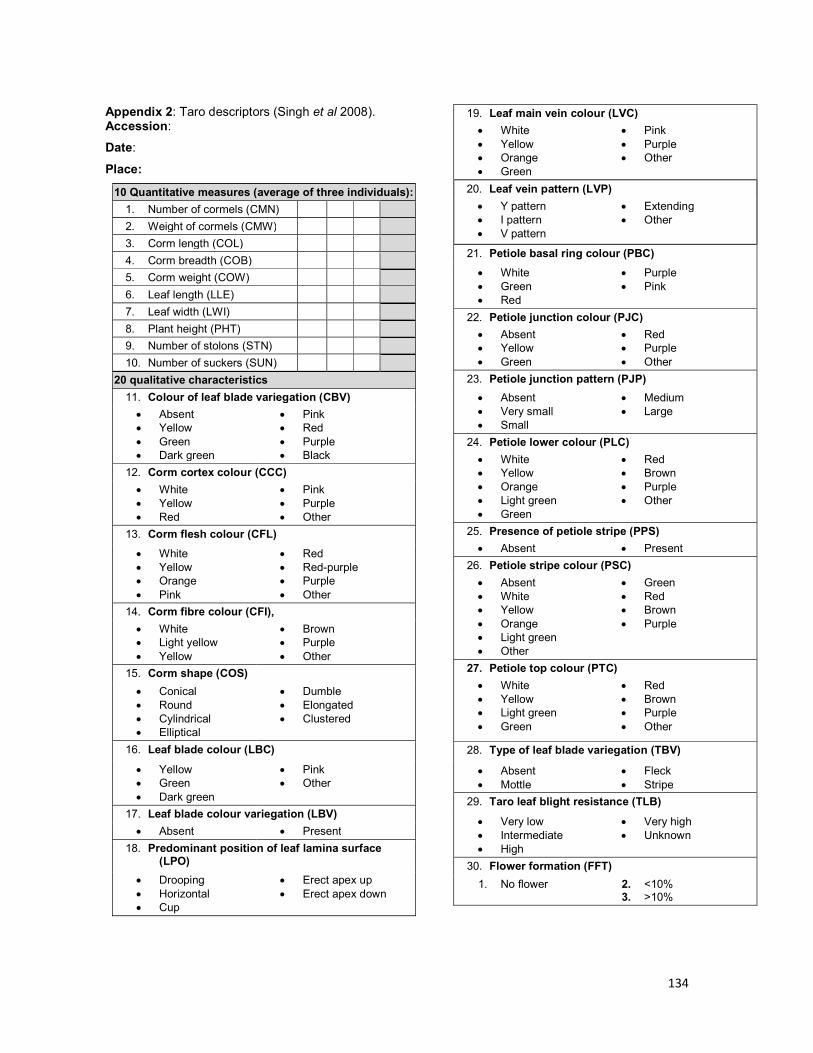
134

Appendix 2: Taro descriptors (Singh et al 2008). Accession:

Date:

Place:

10 Quantitative measures (average of three individuals):

1. Number of cormels (CMN)

2. Weight of cormels (CMW)

3. Corm length (COL)

4. Corm breadth (COB)

5. Corm weight (COW)

6. Leaf length (LLE)

7. Leaf width (LWI)

8. Plant height (PHT)

9. Number of stolons (STN)

10. Number of suckers (SUN)

20 qualitative characteristics

11. Colour of leaf blade variegation (CBV)

Absent Yellow Green Dark green

Pink Red Purple Black

12. Corm cortex colour (CCC)

White Yellow Red

Pink Purple Other

13. Corm flesh colour (CFL)

White Yellow Orange Pink

Red Red-purple Purple Other

14. Corm fibre colour (CFI),

White Light yellow Yellow

Brown Purple Other

15. Corm shape (COS)

Conical Round Cylindrical Elliptical

Dumble Elongated Clustered

16. Leaf blade colour (LBC)

Yellow Green Dark green

Pink Other

17. Leaf blade colour variegation (LBV)

Absent Present

18. Predominant position of leaf lamina surface (LPO)

Drooping Horizontal Cup

Erect apex up Erect apex down

19. Leaf main vein colour (LVC)

White Yellow Orange Green

Pink Purple Other

20. Leaf vein pattern (LVP)

Y pattern I pattern V pattern

Extending Other

21. Petiole basal ring colour (PBC)

White Green Red

Purple Pink

22. Petiole junction colour (PJC)

Absent Yellow Green

Red Purple Other

23. Petiole junction pattern (PJP)

Absent Very small Small

Medium Large

24. Petiole lower colour (PLC)

White Yellow Orange Light green Green

Red Brown Purple Other

25. Presence of petiole stripe (PPS)

Absent Present

26. Petiole stripe colour (PSC)

Absent White Yellow Orange Light green Other

Green Red Brown Purple

27. Petiole top colour (PTC)

White Yellow Light green Green

Red Brown Purple Other

28. Type of leaf blade variegation (TBV)

Absent Mottle

Fleck Stripe

29. Taro leaf blight resistance (TLB)

Very low Intermediate High

Very high Unknown

30. Flower formation (FFT)

1. No flower 2. <10% 3. >10%

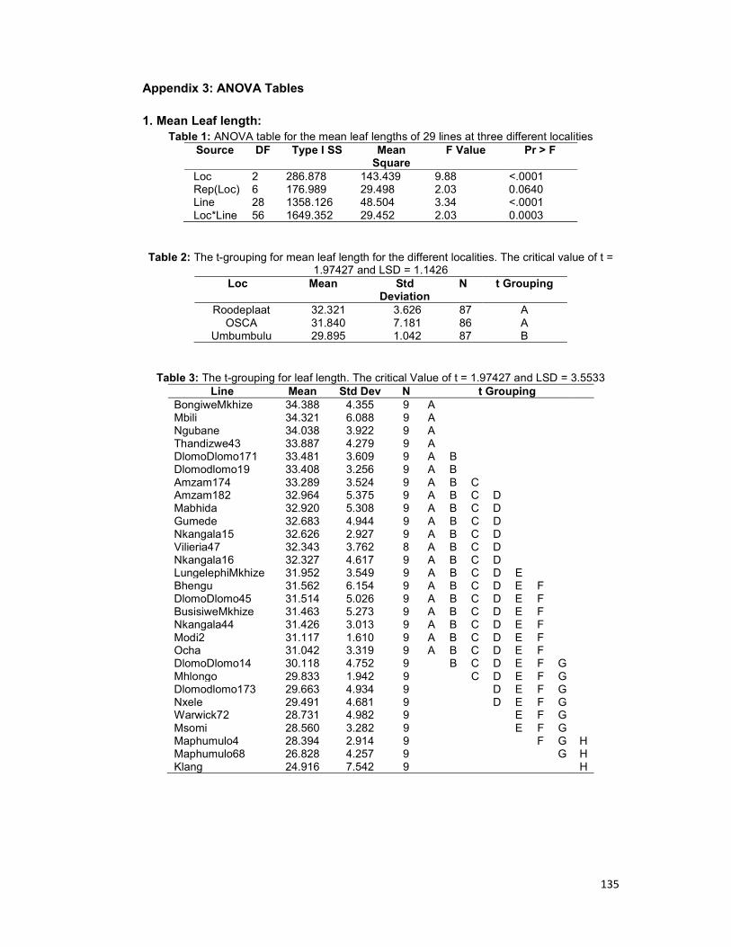
135

Appendix 3: ANOVA Tables 1. Mean Leaf length:

Table 1: ANOVA table for the mean leaf lengths of 29 lines at three different localities Source DF Type I SS Mean

Square F Value Pr > F

Loc 2 286.878 143.439 9.88 <.0001 Rep(Loc) 6 176.989 29.498 2.03 0.0640 Line 28 1358.126 48.504 3.34 <.0001 Loc*Line 56 1649.352 29.452 2.03 0.0003

Table 2: The t-grouping for mean leaf length for the different localities. The critical value of t = 1.97427 and LSD = 1.1426

Loc Mean Std Deviation

N t Grouping

Roodeplaat 32.321 3.626 87 A OSCA 31.840 7.181 86 A

Umbumbulu 29.895 1.042 87 B

Table 3: The t-grouping for leaf length. The critical Value of t = 1.97427 and LSD = 3.5533 Line Mean Std Dev N t Grouping

BongiweMkhize 34.388 4.355 9 A Mbili 34.321 6.088 9 A Ngubane 34.038 3.922 9 A Thandizwe43 33.887 4.279 9 A DlomoDlomo171 33.481 3.609 9 A B Dlomodlomo19 33.408 3.256 9 A B Amzam174 33.289 3.524 9 A B C Amzam182 32.964 5.375 9 A B C D Mabhida 32.920 5.308 9 A B C D Gumede 32.683 4.944 9 A B C D Nkangala15 32.626 2.927 9 A B C D Vilieria47 32.343 3.762 8 A B C D Nkangala16 32.327 4.617 9 A B C D LungelephiMkhize 31.952 3.549 9 A B C D E Bhengu 31.562 6.154 9 A B C D E F DlomoDlomo45 31.514 5.026 9 A B C D E F BusisiweMkhize 31.463 5.273 9 A B C D E F Nkangala44 31.426 3.013 9 A B C D E F Modi2 31.117 1.610 9 A B C D E F Ocha 31.042 3.319 9 A B C D E F DlomoDlomo14 30.118 4.752 9 B C D E F G Mhlongo 29.833 1.942 9 C D E F G Dlomodlomo173 29.663 4.934 9 D E F G Nxele 29.491 4.681 9 D E F G Warwick72 28.731 4.982 9 E F G Msomi 28.560 3.282 9 E F G Maphumulo4 28.394 2.914 9 F G H Maphumulo68 26.828 4.257 9 G H Klang 24.916 7.542 9 H

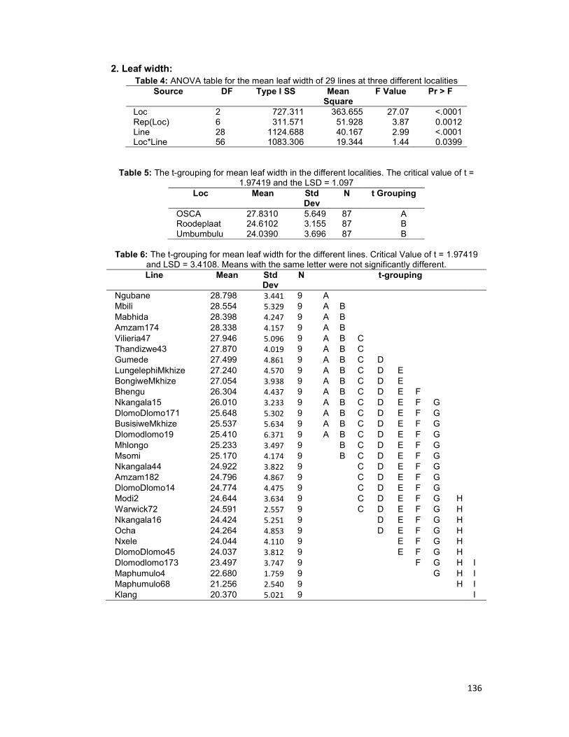
136

2. Leaf width: Table 4: ANOVA table for the mean leaf width of 29 lines at three different localities

Source DF Type I SS Mean Square

F Value Pr > F

Loc 2 727.311 363.655 27.07 <.0001 Rep(Loc) 6 311.571 51.928 3.87 0.0012 Line 28 1124.688 40.167 2.99 <.0001 Loc*Line 56 1083.306 19.344 1.44 0.0399

Table 5: The t-grouping for mean leaf width in the different localities. The critical value of t = 1.97419 and the LSD = 1.097

Loc Mean Std Dev

N t Grouping

OSCA 27.8310 5.649 87 A Roodeplaat 24.6102 3.155 87 B Umbumbulu 24.0390 3.696 87 B

Table 6: The t-grouping for mean leaf width for the different lines. Critical Value of t = 1.97419

and LSD = 3.4108. Means with the same letter were not significantly different. Line Mean Std

Dev N t-grouping

Ngubane 28.798 3.441 9 A Mbili 28.554 5.329 9 A B Mabhida 28.398 4.247 9 A B Amzam174 28.338 4.157 9 A B Vilieria47 27.946 5.096 9 A B C Thandizwe43 27.870 4.019 9 A B C Gumede 27.499 4.861 9 A B C D LungelephiMkhize 27.240 4.570 9 A B C D E BongiweMkhize 27.054 3.938 9 A B C D E Bhengu 26.304 4.437 9 A B C D E F Nkangala15 26.010 3.233 9 A B C D E F G DlomoDlomo171 25.648 5.302 9 A B C D E F G BusisiweMkhize 25.537 5.634 9 A B C D E F G Dlomodlomo19 25.410 6.371 9 A B C D E F G Mhlongo 25.233 3.497 9 B C D E F G Msomi 25.170 4.174 9 B C D E F G Nkangala44 24.922 3.822 9 C D E F G Amzam182 24.796 4.867 9 C D E F G DlomoDlomo14 24.774 4.475 9 C D E F G Modi2 24.644 3.634 9 C D E F G H Warwick72 24.591 2.557 9 C D E F G H Nkangala16 24.424 5.251 9 D E F G H Ocha 24.264 4.853 9 D E F G H Nxele 24.044 4.110 9 E F G H DlomoDlomo45 24.037 3.812 9 E F G H Dlomodlomo173 23.497 3.747 9 F G H I Maphumulo4 22.680 1.759 9 G H I Maphumulo68 21.256 2.540 9 H I Klang 20.370 5.021 9 I

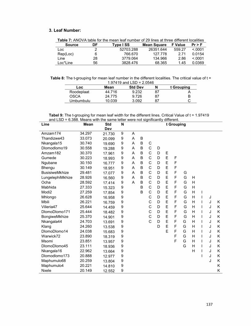
137

3. Leaf Number:

Table 7: ANOVA table for the mean leaf number of 29 lines at three different localities Source DF Type I SS Mean Square F Value Pr > F

Loc 2 52703.288 26351.644 559.27 <.0001 Rep(Loc) 6 766.670 127.778 2.71 0.0154 Line 28 3779.064 134.966 2.86 <.0001 Loc*Line 56 3828.476 68.365 1.45 0.0369

Table 8: The t-grouping for mean leaf number in the different localities. The critical value of t =

1.97419 and LSD = 2.0546 Loc Mean Std Dev N t Grouping

Roodeplaat 44.716 9.232 87 A OSCA 24.775 9.726 87 B Umbumbulu 10.039 3.092 87 C

Tabel 9: The t-grouping for mean leaf width for the different lines. Critical Value of t = 1.97419 and LSD = 6.388. Means with the same letter were not significantly different.

Line Mean Std Dev

N t Grouping

Amzam174 34.297 21.730 9 A Thandizwe43 33.073 20.099 9 A B Nkangala15 30.740 19.690 9 A B C Dlomodlomo19 30.558 19.288 9 A B C D Amzam182 30.370 17.961 9 A B C D E Gumede 30.223 18.993 9 A B C D E F Ngubane 30.150 16.777 9 A B C D E F Bhengu 30.149 18.951 9 A B C D E F BusisiweMkhize 29.481 17.077 9 A B C D E F G LungelephiMkhize 28.926 16.560 9 A B C D E F G H Ocha 28.592 17.414 9 A B C D E F G H Mabhida 27.333 15.323 9 B C D E F G H Modi2 27.259 17.854 9 B C D E F G H I Mhlongo 26.628 16.958 9 C D E F G H I J Mbili 26.221 16.759 9 C D E F G H I J K Vilieria47 25.644 14.459 9 C D E F G H I J K DlomoDlomo171 25.444 18.482 9 C D E F G H I J K BongiweMkhize 25.370 14.901 9 C D E F G H I J K Nkangala44 24.703 13.691 9 C D E F G H I J K Klang 24.260 13.538 9 D E F G H I J K DlomoDlomo14 24.038 15.683 9 E F G H I J K Warwick72 23.890 18.319 9 F G H I J K Msomi 23.851 13.957 9 F G H I J K DlomoDlomo45 23.111 18.936 9 G H I J K Nkangala16 22.962 13.664 9 H I J K Dlomodlomo173 20.888 12.977 9 I J K Maphumulo68 20.259 13.804 9 J K Maphumulo4 20.221 14.810 9 K Nxele 20.149 12.552 9 K

138

4. Plant height: Table 10: ANOVA table for the mean plant height of 29 lines at three different localities Source DF Type I SS Mean

Square F Value

Pr > F

Loc 2 15100.598 7550.299 48.36 <.0001 Rep(Loc) 6 1258.235 209.705 1.34 0.2407 Line 28 12169.043 434.608 2.78 <.0001 Loc*Line 56 12203.793 217.924 1.40 0.0547

Table 11: The t-grouping for mean plant height in the different localities. Means with the same

letter were not significantly different. The critical value of t = 1.97419 and LSD = 3.7401 Loc Mean Std Dev N t Grouping OSCA 80.822 20.505 87 A Roodeplaat 76.799 10.337 87 B Umbumbulu 63.056 8.7001 87 C

Table 12: The t-grouping for mean plant height for the different lines. Critical Value of t = 1.97419 and LSD = 11.629. Means with the same letter were not significantly different.

Line Mean Std Dev N t Grouping Ngubane 85.631 15.146 9 A Amzam174 85.427 13.838 9 A Thandizwe43 82.721 12.298 9 A B BongiweMkhize 81.444 19.136 9 A B C Vilieria47 79.446 14.633 9 A B C D Mbili 79.112 15.641 9 A B C D E Nkangala15 79.088 12.415 9 A B C D E Nkangala16 78.092 18.118 9 A B C D E LungelephiMkhize 77.852 15.405 9 A B C D E DlomoDlomo171 77.740 18.737 9 A B C D E Gumede 76.408 17.881 9 A B C D E F Nkangala44 76.168 11.597 9 A B C D E F Dlomodlomo19 75.647 18.818 9 A B C D E F Mabhida 75.408 11.221 9 A B C D E F Amzam182 74.943 21.427 9 A B C D E F Bhengu 74.666 19.040 9 A B C D E F Mhlongo 71.684 10.312 9 B C D E F G Ocha 71.056 14.201 9 C D E F G H BusisiweMkhize 71.019 18.235 9 C D E F G H Modi2 70.686 16.559 9 C D E F G H Msomi 69.767 16.057 9 D E F G H Warwick72 69.537 12.268 9 D E F G H DlomoDlomo45 68.693 14.753 9 D E F G H DlomoDlomo14 67.722 14.066 9 E F G H Nxele 65.871 14.240 9 F G H Dlomodlomo173 65.563 18.890 9 F G H Maphumulo4 61.220 9.249 9 G H Klang 61.148 7.953 9 G H Maphumulo68 59.454 13.355 9 H

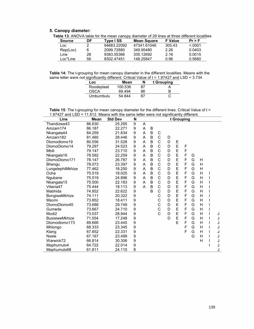
139

5. Canopy diameter: Table 13: ANOVA table for the mean canopy diameter of 29 lines at three different localities

Source DF Type I SS Mean Square F Value Pr > F Loc 2 94683.22092 47341.61046 305.43 <.0001 Rep(Loc) 6 2099.72880 349.95480 2.26 0.0403 Line 28 9383.55366 335.12692 2.16 0.0015 Loc*Line 56 8302.47451 148.25847 0.96 0.5660

Table 14: The t-grouping for mean canopy diameter in the different localities. Means with the same letter were not significantly different. Critical Value of t = 1.97427 and LSD = 3.734

Loc Mean N t Grouping Roodeplaat 100.536 87 A OSCA 69.494 86 B Umbumbulu 54.844 87 C

Table 15: The t-grouping for mean canopy diameter for the different lines. Critical Value of t = 1.97427 and LSD = 11.612. Means with the same letter were not significantly different.

Line Mean Std Dev N t Grouping Thandizwe43 86.630 25.265 9 A Amzam174 86.187 22.271 9 A B Nkangala44 84.259 21.834 9 A B C Amzam182 81.480 28.446 9 A B C D Dlomodlomo19 80.556 31.528 9 A B C D E DlomoDlomo14 79.297 24.523 9 A B C D E F Mbili 79.147 23.710 9 A B C D E F Nkangala16 78.592 22.259 9 A B C D E F G DlomoDlomo171 78.147 26.787 9 A B C D E F G H Bhengu 78.073 23.397 9 A B C D E F G H LungelephiMkhize 77.462 18.250 9 A B C D E F G H Ocha 75.519 18.025 9 A B C D E F G H I Ngubane 75.519 24.896 9 A B C D E F G H I Nkangala15 75.500 22.183 9 A B C D E F G H I Vilieria47 75.444 18.113 9 A B C D E F G H I Mabhida 74.852 22.622 9 B C D E F G H I BongiweMkhize 74.111 20.322 9 C D E F G H I Msomi 73.852 18.411 9 C D E F G H I DlomoDlomo45 73.688 29.749 9 C D E F G H I Gumede 73.667 24.710 9 C D E F G H I Modi2 73.037 28.944 9 C D E F G H I J BusisiweMkhize 71.554 17.248 9 D E F G H I J Dlomodlomo173 69.666 23.445 9 E F G H I J Mhlongo 68.333 23.345 9 F G H I J Klang 67.852 22.331 9 F G H I J Nxele 67.167 23.499 9 G H I J Warwick72 66.814 30.306 9 H I J Maphumulo4 64.722 22.014 9 I J Maphumulo68 61.811 24.110 8 J

140

6. Number of suckers Table 16: ANOVA table for the mean number of suckers of 29 lines at three different localities

Source DF Type I SS Mean Square F Value Pr > F Loc 2 7271.477870 3635.738935 548.68 <.0001 Rep(Loc) 6 353.423462 58.903910 8.89 <.0001 Line 28 947.411842 33.836137 5.11 <.0001 Loc*Line 56 708.662869 12.654694 1.91 0.0009

Table 17: The t-grouping for mean number of suckers in the different localities. Means with the same letter were not significantly different. Critical Value of t = 1.97427 and LSD = 0.772

Loc Mean N t Grouping Roodeplaat 16.0543 86 A OSCA 11.5317 87 B Umbumbulu 3.2761 87 C

Table 18: The t-grouping for mean number of suckers for the different lines. Critical Value of t = 1.97427 and LSD = 2.4009. Means with the same letter were not significantly different. Line Mean Srd

Dev N t Grouping

Amzam174 14.558 7.628 9 A Nkangala15 13.518 8.706 9 A B Thandizwe43 13.408 7.759 9 A B DlomoDlomo171 13.074 8.187 9 A B C Dlomodlomo19 12.184 6.409 9 A B C D Amzam182 12.000 6.423 9 B C D E Ocha 11.927 7.702 9 B C D E Nkangala44 11.371 4.610 9 B C D E F BusisiweMkhize 11.000 7.118 9 C D E F G Modi2 10.999 7.295 9 C D E F G Nkangala16 10.927 5.648 9 C D E F G Ngubane 10.778 6.309 9 C D E F G H Bhengu 10.519 6.345 9 D E F G H Mbili 10.124 9.751 8 D E F G H I BongiweMkhize 10.074 6.702 9 D E F G H I Maphumulo4 10.038 5.096 9 D E F G H I Dlomodlomo173 9.703 6.402 9 E F G H I J Mabhida 9.519 5.470 9 F G H I J LungelephiMkhize 9.109 5.865 9 F G H I J K Gumede 9.073 5.213 9 F G H I J K Vilieria47 8.993 3.960 9 F G H I J K Mhlongo 8.779 5.700 9 G H I J K DlomoDlomo14 8.666 5.099 9 G H I J K DlomoDlomo45 8.442 6.194 9 H I J K Warwick72 8.429 5.973 9 H I J K Klang 8.057 5.689 9 I J K Msomi 8.000 5.196 9 I J K Nxele 7.630 4.774 9 J K Maphumulo68 6.777 4.812 9 K

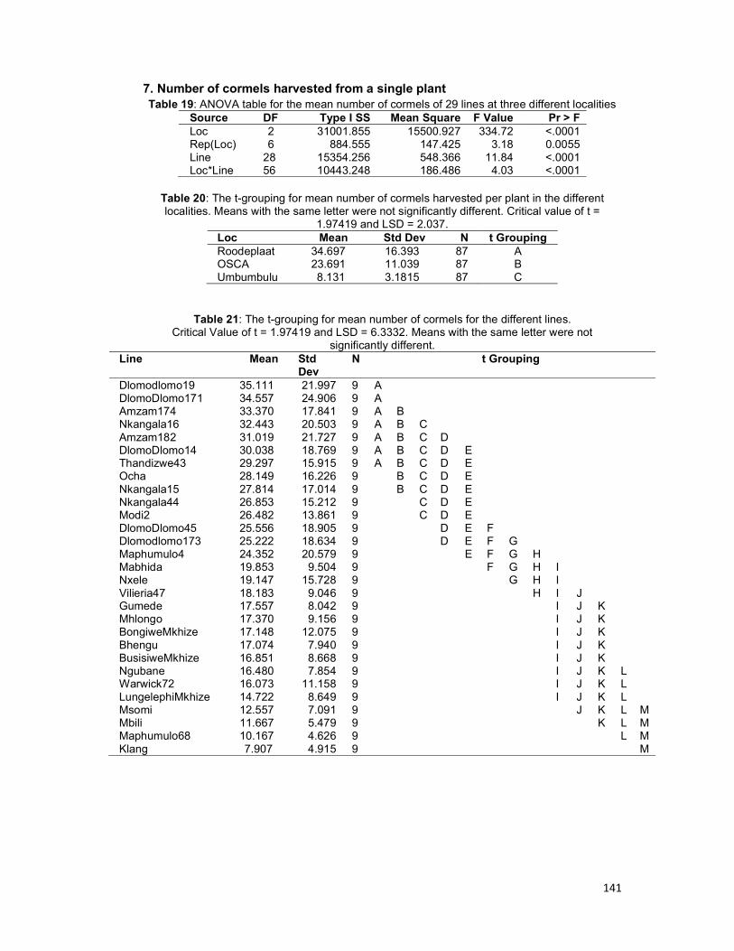
141

7. Number of cormels harvested from a single plant Table 19: ANOVA table for the mean number of cormels of 29 lines at three different localities

Source DF Type I SS Mean Square F Value Pr > F Loc 2 31001.855 15500.927 334.72 <.0001 Rep(Loc) 6 884.555 147.425 3.18 0.0055 Line 28 15354.256 548.366 11.84 <.0001 Loc*Line 56 10443.248 186.486 4.03 <.0001

Table 20: The t-grouping for mean number of cormels harvested per plant in the different localities. Means with the same letter were not significantly different. Critical value of t =

1.97419 and LSD = 2.037. Loc Mean Std Dev N t Grouping Roodeplaat 34.697 16.393 87 A OSCA 23.691 11.039 87 B Umbumbulu 8.131 3.1815 87 C

Table 21: The t-grouping for mean number of cormels for the different lines. Critical Value of t = 1.97419 and LSD = 6.3332. Means with the same letter were not

significantly different. Line Mean Std

Dev N t Grouping

Dlomodlomo19 35.111 21.997 9 A DlomoDlomo171 34.557 24.906 9 A Amzam174 33.370 17.841 9 A B Nkangala16 32.443 20.503 9 A B C Amzam182 31.019 21.727 9 A B C D DlomoDlomo14 30.038 18.769 9 A B C D E Thandizwe43 29.297 15.915 9 A B C D E Ocha 28.149 16.226 9 B C D E Nkangala15 27.814 17.014 9 B C D E Nkangala44 26.853 15.212 9 C D E Modi2 26.482 13.861 9 C D E DlomoDlomo45 25.556 18.905 9 D E F Dlomodlomo173 25.222 18.634 9 D E F G Maphumulo4 24.352 20.579 9 E F G H Mabhida 19.853 9.504 9 F G H I Nxele 19.147 15.728 9 G H I Vilieria47 18.183 9.046 9 H I J Gumede 17.557 8.042 9 I J K Mhlongo 17.370 9.156 9 I J K BongiweMkhize 17.148 12.075 9 I J K Bhengu 17.074 7.940 9 I J K BusisiweMkhize 16.851 8.668 9 I J K Ngubane 16.480 7.854 9 I J K L Warwick72 16.073 11.158 9 I J K L LungelephiMkhize 14.722 8.649 9 I J K L Msomi 12.557 7.091 9 J K L M Mbili 11.667 5.479 9 K L M Maphumulo68 10.167 4.626 9 L M Klang 7.907 4.915 9 M

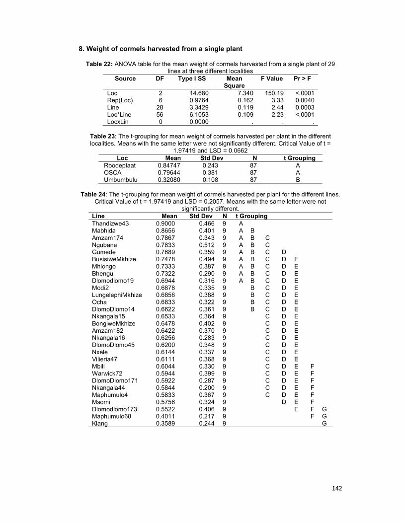
142

8. Weight of cormels harvested from a single plant

Table 22: ANOVA table for the mean weight of cormels harvested from a single plant of 29 lines at three different localities

Source DF Type I SS Mean Square

F Value Pr > F

Loc 2 14.680 7.340 150.19 <.0001 Rep(Loc) 6 0.9764 0.162 3.33 0.0040 Line 28 3.3429 0.119 2.44 0.0003 Loc*Line 56 6.1053 0.109 2.23 <.0001 LocxLin 0 0.0000 . . .

Table 23: The t-grouping for mean weight of cormels harvested per plant in the different localities. Means with the same letter were not significantly different. Critical Value of t =

1.97419 and LSD = 0.0662 Loc Mean Std Dev N t Grouping

Roodeplaat 0.84747 0.243 87 A OSCA 0.79644 0.381 87 A Umbumbulu 0.32080 0.108 87 B

Table 24: The t-grouping for mean weight of cormels harvested per plant for the different lines.

Critical Value of t = 1.97419 and LSD = 0.2057. Means with the same letter were not significantly different.

Line Mean Std Dev N t Grouping Thandizwe43 0.9000 0.466 9 A Mabhida 0.8656 0.401 9 A B Amzam174 0.7867 0.343 9 A B C Ngubane 0.7833 0.512 9 A B C Gumede 0.7689 0.359 9 A B C D BusisiweMkhize 0.7478 0.494 9 A B C D E Mhlongo 0.7333 0.387 9 A B C D E Bhengu 0.7322 0.290 9 A B C D E Dlomodlomo19 0.6944 0.316 9 A B C D E Modi2 0.6878 0.335 9 B C D E LungelephiMkhize 0.6856 0.388 9 B C D E Ocha 0.6833 0.322 9 B C D E DlomoDlomo14 0.6622 0.361 9 B C D E Nkangala15 0.6533 0.364 9 C D E BongiweMkhize 0.6478 0.402 9 C D E Amzam182 0.6422 0.370 9 C D E Nkangala16 0.6256 0.283 9 C D E DlomoDlomo45 0.6200 0.348 9 C D E Nxele 0.6144 0.337 9 C D E Vilieria47 0.6111 0.368 9 C D E Mbili 0.6044 0.330 9 C D E F Warwick72 0.5944 0.399 9 C D E F DlomoDlomo171 0.5922 0.287 9 C D E F Nkangala44 0.5844 0.200 9 C D E F Maphumulo4 0.5833 0.367 9 C D E F Msomi 0.5756 0.324 9 D E F Dlomodlomo173 0.5522 0.406 9 E F G Maphumulo68 0.4011 0.217 9 F G Klang 0.3589 0.244 9 G

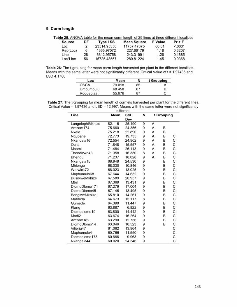
143

9. Corm length

Table 25: ANOVA table for the mean corm length of 29 lines at three different localities Source DF Type I SS Mean Square F Value Pr > F Loc 2 23514.95350 11757.47675 60.81 <.0001 Rep(Loc) 6 1365.97072 227.66179 1.18 0.3207 Line 28 6812.95758 243.31991 1.26 0.1885 Loc*Line 56 15725.48557 280.81224 1.45 0.0368

Table 26: The t-grouping for mean corm length harvested per plant in the different localities. Means with the same letter were not significantly different. Critical Value of t = 1.97436 and LSD 4.1786

Loc Mean N t Grouping OSCA 79.018 85 A Umbumbulu 68.458 87 B Roodeplaat 55.676 87 C

Table 27: The t-grouping for mean length of cormels harvested per plant for the different lines. Critical Value = 1.97436 and LSD = 12.997. Means with the same letter were not significantly

different. Line Mean Std

Dev N t Grouping

LungelephiMkhize 82.116 25.190 9 A Amzam174 75.660 24.356 9 A B Nxele 75.218 22.890 9 A B Ngubane 72.773 19.735 9 A B C Nkangala16 72.554 24.902 9 A B C Ocha 71.848 15.557 9 A B C Msomi 71.484 26.113 9 A B C Thandizwe43 71.358 16.350 8 A B C Bhengu 71.237 18.028 9 A B C Nkangala15 68.949 24.530 9 B C Mhlongo 68.030 10.846 9 B C Warwick72 68.023 18.025 9 B C Maphumulo68 67.644 14.632 9 B C BusisiweMkhize 67.589 20.957 9 B C Mbili 67.369 13.431 9 B C DlomoDlomo171 67.279 17.004 9 B C DlomoDlomo45 67.146 18.495 9 B C BongiweMkhize 65.810 14.261 9 B C Mabhida 64.673 15.117 8 B C Gumede 64.390 11.447 9 B C Klang 63.887 6.822 9 B C Dlomodlomo19 63.800 14.442 9 B C Modi2 63.674 16.264 9 B C Amzam182 63.290 12.736 9 B C DlomoDlomo14 63.046 10.523 9 B C Vilieria47 61.062 13.964 9 C Maphumulo4 60.766 11.550 9 C Dlomodlomo173 60.666 9.963 9 C Nkangala44 60.020 24.346 9 C

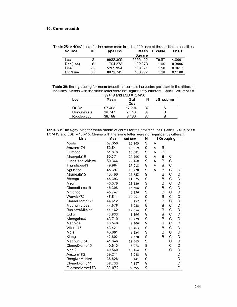
144

10, Corm breadth

Table 28: ANOVA table for the mean corm breath of 29 lines at three different localities Source DF Type I SS Mean

Square F Value Pr > F

Loc 2 19932.305 9966.152 79.57 <.0001 Rep(Loc) 6 794.273 132.378 1.06 0.3906 Line 28 5265.994 188.071 1.50 0.0617 Loc*Line 56 8972.745 160.227 1.28 0.1180

Table 29: the t-grouping for mean breadth of cormels harvested per plant in the different localities. Means with the same letter were not significantly different. Critical Value of t =

1.97419 and LSD = 3.3498 Loc Mean Std

Dev N t Grouping

OSCA 57.463 17.294 87 A Umbumbulu 39.747 7.013 87 B Roodeplaat 38.199 8.436 87 B

Table 30: The t-grouping for mean breath of corms for the different lines. Critical Value of t = 1.97419 and LSD = 10.415. Means with the same letter were not significantly different.

Line Mean Std Dev N t Grouping Nxele 57.358 20.109 9 A Amzam174 52.541 19.819 9 A B Gumede 51.878 15.081 9 A B Nkangala16 50.371 24.596 9 A B C LungelephiMkhize 50.344 23.168 9 A B C Thandizwe43 49.964 17.018 9 A B C Ngubane 48.397 15.720 9 A B C D Nkangala15 46.460 22.752 9 B C D Bhengu 46.393 11.975 9 B C D Msomi 46.379 22.130 9 B C D Dlomodlomo19 46.308 13.308 9 B C D Mhlongo 45.747 8.196 9 B C D Warwick72 45.511 15.561 9 B C D DlomoDlomo171 44.612 9.457 9 B C D Maphumulo68 44.576 6.088 9 B C D BusisiweMkhize 44.162 17.354 9 B C D Ocha 43.833 8.896 9 B C D Nkangala44 43.710 19.779 9 B C D Mabhida 43.540 9.406 9 B C D Vilieria47 43.421 16.463 9 B C D Mbili 43.081 8.154 9 B C D Klang 42.802 7.570 9 B C D Maphumulo4 41.346 12.963 9 C D DlomoDlomo45 40.813 6.073 9 C D Modi2 40.560 15.164 9 C D Amzam182 39.211 8.048 9 D BongiweMkhize 38.828 8.141 9 D DlomoDlomo14 38.733 4.687 9 D Dlomodlomo173 38.072 5.755 9 D

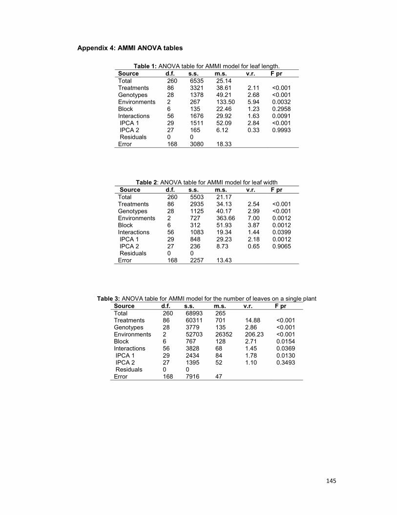
145

Appendix 4: AMMI ANOVA tables

Table 1: ANOVA table for AMMI model for leaf length.

Source d.f. s.s. m.s. v.r. F pr Total 260 6535 25.14 Treatments 86 3321 38.61 2.11 <0.001 Genotypes 28 1378 49.21 2.68 <0.001 Environments 2 267 133.50 5.94 0.0032 Block 6 135 22.46 1.23 0.2958 Interactions 56 1676 29.92 1.63 0.0091 IPCA 1 29 1511 52.09 2.84 <0.001 IPCA 2 27 165 6.12 0.33 0.9993 Residuals 0 0 Error 168 3080 18.33

Table 2: ANOVA table for AMMI model for leaf width Source d.f. s.s. m.s. v.r. F pr Total 260 5503 21.17 Treatments 86 2935 34.13 2.54 <0.001 Genotypes 28 1125 40.17 2.99 <0.001 Environments 2 727 363.66 7.00 0.0012 Block 6 312 51.93 3.87 0.0012 Interactions 56 1083 19.34 1.44 0.0399 IPCA 1 29 848 29.23 2.18 0.0012 IPCA 2 27 236 8.73 0.65 0.9065 Residuals 0 0 Error 168 2257 13.43

Table 3: ANOVA table for AMMI model for the number of leaves on a single plant Source d.f. s.s. m.s. v.r. F pr Total 260 68993 265 Treatments 86 60311 701 14.88 <0.001 Genotypes 28 3779 135 2.86 <0.001 Environments 2 52703 26352 206.23 <0.001 Block 6 767 128 2.71 0.0154 Interactions 56 3828 68 1.45 0.0369 IPCA 1 29 2434 84 1.78 0.0130 IPCA 2 27 1395 52 1.10 0.3493 Residuals 0 0 Error 168 7916 47

146

Table 4: ANOVA table for AMMI model for plant height. Source d.f. s.s. m.s. v.r. F pr Total 260 66962 258 Treatments 86 39473 459 2.94 <0.001 Genotypes 28 12169 435 2.78 <0.001 Environments 2 15101 7550 36.00 <0.001 Block 6 1258 210 1.34 0.2407 Interactions 56 12204 218 1.40 0.0547 IPCA 1 29 9668 333 2.14 0.0015 IPCA 2 27 2536 94 0.60 0.9397 Residuals 0 0 Error 168 26230 156

Table 5: ANOVA table for AMMI model for canopy diameter. Source d.f. s.s. m.s. v.r. F pr Total 260 141826 545 Treatments 86 113865 1324 8.54 <0.001 Genotypes 28 10155 363 2.34 <0.001 Environments 2 95082 47541 137.42 <0.001 Block 6 2076 346 2.23 0.0425 Interactions 56 8628 154 0.99 0.4964 IPCA 1 29 5428 187 1.21 0.2289 IPCA 2 27 3200 119 0.76 0.7916 Residuals 0 0 Error 167 25885 155

Table 6: ANOVA table for AMMI model for the number of suckers per plant. Source d.f. s.s. m.s. v.r. F pr Total 260 10398 40.0 Treatments 86 8757 101.8 13.72 <0.001 Genotypes 28 949 33.9 4.57 <0.001 Environments 2 7201 3600.5 54.77 <0.001 Block 6 394 65.7 8.86 <0.001 Interactions 56 607 10.8 1.46 0.0341 IPCA 1 29 336 11.6 1.56 0.0434 IPCA 2 27 271 10.0 1.35 0.1279 Residuals 0 0 Error 168 1246 7.4

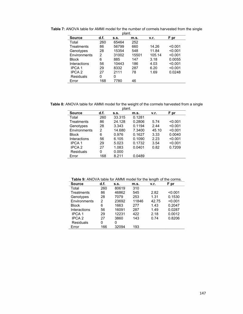
147

Table 7: ANOVA table for AMMI model for the number of cormels harvested from the single plant.

Source d.f. s.s. m.s. v.r. F pr Total 260 65464 252 Treatments 86 56799 660 14.26 <0.001 Genotypes 28 15354 548 11.84 <0.001 Environments 2 31002 15501 105.14 <0.001 Block 6 885 147 3.18 0.0055 Interactions 56 10443 186 4.03 <0.001 IPCA 1 29 8332 287 6.20 <0.001 IPCA 2 27 2111 78 1.69 0.0248 Residuals 0 0 Error 168 7780 46

Table 8: ANOVA table for AMMI model for the weight of the cormels harvested from a single plant.

Source d.f. s.s. m.s. v.r. F pr Total 260 33.315 0.1281 Treatments 86 24.128 0.2806 5.74 <0.001 Genotypes 28 3.343 0.1194 2.44 <0.001 Environments 2 14.680 7.3400 45.10 <0.001 Block 6 0.976 0.1627 3.33 0.0040 Interactions 56 6.105 0.1090 2.23 <0.001 IPCA 1 29 5.023 0.1732 3.54 <0.001 IPCA 2 27 1.083 0.0401 0.82 0.7209 Residuals 0 0.000 Error 168 8.211 0.0489

Table 9: ANOVA table for AMMI model for the length of the corms. Source d.f. s.s. m.s. v.r. F pr Total 260 80619 310 Treatments 86 46862 545 2.82 <0.001 Genotypes 28 7079 253 1.31 0.1530 Environments 2 23692 11846 42.75 <0.001 Block 6 1663 277 1.43 0.2047 Interactions 56 16091 287 1.49 0.0287 IPCA 1 29 12231 422 2.18 0.0012 IPCA 2 27 3860 143 0.74 0.8206 Residuals 0 0 Error 166 32094 193

148

Table 10: ANOVA table for AMMI model for the breadth of the corms d.f. s.s. m.s. v.r. F pr Total 260 56006 215 Treatments 86 34171 397 3.17 <0.001 Genotypes 28 5266 188 1.50 0.0617 Environments 2 19932 9966 75.29 <0.001 Block 6 794 132 1.06 0.3906 Interactions 56 8973 160 1.28 0.1180 IPCA 1 29 7352 254 2.02 0.0030 IPCA 2 27 1621 60 0.48 0.9866 Residuals 0 0 Error 168 21041 125

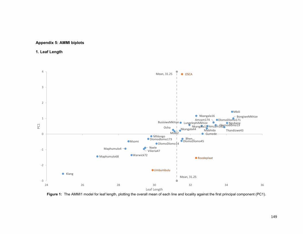
149

Appendix 5: AMMI biplots

1. Leaf Length

Figure 1: The AMMI1 model for leaf length, plotting the overall mean of each line and locality against the first principal component (PC1).

Amzam174

Amzam182

Bhen…

BongiweMkhize

BusisiweMkhize

DlomoDlomo14

DlomoDlomo171

Dlomodlomo173

Dlomodlomo19

DlomoDlomo45

Gumede

Klang

LungelephiMkhize

Mabhida

Maphumulo4

Maphumulo68

Mbili

MhlongoModi2

Msomi

NgubaneNkangala15

Nkangala16

Nkangala44

Nxele

OchaThandizwe43

Vilieria47Warwick72

OSCA

Roodeplaat

Umbumbulu

Mean, 31.25

Mean, 31.25

-3

-2

-1

0

1

2

3

4

24 26 28 30 32 34 36

PC1

Leaf Length

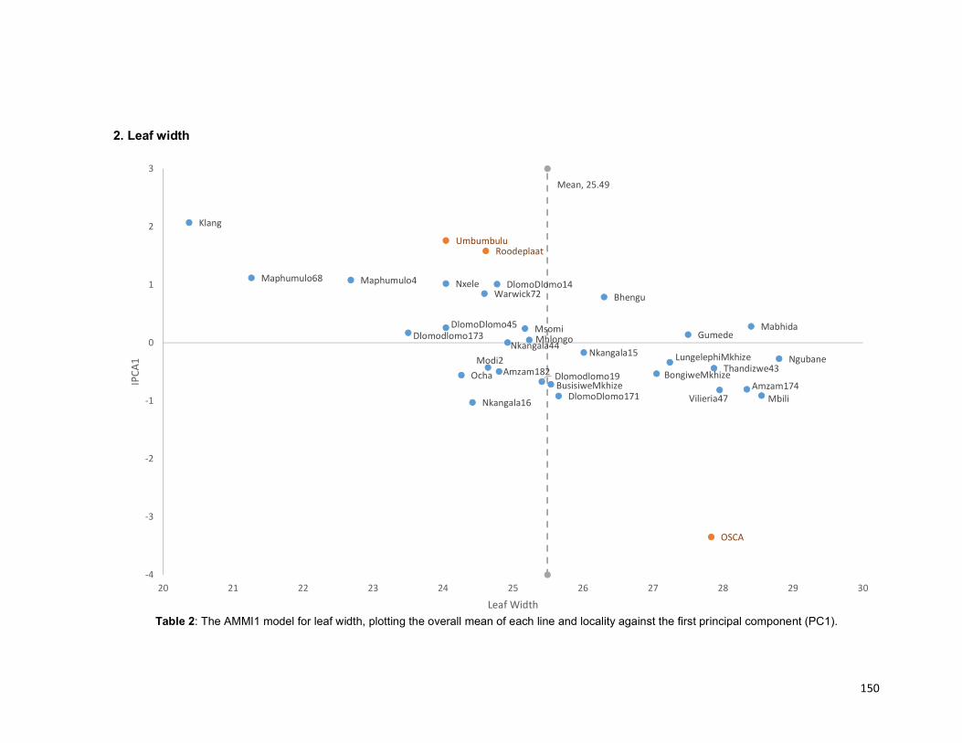
150

2. Leaf width

Table 2: The AMMI1 model for leaf width, plotting the overall mean of each line and locality against the first principal component (PC1).

Amzam174Amzam182

Bhengu

BongiweMkhizeBusisiweMkhize

DlomoDlomo14

DlomoDlomo171

Dlomodlomo173

Dlomodlomo19

DlomoDlomo45Gumede

Klang

LungelephiMkhize

Mabhida

Maphumulo4Maphumulo68

Mbili

Mhlongo

Modi2

Msomi

NgubaneNkangala15

Nkangala16

Nkangala44

Nxele

OchaThandizwe43

Vilieria47

Warwick72

OSCA

RoodeplaatUmbumbulu

Mean, 25.49

-4

-3

-2

-1

0

1

2

3

20 21 22 23 24 25 26 27 28 29 30

IPCA

1

Leaf Width

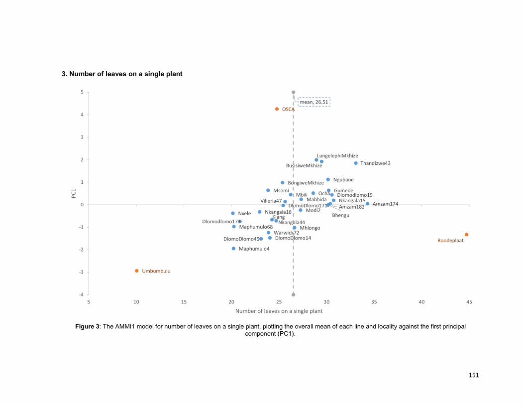
151

3. Number of leaves on a single plant

Figure 3: The AMMI1 model for number of leaves on a single plant, plotting the overall mean of each line and locality against the first principal

component (PC1).

Amzam174Amzam182Bhengu

BongiweMkhize

BusisiweMkhize

DlomoDlomo14

DlomoDlomo171

Dlomodlomo173

Dlomodlomo19

DlomoDlomo45

Gumede

Klang

LungelephiMkhize

Mabhida

Maphumulo4

Maphumulo68

Mbili

Mhlongo

Modi2

Msomi

Ngubane

Nkangala15

Nkangala16

Nkangala44

Nxele

Ocha

Thandizwe43

Vilieria47

Warwick72

OSCA

Roodeplaat

Umbumbulu

mean, 26.51

5 10 15 20 25 30 35 40 45-4

-3

-2

-1

0

1

2

3

4

5

Number of leaves on a single plant

PC1

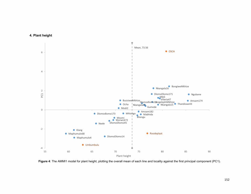
152

4. Plant height

Figure 4: The AMMI1 model for plant height, plotting the overall mean of each line and locality against the first principal component (PC1).

Amzam174

Amzam182

Bhengu

BongiweMkhize

BusisiweMkhize

DlomoDlomo14

DlomoDlomo171

Dlomodlomo173

Dlomodlomo19

DlomoDlomo45

Gumede

Klang

LungelephiMkhize

Mabhida

Maphumulo4Maphumulo68

Mbili

Mhlongo

Modi2

Msomi

Ngubane

Nkangala15

Nkangala16

Nkangala44

Nxele

Ocha Thandizwe43

Vilieria47

Warwick72

OSCA

Roodeplaat

Umbumbulu

Mean, 73.56

-4

-2

0

2

4

6

55 60 65 70 75 80 85 90

PC1

Plant height

153

5. Canopy diameter

Figure 5: The AMMI1 model for canopy diameter, plotting the overall mean of each line and locality against the first principal component (PC1).

Amzam174

Amzam182

Bhengu

BongiweMkhize

BusisiweMkhize DlomoDlomo14DlomoDlomo171

Dlomodlomo173

Dlomodlomo19

DlomoDlomo45

Gumede

Klang

LungelephiMkhizeMabhida

Maphumulo4

Maphumulo68

Mbili

Mhlongo

Modi2

Msomi

Ngubane

Nkangala15

Nkangala16

Nkangala44

Nxele

Ocha

Thandizwe43Vilieria47

Warwick72

OSCA

Roodeplaat

Umbumbulu

Mean, 74.98

-4

-3

-2

-1

0

1

2

3

4

5

6

50 60 70 80 90 100 110

PC1

Canopy Diamater

154

6. Number of suckers

Figure 6: The AMMI1 model for number of suckers, plotting the overall mean of each line and locality against the first principal component (PC1).

Grand mean, 10.25

Amzam174

Amzam182

Bhengu

BongiweMkhize

BusisiweMkhize

DlomoDlomo14

DlomoDlomo171

Dlomodlomo173

Dlomodlomo19

DlomoDlomo45

Gumede

Klang

LungelephiMkhizeMabhida

Maphumulo4

Maphumulo68

Mbili

Mhlongo

Modi2

Msomi

Ngubane

Nkangala15

Nkangala16

Nkangala44

Nxele

OchaThandizwe43

Vilieria47

Warwick72

OSCA

Roodeplaat

Umbumbulu

-2

-1.5

-1

-0.5

0

0.5

1

1.5

2

2.5

3

0 2 4 6 8 10 12 14 16 18

PC1

Mean number of suckers

155

7. Number of Cormels harvested from a single plant

Figure 7: The AMMI1 model for number of cormels, plotting the overall mean of each line and locality against the first principal component (PC1).

Amzam174

Amzam182

Bhengu

BongiweMkhizeBusisiweMkhize

DlomoDlomo14

DlomoDlomo171

Dlomodlomo173

Dlomodlomo19

DlomoDlomo45

Gumede

Klang

LungelephiMkhize Mabhida

Maphumulo4

Maphumulo68

Mbili

Mhlongo

Modi2

Msomi

Ngubane

Nkangala15

Nkangala16

Nkangala44Nxele Ocha

Thandizwe43

Vilieria47

Warwick72 OSCA

Roodeplaat

Umbumbulu

Mean, 22.17

-5

-3

-1

1

3

5

0 5 10 15 20 25 30 35 40

PC1

Number of Cormels

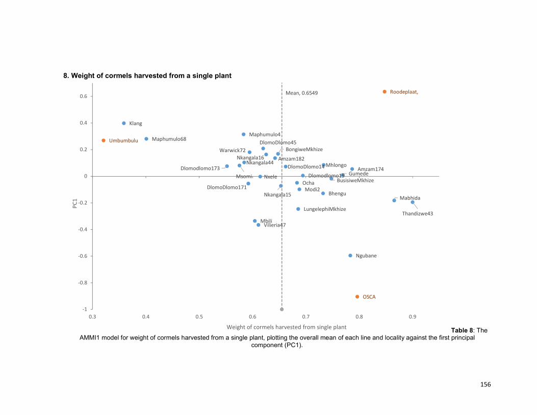
156

8. Weight of cormels harvested from a single plant

Table 8: The AMMI1 model for weight of cormels harvested from a single plant, plotting the overall mean of each line and locality against the first principal

component (PC1).

Amzam174

Amzam182

Bhengu

BongiweMkhize

BusisiweMkhize

DlomoDlomo14

DlomoDlomo171

Dlomodlomo173Dlomodlomo19

DlomoDlomo45

Gumede

Klang

LungelephiMkhize

Mabhida

Maphumulo4Maphumulo68

Mbili

Mhlongo

Modi2

Msomi

Ngubane

Nkangala15

Nkangala16Nkangala44

NxeleOcha

Thandizwe43

Vilieria47

Warwick72

OSCA

Roodeplaat,

Umbumbulu

Mean, 0.6549

0.3 0.4 0.5 0.6 0.7 0.8 0.9-1

-0.8

-0.6

-0.4

-0.2

0

0.2

0.4

0.6

Weight of cormels harvested from single plant

PC1

157

9. Corm length

Figure 9: The AMMI1 model for corm length, plotting the overall mean of each line and locality against the first principal component (PC1).

Amzam174

Amzam182

Bhengu

BongiweMkhize

BusisiweMkhize

DlomoDlomo14

DlomoDlomo171

Dlomodlomo173

Dlomodlomo19

DlomoDlomo45

Gumede

Klang

LungelephiMkhize

Mabhida

Maphumulo4

Maphumulo68

Mbili

Mhlongo

Modi2

Msomi

Ngubane

Nkangala15

Nkangala16

Nkangala44

Nxele

Ocha

Thandizwe43

Vilieria47

Warwick72

OSCA

Roodeplaat

Umbumbulu

-7

-5

-3

-1

1

3

55 60 65 70 75 80 85

PC1

Corm Length

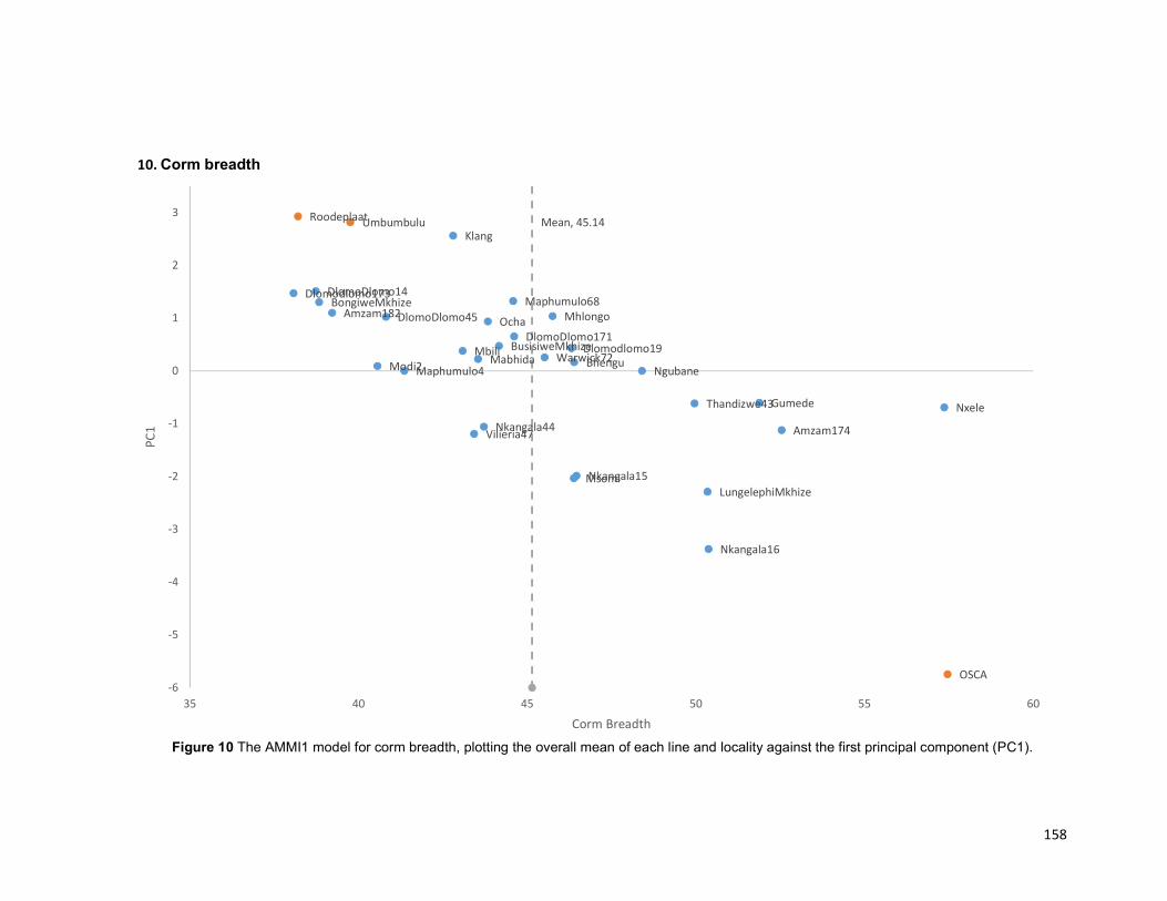
158

10. Corm breadth

Figure 10 The AMMI1 model for corm breadth, plotting the overall mean of each line and locality against the first principal component (PC1).

Nxele

Amzam174

Gumede

Nkangala16

LungelephiMkhize

Thandizwe43

Ngubane

Nkangala15

Bhengu

Msomi

Dlomodlomo19

Mhlongo

Warwick72

DlomoDlomo171

Maphumulo68

BusisiweMkhize

Ocha

Nkangala44

Mabhida

Vilieria47

Mbili

Klang

Maphumulo4

DlomoDlomo45

Modi2

Amzam182BongiweMkhize

DlomoDlomo14Dlomodlomo173

OSCA

RoodeplaatUmbumbulu Mean, 45.14

-6

-5

-4

-3

-2

-1

0

1

2

3

35 40 45 50 55 60

PC1

Corm Breadth

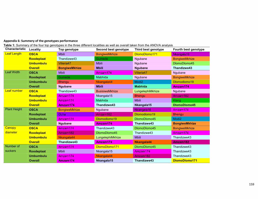
159

Appendix 6: Summery of the genotypes performance Table 1: Summary of the four top genotypes in the three different localities as well as overall taken from the ANOVA analysis Characteristic Locality Top genotype Second best genotype Third best genotype Fourth best genotype Leaf Length OSCA Mbili BongiweMkhize DlomoDlomo171 Nkangala16 Roodeplaat Thandizwe43 Gumede Ngubane BongiweMkhize Umbumbulu Vilieria47 Mbili Ngubane DlomoDlomo45 Overall BongiweMkhize Mbili Ngubane Thandizwe43 Leaf Width OSCA Mbili Amzam174 Vilieria47 Ngubane Roodeplaat Gumede Mabhida Ngubane BongiweMkhize Umbumbulu Bhengu Nkangala44 Modi2 Dlomodlomo19 Overall Ngubane Mbili Mabhida Amzam174 Leaf number OSCA Thandizwe43 BusisiweMkhize LungelephiMkhize Ngubane Roodeplaat Amzam174 Nkangala15 Bhengu Amzam182 Umbumbulu Amzam174 Mabhida Mbili Klang Overall Amzam174 Thandizwe43 Nkangala15 DlomoDlomo45 Plant Height OSCA BongiweMkhize Ngubane Nkangala16 Amzam174 Roodeplaat Ocha Amzam182 Dlomodlomo19 Bhengu Umbumbulu Amzam174 Dlomodlomo19 DlomoDlomo45 Modi2 Overall Ngubane Amzam174 Thandizwe43 BongiweMkhize Canopy OSCA Amzam174 Thandizwe43 DlomoDlomo45 BongiweMkhize diameter Roodeplaat Amzam182 DlomoDlomo45 Thandizwe43 Amzam174 Umbumbulu Nkangala44 LungelephiMkhize Mbili Thandizwe43 Overall Thandizwe43 Amzam174 Nkangala44 Amzam182 Number of OSCA Amzam174 DlomoDlomo171 DlomoDlomo45 Thandizwe43 suckers Roodeplaat Mbili Nkangala15 Amzam174 Thandizwe43 Umbumbulu Amzam174 Nkangala44 Amzam182 Thandizwe43 Overall Amzam174 Nkangala15 Thandizwe43 DlomoDlomo171

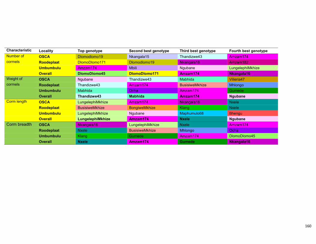
160

Characteristic Locality Top genotype Second best genotype Third best genotype Fourth best genotype Number of OSCA Dlomodlomo19 Nkangala15 Thandizwe43 Amzam174 cormels Roodeplaat DlomoDlomo171 Dlomodlomo19 Nkangala16 Amzam182 Umbumbulu Amzam174 Mbili Ngubane LungelephiMkhize Overall DlomoDlomo45 DlomoDlomo171 Amzam174 Nkangala16 Weight of OSCA Ngubane Thandizwe43 Mabhida Vilieria47 cormels Roodeplaat Thandizwe43 Amzam174 BusisiweMkhize Mhlongo Umbumbulu Mabhida Ocha Amzam174 Gumede Overall Thandizwe43 Mabhida Amzam174 Ngubane Corm length OSCA LungelephiMkhize Amzam174 Nkangala16 Nxele Roodeplaat BusisiweMkhize BongiweMkhize Klang Nxele Umbumbulu LungelephiMkhize Ngubane Maphumulo68 Bhengu Overall LungelephiMkhize Amzam174 Nxele Ngubane

Corm breadth OSCA Nkangala16 LungelephiMkhize Nxele Amzam174 Roodeplaat Nxele BusisiweMkhize Mhlongo Ocha Umbumbulu Klang Gumede Amzam174 DlomoDlomo45 Overall Nxele Amzam174 Gumede Nkangala16

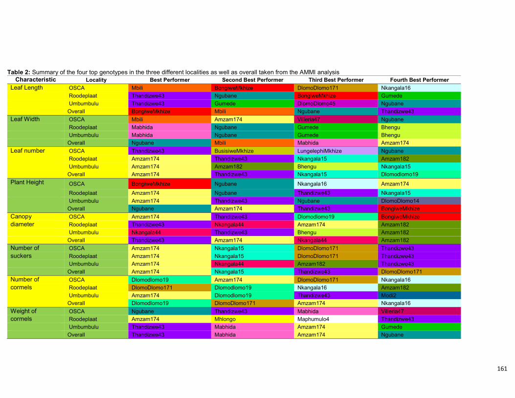
161

Table 2: Summary of the four top genotypes in the three different localities as well as overall taken from the AMMI analysis Characteristic Locality Best Performer Second Best Performer Third Best Performer Fourth Best Performer

Leaf Length OSCA Mbili BongiweMkhize DlomoDlomo171 Nkangala16 Roodeplaat Thandizwe43 Ngubane BongiweMkhize Gumede Umbumbulu Thandizwe43 Gumede DlomoDlomo45 Ngubane Overall BongiweMkhize Mbili Ngubane Thandizwe43

Leaf Width OSCA Mbili Amzam174 Vilieria47 Ngubane Roodeplaat Mabhida Ngubane Gumede Bhengu Umbumbulu Mabhida Ngubane Gumede Bhengu Overall Ngubane Mbili Mabhida Amzam174

Leaf number OSCA Thandizwe43 BusisiweMkhize LungelephiMkhize Ngubane Roodeplaat Amzam174 Thandizwe43 Nkangala15 Amzam182 Umbumbulu Amzam174 Amzam182 Bhengu Nkangala15 Overall Amzam174 Thandizwe43 Nkangala15 Dlomodlomo19

Plant Height OSCA BongiweMkhize Ngubane Nkangala16 Amzam174

Roodeplaat Amzam174 Ngubane Thandizwe43 Nkangala15 Umbumbulu Amzam174 Thandizwe43 Ngubane DlomoDlomo14 Overall Ngubane Amzam174 Thandizwe43 BongiweMkhize

Canopy OSCA Amzam174 Thandizwe43 Dlomodlomo19 BongiweMkhize diameter Roodeplaat Thandizwe43 Nkangala44 Amzam174 Amzam182 Umbumbulu Nkangala44 Thandizwe43 Bhengu Amzam182 Overall Thandizwe43 Amzam174 Nkangala44 Amzam182

Number of OSCA Amzam174 Nkangala15 DlomoDlomo171 Thandizwe43

suckers Roodeplaat Amzam174 Nkangala15 DlomoDlomo171 Thandizwe43 Umbumbulu Amzam174 Nkangala44 Amzam182 Thandizwe43 Overall Amzam174 Nkangala15 Thandizwe43 DlomoDlomo171

Number of OSCA Dlomodlomo19 Amzam174 DlomoDlomo171 Nkangala16 cormels Roodeplaat DlomoDlomo171 Dlomodlomo19 Nkangala16 Amzam182 Umbumbulu Amzam174 Dlomodlomo19 Thandizwe43 Modi2 Overall Dlomodlomo19 DlomoDlomo171 Amzam174 Nkangala16

Weight of OSCA Ngubane Thandizwe43 Mabhida Vilieria47 cormels Roodeplaat Amzam174 Mhlongo Maphumulo4 Thandizwe43 Umbumbulu Thandizwe43 Mabhida Amzam174 Gumede Overall Thandizwe43 Mabhida Amzam174 Ngubane

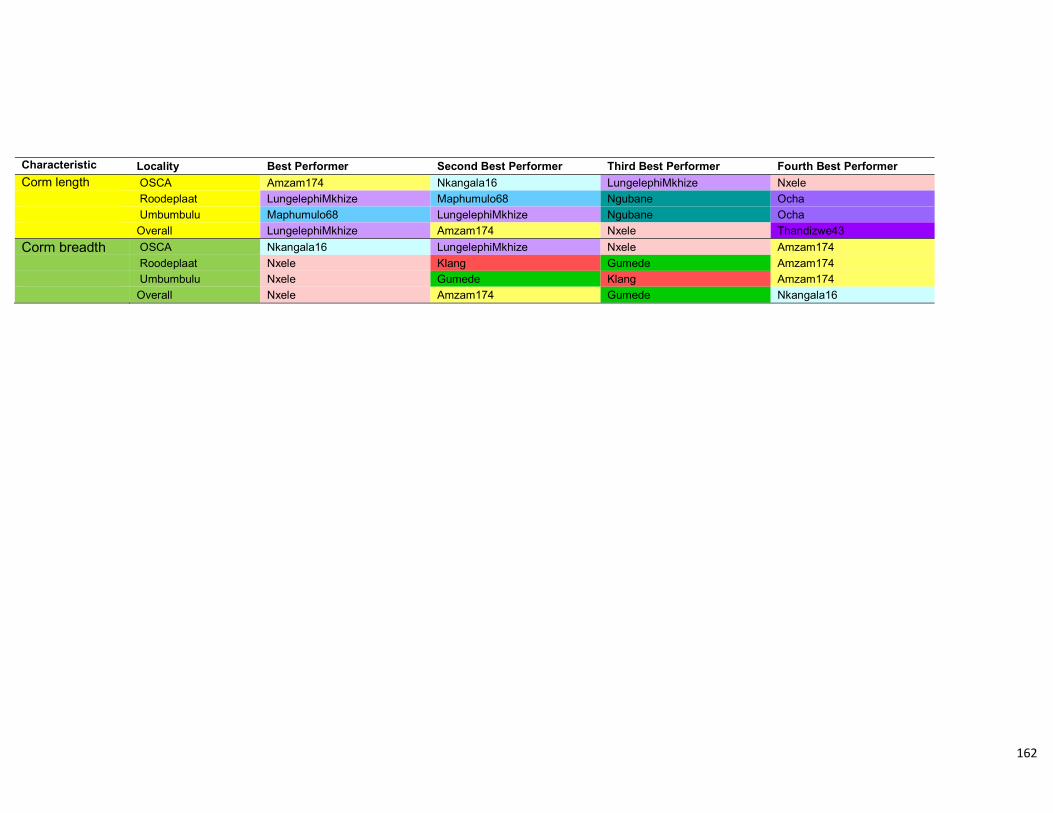
162

Characteristic Locality Best Performer Second Best Performer Third Best Performer Fourth Best Performer

Corm length OSCA Amzam174 Nkangala16 LungelephiMkhize Nxele Roodeplaat LungelephiMkhize Maphumulo68 Ngubane Ocha Umbumbulu Maphumulo68 LungelephiMkhize Ngubane Ocha Overall LungelephiMkhize Amzam174 Nxele Thandizwe43

Corm breadth OSCA Nkangala16 LungelephiMkhize Nxele Amzam174 Roodeplaat Nxele Klang Gumede Amzam174 Umbumbulu Nxele Gumede Klang Amzam174 Overall Nxele Amzam174 Gumede Nkangala16

163

Table 3: Summary of the best genotypes according to the ANOVA and the AMMI analysis for each characteristic in each locality as well as the most stable in instable genotype for each characteristic. Characteristic

Locality ANOVA Best

Performer AMMI Best Performer

Stable Instable

Leaf Length OSCA Mbili Mbili

Roodeplaat Thandizwe43 Thandizwe43 Umbumbulu Vilieria47 Thandizwe43 Overall BongiweMkhize BongiweMkhize Gumede Klang Leaf Width OSCA Mbili Mbili

Roodeplaat Gumede Mabhida Umbumbulu Bhengu Mabhida Overall Ngubane Ngubane Nkangala44 KLang

Leaf number OSCA Thandizwe43 Thandizwe43

Roodeplaat Amzam174 Amzam174 Umbumbulu Amzam174 Amzam174 Overall Amzam174 Amzam174 DlomoDlomo171 LungelephiMkhize Plant Height OSCA BongiweMkhize BongiweMkhize

Roodeplaat Ocha Amzam174 Umbumbulu Amzam174 Amzam174 Overall Ngubane Ngubane Amzam182 Maphumulo4 Canopy OSCA Amzam174 Amzam174

diameter Roodeplaat Amzam182 Thandizwe43 Umbumbulu Nkangala44 Nkangala44 Overall Thandizwe43 Thandizwe43 Mabhida Maphumulo68 Number of OSCA Amzam174 Amzam174

suckers Roodeplaat Mbili Amzam174 Umbumbulu Amzam174 Amzam174 Overall Amzam174 Amzam174 Amzam182 DlomoDlomo171 Number of OSCA Dlomodlomo19 Dlomodlomo19 cormels Roodeplaat DlomoDlomo171 DlomoDlomo171

Umbumbulu Amzam174 Amzam174 Overall DlomoDlomo45 Dlomodlomo19 Modi2 DlomoDlomo171 Weight of OSCA Ngubane Ngubane

cormels Roodeplaat Thandizwe43 Amzam174 Umbumbulu Mabhida Thandizwe43 Overall Thandizwe43 Thandizwe43 Nxele Ngubane Corm length OSCA LungelephiMkhize Amzam174

Roodeplaat BusisiweMkhize LungelephiMkhize Umbumbulu LungelephiMkhize Maphumulo68 Overall LungelephiMkhize LungelephiMkhize DlomoDlomo171 Nkangala16

Corm breadth OSCA Nkangala16 Nkangala16

Roodeplaat Nxele Nxele Umbumbulu Klang Nxele Overall Nxele Nxele Ngubane Nkangala16