RESEARCH SEMINAR IN INTERNATIONAL ECONOMICSfordschool.umich.edu/rsie/workingpapers/Papers401-425/r402.pdf · RESEARCH SEMINAR IN INTERNATIONAL ECONOMICS ... Rich and Poor Countries

RESEARCH SEMINAR IN INTERNATIONAL ECONOMICS

School of Public PolicyUniversity of Michigan

Ann Arbor, Michigan 48109-1220

Discussion Paper No. 402

Rich and Poor Countries in Neoclassical Trade and Growth

Alan V. DeardorffUniversity of Michigan

June 29, 1997

Recent RSIE Discussion Papers are available on the World Wide Webat: http://www.spp.umich.edu/rsie/workingpapers/wp.html

rich.wpdfigures: rich-i.drw

charts: charts.xls

ABSTRACT

Rich and Poor Countries in Neoclassical Trade and Growth

Alan V. Deardorff

The University of Michigan

A neoclassical growth model is used to provide an explanation for a “poverty trap,” or “clubconvergence,” in terms of specialization and international trade. The model has a large numberof countries with access to identical constant-returns-to-scale technologies for producing andtrading three goods using capital and labor. If initial factor endowments of these countries aresufficiently diverse, then initial equilibrium will not involve worldwide factor price equalization. Instead, there will be two cones of diversification, and countries within the lower of these coneswill share identical factor prices and produce relatively labor-intensive goods, while countries inthe upper cone will produce capital-intensive goods. If savings is determined only by wages,then it is quite possible, perhaps even likely, that there will be multiple steady states. Thereforeover time, the poorer group of countries will converge to a low steady-state capital-labor ratioand hence remain poor, while the initially rich countries will converge to a high steady-state andremain rich. This occurs even though all countries share identical technological and behavioralparameters, and it is therefore an example of club convergence. The model is also suggestive ofhow patterns of growth may respond to changes in these parameters for particular countries,including an increase in the savings rate and the use of tariffs.

Keywords: Trade and Growth Correspondence:ConvergencePoverty Trap Alan V. Deardorff

Department of Economics University of Michigan JEL Subject Code: F11, O41 Ann Arbor, MI 48109-1220

Tel. 313-764-6817Fax. 313-764-2769E-mail: [email protected]://www.econ.lsa.umich.edu/~alandear/

*I owe an obvious debt to Oded Galor, whose presentation of his results from Galor(1996) at a conference in Helsingor, Denmark, in August 1996 gave me the idea for this paper. Ihave also benefitted greatly from conversations on this topic with Susanto Basu, Andy Bernard,Ron Cronovich, Pat Deardorff, John Laitner, Bob Stern, and Jaume Ventura, and otherparticipants in seminars at the University of Michigan, M.I.T., and the University of Nevada, LasVegas.

June 29, 1997

Rich and Poor Countriesin Neoclassical Trade and Growth*

Alan V. DeardorffThe University of Michigan

I. Introduction

Why do some countries become rich and seem to stay that way, while others remain mired

in poverty? The simple neoclassical growth model of Solow (1956) and Swan (1956) seems

poorly suited to answering this question, since in the absence of some deus ex machina like

exogenous technological progress, it seems to predict zero long-run per capita growth for all

countries, as well as per capita incomes that differ in steady state only by amounts that can be

explained by differences in saving. Unless the world is divided quite radically into some

countries that save a lot and others that save very little, with few in between, the model seems

unable to explain what some perceive as a growing polarization of the world economy into

nations that are rich and nations that are poor.

In a recent paper, Oded Galor (1996) notes that a comparatively minor modification of the

neoclassical growth model can change this conclusion. If all saving is done out of wages, as

Galor motivates by considering a simple overlapping generations model, then with an

2

appropriately shaped technology it is possible for the neoclassical model to generate multiple

steady states. In that case, even if countries are all alike in their technologies and behavioral

parameters, large enough differences in their initial conditions will divide them into separate

groups, some of which will converge toward a lower steady state and others toward a higher.

Galor calls this phenomenon "club convergence," and he notes a body of empirical evidence, also

reviewed by Quah (1996), in its favor. There also exists a variety of other more elaborate

theoretical growth models that can also yield club convergence, but a strong point of Galor’s

explanation is, with one exception, its simplicity.

The exception, I think, is the contortions that one must go through to get the technology of

the simple model to yield the desired multiple steady states. This is a one-sector model, and it is

simply too well behaved if the production function is, say, Cobb-Douglas. With a fixed portion

of wages saved, the Solow model with Cobb-Douglas production yields a single steady state.

Constant elasticity of substitution production functions are more promising, and indeed if the

elasticity is sufficiently less than one, then the model does indeed yield three steady states, more

or less as suggested by Galor. However, the lowest of these steady states is perhaps too low,

since it has zero per capita income, and the middle steady state is of course unstable. In order to

get two "clubs" that converge to positive but different steady states, one needs a rather special

shape for the per capita savings function, and this in turn would require quite a special shape for

the production function. Thus the Galor model shows that club convergence is possible, but it

does not make it seem particularly likely.

Another feature of the Galor model, in common with a surprising amount of the literature

on the growth convergence of countries and even some of the recent literature on endogenous

It is a one-sector model, and it could therefore describe a country that is completely1

specialized and that therefore exports its one good in exchange for all others.

3

trade and growth, is that it is a model of a closed economy, or at least it allows no explicit role

for international trade. Yet it turns out that by allowing for international trade in much the same1

way as in the early neoclassical trade and growth literature of Oniki and Uzawa (1965) and

others, we can transform Galor’s model into something that is not much more complex, but that

easily yields his special shape for per capita savings. The trick is only to recognize the role of

specialization in international trade. By including multiple goods (the model here will have

three) in a Heckscher-Ohlin model of production and trade, the same heterogeneity in initial

factor endowments that starts Galor’s countries toward different steady states can also prevent

world-wide factor price equalization. There emerge instead two separate cones of diversification,

into which different countries are drawn by the growth process, and in which they then remain,

due to the international factor price differences themselves.

That, then, is the message of this paper: that a model comprising three components --

simple neoclassical growth, savings primarily out of wages perhaps due to overlapping

generations, and multi-good Heckscher-Ohlin trade -- provides a compact explanation of why

countries that start out different may remain so. Interestingly, the model does not suggest that

trade is necessarily a force for making countries more alike, but rather the opposite. Without

trade, these countries seem more likely to converge, although not necessarily to a steady state one

would regard as desirable. Furthermore, the model also has implications for how policy,

including trade policy, may work to change a country’s steady state, and even to permit it to

escape the poverty trap that a low initial capital stock may otherwise imply.

4

I will begin in section II with a brief look at data on the world distribution of national per

capita incomes and what these data suggest about poverty traps and club convergence. In section

III, I w ill briefly recapitulate the Solow growth model and Galor’s variant of it yielding multiple

steady states. Then I will recall, in section IV, the extension of the Solow model to a two-sector

trading economy, such as was the focus of the early neoclassical literature on trade and growth.

In section V, this model will be modified to allow more than two goods and thus the possibility

of multiple cones of diversification. Multiple steady states are then shown to arise naturally from

Galor’s saving assumption, requiring only that some production functions display inelastic (not

necessarily constant) elasticities of substitution. With multiple steady states, otherwise identical

countries can reach different outcomes depending only on their initial conditions. However the

model also suggests interesting effects of having countries with different behavioral parameters.

These comparative static and comparative steady state properties are explored in section V.

Finally, I look at trade policy in section VI, and I conclude in section VII.

II. Poverty Traps and Club Convergence

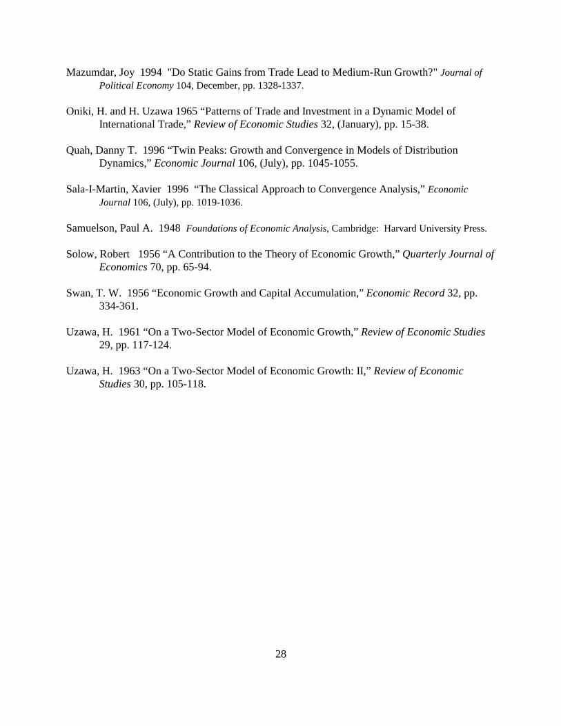
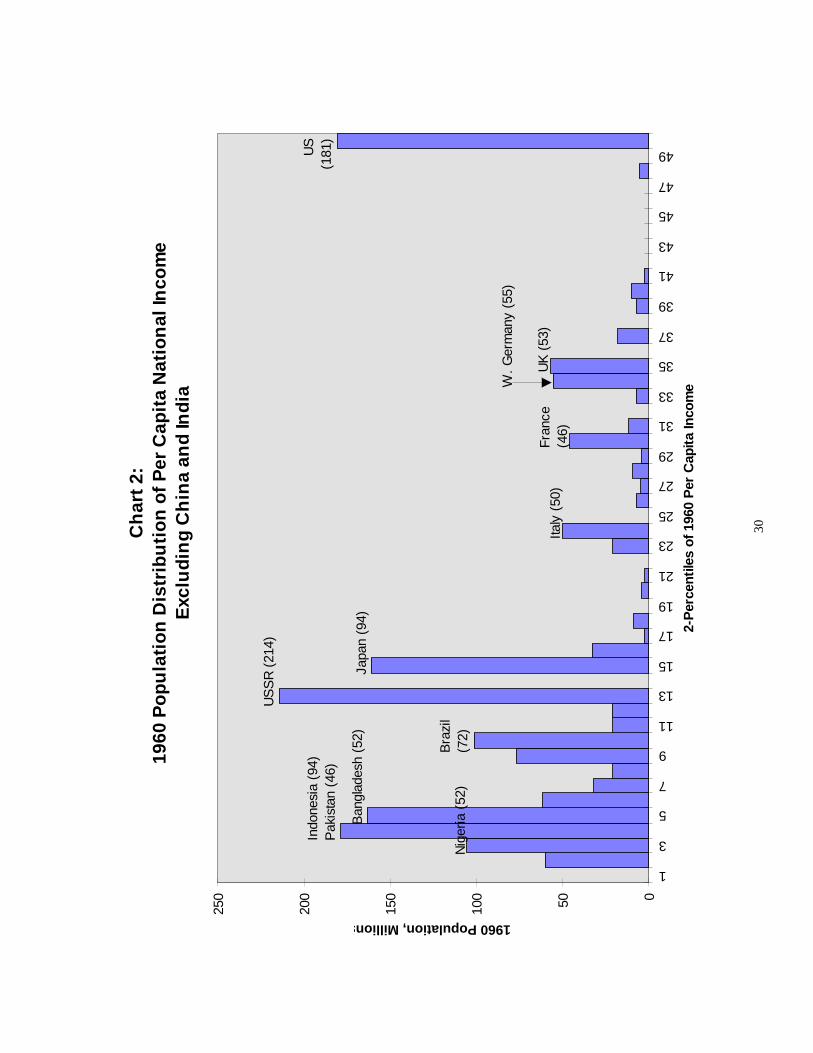
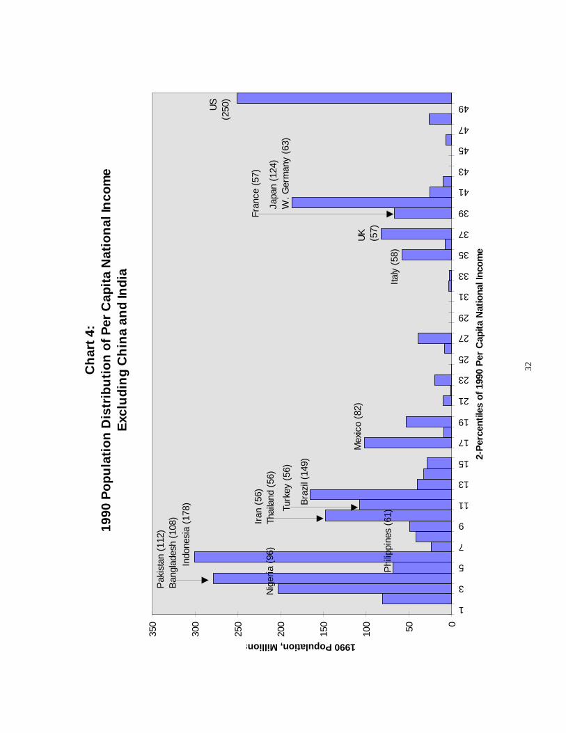
It is hardly news that countries are very unequal in their per capita incomes. The

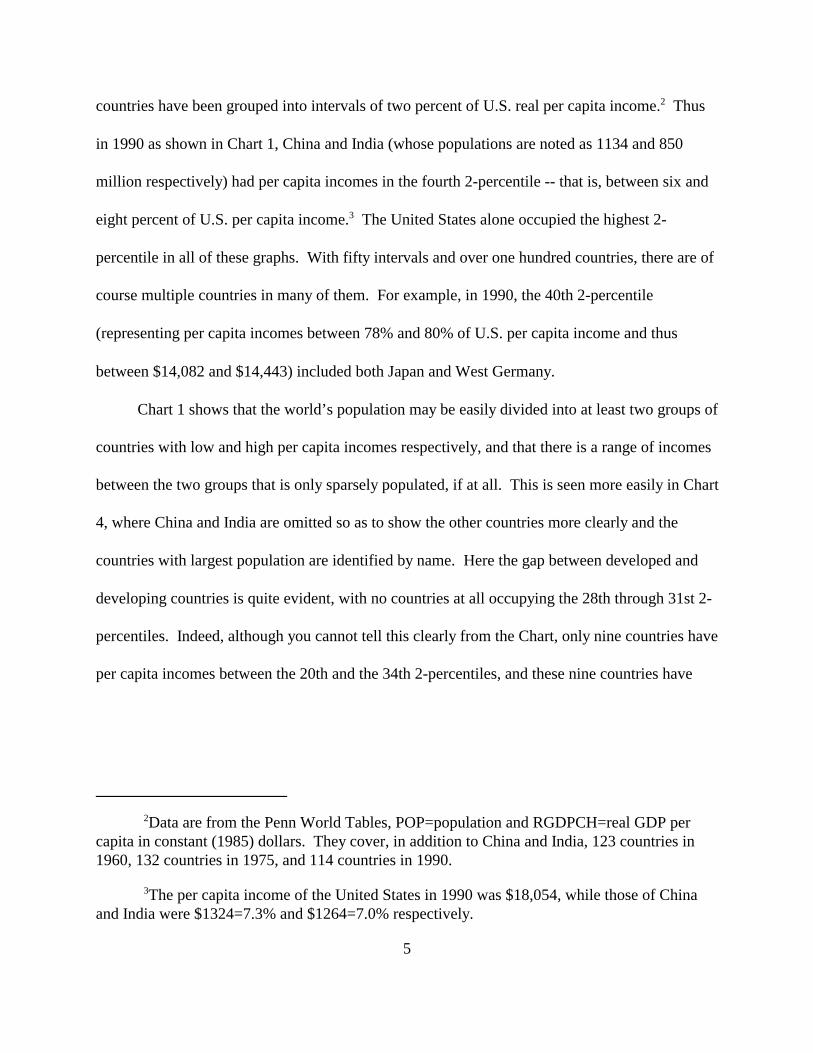
distribution of that inequality across countries may be instructive, however. Chart 1 shows the

distribution for 1990 and, since Chart 1 is dominated by China and India, Charts 2-4 show

similar information for 1960, 1975, and 1990 but excluding these two countries. In all cases, the

charts graph population opposite national per capita income expressed as percentiles of the

highest per capita income, which is that of the United States in each year. For that purpose,

Data are from the Penn World Tables, POP=population and RGDPCH=real GDP per2

capita in constant (1985) dollars. They cover, in addition to China and India, 123 countries in1960, 132 countries in 1975, and 114 countries in 1990.

The per capita income of the United States in 1990 was $18,054, while those of China3

and India were $1324=7.3% and $1264=7.0% respectively.

5

countries have been grouped into intervals of two percent of U.S. real per capita income. Thus2

in 1990 as shown in Chart 1, China and India (whose populations are noted as 1134 and 850

million respectively) had per capita incomes in the fourth 2-percentile -- that is, between six and

eight percent of U.S. per capita income. The United States alone occupied the highest 2-3

percentile in all of these graphs. With fifty intervals and over one hundred countries, there are of

course multiple countries in many of them. For example, in 1990, the 40th 2-percentile

(representing per capita incomes between 78% and 80% of U.S. per capita income and thus

between $14,082 and $14,443) included both Japan and West Germany.

Chart 1 shows that the world’s population may be easily divided into at least two groups of

countries with low and high per capita incomes respectively, and that there is a range of incomes

between the two groups that is only sparsely populated, if at all. This is seen more easily in Chart

4, where China and India are omitted so as to show the other countries more clearly and the

countries with largest population are identified by name. Here the gap between developed and

developing countries is quite evident, with no countries at all occupying the 28th through 31st 2-

percentiles. Indeed, although you cannot tell this clearly from the Chart, only nine countries have

per capita incomes between the 20th and the 34th 2-percentiles, and these nine countries have

Or less than two percent if China and India are included. The nine countries are, in4

decreasing order of per capita income, Singapore, New Zealand, Spain, Israel, Ireland, Cyprus,Taiwan, Trinidad, and Portugal.

See for example Sala-I-Martin (1996).5

6

combined population of only 85 million, or only three percent of world population excluding

China and India.4

It is of course possible for this sort of grouping to exist but to be temporary. Perhaps the

two groups are moving together over time. Others have pursued more formal empirical tests of

this possibility than I will here, where I will be content with looking only at two more graphs of5

these distributions in the past. Chart 2 shows the distribution in 1960, where the most distinctive

feature was that the developed countries were much further behind the United States than in

1990. One can still perceive a perceptible gap between the developed and developing worlds,

although it is not as large or as clear as it became in 1990, and the developed countries were not

as tightly packed.

By 1975, in Chart 3, the countries appeared altogether more spread out, although much of

this impression is due to the progress made by Japan in transforming itself from developing to

developed. Without Japan in Chart 3, the gap between rich and poor would be more clear. In

any case, however, the three graphs together seem to support the impression that there is a

polarization of national per capita incomes and that this polarization is not disappearing.

A possibility of what might be going on here is that the poor countries are mostly

remaining poor, while the rich countries are growing increasing rich and leaving the poor behind.

This explanation is implicit in the literature on endogenous growth, in which countries can grow

indefinitely at different rates, so that the faster growing countries pull further and further ahead.

7

There now exists a plethora of theoretical models to provide this result, but the empirical

evidence in its favor is weak. Charts 2-4 suggest this weakness, since if the rich countries were

growing significantly faster than the poor countries, we should see the countries being drawn

toward the two extreme ends of the distribution, and we do not.

Thus the data are at least mildly suggestive of the possibility that the countries of the world

are neither converging to a single level of per capita income, nor diverging as they would if their

growth rates differed permanently. Instead, there appears to be the presence of, and perhaps the

converge toward, several different levels of per capita income -- exactly as in Galor’s club

convergence. Theoretical explanations of this phenomenon also are not particularly scarce.

Azariadis and Drazen (1990) provided an explanation in terms of “threshold externalities” which

lead to increasing returns to scale in human capital accumulation but only after a threshold level

of human capital has been reached. Barro and Sala-I-Martin (1995) also get this result in a model

with an average product of capital that alternately falls, then rises, then falls. These models are

rather like Galor’s, in that they depend on the particular functional form of some aspect of

technology or behavior. By tinkering with that function, one can generate results of various

sorts, including something rather like what has been observed. The advantage of the model here,

however, is that the special shape needed for club converge arises more naturally from the

economics of production, specialization, and trade in a Heckscher-Ohlin model.

These explanations for club convergence, including mine, also have in common the

property that, if all countries were sufficiently similar in their initial conditions, then club

convergence would not arise. For example, if all countries could somehow start above the

threshold in the Azariadis and Drazen (1990) model, then all could enjoy the high steady state.

Y ' F (K,L)

0L ' nL

0K ' S

k'K/L 0k'dk/dt

0k ' S/L & nk

A constant rate of depreciation is also easily incorporated.6

8

Matsuyama (1996) provided an original and innovative alternative to this property in a model

where some countries must, of necessity, remain poor. In his model there is agglomeration of

different activities in different parts of the world, and this in turn implies the existence of a

“pecking order” among nations, some of whom will be rich but some of whom must remain poor.

III. Solow Growth a la Galor

The Solow growth model is familiar to most. Income, Y, is generated from the

employment of labor L and capital K in a function F that is homogeneous of degree one:

(1)

In the usual one-sector model, F is a production function, although it could, and will below,

represent a more general relationship between factors and income. For later use, Y should be

measured in the same units as investment and therefore the capital stock.

The labor force is assumed to grow at a constant proportional rate, n, while the capital

stock grows due to investment, which is in turn equal to saving, S:6

(2)

(3)

Letting be the capital-labor ratio, its change over time, , is

(4)

f N(0)'4 f N(4)'0

S'sY'sF(K,L)

y'Y/L'F(K,L)/L'F(K/L,1)'f(k)

S/L ' sf(k)

These assumptions include the Inada (1963) conditions that and .7

9

That is, change over time in the capital-labor ratio is critically dependent on the specification of

per capita saving, S/L. In Solow’s model, saving was taken to be a constant fraction, s, of total

income, so that . The homogeneity of F can then be exploited to express per

capita saving in terms of per capita income, :

(5)

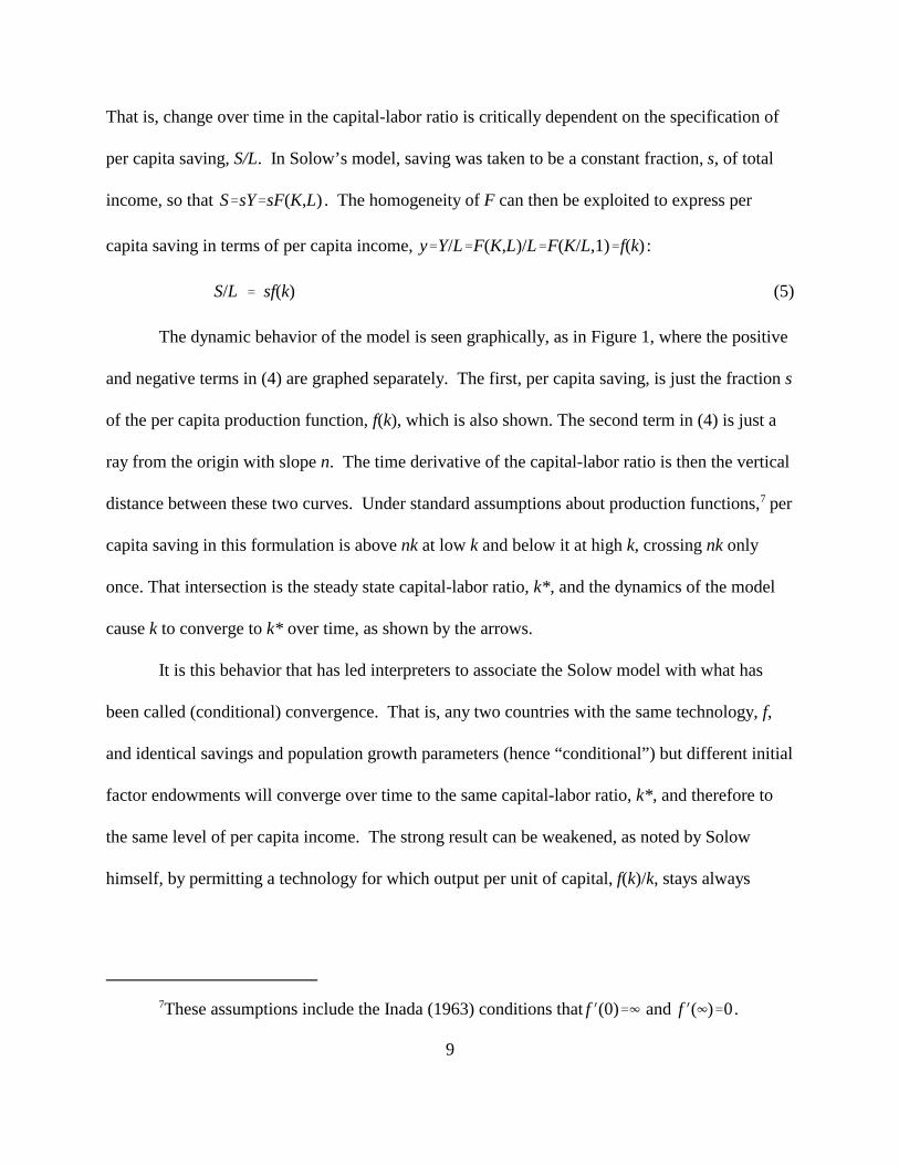
The dynamic behavior of the model is seen graphically, as in Figure 1, where the positive

and negative terms in (4) are graphed separately. The first, per capita saving, is just the fraction s

of the per capita production function, f(k), which is also shown. The second term in (4) is just a

ray from the origin with slope n. The time derivative of the capital-labor ratio is then the vertical

distance between these two curves. Under standard assumptions about production functions, per7

capita saving in this formulation is above nk at low k and below it at high k, crossing nk only

once. That intersection is the steady state capital-labor ratio, k*, and the dynamics of the model

cause k to converge to k* over time, as shown by the arrows.

It is this behavior that has led interpreters to associate the Solow model with what has

been called (conditional) convergence. That is, any two countries with the same technology, f,

and identical savings and population growth parameters (hence “conditional”) but different initial

factor endowments will converge over time to the same capital-labor ratio, k*, and therefore to

the same level of per capita income. The strong result can be weakened, as noted by Solow

himself, by permitting a technology for which output per unit of capital, f(k)/k, stays always

sw

S/L'sww

Thus violating the second Inada Condition.8

This would be the case, for example, if consumers in the two-period overlapping9

generations model had Cobb-Douglas preferences for first and second period consumption.

10

above a lower bound greater than n. This raises the possibility of indefinite endogenous per8

capita growth that has been the focus of so much recent endogenous growth literature. But it

does not help to explain a case that may be more relevant empirically: countries whose growth

does level off, but at vastly different levels of per capita income.

Galor’s (1996) suggested modification of the Solow model to allow for this possibility is

very simple: assume that savings occurs only out of wages, not out of total income. He motivates

this assumption by placing the Solow model in a two-period, overlapping generations context,

with only the first generation working. In such a model, only the first generation can save, and

its income is obtained solely from labor, so that savings is some fraction, , of labor income.

That fraction could in general depend on a variety of things, including the rate of return on

capital, but for simplicity we can take it to be a constant. Savings per capita is then that same9

fraction of labor income per capita, ie., the wage: .

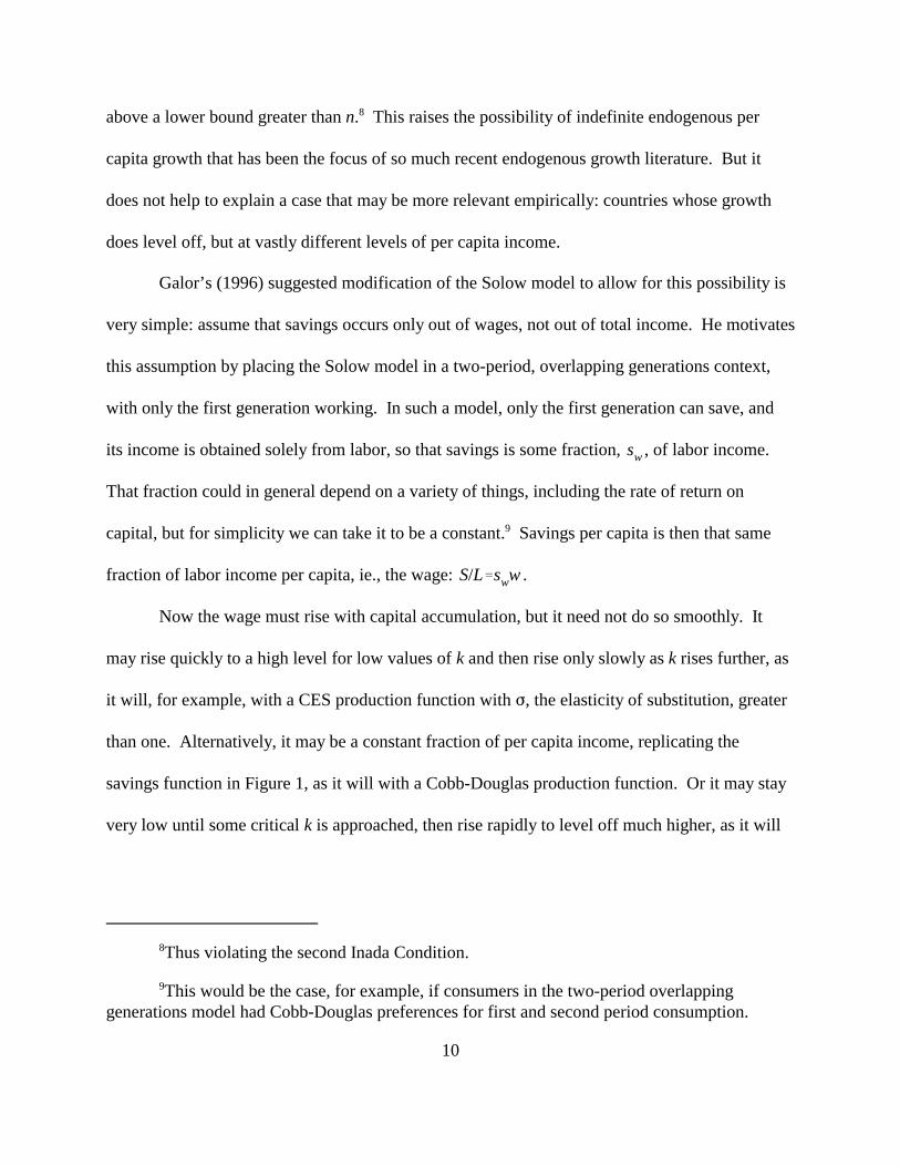
Now the wage must rise with capital accumulation, but it need not do so smoothly. It

may rise quickly to a high level for low values of k and then rise only slowly as k rises further, as

it will, for example, with a CES production function with F, the elasticity of substitution, greater

than one. Alternatively, it may be a constant fraction of per capita income, replicating the

savings function in Figure 1, as it will with a Cobb-Douglas production function. Or it may stay

very low until some critical k is approached, then rise rapidly to level off much higher, as it will

k (

1 , k (

2 k (

3

k (

1 k (

3 k (

2

k (

1 '0

11

with a CES production function if F is sufficiently less than one. This last possibility is shown in

Figure 2.

As seen in Figure 2, savings out of wages can, in the case shown, lead to multiple steady

states, , and . The middle steady state is unstable, and the economy approaches either

or over time depending on whether initial k is below or above . This is more or less

the club-convergence phenomenon, but it takes an extreme form, since . That is, countries

end up either rich or, in effect, dead.

To get multiple steady states that start above zero is quite possible in this simple model,

but it requires that the wage, as a function of k, wiggle even more than the one shown in Figure 2.

Perhaps such a function could be justified, although at this point Galor’s model may begin to

strain the bounds of plausibility.

In any case, the Galor model has another characteristic that seems manifestly

inappropriate for addressing growth of different countries in the world economy. This is that

these countries do not seem to trade. Each produces a single good that it uses for both

consumption and investment, and it has no use for exports or imports. The model could be

reinterpreted to correct this, having each country specialize in a single good, then exchange it at

world prices for what it needs to consume and invest, but that degree of specialization may also

strain credulity. In any case, I will look next at neoclassical growth in the context of a

Heckscher-Ohlin trade model, where patterns of specialization and diversification will be

endogenous.

12

IV. Neoclassical Trade and Growth

Among the many extensions of neoclassical growth theory that were attempted in the

1960s and early 1970s, extensions to incorporate neoclassical trade were among the most

prominent. After Uzawa (1961, 1963) first built and solved a two-sector neoclassical growth

model of a closed economy, Oniki and Uzawa (1965) took the natural next step of allowing two

such countries to trade. In their model, one sector produced a consumption good and the other an

investment good, and the structure of the model was an elegant hybrid of the Solow growth

model and the 2x2x2 Heckscher-Ohlin trade model. It was somewhat cumbersome, however,

and was not itself the basis for many extensions.

I will work here with an approach to this model developed in Deardorff (1974). There I

showed that, taking prices of the two goods as given, the per capita income of a country can be

easily constructed from the per-worker production functions of the two industries, each

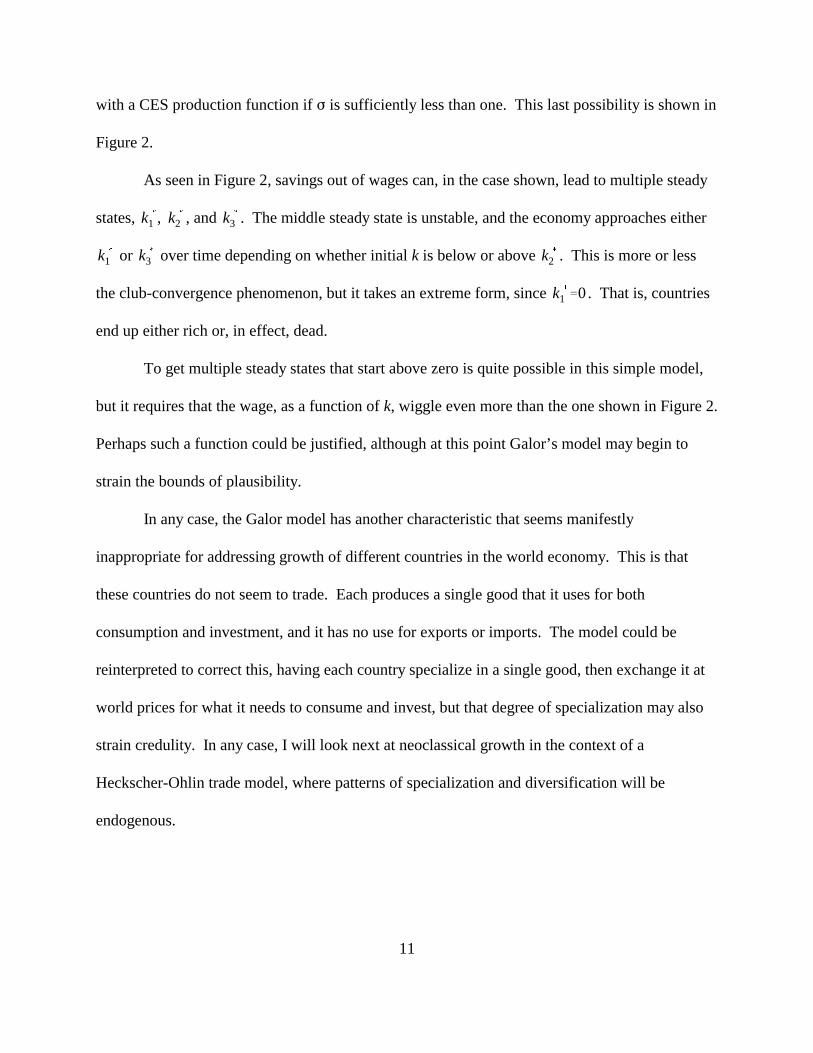
multiplied by its price. As shown in Figure 3 for two goods, labor-intensive X and capital-1

intensive X , the per-worker production functions, f and f , are first drawn as functions of their2 1 2

respective sectoral capital-labor ratios, k and k . Per capita income of the country, y, as a1 2

function of the country’s capital-labor ratio, k, is then the convex hull of f and f . That is, a1 2

straight line tangent to both sectoral curves is drawn from A to B, and y is then given by the

curve OABD. Per capita outputs of the two sectors are given by curves OAFG and OEBD,

which include the diagonals of the trapezoid formed by AB and the perpendiculars from A and B

to the horizontal axis.

Using Solow’s (and Oniki and Uzawa’s) proportional savings assumption, per capita

saving, S/L=sy, is then simply a scaled down version of OABD, itself including a straight

Much of this was done in Deardorff (1971).10

13

segment between the vertical lines under A and B. If prices remain fixed over time, then this per

capita savings curve can be used along with the usual population growth ray, nk, to infer the

dynamics of growth. In the case shown in Figure 3, the steady state at k* has the country

producing both goods, although if it had started its growth at a much lower capital-labor ratio, it

would first have specialized in the more labor-intensive good, X . Under the assumption of1

Oniki and Uzawa that one of the goods is the investment good, the pattern of trade can also be

inferred by comparing the per capita output of that good, given above, to the demand for the

investment good given by sy. In the case shown, for example, if the investment good is the

capital-intensive X , an initially poor country will first produce none of it and instead import all2

that it requires in exchange for the consumption good, then at some point in time begin to

produce it, and eventually, in steady state, export it.

This construction can be used for a variety of purposes, including many of those

commonly served in trade theory by the more familiar Lerner-Pearce diagram based on unit-value

isoquants. However, it is obviously best suited for analysis of neoclassical growth, because of its

similarity to Figure 1 used by Solow. For a small open two-sector economy that takes world

prices as given, it gives a complete picture of the growth process so long as the exogenous world

prices can also be taken as constant over time. The diagram can also provide part of the analysis

of the growth of a closed two sector economy or of a two-country world, although it must be

supplemented in those cases with some other analysis to determine equilibrium prices.10

With proportional saving, this two-sector, open-economy growth model evidently

behaves very similarly to the one-sector closed-economy Solow growth model, and it has the

Of course the world market-clearing prices would be likely to change over time as the11

world factor endowments evolve, but at any point in time the picture would look enough likeFigure 3 to generate convergence.

With only wages saved, the two-good case of Figure 3 will generate club convergence12

somewhat like Figure 2, so long as the elasticity of substitution of the more capital intensivegood is sufficiently small. In that case, and with, say, a Cobb-Douglas labor-intensive sector, percapita saving behaves as follows: It rises in proportion to national income to the left of E, isconstant between E and F, then rises quickly to include almost all income to the right of F. Forappropriate parameters s and n, there will be positive stable steady states to the left of F and alsow

far to the right of F. In this scenario, the poor club does survive with positive income, and it mayeven produce both goods, while the rich club necessarily specializes completely in the capitalintensive good. By making the labor-intensive good also substitution inelastic, another stablesteady state at zero can also be obtained.

14

same implication of conditional convergence of the countries of a trading world. Indeed, one

could have many countries all looking like Figure 3 and trading with the same world economy

whose prices anchor the figure, and all would then converge eventually to the same k* regardless

of their initial conditions.11

Also like the Solow model, this model can be modified following Galor to generate a

form of club convergence. I do not pursue that modification here, because I do not find the

results as plausible as those of the next section, where I also allow for more goods and possible

failure of factor-price equalization. But the interested reader may wish to investigate them.12

V. More Goods

Since the heyday of neoclassical growth theory, attention to the Heckscher-Ohlin model

of international trade has extended beyond the two-good textbook version of the model to allow

for more goods. At the same time, the role of factor price equalization (FPE) in Heckscher-Ohlin

models has been clarified. We now know that if the factor endowments of all the countries in the

See Deardorff (1994b).13

See Deardorff (1979).14

15

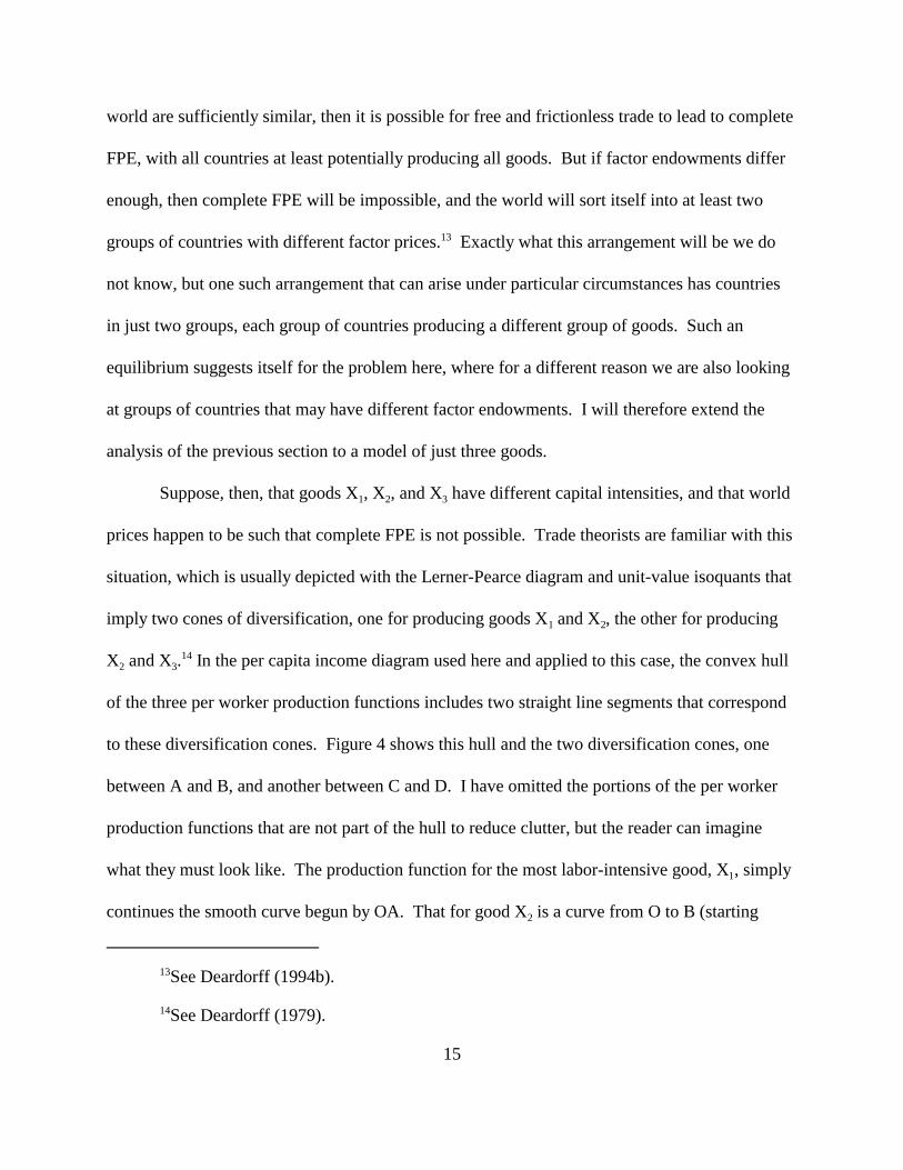
world are sufficiently similar, then it is possible for free and frictionless trade to lead to complete

FPE, with all countries at least potentially producing all goods. But if factor endowments differ

enough, then complete FPE will be impossible, and the world will sort itself into at least two

groups of countries with different factor prices. Exactly what this arrangement will be we do13

not know, but one such arrangement that can arise under particular circumstances has countries

in just two groups, each group of countries producing a different group of goods. Such an

equilibrium suggests itself for the problem here, where for a different reason we are also looking

at groups of countries that may have different factor endowments. I will therefore extend the

analysis of the previous section to a model of just three goods.

Suppose, then, that goods X , X , and X have different capital intensities, and that world1 2 3

prices happen to be such that complete FPE is not possible. Trade theorists are familiar with this

situation, which is usually depicted with the Lerner-Pearce diagram and unit-value isoquants that

imply two cones of diversification, one for producing goods X and X , the other for producing1 2

X and X . In the per capita income diagram used here and applied to this case, the convex hull2 314

of the three per worker production functions includes two straight line segments that correspond

to these diversification cones. Figure 4 shows this hull and the two diversification cones, one

between A and B, and another between C and D. I have omitted the portions of the per worker

production functions that are not part of the hull to reduce clutter, but the reader can imagine

what they must look like. The production function for the most labor-intensive good, X , simply1

continues the smooth curve begun by OA. That for good X is a curve from O to B (starting2

y'f(k) r'f N(k) w'f(k)&rkf(k)

This is a standard feature of two-factor production functions written in intensive form. 15

Per worker output is , the rental price of capital is , and the wage is ,which is the vertical intercept of the tangent to the curve .

16

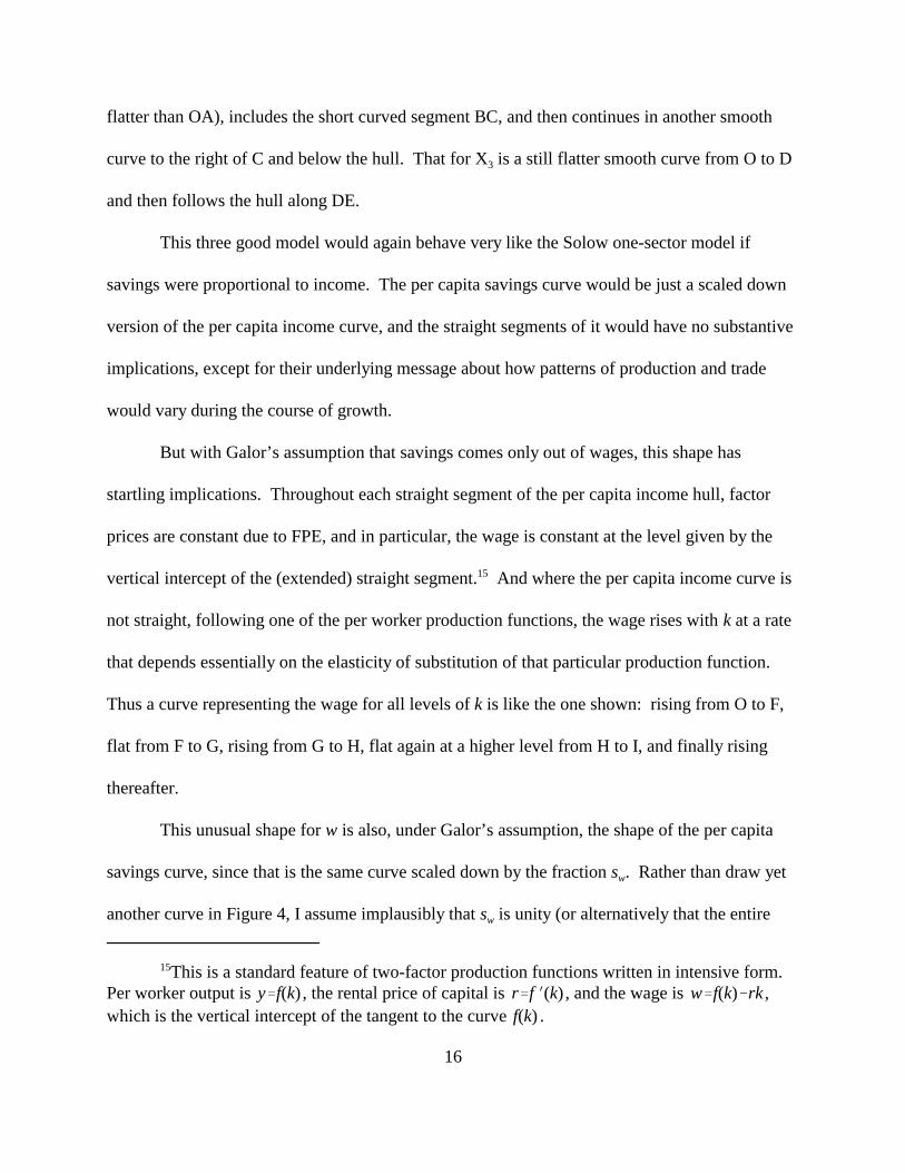
flatter than OA), includes the short curved segment BC, and then continues in another smooth

curve to the right of C and below the hull. That for X is a still flatter smooth curve from O to D3

and then follows the hull along DE.

This three good model would again behave very like the Solow one-sector model if

savings were proportional to income. The per capita savings curve would be just a scaled down

version of the per capita income curve, and the straight segments of it would have no substantive

implications, except for their underlying message about how patterns of production and trade

would vary during the course of growth.

But with Galor’s assumption that savings comes only out of wages, this shape has

startling implications. Throughout each straight segment of the per capita income hull, factor

prices are constant due to FPE, and in particular, the wage is constant at the level given by the

vertical intercept of the (extended) straight segment. And where the per capita income curve is15

not straight, following one of the per worker production functions, the wage rises with k at a rate

that depends essentially on the elasticity of substitution of that particular production function.

Thus a curve representing the wage for all levels of k is like the one shown: rising from O to F,

flat from F to G, rising from G to H, flat again at a higher level from H to I, and finally rising

thereafter.

This unusual shape for w is also, under Galor’s assumption, the shape of the per capita

savings curve, since that is the same curve scaled down by the fraction s . Rather than draw yetw

another curve in Figure 4, I assume implausibly that s is unity (or alternatively that the entirew

k (

1 k (

3

k (

2

k (

2

As long as the segment GH is steep enough to cut rays from the origin from below, as16

shown and as discussed further below, then there will exist values of n such that there aremultiple steady states. However these will not necessarily occur in cones of diversification. Thelatter property is easy to get by drawing the production functions appropriately, as shown, but itis also easy to draw the functions so that a steady state in one cone can only be accompanied byother steady states outside of either cone. Of course, the per capita income curve on which this isall based depends not only on the sectoral production functions, but also on world prices, andthese will have adjusted so that all goods are produced somewhere and world markets clear. Tome that suggests that configurations such as Figure 4, with both steady states in cones ofdiversification, are more likely than configurations in which one steady state involvesspecialization. However, “likely” here has no rigorous meaning. In any case, the behavior of themodel is pretty much the same in either case.

If production functions have low elasticity of substitution, then the wage will rise17

rapidly to the right of point I, and additional steady states will exist with complete specialization.

17

vertical dimension of the figure has been scaled by s ), and I therefore treat the wage curve itselfw

as the per capita savings curve. Inserting a population growth ray, nk, it is then not hard to get

two stable steady states, both in cones of diversification. These are shown as and , and1617

there is also an unstable steady state at . Thus it is not only easy to get multiple steady states –

and thus club convergence – once one allows for multi-good, Heckscher-Ohlin trade; the model

even seems to suggest them as likely.

This is a bit of an overstatement, however, for I have implicitly made several assumptions

that contribute to this result in drawing Figure 4. First, I have drawn the wage curve as quite

steep between points G and H. This will only be the case if the elasticity of substitution in good

X is sufficiently less than one. In contrast, a Cobb-Douglas function would have had the wage2

just proportional to per capita output, and the resulting wage curve would cross rays from the

origin only from above, preventing the unstable crossing at . But with inelastic substitution in

this good of intermediate factor intensity, the wage curve can cross rays from below as shown.

Indeed, if good X were Leontief, points B and C would coincide and GH would be vertical.2

k (

2

18

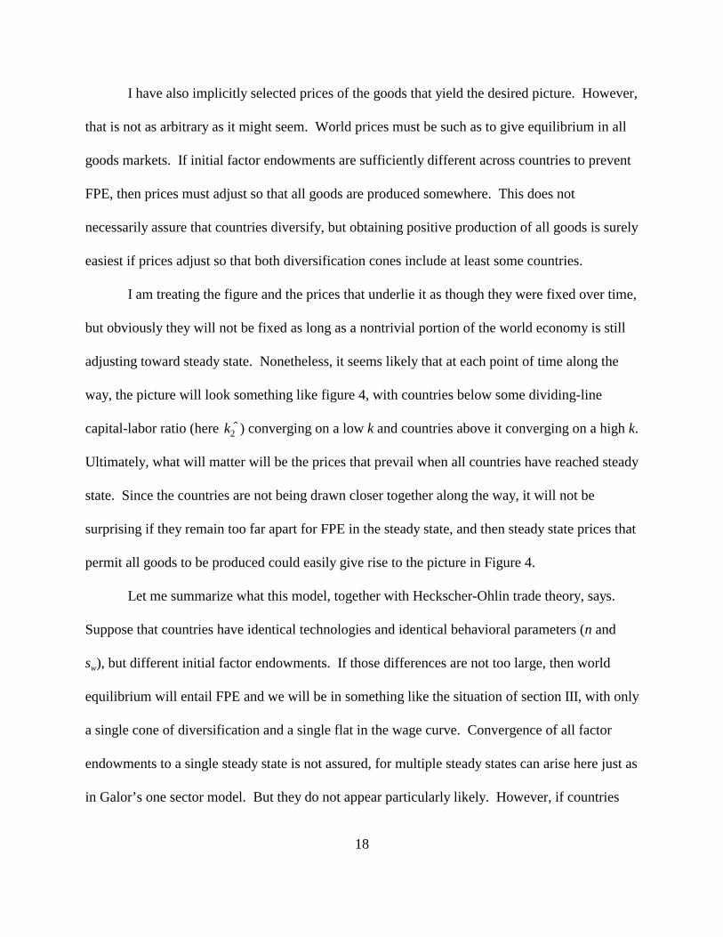
I have also implicitly selected prices of the goods that yield the desired picture. However,

that is not as arbitrary as it might seem. World prices must be such as to give equilibrium in all

goods markets. If initial factor endowments are sufficiently different across countries to prevent

FPE, then prices must adjust so that all goods are produced somewhere. This does not

necessarily assure that countries diversify, but obtaining positive production of all goods is surely

easiest if prices adjust so that both diversification cones include at least some countries.

I am treating the figure and the prices that underlie it as though they were fixed over time,

but obviously they will not be fixed as long as a nontrivial portion of the world economy is still

adjusting toward steady state. Nonetheless, it seems likely that at each point of time along the

way, the picture will look something like figure 4, with countries below some dividing-line

capital-labor ratio (here ) converging on a low k and countries above it converging on a high k.

Ultimately, what will matter will be the prices that prevail when all countries have reached steady

state. Since the countries are not being drawn closer together along the way, it will not be

surprising if they remain too far apart for FPE in the steady state, and then steady state prices that

permit all goods to be produced could easily give rise to the picture in Figure 4.

Let me summarize what this model, together with Heckscher-Ohlin trade theory, says.

Suppose that countries have identical technologies and identical behavioral parameters (n and

s ), but different initial factor endowments. If those differences are not too large, then worldw

equilibrium will entail FPE and we will be in something like the situation of section III, with only

a single cone of diversification and a single flat in the wage curve. Convergence of all factor

endowments to a single steady state is not assured, for multiple steady states can arise here just as

in Galor’s one sector model. But they do not appear particularly likely. However, if countries

k (

1 k (

3 k (

1

sw swN

k (

3

19

begin with endowments too diverse to permit FPE, then market clearing prices will necessarily

imply multiple cones of diversification and a wage curve the wiggles as in Figure 4. As long as

the good of intermediate factor intensity that is produced between these two cones is of

sufficiently low elasticity of substitution, the wiggles will (not just “can”) be big enough to yield

multiple steady states. Thus the initial differences in factor endowments may remain over time,

and the world will evolve toward a permanent situation in which countries remain divided into

two groups, one rich and one poor.

VI. Comparative Statics and Comparative Steady States

Suppose now that we start in such a world steady state, with a large number of countries

that are technologically and behaviorally identical but which, because of history and the

dynamics described above, have sorted themselves into two such groups. What will happen to

one such country if its behavior changes? The solid lines in Figure 5 reproduce the per capita

savings and population growth curves from Figure 4. If we are in a world steady state, some

countries are at and others are at . What happens if a poor country, starting at ,

increases the fraction of its wages that it saves, from to ? A small increase will move its

steady state only slightly to the right, and it will get a small increase in its per capita income over

time, just as in the Solow model. But a larger increase in s , like the one shown, will shift thew

savings curve enough to eliminate the lower steady state. The capital-labor ratio of the country

will therefore begin to rise over time, eventually approaching, if s remains elevated, a steadyw

state even higher than . Thus a comparatively small change in behavior can lead to a large

change in the country’s situation. Poor countries need not be condemned to poverty, it seems,

20

and the cure for poverty here is the usual one: an increase in savings. But the increase has to be

large enough to eliminate the poor steady state entirely, not just move away from it.

What’s more, the increase in saving does not even have to be permanent. If the country

saves at the rate s ’ and then returns to its old ways saving s , growth will continue to k *. Thew w 3

unstable steady state, k *, acts as a threshold that the poor country merely needs to get past in2

order to continue growing like a rich country.

All this assumes that a single, negligibly small poor country attempts to increase savings.

What would happen if the entire group of poor countries were to try to do this? Part of the

answer is that prices would then have to change, and the use of the diagram would be

considerably more complicated. Results will depend in part on which good is the investment

good, since it must serve as the numeraire for comparison with the ray nk. But a likely answer is

not hard to find in the case where the investment good is an import of the poor countries. As the

poor countries all increase their saving out of wages, they will all begin to grow, and as they do,

their output of the most labor-intensive good will fall. To maintain equilibrium in good markets,

the price of that good will have to rise relative to the others. As it does, the first curved segment

of the per capita income curve in Figure 4 will also shift up, while the straight portion from A to

B will become flatter. This raises the wage and shifts the per capita saving curve up even further

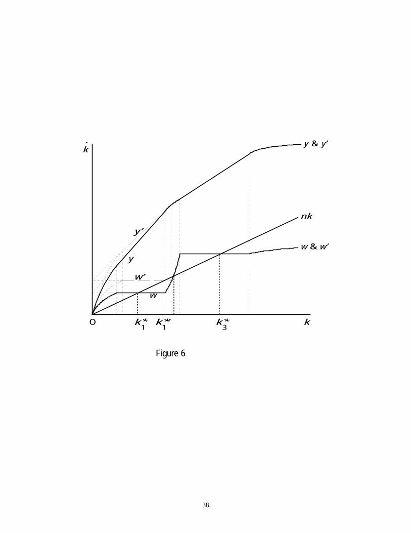
in the relevant range for the poor countries. Figure 6 shows just the second part of this process,

the increase in the price of good X . The total effect is then a combination of Figures 5 and 6. 1

Clearly, and to me surprisingly, a smaller increase in savings by poor countries seems to be

needed for them to escape poverty together than would be needed for them to do it individually!

One needs to be careful about increases in population growth rates, however, since a18

country that raises its population growth above that of the world will not be able to remainnegligibly small, and there will have to be effects on prices. Growth in a neoclassical world withdifferences in population growth rates is explored in Deardorff (1994a), where it is noted thatwith international investment as well as trade, a country with a population growth rate lower thanthe world’s can achieve endogenous sustained per capita growth at a rate that depends on itssavings, much as in endogenous growth models, even without any form of increasing returns toscale or improvement in technology.

It is already known that a tariff can have different effects in a static model with multiple19

cones of diversification than in the traditional Heckscher-Ohlin model. Davis (1996) has

21

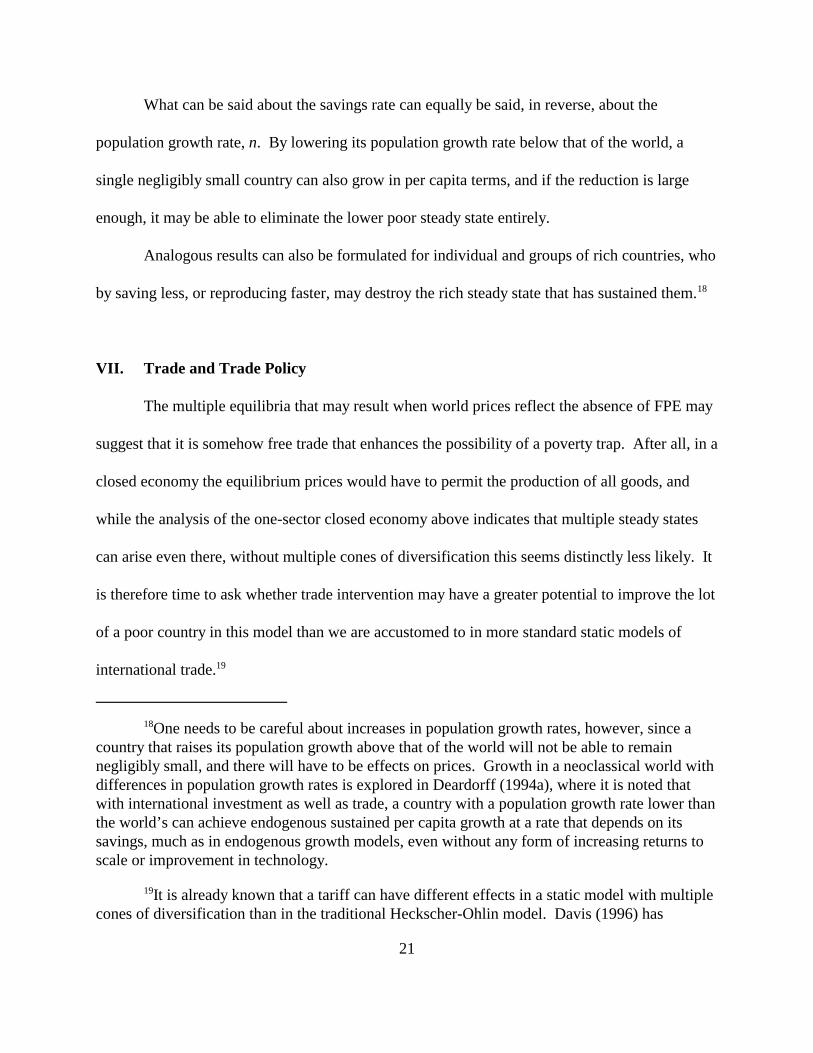
What can be said about the savings rate can equally be said, in reverse, about the

population growth rate, n. By lowering its population growth rate below that of the world, a

single negligibly small country can also grow in per capita terms, and if the reduction is large

enough, it may be able to eliminate the lower poor steady state entirely.

Analogous results can also be formulated for individual and groups of rich countries, who

by saving less, or reproducing faster, may destroy the rich steady state that has sustained them.18

VII. Trade and Trade Policy

The multiple equilibria that may result when world prices reflect the absence of FPE may

suggest that it is somehow free trade that enhances the possibility of a poverty trap. After all, in a

closed economy the equilibrium prices would have to permit the production of all goods, and

while the analysis of the one-sector closed economy above indicates that multiple steady states

can arise even there, without multiple cones of diversification this seems distinctly less likely. It

is therefore time to ask whether trade intervention may have a greater potential to improve the lot

of a poor country in this model than we are accustomed to in more standard static models of

international trade.19

examined the effects of protection and trade liberalization in a static model identical to the oneconsidered here.

Uzawa (1961, 1963) found that if the investment good were capital intensive, this could20

introduce various kinds of instability, either in the disequilibrium dynamics of price adjustmentat a point in time, or in the steady states over time. That has led some to prefer the oppositefactor intensity assumption, for reasons analogous to the Samuelson’s (1948) CorrespondencePrinciple. However it is precisely such instabilities that may cause multiple equilibria such as westudy here, and I therefore would not rule them out.

There is no reason why one could not also examine a country that is different from the21

others in technology or behavioral parameters, but this would add still more to the cases toconsider.

22

To consider trade policy, we must first be careful about how price changes are introduced

into this model. The critical consideration is that the per capita savings curve must be measured

in the same units as capital, since savings is to provide the amount of new capital needed to

sustain steady-state growth along the ray nk. Thus we must identify which of our three goods (or

possibly a combination of them) is used for investment, and then hold the price of that good

constant. Since there is no natural assumption to make regarding the factor intensity of the

investment good, this means that we must consider three possible cases any time a change in

prices occurs.20

In addition, there are two types of country to consider, rich and poor, as well as more than

one possible pattern of trade between them. Allowing for all of these possibilities would be

tedious, and I will therefore focus attention only on trade restrictions levied by a poor country,

leaving the case of rich-country protection to be considered by the reader.

Suppose then that the world starts in a free-trade steady state with large numbers of

technologically and behaviorally identical countries having sorted themselves into rich and poor

groups as discussed above, due to having started with different initial factor endowments. Only21

p3 f3

p1 f1 p2 f2

p1 f1 p2 f2

If tariff revenue is saved, then this slightly improves the chance that the tariff may be22

beneficial. But as usual in second best analysis, any less distorting tax could provide revenues tobe saved and yield a superior outcome.

23

the poor countries can produce the most labor-intensive good, X , and they must therefore export1

it. At the same time, the rich countries must produce and export X . But either group of3

countries could export X to the other, depending on the sizes of the groups and their steady-state2

factor endowments. Thus the poor countries may be importers of only X , or they may import3

both X and X . Again, for the sake of brevity, I will consider only the first of these cases.2 3

That is, our chosen poor country, an importer of X , now levies a tariff on those imports,3

raising the country’s domestic price of X above the world price (which I hold constant, due to3

the presence of many other countries, both rich and poor, who continue to trade freely). If good

X is not the investment good (whose price in the domestic economy we must hold fixed as3

numeraire), then the curve that underlies y would shift upward due to the tariff, raising y

and rotating it counterclockwise to the right of C in Figure 4. If instead, good X is the3

investment good, then the rise in its price above the world price would appear as a downward

shift of both and and thus of the y curve in Figure 4 from O to D. These two

possibilities, both for a small tariff, are shown in panels (a) and (b) of Figure 7.

In both cases, I have kept savings constant, as a fraction of the wage, implicitly assuming

that tariff revenue is not saved. In the case that X is the investment good, panel (a), the223

proportional downward shift of both and causes the wage in the lower diversification

cone to fall. There is also a larger change in the wage in the upper cone, due to the fact that the

tangency at C moves down and to the left, and the vertical intercept of the tangent itself (not

shown) falls substantially. This does not matter for the poor country, however, since its

Of course static welfare, if we were to look at it, would still be reduced by the tariff due23

to the usual inefficiency that it causes in choices between X and other goods. This is a good3

example of Mazumdar’s (1996) point that trade liberalization, even though it may increase staticwelfare by reducing inefficiency, will increase growth only if it lowers the price of theinvestment good, contrary to the claim of Baldwin (1992).

24

endowment ratio is in the lower cone. What does matter is that the wage in the lower cone falls

(by the percent of the tariff), and because this reduces saving the country’s steady state capital-

labor ratio is reduced. Thus when X is the investment good, the tariff levied by the poor country3

just increases its poverty in steady state. This is not surprising, since X is also the import good,3

and what the tariff is doing is making investment more expensive.

If X is not the investment good, the outcome is only slightly better, as shown in panel (b)3

of Figure 7. Now the tariff does shift a portion of the per capita income curve upward, to the

right of C, also moving the tangency at C slightly to the left. However, the vertical intercept of

that tangency falls, and therefore the wage is reduced in the upper cone of diversification. This

does not matter for the poor country, however, since it is not there. Instead, in this case the wage

in the lower cone is left unchanged by the tariff, and there is no effect on the poor country’s

steady state. The tariff here has not hurt growth, but it has not helped either. Thus in neither23

case does a small tariff -- one that leaves the poor country still not producing good X -- help it to3

escape the impoverished steady state.

But what if the tariff were raised still higher, to the point that production of good X were3

to become viable? This would draw factors out of good X , until either X would be imported or2 2

a tariff would be placed on imports of it as well. Assume the latter, so that we examine broad

protection that moves the country all the way to autarky.

p3 f3

p2 f2

p1 f1

p2 f2

p1 f1

p2 f2 p3 f3

p1 f1

25

If X is the investment good, then this means that the downward shifts in Figure 7a cease3

to be equiproportional when production of all three goods becomes possible. Instead in Figure

8a, to keep production of X viable, a tariff will be placed on imports of it as well, and the per2

worker value of production functions for X and X (not shown) will both shift down,1 2

maintaining a common tangency, ANNDNN, with . The latter is shown as the thin solid curve

in Figure 8a. The result is seen to be an even greater reduction in the wage. This lowers saving

even more and causes the country to move to a still poorer steady state.

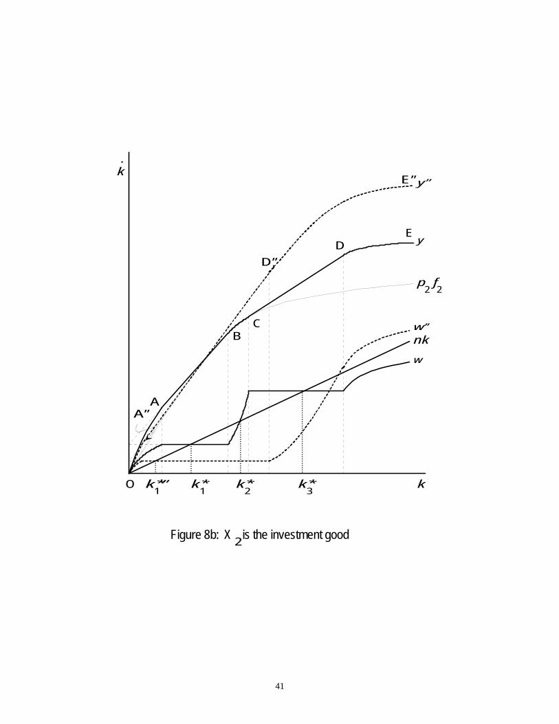
If X is not the investment good, then the continuation of the story begun in Figure 7b3

depends, but only slightly, on which of X or X is the investment good. If X is the investment1 2 2

good, then stays fixed, the thin solid curve in Figure 8b. The further rise in tariff on X3

again requires a tariff also on X , which now shows up as a downward shift in (not shown). 2

In effect, once there is a common tangent to all three curves, ANNDNN, it rolls around the

curve until autarky is reached. Again, the wage in units of the investment good falls, lowering

saving and leading to an even poorer steady state.

Finally, if X is the investment good, then the thin solid curve in Figure 8c remains1

fixed, while the growing tariff on X together with a smaller tariff on X cause and 3 2

(not shown) to shift up, rolling the common tangent to all three curves, ANN DNN, around to

autarky. Yet again, the result is a fall in the wage and therefore in savings, reducing the steady

state.

Therefore, while the exact picture does depend on the identity of the investment good, the

conclusion is robust that a move to autarky by a poor country leads it to an even more

One must be careful, however, in drawing conclusions about welfare across steady24

states, since to get from one steady state to another one traverses a non-steady-state growth pathwhere welfare can be quite different. See Deardorff (1973).

26

impoverished steady state than was attainable with free trade. Therefore it is not international24

trade that should be faulted for the sad steady state that such a country finds itself in with free

trade. The solution to such poverty will not be found in withdrawal from the world market, but

rather in finding some way to increase savings as discussed in the previous section.

VIII. Conclusion

The world of this paper is not a happy one, for it condemns whole populations to

permanent poverty, not because they behave any differently from more fortunate folk, but only

because of their place in history. If that is the case in the real world as well, then it is very

important to find out why, and what can be done to change it. I find it rather surprising that the

Heckscher-Ohlin model of international trade, which I tend to think of as quite well-behaved, can

yield this result in one of its more plausible equilibria.

27

References

Azariadis, Costas and Allan Drazen 1990 “Threshold Externalities in Economic Development,”Quarterly Journal of Economics 105, pp. 501-526.

Baldwin, Richard E. 1992 "Measurable Dynamic Gains from Trade," Journal of PoliticalEconomy 100, pp. 162-174.

Barro, Robert and Xavier Sala-I-Martin 1995 Economic Growth, New York: McGraw Hill.

Davis, Donald R. 1996 “Trade Liberalization and Income Distribution,” in process, Harvard(June).

Deardorff, Alan V. 1971 Growth and Trade in a Two-Sector World, Ph.D. Thesis, CornellUniversity, (June).

Deardorff, Alan V. 1973 “The Gains from Trade In and Out of Steady-State Growth,” OxfordEconomic Papers, 25 (July), 173-91.

Deardorff, Alan V. 1974 “A Geometry of Growth and Trade,” Canadian Journal of Economics7, (May), pp. 295-306.

Deardorff, Alan V. 1979 "Weak Links in the Chain of Comparative Advantage," Journal ofInternational Economics 9, (May), pp. 197-209.

Deardorff, Alan V. 1994a “Growth and International Investment with Diverging Populations,”Oxford Economic Papers 46, (July), pp. 477-491.

Deardorff, Alan V. 1994b "The Possibility of Factor Price Equalization, Revisited," Journal ofInternational Economics 36, pp. 167-175.

Galor, Oded 1996 “Convergence? Inferences from Theoretical Models,” Economic Journal 106,(July), pp. 1056-1069.

Inada, Ken-ichi 1963 “On a Two-Sector Model of Economic Growth: Comments and aGeneralization,” Review of Economic Studies 30, (June), pp. 119-127.

Matsuyama, Kiminori 1996 “Why Are There Rich and Poor Countries?: Symmetry-Breaking inthe World Economy,” NBER Working Paper No. 5697, August.

28

Mazumdar, Joy 1994 "Do Static Gains from Trade Lead to Medium-Run Growth?" Journal ofPolitical Economy 104, December, pp. 1328-1337.

Oniki, H. and H. Uzawa 1965 “Patterns of Trade and Investment in a Dynamic Model ofInternational Trade,” Review of Economic Studies 32, (January), pp. 15-38.

Quah, Danny T. 1996 “Twin Peaks: Growth and Convergence in Models of DistributionDynamics,” Economic Journal 106, (July), pp. 1045-1055.

Sala-I-Martin, Xavier 1996 “The Classical Approach to Convergence Analysis,” EconomicJournal 106, (July), pp. 1019-1036.

Samuelson, Paul A. 1948 Foundations of Economic Analysis, Cambridge: Harvard University Press.

Solow, Robert 1956 “A Contribution to the Theory of Economic Growth,” Quarterly Journal ofEconomics 70, pp. 65-94.

Swan, T. W. 1956 “Economic Growth and Capital Accumulation,” Economic Record 32, pp.334-361.

Uzawa, H. 1961 “On a Two-Sector Model of Economic Growth,” Review of Economic Studies29, pp. 117-124.

Uzawa, H. 1963 “On a Two-Sector Model of Economic Growth: II,” Review of EconomicStudies 30, pp. 105-118.

29Ch

art

1:19

90 P

op

ula

tio

n D

istr

ibu

tio

n o

f P

er C

apit

a N

atio

nal

Inco

me

0

500

1000

1500

2000

2500

1

3

5

7

9

11

13

15

17

19

21

23

25

27

29

31

33

35

37

39

41

43

45

47

49

2-P

erce

ntile

s of

199

0 N

atio

nal P

er C

apita

l Inc

ome

1990 Population, Millions

Chi

na (

1134

)In

dia

(850

)

US

(250

)

30Ch

art

2:19

60 P

op

ula

tio

n D

istr

ibu

tio

n o

f P

er C

apit

a N

atio

nal

Inco

me

Exc

lud

ing

Ch

ina

and

Ind

ia

050100

150

200

250

1

3

5

7

9

11

13

15

17

19

21

23

25

27

29

31

33

35

37

39

41

43

45

47

49

2-P

erce

ntile

s of

196

0 P

er C

apita

Inco

me

1960 Population, Millions

Nig

eria

(52

)

Indo

nesi

a (9

4)P

akis

tan

(46)

Ban

glad

esh

(52)

Bra

zil

(72)

US

SR

(21

4)

Japa

n (9

4)

Italy

(50

)F

ranc

e (4

6)U

K (

53)

W.

Ger

man

y (5

5)

US

(181

)

31Ch

art

3:19

75 P

op

ula

tio

n D

istr

ibu

tio

n o

f P

er C

apit

a N

atio

nal

Inco

me

Exc

lud

ing

Ch

ina

and

Ind

ia

050100

150

200

250

300

350

1

3

5

7

9

11

13

15

17

19

21

23

25

27

29

31

33

35

37

39

41

43

45

47

49

2-P

erce

ntile

s of

197

5 P

er C

apita

Nat

iona

l Inc

ome

1975 Population, Millions

Indo

nesi

a (1

33B

angl

ades

h (7

7)P

akis

tan

(71)

Nig

eria

(61

)

Bra

zil (

108)

US

SR

(25

4)M

exic

o (5

9)

Japa

n (1

12)

Italy

(55

)

UK

(56)

Fra

nce

(53)

W.

Ger

man

y (6

2)

US

(216

)

32Ch

art

4:19

90 P

op

ula

tio

n D

istr

ibu

tio

n o

f P

er C

apit

a N

atio

nal

Inco

me

Exc

lud

ing

Ch

ina

and

Ind

ia

050100

150

200

250

300

350

1

3

5

7

9

11

13

15

17

19

21

23

25

27

29

31

33

35

37

39

41

43

45

47

49

2-P

erce

ntile

s of

199

0 P

er C

apita

Nat

iona

l Inc

ome

1990 Population, Millions

Nig

eria

(96

)

Indo

nesi

a (1

78)

Pak

ista

n (1

12)

Ban

glad

esh

(108

)

Bra

zil (

149)

Turk

ey (

56)

Iran

(56

)Th

aila

nd (

56)

Phi

lippi

nes

(61)

Mex

ico

(82)

Italy

(58

)

UK

(57)

Japa

n (1

24)

W.

Ger

man

y (6

3)

Fra

nce

(57)

US

(250

)

33

k

k .

f(k)

nk

sf(k)

k*

Figure 1

34

k .

f(k)

nk

Figure 2

w(k)

s w(k)w

O=k *1

k *2

k *3

k

35

k .

p f (k )

nk

Figure 3

sy

O k *

2

k

A

B

2 2p f (k )1 1 1

E F G

Dy

36

k .

nk

Figure 4

O kk* k* k*1 2 3

y

A

B

C

D

E

FG

HI

Jw=S/L

37

k .

nk

Figure 5

O kk* k* k*1 2 3

s w(k)w

s w(k)w ’

k*’

38

k .

nk

Figure 6

O kk* k*1 3

y & y’

w & w’

k*’1

w

w’

y

y’

39

k .

nk

Figure 7

O kk* k* k*1 2 3

y

w

A

B C

D

E

3b) X is not the investment good

k .

nk

O kk* k* k*1 2 3

y

w

A

B

C

DE

k*’1

3a) X is the investment good

y’

w’

40

Figure 8a: X is the investment good

k .

nk

O kk* k* k*1 2 3

y, y’’

w

A

B

C

DE

k*’’1

3

A’’

D’’

p f3 3

w

w’’

y

y’’

41

Figure 8b: X is the investment good

k .

nk

O kk* k* k*1 2 3

y

w

A

BC

DE

k*’’1

2

w’’

y’’

p f 2

D’’

A’’

E’’

2

42

Figure 8c: X is the investment good

k .

nk

O kk* k* k*1 2 3

y

w

A

B

C

DE

k*’’1

1

p f1 1

w’’

y’’

A’’

D’’

E’’