RESEARCH PAPER SERIES - E-FINANCEefinance.org.cn/cn/fm/Further evidence on the risk-return... · Further Evidence on the Risk-Return Relationship by Yakov Amihud Stern School of Business

RESEARCH PAPER SERIES

GRADUATE SCHOOL OF BUSINESS

STANFORD UNIVERSITY

RESEARCH PAPER NO. 1248

Further Evidence on the Risk-ReturnRelationship

Yakov AmihudBent Jesper Christensen

Haim Mendelson

November 1992

7,‘~I ~ ‘~

ResearchPaperNo. 1248

Further Evidence on the Risk-Return Relationship

by

Yakov Amihud

New York University

Bent JesperChristensen

New York University

and

Hairn Mendelson

Stanford University

November1992

-J

Further Evidence on the Risk-Return Relationship

by

Yakov Amihud

Stern School of Business

New York University

Bent JesperChristensen

SternSchoolof Business

New York. University

- Haim Mendelson

GraduateSchoolof Business

StanfordUniversity

November1992

We thank SteveBrown for helpful commentsandNikunj Kapadiafor competentprogram-

ming assistance.

Further Evidence on the Risk-Return Relationship

Abstract

Recenttestsof the capital assetpricing model by FamaandFrench(1992) showedthat

thereis no significant relationshipbetweentheaveragereturn andsystematicrisk of corn-

monstocks.We proposetwo econometricmethodsto improvethe efficiencyof theestima-

tion and providemore powerful test statistics: joint pooledcross-sectionand time-series

estimationandgeneralizedleastsquares.Usingthesetechniques,wefind a highly signifi-

cantrelationshipbetweenaverageportfolio returnsandsystematicrisk.,

In arecentarticle,FamaandFrench(1992) (FF) estimatedthe relationshipbetweenstock

- returnsand beta,themeasureof systematicrisk, in orderto test the capitalassetpricing

model (CAPM) of Sharpe(1964),Lintner (1965), Mossin (1966) andBlack (1972). They

found no significant relationshipbetweenreturn and betaeven whenbetawasthe only

regressorin thereturn equation,hencecastingdoubt on the validity of the CAPM. The

presscoverageof this study concludedthat “beta ... is dead”.~ In this paperwe suggest

- that the pressreportsof beta’sdeathweregreatlyexaggerated.

Our resultsshow that the absenceof a significant relationshipbetweenaveragestock

returnsandbetais dueto theestimationmethodologyofFarnaandMacBeth(1973) (FM),

which producestests that arenot sufficiently powerful. We developthe methodologyof

Amihud andMendelson(1986, 1989) (AM) to test the CAPM, and find that the power

of the resulting tests is greaterthanthat of FM’s tests. This methodologyis applied

to examinethe return-betarelationshipusing datafor the period 1953-1990. When we

employ the FM methodology,we find an insignificant relationship,consistentwith FF.

However,when we apply the improvedAM methodology,we find a positive andhighly

significant return-betarelationship.We concludethat betais still alive andwell.

In what follows, we presentthe test methodologiesin sectionI. SectionII describes

ourempirical studyandpresentstheresults. Concludingremarksareofferedin sectionIII.

1 New York Time3,February18, 1992. Seealso “Beta beaten”(TheEconomist,March

7, 1992)and “Bye-bye to Beta” (Forbes,March 30, 1992). Recently,ChanandLakonishok

(1992),employinga similar methodologyasFF, found that for dataspanningover 1932-

1992, thereturn-/3relationshipwasweakly significant.

1

I. Econometric Issues

A. Pooledjoint time-seriesand cross-sectionestimation

Consider a general empirical model for the analysisof the cross-sectionalvariation in

expectedassetreturns,specifiedas

(1) = e7oy + Xy~iy+ eu,

where r~,is a P-vector of returns on P assets in period y, X~, is the P x K matrix of

regressorsande is a column vectorof ones Thecoefficient 70y is the regressionconstant,

71y is thevectorof K coefficientsof the K regressors,ande~arethe P-vectorsof errors.

Theperiod index is y, y = 1,2,... , Y.

In the FM procedurefor testing the CAPM, stocksare aggregatedinto P portfolios

in eachperiod y, y = 1,2,.. . ,Y. For eachportfolio p, p = 1,2,. . . , F, the meanportfolio

return in period y is given by ~ and the regressoris = ~ the systematicrisk

(fi) coefficient for portfolio p. The regressionintercept ‘Yoy is interpretedas the risk-

free rateof return and ‘y~,is the market risk premium. The systematicrisk coefficients

i3~, areestimatedfrom the market model for eachportfolio using the return time series

on the stocks in portfolio p and on the market over sometime precedingperiod y The

useof portfolios increasesthe precisionof the estimatedfi andresolvesthe “errors in the

variables”problemencounteredwhenusing estimatesfor individual stocks2

In eachperiody, anordinaryleastsquares(OLS) cross-sectionalregressionof model(1)

producesestimates(yo~,,5’i~). The estimates5’i~areviewed as the sampledvaluesof a

variate representingthe market risk premium, and thefocusof the test is on whetherits

2 F’F generallyfollow theFM procedure,exceptthat /3 is estimatedfor portfoliosandthe

cross-sectionalregressionsareestimatedon individual stockswith theportfolio-18 assigned

to all stocks in a portfolio This is donebecauseFF add to the regressorsthe company’s

book-to-marketequity variable,which is not studiedin FM nor in this paper

2

- mean, 7i, is positive and significantly different from zero. To this end, the ,Y estimates

• of ‘yl areaveraged, producing ~‘i = ~ E~,~ä’iy. The estimated standard error of ~ is given

by &(~~)= (y(~.~)~ — ~i)2)~, and testsof significance are carriedout using the

statistic t = ~/o(~). In further testsby FM, the matrix X~containedmoreregressors

thaii /3 alone,and ‘Yly was a K-elementvectorfor.K regressors.The estimationand test

proceduresare similar for all regressors. For the FM procedureto be meaningful, the ‘ I—

slopecoefficientsmust havea commonmeanvector ‘Yi, which is theparameterof ultimate

interest,estimatedby ~. The FM test is for this parameter.

In view of the commonparameter‘Yl, it is natural to considerexplicitly the joint

time-seriesandcross-sectionalmodel asgiven by

(2) r=(Iy®e)’yo+X-yi +e.

Here, the YP-vector r stacksthe Y cross-sectionalreturnvectors,i.e., the ~ subvector

is r~,andsimilarly for e. The Y-vector ‘yo stackstheintercepts‘you, theYP x K matrix X

stacksthe matricesXi,,, ly is the Y x Y identity matrix and ® denotesthe Kronecker

product. This is thepooledmodel;employedby AM. In this model, thetestis on whether

5’i, theestimatorof ‘Yi, is greaterthanzero,usinga standardt-test.

A pooled, joint estimationof time-seriesand cross-sectionis known to improve ef-

ficiency (see,e.g., Judgeet al. (1980, Chapter13)). It follows from the Gauss-Markov

theoremthat if the assetsare serially andcross-sectionallyhomoskedasticanduncorre-

lated, then the OLS estimatorin the joint pooled model is optimal. In particular, it is

moreefficient than the FM estimatorand leads to a morepowerfrl teston ‘yr.

To illustrate, consider the (mean-adjusted) model

(3) r~= X~’yiy + Cy.

Here, var(~5’i~)= u~(XX~)~,where o~is the residualvariance.It follows that

- o.2y -

(4) var(~i)= ~

3

Similarly, the estimatorof ‘y~. from the joint pooled estimation, ~, may be computed

by OLS in

(5)

obtained by stacking (3), and

ly(6) var(~i)= o~(~~x~1x~)

y=i

Evidently, the joint pooled estimationdominatesthe FM estimation, that is, var(5’i) �

var(.~i)in the orderingof positive semi-definitematrices. To seethis, use(4) and (6) in

this inequality and multiply throughby Y,yielding

(7) ~ �

which is a consequenceof Jensen’sinequality. Relation (7) saysthat the meanof the

inverseexceedsthe inverseof the meanandfollows since the inverseoperationis convex

(seeFarrell (1985)for detailson thematrix case).Theinequality is strict unless is

the same for all y, y = 1, 2,. . . , Y. - -

B. GeneralizedLeast Squares(GLS) - -

The useof OLS in thejoint pooled procedurewould be optimal if the residualse~,were

cross-sectionallyuncorrelated,and if they werehomoskedasticacrossassets(or portfolios)

and over time. However, thevariance-covariancematrix in eachperiod y doesnot satisfy

the Gauss-Markovassumptions,and in addition, the varianceschangeover time. While

the OLS estimatedcoefficientsarestill unbiasedand consistentundertheseviolations of

the Gauss-Markovassumptions,the estimatesare inefficient. In addition, the standard

errorsestimatedunderthe Gauss-Markovassumptionsarebiasedand inconsistent,and so

arethe resulting test statistics.Underthesecircumstances,GLS is theproperestimation

4

method.3 -

• Assumethat var(e~)= E(e~e~,)= V, is a positive definite matrix, and c~onsider

a matrix W~,such that V~’ = ~ Premultiplying the data in period y by W~,

we replace r~by W~r~and the regressors — by W~eand W11X~.The resulting model

has the same structure as the pooled model (2’~ (except that now e is not a constant

vector), but the error terms of the transformed model have a spherical variance-covariance

matrix Hence, OLS on the transformed data is consistentandefficient in the joint pooled

cross-sectional and time-series regression Thus, our procedure solves two problems first,

it yields consistent test statistics, - and second — it- increases the power of the tests, as

discussed in section A.

A similar GLS methodology can be employed in the FM procedure without pooling

Given var(e~)= V~,andV~’ = ~ we can transformthe datafor period y by pre-

multiplying it by Wa,. The resulting model will have the same structure as model (1), but

the residuals will now adhere to the Gauss-Markov assumptions, thereby increasing the

efficiencyof the estimationand the-powerof the significancetest for ~‘i.

To summarizethis section,the j’oint pooled cross-sectionand.time-seriesestimation

improves ontheFM procedureunderclassicalconditions.Theseconditionscanbeviolated:

theestimationresidualsfor eachperiodarecross-sectionallycorrelatedandheteroskedastic

acrossportfolios, and the variancesmay differ acrossperiods Then, a GLS estimation

increasesefficiencyand leadsto a morepowerful testof the CAPM This appliesto both

thejoint pooledestimationand to the FM estimation By the analysisin sectionA, the

GLS estimationof the joint pooled time-seriesand cross-sectionmodel providesa more

~ See,e.g. Kmenta (1971). In the context of the CAPM, seeBrown and Weinstein

(1983), AM, Shanken(1992) In addition, as arguedby Brown et al (1992), GLS esti-

mation,which effectively standardizesthe observationsby thevariance-covariancematrix

which reflectsboth the residualdispersionand their cross-sectionaldependence,is an ef-

fectiveway to mitigate the survivorshipbias.

5

powerful testthanthat providedby the FM-GLS procedure.Yet, the FM-GLS procedure

‘is more powerful thanthe classicalFM procedure.

II. The Empirical Study

A. Data and methodology • -

In this sectionwepresenttestsof the CAPM usinga number of methodologies. First, we

estimatethe return-fl relationshipemploying two procedures:that of FM, and thejoint

pooledtime-seriesandcross-sectionmethod,asin AM. Next, weapply the GLS procedure

to both the joint pooledestimationand to the FM methodandpresentthe results. We

then extendthe set of regressorsto include, in addition to the portfolio /3, the portfolio

residualstandarddeviationandthe (logarithm of) firm size.

Theempirical work follows the methodologydescribedin both FM andAM. We used

themonthly returndatabaseof theCenterfor Researchin SecuritiesPrices(CRSP)of the

-, • University of Chicagofor stocks tradedon the New York Stock Exchangeover theyears

1946 through 1990. For eachof the years1953 through 1990 — a total of 38 y’~ars—

stocks-were selectedif they had return datafor that year and for the precedingseven

years,unlesstherewere morethan two consecutivemonthsat a time with missingdata

during the sevenyearperiod. The’ deletionof stocks that were delistedduring the year

of study (andthereforehadmissingdatafor the rest of~that year) naturally leadsto the

survivorship bias’ discussedby Brown et al. (1992); we addressthis problemlater. The

returndatausedincludethe return seriesr~tfor eachstock i in montht, andthe equally-

weightedmarketreturn,Rmi. We call thesereturnseries“raw” returns. We alsofollowed

the CAPM studiesof Black, Jensenand Scholes(1972), Litzenbergerand Ramaswamy

(1979),Miller and Scholes(1982),amongothers,andusedexcessreturnsover therisk-free

rate: the return series~ and Rm, were replacedby their excessreturns‘r~~— RFt and

Rmt— RFt, whereRFt is thethree-monthTreasury-billratefor montht (source:Citibase).

In what follows, the sameprocedurewas followed for both raw and excessreturns,and

6

we presentthe results for bo-th (our descriptionhere appliestO the raw returns,but its

extensionto the caseof excessreturnsis obvious).

Eacheight-yearperiodwasdivided into threesubperiods:I of threeyears,II of four

yearsandIII (thetestperiod)of oneyear. In subperiodI, themarketmodelwasestimated

for eachstock by regressingthe °6monthly returnsr,j on the marketreturn Rmj This

providedestimatesof the stocks’ /3 coefficients Next, all stockswere rankedanddivided

into 6 portfolios by size, i e, the numberof sharesoutstandingtimes the price per share —

at the end of subperiodII, and the stockswithin eachsize-portfoliowererankedby their

estimated/3 (from subperiodI) anddivided into 6 beta-portfolios.We thus have36 (6 x 6)

portfolios of stocksrankedby size and beta Our selectionprocedureadmittedbetween

805 and 1838 stocksin eachyear, and thus the numberof stocksin eachportfolio ranged

between 22 and 51. -

For each year y in the test period (subperiod III), we have a preceding four-year

subperiod II. For these four years, we calculated ~ the average return for each portfolio p

in each month t, and estimated the market model

= a~+ /3

pRmi + epi,

obtaining an estimate of the portfolio risk measure /3~. In addition, we retained the

subperiod-IIstandarddeviationsof theregressionresidualse1~,which we denoteby SD~~

The last portfolio characteristic we calculated was the portfolio size variable ~ the

logarithm of the average size of the firms in portfolio p at the end of subpenod II Thus,

each portfolio p in the test period (i e , subperiodIII) y is characterizedby three attributes

based on subperiod-IIdata: fl~,,SD1,7,,and SZ,,~,. -

Finally, we calculatedtheaveragesof theannualreturnsof thestocksin eachportfolio

p over the test period y (subperiod III) Annual buy-and-hold returns4 were shown by

~ Annual returns in tests of the CAPMwere also used by Handa, Kothari and Wasley

(1992) and Kothari, Shanken and Sloan (1992).

7

Blume and Stambaugh (1983) and Roll (1983) to overcome the problem of upward biases

• in return averages resulting from trading noise- and bid-ask spreads because then the spread

effect appears only once and its effect is negligible compared to the annual return. The

result is an estimate of the holding period return on a realistic portfolio of an investor

who decides at the beginning of a year, after having observed the stocks’ risk and size

parameters, to invest an equal amount in each stock and hold this portfolio for a year

After completing this procedure, we have for each year y, y = 1,2, , Y, Y = 38 the

following data ~ /3P~,SD~~and SZpy,p = 1,2, , F, F = 36 Note that the last three

variables, i e, the portfolio characteristics that can be used to predict the return in year

y, are known before the beginning of year y

B. SurvivorshipAdjustment

According the above procedure, stocks which were delisted in the middle of t-he test period

(subpenod III) were not admitted to the sample of that year If the model is to simulate

the investor’s decision at -the beginning of subperiod III, then he or she could not know at

that point whether a stock would be delisted during that year. This results in a potential

survivorship bias (see Barry and Brown (1984), Brown et al. (1992)). If, for example,

high-risk stocks are more likely to be delisted due to bankruptcy, excluding them from the

sample makes the average return of the surviving stocks higher than the average return of

all stocks in that risk group, when accounting for the loss due to bankruptcy Thus, the

survivorship bias may create the appearance of a positive risk-return relationship where

none exists. Onthe other hand, small companies’ stocks are also more likely to be delisted

- due to mergers and acquisitions which can result in very high returns prior to delisting.

Thus, the final effect of the exclusion of delisted stocks is unknown.

To simulate the investor’s decision more accurately without giving him the benefit of

hindsight,we reconstructed the data to obtain a survivorship-adjusted sample It includes

all stocksthat weretradedat thebeginningof period III and satisfied the data requirement

of subperiods I and II The resulting sample size ranged between 818 and 1935 stocks per

8

year. The estimat-ionproceduresover subperiodsI and II are identical to thosedescribed

• for the original samplein subsectionA above.

The stock returns in subperiodIII for the survivorship-adjustedsamplewere com-

putedasfollows. During-subperiodIII, we distinguishbetween three components of each

• delistedstock’s annualreturn: The returnsprior to the delisting month, which needno

adjustments, the return in the delisting month, which we evaluated using the delisting

segment data of the CRSP, and the post-delisting returns, for which the CRSPdata are

generally insufficient

Specifically, if a stock was delisted during subperiod III, the annual return for that

stock was computed by compounding the monthly returns before delisting, then using

-the “Delisting Return” from the delisting segment of C-RSP for the delisting month, and

finally using the monthly market returns (Rmt) for the rest of the year. If the CRSPfiles

had no delisting return but the delisting price was available, the return over the delisting

month was computed from this price and the preceding (last) trading price, and again we

compounded at Rmi after the delisting month. if the delisting price was also missing, We

started compounding at Rmt in the case of unavailableprices,mergersor exchangesfrom

the point at which prices were unavailable and on, but assigned an annual return of —100%

in the case of liquidation, or delisting by an exchange or by the SEC

This methodology is conservative, and it could bias the results againstfinding a sig-

nificant return-fl relationship,becausewe assignto the delisted stock returns that are

commensurate with /3 = 1, ratherthana return associatedwith the stock’sown ~ In

- addition, stocks delisted from an exchange due to bankruptcy do not always result in a

zero value to their holders as we assume here, because they sometimes continue to trade

OTC (usually classified as “pink sheet” stocks). -If these stocks are more likely to belong

to riskier groups,we in fact underestimatethe returnson thehigh-risk portfolios

~ An alternativerule couldbe to simulatea situationby which the investorreinvested

in a portfolio of the same/3 andsizeasthoseof the delistedstock.

9

‘S.

Another related aspect of the survivorship bias is addressed by our GLS procedures.

• As discussedin Brown et al. (1992),the implicit optionvaluein theevaluationof average

returns leads to a positive mean return by virtue of survivorship, and this bias is an

increasingfunctionof the asset’svolatility. We addressthis problemby employing GLS.

All ourestimationswereperformedusingboth theoriginal returndataset,unadjusted,

and the survivorship-adjusted returns.

C. Implementationof the GLSprocedure

The implementation of the GLS procedure requires an estimator of the variance-covariance

matrix Vi,, in each period y Weassume the structure

V~=o~V,

where o~> 0 is ascalarthat allows for heteroskedasticityacrossyears,andV is apositive

definitematrix al-lowing for cross-sectionalcorrelationand heteroskedasticityacrossport-

folios. Given theestimatedOLS residuals~ y = 1,.. . , Y from thepooledmodel (2), the

scalaro~is estimatedby -

-2 -

=

The next step would be to constructscaledresidualsi~ by dividing ~ by ~, and

estimateV by 1’ = ~ ~i3~,/Y, and thus the variance-covariancematrix in period y

would beestimatedby Ô~ However,sincefor eachyear~, is orthogonalto theregressors

andin particularto e (the vectorof ones),~‘~e= 0 andthevariance-covariancematrix thus

estimated would be short-ranked Our GLS procedure resolves this problem by using the

scaled residuals = ~ where is obtained from ~ by eliminating the Jth portfolio

(coordinate). Wethenconstruct , -

iT’s

which is of full rank Let similarly r~,e~andX~beobtainedfrom r~,e andX~by deleting

the Jth row A (F — 1) x (F — 1) matrix W is selectedso that (~rJ)_i = W’W, where

10 -

W is obtainedby the Choleskidecompositionmethod. The dataare thentransformedto

r = Wr~/&~,X = WX~/&7,

,and e = We~/&~.The pooled GLS estimator is computed

by applyingOLS to thetransformeddata, -

= 6*70 + X*’yi + ~*, -

where X* is of dimension Y(F — 1) x K, r* ande* are of dimension Y(P — 1) x 1, andr~’,

e~and X* stack r, e andX, respectively —

To implement the GLSversion of the FM procedure, we transform the data similarly,

using the period-y residuals ê~, from (1) The year-by-year cross-sectional regressions

= e’yo~±X’yiy+ �‘~ - - -

-are then subjected to the usual FM procedure, the overall FM-GLS slopeestimate being

theaverageof the cross-sectionalestimatesand the t-testsemployingthe samplevariance

of the estimatedcoefficients~ - -

D. Empirical Results

We -presentthe resultsof four estimationmethodsusing-fourdatasets. The estimation -

methods are the FMmethod and the joint pooled time-series and cross-section estimation,

andfor eachwe apply the ordinary leastsquares(OLS) andthe generalizedleastsquares

(GLS) estimationmethods We appliedourestimationsboth to theoriginal sample(requir-

ing stocksto havedatathroughtheendof thetestperiod)andto the survivorship-adjusted

sample,usingboth therawreturnsand the excessreturns(over T-bill rates). The annual

return data for the cross-sectional tests are for the period 1953—1990.

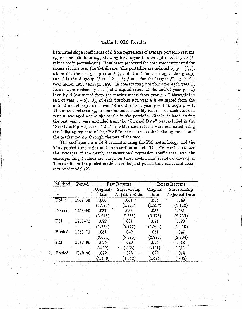
We first considerthecasewherebetais theonly explanatoryvariable,i e, the matrix

X~of explanatoryvariablescontainsonly thevalues/3~. Table I shows theOLS resultsfor

the entire38-yearperiod,1953—1990,andfor the two equal18-yearsubperiods,1953—1971

and 1972—1990

INSERT TABLE I

11

Based on the FM methodology, the resultsshowthat 7’ (estimatedby ‘5~i)is positive

• as expected,but the t statistic implies that it is insignificantly different from zero. The

resultsaresimilar for all four datasetsused.6 This suggeststhat thereis no relationship

betweenaveragestock return and /9, consistentwith theresultsof FF. -

The resultsaresubstantiallydifferent underthejoint pooledcross-sectionandtime-

series estimation,which is more efficient Underthis method, the estimated‘y~is sta-

tistically significant This result is similar for all four datasets used While the joint

pooledtime-seriesand cross-sectionestimationproducesa lower point estimateof 7i, its

varianceis considerablylower and it canbe morereliably distinguishedfrom zero This

demonstratesthebenefit of usingjoint pooledestimationcomparedto the methodof FM

- While the OLS coefficientsare -unbiased,they are inefficiently estimatedand their

variance estimatesarebiased. Consequently,thetest statisticsarebiasedand the power

of the testsis low. This calls for a GLS estimationof themodel. -

INSERT TABLE II

Table II presentsthe GLS estimation results for both methods— the FM and the

joint pooledtime-seriesand cross-section— and for the four datasets. The application

of GLS requiresthe removalof one portfolio (seesectionC, above);the resultspresented

correspondto the elimination of portfolio J = (3,3), a “middle” portfolio This is the

third (out of six) /9 portfolio in thethird (out of six) sizeportfolio, whereportfolio (1,1) is

that of thelargestfirms andwithin it thelargest /3 TableII also reportsthe GLS results

whenwe eliminate insteadeither of the extremeportfolios J = (1, 6) (large firms, small

/3) or J = (6, 1) (small firms, large/3). We reestimatedthe GLS modeleliminatingin turn

eachof the 36 portfolios, and the resultsremainedqualitatively unchanged.

— - The results show that /3 is an important factor in pricing capital assets,consistent

6 We also consideredthe casewhereportfolios were formedby sorting on /3 first and

thenon size, which should leadto strongersignificanceof the /3-coefficient However,the

FM methodologystill indicatedan insignificant return-fl relationship

12

with the CAPM. Under thejoint pooled-GLSmethod, thecoefficient of /3 is positive and

• highly significant. The hypothesis~5’i= 0 is strongly rejeëtedin favor -of the alternative

hypothesis5’, > 0 at significancelevels greaterthan 0.001 (usuallygreaterthan0.0001),

fifty times greaterthanthestandardbenchmarkof 5%. The resultsaresimilar for all four

datasets,and remainunchangedwhen eliminatingportfolios J = (1,6) or J = (6, i).~

This demonstratesthe robustnessof thefl-effect Notably, thepoint estimatesof ‘)‘i under

thejoint pooledtime-seriesandcross-sectionGLS aregenerallysimilar to thoseobtained

under the correspondingOLS estimation procedure,but their statistical significanceis

substantiallyimprovedunderthe GLS. -

Eventhe less-efficientFM estimationmethodproducesmoresignificant resultswhen

applying GLS: thehypothesisthat ‘5’~= 0 which could not be rejectedwhenestimatedby

OLS is rejectedat thestandard-level of significancefor threeof thefour datasetsin favor

of the alternativehypothesis~‘, > 0 In both OLS and GLS estimates, the risk premium

.5~,is of thesameorderof magnitudewhile the significanceof theGLS estimatesis greater

This meansthat when we accountfor the heteroskedasticityacrossyearsas well as the

cross-portfolio heteroskedasticityand,correlations,we obtain lower-varianceestimatesof

7i that are highly significant. Clearly, the power of the test obtained by the joint pooled

cross-sectionand time-seriesGLS estimationis evengreater

Our conclusionis that there is a robust, strongly significant positive relationship

betweensystematicrisk and stock returns

E. Effects of Sizeand StandardDeviation - - -

Testsof the CAPM (asin FM) oftenexaminetheeffect ofunsystematicrisk — thestandard

deviationof themarket-modelresiduals.Under theCAPM, unsystematicrisk shouldnot

~ The results were essentially-the samewhen other portfolios were eliminated. For

example,in the caseof raw returnscalculatedfor our original data,the 36 estimatesof

5~hada meanof 0 0319 and their t-statisticswere between3 47 and 5 36 The detailed

results are available upon request.

13

• - be priced by well-diversified-investors. Another company-specificfactor affecting stock

• returns is the sizeof the company’sequity value, which was found to havea significant

negativeeffect on stock -returns.8 In this Sectionwe apply our methodologyto examine

theserelationships,becauseit couldbearguedthat -the fl-effect reflectstheeffectsof these

othervariables Given that /3 is negativelycorrelatedwith size, the documentedpositive

relationshipbetween/3 andstock returnscould proxy for the size effect Similarly, given

the positive correlationbetweensystematicand unsystematicrisk, the effect of /3 may

well reflect that of the unsystematicrisk Thus, we test whetherthe inclusion of these

explanatoryvariablesin the regressionequationobliteratesthe positive and significant

relationshipbetween/3 andaverageportfolio returns,documentedin SectionD above We

presentresultsfor the survivorship-adjusteddataandconcentrateon t-he most powerful

andefficient method, thejoint pooledtime-seriesandcross-section GLS estimation.

- INSERT TABLE III

First, we consider the addition of the standarddeviationofthemarket-modelresiduals,

1’ SD, which were estimatedfrom the market-modelregressionsin subperiodII for each

portfolio. Thereare threepredictions on the relationshipbetweenexpectedre-turn and

SD (see discussion inAM (1989)): By the CAPM, SD shouldhaveno effect on expected

returnsfor well-diversifiedinvestors,however, if diversification is constrained,the return-

SD relationship will be positive because risk-averse investorsexpect a compensationfor

the imdiversifiedrisk On the other hand, Constantinidesand Scholes(1980) show that

assetswith higherstandarddeviationsprovide investorswith a morevaluabletax trading

option, implying a negativereturn-SDrelationship.

Formaximal efficiency, the variance-covariance matrix ~ shouldbebasedon residuals

from the correctly specified model. WhenintroducingSD, wetestthenull hypothesisthat,

this variableis in fact superfluous,hencewebaseiTi~, on residualsfrom thenull, i e, from

8 SeeBanz (1981),Reinganum(1981) and recentlyFF AM arguedthat the sizeeffect

proxiesfor aliquidity effect

14

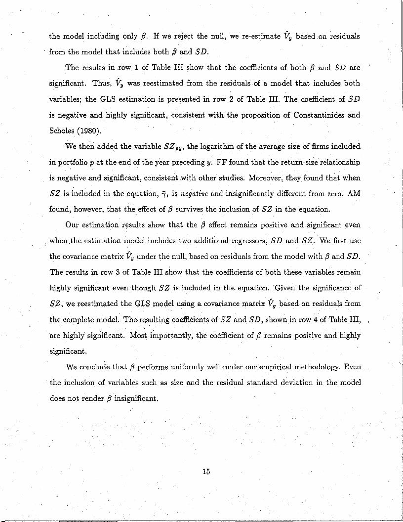
the model including only /3. If we reject the null, we re-estimate~ basedon residuals

from themodel that includesb-oth /9 andSD.

The results in row 1 of Table III show that the coefficientsof both /3 and SD are

significant. Thus, ~ was reestimatedfrom the residualsof a model that includesboth

variables; the GLS estimationis presentedin row 2 of Table HI. The coefficient of SD

is negativeand highly significant, consistentwith the propositionof Constantimdesand

Scholes (1980). - -

We thenaddedthe variableSZ~,thelogarithmof theaveragesizeof firms included

in portfolio p at theendof theyearprecedingy. FF foundthat thereturn-sizerelationship

is negativeandsignificant, consistentwith otherstudies Moreover,theyfoundthat when

SZ is includedin the equation,5~is negativeand insignificantly different from zero. AM

found,however, that the effect of /3 survivesthe- inclusionof SZ in the equation. -

Our estimationresultsshow that the /3 effect remainspositive and significant.even

when the estimationmodel includestwo additional regressors,SD andSZ We first use

thecovariancematrix V~,underthenull, basedon residualsfrom themodelwith /3 andSD

Theresultsin row 3 of TableIII show that the coefficientsof both thesevariablesremain

highly significanteven thoughSZ is includedin the equation. Given the significanceof

SZ,we reestimatedthe GLS model using a covariancematrix T~basedon residualsfrom

thecompletemodel Theresultingcoefficientsof SZandSD, shownin row 4 of TableIII,

arehighly significant Most importantly, the coefficient of /9 remainspositive and highly

- significant. - -

We concludethat /3 performsuniformly well -underourempirical methodology.Even • - -

- the inclusion of variablessuchas size -and the residualstandarddeviationin the model

doesnot render/3 insignificant.

15 -

III. Conclusion

In this paper we presentedtwo econometrictecbniquesto test the capital assetpricing

model (CAPM) that improveon the commonly-usedFama-MacBeth(1973)methodology:

(1) a joint pooledcross-sectionand time-seriesestimationprocedure,and (2) the useof

generalizedleast squaresestimation This method of estimation (usedin Amihud and

Mendelson(1986)) producesmoreefficient estimatesandmore powerful teststhan those

obtainedby the FM methodology A recentstudy by Famaand French (1992) which

applied, in the main, the FM methodfound an insignificant return-fl relationship This

implies that thereis no supportfor the major dictum of the CAPM However,using our

methodologywereachdifferent conclusions. - -

ReplicatingtheFM methodology,we found that thereturn-fl relationshipis insignif-

icant, consistentwith FF. However,using the samedataand employingthejoint pooled

time-seriesandcross-sectionestimation,we obtaineda significantly positive coefficient of

averagereturn on /9 An additional improvementin statistical significancewas obtained

whenwe appliedGLS to accountfor heteroskedasticityover time andacrossportfolios as

well as cross-portfoliocorrelations.’The joint pooled GLS estimationmethod produced

positive and highly significant estimatesof the coefficient of averagereturn on ~8 The

resultswere highly robust to the dataused In particular,weusedraw andexcessreturns

(over the T-bill rates),and adjustedthe datafor a possiblesurvivorship bias The FM

methodology itself was improved when we applied to it the GLS estimation procedure: we

found, again,that thereturn-fl relationshipwaspositive andgenerallysignificant.

The return-fl relationshipremainedhighly significant after including in the model

two additional regressors,the standarddeviationof the market model residualsand the

(logarithmof) firm size Both variableshadnegativeand significantcoefficients However,

the coefficientof the averagereturn on /3 remainedpositive andhighly significant

Weconclude that /9 remainsan important factor in asset pricing

- - 16

REFERENCES

Amihud, Yakov, andHaim Mendelson,1986,Assetpricingand thebid-askspread,Journal

of Financial Economics17, 223—249. -

Amihud, Yakov, and Haim Mendelson, 1989, The effects of beta, bid-ask spread, residual

risk, and sizeon stock returns,Journal of Finance44, 479—486.

Banz,Roif W, 1981, Therelationshipbetweenreturnandmarketvalueof commonstocks

Journal of Financial Economzc39, 3—18

Barry, ChristopherB andStephenJ Brown, 1984, Differential informationandthesmall

firm effect Journal of Financial Economics13, 283—294

Black, Fischer, 1972, Capital market equilibrium with restrictedborrowing, Journal of

Business45, 444—455.

Black, Fischer, Michael C. Jensenand Myron Scholes, 1972, The capital assetpricing

model: Someempirical tests. In Michael C. Jensen,ed., Studiesin the theory of capital

markets(Praeger,New York), 79—121.

Blume, Marshall E and Robert F Stambaugh, 1983, Biases in computing returns An

applicationto the sizeeffect Journal of Financial Economics12, 387—404

Brown, StephenJ, William Goetzmann, Roger G IbbotsonandStephenA Ross,1992,

Survivorshipbias in performancestudies.Reviewof Financial Studies5, 553-580. —

Brown,StephenJ.andMarkI. Weinstein,1983,A New Approachto TestingAssetPricing

- Models: The Bilinear Paradigm, Journal of Finance38, 711—743.

Chan,Louis K.C. andJosefLakonishok,1992, Are thereportson Beta’sdeathpremature?

Working paper,Universityof Illinois at Urbana-Champaign

Constantinides,GeorgeM andMyron S Scholes,1980, Optimal liquidation of assetsin the

presenceof personaltaxes implicationsfor assetpricing, Journal of Finance35, 439—443

- - - - 17 • -

Fama,EugeneF. andKennethR. French,1992,Thecross-sectionof expectedstockreturns,

• Journal of Finance47, 427—465. -

Fama,EugeneF andJamesMacBeth,1973, Risk, returnandequilibrium empiricaltests,

Journal of Political Economy81, 607—636.

Farrell,Roger H., 1985, Multivariate Calculation (Springer-Verlag,New York). - -i

Handa,Puneet,S P Kothari, andCharlesE Wasley,1992,Sensitivityof MultivariateTests

of the CAPM to the ReturnMeasurementInterval Journal of Finance,forthcoming

Judge,GeorgeG, William E Griffiths, R CarterHill, Helmut Lutkepohl and Tsoung-

ChaoLee, 1980, The Theoryand Practice of Econometrics(Wiley, New York)

Kmenta, Jan, 1971, Elementsof Econometrics(Macmillan,New York).

Kothari, S.F.,JayShankenandRichardG. Sloan,1992, Anotherlook at the cross-section

of expectedstockreturn. Mimeo.

Lintner, John,1965, The valuationof risk assetsand theselectionof risky investmentsin

stockportfolios andcapitalbudgets,Reviewof Economics~and Statistics47, 13—37.

Litzenberger,Robert H andKrishnaRamaswamy,1979, The effect of personaltaxesand

dividend on capital asset prices theory and empirical evidence Journal of Financial

Economics7, 163—195

Miller, Merton H and Myron S Scholes, 1982, Dividends and taxes Some empirical

evidence.Journal of Political Economy90, 1118—1141.

Mossin,Jan,1966, Equilibrium in a capitalassetmarket, Econometrica34, 76-8—783.

Reinganuni,Marc R., 1981, Misspecificationof capitalassetpricing: Empiricalanomalies

basedon earningsyields andmarketvalues Journal of Financial Economics9, 19—46

Roll, Richard,1983, On computingmeanreturn andthe small firm premium Journal of

Financial Economics12, 371—386

- - 18

Shanken,Jay,1992, On theestimationof beta-pricingmodels,Reviewof Financial Studies

- • 5, 1—33.

Sharpe,William F., 1964, Capital asset prices: a theory of market equilibrium under

conditionsof risk, Journal of Finance19, 425—442.

19

- - - - Table I: OLS Results

Estimated slope coefficients of /3 fromregressionsofaverageportfolio returnson portfolio beta/3~,allowing for a separateinterceptin. eachyear (t-

valuesareinparentheses).Resultsarepresentedfor bothrawreturnsandforexcessreturnsover theT-Bill rate Theportfoliosareindexedby p = (2,3),where z is the size group (z = 1,2, 6, t = 1 for the largest-sizegroup)and ~ is the /3 group (~= 1,2, 6, ~ = 1 for the largest /3) y is theyear index, 1953 through1990 In. constructingportfoliosfor eachyeary,stocks wererankedby size (total capitalizationat the end of year y — 1)then by j3 (estimated from the market-modelfrom yeary — 7 throughtheendof year y — 5) /3~,of eachportfolio p in yeary is estimatedfrom themarket-modelregressionover 48 months from year y — 4 through y — 1

The annualreturns~ are compoundedmonthly returnsfor eachstock inyeary, averaged across the stocks in the portfolio Stocks delisted duringthetestyeary were excludedfrom the “Original Data” but includedin the -

“Survivorship-AdjustedData,” in. which casereturnswere estimatedusingthedelistmgsegmentofthe CRSPfor thereturnon the delistmgmonthandthemarketreturnthroughtherest of theyear. -

The coefficientsare OLS estimatesusing the FM methodologyand thejoint pooledtime-seriesand cross-sectionmod-el. The FM coefficientsarethe averagesof the yearly crosssectionalregressioncoefficients,and thecorrespondingt-valuesare base.don thesecoefficients’ standarddeviation.Theresultsfor thepooledmethodusethe’jointpooledtime-seriesandcross-sectionalmodel (2)

Method Period Raw Returns ExcessReturnsOriginal Survivorship

- - Data AdjustedDat.a- FM 1953—90

Pooled 1953—90

FM 1953—71

Pooled 1953—71

OriginalData.053

(1.198).037

(3.215).082

(1.273).051

(3.004).025

(.409).022-

(1.436)

SurvivorshipAdjusted_Data

.051 -

(1.164).033

(2.868).081

(1.277).049

(2.895).019

• (.333)- .016(1.032) -

- FM

Pooled

.053(1.185)

.037(3.176)

.081• (1.264)

.051(2.975)

.025(.4th)

- .022(1.416’)

1972—90

1972—90

.049- (1.126)

- -.031(2.733)

.080(1.250)

.047(2.804)

.018(.311).014

(.935)

Table II: GLS Results -

Estimatedcoefficientsfrom GLS regressionsof portfolio returnsr~1,on port-folio beta, /3~,,allowing for a separateinterceptin each year, applyingboth the FM andthejoint pooledtime-seriesand cross-sectionestimationmethodologies(t-valuesin parentheses,seeTableI for a descriptionof thedata) The variance-covanancematricesV~for the GLS procedurewereestimatedfrom the OLS residuals,deletingoneportfolio sothat V~,arenon-singular Unlessotherwisestated,the deletedportfolio is (3,3) Resultsarealsopresentedwhentwo otherportfoliosaredeleted portfolio (1,6)of largesize,low betastocks,and(6,1) ofsmall size,largebetastocks ForFM-GLS,

arebasedon the FM OLS residuals,andfor thejoint pooledGLS, theyarebasedon. thejoint pooled OLS residuals Theresults arepresentedforbothrawreturnsandexcessreturnsover the-T-bill rate,-for theoriginal andthesurvivorship-adjusteddata.

- Method Period - RawReturns ExcessReturns -

Original Survivorship Original SurvivorshipData AdjustedData Data AdjustedData

FM - - 1953—90-

.039(2.138)

.035- • (2.242)

.042(2.295)-

.024(1.574)

Pooled - 1953—90 .035 .027 .034 .027- - - (5.146) (3.939) (4.345) (4.054)

FM 1953—71 .075 .040 .077 .046- (3.087) - • (1.870) (2.803) (3.225)

Pooled 1953—71 ;044(5 481)

.029 -

(3 365).048

(4 967)- .032

(3 976)FM 1972—90 004

(171)029

(1 315)007

(323)001

(044)Pooled 1972—90 012 023 007 016

FM (1,6) 1953—90(965).034

(1.595)

(2 022).040

(2.496)-

(548).040

(1.995)

(1 358).036

(2.169)-

Pooled (1,6), 1953—90 .031(3.997)

.026- (3.836)

.029(3.667)

.031(4.680)

FM (6,1) 1953—90 .037 - .047 .033 .035- (1.839) (3.042) (1.422) (2.174)

Pooled (6,1) 1953—90 .033(4 848)

.029(4 325)

.027 -

(3 370).032

(4 840)

‘I

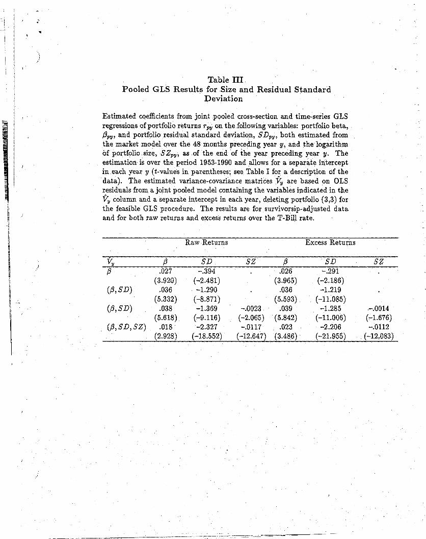
- Table IIIPooled GLS Results for Size and Residual Standard

Deviation - -

Estimatedcoefficients from joint pooledcross-sectionand time-seriesGLSregressionsof portfolio returnsr~on thefollowing variables portfolio beta,/3~,,andportfolio residualstandarddeviation,~ both estimatedfromthemarketmodel over the 48 monthsprecedingyear y, and thelogarithmof portfolio size, SZ~,,as of the end of the year precedingyeary Theestimationis over theperiod 1953-1990and allows for a separateinterceptin eachyeary (t-valuesin parentheses,seeTableI for a descriptionof thedata) The estimatedvariance-covariancematricesV~arebasedon OLSresidualsfrom ajoint pooledmodelcontainingthevariablesindicatedin theV~column and-a separateinterceptin eachyear,deletingportfolio (3,3)forthe feasible GLS procedure.The resultsare for survivorsip-adjusteddataandfor bothrawreturnsand excessreturnsover theT-Bill rate.

. Raw Returns ‘ ExcessReturns -

/3 - SD SZ /3 SD - S~/3 - - .027 - —.394 - .0-26 - —.291 -

• (3.920) (—2.481) - (3.965) (—2.186) -

(/3,SD) .036(5.332)

• —1.290(—8.871)

. ~036(5.593)

—1.219(—11.085)

-

(/3, SD) .038(5.618)

—1.369- (—9.116)

—.0023 -

(—2.065).039

(5.842)—1.285

(—11.006)—.0014

(—1.676)-(/3,SD,SZ) 018

(2 928)—2327

(—18 552)—0117

(—12 647)023

(3 486)—2206

(—21 955)—0112

(—12 083)