Research Article Traction Control of Electric Vehicles Using Sliding-Mode Controller with Tractive Force Observer Suwat Kuntanapreeda Department of Mechanical and Aerospace Engineering, Faculty of Engineering, King Mongkut’s University of Technology North Bangkok, Bangkok 10800, ailand Correspondence should be addressed to Suwat Kuntanapreeda; [email protected] Received 24 June 2014; Revised 26 November 2014; Accepted 1 December 2014; Published 21 December 2014 Academic Editor: Nicolas Hauti` ere Copyright © 2014 Suwat Kuntanapreeda. is is an open access article distributed under the Creative Commons Attribution License, which permits unrestricted use, distribution, and reproduction in any medium, provided the original work is properly cited. Traction control is an important element in modern vehicles to enhance drive efficiency, safety, and stability. Traction is produced by friction between tire and road, which is a nonlinear function of wheel slip. In this paper, a sliding-mode control approach is used to design a robust traction controller. e control objective is to operate vehicles such that a desired wheel slip ratio is achieved. A nonlinearity observer is employed to estimate tire tractive forces, which are used in the control law. Simulation and experimental results have illustrated the success of the proposed observer-based controller. 1. Introduction Electric vehicles (EVs) have become very attractive in replac- ing conventional internal combustion engine vehicles be- cause of environmental and energy issues. ey have received a great attention from the research community. Control methodologies have been actively developed and applied to EVs to improve the EVs performances [1–8]. Traction control plays an important role in vehicle motion control because it can directly enhance drive efficiency, safety, and stability [9, 10]. Traction is the vehicular propulsive force produced by friction between tire and road. e characteristics of the friction are nonlinear and uncertain, which make traction control difficult. e friction depends on many factors such as tire type, road surface, road condition, and wheel slip. Accordingly, an objective of the traction control is to operate vehicles such that a desired wheel slip ratio is obtained. e slip ratio yielding the maximum friction coefficient is usually desired because it yields the maximum torque from the propulsion system to drive the vehicle forward. Traction control of electric vehicles has drawn extensive attention since electric motors can produce very quick and precise torques compared to conventional internal combus- tion engines. In [1], traction control based on a maximum transmission torque estimation (MTTE) approach was pro- posed. e estimation was carried out by an open-loop disturbance observer, which required only the input torque and the wheel speed. e estimated maximum transmission torque was used in the control law as a constraint to prevent the slip. Experimental results illustrated the effectiveness and practicality of the proposed control design. e MTTE approach was extended by replacing the open-loop observer with a closed-loop observer in [2]. By doing this, the robustness of the control system was markedly enhanced. In [3], traction control of electric vehicles using a sliding-mode observer to estimate the maximum friction was presented. e observer was based on the LuGre friction model. e controller used the estimated maximum friction to determine the suited maximum torque for the wheels. Sliding-mode control has been extensively used for con- trol of uncertain nonlinear systems because of its robustness property. e essence of the sliding-mode control is to use a switching control command to drive the controlled system’s state trajectory onto a specified sliding surface in the state space and then to keep the state trajectory moving along this surface [11, 12]. As far as sliding-mode control of vehicles is concerned, wheel slip control of electric vehicles based on a sliding-mode framework was proposed in [4]. A conditional integrator Hindawi Publishing Corporation International Journal of Vehicular Technology Volume 2014, Article ID 829097, 9 pages http://dx.doi.org/10.1155/2014/829097

Welcome message from author
This document is posted to help you gain knowledge. Please leave a comment to let me know what you think about it! Share it to your friends and learn new things together.
Transcript
Research ArticleTraction Control of Electric Vehicles Using Sliding-ModeController with Tractive Force Observer
Suwat Kuntanapreeda
Department of Mechanical and Aerospace Engineering Faculty of Engineering King Mongkutrsquos University ofTechnology North Bangkok Bangkok 10800 Thailand
Correspondence should be addressed to Suwat Kuntanapreeda suwatkmutnbacth
Received 24 June 2014 Revised 26 November 2014 Accepted 1 December 2014 Published 21 December 2014
Academic Editor Nicolas Hautiere
Copyright copy 2014 Suwat Kuntanapreeda This is an open access article distributed under the Creative Commons AttributionLicense which permits unrestricted use distribution and reproduction in any medium provided the original work is properlycited
Traction control is an important element in modern vehicles to enhance drive efficiency safety and stability Traction is producedby friction between tire and road which is a nonlinear function of wheel slip In this paper a sliding-mode control approach is usedto design a robust traction controller The control objective is to operate vehicles such that a desired wheel slip ratio is achieved Anonlinearity observer is employed to estimate tire tractive forces which are used in the control law Simulation and experimentalresults have illustrated the success of the proposed observer-based controller
1 Introduction
Electric vehicles (EVs) have become very attractive in replac-ing conventional internal combustion engine vehicles be-cause of environmental and energy issuesThey have receiveda great attention from the research community Controlmethodologies have been actively developed and applied toEVs to improve the EVs performances [1ndash8]
Traction control plays an important role in vehiclemotioncontrol because it can directly enhance drive efficiency safetyand stability [9 10] Traction is the vehicular propulsiveforce produced by friction between tire and road Thecharacteristics of the friction are nonlinear and uncertainwhichmake traction control difficultThe friction depends onmany factors such as tire type road surface road conditionand wheel slip Accordingly an objective of the tractioncontrol is to operate vehicles such that a desired wheelslip ratio is obtained The slip ratio yielding the maximumfriction coefficient is usually desired because it yields themaximum torque from the propulsion system to drive thevehicle forward
Traction control of electric vehicles has drawn extensiveattention since electric motors can produce very quick andprecise torques compared to conventional internal combus-tion engines In [1] traction control based on a maximum
transmission torque estimation (MTTE) approach was pro-posed The estimation was carried out by an open-loopdisturbance observer which required only the input torqueand the wheel speed The estimated maximum transmissiontorque was used in the control law as a constraint to preventthe slip Experimental results illustrated the effectivenessand practicality of the proposed control design The MTTEapproach was extended by replacing the open-loop observerwith a closed-loop observer in [2] By doing this therobustness of the control system was markedly enhanced In[3] traction control of electric vehicles using a sliding-modeobserver to estimate the maximum friction was presentedThe observer was based on the LuGre friction model Thecontroller used the estimatedmaximum friction to determinethe suited maximum torque for the wheels
Sliding-mode control has been extensively used for con-trol of uncertain nonlinear systems because of its robustnessproperty The essence of the sliding-mode control is to use aswitching control command to drive the controlled systemrsquosstate trajectory onto a specified sliding surface in the statespace and then to keep the state trajectory moving along thissurface [11 12]
As far as sliding-mode control of vehicles is concernedwheel slip control of electric vehicles based on a sliding-modeframework was proposed in [4] A conditional integrator
Hindawi Publishing CorporationInternational Journal of Vehicular TechnologyVolume 2014 Article ID 829097 9 pageshttpdxdoiorg1011552014829097
2 International Journal of Vehicular Technology
approach was employed to overcome the chattering enablinga smooth transition to a PI control law when the slip is closeto the set point Experimental results demonstrated a goodslip regulation and robustness to disturbances In [13] a slid-ing-mode approach to the design of an active braking con-troller was proposed The controlled variable was a convexcombination of wheel deceleration and wheel slip Theapproach offered advantages with respect to pure slip anddeceleration control In [14] a second-order sliding-modetraction force controller for vehicles was proposed Thetraction control was achieved by maintaining the wheel slipat a desired value
This paper presents a robust control scheme for tractioncontrol of electric vehiclesThe control objective is to operatethe vehicles at a desired wheel slip ratio The paper proposesa simple approach to design a traction controller based on asliding-mode control frameworkThemainmotivation of thedesign is the robustness to uncertaintiesThe implementationof the control design requires tractive forces for feedbackbut they are not usually available in practices To overcomethis problem a PI observer developed in [15 16] is usedto estimate the tractive forces The PI observer has anattractive zero-steady-state feature similar to the well-knownPI controllers This synthesis of the sliding-mode tractioncontroller and the PI observer makes the implementationpractical At the end the resulting observer-based controlleris experimentally validated in a single-wheel test rig
The rest of the paper is organized as follows In the nextsection some preliminaries are provided The longitudinaldynamic model of the vehicles used in the paper is presentedin Section 3 followed by the controller and observer designin Section 4 Simulation results are given in Section 5 InSection 6 an experimental study is presentedThe conclusionsof this paper are drawn in Section 7
2 Preliminaries
21 Sliding-Mode Control Sliding-mode control based on theequivalent control method is summarized in this subsectionThe reader is referred to [11 12] for more details of themethod
The controlled system is expressed as
= 119891 (119909) + 119892 (119909) 119906 (1)
where 119909 isin 119877
119899 is the state variable vector 119906 isin 119877
119898 is theinput vector and 119891(sdot) and 119892(sdot) are nonlinear functions Let119878(119909) be a desired sliding surface which is usually chosenaccording to the control objective Based on the equivalentcontrol method the control input vector is written as
119906 = 119906eq + 119906sw (2)
where 119906eq and 119906sw are called the equivalent control andthe switching control respectively The equivalent control119906eq is determined based on the assumption that the systemtrajectory is staying on the sliding surface Thus it is simplyobtained by setting
119878 = 0 (3)
The switching control 119906sw is designed to guarantee that thesystem trajectory moves towards the sliding surface and stayson it It is determined such that the reachability condition
119878
119878 = minus120578 |119878| 120578 gt 0 (4)
is satisfied
22 Nonlinearity Observer The nonlinearity observer devel-oped in [15 16] is provided in this subsection Consider thefollowing nonlinear system
= 119860119909 + 119873120572 (119905) + 119872120590 (119905) + 119861119906
119910 = 119862119909
(5)
where 119909 isin 119877
119899 is the state variable vector 119906 isin 119877119898 is the controlvector119910 isin 119877
119901 is the output vector119860 is the systemmatrix119861 isthe control inputmatrix119862 is the outputmatrix and119872 and119873are the constantmatrices Here120572(119905) is an unknownnonlinearfunction whereas 120590(119905) is a known function The observer isdesigned to estimate 120572(119905)
The fundamental idea of the observer is to approximate120572(119905) by a fictitious system
120572 (119905) asymp 119867V (119905)
V (119905) = 119881V (119905) (6)
By substituting (6) into (5) the system can be expressed as
[
V] = [
119860 119873119867
0 119881
][
119909
V] + [119861 119872
0 0
] [
119906
120590
] (7)
Thus the observer is chosen as
[
V] = [
119860 119873119867
0 119881
][
119909
V] + [119861 119872
0 0
] [
119906
120590
] + [
119871
119909
119871V] (119910 minus 119862119909)
(8)
where 119871119909and 119871V are the observer gain matrices that must be
chosen such that the observer is asymptotically stableIn a special case when 119867 = 119868 and 119881 = 0 are chosen
the observer is reduced to the proportional-integral (PI)observer
= 119860119909 + 119861119906 +119872120590 + 119871
119909(119910 minus 119862119909) + 119873119871V int (119910 minus 119862119909) 119889119905
V = 119871V int (119910 minus 119862119909) 119889119905
(9)
and the estimated nonlinearity is given by
(119905) = V (119905) (10)
The PI observer has been successfully applied to controlproblems [17 18] The reader is referred to [16] for a proof ofthe estimation convergence and an analysis of the estimationerrors
International Journal of Vehicular Technology 3
3 Longitudinal Dynamic Model
A longitudinal dynamic model of two-axle vehicles is pre-sented The model is known as a bicycle model which hasthree degrees of freedomThemodel can be found in [14] andis given as
Vehicle body 119865
119891+ 119865
119903minus 119865loss = 119898
119881
119909
Front axle 119879
119891minus 119903
119891119865
119891= 119868
119891
119891
Rear axle 119879
119903minus 119903
119903119865
119903= 119868
119903
119903
(11)
where 119881119909is the longitudinal velocity of the vehicle center of
gravity 120596119891 120596
119903are the tire rotational speeds (the subscripts 119891
and 119903 stand for the front and rear axle resp)119898 is the vehiclemass 119868
119891 119868
119903are the moments of inertia 119903
119891 119903
119903are the tire
effective rolling radius 119879119891 119879
119903are the input torques 119865
119891 119865
119903are
the tractive forces 119865loss = 119888
119909119881
2
119909sdot sgn(119881
119909) + 119891roll119898119892 combining
the aerodynamic drag and the rolling resistance and 119888
119909
and 119891roll are the aerodynamic drag and rolling resistancecoefficients respectively
The tractive forces are given by
119865
119894= 120583 (120582
119894)119873
119894 119894 = 119891 119903 (12)
where 120583(120582119894) is the friction coefficient function 120582
119894is the wheel
slip ratio defined as
120582
119894=
119903
119894120596
119894minus 119881
119909
119903
119894120596
119894
for driving
119881
119909minus 119903
119894120596
119894
119881
119909
for braking(13)
and119873119891 119873
119903are the normal loads given as
119873
119891=
119897
119903119898119892 minus 119897
ℎ119898
119881
119909
119897
119891+ 119897
119903
119873
119903=
119897
119891119898119892 + 119897
ℎ119898
119881
119909
119897
119891+ 119897
119903
(14)
where 119897
119891is the distance from the front axle to the center
of gravity 119897119903is the distance from the rear axle to the center
of gravity and 119897
ℎis the height of the center of gravity (see
Figure 1)The friction coefficient depends on many factors tire
type road surface road condition wheel slip and so forthThis makes behaviors of the tractive forces complicated Thefriction coefficient usually has to be measured experimen-tallyThe typical friction coefficient in dependency of the slipratio is shown in Figure 2 It illustrates that some amount ofslip is necessary to produce the tractive force on the otherhand an excessive slip leads to a loss of the force
4 Control Design
41 Sliding-Mode Controller Design A sliding-mode con-troller is designed for the system described by (11)ndash(14) The
Vx
120596fTf
rf
Ff
Nf
mg
Floss
lf lr
lh Fr
rr
Tr120596r
Nr
Figure 1 Longitudinal model of vehicles
0 01 02 03 04 05 06 07 08 09 10
01
02
03
04
05
06
07
08
09
1
Slip ratio
Fric
tion
coeffi
cien
t
Dry road
Wet road
Icy road
Figure 2 Typical trends of longitudinal friction coefficient
control objective is to drive the vehicle such that the desiredslip ratio 120582lowast is achieved First define the sliding surface as
119878
119894(120582
119894 120596
119894) = (120582
119894minus 120582
lowast
) 120596
119894 119894 = 119891 119903 120596
119894= 0 (15)
Taking derivative of the sliding surface yields
119878
119894(120582
119894 119881
119909) =
119865loss119903
119894119898
minus
1
119903
119894119898
119865
119891minus
1
119903
119894119898
119865
119903
minus (1 minus 120582
lowast
)
119903
119894
119868
119894
119865
119894+ (1 minus 120582
lowast
)
1
119868
119894
119906
119894
(16)
where 119906119894= 119879
119894 119894 = 119891 119903 Assuming
119878
119894= 0 in (16) results in
119906
119894eq = (
119868
119894
1 minus 120582
lowast)
times (minus
119865loss119903
119894119898
+
1
119903
119894119898
119865
119891+
1
119903
119894119898
119865
119903+ (1 minus 120582
lowast
)
119903
119894
119868
119894
119865
119894)
(17)
Next letting 119906119894= 119906
119894eq + 119906
119894sw and utilizing the reachabilitycondition (4) result in
119906
119894sw = minus120578
119894(
119868
119894
1 minus 120582
lowast) sgn (119878
119894) 120578
119894gt 0 (18)
4 International Journal of Vehicular Technology
where
sgn (119878119894) =
1003816
1003816
1003816
1003816
119878
119894
1003816
1003816
1003816
1003816
119878
119894
=
1 119878
119894gt 0
0 119878
119894= 0
minus1 119878
119894lt 0
(19)
From (17) and (18) the sliding-mode control law can beconcluded as
119906
119894= (
119868
119894
1 minus 120582
lowast)(minus
119865loss119903
119894119898
+
1
119903
119894119898
119865
119891+
1
119903
119894119898
119865
119903
+ (1 minus 120582
lowast
)
119903
119894
119868
119894
119865
119894minus 120578
119894sgn (119878
119894))
(20)
Note that the control law requires 119865119891 119865
119903for feedback but
they are usually not available Thus an observer is needed toestimate 119865
119891 119865
119903
42 Nonlinearity Observer Design Anonlinearity observer isdesigned to estimate 119865
119891 119865
119903 First express (11) in the form (5)
as
=
[
[
0 0 0
0 0 0
0 0 0
]
]
119909 +
[
[
[
[
[
[
[
[
[
1
119898
1
119898
minus
119903
119891
119868
119891
0
0 minus
119903
119903
119868
119903
]
]
]
]
]
]
]
]
]
120572 (119905)
+
[
[
[
1
119898
0
0
]
]
]
120590 (119905) +
[
[
[
[
[
[
0 0
1
119868
119891
0
0
1
119868
119903
]
]
]
]
]
]
119906
119910 =
[
[
1 0 0
0 1 0
0 0 1
]
]
119909
(21)
where 119909119879 = [119881
119909120596
119891120596
119903] 119906119879 = [119879
119891119879
119903] 120572(119905)119879 = [119865
119891119865
119903]
and 120590(119905) = 119865loss Consequently the observer (8) with 119867 = 119868
and 119881 = 0 can be expressed as
119883 =
[
[
[
[
[
[
[
[
[
[
[
[
[
0 0 0
1
119898
1
119898
0 0 0 minus
119903
119891
119868
119891
0
0 0 0 0 minus
119903
119903
119868
119903
0 0 0 0 0
0 0 0 0 0
]
]
]
]
]
]
]
]
]
]
]
]
]
119883 +
[
[
[
[
[
[
[
[
[
[
[
0 0
1
119898
1
119868
119891
0 0
0
1
119868
119903
0
0 0 0
0 0 0
]
]
]
]
]
]
]
]
]
]
]
119880
+ 119871(119910 minus
[
[
1 0 0 0 0
0 1 0 0 0
0 0 1 0 0
]
]
119883)
(22)
where
119883
119879
= [
119881
119909
119891
119903
119865
119891
119865
119903] and 119880
119879
= [119879
119891119879
119903119865loss]
Here 119871 is the observer gain matrix that must be chosen suchthat 119883 rarr 119883 resulting in
119865
119891rarr 119865
119891and
119865
119903rarr 119865
119903as desired
Table 1 Parameters of the vehicle and the friction model
Parameter Value119898 1202 kg119868
119891 119868
119903107 kgm2
119897
119891115m
119897
119903145m
119897
ℎ053m
119888
11990904
119891roll 0013119903
119891 119903
119903032m
119862
1105
119862
22002
119862
304646
5 Numerical Studies and Results
Thevehiclemodel in (11)ndash(14) is used as the control plantThevehicle parameters are adopted from [14] and are summarizedin Table 1 The friction coefficient function used in this paperis the Burckhardt friction model [9]
120583 (120582) = 119862
1(1 minus 119890
minus1198622120582
) minus 119862
3120582 (23)
where11986211198622 and119862
3are model parametersThe values of the
friction model are also listed in Table 1 This friction modelyields the maximum friction coefficient at 120582 asymp 02
51 Sliding-Mode Controller The control law (20) is usedHere it is assumed that 119865
119891 119865
119903are available for feedbackThis
assumption will be removed later in Section 53 The tuningparameters 120578
119891= 120578
119903= 120 are chosen To achieve the
maximum tractive forces the desired slip ratio 120582
lowast is set to02The results are shown in Figures 3ndash5 Note that at time =20 sec a ten-time decrease of the friction coefficient wasintroduced to simulate a change in road condition Figure 3shows that the sliding-mode controller successfully drove thesystem to operate at the desired wheel slip ratio
Time histories of the input torques are presented inFigure 4 It is seen from this figure that the controllereffectively reduced the input torques to keep the wheel slipratios constant when the friction coefficient was decreasedFigure 5 displays time histories of the vehicle velocity andthe tire rotational speeds It shows that the velocity andthe rotational speeds decreased corresponding to the inputtorques
52 Nonlinearity Observer The observer (22) is used Theobserver gain 119871 is determined through the pole-placementtechnique The desired poles are simply chosen to be minus1 minus2minus3 minus4 and minus5 and the following gain matrix is obtained
119871 =
[
[
[
[
[
[
3041 minus0079 0128
minus0239 6545 0911
0241 0664 5414
1853 minus3011 minus8293
minus0715 minus5375 minus1621
]
]
]
]
]
]
(24)
International Journal of Vehicular Technology 5
0 10 20 30 40 50 60 70 80 90 1000
05
1
Time (s)
Time (s)
Time (s)
Time (s)
0 10 20 30 40 50 60 70 80 90 1000
2000
4000
6000
0 10 20 30 40 50 60 70 80 90 1000
05
1
0 10 20 30 40 50 60 70 80 90 1000
5000
10000
Ff
(N)
Fr
(N)
120582f
120582r
Figure 3 Wheel slip ratios and tire tractive forces
0 10 20 30 40 50 60 70 80 90 1000
500100015002000
Time (s)
Time (s)0 10 20 30 40 50 60 70 80 90 100
0100020003000
Tf(N
m)
Tr(N
m)
minus1000
Figure 4 Input torques
The results are shown in Figures 6ndash8The input torques119879119891 119879
119903
were initially set to 500Nm and then stepped up to 1500Nmat time = 200 secThe results show that the observer correctlyestimated all state variables including the tractive forces
Comparisons of true and estimated velocity and rota-tional speeds are presented in Figure 6 It is seen from thefigure that there are overshoots in the estimated rotationalspeeds when the step change of the input torques occurredHowever theywere quickly converged back to the true valuesThe estimations of the tractive forces are presented in Figures
0 10 20 30 40 50 60 70 80 90 1000
50
100
150
Time (s)
Time (s)
Time (s)
0 10 20 30 40 50 60 70 80 90 1000
200
400
600
0 10 20 30 40 50 60 70 80 90 1000
200
400
600
Vx
(ms
)120596f
(rad
s)
120596r
(rad
s)
Figure 5 Velocity and rotational speeds
0 50 100 150 200 250 300 350 4000
100
200
Time (s)
Time (s)
Time (s)
0 50 100 150 200 250 300 350 4000
200
400
600
0 50 100 150 200 250 300 350 4000
200
400
600
Vx
(ms
)120596r
(rad
s)
120596f
(rad
s)
Figure 6 Comparison of true and estimated velocity and rotationalspeeds
7 and 8 In Figure 8 it is seen that the estimations convergedto the true values within 3 and 6 sec for the front and rearwheels respectively
Moreover to investigate the measurement noises effectson the accuracy of the estimations we added zero-meannormal distribution noises with the variance of 50 into allmeasurements We found that the observer still worked wellThe results similar to those in Figures 6ndash8 were obtained
6 International Journal of Vehicular Technology
0 50 100 150 200 250 300 350 4000
005
01
Time (s)
Time (s)
Time (s)
0 50 100 150 200 250 300 350 4000
2000
4000
6000
0 50 100 150 200 250 300 350 4000
005
01
0 50 100 150 200 250 300 350 4000
2000
4000
6000
Time (s)
Fr
(N)
Ff
(N)
120582r
120582f
Figure 7 Wheel slip ratios and comparison of true and estimatedtractive forces
190 195 200 205 210 215 2201000
2000
3000
4000
5000
Time (s)
Time (s)190 195 200 205 210 215 220
1000
2000
3000
4000
5000
True
True
Estimated
Estimated
Ff
(N)
Fr
(N)
Figure 8 Comparison of true and estimated tractive forces aroundtime = 200 sec
Figure 9 displays an example of the results Note that there aresome small oscillations in the estimations due to the noises
53 Sliding-Mode Controller with Nonlinearity Observer Inthis subsection the scenario in Section 51 is resimulatedwithout the availability assumption of 119865
119891 119865
119903 The observer
presented in Section 52 is used to estimate 119865119891 119865
119903 The results
are shown in Figures 10ndash12
200 202 204 206 208 210 212 214 216 218 2204200
4400
4600
4800
Time (s)
Time (s)200 202 204 206 208 210 212 214 216 218 220
4200
4400
4600
4800
Estimated
Estimated
True
True
Ff
(N)
Fr
(N)
Figure 9 Comparison of true and estimated tractive forces whenthe measurements degraded by noises
0 10 20 30 40 50 60 70 80 90 1000
05
1
0 10 20 30 40 50 60 70 80 90 100
0
5000
10000
0 10 20 30 40 50 60 70 80 90 1000
05
1
0 10 20 30 40 50 60 70 80 90 100
0
5000
10000
Time (s)
Time (s)
Time (s)
Time (s)
120582r
120582f
minus5000
minus5000
Ff
(N)
Fr
(N)
Figure 10 Wheel slip ratios and tire tractive forces using theobserver-based controller
Figure 10 shows that the observer-based controller wasable to drive the system to operate at the desired wheelslip ratio Note that there are jumps of the slip ratiosoccurring when the friction coefficient was decreased butthey asymptotically converged back to the desired value Thejumps are due to the dynamics of the observer
International Journal of Vehicular Technology 7
0 10 20 30 40 50 60 70 80 90 100
0
1000
2000
Time (s)
Time (s)0 10 20 30 40 50 60 70 80 90 100
0
1000
2000
3000
minus1000
minus1000
Tf
(Nm
)Tr
(Nm
)
Figure 11 Input torques using the observer-based controller
0 10 20 30 40 50 60 70 80 90 1000
50
100
150
0 10 20 30 40 50 60 70 80 90 1000
500
1000
0 10 20 30 40 50 60 70 80 90 1000
500100015002000
Time (s)
Time (s)
Time (s)
120596r
(rad
s)
120596f
(rad
s)
Vx
(ms
)
Figure 12 Velocity and rotational speeds using the observer-basedcontroller
Time histories of the input torques are presented inFigure 11 Similar to the results in Figure 4 the controllereffectively reduced the input torques to keep the wheel slipratios constant Figure 12 displays time histories of the vehiclevelocity and the tire rotational speeds It is observed thatthere were large overshoots in the rotational speeds whenthe friction was decreased These overshoots are due to thedynamics of the observer
6 Experimental Studies and Results
The experimental studies are carried on a single-wheel testrig (see Figure 13) The test rig simulates the longitudinaldynamic of electric vehicles It consists of a drum set a wheel
Measurementcontrol unit Wheel set
Drum set
Figure 13 Photograph of the single-wheel test rig
set and ameasurementcontrol unitThe role of the drum setis to let the wheel behave like rolling on a road The diameterand width of the drum are approximately 10 and 03 metersrespectively The drum set is also equipped with a rotationalspeed sensor The wheel set consists of a tire a 4-inch-rimwheel a brushedDCmotor and loadingmassesThewheel isdirectly driven by the motor through a rigid shaft The wheelset is also equipped with another rotational speed sensorThe measurementcontrol unit consists of a signal conditioncircuit and a PC computer The computer is installed with a12-bit analogdigital interface boardThe two rotational speedsignals are fed back to the computer through the interfaceboard The control sampling period is 05 sec
A mathematical model of the test rig can be summarized
Drum 119903
2
119889119865 minus 119888
119889119881
119909= 119868
119889
119881
119909
Wheel 119887119881in minus 119903119908119865 minus 119886120596 = 119868
119908
(25)
where 119881119909= Ω119903
119889is the simulated longitudinal velocity Ω is
the drum rotational speed 119903119889is the drum radius 120596 is the
wheel rotational speed 119881in is the motor voltage input 119868119889 119868
119908
are the moments of inertia (the subscripts 119889 and 119908 standfor the drum and wheel resp) 119903
119908is the wheel radius 119886 =
(119896
119879119896
119887119877+119888
119908) and 119887 = (119896
119879119877)119870
0are constants 119896
119879is themotor
torque constant 119896119887is the motor back-EMF constant 119877 is the
motor resistance 119888119889 119888
119908are the damping constants 119870
0is the
gain of the motor-drive unit and 119865 is the tractive force Theparameters of the test rig are summarized in Table 2
61 Control Design First a sliding-mode controller isdesigned Define the sliding surfaces as
119904 (120582 120596
119894) = (120582 minus 120582
lowast
) 120596
119894 120596
119894= 0 (26)
Taking derivative of the sliding surface yields
119904 (120582 119881
119909) =
119888
119889
119868
119889119903
119908
119881
119909minus
119903
2
119889
119868
119889119903
119908
119865
120583minus (1 minus 120582
lowast
)
119886
119868
119908
120596
minus (1 minus 120582
lowast
)
119903
119908
119868
119908
119865
120583+ (1 minus 120582
lowast
)
119887
119868
119908
119906
(27)
8 International Journal of Vehicular Technology
Table 2 Parameters of the experimental test rig
Parameter Value119868
1198892495 kgm2
119868
11990800098 kgm2
119903
11988905m
119903
119908013125m
119886 00392119887 05096119888
119889005Nmsminus1
where 119906 = 119881in By following the procedure in Section 41 thesliding-mode control law can be found as
119906 = (
119868
119908
(1 minus 120582
lowast) 119887
)(minus
119888
119889
119868
119889119903
119908
119881
119909+
119903
2
119889
119868
119889119903
119908
119865
120583+ (1 minus 120582
lowast
)
119886
119868
119908
120596
+ (1 minus 120582
lowast
)
119903
119908
119868
119908
119865
120583minus 120578 sgn (119904))
(28)
Next a tractive force observer is designed Rewrite (25) as
=
[
[
[
minus
119888
119889
119868
119889
0
0 minus
119886
119868
119908
]
]
]
119909 +
[
[
[
[
119903
2
119889
119868
119889
minus
119903
119908
119868
119908
]
]
]
]
119891 (119905) +
[
[
0
119887
119868
119908
]
]
119906
119910 = [
1 0
0 1
] 119909
(29)
where 119909119879 = [119881
119909120596] 119906 = 119881in and 119891(119905) = 119865
120583 By following the
procedure in Section 42 the observer can be concluded as
119883 =
[
[
[
[
[
[
[
minus
119888
119889
119868
119889
0
119903
2
119889
119868
119889
0 minus
119886
119868
119908
minus
119903
119908
119868
119908
0 0 0
]
]
]
]
]
]
]
119883
+
[
[
[
[
[
0
119887
119868
119908
0
]
]
]
]
]
119906 + 119871(119910 minus [
1 0 0
0 1 0
]
119883)
(30)
where 119883119879 = [
119881
119909
119865
120583] and 119906 = 119881in The gain matrix 119871must
be chosen such that 119883 rarr 119883
62 Experimental Results The controller comprises the con-trol law (28) and the observer (30) The parameters inthe control law (28) are chosen as 120582lowast = 02 and 120578= 10The gainmatrix 119871 in the observer (30) is designed by simply placingthe observer poles at minus1 minus2 and minus3 Since the observer isimplemented in a digital computer with the sampling period05 seconds the corresponding discrete-time desired poles
0 10 20 30 40 50 6002468
Time (s)
Time (s)
Time (s)
Time (s)
0 10 20 30 40 50 600
20
40
60
0 10 20 30 40 50 600
05
1
0 10 20 30 40 50 604
6
8
10Vx
(ms
)120596
(rad
s)
Vin
(V)
120582
Figure 14 Experimental results using the observer-based controller
become 06065 03679 and 02231The following gainmatrixis obtained
119871 =
[
[
06306 00006
02680 03062
minus00591 minus01058
]
]
(31)
Experimental results are shown in Figure 14 Here 119881inwas set to 6 volt for the first few seconds prior the activa-tion of controller The results show that the observer-basedcontroller was able to drive the system to operate at 120582 = 02
successfully
7 Conclusions
This paper has proposed a robust observer-based sliding-mode control scheme for a vehicle traction control problemThe sliding-mode controller is designed using an equivalentcontrol method The control objective is to operate thevehicles at a desired wheel slip ratio Based on a PI observerdesign the observer estimates the tractive forces to be usedin the control law Only a vehicle longitudinal velocitymeasurement and the tire rotational speed measurementsare required in the control loop However since the vehiclelongitudinal velocity measurement might not be commonlyfound in vehicles this requirement is considered as thelimitation of the proposed schemeThe simulation and exper-imental results illustrated the effectiveness of the proposed
International Journal of Vehicular Technology 9
observer-based controller Last but not least although thederivation of the sliding-mode control law guarantees theconvergence of the desired slip the coupling of the observerand the controller still does not theoretically confirm theconvergence This theoretical work may be considered as aneeded future research
Conflict of Interests
The author declares that there is no conflict of interestsregarding the publication of this paper
Acknowledgment
The author gratefully acknowledges the support provided byScience and Technology Research Institute King MongkutrsquosUniversity of Technology North Bangkok
References
[1] D Yin S Oh and Y Hori ldquoA novel traction control for EVbased on maximum transmissible torque estimationrdquo IEEETransactions on Industrial Electronics vol 56 no 6 pp 2086ndash2094 2009
[2] J-S Hu D Yin and Y Hori ldquoFault-tolerant traction control ofelectric vehiclesrdquo Control Engineering Practice vol 19 no 2 pp204ndash213 2011
[3] G A Magallan C H De Angelo and G O Garcia ldquoMaxi-mization of the traction forces in a 2WD electric vehiclerdquo IEEETransactions on Vehicular Technology vol 60 no 2 pp 369ndash380 2011
[4] R de Castro R E Araujo and D Freitas ldquoWheel slip controlof EVs based on sliding mode technique with conditionalintegratorsrdquo IEEE Transactions on Industrial Electronics vol 60no 8 pp 3256ndash3271 2013
[5] B Allaoua B Mebarki and A Laoufi ldquoA robust fuzzy slidingmode controller synthesis applied on boost DC-DC converterpower supply for electric vehicle propulsion systemrdquo Interna-tional Journal of Vehicular Technology vol 2013 Article ID587687 9 pages 2013
[6] K Nam H Fujimoto and Y Hori ldquoAdvanced motion controlof electric vehicles based on robust lateral tire force control viaactive front steeringrdquo IEEEASME Transactions on Mechatron-ics vol 19 no 1 pp 289ndash299 2014
[7] V Sharma and S Purwar ldquoNonlinear controllers for a light-weighted all-electric vehicle using chebyshev neural networkrdquoInternational Journal of Vehicular Technology vol 2014 ArticleID 867209 14 pages 2014
[8] L Chen X Sun H Jiang and X Xu ldquoA high-performance con-trol method of constant V119891-controlled induction motor drivesfor electric vehiclesrdquoMathematical Problems in Engineering vol2014 Article ID 386174 10 pages 2014
[9] U Kiencke and L Nielsen Automotive Control Systems ForEngine Driveline and Vehicle Springer New York NY USA2005
[10] R RajamaniVehicleDynamics andControl SpringerNewYorkNY USA 2012
[11] H K Khalil Nonlinear Systems Prentice Hall Upper SaddleRiver NJ USA 1996
[12] C Edwards and S K Spurgeon Sliding Mode Control Theoryand Applications Taylor amp Francis London UK 1998
[13] M Tanelli R Sartori and S M Savaresi ldquoCombining slipand deceleration control for brake-by-wire control systems asliding-mode approachrdquo European Journal of Control vol 13no 6 pp 593ndash611 2007
[14] M Amodeo A Ferrara R Terzaghi and C Vecchio ldquoWheelslip control via second-order sliding-mode generationrdquo IEEETransactions on Intelligent Transportation Systems vol 11 no 1pp 122ndash131 2010
[15] P C Muller ldquoEstimation and compensation of nonlinearitiesrdquoinProceedings of the 1st AsianControl Conference vol 2 pp 641ndash644 Tokyo Japan 1994
[16] P C Muller ldquoDesign of PI-observers and compensators fornonlinear control systemrdquo in Advances in Mechanics Dynamicsand Control F L Chernousko G V Kostin and V V SaurinEds pp 223ndash231 Nauka Moscow Russia 2008
[17] F Heidtmann I Krajcin and D Soffker ldquoObserver-basedcontrol and disturbance compensation of elastic mechanical2D-3D-structuresrdquo in Proceedings of the 2nd International Con-ference on Dynamics Vibration and Control pp 1ndash4 BeijingChina 2006
[18] P Nakkarat and S Kuntanapreeda ldquoObserver-based backstep-ping force control of an electrohydraulic actuatorrdquo ControlEngineering Practice vol 17 no 8 pp 895ndash902 2009
International Journal of
AerospaceEngineeringHindawi Publishing Corporationhttpwwwhindawicom Volume 2014
RoboticsJournal of
Hindawi Publishing Corporationhttpwwwhindawicom Volume 2014
Hindawi Publishing Corporationhttpwwwhindawicom Volume 2014
Active and Passive Electronic Components
Control Scienceand Engineering
Journal of
Hindawi Publishing Corporationhttpwwwhindawicom Volume 2014
International Journal of
RotatingMachinery
Hindawi Publishing Corporationhttpwwwhindawicom Volume 2014
Hindawi Publishing Corporation httpwwwhindawicom
Journal ofEngineeringVolume 2014
Submit your manuscripts athttpwwwhindawicom
VLSI Design
Hindawi Publishing Corporationhttpwwwhindawicom Volume 2014
Hindawi Publishing Corporationhttpwwwhindawicom Volume 2014
Shock and Vibration
Hindawi Publishing Corporationhttpwwwhindawicom Volume 2014
Civil EngineeringAdvances in
Acoustics and VibrationAdvances in
Hindawi Publishing Corporationhttpwwwhindawicom Volume 2014
Hindawi Publishing Corporationhttpwwwhindawicom Volume 2014
Electrical and Computer Engineering
Journal of
Advances inOptoElectronics
Hindawi Publishing Corporation httpwwwhindawicom
Volume 2014
The Scientific World JournalHindawi Publishing Corporation httpwwwhindawicom Volume 2014
SensorsJournal of
Hindawi Publishing Corporationhttpwwwhindawicom Volume 2014
Modelling amp Simulation in EngineeringHindawi Publishing Corporation httpwwwhindawicom Volume 2014
Hindawi Publishing Corporationhttpwwwhindawicom Volume 2014
Chemical EngineeringInternational Journal of Antennas and
Propagation
International Journal of
Hindawi Publishing Corporationhttpwwwhindawicom Volume 2014
Hindawi Publishing Corporationhttpwwwhindawicom Volume 2014
Navigation and Observation
International Journal of
Hindawi Publishing Corporationhttpwwwhindawicom Volume 2014
DistributedSensor Networks
International Journal of
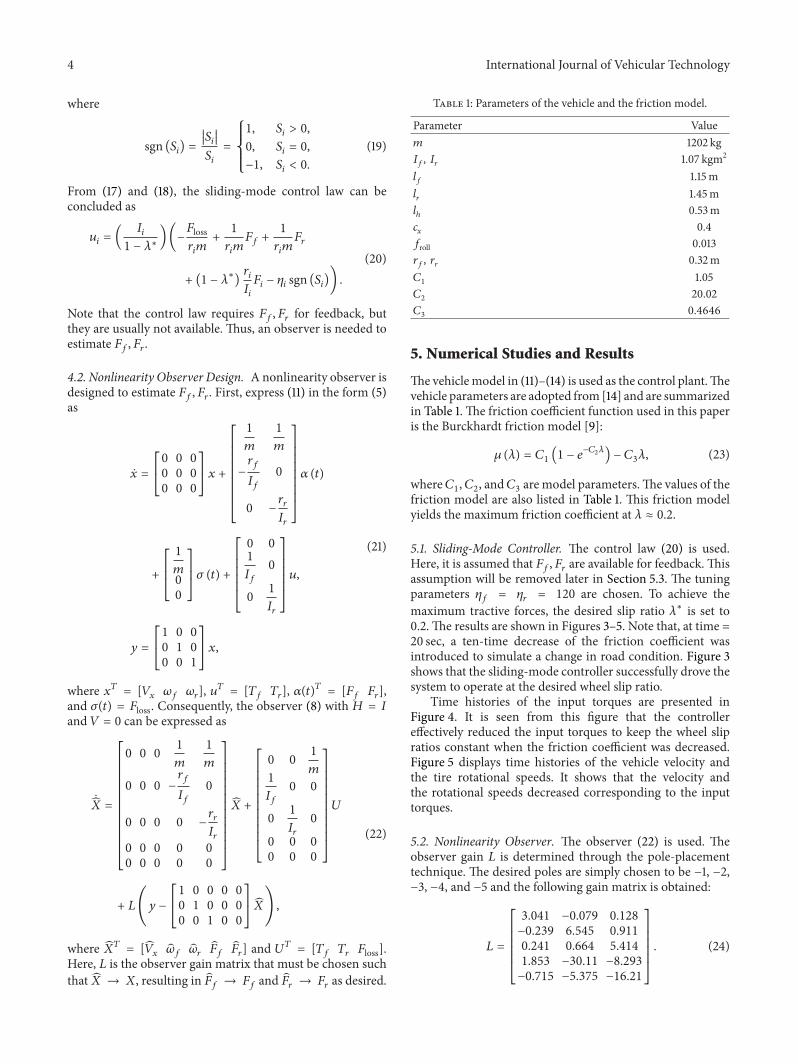
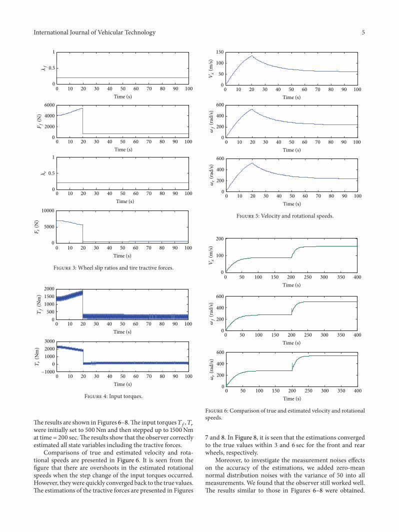
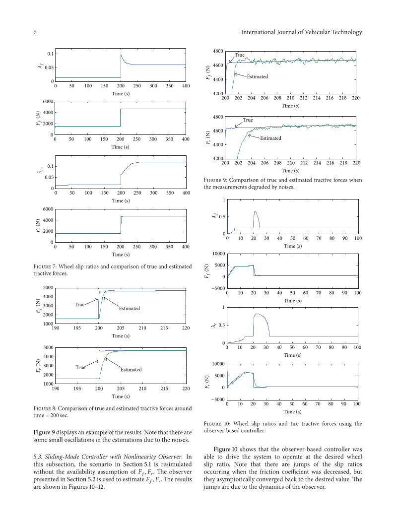
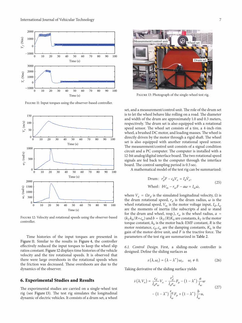
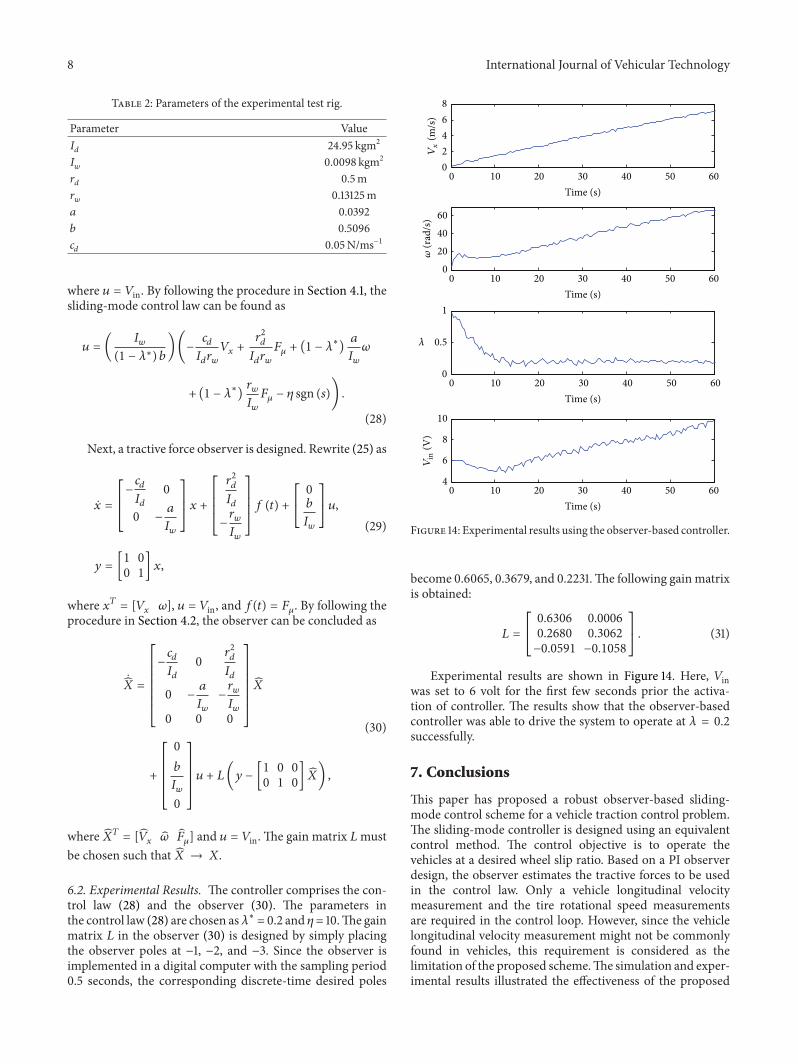

International Journal of
AerospaceEngineeringHindawi Publishing Corporationhttpwwwhindawicom Volume 2014
RoboticsJournal of
Hindawi Publishing Corporationhttpwwwhindawicom Volume 2014
Hindawi Publishing Corporationhttpwwwhindawicom Volume 2014
Active and Passive Electronic Components
Control Scienceand Engineering
Journal of
Hindawi Publishing Corporationhttpwwwhindawicom Volume 2014
International Journal of
RotatingMachinery
Hindawi Publishing Corporationhttpwwwhindawicom Volume 2014
Hindawi Publishing Corporation httpwwwhindawicom
Journal ofEngineeringVolume 2014
Submit your manuscripts athttpwwwhindawicom
VLSI Design
Hindawi Publishing Corporationhttpwwwhindawicom Volume 2014
Hindawi Publishing Corporationhttpwwwhindawicom Volume 2014
Shock and Vibration
Hindawi Publishing Corporationhttpwwwhindawicom Volume 2014
Civil EngineeringAdvances in
Acoustics and VibrationAdvances in
Hindawi Publishing Corporationhttpwwwhindawicom Volume 2014
Hindawi Publishing Corporationhttpwwwhindawicom Volume 2014
Electrical and Computer Engineering
Journal of
Advances inOptoElectronics
Hindawi Publishing Corporation httpwwwhindawicom
Volume 2014
The Scientific World JournalHindawi Publishing Corporation httpwwwhindawicom Volume 2014
SensorsJournal of
Hindawi Publishing Corporationhttpwwwhindawicom Volume 2014
Modelling amp Simulation in EngineeringHindawi Publishing Corporation httpwwwhindawicom Volume 2014
Hindawi Publishing Corporationhttpwwwhindawicom Volume 2014
Chemical EngineeringInternational Journal of Antennas and
Propagation
International Journal of
Hindawi Publishing Corporationhttpwwwhindawicom Volume 2014
Hindawi Publishing Corporationhttpwwwhindawicom Volume 2014
Navigation and Observation
International Journal of
Hindawi Publishing Corporationhttpwwwhindawicom Volume 2014
DistributedSensor Networks
International Journal of
Related Documents