Research Article Approximate Solutions, Thermal Properties ...

Research ArticleApproximate Solutions, Thermal Properties, and SuperstatisticsSolutions to Schrödinger Equation

Ituen Okon ,1 Clement Onate ,2 Ekwevugbe Omugbe ,3 Uduakobong Okorie ,4

Akaninyene Antia ,1 Michael Onyeaju ,5 Chen Wen-Li ,6 and Judith Araujo 7

1University of Uyo, Uyo, Nigeria2Landmark University, Omu-Aran, Nigeria3Federal University of Petroleum Resources, Effurun, Nigeria4Akwa Ibom State University, Uyo, Nigeria5University of Port Harcourt, Port Harcourt, Nigeria6Xi’an Peihua University, Xi’an, China7Instituto Federal do Sudeste de Minas Gerais, Juiz de Fora, Brazil

Correspondence should be addressed to Ituen Okon; [email protected]

Received 16 October 2021; Accepted 17 February 2022; Published 7 March 2022

Academic Editor: Mariana Frank

Copyright © 2022 Ituen Okon et al. This is an open access article distributed under the Creative Commons Attribution License,which permits unrestricted use, distribution, and reproduction in any medium, provided the original work is properly cited. Thepublication of this article was funded by SCOAP3.

In this work, we apply the parametric Nikiforov-Uvarov method to obtain eigensolutions and total normalized wave function ofSchrödinger equation expressed in terms of Jacobi polynomial using Coulomb plus Screened Exponential Hyperbolic Potential(CPSEHP), where we obtained the probability density plots for the proposed potential for various orbital angular quantumnumber, as well as some special cases (Hellmann and Yukawa potential). The proposed potential is best suitable for smallervalues of the screening parameter α. The resulting energy eigenvalue is presented in a close form and extended to studythermal properties and superstatistics expressed in terms of partition function ðZÞ and other thermodynamic properties suchas vibrational mean energy ðUÞ, vibrational specific heat capacity ðCÞ, vibrational entropy ðSÞ, and vibrational free energy ðFÞ.Using the resulting energy equation and with the help of Matlab software, the numerical bound state solutions were obtainedfor various values of the screening parameter (α) as well as different expectation values via Hellmann-Feynman Theorem(HFT). The trend of the partition function and other thermodynamic properties obtained for both thermal properties andsuperstatistics were in excellent agreement with the existing literatures. Due to the analytical mathematical complexities, thesuperstatistics and thermal properties were evaluated using Mathematica 10.0 version software. The proposed potential modelreduces to Hellmann potential, Yukawa potential, Screened Hyperbolic potential, and Coulomb potential as special cases.

1. Introduction

The approximate analytical solutions of one-dimensionalradial Schrödinger equation with a multiple potential func-tion have been studied using a suitable approximationscheme to the centrifugal term within the frame work ofthe parametric Nikiforov-Uvarov method [1]. The solutionsto the wave equations in quantum mechanics and appliedphysics play a crucial role in understanding the importanceof physical systems [2]. The two most important parts instudying Schrödinger equations are the total wave function

and energy eigenvalues [3]. The analytic solutions of waveequations for some physical potentials are possible for l = 0.For l ≠ 0, special approximation schemes like the Greene-Aldrich and Pekeris approximations are employed to deal withthe centrifugal barrier in order to obtain approximate boundstate solutions [4–6]. The Greene-Aldrich approximationscheme is mostly applicable for short range potentials [7].Eigensolutions for both relativistic and nonrelativistic waveequations have been studied with different methods whichinclude the following: Exact quantisation, WKB, Nikiforov-Uvarov method (NU), Laplace transform technique,

HindawiAdvances in High Energy PhysicsVolume 2022, Article ID 5178247, 18 pageshttps://doi.org/10.1155/2022/5178247

asymptotic iteration method, proper quantisation, supersym-metric quantum mechanics approach, vibrational approach,formula method, factorisation method, and Shifted 1/N-expan-sion method [8–13]. Bound state solutions obtained from theSchrödinger equation has practical applications in investigatingtunnelling rate of quantum mechanical systems [14] and massspectra of quarkonia systems [15–19]. Among other goalsachieved in this research article is to apply the Hellmann-Feynman Theorem (HFT) to eigenequation of the Schrödingerwave equations to obtain expectation values of<r−1>nl,<r−2>nl,<T>nl, and <p2>nl analytically. The Hellmann-Feynman Theo-rem gives an insight about chemical bonding and other forcesexisting among atoms of molecules [20–25]. To engage HFTin calculating the expectation values, one needs to promotethe fixed parameter which appears in the Hamiltonian to be acontinuous variable in order to ease the mathematical purposeof taking the derivative [26]. Similarly, the application ofHellmann-Feynman Theorem provides a less mathematicalapproach of obtaining expectation values of a quantummechanical systems [27, 28]. Some of the potential models con-sidered within the framework of relativistic and nonrelativisticwave equations areHulthen-Yukawa Inversely quadratic poten-tial [29], noncentral Inversely quadratic potential [30],ModifiedHylleraas potential [31], Yukawa, Hulthen, Eckart, Deng-Fan,Pseudoharmonic, Kratzer, Woods-Saxon, double ring shape,Coulomb, Tietz–Wei, Tietz-Hua, Deng-Fan, Manning-Rosen,trigonometric Rosen-Morse, hyperbolic scalar, and vectorpotential and exponential type potentials among others[32–50]. Coulomb, hyperbolic, and screened exponential typepotentials have been of interest to researchers in recent timesbecause of their enormous applications in both chemical andphysical sciences. In view of this, Parmar [51] studied ultrage-neralized exponential hyperbolic potential where he obtainedenergy eigenvalues, unnormalized wave function and the parti-tion function. This potential reduces to Yukawa potential,Screened cosine Kratzer potential, Manning-Rosen potential,Hulthen plus Inversely quadratic exponential Mie-type poten-tial, and many others. Diaf et al. [52], in their studies, obtainedeigensolutions to the Schrödinger equation with trigonometricInversely quadratic plus Coulombic hyperbolic potential wherethey obtained energy eigenvalue and normalized wave functionusing the Nikiforov-Uvarov method. Onate [53] examinedbound state solutions of the Schrödinger equation with secondPöschl-Teller-like potential where he obtained vibrational parti-tion function, mean energy, vibrational specific heat capacity,and mean free energy. In that work, the Pöschl-Teller-likepotential was expressed in a hyperbolic form. The practicalapplication of energy eigenvalue of Schrödinger equation ininvestigating the partition function, thermodynamic properties,and superstatistics arouses the interest of many researchers.Recently, Okon et al. [54] obtained the thermodynamic proper-ties and bound state solutions of the Schrödinger equation usingMobius square plus screened Kratzer potential for two diatomicsystems (carbon(II) oxide and scandium fluoride) within theframework of the Nikiforov-Uvarov method. Their results werein agreement to semiclassical WKB among others. They pre-sented energy eigenvalue in a close form in order to obtain par-tition function and other thermodynamic properties. Omugbeet al. [55] recently studied the unified treatment of the nonrela-

tivistic bound state solutions, thermodynamic properties, andexpectation values of exponential-type potentials where theyobtained the thermodynamic properties within the frameworkof semiclassicalWKB approach. The authors studied the specialcases of the potential as Eckart, Manning-Rosen, and Hulthenpotentials. Besides, Oyewumi et al. [56] studied the thermody-namic properties and the approximate solutions of the Schrö-dinger equation with shifted Deng-Fan potential model withinthe framework of asymptotic Iteration method where theyapply Pekeris-type approximation to centrifugal term to obtainrotational-vibrational energy eigenvalues for selected diatomicsystems. A lot of researches have been carried out by Ikotet al. These can be seen in Refs. [57–60]. Also, Boumali andHassanabadi [61] studied thermal properties of a two-dimensional Dirac oscillator under an external magnetic fieldwhere they obtained relativistic spin-1\2 fermions subject toDirac oscillator coupling and a constant magnetic field in bothcommutative and noncommutative spaces.

In this work, we propose a novel potential called Coulombplus Screened Exponential Hyperbolic Potential to studybound state solutions, expectation values, superstatistics, andthermal properties within the framework of the parametricNikiforov-Uvarov method [62]. This article is divided into 9sections. The introduction is given in Section 1. The paramet-ric Nikiforov-Uvarov method is presented in Section 2. Thesolutions of the radial Schrödinger equation are presented inSection 3. The application of Hellmann-Feynman Theoremto obtain expectation values is presented in Section 4. Thethermodynamic properties and superstatistics formulationsare presented in Sections 5 and 6, respectively. Numericalresults and discussion are presented Sections 7 and 8, respec-tively, and the article is concluded in Section 9.

The propose Coulomb plus Screened Hyperbolic Expo-nential Potential (CPSHEP) is given as

V rð Þ = −v1r+ B

r−v2 cosh α

r2

� �e−αr , ð1Þ

where v1 and v2 are the potential depths, B is a real constantparameter, and α is the adjustable screening parameter. ThePekeris-like approximation to the centrifugal term is given as

1r2

= α2

1 − e−αrð Þ2 ⇒ 1r= α

1 − e−αrð Þ : ð2Þ

The graph of Pekeris approximation to centrifugal term isgiven in Figure 1.

2. Parametric Nikiforov-Uvarov (NU) Method

The NU method is based on reducing second order lineardifferential equation to a generalized equation of hypergeo-metric type and provides exact solutions in terms of specialorthogonal functions like Jacobi and Laguerre as well as cor-responding energy eigenvalues [63–70]. The reference equa-tion for parametric NU method according to Tezcan andSever [71] is given as

2 Advances in High Energy Physics

Ψ″ sð Þ + c1 − c2ss 1 − c3sð ÞΨ′ sð Þ + 1

s2 1 − c3sð Þ2 −Ω1s2 +Ω2s −Ω3

� �Ψ sð Þ = 0:

ð3Þ

The condition for energy equation is given as [70].

c2n − 2n + 1ð Þc5 + 2n + 1ð Þ ffiffiffiffic9

p + c3ffiffiffiffic8

pð Þ + n n − 1ð Þc3 + c7+ 2c3c8 + 2 ffiffiffiffiffiffiffiffi

c8c9p = 0:

ð4Þ

The total wave function is given as

ψnl sð Þ =Nnlsc12 1 − c3sð Þ−c12− c13/c3ð ÞP c10−1, c11/c3ð Þ−c10−1ð Þ

n 1 − 2c3sð Þ:ð5Þ

The parametric constants are obtained as follows:

c1 = c2 = c3 = 1, c4 =12 1 − c1ð Þ, c5 =

12 c2 − 2c3ð Þ, c6 = c25 +Ω1,

c7 = 2c4c5 −Ω2, c8 = c24 +Ω3, c9 = c3c7 + c23c8 + c6, c10 = c1 + 2c4 + 2 ffiffiffiffic8

p ,c11 = c2 − 2c5 + 2 ffiffiffiffi

c9p + c3

ffiffiffiffic8

pð Þ, c12 = c4 +ffiffiffiffic8

p , c13 = c5 −ffiffiffiffic9

p + c3ffiffiffiffic8

pð Þ:ð6Þ

3. The Radial Solution of SchrödingerWave Equation

The radial Schrödinger wave equation with the centrifugalterm is given as

d2R rð Þdr2

+ 2μℏ2

E −V rð Þ − ℏ2l l + 1ð Þ2μr2

" #R rð Þ = 0: ð7Þ

Equation (7) can only be solved analytically to obtainexact solution if the angular orbital quantum number l = 0.However, for l > 0, equation (7) can only be solve by usingthe approximations in (2) to the centrifugal term. Substitut-ing equation (1) into (7) gives

d2R rð Þdr2

+ 2μℏ2

Enl +v1r−Be−αr

r+ v2e

−αr cosh α

r2−ℏ2l l + 1ð Þ2μr2

" #R rð Þ = 0:

ð8Þ

By substituting equation (2) into (8) gives the followingequation:

d2R rð Þdr2

+ 2μℏ2

Enl +v1α

1 − e−αrð Þ −Bαe−αr

1 − e−αrð Þ +v2α

2e−αr cosh α

1 − e−αrð Þ2 −ℏ2α2l l + 1ð Þ2μ 1 − e−αrð Þ2

" #R rð Þ = 0:

ð9Þ

By defining s = e−αr and with some simple algebraic sim-plification, equation (9) can be presented in the form

d2R sð Þds2

+ 1 − sð Þs 1 − sð Þ

dRds

+ 1s2 1 − sð Þ2

�− ε2 − χ1� �

s2

+ 2ε2 − δ2 − χ1 + χ2� �

s − ε2 − δ2 + l l + 1ð Þ� �8<:

9=;R sð Þ = 0,

ð10Þ

where

ε2 = −2μEnl

ℏ2α2, δ2 = 2μv1

ℏ2α, χ1 =

2μBℏ2α

, χ2 =2μv2 cosh α

ℏ2:

ð11Þ

Comparing equation (10) to (3), the following polyno-mials were obtain:

Ω1 = ε2 − χ1� �

,Ω2 = 2ε2 − δ2 − χ1 + χ2� �

,Ω3 = ε2 − δ2 + l l + 1ð� �:

ð12Þ

Using equation (6), other parametric constants areobtained as follows:

c1 = c2 = c3 = 1 ; c4 = 0, c5 = −12 , c6 =

14 + ε2 − χ1, c7 = −2ε2 + δ2 + χ1 − χ2,

c8 = ε2 − δ2 + l l + 1ð Þ, c9 =14 − χ2 + l l + 1ð Þ, c10 = 1 + 2

ffiffiffiffiffiffiffiffiffiffiffiffiffiffiffiffiffiffiffiffiffiffiffiffiffiffiffiffiffiffiffiε2 − δ2 + l l + 1ð Þ

q,

c11 = 2 +ffiffiffiffiffiffiffiffiffiffiffiffiffiffiffiffiffiffiffiffiffiffiffiffiffiffiffiffiffiffiffiffiffiffiffi1 − 4χ2 + 4l l + 1ð Þ

q+ 2

ffiffiffiffiffiffiffiffiffiffiffiffiffiffiffiffiffiffiffiffiffiffiffiffiffiffiffiffiffiffiffiε2 − δ2 + l l + 1ð Þ

q, c12 =

ffiffiffiffiffiffiffiffiffiffiffiffiffiffiffiffiffiffiffiffiffiffiffiffiffiffiffiffiffiffiffiε2 − δ2 + l l + 1ð Þ

q,

c13 = −12 −

12

ffiffiffiffiffiffiffiffiffiffiffiffiffiffiffiffiffiffiffiffiffiffiffiffiffiffiffiffiffiffiffiffiffiffiffi1 − 4χ2 + 4l l + 1ð Þ

q+

ffiffiffiffiffiffiffiffiffiffiffiffiffiffiffiffiffiffiffiffiffiffiffiffiffiffiffiffiffiffiffiε2 − δ2 + l l + 1ð Þ

q :

ð13Þ

𝛼 = 0.01𝛼 = 0.02

r

1

0.9

2 3 4 5 6 7 8 9 10

1r2

0.8

0.7

0.6

0.5

0.4

0.3

0.2

0.1

Figure 1: The graph of Pekeris approximation for various values of α.

3Advances in High Energy Physics

Using equations (4), (12), and (13) with much algebraicsimplification, the energy eigenvalue for the proposed poten-tial is given as

Using equation (5), the total unnormalized wave func-tion is given as

Ψnl sð Þ =Nnlsffiffiffiffiffiffiffiffiffiffiffiffiffiffiffiffiffiffiffiffiffiffiε2−δ2+l l+1ð Þð Þp

1 − sð Þ 1/2ð Þ+ 1/2ð Þ ffiffiffiffiffiffiffiffiffiffiffiffiffiffiffiffiffiffiffiffi1+4l l+1ð Þ−4χ2

pP

2ffiffiffiffiffiffiffiffiffiffiffiffiffiffiffiffiffiffiffiffiffiffiε2−δ2+l l+1ð Þð Þpð Þ, ffiffiffiffiffiffiffiffiffiffiffiffiffiffiffiffiffiffiffiffi

1+4l l+1ð Þ−4χ2p� �� �

n 1 − 2sð Þ:

ð15Þ

To obtain the normalization constant of equation (15),we employ the normalization condition

ð∞0

Rnl rð Þj j2dr = 1⇒ð∞0

Nnlsβ 1 − sð ÞηP 2β,2η−1ð Þ

n 1 − 2sð Þh i2

ds = 1, ð16Þ

where

β =ffiffiffiffiffiffiffiffiffiffiffiffiffiffiffiffiffiffiffiffiffiffiffiffiffiffiffiffiffiffiffiffiffiffiffiffiε2 − δ2 + l l + 1ð Þ� �q

, ð17Þ

η = 12 + 1

2ffiffiffiffiffiffiffiffiffiffiffiffiffiffiffiffiffiffiffiffiffiffiffiffiffiffiffiffiffiffiffiffiffiffiffi1 + 4l l + 1ð Þ − 4χ2

q: ð18Þ

The wave function is assumed to be in bound at r ∈ ð0,∞Þ and s = e−αr ∈ ð1, 0Þ.

Equation (15) reduces to

−N2

nl

α

ð01s2β 1 − sð Þ2η P 2β,2η−1ð Þ

n 1 − 2sð Þh i2 ds

s= 1: ð19Þ

Let z = ð1 − 2sÞ such that the boundary of integration ofequation (19) changes from s ∈ ð1, 0Þ to z ∈ ð−1, 1Þ. Then,equation (19) reduces to

N2nl

2α

ð1−1

1 − z2

� �2β−1 1 + z2

� �2ηP 2β,2η−1ð Þn zð Þ

h i2dz = 1: ð20Þ

Using the standard integral,

ð1−1

1 −w2

� �x 1 +w2

� �y

P x,y−1ð Þn wð Þ

h i2dw

= 2x+y+1Γ x + n + 1ð ÞΓ y + n + 1ð Þn!Γ x + y + n + 1ð ÞΓ x + y + 2n + 1ð Þ :

ð21Þ

Let z =w, x = 2β − 1, y = 2η. Then, using equation (20),

the normalization constant can be obtained as

Nnl =ffiffiffiffiffiffiffiffiffiffiffiffiffiffiffiffiffiffiffiffiffiffiffiffiffiffiffiffiffiffiffiffiffiffiffiffiffiffiffiffiffiffiffiffiffiffiffiffiffiffiffiffiffiffiffiffiffiffiffiffiffiffiffiffiffiffiffiffiffiffiffiffi2α n!ð ÞΓ 2β + 2η + nð ÞΓ 2β + 2η + 2nð Þ

2 2β+2ηð ÞΓ 2β + nð ÞΓ 2η + n + 1ð Þ

s: ð22Þ

Hence, the total normalized wave function is given as

Rn,l sð Þ =ffiffiffiffiffiffiffiffiffiffiffiffiffiffiffiffiffiffiffiffiffiffiffiffiffiffiffiffiffiffiffiffiffiffiffiffiffiffiffiffiffiffiffiffiffiffiffiffiffiffiffiffiffiffiffiffiffiffiffiffiffiffiffiffiffiffiffiffiffiffiffiffi2α n!ð ÞΓ 2β + 2η + nð ÞΓ 2β + 2η + 2nð Þ

2 2β+2ηð ÞΓ 2β + nð ÞΓ 2η + n + 1ð Þ

ssβ 1 − sð ÞηP 2β,2η−1ð Þ

n 1 − 2sð Þ:

ð23Þ

4. Expectation Values Using Hellmann-Feynman Theorem

In this section, some expectation values are obtain usingHellmann-Feynman Theorem (HFT). According to theHellmann-Feynman Theorem, the Hamiltonian H for a par-ticular quantum mechanical system is expressed as a func-tion of some parameters q. Let EðqÞ and ΨðqÞ be theeigenvalues and eigenfunction of the Hamiltonian. Then,

∂Enl

∂q= Ψ qð Þ ∂H qð Þ

∂q

��������Ψ qð Þ

� : ð24Þ

For the purpose of clarity, the Hamiltonian for the pro-pose potential using HFT is

H = −ℏ2

2μd

dr2+ ℏ2l l + 1ð Þ

2μr2 −v1r+ B

r−v2 cosh α

r2

� �e−αr:

ð25Þ

4.1. Expectation Value for <r−2>nl. To obtain the expectationvalue for <r−2>nl , we set q = l, to have

r−2� �

n,l = α2 −α2 2l + 1ð Þ

212 2l + 1ð Þ

ffiffiffiffiffiffiffiffiffiffiffiffiffiffiffiffiffiffiffiffiffiffiffiffiffiffiffiffiffiffiffiffiffiffiffiffiffiffiffiffiffiffiffiffiffiffiffil + 1

2

� �2−2v2μ cosh α

ℏ2

s0@

1A

−1/2

+Q6

0@

1AQ7,

ð26Þ

where

Enl =ℏ2α2l l + 1ð Þ

2μ − v1α +ℏ2α2

2μ

�n2 + n + 1/2ð Þ� �

+ n + 1/2ð Þð Þffiffiffiffiffiffiffiffiffiffiffiffiffiffiffiffiffiffiffiffiffiffiffiffiffiffiffiffiffiffiffiffiffiffiffiffiffiffiffiffiffiffiffiffiffiffiffiffiffiffiffiffiffiffiffiffiffiffiffiffiffi1 + 4l l + 1ð Þ − 8v2μ cosh α/ℏ2

� �q+ 2μB/ℏ2α� �

− 2μv1/ℏ2α� �

− 2v2μ cosh α/ℏ2� �

+ 2l l + 1ð Þ2n + 1ð Þ +

ffiffiffiffiffiffiffiffiffiffiffiffiffiffiffiffiffiffiffiffiffiffiffiffiffiffiffiffiffiffiffiffiffiffiffiffiffiffiffiffiffiffiffiffiffiffiffiffiffiffiffiffiffiffiffiffiffiffiffiffiffi1 + 4l l + 1ð Þ − 2v2μ cosh α/ℏ2

� �q8><>:

9>=>;

2

:

ð14Þ

4 Advances in High Energy Physics

4.2. Expectation Value for <r−1>nl. Setting q = B,, then, theexpectation value for <r−1>nl becomes

<r−1 > = −ℏ2α2Q7 × eαr

4μ

�2μ/ℏ2α2� �

n + 1/2ð Þ +ffiffiffiffiffiffiffiffiffiffiffiffiffiffiffiffiffiffiffiffiffiffiffiffiffiffiffiffiffiffiffiffiffiffiffiffiffiffiffiffiffiffiffiffiffiffiffiffiffiffiffiffiffiffiffiffiffiffiffil + 1/2ð Þð Þ2 − 2v2μ cosh α/ℏ2

� �q� �n + 1/2ð Þ +

ffiffiffiffiffiffiffiffiffiffiffiffiffiffiffiffiffiffiffiffiffiffiffiffiffiffiffiffiffiffiffiffiffiffiffiffiffiffiffiffiffiffiffiffiffiffiffiffiffiffiffiffiffiffiffiffiffiffiffil + 1/2ð Þð Þ2 − 2v2μ cosh α/ℏ2

� �q� �2264

375:ð28Þ

4.3. Expectation Value for <T>nl. Setting q = μ, then,

<T>nl =ℏ2α2l l + 1ð Þ

2μ −ℏ2α2Q2

78μ + ℏ2α2Q7

4

� −v2 cosh α

ℏ2ffiffiffiffiffiffiffiffiffiffiffiffiffiffiffiffiffiffiffiffiffiffiffiffiffiffiffiffiffiffiffiffiffiffiffiffiffiffiffiffiffiffiffiffiffiffiffiffiffiffiffiffiffiffiffiffiffiffiffil + 1/2ð Þð Þ2 − 2v2μ cosh α/ℏ2

� �q264

+2/ℏ2α� �

B − v1ð Þ� � ffiffiffiffiffiffiffiffiffiffiffiffiffiffiffiffiffiffiffiffiffiffiffiffiffiffiffiffiffiffiffiffiffiffiffiffiffiffiffiffiffiffiffiffiffiffiffiffiffiffiffiffiffiffiffiffiffiffiffil + 1/2ð Þð Þ2 − 2v2μ cosh α/ℏ2

� �q� �+ v2 cosh α/ℏ2� �

2μB/ℏ2α� �

− 2μv1/ℏ2α� �

+ l l + 1ð Þ� �n + 1/2ð Þ +

ffiffiffiffiffiffiffiffiffiffiffiffiffiffiffiffiffiffiffiffiffiffiffiffiffiffiffiffiffiffiffiffiffiffiffiffiffiffiffiffiffiffiffiffiffiffiffiffiffiffiffiffiffiffiffiffiffiffiffil + 1/2ð Þð Þ2 − 2v2μ cosh α/ℏ2

� �q� �2#:

ð29Þ

4.4. Expectation Value for <p2>nl. The relationship betweenT and p2 is given as T = p2/2μ, therefore

<p2>nl = ℏ2α2l l + 1ð Þ − ℏ2α2Q27

4 + ℏ2α2μQ72

� −v2 cosh α

ℏ2ffiffiffiffiffiffiffiffiffiffiffiffiffiffiffiffiffiffiffiffiffiffiffiffiffiffiffiffiffiffiffiffiffiffiffiffiffiffiffiffiffiffiffiffiffiffiffiffiffiffiffiffiffiffiffiffiffiffiffil + 1/2ð Þð Þ2 − 2v2μ cosh α/ℏ2

� �q264

+2/ℏ2α� �

B − v1ð Þ� � ffiffiffiffiffiffiffiffiffiffiffiffiffiffiffiffiffiffiffiffiffiffiffiffiffiffiffiffiffiffiffiffiffiffiffiffiffiffiffiffiffiffiffiffiffiffiffiffiffiffiffiffiffiffiffiffiffiffiffil + 1/2ð Þð Þ2 − 2v2μ cosh α/ℏ2

� �q� �+ v2 cosh α/ℏ2� �

2μB/ℏ2α� �

− 2μv1/ℏ2α� �

+ l l + 1ð Þ� �n + 1/2ð Þ +

ffiffiffiffiffiffiffiffiffiffiffiffiffiffiffiffiffiffiffiffiffiffiffiffiffiffiffiffiffiffiffiffiffiffiffiffiffiffiffiffiffiffiffiffiffiffiffiffiffiffiffiffiffiffiffiffiffiffiffil + 1/2ð Þð Þ2 − 2v2μ cosh α/ℏ2

� �q� �2#:

ð30Þ

5. Thermodynamic Properties

In this section, we present the thermodynamic properties forthe potential model. The thermodynamic properties ofquantum systems can be obtained from the exact partitionfunction given by

Z βð Þ = 〠λ

n=0e−βEn , ð31Þ

where λ is an upper bound of the vibrational quantum num-ber obtained from the numerical solution of dEn/dn = 0,given as λ = −δ +

ffiffiffiffiffiffiQ3

p, β = 1/kT , where k and T are Boltz-

mann constant and absolute temperature, respectively. Inthe classical limit, the summation in equation (31) can bereplaced with an integral:

Z βð Þ =ðλ0e−βEndn: ð32Þ

In order to obtain the partition function, the energy equa-tion (14) can be presented in a close and compact form as

Enl =ℏ2α2l l + 1ð Þ

2μ − v1α −ℏ2α2

8μ

� n + 12 +

ffiffiffiffiffiffiffiffiffiffiffiffiffiffiffiffiffiffiffiffiffiffiffiffiffiffiffiffiffiffiffiffiffiffiffiffiffiffiffiffiffiffiffiffiffiffil + 1

2

� �2−2v2μ cosh α

ℏ2

s0@

1A

8<:+ 2μB/ℏ2α

� �− 2μv1/ℏ2α� �

+ l l + 1ð Þ� �n + 1/2ð Þ +

ffiffiffiffiffiffiffiffiffiffiffiffiffiffiffiffiffiffiffiffiffiffiffiffiffiffiffiffiffiffiffiffiffiffiffiffiffiffiffiffiffiffiffiffiffiffiffiffiffiffiffiffiffiffiffiffiffiffiffil + 1/2ð Þð Þ2 − 2v2μ cosh α/ℏ2

� �q� �)2

:

ð33Þ

Equation (33) can further be simplified to

Enl =Q1 −Q2 n + δð Þ + Q3n + δð Þ

� �2, ð34Þ

where

Q1 =ℏ2α2l l + 1ð Þ

2μ − v1α,Q2 =ℏ2α2

8μ ,

Q3 =2μBℏ2α

−2μv1ℏ2α

+ l l + 1ð Þ� �

,

δ = 12 +

ffiffiffiffiffiffiffiffiffiffiffiffiffiffiffiffiffiffiffiffiffiffiffiffiffiffiffiffiffiffiffiffiffiffiffiffiffiffiffiffiffiffiffiffiffiffil + 1

2

� �2−2v2μ cosh α

ℏ2

s,

ð35Þ

and equation (34) can be represented in the form

Enl =Q1 −Q2 ρ + Q3ρ

2⇒ − Q2ρ

2 + Q2Q23

ρ2

− 2Q2Q3 −Q1ð Þ, ð36Þ

where

Q6 =2l + 1ð Þ n + 1/2ð Þ +

ffiffiffiffiffiffiffiffiffiffiffiffiffiffiffiffiffiffiffiffiffiffiffiffiffiffiffiffiffiffiffiffiffiffiffiffiffiffiffiffiffiffiffiffiffiffiffiffiffiffiffiffiffiffiffiffiffiffiffil + 1/2ð Þð Þ2 − 2v2μ cosh α/ℏ2

� �q� �− 2μB/ℏ2α� �

− 2μv1/ℏ2α� �

+ l l + 1ð Þ� �1/2ð Þ 2l + 1ð Þ

ffiffiffiffiffiffiffiffiffiffiffiffiffiffiffiffiffiffiffiffiffiffiffiffiffiffiffiffiffiffiffiffiffiffiffiffiffiffiffiffiffiffiffiffiffiffiffiffiffiffiffiffiffiffiffiffiffiffiffil + 1/2ð Þð Þ2 − 2v2μ cosh α/ℏ2

� �q� �− 1/2ð Þ

n + 1/2ð Þ +ffiffiffiffiffiffiffiffiffiffiffiffiffiffiffiffiffiffiffiffiffiffiffiffiffiffiffiffiffiffiffiffiffiffiffiffiffiffiffiffiffiffiffiffiffiffiffiffiffiffiffiffiffiffiffiffiffiffiffil + 1/2ð Þð Þ2 − 2v2μ cosh α/ℏ2

� �q� �2 ,

Q7 = n + 1/2ð Þ +ffiffiffiffiffiffiffiffiffiffiffiffiffiffiffiffiffiffiffiffiffiffiffiffiffiffiffiffiffiffiffiffiffiffiffiffiffiffiffiffiffiffiffiffiffiffiffiffiffiffil + 1/2ð Þð Þ2 − 2v2μ cosh α

ℏ2

r !+ 2μB/ℏ2α

� �− 2μv1/ℏ2α� �

+ l l + 1ð Þ� �n + 1/2ð Þ +

ffiffiffiffiffiffiffiffiffiffiffiffiffiffiffiffiffiffiffiffiffiffiffiffiffiffiffiffiffiffiffiffiffiffiffiffiffiffiffiffiffiffiffiffiffiffiffiffiffiffiffiffiffiffiffiffiffiffiffil + 1/2ð Þð Þ2 − 2v2μ cosh α/ℏ2

� �q� �8><>:

9>=>;:

ð27Þ

5Advances in High Energy Physics

ρ = n + δ: ð37Þ

(i) Partition function is obtained as follows:

Substituting equation (36) into equation (32) taking noteof changes in the integration boundaries using equation (37)gives the partition function as

Z βð Þ = eβ 2Q2Q3−Q1ð Þðλ+δδ

eβ Q2ρ2+ Q2Q

23/ρ2ð Þð Þdρ: ð38Þ

Using Mathematica 10.0 version, the partition functionof equation (38) is given as

Z βð Þ = e−βQ1+2βQ2Q3−2ℵffiffiffiffiffiffiffiffi−βQ2

p ffiffiffiπ

p 2 erf ℵ0 − ℵ/δð Þð Þf g4ffiffiffiffiffiffiffiffiffiffiffi−βQ2

p : ð39Þ

(ii) Vibrational mean energy is given as

(iii) Vibrational entropy is given as

(iv) Vibrational free energy is given as

U βð Þ = −∂ ln Z βð Þ

∂β=

2Q2e2ℵ

ffiffiffiffiffiffiffiffi−βQ2

p−e βQ2 δ4+Q2

3ð Þ/δ2ð Þδ + e βQ2 δ+λð Þ4+Q23ð Þ/ δ+λð Þ2ð Þλ + 2Q2e

2ℵffiffiffiffiffiffiffiffi−βQ2

p ffiffiffiπ

p erf ℵ ℵ2 −ℵ0 − ℵ/δð Þð Þh i

ffiffiffiπ

p erf ℵ0 − ℵ/δð Þð Þ − e4ℵffiffiffiffiffiffiffiffi−βQ2

perf ℵ0 + ℵ/δð Þð Þ + erf ℵ1 − ℵ/ λ + δð Þð Þð Þ + e4ℵ

ffiffiffiffiffiffiffiffi−βQ2

perf ℵ1 + ℵ/ λ + δð Þð Þð Þ

n o8<:

9=;: ð40Þ

S βð Þ = k ln Z βð Þ − kβ∂ ln Z βð Þ

∂β= k ln 1

4ffiffiffiffiffiffiffiffiffiffiffi−βQ2

p e−βQ1+2βQ2Q3−2ℵffiffiffiffiffiffiffiffi−βQ2

p ffiffiffiπ

perf ℵ0 −

ℵδ

� �+ e4ℵ

ffiffiffiffiffiffiffiffi−βQ2

perf ℵ1 +

ℵλ + δð Þ −ℵ0 −

ℵδ

� ��

+ erf ℵ1 −ℵ

λ + δð Þ� �

g − kβ2Q2e

2ffiffiffiffiffiffiffiffi−βQ2

p ffiffiffiffiffiffiffiffiffiffiffiffi−βQ2Q

23

p−e βQ2 δ4+Q2

3ð Þ/δ2ð Þδ + e βQ2 δ+λð Þ4+Q23ð Þ/ δ+λð Þ2ð Þλ + 2Q2e

2ℵffiffiffiffiffiffiffiffi−βQ2

p ffiffiffiπ

p erf ℵ ℵ2 −ℵ0 − ℵ/δð Þð Þh i

ffiffiffiπ

p 2 erf ℵ0 − ℵ/δð Þð Þf g

8<:

9=;:

ð41Þ

F βð Þ = −1βln Z βð Þ = −

1βln e−βQ1+2βQ2Q3−2ℵ

ffiffiffiffiffiffiffiffi−βQ2

p ffiffiffiπ

p

4ffiffiffiffiffiffiffiffiffiffiffi−βQ2

p erf ℵ1 −ℵ

λ + δð Þ +ℵ0 −ℵδ

� �+ e4ℵ

ffiffiffiffiffiffiffiffi−βQ2

perf ℵ1 +

ℵλ + δð Þ −ℵ0 −

ℵδ

� �� � !: ð42Þ

6 Advances in High Energy Physics

(v) Vibrational specific heat capacity is given as

where

6. Superstatistics Formulation

Superstatistics is the superposition of two different statisticswhich is applicable to driven nonequilibrium systems to sta-tistical intensive parameter (β) fluctuation [72]. This inten-sive parameter which undergoes spatiotemporalfluctuations includes chemical potential and energy fluctua-tion which is basically describe in terms of effective Boltz-mann factor [73]. According to Edet et.al [74], the effectiveBoltzmann factor is given as

B Eð Þ =ð∞0e−β′E f β′, β

� �dβ′, ð45Þ

where f ðβ′, βÞ = δðβ − β′Þ is the Dirac delta function. How-ever, the generalized Boltzmann factor expressed in terms ofdeformation parameter q is given as

B Eð Þ = e−βE 1 + q2β

2E2� �

: ð46Þ

The partition function for superstatistics formalism is

then given as

Zs =ð∞0B Eð Þdn: ð47Þ

Substituting equation (34) into equation (46) gives thegeneralized Boltzmann factor equation as

B Eð Þ = 1 + q2β

2 − Q2ρ2 + Q2Q

23

ρ2

� �− 2Q2Q3 −Q1ð Þ

� �2" #e−β − Q2ρ

2+ Q2Q23/ρ2ð Þð Þ− 2Q2Q3−Q1ð Þ½ �:

ð48Þ

Using equation (47), the superstatistics partition func-tion equation is given as

Zs = eβ 2Q2Q3−Q1ð Þð∞0

1 + q2 β

2 − Q2ρ2 + Q2Q

23

ρ2

� �− 2Q2Q3 −Q1ð Þ

� �2" #eβ Q2ρ

2+ Q2Q23/ρ2ð Þð Þdρ:

ð49Þ

Using Mathematica 10.0 version, the partition obtainfrom equation (47) is

C βð Þ = kβ2 ∂2 ln Z βð Þ∂β2

!= k

ffiffiffiffiffiffiffiffiffiffiffi−βQ2

pe2ℵ

ffiffiffiffiffiffiffiffi−βQ2

p×

−erf Λ1ð Þ − e4ℵffiffiffiffiffiffiffiffi−βQ2

perf Λ2ð Þ + erf Λ3ð Þ + e4ℵ

ffiffiffiffiffiffiffiffi−βQ2

perf Λ4ð Þ

h iℵ4 + ℵ2

4/ 4 ffiffiffiπ

p ffiffiffiffiffiffiffiffiffiffiffi−βQ2

p� �� �− 4ℵ erf Λ1 −Λ3ð Þ + e4ℵ

ffiffiffiffiffiffiffiffi−βQ2

perf Λ2 −Λ4ð Þ

h i ffiffiffiffiffiffiffiffiffiffiffi−βQ2

pℵ5 − ℵ8ℵ6/ δ λ + δð Þ

ffiffiffiffiffiffiffiffiffiffiffi−βQ2

p� �2� �+Λ5 −δ2

ffiffiffiffiffiffiffiffiffiffiffi−βQ2

p+ 2ℵ

� �− 2βQ2ℵΛ6 + δ λ + δð Þℵ7

ffiffiffiπ

p erf Λ1ð Þ + e4ℵffiffiffiffiffiffiffiffi−βQ2

perf Λ1ð Þ − erf Λ3ð Þ − e4ℵ

ffiffiffiffiffiffiffiffi−βQ2

perf Λ4ð Þ

h i28>><>>:

9>>=>>;,

ð43Þ

Λ1 =ℵ0 −ℵδ,Λ2 =ℵ0 +

ℵδ,Λ3 =ℵ1 −

ℵλ + δð Þ ,Λ4 =ℵ1 +

ℵλ + δð Þ ,Λ5 = e βQ2 δ4+Q2

3ð Þ/δ2ð Þδ,

Λ6 = e βQ2 δ+λð Þ4+Q23Þ/ δ+λð Þ2ð Þδ; ;ℵ =

ffiffiffiffiffiffiffiffiffiffiffiffiffiffiffiffiffi−βQ2Q

23

q,ℵ0 =

ffiffiffiffiffiffiffiffiffiffiffi−βQ2

pδ,ℵ1 =

ffiffiffiffiffiffiffiffiffiffiffi−βQ2

pλ + δð Þ,

ℵ2 =ℵ0δ + 2δλffiffiffiffiffiffiffiffiffiffiffi−βQ2

p+ λ2

ffiffiffiffiffiffiffiffiffiffiffi−βQ2

p+ℵ

λ + δ,ℵ3 = 2ℵe2ℵ

ffiffiffiffiffiffiffiffi−βQ2

p ffiffiffiπ

p,ℵ4 = −Λ5 + 2Λ6 +ℵ3 erf Λ8 −Λ1ð Þ,

ℵ5 =Λ5 − 2Λ6 +ℵ3 erf Λ2 −Λ8ð Þ,ℵ6 =Q22Q

23 − e2ℵ

ffiffiffiffiffiffiffiffi−βQ2

p ffiffiffiπ

pδ λ + δð Þ erf Λ8 −Λ2ð Þℵ

ffiffiffiffiffiffiffiffiffiffiffi−βQ2

p,

ℵ7 = erf Λ6ð Þ δ2ffiffiffiffiffiffiffiffiffiffiffi−βQ2

p+ 2δλ

ffiffiffiffiffiffiffiffiffiffiffi−βQ2

p+ λ2

ffiffiffiffiffiffiffiffiffiffiffi−βQ2

p− 2ℵ

� �,

ℵ8 = − erf Λ3ð Þ + e4ℵffiffiffiffiffiffiffiffi−βQ2

perf Λ2 −Λ3ð Þ − 4

ffiffiffiπ

pβ2e4ℵ

ffiffiffiffiffiffiffiffi−βQ2

pδ λ + δð Þ erf Λ8ð Þ:

9>>>>>>>>>>>>>>>>>>=>>>>>>>>>>>>>>>>>>;

ð44Þ

Zs =1

16ffiffiffiffiffiffiffiffiffiffiffiffiffiffiffiffiffi−βQ2Q

23

qβQ2

e−βQ1+2βQ2Q3−2ffiffiffiffiffiffiffiffi−βQ2

p ffiffiffiffiffiffiffiffiffiffiffiffi−βQ2Q

23

p ffiffiffiπ

p−32qβ3Q3

2Q33 + 8 + 3q + 4qβQ1 + 4qβ2Q2

1� � ffiffiffiffiffiffiffiffiffiffiffi

−βQ2p ffiffiffiffiffiffiffiffiffiffiffiffiffiffiffiffiffi

−βQ2Q23

q+ 8q 1 + 2βQ1ð Þ −βQ2ð Þ3/2Q3

ffiffiffiffiffiffiffiffiffiffiffiffiffiffiffiffiffi−βQ2Q

23

q+ 8q2β2Q2

2Q23 × 1 + 2βQ1 + 4

ffiffiffiffiffiffiffiffiffiffiffi−βQ2

p ffiffiffiffiffiffiffiffiffiffiffiffiffiffiffiffiffi−βQ2Q

23

q� � � �:

ð50Þ

7Advances in High Energy Physics

We use the same procedure of thermodynamics (Section5) to obtain superstatistics vibrational mean energy (Us),vibrational specific heat capacity (Cs), vibrational entropy(Ss), and vibrational free energy (Fs) from the partitionequation (41). However, this solution is not included in thearticle because of the lengthy and bulky analytical equations.

7. Numerical Results

Using Matlab 10.0 version, the numerical bound state solu-tions for the proposed potential were calculated using (14)for different quantum state. Also, using equations (18),(20), (21), and (22), the expectation values for <r−2>nl , <r−1>nl, <T>nl , and <p2>nl , respectively, were calculated asshown in Tables 1–5.

7.1. Special Cases

(a) Hellmann potential: substituting v2 = 0 into equation(1), then, the potential reduces to Hellmannpotential

v rð Þ = −v1r+ Be−αr

r: ð51Þ

The required energy equation is

Enl =ℏ2α2l l + 1ð Þ

2μ − v1α −ℏ2α2

8μ n + l + 1ð Þ + 2μ/ℏ2α� �

B − v1ð Þ + l l + 1ð Þ� �n + l + 1ð Þ

( )2

:

ð52Þ

The result of equation (52) agrees excellently with Ref.[75].

(b) Yukawa potential: if v1 = v2 = 0, then, equation (1)reduces to Yukawa potential

v rð Þ = Be−αr

r: ð53Þ

The corresponding energy eigenequation is

Enl =ℏ2α2l l + 1ð Þ

2μ −ℏ2α2

8μ n + l + 1ð Þ + 2μB/ℏ2α� �

+ l l + 1ð Þ� �n + l + 1ð Þ

( )2

: ð54Þ

Equation (54) is consistent with result obtain in Ref. [76]in order to prove the mathematical accuracy of our analyti-cal calculation.

(c) Screened-hyperbolic inversely quadratic potential:substituting B = v1 = 0 into equation (1), the poten-tial reduces to screened-hyperbolic inversely qua-dratic potential

v rð Þ = v2e−αr cosh α

r2: ð55Þ

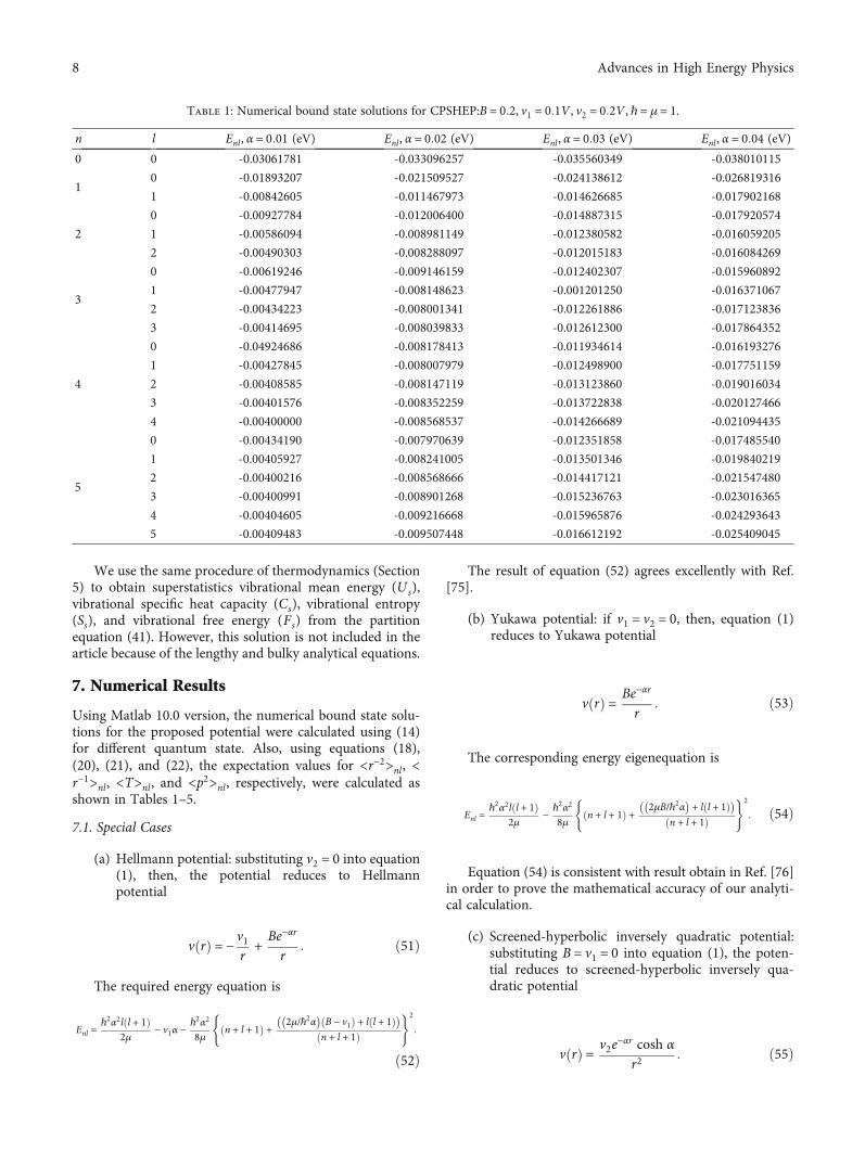
Table 1: Numerical bound state solutions for CPSHEP:B = 0:2, v1 = 0:1V , v2 = 0:2V , ℏ = μ = 1.

n l Enl , α = 0:01 (eV) Enl , α = 0:02 (eV) Enl , α = 0:03 (eV) Enl , α = 0:04 (eV)

0 0 -0.03061781 -0.033096257 -0.035560349 -0.038010115

10 -0.01893207 -0.021509527 -0.024138612 -0.026819316

1 -0.00842605 -0.011467973 -0.014626685 -0.017902168

2

0 -0.00927784 -0.012006400 -0.014887315 -0.017920574

1 -0.00586094 -0.008981149 -0.012380582 -0.016059205

2 -0.00490303 -0.008288097 -0.012015183 -0.016084269

3

0 -0.00619246 -0.009146159 -0.012402307 -0.015960892

1 -0.00477947 -0.008148623 -0.001201250 -0.016371067

2 -0.00434223 -0.008001341 -0.012261886 -0.017123836

3 -0.00414695 -0.008039833 -0.012612300 -0.017864352

4

0 -0.04924686 -0.008178413 -0.011934614 -0.016193276

1 -0.00427845 -0.008007979 -0.012498900 -0.017751159

2 -0.00408585 -0.008147119 -0.013123860 -0.019016034

3 -0.00401576 -0.008352259 -0.013722838 -0.020127466

4 -0.00400000 -0.008568537 -0.014266689 -0.021094435

5

0 -0.00434190 -0.007970639 -0.012351858 -0.017485540

1 -0.00405927 -0.008241005 -0.013501346 -0.019840219

2 -0.00400216 -0.008568666 -0.014417121 -0.021547480

3 -0.00400991 -0.008901268 -0.015236763 -0.023016365

4 -0.00404605 -0.009216668 -0.015965876 -0.024293643

5 -0.00409483 -0.009507448 -0.016612192 -0.025409045

8 Advances in High Energy Physics

The resulting energy eigenvalue is

Enl =ℏ2α2l l + 1ð Þ

2μ −ℏ2α2

8μ n + 12 +

ffiffiffiffiffiffiffiffiffiffiffiffiffiffiffiffiffiffiffiffiffiffiffiffiffiffiffiffiffiffiffiffiffiffiffiffiffiffiffiffiffiffiffiffiffiffiffil + 1

2

� �2−2v2μ cosh α

ℏ2

s0@

1A

8<:

+ l l + 1ð Þn + 1/2ð Þ +

ffiffiffiffiffiffiffiffiffiffiffiffiffiffiffiffiffiffiffiffiffiffiffiffiffiffiffiffiffiffiffiffiffiffiffiffiffiffiffiffiffiffiffiffiffiffiffiffiffiffiffiffiffiffiffiffiffiffiffil + 1/2ð Þð Þ2 − 2v2μ cosh α/ℏ2

� �q� �)2

:

ð56Þ

(d) Coulomb potential: substituting α = 0 into equation(53), then, the potential reduces to Coulombpotential

v rð Þ = Br: ð57Þ

By substituting α = 0 into equation (54), it gives the cor-responding energy eigenvalue for Coulomb’s potential as

Enl = −ℏ2μB2

2 n + l + 1ð Þ2: ð58Þ

Equation (58) agrees we with result obtain in Ref [76].

8. Discussion

Figure 1 is the graph of Pekeris approximation against thescreening parameter α. The nature of the graph shows thatthe approximation is suitable for the proposed potential.Variation of the probability density against the internuclearseparation at various quantum state for l = 0 and l = 1,respectively, is shown in Figures 2(a) and 2(b), respectively.In Figure 2(a), the probability density curves produce ther-mal curves with regular peaks compacted close to the originwith uneven peaks at various internuclear distance. Thiscurve shows that for orbital angular quantum number l = 0, there is more concentration of the electron density at theorigin for all the quantum state studied. The same situationis also observed for l = 1 as shown in Figure 2(b). It can alsobe observed that at every value of the internuclear distance,the probability density for l = 0 is higher than the probabilitydensity for l = 1. Figure 3 shows variation of the probabilitydensity against the internuclear separation at various quan-tum state for l = 0 and l = 1 for Hellmann potential pre-sented in Figures 3(a) and 3(b), respectively. Moreconcentration of the electron density is observed at the ori-gin in both cases. It is also seen that the probability densityobtained for l = 0 is lower than the probability densityobtained for l = 1: In Figure 4, we presented the variationof the probability density against the internuclear separationat various quantum state for l = 0 and l = 1 for Yukawapotential as shown in Figures 4(a) and 4(b), respectively.Here, there are more concentration and localization of

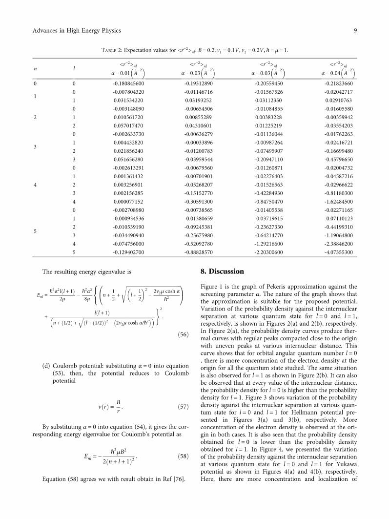
Table 2: Expectation values for <r−2>nl : B = 0:2, v1 = 0:1V , v2 = 0:2V , ℏ = μ = 1.

n l<r−2>nl

α = 0:01 _A−2� � <r−2>nl

α = 0:03 _A−2� � <r−2>nl

α = 0:03 _A−2� � <r−2>nl

α = 0:04 _A−2� �

0 0 -0.180845600 -0.19312890 -0.20559450 -0.21823660

10 -0.007804320 -0.01146716 -0.01567526 -0.02042717

1 0.031534220 0.03193252 0.03112350 0.02910763

2

0 -0.003148090 -0.00654506 -0.01084855 -0.01605580

1 0.010561720 0.00855289 0.00383228 -0.00359942

2 0.057017470 0.04310601 0.01225219 -0.03554203

3

0 -0.002633730 -0.00636279 -0.01136044 -0.01762263

1 0.004432820 -0.00033896 -0.00987264 -0.02416721

2 0.021856240 -0.01200783 -0.07495907 -0.16699480

3 0.051656280 -0.03959544 -0.20947110 -0.45796650

4

0 -0.002613291 -0.00679560 -0.01260871 -0.02004732

1 0.001361432 -0.00701901 -0.02276403 -0.04587216

2 0.003256901 -0.05268207 -0.01526563 -0.02966622

3 0.002156285 -0.15152770 -0.42284930 -0.81180300

4 0.000077152 -0.30591300 -0.84750470 -1.62484500

5

0 -0.002708980 -0.00738565 -0.01405538 -0.02271165

1 -0.000934536 -0.01380659 -0.03719615 -0.07110123

2 -0.010539190 -0.09245381 -0.23627330 -0.44199310

3 -0.034490940 -0.25675980 -0.64214770 -1.19064800

4 -0.074756000 -0.52092780 -1.29216600 -2.38846200

5 -0.129402700 -0.88828570 -2.20300600 -4.07355300

9Advances in High Energy Physics

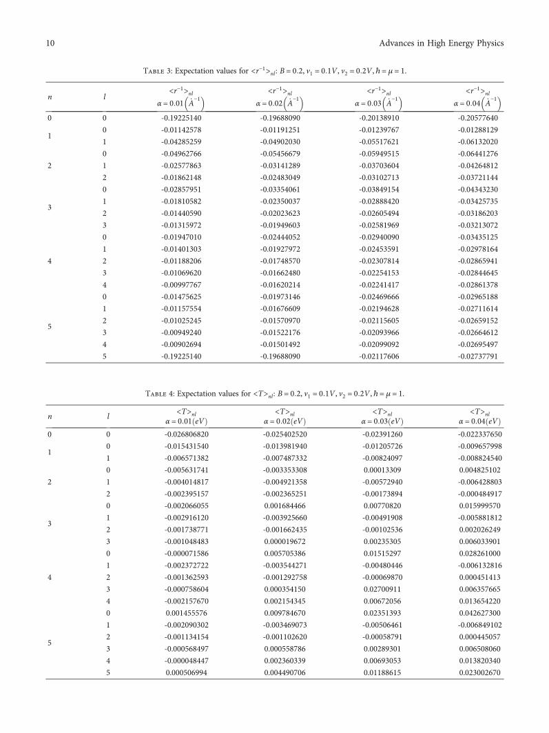
Table 3: Expectation values for <r−1>nl : B = 0:2, v1 = 0:1V , v2 = 0:2V , ℏ = μ = 1.

n l<r−1>nl

α = 0:01 _A−1� � <r−1>nl

α = 0:02 _A−1� � <r−1>nl

α = 0:03 _A−1� � <r−1>nl

α = 0:04 _A−1� �

0 0 -0.19225140 -0.19688090 -0.20138910 -0.20577640

10 -0.01142578 -0.01191251 -0.01239767 -0.01288129

1 -0.04285259 -0.04902030 -0.05517621 -0.06132020

2

0 -0.04962766 -0.05456679 -0.05949515 -0.06441276

1 -0.02577863 -0.03141289 -0.03703604 -0.04264812

2 -0.01862148 -0.02483049 -0.03102713 -0.03721144

3

0 -0.02857951 -0.03354061 -0.03849154 -0.04343230

1 -0.01810582 -0.02350037 -0.02888420 -0.03425735

2 -0.01440590 -0.02023623 -0.02605494 -0.03186203

3 -0.01315972 -0.01949603 -0.02581969 -0.03213072

4

0 -0.01947010 -0.02444052 -0.02940090 -0.03435125

1 -0.01401303 -0.01927972 -0.02453591 -0.02978164

2 -0.01188206 -0.01748570 -0.02307814 -0.02865941

3 -0.01069620 -0.01662480 -0.02254153 -0.02844645

4 -0.00997767 -0.01620214 -0.02241417 -0.02861378

5

0 -0.01475625 -0.01973146 -0.02469666 -0.02965188

1 -0.01157554 -0.01676609 -0.02194628 -0.02711614

2 -0.01025245 -0.01570970 -0.02115605 -0.02659152

3 -0.00949240 -0.01522176 -0.02093966 -0.02664612

4 -0.00902694 -0.01501492 -0.02099092 -0.02695497

5 -0.19225140 -0.19688090 -0.02117606 -0.02737791

Table 4: Expectation values for <T>nl : B = 0:2, v1 = 0:1V , v2 = 0:2V , ℏ = μ = 1.

n l<T>nl

α = 0:01 eVð Þ<T>nl

α = 0:02 eVð Þ<T>nl

α = 0:03 eVð Þ<T>nl

α = 0:04 eVð Þ0 0 -0.026806820 -0.025402520 -0.02391260 -0.022337650

10 -0.015431540 -0.013981940 -0.01205726 -0.009657998

1 -0.006571382 -0.007487332 -0.00824097 -0.008824540

2

0 -0.005631741 -0.003353308 0.00013309 0.004825102

1 -0.004014817 -0.004921358 -0.00572940 -0.006428803

2 -0.002395157 -0.002365251 -0.00173894 -0.000484917

3

0 -0.002066055 0.001684466 0.00770820 0.015999570

1 -0.002916120 -0.003925660 -0.00491908 -0.005881812

2 -0.001738771 -0.001662435 -0.00102536 0.002026249

3 -0.001048483 0.000019672 0.00235305 0.006033901

4

0 -0.000071586 0.005705386 0.01515297 0.028261000

1 -0.002372722 -0.003544271 -0.00480446 -0.006132816

2 -0.001362593 -0.001292758 -0.00069870 0.000451413

3 -0.000758604 0.000354150 0.02700911 0.006357665

4 -0.002157670 0.002154345 0.00672056 0.013654220

5

0 0.001455576 0.009784670 0.02351393 0.042627300

1 -0.002090302 -0.003469073 -0.00506461 -0.006849102

2 -0.001134154 -0.001102620 -0.00058791 0.000445057

3 -0.000568497 0.000558786 0.00289301 0.006508060

4 -0.000048447 0.002360339 0.00693053 0.013820340

5 0.000506994 0.004490706 0.01188615 0.023002670

10 Advances in High Energy Physics

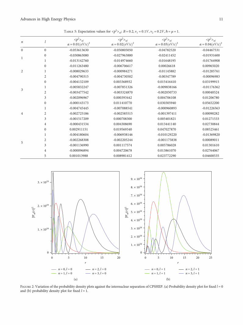
Table 5: Expectation values for <p2>nl : B = 0:2, v1 = 0:1V , v2 = 0:2V , ℏ = μ = 1.

n l<p2>nl

α = 0:01 eV/cð Þ2<p2>nl

α = 0:02 eV/cð Þ2<p2>nl

α = 0:03 eV/cð Þ2<p2>nl

α = 0:04 eV/cð Þ20 0 -0.053613630 -0.050805050 -0.04782520 -0.04467531

10 -0.030863080 -0.027963880 -0.02411452 -0.01931600

1 -0.013142760 -0.014974660 -0.01648195 -0.01764908

2

0 -0.011263480 -0.006706617 0.00026618 0.00965020

1 -0.008029633 -0.000984271 -0.01145882 -0.01285761

2 -0.004790315 -0.004730502 -0.00347789 -0.00096983

3

0 -0.004132109 0.003368932 0.015416410 0.03199915

1 -0.005832247 -0.007851326 -0.009838166 -0.01176362

2 -0.003477542 -0.003324870 -0.002050733 0.00040524

3 -0.002096967 0.000393442 0.004706108 0.01206780

4

0 -0.000143173 0.011410770 0.030305940 0.05652200

1 -0.004745445 -0.007088541 -0.000960893 -0.01226563

2 -0.002725186 -0.002585515 -0.001397411 0.00090282

3 -0.001517209 0.000708300 0.005401821 0.01271533

4 -0.000431534 0.004308690 0.013441140 0.02730844

5

0 0.002911151 0.019569340 0.047027870 0.08525461

1 -0.004180604 -0.006938146 -0.010129220 -0.01369820

2 -0.002268308 -0.002205244 -0.001175838 0.00089011

3 -0.001136990 0.001117574 0.005786028 0.01301610

4 -0.000096894 0.004720678 0.013861070 0.02764067

5 0.001013988 0.008981412 0.023772290 0.04600535

n = 0, l = 0n = 1, l = 0

n = 2, l = 0n = 3, l = 0

r

0 5 10 15 200

1. × 1019

2. × 1019

3. × 1019

|𝛹nl(r

)|2

(a)

n = 0, l = 1n = 1, l = 1

n = 2, l = 1n = 3, l = 1

r

0 5 10 15 20 250

1. × 1016

2. × 1016

3. × 1016

4. × 1016

|𝛹nl(r

)|2

5. × 1016

6. × 1016

7. × 1016

8. × 1016

9. × 1016

(b)

Figure 2: Variation of the probability density plots against the internuclear separation of CPSHEP. (a) Probability density plot for fixed l = 0and (b) probability density plot for fixed l = 1.

11Advances in High Energy Physics

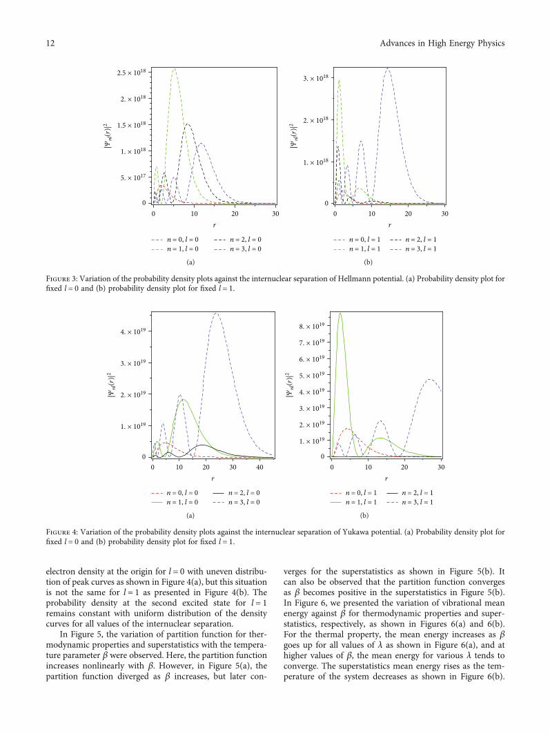
electron density at the origin for l = 0 with uneven distribu-tion of peak curves as shown in Figure 4(a), but this situationis not the same for l = 1 as presented in Figure 4(b). Theprobability density at the second excited state for l = 1remains constant with uniform distribution of the densitycurves for all values of the internuclear separation.

In Figure 5, the variation of partition function for ther-modynamic properties and superstatistics with the tempera-ture parameter β were observed. Here, the partition functionincreases nonlinearly with β. However, in Figure 5(a), thepartition function diverged as β increases, but later con-

verges for the superstatistics as shown in Figure 5(b). Itcan also be observed that the partition function convergesas β becomes positive in the superstatistics in Figure 5(b).In Figure 6, we presented the variation of vibrational meanenergy against β for thermodynamic properties and super-statistics, respectively, as shown in Figures 6(a) and 6(b).For the thermal property, the mean energy increases as βgoes up for all values of λ as shown in Figure 6(a), and athigher values of β, the mean energy for various λ tends toconverge. The superstatistics mean energy rises as the tem-perature of the system decreases as shown in Figure 6(b).

r

0 10 20 30

n = 0, l = 0n = 1, l = 0

n = 2, l = 0n = 3, l = 0

0

2.5 × 1018

2. × 1018

1.5 × 1018

1. × 1018

5. × 1017

|𝛹nl(r

)|2

(a)

r

0 10 20 300

n = 0, l = 1n = 1, l = 1

n = 2, l = 1n = 3, l = 1

3. × 1018

2. × 1018

1. × 1018

|𝛹nl(r

)|2

(b)

Figure 3: Variation of the probability density plots against the internuclear separation of Hellmann potential. (a) Probability density plot forfixed l = 0 and (b) probability density plot for fixed l = 1.

r

0 10 20 30 400

1. × 1019

2. × 1019

3. × 1019

4. × 1019

|𝛹nl(r

)|2

n = 0, l = 0n = 1, l = 0

n = 2, l = 0n = 3, l = 0

(a)

r

0 10 20 300

1. × 1019

2. × 1019

3. × 1019

4. × 1019

|𝛹nl(r

)|2 5. × 1019

6. × 1019

7. × 1019

8. × 1019

n = 0, l = 1n = 1, l = 1

n = 2, l = 1n = 3, l = 1

(b)

Figure 4: Variation of the probability density plots against the internuclear separation of Yukawa potential. (a) Probability density plot forfixed l = 0 and (b) probability density plot for fixed l = 1.

12 Advances in High Energy Physics

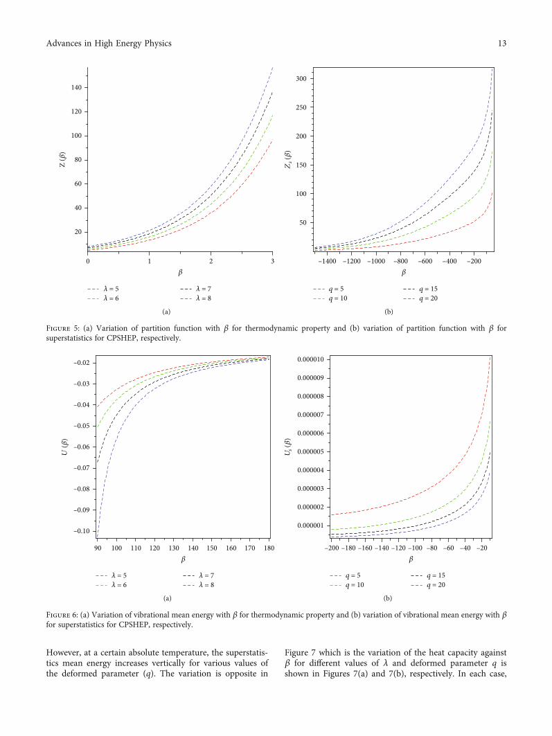
However, at a certain absolute temperature, the superstatis-tics mean energy increases vertically for various values ofthe deformed parameter (q). The variation is opposite in

Figure 7 which is the variation of the heat capacity againstβ for different values of λ and deformed parameter q isshown in Figures 7(a) and 7(b), respectively. In each case,

0 1 2 3

Z (𝛽

)

20

40

60

80

100

120

140

𝛽

𝜆 = 8𝜆 = 7

𝜆 = 6𝜆 = 5

(a)

Zs (𝛽

)

50

–1400 –1200 –1000 –800 –600 –400 –200

100

150

200

250

300

𝛽

q = 20q = 15

q = 10q = 5

(b)

Figure 5: (a) Variation of partition function with β for thermodynamic property and (b) variation of partition function with β forsuperstatistics for CPSHEP, respectively.

90 100 110 120 130 140 150 160 170 180

–0.02

–0.03

–0.04

–0.05

–0.06

–0.07

–0.08

–0.09

–0.10

𝛽

𝜆 = 8𝜆 = 7

𝜆 = 6𝜆 = 5

U (𝛽

)

(a)

–200

0.000010

–180 –160 –140 –120 –100 –80 –60 –40 –20𝛽

q = 20q = 15

q = 10q = 5

Us (𝛽

)

0.000009

0.000008

0.000007

0.000006

0.000005

0.000004

0.000003

0.000002

0.000001

(b)

Figure 6: (a) Variation of vibrational mean energy with β for thermodynamic property and (b) variation of vibrational mean energy with βfor superstatistics for CPSHEP, respectively.

13Advances in High Energy Physics

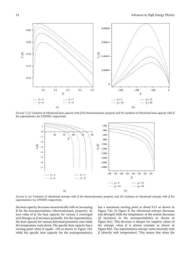
the heat capacity decreases monotonically with an increasingβ for the nonsuperstatistics (thermodynamic property). Atzero value of β, the heat capacity for various λ convergedand diverges as β increases gradually. For the superstatistics,the heat capacity for various deformed parameter rises whilethe temperature cools down. The specific heat capacity has aturning point when β equals -150 as shown in Figure 7(b)while the specific heat capacity for the nonsuperstatistics

has a maximum turning point at about 0.15 as shown inFigure 7(a). In Figure 8, the vibrational entropy decreasesand diverged while the temperature of the system decreases(β increases) in the nonsuperstatistics as shown inFigure 8(a). This decrease is sharper for negative values ofthe entropy when β is almost constant as shown inFigure 8(b). The superstatistics entropy varies inversely withβ (directly with temperature). This means that when the

0.50.40.30.20.1

–0.06

𝛽

𝜆 = 8𝜆 = 7

𝜆 = 6𝜆 = 5

–0.08

–0.10

–0.12

–0.14

C (𝛽

)

(a)

0.00020

0

0

𝛽

–300 –200 –100

Cs (𝛽

)

0.00015

0.00010

0.00005

q = 20q = 15

q = 10q = 5

(b)

Figure 7: (a) Variation of vibrational heat capacity with β for thermodynamic property and (b) variation of vibrational heat capacity with βfor superstatistics for CPSHEP, respectively.

40 50 60 70 800

–1

–2

–3

–4

–5

–6

–7

1

𝛽

S (𝛽

)

𝜆 = 8𝜆 = 7

𝜆 = 6𝜆 = 5

(a)

–200

𝛽

S s (𝛽

)

–400

–600

–800

–1000

–1200

–1400

–1600

–1800

–2000

–80 –70 –60 –50 –40 –30 –20 –10

q = 20q = 15

q = 10q = 5

(b)

Figure 8: (a) Variation of vibrational entropy with β for thermodynamic property and (b) variation of vibrational entropy with β forsuperstatistics for CPSHEP, respectively.

14 Advances in High Energy Physics

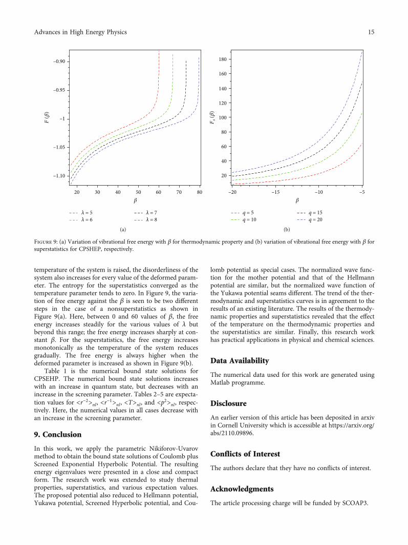
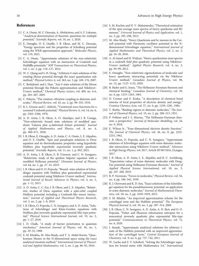
temperature of the system is raised, the disorderliness of thesystem also increases for every value of the deformed param-eter. The entropy for the superstatistics converged as thetemperature parameter tends to zero. In Figure 9, the varia-tion of free energy against the β is seen to be two differentsteps in the case of a nonsuperstatistics as shown inFigure 9(a). Here, between 0 and 60 values of β, the freeenergy increases steadily for the various values of λ butbeyond this range; the free energy increases sharply at con-stant β. For the superstatistics, the free energy increasesmonotonically as the temperature of the system reducesgradually. The free energy is always higher when thedeformed parameter is increased as shown in Figure 9(b).

Table 1 is the numerical bound state solutions forCPSEHP. The numerical bound state solutions increaseswith an increase in quantum state, but decreases with anincrease in the screening parameter. Tables 2–5 are expecta-tion values for <r−2>nl, <r−1>nl , <T>nl, and <p2>nl , respec-tively. Here, the numerical values in all cases decrease withan increase in the screening parameter.

9. Conclusion

In this work, we apply the parametric Nikiforov-Uvarovmethod to obtain the bound state solutions of Coulomb plusScreened Exponential Hyperbolic Potential. The resultingenergy eigenvalues were presented in a close and compactform. The research work was extended to study thermalproperties, superstatistics, and various expectation values.The proposed potential also reduced to Hellmann potential,Yukawa potential, Screened Hyperbolic potential, and Cou-

lomb potential as special cases. The normalized wave func-tion for the mother potential and that of the Hellmannpotential are similar, but the normalized wave function ofthe Yukawa potential seams different. The trend of the ther-modynamic and superstatistics curves is in agreement to theresults of an existing literature. The results of the thermody-namic properties and superstatistics revealed that the effectof the temperature on the thermodynamic properties andthe superstatistics are similar. Finally, this research workhas practical applications in physical and chemical sciences.

Data Availability

The numerical data used for this work are generated usingMatlab programme.

Disclosure

An earlier version of this article has been deposited in arxivin Cornell University which is accessible at https://arxiv.org/abs/2110.09896.

Conflicts of Interest

The authors declare that they have no conflicts of interest.

Acknowledgments

The article processing charge will be funded by SCOAP3.

20

–0.90

30 40 50 60 70 80

F (𝛽

)

𝛽

𝜆 = 8𝜆 = 7

𝜆 = 6𝜆 = 5

–0.95

–1

–1.05

–1.10

(a)

–20 –15 –10 –5

20

40

60

80

100

120

140

160

180

q = 20q = 15

q = 10q = 5

Fs (𝛽

)

𝛽

(b)

Figure 9: (a) Variation of vibrational free energy with β for thermodynamic property and (b) variation of vibrational free energy with β forsuperstatistics for CPSHEP, respectively.

15Advances in High Energy Physics

References

[1] C. A. Onate, M. C. Onyeaju, A. Abolarinwa, and A. F. Lukman,“Analytical determination of theoretic quantities for multiplepotential,” Scientific Reports, vol. 10, no. 1, 2020.

[2] E. Omugbe, O. E. Osafile, I. B. Okon, and M. C. Onyeaju,“Energy spectrum and the properties of Schoiberg potentialusing the WKB approximation approach,” Molecular Physics,vol. 119, 2021.

[3] C. A. Onate, “Approximate solutions of the non-relativisticSchrődinger equation with an interaction of Coulomb andHulthѐn potentials,” SOP Transactions on Theoretical Physics,vol. 1, no. 2, pp. 118–127, 2014.

[4] W. C. Qiang and S. H. Dong, “Arbitrary ℓ-state solutions of therotating Morse potential through the exact quantization rulemethod,” Physical Letters A, vol. 363, no. 3, pp. 169–176, 2007.

[5] C. Berkdemir and J. Han, “Any ℓ-state solutions of the Morsepotential through the Pekeris approximation and Nikiforov-Uvarov method,” Chemical Physics Letters, vol. 409, no. 4-6,pp. 203–207, 2005.

[6] C. Pekeris, “The rotation-vibration coupling in diatomic mol-ecules,” Physical Review, vol. 45, no. 2, pp. 98–103, 1934.

[7] R. L. Greene and C. Aldrich, “Variational wave functions for ascreened Coulomb potential,” Physical Review A, vol. 14, no. 6,pp. 2363–2366, 1976.

[8] A. D. Antia, I. B. Okon, A. O. Akankpo, and J. B. Usanga,“Non-relativistic bound state solutions of modified qua-dratic Yukawa plus q-deformed Eckart potential,” Journalof Applied Mathematics and Physics, vol. 8, no. 4,pp. 660–671, 2020.

[9] I. B. Okon, E. Omugbe, A. D. Antia, C. A. Onate, L. E. Akpabio,and O. E. Osafile, “Spin and pseudospin solutions to Diracequation and its thermodynamic properties using hyperbolicHulthen plus hyperbolic exponential inversely quadraticpotential,” Scientific Reports, vol. 11, no. 1, p. 892, 2021.

[10] A. D. Antia, I. B. Okon, E. B. Umoren, and C. N. Isonguyo,“Relativistic study of the spinless Salpeter equation with amodified Hylleraas potential,” Ukranian Journal of Physics,vol. 64, no. 1, pp. 27–33, 2019.

[11] I. B. Okon and O. O. Popoola, “Bound- state solution of Schro-dinger equation with Hulthen plus generalized exponentialcoulomb potential using Nikiforov-Uvarov method,” Interna-tional Journal of Recent Advances in Physics, vol. 4, no. 3,pp. 1–12, 2015.

[12] A. D. Antia, C. C. Eze, I. B. Okon, and L. E. Akpabio, “Relativ-istic studies of Dirac equation with a spin-orbit coupledHulthen potential including a Coulomb-like tensor interac-tion,” Journal of Applied and Theoretical Physics Research,vol. 3, no. 2, pp. 1–8, 2019.

[13] I. B. Okon, O. Popoola, C. N. Isonguyo, and A. D. Antia, “Solu-tions of Schrödinger and Klein-Gordon equations withHulthen plus inversely quadratic exponential Mie-type poten-tial,” Physical Science International Journal, vol. 19, no. 2,pp. 1–27, 2018.

[14] J. D. Chalk, “A study of barrier penetration in quantummechanics,” American Journal of Physics, vol. 56, no. 1,pp. 29–32, 1988.

[15] E. M. Khokha, M. Abu-Shady, and T. A. Abdel-Karim, “Quar-konium Masses in the N-dimensional space using the exactanalytical iteration method,” International Journal of Theoret-ical and Applied Mathematics, vol. 2, no. 2, pp. 86–92, 2016.

[16] S. M. Kuchin and N. V. Maksimenko, “Theoretical estimationof the spin-average mass spectra of heavy quarkonia and BCmesons,” Universal Journal of Physics and Application, vol. 1,no. 3, pp. 295–298, 2013.

[17] M. Abu-Shady, “Heavy Quarkonia and bc mesons in the Cor-nell potential with Harmonic oscillator potential in the N-dimensional Schrodinger equation,” International Journal ofApplied Mathematics and Theoretical Physics, vol. 2, no. 2,pp. 16–20, 2016.

[18] A. Al-Jamel and H.Widyan, “Heavy quarkoniummass spectrain a coulomb field plus quadratic potential using Nikiforov-Uvarov method,” Applied Physics Research, vol. 4, no. 3,pp. 94–99, 2012.

[19] E. Omugbe, “Non-relativistic eigensolutions of molecular andheavy quarkonia interacting potentials via the NikiforovUvarov method,” Canadian Journal of Physics, vol. 98,no. 12, pp. 1125–1132, 2020.

[20] R. Bader and G. Jones, “The Hellmann-Feynman theorem andchemical binding,” Canadian Journal of Chemistry, vol. 39,no. 6, pp. 1253–1265, 1961.

[21] D. Cremer and E. Kraka, “A description of chemical bondinterms of local properties of electron density and energy,”Croatica Chemica Acta, vol. 57, no. 6, pp. 1259–1281, 1984.

[22] T. Berlin, “Binding regions in diatomic molecules,” The Jour-nal of Chemical Physics, vol. 19, no. 2, pp. 208–213, 1951.

[23] P. Politzer and J. S. Murray, “The Hellmann-Feynman theo-rem: a perspective,” Journal of Molecular Modelling, vol. 24,no. 9, 2018.

[24] E. Wilson Jr., “Four‐dimensional electron density function,”The Journal of Chemical Physics, vol. 36, no. 8, pp. 2232-2233, 1962.

[25] I. B. Okon, O. Popoola, and C. N. Isonguyo, “Approximatesolutions of Schrodinger equation with some diatomic molec-ular interactions using Nikiforov-Uvarov method,” Advancesin High Energy Physics, vol. 2017, Article ID 9671816, 24 pages,2017.

[26] I. B. Okon, A. D. Antia, L. E. Akpabio, and B. U. Archibong,“Expectation values of some diatomic molecules with Deng-Fan potential using Hellmann-Feynman theorem,” Journal ofApplied Physical Science International, vol. 10, no. 5,pp. 247–268, 2019.

[27] R. P. Feynman, “Forces in molecules,” Physical Review, vol. 56,no. 4, pp. 340–343, 1939.

[28] K. J. Oyewumi and K. D. Sen, “Exact solutions of the Schrödin-ger equation for the pseudoharmonic potential: an applicationto some diatomic molecules,” Journal of Mathematical Chem-istry, vol. 50, no. 5, pp. 1039–1059, 2012.

[29] S. M. Ikhdair, “An improved approximation scheme for thecentrifugal term and the Hulthén potential,” The EuropeanPhysical Journal A, vol. 39, no. 3, pp. 307–314, 2009.

[30] I. B. Okon, C. N. Isonguyo, A. D. Antia, A. N. Ikot, and O. O.Popoola, “Fisher and Shannon information entropies for anoncentral inversely quadratic plus exponential Mie-typepotential,” Communications in Theoretical Physics, vol. 72,no. 6, 2020.

[31] J. Stanek, “Approximate analytical solutions for arbitrary l-state of the Hulthén potential with an improved approxima-tion of the centrifugal term,” Central European Journal ofChemistry, vol. 9, no. 4, pp. 737–742, 2011.

[32] W. Lucha and F. F. Schöberl, “Solving the Schrödinger equa-tion for bound states with Mathematica 3.0,” International

16 Advances in High Energy Physics

Journal of Modern Physics C: Computational Physics and Phys-ical Computation, vol. 10, no. 4, pp. 607–619, 1999.

[33] C.-S. Jia, J.-Y. Liu, and P.-Q. Wang, “A new approximationscheme for the centrifugal term and the Hulthen potential,”Physics Letters A, vol. 372, no. 27-28, pp. 4779–4782, 2008.

[34] H. Hassanabadi, E. Maghsoodi, A. N. Ikot, and S. Zarrinkamar,“Approximate arbitrary-state Solutions of Dirac equation formodified Hylleraas and modified Eckart potentials by NUmethod,” Applied Mathematics and computation, vol. 219,no. 17, pp. 9388–9398, 2013.

[35] E. E. Ituen, A. D. Antia, and I. B. Okon, “A nalytical solutionsof non-relativistic Schrodinger equation with hadronic mixedpower-law potentials via Nikiforov-Uvarov method,” WorldJournal of Applied Science and Technology, vol. 4, no. 2,pp. 196–205, 2012.

[36] B. T. Mbadjoun, J. M. Ema’a, J. Yomi, P. E. Abiama, G. H. Ben-Bolie, and P. O. Ateba, “Factorization method for exact solu-tion of the non-central modified Killingbeck potential plus aring-shaped like potential,” Modern Physics Letters A, vol. 34,no. 10.1142/S021773231950072X, 2019.

[37] O. A. Awoga and A. N. Ikot, “Approximate solution of Schrö-dinger equation in D dimensions for inverted generalizedhyperbolic potential,” Pramana, vol. 79, no. 3, pp. 345–356,2012.

[38] E. Omugbe, O. E. Osafile, and I. B. Okon, “WKB energyexpression for the radial Schrödinger equation with a general-ized pseudoharmonic potential,” Asian Journal of Physical andChemical Sciences, vol. 8, no. 2, pp. 13–20, 2020.

[39] E. Omugbe, “Non-relativistic energy spectrum of the Deng-Fan oscillator via the WKB approximation method,” AsianJournal of Physical and Chemical Sciences, vol. 8, no. 1,pp. 26–36, 2020.

[40] C. N. Isonguyo, I. B. Okon, A. N. Ikot, and H. Hassanabadi,“Solution of Klein -Gordon equation for some diatomic mole-cules with new generalized Morse-like potential using SUS-YQM,” Bulletin of the Korean Chemical Society, vol. 35,no. 12, pp. 3443–3446, 2014.

[41] C. Gang, “Bound states for Dirac equation with Wood-Saxonpotential,” Acta Physica Sinica, vol. 53, no. 3, pp. 680–683,2004.

[42] G. Chen, Z. D. Chen, and Z. M. Lou, “Exact bound state solu-tions of the s-wave Klein-Gordon equation with the general-ized Hulthen potential,” Physics Letters A, vol. 331, no. 6,pp. 374–377, 2004.

[43] C. S. Jia, J. W. Dai, L. H. Zhang, J. Y. Liu, and G. D. Zhang,“Molecular spinless energies of the modified Rosen-Morsepotential energy model in higher spatial dimensions,” Chemi-cal Physics Letters, vol. 619, pp. 54–60, 2015.

[44] C. S. Jia, J. W. Dai, L. H. Zhang, Y. J. Liu, and X. L. Peng, “Rel-ativistic energies for diatomic molecule nucleus motions withthe spin symmetry,” Physics Letters A, vol. 379, no. 3,pp. 137–142, 2015.

[45] C. S. Jia, J. Chen, L. Z. Yi, and S. R. Lin, “Equivalence of thedeformed Rosen-Morse potential energy model and Tietzpotential energy model,” Journal of Mathematical Chemistry,vol. 51, no. 8, pp. 2165–2172, 2013.

[46] W. C. Qiang and S. H. Dong, “The Manning–Rosen potentialstudied by a new approximate scheme to the centrifugal term,”Physica Scripta, vol. 79, no. 4, 2009.

[47] X. Y. Gu and S. H. Dong, “Energy spectrum of the Manning-Rosen potential including centrifugal term solved by exact

and proper quantization rules,” Journal of MathematicalChemistry, vol. 49, no. 9, pp. 2053–2062, 2011.

[48] Z. Q. Ma, A. Gonzalez-Cisneros, B. W. Xu, and S. H. Dong,“Energy spectrum of the trigonometric Rosen-Morse potentialusing an improved quantization rule,” Physics letters A,vol. 371, no. 3, pp. 180–184, 2007.

[49] H. Hassanabadi, S. Zarrinkamar, and A. A. Rajabi, “Exact solu-tions of D-dimensional Schrödinger equation for an energy-dependent potential by NU method,” Communication in The-oretical Physics, vol. 55, no. 4, pp. 541–544, 2011.

[50] H. Hassanabadi, E. Maghsodi, S. Zarrinkamar, andH. Rahimov, “An approximate solution of the Dirac equationfor hyperbolic scalar and vector potentials and a coulomb ten-sor interaction by SUSYQM,” Modern Physics Letters A,vol. 26, no. 36, pp. 2703–2718, 2011.

[51] R. H. Parmar, “Solution of the ultra generalized exponential-hyperbolic potential in multi-dimensional space,” Few-BodySystems, vol. 61, no. 4, pp. 1–28, 2020.

[52] A. Diaf, A. Chouchaoui, and R. J. Lombard, “Feynman integraltreatment of the Bargmann potential,” Annals of Physics,vol. 317, no. 2, pp. 354–365, 2005.

[53] C. A. Onate, “Bound state solutions of the SchrӦdinger equa-tion with second PӦschl-Teller like potential model and thevibrational partition function, mean energy and mean freeenergy,” Chinese Journal of Physics, vol. 54, no. 2, pp. 165–174, 2016.

[54] I. B. Okon, O. O. Popoola, E. Omugbe, A. D. Antia, C. N. Iso-nguyo, and E. E. Ituen, “Thermodynamic properties andbound state solutions of Schrodinger equation with Mobiussquare plus screened-Kratzer potential using Nikiforov-Uvarov method,” Computational and Theoretical Chemistry,vol. 1196, 2021.

[55] E. Omugbe, O. E. Osafile, M. C. Onyeaju, I. B. Okon, and C. A.Onate, “The unified treatment on the non-relativistic boundstate solutions, thermodynamic properties and expectationvalues of exponential–type potentials,” Canadian Journal ofPhysics, vol. 99, 2021.

[56] K. J. Oyewumi, B. J. Falaye, C. A. Onate, O. J. Oluwadare, andW. A. Yahya, “Thermodynamics properties and the approxi-mate solutions of the Schrodinger equation with the shiftedDeng-Fan potential model,” Molecular Physics, vol. 112,no. 1, pp. 127–141, 2014.

[57] A. N. Ikot, U. S. Okorie, R. Sever, and G. J. Rampho, “Eigenso-lution, expectation values and thermodynamic properties ofthe screened Kratzer potential,” European Physical JournalPlus, vol. 134, no. 8, 2019.

[58] U. S. Okorie, E. E. Ibekwe, A. N. Ikot, M. C. Onyeaju, and E. O.Chukwuocha, “Thermodynamic properties of the modifiedYukawa potential,” Journal of the Korean Physical Society,vol. 73, no. 9, pp. 1211–1218, 2018.

[59] C. O. Edet, U. S. Okorie, A. T. Ngiangia, and A. N. Ikot,“Bound state solutions of the Schrodinger equation for themodified Kratzer potential plus screened Coulomb poten-tial,” Indian Journal of Physics, vol. 94, no. 4, pp. 425–433, 2020.

[60] U. S. Okorie, A. N. Ikot, M. C. Onyeaju, and E. O. Chukwuo-cha, “A study of thermodynamic properties of quadratic expo-nential type potential in D-dimensions,” Revista Mexicana defisica, vol. 64, no. 6, pp. 608–614, 2018.

[61] A. Boumali and H. Hassanabadi, “The Thermal properties of atwo-dimensional Dirac oscillator under an external magnetic

17Advances in High Energy Physics

field,” The European Physical Journal Plus, vol. 128, no. 10,2013.

[62] I. B. Okon, C. A. Onate, E. Omugbe et al., “Approximate solu-tions, thermal properties and superstatistics solutions toSchrödinger equation,” https://arxiv.org/abs/2110.09896.

[63] O. Bayrak, G. Kocak, and I. Boztosun, “Anyl-state solutions ofthe Hulthén potential by the asymptotic iteration method,”Journal of Physics A: Mathematical and General, vol. 39,no. 37, pp. 11521–11529, 2006.

[64] S. M. Ikhdair and R. Sever, “Relativistic and nonrelativisticbound states of the isotonic oscillator by Nikiforov-Uvarovmethod,” Journal of Mathematical Physics, vol. 52, no. 12,2011.

[65] H. Fakhri and J. Sadeghi, “Supersymmetry approaches to thebound states of the generalizedWoods-Saxon potential,”Mod-ern Physics Letters A, vol. 19, no. 8, pp. 615–625, 2004.

[66] H. Khounfais, T. Boudjedaa, and L. Chetouani, “Scatteringmatrix for Feshbach-Villars equation for spin 0 and 1/2:Woods-Saxon potential,” Czechoslovak Journal of Physics,vol. 54, no. 7, pp. 697–710, 2004.

[67] H. Hassanabadi, S. Zarrinkamar, H. Hamzavi, and A. A.Rajabi, “Exact solutions of D-dimensional Klein-Gordonequation with an energy-dependent potential by using of Niki-forov–Uvarov method,” The Arabian Journal for Science andEngineering, vol. 37, no. 1, pp. 209–215, 2012.

[68] A. Arda and R. Sever, “Approximate analytical solutions of atwo-term diatomic molecular potential with centrifugal bar-rier,” Journal of Mathematical Chemistry, vol. 50, no. 7,pp. 1920–1930, 2012.

[69] S. M. Ikdair and R. Sever, “Exact solutions of the modifiedKratzer potential plus ring-shaped potential in the D-dimensional Schrödinger equation by the Nikiforov-Uvarovmethod,” International Journal of Modern Physics C, vol. 19,no. 2, pp. 221–235, 2008.

[70] C. S. Jia, P. Guo, Y. F. Diao, L. Z. Yi, and X. J. Xie, “Solutions ofDirac equations with the Pöschl-Teller potential,” The Euro-pean Physical Journal A, vol. 34, no. 1, pp. 41–48, 2007.

[71] C. Tezcan and R. Sever, “A general approach for the exact solu-tion of the Schrödinger equation,” International Journal ofTheoretical Physics, vol. 48, no. 2, pp. 337–350, 2009.

[72] C. Beck, “Superstatistics: theory and applications,” ContinuumMechanics and Thermodynamics, vol. 16, no. 3, pp. 293–304,2004.

[73] C. Beck and E. G. Cohen, “Superstatistics,” Physica A, vol. 322,pp. 267–275, 2003.

[74] C. O. Edet, P. O. Amadi, U. S. Okorie, A. Tas, A. N. Ikot, andG. Rampho, “Solutions of Schrodinger equation and thermalproperties of generalized trigonometric Poschl-Teller poten-tial,” Revista Mexicana defisca, vol. 66, pp. 824–839, 2020.

[75] H. Hamzavi, K. E. Thylwe, and A. A. Rajabi, “Approximatebound states solution of the Hellmann potential,” Communi-cations in Theoretical Physics, vol. 60, no. 1, pp. 1–8, 2013.

[76] B. I. Ita, H. Lious, O. U. Akakuru et al., “Bound state solutionsof the Schrödinger equation for the more general exponentialscreened Coulomb potential plus Yukawa (MGESCY) poten-tial using Nikiforov-Uvarov method,” Journal of quantumInformation Science, vol. 8, no. 1, pp. 24–45, 2018.

18 Advances in High Energy Physics