Impacts of fuel price changes on New Zealand transport David Kennedy and Ian Wallis Booz Allen Hamilton (NZ) Ltd, Wellington Land Transport New Zealand Research Report 331

Welcome message from author
This document is posted to help you gain knowledge. Please leave a comment to let me know what you think about it! Share it to your friends and learn new things together.
Transcript
Impacts of fuel price changes on New Zealand transport
David Kennedy and Ian Wallis Booz Allen Hamilton (NZ) Ltd, Wellington
Land Transport New Zealand Research Report 331
ISBN 0-478-28744-5 ISSN 1177-0600
© 2007, Land Transport New Zealand
PO Box 2840, Waterloo Quay, Wellington, New Zealand Telephone 64-4 931 8700; Facsimile 64-4 931 8701 Email: [email protected] Website: www.landtransport.govt.nz
*Kennedy, D., *Wallis, I. 2007. Impacts of fuel price changes on New Zealand transport. Land Transport New Zealand Research Report 331. 138pp.
*formerly of Booz Allen Hamilton (NZ) Ltd, PO Box 10 926, Wellington, New Zealand
Keywords: Australia, bus services, carless days, diesel, econometric, elasticity, fuel, GDP per capita, international fuel consumption, modelling, New Zealand, petrol, price, public transport, rail services, roads, traffic, traffic analysis, traffic modelling

An important note for the reader Land Transport New Zealand is a crown entity established under the Land Transport Management Act 2003. The objective of Land Transport New Zealand is to allocate resources and to undertake its functions in a way that contributes to an integrated, safe, responsive and sustainable land transport system. Each year, Land Transport New Zealand invests a portion of its funds on research that contributes to this objective.
The research detailed in this report was commissioned by Land Transport New Zealand. While this report is believed to be correct at the time of its preparation, Land Transport New Zealand, and its employees and agents involved in its preparation and publication, cannot accept any liability for its contents or for any consequences arising from its use. People using the contents of the document, whether directly or indirectly, should apply and rely on their own skill and judgement. They should not rely on its contents in isolation from other sources of advice and information. If necessary, they should seek appropriate legal or other expert advice in relation to their own circumstances, and to the use of this report. The material contained in this report is the output of research and should not be construed in any way as policy adopted by Land Transport New Zealand but may be used in the formulation of future policy.


500
Contents
Executive summary ............................................................................................................ 7
Abstract ........................................................................................................................... 14
1. Introduction ................................................................................................................ 15
1.1 This report ............................................................................................................ 15 1.2 Project background ................................................................................................ 15 1.3 Project objectives and scope ................................................................................... 16 1.4 Report structure .................................................................................................... 16 1.5 Acknowledgments .................................................................................................. 17
2. Study analyses ............................................................................................................. 18 2.1 Analysis methods................................................................................................... 18
2.1.1 Econometric models ..................................................................................... 18 2.1.2 Data transformations.................................................................................... 19
2.2 Petrol consumption analyses ................................................................................... 21 2.2.1 Source data................................................................................................. 21 2.2.2 Models........................................................................................................ 24 2.2.3 Results ....................................................................................................... 24 2.2.4 Further analysis – have elasticities changed over time? .................................... 26 2.2.5 Further analysis – do petrol price levels affect elasticities? ................................ 27 2.2.6 Further analysis – what was the impact of ‘carless days’?.................................. 27 2.2.7 Concluding comments................................................................................... 27
2.3 Traffic volume analyses .......................................................................................... 28 2.3.1 Source data................................................................................................. 28 2.3.2 Models........................................................................................................ 33 2.3.3 Results and comments.................................................................................. 33 2.3.4 Concluding comments................................................................................... 37
2.4 Public transport analyses ........................................................................................ 38 2.4.1 Source data for Wellington and Christchurch bus services ................................. 38 2.4.2 Models for Wellington and Christchurch bus services ........................................ 38 2.4.3 Results for Wellington and Christchurch bus services ........................................ 39 2.4.4 Comments – Wellington and Christchurch bus services ..................................... 39 2.4.5 Source data and model for Wellington rail services........................................... 40 2.4.6 Results and comments for Wellington rail services............................................ 40
3. Review of earlier research ........................................................................................... 42
3.1 Petrol consumption elasticities................................................................................. 42 3.1.1 New Zealand evidence .................................................................................. 42 3.1.2 Australian evidence ...................................................................................... 42 3.1.3 International evidence .................................................................................. 43 3.1.4 Comparisons and conclusions ........................................................................ 44
3.2 Traffic volume elasticities........................................................................................ 45 3.2.1 New Zealand evidence .................................................................................. 45 3.2.2 Australian evidence ...................................................................................... 45 3.2.3 International evidence .................................................................................. 45 3.2.4 Comparisons and conclusions ........................................................................ 46
3.3 Public transport cross-elasticities ............................................................................. 47 3.3.1 New Zealand evidence .................................................................................. 48 3.3.2 Australian evidence ...................................................................................... 48 3.3.3 International evidence .................................................................................. 49 3.3.4 Comparisons and conclusions ........................................................................ 50

600
4. Conclusions, modelling applications and policy implications ........................................ 52 4.1 What conclusions can be drawn?.............................................................................. 52 4.2 ‘Best estimates’ for petrol consumption and traffic volume elasticities .......................... 53 4.3 ‘Best estimates’ for public transport cross-elasticities ................................................. 55 4.4 Further conclusions ................................................................................................ 55 4.5 Applications for modelling ....................................................................................... 57
4.5.1 Applications to petrol consumption forecasting models...................................... 57 4.5.2 Applications to traffic forecasting models ........................................................ 57 4.5.3 Applications to fiscal planning ........................................................................ 58
4.6 Implications for policy making ................................................................................. 58 4.6.1 Implications for public transport operators and funding agencies........................ 58 4.6.2 Implications for climate change and energy policies.......................................... 58 4.6.3 Implications for road infrastructure investment................................................ 59
4.7 Further research directions ..................................................................................... 59
5
Appendices ....................................................................................................................... 61 A: Price elasticity concepts .............................................................................................. 63
A1 Price elasticity of demand........................................................................................ 63 A2 Cross-price elasticity of demand............................................................................... 63 A3 Long-run and short-run responses............................................................................ 63
B: Econometric analysis methods ..................................................................................... 65
C: Econometric analysis details ........................................................................................ 67
C1 Summary of modelling approach.............................................................................. 67 C1.1 Issues with non-stationarity and spurious regressions....................................... 67 C1.2 Approaches to mitigate the risk of spurious regressions .................................... 67 C1.3 Other diagnostic analyses.............................................................................. 68 C1.4 Generalised least squares.............................................................................. 68 C1.5 Interpretation of season-to-season annual differences
modelling approach ...................................................................................... 68 C1.6 Modelling issues with price changes of differing rapidity .................................... 69 C1.7 Econometric software ................................................................................... 69
C2 Consumption elasticities ......................................................................................... 70 C2.1 Introduction ................................................................................................ 70 C2.2 Comparison of models ................................................................................. 71 C2.3 Criteria for final model selection..................................................................... 72 C2.4 Preferred model: Model A .............................................................................. 72 C2.5 Identification of preferred model .................................................................... 73 C2.6 Multicolinearity ............................................................................................ 74 C2.7 Models A and B – Four-quarter annual differences ............................................ 75 C2.8 Model A incorporating impact of carless days ................................................... 80 C2.9 Model A incorporating impacts of time on petrol consumption
elasticities ................................................................................................... 81 C2.10 Model A incorporating impacts of petrol price levels .......................................... 82 C2.11 Model C – Year-on-year annual differences model ........................................... 82 C2.12 Model D – 12-month annual differences model................................................. 85 C2.13 Model E – Quarterly differences model ............................................................ 87 C2.14 Model F – Annual partial adjustment model ..................................................... 90
C3 Traffic volume elasticities ........................................................................................ 93 C3.1 52-week annual differences ........................................................................... 93
C4 Public transport cross-elasticities ........................................................................... 104 C4.1 Wellington Bus Patronage – Four-quarter annual differences............................ 104 C4.2 Christchurch bus patronage – Four-quarter annual differences ......................... 107
D: Review of previous research ...................................................................................... 111 D1 Petrol consumption elasticities ............................................................................... 112 D2 Traffic volume elasticities ...................................................................................... 120 D3 Public transport cross-elasticities ........................................................................... 124
E: References ................................................................................................................. 133

6
Executive summary
7
Executive summary
This report was prepared to assess evidence on the impacts of petrol price changes on
petrol consumption, traffic volume and public transport patronage in New Zealand. In the
light of this evidence and evidence from Australia and other countries, a set of ‘best
estimate’ petrol price elasticities for the New Zealand context are recommended.
Project background
Transport fuel prices in New Zealand (as in other countries) have varied quite
dramatically over the last five years. It seems likely that, in the future, petrol prices will
increase further but will also continue to be volatile.
Good knowledge of the likely market responses to fuel price changes is important for a
number of transport forecasting applications, including forecasting for:
• Government taxation revenues, including revenues hypothecated to the Land
Transport Fund (and hence available for expenditure on the transport system).
• Fuel import demands, and the consequent impacts of fuel imports on related
macroeconomic variables, such as the current account deficit.
• Transport demand and its associated energy demand.
• Transport emissions, including the impact of climate change policies such as a carbon
charge and the impact on the New Zealand Government’s financial obligations under
the Kyoto Protocol.
• Traffic growth trends, for use in road investment planning and evaluation. (Current
traffic forecasting practices in New Zealand are often based on a continuation of past
traffic growth rates.)
• Public transport planning, particularly in regard to future peak demand levels and
hence rolling stock requirements.
Therefore, this project was designed to contribute to more accurate forecasting processes
by:
• improving information on the responses of motorists to petrol price changes;
• adding to the body of knowledge available for model forecasting and policy analysis.
Project objectives and scope
The overall objective of the project involved obtaining and combining recent information
on petrol price elasticities from two sources:
• Impacts of petrol prices on New Zealand transport by econometric analysis of:
– Petrol consumption (short and longer term);

IMPACTS OF FUEL PRICE CHANGES ON NEW ZEALAND TRANSPORT
8
– Road traffic levels (vehicle kilometres travelled (VKT) by peak/off-peak,
urban/rural);
– Public transport patronage.
• Comparison of petrol price elasticities with international evidence, between New
Zealand and other countries with a strong emphasis on Australia.
The scope of the project was limited to understanding the impacts of petrol prices
although research into diesel price elasticities would also be beneficial.
Impacts of petrol prices on New Zealand transport
Impacts on petrol consumption
The impact of petrol prices on petrol consumption in New Zealand was investigated using
a number of econometric models. Most of these models explicitly estimated the
relationship between percentage changes in petrol prices and percentage changes in
petrol consumption.
The preferred econometric model had several favourable features:
• The coefficients for petrol prices and GDP (Gross Domestic Product) per capita all had
the expected signs.
• The coefficients for petrol prices and GDP per capita were statistically significant.
• The coefficients for petrol prices followed a plausible pattern, in that the initial impact
was -0.15, falling to -0.05 the next year, and then about zero thereafter.
• No evidence of multicolinearity was seen among explanatory variables.
• The time-trend was insignificant and very close to zero.
• The model residuals exhibited desirable features, including stationarity.
The preferred model implies that a 10% (real) rise in the price of petrol will affect petrol
consumption as follows:
• Petrol consumption will decrease by 1.5% within a year;
• Petrol consumption will decrease by 2% after two years;
i.e. Short Run (SR) elasticity = -0.15 and Medium Run (MR) elasticity = -0.20.
Further modelling indicated that the short-run elasticity (the impact of prices on petrol
consumption over the first year) is expected to be constant over time. This elasticity
showed no indication of increasing or decreasing with time.
Impacts on highway traffic volumes
The impact of petrol prices on state highway traffic volumes for cars (<5.5 m length) was
also investigated, using a model that related percentage changes in petrol prices to
percentage changes in traffic volumes.
Executive summary
9
Again, the preferred econometric models had several favourable features:
• The coefficients for petrol prices and GDP per capita all had the expected signs.
• The coefficients for petrol prices were statistically significant (although GDP per capita
was not, apparently because of the short five-year time period which the traffic count
data covered).
• The coefficients for petrol prices followed a plausible pattern, in that the initial impact
was -0.22, falling to -0.08 the next year.
• No evidence of multicolinearity was seen among explanatory variables.
• The model residuals exhibited desirable features, including stationarity.
The urban traffic models imply the following impacts of a 10% (real) rise in petrol prices:
• on urban off-peak traffic, would be relatively large and most of this impact would feed
through immediately in that traffic would fall by 2.7% within a year, and by 3.6% after
two years (i.e. SR = -0.27, MR = -0.36);
• on urban peak traffic, would be smaller and would feed through in a more prolonged
manner in that traffic would fall by only 0.9% within a year, and by 2.4% after two
years (i.e. SR = -0.09, MR = -0.24);
• on rural traffic, would be more subdued, and rural traffic would fall by 1.6% within a
year and by 1.9% after two years (i.e. SR = -0.16, MR = -0.19).
Impacts on public transport patronage
Models for these impacts related percentage changes in petrol consumption to percentage
changes in public transport patronage (for Wellington bus and rail and Christchurch bus).
Unfortunately, the models were unable to produce reliable results due to noise in the data
and a number of missing variables.
Best estimates for petrol consumption and traffic volume elasticities
Drawing on all the results presented in this report, for future policy analysis purposes we
suggest the following elasticity values as most appropriate for New Zealand:
• Fuel consumption elasticities:
Overall: short-run -0.15, long-run -0.30.
• VKT elasticities:
Overall: short-run (<1 year) -0.12, long-run (5+ years) -0.24.
These estimates are based particularly on our study results plus previous New Zealand
(and Australian) studies, but also attempt to reflect the prevailing international
relationships between VKT and consumption elasticities, and between long-run and short-
run estimates.

IMPACTS OF FUEL PRICE CHANGES ON NEW ZEALAND TRANSPORT
10
Best estimates for public transport cross-elasticities
Because studies elsewhere are not transferable, and also patronage modelling appears to
be unreliable, recommendations for a specific set of values for New Zealand conditions
cannot be made.
The weight of evidence (from this and other studies) indicates that:
• Typical New Zealand values, largely based on Wellington evidence, average around 0.1
to 0.2.
• The limited evidence (from New Zealand and elsewhere) is that peak cross-elasticities
are in the order of 2-3 times off-peak elasticities.
• The evidence (from Australian and international sources) suggest that elasticities are
significantly higher than average for longer distance urban trips, especially by rail, and
lower than average for shorter-distance, largely bus, trips.
Conclusions
The findings of this research may also be of interest to policy makers interested in
understanding the impacts of oil shocks, excise taxes or carbon charges.
Our New Zealand petrol consumption elasticities, based on long-term 1974-2006 data,
are:
• on the high side of previous New Zealand and Australian studies,
• slightly lower than the US/Canadian estimates, and
• substantially lower than the European average (but above the UK estimates, at least in
the short-run).
Our New Zealand VKT elasticities, based on recent 2002-2006 data, are:
• higher than typical Australian and international values.
These VKT elasticities appear to be inconsistent with consumption elasticities, and may
only be representative of the impact of petrol prices on state highway traffic.
Our New Zealand VKT elasticity results showed differences between urban peak, urban
off-peak and rural responses. All the indications are that the urban peak elasticity is lower
than the urban off-peak elasticity. This result reflects the less elastic nature of the
commuter market overall, which is not offset by the availability of more competitive
public transport services for many of these trips.
Key findings include the following:
• Petrol prices have a discernible impact on petrol consumption. The short-run and
medium-run elasticities are statistically significant.
Executive summary
11
• Petrol prices appear to have quite a rapid effect on petrol consumption. A strong
impact occurs within a year of a price change, with further impacts diminishing rapidly
for the following year. Further impacts become indiscernible after two years.
• The estimated short-run petrol price elasticities seem surprisingly stable throughout
time.
• Petrol prices have a discernible impact on vehicle traffic, especially highway traffic.
Highway traffic counts appeared to have a pronounced response to petrol prices.
• GDP per capita does not appear to have as much influence on petrol consumption as
petrol prices. However, the positive coefficient suggests that continued GDP growth
will increase unless negated by increasing petrol prices.
• The impacts of petrol prices on public transport patronage appear to be relatively less
predictable. This may be because people do not make decisions about public transport
in a predictable manner which can be ‘linearly related’ to petrol prices.
Applications for modelling
Applications to petrol consumption forecasting models
The ‘dynamic’ petrol price elasticity estimates produced by this research can be
incorporated into petrol consumption forecasting models. To do this, a 1% increase in
petrol price is assumed to have the following impacts on petrol consumption per capita:
• petrol consumption will fall by 0.15% within a year;
• petrol consumption will fall by a further 0.05% the next year;
• petrol consumption will fall by 0.15% over the remaining years (e.g. 0.0115% each
year for 13 years).
Such petrol consumption forecasting models would have a range of applications for policy
analysts/advisers who:
• may be looking at carbon charges or fuel excise charges and who want to understand
the impact of such policies on petrol consumption;
• may want to explore scenarios in which petrol prices rise because of external factors
(e.g. Middle East conflicts, ‘peak oil’ effects on oil prices);
• may want to carry out sensitivity analysis to look at the impacts of a range of different
price paths for petrol prices.
The petrol consumption forecasting models could also incorporate GDP elasticity
estimates, as our econometric research indicates that a 1% increase in GDP per capita
increases petrol consumption per capita by 0.32%.
Applications to traffic forecasting models
Highway traffic elasticity estimates can be incorporated into traffic forecasting models. To
do this, a 1% petrol price increase is assumed to have the following impacts on total
highway traffic per capita for which car and van traffic will fall by:

IMPACTS OF FUEL PRICE CHANGES ON NEW ZEALAND TRANSPORT
12
• 0.22% within a year;
• 0.08% the next year.
Similar assumptions could be used to develop specific forecasting models for subsets of
traffic (rural, urban off-peak and urban peak).
These forecasting models could be used by road controlling authorities when estimating
future traffic flows (and associated travel time benefits) for roading projects.
Applications to fiscal planning
The petrol elasticities produced by this research could also be incorporated in the
Treasury’s fiscal planning processes, e.g. projecting New Zealand’s financial obligations
under the Kyoto Protocol, and understanding the revenue implications of a carbon charge
or an increase in excise tax.
Implications for policy making
Implications for public transport operators and funding agencies
The preliminary econometric analysis of patronage data for public transport described in
this report has identified challenges that will need to be addressed in any future
econometric analysis of patronage data.
• The analysis shows that relationships between petrol prices and public transport use
are not as straightforward as those shown in petrol consumption and traffic. Therefore,
future analysis will need to explore:
– a wide range of models; and
– a wide range of interrelationships between petrol prices and patronage (e.g. very
short run, short run, medium run and long run).
• The analysis shows considerable ‘noise’ in the data because of the omission of
variables that can have a big impact on patronage growth, which make robust
statistical relationships difficult to estimate. Future analysis will need to adjust for this
noise and/or develop econometric methods that accommodate such influences.
Implications for climate change and energy policies
The petrol price elasticities can be incorporated in forecasting models which can be used
to explore the impacts of climate change measures and energy policies such as a carbon
charge. It also provides information for climate change and energy policy-makers.
• Increasing the price of petrol appears to be effective at reducing greenhouse gas
emissions from the transport sector.
• Responses to such price measures would generally be quite rapid as impacts will feed
through into petrol consumption within one to two years.
• Responses of petrol consumption to price changes is surprisingly stable throughout
time so that price measures will always remain an effective policy tool.

Executive summary
13
• GDP per capita has a positive impact on petrol consumption.
Implications for road infrastructure investment
The traffic elasticities indicated that state highway traffic was responsive to petrol prices
in that a 1% increase in petrol prices causes about a 0.3% (or more) reduction in car and
van traffic. This could have implications for road controlling authorities’ assessments of
road projects given the possibility of rising petrol prices in the future.
Increased petrol prices may have a stronger impact on state highway traffic than on local
road traffic, but more evidence would be required to confirm this.
Further research directions
The datasets assembled for our study potentially offer the opportunity for further
statistical analysis beyond that reported here:
• Diesel consumption elasticities could be estimated using similar econometric methods
to those already undertaken for petrol.
• Diesel vehicle traffic elasticities could be estimated using similar econometric methods.
As more data are available the impact of diesel prices on both heavy vehicle traffic
counts and total kilometres driven could also be estimated, as well as the impact of
Road User Charges (RUCs) on traffic counts and kilometres driven:
– Elasticities for heavy vehicle traffic on state highways could be estimated using
vehicle count data from Transit NZ;
– Elasticities for total kilometres driven could be estimated using kilometres driven
data, from 1995 onwards from Land Transport NZ’s RUC database.
• The petrol elasticity models used for this research assume that percentage changes in
petrol consumption (and VKT) are linearly related to percentage changes in petrol
prices. Some evidence, however, showed that percentage changes in petrol
consumption may be linearly related to absolute changes in petrol prices. These two
approaches could be compared and assessed.
• The public transport patronage models employed for this project could be re-estimated
in the future using longer time series, to exploit the ‘natural experiment’ created by
the recent rise and fall in petrol prices.
• Further research into public transport patronage models would enable development of
a greater range of econometric models and approaches (e.g. cointegration and ARIMA
models), and address the econometric ‘noise’ issues identified in this report.
• A more exploratory area of research is the impact of price expectations. Econometric
methods could be developed that simulate price expectation behaviour and attempt to
explain the impacts of price expectations on transport behaviour, e.g. long-run
behavioural responses such as vehicle choice.
IMPACTS OF FUEL PRICE CHANGES ON NEW ZEALAND TRANSPORT
14
Abstract
The impacts of petrol price changes on petrol consumption, traffic volume
and public transport patronage in New Zealand are discussed. Based on this
evidence and that from Australia and other countries, a set of ‘best estimate’
petrol price elasticities for the New Zealand context, of –0.15 for the short
run and of –0.20 for the medium run, are recommended.
Transport fuel prices in New Zealand (as in other countries) have varied quite
dramatically over the last five years. Knowledge of the likely market
responses to fuel price changes is important for transport forecasting
applications, such as those for:
• Government taxation revenues.
• Fuel import demands, and consequent impacts of fuel imports on related
macroeconomic variables.
• Transport demand and its associated energy demand.
• Transport emissions, including the impact of climate change policies.
• Traffic growth trends, for use in road investment planning and evaluation.
• Public transport planning, particularly in regard to future peak demand
levels and hence rolling stock requirements.
Applications and implications of the impacts of petrol price changes on
modelling, policy making and further research are made.

1. Introduction
15
1. Introduction
1.1 This report
This report was prepared to assess evidence on the impacts of petrol price changes on
petrol consumption, traffic volume and public transport patronage in New Zealand (NZ);
and, in the light of this evidence and evidence from Australia and other countries, to
recommend a set of ‘best estimate’ petrol price elasticities in the New Zealand context.
The project was commissioned and funded by Land Transport New Zealand, based on a
concept and approach developed by Booz Allen Hamilton (NZ) Ltd (BAH).
1.2 Project background
Transport fuel prices in New Zealand (as in other countries) have varied quite
dramatically over the last five years. It seems likely that in the future petrol prices will
increase further, but will also continue to be volatile.
Good knowledge of the likely market responses to fuel price changes is important for a
number of transport forecasting applications, including forecasting for:
• Government taxation revenues, including revenues hypothecated to the Land
Transport Fund (and hence available for expenditure on the transport system).
• Fuel import demands, and the consequent impacts of fuel imports on related
macroeconomic variables, such as the current account deficit.
• Transport demand and its associated energy demand.
• Transport emissions, including the impact of climate change policies such as a carbon
charge and the impact on the New Zealand Government’s financial obligations under
the Kyoto Protocol.
• Traffic growth trends, for use in road investment planning and evaluation. (Current
traffic forecasting practices in New Zealand are often based on a continuation of past
traffic growth rates.)
• Public transport planning, particularly in regard to future peak demand levels and
hence rolling stock requirements.
Therefore, this project was designed to improve information on the responses of motorists
to petrol price changes and, in doing so, contribute to improved forecasting processes.
This project reviews and disseminates recent international (and New Zealand) evidence
on petrol price elasticities.
It adds to the body of New Zealand’s knowledge on petrol consumption elasticities with
recent econometric analysis and new econometric modelling approaches.

IMPACTS OF FUEL PRICE CHANGES ON NEW ZEALAND TRANSPORT
16
As well, the project produces the first econometric estimates of traffic volume elasticities
for New Zealand (to the authors’ knowledge). In doing so, the project has illustrated the
potential for future work in this area, using the extensive Transit NZ traffic volume
database. Finally, the project identifies some areas of forecasting (e.g. deriving traffic
growth trends) where incorporation of petrol price impacts may be useful.
1.3 Project objectives and scope
The overall objective of the project was to deliver a set of ‘best estimate’ petrol price
demand elasticities for use for policy analysis purposes in New Zealand. To achieve this
objective the project obtained and combined recent information on petrol price elasticities
from two groups of sources:
• Econometric analysis of the impacts of petrol prices in New Zealand on the following:
– Petrol consumption (short and longer term);
– Road traffic levels (vehicle kilometres travelled (VKT) by peak/off-peak,
urban/rural);
– Public transport patronage.
• Comparison of petrol price elasticities between New Zealand and other countries, with
a strong emphasis on Australia (referring to similarities between both countries).
The scope of the project was limited to understanding the impacts of petrol prices, as was
agreed with the client, Land Transport NZ.
However, research into diesel price elasticities would also be beneficial. Estimation of
diesel price elasticities could be carried out using similar approaches to those discussed in
this report, and would use some data collected in the course of this research. Therefore,
the impacts of diesel prices on diesel consumption, vehicle kilometres travelled (VKT),
and heavy vehicle traffic could potentially be investigated in a future research project.
1.4 Report structure
The rest of this report is structured as follows:
• Chapter 2 summarises the new evidence commissioned for this report and comments
on the quality of the evidence, as indicated by detailed statistical analysis of the
models. The report is concerned primarily with the impacts of petrol price changes on
petrol consumption (1974-2006) and on car/light van traffic volumes (2002-2006).
The estimated impacts of petrol prices on public transport patronage are also
discussed.
• Chapter 3 then compares the new evidence with other evidence from previous
New Zealand, Australian and international studies.
1. Introduction
17
• Chapter 4 draws together all the evidence and develops ‘best estimate’ elasticity
values for use in New Zealand. It also highlights some unresolved issues and aspects
for further research using the dataset now available.
• A number of aspects are dealt with in greater detail in the appendices (and listed on
the contents page).
• One of the features of the study was the use of more advanced econometric modelling
methods than are often adopted in studies of this nature. While this report does not
discuss these methods in detail, Appendix C provides an overview of the methods
used, for the interested reader.
1.5 Acknowledgments
The role of Land Transport New Zealand, which funded the research reported here, is
acknowledged.
The contributions of the peer reviewers: Mark Walkington from the Ministry of Economic
Development (MED); and Jagadish Guria and his colleagues from the Ministry of Transport
(MOT), are acknowledged.
The following New Zealand government departments and agencies gave assistance in the
provision of data: Ministry of Transport, Statistics NZ (SNZ) and, in particular, Transit
New Zealand and the Ministry of Economic Development.
John McDermott from Victoria University (VUW) contributed historical GDP (Gross
Domestic Product) data and Peter Thompson from Statistical Research Associates
provided suggestions during the initial stage of the project.

IMPACTS OF FUEL PRICE CHANGES ON NEW ZEALAND TRANSPORT
18
2. Study analyses
2.1 Analysis methods
2.1.1 Econometric models
The new evidence commissioned for this report – estimated elasticities and cross-
elasticities – was estimated using the econometric models described below, with a
particular emphasis on the ‘season-to-season’ model type described in Models 1a and 1b.
Table 2.1 Econometric models used in this study.
Model type Period of data
Model structure(1) Elasticities from model v (real) petrol price
1a Four-quarter annual differences
t=quarters ∆4t Qt = f(∆4t Pt, ∆4t Pt-4, ∆4t GDPt) Petrol consumption
Public transport patronage
1b 52-week annual differences
w=weeks ∆52w Qw = f(∆52w Pw, ∆52w Pw-52, ∆52w GDPw)
Traffic volumes
2 Year-to-year annual differences
y=years ∆Qy = f(∆Py, ∆Py-1, ∆GDPy) Petrol consumption
3 Partial adjustment model
y=years Qt = f(Qt-1, Pt, GDPt) Petrol consumption
(1) Qt = Consumption, traffic volume or patronage (all per capita), in period t, w or y (logged) Pt = Price of petrol in period t, w or y (logged) GDPt = GDP per capita in period t, w or y (logged) ∆xp = Change in variable over x units of time period p (for example, ∆52w = Change over 52 weeks)
As noted above, the study draws considerably from the econometric approach described
in Models 1a and 1b. This econometric approach was developed by BAH during the course
of the project and in this report the general approach is referred to as the season-to-
season annual differences approach. This approach does not appear to have been used
elsewhere in the literature for estimating price elasticities, although aspects of it are used
elsewhere.1
The season-to-season annual differences model involves calculating the difference
between variables in one quarter (t) (or week (w)) of a year and the same quarter (or
week) in the preceding year. The explanatory variables are all ‘differenced’ in the same
manner. The lag/s of differences in price levels are also added to enable estimation of
long-run impacts of prices.
1 The process of calculating seasonal differences is used in some macroeconomic literature. The
process of including lags of price in a year-to-year differences model does not appear common, but has been used in at least one case (Selvanathan & Selvanathan 1998).
2. Study analyses
19
The advantages of the season-to-season annual differences model include the following:
• It makes the variables stationary (i.e. oscillating around a stable level) and therefore
makes a spurious regression less likely than alternative methods that use non-
stationary data, such as static models and partial adjustment models. For more
discussion of spurious regressions see Appendix C1.
• It addresses seasonality without requiring any assumptions about the structure of
seasonality. In addition, this approach is parsimonious because it does not require
seasonal dummies.
• It enables exploration (and isolation) of short-run and long-run impacts of prices on
quantity demanded, by including the lag of differences in petrol prices.
• It imposes less restrictive assumptions about prices on future quantity demand. In
contrast, partial adjustment models assume that the impact of prices on future
consumption decline exponentially over time. Similarly, distributed lag models
generally assume that the impact of prices on future consumption follows a
mathematical structure of some type, such as an ‘inverted v’ shape.
The other models were used to estimate elasticities but only for petrol consumption
elasticities.
In the annual differences model the dependent variable is the difference between petrol
consumption per capita in one year and consumption per capita in the previous year. The
explanatory variables (including a petrol price lag) are differenced in the same manner.
In the partial adjustment model the dependent variable is petrol consumption. The
explanatory variables are the petrol price, GDP per capita and the petrol consumption in
the previous year. This model is used to estimate three parameters:
• The short-run petrol price elasticity;
• The speed of adjustment;
• The long-run petrol price elasticity.
The long-run petrol price elasticity is calculated as a function of the short-run petrol price
elasticity and the speed of adjustment.
2.1.2 Data transformations
2.1.2.1 Adjustment to real prices
The data, as originally sourced, consisted of nominal petrol price variables. The consumer
price index (CPI) was used to deflate these to create real petrol prices.
The GDP data used for this research was already represented as real GDP; it did not need
to be deflated.
IMPACTS OF FUEL PRICE CHANGES ON NEW ZEALAND TRANSPORT
20
Consumption per capita
Petrol Price GDP per capita
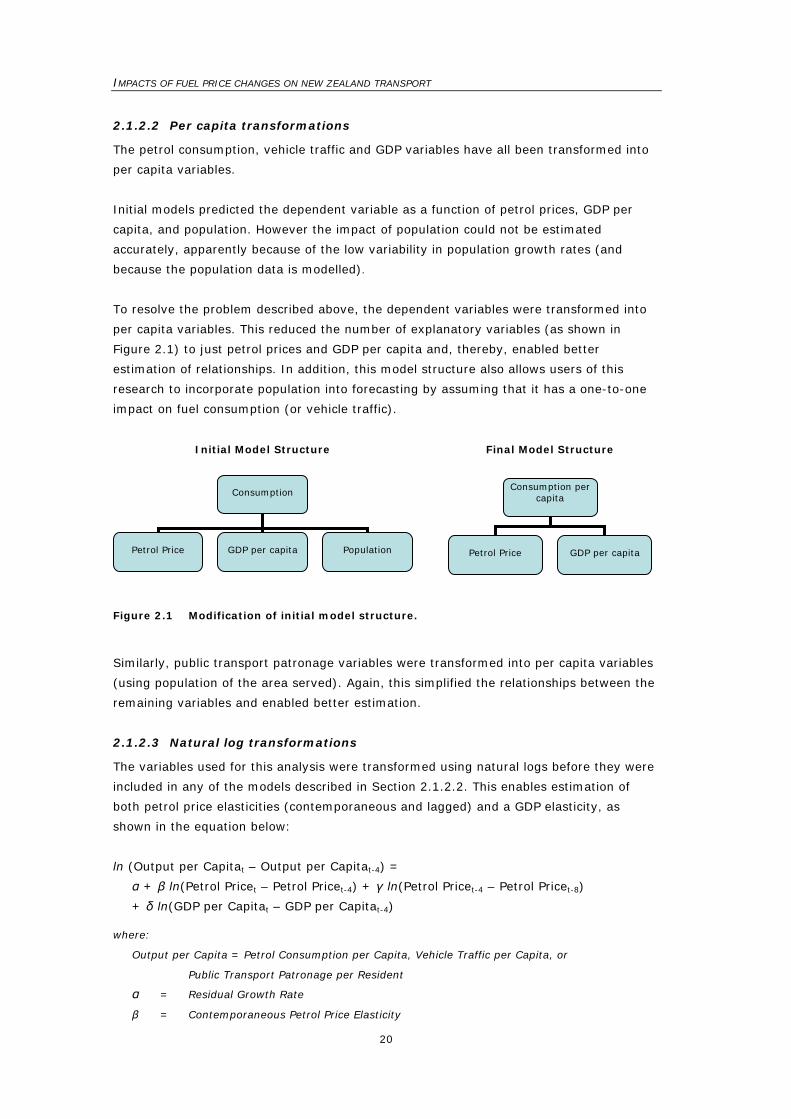
2.1.2.2 Per capita transformations
The petrol consumption, vehicle traffic and GDP variables have all been transformed into
per capita variables.
Initial models predicted the dependent variable as a function of petrol prices, GDP per
capita, and population. However the impact of population could not be estimated
accurately, apparently because of the low variability in population growth rates (and
because the population data is modelled).
To resolve the problem described above, the dependent variables were transformed into
per capita variables. This reduced the number of explanatory variables (as shown in
Figure 2.1) to just petrol prices and GDP per capita and, thereby, enabled better
estimation of relationships. In addition, this model structure also allows users of this
research to incorporate population into forecasting by assuming that it has a one-to-one
impact on fuel consumption (or vehicle traffic).
Initial Model Structure Final Model Structure
Figure 2.1 Modification of initial model structure.
Similarly, public transport patronage variables were transformed into per capita variables
(using population of the area served). Again, this simplified the relationships between the
remaining variables and enabled better estimation.
2.1.2.3 Natural log transformations
The variables used for this analysis were transformed using natural logs before they were
included in any of the models described in Section 2.1.2.2. This enables estimation of
both petrol price elasticities (contemporaneous and lagged) and a GDP elasticity, as
shown in the equation below:
ln (Output per Capitat – Output per Capitat-4) =
α + β ln(Petrol Pricet – Petrol Pricet-4) + γ ln(Petrol Pricet-4 – Petrol Pricet-8)
+ δ ln(GDP per Capitat – GDP per Capitat-4)
where:
Output per Capita = Petrol Consumption per Capita, Vehicle Traffic per Capita, or
Public Transport Patronage per Resident
α = Residual Growth Rate
β = Contemporaneous Petrol Price Elasticity
Consumption
Petrol Price GDP per capita Population

2. Study analyses
21
γ = Lagged Petrol Price Elasticity
δ = GDP per Capita Elasticity
t = quarter
The model type is four-quarter annual differences
The model equation above can also be represented using the notation below:
δ
−
γ
−
−β
−
α
−⎟⎟⎠
⎞⎜⎜⎝
⎛⎟⎟⎠
⎞⎜⎜⎝
⎛⎟⎟⎠
⎞⎜⎜⎝
⎛⋅=⎟⎟
⎠
⎞⎜⎜⎝
⎛
4tt
8t4t
4tt
tt
Capita per GDPCapita per GDP
Price PetrolPrice Petrol
Price PetrolPricet Petrol
eCapita per Output
Capita per Output
4
The models described above are often referred to as double-log (or log-log) models.
Double-log models assume that constant relationships exist between proportional changes
in the explanatory variables and proportional changes in the dependent variable.
Therefore, this report refers to the elasticities produced using such models as constant
point elasticities.2
The double-log model has been used for this research because it is commonly applied
elsewhere in the transport economics literature. In addition, the double-log model
assumes that the demand curve follows a convex shape, an assumption which seems
plausible to the present authors, especially if one assumes diminishing returns to efforts
to reduce petrol consumption.
However, as acknowledged in Section 4.7, there would be merit in investigating
alternative model structures. For example, during this research, some evidence was found
that elasticities might increase with price (see Section 3.1.4).
2.2 Petrol consumption analyses
2.2.1 Source data
The analyses were all undertaken at a national level. Some of the analyses used annual
data covering the period 1974-2005. The remaining analyses used quarterly data
covering the period March 1978–March 2006. Table 2.2 presents a summary of the data
sources used.
For analysis purposes, the following variables were then used for the final modelling
work:
• Petrol delivered per day per capita (dependent variable)
• Petrol price index, deflated by CPI
• GDP per capita
2 This elasticity measure (herein referred to as a constant point elasticity) is also referred to in
certain publications as an ‘arc elasticity’.
IMPACTS OF FUEL PRICE CHANGES ON NEW ZEALAND TRANSPORT
22
Table 2.2 Data sources for petrol consumption analyses.
Item Source, Notes
Petrol deliveries Tonnes of petrol delivered by oil companies (SNZ, MED).
Petrol price index Petrol price index, representing weighted average movement of pump prices for 91 octane, 96 octane petrol and petrol additive, averaged over quarter (SNZ). The petrol price index was deflated using the CPI, to adjust for inflation.
Gross domestic product Real GDP series with interpolation of annual data before 1977 (SNZ, VUW).
Population Quarterly residential population estimates with interpolation of annual data before 1991.
SNZ = Statistics New Zealand, MED = Ministry of Economic Development VUW = Victoria University of Wellington
CPI = Consumer Price Index GPD = Gross Domestic Product
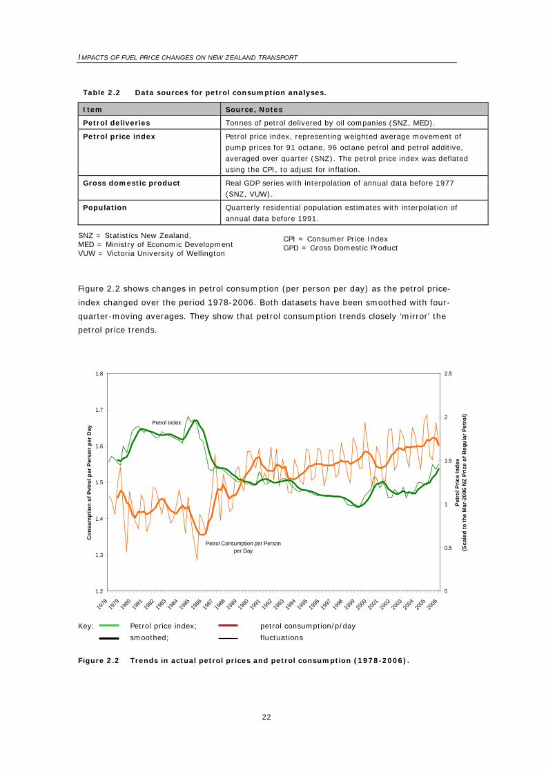
Figure 2.2 shows changes in petrol consumption (per person per day) as the petrol price-
index changed over the period 1978-2006. Both datasets have been smoothed with four-
quarter-moving averages. They show that petrol consumption trends closely ‘mirror’ the
petrol price trends.
Petrol Consumption per Person per Day
Petrol Index
1.2
1.3
1.4
1.5
1.6
1.7
1.8
1978
1979
1980
1981
1982
1983
1984
1985
1986
1987
1988
1989
1990
1991
1992
1993
1994
1995
1996
1997
1998
1999
2000
2001
2002
2003
2004
2005
2006
Con
sum
ptio
n of
Pet
rol p
er P
erso
n pe
r Day
0
0.5
1
1.5
2
2.5
Petr
ol P
rice
Inde
x(S
cale
d to
the
Mar
-200
6 N
Z Pr
ice
of R
egul
ar P
etro
l)
Key: Petrol price index; petrol consumption/p/day
smoothed; fluctuations
Figure 2.2 Trends in actual petrol prices and petrol consumption (1978-2006).
2. Study analyses
23
Petrol Index
GDP per Capita
-40%
-30%
-20%
-10%
0%
10%
20%
30%
1979 1980 1981 1982 1984 1985 1986 1987 1989 1990 1991 1992 1994 1995 1996 1997 1999 2000 2001 2002 2004 2005
Perc
enta
ge C
hang
es O
ver a
Yea
r
Petrol Deliveries per Capita
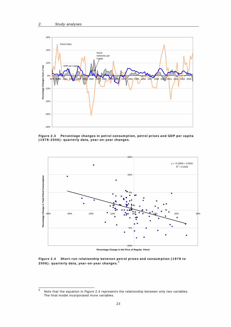
Figure 2.3 Percentage changes in petrol consumption, petrol prices and GDP per capita (1978-2006): quarterly data, year-on-year changes.
y = -0.1658x + 0.0031R2 = 0.2255
-10%
-5%
0%
5%
10%
15%
-40% -30% -20% -10% 0% 10% 20% 30%
Percentage Change in the Price of Regular Petrol
Perc
enta
ge C
hang
e in
Tot
al P
etro
l Con
sum
ptio
n
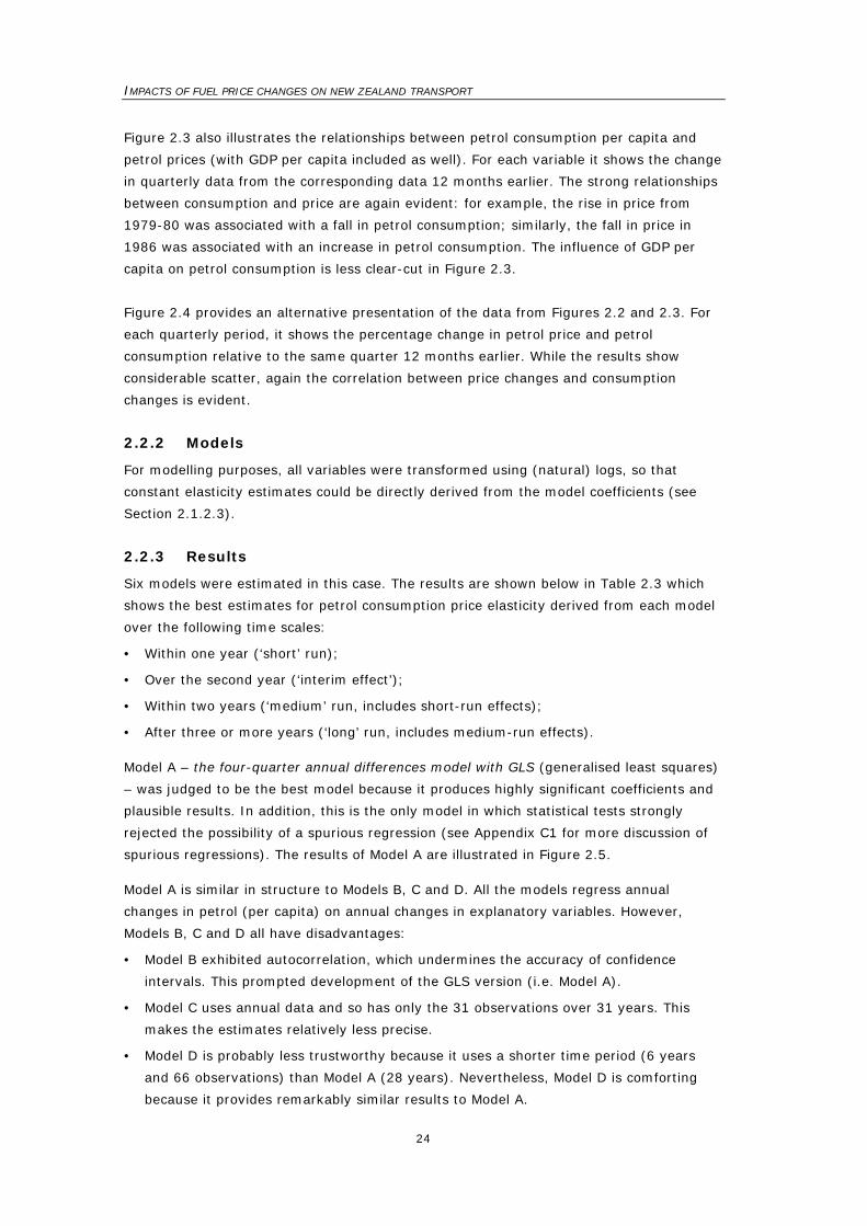
Figure 2.4 Short-run relationship between petrol prices and consumption (1978 to 2006): quarterly data, year-on-year changes.3
3 Note that the equation in Figure 2.4 represents the relationship between only two variables.
The final model incorporated more variables.
IMPACTS OF FUEL PRICE CHANGES ON NEW ZEALAND TRANSPORT
24
Figure 2.3 also illustrates the relationships between petrol consumption per capita and
petrol prices (with GDP per capita included as well). For each variable it shows the change
in quarterly data from the corresponding data 12 months earlier. The strong relationships
between consumption and price are again evident: for example, the rise in price from
1979-80 was associated with a fall in petrol consumption; similarly, the fall in price in
1986 was associated with an increase in petrol consumption. The influence of GDP per
capita on petrol consumption is less clear-cut in Figure 2.3.
Figure 2.4 provides an alternative presentation of the data from Figures 2.2 and 2.3. For
each quarterly period, it shows the percentage change in petrol price and petrol
consumption relative to the same quarter 12 months earlier. While the results show
considerable scatter, again the correlation between price changes and consumption
changes is evident.
2.2.2 Models
For modelling purposes, all variables were transformed using (natural) logs, so that
constant elasticity estimates could be directly derived from the model coefficients (see
Section 2.1.2.3).
2.2.3 Results
Six models were estimated in this case. The results are shown below in Table 2.3 which
shows the best estimates for petrol consumption price elasticity derived from each model
over the following time scales:
• Within one year (‘short’ run);
• Over the second year (‘interim effect’);
• Within two years (‘medium’ run, includes short-run effects);
• After three or more years (‘long’ run, includes medium-run effects).
Model A – the four-quarter annual differences model with GLS (generalised least squares)
– was judged to be the best model because it produces highly significant coefficients and
plausible results. In addition, this is the only model in which statistical tests strongly
rejected the possibility of a spurious regression (see Appendix C1 for more discussion of
spurious regressions). The results of Model A are illustrated in Figure 2.5.
Model A is similar in structure to Models B, C and D. All the models regress annual
changes in petrol (per capita) on annual changes in explanatory variables. However,
Models B, C and D all have disadvantages:
• Model B exhibited autocorrelation, which undermines the accuracy of confidence
intervals. This prompted development of the GLS version (i.e. Model A).
• Model C uses annual data and so has only the 31 observations over 31 years. This
makes the estimates relatively less precise.
• Model D is probably less trustworthy because it uses a shorter time period (6 years
and 66 observations) than Model A (28 years). Nevertheless, Model D is comforting
because it provides remarkably similar results to Model A.
2. Study analyses
25
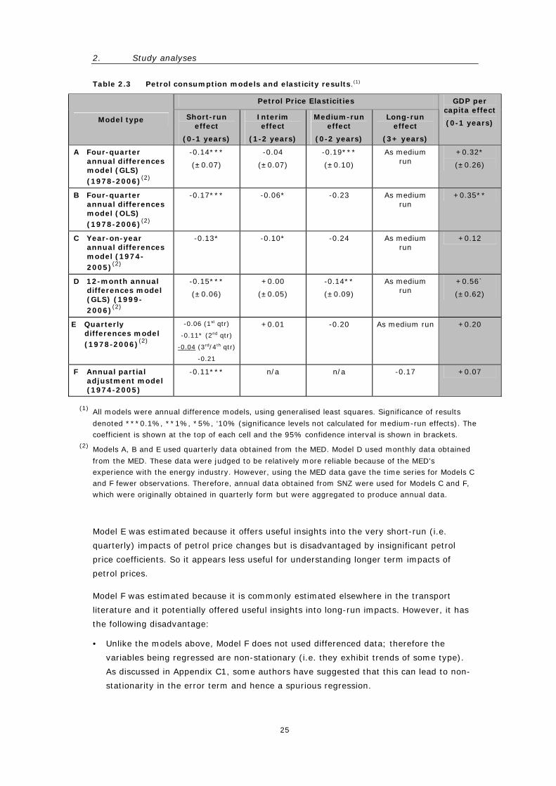
Table 2.3 Petrol consumption models and elasticity results.(1)
Petrol Price Elasticities
Model type Short-run effect
(0-1 years)
Interim effect
(1-2 years)
Medium-run effect
(0-2 years)
Long-run effect
(3+ years)
GDP per capita effect
(0-1 years)
A Four-quarter annual differences model (GLS) (1978-2006)(2)
-0.14***
(±0.07)
-0.04
(±0.07)
-0.19***
(±0.10)
As medium run
+0.32*
(±0.26)
B Four-quarter annual differences model (OLS) (1978-2006)(2)
-0.17*** -0.06* -0.23 As medium run
+0.35**
C Year-on-year annual differences model (1974-2005)(2)
-0.13* -0.10* -0.24 As medium run
+0.12
D 12-month annual differences model (GLS) (1999-2006)(2)
-0.15***
(±0.06)
+0.00
(±0.05)
-0.14**
(±0.09)
As medium run
+0.56`
(±0.62)
E Quarterly differences model (1978-2006)(2)
-0.06 (1st qtr)
-0.11* (2nd qtr)
-0.04 (3rd/4th qtr)
-0.21
+0.01 -0.20 As medium run +0.20
F Annual partial adjustment model (1974-2005)
-0.11*** n/a n/a -0.17 +0.07
(1) All models were annual difference models, using generalised least squares. Significance of results
denoted ***0.1%, **1%, *5%, ‘10% (significance levels not calculated for medium-run effects). The coefficient is shown at the top of each cell and the 95% confidence interval is shown in brackets.
(2) Models A, B and E used quarterly data obtained from the MED. Model D used monthly data obtained
from the MED. These data were judged to be relatively more reliable because of the MED’s experience with the energy industry. However, using the MED data gave the time series for Models C and F fewer observations. Therefore, annual data obtained from SNZ were used for Models C and F, which were originally obtained in quarterly form but were aggregated to produce annual data.
Model E was estimated because it offers useful insights into the very short-run (i.e.
quarterly) impacts of petrol price changes but is disadvantaged by insignificant petrol
price coefficients. So it appears less useful for understanding longer term impacts of
petrol prices.
Model F was estimated because it is commonly estimated elsewhere in the transport
literature and it potentially offered useful insights into long-run impacts. However, it has
the following disadvantage:
• Unlike the models above, Model F does not used differenced data; therefore the
variables being regressed are non-stationary (i.e. they exhibit trends of some type).
As discussed in Appendix C1, some authors have suggested that this can lead to non-
stationarity in the error term and hence a spurious regression.
IMPACTS OF FUEL PRICE CHANGES ON NEW ZEALAND TRANSPORT
26
0.00
-0.04 -0.19
0.00
-0.14
-0.3
-0.25
-0.2
-0.15
-0.1
-0.05
0
Short-Run Effect(0-1 years)
Interim Effect(1-2 years)
Medium-Run Effect(0-2 years)
Estim
ated
Pet
rol P
rice
Elas
ticity
95% Confidence Intervals
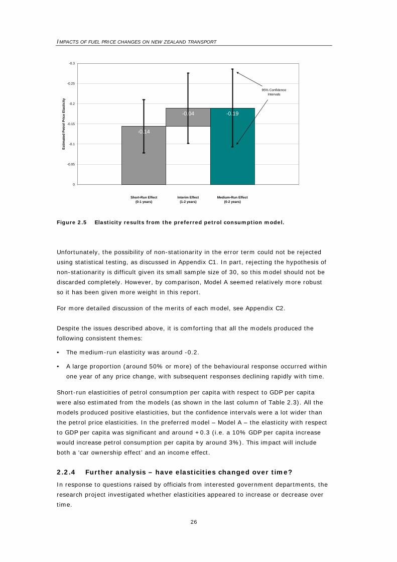
Figure 2.5 Elasticity results from the preferred petrol consumption model.
Unfortunately, the possibility of non-stationarity in the error term could not be rejected
using statistical testing, as discussed in Appendix C1. In part, rejecting the hypothesis of
non-stationarity is difficult given its small sample size of 30, so this model should not be
discarded completely. However, by comparison, Model A seemed relatively more robust
so it has been given more weight in this report.
For more detailed discussion of the merits of each model, see Appendix C2.
Despite the issues described above, it is comforting that all the models produced the
following consistent themes:
• The medium-run elasticity was around -0.2.
• A large proportion (around 50% or more) of the behavioural response occurred within
one year of any price change, with subsequent responses declining rapidly with time.
Short-run elasticities of petrol consumption per capita with respect to GDP per capita
were also estimated from the models (as shown in the last column of Table 2.3). All the
models produced positive elasticities, but the confidence intervals were a lot wider than
the petrol price elasticities. In the preferred model – Model A – the elasticity with respect
to GDP per capita was significant and around +0.3 (i.e. a 10% GDP per capita increase
would increase petrol consumption per capita by around 3%). This impact will include
both a ‘car ownership effect’ and an income effect.
2.2.4 Further analysis – have elasticities changed over time?
In response to questions raised by officials from interested government departments, the
research project investigated whether elasticities appeared to increase or decrease over
time.
2. Study analyses
27
Taken together, the three sources of information below suggest that the short-run
elasticity seems relatively constant over time:
1. Model D (which uses the data from 1999 to 2006) produces remarkably similar
estimates to Model A (which uses data from 1978 to 2006).
2. Model A was broken down into two 15-year periods (1974-89 and 1990-2006). A
separate short-run petrol price elasticity was estimated for each period and the
price elasticity was found to be lower in the second period; however, the difference
was not statistically significant. See Appendix C2.9 in Econometric analysis details:
Consumption elasticities for more detailed discussion.
3. Model A was modified to examine whether the short-run petrol price elasticity
changed systematically with time. The modified model suggested no evidence that
the elasticity grew or fell markedly with time. Again, see Appendix C2.9 in
Econometric analysis details: Consumption elasticities for more detailed discussion.
2.2.5 Further analysis – do petrol price levels affect elasticities?
Model A was also modified to enable simple analysis of the impacts of petrol prices on the
short-run elasticity. A dummy variable was used to distinguish the short-run elasticity
when petrol prices were below NZ$1.50 from the short-run elasticity when petrol prices
were above $1.50. Contrary to expectations, the model implied that the elasticity was
higher when petrol prices were below $1.50; however, the differences were not
statistically significant.
The method used to carry out this analysis was exploratory only and relatively simplistic.
It is still possible that more sophisticated models could be developed that would estimate
petrol price elasticities as a function of absolute petrol price levels. (Some of the
international evidence indicates a tendency for higher elasticities with higher petrol prices,
see Section 3.1.4, Figure 3.1.)
2.2.6 Further analysis – what was the impact of ‘carless days’?
In response to a suggestion from a referee, the impact of the ‘carless day’ policy from
February 1979 to August 1980 was incorporated in Model A as a dummy variable.
The impact of the ‘carless day’ policy dummy variable is shown in Table 2.4. The
coefficient of this dummy variable was insignificant but retention of the dummy is perhaps
justified because it increased Adjusted R2 slightly and it changed the coefficients slightly.
2.2.7 Concluding comments
Taking into account the quality of the various models, the following findings can be drawn
with respect to petrol consumption elasticities:
• A considerable degree of consistency exists across the different model results (despite
reasonably wide margins of error in most cases).

IMPACTS OF FUEL PRICE CHANGES ON NEW ZEALAND TRANSPORT
28
Table 2.4 Petrol consumption models with and without ‘carless days’ dummy used for Model A.
Petrol Price Elasticities
Model type Short-run effect
(0-1 years)
Interim effect
(1-2 years)
Medium-run effect
(0-2 years)
GDP per capita effect
(0-1 years)
‘Carless days‘ policy
dummy
R2 / Adjusted
R2 (OLS
version)
A Without ‘carless days’ dummy
-0.14***
(±0.07)
-0.04
(±0.07)
-0.19***
(±0.10)
+0.32*
(±0.26)
0.31/0.30
B With ‘carless days’ dummy
-0.15***
(±0.07)
-0.05
(±0.07)
-0.20***
(±0.10)
+0.39**
(±0.27)
-0.015
(±0.027)
0.34/0.31
Significance of results denoted as: ***0.1%, **1%, *5%, ‘ 10% (significance levels not calculated for medium-run effects). The coefficient is shown at the top of each cell and the 95% confidence interval is shown in brackets. OLS = ordinary least squares.
• The short-run elasticity estimates, representing the response over a 1-year period, are
around -0.15 (five of the six models give best estimates in the -0.11 to -0.17 range).
• The medium-run elasticities, representing the total response over a 2-year period, are
around -0.20, with further changes beyond 2 years being very small and difficult to
detect with any confidence.
• In all cases, a large proportion (around 50% or more) of the behavioural response
occurred within one year of any price change, with subsequent responses declining
rapidly with time.
These model estimates imply that the impacts of a 10% (real) rise in petrol prices on
consumption per capita would be:
• in the short run (within 1 year), a fall of about 1.5%;
• in the medium run (within 2 years), a fall of about 2.0%.
2.3 Traffic volume analyses
2.3.1 Source data
The analyses were undertaken at a national level using weekly data, and covering the
period 1 January 2002 – 18 June 2006 (4.5 years). Table 2.5 presents a summary of the
data sources used.
2. Study analyses
29
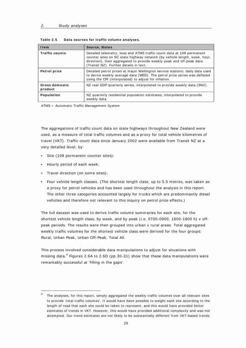
Table 2.5 Data sources for traffic volume analyses.
Item Source, Notes
Traffic counts Detailed telemetry, loop and ATMS traffic count data at 108 permanent counter sites on NZ state highway network (by vehicle length, week, hour, direction), then aggregated to provide weekly peak and off-peak data (Transit NZ). Further details in text.
Petrol price
Detailed petrol prices at major Wellington service stations: daily data used to derive weekly average data (MED). The petrol price series was deflated using the CPI (interpolated) to adjust for inflation.
Gross domestic product
NZ real GDP quarterly series, interpolated to provide weekly data (SNZ).
Population NZ quarterly residential population estimates, interpolated to provide weekly data.
ATMS = Automatic Traffic Management System
The aggregations of traffic count data on state highways throughout New Zealand were
used, as a measure of total traffic volumes and as a proxy for total vehicle kilometres of
travel (VKT). Traffic count data since January 2002 were available from Transit NZ at a
very detailed level, by:
• Site (108 permanent counter sites);
• Hourly period of each week;
• Travel direction (on some sites);
• Four vehicle length classes. (The shortest length class, up to 5.5 metres, was taken as
a proxy for petrol vehicles and has been used throughout the analysis in this report.
The other three categories accounted largely for trucks which are predominantly diesel
vehicles and therefore not relevant to this inquiry on petrol price effects.)
The full dataset was used to derive traffic volume summaries for each site, for the
shortest vehicle length class, by week, and by peak (i.e. 0700-0900, 1600-1800 h) v off-
peak periods. The results were then grouped into urban v rural areas. Total aggregated
weekly traffic volumes for the shortest vehicle class were derived for the four groups:
Rural, Urban Peak, Urban Off-Peak, Total All.
This process involved considerable data manipulations to adjust for situations with
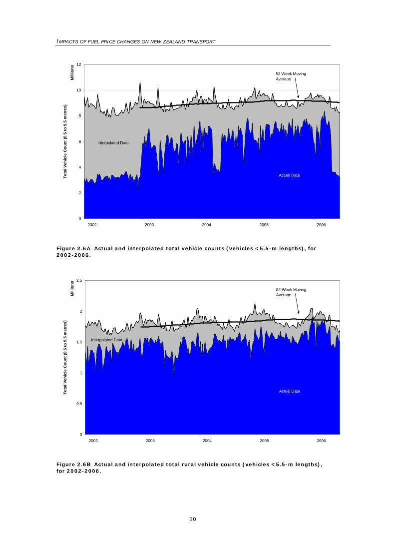
missing data.4 Figures 2.6A to 2.6D (pp.30-31) show that these data manipulations were
remarkably successful at ‘filling in the gaps’.
4 The analyses, for this report, simply aggregated the weekly traffic volumes over all relevant sites
to provide ‘total traffic volumes’. It would have been possible to weight each site according to the length of road that each site could be taken to represent, and this would have provided better estimates of trends in VKT. However, this would have provided additional complexity and was not attempted. Our trend estimates are not likely to be substantially different from VKT-based trends.
IMPACTS OF FUEL PRICE CHANGES ON NEW ZEALAND TRANSPORT
30
0
2
4
6
8
10
12
2002 2003 2004 2005 2006
Mill
ions
Tota
l Veh
icle
Cou
nt (0
.5 to
5.5
met
res)
Actual Data
Interpolated Data
52 Week Moving Average
Figure 2.6A Actual and interpolated total vehicle counts (vehicles <5.5-m lengths), for 2002-2006.
0
0.5
1
1.5
2
2.5
2002 2003 2004 2005 2006
Mill
ions
Tota
l Veh
icle
Cou
nt (0
.5 to
5.5
met
res)
Actual Data
Interpolated Data
52 Week Moving Average
Figure 2.6B Actual and interpolated total rural vehicle counts (vehicles <5.5-m lengths), for 2002-2006.
2. Study analyses
31
0
1
2
3
4
5
6
7
8
2002 2003 2004 2005 2006
Mill
ions
Tota
l Veh
icle
Cou
nt (0
.5 to
5.5
met
res)
Actual Data
Interpolated Data
52 Week Moving Average
Figure 2.6C Actual and interpolated total urban off-peak vehicle counts (vehicles <5.5-m lengths), for 2002-2006.
0
0.5
1
1.5
2
2.5
2002 2003 2004 2005 2006
Mill
ions
Tota
l Veh
icle
Cou
nt (0
.5 to
5.5
met
res)
Actual Data
Interpolated Data
52 Week Moving Average
Figure 2.6D Actual and interpolated total urban peak vehicle counts (vehicles <5.5-m lengths), for 2002-2006.
IMPACTS OF FUEL PRICE CHANGES ON NEW ZEALAND TRANSPORT
32
For analysis purposes, the following weekly variables were used:
• Total traffic volume per week per capita (by four area/period groups) – the dependent
variable;
• Average weekly petrol price, in real terms (deflated by CPI);
• GDP per capita, in real terms;
Samples of the data are shown in Figures 2.6A to 2.6D.
Figure 2.6A gives the total traffic (<5.5 metres length) volumes on a weekly basis,
indicating the extent of adjustments required for missing data. To eliminate seasonality
issues, it also shows the 52-week moving average volume trend: this clearly indicates a
volume peak in the second half of 2005, followed by a significant decline since then.
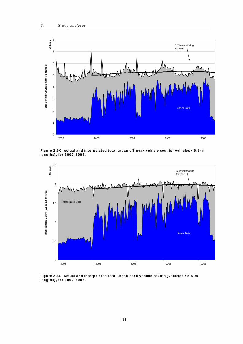
Similar patterns are observed when the data are broken down into rural, urban off-peak
and urban peak traffic counts. Note that the interpolation method seems to have worked
well for rural (Figure 2.6B) and urban peak counts (Figure 2.6D). However, the
interpolation method has not worked as well for urban off-peak counts (Figure 2.6C).
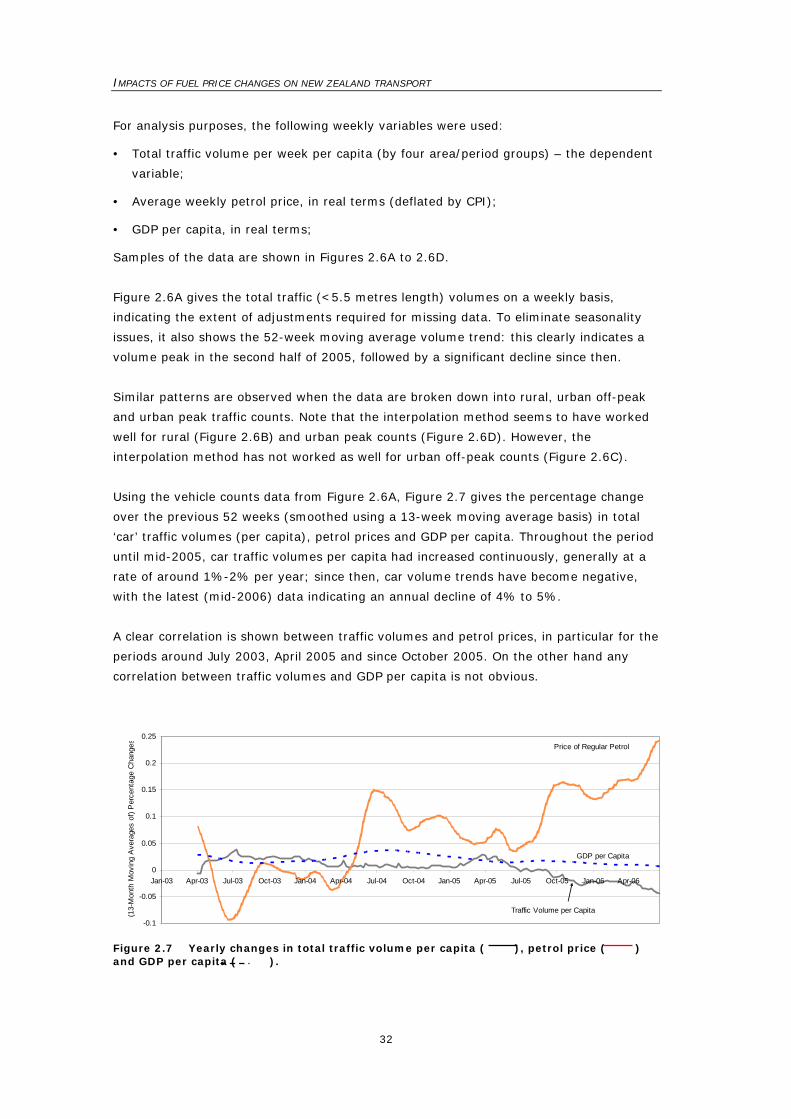
Using the vehicle counts data from Figure 2.6A, Figure 2.7 gives the percentage change
over the previous 52 weeks (smoothed using a 13-week moving average basis) in total
‘car’ traffic volumes (per capita), petrol prices and GDP per capita. Throughout the period
until mid-2005, car traffic volumes per capita had increased continuously, generally at a
rate of around 1%-2% per year; since then, car volume trends have become negative,
with the latest (mid-2006) data indicating an annual decline of 4% to 5%.
A clear correlation is shown between traffic volumes and petrol prices, in particular for the
periods around July 2003, April 2005 and since October 2005. On the other hand any
correlation between traffic volumes and GDP per capita is not obvious.
Price of Regular Petrol
GDP per Capita
-0.1
-0.05
0
0.05
0.1
0.15
0.2
0.25
Jan-03 Apr-03 Jul-03 Oct-03 Jan-04 Apr-04 Jul-04 Oct-04 Jan-05 Apr-05 Jul-05 Oct-05 Jan-06 Apr-06
(13-
Mon
th M
ovin
g A
vera
ges
of) P
erce
ntag
e C
hang
es
Traffic Volume per Capita
Figure 2.7 Yearly changes in total traffic volume per capita ( ), petrol price ( ) and GDP per capita ( ).
2. Study analyses
33
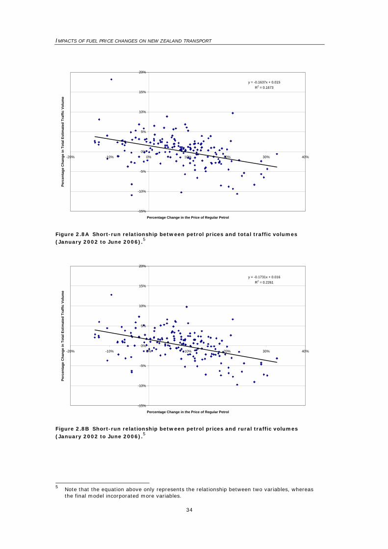
Figures 2.8A-2.8D (pp.34-35) give alternative views, using the same data, of the
relationship between year-on-year changes in car traffic volumes and petrol prices.
For the four groups of traffic counts combined (Figure 2.8A), the best fit line to the data
indicates an ‘underlying’ traffic volume growth of around 1.5-2% per annum (pa) with
constant petrol prices, but changing to zero growth when petrol prices increase at around
10% pa (real terms).
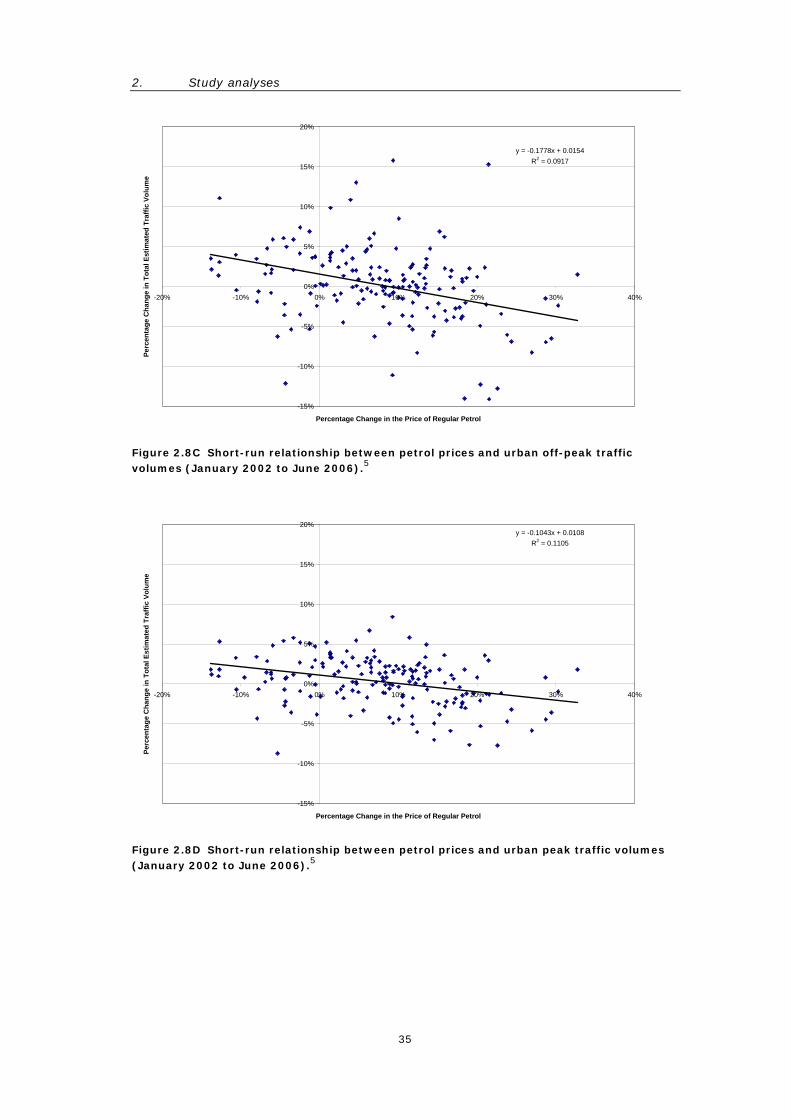
Figures 2.8B (rural traffic), 2.8C (urban off-peak traffic) and 2.8D (urban peak traffic)
show similar trends to Figure 2.8A (total traffic). However, the ‘underlying’ growth rate
for the urban peak count is close to 1% pa, whereas the underlying growth rates for
urban off-peak and rural traffic are closer to 2% pa.
2.3.2 Models
For modelling purposes, the three variables noted above were used, but transformed to
(natural) log form (as for the petrol consumption modelling described earlier).
An annual (52-week) differences model was applied, using the change in the variable for
the week in question from its value 52 weeks previously. If such a model is fitted using
ordinary least squares (OLS) methods, then it produces margins of error that are
inaccurate, due to autocorrelation. Therefore a generalised least squares (GLS) model
was used in preference, so that margins of error could be properly estimated.
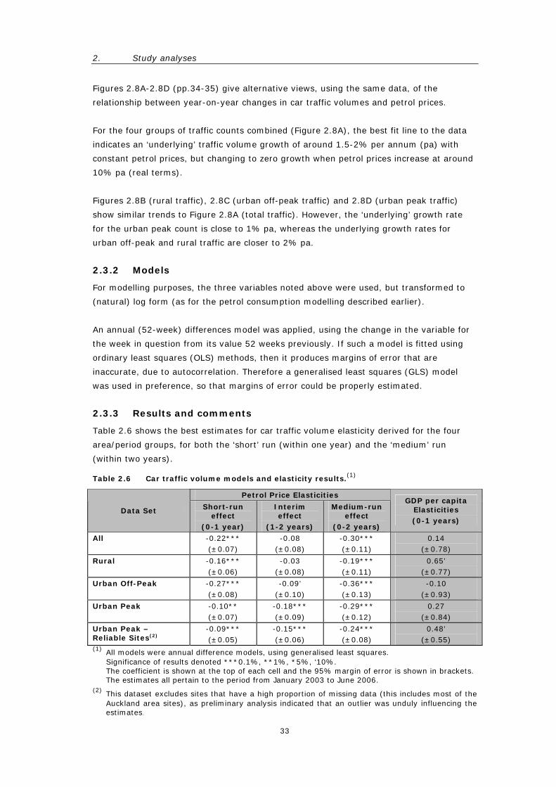
2.3.3 Results and comments
Table 2.6 shows the best estimates for car traffic volume elasticity derived for the four
area/period groups, for both the ‘short’ run (within one year) and the ‘medium’ run
(within two years).
Table 2.6 Car traffic volume models and elasticity results.(1)
Petrol Price Elasticities
Data Set Short-run effect
(0-1 year)
Interim effect
(1-2 years)
Medium-run effect
(0-2 years)
GDP per capita Elasticities (0-1 years)
All -0.22*** (±0.07)
-0.08 (±0.08)
-0.30*** (±0.11)
0.14 (±0.78)
Rural -0.16*** (±0.06)
-0.03 (±0.08)
-0.19*** (±0.11)
0.65’ (±0.77)
Urban Off-Peak -0.27*** (±0.08)
-0.09’ (±0.10)
-0.36*** (±0.13)
-0.10 (±0.93)
Urban Peak -0.10** (±0.07)
-0.18*** (±0.09)
-0.29*** (±0.12)
0.27 (±0.84)
Urban Peak – Reliable Sites(2)
-0.09*** (±0.05)
-0.15*** (±0.06)
-0.24*** (±0.08)
0.48’ (±0.55)
(1) All models were annual difference models, using generalised least squares. Significance of results denoted ***0.1%, **1%, *5%, ‘10%. The coefficient is shown at the top of each cell and the 95% margin of error is shown in brackets. The estimates all pertain to the period from January 2003 to June 2006. (2) This dataset excludes sites that have a high proportion of missing data (this includes most of the
Auckland area sites), as preliminary analysis indicated that an outlier was unduly influencing the estimates.
IMPACTS OF FUEL PRICE CHANGES ON NEW ZEALAND TRANSPORT
34
y = -0.1637x + 0.015R2 = 0.1673
-15%
-10%
-5%
0%
5%
10%
15%
20%
-20% -10% 0% 10% 20% 30% 40%
Percentage Change in the Price of Regular Petrol
Perc
enta
ge C
hang
e in
Tot
al E
stim
ated
Tra
ffic
Volu
me
Figure 2.8A Short-run relationship between petrol prices and total traffic volumes (January 2002 to June 2006).5
y = -0.1731x + 0.016R2 = 0.2261
-15%
-10%
-5%
0%
5%
10%
15%
20%
-20% -10% 0% 10% 20% 30% 40%
Percentage Change in the Price of Regular Petrol
Perc
enta
ge C
hang
e in
Tot
al E
stim
ated
Tra
ffic
Volu
me
Figure 2.8B Short-run relationship between petrol prices and rural traffic volumes (January 2002 to June 2006).5
5 Note that the equation above only represents the relationship between two variables, whereas
the final model incorporated more variables.
2. Study analyses
35
y = -0.1778x + 0.0154R2 = 0.0917
-15%
-10%
-5%
0%
5%
10%
15%
20%
-20% -10% 0% 10% 20% 30% 40%
Percentage Change in the Price of Regular Petrol
Perc
enta
ge C
hang
e in
Tot
al E
stim
ated
Tra
ffic
Volu
me
Figure 2.8C Short-run relationship between petrol prices and urban off-peak traffic volumes (January 2002 to June 2006).5
y = -0.1043x + 0.0108R2 = 0.1105
-15%
-10%
-5%
0%
5%
10%
15%
20%
-20% -10% 0% 10% 20% 30% 40%
Percentage Change in the Price of Regular Petrol
Perc
enta
ge C
hang
e in
Tot
al E
stim
ated
Tra
ffic
Volu
me
Figure 2.8D Short-run relationship between petrol prices and urban peak traffic volumes (January 2002 to June 2006).5
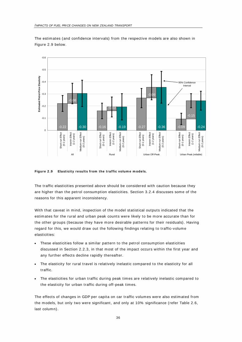
IMPACTS OF FUEL PRICE CHANGES ON NEW ZEALAND TRANSPORT
36
The estimates (and confidence intervals) from the respective models are also shown in
Figure 2.9 below.
-0.22
-0.08
-0.30 -0.16
-0.03
-0.19 -0.27
-0.09
-0.36 -0.09
-0.15
-0.24
-0.6
-0.5
-0.4
-0.3
-0.2
-0.1
0
Shor
t-run
Effe
ct(0
-1 y
ears
)
Inte
rim E
ffect
(1-2
yea
rs)
Med
ium
-run
Effe
ct(0
-2 y
ears
)
Shor
t-run
Effe
ct(0
-1 y
ears
)
Inte
rim E
ffect
(1-2
yea
rs)
Med
ium
-run
Effe
ct(0
-2 y
ears
)
Shor
t-run
Effe
ct(0
-1 y
ears
)
Inte
rim E
ffect
(1-2
yea
rs)
Med
ium
-run
Effe
ct(0
-2 y
ears
)
Shor
t-run
Effe
ct(0
-1 y
ears
)
Inte
rim E
ffect
(1-2
yea
rs)
Med
ium
-run
Effe
ct(0
-2 y
ears
)
All Rural Urban Off-Peak Urban Peak (reliable)
Estim
ated
Pet
rol-P
rice
Elas
ticity
95% Confidence Interval
Figure 2.9 Elasticity results from the traffic volume models.
The traffic elasticities presented above should be considered with caution because they
are higher than the petrol consumption elasticities. Section 3.2.4 discusses some of the
reasons for this apparent inconsistency.
With that caveat in mind, inspection of the model statistical outputs indicated that the
estimates for the rural and urban peak counts were likely to be more accurate than for
the other groups (because they have more desirable patterns for their residuals). Having
regard for this, we would draw out the following findings relating to traffic-volume
elasticities:
• These elasticities follow a similar pattern to the petrol consumption elasticities
discussed in Section 2.2.3, in that most of the impact occurs within the first year and
any further effects decline rapidly thereafter.
• The elasticity for rural travel is relatively inelastic compared to the elasticity for all
traffic.
• The elasticities for urban traffic during peak times are relatively inelastic compared to
the elasticity for urban traffic during off-peak times.
The effects of changes in GDP per capita on car traffic volumes were also estimated from
the models, but only two were significant, and only at 10% significance (refer Table 2.6,
last column).
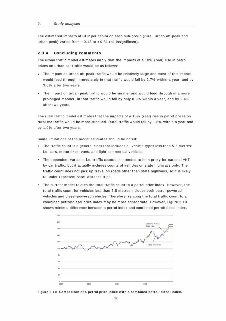
2. Study analyses
37
The estimated impacts of GDP per capita on each sub-group (rural, urban off-peak and
urban peak) varied from +0.13 to +0.81 (all insignificant).
2.3.4 Concluding comments
The urban traffic model estimates imply that the impacts of a 10% (real) rise in petrol
prices on urban car traffic would be as follows:
• The impact on urban off-peak traffic would be relatively large and most of this impact
would feed through immediately in that traffic would fall by 2.7% within a year, and by
3.6% after two years.
• The impact on urban peak traffic would be smaller and would feed through in a more
prolonged manner, in that traffic would fall by only 0.9% within a year, and by 2.4%
after two years.
The rural traffic model estimates that the impacts of a 10% (real) rise in petrol prices on
rural car traffic would be more subdued. Rural traffic would fall by 1.6% within a year and
by 1.9% after two years.
Some limitations of the model estimates should be noted:
• The traffic count is a general class that includes all vehicle types less than 5.5 metres:
i.e. cars, motorbikes, vans, and light commercial vehicles.
• The dependent variable, i.e. traffic counts, is intended to be a proxy for national VKT
by car traffic, but it actually includes counts of vehicles on state highways only. The
traffic count does not pick up travel on roads other than state highways, so it is likely
to under-represent short-distance trips.
• The current model relates the total traffic count to a petrol price index. However, the
total traffic count for vehicles less than 5.5 metres includes both petrol-powered
vehicles and diesel-powered vehicles. Therefore, relating the total traffic count to a
combined petrol/diesel price index may be more appropriate. However, Figure 2.10
shows minimal difference between a petrol index and combined petrol/diesel index.
0
20
40
60
80
100
120
140
160
180
200
2002 2003 2004 2005
Petrol Price Index
Combined Petrol & Diesel Index
Figure 2.10 Comparison of a petrol price index with a combined petrol/diesel index.
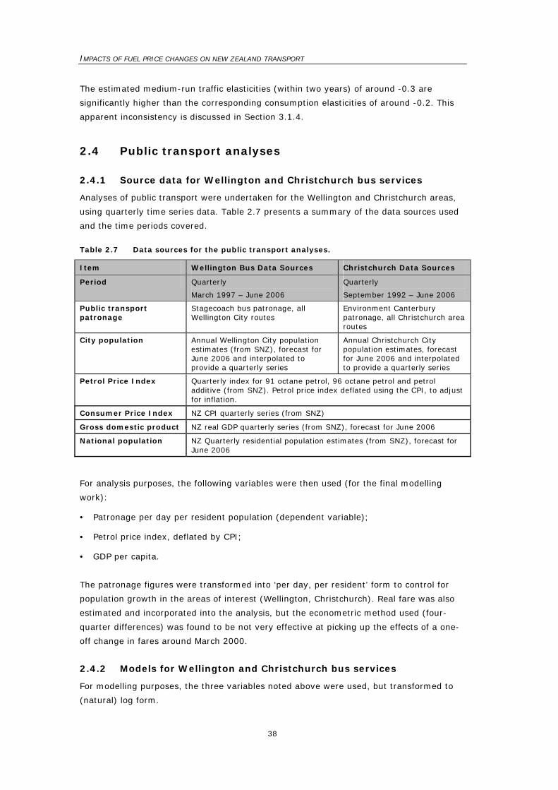
IMPACTS OF FUEL PRICE CHANGES ON NEW ZEALAND TRANSPORT
38
The estimated medium-run traffic elasticities (within two years) of around -0.3 are
significantly higher than the corresponding consumption elasticities of around -0.2. This
apparent inconsistency is discussed in Section 3.1.4.
2.4 Public transport analyses
2.4.1 Source data for Wellington and Christchurch bus services
Analyses of public transport were undertaken for the Wellington and Christchurch areas,
using quarterly time series data. Table 2.7 presents a summary of the data sources used
and the time periods covered.
Table 2.7 Data sources for the public transport analyses.
Item Wellington Bus Data Sources Christchurch Data Sources
Period Quarterly
March 1997 – June 2006
Quarterly
September 1992 – June 2006
Public transport patronage
Stagecoach bus patronage, all Wellington City routes
Environment Canterbury patronage, all Christchurch area routes
City population Annual Wellington City population estimates (from SNZ), forecast for June 2006 and interpolated to provide a quarterly series
Annual Christchurch City population estimates, forecast for June 2006 and interpolated to provide a quarterly series
Petrol Price Index Quarterly index for 91 octane petrol, 96 octane petrol and petrol additive (from SNZ). Petrol price index deflated using the CPI, to adjust for inflation.
Consumer Price Index NZ CPI quarterly series (from SNZ)
Gross domestic product NZ real GDP quarterly series (from SNZ), forecast for June 2006
National population NZ Quarterly residential population estimates (from SNZ), forecast for June 2006
For analysis purposes, the following variables were then used (for the final modelling
work):
• Patronage per day per resident population (dependent variable);
• Petrol price index, deflated by CPI;
• GDP per capita.
The patronage figures were transformed into ‘per day, per resident’ form to control for
population growth in the areas of interest (Wellington, Christchurch). Real fare was also
estimated and incorporated into the analysis, but the econometric method used (four-
quarter differences) was found to be not very effective at picking up the effects of a one-
off change in fares around March 2000.
2.4.2 Models for Wellington and Christchurch bus services
For modelling purposes, the three variables noted above were used, but transformed to
(natural) log form.

2. Study analyses
39
An annual (four-quarter) differences model was applied, using the change in the variable
for the quarter in question from its value four quarters previously. As in previous
analyses, a GLS model was used in preference to an OLS model, so that margins of error
could be more accurately estimated.
2.4.3 Results for Wellington and Christchurch bus services
The results of the Wellington and Christchurch patronage analyses are shown in
Table 2.8.
Table 2.8 Public transport cross-elasticity results for Wellington and Christchurch bus patronage.(1)
Data Set Short-run effect
(0-1 years)
Interim effect
(1-2 years)
Interim effect
(2-3 years)
Interim effect
(3-4 years)
Medium- to Long-run effect
(0-4 years)
GDP effect
(0-1 years)
Quarterly Wellington Stagecoach bus patronage(2)
0.16***
(±0.05)
0.21**
(±0.06)
0.18***
(±0.04)
0.07**
(±0.19)
0.61***
(±0.20)
0.23
(±0.45)
Quarterly Christchurch bus patronage(3)
-0.00
(±0.12)
0.13`
(±0.13)
0.13*
(±0.13)
n/a:
insignificant
0.26 (4)
(±0.40)
0.89*
(±0.76)
(1) The model is a four-quarter annual difference model, using GLS, with an AR(4) error term assumed.
Significance of results denoted ***0.1%, **1%, *5%, ‘10%.
The coefficient is shown at the top of each cell and the 95% confidence interval is shown in brackets.
(2) The estimates pertain to the period March 2000 to June 2006. (3) The estimates pertain to the period September 1994 to June 2006. (4) The estimates for Christchurch bus patronage actually correspond to 0-3 years, rather than the 0-
4 years noted above.
The Wellington bus patronage analysis, if taken at face value, implies a high cross-
elasticity and a strong lagged impact of petrol prices on patronage. The Christchurch bus
patronage estimates are insignificant and, therefore, inconclusive.
2.4.4 Comments – Wellington and Christchurch bus services
The results of the Wellington and Christchurch bus patronage analyses should be
regarded with considerable caution:
• The residuals of the Wellington bus patronage model were unsatisfactory. There was
evidence of negative autocorrelation, non-normality and non-constant variance in
residuals (as noted in Appendix C4). The variance of residuals is non-constant because
it increases with time; this will cause the estimated margins of error to underestimate
the genuine margin of error.

IMPACTS OF FUEL PRICE CHANGES ON NEW ZEALAND TRANSPORT
40
• The Christchurch bus patronage model appeared to suffer from unexplained ‘noise’ in
the data; a number of substantial changes have been made to bus services in the
Christchurch area, and these changes could not be readily accounted for.
• Both the Christchurch bus patronage model and the Wellington bus patronage model
may have been affected by the omission of important variables. For example, the
creation of new routes in Christchurch may have had an influence on patronage, but
this factor had to be omitted from the analysis because data were not available.
These patronage analyses are deemed inconclusive, related both to the implausibility of
the results and to doubts about the statistical validity of the model.
2.4.5 Source data and model for Wellington rail services
Some analysis was also undertaken using data provided by Toll New Zealand. Toll
provided monthly peak passenger rail patronage data for Wellington region for the period
July 2004 to May 2006. (Patronage data before July 2004 was affected by various service
disruptions, and therefore was not collected. This was supplemented by weekly petrol
price data from the MED and GDP data from Statistics NZ which was interpolated to
created a monthly series.)
A twelve-month annual differences model was then fitted, in which changes in total
patronage were compared to changes in petrol prices and GDP. The findings were
inconclusive so a per capita model was not attempted.
2.4.6 Results and comments for Wellington rail services
The results of this analysis were inconclusive. Figure 2.11 shows the percentage change
in patronage for each month compared to the same month in the preceding year, and the
corresponding change in petrol price.
The figure illustrates the absence of any definitive relationship between petrol prices and
patronage. However, the sample consists of only 11 observations so a statistically robust
relationship would have been unlikely.
Again, as with the Wellington and Christchurch bus data, a variety of factors drive
patronage trends and an inability to control for these creates ‘noise’ that makes
discerning accurate cross-elasticities difficult.
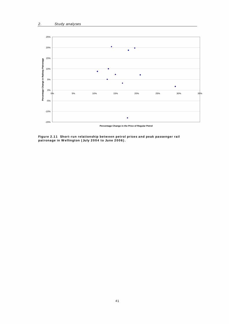
2. Study analyses
41
-15%
-10%
-5%
0%
5%
10%
15%
20%
25%
0% 5% 10% 15% 20% 25% 30% 35%
Percentage Change in the Price of Regular Petrol
Perc
enta
ge C
hang
e in
Rai
lway
Pat
rona
ge
Figure 2.11 Short-run relationship between petrol prices and peak passenger rail patronage in Wellington (July 2004 to June 2006).
IMPACTS OF FUEL PRICE CHANGES ON NEW ZEALAND TRANSPORT
42
3. Review of earlier research
3.1 Petrol consumption elasticities
3.1.1 New Zealand evidence
Table 3.1 summarises previous econometric studies on petrol consumption elasticities in
New Zealand.
Table 3.1 Previous New Zealand studies on petrol consumption elasticities.
Reference for study Short-Run Long-Run Estimation Method
Barns (2002) -0.20 -0.07 Cointegration model
MED (2000) -0.07 -0.19 Partial adjustment model
Ministry of Commerce (1991) -0.03 -0.07 Not established
Waikato University (1982) -0.13 -0.16 Not established
Hughes (1980) -0.11 -0.14 Not established
• Most short-run values are around -0.10 (range -0.03 to -0.13), and long-run values
are around -0.15 (range -0.07 to -0.19).
• The exception is in Barns (2002), who estimated a relatively high short-run elasticity
(-0.20) but a lower long-run figure. While her research methods appear robust, her
relative long-run v short-run findings are contrary to almost all other evidence
internationally.
Note that the estimates derived in our study (around -0.15 in the short run and -0.20 in
the medium run) are at the high end of the range found from these previous New Zealand
studies.
3.1.2 Australian evidence
Table 3.2 summarises econometric studies of petrol consumption elasticities in Australia.
• One of the most robust and transparent studies is that by Sterner et al. (1992). They
fitted a partial adjustment model to Australian data from 1960 to 1985 and employed
valid tests for autocorrelation. They also fitted a number of alternative models which
all produced long-run estimates in the -0.1 to -0.2 range.
• These long-run estimates are supported by research by Samimi (1995), who estimated
a long-run elasticity of -0.13 from data for the period 1980-1993. (Samimi’s research
covered both petrol and diesel, so the petrol price elasticity would be expected to be
rather larger than this estimate.)
• Sterner et al.’s short-run estimate is supported by Harding’s survey (2001). His
elasticity estimate of -0.05 is based on household consumption only, and may
underestimate the total impact, but is still more robust than many time-series
estimates.
3. Review of earlier research
43
Table 3.2 Previous Australian studies on petrol consumption elasticities.
Reference to study Short-run Long-run Not stated or Not established
Estimation Model/ Method6
Brain & Schuyers (1981) -0.11 -0.22 Not established
Donnelly (1984) -0.12 -0.67 Not established
Filmer & Mannion (1979) -0.03 -0.07 Not established
Harding (2001) -0.05 n/a Survey Analysis
Hensher & Young (1991) -0.25 (direct estimate) -0.66 (indirect calculations)
Static Model
Samimi (1995)7 -0.02 -0.13 Cointegration Model
Schou & Johnson (1979) -0.02 to -0.08 Static Models: OLS and Cooley-Prescott
Sterner, Dahl & Franzen (1992)
-0.05 -0.18 Partial Adjustment Model but other models also fitted
• The long-run values centre around -0.15 (four of five values are in the -0.07 to -0.22
range); this is again very similar to the range for New Zealand (the exception is
Donnelly’s estimate of -0.67), but substantially lower than the conclusion in Luk &
Hepburn’s (1993) review.
From this evidence, nothing indicates any significant differences between Australian and
New Zealand consumption elasticities.
3.1.3 International evidence
Sterner et al. (1992) produced estimates of short-run and long-run elasticities for 21
OECD countries. These estimates are useful for comparisons across countries because
they were produced using the same model (a partial adjustment model) and with data
covering the same period (1960-1985). Their estimates aggregated by countries or
regions of particular interest are summarised in Table 3.3.
Table 3.3 International studies for petrol consumption elasticities.
Country/Region Short-run Long-run
Australia -0.05 -0.18
US -0.18 -1.00
Canada -0.25 -1.07
Europe - average - range - UK
-0.28
-0.05 to -0.57 -0.11
-0.88
-0.18 to -2.29 -0.45
Source: Sterner et al. (1992).
6 The estimated method was inferred when not clearly stated: most models that produce distinct
‘short-run’ and ‘long-run’ estimates are partial adjustment models. 7 Samimi (1995) analyses both petrol and diesel consumption together so his estimates are not
strictly petrol price elasticity estimates, but rather transport-fuel price elasticity estimates.
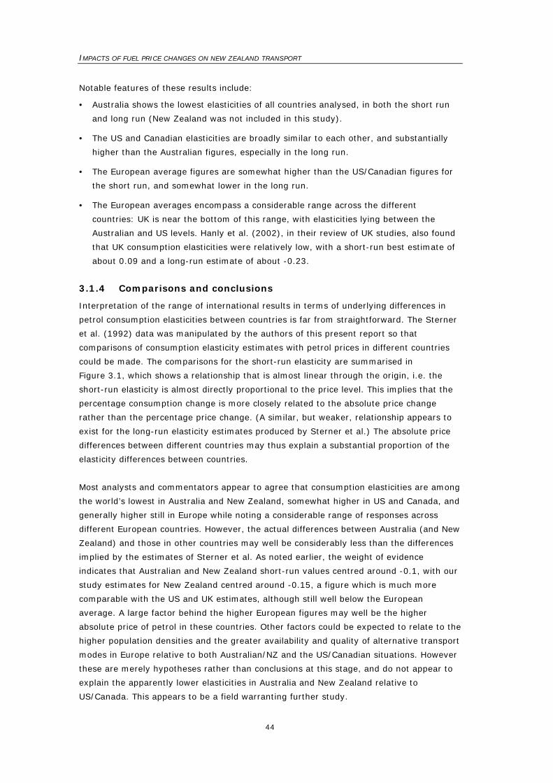
IMPACTS OF FUEL PRICE CHANGES ON NEW ZEALAND TRANSPORT
44
Notable features of these results include:
• Australia shows the lowest elasticities of all countries analysed, in both the short run
and long run (New Zealand was not included in this study).
• The US and Canadian elasticities are broadly similar to each other, and substantially
higher than the Australian figures, especially in the long run.
• The European average figures are somewhat higher than the US/Canadian figures for
the short run, and somewhat lower in the long run.
• The European averages encompass a considerable range across the different
countries: UK is near the bottom of this range, with elasticities lying between the
Australian and US levels. Hanly et al. (2002), in their review of UK studies, also found
that UK consumption elasticities were relatively low, with a short-run best estimate of
about 0.09 and a long-run estimate of about -0.23.
3.1.4 Comparisons and conclusions
Interpretation of the range of international results in terms of underlying differences in
petrol consumption elasticities between countries is far from straightforward. The Sterner
et al. (1992) data was manipulated by the authors of this present report so that
comparisons of consumption elasticity estimates with petrol prices in different countries
could be made. The comparisons for the short-run elasticity are summarised in
Figure 3.1, which shows a relationship that is almost linear through the origin, i.e. the
short-run elasticity is almost directly proportional to the price level. This implies that the
percentage consumption change is more closely related to the absolute price change
rather than the percentage price change. (A similar, but weaker, relationship appears to
exist for the long-run elasticity estimates produced by Sterner et al.) The absolute price
differences between different countries may thus explain a substantial proportion of the
elasticity differences between countries.
Most analysts and commentators appear to agree that consumption elasticities are among
the world’s lowest in Australia and New Zealand, somewhat higher in US and Canada, and
generally higher still in Europe while noting a considerable range of responses across
different European countries. However, the actual differences between Australia (and New
Zealand) and those in other countries may well be considerably less than the differences
implied by the estimates of Sterner et al. As noted earlier, the weight of evidence
indicates that Australian and New Zealand short-run values centred around -0.1, with our
study estimates for New Zealand centred around -0.15, a figure which is much more
comparable with the US and UK estimates, although still well below the European
average. A large factor behind the higher European figures may well be the higher
absolute price of petrol in these countries. Other factors could be expected to relate to the
higher population densities and the greater availability and quality of alternative transport
modes in Europe relative to both Australian/NZ and the US/Canadian situations. However
these are merely hypotheses rather than conclusions at this stage, and do not appear to
explain the apparently lower elasticities in Australia and New Zealand relative to
US/Canada. This appears to be a field warranting further study.
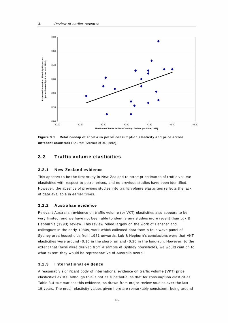
3. Review of earlier research
45
0.00
-0.10
-0.20
-0.30
-0.40
-0.50
-0.60
$0.00 $0.20 $0.40 $0.60 $0.80 $1.00 $1.20
The Price of Petrol in Each Country - Dollars per Litre (1989)
Estim
ated
Sho
rt-R
un E
last
icity
Est
imat
es(a
s es
timat
ed b
y St
erne
r et a
l 199
2)
Figure 3.1 Relationship of short-run petrol consumption elasticity and price across
different countries (Source: Sterner et al. 1992).
3.2 Traffic volume elasticities
3.2.1 New Zealand evidence
This appears to be the first study in New Zealand to attempt estimates of traffic volume
elasticities with respect to petrol prices, and no previous studies have been identified.
However, the absence of previous studies into traffic volume elasticities reflects the lack
of data available in earlier times.
3.2.2 Australian evidence
Relevant Australian evidence on traffic volume (or VKT) elasticities also appears to be
very limited, and we have not been able to identify any studies more recent than Luk &
Hepburn’s (1993) review. This review relied largely on the work of Hensher and
colleagues in the early 1980s, work which collected data from a four-wave panel of
Sydney area households from 1981 onwards. Luk & Hepburn’s conclusions were that VKT
elasticities were around -0.10 in the short-run and -0.26 in the long-run. However, to the
extent that these were derived from a sample of Sydney households, we would caution to
what extent they would be representative of Australia overall.
3.2.3 International evidence
A reasonably significant body of international evidence on traffic volume (VKT) price
elasticities exists, although this is not as substantial as that for consumption elasticities.
Table 3.4 summarises this evidence, as drawn from major review studies over the last
15 years. The mean elasticity values given here are remarkably consistent, being around
IMPACTS OF FUEL PRICE CHANGES ON NEW ZEALAND TRANSPORT
46
-0.15 in the short-run and around -0.30 in the long-run. Unfortunately, without an
extensive in-depth appraisal. it is not possible to assess the quality of the original studies
making up these mean values, nor to examine differences between countries.
Table 3.4 International studies on vehicle kilometre elasticities.(1)
Source Short-run Long-run Notes, Comments
Goodwin (1992) -0.16 -0.33 Major international review: values quoted are mean estimates.
TRACE (1998) / de Jong & Gunn (2000)
-0.16 -0.26 Review of over 50 European studies from the period 1985-1997: values quoted are mean estimates.
Short-run values relate to mode choice change only (might be expected to underestimate total market responses); long-run values allow for full range of behavioural responses.
Graham & Glaister (2002, 2004)
-0.15 -0.31 Major international review: value quotes are mean estimates.
Goodwin et al. (2004)
-0.10 -0.29 Major international review, focusing on studies undertaken in the period 1992-2002, mainly in Europe and US.
Results relate to mean of dynamic estimation studies (static estimation studies gave mean of 0.31).
(1) More complete evidence from international studies is provided in Wallis (2004).
3.2.4 Comparisons and conclusions
We would have anticipated (along with most other researchers in this field) a systematic
relationship between traffic volume elasticities and petrol consumption elasticities. In the
short-run, traffic volume elasticities would be expected to be somewhat lower than
consumption elasticities because behavioural adaptations other than reduced mileage are
possible even in the short-run, through changes in driving styles and speed, use of
smaller cars in multi-car households etc. In the longer run, further adaptations would be
expected in terms of changes in vehicle size and energy efficiency. Thus long-run traffic
volume elasticities would be expected to be substantially lower than consumption
elasticities.
These expected relationships appear to be present in the international data. Comparing
the results from Tables 3.3 and 3.4, the typical short-run VKT elasticity for US, Canada
and Europe (around -0.15) is somewhat below the consumption elasticity (around –0.24);
whereas the long-run VKT elasticities (around -0.30) are markedly lower than the
corresponding averaged consumption elasticities (around -1.00). Goodwin’s reviews of
1992 and 2004 gave a broadly similar pattern of results.
Luk & Hepburn’s 1993 review of Australian elasticity evidence also produced similar
results (although this may have been a lucky outcome given the few and disparate data
sources used). Their best estimates of VKT elasticities (based heavily on Sydney data)
were -0.10 in the short-run, -0.26 in the long-run; while their best estimates of
consumption elasticities were -0.12 and -0.50.
3. Review of earlier research
47
Perhaps unfortunately, the results from our New Zealand work do not exhibit this pattern.
In the short-run (within 1 year), our best estimate traffic volume elasticity (Table 2.6) is
around -0.20 to -0.22, while our petrol consumption elasticity (Table 2.4) is around -0.15.
Similarly, in the medium-run (up to 2 years), our traffic volume elasticity is around -0.30,
while our petrol consumption elasticity is around -0.20.
The reasons behind these apparently anomalous results are, at this stage, not fully clear.
We had conjectured that this inconsistency may have been due to the different time
periods used for analysis. Originally, the consumption analyses covered only the period
1974-2006, while the traffic volume analyses covered the much shorter period 2002-
2006. However, the 12-month annual differences model using the counts from 1999-2006
also produced a short-run consumption elasticity of around -0.15.
Therefore, alternative explanations for the apparent inconsistency have been sought:
• Our traffic volume analyses cover only state highway traffic, and thus seem likely to
over-represent longer distance journeys (relative to traffic movements overall). Our
hypothesis is that longer distance journeys are more price-elastic than the market as a
whole because petrol costs comprise a larger proportion of total travel costs for longer
trips, and many such trips may be of a discretionary nature. Hence our traffic volume
elasticity estimates would be higher than the total market estimates.
• The traffic count analyses cover only vehicles 0.5 to 5.5 metres length. A number of
vehicles may be in the 5.5 to 11 metres range that run on petrol and yet are not as
responsive to petrol prices (being primarily commercial vehicles). Therefore, our
analyses overestimate the total traffic volume elasticity with respect to petrol price.
Our judgement is that the first of these two explanations is likely to be the main cause of
the unexpected traffic volume elasticity results. The second explanation appears unlikely
to be a major cause, as the number of petrol vehicles over 5.5 metres length is very small
relative to the number of petrol vehicles under 5.5 metres. Further investigation of this
issue by analysing count data for local roads may be worthwhile, if a consistent time
series of such data for a number of sites could be obtained.
3.3 Public transport cross-elasticities
Comparisons of public transport cross-elasticity values in different situations should be
used with considerable caution. Compared with direct elasticities, cross-elasticities are
generally more difficult to measure; are sensitive to the ‘base’ market shares of the two
models; and are not as readily transferable between different cities and situations (Wallis
2004). Cross-elasticities tend to be higher in situations where the public transport mode
share is low, as a given percentage change in car travel will represent a higher
percentage change in public transport trips.
While the following sections (3.3.1-3.3.4) discuss cross-elasticity results for public
transport demand with respect to fuel prices across different countries and cities, and
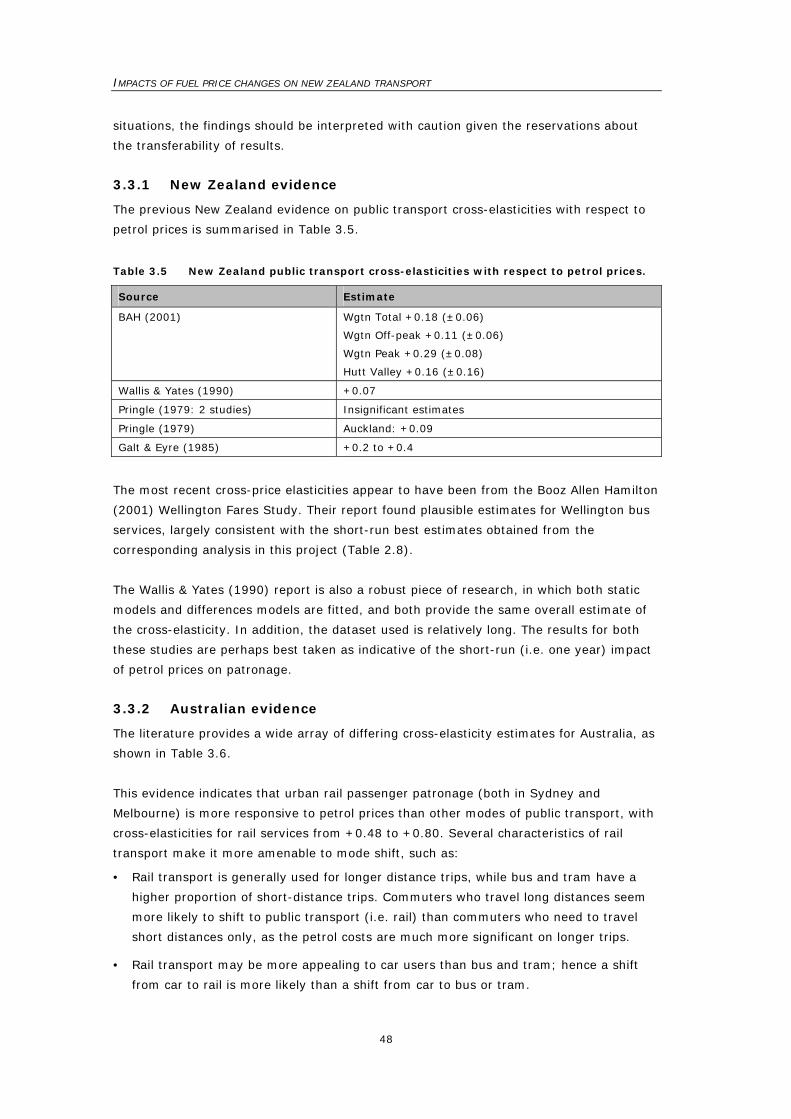
IMPACTS OF FUEL PRICE CHANGES ON NEW ZEALAND TRANSPORT
48
situations, the findings should be interpreted with caution given the reservations about
the transferability of results.
3.3.1 New Zealand evidence
The previous New Zealand evidence on public transport cross-elasticities with respect to
petrol prices is summarised in Table 3.5.
Table 3.5 New Zealand public transport cross-elasticities with respect to petrol prices.
Source Estimate
BAH (2001) Wgtn Total +0.18 (±0.06)
Wgtn Off-peak +0.11 (±0.06)
Wgtn Peak +0.29 (±0.08)
Hutt Valley +0.16 (±0.16)
Wallis & Yates (1990) +0.07
Pringle (1979: 2 studies) Insignificant estimates
Pringle (1979) Auckland: +0.09
Galt & Eyre (1985) +0.2 to +0.4
The most recent cross-price elasticities appear to have been from the Booz Allen Hamilton
(2001) Wellington Fares Study. Their report found plausible estimates for Wellington bus
services, largely consistent with the short-run best estimates obtained from the
corresponding analysis in this project (Table 2.8).
The Wallis & Yates (1990) report is also a robust piece of research, in which both static
models and differences models are fitted, and both provide the same overall estimate of
the cross-elasticity. In addition, the dataset used is relatively long. The results for both
these studies are perhaps best taken as indicative of the short-run (i.e. one year) impact
of petrol prices on patronage.
3.3.2 Australian evidence
The literature provides a wide array of differing cross-elasticity estimates for Australia, as
shown in Table 3.6.
This evidence indicates that urban rail passenger patronage (both in Sydney and
Melbourne) is more responsive to petrol prices than other modes of public transport, with
cross-elasticities for rail services from +0.48 to +0.80. Several characteristics of rail
transport make it more amenable to mode shift, such as:
• Rail transport is generally used for longer distance trips, while bus and tram have a
higher proportion of short-distance trips. Commuters who travel long distances seem
more likely to shift to public transport (i.e. rail) than commuters who need to travel
short distances only, as the petrol costs are much more significant on longer trips.
• Rail transport may be more appealing to car users than bus and tram; hence a shift
from car to rail is more likely than a shift from car to bus or tram.
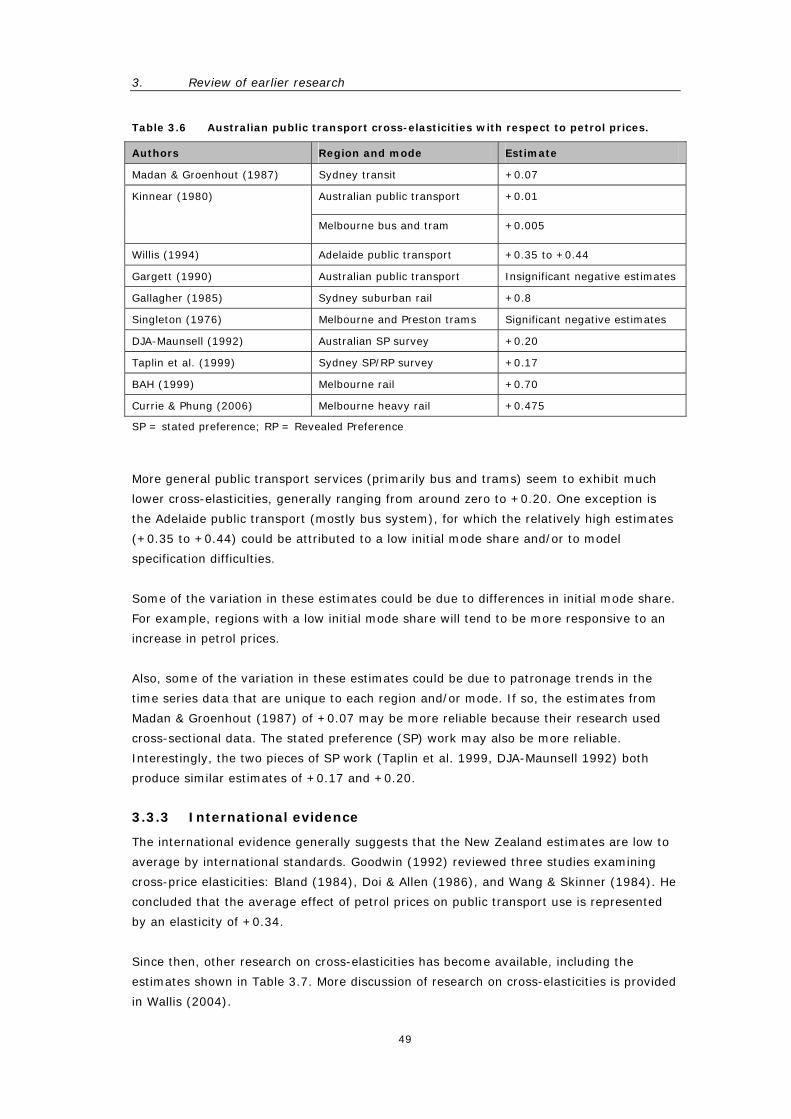
3. Review of earlier research
49
Table 3.6 Australian public transport cross-elasticities with respect to petrol prices.
Authors Region and mode Estimate
Madan & Groenhout (1987) Sydney transit +0.07
Australian public transport +0.01 Kinnear (1980)
Melbourne bus and tram +0.005
Willis (1994) Adelaide public transport +0.35 to +0.44
Gargett (1990) Australian public transport Insignificant negative estimates
Gallagher (1985) Sydney suburban rail +0.8
Singleton (1976) Melbourne and Preston trams Significant negative estimates
DJA-Maunsell (1992) Australian SP survey +0.20
Taplin et al. (1999) Sydney SP/RP survey +0.17
BAH (1999) Melbourne rail +0.70
Currie & Phung (2006) Melbourne heavy rail +0.475
SP = stated preference; RP = Revealed Preference
More general public transport services (primarily bus and trams) seem to exhibit much
lower cross-elasticities, generally ranging from around zero to +0.20. One exception is
the Adelaide public transport (mostly bus system), for which the relatively high estimates
(+0.35 to +0.44) could be attributed to a low initial mode share and/or to model
specification difficulties.
Some of the variation in these estimates could be due to differences in initial mode share.
For example, regions with a low initial mode share will tend to be more responsive to an
increase in petrol prices.
Also, some of the variation in these estimates could be due to patronage trends in the
time series data that are unique to each region and/or mode. If so, the estimates from
Madan & Groenhout (1987) of +0.07 may be more reliable because their research used
cross-sectional data. The stated preference (SP) work may also be more reliable.
Interestingly, the two pieces of SP work (Taplin et al. 1999, DJA-Maunsell 1992) both
produce similar estimates of +0.17 and +0.20.
3.3.3 International evidence
The international evidence generally suggests that the New Zealand estimates are low to
average by international standards. Goodwin (1992) reviewed three studies examining
cross-price elasticities: Bland (1984), Doi & Allen (1986), and Wang & Skinner (1984). He
concluded that the average effect of petrol prices on public transport use is represented
by an elasticity of +0.34.
Since then, other research on cross-elasticities has become available, including the
estimates shown in Table 3.7. More discussion of research on cross-elasticities is provided
in Wallis (2004).
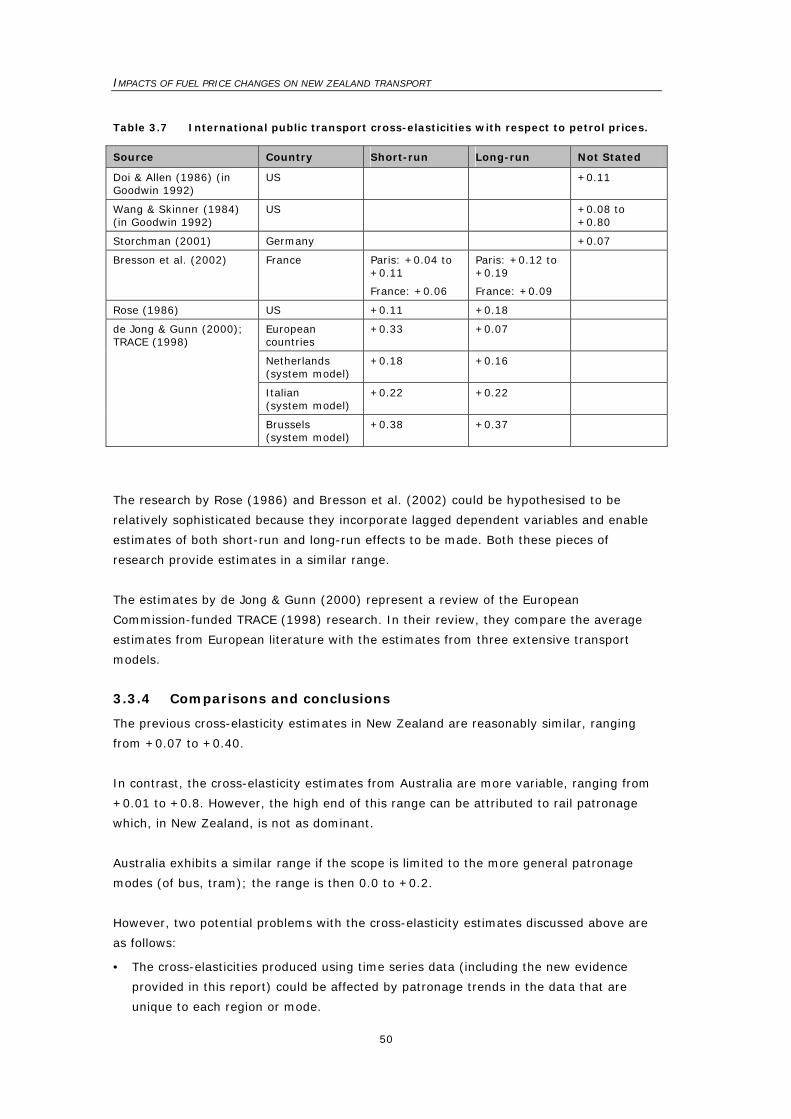
IMPACTS OF FUEL PRICE CHANGES ON NEW ZEALAND TRANSPORT
50
Table 3.7 International public transport cross-elasticities with respect to petrol prices.
Source Country Short-run Long-run Not Stated
Doi & Allen (1986) (in Goodwin 1992)
US +0.11
Wang & Skinner (1984) (in Goodwin 1992)
US +0.08 to +0.80
Storchman (2001) Germany +0.07
Bresson et al. (2002) France Paris: +0.04 to +0.11
France: +0.06
Paris: +0.12 to +0.19
France: +0.09
Rose (1986) US +0.11 +0.18
European countries
+0.33 +0.07
Netherlands (system model)
+0.18 +0.16
Italian (system model)
+0.22 +0.22
de Jong & Gunn (2000); TRACE (1998)
Brussels (system model)
+0.38 +0.37
The research by Rose (1986) and Bresson et al. (2002) could be hypothesised to be
relatively sophisticated because they incorporate lagged dependent variables and enable
estimates of both short-run and long-run effects to be made. Both these pieces of
research provide estimates in a similar range.
The estimates by de Jong & Gunn (2000) represent a review of the European
Commission-funded TRACE (1998) research. In their review, they compare the average
estimates from European literature with the estimates from three extensive transport
models.
3.3.4 Comparisons and conclusions
The previous cross-elasticity estimates in New Zealand are reasonably similar, ranging
from +0.07 to +0.40.
In contrast, the cross-elasticity estimates from Australia are more variable, ranging from
+0.01 to +0.8. However, the high end of this range can be attributed to rail patronage
which, in New Zealand, is not as dominant.
Australia exhibits a similar range if the scope is limited to the more general patronage
modes (of bus, tram); the range is then 0.0 to +0.2.
However, two potential problems with the cross-elasticity estimates discussed above are
as follows:
• The cross-elasticities produced using time series data (including the new evidence
provided in this report) could be affected by patronage trends in the data that are
unique to each region or mode.

3. Review of earlier research
51
To some extent, this problem can be circumvented with examination of estimates
produced using cross-sectional or stated preference studies: these studies suggest
cross-elasticities in the +0.07 to +0.20 range.
• The cross-elasticities estimated for a particular city and mode can not be transferred to
a different situation, especially if the mode shares differ considerably.

IMPACTS OF FUEL PRICE CHANGES ON NEW ZEALAND TRANSPORT
52
4. Conclusions, modelling applications and policy implications
4.1 What conclusions can be drawn?
Table 4.1 draws together and summarises all the evidence presented previously,
providing traffic volume and petrol consumption elasticities from our New Zealand
analyses, previous New Zealand analyses, Australian analyses, and international analyses.
Focusing particularly on the short-run results, our findings are that:
• In terms of traffic volume elasticities, our New Zealand estimates (based on recent
data, 2002-2006) are higher than typical Australian and international values. As noted
in Section 3.2.4, these VKT elasticities appear to be inconsistent with consumption
elasticities, and may only be representative of the impact of petrol prices on state
highway traffic.
• In terms of consumption elasticities, our New Zealand estimates (based on a long-
term data series, 1974-2006) are on the high side of previous New Zealand and
Australian studies, slightly lower than the US/Canadian estimates, and substantially
lower than the European average (but above the UK estimates, at least in the short
run).
Table 4.1 Summary of elasticity evidence.
Elasticity estimates (short-run/long-run)
VKT/Traffic Vol. Consumption Source of results
SR LR SR LR
Notes
This study -0.20 to -0.25
-0.35 -0.15 -0.20+ Traffic figures relate to 2002-06; consumption figures relate to 1974-2006
Other NZ studies -0.1 -0.15
Australian studies -0.1 -0.25 -0.1 -0.15 Some studies indicate much higher LR consumption elasticities
International studies:
US/Canada
UK
Europe average
-0.15
-0.3
-0.2
-0.1
-0.3
-1.0
-0.5
-0.9
Goodwin et al. (2004) stated in their most recent international review that:
The overall picture implied is….if the real price of fuel rises by 10% and stays at
that level, the result is a dynamic process of adjustment such that the following
occur:
(a) Volume of traffic will fall by roundly 1% within about a year, building up to a
reduction of about 3% in the longer run (about 5 years or so).
(b) Volume of fuel consumed will fall by about 2.5% within a year, building up to
a reduction of over 6% in the longer run.
4. Conclusions, modelling applications & policy implications
53
Comparing our study results with this statement suggests that the New Zealand traffic
volume (VKT) effects are greater than these international averaged estimates, but that
the New Zealand consumption effects are rather less than these international estimates.
Our New Zealand results do cast some doubt on the view, quite often expressed, that
New Zealand and Australian elasticities are among the world’s lowest.
One of the most interesting aspects of our New Zealand VKT elasticity results is the
differences between urban peak, urban off-peak and rural responses (and we are not
aware of any other such disaggregated analyses in the international literature). All
indications (Table 2.6) are that the urban peak elasticity (-0.29 medium run) is
substantially lower than the urban off-peak (-0.36) elasticity: this result reflects the less
elastic nature of the commuter market overall, which is not offset by the availability of
more competitive public transport services for many of these trips.
4.2 ‘Best estimates’ for petrol consumption and traffic volume elasticities
Drawing on all the results presented in this report, for future policy analysis purposes we
would suggest that the following elasticity values are the most appropriate for
New Zealand:
• Fuel consumption elasticities:
Overall: short-run -0.15, long-run -0.30.
• VKT elasticities:
Overall: short-run (<1 year) -0.12, long-run (5+ years) -0.24.
These estimates are based particularly on our study results plus previous New Zealand
(and Australian) studies, but attempt to reflect the prevailing international relationships
between VKT and consumption elasticities, and between long-run and short-run
estimates. As is evident from Table 4.1, these recommended values are similar to the
prevailing estimates found in other New Zealand and Australian studies.
The justification for the fuel consumption elasticities is as follows:
• A short-run (0-1 years) elasticity of -0.15 is suggested on the following grounds:
– This is the estimate produced by model A (adjusted for the ‘carless days’ policy,
Section 2.2.6) which we have judged to be the preferred model based on
significance of coefficients and investigation of the residuals (as discussed in
Section 2.2.3 and Appendix C2.9).
– This estimate is consistent with previous New Zealand studies (Section 3.1.1) which
generally found that the short-run elasticity is in the -0.03 to -0.20 range.
• A medium-run (0-2 years) elasticity of -0.20 is recommended because a range of
models fitted for this research produced around this figure after 2 years.
IMPACTS OF FUEL PRICE CHANGES ON NEW ZEALAND TRANSPORT
54
• A long-run elasticity of -0.30 is suggested, based on the following two arguments:
– The international literature generally finds that long-run effect is around 2.5 times
the short-run effect. For example, Goodwin et al. (2004) found that the average
ratio is 2.56. Graham & Glaister (2004) found that the average ratio is 3.1. We
have assumed that the long-run effect is around 2 times the short-run effect
because previous New Zealand studies (see Section 3.1.1) have generally found
lower ratios; also, the research undertaken for this report failed to detect significant
long-run effects beyond two years.
– A long-run elasticity higher than -0.30 would seem unreasonable given that none of
the New Zealand studies found a long-run elasticity above -0.19. Similarly, most
Australian studies estimated a long-run elasticity no higher than -0.22 (with the
sole exception of Donnelly (1984) who used older data and an unexamined
econometric method).
The vehicle traffic elasticities produced by this research appear to provide statistically
robust estimates of the impacts of petrol prices on state highway (largely longer distance)
vehicle traffic for cars and vans. The model used to produce the elasticities seemed
statistically robust and produced plausible estimates. Furthermore, similar estimates were
produced using four separate datasets.
However, the inconsistency (between the vehicle traffic elasticities and the petrol
consumption elasticities) suggest that the vehicle traffic elasticities represent the impact
of petrol prices on state highway VKT but not on total national VKT.
The resolution to this inconsistency, as proposed until further information is obtained, is
to discount the petrol consumption elasticities produced by this research to produce
estimates for total VKT elasticities:
• A short-run (0-1 years) VKT elasticity of -0.12;
• A medium-run (0-2 years) VKT elasticity of -0.15;
• A long-run VKT elasticity of -0.20.
These suggested values are acknowledged to be somewhat subjective, and are drawn
from petrol consumption elasticities and hypotheses of household responses over time to
petrol price changes.
The suggested short-run and medium-run values are based on the petrol consumption
elasticities, which have been judged to be relatively good estimates:
• The short-run VKT elasticity of -0.12 is slightly less than the petrol consumption
elasticity of -0.14, representing a presumption that the main response to petrol prices
is reduced VKT by households.

4. Conclusions, modelling applications & policy implications
55
• The medium-run VKT elasticity of -0.15 is less than the petrol consumption elasticity of
-0.20, with a greater difference between the VKT response and the consumption
response because households may respond in the medium run with more efficient
driving patterns.
The suggested long-run values are based on an assumed ratio between short-run and
long-run VKT elasticities of around +1.7. In addition, the difference between the VKT
response and the consumption response becomes greater in the long run, consistent with
the purchase of more fuel-efficient vehicles in the long run.
4.3 ‘Best estimates’ for public transport cross-elasticities
For reasons discussed in previous sections, we would not recommend any specific set of
values for public transport cross-elasticities for New Zealand conditions.
The weight of evidence (from this and other studies) indicates that:
• Typical New Zealand values, largely based on Wellington evidence, average around 0.1
to 0.2.
• The limited evidence (from New Zealand and elsewhere) is that peak cross-elasticities
are in the order of 2 to 3 times off-peak elasticities.
• The evidence (from Australian and international sources) suggests that elasticities are
significantly higher than average for longer distance urban trips, especially by rail, and
lower than average for shorter distance, largely bus, trips.
4.4 Further conclusions
The elasticities presented in this report can potentially be incorporated into models that
forecast petrol consumption or light vehicle highway traffic trends. The distinction
between short-run and interim petrol-price elasticities enables estimation of the dynamic
impacts of petrol price changes. The short-run elasticity (-0.15) is used to estimate the
impact over the first year, and the interim elasticity (-0.05) is used to estimate the
residual effect over the following year.
For example, the simple model below (Table 4.2) illustrates how the impacts of petrol
prices (and other variables) on petrol consumption can be forecast using estimates from
the revised Model A (with a ‘carless days’ dummy) in Section 2.2.6. (Note that the
hypothetical example in Table 4.2 is only intended for illustrative purposes.)
Note that the ‘best estimates’ recommended in this report are influenced by the estimates
produced by New Zealand and international research. As uncertainty surrounds these
estimates, sensitivity analysis should be employed in forecasting models to take into
account that uncertainty.

IMPACTS OF FUEL PRICE CHANGES ON NEW ZEALAND TRANSPORT
56
Table 4.2 Hypothetical example – Forecasting 2011 petrol consumption based on observed and forecast changes in explanatory variables, using ‘carless days’ dummy.
Explanatory variables Change
Real petrol price Real GDP Population
Forecast impact on petrol consumption for 2011
Observed change in petrol price in 2010
+10%
Forecasts of changes in explanatory variables in 2011
-20% +3% +2%
Elasticity estimates from Model A in S2.2.6
-0.15 -0.05 +0.39 +1.00
-0.05 x (+10%) + -0.15 x (-20%) + +0.39 x (+3%) + 2% = 6%
The findings of this research may also be of interest to policy makers interested in
understanding the impacts of oil shocks, excise taxes or carbon charges. Key findings
include the following:
• Petrol prices have a discernible impact on petrol consumption. The short-run and
medium-run elasticities are statistically significant.
• Petrol prices appear to have quite a rapid effect on petrol consumption. A strong
impact occurs within a year of a price change, with further impacts diminishing rapidly
for the following year. Any further impacts of petrol price changes become
indiscernible after two years.
• The estimated short-run petrol price elasticities seem surprisingly stable throughout
time. Both the 1978-2006 quarterly data and the 1999-2006 monthly data provided
similar short-run estimates: -0.14 v -0.15. In addition, some preliminary variations on
the model (see Appendix C2.9) suggested that there is no systematic tendency for the
short-run petrol price elasticity to increase or decrease over time.
• Petrol prices also have a discernible impact on vehicle traffic, especially highway
traffic. The highway traffic counts appeared to be particularly responsive to petrol
prices.
• GDP per capita does not appear to have as much influence on petrol consumption as
petrol prices (when one takes into account the low variability of GDP growth compared
to petrol price volatility). However, the positive coefficient suggests that petrol
consumption will continue to grow unless petrol prices are increasing.
• The impacts of petrol prices on public transport patronage appear to be relatively less
predictable. This may be because people’s decisions about public transport are not
deterministic: people do not make decisions about public transport in a predictable
manner which can be ‘linearly related’ to petrol prices.
4. Conclusions, modelling applications & policy implications
57
4.5 Applications for modelling
4.5.1 Applications to petrol consumption forecasting models
The petrol price elasticity estimates produced by this report can be incorporated into
petrol consumption forecasting models. To do this, a 1% increase in petrol price is
assumed to have the following impacts on petrol consumption per capita:
• petrol consumption will fall by 0.15% within a year;
• petrol consumption will fall by a further 0.05% the next year;
• petrol consumption will fall by 0.15% over the remaining years (e.g. 0.0115% each
year for 13 years).
The figures provided above illustrate the merits of the ’dynamic’ petrol price elasticities
produced by this report. These ‘dynamic’ elasticities show the manner in which petrol
prices feed through into consumption, in addition to the overall effect.
Such petrol consumption forecasting models would have a range of applications for policy
analysts/advisers who:
• may be looking at carbon charges or fuel excise charges, and who want to understand
the impact of such policies on petrol consumption;
• may want to explore scenarios in which petrol prices rise due to external factors
(e.g. Middle East conflicts, ‘peak oil’ effects on oil prices);
• may want to carry out sensitivity analysis to look at the impacts of a range of different
price paths for petrol prices.
The petrol consumption forecasting models described above could also incorporate GDP
elasticity estimates. Our econometric research indicates that a 1% increase in GDP per
capita increases petrol consumption per capita by 0.32%.
4.5.2 Applications to traffic forecasting models
In a similar manner to the process described in Section 4.5.1, the highway traffic
elasticity estimates presented in Table 2.6 of this report can be incorporated into traffic
forecasting models. To do this, a 1% petrol price increase is assumed to have the
following impacts on total highway traffic per capita:
• Car and van traffic will fall by 0.22% within a year;
• Car and van traffic will fall by 0.08% the next year.
Similar assumptions could be used to develop specific forecasting models for subsets of
traffic (rural, urban off-peak and urban peak).
These forecasting models could be used by road controlling authorities when estimating
future traffic flows (and associated travel time benefits) for roading projects:
IMPACTS OF FUEL PRICE CHANGES ON NEW ZEALAND TRANSPORT
58
• The forecasting models could be fed known or expected changes in petrol prices
(e.g. anticipated carbon charges).
• The forecasting models could be used to carry out sensitivity analysis for which a
range of price paths for petrol could be explored, in order to reflect uncertainties
around the potential ‘peak oil’ effect.
4.5.3 Applications to fiscal planning
The petrol elasticities produced by this report could also be incorporated into the
Treasury’s fiscal planning processes, e.g. projecting New Zealand’s financial obligations
under the first commitment of the Kyoto Protocol, and understanding the revenue
implications of a carbon charge or an increase in excise tax.
The petrol elasticities produced by this report can be used to estimate the impact of such
measures on petrol consumption, and hence revenues from such revenues.
Therefore, New Zealand Treasury may wish to understand the financial implications of a
range of possible price paths for petrol prices.
4.6 Implications for policy making
4.6.1 Implications for public transport operators and funding agencies
The preliminary econometric analysis of patronage data for public transport in this report
has identified challenges that will need to be addressed in any future econometric analysis
of patronage data:
• The analysis shows that relationships between petrol prices and public transport use
are not as straightforward as those shown in petrol consumption and traffic. Therefore,
future analysis will need to:
– explore a wide range of models; and
– explore a wide range of interrelationships between petrol prices and patronage
(e.g. very short-run, short-run, medium run and long-run).
• The analysis shows considerable ‘noise’ in the data, because of the omission of
variables that can have a big impact on patronage growth. This noise makes it difficult
for researchers to estimate robust statistical relationships. Therefore, future analysis
will need to adjust for this ‘noise’ and/or develop econometric methods that
accommodate such influences.
4.6.2 Implications for climate change and energy policies
As discussed above in Section 4.5.1, Applications to petrol consumption forecasting
models, the petrol price elasticities can be incorporated into forecasting models. These
models can also be used to explore the impacts of climate change measures and energy
policies, such as a carbon charge.
4. Conclusions, modelling applications & policy implications
59
However, the research outputs from this report provides information of interest to climate
change and energy policy-makers such as:
• Price measures that increase the price of petrol (e.g. carbon charges, emissions
trading) would appear to be effective tools for reducing greenhouse gas emissions
from the transport sector. All the econometric models that we estimated showed that
the impact of petrol prices was statistically significant.
• The response to such price measures would generally be quite rapid. This could have
implications for climate change policy:
– About half of the impact of petrol prices will feed through into petrol consumption
within a year;
– About two thirds of the impact of petrol prices will feed through into petrol
consumption within two years.
• The response of petrol consumption to petrol prices changes is surprisingly stable
throughout time. Therefore, price measures will always remain an effective policy tool.
• GDP per capita has a positive impact on petrol consumption. Therefore, petrol
consumption will continue to grow unless cancelled out by other drivers such as rising
petrol prices.
4.6.3 Implications for road infrastructure investment
The traffic elasticities indicated that state highway traffic was responsive to petrol prices
in that a 1% increase in petrol prices causes about a 0.3% (or more) reduction in car and
van traffic. This could have implications for road controlling authorities’ assessment of
road projects given the possibility of rising petrol prices in the future.
The report also conjectures that rising petrol prices may have a stronger impact on state
highway traffic than on local road traffic, but acknowledges that more evidence would be
required to confirm if this is the case or not.
4.7 Further research directions
The datasets assembled for our study potentially offer the opportunity for further
statistical analysis which are listed here, and are further to those analysed for this report:
• Diesel consumption elasticities could be estimated, using similar econometric methods
to those already undertaken for petrol.
• Diesel vehicle traffic elasticities could also be estimated, again using similar
econometric methods. However, in this case more data are available which will enable
the estimation of the impact of diesel prices on both heavy vehicle traffic counts and
total kilometres travelled (VKT) (and consequent comparison of the two estimates).
The impact of Road User Charges (RUCs) on traffic counts and kilometres driven could
also be explored. For this analysis the following steps would need to be taken:
IMPACTS OF FUEL PRICE CHANGES ON NEW ZEALAND TRANSPORT
60
– Elasticities for heavy vehicle traffic on state highways could be estimated using
vehicle count data collected from Transit NZ.
– This traffic count dataset could be cleaned to adjust for missing observations.
– This traffic count dataset divides vehicles into four length classes, but to date
(2007) only the shortest length class (<5 m, largely cars and light vans) has been
used to estimate VKT elasticities with respect to petrol price. Diesel-price elasticities
could be derived for longer length classes (>5.5 m) (and this is another aspect for
which very few elasticity estimates are available internationally).
– Elasticities for total kilometres driven could be estimated using a detailed series of
kilometres-driven data available from 1995 onwards.
• The petrol elasticity models used for this research assume that percentage changes in
petrol consumption (and VKT) are linearly related to percentage changes in petrol
prices. However, during this research, evidence showed that percentage changes in
petrol consumption may be linearly related to absolute changes in petrol prices.
• Potentially the two approaches could be compared and assessed on a range of criteria,
including statistical ‘goodness of fit’ tests and also their performance at forecasting.
• The public transport patronage models employed for this project could be re-estimated
in the future using longer time series. In addition to providing more observations, the
longer time series would allow us to exploit the ‘natural experiment’ created by the
recent rise and fall in petrol prices. Further research would also enable development of
a greater range of econometric models and approaches (potentially including
cointegration models and ARIMA models) and would address the econometric ‘noise’
issues identified in this report.
• A more exploratory area of research concerns the impacts of price expectations. The
research commissioned for this report and virtually all the international research
focuses on the impacts of price changes. However, we conjecture that changes in price
expectations may play a role, in addition to actual price changes. Therefore,
econometric methods could be developed that simulate price expectation behaviour
and attempt to explain the impacts of price expectations on transport behaviour
(including long-run behavioural responses such as vehicle choice).

61
Appendices
A Price elasticity concepts
A1 Price elasticity of demand
A2 Cross-price elasticity of demand
A3 Long-run and short-run responses
B Econometric analysis methods
C Econometric analysis details
C1 Summary of modelling approach
C2 Consumption elasticities
C3 Traffic volume elasticities
D Review of previous research
D1 Petrol consumption elasticities
D2 Traffic volume elasticities
D3 Public transport cross-elasticities
E References

IMPACTS OF FUEL PRICE CHANGES ON NEW ZEALAND TRANSPORT
62
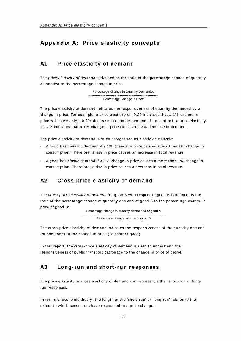
Appendix A: Price elasticity concepts
63
Appendix A: Price elasticity concepts
A1 Price elasticity of demand
The price elasticity of demand is defined as the ratio of the percentage change of quantity
demanded to the percentage change in price:
Percentage Change in Quantity Demanded -----------------------------------------------------------------
Percentage Change in Price
The price elasticity of demand indicates the responsiveness of quantity demanded by a
change in price. For example, a price elasticity of -0.20 indicates that a 1% change in
price will cause only a 0.2% decrease in quantity demanded. In contrast, a price elasticity
of -2.3 indicates that a 1% change in price causes a 2.3% decrease in demand.
The price elasticity of demand is often categorised as elastic or inelastic:
• A good has inelastic demand if a 1% change in price causes a less than 1% change in
consumption. Therefore, a rise in price causes an increase in total revenue.
• A good has elastic demand if a 1% change in price causes a more than 1% change in
consumption. Therefore, a rise in price causes a decrease in total revenue.
A2 Cross-price elasticity of demand
The cross-price elasticity of demand for good A with respect to good B is defined as the
ratio of the percentage change of quantity demand of good A to the percentage change in
price of good B: Percentage change in quantity demanded of good A
------------------------------------------------------------------------------ Percentage change in price of good B
The cross-price elasticity of demand indicates the responsiveness of the quantity demand
(of one good) to the change in price (of another good).
In this report, the cross-price elasticity of demand is used to understand the
responsiveness of public transport patronage to the change in price of petrol.
A3 Long-run and short-run responses
The price elasticity or cross elasticity of demand can represent either short-run or long-
run responses.
In terms of economic theory, the length of the ‘short-run’ or ‘long-run’ relates to the
extent to which consumers have responded to a price change:

IMPACTS OF FUEL PRICE CHANGES ON NEW ZEALAND TRANSPORT
64
• The short-run price elasticity of demand represents the impact of a price change
before consumers have adjusted completely to a price change.
• The long-run price elasticity of demand represents the complete impact of a price
change.
However, some econometric models (namely partial adjustment models) enable the
estimation of the impact of a price change on consumption within a year: therefore, this
one-year price elasticity is conveniently described as the ‘short-run’ price elasticity.
These models also estimate the indefinite impact of a price change, and this is consistent
with a ‘long-run’ price elasticity described in economic theory.
Appendix B: Econometric analysis methods
65
Appendix B: Econometric analysis methods
Table B.1, on page 66, summarises:
• Econometric model forms commonly used in the transport literature in studies such as
this present study (in which some of these models were used); and
• Other models applied in this study which are not commonly found in the transport
literature.
Key to symbols:
C consumption
P petrol price
O output
LR long run
SR short run
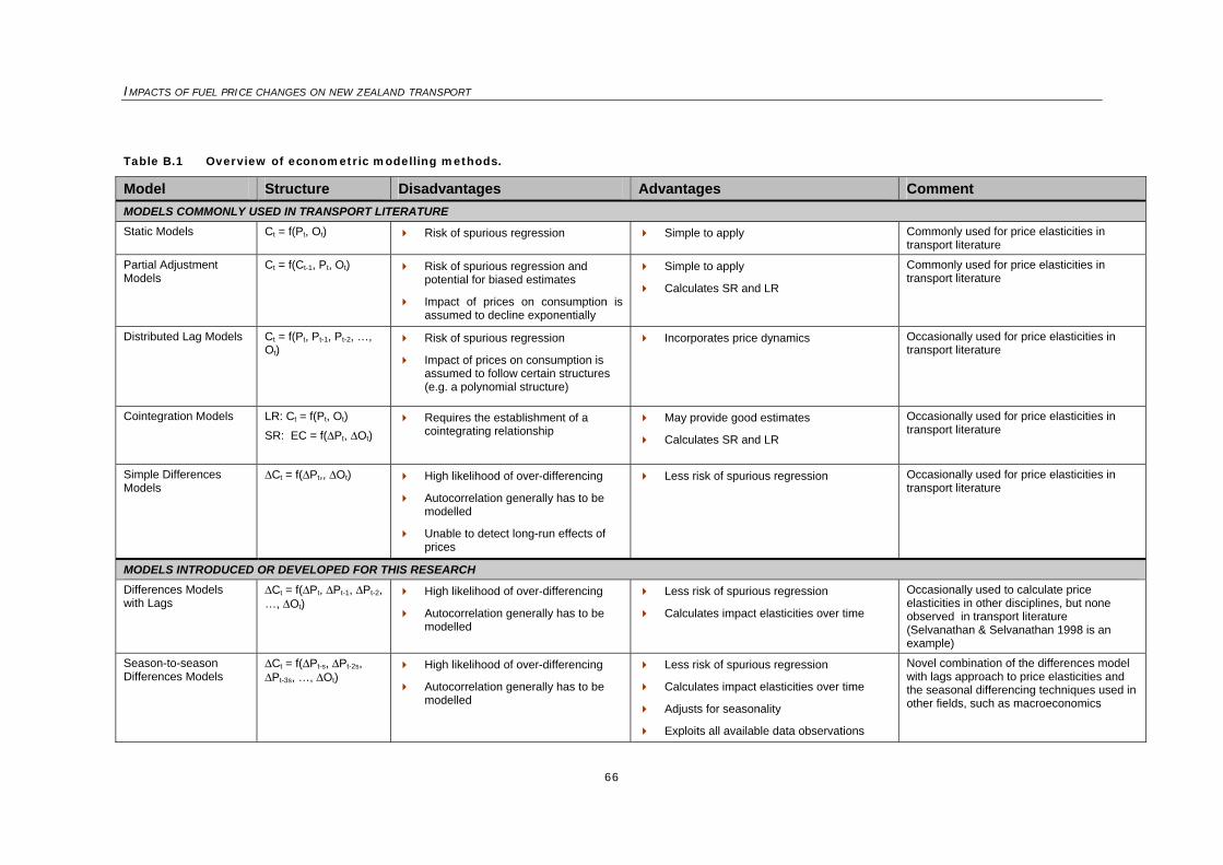
IMPACTS OF FUEL PRICE CHANGES ON NEW ZEALAND TRANSPORT
66
Table B.1 Overview of econometric modelling methods.
Model Structure Disadvantages Advantages Comment MODELS COMMONLY USED IN TRANSPORT LITERATURE Static Models Ct = f(Pt, Ot) Risk of spurious regression Simple to apply Commonly used for price elasticities in
transport literature
Partial Adjustment Models
Ct = f(Ct-1, Pt, Ot) Risk of spurious regression and potential for biased estimates
Impact of prices on consumption is assumed to decline exponentially
Simple to apply
Calculates SR and LR
Commonly used for price elasticities in transport literature
Distributed Lag Models Ct = f(Pt, Pt-1, Pt-2, …, Ot)
Risk of spurious regression
Impact of prices on consumption is assumed to follow certain structures (e.g. a polynomial structure)
Incorporates price dynamics Occasionally used for price elasticities in transport literature
Cointegration Models
LR: Ct = f(Pt, Ot) SR: EC = f(∆Pt, ∆Ot)
Requires the establishment of a cointegrating relationship
May provide good estimates
Calculates SR and LR
Occasionally used for price elasticities in transport literature
Simple Differences Models
∆Ct = f(∆Pt,, ∆Ot) High likelihood of over-differencing
Autocorrelation generally has to be modelled
Unable to detect long-run effects of prices
Less risk of spurious regression Occasionally used for price elasticities in transport literature
MODELS INTRODUCED OR DEVELOPED FOR THIS RESEARCH Differences Models with Lags
∆Ct = f(∆Pt, ∆Pt-1, ∆Pt-2, …, ∆Ot)
High likelihood of over-differencing
Autocorrelation generally has to be modelled
Less risk of spurious regression
Calculates impact elasticities over time
Occasionally used to calculate price elasticities in other disciplines, but none observed in transport literature (Selvanathan & Selvanathan 1998 is an example)
Season-to-season Differences Models
∆Ct = f(∆Pt-s, ∆Pt-2s, ∆Pt-3s, …, ∆Ot)
High likelihood of over-differencing
Autocorrelation generally has to be modelled
Less risk of spurious regression
Calculates impact elasticities over time
Adjusts for seasonality
Exploits all available data observations
Novel combination of the differences model with lags approach to price elasticities and the seasonal differencing techniques used in other fields, such as macroeconomics
Appendix C: Econometric analysis details
67
Appendix C: Econometric analysis details
C1 Summary of modelling approach
C1.1 Issues with non-stationarity and spurious regressions
The modelling approaches adopted for this research were designed, in part, to mitigate
possible risks with regressions involving non-stationary variables. In essence, a variable is
non-stationary if the series has no tendency to revert to a constant mean.
Regressions involving non-stationary variables could be problematic. In a seminal
econometrics paper, Granger & Newbold (1974) showed that a regression involving non-
stationary variables can lead to a spurious regression, in which two completely unrelated
variables can appear to have a precisely estimated relationship even if no such
relationship exists in reality. Phillips (1986) later built on the work of Granger & Newbold,
providing theoretical explanation for their findings.
As noted by Verbeek (2000), the problem is, in essence, that non-stationarity in the
original variables can feed through into non-stationarity in the error term being modelled.
If this happens then the regression could be spurious. Statistical theory does not provide
much guidance about the level of faith to have in regressions involving non-stationarity
error terms. The studies referred to above suggest that the estimates could be
inconsistent and the statistical tests could be invalid. On the other hand, the regression
may be detecting a genuine relationship (and it appears to do so in a number of studies).
C1.2 Approaches to mitigate the risk of spurious regressions
This report acknowledges that regressions involving non-stationary variables are
commonly carried out. Furthermore, these regressions have been shown to often produce
plausible and useful estimates.
However, in light of the uncertainty identified by the econometric literature above, we
decided to use primarily differenced models.8 Differenced models generally make the
dependent variable and the explanatory variables stationary, and hence the error term
being modelled is usually stationary. This solution was recommended by Granger &
Newbold (1974) when they first drew attention to the risk of spurious regressions. They
noted that even differencing is not guaranteed to prevent a spurious regression.
Therefore, we also used an augmented Dickey-Fuller test to test for stationarity in the
8 A number of other benefits are associated with difference models. These advantages include:
- Difference models relate changes in petrol consumption to changes in explanatory variables: this relationship corresponds intuitively to the concept of an elasticity.
- Differencing generally reduces multicollinearity.
- Lags can be explored, without assuming that the explanatory variables have a specific effect on the dependent variable.

IMPACTS OF FUEL PRICE CHANGES ON NEW ZEALAND TRANSPORT
68
error term. If stationarity in the error term can be established then a spurious regression
is unlikely.9
C1.3 Other diagnostic analyses
The models were checked for normality of residuals and for constant variance throughout
time. This is useful for checking the validity of the estimation method, but it is also useful
as a means of checking for model mis-specification.
The models were checked for autocorrelation, using autocorrelation function (ACF) graphs
and partial autocorrelation function (PACF) graphs.
C1.4 Generalised least squares
Any autocorrelation was adjusted for using generalised least squares (GLS). To do this, an
error structure had to be assumed. A range of error structures were explored and the
error structures chosen for modelling were selected based on effectiveness at removing
autocorrelation (as indicated by ACF and PACF graphs). All the final models were fitted
using either an MA(5), MA(4), MA(1) or AR(4) error structure.
C1.5 Interpretation of season-to-season annual differences modelling approach
As noted in Section 2.1.1 of the main report, the econometric modelling implemented
here draws considerably on the approach we referred to as season-to-season annual
differences. This approach is used for consumption models A, B and D, all the traffic
models and all the public transport patronage models.
This modelling approach, in effect, generally assumes that the percentage change in the
dependent variable (e.g. petrol consumption per capita, traffic count per capita) over a
four-quarter period (or a 52-week period) is a linear function of the following:
1. The percentage change in petrol prices over that same four-quarter (or 52-week)
period;
2. The percentage change in petrol prices over the preceding four-quarter (or 52-week)
period;
3. The percentage change in GDP per capita over that same four-quarter (or 52-week)
period;
4. Any residual influences on the change in the dependent variable: these influences are
assumed to be normally distributed and independent of the other explanatory
variables.
The coefficient of the first variable has been interpreted as a short-run petrol price
elasticity: it shows how petrol price changes over a year relate to changes in the
dependent variable over that same year.
9 In addition, this approach negated any need to use augmented Dickey-Fuller tests to check that
the dependent and explanatory variables are stationary.
Appendix C: Econometric analysis details
69
The coefficient of the second variable has been interpreted as an interim-run petrol price
elasticity because it uses a lagged explanatory variable: it shows how petrol price
changes over a year relate to changes in the dependent variable over the next year. (The
coefficient of the third variable is interpreted in a similar manner.)
In this report, these two coefficients have been added together to produce a medium-run
petrol price elasticity: this elasticity shows how petrol price changes over a year relate to
changes in the dependent variable over both the same year and next year.
The method for calculating of the standard errors for the medium-run petrol price
elasticity had to be developed during the course of the research. The variance of this new
variable was calculated as a function of the variances and covariances of the two other
coefficients, using standard statistical variance rules.
C1.6 Modelling issues with price changes of differing rapidity
Consider the following limitation of the model above: a gradual change in petrol prices
over a whole four-quarter (or 52-week) period will be treated the same as a rapid
increase in petrol prices at the end of the period. A referee pointed out that, in reality,
households may react differently to a rapid increase in petrol prices: for example, the
dramatic nature of the price rise may prompt them to change behaviour; alternatively,
the rapidity of the price chance may cause them to dismiss the price change as being
temporary.
This problem is not unique to the model structure described above, and most price
elasticity models give little regard to the speed at which petrol prices change. To address
this, models could be developed that take into account the variance of petrol price
changes during a given period: thus if the price changes rapidly then the variance of price
changes would generally be higher. Or quarterly-differences models (such as consumption
model E) could be used: these models allow researchers to examine price changes over
smaller intervals, and could be modified to allow large changes in petrol prices to have
disproportionately larger impacts on the dependent variable. However, the authors note
that the coefficients produced by consumption model E were not generally statistically
significant, so this approach may not be successful.
This research has not attempted to incorporate the rapidity of price changes into the
modelling approach, but the authors acknowledge that the referee has raised an
interesting issue.
C1.7 Econometric software
The econometric models were all fitted using R software, which is described in
R Development Core Team (2006).
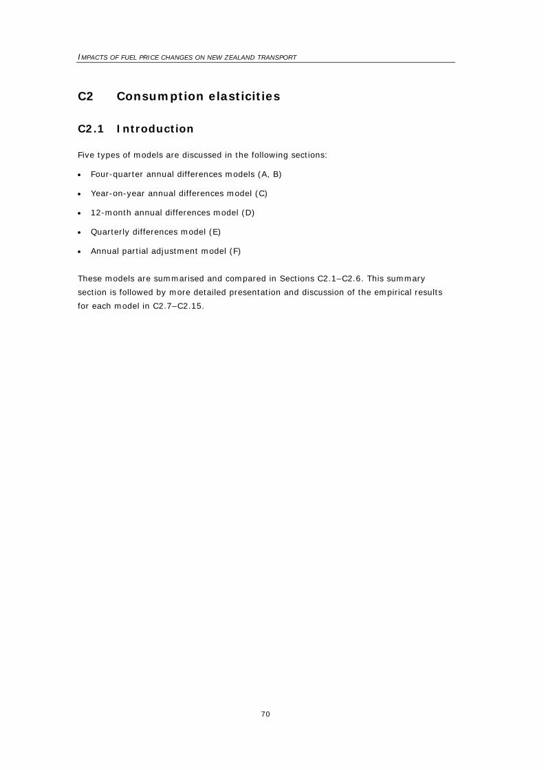
IMPACTS OF FUEL PRICE CHANGES ON NEW ZEALAND TRANSPORT
70
C2 Consumption elasticities
C2.1 Introduction
Five types of models are discussed in the following sections:
• Four-quarter annual differences models (A, B)
• Year-on-year annual differences model (C)
• 12-month annual differences model (D)
• Quarterly differences model (E)
• Annual partial adjustment model (F)
These models are summarised and compared in Sections C2.1–C2.6. This summary
section is followed by more detailed presentation and discussion of the empirical results
for each model in C2.7–C2.15.
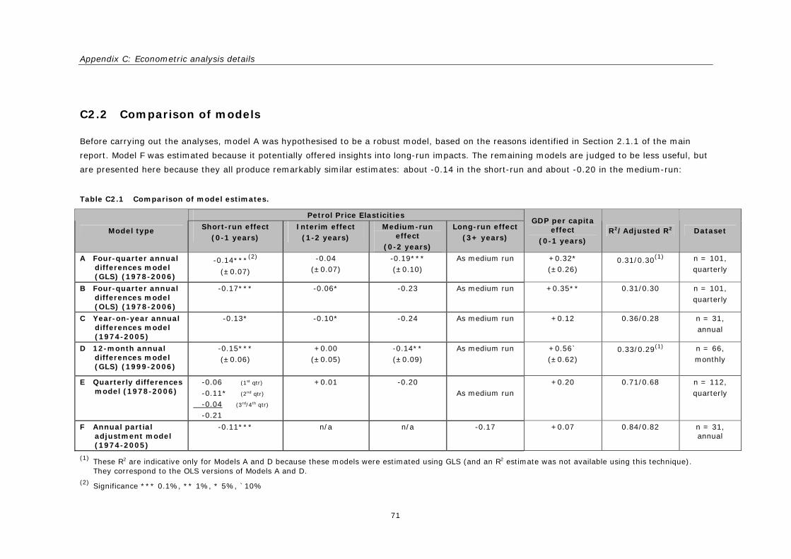
Appendix C: Econometric analysis details
71
C2.2 Comparison of models
Before carrying out the analyses, model A was hypothesised to be a robust model, based on the reasons identified in Section 2.1.1 of the main
report. Model F was estimated because it potentially offered insights into long-run impacts. The remaining models are judged to be less useful, but
are presented here because they all produce remarkably similar estimates: about -0.14 in the short-run and about -0.20 in the medium-run:
Table C2.1 Comparison of model estimates.
Petrol Price Elasticities
Model type Short-run effect (0-1 years)
Interim effect (1-2 years)
Medium-run effect
(0-2 years)
Long-run effect (3+ years)
GDP per capita effect
(0-1 years) R2/Adjusted R2 Dataset
A Four-quarter annual differences model (GLS) (1978-2006)
-0.14***(2)
(±0.07)
-0.04 (±0.07)
-0.19*** (±0.10)
As medium run +0.32* (±0.26)
0.31/0.30(1) n = 101, quarterly
B Four-quarter annual differences model (OLS) (1978-2006)
-0.17*** -0.06* -0.23 As medium run +0.35** 0.31/0.30 n = 101, quarterly
C Year-on-year annual differences model (1974-2005)
-0.13* -0.10* -0.24 As medium run +0.12 0.36/0.28 n = 31, annual
D 12-month annual differences model (GLS) (1999-2006)
-0.15*** (±0.06)
+0.00 (±0.05)
-0.14** (±0.09)
As medium run +0.56` (±0.62)
0.33/0.29(1) n = 66, monthly
E Quarterly differences model (1978-2006)
-0.06 (1st qtr) -0.11* (2nd qtr) -0.04 (3rd/4th qtr) -0.21
+0.01 -0.20 As medium run
+0.20 0.71/0.68 n = 112, quarterly
F Annual partial adjustment model (1974-2005)
-0.11*** n/a n/a -0.17 +0.07 0.84/0.82 n = 31, annual
(1) These R2 are indicative only for Models A and D because these models were estimated using GLS (and an R2 estimate was not available using this technique). They correspond to the OLS versions of Models A and D.
(2) Significance *** 0.1%, ** 1%, * 5%, `10%
IMPACTS OF FUEL PRICE CHANGES ON NEW ZEALAND TRANSPORT
72
C2.3 Criteria for final model selection
The main criteria for final model selection were:
• Statistical validity of residuals
– Is there an expectation and/or evidence of stationarity in the residuals?
– Are the residuals generally normally distributed?
– Is there non-constant variance in the residuals?
– Is there any evidence of autocorrelation in the residuals?
• Plausibility of coefficients
– Are the results plausible and intuitive?
• Statistical power enabled by the sample
– How large is the sample size available for this model?
– How much variability is there in the period that the sample covers?
Because of the wide range of criteria considered, some judgement is required in weighing
up the relative importance of the criteria described above.
C2.4 Preferred model: Model A
Before the analyses were carried out, Model A was assumed to be the ‘centrepiece’ of the
research, because it was expected to produce robust and accurate estimates, for the
reasons identified in Section 2.1.1. (Model F was also hypothesised to be potentially
useful, but its usefulness depended on the extent to which stationarity in the error term
could be established.)
Indeed, Model A did exhibit several favourable characteristics:
• Significant coefficients – Both the short-run petrol price elasticity and the short-run
GDP per capita elasticity are statistically significant at 0.1% significance.
• Plausible coefficients – The petrol price elasticity estimates follow a plausible pattern:
the short-run impact is -0.14 and this falls to -0.04, and become close to zero
thereafter. The GDP per capita coefficient is positive, as would be expected. The
intercept term is insignificant and close to zero, suggesting that the model, albeit
simple, explains trends reasonably well.
• Stationarity in the error term – The process of differencing appears to have succeeded
in causing stationarity in the error term: the hypothesis of stationarity in the error
term was accepted at 1% significance, using an Augmented Dickey-Fuller test.
• Favourable Residual analysis – The ACF and PACF graphs indicate that the GLS
estimation procedure has removed any major autocorrelation in the residuals. The
residuals are distributed in a manner that is consistent with normality.
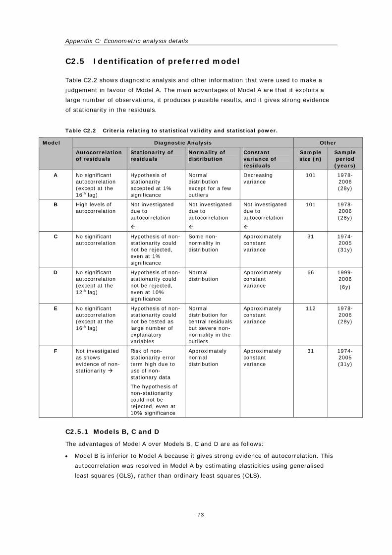
Appendix C: Econometric analysis details
73
C2.5 Identification of preferred model
Table C2.2 shows diagnostic analysis and other information that were used to make a
judgement in favour of Model A. The main advantages of Model A are that it exploits a
large number of observations, it produces plausible results, and it gives strong evidence
of stationarity in the residuals.
Table C2.2 Criteria relating to statistical validity and statistical power.
Diagnostic Analysis Other Model
Autocorrelation of residuals
Stationarity of residuals
Normality of distribution
Constant variance of residuals
Sample size (n)
Sample period (years)
A No significant autocorrelation (except at the 16th lag)
Hypothesis of stationarity accepted at 1% significance
Normal distribution except for a few outliers
Decreasing variance
101 1978-2006 (28y)
B High levels of autocorrelation
Not investigated due to autocorrelation
Not investigated due to autocorrelation
Not investigated due to autocorrelation
101 1978-2006 (28y)
C No significant autocorrelation
Hypothesis of non-stationarity could not be rejected, even at 1% significance
Some non-normality in distribution
Approximately constant variance
31 1974-2005 (31y)
D No significant autocorrelation (except at the 12th lag)
Hypothesis of non-stationarity could not be rejected, even at 10% significance
Normal distribution
Approximately constant variance
66 1999-2006
(6y)
E No significant autocorrelation (except at the 16th lag)
Hypothesis of non-stationarity could not be tested as large number of explanatory variables
Normal distribution for central residuals but severe non-normality in the outliers
Approximately constant variance
112 1978-2006 (28y)
F Not investigated as shows evidence of non-stationarity
Risk of non-stationarity error term high due to use of non-stationary data
The hypothesis of non-stationarity could not be rejected, even at 10% significance
Approximately normal distribution
Approximately constant variance
31 1974-2005 (31y)
C2.5.1 Models B, C and D
The advantages of Model A over Models B, C and D are as follows:
• Model B is inferior to Model A because it gives strong evidence of autocorrelation. This
autocorrelation was resolved in Model A by estimating elasticities using generalised
least squares (GLS), rather than ordinary least squares (OLS).
IMPACTS OF FUEL PRICE CHANGES ON NEW ZEALAND TRANSPORT
74
• Model C is inferior to Model A because it has considerably fewer observations (31
v 101). This may have contributed to the relatively low level of significances and the
less plausible distribution between the short-run effect and the interim effect.
• Model D is inferior to Model A because it has fewer observations (66 v 101) and covers
a shorter time period (6 years). However (somewhat surprisingly) Model D produced
remarkably similar results in terms of coefficients, confidence intervals and the R2. This
similarity is comforting, especially since Model D uses a much smaller time period and
monthly data, rather than quarterly data.
C2.5.2 Model E
Model E is not really comparable with Model A because it uses a different dependent
variable. Model E was estimated because it potentially offered insights how quarterly
changes in petrol prices affect quarterly changes in petrol consumption (whereas Model A
looks only at the response of petrol consumption over a year). Model E produces plausible
quarterly dynamics: if petrol prices increase by 1% in one quarter then petrol
consumption falls by 0.06% in the same quarter, and then 0.11% in the next quarter.
However the impacts of petrol prices tail off in following quarters.
Model E provides a useful insight into quarterly dynamics but it does not seem as useful
as a substitute for the longer-term elasticity estimates provided by Model A. The model
has a high R2 but this is caused primarily by the contribution of highly significant seasonal
dummies. Only one of the price elasticity coefficients is statistically significant. This could
be due to the lack of parsimony (i.e. ability to explain behaviour with as simple a model
as possible) as the model uses eight explanatory variables). Or it could be that quarterly
changes in petrol consumption are less strongly related to petrol price changes than
annual changes in petrol consumption.
C2.5.3 Model F
Model F was estimated because it is commonly used elsewhere in the transport literature
and it potentially offered insights into long-run impacts of petrol prices.
However, Model F uses data that shows non-stationarity so the possibility of a non-
stationarity in the error term is much higher than for any of the models above.
Unfortunately, the possibility of a non-stationary error term could not be rejected, even at
10% significance, using an Augmented Dickey-Fuller test. Admittedly, this may be related
to the small sample size of only 30 observations, so the model should not be discarded
completely. However, by comparison, Model A seemed relatively more robust so it has
been given more weight in this research.
C2.6 Multicolinearity
Most of the models used in this research are differences models. One of the advantages of
differencing is that it reduces multicolinearity because it removes common trends in the
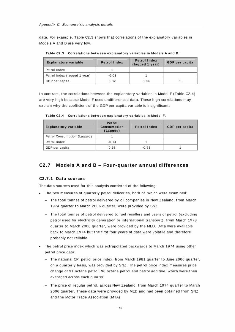
Appendix C: Econometric analysis details
75
data. For example, Table C2.3 shows that correlations of the explanatory variables in
Models A and B are very low.
Table C2.3 Correlations between explanatory variables in Models A and B.
Explanatory variable Petrol Index Petrol Index
(lagged 1 year) GDP per capita
Petrol Index 1
Petrol Index (lagged 1 year) -0.03 1
GDP per capita 0.02 0.04 1
In contrast, the correlations between the explanatory variables in Model F (Table C2.4)
are very high because Model F uses undifferenced data. These high correlations may
explain why the coefficient of the GDP per capita variable is insignificant.
Table C2.4 Correlations between explanatory variables in Model F.
Explanatory variable Petrol
Consumption (Lagged)
Petrol Index GDP per capita
Petrol Consumption (Lagged) 1
Petrol Index -0.74 1
GDP per capita 0.68 -0.63 1
C2.7 Models A and B – Four-quarter annual differences
C2.7.1 Data sources
The data sources used for this analysis consisted of the following:
• The two measures of quarterly petrol deliveries, both of which were examined:
– The total tonnes of petrol delivered by oil companies in New Zealand, from March
1974 quarter to March 2006 quarter, were provided by SNZ.
– The total tonnes of petrol delivered to fuel resellers and users of petrol (excluding
petrol used for electricity generation or international transport), from March 1978
quarter to March 2006 quarter, were provided by the MED. Data were available
back to March 1974 but the first four years of data were volatile and therefore
probably not reliable.
• The petrol price index which was extrapolated backwards to March 1974 using other
petrol price data:
– The national CPI petrol price index, from March 1981 quarter to June 2006 quarter,
on a quarterly basis, was provided by SNZ. The petrol price index measures price
change of 91 octane petrol, 96 octane petrol and petrol additive, which were then
averaged across each quarter.
– The price of regular petrol, across New Zealand, from March 1974 quarter to March
2006 quarter. These data were provided by MED and had been obtained from SNZ
and the Motor Trade Association (MTA).
IMPACTS OF FUEL PRICE CHANGES ON NEW ZEALAND TRANSPORT
76
The MED price of regular petrol tracked the petrol price index very closely (except
for a brief period from September 1986 to June 1991). Therefore, the price index
was extrapolated backwards by assuming a linear relationship between the price
index and the MED price of regular petrol.
The national consumer price index (CPI) from the March 1974 quarter to the June 2006
quarter, on a quarterly basis, was provided by SNZ (and obtained via the Reserve Bank of
New Zealand).
A national gross domestic product (GDP) time series, as developed by Hall & McDermott
(in press) of Victoria University, was used. The time series uses SNZ quarterly data from
June 1977 to December 2005 and interpolates annual data before June 1977 using
quarterly indicators. This time series has several limitations:
• Data before June 1977 is interpolated using indicators, as noted above.
• Data from June 1977 up to March 1987 uses a different method of adjusting
inventories to data from March 1987 onwards.
• Any revisions to SNZ's current GDP series could create inconsistencies because those
revisions are not reflected in the past data series.
• The data series methodology had not been peer-reviewed at the time it was
incorporated into this research project.
The national GDP statistics, as provided by SNZ, were used to extend the Hall &
McDermott series in that the growth rate observed from the December 2005 quarter to
the March 2006 quarter applied to the December 2005 quarter of the Hall & McDermott
series.
The quarterly population estimates from March 1991 to March 2006 were provided by
SNZ. Annual population estimates before 1991 (also from SNZ) were interpolated to
create a quarterly series from March 1974 to March 2006.
C2.7.2 Data manipulation
The quarterly petrol deliveries measures were divided by the number of days in each
quarter so that the measure was consistent across quarters.
The quarterly petrol deliveries measures were also divided by population to create an
additional ‘petrol deliveries per capita’ measure for empirical analysis.
C2.7.3 Models
The preferred models explained changes in petrol consumption per capita in terms of the
following explanatory variables:

Appendix C: Econometric analysis details
77
• Changes in the real petrol price index;
• Lagged changes in the real petrol price index;
• Changes in real GDP per capita.
The preferred models were fitted with data on petrol deliveries from the MED.
A four-quarter annual differences approach was adopted for this model: the dependent
variable was the difference between petrol consumption per capita in a given quarter and
petrol consumption per capita in the same quarter of the previous year. The explanatory
variables were adjusted in the same manner.
OLS - The impacts of the variables described above were initially estimated using a
standard regression technique, known as ordinary least squares (OLS). This model should
produce unbiased estimates. However, the model exhibited autocorrelation in the
residuals which would make the confidence intervals incorrect. To address this, a GLS
model was developed.
GLS – The preferred model was produced through the application of generalised least
squares (GLS) to the variables described above. GLS adjusts estimates and confidence
intervals to take into account autocorrelation in the residuals.
C2.7.4 OLS results (Model B)
Coefficients:
Estimate Std. Error t value Pr(>|t|)
(Intercept) -0.002395 0.003140 -0.763 0.44735
petrol_index -0.169245 0.028229 -5.995 2.90e-08 ***
lag1.petrol_index -0.058492 0.029349 -1.993 0.04886 *
gdp_capita 0.351816 0.110122 3.195 0.00185 **
---
Signif. codes: 0 '***' 0.001 '**' 0.01 '*' 0.05 '.' 0.1 ' ' 1
Residual standard error: 0.02831 on 105 degrees of freedom
Multiple R-Squared: 0.3147, Adjusted R-squared: 0.2952
F-statistic: 16.08 on 3 and 105 DF, p-value: 1.136e-08
C2.7.5 GLS results (Model A)
The model was estimated using GLS, with autocorrelation approximated using an MA(4)
error structure (selected by examination of ACF graphs and PACF graphs, as discussed in
Section C1.4):
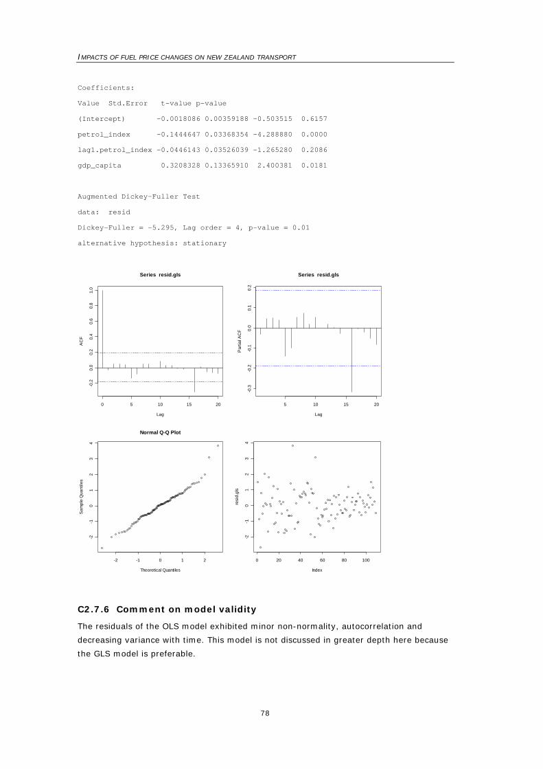
IMPACTS OF FUEL PRICE CHANGES ON NEW ZEALAND TRANSPORT
78
Coefficients:
Value Std.Error t-value p-value
(Intercept) -0.0018086 0.00359188 -0.503515 0.6157
petrol_index -0.1444647 0.03368354 -4.288880 0.0000
lag1.petrol_index -0.0446143 0.03526039 -1.265280 0.2086
gdp_capita 0.3208328 0.13365910 2.400381 0.0181
Augmented Dickey-Fuller Test
data: resid
Dickey-Fuller = -5.295, Lag order = 4, p-value = 0.01
alternative hypothesis: stationary
0 5 10 15 20
-0.2
0.0
0.2
0.4
0.6
0.8
1.0
Lag
AC
F
Series resid.gls
5 10 15 20
-0.3
-0.2
-0.1
0.0
0.1
0.2
Lag
Par
tial A
CF
Series resid.gls
-2 -1 0 1 2
-2-1
01
23
4
Normal Q-Q Plot
Theoretical Quantiles
Sam
ple
Qua
ntile
s
0 20 40 60 80 100
-2-1
01
23
4
Index
resi
d.gl
s
C2.7.6 Comment on model validity
The residuals of the OLS model exhibited minor non-normality, autocorrelation and
decreasing variance with time. This model is not discussed in greater depth here because
the GLS model is preferable.
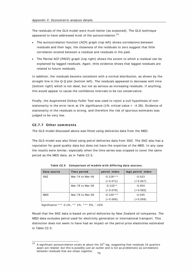
Appendix C: Econometric analysis details
79
The residuals of the GLS model were much better (as expected). The GLS technique
appeared to have addressed most of the autocorrelation.10
• The autocorrelation function (ACF) graph (top left) shows correlations between
residuals and their lags; the closeness of the residuals to zero suggest that little
correlation existed between a residual and residuals in the past.
• The Partial ACF (PACF) graph (top right) shows the extent to which a residual can be
explained by lagged residuals. Again, little evidence shows that lagged residuals are
related to future residuals.
In addition, the residuals become consistent with a normal distribution, as shown by the
straight line in the Q-Q plot (bottom left). The residuals appeared to decrease with time
(bottom right) which is not ideal, but not as serious as increasing residuals. If anything,
this would appear to cause the confidence intervals to be too conservative.
Finally, the Augmented Dickey-Fuller Test was used to reject a null hypothesis of non-
stationarity in the error term at 1% significance (1% critical value = -4.38). Evidence of
stationarity in the residuals is strong, and therefore the risk of spurious estimates was
judged to be very low.
C2.7.7 Other comments
The GLS model discussed above was fitted using deliveries data from the MED.
The GLS model was also fitted using petrol deliveries data from SNZ. The SNZ also has a
reputation for good quality data but does not have the expertise of the MED. In any case
the results were similar, especially when the time series was cropped to cover the same
period as the MED data, as in Table C2.5.
Table C2.5 Comparison of models with differing data sources.
Data source Time period petrol_index lag1.petrol_index
Mar-74 to Mar-06 -0.128***
(+0.071)
-0.023
(+0.067)
SNZ
Mar-78 to Mar-06 -0.132**
(+0.079)
-0.054
(+0.082)
MED Mar-78 to Mar-06 -0.145***
(+0.066)
-0.045
(+0.069)
Significance *** 0.1%, ** 1%, *** 5%, `10%
Recall that the SNZ data is based on petrol deliveries by New Zealand oil companies. The
MED data excludes petrol used for electricity generation or international transport. This
distinction does not seem to have had an impact on the petrol price elasticities estimated
in Table C2.5.
10 A significant autocorrelation exists at about the 16th lag, suggesting that residuals 16 quarters
apart are related, but this is possibly just an outlier and is not as problematic as correlations between residuals that are closer together.

IMPACTS OF FUEL PRICE CHANGES ON NEW ZEALAND TRANSPORT
80
C2.8 Model A incorporating impact of carless days
Upon advice from a referee, the impacts of the ‘carless day’ policy, from February 1979 to
August 1980, were incorporated into Model A. Carless days were modelled using a
dummy variable. The autocorrelation had to be modelled using an MA(5) error term
because the model was not invertible with an MA(4) term.
The results of the inclusion of the ‘carless day’ policy dummy variable follow.
C2.8.1 OLS results
Coefficients:
Estimate Std. Error t value Pr(>|t|)
(Intercept) -0.002493 0.003107 -0.803 0.42409
petrol_index -0.164542 0.028047 -5.867 5.33e-08 ***
lag1.petrol_index -0.075134 0.030452 -2.467 0.01525 *
gdp_capita 0.349469 0.108950 3.208 0.00178 **
carless -0.020225 0.011159 -1.813 0.07279 .
--- Signif. codes: 0 '***' 0.001 '**' 0.01 '*' 0.05 '.' 0.1 ' ' 1
Residual standard error: 0.02801 on 104 degrees of freedom
Multiple R-Squared: 0.3357, Adjusted R-squared: 0.3102
F-statistic: 13.14 on 4 and 104 DF, p-value: 1.067e-08
The GLS version of the model (shown in Section C2.8.2) is more accurate. However, the
OLS version of the model allows us to examine the impact of the ‘carless days’ policy on
‘goodness of fit’. The dummy has increased Model A’s R2 (from 0.31 to 0.34) and the
adjusted R2 has increased from 0.30 to 0.31.
C2.8.2 GLS results (using MA(5) error term)
Coefficients:
Value Std.Error t-value p-value
(Intercept) -0.0028027 0.00429479 -0.652578 0.5155
petrol_index -0.1456843 0.03489129 -4.175378 0.0001
lag1.petrol_index -0.0540431 0.03655035 -1.478592 0.1423
gdp_capita 0.3884184 0.13982254 2.777938 0.0065
carless -0.0152281 0.01440389 -1.057221 0.2929
The inclusion of the dummy variable has also had implications for the model coefficients
produced by the GLS model. The short-run elasticity has increased from -0.14 to -0.15.
The interim elasticity has increased from -0.04 to -0.05. The GDP per capita elasticity has
increased from 0.32 to 0.39, and has now become statistically significant at 1%.
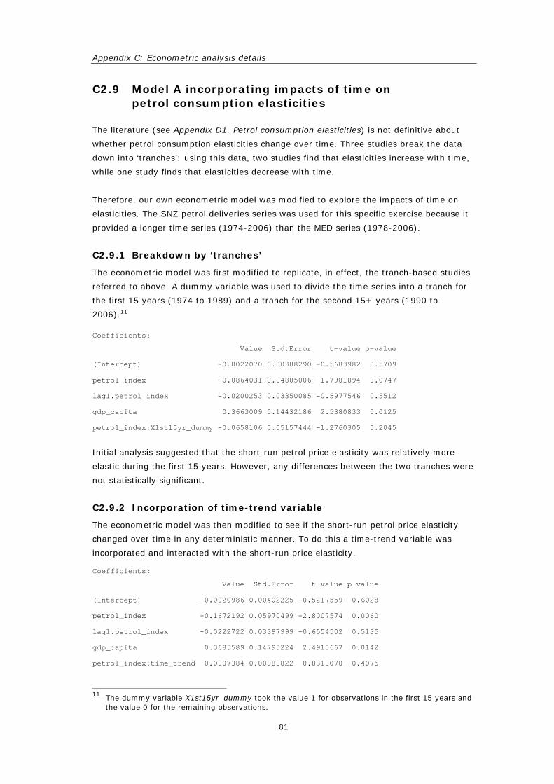
Appendix C: Econometric analysis details
81
C2.9 Model A incorporating impacts of time on petrol consumption elasticities
The literature (see Appendix D1. Petrol consumption elasticities) is not definitive about
whether petrol consumption elasticities change over time. Three studies break the data
down into ‘tranches’: using this data, two studies find that elasticities increase with time,
while one study finds that elasticities decrease with time.
Therefore, our own econometric model was modified to explore the impacts of time on
elasticities. The SNZ petrol deliveries series was used for this specific exercise because it
provided a longer time series (1974-2006) than the MED series (1978-2006).
C2.9.1 Breakdown by ‘tranches’
The econometric model was first modified to replicate, in effect, the tranch-based studies
referred to above. A dummy variable was used to divide the time series into a tranch for
the first 15 years (1974 to 1989) and a tranch for the second 15+ years (1990 to
2006).11
Coefficients:
Value Std.Error t-value p-value
(Intercept) -0.0022070 0.00388290 -0.5683982 0.5709
petrol_index -0.0864031 0.04805006 -1.7981894 0.0747
lag1.petrol_index -0.0200253 0.03350085 -0.5977546 0.5512
gdp_capita 0.3663009 0.14432186 2.5380833 0.0125
petrol_index:X1st15yr_dummy -0.0658106 0.05157444 -1.2760305 0.2045
Initial analysis suggested that the short-run petrol price elasticity was relatively more
elastic during the first 15 years. However, any differences between the two tranches were
not statistically significant.
C2.9.2 Incorporation of time-trend variable
The econometric model was then modified to see if the short-run petrol price elasticity
changed over time in any deterministic manner. To do this a time-trend variable was
incorporated and interacted with the short-run price elasticity.
Coefficients:
Value Std.Error t-value p-value
(Intercept) -0.0020986 0.00402225 -0.5217559 0.6028
petrol_index -0.1672192 0.05970499 -2.8007574 0.0060
lag1.petrol_index -0.0222722 0.03397999 -0.6554502 0.5135
gdp_capita 0.3685589 0.14795224 2.4910667 0.0142
petrol_index:time_trend 0.0007384 0.00088822 0.8313070 0.4075
11 The dummy variable X1st15yr_dummy took the value 1 for observations in the first 15 years and
the value 0 for the remaining observations.
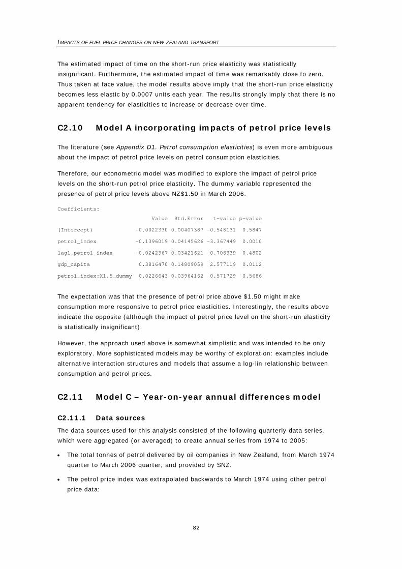
IMPACTS OF FUEL PRICE CHANGES ON NEW ZEALAND TRANSPORT
82
The estimated impact of time on the short-run price elasticity was statistically
insignificant. Furthermore, the estimated impact of time was remarkably close to zero.
Thus taken at face value, the model results above imply that the short-run price elasticity
becomes less elastic by 0.0007 units each year. The results strongly imply that there is no
apparent tendency for elasticities to increase or decrease over time.
C2.10 Model A incorporating impacts of petrol price levels
The literature (see Appendix D1. Petrol consumption elasticities) is even more ambiguous
about the impact of petrol price levels on petrol consumption elasticities.
Therefore, our econometric model was modified to explore the impact of petrol price
levels on the short-run petrol price elasticity. The dummy variable represented the
presence of petrol price levels above NZ$1.50 in March 2006.
Coefficients:
Value Std.Error t-value p-value
(Intercept) -0.0022330 0.00407387 -0.548131 0.5847
petrol_index -0.1396019 0.04145626 -3.367449 0.0010
lag1.petrol_index -0.0242367 0.03421621 -0.708339 0.4802
gdp_capita 0.3816470 0.14809059 2.577119 0.0112
petrol_index:X1.5_dummy 0.0226643 0.03964162 0.571729 0.5686
The expectation was that the presence of petrol price above $1.50 might make
consumption more responsive to petrol price elasticities. Interestingly, the results above
indicate the opposite (although the impact of petrol price level on the short-run elasticity
is statistically insignificant).
However, the approach used above is somewhat simplistic and was intended to be only
exploratory. More sophisticated models may be worthy of exploration: examples include
alternative interaction structures and models that assume a log-lin relationship between
consumption and petrol prices.
C2.11 Model C – Year-on-year annual differences model
C2.11.1 Data sources
The data sources used for this analysis consisted of the following quarterly data series,
which were aggregated (or averaged) to create annual series from 1974 to 2005:
• The total tonnes of petrol delivered by oil companies in New Zealand, from March 1974
quarter to March 2006 quarter, and provided by SNZ.
• The petrol price index was extrapolated backwards to March 1974 using other petrol
price data:
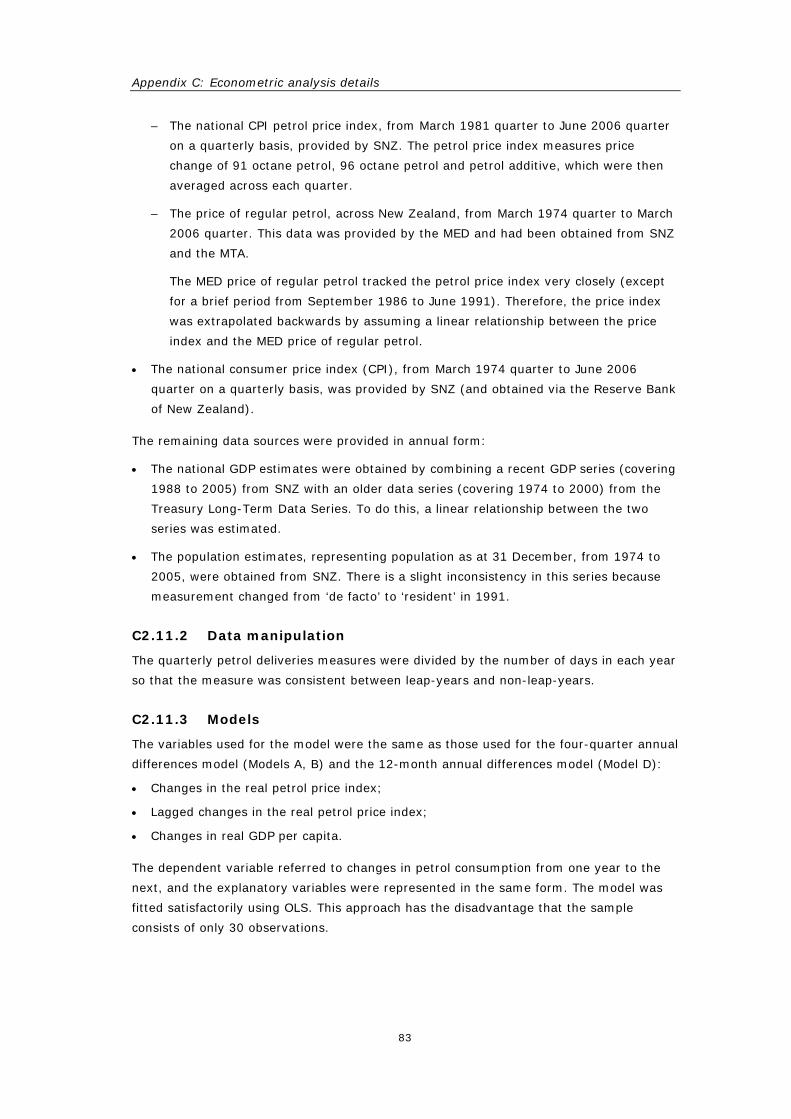
Appendix C: Econometric analysis details
83
– The national CPI petrol price index, from March 1981 quarter to June 2006 quarter
on a quarterly basis, provided by SNZ. The petrol price index measures price
change of 91 octane petrol, 96 octane petrol and petrol additive, which were then
averaged across each quarter.
– The price of regular petrol, across New Zealand, from March 1974 quarter to March
2006 quarter. This data was provided by the MED and had been obtained from SNZ
and the MTA.
The MED price of regular petrol tracked the petrol price index very closely (except
for a brief period from September 1986 to June 1991). Therefore, the price index
was extrapolated backwards by assuming a linear relationship between the price
index and the MED price of regular petrol.
• The national consumer price index (CPI), from March 1974 quarter to June 2006
quarter on a quarterly basis, was provided by SNZ (and obtained via the Reserve Bank
of New Zealand).
The remaining data sources were provided in annual form:
• The national GDP estimates were obtained by combining a recent GDP series (covering
1988 to 2005) from SNZ with an older data series (covering 1974 to 2000) from the
Treasury Long-Term Data Series. To do this, a linear relationship between the two
series was estimated.
• The population estimates, representing population as at 31 December, from 1974 to
2005, were obtained from SNZ. There is a slight inconsistency in this series because
measurement changed from ‘de facto’ to ‘resident’ in 1991.
C2.11.2 Data manipulation
The quarterly petrol deliveries measures were divided by the number of days in each year
so that the measure was consistent between leap-years and non-leap-years.
C2.11.3 Models
The variables used for the model were the same as those used for the four-quarter annual
differences model (Models A, B) and the 12-month annual differences model (Model D):
• Changes in the real petrol price index;
• Lagged changes in the real petrol price index;
• Changes in real GDP per capita.
The dependent variable referred to changes in petrol consumption from one year to the
next, and the explanatory variables were represented in the same form. The model was
fitted satisfactorily using OLS. This approach has the disadvantage that the sample
consists of only 30 observations.
IMPACTS OF FUEL PRICE CHANGES ON NEW ZEALAND TRANSPORT
84
C2.11.4 Results
Coefficients:
Estimate Std. Error t value Pr(>|t|)
(Intercept) 0.0006184 0.0047398 0.130 0.8972
petrol_index -0.1335266 0.0569718 -2.344 0.0270 *
lag1.petrol_index -0.1032838 0.0459402 -2.248 0.0333 *
gdp_capita 0.1196940 0.2044854 0.585 0.5634
--- Signif. codes: 0 '***' 0.001 '**' 0.01 '*' 0.05 '.' 0.1 ' ' 1
Residual standard error: 0.02207 on 26 degrees of freedom
Multiple R-Squared: 0.3366, Adjusted R-squared: 0.2601
F-statistic: 4.397 on 3 and 26 DF, p-value: 0.01248
Augmented Dickey-Fuller Test
data: resid
Dickey-Fuller = -2.4274, Lag order = 3, p-value = 0.4085
alternative hypothesis: stationary
0 2 4 6 8 10 12 14
-0.4
-0.2
0.0
0.2
0.4
0.6
0.8
1.0
Lag
AC
F
Series resid
2 4 6 8 10 12 14
-0.3
-0.2
-0.1
0.0
0.1
0.2
0.3
Lag
Par
tial A
CF
Series resid
-2 -1 0 1 2
-0.0
4-0
.02
0.00
0.02
Normal Q-Q Plot
Theoretical Quantiles
Sam
ple
Qua
ntile
s
0 5 10 15 20 25 30
-0.0
4-0
.02
0.00
0.02
Index
resi
d
C2.11.5 Comment on model validity
This model exhibited favourable residual behaviour, even when fitted simply with OLS.
The ACF and PACF plots illustrate the absence of discernible autocorrelation. The Q-Q plot
provides some support for the assumption of normality and the trends could not be
discerned from the plot of residuals against time.
Appendix C: Econometric analysis details
85
The Augmented Dickey-Fuller test failed to reject a possibility of a non-stationary error
term (10% critical value = -4.21). However, this could be due to the low power of the
test given that a small sample size of 31 was used.
C2.12 Model D – 12-month annual differences model
C2.12.1 Data sources
The data sources used for this analysis consisted of the following:
• The total tonnes of petrol delivered (per month) to fuel resellers and users of petrol
(excluding petrol used for electricity generation or international transport), from
January 1999 to June 2006, and provided by the MED.
• Petrol price data from 1 January 1999 to 18 June 2006. The data consists of daily
retail prices as advertised at major Wellington service stations, and was provided by
the MED. The prices at the mid-point of each month were used as an explanatory
variable.
• The national CPI from December 1999 quarter to June 2006 quarter, on a quarterly
basis, provided by SNZ (and obtained via the Reserve Bank of New Zealand). The time
series was then interpolated to create a monthly time series.
• The national GDP from December 1999 quarter to March 2006 quarter on a quarterly
basis, provided by SNZ. The time series was then interpolated to create a monthly
time series.
• The national population estimates from December 1999 quarter to March 2006 quarter
on a quarterly basis, provided by SNZ. The time series was then interpolated to create
a monthly time series.
C2.12.2 Data manipulations
The quarterly petrol deliveries measures were divided by the number of days in each
month so that the measure was consistent across quarters.
The quarterly petrol deliveries measures were also divided by population to create an
additional ‘petrol deliveries per capita’ measure for empirical analysis.
C2.12.3 Models
This model explained changes in petrol consumption per capita in terms of the following
explanatory variables:
• Changes in the real regular petrol price;
• Lagged changes in the real regular petrol price;
• Changes in real GDP per capita.
The impacts of the variables were estimated using a 12-month annual differences
approach. Because of data limitations, this model covers a shorter time period, but the
use of monthly data enables more observations to be made within each year of data.
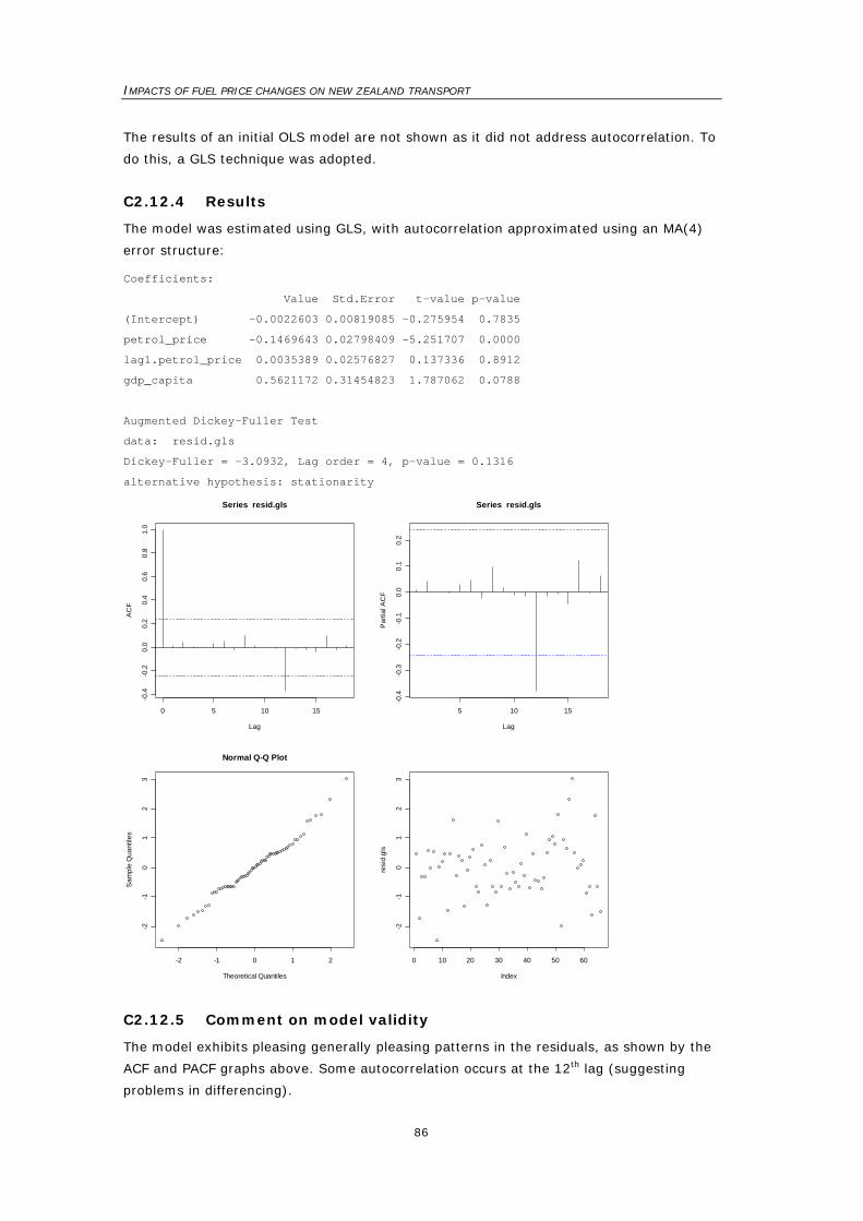
IMPACTS OF FUEL PRICE CHANGES ON NEW ZEALAND TRANSPORT
86
The results of an initial OLS model are not shown as it did not address autocorrelation. To
do this, a GLS technique was adopted.
C2.12.4 Results
The model was estimated using GLS, with autocorrelation approximated using an MA(4)
error structure:
Coefficients:
Value Std.Error t-value p-value
(Intercept) -0.0022603 0.00819085 -0.275954 0.7835
petrol_price -0.1469643 0.02798409 -5.251707 0.0000
lag1.petrol_price 0.0035389 0.02576827 0.137336 0.8912
gdp_capita 0.5621172 0.31454823 1.787062 0.0788
Augmented Dickey-Fuller Test
data: resid.gls
Dickey-Fuller = -3.0932, Lag order = 4, p-value = 0.1316
alternative hypothesis: stationarity
0 5 10 15
-0.4
-0.2
0.0
0.2
0.4
0.6
0.8
1.0
Lag
AC
F
Series resid.gls
5 10 15
-0.4
-0.3
-0.2
-0.1
0.0
0.1
0.2
Lag
Par
tial A
CF
Series resid.gls
-2 -1 0 1 2
-2-1
01
23
Normal Q-Q Plot
Theoretical Quantiles
Sam
ple
Qua
ntile
s
0 10 20 30 40 50 60
-2-1
01
23
Index
resi
d.gl
s
C2.12.5 Comment on model validity
The model exhibits pleasing generally pleasing patterns in the residuals, as shown by the
ACF and PACF graphs above. Some autocorrelation occurs at the 12th lag (suggesting
problems in differencing).

Appendix C: Econometric analysis details
87
The distinctive straight line in the Q-Q plot strongly supports an assumption of normality.
The plot of residuals against time suggests one can reasonably assume that variance is
roughly constant through time.
However, the Augmented Dickey-Fuller test could not reject a hypothesis of non-
stationarity in the error term, even at 10% significance (10% critical value = -4.02).
This model should not be given too much weight, but it produces comforting results, it
performs better than any of the remaining models in the petrol elasticity section, and it
produces similar results to the four-quarter annual differences model.
C2.13 Model E – Quarterly differences model
C2.13.1 Data sources
The data sources used for this analysis consisted of the following:
• The total tonnes of petrol delivered to fuel resellers and users of petrol (excluding
petrol used for electricity generation or international transport), from March 1978
quarter to March 2006 quarter, and provided by the MED. Data were available back to
March 1974 but the first four years of data were volatile and therefore probably not
reliable.
• The petrol price index was extrapolated backwards to March 1978 using other petrol
price data:
– The national CPI petrol price index, from March 1981 quarter to June 2006 quarter
on a quarterly basis, was provided by SNZ. The petrol price index measures price
change of 91 octane petrol, 96 octane petrol and petrol additive, which were then
averaged across each quarter.
– The price of regular petrol, across New Zealand, from March 1974 quarter to March
2006 quarter. This data was provided by the MED and had been obtained from SNZ
and the MTA. The MED price of regular petrol tracked the petrol price index very
closely (except for a brief period from September 1986 to June 1991). Therefore,
the price index was extrapolated backwards by assuming a linear relationship
between the price index and the MED price of regular petrol.
• The national consumer price index (CPI), from March 1974 quarter to June 2006
quarter on a quarterly basis, was provided by SNZ (and obtained via the Reserve Bank
of New Zealand).
• A national GDP time series, as developed by Hall & McDermott (in press) of Victoria
University, was used. The time series uses SNZ quarterly data from June 1977 to
December 2005 and interpolates annual data before June 1977 using quarterly
indicators. This time series has several limitations:
– Data before June 1977 is interpolated using indicators, as noted above.
– Data from June 1977 up to March 1987 uses a different method of adjusting
inventories to data from March 1987 onwards.

IMPACTS OF FUEL PRICE CHANGES ON NEW ZEALAND TRANSPORT
88
– Any revisions to SNZ's current GDP series could create inconsistencies because
those revisions are not reflected in the past data series.
– The data series methodology had not been peer reviewed at the time it was
incorporated into this research project.
• The national GDP statistics, as provided by SNZ, were used to extend the Hall &
McDermott series: the growth rate observed from the December 2005 quarter to the
March 2006 quarter was applied to the December 2005 quarter of the Hall &
McDermott series.
• The quarterly population estimates from March 1991 to March 2006 were provided by
SNZ. Annual population estimates before 1991 (also from SNZ) were interpolated to
create a quarterly series from March 1974 to March 2006.
C2.13.2 Data manipulation
The quarterly petrol deliveries measures were divided by the number of days in each
quarter so that the measure was consistent across quarters.
The quarterly petrol deliveries measures were also divided by population to create an
additional ‘petrol deliveries per capita’ measure for empirical analysis.
C2.13.3 Models
This model was less parsimonious than any of the other models that were fitted. The
model explained changes in petrol consumption per capita from one quarter to the next in
terms of changes in the following explanatory variables:
• The change in the real petrol price index over the same quarter;
• The change in the real petrol price index over the preceding quarter;
• The change in the real petrol price index from the quarter a year before to the quarter
two quarters previously;
• The change in the real petrol price index from the quarter two years before and the
quarter one year previously;
• The change in real GDP per capita over the same quarter;
• Dummies representing the impacts of June, September and December quarters on
growth in petrol consumption in any given quarter.
For the inclusion of dummies to be valid, the assumption was made that seasonal effects
had a predictable and constant impact on changes in petrol consumption. The figures
below validate this assumption because they show that the growth rates from one quarter
to the next are roughly constant, regardless of the year examined.
The model was initially fitted using OLS and then with GLS (to adjust for autocorrelation).
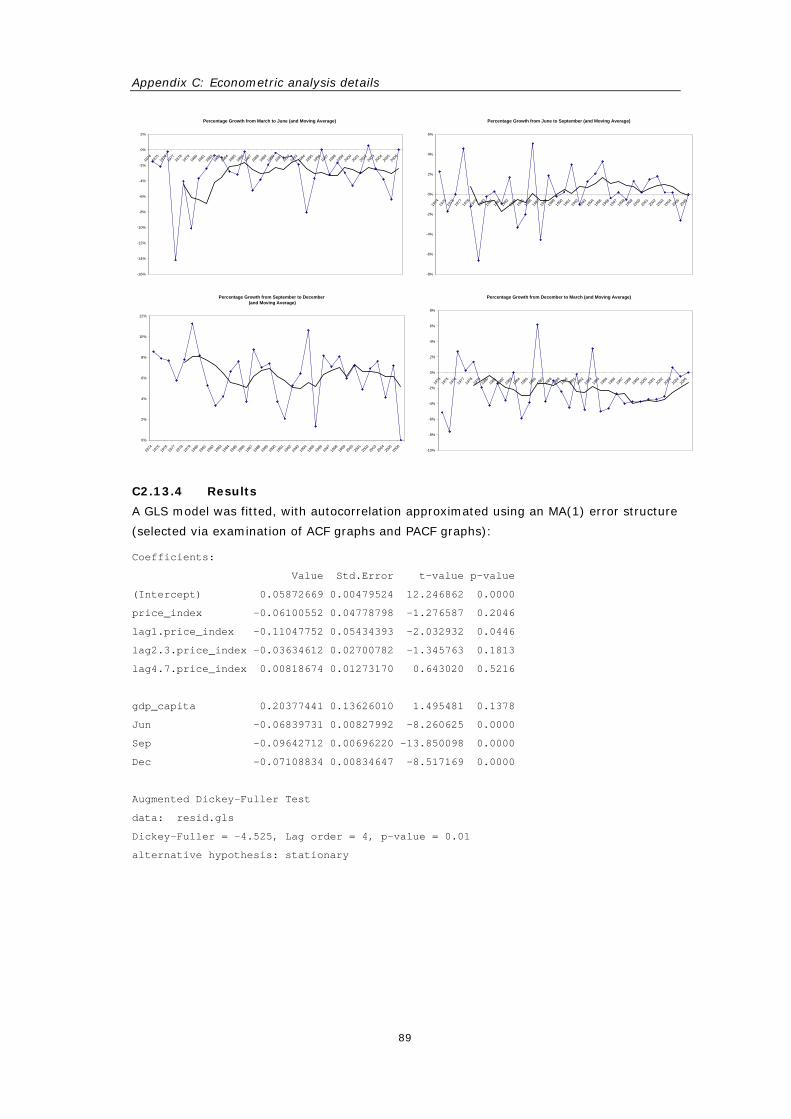
Appendix C: Econometric analysis details
89
C2.13.4 Results
A GLS model was fitted, with autocorrelation approximated using an MA(1) error structure
(selected via examination of ACF graphs and PACF graphs):
Coefficients:
Value Std.Error t-value p-value
(Intercept) 0.05872669 0.00479524 12.246862 0.0000
price_index -0.06100552 0.04778798 -1.276587 0.2046
lag1.price_index -0.11047752 0.05434393 -2.032932 0.0446
lag2.3.price_index -0.03634612 0.02700782 -1.345763 0.1813
lag4.7.price_index 0.00818674 0.01273170 0.643020 0.5216
gdp_capita 0.20377441 0.13626010 1.495481 0.1378
Jun -0.06839731 0.00827992 -8.260625 0.0000
Sep -0.09642712 0.00696220 -13.850098 0.0000
Dec -0.07108834 0.00834647 -8.517169 0.0000
Augmented Dickey-Fuller Test
data: resid.gls
Dickey-Fuller = -4.525, Lag order = 4, p-value = 0.01
alternative hypothesis: stationary
Percentage Growth from June to September (and Moving Average)
-8%
-6%
-4%
-2%
0%
2%
4%
6%
1974
1975
1976
1977
1978
1979
1980
1981
1982
1983
1984
1985
1986
1987
1988
1989
1990
1991
1992
1993
1994
1995
1996
1997
1998
1999
2000
2001
2002
2003
2004
2005
2006
Percentage Growth from March to June (and Moving Average)
-16%
-14%
-12%
-10%
-8%
-6%
-4%
-2%
0%
2%
1974
1975
1976
1977
1978
1979
1980
1981
1982
1983
1984
1985
1986
1987
1988
1989
1990
1991
1992
1993
1994
1995
1996
1997
1998
1999
2000
2001
2002
2003
2004
2005
2006
Percentage Growth from September to December (and Moving Average)
0%
2%
4%
6%
8%
10%
12%
1974
1975
1976
1977
1978
1979
1980
1981
1982
1983
1984
1985
1986
1987
1988
1989
1990
1991
1992
1993
1994
1995
1996
1997
1998
1999
2000
2001
2002
2003
2004
2005
2006
Percentage Growth from December to March (and Moving Average)
-10%
-8%
-6%
-4%
-2%
0%
2%
4%
6%
8%
1974
1975
1976
1977
1978
1979
1980
1981
1982
1983
1984
1985
1986
1987
1988
1989
1990
1991
1992
1993
1994
1995
1996
1997
1998
1999
2000
2001
2002
2003
2004
2005
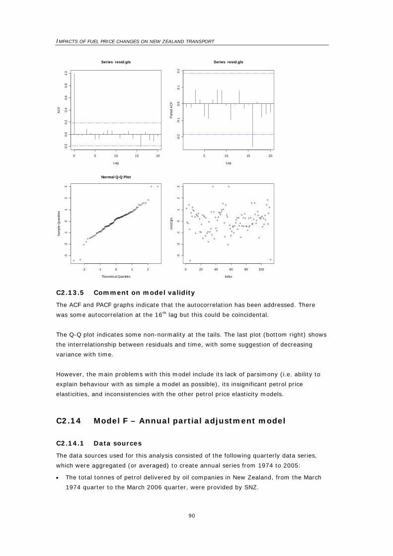
IMPACTS OF FUEL PRICE CHANGES ON NEW ZEALAND TRANSPORT
90
0 5 10 15 20
-0.2
0.0
0.2
0.4
0.6
0.8
1.0
Lag
AC
FSeries resid.gls
5 10 15 20
-0.2
-0.1
0.0
0.1
0.2
Lag
Par
tial A
CF
Series resid.gls
-2 -1 0 1 2
-3-2
-10
12
3
Normal Q-Q Plot
Theoretical Quantiles
Sam
ple
Qua
ntile
s
0 20 40 60 80 100
-3-2
-10
12
3
Index
resi
d.gl
s
C2.13.5 Comment on model validity
The ACF and PACF graphs indicate that the autocorrelation has been addressed. There
was some autocorrelation at the 16th lag but this could be coincidental.
The Q-Q plot indicates some non-normality at the tails. The last plot (bottom right) shows
the interrelationship between residuals and time, with some suggestion of decreasing
variance with time.
However, the main problems with this model include its lack of parsimony (i.e. ability to
explain behaviour with as simple a model as possible), its insignificant petrol price
elasticities, and inconsistencies with the other petrol price elasticity models.
C2.14 Model F – Annual partial adjustment model
C2.14.1 Data sources
The data sources used for this analysis consisted of the following quarterly data series,
which were aggregated (or averaged) to create annual series from 1974 to 2005:
• The total tonnes of petrol delivered by oil companies in New Zealand, from the March
1974 quarter to the March 2006 quarter, were provided by SNZ.
Appendix C: Econometric analysis details
91
• The petrol price index was extrapolated backwards to March 1974 using other petrol
price data:
– The national CPI petrol price index, from the March 1981 quarter to the June 2006
quarter on a quarterly basis, provided by SNZ. The petrol price index measures
price change of 91 octane petrol, 96 octane petrol and petrol additive, which are
then averaged across each quarter.
– The price of regular petrol, across New Zealand, from the March 1974 quarter to
the March 2006 quarter. This data was provided by the MED and had been obtained
from SNZ and the MTA. The MED price of regular petrol tracked the petrol price
index very closely (except for a brief period from September 1986 to June 1991).
Therefore, the price index was extrapolated backwards by assuming a linear
relationship between the price index and the MED price of regular petrol.
• The national CPI, from the March 1974 quarter to the June 2006 quarter on a quarterly
basis, provided by SNZ (and obtained via the Reserve Bank of New Zealand).
The remaining data sources were provided in annual form:
• The national GDP estimates obtained by combining a recent GDP series (covering 1988
to 2005) from SNZ with an older data series (covering 1974 to 2000) from the
Treasury Long-Term Data Series. To do this, a linear relationship between the two
series was estimated.
• The population estimates, representing population as at 31 December, from 1974 to
2005, obtained from SNZ. There is a slight inconsistency in this series because
measurement changed from ‘de facto’ to ‘resident’ in 1991.
C2.14.2 Data manipulation
The quarterly petrol deliveries measures were divided by the number of days in each year
so that the measure was consistent between leap-years and non-leap-years.
C2.14.3 Models
The dependent variable for this model consisted of petrol consumption (logged). The
explanatory variables included the following (all logged):
• The lag of petrol consumption per capita;
• The real petrol price index;
• Real GDP per capita.
This model is used to estimate three parameters:
• The short-run petrol price elasticity;
• The speed of adjustment;
• The long-run petrol price elasticity.
In this model, the long-run petrol price elasticity is assumed to be a function of the short-
run petrol price elasticity and the speed of adjustment. The model was fitted satisfactorily
using OLS.

IMPACTS OF FUEL PRICE CHANGES ON NEW ZEALAND TRANSPORT
92
This model approach has the disadvantage that the sample consists of only 30
observations.
C2.14.4 Results
Coefficients:
Estimate Std. Error t value Pr(>|t|)
(Intercept) 0.07110 0.14173 0.502 0.619956
lag1.petrol_del_capita_ns 0.37550 0.12992 2.890 0.007506 **
petrol_index_ns -0.11057 0.02726 -4.056 0.000382 ***
gdp_capita_ns 0.06824 0.04704 1.451 0.158438
Signif. codes: 0 '***' 0.001 '**' 0.01 '*' 0.05 '.' 0.1 ' ' 1
Residual standard error: 0.01895 on 27 degrees of freedom
Multiple R-Squared: 0.8371, Adjusted R-squared: 0.819
F-statistic: 46.26 on 3 and 27 DF, p-value: 8.982e-11
studentized Breusch-Pagan test
data: results
BP = 2.3367, df = 3, p-value = 0.5055
Augmented Dickey-Fuller Test
data: resid
Dickey-Fuller = -2.0263, Lag order = 2, p-value = 0.5624
alternative hypothesis: stationary
-2 -1 0 1 2
-0.0
4-0
.02
0.00
0.02
0.04
Normal Q-Q Plot
Theoretical Quantiles
Sam
ple
Qua
ntile
s
0 5 10 15 20 25
-0.0
4-0
.02
0.00
0.02
0.04
Index
resi
d
C2.14.5 Comment on model validity
The partial adjustment model exhibited normality of the residuals in the Q-Q plot. The
residuals appear constant throughout time in the plot of residuals against time. In
addition, the Breusch-Pagan test failed to detect first order autocorrelation.
However, the Augmented Dickey-Fuller test failed to reject the possibility of non-
stationarity in the residuals (10% critical value = -4.21). This is particularly concerning
because this model uses data that are definitely non-stationary; therefore the possibility
of non-stationarity in the error term is higher than it would have been with the differences
models.
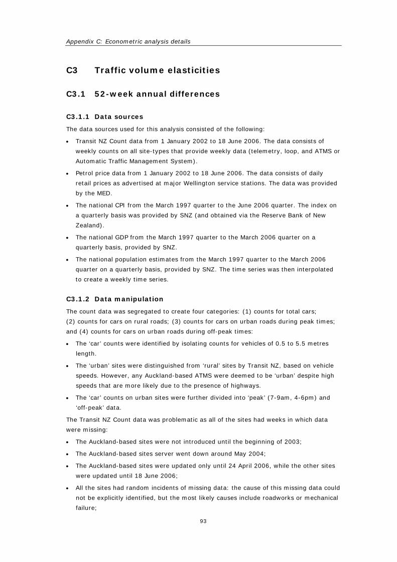
Appendix C: Econometric analysis details
93
C3 Traffic volume elasticities
C3.1 52-week annual differences
C3.1.1 Data sources
The data sources used for this analysis consisted of the following:
• Transit NZ Count data from 1 January 2002 to 18 June 2006. The data consists of
weekly counts on all site-types that provide weekly data (telemetry, loop, and ATMS or
Automatic Traffic Management System).
• Petrol price data from 1 January 2002 to 18 June 2006. The data consists of daily
retail prices as advertised at major Wellington service stations. The data was provided
by the MED.
• The national CPI from the March 1997 quarter to the June 2006 quarter. The index on
a quarterly basis was provided by SNZ (and obtained via the Reserve Bank of New
Zealand).
• The national GDP from the March 1997 quarter to the March 2006 quarter on a
quarterly basis, provided by SNZ.
• The national population estimates from the March 1997 quarter to the March 2006
quarter on a quarterly basis, provided by SNZ. The time series was then interpolated
to create a weekly time series.
C3.1.2 Data manipulation
The count data was segregated to create four categories: (1) counts for total cars;
(2) counts for cars on rural roads; (3) counts for cars on urban roads during peak times;
and (4) counts for cars on urban roads during off-peak times:
• The ‘car’ counts were identified by isolating counts for vehicles of 0.5 to 5.5 metres
length.
• The ‘urban’ sites were distinguished from ‘rural’ sites by Transit NZ, based on vehicle
speeds. However, any Auckland-based ATMS were deemed to be ‘urban’ despite high
speeds that are more likely due to the presence of highways.
• The ‘car’ counts on urban sites were further divided into ‘peak’ (7-9am, 4-6pm) and
‘off-peak’ data.
The Transit NZ Count data was problematic as all of the sites had weeks in which data
were missing:
• The Auckland-based sites were not introduced until the beginning of 2003;
• The Auckland-based sites server went down around May 2004;
• The Auckland-based sites were updated only until 24 April 2006, while the other sites
were updated until 18 June 2006;
• All the sites had random incidents of missing data: the cause of this missing data could
not be explicitly identified, but the most likely causes include roadworks or mechanical
failure;
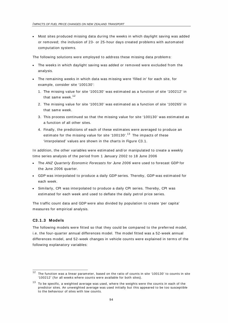
IMPACTS OF FUEL PRICE CHANGES ON NEW ZEALAND TRANSPORT
94
• Most sites produced missing data during the weeks in which daylight saving was added
or removed; the inclusion of 23- or 25-hour days created problems with automated
computation systems.
The following solutions were employed to address these missing data problems:
• The weeks in which daylight saving was added or removed were excluded from the
analysis.
• The remaining weeks in which data was missing were ‘filled in’ for each site, for
example, consider site ‘100130’:
1. The missing value for site ‘100130’ was estimated as a function of site ‘100212’ in
that same week.12
2. The missing value for site ‘100130’ was estimated as a function of site ‘100265’ in
that same week.
3. This process continued so that the missing value for site ‘100130’ was estimated as
a function of all other sites.
4. Finally, the predictions of each of these estimates were averaged to produce an
estimate for the missing value for site ‘100130’.13 The impacts of these
‘interpolated’ values are shown in the charts in Figure C3.1.
In addition, the other variables were estimated and/or manipulated to create a weekly
time series analysis of the period from 1 January 2002 to 18 June 2006
• The ANZ Quarterly Economic Forecasts for June 2006 were used to forecast GDP for
the June 2006 quarter.
• GDP was interpolated to produce a daily GDP series. Thereby, GDP was estimated for
each week.
• Similarly, CPI was interpolated to produce a daily CPI series. Thereby, CPI was
estimated for each week and used to deflate the daily petrol price series.
The traffic count data and GDP were also divided by population to create ‘per capita’
measures for empirical analysis.
C3.1.3 Models
The following models were fitted so that they could be compared to the preferred model,
i.e. the four-quarter annual differences model. The model fitted was a 52-week annual
differences model, and 52-week changes in vehicle counts were explained in terms of the
following explanatory variables:
12 The function was a linear parameter, based on the ratio of counts in site ‘100130’ to counts in site
‘100212’ (for all weeks where counts were available for both sites). 13 To be specific, a weighted average was used, where the weights were the counts in each of the
predictor sites. An unweighted average was used initially but this appeared to be too susceptible to the behaviour of sites with low counts.
Appendix C: Econometric analysis details
95
• Changes in real regular petrol prices over 52 weeks;
• Lagged changes in real regular petrol prices over the previous 52 weeks;
• Changes in GDP per capita over 52 weeks.
Figure C3.1 Actual and interpolated total vehicle counts (vehicles up to 5.5-m lengths), from top left and clockwise: total, rural, off-peak, and peak, for 2002-2006.
In addition to providing symmetry with the four-quarter annual differences model, this
model structure can be justified because the petrol price impacts beyond the first lag
were insignificant.
All the models were estimated using GLS because the OLS models indicated
autocorrelation.
One peer reviewer raised concerns about the effectiveness of the 52-week annual
differences model in the presence of a leap-year in 2004. Because of this leap-year, the
weeks in 2004 do not correspond perfectly with the weeks in 2003 and 2005; for
example, we calculate the difference between a week beginning 5/3/06 and a week
beginning 4/3/04. We acknowledge that this is not ideal and it should be avoided, where
possible, in future empirical analysis of traffic counts, but consider that any occasional
discrepancies will have a low influence given the large number of observations available in
the dataset.
0
2
4
6
8
10
12
2002 2003 2004 2005 2006
Mill
ions
Tota
l Veh
icle
Cou
nt (0
.5 to
5.5
met
res)
Actual Data
Interpolated Data
52 Week Moving Average
0
0.5
1
1.5
2
2.5
2002 2003 2004 2005 2006
Mill
ions
Tota
l Veh
icle
Cou
nt (0
.5 to
5.5
met
res)
Actual Data
Interpolated Data
52 Week Moving Average
0
1
2
3
4
5
6
7
8
2002 2003 2004 2005 2006
Mill
ions
Tota
l Veh
icle
Cou
nt (0
.5 to
5.5
met
res)
Actual Data
Interpolated Data
52 Week Moving Average
0
0.5
1
1.5
2
2.5
2002 2003 2004 2005 2006
Mill
ions
Tota
l Veh
icle
Cou
nt (0
.5 to
5.5
met
res)
Actual Data
Interpolated Data
52 Week Moving Average
IMPACTS OF FUEL PRICE CHANGES ON NEW ZEALAND TRANSPORT
96
C3.1.4 Results – Total counts
Estimated using GLS, with autocorrelation approximated using an MA(4) error structure:
Coefficients:
Value Std.Error t-value p-value
(Intercept) 0.01763369 0.0091041 1.936898 0.0544
petrol_price -0.21986653 0.0334120 -6.580474 0.0000
lag1.petrol_price -0.08377315 0.0431741 -1.940356 0.0540
gdp_capita 0.14299567 0.3906219 0.366072 0.7148
Augmented Dickey-Fuller Test
data: resid.gls
Dickey-Fuller = -4.9991, Lag order = 5, p-value = 0.01
alternative hypothesis: stationary
0 5 10 15 20
0.0
0.2
0.4
0.6
0.8
1.0
Lag
AC
F
Series resid.gls
5 10 15 20
-0.1
0.0
0.1
0.2
Lag
Par
tial A
CF
Series resid.gls
-2 -1 0 1 2
-4-2
02
4
Normal Q-Q Plot
Theoretical Quantiles
Sam
ple
Qua
ntile
s
0 50 100 150
-4-2
02
4
Index
resi
d.gl
s
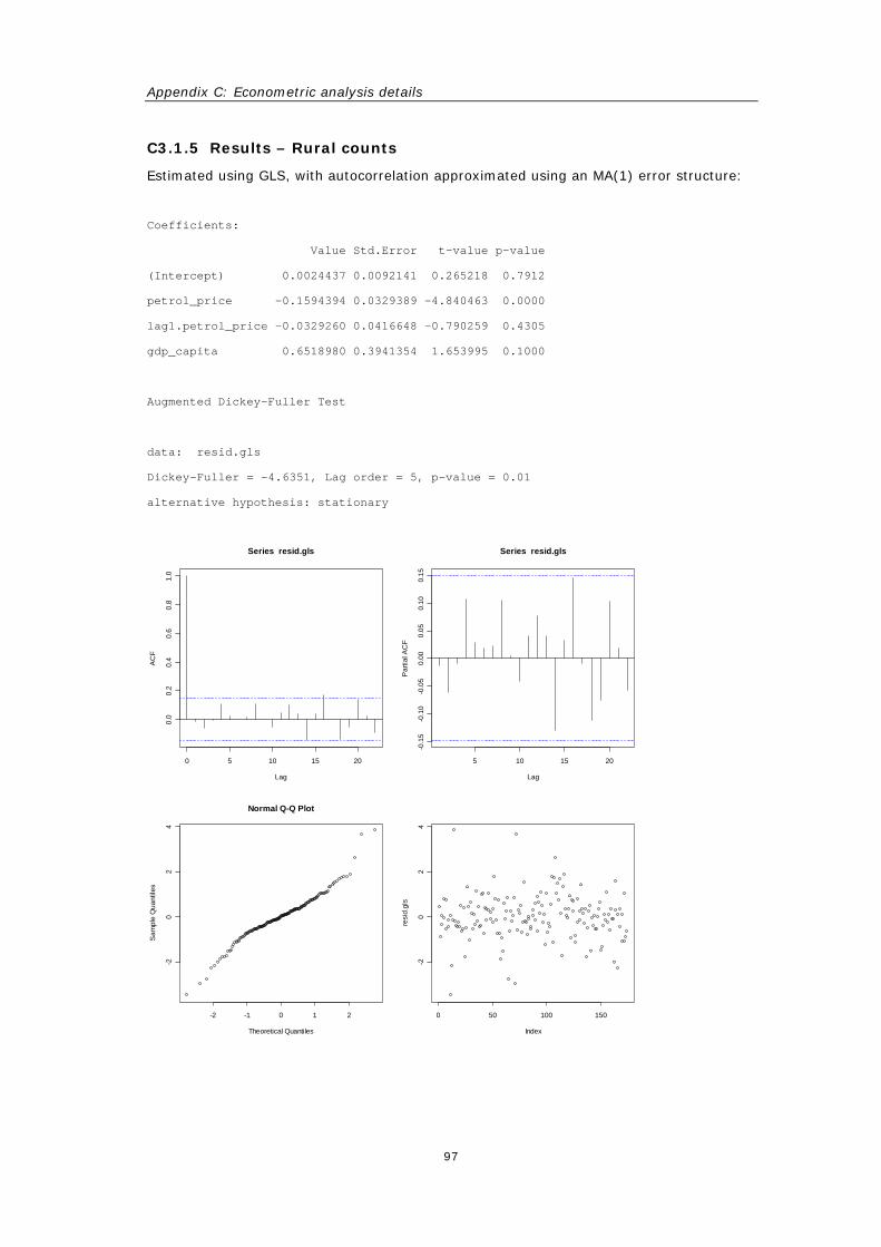
Appendix C: Econometric analysis details
97
C3.1.5 Results – Rural counts
Estimated using GLS, with autocorrelation approximated using an MA(1) error structure:
Coefficients:
Value Std.Error t-value p-value
(Intercept) 0.0024437 0.0092141 0.265218 0.7912
petrol_price -0.1594394 0.0329389 -4.840463 0.0000
lag1.petrol_price -0.0329260 0.0416648 -0.790259 0.4305
gdp_capita 0.6518980 0.3941354 1.653995 0.1000
Augmented Dickey-Fuller Test
data: resid.gls
Dickey-Fuller = -4.6351, Lag order = 5, p-value = 0.01
alternative hypothesis: stationary
0 5 10 15 20
0.0
0.2
0.4
0.6
0.8
1.0
Lag
AC
F
Series resid.gls
5 10 15 20
-0.1
5-0
.10
-0.0
50.
000.
050.
100.
15
Lag
Par
tial A
CF
Series resid.gls
-2 -1 0 1 2
-20
24
Normal Q-Q Plot
Theoretical Quantiles
Sam
ple
Qua
ntile
s
0 50 100 150
-20
24
Index
resi
d.gl
s
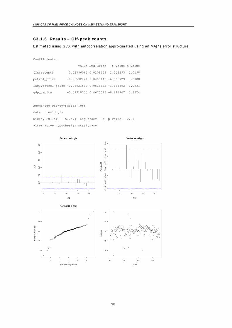
IMPACTS OF FUEL PRICE CHANGES ON NEW ZEALAND TRANSPORT
98
C3.1.6 Results – Off-peak counts
Estimated using GLS, with autocorrelation approximated using an MA(4) error structure:
Coefficients:
Value Std.Error t-value p-value
(Intercept) 0.02556063 0.0108663 2.352293 0.0198
petrol_price -0.26592421 0.0405142 -6.563729 0.0000
lag1.petrol_price -0.08921539 0.0528342 -1.688592 0.0931
gdp_capita -0.09910733 0.4675593 -0.211967 0.8324
Augmented Dickey-Fuller Test
data: resid.gls
Dickey-Fuller = -5.2574, Lag order = 5, p-value = 0.01
alternative hypothesis: stationary
0 5 10 15 20
0.0
0.2
0.4
0.6
0.8
1.0
Lag
AC
F
Series resid.gls
5 10 15 20
-0.1
5-0
.10
-0.0
50.
000.
050.
100.
150.
20
Lag
Par
tial A
CF
Series resid.gls
-2 -1 0 1 2
-4-2
02
4
Normal Q-Q Plot
Theoretical Quantiles
Sam
ple
Qua
ntile
s
0 50 100 150
-4-2
02
4
Index
resi
d.gl
s
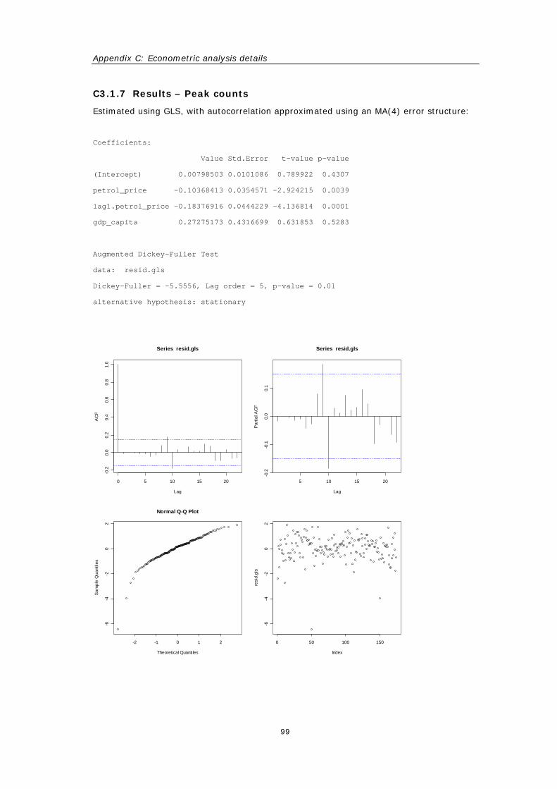
Appendix C: Econometric analysis details
99
C3.1.7 Results – Peak counts
Estimated using GLS, with autocorrelation approximated using an MA(4) error structure:
Coefficients:
Value Std.Error t-value p-value
(Intercept) 0.00798503 0.0101086 0.789922 0.4307
petrol_price -0.10368413 0.0354571 -2.924215 0.0039
lag1.petrol_price -0.18376916 0.0444229 -4.136814 0.0001
gdp_capita 0.27275173 0.4316699 0.631853 0.5283
Augmented Dickey-Fuller Test
data: resid.gls
Dickey-Fuller = -5.5556, Lag order = 5, p-value = 0.01
alternative hypothesis: stationary
0 5 10 15 20
-0.2
0.0
0.2
0.4
0.6
0.8
1.0
Lag
AC
F
Series resid.gls
5 10 15 20
-0.2
-0.1
0.0
0.1
Lag
Par
tial A
CF
Series resid.gls
-2 -1 0 1 2
-6-4
-20
2
Normal Q-Q Plot
Theoretical Quantiles
Sam
ple
Qua
ntile
s
0 50 100 150
-6-4
-20
2
Index
resi
d.gl
s
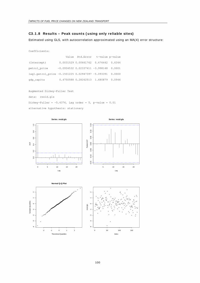
IMPACTS OF FUEL PRICE CHANGES ON NEW ZEALAND TRANSPORT
100
C3.1.8 Results – Peak counts (using only reliable sites)
Estimated using GLS, with autocorrelation approximated using an MA(4) error structure:
Coefficients:
Value Std.Error t-value p-value
(Intercept) 0.0031529 0.00661762 0.476442 0.6344
petrol_price -0.0934532 0.02337411 -3.998148 0.0001
lag1.petrol_price -0.1501225 0.02947397 -5.093391 0.0000
gdp_capita 0.4750588 0.28262513 1.680879 0.0946
Augmented Dickey-Fuller Test
data: resid.gls
Dickey-Fuller = -5.4376, Lag order = 5, p-value = 0.01
alternative hypothesis: stationary
0 5 10 15 20
0.0
0.2
0.4
0.6
0.8
1.0
Lag
AC
F
Series resid.gls
5 10 15 20
-0.1
5-0
.10
-0.0
50.
000.
050.
100.
15
Lag
Par
tial A
CF
Series resid.gls
-2 -1 0 1 2
-4-3
-2-1
01
2
Normal Q-Q Plot
Theoretical Quantiles
Sam
ple
Qua
ntile
s
0 50 100 150
-4-3
-2-1
01
2
Index
resi
d.gl
s
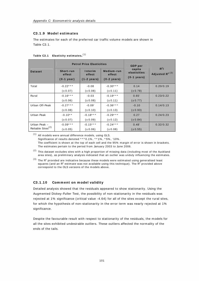
Appendix C: Econometric analysis details
101
C3.1.9 Model estimates
The estimates for each of the preferred car traffic volume models are shown in
Table C3.1.
Table C3.1 Elasticity estimates.(1)
Petrol Price Elasticities
Dataset Short-run effect
(0-1 year)
Interim effect
(1-2 years)
Medium-run effect
(0-2 years)
GDP per capita
elasticities
(0-1 years)
R2/
Adjusted R2 (3)
Total -0.22***
(±0.07)
-0.08
(±0.08)
-0.30***
(±0.11)
0.14
(±0.78)
0.20/0.19
Rural -0.16***
(±0.06)
-0.03
(±0.08)
-0.19***
(±0.11)
0.65’
(±0.77)
0.23/0.22
Urban Off-Peak -0.27***
(±0.08)
-0.09’
(±0.10)
-0.36***
(±0.13)
-0.10
(±0.93)
0.14/0.13
Urban Peak -0.10**
(±0.07)
-0.18***
(±0.09)
-0.29***
(±0.12)
0.27
(±0.84)
0.24/0.23
Urban Peak – Reliable Sites(2)
-0.09***
(±0.05)
-0.15***
(±0.06)
-0.24***
(±0.08)
0.48’
(±0.55)
0.32/0.32
(1) All models were annual difference models, using GLS. Significance of results denoted ***0.1%, **1%, *5%, ‘10%. The coefficient is shown at the top of each cell and the 95% margin of error is shown in brackets. The estimates pertain to the period from January 2003 to June 2006.
(2) This dataset excludes sites with a high proportion of missing data (including most of the Auckland area sites), as preliminary analysis indicated that an outlier was unduly influencing the estimates.
(3) The R2 provided are indicative because these models were estimated using generalised least squares (and an R2 estimate was not available using this technique). The R2 provided above correspond to the OLS versions of the models above.
C3.1.10 Comment on model validity
Detailed analysis showed that the residuals appeared to show stationarity. Using the
Augmented Dickey-Fuller Test, the possibility of non-stationarity in the residuals was
rejected at 1% significance (critical value -4.64) for all of the sites except the rural sites,
for which the hypothesis of non-stationarity in the error term was nearly rejected at 1%
significance.
Despite the favourable result with respect to stationarity of the residuals, the models for
all the sites exhibited undesirable outliers. These outliers affected the normality of the
ends of the tails.
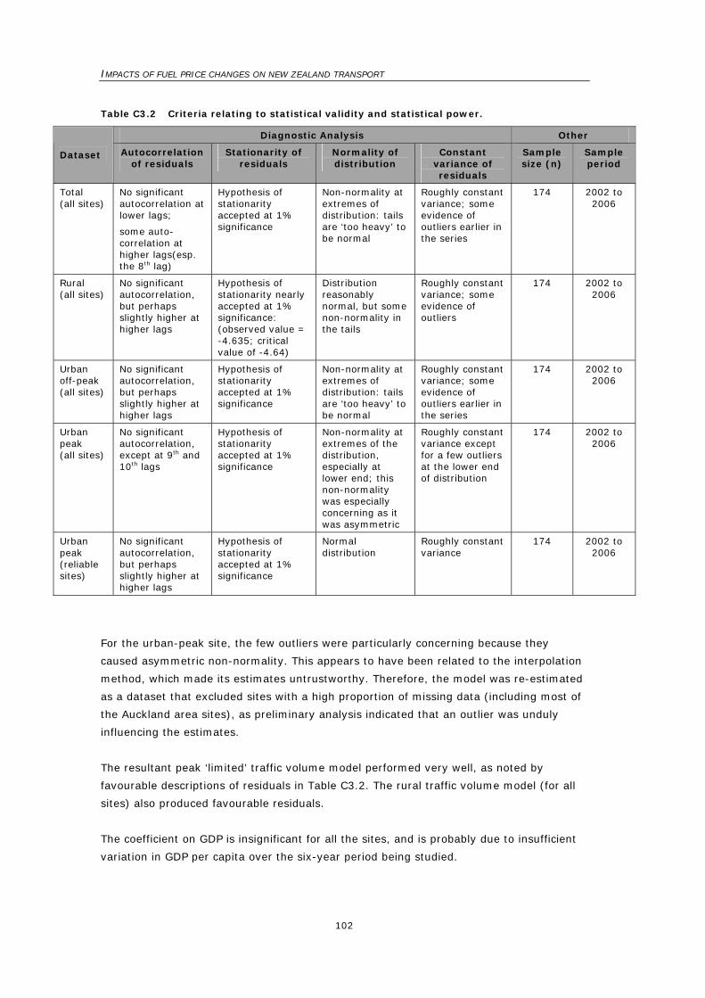
IMPACTS OF FUEL PRICE CHANGES ON NEW ZEALAND TRANSPORT
102
Table C3.2 Criteria relating to statistical validity and statistical power.
Diagnostic Analysis Other
Dataset Autocorrelation of residuals
Stationarity of residuals
Normality of distribution
Constant variance of residuals
Sample size (n)
Sample period
Total (all sites)
No significant autocorrelation at lower lags;
some auto-correlation at higher lags(esp. the 8th lag)
Hypothesis of stationarity accepted at 1% significance
Non-normality at extremes of distribution: tails are ‘too heavy’ to be normal
Roughly constant variance; some evidence of outliers earlier in the series
174 2002 to 2006
Rural (all sites)
No significant autocorrelation, but perhaps slightly higher at higher lags
Hypothesis of stationarity nearly accepted at 1% significance: (observed value = -4.635; critical value of -4.64)
Distribution reasonably normal, but some non-normality in the tails
Roughly constant variance; some evidence of outliers
174 2002 to 2006
Urban off-peak (all sites)
No significant autocorrelation, but perhaps slightly higher at higher lags
Hypothesis of stationarity accepted at 1% significance
Non-normality at extremes of distribution: tails are ‘too heavy’ to be normal
Roughly constant variance; some evidence of outliers earlier in the series
174 2002 to 2006
Urban peak (all sites)
No significant autocorrelation, except at 9th and 10th lags
Hypothesis of stationarity accepted at 1% significance
Non-normality at extremes of the distribution, especially at lower end; this non-normality was especially concerning as it was asymmetric
Roughly constant variance except for a few outliers at the lower end of distribution
174 2002 to 2006
Urban peak (reliable sites)
No significant autocorrelation, but perhaps slightly higher at higher lags
Hypothesis of stationarity accepted at 1% significance
Normal distribution
Roughly constant variance
174 2002 to 2006
For the urban-peak site, the few outliers were particularly concerning because they
caused asymmetric non-normality. This appears to have been related to the interpolation
method, which made its estimates untrustworthy. Therefore, the model was re-estimated
as a dataset that excluded sites with a high proportion of missing data (including most of
the Auckland area sites), as preliminary analysis indicated that an outlier was unduly
influencing the estimates.
The resultant peak ‘limited’ traffic volume model performed very well, as noted by
favourable descriptions of residuals in Table C3.2. The rural traffic volume model (for all
sites) also produced favourable residuals.
The coefficient on GDP is insignificant for all the sites, and is probably due to insufficient
variation in GDP per capita over the six-year period being studied.
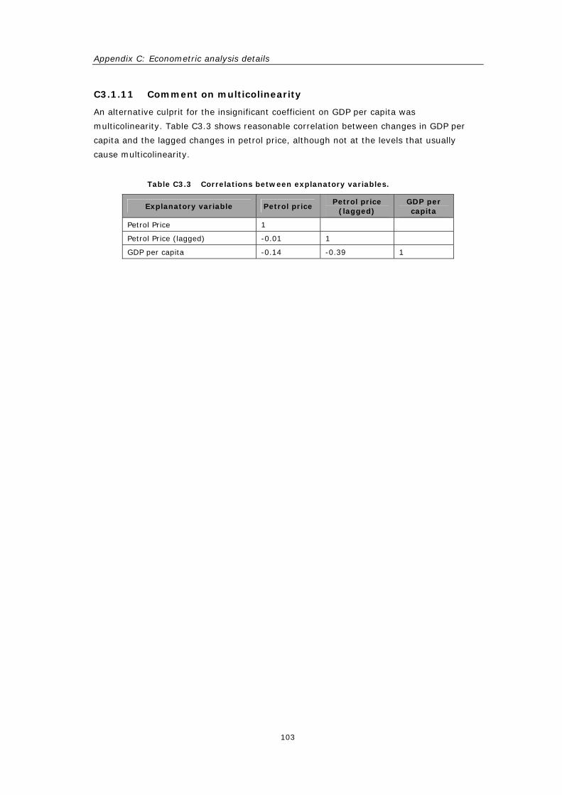
Appendix C: Econometric analysis details
103
C3.1.11 Comment on multicolinearity
An alternative culprit for the insignificant coefficient on GDP per capita was
multicolinearity. Table C3.3 shows reasonable correlation between changes in GDP per
capita and the lagged changes in petrol price, although not at the levels that usually
cause multicolinearity.
Table C3.3 Correlations between explanatory variables.
Explanatory variable Petrol price Petrol price
(lagged) GDP per capita
Petrol Price 1
Petrol Price (lagged) -0.01 1
GDP per capita -0.14 -0.39 1
IMPACTS OF FUEL PRICE CHANGES ON NEW ZEALAND TRANSPORT
104
C4 Public transport cross-elasticities
C4.1 Wellington Bus Patronage – Four-quarter annual differences
C4.1.1 Introduction
The preliminary phase of analysis included time-series analysis of recent patronage data;
this data consisted of patronage from 25 July 1999 to 28 May 2006.
This preliminary analysis produced plausible estimates for the cross-price elasticity of
demand, but these estimates were not significant. Furthermore, the sign of the fare
elasticity was counter-intuitive and the model appeared to exhibit negative
autocorrelation.
These problems prompted the development of a longer time series that incorporated
patronage data from a previous Booz Allen Hamilton study (BAH 2001).
C4.1.2 Data sources
The data sources used for this analysis consisted of the following:
• StageCoach Wellington patronage and revenue time series data:
– The first tranch of data had been provided to BAH for the Wellington Fares Study in
June 2001. This data was provided by StageCoach and consisted of weekly
patronage and revenue across Wellington city routes, from 5 January 1997 to 30
December 2002.
– The second tranch of time-series data was recently provided to BAH by
StageCoach. The data was presented in 4-weekly accounting periods, from 25 July
1999 to 28 May 2006, and consisted of patronage and revenue across Wellington
city routes.
• The Wellington City (territorial authority) population estimates as at 30 June, from
1996 to 2005 on an annual basis, provided by SNZ. The population for 30 June 2006
was forecast based on the assumption that growth would occur at the same rate as
occurred between 30 June 2004 to 30 June 2005. The population was then
interpolated to produce a quarterly series from March 1997 to June 2006.
• The national CPI from the March 1997 quarter to the June 2006 quarter, on a quarterly
basis, provided by SNZ (and obtained via the Reserve Bank of New Zealand).
• The national CPI petrol price index, from the March 1997 quarter to the June 2006
quarter, on a quarterly basis, provided by SNZ. The petrol price index measures price
change of 91 octane petrol, 96 octane petrol and petrol additive, which are then
averaged across each quarter.
Appendix C: Econometric analysis details
105
• The national GDP from the March 1997 quarter to the March 2006 quarter, on a
quarterly basis, provided by SNZ. The ANZ Quarterly Economic Forecasts for June
2006 were used to forecast GDP for the June 2006 quarter.
• The national population estimates from the March 1997 quarter to the March 2006
quarter on a quarterly basis, provided by SNZ. The national population for the June
2006 was projected using past growth rates.14
C4.1.3 Data manipulation
The patronage data was manipulated to create quarterly variables for time series analysis
of the period from March 1997 to June 2006:
• The first tranch of patronage and revenue data was transformed from weekly to
quarterly data. Weeks of data were assigned to the quarter that encompassed them.
Weeks of data that overlapped across quarters was assigned pro rata, based on the
number of days of the week that fell into each quarter.
• The second tranch of patronage and revenue data was transformed from 4-weekly to
quarterly data. Similarly to above, 4-week periods were assigned to the quarter that
encompassed them, and overlapping 4-week periods were assigned on a pro rata
basis.
• The quarterly patronage data was then adjusted to create two measures of patronage:
– The ‘trips per day, per quarter’ measure was calculated by taking quarterly
patronage and dividing by the number of days in each quarter to produce a trips
per day figure.
– The ‘trips per day, per quarter, per Wellington resident’ was calculated by taking
the figure above and dividing by the estimated number of Wellington residents.
The other variables were also manipulated to create variables of interest:
• The revenue and patronage data was used to create an average nominal fare from
March 1997 to December 1999. A separate average nominal fare was created for
March 2000 because fares changed in this period. An average nominal fare was then
calculated from June 2000 to March 2006.
• Both the average nominal fare and the petrol price index were deflated, using the CPI,
to create average real fare and a real petrol price index.
• In addition, the real petrol price index was re-scaled so that the level of the real petrol
price index in the June 2006 quarter was equivalent to the price of regular petrol as at
30 June 2006. This was done to enable easier interpretation of log-lin models.
C4.1.4 Model
A four-quarter annual differences model was estimated. The model was estimated in a
similar fashion to the four-quarter annual differences model for petrol consumption;
14 The forecast growth from March 2006 to June 2006 was assumed to be the same as the average
growth rate at the same time for the past three years (i.e. the average of growth from March 2003 to June 2003, from March 2004 to June 2004, and from March 2005 to June 2005 was calculated).

IMPACTS OF FUEL PRICE CHANGES ON NEW ZEALAND TRANSPORT
106
however, additional lags of petrol prices were included because these were found to be
significant. The model was fitted using GLS.
C4.1.5 Results
A GLS model was estimated, with autocorrelation approximated using an AR(4) error
structure:
Coefficients:
Value Std.Error t-value p-value
(Intercept) -0.01194226 0.00634541 -1.882033 0.0794
petrol_index 0.16251779 0.02528016 6.428670 0.0000
lag1.petrol_index 0.21079527 0.02994290 7.039908 0.0000
lag2.petrol_index 0.17478838 0.01817554 9.616680 0.0000
lag3.petrol_index 0.06500649 0.02505406 2.594649 0.0203
gdp_capita 0.23274742 0.22922344 1.015374 0.3260
Augmented Dickey-Fuller Test
data: resid.gls
Dickey-Fuller = -2.4375, Lag order = 2, p-value = 0.4057
alternative hypothesis: stationary
0 2 4 6 8 10 12
-0.4
-0.2
0.0
0.2
0.4
0.6
0.8
1.0
Lag
AC
F
Series resid.gls
2 4 6 8 10 12
-0.4
-0.2
0.0
0.2
0.4
Lag
Par
tial A
CF
Series resid.gls
-2 -1 0 1 2
-1.5
-1.0
-0.5
0.0
0.5
1.0
1.5
2.0
Normal Q-Q Plot
Theoretical Quantiles
Sam
ple
Qua
ntile
s
5 10 15 20
-1.5
-1.0
-0.5
0.0
0.5
1.0
1.5
2.0
Index
resi
d.gl
s
Appendix C: Econometric analysis details
107
C4.1.6 Comment on model validity
• This model was not considered to be statistically robust. Most importantly, a risk of
spurious regression could not be discounted. Also the Augmented Dickey-Fuller test
shows that the possibility of non-stationarity in the residuals could not be dismissed.
• In addition, the model failed on other criteria for good econometric modelling.
• The ACF plot is satisfactory because it fails to detect autocorrelation. However the
PACF plot suggests that residuals are negatively autocorrelated; this autocorrelation
was not eliminated through the use of the GLS technique.
• The Q-Q plot shows that the residuals distributed in a non-normal manner, with too
much weight distributed close to zero.
• The variance of the residuals appears to increase slightly with time in the plot of
residuals against time, although this is not a definitive pattern.
C4.2 Christchurch bus patronage – Four-quarter annual differences
C4.2.1 Data sources
The data sources used for this analysis consisted of the following:
• Environment Canterbury patronage data.
• The national CPI from the September 1992 quarter to the June 2006 quarter, on a
quarterly basis, provided by SNZ (and obtained via the Reserve Bank of New Zealand).
• The national CPI petrol price index, from the September 1992 quarter to the June
2006 quarter, on a quarterly basis, provided by SNZ. The petrol price index measures
price change of 91 octane petrol, 96 octane petrol and petrol additive, which are then
averaged across each quarter.
• The national GDP from the September 1992 quarter to the March 2006 quarter, on a
quarterly basis, provided by SNZ. The ANZ Quarterly Economic Forecasts for June
2006 were used to forecast GDP for the June 2006 quarter.
• The national population estimates from the September 1992 quarter to the March
2006 quarter, on a quarterly basis, provided by SNZ. The national population for the
June 2006 was projected using past growth rates.15.
• The Christchurch City (territorial authority) resident population estimates. These
consisted of two series, both of which were obtained from the Christchurch City
Council website16 but were originally sourced from SNZ:
15 The forecast growth from March 2006 to June 2006 was assumed to be the same as the average
growth rate at the same time for the past three years (i.e. the average of growth from March 2003 to June 2003, from March 2004 to June 2004, and from March 2005 to June 2005 was calculated).
16 http://www.ccc.govt.nz/Christchurch/FactsStatsAndFigures/
IMPACTS OF FUEL PRICE CHANGES ON NEW ZEALAND TRANSPORT
108
– The first series were estimates excluding census undercount adjustment, as at 30
June, from 1986 to 1995.
– The second series were estimates including undercount adjustment, as at 30 June,
from 1996 to 2005. The population for 30 June 2006 was forecast based on the
assumption that growth would occur at the same rate as occurred between 30 June
2004 to 30 June 2005.
– The two series could not, prima facie, be applied together because the inclusion of
undercounts would have contributed to a spurious jump in population from 1995 to
1996. To redress this, it was assumed that the growth in population from 1995 to
1996 would have been equal to the average of growth from 1994 to 1995 and 1996
to 1997.
C4.2.2 Data manipulation
The quarterly patronage data was adjusted to create two measures of patronage:
• The ‘trips per day, per quarter’ measure was calculated by taking quarterly patronage
and dividing by the number of days in each quarter to produce a trips per day figure.
• The ‘trips per day, per quarter, per Christchurch resident’ was calculated by taking this
figure and dividing it by the estimated number of Christchurch residents.
Other variables were also manipulated to create variables of interest:
• The revenue and patronage data were used to create an average nominal fare from
September 1992 to December 1999. A separate average nominal fare was created for
March 2000 because fares changed during this period. An average nominal fare was
then calculated from June 2000 to March 2006.
• Both the average nominal fare and the petrol price index were deflated, using the CPI,
to create average real fare and a real petrol price index.
• In addition, the real petrol price index was re-scaled so that the level of the real petrol
price index in the June 2006 quarter was equivalent to the price of regular petrol as at
30 June 2006. This was done to enable easier interpretation of log-lin models.
C4.2.3 Model
A four-quarter annual differences model was estimated. The model was estimated in a
similar fashion to the four-quarter annual differences model for petrol consumption.
However, additional lags of petrol prices were included because these were found to be
significant. The model was fitted using GLS.
C4.2.4 Results
A GLS model was estimated, with autocorrelation approximated using an AR(4) error
structure:

Appendix C: Econometric analysis details
109
Coefficients:
Value Std.Error t-value p-value
(Intercept) 0.0247903 0.0185769 1.3344662 0.1898
petrol_index -0.0027489 0.0617919 -0.0444858 0.9647
lag1.petrol_index 0.1273856 0.0683897 1.8626421 0.0701
lag2.petrol_index 0.1318747 0.0644820 2.0451379 0.0476
gdp_capita 0.8902046 0.3870149 2.3001820 0.0269
Augmented Dickey-Fuller Test
data: resid.gls
Dickey-Fuller = -3.072, Lag order = 3, p-value = 0.1494
alternative hypothesis: stationary
0 5 10 15
-0.2
0.0
0.2
0.4
0.6
0.8
1.0
Lag
AC
F
Series resid.gls
5 10 15
-0.3
-0.2
-0.1
0.0
0.1
0.2
0.3
Lag
Par
tial A
CF
Series resid.gls
-2 -1 0 1 2
-2-1
01
2
Normal Q-Q Plot
Theoretical Quantiles
Sam
ple
Qua
ntile
s
0 10 20 30 40
-2-1
01
2
Index
resi
d.gl
s
C4.2.5 Comment on model validity
The residuals were favourable (excluding the risk of non-stationarity discussed below).
The ACF and PACF failed to detect autocorrelation. The Q-Q plot shows a straight line,
consistent with normality. And the plot of residuals against time failed to exhibit any
trends through time (as was desired).

IMPACTS OF FUEL PRICE CHANGES ON NEW ZEALAND TRANSPORT
110
The main problem was that the possibility of spurious estimates could not be disregarded;
also the possibility of non-stationarity in the residuals could not be rejected by the
Augmented Dickey-Fuller Test (although the risk was not as high as observed in the
Wellington patronage analysis).
In addition, all the estimates are insignificant, except for GDP per capita and the last lag
of the petrol price index. This suggests that the model is failing to explain much, and this
failure is perhaps due to the omission of important variables (i.e. improvements in route
services in Christchurch over the time period being studied).
Appendix D: Review of previous literature
111
Appendix D: Review of previous research
Summaries of the literature pertaining to research on effects of transport fuel price
changes that have been published are provided in the following tables:
D1 Petrol consumption elasticities D2 Traffic volume elasticities D3 Public transport cross-elasticities
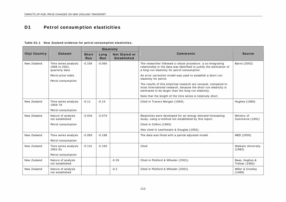
IMPACTS OF FUEL PRICE CHANGES ON NEW ZEALAND TRANSPORT
112
D1 Petrol consumption elasticities
Table D1.1 New Zealand evidence for petrol consumption elasticities.
Elasticity City/Country Dataset Short
Run Long Run
Not Stated or Established
Comments Source
New Zealand Time series analysis: 1989 to 2001, quarterly data
Petrol price index
Petrol consumption
-0.195 -0.065 The researcher followed a robust procedure: a co-integrating relationship in the data was identified to justify the estimation of a long-run elasticity for petrol consumption.
An error correction model was used to establish a short-run elasticity for petrol.
The results of this empirical research are unusual, compared to most international research, because the short-run elasticity is estimated to be larger than the long-run elasticity.
Note that the length of the time series is relatively short.
Barns (2002)
New Zealand Time series analysis: 1969-79
Petrol consumption
-0.11 -0.14 Cited in Travers Morgan (1993). Hughes (1980)
New Zealand Nature of analysis not established
Petrol consumption
-0.034 -0.074 Elasticities were developed for an energy demand forecasting study, using a method not established by this report.
Cited in Collins (1993).
Also cited in Lewthwaite & Douglas (1992).
Ministry of Commerce (1991)
New Zealand Time series analysis
Petrol consumption
-0.065 -0.188 The data was fitted with a partial adjusted model. MED (2000)
New Zealand Time series analysis: 1961-81
Petrol consumption
-0.131 -0.160 Cited Waikato University (1982)
New Zealand Nature of analysis not established
-0.26 Cited in Pickford & Wheeler (2001). Baas, Hughes & Treloar (1982)
New Zealand Nature of analysis not established
-0.2 Cited in Pickford & Wheeler (2001). Miller & Crowley (1989)

Appendix D: Review of previous literature
113
Table D1.1 New Zealand evidence for petrol consumption elasticities.
Elasticity City/Country Dataset Short
Run Long Run
Not Stated or Established
Comments Source
New Zealand Simple analysis of price shock: 1990
-0.2* The researchers noted that a rise in price from 92 cents to 109 cents caused consumption to remain static when it would otherwise have been expected to grow by 4%. On this basis they deduce an elasticity of -0.2.
However, this report notes that some of the impact of the price shock on consumption may have also have been indirect, via a dampening of GDP.
* This elasticity represents a log-lin relationship (i.e. the impact of a 1 cent price rise on the percentage growth in consumption) but since the price is approximately 100 cents this can be interpreted as a similar unit to the other elasticities in this table.
WCS (1991)
New Zealand Simple analysis of price shock: 1971-1976
Petrol consumption
-0.105 Cited in Collins (1993).
A simple demand model was fitted to explain the impact of the 50% rise in real petrol prices, between June 1971 and March 1976.
NZERDC (1977)
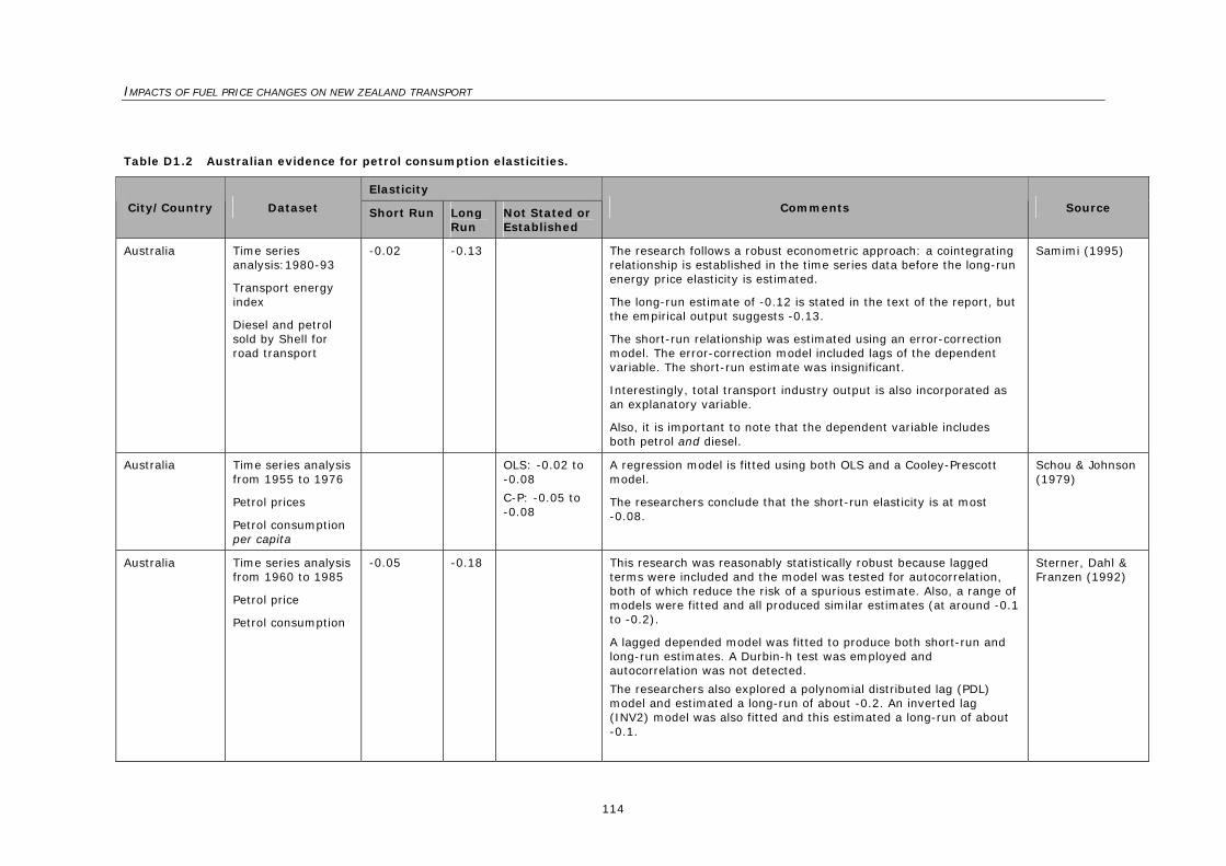
IMPACTS OF FUEL PRICE CHANGES ON NEW ZEALAND TRANSPORT
114
Table D1.2 Australian evidence for petrol consumption elasticities.
Elasticity
City/Country Dataset Short Run Long Run
Not Stated or Established
Comments Source
Australia Time series analysis:1980-93
Transport energy index
Diesel and petrol sold by Shell for road transport
-0.02 -0.13 The research follows a robust econometric approach: a cointegrating relationship is established in the time series data before the long-run energy price elasticity is estimated.
The long-run estimate of -0.12 is stated in the text of the report, but the empirical output suggests -0.13.
The short-run relationship was estimated using an error-correction model. The error-correction model included lags of the dependent variable. The short-run estimate was insignificant.
Interestingly, total transport industry output is also incorporated as an explanatory variable.
Also, it is important to note that the dependent variable includes both petrol and diesel.
Samimi (1995)
Australia Time series analysis from 1955 to 1976
Petrol prices
Petrol consumption per capita
OLS: -0.02 to -0.08
C-P: -0.05 to -0.08
A regression model is fitted using both OLS and a Cooley-Prescott model.
The researchers conclude that the short-run elasticity is at most -0.08.
Schou & Johnson (1979)
Australia Time series analysis from 1960 to 1985
Petrol price
Petrol consumption
-0.05 -0.18 This research was reasonably statistically robust because lagged terms were included and the model was tested for autocorrelation, both of which reduce the risk of a spurious estimate. Also, a range of models were fitted and all produced similar estimates (at around -0.1 to -0.2).
A lagged depended model was fitted to produce both short-run and long-run estimates. A Durbin-h test was employed and autocorrelation was not detected.
The researchers also explored a polynomial distributed lag (PDL) model and estimated a long-run of about -0.2. An inverted lag (INV2) model was also fitted and this estimated a long-run of about -0.1.
Sterner, Dahl & Franzen (1992)
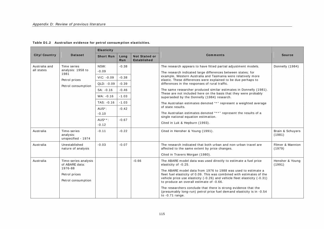
Appendix D: Review of previous literature
115
Table D1.2 Australian evidence for petrol consumption elasticities.
Elasticity
City/Country Dataset Short Run Long Run
Not Stated or Established
Comments Source
NSW:
-0.09
-0.38
VIC: -0.09 -0.38
QLD: -0.09 -0.39
SA: -0.16 -0.46
WA: -0.16 -1.03
TAS: -0.16 -1.03
AUS*:
-0.10
-0.42
Australia and all states
Time series analysis: 1958 to 1981
Petrol prices
Petrol consumption
AUS**:
-0.12
-0.67
The research appears to have fitted partial adjustment models.
The research indicated large differences between states; for example, Western Australia and Tasmania were relatively more elastic. These differences were explained to be due perhaps to differences in the responses of rural traffic.
The same researcher produced similar estimates in Donnelly (1981). These are not included here on the basis that they were probably superseded by the Donnelly (1984) research.
The Australian estimates denoted “*” represent a weighted average of state results.
The Australian estimates denoted “**” represent the results of a single national equation estimation.
Cited in Luk & Hepburn (1993).
Donnelly (1984)
Australia Time-series analysis: unspecified - 1974
-0.11 -0.22 Cited in Hensher & Young (1991). Brain & Schuyers (1981)
Australia Unestablished nature of analysis
-0.03 -0.07 The research indicated that both urban and non-urban travel are affected to the same extent by price changes.
Cited in Travers Morgan (1980).
Filmer & Mannion (1979)
Australia Time-series analysis of ABARE data: 1976-88
Petrol prices
Petrol consumption
-0.66 The ABARE model data was used directly to estimate a fuel price elasticity of -0.25.
The ABARE model data from 1976 to 1988 was used to estimate a fleet fuel elasticity of 0.09. This was combined with estimates of the vehicle price use elasticity (-0.26) and vehicle fleet elasticity (-0.31) to produce an overall estimate of -0.66.
The researchers conclude that there is strong evidence that the (presumably long-run) petrol price fuel demand elasticity is in -0.54 to -0.71 range.
Hensher & Young (1991)
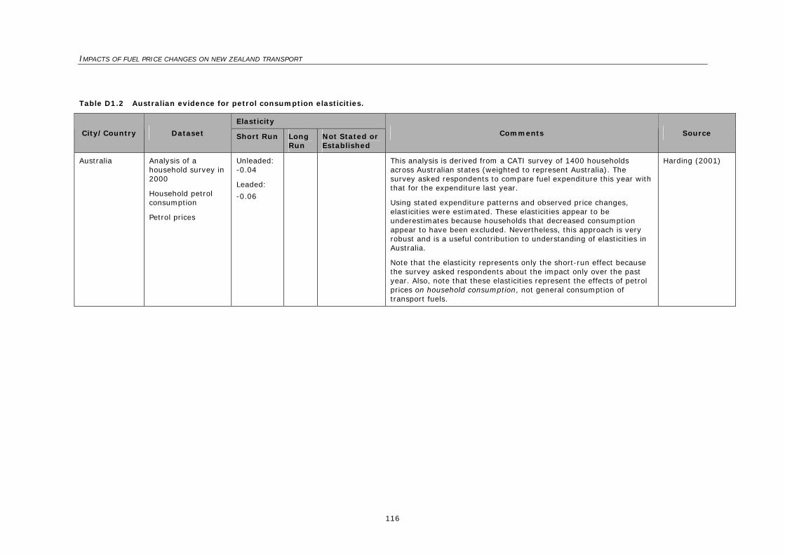
IMPACTS OF FUEL PRICE CHANGES ON NEW ZEALAND TRANSPORT
116
Table D1.2 Australian evidence for petrol consumption elasticities.
Elasticity
City/Country Dataset Short Run Long Run
Not Stated or Established
Comments Source
Australia Analysis of a household survey in 2000
Household petrol consumption
Petrol prices
Unleaded: -0.04
Leaded:
-0.06
This analysis is derived from a CATI survey of 1400 households across Australian states (weighted to represent Australia). The survey asked respondents to compare fuel expenditure this year with that for the expenditure last year.
Using stated expenditure patterns and observed price changes, elasticities were estimated. These elasticities appear to be underestimates because households that decreased consumption appear to have been excluded. Nevertheless, this approach is very robust and is a useful contribution to understanding of elasticities in Australia.
Note that the elasticity represents only the short-run effect because the survey asked respondents about the impact only over the past year. Also, note that these elasticities represent the effects of petrol prices on household consumption, not general consumption of transport fuels.
Harding (2001)

Appendix D: Review of previous literature
117
Table D1.3 International evidence for petrol consumption elasticities.
Elasticity
City/Country Study Type and
Period Short Run
Long Run
Comments Source
All countries Meta-analysis
Petrol and diesel consumption
-0.25 -0.6 Hanly et al. (2002) & Goodwin et al. (2004) conducted a meta-analysis of (both petrol and diesel) fuel price elasticities, and estimated that: - the short-run fuel price elasticity is -0.25;
- the long-run elasticity is around -0.6.
Hanly, Dargay & Goodwin (2002)
Goodwin, Dargay & Hanly (2004)
All countries Literature review
Petrol consumption
-0.2 to
-0.3
-0.6 to
-0.8
Graham & Glaister (2004, 2002) surveyed the international demand literature, with the intention of assessing the magnitude of (petrol only) fuel demand elasticities as reported in the literature, and: - concluded that the average fuel-price elasticity
is in the range of -0.2 to -0.3; - reported that long-run (petrol only) fuel price
elasticity estimates typically fall in the -0.6 to -0.8 band.
They also reviewed a range of cointegration models; most of these models produce short-run estimates less than those generally observed in the literature: and in the range -0.21 to -0.37.
Graham & Glaister (2004, 2002)
All countries Literature review
Petrol consumption
-0.25 -0.58 Espey (1998) carried out a meta-analysis of the literature, and estimated that:
- the short-run (petrol only) fuel-price elasticity was -0.25 on average, with a median elasticity of -0.23;
- the long-run (petrol only) fuel-price elasticity was -0.58 on average, with a median elasticity of -0.43.
Espey (1998)
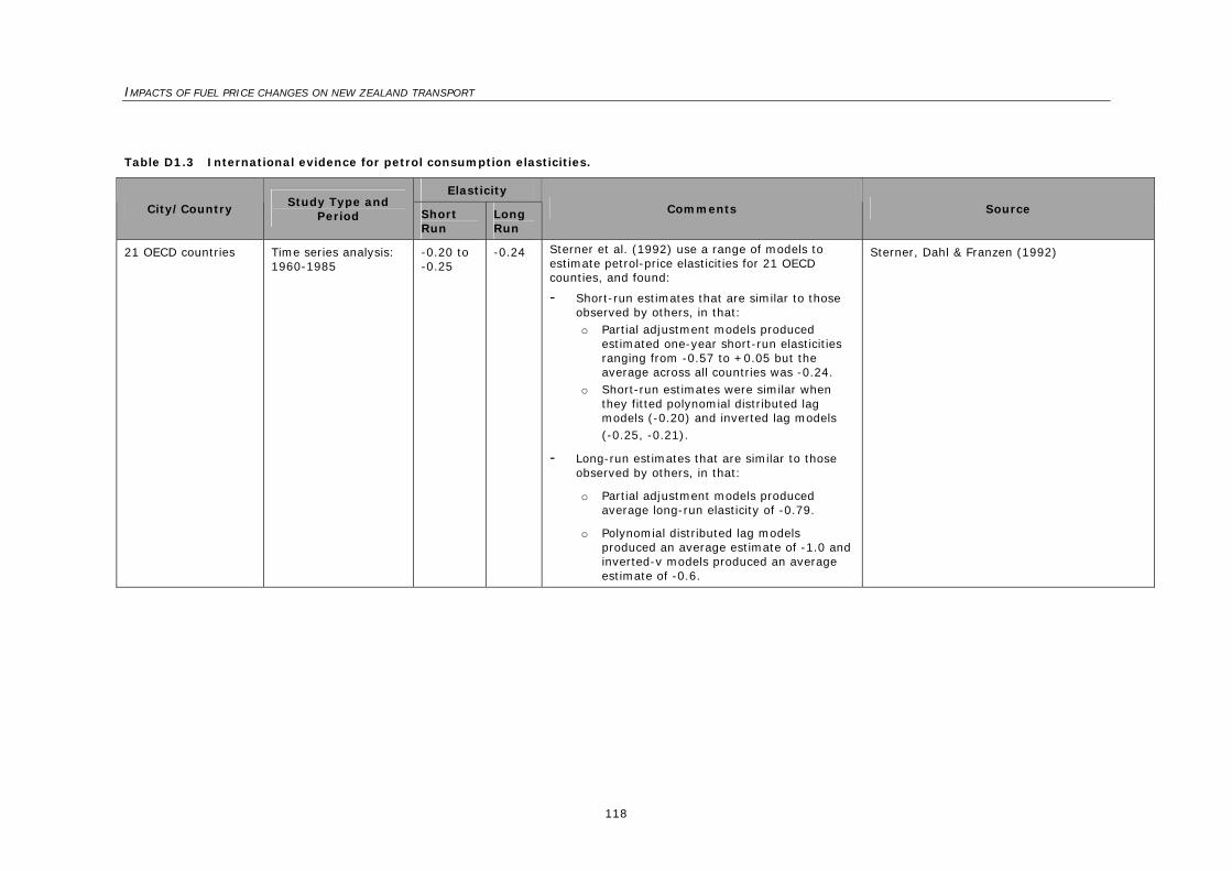
IMPACTS OF FUEL PRICE CHANGES ON NEW ZEALAND TRANSPORT
118
Table D1.3 International evidence for petrol consumption elasticities.
Elasticity
City/Country Study Type and
Period Short Run
Long Run
Comments Source
21 OECD countries Time series analysis: 1960-1985
-0.20 to -0.25
-0.24 Sterner et al. (1992) use a range of models to estimate petrol-price elasticities for 21 OECD counties, and found:
- Short-run estimates that are similar to those observed by others, in that: o Partial adjustment models produced
estimated one-year short-run elasticities ranging from -0.57 to +0.05 but the average across all countries was -0.24.
o Short-run estimates were similar when they fitted polynomial distributed lag models (-0.20) and inverted lag models
(-0.25, -0.21).
- Long-run estimates that are similar to those observed by others, in that:
o Partial adjustment models produced average long-run elasticity of -0.79.
o Polynomial distributed lag models produced an average estimate of -1.0 and inverted-v models produced an average estimate of -0.6.
Sterner, Dahl & Franzen (1992)
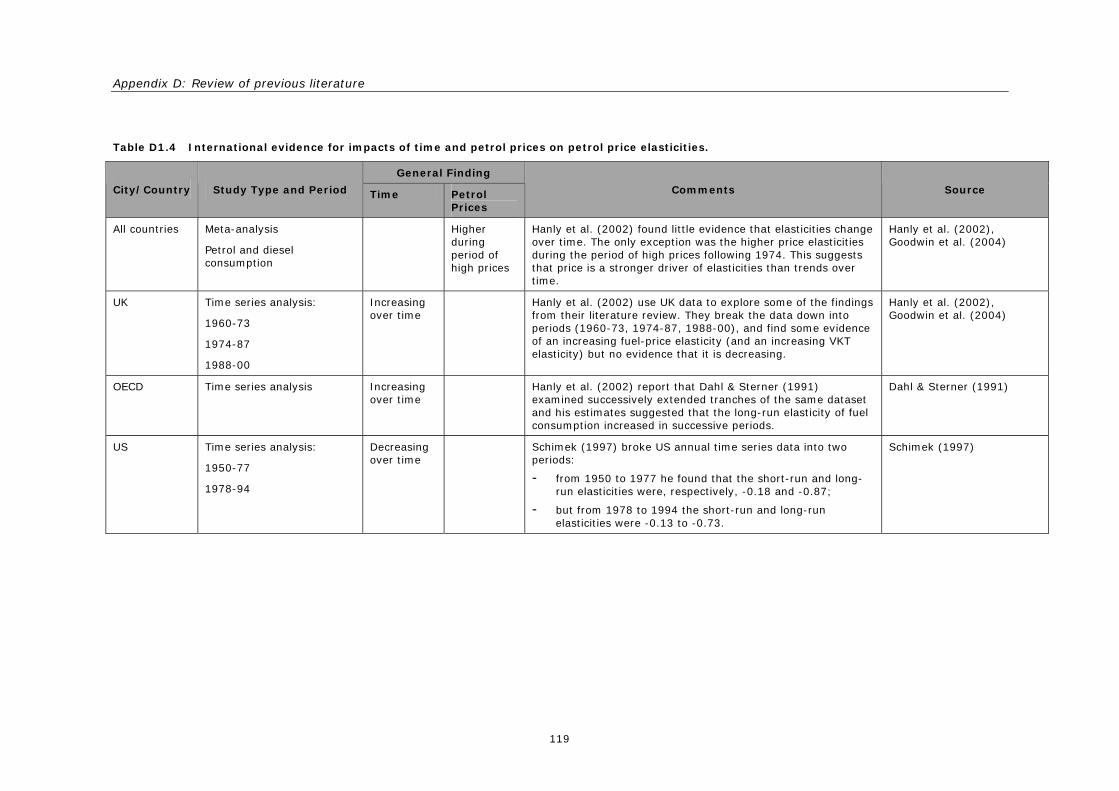
Appendix D: Review of previous literature
119
Table D1.4 International evidence for impacts of time and petrol prices on petrol price elasticities.
General Finding
City/Country Study Type and Period Time Petrol Prices
Comments Source
All countries Meta-analysis
Petrol and diesel consumption
Higher during period of high prices
Hanly et al. (2002) found little evidence that elasticities change over time. The only exception was the higher price elasticities during the period of high prices following 1974. This suggests that price is a stronger driver of elasticities than trends over time.
Hanly et al. (2002), Goodwin et al. (2004)
UK Time series analysis:
1960-73
1974-87
1988-00
Increasing over time
Hanly et al. (2002) use UK data to explore some of the findings from their literature review. They break the data down into periods (1960-73, 1974-87, 1988-00), and find some evidence of an increasing fuel-price elasticity (and an increasing VKT elasticity) but no evidence that it is decreasing.
Hanly et al. (2002), Goodwin et al. (2004)
OECD Time series analysis Increasing over time
Hanly et al. (2002) report that Dahl & Sterner (1991) examined successively extended tranches of the same dataset and his estimates suggested that the long-run elasticity of fuel consumption increased in successive periods.
Dahl & Sterner (1991)
US Time series analysis:
1950-77
1978-94
Decreasing over time
Schimek (1997) broke US annual time series data into two periods:
- from 1950 to 1977 he found that the short-run and long-run elasticities were, respectively, -0.18 and -0.87;
- but from 1978 to 1994 the short-run and long-run elasticities were -0.13 to -0.73.
Schimek (1997)
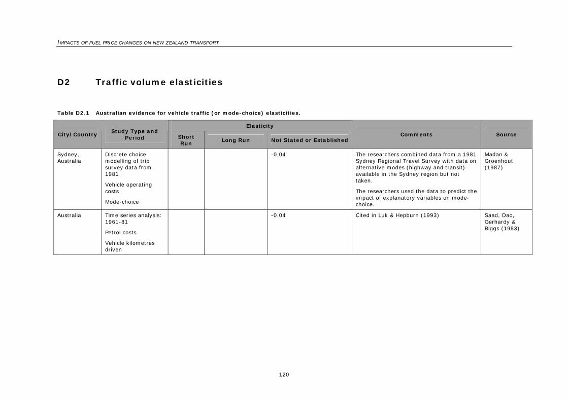
IMPACTS OF FUEL PRICE CHANGES ON NEW ZEALAND TRANSPORT
120
D2 Traffic volume elasticities
Table D2.1 Australian evidence for vehicle traffic (or mode-choice) elasticities.
Elasticity
City/Country Study Type and
Period Short Run
Long Run Not Stated or Established Comments Source
Sydney, Australia
Discrete choice modelling of trip survey data from 1981
Vehicle operating costs
Mode-choice
-0.04 The researchers combined data from a 1981 Sydney Regional Travel Survey with data on alternative modes (highway and transit) available in the Sydney region but not taken.
The researchers used the data to predict the impact of explanatory variables on mode-choice.
Madan & Groenhout (1987)
Saad, Dao, Gerhardy & Biggs (1983)
Australia Time series analysis: 1961-81
Petrol costs
Vehicle kilometres driven
-0.04 Cited in Luk & Hepburn (1993)
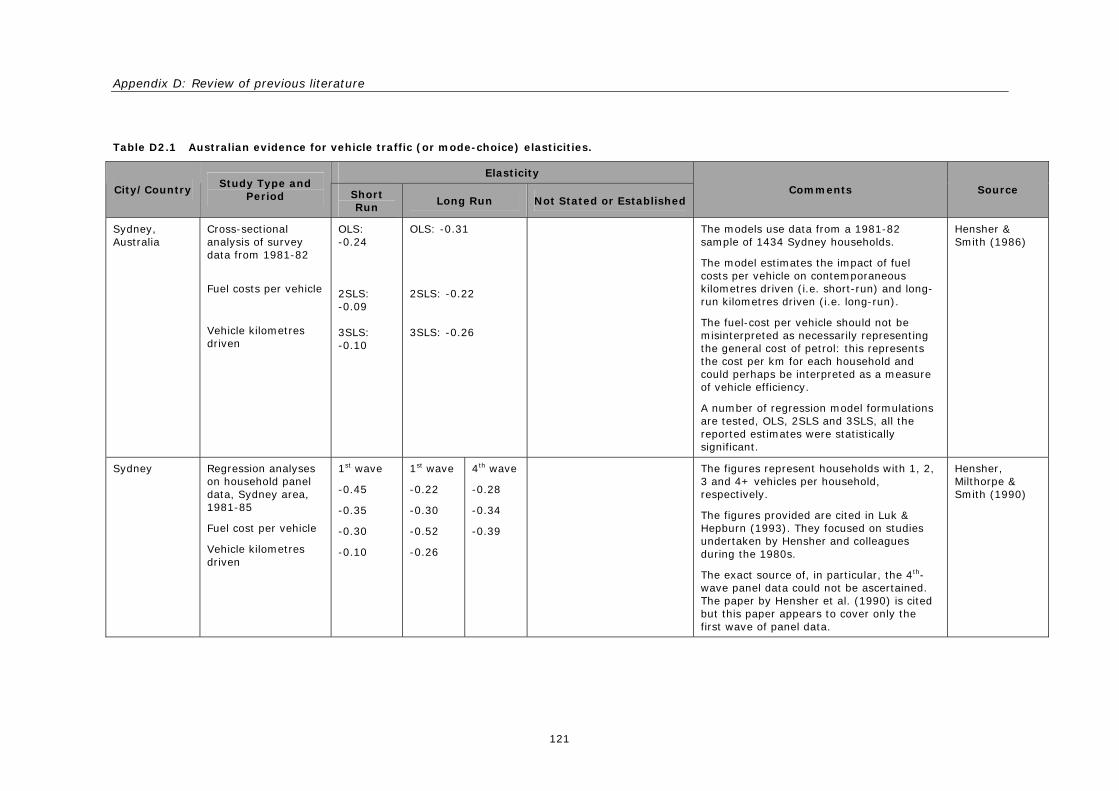
Appendix D: Review of previous literature
121
Table D2.1 Australian evidence for vehicle traffic (or mode-choice) elasticities.
Elasticity
City/Country Study Type and
Period Short Run
Long Run Not Stated or Established Comments Source
Sydney, Australia
Cross-sectional analysis of survey data from 1981-82
Fuel costs per vehicle
Vehicle kilometres driven
OLS: -0.24 2SLS: -0.09 3SLS: -0.10
OLS: -0.31 2SLS: -0.22 3SLS: -0.26
The models use data from a 1981-82 sample of 1434 Sydney households.
The model estimates the impact of fuel costs per vehicle on contemporaneous kilometres driven (i.e. short-run) and long-run kilometres driven (i.e. long-run).
The fuel-cost per vehicle should not be misinterpreted as necessarily representing the general cost of petrol: this represents the cost per km for each household and could perhaps be interpreted as a measure of vehicle efficiency.
A number of regression model formulations are tested, OLS, 2SLS and 3SLS, all the reported estimates were statistically significant.
Hensher & Smith (1986)
Sydney Regression analyses on household panel data, Sydney area, 1981-85
Fuel cost per vehicle
Vehicle kilometres driven
1st wave
-0.45
-0.35
-0.30
-0.10
1st wave
-0.22
-0.30
-0.52
-0.26
4th wave
-0.28
-0.34
-0.39
The figures represent households with 1, 2, 3 and 4+ vehicles per household, respectively.
The figures provided are cited in Luk & Hepburn (1993). They focused on studies undertaken by Hensher and colleagues during the 1980s.
The exact source of, in particular, the 4th-wave panel data could not be ascertained. The paper by Hensher et al. (1990) is cited but this paper appears to cover only the first wave of panel data.
Hensher, Milthorpe & Smith (1990)
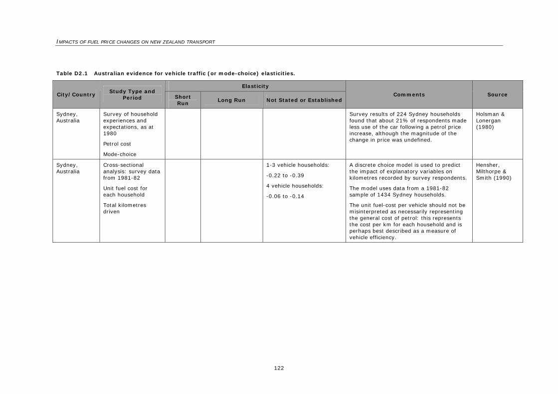
IMPACTS OF FUEL PRICE CHANGES ON NEW ZEALAND TRANSPORT
122
Table D2.1 Australian evidence for vehicle traffic (or mode-choice) elasticities.
Elasticity
City/Country Study Type and
Period Short Run
Long Run Not Stated or Established Comments Source
Sydney, Australia
Survey of household experiences and expectations, as at 1980
Petrol cost
Mode-choice
Survey results of 224 Sydney households found that about 21% of respondents made less use of the car following a petrol price increase, although the magnitude of the change in price was undefined.
Holsman & Lonergan (1980)
Sydney, Australia
Cross-sectional analysis: survey data from 1981-82
Unit fuel cost for each household
Total kilometres driven
1-3 vehicle households:
-0.22 to -0.39
4 vehicle households:
-0.06 to -0.14
A discrete choice model is used to predict the impact of explanatory variables on kilometres recorded by survey respondents.
The model uses data from a 1981-82 sample of 1434 Sydney households.
The unit fuel-cost per vehicle should not be misinterpreted as necessarily representing the general cost of petrol: this represents the cost per km for each household and is perhaps best described as a measure of vehicle efficiency.
Hensher, Milthorpe & Smith (1990)
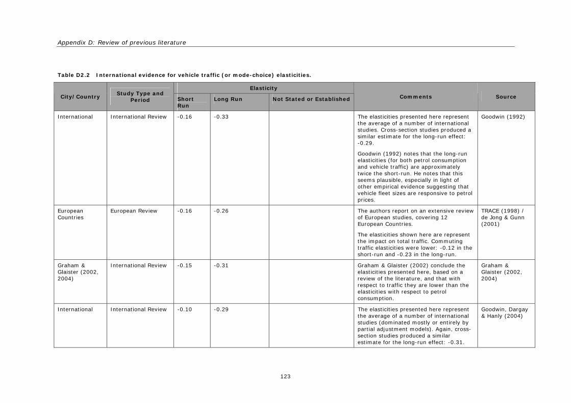
Appendix D: Review of previous literature
123
Table D2.2 International evidence for vehicle traffic (or mode-choice) elasticities.
Elasticity
City/Country Study Type and
Period Short Run
Long Run Not Stated or Established Comments Source
International International Review -0.16 -0.33 The elasticities presented here represent the average of a number of international studies. Cross-section studies produced a similar estimate for the long-run effect: -0.29.
Goodwin (1992) notes that the long-run elasticities (for both petrol consumption and vehicle traffic) are approximately twice the short-run. He notes that this seems plausible, especially in light of other empirical evidence suggesting that vehicle fleet sizes are responsive to petrol prices.
Goodwin (1992)
European Countries
European Review -0.16 -0.26 The authors report on an extensive review of European studies, covering 12 European Countries.
The elasticities shown here are represent the impact on total traffic. Commuting traffic elasticities were lower: -0.12 in the short-run and -0.23 in the long-run.
TRACE (1998) / de Jong & Gunn (2001)
Graham & Glaister (2002, 2004)
International Review -0.15 -0.31 Graham & Glaister (2002) conclude the elasticities presented here, based on a review of the literature, and that with respect to traffic they are lower than the elasticities with respect to petrol consumption.
Graham & Glaister (2002, 2004)
International International Review -0.10 -0.29 The elasticities presented here represent the average of a number of international studies (dominated mostly or entirely by partial adjustment models). Again, cross-section studies produced a similar estimate for the long-run effect: -0.31.
Goodwin, Dargay & Hanly (2004)

IMPACTS OF FUEL PRICE CHANGES ON NEW ZEALAND TRANSPORT
124
D3 Public transport cross-elasticities
Table D3.1 New Zealand evidence for public transport cross-elasticities.
Elasticity
City/Country Study Type and
Period Short Run Long Run Not Stated or Established
Comments
Source
New Zealand for seven main centres:
Auckland, Wellington, Christchurch, Dunedin, New Plymouth, Invercargill and Timaru
Time series analysis: 1959-89, annual data
Petrol
PT Patronage
average:
+0.07
This 1990 research by Travers Morgan examined patronage trends across seven main centres.
Both static regression models and differences models were fitted and both produced an average estimate of +0.07. This estimate was found to be insignificant.
The differences model is quite robust and will produce a good estimate of at least the short-run effect (although it may not pick-up long-run effects).
Furthermore, the estimates benefit from a high quality dataset with considerable length (30 years) and scope (seven main centres).
Travers Morgan (1990)
Wallis & Yates (1990)
New Zealand, Auckland
Time series analysis: 1967-78
Car operating costs
PT patronage
+0.09 Cited in Travers Morgan (1990).
Note that the research estimated a cross-elasticity with respect to total car operating costs.
Pringle (1979)
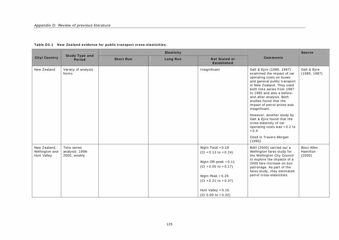
Appendix D: Review of previous literature
125
Table D3.1 New Zealand evidence for public transport cross-elasticities.
Elasticity
City/Country Study Type and
Period Short Run Long Run Not Stated or Established
Comments
Source
New Zealand Variety of analysis forms
Insignificant Galt & Eyre (1985, 1987) examined the impact of car operating costs on buses and general public transport in New Zealand. They used both time series from 1987 to 1985 and also a before-and-after analysis. Both studies found that the impact of petrol prices was insignificant.
However, another study by Galt & Eyre found that the cross-elasticity of car operating costs was +0.2 to +0.4.
Cited in Travers Morgan (1990).
Galt & Eyre (1985, 1987)
New Zealand, Wellington and Hutt Valley
Time series analysis: 1998-2000, weekly
Wgtn Total +0.18 (CI +0.13 to +0.24) Wgtn Off-peak +0.11 (CI +0.05 to +0.17) Wgtn Peak +0.29 (CI +0.21 to +0.37) Hutt Valley +0.16 (CI 0.00 to +0.32)
BAH (2000) carried out a Wellington fares study for the Wellington City Council to explore the impacts of a 2000 fare-increase on bus patronage. As part of the fares study, they estimated petrol cross-elasticities.
Booz Allen Hamilton (2000)
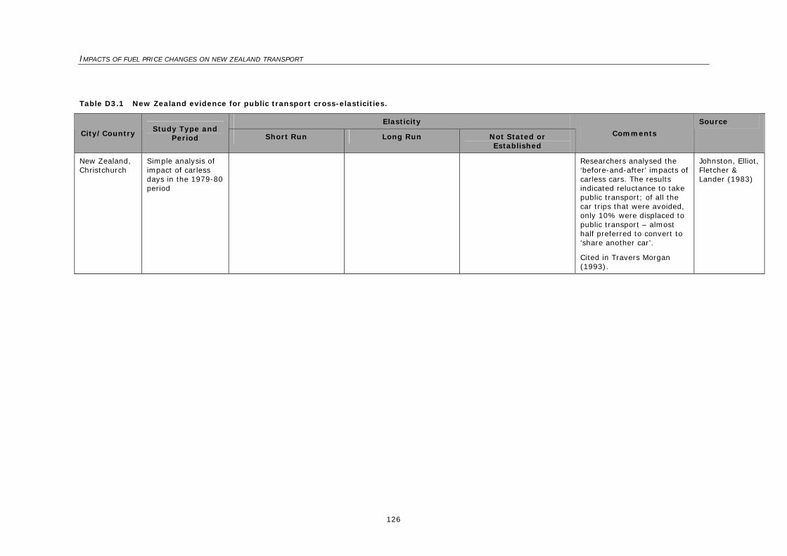
IMPACTS OF FUEL PRICE CHANGES ON NEW ZEALAND TRANSPORT
126
Table D3.1 New Zealand evidence for public transport cross-elasticities.
Elasticity
City/Country Study Type and
Period Short Run Long Run Not Stated or Established
Comments
Source
New Zealand, Christchurch
Simple analysis of impact of carless days in the 1979-80 period
Researchers analysed the ‘before-and-after’ impacts of carless cars. The results indicated reluctance to take public transport; of all the car trips that were avoided, only 10% were displaced to public transport – almost half preferred to convert to ‘share another car’.
Cited in Travers Morgan (1993).
Johnston, Elliot, Fletcher & Lander (1983)
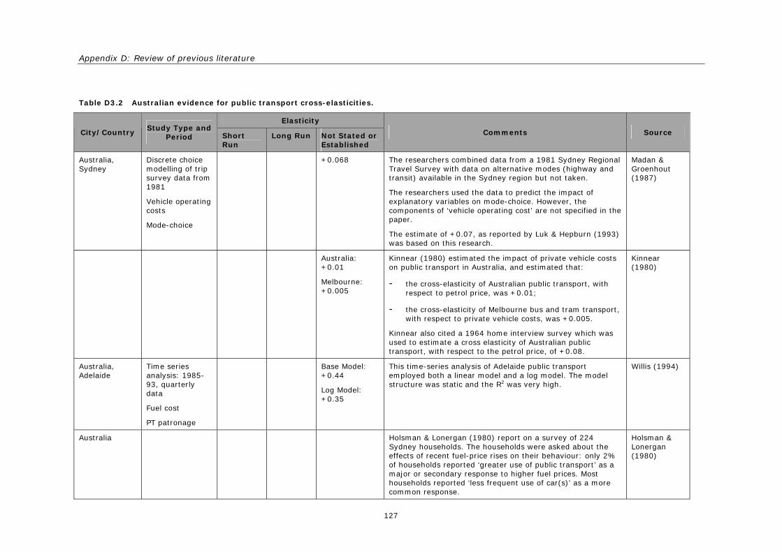
Appendix D: Review of previous literature
127
Table D3.2 Australian evidence for public transport cross-elasticities.
Elasticity
City/Country Study Type and
Period Short Run
Long Run Not Stated or Established
Comments Source
Australia, Sydney
Discrete choice modelling of trip survey data from 1981
Vehicle operating costs
Mode-choice
+0.068 The researchers combined data from a 1981 Sydney Regional Travel Survey with data on alternative modes (highway and transit) available in the Sydney region but not taken.
The researchers used the data to predict the impact of explanatory variables on mode-choice. However, the components of ‘vehicle operating cost’ are not specified in the paper.
The estimate of +0.07, as reported by Luk & Hepburn (1993) was based on this research.
Madan & Groenhout (1987)
Australia: +0.01
Melbourne: +0.005
Kinnear (1980) estimated the impact of private vehicle costs on public transport in Australia, and estimated that:
- the cross-elasticity of Australian public transport, with respect to petrol price, was +0.01;
- the cross-elasticity of Melbourne bus and tram transport, with respect to private vehicle costs, was +0.005.
Kinnear also cited a 1964 home interview survey which was used to estimate a cross elasticity of Australian public transport, with respect to the petrol price, of +0.08.
Kinnear (1980)
Australia, Adelaide
Time series analysis: 1985-93, quarterly data
Fuel cost
PT patronage
Base Model: +0.44
Log Model: +0.35
This time-series analysis of Adelaide public transport employed both a linear model and a log model. The model structure was static and the R2 was very high.
Willis (1994)
Australia Holsman & Lonergan (1980) report on a survey of 224 Sydney households. The households were asked about the effects of recent fuel-price rises on their behaviour: only 2% of households reported ‘greater use of public transport’ as a major or secondary response to higher fuel prices. Most households reported ‘less frequent use of car(s)’ as a more common response.
Holsman & Lonergan (1980)
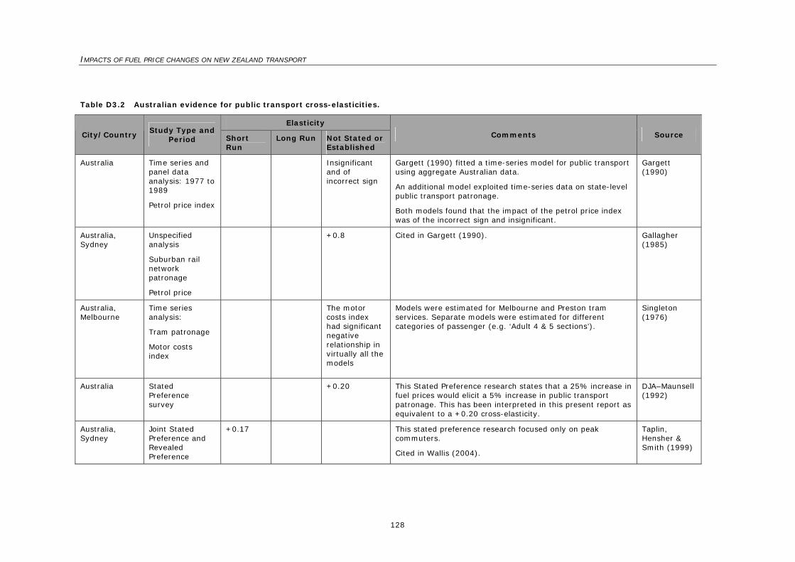
IMPACTS OF FUEL PRICE CHANGES ON NEW ZEALAND TRANSPORT
128
Table D3.2 Australian evidence for public transport cross-elasticities.
Elasticity
City/Country Study Type and
Period Short Run
Long Run Not Stated or Established
Comments Source
Australia Time series and panel data analysis: 1977 to 1989
Petrol price index
Insignificant and of incorrect sign
Gargett (1990) fitted a time-series model for public transport using aggregate Australian data.
An additional model exploited time-series data on state-level public transport patronage.
Both models found that the impact of the petrol price index was of the incorrect sign and insignificant.
Gargett (1990)
Australia, Sydney
Unspecified analysis
Suburban rail network patronage
Petrol price
+0.8 Cited in Gargett (1990). Gallagher (1985)
Australia, Melbourne
Time series analysis:
Tram patronage
Motor costs index
The motor costs index had significant negative relationship in virtually all the models
Models were estimated for Melbourne and Preston tram services. Separate models were estimated for different categories of passenger (e.g. ‘Adult 4 & 5 sections’).
Singleton (1976)
Australia Stated Preference survey
+0.20 This Stated Preference research states that a 25% increase in fuel prices would elicit a 5% increase in public transport patronage. This has been interpreted in this present report as equivalent to a +0.20 cross-elasticity.
DJA–Maunsell (1992)
Australia, Sydney
Joint Stated Preference and Revealed Preference
+0.17 This stated preference research focused only on peak commuters.
Cited in Wallis (2004).
Taplin, Hensher & Smith (1999)
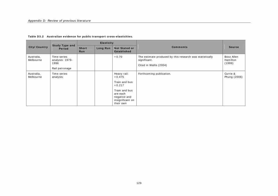
Appendix D: Review of previous literature
129
Table D3.2 Australian evidence for public transport cross-elasticities.
Elasticity
City/Country Study Type and
Period Short Run
Long Run Not Stated or Established
Comments Source
Australia, Melbourne
Time series analysis: 1979-1996
Rail patronage
+0.70 The estimate produced by this research was statistically significant.
Cited in Wallis (2004)
Booz Allen Hamilton (1999)
Australia, Melbourne
Time series analysis:
Heavy rail: +0.475
Train and bus: +0.217
Tram and bus are each negative and insignificant on their own
Forthcoming publication. Currie & Phung (2006)
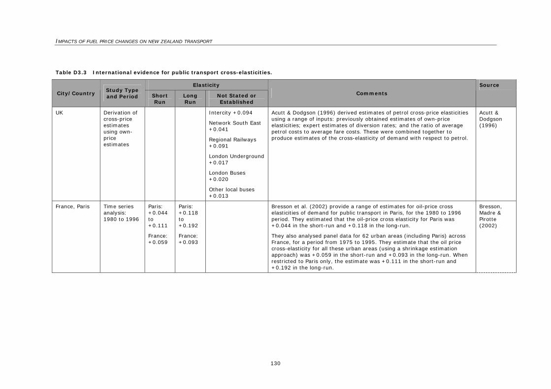
IMPACTS OF FUEL PRICE CHANGES ON NEW ZEALAND TRANSPORT
130
Table D3.3 International evidence for public transport cross-elasticities.
Elasticity
City/Country Study Type and Period Short
Run Long Run
Not Stated or Established
Comments
Source
UK Derivation of cross-price estimates using own-price estimates
Intercity +0.094
Network South East +0.041
Regional Railways +0.091
London Underground +0.017
London Buses +0.020
Other local buses +0.013
Acutt & Dodgson (1996) derived estimates of petrol cross-price elasticities using a range of inputs: previously obtained estimates of own-price elasticities; expert estimates of diversion rates; and the ratio of average petrol costs to average fare costs. These were combined together to produce estimates of the cross-elasticity of demand with respect to petrol.
Acutt & Dodgson (1996)
France, Paris Time series analysis: 1980 to 1996
Paris: +0.044 to +0.111
France: +0.059
Paris: +0.118 to +0.192
France: +0.093
Bresson et al. (2002) provide a range of estimates for oil-price cross elasticities of demand for public transport in Paris, for the 1980 to 1996 period. They estimated that the oil-price cross elasticity for Paris was +0.044 in the short-run and +0.118 in the long-run.
They also analysed panel data for 62 urban areas (including Paris) across France, for a period from 1975 to 1995. They estimate that the oil price cross-elasticity for all these urban areas (using a shrinkage estimation approach) was +0.059 in the short-run and +0.093 in the long-run. When restricted to Paris only, the estimate was +0.111 in the short-run and +0.192 in the long-run.
Bresson, Madre & Pirotte (2002)
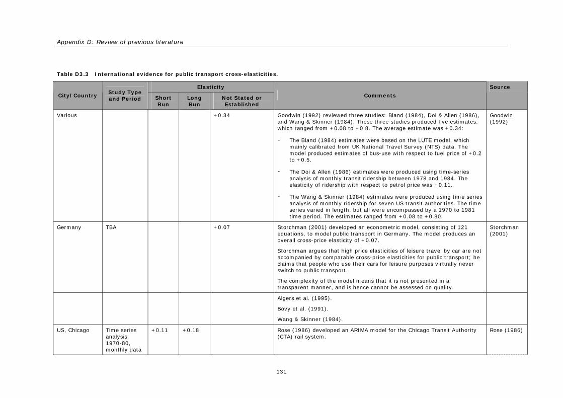
Appendix D: Review of previous literature
131
Table D3.3 International evidence for public transport cross-elasticities.
Elasticity
City/Country Study Type and Period Short
Run Long Run
Not Stated or Established
Comments
Source
Various +0.34 Goodwin (1992) reviewed three studies: Bland (1984), Doi & Allen (1986), and Wang & Skinner (1984). These three studies produced five estimates, which ranged from +0.08 to +0.8. The average estimate was +0.34:
- The Bland (1984) estimates were based on the LUTE model, which mainly calibrated from UK National Travel Survey (NTS) data. The model produced estimates of bus-use with respect to fuel price of +0.2 to +0.5.
- The Doi & Allen (1986) estimates were produced using time-series analysis of monthly transit ridership between 1978 and 1984. The elasticity of ridership with respect to petrol price was +0.11.
- The Wang & Skinner (1984) estimates were produced using time series analysis of monthly ridership for seven US transit authorities. The time series varied in length, but all were encompassed by a 1970 to 1981 time period. The estimates ranged from +0.08 to +0.80.
Goodwin (1992)
Germany TBA +0.07 Storchman (2001) developed an econometric model, consisting of 121 equations, to model public transport in Germany. The model produces an overall cross-price elasticity of +0.07.
Storchman argues that high price elasticities of leisure travel by car are not accompanied by comparable cross-price elasticities for public transport; he claims that people who use their cars for leisure purposes virtually never switch to public transport.
The complexity of the model means that it is not presented in a transparent manner, and is hence cannot be assessed on quality.
Storchman (2001)
Algers et al. (1995).
Bovy et al. (1991).
Wang & Skinner (1984).
US, Chicago Time series analysis: 1970-80, monthly data
+0.11 +0.18 Rose (1986) developed an ARIMA model for the Chicago Transit Authority (CTA) rail system.
Rose (1986)
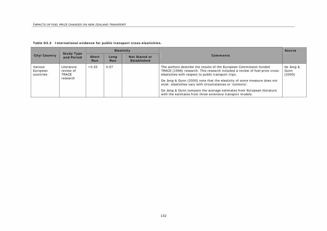
IMPACTS OF FUEL PRICE CHANGES ON NEW ZEALAND TRANSPORT
132
Table D3.3 International evidence for public transport cross-elasticities.
Elasticity
City/Country Study Type and Period Short
Run Long Run
Not Stated or Established
Comments
Source
Various European countries
Literature review of TRACE research
+0.33 0.07 The authors describe the results of the European Commission-funded TRACE (1998) research. This research included a review of fuel-price cross-elasticities with respect to public transport trips.
De Jong & Gunn (2000) note that the elasticity of some measure does not exist; elasticities vary with circumstances or ‘contexts’.
De Jong & Gunn compare the average estimates from European literature with the estimates from three extensive transport models.
de Jong & Gunn (2000)

Appendix E: References
133
Appendix E: References
Acutt, M.Z., Dodgson, J.S. 1996. Cross-elasticities of demand for travel. Transport Policy
2(4): 271-277.
Algers, S., Daly, A., Kjellman, P., Widlert, S. 1995. Stockholm Model System (SIMS):
application. Topic 25. 7th WCTR Conference 2: 345-360.
Allan, R.R., Lennox, L.G., Bone, I.H. 1977. Energy in transport. Beca Carter Hollings &
Ferner Ltd for NZ Energy Research & Development Committee. NZ ERDC Report
no. 27.
Baas, H.J., Hughes, W.R., Treloar, C.G. 1982. Elasticities of demand for petrol and
aviation fuel in New Zealand, 1961-1981. Technical Publication No.20. Wellington:
Ministry of Energy.
BAH. 1999. Melbourne tram and train forecasts. Serco, 1999.
BAH. 2000. Appraisal of patronage trends and prospects: Australian patronage trends
analysis. Metro Tasmania Pty Ltd. Working paper A2510/WP/C2.
BAH (NZ). 2001. Wellington fares study. Wellington Regional Council. BAH NZ Review
paper Z1163. 16pp.
Balcombe, R., Mackett, R., Paulley, N., Preston, J., Shires, J., Titheridge, H.,
Wardman, M., White, P. 2004. The demand for public transport: a practical guide.
TRL Report. TRL Ltd, Crowthorne, Berkshire, UK.
Barns, S.A. 2002. Fuel price and fuel consumption in New Zealand: Would a fuel tax
reduce consumption. Proceedings of Eighth Annual Conference of the New Zealand
Agricultural and Resource Economics Society. Lincoln University: AERU Discussion
Paper No. 149. 20pp.
Bland, B.H. 1984. Effect of fuel prices on fuel use and travel patterns. TRRL Laboratory
Report 1114. 31pp.
Bovy, P.H.L., van der Waard, J., Baanders, A. 1991. Substitution of travel demand
between car and public transport possibilities. PTRC SAM Seminar H 1991.
Brain, P., Schuyers, G. 1981. Energy and the Australian Economy. Longman Cheshire.
Bresson, G., Madre, J.L., Pirotte, A. 2002. Forecasting demand for public transport in
Paris region: comparison between time-series and panel data econometrics
approaches. Working Paper. Université Paris II Panthéon-Assas.
Collins, C. 1993. Transport energy management policies: potential in New Zealand. EECA
(Energy Efficiency & Conservation Authority) report. 59pp.

IMPACTS OF FUEL PRICE CHANGES ON NEW ZEALAND TRANSPORT
134
Currie, G., Phung, J. 2006. Exploring the impacts of fuel price increases on public
transport use in Melbourne. Paper presented at 29th Australasian Transport Research
Forum. 13pp.
Dahl, C., Roman, C. 2004. Energy demand elasticities – fact or fiction: a survey update.
Companion piece to paper presented at Energy, Environment and Economics in a New
Era, 24th USAEE/IAEE North American Conference, Washington, DC, July 8-10, 2004.
Dahl, C., Sterner, T. 1991. A survey of econometric gasoline demand elasticities.
International Journal of Energy Systems 11(2): 53-76.
de Jong, G., Gunn, H. 2000. Recent evidence on car cost and time elasticities of travel
demand in Europe. Journal of Transport Economics & Policy 35(2): 137-160.
de Jong, G.C., Tegge, O., Dohmen, R., Ettema, D.F., Hamer, R.N., Massiani, J., van
Vuren, T. 1998. Review of existing evidence on time and cost elasticities of travel
demand and on value of travel time. EC TRACE Project Deliverable 1 (DGT Contract
RO-97-SC. 2035).
DJA–Maunsell. 1992. Improving public transport viability. Working Paper VII.
20792.00\PEP\R-785.
Doi, M., Allen. W.B. 1986. A time series analysis of monthly ridership for an urban rail
rapid transit line. Transportation 13(3): 257-169.
Donnelly, W.A. 1981. The demand for petrol in Australia. Australian University, Canberra,
Centre for Resources & Environmental Studies Working Paper.
Donnelly, W.A. 1984. The Australian demand for petrol. International Journal of Transport
Economics 11(2/3): 198-205.
Espey, M. 1998. Gasoline demand revisited: an international meta-analysis of elasticities.
Energy Economics 20: 273-295.
Filmer, R.J., Mannion, R. 1979. Petrol prices and passenger motor vehicle travel. Paper to
the Economic Modelling Session of the Regional Science Association Conference,
Albury–Wodonga, Australia.
Gallagher, M.J. 1985. An empirical study of the dynamics of Sydney suburban rail
patronage and its implications for before & after studies. Australasian Transport
Research Forum: 19-41.
Galt, M.N., Eyre, A.J. 1985. A study into the factors which influence the demand for urban
bus travel. Interim report. 18pp. Prepared for the Ministry of Transport, Research
Committee, Urban Transport Council, New Zealand.
Galt, M.N., Eyre, A.J. 1987. Demand elasticities in New Zealand public transport: an
introduction. 40pp. Urban Transport Council, New Zealand.

Appendix E: References
135
Gargett, D. 1990. Aggregate modelling of urban public transport demand. Paper to
Economic Society of Australia, 19th Annual Conference, University of NSW. 12pp.
Girard, S., Camisa, X. 2005. Higher fuel prices, The impact on Quebec’s budget balance.
Fiscal and Budget Studies 1(2).
Goodwin, P.B. 1992. A review of new demand elasticities with special reference to short
and long run effects of price changes. Journal of Transport Economics & Policy 26(2):
155-163.
Goodwin, P., Dargay, J., Hanly, M. 2004. Elasticities of road traffic and fuel consumption
with respect to price and income: a review. Transport Reviews 24(3): 275-292.
Graham, D.J., Glaister, S. 2002. The demand for automobile fuel. Journal of Transport
Economics & Policy 36(1).
Graham, D.J., Glaister, S. 2004. Road traffic demand elasticity estimates: a review.
Transport Reviews 24(3): 261-274.
Granger, C.W.J., Newbold, P. 1974. Spurious regressions in econometrics. Journal of
Econometrics 2: 111-120.
Hall, V.B., McDermott, C.J. 2006. The New Zealand business cycle: Return to golden
days? VUW (in press).
Hanly, M., Dargay, J., Goodwin, P. 2002. Review of income and price elasticities in the
demand for road traffic. University of London Centre for Transport Studies ESRC
Transport Studies Unit.
Harding, D. 2001. Macroeconomic effects of petrol prices. Mercer-Melbourne Institute
Quarterly Bulletin of Economic Trends (1.01): 21-28.
Hensher, D.A., Milthorpe, F.W., Smith, N.C. 1990. The demand for vehicle use in the
urban household sector. Journal of Transport Economics & Policy 24: 119-137.
Hensher, D.A., Smith, N.C. 1986. A structural model of the use of automobiles by
households: a case study of urban Australia. Transport Reviews 6(1): 87-111.
Hensher, D.A., Young, J.L. 1991. Fuel demand forecasts and demand elasticities for
Australian transport fuel. BTCE Occasional Paper 103. 103pp. Bureau of Transport &
Communications Economics.
Holsman, A.J., Lonergan, N.G. 1980. The impact of rising fuel prices on household
behaviour in Sydney. Proceedings of ATRF: 207-226.
Hughes, W.R. 1980. Petrol consumption in New Zealand 1969-79: Fixed and time varying
parameter results. New Zealand Economic Papers 14: 28-43.
Johnston, W.B., Elliott, J.M.C., Fletcher, I.R., Lauder, G.A. 1983. New Zealand’s Carless
Day scheme: people's responses to restriction of car use. Transport Reviews 3(4):
399-410.
IMPACTS OF FUEL PRICE CHANGES ON NEW ZEALAND TRANSPORT
136
Kinnear, R.L. 1980. MMTB-patronage estimation procedures. Metropolitan Melbourne
Transport Board Report. 30pp.
Lewthwaite, N.B., Douglas, N. 1992. Greater Wellington area transportation study.
Murray-North Ltd, April 1992.
Luk, J., Hepburn, S. 1993. New review of Australian travel demand elasticities. ARRB
Research Report 249. 22pp. ARRB, Victoria, Australia.
Madan, D.B., Groenhout, R. 1987. Modelling travel mode choices for the Sydney work
trip. Journal of Transport Economics & Policy 21(2): 135-149.
Miller, E.J., Crowley, D.F. 1989. Panel survey approach to measuring transit route service
elasticities of demand. Transportation Research Record 1209: 26-31.
Ministry of Commerce and NZIER 1991. Energy demand forecasts – some initial results.
Ministry of Commerce, Wellington.
Phillips, P.C.B. 1986. Understanding spurious regressions in econometrics. Journal of
Econometrics 33: 311-340.
Pickford, M., Wheeler, C. 2001. The petrol industry: deregulation, entry and competition.
NZ Trade Consortium Working Paper No.12. NZ Trade Consortium & NZ Institute of
Economic Research Inc. (NZIER). 71pp.
Pringle, W.D. 1979. Funding guidelines for shared transport. Auckland Regional Council
Paper. 20pp.
R Development Core Team. 2006. R: A language and environment for statistical
computing. R Foundation for Statistical Computing, Vienna, Austria. ISBN 3-900051-
07-0, URL http://www.R-project.org
Rose, G. 1986. Transit passenger response: short and long term elasticities using time
series analysis. Transportation 13: 131-141.
Saad, M.M., Dao, D.M., Gerhardy, S., Biggs, A. 1983. Demand for road travel. Paper
presented at 5th Conference of Australian Institutes of Transport Research, Brisbane.
Samimi, R. 1995. Road transport energy demand in Australia. Energy Economics 17(4):
329-339.
Schimek, P. 1997. Gasoline and travel demand models using time series and cross-
section data from United States. Transportation Research Record 1558: 83-89.
Schou, K., Johnson, L.W. 1979. The short-run price elasticity of demand for petrol in
Australia. International Journal of Transport Economics 6(3): 357-364.
Selvanathan, S., Selvanathan, E.A. 1998. The effect of the price of gold on its production:
a time-series analysis. School of International Business, Griffith University,
Queensland, Australia. 16pp.
Appendix E: References
137
Singleton, D.J. 1976. The analysis of the use of urban public transport utilising existing
data sources. Paper to Transport Seminar, University of Melbourne. University of
Melbourne Department of Civil Engineering, Ove Arup & Partners.
Sterner, T., Dahl, C., Franzen, M. 1992. Gasoline tax policy, carbon emissions and the
Global Environment. Journal of Transport Economics & Policy 26(2): 109-119.
Storchmann, K.H. 2001. The impact of fuel taxes on public transport – an empirical
assessment for Germany. Transport Policy 8(1): 19-28.
Taplin, J.H.E., Hensher, D.A., Smith, B. 1999. Preserving the symmetry of estimated
commuter travel elasticities. Transportation Research Part B, 33: 215-232.
TRACE Consortium. 1998. Outcome of review on elasticities and values of time. TRACE
Deliverable 1.
Travers Morgan. 1980. Adelaide urban transport pricing study, interim report. Director-
General of Transport, South Australia (Ref J041).
Travers Morgan. 1990a. Analysis of public transport patronage trends. For Transit NZ.
Travers Morgan Report Z1845.
Travers Morgan. 1990b. Road transport: future directions. Transport pricing. RTA NSW,
Australia. Travers Morgan Report Z2262.
Travers Morgan. 1990c. Trends in Wellington rail patronage 1985-90. NZ Rail Ltd,
Wellington, New Zealand. Travers Morgan Report Z9027/RE/WLG. 7pp.
Travers Morgan. 1990d. Urban bus study Stage 3. Analysis of public transport patronage
trends. TM Report Z1845.R2. 24pp. + Appendices A-C.
Travers Morgan. 1993. Effects of petrol price changes on car travel: review of the
evidence. Auckland Regional Council. Travers Morgan Report Z9147.N2. 11pp.
Verbeek, M. 2000. A guide to modern econometrics. Publisher: John Wiley & Sons Ltd.
Waikato University. 1982. Reference details not established.
Wallis, I. 2004. Review of passenger transport demand elasticities. Booz Allen Hamilton,
Transfund New Zealand Research Report No. 248. 118pp. 12 Appendices.
Wallis, I.P., Yates, P. 1990. Public transport patronage trends in New Zealand. Where are
all the passengers going? ATRF document (19pp. unpaged).
Wang, G.H., Skinner, D. 1984. The impact of fare and gasoline price changes on monthly
transit leadership: empirical evidence from seven US transit authorities. Transportation
Research 18B: 29-41.
Wardman, M. 1997. Disaggregate urban mode choice models: review of British evidence
with special reference to cross-elasticities. ITS Leeds, WP 505. 26pp. Institute of
Transport Studies, Leeds University, UK.

IMPACTS OF FUEL PRICE CHANGES ON NEW ZEALAND TRANSPORT
138
Willis, D. 1994. Adelaide public transport patronage regression study 1985-1993. Paper
for Master of Transport Management, University of Sydney. 14pp. + Appendices.
Works Consultancy Services Ltd (WCS). 1991. Regional fuel tax study. Wellington
Regional Council, New Zealand. 44pp.


600
Related Documents