Resale Price Maintenance and Interlocking Relationships ∗ Patrick Rey † Thibaud Vergé ‡ July 1, 2008 Abstract An often expressed idea to motivate the per se illegality of RPM is that it can limit interbrand as well as intrabrand competition. This paper analyzes this argument in a context where manufacturers and retailers enter into interlocking relationships. It is shown that, even as part of purely bilateral vertical contracts, RPM indeed limits the exercise of both inter- and intra-brand competition and can generate industry-wide monopoly pricing. The final impact on prices depends on the extent of potential competition at either level as well as on the manufacturers’ and retailers’ influence in determining the terms of the contracts. Our analysis sheds a new light on ongoing legal developments and is supported by recent empirical studies. JEL: D4, L13, L41, L42 Keywords: Resale Price Maintenance, Collusion, Successive duopoly. ∗ We benefited from helpful discussions with Rodolphe Dos Santos Ferreira, Bruno Jullien and Jean Tirole on an earlier draft. We are also grateful to Eric Avenel, Bill Rogerson, the Editor (Pierre Régibeau) and two anonymous referees for their remarks. † Toulouse School of Economics (GREMAQ, IDEI) and Institut Universitaire de France. ‡ CREST-LEI. 1

Welcome message from author
This document is posted to help you gain knowledge. Please leave a comment to let me know what you think about it! Share it to your friends and learn new things together.
Transcript

Resale Price Maintenance and Interlocking
Relationships∗
Patrick Rey† Thibaud Vergé‡
July 1, 2008
Abstract
An often expressed idea to motivate the per se illegality of RPM is that it
can limit interbrand as well as intrabrand competition. This paper analyzes this
argument in a context where manufacturers and retailers enter into interlocking
relationships. It is shown that, even as part of purely bilateral vertical contracts,
RPM indeed limits the exercise of both inter- and intra-brand competition and can
generate industry-wide monopoly pricing. The final impact on prices depends on the
extent of potential competition at either level as well as on the manufacturers’ and
retailers’ influence in determining the terms of the contracts. Our analysis sheds
a new light on ongoing legal developments and is supported by recent empirical
studies.
JEL: D4, L13, L41, L42
Keywords: Resale Price Maintenance, Collusion, Successive duopoly.
∗We benefited from helpful discussions with Rodolphe Dos Santos Ferreira, Bruno Jullien and Jean
Tirole on an earlier draft. We are also grateful to Eric Avenel, Bill Rogerson, the Editor (Pierre Régibeau)
and two anonymous referees for their remarks.†Toulouse School of Economics (GREMAQ, IDEI) and Institut Universitaire de France.‡CREST-LEI.
1

1 Introduction
The attitude of competition authorities and courts towards vertical restraints varies sig-
nificantly from one country to another or from one period to another.1 Still, a consen-
sus emerges against resale price maintenance (RPM), a restraint according to which the
manufacturer sets the final price that retailers charge to consumers. While competition
authorities are sometimes tolerant towards some variants of RPM such as price ceilings
and recommended or advertised prices, they usually treat price floors and strict RPM as
per se illegal. For example, when the European Commission adopted a more open attitude
towards non-price restrictions, it maintained RPM on a black list — with only one other
restraint. In France, price floors are per se illegal and, in Lypobar vs. La Croissanterie
(1989), the Paris Court of Appeal ruled that RPM was an abuse of franchisees’ economic
dependency. A recent exception to this consensus concerns the U.S., where the Supreme
Court overturned last year the long-established per se illegality of price floors, adopting
instead a rule of reason approach.2
The economic analysis of vertical restraints is more ambiguous: it is not clear that
RPM has a more negative impact on welfare than other vertical restraints that limit
intrabrand competition. Instead, both price (e.g., RPM) and non-price restraints (e.g.,
exclusive territories) may have positive or negative effects on welfare, depending on the
context in which they are used.3 In particular, both price and non-price vertical restraints
can deal with vertical coordination problems.4 For instance, combined with non-linear
wholesale tariffs, RPM or exclusive territories can equally limit free-riding problems cre-
ated by strong intrabrand competition.5 Quite a few papers have moreover pointed at
specific efficiency benefits of RPM.6 Vertical restraints may also affect interbrand com-
petition. Manufacturers can for example impose restraints on retailers so as to become
“less aggressive”. Through strategic complementarity, this in turn induces their rivals
to respond less aggressively (e.g., increase their wholesale prices) ultimately leading to1For an overview of the legal frameworks regarding vertical restraints, see OECD (1994) or the Euro-
pean Commission’s Green Paper on Vertical Restraints (1996). Comanor and Rey (1996) also compares
the evolution of the attitudes of the U.S. competition authorities and within the European Community.2See Leegin Creative Leather Products, Inc. v. PSKS, Inc., 127 S.Ct 2705 (2007).3See Motta (2004, chapter 6) or Rey and Vergé (2008) for recent surveys of that literature.4Rey and Tirole (1986) offers an overview of the relative merits of price and non-price restrictions in
improving vertical coordination.5Note however, that depending on the structure of consumer demand, such restraints may harm or
enhance economic welfare. See (among others) Spence (1975), Comanor (1985), Caillaud and Rey (1987),
or more recently Schulz (2007).6For example, Marvel and McCafferty (1984) stress that RPM can help manufacturers to purchase
certification from reputable dealers. Deneckere, Marvel and Peck (1996, 1997) and Wang (2004) show
that RPM can encourage retailers to hold inventories in the presence of demand uncertainty, while Chen
(1999) shows that RPM may help controlling retail price discrimination.
2

higher prices and profits.7 To achieve this, manufacturers must however give retailers
some freedom in their pricing policies. Granting exclusive territories (thus eliminating
intrabrand competition) would for example serve this purpose and have an adverse effect
on consumer surplus and economic welfare, whereas RPM would have no impact since it
also eliminates the retailers’ freedom to choose their retail prices. Overall, a comparison
of the welfare effects of exclusive territories, RPM and exclusive dealing does not clearly
justify a more lenient attitude towards non-price restrictions.8
There is however one last argument that has often been made by courts to justify
a negative attitude towards price restrictions. For example, in Business Electronics, the
Supreme Court justified the per se illegality of RPM by claiming that “there was sup-
port for the proposition that vertical price restraints reduce inter-brand price competition
because they facilitate cartelizing.” This type of argument has been informally used by
Telser (1960) and Mathewson and Winter (1998). It was however formalized only very
recently by Jullien and Rey (2007) who stress that, by making retail prices less responsive
to local shocks on retail cost or demand, RPM yields more uniform prices that facilitate
tacit collusion — by making deviations easier to detect.
This paper analyzes this “facilitating practice” argument from a different perspec-
tive. We show that, even in the absence of repeated interactions, RPM can eliminate
any scope for effective competition when manufacturers and retailers engage in “inter-
locking relationships”, that is, when manufacturers distribute their goods through the
same competing distributors. The intuition is relatively simple. In the case of a (local)
retail monopoly we know that, through “common agency”, competing manufacturers can
avoid interbrand competition, e.g., by selling at cost in exchange for a fixed fee: since
manufacturers internalize through fixed fees the impact of prices on the retailer’s profit,
eliminating the upstream margin on one brand transforms a rival manufacturer into a
residual claimant on the sales of both brands. As a result, rival manufacturers have in-
centives to maintain retail prices at the monopoly level, which can be achieved precisely
by selling at cost. Simple two-part tariffs therefore suffice to maintain monopoly prices and
profits.9 This is no longer the case when there is competition not only between brands,
but also between retailers, which tends to reduce retail margins. Manufacturers then have
conflicting incentives: they still want to keep low upstream margins in order to avoid
interbrand competition but they need now to increase their wholesale prices in order to
maintain high retail prices despite intrabrand competition. As we will see, two-part tariffs
no longer suffice to maintain industry profits, and retail prices are instead set below their
monopoly level. Manufacturers can however use RPM to eliminate intrabrand competi-7See for example Rey and Stiglitz (1988, 1995) and Bonanno and Vickers (1988).8See Caballero-Sanz and Rey (1996).9See Bernheim and Whinston (1985, 1998) and O’Brien and Shaffer (1997).
3

tion and restore monopoly prices and profits. In particular, selling at cost (for a fee) still
makes rivals internalize (through their own fixed fees) the full impact of their prices on
the sales of a manufacturer’s brand. At the same time, a manufacturer can now main-
tain high retail prices for its brand through RPM. Combining two-part tariffs with RPM
thus provides a mechanism through which manufacturers can give each other incentives
to maintain high retail prices and profits. Both interbrand and intrabrand competition
are then totally eliminated, even though contracts (including retail prices) are negotiated
on a purely bilateral basis. In the absence of any retail bottleneck (e.g., when there are
potential competitors for each retail location), manufacturers clearly benefit from this,
since they can appropriate most of the profits that they generate. When instead retailers
have market power, manufacturers need to leave them some rents, thus reducing their
incentives to deal with both retailers and to maintain monopoly prices. As a result, all
channels may not be active and manufacturers may moreover favor lower prices, in order
to keep a larger share of an admittedly smaller pie, whereas retailers would instead favor
higher retail prices.
Note that the mechanism identified here could not be replicated through other stan-
dard means of reducing intrabrand competition, e.g., by granting an exclusive right over
some territory. Indeed, RPM allows manufacturers to avoid interbrand competition even
when, due to retailers’ differentiation strategies, meeting consumer demand makes it un-
desirable to grant exclusive territories and exclude some of the established retailers.
This paper is closely related to that of Dobson and Waterson (2007), who study a
similar bilateral duopoly with interlocking relationships. Assuming that manufacturers
use (inefficient) linear wholesale prices, they show that the welfare effects of RPM depend
on the relative degree of upstream and downstream differentiation as well as on retailers’
and manufacturers’ bargaining powers; RPM can be socially preferable when retailers are
in a weak bargaining position, because the double-marginalization problems generated by
the restriction to linear wholesale prices is more severe in such circumstances.10 In order
to eliminate double marginalization problems and focus instead on the impact of RPM
on interbrand and intrabrand competition, we do not restrict attention to linear tariffs
but allow for bilaterally efficient (two-part) wholesale tariffs.11
Our analysis sheds an interesting light on recent legal developments. While the US
Supreme Court recently overturned the per illegality of RPM, in France, RPM, together10In a similar context, Allain and Chambolle (2007) moreover show that non-discriminatory price floors
can help maintain high retail prices even when manufacturers can grant secret rebates.11Another difference concerns the equilibrium concept. To reflect different bargaining powers, Dobson
and Waterson (2007) assume that wholesale prices are determined by simultaneous pairwise bargaining.
This supposes that a manufacturer has two independent divisions, each of them negotiating with one
retailer not taking into account the impact of its own negotiation on the other division.
4

with non-linear wholesale tariffs, has instead raised concerns in markets where multiple
producers distribute their goods through the same retailers. For example, in Decem-
ber 2005, the Conseil de la Concurrence (one of the two French competition authorities)
condemned brown goods manufacturers Panasonic, Philips and Sony for “vertical collu-
sion” with their wholesalers and retailers. The Conseil de la Concurrence concluded that
there was evidence that these manufacturers were actively monitoring retailers in order to
ensure that they were actually following their recommended retail prices (this was espe-
cially the case for new lines of products) and were pushing wholesalers to refuse to supply
retailers that were cutting prices.12 In similar cases, the major perfume manufacturers
(L’Oréal, Chanel, Guerlain, Dior, ...) and retailers (Nocibé, Marionnaud, Séphora) were
fined a total of 44 million euros, and toy manufacturers (Chicco, Lego, ...) and retailers
(Carrefour, JouéClub, ...) were fined a total of 37 million euros for the same practices.13
Our analysis is also relevant for the ongoing reform of the French competition rules
banning below-cost pricing. In order to simplify billing methods and enhance trans-
parency, a law adopted in 1996 defined the relevant cost threshold as the invoice-price
paid by the retailer at the time of delivery. As a result, retailers could no longer pass on
to consumers many rebates, such as quantity and end-of-year discounts or slotting fees,
which do not usually appear on invoices. It has been argued that the regulation was legal-
izing minimum RPM: the invoice price, determined by the manufacturer’s general terms
of sales, de facto imposed a minimum retail price eliminating intrabrand competition, and
retailers then negotiated “backroom rebates” to maintain their margins. The regulation
has been heavily criticized as being responsible for the important price increases that have
taken place after 1997, especially for the major national brands present in all supermarket
chains. As we will see, our analytical framework supports this claim and has moreover
been validated by recent empirical studies of the French bottled water market.14
This paper is organized as follows. Section 2 presents our framework, where two rival
manufacturers distribute their goods through two competing retailers; this framework
allows for interlocking relationships (or “double common agency”): each manufacturer
can deal with both retailers, and conversely each retailer can carry both brands. Section
3 provides a preliminary analysis of such double common agency situations: while retail
prices are lower than the monopoly price in the absence of RPM, with RPM there exist
many equilibria, including one in which retail prices and manufacturers’ profits are at the12These three manufacturers were respectively fined 2.4, 16 and 16 million euros. Panasonic was later
cleared by the Court of Appeal. Other major manufacturers present on the French market were also
investigated, but the Conseil de la Concurrence did not find enough evidence to convict them. See
Conseil de la Concurrence, decision 05-D-66, December 2005.13See Conseil de la Concurrence, decisions 06-D-04 (March 2006, Perfumes) and 07-D-50 (December
2007, Toys).14See Bonnet and Dubois (2004 and 2007).
5

monopoly level. We then endogenize the market structure. Section 4 studies situations
with potential competition downstream for each retail location. Both brands are then
always present at both retail locations and the previous analysis applies; in particular,
when RPM is allowed, there always exists an equilibriumwith monopoly prices and profits.
Section 5 turns to the case of retail bottlenecks, where manufacturers cannot bypass
established retailers. Manufacturers must then leave a rent to retailers to induce them
to sell their products; relatedly, they can attempt to eliminate competitors by convincing
retailers to reject their rival’s offer. As a result, it can be the case that no equilibrium
exists where both manufacturers are present in both retail outlets, even though there is
demand for each brand at each store. In addition, while there may exist a continuum
of equilibria with RPM, equilibria with higher retail prices now involve larger rents for
the retailers and lower profits for the manufacturer — implying that manufacturers favor
equilibria with rather “competitive” prices. Section 6 discusses the policy implications of
our analysis and concludes.
2 The Basic Framework
There are two manufacturers, A and B, each producing its own brand and two differ-
entiated retailers, 1 and 2. Retailers differ, for example, in their location or the ser-
vices they provide to consumers. If both retailers carry both brands, consumers choose
among four imperfectly substitutable “products”, each manufacturer producing two of
them ({A1, A2} and {B1, B2}, respectively) and each retailer distributing two of them({A1, B1} and {A2, B2}, respectively).In order to avoid that one firm - manufacturer or retailer - plays a particular role, we
suppose that demand functions are symmetric; for any price vector p = (pA1, pB1, pA2, pB2) ,
any i 6= h ∈ {A,B} and any j 6= k ∈ {1, 2} , Dij (p) ≡ D (pij, phj, pik, phk) , where the de-mand function D (.) is continuously differentiable. In what follows, we will drop the ar-
guments in Dij when there is no risk of confusion, and systematically use subscripts i
and h for the two manufacturers, and j and k for the two retailers. The products being
(imperfect) substitutes, we suppose that the demand for one product decreases with the
price of that product and increases with the other prices:15 ∂1D < 016 and ∂nD > 0 for
n = 2, 3, 4 . Furthermore, we suppose that direct effects dominate, so that demand de-
creases if all prices increase:P4
n=1 ∂nD < 0 . We also assume that both production and15This assumption seems reasonable but is not always maintained. For example, Dobson and Waterson
(2007) consider a linear model where the price of one product decreases when the quantity of any product
increases. However, their specific assumptions then imply that the demand for one brand in one store
decreases when the price of the competing brand increases in the competing store (∂4D < 0).16We denote by ∂nf the partial derivative of f with respect to its nth argument.
6
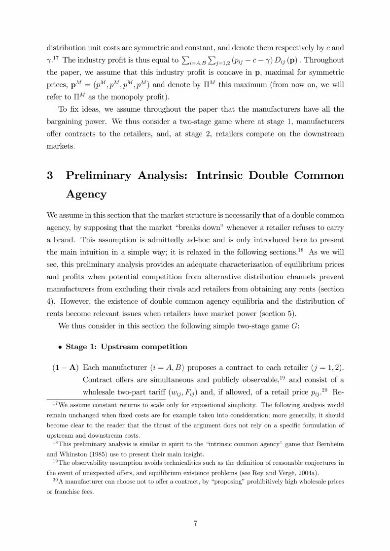
distribution unit costs are symmetric and constant, and denote them respectively by c and
γ.17 The industry profit is thus equal toP
i=A,B
Pj=1,2 (pij − c− γ)Dij (p) . Throughout
the paper, we assume that this industry profit is concave in p, maximal for symmetric
prices, pM = (pM , pM , pM , pM) and denote by ΠM this maximum (from now on, we will
refer to ΠM as the monopoly profit).
To fix ideas, we assume throughout the paper that the manufacturers have all the
bargaining power. We thus consider a two-stage game where at stage 1, manufacturers
offer contracts to the retailers, and, at stage 2, retailers compete on the downstream
markets.
3 Preliminary Analysis: Intrinsic Double Common
Agency
We assume in this section that the market structure is necessarily that of a double common
agency, by supposing that the market “breaks down” whenever a retailer refuses to carry
a brand. This assumption is admittedly ad-hoc and is only introduced here to present
the main intuition in a simple way; it is relaxed in the following sections.18 As we will
see, this preliminary analysis provides an adequate characterization of equilibrium prices
and profits when potential competition from alternative distribution channels prevent
manufacturers from excluding their rivals and retailers from obtaining any rents (section
4). However, the existence of double common agency equilibria and the distribution of
rents become relevant issues when retailers have market power (section 5).
We thus consider in this section the following simple two-stage game G:
• Stage 1: Upstream competition
(1−A) Each manufacturer (i = A,B) proposes a contract to each retailer (j = 1, 2).Contract offers are simultaneous and publicly observable,19 and consist of a
wholesale two-part tariff (wij, Fij) and, if allowed, of a retail price pij.20 Re-17We assume constant returns to scale only for expositional simplicity. The following analysis would
remain unchanged when fixed costs are for example taken into consideration; more generally, it should
become clear to the reader that the thrust of the argument does not rely on a specific formulation of
upstream and downstream costs.18This preliminary analysis is similar in spirit to the “intrinsic common agency” game that Bernheim
and Whinston (1985) use to present their main insight.19The observability assumption avoids technicalities such as the definition of reasonable conjectures in
the event of unexpected offers, and equilibrium existence problems (see Rey and Vergé, 2004a).20A manufacturer can choose not to offer a contract, by “proposing” prohibitively high wholesale prices
or franchise fees.
7

tailers then simultaneously decide whether to accept or reject the offers, and
acceptance decisions are public.
(1−B) If all offers are accepted, the game proceeds to stage 2; otherwise, the marketbreaks-down and the game ends with all firms earning zero profits.
• Stage 2: Downstream competition
Retailers simultaneously set retail prices (as imposed by the manufacturer under
RPM) for all the brands they have accepted to carry, demands are satisfied and
payments made according to the contracts.
The simplifying “market break-down” assumption ensures that manufacturers offer
contracts that are acceptable by both retailers, and that retailers never obtain more than
their reservation utility, which we normalize to zero.
3.1 Two-Part Tariffs
Let us first suppose that contracts can only consist of two-part tariffs. In the second
stage, each retailer j = 1, 2 sets its prices pAj and pBj so as to maximize its profit,
given by πj =P
i=A,B (pij − wij − γ)Dij − Fij . We assume that there exists a uniqueretail price equilibrium for any vector of wholesale prices w = (wA1, wB1, wA2, wB2) , and
denote by pr (w) = (prA1 (w) , prB1 (w) , p
rA2 (w) , p
rB2 (w)) the equilibrium retail prices, and
by Drij (w) = Dij (p
r (w)) the resulting demand for each product.
In the first stage each manufacturer i chooses wholesale prices wi1 and wi2, and fran-
chise fees Fi1 and Fi2, so as to maximize its profit subject to retailers’ participation
constraints. Since retailers can only accept both offers or earn zero profit, manufacturer
i seeks to solve:
max(wij ,Fij)j=1,2
Pj=1,2
¡(wij − c)Dr
ij(w) + Fij¢,
s.t.P
h=A,B
¡¡prhj (w)− whj − γ
¢Drhj (w)− Fhj
¢≥ 0, for any j = 1, 2.
The participation constraints are clearly binding and the program is thus equivalent to:
maxwi1,wi2
Πri (w) ≡Xj=1,2
¡¡prij (w)− c− γ
¢Drij (w) + (p
rhj (w)− whj − γ)Dr
hj (w)¢.
In other words, through the franchise fees each manufacturer i internalizes the impact
of its pricing decisions on (i) the entire margins (pij − c− γ) on its own product (for
i = 1, 2) and (ii) the retail margins (phj − whj − γ) on the rival’s product; it therefore
ignores the rival’s upstreammargins (whj − c). As a result, (symmetric) equilibrium pricesare somewhat competitive (i.e., below the monopoly level) whenever the retail equilibrium
satisfies weak regularity conditions.
8

Assumption 1
i) For symmetric wholesale prices (wi1 = wi2 = wi for i = A,B), equilibrium re-
tail prices are symmetric: pri1 = pri2 ≡ ep (wi, wh) for i 6= h = A,B , leading to symmetric
quantities Dri1 = D
ri2 ≡ eD (wi, wh) ; moreover:
ii) an increase in all wholesale prices increases retail prices: ∂1ep+ ∂2ep > 0 ;iii) an increase in one manufacturer’s wholesale prices decreases the demand for that
manufacturer and increases the demand for its rival: ∂1 eD < 0 < ∂2 eD .These conditions are for example satisfied when retail prices are strategic complements
and direct effects dominate indirect ones.21 In particular, they are satisfied in the linear
demand case analyzed in section 5.
Proposition 1 Without RPM, under Assumption 1, any symmetric equilibrium of the
form wij = we and pij = pe is such that retailers earn zero profit and c < we < pe < pM .
Proof. See Appendix A.
If there were a monopoly at either level, (public) two-part tariffs would instead lead to
retail prices equal to monopoly prices. If, for example, a single manufacturer were selling
through competing retailers, it would set wholesale prices high enough to induce retail
prices at the monopoly level — and could then recover retail margins through franchise
fees. Likewise, if a single retailer were acting as a common agent for several manufacturers,
as in Bernheim and Whinston (1985), manufacturers would sell at marginal cost, thereby
inducing the retailer to adopt monopoly prices, and could recover again profits through
franchise fees.
Here, in contrast, the existence of competition at both the upstream and downstream
levels maintains retail prices below the monopoly level. This is because, as noted above,
manufacturers only take into account the retail margin on their rival’s products, and thus
fail to account that a reduction in their own prices hurt their rival’s upstream profits. If, for
example, retailers are pure Bertrand competitors (that is, assuming away any downstream
differentiation), they are both active only if wholesale prices are symmetric (wij = wi),
in which case retail prices simply reflect wholesale prices (pij = wi) and franchise fees
are zero, so that manufacturer i’s profit reduces to Πri (w) ≡ (wi − c− γ) D̂i (wA, wB) ,
where D̂i (pA, pB) represents the demand for product i = A,B when the price of product
A (respectively B) is pA (respectively pB). The situation is then formally the same as if
the two manufacturers were directly competing against each other.
21For example, ∂1ep ≥ ∂2ep ≥ 0 implies ∂1 eD < 0 and ∂1ep > ³−λR/λ̂R´ ∂2ep ≥ 0, where λR (respectively,λ̂R) denotes the impact on demand for the “product” ij of a uniform increase in retailer j’s (respectively,
retailer k’s) prices, implies ∂2 eD > 0.
9

3.2 Resale Price Maintenance
Suppose now that manufacturers can resort to RPM. Imposing retail prices is then always
a dominant strategy for the manufacturers: whatever the strategy adopted by its rival,
a manufacturer can always replicate, with RPM, the retail prices that would emerge and
the profits it would earn without RPM.
Under RPM, the last stage of the game is straightforward. In the first stage, given the
market break-down assumption, if manufacturer h imposes retail prices (ph1, ph2), manu-
facturer i will choose wholesale prices wi1 and wi2, retail prices pi1 and pi2, and franchises
Fi1 and Fi2 so as maximize its profit, given the retailers’ participation constraints:
max(wij ,pij ,Fij)j=1,2
Pj=1,2 ((wij − c)Dij (p) + Fij) ,
s.t.P
h=A,B ((phj − whj − γ)Dhj (p)− Fhj) ≥ 0, for any j = 1, 2.
or, since the participation constraints are clearly binding:
max(pi1,pi2)
Π (p, wh1, wh2) ≡Xj=1,2
((pij − c− γ)Dij (p) + (phj − whj − γ)Dhj (p)) (1)
As before, each manufacturer fully internalizes (through the franchise fees that it can
extract from the retailers) the entire margins on its product, but internalizes only the
retail margins on the rival’s product. But now, the manufacturer’s wholesale prices no
longer affect its profit (previously, these wholesale prices had an indirect effect through
retailers’ prices, which are now directly controlled by the manufacturer); however, as
the program (1) makes clear, these wholesale prices affect the rival’s profit and thus the
equilibrium behavior of the competitor. As a result, there usually exists a continuum of
equilibria — one equilibrium for every profile of wholesale prices w = (wA1, wB1, wA2, wB2).
If for example manufacturer h sells at cost (wh1 = wh2 = c), program (1) becomes:
maxpi1,pi2
Xj=1,2
((pij − c− γ)Dij (p) + (phj − c− γ)Dhj (p))
Manufacturer i then fully internalizes the impact of its retail prices on aggregate profits,
and thus sets its prices at the monopoly level if manufacturer h does also so; there thus
exists an equilibrium in which both manufacturers set wholesale prices to c and retail
prices to the monopoly level, and share monopoly profits. RPM can thus prevent the
exercise of interbrand as well as intrabrand competition.22
If instead manufacturers adopt wholesale prices above cost, they tend to choose more
aggressive retail prices for their own brand, since they do not take into account the up-
stream margins on the rival brand. As a result, one expects an inverse relation between22The argument still applies when marginal costs are not constant, interpreting c as the marginal cost
for monopolistic production levels.
10

wholesale and retail prices. The next proposition confirms this intuition under the follow-
ing regularity conditions:
Assumption 2
i) For wh1 = wh2 = wh and ph1 = ph2 = ph, and i 6= h ∈ {A,B}, the revenue functionΠ is single-peaked in (pi1, pi2) and maximal for symmetric prices, p̂i1 = p̂i2 = p̂ (ph, wh);
ii) p̂ (., .) satisfies 0 < ∂1p̂ < 1 and, for any w, the function p→ p̂ (p, w) has a unique
fixed point.
This assumption first states that retail price responses are well defined and preserve
symmetry; in addition, for any symmetric profile of wholesale prices, there exists a unique,
stable, “retail equilibrium” (looking at a reduced strategic game where manufacturers
would simply choose retail prices, taking wholesale prices as given). We have:
Proposition 2 If RPM is allowed then:
i) There exists a symmetric subgame perfect equilibrium in which wholesale prices are
equal to cost (w∗ = c), retail prices are at the monopoly level¡p∗ = pM
¢, retailers earn
zero profit and manufacturers share equally the monopoly profit.
ii) Under Assumption 2, there exists a decreasing function p∗ (.) such that, for any w∗
there exists a symmetric subgame perfect equilibrium in which wholesale prices are equal
to w∗, retail prices are equal to p∗ (w∗) , and retailers earn zero profit.
Proof. See Appendix B.
There is thus a continuum of symmetric equilibria and, within this set of equilibria,
retail prices are inversely related to wholesale prices. Retail prices are at the monopoly
level when wholesale prices are equal to cost — in this equilibrium, manufacturers thus
“eliminate” any competition and achieve monopoly profits — while upstream mark-ups
sustain lower retail prices.23 In essence, with RPM, the situation is one where manu-
facturers deal with two, non-competing, common agents. Consider for example the polar
case where retailers are pure Bertrand competitors (no downstream differentiation). With
RPM the manufacturers eliminate retail competition and de facto allocate half of the de-
mand for their products to each retailer; the monopolistic equilibrium then simply mimics
the Bernheim and Whinston (1985) common agency equilibrium (without RPM) within
each half-market. The above analysis generalizes this insight to the case where retailers
are differentiated.
23Conversely, negative upstream margins would sustain retail prices above the monopoly level. The
range of equilibrium prices depends on the domain of validity of Assumption 2. For example, for the
linear demand used in section 5, any retail price from c+ γ up to the price for which quantities are 0 can
be sustained.
11

• Bilateral bargaining power
While we have assumed here that manufacturers have all the bargaining power and
make take-it or leave-it offers to retailers, the analysis is similar if retailers are the ones
that propose the contracts in stage 1 − A. Suppose for example that retailers have allthe bargaining power. With RPM, there again exists an equilibrium in which prices are
at the monopoly level — although now the retailers rather than the manufacturers get all
the profits. To achieve this, however, instead of removing the upstream margin (w∗ = c) ,
the retailers remove the downstream margin¡w∗ = pM
¢, so as to allow each of them to
internalize the whole margin on the manufacturers’ sales through the other retailer —
franchise fees being used to extract the manufacturers’ expected revenues (slotting fees -
i.e. negative franchise fees - are needed in this setting to transfer profits downstream).
3.3 Effort and Equilibrium Selection
Resorting to RPM generates a coordination problem that does not arise in the context of a
single common agent:24 there exist here (infinitely) many other equilibria, including very
competitive ones.25 While there always exists an equilibrium yielding monopoly profits
(even in the absence of Assumption 2), the manufacturers may end up being locked into
a “bad” equilibrium.
This multiplicity comes from the fact that manufacturers have more control variables
than “needed.” Retail prices allow a manufacturer to monitor the joint profits earned
together with the retailers, while both franchise fees and wholesale prices can be used to
recover retailers’ profits. The multiplicity of equilibria then derives from the fact that a
manufacturer is indifferent with respect to the level of its wholesale prices, which however
drive its rival’s decisions. It is thus difficult to draw policy implications, since some
equilibria are better and others worse than the equilibrium that would emerge in the
absence of RPM.
One way to circumvent this issue is to introduce a (non contractible) retail effort
which affects the demand and is chosen by the retailers at the same time as they set
prices. To fix ideas, suppose that, at the downstream competition stage, each retailer can
increase the demand for a brand it distributes by exerting some costly effort. In contrast24In single common agency situations, several equilibria exist but they only differ on how the manufac-
turers share the monopoly profit. In particular, there exists a unique symmetric equilibrium in two-part
(or non-linear) tariffs, which yields the monopoly outcome. However, introducing RPM would again
generate a multiplicity of (symmetric) equilibria, since as above each manufacturer would respond to its
rival’s wholesale price and be indifferent as to its own wholesale price. Introducing RPM in that case is
not helpful and even possibly harmful for the manufacturers.25While the previous proposition shows that there exists a continuum of symmetric equilibria, the same
logic allows as well to construct equilibria around asymmetric profiles of wholesale prices.
12
with the previous situation, manufacturers are no longer indifferent as to the choice of
their wholesale prices, since they affect retail efforts. There are no longer more control
variables than targets, as a consequence, the multiplicity disappears. To provide adequate
incentives, manufacturers must make retailers residual claimants for their efforts, which
requires wholesale prices equal to marginal cost. As a result, in equilibrium the wholesale
prices are always equal to the marginal cost, and the only equilibria that are robust to
the introduction of retail efforts therefore lead to the monopoly outcome.26
4 Competitive Retailers
The previous “market break-down” assumption imposes double common agency as the
equilibrium market structure and moreover implies that manufacturers extract all prof-
its. While this assumption is clearly ad-hoc and, as such, unrealistic, it captures the
essential ingredients of potential retail competition. Indeed, if manufacturers can always
find equally efficient alternative channels for each relevant retail location then, as in the
previous section, the following two features are likely to hold:
• retailers have no bargaining power, so that manufacturers extract all profits;
• manufacturers cannot exclude their rivals from any retail location.
The analysis of the precedent section is then likely to prevail: manufacturers are
deemed to “accommodate” each other and their best strategy is to maintain monopoly
prices and share the monopoly profits, which they can indeed achieve by adopting common
retailers (rather than marketing their products themselves or through different retailers)
and eliminating intrabrand competition between these common retailers through RPM.
To capture the absence of retail bottleneck in a simple way, we now interpret Dijas the demand for brand i = A,B at retail location j = 1, 2; and assume that, for
each retail location, each manufacturer has access to at least one potential alternative,
equally efficient retailer. Manufacturers can thus either distribute their products through
the established retailers (who can carry both brands) or bypass them and use instead
alternative (exclusive) retailers. We denote 1A, 1B, 2A and 2B the alternative retailers and
assume that they face the same retail cost γ as the established retailers. In order to stick
as much as possible to the above analysis, we assume that manufacturers first try to deal
with established retailers and therefore adapt the competitive game G by modifying the
second step of the upstream competition stage as follows:26The complete analysis is available in an earlier version of this paper (Rey and Vergé, 2004b).
13

(1−B) Whenever a manufacturer has an offer rejected by a retailer, it proposes a con-tract to its relevant alternative retailer. All offers to alternative retailers are again
simultaneous and public, as well as their acceptance decisions.
The first step of the upstream competition stage thus still allows the manufacturers
to adopt a common retailer at each location, while the second step now captures the
absence of retail bottleneck: a manufacturer whose offer is rejected in step 1 − A can
still market its product through the alternative retailer in step 1 − B. This, in effect,prevents manufacturers from trying to foreclose their rivals’ access to consumers; as we
will see, it also encourages retailers to accept any offer that gives them non-negative
profits. More generally, alternative retailers need not be exclusive and might well deal
with both manufacturers; conversely, manufacturers could also make offers to alternative
retailers at stage one as well (see the discussion below). This would not affect the essence
of the analysis but would however complicate its exposition, by increasing the number of
cases to be considered.
In the absence of RPM, a retailer that chooses to carry a single brand — brand A,
say — is likely to face tougher competition, since manufacturer B will then turn to its
alternative retailer, who will no longer internalize the impact of its price on brand A.
In addition, when dealing with its alternative retailer, manufacturer B will no longer
internalize the other retailers’ margins (since their fees have already been negotiated).
This makes manufacturer B more aggressive (through a lower wholesale price for the
alternative retailer), which further tends to result in lower retail prices and downstream
profits. As a result, refusing the offer of one manufacturer in step 1−A is therefore likelyto make the other manufacturer’s offer less attractive and, as in the previous section the
retailers’ relevant choices are then to accept both offers or none.27 The proof of proposition
1 then carries over, ensuring that in equilibrium, retailers obtain no rent and prices are
somewhat competitive, not only when the manufacturers rely on different retailers in a
given local market, but also when they rely on common retailers.
When RPM is allowed, the preliminary analysis outlines a candidate equilibrium where
manufacturers share the monopoly profit: in this candidate equilibrium, manufacturers
adopt the established retailers as common agents, sell at cost, impose monopolistic retail
prices and extract all profits through franchise fees. By construction, no deviation is27Providing general conditions under which mono-branding results in lower retail prices and profits
proves cumbersome, but it holds for example in the linear model that we consider in the next section. It
holds as well if the “alternative retailer” consists of direct distribution: in that case, the wholesale price
goes down to cost and, failing to internalize the impact of its price on the other brand, a mono-brand
retailer moreover sets a lower margin than a multi-brand retailer would do. Retail prices and downstream
profits are then lower whenever retail prices are strategic complements and the retail equilibrium is stable.
14

profitable for a manufacturer if retailers keep accepting the rival’s offers.28 However, by
deviating and opting for a more aggressive behavior, a manufacturer can now discourage a
retailer from carrying the rival brand.29 In essence, such moves allow the deviating man-
ufacturer to act as a Stackelberg leader: imposing a price below the monopoly level forces
the rival to deal with the alternative retailers and therefore to set retail prices that “best
respond” to the deviating manufacturer’s prices. Such deviations are however unattrac-
tive when, as one may expect, Stackelberg profits — which involve some competition — are
lower than monopoly profits.
The following proposition confirms this intuition and shows that, under mild condi-
tions, the previous characterization of double common agency equilibrium outcomes still
applies in the absence of the "market break-down assumption. To introduce the relevant
conditions, we need to consider two hypothetical scenarios of Stackelberg competition: in
the first scenario, the leader (respectively, the follower) produces at cost c+ γ the “prod-
ucts” A1 and A2 (respectively, B1 and B2); in the second scenario, the leader produces
three products, A1, A2 and B1, while the follower produces B2. The first scenario is thus
a mere extension of the standard Stackelberg price competition to a symmetric duopoly
in which each firm produces and sells two products, while the second scenario involves
asymmetric firms.
Assumption 3 In the two Stackelberg scenarios just described, the leader’s average profit
is, per product, lower than the monopoly profit.
In the first scenario, the requirement is satisfied whenever prices are strategic com-
plements: Gal-Or (1985) shows indeed that the leader’s profit is then lower than the
follower’s profit,30 and since the industry-wide profit cannot exceed the monopoly level,
the leader’s profit is thus less than half the monopoly profit. Amir and Grilo (1994) note
that the comparison between the leader’s and the follower’s profits is more ambiguous
when they are in an asymmetric position, as in the second scenario; however, there is still
some competition between the two firms, and since the follower sells one product only,
it is likely to be even more aggressive, so that the above requirement sounds again quite
reasonable. Assumption 3 is for example always satisfied in the linear case analyzed in28Since each manufacturer gets half the monopoly profit when its offers are accepted by the two retailers,
and retailers will not accept offers that yield negative profits.29Retailers will refuse the manufacturer’s offer, which involves a franchise fee equal to the monopoly
profit (per product), whenever they expect rival prices below the monopoly level.30When prices are strategic complements, the leader (L) is willing to increase its prices in order to
encourage the follower (F ) to (partially) follow-up and, as a result, in equilibrium L’s prices are higher
than F ’s ones; thus, F “best responds” to L’s comparatively higher prices, while L does not even best
respond to F ’s lower prices.
15

section 5 as well as when prices are strategic complements and there is strong intrabrand
or interbrand competition.31
Assumption 4 The revenue function π (p) = (p− c− γ)D¡p, pM , pM , pM
¢is maximal
for a price lower than pM .32
Proposition 3 When RPM is allowed, under Assumptions 3 and 4, there exists a sub-
game perfect equilibrium where manufacturers adopt common retailers (double common
agency) and set wholesale prices to marginal cost (wc = c) and retail prices to the monopoly
level¡pc = pM
¢, and achieve monopoly profits (that is, retail profits are zero).
Proof. See Appendix C.
The intuition underlying this result is straightforward. It is impossible for a manufac-
turer to exclude its competitor from any location, since the rival always finds it profitable
to deal with its alternative retailer at that location in the second stage. But then, the best
way to “accommodate” the rival manufacturer is by adopting RPM and sharing retail-
ers. As noted in the previous section, RPM eliminates competition between the common
agents, and common agency “eliminates” competition between the manufacturers.
Two-part tariffs play an important role in the analysis; franchise fees provide an
additional instrument for profit-sharing which, in the absence of RPM, avoids double-
marginalization problems; with RPM, franchise fees allow manufacturers to extract all
retail revenues and thus encourage them to maintain monopoly prices and profits. How-
ever, franchise fees are not essential for the argument and other types of contracts would
generate a similar analysis. Consider for example royalties instead of franchise fees. In
the absence of RPM, they eliminate double marginalization as well and, together with
RPM, asking each retailer to pay back to the manufacturer a percentage of its total profit
(almost half of it, say) still sustain an equilibrium with monopoly prices.
Proposition 3 extends the insights of Bernheim and Whinston (1985) to the case of
“double common agency”. Our analyses share two essential “ingredients” that derive from31The second, asymmetric Stackelberg scenario boils down to a symmetric Stackelberg duopoly when
there is strong intrabrand and/or interbrand competition. Suppose for example that retailers are perfect
substitutes (no downstream differentiation); that is, there is a demand Di (pA, pB) for brand i = A,B and
perfect Bertrand competition between stores. Then, in the asymmetric Stackelberg scenario, the leader
anticipates that the follower will undercut its price for B (that is, pB2 ≤ pB1) and the analysis is the sameas for a standard symmetric Stackelberg duopoly between a leader producing A and a follower producing
B.32Since π0
¡pM¢= D
¡pM¢+¡pM − c− γ
¢∂1D = −
¡pM − c− γ
¢(∂2D + ∂3D + ∂4D) < 0 (with all
derivatives of D evaluated at pM ), this assumption holds, for instance, if π (p) is single-peaked. This is
clearly the case in our linear demand example.
16

some form of potential competition in the downstream market: (i) retailers accept any
offer as long as their expected profit is non-negative; and (ii)manufacturers cannot exclude
their competitors. This derives here from the manufacturers’ ability to use alternative
retailers when an offer has been rejected. Other situations sharing the same ingredients
(i) and (ii) would yield the same outcome:
• There could be more than one alternative retailer, and these alternative retailersmight also carry both brands; in the same vein, the manufacturers could choose
which retailer to contact first. Thus for example, the analysis would carry over
when in each location there exists a competitive supply of potential retailers, to
which the manufacturers propose contracts in turn, until an offer is accepted.
• Another possibility would be to extend the framework of Bernheim and Whinston
(1985) to the case of multiple retail locations: we could for example allow manu-
facturers to make simultaneous (but withdrawable) offers to several retailers before
choosing, in each location, (at most) one retailer among those that have accepted
an offer.33
• Instead of using alternative retailers, a manufacturer could also sell directly to con-sumers. While establishing its own retail outlet might involve some significant set-up
costs, our analysis would carry over as long as those set-up costs do not exceed the
additional profit that they would generate, and as long as the marginal cost of direct
distribution does not significantly exceed that of established retailers. This alterna-
tive might be particularly plausible in sectors where internet sales constitute a good
substitute for in-store sales.
The admittedly ad-hoc but simplifying “market break-down” of the previous section
is thus not crucial and there exists a wide range of situations for which monopoly prices
(through the adoption of common retailers and RPM) constitute a likely outcome. They
are indeed many markets with no retail bottlenecks, such as the car retailing sector for
instance.
Note finally that, while the equilibrium multiplicity issue still arises here, it is however
somewhat less acute than before: some of the previously-described equilibria involve low
industry profits and would therefore be destabilized by a manufacturer’s attempt to con-
vince established retailers to carry only its own brand — thereby placing this manufacturer
in the position of a (admittedly constrained) Stackelberg leader. In addition, the intro-
duction of (arbitrarily small) retail efforts would again single out the equilibrium where
retailers are residual claimants — and retail prices are at the monopoly level.33In a previous version of this paper (Rey and Vergé, 2004b), we obtained indeed a similar result using
a framework more directly inspired by Bernheim and Whinston’s original analysis of common agency.
17

5 Retail Market Power
We now turn to situations where manufacturers cannot bypass the established retailers.
The existence of retail bottlenecks raises two issues. First, a manufacturer can now try
to eliminate its rivals, by inducing retailers to carry exclusively its own brand; while
this might induce more competitive outcomes, we show that it may also prevent the
brands from being offered at both stores — despite the fact that there is demand for each
brand at each store. Second, retailers now have some market power and manufacturers
must therefore share the profits with them. As a result, while RPM may again allow
manufacturers to maintain monopoly prices, they may favor an equilibrium with lower
retail prices in order to reduce retail rents — that is, they may prefer more competitive
prices, and have a bigger share of a smaller pie.
Assuming that only the two established retailers (1 and 2) can reach consumers, we
simply remove the part (1−B) of our game G, i.e., once retailers have decided whichcontracts to accept, the game always proceeds to stage 2 (downstream competition). In
a double common agency situation, manufacturers must now ensure that retailers get at
least as much as they could obtain by selling exclusively the rival brand; as we will see,
this implies that manufacturers must leave a rent to retailers — that is, they cannot extract
all the industry profits, even if they can make take-it-or-leave-it offers.34
The existence of these rents — and the fact that they must be evaluated for asym-
metric structures too — somewhat complicates the analysis. We could provide a partial
characterization of double common agency equilibria for general demand structures, but
it is difficult to assess the existence of these equilibria and thus to evaluate the impact of
RPM on prices and profits. In order to shed some light, we therefore restrict attention in
this section to a linear model where costs are normalized to zero, c = γ = 0 , and demand
is given by:35
Dij (p) = 1− pij + αphj + βpik + αβphk,
with α,β ≥ 0 . The parameter α measures the degree of interbrand substitutability; thedemands for brands A and B are independent when α = 0 and the brands become
closer substitutes as α increases. Similarly, β measures the degree of intrabrand sub-
stitutability.36 To ensure that demand decreases when all prices increase, we suppose34They may be able to reduce retailers’ rents by making both exclusive and non-exclusive offers; we
rule out this possibility, however, in order to better assess the impact of retail market power.35The expression of the demand is valid as long as all four products are effectively sold. When product
ij is not sold (e.g., when the above demand would be negative or when retailer j refuses to carry brand
i), the demand for the other products must be evaluated by replacing the price of that product with a
virtual price p̄ij , computed by equating Dij to zero (i.e., p̄ij = 1 + αphj + βpik + αβphk).36For simplicity, we moreover assume that the parameter that measures the effect of an increase in one
price on the demand for the rival brand at the rival store is simply the product of the intrabrand and
18

α+ β + αβ < 1 .
5.1 Two-Part Tariffs
Starting with the case where RPM is not allowed, we first show that retailers’ market
power gives them positive rents whenever they carry both brands.
Given a vector of wholesale prices w = (wA1, wB1, wA2, wB2) (with the convention
wij = ∅ if retailer j does not carry brand i), at the last stage retail competition leads to avector of equilibrium prices pr (w) =
¡prij (w)
¢i;j(with prij = p̄ij if wij = ∅ — see footnote
35) and quantities Drij (w) = D
¡prij, p
rhj, p
rik, p
rhk
¢. A retailer — retailer 1, say — accepts to
carry both brands if, by doing so, it earns profits that are not only non-negative, but also
higher than what it could obtain by selling only one brand. Therefore in any equilibrium
where both retailers carry both products, the contract between A and 1 must satisfy the
following constraints:Xi=A,B
((pri1 − wi1)Dri1 − Fi1) ≥ max
h0, (p̃B1 − wB1)D̃B1 − FB1, (p̂A1 − wA1)D̂A1 − FA1
i,
where p̃B1 and D̃B1 (respectively p̂A1 and D̂A1) denote the prices and quantities that result
from retail competition when retailer 1 carries only brand B (respectively, brand A).37
Removing one brand from one store eliminates one of the available “products”, and
thus increases the demand for the remaining products. This gives retailer 1 an incentive
to raise pB1,and the nature of the retail price equilibrium (strategic complementarity of
prices, stability of the equilibrium) then implies that, in the new equilibrium, all retail
prices are higher. Moreover, in the new equilibrium, retailer 1 makes more profit on prod-
uct B− 1 both because of the report from product A− 1 and of the increase in the rival’sprices. Therefore, (p̃B1 − wB1)D̃B1 > (prB1 − wB1)Dr
B1 , and a similar argument ensures
that (p̂A1 − wA1)D̂A1 > (prA1 − wA1)DrA1 . Retailer 1 can therefore guarantee itself a pos-
itive profit, and, in a symmetric situation, the retailers’ relevant participation constraint
is thus:
πr (w,w;w,w)− 2F ≥ πr (w, ∅;w,w)−F ⇐⇒ F ≤ πr (w,w;w,w)−πr (w, ∅;w,w) , (2)
where πr (wAj, wBj;wAk, wBk) =P
i=A,B
¡prij − wij
¢Drij denotes the retail profit (gross of
the franchise fees) of retailer j for any vector of wholesale prices (with the convention that
wij = ∅ if retailer j does not carry brand i).The analysis carried out in the absence of retail bottlenecks (sections 3 and 4) relies on
the premise that retailers’ participation constraints are binding in equilibrium. Due to the
interbrand parameters.37These prices and quantities are p̃B1 = p
rB1 (∅, wB1, wA2, wB2) , D̃B1 = D
rB1 (∅, wB1, wA2, wB2) ,
p̂A1 = prA1 (wA1, ∅, wA2, wB2) and D̂A1 = Dr
A1 (wA1, ∅, wA2, wB2) .
19

possible existence of multiple continuation equilibria for a given set of offers complicates
the analysis. It can for instance be shown that, when the following inequalities hold:
πr (w,w; ∅, w)− πr (w, ∅; ∅, w) < F < πr (w,w;w,w)− πr (w, ∅;w,w) , (3)
there exist two continuation equilibria: one where both retailers carry both brands (dou-
ble common agency) and in which one retailer carries brand A while its rival carries brand
B (“mon-branding”). Such multiplicity may then be used to sustain equilibria of the con-
tracting game in which retailers obtain more than is necessary to meet their participation
constraints, by punishing deviating manufacturers through a switch to alternative, worse,
continuation equilibria. In the linear model adopted in this section, there exists a thresh-
old β (α) > 0, that guarantees that (3) never holds for any β < β (α), thereby ensuring
that the retailers’ participation constraint must be binding in any (symmetric) common
agency equilibrium.
The next proposition shows that, due to retailers’ market power, it may be the case
that no symmetric equilibrium exists where both retailers carry both brands.
Proposition 4 For any α, there exists a threshold β (α) > 0, such that, without Resale
Price Maintenance, there exists no symmetric equilibrium with double common agency for
β < β (α).
Proof. See Appendix D.
Even though there is a positive demand for each brand at each store, there often
does not exist an equilibrium where both retailers sell both products. The intuition
is the following: in equilibrium, each retailer must be indifferent between accepting or
refusing to carry each particular brand. A deviating manufacturer (manufacturer A, say)
can therefore easily break this indifference and convince one retailer to accept only its
own offer, while ensuring that the second retailer continues to carry both brands. It
can indeed slightly change its wholesale price to break the indifference between carrying
both brands and carrying brand A only (this comparison does not depend on the fixed
fee set by manufacturer A), and slightly change its fixed fee to break the indifference
between carrynig both brands and carrying brand B only. Since the deviation can be
made arbitrarily small, it does not affect the best responses to the other decisions by the
rival retailer, and this guarantees that, in any continuation equilibrium, manufacturer B
is partially excluded: a retailer then carries both brands while its rival only carries brand
A.38 Such a deviation does (almost) not affect the payments received by manufacturer A38If the deviation is symmetric, there exists two outcome-equilibrium continuation equilibria.
20

through the fixed fees, but it increases its sales since brand B is not longer carried by one
retailer. The deviation is therefore profitable whenever the wholesale margin is positive.
Suppose now that the wholesale margin is non-positive (w ≤ c) and consider a small(symmetric) deviation by manufacturer A that consists of offering a wholesale price
v = w ± ε and adjusting its fixed fee to ensure that double common agency is now
the unique continuation equilibrium. This can easily be done since the wholesale price
(resp. fixed fee) can again be adjusted to break the retailers’ indifference towards prefer-
ring to carry both brands rather than brand A (resp. brand B) only. Given our linear
demand specification, it can be shown that it requires increasing the wholesale price (i.e.
v = w+ ε, with ε > 0).39 Such a deviation is thus profitable (when the wholesale margin
is positive) when we have:
∂¡(v − c)Dr
Aj (v, w, v, w) + πr (v, w; v, w)− πr (∅, w; v, w)¢
∂v
¯̄̄̄¯v=w
> 0,
condition which holds for any β < β (α).
As a result, and in contrast with the standard single common agent case (i.e., when
selling their products through a single retailer), in which there always exists a common
agency equilibrium, there does not always exist a “double common agency” equilibrium.
The main difference is that the rent that manufacturer i must leave to retailer k now
depends on the tariff offered to retailer h, which, among other things, implies that, when
deviating towards “de facto exclusive deals”, a manufacturer can affect the rent it has to
leave to each retailer.
5.2 Resale Price Maintenance
When manufacturers impose retail prices, in any symmetric equilibrium where both re-
tailers carry both brands, the contract (w, p, F ) must meet the following two constraints:
F ≤ (p− w)D (p, p, p, p), otherwise retailers would obtain negative profits and a retailerwould never accept both contracts; and
2 ((p− w)D (p, p, p, p)− F ) ≥ (p− w)D (p, ∅, p, p)− F
⇔ F ≤ (p− w)D (p, p, p, p)− (p− w) (D (p, ∅, p, p)−D (p, p, p, p)) ,
where D (pij, ∅, phj, phk) denotes the demand for brand i at retailer j when this retailercarries only that brand. Since removing a product increases the demand for the remaining
ones, D (p, ∅, p, p) > D (p, p, p, p), and retailers thus earn again a positive rent when theretailer margin (p− w) is positive. The next proposition shows that such equilibria doexist and describe some of their properties:39This would also be the case with general demands (also it requires some additional assumptions on
the profit function πr), whenever πr (v, w; v, w)− πr (v, ∅; v, w) is increasing in v.
21

Proposition 5 For any α, there exists a threshold βRPM
(α) > 0 such that, for any
β ≤ βRPM
(α), there exists a continuum of symmetric equilibria with RPM and dou-
ble common agency. More precisely, for any β < βRPM
(α), there exist p (α,β) ≤ pM
and p (α, β) ≥ pM (with at least one of the inequality being strict), such that for any
p∗ ∈£p (α,β) , p (α,β)
¤, there exists a symmetric equilibrium with RPM where, for any
i = A,B and any j = 1, 2 , pij = p∗ and:
• wij = w∗, where w∗ is inversely related to p∗ and characterized by:
p∗ =1− α(1− β)w∗
2(1− α− β);
• retailers’ profits are equal to (p∗ − w∗) [D (p∗, ∅, p∗, p∗)−D∗] and increase in p∗ aslong as p∗ ≤ pM ;
• manufacturers’ profits are a decreasing function of p∗.
Proof. See Appendix E.
Note that proposition 5 only provides sufficient conditions for the existence of sym-
metric equilibria with double common agency. There may exist other equilibria, including
other symmetric double common agency equilibria. Figure 1 represents the range of values
for which the results of propositions 4 and 5 apply.
Despite the presence of retail rents, the equilibrium retail price is still inversely related
to the equilibrium wholesale price. When manufacturer h offers both retailers a wholesale
price wh and imposes a retail price ph, manufacturer i’s best response, ep (ph, wh), is givenby:
ep (ph, wh) = argmaxpi
{(pi − c− γ)D (pi, ph, pi, ph) + (ph − wh − γ)D (ph, pi, ph, pi)
− (ph − wh − γ)D (ph, ∅, ph, pi)}
Two effects are now at work. As in the absence of retail rents, manufacturer i has an
incentive to increase the sales of its own products by being more aggressive, since it
earns the full margin on these products and only internalizes (through the franchise fees)
the retail margin on the sales of its rival’s products. Moreover, this incentive to free-
ride on the sales of the rival’s products is greater, the lower the retail margin on those
products. Therefore, in the absence of rents, an increase in the wholesale price wh makes
manufacturer i more aggressive.
However, the rent effect (the negative term on the second line of the above program)
goes in the opposite direction. In order to reduce the rent left to retailer j, a manufacturer
has an incentive to impose a low retail price on its rival, as this lowers the demand for
22

0.2 0.4 0.6 0.8 1
0.2
0.4
0.6
0.8
1
α
β
No Double Common Agency Equilibrium with Two-Part Tariffs
Equilibrium with RPM and Monopoly Prices
Figure 1: Existence of a double common agency equilibrium with monopoly prices
retailer j. However, an increase in wh reduces, ceteris paribus, all retailers’ rents; which
in turn reduces the manufacturer incentives to behave aggressively. This effect would
thus increase manufacturer h’s reaction function to any price ph. This second effect is
however always dominated in the linear demand case; manufacturer h’s reaction function,ep (ph, wh), thus remains decreasing in wh, as in the absence of rents, and the equilibriumretail p∗ is again inversely related to the equilibrium wholesale price w∗.
This rent effect also affects the equilibrium wholesale price that is necessary to sustain
monopoly retail prices. In the absence of rents, if manufacturer h sets its wholesale prices
equal to marginal cost (wh = c), manufacturer i’s profit coincides (up to a constant, equal
to the sum of its rival’s franchise fees) with the industry profit. As a result, if manufacturer
h sets its retail prices at the monopoly level, manufacturer i’s best response is to set its
own retail prices at the monopoly level too¡bp ¡pM , c¢ = pM¢. This is no longer the case
here, since manufacturer i has now additional incentives to lower its retail prices, in order
to reduce the rent left to retailers. Therefore, its best response to ph is lower than in the
absence of rents: ep (ph, wh) < bp (ph, wh) . This implies that, for wholesale prices equal tomarginal cost (w∗ = c) , the corresponding (symmetric) equilibrium retail price is lower
than the monopoly price. In the linear demand case (with c = γ = 0), we have indeed:
p∗ (0) =1
2(1− α− β)< pM .
23

However, since p̄ ≥ pM , there still exists some wM ∈ [w, 0] such that p∗¡wM
¢= pM :
manufacturers can sustain monopoly prices, but to do so they must set wholesale prices
below their marginal cost of production.
Subsidizing wholesale prices increases retail rents, however. In equilibrium, this rent
(per retailer and per brand) is equal to:40
π∗R = (p∗ − w∗) [D (p∗, ∅, p∗, p∗)−D (p∗, p∗, p∗, p∗)] = α(p∗ − w∗)D∗.
Therefore,1
α
dπ∗Rdp∗
=d (p∗ − w∗)
dp∗D∗ + (p∗ − w∗) dD
∗
dp∗.
Given the inverse relationship between p∗ and w∗, the mark-up (p∗ − w∗) increases withp∗ and this effect dominates when p∗ is small, since then (p∗ − w∗) is small and D∗ islarge.
Manufacturers’ profits (per retailer) are of the form π∗P = p∗D∗ − π∗R . Hence, starting
from p∗ = p, manufacturers face a trade-off between increasing industry profits (by raising
retail prices to the monopoly level) and reducing retail rents (by maintaining low retail
prices). Proposition 5 shows that in this linear model, the rent effect dominates; therefore:
Corollary 1 Among the equilibria with double common agency described in proposition 5,
manufacturers prefer the equilibrium with the lowest retail price, whereas retailers prefer
the equilibrium with the highest retail price, which exceeds the monopoly level.
6 Policy Discussion
This paper highlights how RPM can eliminate any scope for effective competition when
producers distribute their goods through the same competing retailers (“interlocking re-
lationships”). The intuition is relatively simple. As in the single common agent case,
distributing their products through the same retailers allow the manufacturers to elim-
inate, or at least soften, interbrand competition. However, when dealing with several
(common) retailers, intrabrand competition dissipates profits and prevents manufacturers
from maintaining monopoly prices. In this context, RPM can restore monopoly prices
and profits. In essence, RPM eliminates competition between retailers, while “common
agency” eliminates competition between manufacturers. Since the mechanism identified
by our analysis cannot be replicated through other vertical restraints (e.g., exclusive deal-
ing or exclusive territories), this paper offers one of the few arguments to justify the
negative attitude of the courts towards price restrictions.40By definition, D (p∗, ∅, p∗, p∗) = D (p∗, p, p∗, p∗) , where p = 1 + (α+ β + αβ) p∗ . We thus have:
D (p∗, ∅, p∗, p∗) = 1− p∗ + αp+ βp∗ + αβp∗ = (1 + α)D (p∗, p∗, p∗, p∗) .
24

Our analysis thus supports the concerns of the French Conseil de la Concurrence when,
as mentioned in the introduction, it condemned (in three separate cases) brown goods,
perfume and toy manufacturers for engaging, through RPM, into “vertical collusion” with
leading multi-brand retailers. It also supports the ongoing efforts to reform the French law,
adopted in 1996, that allowed manufacturers to impose de facto price floors by abusing no-
resale-below-cost regulations, and which has been blamed for the important price increases
that have taken place in the last decade, especially for national brands in supermarket
chains. Our analysis supports this claim and shows that RPM can actually eliminate
competition, not only among competing fascias, but also among competing brands. This
possibility has been validated by recent empirical studies. Using data about retail prices
of food products in French retail chains during the period 1994-1999, Biscourp, Boutin
and Vergé (2008) find that the correlation between retail prices and the concentration of
local retail markets was important before 1997 and no longer significant after that date.
This suggests that the price increases that occurred after 1997 were indeed due to the
impact of the new legislation on intrabrand competition.
Our analysis also shows that double agency equilibria may fail to exist in the pres-
ence of real retail bottlenecks, while there can be a continuum of equilibrium retail prices
with RPM (including at the monopoly level). The existence of equilibria of given types
(common multi-brand retailers versus mono-brand retailers, for example), as well as the
choice of a particular equilibrium, constitute interesting questions, which recent empiri-
cal analyses have started to address: Bonnet and Dubois (2004 and 2007), for instance,
study the French market of bottled water during the 1998-2001 period, using a structural
econometric model based on micro-level data. They build on Berto Villas-Boas (2007),
who extends the empirical approach developed by Berry, Levinsohn and Pakes (1995) to
multiple stages of competition (upstream competition among manufacturers and down-
stream competition among retailers), to compare different scenarii: linear or two-part
tariffs for wholesale prices, RPM or not for retail prices, etc. In particular, Bonnet and
Dubois (2004) carry a structural estimation of a model directly inspired by the analysis
presented in our section 4. Comparing different types of vertical contracts, they conclude
that the most likely scenario is the one with two-part tariffs, RPM and no retail margin.41
Their finding thus supports the interpretation of the 1996 law as legalizing RPM, as well
as our analysis of its impact on prices and profits. When simulating the impact of an ef-
fective ban on RPM, they find that retail prices would decrease by about 7% on average.
Bonnet and Dubois (2007) extends the analysis to allow for endogenous retail rents (as in
our section 5) and conclude again that two-part tariffs and resale price maintenance are
widely used, but also that the most likely scenario is one where retailers’ outside options41Berto Villas-Boas (2007) studies the distribution of yoghurts by supermarkets in California and also
finds that non-linear prices are widely used. However, she does not test for the presence of RPM.
25

are fixed (thus closer to the variant we study in section 4).
Our analysis thus suggests a cautious attitude towards price restrictions in situations
where rival manufacturers rely on the same competing retailers, even — and possibly more
so — in the absence of retail bottlenecks.
26

References
[1] Allain, Marie-Laure and Claire Chambolle (2007), “Forbidding Resale at a Loss: A
Strategic Inflationary Mechanism”, mimeo.
[2] Amir, Rabah and Isabel Grilo (1994), “Stackelberg versus Cournot/Bertrand Equi-
librium”, Universite Catholique de Louvain CORE Discussion Paper 9424.
[3] Bernheim, Douglas and Michael Whinston (1985), “Common Agency as a Device for
Facilitating Collusion”, Rand Journal of Economics, 16(2), 269-281.
[4] Bernheim, Douglas and Michael Whinston (1998), “Exclusive Dealing”, Journal of
Political Economy, 106, 64-103.
[5] Berry, Steven, James Levinsohn and Ariel Pakes (1995), “Automobile Prices in Mar-
ket Equilibrium”, Econometrica, 63(4), 841-890.
[6] Berto Villas-Boas, Sofia (2007), “Vertical Relationships Between Manufacturers and
Retailers: Inference With Limited Data”, Review of Economic Studies, 74(2), 625-
652.
[7] Biscourp, Pierre, Xavier Boutin and Thibaud Vergé (2008), “The Effects of Retail
Regulations on Prices: Evidence from the Loi Galland”, INSEE-DESE Discussion
Paper G2008/02.
[8] Bonanno, Giacomo and John Vickers (1988), “Vertical Separation”, Journal of In-
dustrial Economics, 36, 257-265.
[9] Bonnet, Céline and Pierre Dubois (2004), “Inference on Vertical Contracts between
Manufacturers and Retailers Allowing for Non Linear Pricing and Resale Price Main-
tenance”, mimeo.
[10] Bonnet, Céline and Pierre Dubois (2007), “Non Linear Contracting and Endogenous
Buyer Power between Manufacturers and Retailers: Identification and Estimation on
Differentiated Products”, mimeo.
[11] Caballero-Sanz, Francesco and Patrick Rey (1996), “The Policy Implications of the
Economic Analysis of Vertical Restraints”, Economic Papers n◦ 119, European Com-
mission.
[12] Caillaud, Bernard and Patrick Rey (1987). “A Note on Vertical Restraints with the
Provision of Distribution Services.” Working Paper INSEE and MIT.
27

[13] Caillaud, Bernard and Patrick Rey (1995), “Strategic Aspects of Vertical Delegation”,
European Economic Review, 39, 421-431.
[14] Chen, Yongmin (1999), “Oligopoly Price Discrimination and Resale Price Mainte-
nance”, Rand Journal of Economics, 30(3), 441-455.
[15] Comanor, William (1985), “Vertical Price Fixing and Market Restrictions and the
New Antitrust Policy”, Harvard Law Review, 98, 983-1002.
[16] Comanor, William and Patrick Rey (1997), “Competition Policy towards Vertical
Restraints in the US and Europe”, Empirica, 24(1-2), 37-52.
[17] Deneckere, Raymond, Howard P. Marvel and James Peck (1996), “Demand Uncer-
tainty, Inventories, and Resale Price Maintenance”, Quarterly Journal of Economics,
111, 885-913.
[18] Deneckere, Raymond, Howard P. Marvel and James Peck (1997), “Demand Uncer-
tainty and Price Maintenance: Markdowns as Destructive Competition”, American
Economic Review, 87, 619-641.
[19] Dobson, Paul and Michael Waterson (2007), “The Competition Effects of Industry-
wide Vertical Price Fixing in Bilateral Oligopoly”, International Journal of Industrial
Organization, 25(5), 935-962.
[20] European Commission (1996), Green Paper on Vertical Restraints.
[21] Gal-Or, Esther (1985), “First Mover and Second Mover Advantages”, International
Economic Review, 26(3), 649-653.
[22] Hart, Oliver and Jean Tirole (1990), “Vertical Integration and Market Foreclosure”,
Brookings Papers on Economic Activity: Microeconomics, 205-276.
[23] Jullien, Bruno and Patrick Rey (2007), “Resale Price Maintenance and Collusion”,
Rand Journal of Economics, 38(4), 983-1001.
[24] Marvel, Howard P. and Stephen McCafferty (1984), “Resale Price Maintenance and
Quality Certification”, Rand Journal of Economics, 15(3), 346-359.
[25] Mathewson, Frank and Ralph Winter (1998), “The Law and Economics of Resale
Price Maintenance”, Review of Industrial Organization, 13, 57-84.
[26] McAfee, R. Preston and Marius Schwartz (1994), “Opportunism in Multilateral Ver-
tical Contracting: Nondiscrimination, Exclusivity and Uniformity”, American Eco-
nomic Review 84(1), 210-230.
28

[27] Motta, Massimo (2004), Competition Policy: Theory and Practice, MIT Press.
[28] O’Brien, Daniel and Greg Shaffer (1997), “Non-Linear Supply Contracts, Exclusive
Dealing, and Equilibrium Market Foreclosure”, Journal of Economics and Manage-
ment Strategy, 6, 755-785.
[29] OECD (1994), Competition Policy and Vertical Restraints:Franchising Agreements,
Paris.
[30] Rey, Patrick and Joseph Stiglitz (1988), “Vertical Restraints and Producers Compe-
tition”, European Economic Review, 32, 561-568.
[31] Rey, Patrick and Joseph Stiglitz (1995), “The Role of Exclusive Territories in Pro-
ducer’s Competition”, Rand Journal of Economics, 26, 431-451.
[32] Rey, Patrick and Jean Tirole (1986), “The Logic of Vertical Restraints”, American
Economic Review, 76, 921-939.
[33] Rey, Patrick and Jean Tirole (2007), “A Primer on Foreclosure”, in Mark Armstrong
and Rob Porter Eds., Handbook of Industrial Organization, Vol 3, North-Holland.
[34] Rey, Patrick and Thibaud Vergé (2004a), “Bilateral Control with Vertical Contracts”,
Rand Journal of Economics, 35(4), 728-746.
[35] Rey, Patrick and Thibaud Vergé (2004b), “Resale Price Maintenance and Horizontal
Cartel”, CMPO Working Paper 02/047.
[36] Rey, Patrick and Thibaud Vergé (2008), “The Economics of Vertical Restraints”, in
Paolo Buccirossi Ed., Handbook of Antitrust Economics, MIT Press.
[37] Schulz, Norbert (2007), “Does the Service Argument Justify Resale Price Mainte-
nance?”, Journal of Institutional and Theoretical Economics, 163(2), 236-255.
[38] Spence, Michael (1975), “Monopoly, Quality and Regulation”, Bell Journal of Eco-
nomics, 6, 417-429.
[39] Telser, Lester (1960), “Why Should Manufacturer Want Fair Trade,” Journal of Law
and Economics, 3, 86-105.
[40] Wang, Hao (2004), “Resale price maintenance in an oligopoly with uncertain de-
mand”, International Journal of Industrial Organization, 22, 389-411.
29

A Proof of Proposition 1
We first show that equilibrium upstream margins are positive (we > c). The conclusion
then follows from the fact that manufacturers fail to account for (and thus “free-ride” on)
their rivals’ upstreammargins. At a symmetric equilibrium of the form (pij = pe, wij = we),
manufacturer i must find it optimal to choose wi1 = wi2 = we when its rival adopts
wh1 = wh2 = we; w = we must therefore maximize:
2h(ep (w,we)− c− γ) eD (w,we) + (ep (we, w)− we − γ) eD (we, w)i .
The first-order condition yields (with D evaluated at pe and the derivatives of eD andep evaluated at (we, we)) : (∂1ep+ ∂2ep)D + (pe − c− γ) ∂1 eD + (pe − we − γ) ∂2 eD = 0,
implying:
(∂1ep+ ∂2ep)D + ³∂1 eD + ∂2 eD´ (pe − we − γ) = − (we − c) ∂1 eD. (4)
Note that ∂1 eD = λM∂1ep+ λ̂M∂2ep and ∂2 eD = λM∂2ep+ λ̂M∂1ep , where λM ≡ ∂1D + ∂3D
represents the marginal impact on the demand for “product” i− j of a uniform increase
in the retail prices for brand i, while λ̂M ≡ ∂2D + ∂4D represents instead the impact of
the rival manufacturer’s retail prices. Therefore, (4) can be rewritten as:
(∂1ep+ ∂2ep) [D + λ (pe − we − γ)] = − (we − c) ∂1 eD, (5)
where λ ≡ λM + λ̂M represents the impact on demand of a uniform increase in all retail
prices and is thus negative. But a symmetric retail equilibrium is characterized by the
first-order condition:
D = −λR (pe − we − γ) , (6)
where λR ≡ ∂1D+∂2D represents the impact on the demand for “product” ij of a uniform
increase in retailer j’s prices. Combining (5) and (6) yields:
(∂1ep+ ∂2ep) λ̂R (pe − w − γ) = − (we − c) ∂1 eD, (7)
where λ̂R ≡ ∂3D + ∂4D = λ − λD represents the marginal impact on demand of a
simultaneous increase in the rival retailer’s prices and is thus positive. Note that λR < 0
(since λ < 0 < λ̂R), and thus (6) implies pe ≥ we + γ. But then, since ∂1ep+ ∂2ep > 0 and∂1 eD < 0 from Assumption 1, (7) implies we > c.
The first-order condition (4) can now be rewritten as:
(∂1ep+ ∂2ep)D + ³∂1 eD + ∂2 eD´ (pe − c− γ) = (we − c) ∂2 eD.Given that ∂1 eD + ∂2 eD = λ (∂1ep+ ∂2ep) and ∂1ep + ∂2ep > 0, having we > c implies that
D + λ (pe − c− γ) > 0 . This in turn implies that, starting from p = pe, a uniform increase
in all prices increases the monopoly profit. By assumption the monopoly profit is single-
peaked at pM and thus, pe < pM .
30

B Proof of Proposition 2
If manufacturer h adopts wh1 = wh2 = w∗ and ph1 = ph2 = p∗, from Assumption 2, man-
ufacturer i’s revenue function Π is single-peaked in (pi1, pi2) and maximal for symmetric
prices, p̂i1 = p̂i2 = p̂ (p∗, w∗); this price maximizes Π (p, p∗, p, p∗, w∗, w∗) and thus solves:
p̂ (p∗, w∗) = argmaxpf (p, p∗, w∗) ≡ (p− c− γ)D (p, p∗, p, p∗)+(p∗−w∗−γ)D (p∗, p, p∗, p) .
Obviously, pM = p̂¡pM , c
¢; thus
¡w∗ = c, p∗ = pM
¢always constitutes an equilibrium. In
addition, for any wholesale price w∗ there exists a price p∗ satisfying p∗ = p̂ (p∗, w∗); this
price is characterized by the first-order equation:
D + λM (p∗ − c− γ) + λ̂M (p
∗ − w∗ − γ) = 0,
with λM and λ̂M as defined in the previous section. To establish that p∗ decreases when
w∗ increases, note first that ∂213f = −λ̂M < 0 . Therefore, a standard revealed preferenceargument leads to ∂2p̂ < 0. From Assumption 2, 0 < ∂1p̂ < 1, implying that the fixed
point of p→ p̂ (p, w∗) decreases when w∗ increases.
C Proof of Proposition 3
The proof is constructive and based on the following candidate equilibrium path: both
manufacturers offer the contract Cc =¡wc = c, pc = pM , F c =
¡pM − c− γ
¢D¡pM¢¢to
the “established” retailers 1 and 2 and all four offers are accepted at stage 1−A. Retailersthus make zero profits and manufacturers share the monopoly profit.
No profitable deviation for the retailers
Since rejecting both offers yields zero profit for a retailer, the only deviation to consider
is one in which retailer j (j = 1, 2) rejects one offer (say, manufacturer i’s offer) while
accepting the second one. In this case, because wc = c , manufacturer i always finds it
profitable to deal with the alternative retailer ji, and, under Assumption 4 sets a retail
price, p∗∗ = argmaxp
(p− c− γ)D¡p, pM , pM , pM
¢< pM . Retailer j then sells a quantity
of product h− j lower than D¡pM¢and thus achieves a negative profit.
No profitable deviation for the manufacturers
A deviation by manufacturer i at stage 1 − A may affect the set of contracts that are
accepted at this stage. We therefore evaluate the profitability of such a deviation for all
possible market structures. Remember that if all offers Cc are accepted, manufacturer i
gets πM
2. The deviations fall into three categories:
31

Manufacturer h’s offers have both been accepted
We can easily rule out any such deviation since both retailers j and k would then have
accepted to pay F c = πM
4each to the manufacturer h. Since the industry profit cannot
exceed πM , and a retailer would never accept an offer that generates losses, manufacturer
i will never be able to achieve more than πM − 2F c = πM
2.
Manufacturer h’s offers have both been rejected
At stage 1−B, manufacturer h thus deals with the alternative retailers (1h and 2h) andchooses the prices, ph1 and ph2, that are its best replies to the prices pi1 and pi2 that have
either been accepted by the retailer(s) at stage 1− A, or that are set by manufacturer i(dealing with retailers 1i and 2i) at stage 1−B. The prices ph1 and ph2 are therefore equalto the prices set by the follower of our first Stackelberg scenario when the leader sets prices
pi1 and pi2.42 Given that manufacturer i’s profit can only come from the sales of products
i− 1 and i− 2 (through either the “established” or the “alternative” retailers), its profitcannot exceed that of the leader of this first Stackelberg scenario which, by Assumption
3, is lower than πM
2.
Only one of manufacturer h’s offers has been accepted (say, by retailer j)
At stage 1−B, manufacturer h thus sells product h−k through the “alternative” retailerkh. Given that whj = c, it chooses the price phk that maximizes the profit made on
the sales of this product. This price is thus the follower’s best response in our second
Stackelberg scenario where the leader sets prices pi1, pi2 and ph1 = pM .43
We now have two possibilities to consider depending on whether the deviation is such
that retailer j accepts manufacturer i’s offer or not.
• Suppose first that the deviation is such that the offer i − j is accepted. In thiscase, manufacturer i can recover, through the franchise Fij, the retail profit made by
retailer j on product h − j minus the franchise FC = πM
4that retailer j has to pay to
manufacturer h. Given that whj = c , the retail margin is equal to the total margin, and
manufacturer i thus sets prices pi1 and pi2 (simultaneously or not), taking into account
the total margin (wholesale plus retail) on products i− 1 and i− 2, but also on producth − j. Remember however that manufacturer i cannot set the price of this last product(this price is necessarily phj = pM ) and that a share equal to πM
4of the profit made on
product h− j has to be paid to manufacturer h. Therefore, manufacturer i’s profit cannot42In this scenario, the leader (respectively, the follower) produces and sells at cost c+γ the “products”
A1 and A2 (respectively, B1 and B2).43In this scenario, the leader produces and sells at cost c+ γ the “products” A1, A2 and B1, while the
follower produces and sells at cost c+ γ the “products” B2.
32

exceed that of the leader of the second Stackelberg scenario minus πM
4. Under Assumption
3, this profit is lower than 3πM
4− πM
4= πM
2.
• Suppose finally that the deviation is such that the offer i − j is rejected. Forsuch a situation to arise at the end of stage 1 − A, the contracts must be such thatretailer j expects its retail profit (on product h− j) to cover the franchise to be paid tomanufacturer h. This means that the profit generated by product h− j has to be largerthan πM
4. However, if this is the case, manufacturer i would rather make an offer to retailer
j (rather than distributing the product through the alternative retailer ji) to recover all
the profit generated aboveπM
4on product h− j.
D Proof of Proposition 4
We now focus here on values of the parameters α and β for which:
πr (w,w;w,w)− πr (w, ∅;w,w) < πr (w,w; ∅, w)− πr (w, ∅; ∅, w) . (8)
In the linear demand case, it can be shown that the condition (8) does not depend on w,
and simply rewrites as β < β (α) , where β (α) > 0 is uniquely defined. We assume, in
what follows, that β ≤ β (α) , i.e. the gain from accepting both offers rather manufacturer
A’s offer only is larger when the rival retailer has accepted manufacturer B’s offer only
than when it has accepted both offers.
In the linear demand, it can be shown, that this gain is also larger than when the rival
retailer has rejected both offers, i.e., whenever β < β (α) , we have:
πr (w,w;w,w)− πr (w, ∅;w,w) < πr (w,w; ∅, ∅)− πr (w, ∅; ∅, ∅) .
In lemma 1, we had already shown that, for double common agency to be an equi-
librium, it suffices to check that each retailer preferred to accept both offers rather than
one, when its rival accepts both offers. The only relevant constraint is then:
F ≤ πr (w,w;w,w)− πr (w, ∅;w,w) . (9)
All of this implies that whenever (9) is satisfied, the unique continuation equilibrium
is one where the two retailers decide to carry both brands. If (9) were not binding, it
would then be profitable for a manufacturer to slightly increase its franchise fees, since
this would affect neither the equilibrium market structure, nor the equilibrium prices and
quantities. As a result, in any (symmetric) double common agency equilibrium, we have:
F = πr (w,w;w,w)− πr (w, ∅;w,w) .
To show that no symmetric, double common agency equilibrium exists, we now build,
for any admissible value of w, a profitable deviation for one of the manufacturers.44 We44A value of w is admissible, whenever the corresponding retail price and quantities are positive.
33

first concentrate on w > 0 , and consider a deviation where manufacturer A offers the
contract (v,G) such that v = w − ε and G = πr (v, ∅; v, w)− πr (∅, w; v, w) + F − η ,with
ε, η > 0 . Note that, when ε and η tend to 0, (v,G) tends to (w,F ) . Therefore, for ε and
η small enough, it is still a best reply for a retailer to accept both contracts whenever the
rival retailer has rejected at least one contract. Suppose now that retailer k has accepted
both offers. Since ε and η are small, it cannot be a best response to reject both offers. As
we now show, it is a best response to accept only manufacturer A’s offer:
πr (v, ∅; v, w)−G = πr (∅, w; v, w)− F + η > πr (∅, w; v, w)− F.
Moreover,
πr (v, ∅; v, w)−G > πr (v, w; v, w)−G− F
⇔ πr (w,w;w,w)− πr (w, ∅;w,w) > πr (v, w; v, w)− πr (v, ∅; v, w) ,
condition which is always satisfied in the linear demand case whenever v < w. Such a
deviation thus allows manufacturer A to partially exclude its rival; it also increases the
sales of its products, without (substantially) affecting the franchise fees it receives. The
deviation is thus profitable as long as the wholesale margin is strictly positive (w > 0) .
Suppose now that w ≤ c, and consider a (symmetric) deviation by manufacturer Athat consists of offering the contract (v,G), with v = w + ε and
G = πr (v, w; v, w)− πr (∅, w; v, w)− η,
with ε, η > 0 close to 0. In the linear case, it is possible to check that double common
agency is the unique continuation equilibrium, and that the deviation, which yields the
following profit to manufacturer A :
ΠdevA (v;w) = 2vDrij (v, w, v, w) + πr (v, w; v, w)− πr (∅, w; v, w)− 2η,
is indeed profitable for some ε, η > 0 close to 0. This thus concludes the proof that no
“double common agency equilibrium” exists when β < β (α) .
E Proof of Proposition 5
We look for sufficient conditions on w∗ to ensure that C∗ = (w∗, p∗, F ∗), where
p∗ =1− α(1− β)w∗
2(1− α− β)and F ∗ = (1− α)(p∗ − w∗)D (p∗) ,
is the equilibrium wholesale contract of a symmetric double common agency equilibrium.
We only sketch the proof here; a more detailed proof is available upon request. Note that
34

we have constrained the retail price p∗ to be higher than the marginal wholesale price
w∗, therefore imposing w∗ ≤ wmax = 12−α−2β−αβ . Moreover, quantities must be positive,
thereby constraining w∗ to be such that:
q∗ = D (p∗) ≥ 0⇔ w∗ ≥ wmin = − 1−αα(1−α−β−αβ) .
In what follows, we only provide sufficient conditions that guarantee that no deviation
by a manufacturer can be profitable. Depending on the contracts Ci1 and Ci2 offered
by manufacturer i, the set of contracts accepted by the retailers differs, and we should
therefore analyze the effects of a deviation on manufacturer i’s profits for any possible
market structure. There are 16 such structures, but symmetry reduces this number to
10. Moreover it cannot be profitable for a manufacturer to deviate in such a way that its
contracts would both be rejected, leaving only 7 structures to analyze.
Structure 0 : Double common agency
In order to obtain a continuation equilibrium where both retailers carry both brands,
manufacturer i has to propose contracts Ci1 and Ci2 such that, for j 6= k ∈ {1, 2} :
(pij − wij)D (pi1, p∗, pik, p∗)− Fij + (p∗ − w∗)D (p∗, pij, p∗, pik)− F ∗ ≥ ...
... ≥ 0 (10)
... ≥ (p∗ − w∗)D (p∗, ∅, p∗, pik)− F ∗ (11)
... ≥ (pij − wij)D (pij, ∅, pik, p∗)− Fij (12)
Constraint (11) implies that maximal fixed fee that manufacturer i can obtain from
retailer j is:
Fij = (pij − wij)D (pij, p∗, pik, p∗) + (p∗ − w∗) (D (p∗, pij, p∗, pik)−D (p∗, ∅, p∗, pik)) .
Its maximal profit is therefore:
πi(pij, pik) =X
j 6=k=1,2(pijD (pij, p
∗, pik, p∗) + (p∗ − w∗) (D (p∗, pij, p∗, pik)−D (p∗, ∅, p∗, pik))) .
This profit is maximized for pij = pik = p∗, so that a deviation to “double common
agency” cannot be profitable.
Structure 1 : (ij − ik − hj), contract Chk is rejected.
In order to ensure that this structure can be a continuation equilibrium, contracts Cijand Cik must satisfy the following constraints:
(pij − wij)D(pij, p∗, pik, ∅)− Fij + (p∗ − w∗)D(p∗, pij, ∅, pik)− F ∗ ≥ ...
35

... ≥ 0 (13)
... ≥ (p∗ − w∗)D(p∗, ∅, ∅, pik)− F ∗ (14)
... ≥ (pij − wij)D(pij, ∅, pik, ∅)− Fij (15)
and
(pik − wik)D(pik, ∅, pij, p∗)− Fik ≥ ...
... ≥ 0 (16)
... ≥ (p∗ − w∗)D(p∗, ∅, p∗, pij)− F ∗ (17)
... ≥ (pik − wik)D(pik, p∗, pij, p∗)− Fik + (p∗ − w∗)D(p∗, pik, p∗, pij)− F ∗ (18)
Wholesale prices wij and wik can be set so that constraints (15) and (18) are satisfied.
If manufacturer i sets the maximal possible fixed fees, its profit is:
πS1(pij, pik) = pijD(pij, p∗, pik, ∅)−max [0, (p∗ − w∗) (D(p∗, ∅, ∅, pik)− (1− α)q∗)]
+pikD(pik, ∅, pij, p∗)−max [0, (p∗ − w∗) (D(p∗, ∅, p∗, pij)− (1− α)q∗)]
+(p∗ − w∗) [D(p∗, pij, ∅, pik)− (1− α)q∗]
It is now sufficient to compare the maximal value of this profit with π∗P (w∗), that is,
consider the sign of the expression: ∆1(w∗) = max
pij ,pikπS1(pij, pik)− π∗P (w
∗) . With linear
demands, we can show that there exist a non-trivial interval [w1(α,β), w1(α,β)] within
which such a deviation is never profitable, i.e.: ∆1(w∗) ≤ 0 .
Remaining Structures
Repeating the analysis for each of the five remaining structures generates additional re-
strictions, wmin ≤ wi(α, β) ≤ w∗ ≤ wi(α, β) ≤ wmax , for any i = 2, ..., 6. Let us now de-fine:
w(α,β) = max
∙wM , max
i=1,...,6wi(α,β)
¸and w (α, β) = min
i=1,...,6wi(α,β).
We then verify that, for the values of the parameters α and β given by figure 1, i.e.
whenever β ≤ βRPM
(α) , we have w(α,β) = wM ≤ w(α, β)⇔ p(α,β) ≤ pM ≤ p(α,β) .
36
Related Documents