Representations of Algebraic Quantum Groups and Reconstruction Theorems for Tensor Categories

arX

iv:m

ath/

0203

206v

1 [

mat

h.Q

A]

20

Mar

200

2

Representations of Algebraic Quantum Groups and

Reconstruction Theorems for Tensor Categories

M. Muger, J. E. Roberts and L. Tuset

February 1, 2008

Abstract

We give a pedagogical survey of those aspects of the abstract representation theory of quantum groups

which are related to the Tannaka-Krein reconstruction problem. We show that every concrete semisimple

tensor ∗-category with conjugates is equivalent to the category of finite dimensional non-degenerate ∗-

representations of a discrete algebraic quantum group. Working in the self-dual framework of algebraic

quantum groups, we then relate this to earlier results of S. L. Woronowicz and S. Yamagami. We establish

the relation between braidings and R-matrices in this context. Our approach emphasizes the role of the

natural transformations of the embedding functor. Thanks to the semisimplicity of our categories and the

emphasis on representations rather than corepresentations, our proof is more direct and conceptual than

previous reconstructions. As a special case, we reprove the classical Tannaka-Krein result for compact groups.

It is only here that analytic aspects enter, otherwise we proceed in a purely algebraic way. In particular, the

existence of a Haar functional is reduced to a well known general result concerning discrete multiplier Hopf

∗-algebras.

1 Introduction

Pontryagin’s duality theory for locally compact abelian groups and the Tannaka-Krein theory for compactgroups are two major results in the theory of harmonic analysis on topological groups [14]. The Pontryaginduality theorem is a statement concerning characters, whereas the Tannaka-Krein theorem is a statementinvolving irreducible unitary representations. These two notions coincide whenever the group is both abelianand compact.

Pontryagin’s theorem can be stated more generally for locally compact quantum groups [21], a notionevolving out of Kac algebras [11] and compact matrix pseudogroups [40].

The theory of representations is most naturally developed in the language of tensor categories [24]. The cat-egory of finite dimensional representations of a compact group is a symmetric tensor ∗-category with conjugates[9], and the Tannaka-Krein theorem tells us how to reconstruct the group from the latter. In 1988, startingfrom a tensor ∗-category [12] with conjugates and admitting a generator, but assuming neither a symmetry nora braiding, S. L. Woronowicz reconstructed [41] a compact matrix pseudogroup [40] having the given categoryas its category of finite dimensional unitary corepresentations. No general definition of a compact quantumgroup existed at the time. Once it did, his proof generalizes to categories without generator. Alternatively, onecan use the fact that every ∗-category and every compact quantum group are inductive limits of categories withgenerators and of compact matrix pseudogroups, respectively.

For the Tannaka-Krein results mentioned so far, the starting point is a concrete category, i.e. a (non-full)subcategory of the tensor category of Hilbert spaces. It is conceptually more satisfactory to start from anabstract tensor category together with a faithful tensor functor into the category of Hilbert spaces. In the workof N. Saavedra Rivano [31] the group associated with a concrete symmetric tensor category was identified asthe group of natural monoidal automorphisms of the embedding functor as Tannaka had effectively done [33]before the advent of category theory. The idea of considering the natural transformations of the embeddingfunctor was generalized in the work of K.-H. Ulbrich [34], where a given concrete tensor category is identifiedas the category of comodules over a Hopf algebra, cf. also [45].

1

While the role of the natural transformations of the embedding functor is obscure in Woronowicz’s approach,they appear at least implicitly in the work of S. Yamagami [43], who considered representations of discrete quan-tum groups. His approach has two drawbacks. On the one hand, he assumes that the category is equipped withan additional piece of structure, an ‘ε-structure’. A very similar notion naturally arises in recent axiomatizationsof tensor categories with two-sided duals [2], but it is quite superfluous if one works with ∗-categories. Thiswill become clear in our treatment. (Yamagami has recently proved a result [44, Theorem 3.6] implying that,passing if necessary to an equivalent tensor ∗-category, there is an essentially unique ε-structure.) On the otherhand, the von Neumann algebraic formulation of discrete quantum groups used in [43] is considerably moreinvolved than current definitions, in that it unnecessarily mixes analytic and algebraic structures.

In neither of [40, 43] does one find a complete proof of equivalence between the given category and therepresentation category of the derived quantum group. Also questions of uniqueness and braidings have notbeen addressed.

It is well known that the self-duality of the category of finite dimensional Hopf algebras breaks down in theinfinite dimensional case. Motivated by the desire to find a purely algebraic framework for quantum groupsadmitting a version of Pontryagin duality, A. Van Daele developed the theory of algebraic quantum groups(aqg) [37]. This is achieved by admitting non-unital algebras and requiring the existence of a positive and left-invariant functional, the Haar functional. All compact and all discrete quantum groups are aqg, and every aqghas a unique analytic extension to a locally compact quantum group [20], having an equivalent von Neumannalgebraic version [22]. A discrete multiplier Hopf ∗-algebra [35] can be shown to have a Haar functional renderingit a discrete aqg.

The purpose of the present paper is to give a coherent and reasonably complete survey of the Tannaka-Krein theory of quantum groups. The only other review we are aware of is [15], which appeared ten years ago.At the time, no appropriate self-dual category of quantum groups existed. (In the same year, P. Podles andWoronowicz, in defining a discrete quantum group, took the first step in this direction [28].) The approach toTannakian categories motivated by algebraic geometry is well reviewed in [6], where, however, only symmetrictensor categories are considered.

Our approach to generalized Tannaka-Krein theory adopts the philosophy on quantum groups in [41, 43],meaning a self-dual category with emphasis on ∗-categories. In contradistinction to these authors we wish todistinguish categorical from quantum group aspects as well as algebraic from analytic aspects as far as possible.Following [31, 7, 34, 45], we emphasize natural transformations of the embedding functor. Yet, our use of naturaltransformations is more direct and we work with representations rather than corepresentations. The algebraproduct is just the composition of natural transformations and the coproduct is defined directly in terms of thetensor structure, the tensor unit giving rise to the counit. This yields a quantum semigroup, whose discretenessis an immediate consequence of the semisimplicity of the category. (The semisimplicity of ∗-categories avoidsappealing to the theorem of Barr-Beck in [31, 7] and to proceed in a pedestrian way, using only the definitionof natural transformations.) The coinverse now arises from the conjugation in the category. The result is adiscrete multiplier Hopf ∗-algebra. Thus our reconstruction of the discrete aqg is purely algebraic, the existenceof the Haar functional following by quantum group theory.

The selfduality of the category of aqg and the existence of analytic extensions allow us to to relate ourreconstruction result to those of Woronowicz and Yamagami on one hand and the purely algebraic ones on theother [34, 45]. In particular, making use of the universal unitary corepresentation of an aqg introduced by J.Kustermans [18], we prove that the tensor ∗-category of ∗-representations (or modules) of a discrete aqg (A,∆) isequivalent to the tensor ∗-category of unitary corepresentations (or comodules) of the dual compact aqg (A, ∆).We provide these categories with conjugates (for representations of discrete aqg this has not been worked outbefore). We also show that the tensor ∗-category of pointwise continuous finite dimensional ∗-representationsof a sub Hopf ∗-algebra of the maximal dual (or Sweedler dual) Hopf ∗-algebra of a compact quantum group isequivalent to any of the tensor ∗-categories mentioned above, whenever the Hopf ∗-algebra separates the regularfunctions associated with the compact quantum group. This is a useful result since it applies to the deformeduniversal enveloping Lie algebras Uq(g) of M. Jimbo and V.G. Drinfeld. It therefore links these axiomaticquantum group results to the more familiar context of quantum groups given by deformations of semisimple Liealgebras g. Indeed, this is how the latter can be shown to produce compact (or discrete) quantum groups andhow Woronowicz [41] constructed the compact matrix pseudogroup SUq(N).

2

The correspondence between infinite dimensional representations and corepresentations was already estab-lished in [28] and [18], but only for the objects of the respective categories, morphisms and the tensor structurewere not considered. In [39] tensor structure and braiding were taken into account in a purely algebraic contextand, while studying the amenability of quantum groups, the correspondence between tensor C*-categories ofinfinite dimensional representations and corepresentations was established in [3, 4], for the various analyticversions of aqg and lcqg. The latter results rely on the theory of infinite dimensional representations and corep-resentations and of the construction of the universal corepresentation for lcqg developed in [19]. But none ofthis work touched on Tannaka-Krein reconstruction, since conjugates do not exist in the infinite dimensionalcase. Another type of reconstruction result for tensor C*-categories involving infinite dimensional objects wasundertaken in [10] from the point of view of multiplicative unitaries and the regular corepresentation.

For a discrete aqg (A,∆) we establish a bijection between braidings of the category Repf (A,∆) and R-matrices in the multiplier algebra M(A⊗A). To the best of our knowledge this is the first such result rigorouslyproven in an axiomatic framework for quantum groups. If the category is symmetric and the embeddingfunctor maps the braiding into the canonical braiding of the category of Hilbert spaces, the discrete aqg iscocommutative.

For any discrete aqg there is a compact group G, the intrinsic group, and for cocommutative (A,∆) weprove an equivalence Repf (A,∆) ≃ Repf G of tensor ∗-categories. This is the only point in our approach wereanalysis plays a role, in that we use the theorems of Gelfand, Krein-Milman, Stone-Weierstrass, etc. In thetheory of locally compact quantum groups it is well known that commutative and cocommutative quantumgroups are Kac algebras. Furthermore, commutative (resp. cocommutative) lcqg are of the form (C(G),∆)(resp. (C∗

r (G),∆)) for a locally compact group G. Finally, a commutative compact aqg is the algebra of regularfunctions on a compact group G, but cocommutative discrete aqg are inconvenient to characterize. This is why,alternatively, we give the more instructive and direct proof of the above equivalence of categories. In passingwe give a description of a cocommutative aqg in terms of the intrinsic group G.

It cannot be emphasized strongly enough that all Tannaka-Krein type results discussed so far depend on thetensor ∗-category being concrete, i.e. coming with a faithful tensor functor into the category of Hilbert spaces.There are applications in pure mathematics and in quantum field theory, where such a functor is not given apriori. For symmetric categories, it was first shown by S. Doplicher and J. E. Roberts [9] that such a functoralways exists. An alternative approach in a more algebraic setting was given by P. Deligne [8]. The questionsof existence and uniqueness of an embedding functor will be addressed anew in a sequel to this paper.

The above discussion did not follow the order of presentation. Let us therefore give a brief overview of theorganization of this paper. In the next section we provide some preliminaries on tensor ∗-categories and aqg.Concerning the former we are quite brief, since much of this material is almost universally known. Concerningthe latter we focus in particular on the discrete and compact cases and discuss the examples related to groups.In Section 3 we treat the representation and corepresentation theory of discrete and compact aqg, respectively,from a tensor ∗-category point of view. To this end, we recall the universal corepresentation due to Kustermans,and we discuss conjugates in these categories. The special case of cocommutative discrete aqg is considered inSection 4. Section 5 is the heart of this paper. There we construct a discrete quantum semigroup from a tensor∗-category, deriving the coinverse from the conjugation and leading to a discrete aqg. The precise statement ofthe generalized Tannaka-Krein theorem for quantum groups is then made in Theorem 5.25. In the final Section6 we establish the bijection between braidings and R-matrices. In the case of a symmetric tensor ∗-categorywith symmetric embedding functor we recover the classical Tannaka-Krein theorem for compact groups.

2 Preliminaries

2.1 Tensor Categories

For the definitions of categories, functors and natural transformations we refer, e.g., to [24]. In this subsectionwe briefly recall some of the less standard notions of category theory which will be needed here, others will beintroduced as we proceed. We may occasionally say ‘arrows’ instead of ‘morphisms’ in order to avoid confusionwith algebra homomorphisms. All categories which we consider are essentially small, i.e. equivalent to a small

3

category. We mostly speak of ‘tensor categories’ rather than ‘monoidal categories’ but cannot avoid the adjective‘monoidal’. In view of the coherence theorems for (braided, symmetric) tensor categories we may assume alltensor categories to be strict, satisfying X⊗(Y ⊗Z) = (X⊗Y )⊗Z for all X,Y, Z. Following widespread use, wealso consider the tensor categories of vector spaces as strict, appealing to the canonical isomorphisms to identifyX ⊗ (Y ⊗ Z) with (X ⊗ Y ) ⊗ Z. We often write XY in the place of X ⊗ Y . By H we mean the strictificationof Hilb. (We also suppress all other canonical isomorphisms in Hilb, identifying B(H ⊗K) = B(H) ⊗ B(K).)Note, however, that one cannot assume all tensor functors to be strict without losing generality. Thus we needthe following.

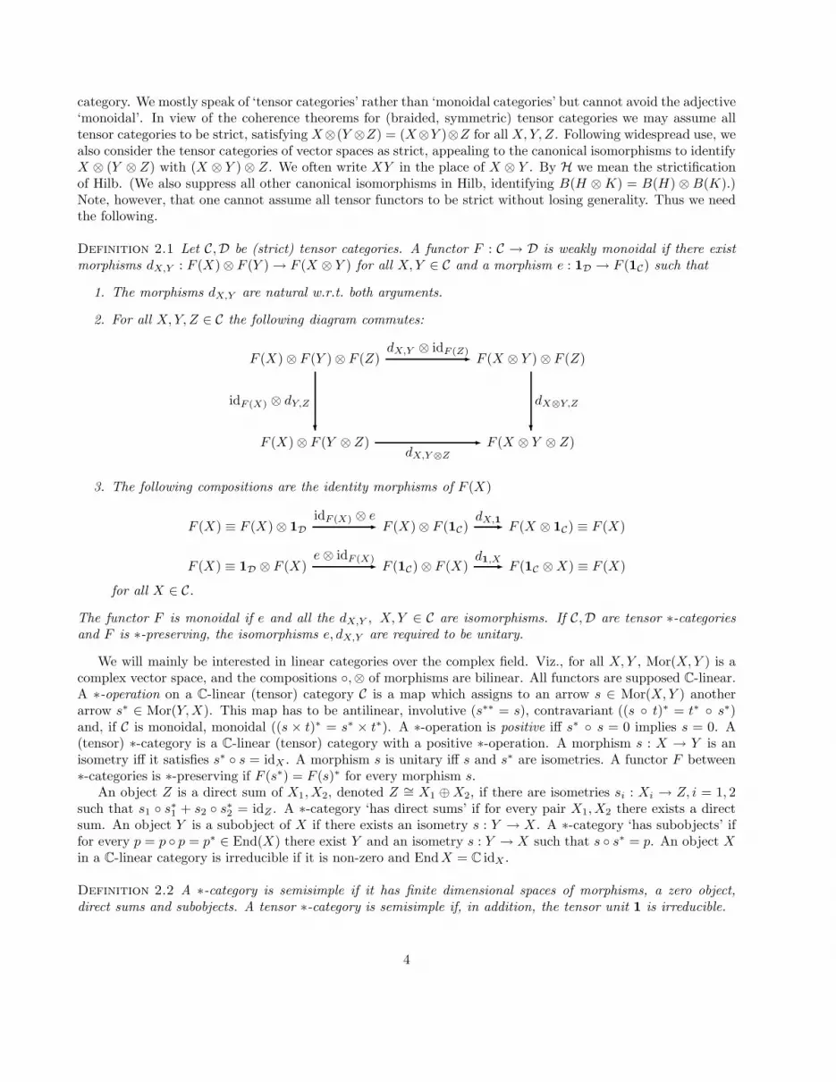
Definition 2.1 Let C,D be (strict) tensor categories. A functor F : C → D is weakly monoidal if there existmorphisms dX,Y : F (X) ⊗ F (Y ) → F (X ⊗ Y ) for all X,Y ∈ C and a morphism e : 1D → F (1C) such that

1. The morphisms dX,Y are natural w.r.t. both arguments.

2. For all X,Y, Z ∈ C the following diagram commutes:

F (X) ⊗ F (Y ) ⊗ F (Z)dX,Y ⊗ idF (Z)

- F (X ⊗ Y ) ⊗ F (Z)

F (X) ⊗ F (Y ⊗ Z)

idF (X) ⊗ dY,Z

?

dX,Y⊗Z

- F (X ⊗ Y ⊗ Z)

dX⊗Y,Z

?

3. The following compositions are the identity morphisms of F (X)

F (X) ≡ F (X) ⊗ 1D

idF (X) ⊗ e- F (X) ⊗ F (1C)

dX,1- F (X ⊗ 1C) ≡ F (X)

F (X) ≡ 1D ⊗ F (X)e⊗ idF (X)

- F (1C) ⊗ F (X)d1,X

- F (1C ⊗X) ≡ F (X)

for all X ∈ C.

The functor F is monoidal if e and all the dX,Y , X, Y ∈ C are isomorphisms. If C,D are tensor ∗-categoriesand F is ∗-preserving, the isomorphisms e, dX,Y are required to be unitary.

We will mainly be interested in linear categories over the complex field. Viz., for all X,Y , Mor(X,Y ) is acomplex vector space, and the compositions ◦,⊗ of morphisms are bilinear. All functors are supposed C-linear.A ∗-operation on a C-linear (tensor) category C is a map which assigns to an arrow s ∈ Mor(X,Y ) anotherarrow s∗ ∈ Mor(Y,X). This map has to be antilinear, involutive (s∗∗ = s), contravariant ((s ◦ t)∗ = t∗ ◦ s∗)and, if C is monoidal, monoidal ((s × t)∗ = s∗ × t∗). A ∗-operation is positive iff s∗ ◦ s = 0 implies s = 0. A(tensor) ∗-category is a C-linear (tensor) category with a positive ∗-operation. A morphism s : X → Y is anisometry iff it satisfies s∗ ◦ s = idX . A morphism s is unitary iff s and s∗ are isometries. A functor F between∗-categories is ∗-preserving if F (s∗) = F (s)∗ for every morphism s.

An object Z is a direct sum of X1, X2, denoted Z ∼= X1 ⊕X2, if there are isometries si : Xi → Z, i = 1, 2such that s1 ◦ s∗1 + s2 ◦ s

∗2 = idZ . A ∗-category ‘has direct sums’ if for every pair X1, X2 there exists a direct

sum. An object Y is a subobject of X if there exists an isometry s : Y → X . A ∗-category ‘has subobjects’ iffor every p = p ◦ p = p∗ ∈ End(X) there exist Y and an isometry s : Y → X such that s ◦ s∗ = p. An object Xin a C-linear category is irreducible if it is non-zero and EndX = C idX .

Definition 2.2 A ∗-category is semisimple if it has finite dimensional spaces of morphisms, a zero object,direct sums and subobjects. A tensor ∗-category is semisimple if, in addition, the tensor unit 1 is irreducible.

4

In a semisimple ∗-category C, End(X) is a finite dimensional C∗-algebra for every X , and every object is a finitedirect sum of irreducible objects. (It is well-known that a category which is semisimple in our sense is abelianand semisimple in the usual sense, i.e. all exact sequences split.)

Let C be a tensor ∗-category and X ∈ C. A ‘solution of the conjugate equations’ is a triple (X, r, r), whereX ∈ C and r : 1 → X ⊗X, r : 1 → X ⊗X satisfy

r∗ ⊗ idX ◦ idX ⊗ r = idX ,

r∗ ⊗ idX ◦ idX ⊗ r = idX .

A tensor ∗-category C ‘has conjugates’ if there is a solution of the conjugate equations for every X ∈ C. Asolution (X, r, r) is normalized iff r∗ ◦ r = r∗ ◦ r. It is a standard solution iff there are irreducible objectsXi, i ∈ IX , solutions (Xi, ri, ri) of the conjugate equations and isometries vi : Xi → X,wi : Xi → X, i ∈ IXsatisfying

v∗i ◦ vj = δij idXi,

∑

i

vi ◦ v∗i = idX ,

similar equations for wi, and we have

r =∑

i

wi ⊗ vi ◦ ri, r =∑

i

vi ⊗ wi ◦ ri.

We define the (intrinsic or categorical) dimension d(X) ∈ R+ of X by r∗ ◦ r = d(X)id1 where (X, r, r) is anormalized standard solution. One can prove the following facts, cf. [23]. The dimension is additive underdirect sums and multiplicative under tensor products. It takes values in the set {2 cos π

n, n = 3, 4, . . .} ∪ [2,∞),

in particular d(X) ≥ 1 with d(X) = 1 iff X ⊗X ∼= 1 iff X is invertible, i.e. there exists Y such that X ⊗Y ∼= 1.If d(X) = 1 then X is irreducible. In the category H of Hilbert spaces we have dH(H) = dimC H .

We briefly comment on a somewhat more general setting. A C∗-(tensor) category is a (tensor) ∗-categorywhere Mor(X,Y ) is a Banach space for every pair (X,Y ) of objects and the norms satisfy ‖X∗ ◦ X‖ = ‖X‖2.A W ∗-category is a C∗-category where every Mor(X,Y ) is the dual of a Banach space for every pair (X,Y ).In a C∗-category with conjugates and irreducible tensor unit all spaces of morphisms are finite dimensional.This is useful in applications where this finite dimensionality is not known a priori, like in quantum field theory.Conversely, every ∗-category which is semisimple in our sense is a W ∗-category, cf. [25]. In a W ∗-category,every morphism s : X → Y has a polar decomposition s = pu, where p is positive and u a partial isometry.As a consequence, whenever Mor(X,Y ) contains a split monic (or isomorphism), it also contains an isometry(respectively, unitary). This shows that most of the above definitions, e.g., of direct sums, are equivalent to thethe usual ones as given, e.g., in [24].

If C is a semisimple tensor ∗-category we denote the set of isomorphism classes of irreducible objects by IC .Let (Xi, i ∈ IC) be a complete set of irreducible objects and write di = d(Xi). We have 0 ∈ IC such that X0

∼= 1.If C has conjugates, IC comes with an involution i 7→ ı such that Xı is a conjugate of Xi. For i, j, k ∈ IC wedefine Nk

ij = dimMor(Xk, Xi ⊗Xj). These numbers satisfy the following properties.

1. For every pair (i, j) there are only finitely many k ∈ IC such that Nkij 6= 0. We have Xi ⊗ Xj

∼=⊕k∈IC

Nkij Xk and thus didj =

∑kN

kijdk.

2.∑

l

N lijN

mlk =

∑

n

NminN

njk for all i, j, k,m ∈ IC .

3. Nkij = N i

k = N jık = N

ki= N ı

jk= Nk

,ı for all i, j, k ∈ IC .

4. N0ij = δi,.

5. If C is braided, cf. Section 6, then Nkij = Nk

ji for all i, j, k ∈ IC .

5

2.2 Algebraic Quantum Groups

In this subsection we briefly outline those aspects of the theory of aqg that will be needed in the sequel. Forthe details and proofs, see the original references [35, 37].

Every algebra will be a (not necessarily unital) associative algebra over the complex field C. The identitymap on a set V will be denoted by ι. If V and W are linear spaces, V ′ denotes the linear space of linearfunctionals on V and V ⊗W denotes the linear space tensor product of V and W . The flip map σ from V ⊗Wto W ⊗ V is the linear map sending v ⊗ w onto w ⊗ v, for all v ∈ V and w ∈ W . If V and W are Hilbertspaces, V ⊗W denotes their Hilbert space tensor product; we denote by B(V ) and B0(V ) the C*-algebras ofbounded linear operators and compact operators on V , respectively. If V and W are algebras, V ⊗W denotestheir algebra tensor product. If V and W are C*-algebras, then V ⊗W will denote their C*-tensor productwith respect to the minimal C*-norm.

An algebra A is non-degenerate if for any a ∈ A such that ab = 0 for all b ∈ A or ba = 0 for all b ∈ A, wehave a = 0. Obviously, all unital algebras are non-degenerate. If A and B are non-degenerate algebras, so isA⊗B. From now on all algebras are assumed to be non-degenerate.

Let A be a ∗-algebra and denote by EndA the unital algebra of linear maps from A to itself. Let

M(A) = {x ∈ EndA | ∃y ∈ EndA such that x(a)∗b = a∗y(b) ∀a, b ∈ A}.

Then M(A) is a unital subalgebra of EndA. The linear map y associated to a given x ∈ M(A) is uniquelydetermined by non-degeneracy and we denote it by x∗. The unital algebra M(A) becomes a ∗-algebra whenendowed with the involution x 7→ x∗. This unital ∗-algebra is called the multiplier algebra of A.

Suppose that A is an ideal in a ∗-algebra B. For b ∈ B, define Lb ∈ M(A) by Lb(a) = ba, for all a ∈ A.Then the map L : B → M(A), b 7→ Lb, is a homomorphism. If A is an essential ideal in B in the sense thatan element b of B is necessarily equal to zero if ba = 0, for all a ∈ A, or ab = 0, for all a ∈ A, then L isinjective. In particular, A is an essential ideal in itself (by non-degeneracy) and therefore we have an injectivehomomorphism L : A → M(A). We identify the image of A under L with A. Then A is an essential ideal ofM(A). (In fact, M(A) is the ‘largest’ algebra containing A as an essential ideal.) Obviously, M(A) = A iff Ais unital.

If A andB are ∗-algebras, then it is easily verified that A⊗B is an essential self-adjoint ideal inM(A)⊗M(B).Hence, by the preceding remarks, there exists a canonical injective ∗-homomorphism from M(A) ⊗M(B) intoM(A ⊗ B). We use this to identify M(A) ⊗M(B) as a unital ∗-subalgebra of M(A ⊗ B). In general, thesealgebras are not equal. A linear map π : A → B is said to be non-degenerate if π(A)B = B and Bπ(A) = B.Here, as elsewhere, π(A)B denotes the linear span of {π(a)b | a ∈ A, b ∈ B}. Whenever π is non-degenerateand multiplicative (resp. non-degenerate and antimultiplicative), there exists a unique extension to a unitalhomomorphism (resp. antihomomorphism) π : M(A) →M(B). We shall henceforth use the same symbol π todenote the original map and its extension π. A representation of a ∗-algebra is a non-degenerate homomorphismπ : A→ B(K), where K is a Hilbert space.

If ω is a linear functional on A and x ∈ M(A), we define the linear functionals xω and ωx on A by setting(xω)(a) = ω(ax) and (ωx)(a) = ω(xa), for all a ∈ A. We need the leg numbering notation. Take three ∗-algebrasA, B, C. It can be shown that there exists a non-degenerate ∗-homomorphism θ13 : A⊗ C → M(A ⊗ B ⊗ C)such that θ13(a ⊗ c) = a ⊗ 1 ⊗ c, for all a ∈ A, c ∈ C. Thus, it has a unique extension to M(A ⊗ C). Setx13 = θ13(x), for all x ∈M(A⊗ C). The other variants of the leg numbering notation are defined similarly.

The triple product A ⊗ A ⊗ A is an essential ideal of both M(A ⊗ A) ⊗ A and A ⊗ M(A ⊗ A), thusM(M(A⊗A) ⊗A) ⊂M(A⊗A⊗A) and M(A⊗M(A⊗A)) ⊂M(A⊗A⊗A).

Definition 2.3 A multiplier Hopf ∗-algebra (A,∆) consists of a ∗-algebra A and a ∗-homomorphism ∆ fromA into M(A⊗A) such that

1. (∆ ⊗ ι)∆ = (ι ⊗ ∆)∆.

2. The linear mappings T1, T2 from A⊗A into M(A⊗A) such that

T1(a⊗ b) = ∆(a)(b ⊗ 1),

T2(a⊗ b) = ∆(a)(1 ⊗ b)

6

for all a, b ∈ A, are bijections from A⊗A to A⊗A.

Here the (unique) extension of ∆ ⊗ ι : A ⊗ A → M(A ⊗ A ⊗ A) to M(A ⊗ A) is understood and similarly forι⊗ ∆. Condition (ii) implies that ∆(a)(b ⊗ 1),∆(a)(1 ⊗ b) ∈M(A⊗A) lie in fact in A⊗A.

We say that two multiplier Hopf ∗-algebras (A1,∆1) and (A2,∆2) are isomorphic, and write (A1,∆1) ∼=(A2,∆2), if there exists a bijective ∗-homomorphism θ : A1 → A2 such that (θ ⊗ θ)∆1 = ∆2θ.

The following result shows that multiplier Hopf ∗-algebras share most properties with Hopf algebras. Letm : A⊗A→ A denote the linear extension of the multiplication map. Note that m is a ∗-homomorphism iff Ais commutative.

Proposition 2.4 Let (A,∆) be a multiplier Hopf ∗-algebra. There exist a unique ∗-homomorphism ε : A→ C

and a unique invertible antimultiplicative S ∈ EndA such that

1. (ε⊗ ι)(∆(a)(1 ⊗ b)) = ab,

2. (ι⊗ ε)(∆(a)(b ⊗ 1)) = ab,

3. m(S ⊗ ι)(∆(a)(1 ⊗ b)) = ε(a)b,

4. m(ι⊗ S)(∆(a)(b ⊗ 1)) = ε(a)b

for all a, b ∈ A. We call ε the counit and S the coinverse. Conversely, if (A⊗1)∆(A) ⊂ A⊗A and (A⊗1)∆(A) ⊂A ⊗ A and there exist linear maps ε : A → C and S : A → A satisfying properties 1-4 with S invertible, then(A,∆) is a multiplier Hopf ∗-algebra.

We denote mop = mσ and ∆op = σ∆ where σ(a ⊗ b) = b ⊗ a is the flip ∗-automorphism of A ⊗ A andM(A ⊗ A). Aop denotes the vector space A with multiplication mop. The following result follows easily fromthe uniqueness of the counit and coinverse.

Proposition 2.5 The antipode S is invertible and

1. S−1(a) = S(a∗)∗ ∀a ∈ A.

2. (S ⊗ S)(∆(a)(1 ⊗ b)) = (1 ⊗ S(b))∆opS(a) ∀a, b ∈ A.

3. εS = ε.

4. (Aop,∆) and (A,∆op) are multiplier Hopf ∗-algebras with counit ε and coinverse S−1.

Definition 2.6 A linear functional ω on a multiplier Hopf ∗-algebra (A,∆) is called

1. positive iff ω(a∗a) ≥ 0 ∀a ∈ A,

2. faithful iff it is positive and ω(a∗a) = 0 ⇒ a = 0 ∀a ∈ A,

3. left-invariant iff (ι⊗ ω)(∆(a)(b ⊗ 1)) = ω(a)b ∀a, b ∈ A,

4. right-invariant iff (ω ⊗ ι)((1 ⊗ b)∆(a)) = ω(a)b ∀a, b ∈ A.

Thus ω is left-invariant iff ωS is right-invariant.

Definition 2.7 An aqg is a multiplier Hopf ∗-algebra (A,∆) which admits a non-zero left-invariant positivelinear functional ϕ.

Theorem 2.8 Let (A,∆) be an aqg with positive left-invariant functional ϕ. Then

1. ϕ is faithful.

7

2. If ω is a left-invariant functional, there exists c ∈ C such that ω = cϕ.

3. If ω is a right-invariant functional, there exists c ∈ C such that ω = cϕS.

An immediate consequence is that the ∗-operation is positive, viz. a∗a = 0 ⇒ a = 0, which clearly isstronger than non-degeneracy. Furthermore, there exists a unique complex number µ such that ϕS2 = µϕ. Itcan be proved that |µ| = 1, but it has recently been discovered that µ 6= 1 for the quantum group version ofax + b [38]. Every aqg (A,∆) has the property that to any a ∈ A, there exists c ∈ A such that ac = ca = a.Two aqg are said to be isomorphic if they are isomorphic as multiplier Hopf ∗-algebras and we use the samenotation ∼= to denote this.

Set ψ = ϕS. Then ψ is a non-zero right-invariant linear functional on A. However, in general, ψ will notbe positive. It is known that there exists a non-zero positive right-invariant linear functional on A. To ϕ thereexistence a unique automorphism ρ on A such that ϕ(ab) = ϕ(bρ(a)), for every a, b ∈ A. We refer to this as theweak KMS-property of ϕ. Moreover, we have ∆ρ = (S2 ⊗ ρ)∆ and ρ(ρ(a∗)∗) = a, for every a ∈ A. Also thereexists an automorphism ρ′ for the right-invariant functional ψ, that is, ρ′ is an automorphism on A such thatψ(ab) = ψ(bρ′(a)), for every a, b ∈ A.

It is possible to introduce a modular function for aqg. It is an invertible element δ in M(A) such that(ϕ⊗ ι)(∆(a)(1 ⊗ b)) = ϕ(a)δb, for every a, b ∈ A. This modular function satisfies

∆(δ) = δ ⊗ δ, ε(δ) = 1, S(δ) = δ−1.

As in the classical case we have

ϕ(S(a)) = ϕ(aδ) = µϕ(δa) ∀a ∈ A.

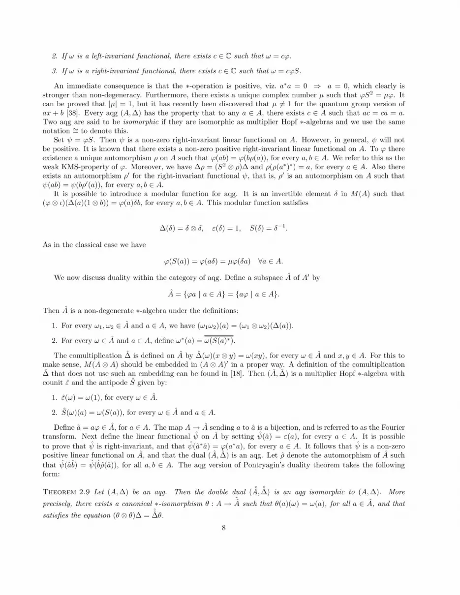
We now discuss duality within the category of aqg. Define a subspace A of A′ by

A = {ϕa | a ∈ A} = {aϕ | a ∈ A}.

Then A is a non-degenerate ∗-algebra under the definitions:

1. For every ω1, ω2 ∈ A and a ∈ A, we have (ω1ω2)(a) = (ω1 ⊗ ω2)(∆(a)).

2. For every ω ∈ A and a ∈ A, define ω∗(a) = ω(S(a)∗).

The comultiplication ∆ is defined on A by ∆(ω)(x ⊗ y) = ω(xy), for every ω ∈ A and x, y ∈ A. For this tomake sense, M(A ⊗ A) should be embedded in (A ⊗ A)′ in a proper way. A definition of the comultiplication∆ that does not use such an embedding can be found in [18]. Then (A, ∆) is a multiplier Hopf ∗-algebra withcounit ε and the antipode S given by:

1. ε(ω) = ω(1), for every ω ∈ A.

2. S(ω)(a) = ω(S(a)), for every ω ∈ A and a ∈ A.

Define a = aϕ ∈ A, for a ∈ A. The map A→ A sending a to a is a bijection, and is referred to as the Fouriertransform. Next define the linear functional ψ on A by setting ψ(a) = ε(a), for every a ∈ A. It is possible

to prove that ψ is right-invariant, and that ψ(a∗a) = ϕ(a∗a), for every a ∈ A. It follows that ψ is a non-zeropositive linear functional on A, and that the dual (A, ∆) is an aqg. Let ρ denote the automorphism of A such

that ψ(ab) = ψ(bρ(a)), for all a, b ∈ A. The aqg version of Pontryagin’s duality theorem takes the followingform:

Theorem 2.9 Let (A,∆) be an aqg. Then the double dual (A, ∆) is an aqg isomorphic to (A,∆). More

precisely, there exists a canonical ∗-isomorphism θ : A →ˆA such that θ(a)(ω) = ω(a), for all a ∈ A, and that

satisfies the equation (θ ⊗ θ)∆ =ˆ∆θ.

8

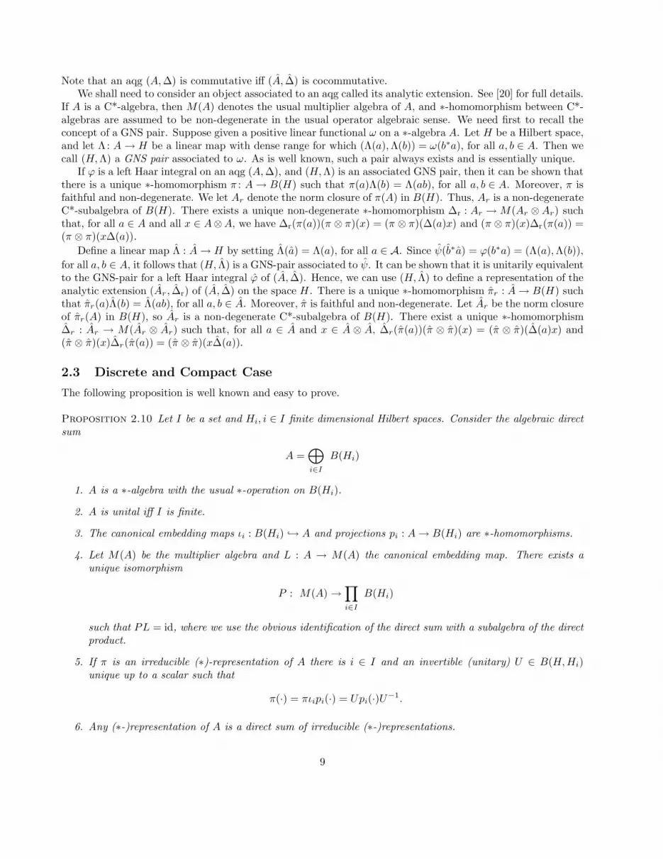
Note that an aqg (A,∆) is commutative iff (A, ∆) is cocommutative.We shall need to consider an object associated to an aqg called its analytic extension. See [20] for full details.

If A is a C*-algebra, then M(A) denotes the usual multiplier algebra of A, and ∗-homomorphism between C*-algebras are assumed to be non-degenerate in the usual operator algebraic sense. We need first to recall theconcept of a GNS pair. Suppose given a positive linear functional ω on a ∗-algebra A. Let H be a Hilbert space,and let Λ: A→ H be a linear map with dense range for which (Λ(a),Λ(b)) = ω(b∗a), for all a, b ∈ A. Then wecall (H,Λ) a GNS pair associated to ω. As is well known, such a pair always exists and is essentially unique.

If ϕ is a left Haar integral on an aqg (A,∆), and (H,Λ) is an associated GNS pair, then it can be shown thatthere is a unique ∗-homomorphism π : A→ B(H) such that π(a)Λ(b) = Λ(ab), for all a, b ∈ A. Moreover, π isfaithful and non-degenerate. We let Ar denote the norm closure of π(A) in B(H). Thus, Ar is a non-degenerateC*-subalgebra of B(H). There exists a unique non-degenerate ∗-homomorphism ∆r : Ar →M(Ar ⊗Ar) suchthat, for all a ∈ A and all x ∈ A⊗A, we have ∆r(π(a))(π ⊗ π)(x) = (π ⊗ π)(∆(a)x) and (π ⊗ π)(x)∆r(π(a)) =(π ⊗ π)(x∆(a)).

Define a linear map Λ : A→ H by setting Λ(a) = Λ(a), for all a ∈ A. Since ψ(b∗a) = ϕ(b∗a) = (Λ(a),Λ(b)),

for all a, b ∈ A, it follows that (H, Λ) is a GNS-pair associated to ψ. It can be shown that it is unitarily equivalentto the GNS-pair for a left Haar integral ϕ of (A, ∆). Hence, we can use (H, Λ) to define a representation of theanalytic extension (Ar , ∆r) of (A, ∆) on the space H . There is a unique ∗-homomorphism πr : A→ B(H) suchthat πr(a)Λ(b) = Λ(ab), for all a, b ∈ A. Moreover, π is faithful and non-degenerate. Let Ar be the norm closureof πr(A) in B(H), so Ar is a non-degenerate C*-subalgebra of B(H). There exist a unique ∗-homomorphism∆r : Ar → M(Ar ⊗ Ar) such that, for all a ∈ A and x ∈ A ⊗ A, ∆r(π(a))(π ⊗ π)(x) = (π ⊗ π)(∆(a)x) and(π ⊗ π)(x)∆r(π(a)) = (π ⊗ π)(x∆(a)).

2.3 Discrete and Compact Case

The following proposition is well known and easy to prove.

Proposition 2.10 Let I be a set and Hi, i ∈ I finite dimensional Hilbert spaces. Consider the algebraic directsum

A =⊕

i∈I

B(Hi)

1. A is a ∗-algebra with the usual ∗-operation on B(Hi).

2. A is unital iff I is finite.

3. The canonical embedding maps ιi : B(Hi) → A and projections pi : A→ B(Hi) are ∗-homomorphisms.

4. Let M(A) be the multiplier algebra and L : A → M(A) the canonical embedding map. There exists aunique isomorphism

P : M(A) →∏

i∈I

B(Hi)

such that PL = id, where we use the obvious identification of the direct sum with a subalgebra of the directproduct.

5. If π is an irreducible (∗)-representation of A there is i ∈ I and an invertible (unitary) U ∈ B(H,Hi)unique up to a scalar such that

π(·) = πιipi(·) = Upi(·)U−1.

6. Any (∗-)representation of A is a direct sum of irreducible (∗-)representations.

9

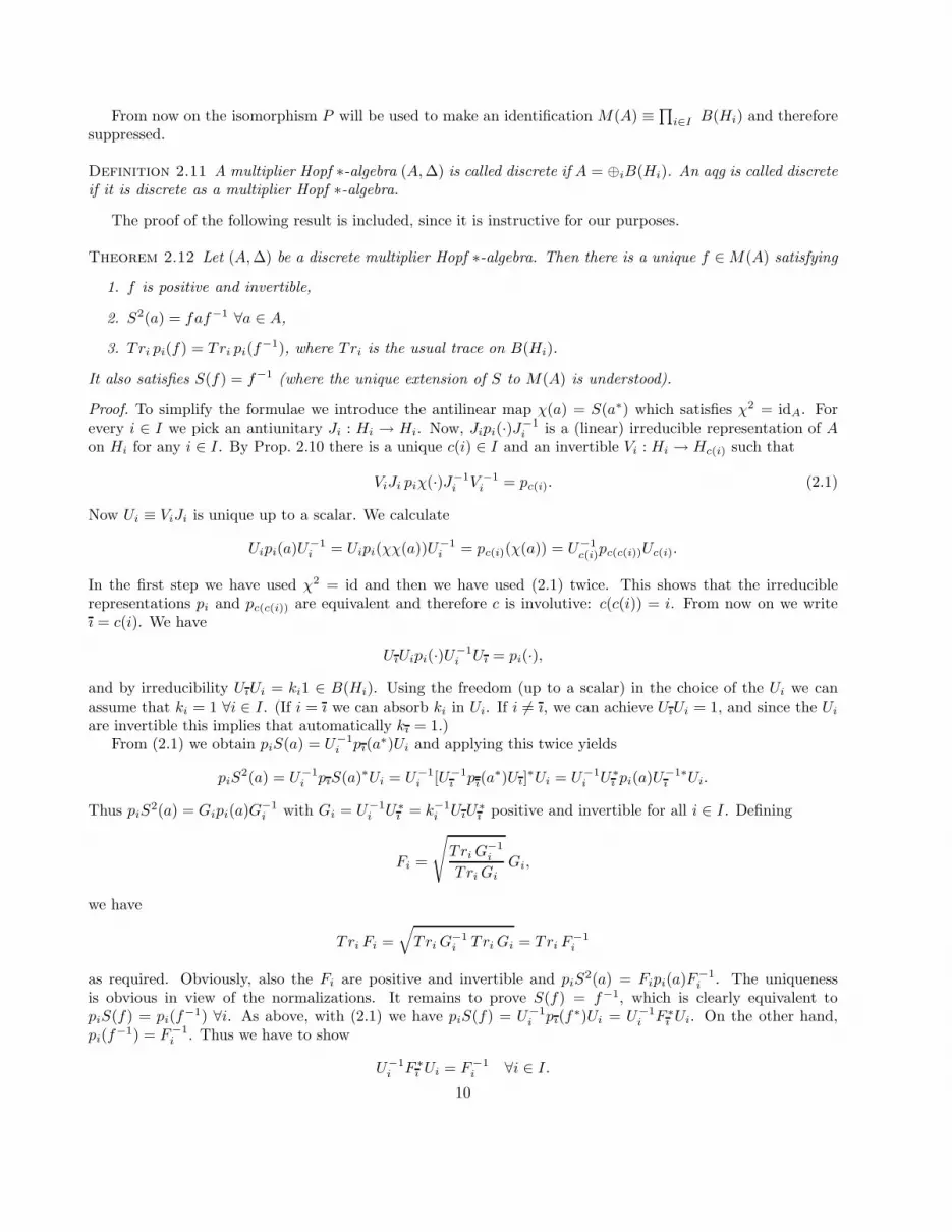
From now on the isomorphism P will be used to make an identification M(A) ≡∏i∈I B(Hi) and therefore

suppressed.

Definition 2.11 A multiplier Hopf ∗-algebra (A,∆) is called discrete if A = ⊕iB(Hi). An aqg is called discreteif it is discrete as a multiplier Hopf ∗-algebra.

The proof of the following result is included, since it is instructive for our purposes.

Theorem 2.12 Let (A,∆) be a discrete multiplier Hopf ∗-algebra. Then there is a unique f ∈M(A) satisfying

1. f is positive and invertible,

2. S2(a) = faf−1 ∀a ∈ A,

3. Tri pi(f) = Tri pi(f−1), where Tri is the usual trace on B(Hi).

It also satisfies S(f) = f−1 (where the unique extension of S to M(A) is understood).

Proof. To simplify the formulae we introduce the antilinear map χ(a) = S(a∗) which satisfies χ2 = idA. Forevery i ∈ I we pick an antiunitary Ji : Hi → Hi. Now, Jipi(·)J

−1i is a (linear) irreducible representation of A

on Hi for any i ∈ I. By Prop. 2.10 there is a unique c(i) ∈ I and an invertible Vi : Hi → Hc(i) such that

ViJi piχ(·)J−1i V −1

i = pc(i). (2.1)

Now Ui ≡ ViJi is unique up to a scalar. We calculate

Uipi(a)U−1i = Uipi(χχ(a))U−1

i = pc(i)(χ(a)) = U−1c(i)pc(c(i))Uc(i).

In the first step we have used χ2 = id and then we have used (2.1) twice. This shows that the irreduciblerepresentations pi and pc(c(i)) are equivalent and therefore c is involutive: c(c(i)) = i. From now on we writeı = c(i). We have

UıUipi(·)U−1i Uı = pi(·),

and by irreducibility UıUi = ki1 ∈ B(Hi). Using the freedom (up to a scalar) in the choice of the Ui we canassume that ki = 1 ∀i ∈ I. (If i = ı we can absorb ki in Ui. If i 6= ı, we can achieve UıUi = 1, and since the Uiare invertible this implies that automatically kı = 1.)

From (2.1) we obtain piS(a) = U−1i pı(a

∗)Ui and applying this twice yields

piS2(a) = U−1

i pıS(a)∗Ui = U−1i [U−1

ı pı(a∗)Uı]

∗Ui = U−1i U∗

ı pi(a)U−1∗ı Ui.

Thus piS2(a) = Gipi(a)G

−1i with Gi = U−1

i U∗ı = k−1

i UıU∗ı positive and invertible for all i ∈ I. Defining

Fi =

√TriG

−1i

TriGiGi,

we have

Tri Fi =

√TriG

−1i TriGi = Tri F

−1i

as required. Obviously, also the Fi are positive and invertible and piS2(a) = Fipi(a)F

−1i . The uniqueness

is obvious in view of the normalizations. It remains to prove S(f) = f−1, which is clearly equivalent topiS(f) = pi(f

−1) ∀i. As above, with (2.1) we have piS(f) = U−1i pı(f

∗)Ui = U−1i F ∗

ı Ui. On the other hand,pi(f

−1) = F−1i . Thus we have to show

U−1i F ∗

ı Ui = F−1i ∀i ∈ I.

10

Inserting the definition of the Fi this is equivalent to

U−1i

√TrıG

−1ı

TrıGıUiU

−1∗ı Ui =

√TriGi

TriG−1i

U∗−1ı Ui ∀i ∈ I.

This is clearly equivalent to

TrıG−1ı TriG

−1i = TriGi TrıGı ∀i ∈ I.

Plugging in Gi = U−1i U∗

ı this is an easy computation which we omit. (One uses Uı = U−1i and cyclicity of the

traces.) �

Theorem 2.13 A discrete multiplier Hopf ∗-algebra (A,∆) admits a non-zero left-invariant positive linearfunctional ϕ, thus is an aqg.

Proposition 2.14 An aqg (A,∆) is discrete iff there exists h ∈ A such that ah = ε(a)h, for all a ∈ A.

Definition 2.15 An aqg (A,∆) is called compact if A is unital.

Note that an aqg (A,∆) is compact iff it is a Hopf ∗-algebra. Hence the analytical extension of a compactaqg is a compact quantum group in the sense of S.L. Woronowicz. A multiplier Hopf ∗-algebra (A,∆) with Aunital is not necessarily an aqg, but this is the case whenever A has a C*-algebra envelope. It is easily seenthat (A,∆) is compact and discrete iff A is finite dimensional.

Theorem 2.16 Let (A,∆) be an aqg. Then (A,∆) is compact iff (A, ∆) is discrete.

2.4 Examples

The examples discussed below are treated in depth in [11]. The translation into the framework of aqgis straight-forward and is recommended as an exercise.

Throughout this section let Γ denote a discrete group with unit e. Consider the group algebra CΓ and thealgebra Cc(Γ) of finitely supported complex valued functions with the usual pointwise operations. They areboth non-degenerate ∗-algebras. The group algebra has unit δe, whereas Cc(Γ) has a unit iff Γ is finite.

In the group algebra case (CΓ,∆) the comultiplication is given by ∆(δg) = δg⊗δg and yields a Hopf ∗-algebrawith counit ε(δg) = 1 and coinverse S(δg) = δg−1 , for all g ∈ Γ. The functional defined by ϕ(δg) = δg,e, forg ∈ Γ, is unital, positive and both left and right invariant, so (CΓ,∆) is a cocommutative compact aqg.

Note that M(Cc(Γ)) ∼= C(Γ), where C(Γ) is the unital ∗-algebra of all functions on Γ, and that Cc(Γ×Γ) ∼=Cc(Γ) ⊗ Cc(Γ) (as ∗-algebras). Thus the algebra Cc(Γ) has comultiplication ∆ : Cc(Γ) → M(Cc(Γ) ⊗ Cc(Γ))given by ∆(a)(g, h) = a(gh) for a ∈ Cc(Γ) and g, h ∈ Γ. It is easy to see that the support of ∆(a) fora ∈ Cc(Γ) is infinite whenever Γ is. This shows that the Hopf algebra framework is too restrictive to coverthis example. For (Cc(Γ),∆) we have ε(a) = a(e) and S(a)(g) = a(g−1) where a ∈ Cc(Γ × Γ) and g ∈ Γ. Theintegral ϕ(a) =

∑g∈Γ a(g), a ∈ CΓ, w.r.t. the counting measure is positive and both left and right invariant,

so (Cc(Γ),∆) is a commutative discrete aqg.The following proposition shows that these two examples exhaust the cocommutative compact aqg and the

commutative discrete aqg.

Proposition 2.17 Let (A,∆) be an aqg. Then

1. (A,∆) is discrete and commutative iff there exists a discrete group Γ such that (A,∆) ∼= (Cc(Γ),∆).

2. (A,∆) is compact and co-commutative iff there exists a discrete group Γ such that (A,∆) ∼= (CΓ,∆).

11

It is also easy to check that (CΓ, ∆) ∼= (Cc(Γ),∆) and ( ˆCc(Γ), ∆) ∼= (CΓ,∆), so they are dual to each other.Giving a characterization of the commutative compact and the cocommutative discrete algebraic quantum

groups on the algebraic level, is less immediate and requires some (co-) representation theory. For the momentwe mention that the commutative-compact case can be described in terms of the algebra of regular functionson a compact group, and we make here an analytic statement concerning both cases.

Proposition 2.18 Let (A,∆) be an aqg with analytic extension (Ar,∆r). Then

1. (A,∆) is compact and commutative iff there exists a compact group G such that (Ar,∆r) ∼= (C(G),∆r).

2. (A,∆) is discrete and cocommutative iff there exists a compact group G such that (Ar,∆r) ∼= (C∗r (G),∆r).

Again these two cases are dual to each other. Here C(G) denotes the C*-algebra of continuous functions onG with uniform norm, whereas C∗

r (G) denotes the reduced group C*-algebra of G. Since a compact group Gis amenable, C∗

r (G) coincides with the universal group C*-algebra C∗(G), and therefore, as we shall see veryexplicitly in the next section, the representation theory of a discrete cocommutative aqg coincides with that ofG. We shall also give a simple algebraic description of the associated aqg in this case.

3 Representation Theory

3.1 The Universal Corepresentation

Throughout this section (A,∆) stands for an arbitrary aqg and B denotes a ∗-algebra. We recall the universalcorepresentation U of (A,∆) and discuss its various properties [18].

Definition 3.1 A corepresentation of (A,∆) on B is an element V ∈M(A⊗B) such that (∆⊗ ι)V = V13V23.

Proposition 3.2 Suppose V is a corepresentation of (A,∆) on B. Then the following are equivalent:

1. V is invertible in M(A⊗B) with V −1 = (S ⊗ ι)V .

2. (ε⊗ ι)V = 1.

3. V (A⊗B) = A⊗B = (A⊗B)V .

A corepresentation V satisfying these equivalent conditions is said to be non-degenerate.

Definition 3.3 A unitary corepresentation V of (A,∆) on B is a corepresentation on B which is a unitaryelement of M(A⊗B).

The following result is fundamental for corepresentations of aqg. We regard elements of A⊗ A as endomor-phisms of A.

Theorem 3.4 There exists a unique element U ∈M(A⊗ A) such that

[U(x⊗ ω)](y) = (ι⊗ ω)(∆(y)(x ⊗ 1))

[(x ⊗ ω)U ](y) = (ω ⊗ ι)((1 ⊗ x)∆(y))

for all x, y ∈ A and ω ∈ A. Moreover, we have the following properties for U :

1. U is unitary in M(A⊗ A).

2. (∆ ⊗ ι)U = U13U23.

12

3. (ι⊗ ∆)U = U12U13.

4. (ω ⊗ ι)U = ω for all ω ∈ A.

5. (ι⊗ a)U = a for all a ∈ A, where a acts on A by the identification A = A.

Note that claims 1 and 2 say that U is a unitary corepresentation of (A,∆) on A, whereas claims 1 and 3say that σ(U) is a unitary corepresentation of (A, ∆) on A. Below we will explain why U is called the universalcorepresentation of (A,∆). It follows that σ(U) is the universal corepresentation of (A, ∆).

Let Hom(A,B) denote the set of ∗-homomorphisms from A to M(B) satisfying θ(A)B = B.

Proposition 3.5 Let V ∈M(A⊗B) and consider the linear map

πV : A→M(B), ω 7→ (ω ⊗ ι)V.

Then the following equivalences hold:

1. V is a corepresentation (of (A,∆) on B) iff πV is multiplicative.

2. V is a non-degenerate corepresentation iff πV is multiplicative and non-degenerate.

3. V is a unitary corepresentation iff πV ∈ Hom(A, B).

The universality of U can now be formulated as follows.

Theorem 3.6 For any unitary corepresentation V of (A,∆) on B and any θ ∈ Hom(A, B), we have:

1. (ι⊗ πV )U = V .

2. π(ι⊗θ)U = θ.

The result remains valid for the non-degenerate situation without ∗-operation.

Definition 3.7 Let B′ be non-degenerate ∗-algebra. For θ ∈ Hom(A,B) and θ′ ∈ Hom(A,B′) we defineθ × θ′ ∈ Hom(A,B ⊗B′) by θ × θ′ = (θ ⊗ θ′)∆. If V and V ′ are unitary corepresentations of (A,∆) on B andB′, respectively, we define a unitary corepresentation V × V ′ of (A,∆) on B ⊗B′ by V × V ′ = V12V

′13.

Theorem 3.8 The map sending unitary corepresentations V of (A,∆) on B to πV ∈ Hom(A, B), is a bijection.Let V ′ be a unitary corepresentation of (A,∆) on B′. Then πV×V ′ = πV × πV ′ . For the universal corepre-sentation U of (A,∆) on A we have πU = ι ∈ Hom(A, A), and finally for the trivial unitary corepresentation1 ⊗ 1 ∈ A⊗B(C) of (A,∆) we have π1⊗1 = ε, where ε is the counit of (A, ∆).

Proof. The only part which is not immediate from the results above, is the identity πV×V ′ = πV ×πV ′ . To showthis, first note that

V × V ′ = V12V′13 = [(ι⊗ πV )U ]12[(ι ⊗ πV ′)U ]13 = (ι⊗ πV ⊗ πV ′)(U12U13)

= (ι⊗ πV ⊗ πV ′)(ι⊗ ∆)U = (ι⊗ (πV ⊗ πV ′)∆)U = (ι⊗ πV × πV ′)U.

Thus we may conclude that

πV×V ′(ω) = (ω ⊗ ι⊗ ι)(V × V ′) = (ω ⊗ ι⊗ ι)(ι ⊗ πV × πV ′)U = (πV × πV ′)(ω ⊗ ι)U = (πV × πV ′)(ω),

for all ω ∈ A. �

13

Remark 3.9 The correspondence established in Theorem 3.8 is in fact a functor if we define arrows for rep-resentations and corepresentations on ∗-algebras in the following way. For any objects π ∈ Hom(A,B) andπ′ ∈ Hom(A,B′) define an arrow f : π → π′ to be f ∈ Hom(B,B′) such that fπ = π′. Similarly, if V and V ′

are unitary corepresentations of (A,∆) on B and B′, respectively, we define an arrow f : V → V ′ between theseobjects to be f ∈ Hom(B,B′) such that V ′ = (ι ⊗ f)V . Then the correspondence V 7→ πV in Theorem 3.8 isan equivalence of tensor categories (they are not ∗-categories). 2

Remark 3.10 We remark on the tensor categories of actions and coactions of an aqg (A,∆) on ∗-algebras.By an action γ of (A,∆) on a ∗-algebra B, we mean a surjective linear map γ : A ⊗ B → B such that

γ(m⊗ ι) = γ(ι⊗ γ). An arrow f : γ → γ′ is an element f ∈ Hom(B,B′) such that fγ = γ′f . We do not definetensor products in the general case.

Given π ∈ Hom(A,B), we define the action γπ of (A,∆) on B by γπ(a⊗ b) = π(a)b, for all a ∈ A and b ∈ B.Using non-degeneracy of f , we see that for any f ∈ Hom(B,B′), we have f : π → π′ iff f : γπ → γπ′ . Thusπ 7→ γπ is an equivalence of the tensor category of non-degenerate ∗-representations of (A,∆) on ∗-algebras tothe tensor category of actions of (A,∆) on ∗-algebras contained in the image of the functor and with tensorproduct γπ × γπ′ simply defined to be the action γπ×π′ . We have not incorporated the ∗-preserving property ofπ in γπ and the axioms for actions.

A coaction δ of (A,∆) on a ∗-algebra B is a δ ∈ Hom(B,A ⊗ B) such that (ι ⊗ δ)δ = (∆ ⊗ ι)δ and(ε ⊗ ι)δ = ι. Such coactions form a tensor category, an arrow f : δ → δ′ being an element f ∈ Hom(B,B′)such that (ι ⊗ f)δ = δ′f and the tensor product δ × δ′ being the comodule of (A,∆) on B ⊗ B′ given by(δ × δ′)(b⊗ b′) = δ(b)12δ

′(b′)13, for all b ∈ B and b′ ∈ B′.Let V be a unitary corepresentation of (A,∆) on B. Then the linear map δV : B → M(A ⊗ B) given by

δV (b) = V (1 ⊗ b)V ∗ for all b ∈ B, is indeed a coaction of (A,∆op) on B. Non-degeneracy of δV follows fromV (A⊗B) = A⊗B, and the formula (ι⊗ δV )δV = (∆op ⊗ ι)δV follows from the calculation

(ι⊗ δV )δV (b) = (ι⊗ δV )V (1 ⊗ δV (b))((ι ⊗ δV )V )∗ = V23V13V∗23(1 ⊗ V (1 ⊗ b)V ∗)(V23V13V

∗23)

∗

= V23V13(1 ⊗ 1 ⊗ b)V ∗13V

∗23 = (∆op ⊗ ι)V (1 ⊗ 1 ⊗ b)((∆op ⊗ ι)V )∗ = (∆op ⊗ ι)(V (1 ⊗ b)V ∗)

= (∆op ⊗ ι)δV (b)

for all b ∈ B. Note that any arrow f : V → V ′ will be an arrow f : δV → δV ′ , but the converse is nottrue (consider B′ commutative). So we have a tensor functor V 7→ δV from the tensor category of unitarycorepresentations of (A,∆) on ∗-algebras to the tensor category of coactions of (A,∆op) on ∗-algebras, whichin general, is not an equivalence. 2

3.2 Representations vs. Corepresentations as Tensor ∗-Categories

We now proceed to establish the correspondence between representations of an aqg (A,∆) and corepresentationsof (A, ∆), restricting ourselves to finite dimensional Hilbert spaces. For homomorphisms π : A → EndK thereare two different notions of non-degeneracy which, fortunately, are equivalent for K finite dimensional.

Lemma 3.11 Let A be an algebra and K a finite dimensional vector space. For a homomorphism π : A→ EndKthe conditions π(A)EndK = EndK and π(A)K = K are equivalent.

Proof. For K finite dimensional we clearly have (EndK)K = K. Assuming π(A)EndK = EndK we compute

π(A)K = π(A)((EndK)K) = (π(A)EndK)K = (EndK)K = K.

Conversely, assume π(A)K = K. With the isomorphism α : K ⊗K∗ → EndK determined by α(x ⊗ φ)(z) =xφ(z) for x, z ∈ K,φ ∈ K∗ we have (sα(x⊗ φ))(z) = sxφ(z) = α(sx ⊗ φ)(z) and therefore

π(A)EndK = π(A)α(K ⊗K∗) = α((π(A)K) ⊗K∗) = α(K ⊗K∗) = EndK,

as desired. �

14

Definition 3.12 Let (A,∆) be an aqg. Let Repf (A,∆) denote the class of (algebraically) non-degenerate∗-representations of A on finite dimensional Hilbert spaces including the zero representation 0. Let π1, π2 ∈Repf (A,∆). Then πi ∈ Hom(A,B(Ki)), so we define π1 × π2 ∈ Hom(A,B(K1) ⊗ B(K2)) = Hom(A,B(K1 ⊗K2)) ⊂ Repf (A,∆) according to Definition 3.7.

We regard Repf (A,∆) as a tensor ∗-category with representations as objects and intertwiners as arrows.(Recall that a zero representation 0 is not regarded as an irreducible object.) The tensor product is the onegiven in the definition above. Clearly, Repf (A,∆) is a tensor ∗-category with the counit ε as the irreducibleunit. Of course, the ∗-operation in the category is the usual Hilbert space adjoint of operators.

Definition 3.13 We say V is a finite dimensional unitary corepresentation of an aqg (A,∆) on a Hilbert spaceK if K is finite dimensional and V is a unitary corepresentation of (A,∆) on the unital ∗-algebra B(K) oflinear operators on K. Let Corepf (A,∆) denote the class of all such unitary corepresentations including thezero corepresentation 0. Let V, V ′ ∈ Corepf (A,∆). Then we define the unitary corepresentation V × V ′ of(A,∆) on B(K) ⊗ B(K ′) = B(K ⊗K ′) according to Definition 3.7. Clearly, we have V × V ′ ∈ Corepf (A,∆).

We regard Corepf (A,∆) as a tensor ∗-category with corepresentations as objects and intertwiners as arrows.Recall that T ∈ B(K,K ′) is an intertwiner between two corepresentations V, V ′ ∈ Corepf (A,∆) iff T (ω⊗ ι)V =

(ω ⊗ ι)V ′T , for all ω ∈ A. The tensor product is the one given in the definition above. Clearly, Corepf (A,∆)is a tensor ∗-category with the unit 1 ⊗ 1 as the irreducible unit. Again, the ∗-operation in the category is theusual Hilbert space adjoint of operators.

The two tensor categories are related in the following way.

Theorem 3.14 Let notation be as above. The correspondence

P : Corepf (A,∆) → Repf (A, ∆), V 7→ πV

provided by Proposition 3.5 together with the identity map on morphisms gives rise to an isomorphism of tensor∗-categories.

Proof. The proof is immediate from Theorem 3.8. �

Remark 3.15 A similar result can be obtained for the infinite dimensional case. One needs then to talk about∗-representations which are non-degenerate in the C∗-algebra sense, so π ∈ Rep(A,∆) iff the exists a (possiblyinfinite dimensional) Hilbert space K and a ∗-homomorphism π : A→ B(K) such that the vector space π(A)Kis dense in K. The tensor ∗-category Corep(Ar,∆r) of unitary corepresentations on Hilbert spaces consists ofHilbert spacesK and unitaries V ∈M(Ar⊗B0(K)) such that (∆r⊗ι)V = V13V23. For the exact correspondencethus established, see [5].

We will look at another way of obtaining a tensor ∗-category Repf (Aos, ∆) from a compact aqg (A,∆)

which is equivalent to Corepf (A,∆). This can sometimes come in very handy, especially when dealing withrepresentations of quantized universal enveloping Lie algebras Uq(g).

First recall that (A,∆) is a Hopf ∗-algebra with counit ε, coinverse S and unit I, so the vector space A′ of alllinear functionals on A is a unital ∗-algebra with unit ε, product ωη = (ω ⊗ η)∆ ∈ A′ and ∗-operation ω∗ ∈ A′

given by ω∗(a) = ω(S(a)∗), for all a ∈ A. Define a linear map ∆ : A′ → (A ⊗ A)′ by ∆(ω)(a ⊗ b) = ω(ab), forall ω ∈ A′ and a, b ∈ A. Consider the subspace Ao of A′ given by

Ao = {ω ∈ A′ | ∆(ω) ∈ A′ ⊗A′},

where we understand the embedding A′⊗A′ ⊂ (A⊗A)′. Then (Ao, ∆) is called the maximal dual Hopf ∗-algebra

of (A,∆). Note that for f ∈ M(A) as in Theorem 2.12, we have f ∈ Ao and ∆(f) = f ⊗ f . Regard Ao asa locally convex topological vector space with pointwise convergence, so ωλ → ω in Ao if ωλ(a) → ω(a), forall a ∈ A. The continuous unital ∗-representations of (Ao, ∆) on finite dimensional Hilbert spaces clearly forma tensor ∗-category with conjugates given by the same formulas as for Repf (A, ∆). Note that in general, themaximal dual Hopf ∗-algebra can be very small!

15

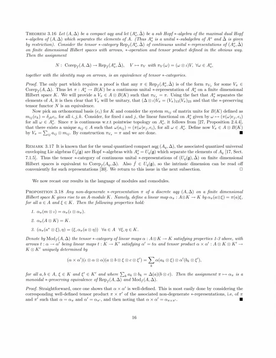
Theorem 3.16 Let (A,∆) be a compact aqg and let (Aos, ∆) be a sub Hopf ∗-algebra of the maximal dual Hopf∗-algebra of (A,∆) which separates the elements of A. (Thus Aos is a unital ∗-subalgebra of Ao and ∆ is givenby restriction). Consider the tensor ∗-category Repf (A

os, ∆) of continuous unital ∗-representations of (Aos, ∆)

on finite dimensional Hilbert spaces with arrows, ∗-operation and tensor product defined in the obvious way.Then the assignment

N : Corepf (A,∆) → Repf (Aos, ∆), V 7→ πV with πV (ω) = (ω ⊗ ι)V, ∀ω ∈ Aos,

together with the identity map on arrows, is an equivalence of tensor ∗-categories.

Proof. The only part which requires a proof is that any π ∈ Repf (Aos, ∆) is of the form πVπ

for some Vπ ∈Corepf (A,∆). Thus let π : Aos → B(K) be a continuous unital ∗-representation of Aos on a finite dimensionalHilbert space K. We will provide a Vπ ∈ A ⊗ B(K) such that πVπ

= π. Using the fact that Aos separates theelements of A, it is then clear that Vπ will be unitary, that (∆⊗ ι)Vπ = (Vπ)13(Vπ)23 and that the ∗-preservingtensor functor N is an equivalence.

Now pick an orthonormal basis (ei) for K and consider the system mij of matrix units for B(K) defined asmij(ek) = δjkei, for all i, j, k. Consider, for fixed i and j, the linear functional on Aos given by ω 7→ (π(ω)ej , ei)for all ω ∈ Aos. Since π is continuous w.r.t pointwise topology on Aos, it follows from [27, Proposition 2.4.4],that there exists a unique aij ∈ A such that ω(aij) = (π(ω)ej , ei), for all ω ∈ Aos. Define now Vπ ∈ A ⊗ B(K)by Vπ =

∑ij aij ⊗mij . By construction πVπ

= π and we are done. �

Remark 3.17 It is known that for the usual quantized compact aqg (Aq ,∆), the associated quantized universalenveloping Lie algebras Uq(g) are Hopf ∗-algebras with Aos = Uq(g) which separate the elements of Aq [17, Sect.

7.1.5]. Thus the tensor ∗-category of continuous unital ∗-representations of (Uq(g), ∆) on finite dimensional

Hilbert spaces is equivalent to Corepf (Aq,∆). Also f ∈ Uq(g), so the intrinsic dimension can be read offconveniently for such representations [30]. We return to this issue in the next subsection. 2

We now recast our results in the language of modules and comodules.

Proposition 3.18 Any non-degenerate ∗-representation π of a discrete aqg (A,∆) on a finite dimensionalHilbert space K gives rise to an A-module K. Namely, define a linear map απ : A⊗K → K by απ(a⊗ξ) = π(a)ξ,for all a ∈ A and ξ ∈ K. Then the following properties hold:

1. απ(m⊗ ι) = απ(ι⊗ απ).

2. απ(A⊗K) = K.

3. (απ(a∗ ⊗ ξ), η) = (ξ, απ(a⊗ η)) ∀a ∈ A ∀ξ, η ∈ K.

Denote by Modf (A,∆) the tensor ∗-category of linear maps α : A⊗K → K satisfying properties 1-3 above, witharrows t : α → α′ being linear maps t : K → K ′ satisfying α′ = tα and tensor product α × α′ : A⊗K ⊗K ′ →K ⊗K ′ uniquely determined by

(α× α′)(ι⊗ α⊗ α)(a⊗ b⊗ ξ ⊗ c⊗ ξ′) =∑

k

α(ak ⊗ ξ) ⊗ α′(bk ⊗ ξ′),

for all a, b ∈ A, ξ ∈ K and ξ′ ∈ K ′ and where∑

k ak ⊗ bk = ∆(a)(b ⊗ c). Then the assignment π 7→ απ is amonoidal ∗-preserving equivalence of Repf (A,∆) and Modf (A,∆).

Proof. Straightforward, once one shows that α× α′ is well-defined. This is most easily done by considering thecorresponding well-defined tensor product π × π′ of the associated non-degenerate ∗-representations, i.e, of πand π′ such that α = απ and α′ = απ′ , and then noting that α× α′ = απ×π′ . �

16

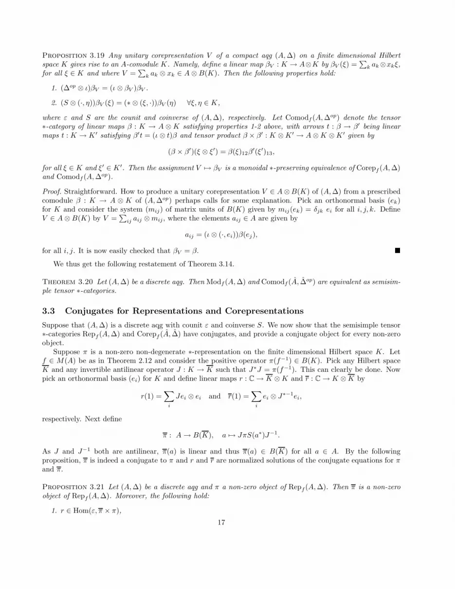
Proposition 3.19 Any unitary corepresentation V of a compact aqg (A,∆) on a finite dimensional Hilbertspace K gives rise to an A-comodule K. Namely, define a linear map βV : K → A⊗K by βV (ξ) =

∑k ak⊗xkξ,

for all ξ ∈ K and where V =∑

k ak ⊗ xk ∈ A⊗B(K). Then the following properties hold:

1. (∆op ⊗ ι)βV = (ι⊗ βV )βV .

2. (S ⊗ (·, η))βV (ξ) = (∗ ⊗ (ξ, ·))βV (η) ∀ξ, η ∈ K,

where ε and S are the counit and coinverse of (A,∆), respectively. Let Comodf (A,∆op) denote the tensor

∗-category of linear maps β : K → A ⊗K satisfying properties 1-2 above, with arrows t : β → β′ being linearmaps t : K → K ′ satisfying β′t = (ι⊗ t)β and tensor product β × β′ : K ⊗K ′ → A⊗K ⊗K ′ given by

(β × β′)(ξ ⊗ ξ′) = β(ξ)12β′(ξ′)13,

for all ξ ∈ K and ξ′ ∈ K ′. Then the assignment V 7→ βV is a monoidal ∗-preserving equivalence of Corepf (A,∆)and Comodf (A,∆

op).

Proof. Straightforward. How to produce a unitary corepresentation V ∈ A⊗B(K) of (A,∆) from a prescribedcomodule β : K → A ⊗ K of (A,∆op) perhaps calls for some explanation. Pick an orthonormal basis (ek)for K and consider the system (mij) of matrix units of B(K) given by mij(ek) = δjk ei for all i, j, k. DefineV ∈ A⊗B(K) by V =

∑ij aij ⊗mij , where the elements aij ∈ A are given by

aij = (ι ⊗ (·, ei))β(ej),

for all i, j. It is now easily checked that βV = β. �

We thus get the following restatement of Theorem 3.14.

Theorem 3.20 Let (A,∆) be a discrete aqg. Then Modf (A,∆) and Comodf (A, ∆op) are equivalent as semisim-

ple tensor ∗-categories.

3.3 Conjugates for Representations and Corepresentations

Suppose that (A,∆) is a discrete aqg with counit ε and coinverse S. We now show that the semisimple tensor∗-categories Repf (A,∆) and Corepf (A, ∆) have conjugates, and provide a conjugate object for every non-zeroobject.

Suppose π is a non-zero non-degenerate ∗-representation on the finite dimensional Hilbert space K. Letf ∈ M(A) be as in Theorem 2.12 and consider the positive operator π(f−1) ∈ B(K). Pick any Hilbert spaceK and any invertible antilinear operator J : K → K such that J∗J = π(f−1). This can clearly be done. Nowpick an orthonormal basis (ei) for K and define linear maps r : C → K ⊗K and r : C → K ⊗K by

r(1) =∑

i

Jei ⊗ ei and r(1) =∑

i

ei ⊗ J∗−1ei,

respectively. Next define

π : A→ B(K), a 7→ JπS(a∗)J−1.

As J and J−1 both are antilinear, π(a) is linear and thus π(a) ∈ B(K) for all a ∈ A. By the followingproposition, π is indeed a conjugate to π and r and r are normalized solutions of the conjugate equations for πand π.

Proposition 3.21 Let (A,∆) be a discrete aqg and π a non-zero object of Repf (A,∆). Then π is a non-zeroobject of Repf (A,∆). Moreover, the following hold:

1. r ∈ Hom(ε, π × π),

17

2. r ∈ Hom(ε, π × π),

3. r∗ ⊗ idπ ◦ idπ ⊗ r = idπ,

4. r∗ ⊗ idπ ◦ idπ ⊗ r = idπ,

5. r∗ ◦ r = r∗ ◦ r.

Proof. Claims 3 and 4 hold for any invertible antilinear map J , as is easily verified. Claim 5 is simply arestatement of the fact Trπ(f) = Trπ(f−1) stated in Theorem 2.12. To show that π ∈ Repf (A,∆), we first notethat π is linear (as AdJ and ∗ are both antilinear), multiplicative and non-degenerate, thus non-zero. To seethat π is ∗-preserving, first notice that S(a∗)∗ = S−1(a) and S2(a) = faf−1 for all a ∈ A, and then calculate

π(a)∗ = J∗−1πS−1(a)J∗ = Jπ(f)πS−1(a)π(f−1)J−1 = JπS(a)J−1 = π(a∗),

for all a ∈ A.It remains to show relations 1 and 2. We prove only the first, the second being proved similarly. Now

r ∈ Hom(ε, π × π) simply means that ε(a)r(1) = (π × π)(a)r(1), for all a ∈ A. By the non-degeneracy of π itthus suffices to show that

(ε(a)r(1), J∗−1ej ⊗ π(b∗)el) = ((π × π)(a)r(1), J∗−1ej ⊗ π(b∗)el)

for all a, b ∈ A and all j, l. On the l.h.s. we have

(ε(a)r(1), J∗−1ej ⊗ π(b∗)el) = ε(a)∑

i

(Jei, J∗−1ej)(ei, π(b∗)el)

= ε(a)∑

i

δij(ei, π(b∗)el) = ε(a)(ej , π(b∗)el) = (π(ε(a)b)ej , el).

To see that the r.h.s. coincides with this expression, first write (1 ⊗ b)∆(a) =∑

k ak ⊗ bk and notice that

∑

k

bkS(a∗k)∗ =

∑

k

bkS−1(ak) = m(ι⊗ S−1)(

∑

k

bk ⊗ ak) = m(ι⊗ S−1)((b ⊗ 1)∆op(a)) = ε(a)b.

Hence

((π × π)(a)r(1), J∗−1ej ⊗ π(b∗)el) =∑

i

((π ⊗ π)∆(a)(Jei ⊗ ei), J∗−1ej ⊗ π(b∗)el)

=∑

i

((π ⊗ π)(1 ⊗ b)(π ⊗ π)∆(a)(Jei ⊗ ei), J∗−1ej ⊗ el)

=∑

i

((π ⊗ π)((1 ⊗ b)∆(a))(Jei ⊗ ei), J∗−1ej ⊗ el)

=∑

ik

(π(ak)Jei ⊗ π(bk)ei, J∗−1ej ⊗ el) =

∑

ik

(JπS(a∗k)ei ⊗ π(bk)ei, J∗−1ej ⊗ el)

=∑

ik

(JπS(a∗k)ei, J∗−1ej)(π(bk)ei, el) =

∑

ik

(ej , πS(a∗k)ei)(π(bk)ei, el)

=∑

ik

(πS(a∗k)∗ej , ei)(π(bk)ei, el) =

∑

k

(π(bk)∑

i

(πS(a∗k)∗ej , ei)ei, el)

=∑

k

(π(bk)πS(a∗k)∗ej, el) = (π(

∑

k

bkS(a∗k)∗)ej, el) = (π(ε(a)b)ej , el),

as desired. �

18

Note that for a discrete aqg (A,∆), the intrinsic dimension d(π) of an irreducible object π ∈ Repf (A,∆) isthen given by

d(π) = r∗ ◦ r = r∗ ◦ r = Trπ(f) = Tr π(f−1).

In fact, the latter two expressions can be thought of as the quantum dimension of π [30] and gives the intrinsicdimension for any π ∈ Repf (A,∆). By the Schwarz inequality for the inner product given by Tr it follows thatif d(π) equals the dimension of the Hilbert space on which π acts, then π(f) = 1. Thus the von Neumannextension of (A,∆) is a Kac algebra iff the intrinsic dimension of any finite dimensional representation coincideswith the dimension of the Hilbert space on which it acts.

Suppose now that (A,∆) is a compact agq with counit ε and coinverse S. We would like to find an expressionfor the conjugate unitary corepresentation V of a non-zero object V ∈ Corepf (A,∆). To this end, we will use

the correspondence between Repf (A, ∆) and Corepf (A,∆) established in Theorem 3.14. Recall that the dual

(A, ∆) of (A,∆) is a discrete aqg. Let ε denote its counit, S its coinverse, and let f ∈M(A) be as in Theorem2.12.

Let V ∈ A⊗B(K) be a non-zero unitary corepresentation of (A,∆) on a finite dimensional Hilbert space K.

Pick a finite dimensional Hilbert space K and a antilinear map J : K → K such that J∗J = πV (f−1) ∈ B(K).Given any invertible antilinear map J we define a linear map j : B(K) → B(K) by j(x) = Jx∗J−1, for allx ∈ B(K).

Proposition 3.22 Suppose (A,∆) is a compact aqg. Let V be a unitary corepresentation of (A,∆) on a finite

dimensional Hilbert space K with J∗J = πV (f−1) ∈ B(K). Define V ∈ A ⊗ B(K) by V = (S−1 ⊗ j)V . Thenthe following hold:

1. V (1 ⊗ J∗J) = (1 ⊗ J∗J)(S2 ⊗ ι)V ,

2. V ∈ Corepf (A,∆),

3. πV = πV . (Here it is understood that the same J : K → K is used in both constructions.)

Proof. To prove 1., observe that

(ω ⊗ ι)V J∗J = πV (ω)πV (f−1) = πV (ωf−1) = πV (f−1)πV (fωf−1)

= J∗JπV (S2(ω)) = J∗J(S2(ω) ⊗ ι)V = J∗J(ω ⊗ ι)(S2 ⊗ ι)V

for all ω ∈ A.To prove 3., note first that S(ω)(a) = ωS(a) and ω∗(a) = ω(S(a)∗) for all a ∈ A and ω ∈ A. Writing

V =∑

k ak ⊗ xk we compute∑

k

S(ω∗)(ak)xk =∑

k

ω∗S(ak)xk = (ω∗ ⊗ ι)(S ⊗ ι)V = (ω∗ ⊗ ι)(V ∗)

=∑

k

ω∗(a∗k)x∗k =

∑

k

ω(S(a∗k)∗)x∗k =

∑

k

ωS−1(ak)x∗k.

Since (S ⊗ ι)V = V ∗, we thus obtain

πV (ω) = JπV S(ω∗)J−1 = J(S(ω∗) ⊗ ι)V J−1 =∑

k

J(S(ω∗)(ak)xk)J−1 =

∑

k

J(ωS−1(ak)x∗k)J

−1

=∑

k

ωS−1(ak)Jx∗kJ

−1 = (ω ⊗ ι)(S−1 ⊗ j)(∑

k

ak ⊗ xk) = (ω ⊗ ι)(S−1 ⊗ j)V = πV (ω)

for all ω ∈ A, proving 3. Now 3., together with Proposition 3.5 and Proposition 3.21, imply 2., completing theproof. �

This suggests the following proposition, which is a formulation more intrinsic to the category Corepf (A,∆).

19

Proposition 3.23 Let (A,∆) be a compact aqg and V ∈ Corepf (A,∆) be non-zero. Pick a finite dimensional

Hilbert space K and any antilinear map J : K → K such that V (1 ⊗ J∗J) = (1 ⊗ J∗J)(S2 ⊗ ι)V . ThenV ∈ A ⊗ B(K) given by V = (S−1 ⊗ j)V belongs to Corepf (A,∆). It is a conjugate of V with normalized

solutions r ∈ Hom(1 ⊗ 1, V × V ), r ∈ Hom(1 ⊗ 1, V × V ) of the conjugate equations for V and V given by

r(1) =∑

i

Jei ⊗ ei and r(1) =∑

i

ei ⊗ J∗−1ei.

Proof. The irreducible case follows from Proposition 3.21, Theorem 3.14 and the fact that J∗J is the unique (upto a positive scalar) positive operator in B(K) with the property V (1⊗J∗J) = (1⊗J∗J)(S2 ⊗ ι)V [40, 30]. Wecontent ourselves with proving one of the least obvious parts of the proposition, namely that r, defined above,belongs to Hom(1 ⊗ 1, V × V ). In other words we must show that r(ω ⊗ ι)(1 ⊗ 1) = (ω ⊗ ι ⊗ ι)(V × V )r orω(1)r(1) = (ω⊗ι⊗ι)(V ×V )r(1) for all ω ∈ A. Write V =

∑k ak⊗xk ∈ A⊗B(K), so V =

∑k S

−1(ak)⊗Jx∗kJ

−1.

For any ω ∈ A and any elements ej , er in the chosen orthonormal basis for K, we then get

((ω ⊗ ι⊗ ι)(V × V )r(1), J∗−1ej ⊗ er) =∑

i

((ω ⊗ ι⊗ ι)(V 12V13)(Jei ⊗ ei), J∗−1ej ⊗ er)

=∑

ikl

ω(S−1(ak)al)(Jx∗kJ

−1Jei, J∗−1ej)(xlei, er) =

∑

ikl

ω(S−1(ak)al)(Jx∗kei, J

∗−1ej)(xlei, er)

=∑

ikl

ω(S−1(ak)al)(ej , x∗kei)(xlei, er) =

∑

ikl

ω(S−1(ak)al)(xkej , ei)(xlei, er)

=∑

kl

ω(S−1(ak)al)(xl∑

i

(xkej , ei)ei, er) =∑

kl

ω(S−1(ak)al)(xlxkej , er)

=∑

kl

ωS−1(S(al)ak)(xlxkej, er) =∑

kl

ωS−1(a∗l ak)(x∗l xkej, er)

= (ωS−1 ⊗ ωej ,er)(V ∗V ) = (ω ⊗ ωej ,er

)(1 ⊗ 1) = ω(1)(ej , er)

=∑

i

ω(1)(Jei, J∗−1ej)(ei, er) = (ω(1)r(1), J∗−1ej ⊗ er),

where

ωej ,er: B(K) → C, x 7→ (xej , er).

Thus

(ω ⊗ ι⊗ ι)(V × V )r(1) = ω(1)r(1),

completing the proof. �

Remark 3.24 In the last two results, the conjugates can be expressed alternatively in terms of the unitaryantipode R and an antiunitary J [5]. 2

4 Cocommutative Algebraic Quantum Groups vs. Compact Groups

Definition 4.1 Let (A,∆) be an aqg. The intrinsic group G of (A,∆) is the following subgroup of the unitariesin the multiplier algebra M(A):

G = {g ∈M(A) | ∆g = g ⊗ g, g∗g = gg∗ = 1}.

Since the extended comultiplication ∆ : M(A) → M(A ⊗ A) is a unital ∗-homomorphism and the algebraM(A) is associative, the set G is indeed a group. It is easy to see that ε(g) = 1 and S(g) = g−1 = g∗, for anyg ∈ G.

20

Remark 4.2 It can be shown that any bounded group-like element of M(A) is automatically unitary withS(g) = g∗. A proof of this may be found in [20] and [11], but the above definition suffices for our purposes.

Lemma 4.3 Let (A,∆) be a discrete aqg. Equipped with the product topology, M(A) =∏i∈I B(Hi) is a complete

locally convex topological vector space and A is dense in M(A).

Proof. Since the blocks B(Hi) are Banach spaces, the functions ‖pi(·)‖ form a separating family of seminormswhich induces the product topology. Completeness is obvious by semisimplicity of the B(Hi), i ∈ I. To seethat A is dense in M(A), let x ∈ M(A) and consider the net (xλ)λ∈Λ in A given by xλ = ⊕i∈λpi(x), where Λis the collection of finite subsets of I directed by inclusions. Then clearly xλ → x. �

Proposition 4.4 If (A,∆) is a discrete aqg, its intrinsic group G is a compact topological group w.r.t. theproduct topology on M(A).

Proof. Note that a net (gλ) converges to g in G iff pi(gλ) → pi(g) in norm, for all i ∈ I. By Tychonov’s theoremit suffices to show that G is closed in

∏i∈I U(B(Hi)). Given a net (gλ) in G which converges to a ∈M(A), we

must show that ∆a = a ⊗ a. Let i, j ∈ I and consider the finite dimensional non-degenerate ∗-representation(pi ⊗ pj)∆ : A→ B(Hi ⊗Hj). By Proposition 2.10, we may write

(pi ⊗ pj)∆ ≃⊕

k∈I

Nkij pk.

Since both these expressions are non-degenerate ∗-representations, they extend to equivalent unital ∗-representationsof M(A), which we now identify. Therefore

(pi ⊗ pj)∆a =⊕

k∈I

Nkij pk(a) = lim

λ

⊕

k∈I

Nkij pk(gλ) = lim

λ(pi ⊗ pj)∆gλ

= limλpi(gλ) ⊗ pj(gλ) = pi(a) ⊗ pj(a) = (pi ⊗ pj)(a⊗ a),

thus ∆a = a⊗ a and G is closed. �

Remark 4.5 Note furthermore that in the proof of the proposition we have shown that

∆ : M(A) =∏

i∈I

B(Hi) →M(A⊗A) =∏

i,j∈I

B(Hi ⊗Hj)

is continuous w.r.t. the product topologies.

Proposition 4.6 Suppose (A,∆) is a discrete aqg with intrinsic group G. Let π be a non-degenerate ∗-representation of A on a finite dimensional Hilbert space K. Define a map uπ : G→ B(K) by

uπ : g 7→ π(g),

where the extension of π to M(A) is understood. Then uπ is strongly continuous and D : (K,π) 7→ (K,uπ)together with the identity map on the morphisms is a faithful and tensor functor from Repf (A,∆) to the categoryRepf G of finite dimensional continuous representations of G.

21

Proof. Continuity of uπ w.r.t. the topology on G is obvious. As π : M(A) → B(K) is a unital ∗-homomorphism,clearly (K,uπ) ∈ RepG. Functoriality and faithfulness of D are obvious. Monoidality follows from the calcula-tion

D(π1 × π2)(g) = (π1 ⊗ π2)∆g = π1(g) ⊗ π2(g) = uπ1(g) ⊗ uπ2

(g) = (uπ1× uπ2

)(g)

for all g ∈ G and πi ∈ Rep(A,∆). Every π ∈ Rep(A,∆) is equivalent to a direct sum of the representations piby Proposition 2.10. Each upi

is (strongly) continuous and therefore the direct sum is strongly continuous. �

Thus far we have not assumed (A,∆) to be cocommutative. The following characterization of cocommuta-tivity will be crucial for proving that D gives rise to an equivalence of categories.

Theorem 4.7 A discrete aqg (A,∆) is cocommutative iff

spanC{g | g ∈ G} = M(A).

Remark 4.8 This theorem implies that

spanC{pi(g) | g ∈ G} = B(Hi)

for every i ∈ I and in particular that A = spanC{gIi | i ∈ I, g ∈ G}. These results are rigorous formulations ofthe heuristic idea that a cocommutative aqg is ‘spanned by its grouplike elements’. Before we give the proof ofTheorem 4.7 we show that it leads to the desired equivalence of categories.

In what follows we fix a cocommutative discrete aqg (A,∆) where A = ⊕i∈IB(Hi) and let G denote itsintrinsic group. For every i ∈ I, ui : g 7→ pi(g) ∈ B(Hi) is a continuous unitary representation of G. ByTheorem 4.7, the span of pi(g), g ∈ G is dense in B(Hi), thus ui is irreducible. This defines a map γ : I → IG.

Proposition 4.9 The map γ is a bijection.

Proof. If there is a unitary V : Hi → Hj such that V pi(g) = pj(g)V for all g ∈ G then V pi(x) = pj(x)V for allx ∈ spanC{g | g ∈ G}. Since these x are dense in M(A) by Theorem 4.7 and the pi are continuous we concludethat V pi(x) = pj(x)V for all x ∈M(A), thus i = j so that γ : I → IG is injective.

Obviously if g 6= e there is an i ∈ I such that pi(g) 6= 1B(Hi). Since the category Repf (A,∆) is monoidaland has conjugates, γ(I) ⊂ IG is closed w.r.t. conjugation and tensor products and reduction. The surjectivityof γ now follows from the following well known group theoretical fact. �

Lemma 4.10 Let G be a compact group and let J ⊂ IG be closed w.r.t. conjugation and tensor products andreduction. If J separates points on G then J = IG.

Proof. For every equivalence class i ∈ IG pick a representative ui. The assumptions on J imply that the spanof the matrix elements (uj)nm, j ∈ J is a unital ∗-subalgebra of C(G). Since it separates the points of G it isdense in C(G) by the Stone-Weierstrass theorem and therefore dense in L2(G,µ), where µ is the Haar measure.If there were a k ∈ IG\J then by the Peter-Weyl theorem the matrix elements of uk would be orthogonal to thedense subspace of L2(G,µ) generated by the (uj)nm, j ∈ J , which is a contradiction. �

Theorem 4.11 Let (A,∆) be a cocommutative discrete aqg and G its intrinsic group. Then the functor D :Rep(A,∆) → RepG induces a canonical equivalence of tensor ∗-categories:

Repf (A,∆)⊗≃ Repf G.

22

Proof. In view of Proposition 4.6 it only remains to prove that the functor D is full and essentially surjective.By Proposition 2.10 the category Repf (A,∆) is semisimple, and for a compact group G the semisimplicity ofRepfG is well known. Recall from Section 2.1 that a faithful functor between semisimple categories is full ifand only if it maps simple objects to simple objects and non-isomorphic simple objects have non-isomorphicimages. The first property was used to define the map γ of Proposition 4.9, and the second is the injectivity ofγ. Finally, essential surjectivity of D is expressed by surjectivity of γ. Since D is monoidal it gives rise to anequivalence of tensor categories by [31]. �

Now we prove the characterization of cocommutative discrete aqg used above.

Proof of Theorem 4.7. Clearly, if the closure of spanC{g | g ∈ G} is M(A), then by linearity and continuity of∆ : M(A) →M(A⊗A), we see that (A,∆) is cocommutative. We prove the converse direction. By Lemma 4.3it suffices to show that any x ∈ A is the limit of linear combinations of elements of G. Fix x ∈ A. For any aqg(A,∆) there exists a linear inclusion Q : A → A∗

r determined by

Q(b)πr(a) = a(b) = ϕ(ba)

for all a, b ∈ A. To see this, to any a, b ∈ A we can choose an element c ∈ A such that cb∗∗

= b∗∗. (Such c can

be obtained as inverse Fourier transform of a local unit for b∗∗

in A.) Now we observe that

Q(b)πr(a) = ϕ((b∗)∗a) = ψ(b∗∗a) = ψ(cb∗

∗a) = ψ(b∗

∗aρ(c)) = (πr(a)Λ(ρ(c)), Λ(b∗)),

so Q(b) = (·Λ(ρ(c)), Λ(b∗)). Now Ar is a unital commutative C∗-algebra. Let Y be the set of ∗-characters onAr. Gelfand’s theorem tells us that Y is a compact Hausdorff space and that the map Γ : Ar → C(Y ) givenby Γ(a)(y) = y(a), for all a ∈ Ar and y ∈ Y , is a unital ∗-isomorphism from Ar to the C∗-algebra C(Y ) ofcontinuous functions on Y . Thus Q(x)Γ−1 ∈ C(Y )∗. By the Krein-Milman theorem for probability measures[27, Theorem 2.5.4] any element of C(Y )∗ is a w∗-limit of linear combinations of Dirac measures δy ∈ C(Y )∗.Hence we may write

Q(x)Γ−1 = limλ

∑

k

cλkδyλk

for some cλk ∈ C and yλk ∈ Y . Thus we get

a(x) = Q(x)πr(a) = Q(x)Γ−1Γπr(a) = limλ

∑

k

cλkδyλkΓπr(a)

= limλ

∑

k

cλkΓπr(a)(yλk) = limλ

∑

k

cλk yλkπr(a)

for all a ∈ A. Now the yλkπr : A→ C are unital ∗-homomorphisms, so we may define gλk ∈M(A) by

gλk = (ι⊗ yλk πr)U,

where U ∈ M(A ⊗ A) is the universal corepresentation of (A,∆). Since U is unitary, so are the elements gλkand moreover,

∆gλk = ∆(ι⊗ yλk πr)U = (ι⊗ ι⊗ yλk πr)(∆ ⊗ ι)U = (ι⊗ yλk πr)(U13U23)

= (ι⊗ yλk πr)U ⊗ (ι⊗ yλk πr)U = gλk ⊗ gλk,

thus all gλk ∈ G.Now for any ξ ∈ B(Hi)

′ and i ∈ I observe that ξpi ∈ A since ϕ is, up to a factor di, the trace on B(Hi).Thus by Theorem 3.4 we have (ξpi ⊗ ι)U = ξpi. Hence by the previous formulae we get

ξpi(x) = limλ

∑

k

cλk yλkπr(ξpi) = limλ

∑

k

cλk yλkπr(ξpi ⊗ ι)U

= limλ

∑

k

cλk ξpi(ι⊗ yλk πr)U = limλ

∑

k

cλk ξpi(gλk) = limλξpi(

∑

k

cλk gλk).

23

Since this is true for all i ∈ I and ξ ∈ B(Hi)′, we thus get

x = limλ

∑

k

cλk gλk

as desired. �

This concludes the proof of Theorem 4.7.

Corollary 4.12 For every i ∈ I we have spanC{pi(g) | g ∈ G} = B(Hi).

Proof. First we show that for 0 6= a ∈ A, there exist g ∈ G such that ϕ(ga) 6= 0. Thus let 0 6= a ∈ A. Thenthere exists x ∈ A such that a(x) = ϕ(xa) 6= 0, thus a = ϕ(·a) 6= 0. Furthermore, there exists a finite set Λ ⊂ Isuch that

a(b) = ϕ(ba) =∑

i∈Λ

diTri(pi(ba)),

for all b ∈M(A). Since the product in M(A) is continuous, we thus see that a : M(A) → C is continuous. Thusby Theorem 4.7 there exists g ∈ G such that ϕ(ga) 6= 0.

Assume now that spanC{pi(g) | g ∈ G} 6= B(Hi). Then there exists a non-zero a ∈ B(Hi) such thatTrB(Hi)(pi(g)a) = 0 for all g ∈ G. Since ϕ ↾ B(Hi) = diTrB(Hi), this is a contradiction. �

Let G be a compact group and consider a unitary representation u : G → B(K) of G on some finitedimensional Hilbert space K. Since u is continuous (here with respect to the norm), we have u ∈ C(G,B(K)).Since C(G,B(K)) ∼= C(G) ⊗ B(K), we may thus regard u as a unitary element V of the unital ∗-algebraC(G) ⊗ B(K). Now u : G → B(K) being a representation simply means that (∆ ⊗ ι)V = V13V23, where∆ : C(G) → C(G × G) ∼= C(G) ⊗ C(G) is given by ∆(a)(g, g′) = a(gg′), for all a ∈ C(G) and g, g′ ∈ G.Thus V is a unitary corepresentation of the commutative compact quantum group (C(G),∆) in the sense ofWoronowicz. It is easy to see that one may recover u from V by u(g) = (δg ⊗ ι)V , for g ∈ G.

Theorem 4.13 Let (A,∆) be a cocommutative discrete aqg, so (A, ∆) is a commutative compact aqg. Let Gbe the compact group such that (C(G),∆) ∼= (Ar, ∆r). For any V ∈ Corepf (A, ∆), let V ∈ C(G) ⊗ B(K) be

the unitary corepresentation of (C(G),∆) given by V = (πr ⊗ ι)V . Then there exists an isomorphism from Gto the intrinsic group of (A,∆) given by

g 7→ g = (ι⊗ δgπr)U ∈M(A),

where U is the universal corepresentation of (A,∆). Moreover, the equivalence

Corepf (A, ∆)P−→ Repf (A,∆)

Df−→ RepfG

given by the composition

V 7→ πV 7→ uπV=: uV ,

with P and Df established in Theorem 3.14 and Theorem 4.11, is described more directly by

uV (g) = (δg ⊗ ι)V ,

for all g ∈ G.

Proof. From the proof of Theorem 4.7, it is easily seen that g 7→ g is indeed a homeomorphism from Gto the intrinsic group of (A,∆) which also preserves the products. Let g ∈ G. We proceed to show that

24

uV (g) = (δg ⊗ ι)V . Since V ∈ A⊗B(K) we may write V =∑

k ωk ⊗ xk for ωk ∈ A and xk ∈ B(K). Then

uV (g) = uV ((ι ⊗ δgπr)U) = πV ((ι ⊗ δgπr)U)

= ([(ι⊗ δgπr)U ] ⊗ ι)V =∑

k

[(ι ⊗ δgπr)U ](ωk)xk =∑

k

(ωk ⊗ δgπr)Uxk

=∑

k

δgπr((ωk ⊗ ι)U)xk =∑

k

δgπr(ωk)xk = (δgπr ⊗ ι)(∑

k

ωk ⊗ xk) = (δgπr ⊗ ι)V = (δg ⊗ ι)V ,

as claimed. �

5 From Concrete Tensor Categories to Discrete Quantum Groups

The strategy we adopt in this section was been pursued by J.E. Roberts [29] in the discrete Kac algebra case,and has then been adapted to the more algebraic setting of discrete aqg (A,∆) by the authors.

5.1 Natural Transformations of ∗-Preserving Functors

Proposition 5.1 Let D,K be ∗-categories and F : D → K a ∗-preserving functor. Let NatF be the set of allnatural transformations from F to itself, viz.

NatF = {b = (bX ∈ EndF (X), X ∈ D) | F (s) ◦ bX = bY ◦ F (s) ∀s : X → Y }.

Then with the following pointwise operations NatF is a unital ∗-algebra:

(λb + λ′b′)X = λbX + λ′b′X ,

(bb′)X = bX ◦ b′X ,

(b∗)X = (bX)∗,

1X = idF (X),

for b, b′ ∈ NatF, λ, λ′ ∈ C and X ∈ D.

Proof. If s ∈ Mor(X,Y ), then

F (s) ◦ (b∗)X = (bX ◦ F (s∗))∗ = (F (s∗) ◦ bY )∗ = (b∗)Y ◦ F (s),

where we have used F (s∗) = F (s)∗. Thus b∗ ∈ NatF . Similarly, we get bb′, λb + λ′b′ ∈ NatF , so with theseoperations NatF is a ∗-algebra. Obviously 1 is a unit for NatF . �

Definition 5.2 Let B be a ∗-algebra and K a ∗-category. Then the category RepKB of ‘representations of Bin K’ has as objects the pairs (X,πX), where X ∈ ObjK and πX is a non-degenerate ∗-homomorphism of Binto EndX. The morphisms are given by

MorRepKB((X,πX), (Y, πY )) = {s ∈ MorK(X,Y ) | s ◦ πX(b) = πY (b) ◦ s ∀b ∈ B}.

Note that if K = H, the category of finite dimensional Hilbert spaces, we have EndH = B(H). Thus ourdefinition reduces to the usual notion of finite dimensional non-degenerate ∗-representations of B: RepHB =Repf B.

Proposition 5.3 Let C,K be ∗-categories and E : C → K a ∗-preserving functor. Define a unital ∗-algebraB = NatE. There is a ∗-preserving functor F : C → RepKB satisfying K ◦ F = E, where K : RepKB →K, (X,πX) 7→ X is the forgetful functor.

25

Proof. We set F (X) = (E(X), πX) for X ∈ ObjC and F (s) = E(s) for the morphisms of C. Here the ∗-representation πX is defined by

πX : B → EndX, b 7→ bX .

That F really is a functor follows from

F (s) ◦ πX(b) = E(s) ◦ bX = bY ◦ E(s) = πY (b) ◦ F (s) ∀s : X → Y ∀b ∈ B,

where we used b ∈ B = NatE. �

Proposition 5.4 Let D be a semisimple ∗-category, K a ∗-category and F : D → K a ∗-preserving functor.Then there is an isomorphism

ψF : NatF →∏

i∈ID

EndF (Xi)

of ∗-algebras.

Proof. We define a map ψF : NatF →∏i∈ID

EndF (Xi) by

ψF (b) =∏

i∈ID

bXi

for all b ∈ NatF . Clearly ψF is a unital ∗-algebra homomorphism. We first show that it is injective. SupposeψF (b) = 0, so bXi

= 0 for all i ∈ ID. Let X ∈ D. We must show that bX = 0. Recall that, for anyi ∈ ID, Mor(Xi, X) is a Hilbert space with the inner product (s, t)idXi

= t∗s and that every s ∈ Mor(Xi, X) isa multiple of an isometry. Let siα ∈ Mor(Xi, X), i ∈ IC , α = 1, . . . ,dimMor(Xi, X) be an orthonormal basisw.r.t. this inner product satisfying

∑iα siα ◦ s∗iα = idX . Hence

bX = bX ◦ F (idX) =∑

iα

bX ◦ F (si ◦ s∗i ) =

∑

iα

F (si) ◦ bXi◦ F (s∗i ) = 0,

and injectivity of ψF follows.Next we prove surjectivity of ψF . Given (bi ∈ EndF (Xi), i ∈ ID) we need to construct b ∈ NatF such

that ψF (b) =∏i∈ID

bi. Thus let X ∈ D. As above, pick a basis of isometries siα ∈ Mor(Xi, X), i ∈ ID, with∑iα siα ◦ s∗iα = idX . Define bX ∈ EndF (X) by

bX =∑

iα

F (siα) ◦ bi ◦ F (s∗iα).

Another choice of orthonormal bases (siα) in Mor(Xi, X), i ∈ ID does not affect bX since any two such bases arerelated by an orthogonal transformation. It remains to show that b ∈ NatF , viz. F (s) ◦ bX = bY ◦ F (s) ∀s :X → Y . To this purpose consider u ∈ Mor(X,Y ). Pick isometries tjβ ∈ Mor(Yj , Y ), with

∑jβ tjβ ◦ t∗jβ = idY ,

and define bY ∈ EndF (Y ) by

bY =∑

jβ

F (tjβ) ◦ bj ◦ F (t∗jβ).

Then

F (u) ◦ bX =∑

iα

F (u ◦ siα) ◦ bi ◦ F (s∗iα) =∑

iα,jβ

F (tjβ ◦ t∗jβ ◦ u ◦ siα) ◦ bi ◦ F (s∗iα).

But t∗jβ ◦ u ◦ siα ∈ Mor(Xi, Xj) is zero unless i = j and otherwise a scalar multiple of idXi. Hence

F (u) ◦ bX =∑

iαβ

F (tiβ ◦ (t∗iβ ◦ u ◦ siα)) ◦ bi ◦ F (s∗iα) =∑

iα,jβ

F (tjβ) ◦ bj ◦ F (t∗jβ ◦ u ◦ siα ◦ s∗iα) = bY ◦ F (u).

26

The last identity in this equation follows by precisely the same sort of argument as used before. This proves thenaturality of the family b ∈ NatF . Obviously we have bXi

= bi for all i ∈ ID. Thus ψF (b) =∏i∈ID

bi, whichproves surjectivity of ψF . �

The isomorphism ψF depends on the chosen family Xi, i ∈ I of irreducibles in C, but is canonical once thelatter is fixed. Thus there is no risk in suppressing it and writing NatF =

∏i∈ID

EndF (Xi), as will be done inthe sequel.

Example 5.5 The simplest application of this proposition is to the identity D → D, when we get

Nat (Id) ∼=∏

i∈ID

C.

Examples of natural transformations of the identity are the ‘twists’ appearing in the context of braided tensorcategories. 2

Example 5.6 Suppose D is a tensor ∗-category with tensor product ⊗. A less trivial application of theproposition is the case of the tensor functor F = ⊗ : D×D → D, where D×D is the product ∗-category. Notethat the isomorphism classes of irreducible objects in D ×D are precisely ID × ID. By semisimplicity of D wehave a finite decomposition

Xi ⊗Xj∼=⊕

k∈ID

NkijXk,

for any i, j ∈ ID and thus End(Xi ⊗Xj) ∼=⊕

k∈IDMNk

ij(C). We therefore obtain

Nat⊗ ∼=∏

i,j,k∈ID

Nkij6=0

MNkij

(C).

2

The following example is a continuation of Example 5.5.

Example 5.7 Suppose C is a semisimple ∗-category. Consider the ∗-algebra A = ⊕i∈ICC. Then Proposition 5.3provides an equivalence F : C → Repf A of categories such that F (Xi) ∼= pi for all i ∈ IC . Let K : Repf A→ Hbe the forgetful functor. Then K ◦ F is an embedding functor for C as a ∗-category. By Proposition 5.4 andExample 5.5 we also conclude that

Nat(K ◦ F ) ∼= Nat Id ∼=∏

i∈IC

C.

(Here of course, it does not make sense to say that the functors Id and K ◦ F are unitarily equivalent.) Supposenow that C is in addition a tensor category. Then the faithful functor K ◦ F cannot in general be monoidal.To see this let Xi, Xj with i, j ∈ IC . Then K ◦ F (Xi) ∼= K(pi) ∼= C, so K ◦ F (Xi)⊗K ◦ F (Xj) ∼= C, whereas

K ◦ F (Xi ⊗Xj) ∼=⊕

k∈IC

Nkij K ◦ F (Xk) ∼=

⊕

k∈IC

Nkij C,

where we used the decomposition Xi ⊗Xj∼= ⊕k∈ICN

kij Xk. 2

27

Given a ∗-preserving functor E : C → K and writing B = NatE it is natural to ask under which conditionsthe functor F : C → RepKB defined in Proposition 5.3 is an equivalence of categories. Instead of pursuing thisline further we restrict ourselves to the case where C is semisimple and K = H. Then EndE(X) is a finitedimensional matrix algebra for every X ∈ C and Proposition 5.4 shows that NatE is a direct product of matrixalgebras. The representation theory of such algebras is quite intricate, cf. [13]. There it is shown, among otherresults, that every irreducible representation of B =

∏i∈I B(Hi) is equivalent to a projection pi iff the index

set I has less than measurable cardinality. In practice, this is no serious restriction but for reasons which willbecome clear in the next subsection we prefer to work with direct sums instead of direct products.

Theorem 5.8 Let C be a semisimple ∗-category and E : C → H a ∗-preserving functor. The ∗-algebra A =⊕i∈ICB(E(Xi)) embeds canonically into NatE ∼=

∏i∈IC

B(E(Xi)). The functor

F : C → RepfA, F (X) = (E(X), πX), πX(a) = aX ∀a ∈ A, F (s) = E(s)

satisfies K ◦ F = E. It gives rise to an equivalence of categories iff E is faithful.

Proof. F as defined above differs from the functor defined in Proposition 5.3 only in the restriction of therepresentations πX to A ⊂ NatE. Thus it clearly is a ∗-preserving functor. By definition it is clear thatK ◦ F = E. Since F coincides with E on morphisms, E is faithful if F is an equivalence. Assume now thatE is faithful. Let X ∈ C be irreducible. Then F (X) is a representation πX : a 7→ aX of A on the Hilbertspace E(X). As is clear from the proof of Proposition 5.4, for X = Xi we have πX = pi, which clearly isirreducible. Since a ∈ A is a natural transformation, πX : a 7→ aX is an irreducible ∗-representation wheneverX is irreducible. Consider i 6= j, i, j ∈ IC . By Proposition 2.10, the projections pi = F (Xi), pj = F (Xj) areinequivalent ∗-representations. By semisimplicity of RepfA this implies that F is full. Since the pi, i ∈ ICexhaust the equivalence classes of irreducible ∗-representations of A it is clear that F is essentially surjective,completing the proof. �

Remark 5.9 The theorem remains true if one replaces A by the direct product algebra NatE provided onemakes the additional assumption that the set IC of isomorphism classes of C has less than measurable cardinality.2

5.2 Concrete Tensor ∗-Categories and Discrete Quantum Semigroups

From now on, C will be a semisimple strict tensor ∗-category. (As discussed in the Introduction, the strictnessassumption does not entail a loss of generality.) We will introduce other requirements as we proceed. ByTheorem 5.8 we have associated a ∗-algebra A to a ∗-preserving functor E : C → H. The aim of this subsectionis to endow A with the structure of a discrete aqg under suitable conditions on C and E. To bring out thespecial role of the target category H, we work in a more general setting as far as seems justifiable.

Let E : C → D be a ∗-preserving tensor functor into some tensor ∗-category D. Recall that by Proposition5.1, NatE is a unital ∗-algebra for every ∗-preserving functor E : C → D.

Proposition 5.10 Let C,D be tensor ∗-categories, C being strict, and let E : C → D be a ∗-preserving tensorfunctor. Then

∆ : NatE → NatE⊗, b = (bX) 7→ ∆(b) = (∆(b)Y,Z), ∆(b)Y,Z = bY⊗Z

defines a unital ∗-homomorphism.

Proof. The morphisms in C × C are of the form s × t where s : Y → Y ′, t : Z → Z ′. Then s ⊗ t ∈Mor(Y ⊗ Z, Y ′ ⊗ Z ′). We compute

(E⊗)(s× t) ◦ ∆(b)Y,Z = E(s⊗ t) ◦ bY⊗Z = bY ′⊗Z′ ◦ E(s⊗ t) = ∆(b)Y ′,Z′ ◦ (E⊗)(s× t),

28

where we used b = (bX) ∈ NatE. We conclude that ∆(b) ∈ NatE⊗. That b 7→ ∆(b) is a unital ∗-homomorphismfollows immediately from Proposition 5.1. �

We now consider the analogues of (∆⊗ ι), C being strict, and (ι⊗∆) in the present general setting. ⊗2 willdenote the functor ⊗ ◦ (⊗× Id) = ⊗ ◦ (Id×⊗) : C × C × C → C, where we have used the strictness of C.

Proposition 5.11 Let C,D be tensor ∗-categories and let E : C → D be a ∗-preserving tensor functor. There

are unital ∗-homomorphisms ∆ ⊗ ι, ι⊗ ∆ : NatE⊗ → NatE⊗2 defined by

∆ ⊗ ι : NatE⊗ → NatE⊗2, b = (bX,Y ) 7→ (∆ ⊗ ι)(b) = ((∆ ⊗ ι)(b)U,V,W ), (∆ ⊗ ι)(b)U,V,W = bU⊗V,W ,

ι⊗ ∆ : NatE⊗ → NatE⊗2, b = (bX,Y ) 7→ (ι⊗ ∆)(b) = ((ι ⊗ ∆)(b)U,V,W ), (ι⊗ ∆)(b)U,V,W = bU,V⊗W .

These morphisms satisfy (∆ ⊗ ι)∆ = (ι⊗ ∆)∆.

Proof. That (∆ ⊗ ι)(b) ∈ NatE⊗2 for b ∈ NatE⊗ follows from the following computation:

(E⊗2)(s× t× u) ◦ (∆ ⊗ ι)(b)Y,Z,W = E(s⊗ t⊗ u) ◦ bY⊗Z,W

= bY ′⊗Z′,W ′ ◦ E(s⊗ t⊗ u) = (∆ ⊗ ι)(b)Y ′,Z′,W ′ ◦ (E⊗2)(s× t× u),

whenever s : U → U ′, t : V → V ′, u : W → W ′. The argument for (ι⊗ ∆)(b) is completely analogous. Clearly,

both maps (∆ ⊗ ι), (ι⊗ ∆) are unital ∗-homomorphisms. The coassociativity property follows from

(∆ ⊗ ι)∆(b)U,V,W = ∆(b)U⊗V,W = b(U⊗V )⊗W = bU⊗(V⊗W ) = ∆(b)U,V⊗W = (∆ ⊗ ι)∆(b)U,V,W

with b ∈ EndE, where we have used the strictness of C. �

Proposition 5.12 There are unital ∗-homomorphisms ε : NatE → End(E(1)) and ε⊗ ι, ˜ι⊗ ε : NatE⊗ →NatE defined by

ε : NatE → End(E(1)), b = (bX) 7→ b1,

ε⊗ ι : NatE⊗ → NatE, b = (bX,Y ) 7→ (ε⊗ ι)(b) = ((ε⊗ ι)(b)X), (ε⊗ ι)(b)X = b1,X ,

ι⊗ ε : NatE⊗ → NatE, b = (bX,Y ) 7→ ( ˜ι⊗ ε)(b) = (( ˜ι⊗ ε)(b)X), ( ˜ι⊗ ε)(b)X = bX,1.

They satisfy (ε⊗ ι)∆ = ( ˜ι⊗ ε)∆ = ι.

Proof. Clearly, the map ε : b = (bX) 7→ b1 ∈ EndE(1) is a unital ∗-homomorphism. The proofs that(ε⊗ ι)(b), (ι ⊗ ε)(b) are in fact in NatE and that the maps b 7→ (ε⊗ ι)(b), b 7→ (ι⊗ ε)(b) are ∗-homomorphismsproceed along the same lines as for coproducts and are therefore omitted. For b ∈ NatE the computation

(ε⊗ ι)∆(b) = ∆(b)1,X = b1⊗X = bX = bX⊗1 = ∆(b)X,1 = (ι⊗ ε)∆(b),

where we used the strictness of the unit 1, concludes the proof. �

We have thus seen that we can define a ‘coproduct’ ∆ : NatE → NatE⊗ and a ‘counit’ ε : NatE → EndE(1)satisfying analogues of the usual properties. A priori, however, NatE⊗ has nothing to do with NatE ⊗NatE,regardless of how we interpret the tensor product. The following result indicates how to proceed. We nowassume that C is semisimple. As before, by IC we denote the set of isomorphism classes of irreducible objectsof C. For every i ∈ IC we pick a representative Xi.

Definition 5.13 Given a tensor ∗-category C, an embedding functor (for C) is a faithful ∗-preserving tensorfunctor E : C → H. A concrete tensor ∗-category is a tensor ∗-category together with an embedding functor.

29

Proposition 5.14 Let C be a semisimple tensor ∗-category and E : C → H an embedding functor. With the∗-algebra A =

⊕i∈IC

B(E(Xi)) we have the following canonical ∗-isomorphisms:

NatEψ1

−→ M(A) =∏i∈IC

B(E(Xi)),

NatE⊗ψ2

−→ M(A⊗A) =∏i,j∈IC

B(E(Xi)) ⊗B(E(Xj)),

NatE⊗2 ψ3

−→ M(A⊗A⊗A) =∏i,j,k∈IC

B(E(Xi)) ⊗B(E(Xj)) ⊗B(E(Xk)).

Proof. The isomorphism ψ1 was established in Propositions 5.4 and 2.10 and suppressed subsequently. As toψ2, we have

NatE⊗ =∏i,j∈IC

EndE(Xi ⊗Xj) ∼=∏i,j∈IC

End (E(Xi) ⊗ E(Xj))

=∏i,j∈IC

B(E(Xi) ⊗ E(Xj)) =∏i,j∈IC

B(E(Xi)) ⊗B(E(Xj)) = M(A⊗A).

Here we used the identification B(H ⊗ K) ≡ B(H) ⊗ B(K) for finite dimensional Hilbert spaces and theidentifications made after Propositions 2.10 and 5.4. The isomorphism between EndE(Xi⊗Xj) and EndE(Xi)⊗E(Xj) is induced in the canonical way from the isomorphism dEXi,Xj

: E(Xi) ⊗ E(Xj) → E(Xi ⊗ Xj) which

makes E monoidal. Unitarity of the dEXi,Xjimplies that ψ2 is ∗-preserving. The argument for ψ3 is completely

analogous. �

Remark 5.15 In the above proof it was crucial that the canonical ∗-homomorphisms ⊗ : EndX ⊗C EndY →End(X ⊗ Y ) are ∗-isomorphisms for all X,Y ∈ H. A semisimple tensor ∗-category has this property iff everyobject is a finite direct sum of copies of the tensor unit 1. [Proof. The ‘if’ clause is easy. As to the ‘onlyif’ part, let Z be irreducible and consider X ∼= Y ∼= 1 ⊕ Z, thus X ⊗ Y ∼= 1 ⊕ Z ⊕ Z ⊕ Z2. If Z 6∼= 1 thenEndX ⊗C EndY ∼= C2 ⊗C2 is commutative whereas End(X ⊗Y ) is non-commutative since X⊗Y contains theirreducible Z with multiplicity at least two. This contradicts EndX ⊗C EndY ∼= End(X ⊗ Y ).] This propertyis known to characterize the (semisimple) tensor ∗-category H uniquely up to equivalence. We thus see thatwith E = Id : C → C, we cannot conclude that NatE⊗ ∼= M(A⊗A). This is consistent with the computationof Nat⊗ in Example 5.6. 2

From now on we restrict ourselves to the case we are ultimately interested in.

Definition 5.16 Let C be a semisimple tensor ∗-category and let E : C → H be an embedding functor. Usingthe preceding results we define unital ∗-homomorphisms as follows.

ε : M(A) → C, a 7→ ε ◦ ψ−11 (a),

∆ : M(A) →M(A⊗A), a 7→ ψ2 ◦ ∆ ◦ ψ−11 (a).

Here we have implicitly used the irreducibility of E(1C) ∼= 1H∼= C, giving rise to the isomorphism ψ0 :

EndE(1) → C, c idE(1) 7→ c.

Remark 5.17 1. In the sequel we will usually use the isomorphisms ψ1, ψ2 to identify M(A) ≡ NatE, M(A⊗A) ≡ NatE⊗ and suppress the symbols ψ1, ψ2. Thus for a ∈M(A), i ∈ I, ai will denote both the i-componentof a in

∏i∈I B(E(Xi)) and the action aXi

on E(Xi) of the natural transformation ψ−11 (a) ∈ NatE.

2. Let a ∈M(A). As ∆(a)ij = aXi⊗Xjand (a⊗ a)ij = ai ⊗ aj we find

∆(a) = a⊗ a ⇔ aXi⊗Xj= aXi

⊗ aXj∀i, j ∈ I.

Thus the grouplike elements of M(A) are in one-to-one correspondence with those natural transformations ofthe embedding functor which respect the tensor structure. 2

30

Lemma 5.18 The restriction ∆ = ∆ ↾ A is a non-degenerate ∗-homomorphism from A to M(A ⊗ A), i.e.∆(A)(A ⊗A) = (A⊗A)∆(A) = (A⊗A).

Proof. To simplify the notation we write Hi = B(E(Xi)) and use the isomorphisms ψ1, ψ2 to identify M(A)with NatE and M(A ⊗ A) with NatE⊗. We will only prove ∆(A)(A ⊗ A) = (A ⊗ A), the proof of the otheridentity being completely analogous. As A = ⊕iB(Hi), it suffices to show that for every i, j ∈ IC there is ac ∈ A with ∆(c)(Ii ⊗ Ij) = Ii ⊗ Ij , since this implies ai ⊗ bj = ∆(c)(Ii ⊗ Ij)(ai ⊗ bj) ∈ ∆(A)(A ⊗ A) forall ai ∈ B(Hi), bj ∈ B(Hj). Recall from the Propositions 5.14 and 5.4 that M(A) is isomorphic to the ∗-algebra of natural transformations of E, and these are uniquely determined by their actions on the irreducibles:M(A) ∋ b ↔ (bi), where bi ≡ bXi

. Similarly, M(A ⊗ A) ∋ b ↔ (bij) with bij ≡ bXi,Xj. By the definition of ∆

we have ∆(b)ij = bXi⊗Xj. As usual, let (vkαij , α = 1, . . . , Nk

ij) be an orthonormal basis in Mor(Xk, Xi ⊗Xj) forall i, j, k ∈ IC . Since b ∈M(A) ≡ EndE is a natural transformation we have

∆(b)ij = bXi⊗Xj= bXi⊗Xj

◦ idE(Xi⊗Xj) = bXi⊗Xj◦ E

(∑

kα

vkαij ◦ vkα∗ij

)=∑

kα

E(vkαij ) ◦ bk ◦ E(vkα∗ij ).

Now fix i0, j0 ∈ IC and let bk = idE(Xk) if Xk is contained in Xi0 ⊗ Xj0 and bk = 0 otherwise. SinceXk ≺ Xi0 ⊗Xj0 only for finitely many k we have b = (bk) ∈ A and

∆(b)i0j0 =∑

kα

E(vkαi0j0) ◦ idE(Xk) ◦ E(vkα∗i0j0) =

∑

kα

E(vkαi0j0 ◦ vkα∗i0j0) = E(idXi0

⊗Xj0) = idE(Xi0

⊗Xj0).

Having identified NatE⊗ ≡M(A⊗A) this precisely means that the (i0, j0)-component of ∆(b) ∈M(A⊗A) =∏ij B(Hi) ⊗B(Hj) is the identity Ii0 ⊗ Ij0 and therefore ∆(b)(Ii0 ⊗ Ij0) = (Ii0 ⊗ Ij0 ) as desired. �

Corollary 5.19 Defining ∗-homomorphisms ε : A→ C and ∆ : A→M(A⊗A) by ε = ε ↾ A and ∆ = ∆ ↾ A,ε and ∆ are the unique extensions of ε and ∆, respectively, to M(A).

Proof. It is clear that ε is not identically zero, thus non-degenerate. Non-degeneracy of ∆ has been proven inLemma 5.18. Now the claim follows from the fact [35] that a non-degenerate ∗-homomorphism φ : A→ M(B)has a unique extension to a unital ∗-homomorphism φ : M(A) →M(B). �

Proposition 5.20 Let C be a semisimple tensor ∗-category and E : C → H an embedding functor. Then the∗-algebra A = ⊕i∈ICB(E(Xi)) is a discrete quantum semigroup, i.e. has a non-degenerate coproduct ∆ : A →M(A⊗A) in the sense of [35] and a counit ε : A→ C.

Proof. By Lemma 5.18, ∆ is non-degenerate, thus also ∆ ⊗ ι : A ⊗ A → M(A ⊗ A) ⊗ A ⊂ M(A ⊗ A ⊗ A) isnon-degenerate and extends uniquely to ∆ ⊗ ι : M(A⊗A) →M(A⊗A⊗A). Another unital ∗-homomorphism

M(A⊗A) →M(A⊗A⊗A) is given by ψ3 ◦ (∆ ⊗ ι) ◦ ψ−12 . The latter clearly restricts to ∆⊗ ι on A⊗A, thus it

coincides with ∆ ⊗ ι on all of M(A⊗A). In the same way we make sense of ι⊗ ∆ : M(A⊗A) →M(A⊗A⊗A)

and see that it coincides with ψ3 ◦ (ι⊗ ∆) ◦ ψ−12 . Now, the coassociativity property proved in Proposition 5.11

implies

∆ ⊗ ι ◦ ∆ = ι⊗ ∆ ◦ ∆ : M(A) →M(A⊗A⊗A),

which is the proper formulation of coassociativity for (A,∆).As observed earlier, the ∗-homomorphism ε : A → C is non-degenerate, thus ε ⊗ ι, ι ⊗ ε : A ⊗ A → A

are non-degenerate too and have unique extensions ε⊗ ι, ι⊗ ε to M(A ⊗ A). Again, it is clear that ε⊗ ι =ψ1 ◦ (ε⊗ ι) ◦ ψ−1

2 and similarly for ι⊗ ε. Thus with Proposition 5.12 we conclude

ε⊗ ι ◦ ∆ = ι⊗ ε ◦ ∆ = id : M(A) →M(A).

We conclude that (A,∆) is a discrete quantum semigroup. �

31

Theorem 5.21 Let C be a semisimple tensor ∗-category and E : C → H an embedding functor. Let (A,∆) bethe corresponding discrete quantum semigroup. Then the functor F : C → Repf (A,∆) defined by

F (X) = (E(X), πX), πX(a) = aX ∀a ∈ A, F (s) = E(s)

provides an equivalence of tensor ∗-categories such that K ◦ F = E.

Proof. With A and F : C → RepfA as defined in Theorem 5.8 we have an equivalence of categories. It remains toshow that F : C → Repf (A,∆) is monoidal for the monoidal structure of Repf (A,∆) in Definition 3.12. Thus we

must exhibit isomorphisms dFX,Y : F (X)⊗F (Y ) → F (X⊗Y ) satisfying the conditions of Definition 2.1. In view

of F (X) = (E(X), πX), an obvious candidate is the isomorphism dEX,Y : E(X)⊗E(Y ) → E(X⊗Y ) which we have

by virtue of the assumed monoidality of E. If we set dFX,Y = dEX,Y for all X,Y ∈ C, the equations in Definition

2.1 are clearly satisfied. It only remains to prove that dFX,Y is in MorRepf (A,∆)(F (X) ⊗ F (Y ), F (X ⊗ Y )), i.e.

dFX,Y ◦ (πX × πY )(a) = πX⊗Y (a) ◦ dFX,Y ∀a ∈ A.

Keeping in mind the various identifications we have made so far, we get

dFX,Y ◦ (πX × πY )(a) = dFX,Y ◦ (πX ⊗ πY )∆(a) = dFX,Y ◦ (πX ⊗ πY )∆(a)

= dFX,Y ◦ (πX ⊗ πY )ψ2∆(a) = πX,Y ∆(a) ◦ dFX,Y = aX⊗Y ◦ dFX,Y = πX⊗Y (a) ◦ dFX,Y

for all a ∈ A. (The reader is invited to check the required identity explicitly for X = Xi, Y = Xj, as suffices bynaturality of the isomorphisms dF .) �

5.3 Conjugates and Antipodes: Discrete Quantum Groups

We have already seen that the concrete semisimple tensor ∗-categories Repf (A,∆) and Corepf (A, ∆) come withconjugates whenever (A,∆) is a discrete aqg. In this section we prove the converse. We start off with a coupleof preparatory results.

Lemma 5.22 Let C be a semisimple tensor ∗-category with conjugates and let E : C → H be an embeddingfunctor. Then the coproduct ∆ : A→M(A⊗A) for the discrete quantum semigroup (A,∆) given by Proposition5.20 has the following inclusion properties

(1 ⊗A)∆(A) ⊂ A⊗A, (A⊗ 1)∆(A) ⊂ A⊗A.

Proof. We prove only the inclusion (A ⊗ 1)∆(A) ⊂ A ⊗ A, the proof of the inclusion (1 ⊗ A)∆(A) ⊂ A ⊗ Abeing completely analogous. We need to show that (a⊗ 1)∆(b) ∈ A⊗A for all a, b ∈ A. It is clearly sufficientto show this for b = (bi) where all components except i = m vanish and for a = In. By the calculation done inthe proof of Lemma 5.18 we have

∆(b)ij = bXi⊗Xj=∑

k∈IC

Nkij∑

α=1

E(V kαij ) ◦ bk ◦ E(V kα∗ij ) ∈ EndE(Xi ⊗Xj).

In view of a = In and bi = 0 for i 6= m we obtain

((a⊗ 1)∆(b))ij = δi,n

Nmnj∑

α=1

E(V mαnj ) ◦ bm ◦ E(V mα∗nj ).

Now, since C has conjugates we have isomorphisms Mor(Xn⊗Xj , Xm) ∼= Mor(Xj , Xn⊗Xm). By semisimplicity,for fixed n,m the latter space is non-zero only for finitely many j ∈ IC . Thus ((a ⊗ 1)∆(b))ij is non-zero onlyfor i = n and finitely many j and therefore (a⊗ 1)∆(b) ∈ A⊗A. �

32

Proposition 5.23 Let C be a semisimple tensor ∗-category with conjugates and let E : C → H be an embeddingfunctor. Let b = (bX,Y ) ∈ NatE⊗. Using the identifications B((E(X ⊗ Y )) = B(E(X)) ⊗ B(E(Y )), forany objects X and Y in C, we may write bX,X =

∑k a

kX ⊗ bkX ∈ B(E(X)) ⊗ B(E(X)), and then define

m(b)X ∈ B(E(X)) by

m(b)X =∑

k

akX ◦ bkX ,

for any object X ∈ C. This gives a unital linear map m : NatE⊗ → NatE which sends b ∈ NatE⊗ to m(b).Furthermore, it restricts to the linearized multiplication m : A⊗A→ A on A ⊂ NatE.

Proof. The bilinear multiplication map from B(E(X)) ⊗ B(E(X)) to B(E(X)) exists since E(X) is finitedimensional. The rest is obvious. �

Proposition 5.24 Let C be a semisimple tensor ∗-category with conjugates and let E : C → H be an embeddingfunctor. Then the discrete quantum semigroup (A,∆) given by Proposition 5.20 is a discrete aqg. The coinverseS : A→ A is given by

S(a)X = E(idX ⊗ r∗X) ◦ idE(X) ⊗ aX ⊗ idE(X) ◦ E(rX ⊗ idX)

for all a ∈ A ⊂ NatE and objects X in C, and where (rX , rX , X) is any solution of the conjugate equationsassociated to X.

Proof. In view of Proposition 2.4 it is sufficient to show that (A⊗ 1)∆(A) ⊂ A⊗A and (1 ⊗A)∆(A) ⊂ A⊗Aand to produce an invertible coinverse S. We thus get an aqg since Theorem 2.13 provides a (non-zero) left-invariant positive functional for discrete multiplier Hopf ∗-algebras. Now the inclusions (A⊗ 1)∆(A) ⊂ A⊗ Aand (1 ⊗A)∆(A) ⊂ A⊗A are the content of Lemma 5.22.

We show that the map S : A → A given by the formula in the theorem is well-defined. We first showthat for a ∈ A and X ∈ C, the formula for S(a)X ∈ EndE(X) does not depend on the choice of solution

(rX , rX , X) of the conjugate equations associated to X . Suppose therefore that (r′X , r′X , X

′) is another solution

of the conjugate equations associated to X . By [23] there exists a unique invertible t ∈ Hom(X,X′) such that

r′X = t⊗ idX ◦ rX and r′X = idX ⊗ t∗−1 ◦ rX . Thus

E(idX ⊗ r′∗X) ◦ idE(X) ⊗ a

X′ ⊗ idE(X) ◦ E(r′X ⊗ idX)

= E(idX ⊗ (r∗X ◦ t∗ ⊗ idX)) ◦ idE(X) ⊗ aX

′ ⊗ idE(X) ◦ E((idX ⊗ t∗−1 ◦ rX) ⊗ idX)

= E(idX ⊗ r∗X) ◦ idE(t) ⊗ (E(t∗) ◦ aX

′ ◦ E(t∗−1)) ⊗ idE(X) ◦ E(rX ⊗ idX)

= E(idX ⊗ r∗X) ◦ idE(X) ⊗ (E(t∗ ◦ t∗−1 ◦ aX) ⊗ idE(X)) ◦ E(rX ⊗ idX)

= E(idX ⊗ r∗X) ◦ (idE(X) ⊗ aX ⊗ idE(X)) ◦ E(rX ⊗ idX),

and S(a)X ∈ EndE(X) does not depend on the choice of solution (rX , rX , X) of the conjugate equationsassociated with X .

Next we show that S(a) = (S(a)X) ∈ NatE for a ∈ A, i.e., we must show that E(t) ◦ S(a)X = S(a)Y ◦ E(t),for all a ∈ A and t ∈ Hom(X,Y ). By the existence of the transpose t•∗ ∈ Hom(Y,X) given in [23], we get

E(t) ◦ S(a)X = E(idY ⊗ r∗X) ◦ E(t) ⊗ aX ⊗ idE(X) ◦ E(rX ⊗ idX)

= E(idY ⊗ r∗X) ◦ idE(Y ) ⊗ aX ⊗ idE(X) ◦ E((t⊗ idX ◦ rX) ⊗ idX)

= E(idY ⊗ r∗X) ◦ idE(Y ) ⊗ aX ⊗ idE(X) ◦ E((idY ⊗ t•∗ ◦ rY ) ⊗ idX)

= E(idY ⊗ r∗X) ◦ idE(Y ) ⊗ (aX ◦ E(t•∗)) ⊗ idE(X) ◦ E(rY ⊗ idX)

= E(idY ⊗ r∗X) ◦ idE(Y ) ⊗ (E(t•∗) ◦ aY ) ⊗ idE(X) ◦ E(rY ⊗ idX)

= E(idY ⊗ (r∗X ◦ t•∗ ⊗ idX)) ◦ idE(Y ) ⊗ aY ⊗ idE(X) ◦ E(rY ⊗ idX)

= E(idY ⊗ (r∗Y ◦ idY ⊗ t)) ◦ idE(Y ) ⊗ aY ⊗ idE(X) ◦ E(rY ⊗ idX)

= E(idY ⊗ r∗Y ) ◦ idE(Y ) ⊗ aY ⊗ E(t) ◦ E(rY ⊗ idY )

= S(a)Y ◦ E(t),

33

as desired.Clearly, we have S(a) ∈ A for all a ∈ A and it is also clear that the map S is linear. We must prove the two

identities

m(ι⊗ S)((a⊗ 1)∆(b)) = ε(b)a, m(S ⊗ ι)((1 ⊗ a)∆(b)) = ε(b)a,

for all a, b ∈ A. We prove only the first one. Thus let a, b ∈ A and write (a ⊗ 1)∆(b) =∑k a

k ⊗ bk for someak, bk ∈ A. This means that

(aX ⊗ 1Y ) ◦ bX⊗Y =∑

k

akX ⊗ bkY

for all objects X and Y of C. Thus we get

m(ι⊗ S)((a⊗ 1)∆(b))X =∑

k

m(ak ⊗ S(bk))X =∑

k

akX ◦ S(bk)X

=∑

k

akX ◦ E(idX ⊗ r∗X) ◦ idX ⊗ bkX⊗ idE(X) ◦ E(rX ⊗ idX)

= E(idX ⊗ r∗X) ◦ (∑

k

akX ⊗ bkX

) ⊗ idE(X) ◦ E(rX ⊗ idX)

= E(idX ⊗ r∗X) ◦ (aX ⊗ idE(X) ◦ bX⊗X) ⊗ idE(X) ◦ E(rX ⊗ idX)

= aX ◦ E(idX ⊗ r∗X) ◦ bX⊗X ⊗ idE(X) ◦ E(rX ⊗ idX)

= aX ◦ E(idX ⊗ r∗X) ◦ E(rX ⊗ idX)b1 = aX ◦ E(idX ⊗ r∗X ◦ rX ⊗ idX)b1

= aX ◦ E(idX)b1 = aXb1 = aXε(b) = (ε(b)a)X

for all objects X in C, so m(ι⊗ S)((a⊗ 1)∆(b)) = ε(b)a as natural transformations.It remains to show that S is invertible. We do that by showing S(S(a)∗) = a∗ for all a ∈ A. Now with

X ∈ C, we calculate

S(S(a)∗)X = E(idX ⊗ r∗X) ◦ idE(X) ⊗ S(a)∗X⊗ idE(X) ◦ E(rX ⊗ idX)

= E(idX ⊗ r∗X) ◦ idE(X) ⊗ [E(idX ⊗ r∗X) ◦ idE(X) ⊗ aX ⊗ idE(X) ◦ E(rX ⊗ idX)]∗ ⊗ idE(X) ◦ E(rX ⊗ idX),

where we used (rX , rX , X) as a solution of the conjugate equations for X ∈ C. Thus

S(S(a)∗)X

= E(idX ⊗ r∗X) ◦ idE(X) ⊗ [E(r∗X ⊗ idX) ◦ idE(X) ⊗ a∗X ⊗ idE(X) ◦ E(idX ⊗ rX)] ⊗ idE(X) ◦ E(rX ⊗ idX)

= E(idX ⊗ r∗X ◦ idX ⊗ r∗X ⊗ idX⊗X) ◦ idE(X⊗X) ⊗ a∗X ⊗ idE(X⊗X) ◦ E(idX⊗X ⊗ rX ⊗ idX ◦ rX ⊗ idX)

= E(idX ⊗ r∗X ⊗ r∗X) ◦ idE(X⊗X) ⊗ a∗X ⊗ idE(X⊗X) ◦ E(rX ⊗ rX ⊗ idX)

= E(idX ⊗ r∗X ⊗ r∗X ◦ rX ⊗ idX⊗X⊗X) ◦ a∗X ⊗ idE(X⊗X) ◦ E(rX ⊗ idX)

= E((idX ⊗ r∗X) ◦ (rX ⊗ idX) ⊗ idX⊗X ◦ idX ⊗ r∗X) ◦ a∗X ⊗ idE(X⊗X) ◦ E(rX ⊗ idX)

= E(idX ⊗ r∗X) ◦ a∗X ⊗ idE(X⊗X) ◦ E(rX ⊗ idX) = a∗X ◦ E(idX ⊗ r∗X ◦ rX ⊗ idX)

= a∗X ◦ idE(X) = a∗X = (a∗)X .

�

After these preparatory computations, the following Main Result is essentially a restatement of Theorem5.21 and Proposition 5.24.

Theorem 5.25 Let C be a semisimple tensor ∗-category with conjugates and E : C → H an embedding functor.Let (A,∆) be the corresponding discrete aqg. Then the functor F : C → Repf (A,∆) defined by

F (X) = (E(X), πX), πX(a) = aX ∀a ∈ A, F (s) = E(s)

provides an equivalence of tensor ∗-categories such that K ◦ F = E.

34

Remark 5.26 1. In combination with Theorem 3.14 this gives Woronowicz’ generalized Tannaka-Krein result.Woronowicz constructs Corepf (A, ∆) for a compact aqg (A, ∆) more directly and uses the universal corepre-sentation U of (A,∆) implicitly. In his proof Woronowicz constructs a compact matrix pseudogroup from acategory with a generator. Our result is more general in that this assumption is redundant.

2. In view of Theorem 3.20, an alternative reconstruction theorem for a concrete semisimple tensor ∗-categoryC with conjugates would be that

C⊗∼= Comodf (A, ∆

op),

where (A, ∆op) is a Hopf ∗-algebra with a positive invariant functional. We refer to [34, 15] for similar construc-tions, where concrete non-semisimple tensor categories are shown to be equivalent to tensor categories of finitedimensional comodules over (infinite dimensional) Hopf algebras (with no ∗-operation). 2

We now discuss how the aqg (A,∆) depends on the choice of the embedding functor E. This discussion isonly preliminary and will be taken up again in part II of this series. We need the following

Definition 5.27 Let C,D be strict tensor categories and E,E′ : C → D be tensor functors (with structural

isomorphisms e, e′, dX,Y , d′X,Y ). Then E,E′ are said to be isomorphic as tensor functors, E

⊗∼= E′, if the

diagram

E(X) ⊗ E(Y )uX ⊗ uY

- E′(X) ⊗ E′(Y )

E(X ⊗ Y )

dX,Y

?

uX⊗Y

- E′(X ⊗ Y )

d′X,Y

?

(5.1)

commutes for all X,Y ∈ C, where u : E → E′ is a natural transformation whose components uX : E(X) →E′(X) are isomorphisms. A similar and obvious commutative diagram involves the structural isomorphismse, e′. If C,D are tensor ∗-categories and E,E′ are ∗-preserving then all uX must be unitary.

Proposition 5.28 Let C be a semisimple tensor ∗-category C with conjugates. Let E,E′ : C → H be embedding

functors, and let (A,∆), (A′,∆′) be the corresponding discrete aqg. An isomorphism u : E⊗∼= E′ gives rise to an

isomorphism θ : (A,∆) ∼= (A′,∆′) with π′Xθ = πX for all X ∈ C.

Proof. Let u : E → E′ be a unitary equivalence of tensor ∗-functors. Then θ : NatE → NatE′ given byθ(a)X = uXaXu

∗X for a ∈ NatE and X ∈ C restricts to a unital ∗-homomorphism from A to A′. Suppressing

as usual the natural transformations d and d′, we clearly have ∆′(θ(a))(X,Y ) = uX⊗Y aX⊗Y u∗X⊗Y , whereas

(θ ⊗ θ)∆(a)(X,Y ) = (uX ⊗ uY )aX⊗Y (u∗X ⊗ u∗Y ), for all a ∈ NatE and X,Y ∈ C. Since uX⊗Y = uX ⊗ uY , for allX,Y ∈ C, we get (θ ⊗ θ)∆ = ∆′θ, and (A,∆) ∼= (A′,∆′). �

The following definition will be useful in our discussion of embedded symmetric tensor categories.

Definition 5.29 Let C,D be tensor categories and E : C → D a tensor functor. Then the automorphism groupAut⊗E consists of the natural isomorphisms of E for which the diagram (5.1) commutes (with E′ = E), togetherwith the obvious componentwise group structure. If C is a tensor ∗-category and E is a ∗-preserving embeddingfunctor then the intrinsic group GE is the subgroup of Aut⊗E where all uX are unitaries.

35

5.4 The Non-∗ Case

Our starting point in this paper is a tensor ∗-category with direct sums, subobjects, conjugates and irreducibleunit. From it we (re)construct a multiplier Hopf ∗-algebra with positive left invariant functional. Such algebraswere called algebraic quantum groups (aqg) by Van Daele, who now prefers to speak of ‘multiplier Hopf ∗-algebras with integrals’. We stick to ‘algebraic quantum groups’ mainly for the sake of definiteness and brevity.When A is no longer a ∗-algebra and the invariant functional is required to be faithful rather than positive(ϕ(ab) = 0 for all a ∈ A implies b = 0) we arrive at the notion of a regular multiplier Hopf algebras withleft invariant functional. Essentially the entire theory works just as well in this setting, provided one adoptsa modified notion of dual. We say a tensor category is rigid if every object X comes with a chosen left dualX and morphisms eX : X ⊗ X → 1 and dX : 1 → X ⊗ X satisfying the triangular equations instead of theconjugate equations. In a semisimple category, left duals are automatically two-sided duals since dual morphismse′X : 1 → X ⊗ X and d′X : X ⊗ X → 1 exist. Adopting the standard definition of semisimple categories asabelian categories with all exact sequences splitting, one can prove the following:

Theorem 5.30 Let F be an algebraically closed field (of arbitrary characteristic). Let C be a F-linear semisimplerigid tensor category with End1 ∼= F and let E : C → VectF be a faithful tensor functor. Then there isa discrete regular multiplier Hopf algebra (A,∆) with faithful left invariant functional ϕ and an equivalenceF : C → Rep(A,∆) such that K ◦ F = E.

The proof proceeds exactly as for ∗-categories, ignoring all references to the ∗-preserving property of E andthe ∗-involution of A. Again, existence, uniqueness and faithfulness of the invariant functional are proven usingresults due to Van Daele. Only the construction of the coinverse requires careful examination since the notionof dual is different.

We close with some remarks on the two different notions of discreteness applying to multiplier Hopf algebras.In analogy to the ∗-case, a regular multiplier Hopf algebra (A,∆) with left invariant functional is called discreteif A is a direct sum of finite dimensional matrix algebras over F. In the non-∗ case Proposition 2.14 fails, and(A,∆) is said to be of discrete type iff there exists 0 6= h ∈ A such that ah = ε(a)h for all a ∈ A. As in the∗-case, (A,∆) is of compact type or, equivalently, compact if A has a unit. It is well known [37] that (A,∆) isof discrete type iff (A, ∆) is of compact type.

Every discrete multiplier Hopf algebra has a copy of F as a direct summand, corresponding to the one-dimensional representation ε. The unit I0 of this algebra has the property aI0 = I0a = ε(a)I0, thus a discretemultiplier Hopf algebra is of discrete type. The following characterizes discrete multiplier Hopf algebras, gen-eralizing a well known result for finite dimensional Hopf algebras (which automatically possess integrals).

Proposition 5.31 Let (A,∆) and (A, ∆) be mutually dual regular multiplier Hopf algebras with faithful leftinvariant functionals. Then the following are equivalent:

1. (A,∆) is discrete.

2. (A,∆) is of discrete type and h can be chosen to be idempotent.

3. (A, ∆) is of compact type and ϕ(1) 6= 0.

Proof. The implication 1.⇒2. has been discussed before. Assuming 2., we have h = hh = ε(h)h, thus ε(h) = 1.Conversely, if ε(h) 6= 0 then h/ε(h) satisfies 2. Now, 2. implies that (A, ∆) is compact, and compactness impliesthe existence of 0 6= h ∈ A satisfying xh = ε(x)h for all x ∈ A. By definition of the dual (A, ∆) and assumingthe normalization ϕ(h) = 1, we have ϕ(1) = ε(h), yielding the equivalence 2.⇔3. Now assume 3. holds. Then(A, ∆) is a Hopf algebra with left invariant functional ϕ satisfying ϕ(1) 6= 0. By classical results, cf., e.g., [32,14.0.3] or [1, Theorem 3.3.2], it follows that (A, ∆) is cosemisimple. This means that the F-coalgebra (A, ∆, ε)is a direct sum of finite dimensional coalgebras. Since F is algebraically closed, every finite dimensional F-coalgebra is a matrix coalgebra, i.e. it has a basis {aij , 1 ≤ i, j ≤ n} such that ∆(aij) =

∑l ail ⊗ alj . Since

36

A = {ϕ(·a), a ∈ A} ⊂ A∗ and ϕ is faithful, A has a basis {bαij = ϕ(·aαij), α ∈ I, 1 ≤ i, j ≤ nα ∈ N}. These

elements multiply according to bαijbα′

i′j′ = δαα′δji′bαij′ , thus

A =⊕

α∈I

Mnα(F),

as desired. �

Remark 5.32 1. In the ∗-case, ϕ is positive and 1 > 0, thus discrete type implies discreteness.2. We indicate how Proposition 5.31 can be used to prove Theorem 5.30. Given a semisimple tensor category

C with embedding functor E, by [34] there exists a Hopf algebra H such that C ≃ ComodH . By [32, 14.0.3],semisimplicity of C implies the existence of a left invariant functional ϕ on H , satisfying ϕ(1) 6= 0. Thus (H, ∆)is a compact multiplier Hopf algebra with left invariant functional. Its dual (A,∆) then is a discrete multiplierHopf algebra with left invariant functional, and by Theorem 3.14 we have C ≃ Repf (A,∆). However, the directproof of Theorem 5.30 analogous to the proof of Theorem 5.25 is more direct and instructive. 2

6 Concrete Braided and Symmetric Categories

In this section we prove that a braiding for the concrete tensor ∗-category C gives rise to an R-matrix for theassociated aqg (A,∆). If C is symmetric and the embedding functor E is symmetric monoidal then we mayconclude that (A,∆) is cocommutative.

The flip automorphism σ of A⊗A defined by σ(a⊗ b) = b⊗ a is a non-degenerate ∗-homomorphism. Thusthere exists a unique extension to an involutive ∗-automorphism of M(A ⊗ A) which we denote by the samesymbol.

Definition 6.1 An aqg (A,∆) is said to be quasitriangular w.r.t. R iff R is an invertible element of M(A⊗A)and satisfies

1. (∆ ⊗ ι)(R) = R13R23,

2. (ι⊗ ∆)(R) = R13R12,

3. ∆op = R∆(·)R−1,

where ∆op ≡ σ∆. We sometimes refer to such an element R as an R-matrix. If, in addition, σ(R) = R−1 wecall (A,∆) triangular.

The first equation means that the invertible element R ∈M(A⊗A) is a non-degenerate corepresentation of(A,∆) on A. It is easy to see that (A,∆) is quasitriangular w.r.t. R iff (A,∆op) is quasitriangular w.r.t. σ(R).

Definition 6.2 A braiding for a (strict) tensor category C is a family of isomorphisms cX,Y : X⊗Y → Y ⊗X,for all X,Y ∈ C natural in both arguments

t⊗ s ◦ cX,Y = cX′,Y ′ ◦ s⊗ t ∀s : X → X ′, t : Y → Y ′,

satisfying

cX,Y⊗Z = idY ⊗ cX,Z ◦ cX,Y ⊗ idZ ,

cX⊗Y,Z = cX,Z ⊗ idY ◦ idX ⊗ cY,Z ,

cX,1 = c1,X = idX

for all X,Y, Z ∈ C. A braiding is called a symmetry if, in addition, it satisfies

cX,Y ◦ cY,X = idY⊗X ∀X,Y ∈ C.

37

A tensor category with a (chosen) braiding or symmetry is called a braided or symmetric tensor category,respectively. A braided functor F : C → D is a monoidal functor between strict braided tensor categories making

F (X) ⊗ F (Y )dFX,Y

- F (X ⊗ Y )

F (Y ) ⊗ F (X)

cF (X),F (Y )

?

dFY,X

- F (Y ⊗X)

F (cX,Y )

?

(6.1)

commutative for all X,Y ∈ C.

The following result establishes the relation between R-matrices for (A,∆) and braidings for Repf (A,∆).

Proposition 6.3 Let (A,∆) be a discrete aqg. Let R ∈M(A⊗A) and consider

c(H,π),(H′,π′) ≡ ΣH,H′ (π ⊗ π′)(R), (H,π), (H ′, π′) ∈ Repf (A,∆).

Here ΣH,K is the canonical unitary flip from H ⊗K → K ⊗H. Then the family (c(H,π),(H′,π′)) is a braidingfor Repf (A,∆) iff R is an R-matrix. Also c(H,π),(H′,π′) is unitary for all (H,π), (H ′, π′) iff R is unitary. Ifthese equivalent conditions are satisfied then (A,∆) is triangular iff the corresponding braiding for Repf (A,∆)is symmetric.

Proof. Throughout the proof we write cπ,π′ for c(H,π),(H′,π′) and note that cπ,π′ : H ⊗ H ′ → H ′ ⊗ H , for all(H,π), (H ′π′) ∈ Repf (A,∆). Also note that

(π ⊗ π′) σ(a) = ΣH′,H (π′ ⊗ π) (a) ΣH,H′ ∀ (H,π), (H ′, π′) ∈ Repf (A,∆) ∀ a ∈M(A⊗A).

Now suppose R ∈M(A⊗A) satisfies ∆op(·)R = R∆(·). Then

cπ,π′ (π × π′)(a) = ΣH,H′ (π ⊗ π′)(R) (π ⊗ π′)∆(a) = ΣH,H′ (π ⊗ π′)(R∆(a)) = ΣH,H′ (π ⊗ π′)(∆op(a)R)

= ΣH,H′ (π ⊗ π′)∆op(a) (π ⊗ π′)(R) = ΣH,H′ (π ⊗ π′)(σ∆(a)) ΣH′,H ΣH,H′ (π ⊗ π′)(R)

= (π′ ⊗ π)∆(a) ΣH,H′ (π ⊗ π′)(R) = (π′ × π)(a) cπ,π′ ,

so we have seen that cπ,π′ : π × π′ → π′ × π for all π, π′ ∈ Repf (A,∆). Conversely, by reversing the abovecalculations, we see that ∆op(·)R = R∆(·) if cπ,π′ : π × π′ → π′ × π for all π, π′ ∈ Repf (A,∆).

It is straightforward to see that R is invertible iff cπ,π′ : π × π′ → π′ × π is an isomorphism for allπ, π′ ∈ Repf (A,∆), that R is unitary iff cπ,π′ is unitary for all π, π′ ∈ Repf (A,∆), and that R−1 = σ(R)iff cπ′,π cπ,π′ = idπ,π′ for all π, π′ ∈ Repf (A,∆).

Pick π, π′, π′′ ∈ Repf (A,∆). Then

(π ⊗ π′ ⊗ π′′)(ι⊗ ∆)(R) = (π ⊗ (π′ × π′′))(R)

= ΣH′⊗H′′,H ΣH,H′⊗H′′ (π ⊗ (π′ × π′′))(R) = ΣH′⊗H′′,H cπ,π′×π′′ ,

whereas

(π ⊗ π′ ⊗ π′′)(R13R12) = (ΣH′′,H ΣH,H′′ (π ⊗ π′′)(R))13 (ΣH′,H ΣH,H′ (π ⊗ π′)(R))12

= (ΣH′′,H cπ,π′′)13 (ΣH′,H cπ,π′)12 = (ΣH′′,H)13 (cπ,π′′)13 (ΣH′,H)12 (cπ,π′)12

= ΣH′⊗H′′,H (cπ,π′′)23 (cπ,π′)12.

Hence (ι⊗ ∆)(R) = R13R12 iff

cπ,π′×π′′ = (cπ,π′′)23 (cπ,π′)12 = idπ′ ⊗ cπ,π′′ ◦ cπ,π′ ⊗ idπ′′ ,

38

for all π, π′, π′′ ∈ Repf (A,∆). Similarly, one shows that (∆ ⊗ ι)R = R13R23 iff

cπ×π′,π′′ = (cπ,π′′)12 (cπ′,π′′)23 = cπ,π′′ ⊗ idπ′ ◦ idπ ⊗ cπ′,π′′ ,

for all π, π′, π′′ ∈ Repf (A,∆). �

Theorem 6.4 Let C be a semisimple braided tensor ∗-category with conjugates and E : C → H a faithful ∗-preserving tensor functor. Let (A,∆) and F : C → Repf (A,∆) be as constructed in Theorem 5.25. Then (A,∆)is quasitriangular w.r.t. a unique R ∈M(A⊗A) such that the functor F : C → Repf (A,∆) is an equivalence ofbraided tensor categories w.r.t. the braiding for Repf (A,∆) provided by R. R is unitary iff cX,Y is unitary forall X,Y . (A,∆) is triangular iff the corresponding braiding for Repf (A,∆) is symmetric.

Proof. For i, j ∈ IC we have

F (cXi,Xj) ∈ MorH(E(Xi) ⊗ E(Xj), E(Xj) ⊗ E(Xi)) = B(E(Xi) ⊗ E(Xj), E(Xj) ⊗ E(Xi)).

Thus ΣE(Xj),E(Xi)F (cXi,Xj) ∈ B(E(Xi) ⊗E(Xj)) and we can define R ∈M(A⊗A) =

∏ij B(E(Xi)⊗E(Xj))

by Rij = ΣE(Xj),E(Xi)F (cXi,Xj). Naturality of the braiding and functoriality of F now imply that we have

F (cX,Y ) = ΣE(X),E(Y ) (πX ⊗ πY )(R) ∀X,Y ∈ C.

Since F is an equivalence, we see that the family F (cX,Y ) is a braiding for Repf (A,∆). Denote this familyby (c(E(X),πX),(E(Y ),πY )), so

c(E(X),πX),(E(Y ),πY ) = ΣE(X),E(Y ) (πX ⊗ πY )(R) ∀X,Y ∈ C.

By Proposition 6.3, the element R ∈M(A⊗A) is therefore an R-matrix which is unitary iff cX,Y is unitary for allX,Y and satisfies σ(R) = R−1 iff cY,X ◦ cX,Y = idX⊗Y for all X,Y . With the braiding on Repf (A,∆) given byR according to Proposition 6.3, we get by definition F (cX,Y ) = cF (X),F (Y ), for all X,Y , as F (X) = (E(X), πX)for all X . Thus F is a braided functor. �

Remark 6.5 It seems worthwhile comparing our result with [16, Proposition XIII.1.4], where it is shown thatthe tensor category of left modules over a bialgebra (H,m, η,∆, ε) is braided iff H is quasitriangular w.r.t. someR-matrix. The proof uses the left regular representation of H and therefore would not apply to the categoryof finite dimensional H-modules if H is infinite dimensional. Our setting differs too in that A is non-unitalwhenever it is infinite dimensional. 2

Remark 6.6 As is well known, the category H of Hilbert spaces has a unique braiding, the flip ΣH,K : H⊗K →K ⊗H . It is thus natural to ask when the functors E respects this braiding. If so, then

E(cX,Y ◦ cY,X) = E(cX,Y ) ◦ E(cY,X) = ΣE(X),E(Y ) ◦ ΣE(Y ),E(X) = idE(Y )⊗E(X) = idE(Y⊗X) = E(idY⊗X),

where we suppressed the isomorphisms dEX,Y as is our policy throughout. If E is faithful this implies cX,Y ◦cY,X = idY⊗X , thus C is symmetric. In other words, for non-symmetric categories C there is no embeddingfunctor satisfying E(cX,Y ) = ΣE(X),E(Y ). For symmetric C we have the following easy yet important result. 2

Corollary 6.7 Let C be a semisimple symmetric tensor ∗-category and let E : C → H be a symmetric em-bedding functor, i.e., E(cX,Y ) = ΣE(X),E(Y ) for all X,Y ∈ C. Then the corresponding discrete aqg (A,∆) iscocommutative and F is a ∗-preserving symmetric monoidal equivalence.

39

Proof. It is clear from the definition of the R-matrix R in the proof of Theorem 6.4, that R = 1 in this case, so∆op = ∆. �

We are now in a position to re-prove the classical Tannaka-Krein duality theorem for compact groups.

Theorem 6.8 Let C be a semisimple tensor ∗-category with conjugates and unitary symmetry, and let E : C →H be a ∗-preserving faithful symmetric tensor functor. Then there exists a compact group G and an equivalenceF ′ : C → RepfG of symmetric tensor ∗-categories such that K ′ ◦F ′ = E, where K ′ : RepfG→ H is the forgetfulfunctor. The group G is canonically isomorphic to the intrinsic group GE of the embedding functor.

Proof. Under the given assumptions, Theorem 6.4 provides us with a discrete aqg (A,∆) and an equivalenceF : C → Repf (A,∆) of tensor ∗-categories such that K ◦ F = E. By assumption, E preserves the symmetries,i.e. E(cX,Y ) = ΣE(X),E(Y ) for all X,Y ∈ C. Then by Corollary 6.7 (A,∆) is cocommutative. Let G be theintrinsic group of (A,∆) as defined in Definition 4.1. By Theorem 4.11 we have a (concretely given) equivalenceD : Repf (A,∆) → RepfG of tensor ∗-categories. Thus the composition F ′ = D ◦F : C → RepfG is the desiredequivalence of tensor ∗-categories. It satisfies K ′◦F ′ = K ′◦D◦F = K ◦F = E. The final claim is obvious, sincethe unitary grouplike elements of (A,∆) are by definition of (A,∆) precisely the unitary natural isomorphismsof E that are compatible with the tensor structures, in the sense of (5.1). �

We end this section with some general facts on R-matrices for quasitriangular aqg.

Proposition 6.9 Let (A,∆) be a quasitriangular aqg w.r.t. R. Then the following statements hold:

1. R12R13R23 = R23R13R12.

2. (ε⊗ ι)R = 1 = (ι⊗ ε)R.

3. (S ⊗ ι)R = R−1 = (ι⊗ S−1)(R).

4. (S ⊗ S)R = R.

The first equation is called the ‘quantum Yang-Baxter equation’.

Proof. R is a non-degenerate corepresentation of (A,∆) on A, so 2. and the first equation in 3. follow imme-diately. The second equation in 3. thus follows by noting that (A,∆op) is quasitriangular w.r.t. σ(R) withcoinverse S−1. Claim 4 follows from 3. by (S⊗S)R = (ι⊗S)(S⊗ ι)R = (ι⊗S)(R−1) = (ι⊗S)(ι⊗S−1)R = R.Finally, to prove 1. first note that both the maps ∆op ⊗ ι and R12(∆ ⊗ ι)(·)R−1

12 are non-degenerate homo-morphisms from A ⊗ A to M(A ⊗ A ⊗ A), and thus both have unique extensions to M(A ⊗ A). Because∆op = R∆(·)R−1 these maps clearly coincide on A⊗A, and thus on M(A⊗A), extensions being unique. Hence

R12R13R23R−112 = R12(∆ ⊗ ι)(R)R−1

12 = (∆op ⊗ ι)(R) = (σ ⊗ ι)(∆ ⊗ ι)(R) = (σ ⊗ ι)(R13R23) = R23R13,

as desired. �

Proposition 6.10 Suppose (A,∆) is a quasitriangular aqg w.r.t. R. Let U denote the universal corepresen-tation of (A,∆) as defined in Theorem 3.4. Define πR : A → M(A) as in Proposition 3.5. Then the followinghold:

1. πR is a non-degenerate homomorphism.

2. (πR ⊗ πR)∆ = ∆opπR.

3. ∆op(·)(ι ⊗ πR)U = (ι⊗ πR)U∆(·).

Conversely, any map π : A→ M(A) satisfying these three properties arises from a unique R ∈M(A⊗A) withπ = πR making (A,∆) into a quasitriangular aqg. Moreover, the map πR is ∗-preserving iff R is unitary.

40

Proof. It suffices to show that statement 2 is equivalent to (ι⊗∆)(R) = R13R12, this being the only non-trivialstep not covered by Proposition 3.5 and Theorem 3.6. But by Theorem 3.4, we get

(πR ⊗ πR)∆ω = (πR ⊗ πR)∆(ω ⊗ ι)U = (πR ⊗ πR)(ω ⊗ ι⊗ ι)(ι ⊗ ∆)U = (πR ⊗ πR)(ω ⊗ ι⊗ ι)(U12U13)

= (ω ⊗ ι⊗ ι)(ι ⊗ πR ⊗ πR)(U12U13) = (ω ⊗ ι⊗ ι)[((ι ⊗ πR)U)12((ι ⊗ πR)U)13] = (ω ⊗ ι⊗ ι)(R12R13)

for all ω ∈ A, whereas

∆opπR(ω) = ∆op(ω ⊗ ι)R = (ω ⊗ ι⊗ ι)(ι ⊗ ∆op)R

for all ω ∈ A. �

Note that 1. and 2. just mean that πR is a morphism of multiplier Hopf algebras from (A, ∆) to (A,∆op).It is even an aqg morphism iff R is unitary by the last statement of the proposition.

In Definition 3.13 we introduced the tensor product V × V ′ = V12V′13 ∈ M(A ⊗ B ⊗ B′) of two unitary

corepresentations V and V ′ on B and B′, respectively. Another choice of a tensor product which works equallywell, is given by V ×op V

′ = V ′13V12 ∈M(A⊗B ⊗B′). In general there is no relation between these two tensor

products. In view of the relation between representations of an aqg and corepresentations of its dual aqg (andthe relation between the identity representation and the universal corepresentation), the following result shouldnot come as a big surprise.

Proposition 6.11 Let (A,∆) be an aqg with universal corepresentation U , so hatU = σ(U) is the universalcorepresentation of (A, ∆) on A. Let R be any element of M(A⊗A). Then ∆op(·)R = R∆(·) iff

(U ×op U)R23 = R23(U × U).

Proof. By Theorem 3.4, we get

∆op(a)R = (∆op(ι⊗ a)U)R = (σ∆(ι ⊗ a)U)R

= ((σ ⊗ a)(∆ ⊗ ι)U)R = ((ι⊗ ι⊗ a)(σ ⊗ ι)(U13U23))R = (ι⊗ ι⊗ a)(U23U13R12)

for all a ∈ A, whereas

R∆(a) = R∆(ι⊗ a)U = R(ι⊗ ι⊗ a)(∆ ⊗ ι)U = R(ι⊗ ι⊗ a)(U13U23) = (ι⊗ ι⊗ a)(R12U13U23)

for all a ∈ A. Hence ∆op(·)R = R∆(·) iff U23U13R12 = R12U13U23. Permuting indices, we see that the latterequation is equivalent to U31U21R23 = R23U21U31, which again is equivalent to U13U12R23 = R23U12U13 asdesired. �

So given any unitary R-matrix R, the map f ∈ Hom(A⊗A,A⊗A) given by f(b) = RbR∗, for all b ∈ A⊗A,is an arrow from ∆ to ∆op and from U × U to U ×op U in the sense of Remark 3.9. Also δR(a) = f(1 ⊗ a)for a ∈ A, is a coaction in the sense of Remark 3.10. Similarly, the linear map δ′R : A → M(A ⊗ A) given byδ′R(a) = f(a⊗ 1), for all a ∈ A, is a non-degenerate ∗-homomorphism such that (δ′R ⊗ ι)δ′R = (ι⊗ ∆op)δ′R and(ι ⊗ ε)δ′R = ι.

References

[1] E. Abe: Hopf Algebras. Cambridge University Press, 1977.

[2] J. Barrett & B. Westbury: Spherical categories. Adv. Math. 143, 357–375 (1999).

[3] E. Bedos, R. Conti & L. Tuset: On amenability and co-amenability of algebraic quantum groups and theircorepresentations. math.OA/0111027.

41

[4] E. Bedos & L. Tuset: Amenability of locally compact quantum groups. Preprint (2001).

[5] E. Bedos, G. J. Murphy & L. Tuset: Co-amenability of compact quantum groups. Journ. Geom. Phys. 40,130–153 (2001).

[6] L. Breen: Tannakian categories. Proc. Symp. Pure Math. 55, 337–376 (1994).

[7] P. Deligne & J. S. Milne: Tannakian categories. Lecture notes in mathematics 900, 101–228. Springer 1982.

[8] P. Deligne: Categories tannakiennes. In: P. Cartier et al. (eds.): Grothendieck Festschrift, vol. II, pp.111–195. Birkhauser Verlag 1991.

[9] S. Doplicher & J. E. Roberts: A new duality theory for compact groups. Invent. Math. 98, 157–218 (1989).

[10] S. Doplicher, C. Pinzari & J. E. Roberts: An algebraic duality theory for multiplicative unitaries. Internat.J. Math. 12, 415–459 (2001).

[11] M. Enock & J. M. Schwartz: Kac Algebras and Duality of Locally Compact Groups. Springer Verlag, 1980.

[12] P. Ghez, R. Lima & J. E. Roberts: W ∗-Categories. Pac. Journ. Math. 12, 79–109 (1985).

[13] D. Guido & L. Tuset: Representations of direct products of matrix algebras. Fund. Math. 169, 145–160(2001).

[14] E. Hewitt & K. A. Ross: Abstract Harmonic Analysis I & II. 2nd ed., Springer Verlag, 1994.

[15] A. Joyal & R. Street: An introduction to Tannaka duality and quantum groups. In: Proceedings of theconference on category theory, Como 1990. Lecture notes in mathematics 1488, 413–492 (1991).

[16] C. Kassel: Quantum Groups. Springer Verlag, 1995.

[17] A. Klimyk & K. Schmudgen: Quantum Groups and their Representations. Springer Verlag, 1997.

[18] J. Kustermans: Examining the dual of an algebraic quantum group. funct-an/9704004.

[19] J. Kustermans: Locally compact quantum groups in the universal setting. Internat. J. Math. 12, 289–338(2001).

[20] J. Kustermans & A. Van Daele: C∗-algebraic quantum groups arising from algebraic quantum groups.Internat. J. Math. 8, 1067–1139 (1997).

[21] Kustermans, J. and Vaes, S.: Locally Compact Quantum Groups. Ann. Scient. Ec. Norm. Sup. 33, 837–934(2000).

[22] Kustermans, J. and Vaes, S.: Locally Compact Quantum Groups in the von Neumann algebraic setting.math.QA/0005219.

[23] R. Longo & J. E. Roberts: A theory of dimension. K-Theory 11, 103–159 (1997).

[24] S. Mac Lane: Categories for the Working Mathematician. 2nd edition. Springer, 1997.

[25] M. Muger: Galois theory for braided tensor categories and the modular closure. Adv. Math. 150, 151–201(2000).

[26] M. Muger: From subfactors to categories and topology I. Frobenius algebras in and Morita equivalence oftensor categories. math.CT/0111204.

[27] G. Pedersen: Analysis Now. Springer Verlag, 1989.

[28] P. Podles & S. L. Woronowicz: Quantum deformation of Lorentz group. Commun. Math. Phys. 130,381–431 (1990).

42

[29] J. E. Roberts: The reconstruction problem. Unpublished notes.

[30] J. E. Roberts & L. Tuset: On the equality of q-dimensions and intrinsic dimension. J. Pure Appl. Alg. 156,329–343 (2001).

[31] N. Saavedra Rivano: Categories Tannakiennes. Lecture notes in mathematics 265. Springer Verlag, 1972.

[32] M. E. Sweedler: Hopf Algebras. Benjamin, 1969.

[33] T. Tannaka: Uber den Dualitatssatz der nichtkommutativen topologischen Gruppen. Tohoku Math. Journ.45, 1–12 (1939).

[34] K.-H. Ulbrich: On Hopf algebras and rigid monoidal categories. Israel Math. J. 72, 252–256 (1990).

[35] A. Van Daele: Multiplier Hopf algebras. Trans. Amer. Math. Soc. 342, 917–932 (1994).

[36] A. Van Daele: Discrete quantum groups. Journ. Alg. 180, 431–444 (1996).

[37] A. Van Daele: An algebraic framework for group duality. Adv. in Math. 140, 323–366 (1998).

[38] A. Van Daele: The Haar measure on some locally compact quantum groups. math.OA/0109004.

[39] A. Van Daele & Y. Zhang: Corepresentation theory of multiplier Hopf algebra I. Internat. Journ. Math.10, 503-539 (1999).

[40] S. L. Woronowicz: Compact matrix pseudogroups. Commun. Math. Phys. 111, 613–665 (1987).

[41] S. L. Woronowicz: Tannaka-Krein duality for compact matrix pseudogroups. Invent. Math. 93, 35–76(1988).

[42] S. L. Woronowicz: Compact quantum groups. In: A. Connes, K. Gawedzki & J. Zinn-Justin (eds.):Symetries Quantiques. [Quantum Symmetries]. Proceedings of the NATO Advanced Study Institute Sum-mer School in Theoretical Physics in Les Houches, 1995. North-Holland, 1998.

[43] S. Yamagami: On unitary representation theories of compact quantum groups. Commun. Math. Phys. 167,509–529 (1995).

[44] S. Yamagami: Frobenius duality in C∗-tensor categories. Preprint, 2000.

[45] D. N. Yetter: Quantum groups and representations of monoidal categories. Math. Proc. Camb. Phil. Soc.108, 261–290 (1990).

Addresses of the authors:

Michael Muger, Korteweg-de Vries Instituut, Universiteit van Amsterdam, Amsterdam, Netherlands.E-mail: [email protected].

John E. Roberts, Dipartimento di Matematica, Universita di Roma II ‘Tor Vergata’, Roma, Italy.E-mail: [email protected].

Lars Tuset, Faculty of Engineering, Oslo University College, Oslo, Norway.E-mail: [email protected].

43