Report of the Second IOTC CPUE Workshop on Longline ...

Report of the Second IOTC CPUE

Workshop on Longline Fisheries

Taipei, April 30th – May 2nd, 2015.

1 ISSF Consultant, Email: [email protected], 2 National Research Institute of Far Seas Fisheries, Japan Email: [email protected] 3 Nanhua University, invited Taiwanese expert Email: [email protected] 4 Nation Fisheries Research and Development Institute, Republic of Korea. . Email: [email protected], and [email protected] 5 IOTC Stock Assessment Expert, PO Box 1011, Victoria, Seychelles Email: [email protected]

DISTRIBUTION: BIBLIOGRAPHIC ENTRY

Participants in the Session

Members of the Commission

Other interested Nations and International Organizations

FAO Fisheries Department

FAO Regional Fishery Officers

Hoyle, S.D.1 , Okamoto, H.2, Yeh, Y.3, Kim, Z.4, Lee, S.4 and

Sharma, R5. IOTC–CPUEWS–02 2015: Report of the

Second IOTC CPUE Workshop on Longline Fisheries,

April 30th– May 2nd, 2015. IOTC–2015–CPUEWS02–

R[E]: 128pp.

mailto:[email protected]






david

Typewritten Text

david

Typewritten Text

Received: 2 Ocotber 2015 IOTC-2015-WPTT17-23

david

Typewritten Text

The designations employed and the presentation of material in

this publication and its lists do not imply the expression of any

opinion whatsoever on the part of the Indian Ocean Tuna

Commission (IOTC) or the Food and Agriculture Organization

(FAO) of the United Nations concerning the legal or

development status of any country, territory, city or area or of

its authorities, or concerning the delimitation of its frontiers or

boundaries.

This work is copyright. Fair dealing for study, research, news

reporting, criticism or review is permitted. Selected passages,

tables or diagrams may be reproduced for such purposes

provided acknowledgment of the source is included. Major

extracts or the entire document may not be reproduced by any

process without the written permission of the Executive

Secretary, IOTC.

The Indian Ocean Tuna Commission has exercised due care

and skill in the preparation and compilation of the information

and data set out in this publication. Notwithstanding, the

Indian Ocean Tuna Commission, employees and advisers

disclaim all liability, including liability for negligence, for any

loss, damage, injury, expense or cost incurred by any person as

a result of accessing, using or relying upon any of the

information or data set out in this publication to the maximum

extent permitted by law.

Contact details:

Indian Ocean Tuna Commission

Le Chantier Mall

PO Box 1011

Victoria, Mahé, Seychelles

Ph: +248 4225 494

Fax: +248 4224 364

Email: [email protected]

Website: http://www.iotc.org


http://www.iotc.org/

ACRONYMS

BET Bigeye Tuna

CCSBT Commission for the Conservation of Southern Bluefin Tuna

CPCs Contracting parties and cooperating non-contracting parties

CPUE Catch per unit of effort

EU European Union

EEZ Exclusive Economic Zone

EOF Empirical Orthogonal Function

ENV Environmental Effect

FAD Fish-aggregating device

FAO Food and Agriculture Organization of the United Nations

GPS Geographical Positioning System

HBF Hooks between Floats

IEO Instituto Español de Oceanografía, Spain

IATTC Inter-American Tropical Tuna Commission

ICCAT International Commission for the Conservation of Atlantic Tunas

IOTC Indian Ocean Tuna Commission

IRD Institut de recherche pour le dévelopement, France

GAM Generalized Additive Model

GLM Generalized Linear Model

GLMM Generalized Linear Mixed Model

LL Longline

MFCL Multifan-CL

MPF Meeting Participation Fund

MSY Maximum sustainable yield

OFCF Overseas Fishery Cooperation Foundation of Japan

PL Pole and Line

NBF/NHBF Number of Hooks between Floats

NFRDI National Fisheries Research and Development Institute, Korea

PS Purse-seine

R R Package for Statistical Computing

ROP Regional Observer Programme

ROS Regional Observer Scheme

SAS Software for Analyzing Data

SC Scientific Committee of the IOTC

SST Sea Surface Temperature

STD Standardized

SWO Swordfish

tRFMO tuna Regional Fishery Management Organization

VMS Vessel Monitoring System

WP Working Party of the IOTC

WPB Working Party on Billfish of the IOTC

WPEB Working Party on Ecosystems and Bycatch of the IOTC

WPM Working Party on Methods of the IOTC

WPNT Working Party on Neritic Tunas of the IOTC

WPDCS Working Party on Data Collection and Statistics of the IOTC

WPTmT Working Party on Temperate Tunas of the IOTC

WPTT Working Party on Tropical Tunas of the IOTC

YFT Yellowfin Tuna

HOW TO INTERPRET TERMINOLOGY CONTAINED IN THIS REPORT

Level 1: From a subsidiary body of the Commission to the next level in the structure of the

Commission:

RECOMMENDED, RECOMMENDATION: Any conclusion or request for an action to be

undertaken, from a subsidiary body of the Commission (Committee or Working Party), which

is to be formally provided to the next level in the structure of the Commission for its

consideration/endorsement (e.g. from a Working Party to the Scientific Committee; from a

Committee to the Commission). The intention is that the higher body will consider the

recommended action for endorsement under its own mandate, if the subsidiary body does not

already have the required mandate. Ideally this should be task specific and contain a timeframe

for completion.

Level 2: From a subsidiary body of the Commission to a CPC, the IOTC Secretariat, or other body

(not the Commission) to carry out a specified task:

REQUESTED: This term should only be used by a subsidiary body of the Commission if it

does not wish to have the request formally adopted/endorsed by the next level in the structure

of the Commission. For example, if a Committee wishes to seek additional input from a CPC

on a particular topic, but does not wish to formalise the request beyond the mandate of the

Committee, it may request that a set action be undertaken. Ideally this should be task specific

and contain a timeframe for the completion.

Level 3: General terms to be used for consistency:

AGREED: Any point of discussion from a meeting which the IOTC body considers to be an

agreed course of action covered by its mandate, which has not already been dealt with under

Level 1 or level 2 above; a general point of agreement among delegations/participants of a

meeting which does not need to be considered/adopted by the next level in the Commission’s

structure.

NOTED/NOTING: Any point of discussion from a meeting which the IOTC body considers to

be important enough to record in a meeting report for future reference.

Any other term: Any other term may be used in addition to the Level 3 terms to highlight to the reader of

and IOTC report, the importance of the relevant paragraph. However, other terms used are considered for

explanatory/informational purposes only and shall have no higher rating within the reporting terminology

hierarchy than Level 3, described above (e.g. CONSIDERED; URGED; ACKNOWLEDGED).

Executive Summary

A Workshop assessing CPUE trends and techniques used by the IOTC was held in Taipei from April 30th

to May 2nd, 2015. The meeting covered some key aspects as to why there were differences in some of the

longline fleets and addressed the following objectives that were identified in the 1st CPUE Workshop

(IOTC–2013–CPUEWS01):

“To assess why the CPUE’s may diverge, and to identify improved methods for developing and

selecting appropriate indices of abundance for Yellowfin and Bigeye Tuna. The following issues

will be addressed:

1) Conduct analyses to characterise the fisheries, including exploratory analyses of the data

to develop understanding of factors likely to affect CPUE.

2) Assess filtering criteria used by the primary CPC’s to test whether differences arise due

to different ways of filtering the data, and rerunning the analysis with similar criteria.

3) Use the approach demonstrated by Hoyle and Okamoto (2011) in WCPFC to assess fleet

efficiency by decade and then calibrate the signal to assess if we have similar trends by

area.

4) Use approaches to determine targeting and then filter the data and reanalyze with

respect to directed species for analysis.

5) Use operational level data in analyses of data for each fleet, and also in a joint meeting

across the CPC’s.”

The following broad conclusions were drawn from the analysis:

The discrepancies between indices from different fleets appear to be primarily caused by the input

datasets rather than the standardisation process.

Data filtering approaches need to be considered carefully. Differences in indices from Taiwanese

and Japanese data could be primarily because of low log book coverage and misreporting in

Taiwanese longline data.

It is important to examine and include targeting effects in the standardization either through direct

measures where available or indirect measures (clustering analysis).

It is important to combine the reliable data from all longline datasets together in a common

approach as this increases the sample size when we have low coverage on some fleets, as well as

gives us representative samples on effort distribution and coverage on larger areas.

The standardisation process used in the current analysis possibly improved indices for bigeye

tuna and yellowfin tuna. Statistically based approaches (processes/sampling) that affect catch

rates should be used in the standardisation procedure (e.g. 5 degree squares, weighted samples

across areas, and vessel effects). It is ENCOURAGED to use these and other approaches (e.g.

time-area interactions and time-vessel interactions) to examine historical change of catchability,

and CPUE standardisation to produce indices, in future analyses.

TABLE OF CONTENTS

ACRONYMS ............................................................................................................................................... 3

EXECUTIVE SUMMARY ........................................................................................................................ 5

OPENING OF THE MEETING AND ADOPTION OF THE AGENDA ............................................. 7

OPERATIONAL DATA RESOLUTION AND ISSUES ......................................................................... 7

RECOMMENDED ANALYSIS AND COVARIATES ........................................................................... 8

FUTURE STEPS FOR FURTHER ANALYSIS ...................................................................................... 8

REFERENCES .......................................................................................................................................... 10

APPENDIX I: LIST OF PARTICIPANTS ............................................................................................ 11

APPENDIX II: AGENDA FOR IOTC CPUE STANDARDIZATION WORKING GROUP

MEETING APRIL 30TH-MAY 2ND, 2015. ............................................................................................. 12

APPENDIX III : TERMS OF REFERENCE: PROTOCOLS DEVELOPED FOR CPUE

WORKSHOP BETWEEN TAIWANESE, JAPANESE, AND KOREAN AND CHINESE FLEETS

FOR TROPICAL TUNAS ......................................................................................................................... 13

APPENDIX IV : DRAFT REPORT OF HOYLE ET. AL .................................................................... 14

Page 7 of 124

OPENING OF THE MEETING AND ADOPTION OF THE AGENDA

1. A small Working group to assess differences in the main Longline fleets was held in Taipei from April 30th to May 2nd,

2015. The meeting was attended by scientists of the main longline fleets in the Indian Ocean, as well as the IOTC

Secretariat (see Appendix I).

2. The organisation of this workshop was recommended based on the SC 2014 (SC17.Appendix IX), as well as the 1st

CPUE Workshop held in San Sebastian in 2013 (IOTC–2013–CPUEWS01–R).

3. The participants of the meeting are listed in Appendix I and the agenda for the Meeting was adopted as presented in

Appendix II.

4. The IOTC Secretariat informed participants about the scope of the workshop and the expected outcomes. The agenda

was adopted (Appendix II); and the participants were introduced.

5. IOTC would like to thank the lead Principal Investigator, Dr. Simon Hoyle and the CPC’s (Dr. Okamoto, Dr. Yeh, Dr.

Lee and Dr. Kim) for the excellent work and effort put into the report produced so far (Appendix IV). IOTC would

also like to thank ISSF for funding this work (TOR are included in Appendix III).

OPERATIONAL DATA RESOLUTION AND ISSUES

6. Data need to be cleaned and filtered for obvious errors, as was done in the analysis (Appendix IV). Data were cleaned

by removing obvious errors and missing values. Unlikely but potentially plausible values (e.g. sets with very large

catches of a species) were retained. Each set was allocated to a yellowfin region (consistent with the definitions in the

yellowfin stock assessment, Langley et al. 2012), and data outside these areas ignored. Lunar illumination was

inferred from set date and added to each dataset. A standard dataset was produced for each fleet.

7. The following were AGREED based on the exploratory analyses (Appendix IV) as to reasons why there may be

differences between the series from the Japanese and Taiwanese fleets:

i. Data coverage was greatest for Japan at over 50% in all years but one since 1954, and over 85% since

1976. Coverage of the Rep. of Korea fleet became moderately high by 1978 and averaged about 60%

until a recent increase to very high levels beginning in 2009. Coverage of the Taiwanese fleet has been

variable, beginning in 1979 at 63%, then declining from 77% in 1980 to 4% in 1992, and increasing again

to a high level by 2004. Taiwanese data from 1967–79 are often standardized to provide indices, but the

original operational data have been lost, so we cannot explore the factors driving this period of the

aggregated data indices.

ii. The Working Group RECOMMENDED that more credence should be given to indices based on

operational data, since analyses of these data can take more factors into account, and analysts are better

able to check the data for inconsistencies and errors.

iii. The period of very low coverage in the Taiwanese fleets dataset was due to loss of incentives for the

vessels to provide logbooks. The cancellation of foreign exchange controls in 1987 broke the binding

between logbook submission and fish trade, thus the fishers could directly sell their catch bypassing

government controls, and not provide log-book catches for this period. Biases in indices based on

Taiwanese data from this period may be reduced by analyses incorporating vessel effects and cluster

analysis.

iv. It was NOTED that Taiwanese CPUE in southern regions is affected by the rapid recent growth of the

oilfish fishery. This is a new fishery with significantly lower catchability for tunas. It is important for

CPUE indices to adjust for this change in catchability. The Working Group (WG) RECOMMENDED

that future tuna CPUE standardizations should use appropriate methods to identify effort targeted at

oilfish and either remove it from the dataset, or include a categorical variable for targeting method in the

standardization. The WG RECOMMENDED that oilfish data variable should be provided to data

analysts producing the CPUE index.

v. It was NOTED that differences in CPUE series for a series of years was examined for the Taiwanese

fleet, and attributed due to either low sampling coverage of logbook data (between 1982-2000) or

misreporting across oceans (Atlantic and Indian oceans) for BET catches between 2002-2004. In the 1st

case, we RECOMMEND development of minimum criteria (e.g. 10% using a simple random stratified

Page 8 of 124

sample) for logbook coverage to use data in standardization processes. In the 2nd case, the WG

RECOMMENDED identifying vessels through exploratory analysis that were misreporting, and

excluding them from the dataset in the standardization analysis.

8. The CPUEWS RECOMMENDED that Taiwanese fleets provide all available logbook data to data analysts,

representing the best and most complete information possible. This stems from the fact that the dataset currently used

by the Taiwanese scientists is incomplete and not updated with logbooks that arrive after finalization.

9. The CPUEWS ENCOURAGED that vessel identity information for the Japanese fleets for the period prior to 1979

should be obtained either from the original logbooks or from some other source, to the greatest extent possible to

allow estimation of catchability change during this period and to permit cluster analysis using vessel level data.

During this period there was significant technological change (e.g. deep freezers) and targeting changes (e.g. YFT to

BET).

RECOMMENDED ANALYSIS AND COVARIATES

11. The WG NOTED that cluster analysis and related approaches (e.g. PCA methods) to identify effort associated with

different fishing strategies, should be used when direct measures of directed effort (e.g. HBF) are unavailable or less

effective.

12. The WG RECOMMENDED that examining operation level data across all LL fleets (Korea, Japan, and Taiwanese)

will give us a better idea of what is going on with the fishery and stock especially if some datasets have low sample

sizes or effort in some years, and others have higher sample sizes and effort, so we have a representative sample

covering the broadest areas in the Indian Ocean. This will also avoid having no information in certain strata if a fleet

were not operating there, and avoid combining two indices in that case.

13. The WG NOTED that using filtered operational data from different fleets is generally appropriate as long as different

catchability of the fleets is accounted for (e.g. using vessel id), rather than computing indices separately across fleets

and then averaging them after the standardization process.

14. The WG NOTED that using vessel effects would enable estimation of historical change in catchability over time. The

WG NOTED that vessel effect should be included in the standardization process in subsequent years, as in some

cases these tend to change the trend of the series used in assessments, and can have a significant effect on the overall

outcome of the assessment. The WG also NOTED that vessel effects is a surrogate variable until more direct

measures of catchability changes attributed to fishing can be incorporated into the standardization process.

15. The WG NOTED that a small resolution area effect (5*5 degree) should also be used in conjunction with the data

examined, and that biases due to shifting effort concentration should be avoided by giving equal weight to data from

each time-area stratum, by a combination of adjusting the statistical weights in the model, and/or randomly sampling

an equal number of sets from each stratum.

16. The WG NOTED that an examination of CPUE standardization using a vessel effect, 5 degree square areas, and area

weighted index did not fix the discrepancies between Taiwanese and Japanese fleets on BET or YFT. However, it was

ENCOURAGED that CPC’s use this technique in subsequent analysis.

FUTURE STEPS FOR FURTHER ANALYSIS

17. It was NOTED that clustering approaches and other ways to define targeting should be further explored. The effect of

these analysis in defining a subset of operational data (sets/hauls) and its effects on the standardization be tested.

18. It was NOTED that time-area interactions within regions need further examination. .

19. It was NOTED that using a subset of vessels to examine Vessel-Year interactions over time would be important to

understand vessel-dynamics, and their reasons for their change in efficiency over time.

OVERALL CONCLUSION 20. It was NOTED that this report (Appendix IV) covers substantial work regarding comparing the sources of

information, uncertainties, and discrepancies across series on Longline fleets. This has been an issue in IOTC for over

10 years, and we hope that this is sufficient to address the issues identified.

ADOPTION OF THE REPORT

Page 9 of 124

21. The Report of the 2nd IOTC CPUE Workshop on Longline fisheries was adopted on 2nd May 2015.

Page 10 of 124

References

Campbell, R. A. (2014). A new spatial framework incorporating uncertain stock and fleet dynamics for estimating fish

abundance. Fish and Fisheries. DOI: 10.1111/faf.12091.

Campbell, R. 2004. CPUE standardisation and the construction of indices of stock abundance in a spatially varying

fishery using general linear models. Fish Res. 70:209-227.

Hoyle, S. D. and H. Okamoto (2011). Analyses of Japanese longline operational catch and effort for bigeye and yellowfin

tuna in the WCPO. WCPFC-SC7-SA-IP-01. Pohnpei, Federated States of Micronesia.

IOTC–WPCPUE01–R 2013. Report of the IOTC CPUE Workshop, 21-22 October, 2013. IOTC -2013-CPUE: 38 pp.

Langley, A. Herrera, M. and Sharma, R. 2013. Stock Assessment for Bigeye Tuna in the Indian Ocean for 2012. IOTC

Working Party Document IOTC-2013-WPTT-15-30.

Page 11 of 124

APPENDIX I

List of Participants

Dr. Simon Hoyle

ISSF consultant, New Zealand


Dr. Sung Il Lee

National Fisheries Research and Development Institute,

Republic of Korea


Dr. Zang Geun Kim

National Fisheries Research and Development Institute,

Republic of Korea


Dr. Hiroaki Okamoto

National Research Institute of Far Seas Fisheries,

Japan


Dr. Yu-Min Yeh

Nanhua University,

invited Taiwanese expert

Email: [email protected] Ms. Chang Shu-Ting,

Overseas Fisheries Development Council,



Mr Ren-Fen Wu

Overseas Fisheries Development Council,



Dr. Rishi Sharma

IOTC Stock Assessment Expert,

Seychelles







12

APPENDIX II

Agenda for IOTC CPUE Standardization Working Group Meeting April 30th-May 2nd, 2015.

1. Operational data resolution and issues (April 30th):

a. Longline Fleets (LL) : Japan

b. Longline Fleets (LL) : Taiwanese Fleets

c. Longline Fleets (LL) : Korea

2. Errors and possible approaches to use (May 1st)

3. Final CPUE series for LL fisheries for YFT and BET (May 1st)

Issue 1: Fishery changes over time (including targeting and technological creep):

Issue 2: Spatial Structure changes:

Issue 3: Other CPUE issues

Issue 4: Differences in fleets and possible attributes for them

Issue 5: Bias in CPUE and Management Implications

4. Discussion & Endorsement (May 1st and May 2nd)

5. Next Steps

13

Appendix III Please refer to the Terms of reference shown in Appendix IX of the IOTC–SC17 2014. Report of the Seventeenth Session

of the IOTC Scientific Committee. Seychelles, 8–12 December 2014. IOTC–2014–SC17–R[E]: 357 pp.

14

Appendix IV : Draft Report of Hoyle et. Al

15

Report on collaborative study of tropical tuna CPUE from Indian

Ocean longline fleets

Simon D. Hoyle6, Yu-Min Yeh7, Hiroaki Okamoto8, Zang Geun Kim9, and Sung Il Lee.

Contents

1 Contents

APPENDIX IV : DRAFT REPORT OF HOYLE ET. AL ........................................................................... 14

A. EXECUTIVE SUMMARY ............................................................................................................................... 19 B. INTRODUCTION ........................................................................................................................................ 23 C. BACKGROUND ......................................................................................................................................... 23

i. Protocols ............................................................................................................................................. 23 ii. High Priority ........................................................................................................................................ 23 iii. Spatial-Temporal Hypothesis Concerning the Stock ........................................................................... 24 iv. Spatial-Temporal Hypotheses Concerning Fishing Effort .................................................................... 24

D. METHODS .............................................................................................................................................. 25 i. Data cleaning and preparation ........................................................................................................... 25 ii. Assess data filtering criteria................................................................................................................ 28 iii. Data characterization ......................................................................................................................... 28 iv. Focus on specific periods ..................................................................................................................... 28 v. Targeting analyses .............................................................................................................................. 29 vi. CPUE standardization, and fleet efficiency analyses .......................................................................... 31

E. RESULTS AND DISCUSSION ......................................................................................................................... 34 i. Descriptions of data recovery and entry processes. ............................................................................ 34 ii. Logbook coverage ............................................................................................................................... 35 iii. Review availability of variables through time. .................................................................................... 38 iv. Data filtering during analysis .............................................................................................................. 38 v. Focus on specific periods ..................................................................................................................... 41 vi. Cluster analysis ................................................................................................................................... 42 vii. CPUE Standardization ......................................................................................................................... 45

F. ACKNOWLEDGMENTS ................................................................................................................................ 48 G. REFERENCES ............................................................................................................................................ 49 H. TABLES ................................................................................................................................................... 51 I. FIGURES ................................................................................................................................................. 65

6 ISSF consultant. Email: [email protected]. 7 Nanhua University, invited Taiwanese expert . Email: [email protected] 8 National Research Institute of Far Seas Fisheries, Japan. Email: [email protected] 9 National Fisheries Research and Development Institute, Republic of Korea. Email: [email protected], and [email protected].






16

Tables Table 1: Data format for Japanese longline dataset. ................................................................................... 51 Table 2: Number of available data by variable in the Japanese longline dataset. ....................................... 52 Table 3: Data format for Taiwanese longline dataset. ................................................................................ 54 Table 4: Tonnage as indicated by first digit of TW callsign. ...................................................................... 55 Table 5: Codes in the Remarks field of the TW dataset, indicating outliers. .............................................. 55 Table 6a: Taiwanese data sample sizes by variable. ................................................................................... 56 Table 7: Korean data description. ............................................................................................................... 58 Table 8: Comparison of field availability among the three fleets. .............................................................. 59 Table 9: For Taiwanese effort in the south-western region 3, average percentage of each species per

set, by cluster, as estimated by 6 clustering methods. ................................................................................. 60 Table 10: Numbers of clusters identified in sets from each region and fishing fleet. ................................. 61 Table 11: Indices for regions 2 and 5 derived from the joint model that included all data from Japan

and Korea, and Taiwanese data from 2005. ................................................................................................ 62

Figures Figure 1: Standardized bigeye tuna CPUE by region and year-qtr based on aggregated Japanese (red

circles) and Taiwanese (blue triangles) data held by IOTC. ....................................................................... 65 Figure 2: Standardized yellowfin tuna CPUE by region and year-qtr based on aggregated Japanese

(red circles) and Taiwanese (blue triangles) data held by IOTC. ............................................................... 66 Figure 3: Standardized bigeye tuna CPUE by region and year based on aggregated Japanese (red

circles) and Taiwanese (blue triangles) data held by IOTC. ....................................................................... 67 Figure 4: Standardized yellowfin tuna CPUE by region and year based on aggregated Japanese (red

circles) and Taiwanese (blue triangles) data held by IOTC. ....................................................................... 68 Figure 5: Sets per day by region for the Japanese fleet. .............................................................................. 69 Figure 6: Sets per day by region for the Taiwanese fleet. ........................................................................... 70 Figure 7: Sets per day by region for the Korean fleet ................................................................................. 71 Figure 8: Proportions of Taiwanese sets reporting data at one degree resolution and reporting numbers

of hooks between floats. ............................................................................................................................. 72 Figure 9: Histogram of hooks per set in data by fishing fleet. .................................................................... 73 Figure 10: Histogram of hooks per set by 5 year period for the Taiwanese fleet. ...................................... 74 Figure 11: Numbers of fish recorded in the Taiwanese database as bluefin and southern bluefin (SBF)

by year. ........................................................................................................................................................ 75 Figure 12: Proportions of sets retained after data cleaning for analyses in this paper, by region and

yrqtr, for Japanese (top left), Taiwanese (top right), and Korean (bottom left) data. ................................. 76 Figure 13: Logbook coverage of the bigeye and yellowfin catch by fleet and year, based on logbook

catch divided by total Task 1 catch. ............................................................................................................ 77 Figure 14: Reduction of in effort per year-qtr caused by restricting Japanese data to strata (year-qtr-

5x5 square) with at last 5000 hoooks. ......................................................................................................... 78 Figure 15: HBF by year-qtr and region in the Japanese data. Circle sizes are proportion to the number

of sets. ......................................................................................................................................................... 79 Figure 16: Proportion of Japanese sets with more than 21 HBF, by region and 5 year period. .................. 80 Figure 17: Proportion of Taiwanese sets with no catch of the main species. ............................................. 81 Figure 18: Proportions of Taiwanese sets by year and region sets the catch of only one species. ............. 82 Figure 19: Proportion of Japanese sets by region and year in which only one species recorded. The red

circles indicate the number of sets reported. ............................................................................................... 83 Figure 20: Proportion of Korean sets by region and year in which only one species recorded. The red

circles indicate the number of sets reported. ............................................................................................... 84 Figure 21: Proportion of sets marked by OFDC as outliers, by region and year in the Taiwanese

dataset. ........................................................................................................................................................ 85 Figure 22: Proportion of Taiwanese sets removed by standard cleaning process. ...................................... 86

17

Figure 23: The effect on nominal CPUE of cleaning the Taiwanese dataset, based on cleaned CPUE /

original CPUE. ............................................................................................................................................ 87 Figure 24: Percentages of Taiwanese catch in number reported as ‘other’ species, by 10 year period,

mapped by 5 degree square. More yellow indicates a higher percentage of ‘other’ species. Contour

lines occur at 5% intervals. Note that, due to the spatial aggregation, some areas are coloured when

they received no fishing effort .................................................................................................................... 88 Figure 25: Percentages of Taiwanese catch in number reported as ‘other’ species, by 5 year period,

mapped by 1 degree square. More yellow indicates a higher percentage of ‘other’ species. Contour

lines occur at 5% intervals. Note that, due to the spatial aggregation, some areas are coloured when

they received no fishing effort .................................................................................................................... 89 Figure 26: Proportion of vessels identified as oilfish vessels in the Taiwanese dataset. ............................ 90 Figure 27: Taiwanese catch rates per hundred hooks of oilfish, sharks, skipjack, and other tunas, by

region and year-qtr. ..................................................................................................................................... 91 Figure 28: Frequency distribution of bigeye catch in number per set by year from 1977 to 2000 in the

tropical Indian Ocean from 10N to 15S. ..................................................................................................... 92 Figure 29: Frequency distribution of bigeye catch in number per set by year from 2000 to 2008 in the

tropical Indian Ocean from 10N to 15S ...................................................................................................... 93 Figure 30: Taiwanese effort distribution by latitude and longitude (x axis) and year (y axis). .................. 94 Figure 31: Japanese effort distribution by latitude and longitude (x axis) and year (y axis). ..................... 95 Figure 32: Korean effort distribution by latitude and longitude (x axis) and year (y axis)......................... 96 Figure 33: Plots showing analyses to estimate the number of distinct classes of species composition in

Taiwanese region 3. These are based on a hierarchical Ward clustering analysis of trip-level data (top

left); within-group sums of squares from kmeans analyses with a range of numbers of clusters (top

right); and analyses of the numbers of components to retain from a principal component analysis of

trip-level (bottom left) and set-level (bottom right) data. ........................................................................... 97 Figure 34: Boxplot showing the distributions of variables associated with sets in each hcltrp cluster

for the Taiwanese dataset in region 3. Box widths indicates the proportional numbers of sets in each

cluster. ......................................................................................................................................................... 98 Figure 35: Hierarchical clustering trees produced by the hclust function in R, for Japanese trip-level

data by region. ............................................................................................................................................. 99 Figure 36: Residual sums of squares (y axis) from kmeans clustering with different numbers of

clusters (x axis), for Japanese trip-level data, by region. .......................................................................... 100 Figure 37: Hierarchical clustering trees produced by the hclust function in R, for Taiwanese trip-level

data by region. ........................................................................................................................................... 101 Figure 38: Hierarchical clustering trees produced by the hclust function in R, for Korean trip-level

data by region. ........................................................................................................................................... 102 Figure 39: For Japanese effort in region 2 for the period 1985-1994, for each species, boxplot of the

proportion of the species in the set versus decile of the first principal component. ................................. 103 Figure 40: For Japanese effort in region 2 for the period 1985-1994, map of average values of the first

principal component of trip-level PCA, by 1 degree square. Red represents low values and yellow

high values. ............................................................................................................................................... 104 Figure 41: For Japanese effort in region 2 for the period 1985-1994, for each available covariate,

boxplot of the distribution of values of the first principal component versus values of the covariate. ..... 105 Figure 42 For Japanese effort in region 2 for the period 1995-2004, for each available covariate,

boxplot of the distribution of values of the first principal component versus values of the covariate. ..... 105 Figure 43: For Japanese effort in region 5 for the period 1955-1964, for each species, boxplot of the

proportion of the species in the set versus the cluster. The widths of the boxes are proportional to the

number of sets in the cluster. Clustering was performed using the kmeans method on untransformed

set-level data. ............................................................................................................................................ 106 Figure 44: Japanese proportion yellowfin in the catch of yellowfin, albacore, and bigeye, mapped by 5

year period. ............................................................................................................................................... 107 Figure 45: Taiwanese proportion yellowfin in the catch of yellowfin, albacore, and bigeye, mapped by

5 year period. ............................................................................................................................................ 108 Figure 46: Korean proportion yellowfin in the catch of yellowfin, albacore, and bigeye, mapped by 5

year period. ............................................................................................................................................... 108

18

Figure 47: Influence plots for bigeye tuna CPUE in region 2 by the Japanese fleet. The top left plots

shows the change in the CPUE time series caused by each covariate. The top right plot shows the

influence of vessel effects. The bottom left plot shows the influence of the number of hooks, and the

bottom right plot shows the influence of lunar illumination. .................................................................... 109 Figure 48: Influence plots for bigeye tuna CPUE in region 2 by the Taiwanese fleet. The top left plots


influence of vessel effects. The bottom left plot shows the influence of the number of hooks, and the

bottom right plot shows the influence of lunar illumination. .................................................................... 110 Figure 49: Influence plots for bigeye tuna CPUE in region 2 by the Taiwanese fleet. Each of the plot

shows the influence of a bait type on CPUE ............................................................................................. 111 Figure 50: Influence plots for bigeye tuna CPUE in region 2 by the Korean fleet. The top left plots


influence of vessel effects, the mid- left plot the number of hooks, the mid-right plot HBF, and the

bottom left the lunar illumination. ............................................................................................................ 112 Figure 51: Japanese CPUE indices for bigeye and yellowfin in the equatorial regions 2 and 5. In each

set of figures, the lower panel shows indices estimated without vessel effects (black dots), and with

vessel effects (red lines). The upper panel shows the ratio of the two sets of indices, which indicates

the change in catchability through time. ................................................................................................... 113 Figure 52: Taiwanese CPUE indices for bigeye and yellowfin in the equatorial regions 2 and 5. In

each set of figures, the lower panel shows indices estimated without vessel effects (black dots), and

with vessel effects (red lines). The upper panel shows the ratio of the two sets of indices, which

indicates the change in catchability through time. .................................................................................... 114 Figure 53: Korean CPUE indices for bigeye and yellowfin in the equatorial regions 2 and 5. In each

set of figures, the lower panel shows indices estimated without vessel effects (black dots), and with

vessel effects (red lines). The upper panel shows the ratio of the two sets of indices, which indicates

the change in catchability through time. ................................................................................................... 115 Figure 54: Comparison of bigeye indices among fleets. Indices have been adjusted so that they have

the same average value across those periods in which all fleets have a parameter estimate. ................... 116 Figure 55: Comparison of yellowfin indices among fleets. Indices have been adjusted so that they

have the same average value across those periods in which all fleets have a parameter estimate. ........... 117 Figure 56: Comparisons of CPUE time series presented at WPTT 2014 (black) and estimated during

this collaborative project (red), for TW and JP, YFT and BET, in region 2 and region 5. ....................... 118 Figure 57: Ratios of CPUE estimated in 2014 divided by CPUE estimated in this project. ..................... 119 Figure 58: Ratios of Taiwanese and Japanese CPUE estimates based on WPTT 2014 results (black

circles) and results from this study (red triangles). ................................................................................... 120 Figure 59: Sets per day by region in the joint dataset, which combines all data from Japan and Korea,

and Taiwanese data from 2005. ................................................................................................................ 121 Figure 60: Number of 5 degree squares with data in the joint dataset by year-qtr and region. ................ 122 Figure 61: Joint CPUE indices for bigeye and yellowfin in the equatorial regions 2 and 5. In each set

of figures, the lower panel shows indices estimated without vessel effects (black dots), and with vessel

effects (red lines). The upper panel shows the ratio of the two sets of indices, which indicates the

change in catchability through time. ......................................................................................................... 123 Figure 62: CPUE indices with (red line) and without (black dots) clusters as categorical variables in

the standardization model. The top figure shows the result of dividing the indices with clustering by

the indices without clustering. The increasing trend indicates a trend towards a higher proportion of

clusters with higher bigeye catchability. ................................................................................................... 124

19

a. Executive Summary

In March and April 2015 a collaborative study was conducted between national scientists with

expertise in Japanese, Taiwanese, and Korean longline fleets, and an independent scientist. The

workshop addressed Terms of Reference covering several important and longstanding issues related

to the bigeye and yellowfin tuna CPUE indices in the Indian Ocean, based on data from the Japanese

and Taiwanese fleets. Data from the Korean longline fleet were also considered, as a valuable source

of independent information. The study was funded by the International Seafood Sustainability

Foundation (ISSF).

Terms of Reference:

6) Develop understanding of factors likely to affect CPUE.

7) Assess filtering criteria used by the primary CPC’s to test whether differences arise due to

different ways of filtering the data, and rerunning the analysis with similar criteria.


efficiency by decade and then calibrate the signal to assess if we have similar trends by area.

9) Use approaches to determine targeting and then filter the data and reanalyze with respect to

directed species for analysis.

10) Use operational level data in analyses of data for each fleet, and also in a joint meeting across

the CPC’s.

Data were provided for the three fleets in similar but somewhat different formats, with varying

combinations of species and variables, due to differences between the fisheries’ data collection forms

and processes, and their changes through time. See Table 8 for a comparison of field availabilities

among the three fleets. All datasets reported set date, number of hooks, hooks between floats for at

least part of the time series, set location at some resolution, vessel identity for part or all of the

dataset, and catch in number of albacore, bigeye, yellowfin, southern bluefin tuna, swordfish, blue

marlin, striped marlin, and black marlin.

Japanese operational data were available from 1952-2013, with location reported to 1 degree of

latitude and longitude, vessel call sign from 1979, hooks between floats for much of the time series,

and date of trip start (Table 1 and Table 2). The Taiwanese operational data were available 1979-

2013, with vessel call sign available for the whole time period along with information on vessel size;

set location at 5 degree resolution until 1994, and one degree subsequently; number of hooks between

floats from 1995; and catches in number for the species above plus other tuna, other billfish, skipjack,

shark, and other species; equivalent values in weight for all species; SST; bait type fields (‘Pacific

saury’, ‘mackerel’, ‘squid’, ‘milkfish’, and ‘other’); depth of hooks (m); set type (type of target);

remarks (indicating outliers); departure date from port; starting date of operations on a trip; stopping

date of operations on a trip; and arrival date at port (Table 3). Korean data were available for 1971 to

2014 (Table 7), with the standard fields and vessel id, operation location to 1 degree, hooks between

floats calculated for each set, and additional species ‘other’, sailfish, shark, and skipjack.

Data were cleaned by removing obvious errors and missing values (Figure 12). Unlikely but

potentially plausible values (e.g. sets with very large catches of a species) were retained. Each set was

allocated to a yellowfin region (consistent with the definitions in the yellowfin stock assessment,

Langley et al. 2012), and data outside these areas ignored. Lunar illumination was inferred from set

date and added to each dataset. A standard dataset was produced for each fleet. A very high

proportion of Taiwanese sets reported 3000 hooks per set, to an increasing degree through time. This

20

differed from the other fleets. This remarkable uniformity may be genuine, or may indicate a reporting

problem, and warrants further investigation.

We examined factors associated with Japanese and Taiwanese data acquisition, correction, and

filtering which may affect the representativeness of the data available to the analysis. We also

examined equivalent processes for Korean data, to the extent possible in the time available.

Data coverage was greatest for Japan at over 50% in all years but one since 1954, and over 85% since

1976. Coverage of the Korean fleet became moderately high by 1978 and averaged about 60% until a

recent increase to very high levels beginning in 2009. Coverage of the Taiwanese fleet has been

variable, beginning in 1979 at 63%, then declining from 77% in 1980 to 4% in 1992, and increasing

again to a high level by 2004. Aggregate Taiwanese data from 1967-1979 are often standardized to

provide indices, but the original operational data have been lost, so we cannot explore the factors

driving this period of the aggregated data indices. More credence should be given to indices based on

operational data, since analyses of these data can take more factors into account, and analysts are

better able to check the data for inconsistencies and errors.

The period of very low coverage in the Taiwanese dataset was due to loss of incentives for the vessels

to provide logbooks, linked to changes in the economic environment and in the market. It occurred

during a period of transition between different targeting practices, and development of a bigeye

fishery. Location validation was also reduced, as vessels stopped reporting their locations by radio.

Vessels that submitted logbooks may have fished differently from those that did not report, which

would have affected the representativeness of the data. During the coverage decline, vessels targeting

bigeye may have had less incentive to report than those targeting albacore, and the mix of targeting

changed through time. The low coverage and changing targeting appears likely to have affected

standardized catch rates. Biases in indices based on Taiwanese data from this period may be reduced

by analyses incorporating vessel effects and cluster analysis. We recommend further exploration of

these kinds of analyses for the Taiwanese data.

The way Taiwanese logbooks are managed reduces the availability of data for analysis. Logbooks that

arrive after the data have been ‘finalized’ (currently over a year after the end of the calendar year of

the data) are never added to the dataset that is provided to CPUE analysts. It is unclear what

proportion of potentially-available logbook data are omitted as a result. As a comparison, all Japanese

logbooks are included in the data provided to analysts, no matter how late they are provided.

We recommend that Taiwanese data managers provide all available logbook data to data analysts,

representing the best and most comprehensive information possible.

The Japanese, Taiwanese, and Korean logbooks have changed through time, in ways that affect the

ability to estimate abundance indices. Two important concerns are the availability of vessel identities,

and of hooks between floats.

Vessel identities are available in the Japanese data from 1979, which makes it possible to estimate

changes in fishing power after this time. Japanese vessel ids are missing before 1979, and obtaining

them, or developing an alternative identifier such as one based on vessel name, would be very

valuable because there were major changes in fishing strategy before this time, with the introduction

of low temperature freezers, and increased targeting of bigeye and yellowfin. Catchability of bigeye

tuna is likely to have increased considerably in the period before 1979 due to changes in both

targeting and fishing technology. Including vessel identities in this earlier period would likely lead to

much better abundance indices for all species, including bigeye, yellowfin, and albacore tuna. We

21

encourage efforts to obtain vessel identity information for this period either from the original

logbooks or from some other source, to the greatest extent possible.

Methods for data filtering were described by Japanese and Taiwanese analysts. Data filtering methods

may vary between analyses, and these were provided as examples. The Japanese methods removed

relatively few records, too few to affect CPUE indices. The Taiwanese methods removed a relatively

high proportion of records, and the CPUE trend in the remaining records was changed significantly,

particularly in region 1 and the southern regions 3 and 4. We therefore recommend careful

consideration of the details of the data removal process, particularly the removal of sets that report a

single species, which removed the highest proportion of sets. Single species catches should be

considered by species and by region. We recommend that sets with no catches of the main species are

not removed by default but based on an understanding of the reasons for their occurrence, and that

alternative methods such as cluster analysis to identify targeting may be more effective, depending on

the data quality. We also recommend that a consistent approach to outliers should be applied across

the whole time series, and that approach should be adjusted according to the requirements of the

analysis.

Taiwanese CPUE in southern regions is affected by the rapid recent growth of the oilfish fishery. This

is a new fishery with significantly lower catchability for tunas. It is important for CPUE indices to

adjust for this change in catchability. We recommend that future tuna CPUE standardizations should

use appropriate methods to identify effort targeted at oilfish and either remove it from the dataset, or

include a categorical variable for targeting method in the standardization. Some cluster analysis

methods successfully identified this type of effort, and using this approach is probably preferable to

the identification of oilfish vessels. The analyst should have access to the ‘oilfish’ variable, which was

added to the logbook in 2009.

We considered in detail two periods during which the BET and YFT CPUE trends differed between

Japanese and Taiwanese indices. These periods were 1967-2000 and 2002-2004. For the first period,

availability of operational CPUE differed between the fleets, with Taiwanese operational CPUE

unavailable before 1978. Logbook coverage was less than 40% for the Taiwanese fishery between

1987 and 1996, with lowest value of 4% in 1992. When coverage was low, the Taiwanese bigeye and

yellowfin indices are more variable and appeared to be less consistent with the Japanese indices.

During the period of low coverage the Taiwanese indices may be affected by uncertainty due to low

sample sizes, and bias due to varying motives for data submission across the fleet. The data are likely

to be less representative of the fleet than at times when coverage rates are higher. It is difficult to

identify a threshold requirement for the level of coverage, but we should be cautious about basing

management on coverage levels as low as 4%. The combined use of cluster analysis and vessel effects

may be able to reduce bias, but we were not able to fully address this question in the available time.

Bigeye CPUE trends during the 2002-2004 period were very different for the Japanese and Taiwanese

fisheries. Japanese CPUE was generally stable and consistent with surrounding periods, while

Taiwanese CPUE rose sharply to peak in 2003, returning to previous levels in 2005. At the same time,

the frequency distribution of Taiwanese catches changed considerably with a large increase in average

catch per set, while the Japanese and Korean catches did not. This period coincides with what is

believed to be a period of misreporting (‘laundering’) of the origins of bigeye catches, with some

catches of Atlantic bigeye (which was subject to a catch limit) reported as being from the Indian

Ocean (ICCAT 2005, IOTC 2005). False reporting of bigeye tuna catch during this period by some

vessels has been acknowledged by Taiwanese fishery managers (IOTC 2005). We were unable to

identify vessels that may have participated in fish laundering, and remove them from further analyses.

22

We recommend that Taiwanese bigeye CPUE for this period should not be considered reliable. We

recommend work to, if possible, identify those vessels that should be removed from the dataset for

this period, to avoid the effects of misreporting.

We applied cluster analysis and PCA methods to identify effort associated with different fishing

strategies, using a range of approaches. We identified the methods that most successfully identified

and separated the oilfish fishery in region 3, and applied these methods to other areas. Clustering and

related approaches are best used when there are clearly different fishing methods that target different

species.

It is likely that vessels are able to preferentially target bigeye or yellowfin. However, in the equatorial

regions the differences between bigeye and yellowfin targeting are subtle, and may be difficult to

detect with clustering. Targeting is probably less an either/or strategy than a mixture of variables that

shift the species composition one way or the other. In this situation, the best strategy is currently

unclear and requires further investigation. We recommend using simulation to explore this issue. We

also recommend exploring clusters in the data at finer spatial scales, particularly within the western

equatorial area.

We standardized CPUE for individual fleets, and also for a joint dataset. Using the joint dataset

increased the number of time periods and regions for which indices were estimable, and the precision

of the estimates.

We estimated vessel effects for each fleet for the equatorial area. Japanese effort showed increasing

catchability for bigeye in both regions 2 and 5 after 1979, but not for yellowfin, for which catchability

varied through time. Yellowfin targeting is thought to occur at smaller spatial scales and particularly

in the west of region 2, so we recommend further analyses at a finer spatial scale. Catchability

estimates did not change substantially for Taiwanese effort for either bigeye or yellowfin. For Korea,

bigeye catchability showed an increasing trend in region 2, but there was little increase in region 5, or

for yellowfin in either region.

Categorical variables for clustering were included in the standardization of the joint dataset for

bigeye. The effect was to estimate a steep increase in average bigeye catchability across the fleet

during the time series before 1979, and much smaller effects after this time. We recommend further

work on this approach, exploring a range of options, since using this approach may quite strongly

affect the CPUE indices, and consequently the outcomes of the stock assessments.

The approach to CPUE standardization used in this study produced significant changes from the

approaches used in papers presented to the 2014 WPTT (Ochi et al. 2014, Ochi et al. 2014, Yeh

2014). However, differences between indices from the Japanese and Taiwanese fleets remained, and

were not significantly reduced.

23

b. Introduction

In March and April 2015 a collaborative study of longline data and CPUE standardization for bigeye

and yellowfin tuna was conducted between scientists with expertise in Japanese, Taiwanese, and

Korean fleets, and an independent scientist. The study was funded by the International Seafood

Sustainability Foundation (ISSF). The study addressed the Terms of Reference outlined below, which

cover the most important issues that had previously been highlighted by different working parties.

Work was carried out, for those factors relevant to them, for the following:

• Area: Indian Ocean

• Fleets: Japanese longline; Taiwanese longline, Korean longline

• Stocks: Bigeye tuna and yellowfin tuna

c. Background

b) Based on some key recommendations that came out of the CPUE Workshop held in San Sebastian, an inter-sessional meeting was recommended between Taiwanese, Japanese, Korean and Chinese scientists to understand why the CPUE series diverged for various temperate and tropical tuna in the Indian Ocean. These divergences can be observed in Figure 1,Figure 2, Figure 3, and Figure 4, which show standardized quarterly bigeye and yellowfin CPUE for the Japanese and Taiwanese fleets. The rationale or possible reasons for the divergence are reflected in paragraph 58 and paragraph 59 of the report (IOTC–WP-CPUE-1 2013):

c) One of the strongest recommendations made at the workshop by the participants was the

following:

d) “In areas where CPUE’s diverged the CPC’s were encouraged to meet inter-sessional to resolve the differences. In addition, the major CPC’s were encouraged to develop a combined CPUE from multiple fleets so it may capture the true abundance better. Approaches to possibly pursue are the following: i) Assess filtering approaches on data and whether they have an effect, ii) examine spatial resolution on fleets operating and whether this is the primary reason for differences, and iii) examine fleet efficiencies by area, iv) use operational data for the standardization, and v) have a meeting amongst all operational level data across all fleets to assess an approach where we may look at catch rates across the broad areas”.

e) In 2014, Japanese and Taiwanese scientists worked inter-sessionally to deal with the issues identified in paragraph 63, above. Papers presented at the 16th IOTC Working Party of Tropical Tunas in Bali, Indonesia, demonstrated significant progress towards addressing the discrepancies, but the WPTT acknowledged the need for further work (reflected in paragraphs 95, 96, 97, and 98 of the report of WPTT16).

f) To address these concerns, a work plan with some protocols is defined below. These are meant

to be guidelines and analysts could use these or some other measures to examine these effects.

i. Protocols

To assess why the CPUE’s may diverge, and to identify improved methods for developing and

selecting appropriate indices of abundance for Yellowfin and Bigeye Tuna. The following issues will

be addressed:

ii. High Priority

11) Conduct analyses to characterise the fisheries, including exploratory analyses of the data to

develop understanding of factors likely to affect CPUE.

12) Assess filtering criteria used by the primary CPC’s to test whether differences arise due to

different ways of filtering the data, and rerunning the analysis with similar criteria.

24


efficiency by decade and then calibrate the signal to assess if we have similar trends by area.

14) Use approaches to determine targeting and then filter the data and reanalyze with respect to

directed species for analysis.

15) Use operational level data in analyses of data for each fleet, and also in a joint meeting across

the CPC’s.

To support these analysis, consider alternative stock and fishery hypotheses (suggested by Campbell

2014).

iii. Spatial-Temporal Hypothesis Concerning the Stock

- Option 1:

a) S1a: The spatial extent of the stock remains constant over time.

b) S1b: The spatial extent of the stock can vary over time.

- Option 2:

a) S2a: The distribution of the stock remains constant over time, such that the

proportional increase or decrease in the density of the stock between years is

similar in all regions. (i.e. on average, the proportional change is independent of

the density in a given region).

b) S2b: The distribution of the stock changes over time, such that the proportional

increase or decrease in the density of the stock between years can vary between

regions. (i.e. on average, the proportional change is a function of the density in a

given region, or other factors.)

- Option 3:

a) S3a: There is strong continuity in the spatial distribution of the stock over time.

b) S3b: There is weak continuity in the spatial distribution of the stock over time.

- Option 4:

c) S4a: There is strong continuity in the spatial/temporal migration patterns of the

stock over time.

d) S4b. There is weak continuity in the spatial/temporal migration patterns of the

stock over time.

iv. Spatial-Temporal Hypotheses Concerning Fishing Effort

- Option 1:

a) E1a: On average the areas fished have a similar stock density to the areas not

fished.

25

b) E1b: On average, the areas fished have a greater stock density than the areas

not fished.

- Option 2:

a) E2a: There are no management restrictions which limit the choice of areas

which are available to the fishing fleets.

b) E2b: There are management restrictions which limit the choice of areas which

are available to the fishing fleets.

- Option 3:

a) E3a: There are no socio-economic restrictions which limit the choice of areas


b) E3b: There are socio-economic restrictions which limit the choice of areas


b. Methods

i. Data cleaning and preparation

The three datasets had many similarities but also significant differences. The variables differed

somewhat among datasets, as did other aspects such as the sample sizes, the data coverage and the

natures of the fleets.

Data preparation and analyses were carried out using R version 3.1.2 (R Core Team 2014).

1. Data

In this section we describe the datasets provided by Japanese, Taiwanese, and Korean data managers,

and the methods that we used to prepare and clean the data for analysis. As the provided datasets were

prepared for this collaborative study, the data do not include all information potentially included in

logbook data. The cleaning described here differs from the standard cleaning procedures by national

scientists when producing CPUE indices. These procedures are discussed later.

Japanese data were available from 1952-2013 (Figure 5), with fields year, month and day of

operation, location to 1 degree of latitude and longitude, vessel call sign, no. of hooks between floats,

number of hooks per set, date of the start of the fishing cruise, and catch in number of southern

bluefin tuna, albacore, bigeye, yellowfin, swordfish, striped marlin, blue marlin, and black marlin

(Table 1 and Table 2).

The Taiwanese operational data were available 1979-2013 (Figure 6), with fields year, month and day

of operation; vessel call sign; operational area (a code indicating fishing location at 5 degree

resolution); operation location at one degree resolution (from 1994); number of hooks between floats

(from 1995); number of hooks per set; catches in number for the species albacore, bigeye, yellowfin,

bluefin (from 1993), southern bluefin (from 1994), other tuna, swordfish, striped marlin, blue marlin,

black marlin, other billfish, skipjack, shark, and other species; equivalent values in weight for all

species; SST; bait type fields for ‘Pacific saury’, ‘mackerel’, ‘squid’, ‘milkfish’, and ‘other’; depth of

26

hooks (m); set type (type of target, from 2006); remarks (indicating outliers); departure date from

port; starting date of operations on a trip; stopping date of operations on a trip; arrival date at port

(Table 3: Data format for Taiwanese longline dataset. and Table 6).

Korean operational data were available for 1971 to 2014 (Table 7, Figure 7), with fields vessel id,

operation date, operation location to 1 degree, number of hooks, number of floats, and catch by

species in number for albacore, bigeye, black marlin, blue marlin, striped marlin, other species,

Pacific bluefin, southern bluefin, sailfish, shark, skipjack, swordfish, and yellowfin.

The contents and preparation of logbook data is described below for each variable. See Table 8 for a

comparison of field availability among the three fleets.

In the Japanese data international call sign was available 1979 - present, and was selected as the

vessel identifier. Call sign is unique to the vessel and held throughout the vessel’s working life. In the

Taiwanese data, the international call sign was available for each set, and was also selected as the

vessel identifier. The first digit of the Taiwanese callsign indicated the tonnage of the vessel (Table

4). In the Korean data the callsigns were understood to have changed through time to some extent, and

so vessel ids were assigned based on a combination of vessel names and vessel callsigns. For all

fleets, the vessel id was rendered anonymous by changing it to an arbitrary integer. Sets without a

vessel call sign were allocated a vessel id of ‘1’. For joint analyses, care was taken to assign different

vessel ids to vessels from different fleets.

In all Japanese and Korean data, and in most Taiwanese data from 1994, latitude and longitude were

reported at 1 degree resolution, with a code to indicate north or south, west or east. The time series of

proportions of Taiwanese sets reporting at one degree resolution data are shown in Figure 8.

Taiwanese fishing locations were otherwise reported at 5 degree square resolution using a logbook

code. All data were adjusted to represent the south-western corner of the 1 x 1 degree square, and

longitudes translated into 360 degree format. Each set was allocated to a yellowfin region (consistent

with the definitions in the yellowfin stock assessment, Langley et al. 2012) and a bigeye region

(consistent with the bigeye assessment, Langley et al. 2013), and data outside these areas ignored.

Location information was used to calculate the 5 degree square (latitude and longitude).

Hooks per set was reported in all datasets (Figure 9), and the few sets without hooks were deleted. For

the purposes of further analyses, we cleaned the data by removing data likely to be in error. The

criteria were selected after discussion with experts in the respective datasets. In the Japanese and

Korean data, hooks per set above 5000 and less than 200 were removed. In the Taiwanese data hooks

per set over 4500 and less than 200 were removed. The difference between fleets was unintentional,

but there were very few sets with 4500-5000 sets, so there was little or no impact on results. A very

high proportion of Taiwanese sets reported 3000 hooks per set, to an increasing degree through time

(Figure 10). This difference from the other fleets and remarkable uniformity may be genuine, or may

indicate a reporting problem, and warrants further investigation.

The three fleets all reported catch by species in numbers, but for slightly different species. The

Japanese reported bigeye, yellowfin, albacore, southern bluefin tuna, swordfish, striped marlin, blue

marlin, black marlin. The Taiwanese reported all these but included fields for skipjack, bluefin,

sharks, other tunas, other billfish, and other species. The Taiwanese also reported catch by species in

weight, but we used only the number information. Korea reported the same species as Japan and also

skipjack, bluefin, sailfish, sharks, and other species. The sailfish category may include shortbill

spearfish (Uozumi 1999)

27

In the Taiwanese logbook, columns for bluefin and southern bluefin tuna were added in 1994. Prior to

this bluefin were only recorded in the database when individuals changed the heading in the logbook.

The number of reported bluefin increased substantially in 1994 (Figure 11). We reassigned any fish

reported as bluefin to the southern bluefin tuna category. The field labelled ‘white marlin’ represents

striped marlin in the Indian Ocean. With the three fields for ‘other’ species, ‘other tunas’ are thought

to be mostly neritic tunas, ‘other billfish’ may represent mostly sailfish and possibly shortbill

spearfish, and ‘other fish’ particularly in recent years mostly oilfish.

In the logbooks of each fleet some very large catches were reported at times for individual species,

but were not removed since there was anecdotal evidence that they may be genuine, and because they

are unlikely to affect results substantially. Further investigation should consider the pros and cons of

retaining these values.

In the Japanese logbook hooks between floats (HBF) were available for almost all sets 1971-2010

(Table 2), and for a high proportion of sets 1958-1966. Sets after 1975 with HBF missing or > 25

were removed. Sets before 1975 with missing HBF were allocated HBF of 5, according to standard

practice with Japanese longline data (e.g. Langley et al. 2005, Hoyle et al. 2013, Ochi et al. 2014). In

the Taiwanese logbook hooks between floats (HBF) were available from 1995. In the Korean logbook

HBF was not available but the number of floats was reported, so we calculated HBF by dividing the

number of hooks by the number of floats and rounding it to a whole number.

Dates of sets were used to calculate the years and quarters (year-quarter) in which the sets occurred.

They were also used to calculate the level of illumination from the moon, using the function

lunar.illumination() from the lunar package in R (Lazaridis 2014). Moon phase has often been

observed to affect catchability of pelagic fish, and is associated in some cases with changing targeting

practices (Poisson et al. 2010).

In the Taiwanese dataset SST was reported for many sets, but temperature information depends on the

ship’s measuring equipment, which may not be accurately calibrated. These data are also collected by

Japanese vessels, but were not provided in the Japanese dataset because the accuracy of the estimates

has been found to be insufficient (Hoyle et al. 2010). It may contain useful information but we did not

have time to investigate its potential utility. SST from either vessels or oceanographic models is often

used in standardizations that do not include 5 degree square. However, 5 degree square generally

explains more variation and is preferred for several reasons, one of them being that the use of SST can

bias abundance estimates (Hoyle et al. 2014).

Hook depth was recorded occasionally between 1995 and 2001 but always in fewer than 10% of sets.

It was not used in analyses. Set type indicated whether a set was targeted at bigeye, albacore, or both

species, and was reported for all sets from 2006. It was not used in analyses.

The Taiwanese dataset reported bait type by set as a binomial variable, which recorded whether

Pacific saury, mackerel, squid, milkfish, and other species were used. More than one bait type could

be used on each set. Bait was reported in almost all sets, and was explored in later analyses and

included in some exploratory standardizations.

The remarks section of the Taiwanese dataset indicated outliers and other anomalies. Codes and

criteria for outliers changed in 2012. Before 2012 an outlier was flagged if there was catch of more

than 5 tons of a species per set, or outliers in the distribution of species catch number per set. From

2012 an outlier was flagged according to the ‘IQR rule’. 1. Arrange average catch numbers per set

(within a year) for all vessels in order. 2. Calculate first quartile (Q1), third quartile (Q3) and the

28

interquartile range (IQR=Q3-Q1). 3. Compute Q1-1.5 x IQR and Compute Q3+1.5 x IQR. Anything

outside this range is an outlier. This outlier information is used in the standard data cleaning

procedures for Taiwanese standardisations. We did not use the outlier information in data cleaning for

this paper.

After data cleaning, a standard dataset was produced for each fleet to be used in subsequent analyses.

ii. Assess data filtering criteria

We broadened this aspect of the study beyond data filtering to include all processes on the pathway

between the catch by the fishing vessels at one end, and the analysis of catch and effort data at the

other. Systematic bias in any one of these processes may affect the distribution of the data that go into

the CPUE analysis. These processes include data entry into logbooks, submission of logbooks to the

administration, data entry and range checking, and cleaning and filtering by data analysts.

Investigations of data filtering focused on Japanese and Taiwanese datasets, since these were the two

fleets for which the differences in indices were of particular interest.

We used the following approaches:

1) Investigate literature on data recovery and entry processes. We sought reports that

documented the processes used to obtain logbooks, enter data, and check its validity. These

detailed descriptions may suggest potential biases. We also discussed these processes with

responsible staff.

2) Estimate data coverage across fleets. Coverage is the proportion of the catch or effort for

which operational data are available. Low levels of coverage may result in unrepresentative

data, because vessels that submit logbooks may fish differently from those that do not report.

We examined data coverage by comparing the total catches in the logbook data with total

Task 1 catches reported to the IOTC.

3) Review data availability changes through time. Changes in logbooks and technologies have

affected the availability of some variables, such as information on hooks between floats. Data

quality has also changed, affecting the proportion of usable data. We summarise the effects of

these changes.

4) Obtain descriptions of data filtering during analysis. During the analysis process, analysts

clean and prepare the data. Differences in data preparation processes may affect the resulting

indices.

iii. Data characterization

Data characterization was carried out by plotting

iv. Focus on specific periods

Previous work and preliminary analyses during this project identified periods with particular

divergence between the Taiwanese and the Japanese CPUE indices for bigeye tuna. The two periods

of interest were firstly 1970-2000, and secondly 2001-2004.

We explored reasons for the differences between 1970-2000 datasets by comparing the available

operational CPUE, considering possible effects of changing fishing practices, and comparing logbook

sample sizes and coverage.

29

The 2002-4 period show very different trends in bigeye CPUE by Japanese and Taiwanese vessels.

First we examined the frequency distributions of bigeye catch in number per set by year and fleet in

the equatorial area. Frequencies per fleet were overlaid on the plot for each year to identify how the

indices differed between the Japanese, Taiwanese, and Korean fleets. Secondly, we examined the

spatial distributions of effort for each flag, to explore possible contributions to bigeye catch

distribution of changes in fishing effort distribution.

v. Targeting analyses

1. Cluster analysis

We used a number of approaches to cluster the data, following the approaches used by Bigelow and

Hoyle (2012), and adding an approach used by Winker et al. (2014).

Analyses used species composition to group the data. Initially, we prepared the data by removing all

sets with no catch of any of the species, and calculated proportional species composition by dividing

the catch in numbers of each species by catch in numbers of all species in the set. Thus the species

composition values of each set summed to 1. This ensured that large catches and small catches were

treated as equivalent.

Two data formats were used for clustering. The first format was the untransformed species

composition data. For the second format the data were transformed by centering and scaling, so as to

reduce the dominance of species with higher average catches. Centering was performed by subtracting

the column mean from each column, and scaling was performed by dividing the centered columns by

their standard deviations.

Set level data contains variability in species composition due to the randomness of chance encounters

between fishing gear and schools of fish. This variability leads to some misallocation of sets using

different fishing strategies. Aggregating the data tends to reduce the variability, and therefore reduce

misallocation of sets. For these analyses we aggregated the data by vessel-month, assuming that

individual vessels tend to follow a consistent fishing strategy through time. One trade-off with this

approach is that vessels may change their fishing strategy within a month, which would result in

misallocation of sets. For the purposes of this paper we refer to aggregation by vessel-month as trip-

level aggregation, although the time scale is (for distant water vessels) in most cases shorter than a

fishing trip.

We used three different clustering methods: Ward hclust, clara, and kmeans. The hierarchical

clustering method Ward hclust was implemented with function hclust in R, option ‘Ward.D’, after

generating a Euclidean dissimilarity structure with function ‘dist’. This approach differs from the

standard Ward D method which can be implemented by either taking the square of the dissimilarity

matrix or using method ‘ward.D2’ (Murtagh and Legendre 2014). However in practice the method

gave similar patterns of clusters to the other methods, more reliably than ward.D2 in the cases we

examined.

The clara method is an efficient clustering approach for working with large datasets (Kaufman and

Rousseeuw 2009). It was implemented with the function clara in package cluster (Maechler et al.

2014).

30

The kmeans method minimises the sum of squares from points to the cluster centers, using the

algorithm of Hartigan and Wong (1979). It was implemented using function kmeans() in the R stats

package (R Core Team 2014).

Kmeans and clara clustering were applied to both set-level and trip-level data. Clustering using hclust

was applied only to trip-level data, because set-level clustering took too long to be practical in the

available time.

We applied the following 6 approaches:

1. kmeans clustering of untransformed set-level species composition;

2. kmeans clustering of transformed set-level species composition;

3. clara clustering of transformed set-level species composition;

4. kmeans clustering of transformed trip-level species composition;

5. clara clustering of transformed trip-level species composition;

6. hclust clustering of transformed trip-level species composition.

2. Principal components analysis

We used the approach developed by Winker et al. (2013, 2014) to examine groups in the data. In this

method the proportional species compositions are first transformed by taking the fourth root, in order

to reduce the dominance of individual species. Principal components are estimated using the function

prcomp() in the R stats package (R Core Team 2014). This function centers and scales the data

internally, using the same approach as with the transformed data for the cluster analysis. We applied

principal components analysis to set-level data and to aggregated ‘trip-level’ data (see cluster analysis

section for definition).

3. Selecting the number of groups

We used several subjective approaches to select the appropriate number of clusters. In most cases the

approaches suggested the same or similar numbers of groups. First, we applied hclust to transformed

trip-level data and examined the hierarchical trees, subjectively estimating the number of distinct

branches. Second, we ran kmeans analyses on untransformed trip-level data with number of groups k

ranging from 2 to 25, and plotted the deviance against k. The optimal group number was the lowest

value of k after which the rate of decline of deviance became slower and smoother. Third, following

Winker et al (2014) we applied the nScree() function from the R nFactors package (Raiche and Magis

2010), which uses various approaches (Scree test, Kaiser rule, parallel analysis, optimal coordinates,

acceleration factor) to estimate the number of components to retain in an exploratory PCA.

4. Plotting

We plotted the clusters and PCAs to explore the relationships between them and the species

composition and other variables, such as HBF, number of hooks, year, and set location. Plots included

boxplots of a) proportion of each species in the catch, by cluster, for each clustering method; b) the

distributions of variables by cluster, for each clustering method; c) the proportions of each species in

the catch, by percentiles of the principal components; d) the distributions of variables by percentiles

of the principal components; e) maps of the spatial distribution of mean principal components, one

map for each PC; f), g), and h) as for c, d, and e, but for PCs based on trip-level rather than set-level

data.

31

vi. CPUE standardization, and fleet efficiency analyses

CPUE standardization methods generally followed the approaches used by Hoyle and Okamoto

(2011), with some modifications.

1. GLM analyses

The operational data were standardized using generalized linear models in R. Analyses were

conducted separately for each region and fleet, and for bigeye and yellowfin. Each model was run on

a computer with 16GB of memory. Initial exploratory analyses were carried out for region 2, for

bigeye and yellowfin and for all flags, using generalized linear models that assumed a lognormal

positive distribution. The following model was used:

ln(𝐶𝑃𝑈𝐸𝑠 + 𝑘) ~ 𝑦𝑟𝑞𝑡𝑟 + 𝑣𝑒𝑠𝑠𝑖𝑑 + 𝑙𝑎𝑡𝑙𝑜𝑛𝑔5 + 𝑓(ℎ𝑜𝑜𝑘𝑠) + 𝑔(𝐻𝐵𝐹) + ℎ(𝑚𝑜𝑜𝑛) + 𝜖

The constant k, added to allow for modelling sets with zero catches of the species of interest, was

10% of the mean CPUE for all sets. The functions f(), g() and h() were cubic splines, with 11, 7, and 4

degrees of freedom respectively. The variable ‘moon’ was the lunar illumination on the day of the set.

In the analyses with Taiwanese data, categorical variables indicating the use of 5 bait types (Pacific

saury, mackerel, squid, milkfish, and other species) were also available, and these 5 additional

variables were included in exploratory standardizations for the Taiwanese data.

For the final analyses, data were prepared by selecting operational data by region, for vessels that had

fished for at least N quarters in that region. The standard level of N was 8 quarters. The number of

sets was also limited for each 5 degree square * year-quarter stratum, by randomly selecting 150 sets

without replacement from strata with more than this number of sets. Testing suggested that the effects

of random variation were reduced to very low levels at 30 sets per stratum (Hoyle and Okamoto

2011), suggesting that 150 sets was more than adequate.

The delta lognormal approach to standardization (Lo et al. 1992, Maunder and Punt 2004) was used.

This approach uses a binomial distribution for the probability w of catch being zero and a probability

distribution f(y) , where y was log(catch/hooks set), for non-zero catches. An index was estimated for

each year-quarter, which was the product of the year effects for the two model components, (1 −

𝑤). 𝐸(𝑦|𝑦 ≠ 0).

Pr(𝑌 = 𝑦) = {𝑤, 𝑦 = 0

(1 − 𝑤)𝑓(𝑦) 𝑜𝑡ℎ𝑒𝑟𝑤𝑖𝑠𝑒

g(w) = z = Intercept + Year-quarter + 5 degree square location + h(hooks between floats) + h(number

of hooks set), where g is the logistic function, and h is a 6th order polynomial function.

f(y) = u = Intercept + Year-quarter + 5 degree square location + h(hooks between floats)

The categorical variables year-quarter and 5 degree latitude-longitude square were fitted in all

analyses. The continuous variable HBF was fitted as a cubic spline with 10 degrees of freedom,

giving it considerable flexibility. The number of hooks was included as a covariate using a cubic

spline with 10 degrees of freedom. Analyses of the vessel effect included the vessel identifier (vessel

id) as a categorical variable.

Models were fitted separately for bigeye tuna and yellowfin tuna.

32

For both species for the positive lognormal GLMs, model fits were examined by plotting the residual

densities and using Q-Q plots.

Data in the positive lognormal GLM were ‘area-weighted’, with the weights of the sets adjusted so

that the total weight per year-quarter in each 5 degree square would sum to 1. This method was based

on the approach identified using simulation by Punsly (1987) and Campbell (2004), that for set j in

area i and year-qtr t, the weighting function that gave the least average bias was: 𝑤𝑖𝑗𝑡 =

𝑙𝑜𝑔(ℎ𝑖𝑗𝑡+1)

∑ log(ℎ𝑖𝑗𝑡+1)𝑛𝑗=1

. Given the relatively low variation in number of hooks between sets in a stratum, we

simplified this to 𝑤𝑖𝑗𝑡 =ℎ𝑖𝑗𝑡

∑ ℎ𝑖𝑗𝑡𝑛𝑗=1

.

2. Covariate effects

The effects of covariates were examined in two ways. First, in exploratory analyses we used the

package influ (Bentley et al. 2011) to show the influence of each covariate. Secondly, in the final

weighted analyses we plotted the predicted effects, with 95% confidence limits, of each parameter at

observed values of the explanatory variables.

Spatial effects with 95% confidence intervals were plotted by latitude.

The cumulative vessel effects through time were examined by plotting each vessel’s effect at every

time that vessel made a set. An average vessel effect over time was examined by calculating the mean

of the vessel effects for all sets made by the fleet during each time period, and this was also plotted.

3. Vessel effects and catchability

Changes in catchability through time were investigated by fitting to the operational data both with and

without a term for individual vessel. For example, for the lognormal positive approach the following

GLM was used, where t are the abundance indices, i are the coefficients for the 5 degree lat-long

squares, and vessel is the vessel effects.

𝑙𝑜𝑔 (𝑏𝑒𝑡

ℎ𝑜𝑜𝑘𝑠) = 𝑐 + 𝛼𝑡 + 𝛽𝑖 + 𝑓(𝐻𝐵𝐹) + 𝑔(ℎ𝑜𝑜𝑘𝑠) + 𝛾𝑣𝑒𝑠𝑠𝑒𝑙 + 𝜖𝑠𝑒𝑡

The two models were designated respectively the ‘base model’ and the ‘vessel-effects model’.

Abundance indices were calculated for each model, and normalized to average 1.

For all model comparisons, the indices estimated for each year-quarter were compared by dividing the

base model by the vessel effects model, plotting the time series of ratios, and fitting a log-linear

regression. The slope of the regression represented the average annual compounding rate of change in

fishing power attributable to changes in the vessel identities; i.e. the introduction of new vessels and

retirement of old vessels. Gradients are shown on the figures, together with confidence intervals.

4. Indices of abundance

Indices of abundance were obtained by running the delta lognormal GLM model with the standard

settings, including vessel effects. Binomial time effects were obtained by taking the time effects from

the glm and setting their mean to the proportion of positive sets across the whole dataset.

Alternatively, the mean could be set to the mean of the average annual proportions of positive sets.

However, the main aim with this approach is to obtain a CPUE that varies appropriately, since

variability for a binomial is greater when the mean is at 0.5 than at 0.02 or 0.98, but the multiplicative

33

effect of the variability is greatest when the mean is low. Lognormal positive time effects were

obtained by exponentiating the time effects from the glm. This approach does not provide an

uncertainty estimate for the base temporal effect, but comprehensive estimates of observation error

were not of interest to us in this study. The outcomes were reported as relative CPUE with mean of 1.

When comparing indices between fleets it is necessary to adjust each fleet onto a comparable scale.

Normally each index is divided through by its mean, giving an average of 1, but when indices cover

different parts of the time series, they need to be adjusted to have the same average during the period

of overlap. We therefore identified, for each combination of species and area, the shared year-qtrs in

which indices were estimated for all fleets. We then divided each index through by its average during

the shared year-qtrs.

5. Joint analyses

We pooled data from multiple fleets into a single analysis for years 1952-2013. The pooled dataset

included all data from the Japanese (1952-2013) and Korean (1971-2013) fleets, and Taiwanese data

for years 2005-2013. Due to time constraints, these analyses were run after first including only vessels

that fished in at least 8 quarters, and then subsampling a maximum of 150 sets per stratum (year-

quarter by 5 degree square) without replacement.

6. Fishing strategy from clustering

We explored the potential to adjust for fishing strategy by including cluster categories in the models.

Due to time constraints clustering was applied only to the joint models, and only one type of

clustering was tested in the standardization: kmeans clustering of untransformed set-level data.

Cluster categories were included in models as categorical variables. Clusters from different fleets

were treated separately. As with vessel effects, the effect of clustering was examined by taking the

ratios of the indices from models with and without the cluster variable. Due to time constraints the

models were run with a smaller dataset, with a random selection of 20 samples per stratum.

7. Summary of options

CPUE analyses were carried out across several dimensions, including both yellowfin and bigeye tuna;

for each fleet separately (Japanese, Taiwanese, and Korean) and in a joint analysis; for two regions:

the equatorial YFT regions 2 and 5; and joint analyses were also applied with cluster categories.

34

c. Results and Discussion

i. Descriptions of data recovery and entry processes.

1. Taiwanese data

There are several key resources for understanding the Taiwanese data entry and management systems.

An IOTC document from 2013 describes the current systems (Overseas Fisheries Development

Council 2013). Another key resource is a report prepared by the Assistant Executive Secretary of

ICCAT, Dr P. M. Miyake, who in 1997 visited the Taiwanese data management agencies for an

extended period to carry out a review of the data collection system and database (Anonymous 1998).

2. Japanese data

Prior to 1962 logbooks were not submitted to the Japanese Fisheries Agency. Data collection

processes are described by Suda and Schaefer (1965). Data “were collected by scientists from the

Nankai Regional Fisheries Research Laboratory (NRFRL) from fishing vessels landing at Tokyo and

Yaizu and by the Kanagawa Prefectural Fisheries Experimental Station from fishing vessels landing at

Misaki. At the fish markets at these ports, investigators from the research laboratories visit

commercial fishing vessels landing their catches there, and collect from their log books information

for each individual fishing day including (1) date (2) location (3) amount of fishing gear used, that is

number of units of fishing gear and number of hooks (4) numbers of each species of fish captured and

(5) incidental information concerning oceanographic and other conditions. Because almost all

commercial fishing vessels keep good log books, at least 80% and in some years as high at of the

landings at these fish markets are covered by such detailed logbook records.” Catches were also

unloaded at other ports where investigators were not stationed. During this period coverage averaged

a little under 60% (Figure 13), and differences between ports may have introduced some bias to the

data collection processes.

A paper describing the processes in detail after 1962 was not immediately available, so we report the

standard processes below.

a. Data collection systems

Since 1962 the owners of fishing vessels have been obliged to submit logsheets on their operations

and catch information to the Japanese government. As previously discussed, the longline logsheet

records set by set data on catch number and weight for each species, and operational data such as

fishing date and location, fishing effort (the number of hooks), the number of hooks between floats,

and sea surface temperature. Catch weight information was not included in the logbook till 1993.

Tunas, swordfish, billfishes, skipjack and shark species are included separately by species in the catch

category. The species included in the logsheets have changed historically. In addition, information on

the cruise (date and port of starting and finishing of the cruise, vessel name, size, license number, call

sign), the number of crew and the configuration of the fishing gear (material of main line and branch

line) are reported at the top of the sheet for each cruise.

b. 2. Data compilation with special respect to the error check procedure.

All longline vessel logsheets submitted by vessel owners are transferred to the NRIFSF (National

Research Institute of Far Seas Fisheries) via the Japan Fishery Agency. The data recorded is compiled

into electronic format with the following error check and correction process.

35

1) Check before data entry

At NRIFSF the logsheet is checked by eye to see that all the required items are recorded. Missing

records are filled in by NRIFSF staff, who contact the vessel or vessel owner (fishing company) if

necessary. Lack of a call sign record can be easily filled using the vessel list. However, if the number

of hooks used is not recorded completely, the correct value must be obtained by contacting the vessel

or its owner. In addition, simple errors such as ton or kg in the units of catch weight are also

corrected.

2) Data entry

Data entry of logsheet via PC is conducted by two people for each logsheet. Both sets of entered data

are compared to detect errors.

3) Error checks after electronic data entry

The following logical checks are conducted on the entered electronic file, using an error checking

program.

i) Duplication: Check whether the same cruise has already been entered. When the user and owner of

the vessel are different, the logbook is sometimes submitted twice.

ii) Header (information on vessel and cruise): Check that the vessel name, license number, call sign,

vessel size, date of start and end of cruise, etc. are correctly recorded.

iii) Body (information on longline set): Fishing date, fishing location, range of the number of hooks

between float, range of hooks used in one set, range of catch in number for each species, range in

average weight for each species, etc. are checked. For example, errors are detected such as, fishing

locations on land, catch of southern bluefin tuna at 35 degree north, the number of hooks between

floats larger than the number of hooks used for the set, 90kg average weight of albacore, etc.

iv) Relationships: Check for errors such as the distance between two operations on consecutive days

is too large, date of operation is outside the cruise period, etc.

Errors detected by these procedures are corrected by NRIFSF scientists. If correction is not feasible

based on their knowledge and experience, they contact the vessel or vessel owner directly.

Using the electronic file of logsheet data, the NRIFSF (National Research Institute of Far Seas

Fisheries) compiles statistics on these fisheries. The institute also prepares and sends these statistics in

required forms to each international organizations for fisheries resource management (SPC, ICCAT,

IATTC, IPTP, etc).

ii. Logbook coverage

Logbook coverage was estimated by fleet by summing the logbook catch for each year and dividing

by the Task 1 catch estimates submitted to the IOTC. These estimates depend to some extent on the

accuracy of the Task 1 estimates, but nevertheless are useful to indicate patterns of data recovery.

When coverage is low, the parts of the fleet that provide logbooks may not be representative of the

whole fleet

36

Results by fleet are presented in Figure 13. Japanese coverage has been relatively high at over 50% in

all years but one since 1954, and over 85% since 1976. Coverage of the Korean fleet became

moderately high by 1978 and averaged about 60% until a recent increase to very high levels

beginning in 2009. Logbook coverage of the Taiwanese fleet has been more variable. Logbook

coverage begins in 1979 at a relatively high 63%, but then declines from a high of 77% in 1980 to

reach 4% in 1992. It then increases again to reach a level nominally exceeding 100% in 2004. There

are different ways of calculating coverage, and these values differ somewhat from other estimates

which may address total effort, or other species (e.g. Anonymous 1998, Table 6).

The Taiwanese distant water fishery began in the early 1960’s, and logbook collection began in 1967.

Logbooks for 1967-1978 have been lost, and only aggregated data from this period are available for

analysis. Incentives for vessels to report were provided by Taiwanese currency controls. Submission

of ‘verification of fishing vessels’ sales settlement’ was a requirement for vessels to obtain payment in

foreign exchange (Anonymous 1998). However, after currency controls were removed in 1987 this

incentive was lost, and reporting rates declined. In addition, vessels with low-temperature freezers

began to target bigeye and yellowfin for the sashimi market, and unload in Japan, so that their sales

were not reported.

During this period there were substantial changes in the fishing patterns of Taiwanese longliners. Here

we quote Lee and Liu (1996) at length. “In the early 1980s the Taiwanese tuna longliners usually

focused on the target species during the whole fishing voyage: the regular longliners usually targeted

albacore, and the deep longliners usually targeted bigeye and yellowfin tunas. However, many vessels

recently operate according to the captain's decisions rather than to registered fishing pattern: for

instance, a registered longliner with super freezer, i.e., a deep longliner, maybe possibly operate like a

regular longliner. In other words, a deep longliner targets bigeye and yellowfin tunas some days, and

changes to target albacore other days like a regular longliner in the same voyage, and vice versa.”

“At the same time, two apparent changes in obtaining fishery information have resulted in

discrepancies of catch estimates, and the fishing pattern change combined with fishery policy changes

have resulted in a decline of logbook recoveries and incomplete statistics of tuna trade reports since

1987. First, the tuna trade reports are provided to the proper fishery authorities by commercial tuna

trans-shipping agencies, but recently tuna trades have been made by boat owners themselves rather

than by the customary trans-shipment. Therefore, the trade reports by agencies may or may not

include entire catches of all species according to type of fishing vessel and species traded. Secondary,

the change of daily report and communication between boats and the Fishery Radio Station. A boat is

not required to submit the logbooks in prior and can also report the daily fishing position by SSB

rather than in the usual way by radio. Therefore, the recovery of logbooks decreases significantly and

the daily real fishing position and catches of target species are hardly known.”

“As a result of changing fishing patterns and these poor recovery conditions, the more fundamental

data used to estimate monthly catches by 5° x 5° square block become needed from all possible

sources. This has been pursued mainly by Dr. C. C. Hsu. Initially vessel logbooks, daily reports of

Kaohsiung Fishery Radio Station, and trade reports of trans-shipped agencies were used; additional

data included reports on Japanese imports of commodities by country, the catch statistics of the Tuna

Association, and the number of boats operating in Indian Ocean by month. The unloaded measures by

Shin Nippon Kentei Kaisha by boats have also been collected since 1994. All the modifications above

are to estimate the correct and true monthly catches by 5° x 5° degree square block.” (Lee and Liu

1996).

37

Logbooks were gathered by the Deep Sea Fishery Research and Development Center until 1991, and

then by the Kaohsiung District Authority, where the longline fleet is based. Logbooks were

transferred to the Fisheries Agency, Council of Agriculture and (until 1995) to the Institute of

Oceanography at the National Taiwan University. In 1995, when coverage was at a very low level, the

data processing at the University was transferred to the Overseas Fisheries Development Council

(OFDC).

In 1996 the incentive to provide data was reintroduced by a requirement for logbooks if the vessel was

to receive a fishing license, and reporting rates increased again. In 2002 the Taiwanese Fisheries

Agency introduced a ‘Statistical Document’ mechanism, and combined with other factors such as the

introductions of VMS and e-logbooks, this has resulted in further coverage improvement (Overseas

Fisheries Development Council 2013).

Low levels of coverage may result in unrepresentative data, because vessels that submit logbooks may

fish differently from those that do not report. During the coverage decline in the early 1990s, many

vessels targeting tropical tuna traded their catch in Japan and were therefore unlikely to provide

logbooks, while vessels targeting albacore were more likely to retain their traditional Taiwanese

fishing agents, so that logbooks were more likely to be submitted. Higher coverage of albacore

targeting vessels has been supported by discussions with Taiwanese commercial agents in Kaohsiung.

This implies a mix of both changing targeting through time, and different reporting rates for each

targeting method. The combination of low coverage and changing targeting appears likely to have

affected standardized catch rates.

Changes in the mechanisms and timing of logbook recovery may also have reduced the reliability of

location estimates. Lee and Liu report a reduction in fishing position reports via the Fishery Radio

Station, and an increasingly complex procedure for estimating catch by 5 degree square.

The way Taiwanese logbooks are managed has implications for estimation of coverage. The system

prioritizes consistency between total catch and effort in the official logbooks and in the Task 1 and 2

data. There are several stages in the data collection process. Preliminary data become available in the

calendar year following the fishing effort. After a certain period, currently a further year, the data are

considered to be finalized. Thus during 2015, preliminary data become available for 2014, and data

are finalized for 2013. As usual in distant water longline fisheries, some logbooks take a long time to

be delivered to fisheries managers. Logbooks that arrive after the data have been finalized are entered

into databases, but are not provided to CPUE analysts. It is unclear what proportion of potentially-

available logbook data are omitted as a result. As a comparison, all Japanese logbooks are included in

the data provided to analysts, no matter how late they are provided.

The coverage estimates of more than 100% in 2004 and 2005 may have occurred along with a one-off

re-analysis of the logbook data in 2008, which increased the catch in the ‘accepted’ logbooks.

Alternatively, some catch may have been removed from the Task 1 data when adjusting the catch for

fish laundering from the Atlantic to the Indian Ocean (see section v.2).

We recommend that Taiwanese data managers provide all available logbook data to data analysts,

representing the best and most comprehensive information possible.

38

iii. Review availability of variables through time.

The Japanese, Taiwanese, and Korean logbooks have changed through time, in ways that affect the

ability to estimate abundance indices. Three important concerns are the availability of operational

data, of vessel identities, and of hooks between floats.

Operational data are available for the Japanese fleet from 1952, whereas the Taiwanese operational

dataset begins in 1978. Aggregated data for the Taiwanese fleet go back to 1967, but aggregated data

have many disadvantages for standardization when compared with operational data. Operational data

provide much more information about the fishery. The patterns in catches by individual sets can be

informative about changes in the fishery, permitting analyses that are not possible with aggregated

data. They can also be used to understand the quality of the data. They can be used to investigate

changes in fishing power (e.g. Hoyle 2009, Hoyle and Okamoto 2011), targeting behaviour and fine

scale movement dynamics (Hoyle and Okamoto 2013). Accounting for changes in fishing power

through time can significantly change indices of abundance, and therefore affect the results of stock

assessments. Targeting analyses based on species composition data (He et al. 1997, Bigelow and

Hoyle 2009, Winker et al. 2013) can also significantly change abundance indices and stock

assessment outcomes.

Vessel identities are available in the Japanese data from 1979, which makes it possible to estimate

changes in fishing power after this time. They are available in the Taiwanese and Korean datasets

over a similar period, although there is some missing data for the Korean fleet, particularly 1995-2004

(Table 7). The lack of Japanese vessel ids before 1979 is problematic because there were major

changes in fishing strategy before this time, with the introduction of vessels with low temperature

freezers, and increased targeting of bigeye and yellowfin for sashimi markets. Most of Japan’s distant-

water longliners were equipped with super-cold freezers by 1970 (Ward and Hindmarsh 2007).

Catchability of bigeye tuna is likely to have increased considerably in the period before 1979 due to

changes in both targeting and fishing technology. Including vessel identities in this earlier period

would likely lead to much better abundance indices for all species, including bigeye, yellowfin, and

albacore tuna.

Data on hooks between floats can be used to identify targeting strategy. It is an imperfect targeting

indicator because its use in different fishing strategies has changed through time, as associated

technology has also changed, such as with the introduction of monofilament mainlines. However there

is a general pattern of higher HBF being used to fish deeper and target bigeye tuna, with intermediate

HBF to target albacore and low HBF of 3-5 to target swordfish. For the Japanese fleet HBF is

available to some extent for the whole time series, and the gaps can be filled acceptably by assuming

5 HBF before 1975, when HBF was less variable. For the Taiwanese fleet, HBF is not reported before

1995, and approaches full coverage in 2002 (Table 6). This is a relatively short time series, and the

large changes in fishing practices before 2002 make it inappropriate to assume default HBF values for

the missing data. Thus HBF cannot be used in long-term standardizations of Taiwanese data. Korean

data include data on floats used per set for the whole time series, so it is possible to use HBF in

standardizations.

iv. Data filtering during analysis

1. Japanese data cleaning

This process describes an example of Japanese data cleaning, used in the past for CPUE

standardization. The cleaning process varies according to the analyses being undertaken. Note that the

39

processes described in this section differ from those used in data preparation for this paper (Figure

12).

1. Use only strata including more than 5000 hooks

2. Range of NHBF from 5 to 21.

3. For vessel effect, include only vessels that appear for more than three years.

4. SST range from 5C to 40C. This is designed to remove spurious values outside the possible

range.

We examined the effects of these on the number of sets available for analysis. The restriction to strata

with at least 5000 hooks removed a significant amount of effort in the northern regions 1 and 6, but

comparatively little elsewhere (Figure 14). Strata with few than 5000 hooks are likely to include only

one set. Removing these strata is suggested.

Sets with HBF higher than 21 were rare for most of the history of the fishery but have started to occur

more frequently, particularly in 2013 in region 5 (Figure 15 and Figure 16). The filter removed very

few sets during the period when the TW and JP time series differed, so cannot be associated with the

observed differences. However, the recent higher HBF may represent a new fishing strategy, and

removing a high proportion of sets may change the results of the analysis. This filtering approach is

likely to be inappropriate for future analyses.

Filtering data according to the length of a vessel’s time series is only done for analyses that include

vessel effects, so is independent of the differences between JP and TW time series. Restricting data in

this way can affect the resulting indices, depending on the specified length of the time series.

However we did not explore the effect of using different time periods.

SST data were not provided in the Japanese dataset, so we did not consider this filtering method. It is

likely that few sets would be affected, except in cases of faulty temperature measurements.

2. Taiwanese data cleaning

The process described below is an example of approaches used in the past for CPUE standardization.

The cleaning process varies according to the analyses being undertaken.

1. Exclude sets with no catch information on the main species (bigeye tuna, yellowfin tuna,

albacore tuna) ;

2. Exclude sets where only one species is recorded;

3. Exclude NHBF > 25 ;

4. Exclude sets with unreasonably large or small numbers of hooks (> 10000 or < 1000 );

5. Exclude records marked by OFDC (data provider) as an outlier (ex. extremely high bigeye

catch for a set).

The proportions of sets with no catch of the main species bigeye, yellowfin, or albacore were low in

the core equatorial areas, but significant in regions 1 and 3 (Figure 17). The catch in region 3 is likely

to represent effort targeted at either southern bluefin tuna or (in recent years) oilfish. This approach

does not remove all the data targeted at other species, and the inconsistent reporting of non-target

species suggests that this method may introduce rather than reduce bias. There are more reliable and

40

consistent approaches for removing effort targeting other species. We recommend that sets with no

catches of the main species are not removed by default, and that alternative methods to identify

targeting such as cluster analysis are used instead.

The proportions of sets in which only one species was recorded were substantial in all regions,

particularly in YFT region 1 where they reached over 50% in some years (Figure 18). They were also

quite significant in region 3 and 4 with up to 35% and 45% of sets respectively. They were least

important in regions 2 and 5 with an average of less than 10%. For comparison, we investigated the

proportion of single species catch in the Japanese and Korean datasets (Figure 19 and Figure 20). The

proportions of single species sets were in all but region 4 lower on average than in the Taiwanese

dataset, but single species catches occur in both datasets. Region 4 for Korea has a period with very

high proportion of single species sets from about 1993-2003. Sample sizes are low at this time, with

fewer than 800 sets per year.

Single species sets are believed in most cases to occur due to incorrect reporting rather than true

catches of only one species. A common scenario may be the vessel owner filling out the logbook later,

rather than the skipper. However there will also have been a few cases where only one species was

caught, and more cases in which only one of the major species (bigeye, yellowfin, albacore, or

southern bluefin tuna) was caught. It would be useful to explore this issue further by examining a

series of sets for individual vessels, and by making comparisons with Japanese data. It would also be

useful to further explore the data and examine which species are recorded in the single species

catches. For example, albacore-targeting and bigeye-targeting vessels may have different probabilities

of recording single species catch, and these proportions may have changed through time.

The proportions of sets with HBF > 25 were very low. Similarly, there were very few sets with <

1000 or > 10000 hooks, with frequency too low to be concerned about.

The number of sets marked by OFDC as outliers changed through time (Figure 21), with a steep

increase starting in 2012, resulting in the removal of over 20% of sets in some regions. This change is

associated with a change in the outlier coding practices in 2013. The increase in outliers may therefore

be due to a change in data checking procedures during data entry, rather than due to a marked

deterioration in data quality.

We recommend that analysts should not use these outlier flags to select data to remove from the

dataset, because it appears that the flags have not been applied consistently through time, and because

data cleaning requirements vary between analyses. Instead, data analysts should apply criteria

appropriate to each analysis, possibly based on the principles in the OFDC code, to check and clean

the entire dataset according to consistent criteria.

The current Taiwanese data selection procedures remove a large proportion of data from the analysis

(Figure 22). The proportions removed vary through time, but in each region they exceed 20% at times.

In some regions they have a considerable effect on the nominal CPUE (Figure 23). Their effect on

CPUE is generally small in the equatorial regions, except in the most recent periods when its impact

on the assessment will be most important. The effects of data cleaning on standardized CPUE may

differ from nominal CPUE due to selective deletion of some covariate combinations. However these

results raise a flag indicating that, to the extent that these procedures have been followed in past

analyses, they may have introduced bias into the CPUE indices, particularly in regions 3 and 4. Such

relatively large effects on CPUE are concerning and should be addressed.

41

a. Other issues

In recent years the Taiwanese longliner catch of ‘other’ species has greatly increased, particularly in

southern regions (Figure 24 and Figure 25). This ‘other species’ catch is mostly oilfish (Ruvettus

pretiosus) and escolar (Lepidocybium flavobrunneum), which are deliberately targeted. The oilfish

fishery has become very important since 2005 (Chang 2011). A high proportion of vessels have

switched target from albacore to oilfish. Catch is not required to be reported in logbooks (Chang

2011), and may therefore have been underreported in the ‘other species’ category. Tuna catch rates of

effort directed at oilfish are likely to be considerably lower than from tuna-directed effort, which

needs to be taken into account in bigeye, yellowfin, and albacore CPUE standardizations for regions 3

and 4.

The OFDC database identifies vessels targeting oilfish, and we have plotted the proportion of sets by

identified oilfish vessels by region and year-qtr (Figure 26). The identification process appears to have

varied through time, since identified vessel numbers peaked in 2007 and declined to zero, but oilfish

catch rates remained high after that time (Figure 27). Since vessels that normally target tuna have

been targeting oilfish, it is also possible that some vessels target both species at different times, which

would make it difficult to reliably identify which vessels are targeting which species, and when.

Further investigation may be required, including research into the fishery, and more in-depth data

analyses including cluster analysis.

We recommend that future tuna CPUE standardizations should use appropriate methods to identify

effort targeted at oilfish and either remove it from the dataset, or include a categorical variable for

targeting method in the standardization. Clustering appears to successfully identify oilfish targeting,

and its implementation is likely to improve indices for all species in regions 3 and 4.

v. Focus on specific periods

1. 1967-2000

Both bigeye and yellowfin CPUE showed different trends for the 1967-2000 period. For bigeye the

differences were clearest in region 2, with Taiwanese CPUE not showing the same increase as Japan

in the mid-1970s and remaining lower than Japanese CPUE until 1990, but then jumping higher from

about 1991 until 2000. The clearest difference in the yellowfin CPUE is that both datasets show a

period of high CPUE early in the time series in regions 2 to 5, but the period of high Taiwanese CPUE

occurs approximately 15 years after the Japanese.

The availability of operational CPUE differs between the fleets, with Taiwanese operational CPUE

unavailable before 1978. We therefore cannot examine the data involved in the initial CPUE decline

in the yellowfin dataset.

Logbook coverage was less than 40% for the Taiwanese fleet between 1987 and 1996 (Figure 13).

During this period the Taiwanese bigeye and yellowfin indices are very variable and appear to be less

consistent with the Japanese indices. These estimates may be affected by lower sample sizes, varying

motives for data submission across the fleet may have biased the data, or the data may simply be less

representative of the fleet than at times when coverage rates are higher.

2. 2002-2004

The 2002-4 period show very different trends in bigeye CPUE by Japanese and Taiwanese vessels, in

equatorial regions 2 and 5, and southern regions 3 and 4 (Figure 1 and Figure 3). Trends in the

42

Japanese CPUE were generally stable and consistent with surrounding periods. Taiwanese CPUE

spiked upwards to a peak in 2003, returning to previous levels in 2005. A similar but smaller

difference is observed in the yellowfin CPUE for the same period (Figure 2 and Figure 4).

The frequency distributions of bigeye catches by Taiwanese, Japanese, and Korean vessels are

generally similar for 1977-2001, and 2005-2008 (Figure 28 and Figure 29), though there is more

variability at the lower frequencies, all three fleets appear to diverge in 1987-91, and Korea diverges

in 1983-85. However, during 2002-2004 the frequency distribution of Taiwanese catches changes

considerably, and many more bigeye are caught on average than in Korean and Japanese sets (Figure

29).

There appear to have been some changes in the spatial distribution of Japanese equatorial fishing

effort in about 1987 with effort south of the equator moving from east to west (Figure 31), which may

have contributed to the divergences among fleets at this time. The spatial distribution of Taiwanese

fishing effort was quite consistent during the period 2000-2008, with no major changes in 2002-2004

(Figure 30), which did not support the possibility that fishing location might be responsible for this

change in the catch per set of bigeye. Korean fishing effort declined during this period but no major

changes in spatial distribution were apparent (Figure 32).

This period coincides with what is believed to be misreporting (‘laundering’) of the origins of bigeye

catches, such that a proportion of the catches of bigeye from the Atlantic Ocean were reported as

being from the Indian Ocean (ICCAT 2005, IOTC 2005). The existence of fish laundering during this

period by some vessels has been acknowledged by Taiwanese fishery managers (IOTC 2005). We

endeavoured to identify vessels that may have participated in fish laundering, so that they could be

removed from further analyses, but were unable to do so.

vi. Cluster analysis

The aims of the cluster analysis were firstly to identify whether cluster analysis could identify distinct

fishing strategies in each fleet and region; secondly to use the cluster analysis to identify these fishing

strategies in the data for each fleet and region, and so to better understand the fishing practices; and

thirdly to assign each unit of fishing effort to a particular fishing strategy, so that the clusters could be

used in standardization. In this section we consider each of these aims. The next stage is considered in

the following section on CPUE standardization.

To test the ability of cluster analysis to detect fishing practices that are known to differ, we focused on

region 3 in which a new fishery based on escolar and oilfish has developed since 2006. There are also

believed to be a long-term albacore fishery and, more recently, some targeting of bigeye and

yellowfin.

We applied a series of methods to determine the appropriate number of clusters or groups in the data,

and identified 3 clusters as the number with the most support (Figure 33).

Comparing among the 6 clustering methods (Table 9), we found that species composition averaging

93% ‘other’ in one cluster, 83% albacore in another cluster, and a mix of bigeye, yellowfin and

swordfish in a third cluster were identified at the trip (i.e. vessel-month) level by hcltrip, suggesting

that oilfish targeting can represent the majority of the catch. Similar patterns were identified by the

methods using clara clustering at trip level (87%, 78%) and untransformed kmeans clustering at set

level (FT, 91%, 81%). Other methods either produced less separation between compositions of the

43

major species (transformed kmeans trip, 41%, 46%; transformed kmeans set, 93%, 42%), or contained

relatively few sets in one or more clusters (clara set, 97%, 87%).

In the hclust trip, clara trip, and untransformed kmeans set results, the ‘other’ cluster comprised

approximately ¼ of all sets, with a little less than ½ in the bigeye-yellowfin cluster, and over ¼ in the

albacore cluster (Figure 34). The hclust method allocated somewhat more sets to the bigeye mixed

cluster and fewer to the other two clusters, compared to the other two methods. In each case the

albacore cluster dominated from the start of the fishery until the early 2000s when the bigeye-

yellowfin cluster became significant. The ‘other’ cluster has only occurred in recent years (Year panel

in Figure 34). Spatially, the ‘other’ cluster occurs in the far south and west of region 3 (Lat and Lon

panels in Figure 34).

Similarly, in results from both the set level and trip level PCA, ‘other’ species varied strongly in all

three principal components. The meaning of these patterns in the principal components is more

difficult to interpret than the groups identified by clustering, and validation would require simulation,

but these methods are also likely to have identified the strong targeting patterns in the species

composition data. Thus PCA may also be a suitable method for identifying targeting.

The hclust trip, clara trip, and untransformed kmeans set methods appear to have successfully

separated Taiwanese effort in region 3 into 3 different fishing strategies. These fishing strategies are

supported by our understanding of the fisheries. We therefore applied these methods to other regions

and fleets.

Hierarchical clustering trees for trip-level data are shown for Japanese (Figure 35 and Figure 36),

Taiwanese (Figure 37), and Korean (Figure 38) data, showing the standard numbers of clusters

selected for each dataset and region.

We applied the approaches to the western equatorial region 2, to explore the potential to identify

bigeye and yellowfin targeting. For the Taiwanese dataset, both the clara and FT methods identified a

cluster with more catch of ‘other species’ and sharks, and a lower proportion of bigeye and yellowfin.

This cluster was more common in recent years, but in other respects (location, hooks, HBF) was quite

similar to the other two clusters. The second and third clusters had higher and lower proportions of

bigeye and yellowfin tuna, although each included both species, and for other species were fairly

similar. The cluster with more bigeye occurred on average further east

A parsimonious explanation for the three clusters may be that a) ‘other’ species and sharks are being

reported more often in recent years, which explains the first cluster, and b) bigeye are more common

in the east and yellowfin in the west, which explains the second and third clusters.

The Japanese data were separated into two clusters and the untransformed kmeans set analyses also

split the data into sets with higher proportions of either bigeye or yellowfin. The cluster with more

bigeye was further north and east, with higher HBF, and more recent. Trip-level clusters for the whole

dataset were problematic for Japanese data because with no vessels information before 1979, the

vessel-month grouping had inadvertently grouped all sets by month. Running the same analyses by

decade grouped the data in similar ways. Clusters with more bigeye were further north and east, but

were generally similar in HBF and numbers of hooks.

Principal components of the Japanese dataset at the set level showed strongly contrasting patterns in

bigeye and yellowfin species composition. At trip level, however, the patterns were generally weak

with low contrast between species (Figure 39). Differences in species composition at the set level may

44

be mostly driven by chance events such as encounters with schools of different species, mediated by

spatial differences in species composition (Figure 40). Effort taking a higher proportion of bigeye

seems to be distributed further north and east (Figure 40 and Figure 41). There was little evidence of

higher HBF for vessel-months with a higher proportion of bigeye tuna. However there was some

evidence for differences in fishing behaviour associated with species composition, since the PC

associated with more yellowfin and fewer bigeye showed a bimodal relationship with numbers of

hooks, particularly in the 1995-2004 data (Figure 42). There was also significant variation among

vessels and strong trends with time effects.

There are too many different combinations to report on them all here. However an overview suggests

that in the early period there were more fishing practices in the equatorial areas than there now are. In

region 5, the 1955-64 Japanese data show significant albacore and SBT targeting, as well as bigeye

and yellowfin (Figure 43). The SBT cluster is gone from the 1965-74 clustering, but an albacore

cluster persists in each analysis until 2005-13, with a steadily reducing share of sets. Unfortunately

however the Japanese analyses before 1979 use only set-level data, so it is not possible to identify

(whether there are) vessels that consistently targeted albacore. The 1985-94 analysis at vessel-month

level does not identify an albacore cluster, suggesting that sets catching mainly albacore may, for

Japanese vessels at this time, have occurred by chance.

Taiwanese and Korean vessels also show evidence of some albacore targeting in region 5 at certain

times. It is less evident in region 2.

Apart from periods from SBT and (assumed) albacore targeting, in the equatorial regions there are not

major differences in species composition among vessel-months. The patterns that occur may be

adequately explained by the available covariates. In particular, there is no apparent evidence in the

Japanese or Taiwanese data of large changes in fishing strategy that might explain the contrasting

CPUE trends.

Clustering and related approaches are best used when there are clearly different fishing methods that

target different species. This appears to be the case in the southern regions 3 and 4 where vessels have

3 different fishing strategies, targeting albacore; oilfish and escolar; or bigeye and yellowfin. In the

equatorial regions however, clustering is identifying a small amount of distinct targeting practices

(albacore and SBT) but the differences between bigeye and yellowfin targeting are more subtle, and

harder to detect with clustering.

It is likely that vessels are able to preferentially target bigeye or yellowfin. The catch compositions of

Japanese (Figure 44), Taiwanese (Figure 45), and Korean (Figure 46) vessels differ when fishing in

the same areas and times. From 1995-2010 Japanese vessels reported 60-70% yellowfin on average in

the area north of Madagascar, while Taiwanese vessels averaged 30-40%, and Korean 30-50%.

Relative catch rates are affected by factors including set depth, bait type and time of set. These factors

are in some cases unavailable or difficult to identify from logbook data. With the introduction of

monofilament line, the relationship between HBF and set depth changed, and given the buoyancy of

monofilament set depth may now be less closely related to HBF and more affected by weights on the

line.

However, using cluster analysis to identify bigeye and yellowfin targeting is challenging, since

targeting is probably less an either/or strategy than a mixture of variables that shift the species

composition one way or the other. Also, given that the species are often caught together, when

clustering at the set level random variation in species composition between sets is likely to misallocate

45

some individual sets to the wrong fishing strategy. Aggregating the data across multiple sets, or using

more sophisticated approaches such as latent variable modelling, are more likely to be effective.

These methods require information on vessel id, which currently limits such modelling to periods

after 1979.

In this situation, the best strategy is currently unclear and requires further investigation. Using clusters

or principal components that are not well justified is a type of over-fitting. The clusters can become

confounded with the year effect, which causes problems rather than solves them. We recommend

using simulation to explore this issue. We also recommend exploring clustering at finer spatial scales,

particularly in western equatorial areas, given the apparent yellowfin targeting to the west of

Madagascar.

vii. CPUE Standardization

The aims of the CPUE standardization were to:

a) explore the effects of covariates available in each dataset, so as to identify potential

improvements to models;

b) explore patterns in catchability change through time, by species, fleet and region;

c) explore the possibility of using the identified clusters to remove the effects of target change,

and improve CPUE indices; and to

d) combine data from different fleets and develop a joint CPUE index.

1. Covariate effects

There was limited time for exploratory analyses with influence plots, and they were not applied for all

combinations of options. Here we present an example result for each flag, for bigeye in region 2.

Vessel effects were important for the Japanese (Figure 47) and Korean fleets (Figure 50), showing

increasing catchability of bigeye tuna, while for the Taiwanese fleet there was little apparent change

in catchability through time (Figure 48). For the Japanese fleet we estimate about a 30% increase in

bigeye catchability since 1979. For the Korean fleet we estimate about 25% increase over the same

period, although estimates are less precise in recent years due to the very low levels of fishing effort.

Covariate effects for number of hooks per set were complex for Japan, but on average the increasing

number of hooks per set was paralleled by a decrease in catch per hook. The catch per set may have

changed much less or not at all, and set may be an appropriate unit of effort for bigeye. This effect is

interesting and suggests it may be generally useful to include the number of hooks per set as a

covariate in the standardization, and perhaps to use catch rather than catch/hooks as the response

variable. For Taiwanese effort, hooks per set was fairly stable through time. There was quite strong

variation in the catchability coefficient at closely spaced intervals of hook number. The overall

influence of hook number on average catchability was small. Similarly, for Korea the average hook

number has varied through time, declining in the 1990s and increasing more recently. However the

overall influence on catchability has been low.

For Japanese effort, bigeye catchability increased with HBF, and the trend of increasing HBF led to

an increase in fishing power. For Taiwanese effort HBF was not included in the models. For Korean

effort the HBF covariates were opposite to the expected pattern, declining with higher HBF. There

may be issues with low sample sizes and confounding with fleet movements in recent years.

46

The effect of lunar illumination on bigeye catches varied between fleets. There was generally higher

catchability at the full moon, with about 3% difference between minimum and maximum for Japanese

effort, and 7% for Taiwanese effort, but only about 1% for Korean effort. Japanese and Korean effort

also showed higher catchability at the new moon. The existence of lunar effects on catch rates of

pelagic fish is well known (Poisson et al. 2010). Bigeye targeting may occur with surface setting

during the new moon (Anonymous 1998). Anecdotal evidence reported by Beverly et al. (2003)

indicates that bigeye catches are slightly better during full moons, and that “large bigeye come close

to the surface to feed at night in equatorial waters and can be caught a few days before, during, and a

few days after a full moon. These full moon sets are shallow, down to about 50 to 100 m using squid

for bait, and are made in the evening and hauled the following morning.”

Differences between fleets may reflect differing fishing behaviour. There is anecdotal evidence that

some of the Taiwanese fleet sets their longlines differently at different times of the lunar month.

Seychelles longline fleets have been observed to set more frequently on the full moon (Kolody et al.

2010).

Bait effects were significant for the Taiwanese fleet, but surprisingly every bait type appeared to

positively affect bigeye catch rates (Figure 49), with effect sizes of between 5% and 7%. This result

may reflect higher bigeye catch rates when more diverse baits are used, or for vessels that bother to

report more bait types, but this is unclear and further investigation is required. Results for yellowfin

were mostly the other way, with positive influence for ‘other species’ but negative for all others. Bait

type was not used in subsequent analyses.

2. Catchability change

Bigeye catchability associated with vessel effects increased strongly for the Japanese fleet in regions 2

and 5, between 1979 and 2013 (Figure 51). The vessels targeting bigeye tuna at the end of the period

are estimated to be more efficient at targeting bigeye tuna by 30%. These are the effects associated

with changing vessels. Other effects, such as the introduction of new technology and knowledge to

existing vessels, or target change by existing vessels, are not included. Where such changes are

introduced to existing vessels as well as new vessels, they may reduce the estimates of catchability

change. We therefore suggest that our estimate should be seen as a minimum. Catchability change for

yellowfin tuna was variable for region 2 and negative for region 5, for the Japanese fleet. This

suggests that the Japanese fleet may have changed their target preference towards bigeye tuna.

No effects could be estimated before 1979 due to the lack of vessel ids. During the period before

1979, the Japanese fleet changed target from predominantly albacore fishing to target bigeye and

yellowfin for the sashimi market. By 1970, most vessels had very low temperature freezers. This

period of major target change is likely to have been associated with increasing fishing power for

bigeye and reducing fishing power for yellowfin. The availability of vessel ids for this period would

probably considerably improve the indices for bigeye and yellowfin, and affect the results of the stock

assessments.

The Taiwanese fleet showed little change in catchability for either bigeye or yellowfin tuna, in either

of the two equatorial regions (Figure 52).

The Korean fleet showed increasing catchability for bigeye tuna in region 2, but little change for

bigeye in region 5, or yellowfin in region 2 or 5 (Figure 53).

47

The differing patterns of catchability change estimated here suggest different dynamics in the

Japanese and Taiwanese fleets, which may have contributed to the differences in the indices.

3. Comparisons among fleets

We compared the final CPUE indices estimated for each fleet, after adjusting to put the fleets on

comparable scales. For bigeye, indices for the Korean fleet were generally similar to the Japanese

indices, although there were some differences in region 5 in the 1990s, when sample sizes were low

(Figure 54).

The approach to CPUE standardization used in this study produced significant changes from the

approaches used in papers presented to the 2014 WPTT (Ochi et al. 2014, Ochi et al. 2014, Yeh 2014)

(Figure 56 and Figure 57). The Japanese bigeye indices in 2014 used a modelling approach that did

not include vessel effects, but did include SST and interactions between HBF and mainline type. The

Japanese approach to YFT used a similar approach but without SST, and included an interaction

between HBF and branchline type. The variables used in the Taiwanese modelling approaches were

similar to those used in this study, but fitted models across the whole of the tropical area. The bigeye

area is also slightly different from the YFT area which was used in this study. Both the Japanese and

Taiwanese models used log(CPUE + const) as the response variable, with the constant 10% of the

mean CPUE, whereas we used delta lognormal modelling in this study. None of the 2014 WPTT

models adjusted statistical weights to account for shifting effort concentrations.

With the approaches used in this study, differences between the Japanese and Taiwanese fleets

remained, particularly after 2000 (Figure 58). After the sharp peak in 2003-4 there was a coming-

together, but then the indices diverged again 2008-2011 in both regions.

The yellowfin indices for all three fleets were relatively similar for most of the time series (Figure

55). There was a small divergence between the Japanese and Taiwanese indices after 2000 in region 5

but not in region 2.

4. Joint analyses

We pooled the Japanese (1952-2013), Korean (1971-2013), and Taiwanese data (2005-2013), which

increased the sample sizes in all regions and time periods (Figure 59 and Figure 60). This was

particularly apparent in the most recent time period, when Japanese effort becomes very low in region

2. We were able to estimate CPUE indices for all quarters, using the combined dataset (Figure 61).

5. Including clusters

We included clustering in the standardization model, to account for the different catchabilities of

different fishing techniques, and allow for the effect on abundance indices of changing proportions of

clusters through time. We included clusters based on kmeans clustering of untransformed set level

species proportions.

Including clustering changed the CPUE trend, increasing the decline in the index of abundance for

bigeye tuna (Figure 62). This suggests that there has been an increase in the proportion of effort in

clusters with higher catchability for bigeye tuna. It is interesting that the effect of clustering is

stronger during the period when there are no vessel ids. It is possible that the clustering may be

performing the role of vessel effects, by accounting for catchability change. However it may simply

be adjusting for the increasing proportion of bigeye in the catch.

48

We caution that the analyses here were done rapidly and more time is needed to try different

permutations, check the outcomes, or test possible improvements. Nevertheless this result

demonstrates the potential to use clustering, and the likelihood that it will significantly change, and

possibly improve, CPUE indices.

d. Acknowledgments

Thanks to the International Seafood Sustainability Foundation (ISSF) for funding this work. We are

grateful to the IOTC for facilitating, and particularly Rondolph Payet, and David Wilson. Special

thanks to Rishi Sharma of IOTC for facilitating, chairing the final meeting and for contributing

substantially to the review and development of this work. Thanks to the Taiwanese Fisheries Agency,

Taiwanese Overseas Fisheries Development Council, and the National Fisheries Research and

Development Institute of Korea for providing their facilities and support. Thanks to Ren-Fen Wu and

Lisa Chang for their thoughtful contributions and organizational support.

49

e. References

Anonymous (1998). Critical review of the data collection and processing system of Chinese Taipei,

and revision of statistics for its LL fleet (Taipei, July 1997). SCRS/97/017, ICCAT: 141-204.

Anonymous (1998). Proceedings of the first world meeting on bigeye tuna. R. B. Deriso, W. H.

Bayliff and N. J. Webb. La Jolla, California, INTER-AMERICAN TROPICAL TUNA

COMMISSION COMISION INTERAMERICANA DEL ATUN TROPICAL.

Bentley, N., T. H. Kendrick, P. J. Starr and P. A. Breen (2011). "Influence plots and metrics: tools for

better understanding fisheries catch-per-unit-effort standardizations." ICES Journal of Marine Science

69(1): 84-88.

Beverly, S., L. Chapman and W. Sokimi (2003). Horizontal longline fishing methods and techniques:

a manual for fishermen, Secretariat of the Pacific Community.

Bigelow, K. A. and S. D. Hoyle (2009). Standardized CPUE for distant–water fleets targeting south

Pacific albacore. WCPFC-SC5-SA-WP-5.

Bigelow, K. A. and S. D. Hoyle (2012). Standardized CPUE for South Pacific albacore. WCPFC-

SC8-SA-IP-14.

Campbell, R. A. (2004). "CPUE standardisation and the construction of indices of stock abundance in

a spatially varying fishery using general linear models." Fisheries Research 70(2-3): 209-227.

Chang, S.-K. (2011). "Application of a vessel monitoring system to advance sustainable fisheries

management—Benefits received in Taiwan." Marine Policy 35(2): 116-121.

Hartigan, J. A. and M. A. Wong (1979). "Algorithm AS 136: A k-means clustering algorithm."

Journal of the Royal Statistical Society.Series C (Applied Statistics) 28(1): 100-108.

He, X., K. A. Bigelow and C. H. Boggs (1997). "Cluster analysis of longline sets and fishing

strategies within the Hawaii-based fishery." Fisheries Research 31(1-2): 147-158.

Hoyle, S., N. Davies and S.-K. Chang (2013). Analysis of swordfish catch per unit effort data for

Japanese and Chinese Taipei longline fleets in the southwest Pacific Ocean, WCPFC-SC9-2013/SA-

IP-03. WCPFC Scientific Committee, Ninth Regular Session, 7-15 August 2012, Busan, Republic of

Korea.

Hoyle, S. D. (2009). CPUE standardisation for bigeye and yellowfin tuna in the western and central

pacific ocean. WCPFC-SC5-2009/SA-WP-1: 56.

Hoyle, S. D., A. D. Langley and R. A. Campbell (2014). "Recommended approaches for

standardizing CPUE data from pelagic fisheries."

Hoyle, S. D. and H. Okamoto (2011). Analyses of Japanese longline operational catch and effort for

bigeye and yellowfin tuna in the WCPO. WCPFC-SC7-SA-IP-01. Pohnpei, Federated States of

Micronesia.

Hoyle, S. D. and H. Okamoto (2013). Target changes in the tropical WCPO Japanese longline fishery,

and their effects on species composition. WCPFC-SC9-2013/SA-IP-04.

Hoyle, S. D., H. Shono, H. Okamoto and A. D. Langley (2010). Factors affecting Japanese longline

CPUE for bigeye tuna in the WCPO: analyses of operational data. WCPFC.

ICCAT (2005). ICCAT Report for the Biennial Period, 2004-2005, Part II (2005). International

Commission for the Conservation of Atlantic Tunas.

IOTC (2005). Report of the Ninth Session of the Indian Ocean Tuna Commission. 15th session: IOTC

Doc IOTC-2011-S15-R [E]. Victoria, Seychelles, Indian Ocean Tuna Commission.

Kaufman, L. and P. J. Rousseeuw (2009). Finding groups in data: an introduction to cluster analysis,

John Wiley & Sons.

Kolody, D., J. Robinson and V. Lucas (2010). "Swordfish Catch Rate Standardization for the

Seychelles Semi-Industrial and Industrial Longline Fleets." Working Party IOTC-2010-WPB-04.

Langley, A., K. Bigelow, M. Maunder and N. Miyabe (2005). Longline CPUE indices for bigeye and

yellowfin in the Pacific Ocean using GLM and statistical habitat standardisation methods. SA WP-8.

WCPFC-SC1, Noumea, New Caledonia: 8-19.

Langley, A., M. Herrera and J. Million (2012). Stock assessment of yellowfin tuna in the Indian

Ocean using MULTIFAN-CL. Working Party on Tropical Tuna, Indian Ocean Tuna Commission.

IOTC–2012–WPTT14–38 Rev_1.

Langley, A., M. Herrera and R. Sharma (2013). "Stock assessment of bigeye tuna in the Indian Ocean

for 2012." IOTC Working Party Document.

50

Lazaridis, E. (2014). lunar: Lunar Phase & Distance, Seasons and Other Environmental Factors

(Version 0.1-04). Available from http://statistics.lazaridis.eu.

Lee, Y.-C. and H.-C. Liu (1996). "The tuna statistics procedures of Taiwan longline and gillnet

Fisheries in the Indian Ocean." IPTP Collective Volumes(9): 368-369.

Lo, N. C. H., L. D. Jacobson and J. L. Squire (1992). "Indices of relative abundance from fish spotter

data based on delta-lognormal models." Canadian Journal of Fisheries and Aquatic Sciences 49(12):

2515-2526.

Maechler, M., P. Rousseeuw, A. Struyf, M. Hubert, K. Hornik, M. Studer and P. Roudier (2014).

Package ‘cluster’.

Maunder, M. N. and A. E. Punt (2004). "Standardizing catch and effort data: a review of recent

approaches." Fisheries Research 70(2-3): 141-159.

Murtagh, F. and P. Legendre (2014). "Ward’s Hierarchical Agglomerative Clustering Method: Which

Algorithms Implement Ward’s Criterion?" Journal of Classification 31(3): 274-295.

Ochi, D., T. Matsumoto, H. Okamoto and T. Kitakado (2014). Japanese longline CPUE for yellowfin

tuna in the Indian Ocean up to 2013 standardized by generalized linear model. IOTC-2014-WPTT16-

47 Rev_1. IOTC Working Party on Tropical Tunas, Bali, Indonesia: 37.

Ochi, D., T. Matsumoto, K. Satoh and H. Okamoto (2014). Japanese longline CPUE for bigeye tuna

in the Indian Ocean standardized by GLM. IOTC–2014–WPTT16–29 Rev_1. IOTC Working Party

on Tropical Tunas, Bali, Indonesia: 28.

Overseas Fisheries Development Council (2013). Data Collection and Processing System of Statistics

for the Taiwanese Deep-Sea Longline Fishery. IOTC Working Party on Tropical Tunas (WPTT) 15.

San Sebastian, Spain. IOTC–2013–WPTT15–40 Rev_1.

Poisson, F., J.-C. Gaertner, M. Taquet, J.-P. Durbec and K. Bigelow (2010). "Effects of lunar cycle

and fishing operations on longline-caught pelagic fish: fishing performance, capture time, and

survival of fish." Fishery Bulletin 108: 268-281.

Punsly, R. (1987). Estimation of the relative annual abundance of yellowfin tuna, Thunnus albacares ,

in the eastern Pacific Ocean during 1970-1985. LA JOLLA, CA ( ), I-ATTC.

R Core Team (2014). R: A Language and environment for statistical computing. Vienna, Austria, R

Foundation for Statistical Computing.

Raiche, G. and D. Magis (2010). "nFactors: Parallel analysis and non graphical solutions to the Cattell

Scree Test." R package version 2(3).

Suda, A. and M. B. Schaefer (1965). "General review of the Japanese tuna longline fishery in the

Eastern Tropical Pacific Ocean 1956 -1962." IATTC Bulletin 9(6): 307-462.

Uozumi, Y. (1999). BBRG-6. Review of Problems on Stock Assessment of Marlins Laying Stress on

the Coverage of landing and Catch and Effort Information in the Pacific Ocean. 12th Standing

Committee on Tuna and Billfish (SCTB). Tahiti, French Polynesia: 9 pages.

Ward, P. and S. Hindmarsh (2007). "An overview of historical changes in the fishing gear and

practices of pelagic longliners, with particular reference to Japan’s Pacific fleet." Reviews in Fish

Biology and Fisheries 17(4): 501-516.

Winker, H., S. E. Kerwath and C. G. Attwood (2013). "Comparison of two approaches to standardize

catch-per-unit-effort for targeting behaviour in a multispecies hand-line fishery." Fisheries Research

139: 118-131.

Winker, H., S. E. Kerwath and C. G. Attwood (2014). "Proof of concept for a novel procedure to

standardize multispecies catch and effort data." Fisheries Research 155: 149-159.

Yeh, Y.-M. (2014). Preliminary analysis of Taiwanese longline fisheries based on operational catch

and effort data for bigeye and yellowfin tuna in the Indian Ocean. IOTC 16th Working Party on

Tropical Tunas (WPTT). Bali, Indonesia: 42.

http://statistics.lazaridis.eu/

51

f. Tables

Table 1: Data format for Japanese longline dataset.

Items Type Column 1952-

1957

1959-

1966

1967-

1975

1976-

1993

1994-

2013

operation year integer 1-4 YES YES YES YES YES

operation month integer 5-6 YES YES YES YES YES

operation day integer 7-8 YES YES YES YES YES

operation latitude integer 9-10 YES YES YES YES YES

operation latitude code integer 11 YES YES YES YES YES

operation longitude integer 12-14 YES YES YES YES YES

operation longitude code integer 15 YES YES YES YES YES

call sign characte

r

16-21 NO NO NO YES YES

no. of hooks between float integer 22-24 NO YES NO YES YES

total no. of hooks per set integer 25-30 YES YES YES YES YES

SBT catch in number integer 31-33 YES YES YES YES YES

albacore catch in number integer 34-36 YES YES YES YES YES

bigeye catch in number integer 37-39 YES YES YES YES YES

yellowfin catch in number integer 40-42 YES YES YES YES YES

swordfish catch in number integer 43-45 YES YES YES YES YES

striped marlin catch in

number

integer 46-48 YES YES YES YES YES

blue marlin catch in

number


black marlin catch in

number


day of cruise start integer NO YES NO YES

(79-93)

YES

52

Table 2: Number of available data by variable in the Japanese longline dataset. No. of Operation Latitude Longitude Call HBF Total number of SBT catch ALB catch BET catch YFT catch SWO catch MLS catch BUM catch BLA catch day

of

YEAR operation Date sign hooks per set in number in number in number in number in number in number in number in number cruise

start

1952 136 136 136 136 0 0 136 136 136 136 136 136 136 136 136 0

1953 1065 1065 1065 1065 0 0 1065 1065 1065 1065 1065 1065 1065 1065 1065 0

1954 4289 4289 4289 4289 0 0 4289 4289 4289 4289 4289 4289 4289 4289 4289 0

1955 6411 6411 6411 6411 0 0 6411 6411 6411 6411 6411 6411 6411 6411 6411 0

1956 11293 11293 11293 11293 0 0 11293 11293 11293 11293 11293 11293 11293 11293 11293 0

1957 7833 7833 7833 7833 0 99 7833 7833 7833 7833 7833 7833 7833 7833 7833 103

1958 8149 8149 8149 8149 0 6055 8149 8149 8149 8149 8149 8149 8149 8149 8149 7086

1959 9983 9983 9983 9983 0 7048 9983 9983 9983 9983 9983 9983 9983 9983 9983 9111

1960 13701 13701 13701 13701 0 10139 13701 13701 13701 13701 13701 13701 13701 13701 13701 12546

1961 12553 12553 12553 12553 0 10103 12553 12553 12553 12553 12553 12553 12553 12553 12553 11655

1962 22365 22365 22365 22365 0 11759 22365 22365 22365 22365 22365 22365 22365 22365 22365 21195

1963 23315 23315 23315 23315 0 11397 23315 23315 23315 23315 23315 23315 23315 23315 23315 23278

1964 28868 28868 28868 28868 0 13686 28865 28868 28868 28868 28868 28868 28868 28868 28868 28868

1965 28631 28631 28631 28631 0 25152 28631 28631 28631 28631 28631 28631 28631 28631 28631 28631

1966 32773 32773 32272 32773 0 31574 32773 11057 32773 32773 32773 32773 19904 17978 13959 32773

1967 58000 58000 57853 58000 0 9215 58000 51436 58000 58000 58000 58000 53732 53166 51628 9343

1968 40033 40033 40033 40033 0 0 40033 40033 40033 40033 40033 40033 40033 40033 40033 0

1969 36172 36172 36172 36172 0 0 36172 36172 36172 36172 36172 36172 36172 36172 36172 0

1970 29393 29393 29393 29393 0 0 29393 29393 29393 29393 29393 29393 29393 29393 29393 0

1971 27402 27402 27402 27402 0 26248 27402 27402 27402 27402 27402 27402 27402 27402 27402 0

1972 21220 21220 21220 21220 0 20571 21220 21220 21220 21220 21220 21220 21220 21220 21220 0

1973 24968 24968 24968 24968 0 24036 24968 24968 24968 24968 24968 24968 24968 24968 24968 0

1974 28492 28492 28492 28492 0 27700 28492 28492 28492 28492 28492 28492 28492 28492 28492 0

1975 30287 30287 30287 30287 0 29062 30287 30287 30287 30287 30287 30287 30287 30287 30287 0

1976 26590 26590 26590 26590 0 26039 26590 26590 26590 26590 26590 26590 26590 26590 26590 0

1977 22150 22150 22150 22150 0 21780 22150 22150 22150 22150 22150 22150 22150 22150 22150 0

1978 22530 22530 22530 22530 0 22080 22530 22530 22530 22530 22530 22530 22530 22530 22530 0

1979 28551 28551 28551 28551 27857 23552 28551 28551 28551 28551 28551 28551 28551 28551 28551 28551

1980 31506 31506 31506 31506 30464 30454 31506 31506 31506 31506 31506 31506 31506 31506 31506 31506

1981 31368 31368 31368 31368 30288 30929 31368 31368 31368 31368 31368 31368 31368 31368 31368 31368

1982 32732 32732 32732 32732 31638 31994 32732 32732 32732 32732 32732 32732 32732 32732 32732 32732

1983 40153 40153 40153 40153 39541 38643 40153 40153 40153 40153 40153 40153 40153 40153 40153 40153

53

1984 42800 42800 42800 42800 41992 41438 42800 42800 42800 42800 42800 42800 42800 42800 42800 42800

1985 46245 46245 46245 46245 45431 45332 46245 46245 46245 46245 46245 46245 46245 46245 46245 46245

1986 42564 42564 42564 42564 41657 41762 42564 42564 42564 42564 42564 42564 42564 42564 42564 42564

1987 35539 35539 35539 35539 34475 35150 35539 35539 35539 35539 35539 35539 35539 35539 35539 35539

1988 28739 28739 28739 28739 28302 28638 28739 28739 28739 28739 28739 28739 28739 28739 28739 28739

1989 25988 25988 25988 25988 25818 25317 25988 25988 25988 25988 25988 25988 25988 25988 25988 25988

1990 17475 17475 17475 17475 17450 17218 17475 17475 17475 17475 17475 17475 17475 17475 17475 17475

1991 20227 20227 20227 20227 20227 19354 20227 20227 20227 20227 20227 20227 20227 20227 20227 20227

1992 19672 19672 19672 19672 19672 19338 19672 19672 19672 19672 19672 19672 19672 19672 19672 19672

1993 17153 17153 17153 17153 17153 16990 17153 17153 17153 17153 17153 17153 17153 17153 17153 17153

1994 25637 25637 25637 25637 25637 25471 25637 25637 25637 25637 25637 25637 25637 25637 25637 25637

1995 30588 30588 30588 30588 30588 30437 30588 30588 30588 30588 30588 30588 30588 30588 30588 30588

1996 35991 35991 35991 35991 35991 35713 35991 35991 35991 35991 35991 35991 35991 35991 35991 35991

1997 40691 40691 40691 40691 40691 40459 40691 40691 40691 40691 40691 40691 40691 40691 40691 40691

1998 37609 37609 37609 37609 37609 37262 37609 37609 37609 37609 37609 37609 37609 37609 37609 37609

1999 33249 33249 33249 33249 33249 32875 33249 33249 33249 33249 33249 33249 33249 33249 33249 33249

2000 32199 32199 32199 32199 32199 31767 32199 32199 32199 32199 32199 32199 32199 32199 32199 32199

2001 34827 34827 34827 34827 34827 34204 34827 34827 34827 34827 34827 34827 34827 34827 34827 34827

2002 31471 31471 31471 31471 31471 30926 31471 31471 31471 31471 31471 31471 31471 31471 31471 31471

2003 23827 23827 23827 23827 23827 23021 23827 23827 23827 23827 23827 23827 23827 23827 23827 23827

2004 30271 30271 30271 30271 30271 29330 30271 30271 30271 30271 30271 30271 30271 30271 30271 30271

2005 34389 34389 34389 34389 34389 33294 34389 34389 34389 34389 34389 34389 34389 34389 34389 34389

2006 34021 34021 34021 34021 34021 33634 34021 34021 34021 34021 34021 34021 34021 34021 34021 34021

2007 30708 30708 30708 30708 30708 30675 30708 30708 30708 30708 30708 30708 30708 30708 30708 30708

2008 25552 25552 25552 25552 25552 25519 25552 25552 25552 25552 25552 25552 25552 25552 25552 25552

2009 20454 20454 20454 20454 20454 20421 20454 20454 20454 20454 20454 20454 20454 20454 20454 20454

2010 12286 12286 12286 12286 12286 12286 12286 12286 12286 12286 12286 12286 12286 12286 12286 12286

2011 10131 10131 10131 10131 10131 10131 10131 10131 10131 10131 10131 10131 10131 10131 10131 10131

2012 10607 10607 10607 10607 10607 10607 10607 10607 10607 10607 10607 10607 10607 10607 10607 10607

2013 9974 9974 9974 9974 9974 9974 9974 9974 9974 9974 9974 9974 9974 9974 9974 9974

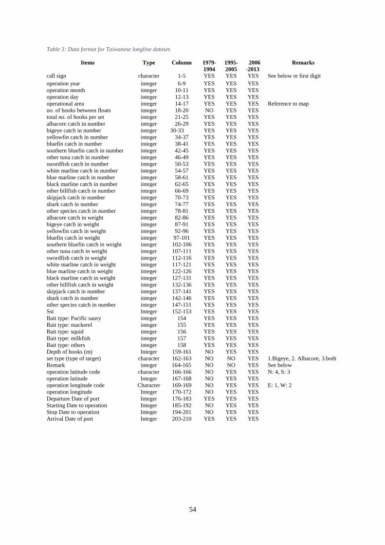
54

Table 3: Data format for Taiwanese longline dataset.

Items Type Column 1979-

1994

1995-

2005

2006

-2013

Remarks

call sign character 1-5 YES YES YES See below re first digit

operation year integer 6-9 YES YES YES

operation month integer 10-11 YES YES YES

operation day integer 12-13 YES YES YES

operational area integer 14-17 YES YES YES Reference to map

no. of hooks between floats integer 18-20 NO YES YES

total no. of hooks per set integer 21-25 YES YES YES

albacore catch in number integer 26-29 YES YES YES

bigeye catch in number integer 30-33 YES YES YES

yellowfin catch in number integer 34-37 YES YES YES

bluefin catch in number integer 38-41 YES YES YES

southern bluefin catch in number integer 42-45 YES YES YES

other tuna catch in number integer 46-49 YES YES YES

swordfish catch in number integer 50-53 YES YES YES

white marline catch in number integer 54-57 YES YES YES

blue marline catch in number integer 58-61 YES YES YES

black marline catch in number integer 62-65 YES YES YES

other billfish catch in number integer 66-69 YES YES YES

skipjack catch in number integer 70-73 YES YES YES

shark catch in number integer 74-77 YES YES YES

other species catch in number integer 78-81 YES YES YES

albacore catch in weight integer 82-86 YES YES YES

bigeye catch in weight integer 87-91 YES YES YES

yellowfin catch in weight integer 92-96 YES YES YES

bluefin catch in weight integer 97-101 YES YES YES

southern bluefin catch in weight integer 102-106 YES YES YES

other tuna catch in weight integer 107-111 YES YES YES

swordfish catch in weight integer 112-116 YES YES YES

white marline catch in weight integer 117-121 YES YES YES

blue marline catch in weight integer 122-126 YES YES YES

black marline catch in weight integer 127-131 YES YES YES

other billfish catch in weight integer 132-136 YES YES YES

skipjack catch in number integer 137-141 YES YES YES

shark catch in number integer 142-146 YES YES YES

other species catch in number integer 147-151 YES YES YES

Sst Integer 152-153 YES YES YES

Bait type: Pacific saury integer 154 YES YES YES

Bait type: mackerel integer 155 YES YES YES

Bait type: squid integer 156 YES YES YES

Bait type: milkfish integer 157 YES YES YES

Bait type: others integer 158 YES YES YES

Depth of hooks (m) Integer 159-161 NO YES YES

set type (type of target) character 162-163 NO NO YES 1.Bigeye, 2. Albacore, 3.both

Remark integer 164-165 NO NO YES See below

operation latitude code character 166-166 NO YES YES N: 4, S: 3

operation latitude Integer 167-168 NO YES YES

operation longitude code Character 169-169 NO YES YES E: 1, W: 2

operation longitude Integer 170-172 NO YES YES

Departure Date of port Integer 176-183 YES YES YES

Starting Date to operation Integer 185-192 NO YES YES

Stop Date to operation Integer 194-201 NO YES YES

Arrival Date of port Integer 203-210 YES YES YES

55

Table 4: Tonnage as indicated by first digit of TW callsign.

First digit Tonnage

1 >= 5 and < 10 tonnes

2 >= 10 and < 20 tonnes

3 >= 20 and < 50 tonnes

4 >= 50 and < 100 tonnes

5 >= 100 and < 200 tonnes

6 >= 200 and < 500 tonnes

7 >= 500 and < 1,000 tonnes

8 >= 1,000 tonnes

Table 5: Codes in the Remarks field of the TW dataset, indicating outliers.

Dates Code Outliers

2007-2011 G1 extremely high BET catch

G4 extremely high ALB

G6 extremely high YFT catch

G8 extremely high SWO;

SF for a given year and vessel, record only single species catch for 3

successive months

2012-2013 G1 extremely high ALB catch

G2 extremely high BET

G3 extremely high YFT catch

G7 extremely high SWO

GH abnormal total no. of hooks per set

GL more than one anomaly

SF for a given year and vessel, only record single species catch for 3

successive months

2007-2011:

1.G1:extremely high BET catch ( > 5 tons per set or outliers in the distribution of bet catch number per set) ; G4: extremely high ALB; G6: extremely high YFT catch; G8: extremely high SWO;

SF: for a given year and a given vessel, record only single species catch for three successive months.

2012-2013:

G1: extremely high ALB catch (Based on definition of IOTC BET regions, for a given year and a given region, average catch numbers

per set for a given vessel. Then use the IQR Rule*. Remark all sets by the vessel which reported the outlier for the given year and region);

G2: extremely high BET;

G3: extremely high YFT catch; G7: extremely high SWO;

GH: abnormal total no. of hooks per set; GL: if there are more than one anomaly.

SF: for a given year and a given vessel, only record single species catch for three successive months.

Criteria for outliers

( > 5 tons per set or outliers in the distribution of bet catch number per set)

*IQR Rule for Outliers

1. Arrange average catch numbers per set for all vessels in order.

2. Calculate first quartile (Q1), third quartile (Q3) and the interquartile range (IQR=Q3-Q1). 3. Compute Q1-1.5 x IQR and Compute Q3+1.5 x IQR. Anything outside this range is an outlier.

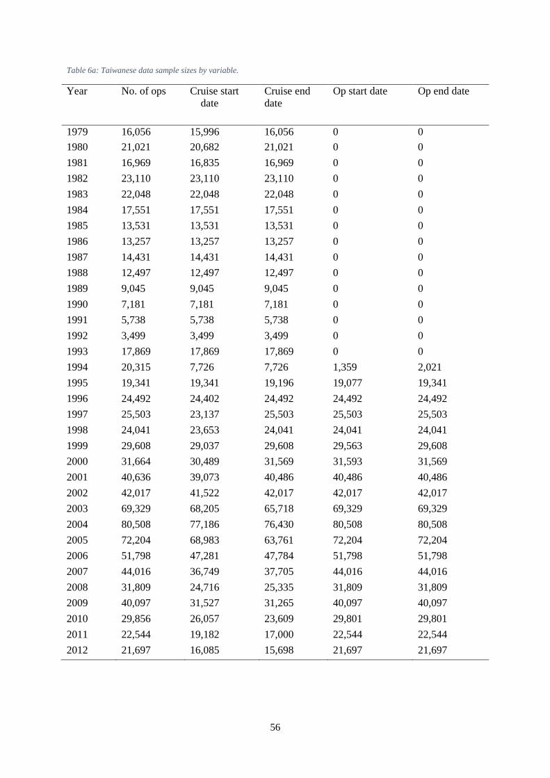
56

Table 6a: Taiwanese data sample sizes by variable.

Year No. of ops Cruise start

date

Cruise end

date

Op start date Op end date

1979 16,056 15,996 16,056 0 0

1980 21,021 20,682 21,021 0 0

1981 16,969 16,835 16,969 0 0

1982 23,110 23,110 23,110 0 0

1983 22,048 22,048 22,048 0 0

1984 17,551 17,551 17,551 0 0

1985 13,531 13,531 13,531 0 0

1986 13,257 13,257 13,257 0 0

1987 14,431 14,431 14,431 0 0

1988 12,497 12,497 12,497 0 0

1989 9,045 9,045 9,045 0 0

1990 7,181 7,181 7,181 0 0

1991 5,738 5,738 5,738 0 0

1992 3,499 3,499 3,499 0 0

1993 17,869 17,869 17,869 0 0

1994 20,315 7,726 7,726 1,359 2,021

1995 19,341 19,341 19,196 19,077 19,341

1996 24,492 24,402 24,492 24,492 24,492

1997 25,503 23,137 25,503 25,503 25,503

1998 24,041 23,653 24,041 24,041 24,041

1999 29,608 29,037 29,608 29,563 29,608

2000 31,664 30,489 31,569 31,593 31,569

2001 40,636 39,073 40,486 40,486 40,486

2002 42,017 41,522 42,017 42,017 42,017

2003 69,329 68,205 65,718 69,329 69,329

2004 80,508 77,186 76,430 80,508 80,508

2005 72,204 68,983 63,761 72,204 72,204

2006 51,798 47,281 47,784 51,798 51,798

2007 44,016 36,749 37,705 44,016 44,016

2008 31,809 24,716 25,335 31,809 31,809

2009 40,097 31,527 31,265 40,097 40,097

2010 29,856 26,057 23,609 29,801 29,801

2011 22,544 19,182 17,000 22,544 22,544

2012 21,697 16,085 15,698 21,697 21,697

57

Table 6b: Taiwanese data sample sizes by variable.

Year No. of ops Set type Lat & long in

1 degree

NHBF After cleaning

1979 16,056 0 0 0 12,758

1980 21,021 0 0 0 16,889

1981 16,969 0 0 0 13,561

1982 23,110 0 0 0 17,786

1983 22,048 0 0 0 17,129

1984 17,551 0 0 0 14,339

1985 13,531 0 0 0 11,888

1986 13,257 0 0 0 10,491

1987 14,431 0 0 0 11,018

1988 12,497 0 0 0 10,434

1989 9,045 0 0 0 7,099

1990 7,181 0 0 0 5,787

1991 5,738 0 0 0 4,993

1992 3,499 0 0 0 2,907

1993 17,869 0 0 0 11,662

1994 20,315 0 20,315 0 15,635

1995 19,341 0 12,051 7,116 15,319

1996 24,492 0 18,408 10,884 18,760

1997 25,503 0 20,565 9,495 20,255

1998 24,041 0 19,785 10,022 20,482

1999 29,608 0 24,603 14,198 26,090

2000 31,664 0 26,723 16,022 27,429

2001 40,636 0 37,853 32,575 36,308

2002 42,017 0 38,204 40,768 37,475

2003 69,329 0 53,455 69,183 37,338

2004 80,508 0 76,388 80,402 70,125

2005 72,204 0 70,135 72,204 57,497

2006 51,798 51,798 50,987 51,798 38,910

2007 44,016 44,016 43,506 44,016 32,622

2008 31,809 31,809 31,176 31,809 23,602

2009 40,097 40,097 39,355 40,097 30,773

2010 29,856 29,856 29,756 29,856 23,342

2011 22,544 22,544 22,544 22,544 17,701

2012 21,697 21,697 21,696 21,697 14,723

58

Table 7: Korean data description.

Year No. of ops VESSEL

NAME_rev

Vessel id

coverage (%) Hooks Floats Op date

1971 34 34 100.0 34 34 34

1972 3265 53 1.6 3265 3265 3265

1973 508 508 100.0 508 241 508

1974 1255 1255 100.0 1255 93 1255

1975 5313 5051 95.1 5021 334 5313

1976 119 119 100.0 119 119 119

1977 3714 3714 100.0 3714 3714 3736

1978 23191 22882 98.7 23191 23191 23191

1979 10509 10433 99.3 10509 10509 10651

1980 20446 19874 97.2 20446 20446 20408

1981 15566 15527 99.7 15566 15566 15585

1982 17119 16593 96.9 17119 17119 17176

1983 19255 18216 94.6 19255 19255 19255

1984 7912 7684 97.1 7912 7912 8080

1985 11386 10887 95.6 11386 11386 11530

1986 14374 14157 98.5 14374 14374 14462

1987 14810 14660 99.0 14810 14810 14810

1988 17568 17409 99.1 17568 17568 17568

1989 18771 18127 96.6 18771 18771 18771

1990 14162 14073 99.4 14162 14162 14162

1991 4533 4533 100.0 4533 4533 4533

1992 7005 7005 100.0 7005 7005 7005

1993 9569 9569 100.0 9569 9569 9569

1994 10141 9065 89.4 10141 10141 10141

1995 7577 5332 70.4 7577 7577 7577

1996 12218 7501 61.4 12218 12218 12218

1997 13740 8031 58.4 13740 13740 13740

1998 5165 2239 43.3 5165 5165 5165

1999 2833 1783 62.9 2833 2833 2833

2000 4236 2394 56.5 4236 4236 4236

2001 3162 1929 61.0 3162 3162 3162

2002 1479 1341 90.7 1479 1479 1638

2003 2627 1474 56.1 2627 2627 2627

2004 4345 3004 69.1 4345 4345 4345

2005 2443 2443 100.0 2443 2443 2444

2006 3597 3508 97.5 3597 3597 3597

2007 3371 3197 94.8 3371 3371 3371

2008 2330 2330 100.0 2330 2330 2330

2009 3273 3273 100.0 3273 3273 3273

2010 1851 1851 100.0 1851 1851 1851

2011 1658 1658 100.0 1658 1658 1658

2012 1295 1295 100.0 1295 1295 1295

2013 1659 1659 100.0 1659 1659 1659

2014 1802 1802 100.0 1802 1802 1802

59

Table 8: Comparison of field availability among the three fleets.

Items JP TW KR

call sign 1979- Y Y

operation date Y Y Y

Location – 5x5 Y Y Y

Location – 1x1 Y 1994- Y

no. of hooks between float * # &

total no. of hooks per set Y Y Y

albacore catch in number Y Y Y

bigeye catch in number Y Y Y

yellowfin catch in number Y Y Y

southern bluefin catch in

number

Y 1994- Y

other tuna catch in number N Y N

swordfish catch in number Y Y Y

striped marlin catch in number Y Y Y

blue marlin catch in number Y Y Y

black marlin catch in number Y Y Y

sailfish catch in numbers N ^ Y

skipjack catch in number N Y Y

shark catch in number N Y Y

other species catch in number N Y1 Y1

Bait type: Pacific saury Y N N

Bait type: mackerel Y N N

Bait type: squid Y N N

Bait type: milkfish Y N N

Bait type: others Y N N

* High coverage since 1971, variable earlier

# Coverage increasing from 1994 to reach 100% by 2003

& number of floats reported for full dataset, and HBF estimated as HBF= hooks/floats

$ No field for SBT before 1994, only reported when skipper changed the field code

^ Reported in ‘other billfish catch’

1 Different species mix between TW and KR.

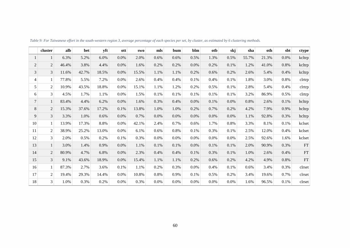
60

Table 9: For Taiwanese effort in the south-western region 3, average percentage of each species per set, by cluster, as estimated by 6 clustering methods.

cluster alb bet yft ott swo mls bum blm otb skj sha oth sbt ctype

1 1 6.3% 5.2% 6.0% 0.0% 2.0% 0.6% 0.6% 0.5% 1.3% 0.5% 55.7% 21.3% 0.0% kcltrp

2 2 46.4% 3.8% 4.4% 0.0% 1.6% 0.2% 0.2% 0.0% 0.2% 0.1% 1.2% 41.0% 0.8% kcltrp

3 3 11.6% 42.7% 18.5% 0.0% 15.5% 1.1% 1.1% 0.2% 0.6% 0.2% 2.6% 5.4% 0.4% kcltrp

4 1 77.8% 5.5% 7.2% 0.0% 2.6% 0.4% 0.4% 0.1% 0.4% 0.1% 1.8% 3.0% 0.8% clrtrp

5 2 10.9% 43.5% 18.8% 0.0% 15.1% 1.1% 1.2% 0.2% 0.5% 0.1% 2.8% 5.4% 0.4% clrtrp

6 3 4.5% 1.7% 1.1% 0.0% 1.5% 0.1% 0.1% 0.1% 0.1% 0.1% 3.2% 86.9% 0.5% clrtrp

7 1 83.4% 4.4% 6.2% 0.0% 1.6% 0.3% 0.4% 0.0% 0.1% 0.0% 0.8% 2.6% 0.1% hcltrp

8 2 15.3% 37.6% 17.2% 0.1% 13.8% 1.0% 1.0% 0.2% 0.7% 0.2% 4.2% 7.9% 0.9% hcltrp

9 3 3.3% 1.0% 0.6% 0.0% 0.7% 0.0% 0.0% 0.0% 0.0% 0.0% 1.1% 92.8% 0.3% hcltrp

10 1 13.9% 17.3% 8.8% 0.0% 42.1% 2.4% 0.7% 0.6% 1.7% 0.8% 3.3% 8.1% 0.1% kclset

11 2 38.9% 25.2% 13.0% 0.0% 6.1% 0.6% 0.8% 0.1% 0.3% 0.1% 2.5% 12.0% 0.4% kclset

12 3 2.0% 0.5% 0.2% 0.1% 0.3% 0.0% 0.0% 0.0% 0.0% 0.0% 2.5% 92.6% 1.6% kclset

13 1 3.0% 1.4% 0.9% 0.0% 1.1% 0.1% 0.1% 0.0% 0.1% 0.1% 2.0% 90.9% 0.3% FT

14 2 80.9% 4.7% 6.8% 0.0% 2.3% 0.4% 0.4% 0.1% 0.3% 0.1% 1.0% 2.6% 0.4% FT

15 3 9.1% 43.6% 18.9% 0.0% 15.4% 1.1% 1.1% 0.2% 0.6% 0.2% 4.2% 4.9% 0.8% FT

16 1 87.3% 2.7% 3.6% 0.1% 1.1% 0.2% 0.3% 0.0% 0.4% 0.1% 0.6% 3.4% 0.3% clrset

17 2 19.4% 29.3% 14.4% 0.0% 10.8% 0.8% 0.9% 0.1% 0.5% 0.2% 3.4% 19.6% 0.7% clrset

18 3 1.0% 0.3% 0.2% 0.0% 0.3% 0.0% 0.0% 0.0% 0.0% 0.0% 1.6% 96.5% 0.1% clrset

61

Table 10: Numbers of clusters identified in sets from each region and fishing fleet.

JP TW KR

Region 2 2 3 3

Region 3 3 3 3

Region 4 4 4 4

Region 5 2 3 2

62

Table 11: Indices for regions 2 and 5 derived from the

joint model that included all data from Japan and Korea,

and Taiwanese data from 2005.

Year-Qtr BET Region 2

BET Region 5

YFT Region 2

YFT Region 5

1952.125 NA NA NA NA



1952.875 NA 1.7653 NA 10.5212

1953.125 NA 1.1144 NA 4.1852

1953.375 NA 1.7509 NA 3.7193


1953.875 NA 2.2694 NA 4.7407

1954.125 NA 1.8396 NA 4.4747

1954.375 NA 1.7186 NA 4.4621

1954.625 2.0280 1.5344 5.9700 2.8857

1954.875 1.0958 1.5906 7.4568 3.6252

1955.125 0.9035 1.6344 8.3431 4.9343

1955.375 1.4600 1.8107 9.5702 5.0379

1955.625 1.8874 2.2459 5.5421 2.8362

1955.875 1.7399 2.2317 5.6063 3.6162

1956.125 0.8843 1.7415 5.4644 4.2997

1956.375 1.3491 1.4249 5.1134 4.1237

1956.625 1.9686 1.9394 4.0126 2.4683

1956.875 1.7412 2.0617 3.9447 2.9655

1957.125 0.9803 1.6174 4.1995 3.0059

1957.375 1.3844 1.5284 2.5687 2.6514

1957.625 1.7054 1.8846 1.4033 1.7404

1957.875 0.9976 2.3118 3.6058 2.5683

1958.125 0.8024 1.9480 2.8111 2.4400

1958.375 1.7415 1.1863 2.4826 2.1511

1958.625 2.2505 1.1674 2.1094 1.2416

1958.875 1.2084 1.6256 4.1279 2.3425

1959.125 0.8733 1.3624 4.0225 2.2140

1959.375 1.7617 1.2575 4.9147 2.3208

1959.625 1.5901 1.5005 1.7183 1.2582

1959.875 NA 1.4927 NA 2.2403

1960.125 1.1504 1.3965 3.2367 2.0167

1960.375 1.3779 1.8591 3.3918 2.4048

1960.625 1.8798 1.5782 2.2706 1.6598

1960.875 1.9693 1.3225 3.3304 3.0649

1961.125 0.8771 1.4034 2.8862 1.7870

1961.375 1.2069 1.5360 3.1489 1.5356

1961.625 0.9202 2.2029 2.7415 1.2017

1961.875 1.0319 1.9939 2.9497 1.9154

1962.125 1.2351 1.6267 2.6925 2.2048


BET Region 5

YFT Region 2

YFT Region 5

1962.375 1.3768 1.3582 1.8445 2.1023

1962.625 1.0932 1.7368 1.1652 1.6277

1962.875 1.3048 1.8476 1.9678 1.6692

1963.125 0.8668 1.6843 1.7556 1.1305

1963.375 1.1952 1.2836 1.2023 1.0059

1963.625 1.3449 1.5972 0.9466 0.8615

1963.875 1.2124 1.3284 1.6878 1.1583

1964.125 0.9233 1.5529 1.2274 1.3272

1964.375 1.4070 1.3317 0.7813 1.5303

1964.625 1.0945 1.4637 0.7687 1.0371

1964.875 0.9869 1.3055 0.7538 0.7623

1965.125 0.7860 1.2910 0.8555 0.8867

1965.375 0.8774 1.1629 0.9293 1.0606

1965.625 0.9094 1.0913 0.6349 0.6642

1965.875 1.2372 1.2237 1.5015 0.9414

1966.125 1.2607 1.5843 1.6344 1.1843

1966.375 1.0676 1.0408 1.4238 1.5427

1966.625 0.9850 1.6070 1.5336 1.2610

1966.875 1.3661 1.4645 1.6057 1.2408

1967.125 1.0379 1.4767 0.8536 1.1726

1967.375 0.6483 1.1732 0.8704 0.9390

1967.625 0.9789 1.4077 0.4611 0.8935

1967.875 0.6777 1.3973 0.5374 1.1279

1968.125 1.1830 1.3242 2.4712 1.1654

1968.375 1.2893 1.1976 3.1893 1.1289

1968.625 1.3040 1.5949 0.9189 0.6654

1968.875 1.2003 1.6116 1.6295 0.7676

1969.125 1.3278 1.4697 1.1728 0.9902

1969.375 0.8652 1.0592 0.8552 1.1983

1969.625 0.9417 1.3620 1.2322 0.8101

1969.875 1.0907 1.5718 1.2020 1.0540

1970.125 1.1524 1.6674 0.6829 1.0135

1970.375 0.6395 1.3365 0.3531 0.6843

1970.625 1.1051 1.5476 0.4841 1.9619

1970.875 0.7627 1.0858 0.6505 0.9302

1971.125 0.7138 0.9056 0.6165 0.8923

1971.375 1.0574 0.7903 0.6943 1.3535

1971.625 1.4901 0.9165 1.2358 0.5946

1971.875 1.1241 1.1344 0.9702 1.0541

1972.125 1.1267 1.0980 0.5658 0.9617

1972.375 1.0944 1.0049 0.6289 0.6363

1972.625 0.9324 1.0254 0.9196 0.8709

1972.875 1.6379 NA 0.8376 NA

1973.125 1.6445 1.3110 0.7004 1.1806

63


BET Region 5

YFT Region 2

YFT Region 5

1973.375 2.1178 1.1847 0.5010 0.8745

1973.625 0.7367 NA 0.3715 NA

1973.875 0.9550 1.0973 0.5407 0.7520

1974.125 0.8487 1.4664 0.2486 0.5285

1974.375 0.9469 0.9225 0.4283 0.8718

1974.625 1.1537 1.1233 0.4621 0.5965

1974.875 1.1468 0.9911 0.2780 0.6488

1975.125 1.0454 0.6544 0.2080 0.6344

1975.375 0.6196 0.7741 0.3182 0.5340

1975.625 0.7846 0.8053 0.4660 0.5079

1975.875 0.7810 0.7544 0.7813 0.4986

1976.125 0.5701 0.7140 0.1848 0.4862

1976.375 0.7903 0.8943 0.6620 0.6442

1976.625 0.7540 1.2248 0.4141 0.5754

1976.875 NA 0.9605 NA 0.8139

1977.125 1.7037 1.2618 0.4825 0.7424

1977.375 2.3748 NA 0.8731 NA

1977.625 1.8510 1.3530 0.7913 0.6020

1977.875 2.3115 1.3343 1.2370 0.9908

1978.125 2.5911 2.0167 0.6063 1.2969

1978.375 1.8760 2.5830 0.3968 1.2119

1978.625 1.4618 1.7267 0.3546 0.3997

1978.875 1.4661 1.6235 0.8413 0.3497

1979.125 1.6696 1.2970 0.3472 0.5521

1979.375 1.1977 1.4656 0.2461 0.6623

1979.625 0.9554 1.4061 0.2388 0.6813

1979.875 1.1276 1.1353 0.2523 0.4080

1980.125 0.8990 1.0150 0.1745 0.5146

1980.375 1.2300 1.1696 0.2546 0.7246

1980.625 1.0905 1.1381 0.2939 0.4646

1980.875 1.4951 1.1305 0.3939 0.2880

1981.125 1.0400 0.8769 0.1553 0.3059

1981.375 1.2257 0.6191 0.3466 0.4016

1981.625 1.1199 0.9291 0.2557 0.6070

1981.875 1.2123 1.1352 0.4386 0.5061

1982.125 1.0009 1.1060 0.2095 0.3555

1982.375 1.3402 1.0707 0.5793 0.5735

1982.625 1.0476 0.9832 0.3549 0.4222

1982.875 1.0813 1.3170 0.7149 0.3414

1983.125 1.0116 1.1024 0.3568 0.3708

1983.375 1.0508 1.1455 0.4225 0.5999

1983.625 0.7734 1.0871 0.3326 0.4125

1983.875 0.9887 1.0314 0.6057 0.5986

1984.125 0.9057 0.9603 0.2775 0.4812


BET Region 5

YFT Region 2

YFT Region 5

1984.375 0.8972 0.5804 0.4093 0.8919

1984.625 1.0672 0.8331 0.2944 0.4892

1984.875 0.7982 1.2169 0.4235 0.5244

1985.125 0.8290 0.8975 0.2829 0.4551

1985.375 0.8097 0.7001 0.3388 0.7691

1985.625 1.0359 0.9828 0.3811 0.6655

1985.875 1.1401 0.9560 0.6779 0.4844

1986.125 0.8136 0.9625 0.5227 0.3075

1986.375 0.8768 0.8718 0.7137 0.6498

1986.625 1.0601 0.9525 0.3205 0.6177

1986.875 1.1713 1.7477 0.6117 0.4603

1987.125 1.1063 1.1204 0.4495 0.3605

1987.375 1.0471 0.9171 0.4524 1.0478

1987.625 0.9940 0.9840 0.2558 0.4963

1987.875 1.2097 1.0489 0.5782 0.3192

1988.125 1.2291 1.2948 0.5661 0.4842

1988.375 0.8712 0.8328 0.4352 0.9794

1988.625 0.6943 0.5870 0.2684 0.6431

1988.875 0.8603 1.0797 0.2544 0.4257

1989.125 0.5316 1.0580 0.1462 0.4750

1989.375 0.5455 0.5849 0.2674 0.3088

1989.625 0.5987 0.6164 0.2117 0.2478

1989.875 0.8389 0.9053 0.3275 0.2672

1990.125 0.6647 0.7296 0.2912 0.4252

1990.375 0.7711 0.4849 0.2122 0.5714

1990.625 0.5908 0.6898 0.1750 0.6153

1990.875 0.6823 0.6294 0.2485 0.1656

1991.125 0.5525 0.8360 0.3401 0.3106

1991.375 0.5651 NA 0.4940 NA

1991.625 0.7570 NA 0.1644 NA

1991.875 0.9768 0.1988 0.3520 0.4413

1992.125 0.7010 0.7803 0.3426 0.2465

1992.375 0.6782 NA 0.2750 NA

1992.625 0.7368 NA 0.1178 NA

1992.875 1.0083 0.5565 0.2709 0.3370

1993.125 0.6706 0.5970 0.2471 0.0972

1993.375 0.6782 NA 0.3276 NA

1993.625 0.7925 0.7541 0.1693 0.4012

1993.875 0.8838 0.6839 0.2892 0.2824

1994.125 0.5244 0.4756 0.1645 0.1244

1994.375 0.7461 0.6556 0.2225 0.1308

1994.625 0.7430 0.7320 0.1343 0.2435

1994.875 0.8989 0.7928 0.1629 0.1160

1995.125 0.6665 0.5732 0.1288 0.1245

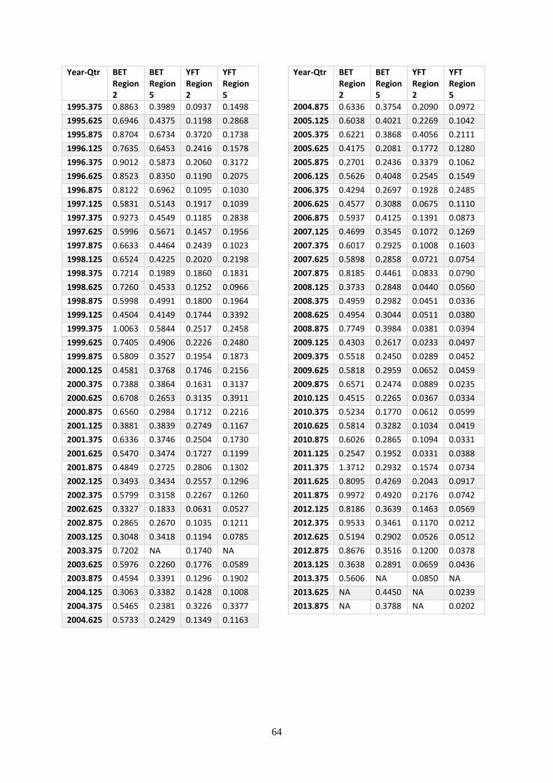
64


BET Region 5

YFT Region 2

YFT Region 5

1995.375 0.8863 0.3989 0.0937 0.1498

1995.625 0.6946 0.4375 0.1198 0.2868

1995.875 0.8704 0.6734 0.3720 0.1738

1996.125 0.7635 0.6453 0.2416 0.1578

1996.375 0.9012 0.5873 0.2060 0.3172

1996.625 0.8523 0.8350 0.1190 0.2075

1996.875 0.8122 0.6962 0.1095 0.1030

1997.125 0.5831 0.5143 0.1917 0.1039

1997.375 0.9273 0.4549 0.1185 0.2838

1997.625 0.5996 0.5671 0.1457 0.1956

1997.875 0.6633 0.4464 0.2439 0.1023

1998.125 0.6524 0.4225 0.2020 0.2198

1998.375 0.7214 0.1989 0.1860 0.1831

1998.625 0.7260 0.4533 0.1252 0.0966

1998.875 0.5998 0.4991 0.1800 0.1964

1999.125 0.4504 0.4149 0.1744 0.3392

1999.375 1.0063 0.5844 0.2517 0.2458

1999.625 0.7405 0.4906 0.2226 0.2480

1999.875 0.5809 0.3527 0.1954 0.1873

2000.125 0.4581 0.3768 0.1746 0.2156

2000.375 0.7388 0.3864 0.1631 0.3137

2000.625 0.6708 0.2653 0.3135 0.3911

2000.875 0.6560 0.2984 0.1712 0.2216

2001.125 0.3881 0.3839 0.2749 0.1167

2001.375 0.6336 0.3746 0.2504 0.1730

2001.625 0.5470 0.3474 0.1727 0.1199

2001.875 0.4849 0.2725 0.2806 0.1302

2002.125 0.3493 0.3434 0.2557 0.1296

2002.375 0.5799 0.3158 0.2267 0.1260

2002.625 0.3327 0.1833 0.0631 0.0527

2002.875 0.2865 0.2670 0.1035 0.1211

2003.125 0.3048 0.3418 0.1194 0.0785

2003.375 0.7202 NA 0.1740 NA

2003.625 0.5976 0.2260 0.1776 0.0589

2003.875 0.4594 0.3391 0.1296 0.1902

2004.125 0.3063 0.3382 0.1428 0.1008

2004.375 0.5465 0.2381 0.3226 0.3377

2004.625 0.5733 0.2429 0.1349 0.1163


BET Region 5

YFT Region 2

YFT Region 5

2004.875 0.6336 0.3754 0.2090 0.0972

2005.125 0.6038 0.4021 0.2269 0.1042

2005.375 0.6221 0.3868 0.4056 0.2111

2005.625 0.4175 0.2081 0.1772 0.1280

2005.875 0.2701 0.2436 0.3379 0.1062

2006.125 0.5626 0.4048 0.2545 0.1549

2006.375 0.4294 0.2697 0.1928 0.2485

2006.625 0.4577 0.3088 0.0675 0.1110

2006.875 0.5937 0.4125 0.1391 0.0873

2007.125 0.4699 0.3545 0.1072 0.1269

2007.375 0.6017 0.2925 0.1008 0.1603

2007.625 0.5898 0.2858 0.0721 0.0754

2007.875 0.8185 0.4461 0.0833 0.0790

2008.125 0.3733 0.2848 0.0440 0.0560

2008.375 0.4959 0.2982 0.0451 0.0336

2008.625 0.4954 0.3044 0.0511 0.0380

2008.875 0.7749 0.3984 0.0381 0.0394

2009.125 0.4303 0.2617 0.0233 0.0497

2009.375 0.5518 0.2450 0.0289 0.0452

2009.625 0.5818 0.2959 0.0652 0.0459

2009.875 0.6571 0.2474 0.0889 0.0235

2010.125 0.4515 0.2265 0.0367 0.0334

2010.375 0.5234 0.1770 0.0612 0.0599

2010.625 0.5814 0.3282 0.1034 0.0419

2010.875 0.6026 0.2865 0.1094 0.0331

2011.125 0.2547 0.1952 0.0331 0.0388

2011.375 1.3712 0.2932 0.1574 0.0734

2011.625 0.8095 0.4269 0.2043 0.0917

2011.875 0.9972 0.4920 0.2176 0.0742

2012.125 0.8186 0.3639 0.1463 0.0569

2012.375 0.9533 0.3461 0.1170 0.0212

2012.625 0.5194 0.2902 0.0526 0.0512

2012.875 0.8676 0.3516 0.1200 0.0378

2013.125 0.3638 0.2891 0.0659 0.0436

2013.375 0.5606 NA 0.0850 NA

2013.625 NA 0.4450 NA 0.0239

2013.875 NA 0.3788 NA 0.0202

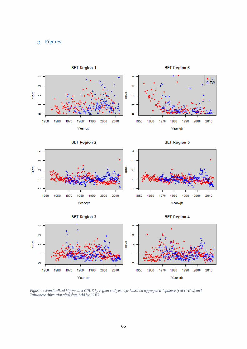
65

g. Figures

Figure 1: Standardized bigeye tuna CPUE by region and year-qtr based on aggregated Japanese (red circles) and

Taiwanese (blue triangles) data held by IOTC.

66

Figure 2: Standardized yellowfin tuna CPUE by region and year-qtr based on aggregated Japanese (red circles) and

Taiwanese (blue triangles) data held by IOTC.

67

Figure 3: Standardized bigeye tuna CPUE by region and year based on aggregated Japanese (red circles) and Taiwanese

(blue triangles) data held by IOTC.

68

Figure 4: Standardized yellowfin tuna CPUE by region and year based on aggregated Japanese (red circles) and Taiwanese

(blue triangles) data held by IOTC.

69

Figure 5: Sets per day by region for the Japanese fleet.

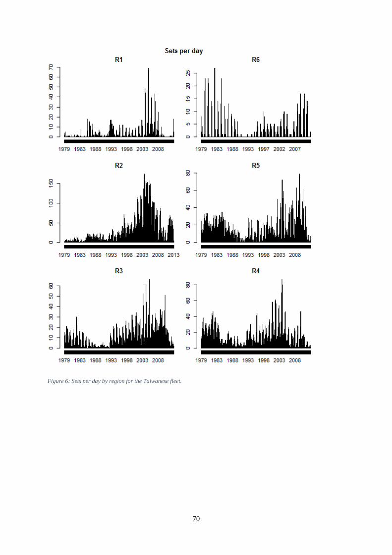
70

Figure 6: Sets per day by region for the Taiwanese fleet.

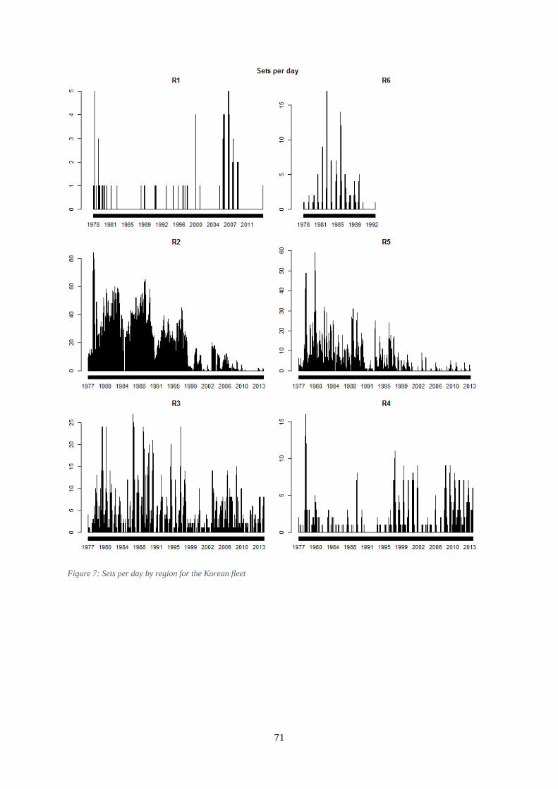
71

Figure 7: Sets per day by region for the Korean fleet

72

Figure 8: Proportions of Taiwanese sets reporting data at one degree resolution and reporting numbers of hooks between

floats.

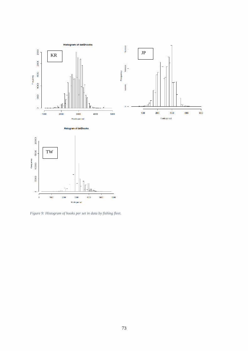
73

Figure 9: Histogram of hooks per set in data by fishing fleet.

KR JP

TW

74

Figure 10: Histogram of hooks per set by 5 year period for the Taiwanese fleet.

75

Figure 11: Numbers of fish recorded in the Taiwanese database as bluefin and southern bluefin (SBF) by year.

76

Figure 12: Proportions of sets retained after data cleaning for analyses in this paper, by region and yrqtr, for Japanese (top

left), Taiwanese (top right), and Korean (bottom left) data.

77

Figure 13: Logbook coverage of the bigeye and yellowfin catch by fleet and year, based on logbook catch divided by total

Task 1 catch.

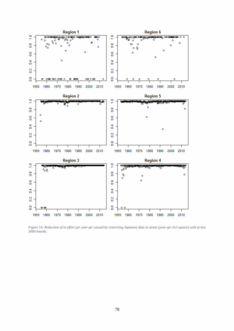
78

Figure 14: Reduction of in effort per year-qtr caused by restricting Japanese data to strata (year-qtr-5x5 square) with at last

5000 hoooks.

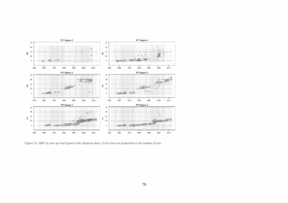
79

Figure 15: HBF by year-qtr and region in the Japanese data. Circle sizes are proportion to the number of sets.

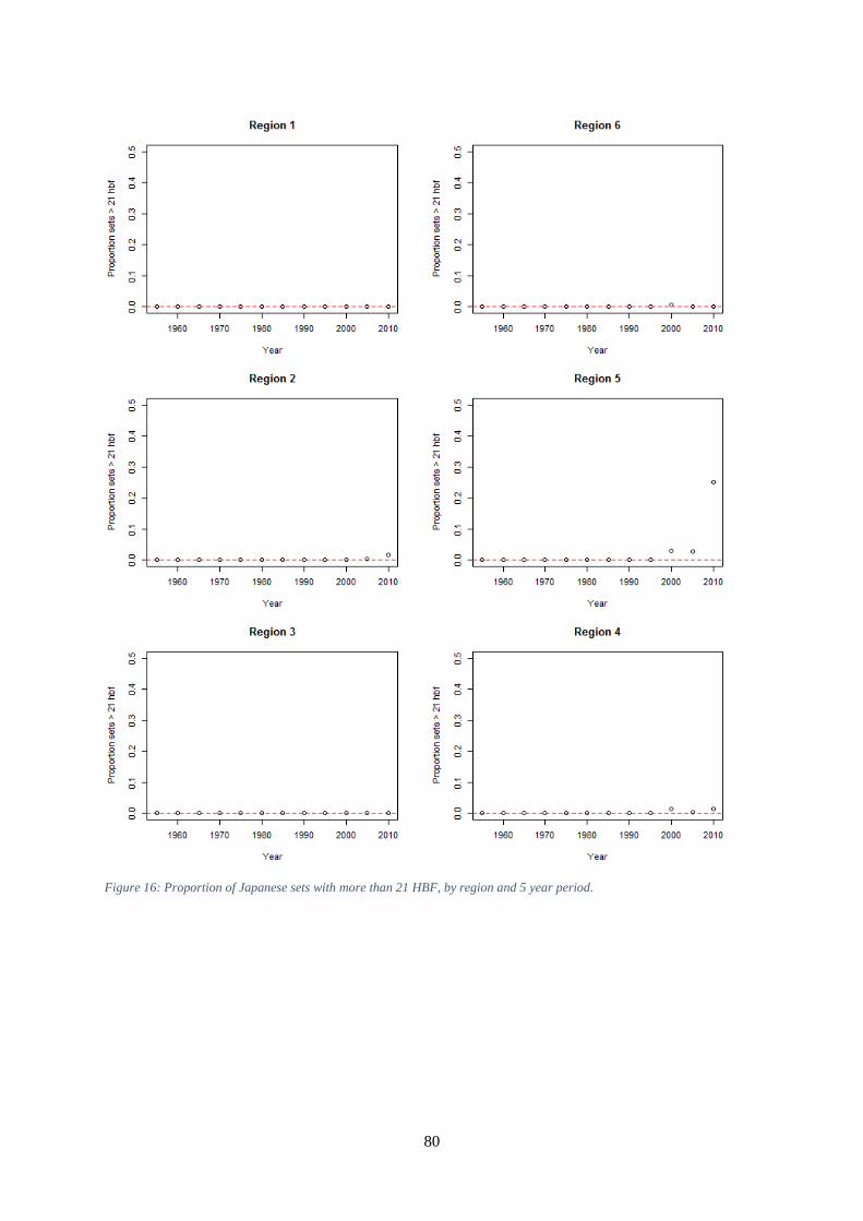
80

Figure 16: Proportion of Japanese sets with more than 21 HBF, by region and 5 year period.

81

Figure 17: Proportion of Taiwanese sets with no catch of the main species.

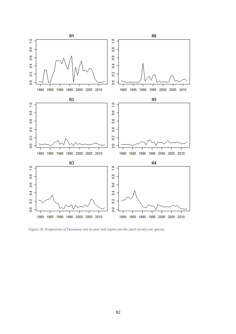
82

Figure 18: Proportions of Taiwanese sets by year and region sets the catch of only one species.

83

Figure 19: Proportion of Japanese sets by region and year in which only one species recorded. The red circles indicate the

number of sets reported.

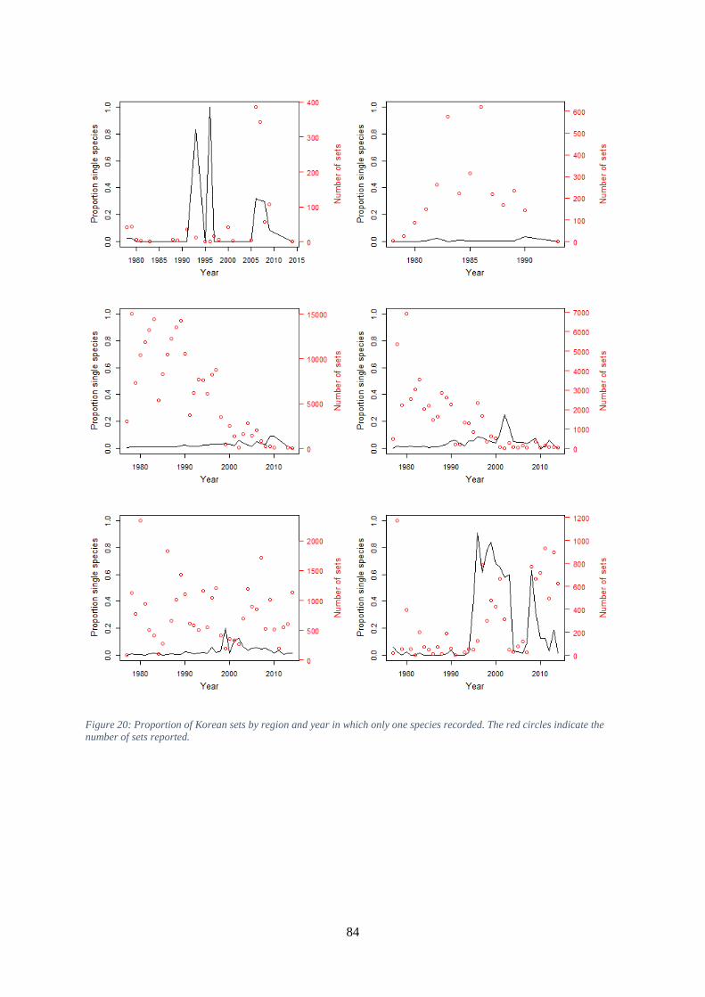
84

Figure 20: Proportion of Korean sets by region and year in which only one species recorded. The red circles indicate the

number of sets reported.

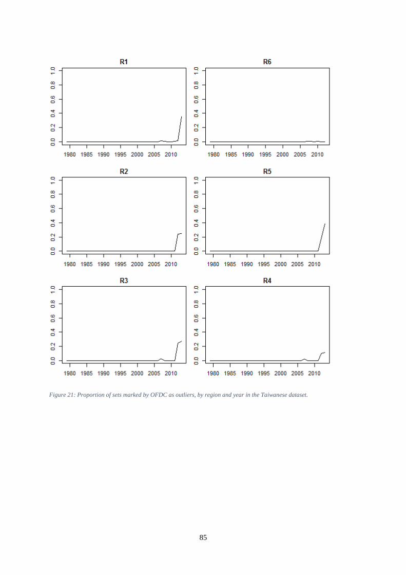
85

Figure 21: Proportion of sets marked by OFDC as outliers, by region and year in the Taiwanese dataset.

86

Figure 22: Proportion of Taiwanese sets removed by standard cleaning process.

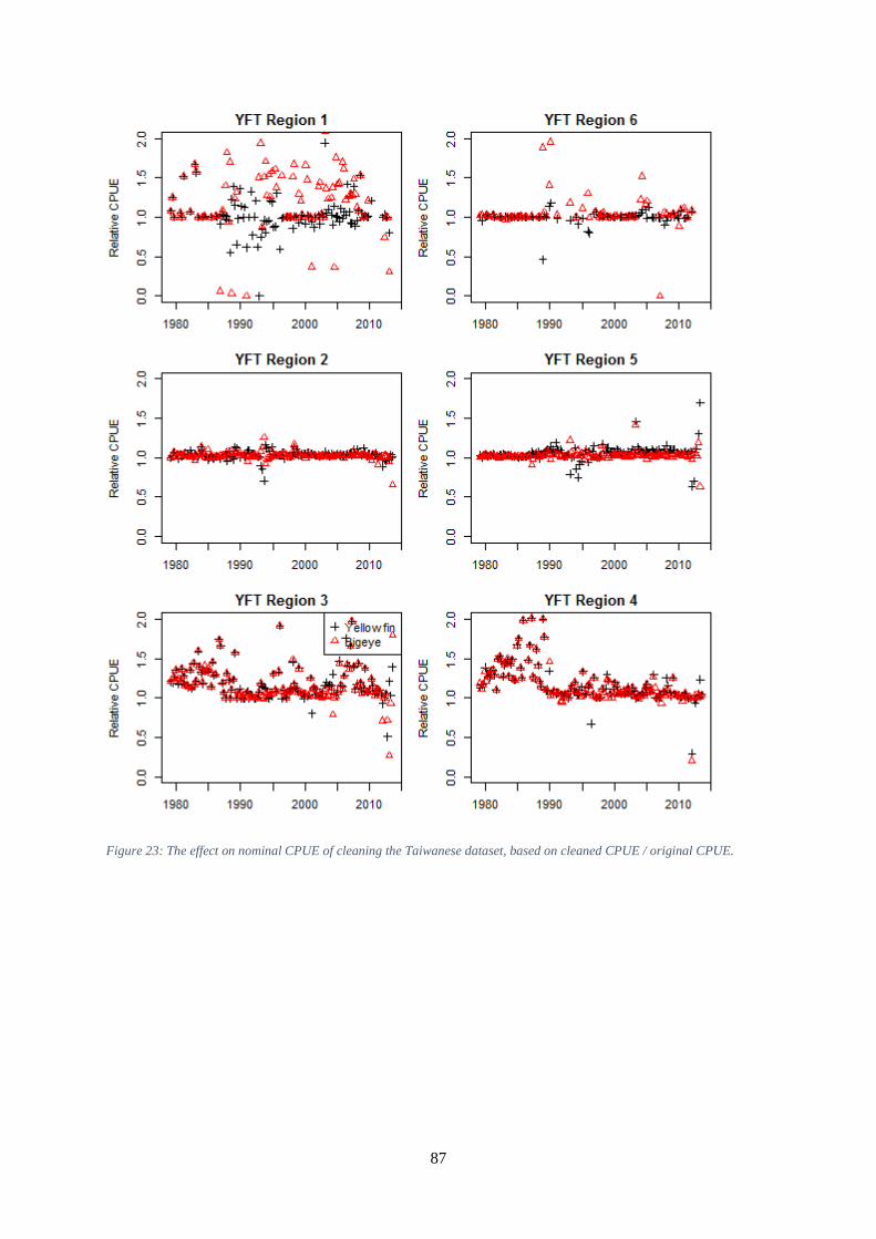
87

Figure 23: The effect on nominal CPUE of cleaning the Taiwanese dataset, based on cleaned CPUE / original CPUE.

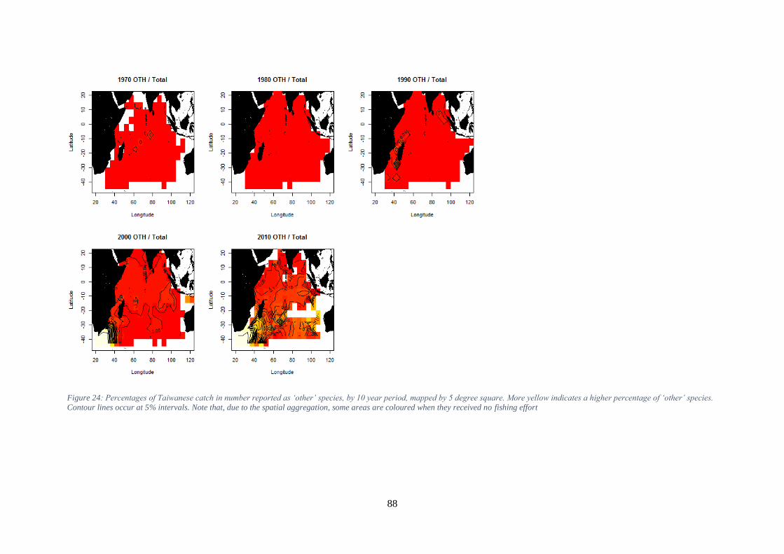
88

Figure 24: Percentages of Taiwanese catch in number reported as ‘other’ species, by 10 year period, mapped by 5 degree square. More yellow indicates a higher percentage of ‘other’ species.

Contour lines occur at 5% intervals. Note that, due to the spatial aggregation, some areas are coloured when they received no fishing effort

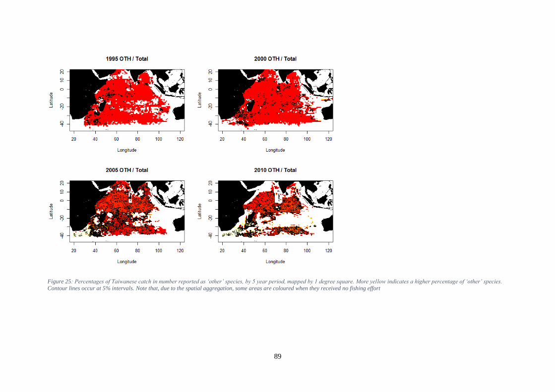
89

Figure 25: Percentages of Taiwanese catch in number reported as ‘other’ species, by 5 year period, mapped by 1 degree square. More yellow indicates a higher percentage of ‘other’ species.

Contour lines occur at 5% intervals. Note that, due to the spatial aggregation, some areas are coloured when they received no fishing effort

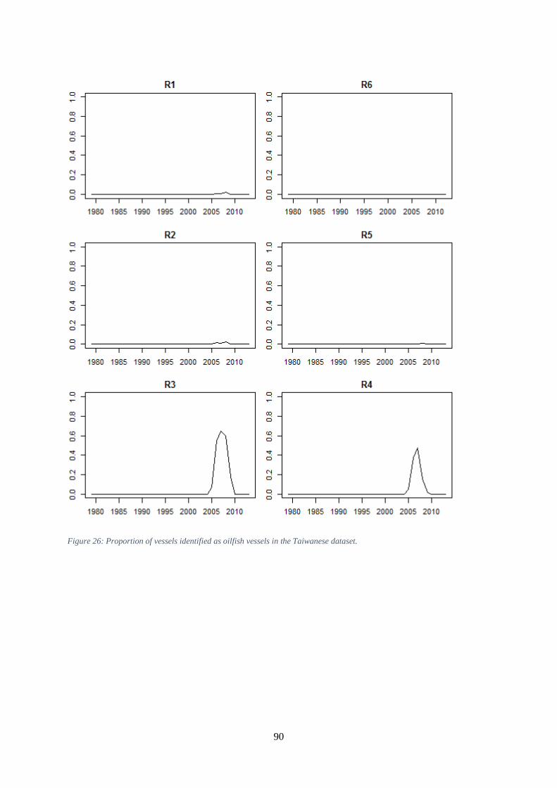
90

Figure 26: Proportion of vessels identified as oilfish vessels in the Taiwanese dataset.

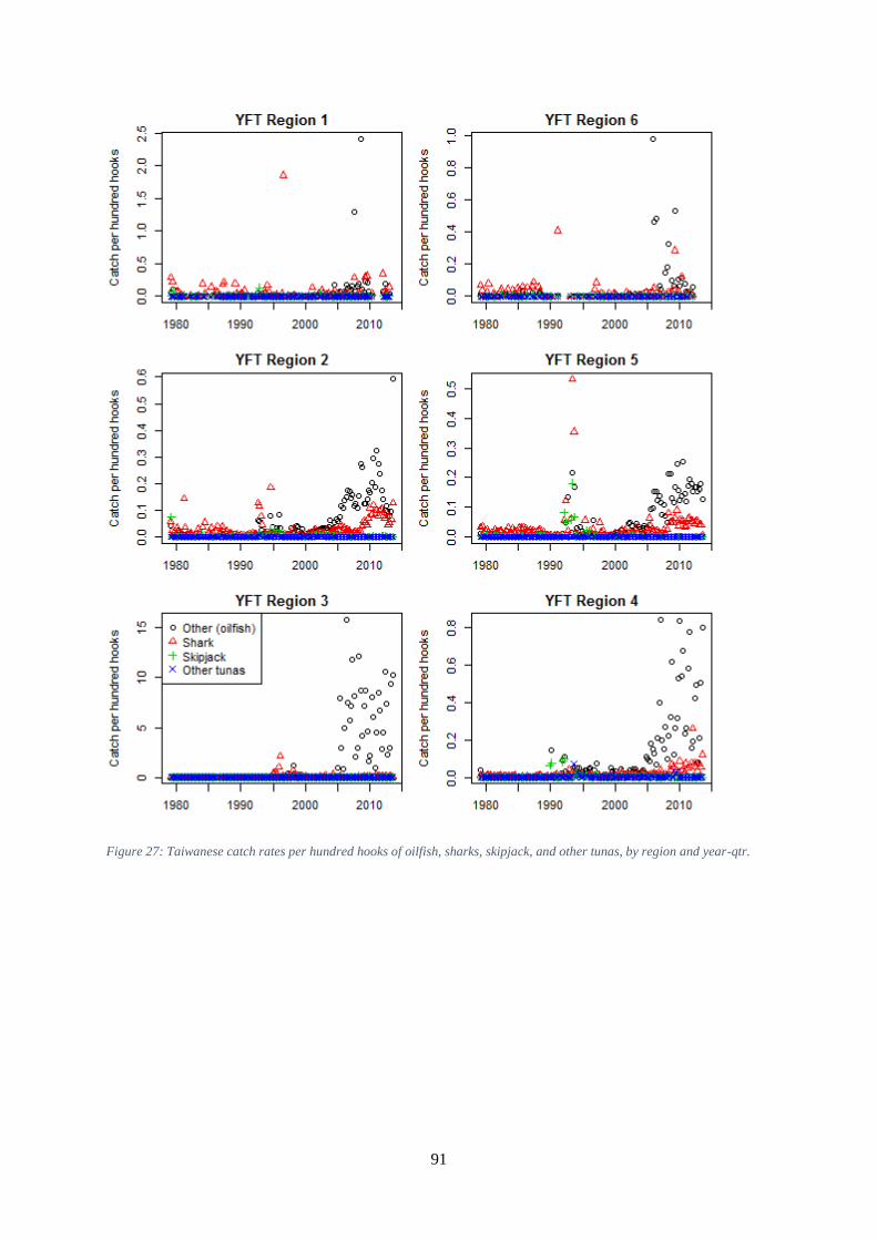
91

Figure 27: Taiwanese catch rates per hundred hooks of oilfish, sharks, skipjack, and other tunas, by region and year-qtr.

92

Figure 28: Frequency distribution of bigeye catch in number per set by year from 1977 to 2000 in the tropical Indian Ocean from 10N to 15S.

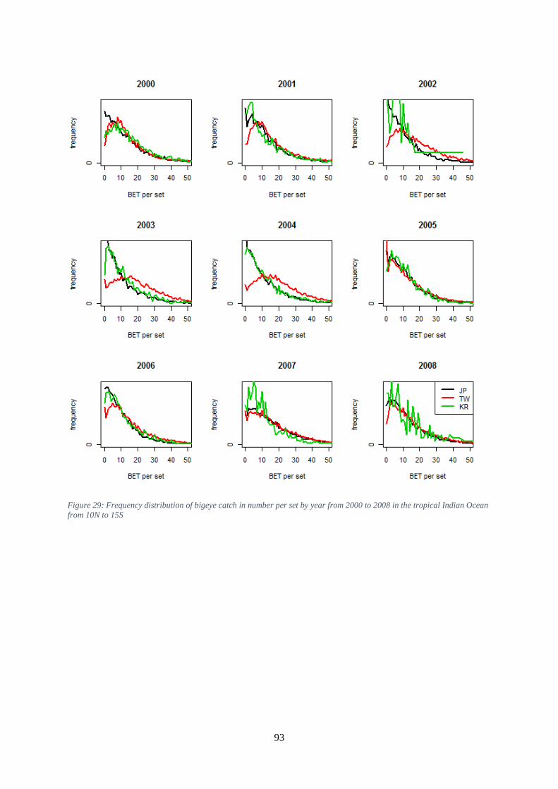
93

Figure 29: Frequency distribution of bigeye catch in number per set by year from 2000 to 2008 in the tropical Indian Ocean

from 10N to 15S

94

Figure 30: Taiwanese effort distribution by latitude and longitude (x axis) and year (y axis).

1975

1980

1985

1990

1995

2000

2005

2010

2015

-3610 -3110 -2610 -2110 -1610 -1110 -610 -110 390 890 1390 1890 2390

-15S 10N 0

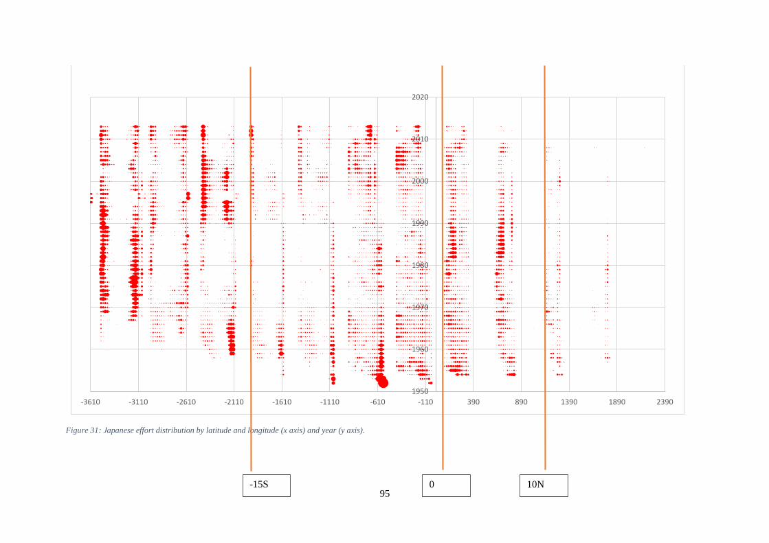
95

Figure 31: Japanese effort distribution by latitude and longitude (x axis) and year (y axis).

1950

1960

1970

1980

1990

2000

2010

2020

-3610 -3110 -2610 -2110 -1610 -1110 -610 -110 390 890 1390 1890 2390

-15S 10N 0

96

Figure 32: Korean effort distribution by latitude and longitude (x axis) and year (y axis).

1970

1975

1980

1985

1990

1995

2000

2005

2010

2015

-3610 -3110 -2610 -2110 -1610 -1110 -610 -110 390 890 1390 1890 2390

year

-15S 0 10N

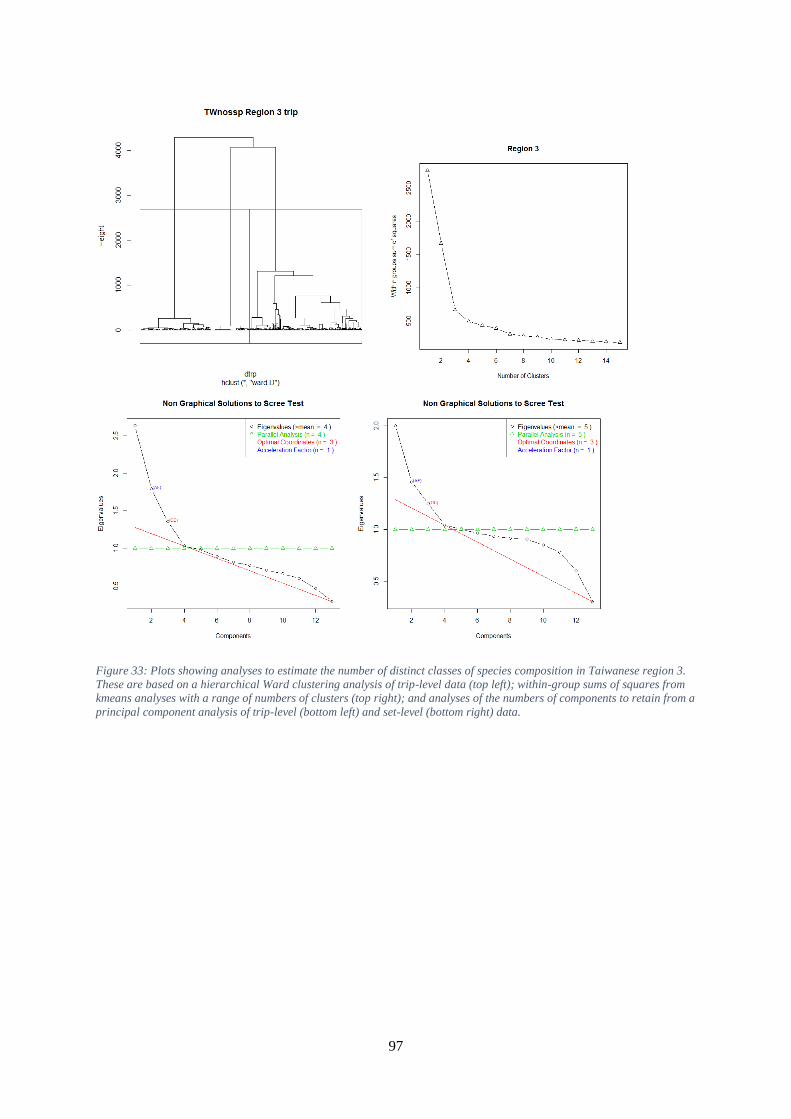
97

Figure 33: Plots showing analyses to estimate the number of distinct classes of species composition in Taiwanese region 3.

These are based on a hierarchical Ward clustering analysis of trip-level data (top left); within-group sums of squares from

kmeans analyses with a range of numbers of clusters (top right); and analyses of the numbers of components to retain from a

principal component analysis of trip-level (bottom left) and set-level (bottom right) data.

98

Figure 34: Boxplot showing the distributions of variables associated with sets in each hcltrp cluster for the Taiwanese

dataset in region 3. Box widths indicates the proportional numbers of sets in each cluster.

99

Figure 35: Hierarchical clustering trees produced by the hclust function in R, for Japanese trip-level data by region.

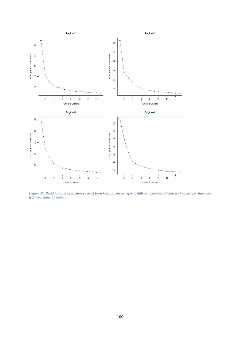
100

Figure 36: Residual sums of squares (y axis) from kmeans clustering with different numbers of clusters (x axis), for Japanese

trip-level data, by region.

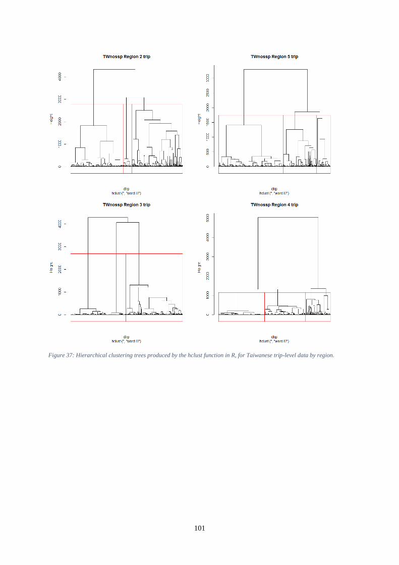
101

Figure 37: Hierarchical clustering trees produced by the hclust function in R, for Taiwanese trip-level data by region.

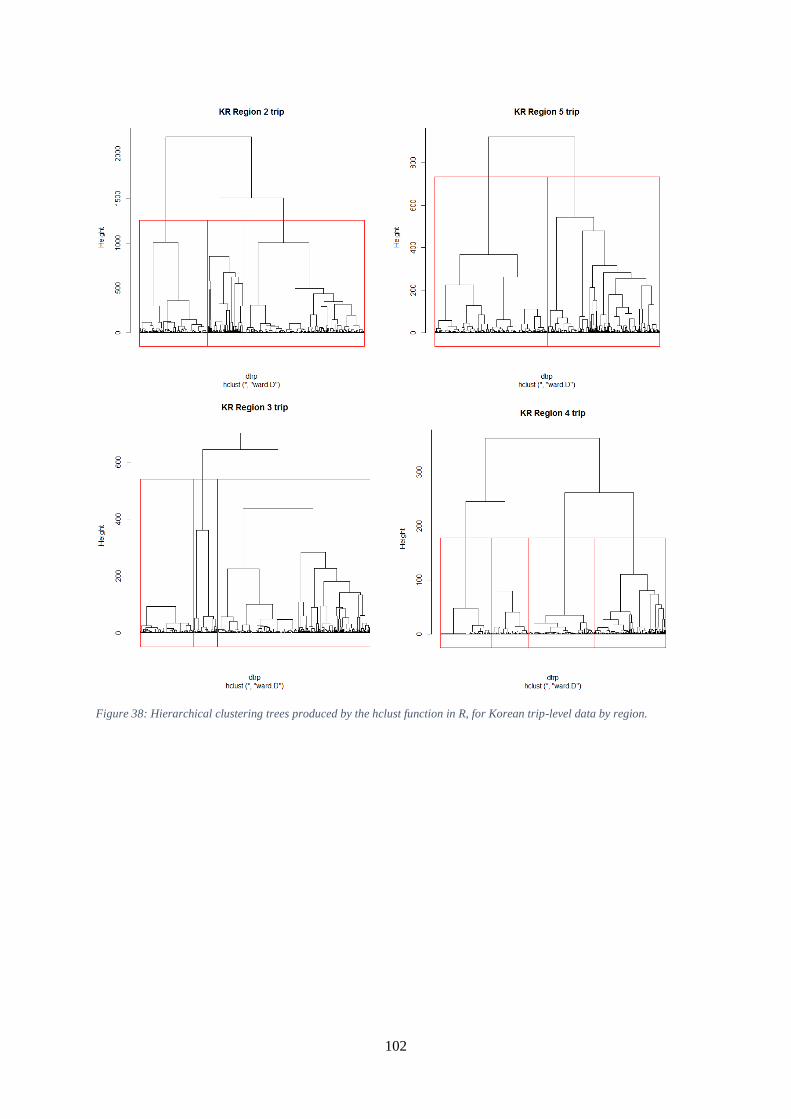
102

Figure 38: Hierarchical clustering trees produced by the hclust function in R, for Korean trip-level data by region.

103

Figure 39: For Japanese effort in region 2 for the period 1985-1994, for each species, boxplot of the proportion of the

species in the set versus decile of the first principal component.

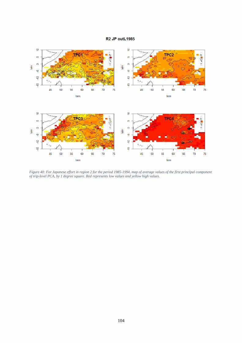
104

Figure 40: For Japanese effort in region 2 for the period 1985-1994, map of average values of the first principal component

of trip-level PCA, by 1 degree square. Red represents low values and yellow high values.

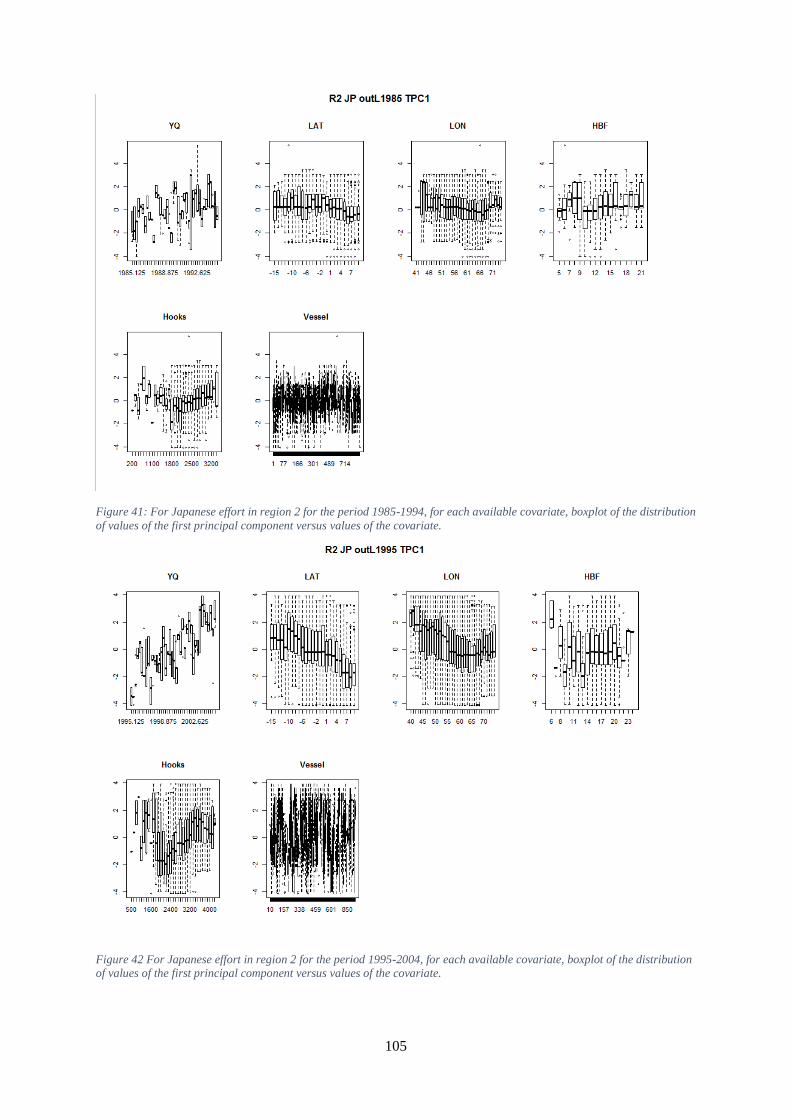
105

Figure 41: For Japanese effort in region 2 for the period 1985-1994, for each available covariate, boxplot of the distribution

of values of the first principal component versus values of the covariate.

Figure 42 For Japanese effort in region 2 for the period 1995-2004, for each available covariate, boxplot of the distribution

of values of the first principal component versus values of the covariate.

106

Figure 43: For Japanese effort in region 5 for the period 1955-1964, for each species, boxplot of the proportion of the

species in the set versus the cluster. The widths of the boxes are proportional to the number of sets in the cluster. Clustering

was performed using the kmeans method on untransformed set-level data.

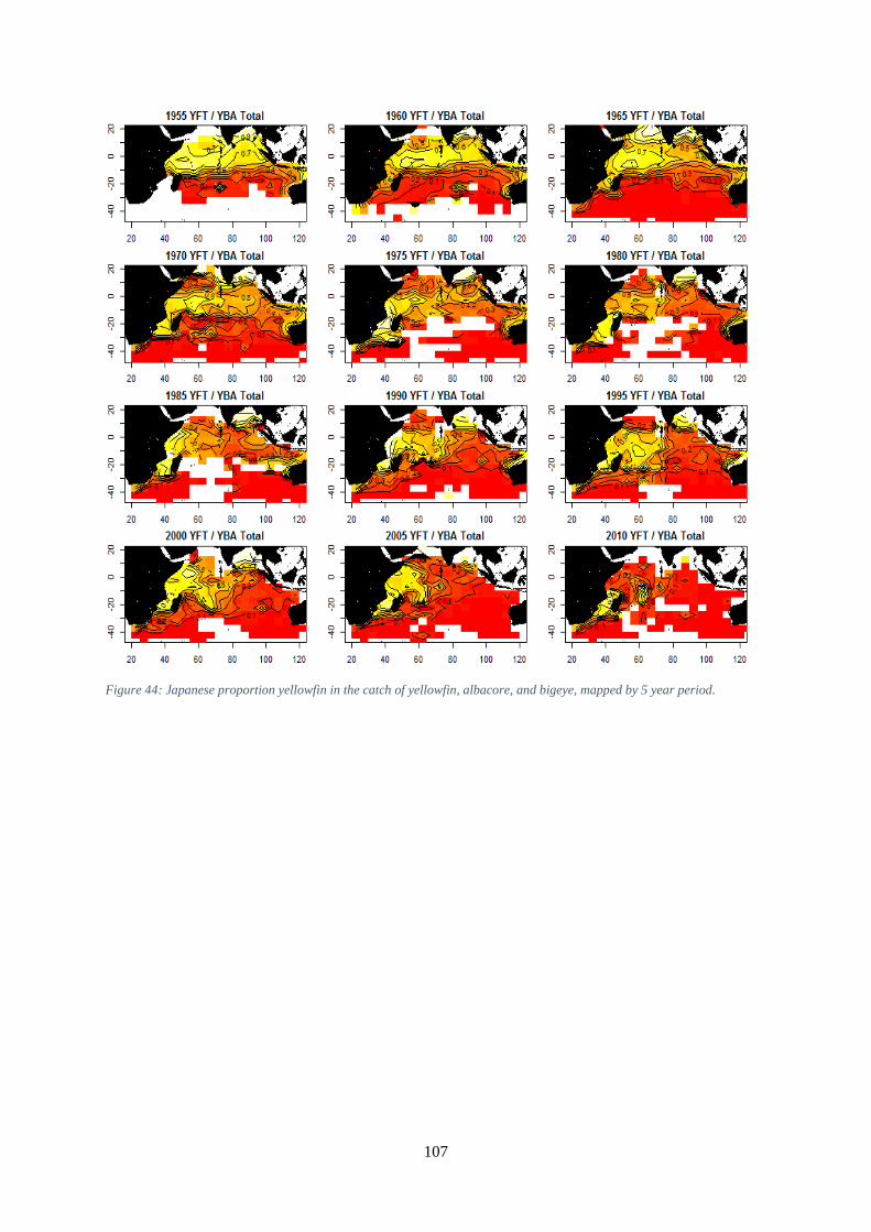
107

Figure 44: Japanese proportion yellowfin in the catch of yellowfin, albacore, and bigeye, mapped by 5 year period.

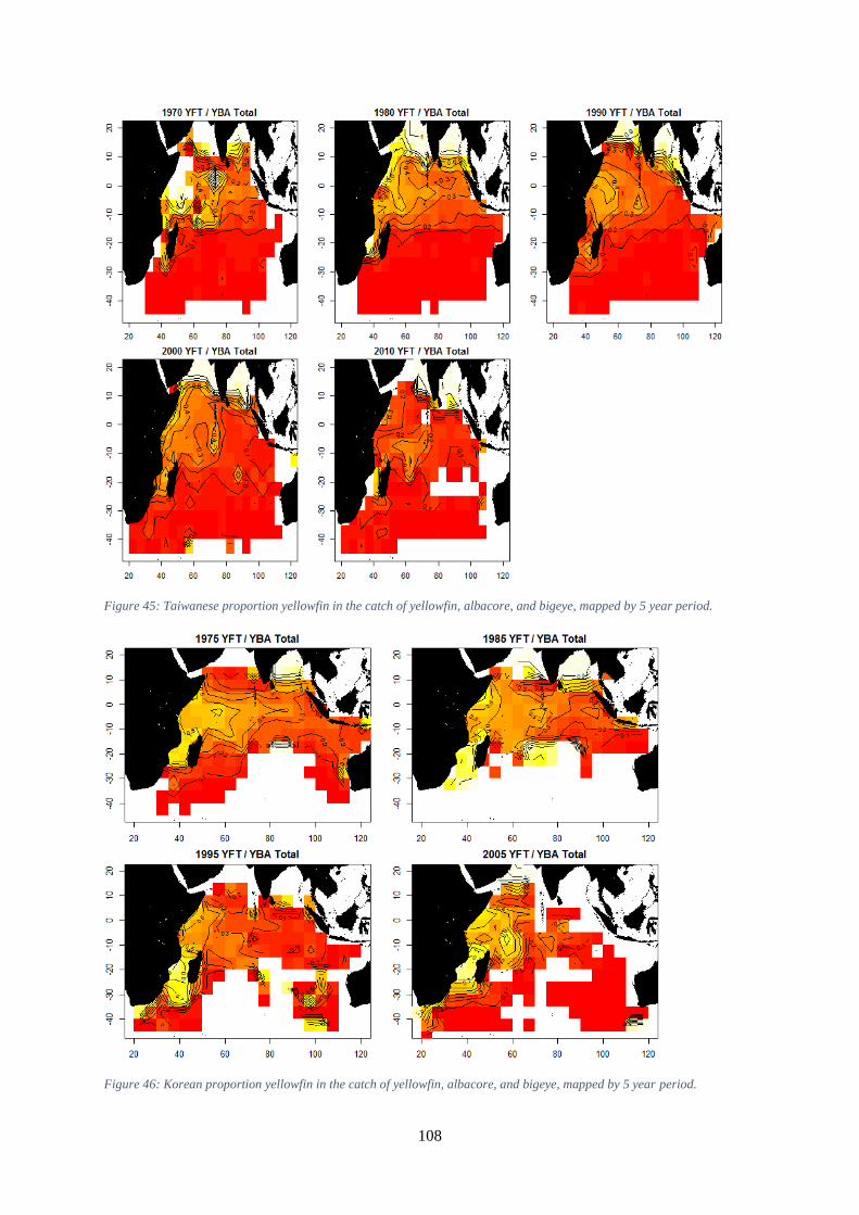
108

Figure 45: Taiwanese proportion yellowfin in the catch of yellowfin, albacore, and bigeye, mapped by 5 year period.

Figure 46: Korean proportion yellowfin in the catch of yellowfin, albacore, and bigeye, mapped by 5 year period.

109

Figure 47: Influence plots for bigeye tuna CPUE in region 2 by the Japanese fleet. The top left plots shows the change in the

CPUE time series caused by each covariate. The top right plot shows the influence of vessel effects. The bottom left plot

shows the influence of the number of hooks, and the bottom right plot shows the influence of lunar illumination.

110

Figure 48: Influence plots for bigeye tuna CPUE in region 2 by the Taiwanese fleet. The top left plots shows the change in

the CPUE time series caused by each covariate. The top right plot shows the influence of vessel effects. The bottom left plot

shows the influence of the number of hooks, and the bottom right plot shows the influence of lunar illumination.

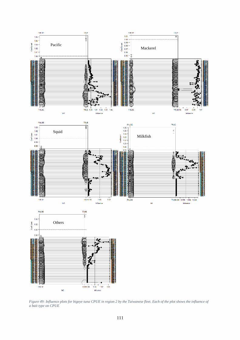
111

Figure 49: Influence plots for bigeye tuna CPUE in region 2 by the Taiwanese fleet. Each of the plot shows the influence of

a bait type on CPUE

Others

Milkfish

Pacific

saury Mackerel

Squid

112

Figure 50: Influence plots for bigeye tuna CPUE in region 2 by the Korean fleet. The top left plots shows the change in the

CPUE time series caused by each covariate. The top right plot shows the influence of vessel effects, the mid- left plot the

number of hooks, the mid-right plot HBF, and the bottom left the lunar illumination.

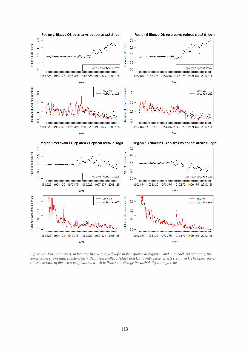
113

Figure 51: Japanese CPUE indices for bigeye and yellowfin in the equatorial regions 2 and 5. In each set of figures, the

lower panel shows indices estimated without vessel effects (black dots), and with vessel effects (red lines). The upper panel

shows the ratio of the two sets of indices, which indicates the change in catchability through time.

114

Figure 52: Taiwanese CPUE indices for bigeye and yellowfin in the equatorial regions 2 and 5. In each set of figures, the

lower panel shows indices estimated without vessel effects (black dots), and with vessel effects (red lines). The upper panel

shows the ratio of the two sets of indices, which indicates the change in catchability through time.

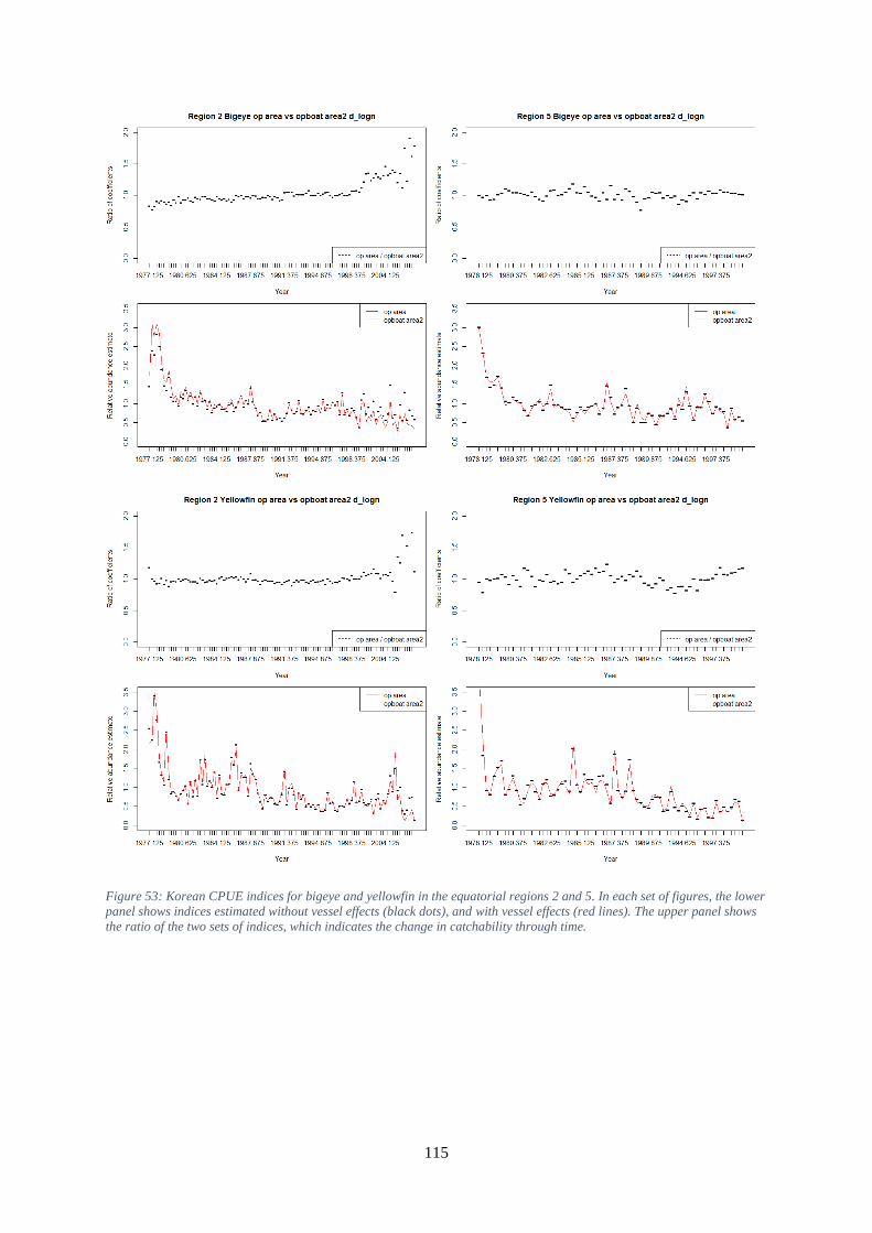
115

Figure 53: Korean CPUE indices for bigeye and yellowfin in the equatorial regions 2 and 5. In each set of figures, the lower

panel shows indices estimated without vessel effects (black dots), and with vessel effects (red lines). The upper panel shows

the ratio of the two sets of indices, which indicates the change in catchability through time.

116

Figure 54: Comparison of bigeye indices among fleets. Indices have been adjusted so that they have the same average value

across those periods in which all fleets have a parameter estimate.

117

Figure 55: Comparison of yellowfin indices among fleets. Indices have been adjusted so that they have the same average

value across those periods in which all fleets have a parameter estimate.

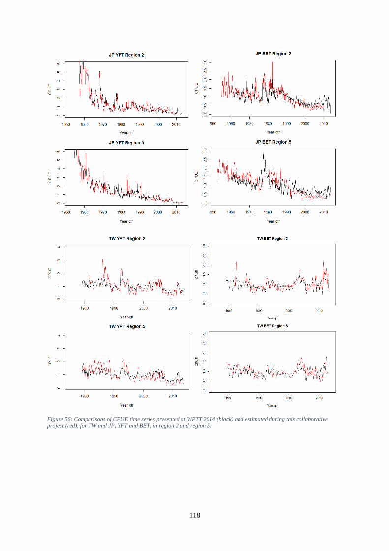
118

Figure 56: Comparisons of CPUE time series presented at WPTT 2014 (black) and estimated during this collaborative

project (red), for TW and JP, YFT and BET, in region 2 and region 5.

119

Figure 57: Ratios of CPUE estimated in 2014 divided by CPUE estimated in this project.

120

Figure 58: Ratios of Taiwanese and Japanese CPUE estimates based on WPTT 2014 results (black circles) and results from

this study (red triangles).

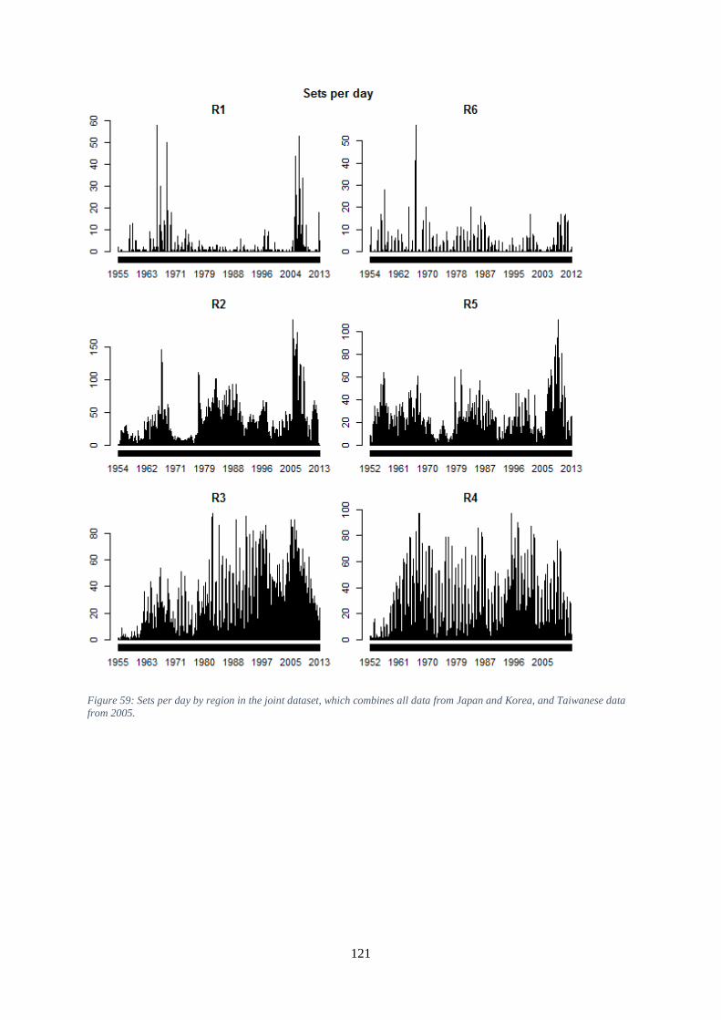
121

Figure 59: Sets per day by region in the joint dataset, which combines all data from Japan and Korea, and Taiwanese data

from 2005.

122

Figure 60: Number of 5 degree squares with data in the joint dataset by year-qtr and region.

123

Figure 61: Joint CPUE indices for bigeye and yellowfin in the equatorial regions 2 and 5. In each set of figures, the lower

panel shows indices estimated without vessel effects (black dots), and with vessel effects (red lines). The upper panel shows

the ratio of the two sets of indices, which indicates the change in catchability through time.

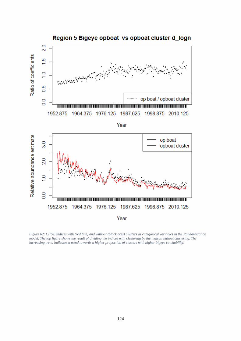
124

Figure 62: CPUE indices with (red line) and without (black dots) clusters as categorical variables in the standardization

model. The top figure shows the result of dividing the indices with clustering by the indices without clustering. The

increasing trend indicates a trend towards a higher proportion of clusters with higher bigeye catchability.

Report of the Second IOTC CPUE Workshop on Longline ...

Documents