Report: North American Midstream Infrastructure Through 2035: Leaning into the Headwinds

North American Midstream

Infrastructure Through 2035:

Leaning into the Headwinds

Prepared by

ICF International

9300 Lee Highway

Fairfax, VA 22031

April 12, 2016

Prepared for

The INGAA Foundation, Inc.

Report No. 2016.02

Copyright ® 2016 by the INGAA Foundation, Inc.

The INGAA Foundation, Inc.

20 F Street, NW, Suite 450

Washington, DC 20001

2

ICF Authors: Kevin Petak, Ananth Chikkatur, Julio Manik, Srirama Palagummi, and Kevin Greene

Acknowledgments: The INGAA Foundation wishes to thank members of this study’s

Steering Committee for their oversight and guidance.

About the INGAA Foundation: The Interstate Natural Gas Association of America (INGAA) is a trade organization that advocates regulatory and legislative positions of

importance to the natural gas pipeline industry in North America. The INGAA Foundation was formed in 1990 by INGAA to advance the use of natural gas for the

benefit of the environment and the consuming public. The Foundation, which is composed of over 150 members, works to facilitate the efficient construction and safe,

reliable operation of the North American natural gas pipeline system, and promotes natural gas infrastructure development worldwide.

About ICF International: ICF International (NASDAQ:ICFI) provides professional

services and technology solutions that deliver beneficial impact in areas critical to the world's future. The firm combines passion for its work with industry expertise and

innovative analytics to produce compelling results throughout the entire program lifecycle, from research and analysis through implementation and improvement. Since

1969, ICF has been serving government at all levels, major corporations, and multilateral institutions. More than 5,000 employees serve these clients from more than

65 offices worldwide

Waivers. Those viewing this Material hereby waive any claim at any time, whether now or in the future, against ICF, its officers, directors, employees, or agents arising out of or in connection with this Material. In no event whatsoever shall ICF, its officers, directors,

employees, or agents be liable to those viewing this Material.

Warranties and Representations. ICF endeavors to provide information and projections consistent with standard practices in a professional manner. ICF MAKES NO WARRANTIES, HOWEVER, EXPRESS OR IMPLIED (INCLUDING WITHOUT LIMITATION ANY WARRANTIES OR MERCHANTABILITY OR FITNESS FOR A

PARTICULAR PURPOSE), AS TO THIS MATERIAL. Specifically but without limitation, ICF makes no warranty or guarantee regarding the accuracy of any forecasts,

estimates, analyses, or that such work products will be accepted by any legal or regulatory body.

Contacts:

The INGAA Foundation, Inc. ICF International

Richard Hoffmann, Executive Director Kevin Petak, Vice President 20 F Street, NW, Suite 450 9300 Lee Highway

Washington, DC 20001 Fairfax, VA 22031 [email protected] [email protected]

3

Table of Contents

Executive Summary .................................................................................................................. 5

1 Introduction ...................................................................................................................... 13

1.1 Study Objectives ................................................................................................................... 13

1.2 Scope of Work ...................................................................................................................... 14

1.3 Study Regions....................................................................................................................... 14

1.4 Infrastructure Coverage ........................................................................................................ 15

1.5 Report Structure ................................................................................................................... 17

2 Methodology .................................................................................................................... 18

2.1 Modeling Framework ............................................................................................................ 18

2.2 Midstream Infrastructure Methodology and Assumptions .................................................... 19

3 Summary of Scenario Results ........................................................................................ 24

3.1 Defining This Study’s Scenarios ........................................................................................... 24

3.2 This Study’s Projected Trends for Oil and Gas Prices ......................................................... 26

3.3 Natural Gas Demand ............................................................................................................ 29

3.4 Production Trends ................................................................................................................ 33

4 Midstream Infrastructure Requirements ........................................................................ 43

4.1 Natural Gas ........................................................................................................................... 43

4.2 Natural Gas Liquids (NGLs) ................................................................................................. 63

4.3 Crude Oil and Lease Condensate ........................................................................................ 71

4.4 Summary of Midstream Infrastructure Metrics and Expenditures ........................................ 80

5 Incremental Expenditures for Integrity Management and NOx Control ....................... 85

5.1 Methodology and Assumptions ............................................................................................ 85

5.2 Total Capital Expenditure for Midstream Infrastructure ....................................................... 86

6 Economic Impact Methodology Assumptions ............................................................... 88

6.1 IMPLAN Modeling ................................................................................................................. 88

6.2 National-Level Economic Impacts ........................................................................................ 88

6.3 Regional-level Economic Impacts ........................................................................................ 90

4

7 Results of Economic Impact Analysis ............................................................................ 93

7.1 U.S. and Canada: Economic Impacts, 2015-2035 ............................................................... 93

7.2 U.S. and Canada Total Employment by Asset Category ..................................................... 94

7.3 U.S. and Canada Total Employment by Industry Sector ..................................................... 95

7.4 Total Employment by Region ............................................................................................... 96

7.5 Total Employment by State .................................................................................................. 96

8 Conclusions ..................................................................................................................... 99

Appendix A: ICF Modeling Tools ......................................................................................... 106

GMM Description .......................................................................................................................... 106

Detailed Production Report (DPR) ................................................................................................. 108

NGLs Transport Model (NGLTM) description ................................................................................ 110

Crude Oil Transport Model (COTM) description ............................................................................ 112

Appendix B: Infrastructure Metrics Assumptions .............................................................. 114

Appendix C: IMPLAN Industries in Each Industrial Sector ................................................ 116

5

Executive Summary

Background

The widely recognized 2014 INGAA Foundation infrastructure study projected significant infrastructure

development, driven by robust market growth and continued development of North American

unconventional natural gas and crude oil supplies. Market conditions have changed dramatically since

completion of that study, warranting an updated analysis of infrastructure development. This new

INGAA Foundation study has been undertaken with recent market changes in mind, and like past

studies, is focused on estimating future natural gas, natural gas liquids (NGL), and oil midstream

requirements and the potential capital expenditures associated with that development. This study

specifically analyzes the potential impacts of reduced commodity (i.e., oil and gas) prices and factors in

uncertainty about the economic outlook.

Like past studies, this study informs industry, policymakers and stakeholders about the ongoing

dynamics of North America’s energy markets and the infrastructure needed to ensure that consumers

benefit from the abundance of natural gas, crude oil and NGLs spread across the United States and

Canada. As with previous studies, impacts of midstream infrastructure investments on jobs and the

economy are evaluated, providing guidance to policymakers as they seek to promote job growth and

economic development, protect the environment, increase energy security and reduce the trade deficit.

In the context of this analysis, midstream infrastructure includes:

Natural gas gathering and lease equipment, processing, pipeline transportation and storage, and

LNG export facilities.

NGL pipeline transportation, fractionation and export facilities.

Crude oil gathering and lease equipment, pipeline transportation and storage facilities.

Scenario Trends

Significant questions affecting midstream infrastructure development have been created by sustained

low oil and natural gas prices, an uncertain global and domestic economic outlook, and the pace at

which public policy will affect energy markets. Hence, this study considers two distinct scenarios – a

High Case and a Low Case – each reflecting very different pathways for supply growth and market

development:

The High Case is best characterized as a plausibly optimistic case for midstream infrastructure

development. The case assumes a rebound in global economic activity that spurs increased use

of natural gas and oil over time and fosters a more robust pricing environment for oil and gas

supply development.

The Low Case is best characterized as a less-optimistic case, in which a slower economic

recovery reduces the need for oil and gas development. The case assumes more robust

penetration of energy efficiency and non-gas resources to support future power generation.

6

Figure ES - 1: Consumption (top) and Production (middle and bottom) trends in the Low and High Cases

The key demand and production trends in the two scenarios are shown in Figure ES-1. As noted above,

the market growth projected for each case is very different. The Low Case projects that natural gas use

rises to merely 110 Bcfd by 2035, while the High Case projects growth to over 130 Bcfd. The most

noticeable difference in the trends occurs in the power sector, where the Low Case assumes lower

7

electricity demand growth, greater energy efficiency and more significant penetration of non-gas

generating resources. In the Low Case, crude oil and condensate production is projected to decline from

13.4 million barrels per day in 2015 to 10.7 million barrels per day in 2035 due to lower oil prices. In the

High Case, oil and condensate production is expected to be relatively flat over the forecast period. NGLs

production is expected to rise from 4.2 million barrels per day in 2015 to about 5.7 million barrels per

day by 2035 in the Low Case and 6.5 million barrels per day in the High Case.

On the supply side, shale gas production growth remains robust, motivating development of natural gas

infrastructure. This is the case even though, compared with the 2014 study, both of this study’s

scenarios project lower well completions. While new midstream infrastructure is needed, it is less than

was anticipated by the 2014 study, as both the number and scale of projects declines from the level of

activity that has occurred during the past five years. At the same time, even though fewer miles of pipe

are required in the future, investment in new gas pipelines remains significant because of continued

production growth from low-cost production areas like the Marcellus and Utica. Put another way,

incremental production from low-cost areas tends to offset declines in activity elsewhere.

Rounding out this supply-demand picture, NGL production will generally track natural gas production, as

a substantial portion of new natural gas production has a relatively high liquids content. A key difference

with the 2014 study, however, is that the growth of oil production is much less pronounced due to the

reduced oil prices assumed in this study.

Pipeline Capacity Additions

The key trends from 2015 through 2035 for this work are summarized as follows:

U.S. and Canadian natural gas transportation capacity addition1 is projected at 44 to 58 Bcfd for

the two scenarios, with a midpoint value of 51 Bcfd.

U.S. and Canadian NGL capacity addition is projected to be 1.1 to 2.3 million BPD for the two

scenarios, with a midpoint of 1.7 million BPD.

U.S. and Canadian oil pipeline capacity addition is projected at 4.5 to 6.9 million BPD, with a

midpoint value of 5.7 million BPD.

As noted above, even though continued infrastructure development is significant, future midstream

development will be less than it has been recently as the market has undergone a very robust period of

development (i.e., $40 to $50 billion of annual investment) between 2010 and 2015, with aggressive

development of unconventional resources. In 2016, we expect continued buildout of gas, oil, and NGL

infrastructure with many pipelines already under construction. About 40 to 50 percent of the natural gas

capacity originates in the U.S. Northeast, home to Marcellus and Utica development. Significant capacity

is also built in the U.S. Southwest, mostly associated with LNG and Mexican export activity.

A significant amount of natural gas pipeline development is projected to occur during the next five

years, with a noticeable drop after 2020, especially in the Low Case where continued market growth is

1 Unlike the 2014 study, takeaway capacity includes both inter-regional pipelines and intra-regional pipelines, as many such pipes are being built, particularly in the Marcellus and Utica regions.

8

much more modest. Over the next four years (2017 through 2020), Marcellus and Utica transport

capacity increases by roughly 12 Bcfd in the High Case, with substantial increases in capacity to support

natural gas exports. Further out (2020 through 2035), roughly 15 Bcfd of incremental capacity is built

across North America (i.e., 1 Bcfd per year) in the High Case, mostly to satisfy growth in gas-fired power

generation. With gas-fired generation growth being much more modest in the Low Case, only about half

of the natural gas capacity added after 2020 in the High Case is also included in the Low Case.

A large portion of oil-related pipeline capacity (3.3 million BPD) has already been built and was placed

into service by late 2015. Most, if not all of the oil projects to be commissioned in 2016 are likely to be

completed, as they are already under construction. However, due to delays, some projects may not

come on line until 2017. In each case, only very modest (or no) oil pipeline development occurs after

2017.

Midstream Infrastructure Expenditure

This study’s cases show:

Capital expenditure (CAPEX) for new midstream infrastructure will range from $471 billion to

$621 billion over the next 20 years (see Figure ES-2), with a midpoint expenditure of $546

billion. On an annual average basis, the expenditure is $22.5 to $30.0 billion per year.

Investment in pipelines (including both transmission and gathering lines and compression and

pumping) will range from $183 billion to $282 billion, with a midpoint CAPEX of $232 billion.

As shown in Figure ES-2, most of this activity is associated with natural gas development, with much

lesser investment for oil and NGL-related assets. The figure also shows that development in the Low

Case averages about $5 to $10 billion per year below development in the High Case.

Figure ES - 2: Capital Expenditure for New Infrastructure from 2015 through 2035 (Billions of 2015$)

9

A breakdown of total capital expenditures across different infrastructure categories, including the

midpoint values, is summarized in Table ES-1. The table generally shows that about 30 percent of the

future investment occurs in transmission pipeline development, with the majority being spent for gas

pipelines. Nearly 90 percent of transmission pipeline expenditure is for the pipeline itself, with the

remainder being spent on compression and pumping. Investment for gathering systems is also very

significant, with about 20 percent of total investment.

Table ES - 1: Midstream Infrastructure Capital Expenditure by Infrastructure Categories

Item Low Case High Case Midpoint

Total Investment in All Infrastructure 471 621 546

Natural Gas Infrastructure 267 352 310

Oil and NGL Infrastructure 180 245 212

Incremental Integrity Management & Emissions Control

24 24 24

Gas and Oil Transport 123 208 166

Gas Pipelines 90 145 118

Pipe 77 127 102

Compressors 13 18 16

Oil and NGL Pipelines 33 63 48

Pipe 29 54 41

Pumping 4 9 7

Gathering Systems 104 128 116

Pipe 36 43 39

Compressors and Pumps 23 30 27

Processing and Fractionation 45 55 50

Gas Storage and LNG & NGL Export Facilities 80 90 85

All Other Infrastructure (Lease Facilities) 140 171 155

It is also worth noting that the INGAA Foundation has included an estimated incremental expenditure of

$24 billion for integrity management and NOx control as part of the total expenditure on pipelines. This

incremental amount represents additional CAPEX for integrity management activities that were

anticipated at the time the study was prepared and emissions control requirements to satisfy new

ambient air (NAAQS) standards for nitrogen oxides (NOx). This incremental expenditure should be

interpreted as a ballpark estimate at this point in time because estimated integrity management costs

have not been adjusted to reflect the particulars of recently proposed pipeline safety rules.

10

Infrastructure Metrics

Key metrics from 2015 through 2035 are summarized as follows:

Between 264,000 and 329,000 miles of pipeline (including both gathering and transport lines)

are added (with a midpoint value of 296,000 miles).

Between 18,000 and 29,000 miles (midpoint of 23,000 miles) of new natural gas transmission

lines will be built.

In total, 30,000 to 48,000 miles (midpoint of 39,000 miles) of new pipeline will be needed for

gas, oil, and NGL transport.

Between 234,000 and 281,000 miles (midpoint of 257,000 miles) of new gas and oil gathering

line will be needed to collect incremental production between 682,000 and 823,000 new oil and

gas wells (midpoint of 752,000 new oil and gas wells).

Compression for the new gas transmission lines ranges from 4.3 to 6.2 million horsepower

(midpoint 5.2 million horsepower).

Compression needed for new gas gathering ranges from 7.6 to 9.7 million horsepower (midpoint

8.7 million horsepower).

Total compression and pumping needed for all gathering and transmission lines range from 13.0

to 18.5 million horsepower (midpoint 15.8 million horsepower).

The total CAPEX for pipelines (i.e., for both miles of line and the total pumping and compression

needs) is between $183 and $282 billion (with a midpoint value of $232 billion).

About 120 to 290 Bcf of new working gas capacity, with a CAPEX of $2.3 to $4.8 billion added

(midpoint 3.6 billion).

Table ES - 2: Pipeline Miles, Compression, and Associated Capital Expenditures from 2015-2035

11

Table ES-3 compares natural gas metrics for each of this study’s scenarios, and also compares annual

average values against relevant values from 2014 Study. The metrics clearly demonstrate that much new

infrastructure is needed despite the market changes that have occurred during the past few years. Even

the Low Case, which is generally showing statistics that are between 20 percent and 30 percent lower

than those in the High Case, requires significant infrastructure development, particularly to

accommodate continued production growth and facilitate the development of LNG and Mexican

exports. Nevertheless, each of this study’s cases generally shows less natural gas infrastructure

development when compared with the 2014 study.

Table ES - 3: Natural Gas Metrics

Economic Impact from the Midstream Infrastructure Expenditure

This study shows that:

Development of new infrastructure will add $655 billion to $861 billion of value to the U.S. and

Canadian economies and result in employment of 323,000 and 425,000 people per year.

While many of the jobs associated with midstream development are concentrated in the

Southwestern and Northeastern U.S. and in Canada, the positive economic impacts of

infrastructure development are geographically widespread.

This study, like the 2014 study, projects significant employment impacts from new infrastructure

development. Every $100 million of investment in new infrastructure creates an average of about 70

jobs over the projection period and adds roughly $139 million in value to the U.S. and Canadian

12

economies. This result is consistent across each of the study’s cases. The midpoint estimate is that

about 375,000 jobs per year will be created with a value added of $760 billion to the economy and $260

billion in taxes. By infrastructure category, investment and employment levels will be most significant

for the development of transmission pipelines and lease equipment in both scenarios. More than half of

the jobs associated with midstream infrastructure development will occur in the services sector and

other category.

While many of the economic benefits accrue directly to companies active in midstream development,

there are many indirect and induced benefits that occur in many other industries, and a substantial

number of service sector jobs are created as a result of the midstream development. All sectors and

regions of North America benefit from infrastructure development.

The top ten states in the U.S. with total employment resulting from midstream investment are Texas,

Pennsylvania, Louisiana, Ohio, California,2 New York, Oklahoma, Illinois, Kansas and West Virginia. Texas

will have the most significant job creation as a result of LNG export activity and shale gas and tight oil

development. Pennsylvania and Louisiana will have similar levels of employment. Pennsylvania’s job

creation is driven by Marcellus/Utica development, while Louisiana’s job creation is related to LNG

export facility development.

2 California ranks fourth in terms of employment mostly due to indirect and induced jobs (over 90 percent of total jobs in California) from industry inter-linkages within California and from other states. The modest direct expenditures are related to enhanced oil recovery (EOR) activities and Monterey shale development.

13

1 Introduction

1.1 Study Objectives The energy landscape has changed significantly in the two years since completion of the last INGAA

Foundation midstream infrastructure study.3 Most notably, there has been a significant decline in

energy prices, with oil prices dropping from over $100 per barrel to under $30 per barrel at the

beginning of 2016, and North American natural gas prices recently falling below $2 per million British

thermal units (MMBtu). Despite these declines, robust growth in natural gas production from shale

formations, such as the Marcellus and Utica, has continued at a rapid pace. In addition, declining

economic activity in Asia, among other factors, has created an uncertain environment for future energy

investments, including midstream development.

While robust growth in U.S. and Canadian natural gas production has continued to support the

development of liquefied natural gas (LNG) export terminals and associated midstream infrastructure

development, lower oil and LNG prices, combined with lower expectations of future global economic

growth, have reduced the momentum of LNG export activity. At the same time, there is growing

uncertainty about the extent of domestic growth of natural gas use in the power sector. This 2016

INGAA Foundation study is designed to shed light on how these uncertainties might affect midstream

infrastructure investments over the next 20 years.

The objective of this new study is to inform the industry, policymakers, and stakeholders about the new

dynamics of North America’s energy markets based on a detailed supply-demand outlook. This study

assesses the infrastructure needed in light of these uncertainties. The study estimates midstream

infrastructure requirements for natural gas, natural gas liquids (NGLs), and crude oil; provides estimates

for capital expenditures needed in response to new integrity management rules and requirements for

greater reduction of nitrogen oxides (NOx); and assesses the associated economic benefits, most

notably Gross Domestic Product (GDP) and jobs impacts, of expected infrastructure investments.

The study considers recent trends and uncertainties in future commodity prices and investigates the

impacts of those trends on future infrastructure requirements in two distinct scenarios: a “High Case”

and a “Low Case”:

The study’s High Case is best characterized as a plausibly optimistic case for midstream

infrastructure development. This case assumes a rebound in global economic activity that spurs

increased use of natural gas and oil over time.

The study’s Low Case is best characterized as a plausibly less-optimistic case for midstream

infrastructure development. In this case, there is a slower recovery in global economies,

reducing the need for oil and gas development. In addition, the case assumes more robust

penetration of energy efficiencies and non-gas resources to satisfy future power generation

needs.

3 http://www.ingaa.org/File.aspx?id=21498

14

1.2 Scope of Work This 2016 study assesses midstream infrastructure needs through 2035 and includes an extensive

update of trends in the production of natural gas, NGLs, and oil. The study considers the following:

Regional natural gas supply-demand projections that rely on the most current market trends.

North American exploration and production activity that is supported by a robust, cost-effective,

and growing resource base for oil and natural gas.

An assessment of natural gas use in power plants, considering load requirements and an ever-

changing mix of generation assets.

An assessment of lease equipment, gathering, processing, and fractionation needs to permit the

delivery of hydrocarbons to an already extensive pipeline grid that supports delivery to markets

and end-users.

Review of underground natural gas storage requirements by region.

Analysis of NGLs and oil infrastructure requirements.

It is also worth noting that the INGAA Foundation has included an estimated incremental expenditure of

$24 billion for integrity management and NOx control as part of the total expenditure on pipelines. This

incremental amount represents incremental capital expenditures for integrity management activities

that were anticipated at the time this study was prepared and emissions control requirements to satisfy

new ambient air (NAAQS) standards for nitrogen oxides (NOx). This incremental expenditure should be

interpreted as a ballpark estimate at this point in time because estimated integrity management costs

have not been adjusted to reflect the particulars of the recently proposed pipeline safety rules by the

Pipeline and Hazardous Materials Safety Administration (PHMSA).

In addition to assessing expenditures for oil, NGLs, and natural gas pipeline system development, this

study shows the levels of investment required for oil and gas gathering system expansion, gas

processing plant development, gas storage field buildout, power generation, crude oil storage terminal

development, NGLs fractionation capacity development, NGLs export facilities buildout, oil and gas lease

equipment development, and LNG export facility construction. Midstream development covers all

facilities from the wellhead to the city-gate (or directly to the end-user in the case of power plants and

industrial facilities). The study, however, does not include refurbishment and replacement expenditures

for non-pipeline assets.

The economic impact analysis is based on IMPLAN modeling, which provides direct, indirect, and

induced impacts of the midstream development on the economy. The study expands on the scope of

the 2014 study by assessing state-level impacts.

1.3 Study Regions The study reports results based on the Energy Information Administration pipeline regions for the U.S.

Lower 48. Results are also reported for offshore Gulf of Mexico, Canada, and Alaska (see Figure 1 for a

15

map showing all of the regions applied herein). This is the same regional format applied in the 2014

study.

The Marcellus and Utica shale plays are split between the Northeast and Midwest. Large gas and NGLs

production growth from these regions is expected to drive much of the infrastructure development in

the future. Regions with large gas demand growth also will drive infrastructure development. In general,

the Southwest is currently the largest consuming region and remains such for the foreseeable future.

The Northeast, Midwest, and Southeast will exhibit significant power-generation demand growth, driven

by coal plant and nuclear power plant retirements, and these regions will have large investments in

transmission pipelines and laterals. Gas demand growth in Canada from power generation, gas use for

oil sands development, and LNG exports from British Columbia may result in significant investments in

gas infrastructure.

Figure 1: Study Regions

1.4 Infrastructure Coverage Table 1 lists the natural gas, NGLs, and crude oil infrastructure assessed in this study. The categories of

mainline pipeline, lateral pipeline, and gathering pipeline are used to group gas pipeline projects

included in the analysis. Separate categories also exist for NGLs and crude oil pipelines.

A mainline pipeline is defined as the pipeline from supply areas to market areas, and a lateral is an

isolated segment that connects individual facilities or a cluster of facilities to a pipeline’s mainline.

Lateral development is often associated with only a few specific receipt and delivery points while

mainline development supports deliveries more broadly between multiple suppliers and multiple end-

users. Laterals are often smaller-diameter pipelines, while mainlines can be of any size, depending on

collective receipt and delivery point requirements. A gas gathering pipeline is the pipe that connects

wells to a mainline or to a gas processing plant that removes liquids and non-hydrocarbon gases. An oil

gathering pipeline collects and delivers crude oil from oil wells and condensate from gas wells to nearby

crude oil storage and treatment tanks or to crude oil transmission mainlines.

16

Lease equipment for oil wells includes accessory equipment, the disposal system, electrification,

flowlines, free water knockout units, heater treaters, Lease Automatic Custody Transfer (LACT) units,

manifolds, producing separators, production pumping equipment, production pumps, production valves

and mandrels, storage tanks, and test separators. Lease equipment for gas wells includes dehydrators,

disposal pumps, electrification, flowlines and connections, the production package, production pumping

equipment, production pumps, and storage tanks.

Table 1: Midstream Infrastructure Classifications

Natural Gas

Gas Transmission Mainline

Compressors for Gas Transmission Mainline

Gas Power Plant Laterals

Gas Storage Laterals

Gas Processing Plant Laterals

Gas Gathering Line

Compressors for Gas Gathering Line

Gas Lease Equipment

Gas Storage Fields

Gas Processing Plants

LNG Export Facilities

Natural Gas Liquids (NGLs)

NGLs Transmission Mainline

Pump for NGLs Transmission Mainline

NGLs Fractionation Facilities

NGLs Export Facilities

Crude Oil

Crude Oil Transmission Mainline

Pump for Crude Oil Transmission Mainline

Crude Oil Gathering Line

Crude Oil Lease Equipment

Crude Oil Storage Laterals

Crude Oil Storage Tanks

17

1.5 Report Structure The remainder of this report contains the following information:

Section 2 provides an overview of the modeling methodology and the methodology applied to

assess midstream infrastructure development and its associated capital expenditures. Specific

details for relevant metrics for each type of midstream asset are provided in Appendix B.

Section 3 explains the two INGAA Foundation scenarios applied in this study, presents the

trends for oil and gas prices, provides the trends for demand, production and flows, and

examines market dynamics for gas, NGLs, and oil pipeline capacity.

Section 4 provides the details for midstream development. The section starts with an overview,

followed by a detailed discussion that examines infrastructure development in the two

scenarios. Infrastructure development for both scenarios is compared with infrastructure

development results from the 2014 study.

Section 5 includes an estimated incremental expenditure for integrity management activities

that were anticipated at the time the study was prepared and for NOx control as part of the

total expenditure on pipelines. The estimated expenditures have not been adjusted to reflect

the particulars of PHMSA’s recently proposed pipeline safety rules. These are additional costs

that were not considered in the 2014 study.

Section 6 lays out the methodology and inputs for the IMPLAN modeling that is applied to derive

the economic impacts of the projected midstream development expenditures.

Section 7 provides results of the IMPLAN modeling, including state-level assessment of GDP and

employment.

Section 8 summarizes the key conclusions for the study.

There are three appendices for this report:

Appendix A provides additional details for the ICF modeling tools applied to complete this

analysis.

Appendix B provides a table of the metrics applied to derive the infrastructure development

results.

Appendix C shows the various industry categories that are applied in the IMPLAN modeling.

18

2 Methodology

2.1 Modeling Framework In this study, midstream infrastructure development and capital expenditure requirements are

determined based on ICF’s Midstream Infrastructure Report (MIR) process, depicted in Figure 2. ICF’s

MIR relies on four proprietary modeling tools, namely ICF’s Gas Market Model (GMM), the Detailed

Production Report (DPR), a NGLs Transport Model (NGLTM), and a Crude Oil Transport Model (COTM).

Detailed descriptions of these tools are provided in Appendix A.

The GMM, a full supply-demand equilibrium model of the North American gas market, is a widely used

model for North American gas markets. It determines natural gas prices, production, and demand by

sector and region. The GMM projects gas transmission capacity that is likely to be developed based on

gas market and supply dynamics.

ICF’s DPR, a vintage production model, is used to estimate the number of oil and gas well completions

and well recoveries based on the levels of gas production that are calculated in the GMM. Crude oil and

NGLs production projections are estimated in the DPR based on assumed liquids-to-gas ratios.

ICF’s NGLTM and COTM are used to evaluate NGLs and crude oil flows and estimate pipeline capacity

requirements. The models rely on NGLs and crude oil production from the DPR, and consider pipelines,

railways, trucking routes, and marine channels as means of transporting raw (y-mix) and purity NGLs and

crude oil from production areas to refineries, export terminals, and processing and industrial facilities

that use the hydrocarbons either as fuel or feedstock.

Figure 2: Modeling Tools for the Midstream Infrastructure Report

19

2.2 Midstream Infrastructure Methodology and Assumptions The MIR projects natural gas, NGLs, and crude oil infrastructure requirements by considering:

Regional natural gas supply-demand growth based on scenario market trends;

Well completion and production by region;

Gas processing and NGLs fractionation requirements;

Changes in power plant gas use;

Regional underground natural gas storage needs; and

Changes in transportation of natural gas, NGLs, and oil brought on by regional supply-demand

balances, changing market forces, and world trade of raw and refined energy products.

2.2.1 Infrastructure Methodology

This section describes the methodology and assumptions that underlie the estimates of capital

expenditures for midstream infrastructure buildout. The assumptions used to form the basis for

estimating infrastructure development and the capital expenditures associated with that development

are set forth in Appendix B: Infrastructure Metrics Assumptions.

Near-term infrastructure development includes projects that are currently under construction or are

sufficiently advanced in the development process. Unplanned projects are included in the projection

when the market signals the need for new capacity, as when the basis between two regions grows

sufficiently to justify a new pipeline. In the High Case, ICF assumes that the near-term planned projects

will be built without significant delays in permitting and construction. In the Low Case, some planned

projects are likely to be delayed due to increased uncertainty regarding project development and

market conditions. Unplanned projects are built as per-market signals, but the development of such

projects is generally more robust in the High Case.

As in the 2014 report, lease equipment, gathering, processing, and fractionation projects are included in

this infrastructure assessment. These types of projects are built as needed to support supply

development. While these projects typically are financed as part of upstream project development, they

are included in this analysis because many of the investments are undertaken by companies active in the

midstream space.

Natural gas transmission pipeline needs are based on projections from the GMM. The decision to add

pipeline capacity is based on supply growth and market evolution within and across geographic areas.

Projects that are currently under development (including projects characterized as new pipeline,

expansion projects, repurposing projects, and reversals of pipelines) are included in the transmission

pipeline stack for each of this study’s scenarios. Additional transmission capability is then added in

response to future supply development and market growth, and this additional capacity is linked to

basis differentials. Pipeline mileage and compression for the additional capacity are then calculated

using rule-of-thumb estimates, which are based on historical capacity expansion data along various

20

pipeline corridors.4 Some routine replacement of older transmission pipeline segments, in response to

the results of integrity management assessments, is included in ICF’s estimates of gas transmission

mileage.

The mileage for gas gathering lines is computed by considering incremental gas production and well

completions. Gathering line estimates are calculated using the number of well completions, estimated

ultimate recovery (EUR) per well, well spacing, and number of wells in multi-well pad configurations and

by assuming a certain amount of gathering line mileage per well. Compression requirements for gas

gathering lines are estimated based on production levels and by assuming a defined horsepower-to-

production ratio.

Gas processing plant capacity is computed by assuming that a portion of the production growth requires

new processing capacity. The number of processing plants that is needed is estimated based on the total

incremental processing capacity that is required and on average plant size for each geographic area.

Pipeline lateral requirements for connecting processing plants with pipeline mainlines are calculated

based on the number of new plants that are required, with an assumed mileage for each lateral. The

diameter of the laterals is estimated based on the size of the gas processing plants in a geographic area.

The number of unplanned gas-fired power plants is derived by considering the growth of gas-fired

power generation from the GMM. The total incremental gas power plant capacity is applied to estimate

the number of new gas power plants that will be built in each geographic area, based on assumed plant

sizes. The required lateral pipeline mileage is then calculated using an assumed mileage per plant. The

diameter for the laterals is estimated based on the required throughput for each plant, calculated based

on each plant’s heat rate.

The decision to add unplanned natural gas storage capacity is based on market growth and seasonal

price spreads. Each of this study’s scenarios includes only announced natural gas storage projects

because the seasonal price spreads that are computed by ICF’s GMM are not high enough to support

additional storage development. Most industry observers recognize that gas storage development over

the past decade has outpaced market growth. This omission of additional storage projects is a key

difference between this study and the 2014 study, which had included unplanned additional storage

projects. Lateral mileage and sizing and compression needs for planned storage projects are included

when such information is available.

As mentioned earlier, the level of LNG export development is different across the study’s cases. The

evolution of LNG export activity is dependent on a number of factors, most notably global development

of LNG trade, competition with LNG export facilities developed elsewhere, and counterparty interest in

incremental gas supply. Each scenario paints a different picture for LNG development based on the

underlying economic activity and assumed oil prices.

4 Historical projects have been used to estimate how many miles are needed for future development on different pipeline corridors.

21

NGLs pipeline capacity is based on supply development, North American market growth, and export

activity. Announced NGLs pipeline projects are included for each of the study’s cases. NGLs raw-mix

pipelines and pipelines built to transport a single liquid (for example, ethane or propane) or a mix of

condensate products (for example, pentanes-plus) to be used as a diluent for oil transport are included.

New, additional projects are included to support future supply development and market growth. NGLs

produced in relatively constrained areas require new pipelines to allow shipping to market areas or

export facilities. Otherwise, ethane rejection5 may rise to levels that are unsupported by gas pipelines or

the liquids will be stranded, potentially limiting gas supply development. Pipeline mileage for additional,

new projects is estimated based on the distance between geographic areas, and the size of the pipeline

and pumping requirements are estimated based on expected throughput.

NGLs lateral mileage from gas processing and fractionation facilities to a NGLs transmission line is

calculated based on the amount of NGLs that are processed (i.e., removed from the gas stream). Lateral

mileage and the diameter for each lateral are estimated based on an assumed number of miles per

volume of NGLs processed and based on an average processing-fractionation plant size.

Incremental NGLs fractionation capacity is estimated based on NGLs supply development and market

growth. NGLs export capacity is assumed in each of the scenarios, based on the underlying environment

for global NGLs use.

Oil gathering line connections are required only for high-productivity oil wells. Wells with low

productivity do not require gathering lines, as oil production is handled with local tank storage and field

trucking. A “cutoff” for EUR is assumed to separate high and low productivity wells. Oil gathering line

mileage is then derived based on the number of wells per drill site, assuming an average mileage of

gathering line is needed for each of the high-productivity wells.

The need for crude oil transmission capacity is based on supply development and import-export activity.

The study also considers rail and trucking of oil as transport options. Announced pipeline projects have

been included in the pipeline stack for each scenario, but the analysis assumes that a number of projects

will be delayed or cancelled, depending on the progress of supply development. If unknown, pipeline

mileage is estimated based on the distance between the relevant geographic areas for each project. The

sizing of the pipeline and pumping requirements is estimated based on throughput. Because of the

lower oil prices assumed in each of this study’s scenarios, North American oil development is not nearly

as great as it was in the 2014 study, so oil pipeline development is significantly lower in this study.

Crude oil storage is added based on oil production growth within geographic areas. The number of crude

oil tanks is computed based on the required storage capacity for fields, assuming an average tank size.

The required number of tank farms is computed based on an average number of storage tanks per tank

farm. The number of pipeline laterals needed to connect the storage capacity is estimated by assuming

that so many miles of lateral are needed per tank farm.

5 Ethane rejection refers to the ethane that is left in the gas stream rather than being separated from the gas stream and sold as a liquid. If too much ethane is rejected into the gas stream, it will exceed the gas pipeline quality specifications.

22

2.2.2 Capital Requirements for Midstream Infrastructure Development

Unit cost measures have been derived for mainline and gathering pipelines, compressors, and pumps,

gas processing capacity, and gas storage using historical expenditure information provided by various

sources. Unit cost measures are applied to estimate total expenditures for midstream infrastructure

development. As in the prior study, this study assumes that unit costs will remain constant (in real 2015

dollars) at the most recent value over the entire projection period.

Pipeline cost assumptions have been derived by considering the Oil and Gas Journal (OGJ) “Annual

Pipeline Economics Special Report, U.S. Pipeline Economics Study, 2015.” Based on the survey provided

in the OGJ report, costs are currently $155,000 per inch-mile, versus the assumed value of $163,000 per

inch-mile (in 2015 dollars) in the 2014 study. This relatively small 5-percent reduction in costs occurs

because the sample of projects included in the latest OGJ study is larger than the sample in 2014,

providing a more robust basis for cost estimation.

Regional costs vary significantly, as shown in Table 2. For example, costs are considerably higher in the

Northeast and significantly lower in the Southwest.

Table 2: Pipeline Regional Factors

Region Regional Cost Factors Canada 0.80 Central 0.68

Midwest 1.25 Northeast 1.61 Offshore 1.00

Southeast 0.88 Southwest 0.81 Western 1.03

Smaller-diameter pipes, used mostly in gathering systems, have lower costs that vary by diameter. As

shown in Table 3, costs for pipes between 1 and 16 inches in diameter are assumed to range from about

$55,000 to $146,000 per inch-mile, well below the average inch-mile cost of larger-diameter pipes

discussed above.

Table 3: Gathering Line Costs

Diameter (Inches)

Gathering Line Costs (2015$/inch-mile)

1 $55,147

2 $41,360

4 $34,467

6 $28,827

8 $30,080

10 $47,000

12 $81,467

14 $131,601

16 $145,701

23

The OGJ report estimates average compression costs at $3,000 per horsepower (in 2015 dollars),

compared with $2,800 per horsepower in the prior study. Compression costs also vary by region, with

costs being highest in the Midwest and lowest in the West.

Table 4: Compression and Pumping Regional Factors

Region Regional Cost Factors Canada 1.00 Central 1.31

Midwest 1.34 Northeast 1.09 Offshore 1.00

Southeast 0.90 Southwest 0.87 Western 0.80

Gas storage field costs are provided in Table 5. Costs vary depending on the type of underground

storage field (i.e., salt cavern, depleted reservoir, or aquifer) with an average $32 million per billion

cubic feet (Bcf) of working gas capacity applied for new projects and $27 million per Bcf of working gas

capacity for expansion projects.

Table 5: Natural Gas Storage Costs (Millions of 2015$ per Bcf of Working Gas Capacity)

Field Type Expansion New

Salt Cavern $30 $35

Depleted Reservoir $17 $20

Aquifer $34 $42

Gas processing costs (not including compression) are roughly $525,000 per million cubic feet per day

(MMcfd) of processed gas. Costs of LNG export facilities, as identified in U.S. Department of Energy

export applications and other publicly available sources, average around $5 billion to $6 billion per

billion cubic feet per day (Bcfd) of export capacity. Lease equipment costs have been estimated from EIA

Oil and Gas Lease Equipment and Operating Cost data, and the cost is adjusted to current levels (2015

dollars) based on Producer Price Index Industry Data from the Bureau of Labor Statistics. Those costs

average $103,000 per gas well and $250,000 per oil well (in 2015 dollars). Costs for NGLs fractionation

facilities average $6,600 per barrel of oil equivalent (BOE) of processed NGL. Costs for NGLs export

facilities are purity dependent, averaging $6,300 per BOE of ethane processed, $5,100 per BOE of

propane processed, and $5,100 per BOE of butane processed. Finally, the unit cost for crude oil storage

tanks is assumed to be about $15 per barrel of oil produced.

24

3 Summary of Scenario Results

3.1 Defining This Study’s Scenarios As noted earlier, oil and gas markets are in turmoil, with low commodity prices creating an uncertain

future for continued supply development. Since June 2014, crude oil prices have declined precipitously,

mainly due to a supply glut and reduced market growth. According to EIA, U.S. crude oil production

increased by more than 50 percent from 2012 to 2015, peaking at about 9.7 million barrels per day in

April 2015. The increase has come almost entirely from development of tight oil and shale plays. During

the same period, crude oil production in Canada increased by 15 percent with the development of

Western Canada’s oil sands and tight oil and shale plays. These factors have reduced U.S. crude oil

imports and have contributed to a significant supply overhang in global markets.

At the same time, Saudi Arabia’s decision to maintain production to defend market share (even in the

face of low oil prices) has exacerbated the supply glut in global markets. In addition, the removal of

economic sanctions on Iran and the projected expansion of Iranian production are likely to keep the

global supply of crude oil relatively high for some period of time.

Global demand has weakened due to an economic slowdown in Asia and continued economic weakness

in the European Union. Both of these factors (i.e., the supply glut coupled with weak demand) have led

to record crude oil inventory levels and the collapse of crude oil prices.

Uncertainty regarding demand growth is driven by an uncertain economic outlook for the world’s

economies, including the United States, Canada, the European Union, and China. Over the past decade,

demand for oil has mainly been driven by Chinese and, more generally, Asian economic activity. Now,

with China’s economic activity slowing over the past year, there is significant uncertainty about future

activity. U.S. and Canadian economic activity has also slowed during recent years, leaving the outlook for

future growth very uncertain.

Lower oil prices have also clouded the potential for LNG exports, as the oil-gas price spread has shrunk.

This, in turn, affects the volume and timing of North American exports. Adding to the clouded outlook,

lingering uncertainties about the regulation of carbon emissions, and the potential for increased energy

efficiency and increased market penetration by renewable energy technologies, create questions about

growth in demand for electricity and the magnitude and timing of growth of gas demand in the U.S.

power sector.

The scale of uncertainty that currently exists in energy markets is more pronounced than it has been in

quite some time, making it is difficult, if not impossible, to develop a single “base case” scenario to

represent oil and gas supply development and market growth and the associated infrastructure needs.

For this reason, the INGAA Foundation has opted to develop two likely scenarios in this study, an

“optimistic” High Case and a “less-optimistic” Low Case. These two scenarios may be viewed as plausible

outcomes that bracket potential uncertainties for future market growth and infrastructure

development.

25

The macroeconomic assumptions for this study’s scenarios are summarized in Table 6. Real U.S. GDP

growth is assumed to increase at 2.6 percent per year in the High Case. In the Low Case, U.S. GDP is

assumed to grow at 2 percent per year from 2016 through 2025 and rebound to 2.6 percent per year

thereafter. Canadian economic activity tracks U.S. activity in each scenario. Crude oil prices,6 while

summarized in Table 6 for completeness, are discussed in detail later in the report. After 2015, inflation

is assumed to average 2.1 percent per year in the High Case and 1.5 percent per year in the Low Case.

Although unlisted in Table 6, both scenarios assume that U.S. population will grow at an average of

about 1 percent per year. Also not listed because it is not a macroeconomic parameter (it is instead a

more general parameter applied in each scenario), weather is assumed to be consistent with averages

over a recent 20-year period. Specifically, both scenarios consider Heating and Cooling Degree Days that

are based on averages observed from 1992 through 2011.

Table 6: Key Macroeconomic Differences Between the High Case and the Low Case Scenarios

INGAA High Case (Optimistic) INGAA Low Case (Less

Optimistic)

U.S. Economic Growth Rate (GDP Growth Rate)

2016 onwards: 2.6% 2016-2025 = 2.0%

2026-forward = 2.6%

Industrial Production Growth Rate 2.3% per year 2016-2025 = 1.7%

2026-forward = 2.3%

Oil Price in real 2014$/bbl (Refiners' Average Cost of Crude)

2016-2025 = $46-$75 2026-forward = $75

2016-2030 = $30-$75 2031-forward = $75

Inflation Rate 2.1% 1.5%

A summary of key market trends is shown in Table 7. Both cases include demand growth and

infrastructure development, but the pace and scale of development is considerably different for each

scenario. By 2035, total U.S. and Canadian gas consumption in the High Case is about 3 trillion cubic feet

(Tcf) above the level in the 2014 study. More than 75 percent of this increase is in power sector gas use.

Reduced gas prices contribute to this increase. In addition, environmental regulations, such as the

Mercury and Air Toxics Standards (MATS), continue to favor gas over coal generation. Increases in

renewable generation and retirement of nuclear plants also foster development of gas generation, as

gas generation is needed to complement the development of renewable resources or replace retired

assets. Development of new gas-fired power plants in Mexico boosts natural gas exports from the

United States to Mexico.

By 2035, total U.S. and Canadian gas consumption in the Low Case is about 6.2 Tcf lower than in the

High Case. This result is mainly attributed to the reduced growth of gas generation in the power sector.

Reduced electric load growth (i.e., 0.3 percent per year versus 1 percent per year in the High Case) and

increased penetration of renewable resources are the primary factors that drive this trend. In addition, a

6 Refiner’s acquisition cost of crude (RACC) represents the average price for all crude oil landed at U.S. refineries. Its average has been fairly close to the price for West Texas Intermediate (WTI) crude over the past few years. We assume that RACC and WTI will remain closely linked in the future.

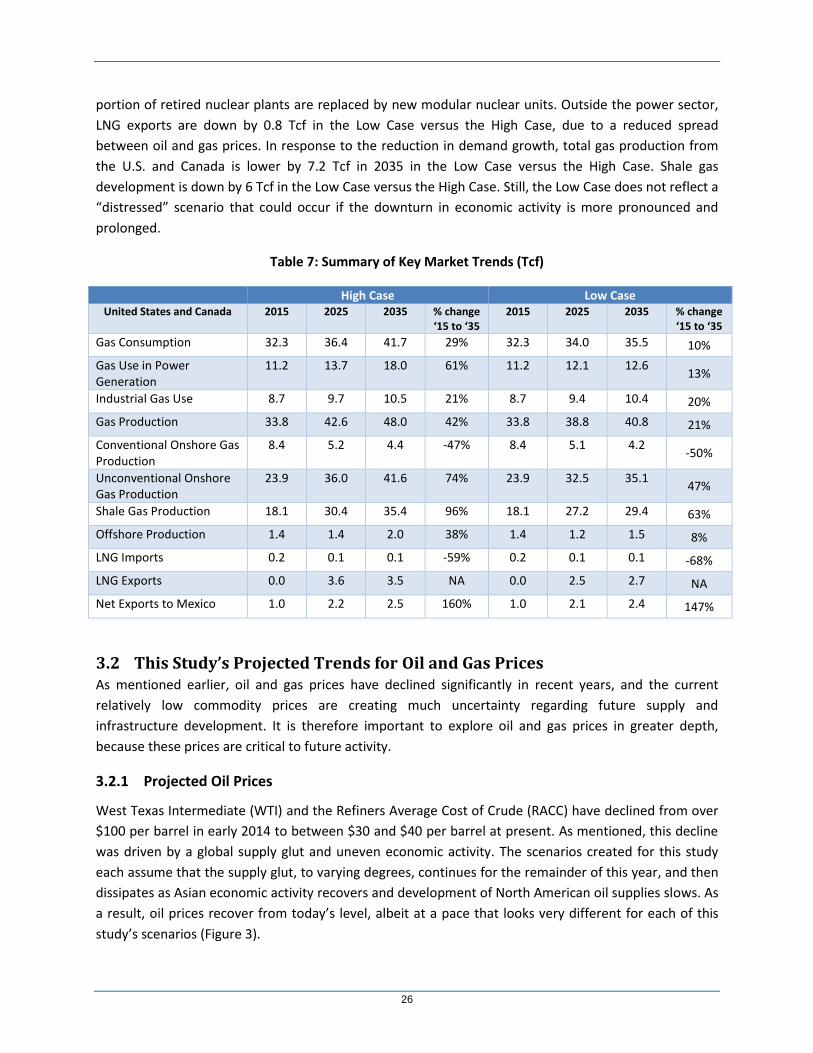
26

portion of retired nuclear plants are replaced by new modular nuclear units. Outside the power sector,

LNG exports are down by 0.8 Tcf in the Low Case versus the High Case, due to a reduced spread

between oil and gas prices. In response to the reduction in demand growth, total gas production from

the U.S. and Canada is lower by 7.2 Tcf in 2035 in the Low Case versus the High Case. Shale gas

development is down by 6 Tcf in the Low Case versus the High Case. Still, the Low Case does not reflect a

“distressed” scenario that could occur if the downturn in economic activity is more pronounced and

prolonged.

Table 7: Summary of Key Market Trends (Tcf)

High Case Low Case United States and Canada 2015 2025 2035 % change

‘15 to ‘35 2015 2025 2035 % change

‘15 to ‘35

Gas Consumption 32.3 36.4 41.7 29% 32.3 34.0 35.5 10%

Gas Use in Power Generation

11.2 13.7 18.0 61% 11.2 12.1 12.6 13%

Industrial Gas Use 8.7 9.7 10.5 21% 8.7 9.4 10.4 20%

Gas Production 33.8 42.6 48.0 42% 33.8 38.8 40.8 21%

Conventional Onshore Gas Production

8.4 5.2 4.4 -47% 8.4 5.1 4.2 -50%

Unconventional Onshore Gas Production

23.9 36.0 41.6 74% 23.9 32.5 35.1 47%

Shale Gas Production 18.1 30.4 35.4 96% 18.1 27.2 29.4 63%

Offshore Production 1.4 1.4 2.0 38% 1.4 1.2 1.5 8%

LNG Imports 0.2 0.1 0.1 -59% 0.2 0.1 0.1 -68%

LNG Exports 0.0 3.6 3.5 NA 0.0 2.5 2.7 NA

Net Exports to Mexico 1.0 2.2 2.5 160% 1.0 2.1 2.4 147%

3.2 This Study’s Projected Trends for Oil and Gas Prices As mentioned earlier, oil and gas prices have declined significantly in recent years, and the current

relatively low commodity prices are creating much uncertainty regarding future supply and

infrastructure development. It is therefore important to explore oil and gas prices in greater depth,

because these prices are critical to future activity.

3.2.1 Projected Oil Prices

West Texas Intermediate (WTI) and the Refiners Average Cost of Crude (RACC) have declined from over

$100 per barrel in early 2014 to between $30 and $40 per barrel at present. As mentioned, this decline

was driven by a global supply glut and uneven economic activity. The scenarios created for this study

each assume that the supply glut, to varying degrees, continues for the remainder of this year, and then

dissipates as Asian economic activity recovers and development of North American oil supplies slows. As

a result, oil prices recover from today’s level, albeit at a pace that looks very different for each of this

study’s scenarios (Figure 3).

27

In each scenario, oil prices recover to a longer-term price of $75 per barrel, consistent with the marginal

cost of supply. Even though each of the scenarios shows a significant recovery to this longer-term price,

the level still is lower than the longer-term level of roughly $100 per barrel assumed in the 2014 study.

Thus, North America’s oil production and its associated infrastructure development is greatly reduced

when compared with corresponding levels in the 2014 study.

As also shown in Figure 3 and as mentioned above, the pace of recovery is much slower for the Low

Case versus the High Case. While the High Case shows a more pronounced oil price rebound in 2016,

followed by a U-shaped recovery to $75 per barrel by 2025, the Low Case shows a much less

pronounced rebound with a slower V-shaped recovery to $75 per barrel by 2030. The Low Case assumes

oil prices below $40 per barrel until 2018 (in 2015 dollars).

The environment that underlies the High Case is a more rapid resumption of economic activity, reflected

by increased GDP growth assumed in the case. Thus, the global supply overhang dissipates more quickly

in the High Case while, conversely, economic activity recovers much more slowly in the Low Case,

reflected in the case’s reduced GDP growth. Consequently, the global supply overhang is more

pronounced and prolonged in the Low Case. The ramifications of the oil price trend assumed in the Low

Case are that the supply development and market growth that underpin infrastructure development are

delayed and less pronounced when compared with corresponding growth in the High Case.

Figure 3: U.S. Refiner Acquisition Cost of Crude Oil

28

3.2.2 Projected Natural Gas Prices

Like oil prices, natural gas prices have declined significantly in recent years. While Henry Hub prices

averaged close to $4 per MMBtu from 2010 through 2014, these prices recently declined to under $2

per MMBtu. This trend has been driven by robust supply growth that has outpaced market growth.

Recent declines in gas prices have also been driven by much milder than normal winter weather, which

has further weakened the supply-demand balance.

ICF’s GMM price projections for the scenarios that are considered in this study show that Henry Hub gas

prices will continue to remain relatively low during the next 12 to 24 months until gas demand grows

more robustly. Henry Hub gas prices are projected to average under $3 per MMBtu throughout the

remainder of 2016 (Figure 4). However, as demand growth accelerates, gas prices, like oil prices, are

projected to increase. Even so, the rate of increase and longer-term prices are very different for each

scenario.

Figure 4: Average Annual Natural Gas Prices at Henry Hub

A robust increase in LNG and Mexican exports drives prices up between 2017 and 2025 in both cases.

That demand growth will push prices high enough to support the necessary development of shale

resources, but not so high as to impair market growth. Still, relatively low drilling costs and continued

increases in well productivity will offset and reduce the upward pressure on prices caused by growing

demand.

In the High Case, gas prices rise to between $4.00 and $5.50 per MMBtu after 2020. Robust demand

growth, particularly from LNG and Mexican exports and gas-fired power generation, drive total gas use

in the United States and Canada up to about 47 Tcf by 2035. Even with this robust demand growth,

natural gas prices in the High Case are lower than the levels projected in the prior study because

29

continued improvements in well productivity have spurred the prolific development of shale gas plays

across North America.

Henry Hub prices in the Low Case are projected to be much lower than in the High Case (i.e., an average

$0.50 to $1.00 per MMBtu or 15 percent lower between 2020 and 2035). Gas use in the Low Case rises

to slightly above 40 Tcf by 2035, well below the level projected in the High Case. Clearly, reduced

economic activity coupled with a much more modest growth in gas-fired power generation places less

upward pressure on natural gas prices.

3.3 Natural Gas Demand Key assumptions underpinning natural gas demand are summarized in Table 8. In the High Case, electric

load is assumed to grow at 0.9 percent per year from 2016 to 2020, and at 1.0 percent per year after

2020. In the Low Case, electric load growth is projected to increase by only 0.3 percent per year

throughout the projection. In both cases, about 100 GW of coal-fired capacity is projected to retire, and

all nuclear plants are assumed to retire at their 60-year life. However, in the Low Case, modular nuclear

units are expected to replace 25 percent of retired nuclear capacity, and the capacity of two of the most

recently constructed nuclear power plants is expected to be expanded by 25 percent. These changes

reduce demand for gas in the Low Case. Renewable penetration in the High Case is consistent with RPS

standards, while renewable penetration in the Low Case is assumed to increase by 30 percent relative to

the High Case, further reducing the growth of gas demand.

Table 8: Natural Gas Demand Assumptions

INGAA High Case (Optimistic) INGAA Low Case (Less-Optimistic)

Electric sales growth (net of energy efficiency)

2016-20 change: 0.9 percent per year 2021-35 change: 1.0 percent per year

2016 onwards: 0.3 percent per year

Gas demand for bitumen production from Alberta Oil

Sands

Bitumen production increases to over 3.5 million barrels per day by 2030 Gas use for oil sands development

increases to 2.4 Bcfd by 2030

Bitumen production increases to 2.75 million barrels per day by 2030

Gas use for oil sands development increases to 1.75 Bcfd by 2030

LNG exports

U.S. Gulf Coast: peak at 8.8 Bcfd by 2025

U.S. East Coast: peak at 1.0 Bcfd by 2024

U.S. West Coast: No exports Alaska: No incremental exports

British Columbia: 1.4 Bcfd by 2028

U.S. Gulf Coast: peak at 6.0 Bcfd by 2029

U.S. East Coast: peak at 0.7 Bcfd by 2028

U.S. West Coast: No exports Alaska: No incremental exports

British Columbia: 0.9 Bcfd by 2032

Exports to Mexico Increases to 6 Bcfd by 2025 to 6.8 Bcfd

by 2035 Lower than High Case by 5%

30

Although not reflected in Table 8, the High Case projects relatively unchanged residential and

commercial gas load. While population growth and oil-to-gas conversions increase the number of

households that rely on gas, efficiency and conservation measures reduce individual household use. This

trend is even true for the Northeast United States, where oil-to-gas conversions are more prevalent

because conservation and efficiency measures tend to overwhelm other factors. The Low Case projects

a modest decline in R/C gas load due to even greater efficiency gains.

The High Case projects a relatively strong post-recession recovery in demand with continued growth of

petrochemical activity. Conversely, the Low Case projects flatter industrial load because of lower growth

in industrial activity. Each case projects slight increases in natural gas used to meet energy needs at

drilling rigs (up to 60 Bcf/yr by 2020) and as fuel for trucks used in the hydraulic fracturing process (up to

50 Bcf/yr by 2020).

Mexico's growth in gas use outpaces development of its domestic supplies, resulting in an increase in

U.S. gas exports to Mexico in both cases. Export volumes grow at a lower rate in the Low Case because

reduced oil prices foster less replacement of oil generation with gas generation. The High Case projects

over 11 Bcfd of LNG export capacity for the U.S. and Canada, with exports averaging 8.3 Bcfd from 2016

to 2035 while the Low Case projects 8 Bcfd of capacity, with exports averaging 5.8 Bcfd from 2016 to

2035. The lower oil-gas price spread promotes less LNG export in the Low Case.

3.3.1 Summary of Projected Natural Gas Use

Total gas consumption, including LNG and Mexican exports, is projected to increase by 1.8 percent per

year in the High Case, reaching an average of just over 130 Bcfd by 2035 (Figure 5). This total includes

about 10 Bcfd of LNG exports and 7 Bcfd of exports to Mexico by 2035.

This is an 8-percent increase in gas use compared to the prior study. The increase is attributable

primarily to assumed incremental LNG exports and additional exports to Mexico. Also, gas used in the

power sector is up in this study because the reduced gas price levels result in greater displacement of

coal generation.

In the near term, incremental gas use is driven mostly by growth in exports. In the longer term, the

power sector becomes the largest single source of incremental gas consumption. Between 2016 and

2020, growth in the sector’s gas use is driven by natural gas capacity replacing coal plants. Accelerated

growth is projected after 2020, when Federal carbon regulation is assumed. After 2030, nuclear plant

retirements usher in a new round of growth.

Total gas consumption, including LNG and Mexican exports, is projected to be almost 20 Bcfd lower by

2035 in the Low Case. Reduced economic activity does not bode well for energy use, leading to reduced

electric load growth that adversely affects natural gas used for power generation. By 2035, power

generation gas use in the Low Case is 14.5 Bcfd lower than in the High Case. Lower electric load growth,

higher renewable penetration, and the penetration of modular nuclear units are the primary drivers of

this trend. LNG exports are also lower by more than 2 Bcfd through 2035, as global LNG trade is reduced

at the lower levels of economic activity that are assumed in the case.

31

Figure 5: Projected U.S. and Canadian Natural Gas Use (Average Annual Bcfd)

3.3.2 Regional Natural Gas Use

Regional natural gas use is higher in all U.S. regions in the High Case relative to the prior study except for

the Offshore region, where lease and plant use is slightly below the prior study’s levels. Regional gas use

is lower in all regions in the Low Case versus the High Case (Figure 6), primarily because of lower growth

in gas used for power generation. The largest drop occurs in the Southeast, followed by the Northeast,

Southwest, Midwest, and West, relative to the High Case. Demand in the Southwest is also impacted by

LNG export and Mexican export activity.

High Case

Low Case

32

Figure 6: Regional Natural Gas Demand (Average Annual Bcfd)

High Case

Low Case

33

Regions that exhibit the largest growth in local consumption are the Northeast followed closely by the

Southeast and Southwest. All geographic areas exhibit significant growth in power-generation gas use,

mostly driven by coal and nuclear plant retirements. Northeast demand is spurred by relatively low gas

prices resulting from robust production growth from the Marcellus and Utica. When LNG exports are

considered as part of the total, the Southwest is the area that experiences the largest increase in gas

disposition because the majority of LNG exports occur from that region. Canada also experiences a

relatively robust market growth, attributed to growing gas use for oil sands development and LNG

exports from British Columbia.

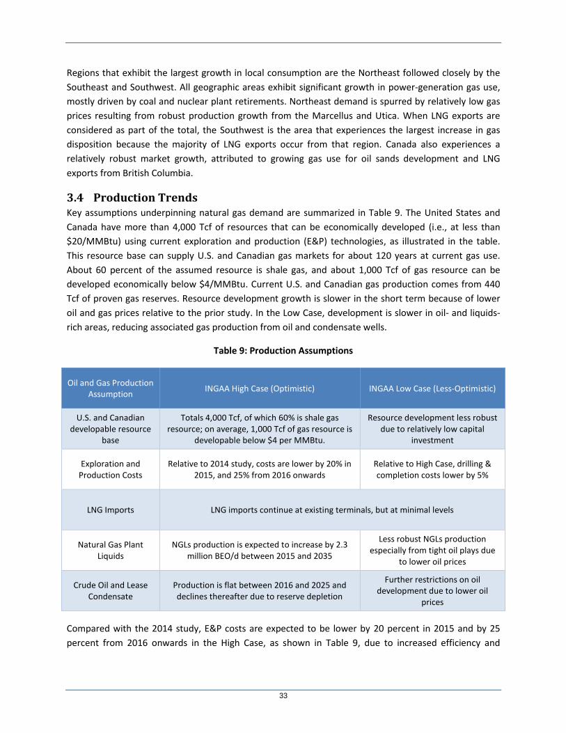
3.4 Production Trends Key assumptions underpinning natural gas demand are summarized in Table 9. The United States and

Canada have more than 4,000 Tcf of resources that can be economically developed (i.e., at less than

$20/MMBtu) using current exploration and production (E&P) technologies, as illustrated in the table.

This resource base can supply U.S. and Canadian gas markets for about 120 years at current gas use.

About 60 percent of the assumed resource is shale gas, and about 1,000 Tcf of gas resource can be

developed economically below $4/MMBtu. Current U.S. and Canadian gas production comes from 440

Tcf of proven gas reserves. Resource development growth is slower in the short term because of lower

oil and gas prices relative to the prior study. In the Low Case, development is slower in oil- and liquids-

rich areas, reducing associated gas production from oil and condensate wells.

Table 9: Production Assumptions

Oil and Gas Production Assumption

INGAA High Case (Optimistic) INGAA Low Case (Less-Optimistic)

U.S. and Canadian developable resource

base

Totals 4,000 Tcf, of which 60% is shale gas resource; on average, 1,000 Tcf of gas resource is

developable below $4 per MMBtu.

Resource development less robust due to relatively low capital

investment

Exploration and Production Costs

Relative to 2014 study, costs are lower by 20% in 2015, and 25% from 2016 onwards

Relative to High Case, drilling & completion costs lower by 5%

LNG Imports LNG imports continue at existing terminals, but at minimal levels

Natural Gas Plant Liquids

NGLs production is expected to increase by 2.3 million BEO/d between 2015 and 2035

Less robust NGLs production especially from tight oil plays due

to lower oil prices

Crude Oil and Lease Condensate

Production is flat between 2016 and 2025 and declines thereafter due to reserve depletion

Further restrictions on oil development due to lower oil

prices

Compared with the 2014 study, E&P costs are expected to be lower by 20 percent in 2015 and by 25

percent from 2016 onwards in the High Case, as shown in Table 9, due to increased efficiency and

34

technology improvements. In the Low Case, the E&P costs are 5 percent lower than in the High Case due

to lower oil prices and weaker economic activity.

The study assumes no new significant production restrictions (e.g., hydraulic fracturing regulations) that

impede supply development and, in general, the abundant resource base is expected to be economically

produced to balance demand.

LNG imports do not make up a significant portion of U.S. gas supplies in either case, and the economics

do not support the development of gas supplies from the Arctic region. As a result, neither the Alaska

nor Mackenzie Delta pipelines are included in either case.

Figure 7: U.S. and Canada Natural Gas Resource Base

Due to lower oil price projections in both cases relative to the 2014 study, the study does not project

that oil production will grow at a high rate in North America. Crude oil and NGLs production projections

are projected using ICF’s DPR, which is a vintage production model based on an estimated number of

drilled and completed wells, well recoveries, and representative decline curves for almost 60 different

supply areas throughout the United States and Canada.

3.4.1 Summary of Projected Natural Gas Production

Total gas production is projected to increase by 1.8 percent per year in the High Case, rising to over 130

Bcfd by 2035, primarily from shale gas production (see Figure 8).

35

Figure 8: Projected U.S. and Canadian Natural Gas Production (Average Annual - Bcfd)

By 2020, shale gas production is expected to account for about two-thirds of all U.S. and Canadian gas

production, growing to nearly 75 percent of the total gas production by 2035. Conventional gas

production is projected to continue its decline at an annual rate of 3.2 percent in the High Case. By 2035,

High Case

Low Case

36

the High Case projects that production of associated gas production (i.e., gas produced from oil wells)

will reach about 19 Bcfd (about 14 percent of total gas production), which would be about 2.6 Bcfd

higher than current levels. Offshore gas production grows more slowly at an annual rate of 1.4 percent.

The significant production growth, and shifts in production locations over time, is primarily due to

increasing shale gas production. This remains a critical driver for midstream infrastructure development

opportunities, particularly in the high-growth Marcellus and Utica plays.

Lower market growth and reduced economic incentives for gas development result in a slower rate of

production growth in the Low Case. Natural gas production grows at only 1 percent, with a projected gas

production of about 110 Bcfd by 2035. About 70 percent of this reduction occurs in Marcellus,

Haynesville, Barnett, Fayetteville, Eagle Ford, and Western Canadian shale plays. Conventional gas

declines a bit faster rate (3.5 percent) compared with the High Case, and offshore gas production

declines significantly with a 0.2 percent annual growth rate in the Low Case.

3.4.2 Regional Natural Gas Production

Gas production in both cases is projected to grow substantially in the Northeast, Midwest, Southwest,

and Canada due to an increase in production from shale plays. Production growth in the Northeast and

Midwest (mostly from the Marcellus and Utica shale plays) is expected to dominate, rising from its

current level of around 18 Bcfd to about 43 Bcfd by 2035 in the High Case (Figure 9), which would be

about 70 percent higher than the projected production in the 2014 study. The increased production

displaces production growth that would have occurred in other U.S. regions—for example, relative to

the 2014 study, gas production by 2035 in Central, Southwest, and Offshore regions is projected to be

lower by 19 percent, 11 percent, and 25 percent, respectively.

Southwest production growth (incremental production of 4.5 Bcfd between 2015 and 2035) is driven by

development in the Haynesville and Woodford shale plays in addition to the liquids-rich Eagle Ford shale

play. Rockies gas production in the Central region is expected to grow slowly (an incremental 2.2 Bcfd

between 2015 and 2035) due to reduced associated gas production and lower natural gas prices in the

near term that make it difficult to compete against more economic shale plays. Canadian production

growth is largely from the Montney shale play, and to a more limited extent the Horn River play, in

British Columbia, offsetting declining conventional gas production. By 2035, Canadian gas production is

higher by 22 percent in the High Case compared with the 2014 study projections.

Gas production is lower across all regions in the Low Case, although the Marcellus and Utica continue to

dominate due to their lower cost. Production in the Northeast and Midwest is projected to rise from 18

Bcfd in 2015 to 38 Bcfd by 2035 in the Low Case, which 5 Bcfd less than the projected production in the

High Case. However, the displacement impact of the Marcellus and Utica is greater in the Low Case, as

gas production by 2035 in Central, Southwest, and Offshore regions is lower by 31 percent, 30 percent,

and 42 percent, respectively, compared with the 2014 study. The largest drop in production is from

Southwest region, primarily due to decreasing production from the Haynesville, Fayetteville, Eagle Ford,

and Woodford shale plays. Production in the Central region is projected to decrease due to a decline in

the production of conventional, tight gas, and shale gas production from Niobrara, Uinta, Piceance, and

Bakken plays.

37

Figure 9: Regional Natural Gas Production (Bcfd)

High Case

Low Case

38

3.4.3 Summary of Projected Liquids Production

Overall production of liquids (crude oil, condensate, and NGLs) is projected to increase by about 3

million barrels per day between 2015 and 2035 in the High Case, mostly due to growth in NGLs

production. In contrast, production in the Low Case is projected to decrease throughout the forecast

period by about a million barrels per day, mostly due to a decline in crude oil production (Figure 10).

Total liquid production is projected to be lower by nearly 4 million barrels per day by 2035 in the Low

Case relative to the High Case—with three-quarters of the reduction coming from crude oil and lease

condensate production. About half of this decreased oil production in the Low Case is from Alberta’s oil

sands, along with reduced activity in the deep waters of the Gulf of Mexico and in the Bakken, Eagle

Ford, and other tight oil plays.

In the High Case, crude oil and condensate production in the United States and Canada is projected to

decline from 13.4 million barrels per day in 2015 to 12.9 million barrels per day in 2019, due to lower oil

prices in the near term (Figure 10). Beyond 2019, production is expected to be fairly flat, rising to 13.5

million barrels per day (i.e., close to 2015 production levels) by 2035, with resource depletion affecting

production after 2030. In the Low Case, crude oil and condensate production is projected to decline

throughout the forecast to reach 10.7 million barrels per day in 2035 due to lower oil prices. Compared

with the 2014 study, crude oil and condensate production by 2035 is lower by about 25 percent and 41

percent in the High Case and Low Case, respectively.

NGLs production remains relatively strong due to continued growth in gas production projected in both

cases. In the High Case, NGLs production is expected to rise from 4.2 million barrels per day in 2015 to

6.5 million barrels per day in 2025, and to remain flat thereafter (Figure 10). Projected NGLs production

is lower by about 800,000 barrels per day in the Low Case by 2035. Compared with the 2014 study, NGLs

production by 2035 is projected to increase by two percent in the High Case, whereas in the Low Case

production is projected to decrease by 11 percent.

39

Figure 10: U.S. and Canadian Liquids Production (MMBPD)

3.4.4 Regional Liquids Production

Most regions in the U.S. are projected to experience declining oil production, except for deep-water Gulf

of Mexico production in the Offshore region. The largest oil production growth in the High Case comes

from oil sands in Western Canada followed by offshore production in the Gulf of Mexico. Oil production

from Canada in the High Case increases by 33 percent from current levels to reach 5.5 million barrels per

Low Case

High Case

40

day by 2035. Oil production from Canadian oil sands is expected to grow from about 2.3 million barrels

per day in 2015 to 4.1 million barrels per day by 2035, primarily due to existing and under-construction

oil sands projects.7 Despite the growth, the 2035 oil sands production in the High Case is 30 percent

lower than production projected in the 2014 study. Production from the Offshore region increases by 43

percent from current levels to reach 1.9 million barrels per day (Figure 11). Oil production is significantly

lower in the Central region and in Western Canada compared with the 2014 study due to the lower oil

price projection in the current study.

Oil production is lower than current levels in all regions in the Low Case, with 20 percent less in the Low

Case relative to the High Case by 2035. Lower Canadian production accounts for more than half of the

reduction. Compared with the 2014 study, the oil sands production in 2035 is lower by about 50

percent.

The growth in NGLs production comes from a variety of shale plays, most notably the Marcellus and

Utica (Northeast), Woodford and Eagle Ford (Southwest), and Western Canadian (Montney and Horn

River) plays. However, growth of liquids hinges on the development of transport capability and markets

for the NGLs. Absent such development, NGLs production would be stranded in a number of key areas,

posing challenges not only for liquids development but for gas development as well.

In the High Case, NGLs production from the Northeast is projected to almost triple from 0.5 million

barrels per day in 2015 to 1.5 million barrels per day by 2035 (Figure 12). NGLs production from Canada

is expected to increase by 49 percent from current levels to reach 1.1 million barrels per day in 2035.

NGLs export capacity from the United States and Canada is assumed to be 1,800 MBPD in the High Case.

Compared with the 2014 study, NGLs production in the High Case in 2035 is higher by about 2 percent in

2035, despite lower liquids prices. Relative to the prior study, NGLs production in the Central region is

lower, but significantly higher in the Northeast.

In the Low Case, NGLs production decreases by about 13 percent in 2035 relative to the High Case, with

the Southwest, Central, and Canada regions accounting for more than 75 percent of the total reduction.

NGLs production in the Southwest, Central, and Canada regions is down by 33 percent, 24 percent, and

20 percent, respectively. Production from the Northeast is only marginally lower, with 1.3 million barrels

per day in 2035. Similarly, Western Canadian production is projected to increase by nearly 30 percent

from current levels to reach 1.0 million barrels per day in 2035. Relative to the High Case, NGLs export

capacity is assumed to be at 1,600 MBPD in the Low Case.

7 These projects can withstand lower oil prices in the near term as they are designed to operate for about 30 to 40 years.

41

Figure 11: Regional Crude Oil and Condensate Production (MMBPD)

High Case

Low Case

42

Figure 12: Regional Natural Gas Liquids Production (MMBPD)

High Case

Low Case

43

4 Midstream Infrastructure Requirements

The supply and demand dynamics discussed in the previous sections lay the foundations for determining

the need for new transmission pipeline capacity. New infrastructure will be required to move

hydrocarbons from regions where production is expected to grow to locations where the hydrocarbons

are used. The amount of midstream infrastructure and its associated capital investment depends on

how the produced volumes of natural gas, NGLs, and crude oil are moved to demand centers. The

methodology for determining the required infrastructure was discussed in Section 2, with detailed

assumptions being provided in Appendix B.

In this section, for each hydrocarbon the expected flow patterns and required takeaway capacity are

first discussed, followed by a discussion of the infrastructure metrics and required capital expenditures.

The regional breakout of expenditures is then presented. The section concludes with a summary of the

midstream infrastructure metrics and expenditures for oil and gas production and transport in both the

High and the Low Cases.

4.1 Natural Gas Growth in natural-gas-related infrastructure has been significant over the past five years, with

substantial additions to transmission pipeline capacity put in service in 2015. Additional capacity is

expected to come online over the next two to three years, despite the current low price environment.

Many of these upcoming projects, particularly those slated to come online in 2016, are already under

construction and several others have momentum due to recent regulatory approvals based on signed

contracts with producers, end-users, or other shippers. The overall capacity and timeframe for these

upcoming and future transmission projects are discussed below.

Long-term contracts for transportation services provide the financial basis for pipeline companies to

pursue projects. However, with the current downturn in oil and gas prices, many producers are finding it

difficult to hold pipeline capacity. In the rapidly growing areas like the Marcellus and Utica, however,

there is likely to be sufficient supply and demand-driven motivation to build new capacity. Insufficient

infrastructure in this region has particularly hurt producers with low prices and sustained high basis

differentials for several years now. These producers are likely to view the cost of pipeline transport to be

relatively small compared with the revenues lost as a result of price reductions or well shut-ins.

4.1.1 Natural Gas Flow and Capacity Needs

Based on the capacity additions and the supply-demand trends, flows are projected along various

pipeline corridors. The current flows in 2015 are shown in Figure 13, and the flows in 2035 are shown in

Figure 14 and Figure 15 for the High Case and Low Case, respectively. The difference in flows between

2035 and 2015 is used to evaluate how the flow patterns are likely to change over time, with attendant

implications for capacity additions. The discussion below is organized by various production regions,

starting with the Appalachian region.

44

Appalachian Region

The main story for gas flows in the Appalachian region is the continuing displacement of Gulf Coast gas

across the eastern part of North America due to the rising production from the Marcellus and Utica

juggernaut. The level of displacement is currently limited by the takeaway capacity available for

transportation from the region. For this study, the “takeaway capacity” total includes the capacity of

interregional pipelines that move gas from one region to another region, as well as intraregional

pipeline capacity. The capacity of intraregional pipelines is included in this study because there are a

number of new intraregional pipeline projects designed to support production, particularly in the

Marcellus/Utica region and in Canada.8 Another key part of the story is that pipelines that have

historically transported gas from the Midwest or the Gulf Coast to the Northeast have started to reverse

flow direction to transport Northeast supplies to markets that traditionally received Gulf Coast gas or

even areas that have served as supply regions. For example, new pipelines are being planned to supply

gas to the Midwest and the Southeast.

In the High Case, nearly 20 Bcfd of takeaway capacity is needed over time to move gas from the

Marcellus and Utica region to several markets. In particular, flows to the New York, New Jersey, and the

New England markets increase by about 50 percent, rising from about 9 Bcfd in 2015 to nearly 14 Bcfd in

2035. Flows to the Midwest are expected to more than triple from the current average of 1.7 Bcfd to

nearly 5.6 Bcfd by 2035, as a surge of capacity is expected to come online, including capacity on the

Rockies Express Pipeline and either Energy Transfer’s Rover Pipeline or Spectra Energy’s Nexus Gas

Transmission project. These pipelines will allow Marcellus and Utica supplies to reach Midwest and

Ontario markets, as well as Gulf Coast markets.

Gas from the Northeast is also projected to support LNG export demand. Pipelines including Tennessee

Gas Pipeline, Texas Eastern Transmission, Columbia Gas Transmission, Transcontinental Pipeline, and

others are reversing their traditional northward flow to move gas to the Southeast and the Gulf Coast.

Flows from Appalachia to the Gulf Coast and the Southeast in the High Case are expected to average

near 2.5 Bcfd by 2035, as projects such as Columbia Gas’ Leach Xpress, Tennessee Gas Pipeline’s Broad

Run projects and South Louisiana Supply projects, and Transcontinental Pipeline’s Atlantic Sunrise

project, in addition to others, enter service over the next four to five years.

Gas flows from the Appalachian region in the Low Case remain strong toward the Northeastern markets

of New York, New Jersey, and New England due to rising power generation demand, even though the

overall electricity demand is lower. Flows to the Midwest are similar to flows in the High Case, averaging

around 5.5 Bcfd. Many pipeline capacity projects originating in the Appalachian region are expected to

go forward as various demand centers replace their current supply with the low-cost gas from Marcellus

and Utica. Relative to the High Case, pipelines moving gas from north to south will have higher load

factors. Southbound flows average nearly 3.9 Bcfd in 2035 in the Low Case, which is an incremental 1.4

Bcfd higher than in the High Case.

8 This definition of takeaway capacity is different than in the 2014 Study, which considered only interregional pipelines.

45

Figure 13: Natural Gas Flows in 2015

46

Figure 14: Natural Gas Flows in 2035 – High Case

47

Figure 15: Natural Gas Flows in 2035 – Low Case

48

Southwest Region

In the Gulf Coast area, flows from the Permian and other shale areas, such as the Barnett, continue to

move eastward and southward across Texas. Some gas from the Eagle Ford is also moving eastward, but

a large part of this gas supplies Mexican exports. Currently, gas flowing eastward across Texas and into

Louisiana averages nearly 10 Bcfd. Most of this gas enters the confluence of long-haul interstate

pipelines in Louisiana before flowing northward to the Atlantic Coast, particularly during the winter

months. By 2035, however, strong gas-on-gas competition with Appalachian supplies results in a

projected decline in these eastward flows from 10 Bcfd to nearly 6 Bcfd in the High Case. This, in turn,

significantly reduces northbound flows on Tennessee Gas Pipeline, Transcontinental Pipeline, Texas

Eastern Transmission, Columbia Gulf, and others. Concurrently, southward flows from the Marcellus and

Utica will increase from a 2015 average of 0.5 Bcfd to roughly 2.5 Bcfd by 2035 in the High Case. There is

a strong seasonality to the southbound flows, which are greater in the summer than in the winter. As

noted earlier, in the Low Case the higher net north-to-south flow from the Appalachia results in roughly

4.5 Bcfd lower flows from the Gulf Coast region to the Eastern seaboard (Figure 15), relative to the High

Case.

With growing LNG exports and Mexican exports, much of the gas produced in the Southwest remains in

the region. Reversal of natural gas flows from north to south also helps to meet the growing LNG and

Mexico export demand, as cheaper Marcellus and Utica gas displaces the supply from traditional gas

plays in the Southwest region. By 2035, LNG exports from the United States are expected to reach about

8.1 Bcfd in High Case, with 7.2 Bcfd of exports originating from the U.S. Gulf Coast. Most of the gas for

LNG exports will come from Southwest production. A number of projects are anticipated to come online

to facilitate pipeline exports to meet rapidly growing power generation demand in Mexico. In 2015, total

flows to Mexico averaged close to 2.6 Bcfd and are projected to increase to 6.8 Bcfd by 2035 in the High

Case. The primary gas supplies for exports to Mexico will likely come from the Rockies via the El Paso

Natural Gas system, as well as from the Permian Basin and Eagle Ford Shale, given their relative

proximity to the border. Exports from South Texas to Mexico are expected to increase from 1.5 Bcfd in

2015 to 3.3 Bcfd by 2035. Additionally, LNG exports are set to increase significantly once first shipments

start in 2016.

In the Low Case, both LNG exports and pipeline exports to Mexico are reduced from the High Case. LNG

exports from the Gulf Coast average over 5.5 Bcfd (a reduction of roughly 1.7 Bcfd from the High Case).

Pipeline exports to Mexico are reduced modestly by roughly 0.4 Bcfd from the High Case, increasing

from the current 2.6 Bcfd to nearly 6.4 Bcfd by 2035.

Rockies/Western Region

In the Western region, Rockies gas continues to flow southwest along Kern River Gas Transmission,

serving markets in Utah, Nevada, and Southern California. Rockies gas has also continued to make its

way south into the El Paso and Transwestern systems, both of which serve the Desert Southwest and

Southern California. In both cases, Rockies gas flows into Southern California are expected to remain

49

similar to flows in 2015 as demand projections remain fairly flat. There are no anticipated pipeline

expansions in the region, and gas flows will likely remain stable.

Recently, Rockies flows have supported exports to Mexico and pipelines such as El Paso and

Transwestern are supporting the flow of Rockies gas to Mexico. Flows out of West Texas and the

Permian Basin into Mexico currently average close to 0.4 Bcfd but are expected to be above 2.2 Bcfd by

2035 in both cases.

Rockies gas flow toward the Midwest is expected to remain flat relative to 2015, with annual average

flows of 3.1 Bcfd in the High Case, while the flow decreases to 2.8 Bcfd in the Low Case. This is a result of

competition from both Western Canadian gas (which is essentially stranded without significant LNG

exports) and Appalachian gas moving westward.

Western Canadian Region

Western Canadian production continues to flow eastward toward both U.S. Midwest markets and

Eastern Canadian markets. In the High Case, Western Canadian flows to Eastern Canada remain flat at

about 1.7 Bcfd, and they decrease to 1.3 Bcfd in the Low Case. Flows toward the Central United States

are expected to increase from 4.4 Bcfd in 2015 to 5.9 Bcfd by 2035 in the High Case and 5.6 Bcfd by 2035

in the Low Case. Western Canadian gas also supplies the Northwest United States and California, with

flows remaining flat at around 2.7 Bcfd in the both cases.

Takeaway Pipeline Capacity for Natural Gas

Pipeline capacity is needed to accommodate the flows described above. A summary of the expected

new pipeline builds in the two scenarios across the various regions is provided in Table 10, and details

about the incremental capacity additions for the two cases are provided in Table 11 and Table 12.

Table 10: Capacity Addition Trends From 2016 Onwards

Time Period

High Case Low Case

2016 Surge of pipeline capacity comes into service, as many projects have started construction;

Takeaway capacity out of Marcellus and Utica region increases;

Gulf Coast projects such as Cameron Pipeline expansion come into service as LNG exports begin to ramp;

U.S. Northeast supplies gain more access to Ontario markets through a number of expansions;

Similar to High Case, substantial capacity comes online due to heavy momentum;

Growing takeaway capacity in the Marcellus and Utica region, with the exception of the Constitution Pipeline;

Increased delivery capacity into Gulf Coast to support oncoming LNG Exports;

Increased pipeline capacity linking U.S. Northeast supplies to Ontario;

50

2017-2020

Substantial increase in Marcellus and Utica takeaway capacity, reaching Midwest, Gulf Coast, and Southeast markets;

Capacity additions in Western Canada, supporting British Columbia LNG exports, as well as flows to Eastern Canada and Central U.S.;

Substantial increases in pipeline export capacity to Mexico, to support oncoming Mexico power generation demand;

Nearly 13% less capacity added between 2017-2020 in the Low Case;

Slower production growth delays timing of takeaway capacity out of the Marcellus and Utica region, reducing total capacity;

Reduced delivery capacity supporting British Columbia and Gulf Coast exports;

Similar increases in pipeline export capacity to Mexico, due to anticipated growth in power generation demand;

2020-2035

Roughly 14.7 Bcfd in capacity added over 15 years, with large increases in 2025 to support Southeast power generation;

Increase in capacity linking Marcellus and Utica supplies to the Gulf Coast for LNG exports, as well as the Southeast for power generation;

Increased capacity in Western Canada in support of British Columbia LNG exports.

Close to half of the capacity added in the High Case comes online in the Low Case between 2020-2035;

Increase in capacity linking Marcellus and Utica supplies to the Gulf Coast;

Increased capacity in Western Canada to support LNG exports from British Columbia;

Strong reduction in capacity growth to serve the Southeast power generation market.

Table 11: Natural Gas Pipeline Takeaway Capacity Additions in the High Case (Bcfd)

2015 2016 2017-2020 2021-2025 2026-2030 2031-2035 2015-2035

U.S. and Canada 7.9 9.2 26.3 6.8 5.5 2.4 58.2

U.S. 7.4 6.9 23.3 4.8 4.0 1.9 48.3

Canada 0.6 2.4 2.9 2.1 1.5 0.5 9.9

Central - - 1.4 0.5 - 0.3 2.2

Midwest 2.5 2.4 1.6 - - - 6.5

Northeast 1.4 4.5 12.2 1.0 1.9 - 21.0

Offshore - - - - - - -

Southeast 1.4 - 3.2 1.8 - 1.1 7.5

Southwest 2.1 - 4.4 1.5 2.2 0.5 10.6

Western - - 0.6 - - - 0.6

51

Table 12: Natural Gas Pipeline Takeaway Capacity Additions in the Low Case (Bcfd)

2015 2016 2017-2020 2021-2025 2026-2030 2031-2035 2015-2035

U.S. and Canada 7.9 8.6 21.8 3.8 2.2 0.5 44.8

U.S. 7.4 6.2 18.9 1.7 0.7 - 34.9

Canada 0.6 2.4 2.9 2.1 1.5 0.5 9.9

Central - - 0.8 - - - 0.8

Midwest 2.5 2.4 0.6 - - - 5.5

Northeast 1.4 3.8 11.4 1.0 0.4 - 18.0

Offshore - - - - - - -

Southeast 1.4 - 1.2 - - - 2.6

Southwest 2.1 - 4.4 0.7 0.4 - 7.5

Western - - 0.6 - - - 0.6

In the High Case, approximately 58 Bcfd of incremental natural gas takeaway mainline capacity is

required between 2015 and 2035, with most of the capacity being added in the Northeast, Southwest,

and Canada. In comparison, over the last five years between 2010 and 2014 the total incremental

takeaway capacity additions were roughly 34 Bcfd. In 2015, nearly 8 Bcfd of capacity was added—spread

across the central (Midwest and Southwest) and eastern (Northeast and Southeast) parts of the United

States.

Figure 16 illustrates the regional breakdown of total capacity additions for both scenarios. In 2016,

about 9 Bcfd of new capacity is expected to come online in the High Case, mostly dominated by builds in

the Northeast, Midwest, and Canada. These 2016 projects already have regulatory approvals from either

FERC, the Canadian National Energy Board, or the Ontario Energy Board, and most of them are already

under construction or will begin construction soon.9 The capacity expansions within Canada in 2016 are

intended to enable the flow of Marcellus and Utica production into Ontario. About 20 Bcfd of

incremental takeaway capacity between 2016 and 2035 (Table 11) is needed to move the projected

Marcellus and Utica production. About 6 Bcfd of new pipeline capacity is added in the Southeast region

between 2016 and 2035 to connect Marcellus and Utica production to this region.10 An additional 10

Bcfd of new pipeline capacity is built in the Southwest region to support Mexican and LNG exports.

9 For example, projects such as Algonquin Gas Transmission’s Algonquin Incremental Market (AIM) expansion, Texas Gas Transmission’s Ohio Louisiana Access project, and Rockies Express Pipeline’s Zone Three Capacity Enhancement are already under construction. 10 In the High Case, all three major projects to the South Atlantic (EQT’s Mountain Valley project, Dominion’s Atlantic Coast Pipeline, and Williams Transco’s Atlantic Sunrise project) are expected to go forward.

52

Figure 16: Gas Pipeline Additions 2015-2035

As illustrated in Figure 17, capacity additions decrease significantly after 2018, with limited additions

beyond 2020.11 As a result, the relatively high growth period of infrastructure development over the last

few years and in the near term will create an “overbuild” condition that leads to weak investments in

the long term.

Figure 17: Capacity Additions in High and Low Cases (MMcfd)

In the Low Case, the total required takeaway capacity addition is about 45 Bcfd, about 23 percent less

than the capacity addition required in the High Case. Out of the 45 Bcfd of additions, 35 Bcfd is in the

11 The capacity addition in 2025 is for transporting gas from Western Canadian shale plays to the British Columbia coast for LNG export, through projects such as Chevron’s Pacific Trail Pipeline and TransCanada’s North Montney Mainline.

53

United States. Table 11 details the specific trends of capacity addition over time, and these trends are

also illustrated in Figure 17. Compared with the High Case, the required capacity addition in the

Northeast drops to 18 Bcfd (a 14-percent reduction). As in the High Case, the Northeast represents the

bulk of capacity additions between 2015 and 2035 at 33 percent (Figure 16). In the Low Case, reduced

demand and a slower-growing economy delay infrastructure development and, in particular, projects

out of the Marcellus and Utica region are delayed by as much as three years (Figure 17). Only two of the

three Appalachia-to South-Atlantic projects move forward in the Low Case, due to reduced power

generation demand.

4.1.2 Summary of Natural Gas Metrics

More than 800,000 well completions are needed between 2015 and 2035 in the High Case, and nearly

700,000 well completions are needed in the Low Case (Table 13) to produce oil and gas at the levels

discussed in Section 3. About 70 percent of these wells are expected to be oil wells, with the rest being

gas wells.

Table 13: Natural Gas Infrastructure Metrics

High Case, 2015-2035

High Case

Average Annual

Low Case, 2015-2035

Low Case

Average Annual

Average Annual Change (Low vs High)

Average Annual Change (%, Low vs High)

Gas Well Completions (1,000s) 258 12 227 11 -1 -12%

Oil Well Completions (1,000s) 565 27 455 22 -5 -19%

Total Well Completions (1,000s) 823 39 682 32 -7 -17%

Miles of Transmission Mainline (1,000s) 15.6 0.7 9.2 0.4 -0.3 -41%

Miles of Laterals to/from Power Plants, Storage Fields and Processing Plants (1,000s)

13.7 0.7 8.4 0.4 -0.3 -39%

Miles of Gas Gathering Line (1,000s) 179.3 8.5 149.8 7.1 -1.4 -16%

Inch-Miles of Transmission Mainline (1,000s) 510 24 304 14 -10 -40%

Inch-Miles of Laterals to/from Power Plants, Storage Fields and Processing Plants (1,000s)

292 14 178 8 -5 -39%

Inch-Miles of Gathering Line (1,000s) 707 34 598 28 -5 -16%

Compression for Pipelines (1,000 HP) 6,205 295 4,252 202 -93 -31%

Compression for Gathering Line (1,000 HP) 9,726 463 7,628 363 -100 -22%

Number of New Gas Power Plants 749 36 437 21 -15 -42%

Gas Storage (Bcf Working Gas) 288 14 123 6 -8 -57%

Processing Capacity (Bcfd) 41.9 2.0 34.0 1.6 -0.4 -19%

LNG Export Facilities (Bcfd) 12.0 0.6 10.6 0.5 -0.1 -12%

Table 14 compares gas infrastructure metrics with the 2014 study. Well completions in the High Case are

about 30 percent lower compared with the prior study, as the current study revised the modeling of oil

and gas well drilling and completion by adapting a “learning curve” concept. The “learning curve”

accounts for technology and efficiency improvements in horizontal drilling and hydraulic fracturing

(e.g., longer lateral and higher fracture density) over the last few years, with more wells being drilled

54

and completed. The new methodology results in higher well productivity or higher EUR per well

compared with the 2014 study. Furthermore, the current methodology accounts for recent trends of

improved EUR per well as a result of producers drilling in lower-cost sweet spots to keep up with lower

commodity prices. Higher productivity results in greater production from a smaller number of well

completions.

Table 14: Natural Gas Metrics, Current Study Versus 2014 Study, 2015-2035

High Case Average Annual

Low Case Average Annual

2014 Study Average Annual

Gas Well Completions (1,000s) 12 11 14

Oil Well Completions (1,000s) 27 22 41

Total Well Completions (1,000s) 39 32 55

Miles of Transmission Mainline (1,000s) 0.7 0.4 0.9

Miles of Laterals to/from Power Plants, Storage Fields and Processing Plants (1,000s)

0.7 0.4 0.8

Miles of Gas Gathering Line (1,000s) 8.5 7.1 13.7

Inch-Miles of Transmission Mainline (1,000s) 24 14 26

Inch-Miles of Laterals to/from Power Plants, Storage Fields and Processing Plants (1,000s)

14 8 13

Inch-Miles of Gathering Line (1,000s) 34 28 50

Compression for Pipelines (1,000 HP) 295 202 196

Compression for Gathering Line (1,000 HP) 463 363 371

Number of New Gas Power Plants 36 21 36

Gas Storage (Bcf Working Gas) 14 6 34

Processing Capacity (Bcfd) 2.0 1.6 1.5

LNG Export Facilities (Bcfd) 0.6 0.5 0.4

The mileage for gas gathering line and gas transport in the High Case is lower than the 2014 study

because of fewer well completions and more pipeline-reversal projects that do not need major pipeline

development. On the other hand, the High Case projects nearly 35 percent higher compression needs

relative to the prior study because of pipeline-reversal projects and increased production. This study

also assumes larger-diameter pipes for connecting gas power plants and processing plants, resulting in

lower mileage for laterals.

This study projects lower new working gas capability for gas storage compared with the 2014 study, as

natural gas storage is currently overbuilt and existing storage capacity is sufficient in most regions to

meet the seasonal demand. Gas processing capability and LNG export capacity in both cases are above

the projection from the prior study, largely because a greater number of LNG units are already under

construction than what was anticipated in 2014.

4.1.3 Miles of New Gas Gathering Line and Transmission Pipeline

Figure 18 compares miles of new gas gathering and transmission pipeline added in the two cases. The

top charts include both gathering and transmission pipes, the bottom charts show only the transmission

55

pipes. The High Case is projected to add about an average of 8,500 miles per year of new gathering lines

from 2015 through 2035 (see Figure 18), and about 1,400 miles of new gas transmission line will be

added each year on average, about 54 percent of which will be mainline miles and the rest lateral

connections to power plants, processing plants, and gas storage fields.

The Low Case is projected to add an average of 7,100 miles per year of new gathering lines, and an

average of about 850 miles of new gas transmission lines is expected to be added each year (a 40-

percent reduction from the High Case), split almost evenly between mainline miles and lateral

connections.

As mentioned earlier, infrastructure development, especially for transmission pipelines, is expected to

be robust in the near term, as several projects are already under construction or well along in the

planning stage. The resulting overbuild condition will lead to lower levels of new pipeline installations

after 2020, as discussed earlier.

Figure 18: Miles of New Gas Gathering and Transmission Pipeline Added

56

4.1.4 Natural Gas Capital Expenditures

Significant investment is needed to support the robust incremental infrastructure builds for natural gas

transport. Table 15 shows the required investment in new natural gas transmission capacity (including

new mainlines, natural gas storage fields, processing facilities, laterals to and from storage, power

plants, and processing facilities, and gas lease equipment and LNG export facilities) from 2015 to 2035.

In the High Case, investment of approximately $17 billion per year on average is required between 2015

through 2035, totaling $353 billion (real 2015 dollars). Unit cost measures, along with their comparison

with the 2014 study, are provided in Section 2.2.2.

Reduction in gas infrastructure development in the Low Case results in 25-percent lower investment

requirements. The greatest change from the High Case is reduced expenditures for gas transport

pipelines, which drop by $2.3 billion per year on average. However, a decline in investments for gas

gathering and surface equipment associated with gas development is much more modest. Investment in

new LNG export facilities is projected to total about $75 billion in the High Case compared with about

$70 billion in the Low Case.

Table 15: Natural Gas Capital Expenditures (2015$)

(Billions of Real Dollars) High Case,

2015-2035

High Case Average Annual

Low Case, 2015-2035

Low Case Average Annual

Average Annual Change (Low vs High)

Average Annual Change

(%, Low vs High)

Gas Transmission Mainline Pipe $76.5 $3.6 $46.2 $2.2 -$1.4 -40%

Laterals to/from Power Plants, Gas Storage and Processing Plants

$50.4 $2.4 $30.6 $1.5 -$0.9 -39%

Gathering Line (pipe only) $33.7 $1.6 $28.4 $1.4 -$0.3 -16%

Gas Gathering Line Compression $29.8 $1.4 $23.5 $1.1 -$0.3 -21%

Gas Lease Equipment $27.0 $1.3 $23.7 $1.1 -$0.2 -12%

Gas Pipeline & Storage Compression

$18.4 $0.9 $12.8 $0.6 -$0.3 -31%

Gas Storage Fields $4.8 $0.2 $2.3 $0.1 -$0.1 -52%

Gas Processing Capacity $34.9 $1.7 $28.3 $1.3 -$0.3 -19%

LNG Export Facilities $76.8 $3.7 $70.8 $3.4 -$0.3 -8%

Total Capital Expenditures $352.3 $16.8 $266.6 $12.7 -$4.1 -24%

Figure 19 shows the expenditures for natural gas pipelines by various pipeline type. Transmission

pipelines account for most of the expenditures in both cases, with most of the expenditures occurring

before 2020. Beyond 2020 the expenditures are primarily for laterals and gathering pipelines, as the

amount of transmission lines built decreases. The year 2025 is an exception, as pipelines are planned to

transport Western Canadian gas to the British Columbia coast for LNG export.

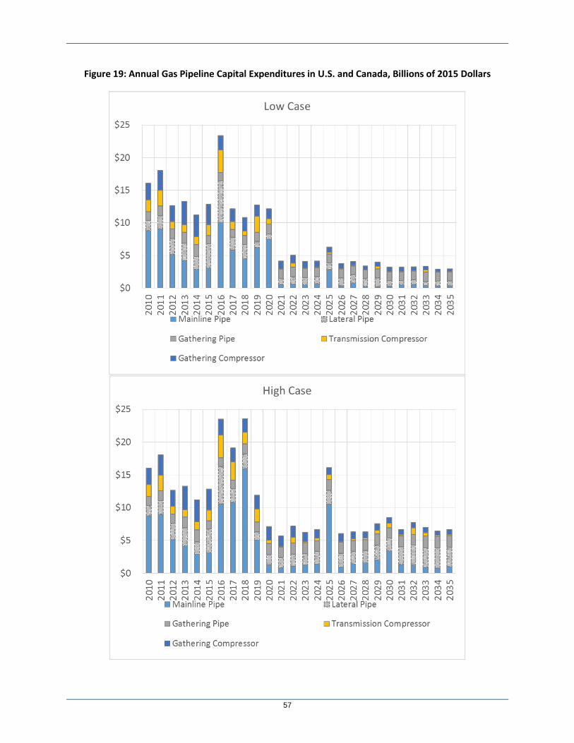
57

Figure 19: Annual Gas Pipeline Capital Expenditures in U.S. and Canada, Billions of 2015 Dollars

58

Annual spending patterns are similar in both cases, with large investments in the near term and more

limited investments after 2020 (Figure 20). Investments in 2016 total about $40 billion for both cases,

given that almost all of the 2016 projects are under construction. After 2019, the investments for gas

infrastructure are much lower in both cases because new capacities installed in 2015-2019 are sufficient

to support a large portion of projected production growth. Therefore, average investments after 2020

are about a quarter of the investments during 2016-2019 (Figure 20).

The drop in investment might occur sooner than 2020. The way in which expenditures are reported in

this analysis so far is the same as in the previous INGAA Foundation reports, wherein the expenditures

are reported in the year the projects are completed (i.e., using the “Year of Commissioning” approach).

However, the actual capital spending for a project occurs before a project is commissioned. For

example, purchase orders for pipeline, machinery, and other equipment generally are placed two to

three years before commissioning. Taking this into consideration, ICF developed a second methodology

to show how capital expenditures could occur over time, wherein the capital expenditure for each

project is spent equally across three years: each of the two years before the project, and the year the

project comes online (i.e., a “Three-Year Spread” approach). Figure 21 shows the annual expenditure

trend using this methodology, which smooths out the annual expenditure trend (shown in Figure 20)

throughout the projection period.

The Three-Year Spread approach shows that spending in gas infrastructure development could decline

after 2016 in both cases (Figure 21). As noted above, increased investments around 2025 in both cases

are related to expenditures related to LNG export projects in Western Canada.

Figure 20: Annual Natural Gas Capital Expenditures for New Infrastructure, Year of Commissioning, Billions of 2015 Dollars

59

Figure 21: Annual Natural Gas Capital Expenditures for New Infrastructure, Three-Year Spread, Billions of 2015 Dollars

In the subsequent charts and tables, the capital expenditures are based on the Year of Commissioning

approach, unless otherwise noted, in order to be consistent with the previous INGAA Foundation

infrastructure reports.

Table 16 compares investments in gas infrastructure with the 2014 study, where the average annual

investments were $14.9 billion per year. This is about halfway between the High Case and Low Case

expenditure requirements. The High Case has smaller investments in the gas transmission mainline

category ($3.6 billion per year), relative to the 2014 study ($4.2 billion per year) due to expectations of

more investments in pipeline reversal projects to transport the Marcellus and Utica gas production.

However, as noted earlier, this results in greater investments in compressors, relative to the 2014 study,

as shown in Table 16. Compression investments for pipeline and storage in the High Case are almost

twice the anticipated expenditures in the 2014 study.

In the gathering sector, less investment for new pipe and more investment for compression is projected

in the High Case relative to the prior study. The shift is due to the higher productivity of wells that leads

to fewer well completions and less gathering-line mileage relative to the 2014 study. In the Low Case,

new gathering-line pipe investments are significantly lower (at $1.4 billion), while gathering-line

compression is similar (at $1.1 billion) to the 2014 study.

60

Table 16: Natural Gas Capital Expenditures (2015$), Current Study Versus Prior Study, 2015-2035

(Billions of Real Dollars) Low Case Average Annual

High Case Average Annual

2014 Study Average Annual*

Gas Transmission Mainline Pipe $2.2 $3.6 $4.2

Laterals to/from Power Plants, Gas Storage and Processing Plants

$1.5 $2.4 $2.2

Gathering Line (pipe only) $1.4 $1.6 $1.7

Gas Gathering Line Compression $1.1 $1.4 $1.1

Gas Lease Equipment $1.1 $1.3 $1.3

Gas Pipeline & Storage Compression $0.6 $0.9 $0.5

Gas Storage Fields $0.1 $0.2 $0.5

Gas Processing Capacity $1.3 $1.7 $1.2

LNG Export Facilities $3.4 $3.7 $2.2

Total Capital Expenditures $12.7 $16.8 $14.9

*Capital expenditures reported in the prior study were converted from 2012$ to 2015$ using 4.3 percent inflation factor.

The higher production levels in the High Case require more investments in gas processing relative to the

2014 study: investment in gas processing capacity is $1.7 billion per year in the High Case but only $1.2

billion per year in the prior study. The Low Case processing capacity investments are also higher than in

the 2014 study.

As discussed earlier, investments in gas storage fields are much lower compared with the prior study, as

existing storage capacity is sufficient in most regions to meet seasonal demand. On the other hand,

investment in new LNG export facilities is much higher in both cases, with 12 Bcfd of LNG export

capacity in the High Case and 10.6 Bcfd in the Low Case. The 2014 study anticipated only 9.3 Bcfd of

exports. The unit costs of LNG export infrastructure are also higher than in the prior study (see section

2.2.2).

4.1.5 Regional Natural Gas Capital Expenditures

Detailed regional breakout of gas transmission pipeline infrastructure requirements (mainline, laterals,

and compression) from 2015 through 2035 for both cases is provided in Table 17.

Figure 22 and Figure 23 show the regional capital expenditures for gas infrastructure in the High Case

and the Low Case, respectively. In the Low Case, infrastructure investment is lower across all regions

and in all asset categories relative to the High Case (Figure 23). In the both cases, the largest share of

regional investment (31 to 34 percent) will occur in the Southwest, which has been an area of significant

shale gas development and is expected to invest in significant LNG export infrastructure. Gas

infrastructure investment in this area is expected to total $112 billion throughout the projection period

in the High Case, with $54 billion (48 percent of the regional total) being spent for LNG export projects.

61

Table 17: Regional Natural Gas Pipeline Metrics and Capital Expenditures, High Case vs. Low Case

The High Case projects large investments in transmission pipelines (both in mainline and laterals) in the

Northeast and in the Southeast, driven by Marcellus and Utica gas production that requires new

takeaway capacity (new, expansion, or reversal pipeline projects) to bring gas to markets. Southeast

investments are mostly related to pipeline projects (mainline and laterals) to deliver gas to power

plants, as this region will see significant coal plant retirements, with gas-fired capacity being the primary

replacement. The Southeast is the most impacted region in the Low Case, with investment being lower

by about $26 billion (70 percent lower) compared with the High Case.

Canada is likely to experience significant investments in new gas infrastructure as a result of robust

development in shale and tight oil plays in Western Canada and in LNG exports from British Columbia.

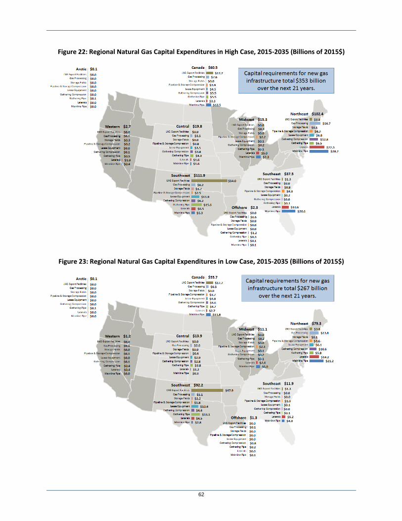
62

Figure 22: Regional Natural Gas Capital Expenditures in High Case, 2015-2035 (Billions of 2015$)

Figure 23: Regional Natural Gas Capital Expenditures in Low Case, 2015-2035 (Billions of 2015$)

63

4.2 Natural Gas Liquids (NGLs)

4.2.1 NGLs Flows and Pipeline Capacity Additions

Dramatic growth in NGLs supply over the past few years has resulted in significant shifts in NGLs market

dynamics. NGLs supply is governed by natural gas production, and high oil and liquids prices from 2010

to 2014 resulted in production from wetter plays. As discussed in section 3.4.4, future growth in NGLs

production is reliant on a variety of shale plays, most notably the Marcellus and Utica, and the growth

hinges on the development of transport capability and markets for the NGLs.

Figure 24 shows a stylistic map for expected NGLs flows in the High and Low Cases; the stylistic maps are

similar to the ones presented in the 2014 INGAA study. Arrows shown on the maps are sized to depict

the relative changes in flow from today through 2035. Arrows that increase in width from their

origination point to the terminus represent an increasing flow over time, and arrows that decrease in

width from their origination point to the terminus represent a declining flow over time. For NGLs

transport, the arrows are color coded and indicate the type of liquid being transported (raw mix, pure

product, and diluent transport). Rail transport corridors are shown as dashed lines, where applicable.

The maps also include “production wedges” that depict relative changes in regional production and

“import and export wedges” that depict relative changes in import and export activity at various

locations.

Figure 24: Natural Gas Liquids Flows – Stylistic maps

Table 18 and Table 19 show the projected takeaway capacity for NGLs in the High Case and the Low

Case, respectively. In the High Case, an overall 2.3 million barrels per day of takeaway pipeline capacity

is added in the United States and Canada from 2015 through 2035, with about 550,000 barrels per day

of capacity installed in 2015. Most of the capacity is added in the Midwest, Northeast, and Southwest,

with the bulk being installed before 2020 (Table 18). In contrast, between 2010 and 2014 about 5.4

million barrels per day of incremental capacity was added. Hence, even under the High Case only about

half of the capacity added in previous five years will be installed over the next 21 years (2015 to 2035).

Low Case High Case

64

The 2014 study projected an incremental takeaway capacity of 3 million barrels per day between 2015

and 2035, which was higher than the current study’s High Case projection.

In the Low Case, the projected takeaway capacity is about half that of the High Case, at only 1.1 million

barrels per day from 2015 through 2035. Essentially, no new NGLs pipelines are projected beyond 2020,

as rail and truck transport continue to dominate because of the uncertain environment of the Low Case

(Table 19).

Table 18: NGLs Takeaway Pipeline Capacity Added in the High Case (Million Bbl/d)

2015 2016 2017-2020

2021-2025

2026-2030

2031-2035

2015-2035

U.S. and Canada 0.6 0.3 1.2 - 0.2 - 2.3

U.S. 0.5 0.3 1.2 - 0.2 - 2.2

Canada 0.1 - - - - - 0.1

Central 0.1 - 0.2 - - - 0.3

Midwest 0.1 0.3 0.4 - 0.2 - 0.9

Northeast 0.1 0.1 0.5 - - - 0.6

Southeast - - - - - - -

Southwest 0.3 - 0.2 - - - 0.4

Western - - - - - - -

Table 19: NGLs Takeaway Pipeline Capacity Added in the Low Case (Million Bbl/d)

2015 2016 2017- 2020

2021- 2025

2026- 2030

2031- 2035

2015- 2035

U.S. and Canada 0.6 0.1 0.4 - - - 1.1

U.S. 0.5 0.1 0.4 - - - 1.0

Canada 0.1 - - - - - 0.1

Central 0.1 - 0.1 - - - 0.2

Midwest 0.1 - 0.1 - - - 0.2

Northeast 0.1 0.1 0.1 - - - 0.2

Southeast - - - - - - -

Southwest 0.3 - 0.2 - - - 0.4

Western - - - - - - -

65

As the stylistic flow maps (Figure 24) indicate, domestic demand is not expected to absorb all of the

growth in NGLs production, opening the doors to more U.S. exports from the Gulf Coast, Mid-Atlantic

(Marcus Hook), and Pacific Northwest, especially with expected rises in competitive prices for North

American liquids in the global market.

Given the significant production of gas in the Marcellus and Utica plays, NGLs production from the

Northeast is expected to grow the most, while more limited growth is expected from the Montney shale

in Western Canada and the Eagle Ford shale in South Texas. Significant investment in infrastructure will

be needed over the next 10 years to link these supplies with market hubs at Mont Belvieu (Texas),

Conway (Kansas), Sarnia (Ontario), and Aux Sable (Illinois). These markets are attractive because of their

relatively high liquidity, storage capacity, and connectivity to other markets, including export facilities,

particularly from Marcus Hook, which is the closest export option for NGLs produced in the Marcellus

and Utica region.

In the High Case, NGLs from the Northeast are projected to be transported as raw NGLs (y-mix) to the

Gulf Coast to supply ethylene crackers and propane dehydrogenation (PDH) facilities in the Gulf Coast. A

limited number of fractionation facilities are also projected in the Northeast. As a result, a large share of

Marcellus and Utica NGLs that are not contracted for exports to Marcus Hook will flow to the Gulf Coast

toward Mont Belvieu, while a smaller share will flow to the Sarnia market in Ontario; projects have been

proposed already to move NGLs along these corridors. Currently, Enterprise Products Partners’

Appalachia-to-Texas pipeline (ATEX) flows ethane and propane from the Marcellus and Utica shales to

Mont Belvieu. Kinder Morgan has proposed the Utica Marcellus-to-Texas Pipeline (UMTP) to transport y-

mix to Mont Belvieu; this pipeline is expected to come online during 2018. In addition, Kinder Morgan

has proposed the Utopia East project (formerly UTOPIA) to transport up to 75,000 bpd of ethane and

ethane-propane mixtures from the Northeast to Windsor, Ontario. Both of these projects are included in

both cases.

In the Low Case, lower NGLs production in the Northeast favors continued rail transport to the Gulf

Coast and other demand centers. Furthermore, with more limited pipeline capacity, more fractionation

facilities are projected in the Northeast, closer to supply sources.

In the Midwest and Central regions, modest production growth in both cases, predominantly from the

Bakken Shale and central Rockies region, is expected to make its way to the Mid-Continent and Gulf

Coast regions via the existing Overland Pass system, the Bakken System, and the Mid-America Pipeline

System. As a result, minimal capacity increases are required in the future as excess supply is transported

via either truck or rail. Several expansions (e.g., Front Range, Southern Lights, and ONEOK), new

pipelines (e.g., Mariner East II), and repurposed oil pipelines (e.g., Enbridge Oil and Vantage) are

expected to go forward in the High Case. In the Low Case, the expected capacity additions are much

lower, as rail and truck transport is expected to dominate.

In Western Canada, liquids production is anticipated to rise through 2035 in both cases, with rail and

trucks being the primary transport option for NGLs. Propane exports to Asian markets, particularly from

the Pacific Northwest, are viable in both cases.

66

4.2.2 Summary of NGLs Metrics

Table 20 provides the key metrics for NGLs infrastructure buildout in both cases. The High Case requires

more than 12,000 miles of new NGLs transmission lines over the projection period (2015 to 2035). The

Low Case, with lower NGLs production growth, will require 20 percent (about 2,400 miles) less new

pipeline installation than the High Case. Without these pipeline additions, NGLs have to be moved using

alternative modes of transportation, principally rail shipments and trucking. Rail and trucks already

transport large volumes of NGLs even though pipelines are generally more economical than these

options.

In the High Case, new lines are supported with over 450,000 horsepower of pumping to move the liquids

through the pipelines. The relatively high pumping need allows for repurposing of oil pipelines with

additional pumping. Fewer pipeline projects in the Low Case results require less new pumping capability

compared with the High Case. The new pumping units in the Low Case call for much less horsepower,

almost 45 percent or about 195,000 horsepower lower compared with the High Case.

In addition to significant investment in new NGLs transportation, the High Case projects almost 3 million

barrels per day of fractionation capacity to separate the liquids into various purity products, and roughly

1.7 million barrels per day of new export capacity to facilitate the movement of liquids to foreign

countries. Most of the new fractionation capacity will be built in the Gulf Coast, the traditional area for

fractionation expansion, as well as in the Midwest and Northeast to support NGLs production growth

from the Marcellus and Utica. In the Low Case, new fractionation and LNG export capacity are lower by

19 percent and 13 percent, respectively, due to lower levels of NGLs production.

Table 20: Natural Gas Liquids Metrics in High Case Versus Low Case

High Case, 2015-2035

High Case

Average Annual

Low Case, 2015-2035

Low Case

Average Annual

Average Annual Change (Low vs High)

Average Annual Change (%, Low vs High)

Miles of Transmission Mainline (1000s) 12.1 0.6 9.7 0.5 -0.1 -20%

Inch-Miles of Transmission Mainline (1000s) 176 8 138 7 -2 -22%

Pump for Transmission Mainline (1000 HP) 454 22 259 12 -9 -43%

Fractionation Capacity Built (MBOE/d) 2,974 142 2,421 115 -26 -19%

NGLs Export Facility Capacity Built (MBOE/d) 1,698 81 1,479 70 -10 -13%

Table 21 compares the NGLs infrastructure metrics with the 2014 study. Except for the export capacity,

all of the liquids metrics in the prior study are similar to the metrics in the High Case scenario from this

study. However, greater NGLs production growth in the High Case (relative to the prior study) results in

higher export volumes. In the Low Case, although there is lower production, lower fractionation capacity

expansion results in greater NGLs exports capability from the United States and Canada, relative to the

prior study.

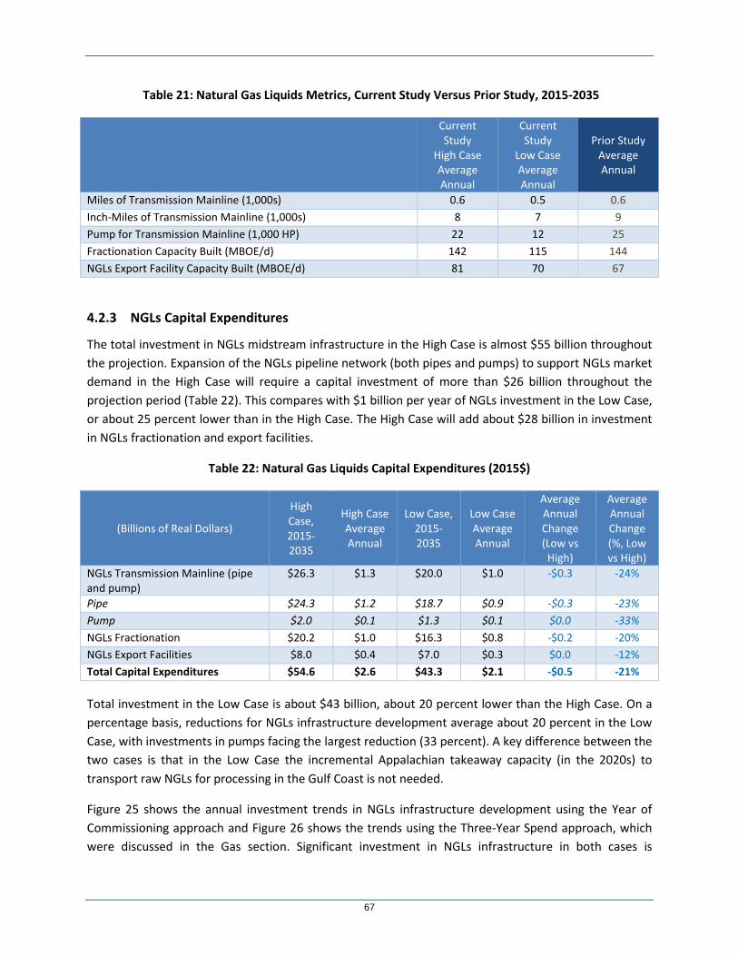
67

Table 21: Natural Gas Liquids Metrics, Current Study Versus Prior Study, 2015-2035

Current Study

High Case Average Annual

Current Study

Low Case Average Annual

Prior Study Average Annual

Miles of Transmission Mainline (1,000s) 0.6 0.5 0.6

Inch-Miles of Transmission Mainline (1,000s) 8 7 9

Pump for Transmission Mainline (1,000 HP) 22 12 25

Fractionation Capacity Built (MBOE/d) 142 115 144

NGLs Export Facility Capacity Built (MBOE/d) 81 70 67

4.2.3 NGLs Capital Expenditures

The total investment in NGLs midstream infrastructure in the High Case is almost $55 billion throughout

the projection. Expansion of the NGLs pipeline network (both pipes and pumps) to support NGLs market

demand in the High Case will require a capital investment of more than $26 billion throughout the

projection period (Table 22). This compares with $1 billion per year of NGLs investment in the Low Case,

or about 25 percent lower than in the High Case. The High Case will add about $28 billion in investment

in NGLs fractionation and export facilities.

Table 22: Natural Gas Liquids Capital Expenditures (2015$)

(Billions of Real Dollars)

High Case, 2015-2035

High Case Average Annual

Low Case, 2015-2035

Low Case Average Annual

Average Annual Change (Low vs High)

Average Annual Change (%, Low vs High)

NGLs Transmission Mainline (pipe and pump)

$26.3 $1.3 $20.0 $1.0 -$0.3 -24%

Pipe $24.3 $1.2 $18.7 $0.9 -$0.3 -23%

Pump $2.0 $0.1 $1.3 $0.1 $0.0 -33%

NGLs Fractionation $20.2 $1.0 $16.3 $0.8 -$0.2 -20%

NGLs Export Facilities $8.0 $0.4 $7.0 $0.3 $0.0 -12%

Total Capital Expenditures $54.6 $2.6 $43.3 $2.1 -$0.5 -21%

Total investment in the Low Case is about $43 billion, about 20 percent lower than the High Case. On a

percentage basis, reductions for NGLs infrastructure development average about 20 percent in the Low

Case, with investments in pumps facing the largest reduction (33 percent). A key difference between the

two cases is that in the Low Case the incremental Appalachian takeaway capacity (in the 2020s) to

transport raw NGLs for processing in the Gulf Coast is not needed.

Figure 25 shows the annual investment trends in NGLs infrastructure development using the Year of

Commissioning approach and Figure 26 shows the trends using the Three-Year Spend approach, which

were discussed in the Gas section. Significant investment in NGLs infrastructure in both cases is

68

expected from 2016 to 2019 because several projects are already under construction and some are in

advanced stages. However, investment falls off significantly after 2020, as the robust growth in NGLs

development over the last few years and in the near term will be adequate to support a significant

portion of the future growth.

A comparison of NGLs infrastructure investments with the 2014 study is provided in Table 23. As with

the metrics discussed earlier, the level of NGLs infrastructure investments in the 2014 study is similar to

the metrics from the High Case of this study.

Table 23: NGLs Capital Expenditures (2015$), Current Study vs. Prior Study, 2015-2035

(Billions of Real Dollars) High Case

Average Annual Low Case

Average Annual Prior Study

Average Annual

NGLs Transmission Mainline (pipe and pump) $1.3 $1.0 $1.2

Pipe $1.2 $0.9 $1.1

Pump $0.1 $0.1 $0.1

NGLs Fractionation $1.0 $0.8 $1.0

NGLs Export Facilities $0.4 $0.3 $0.3

Total Capital Expenditures $2.6 $2.1 $2.4

Figure 25: Annual NGLs Capital Expenditures for New Infrastructure, Year of Commissioning, Billions of 2015 Dollars

69

Figure 26: Annual NGLs Capital Expenditures for New Infrastructure, Three-Year Spread, Billions of 2015 Dollars

4.2.4 Regional NGLs Capital Expenditures

Figure 27 and Figure 28 show regional breakout of total NGLs infrastructure spending in the High Case

and the Low Case throughout the projection period.

In the High Case, large expenditures for NGLs transport are expected in liquids-rich producing regions in

the Northeast, Southwest, Midwest, and Canada. The largest NGLs infrastructure investments will take

place in the Southwest, over $25 billion from 2015 through 2035, driven by large NGLs production

growth from the liquids-rich Eagle Ford, Anadarko Woodford, and Permian plays. The region will require

$6 billion investment in new propane export facilities, almost $10 billion investment for new NGLs

fractionation capacity, and over $9 billion investment in new pipeline infrastructure.

Large expenditures in the Northeast and Midwest derive from the high NGLs production growth from

the Marcellus and Utica. These regions will require more than $10 billion in investments in new pipeline

and pumping capability to transport liquids produced from the Marcellus and Utica for fractionation in

the Gulf Coast. NGLs transport expenditures in Canada mostly support production growth from

Montney, Horn River, and Duvernay.

70

Figure 27: Regional Natural Gas Liquids Capital Expenditures in High Case, 2015-2035 (Billions of 2015$)

Figure 28: Regional Natural Gas Liquids Capital Expenditures in Low Case, 2015-2035 (Billions of 2015$)

71

The uncertainties created by relatively lower liquids prices in the Low Case pose significant risks for new

pipelines. Specifically, subscribers of new capacity are likely to be more hesitant about longer-term

investments and may attach a greater value to optionality (i.e., continuing to rely on rail and truck

transport) in the riskier environment. On the other hand, in areas where supply development is most

cost-effective and not as risky, pipelines remain an attractive alternative because they offer a lower unit

cost for transport compared with rail and trucking alternatives.

In the Low Case, all regions except Northeast will require lower NGLs investment given less robust NGLs

market growth compared with the High Case. The largest impact is seen in the Southwest, where

pipeline investment, fractionation, and export facility developments are all reduced in the Low Case. In

the Northeast, the total infrastructure spending is higher in the Low Case relative to the High Case due

to increased fractionation demand in the Low Case. As discussed earlier, the High Case projects an

incremental $4 billion of Appalachian takeaway capacity to transport raw NGLs for processing in the Gulf

Coast. The Low Case, however, cannot support this transport option because of lower production

growth while higher fractionation capacity is required to process NGLs production growth locally.

4.3 Crude Oil and Lease Condensate

4.3.1 Crude Oil Flows and Pipeline Capacity Additions

Infrastructure for transporting North American crude oil and lease condensate is expected to increase in

the near term, with the bulk of projects coming online between 2016 and 2020. Near-term projects

carry heavy momentum due to recent regulatory approvals and the need to use existing right-of-ways

for a number of expansions. Figure 29 shows the stylistic maps in the High and Low Cases for crude oil

and lease condensate flows. However, the extent of projected infrastructure development is much

smaller than that projected in the 2014 study, as discussed further below.

Figure 29: Crude Oil Flows – Stylistic map

Low Case High Case

72

Table 24 and Table 25 illustrate the potential levels of North American crude oil takeaway capacity

needed over the next 20 years by supply region. As with natural gas and NGLs, most of the crude oil

infrastructure needed for the next 20 years will be placed in service between 2016 and 2020. Significant

capacity is also projected to have been placed into service in 2015.

Table 24: Crude Oil and Lease Condensate Takeaway Pipeline Capacity Added in the High Case (Million Bbl/d)

2015 2016 2017-2020 2021-2025 2026-2035 2015-2035

U.S. and Canada 3.3 1.2 2.0 0.5 - 6.9

U.S. 1.6 0.6 0.8 0.1 - 3.2

Canada 1.7 0.5 1.2 0.4 - 3.8

Central - - 0.5 0.1 - 0.6

Midwest 1.3 0.6 - - - 2.0

Northeast - - - - - -

Offshore - - - - - -

Southeast - - - - - -

Southwest 0.3 - 0.3 - - 0.6

Western - - - - - -

Table 25: Crude Oil and Lease Condensate Takeaway Pipeline Capacity Added in the Low Case (Million Bbl/d)

2015 2016 2017-2020 2021-2025 2026-2035 2015-2035

U.S. and Canada 3.3 1.2 - - - 4.5

U.S. 1.6 0.6 - - - 2.3

Canada 1.7 0.5 - - - 2.2

Central - - - - - -

Midwest 1.3 0.6 - - - 2.0

Northeast - - - - - -

Offshore - - - - - -

Southeast - - - - - -

Southwest 0.3 - - - - 0.3

Western - - - - - -

73

In the 2014 study, the total projected crude oil and lease condensate takeaway capacity additions

between 2015 and 2035 were 7.9 million barrels per day, higher than the High Case projection of 6.9

million barrels per day and much higher than the $4.5 million projected in the Low Case. In comparison,

over the past five years (2010-2014) incremental capacity additions totaled 7.5 million barrels per day—

indicating that sufficient capacity has been built already and only a limited amount of incremental

capacity is necessary in 2016 and beyond, especially given projected oil prices.

Because of declining production and an increase in rail utilization needed to maintain optionality under

uncertain prices, there is a sharp drop-off in required pipeline infrastructure post-2025 in both cases.

One key uncertainty that could change this dynamic is increased export of crude oil. Higher exports

could require more capacity additions to accommodate increased flows to export regions—likely in the

Gulf Coast, Mid-Atlantic, and the Pacific Northwest.

Despite declining production in many regions including the Bakken Shale, the Rockies, and the Eagle

Ford, recent investment in refineries in the Midwest, Mid-Continent, and Gulf Coast is expected to keep

North American crude oil consumption relatively stable. As a result, the market supports incremental

infrastructure additions to these demand centers, particularly in the High Case.

In the High Case, crude oil flows from the Bakken as well as the oil sands in Western Canada will flow

toward the Central and Midwest U.S. regions as a number of proposed projects come online over the

next four years. As crude makes its way to these regions, it will either be consumed by local refineries or

will continue flowing via existing pipeline infrastructure and rail to Cushing, Oklahoma, as well as the

Gulf Coast regions.

In the Low Case, lower production out of the Bakken does not support incremental increases in pipeline

infrastructure, and therefore crude oil is moved by rail or existing pipelines. Crude still flows from

Western Canada to the U.S. Central and Midwest on pipeline projects that are expected to come online

during 2016. Similar to the High Case, crude oil that is not consumed at local refineries will be

transported to Cushing, Oklahoma or the Gulf Coast by rail or existing pipeline infrastructure.

In both cases, Eagle Ford production is forecast to decline; however, despite the decrease in local

production, there will still be sufficient supply for Gulf Coast refineries, thanks to an influx of crude

accumulating in the Mid-Continent region as well as from West Texas. Foreign imports are likely to

decline in both cases, as refineries in the Gulf Coast consume more domestically available crude.

In the High Case, pipeline capacity is built between West Texas and the Gulf Coast as production grows

modestly in the Permian Basin. In the Low Case, however, crude is shipped via rail and trucks as a

relatively flat supply growth profile does not support pipeline investment.

A number of pipeline projects have been proposed in Canada. Most of these projects seek to move

crude from Northern Alberta to Southern Alberta, where it can be transported to a number of markets

via pipeline or rail. In both cases, the study forecasts an increase in flows to the West Coast for eventual

exports, and to the Midwest to meet refinery demand. As a result, the study places new incremental

74

infrastructure along each of these corridors from Western Canada. For example, TransCanada’s project

is proposed to carry roughly 1.1 million barrels per day from Western Canada to Ontario.

4.3.2 Crude Oil Metrics

Crude oil development metrics are compared in Table 26. In the High Case, about 565,000 new oil wells

are needed to maintain the required production levels, compared with 455,000 wells (a 19-percent

reduction) in the Low Case. Connecting these new oil wells to pipelines will require over 100,000 miles

of gathering line connections in the High Case and roughly 85,000 miles in the Low Case (a 17-percent

reduction).

Table 26: Crude Oil Metrics

High Case, 2015-2035

High Case

Average Annual

Low Case, 2015-2035

Low Case

Average Annual

Average Annual Change (Low vs High)

Average Annual Change (%, Low vs High)

Oil Well Completions (1,000s) 565 27 455 22 -5 -19%

Miles of Crude Oil Gathering Line (1,000s) 101.3 4.8 84.2 4.0 -0.8 -17%

Miles of Transmission Mainline (1,000s) 6.6 0.3 2.6 0.1 -0.2 -61%

Miles of Crude Oil Storage Laterals (1,000s) 0.3 0.0 0.2 0.0 0.0 -49%

Inch-Miles of Crude Oil Gathering Line (1,000s)

236 11 196 9 -2 -17%

Inch-Miles of Transmission Mainline (1,000s) 211 10 81 4 -6 -62%

Inch-Miles of Crude Oil Storage Laterals (1,000s)

5 0 3 0 0 -49%

Pump for Transmission Mainline (1,000 HP) 2,165 103 848 40 -63 -61%

Crude Storage Capacity Built (MMBbl) 50 2 28 1 -1 -44%

Number of Crude Storage Tanks Built 10,013 477 5,582 266 -211 -44%

Number of Crude Storage Farms Built 15 1 8 0 0 -49%

Even in the Low Case, new oil wells are needed to maintain production with the faster decline profile of

oil wells in the shale oil and tight oil plays. Tight oil wells feature a rapid production decline profile

within the first couple of years of production, and therefore incremental well completions are needed to

replace the production decline from existing wells. These new well completions result in significant

growth in the midstream infrastructure development (even in the Low Case).

The High Case projects about 6,600 miles of new oil pipeline (including both mainline and laterals

projects) supported by roughly 2.2 million horsepower of new pumping capability from 2015 to 2035.

Declining oil production projected in the Low Case results in a reduction of 60 percent (4,000 miles) in

new crude oil pipeline requirements relative to the High Case. New pumping capability for oil transport

in the Low Case is reduced by over 1.3 million horsepower, a 60-percent reduction.

The amount of storage capacity is expected to be limited in both cases (about 50 million barrels are

projected in the High Case and 30 million barrels in the Low Case), resulting in reduced mileage of

storage laterals. New crude oil capacity is vital to ensuring that production can be stored temporarily

75

when refineries are removed from service for maintenance and to enable producers to manage

imbalances in markets. The number of crude oil farms and tanks for storage is significantly lower in the

Low Case, down by an average 45 percent from the High Case (Table 26).

The alternative to pipeline transport of oil is increased reliance on rail and trucks, and our projection

assumes that the levels of rail and truck transport of crude oil remain fairly constant with today’s levels.

As discussed earlier, rail and truck movement is more flexible than pipeline transport because routes

can shift in response to market conditions.

Table 27 compares crude oil infrastructure development with the 2014 study, which assumed a flat

crude oil price of over $100/bbl (in 2015 dollars) throughout the projection. Lower prices and slower

trends result in much lower crude production growth in this study, and in a significant reduction in the

development of all crude oil infrastructure compared with the prior study.

Table 27: Crude Oil Metrics, Current Study Versus Prior Study, 2015-2035

High Case Average Annual

Low Case Average Annual

Prior Study

Average Annual

Oil Well Completions (1,000s) 27 22 41

Miles of Crude Oil Gathering Line (1,000s) 4.8 4.0 7.8

Miles of Transmission Mainline (1,000s) 0.3 0.1 0.6

Inch-Miles of Crude Oil Gathering Line (1,000s) 11 9 17

Inch-Miles of Transmission Mainline (1,000s) 10 4 16

Pump for Transmission Mainline (1,000 HP) 103 40 131

Crude Storage Capacity Built (MMBbl) 2 1 5

Number of Crude Storage Tanks Built 477 266 980

Number of Crude Storage Farms Built 1 0 1

4.3.3 Crude Oil Capital Expenditures

The High Case is projected to require about $190 billion of investments in midstream infrastructure

throughout the projection (Table 28), and investments in the Low Case are lower by about 28 percent

($52 billion), relative to the High Case. In the High Case, expansion of the existing oil pipeline grid,

including oil gathering lines and pumping capability, requires a capital expenditure totaling almost $46

billion throughout the projection period, and in the Low Case $21 billion is necessary (more than a 50-

percent reduction relative to the High Case).

In addition to investment in oil pipelines, more than $140 billion is necessary in the High Case for new

surface equipment to support incremental oil production. The surface equipment includes pumps,

valves and manifolds, flowlines and connections, stock tanks, separators, and heater-treaters. The Low

Case requires about 20 percent less investment in new oil surface equipment, consistent with the

reduction in new well completions. Investments in new oil storage terminals will be modest ($0.7 billion

in the High Case and $0.4 billion in the Low Case), as oil production growth in the both cases is limited.

76

As with NGLs, the uncertainties from lower crude oil prices in the Low Case pose risks for new pipeline

investments, as subscribers of new capacity are likely to be more hesitant about longer-term

investments in the Low Case. Hence, rail and trucking services are expected to remain robust.12

Table 28: Crude Oil Capital Expenditures (2015$)

(Billions of Real Dollars) High Case,

2015-2035

High Case Average Annual

Low Case, 2015-2035

Low Case Average Annual

Average Annual Change (Low vs High)

Average Annual Change (%, Low vs High)

Crude Oil Gathering Line (pipe only) $9.3 $0.4 $7.7 $0.4 -$0.1 -17%

Crude Oil Lease Equipment $142.8 $6.8 $115.2 $5.5 -$1.3 -19%

Crude Oil Transmission Mainline (pipe and pump)

$36.4 $1.7 $13.8 $0.7 -$1.1 -62%

Pipe $29.4 $1.4 $10.8 $0.5 -$0.9 -63%

Pump $7.0 $0.3 $3.0 $0.1 -$0.2 -57%

Crude Oil Storage Laterals $0.7 $0.0 $0.3 $0.0 $0.0 -48%

Crude Oil Storage Tanks $0.7 $0.0 $0.4 $0.0 $0.0 -40%

Total Capital Expenditures $189.8 $9.0 $137.5 $6.5 -$2.5 -28%

Annual investment trends of crude oil infrastructure development are shown in Figure 30, using the Year

of Commissioning approach. The Three-Year Spread approach shown in Figure 31 shows a smoother

near-term spending trend. Large investments in midstream infrastructure in both cases to support oil

production is unlikely under the projected oil price scenarios. While investments in new well

competitions and gathering lines will continue, there will be fewer large pipelines being constructed for

oil transport in both cases.

Peak investment for crude oil infrastructure was reached in 2014, when oil prices were well above $100

per barrel. The decline in infrastructure development started in 2015 and is expected to decline further

in both cases through 2018. Crude oil price recovery, starting in 2020, has a positive impact on

infrastructure development thereafter. The Energy East pipeline project is expected to dominate

expenditures in 2019 in the High Case (as noted earlier, this project is not expected to come online in

the Low Case). In 2022, condensate exports from British Columbia result in higher expenditures in both

cases.

12 Investments in rail and trucking transport options are not considered here.

77

Figure 30: Annual Crude Oil Capital Expenditures for New Infrastructure, Year of Commissioning, Billions of 2015 Dollars

Figure 31: Annual Crude Oil Capital Expenditures for New Infrastructure, Three-Year Spread, Billions of 2015 Dollars

78

Crude oil infrastructure investments are compared with the 2014 study in Table 29. The 2014 study

projects much higher crude oil infrastructure investments largely because it assumed $100/barrel oil

prices for the projection period. The total expenditure in the 2014 study was about $3.5 billion (or 40

percent) more than the projected expenditures in the High Case, and nearly 90 percent higher than the

Low Case expenditures.

Table 29: Crude Oil Capital Expenditures (2015$), Current Study Versus Prior Study, 2015-2035

(Billions of Real Dollars) High Case

Average Annual Low Case

Average Annual Prior Study

Average Annual Crude Oil Gathering Line (pipe only) $0.4 $0.4 $0.6

Crude Oil Lease Equipment $6.8 $5.5 $9.1

Crude Oil Transmission Mainline (pipe and pump) $1.7 $0.7 $2.5

Pipe $1.4 $0.5 $2.2

Pump $0.3 $0.1 $0.4

Crude Oil Storage Laterals $0.0 $0.0 $0.1

Crude Oil Storage Tanks $0.0 $0.0 $0.1

Total Capital Expenditures $9.0 $6.5 $12.4

4.3.4 Regional Crude Oil Capital Expenditures

As with natural gas and NGLs, the largest infrastructure investment in the High Case is projected to be in

the Southwest region (Figure 32) due to significant activities in the Permian, South Texas, and the

relatively new SCOOP and STACK plays in Oklahoma. The region’s total expenditures through 2035 are

projected to be over $96 billion, which is more than 50 percent of total oil-related expenditures in the

U.S. and Canada. Most of the expenditures in the Southwest region (85 percent) will be in new surface

equipment to support incremental oil production. Robust investment in Canada, over $40 billion

throughout the projection, is driven by oil sands development in Alberta. Investments in the Central

region total $33 billion due to developments in the Bakken and Niobrara tight oil plays.

All regions in the Low Case will experience flat or declining oil production (Figure 33), resulting in lower

oil infrastructure expenditures across all regions and asset categories compared with the High Case. The

reduction in the U.S. Central region and Canada is about $25 billion in total, accounting for about 47

percent of the change. The Southwest region will also be hit hard. Of the $52 billion reduction in oil

infrastructure investments in the Low Case, 36 percent ($19 billion) will be in the Southwest. Declines in

tight oil development in these regions is the primary reason for reduced investment in the Low Case,

particularly in the lease equipment category.

79

Figure 32: Regional Crude Oil Capital Expenditures in High Case, 2015-2035 (Billions of 2015$)

Figure 33: Regional Crude Oil Capital Expenditures in Low Case, 2015-2035 (Billions of 2015$)

80

4.4 Summary of Midstream Infrastructure Metrics and Expenditures

4.4.1 Capital Expenditures for New Infrastructure

Total infrastructure investments in the two scenarios are substantial (Figure 34)—about $600 billion (in

2015 dollars) in the High Case and about $450 billion in the Low Case from 2015 to 2035. Overall

expenditure is lower by $150 billion in the Low Case relative to the High Case, with oil and gas being

more affected than NGLs. In the Low Case, infrastructure expenditure is smaller than the High Case, but

is still prompted by continued production increases and regional investments supporting takeaway

capacity out of the Northeast and LNG exports.

Figure 34: Capital Expenditures for New Infrastructure (Billions of 2015$)

Figure 35 shows how required investments are spread over time using the same methodology used in

the 2014 INGAA study. As mentioned earlier, in this approach the capital expenditures are assumed to

be spent in the same year the infrastructure is put in place. Figure 36 shows annual expenditure trend

using the Three-Year Spread methodology.

81

Figure 35: Annual Capital Expenditures for New Infrastructure, Year of Commissioning, Billions of 2015 Dollars

Figure 36: Annual Capital Expenditures for New Infrastructure, Three-Year Spread, Billions of 2015 Dollars

In the near term, the oil, gas, and NGLs infrastructure investments are expected to be robust, as several

projects are already under construction or well along in the planning stage for commissioning in 2016.

Midstream infrastructure development over the past three years (2013 to 2015) has also been strong

and investment in new infrastructure in 2015 is expected to be about $44 billion. This period of

relatively high growth in infrastructure development will create an “overbuild” condition that leads to

weak investments in the long term. In the High Case, average investment between 2016 and 2019 is

almost $55 billion per year, more than twice the average investment of about $21 billion per year

82

between 2020 and 2035. In the Low Case, average investments are expected to be delayed in the near

term, with about $43 billion per year in the 2016-2019 period, and $14.5 billion per year between 2020

and 2035.

The Three-Year Spread approach suggests that expenditure for oil, gas and NGLs infrastructure

investments in the Low Case has already peaked in 2014 and has started to slow down, while in the High

Case the peak will occur in 2016, primarily due to U.S. LNG projects. It also suggests that overall

investments will slow significantly by 2020. Increased investments in 2025 in both cases are due to LNG

exports from Canada. While the reduction in the midstream infrastructure expenditure relative to the

recent past seems to be more striking in this “smoothed” approach, the future trend beyond 2018 and

2019 is for lower investment in midstream infrastructure development.

4.4.2 Pipeline Miles, Compression, and Capital Expenditures by Diameter Class and Type of

Transport

In the High Case scenario, 330,000 miles of new gathering and transport pipeline and almost 19 million

horsepower for new compression and pumping capabilities will be required over the 20-year period of

2015 to 2035 (Table 30 and Table 31). In contrast, the 2014 study estimated 510,000 miles of new pipes

and 15 million horsepower of new compression and pumping capabilities. New pipeline requirements in

the Low Case are lower by 65,000 miles (or 20 percent) and 5.5 million horsepower (30 percent)

compared with the High Case by 2035. This includes gathering lines and pipeline transport for gas, NGLs,

and crude oil and also compression and pumping requirements in the United States and Canada.

Table 30: Gathering and Transmission Pipeline Miles, 2015-2035

Pipeline (Thousand Miles)

1" to ≤ 8" > 8" to ≤ 16" > 16" to ≤ 24" > 24" Total % of Total

HIGH CASE

Natural Gas 163.4 21.2 11.8 12.2 208.6 63%

NGL 0.5 10.7 0.8 0.1 12.1 4%

Crude Oil 101.3 0.6 1.2 5.1 108.2 33%

Total 265.3 32.5 13.8 17.4 329.0 100%

LOW CASE

Natural Gas 136.4 16.9 6.5 7.6 167.4 63%

NGL 0.5 8.5 0.5 0.1 9.7 4%

Crude Oil 84.2 0.2 0.6 2.0 86.9 33%

Total 221.1 25.6 7.6 9.7 264.0 100%

83

Table 31: Compression and Pump Requirements, 2015-2035

Compression and Pump (Thousand

HP)

1" to ≤ 8"

> 8" to ≤ 16"

> 16" to ≤ 24"

> 24" Total % of Total

HIGH CASE

Natural Gas 4,875 6,900 294 3,861 15,930 86%

NGL 303 102 33 16 454 2%

Crude Oil 35 15 151 1,964 2,165 12%

Total 5,213 7,017 477 5,841 18,549 100%

LOW CASE

Natural Gas 3,897 5,194 168 2,621 11,881 91%

NGL 147 75 22 16 259 2%

Crude Oil 35 10 68 735 848 7%

Total 4,079 5,279 258 3,372 12,988 100%

The required capital expenditure in the High Case for the gathering and transmission pipeline,

compression, and pumping is projected to total about $280 billion (in 2015 dollars) over the projection

period. In the 2014 study, the total pipeline capital expenditure was estimated at a similar amount of

$295 billion (in real 2015 dollars), with natural gas accounting for about 70 percent of the investment.

The mix of expenditures across hydrocarbon type is similar in both cases. About 75 percent of the

expenditures for pipelines in both the High and Low Cases will be for natural gas gathering and

transport, with oil and NGLs gathering and transport accounting for the remainder. Total pipeline,

compression, and pumping expenditures in the Low Case are projected to total about $180 billion (in

2015 dollars) throughout the projection period, over 35 percent less than the roughly $280 billion in the

High Case. The largest percentage reduction is in crude oil infrastructure development (over 50 percent)

due to lower oil price assumptions lowering the crude oil production projections (Table 32).

Table 32: Pipeline Capital Expenditures, 2015-2035

Capital Expenditures

(Billions of 2015$) 1" to ≤ 8" > 8" to ≤ 16" > 16" to ≤ 24" > 24" Total

% of Total

HIGH CASE

Natural Gas $33.6 $48.0 $45.6 $81.8 $209.0 74%

NGL $2.0 $21.0 $3.1 $0.2 $26.3 9%

Crude Oil $9.4 $0.9 $4.2 $31.8 $46.4 16%

Total $45.1 $69.9 $52.8 $113.9 $281.6 100%

LOW CASE

Natural Gas $27.8 $36.5 $25.3 $51.9 $141.5 77%

NGL $1.5 $16.1 $2.1 $0.2 $20.0 11%

Crude Oil $7.8 $0.4 $1.5 $12.2 $21.9 12%

Total $37.2 $52.9 $28.9 $64.3 $183.3 100%

84

The expenditures shown in Table 32 do not include incremental integrity management capital

expenditures for natural gas transmission pipelines. These expenses are estimated at another $24 billion

throughout the projection period, as discussed in the next section.

Historically, the industry has proven its ability to finance and construct the levels of pipeline and

gathering capability projected in the two cases. Industry investments in new gathering and transport

lines have averaged about $15 billion per year over the past decade; hence, the levels of projected

future investment are consistent with the pipeline construction that already has occurred. During the

past decade, companies active in the midstream space have placed into service roughly 15,000 miles of

new natural gas pipelines at a cost of more than $50 billion, which is consistent with projected

expenditures in the large-diameter category.

Pipes with a diameter greater than 24 inches will account for more than 40 percent of the pipeline and

gathering line investments in the High Case (and 35 percent in the Low Case) even though they account

for only about 5 percent of the total miles added over the forecast period (2015-2035).13 Pipes with

diameters less than or equal to eight inches account for the majority of new pipe mileage that is needed

over time, but investment in such facilities is more modest at 16 percent of the total investment in the

High Case (and 20 percent in the Low Case). These smaller-diameter pipes are mostly used for gathering

gas, oil, and NGLs.

The percentage decrease in small-diameter pipes in the Low Case is much smaller, about half that for

higher-diameter pipes, as significant investment is needed for gathering systems due to the nature of

production profile of wells in the shale plays. Furthermore, gathering lines (small-diameter pipe) are

location-specific (i.e., as new areas are developed, additional gathering lines are needed to transport the

produced hydrocarbons directly to processing plants or to other larger-diameter gathering systems).

13 This is because pipes of that size have a much greater unit cost than smaller-diameter pipes.

85

5 Incremental Expenditures for Integrity Management and NOx Control

5.1 Methodology and Assumptions PHMSA’s existing Gas Transmission Integrity Management Rule (49 CFR Part 192, Subpart O) specifies

how pipeline operators must identify, prioritize, assess, evaluate, repair, and validate the integrity of gas

transmission pipelines in High Consequence Areas (HCAs)—i.e., specific areas with populated and

occupied areas. Pipeline operators already plan to conduct replacement and refurbishment of pipelines

for integrity management. Integrity inspections may be performed by several methods: (1) an internal

“in-line” inspection using a “smart pig” device; (2) hydrostatic pressure testing (filling the pipe with

water and pressurizing it well above operating pressures to verify a safety margin); (3) direct assessment

(digging up and visually inspecting sections of pipe) or (4) “other alternative methods that the Secretary

of Transportation determines would provide an equal or greater level of safety.” The pipeline operator is

required by PHMSA regulations to repair all non-innocuous imperfections and adjust operation and

maintenance practices to minimize “reportable incidents.”14 The capital expenses associated with such

routine replacement and refurbishment of natural gas transmission pipelines are included in the

expenditures shown earlier.

However, pipeline owners now expect to make additional capital expenditures, including an estimated

incremental expenditure of $24 billion for integrity management and NOx control, as part of the total

expenditure on pipelines. This incremental amount represents additional expenditures for integrity

management activities that were anticipated at the time this study was prepared and emissions control

requirements to satisfy new ambient air (NAAQS) standards for nitrogen oxides (NOx). This incremental

expenditure should be interpreted as a ballpark estimate at this point in time because estimated

integrity management costs have not been adjusted to reflect the particulars of PHMSA’s recently

proposed pipeline safety rules.

The new National Ambient Air Quality Standards (NAAQS) for ozone and the one-hour nitrogen dioxide

(NO2) emissions, which are precursors to ozone formation, potentially require the reduction of NOx

from existing compression equipment, as a significant number of stationary engines drive natural gas

compressors in interstate natural gas pipelines. However, litigation and scheduling delays have slowed

the regulatory process. While there is uncertainty about the breadth (i.e., how geographically broad),

depth (i.e., stringency of the rule), and schedule for complying with the new NOx regulations, it is likely

that many of the natural-gas-fired reciprocating engines in the existing prime mover fleet will require

NOx control by 2025.15

INGAA Foundation wished to include the incremental capital expenditure that could be spent by natural

gas pipeline owners over the coming decade in this study. As such, this study includes the capital portion

of the incremental expenditure that is planned for in-line inspection, hydrostatic testing, and valve

14 http://www.ingaa.org/cms/4925.aspx 15 http://www.ingaa.org/Foundation/Foundation-Reports/NOx.aspx

86

automation, as well as the incremental capital expenditure that is planned for upgrading existing

reciprocating engines with low NOx control to meet the new NAAQS standards.

5.2 Total Capital Expenditure for Midstream Infrastructure The expenditures information was provided to ICF by the INGAA Foundation, and the regional breakout

of the anticipated expenditures is shown in Table 33.

Table 33: Incremental Capital Expenditure Estimates in U.S. (Billions of 2015$), 2015-2035

Gas Pipelines and

Compressors

Central $4.4

Midwest $3.4

Northeast $2.4

Offshore $0.2

Southeast $3.7

Southwest $7.6

Western $2.1

Arctic $0.1

Total $23.9

Figure 37: Total Capital Investments for Midstream Infrastructure, Including Incremental Integrity Management and NOx Control Expenditures

87

Total capital expenditures for integrity management on pipelines and installing low-NOx equipment on

compressors will be about $24 billion from 2015 through 2035. A third of the incremental replacement

and refurbishment of natural gas pipelines will occur in the Southwest region, given that this region has

a large mileage of pipelines that are of older vintage. The Central, Midwest, and Southeast regions are

next in line (with about 15 to 20 percent of total expenditures each), given that these regions have older

pipelines that require additional integrity management. The expenditures for compressor upgrades are

similar to those for pipelines.

The addition of the $24 billion of incremental capital expenditures to the total expenditures discussed

earlier brings the total midstream infrastructure investments to about $621 billion in the High Case and

$471 billion in the Low Case. The pie chart in

Figure 37 summarizes total infrastructure expenditures projected across oil, gas, and NGLs for both

scenarios after adding the incremental capital expenditures discussed in this section.

These total expenditures are used for the economic analysis appearing in the following sections.

88

6 Economic Impact Methodology Assumptions

6.1 IMPLAN Modeling As with the previous INGAA studies, this study uses IMPLAN modeling for economic impact analysis.

IMPLAN, a proprietary model maintained by the Minnesota IMPLAN Group (http://www.implan.com), is

a widely used and effective regional economic analysis model that uses average expenditure data from

industries. Expenditures in these industries “reverberate” up to the supplier industries; IMPLAN traces

and calculates the multiple rounds of secondary indirect and induced economic impacts throughout the

supply chain for each region.

The model uses multipliers to trace and calculate the flow of dollars from the industries that originate

the economic activity to supplier industries that generate additional activity. These multipliers are thus

coefficients that “describe the response of the economy to a stimulus (a change in demand or

production).” Three types of impacts are used in IMPLAN:

• Direct—represents the economic impacts (e.g., employment or output changes) due to the

direct investments, such as payments to companies in the relevant industries for the asset

category in this study (see Table 34).

• Indirect—represents the economic impacts due to the industry interlinkages caused by the

iteration of industries purchasing from industries and brought about by the changes in final

demands (e.g., when a pipeline manufacturer purchases steel from another company).

• Induced—represents the economic impacts on all local industries from consumers’

consumption expenditures arising from the new household incomes that are generated by

the direct and indirect effects of the final demand changes (e.g., a worker purchases new

clothing or purchases food in restaurants).

The total impact is simply the sum of the direct and the multiple rounds of secondary indirect and

induced impacts that occur within the region. IMPLAN then uses this total impact to calculate

subsequent impacts such as total jobs created, total labor income, total value added or gross domestic

product (GDP), and tax impacts. This methodology, and the use of IMPLAN is well-established and

consistent with numerous other studies.

6.2 National-Level Economic Impacts In this study, IMPLAN is used to calculate national-level economic impacts. Input to the IMPLAN model is

a set of direct investments or capital expenditures (i.e., Direct Output in IMPLAN modeling) by industry.

For IMPLAN modeling, the capital expenditures in this study are grouped into eleven asset categories:

• Gathering Line (excludes compressors)

• Lease Equipment

• Gas Processing

• Pipeline (excludes compressors and pumps)

• Compressors (gathering line, pipeline, and gas storage)

• Pumps

89

• Underground Gas Storage (excludes compressors and pipelines)

• LNG Plant

• NGLs Fractionation Plant

• NGLs Export Facility

• Crude Oil Storage Tanks

The IMPLAN model considers hundreds of industries associated with the eleven assets listed above. In

this report, the larger set of industries considered by IMPLAN are categorized into six industry sectors:

• Oil, Gas, & Other Mining

• Construction

• Manufacturing

• Wholesale and retail trade

• Transportation

• Services & All Other

The relevant IMPLAN industries for the six industry sectors are shown in Appendix C. Table 34 provides

allocations of capital expenditures by industry sector for each asset category in the national IMPLAN

analysis. The Services & All Other category includes services outside of the energy business, including

hotels, restaurants, and merchandise providers. The allocations vary depending on the type of

infrastructure for the investment. Asset category Pipeline (excludes compressors and pumps), for

example, allocates 36.2 percent of the capital expenditures to industry sector Construction, 29.4 percent

to Manufacturing, 26.5 percent to Services & All Other, and the remainders to Oil, Gas, & Other Mining,

Transportation, and Wholesale and Retail Trade. In the total of all asset categories, more than 70

percent of the investment expenditures will be in manufacturing, construction, and oil and gas industry

sectors.

These allocations are based on expenditures by individual IMPLAN industries (see Appendix C). In the

Pipeline asset category, for example, most of the expenditures in industry sector Construction, over 85

percent, is allocated to IMPLAN industry “Steel product manufacturing from purchased steel,” and over

10 percent is allocated to IMPLAN industry “Valve and fittings other than plumbing manufacturing.”

Using the allocations shown in Table 34, eleven investment expenditure sets are created for each of the

two scenarios and the economic impacts of these expenditures are then calculated using a national

IMPLAN analysis for each of the eleven investment expenditure sets. Results from IMPLAN include

direct, indirect, and induced impacts for jobs created, labor income, and value added or GDP by industry

sector.

National-level tax revenues (Federal and state/provincial/local) are then calculated from total value

added and tax rates on GDP. Table 35 provides tax rates on GDP assumed for Federal and

state/province/local government throughout the projection. Total Federal and local tax rates will

average 35 percent in the United States and 31 percent in Canada.

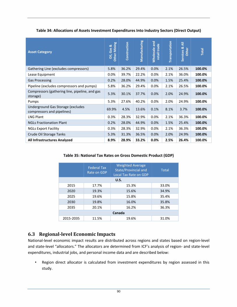
90

Table 34: Allocations of Assets Investment Expenditures Into Industry Sectors (Direct Output)

Asset Category

Oil,

Gas

&

Oth

er

Min

ing

Co

nst

ruct

ion

Man

ufa

ctu

rin

g

Wh

ole

sale

an

d

reta

il tr

ade

Tran

spo

rtat

ion

Serv

ice

s &

All

Oth

er

Tota

l

Gathering Line (excludes compressors) 5.8% 36.2% 29.4% 0.0% 2.1% 26.5% 100.0%

Lease Equipment 0.0% 39.7% 22.2% 0.0% 2.1% 36.0% 100.0%

Gas Processing 0.2% 28.0% 44.9% 0.0% 1.5% 25.4% 100.0%

Pipeline (excludes compressors and pumps) 5.8% 36.2% 29.4% 0.0% 2.1% 26.5% 100.0%

Compressors (gathering line, pipeline, and gas storage)

5.3% 30.1% 37.7% 0.0% 2.0% 24.9% 100.0%

Pumps 5.3% 27.6% 40.2% 0.0% 2.0% 24.9% 100.0%

Underground Gas Storage (excludes compressors and pipelines)

69.9% 4.5% 13.6% 0.1% 8.1% 3.7% 100.0%

LNG Plant 0.3% 28.3% 32.9% 0.0% 2.1% 36.3% 100.0%

NGLs Fractionation Plant 0.2% 28.0% 44.9% 0.0% 1.5% 25.4% 100.0%

NGLs Export Facility 0.3% 28.3% 32.9% 0.0% 2.1% 36.3% 100.0%

Crude Oil Storage Tanks 5.3% 31.3% 36.5% 0.0% 2.0% 24.9% 100.0%

All Infrastructures Analyzed 8.9% 28.9% 33.2% 0.0% 2.5% 26.4% 100.0%

Table 35: National Tax Rates on Gross Domestic Product (GDP)

Federal Tax

Rate on GDP

Weighted Average State/Provincial and

Local Tax Rate on GDP Total

U.S.

2015 17.7% 15.3% 33.0%

2020 19.3% 15.6% 34.9%

2025 19.6% 15.8% 35.4%

2030 19.8% 16.0% 35.8%

2035 20.1% 16.2% 36.3%

Canada

2015-2035 11.5% 19.6% 31.0%

6.3 Regional-level Economic Impacts National-level economic impact results are distributed across regions and states based on region-level

and state-level “allocators.” The allocators are determined from ICF’s analysis of region- and state-level

expenditures, industrial jobs, and personal income data and are described below:

• Region direct allocator is calculated from investment expenditures by region assessed in this

study.

91

• Infrastructure projects in each asset category and region are mapped to states to calculate

state-level investment expenditures by asset category. State direct allocator is based on

investment expenditures by state.

• State indirect industrial jobs allocator is the weighted average of industries that support

construction and equipping industrial activities based on IMPLAN input-output model and U.S.

Bureau of Labor statistics data. Region indirect industrial jobs allocator, as shown in Table 36, is

calculated from state data.

• State personal income allocator is based on state personal income FY 2013 from Tax Policy

Center data. Region personal income allocator, as shown in Table 36, is calculated from state

data.

• U.S. state/local tax allocator is based on “State and Local General Revenue as a Percentage of

Personal Income FY 2013” from the Urban Tax Policy Center. State/local tax allocator by region,

as shown in Table 37, is calculated from state data.

The following procedure describes the assumptions on how the national-level economic impacts

calculated using IMPLAN are distributed to regions.

• National “direct” impacts (e.g., direct value added) are distributed to regions and states based

on region and state direct allocators. Investment expenditures for the U.S. Offshore region are

assumed to be spent in the Southwest region and the corresponding states.

• National “indirect” impacts (e.g., indirect value added) are distributed to regions and states

based on a combination of region and state direct allocators (60 percent weight) and indirect

industrial jobs allocators (40 percent weight).

• National “induced” impacts are distributed to regions and states based on a combination of

region and state “Direct & Indirect Value Added” allocators (40 percent weight) and personal

income allocators (60 percent weight). Region and state “Direct & Indirect Value Added”

allocators are calculated from the sum of region and state direct value added and indirect value

added, as discussed above.

• Total U.S. state and local tax revenues are distributed to regions and states based on U.S.

state/local tax allocator.

Table 36: Region-Level Allocators for Economic Impacts

Region Indirect Industrial Jobsa State Personal Income 2013

b

Central 6.6% 7.7%

Midwest 26.8% 15.9%

Northeast 25.7% 27.5%

Southeast 16.5% 17.4%

Southwest 12.7% 11.7%

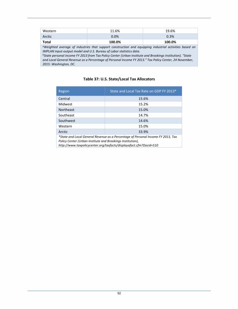
92

Western 11.6% 19.6%

Arctic 0.0% 0.3%

Total 100.0% 100.0% aWeighted average of industries that support construction and equipping industrial activities based on IMPLAN input-output model and U.S. Bureau of Labor statistics data. bState personal income FY 2013 from Tax Policy Center (Urban Institute and Brookings Institution). “State and Local General Revenue as a Percentage of Personal Income FY 2013.” Tax Policy Center, 24 November, 2015: Washington, DC.

Table 37: U.S. State/Local Tax Allocators

Region State and Local Tax Rate on GDP FY 2013*

Central 15.6%

Midwest 15.2%

Northeast 15.0%

Southeast 14.7%

Southwest 14.6%

Western 15.0%

Arctic 33.9%

*State and Local General Revenue as a Percentage of Personal Income FY 2013, Tax Policy Center (Urban Institute and Brookings Institution), http://www.taxpolicycenter.org/taxfacts/displayafact.cfm?Docid=510

93

7 Results of Economic Impact Analysis

7.1 U.S. and Canada: Economic Impacts, 2015-2035 The level of investment in midstream infrastructure in each of the two scenarios will create many

positive economic effects. The economic benefits resulting from the High Case and Low Case are

summarized in Table 38. Results for economic impact analysis discussed below include direct, indirect,

and induced categories.

In the High Case, the projected investments of $621 billion for new assets and incremental integrity

management program yield an average of roughly 425,000 jobs each year across the United States and

Canada from 2015 through 2035.16,17 The Low Case, with $471 billion investments, will generate about

323,000 jobs each year throughout the projection.

The cumulative 2015 through 2035 midstream investments are estimated to create $572 billion in labor

income (including wages and benefits) in the High Case and $434 billion in the Low Case. The annual

average wages and benefits (total labor income divided by total jobs from 2015 to 2035) are similar in

both cases, about $64,000 per job across all affected industries and all direct, indirect, and induced

categories.18 Average wages and benefits for direct jobs are much higher, about $78,000 per job,

compared with $66,700 per job and $50,800 for indirect and induced categories, respectively. Average

direct wages and benefits for pipeline workers are roughly $80,000 per job.

The cumulative 2015 through 2035 midstream investments across the United States and Canada are

estimated to contribute roughly $861 billion and $655 billion in value added in the High Case and the

Low Case, respectively. Value added for a firm is its sales revenue less the costs of goods and services

purchased. The sum of the value added in all industries is the gross domestic product, or the total value

of all final goods and services produced in the nation.

From 2015 through 2035, total state/provincial and local taxes generated from midstream development

will be $141 billion in the High Case and $107 billion in the Low Case. Total Federal tax revenues will be

$154 billion in the High Case and $116 billion in the Low Case across the United States and Canada.

16 The annual average job figures used in this study are calculated as the total job-years created during the study period, as determined by IMPLAN, divided by the years in the study period. IMPLAN’s glossary of terms defines a job as the annual average of monthly jobs in that industry but also points out that this can be one job lasting 12 months, two jobs lasting six months each, or three jobs lasting four months each, and also explains that a job can be either full time or part time. 17 The jobs discussed here include those necessary to manufacture and construct infrastructure and the indirect and induced jobs linked to that process. They do not include jobs that would be necessary to operate and maintain the new infrastructure because O&M costs were not considered in the infrastructure analysis discussed earlier. 18 Labor income includes all forms of employment income, including employee compensation (wages and benefits) and proprietor income.

94

Table 38: U.S. and Canada: Economic Impacts, 2015-2035

Impact Type Employment

(Jobs each Year)

Annual Wages and

Benefits (2015$ Per

Job)

Labor Income

(Billions of 2015$)

Value Added

(Billions of 2015$)

State/Provincial and Local Tax

Revenues (Billions of

2015$)

Federal Tax

Revenues (Billions of

2015$)

Low Case, Total Expenditures = $471.2 (Billions of 2015$)

Direct 107,752 $77,689 $175.8 $215.7

Indirect 86,556 $66,489 $120.9 $193.9

Induced 128,839 $50,733 $137.3 $245.4

Total 323,146 $63,941 $433.9 $655.0 $107.3 $116.1

High Case, Total Expenditures = $620.8 (Billions of 2015$)

Direct 141,530 $77,971 $231.7 $282.6

Indirect 114,088 $66,631 $159.6 $256.3

Induced 168,960 $50,800 $180.2 $322.3

Total 424,579 $64,111 $571.6 $861.2 $140.9 $154.0

7.2 U.S. and Canada Total Employment by Asset Category The breakout of the impacts on total employment by infrastructure category is shown in Figure 38. By

infrastructure category, development of transmission pipelines and lease equipment will have the most

significant effect on investment and employment levels, with more than half of the total investment and

employment concentrated in these two categories in both cases.

Figure 38: Total Employment by Asset Category, 2015-2035 (Jobs Each Year)

95

Jobs associated with manufacturing and building pipelines hold a slight edge over the jobs associated

with constructing and deploying lease equipment. However, the total jobs in each of these categories

are not much different, making the two categories almost equally important in the projection.

Outside of these categories, employment in other categories is proportionate to the investment levels

projected in the cases and, collectively, there are thousands of jobs and value added spread across the

range of infrastructure that is developed in the projections.

7.3 U.S. and Canada Total Employment by Industry Sector More than half of the jobs associated with midstream infrastructure development will occur in the

Services and All Other category (see Figure 39). This is a consistent finding across each of the cases. This

category includes a significant number of induced jobs in services outside of the energy business,

including hotels, restaurants, and merchandise providers.

However, companies directly involved in the development of midstream infrastructure also will see a

significant number of new jobs because the number of jobs concentrated in manufacturing and

construction of the infrastructure and in oil, gas, and mining operations that are directly associated with

developing the assets is significant. There are more than 130,000 jobs directly involved in the

development of the infrastructure in the High Case, and the majority of those jobs are in construction

and manufacturing. The Low Case shows a similar ratio.

The data, while showing a heavy concentration of labor and value directly attributed to development of

the assets, also show that the economic benefits of midstream infrastructure development are

widespread across all industries.

Figure 39: Total Employment by Industry Sector, 2015-2035 (Jobs Each Year)

96

7.4 Total Employment by Region Figure 40 provides the breakout of the impacts on total employment by region. Over 65 percent of the

jobs associated with midstream development are concentrated in the U.S. Southwest and Northeast and

in Canada. There are about 220,000 jobs concentrated in these areas in the High Case, compared with

about 230,000 jobs in these areas in the Low Case. These areas have been home to significant

midstream development historically, so it is not a surprise that the areas account for many of the jobs

needed for the development of new infrastructure in the future. The U.S. Northeast, home to Marcellus

and Utica development, ranks second in total employment associated with midstream development.

Thus, the economic benefits of midstream infrastructure development are geographically widespread,

and not concentrated in any single area of the United States or Canada. In part, this is because there are

many induced jobs—almost 170,000 jobs each year in the High Case and over 130,000 jobs each year

(see Table 38) in the Low Case—that are somewhat related to population distribution across the United

States and Canada.

Figure 40: Total Employment by Region, 2015-2035 (Jobs Each Year)

7.5 Total Employment by State Figure 41 shows the 10 states in the United States with the most employment impacts from midstream

investments: Texas, Pennsylvania, Louisiana, Ohio, California, New York, Oklahoma, Illinois, Kansas, and

West Virginia. The rank was based on employment figures in the High Case. The top 10 states represent

over 60 percent of the total U.S. jobs associated with midstream development. There are roughly

218,000 jobs in these states in the High Case, compared with about 169,000 jobs in the Low Case.

Impacts on midstream development in the Gulf Coast will be concentrated in Texas and Louisiana. Jobs

97

impacts in Pennsylvania and Ohio are mostly attributed to the development in the Marcellus and Utica

shale plays.

The full state-level breakout of U.S. jobs associated with the midstream development in the two

scenarios is shown in Figure 42. Total jobs needed in the United States are roughly 350,000 in the High

Case and 260,000 in the Low Case. The states in the bar charts were ordered from the highest

employment to the lowest based on data from the High Case. Texas will see the highest number of jobs

resulting from infrastructure development related to LNG exports and shale gas and tight oil

developments. Pennsylvania and Louisiana will see a similar level of jobs driven by significant

infrastructure developments in the Marcellus shale and LNG export facilities in Louisiana. California,

with modest direct expenditures related to enhanced oil recovery (EOR) activities and Monterey shale

development, ranks fourth in terms of employment, mostly due to indirect and induced jobs (over 90

percent of total jobs in California) from industry interlinkages within California and from other states.

Figure 41: Total Employment by State, 2015-2035 (Jobs Each Year)

98

Figure 42: U.S. Employment by State, 2015-2035 (Jobs Each Year)

99

8 Conclusions

The collapse of oil and natural gas prices, driven by global supply-demand dynamics among other

factors, has created an environment of great uncertainty for future energy investments, including

midstream investment. This INGAA Foundation study was completed to shed light on how these

uncertainties might affect midstream infrastructure development over the next 20 years. The study

concludes that the level of infrastructure development remains significant, but the extent of

development will depend on market evolution.

The study considers two scenarios: a “High Case,” which is a plausible optimistic case with rising oil and

gas demand resulting from a rebound in global economic activity, and a “Low Case,” which is a plausible

less-optimistic case assuming slower recovery of oil and gas demand due to a less robust rebound of

economic activity over the next five years. While the High Case shows a more pronounced rebound in oil

prices this year, followed by a U-shaped recovery to $75 per barrel (in real 2015 dollars) by 2025, the

Low Case shows a much less pronounced rebound, with a slower V-shaped recovery to $75 per barrel by

2030, with oil prices remaining below $40 per barrel until 2018. Although these cases do not represent

the upper bound and lower bound of possible midstream infrastructure investments, they highlight how

key factors are likely to affect supply and demand trends and the resulting effects on midstream

infrastructure development.

In both scenarios, growth in shale gas production continues and production growth from cost-effective

plays like the Marcellus and Utica will be the main driver of midstream infrastructure development.

Robust supply growth will continue to foster new pipelines, pipeline reversals, and compression

projects. LNG export facilities along the Gulf Coast and pipeline exports to Mexico will also promote

midstream infrastructure investments, particularly for the Southwest. While increases in power

generation gas use will also spur midstream infrastructure development, the increase is very modest in

the Low Case because power generation gas use does not increase much over time.

A significant amount of the required midstream development is projected to occur between 2015 and

2020. Investments in the longer term (beyond 2020) are very dependent on the rebound of the global

economy and the extent to which gas use grows in the power sector. Much of the near-term

infrastructure development is associated with projects that are already under construction or in

advanced stages, in response to the robust supply growth that the market has been experiencing.

Considering these dynamics and the difficulty of selecting a specific set of economic attributes, we have

also included a midpoint of the two scenarios studied. This midpoint is likely a fair representation of the

midstream infrastructure that might result. These details are presented at the end of this section.

Summary of Scenario Trends

The supply and demand trends that underpin the study’s scenarios and infrastructure development are

summarized below:

The High Case assumes that the price of oil will recover to $75 per barrel by 2025.

100

o It projects significant gas market growth, with Henry Hub gas prices rising from below $3

per MMBtu to an average of about $5 per MMBtu in the longer term. Significant

infrastructure will be needed to support the scenario’s growing gas use.

The Low Case assumes slower oil price recovery.

o The scenario projects about half of the gas market growth that is projected in the High

Case, with long-term Henry Hub prices averaging around $4 per MMBtu. However, even

in the Low Case significant midstream infrastructure development will be required.

Both the High Case and Low Case project significant gas supply development from shale

resources. U.S and Canada gas production grows by nearly 2 percent per year in the High Case

and at roughly 1 percent per year in the Low Case.

Both cases project substantial production growth from the Marcellus and Utica shale plays,

fostering robust development of infrastructure within and out of the relevant areas.

NGLs production growth, like natural gas, is robust in each of the cases, necessitating

development of fractionation and transport capability for NGLs, particularly out of areas like the

Marcellus and Utica and Western Canada.

The High Case projects that crude oil and condensate production will remain relatively flat in

total. However, some areas are growing while other areas are declining, necessitating

development of oil-focused infrastructure in a number of areas. The Low Case projects more

pronounced declines in oil production throughout North America, and development of oil-

focused infrastructure is greatly reduced in that scenario.

Summary of Natural Gas Infrastructure Development Including the Midpoint

Almost 45 Bcfd of new gas takeaway transmission capability is required in the Low Case, compared with roughly 60 Bcfd in the High Case. While the Low Case depicts less robust pipeline development for natural gas, the development is still very significant. The midpoint is about 52 Bcfd.

The scenarios require between 440 (Low Case) and 740 (High Case) miles per year of new mainlines to transport natural gas. The midpoint is 525 miles per year.

An additional 400 (Low Case) to over 650 (High Case) miles per year in new laterals are required to support gas deliveries. The midpoint is 525 miles per year.

Roughly 7,100 (Low Case) to 8,500 (High Case) miles per year of new gas gathering lines are required to support production development. The midpoint is 7,800 miles per year.

Between 34 (Low Case) and 42 (High Case) Bcfd of new processing capability are required. The midpoint is 38 Bcfd.

Between 6 (Low Case) and 14 (High Case) Bcf per year of new working gas capacity will be built for gas storage. The midpoint is 10 Bcfd.

Between 200,000 (Low Case) to 300,000 (High Case) horsepower per year are required to support gas transport. The midpoint is 250,000 horsepower per year.

101

Between 360,000 (Low Case) to 460,000 (High Case) horsepower per year are required for pressure support in gas gathering operations. The midpoint is 410,000 horsepower per year.

Between 10.6 (Low Case) and 12 (High Case) Bcfd of new LNG export capacity will be built. The midpoint is 11.3 Bcfd.

Summary of NGLs infrastructure Development

• Between 1.1 (Low Case) and 2.3 (High Case) million BPD of new NGLs transport capability is required. The midpoint is 2.2 Bcfd.

• Between 460 (Low Case) and 575 (High Case) miles per year of new NGLs transmission line will be built. The midpoint is 517 miles per year.

• Between 12,000 (Low Case) and 22,000 (High Case) horsepower per year will be built to pump NGLs along transmission lines. The midpoint is 17,000 horsepower per year.

• Between 42 (Low Case) and 50 (High Case) million barrels of oil equivalent (MMBOE) per year of new NGLs fractionation capacity will be built to support development of new NGLs supplies. The midpoint is 46 MMBOE per year.

• Between 26 (Low Case) and 30 (High Case) MMBOE per year of new NGLs export capacity will be built to support export of NGLs into international markets. The midpoint is 28 MMBOE of NGLs export capacity.

Summary of Oil infrastructure Development

Between 5.7 (Low Case) and 6.9 (High Case) million BPD of new oil transmission capacity is built, but much of that capacity has already been completed (in 2015) or is already under development. The midpoint is 6.3 MMBPD of capacity.

Between 120 (Low Case) and 315 (High Case) miles per year of new oil transmission line is required. The midpoint is 218 miles per year.

Between 7 (Low Case) and 14 (High Case) miles per year of lines within oil storage facilities are needed. The midpoint is 11 miles per year.

Between 4,000 (Low Case) and 4,800 (High Case) miles per year of new oil gathering lines are required. The midpoint is 4,400 miles per year.

Between 40,000 (Low Case) and 105,000 (High Case) horsepower per year are needed to pump oil along transmission lines. The midpoint is 72,000 horsepower per year.

Between 1.5 (Low Case) and 2.5 (High Case) MMBbl per year of new crude oil storage capacity are required. The midpoint is 2.0 MMBbl per year.

102

Summary of Capital Expenditures for New Infrastructure

Total capital expenditures for midstream infrastructure from 2015 to 2035 are about $450 billion or

about $21 billion per year in the Low Case and $600 billion or roughly $28 billion per year in the High

Case. The midpoint is $25 billion per year. About 60 percent of the expenditure is attributed to delivery

of natural gas, roughly 30 percent is for crude oil and lease condensate deliveries, and the remaining 10

percent is for NGL deliveries. The report also estimates incremental expenditures of $24 billion for

natural gas transmission integrity management and emissions control.

In 2015, nearly $45 billion has been spent on new infrastructure, which is about 7 percent of the total

expenditure in the High Case and 10 percent of the total expenditure in the Low Case. Furthermore,

there is a significant amount of planned infrastructure developed in the near term (i.e., from 2016 to

2019), as most of the projects are either currently being built or nearing construction. However, some

projects are at risk, particularly if shippers back out due to prolonged commodity price uncertainty. The

Low Case captures some, but not all, of this risk.

In the High Case, investment between 2016 and 2019 is almost $220 billion versus $170 billion in the

Low Case. The midpoint is $195 billion. Thus, the infrastructure expenditures between 2015 and 2019

(five years), relative to the total expenditure over the 2015-2035 period (21 years), are about 44 percent

of the total in the High Case and about 48 percent of the total in the Low Case. Clearly, the scenarios

show that development will slow after the next five years.

The decline in investments may occur much sooner than 2020. As in previous INGAA reports, this study

reports expenditures in the year projects are completed (i.e., in the “Year of Commissioning”). However,

actual capital spending typically occurs well before a project is commissioned, sometimes three or four

years before the commissioning date. That is because orders for pipelines, machinery, and other

equipment are placed two-to-three years in advance of commissioning as the project is being built.

Taking this into consideration, and if it is assumed that the capital expenditure for each project is spent

equally across three years (two years before the year in which the project is commissioned, and during

the year of commissioning; i.e., a “Three-Year Spread” approach), then expenditures for oil, gas, and

NGLs infrastructure investments in the Low Case peaked in 2014 and has already started to slow down.

In the High Case, the peak will occur this year, primarily due to U.S. LNG projects that are already

underway. Hence, the future beyond this year shows markedly lower investments in midstream

infrastructure development.

A summary of the asset-specific details for the infrastructure expenditures between 2015 and 2035 is

given below (in 2015 dollars):

• Oil and gas lease equipment will need over $6.6 billion per year in the Low Case and $8 billion

per year in the High Case. The midpoint is $7.3 billion per year.

• New or expanded gas and liquids mainline capacity will be about $4.9 billion per year in the Low

Case and $7.6 billion per year in the High Case. The midpoint is $6.25 billion per year.

103

• About $2.8 billion per year in the Low Case and about $3.5 billion per year in the High Case is

required for oil and gas gathering lines. The midpoint is $3.15 billion per year.

• Laterals expenditures are projected to be about $1.5 billion per year in the Low Case and $2.4

billion per year in the High Case. The midpoint is $1.95 billion per year.

• LNG export facilities expenditures are estimated at $3.4 billion per year in the Low Case and

$3.7 billion per year in the High Case. The midpoint is $3.55 billion per year.

• About $1.3 billion per year in the Low Case and $1.7 billion per year in the High Case is projected

for processing plants. The midpoint is $1.5 billion per year.

• NGLs fractionation plants expenditures will be about $0.8 billion per year in the Low Case and

$1.0 billion per year in the High Case. The midpoint is $0.9 billion per year.

• The remainder, about $0.5 billion per year in the Low Case and $0.6 billion in the High Case, is

for underground gas storage, crude oil storage, and NGLs export facilities. The midpoint is $0.55

billion per year.

As mentioned above, the spending for midstream infrastructure buildout will occur mostly in the 2015-

2019 period.

The largest share of gas-related investment will occur in the Southwest (New Mexico, Texas, Oklahoma,

Louisiana, and Arkansas), which has been an area of significant shale gas development and is expected

to be the largest exporter of LNG. Gas infrastructure investment in this area is expected to total $112

billion throughout the projection period with $54 billion (48 percent of the regional total) being spent

for LNG export projects. Large investments in gas transmission pipelines (both mainline and laterals) are

projected for the Northeast and the Southeast. Northeast investments are mostly driven by Marcellus

and Utica gas growth that requires new takeaway capacity (new, expansion, or reversal pipeline

projects) to bring gas to markets. Investment in the Southeast is mostly related to pipeline projects

(mainline and laterals) to deliver gas to power plants, because gas-fired power plants will be the primary

replacement for coal plants being retired in this area.

In the High Case, large expenditures are made for NGLs transport in liquids-rich producing regions in the

Southwest, Northeast, Southwest, Midwest, and Canada. The largest NGLs infrastructure investments

(over $25 billion from 2015-2035) will take place in the Southwest. Significant expenditures in the

Northeast and Midwest are due to the high NGLs production growth from the Marcellus and Utica shale

plays. These regions will require over $10 billion in investments in new pipeline and pumping capability

to bring liquids produced from the Marcellus and Utica shale plays to the Gulf Coast for fractionation.

In the Low Case, all regions, with the exception of the Northeast, will require less NGLs investment as a

result of less-robust NGLs market growth compared with the High Case. The uncertainties created by

relatively lower liquids prices in this scenario pose risks and challenges for new pipelines. Specifically,

subscribers of new capacity are likely to be more hesitant about longer-term investments and may

104

attach a greater value to optionality. In the Northeast, higher total infrastructure spending in the Low

Case relative to the High Case is due to increased fractionation expansion in the Low Case.

As with the NGLs, the uncertainties created by relatively lower crude oil prices in the Low Case pose risks

for new pipelines. Subscribers of new capacity are likely to be more hesitant about longer-term

investments due to a riskier environment in the Low Case. Rail and trucking services are thus expected

to remain robust. (Investment in these alternative transport options is not considered here.) The largest

infrastructure investment related to crude oil will occur in the Southwest because of significant activities

in tight oil plays in the Permian, South Texas, and Oklahoma. The Southwest region will be hit the

hardest in the Low Case; out of the $52-billion reduction in oil infrastructure investments in the Low

Case, 36 percent or about $19 billion will be in the Southwest. Drops in Central and Canada, about $25

billion in total, will account for about 47 percent of the change. The big declines in development

activities in the tight oil plays in these regions are due to much slower oil price recovery in the Low Case.

Canada also is likely to experience significant investments in new gas infrastructure as a result of robust

development in shale and tight oil plays in Western Canada and also large LNG exports from British

Columbia. NGLs transport expenditures in Canada are mostly to support production growth from

Montney, Horn River, and Duvernay shale and tight oil plays. Robust oil-related investment in Canada,

over $40 billion in the High Case, is driven by oil sands development in Alberta.

Using IMPLAN modeling, the economic benefits of the projected infrastructure expenditures are

calculated. The significant economic benefits of midstream infrastructure development are summarized

below:

• Every $100 million of investment in new infrastructure creates an average of about 70 jobs over

the projection period and adds roughly $139 million in value to the U.S. and Canadian

economies in both cases.

• The Low Case projects that roughly 325,000 jobs per year will be needed to accomplish the

levels of infrastructure development that occur in the case. The development of the

infrastructure will yield a value added of roughly $655 billion to the U.S. and Canadian

economies, and Federal, state/provincial, and local taxes totaling roughly $225 billion from 2015

through 2035.

• The High Case projects that an average of roughly 425,000 jobs per year will be needed to

accomplish the levels of infrastructure development that occur in the case. The development of

the infrastructure will yield a value added of roughly $860 billion to the U.S. and Canadian

economies, and Federal, state/provincial, and local taxes totaling roughly $295 billion from 2015

through 2035.

• The midpoint is 375,000 jobs per year with a value added of $760 billion to the economy and

$260 billion in taxes. By infrastructure category, investment and employment levels will be most

significant for the development of transmission pipelines and lease equipment in both cases.

105

More than half of the jobs associated with midstream infrastructure development will occur in

the Services and All Other category.

• While many of the economic benefits accrue directly to companies active in midstream

development, there are many indirect and induced benefits that occur in many other industries,

and a substantial number of service sector jobs are created as a result of the midstream

development.

• Although many of the economic benefits are concentrated in areas where midstream

development has been historically prevalent, the benefits are geographically widespread. All

sectors and regions of North America benefit from the infrastructure development.

• Over 65 percent of the jobs associated with midstream development are concentrated in the

Southwestern and Northeastern United States and in Canada. The top 10 states in the United

States with total employment from the midstream investment are Texas, Pennsylvania,

Louisiana, Ohio, California, New York, Oklahoma, Illinois, Kansas, and West Virginia. Texas will

have the greatest number of jobs resulting from significant infrastructure development related

to LNG exports and shale gas and tight oil developments. Jobs in Pennsylvania will be driven by

developments in the Marcellus shale, while job creation in Louisiana will be driven by

infrastructure developments for LNG export facilities.

106

Appendix A: ICF Modeling Tools

GMM Description

ICF’s Gas Market Model (GMM) is an internationally recognized modeling and market analysis system for the North American gas market. The GMM was developed by Energy and Environmental Analysis, Inc., now a wholly owned business unit within ICF International, in the mid-1990s to provide forecasts of the North American natural gas market under different assumptions. In its infancy, the model was used to simulate changes in the gas market that occur when major new sources of gas supply are delivered into the marketplace.

GMM has been used to complete strategic planning studies for many private sector companies. The different studies include:

Analyses of different pipeline expansions

Measuring the impact of gas-fired power generation growth

Assessing the impact of low and high gas supply

Assessing the impact of different regulatory environments

In addition to its use for strategic planning studies, the model has been widely used by a number of institutional clients and advisory councils, including the recent Interstate Natural Gas Association of America (INGAA) study. The model was also the primary tool used to complete the widely referenced study on the North American Gas market for the National Petroleum Council in 2003.

GMM is a full supply/demand equilibrium model of the North American gas market. The model solves for monthly natural gas prices throughout North America, given different supply/demand conditions, the assumptions for which are specified by the user.

Exhibit 1: GMM Structure

Source: ICF GMM®

There are nine different components of ICF’s model, as shown in Exhibit 1. The inputs for the model are provided through a “drivers” spreadsheet. The user provides assumptions for weather, economic growth, oil prices, and gas supply deliverability, among other variables. ICF’s market reconnaissance keeps the model up

107

to date with generating capacity, storage and pipeline expansions, and the impact of regulatory changes in gas transmission. This is important to maintaining model credibility and confidence of results.

Overall, the model solves for monthly market clearing prices by considering the interaction between supply and demand curves at each of the model’s nodes. On the supply side of the equation, prices are determined by production and storage price curves that reflect prices as a function of production and storage utilization (Exhibit 2). Total U.S. and Canadian gas supplies include production, LNG imports, and storage withdrawals (in the withdrawal season only).19 Gas production is solved in 81 distinct regions throughout the United States and Canada, and is represented by both short- and long-run supply curves. In the short run (i.e., the current month), gas production is bound by the amount of available productive capacity. In the long run, productive capacity changes as a function of the available gas resource, the cost of development, and the solved gas price. North American LNG imports and exports are exogenously specified by the selected scenario. For each modeling, ICF includes its own projection of North American LNG imports and export by terminal.

Prices are also influenced by “pipeline discount” curves, which reflect the change in basis or the marginal value of gas transmission as a function of the load factor of the pipeline corridor. The structure of the transmission network is shown in Exhibit 3. The discount curves have been empirically fit to historic basis values and pipeline load factors on each pipeline corridor. Pipeline capacity expansions are exogenously specified for each scenario.

Exhibit 2: Natural Gas Supply and Demand Curves in the GMM

Source: ICF GMM®

On the demand-side of the equation, prices are represented by a curve that captures the fuel-switching behavior of end-users at different price levels. The gas demand routine solves for gas demand across different sectors, given economic growth, weather, and the level of price competition between gas and oil. The electric power module solves for the power generation dispatch on a regional basis to determine the amount of gas used in power generation, which is allocated along with end-use gas demand to model nodes. The GMM forecast for power generation is consistent with ICF’s Integrated Planning Model (IPM®), and the GMM power module allows for elasticity around IPM results to allow for seasonal/monthly variations. The GMM provides IPM with gas supply curves and basis that is used to determine gas prices for power plants

19 Storage withdrawals are solved within the model based on “storage supply curves” that reflect the level of withdrawals relative to gas prices. The curves have been fit to historical price and withdrawal data.

108

within the IPM framework. The demand forecast for gas in the power sector from the IPM is then used as a benchmark to iterate both models until the gas prices and gas demand from power plants are converged in both models. Furthermore, IPM provides coal and oil retirements, and generation forecast from nuclear, hydro, and non-hydro renewables that is used in the GMM electric power model.

The GMM balances supply and demand at all nodes in the model at the market clearing prices determined by the shape of the supply, demand, and transportation curves. The model nodes are tied together by a series of network links in the gas transportation module. The gas supply component of the model solves for node-level natural gas deliverability or supply capability, including LNG import levels. The model solves for gas storage injections and withdrawals at different gas prices. The components of supply (i.e., gas deliverability, storage withdrawals, supplemental gas, LNG imports, and Mexican imports) are balanced against demand (i.e., end-use demand, power generation gas demand, LNG exports, and Mexican exports) at each of the nodes and gas prices are solved for in the market simulation module.

Unlike other commercially available models for the gas industry, ICF does significant backcasting (calibration) of the model’s curves and relationships on a monthly basis to make sure that the model reliably reflects historical gas market behavior, instilling confidence in the projected results.

Exhibit 3: GMM Transmission Network

Source: ICF GMM®

Detailed Production Report (DPR) ICF’s Detailed Production Report (DPR) is a gas and oil vintage well production model that provides a complete outlook for U.S. and Canada natural gas, natural gas liquids (NGLs), and crude oil (Exhibit 4). The DPR presents annual production projections for more than 50 basins throughout the U.S. and Canada, and includes total production for both the U.S. and Canada. The report’s gas production projections are linked to

109

ICF’s Natural Gas-Strategic Outlook, which provides additional insight into the future of the North American natural gas market. The DPR contains many findings that will be of interest to oil and gas producers, field services companies, and the investment community, including:

Projected gas, oil, and NGLs production by year and by region through 2035.

Projected gas and oil well activity by year and region through 2035.

Vintage production charts for each region, showing how production changes over time.

Estimated ultimate recovery (EUR) statistics for oil, gas, and NGLs wells by region. The DPR was developed by ICF in the 2011 and its forecasts have been widely used by a number of institutional clients and advisory councils. The INGAA midstream infrastructure studies in 2011 and recently in March 2014 relied on the DPR for natural gas, NGL, and oil production trends based on projections of gas and oil drilling activity to assess midstream infrastructure needs in the U.S. and Canada through 2035.

Exhibit 4: Example Vintage Production from DPR

Source: ICF International DPR’s historical gas/oil well completions, gas/NGLs/crude oil production, and gas-to-liquids ratio are calibrated to most recent statistics. The historical data is also used to estimate gas/NGLs/crude oil EURs. The main drivers for DPR forecasts are gas production forecast from ICF Gas Market Model (GMM) and expected gas and oil well production decline curves (Exhibit 4). The GMM node-level annual gas production is mapped to each of the 56 DPR plays/production basins and broken out by gas resource type (Exhibit 5). DPR projections are also affected by assumptions on expected gas versus oil directed drilling ratio over time, EUR improvements due to advancements in horizontal drilling hydraulic fracturing technology or EUR reduction as drilling activities move away from sweet spots, and changes to production decline profiles due to changes in production operation such as chocking the well to improve EURs.

110

Exhibit 4: Example Oil and Gas Well Decline Curves

Source: ICF International

Exhibit 5: Example Breakout of Gas Production by Type

Source: ICF International

NGLs Transport Model (NGLTM) description ICF has developed a Natural Gas Liquids Transport Model (NGLTM) to represent the annual transport of NGLs in the U.S. and Canada. The model can move “raw mix” NGLs and “pure” NGLs products between supply areas and market areas along active corridors representing existing or future pipeline paths, as well as existing and future paths for rail movement of NGLs. Imports and exports of NGLs products are also represented in the model framework. NGLs production is based on ICF’s Detailed Production Report. Excess production is moved from growing supply areas to the dominant NGLs demand centers along the Gulf coast. Imports and exports of pure NGLs products bring the market areas into balance. NGLTM also includes estimates of ethane rejection due to growing production that outpaces demand and infrastructure growth.

111

Exhibit 6: NGLTM Paths

The NGLTM contains 27 supply/demand areas for the U.S. and Canada. The areas are connected by roughly 200 corridors representing individual pipeline projects and other forms of available transport (truck, rail, and ship) to move both raw NGLs (y-mix) and pure NGLs products like Ethane and Propane from production areas to demand areas.

The model minimizes the cost of transport between areas using mileage-based transport costs with pipelines assumed to have significantly lower per unit transport cost than rail and truck transport.

The model solves for annual NGLs flows between areas. Raw mix and purity movements are accounted for separately.

Capacity on individual NGLs pipelines and pipeline expansion projects are often represented separately. Pipeline capacity on petroleum products pipelines that move NGLs, rich gas natural gas pipelines, or crude lines that transport raw mix or diluent products may also be represented in the model as NGLs transport capacity.

Annual supply, demand, and imports/exports of NGLs are set by assumption or by other analysis using ICF’s models and forecasting tools.

In this is an annual model, short term or seasonal storage of NGLs in raw or purity form is not included.

Capacity for transporting NGLs within each supply/demand area is not specifically modeled, but intra-area projects may be included to estimate pipeline infrastructure cost needs.

Refined petroleum products like gasoline or diesel fuel are not included in the movements of this model, but refined bi-products which resemble the heavier NGLs and can be used as diluents to Canadian oil sands crude are represented.

The model contains a historical build stack of capacity currently available and planned in the future. Actual or announced costs of pipeline projects are included where available and costs for expansions and new pipeline builds are estimated by ICF. Additional unplanned capacity required to balance the production with demand is added based on ICF’s best knowledge of the individual NGLs markets.

112

Crude Oil Transport Model (COTM) description ICF has developed a Crude Oil Transport Model (COTM) to represent the annual transport of crude oil in the U.S. and Canada. The model can move crude oil between supply areas and market areas along active corridors representing existing or future pipeline paths, as well as existing and future paths for rail movements of crude oil. Imports and exports of crude oil are also represented in the model framework. The COTM contains 32 supply/demand areas for the U.S. and Canada. Crude oil production is based on ICF’s Detailed Production Report. Excess production is moved from growing supply areas to the dominant oil demand centers along the Gulf Coast. Imports and exports (if allowed) of crude oil bring the market areas into balance.

Exhibit 7: COTM Paths

The supply and demand areas are connected by over 250 corridors representing individual pipeline projects and other forms of available transport (truck, rail, and ship) to move crude oil from production areas to demand areas.

Refinery capacity is not assumed to grow. However, refineries may change crude slate over time.

U.S. refinery run is specified by the client or based on EIA AEO projection. Canada refinery run is held to historical levels or set by client.

Crude storage year over year is not modeled.

Net imports into Canada can be negative which means crude can be exported from east and west coasts of Canada.

Current assumption is that net imports into the U.S. Gulf Coast can achieve a minimum level of 0 MBPD annually. Under current laws, U.S. crude exports are only allowed if certain conditions are met (e.g., heavy California crude, Alaska North Slope crude, Cook Inlet crude, exports to Canada).

Model also allows for exports of crude (negative imports) in the U.S. Gulf Coast.

113

Pipeline and railroad capacity along each corridor is specified as inputs. Existing capacity is augmented by a stack of announced projects in the U.S. and Canada. Additional unplanned projects are added to allow the markets to balance or facilitate the export of oil.

Rates for transport are based on the corridor distance and ICF’s proprietary cost information. ICF assumes that rail corridor rates include additional costs for loading and unloading.

The model contains a historical build stack of capacity currently available and planned in the future. Actual or announced costs of pipeline projects are included where available and costs for expansions and new pipeline builds are estimated by ICF. Additional unplanned capacity required to balance the production with demand is added based on ICF’s best knowledge of the individual crude markets.

114

Appendix B: Infrastructure Metrics Assumptions

Metrics Assumptions

Gas gathering line miles per well Low productivity gas wells and low productivity associated gas from oil wells use small-diameter gathering pipelines and are assumed to require an average of 0.35 miles/well and 0.25 miles/well, respectively. Higher productivity gas and oil wells require larger-diameter but shorter gathering pipelines. Factors are applied to adjust miles/well and diameter based on number of wells per pad. Miles/well factor goes from 1.0 for 4-well pad to 0.5 for 8-well pad configuration. Diameter factor goes from 1.0 for 4-well pad to 1.4 for 8-well pad.

Oil gathering line miles per well (for high-productivity wells)

0.25 miles/well for 4-well pad and 0.125 miles/wells for 8-well pad.

Low-productivity non-associated gas EUR cutoff

EUR less than 0.5 Bcfd/gas well

Low-productivity associated gas EUR cutoff

EUR less than 0.15 Bcfd/oil well

Low-productivity oil well EUR cutoff EUR less than 30,000 barrels/well

Number of wells per pad An average of 4 wells per pad is assumed for 2015; the number of wells per pad is assumed to increase linearly to 8 wells per pad by 2035. Higher wells per pad decreases total gathering line mileage but gathering lines will have higher diameters.

Gas gathering line compression 141 Horsepower/MMcfd

Portion of gas production growth needs new processing capacity

Average 60 percent, vary by play/region.

Gas processing plant size Between 25 to 600 MMcfd, average 275 MMcfd, vary by play/region.

Gas lateral miles for processing plant 20 miles/plant

Gas lateral diameter for processing plant

Between 10 to 30 inches, calculated using Panhandle Equation.

Gas power plant capacity Average plant size is 500 MW (large plant). Incremental dispatchable capacity by GMM power region is split into multiple 500 MW gas power plant projects. The remainders, larger than 50 MW, are binned as small gas power plant projects.

Gas lateral miles for gas power plant 15 miles/power plant

Gas lateral diameter for gas power plant

24 inches for large power plant. Diameter for small power plants is calculated using Panhandle Equation assuming 8,000 Btu/kWh heat rate (to estimate gas throughput).

115

Metrics Assumptions

Compression requirements for gas storage fields

1,880 HP/Bcf for salt cavern storage, 610 HP/Bcf for depleted reservoir storage, and 1,200 HP/Bcf for aquifer reservoir storage.

LNG export capacity in the U.S. and Canada

12 Bcfd for the High Case and 10.6 Bcfd for the Low Case.

Portion of NGLs production growth needs new lateral capacity

Average 85 percent, vary by play/region.

NGLs lateral miles Between 50 to 400 miles per 100,000 BPD of NGLs processed, vary by play/region.

NGLs lateral diameter Between 10 to 16 inches, vary by play/region.

NGLs export capacity in the U.S. and Canada

1,800 MBPD in the High Case and 1,600 MBPD in the Low Case.

Crude storage tank capacity Average 5,000 barrels.

Crude storage tank farm size Average of 750 tanks per farm in the U.S. and 500 tanks per farm in Canada.

Crude storage laterals Average 20 miles per tank farm with diameter ranging between 12 and 24 inches.

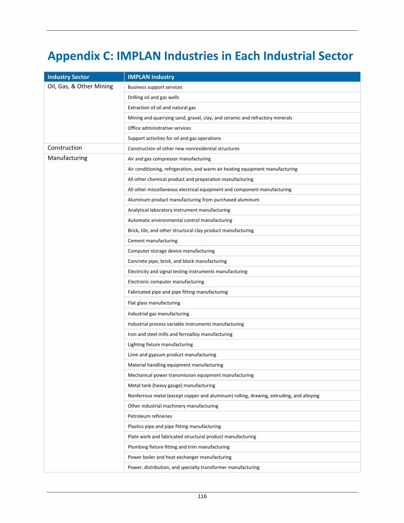
116

Appendix C: IMPLAN Industries in Each Industrial Sector

Industry Sector IMPLAN Industry

Oil, Gas, & Other Mining Business support services

Drilling oil and gas wells

Extraction of oil and natural gas

Mining and quarrying sand, gravel, clay, and ceramic and refractory minerals

Office administrative services

Support activities for oil and gas operations

Construction Construction of other new nonresidential structures

Manufacturing Air and gas compressor manufacturing

Air conditioning, refrigeration, and warm air heating equipment manufacturing

All other chemical product and preparation manufacturing

All other miscellaneous electrical equipment and component manufacturing

Aluminum product manufacturing from purchased aluminum

Analytical laboratory instrument manufacturing

Automatic environmental control manufacturing

Brick, tile, and other structural clay product manufacturing

Cement manufacturing

Computer storage device manufacturing

Concrete pipe, brick, and block manufacturing

Electricity and signal testing instruments manufacturing

Electronic computer manufacturing

Fabricated pipe and pipe fitting manufacturing

Flat glass manufacturing

Industrial gas manufacturing

Industrial process variable instruments manufacturing

Iron and steel mills and ferroalloy manufacturing

Lighting fixture manufacturing

Lime and gypsum product manufacturing

Material handling equipment manufacturing

Mechanical power transmission equipment manufacturing

Metal tank (heavy gauge) manufacturing

Nonferrous metal (except copper and aluminum) rolling, drawing, extruding, and alloying

Other industrial machinery manufacturing

Petroleum refineries

Plastics pipe and pipe fitting manufacturing

Plate work and fabricated structural product manufacturing

Plumbing fixture fitting and trim manufacturing

Power boiler and heat exchanger manufacturing

Power, distribution, and specialty transformer manufacturing

117

Industry Sector IMPLAN Industry

Pump and pumping equipment manufacturing

Relay and industrial control manufacturing

Ship building and repairing

Steel product manufacturing from purchased steel

Telephone apparatus manufacturing

Travel trailer and camper manufacturing

Turbine and turbine generator set units manufacturing

Turned product and screw, nut, and bolt manufacturing

Valve and fittings other than plumbing manufacturing

Watch, clock, and other measuring and controlling device manufacturing

Wholesale and retail trade Wholesale trade businesses

Transportation Transit and ground passenger transportation

Transport by air

Transport by rail

Transport by truck

Transport by water

Services & All Other All other miscellaneous professional, scientific, and technical services

Architectural, engineering, and related services

Employment and payroll only (state & local govt, non-education)

Environmental and other technical consulting services

Food services and drinking places

Hotels and motels, including casino hotels

Insurance carriers

Legal services

Management, scientific, and technical consulting services

Nondepository credit intermediation and related activities

Private household operations

Waste management and remediation services

Water, sewage, and other treatment and delivery systems

118