CHAPTER 1 INTRODUCTION 1

Report New
Dec 12, 2015
Project report
Welcome message from author
This document is posted to help you gain knowledge. Please leave a comment to let me know what you think about it! Share it to your friends and learn new things together.
Transcript

CHAPTER 1
INTRODUCTION
1.0 INTRODUCTION
1

1.1 Introduction:
Many heat transfer applications, such as steam generators in a boiler or air cooling
in the coil of an air conditioner, can be modeled in a bank of tubes containing a flowing fluid at
one temperature that is immersed in a second fluid in a cross flow at different temperature. CFD
simulations are a useful tool for understanding flow and heat transfer principles as well as for
modeling these type of geometries Both fluids considered in the present study are water, and
flow is classified as laminar and steady, with Reynolds number between 100-600.The mass flow
rate of the cross flow and diameter is been varied (such as 0.05, 0.1, 0.15, 0.20, 0.25, 0.30
kg/sec) and the models are used to predict the flow and temperature fields that result from
convective heat transfer. Due to symmetry of the tube bank and the periodicity of the flow
inherent in the tube bank geometry, only a portion of the geometry will be modeled and with
symmetry applied to the outer boundaries. The inflow boundary will be redefined as a periodic
zone and the outflow boundary is defined as the shadow.
The geometry and flow features in industrial applications can be repetitive in nature. In
such cases, it is possible to analyze the flow system using only the section of geometry or single
building. Doing so helps to reduce the computational effort, without compromising the accuracy.
The repetition may be either translational as shown in fig.
2

Figure1.1.1: Schematic representation of periodic planes
It is easy to see from the above fig. if the entire region consists the large numbers of modulus
were used as a calculation domain the required computer storage and time would be truly excessive. A
practical alternative is provided by recognizing that, beyond a certain development length, the velocity
fields and temperature fields will repeat itself module after module. Therefore, it is possible to calculate
the flow and heat transfer directly for typical model.
1.2 OBJECTIVES OF DISSERTATION:
In the present paper tubes of different diameters and different mass flow rates
are considered to examine the optimal flow distribution. Further the problem has been subjected
to effect of materials used for tubes manufacturing on heat transfer rate. Materials considered are
aluminum which is used widely for manufacture of tubes, copper and alloys. Results show
significant variations between alloy and aluminum, copper as tube materials. Results emphasize
the utilization of alloys in place of aluminum and copper as tube material serves better heat
transfer with most economic way.
3

4

CHAPTER 2
INTRODUCTION TO
SIMULATION
2.0 INTRODUCTION TO SIMULATION
2.1 INTRODUCTION:
5

Simulation is the imitation of the operation of a real-world process or system over time.
[1] The act of simulating something first requires that a model be developed; this model represents
the key characteristics or behaviors of the selected physical or abstract system or process. The
model represents the system itself, whereas the simulation represents the operation of the system
over time.
Simulation is an important feature in engineering systems or any system that involves
many processes. For example in electrical engineering, delay lines may be used to
simulate propagation delay and phase shift caused by an actual transmission line.
Similarly, dummy loads may be used to simulate impedance without simulating propagation, and
is used in situations where propagation is unwanted. A simulator may imitate only a few of the
operations and functions of the unit it simulates. Contrast with: emulate.
Most engineering simulations entail mathematical modelling and computer assisted
investigation. There are many cases, however, where mathematical modelling is not reliable.
Simulations of fluid dynamics problems often require both mathematical and physical
simulations. In these cases the physical models require dynamic similitude. Physical and
chemical simulations have also direct realistic uses, rather than research uses; in chemical
engineering, for example, process simulations are used to give the process parameters
immediately used for operating chemical plants, such as oil refineries.
Historically, simulations used in different fields developed largely independently, but 20th
century studies of Systems and Cybernetics combined with spreading use of computers across all
those fields have led to some unification and a more systematic view of the concept.
6

Physical simulation refers to simulation in which physical objects are substituted for the real
thing (some circles[4]use the term for computer simulations modelling selected laws of physics,
but this article doesn't). These physical objects are often chosen because they are smaller or
cheaper than the actual object or system.
Interactive simulation is a special kind of physical simulation, often referred to as a human in the
loop simulation, in which physical simulations include human operators, such as in a flight
simulator or a driving simulator.
Human in the loop simulations can include a computer simulation as a so-called synthetic
environment.
There are different types of simulations according to the field or stream suiting for research. Here
we are using engineering simulation with the help of Computational Fluid Dynamics software.
2.2 Need for CFD
Conventional engineering analyses rely heavily on empirical correlations so it is not
possible to obtain the results for specific flow and heat transfer patterns in heat exchanger of
arbitrary geometry. Successful modeling of such process lies on quantifying the heat, mass and
momentum transport phenomena. Today’s design processes must be more accurate while
minimizing development costs to compete in a world economy. This forces engineering
companies to take advantage of design tools which augment existing experience and empirical
data while minimizing cost. One tool which excels under these conditions is Computational Fluid
Dynamics (CFD), makes it possible to numerically solve flow and energy balances in
complicated geometries.
7
Computational Fluid Dynamics simulates the physical flow, heat transfer, and
combustion phenomena of solids, liquids, and gases and executing on high speed, large memory
workstations. CFD has significant cost advantages when compared to physical modeling and
field testing and also, provides additional insight into the physical phenomena being analyzed
due to the availability of data that can be analyzed and the flexibility with which geometric
changes can be studied. Effective heat transfer parameters estimated from CFD results matched
theoretical model predictions reasonably well. Heat exchangers have been extensively researched
both experimentally and numerically. However, most of the CFD simulation on heat exchangers
was aimed at model validation.
Hilde VAN DER VYVER, Jaco DIRKER AND Jousa P. MEYER, who investigated the
validation of a CFD model of a three dimensional Tube-in-Tube Heat Exchanger. The heat
transfer coefficients and the friction factors were determined with CFD and compared to
established correlations. The results showed the reasonable agreement with empirical correlation,
while the trends were similar. When compared with experimental data the CFD model results
showed good agreement. The average error was 5.5% and the results compared well with
correlation. It can be concluded that the CFD software modeled a Tube-in-Tube Heat Exchanger
in three- dimensional accurately.
2.3 simulation phenomena in heat exchangers
8

Fig. 2.3.1 Heat transfer for heat exchanger.
The second law of thermodynamics states that heat always flows spontaneously from
hotter region to a cooler region. All active and passive devices are sources of heat. These devices
are always hotter than the average temperature of their immediate surroundings. There are three
mechanisms for heat transfer viz, conduction, convection and radiation.
2.3.1 Shell and Tube Heat Exchanger
Shell and Tube heat exchangers in their various construction modifications are probably
the most widespread and commonly used basic heat exchanger configuration in the process
industries. The shell and tube heat exchanger provides a comparatively large ratio of heat
transfer area to volume and weight. It provides heat transfer surface in form which is relatively
easy to construct in a wide range of sizes and which is mechanically rugged enough to with stand
normal shop fabrication stresses, shipping and field erection stresses and normal operating
conditions. There are many modifications of the basic configuration which used to solve special
problems.
9

Figure 2.3.1.1 shell and tube heat exchanger model.
Flow past tube banks with variety of configurations has wide applications, such as heat
exchangers, nuclear reactors, boilers, condensers, waste heat recovery systems etc. An
understanding of wake behavior and the associated dynamics for flow about a single cylinder and
an array of tubes forms the first step towards better and improved design of heat transfer
equipment. Due to smaller flow passages, and a tighter packing of the tube bundle, heat
exchanger design range is sometimes well within the laminar flow regime. A common
understanding is that turbulent slows provide high heat transfer coefficients but, on the contrary,
it leads to increased pumping costs. Therefore, laminar flow heat exchangers can also offer
substantial weight, volume, space and cost savings. Thus, there is wide interest in the study of
fluid friction and heat transfer in heat exchangers where the shell side fluid can be classified as
laminar. A part from heat exchanger (compact and shell and tube etc) applications of laminar
10

flow theory over tube has relevance in aerospace, nuclear, bio medical, electronics and
instrumentation fields. Such a wide range of practical applications have motivated the analysis
on flow past a bundle of tubes in laminar flow.
2.3.2 Heat Exchanger Tubes
Figure 2.3.2.1 common tube layouts for exchangers.
The tubes are the basic components of the shell and Tube heat exchanger, providing the
heat transfer surface between on fluid flowing inside the tube and the other fluid flowing across
outside of the tubes. The tubes may be seamless or welded and most commonly made of copper
or steel alloys. Other alloys for specific applications the tubes are available in a variety of metals
which includes admiralty, Muntz metal, brass, 70-30 copper nickel, aluminum bronze,
aluminum. They are available in a number of different wall thicknesses. Tubes in heat
exchangers are laid out on either square or triangular patterns as shown in fig. 1.4. The
advantage of square pitch is that the tubes are accessible for external cleaning and cause a lower
pressure drop when fluid flows in the direction indicated in the fig.1.4.
2.3.3 Shell-side film coefficients
11

The heat transfer coefficients outside tube bundle are referred to as shell-side
coefficients. When the tube bundle employs baffles, which serves two functions: most
importantly they support the tubes in the proper position during assembly and operation and
prevent vibration of the tubes caused by flow-induced eddies. Secondly they guide the shell-side
flow back and forth across the tube field, increasing the velocity and the heat transfer coefficient.
In square pitch, as shown in fig.1.5 the velocity of the fluid undergoes continuous
fluctuation because of the constricted area between adjacent tubes compared with the flow area
between successive rows. In triangular pitch even greater turbulence is encountered because the
fluid flowing between adjacent tubes at high velocity impinges directly on the succeeding rows.
The indicates that, when the pressure drop and cleavability are of little consequence, triangular
pitch is superior for the attainment of high shell-side film coefficients. This is the actually the
case, and under comparable conditions of flow and tube size the coefficients for triangular pitch
are roughly 25% greater than for square pitch.
2.3.4 Shell-side mass velocity
Shell is simply the container for the shell-side fluid. The shell is commonly has a circular
cross section and is commonly made by rolling a metal plate of appropriate dimensions into a
cylinder and welding the longitudinal joint. In large exchangers the shell is made out of carbon
steel wherever possible for reasons of economy. Though other alloys can be and are used when
corrosion (or) high temperature strength demand must be met. The linear and mass velocities of
the fluid change continuously across the bundle, since the width of the shell and number of tube
vary from row to row.
2.3.5 Shell-side Pressure Drop
12

The total pressure, ∆p, across a system consists of three components:
A static pressure difference, ∆Ps ,due to the density and elevation of the fluid.
A pressure differential, ∆P, due to the change of momentum.
A pressure differential due to frictional losses, ∆P.
∆Pt = ∆Ps + ∆Pm + ∆Pf
2.3.6 Allocation of Stream in a Shell and tube Exchanger
In principle, either stream entering a shell and tube exchange may be put on either side-
tube-side or shell of the surface. However, there are four considerations which exert a strong
influence upon which choice will result in the most economical exchanger:
1. High pressure: If one of the streams is at a high pressure, it is desirable to put that stream
inside the tubes. In this case, only the tubes and the tube-side fittings need be designed to
withstand the high pressure, whereas the shell may be made of lighter weight metal.
Obviously, if both streams are at high pressure, a heavy shell will be required and other
considerations will dictate which fluid goes in the tube. In any case, high shell side
pressure puts a premium on the design of long, small diameters exchangers.
2. Corrosion: Corrosion generally dictates the choice of material of construction, rather than
exchanger design. However, since most corrosion- resistant alloys are more expensive
than the ordinary materials of construction; the corrosive fluid will ordinarily be placed in
the tubes so that so that at least the shell need not be made of corrosion- resistant
material. If the corrosion cannot be effectively prevented but only slowed by choice of
material ,a design must be chosen in which corrodible components can be easily replaced
(unless it is more economical to scrap the whole unit and start over.)
13

3. Fouling: Fouling enters into the design of almost every process exchanger to a
measurable extent, but certain streams foul so badly that the entire design is dominated
by feature which seek
a. To minimize fouling (e.g. high velocity, avoidance of dead or eddy flow regions)
b. To facilitate cleaning ( fouling fluid on tube-side, wide pitch and rotated square
layout if shell-side fluid is fouling) or
c. To extend operational life by multiple units.
4. Low heat transfer coefficient: If one stream has an inherently low heat transfer coefficient
(such as low pressure gases or viscous liquids), this stream is preferentially put on the
shell-side so that extended surface may be used to reduce the total cost of the heat
exchanger.
2.4 Applications
The following are the applications where simulation plays an important role in engineering
applications.
2.4.1 Pulverized Application:
A numerical analysis was performed on a coal pulverize that was experiencing high coal
reject rates believed to be caused by poor primary air distribution in the pulverize wind box.
A three dimensional isothermal flow model was analyzed from the outlet of the primary air
fan through the pulverize wind box throat. The results showed high air velocities in the duct
entering the pulverize wind box. These conditions resulted from the physical arrangement of
the duct work and proximity of the primary air fan. Low velocity air flow region are created
in the pulverize throat near the mill inlet. These low velocity regions increase the pulverizer’s
14

coal reject rates. Improvements were designed and installed which include an air scoop in the
upper section of the duct work extending into the mill. The scoop redirected air through the
pulverize throat at the entrance region of the mill. The result is an improved total air
distribution through the pulverize throat. The wind box throat was divided into eight equal
regions for the purpose of this analysis.
2.4.2 Micronized Coal Nozzle Application:
Some boiler application utilize a micronized coal which is an order of magnitude smaller
than pulverized coal. These applications encounter special problems in the transportation of
the particles. The small particles tend to reattach with each other forming coal deposits on
inner surfaces which eventually plug the air flow. Numerical modeling is used to determine
where the buildups are forming and why. Flow modification devices are then designed to
reduce and/or eliminate these buildup regions. An example of this application was a case
utilizing micronized coal fired burner. The results showed that the coal particles were
impacting and collecting on the underside of the oil gun and tempering air duct inside the
burner. The tempering air duct was removed from the primary air stream while the tempering
air was forced along the underside of oil gun. This allowed the tempering to buffer the
underside of the oil gun helping the primary air micronized coal to turn along the burner and
into the furnace.
2.4.3 Coal Gasification Application:
A numerical flow and combustion project was completed to study the performance of an
entrained flow type coal gasification process. This atmospheric process burns pulverized coal
with oxygen in sub-stoichimetric conditions to produce a useful, clean gas. A key design and
15

operational parameter for gasifier is carbon efficiency, carbon efficiency represents the
fraction of carbon that is converted to a gas phase and establishes. The gas composition at the
combustor exit. In practice steam is often injected at the burners in an effort to improve
carbon efficiency. The analysis focused on the impact to carbon efficiency when varying the
oxygen to carbon ratio and when using steam injection at the burners. The results of this
gasifier indicate that for steam injection to improve carbon conversion there must be
sufficient oxygen to maintain the higher temperature region.
2.4.4 Convection Pass Erosion Application:
Erosion plagues numerous areas of power plant equipment. One such example is
convection pass region in the boilers firing pulverized coal. In this example, convection pass
tubes are eroded when ash particles are conveyed by flue gas and impact the tube surface.
The impaction of particle removes a small amount of tube material. Repeated over long
periods of time, the tube can fail as the thickness is no longer adequate to support the
required temperature verses pressure stress conditions. The tube wall material and thickness
are typically establishes the abrasiveness properties of the ash. The only remaining design
parameter to minimize erosion is velocity. Numerical models have successfully been used to
identify regions of high local velocity and thus erosion rates. This analysis tool can be used
to recommend geometric changes or flow modifying devices to reduce the peak velocities,
extending the life tube tanks.
2.4.5 Scrubber Applications:
Coal combustion can cause high SO2 emissions depending on the sulphur content in the
fuel . Wet scrubbers are used to remove sulphur from the flue gas is released to the
16

atmosphere in a process known as desulphurization. A perforated plate , or tray, is located
between the gas inlet and slurry spray nozzles. The tray acts as gas-liquid contacting device
which allows for additional SO2 to be absorbed by the slurry. The slurry passes to tray and
drains into bottom of the tower. A numerical model was used to design flow modification
devices which provide uniform flow at the absorber tray. The numerical model indicates that
installing turning vanes at the inlet to the absorber greatly improved the gas distribution. The
final arrangement also included an inclined plate inside the tower to further improve the gas
distribution for the tray.
2.4.6 Steam Drum Application:
The size and number of down comers on steam drums have a significant impact on unit
performance and cost. Numerical modeling has been used to assist in optimizing the number
of down comers. Critical to this evaluation are water side circulation, feed water thermal
mixing, thermal stress, drum water level control, overall cost, maintenance, and construction.
Numerical model was utilized to analyze floe characteristics within the steam drum, perform
a thermal mixing analysis of the feed water distribution, and evaluate a thermal stress model
for a section of the drum head and shell. The analysis presented consists of a comparison
between a four down comer and a three down comer design. The four down comer design
utilize two end and two shell down comers. The three down comer design utilize all shell
down comers. The numerical model analyzed the flow distribution of the saturated liquid
which provided insight to the potential of carry-over ( water flooding the cyclone separators)
and carry under ( entrained steam entering the down comer). Shell temperature differentials
were examined to minimize thermal stress on the pressure vessel extending the useful life of
the stream drum. The model incorporated conjugate heat transfer to represent the feed water
17

and saturated liquid thermal mixing. The numerical results in conjunction with other analyses
provided an optimized down comer and feed water pipe arrangement. The result was
substantial cost savings while maintaining all functional aspects of the design. This example
illustrates how numerical modeling can be used to augment traditional analysis techniques
and several successes have been demonstrated for non-reacting flow problems. Due to the
cost effectiveness and successes of the past, increased software capacity, and more
economical computers, numerical modeling will continue to grow in the power industry.
18

CHAPTER-3
LITERATURE REVIEW
3.0 LITERATURE REVIEW
Bank of tubes are found in many industrial processes and in the nuclear industry, being
the most common geometry used in heat exchanger. The heat is transferred from the fluid inside
the tubes to the flow outside them.
19

In the shell and tube heat exchanger, the cross flow through the banks is obtained by
means of baffle plates, responsible for changing the direction of the flow and for increasing the
heat exchange time between fluid and the heated surfaces.
Numerical analysis of the laminar flow with heat transfer between parallel plates with
baffles was performed by Kelkar and Patankar [2]. Results show that the flow is characterized by
strong deformations and large recirculation regions. In general, Nusselt number and friction
coefficient (FR) increase with the Reynolds number.
Measurement using LDA technique in the turbulent flow in a duct with several baffle
plates were performed by Berner et al. [3], with the purpose of determining the number of baffles
necessary for obtaining a periodic boundary condition and the dependence on Reynolds number
and the geometry. Results showed that with a Reynolds number of 5.17×10³, four baffles are
necessary for obtaining a periodic boundary condition. By increasing the Reynolds number to
1.02×10⁴, a periodic boundary condition is obtained with three baffles.
A significant amount of research has focused both on channels with internal obstructions
and tortuous channels, to determine the configurations that lead to the most vigorous mixing and
highest rate of heat transfer. Popiel and Van Der Merwe [4] and Popiel and Wojkowiak [5] who
studied experimental pressure drops for geometries with an undulating sinusoidal or U-bend
configuration. In these papers, the effects of Reynolds number, curvature, wavelength and
amplitude on the friction factor were investigated in laminar and low Reynolds number turbulent
flow. An interesting observation made by these authors is that when the friction factor is plotted
against the Reynolds number, there is either no definite transition from laminar to turbulent flow,
or a delayed transition relative to that of a straight pipe. It is hypothesized by Popiel and Van der
20

Merwe [4] that a smooth transition to turbulence occurs due to the secondary flows produced
within the complex geometry. Dean [6] originally observed that the mixing effects of these
secondary flows are steadily replaced by the development of turbulent secondary flow.
A method to study fully developed flow and heat transfer in channels with periodically
varying shape was first developed by Patankar et al. [7] for the analysis of an offset-plate fin heat
exchanger. Their methods takes advantage of the repeating nature of the flow field to minimize
the extent of the computational domain. The method of Parankar et al. [7] assumes that for a
periodic geometry, the flow is periodic with a prescribed linear pressure gradient being applied
to drive the flow. The outlet velocity field and its gradient are wrapped to the inlet to produce
periodic boundary conditions. Flow velocities within the geometry are then calculated using
momentum and mass conservation equations, assuming constant fluid properties.
Webb and Ramadhyani [8] and Park et al.[9] analyzed fully developed flow and heat
transfer in periodic geometries following the methodof Patankar. Webb and Ramadhyani [8]
studied parallel plate channels with transverse ribs; they presented a comparison with the
performance of a straight channel, and reported an increase in both the heat transfer rate and
pressure drop as the Reynolds number is increased. Park et al. [9] incorporated optimization of
the heat transfer rate and pressure drop into their study of the flow and thermal field of plate heat
exchangers with staggered pin arrays.
N.R. Rosaguti, D.F. Fletcher, and B.S. Haynes [10] analyzed fully developed flow and
Heat Transfer in geometries that are periodic in the flow direction. They have studied laminar
flow in serpentine duct of circular cross section with a constant heat flux applied at the walls,
they measured the performance of serpentine channel by comparing pressure drop and rate of
21
heat transfer in these channels to that achieved by fully developed flow in a straight pipe equal
path length. Flow characteristics within such channels are complex, leading to high rates of heat
transfer, whilst low pressure loss is maintained. Dean vortices act to suppress the onset of
recirculation around each bend and are the main contributing factor to these high levels of heat
transfer performance, and low normalized friction factor. For L/d=4.5, Rc/d=1 and Pr=6.13 two
of vortices are observed at Reynolds Number above 150. This flow structure occurs immediately
after bends that turn in an opposite direction to the one previous.
The influence of L/d on Heat Transfer and pressure drop has been shown for a fixed
Reynolds Number. Increasing L/d increases the rate of heat transfer and decreases the pressure
drop relative to that of fully developed flow in a straight pipe.
L.C. Demartini , H.A. Vielmo, and S.V. Moller [11] investigated the numerical and
experimental analysis of the turbulent flow of air inside a channel of rectangular section,
containing two rectangular baffle plates, where the two plates were placed in opposite walls.
The scope of the problem is to identify the characteristics of the flow, pressure distribution as
well as the existence and extension of possible recirculation in Heat Exchanger. The geometry of
the problem is a simplification of the geometry baffle plate found in Shell- and- tube Heat
Exchanger. The most important features observed are the high pressure regions formed upstream
of both baffle plates and the extension of the low pressure regions on the downstream region.
The latter are strongly associated with the boundary layer separation on the tip of the baffle
plates, which is also influenced by the thickness of the baffle plates. Low and high pressure
regions are associated to recirculation regions. The most intense is that occurring downstream of
the second baffle plate, responsible for the high flow velocities observed at the outlet of the test
section, creating a negative velocity profiles which introduces mass inside the test section
through the outlet.
Numerical studies of unsteady laminar flow heat transfer in grooved channel flows of
especial relevance to electronic system was performed by Y.M. Chung & P.G. Tucker [12]. The
22

validity of a commonly used periodic flow assumption is explored. Predictions for Re=500 show
the flow typically can become periodic by around the fifth groove. Hence, when modeling IC
rows on circuit boards the popular periodic flow assumption might not be valid for significant
area.
Baier et al. [13] investigated the mass transfer rate in spatially periodic flows through
staggered array. In their method the velocity field was obtained numerically using the creeping
flow assumption where as the mass transfer coefficients were obtained using boundary layer
theory. The drawback of their method is that the influence of the boundary layer thickness
caused by the recirculation between the adjacent tubes inside the array cannot be correctly taken
into account. The calculation procedure is therefore limited to the range of creeping flow. Bao &
Lipscomb [14] analyzed the mass transfer in axial flows method was used to solve governing
momentum and conservation of mass equations in their prediction. One of the limitations of their
method is that it cannot be applied to the cross flow fiber module that is more complex than the
axial flow module.
Several studies on the numerical simulation of hydrodynamic and heat transfer of flow
through tube Massey [15] and Wung & Chen [16]. It was reported that heat transfer coefficients
in the shell-side of cross flow units are higher than those in parallel units in all the test cases.
Further more Schoner et al. [17] found that the transfer processes are additionally faster when the
hollow fibers are evenly spaced in modules.
T.Li, N.G. Dean and J.A.M. Kuipers [18] studied numerical predictions of mass transfer
at the shell-side in in-line hollow fiber tube arrays subject to cross flow. The computational grid
was obtained through a domain decomposition method combined with orthogonal gid generation.
Though the mass transfer is affected by many factors, such as hydrodynamic, the number of
tubes and the tube length etc., their attention was only on the influence of hydrodynamics and the
pitch to diameter ratio on the mass transfer. The analysis of the variation of concentration field
demonstrates that when diffusion is dominant in the mass transfer the concentration field tends to
be relatively homogenous, whereas when convection is dominant the concentration field differs
23

considerably along the downstream direction. The results showed that the mass transfer
coefficient decreases drastically after the front tube with the increase of tube number along the
longitudinal direction especially after the first tube, but tends to a stable decrease. The numerical
predictions show that the mass transfer coefficient is a strong function of Reynolds number,
Schmidt number and pitch-to-diameter ratio. The mass transfer coefficient is increased with
increase of Reynolds number and Schmidt number, but with decrease of pitch-to-diameter ratio.
J. Tian,T. Kim, T.J. Lu, H.P. Hodson, D.T. Queheillalt, D.J. Sypeck, H. N. Wadley [19]
investigated the fluid flow and heat transfer features of cellular metal lattice structure made from
copper by transient liquid phase bonding and brazing of plane weave copper meshes (screens)
were experimentally characterized under steady state forced air convection. Due to the inherent
structural anisotropy of this metal textile derived structure, the characterizations were performed
for several configurations to identify the preferable orientations for maximizing thermal
performance as a heat dissipation medium. The results show that the friction factor of bonded
wire screens is not simply a function of porosity as stochastic materials such as open-celled
metal foams and packed beds, but also a function of orientation. The overall heat transfere
depends on porosity and surface area density, but only weakly on orientation. For the range of
Reynolds numbers considered (700-10,000) fluid flow in all textile meshes dominated. The
friction factor in all cases is independent of the coolant velocity. The friction factor based on the
unit pore size depends mainly on the open area ratio. If the channel height is chosen as the length
scale, the friction factor is also a function of pore size and flow direction. The transfer of heat
cross the meshes depends on two competing mechanisms: solid conduction and forced
convection. At a given Reynolds number, porosity and surface area density are two key
parameters controlling heat transfer. At a given porosity, the heat dissipation rate increases as the
24

surface area density is increased. With increasing porosity, conduction decreases while
convection increases. Consequently, for a fixed surface area density, there exists an optional
porosity for maximum heat dissipation. For copper textiles studied, this optional porosity is
about 0.75.
S. Y. Chung and Hyung Jin Sung [20] studied a direct numerical simulation for turbulent
heat transfer in a concentric annulus at Redh=8900 and Pr= 0.71 for two radius ratio (R1/R2=R*,
0.1 and 0.5) and q*= 1.0. Main emphasis is placed on the transverse curvature effect on near-wall
turbulent thermal structure. The nusselt numbers and mean temperature profiles were represented
to show and compare the mean thermal properties between near the inner and outer walls. It was
found that the slope of the mean temperature profile near the inner wall was lower than that near
the outer wall in the logarithmic region. Overall turbulent thermal statistics near the outer walls
were larger than those near the inner walls due to the transverse curvature. This tendency was
more apparent for small radius ratio. The cross-correlation between velocity and temperature
indicated that the coherent thermal structures near the outer walls were stronger than those near
the inner walls. The fluctuating temperature variance turbulence heat flux budgets were
illustrated to confirm the results of the lower order statistics. The numerical results showed that
the turbulent thermal structures near the outer wall were more activated than those near the inner
wall, which may be attributed to the different vortex regeneration processes between the inner
and outer walls.
A. WITRY and M.H. AI-HAJERI and Ali A. BONDOK [21], studied thermal
performance of plate heat exchanger configurations currently form the backbone of today’s
process industry. For this purpose, the aluminum roll-bonding technique widely used in
manufacturing the cooling compartments for domestic refrigeration was used; it is possible to
25

manufacture a wide range of heat exchanger configurations that can help augment heat transfer
whilst reducing pressure drops. Aluminum thin sheets against each other. With the help of an
anti-adhesive profile on the inner side of the two sheets, it is possible to form a pattern of internal
flow passage to the required shape by applying relatively high internal air pressures blowing the
sheets out to form a variety of internal flow-passages shapes. The high air pressures create
internal flow-passages that match the adhesive applied areas, whilst also creating a similar
pattern on the plate’s external surface. One such design where successive rows and columns of
equally spaced staggered dimple help provide high levels of heat transfer augmentation of both
sides of the heat exchanger and a wide cross sectional area that would lower pressure drops. The
internal flows wall angle is 450. A 1800 turn in flow direction also allows the flow to have a
longer thermal length whilst adding extra “effective” heat transfer areas.
The wider cross sectional area on both sides of the plate allows the flow(s) lower
velocities giving lower pressure drops for the critical internal flow side than that for its tubular
counterpart heat exchanger geometry. At the inlet, outlet and 1800 bend, a number of dimples
have been removed to allow the flow the chance to re-distribute itself without causing high
pressure losses and to serve as an internal collection-distributor. Further modifications to this
geometry could include adding pin-fin on the outer plate surface to add roughness and to help
completely destroy any re-circulations and boundary layer flows generated there. Using
Computational Fluid Dynamics, it is hereby sought to model the flow and heat transfer
performance characteristics for one such design as a possible replacement for the conventional
automotive radiator. CFD results obtained are compared with the testing performance data for
automotive radiator with a 27mm coolant side diameter. Results showed that the high inlet
pressure is lost due to the direct hit against the dimple facing the inlet and to the sudden
26

enlargement in cross-sectional area. This indicates the need for more dimples to be removed for a
longer hydraulic length from the flow’s path. Beyond the inlet region, the flow begins to form
major re-circulatory flows whilst trying to find the shortest way towards the outlet. This leads to
the generation of a low-pressure region near the inlet jet causing high flow shear levels.
The high coolant velocities lead to exceedingly high heat transfer coefficients especially
near the inlet. Here, a rapid temperature drop takes place in the vicinity of areas where the flow
came to lower velocities next to high velocity regions. The external airflows over the dimpled
valleys, no reverse flow re-circulation can be noticed here leading to speculation of the existence
of high and low flow speeds domains. This reduces the amount of heat pick up from the external
surface by the cold air and will lead to lower convection values. The extreme levels of flow
impingement, vortex shedding and surface rubbing observed inside the plate out-weigh the
external air shell side flow. Partially, this can be also attributed to the use of water, a better heat
transfer agent inside the plate. Since the external surface represents a smooth wavy channel,
further measures can be introduced to encourage mixing on the shell side that would allow ‘h’
values there further allowing ‘U’ values to increase. Regarding heat transfer performance of
dimple plate heat exchanger, results clearly showed that due to increase in heat transfer areas the
possibility is to gain increased heat transfer levels. With the already high levels of ‘h’ values
observed on the water side, increases in shell side air flow rates tend to the main factor
controlling performance improvement. This is especially true when considering that the common
radiator today makes extensive use of fins to promote heat transfer on the shell side. The authors
finally concluded that dimple heat exchanger promises the following advantages:
Higher heat transfer levels
27

Lower pressure drop levels
Lower overall vehicle drag
Smaller size radiators
Cheaper to manufacture
Numerical analysis on several typical applications to new, existing and retrofit equipment
using CFD techniques for a modern Boiler design has been performed by T.V. Mull, Jr., M.W. r
28

CHAPTER-4
COMPUTATIONAL FLUID
DYNAMICS (CFD)
4.0 COMPUTATIONAL FLUID DYNAMICS (CFD)
4.1 INTRODUCTION
29
Objective
Design parameters
CFD solver Response
Parameters
ConstraintsConstraints

Figure 4.1.1. The design optimization problem
At present in order to shorten product development time, there is a strong tendency to
perform thermal design using computational fluid dynamics (CFD) tools instead of experiments.
CFD is a method that is becoming more and more popular in the modeling of flow systems in
many fields, including reaction Engineering.
It is recognized that thermal experiments remain essential during the final design stages.
CFD based modeling however many advantages have during preliminary design, because it is
less time-consuming than experiments and because it allows greater flexibility.
Early experience with CFD based modeling has shown that these computational tools
should be used carefully. Any kind of CFD computation requires the specification of inlet and
boundary conditions. Obviously these conditions determine the flow and temperature field
resulting from the CFD computation. The specification of inlet and boundary conditions requires
experimental information. Therefore supporting experiments are to be carried out before any
attempt is made to obtain results from a CFD simulation.
4.1.1 Theory
30

Solutions in CFD are obtained by numerically solving a number of balances over a large
number of control volumes or elements. The numerical solution is obtained by supplying
boundary conditions to the model boundaries and iteration of an initially guessed solution.
The balances, dealing with fluid flow, are based on the Navier Stokes Equations for
conservation of mass (continuity) and momentum. These equations are modified per case to
solve a specific problem.
The control volumes (or) elements, the mesh are designed to fill a large scale geometry,
described in a CAD file. The density of these elements in the overall geometry is determined by
the user and affects the final solution. Too coarse a mesh will result in an over simplified flow
profile, possibly obscuring essential flow characteristics. Too fine meshes will unnecessarily
increasing iteration time.
After boundary conditions are set on the large scale geometry the CFD code will iterate
the entire mesh using balances and the boundary conditions to find a converging numerical
solution for the specific case.
4.1.2 The strategy of CFD
Broadly, the strategy of CFD is to replace the continuous problem domain with a discrete
domain using a grid. In the continuous domain, each flow variable is defined at every point in the
31

domain. For instance, the pressure p in the continuous 1D domain shown in the figure below
would be given as
P = p(x); 0<x<1 (3.1)
In the discrete domain, each flow variable is defined only at the grid points. So, in the discrete
domain shown below, the pressure would be defined only at the N grid points.
Pi = p(xi); i=1,2,.......N (3.2)
Continuous Domain Discrete Domain
0≤ x ≤ 1 x = x1 + x2,……xn
X=0 x=1 x1 xn
Coupled PDEs+ boundary condition Coupled algebraic eqs.
in continuous variables in discrete variables
In a CFD solution, one would directly solve for the relevant flow variables only at the grid
points. The values at other locations are determined by interpolating the values at the grid points.
The governing partial differential equations and boundary conditions are defined in terms
of the continuous variables p, Vi etc. One can approximate these in the discrete domain in terms
of the discrete variables pi, Vi etc. The discrete system is a large set of coupled, algebraic
equations in the discrete variables, setting up the discrete system and solving it (which is a
matrix inversion problem) involves a very large number of repetitive calculations and is done by
the digital computer.
4.2 Physical and Mathematical basis of the CFD
All mathematical simulations are carried out within commercial software package environment,
FLUENT. The governing equations solved for the flow fields are the standard conservation
32

equations of mass and momentum in the mathematical simulations. The equation for RTD is a
normal species transportation equation. For trajectories of the inclusion, discrete phase model
(DPM) is employed with revised wall boundary conditions. The free surface and tundish walls
have different boundary conditions (such as reflection and entrapment) for droplets/solid
inclusion particles. Taking the range of inclusion particles’ diameter (Chevrier and Cramb, 2005)
and the shapes for different types of inclusions (Beskow, et al., 2002) into consideration,
the boundaries and drag law for particles are then revised by user defined function (UDF) and
shape correction coefficient. During trajectory simulations, Stokes-Cunningham drag law is
employed with Cunningham correction. Inclusions sometimes could be liquid phase. It is
difficult to set the correction coefficient (Haider and Levenspiel, 1989) exactly since droplets can
move and deform continuously. While Sinha and Sahai (1993) set both top free face and walls as
trap boundary, Lopez-Ramirez et al. (2001) did not illustrate the boundary conditions for
inclusion. Zhang, et al. (2000) divided the tundish into two kinds of separate zones. The walls are
set as reflection boundary in this work for comparison of separation ratios of inclusion in SFT
and a tundish with TI. Although most of the reports indicate that the free surface is a trap
boundary, there is a possibility of re-entrainment (Bouris and Bergeles, 1998) to be considered.
4.2.1 Fluid Flow Fundamentals
33
Fundamental physical principles
Figure 4.2.1.1 Block Diagram of physical and Mathematical basis
The physical aspects of any fluid flow are governed by three fundamental principles.
Mass is conserved; Newton’s second law and Energy is conserved. These fundamental principles
can be expressed in terms of mathematical equations, which in their most general form are
usually partial differential equations. Computational Fluid Dynamics (CFD) is the science of
34
Mass is conserved
Newton’s second law
Energy is conserved
Models of flow
Fixed finite control volume
Moving finite control volume
Fixed infinitesimally small volume
Moving infinitesimally small
volume
Governing equations of fluid flow
Continuity equation
Momentum equation
Energy equation
Forms of these equations particularly suited for CFD

determining a numerical solution to the governing equations of fluid flow whilst advancing the
solution through space or time to obtain a numerical description of the complete flow field of
interest.
The governing equations for Newtonian fluid dynamics, the unsteady Navier-stokes
equations, have been known for over a century. However, the analytical investigation of reduced
forms of these equations is still an active area of research as is the problem of turbulent closure
for the Reynolds averaged form of the equations. For non-Newtonian fluid dynamics, chemically
reacting flows and multiphase flows theoretical developments are at a less advanced stage.
Experimental fluid dynamics has played an important role in validating and delineating
the limits of the various approximations to the governing equations. The wind tunnel, for
example, as a piece of experimental equipment, provides an effective means of simulating real
flows. Traditionally this has provided a cost effective alternative to full scale measurement.
However, in the design of the equipment that depends critically on the flow scale measurement
as part of the design process is economically impractical. This situation has led to an increasing
interest in the development of a numerical wind tunnel.
4.2.2 The Governing equations
In the case of steady- two dimensional flow, the continuity (conservation of mass) equation is :
∂ ( ρu )∂ x
+∂ ( ρv )∂ y
=0 (3.3)
35

For incompressible flow, the momentum equations are the x direction:
ρu∂ u∂ x
+ ρv∂u∂ y
=−∂ ρ
∂ x+
∂(2 µ∂ u∂ x )
∂ x+
∂(µ [ ∂ u∂ y
+ ∂ v∂ x ])
∂ y
(3.4.a)
And for y direction:
ρu∂ v∂ x
+ ρv∂ v∂ y
=−∂ ρ∂ y
− ρg+
∂ (µ [ ∂ v∂ x
+ ∂ u∂ y ])
∂ x+
∂(2 µ∂ v∂ y )
∂ y, (3.4.b)
The energy conservation equation for the fluid, neglecting viscous dissipation and compression
heating, is:
ρ Cp(u ∂T∂ x
+v∂T∂ y )=
∂(k∂T∂ x )
∂ x+∂
k∂ T∂ y
∂ y (3.5)
The above equations are called Navier-Stokes.
The above non linear partial differential equations are solved using a standard well-
verified discretization technique which in turn forms algebraic equations. These equations
particularly suited for CFD. The following section illustrates the discretization techniques.
4.3 method of solution:
36Discretization techniques
Figure 4.3.1 Block diagram of Numerical Solution Techniques in CFD
4.3.1 Discretization
37
Finite difference Finite volume Finite element
Basic derivations of finite difference: order
of accuracy
Basic derivations of finite-volume equations
Finite-difference equations: truncation
error
Types of solutions: explicit and implicit
Stability analysis

To solve the non-linear partial differential equations from the previous section, it is
necessary to impose a grid on the flow domain of interest, see fig. 3.4. Discrete values of fluid
velocities, properties, pressure and temperature, are stored at each grid point (the intersection of
two grid lines). To obtain a matrix of algebraic equations, a control volume is constructed
(shaded area in the figure) whose boundaries (shown by dashed lines) lie midway between grid P
and its neighbours N, S, E, W, A complex process of formal integration of the differential
equations over the control volume, followed by interpolation schemes to determine flow
quantities at the control volume boundaries (n, s, e, w) in fig. 3.4. finally yield a set of algebraic
equations for each grid point P:
(Ap -B) Φp – ΣA cΦc = C (3.6)
Where the subscript c on Σ, A and Φ refers to a summation over neighbour nodes N, S, E and W,
Φ is a general symbol for the quantity being solved for (u, v or t), AP, etc. Are combined
convection-diffusion coefficients (obtained from integration and interpolation), and B and C are,
respectively, the implicit and explicit source terms (and generally represent the force(s) which
drive the flow, e.g. a pressure difference).
38

Figure 4.3.1.1 control volume on grid point
4.3.2 Discretization using finite-volume method:
In the finite-volume method, quadrilateral/triangle is commonly referred to as a “cell”
and a grid point as a “node”. In 2D, one could also have triangular cells. In 3D, cells are usually
=hexahedral, tetrahedral, or prisms. In the finite volume approach, the integral form of the
conversation equations for each cell. For example, the integral forms of the continuity equation
for steady, incompressible flow is
∫ v .n dS=0 (3.7)
the integration is over the surface S of the control volume and nˆ is the outward normal at the
surface. Physically, this equation means that the net volume flow into the control volume is zero.
Consider the rectangular cell shown below.
39

Face 4 (u4, v4)
Face 1 face 3 (u3, v3)
∆y (u1 , v1)
Face 2 ( u2, v2)
The velocity at face i taken to be V i = ui iˆ+ vj jˆ. applying the mass conservation equation ( 3.7 )
to control volume defined by the cell gives
-u1 ∆y – v2 ∆x + u3 ∆y +v4∆x =0 (3.8)
This is the discrete form of the continuity equation for the cell. It is equivalent to
summing up the net mass flow into the control volume and setting it to zero. So it ensures that
the net mass flow into the cell is zero i.e. that mass is conserved for the cell. Usually the values
at the cell centers are stored. The face values u1, u2, etc. are obtained by suitably interpolating the
cell-center values for adjacent cells.
Similarly, one can obtain discrete equations for the conservation of momentum and
energy for the cell. One can readily extend these ideas to any general cell shape in 2D or 3D and
any conservation equation.
4.3.3 Explicit and Implicit Schemes
The difference between explicit and implicit schemes can be most easily illustrated by
applying them to the wave equation:
∂ u∂ t
+c∂ u∂ x
=0 (3.9)
40

Where c is the wave speed. One possible way to discretize this equation at grid point i and time-
level n is :
Uin- ui
n-1/ ∆t + c (uin-1 – ui-1
n-1/ ∆x = 0(∆t, ∆x) (3.10)
The crucial thing to note here is that the spatial derivative is evaluated at the n-1 time-level.
Solving for uin gives
Uin = [ 1- ( c ∆t/∆x) ] ui
n-1 + ( c ∆t/∆x) ui-1n-1 =0 (3.11)
This is an explicit expression i.e. the value of u in at any grid point can be calculated
directly from this expression without the need for any matrix inversion. The scheme in (3.10) is
known as an explicit scheme. Since uin at each grid point can be updated independently, these
schemes are easy to implement on the computer. On the downside, it turns out that this scheme is
stable only when
C≡ c ∆t/∆x ≤ 1 (3.12)
Where C is called the Courant number. This condition is referred to as the Courant- Friedrichs-
Lewy or CFL condition. While a detailed derivation of the CFL condition through stability
analysis is outside the scope of the current discussion, it can seen that the coefficient of u in-1 in
(3.11) changes sign depending on whether c>1 or c< 1 leading to very different behavior in the
two cases. The CFL condition places a rather severe limitation on ∆tmax.
In an implicit scheme, the spatial derivative term is evaluated at the n time- level:
Uin – ui
n-1/∆t + c ( uin – ui-1
n)/∆x = 0 ( ∆t, ∆x) (3.13)
In this case, uin can’t update at each grid point independently, instead, need to solve a system of
algebraic equation in order to calculate the values at all grid points simultaneously. It can be
41
shown that the scheme is unconditionally stable so the numerical errors will be damped out
irrespective of how large is time-step.
4.3.4 Stability Analysis
A numerical method is referred to stable when the iterative process converges and it is
being unstable when diverges. It is not possible to carry out an exact stability analysis for the
Navier-stokes equations. But a stability analysis of simpler, model equations provides useful
insight and approximate conditions for stability. As mentioned earlier, a common strategy used
in CFD codes for steady problems is to solve the unsteady equations and march in time until the
solution converges to a steady state. A stability analysis is usually performed in the context of
time-marching. While using time-marching to a steady state, the only interest is accurately
obtaining the asymptotic behavior at large times. So it is considered taking as large a time-step
∆t as possible to reach the steady state in the least number of time-steps. There is usually a
maximum allowable time-step ∆tmax beyond which the numerical scheme is unstable. If ∆t >
∆tmax, the numerical errors will grow exponentially in time causing the solution to diverge from
the steady-state result. The value of ∆tmax depends on the numerical discretization scheme used.
There are two classes of numerical schemes, explicit and implicit, with very different stability
characteristics.
The stability limits discussed above apply specifically to the wave equation. In general,
explicit schemes applied to the Navier-Stokes equations have the same restriction that the
courant number needs to be less than or equal to one. Implicit schemes are not unconditionally
stable for Navier-Stokes equations since the nonlinearities in the governing equations often limit
stability. However, they allow a much larger courant number than explicit schemes. The specific
value of the maximum allowable Courant number is problem dependent.
42

Some points to note:
1. CFD codes will allow you to set the Courant number (which is also referred to as the
CFL number) when using time-stepping. Taking larger time-steps leads to faster
convergence to the steady state, so it is advantageous to set the Courant number as large
as possible within the limits of stability.
2. A lower courant number is required during start-up when changes in the solution are
highly nonlinear but it can be increased as the solution progresses.
3. Under- relaxation for non-time stepping.
4.4 Fluent as a modeling and analysis tool:
In parallel with the construction of physical models, a succession of computational fluid
dynamics (CFD) models were developed during the prototype design phase. The software chosen
for numerical modelling in this project was fluent. The software was easily learned and very
flexible in use. Boundary conditions could be set up quickly and the software could rapidly solve
problems involving complex flows ranging from incompressible (low subsonic) to mildly
compressible (Transonic) to highly compressible (Super sonic) flows. The wealth of physical
models in Fluent allows to accurately predicting laminar and turbulent flows, various modes of
heat transfer. Chemical reactions, multiphase flows, and other phenomena with complete mesh
flexibility and solution based mesh adoption.
The governing partial differential equations for the conservation of momentum and
scalars such as mass, energy and turbulence are solved in the integral form. Fluent uses a control-
volume based technique. The governing equations are solved sequentially. The fact that these
equations are coupled makes it necessary to perform several iterations of the solution loop before
43

convergence can be reached. The solution loop consists of seven steps that are performed in
order.
The momentum equations for all directions are each solved using the current pressure
values (initially the boundary condition is used), in order to update the velocity field.
The obtained velocities may not satisfy the continuity equation locally. Using the
continuity equation and the linear zed momentum equation a ‘Poisson-type’ equation for
pressure correction is derived. Using this pressure correction the pressure and velocities
are corrected to achieve continuity.
K and ε equations are solved with corrected velocity field.
All other equations (energy, species conservation etc.) are solved using the corrected
values of the variables.
Fluid properties are updated.
Any additional inter-phase source terms are updated.
A check for convergences is performed.
These seven steps are continued until in the last step the convergence criteria are met.
4.5 Imposing Boundary Conditions:
The boundary conditions determine the flow and thermal variables on the boundaries of
the physical model. There are a number of classifications of boundary conditions:
44

Flow inlet and exit boundaries: pressure inlet, velocity inlet, inlet vent, intake fan,
pressure outlet, out flow, outlet fan, and exhaust fan.
Wall, repeating, and pole boundaries: wall, symmetry, periodic, and axis.
Internal cell zone: fluid, solid.
Internal face boundaries: fan, radiator, porous jump, wall, interior.
With the determination of the boundary conditions the physical model has been defined and
numerical solution will be provided.
45

CHAPTER 5
MODELING OF PERIODIC
FLOW USING GAMBIT AND
FLUENT
46

5.0 MODELING OF PERIODIC FLOW USING GAMBIT AND
FLUENT
5.1 Introduction
Many industrial applications, such as steam generation in a boiler, air cooling in the coil
of air conditioner and different type of heat exchangers uses tube banks to accomplish a desired
total heat transfer.
The system considered for the present problem, consisted bank of tubes containing a flowing
fluid at one temperature that is immersed in a second fluid in cross flow at a different
temperature. Both fluids are water, and the flow is classified as laminar and steady, with a
Reynolds number of approximately 100.The mass flow rate of cross flow is known, and the
model is used to predict the flow and temperature fields that result from convective heat transfer
due to the fluid flowing over tubes.
The figure depicts the frequently used tube banks in staggered arrangements. The
situation is characterized by repetition of an identical module shown as transverse tubes. Due to
symmetry of the tube bank, and the periodicity of the flow inherent in the tube geometry, only a
portion of the geometry will be modeled as two dimensional periods heat flows with symmetry
applied to the outer boundaries.
5.2 CFD modeling of a periodic model
Creating physical domain and meshing
Creating periodic zones
Set the material properties and imposing boundary conditions
47

Calculating the solutions using segregated solver.
5.2.1 Modeling details and meshing
Figure 5.2.1.1: Schematic diagram of the problem
The modeling and meshing package used is GAMBIT. The geometry consists of a periodic inlet
and outlet boundaries, tube walls. The bank consists of uniformly spaced tubes with a diameter
D, which are staggered in the direction of cross flow. Their centers are separated by a distance of
2cm in x-direction and 1 cm in y-direction.
The periodic domain shown by dashed lines in fig 4.1.is modeled for different tube
diameter viz., D=0.8cm, 1.0cm, 1.2cm and 1.4cm while keeping the same dimensions in the x
and y direction. The entire domain is meshed using a successive ratio scheme with quadrilateral
cells. Then the mesh is exported to FLUENT where the periodic zones are created as the inflow
48

boundary is redefined as a periodic zone and the outer flow boundary defined as its shadow, and
to set physical data, boundary condition. The resulting mesh for four models is shown in fig 4.2
Fig 5.2.1.2 Mesh for the periodic tube of diameters 0.8, 1.0, 1.2, 1.4cm
The amount of cells, faces, nodes created while meshing for each domain is tabulated in a table .
49

5.3 Material properties and boundary conditions
The material properties of working fluid (water) flowing over tube bank at bulk temperature of
300K, are:
ρ = 998.2kg/m3
µ = 0.001003kg/m-s
Cp = 4182 J/kg-k
K= 0.6 W/m-k
The boundary conditions applied on physical domain are as followed
Table 5.3.1: Boundary conditions assigned in FLUENT
Fluid flow is one of the important characteristic of a tube bank. It is strongly effects the
heat transfer process of a periodic domain and its overall performance. In this paper, different
50
Boundary Assigned as
Inlet Periodic
Outlet Periodic
Tube walls Wall
Outer walls Symmetry

mass flow rates at free stream temperature, 300Kwere used and the wall temperature of the tube
which was treated as heated section was set at 400K as periodic boundary conditions for each
model which are tabulated as follows:
Table 5.3.2: Mass flow rates for different tube diameter
Tube diameter(D)
(cm)
Periodic condition
(Kg/s)
0.8 m=0.05-0.30
1.0 m=0.05,0.30
1.2 m=0.05-0.30
1.4 m=0.05-0.30
The wall temperature of the tube which was treated as heated section was set at 400k.
5.4 Solution using Segregate Solver:
The computational domain was solved using the solver settings as segregated, implicit,
two-dimensional and steady state condition. The numerical simulation of the Navier Stokes
equations, which governs the fluid flow and heat transfer, make use of the finite control volume
method. CFD solved for temperature, pressure and flow velocity at every cell. Heat transfer was
modeled through the energy equation. The simulation process was performed until the
51

convergence and an accurate balance of mass and energy were achieved. The solution process is
iterative, with each iteration in a steady state problem. There are two main iteration parameters to
be set before commencing with the simulation. The under-relaxation factor determines the
solution adjustment for each iteration; the residual cut off value determines when the iteration
process can be terminated. The under-relaxation factor is an arbitrary number that determines the
solution adjustment between two iterations; a high factor will result in a large adjustment and
will result in a fast convergence, if the system is stable. In a less stable or particularly nonlinear
system, for example in some turbulent flow or high- Rayleigh-number natural convection cases,
a high under-relaxation may lead to divergence, an increase in error. It is therefore necessary to
adjust the under- relaxation factor specifically to the system for which a solution is to be found.
Lowering the under-relaxation factor in these unstable systems will lead to a smaller step change
between the iterations, leading to less adjustment in each step. This slows down the iterations
process but decreases the chance for divergence of the residual values.
The second parameter, the residual value, determines when a solution is converged. The
residual value (a difference between the current and former solution value) is taken as a measure
for convergence. In a infinite precision process the residuals will go to zero as the process
converges. On actual computers the residuals decay to a certain small value (round-off) and then
stop changing. This decay may be up to six orders of magnitude for single precision
computations. By setting the upper limit of the residual values the ‘cut-off’ value for
convergence is set. When the set value is reached the process is considered to have reached its
‘round-off’ value and the iteration process is stopped.
Finally the under-relaxation factors and the residual cut-off values are set. Under-
relaxation factors were set slightly below their default values to ensure stable convergence.
52

Residual values were kept at their default values, 1.0e-6 for the energy residual, 1.0e-3 for all
others, continuity, and velocities. The residual cut-off value for the energy balance is lower
because it tends to be less stable than the other balances; the lower residual cut-off ensures that
the energy solution has the same accuracy as the other values.
The convergence plots for each domain and each mass flow rate are shown in below
figures.
5.5 Convergence plot for each domain and for each mass flow rate
The convergence plots for the tubes are shown in the below figures at different diameters and
mass flow rates i.e. D=0.8cm, 1.0cm, 1.2 cm and m= 0.05, 0.10, 0.15, 0.20, 0.25, 0.30kg/s
5.5.1 Convergence plot for different mass flow rates with diameter D=0.8cm
Figure 5.5.1.1 convergence plot for tube D=0.8cm Figure 5.5.1.2 convergence plot for tube
and mass flow rate m=0.05kg/s D=0.8cm and mass flow rate m=0.10kg/s
53

Figure 5.5.1.3 convergence plot for tube D=0.8cm Figure 5.5.1.4convergence plot for tube
and mass flow rate m=0.15kg/s D=0.8cm and mass flow rate m=0.20kg/s
54

Figure 5.5.1.5 convergence plot for tube D=0.8cm Figure 5.5.1.6 convergence plot for tube
and mass flow rate m=0.25kg/s D=0.8cm and mass flow rate m=0.30kg/s
5.5.2 Convergence plot for different mass flow rates with diameter D=1.0cm
55

Figure 5.5.2.1 convergence plot for tube D=1.0cm Figure 5.5.2.2 convergence plot for tube
and mass flow rate m=0.05kg/s D=1.0cm and mass flow rate m=0.10kg/s
56

Figure 5.5.2.3 convergence plot for tube D=1.0cm Figure 5.5.2.4convergence plot for tube
and mass flow rate m=0.15kg/s D=1.0cm and mass flow rate m=0.20kg/s
Figure 5.5.2.5 convergence plot for tube D=1.0cm
Figure 5.5.2.6 convergence plot for tube
and mass flow rate m=0.25kg/s
D=1.0cm and mass flow rate m=0.30kg/s
5.5.3 Convergence plot for different mass flow
rates with diameter D=1.2cm
57

Figure 5.5.3.1 convergence plot for tube D=1.2cm Figure 5.5.3.2 convergence plot for tube
and mass flow rate m=0.05kg/s D=1.2cm and mass flow rate m=0.10kg/s
Figure 5.5.3.3 convergence plot for tube D=1.2cm Figure 5.5.3.4 convergence plot for tube
and mass flow rate m=0.15kg/s
D=1.2cm and mass flow rate m=0.20kg/s
58

Figure 5.5.3.5 convergence plot for tube D=1.2cm Figure 5.5.3.6 convergence plot for tube
and mass flow rate m=0.25kg/s D=1.2cm and mass flow rate m=0.30kg/s
CHAPTER-6
RESULTS AND DISCUSSIONS
59

6.0 RESULTS AND DISCUSSIONS
This chapter gives an insight of the findings that are obtained from the analysis of the 2-D
bunch of tubes done in CFD. Different modifications on the basic geometry were
investigated to optimize the flow of fluid inside the tube. In order to find the optimum
performance results of and heat transfer rate geometric parameters has been varied and these
results are projected below. It is assumed that the flow is exhausted to atmosphere; the meshed
model of different diameter tubes are shown in below figure,
60

Figure 6.1 Meshed models of tubes with different diameters
Figures below represent the results generated by FLUENT. In these figures the fluid
characteristics like velocity, pressure and temperature are shown by different color.
A particular color does not give single value of these characteristics, but show the range of these
values. If the value of a characteristic at a particular point falls in this range, there will be color
of that range.
6.1 Variation of static pressure for different tube diameter and mass flow rate
61

The static pressure distribution along the tubes are shown in the below figures at different
diameters and mass flow rates i.e. D=0.8cm, 1.0cm, 1.2 cm and m= 0.05, 0.10, 0.15, 0.20, 0.25,
0.30kg/s
6.1.1 Variation of static pressure for different mass flow rates with diameter D=0.8cm
Figure 6.1.1.1 contours of static pressure, D=0.8cm Figure 6.1.1.2 contours of static pressure,
and mass flow rate m=0.05kg/s D=0.8cm and mass flow rate m=0.10kg/s
62

63
Figure 6.1.1.5 contours of static pressure, D=0.8cm Figure 6.1.1.6 contours of static pressure,
and mass flow rate m=0.25kg/s D=0.8cm and mass flow rate m=0.30kg/s
6.1.2 Variation of static pressure for different mass flow rates with diameter D=1.0cm
Figure 6.1.2.1 contours of static pressure, D=1.0cm Figure 6.1.2.2 contours of static pressure,
and mass flow rate m=0.05kg/s D=1.0cm and mass flow rate m=0.10kg/s
64

Figure 6.1.2.3 contours of static pressure, D=1.0cm Figure 6.1.2.4 contours of static pressure,
and mass flow rate m=0.15kg/s D=1.0cm and mass flow rate m=0.20kg/s
65

Figure 6.1.2.5 contours of static pressure, D=1.0cm Figure 6.1.2.6 contours of static pressure,
and mass flow rate m=0.25kg/s D=1.0cm and mass flow rate m=0.30kg/s
6.1.3 Variation of static pressure for different mass flow rates with diameter D=1.2cm
Figure 6.1.3.1contours of static pressure, D=1.2cm Figure 6.1.3.2 contours of static pressure,
and mass flow rate m=0.05kg/s D=1.2cm and mass flow rate m=0.10kg/s
66

Figure 6.1.3.3 contours of static pressure, D=1.2cm Figure 6.1.3.4 contours of static pressure,
and mass flow rate m=0.15kg/s D=1.2cm and mass flow rate m=0.20kg/s
Figure 6.1.3.5 contours of static pressure, D=1.2cm Figure 6.1.3.6 contours of static pressure,
and mass flow rate m=0.25kg/s D=1.2cm and mass flow rate m=0.30kg/s
The pressure contours are displayed in figures.6.1.1 to 6.1.3 do not include the linear pressure
gradient computed by solver, thus the contours are periodic at the inflow and outflow boundaries.
67

The figures reveal that the static pressure exerts at stagnation point differ mass flow rate have
significant variation. It can be seen from fig 5.1, 5.2 the pressure at the stagnation point have
almost similar magnitude in both cases while the flow past the tube the pressure varies
drastically from one mass flow rate to the other mass flow rate. From fig 5.3 it can be observed,
the pressure at stagnation point as well as the flow past the tube surface varies relatively more as
compared to the previous geometries due to increase in tube diameter. Finally, it can be
concluded that by changing the tube diameter and mass flow rate the pressure drop increases.
6.2 Static Temperature for different Tube Diameters and Mass Flow Rates
The static temperature distribution along the tubes are shown in the below figures at different
diameters and mass flow rates i.e. D=0.8cm, 1.0cm, 1.2 cm and m= 0.05, 0.10, 0.15, 0.20, 0.25,
0.30kg/s
68

6.2.1 Static Temperature for different mass flow rates with diameter D=0.8cm
Figure 6.2.1.1 contours of static temperature, D=0.8cm Figure 6.2.1.2contours of static temperature,
and mass flow rate m=0.05kg/s D=0.8cm and mass flow rate m=0.10kg/s
Figure 6.2.1.3 contours of static temperature, D=0.8cm Figure 6.2.1.4 contours of static temperature,
and mass flow rate m=0.15kg/s D=0.8cm and mass flow rate m=0.20kg/s
69
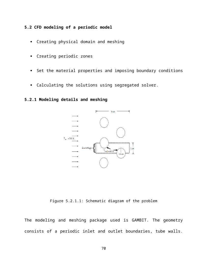
Figure 6.2.1.5 contours of static temperature, D=0.8cm Figure 6.2.1.6 contours of static temperature,
and mass flow rate m=0.25kg/s D=0.8cm and mass flow rate m=0.30kg/s
6.2.2 Static Temperature for different mass flow rates with diameter D=1.0cm
70

Figure 6.2.2.1 contours of static temperature, D=1.0cm Figure 6.2.2.2 contours of static temperature,
and mass flow rate m=0.05kg/s D=1.0cm and mass flow rate m=0.10kg/s
71

Figure 6.2.2.3 contours of static temperature, D=1.0cm Figure 6.2.2.4 contours of static temperature,
and mass flow rate m=0.15kg/s D=1.0cm and mass flow rate m=0.20kg/s
72

Figure 6.2.2.5 contours of static temperature, D=1.0cm Figure 6.2.2.6 contours of static temperature,
and mass flow rate m=0.25kg/s D=1.0cm and mass flow rate m=0.30kg/s
6.2.3 Static Temperature for different mass flow rates with diameter D=1.2cm
73
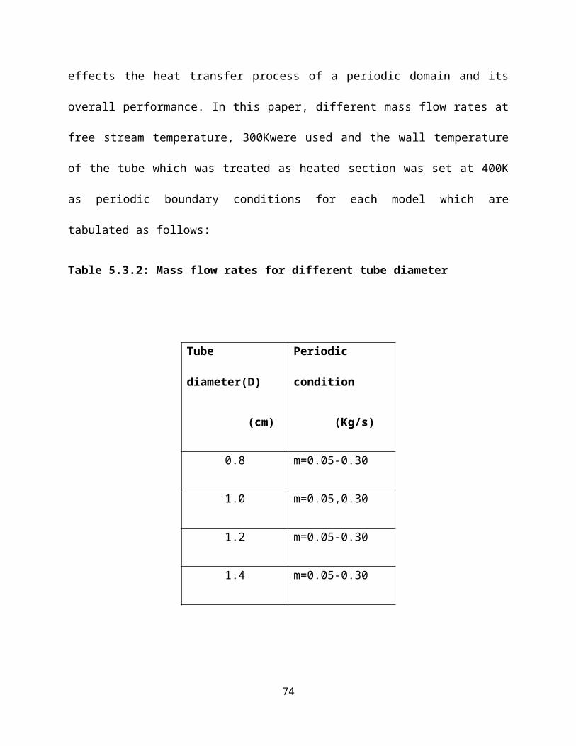
Figure 6.2.3.3 contours of static temperature, D=1.2cm Figure 6.2.3.4 contours of static temperature,
and mass flow rate m=0.15kg/s D=1.2cm and mass flow rate m=0.20kg/s
74

Figure 6.2.3.5 contours of static temperature, D=1.2cm Figure 6.2.3.6 contours of static temperature,
and mass flow rate m=0.25kg/s D=1.2cm and mass flow rate m=0.30kg/s
The contours displayed in fig.6.2.1 to 6.2.3 reveal the temperature increases in the fluid due to
heat transfer from the tubes. The hotter fluid is confined to the near-wall and wake regions, while
a narrow stream of cooler fluid is convected through the tube bank. The consequences of
different mass flow rates to the fluid temperature distribution are shown in the above said
figures. It can be seen that higher heat flow rate was obtained from low mass flow rates. The
75

temperature scale is similar, when compared to one model to other three models for all mass
flow rates.
6.3 Velocity vector for different tube diameters and mass flow rates:
The static velocity distribution along the tubes are shown in the below figures at different
diameters and mass flow rates i.e. D=0.8cm, 1.0cm, 1.2 cm and m= 0.05, 0.10, 0.15, 0.20, 0.25,
0.30kg/s.
6.3.1 Velocity vector for different mass flow rates with diameter D=0.8cm
Figure 6.3.1.1 velocity vector, D=0.8cm Figure 6.3.1.2 velocity vector, D=0.8cm
and mass flow rate m=0.05kg/s and mass flow rate m=0.10kg/s
76

Figure 6.3.1.3 velocity vector, D=0.8cm Figure 6.3.1.4 velocity vector, D=0.8cm
and mass flow rate m=0.15kg/s and mass flow rate m=0.20kg/s
77

Figure 6.3.1.5 velocity vector, D=0.8cm Figure 6.3.1.6 velocity vector, D=0.8cm
and mass flow rate m=0.25kg/s and mass flow rate m=0.30kg/s
6.3.2 Velocity vector for different mass flow rates with diameter D=1.0cm
78

Figure 6.3.2.1 velocity vector, D=1.0cm Figure 6.3.2.2 velocity vector, D=1.0cm
and mass flow rate m=0.05kg/s and mass flow rate m=0.10kg/s
Figure 6.3.2.3 velocity vector, D=1.0cm Figure 6.3.2.4 velocity vector, D=1.0cm
and mass flow rate m=0.15kg/s and mass flow rate m=0.20kg/s
79

Figure 6.3.2.5 velocity vector, D=1.0cm Figure 6.3.2.6 velocity vector, D=1.0cm
and mass flow rate m=0.25kg/s and mass flow rate m=0.30kg/s
6.3.3 Velocity vector for different mass flow
rates with diameter D=1.2cm
80
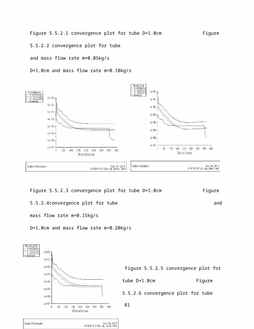
Figure 6.3.3.3 velocity vector, D=1.2cm
Figure 6.3.3.4 velocity vector, D=1.2cm
and mass flow rate m=0.15kg/s
and mass flow rate m=0.20kg/s
81

Figure 6.3.3.5 velocity vector, D=1.2cm Figure 6.3.3.6 velocity vector, D=1.2cm
and mass flow rate m=0.25kg/s and mass flow rate m=0.30kg/s
When the fluid through the bank of tubes the maximum velocity occur at either the transverse
plane or the diagonal plane where the flow area is minimum. The velocity vectors displayed in
fig 6.3.1 to 6.3.3 reveal that the numerical results show very low velocity values adjacent to the
tube surface. In the regimes between the tubes i.e., at the transverse plane the maximum velocity
was occurred:
Since
82

SD = [ SL2 + ( Sr/2)2]0.5 > Sr + D/2, (6.1)
The figures clearly show the boundary layer development along with the tube surface. It
can be observed that the boundary layer detaches from the surface early due to less momentum
of fluid in laminar flow, since the position of the separation point is highly depends on the
Reynolds number. Finally, it can be observed from all the velocity vector diagrams, if the mass
flow rate increased the velocity also increases and narrow stream of maximum velocity fluid
through the tube bank.
6.4 Static Pressure for different tube diameters and mass flow rates with symmetry:
The static velocity distribution along the tubes are shown in the below figures at different
diameters and mass flow rates i.e. D=0.8cm, 1.0cm, 1.2 cm and m= 0.05, 0.10, 0.15, 0.20, 0.25,
0.30kg/s.
6.4.1 Static Pressure for different mass flow rates with diameter D=0.8cm
Figure 6.4.1.1 contours of static pressure, D=0.8cm Figure 6.4.1.2 contours of static pressure,
and mass flow rate m=0.05kg/s D=0.8cm and mass flow rate m=0.10kg/s
83

Figure 6.4.1.3 contours of static pressure, D=0.8cm Figure 6.4.1.4 contours of static pressure,
and mass flow rate m=0.15kg/s D=0.8cm and mass flow rate m=0.20kg/s
84
Figure 6.4.1.5 contours of static pressure, D=0.8cm Figure 6.4.1.6 contours of static pressure,
and mass flow rate m=0.25kg/s D=0.8cm and mass flow rate m=0.30kg/s
6.4.2 Static Pressure for different mass flow rates with diameter D=1.0cm
85

Figure 6.4.2.1 contours of static pressure, D=1.0cm Figure 6.4.2.2contours of static pressure,
and mass flow rate m=0.05kg/s D=1.0cm and mass flow rate m=0.10kg/s
86

Figure 6.4.2.3 contours of static pressure, D=1.0cm Figure 6.4.2.4 contours of static pressure,
and mass flow rate m=0.15kg/s D=1.0cm and mass flow rate m=0.20kg/s
87

Figure 6.4.2.5 contours of static pressure, D=1.0cm Figure 6.4.2.6 contours of static pressure,
and mass flow rate m=0.25kg/s D=1.0cm and mass flow rate m=0.30kg/s
6.4.3 Static Pressure for different mass flow rates with diameter D=1.2cm
Figure 6.4.3.1 contours of static pressure, D=1.2cm Figure 6.4.3.2 contours of static pressure,
and mass flow rate m=0.05kg/s D=1.2cm and mass flow rate m=0.10kg/s
88

Figure 6.4.3.3 contours of static pressure, D=1.2cm Figure 6.4.3.4 contours of static pressure,
and mass flow rate m=0.15kg/s
D=1.2cm and mass flow rate m=0.20kg/s
89
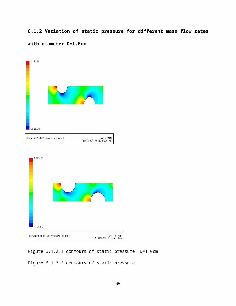
Figure 6.4.3.5 contours of static pressure, D=1.2cm Figure 6.4.3.6 contours of static pressure,
and mass flow rate m=0.25kg/s D=1.2cm and mass flow rate m=0.30kg/s
The pressure contours are displayed in fig 6.4.1 to 6.4.3 with symmetry. The figures revealed
that the static pressure exerts at stagnation point for different mass flow rates have significant
variation. From the figure it can be observed that, the pressure at stagnation point as well as the
flow past the tubes surface varies relatively more compared to the previous geometries due to
increase in tube diameter.
6.5 Static temperature variation in y-axis for different tube diameters and mass flow rates:
The static temperature variation in y-axis along the tubes are shown in the below figures at
different diameters and mass flow rates i.e. D=0.8cm, 1.0cm, 1.2 cm and m= 0.05, 0.10, 0.15,
0.20, 0.25, 0.30kg/s.
90

6.5.1 Static temperature variation in y-axis for different mass flow rates with diameter
D=0.8cm
Figure 6.5.1.1 static temperature, D=0.8cm Figure 6.5.1.2 static temperature,
and mass flow rate m=0.05kg/s D=0.8cm and mass flow rate m=0.10kg/s
91

Figure 6.5.1.3 static temperature, D=0.8cm Figure 6.5.1.4 static temperature,
and mass flow rate m=0.15kg/s D=0.8cm and mass flow rate m=0.20kg/s
92
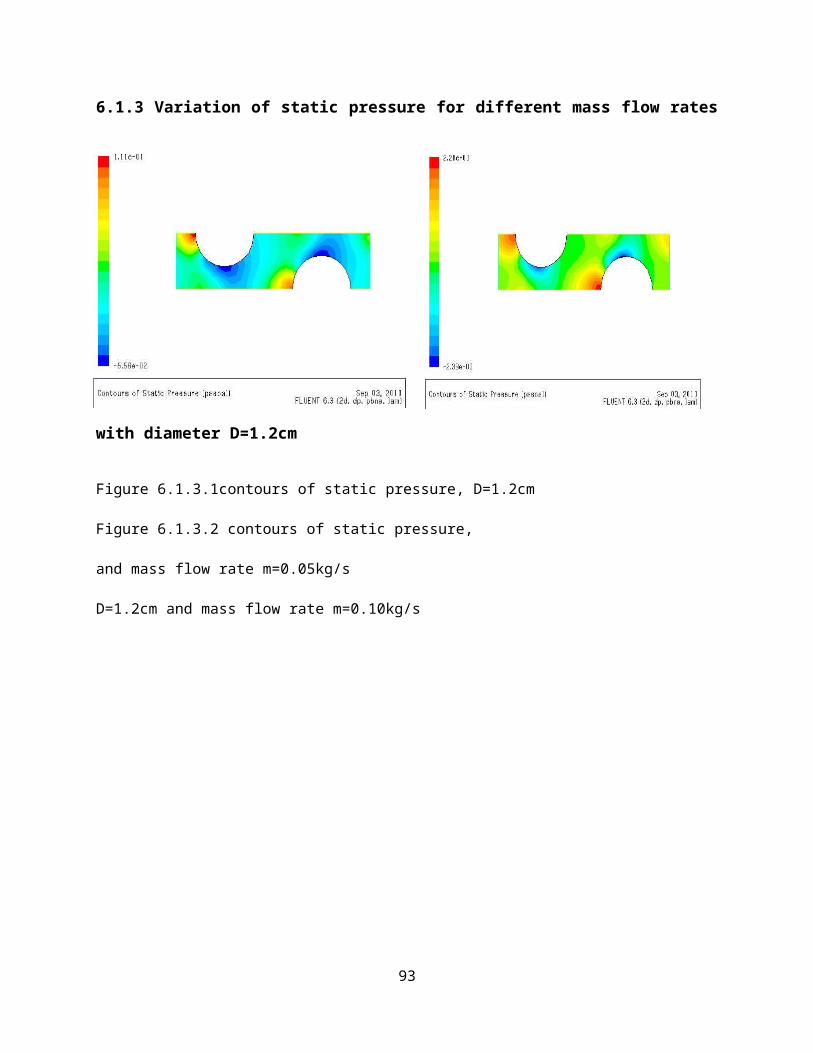
Figure 6.5.1.5 static temperature, D=0.8cm Figure 6.5.1.6 static temperature,
and mass flow rate m=0.25kg/s D=0.8cm and mass flow rate m=0.30kg/s
6.5.2 Static temperature variation in y-axis for different mass flow rates with diameter
D=1.0cm
93

Figure 6.5.2.3 static temperature, D=1.0cm Figure 6.5.2.4 static temperature,
and mass flow rate m=0.15kg/s
D=1.0cm and mass flow rate m=0.20kg/s
94

6.5.3 Static temperature variation in y-axis for different mass flow rates with diameter
D=1.2cm
Figure 6.5.3.1 static temperature, D=1.2cm Figure 6.5.3.2 static temperature,
and mass flow rate m=0.05kg/s D=1.2cm and mass flow rate m=0.10kg/s
95

Figure 6.5.3.5 static temperature, D=1.2cm Figure 6.5.3.6 static temperature,
and mass flow rate m=0.25kg/s D=1.2cm and mass flow rate m=0.30kg/s
96

Iso-surfaces was created corresponding to the vertical cross-section through the first tube, half
way between the two tubes and through the second tube. The figure 5.13 to 5.15 depicts the static
temperature on cross-section of constant x-direction with the y-direction is the one which
temperature varies. It can be observed that at the tube wall fluid attains approximately the tube
wall temperature and minium at the middle of the successive rows of tube bank
6.6 Static Pressure Variation in y-axis for different tube diameters and mass flow rates:
The static pressure variation in y-axis along the tubes are shown in the below figures at different
diameters and mass flow rates i.e. D=0.8cm, 1.0cm, 1.2 cm and m= 0.05, 0.10, 0.15, 0.20, 0.25,
0.30kg/s.
6.6.1 Static Pressure Variation in y-axis for different mass flow rates with diameter
D=0.8cm
Figure 6.6.1.1 static pressure, D=0.8cm Figure 6.6.1.2 static pressure
and mass flow rate m=0.05kg/s D=0.8cm and mass flow rate m=0.10kg/s
97

Figure 6.6.1.5 static pressure, D=0.8cm Figure 6.6.1.6 static pressure
and mass flow rate m=0.25kg/s D=0.8cm and mass flow rate m=0.30kg/s
98

6.6.2 Static Pressure Variation in y-axis for different mass flow rates with diameter
D=1.0cm
99

Figure 6.6.2.3 static pressure, D=1.0cm Figure 6.6.2.4 static pressure
and mass flow rate m=0.15kg/s D=1.0cm and mass flow rate m=0.20kg/s
Figure 6.6.2.5 static pressure, D=1.0cm Figure 6.6.2.6 static pressure
and mass flow rate m=0.25kg/s D=1.0cm and mass flow rate m=0.30kg/s
6.6.3 Static Pressure Variation in y-axis for different mass flow rates with diameter
D=1.2cm
100

Figure 6.6.3.1static pressure, D=1.2cm Figure 6.6.3.2 static pressure
and mass flow rate m=0.05kg/s D=1.2cm and mass flow rate m=0.10kg/s
101

Figure 6.6.3.3 static pressure, D=1.2cm Figure 6.6.3.4 static pressure
and mass flow rate m=0.15kg/s
Figure 6.6.3.5 static pressure, D=1.2cm
Figure 6.6.3.6 static pressure
and mass flow rate m=0.25kg/s
102

D=1.2cm and mass flow rate m=0.30kg/s
Similarly, the static pressure variation along y-direction is shown in fig. 5.16 to 5.18. The
pressure drop allowance in tube bank is the static fluid pressure which drives the fluid through it.
The pressure drop is greatly influenced by the spacing of the succeeding rows of tubes, their
layout and closeness. From the xy-plots, it can be observed, when mass flow rate increases the
pressure drop increases due to length of the recirculation zone behind the tube has an influence
on pressure drop.
6.7 Nusselt number plot:
The Nusselt number plot for different diameter tubes are shown in the below figures at different
diameters and mass flow rates i.e. D=0.8cm, 1.0cm, 1.2 cm and m= 0.05, 0.10, 0.15, 0.20, 0.25,
0.30kg/s.
6.7.1 Nusselt number plot with different mass flow rates with diameter D=0.8cm
103

Figure 6.7.1.1 Nusselt number plot D=0.08m Figure 6.7.1.2 Nusselt number plot D=0.08m for
for mass flow rate m=0.05kg/s mass flow rate m=0.10kg/s
104

Figure 6.7.1.3 Nusselt number plot D=0.08m Figure 6.7.1.4 Nusselt number plot D=0.08m for
for mass flow rate m=0.15kg/s mass flow rate m=0.20kg/s
105

Figure 6.7.1.5 Nusselt number plot D=0.08m Figure 6.7.1.6 Nusselt number plot D=0.08m for
for mass flow rate m=0.25kg/s mass flow rate m=0.30kg/s
6.7.2 Nusselt number plot with different mass flow rates with diameter D=1.0cm
106

Figure 6.7.2.1 Nusselt number plot D=1.0m for Figure 6.7.2.2 Nusselt number plot D=1.0m for
Mass flow rate m=0.05kg/s Mass flow rate m=0.10kg/s
Figure 6.7.2.3 Nusselt number plot D=1.0m for Figure 6.7.2.4 Nusselt number plot D=1.0m for
Mass flow rate m=0.15kg/s Mass flow rate m=0.20kg/s
107

Figure 6.7.2.5 Nusselt number plot D=1.0m for Figure 6.7.2.6 Nusselt number plot D=1.0m for
Mass flow rate m=0.25kg/s Mass flow rate m=0.30kg/s
6.7.3 Nusselt number plot with different mass flow rates with diameter D=1.2cm
Figure 6.7.3.1 Nusselt number plot D=1.2m for Figure 6.7.3.2 Nusselt number plot
D=1.2m for
Mass flow rate m=0.05kg/s Mass flow rate m=0.10kg/s
108
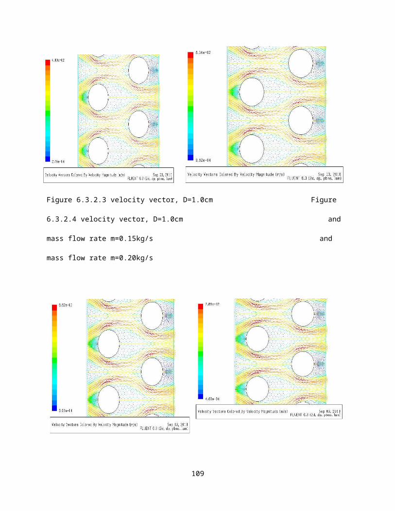
Figure 6.7.3.3 Nusselt number plot D=1.2m for Figure 6.7.3.4 Nusselt number plot D=1.2m for
Mass flow rate m=0.15kg/s Mass flow rate m=0.20kg/s
Figure 6.7.3.5 Nusselt number plot D=1.2m for Figure 6.7.3.6 Nusselt number plot
D=1.2m for
Mass flow rate m=0.25kg/s Mass flow rate m=0.30kg/s
109

Iso-surfaces was created corresponding to the vertical cross-section through the first tube, half
way between the two tubes and through the second tube. The figure 6.7.1 to 6.7.3 depicts the
nusselt number on cross section of constant x-direction with the y-direction is the one which
nusselt number varies. It can be observed that at the tube wall fluid attains approximately the
tube wall temperature and minium at the middle of the successive rows of tube bank
6.8 Verification of Results:
The maximum velocity magnitude obtained from simulation is used to calculate the
Reynolds number from the following expression,
ReDmax = 𝝆µmax D/µ (6.2)
With the above ReDmax the Nusselt number was calculated using the correlation:
Nu = C1 ( C Ren Pr0.33) (6.3)
The total surface heat flux values obtained from the simulation was used to calculate the
Nu values at x=0.01 viz., at the middle of first tube which was used to compare with correlation
values. Table 5.1 presents results generated using different mass flow rates for different physical
models. The results obtained from the simulation were compared to correlation results; the
average error percentages for the different tube diameters are tabulated in table 5.7. It can be
observed that for 1.0cm diameter of tube and 0.05kg/s of mass flow rate the average error for
other the Nusselt number was 3.63% while for other physical models with various mass flow
110

rates the average error variation was significant. The FLUENT and correlation Nusselt number
are shown in fig.
From the above simulation, the following tabular is created with different diameters, with
different mass flow rates and with different tube materials we can verify the simulation results
and theoretical results with the help of equation 6.2 and 6.3
Table 6.8.1 Predicted values of FLUENT Vs Correlation for aluminum
Diameter
(cm)
Mass
flow
rate
(kg/s)
Max
velocity(m/s)
ReD Pr NuD(corr
)
NuDx=0/01 %error
0.8 0.05 0.0115 91.559 6.99091 9.296 8.278 0.1095
0.10 0.0238 189.488 6.99091 13.97 8.975 0.3575
0.15 0.0382 304.137 6.99091 18.20 8.125 0.55405
0.20 0.0512 407.639 6.99091 21.45 5.675 0.7356
0.25 0.0654 520.690 6.99091 24.606 2.650 0.8923
0.30 0.0795 632.95 6.99091 27.449 4.740 0.827
1.00 0.05 0.0095 94.544 6.99091 34.30 13.366 0.6114
0.10 0.0201 200.03 6.99091 14.40 18.465 0.2198
0.15 0.0324 322.44 6.99091 18.81 23.785 0.2208
0.20 0.0425 422.96 6.99091 21.90 27.082 0.191
0.25 0.0593 590.16 6.99091 24.89 27.750 0.1027
0.30 0.0689 685.70 6.99091 28.707 28.590 0.00409
1.2 0.05 0.00752 89.808 6.99091 9.19 16.150 0.4305
0.10 0.1625 194.066 6.99091 14.158 22.230 0.36309
0.15 0.02534 302.62 6.99091 18.15 24.820 0.2684
0.20 0.03675 438.889 6.99091 22.36 27.120 0.1755
0.25 0.04635 553.53 6.99091 25.463 27.345 0.0688
0.30 0.05780 690.28 6.99091 28.814 27.565 0.0433
111

Table 6.8.2 Predicted values of FLUENT Vs Correlation for copper
Diameter
(cm)
Mass
flow rate
(kg/s)
Max
Velocity
(m/s)
ReD Pr NuD(corr) NuDx=0.01 %error
0.8 0.05 0.011462 91.257 6.99091 9.279 8.72 0.0602
0.10 0.0231 183.915 6.99091 13.738 8.95 0.3485
0.15 0.0335 266.717 6.99091 16.99 7.84 0.536
0.20 0.0502 399.67 6.99091 21.21 5.15 0.757
0.25 0.0675 537.41 6.99091 23.62 2.45 0.896
0.30 0.0819 652.06 6.99091 27.91 4.75 0.829
1.0 0.05 0.0092 91.55 6.99091 9.29 13.15 0.293
0.10 0.019 189.09 6.99091 13.95 19.72 0.292
0.15 0.0316 314.487 6.99091 18.55 23.82 0.2211
0.20 0.0420 417.99 6.99091 21.75 25.94 0.1612
0.25 0.0542 539.406 6.99091 25.09 27.45 0.0856
0.30 0.0653 679.73 6.99091 28.94 27.12 0.062
1.2 0.05 0.00778 92.913 6.99091 9.37 16.00 0.4141
0.10 0.0160 191.67 6.99091 14.06 23.82 0.4097
0.15 0.0258 308.118 6.99091 18.34 24.88 0.2627
0.20 0.0367 431.126 6.99091 22.13 25.87 0.144
0.25 0.0466 556.52 6.99091 24.09 26.82 0.101
0.30 0.0578 690.28 6.99091 28.81 27.02 0.0622
112

Table 6.8.3 Predicted values of FLUENT Vs Correlation for (Ni-Cr alloy)
Diameter
(cm)
Mass
flow rate
(kg/s)
Max
velocity
(m/s)
ReD Pr NuD(corr) NuDx=0.01 % Error
0.8 0.05 0.0103 82.005 6.99091 8.740 8.12 0.0709
0.10 0.0227 180.730 6.99091 13.60 8.48 0.3760
0.15 0.0363 289.010 6.99091 17.69 7.61 0.5701
0.20 0.0512 417.990 6.99091 21.75 5.02 0.769
0.25 0.0682 542.988 6.99091 25.19 2.532 0.8995
0.30 0.0826 657.637 6.99091 28.04 4.940 0.823
1.0 0.05 0.00913 90.863 6.99091 9.256 13.00 0.6114
0.10 0.0199 198.04 6.99091 14.32 18.245 0.2151
0.15 0.0327 325.43 6.99091 17.45 23.567 0.2592
0.20 0.0432 429.93 6.99091 22.10 27.254 0.1889
0.25 0.0515 512.53 6.99091 24.36 27.89 0.1256
0.30 0.0599 596.133 6.99091 26.543 28.674 0.0743
1.2 0.05 0.00783 93.510 6.99091 9.406 14.150 0.335
1.00 0.01656 197.768 6.99091 14.309 19.532 0.267
0.15 0.02534 302.62 6.99091 18.15 24.820 0.2684
0.20 0.0383 457.400 6.99091 22.88 27.12 0.156
0.25 0.0498 594.74 6.99091 26.508 28.645 0.0746
0.30 0.05245 626.86 6.99091 27.289 29.565 0.67769
113

For better understanding of theoretical values and simulation values for different diameters and
mass flow rates, the following graphs are drawn.
0.05000000000000
01
0.1 0.15 0.2 0.25 0.30
5
10
15
20
25
30
35
40
diamter 0.8diameter 1.0diameter 1.2
mass flow rates (kg/s)
Nu
ssel
t n
um
ber
cor
rela
tion
Figure 6.8.1 mass flow rates Vs Nusselt number for Aluminum tubes
0.05 0.1 0.15 0.2 0.25 0.30
5
10
15
20
25
30
35
diameter 0.8diameter 1.0diameter 1.2
mass flow rates (kg/s)
Nu
ssel
t n
um
ber
cor
rela
tion
114

Figure 6.8.2 mass flow rate Vs Nusselt number for copper tubes.
0.05 0.1 0.15 0.2 0.25 0.30
5
10
15
20
25
30
diameter 0.8diameter 1.0diameter 1.2
mass flow rates (kg/s)
nu
ssel
t n
um
ber
cor
rela
tion
e
Figure 6.8.3mass flow rate Vs Nusselt number correlation for Nickel-Chromium base super alloy base
tube.
0.05 0.1 0.15 0.2 0.25 0.30
5
10
15
20
25
30
dimater -.8diameter 1.0diameter 1.2
mass fow rates (kg/s)
Nu
ssel
t n
um
ber
th
eore
tica
l
Figure 6.8.4 mass flow rate VsNusselt number theoretical for aluminum
115
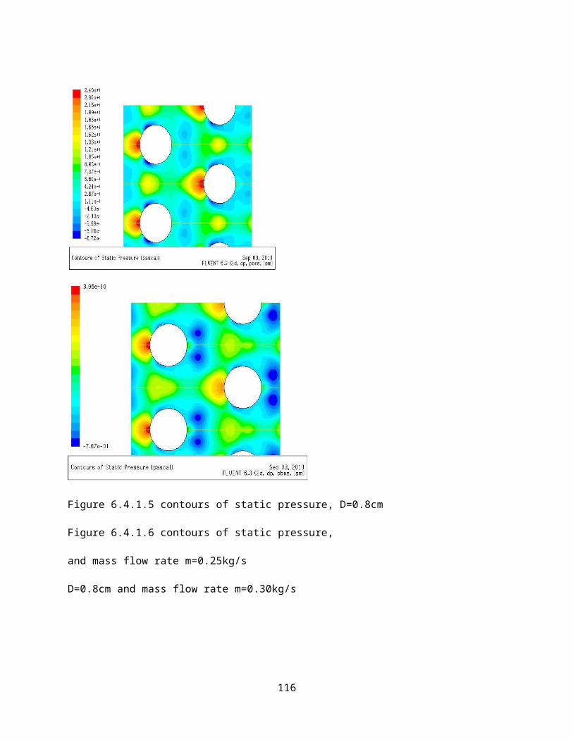
0.05 0.1 0.15 0.2 0.25 0.30
5
10
15
20
25
30
diameter 0.8diameter 1.0diameter 1.2
mass flow rates (kg/s)
nu
ssel
t n
um
ber
th
eore
tica
l
Figure 6.8.5 mass flow rates Vs Nusselt number theoretical for copper tubes.
0.05 0.1 0.15 0.2 0.25 0.30
5
10
15
20
25
30
35
diameter 0.8diameter 1.0diameter 1.2
mass flow rates (kg/s)
nu
ssel
t n
um
ber
th
eore
tica
l
Figure 6.8.6 mass flow rates Vs Nusselt number theoretical for Nickel- chromium base super alloy.
116

0.05 0.1 0.15 0.2 0.25 0.30
5
10
15
20
25
30
aluminiumcopperNi-Cr alloy
mass flow rates (kg/s)
Nu
ssel
t n
um
ber
Figure 6.8.7 mass flow Vs Nusselt number for different materials at d=0.08cm
0.05 0.1 0.15 0.2 0.25 0.30
5
10
15
20
25
30
35
40
aluminiumcopperNi-Cr alloy
mass flow rates kg/s
nu
ssel
t n
um
ber
Figure 6.8.8 mass flow rates Vs Nusselt number for different materials at d=1.0cm
117

0.05 0.1 0.15 0.2 0.25 0.30
5
10
15
20
25
30
35
aluminiumcopperNi-Cr alloy
mass flow rates (kg/s)
nu
ssel
t n
um
ber
Figure 6.8.9 mass flow rates Vs mass flow rates for different materials at d=1.20cm
From the above graphs the observations are:
The effect of different mass flow rates on both flow and heat transfer is significant. It was
observed that 1.0cm diameter of tubes and 0.05kg/s mass flow gives the best results as
34.30 Nusselt number.
From the above graphs we can observe that alloys serves as a better material for tube
when compare with copper and aluminum.
The effect of mass flow rates on both flow and heat transfer is significant. This is due to
variation of space of the surrounding tubes.
It was observed optimal flow distribution was found for 0.8cm diameter and 0.05kg/s
mass flow rate in case of alloy.
118

CHAPTER 6
CONCLUSIONS
6.0 CONCLUSIONS
119

Mode and mesh creation n CFD is one of the most important phases of simulation. The
model and mesh density determine the accuracy and flexibility of the simulations. Too dense a
mesh will unnecessarily increase the solution time; too coarse a mesh will reach to a divergent
solution quickly. But will not show an accurate flow profile. An optimal mesh is denser in areas
where there are no flow profile changes.
A two- dimensional numerical solution of flow and heat transfer in a bank of tubes which
is used in industrial applications has been carried out.
Laminar flow past a tube bank is numerically simulated in the low Reynolds number
regime. Velocity vector depicts zones of recirculation between the tubes. Nusselt number
variations are obtained and pressure distribution along the bundle cross section is
presented.
The effect of different mass flow rates on both flow and heat transfer is significant. This
is due to the variation of space of the succeeding rows of tubes. It was observed that
1.0cm diameter of tubes and 0.05kg/s mass flow rate gives the best results.
Mass flow rate has an important effect to heat transfer. An optimal flow distribution can
result in a higher temperature distribution and low pressure drop. It was observed that the
optimal flow distribution was occurred in 1.0cm diameter and 0.05kg/s mass flow rate.
CFD simulations are a useful tool for understanding flow and heat transfer principles as
well as for modeling these types of geometries.
It was observed that 1.0cm diameter of tubes and 0.30kg/s mass flow rate yields optimum
results for aluminum as tube material, where as it was observed that 0.8cm and 0.05kg/s
mass flow rate in case of copperas tube material.
120

From the above graphs we observed that alloys serves as a better material for tube
compared with copper and aluminum.
Alloy (Nickel-Chromium based) serves as a better material for heat transfer applications
with low cost
Further improvements of heat transfer and fluid flow modeling can be possible by
modeling three dimensional models and changing the working fluid.
121

APPENDICES
Table (A) Mesh Details of tubes with varying diameters
Diameter (D) Cells Faces Nodes
0.8cm 1921 3942 2052
122

1.0cm 1510 3115 1636
1.2cm 1787 3689 1933
1.4cm 1545 3212 1698
123

REFERNCES
Patankar, S.V. and spalding. D.B. (1974), “ A calculation for the transient and steady
state behaviour of shell- and- tube Heat Exchanger”. Heat transfer design and theory
sourcebook. Afgan A.A. and Schluner E.U.. Washington. Pp. 155-176.
124

KelKar, K.M and Patankar, S. V., 1987” Numerical prediction of flow and Heat transfer
in a parallel plate channel with staggered fins”, Journal of Heat Transfer, vol. 109, pp 25-
30.
Berner, C., Durst, F. And McEligot, D.M., “Flow around Baffles”, Journal of Heat
Transfer, vol. 106 pp 743-749.
Popiel, C.o & Vander Merwe, D.F., “Friction factor in sine-pipe flow, Journal of fluids
Engineering”, 118, 1996, 341-345.
Popiel, C.O & Wojkowiak, J., “friction factor in U-type undulated pipe flow, Journal of
fluids Engineering”, 122, 2000, 260-263.
Dean, W. R., Note on the motion of fluid in a curved pipe, The London, Edinburgh and
Dublin philosophical Magazine, 7 (14), 1927, 208-223.
Patankar, S.V., Liu, C.H & Sparrow, E.M., “Fully developed flow and Heat Transfer in
ducts having streamwise periodic variation in cross-sectional area”, Journal of Heat
Transfer, 99, 1977, 180-186.
Webb, B.W & Ramdhyani, S., “Conjugate Heat Transfer in an channel with staggered
Ribs” Int. Journal of Heat and Mass Transfer 28(9), 1985,1679-1687.
Park, K., Choi, D-H & Lee, K-s., “design optimization of plate heat exchanger with
staggered pins”, 14th Int. Symp.on Transport phenomena, Bali, Indonesia, 6-9 July 2003.
N.R. Rosaguti, D.F. Fletcher & B.S. Haynes “Laminar flow in a periodic serpentine”. 15 th
Australasian fluid mechanics conference. The University of Sydney, Sydney, Australia
13-17 December 2004.
125

L.C Demartini, H.A. Vielmo, S.V. Moller “Numeric and experimental analysis of
turbulent flow through a channel with baffle plates”, J. Braz. Soc. Mech.Sci & Eng. Vol
26 No.2 Rio de Janeiro Apr/June 2004.
Baier, G., Grateful, T.M. Graham, M.D. & Lightfoot E.N.(1999), “ Prediction of mass
transfer rates in spatially periodic flow”, Chem. Eng. Sci., 54,343-355.
Bao, L. & Lipscomb, G.G., 2002 “ Well-developed mass transfer in axial flows through
randomly packed fiber bundles with constant wall flux”, Chem. Eng. Sci., 57, 125-132.
Launder, B.E. & Massey, T.H 1978 “The numerical predictions of viscous flow and heat
transfer in tubefer bank”. J. Heat transfer, 100, 565-571.
Wung, T.S. & Chen, C.J. (1989), “Finite analytic solution of convective Heat transfer for
tube arrays in cross flow: part- I flow field analysis”, ASME J. Heat Transfer, 111, 633-
640.
Schoner, P., Plucinski, W.N. & Daiminger, U. (1998), “Mass transfer in the shell side of
cross flow hollow fiber modules”, Chem. Eng. Sci. 53, 2319-2326.
T.Li, N.G. Deen & J.A D.G. M. Kuipers, faculty of Sci. & Tech, University of Twente, “
Numerical study of Hydrodynamics and mass transfer of in line fiber arrays in laminar
cross flow”, 3rd International conference on CFD in the Minerals and process Industries
CSIRO, Melbourne, Australia 10-12 December 2003, pg, 87-92.
T.V. Mull, Jr., M.W. Hopkins and D.G. White “Numerical Simulation Models for a
Modern Boiler Design “, Power-Gen International’ 96, December 4-6, 1996, Orlando,
Florida, U.S.A
Chung, Y.M., Tucker, P.G., “Assessment of periodic flow assessment for unsteady state
Heat Transfer in grooved channels; Transaction of the ASME, Vol.126, Dec (2004).
126

127

GLOSSARY
Reynolds number (2): In fluid mechanics, the Reynolds number (Re) is a dimensionless
number that gives a measure of the ratio of inertial forces to viscous forces and consequently
quantifies the relative importance of these two types of forces for given flow conditions.
Simulation (6): is the imitation of the operation of a real-world process or system over time. The
act of simulating something first requires that a model be developed; this model represents the
key characteristics or behaviors of the selected physical or abstract system or process.
128

Control volumes (33): In fluid mechanics and thermodynamics, a control volume is a
mathematical abstraction employed in the process of creating mathematical models of physical
processes. In an inertial frame of reference, it is a volume fixed in space or moving with constant
velocity through which the fluid (gas or liquid) flows. The surface enclosing the control volume
is referred to as the control surface.
Discretization (36): In mathematics, discretization concerns the process of
transferring continuous models and equations into discrete counterparts. This process is usually
carried out as a first step toward making them suitable for numerical evaluation and
implementation on digital computers.
Nusselt Number (96): In heat transfer at a boundary (surface) within a fluid, the Nusselt
number is the ratio of convective to conductive heat transfer across (normal to) the boundary.
129
Related Documents