Replication in one-dimensional cellular automata Janko Gravner Mathematics Department University of California Davis, CA 95616 e-mail: [email protected] Genna Gliner Mathematics Department University of California Davis, CA 95616 e-mail: [email protected] Mason Pelfrey Mathematics Department University of California Davis, CA 95616 e-mail: [email protected] (Second version, June 2011) Abstract. In cellular automata (CA), replication is the ability to indefinitely generate copies of a finite collection of patterns, starting from finite seeds. A transparent feature of additive CA, replication mechanisms are less clear in the absence of additivity; this paper investigates such dynamics through several examples. For the 1 Or 2 rule and its generalizations, replication is inevitable and we investigate self-organization properties. In the Perturbed Exactly 1 rule we study frequency of replicators and the new phenomenon called quasireplication. The last CA is the Extended 1 Or 3 rule, which allows for replication on different backgrounds. We employ a mixture of rigorous and empirical techniques. 2000 Mathematics Subject Classification . 37B15, 68Q80. Keywords : additivity, cellular automaton, entropy, ether, quasireplicator, replicator. Acknowledgments. This work owes a great deal to the long-term collaboration between JG and David Griffeath, and their many discussions on the topic of this paper. The authors are also thankful to the anonymous referee whose insights greatly improved the paper’s accuracy and presentation, and to Ander Holroyd for pointing out a mistake in a previous version. Support. JG was partially supported by NSF grant DMS–0204376 and the Republic of Slove- nia’s Ministry of Science program P1-285. GG and MP were also supported by the same NSF grant, as well as by a VIGRE grant to the UC Davis Mathematics Department.

Welcome message from author
This document is posted to help you gain knowledge. Please leave a comment to let me know what you think about it! Share it to your friends and learn new things together.
Transcript
Replication in one-dimensional cellular automata
Janko GravnerMathematics DepartmentUniversity of California
Davis, CA 95616e-mail: [email protected]
Genna GlinerMathematics DepartmentUniversity of California
Davis, CA 95616e-mail: [email protected]
Mason PelfreyMathematics DepartmentUniversity of California
Davis, CA 95616e-mail: [email protected]
(Second version, June 2011)
Abstract. In cellular automata (CA), replication is the ability to indefinitely generate copies ofa finite collection of patterns, starting from finite seeds. A transparent feature of additive CA,replication mechanisms are less clear in the absence of additivity; this paper investigates suchdynamics through several examples. For the 1 Or 2 rule and its generalizations, replication isinevitable and we investigate self-organization properties. In the Perturbed Exactly 1 rule westudy frequency of replicators and the new phenomenon called quasireplication. The last CA isthe Extended 1 Or 3 rule, which allows for replication on different backgrounds. We employ amixture of rigorous and empirical techniques.
2000 Mathematics Subject Classification. 37B15, 68Q80.
Keywords: additivity, cellular automaton, entropy, ether, quasireplicator, replicator.
Acknowledgments. This work owes a great deal to the long-term collaboration between JGand David Griffeath, and their many discussions on the topic of this paper. The authors arealso thankful to the anonymous referee whose insights greatly improved the paper’s accuracyand presentation, and to Ander Holroyd for pointing out a mistake in a previous version.
Support. JG was partially supported by NSF grant DMS–0204376 and the Republic of Slove-nia’s Ministry of Science program P1-285. GG and MP were also supported by the same NSFgrant, as well as by a VIGRE grant to the UC Davis Mathematics Department.
1 Introduction
During the evolution of many simple cellular automata (CA) rules, especially those relatedto the Game of Life, the following phenomenon is frequently observed: “a configuration ofoccupied sites makes copies of itself, then the copies make copies of themselves, and these copiesmove toward one another. [. . . ] When the innermost copies collide, they annihilate, [while]the outermost [ones] continue to reproduce. This pattern repeats, ad infinitum” [Eva2]. Theresulting space-time picture is sometimes called fractal [CD] or nested [Wol3], but we prefer themore descriptive term replication [Eva1, Eva2]. Traditionally associated with additivity [CD],this type of behavior occurs for no a priori reason in numerous CA, in one and two dimensions[Epp]. In the present paper, we focus on selected one-dimensional examples.
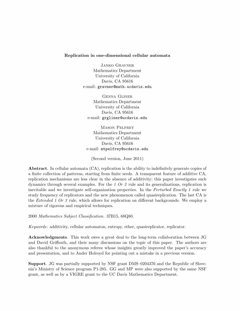
To illustrate our main ideas, two CA (whose rules are defined later in this section) were runfrom a small random seed. Fig. 1 depicts the resulting space-time configurations; the time axis inall our pictures and descriptions is oriented downward , as is common in this field. In each case ofFig. 1, triangular regions appear, either empty or filled with a simple periodic pattern. Is this abeginning of a recursive behavior, with larger and larger regular regions? What kind of periodicpatterns can be generated? What mechanisms govern the initial self-organization phase? Howtypical is such a dynamics for a given CA? Much of the rest of the paper is devoted to preciseformulations of such questions, and to techniques for obtaining at least partial answers.
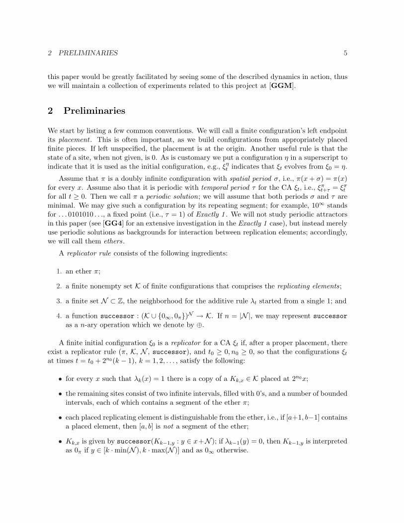
Fig. 1. Two replicator examples, both at time 100. Left: Quota with θ = 2, started from1111001101101101100011; right: Extended 1 Or 3 , started from 2221032011102133101.
We present a basic replication setup in Section 2, defining the ingredients that go into thedescription of a replication scheme. Given the diverse circumstances in which replicators appear[Eva1, Eva2, Epp], it seems unlikely that one could formulate either wide-ranging necessaryand sufficient conditions on existence of replicators, or estimate the likelihood of their appearancefrom random initial states independently of the details of a particular rule. Instead, we developa list of issues one might look at when presented with a CA rule capable of replication. Wealso do not close the book on any of the presented examples, and conclude the paper with aninventory of interesting open problems.
We call a configuration a finite or infinite sequence of elements from S, where S = {0, 1, . . . , s−1} is a finite set of states. When the sequence is doubly infinite, a configuration gives each sitein Z either the empty state 0, or one of s − 1 occupied states. We will assume that time in-creases in discrete steps, t = 0, 1, 2, 3, . . . , and that configurations ξt evolve by a CA rule. A
1 INTRODUCTION 2
configuration is finite if it has only finitely many occupied sites; the initial configuration ξ0 willbe typically assumed finite, and will in this case often be referred to as a seed . As we follow theusual convention [GG4] that the state of a site, when unspecified, is assumed to be 0, we maygive a finite configuration as a finite sequence of states. Finally, when S = {0, 1} we identifythe configuration ξt with its set {ξt = 1} of occupied sites at time t. In all examples we present,the quiescent (all 0’s) state is mapped into itself; to avoid the trivial case we will always assumethat a seed is non-quiescent.
We are interested in cases when a CA replicates, that is, makes copies of a finite collectionof finite configurations, called replicating elements, indefinitely. Such dynamics may occur forall, or only for some, seeds. As in [GG4], we identify the seed with the attractor, calling ita replicator if it leads to replication regardless of whether the seed is among the replicatingelements.
The easiest to study are additive CA, which for our purposes have S = {0, 1} and are givenby a finite (neighborhood) N ⊂ Z. Then the CA λt is given for t = 0, 1, . . . by addition modulo2 over the neighborhood given by N :
λt+1(x) =∑
k∈Nλt(x + k) mod 2.
The most basic example is known as Rule 90 [Wol1] and has N = {−1, 1}. It has been longknown that, at large enough times of the form 2n, the occupied set consists of two identicalcopies of the seed (which, we emphasize again, is finite), separated by 0’s. Another additiverule, 1 Or 3 or Rule 150 , in which N = {−1, 0, 1}, behaves in the same way, except that thenumber of copies is now three; in fact, every additive CA replicates any seed, and the numberof copies at large dyadic power times equals cardinality of N . Additive rules commute withaddition modulo 2 and seem to be the only class of CA rules amenable to general mathematicaltheory (e.g., [Wol1, CD, Wil1, Wil2, FLM, HPS]), thus they play a role analogous to lineardynamical systems, and are for this reason sometimes called linear .
As we will see more formally in Section 2, a CA started from a particular seed replicates if itsimulates an additive CA started from a single 1 at the origin. This is a very weak version of theimportant notion of intrinsic simulation, which demands that one CA is able to simulate anotherstarted from any initial configuration (see [Oll] and subsequent work of the same author). Wealso remark that, if a seed is a replicator, its trajectory can be efficiently predicted ([Moo]).
We now introduce the examples of nonadditive CA considered in this paper. These haveall previously appeared in the literature, and are selected for connections to other interestingdynamics, such as two-dimensional CA growth [GG1, GG2, GG3] and coupled logistic-typemaps [GG4], and especially for their simplicity. In particular, each of our CA uses ether a range1 or a range 2 neighborhood, i.e., the neighborhood of an integer point x is either {x−1, x, x+1}or {x− 2, x− 1, x, x + 1, x + 2}.
We begin by the rule we consider the prototypical nonadditive dynamics [GG4], namely theExactly 1 CA (often called Rule 26 [Wol1]), in which x becomes occupied at time t + 1 if andonly it has exactly 1 occupied nearest neighbor at time t:
ξt+1(x) = 1 ⇐⇒ |ξt ∩ {x− 1, x, x + 1}| = 1.
1 INTRODUCTION 3
(The vertical bars denote cardinality.) Replication is common in this CA among small seeds.For large seeds, chaotic evolution is by far the likeliest, and periodic seeds also exist. The paper[GG4] contains a detailed study including many replication examples.
The next rule is also quite well-known. We call it the 1 Or 2 CA, but it is also known asRule 126 [Jen3, Jen4, GG3]. It has binary states and its rule mandates that the state of x isoccupied at time t + 1 if and only if either one or two of its range 1 neighbors of x are occupiedat time t:
ξt+1(x) = 1 ⇐⇒ |ξt ∩ {x− 1, x, x + 1}| ∈ {1, 2}.This rule is not additive; nevertheless it replicates for every seed, and it always has essentiallya single replicating element. We call such CA quasiadditive, and two additional such examples(which are not additive) have been studied [Jen2, Jen3, Jen4]. The replicating element canbe very different from the seed, due to a long onset time before the replication commences. Wewill study the distribution of onset times in Section 3.
We also prove that two natural generalizations of Jen’s rules to range 2 are both quasiadditive.These are Quota rules [CD] with a threshold parameter θ and stipulate that a point becomesoccupied if it sees at least θ 1’s and at least θ 0’s in its range 2 neighborhood:
ξt+1(x) = 1 ⇐⇒ |ξt ∩ {x− 2, x− 1, x, x + 1, x + 2}| ∈ [θ, 5− θ].
As described in Section 4, these have an extra self-organizing period before they enter the Jenregime. When θ = 1 this period is trivial and lasts a single time step, but when θ = 2 aLyapunov function drives the dynamics toward a configuration with sufficient regularity.
Next we describe a CA we call Perturbed Exactly 1 , introduced in [BP]. This rule also hasbinary states but now x is occupied at time t+1 if and only if at time t either (1) it has exactly2 occupied sites among its five nearest neighbors or (2) the single occupied site among its fivenearest neighbors is positioned among the three nearest neighbors:
ξt+1(x) = 1 ⇐⇒ |ξt ∩ {x− 2, x− 1, x, x + 1, x + 2}| = 2 or|ξt ∩ {x− 1, x, x + 1}| = 1 and ξt(x− 2) = ξt(x + 2) = 0.
First few experiments with small seeds, as well as the account in [BP], suggest that replicationalways happens for Perturbed Exactly 1 , but this is not the case. However, as we demonstratein Section 5, replication is indeed quite common, although, as is Exactly 1 , this CA is capable ofchaotic behavior. Even more interesting, and challenging to study, is a new type of behavior wecall quasireplication, whereby the occupied set within space-time is fractal, in the appropriatelimit, even in the absence of replication (see Section 6).
In the examples presented so far, all the known instances of replication proceed on an emptybackground, but nonzero periodic backgrounds, called ethers, are also possible. Rule 186 [Wol3],for instance, always replicates on the fully occupied ether (which can be easily proved because itsevolution is the“photographic negative” of the one for Rule 146 studied in [Jen4]). Perhaps thesimplest example which admits both the zero ether and a nonzero one is the Embossed TrianglesCA, introduced by M. Wojtovicz in [Woj]. In this range 2 rule, a 1 survives by contact with

1 INTRODUCTION 4
two or three 1’s (including itself), and a 0 changes to 1 by contact with two, three, or four 1’s:
ξt+1(x) = 1 ⇐⇒ ξt(x) = 1 and |ξt ∩ {x− 2, x− 1, x, x + 1, x + 2}| ∈ {2, 3}or ξt(x) = 0 and |ξt ∩ {x− 2, x− 1, x, x + 1, x + 1}| ∈ {2, 3, 4}.
Both Quota and Embossed Triangles fit into context of Larger Than Life CA [Eva1], whichseem to be a particularly fertile ground for replication.
To our knowledge, the best case to investigate multiple ethers is our last rule, which requiresa little motivation. One of the most interesting two-dimensional solidification CA is Box 13[GG3]. In this dynamics on Z2 with binary states, an occupied site always stays occupied,while an empty state becomes occupied if it has either 1 or 3 already occupied sites in its Mooreneighborhood, i.e., among its nearest eight sites. Assume that all of the initially occupied sitesare initially on or below the x-axis, and that the x-axis contains at least one occupied site. Then,for any CA that uses the Moore neighborhood, the configuration at time t on the line y = t onlydepends on the configuration on the line y = t − 1 at time t − 1, and this dependence definesthe extreme boundary dynamics (EBD) for the CA.
For the Box 13 solidification, EBD is the additive 1 Or 3 rule; thus, by analogy to Hex[GG2] or Diamond [BDR] rules, one expects at first that this solidification CA is amenable tocomplete analysis. However, a new problem appears: the web of occupied sites generated by theEBD “leaks,” and therefore fails to divide the lattice into independent regions with a renewalstructure. A more successful approach involves keeping track of two extreme lines, y = t andy = t−1. The resulting one-dimensional CA, which we call 2-level EBD for Box 13 , or Extended1 Or 3 , is no longer additive. For a given x, we code the four occupation possibilities of (x, t−1)and (x, t) at time t as 00 = 0, 01 = 1, 10 = 2 and 11 = 3 to obtain a CA with S = {0, 1, 2, 3},and the following convoluted rule. First compute
c1 = (ξt(x− 1) + ξt(x) + ξt(x + 1)) mod 2,
c2 =⌈
ξt(x− 1)2
⌉+
⌈ξt(x)
2
⌉+
⌈ξt(x + 1)
2
⌉,
and then let
ξt+1(x) =
{c1 + 2, if either ξt(x) mod 2 = 1 or c2 ∈ {1, 3},c1, otherwise.
Replication in Extended 1 Or 3 is common, on a zero ether or on one of many other ethers(see Section 7). In fact, an overwhelming proportion of large seeds seem to replicate. On theother hand, we will demonstrate that a simple seed is a non-replicating quasireplicator. There issome empirical evidence for existence of a much more complex evolution with different propertiesthan, say, the Exactly 1 chaos [GG4]. However, some seeds take an extraordinarily long timeto organize and the possibility of ethers with enormous periods cannot be eliminated; thusconjectures of asymptotic behavior based on even millions of updates are precarious.
The above cautionary note is important, but the role of the computer experimentation inpresent investigations cannot be overstated. Many of our results were first conjectured throughcomputer experimentation, using MCell [Woj], or one of our many ad hoc programs. Reading
2 PRELIMINARIES 5
this paper would be greatly facilitated by seeing some of the described dynamics in action, thuswe will maintain a collection of experiments related to this project at [GGM].
2 Preliminaries
We start by listing a few common conventions. We will call a finite configuration’s left endpointits placement . This is often important, as we build configurations from appropriately placedfinite pieces. If left unspecified, the placement is at the origin. Another useful rule is that thestate of a site, when not given, is 0. As is customary we put a configuration η in a superscript toindicate that it is used as the initial configuration, e.g., ξη
t indicates that ξt evolves from ξ0 = η.
Assume that π is a doubly infinite configuration with spatial period σ, i.e., π(x + σ) = π(x)for every x. Assume also that it is periodic with temporal period τ for the CA ξt, i.e., ξπ
t+τ = ξπt
for all t ≥ 0. Then we call π a periodic solution; we will assume that both periods σ and τ areminimal. We may give such a configuration by its repeating segment; for example, 10∞ standsfor . . . 0101010 . . ., a fixed point (i.e., τ = 1) of Exactly 1 . We will not study periodic attractorsin this paper (see [GG4] for an extensive investigation in the Exactly 1 case), but instead merelyuse periodic solutions as backgrounds for interaction between replication elements; accordingly,we will call them ethers.
A replicator rule consists of the following ingredients:
1. an ether π;
2. a finite nonempty set K of finite configurations that comprises the replicating elements;
3. a finite set N ⊂ Z, the neighborhood for the additive rule λt started from a single 1; and
4. a function successor : (K ∪ {0∞, 0π})N → K. If n = |N |, we may represent successoras a n-ary operation which we denote by ⊕.
A finite initial configuration ξ0 is a replicator for a CA ξt if, after a proper placement, thereexist a replicator rule (π, K, N , successor), and t0 ≥ 0, n0 ≥ 0, so that the configurations ξt
at times t = t0 + 2n0(k − 1), k = 1, 2, . . . , satisfy the following:
• for every x such that λk(x) = 1 there is a copy of a Kk,x ∈ K placed at 2n0x;
• the remaining sites consist of two infinite intervals, filled with 0’s, and a number of boundedintervals, each of which contains a segment of the ether π;
• each placed replicating element is distinguishable from the ether, i.e., if [a+1, b−1] containsa placed element, then [a, b] is not a segment of the ether;
• Kk,x is given by successor(Kk−1,y : y ∈ x+N ); if λk−1(y) = 0, then Kk−1,y is interpretedas 0π if y ∈ [k ·min(N ), k ·max(N )] and as 0∞ otherwise.
2 PRELIMINARIES 6
We will assume, without loss of generality, that a fixed replicating element K, when incontact with the ether π from either side, encounters π in the same spatial phase: the first σstates of π are the same on either side of every occurrence of K.
Thus all Kk,x are determined by the initial elements K1,x, x ∈ N , and successive applicationsof the succession rule successor. Also note that the replicating elements may be replaced bytheir successors by the original CA rule, so K is not unique. In our examples and in Section 3, wewill take a K with the smallest cardinality and assume not all of its elements can be shortened(while still remaining a set of replicating elements). Then we will assume that the onset timet0 and the replication time 2n0 are minimal (note that selection of t0 and the two elements atthat time determines n0). The final, and very important, remark is that the specification ofthe rule successor may not be complete; then one has to give an argument that the missinginteractions never happen.
We call ξ0 a maternal replicator if the ether is the zero configuration, and there exists aconfiguration K so that any configuration in K equals K, possibly with 0’s appended at eitherend. Any replicator which is not maternal is fraternal .
We call a CA for which every seed is a maternal replicator quasiadditive. Every additive CAis quasiadditive; this well-known folk result is easy to prove [CD]. Not too many quasiadditiveCA that are not additive are known, but three are introduced in [Jen3]: 1 Or 2 , Rule 18, andRule 146 . Existence of a fraternal indicator is thus a sign of an essential nonadditivity in a CArule.
We remark that the definition of a replicator can be substantially simplified when the etheris zero and λt is Rule 90 , that is, when N = {−1, 1}. See [GG4] for the definition in that case,and for many illustrative examples of maternal and fraternal replicators for Exactly 1 rule. Forhigher-dimensional emulation of additive rules, see [Eva2].
It is important to realize that one could formulate a condition to verify that an initial stateis a replicator after only finitely many replications, when all possible interactions have takenplace; see [GG3] for some examples, and we give another below. Thus in every particularinstance a computer can be used to verify that a seed is replicator. Invariably, the details ofsuch verifications do not translate well from the computer screen to text, hence they are largelyomitted from the paper.
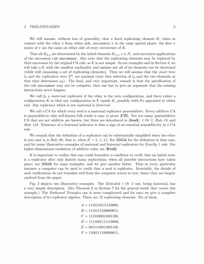
Fig. 2 depicts two illustrative examples. The Extended 1 Or 3 one, being maternal, hasa very simple description. (See Theorem 6 in Section 7 for the general result that covers thisexample.) The Embossed Triangles one is more complicated and for once we give a completedescription of its replicator algebra. There are 12 replicating elements. Six of them,
A = 1110110111110000,B = 1110111100000011,C = 1110100011001100,D = 1111001111110000,E = 0011110011001100,F = 1100111100000011,
2 PRELIMINARIES 7
inhabit the left portion of the space-time configuration. The remaining six, distinguished bythe superscript R, inhabit the right portion, and are mirror images, with appropriate segmentsof the ether (ten sites in each case) added to make their placement correct. The only left-rightinteractions are between A and AR at the beginning, and between D and DR later on, both ofcourse giving 0π. Here is the list of other interactions, denoted by the noncommutative operation⊕:
A⊕ 0π = E, 0∞ ⊕A = B,
B ⊕ 0π = D, 0∞ ⊕B = C,
C ⊕ 0π = F, 0∞ ⊕ C = A,
D ⊕ 0π = E, 0π ⊕D = F,
E ⊕ 0π = F, 0π ⊕ E = D,
F ⊕ 0π = D, 0π ⊕ F = E,
A⊕ F = B ⊕E = C ⊕D = D ⊕ F = E ⊕D = F ⊕E = 0π.
The last verification, 0π ⊕D = F , occurs at time 248 = t0 + (15 − 1) · 2n0 , and one can proveby induction that no other interactions ever occur. Therefore, it is at time 248 that we can betruly certain that this dynamics emulates Rule 90 .
Fig. 2. Two replication examples; in each case, the configurations at the onset time and atthree multiples of the replication time thereafter are highlighted in black. Left: Extended 1Or 3 from A = 33033000333, a maternal replicator, in which K = {A}, t0 = 2n0 = 16, andN = {0,±1}; the states 3, 2 and 1 are in progressively lighter shades of gray. Translations ofA occur at positions given by the locations of 1’s, multiplied by 16, in the additive 1 Or 3 CA.Right: Embossed Triangles from 1110110111, with N = {±1}, ether π = 111100∞ with σ = 6,τ = 2, K and successor described in the text, and t0 = 24, n0 = 4. The additive CA is thusRule 90 and the elements (from left to right) at time t0 are A and AR; then B and BR at timet0 + 2n0 ; then C, D, DR, and CR at time t0 + 2 · 2n0 ; and then A and AR at time t0 + 3 · 2n0 .
Define the space-time occupied set
At = {(s, x) : 0 ≤ s ≤ t, ξs(x) > 0} ⊂ Z2.
Assume the rescaled subsequence
An =12n
A2n ⊂ R2
converges to a limit set A∞ in the Hausdorff metric. Then we call A∞ a Willson limit of theCA; clearly, it may depend on the seed. We call a seed ξ0 a quasireplicator if A∞ exists, and has
2 PRELIMINARIES 8
its Hausdorff dimension in the open interval (1, 2). The following theorem follows immediatelyfrom [Wil2].
Theorem 1. Every replicator with zero ether is a quasireplicator.
In Sections 6 and 7 we give examples of seeds that are provably quasireplicators but notreplicators.
Denote A∞ = ∪tAt, and let µε be ε2 times the counting measure on ε ·A∞. That is, for anyBorel set B, µε(B) = ε2 · |B ∩ (εA∞)|. Fix an open set W ⊂ R2. We say that A∞ has density ρon W if for any continuous function f , which is compactly supported inside W ,
∫f dµε → ρ ·
∫f dx,
as ε → 0. Our default choice of W will be the wedge W = {(x, t) : t min(N ) < x < tmax(N )}.It is easy to see that a quasireplicator has density 0, whereas a replicator with a nozero etherhas a strictly positive density (and hence the Willson limit of dimension 2). The same property,albeit perhaps on a smaller wedge, also holds for apparently ubiquitous chaotic seeds [GG4],although it has not been rigorously proved that any seed is chaotic for any CA.
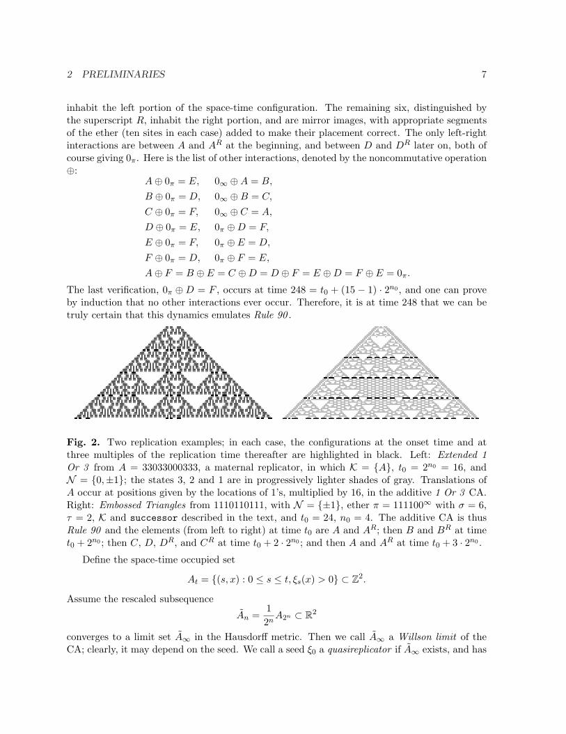
In our replicator definition we have assumed a single ether. A more general definition wouldallow mixed replicators which allow for any ether from a finite collection in intervals betweenreplicators. We could also allow stitches, bounded perturbations of the ether near, say the origin,which do not effect interaction between the elements. Such cases are common but complicatethe discussion without adding anything new; nevertheless, we provide two examples of mixedreplicators in Fig. 3. A much more substantial generalization would allow for an arbitrary groupin place of Z2, and this would certainly be necessary for a complete study of CA replication.
Fig. 3. Embossed Triangles at time t = 262, from 1110111 (left) and 11101 (right), both mixedexamples with two ethers, π1 ≡ 0 and π2 = 111100∞. Note that the Willson limit does not existfor the left example (whose ether is also stitched).
For a given property of evolution, i.e., a set of space-time configurations P ⊂ 2SZ×Z+ , wedefine its entropy h = hP as follows. Call a seed of length n + 2 any configuration in [0, n + 1],with ξ0(0) 6= 0, ξ0(n + 1) 6= 0 (and 0’s in [0, n + 1]c). Let NP,n be the number of seeds ξ0 oflength n + 2 that make (x, t) 7→ ξt(x) a member of P. Then
h = hP = lim infn→∞
1n
logs NP,n.
3 ONSET TIMES IN 1 OR 2 9
This quantity measures the amount of choice per position one has in the design of a long seedwhose evolution satisfies a given property, and has little to do with space-time entropies ofearly CA research [Wol1, Wol2]. Note that we normalize so that without any constraints, i.e.,P = 2SZ×Z+ , h = 1. We often restrict the n’s in the limit to odd or even subsequences, whichwe indicate in the superscript, ho or he.
3 Onset times in 1 Or 2
Throughout the paper, we will call a block a maximal contiguous interval of a single state, withits length equal to its number of sites.
The 1 Or 2 CA is perhaps the simplest quasiadditive one [GG3], thus it presents an op-portunity to take a closer look at the onset times t0 and the resulting replicating elements.As we will explain below, there are simple algorithmic definitions for both, which facilitate anempirical analysis. Any rigorous confirmation of our conclusions would have to proceed throughunderstanding of the annihilating diffusion of odd blocks [HC, EN] and statistical propertiesof configurations up to the additivity time defined below. This still presents a very substantialchallenge.
We now describe the key features of the 1 Or 2 evolution [Jen3, GG3]. Every block hasa unique successor, either the block of 0’s of length diminished by 2 immediately below, or,for blocks of length 1 and 2, a larger block of 1’s immediately below. New blocks appear, butthey are always of even length, and the odd blocks pairwise annihilate when their successor isthe same block. There is a finite time, which we call the additivity time ta, the least time atwhich at most one block of odd length is left. For t ≥ ta, the dynamics is conjugate to Rule 90 :if we enlarge the odd block (if any) by insertion of a site of the same state, the configurationevolves by Rule 90 thereafter, and the state ξt is obtained by deletion of the extra site from thesuccessor of the modified block. Maternal replication easily follows [GG4].
It is well known, and easy to show, that Rule 90 is injective but not surjective on finiteconfigurations. Thus every finite configuration A has a unique predecessor P (A) of shortestlength. We also denote by J(A) the Jen’s conjugacy map, which inserts a site of the same stateinto every odd block of A.
Assume we start ξt from a seed of length n + 2. By parity, if n is even, there are no oddblocks at time ta and the dynamics is Rule 90 thereafter. If n is odd there is a single odd block,which is at replication times the middle block of 0’s [GG4].
Proposition 3.1. If n is even, the shortest representation of the only replicating element isP (ξta). If n is odd there are two replicating elements: P (J(ξta)) and the same one with aprefixed 0.
In either case, t0 is the first time t ≥ ta at which ξt consists of two identical configurationsplaced at distance 2n0+1 (n even) or 2n0+1 − 1 (n odd) for some n0 ≥ 0. This determines thereplication time 2n0.
Proof. It is clear that the claimed elements replicate, and a shorter element would yield a shorter
3 ONSET TIMES IN 1 OR 2 10
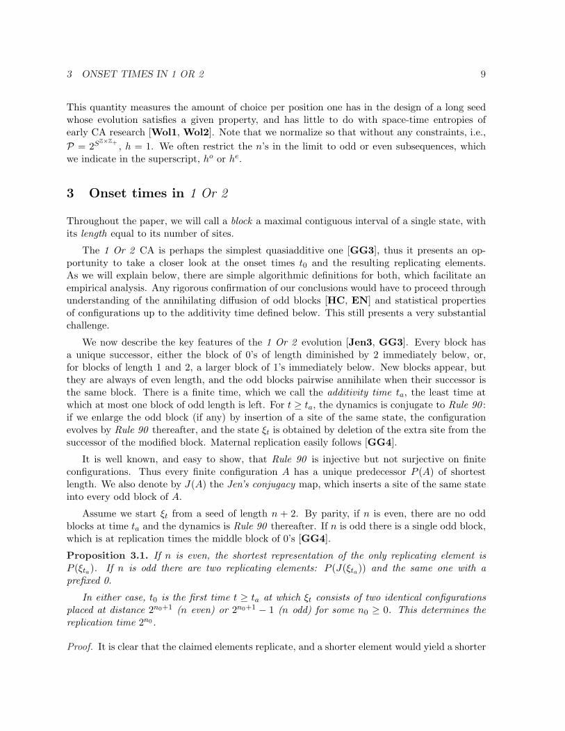
Rule 90 ancestor of J(ξta). If n is even, then 2n0−1 = t0 − ta is the first power of 2 greater orequal to the length n0 + 2 + 2ta, as this is the first time the additive dynamics “separates” thetwo copies of ξta . If n is odd, however, one needs to wait until the successor of the odd blockin ξta is the middle block of 0’s between the two elements, and this happens precisely at theclaimed time. See Fig. 4 for an illustration.
Fig. 4. 1 Or 2 from A = 1110011000011 (left) and J(A). Here P (J(A)) = 1100111. Observethat ta = 0 for both, that t0 = 5 on the right, but t0 = 13 on the left as the odd block at t = 5is not the middle block of 0’s.
Using Proposition 3.1, we computed the distributions of ta and t0 for small seed lengths, andthe resulting histograms for n = 25 are presented in Fig. 6. It is clear that the onset times areeven for low n highly clustered. The highest peaks in the histogram for ta are approximated bypowers of 2. These are the times when odd blocks annihilate each other on the upper borders oflarge triangles of 0’s, which are bound to appear as the dynamics is conjugate to Rule 90 whenthe number of odd blocks is constant [Jen3]. This is the prevailing annihilation mechanism— within nearly chaotic regions of small vacant triangles the odd blocks undergo much slowerdiffusive annihilation [HC]; see also Fig. 5 for an example. (The much smaller peaks at the tail ofthe distribution have to do with fine details of annihilation process and predecessor distributionand are harder to quantify.)
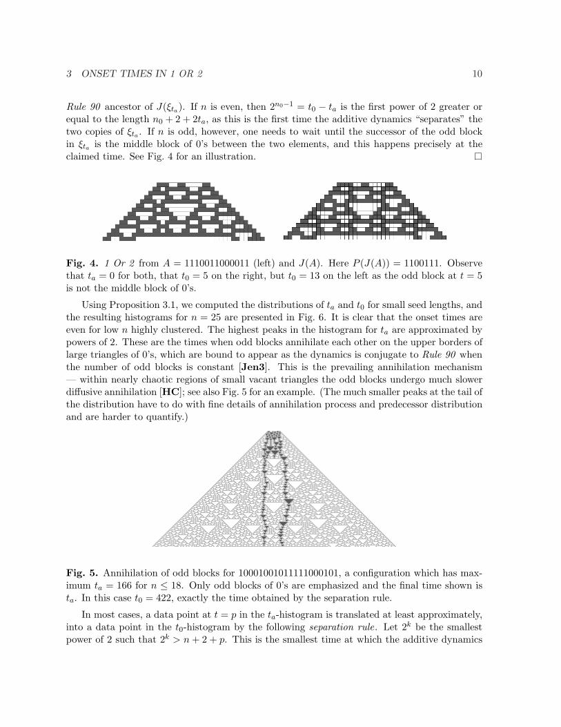
Fig. 5. Annihilation of odd blocks for 10001001011111000101, a configuration which has max-imum ta = 166 for n ≤ 18. Only odd blocks of 0’s are emphasized and the final time shown ista. In this case t0 = 422, exactly the time obtained by the separation rule.
In most cases, a data point at t = p in the ta-histogram is translated at least approximately,into a data point in the t0-histogram by the following separation rule. Let 2k be the smallestpower of 2 such that 2k > n + 2 + p. This is the smallest time at which the additive dynamics

3 ONSET TIMES IN 1 OR 2 11
separates two copies of the “fixed” configuration at time p, which has length n + 2 + p. Thisyields a data point p + 2k in t0-histogram. (How accurate is this rule depends on the locationof the odd interval in the configuration at time p and on its predecessors.) For example, theta-peak at 17 in Fig. 6 yields a t0-peak at 17+64 = 81. The times between peaks in ta-histogramare also subject to the separation mechanism, which thus leads to a more clustered nature oft0-histogram.
0
1e+006
2e+006
3e+006
4e+006
0 10 20 30 40 50 60 70 80 90 100
0
400
800
1200
100 120 140 160 180
0
400000
800000
1.2e+006
1.6e+006
2e+006
2.4e+006
0 50 100 150 200 250 300
0
500
1000
1500
300 350 400 450
Fig. 6. Histograms for seeds of length 27 (n = 25). Left: additivity time ta; right: onset timet0. The insets show tails of the distributions on a smaller y-scales (the rightmost data pointsare max ta = 179 and max t0 = 435).
As additive dynamics and annihilating diffusion of odd blocks interact, the location of ta-peaks diverges significantly from powers of 2 for larger n. In addition, there is noticeabledifference between seeds of odd and even length, as the former are more capable of havingsmaller additivity times. For a clearer picture, we restrict to even n, and provide the evolutionof empirical ta-histograms, based on 50n samples, for even n from 50 to 250; the results areshown in Fig. 7. We observe that there are three or four prominent peaks; when n is arounda power of 2 the peak at the smallest time gradually lowers while the one at the highest timestarts rising.
80
120
160
200
240 0
500 1000
1500 2000
2500 3000
50
120
n
t
Fig. 7. Evolution of ta-histograms.

4 MATERNAL REPLICATION IN QUOTA 12
4 Maternal replication in Quota
We begin by noting the useful complement property of Quota CA: if ηc = 1 − η, then ξηc
t = ξηt
for t ≥ 1.
Theorem 2. Quota with θ = 1 is a quasireplicator.
Proof. Step 1 (self-organization). At time 1, and hence afterward, all blocks of 1’s are of lengthat least 4.
To prove this, assume that ξ1(x) = ξ1(x+4) = 0 at time 1. This means that ξ0 is either all 0or all 1 on [x− 2, x+2] and the same is true for [x+2, x+6], and consequently on [x− 2, x+6].Thus ξ1(y) = 0 for x ≤ y ≤ x + 4.
Next four steps deal with the Jen regime, whereby irregular blocks (in this case those whoselengths are not 0 modulo 4), diffuse and pairwise annihilate. The proofs are straightforwardchecks [Jen4].
Step 2 (block succession). Assume that 1’s in ξ0 occur only in blocks of length at least 4. Thenevery block has a unique successor , a block immediately below it. A block of 0’s, or that of 1’s,of length ` ≥ 5 shrinks into a block of 0’s of length `− 4. A block of 0’s, or that of 1’s, of length` ≤ 4 has as a successor a block of 1’s of length at least 5.
Step 3 (additive configurations). Assume that all blocks of ξ0 are of length divisible by 4.Then this is true for all t. Moreover, assume also that ξ0(0) = 1 and ξ0(−1) = 0, and letλt(x) = ξ2t(4x). Then λt evolves as Rule 90 .
Step 4 (Jen conjugacy). Keep the assumption from Step 2. For every configuration ξ, defineJ(ξ) to be the configuration that elongates every block of length ` to the length 4 · d`/4e. If thenumber of blocks of length not equal to 0 mod 4 is constant during time interval [0, t1], thenJ(ξt) is the same as ξt evolved from J(ξ0).
The proof is now concluded by an argument exactly like that for Lemma 3.5 in [GG4].
We now turn to the more interesting θ = 2 case. We say that a seed ξ0 dies out if ξt ≡ 0 forsome t. This case is not as easy to handle as Theorem 2, in particular the self-organization timeis not uniformly bounded as isolated 1’s and 0’s may persist for arbitrarily long time: 0001∞
and 011∞ are periodic with temporal periods 2 and 1, respectively.
Theorem 3. Every seed for Quota with θ = 2 is either a maternal replicator or it dies out.The seeds that die out are exactly those that have only isolated 1’s separated by at least 3 0’s.
This is one of the rare nontrivial cases for which the entropy for all qualitatively differentevolutions is computable. We state the result, the proof of which is a computational exercise,below.
Corollary 4.1. Assume Quota CA with θ = 2. Large seeds are maternal replicators withprobability approaching 1, hence entropy 1. The entropy of seeds that die out equals log2 λ ≈0.4650, where λ is the largest root of λ4 − λ3 − 1 = 0.
4 MATERNAL REPLICATION IN QUOTA 13
Proof. For a configuration ξt, let ι(ξt) be the position of its leftmost site whose state is differentfrom that of both neighbors. We will prove in Step 1 below that ι(ξt) is a Lyapunov function forQuota, which drives ξt into a regular configuration in which all blocks are of length at least 2;the Jen regime then proceeds until all the blocks but possibly one have even length. Thereafterthe dynamics is conjugate to Rule 90 . After Step 1, the argument for the first claim in Theorem3 is thus very similar to the ones in [Jen4], [GG4], or Theorem 2 above, so it is omitted.
Step 1 (self-organization). For all t:
max{ι(ξt+1), ι(ξt+2)} ≥ ι(ξt) + 1.
Therefore, all blocks have length at least 2 for large enough t.
This claim involves finitely many configurations and can be easily checked by computer, butwe find a written-out proof much more illuminating.
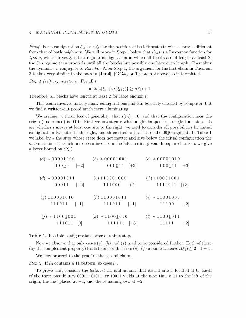
We assume, without loss of generality, that ι(ξ0) = 0, and that the configuration near theorigin (underlined) is 0010. First we investigate what might happen in a single time step. Tosee whether ι moves at least one site to the right, we need to consider all possibilities for initialconfiguration two sites to the right, and three sites to the left, of the 0010 segment. In Table 1we label by ∗ the sites whose state does not matter and give below the initial configuration thestates at time 1, which are determined from the information given. In square brackets we givea lower bound on ι(ξ1).
(a) ∗ 0 0 0 0 1 0 0 00 0 0 0 0 [+2]
(b) ∗ 0 0 0 0 1 0 0 10 0 0 0 1 1 [+3]
(c) ∗ 0 0 0 0 1 0 1 00 0 0 1 1 1 [+3]
(d) ∗ 0 0 0 0 1 0 1 10 0 0 1 1 [+2]
(e) 1 1 0 0 0 1 0 0 01 1 1 0 0 0 [+2]
(f) 1 1 0 0 0 1 0 0 11 1 1 0 0 1 1 [+3]
(g) 1 1 0 0 0 1 0 1 01 1 1 0 1 1 [−1]
(h) 1 1 0 0 0 1 0 1 11 1 1 0 1 1 [−1]
(i) ∗ 1 1 0 0 1 0 0 01 1 1 0 0 [+2]
(j) ∗ 1 1 0 0 1 0 0 11 1 1 0 1 1 [0]
(k) ∗ 1 1 0 0 1 0 1 01 1 1 1 1 1 [+3]
(l) ∗ 1 1 0 0 1 0 1 11 1 1 1 1 [+2]
Table 1. Possible configurations after one time step.
Now we observe that only cases (g), (h) and (j) need to be considered further. Each of these(by the complement property) leads to one of the cases (a)–(f) at time 1, hence ι(ξ2) ≥ 2−1 = 1.
We now proceed to the proof of the second claim.
Step 2 . If ξ0 contains a 11 pattern, so does ξ1.
To prove this, consider the leftmost 11, and assume that its left site is located at 0. Eachof the three possibilities 00011, 01011, or 10011 yields at the next time a 11 to the left of theorigin, the first placed at −1, and the remaining two at −2.

5 REPLICATORS IN PERTURBED EXACTLY 1 14
To finish the proof of the second claim in Theorem 3, observe first that if there is no 11 inξ0, but there are two 1’s at distance at most 3, then there is a 11 in ξ1. The condition given isby Step 2 thus necessary for a seed to die out.
To prove sufficiency assume that every pair of 1’s in ξ0 is at distance 4 or more. Then thesame holds for ξ1 (as such pair can only generate a 1 at the midpoint between them when theyare at distance 4), and then, by Step 1, ξt ≡ 0 for some t.
5 Replicators in Perturbed Exactly 1
We begin by the count of replicators for seeds of length n + 2 up to 17. Our method checksfor the “mass extinction” signature of replication by a time cutoff: the evolution runs to timet = 2000, and once t > 200 we check whether the density between the extreme 1’s changes fromabove 0.9 to below 0.1. Maternal cases are then distinguished as those for which the occupiedsites after the density drop consist of two configurations that are equal up to translation. Thesuccessful pass of this check produced a replicator in every case we investigated further, althoughwe do not have a proof that this method is completely reliable. The results are shown in Table 2below. We remark that in most cases (i.e., in all chaotic ones) we have no argument that wouldpreclude a later onset of replication, so we can only produce lower bounds.
n all maternal fraternal0 1 1 01 2 2 02 4 4 03 8 8 04 16 8 85 32 28 46 64 30 347 128 103 238 249 79 1709 512 398 11410 975 296 67911 2046 1500 53812 3907 720 318713 8156 5941 221514 15265 2952 1231315 13957 10050 3907
Table 2. Replicator counts for small seeds.
It is remarkable that, modulo mirror images, only four out the 1024 smallest seeds, i.e., thoseof length at most 11, are not replicators. The four “anomalies” have length 10: 1001100111 and1100101111 both lead to the quasireplicating seed of Theorem 5, 1100110011 is presumablyanother quasireplicator (see Section 6 for evidence), and 1001001101 appears to be a chaoticseed in the sense of [GG4]. The resulting (maximal) chaotic wedge has density 0.375, and other

5 REPLICATORS IN PERTURBED EXACTLY 1 15
properties similar to Exactly 1 chaos, except that there seem to be no quasiperiodic regions, dueto the fact that the wedge spreads slower than the speed of light.
Prevalence for replicators for smaller seeds has its counterpart in relatively large replicatorentropy constants, to which we now turn our attention.
Theorem 4. The entropy of odd maternal replicators, and that of fraternal replicators, are eachat least 0.8923. The entropy of even maternal replicators is at least 0.7741.
We begin by three propositions which will establish sufficient conditions for various types ofreplication. We call an initial state ξ0 additive if each 1-block is of odd length and each 0-blockis of odd length at least 3.
Proposition 5.1. Assume that ξ0 is additive and placed so that the leftmost occupied site is atthe origin. Create the initial state λ0 for Rule 90 by changing all 1’s in ξ0 at odd locations to0. Then ξt is obtained by changing every isolated 0 in λt to 1. In particular, ξt is additive forall t, and a maternal replicator.
Proof. Clearly it is enough to verify the statement for t = 1. We proceed two steps.
Step 1 . For odd x, ξ1(x) = λ1(x).
Assume that the ξ0 states in the range 2 neighborhood of x are abcde. Under our conditions,none of a, c, and e can be an endpoint of a block of 1’s. Thus by symmetry there are five caseswe have to check: 00000, 11000, 11110, 11111, 01110, and 01000. In the second and the lastcase ξ1(x) = λ1(x) = 1, and in the other three cases they are both 0.
Step 2 . For even x, ξ1(x) = 1 if and only if λ1(x− 1) = λ1(x + 1) = 1. (Note that λ1(x) = 0.)
Now we need to check all possible ξ0 configurations in [x − 3, x + 3]. By symmetry, thereare nine of them: 0000000, 0100000, 0111000, 0111110, 1100000, 1111000, 1111110, 0100010,1111111. In order, they result in the following configurations (ξ1, λ1) within [x − 1, x + 1]:(000, 000), (100, 100), (001, 001), (000, 000), (100, 100), (001, 001), (000, 000), (111, 101), (000, 000),verifying Step 2.
Proposition 5.2. Assume that all 1’s in ξ0 are isolated and the length of all blocks of 0’s haslength 3 mod 4, except that a single block of 0’s has even length. Then ξ0 is an even maternalreplicator.
Proof. We refer back to the previous proposition, and note that in the absence of the irregularblock the comparison dynamics λt starts from λ0 which has 1’s only on locations 3 mod 4. Thisis then true for λt at every even time t, while at odd times t, λt(x) = 1 implies that at least oneof λt(x− 1), λt(x + 1) is also 1. This claim is easily proved by induction.
Consequently, ξt = λt for even t, while for odd t all blocks of 1’s in ξt are of length at least 3.Chose a block of 0’s and track its successors through time: if its length is at least 7, it shrinksby 2 at each of the next two time steps; if its length is 3, its successor is a block of 1’s of lengthat least 7, and then a block of at least 7 0’s at the next time.

5 REPLICATORS IN PERTURBED EXACTLY 1 16
Remove a 0 from the chosen 0-block. If it is now of length 2, its successor is an even blockof 1’s of length at least 6, and then a 0-block of length at least 6. If the initially modified blockis of length at least 6, then it merely shrinks by 2, and then by 2 again.
Now add a 0 to the chosen 0-block. If it is now of length 4, its successor is a block of two0’s flanked by two 1-blocks of length at least 3, resulting next time in an even 0-block of lengthat least 8. Again, if the initially modified block is longer (now of length at least 8), it merelyshrinks by 2 in each of the next time steps.
Therefore, if one starts from one of the assumed initial conditions, and the irregular blockis of length 0 mod 4 or 2 mod 4, the resulting dynamics is conjugate to the one with the block“fixed” by, respectively, adding or removing one site.
We remark that Proposition 5.2 does not hold for a larger number of even blocks, as theirinteractions may easily destroy the conjugacy.
Next, we construct fraternal replicators by suitable edge modifications.
Proposition 5.3. A seed η is placed so that its leftmost 1 is at the origin. Assume that anotherseed η′ equals η on nonnegative sites, and that η′ is of one of the two types below. Then ξη
t (x) =ξη′t (x) for x ≥ −t, t ≥ 0.
Thin configuration. Assume that η(0) = η(1) = η(2) = 1. In addition, to the left of theorigin, η′ only has isolated 1’s and blocks of 0’s of lengths 3 mod 4, except for the block of 0’simmediately to the left of the origin, which has length 0 mod 4.
Thick configuration. Alternatively, assume that η(0) = 1, η(1) = η(2) = 0. Now requirethat, to the left of the origin, η′ only has blocks of 1’s of length 3 mod 4 and blocks of 0’s oflengths 1 mod 4, except for the block of 0’s immediately to the left of the origin, which has length2 mod 4.
Proof. Start by observing that the leftmost three states of the configuration ξηt are in a cycle
111–100 of length two.
Form η′′ by erasing all 1’s from η′ on nonnegative sites, and run the dynamics for a singletime step. As the proof of Proposition 5.1 demonstrates, a configuration of the thick type turnsinto configuration of the thin type, and vice versa (except for the now meaningless requirementon the block of 0’s to the left of the origin).
Thus, we need to verify that the configuration ξη′1 at time 1 in [−2, 1] is 0100 in the thin
case and 0111 in the thick case, and that the block of 0’s that covers −1 has the correct lengthmod 4. But the check of this is trivial for the thin type, and also for the thick type when theblock of 0’s to the left of the origin has length at least 6. When the η′ configuration in [−5, 2] is11100100, then ξη′
1 in [−5, 1] is 0000111, and the length of the block of 0’s is larger by a singlesite from what it would be if started from η′′, thus of length 2 mod 4.
We now proceed to prove Theorem 4 in three separate cases.
5 REPLICATORS IN PERTURBED EXACTLY 1 17
Transitions from the 12 0-types:
0 0 0 00
↗↘
0 0 0 00
0 0 0 11
0 0 0 11
↗↘
0 0 1 01
0 0 1 1q
0 1 0 01
↗↘
1 0 0 0q
1 0 0 1q
0 1 0 10
−→ 1 0 1 10
0 1 0 11
−→ 1 0 1 0q
1 0 0 00
−→ 0 0 0 00
1 0 0 01
−→ 0 0 0 11
1 0 0 10
−→ 0 0 1 1q
1 0 0 11
−→ 0 0 1 01
1 1 0 00
−→ 1 0 0 1q
1 1 0 01
−→ 1 0 0 0q
1 1 0 10
↗↘
1 0 1 0q
1 0 1 10
Transitions from the 11 1-types:
0 0 1 01
↗↘
0 1 0 01
0 1 0 1q
0 0 1 10
−→ 0 1 1 10
0 1 1 01
−→ 0 1 1 0q
0 1 1 00
−→ 1 1 0 10
0 1 1 01
−→ 1 1 0 0q
0 1 1 10
↗↘
1 1 1 00
1 1 1 10
1 0 1 00
−→ 0 1 0 1q
1 0 1 01
−→ 0 1 0 11
0 1 1 10
↗↘
0 1 1 0q
0 1 1 10
1 1 1 00
↗↘
1 1 0 0q
1 1 0 10
1 1 1 10
↗↘
1 1 1 00
1 1 1 10
Table 3. Transition rules for the quintuples.
Proof. (Odd maternal case.) We suitably modify the method from [GG4], by counting prede-cessors of additive configurations, i.e., configurations that lead to an additive state after j-steps.Essentially, we reinterpret de Bruijn diagram ideas [Jen1] in a format suitable for efficient sparse
5 REPLICATORS IN PERTURBED EXACTLY 1 18
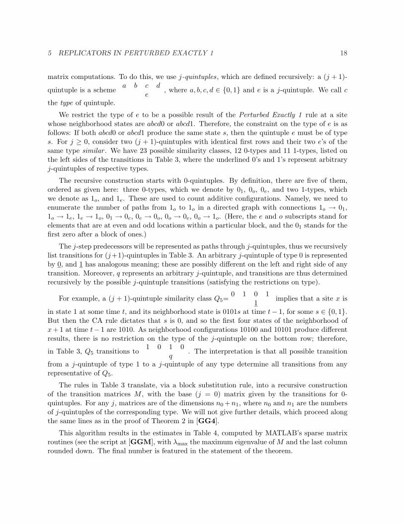
matrix computations. To do this, we use j-quintuples, which are defined recursively: a (j + 1)-
quintuple is a schemea b c d
e, where a, b, c, d ∈ {0, 1} and e is a j-quintuple. We call c
the type of quintuple.
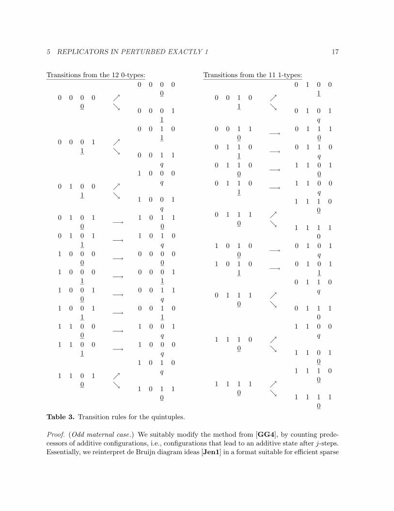
We restrict the type of e to be a possible result of the Perturbed Exactly 1 rule at a sitewhose neighborhood states are abcd0 or abcd1. Therefore, the constraint on the type of e is asfollows: If both abcd0 or abcd1 produce the same state s, then the quintuple e must be of types. For j ≥ 0, consider two (j + 1)-quintuples with identical first rows and their two e’s of thesame type similar . We have 23 possible similarity classes, 12 0-types and 11 1-types, listed onthe left sides of the transitions in Table 3, where the underlined 0’s and 1’s represent arbitraryj-quintuples of respective types.
The recursive construction starts with 0-quintuples. By definition, there are five of them,ordered as given here: three 0-types, which we denote by 01, 0o, 0e, and two 1-types, whichwe denote as 1o, and 1e. These are used to count additive configurations. Namely, we need toenumerate the number of paths from 1o to 1o in a directed graph with connections 1o → 01,1o → 1e, 1e → 1o, 01 → 0e, 0e → 0o, 0o → 0e, 0o → 1o. (Here, the e and o subscripts stand forelements that are at even and odd locations within a particular block, and the 01 stands for thefirst zero after a block of ones.)
The j-step predecessors will be represented as paths through j-quintuples, thus we recursivelylist transitions for (j+1)-quintuples in Table 3. An arbitrary j-quintuple of type 0 is representedby 0, and 1 has analogous meaning; these are possibly different on the left and right side of anytransition. Moreover, q represents an arbitrary j-quintuple, and transitions are thus determinedrecursively by the possible j-quintuple transitions (satisfying the restrictions on type).
For example, a (j + 1)-quintuple similarity class Q5=0 1 0 1
1implies that a site x is
in state 1 at some time t, and its neighborhood state is 0101s at time t− 1, for some s ∈ {0, 1}.But then the CA rule dictates that s is 0, and so the first four states of the neighborhood ofx+1 at time t− 1 are 1010. As neighborhood configurations 10100 and 10101 produce differentresults, there is no restriction on the type of the j-quintuple on the bottom row; therefore,
in Table 3, Q5 transitions to1 0 1 0
q. The interpretation is that all possible transition
from a j-quintuple of type 1 to a j-quintuple of any type determine all transitions from anyrepresentative of Q5.
The rules in Table 3 translate, via a block substitution rule, into a recursive constructionof the transition matrices M , with the base (j = 0) matrix given by the transitions for 0-quintuples. For any j, matrices are of the dimensions n0 +n1, where n0 and n1 are the numbersof j-quintuples of the corresponding type. We will not give further details, which proceed alongthe same lines as in the proof of Theorem 2 in [GG4].
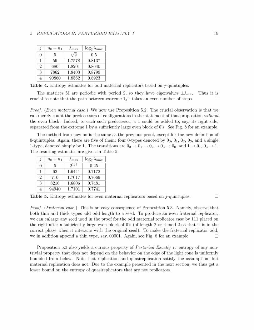
This algorithm results in the estimates in Table 4, computed by MATLAB’s sparse matrixroutines (see the script at [GGM], with λmax the maximum eigenvalue of M and the last columnrounded down. The final number is featured in the statement of the theorem.
5 REPLICATORS IN PERTURBED EXACTLY 1 19
j n0 + n1 λmax log2 λmax
0 5√
2 0.51 59 1.7578 0.81372 680 1.8201 0.86403 7862 1.8403 0.87994 90860 1.8562 0.8923
Table 4. Entropy estimates for odd maternal replicators based on j-quintuples.
The matrices M are periodic with period 2, so they have eigenvalues ±λmax. Thus it iscrucial to note that the path between extreme 1o’s takes an even number of steps.
Proof. (Even maternal case.) We now use Proposition 5.2. The crucial observation is that wecan merely count the predecessors of configurations in the statement of that proposition withoutthe even block. Indeed, to each such predecessor, a 1 could be added to, say, its right side,separated from the extreme 1 by a sufficiently large even block of 0’s. See Fig. 8 for an example.
The method from now on is the same as the previous proof, except for the new definition of0-quintuples. Again, there are five of them: four 0-types denoted by 00, 01, 02, 03, and a single1-type, denoted simply by 1. The transitions are 00 → 01 → 02 → 03 → 00, and 1 → 01, 03 → 1.The resulting estimates are given in Table 5.
j n0 + n1 λmax log2 λmax
0 5 21/4 0.251 62 1.6441 0.71722 710 1.7017 0.76693 8216 1.6806 0.74814 94940 1.7101 0.7741
Table 5. Entropy estimates for even maternal replicators based on j-quintuples.
Proof. (Fraternal case.) This is an easy consequence of Proposition 5.3. Namely, observe thatboth thin and thick types add odd length to a seed. To produce an even fraternal replicator,we can enlarge any seed used in the proof for the odd maternal replicator case by 111 placed onthe right after a sufficiently large even block of 0’s (of length 2 or 4 mod 2 so that it is in thecorrect phase when it interacts with the original seed). To make the fraternal replicator odd,we in addition append a thin type, say, 00001. Again, see Fig. 8 for an example.
Proposition 5.3 also yields a curious property of Perturbed Exactly 1 : entropy of any non-trivial property that does not depend on the behavior on the edge of the light cone is uniformlybounded from below. Note that replication and quasireplication satisfy the assumption, butmaternal replication does not. Due to the example presented in the next section, we thus get alower bound on the entropy of quasireplicators that are not replicators.

5 REPLICATORS IN PERTURBED EXACTLY 1 20
Fig. 8. Constructions in the proof of Theorem 4. Top left is the evolution from seed A =110000001 whose configuration becomes additive in four steps and is therefore an odd maternalreplicator. Top right seed, A[10 0’s ]1, is designed to lead to a configuration from Proposition5.2 in 4 steps, thus is an even maternal replicator. Bottom two seeds are A[10 0’s ]111 and A[100’s ]11100001, an even and an odd fraternal replicator.
Proposition 5.4. If there exist a seed with property P, i.e., P 6= ∅, and that, for an arbitraryk ∈ Z and any seed, P only depends on the configuration on {(x, t) : x ≥ k − t}. Then theentropy of P is at least 0.8075.
Proof. It is easy to verify that, started from any seed, the left edge of any configuration is either100 or 111 by time 2: if the left edge is 1010 or 1100 then this already happens at time 1, in theremaining two cases, 1011 and 1101, the left edge is 1100 at time 1.
Thus, by Proposition 5.3, the entropy is at least the entropy of the seeds which start witha single 1, then to the left a configuration of the second type, then to its left a configuration ofthe first type, etc., and also at least the entropy of their predecessor set.
The base (j = 0) directed graph now has 13 vertices, labeled 1 and 0thini , 0thick
i , 1thicki ,
i = 0, 1, 2, 3. Any symbol with subscript i transitions to the same symbol with subscript (i +1) mod 4 and in addition we have transitions 1 → 0thin
1 , 1thick3 → 0thick
1 , 0thin3 → 1, 0thin
2 → 1thick1 ,
0thick1 → 1thick
1 , 0thick0 → 1. The resulting matrix substitution scheme yields the estimates in
Table 6.j n0 + n1 λmax log2 λmax
0 13 1.3339 0.41571 154 1.6828 0.75082 1774 1.7364 0.79613 20512 1.7431 0.80174 237052 1.7502 0.8075
Table 6. Entropy estimates for edge modifications based on j-quintuples.
6 QUASIREPLICATORS IN PERTURBED EXACTLY 1 21
6 Quasireplicators in Perturbed Exactly 1
We begin with the main task of this section, which is to give a complete proof that a particularinitial state leads to a fractal Willson limit, but not to replication.
Theorem 5. Initial state 1000111[10 0’s]1000111 is a quasireplicator, but not a replicator, forPerturbed Exactly 1 .
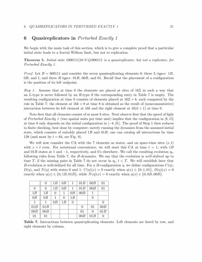
Proof. Let B = 000111 and consider the seven quasireplicating elements 0; three L-types: 1B,0B, and 1; and three R-types: 01B, 00B, and 01. Recall that the placement of a configurationis the position of its left endpoint.
Step 1 . Assume that at time 0 the elements are placed at sites of 16Z in such a way thatan L-type is never followed by an R-type if the corresponding entry in Table 7 is empty. Theresulting configuration at time 8 consists of elements placed at 16Z+ 8, each computed by therule in Table 7: the element at 16k + 8 at time 8 is obtained as the result of (noncommutative)interaction between its left element at 16k and the right element at 16(k + 1) at time 0.
Note first that all elements consist of at most 8 sites. Next observe first that the speed of lightof Perturbed Exactly 1 (two spatial units per time unit) implies that the configuration in [8, 15]at time 8 only depends on the initial configuration in [−8, 31]. The proof of Step 1 then reducesto finite checking, best done by computer; merely running the dynamics from the assumed initialstate, which consists of suitably placed 1B and 01B, one can catalog all interactions by time128 (and most by t = 64, see Fig. 9).
We will now consider the CA with the 7 elements as states, and on space-time sites (x, t)with x + t even. For notational convenience, we will start this CA at time t = 1, with 1Band 01B states at 1 and −1, respectively, and 0’s elsewhere. We call the resulting evolution ηt,following rules from Table 7, the B-dynamics. We say that the evolution is well-defined up totime T , if the missing pairs in Table 7 do not occur in ηt, t < T . We will establish later thatB-evolution is well-defined for all time. For a B-configuration η, we define configurations C(η),D(η), and N(η) with states 0 and 1: C(η)(x) = 0 exactly when η(x) ∈ {0, 1, 01}, D(η)(x) = 0exactly when η(x) ∈ {0, 1B, 01B}, while N(η)(x) = 0 exactly when η(x) ∈ {0, 0B, 00B}.
0 1B 0B 1 01B 00B 010 0 1B 0B 1 01B 00B 01
1B 1B 0 1 0B 00B 10B 0B 1 0 1B 01 1 0B 1B 0 0
01B 01B 0 01 00B
00B 00B 01 0 01B
01 01 00B 01B 0
Table 7. Interactions between quasireplicating elements. Left elements are listed by row, andright elements by column.
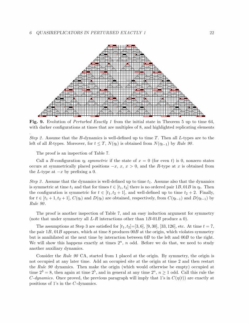
6 QUASIREPLICATORS IN PERTURBED EXACTLY 1 22
Fig. 9. Evolution of Perturbed Exactly 1 from the initial state in Theorem 5 up to time 64,with darker configurations at times that are multiples of 8, and highlighted replicating elements.Step 2 . Assume that the B-dynamics is well-defined up to time T . Then all L-types are to theleft of all R-types. Moreover, for t ≤ T , N(ηt) is obtained from N(ηt−1) by Rule 90 .
The proof is an inspection of Table 7.
Call a B-configuration ηt symmetric if the state of x = 0 (for even t) is 0, nonzero statesoccurs at symmetrically placed positions −x, x, x > 0, and the R-type at x is obtained fromthe L-type at −x by prefixing a 0.
Step 3 . Assume that the dynamics is well-defined up to time t1. Assume also that the dynamicsis symmetric at time t1 and that for times t ∈ [t1, t2] there is no ordered pair 1B, 01B in ηt. Thenthe configuration is symmetric for t ∈ [t1, t2 + 1], and well-defined up to time t2 + 2. Finally,for t ∈ [t1 + 1, t2 + 1], C(ηt) and D(ηt) are obtained, respectively, from C(ηt−1) and D(ηt−1) byRule 90 .
The proof is another inspection of Table 7, and an easy induction argument for symmetry(note that under symmetry all L-R interactions other than 1B-01B produce a 0).
The assumptions at Step 3 are satisfied for [t1, t2]=[3, 6], [9, 30], [33, 126], etc. At time t = 7,the pair 1B, 01B appears, which at time 8 produces 00B at the origin, which violates symmetrybut is annihilated at the next time by interaction between 0B to the left and 00B to the right.We will show this happens exactly at times 2n, n odd. Before we do that, we need to studyanother auxiliary dynamics.
Consider the Rule 90 CA, started from 1 placed at the origin. By symmetry, the origin isnot occupied at any later time. Add an occupied site at the origin at time 2 and then restartthe Rule 90 dynamics. Then make the origin (which would otherwise be empty) occupied attime 23 = 8, then again at time 25, and in general at any time 2n, n ≥ 1 odd. Call this rule theC-dynamics. Once proved, the previous paragraph will imply that 1’s in C(η(t)) are exactly atpositions of 1’s in the C-dynamics.
6 QUASIREPLICATORS IN PERTURBED EXACTLY 1 23
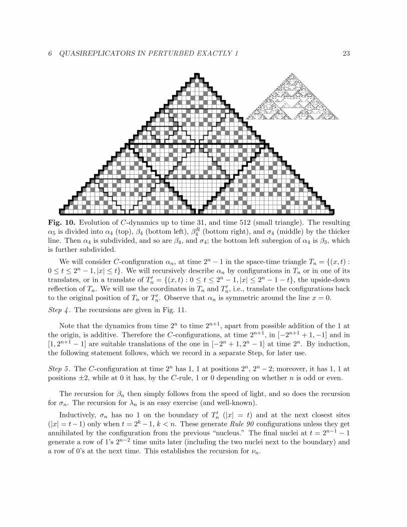
Fig. 10. Evolution of C-dynamics up to time 31, and time 512 (small triangle). The resultingα5 is divided into α4 (top), β4 (bottom left), βR
4 (bottom right), and σ4 (middle) by the thickerline. Then α4 is subdivided, and so are β4, and σ4; the bottom left subregion of α4 is β3, whichis further subdivided.
We will consider C-configuration αn, at time 2n − 1 in the space-time triangle Tn = {(x, t) :0 ≤ t ≤ 2n − 1, |x| ≤ t}. We will recursively describe αn by configurations in Tn or in one of itstranslates, or in a translate of T ′n = {(x, t) : 0 ≤ t ≤ 2n − 1, |x| ≤ 2n − 1− t}, the upside-downreflection of Tn. We will use the coordinates in Tn and T ′n, i.e., translate the configurations backto the original position of Tn or T ′n. Observe that αn is symmetric around the line x = 0.
Step 4 . The recursions are given in Fig. 11.
Note that the dynamics from time 2n to time 2n+1, apart from possible addition of the 1 atthe origin, is additive. Therefore the C-configurations, at time 2n+1, in [−2n+1 + 1,−1] and in[1, 2n+1 − 1] are suitable translations of the one in [−2n + 1, 2n − 1] at time 2n. By induction,the following statement follows, which we record in a separate Step, for later use.
Step 5 . The C-configuration at time 2n has 1, 1 at positions 2n, 2n− 2; moreover, it has 1, 1 atpositions ±2, while at 0 it has, by the C-rule, 1 or 0 depending on whether n is odd or even.
The recursion for βn then simply follows from the speed of light, and so does the recursionfor σn. The recursion for λn is an easy exercise (and well-known).
Inductively, σn has no 1 on the boundary of T ′n (|x| = t) and at the next closest sites(|x| = t−1) only when t = 2k−1, k < n. These generate Rule 90 configurations unless they getannihilated by the configuration from the previous “nucleus.” The final nuclei at t = 2n−1 − 1generate a row of 1’s 2n−2 time units later (including the two nuclei next to the boundary) anda row of 0’s at the next time. This establishes the recursion for νn.

6 QUASIREPLICATORS IN PERTURBED EXACTLY 1 24
To establish the recursion for γn and δn, we argue by additivity that γn = βRn + λn mod 2
for odd n, and thus δn = (βRn + λn) mod 2 for even n. For example, the bottom right corner
configuration of δn is, modulo 2,
(γn−1 + λn−1)R = γRn−1 + λn−1 = βn−1 + λn−1 + λn−1 = βn−1.
βn, n even: βn, n odd:
βTn−1
βn−1
βn−1
σn−1
γn−1
βn−1
βn−1
σn−1
λn−1
λn−1
λn−10
λn:
δn−1
δn−1
δTn−1
σn−1
γn, n even: δn, n odd:
γn−1
γn−1
βn−1
σn−1
σn:νn−1
σn−1 σn−1
0
νn:
λn−1
νn−2
λn−10
0
αn:
βTn−1
αn−1
βn−1
σn−1
Fig. 11. Recursive specification of αn. The superscript T indicates the mirror image of aconfiguration. This implies that the set of space-time occupied sites is exactly solvable [GG1].Here, λn is generated by Rule 90 from a singleton at the top site of Tn. See Fig. 10 for examples.
Call a pair of binary configuration α and α′ in Tn r-close if for each 1 in α there is a 1 in α′
at `∞ distance at most r, and vice versa.
Step 6 . When defined at the same n, each pair of configurations βn, βRn γn, δn are 2-close.
This easily follows from the Step 4 recursion, by induction.
6 QUASIREPLICATORS IN PERTURBED EXACTLY 1 25
Step 7 . At x = t, t = 0, 1, . . . 2n − 1, βn has states 10[2 1’s][4 0’s] . . . , ending with an interval of2n−1 0’s or 2n−1 1’s, depending on whether n is odd or even.
This again follows by induction: the leftmost 1 on the bottom line of λn−1 either annihilateswith the rightmost 1 in the bottom line of βn−1 (odd n), or generates a 1 which propagatesleftward due to the empty bottom triangle of σn.
Step 8 . The B-dynamics ηt is well-defined for all times. At any time t ≥ 1, C(ηt) is given bythe C-dynamics.
Assume inductively that this holds up to time 2n, for some odd n. By Step 2, up to thattime, all states corresponding to 1’s in the translations of configuration σn are 0B or 00B.Moreover, all 1’s in position described in Step 7 must be occupied by 1B or 01B in the B-dynamics: certainly the top 1 is, and the rest follows by the B-interactions. Thus, by recursionfor αn, B-dynamics produces a 00B at x = 0 at time 2n+1, which by Step 5 gets immediatelyannihilated against its occupied neighbors, as the extra 1 does in the C-dynamics. By Step 3the claim in Step 8 holds up to time 2n+2.
The configuration αn misses the states 1 and 01 in the B-dynamics, and the next stepexplains how those are added. The union, ∪, of two configurations is simply the or operationbetween them, i.e., it has a 1 exactly where at least one of them has a 1.
Step 9 . The nonzero states within Tn in the B-dynamics are located precisely at nonzeropositions of αn ∪ λn.
To prove this, we observe that D(ηt) evolves by the C-dynamics, except that the first occupiedsite occurs at x = 0 at time 2 is at time 2. Therefore, the positions of nonzero B-states withinTn are at ⋃
t≤n
(C(ηt) ∪D(ηt)) = αn ∪ (αn + λn) = αn ∪ λn,
where the sum is as usual reduced modulo 2.
Step 10 . Conclusion of the proof.
We will show that the C-dynamics is not a replicator and that its Willson limit, which is thelimit of configurations 2−nαn, is fractal. As we will see this limit has Hausdorff dimension thesame as that of the limit of 2−nλn, which is log 3/ log 2, and then Step 10 finishes the proof.
By Step 6, the odd and even n give the same limit. This limit is a Mauldin-Williams fractal[MW, BM] and thus has its Hausdorff dimension equal to its box dimension, and determined bythe largest eigenvalue of an appropriate matrix given by the recursion in Step 4. The dimensionin fact does equal to log 3/ log 2, so it is the same as for the Sierpinski gasket. However, theHausdorff measure for this exponent is infinite, which is easily shown by the methods in [MW].(The small triangle in Fig. 10 approximates this fractal.)
To demonstrate that the C-dynamics is not a replicator, observe first that the ether couldonly be 0, and that by induction every line on the top half of the configuration σn, n ≥ 2,
7 REPLICATION AND QUASIREPLICATION IN EXTENDED 1 OR 3 26
contains at least two occupied points. Thus, by iterating the recursion for σn, every one of first2k, k ≥ 2 lines contains at least 2n−k points. It follows that the number of occupied points attimes 2n + 2k, n = 1, 2 . . ., is not bounded for any fixed k, which violates a necessary conditionfor a replicator.
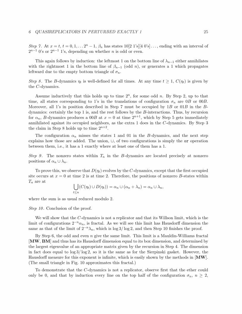
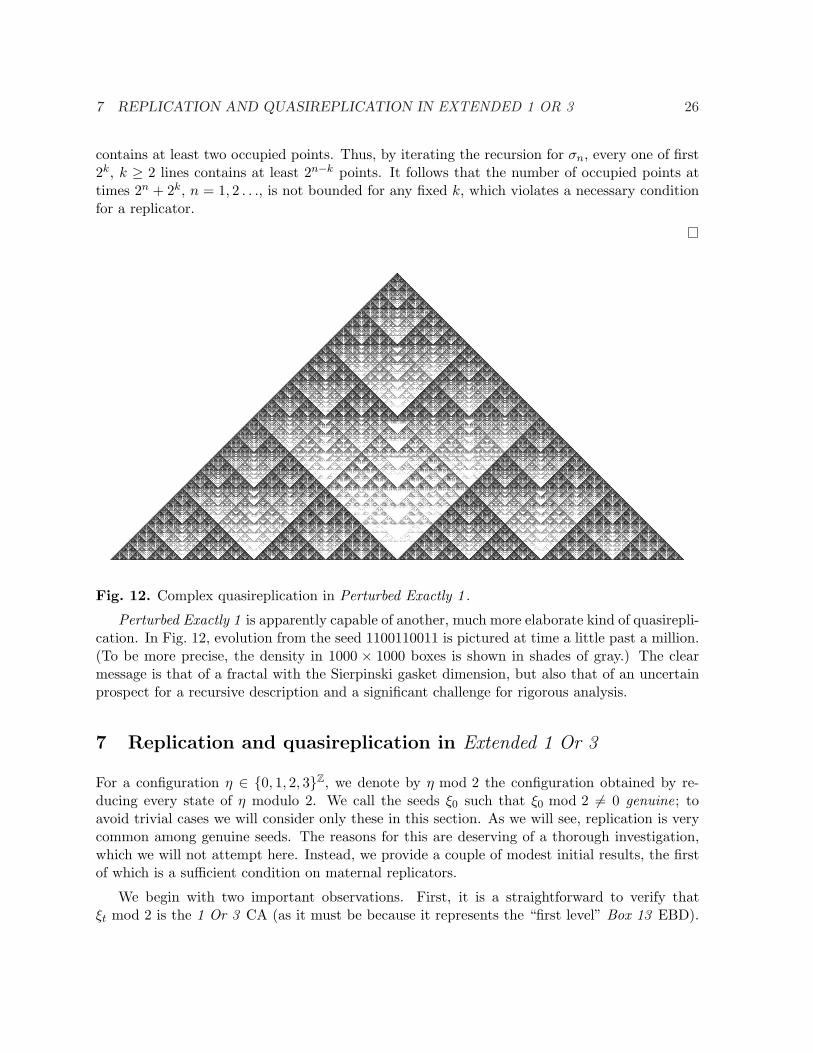
Fig. 12. Complex quasireplication in Perturbed Exactly 1 .
Perturbed Exactly 1 is apparently capable of another, much more elaborate kind of quasirepli-cation. In Fig. 12, evolution from the seed 1100110011 is pictured at time a little past a million.(To be more precise, the density in 1000 × 1000 boxes is shown in shades of gray.) The clearmessage is that of a fractal with the Sierpinski gasket dimension, but also that of an uncertainprospect for a recursive description and a significant challenge for rigorous analysis.
7 Replication and quasireplication in Extended 1 Or 3
For a configuration η ∈ {0, 1, 2, 3}Z, we denote by η mod 2 the configuration obtained by re-ducing every state of η modulo 2. We call the seeds ξ0 such that ξ0 mod 2 6= 0 genuine; toavoid trivial cases we will consider only these in this section. As we will see, replication is verycommon among genuine seeds. The reasons for this are deserving of a thorough investigation,which we will not attempt here. Instead, we provide a couple of modest initial results, the firstof which is a sufficient condition on maternal replicators.
We begin with two important observations. First, it is a straightforward to verify thatξt mod 2 is the 1 Or 3 CA (as it must be because it represents the “first level” Box 13 EBD).
7 REPLICATION AND QUASIREPLICATION IN EXTENDED 1 OR 3 27
Moreover, if the initial state consists only of 0’s and 2’s (i.e., there are no first level sites), thenξt/2 is again 1 Or 3 .
Theorem 6. Assume that a seed has only 0’s and 3’s. Mark a site if it is either in state 3 withboth neighbors in state 3 or both neighbors in state 0, or in state 0 with a neighbor in state 3 andthe other in state 0. Assume the distances between successive marked sites are all even. Thenthe seed is a maternal replicator. In particular, the entropy of odd genuine maternal replicatorsis at least 0.25.
Proof.
Step 1 . Assume that ξ0 ∈ {0, 3}Z and that no marked sites are neighbors at time 0 (but can beotherwise at an odd distance). Then ξ2 ∈ {0, 3}Z.
To verify this, we pick an x and consider all possible ξ0 configurations in [x− 2, x + 2]. Upto symmetry, there are 20 of them. Of these, six (00030, 00303, 03003, 03033, 30033, 33333)have marked neighboring sites in [x− 1, x + 1]. Further six (00000, 00333, 03030, 30003, 03303,33033) result in ξ2(x) = 0, and the remaining eight in ξ2(x) = 3.
Step 2 . If the stated assumptions hold for ξ0, they do so for ξ2.
Observe that, at time 0, x is marked exactly when ξ1(x) mod 2 = 1. Therefore, by Step 1,we need to show that if 1 or 3 , that is, λt = ξt mod 2, has only even sites occupied in λ0, thesame is true for λ2. By cancellative duality [Gri], for any y,
λ2(y) = |λ{y}2 ∩ λ0| mod 2 = |{y − 2, y, y + 2} ∩ λ0| mod 2,
and the intersection is clearly empty if y is odd.
To finish the proof, merely note that λt replicates and at times t = 2n, n ≥ 1, ξt = 3 · λt.The entropy statement follows from the fact that building a configuration with stated propertiesfrom the leftmost 3 rightward one has two choices at each odd step and a single choice (albeitdependent on the preceding choices) at each even step.
Call a replicator for Extended 1 Or 3 regular if, perhaps after an enlargement of n0, thereexist a replicating element A such that either the interaction A⊕ 0π ⊕ 0π occurs and equals A,or the same holds for the interaction 0π ⊕ 0π ⊕ A. In other words, spreading into the ether, Acreates an appropriately positioned copy of itself in some 2i time steps. To date, every replicatorwe have checked turned out to be regular. The following proposition exploits the connections tothe “ordinary” 1 Or 3 rule.
Proposition 7.1. Every ether for an Extended 1 Or 3 replicator consists only of 0’s and 2’s.After all 2’s are replaced by 1’s, an ether is a periodic solution for 1 Or 3 .
Assume ξ0 is a regular replicator. Then σ is a power of 2; moreover, if σ ≥ 2, τ = σ/2.
Proof. Again, denote λt = ξt mod 2. For any seed, 1 Or 3 replicates with 0 ether. To be moreprecise, let Ak be the occupied set of λ
{0}k . Then there are times t1 and 2n1 so that, for all
k = 1, 2, . . . , the configuration of λt at times tk = t1 + (k − 1)2n1 consists of identical finite
7 REPLICATION AND QUASIREPLICATION IN EXTENDED 1 OR 3 28
configurations placed at positions of 2n1Ak, with 0’s elsewhere. Therefore, at times tk + 1, theExtended 1 Or 3 dynamics creates only 2’s outside of a uniformly bounded neighborhood of2n1Ak. If replaced by 1’s, these 2’s obey the 1 Or 3 rule. This proves assertions in the firstparagraph.
For a regular replicator, there must exist an i so that the ether π agrees with its translationby 2i, hence σ must divide 2i. For the last claim, we need to show that any periodic solutionfor 1 Or 3 , whose spatial period σ ≥ 2 is a power of 2, has temporal period τ = σ/2. Startingfrom a single 1 at the origin, 1 Or 3 generates, at time σ/2, 1’s at 0 and at ±σ/2. Therefore,by additivity, if one starts with 1’s at jσ, j ∈ Z, this state is reproduced at time σ/2. Anotherapplication of additivity demonstrates that τ divides σ/2 for any state with spatial period σ.To finish the proof, we need to show that τ does not divide σ/4.
As the spatial period is σ but not σ/2, we can assume, via a translation, that for all j ∈ Z,2jσ/2 contain 1’s and (2j − 1)σ/2 contain 0’s. If the 1 at the origin is to be reproduced at timeσ/4, either ±σ/4 both contain 0’s, or both contain 1’s. But in either case the two states are notreproduced at time σ/4.
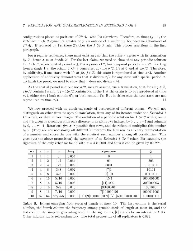
We now proceed with an empirical study of occurrence of different ethers. We will notdistinguish an ether from its spatial translation, from any of its iterates under the Extended 1Or 3 rule, or their mirror images. The evolution of a periodic solution for 1 Or 3 with given σand τ is given by a configuration on a discrete torus with rows indexed by 0, . . . , τ−1 and columnsby 0, . . . , σ− 1. Rotations give σ · τ possible first rows, and the reflection multiplies this numberby 2. (They are not necessarily all different.) Interpret the first row as a binary representationof a number and chose the one with the smallest such number among all possibilities. Thisgives (via the above proposition) the signature of an Extended 1 Or 3 ether. For example, thesignature of the only ether we found with σ = 4 is 0001 and thus it can be given by 0002∞.
no. τ σ ρ freq. signature ξ0
1 1 1 0 0.654 0 12 1 2 1/2 0.064 01 3033 2 4 1/2 0.029 0001 10010014 4 8 3/8 0.092 [7]1 101115 4 8 3/8 0.009 [5]101 1001100116 8 16 5/16 0.006 [15]1 10000010017 8 16 5/16 0.003 [11]10001 3000000038 8 16 3/8 0.013 [9]1000101 100101019 8 16 7/16 0.009 [7]101010101 100001100110 32 64 97/256 0.003 [11]1[9]100010101[9]1[7]1[5]10101000101 1101000111
Table 8. Ethers emerging from seeds of length at most 10. The first column is the serialnumber, the fourth column the frequency among genuine seeds of length at most 10, and thelast column the simplest generating seed. In the signatures, [k] stands for an interval of k 0’s.Other information is self-explanatory. The total proportion of all replicators is 0.883.
7 REPLICATION AND QUASIREPLICATION IN EXTENDED 1 OR 3 29
We look for replicators via the following algorithm. Start by picking two positive integers dand σmax. Build two sequences of length 2d−1 at time t = 2d + 2d−3: (a0, . . . , a2d−1−1) = (ξt(x) :−2d + 2d−2 < x ≤ −2d−2) and (b0, . . . , b2d−1−1) = (ξt(x) : 2d−2 ≤ x < 2d − 2d−2). Then checkwhether ai = ai+σ = bi+p for some 0 ≤ p < σ ≤ σmax and all i < 2d−1 − σ. As in Section 5, asuccessful pass of this check does not constitute a proof that a seed is a replicator, but again itappears to be a reliable sufficient condition for the choices we use, d = 12 and σmax = 128. Firstwe ran this algorithm on every seed of length at most 10 and found 10 different ethers, whichare given in the Table 8.
It is not feasible to analyze all seeds of larger lengths, so we resorted to random samples,and found that the proportion of replicators rapidly approaches 1. In fact, in a sample of 105
randomly chosen seeds of length at most 100, every single instance was a replicator with σ ≤ 64.There were 152 different ethers, and the most common were nos. 1, 4, 2, 3, 5, and 9, withrespective frequencies 0.64, 0.1, 0.05, 0.05, 0.03, and 0.02.
How confident can we be that not all seeds are replicators? Certainly there are mixedexamples, but we are more interested in genuinely different behaviors. For example, the seeds110111 and 1000011 appear to exhibit (different) chaotic dynamics during the first few thousandtime steps, but then nearly (but not quite) replicate in the next million steps. It is at least clearthat each of these two has a very long self-organizing epoch, and consequently our computationsfail to suggest a coherent hypothesis.
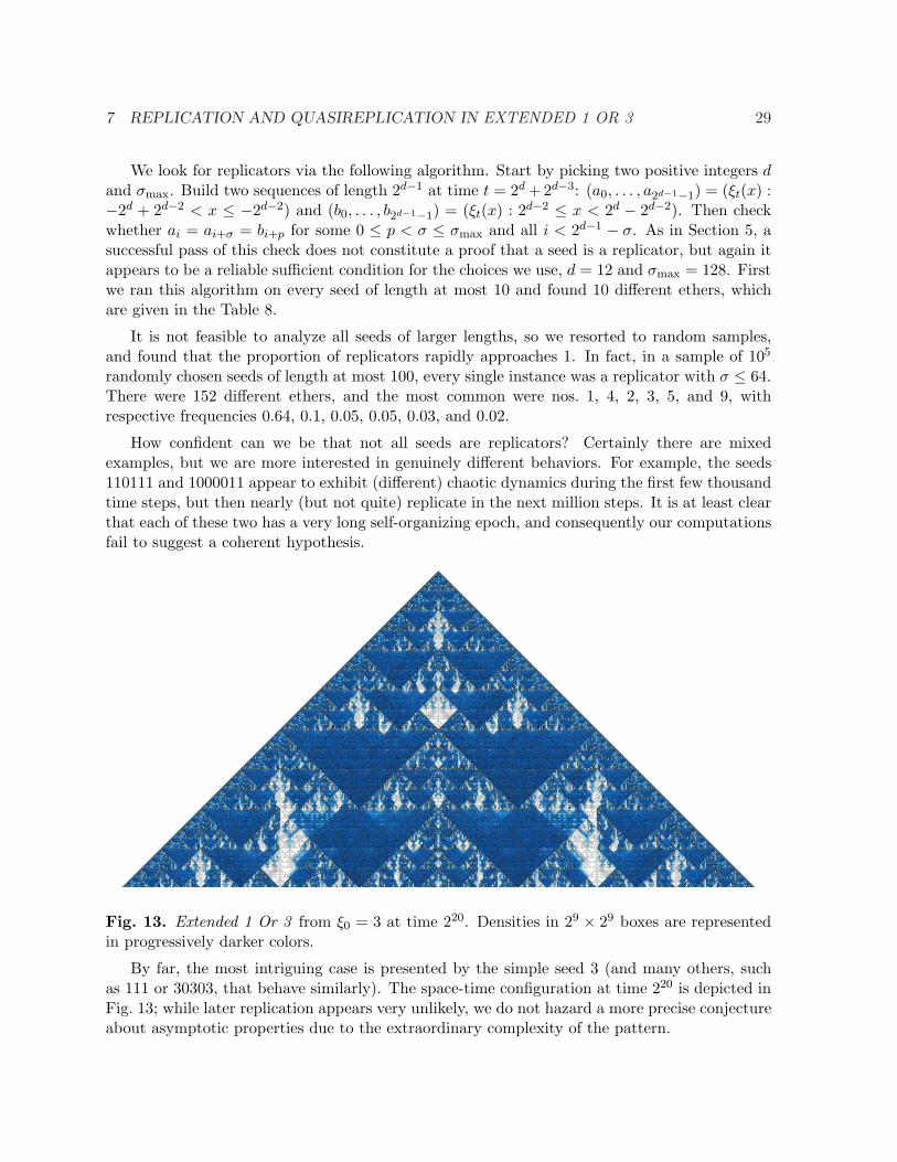
Fig. 13. Extended 1 Or 3 from ξ0 = 3 at time 220. Densities in 29 × 29 boxes are representedin progressively darker colors.
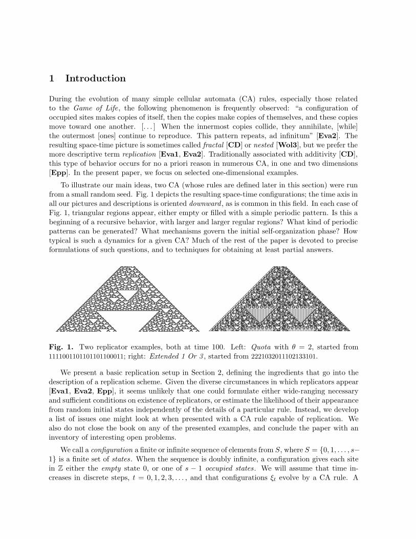
By far, the most intriguing case is presented by the simple seed 3 (and many others, suchas 111 or 30303, that behave similarly). The space-time configuration at time 220 is depicted inFig. 13; while later replication appears very unlikely, we do not hazard a more precise conjectureabout asymptotic properties due to the extraordinary complexity of the pattern.
7 REPLICATION AND QUASIREPLICATION IN EXTENDED 1 OR 3 30
Finally, we do have an example which is provably non-replicating and a sketch of its analysisis a fitting conclusion to the paper.
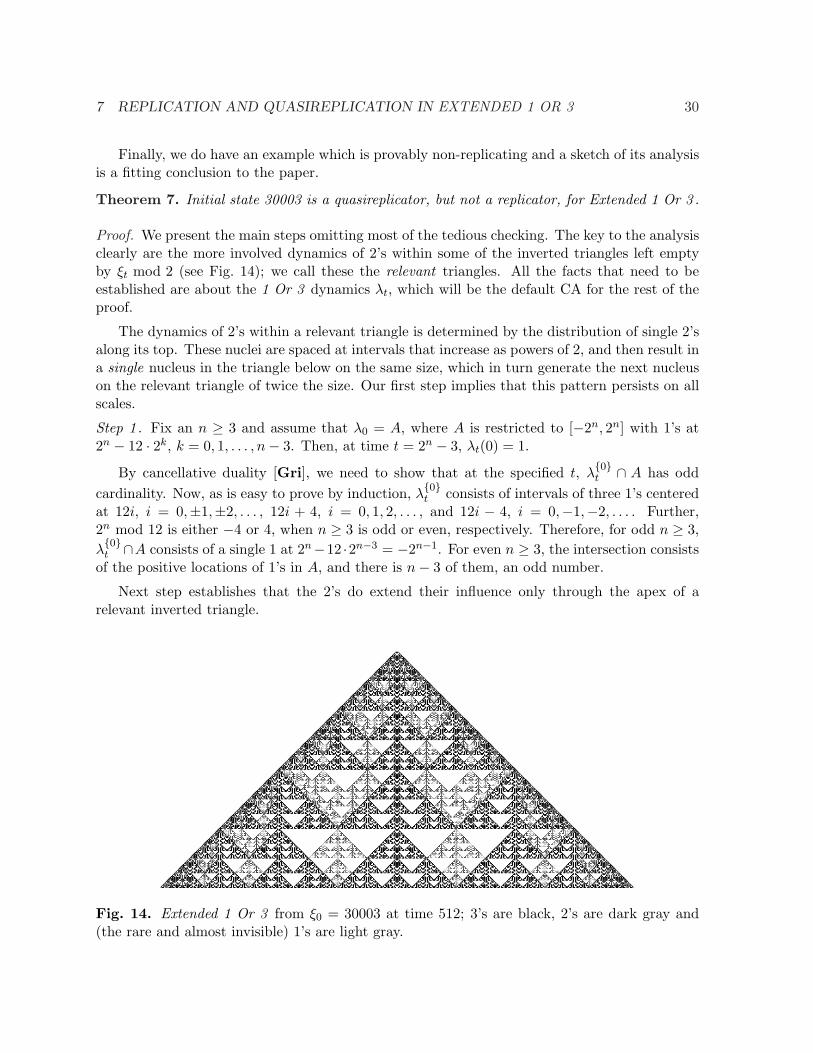
Theorem 7. Initial state 30003 is a quasireplicator, but not a replicator, for Extended 1 Or 3 .
Proof. We present the main steps omitting most of the tedious checking. The key to the analysisclearly are the more involved dynamics of 2’s within some of the inverted triangles left emptyby ξt mod 2 (see Fig. 14); we call these the relevant triangles. All the facts that need to beestablished are about the 1 Or 3 dynamics λt, which will be the default CA for the rest of theproof.
The dynamics of 2’s within a relevant triangle is determined by the distribution of single 2’salong its top. These nuclei are spaced at intervals that increase as powers of 2, and then result ina single nucleus in the triangle below on the same size, which in turn generate the next nucleuson the relevant triangle of twice the size. Our first step implies that this pattern persists on allscales.
Step 1 . Fix an n ≥ 3 and assume that λ0 = A, where A is restricted to [−2n, 2n] with 1’s at2n − 12 · 2k, k = 0, 1, . . . , n− 3. Then, at time t = 2n − 3, λt(0) = 1.
By cancellative duality [Gri], we need to show that at the specified t, λ{0}t ∩ A has odd
cardinality. Now, as is easy to prove by induction, λ{0}t consists of intervals of three 1’s centered
at 12i, i = 0,±1,±2, . . . , 12i + 4, i = 0, 1, 2, . . . , and 12i − 4, i = 0,−1,−2, . . . . Further,2n mod 12 is either −4 or 4, when n ≥ 3 is odd or even, respectively. Therefore, for odd n ≥ 3,λ{0}t ∩A consists of a single 1 at 2n−12 ·2n−3 = −2n−1. For even n ≥ 3, the intersection consists
of the positive locations of 1’s in A, and there is n− 3 of them, an odd number.
Next step establishes that the 2’s do extend their influence only through the apex of arelevant inverted triangle.
Fig. 14. Extended 1 Or 3 from ξ0 = 30003 at time 512; 3’s are black, 2’s are dark gray and(the rare and almost invisible) 1’s are light gray.

7 REPLICATION AND QUASIREPLICATION IN EXTENDED 1 OR 3 31
Step 2 . Starting from the same initial state as in Step 1, λj(x) = 0 at all even times j ≤ 2n − 4and x = ±(2n − j − 3).
This follows from cancellative duality and the fact that, for even j, λ{0}j occupies only even
positions — in fact, by additivity, its 1’s are located at twice the locations of 1’s in λ{0}j/2.
These two steps already show that the Willson limit, if it exists, must be fractal with thesame dimension as that of 1 Or 3 , log(1+
√5)/ log 2. Indeed, the union of all the sets generated
from all the nuclei within the relevant triangles, together with the set generated by ξt mod 2, issuch a fractal and is an upper bond for our Willson limit. Also, a similar argument as in theproof of Theorem 5 demonstrates non-replication.
To demonstrate the existence of Willson limit and thus complete the argument, we need tospecify a recursive description of the state within the relevant triangles. After a proper spaceand time rescaling, this reduces to the scheme for αn described in the next step.
region top/bottom left right middleα00 α11 ν α00 γ1000
α11 α11 ν α10 γ1110
α10 α01 ν α00 γ1100
α01 α01 ν α10 γ1010
γ1000 σ001 σ111 γ1111 ν
γ1111 σ011 σ100 γ0111 0γ0111 σ011 σ010 γ0111 0γ1110 σ011 σ100 γ0101 0γ0101 σ011 σ010 γ0001 0γ0001 σ001 σ001 γ1101 ν
γ1101 σ011 σ100 γ0001 0γ1100 σ011 σ100 γ0011 0γ0011 σ001 σ001 γ1011 ν
γ1011 σ001 σ111 γ1011 ν
γ1010 σ001 σ111 γ1001 ν
γ1001 σ001 σ111 γ1101 ν
ν ν 0 0 σ010
σ001 0 0 σ011 0σ011 σ010 σ011 σ101 ν
σ111 σ010 σ101 σ101 ν
σ010 σ010 σ011 σ110 ν
σ101 0 σ110 σ011 0
Table 9. Recursive specification for the defined configurations; σ100 and σ110 are given bysymmetry and the four missing γ’s never appear.
Step 3 . Assume that n ≥ 2; we will suppress the subscript n, which we will call level , from αand all other configurations and regions.
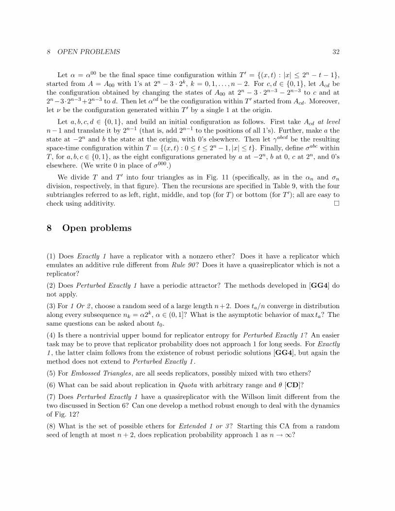
8 OPEN PROBLEMS 32
Let α = α00 be the final space time configuration within T ′ = {(x, t) : |x| ≤ 2n − t − 1},started from A = A00 with 1’s at 2n − 3 · 2k, k = 0, 1, . . . , n − 2. For c, d ∈ {0, 1}, let Acd bethe configuration obtained by changing the states of A00 at 2n − 3 · 2n−3 − 2n−3 to c and at2n−3 ·2n−3+2n−3 to d. Then let αcd be the configuration within T ′ started from Acd. Moreover,let ν be the configuration generated within T ′ by a single 1 at the origin.
Let a, b, c, d ∈ {0, 1}, and build an initial configuration as follows. First take Acd at leveln−1 and translate it by 2n−1 (that is, add 2n−1 to the positions of all 1’s). Further, make a thestate at −2n and b the state at the origin, with 0’s elsewhere. Then let γabcd be the resultingspace-time configuration within T = {(x, t) : 0 ≤ t ≤ 2n− 1, |x| ≤ t}. Finally, define σabc withinT , for a, b, c ∈ {0, 1}, as the eight configurations generated by a at −2n, b at 0, c at 2n, and 0’selsewhere. (We write 0 in place of σ000.)
We divide T and T ′ into four triangles as in Fig. 11 (specifically, as in the αn and σn
division, respectively, in that figure). Then the recursions are specified in Table 9, with the foursubtriangles referred to as left, right, middle, and top (for T ) or bottom (for T ′); all are easy tocheck using additivity.
8 Open problems
(1) Does Exactly 1 have a replicator with a nonzero ether? Does it have a replicator whichemulates an additive rule different from Rule 90? Does it have a quasireplicator which is not areplicator?
(2) Does Perturbed Exactly 1 have a periodic attractor? The methods developed in [GG4] donot apply.
(3) For 1 Or 2 , choose a random seed of a large length n+2. Does ta/n converge in distributionalong every subsequence nk = α2k, α ∈ (0, 1]? What is the asymptotic behavior of max ta? Thesame questions can be asked about t0.
(4) Is there a nontrivial upper bound for replicator entropy for Perturbed Exactly 1? An easiertask may be to prove that replicator probability does not approach 1 for long seeds. For Exactly1 , the latter claim follows from the existence of robust periodic solutions [GG4], but again themethod does not extend to Perturbed Exactly 1 .
(5) For Embossed Triangles, are all seeds replicators, possibly mixed with two ethers?
(6) What can be said about replication in Quota with arbitrary range and θ [CD]?
(7) Does Perturbed Exactly 1 have a quasireplicator with the Willson limit different from thetwo discussed in Section 6? Can one develop a method robust enough to deal with the dynamicsof Fig. 12?
(8) What is the set of possible ethers for Extended 1 or 3? Starting this CA from a randomseed of length at most n + 2, does replication probability approach 1 as n →∞?

REFERENCES 33
References
[BP] E. Bilotta, P. Pantano, Emergent patterning phenomena in 2D cellular automata, ArtificialLife 11 (2005), 339–362.
[BM] A. Berlinkov, R. D. Mauldin, Packing measure and dimension of random fractals, Journalof Theoretical Probability 15 (2002), 695–713.
[BDR] C. D. Brummitt, H. Delventhal, M. Retzlaff, Packard snowflakes on the von Neumannneighborhood , Journal of Cellular Automata 3 (2008), 57–80.
[CD] K. Culik, S. Dube, Fractal and Recurrent Behavior of Cellular Automata, Complex Sys-tems 3 (1989), 253–267.
[EN] K. Eloranta, E. Nummelin, The kink of cellular automaton Rule 18 performs a randomwalk , Journal of Statistical Physics 69 (1992), 1131-1136.
[Epp] D. Eppstein, Cellular Automata: Replicators.http://www.ics.uci.edu/ eppstein/ca/replicators/
[Eva1] K. M. Evans, “Larger than Life; it’s so nonlinear.” Ph. D. Thesis, University of Wiscon-sin, Madison, 1996.
[Eva2] K. M. Evans, Replicators and Larger than Life examples, in “New Constructions inCellular Automata,” eds. D. Griffeath and C. Moore, Oxford University Press, 2003, 119–159.
[FLM] P. Favatia, G. Lotti, L. Margara, Additive one-dimensional cellular automata are chaoticaccording to Devaney’s definition of chaos, Theoretical Computer Science 174 (1997), 157–170.
[GG1] J. Gravner, D. Griffeath, Cellular automaton growth on Z2: theorems, examples andproblems, Advances in Applied Mathematics 21 (1998), 241–304.
[GG2] J. Gravner, D. Griffeath, Modeling snow crystal growth I: rigorous results for Packard’sdigital snowflakes, Experimental Mathematics 15 (2006), 421-444.
[GG3] J. Gravner, D. Griffeath, Asymptotic densities for Packard Box rules, Nonlinearity 22(2009), 1817–1846.
[GG4] J. Gravner, D. Griffeath, The one-dimensional Exactly 1 cellular automaton: replication,periodicity, and chaos from finite seeds, Journal of Statistical Physics 142 (2011), 168–200.
[GGM] J. Gravner, G. Gliner, M. Pelfrey, One-dimensional replicators: examples.http://math.udavis.edu/~gravner/replicators.html
[Gri] D. Griffeath, “Additive and Cancellative Interacting Particle Systems.” Springer, 1979.
REFERENCES 34
[HC] J. E. Hanson, J. P. Crutchfield, The Attractor-Basin Portrait of a Cellular Automaton,Journal of Statistical Physics 66 (1992) 1415-1462.
[HPS] F. v. Haeseler, H.-O. Peitgen, G. Skordev, Global analysis of self-similarity features ofcellular automata: selected examples, Physica D 86 (1995), 64–80.
[Jen1] E. Jen, Enumeration of preimages of cellular automata, Complex Systems 3 (1989),421–456.
[Jen2] E. Jen, Aperiodicity in one-dimensional cellular automata, Physica D 45 (1990), 3–18.
[Jen3] E. Jen, Exact solvability and quasiperiodicity of one-dimensional cellular automata, Non-linearity 4 (1991), 251–276.
[Jen4] E. Jen, Transience and dislocations in one-dimensional cellular automata. In “Cellularautomata and cooperative systems (Les Houches, 1992),” NATO Adv. Sci. Inst. Ser. CMath. Phys. Sci., 396, Kluwer Acad. Publ., 1993, 299–310.
[MW] R. D. Mauldin, S. C. Williams, Hausdorff Dimension in Graph Directed Constructions,Transactions of the American Mathematical Society, 309(1988), 811–829.
[Moo] C. Moore, Predicting non-linear cellular automata quickly by decomposing them intolinear ones, Physica D 111 (1998), 27–41.
[Oll] N. Ollinger, The intrinsic universality problem of one-dimensional cellular automata. In“Symposium on Theoretical Aspects of Computer Science (STACS 2003),” eds. H. Alt andM. Habib, Springer, Berlin, 2003, 632-641).
[Wil1] S. J. Willson, Cellular automata can generate fractals, Discrete Appl. Math. 8 (1984),91–99.
[Wil2] S. J. Willson, Computing fractal dimensions for additive cellular automata, Physica D24 (1987), 190–206.
[Woj] M. Wojtowicz, Mirek’s Cellebration: a 1D and 2D Cellular Automata explorer .http://www.mirwoj.opus.chelm.pl/ca/
[Wol1] S. Wolfram, Statistical Mechanics of Cellular Automata, Rev. Mod. Phys. 55 (1983)601–644.
[Wol2] S. Wolfram, Computational Theory of Cellular Automata, Communications in Mathe-matical Physics 96 (1984), 15–57.
[Wol3] S. Wolfram, “A New Kind of Science.” Wolfram Media, 2002.
Related Documents


![Janko Gravner gravner@math.ucdavis.edu Genna Gliner …gravner/replication/rep.pdf · 2011. 2. 17. · Rule 126 [Jen2, Jen3, GG3]. It has binary states and its rule mandates that](https://static.cupdf.com/doc/110x72/6100d7b11c1b361c004db305/janko-gravner-gravnermath-genna-gliner-gravnerreplicationreppdf-2011-2.jpg)


