Renormalizing rectangles and other topics in random matrix theory

arX

iv:c

ond-

mat

/960

9190

v2 2

0 Se

p 19

96

NSF-ITP-96-68

hep-th/9609190

RENORMALIZING RECTANGLES AND OTHER TOPICS

IN RANDOM MATRIX THEORY

Joshua Feinberg & A. Zee

Institute for Theoretical Physics

University of California,

Santa Barbara, CA 93106, USA

AbstractWe consider random Hermitian matrices made of complex or real M × N

rectangular blocks, where the blocks are drawn from various ensembles. Thesematrices have N pairs of opposite real nonvanishing eigenvalues, as well asM − N zero eigenvalues (for M > N .) These zero eigenvalues are “kinemat-ical” in the sense that they are independent of randomness. We study theeigenvalue distribution of these matrices to leading order in the large N,M

limit, in which the “rectangularity” r = MN is held fixed. We apply a variety of

methods in our study. We study Gaussian ensembles by a simple diagrammaticmethod, by the Dyson gas approach, and by a generalization of the Kazakovmethod. These methods make use of the invariance of such ensembles underthe action of symmetry groups. The more complicated Wigner ensemble, whichdoes not enjoy such symmetry properties, is studied by large N renormalizationtechniques. In addition to the kinematical δ-function spike in the eigenvaluedensity which corresponds to zero eigenvalues, we find for both types of en-sembles that if |r − 1| is held fixed as N → ∞, the N non-zero eigenvaluesgive rise to two separated lobes that are located symmetrically with respect tothe origin. This separation arises because the non-zero eigenvalues are repelledmacroscopically from the origin. Finally, we study the oscillatory behavior ofthe eigenvalue distribution near the endpoints of the lobes, a behavior governedby Airy functions. As r → 1 the lobes come closer, and the Airy oscillatory be-havior near the endpoints that are close to zero breaks down. We interpret thisbreakdown as a signal that r → 1 drives a cross over to the oscillation governedby Bessel functions near the origin for matrices made of square blocks.

PACS numbers: 11.10.Lm, 11.15.Pg, 11.10.Kk, 71.27.+a

1 Introduction

In random matrix theory, a number of authors [1, 2, 3, 4, 5, 6, 7, 8] have studied the

eigenvalue distribution of a Hermitian matrix H of the form

H =(

0 C†

C 0

)

, (1.1)

in which C is an N × N complex random matrix taken from an ensemble with the

probability distribution

P (C) =1

Zexp(−NTrC†C) , (1.2)

with N tending to infinity. These so-called chiral matrices appear in a variety of

physical problems. For example, in quantum chromodynamics one typically inte-

grates over the quarks and studies the so-called fermion determinant. The gluon

fluctuations are then often treated approximately by saying that they effectively ren-

der the relevant matrix in the determinant random [1, 9, 10]. The chiral structure

corresponds to left and right handed quarks. As another example, Hikami, Shirai,

and Wegner [11, 12, 13] have proposed a model for electron scattering off impurities

in quantum Hall fluids in the spin-degenerate limit. The blocks in (1.1) correspond to

spin up and spin down electrons. In the same spirit, one may consider any problem

involving random scattering between two groups of states, for example, between two

cavities. As pointed out by Nagao and Slevin [4], these matrices also appear in the

study of transport in disordered conductors. In this paper, we study a slight gener-

alization of this problem, with C taken to be an M ×N rectangular matrix, with M

and N both tending to infinity. For M − N of order N0, we expect the density of

eigenvalues to be the same as for the M = N case. Here we would like to study the

case where the measure of rectangularity,

r ≡ M/N , (1.3)

is held fixed as both M and N tend to infinity. Some aspects of this problem have

been studied before and we will note the appropriate references below. We denote

1

the matrix elements of C by

Ciα, where i = 1, 2, ..., M and α = 1, 2, ..., N.

With no loss of generality we assume throughout this paper that M ≥ N , namely,

that r ≥ 1. Our notation is such that Latin indices always run from 1 through M ,

whereas indices denoted by Greek letters run from 1 to N .1 As a result of their specific

structure these matrices have N pairs of opposite real nonvanishing eigenvalues, as

well as M−N zero eigenvalues. These zero eigenvalues are “kinematical” in the sense

that they are independent of the probability distribution.

We derive the eigenvalue distribution of these matrices to leading order in the large

N, M approximation for various ensembles of random blocks. We consider random

Hermitian matrices made of complex or real M × N rectangular blocks, where the

blocks are drawn either from ensembles symmetric under some group action or from

non-symmetric ensembles. For concreteness, we specialize to Gaussian ensembles in

the first case. In the second case we analyze matrices of the “Wigner Class”, namely,

blocks whose entries are drawn independently one of the other from the probability

distribution. We find, not surprisingly, that to leading order in the large N, M ap-

proximation, all the ensembles we studied result in the same eigenvalue distribution.

In addition to the kinematical δ-function spike in the eigenvalue density which corre-

sponds to zero eigenvalues, we find that if |r − 1| does not scale to zero as N → ∞,

the N non-zero eigenvalues give rise to two well separated lobes that are located

symmetrically with respect to the origin. For random Hermitian matrices that are

not made of blocks, the qualitative universality of the Wigner semicircular eigenvalue

distribution is well understood as a result of the competition between level repulsion

and the fact that very large eigenvalues are suppressed. Similar arguments explain

the universality of the eigenvalue distribution we observe here for matrices made of

rectangular blocks. Each lobe arises qualitatively for the same reasons that lead to the

semicircular distribution. In addition, separation of the two lobes arises because the

1We shall deviate slightly from this convention only in section 2 where µ, ν will run over allpossible M + N values. No confusion should arise.

2

non-zero eigenvalues are repelled from the origin by the macroscopic number (M−N)

of zero eigenvalues.

In this paper C†C and CC† are Hermitian non-negative matrices of dimensions

N × N and M × M , respectively. We are interested in the expectation value of the

resolvent

GN,M(z) =1

N + MTr

1

z − H. (1.4)

A straightforward calculation then yields a simple relation between GN,M(z) and the

resolvents of C†C and CC†,

GN,M(z) =z

N + M

[

Tr(N)

1

z2 − C†C+ Tr

(M)

1

z2 − CC†

]

(1.5)

where the subscript on each trace indicates the dimension of the matrix which is

being traced over. The z2 dependence of the resolvents in (1.5) arises because the

eigenvalues of H in (1.1) occur in real opposite pairs. Indeed, given an N dimensional

vector x and an M dimensional vector y such that(

xy

)

is an eigenvector of H for an

eigenvalue λ, then(

x−y

)

is an eigenvector for −λ. In other words the matrix H (the

“Dirac” operator, with its “chiral” components C and C†) anti-commutes with the

“γ5” matrix(

1N 00 −1M

)

. The cyclic property of the trace implies the basic relation

Tr(M)

1

z2 − CC† = Tr(N)

1

z2 − C†C+

M − N

z2. (1.6)

This relation reflects the fact that C†C and CC† share the same strictly positive

eigenvalues, but the M × M matrix CC† has additional M − N zero eigenvalues.

Combining (1.5) and (1.6) we therefore arrive at the two alternative expressions

GN,M(z) =(

M − N

N + M

)

1

z+

2z

M + NTr

(N)

1

z2 − C†C

=(

N − M

N + M

)

1

z+

2z

M + NTr

(M)

1

z2 − CC† , (1.7)

that allow us to express GN,M(z) solely in terms of either C†C or in terms of CC†.

For later use we introduce the following notation

GN(w) =1

NTr

(N)

1

w − C†C, GM(w) =

1

MTr

(M)

1

w − CC† (1.8)

3

in terms of which we rewrite (1.7) as

GN,M(z) =(

M − N

N + M

)

1

z+(

2N

M + N

)

zGN (z2)

=(

N − M

N + M

)

1

z+(

2M

M + N

)

zGM (z2) . (1.9)

Throughout this paper G stands for an unaveraged resolvent. The corresponding

averaged quantity will be denoted simply by G.

This paper is organized as follows. We will first apply a variety of methods to study

the density of eigenvalues. In Section 2 we derive the density of states of matrices H

whose rectangular blocks are drawn either from the unitary or from the orthogonal

Gaussian ensemble, employing diagrammatic techniques. Section 3 is devoted to

blocks with independent entries (which we refered to [14] as the “Wigner Class”.)

This ensemble is more difficult to handle, because of lack of symmetry. We overcome

this difficulty by applying recursive manipulations of the large N renormalization

group[15, 16, 17]. We find that as far as the density of states is concerned, this

ensemble falls (in the planar limit) into the same universality class as the symmetric

ensembles. In Appendix A we provide a proof of the central limit theorem by means

of the large N renormalization group, as yet another example of its usefulness. In

Section 4 we present the Dyson gas approach to these issues. After completing our

work we realized that the results we obtained following the Dyson gas approach

already appeared in [18]. Nevertheless, we include this section here for the paper to

be self-contained and also because Section 5 partly relies on it. In Section 5 we first

generalize Kazakov’s method [19] to rederive the results of Section 2, and then use

this method to determine the oscillatory fine structure of the eigenvalue density in

Section 2, close to its support endpoints. We find that this oscillatory behavior is

governed by Airy functions. As r → 1 the lobes come closer, and the Airy oscillatory

behavior near the endpoints that are close to zero breaks down. We interpret this

breakdown as a signal that in the limit r → 1 drives a cross over to the oscillation

near the origin in the density of eigenvalues of matrices made of square blocks, an

oscillation governed by Bessel functions.

4

2 A diagrammatic approach

As a simple warm up exercise, and in order to set the stage, let us first apply the

by-now well-known diagrammatic method to derive the Green’s function

G(z) =1

N + M〈Tr

1

z − H〉 (2.1)

in the large N, M limit. To this end, let us consider the averaged resolvent

Gµν(z) = 〈

(

1

z − H

)µ

ν〉 (2.2)

where the indices µ and ν run over all possible M + N values. The average in (2.2)

is performed with respect to the Gaussian measure

P (C) =1

Zexp [−

√NM m2 Tr C†C] , (2.3)

where

Z =∫ M∏

i=1

N∏

α=1

d Re Ciα d Im Ciα exp [−√

NM m2 Tr C†C] (2.4)

is the partition function. We have introduced a normalization factor of√

MN in (2.3)

so as to be consistent with (1.2) in the N = M case. This factor renders (2.3) and (2.4)

manifestly symmetric under M ↔ N . Some other normalizations, not symmetrical

under M ↔ N , can always be introduced by multiplying the parameter m2 by an

appropriate factor of r = MN

. Borrowing some terminology of gauge field theory we

may consider C, C† as “gluons” (in zero space-time dimensions), and Gµν (z) as the

propagator of “quarks” (with complex mass z) which couple to these “gluons”. We

now proceed to calculate Gµν(z) diagrammatically. The two-point correlator associated

with (2.3) is clearly

〈CiαC∗jβ〉 =

1

m2√

MNδijδαβ . (2.5)

This expression is the gluon propagator. The bare quark propagator is simply 1z. The

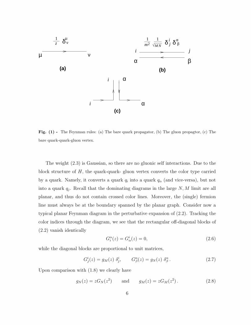
quark-quark-gluon vertex factor is 1. These Feynman rules are summarized in Fig.

(1).

5

α

α

z1 δ

µβα

i

i

(a) (b)

(c)

νµ

ν

11δ i

j δαβ2m

i jM N

Fig. (1) - The Feynman rules: (a) The bare quark propagator, (b) The gluon propagtor, (c) The

bare quark-quark-gluon vertex.

The weight (2.3) is Gaussian, so there are no gluonic self interactions. Due to the

block structure of H , the quark-quark- gluon vertex converts the color type carried

by a quark. Namely, it converts a quark qi into a quark qα (and vice-versa), but not

into a quark qj . Recall that the dominating diagrams in the large N, M limit are all

planar, and thus do not contain crossed color lines. Moreover, the (single) fermion

line must always be at the boundary spanned by the planar graph. Consider now a

typical planar Feynman diagram in the perturbative expansion of (2.2). Tracking the

color indices through the diagram, we see that the rectangular off-diagonal blocks of

(2.2) vanish identically

Gαi (z) = Gi

α(z) = 0, (2.6)

while the diagonal blocks are proportional to unit matrices,

Gij(z) = gM(z) δi

j , Gαβ(z) = gN(z) δα

β . (2.7)

Upon comparison with (1.8) we clearly have

gN(z) = zGN (z2) and gM(z) = zGM(z2) . (2.8)

6

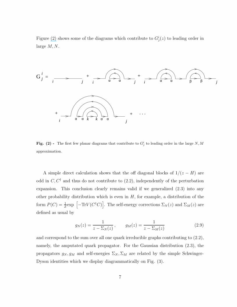
Figure (2) shows some of the diagrams which contribute to Gij(z) to leading order in

large M, N .

G ji

= + +i j i α α β β jj iα α

+ + . . .

i jkα α α αk

Fig. (2) - The first few planar diagrams that contribute to Gij to leading order in the large N, M

approximation.

A simple direct calculation shows that the off diagonal blocks of 1/(z − H) are

odd in C, C† and thus do not contribute to (2.2), independently of the perturbation

expansion. This conclusion clearly remains valid if we generalized (2.3) into any

other probability distribution which is even in H , for example, a distribution of the

form P (C) = 1Zexp

[

−TrV (C†C)]

. The self-energy corrections ΣN (z) and ΣM (z) are

defined as usual by

gN(z) =1

z − ΣN (z), gM(z) =

1

z − ΣM(z)(2.9)

and correspond to the sum over all one quark irreducible graphs contributing to (2.2),

namely, the amputated quark propagator. For the Gaussian distribution (2.3), the

propagators gN , gM and self-energies ΣN , ΣM are related by the simple Schwinger-

Dyson identities which we display diagrammatically on Fig. (3).

7

ΣN

=1α

Σ=1i

M

GNΣ

βα i i

iiα β

=

Gα α

ααj i ji

=ΣM

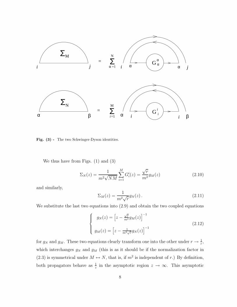
Fig. (3) - The two Schwinger-Dyson identities.

We thus have from Figs. (1) and (3)

ΣN (z) =1

m2√

NM

M∑

i=1

Gii(z) =

√r

m2gM(z) (2.10)

and similarly,

ΣM(z) =1

m2√

rgN(z) . (2.11)

We substitute the last two equations into (2.9) and obtain the two coupled equations

gN(z) =[

z −√

rm2 gM(z)

]−1

gM(z) =[

z − 1m2

√rgN(z)

]−1(2.12)

for gN and gM . These two equations clearly transform one into the other under r → 1r,

which interchanges gN and gM (this is as it should be if the normalization factor in

(2.3) is symmetrical under M ↔ N , that is, if m2 is independent of r.) By definition,

both propagators behave as 1z

in the asymptotic region z → ∞. This asymptotic

8

behavior picks up the physical solution of the quadratic equations for gN and gM , and

we find

gN(z) =2

(a − b)2

1

z

[

z2 − ab −√

(z2 − a2) (z2 − b2)]

gM(z) =2

(a + b)2

1

z

[

z2 + ab −√

(z2 − a2) (z2 − b2)]

, (2.13)

where

a =1

m(r

14 + r−

14 ) , b =

1

m(r

14 − r−

14 ). (2.14)

Note that b measures of the deviation of rectangles from squares: for r = 1, b vanishes.

The Green’s function (2.1) is thus given by

G(z) =1

N + M

N+M∑

µ=1

Gµµ(z) =

gN(z) + rgM(z)

1 + r(2.15)

where we used (2.2) and (2.7). Finally, upon substituting (2.13) into (2.15) we find

that the averaged Green’s function of H is

G(z) =2

a2 + b2

1

z

[

z2 −√

(z2 − b2)(z2 − a2)]

. (2.16)

Let us inspect now some of the features of (2.16). As we discussed in the intro-

duction, H has M − N “kinematical” zero eigenvalues, regardless of any ensemble

averaging. In contrast, C†C on the average does not have any zero eigenvalues as

we have already discussed. Thus, by definition, GN,M(z) has a simple pole at z = 0

with residue M−NM+N

= r−1r+1

, which is the first term on the right side of (1.9). As we

can see from (2.14), our expression (2.16) clearly satisfies this condition provided√

(z2 − b2)(z2 − a2) → −ab as z → 0. This sign of the square root corresponds to

drawing all four cuts associated with the square root to the left of the branch point

out of which they emanate. In addition, (2.14) is consistent with the required asymp-

totic behavior 1z

of (2.16) as z → ∞. The averaged eigenvalue density of H is the

discontinuity in (2.16) as we cross the real axis, except for the origin, which contains

the “kinematical” zero eigenvalues of H . It is therefore given by

ρ(λ) =r − 1

r + 1δ(λ) +

2

π|λ|θ [(a2 − λ2) (λ2 − b2)]

a2 + b2

√

(a2 − λ2) (λ2 − b2) . (2.17)

9

The Green’s function (2.16) corresponds to the Hamiltonian (1.1). With only

little more effort it is possible to generalize our discussion to calculate the Green’s

function of the Hamiltonian

H =(

ǫ C†

C −ǫ

)

, (2.18)

where ǫ is a fixed “energy”. The off-diagonal blocks fluctuate as before. This Hamilto-

nian may describe, for example, tunneling between two energy levels with degeneracies

N and M that are seperated by an energy difference 2ǫ. For such a Hamiltonian (1.5)

is modified into

GN,M(z) =z + ǫ

r + 1GN(w) +

r (z − ǫ)

r + 1GM(w) (2.19)

where

w = z2 − ǫ2 ,

such that the identifications (2.8) become

gN(z) = (z + ǫ)GN (w) and gM(z) = (z − ǫ)GM (w) . (2.20)

The bare quark propagator in Fig. (1) is split into two pieces, namely, 1z−ǫ

for quarks

carrying a U(N) color index and 1z+ǫ

for quarks carrying a U(M) index. The defini-

tions in (2.9) change accordingly into

gN(z) =1

z − ǫ − ΣN (z), gM(z) =

1

z + ǫ − ΣM (z). (2.21)

The Schwinger-Dyson identities (2.10) and (2.11) are unchanged. We note that the

set of equations (2.10), (2.11) and (2.21) are now invariant under r → 1r

and ǫ → −ǫ,

which permutes the two energy levels in H and thus interchanges gN and gM . With

these observation it is straightforward to see that (2.13) becomes

gN(z) =2

(a − b)2

1

(z − ǫ)

[

w − ab −√

(w − a2) (w − b2)]

gM(z) =2

(a + b)2

1

(z + ǫ)

[

w + ab −√

(w − a2) (w − b2)]

, (2.22)

10

with the same a and b as before. Thus, (2.15) and (2.16) finally become

G(z) =2

(a2 + b2)

1

w

{

z[

w −√

(w − a2) (w − b2)]

− abǫ}

, (2.23)

which is manifestly invariant under a permutation of the two energy levels of H .

Note that the matrix (2.18) has precisely M − N “kinematical” (i.e., independently

of the ensemble for C) eigenvectors which correspond to eigenvalue −ǫ. This means

that (2.23) has a simple pole at z = −ǫ with residue r−1r+1

, and no pole at z =

+ǫ. This property holds provided√

(w − a2) (w − b2) → −ab as w → 0 which we

already encountered in our analysis of the ǫ = 0 case. The eigenvalue distribution

corresponding to (2.23) is therefore

ρ(λ) =r − 1

r + 1δ(λ + ǫ) +

θ [(a2 + ǫ2 − λ2) (λ2 − b2 − ǫ2)]

π (a2 + b2)

2 |λ|(λ2 − ǫ2)

√

(a2 + ǫ2 − λ2) (λ2 − b2 − ǫ2) .(2.24)

In the limit (mǫ) → ∞, the randomness in (2.18) is suppressed, and (2.24) should

reproduce the eigenvalue distribution of the deterministic part of (2.18). This is

indeed the case. In this limit we have aǫ, b

ǫ→ 0 so both lobes in (2.24) shrink. Each

lobe contains N eigenvalues, whose number is preserved as the lobes shrink to zero

width, and thus produce δ function spikes of strength NM+N

each. The right lobe

produces in this way a spike at λ = ǫ, while the left lobe coalesces with the already

existing δ(λ+ ǫ) spike in (2.24) which contains M −N eigenvalues, and thus produces

a spike containing M eigenvalues.

11

3 Blocks with independent matrix elements and

their renormalization group analysis

It is rather difficult to apply the diagrammatic method and sum all the planar dia-

grams that contribute to G(z) in case of non-Gaussian ensembles. For such ensembles

that are invariant under the action of some symmetry group one may invoke other

methods. However, these methods are inapplicable to ensembles lacking the action

of a symmetry group.

A class of block structure random matrix models that is not unitary (or orthogo-

nal) invariant involves matrix blocks C in which each matrix element Ciα is randomly

distributed independently of the others, with the same distribution for all matrix

elements. We normalize the matrix elements Ciα symmetrically with respect to M

and N , such that the two-point correlator

〈CiαC∗jβ〉 =

σ2

√MN

δijδαβ (3.1)

of this probability distribution would coincide with the two point correlator of the

Gaussian distribution dµ(C) ∼ exp[

−√

MNσ2 TrC†C

]

. For notational simplicity we

replaced here the m−2 in (2.3) by σ2. For this class of matrix models the method of

orthogonal polynomials is not directly applicable, and alternative methods should be

sought for.

For concreteness as well as for simplicity, we consider below the probability dis-

tribution in which Ciα may take one of the two values

± σ

(NM)1/4(3.2)

with equal probability, where σ is a finite number. However, it will be clear from the

discussion below, that our conclusions are not limited to this particular distribution.

In order to keep our formulas generic, we therefore treat the Ciα as complex numbers,

as long as we do not utilize (3.2) explicitly.

For this ensemble |Ciα|2 = σ2√

MNdeterministically, and thus in particular the

12

diagonal matrix elements of C†C and CC† do not fluctuate and are given by

(C†C)αα = σ2√

r and (CC†)ii = σ2/√

r . (3.3)

We use this convenient property of (3.2) in our calculations below. This, however,

is done with no loss of generality, because in the generic case the non-fluctuating

quantities in (3.3) should simply be replaced by their averages, which are given on

the right hand side of (3.3).

The random matrix distribution we consider is a generalization of the very first

model studied by Wigner[20] into random matrices with block structure. Indeed,

Wigner originally considered large N × N random Hermitean matrices φ, whose ele-

ments φij = φ∗ji were either + σ√

Nor − σ√

N, with equal probability. This matrix model

follows a semi-circle law for the density of eigenvalues. This semi-circular profile of

the eigenvalue density was rederived recently[15] using a large N “renormalization

group” inspired approach[16]. In what follows, we apply the same method to find

the eigenvalue density ρ(λ) of the random block matrices with independent entries

introduced above.

We are interested in

G(z) = limN,M→∞

GN,M(z) (3.4)

from which ρ(λ) = 1πImG(λ−iǫ) may be extracted immediately. We start our “renor-

malization group” calculation by trying to relate GN+1,M(z) to GN,M(z). To this end

we consider the M × (N + 1) block

C ′ = (C, v)

where v is an M dimensional vector. By definition, each element of C ′ may take now

one of the two values ± σ

[(N+1)M ]1/4 with equal probability. A comparison with the

original N × M block suggests then that we may draw the C ′iα from (3.2) provided

we rescale the σ parameter in that equation into

σ′ = σ(

N

N + 1

)

14

. (3.5)

13

The non-fluctuating norm squared of v is then given by

v†v ≡ (C ′†C ′)N+1,N+1 = σ′ 2√

r . (3.6)

Following [15], we obtain2 after some straightforward algebra

(N + 1)GN+1(w) ≡ Tr(N+1)

1

w − C ′†C ′

= Tr(N)

1

w − C†C − C† v⊗v†

w−v†vC+

1

w − v†v − v†C 1w−C†C C†v

(3.7)

where w = z2. We now average over the distribution governing C ′, keeping terms up

to O(N0). We first average over the components of v.

Expanding the two fractions on the right hand side of (3.7) into geometric series

we see that we have to average products of the form v∗i vjv

∗kvl · · · v∗

pvq, which contract

against products of elements of matrices independent of the vi . Clearly,

< v∗i vj >=< C

′∗i,N+1C

′j,N+1 >=

σ′ 2

√MN

δij

simply produces a single trace, multiplied by σ′ 2√

NM. The next non-vanishing correlator

is

< v∗i vjv

∗kvl >=

σ′ 4

NM(δijδkl + δikδjl − δijkl) , (3.8)

where δijkl = 1 when i = j = k = l and 0 otherwise. The last piece in (3.8)

is by definition the fourth order cumulant of the distribution, added to the usual

pairs of Wick contractions. The correlator (3.8) then contracts against two matrices

in the geometrical series mentioned above, producing a term of order(

σ′ 2√

NM

)2. In

the large N, M limit, the dominating term in this contraction is the term with the

maximal independent index summations, which amounts here to two traces. These

two traces are produced here only by a single pair of Wick contractions. The other

pair of Wick contractions (which produces only a single trace) as well as the fourth

order cumulant are therefore negligible in the large N, M limit, and may be discarded

to leading order. This structure persists for correlators of higher order. The 2n

2The analogue of v†v in [15] was a quantity of O( 1

N) which was therefore neglected in the N → ∞

limit. Here v†v is a finite number and must be therefore retained.

14

point correlator produces in the geometric series a term proportional to(

σ′ 2√

NM

)n. In

that term, a unique string of n Wick contractions produces the maximal number n

of traces, and therefore dominates the large N, M limit. At this point it becomes

clear why our calculation, and therefore, the results it leads to are insensitive to the

details of the distribution of the Ciα. Clearly, only Wick contractions dominate these

averages in this limit, and thus only the two point function (3.1) of the distribution

matters. This insensitivity to the detials of the distribution was checked explicitly

in [15], where various distributions led to the same result. The leading terms in the

geometric series may be resummed, and one finds the v average

〈Tr(N+1)

1

w − C ′†C ′ 〉v = Tr(N)

1

w − C†C

+∂

∂wlog

[

w + (N − M)σ′ 2

√NM

− σ′ 2

√NM

w Tr(N)

1

w − C†C

]

. (3.9)

Invoking large N factorisation, we can average over the remaining block C immedi-

ately, by replacing GN inside the logarithm in (3.9) by its average. Thus,

(N + 1)GN+1(w) = NGN (w) +∂

∂wlog

[

w +(1 − r)σ′ 2

√r

− σ′ 2

√r

w GN(w)

]

. (3.10)

Remarkably, in the large N, M limit, the v average of GN+1(w) involves only GN (w),

and thus (3.10) is indeed a local (along the N axis) recursion relation involving only

GN type Green’s functions. This means that the large N “renormalization group”

recursions for the full Green’s function GN,M close among themselves as we now show.

Combining (1.9) and (3.10), we obtain the recursion relation for the complete

averaged Green’s function (1.4)

(N + M + 1)GN+1,M(z, σ′) − (N + M)GN,M (z, σ′) =

∂

∂zlog

[

z +(1 − r)σ′ 2

2z√

r− (r + 1)σ′ 2

2√

rGN,M(z, σ′)

]

, (3.11)

where we have displayed the explicit σ′ parameter associated with the larger C ′ block.

15

In the large N limit (3.5) becomes σ′ = σ− σ4N

+· · ·. In this limit, the only possible

explicit N, M dependence in GN,M is through the finite ratio r = MN

. Therefore we

may write the left hand side of (3.11) as

[(N + M + 1)GN+1,M(z, σ′) − (N + M)GN,M (z, σ)] + (N + M) [GN,M(z, σ) − GN,M(z, σ′)]

=∂

∂N[(N + M)GN,M(z, σ)] +

(N + M)

4Nσ

∂

∂σGN,M(z, σ)

= GN,M(z, σ) − r(r + 1)∂

∂rGN,M(z, σ) +

r + 1

4σ

∂

∂σGN,M(z, σ) . (3.12)

To leading order in 1N

we may drop the N, M indices of the Green’s function, replacing

it by its asymptotic limit (3.4), and replace σ′ by σ inside the logarithm in (3.11).

The recursion relation (3.11) thus becomes a partial differential equation

G(z, σ) − r(r + 1)∂

∂rG(z, σ) +

r + 1

4σ

∂

∂σG(z, σ) =

∂

∂zlog

[

z +(1 − r)σ2

2z√

r− (r + 1)σ2

2√

rG(z, σ)

]

(3.13)

It is easy to see from (1.4) and (3.4) that G(z, σ) satisfies the simple scaling rule

G (z, σ) =1

σG(

z

σ, 1)

(3.14)

which implies that

σ∂

∂σG(z, σ) = −z

∂

∂zG(z, σ) − G(z, σ) . (3.15)

Thus, using (3.15) to eliminate σ ∂∂σ

G(z, σ) from (3.13) we arrive at the final form of

our differential equation for G(z, σ), namely,

3 − r

4G(z, σ) − r(r + 1)

∂

∂rG(z, σ) − r + 1

4z

∂

∂zG(z, σ) =

∂

∂zlog

[

z +(1 − r)σ2

2z√

r− (r + 1)σ2

2√

rG(z, σ)

]

. (3.16)

16

This equation tells us how a change in z can be compensated by a change in the

rectangularity r.

As a consistency check of our results we can repeat the recursive procedure dis-

cussed above, but instead of adding an M dimensional column vector to C, we add

to it an N dimensional row vector u, creating an (M + 1) × N block C ′′

C ′′ =

C

u

.

The recursion relation in this case connects, in the large N, M limit, GM+1(w) and

GM(w), and therefore relates GN,M+1(z) to GN,M(z). Thus, we simply interchange

N ↔ M in all steps of our calculation above, namely, r ↔ 1r. The differential equation

for G(z, σ) we derived from this recursion reads

3r − 1

4rG(z, σ) + (r + 1)

∂

∂rG(z, σ) − r + 1

4rz

∂

∂zG(z, σ) =

∂

∂zlog

[

z − (1 − r)σ2

2z√

r− (r + 1)σ2

2√

rG(z, σ)

]

, (3.17)

which is indeed the transform of (3.16) under r → 1r.

The fact that G(z, σ) satisfies both (3.16) and its tranform under r → 1r

means

that G(z, σ, r) = G(z, σ, 1r). This r inversion symmetry of G should be anticipated

from our N, M symmetric definition of the probability distribution (3.1) in the first

place. An important consequence of this r inversion symmetry is that ∂∂r

G vanishes3at

r = 1. Thus, at the point r = 1, i.e., for Hamiltonians made of square blocks, (3.16)

reduces to the differential equation

G(z, σ) − z∂

∂zG(z, σ) = 2

∂

∂zlog

[

z − σ2 G(z, σ)]

(3.18)

previously derived in [15], as expected.

As was stated at the beginning of this section, only the two point correlator (3.1)

of the random matrix distribution was relevant in the derivation of (3.16). Hence, the

3This is simply because if f(r) = f(

r−1)

, then ∂∂r

f(r) = −r−2 ∂∂r−1 f

(

r−1)

, and therefore f ′(1) =−f ′(1) = 0.

17

Green’s function G(z) of any distribution obeying (3.1) is a solution of (3.16). We

have thus shown that for the Wigner ensemble G(z) and the density of eigenvalues

are universal. In particular, the complex Hermitean distribution (2.3) as well as

the real symmetric distribution (4.16) of the previous section respect (3.1) upon the

identification m2 = σ−2. Thus, their Green’s function (2.16) must be a solution of

(3.16). A simple check verifies that this is indeed the case. Therefore, the density of

eigenvalues ρ(λ) = 1πImG(λ − iǫ) is given by (2.17).

As yet another example of the usefulness of the large N renormalization group we

use it to prove the central limit theorem in Appendix A.

By a simple power counting argument (see Section 2 of [14], and also [17]) it is

straightforward to extend the diagrammatic method of the previous section to treat

the probability distribution considered in this section as well.

18

4 Dyson gas approach

In this section we present the Dyson gas approach to study the eigenvalue distribution

of matrices made of rectangular blocks. After completing our calculations we realized

that our results were previously obtained by Periwal et al. in [18]. We assume that

the M × N rectangular blocks Ciα of the Hamiltonian H in (1.1) admit the action

of some symmetry group. Here we focus on blocks with complex entries, but we will

state some results concerning blocks with real entries in the end. The complex blocks

are endowed with the natural U(M) × U(N) action

C → V CU , V ∈ U(M) , U ∈ U(N) . (4.1)

One can use this action to bring C to the form

C =

ΛN

0(M−N)×N

(4.2)

where ΛN is a real diagonal N × N matrix diag(λ1, · · · , λN). Therefore, the Hermi-

tian matrix H in (1.1) is a generator of the symmetric space U(M + N)/U(M) ⊗U(N). From these considerations it is clear that C†C may be diagonalized into

diag(λ21, · · · , λ2

N) and CC† into the same form, but with additional M − N zeros, in

accordance with (1.6). The probability distribution has to be invariant under (4.1).

Here we consider distributions of the form

P (C) =1

Zexp

[

−√

MN Tr V (C†C)]

(4.3)

where V is a polynomial and Z is the partition function of these matrices.

We are interested only in averages of quantities that are invariant under (4.1).

We thus transform from the Cartesian coordinates Ciα to polar coordinates Vij , Uαβ

and λα. Integrations over the unitary groups are irrelevant in calculating averages of

invariant quantities, which involve only the eigenvalues sα = λ2α of C†C.

The partition function for these eigenvalues then reads [18]

Z =N∏

α=1

∞∫

0

dsα exp [−√

NM V (sα)]N∏

β=1

sM−Nβ

∏

1≤γ<δ≤N

(sγ − sδ)2 . (4.4)

19

The last two products constitute the Jacobian associated with polar coordinates. In

particular,∏

(sγ − sδ)2 is the familiar Vandermonde determinant. The other product

is a feature peculiar to non-square blocks. As a trivial check of the validity of (4.4),

note that the integration measures in (2.4) and (4.4) have the same scaling dimension

under C → ξC, ξ > 0.

Following Dyson, we observe that (4.4) may be interpreted as the partition func-

tion for a one dimensional gas of particles whose coordinates are given by the eigen-

values sα. The integrand in (4.4) may be expressed as exp [−√

NM E ] where

E =N∑

α=1

[

V (sα) − r − 1√r

log sα

]

− 1

N√

r

∑

1≤α<β≤N

log (sα − sβ)2 (4.5)

is the energy functional of the Dyson gas. In the large N, M limit (4.4) is governed by

the saddle point of (4.5), namely, by a C†C eigenvalue distribution {sα} that satisfies

∂E∂sα

= V ′(sα) − r − 1√r

1

sα

− 2

N√

r

N ′∑

β=1

1

sα − sβ

. (4.6)

Here the prime over the sum symbol indicates that β = α is excluded from the sum.

We now turn our attention to the average eigenvalue density of H , which we may

readily deduce[21] from the averaged Green’s function GN,M(z) in (1.4). The sα are

eigenvalues of C†C. We thus calculate first GN(z2), which according to (1.8), is given

by

GN(w) =1

N

N∑

α=1

〈 1

w − sα

〉 . (4.7)

Here the angular brackets denote averaging with respect to (4.4). By definition,

GN(w) behaves asymptotically as

GN(w)−→w→∞

1

w. (4.8)

It is clear from (4.7) that for s > 0, ǫ → 0+ we have

GN(s − iǫ) =1

NP.P.

N∑

α=1

〈 1

s − sα〉 +

iπ

N

N∑

α=1

〈δ(s − sα)〉 (4.9)

20

where P.P. stands for the principal value. Therefore, the average eigenvalue density

of C†C is given by 1π

Im GN (s− iǫ). In the large N, M limit, the real part of (4.9) is

fixed by (4.6), namely,

Re GN (s − iǫ) =1

2

[√r V ′(s) − (r − 1)

1

s

]

. (4.10)

The potential V (s) in (4.3) clearly has at least one minimum for s > 0, and will

therefore cause the eigenvalues to coalesce into a single finite band or more along the

real positive axis. Moreover, the log s term in (4.5) clearly implies that the {sα} are

repelled from the origin. We thus anticipate that the lowest band will be located at

a finite distance from the origin s = 0.

At this point we depart from discussing the general distribution and assume for

simplicity that the probability distribution is given by the Gaussian distribution (2.3)

with

V (s) = m2 s . (4.11)

In this case we expect the {sα} to be contained in the single finite segment 0 < b2 <

s < a2, with a > b > 0 yet to be determined.4 This means that GN(w) should have

a cut connecting b2 and a2. This conclusion, together with (4.10) imply that GN(w)

must be of the form

GN(w) =1

2

[√r m2 − (r − 1)

1

w

]

+ F (w)√

(w − b2)(w − a2) ,

where F (w) is analytic in the w plane (with the origin excluded.) The asymptotic

behavior (4.8) then fixes

F (w) = −√

r m2

2w, a2 + b2 =

2

m2

(√r +

1√r

)

(4.12)

and thus,

GN(w) =1

2w

[√r m2 w − r + 1 −

√r m2

√

(w − b2)(w − a2)]

. (4.13)

4We find below, of course, that a and b coincide with the expressions in (2.14).

21

The eigenvalue distribution of C†C is therefore

ρ(s) =1

πIm GN (s − iǫ) =

√r m2

2πs

√

(s − b2)(a2 − s) (4.14)

for b2 < s < a2, and zero elsewhere.

We now substitute GN(z2) from (4.13) into (1.9) to obtain an expression for

GN,M(z). As we discussed in the introduction and in section 2, GN,M(z) has a simple

pole at z = 0 with residue M−NM+N

= r−1r+1

, which is the first term on the right side of

(1.9). We thus conclude from (1.9) that wGN(w) must vanish at w = 0, which in

turn implies a second condition5 on a, b, namely,

ab =r − 1

m2√

r. (4.15)

We are now able to fix a and b from (4.12) and (4.15) and find that they are given

by (2.14). We thus find that GN,M(z) coincides with (2.16) and that the averaged

eigenvalue density of H is the expression in (2.17).

We close this section by sketching the similar analysis of Gaussian random Hamil-

tonians made of real M ×N blocks C. We parametrize the Gaussian real orthogonal

ensemble by

P (C) =1

Zexp [−m2

2

√NM Tr CT C] (4.16)

with the partition function

Z =∫ M∏

i=1

N∏

α=1

d Ciα exp [−m2

2

√NM Tr CT C] . (4.17)

The two point correlator associated with (4.16) is clearly

〈CiαCjβ〉 =1

m2√

MNδijδαβ . (4.18)

Note that (2.3) and (4.16) are conventionally parametrized in such a way that (2.5)

and (4.18) coincide.

5Note that the Riemann sheet of the square root in (4.13) is such that√

(0 − b2)(0 − a2) = −ab,as we already observed in section 2.

22

The partition function for the corresponding Dyson gas reads [18]

Z =N∏

α=1

∞∫

0

dsα exp [−1

2

√NM m2 sα]

N∏

β=1

sM−N−1

2β

∏

1≤γ<δ≤N

|sγ − sδ| . (4.19)

As before, the last two products constitute the Jacobian associated with polar coor-

dinates. The energy functional E of the Dyson gas is now

E =1

2

N∑

α=1

(

m2 sα − r − 1 − 1N√

rlog sα

)

− 1

N√

r

∑

1≤α<β≤N

log (sα − sβ)2

. (4.20)

Thus, in the large N, M limit, (4.20) becomes precisely one half of the corresponding

expression (4.5) for complex Hermitian matrices, and our discussion following (4.6)

through (2.17) remains intact.

23

5 Kazakov’s method extended to rectangular com-

plex matrices

5.1 Contour integral

Gaussian matrix ensembles may be studied in many ways. Several years ago,

Kazakov introduced a method [19] for treating the usual Gaussian ensemble of ran-

dom Hermitian matrices, which was later extended and applied to a study of random

Hermitian matrices made of square blocks[7]. Here we generalize it to random Her-

mitian matrices made of rectangular blocks. It consists of adding to the probability

distribution a matrix source, which will be set to zero at the end of the calculation,

leaving us with a simple integral representation for finite N . As we will see, one

cannot let the source go to zero before one reaches the final step. We modify the

probability distribution (2.3) of the matrix6 C†C by adding a source A, an N × N

Hermitian matrix with eigenvalues (a1, · · · , aN) :

PA(C) =1

ZA

exp(−√

MNTrC†C −√

MNTrAC†C). (5.1)

Next we introduce the Fourier transform of the average resolvent with this modified

distribution:

UA(t) = 〈 1

NTreitC†C〉

A(5.2)

from which we recover the eigenvalue density

ρ(s) =∫ ∞

−∞

dt

2πe−itsU0(t) = 〈 1

NTrδ

(

s − C†C)

〉 (5.3)

of C†C, after setting the source A to zero. Without loss of generality we can assume

that A is a diagonal matrix. Let us now calculate UA(t). We first integrate over

the N × N unitary matrix U which diagonalizes C†C . This is done through the

well-known Itzykson-Zuber integral over the unitary group [22]

∫

dU exp(TrAUBU †) =det[eaαbβ ]

∆(A)∆(B)(5.4)

6For notational simplicity we set m2 = 1 in (2.3) throughout this section

24

where ∆(A) is the Vandermonde determinant constructed with the eigenvalues of A:

∆(A) =∏

α<β

(aα − aβ) , (5.5)

(b1, · · · , bN ) are the eigenvalues of B, and ∆(B) is the Vandermonde determinant built

out of them. We are then led to

UA(t) =1

ZA ∆(A)

1

N

N∑

α=1

∫

ds1 · · · dsN eitsα ∆(s1, · · · , sN)

×

N∏

β=1

sβ

M−N

exp

−√

MNN∑

γ=1

sγ (1 + aγ)

. (5.6)

We now integrate over the sα’s. It is easy to prove (for example, by using the Faddeev-

Popov method) that

∫

ds1 · · · dsN ∆(s1, · · · , sN)

N∏

β=1

sβ

M−N

exp(−N∑

α=1

sαbα)

= CN∆(b1, · · · , bN )

(∏N

1 bα)M(5.7)

where CN is a constant independent of the bα. Note that (5.7) is valid also for M = N .

With the normalization UA(0) = 1, we could always divide, at any intermediate step

of the calculation, the expression we obtain for UA(t) by its value at t = 0, and thus

the overall multiplicative factors in (5.6) and (5.7) are not needed.

We now apply this identity to the N terms of (5.6), with

b(α)β (t) =

√MN(1 + aβ − it√

MNδα,β) (5.8)

and obtain

UA(t) =1

N

N∑

α=1

N∏

β=1

(1 + aβ

1 + aβ − it√MN

δα,β

)M∏

β<γ

aβ − aγ − it√MN

(δα,β − δα,γ)

aβ − aγ

=1

N

N∑

α=1

[1 + aα

1 + aα − it√MN

]M∏

γ 6=α

(aα − aγ − it√

MN

aα − aγ

) (5.9)

25

As a consistency check, note that for M = N , (5.9) coincides with Eq. (3.9) of [7].

This sum over N terms may be conveniently replaced by a contour integral in the

complex plane:

UA(t) =i√

MN

t

∮ du

2πi

1 + u

1 + u − it√MN

MN∏

γ=1

u − aγ − it√MN

u − aγ(5.10)

in which the contour encloses all the aγ ’s and no other singularity. It is now, and

only now, possible to let all the aγ’s go to zero. We thus obtain a simple expression

for U0(t),

U0(t) =i√

MN

t

∮

du

2πi

(

1 − itu√

MN

)N

(

1 − it(1+u)

√MN

)M . (5.11)

Note that this representation of U0(t) as a contour integral over one single complex

variable is exact for any finite M, N , including M = N = 1.

5.2 The density of states

In the large M, N limit (with finite r = MN

), for finite t, the integrand in (5.11)

becomes eit

( √r

u+1− 1

u√

r

)

and therefore U0(t) approaches

U0(t) =

√r

it

∮ du

2πie

it

[ √r

(1−u)+ 1

u√

r

]

(5.12)

where we changed u into −u.

Setting z = 1u√

r+

√r

1−uwe change variables to

u =z −√

r + 1√r−√

(

z −√r + 1√

r

)2 − 4z√r

2z(5.13)

Then the integral of (5.12) becomes, after an integration by parts,

U0(t) =

√r

it

∮ dz

2πi

du

dzeitz = −

√r∮ dz

2πiu(z) eitz

= −√

r∮

dz

2πi

z −√

r +1√r−

√

√

√

√

(

z −√

r +1√r

)2

− 4z√r

eitz

2z

=

√r

2π

∫ a2

b2

dx

x

√

(a2 − x) (x − b2) eitx (5.14)

26

where a and b are given in (2.14). Therefore, we have from (5.3)

ρ(s) =∫ dt

2πe−itsU0(t)

=

√r

2π

√

(a2 − s) (s − b2)

s(5.15)

for b2 ≤ s ≤ a2, and zero elsewhere. This expression coincides with (4.14) as expected.

We observe from (1.9) that ρ(λ) and ρ(s) ≡ ρ(λ2) are related by

ρ(λ) =r − 1

r + 1δ(λ) +

2|λ|r + 1

ρ(λ2) . (5.16)

Substituting (5.15) into (5.16) we obtain (2.17) once again, as we should.

5.3 The edges of the eigenvalue distribution

It is easy to apply this same method for studying the cross-over at the edges of

the eigenvalue distributions (2.17) or (5.15), namely, in the vicinity of the end points

s = a2 and s = b2. To this end, we observe from (5.3) and (5.11) that

∂ρ(s)

∂s=

√r∫ ∞

−∞

dt

2πe−its

∮ du

2πi

(

1 − itNu

√r

)N

(

1 − it√

rM(1+u)

)M (5.17)

where the purpose of the s derivative is to get rid of the simple pole at t = 0 in (5.11).

By changing t to√

MN t and then t to t + iu, as well as u to −iu, we obtain the

factorized expression

∂ρ(s)

∂s= −iM

(

∫ ∞

−∞

dt

2πe−i

√MN ts tN

(t + i)M

)

·(

∮

du

2πiei

√MN us (u + i)M

uN

)

(5.18)

The advantage of (5.18) is that it is relatively easy to study its large N, M behavior

by saddle point techniques. We observe that the t integral may be written as

IN,M =∫ +∞

−∞dte−

√NM Seff (5.19)

where Seff is given by

Seff = i s t +√

r log (t + i) − 1√r

log t . (5.20)

27

Similarly, the integrand of the u integration is e√

NM Seff . Thus, the large N, M be-

havior of (5.17) is determined by the saddle points of a single function Seff . Consider

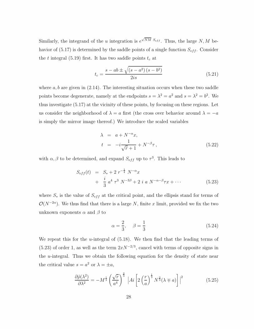
the t integral (5.19) first. It has two saddle points tc at

tc =s − ab ±

√

(s − a2) (s − b2)

2is(5.21)

where a, b are given in (2.14). The interesting situation occurs when these two saddle

points become degenerate, namely at the endpoints s = λ2 = a2 and s = λ2 = b2. We

thus investigate (5.17) at the vicinity of these points, by focusing on these regions. Let

us consider the neighborhood of λ = a first (the cross over behavior around λ = −a

is simply the mirror image thereof.) We introduce the scaled variables

λ = a + N−αx,

t = −i1√

r + 1+ N−βτ , (5.22)

with α, β to be determined, and expand Seff up to τ 3. This leads to

Seff (t) = S∗ + 2 r−14 N−αx

+i

3a4 τ 3 N−3β + 2 i a N−α−βτx + · · · (5.23)

where S∗ is the value of Seff at the critical point, and the ellipsis stand for terms of

O(N−2α). We thus find that there is a large N , finite x limit, provided we fix the two

unknown exponents α and β to

α =2

3, β =

1

3(5.24)

We repeat this for the u-integral of (5.18). We then find that the leading terms of

(5.23) of order 1, as well as the term 2xN−2/3, cancel with terms of opposite signs in

the u-integral. Thus we obtain the following equation for the density of state near

the critical value s = a2 or λ = ±a,

∂ρ(λ2)

∂λ2= −M

13

(√r

a4

) 23 ∣

∣

∣Ai

[

2(

r

a

) 13

N23 (λ ∓ a)

]

∣

∣

∣

2(5.25)

28

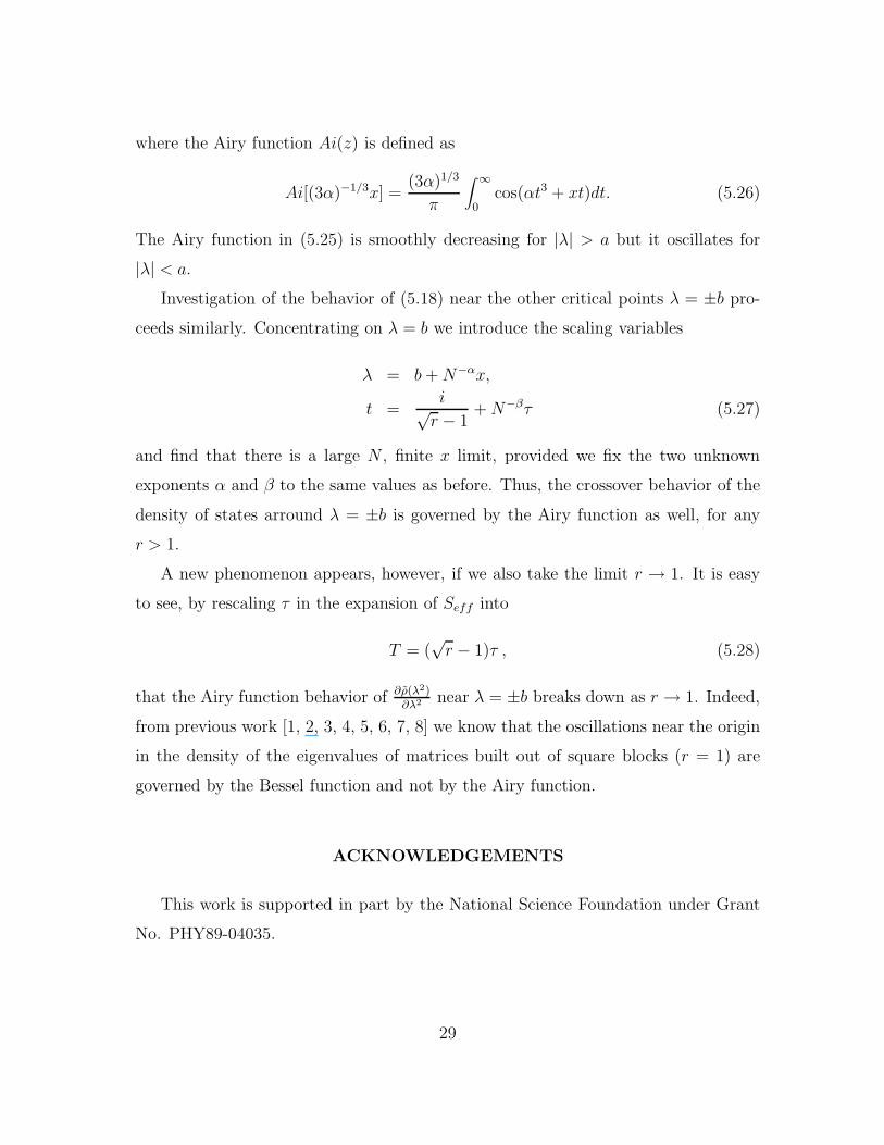
where the Airy function Ai(z) is defined as

Ai[(3α)−1/3x] =(3α)1/3

π

∫ ∞

0cos(αt3 + xt)dt. (5.26)

The Airy function in (5.25) is smoothly decreasing for |λ| > a but it oscillates for

|λ| < a.

Investigation of the behavior of (5.18) near the other critical points λ = ±b pro-

ceeds similarly. Concentrating on λ = b we introduce the scaling variables

λ = b + N−αx,

t =i√

r − 1+ N−βτ (5.27)

and find that there is a large N , finite x limit, provided we fix the two unknown

exponents α and β to the same values as before. Thus, the crossover behavior of the

density of states arround λ = ±b is governed by the Airy function as well, for any

r > 1.

A new phenomenon appears, however, if we also take the limit r → 1. It is easy

to see, by rescaling τ in the expansion of Seff into

T = (√

r − 1)τ , (5.28)

that the Airy function behavior of ∂ρ(λ2)∂λ2 near λ = ±b breaks down as r → 1. Indeed,

from previous work [1, 2, 3, 4, 5, 6, 7, 8] we know that the oscillations near the origin

in the density of the eigenvalues of matrices built out of square blocks (r = 1) are

governed by the Bessel function and not by the Airy function.

ACKNOWLEDGEMENTS

This work is supported in part by the National Science Foundation under Grant

No. PHY89-04035.

29

Appendix : The Central Limit Theorem - A Renormalization Group

Proof

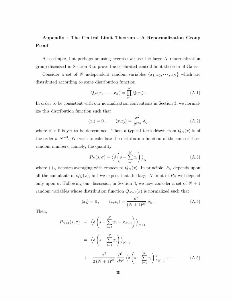
As a simple, but perhaps amusing exercise we use the large N renormalization

group discussed in Section 3 to prove the celebrated central limit theorem of Gauss.

Consider a set of N independent random variables {x1, x2, · · · , xN} which are

distributed according to some distribution function

QN(x1, · · · , xN) =N∏

i=1

Q(xi) . (A.1)

In order to be consistent with our normalization conventions in Section 3, we normal-

ize this distribution function such that

〈xi〉 = 0 , 〈xixj〉 =σ2

N2βδij (A.2)

where β > 0 is yet to be determined. Thus, a typical term drawn from QN(x) is of

the order σ N−β . We wish to calculate the distribution function of the sum of these

random numbers, namely, the quantity

PN(s, σ) =⟨

δ

(

s −N∑

i=1

xi

)

⟩

N(A.3)

where 〈·〉N denotes averaging with respect to QN (x). In principle, PN depends upon

all the cumulants of QN (x), but we expect that the large N limit of PN will depend

only upon σ. Following our discussion in Section 3, we now consider a set of N + 1

random variables whose distribution function QN+1(x) is normalized such that

〈xi〉 = 0 , 〈xixj〉 =σ2

(N + 1)2βδij . (A.4)

Then,

PN+1(s, σ) =⟨

δ

(

s −N∑

i=1

xi − xN+1

)

⟩

N+1

=⟨

δ

(

s −N∑

i=1

xi

)

⟩

N+1

+σ2

2 (N + 1)2β

∂2

∂s2

⟨

δ

(

s −N∑

i=1

xi

)

⟩

N+1+ · · · (A.5)

30

where we used (A.4). The ellipsis stand for cumulants of order higher than two, which

are clearly suppressed by powers of N−β , and we neglect them henceforth. Comparing

(A.2) and (A.4) we also see that

⟨

δ

(

s −N∑

i=1

xi

)

⟩

N+1= PN(s, σ′) (A.6)

with

σ′ =(

N

N + 1

)β

σ = (1 − β

N) σ + · · · (A.7)

We now use (A.6) and (A.7) to rewrite (A.5) as

PN+1(s, σ) =

[

1 − β

Nσ

∂

∂σ+

σ2

2N2β

∂2

∂s2

]

PN(s, σ) (A.8)

where we neglected terms of O( 1N2β+1 ). We observe from (A.8) that variations of σ

are as important as variations of s in the large N limit only if

β =1

2(A.9)

which fixes β. We thus conclude that

N∂PN

N=

σ

2

[

σ∂2

∂s2− ∂

∂σ

]

PN(s, σ) . (A.10)

The left hand side of (A.9) must vanish if PN has a large N limit

PN(s, σ) −→N→∞

P (s, σ) , (A.11)

and thus[

σ∂2

∂s2− ∂

∂σ

]

P (s, σ) = 0 . (A.12)

A simple scaling argument, similar to the one invoked in Section 3, leads to the

relation

P (s, σ) =1

σP (

s

σ, 1) (A.13)

which implies that

σ∂

∂σP = −P − s

∂

∂sP . (A.14)

31

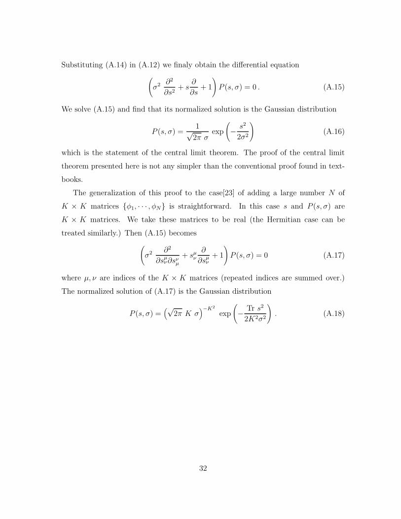
Substituting (A.14) in (A.12) we finaly obtain the differential equation

(

σ2 ∂2

∂s2+ s

∂

∂s+ 1

)

P (s, σ) = 0 . (A.15)

We solve (A.15) and find that its normalized solution is the Gaussian distribution

P (s, σ) =1√

2π σexp

(

− s2

2σ2

)

(A.16)

which is the statement of the central limit theorem. The proof of the central limit

theorem presented here is not any simpler than the conventional proof found in text-

books.

The generalization of this proof to the case[23] of adding a large number N of

K × K matrices {φ1, · · · , φN} is straightforward. In this case s and P (s, σ) are

K × K matrices. We take these matrices to be real (the Hermitian case can be

treated similarly.) Then (A.15) becomes

(

σ2 ∂2

∂sµν∂sν

µ

+ sµν

∂

∂sµν

+ 1

)

P (s, σ) = 0 (A.17)

where µ, ν are indices of the K × K matrices (repeated indices are summed over.)

The normalized solution of (A.17) is the Gaussian distribution

P (s, σ) =(√

2π K σ)−K2

exp

(

− Tr s2

2K2σ2

)

. (A.18)

32

References

[1] J. J. M. Verbaarschot, Nucl. Phys. B426 (1994) 559.

[2] J. Ambjørn, “Quantization of Geometry,” in Les Houches 1990, edited by J. Dal-

ibard et al. See section 4.3 and references therein.

[3] J. Ambjørn, J. Jurkiewicz, and Yu. M. Makeenko, Phys. Lett. B251 (1990) 517.

[4] K. Slevin and T. Nagao, Phys. Rev. Lett. 70 (1993) 635, Phys. Rev. B 50 (1994)

2380. T. Nagao and K. Slevin, J. Math. Phys. 34 (1993) 2075, 2317.

[5] T. Nagao and P. J. Forrester, Nucl. Phys. B 435 (FS) (1995) 401.

[6] A. V. Andreev, B. D. Simons and N. Taniguchi, Nucl. Phys. B 432 (1994) 485.

[7] E. Brezin, S. Hikami and A. Zee, Nucl. Phys.B 464 (1996) 411.

[8] S. Nishigaki preprint, hep-th/9606099.

[9] J. J. M. Verbaarschot and I. Zahed, Phys. Rev. Lett. 70 (1993) 3852.

[10] J. Jurkiewicz, M.A. Novak, and I. Zahed, preprint hep- ph/9603308. M.A. Novak,

G. Papp and I. Zahed, preprint hep- ph/9603348.

[11] S. Hikami and A. Zee, Nucl. Phys. B 446 , (1995) 337.

[12] S. Hikami, M. Shirai and F. Wegner, Nucl. Phys. B 408 (1993) 415.

[13] C.B. Hanna, D.P. Arovas, K. Mullen and S.M. Girvin, cond-mat 9412102.

[14] E. Brezin and A. Zee, Phys. Rev. E 49 , (1994) 2588.

[15] E. Brezin and A. Zee, Comp. Rend. Acad. Sci., (Paris) 317, (1993) 735.

[16] E. Brezin and J. Zinn-Justin, Phys. Lett B 288, 54 (1992).

S. Higuchi, C. Itoh, S. Nishigaki and N. Sakai, Phys. Lett. B 318, (1993) 63;

Nucl. Phys. B 434, (1995) 283, Err.-ibid. B 441, (1995) 405.

33

[17] J. D’Anna and A. Zee, Phys. Rev. E 53, (1996) 1399.

[18] A. Anderson, R. C. Myers and V. Periwal, Phys. Lett.B 254 (1991) 89, Nucl.

Phys. B 360, (1991) 463.

R. C. Myers and V. Periwal, Nucl. Phys. B 390, (1991) 716.

[19] V. A. Kazakov, Nucl. Phys. B 354 (1991) 614.

[20] E.P. Wigner, Can. Math. Congr. Proc. p.174, University of Toronto Press (1957),

reprinted in C. E. Porter, Statistical Theories of Spectra: Fluctuation (Aca-

demic, New york, 1965). See also M. L. Mehta, Random Matrices (Academic,

New York, 1991).

[21] E.Brezin, C. Itzykson, G. Parisi and J. -B. Zuber, Comm. Math. Phys. 59, 35

(1978).

[22] C. Itzykson and J. -B. Zuber, J. Math. Phys. 21 (1980) 411.

[23] A. Zee, Nucl. Phys. B 354, in press.

34