1 Renewable Energy Tariffs Price-Setting from the Profitability Index Method Bernard CHABOT Senior Expert ADEME 500 route des lucioles - 06560 Valbonne - France E-mail: bernard.chabot @ ademe.fr OPA – OEB – OSEA - ADEME Workshop – Oct. 7th, 2005 www.ademe.fr

Welcome message from author
This document is posted to help you gain knowledge. Please leave a comment to let me know what you think about it! Share it to your friends and learn new things together.
Transcript

1
Renewable Energy Tariffs Price-Setting
from the Profitability Index Method
Bernard CHABOTSenior Expert
ADEME500 route des lucioles - 06560 Valbonne - France
E-mail: [email protected]
OPA – OEB – OSEA - ADEME Workshop – Oct. 7th, 2005
www.ademe.fr

2
I
Market regulationFor renewables

3
Market regulations in favour of Renewables
Success from regulation from prices : Germany, Spain,France, Portugal…
Advantages of regulation from quantities are not yetdemonstrated, and price for consumer are higher: wind UK> 10 c€/kWh, Italy > 15 c€/kWh vs 7 to 9 G, Sp, F, Portugal
Sea based RE for power Regul. From prices Regul. from quantitiesTargeted on Subsidies Calls for tenders
initial Fiscal incentivesInvestment Soft loans
Targeted on Environnemental bonus Quotas + green certificatesProduction Simple guaranteed tariffs or + carbon credits
Advanced tariffs systems + derivative marketsSource: adapted from Menanteau & alii "How to promote RES successfully & effectively", Energy Policy, vol 32/6, 20

4
Two main options to regulate market for RES
Regulation by quantitiesQuotas + competitive calls for tenders (eg: UK, France, Ir)Quotas verified from RECs in % of consumption (or sales) +
penalties in case of no compliance (UK, Be, It)Regulation by prices"Fixed prices" (eg wind power in Dk & Germany in the 90's)"Environ. premiums" over the annual avoided cost (Spain)"ADVANCED TARIFFS" (eg wind in Germany, France, Portugal)Defined for each technologyDefined for each project, e. g. if variable average wind speed in diff. sitesFixed tariff within a contract, e. g. defined first from the potential and then
from the actual energy yield measured during the first 5 yearsTariffs for new projects may decrease each year to take into account costs
decrease

5
II
Introduction to theProfitability Index Method

6
The context to apply the PI method
A global economic analysis for preliminary studies Constant inflation, results in constant money of year 0 Constant mean yearly Cash-flows :Defines the « references cases »By extension following cases are also relevant :Cash-flows parameters varying by x%/year above or under inflation rateCash-flows parameters varying by steps (e.g. wind tariffs T1, T2)Variable cash – flows (replaced by the equivalent constant cash-flow)
Links with other methods :Direct access from PI to IRR (Internal rate of Return), PBP (pay back period),
but much more precise (linear variation of PI versus NPV)Direct link of PI versus Margin on Cost ==> link with industrial and
commercial strategies and policiesWise states: almost same economic and fiscal profitability levels
7
III
The linear and universal model:Profitability Index versus Tariff

8
The model PI = NPV / I = f(tariff T)
NPV = (-I + Sum of discounted economic CFs before taxon profit in constant $ of year 0, from year 1 to n)
Discounted CF of year j = CFj / (1+t)^jFor constant Cash-Flow CF from years 1 to n:Sum of discount. CFs = CF / CRF(t,n), with CRF = t / (1-(1+t)^-n
Variable CFs can be replaced by the « constant equivalentCF » which gives the same economic profitability than then variable CFs
By definition: Profitability Index = PI = NPV / IPI results from tariff T by a linear relationship :PI= a (T-Cvu) – bWhere a and b are defined by project ratios (costs, energy yield)And Cvu is the variable cost due to fuel costSo Cvu is zero for hydro, wind, solar, geothermal power plants

9
The model PI = f(tariff T) (2)Gives access to the universal linear diagram : PI versus tariff TPI = aT - b = (Nh / CRF.Iu)(T - Cvu) - (1 + Kom / CRF)With : T = kWh tariff; Iu = I / P, Nh = Ea / P, Kom = Dom / I, CRF= t / (1 - (1+t)exp-n),
Cvu = variable part of the kWh cost = 0 for renewables, except biomassWhere I = initial investment cost ; P = rated power ; Ea = annual energy sold ; Dom =
annual O&M expenses, t = discount rate (AWCC) ; n = years of operation
M
Tariff T
Cvu
ODC
PI
TV
-(1+Kom/CRF)
Com Ci
-1 S
Cost Price
Ci = CRF*Iu/NhCom = Kom*Iu/NhCvu = 0 for wind,hydro, solar

10
The model PI = f(tariff TV) (3)Gives access to the direct link between PI and the Margin On Cost
MOC = (Price - Cost) / Cost = (TV-ODC) / ODC) :From our Thalès colleague, from the green and yellow triangles: PI / 1 = (TV - ODC) / Ci ===> TV = ODC + PI*Ci ==> basic role of Ci PI = MOC / (Ci/ODC) ==> MOC = (Ci/ODC)*PI ==> basic role of Ci/CGA
M
Tariff TV
Cvu
ODC
PI
TV
-(1+Kom/CRF)
Com Ci
-1 S
Cost Price
Golden rule
PI > 0,3

11
The link: PI = k.MOC (2)
The « zero fuel cost RETs paradox » (wind, hydro, solar,geothermal based power plants) :(MOCwind / MOCfossil) = (cost / non fuel cost part)fossilMOC wind = 2 times MOC coal = 3 times MOC nat. gas !Minimum 10 % MOC from coal plants ==> PI = 0,3
Implies also minimum PI value of 0.3 for RE projects
Wind: Coal: Nat.gas:120
110 106
Different selling prices for thesame profitability (PI = 0.3)
Fuel cost part
Non-Fuel cost part
Same kWh cost100

12
Comparing criteria PI, IRR, DPBT IRR, DPBT: values of t and n for which project NPV = 0Profitability if: IRR > AWCC = t, and if DPBT < nsimple PBT=I / CF=> Profitability if SPBT < 1 / CRFLimits and actual and potential problems (IRR & PBTs):Criteria not proportional to profitability in $ of NPVNo fixed and universal "zero point" for profitability = 0No direct access to the project NPVNo possible use with simple formulas
Versus advantages of the PI criteria:PI is proportional to the profitability in $ (NPV)Logical starting point: PI = 0 for profitability zeroDirect access to the NPV (from the definition: NPV = PI.I)Direct explicit formula possible using PI (like °K versus °C !)

13
From efficient PI value to IRR and PBT rational values
Link PI IRR (Internal Rate of Return of the project):CRF (IRR, n) = (1 + PI).CRF (t, n) ;with (1+PI) = Benefit /Cost Ratio NPV = I * PI = I * {[CRF(TRI,n)/CRF(t,n)] - 1}
Link PI DPBT (Discounted Pay-Back Time):CRF (t, DPBT) = (1 + PI).CRF (t, n)
Link PI SPBT (Simple Pay-Back Time) :SPBT=1 / (1 + PI).CRF(t, n)=1 / CRF(t, DPBT)=1/CRF(IRR, n)
See following graphs and examples

14
Links PI / IRR for n = 15 years Ex: t = 6 %: 100 % PI variation from 0.15 to 0.3 : IRR vary only from 8 to 10.3 %
TRI = f(TEC, t) pour n = 15 ans
0 %1 %
5 %
10 %
12 %
t = 15 %
0
5
10
15
20
25
30
0 0,1 0,2 0,3 0,4 0,5 0,6 0,7
TEC = VAN/I
TR
I (%
)

15
Link PI / discounted PBT for t = 6 % Ex: n = 15 years: 100 % PI variation from 0.15 to 0.3 : PBT vary only from 8.2 to 7 years !
TRA = f (TEC, n) pour t = 6 %
358101215
20
n = 30 ans
0123456789
1011121314151617181920
0 0,1 0,2 0,3 0,4 0,5 0,6 0,7
TEC = VAN/I
TR
A (a
ns)

16
Links PI / simple PBT Ex1 : 15 years 6 %: sPBT vary from 8 to 7 years ==> PI and NPV divided by 2 !
Lien entre le Temps de retour Brut TRB et le TEC
5 ans, 10%
10 ans, 8%
15 ans, 6%
25 ans, 5%
0123456789
101112131415
0 0,1 0,2 0,3 0,4 0,5 0,6 0,7 0,8 0,9 1 1,1 1,2
TEC
TR
B (a
ns)
Actualisation:

17
IV
Case study of an advanced tariff:The 2001 French Wind Power
Tariff System

18
The French advanced wind tariff sytem
Two successive tariffs levels :T1 fixed for all projects from years 1 to 5 (= German idea !)T2 variable for projects from years 6 to 15 (diff. from Germ.)T1 and T2 define a virtual constant “equivalent tariff”, Teq
For a specific project :Nh = averaged Ey / P from values years 1 to 5 (hours/year)T2: linear calculation from values at Nhr = 2000, 2600, 3600Teq from (T1, T2, t)
5 15
T1
T2Years
Tariffs
Teq

19
Tariffs: Other Principles and Final “Details”Indexation for tariffs within a specific contract:Only 60% ==> decrease of profitability with inflation rate
Provisional tariffs decrease for next years: -3.3 % per year from 2003 (current EUROS)Formula for correction from inflation from 2003+
Reference Nh value: average on 3 years (5 -worst-best)

20
Wind tariffs: June 8th 2001 Arrêté, 2001 tariffs
Hypothesis for Teq:Real discount rate t = 6.5%n = 15 years
Reference values for 2001 tariffsMainland France, projects < 12 MW
P (MW) P (MW) cEUR / kWhNh: <1500 <1500 T1 T2 Teq
Nhmin: 2000 1900 8,38 8,38 8,38Nhint: 2600 2400 8,38 5,95 7,02
Nhmax: 3600 3300 8,38 3,05 5,41Corsica & Overseas Depart. projects <12 MW
P (MW) P (MW) cEUR / kWhNh: <1500 <1500 T1 T2 Teq
Nhmin: 2050 9,15 9,15 9,15Nhint: 2400 9,15 7,47 8,21
Nhmax: 330 9,15 4,57 6,59
2001 Tariffs (M ainland France, P < 1500 M W )
8,38
5,95
3,05
7,028,38
5,41
0123456789
1800
2000
2200
2400
2600
2800
3000
3200
3400
3600
Nh (hours/year at rated power)
cEU
R /
kWh .
T1 T2 Teq

21
Tariffs: 2001 potential profitability (Mainland)
Reference case (P < 12 MW per project):Iu=1067 EUR/kW. Value at year 16: 15% of initial invest.Yearly O&M expenses: Kom = 4 % of initial investmentMean inflation rate 2001 - 2015: i = 0% or i = 2 % / yearProfitability index: NPV per € invested
Profitability Index - 2001, Mainland
i=0 %
i=2%
0,0
0,1
0,2
0,3
0,4
0,5
1800
2000
2200
2400
2600
2800
3000
3200
3400
3600
Nh (hours/year at rated power)
PI =
NPV
/ I
Internal Rate of Return - 2001, Mainland
i=0 %i=2%
56789
10111213
1800
2000
2200
2400
2600
2800
3000
3200
3400
3600
Nh (hours/year at rated power)IR
R (%
)

22
Wind Power development in France
+ 156(+73 %)
405 MW(+ 70 %)
0
100
200
300
400
500
1997 1998 1999 2000 2001 2002 2003 2004 2005

23
Effectiveness of wind tarifs: 3 GW of Buill. Permits
Répartition 6/05 des 3087 MW de demandes de raccordement RPD
Biomasse: 13,3; 0,4% PV: 6,8; 0,2%
Biogaz : 33,3; 1%
Géothermie; 0Hydro : 41, 1%
Eolien: 2991 MW,
97%

24
France: Potential Wind Power Development up to 2020
MWonshore
6 000
11 600
Total France
7 700
17 260
dP/year (MW)1 870 1 870
Germany (WindEnergy
04)
0
5 000
10 000
15 000
20 000
25 000
30 000
35 000
2000 2005 2010 2015 2020

25
Global Wind power Market Asessement (BTM05)
Eolien monde: historique 1996-2004 et perspectivesParc: GW, production: TWh/an - Source: BTM Consult 2005
48 GW
235 GW
134 GW96 TWh
280 TWh
530 TWh
0
100
200
300
400
500
600
1995 2000 2005 2010 2015
GW
, TW
h/an
GWTWh/an

26
Global PVmarket: history and one scenario
Production Cellules Photovoltaïques (MWc/an)
202287
401560
750
1256
0
500
1000
1500
1998 1999 2000 2001 2002 2003 2004 2005
Prospective 2005-20020
14 07629 553
MWc/an
74 770
Cumul: 188 832
MWc
0
50000
100000
150000
200000
2000 2005 2010 2015 2020

27
PV pricing: Case study OSEA (soft loans)
Place Iu I Nh ODC PIi Si Siu TV TV(Eia kWh/m2.year) $/Wp $ h/year $/kWh $/kWh % $/kWh % $ $/Wp $/kWh €/kWh
12 36 000,0 825 1,018 0,727 71% 0,291 29% 0,000 0 0,00 1,02 0,61TORONTO 10 30 000,0 825 0,848 0,606 71% 0,242 29% 0,000 0 0,00 0,85 0,51
1100 7 21 000,0 825 0,594 0,424 71% 0,170 29% 0,000 0 0,00 0,59 0,3612 36 000,0 825 1,018 0,727 71% 0,291 29% -0,300 10 800 3,60 0,80 0,48
TORONTO 10 30 000,0 825 0,848 0,606 71% 0,242 29% -0,300 9 000 3,00 0,67 0,401100 7 21 000,0 825 0,594 0,424 71% 0,170 29% -0,300 6 300 2,10 0,47 0,28
12 36 000,0 1050 0,800 0,571 71% 0,229 29% 0,000 0 0,00 0,80 0,48OTTAWA 10 30 000,0 1050 0,667 0,476 71% 0,190 29% 0,000 0 0,00 0,67 0,40
1400 7 21 000,0 1050 0,467 0,333 71% 0,133 29% 0,000 0 0,00 0,47 0,28
Ci Com
Either PI = 0 or if PI < 0: subsidy Si on initial investmentTwo cases: t = 3 % and t = 0 % (“soft loans”)Two locations: Toronto (1100 kWh/m2.year in the plane of PV modules and Ottawa (1400 kWh/m2.year)

28
The coming Energy and Climate crisis…
29
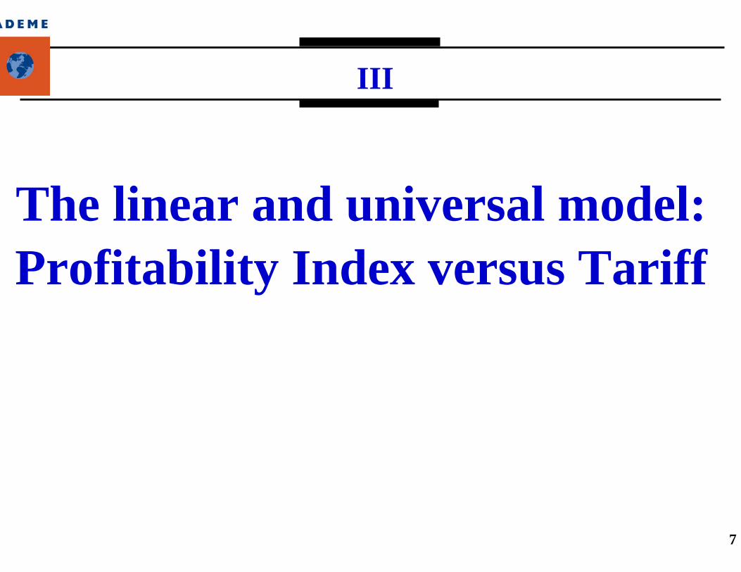
Wind Tariffs as an insurance against increasing power prices
Tarif TVe kWh centrale à gaz à CC avec et sans pénalité 20 €/tCO2(TEC = 0,4, t = 5 %, n = 20 ans, Iu = 633 €/kW, kem = 5,7 %, Re = 59 %)
0,023
0,037
0,054
0,068
0,009
0,022
0,031
0,040
0,054
0,046
0,00
0,01
0,02
0,03
0,04
0,05
0,06
0,07
0,08
0,09
10 15 20 25 30 35 40 45 50 55 60
Coût équivalent constant sur 20 ans énergie primaire gaz en $/bep
€/kW
he
Tve kWhe GazCvu (part comb.)TVe+CO2
Tarifs éoliens
2000 h/an 2001
3600 h/an 2001 ou 2400 h/an 2010
2000 h/an 2010

30
V
Case Study 2:OSEA Wind Power Pricing
Workshop 1/2005
31
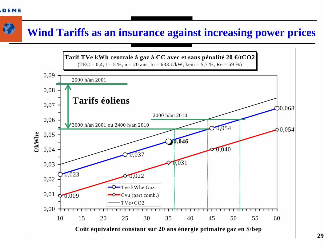
Preliminary results in January 2005 Capacity factor Nh replaced by Specific energy yield Ey (kWh/year.m2) Hypothesis: full indexation to inflation (constant power purchase of tariff)
Tariffs versus energy yield per kWh/m2t = 5% (real), n = 20 years, Kom = 4%, Iu = 1600 $/kW
7,6
10,0
14,8
10,111,7
0,0
5,0
10,0
15,0
600 700 800 900 1 000 1 100 1 200 1 300
Eas (kWh/m2.year)
c$C
/kW
hT2T1Teq 20 y
Profitability Index Versus Energy Yield per m2
0,350
0,100
0,250
0,00
0,05
0,10
0,15
0,20
0,25
0,30
0,35
0,40
500 600 700 800 900 1 000 1 100 1 200
Eas (kWh/m2.year)
ys

32
Information on project IRR from PI values
Project IRR on 20 years (% real or nominal)
6,27,8
8,8
12,1
9,311,0
0
5
10
15
20
500 600 700 800 900 1 000 1 100 1 200
Eas (kWh/m2.year)
%
IRR real IRR nominal

33
III
Taking into account or designingpotential incentives for
renewables

34
Designing an « Efficient tariff »Defining a tariff for a sustainable good or service
M
TV
Cvu
ODC
PI
TVr
-(1+Kom/CRF)
PIr
-1S
ComCi
Golden rule:PI > 0.3
« Efficient tariff"
« Cost"

35
Effect of a subsidy si on the initial investment ISimple relationship :
Subsidy rate si: si = (PIf - PIi) / (1 + PIf) where:PIf = target value of final profitability index PI (after subsidy)PIi = initial PI value (before subsidy)
The "PI versus tariff" line turns around its "S" point
TV
Cvu
PI
TV
PIi
-1S
PIf
Com

36
Impact of soft loansConventional financing scheme: to = AWCC0 ==> CRFo(to,n)Soft loans => soft financing ==> ts < to ==> CRFs(ts,n) < CRFo(to,n)Increase of PI: (1 + PIs) / ( 1 + PIo) = CRFo / CRFs
Equivalent subsidy si on investment: si = 1- CRFs/CRFo
TV
Cvu
PI
TVr
PIi
-1S
PIf
Com

37
Potential impact of selling "Carbon Credits"Avoided CO2 emissions : Quce (kg CO2/kWhe). Selling price of
carbon credit : TVce (€ / avoided kg of CO2). Price bonus: TVce*QuceThe "PI line" translates horizontally of a TVce*Quce value (€/kWhe) The Thalès - Chabot theorem: dPI = (Quce*TVce) / CiOr: dPI = {(Quce*TVce)/CGA} /(Ci/CGA) => basic role of Ci/CGA
M
TV
Cvu
ODC
PI
TV0
-(1+Kom/CRFa)
PIi
-1S
PIf
-Quce*TVce
dPI
Ci

38
Conclusions
"A bit of theory is very practical"Simple, innovative and powerful method and tools to
define market deployment strategies and policies forsustainable energy technologies
A vast prospect for use :Extension to all other energy services : energy savings, energy
efficiency, DSM (see ECEEE 2005 Mandelieu conference)Clean and efficient buildings versus conventional onesClean and efficient industrial process versus conventional onesCO2 policies: easy demonstration that CO2 taxes would lead to
coal based power plants instead of natural gas combined cycles !Potential stranded costs analysis in a context of rising fossil fuels
costs.ADEME is open to co-operation by sharing knowledge
and experience
Related Documents