Welcome message from author
This document is posted to help you gain knowledge. Please leave a comment to let me know what you think about it! Share it to your friends and learn new things together.
Transcript


Renewable Energy Resources
Renewable Energy Resources is a numerate and quantitative text covering the full range of renew able energy technologies and their implementation worldwide. Energy supplies from renewables (such as from biofuels, solar heat, photovoltaics, wind, hydro, wave, tidal, geothermal and ocean-thermal) are essential components of every nation’s energy strategy, not least because of concerns for the local and global environment, for energy security and for sustainability. Thus, in the years between the first and this third edition, most renewable energy technologies have grown from fledgling impact to significant importance because they make good sense, good policy and good business.
This third edition has been extensively updated in light of these developments, while maintaining the book’s emphasis on fundamentals, complemented by analysis of applications. Renewable energy helps secure national resources, mitigates pollution and climate change, and provides cost-effective services. These benefits are analyzed and illustrated with case studies and worked examples. The book recognizes the importance of cost-effectiveness and efficiency of end-use. Each chapter begins with fundamental scientific theory, and then considers applications, environmental impact and socio-economic aspects before concluding with Quick Questions for self-revision, and Set Problems. The book includes Reviews of basic theory underlying renewable energy technologies, such as electrical power, fluid dynamics, heat transfer and solid-state physics. Common symbols and cross-referencing apply throughout; essential data are tabulated in appendices.
An associated updated eResource provides supplementary material on particular topics, plus a solu-tions guide to Set Problems for registered instructors only.
Renewable Energy Resources supports multi-disciplinary Master’s degrees in science and engineer-ing, and specialist modules in first degrees. Practising scientists and engineers who have not had a comprehensive training in renewable energy will find it a useful introductory text and a reference book.
John Twidell has considerable experience in renewable energy as an academic professor in both the UK and abroad, teaching undergraduate and postgraduate courses and supervising research stu-dents. He has participated in the extraordinary growth of renewable energy as a research contract or, journal editor, board member of wind and solar professional associations, and company director. University positions have been in Scotland, England, Sudan and Fiji. The family home operates with solar heat and electricity, biomass heat and an all-electric car; the aim is to practice what is preached.
Tony Weir has worked on energy and environment issues in the Pacific Islands and Australia for over 30 years. He has researched and taught on renewable energy and on climate change at the University of the South Pacific and elsewhere, and was a Lead Author for the 2011 IPCC Special Report on Renewable Energy. He has also managed a large international program of renewable energy projects and been a policy advisor to the Australian government, specializing in the interface between technol-ogy and policy.
www.routledge.com/books/details/9780415584388
TWIDELL PAGINATION.indb 1 01/12/2014 11:35

“Renewable energy requires an active approach, based on facts and data. Twidell and Weir, drawing on decades of experience, demonstrate this, making clear connections between basic theoretical concepts in energy and the workings of real systems. It is a delight to see the field having advanced to this level, where a book like Renewable Energy Resources can focus on the very real experiences of the energy systems of the coming decades.” – Professor Daniel Kammen, Director, Renewable and Appropriate
Energy Laboratory, University of California, Berkeley, USA
“Solar and wind power are now proven, reliable, ever-cheaper sources of electricity that can play a major role in powering the world. Along with other long-established renewables such as hydropower, and complemented by improved energy efficiency and appropriate institutional support, they can be key to sustainable development. This book can play a vital role in educating the people who are needed to make it happen.”
– Professor Martin Green, Director, Australian Centre for Advanced Photovoltaics, University of New South Wales, Australia
“The solar revolution that’s been talked about for so long is with us here and now. This new edition of Renewable Energy Resources, like earlier editions, will undoubtedly make a significant contribution to informing both those involved with the technology and those in policy-making. This is critical if the promise of renewable energy is to be delivered as expeditiously and cost-effectively as is now needed.”
– Jonathon Porritt, Founder Director, Forum for the Future
“I welcome this excellent third edition of Twidell and Weir with its comprehensive yet accessible coverage of all forms of renewable energy. The technologies and the physics behind them are explained with just the right amount of math, and they include a realistic summary of the economic and societal implications.”
– Emeritus Professor William Moomaw, Tufts University, USA and Coordinating Lead Author, IPCC Special Report on Renewable Energy
“I highly recommend this book for its thorough introduction to all the important aspects of the topic of Renewable Energy Resources. The book is excellent in its completeness and description of the relevant different sources. Moreover it is strong in theory and applications. From a scientific and engineering point this book is a must.”
– Professor Henrik Lund, Aalborg University, Denmark and Editor-in-Chief of the international journal Energy
“Over the years, I have used this excellent text for introducing Physics and Engineering students to the science and technology of renewable energy systems. The updated edition will be of immense value as sustainable energy technologies join the mainstream and there is an increasing need for human capacity at all levels. I look forward to the new edition and hope to use it extensively.”
– Dr Atul Raturi, University of the South Pacific, Fiji
“Our school has used Renewable Energy Resources since 2005, as it was one of the few texts that covered the field with a good balance between background theory and practical applications of RE systems. The new updated edition looks great and I am looking forward to using it in my classes.”
– Dr Alistair Sproul, University of New South Wales, Australia
“I have used the extremely valuable second edition of this book for our postgraduate courses on energy conver-sion technologies. My students and I welcome this new edition, as it has been very well updated and extended with study aids, case studies and photos which even further improve its readability as a textbook.”
– Dr Wilfried van Sark, Utrecht University, Netherlands
Praise for the 2nd edition“Twidell and Weir are masters of their subject and join the ranks of acomplished authors who have made a pow-erful contribution to the field. Renewable Energy Resources is a superb reference work.”
– Paul Gipe, www.wind-works.org
“It’s ideal for student use - authoritative, compact and comprehensive, with plenty of references out to more detailed texts ... a very valuable book.”
– Professor Dave Elliott of the Open University, UK, in Renew 162 2006
“What we need to combat climate change is a stream of students and graduates with the knowledge they can gain from this book ... suitable not only for engineering students but also for policy-makers and all those con-cerned with energy and the environment.’
– Corin Millais, CEO Climate Institute
TWIDELL PAGINATION.indb 2 01/12/2014 11:35

Renewable Energy Resources
Third edition
John Twidell and Tony Weir
TWIDELL PAGINATION.indb 3 01/12/2014 11:35

First published 1986by E&FN Spon Ltd
Second edition published 2006by Routledge
Third edition published 2015by Routledge2 Park Square, Milton Park, Abingdon, Oxon OX14 4RN
and by Routledge711 Third Avenue, New York, NY 10017
Routledge is an imprint of the Taylor & Francis Group, an informa business
© 1986, 2006, 2015 John Twidell and Tony Weir
The right of John Twidell and Tony Weir to be identified as authors of this work has been asserted by them in accordance with sections 77 and 78 of the Copyright, Designs and Patents Act 1988.
All rights reserved. No part of this book may be reprinted or reproduced or utilized in any form or by any electronic, mechanical, or other means, now known or hereafter invented, including photocopying and recording, or in any information storage or retrieval system, without permission in writing from the publishers.
The publisher makes no representation, express or implied, with regard to the accuracy of the information contained in this book and cannot accept any legal responsibility or liability for any errors or omissions that may be made.
Trademark notice: Product or corporate names may be trademarks or registered trademarks, and are used only for identification and explanation without intent to infringe.
British Library Cataloguing-in-Publication DataA catalogue record for this book is available from the British Library
Library of Congress Cataloging-in-Publication DataTwidell, John, author.Renewable energy resources / John Twidell and Tony Weir. -- Third edition.pages cmIncludes bibliographical references and index.1. Renewable energy sources. I. Weir, Tony, author. II. Title.TJ808.T95 2015621.042--dc232014018436
ISBN: 978-0-415-58437-1 (hbk)ISBN: 978-0-415-58438-8 (pbk)ISBN: 978-1-315-76641-6 (ebk)
Typeset in Univers byServis Filmsetting Ltd, Stockport, Cheshire
TWIDELL PAGINATION.indb 4 01/12/2014 11:35

This book is dedicated to our wives, Mary and Christine, who have supported us continuously in the labor
of textbook writing.
TWIDELL PAGINATION.indb 5 01/12/2014 11:35

TWIDELL PAGINATION.indb 6 01/12/2014 11:35
Page Intentionally Left Blank
CONTENTS
Preface xvFigure and photo acknowledgments xixList of symbols xxiiiList of abbreviations xxx
1 Principles of renewable energy 1 §1.1 Introduction 3
§1.2 Energy and sustainable development 4 §1.3 Fundamentals 9 §1.4 Scientific principles of renewable energy 14 §1.5 Technical implications 18 §1.6 Standards and regulations 27 §1.7 Social implications 27 Chapter summary/Quick questions/Problems/Bibliography 30
2 Solar radiation and the greenhouse effect 37 §2.1 Introduction 39 §2.2 Extraterrestrial solar radiation 40 §2.3 Components of radiation 41 §2.4 Geometry of the Earth and the Sun 42 §2.5 Geometry of collector and the solar beam 46 §2.6 Atmospheric transmission, absorption and reflection 49 §2.7 Measuring solar radiation 57 §2.8 Site estimation of solar radiation 57 §2.9 Greenhouse effect and climate change 62 Chapter summary/Quick questions/Problems/Bibliography 68 Box 2.1 Radiation transmitted, absorbed and scattered by
the Earth’s atmosphere 55 Box 2.2 Units of gas concentration 65 Box 2.3 Why we know that recent increases in CO2 and in
temperature are due to human activity (anthropogenic) 66
TWIDELL PAGINATION.indb 7 01/12/2014 11:35

viii Contents
3 Solar water heating 75 §3.1 Introduction 77 §3.2 Calculation of heat balance: general remarks 79 §3.3 Flat-plate collectors 81 §3.4 Systems with separate storage 88 §3.5 Selective surfaces 92 §3.6 Evacuated collectors 96 §3.7 Instrumentation and monitoring 99 §3.8 Social and environmental aspects 100 Chapter summary/Quick questions/Problems/Bibliography 101 Box 3.1 Reference temperature Tref for heat circuit modeling 86
4 Other solar thermal applications 108 §4.1 Introduction 110 §4.2 Air heaters 110 §4.3 Crop driers 112 §4.4 Solar thermal refrigeration and cooling 117 §4.5 Water desalination 120 §4.6 Solar salt-gradient ponds 122 §4.7 Solar concentrators 123 §4.8 Concentrated Solar Thermal Power (CSTP) for
electricity generation 132 §4.9 Fuel and chemical synthesis from concentrated solar 140 §4.10 Social and environmental aspects 141 Chapter summary/Quick questions/Problems/Bibliography 142 Box 4.1 Solar desiccant cooling 120
5 Photovoltaic (PV) power technology 151 §5.1 Introduction 153 §5.2 Photovoltaic circuit properties 156 §5.3 Applications and systems 161 §5.4 Maximizing cell efficiency (Si cells) 167 §5.5 Solar cell and module manufacture 176 §5.6 Types and adaptations of photovoltaics 179 §5.7 Social, economic and environmental aspects 191 Chapter summary/Quick questions/Problems/Bibliography 197 Box 5.1 Self-cleaning glass on module PV covers 167 Box 5.2 Solar radiation absorption at p–n junction 171 Box 5.3 Manufacture of silicon crystalline cells and modules 176 Box 5.4 An example of a sophisticated Si solar cell 185
6 Hydropower 202 §6.1 Introduction 204 §6.2 Principles 208 §6.3 Assessing the resource 209 §6.4 Impulse turbines 212
TWIDELL PAGINATION.indb 8 01/12/2014 11:35

Contents ix
§6.5 Reaction turbines 217 §6.6 Hydroelectric systems 220 §6.7 Pumped hydro storage 224 §6.8 Social and environmental aspects 225 Chapter summary/Quick questions/Problems/Bibliography 227 Box 6.1 Measurement of flow rate Q 210 Box 6.2 ‘Specific speed’ 216 Box 6.3 The Three Gorges hydroelectric installation, China 221
7 Wind resource 234 §7.1 Introduction 236 §7.2 World wind 237 §7.3 Characteristics of the wind 242 §7.4 Wind instrumentation, measurement, and
computational tools and prediction 258 Chapter summary/Quick questions/Problems/Bibliography 264
8 Wind power technology 267 §8.1 Introduction 269 §8.2 Turbine types and terms 272 §8.3 Linear momentum theory 277 §8.4 Angular momentum theory 286 §8.5 Dynamic matching 289 §8.6 Blade element theory 295 §8.7 Power extraction by a turbine 299 §8.8 Electricity generation 303 §8.9 Mechanical power 314 §8.10 Social, economic and environmental
considerations 316 Chapter summary/Quick questions/Problems/Bibliography 318 Box 8.1 Experiencing lift and drag forces 290 Box 8.2 Multimode wind power system with
load-management control at Fair lsle, Scotland 313
9 Biomass resources from photosynthesis 324 §9.1 Introduction 326 §9.2 Photosynthesis: a key process for life on Earth 327 §9.3 Trophic level photosynthesis 328 §9.4 Relation of photosynthesis to other plant processes 331 §9.5 Photosynthesis at the cellular and molecular level 332 §9.6 Energy farming: biomass production for energy 343 §9.7 R&D to ‘improve’ photosynthesis 350 §9.8 Social and environmental aspects 351 Chapter summary/Quick questions/Problems/Bibliography 354 Box 9.1 Structure of plant leaves 334
TWIDELL PAGINATION.indb 9 01/12/2014 11:35
x Contents
Box 9.2 Sugar cane: an example of energy farming 344 Box 9.3 How is biomass resource assessed? 349
10 Bioenergy technologies 359 §10.1 Introduction 361 §10.2 Biofuel classification 364 §10.3 Direct combustion for heat 369 §10.4 Pyrolysis (destructive distillation) 374 §10.5 Further thermochemical processes 378 §10.6 Alcoholic fermentation 379 §10.7 Anaerobic digestion for biogas 387 §10.8 Wastes and residues 395 §10.9 Biodiesel from vegetable oils and algae 396 §10.10 Social and environmental aspects 398 Chapter summary/Quick questions/Problems/Bibliography 401 Box 10.1 Gross and net calorific values 366 Box 10.2 Ethanol in Brazil 383 Box 10.3 Bio/fossil balance of liquid biofuels 385 Box 10.4 Greenhouse gas balance of liquid biofuels 387
11 Wave power 408 §11.1 Introduction 410 §11.2 Wave motion 413 §11.3 Wave energy and power 417 §11.4 Real (irregular) sea waves: patterns and power 421 §11.5 Energy extraction from devices 427 §11.6 Wave power devices 430 §11.7 Social, economic and and environmental aspects 437 Chapter summary/Quick questions/Problems/Bibliography 439 Box 11.1 Satellite measurement of wave height, etc. 423 Box 11.2 Wave energy in the UK 430 Box 11.3 Basic theory of an OWC device 434
12 Tidal-current and tidal-range power 445 §12.1 Introduction 447 §12.2 The cause of tides 450 §12.3 Enhancement of tides 456 §12.4 Tidal-current/stream power 459 §12.5 Tidal-range power 465 §12.6 World tidal power sites 467 §12.7 Social and environmental aspects 469 Chapter summary/Quick questions/Problems/Bibliography 471 Box 12.1 Tsunamis 457 Box 12.2 Blockage effects on turbine output
in narrow channels 464
TWIDELL PAGINATION.indb 10 01/12/2014 11:35
Contents xi
13 Ocean gradient energy: OTEC and osmotic power 476 §13.1 General introduction 478 §13.2 Ocean Thermal Energy Conversion (OTEC):
introduction 478 §13.3 OTEC principles 479 §13.4 Practical considerations about OTEC 483 §13.5 Devices 486 §13.6 Related technologies 487 §13.7 Social, economic and environmental aspects 488 §13.8 Osmotic power from salinity gradients 489 Chapter summary/Quick questions/Problems/Bibliography 491 Box 13.1 Rankine cycle engine 482
14 Geothermal energy 495 §14.1 Introduction 497 §14.2 Geophysics 500 §14.3 Dry rock and hot aquifer analysis 503 §14.4 Harnessing geothermal resources 507 §14.5 Ground-source heat pumps 512 §14.6 Social and environmental aspects 514 Chapter summary/Quick questions/Problems/Bibliography 516
15 Energy systems: integration, distribution and storage 521 §15.1 Introduction 523 §15.2 Energy systems 523 §15.3 Distribution technologies 526 §15.4 Electricity supply and networks 530 §15.5 Comparison of technologies for energy storage 538 §15.6 Energy storage for grid electricity 541 §15.7 Batteries 544 §15.8 Fuel cells 552 §15.9 Chemicals as energy stores 553 §15.10 Storage for heating and cooling systems 555 §15.11 Transport systems 558 §15.12 Social and environmental aspects of energy
supply and storage 559 Chapter summary/Quick questions/Problems/Bibliography 560 Box 15.1 It’s a myth that energy storage is a challenge
only for renewable energy 532 Box 15.2 Self-sufficient energy systems 532 Box 15.3 Capacity credit, dispatchability and predictability 535 Box 15.4 Grid stability with high wind penetration:
west Denmark and Ireland 536 Box 15.5 Combining many types of RE enables large
RE penetration: two modeled cases 537 Box 15.6 Scaling up batteries: flow cells 550
TWIDELL PAGINATION.indb 11 01/12/2014 11:35
xii Contents
Box 15.7 A small island autonomous wind-hydrogen energy system 554
16 Using energy efficiently 567 §16.1 Introduction 569 §16.2 Energy services 571 §16.3 Energy end-use by sector 574 §16.4 Energy-efficient solar buildings 576 §16.5 Transport 591 §16.6 Manufacturing industry 599 §16.7 Domestic energy use 601 §16.8 Social and environmental aspects 602 Chapter summary/Quick questions/Problems/Bibliography 605
Box 16.1 Maximum efficiency of heat engines 573 Box 16.2 The impact of technology change in
lighting in England, 1500–2000 573 Box 16.3 Summary of RE applications in selected
end-use sectors 575 Box 16.4 Building codes 578 Box 16.5 The Solar Decathlon 586 Box 16.6 Electrochromic windows 589 Box 16.7 Curitiba: a case study of urban design for
sustainability and reduced energy demand 595 Box 16.8 Proper sizing of pipes and pumps saves energy 600 Box 16.9 Energy use in China 604
17 Institutional and economic factors 612 §17.1 Introduction 614 §17.2 Socio-political factors 614 §17.3 Economics 620 §17.4 Life cycle analysis 622 §17.5 Policy tools 623 §17.6 Quantifying choice 626 §17.7 Present status of renewable energy 635 §17.8 The way ahead 635 Chapter summary/Quick questions/Problems/Bibliography 641 Box 17.1 Climate change projections and impacts 615 Box 17.2 External costs of energy 621 Box 17.3 Environmental impact assessment matrix 625 Box 17.4 Some definitions 627 Box 17.5 Contrasting energy scenarios: ‘Business As Usual’
vs. ‘Energy Revolution’ 640
Review 1 Electrical power for renewables 647 §R1.1 Introduction 648 §R1.2 Electricity transmission: principles 648
TWIDELL PAGINATION.indb 12 01/12/2014 11:35
Contents xiii
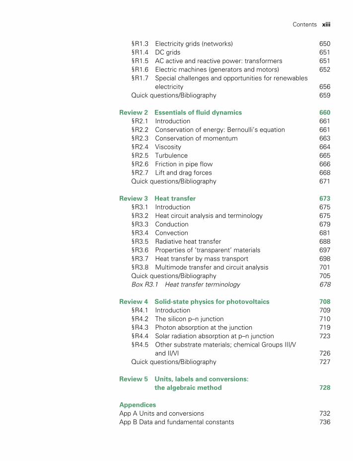
§R1.3 Electricity grids (networks) 650 §R1.4 DC grids 651 §R1.5 AC active and reactive power: transformers 651 §R1.6 Electric machines (generators and motors) 652 §R1.7 Special challenges and opportunities for renewables
electricity 656 Quick questions/Bibliography 659
Review 2 Essentials of fluid dynamics 660 §R2.1 Introduction 661 §R2.2 Conservation of energy: Bernoulli’s equation 661 §R2.3 Conservation of momentum 663 §R2.4 Viscosity 664 §R2.5 Turbulence 665 §R2.6 Friction in pipe flow 666 §R2.7 Lift and drag forces 668 Quick questions/Bibliography 671
Review 3 Heat transfer 673 §R3.1 Introduction 675 §R3.2 Heat circuit analysis and terminology 675 §R3.3 Conduction 679 §R3.4 Convection 681 §R3.5 Radiative heat transfer 688 §R3.6 Properties of ‘transparent’ materials 697 §R3.7 Heat transfer by mass transport 698 §R3.8 Multimode transfer and circuit analysis 701 Quick questions/Bibliography 705 Box R3.1 Heat transfer terminology 678
Review 4 Solid-state physics for photovoltaics 708 §R4.1 Introduction 709 §R4.2 The silicon p–n junction 710 §R4.3 Photon absorption at the junction 719 §R4.4 Solar radiation absorption at p–n junction 723 §R4.5 Other substrate materials; chemical Groups III/V
and II/VI 726 Quick questions/Bibliography 727
Review 5 Units, labels and conversions: the algebraic method 728
AppendicesApp A Units and conversions 732App B Data and fundamental constants 736
TWIDELL PAGINATION.indb 13 01/12/2014 11:35
xiv Contents
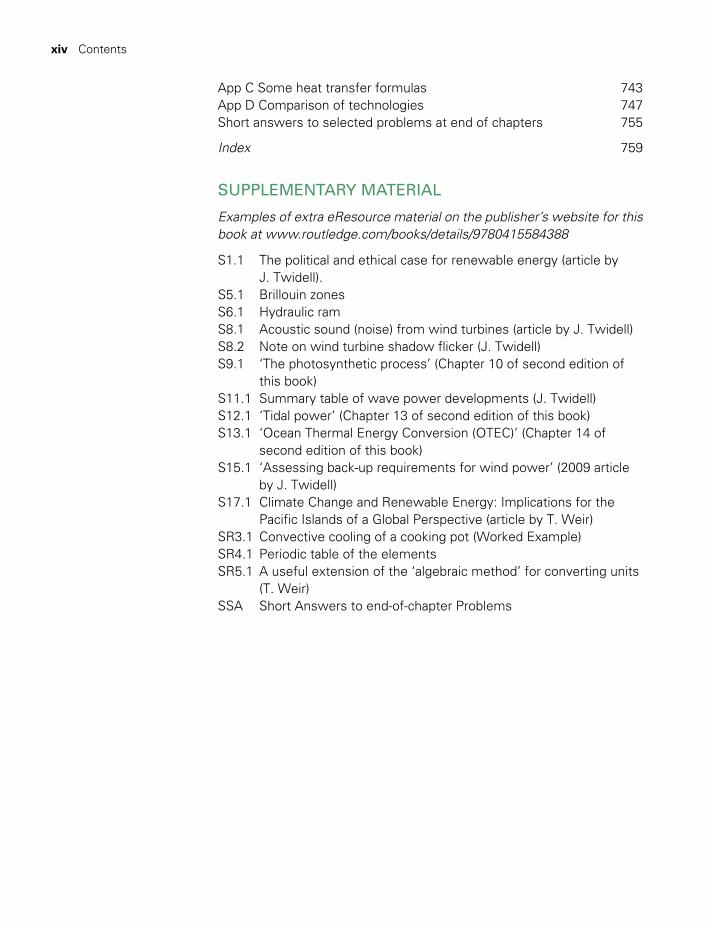
App C Some heat transfer formulas 743App D Comparison of technologies 747Short answers to selected problems at end of chapters 755
Index 759
SUPPLEMENTARY MATERIAL
Examples of extra eResource material on the publisher’s website for this book at www.routledge.com/books/details/9780415584388
S1.1 The political and ethical case for renewable energy (article by J. Twidell).
S5.1 Brillouin zonesS6.1 Hydraulic ramS8.1 Acoustic sound (noise) from wind turbines (article by J. Twidell)S8.2 Note on wind turbine shadow flicker (J. Twidell)S9.1 ‘The photosynthetic process’ (Chapter 10 of second edition of
this book)S11.1 Summary table of wave power developments (J. Twidell)S12.1 ‘Tidal power’ (Chapter 13 of second edition of this book)S13.1 ‘Ocean Thermal Energy Conversion (OTEC)’ (Chapter 14 of
second edition of this book)S15.1 ‘Assessing back-up requirements for wind power’ (2009 article
by J. Twidell)S17.1 Climate Change and Renewable Energy: Implications for the
Pacific Islands of a Global Perspective (article by T. Weir)SR3.1 Convective cooling of a cooking pot (Worked Example) SR4.1 Periodic table of the elementsSR5.1 A useful extension of the ‘algebraic method’ for converting units
(T. Weir)SSA Short Answers to end-of-chapter Problems
TWIDELL PAGINATION.indb 14 01/12/2014 11:35

PREFACE
Why a third edition?
For this third edition of Renewable Energy Resources, we have made significant changes in recognition of the outstanding progress of renew-ables worldwide. The basic principles remain the same, but feedback from earlier editions enables us to explain and analyze these more beneficially. Important aspects of new technology have been introduced and, most importantly, we have enlarged the analysis of the institutional factors enabling most countries to establish and increase renewables capacity.
When we wrote the first edition in the 1980s, modern applications of renewable energy were new and largely ignored by central planners. Renewables (apart from hydropower) were seen mainly as part of ‘appro-priate and intermediate technology’, often for small-scale applications and rural development. In retrospect this concept was correct, but of limited vision. Yes, domestic and village application is a necessity; renewables continue to cater for such needs, now with assured experience and proven technology. However, since those early days, renewables have moved from the periphery of development towards mainstream infra-structure while incorporating significant improvements in technology. ‘Small’ is no longer suspect; for instance, ‘microgeneration’ is accepted technology throughout the developed and developing world, especially as the sum total of many installations reaches national significance. We ourselves have transformed our own homes and improved our lifestyles by incorporating renewables technology that is widely available; we are grateful for these successes. Such development is no longer unusual, with the totality of renewable energy substantial. Commercial-scale appli-cations are common, not only for long-established hydropower but also for ‘new renewables’, especially the ‘big three’ of biomass, solar and wind. Major utilities incorporate renewables divisions, with larger and much replicated plant that can no longer be described as ‘small’ or ‘irrele-vant’. Such success implies utilizing varied and dispersed resources in an environmentally acceptable and cost-effective manner. Today, whole
TWIDELL PAGINATION.indb 15 01/12/2014 11:35
xvi Preface
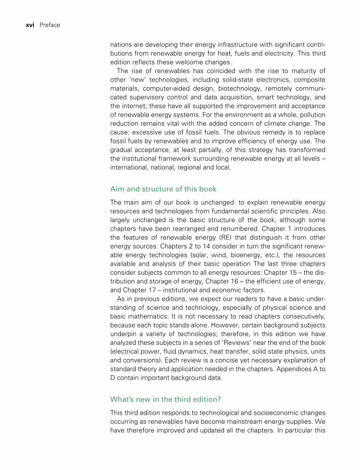
nations are developing their energy infrastructure with significant contri-butions from renewable energy for heat, fuels and electricity. This third edition reflects these welcome changes.
The rise of renewables has coincided with the rise to maturity of other ‘new’ technologies, including solid-state electronics, composite materials, computer-aided design, biotechnology, remotely communi-cated supervisory control and data acquisition, smart technology, and the internet; these have all supported the improvement and acceptance of renewable energy systems. For the environment as a whole, pollution reduction remains vital with the added concern of climate change. The cause: excessive use of fossil fuels. The obvious remedy is to replace fossil fuels by renewables and to improve efficiency of energy use. The gradual acceptance, at least partially, of this strategy has transformed the institutional framework surrounding renewable energy at all levels – international, national, regional and local.
Aim and structure of this book
The main aim of our book is unchanged: to explain renewable energy resources and technologies from fundamental scientific principles. Also largely unchanged is the basic structure of the book, although some chapters have been rearranged and renumbered. Chapter 1 introduces the features of renewable energy (RE) that distinguish it from other energy sources. Chapters 2 to 14 consider in turn the significant renew-able energy technologies (solar, wind, bioenergy, etc.), the resources available and analysis of their basic operation The last three chapters consider subjects common to all energy resources: Chapter 15 – the dis-tribution and storage of energy, Chapter 16 – the efficient use of energy, and Chapter 17 – institutional and economic factors.
As in previous editions, we expect our readers to have a basic under-standing of science and technology, especially of physical science and basic mathematics. It is not necessary to read chapters consecutively, because each topic stands alone. However, certain background subjects underpin a variety of technologies; therefore, in this edition we have analyzed these subjects in a series of ‘Reviews’ near the end of the book (electrical power, fluid dynamics, heat transfer, solid state physics, units and conversions). Each review is a concise yet necessary explanation of standard theory and application needed in the chapters. Appendices A to D contain important background data.
What’s new in the third edition?
This third edition responds to technological and socioeconomic changes occurring as renewables have become mainstream energy supplies. We have therefore improved and updated all the chapters. In particular this
TWIDELL PAGINATION.indb 16 01/12/2014 11:35

Preface xvii
applies to solar photovoltaics, wind power and bioenergy; each of these subjects now has two chapters: one on the resource and the other on the technology. Chapter 16 – ‘Using energy efficiently’ – is new, since this is a vital subject for all forms of energy supply and presents some particular opportunities with renewables. New material has been added on the science of the greenhouse effect and projected climate change in Chapter 2, being a further reason for institutional and economic apprecia-tion of renewables (Chapter 17).
We still work from first principles with unified symbolism throughout; we have tried hard to be user friendly by improving presentation and explanations. Each technology is introduced with fundamental analysis and details of international acceptance. Data on installed capacities and institutional acceptance have been updated to the time of publication. For updating, we list recommended websites (including that for this book), journals and other publications; internet searches are of course invalua-ble. This third edition has more ‘boxed examples’ and other such devices for focused information. We have extended the self-study mater ial by grading the end-of-chapter problems, and by including chapter summa-ries and ‘Quick questions’ for rapid revision. Short answer guidance for problems is at the end of the book.
Detailed solutions to all the end-of-chapter problems (password pro-tected for instructors only!) are in a new associated website at www.routledge.com/books/details/9780415584388. The public area of this website includes useful supplementary material, including the complete text of three chapters from the second edition: on OTEC, tidal range power and photosynthesis, which have some background material omitted from this third edition to help keep the length of the printed book manageable.
NOTE TO READERS: ‘BORDERED TEXT’
To help readers we use ruled borders (e.g. as here) for:
Boxes: case studies or additional technical detail.
Worked Examples: numerical analysis usually with algebraic numbered equations.
Derivations: blocks of mathematical text, the less mathematically may omit them initially.
Acknowledgments
In earlier editions we acknowledge the support of the many people who helped in the production and content of those stages; we are of course still grateful to them. In addition, we thank all those who have provided detailed comments on earlier editions, in particular, Professor G. Farquhar
TWIDELL PAGINATION.indb 17 01/12/2014 11:35

xviii Preface
and Dr Fred Chow (Australian National University), Professor J. Falnes (Norwegian University of Science and Technology), and other academics and students worldwide who have contacted us regarding their use of the book. Over the years, we have been supported by our colleagues and by undergraduate and postgraduate students at Strathclyde University, De Montfort University, Reading University, Oxford University and London City University (JT), and at the University of the South Pacific (JT and ADW); they have inspired us to continuously improve the book.
TW acknowledges financial support for his work on RE from Project DirEKT (EU) and from the Intergovernmental Panel on Climate Change (WG3), and thanks Shivneel Prasad of USP for research assistance, and Professor George Baird (Victoria University of Wellington), Dr Alistair Sproul (University of New South Wales) and Dr M.R. Ahmed (USP) for helpful advice on particular subjects. JWT acknowledges the many agen-cies in the EU and the UK who have funded his research projects and demonstrations in renewables, especially solar thermal and photovol-taics, wind power, solar buildings and institutional policies. We both acknowledge the importance to us of the many books, journal papers, websites and events where we have gained information about renewa-bles; there is no way we could write this book without them and trust that we have acknowledged such help by referencing. We apologize if acknowledgment has been insufficient.
We thank a succession of editors and other staff at Taylor & Francis/Routledge/Earthscan, and last but not least our families for their patience and encouragement; we have each been blessed with an added family generation for each subsequent edition of the book. May there be a fourth.
John W. Twidell MA, DPhil, FInstP (UK) A.D. (Tony) Weir BSc, PhD (Canberra, Australia)
Please write to us at AMSET Centre, Horninghold, Leicestershire LE16 8DH, UK
Or email to [email protected]
TWIDELL PAGINATION.indb 18 01/12/2014 11:35

Figure and photo acknowledgments
Note: full bibliographic references for sources not fully described here are given in the Bibliography of the appropriate chapter.
Cover Westmill Co-operative Solar Farm (capacity 5 MW) and Westmill Co-operative Windfarm (capacity 6.5 MW) are sited together near Watchfield, 37 km south west of Oxford, UK. The two co-operatives support a Community Fund ‘Weset’. Further details at www.westmillsolar.coop, www.westmill.coop and www.weset.org
1.3 Drawn using data from www.iea.org/statistics.2.9 After Duffie and Beckman (2006).2.10(a) After Monteith and Unsworth (2007).2.12(a) IPCC (2007, FAQ1.1 Fig. 1).2.13 Charts prepared by Robert Rohde for the Global Warming Art
Project, available online at: http://commons.wikimedia.org/wiki/File:AtmosphericTransmission.png, slightly adapted here under Creative Commons Attribution-Share Alike 3.0 unported License.
2.16 (a), (b) and (d) Kipp & Zonen.2.16 (c) Professor Dr. Volker Quaschning of HTW Berlin
(www.volker-quaschning.de/fotos/messung/index_e.php).2.17 Adapted from C.P. Jacovides, F.S. Tymvios, V.D.
Assimakopoulos and N.A. Kaltsounides (2006),‘Comparative study of various correlations in estimating hourly diffuse fraction of global solar radiation’, Renewable Energy, 31, 2492–2504.
2.18 From Duffie and Beckman (2006) (by permission of John Wiley & Sons Inc.).
2.19(a) Adapted from IPCC WG1 (2007, Fig. SPM.1).2.19(b) WMO (2013).2.19(c) Plotted from data from US National Snow and Ice Data Center,
with author’s own extrapolation.
TWIDELL PAGINATION.indb 19 01/12/2014 11:35
xx Figure and photo acknowledgments
3.1(b) Photo from www.greenenergynorthwales.com, used with permission.
3.6 After Morrison (2001).4.1(b) Photo by permission of the Rural Renewable Energy Alliance,
Pine River, MN, USA (http://www.rreal.org/solar-assistance/).4.4(b) Photo by courtesy of Thermax Europe Ltd.4.5(b) Photo by courtesy of Aquamate Products UK.4.10 Photo by courtesy of James Lindsay, Sun Fire Cooking.4.11 Adapted from IEA CSP Technology Roadmap (2010).4.12 Map © METEOTEST; based on www.meteonorm.
com,reproduced with permission.4.13(b) NREL image 19882, photo from AREVA Solar.4.13(c) Photo copyright © Abengoa Solar, reproduced with permission.4.13(d) Photo by courtesy of Dr. John Pye of ANU.4.14 Adapted from IEA, CSP Technology Roadmap (2010).4.15 Photo copyright © Abengoa Solar, reproduced with permission.5.1 US Air Force photo.5.2 Plotted using data from European Photovoltaic Industry
Association.5.7(a) Photo by courtesy of BP Solar.5.7(b) Photo by courtesy of Solar Electric Light Fund.5.8(b) Photo by courtesy of BP Solar.5.17(a) Adapted from http://www.utech-solar.com/en/product/Wafer-
Production-ProcessB/prd-03.html.5.18 From ARC Photovoltaics Centre of Excellence, Annual Report
2010 –11, University of New South Wales.5.20 www.nrel.gov/continuum/spectrum/awards.cfm.5.21 Reproduced with permission from Green (2001).5.22 Reproduced with permission from Green (2001).5.25 Adapted from D. Feldman et al., Photovoltaic Pricing Trends:
Historical, Recent, and Near-Term Projections, National Renewable Energy Laboratory, USA (June 2013).
5.26(b) Photo copyright © 2014 Sundaya, reproduced with permission of Sundaya International Pte Ltd.
5.26(c) Image by courtesy of Fiji Department of Energy.5.27(a) Photo by courtesy of BP Solar.5.27(b) Photo © Westmill Solar Co-operative, used with permission.6.2 Photo courtesy of Snowy Hydro Limited.6.5(b) Photo Voith Siemens Hydro Power Generation, reproduced
under Creative Commons Attribution-Share Alike 3.0 License6.10 Photo by Le Grand Portage, reproduced under Creative
Commons Attribution 2.0 License.7.2 http://earthobservatory.nasa.gov/IOTD/view.php?id=1824;
[note: this site also has a month-by-month animation] [accessed 1/10/2013]
TWIDELL PAGINATION.indb 20 01/12/2014 11:35

Figure and photo acknowledgments xxi
7.3(a) European Wind Atlas, DTU Wind Energy (Formerly Risø National Laboratory)
7.3(b) http://rredc.nrel.gov/wind/pubs/atlas/maps/chap2/2-01m.html.7.4(b) After Petersen (1975).7.5 After Bowden et al. (1983).7.7, 7.8, 7.9 and 7.10 Based on data of Barbour (1984).7.12(b) Photo of model 81000 by courtesy of RM Young Company.7.12(d) From www.tuvnel.com/tuvnel/article_measuring_flow_
regimes_around_large_wind_turbines_using_remote_sensing_techniques/ (NEL, branch of TuV SuD, Germany).
8.9(b) Photo by Jerome Samson, used under Creative Commons Attribution-Share Alike 3.0 Unported license.
8.11(a) Author photo.8.16(e) Photo by Dennis Schroeder (NREL image 21910).8.23 Photo by Warren Gretz (NREL image 6332).8.24(a) Photo by courtesy of Jonathan Clark, Lubenham, UK. 8.24(b) Photo by Martin Pettitt, cropped under Creative Commons
Attribution 2.0 Generic license.8.25(b) Photo from www.edupic.net/Images/Science/wind_power_
well_pump01.JPG, used with permission.9.12 Photo by Mariordo, reproduced under Creative Commons
Attribution-Share Alike 3.0 Unported License.10.8(d) photo by courtesy of AnDigestion Ltd.11.1(a) Satellite altimetry data merged by Ifremer and mapped by
CLS for the learn.eo project.11.1(b) Adapted from NEL (1976).11.10(a) Map from www.oceanor.no/Services/SCWM, adapted
with permission of Stephen Barstow, Senior Ocean Wave Climatologist .
11.11 From Shaw (1982).11.12 After Glendenning (1977).11.13 Adapted from a sketch by Prof J. Falnes of NTNU.11.15(a) Redrawn from http://amsacta.unibo.it/3062/1/overtopping_
devicex.pdf.11.15(b) Photo: Wave Dragon Aps, Denmark, used with permission.11.18 From Wang et al. (2002).12.1 Adapted from OpenHydro.com and Sorensen (2011).12.8(a) Image by courtesy of Siemens Marine Current Turbines,
Bristol, England.12.8(b) Image from www.Openhydro.com, used with permission.12.8(c) Image by courtesy of Dr Aggides, University of Lancaster.12.9 After Consul et al. (2013, Fig. 8.).13.1 US Department of Energy.13.6(a) Photo by US Department of Energy.13.8 After Aalberg (2003).
TWIDELL PAGINATION.indb 21 01/12/2014 11:35
xxii Figure and photo acknowledgments
14.5(b) Photo by US National Park Service.14.8 After EERE (2004).14.10 Photo by courtesy of Contact Energy, New Zealand.15.2 Sims et al. (2011, fig. 7.16).15.4 © Robert Rohatensky (2007), reproduced under a Design
Science License from http://www.energytower.org/cawegs.html.
15.7 www.electropaedia.com, used with permission.16.3(a) Plotted from data in US-EIA International Energy Outlook 2011.16.3(b) Plotted from data in UK Department of Energy and Climate
Change, Energy Consumption in the UK (2012 update).16.5(a) reproduced from CF Hall, Arctic Researches and Life Among
the Esquimaux, Harper Brothers, New York (1865).16.5(b) Photo by courtesy of UrbanDB.com.16.6(a) From Twidell et al. (1994).16.6(b) Photo by Jim Tetro for the US Department of Energy Solar
Decathlon.16.6(c) and 16.6(d) Reproduced from G. Baird (2010) Sustainable
Buildings in Practice: What the users think, Routledge, Abingdon.
16.7 Photo and sketch from G. Baird (2010) Sustainable Buildings in Practice: What the users think, Routledge, Abingdon.
16.8(b) Photo by Wade Johanson, cropped and used here under Creative Commons Attribution Generic 2.0 License.
16.9 US Energy Administration, International Energy Outlook 2011, fig. 33.
16.10 Chart from Kick the Habit: A UN Guide to Climate Neutrality, UNEP/GRID-Arendal.
16.11 Photo by Mario Roberto Duran Ortiz Mariordo, used under Creative Commons Attribution Unported 3.0 license.
16.12 Replotted from data in UK Department of Energy and Climate Change (2011), Energy Consumption in UK.
17.1 Adapted from IPCC Synthesis Report (2007), fig. SPM-11.17.2 From G. Nemet (2009) ‘Interim monitoring of cost dynamics
for publicly supported energytechnologies’, Energy Policy, 37, 825–835.
17.3 After Hohmeyer (1988).17.4 Drawn from data in IPCC SRREN (2011), table 10.3.R1.4 [US] Lawrence Livermore National Laboratory.D1 Chart from IPCC SRREN (2011, fig. 1.17).D2(a) Replotted from data in SRREN (2011, fig. 1.10).D3 IPCC SRREN (2011, fig. 9-8).D5 From IRENA (2013), Renewable Power Generation Costs in
2012: An overview.D6 IPCC SRREN (2011, fig. 1-20).
TWIDELL PAGINATION.indb 22 01/12/2014 11:35
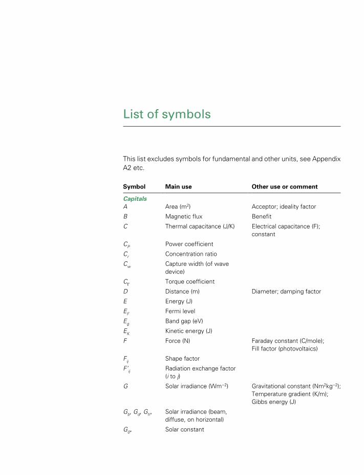
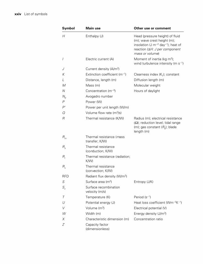
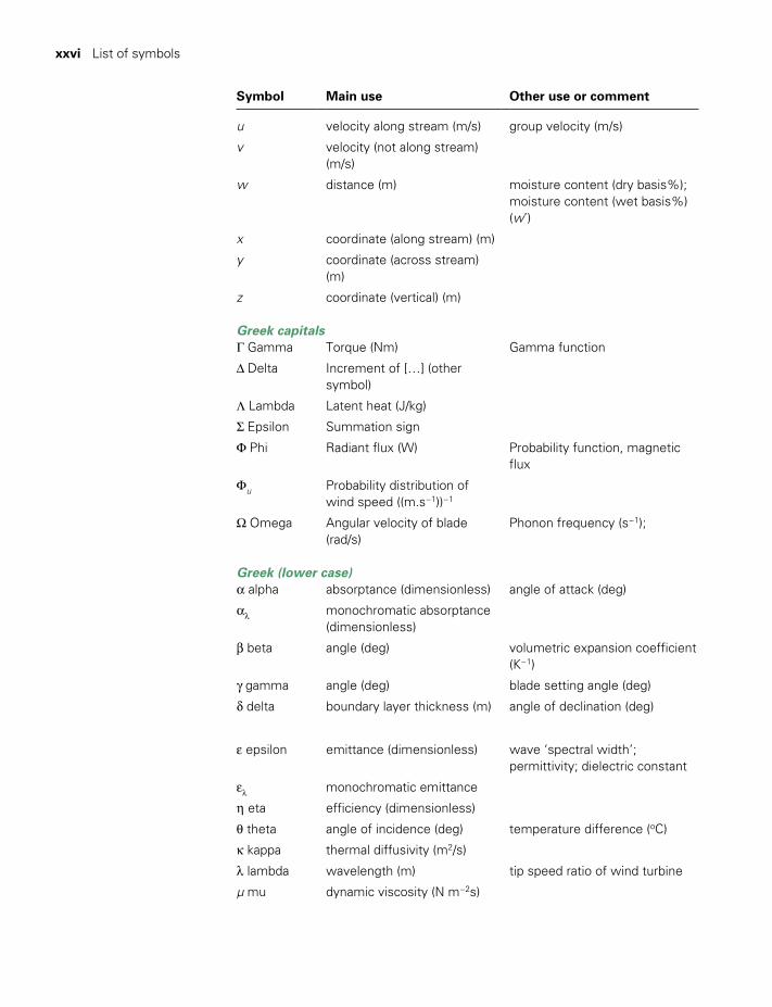
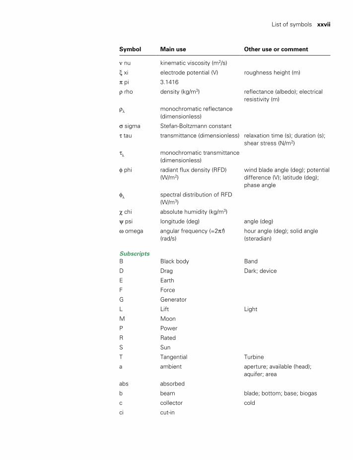
List of symbols
This list excludes symbols for fundamental and other units, see Appendix A2 etc.
Symbol Main use Other use or comment
CapitalsA Area (m2) Acceptor; ideality factor
B Magnetic flux Benefit
C Thermal capacitance (J/K) Electrical capacitance (F); constant
CP Power coefficient
Cr Concentration ratio
Cw Capture width (of wave device)
CΓ Torque coefficient
D Distance (m) Diameter; damping factor
E Energy (J)
EF Fermi level
Eg Band gap (eV)
EK Kinetic energy (J)
F Force (N) Faraday constant (C/mole); Fill factor (photovoltaics)
Fij Shape factor
F’ij Radiation exchange factor (i to j)
G Solar irradiance (Wm−2) Gravitational constant (Nm2kg−2);Temperature gradient (K/m);Gibbs energy (J)
Gb, Gd, Gh* Solar irradiance (beam, diffuse, on horizontal)
G0* Solar constant
TWIDELL PAGINATION.indb 23 01/12/2014 11:35
xxiv List of symbols
Symbol Main use Other use or comment
H Enthalpy (J) Head (pressure height) of fluid (m); wave crest height (m); insolation (J m−2 day−1); heat of reaction (ΔH: J per component mass or volume)
I Electric current (A) Moment of inertia (kg m2);wind turbulence intensity (m s−1)
J Current density (A/m2)
K Extinction coefficient (m−1) Clearness index (KT); constant
L Distance, length (m) Diffusion length (m)
M Mass (m) Molecular weight
N Concentration (m−3) Hours of daylight
N0 Avogadro number
P Power (W)
P’ Power per unit length (W/m)
Q Volume flow rate (m3/s)
R Thermal resistance (K/W) Radius (m); electrical resistance (Ω); reduction level; tidal range (m); gas constant (R0); blade length (m)
Rm Thermal resistance (mass transfer; K/W)
Rn Thermal resistance (conduction; K/W)
Rr Thermal resistance (radiation; K/W)
Rv Thermal resistance (convection; K/W)
RFD Radiant flux density (W/m2)
S Surface area (m2) Entropy (J/K)
Sv Surface recombination velocity (m/s)
T Temperature (K) Period (s−1)
U Potential energy (J) Heat loss coefficient (Wm−2K−1)
V Volume (m3) Electrical potential (V)
W Width (m) Energy density (J/m3)
X Characteristic dimension (m) Concentration ratio
Z Capacity factor (dimensionless)
TWIDELL PAGINATION.indb 24 01/12/2014 11:35

List of symbols xxv
Symbol Main use Other use or comment
Script capitals (non-dimensional numbers characterizing fluid flow; all dimensionless)
A Rayleigh numberG Grashof number Graetz numberN Nusselt numberP Prandtl numberR Reynolds numberS Shape number (of turbine)
Lower casea amplitude (m) wind interference factor;
radius (m)
b wind profile exponent width (m)
c specific heat capacity (J kg−1 K−1)
speed of light (m/s); phase velocity of wave (m/s); chord length (m); Weibull speed factor (m/s)
d distance (m) diameter (m); depth (m); zero plane displacement (wind) (m)
e elementary charge (C) base of natural logarithms (2.718); ellipticity; external
f frequency of cycles (Hz = s−1) pipe friction coefficient; fraction; force per unit length (N m−1)
g acceleration due to gravity (m/s2)
h heat transfer coefficient (Wm−2K−1)
vertical displacement (m); Planck constant (Js)
i √−1 internal
k thermal conductivity (Wm−1K−1)
wave vector (=2π/λ); Boltzmann constant (=1.38 × 10⁻²³ J/K)
l distance (m)
m mass (kg) air mass ratio
n number number of nozzles, of hours of bright sunshine, of wind turbine blades; electron concentration (m−3)
p pressure (Nm−2 = Pa) hole concentration (m−3)
q power per unit area (W/m2)
r thermal resistivity of unit area (often called ‘r-value’; r = RA) (m2K/W)
radius (m); distance (m)
s angle of slope (degrees)
t time (s) thickness (m)
TWIDELL PAGINATION.indb 25 01/12/2014 11:35
xxvi List of symbols
Symbol Main use Other use or comment
u velocity along stream (m/s) group velocity (m/s)
v velocity (not along stream) (m/s)
w distance (m) moisture content (dry basis%); moisture content (wet basis%) (w’)
x coordinate (along stream) (m)
y coordinate (across stream) (m)
z coordinate (vertical) (m)
Greek capitalsΓ Gamma Torque (Nm) Gamma function
Δ Delta Increment of […] (other symbol)
Λ Lambda Latent heat (J/kg)
Σ Epsilon Summation sign
Φ Phi Radiant flux (W) Probability function, magnetic flux
Φu Probability distribution of wind speed ((m.s−1))−1
Ω Omega Angular velocity of blade (rad/s)
Phonon frequency (s−1);
Greek (lower case)α alpha absorptance (dimensionless) angle of attack (deg)
αλ monochromatic absorptance (dimensionless)
β beta angle (deg) volumetric expansion coefficient (K−1)
γ gamma angle (deg) blade setting angle (deg)
δ delta boundary layer thickness (m) angle of declination (deg)
ε epsilon emittance (dimensionless) wave ‘spectral width’; permittivity; dielectric constant
ελ monochromatic emittance
η eta efficiency (dimensionless)
θ theta angle of incidence (deg) temperature difference (oC)
κ kappa thermal diffusivity (m2/s)
λ lambda wavelength (m) tip speed ratio of wind turbine
μ mu dynamic viscosity (N m−2s)
TWIDELL PAGINATION.indb 26 01/12/2014 11:35
List of symbols xxvii
Symbol Main use Other use or comment
ν nu kinematic viscosity (m2/s)
ξ xi electrode potential (V) roughness height (m)
π pi 3.1416
ρ rho density (kg/m3) reflectance (albedo); electrical resistivity (m)
ρλ monochromatic reflectance (dimensionless)
σ sigma Stefan-Boltzmann constant
τ tau transmittance (dimensionless) relaxation time (s); duration (s); shear stress (N/m2)
τλ monochromatic transmittance (dimensionless)
f phi radiant flux density (RFD) (W/m2)
wind blade angle (deg); potential difference (V); latitude (deg); phase angle
fλ spectral distribution of RFD (W/m3)
χ chi absolute humidity (kg/m3)
ψ psi longitude (deg) angle (deg)
ω omega angular frequency (=2πf) (rad/s)
hour angle (deg); solid angle (steradian)
SubscriptsB Black body Band
D Drag Dark; device
E Earth
F Force
G Generator
L Lift Light
M Moon
P Power
R Rated
S Sun
T Tangential Turbine
a ambient aperture; available (head); aquifer; area
abs absorbed
b beam blade; bottom; base; biogas
c collector cold
ci cut-in
TWIDELL PAGINATION.indb 27 01/12/2014 11:35

xxviii List of symbols
Symbol Main use Other use or comment
co cut-out
cov cover
d diffuse dopant; digester
e electrical equilibrium; energy
f fluid forced; friction; flow; flux
g glass generation current; band gap
h horizontal hot
i integer intrinsic
in incident (incoming)
int internal
j integer
m mass transfer mean (average); methane
max maximum
maxp maximum power
n conduction
net heat flow across surface
o (read as numeral zero)
oc open circuit
p plate peak; positive charge carriers (holes); performance
r radiation relative; recombination; room; resonant; rock; relative
rad radiated
refl reflected
rms root mean square
s surface significant; saturated; Sun; sky
sc short circuit
t tip total
th thermal
trans transmitted
u useful
v convection vapor
w wind water; width
z zenith
λ monochromatic (e.g. αλ)
0 distant approach ambient; extra-terrestrial; dry matter; saturated; ground-level
1 entry to device first
2 exit from device second
TWIDELL PAGINATION.indb 28 01/12/2014 11:35

List of symbols xxix
Symbol Main use Other use or comment
3 output third
Superscriptm or max maximum
* measured perpendicular to direction of propagation (e.g. Gb*)
· (dot) rate of , e.g. m
Other symbols and abbreviationsBold face vector, e.g. F
ch. chapter
§ section (within chapters)
= mathematical equality
≈ approximate equality (within about 20%)
~ equality in order of magnitude (within a factor of 2 to 10)
≡ mathematical identity (or definition), equivalent
TWIDELL PAGINATION.indb 29 01/12/2014 11:35

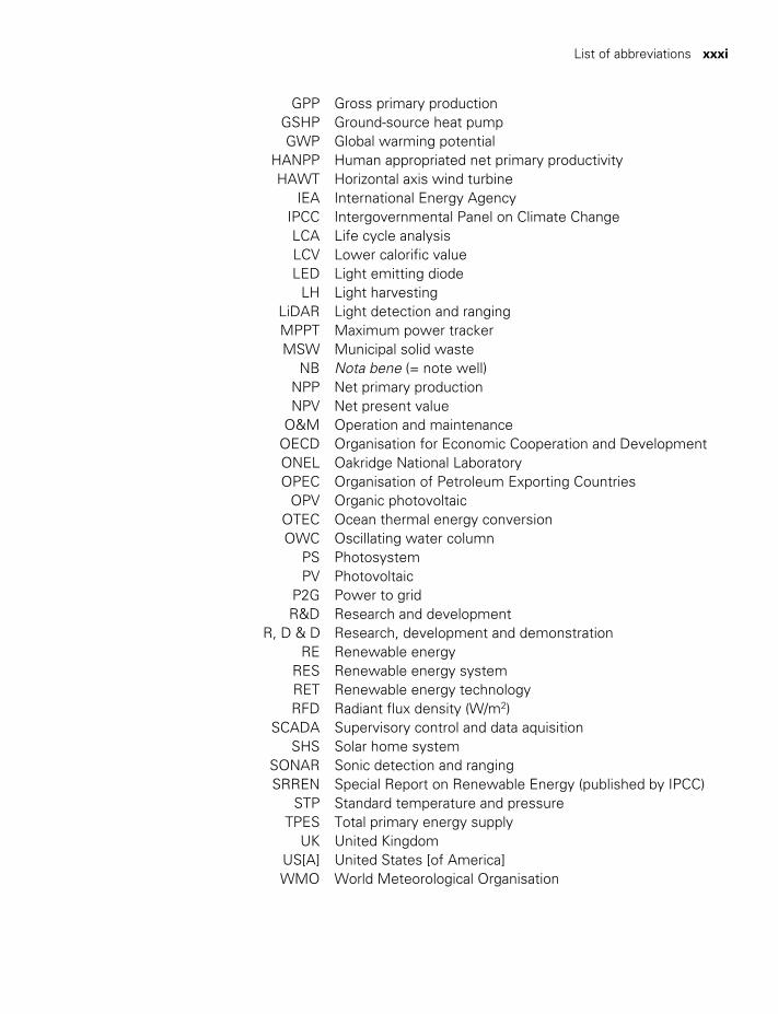
List of abbreviations (acronyms)
This list excludes most chemical symbols and abbreviations of standard units; see also the Index, and Appendix A for units.
AC Alternating current AM Air–mass ratio BoS Balance of system CCS Carbon capture and storage CFL Compact fluorescent light CHP Combined heat and power CO2 Carbon dioxide CO2eq CO2 equivalent for other climate-change-forcing gases COP Coefficient of Performance CSP Concentrated solar power (= CSTP) CSTP Concentrated solar thermal power DC Direct current DCF Discounted cash flow DNI Direct normal insolation (= irradiance) DOWA Deep ocean water applications EC Electrochemical capacitor EGS Enhanced geothermal system[s] EIA Environmental Impact Assessment EMF Electromotive force (equivalent to Voltage) EU European Union EV Electric vehicle FF Fossil fuel GCV Gross calorific value GDP Gross domestic product GER Gross energy requirement GHG Greenhouse gas GHP Geothermal heat pump (= GSHP) GMST Global mean surface temperature GOES Geostationary Operational Environmental Satellite
TWIDELL PAGINATION.indb 30 01/12/2014 11:35
List of abbreviations xxxi
GPP Gross primary production GSHP Ground-source heat pump GWP Global warming potential HANPP Human appropriated net primary productivity HAWT Horizontal axis wind turbine IEA International Energy Agency IPCC Intergovernmental Panel on Climate Change LCA Life cycle analysis LCV Lower calorific value LED Light emitting diode LH Light harvesting LiDAR Light detection and ranging MPPT Maximum power tracker MSW Municipal solid waste NB Nota bene (= note well) NPP Net primary production NPV Net present value O&M Operation and maintenance OECD Organisation for Economic Cooperation and Development ONEL Oakridge National Laboratory OPEC Organisation of Petroleum Exporting Countries OPV Organic photovoltaic OTEC Ocean thermal energy conversion OWC Oscillating water column PS Photosystem PV Photovoltaic P2G Power to grid R&D Research and development R, D & D Research, development and demonstration RE Renewable energy RES Renewable energy system RET Renewable energy technology RFD Radiant flux density (W/m2) SCADA Supervisory control and data aquisition SHS Solar home system SONAR Sonic detection and ranging SRREN Special Report on Renewable Energy (published by IPCC) STP Standard temperature and pressure TPES Total primary energy supply UK United Kingdom US[A] United States [of America] WMO World Meteorological Organisation
TWIDELL PAGINATION.indb 31 01/12/2014 11:35

TWIDELL PAGINATION.indb 32 01/12/2014 11:35
Page Intentionally Left Blank
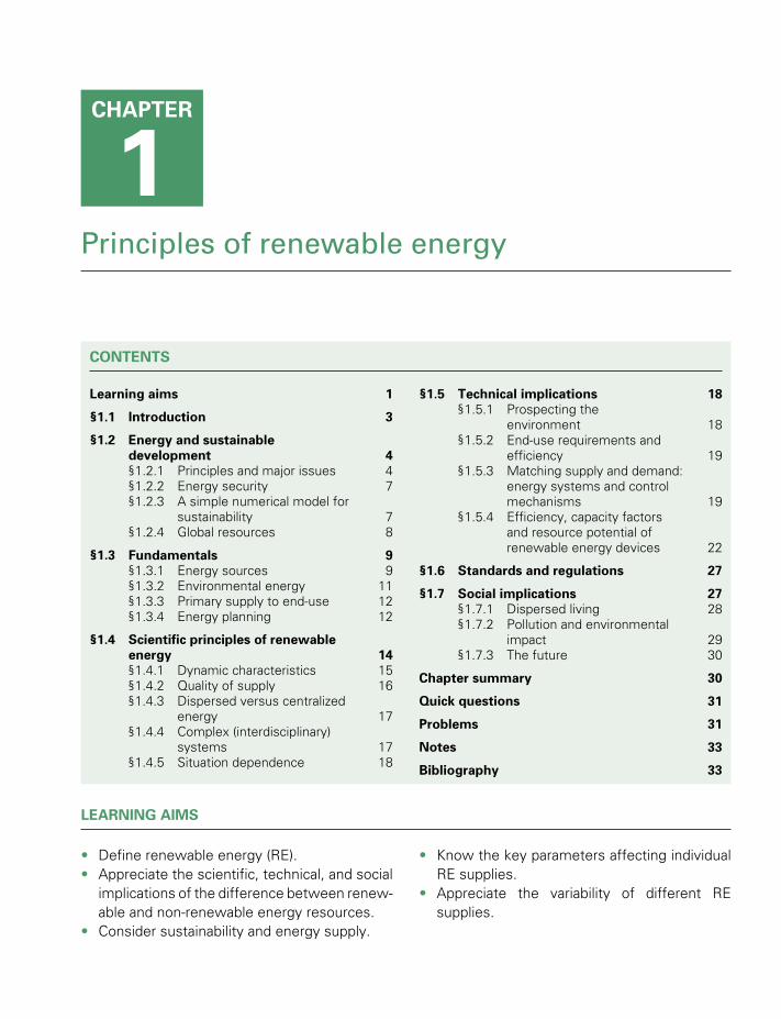
Principles of renewable energy
CONTENTS
Learning aims 1
§1.1 Introduction 3
§1.2 Energy and sustainable development 4§1.2.1 Principles and major issues 4§1.2.2 Energy security 7§1.2.3 A simple numerical model for
sustainability 7§1.2.4 Global resources 8
§1.3 Fundamentals 9§1.3.1 Energy sources 9§1.3.2 Environmental energy 11§1.3.3 Primary supply to end-use 12§1.3.4 Energy planning 12
§1.4 Scientific principles of renewable energy 14§1.4.1 Dynamic characteristics 15§1.4.2 Quality of supply 16§1.4.3 Dispersed versus centralized
energy 17§1.4.4 Complex (interdisciplinary)
systems 17§1.4.5 Situation dependence 18
§1.5 Technical implications 18§1.5.1 Prospecting the
environment 18§1.5.2 End-use requirements and
efficiency 19§1.5.3 Matching supply and demand:
energy systems and control mechanisms 19
§1.5.4 Efficiency, capacity factors and resource potential of renewable energy devices 22
§1.6 Standards and regulations 27
§1.7 Social implications 27§1.7.1 Dispersed living 28§1.7.2 Pollution and environmental
impact 29§1.7.3 The future 30
Chapter summary 30
Quick questions 31
Problems 31
Notes 33
Bibliography 33
CHAPTER
1
LEARNING AIMS
• Define renewable energy (RE).• Appreciate the scientific, technical, and social
implications of the difference between renew-able and non-renewable energy resources.
• Consider sustainability and energy supply.
• Know the key parameters affecting individual RE supplies.
• Appreciate the variability of different RE supplies.
TWIDELL PAGINATION.indb 1 01/12/2014 11:35

2 Principles of renewable energy
• Consider methods and controls to optimize the use of renewable energy.
• Relate energy supplies to environmental impact.
LIST OF FIGURES
1.1 Contrast between renewable (green) and finite (brown) energy supplies. 91.2 Natural energy currents on the Earth, showing renewable energy system. 111.3 Energy flow diagrams for Austria in 2010. 131.4 Matching renewable energy supply to end-use. 20
LIST OF TABLES
1.1 Comparison of renewable and conventional energy systems. 101.2 Intensity and frequency properties of renewable sources. 151.3 Factors influencing capacity factors. 26
TWIDELL PAGINATION.indb 2 01/12/2014 11:35
§1.1 Introduction 3
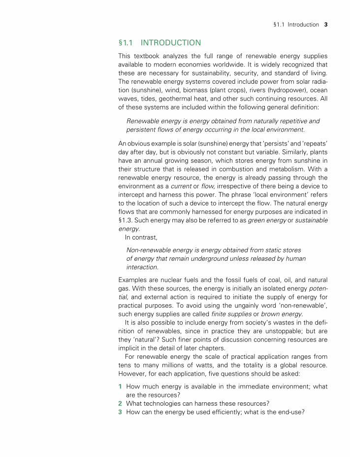
§1.1 INTRODUCTION
This textbook analyzes the full range of renewable energy supplies available to modern economies worldwide. It is widely recognized that these are necessary for sustainability, security, and standard of living. The renewable energy systems covered include power from solar radia-tion (sunshine), wind, biomass (plant crops), rivers (hydropower), ocean waves, tides, geothermal heat, and other such continuing resources. All of these systems are included within the following general definition:
Renewable energy is energy obtained from naturally repetitive and persistent flows of energy occurring in the local environment.
An obvious example is solar (sunshine) energy that ‘persists’ and ‘repeats’ day after day, but is obviously not constant but variable. Similarly, plants have an annual growing season, which stores energy from sunshine in their structure that is released in combustion and metabolism. With a renewable energy resource, the energy is already passing through the environment as a current or flow, irrespective of there being a device to intercept and harness this power. The phrase ‘local environment’ refers to the location of such a device to intercept the flow. The natural energy flows that are commonly harnessed for energy purposes are indicated in §1.3. Such energy may also be referred to as green energy or sustainable energy.
In contrast,
Non-renewable energy is energy obtained from static stores of energy that remain underground unless released by human interaction.
Examples are nuclear fuels and the fossil fuels of coal, oil, and natural gas. With these sources, the energy is initially an isolated energy poten-tial, and external action is required to initiate the supply of energy for practical purposes. To avoid using the ungainly word ‘non-renewable’, such energy supplies are called finite supplies or brown energy.
It is also possible to include energy from society’s wastes in the defi-nition of renewables, since in practice they are unstoppable; but are they ‘natural’? Such finer points of discussion concerning resources are implicit in the detail of later chapters.
For renewable energy the scale of practical application ranges from tens to many millions of watts, and the totality is a global resource. However, for each application, five questions should be asked:
1 How much energy is available in the immediate environment; what are the resources?
2 What technologies can harness these resources?3 How can the energy be used efficiently; what is the end-use?
TWIDELL PAGINATION.indb 3 01/12/2014 11:35

4 Principles of renewable energy
4 What is the environmental impact of the technology, including its implications for climate change?
5 What is the cost-effectiveness of the energy supply as compared with other supplies?
The first three are technical questions considered in the central chap-ters of this book by type of renewables technology. The fourth ques-tion relates to broad issues of planning, social responsibility, sustainable development, and global impact; these are considered in the concluding section of each technology chapter and in Chapter 17. The fifth and final question is a dominant question for consumers, but is greatly influenced by government and other policies, considered as ‘institutional factors’ in Chapter 17. The evaluation of ‘cost-effectiveness’ depends significantly upon the following factors:
a Appreciating the distinctive scientific principles of renewable energy (§1.4).
b the efficiency of each stage of the energy supply in terms of both min-imizing losses and maximizing economic and social benefits (§16.2).
c Considering externalities and social costs (Box 17.2).d Considering both costs and benefits over the lifetime of a project
(which may be > ~30 years).
In this book we analyze (a) and (b) in detail, since they apply universally. The second two, (c) and (d) have aspects that depend on particular econ-omies, and so we only explain the principles involved.
§1.2 ENERGY AND SUSTAINABLE DEVELOPMENT
§1.2.1 Principles and major issues
Sustainable development may be broadly defined as living, producing, and consuming in a manner that meets the needs of the present without compromising the ability of future generations to meet their own needs. It has become one of the key guiding principles for policy in the 21st century. The principle is affirmed worldwide by politicians, industrialists, environmentalists, economists, and theologians as they seek interna-tional, national, and local cooperation. However, reaching specific agreed policies and actions is proving much harder!
In the international context, the word ‘development’ refers to improve-ment in quality of life, including improving standards of living in less developed countries. The aim of sustainable development is to achieve this aim while safeguarding the ecological processes upon which life depends. Locally, progressive businesses seek a positive triple bottom line (i.e. a positive contribution to the economic, social, and environmen-tal well-being of the community in which they operate).
TWIDELL PAGINATION.indb 4 01/12/2014 11:35

§1.2 Energy and sustainable development 5
The concept of sustainable development first reached global import-ance in the seminal report of the UN World Commission on Environment and Development (1987); since then this theme has percolated slowly and erratically into most national economies. The need is to recognize the scale and unevenness of economic development and population growth, which place unprecedented pressures on our planet’s lands, waters, and other natural resources. Some of these pressures are severe enough to threaten the very survival of some regional populations and in the longer term to lead to disruptive global change. The way people live, especially regarding production and consumption, will have to adapt due to ecological and economic pressures. Nevertheless, the economic and social pain of such changes can be eased by foresight, planning, and political and community will.
Energy resources exemplify these issues. Reliable energy supply is essential in all economies for lighting, heating, communications, comput-ers, industrial equipment, transport, etc. Purchases of energy account for 5 to10% of gross national product in developed economies. However, in some developing countries, fossil fuel imports (i.e. coal, oil, and gas) may cost over half the value of total exports; such economies are unsustain-able, and an economic challenge for sustainable development. World energy use increased more than ten-fold during the 20th century, pre-dominantly from fossil fuels and with the addition of electricity from nuclear power. In the 21st century, further increases in world energy consumption may be expected, largely due to rising industrialization and demand in previously less developed countries, aggravated by gross inef-ficiencies in all countries. Whatever the energy source, there is an over-riding need for efficient transformation, distribution, and use of energy.
Fossil fuels are not being newly formed at any significant rate, and thus current stocks are ultimately finite. The location and amount of such stocks depend on the latest surveys. Clearly the dominant fossil fuel by mass is coal. The reserve lifetime of a resource may be defined as the known accessible amount divided by the rate of present use. By this defi-nition, the lifetime of oil and gas resources is usually only a few decades, whereas the lifetime for coal is a few centuries. Economics predicts that as the lifetime of a fuel reserve shortens, so the fuel price increases; subsequently, therefore, demand falls and previously more expensive sources and alternatives enter the market. This process tends to make the original source last longer than an immediate calculation indicates. In practice, many other factors are involved, especially government policy and international relations. Nevertheless, the basic geological fact remains: fossil fuel reserves are limited and so the current patterns of energy consumption and growth are not sustainable in the longer term.
Moreover, the emissions from fossil fuel use (and indeed nuclear power) increasingly determine another fundamental limitation on their continued use. These emissions bring substances derived from
TWIDELL PAGINATION.indb 5 01/12/2014 11:35

6 Principles of renewable energy
underground materials (e.g. carbon dioxide) into the Earth’s atmosphere and oceans that were not present before. In particular, emissions of carbon dioxide (CO2) from the combustion of fossil fuels have significantly raised the concentration of CO2 in the global atmosphere. Authoritative scientific opinion is in agreement that if this continues, the greenhouse effect will be enhanced and so lead to significant climate change within a century or sooner, which could have a major adverse impact upon food production, water supply, and society (e.g. through increased floods and storms (IPCC 2007, 2013/2014)); see also §2.9. Sadly, concrete action is slow, not least owing to the reluctance of governments in industrial-ized countries to disturb the lifestyle of their voters. However, potential climate change, and related sustainability issues, is now established as one of the major drivers of energy policy.
In contrast to fossil and nuclear fuels, renewable energy (RE) supply in operation does not add to elements in the atmosphere and hydrosphere. In particular, there is no additional input of greenhouse gases (GHGs). Although there are normally such emissions from the manufacture of all types of energy equipment, these are always considerably less per unit of energy generated than emitted over the lifetime of fossil fuel plant (see data in Appendix D). Therefore, both nuclear power and renewables significantly reduce GHG emissions if replacing fossil fuels. Moreover, since RE supplies are obtained from ongoing flows of energy in the natural environment, all renewable energy sources should be sustain-able. Nevertheless, great care is needed to consider actual situations, as noted in the following quotation:
For a renewable energy resource to be sustainable, it must be inexhaustible and not damage the delivery of environmental goods and services including the climate system. For example, to be sustainable, biofuel production should not increase net CO2 emissions, should not adversely affect food security, nor require excessive use of water and chemicals, nor threaten biodiversity. To be sustainable, energy must also be economically affordable over the long term; it must meet societal needs and be compatible with social norms now and in the future. Indeed, as use of RE technologies accelerates, a balance will have to be struck among the several dimensions of sustainable development. It is important to assess the entire lifecycle of each energy source to ensure that all of the dimensions of sustainability are met. (IPCC 2011, §1.1.5)
In analyzing harm and benefit, the full external costs of obtaining mate-rials and fuels, and of paying for damage from emissions, should be inter-nalized in costs, as discussed in Chapter 17. Doing so takes into account: (i) the finite nature of fossil and nuclear fuel materials; (ii) the harm of emissions; and (iii) ecological sustainability. Such fundamental analyses
TWIDELL PAGINATION.indb 6 01/12/2014 11:35
§1.2 Energy and sustainable development 7
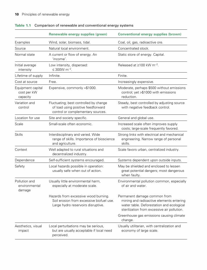
usually conclude that combining renewable energy with the efficient use of energy is more cost-effective than the traditional use of fossil and nuclear fuels, which are unsustainable in the longer term. In short, renewable energy supplies are much more compatible with sustainable development than are fossil and nuclear fuels in regard to both resource limitations and environmental impacts (see Table 1.1).
Consequently, almost all national energy plans include four vital factors for improving or maintaining benefit from energy:
1 increased harnessing of renewable supplies;2 increased efficiency of supply and end-use;3 reduction in pollution;4 consideration of employment, security, and lifestyle.
§1.2.2 Energy security
Nations, and indeed individuals, need secure energy supplies; they need to know that sufficient and appropriate energy will reach them in the future. Being in control of independent and assured supplies is therefore important – renewables offer this so long as the technologies function and are affordable.
§1.2.3 A simple numerical model for sustainability
Consider the following simple model describing the need for commercial and non-commercial energy resources:
R = E N (1.1)
Here R is the total yearly energy consumption for a population of N people. E is the per capita use of energy averaged over one year, related closely to the provision of food and manufactured goods. On a world scale, the dominant supply of energy is from commercial sources, especially fossil fuels; however, significant use of non-commercial energy may occur (e.g. fuel-wood, passive solar heating) which is often absent from most offi-cial and company statistics. In terms of total commercial energy use, E on a world per capita level is about 2.1 kW, but regional average values range widely, with North America 9.3 kW, Europe 4.6 kW, and several regions of Central Africa 0.2 kW. The inclusion of non-commercial energy increases all these figures, especially in countries with low values of E.
Standard of living relates in a complex and an ill-defined way to E. Thus, per capita gross national product S (a crude measure of standard of living) may be related to E by:
S = f E (1.2)
Here f is a complex and nonlinear coefficient that is itself a function of many factors. It may be considered an efficiency for transforming energy
TWIDELL PAGINATION.indb 7 01/12/2014 11:35
8 Principles of renewable energy
into wealth and, by traditional economics, is expected to be as large as possible. However, S does not increase uniformly as E increases. Indeed, S may even decrease for large E (e.g. due to pollution or technical ineffi-ciency). Obviously, unnecessary waste of energy leads to smaller values of f than would otherwise be possible. Substituting for E in (1.1), the national requirement for energy becomes:
R = (S N) / f (1.3)
so
DR/R = DS / S + DN / N - Df / f (1.4)
Now consider substituting global values for the parameters in (1.4). In 50 years the world population N increased from 2.5 billion in 1950 to over 7.2 billion in 2013. It is now increasing at approximately 2 to 3% per year so as to double every 20 to 30 years. Tragically high infant mortality and low life expectancy tend to hide the intrinsic pressures of population growth in many countries. Conventional economists seek exponential growth of S at 2 to 5% per year. Thus, in (1.4), at constant efficiency parameter f, the growth of total world energy supply is effectively the sum of population and economic growth (i.e. 4 to 8% per year). Without new supplies, such growth cannot be maintained. Yet, at the same time as more energy is required, fossil and nuclear fuels are being depleted, and debilitating pollution and climate change increase.
An obvious way to overcome such constraints is to increase renew-able energy supplies. Most importantly, from (1.3) and (1.4), it is vital to increase the efficiency parameter f (i.e. to have a positive value of Df). Consequently, if there is a growth rate in the efficient use and generation of energy, then S (standard of living) increases while R (resource use) decreases.
§1.2.4 Global resources
With the most energy-efficient modern equipment, buildings, and trans-portation, a justifiable target for energy use in a modern society is E = 2 kW per person (i.e. approximately the current global average usage, yet with a far higher standard of living). Is this possible, even in principle, from renewable energy? Each square metre of the Earth’s habitable surface is crossed by or accessible to an average energy flux of about 500 W (see Problem 1.1). This includes solar, wind, or other renewable energy forms in an overall estimate. If this flux is harnessed at just 4% efficiency, 2 kW of power can be drawn from an area of 10m × 10m, assuming suitable methods. Suburban areas of residential towns have population densities of about 500 people km–2. At 2 kW per person, the total energy demand of l000 kW/km2 could be obtained in this way by using just 5% of the local land area for energy production, thus allowing for the ‘technical
TWIDELL PAGINATION.indb 8 01/12/2014 11:35
§1.3 Fundamentals 9
potential’ of RE being less than the ‘theoretical potential’, as indicated in Fig.1.2 and §1.5.4. Thus, renewable energy supplies may, in principle, provide a satisfactory standard of living worldwide, but only if methods exist to extract, use, and store the energy satisfactorily at realistic costs. This book will consider both the technical background of a great variety of possible methods and a summary of the institutional factors involved.
§1.3 FUNDAMENTALS
§1.3.1 Energy sources
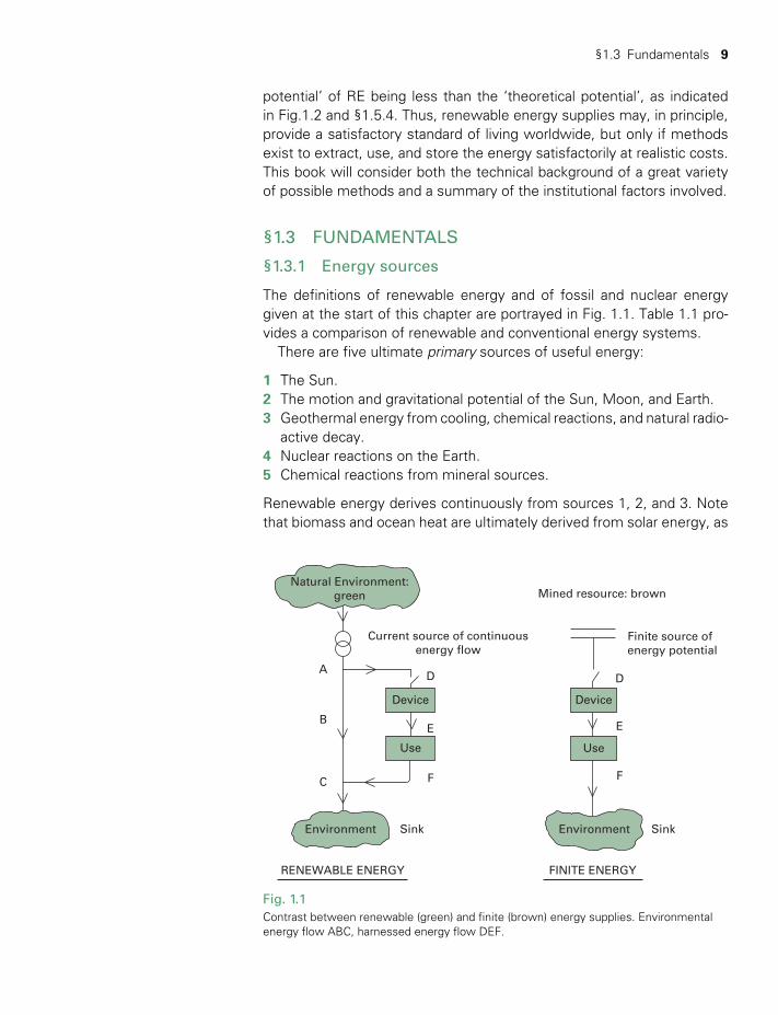
The definitions of renewable energy and of fossil and nuclear energy given at the start of this chapter are portrayed in Fig. 1.1. Table 1.1 pro-vides a comparison of renewable and conventional energy systems.
There are five ultimate primary sources of useful energy:
1 The Sun.2 The motion and gravitational potential of the Sun, Moon, and Earth.3 Geothermal energy from cooling, chemical reactions, and natural radio-
active decay.4 Nuclear reactions on the Earth.5 Chemical reactions from mineral sources.
Renewable energy derives continuously from sources 1, 2, and 3. Note that biomass and ocean heat are ultimately derived from solar energy, as
Natural Environment:green Mined resource: brown
Current source of continuousenergy flow
A
C
D
E
F
B
Device
Use
D
E
F
Device
Use
Environment Sink Environment Sink
Finite source ofenergy potential
RENEWABLE ENERGY FINITE ENERGY
Fig. 1.1Contrast between renewable (green) and finite (brown) energy supplies. Environmental energy flow ABC, harnessed energy flow DEF.
TWIDELL PAGINATION.indb 9 01/12/2014 11:35
10 Principles of renewable energy
Table 1.1 Comparison of renewable and conventional energy systems
Renewable energy supplies (green) Conventional energy supplies (brown)
Examples Wind, solar, biomass, tidal. Coal, oil, gas, radioactive ore.
Source Natural local environment. Concentrated stock.
Normal state A current or flow of energy. An ‘income’.
Static store of energy. Capital.
Initial average intensity
Low intensity, dispersed: ≤ 300W m-2.
Released at ≥100 kW m-2.
Lifetime of supply Infinite. Finite.
Cost at source Free. Increasingly expensive.
Equipment capital cost per kW
capacity
Expensive, commonly ≈$1000. Moderate, perhaps $500 without emissions control; yet >$1000 with emissions
reduction.
Variation and control
Fluctuating; best controlled by change of load using positive feedforward
control or complementary sources.
Steady, best controlled by adjusting source with negative feedback control.
Location for use Site and society specific. General and global use.
Scale Small-scale often economic. Increased scale often improves supply costs; large-scale frequently favored.
Skills Interdisciplinary and varied. Wide range of skills. Importance of bioscience
and agriculture.
Strong links with electrical and mechanical engineering. Narrow range of personal
skills.
Context Well adapted to rural situations and decentralized industry.
Scale favors urban, centralized industry.
Dependence Self-sufficient systems encouraged. Systems dependent upon outside inputs.
Safety Local hazards possible in operation: usually safe when out of action.
May be shielded and enclosed to lessen great potential dangers; most dangerous
when faulty.
Pollution and environmental
damage
Usually little environmental harm, especially at moderate scale.
Environmental pollution common, especially of air and water.
Hazards from excessive wood burning. Soil erosion from excessive biofuel use.
Large hydro reservoirs disruptive.
Permanent damage common from mining and radioactive elements entering
water table. Deforestation and ecological sterilization from excessive air pollution.
Greenhouse gas emissions causing climate change.
Aesthetics, visual impact
Local perturbations may be serious, but are usually acceptable if local need
perceived.
Usually utilitarian, with centralization and economy of large scale.
TWIDELL PAGINATION.indb 10 01/12/2014 11:35
§1.3 Fundamentals 11
indicated in Fig. 1.2, and that not all geothermal energy is renewable in a strict sense, as explained in Chapter 14. Finite energy is derived from sources 1 (fossil fuels), 4, and 5. The fifth category is relatively minor, but is useful for primary batteries (e.g. ‘dry cells’).
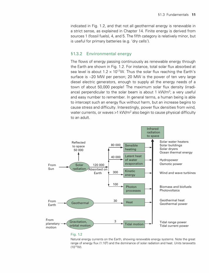
§1.3.2 Environmental energy
The flows of energy passing continuously as renewable energy through the Earth are shown in Fig. 1.2. For instance, total solar flux absorbed at sea level is about 1.2 × 10¹⁷W. Thus the solar flux reaching the Earth’s surface is ~20 MW per person; 20 MW is the power of ten very large diesel electric generators, enough to supply all the energy needs of a town of about 50,000 people! The maximum solar flux density (irradi-ance) perpendicular to the solar beam is about 1 kW/m2; a very useful and easy number to remember. In general terms, a human being is able to intercept such an energy flux without harm, but an increase begins to cause stress and difficulty. Interestingly, power flux densities from wind, water currents, or waves >1 kW/m2 also begin to cause physical difficulty to an adult.
Fig. 1.2Natural energy currents on the Earth, showing renewable energy systems. Note the great range of energy flux (1:105) and the dominance of solar radiation and heat. Units terawatts (1012W).
Reflectedto space50 000
Solarradiation
FromSun
FromEarth
Fromplanetarymotion
120 000Absorbed on
Earth
40 000
80 000 Sensibleheating
Latent heatof waterevaporation
300 Kinetic energy
Photonprocesses
Geothermal30
100
Heat
Gravitation,orbital motion Tidal motion
3
Infraredradiationto space
Solar water heatersSolar buildingsSolar dryersOcean thermal energy
HydropowerOsmotic power
Wind and wave turbines
Biomass and biofuelsPhotovoltaics
Geothermal heatGeothermal power
Tidal range powerTidal current power
TWIDELL PAGINATION.indb 11 01/12/2014 11:35
12 Principles of renewable energy
However, the global data in Fig. 1.2 are of little value for practical engi-neering applications, since particular sites can have remarkably differ-ent environments and possibilities for harnessing renewable energy. Obviously, flat regions, such as Denmark, have little opportunity for hydro-power but may have wind power. Yet neighboring regions (e.g. Norway) may have vast hydro potential. Tropical rain forests may have biomass energy sources, but deserts at the same latitude have none (moreover, forests must not be destroyed, which would make more deserts). Thus, practical renewable energy systems have to be matched to particular local environmental energy flows occurring in a particular region.
§1.3.3 Primary supply to end-use
All energy systems may be visualized as a series of pipes or circuits through which the energy currents are channeled and transformed to become useful in domestic, industrial, and agricultural circumstances. Fig. 1.3(a) and Fig. 1.4 are Sankey diagrams of energy supply, which show the energy flows through a national energy system (often called a ‘spaghetti diagram’ because of its appearance). Sections across such a diagram may be drawn as pie charts showing primary energy supply and energy supply to end-use (Fig. 1.3(b)). Note how the total energy end-use is less than the primary supply due to losses in the transformation pro-cesses, notably the generation of electricity from fossil fuels.
§1.3.4 Energy planning
Certain common principles apply for designing and assessing energy supply and use, whether we are considering energy supply at the level of a nation, a city, or a household.
1 Complete energy systems must be analyzed, and supply should not be considered separately from end-use. Unfortunately, precise needs for energy are too frequently forgotten, and supplies are not well matched to end-use. Energy losses and uneconomic operation there-fore frequently result. For instance, if a dominant domestic energy requirement is heat for warmth or hot water, it is irresponsible to generate grid quality electricity from a fuel, waste the majority of the energy as thermal emission from the boiler and turbine, distribute the electricity with losses, and then dissipate the delivered electricity as heat: a total loss of about 75%! Sadly, such inefficiency, disregard for resources, and unnecessary associated pollution often occur. Heating would be more efficient and cost-effective from direct heat production with local distribution. Even better is to combine electricity genera-tion with the heat production using CHP (combined heat and power (electricity)).
TWIDELL PAGINATION.indb 12 01/12/2014 11:35
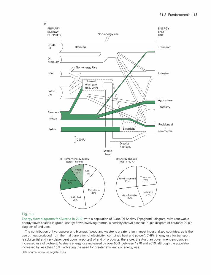
§1.3 Fundamentals 13
Fig. 1.3Energy flow diagrams for Austria in 2010, with a population of 8.4m. (a) Sankey (‘spaghetti’) diagram, with renewable energy flows shaded in green; energy flows involving thermal electricity shown dashed; (b) pie diagram of sources; (c) pie diagram of end uses. The contribution of hydropower and biomass (wood and waste) is greater than in most industrialized countries, as is the use of heat produced from thermal generation of electricity (‘combined heat and power’, CHP). Energy use for transport is substantial and very dependent upon (imported) oil and oil products; therefore, the Austrian government encourages increased use of biofuels. Austria’s energy use increased by over 50% between 1970 and 2010, although the population increased by less than 10%, indicating the need for greater efficiency of energy use.Data source: www.iea.org/statistics.
PRIMARYENERGYSUPPLIES
(a)
Crudeoil
Non-energy use
Non-energy Use
Thermalelec. gen(inc. CHP)
Refining
Oilproducts
Coal
Fossilgas
Biomass+
waste
Hydro
200 PJ
Wasteheat
Districtheat etc.
Electricity
Residential+
commercial
Agriculture+
forestry
Industry
Transport
ENERGYENDUSE
(b) Primary energy supply(total: 1410 PJ)
Coal10%
Fossil gas25%
Bio + waste18%
Hydro10%
Petroleum37%
(c) Energy end-use (total: 1150 PJ)
Resid + comm'l27%
Transport23%
Industry21%Ag + Forestry
29%
TWIDELL PAGINATION.indb 13 01/12/2014 11:35
14 Principles of renewable energy
2 System efficiency calculations can be most revealing and can pin-point unnecessary losses. Here we define ‘efficiency’ as the ratio of the useful energy output from a process to the total energy input to that process. Consider electric lighting produced from ‘conventional’ thermally generated mains electricity and lamps. Successive energy efficiencies would be: electricity generation ~30%, distribution ~90%, and incandescent lighting (energy in visible radiation, usually with a light-shade) 4 to 5%. The total efficiency is about 1 to 1.5%. Contrast this with the cogeneration of useful heat and electricity (energy efficiency ~85%), distribution (~90%), and lighting in modern low-consumption compact fluorescent (CFL) lights (~22%) or light emitting diode (LED) lights (~80%). The total efficiency is now about 17 to 60%, an energy efficiency improvement by factors of 10 to 40! The total life cycle cost of the more efficient system will be much less than for the conventional system, despite higher per unit capital costs, because (i) less generating capacity and fuel are needed, and (ii) equipment (especially lamps) lasts longer (see Problems 1.2 and 1.3).
3 Energy management is always important to improve overall efficiency and reduce economic losses. No energy supply is free, and renewable supplies are capital intensive. Thus, there is no excuse for wasting energy of any form unnecessarily. Efficiency with finite fuels reduces pollution; efficiency with renewables reduces capital costs. Chapters 15, 16, and 17 contain further details and examples.
§1.4 SCIENTIFIC PRINCIPLES OF RENEWABLE ENERGY1
§1.1 and Fig. 1.1 indicate the fundamental differences between renew-able (green) and finite (brown) energy supplies. As a consequence, the efficient use of renewable energy requires the correct application of certain principles; for instance, to realize that the potential for a par-ticular renewable energy supply at a site depends on first understand-ing and quantifying the natural environmental energy flows at that site (e.g. wind speeds, solar irradiance). This usually requires at least a year of measurement, but may be evaluated from established records (e.g. meteorological records). The same is true for the use of wastes (e.g. animal slurry for biogas). Diagrammatically, in Fig. 1.1 the energy current ABC must be assessed before the diverted flow through DEF is established.
TWIDELL PAGINATION.indb 14 01/12/2014 11:35
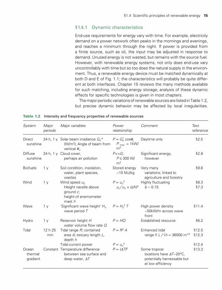
§1.4 Scientific principles of renewable energy 15
§1.4.1 Dynamic characteristics
End-use requirements for energy vary with time. For example, electricity demand on a power network often peaks in the mornings and evenings, and reaches a minimum through the night. If power is provided from a finite source, such as oil, the input may be adjusted in response to demand. Unused energy is not wasted, but remains with the source fuel. However, with renewable energy systems, not only does end-use vary uncontrollably with time but so too does the natural supply in the environ-ment. Thus, a renewable energy device must be matched dynamically at both D and E of Fig. 1.1; the characteristics will probably be quite differ-ent at both interfaces. Chapter 15 reviews the many methods available for such matching, including energy storage; analysis of these dynamic effects for specific technologies is given in most chapters.
The major periodic variations of renewable sources are listed in Table 1.2, but precise dynamic behavior may be affected by local irregularities.
Table 1.2 Intensity and frequency properties of renewable sources
System Major periods
Major variables Power relationship
Comment Text reference
Direct sunshine
24 h, 1 y Solar beam irradiance Gb* (W/m2); Angle of beam from
vertical q z
P ∝ Gb* cosqz
P max. = 1kW/m2
Daytime only §2.5
Diffuse sunshine
24 h, 1 y Cloud cover, perhaps air pollution
P<<G; P ≤ 300 W/
m2
Significant energy, however
§2.8
Biofuels 1 y Soil condition, insolation, water, plant species,
wastes
Stored energy ~10 MJ/kg
Very many variations; linked to
agriculture and forestry
§9.6
Wind 1 y Wind speed u0 Height nacelle above
ground z ; height of anemometer mast h
P ∝ uo3
uz / uh = (z/h)bHighly fluctuating b ~ 0.15
§8.3§7.3
Wave 1 y ‘Significant wave height’ Hs
wave period TP ∝ Hs
2 T High power density ~50kW/m across wave
front
§11.4
Hydro 1 y Reservoir height H water volume flow rate Q
P ∝ HQ Established resource §6.2
Tidal 12 h 25 min
Tidal range R; contained area A; estuary length L,
depth h Tidal-current power
P ∝ R2 A
P ∝ uo3
Enhanced tidal range if L / √h = 36000 m1/2
§12.5§12.3
§12.4Ocean thermal
gradient
Constant Temperature difference between sea surface and
deep water, DT
P ∝ (DT)2 Some tropical locations have DT~20°C,
potentially harnessable but at low efficiency
§13.3
TWIDELL PAGINATION.indb 15 01/12/2014 11:35
16 Principles of renewable energy
Systems range from the very variable (e.g. wind power) to the highly predictable (e.g. tidal power). Sunshine may be highly predictable in some regions (e.g. Sudan) but somewhat random in others (e.g. the UK).
§1.4.2 Quality of supply
We define quality as the proportion of an energy source that can be converted to mechanical work. Thus, electricity has high quality because when consumed in an electric motor, >90% of the input energy may be converted to mechanical work, say, to lift a weight; the heat losses are therefore small: <10%. The quality of nuclear, fossil, or biomass fuel in a single-stage, thermal power station is moderate, because only about 33% of the calorific value of the fuel is transformed into mechanical work and about 67% is lost as heat to the environment. If the fuel is used in a combined cycle power station (e.g. methane gas turbine stage fol-lowed by steam turbine), the quality is increased to ~50%. It is possible to analyze such factors in terms of the thermodynamic variable exergy, defined here as ‘the theoretical maximum amount of work obtainable, at a particular environmental temperature, from an energy source’.
Renewable energy supply systems are divided into three broad classes.
1 Mechanical supplies, such as hydro (Chapter 6) , wind (Chapters 7 and 8), wave (Chapter 11), and tidal power (Chapter 12). The mechan-ical source of power is usually transformed into electricity at high effi-ciency. The proportion of power in the environment extracted by the devices is determined by the operational limits of the process, linked to the variability of the source, as explained in later chapters. The proportions are, typically, wind ~35%, hydro ~80%, wave ~30%, and tidal (range) ~60%. These proportions relate to the capacity factor and load hours of the devices (see §1.5.4 and Table D4 in Appendix D).
2 Heat supplies, such as biomass combustion (Chapter 10) and solar collectors (Chapters 3 and 4). These sources provide heat at high effi-ciency. However, the maximum proportion of heat energy extractable as mechanical work, and hence electricity, is given by the second law of thermodynamics and the Carnot Theorem, which assumes revers-ible, infinitely long transformations. In practice, maximum mechanical power produced in a dynamic process is about half that predicted by the Carnot criteria. For thermal boiler heat engines and internal com-bustion engines, maximum realizable quality is about 35%.
3 Photon processes, such as photosynthesis and photochemistry (Chapter 9) and photovoltaic conversion (Chapter 5). For example, solar photons of a single frequency may be transformed into mechanical work with high efficiency using a matched solar cell. In practice, the broad band of frequencies in the solar spectrum makes matching dif-ficult and photon conversion efficiencies of 25% are considered good.
TWIDELL PAGINATION.indb 16 01/12/2014 11:35
§1.4 Scientific principles of renewable energy 17
§1.4.3 Dispersed versus centralized energy
A pronounced difference between renewable and finite energy sup-plies is the energy flux density at the initial transformation. Renewable energy commonly arrives with a flux density of about 1 kW/m2 (e.g. solar beam irradiance, energy in the wind at 10m/s), whereas finite centralized sources have energy flux densities that are orders of magnitude greater. For instance, boiler tubes in gas furnaces easily transfer 100 kW/m2, and in a nuclear reactor the first wall heat exchanger must transmit several MW/m2. At end-use after distribution, however, supplies from finite sources must be greatly reduced in flux density. Thus, apart from major exceptions such as metal refining, end-use loads for both renew-able and finite supplies are similar. In general, finite energy is most easily ‘produced’2 centrally and is expensive to distribute. Renewable energy is most easily ‘produced’ in dispersed locations and is expensive to concentrate.
Thus, renewable energy technologies encourage dispersed and dis-tributed energy systems. These are installed by companies and utilities, for example, as wind farms (§8.8), tidal current plant (§12.4), sugar cane mills (§9.6), and also as smaller scale microgeneration of heat and/or electricity by individuals, small businesses, and communities as alterna-tives or supplements to traditional centralized grid-connected power. Examples of microgeneration include photovoltaic arrays (§5.3), com-bined heat and power on industrial sites, and biogas on farms (§10.7). A worldwide benefit, especially in developing countries, is that modern renewable energy technologies enable remote communities to enjoy benefits and services (e.g. lighting and telecommunications) previously confined to urban populations. When renewables installations are of a large scale of 500 MW or more (e.g. offshore wind farms, hydro gen-eration, biomass thermal plants), then special transportation and elec-tricity high-voltage transmission lines are needed; often these delivery systems feed the energy to urban complexes.
§1.4.4 Complex (interdisciplinary) systems
Renewable energy supplies are intimately linked to the natural environ-ment, which is not the preserve of just one academic discipline such as physics or electrical engineering. Frequently it is necessary to cross disci-plinary boundaries from as far apart as, say, plant physiology to electronic control engineering. For example, modern sugar cane industries produce not only sugar but also liquid fuel (ethanol). The complete process in a rural society requires input from agricultural science and sociology, as well as chemical, mechanical, and electrical engineering (see Boxes 9.2 and 10.2).
TWIDELL PAGINATION.indb 17 01/12/2014 11:35
18 Principles of renewable energy
§1.4.5 Situation dependence
No single renewable energy system is universally applicable, since the ability of the local environment to supply the energy and the suitability of society to accept the energy vary greatly. It is as necessary to ‘prospect’ the environment for renewable energy as it is to prospect geological formations for oil. Nevertheless, appraising the potential of renewables resources is usually much easier and cheaper than prospecting for oil! It is also necessary to conduct energy surveys of the domestic, agricul-tural, and industrial needs of the local community. Particular end-use needs and local renewable energy supplies may then be matched, subject to economic and environmental constraints. In this respect renewable energy is similar to agriculture. Particular environments and soils are suitable for some crops and not for others, and the market pull for selling the produce will depend upon particular needs. Thus, solar energy systems in southern Italy should be quite different from those in Belgium or indeed in northern Italy. Corn alcohol fuels may be suit-able for farmers in Missouri but not in New England. The consequence is that planning for optimum renewables supply and use tends to apply to regions of distance scale ~250 km, but not 2500 km, because over greater distances supply options are likely to change. Unfortunately, large urban and industrialized societies have built up in ways that are not well suited to such flexibility and variation for optimizing renewables supply and demand.
§1.5 TECHNICAL IMPLICATIONS
§1.5.1 Prospecting the environment
The first step is a rapid appraisal of which renewables sources are in suf-ficient quantities to warrant more detailed monitoring. The order of mag-nitude formulae given in the relevant ‘technology’ chapters suffice for this purpose. Owing to seasonal variations in most renewables options (wet season to dry season or winter to summer), the resource (energy flow) has to be monitored for at least a full year at the site in question. For large-scale projects (e.g. hydro of ~100 MW), a decade or more of data may be needed. Ongoing analysis must ensure that useful data are being recorded, particularly with respect to dynamic characteristics of the energy systems planned. Meteorological data are always important, but unfortunately the sites of official stations are often different from the energy-generating sites, and the methods of recording and analysis are not ideal for energy prospecting. However, an important use of the long-term data from official monitoring stations is as a base for compari-son with local site variations. Thus, wind velocity may be monitored for several months at a prospective generating site and compared with data from the nearest official base station. Extrapolation using many years of
TWIDELL PAGINATION.indb 18 01/12/2014 11:35
§1.5 Technical implications 19
base station data may then be possible. Nevertheless, long-term varia-tions in weather occur, with the debate continuing about how much is due to human-induced climate change.
Data unrelated to normal meteorological measurements may be dif-ficult to obtain. In particular, flows of biomass and waste materials will often not have been previously assessed, and will not have been con-sidered for energy generation. In general, prospecting for supplies of renewable energy requires specialized methods and equipment that demand significant resources of finance and manpower. Fortunately the links with meteorology, agriculture, and marine science give rise to a considerable amount of basic information.
§1.5.2 End-use requirements and efficiency
Since no energy supply is cheap or occurs without some form of envi-ronmental disruption, it is essential to use energy efficiently (often called energy conservation). With electrical systems the end-use requirement is called the load or demand; the size and dynamic characteristics of the generation need to be matched to the load requirements. As explained in Chapter 16, money spent on energy conservation and improvements in end-use efficiency usually give better long-term benefits than money spent on increased generation and supply capacity. The largest energy requirements are usually for heat and transport. Both uses are associ-ated with energy storage capacity in thermal mass, batteries, or fuel tanks, and the inclusion of these components in energy system design can greatly improve overall efficiency.
§1.5.3 Matching supply and demand: energy systems and control mechanisms
After quantification and analysis of the separate dynamic characteris-tics of end-use demands and environmental supply options, the total demand and supply are joined (integrated) as an ‘energy system’. The following outline introduces key concepts of the practical systems dis-cussed in later chapters, including Chapter 15 (which deals in more specific terms with energy grids, energy storage, and energy transmis-sion). Several of the systems relate also to developments of ‘smart’ technology, which are being brought into utility supply of electricity from grid networks. Such smart technology is also important for autonomous systems.
The principles apply in some measure to supplies of heat and fuels, but are immediately applicable to matching electricity supply and demand. Therefore, in Fig. 1.4, we use the electrical symbol of (i) of an unstop-pable ‘current supply’ (two intertwined circles) for renewables sources, since the energy in the environment flows whatever the need; (ii) of a
TWIDELL PAGINATION.indb 19 01/12/2014 11:35
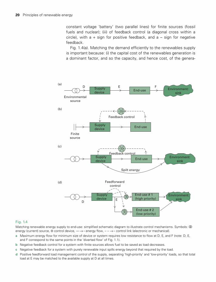
20 Principles of renewable energy
constant voltage ‘battery’ (two parallel lines) for finite sources (fossil fuels and nuclear); (iii) of feedback control (a diagonal cross within a circle), with a + sign for positive feedback, and a – sign for negative feedback.
Fig. 1.4(a). Matching the demand efficiently to the renewables supply is important because: (i) the capital cost of the renewables generation is a dominant factor, and so the capacity, and hence cost, of the genera-
Supplydevice
Supplydevice
Finitesource
Supplydevice
Supplydevice
DE
Feedback control
Feedback control
+
++
++
–
+–
Feedforward control
Spilt energy
End-use
End-use
End-use # 1(high priority)
End-use # 2(low priority)
End-use
Environment:sink
Environment:sink
Environment:sink
Environmentalsource
FD(a)
(b)
(c)
(d)
E
Fig. 1.4Matching renewable energy supply to end-use: simplified schematic diagram to illustrate control mechanisms. Symbols: OO energy (current) source, ⊗ control device, -- → - energy flow, - - → - control link (electronic or mechanical).a Maximum energy flow for minimum size of device or system requires low resistance to flow at D, E, and F (note: D, E,
and F correspond to the same points in the ‘diverted flow’ of Fig. 1.1).b Negative feedback control for a system with finite sources allows fuel to be saved as load decreases. c Negative feedback for a system with purely renewable input spills energy beyond that required by the load. d Positive feedforward load management control of the supply, separating ‘high-priority’ and ‘low-priority’ loads, so that total
load at E may be matched to the available supply at D at all times.
TWIDELL PAGINATION.indb 20 01/12/2014 11:35
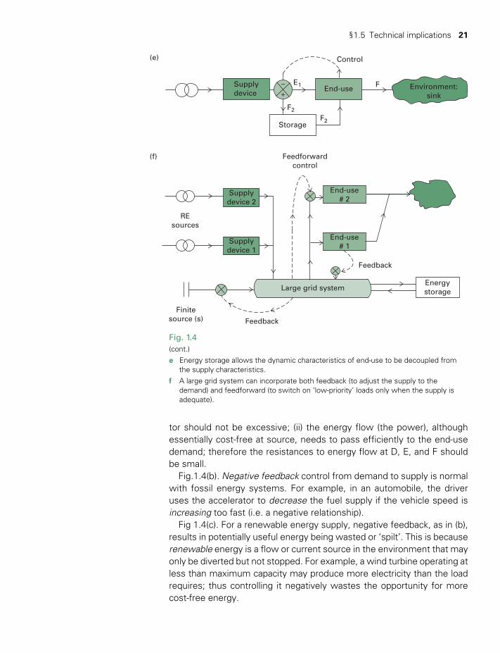
§1.5 Technical implications 21
tor should not be excessive; (ii) the energy flow (the power), although essentially cost-free at source, needs to pass efficiently to the end-use demand; therefore the resistances to energy flow at D, E, and F should be small.
Fig.1.4(b). Negative feedback control from demand to supply is normal with fossil energy systems. For example, in an automobile, the driver uses the accelerator to decrease the fuel supply if the vehicle speed is increasing too fast (i.e. a negative relationship).
Fig 1.4(c). For a renewable energy supply, negative feedback, as in (b), results in potentially useful energy being wasted or ‘spilt’. This is because renewable energy is a flow or current source in the environment that may only be diverted but not stopped. For example, a wind turbine operating at less than maximum capacity may produce more electricity than the load requires; thus controlling it negatively wastes the opportunity for more cost-free energy.
(e)
(f)
Supplydevice
Supplydevice 2
Supplydevice 1
End-use# 2
End-use# 1
End-use
Storage
Feedforwardcontrol
Feedback
REsources
Finitesource (s) Feedback
Large grid systemEnergystorage
Control
E1
+–
F2
F2
F Environment:sink
Fig. 1.4(cont.)e Energy storage allows the dynamic characteristics of end-use to be decoupled from
the supply characteristics. f A large grid system can incorporate both feedback (to adjust the supply to the
demand) and feedforward (to switch on ‘low-priority’ loads only when the supply is adequate).
TWIDELL PAGINATION.indb 21 01/12/2014 11:35
22 Principles of renewable energy
Fig 1.4(d). Here feedforward load management control of the renew-able energy supply separately services ‘high-priority’ and ‘low-priority’ loads. The ‘low-priority’ loads are sized so that automatic adjustments will enable the total load to match the available supply at D at all times. Suitable low-priority loads have storage capacity (e.g. a hot water tank or deep-freeze), or will tolerate interrupted supply (e.g. a clothes washer). The supplier encourages users to connect such loads by offering electric-ity at reduced tariffs. This method is familiar as ‘off-peak’ utility grid elec-tricity, and as with some autonomous systems, such as the wind-based system on the small Scottish Island of Fair Isle (see Box 8.2), and with some mini-hydro systems (§6.6).
Fig. 1.4(e). An obvious way to match supplies and demands that have different dynamic characteristics, and yet not to lose otherwise ‘harness-able’ energy, is to incorporate storage (see Chapter 15).
Fig. 1.4(f). The great majority of renewable energy electricity genera-tors are grid-connected to utility networks. This includes microgenera-tors, so allowing immediate import when the microgenerator supply is insufficient to meet demand and immediate export when there is more than sufficient generation. The result is to decouple local supply from local demand. By so using the grid for both the export and import of energy, the grid becomes a ‘virtual store’. Moreover, there is still the benefit of having switchable loads to optimize the on-site use of the microgeneration.
§1.5.4 Efficiency, capacity factors and resource potential of renewable energy devices
(a) EfficiencyA common question from the public is: ‘How efficient are renewable energy devices, for instance, wind turbines and solar panels?’ However, what appears to be a simple question cannot be answered so easily. Neither is it easy to answer questions like ‘How efficient is that motor car?’ or ‘How efficient is that athlete?, or ‘How efficient is that electric clock?’ Questions like these are never simple, especially as the ques-tioner often means: ‘Is that device cost-effective?’ Suggested responses to a questioner are given as follows.
Does ‘efficiency’ matter? It seems obvious at first sight that techno-logical devices should be ‘efficient’. However, this word means different things to different people about different technologies, as the exam-ples below illustrate for energy generation devices. For a refrigerator, for example, the concept of efficiency includes considering if the volume is sufficient for the needs, if the door opens and closes easily, and if the electricity consumption is acceptable. In practice, many factors are
TWIDELL PAGINATION.indb 22 01/12/2014 11:35
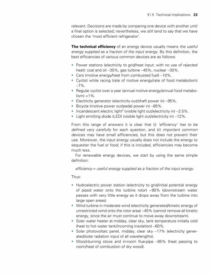
§1.5 Technical implications 23
relevant. Decisions are made by comparing one device with another until a final option is selected; nevertheless, we still tend to say that we have chosen the ‘most efficient refrigerator’.
The technical efficiency of an energy device usually means the useful energy supplied as a fraction of the input energy. By this definition, the best efficiencies of various common devices are as follows:
• Power stations (electricity to grid/heat input; with no use of rejected heat): coal and oil ~35%, gas turbine ~45%, nuclear ~30%.
• Cars (motive energy/heat from combusted fuel) ~10%.• Cyclist while racing (rate of motive energy/rate of food metabolism)
~7%.• Regular cyclist over a year (annual motive energy/annual food metabo-
lism) <1%.• Electricity generator (electricity out/shaft power in) ~95%.• Bicycle (motive power out/pedal power in) ~85%.• Incandescent electric light3 (visible light out/electricity in) ~2.5%.• Light emitting diode (LED) (visible light out/electricity in) ~12%.
From this range of answers it is clear that (i) ‘efficiency’ has to be defined very carefully for each question, and (ii) important common devices may have small efficiencies, but this does not prevent their use. Moreover, the input energy usually does not include the energy to sequester the fuel or food; if this is included, efficiencies may become much less.
For renewable energy devices, we start by using the same simple definition:
efficiency = useful energy supplied as a fraction of the input energy
Thus:
• Hydroelectric power station (electricity to grid/initial potential energy of piped water onto the turbine rotor) ~90% (downstream water passes with very little energy as it drops away from the turbine into large open areas).
• Wind turbine in moderate wind (electricity generated/kinetic energy of unrestricted wind onto the rotor area) ~45% (cannot remove all kinetic energy, since the air must continue to move away downstream).
• Solar water heater at midday, clear sky, tank temperature initially cold (heat to hot water tank/incoming insolation) ~60%.
• Solar photovoltaic panel, midday, clear sky ~17% (electricity gener-ated/solar radiation input of all wavelengths).
• Wood-burning stove and in-room flue-pipe ~85% (heat passing to room/heat of combustion of dry wood).
TWIDELL PAGINATION.indb 23 01/12/2014 11:35
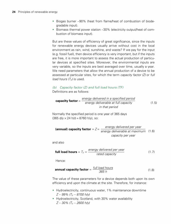
24 Principles of renewable energy
• Biogas burner ~90% (heat from flame/heat of combustion of biode-gradable input).
• Biomass thermal power station ~30% (electricity output/heat of com-bustion of biomass input).
But are these values of efficiency of great significance, since the inputs for renewable energy devices usually arrive without cost in the local environment as rain, wind, sunshine, and waste? If we pay for the input (e.g. fossil fuel), then device efficiency is very important, but if the inputs are free, it is more important to assess the actual production of particu-lar devices at specified sites. Moreover, the environmental inputs are very variable, so the inputs are best averaged over time, usually a year. We need parameters that allow the annual production of a device to be assessed at particular sites, for which the term capacity factor (Z) or full load hours (T F) is used.
(b) Capacity factor (Z) and full load hours (T F )Definitions are as follows:
capacity factor =energy delivered in a specified period
(1.5)energy deliverable at full capacity in that period
Normally the specified period is one year of 365 days (365 d/y × 24 h/d = 8760 h/y), so:
(annual) capacity factor = Z =energy delivered per year
energy deliverable at maximum capacity per year
(1.6)
and also
full load hours = TF = energy delivered per year
rated capacity(1.7)
Hence:
annual capacity factor = full load hours365 h (1.8)
The value of these parameters for a device depends both upon its own efficiency and upon the climate at the site. Therefore, for instance:
• Hydroelectricity, continuous water, 1% maintenance downtime Z ~ 99% (TF ~ 8700 h/y)
• Hydroelectricity, Scotland, with 30% water availability Z ~ 30% (TF ~ 2600 h/y)
TWIDELL PAGINATION.indb 24 01/12/2014 11:35

§1.5 Technical implications 25
• Wind turbine in central Germany (moderate winds) Z~ 18% (TF ~ 1600 h/y)
• Wind turbine in Wellington, New Zealand (‘the windy city’) Z~ 45% (TF ~ 3900 h/y)
• PV tracking solar panel in northern Chile (nearly cloudless) Z~ 40% (TF ~ 3500 h/y)
• PV fixed orientation solar panel, central England (often cloudy) Z~ 10% (TF ~ 880 h/y)
• Biomass combustion for thermal power plant Z ~ 90% (TF ~ 7900 h/y)• Tidal range (barrage) power Z ~ 25% (TF ~ 2200 h/y)• Wave power, vigorous site (potential) Z ~ 30% (TF ~ 2600 h/y)• Tidal stream (current) power (potential) Z ~ 20% (TF ~ 1800 h/y)• Ocean thermal power (OTEC potential) Z ~ 90% (TF ~ 7900 h/y)
Capacity factors are most frequently discussed in the case of electrical power generation, but the concept may be applied more widely. Note that solar devices can only capture sunshine in daytime, so if ‘year’ includes night-time, then Z(solar) is at most 50%, even for a perfect device in an average day of 12 hours.
Note also that values of Z and TF are both independent of the capacity of the device, so if their values for a particular site and technology are considered small, increased output may only be obtained by increas-ing the capacity of the installation. In addition, since the comparison is with the maximum capacity of the device itself, these factors do not in themselves give information about efficiency. They do, however, allow different devices of the same technology to be compared, either by type on the same site or by site with similar devices.
Obviously, manufacturers and device owners try to maximize Z and TF with values that approach the theoretical maxima, but there are usually limitations owing to the particular technology and site and application. Table 1.3 attempts to summarize these factors. Table D4 of Appendix D indicates the range of Z found across the world for a range of technologies.
(c) The resource potentialThe resource potential of a renewable device is the energy it can supply per year. The resource may be estimated at any geographic scale, from a household to the whole world. There are two common measures of resource potential in a geographical area:
1 The theoretical potential is derived from natural and climatic (physical) parameters (e.g. total solar radiation received on a continent’s surface). The ‘natural energy currents’ shown in Fig. 1.2 are an example at global scale. It is the upper limit of what may be produced from an energy resource based on physical principles and current scientific
TWIDELL PAGINATION.indb 25 01/12/2014 11:35
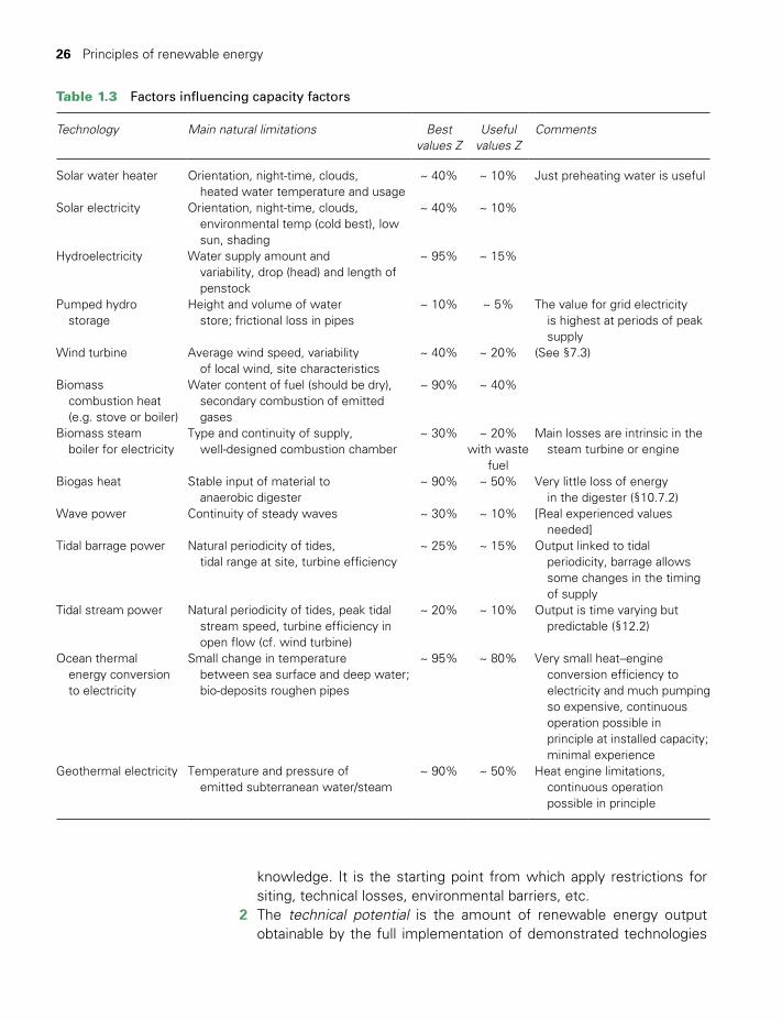
26 Principles of renewable energy
knowledge. It is the starting point from which apply restrictions for siting, technical losses, environmental barriers, etc.
2 The technical potential is the amount of renewable energy output obtainable by the full implementation of demonstrated technologies
Table 1.3 Factors influencing capacity factors
Technology Main natural limitations Best values Z
Useful values Z
Comments
Solar water heater Orientation, night-time, clouds, heated water temperature and usage
~ 40% ~ 10% Just preheating water is useful
Solar electricity Orientation, night-time, clouds, environmental temp (cold best), low
sun, shading
~ 40% ~ 10%
Hydroelectricity Water supply amount and variability, drop (head) and length of
penstock
~ 95% ~ 15%
Pumped hydro storage
Height and volume of water store; frictional loss in pipes
~ 10% ~ 5% The value for grid electricity is highest at periods of peak
supplyWind turbine Average wind speed, variability
of local wind, site characteristics~ 40% ~ 20% (See §7.3)
Biomass combustion heat
(e.g. stove or boiler)
Water content of fuel (should be dry), secondary combustion of emitted
gases
~ 90% ~ 40%
Biomass steam boiler for electricity
Type and continuity of supply, well-designed combustion chamber
~ 30% ~ 20% with waste
fuel
Main losses are intrinsic in the steam turbine or engine
Biogas heat Stable input of material to anaerobic digester
~ 90% ~ 50% Very little loss of energy in the digester (§10.7.2)
Wave power Continuity of steady waves ~ 30% ~ 10% [Real experienced values needed]
Tidal barrage power Natural periodicity of tides, tidal range at site, turbine efficiency
~ 25% ~ 15% Output linked to tidal periodicity, barrage allows
some changes in the timing of supply
Tidal stream power Natural periodicity of tides, peak tidal stream speed, turbine efficiency in
open flow (cf. wind turbine)
~ 20% ~ 10% Output is time varying but predictable (§12.2)
Ocean thermal energy conversion
to electricity
Small change in temperature between sea surface and deep water;
bio-deposits roughen pipes
~ 95% ~ 80% Very small heat–engine conversion efficiency to
electricity and much pumping so expensive, continuous operation possible in principle at installed capacity; minimal experience
Geothermal electricity Temperature and pressure of emitted subterranean water/steam
~ 90% ~ 50% Heat engine limitations, continuous operation
possible in principle
TWIDELL PAGINATION.indb 26 01/12/2014 11:35

§1.7 Social implications 27
or practices in the specified region. No explicit reference is made to costs, institutional policies, or other man-made barriers that may limit take-up of the technology. From the technical potential, more practical estimates can be made allowing for other constraints (e.g. avoiding sites of scientific/ecological value, prioritizing biomass for food use ahead of its use for energy, applying cost limits, etc.).
See Verbruggen et al. (2014) for a detailed discussion of these and other related concepts.
Estimates of technical potential are given in later chapters of this book. Numerous man-made barriers are discussed in Chapter 17.
Several other indicators are discussed in Chapter 15 and tabulated in Appendix D.
§1.6 STANDARDS AND REGULATIONS
Renewable energy developments and equipment are major aspects of business and economies, which, as with so much else, benefit from having agreed national and international standards and regulations. Financiers (e.g. banks) and insurers require that all equipment meets national and international standards. For instance, safety is always a prime concern, so there are many requirements associated with the design and construction of renewable energy equipment (e.g. wind turbine braking and the electrical insulation of photovoltaic modules). Safety and other government regulations are part of the institutional framework for energy systems, which is discussed in Chapter 17.
The IEC (International Electrochemical Commission) is the inter-national body that oversees many standards in all disciplines; it has a special section for renewable energy (see <http://www.iec.ch/renewa-bles/ >), but of course many standards are common to a wider range of technology.
§1.7 SOCIAL IMPLICATIONS
The Industrial Revolution in Europe and North America, as well as industrial development in all countries, have profoundly affected social structures and patterns of living. The influence of energy sources is a driving function for such change. For instance, there is a historic relation-ship between coal-mining and the development of industrialized coun-tries. Norway and other similar countries have been greatly influenced by hydropower. Denmark has found a major industry in wind turbine manufacture. In the non-industrialized countries, relatively cheap oil sup-plies became available in the 1950s at the same time as many countries obtained independence from colonialism, so providing energy for their development. Thus, in all countries, energy generation and its use have
TWIDELL PAGINATION.indb 27 01/12/2014 11:35

28 Principles of renewable energy
led to profound changes in wealth and lifestyle. The need for secure energy supplies is obvious, and supplies from a country’s own resources support such security, in particular the renewable energy technologies applicable in each country.
§1.7.1 Dispersed living
In §1.1 and §1.4.3 the dispersed and low energy flux density of renew-able sources was discussed. Renewable energy arrives dispersed in the environment and is difficult and expensive to concentrate. By contrast, finite energy sources are energy stores that are easily concentrated at source and expensive to disperse. Thus, electrical distribution grids from fossil fuel and nuclear sources have tended to radiate from central, inten-sive distribution points, typically with ~1000 MW capacity. Industry has developed on these grids, with heavy industry closest to the points of intensive supply. Domestic populations have grown in response to the employment opportunities of industry and commerce. Similar effects have occurred with the relationships between coal-mining and steel pro-duction, oil refining and chemical engineering, and the availability of gas supplies and urban complexes.
This physical review of the effect of the primary flux density of energy sources suggests that the widespread application of renewable energy will favor dispersed, rather than concentrated, communities. Links with agriculture are likely to be important. Electricity grids in such situations may have input from smaller scale, embedded generation (i.e. ‘micro-generation’) and larger scale commercial developments of wind and solar farms, of generation from biomass and wastes, and of marine energy technology. On such grids, power flows variably in both directions according to local generation and local demand. Some renewable energy sources, notably solar, are suited to microgeneration in both urban and rural areas. Others (e.g. biomass) rely on energy flows that are generally more accessible in rural areas. Regions near the sea have in practice many opportunities for power generation (e.g. from waves, tides, and offshore wind farms).
Nevertheless, more than half of the world’s population now live in urban areas (including at least 40% of the populations of Africa and Asia, which were still largely rural 30 years ago), and to date this proportion continues to increase. Modern renewable energy technology can serve the cities in which most people now live, not only through microgenera-tion and smart grids (§15.4.3) but also through the large-scale harnessing of hydropower, wind power, and bioenergy at sites where those energy flows are plentiful and with modern means of transmitting energy, as outlined in Chapter 15. Thus, RE will be important to future populations, both urban and rural.
TWIDELL PAGINATION.indb 28 01/12/2014 11:35

§1.7 Social implications 29
§1.7.2 Pollution and environmental impact
Harmful emissions may be classified as chemical (as from fossil fuel and nuclear power plant), physical (including acoustic noise and radioactivity), and biological (including pathogens).
Such pollution from energy systems is overwhelmingly a result of using ‘brown’ fuels, both fossil and nuclear. This applies in particular to the greenhouse gas (GHG) emissions, which are a major cause of potentially dangerous climate change. As pointed out in §1.2.1 and further discussed in Chapter 17, reducing GHG emissions is one of the major driving forces behind the growing demand for renewables technologies.
Renewable energy is always extracted from flows of energy already compatible with the environment (Fig. 1.1). The energy is then returned to the environment, so no thermal pollution can occur on any-thing but a small scale. Likewise, material and chemical pollution in air (and, in particular, GHG emissions), water, and refuse tend to be minimal. An exception is air pollution from the incomplete combus-tion of biomass or refuses (see Chapter 10). Environmental pollution does occur if brown energy is used for the materials and manufac-ture of renewable energy devices, but this is small over the lifetime of the equipment and will decrease in proportion to the adoption of renewables.
The majority of renewable technologies produce significantly fewer conventional air and water pollutants than fossil fuels, but neverthe-less impact upon the environment by being sited within large areas of land as, for example, reservoir hydropower (which can also release methane from submerged vegetation) and biofuels. Some renewables, especially wind power, do not interrupt the regular use of land for agri-culture or recreation. In contrast, fossil fuel mining (especially of coal and uranium) has very negative impacts upon the surrounding land and its use.
There may also be some impacts upon water resources. For example, limited water availability for cooling thermal power plants decreases their efficiency, which can affect plants operating on coal, biomass, gas, nuclear, and concentrating solar power. There have been significant power reductions from nuclear and coal plants during periodic droughts in the USA and France. However, electricity production from wind and solar PV requires very little water compared to thermal conversion tech-nologies, and has no impacts upon water quality.
The environmental impact of a renewable energy system depends on the particular technology and circumstances. We consider these aspects in the final section of each technology chapter. General institutional factors, often related to the abatement of pollution, are considered in Chapter 17.
TWIDELL PAGINATION.indb 29 01/12/2014 11:35
30 Principles of renewable energy
§1.7.3 The future
We know that many changes in social patterns are related to energy supplies. We may expect further changes to occur as renewable energy systems become even more widespread. The influence of modern science and technology ensures that there are considerable improve-ments to older technologies, and subsequently standards of living can be expected to rise, especially in rural and previously less developed regions. It is impossible to predict exactly the long-term effect of such changes in energy supply, but the sustainable nature of renewable energy should produce greater socioeconomic stability than has been the case with fossil fuels and nuclear power. In particular we expect the great diversity of renewable energy supplies to be associated with a similar diversity in local economic and social characteristics. We certainly agree with one of the major conclusions of IPCC (2011), namely:
There are few, if any, technical limits to the planned integration of renewable energy technologies across the very broad range of present energy supply systems worldwide, though other barriers [e.g. economic and institutional] may exist.
Future prospects for renewable energy are further discussed in the concluding section (§17.8) of this book.
CHAPTER SUMMARY
Renewable energy is energy obtained from natural and persistent flows of energy occurring in the immediate environment. Examples of such energy flows include solar radiation, wind, falling water, biomass, and ocean tides.
Sustainable development means living, producing, and consuming in a manner that meets the needs of the present without compromising the ability of future generations to meet their own needs. A major threat to sustainable development is climate change caused by greenhouse gases emitted from fossil fuels. This and the finite nature of fossil and nuclear fuel materials make it essential to expand renewable energy supplies and to use energy more efficiently.
Comparison of the energy required per person with the natural energy flows from the Sun and other renewable sources suggests that renewable energy supplies may provide a satisfactory standard of living for all, but only if methods exist to extract, use, and store the energy satisfactorily at realistic costs.
Failure to understand the distinctive scientific principles for harnessing renewable energy will almost certainly lead to poor engineering and uneconomic operation. Energy supply should not be considered separately from end-use. Energy management is important to improve overall efficiency and reduce economic losses. Efficiency with finite fuels reduces pollution; efficiency with renewables reduces capital costs. With renewable energy systems, not only does consumers’ end-use vary uncontrollably with time but so too does much of the natural supply in the environment. Renewable energy commonly arrives at about 1 kW/m2, whereas finite centralized sources have much greater energy flux densities; therefore, renewables generation and supply will be spread over dispersed areas and situations.
TWIDELL PAGINATION.indb 30 01/12/2014 11:35

Problems 31
QUICK QUESTIONS
Note: Answers are in the text of the relevant sections of this chapter, or may be readily inferred from them.
1 Considering primary resources, what distinguishes renewable energy from fossil and nuclear fuels?
2 Other than price, what other factors influence the acceptance of an energy supply?
3 Compare the per capita energy consumption of your own country with two countries in other continents.
4 Name five independent ultimately primary sources of energy. 5 Compare the energy consumption per unit of useful light of incan-
descent, fluorescent, and light emitting diode lights. 6 Explain the thermodynamic ‘quality’ of an energy supply and how
this affects its use. 7 What is ‘smart’ technology and how can it benefit the uptake and use
of renewable energy? 8 What is capacity factor and how does it relate to full load hours per
year? 9 What is ‘energy security’? Compare this for fossil fuels, nuclear
power, and renewable energy.10 Compare the environmental impact (including noise and pollution) of
energy generation from fossil fuels, nuclear power, and renewable energy.
PROBLEMS
1.1 (a) Show that the average solar irradiance absorbed during 24 hours over the whole of the Earth’s surface is about 230 Wm-2 (see Fig. 1.2).
For individuals, modern renewable energy technologies encourage self-generation and local energy systems (microgeneration). Modern renewable energy technology can serve not only rural areas, but also the cities in which most people now live, through microgeneration and smart grids. Larger scale harnessing of hydropower, wind power, and bioenergy at sites where those energy flows are plentiful utilizes modern means of transmitting and delivering the energy to urban complexes and larger industry. Historical precedent suggests that the major growth of renewables will influence social structures and national economies.
The first step in designing a renewable energy supply is the rapid appraisal of which renewable sources are in sufficient quantities to warrant more detailed monitoring. Owing to seasonal variations in most RE flows, good engineering design requires monitoring of the resource for at least a full year at the site in question.
TWIDELL PAGINATION.indb 31 01/12/2014 11:35

32 Principles of renewable energy
(b) Using devices, the average local power accessible can be increased e.g. by tilting solar devices towards the Sun and by intercepting winds. Is it reasonable to state that ‘each square metre of the Earth’s habitable surface is crossed or accessible to an average flux of about 500W’?
1.2 Compare the direct costs to the consumer of using:
(a) a succession of ten 100 W incandescent light bulbs with an efficiency for electricity to visible light of 5%, life of 1000 hours, price 0.5 Euro;
(b) one compact fluorescent lamp (CFL) giving the same illumina-tion at 22% efficiency, life of 10,000 hours, price 3.0 Euro: use a fixed electricity price of 0.10 E/kWh;
(c) Calculate the approximate payback time in lighting hours of (b) against (a). (See also Problem 17.1 which allows for the more sophisticated discounted costs.)
1.3 Repeat the calculation of problem 1.2, with prices of your local lamps and electricity. Both the price of CFLs in local shops and of electricity vary markedly, so your answers may differ significantly. Nevertheless, it is highly likely that the significant lifetime savings will still occur.
The following Problems, marked * are particularly suitable for class discussion:
*1.4 Economists argue that as supplies of oil reserves grow less, the price will go up, so that demand falls and previously uneconomic supplies would come into production. This tends to make the resource last longer than would be suggested by a simple calcu-lation (based on ‘today’s reserves’ divided by ‘today’s use’) . On the other hand, demand increases driven by increased economic development in developing countries tend to shorten the life of the reserve. Discuss.
*1.5 Is your lifestyle sustainable? If not, what changes would make it so?
*1.6 Can we expect renewable energy supplies to be universally appli-cable? Clarify your answer by explaining which renewables are most applicable in your home area.
*1.7 Predict the energy supplies in 30 years’ time for the region where you live and explain why changes may have occurred.
TWIDELL PAGINATION.indb 32 01/12/2014 11:35
Bibliography 33
NOTES
1 Readers who encounter an occasional technical term unfamiliar to them which is not explained in the sur-rounding text are advised to consult the Index for further guidance.
2 Although ‘energy production’ is the industry-standard word, it is a fundamental physical principle that energy can only be transformed from one form to another, not ‘produced’.
3 Efficiency and efficacy of lighting are complex with various definitions; ballpark dimensionless figures are given here; for more details, see http://en.wikipedia.org/wiki/Luminous_efficacy.
BIBLIOGRAPHY
Refer to the bibliographies at the end of each chapter for particular subjects.
Surveys of renewable energy technology and resources
Boyle, G. (ed.) (2012, 3rd edn) Renewable Energy: Power for a sustainable future, Oxford University Press, Oxford. Excellent introduction for both scientific and non-scientific readers.
IPCC (2011) O. Edenhofer, R. Pichs-Madruga, Y. Sokona, K. Seyboth, P. Matschoss, S. Kadner, T. Zwickel, P. Eickemeier, G. Hansen, S. Schlömer and C. von Stechow (eds), IPCC Special Report on Renewable Energy Sources and Climate Change Mitigation, Cambridge University Press, Cambridge. (Full text available at http://srren.ipcc-wg3.de/report.) Authoritative review of the state of the art of individual technologies and of current usage and future prospects for RE. On principles, see especially ch. 1. Also includes a useful Glossary.
Kishore, V.V.N (ed.) (2009) Renewable Energy Engineering and Practice, Earthscan, Abingdon. Another multi-author tome (~900 pages); more advanced level than this book, as ‘aimed at practioners’.
Kreith, F. and Goswami, D.Y. (eds) (2007) Handbook of Energy Efficiency and Renewable Energy, CRC Press, London. Door-stopping multi-author work (>1000 pages!), comprehensive and detailed, but still readable, though sometimes with US emphasis.
Sørensen, B. (2011, 4th edn) Renewable Energy, Academic Press, London. Outstandingly the best theoretical text at postgraduate level, considering energy from the environment to final use.
Tester, J.W., Drake, E., Driscoll, M., Golay, M. and Peters, W. (2012, 2nd edn) Sustainable Energy: Choosing among options, MIT Press, Cambridge, MA. Wide-ranging text, including chapters not only on individual RE technologies but also fossil fuels, and nuclear power, and global environment, economics, and energy systems.
Energy, society, and the environment (including ‘sustainable development’)
See also the bibliography for Chapter 17.
Cassedy, E.S. and Grossman, P.G. (2002, 2nd edn) Introduction to Energy: Resources, technology and society, Cambridge University Press, Cambridge. Good non-technical account for ‘science and society’ courses.
Elliott, D. (ed.) (2010) Sustainable Energy: Opportunities and limitations, Palgrave Macmillan, Basingstoke. Brief survey of technologies, but more extensive discussion of institutional and societal aspects; UK focus.
Everett, R., Boyle, G., Peake, S. and Ramage, J. (eds) (2011, 2nd edn) Energy Systems and Sustainability: Power for a sustainable future, Oxford University Press, Oxford. Good non-technical account for ‘science and society’ courses.
TWIDELL PAGINATION.indb 33 01/12/2014 11:35

34 Principles of renewable energy
Goldemberg, J. and Lucon, J. (2009, 2nd edn) Energy, Environment and Development, Routledge, London. Wide-ranging and readable exposition of the links between energy and social and economic development and sustainability, with consideration of equity within and between countries by Brazilian experts.
Houghton, J.T. (2009, 4th edn) Global Warming: The complete briefing, Cambridge University Press, Cambridge. Straightforward and didactic. Harmonises with the official IPCC Reports (Houghton was Chair of IPCC).
Intergovernmental Panel on Climate Change (IPCC) Fifth Assessment Report (2014). See also the IPCC Fourth Assessment Report (2007), especially its ‘Summary for Policy Makers: Synthesis report’. See IPCC website listed below; the full report is in three large volumes, published by Cambridge University Press.
McNeill, J.R. (2000) Something New under the Sun: An environmental history of the twentieth century, Penguin, London. The growth of fossil fuel-fired cities and their impacts on water, air, and the biosphere.
Von Weizsacker, E., Lovins, A.B. and Lovins, H. (2000) Factor Four: Doubling wealth, halving resource use, Penguin, London. Explores the wider social and political issues of energy supply, especially those associated with renewable and nuclear supplies.
World Commission on Environment and Development (1987) Our Common Future, Oxford University Press, Oxford (the ‘Bruntland Report’). A seminal work, warning about the key issues in plain language for politicians.
Official publications (including energy statistics and projections)
See also below under journals and websites, as many official publications, especially those of a statistical nature, are updated every year or two.
United Nations agencies produce a wide range of essential publications regarding energy, nearly all of which are freely downloadable. These are especially important for data. For instance, we recommend the following:
United Nations World Energy Statistics Yearbook, annual. Gives statistics of energy consumption around the world, classified by source, country, continent, etc., but counts only ‘commercial energy’ (i.e. excludes firewood, etc.). Online (with much other energy data) at http://unstats.un.org/unsd/energy/.
Government publications are always important; see e.g. the UK Department of Energy Series of Energy Papers. Such publications are usually clearly written and include economic factors at the time of writing. Basic principles are covered, but usually without the details required for serious study. (Annual updates of many government and UN publications are also available through the corresponding websites.)
World Energy Council (2001) Survey of World Energy Resources. Compiled every five years or so by the WEC, which comprises mainly energy utility companies from around the world; covers both renewable and non-renewable resources.
International Energy Agency, World Energy Outlook (annual), Paris. Focus is on fossil fuel resources and use, based on detailed projections for each member country, and for those non-member countries which are signifi-cant in world energy markets (e.g. OPEC and China). IEA Energy statistics are freely available online at www.iea.org/statistics/.
Do-it-yourself publications
There are many publications available to the general public and enthusiasts, mostly focused on one particular RE technology. Do not ignore these, but take care if the tasks are made to look easy. Many of these publications give stimulating ideas and are attractive to read.
TWIDELL PAGINATION.indb 34 01/12/2014 11:35

Bibliography 35
Specific reference
Verbruggen, A., Fischedick, M., Moomaw, W., Weir, T., Nadai, A., Nilsson, L.A., Nyboer, J. and Sathaye, J. (2010) ‘Renewable energy costs, potentials, barriers: Conceptual issues’, Energy Policy, 38, 850–861 (February), DOI: 10.1016/j.enpol.2009.10.036.
Journals, trade indexes, and websites
Renewable energy and, more generally, energy technology and policy are continually advancing. For serious study it is necessary to refer from time to time to the periodical literature (journals and magazines). Websites of key organizations, such as those listed below, also carry updates of some of the key references, especially those of a statistical nature.
We urge readers to scan the serious scientific and engineering journals (e.g. New Scientist, Annual Review of Energy and the Environment), and magazines (e.g. Electrical Review, Modern Power Systems, Renewable Energy World). These publications regularly cover renewable energy projects among their general articles. The magazine Renewable Energy Focus, published for the International Solar Energy Society, carries numerous well-illustrated articles on all aspects of renewable energy. The series Advances in Solar Energy, published by the American Solar Energy Society, comprises annual volumes of high-level reviews, including all solar tech-nologies and some solar-derived technologies (e.g. wind power and biomass). There are also many specialist and academic journals, such as Renewable and Sustainable Energy Reviews, Solar Energy, Wind Engineering, Renewable Energy, and Biomass and Bioenergy, referred to in the relevant chapters.
As renewable energy has developed commercially, many indexes of companies and products have been pro-duced; most are updated annually (e.g. European Directory of Renewable Energy Supplies and Services, annual, ed. B. Cross, James and James, London).
www.iea.orgThe International Energy Agency (IEA) comprises the governments of about 20 industrialized countries; its publications cover policies, energy statistics, and trends, and to a lesser extent technologies; it also coordinates and publishes much collaborative international R&D, including clearly written appraisals of the state of the art of numerous renewable energy technologies. Its publications draw upon detailed inputs from member countries.
www.irena.orgThe International Renewable Energy Agency was founded in 2009 as an intergovernmental agency to promote renewable energy. Produces many useful reports.
www.worldenergy.orgThe World Energy Council comprises mainly energy utility companies from around the world, who cooperate to produce surveys and projections of resources, technologies, and prices.
www.ipcc.chThe Intergovernmental Panel on Climate Change (IPCC) is a panel of some 2000 scientists convened by the United Nations to report on the science, economics, and mitigation of greenhouse gases and climate change; their reports, issued every five years or so, are regarded as authoritative. Summaries are available on the website.
www.practicalaction.orgFormerly known as ITDG, the Intermediate Technology Development Group. Develops and promotes simple and cheap but effective technology – including renewable energy technologies – for use in rural areas of developing countries. They have an extensive publication list plus online ‘technical briefs’.
TWIDELL PAGINATION.indb 35 01/12/2014 11:35

36 Principles of renewable energy
www.ewea.orgThe European Wind Energy Association is one of many renewable energy associations, all of which have useful websites. Most such associations are ‘trade associations’, as funded by members in the named renewable energy industry. However, they are aware of the public and educational interest, and so have information and give connections for specialist information.
www.ren21.netThe Renewable Energy policy network. See especially their annual Global Status Report.
TWIDELL PAGINATION.indb 36 01/12/2014 11:35
Solar radiation and the greenhouse effect
CHAPTER
2
CONTENTS
Learning aims 38§2.1 Introduction 39§2.2 Extra-terrestrial solar radiation 40§2.3 Components of radiation 41§2.4 Geometry of the Earth and the Sun 42
§2.4.1 Definitions 42§2.4.2 Latitude, season, and daily
insolation 44§2.5 Geometry of the collector
and the solar beam 46§2.5.1 Definitions 46§2.5.2 Angle between beam and
collector 47§2.5.3 Optimum orientation of
a collector 48§2.5.4 Hourly variation of irradiance 49
§2.6 Atmospheric transmission, absorption and reflection 49§2.6.1 Reflection 51§2.6.2 Air–mass ratio 52§2.6.3 Sky temperature 56§2.6.4 Solar spectrum received at
the Earth’s surface 56§2.7 Measuring solar radiation 57§2.8 Site estimation of solar radiation 57
§2.8.1 Requirements 57§2.8.2 Statistical variation 58§2.8.3 Sunshine hours as a measure
of insolation 59
§2.8.4 Geostationary Operational Environmental Satellites (GOES) 59
§2.8.5 Focusable beam radiation and the Clearness Index 60
§2.8.6 Effect of collector inclination 60
§2.9 Greenhouse effect and climate change 62§2.9.1 Radiative balance of
the Earth 62§2.9.2 The greenhouse effect,
radiative forcing, and climate change 63
§2.9.3 Climate change: observations 64§2.9.4 Climate change: projections,
impacts, and mitigation 67
Chapter summary 68
Quick questions 68
Problems 69
Notes 72
Bibliography 72
Box 2.1 Radiation transmitted, absorbed and scattered by the Earth’s atmosphere 55
Box 2.2 Units of gas concentration 65
Box 2.3 Why we know that recent increases in CO2 and in temperature are due to human activity (anthropogenic) 66
TWIDELL PAGINATION.indb 37 01/12/2014 11:35
38 Solar radiation and the greenhouse effect
LEARNING AIMS
• Appreciate solar radiation’s effect on the Earth’s temperature.
• Sketch the solar spectrum at source and at the Earth’s surface.
• Identify key processes in solar radiation absorption in the atmosphere, and how this implies the two spectral ‘windows’ in the Earth’s atmosphere.
• Outline the basic and enhanced greenhouse effects.
• Name measurement methods and instrumen-tation for solar radiation.
• Estimate solar irradiance (Wm-2) and daily insolation (MJm-2day-1) at any location and season.
LIST OF FIGURES
2.1 Spectral distribution of extra-terrestrial solar irradiance, G*0λ. 402.2 Origin of direct beam and diffuse radiation. 412.3 Techniques to measure various components of solar radiation. 422.4 Definition sketch for latitude f and longitude y (see text for detail). 422.5 The Earth revolving around the Sun. 432.6 The Earth, as seen from a point further along its orbit. 442.7 Variation with season and latitude of Hh, the solar energy (daily insolation) received on a horizontal
plane on a clear day. 452.8 Cross-sections through the Earth at solar noon. 462.9 Zenith angle, angle of incidence, slope and azimuth angle for a tilted surface. 472.10 (a) Irradiance on a horizontal surface (b) Typical variation of irradiance on a horizontal surface for
a day of variable cloud. 502.11 Effects occurring as extra-terrestrial solar radiation passes through the Earth’s atmosphere. 512.12 Estimate of the Earth’s annual and global mean energy balance. 522.13 Radiation transmitted and absorbed by the atmosphere as a function of wavelength. 542.14 Air–mass ratio m = sec θz. 542.15 Spectral distributions of solar irradiance. 562.16 Photographs of various solar instruments. 582.17 Fraction of diffuse irradiation plotted against the Clearness Index for a wide range of hourly
field data. 612.18 Variation in estimated average daily insolation on a surface at various slopes. 622.19 Observations of GHGs and their physical effect. 66
TWIDELL PAGINATION.indb 38 01/12/2014 11:35
§2.1 Introduction 39
§2.1 INTRODUCTION
This chapter explains how solar radiation links the Earth with the Sun and how the Earth’s atmosphere controls this energy flux. Later chap-ters show how the received solar radiation (sometimes called insolation) powers renewable energy devices.
The main aim of this chapter is to calculate the insolation available as input to a solar device at a specific location, orientation, and time.
Solar radiation reaches the Earth’s surface at a maximum flux density (irradiance) of about 1.0 kW/m2 in a wavelength band between 0.3 and 2.5 mm. The spectral distribution is determined by the ~6000 K surface temperature of the Sun; it is called shortwave radiation and includes the visible spectrum. This solar irradiance at ground level varies from about 3 to 30 MJ/(m2 day), depending on place, time, and weather. Its ‘ thermodynamic quality’ relates to the extreme ‘white-hot temper-ature’ of the source and so is much greater than from conventional engineering sources. The flux may be used both thermally e.g. for heat engines (see §4.8) and for photophysical and photochemical processes i.e. photovoltaic electricity and the photosynthesis of biomass (see Chapters 5 and 9).
How radiation is transmitted through a cloudless atmosphere depends on (a) the frequency of the radiation, and (b) the radiation absorptance of the gases and vapours present. Consequently, gases (including water vapor) in the atmosphere cause the Earth’s surface temperature to increase on average about 30°C more than with no atmosphere (see §2.9.1). These transmission and absorption characteristics of the atmosphere have simi-larities with glass, so the extra warming is called the ‘greenhouse effect’, and the gases concerned are called greenhouse gases (GHGs).
The greenhouse effect is a natural characteristic of the Earth, and of crucial importance for global sustained ecology, because the ‘normal’ temperature increase allows most surface water to be liquid rather than solid. However, the magnitude of the greenhouse effect depends critically upon the atmospheric concentration GHGs, in particular H2O and CO2.
However, the continuing rapid utilization of fossil fuels in the past 200 years has caused atmospheric CO2 concentration to increase well beyond levels found in the previous million years. Such externally imposed changes perturb the Earth system’s radiation balance by radia-tive forcing (i.e. an effective net increase in total irradiance caused by an added atmospheric component).
As authoritatively documented, for example, by IPCC (2007), this is forcing an increase in the mean temperature at the Earth’s surface, so precipitating climate change (see §2.9). Replacing fossil fuels with renewable energy reduces this forcing, so reducing the likelihood of harmful social and environmental effects (see §1.2 and Box 17.1).
TWIDELL PAGINATION.indb 39 01/12/2014 11:35
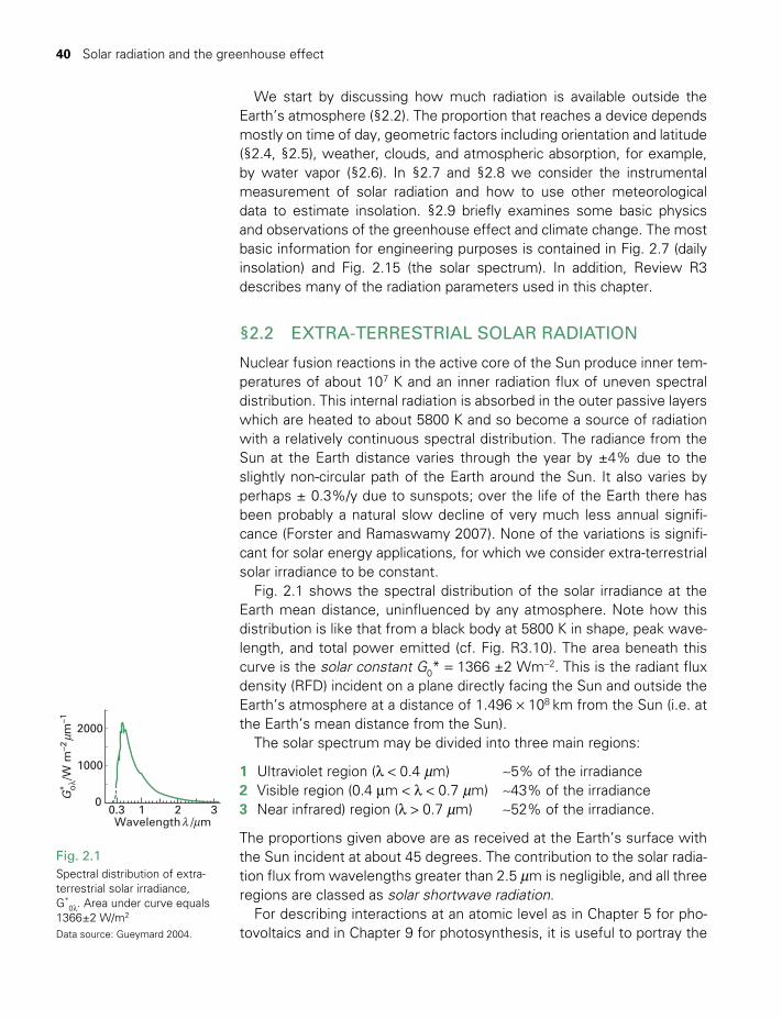
40 Solar radiation and the greenhouse effect
We start by discussing how much radiation is available outside the Earth’s atmosphere (§2.2). The proportion that reaches a device depends mostly on time of day, geometric factors including orientation and latitude (§2.4, §2.5), weather, clouds, and atmospheric absorption, for example, by water vapor (§2.6). In §2.7 and §2.8 we consider the instrumental measurement of solar radiation and how to use other meteorological data to estimate insolation. §2.9 briefly examines some basic physics and observations of the greenhouse effect and climate change. The most basic information for engineering purposes is contained in Fig. 2.7 (daily insolation) and Fig. 2.15 (the solar spectrum). In addition, Review R3 describes many of the radiation parameters used in this chapter.
§2.2 EXTRA-TERRESTRIAL SOLAR RADIATION
Nuclear fusion reactions in the active core of the Sun produce inner tem-peratures of about 107 K and an inner radiation flux of uneven spectral distribution. This internal radiation is absorbed in the outer passive layers which are heated to about 5800 K and so become a source of radiation with a relatively continuous spectral distribution. The radiance from the Sun at the Earth distance varies through the year by ±4% due to the slightly non-circular path of the Earth around the Sun. It also varies by perhaps ± 0.3%/y due to sunspots; over the life of the Earth there has been probably a natural slow decline of very much less annual signifi-cance (Forster and Ramaswamy 2007). None of the variations is signifi-cant for solar energy applications, for which we consider extra-terrestrial solar irradiance to be constant.
Fig. 2.1 shows the spectral distribution of the solar irradiance at the Earth mean distance, uninfluenced by any atmosphere. Note how this distribution is like that from a black body at 5800 K in shape, peak wave-length, and total power emitted (cf. Fig. R3.10). The area beneath this curve is the solar constant G0* = 1366 ±2 Wm-2. This is the radiant flux density (RFD) incident on a plane directly facing the Sun and outside the Earth’s atmosphere at a distance of 1.496 × 10⁸ km from the Sun (i.e. at the Earth’s mean distance from the Sun).
The solar spectrum may be divided into three main regions:
1 Ultraviolet region (λ < 0.4 mm) ~5% of the irradiance2 Visible region (0.4 mm < λ < 0.7 mm) ~43% of the irradiance3 Near infrared) region (λ > 0.7 mm) ~52% of the irradiance.
The proportions given above are as received at the Earth’s surface with the Sun incident at about 45 degrees. The contribution to the solar radia-tion flux from wavelengths greater than 2.5 mm is negligible, and all three regions are classed as solar shortwave radiation.
For describing interactions at an atomic level as in Chapter 5 for pho-tovoltaics and in Chapter 9 for photosynthesis, it is useful to portray the
2000
1000
00.3 1Wavelength / m
G* o
λ/W
m–2
m
–1
µ
2 3λ µ
Fig. 2.1Spectral distribution of extra-terrestrial solar irradiance, G*
0λ. Area under curve equals 1366±2 W/m2
Data source: Gueymard 2004.
TWIDELL PAGINATION.indb 40 01/12/2014 11:35
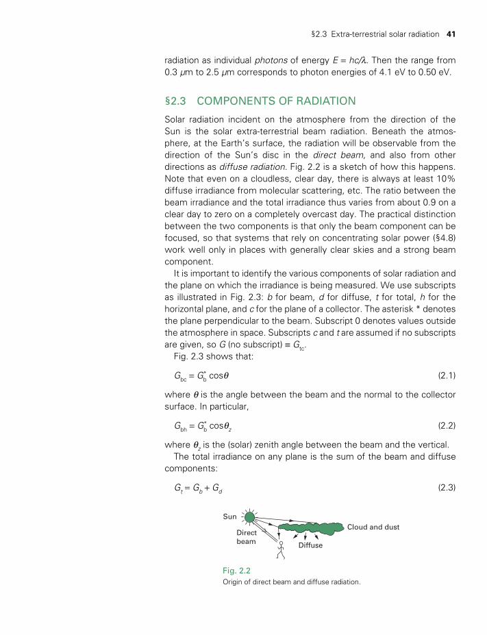
§2.3 Extra-terrestrial solar radiation 41
radiation as individual photons of energy E = hc/λ. Then the range from 0.3 μm to 2.5 μm corresponds to photon energies of 4.1 eV to 0.50 eV.
§2.3 COMPONENTS OF RADIATION
Solar radiation incident on the atmosphere from the direction of the Sun is the solar extra-terrestrial beam radiation. Beneath the atmos-phere, at the Earth’s surface, the radiation will be observable from the direction of the Sun’s disc in the direct beam, and also from other directions as diffuse radiation. Fig. 2.2 is a sketch of how this happens. Note that even on a cloudless, clear day, there is always at least 10% diffuse irradiance from molecular scattering, etc. The ratio between the beam irradiance and the total irradiance thus varies from about 0.9 on a clear day to zero on a completely overcast day. The practical distinction between the two components is that only the beam component can be focused, so that systems that rely on concentrating solar power (§4.8) work well only in places with generally clear skies and a strong beam component.
It is important to identify the various components of solar radiation and the plane on which the irradiance is being measured. We use subscripts as illustrated in Fig. 2.3: b for beam, d for diffuse, t for total, h for the horizontal plane, and c for the plane of a collector. The asterisk * denotes the plane perpendicular to the beam. Subscript 0 denotes values outside the atmosphere in space. Subscripts c and t are assumed if no subscripts are given, so G (no subscript) ≡ Gtc.
Fig. 2.3 shows that:
Gbc = Gb* cosθ (2.1)
where θ is the angle between the beam and the normal to the collector surface. In particular,
Gbh = Gb* cosθz (2.2)
where θz is the (solar) zenith angle between the beam and the vertical.The total irradiance on any plane is the sum of the beam and diffuse
components:
Gt = Gb + Gd (2.3)
Sun
Directbeam Diffuse
Cloud and dust
Fig. 2.2Origin of direct beam and diffuse radiation.
TWIDELL PAGINATION.indb 41 01/12/2014 11:35
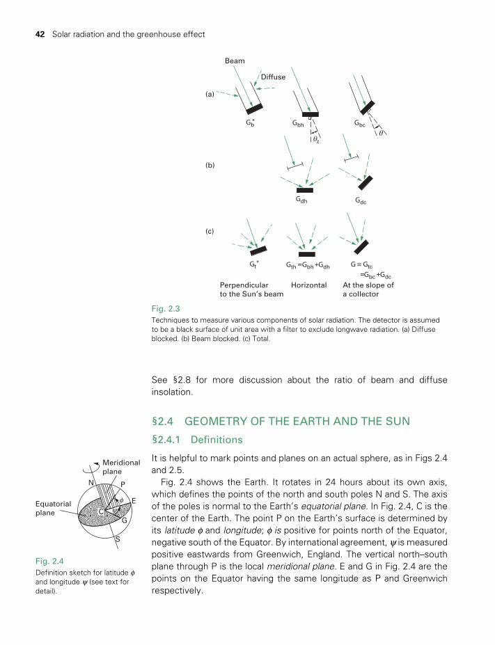
42 Solar radiation and the greenhouse effect
See §2.8 for more discussion about the ratio of beam and diffuse insolation.
§2.4 GEOMETRY OF THE EARTH AND THE SUN
§2.4.1 Definitions
It is helpful to mark points and planes on an actual sphere, as in Figs 2.4 and 2.5.
Fig. 2.4 shows the Earth. It rotates in 24 hours about its own axis, which defines the points of the north and south poles N and S. The axis of the poles is normal to the Earth’s equatorial plane. In Fig. 2.4, C is the center of the Earth. The point P on the Earth’s surface is determined by its latitude f and longitude; f is positive for points north of the Equator, negative south of the Equator. By international agreement, y is measured positive eastwards from Greenwich, England. The vertical north–south plane through P is the local meridional plane. E and G in Fig. 2.4 are the points on the Equator having the same longitude as P and Greenwich respectively.
Beam
(a)
(b)
(c)
Perpendicularto the Sun’s beam
Horizontal
==
++
At the slope ofa collector
Gb*
Gt*
Gbh Gbc
zθ
θ
GdcGdh
Gth Gbh G ≡ Gtc
Gbc Gdc
Gdh
Diffuse
Fig. 2.3Techniques to measure various components of solar radiation. The detector is assumed to be a black surface of unit area with a filter to exclude longwave radiation. (a) Diffuse blocked. (b) Beam blocked. (c) Total.
Meridionalplane
P
Eφ
G
S
C
N
Equatorialplane ψ
Fig. 2.4Definition sketch for latitude f and longitude y (see text for detail).
TWIDELL PAGINATION.indb 42 01/12/2014 11:35
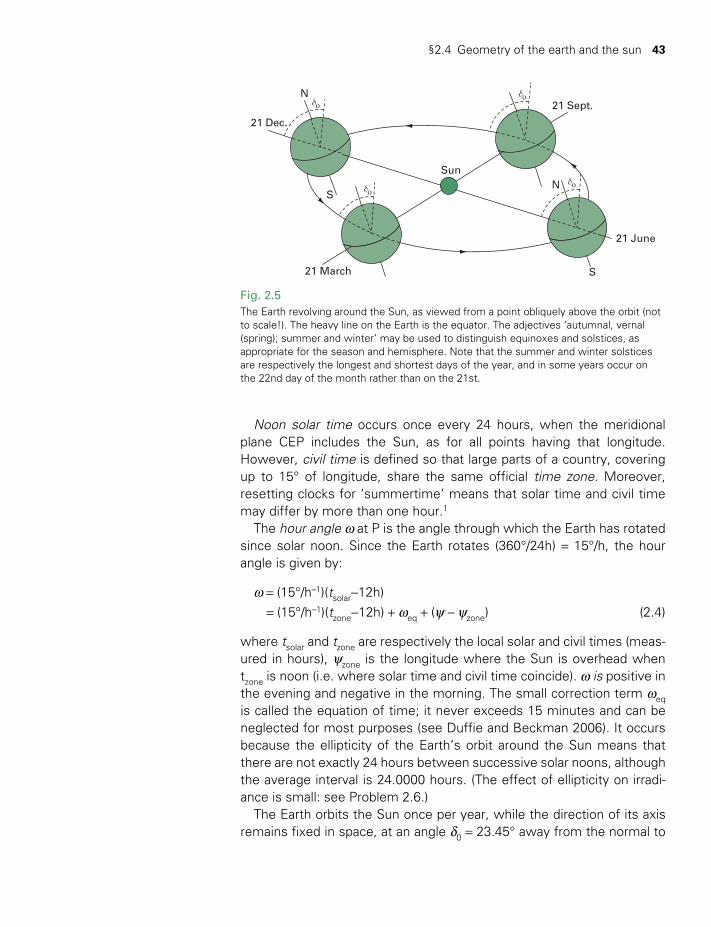
§2.4 Geometry of the earth and the sun 43
Noon solar time occurs once every 24 hours, when the meridional plane CEP includes the Sun, as for all points having that longitude. However, civil time is defined so that large parts of a country, covering up to 15° of longitude, share the same official time zone. Moreover, resetting clocks for ‘summertime’ means that solar time and civil time may differ by more than one hour.1
The hour angle w at P is the angle through which the Earth has rotated since solar noon. Since the Earth rotates (360°/24h) = 15°/h, the hour angle is given by:
w = (15°/h–1)(tsolar-12h) = (15°/h–1)(tzone-12h) + weq + (y – yzone) (2.4)
where tsolar and tzone are respectively the local solar and civil times (meas-ured in hours), yzone is the longitude where the Sun is overhead when tzone is noon (i.e. where solar time and civil time coincide). w is positive in the evening and negative in the morning. The small correction term weq is called the equation of time; it never exceeds 15 minutes and can be neglected for most purposes (see Duffie and Beckman 2006). It occurs because the ellipticity of the Earth’s orbit around the Sun means that there are not exactly 24 hours between successive solar noons, although the average interval is 24.0000 hours. (The effect of ellipticity on irradi-ance is small: see Problem 2.6.)
The Earth orbits the Sun once per year, while the direction of its axis remains fixed in space, at an angle d0 = 23.45° away from the normal to
Fig. 2.5The Earth revolving around the Sun, as viewed from a point obliquely above the orbit (not to scale!). The heavy line on the Earth is the equator. The adjectives ‘autumnal, vernal (spring); summer and winter’ may be used to distinguish equinoxes and solstices, as appropriate for the season and hemisphere. Note that the summer and winter solstices are respectively the longest and shortest days of the year, and in some years occur on the 22nd day of the month rather than on the 21st.
N
21 Dec.
S
21 March
Sun
21 Sept.
21 June
S
N
δο
δοδο
δο
TWIDELL PAGINATION.indb 43 01/12/2014 11:35
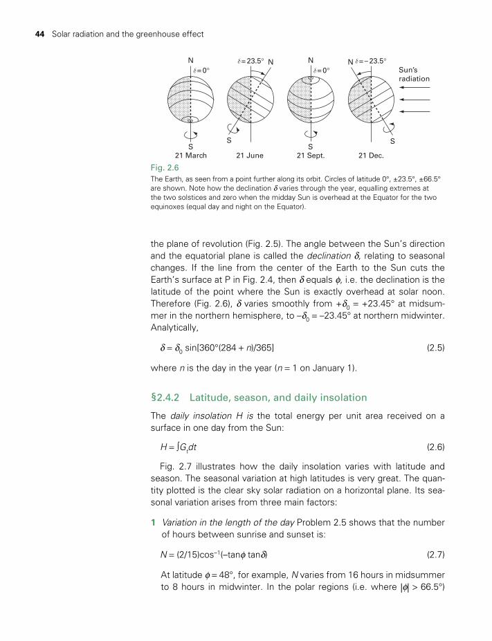
44 Solar radiation and the greenhouse effect
the plane of revolution (Fig. 2.5). The angle between the Sun’s direction and the equatorial plane is called the declination d, relating to seasonal changes. If the line from the center of the Earth to the Sun cuts the Earth’s surface at P in Fig. 2.4, then d equals f, i.e. the declination is the latitude of the point where the Sun is exactly overhead at solar noon. Therefore (Fig. 2.6), d varies smoothly from +d0 = +23.45° at midsum-mer in the northern hemisphere, to –d0 = –23.45° at northern midwinter. Analytically,
d = d0 sin[360°(284 + n)/365] (2.5)
where n is the day in the year (n = 1 on January 1).
§2.4.2 Latitude, season, and daily insolation
The daily insolation H is the total energy per unit area received on a surface in one day from the Sun:
H = ∫Gtdt (2.6)
Fig. 2.7 illustrates how the daily insolation varies with latitude and season. The seasonal variation at high latitudes is very great. The quan-tity plotted is the clear sky solar radiation on a horizontal plane. Its sea-sonal variation arises from three main factors:
1 Variation in the length of the day Problem 2.5 shows that the number of hours between sunrise and sunset is:
N = (2/15)cos–1(–tanf tand) (2.7)
At latitude f = 48°, for example, N varies from 16 hours in midsummer to 8 hours in midwinter. In the polar regions (i.e. where |f| > 66.5°)
21 March
N N NN
S SSS
21 June 21 Sept. 21 Dec.
Sun’sradiation
δ = 0° δ = 0°δ = 23.5° δ = – 23.5°
Fig. 2.6The Earth, as seen from a point further along its orbit. Circles of latitude 0°, ±23.5°, ±66.5° are shown. Note how the declination d varies through the year, equalling extremes at the two solstices and zero when the midday Sun is overhead at the Equator for the two equinoxes (equal day and night on the Equator).
TWIDELL PAGINATION.indb 44 01/12/2014 11:35
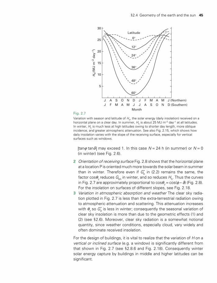
§2.4 Geometry of the earth and the sun 45
|tanϕ tand | may exceed 1. In this case N = 24 h (in summer) or N = 0 (in winter) (see Fig. 2.6).
2 Orientation of receiving surface Fig. 2.8 shows that the horizontal plane at a location P is oriented much more towards the solar beam in summer than in winter. Therefore even if Gb
* in (2.2) remains the same, the factor cosθz reduces Gbh in winter, and so reduces Hh. Thus the curves in Fig. 2.7 are approximately proportional to cosθz = cos(f – d) (Fig. 2.8). For the insolation on surfaces of different slopes, see Fig. 2.18.
3 Variation in atmospheric absorption and weather The clear sky radia-tion plotted in Fig. 2.7 is less than the extra-terrestrial radiation owing to atmospheric attenuation and scattering. This attenuation increases with θz so Gb
* is less in winter; consequently the seasonal variation of clear sky insolation is more than due to the geometric effects (1) and (2) (see §2.6). Moreover, clear sky radiation is a somewhat notional quantity, since weather conditions, especially cloud, vary widely and often dominate received insolation.
For the design of buildings, it is vital to realize that the variation of H on a vertical or inclined surface (e.g. a window) is significantly different from that shown in Fig. 2.7 (see §2.8.6 and Fig. 2.18). Consequently winter solar energy capture by buildings in middle and higher latitudes can be significant.
30
Hh/(
MJ
m–2
day
–1)
25
20
15
10
5
J (Northern)J A S O N D J F M A M
Month
Latitude
0°
12°
24°
36°
48°
60°
J F M A M J J A S O N D (Southern)
Fig. 2.7Variation with season and latitude of Hh, the solar energy (daily insolation) received on a horizontal plane on a clear day. In summer, Hh is about 25 MJ m–2 day–1 at all latitudes. In winter, Hh is much less at high latitudes owing to shorter day length, more oblique incidence, and greater atmospheric attenuation. See also Fig. 2.15, which shows how daily insolation varies with the slope of the receiving surface, especially for vertical surfaces such as windows.
TWIDELL PAGINATION.indb 45 01/12/2014 11:35
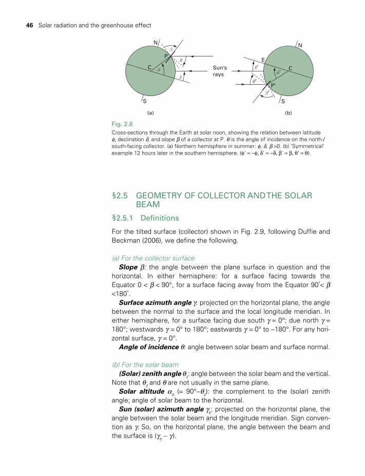
46 Solar radiation and the greenhouse effect
§2.5 GEOMETRY OF COLLECTOR AND THE SOLAR BEAM
§2.5.1 Definitions
For the tilted surface (collector) shown in Fig. 2.9, following Duffie and Beckman (2006), we define the following.
(a) For the collector surfaceSlope b: the angle between the plane surface in question and the
horizontal. In either hemisphere: for a surface facing towards the Equator 0 < b < 90°, for a surface facing away from the Equator 90°< b <180°.
Surface azimuth angle g: projected on the horizontal plane, the angle between the normal to the surface and the local longitude meridian. In either hemisphere, for a surface facing due south g = 0°; due north g = 180°; westwards g = 0° to 180°; eastwards g = 0° to -180°. For any hori-zontal surface, g = 0°.
Angle of incidence θ: angle between solar beam and surface normal.
(b) For the solar beam(Solar) zenith angle θz: angle between the solar beam and the vertical.
Note that θz and θ are not usually in the same plane.Solar altitude as (= 90°-θz): the complement to the (solar) zenith
angle; angle of solar beam to the horizontal.Sun (solar) azimuth angle gs: projected on the horizontal plane, the
angle between the solar beam and the longitude meridian. Sign conven-tion as g. So, on the horizontal plane, the angle between the beam and the surface is (gs - g ).
C
S
(a) (b)
Sun’srays
P
N
E
N
C
S
P’
δ
δ′θ
θ′
β
β′
φ φ′
Fig. 2.8Cross-sections through the Earth at solar noon, showing the relation between latitude f, declination d, and slope b of a collector at P. θ is the angle of incidence on the north-/south-facing collector. (a) Northern hemisphere in summer: f, d, b >0. (b) ‘Symmetrical’ example 12 hours later in the southern hemisphere. (f' = -f, d' = -d, b' = b, θ' = θ).
TWIDELL PAGINATION.indb 46 01/12/2014 11:35
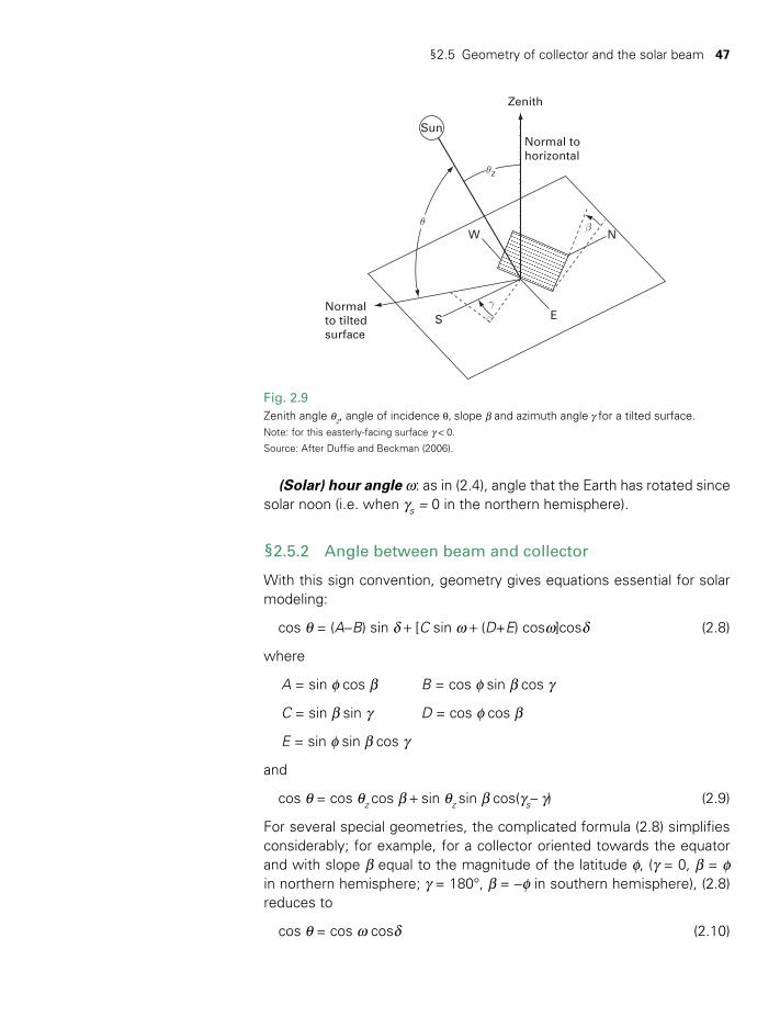
§2.5 Geometry of collector and the solar beam 47
(Solar) hour angle w: as in (2.4), angle that the Earth has rotated since solar noon (i.e. when gs = 0 in the northern hemisphere).
§2.5.2 Angle between beam and collector
With this sign convention, geometry gives equations essential for solar modeling:
cos θ = (A-B) sin d + [C sin w + (D+E) cosw]cosd (2.8)
where
A = sin f cos b B = cos f sin b cos g
C = sin b sin g D = cos f cos b
E = sin f sin b cos g
and
cos θ = cos θz cos b + sin θz sin b cos(gs– g) (2.9)
For several special geometries, the complicated formula (2.8) simplifies considerably; for example, for a collector oriented towards the equator and with slope b equal to the magnitude of the latitude f, (g = 0, b = f in northern hemisphere; g = 180°, b = -f in southern hemisphere), (2.8) reduces to
cos θ = cos w cosd (2.10)
Normal tohorizontal
Zenith
Sun
W
E
N
SNormalto tiltedsurface
θz
θ
γ
β
Fig. 2.9Zenith angle θz, angle of incidence θ, slope b and azimuth angle g for a tilted surface. Note: for this easterly-facing surface g < 0.
Source: After Duffie and Beckman (2006).
TWIDELL PAGINATION.indb 47 01/12/2014 11:35

48 Solar radiation and the greenhouse effect
123456789
101112131415161718192021222324252627282930313233343536373839404142434445
For a horizontal plane, b = 0 and (2.8) reduces to
cos θZ = sin f sin d + cos f cos w cosd (2.11)
Two cautions should be noted about (2.8) and similar formulas:
1 At higher latitudes in summer, θ exceeds 90° in early to mid-morning and from mid- to late evening, when the Sun rises from or falls to the observer’s horizon (i.e. cos θ negative). When this happens, for instance, on a south-facing surface in the northern hemisphere, the irradiance will be on the back of a collector, not the front.
2 Formulas are normally derived for the case when all angles are posi-tive, and in particular f > 0. Some northern latitude writers pay insuf-ficient attention to sign, so often their formulas do not apply in the southern hemisphere. Southern readers should check all given for-mulas, for example, by constructing complementary diagrams such as Figs 2.8(a) and (b), in which θ' = θ, and checking that the signs in the given formula agree.
§2.5.3 Optimum orientation of a collector
A parabolic concentrating collector (§4.8.2) must always point towards the direction of the solar beam (i.e. θ = 0). However, the optimum
WORKED EXAMPLE 2.1 CALCULATION OF ANGLE OF INCIDENCE
Calculate the angle of incidence of beam radiation on a surface located at Glasgow, Scotland (56°N, 4°W) at 10 a.m. on 1 February, if the surface is oriented 20° east of south, and tilted at 40° to the horizontal.
Solution
February 1 is day 32 of the year (n = 32), so from
d = 23.45° sin[360°(284 + 32)/365] = –17.5°
Civil time in Glasgow winter is Greenwich Mean Time, which is solar time (±15 min) at longitude fzone = 0. Hence tsolar ≈ 10 h, so (2.4) gives w = -30°.
Thus f = +56°, g = –20° and b = +40°, so that in (2.8)
A = sin 56° cos 40° = 0.635 B = cos 56° sin 40°cos(–20°) = 0.338C = sin 40° sin(-20°) = -0.220 D = cos 56° cos 40° = 0.428 E = sin 56° sin 40°cos(–20°) = 0.500
hence
cos θ = (0.635–0.338)sin(–17.5°) + [–0.220sin(–30°) + (0.428 + 0.500) cos(–30°)]cos(–17.5°)
= 0.783
So θ = 38.5°
TWIDELL PAGINATION.indb 48 01/12/2014 11:35
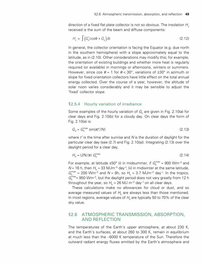
§2.6 Atmospheric transmission, absorption, and reflection 49
direction of a fixed flat plate collector is not so obvious. The insolation Hc received is the sum of the beam and diffuse components:
H G G= cos dtc b*
d∫ ( )θ + (2.12)
In general, the collector orientation is facing the Equator (e.g. due north in the southern hemisphere) with a slope approximately equal to the latitude, as in (2.10). Other considerations may modify this; for example, the orientation of existing buildings and whether more heat is regularly required (or available) in mornings or afternoons, winters or summers. However, since cos θ ≈ 1 for θ < 30°, variations of ±30° in azimuth or slope for fixed orientation collectors have little effect on the total annual energy collected. Over the course of a year, however, the altitude of solar noon varies considerably and it may be sensible to adjust the ‘fixed’ collector slope.
§2.5.4 Hourly variation of irradiance
Some examples of the hourly variation of Gh are given in Fig. 2.10(a) for clear days and Fig. 2.10(b) for a cloudy day. On clear days the form of Fig. 2.10(a) is:
Gh ≈ Ghmax sin(πt′ / N ) (2.13)
where t’ is the time after sunrise and N is the duration of daylight for the particular clear day (see (2.7) and Fig. 2.10(a)). Integrating (2.13) over the daylight period for a clear day,
Hh ≈ (2N / π ) Ghmax (2.14)
For example, at latitude ±50° (i) in midsummer, if Ghmax ≈ 900 Wm–2 and
N ≈ 16 h, then Hh ≈ 33 MJm–2 day–l; (ii) in midwinter at the same latitude, Gh
max ≈ 200 Wm–2 and N ≈ 8h, so Hh ≈ 3.7 MJm–2 day–l. In the tropics, Gh
max≈ 950 Wm–2, but the daylight period does not vary greatly from 12 h throughout the year, so Hh ≈ 26 MJ m–2 day–1 on all clear days.
These calculations make no allowances for cloud or dust, and so average measured values of Hh are always less than those mentioned. In most regions, average values of Hh are typically 50 to 70% of the clear sky value.
§2.6 ATMOSPHERIC TRANSMISSION, ABSORPTION, AND REFLECTION
The temperatures of the Earth’s upper atmosphere, at about 230 K, and the Earth’s surfaces, at about 260 to 300 K, remain in equilibrium at much less than the ~6000 K temperature of the Sun. Therefore the outward radiant energy fluxes emitted by the Earth’s atmosphere and
TWIDELL PAGINATION.indb 49 01/12/2014 11:35
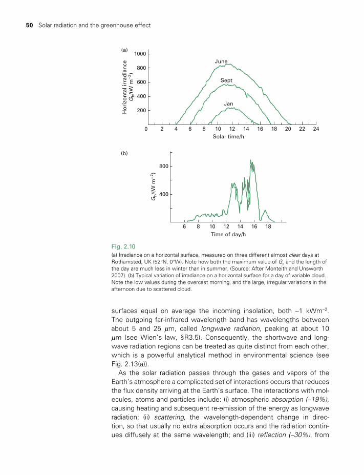
50 Solar radiation and the greenhouse effect
surfaces equal on average the incoming insolation, both ~1 kWm–2. The outgoing far-infrared wavelength band has wavelengths between about 5 and 25 mm, called longwave radiation, peaking at about 10 mm (see Wien’s law, §R3.5). Consequently, the shortwave and long-wave radiation regions can be treated as quite distinct from each other, which is a powerful analytical method in environmental science (see Fig. 2.13(a)).
As the solar radiation passes through the gases and vapors of the Earth’s atmosphere a complicated set of interactions occurs that reduces the flux density arriving at the Earth’s surface. The interactions with mol-ecules, atoms and particles include: (i) atmospheric absorption (~19%), causing heating and subsequent re-emission of the energy as longwave radiation; (ii) scattering, the wavelength-dependent change in direc-tion, so that usually no extra absorption occurs and the radiation contin-ues diffusely at the same wavelength; and (iii) reflection (~30%), from
Fig. 2.10(a) Irradiance on a horizontal surface, measured on three different almost clear days at Rothamsted, UK (52°N, 0°W). Note how both the maximum value of Gh and the length of the day are much less in winter than in summer. (Source: After Monteith and Unsworth 2007). (b) Typical variation of irradiance on a horizontal surface for a day of variable cloud. Note the low values during the overcast morning, and the large, irregular variations in the afternoon due to scattered cloud.
June1000
800
600
400
200
(b)
(a)
Time of day/h
Solar time/h
800
400
Gh/(
W m
−2)
Ho
rizo
nta
l irr
adia
nce
Gh/(
W m
−2)
6 8 10 12 14 16 18
0 2 4 6 8 10 12 14 16 18 20 22 24
Sept
Jan
TWIDELL PAGINATION.indb 50 01/12/2014 11:35
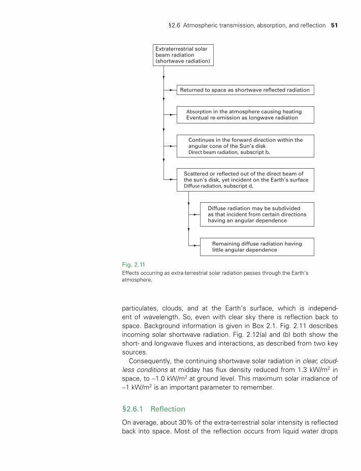
§2.6 Atmospheric transmission, absorption, and reflection 51
particulates, clouds, and at the Earth’s surface, which is independ-ent of wavelength. So, even with clear sky there is reflection back to space. Background information is given in Box 2.1. Fig. 2.11 describes incoming solar shortwave radiation. Fig. 2.12(a) and (b) both show the short- and longwave fluxes and interactions, as described from two key sources.
Consequently, the continuing shortwave solar radiation in clear, cloud-less conditions at midday has flux density reduced from 1.3 kW/m2 in space, to ~1.0 kW/m2 at ground level. This maximum solar irradiance of ~1 kW/m2 is an important parameter to remember.
§2.6.1 Reflection
On average, about 30% of the extra-terrestrial solar intensity is reflected back into space. Most of the reflection occurs from liquid water drops
Extraterrestrial solarbeam radiation(shortwave radiation)
Returned to space as shortwave reflected radiation
Absorption in the atmosphere causing heatingEventual re-emission as longwave radiation
Continues in the forward direction within theangular cone of the Sun’s diskDirect beam radiation, subscript b.
Scattered or reflected out of the direct beam ofthe sun’s disk, yet incident on the Earth’s surfaceDiuse radiation, subscript d.
Diffuse radiation may be subdividedas that incident from certain directionshaving an angular dependence
Remaining diffuse radiation havinglittle angular dependence
Fig. 2.11Effects occurring as extra-terrestrial solar radiation passes through the Earth’s atmosphere.
TWIDELL PAGINATION.indb 51 01/12/2014 11:35
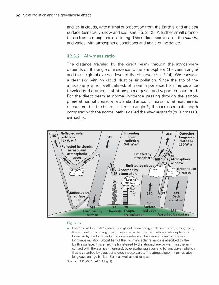
52 Solar radiation and the greenhouse effect
107Reflected solarradiation107 Wm–2
Reflected by clouds,aerosol andatmospheric
gases77
Reflected bysurface
30
168Absorbed by
surface
235
Greenhousegases
324Absorbed by surface
324Back
radiation
40
Atmosphericwindow
40
30165
Outgoinglongwaveradiation235 Wm–2
Incomingsolar
radiation342 Wm–2
Emitted byatmosphere
Emitted by cloudsAbsorbed byatmosphere
Latent78 heat
350
390Surface
radiation78Evapo-transpiration
24Thermals
24
67
342
Fig. 2.12a Estimate of the Earth’s annual and global mean energy balance. Over the long term,
the amount of incoming solar radiation absorbed by the Earth and atmosphere is balanced by the Earth and atmosphere releasing the same amount of outgoing longwave radiation. About half of the incoming solar radiation is absorbed by the Earth’s surface. This energy is transferred to the atmosphere by warming the air in contact with the surface (thermals), by evapotranspiration and by longwave radiation that is absorbed by clouds and greenhouse gases. The atmosphere in turn radiates longwave energy back to Earth as well as out to space.
Source: IPCC (2007, FAQ1.1 Fig. 1).
and ice in clouds, with a smaller proportion from the Earth’s land and sea surface (especially snow and ice) (see Fig. 2.12). A further small propor-tion is from atmospheric scattering. This reflectance is called the albedo, and varies with atmospheric conditions and angle of incidence.
§2.6.2 Air–mass ratio
The distance traveled by the direct beam through the atmosphere depends on the angle of incidence to the atmosphere (the zenith angle) and the height above sea level of the observer (Fig. 2.14). We consider a clear sky with no cloud, dust or air pollution. Since the top of the atmosphere is not well defined, of more importance than the distance traveled is the amount of atmospheric gases and vapors encountered. For the direct beam at normal incidence passing through the atmos-phere at normal pressure, a standard amount (‘mass’) of atmosphere is encountered. If the beam is at zenith angle θz, the increased path length compared with the normal path is called the air–mass ratio (or ‘air mass’), symbol m.
TWIDELL PAGINATION.indb 52 01/12/2014 11:35
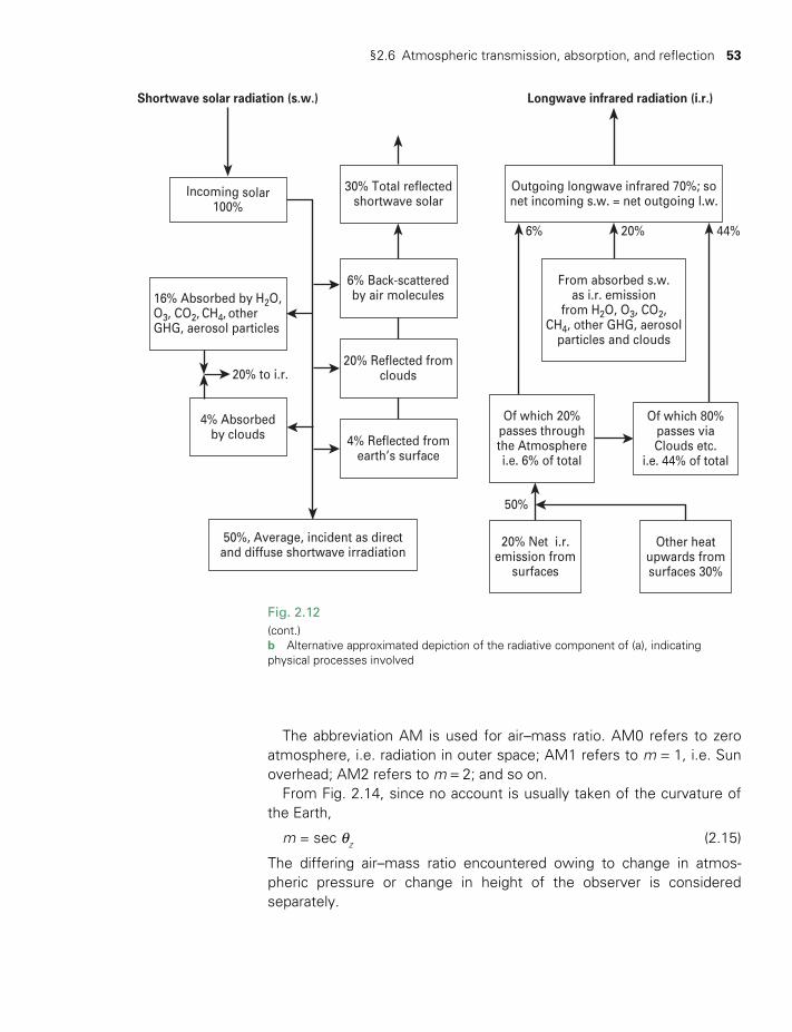
§2.6 Atmospheric transmission, absorption, and reflection 53
The abbreviation AM is used for air–mass ratio. AM0 refers to zero atmosphere, i.e. radiation in outer space; AM1 refers to m = 1, i.e. Sun overhead; AM2 refers to m = 2; and so on.
From Fig. 2.14, since no account is usually taken of the curvature of the Earth,
m = sec θz (2.15)
The differing air–mass ratio encountered owing to change in atmos-pheric pressure or change in height of the observer is considered separately.
Shortwave solar radiation (s.w.) Longwave infrared radiation (i.r.)
16% Absorbed by H2O,O3, CO2, CH4, otherGHG, aerosol particles
4% Absorbedby clouds
50%, Average, incident as directand diffuse shortwave irradiation
6% Back-scatteredby air molecules
4% Reflected fromearth’s surface
20% Reflected fromclouds20% to i.r.
50%
6% 20% 44%
Outgoing longwave infrared 70%; sonet incoming s.w. = net outgoing l.w.
20% Net i.r.emission from
surfaces
Other heatupwards fromsurfaces 30%
From absorbed s.w.as i.r. emission
from H2O, O3, CO2,CH4, other GHG, aerosol
particles and clouds
Of which 20%passes throughthe Atmospherei.e. 6% of total
Of which 80%passes viaClouds etc.
i.e. 44% of total
30% Total reflectedshortwave solar
Incoming solar100%
Fig. 2.12(cont.)b Alternative approximated depiction of the radiative component of (a), indicating physical processes involved
TWIDELL PAGINATION.indb 53 01/12/2014 11:35

54 Solar radiation and the greenhouse effect
(a)
(b)
(c)
Fig. 2.13Radiation transmitted and absorbed by the atmosphere as a function of wavelength.a Monochromatic radiant flux density fλ for downgoing (‘shortwave’) solar
radiation and upgoing thermal (‘longwave’) radiation. (Note: drawn with peaks normalized.)
b Total monochromatic absorptance aλ of the atmosphere.c Contributions to aλ from various gases and other effects. See text (Box 2.1) for further details.
Sea level
Zenith angle
Atmosphere : clear skyNormal incidence:unit path
θzPathincreased bya factor m
Fig. 2.14Air–mass ratio m = sec θz.
TWIDELL PAGINATION.indb 54 01/12/2014 11:35
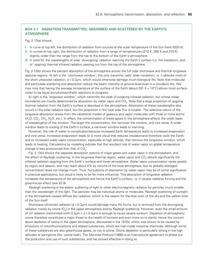
§2.6 Atmospheric transmission, absorption, and reflection 55
BOX 2.1 RADIATION TRANSMITTED, ABSORBED AND SCATTERED BY THE EARTH’S ATMOSPHERE
Fig. 2.13(a) shows:
i In curve at top left, the distribution of radiation from sources at the outer temperature of the Sun (here 5525 K). ii In curves at top right, the distribution of radiation from a range of temperatures (210 K, 260 K and 310 K)
slightly wider than the range from the top to the bottom of the Earth’s atmosphere. iii In solid fill, the wavelengths of solar ‘downgoing’ radiation reaching the Earth’s surface (i.e. the insolation), and
of ‘upgoing’ thermal infrared radiation passing out from the top of the atmosphere.
Fig. 2.13(b) shows the percent absorption of the atmosphere across the full solar shortwave and thermal longwave spectral regions. At left is the ‘shortwave window’; this only transmits ‘safe’ solar insolation; i.e. it absorbs most of the short ultraviolet radiation, λ < 0.3μm, which would otherwise damage much biological life. Note that molecular and particulate scattering and absorption reduce the beam intensity at ground level even in a cloudless sky. We may note that having the average temperature at the surface of the Earth (about 291 K = 14°C) allows most surface water to be liquid and photosynthetic reactions to progress.
At right is the ‘longwave window’, which transmits the peak of outgoing infrared radiation, but whose steep boundaries are mostly determined by absorption by water vapor and CO2. Note that a large proportion of upgoing thermal radiation from the Earth’s surface is absorbed in the atmosphere. Absorption at these wavelengths also occurs in the solar radiative input, but the proportion in the total solar flux is smaller. The selective nature of the longwave absorption arises from the vibrational modes of gaseous and vapor molecules with three or more atoms (H2O, CO2, CH4, N2O, etc.). In effect, the concentration of these gases in the atmosphere affects the width (span of wavelengths) of the window. The larger the concentration, the narrower the window, and vice versa. A wider window leads to cooling of the Earth’s surface; a narrower window leads to warming.
However, the role of water is complicated because increased Earth temperature leads to increased evaporation and vice versa. Increased evaporation leads to (i) more cloud that reduces insolationand therefore cools the Earth; and (ii) increased water vapor concentration, especially at high altitude, that narrows the longwave window, which leads to heating. Calculations by modeling indicate that the resultant role of water vapor on global temperature change is less pronounced than that of CO2.
Fig. 2.13(c) shows the separate absorption spectra of major gases and water vapor in the atmosphere, and the effect of Rayleigh scattering. In the longwave thermal region, water vapor and CO2 absorb significantly the infrared radiation upgoing from the Earth’s surface and lower atmosphere. Water vapor concentration varies greatly by region and season, and may reach about 4% by volume of the local atmosphere, but its globally averaged concentration does not change much. Thus, fluctuations of absorption by water vapor may be of some significance in practical applications, but cloud is likely to be far more influential. This absorption of longwave radiation increases the temperature of the atmosphere and hence the Earth’s surface, i.e. it causes radiative forcing and the greenhouse effect (see §2.9).
Rayleigh scattering is the elastic scattering of light or other electromagnetic radiation by particles much smaller than the wavelength of the light. The particles may be individual atoms or molecules. Rayleigh scattering of sunlight in the atmosphere causes diffuse sky radiation, which is the reason for the blue color of the sky and the yellow tone of the Sun itself.
Shortwave ultraviolet radiation (λ < 0.3μm) would damage many life forms, but is removed from the downgoing radiation mostly by ozone (O3) in the upper atmosphere and by Rayleigh scattering. However, even the small amount of UV radiation transmitted (with 0.3μm < λ < 0.4μm) is enough to cause severe sunburn. Depletion of atmospheric ozone therefore constitutes a major threat to the health of humans and even more so to plants; hence the concern about depletion of ozone in the upper atmosphere, discovered in the 1970s, which was shown to be caused by emissions of chlorofluorocarbons and related substances, which are man-made industrial chemicals. Although some of these substances are also greenhouse gases, so too is ozone, Ozone depletion is particularly strong in the high latitudes at springtime (the ‘ozone hole’). The Montreal Protocol (1989) is an international agreement to phase out the production and use of such substances, and has proved effective in doing so.
TWIDELL PAGINATION.indb 55 01/12/2014 11:35
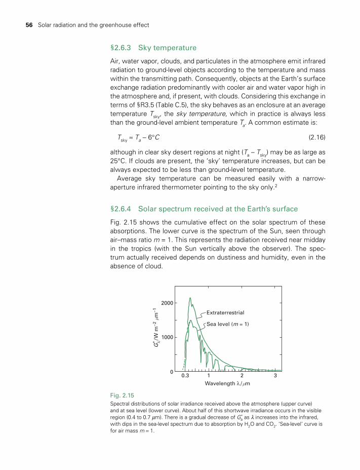
56 Solar radiation and the greenhouse effect
Wavelength λ /µm
G* λ/W
m−2
µm
−1 Extraterrestrial
Sea level (m = 1)
0.30
1000
2000
1 2 3
Fig. 2.15Spectral distributions of solar irradiance received above the atmosphere (upper curve) and at sea level (lower curve). About half of this shortwave irradiance occurs in the visible region (0.4 to 0.7 mm). There is a gradual decrease of Gb
* as λ increases into the infrared, with dips in the sea-level spectrum due to absorption by H2O and CO2. ‘Sea-level’ curve is for air mass m = 1.
§2.6.3 Sky temperature
Air, water vapor, clouds, and particulates in the atmosphere emit infrared radiation to ground-level objects according to the temperature and mass within the transmitting path. Consequently, objects at the Earth’s surface exchange radiation predominantly with cooler air and water vapor high in the atmosphere and, if present, with clouds. Considering this exchange in terms of §R3.5 (Table C.5), the sky behaves as an enclosure at an average temperature Tsky, the sky temperature, which in practice is always less than the ground-level ambient temperature Ta. A common estimate is:
Tsky ≈ Ta - 6°C (2.16)
although in clear sky desert regions at night (Ta – Tsky) may be as large as 25°C. If clouds are present, the ‘sky’ temperature increases, but can be always expected to be less than ground-level temperature.
Average sky temperature can be measured easily with a narrow- aperture infrared thermometer pointing to the sky only.2
§2.6.4 Solar spectrum received at the Earth’s surface
Fig. 2.15 shows the cumulative effect on the solar spectrum of these absorptions. The lower curve is the spectrum of the Sun, seen through air–mass ratio m = 1. This represents the radiation received near midday in the tropics (with the Sun vertically above the observer). The spec-trum actually received depends on dustiness and humidity, even in the absence of cloud.
TWIDELL PAGINATION.indb 56 01/12/2014 11:35

§2.8 Site estimation of solar radiation 57
§2.7 MEASURING SOLAR RADIATION
For measuring solar radiation there is a range of instruments, e.g. Fig. 2.16, many with confusing names! Fundamental (absolute) meas-urements at standards laboratories use active cavity radiometers; the solar beam is absorbed on a matt black surface of area A, whose tem-perature rise is measured and compared with the temperature rise in an identical (shaded) absorber heated electrically. In principle, then,
aAGb* = Pelec (2.17)
The geometry is such that the absorptance a = 0.999. Notable uses are for satellite measurements of the solar constant, and for calibration of secondary instruments.
Selected meteorological stations have World Meteorological Office (WMO) standardized pyranometers with an absolute accuracy ~3%. In essence, they have thermocouple junctions (a thermopile) under a black surface, all under a glass hemisphere; the temperature increase caused by the absorbed insolation produces a calibrated voltage. In practice they are designed and manufactured with great expertise. The basic meas-urement is total irradiance on a horizontal surface Gth (Fig. 2.3(c)). Other measurements can be: (i) of diffuse radiation only, with direct radiation prevented by an adjustable shade ring; (ii) of beam radiation Gb
* only that enters a collimating tube continuously tracking the Sun’s path (a pyroheliometer).
For field use (e.g. measuring irradiance on different parts of a build-ing) there are much cheaper instruments, often called ‘solarimeters’ (although this term is also used for pyranometers), which are usually solar cells calibrated against a WMO-standardized instrument. Their absolute accuracy is typically only ~15%, owing to the spectral response of Si cells (Fig. R4.11 in Review 4), but for comparisons their reproduc-ibility is likely to be better than 5%.
§2.8 SITE ESTIMATION OF SOLAR RADIATION
§2.8.1 Requirements
All solar devices utilize shortwave solar irradiation; thus solar develop-ment and use depend on measuring and predicting both the instant and integrated insolation at the place of use. Fortunately, integrated over a day or more, unshaded insolation is not site dependent across regional distances, so regional meteorological data can be used directly. (This contrasts with, say, wind power, which is very site dependent.) Typical time variation data will also apply regionally and may be used to simulate performance of devices during development. Therefore diurnal and longer averaged solar data taken from meteorological stations and
TWIDELL PAGINATION.indb 57 01/12/2014 11:35
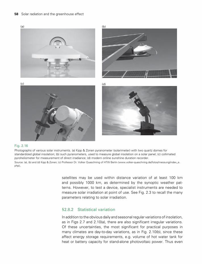
58 Solar radiation and the greenhouse effect
satellites may be used within distance variation of at least 100 km and possibly 1000 km, as determined by the synoptic weather pat-terns. However, to test a device, specialist instruments are needed to measure solar irradiation at point of use. See Fig. 2.3 to recall the many parameters relating to solar irradiation.
§2.8.2 Statistical variation
In addition to the obvious daily and seasonal regular variations of insolation, as in Figs 2.7 and 2.10(a), there are also significant irregular variations. Of these uncertainties, the most significant for practical purposes in many climates are day-to-day variations, as in Fig. 2.10(b), since these affect energy storage requirements, e.g. volume of hot water tank for heat or battery capacity for stand-alone photovoltaic power. Thus even
(a) (b)
(c) (d)
Fig. 2.16Photographs of various solar instruments. (a) Kipp & Zonen pyranometer (solarimeter) with two quartz domes for standardized global insolation; (b) such pyranometers, used to measure global insolation on a solar panel; (c) collimated pyroheliometer for measurement of direct irradiance; (d) modern online sunshine duration recorder.Source: (a), (b) and (d) Kipp & Zonen; (c) Professor Dr. Volker Quaschning of HTW Berlin (www.volker-quaschning.de/fotos/messung/index_e.php);.
TWIDELL PAGINATION.indb 58 01/12/2014 11:36

§2.8 Site estimation of solar radiation 59
a complete record of past irradiance can only be used to statistically predict future irradiance with an estimated range of uncertainty.
§2.8.3 Sunshine hours as a measure of insolation
All major meteorological stations measure daily the ‘hours of bright sunshine’ n, for which records should be available for many decades. Traditionally n is measured with a spherical Campbell-Stokes recorder which incorporates a standard marked card positioned behind a magnify-ing glass. When the sunshine is ‘bright’, the focused direct beam burns an elongated hole in the card. The observer obtains n from the total burnt length on each day’s card. Sunshine hours are also measured by electronic devices.
National and international meteorological stations are loath to change the meteorological instruments they have used perhaps for tens to a hundred years. Simple examples are mercury thermometers and Campbell-Stokes sunshine-hour recorders. Long-term data runs are important, especially for analyzing climate change, so changing instrumentation may introduce unknown errors. Yet modern instruments are likely to be more accu-rate, able to record electronically, and less demanding of human time.
Since Campbell-Stokes and more modern sunshine recorders are straightforward instruments, historically they are have been used world-wide to correlate sunshine hours with insolation (H). Correlation equa-tions are often of the form:
H = H0[a + b(n / N )] (2.18)
where (for the day in question) H0 is the horizontal radiation with no atmosphere (i.e. free space equivalence, calculated as in Problem 2.6) and N is the ‘length’ of the day in hours (2.7). However, the regres-sion coefficients a and b vary from site to site. Even so, the correlation coefficient is usually only about 0.7, i.e. values of measured insolation are widely scattered from those predicted from the equation.
Many other climatological correlations with insolation have been proposed, using such variables as latitude, ambient temperature, humidity, and cloud cover. Most have a limited accuracy and range of applicability.
§2.8.4 Geostationary Operational Environmental Satellites (GOES)
Measurement and sensing of environmental parameters using satellites have had a profound impact upon environmental analysis and availabil-ity of information. However, the correlation of ground measurements with satellite measurements is not straightforward. A simple example is satellite measurement of ground-level insolation. The satellite can measure separately downcoming shortwave solar irradiance (insolation)
TWIDELL PAGINATION.indb 59 01/12/2014 11:36
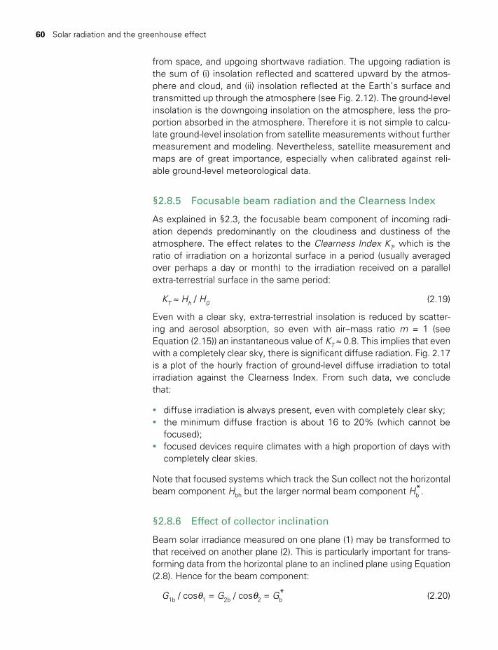
60 Solar radiation and the greenhouse effect
from space, and upgoing shortwave radiation. The upgoing radiation is the sum of (i) insolation reflected and scattered upward by the atmos-phere and cloud, and (ii) insolation reflected at the Earth’s surface and transmitted up through the atmosphere (see Fig. 2.12). The ground-level insolation is the downgoing insolation on the atmosphere, less the pro-portion absorbed in the atmosphere. Therefore it is not simple to calcu-late ground-level insolation from satellite measurements without further measurement and modeling. Nevertheless, satellite measurement and maps are of great importance, especially when calibrated against reli-able ground-level meteorological data.
§2.8.5 Focusable beam radiation and the Clearness Index
As explained in §2.3, the focusable beam component of incoming radi-ation depends predominantly on the cloudiness and dustiness of the atmosphere. The effect relates to the Clearness Index KT, which is the ratio of irradiation on a horizontal surface in a period (usually averaged over perhaps a day or month) to the irradiation received on a parallel extra-terrestrial surface in the same period:
KT ≈ Hh / H0 (2.19)
Even with a clear sky, extra-terrestrial insolation is reduced by scatter-ing and aerosol absorption, so even with air–mass ratio m = 1 (see Equation (2.15)) an instantaneous value of KT ≈ 0.8. This implies that even with a completely clear sky, there is significant diffuse radiation. Fig. 2.17 is a plot of the hourly fraction of ground-level diffuse irradiation to total irradiation against the Clearness Index. From such data, we conclude that:
• diffuse irradiation is always present, even with completely clear sky;• the minimum diffuse fraction is about 16 to 20% (which cannot be
focused);• focused devices require climates with a high proportion of days with
completely clear skies.
Note that focused systems which track the Sun collect not the horizontal beam component Hbh but the larger normal beam component Hb
*.
§2.8.6 Effect of collector inclination
Beam solar irradiance measured on one plane (1) may be transformed to that received on another plane (2). This is particularly important for trans-forming data from the horizontal plane to an inclined plane using Equation (2.8). Hence for the beam component:
G1b / cosθ1 = G2b / cosθ2 = Gb* (2.20)
TWIDELL PAGINATION.indb 60 01/12/2014 11:36
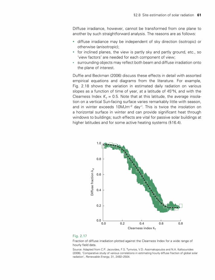
§2.8 Site estimation of solar radiation 61
Diffuse irradiance, however, cannot be transformed from one plane to another by such straightforward analysis. The reasons are as follows:
• diffuse irradiance may be independent of sky direction (isotropic) or otherwise (anisotropic);
• for inclined planes, the view is partly sky and partly ground, etc., so ‘view factors’ are needed for each component of view;
• surrounding objects may reflect both beam and diffuse irradiation onto the plane of interest.
Duffie and Beckman (2006) discuss these effects in detail with assorted empirical equations and diagrams from the literature. For example, Fig. 2.18 shows the variation in estimated daily radiation on various slopes as a function of time of year, at a latitude of 45°N, and with the Clearness Index KT = 0.5. Note that at this latitude, the average insola-tion on a vertical Sun-facing surface varies remarkably little with season, and in winter exceeds 10MJm–2 day–l. This is twice the insolation on a horizontal surface in winter and can provide significant heat through windows to buildings; such effects are vital for passive solar buildings at higher latitudes and for some active heating systems (§16.4).
Clearness index KT
Dif
fuse
fra
ctio
n k
d
0.0 0.2 0.4 0.6 0.80.0
0.2
0.4
0.6
0.8
1.0
Fig. 2.17Fraction of diffuse irradiation plotted against the Clearness Index for a wide range of hourly field data. Source: Adapted from C.P. Jacovides, F.S. Tymvios, V.D. Assimakopoulos and N.A. Kaltsounides (2006), ‘Comparative study of various correlations in estimating hourly diffuse fraction of global solar radiation’, Renewable Energy, 31, 2492–2504.
TWIDELL PAGINATION.indb 61 01/12/2014 11:36
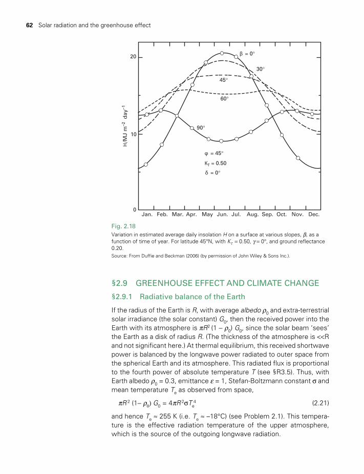
62 Solar radiation and the greenhouse effect
20
10
0Jan. Feb. Mar.
β = 0°
30°
45°
60°
90°
φ = 45°
KT = 0.50
δ = 0°
Apr. May Jun. Jul. Aug. Sep. Oct. Nov. Dec.
H/M
J m
–2 d
ay–1
Fig. 2.18Variation in estimated average daily insolation H on a surface at various slopes, b, as a function of time of year. For latitude 45°N, with KT = 0.50, g = 0°, and ground reflectance 0.20. Source: From Duffie and Beckman (2006) (by permission of John Wiley & Sons Inc.).
§2.9 GREENHOUSE EFFECT AND CLIMATE CHANGE
§2.9.1 Radiative balance of the Earth
If the radius of the Earth is R, with average albedo ρ0 and extra- terrestrial solar irradiance (the solar constant) G0, then the received power into the Earth with its atmosphere is πR2 (1 - ρ0) G0, since the solar beam ‘sees’ the Earth as a disk of radius R. (The thickness of the atmosphere is <<R and not significant here.) At thermal equilibrium, this received shortwave power is balanced by the longwave power radiated to outer space from the spherical Earth and its atmosphere. This radiated flux is proportional to the fourth power of absolute temperature T (see §R3.5). Thus, with Earth albedo ρ0 = 0.3, emittance e = 1, Stefan-Boltzmann constant s and mean temperature Te as observed from space,
πR 2 (1- ρ0) G0 = 4πR 2sTe4 (2.21)
and hence Te ≈ 255 K (i.e. Te ≈ –18°C) (see Problem 2.1). This tempera-ture is the effective radiation temperature of the upper atmosphere, which is the source of the outgoing longwave radiation.
TWIDELL PAGINATION.indb 62 01/12/2014 11:36
§2.9 Greenhouse effect and climate change 63
Thus, the longwave radiation from the Earth and its atmosphere has approximately the spectral distribution of a black body at 250 K. As indi-cated in Fig. 2.13, the outgoing radiation occurs in a wavelength band between about 7 and 15 mm, with a peak at about 10mm (according to Wien’s law, §R3.5). Note that the above calculation does not need to involve the temperature of the Earth’s surfaces and lower atmosphere.
It is apparent from Fig. 2.13 that a definite distinction can be made between the spectral distribution of the Sun’s radiation (shortwave) and that from the thermal sources of the Earth and the atmosphere (long-wave). The infrared longwave fluxes at the Earth’s surface are them-selves complex and large. The atmosphere radiates down to this surface as well as up and out into space. When measuring radiation, or when determining the energy balance of an area of ground or a device, it is extremely important to be aware of the invisible infrared fluxes in the environment, which may be ~1 kWm-2.
§2.9.2 The greenhouse effect, radiative forcing, and climate change
The Earth’s average surface temperature of about 14°C is about 30°C more than the temperature of the outer atmosphere. In effect, the atmosphere acts as an infrared ‘blanket’, because certain gases and water vapor in it absorb longwave radiation (see Box 2.1). This infrared absorption occurs both with incoming solar radiation in daytime and with outgoing heat radiation continuously; the total effect produces a warmer Earth’s surface than otherwise. This increase in surface temperature (relative to what it would be without the atmosphere) is called the green-house effect, because the glass of a horticultural glasshouse (a green-house) likewise (i) absorbs infrared radiation, including that emitted from objects inside the glasshouse for 24 hours per day; and (ii) allows the incoming shortwave solar radiation to be transmitted during daytime (see Fig. R3.12). The change in net radiative energy flux because of the glass maintains the temperature inside the greenhouse above ambient temperature outside, which is the main purpose of agricultural green-houses in middle and higher latitude countries and of conservatories abutting buildings. (In the horticultural case, the temperature is further increased since the enclosure reduces natural and wind-forced convec-tive heat loss.)
Without the greenhouse effect, on Earth most water would be ice, photosynthetic rates would be far less and life would be profoundly different. The gases responsible, notably carbon dioxide (CO2), nitrous oxide (N2O), and methane (CH4), are called greenhouse gases (GHGs). The greenhouse effect is a natural characteristic of the Earth and its atmosphere, closely related to established ecological processes. In the past 200 years especially, mankind’s industries and agricultural practices
TWIDELL PAGINATION.indb 63 01/12/2014 11:36
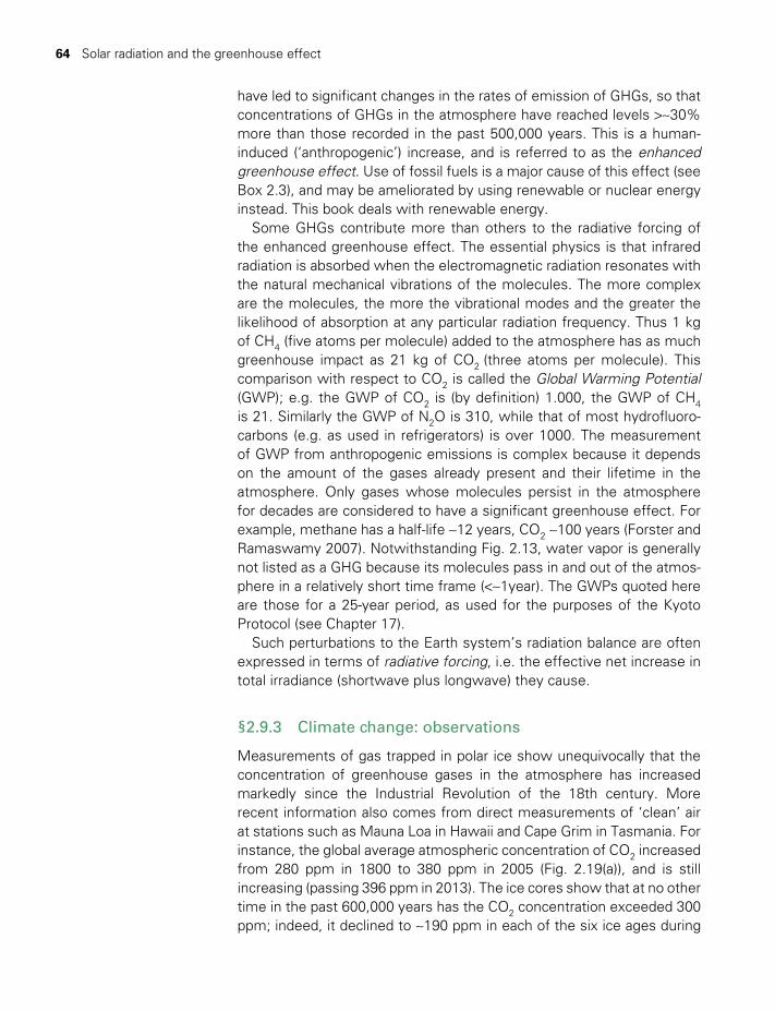
64 Solar radiation and the greenhouse effect
have led to significant changes in the rates of emission of GHGs, so that concentrations of GHGs in the atmosphere have reached levels >~30% more than those recorded in the past 500,000 years. This is a human-induced (‘anthropogenic’) increase, and is referred to as the enhanced greenhouse effect. Use of fossil fuels is a major cause of this effect (see Box 2.3), and may be ameliorated by using renewable or nuclear energy instead. This book deals with renewable energy.
Some GHGs contribute more than others to the radiative forcing of the enhanced greenhouse effect. The essential physics is that infrared radiation is absorbed when the electromagnetic radiation resonates with the natural mechanical vibrations of the molecules. The more complex are the molecules, the more the vibrational modes and the greater the likelihood of absorption at any particular radiation frequency. Thus 1 kg of CH4 (five atoms per molecule) added to the atmosphere has as much greenhouse impact as 21 kg of CO2 (three atoms per molecule). This comparison with respect to CO2 is called the Global Warming Potential (GWP); e.g. the GWP of CO2 is (by definition) 1.000, the GWP of CH4 is 21. Similarly the GWP of N2O is 310, while that of most hydrofluoro-carbons (e.g. as used in refrigerators) is over 1000. The measurement of GWP from anthropogenic emissions is complex because it depends on the amount of the gases already present and their lifetime in the atmosphere. Only gases whose molecules persist in the atmosphere for decades are considered to have a significant greenhouse effect. For example, methane has a half-life ~12 years, CO2 ~100 years (Forster and Ramaswamy 2007). Notwithstanding Fig. 2.13, water vapor is generally not listed as a GHG because its molecules pass in and out of the atmos-phere in a relatively short time frame (<~1year). The GWPs quoted here are those for a 25-year period, as used for the purposes of the Kyoto Protocol (see Chapter 17).
Such perturbations to the Earth system’s radiation balance are often expressed in terms of radiative forcing, i.e. the effective net increase in total irradiance (shortwave plus longwave) they cause.
§2.9.3 Climate change: observations
Measurements of gas trapped in polar ice show unequivocally that the concentration of greenhouse gases in the atmosphere has increased markedly since the Industrial Revolution of the 18th century. More recent information also comes from direct measurements of ‘clean’ air at stations such as Mauna Loa in Hawaii and Cape Grim in Tasmania. For instance, the global average atmospheric concentration of CO2 increased from 280 ppm in 1800 to 380 ppm in 2005 (Fig. 2.19(a)), and is still increasing (passing 396 ppm in 2013). The ice cores show that at no other time in the past 600,000 years has the CO2 concentration exceeded 300 ppm; indeed, it declined to ~190 ppm in each of the six ice ages during
TWIDELL PAGINATION.indb 64 01/12/2014 11:36
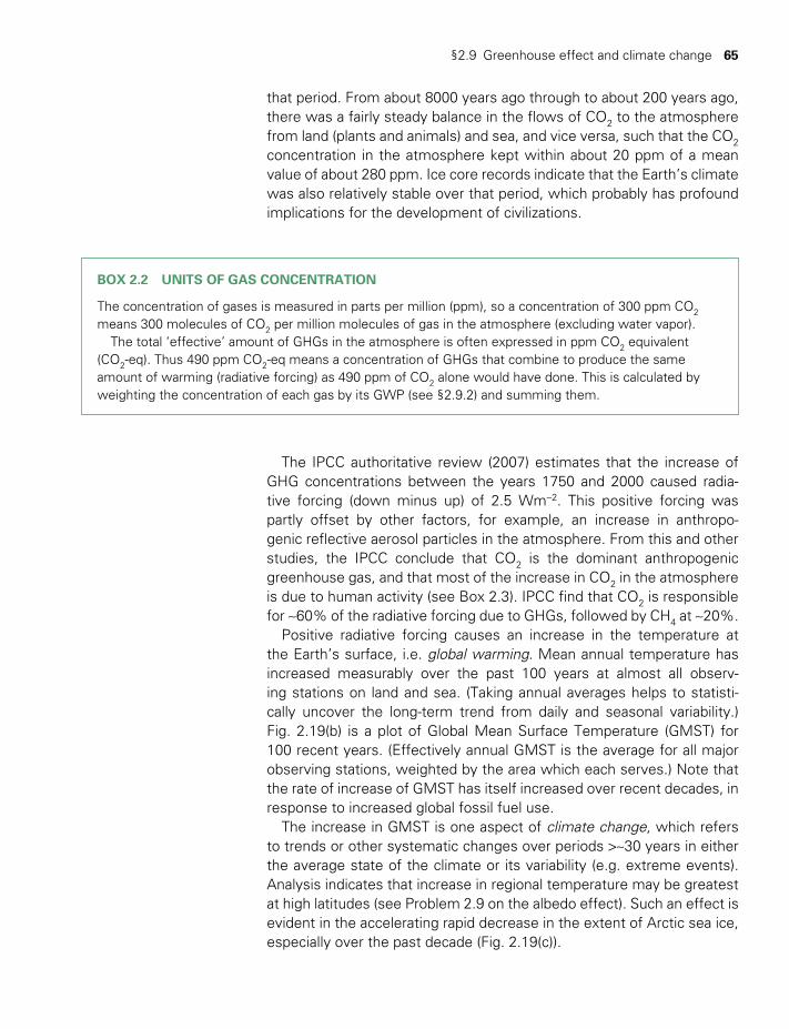
§2.9 Greenhouse effect and climate change 65
that period. From about 8000 years ago through to about 200 years ago, there was a fairly steady balance in the flows of CO2 to the atmosphere from land (plants and animals) and sea, and vice versa, such that the CO2 concentration in the atmosphere kept within about 20 ppm of a mean value of about 280 ppm. Ice core records indicate that the Earth’s climate was also relatively stable over that period, which probably has profound implications for the development of civilizations.
BOX 2.2 UNITS OF GAS CONCENTRATION
The concentration of gases is measured in parts per million (ppm), so a concentration of 300 ppm CO2 means 300 molecules of CO2 per million molecules of gas in the atmosphere (excluding water vapor).
The total ‘effective’ amount of GHGs in the atmosphere is often expressed in ppm CO2 equivalent (CO2-eq). Thus 490 ppm CO2-eq means a concentration of GHGs that combine to produce the same amount of warming (radiative forcing) as 490 ppm of CO2 alone would have done. This is calculated by weighting the concentration of each gas by its GWP (see §2.9.2) and summing them.
The IPCC authoritative review (2007) estimates that the increase of GHG concentrations between the years 1750 and 2000 caused radia-tive forcing (down minus up) of 2.5 Wm-2. This positive forcing was partly offset by other factors, for example, an increase in anthropo-genic reflective aerosol particles in the atmosphere. From this and other studies, the IPCC conclude that CO2 is the dominant anthropogenic greenhouse gas, and that most of the increase in CO2 in the atmosphere is due to human activity (see Box 2.3). IPCC find that CO2 is responsible for ~60% of the radiative forcing due to GHGs, followed by CH4 at ~20%.
Positive radiative forcing causes an increase in the temperature at the Earth’s surface, i.e. global warming. Mean annual temperature has increased measurably over the past 100 years at almost all observ-ing stations on land and sea. (Taking annual averages helps to statisti-cally uncover the long-term trend from daily and seasonal variability.) Fig. 2.19(b) is a plot of Global Mean Surface Temperature (GMST) for 100 recent years. (Effectively annual GMST is the average for all major observing stations, weighted by the area which each serves.) Note that the rate of increase of GMST has itself increased over recent decades, in response to increased global fossil fuel use.
The increase in GMST is one aspect of climate change, which refers to trends or other systematic changes over periods >~30 years in either the average state of the climate or its variability (e.g. extreme events). Analysis indicates that increase in regional temperature may be greatest at high latitudes (see Problem 2.9 on the albedo effect). Such an effect is evident in the accelerating rapid decrease in the extent of Arctic sea ice, especially over the past decade (Fig. 2.19(c)).
TWIDELL PAGINATION.indb 65 01/12/2014 11:36
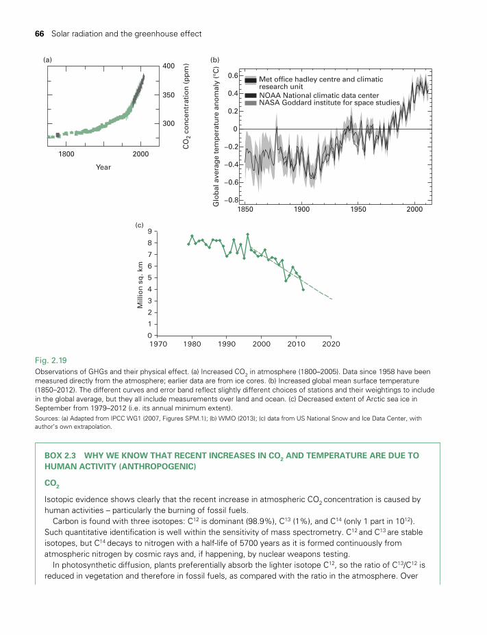
66 Solar radiation and the greenhouse effect
Fig. 2.19Observations of GHGs and their physical effect. (a) Increased CO2 in atmosphere (1800–2005). Data since 1958 have been measured directly from the atmosphere; earlier data are from ice cores. (b) Increased global mean surface temperature (1850–2012). The different curves and error band reflect slightly different choices of stations and their weightings to include in the global average, but they all include measurements over land and ocean. (c) Decreased extent of Arctic sea ice in September from 1979–2012 (i.e. its annual minimum extent). Sources: (a) Adapted from IPCC WG1 (2007, Figures SPM.1); (b) WMO (2013); (c) data from US National Snow and Ice Data Center, with author’s own extrapolation.
(a)
1800
Year
2000
300
350
400
CO
2 co
nce
ntr
atio
n (
pp
m)
1850 1900 1950 2000Year
−0.8
−0.6
−0.4
−0.2
0
0.2
0.4
0.6
(b)
Glo
bal
ave
rag
e te
mp
erat
ure
an
om
aly
(°C
)
Met office hadley centre and climatic research unitNOAA National climatic data centerNASA Goddard institute for space studies
0
1
2
3
4
5
6
7
8
9(c)
1970 1980 1990 2000 2010 2020
Mill
ion
sq. k
m
BOX 2.3 WHY WE KNOW THAT RECENT INCREASES IN CO2 AND TEMPERATURE ARE DUE TO HUMAN ACTIVITY (ANTHROPOGENIC)
CO2
Isotopic evidence shows clearly that the recent increase in atmospheric CO2 concentration is caused by human activities – particularly the burning of fossil fuels.
Carbon is found with three isotopes: C12 is dominant (98.9%), C13 (1%), and C14 (only 1 part in 1012). Such quantitative identification is well within the sensitivity of mass spectrometry. C12 and C13 are stable isotopes, but C14 decays to nitrogen with a half-life of 5700 years as it is formed continuously from atmospheric nitrogen by cosmic rays and, if happening, by nuclear weapons testing.
In photosynthetic diffusion, plants preferentially absorb the lighter isotope C12, so the ratio of C13/C12 is reduced in vegetation and therefore in fossil fuels, as compared with the ratio in the atmosphere. Over
TWIDELL PAGINATION.indb 66 01/12/2014 11:36

§2.9 Greenhouse effect and climate change 67
As the atmosphere warms in contact with the oceans, it accepts more water vapor (see Fig. 4.3); hence rainfall intensity increases. Increased evaporation from warm oceans (T > 28°C) favors tropical cyclones, which may therefore be expected to increase in intensity.
§2.9.4 Climate change: projections, impacts, and mitigation
Authoritative studies predict that if fossil fuel combustion continues at current or increased rates, climate change will become much more severe by 2050 and beyond, with dire environmental and social consequences (IPCC Synthesis 2007). These projections and impacts are outlined in Chapter 17, as the need to mitigate human-induced climate change and thus to minimize these consequences is one of the major institutional and social factors encouraging the replacement of fossil fuel sources (which emit large amounts of CO2) by renewable energy resources (which do not).
the age of the Earth, atmospheric CO2 has formed: (i) from the decay and combustion of plant material in biomass and fossil fuels; and (ii) from volcanic and other emissions from subterranean Earth. In the latter there is no preferential increase in the proportion of C12 and therefore no change in the C13/C12 ratio. However, the ratio of C13 to C12 in the atmosphere has been declining, showing that the additional C12 comes from combusting fossil fuels and forest burning.
C14 is not present in fossil fuels owing to the relatively short half-life. Prior to atmospheric testing of nuclear weapons, decreases in the relative amount of C14 showed that increased C12
occurred from fossil fuel carbon being added to the atmosphere. In addition, oxygen concentration in the atmosphere has declined, while CO2 concentration has increased, because oxygen is depleted as fossil fuels are burned (IPCC 2007; Houghton 2009). Similar analysis of carbon isotopes is used to study methane emissions into the atmosphere from biological and fossil sources.
Temperature
The evidence that links the observed global warming to an anthropogenic increase in GHGs, rather than to various ‘natural’ forcings (such as solar variability and volcanoes), is less direct than that for the anthropogenic origin of the increase in CO2. The basic physics set out in Box 2.1 is a strong pointer, but the most persuasive evidence comes from global climate models. These models numerically follow the transport of mass, energy, and other key variables over time in a 3-D grid representing the atmosphere, with special attention paid to the interaction of the atmosphere and oceans. For climate studies, the models are run forward over much longer periods than the few days for which they are run for weather forecasting.
Essentially, simulations by a range of models, starting from about the year 1900, which include both natural and human forcings, track the observed increase of ~0.7°C in GMST since c.1950 (Fig. 2.19(b)), but the same models ‘project’ a decrease of ~0.2°C if only natural forcings are included. For more detailed discussion of the attribution of global warming to human influence, see IPCC (2007, ch. 9) or Houghton (2009). IPCC (2013) affirm this causation in even stronger terms.
TWIDELL PAGINATION.indb 67 01/12/2014 11:36

68 Solar radiation and the greenhouse effect
CHAPTER SUMMARY
Solar radiation reaches the Earth’s surface at a maximum flux density of about 1.0 kW/m2 in a wavelength band between 0.3 and 2.5 mm, which includes the visible region from ~0.4 to 0.7mm. For inhabited areas, this flux varies from about 3 to 30 MJ m–2 day–l, depending on place, time, and weather. The spectral distribution is determined by the 6000K surface temperature of the Sun, so it is an energy flux of very high thermodynamic quality.
The most important factors are summarized in Fig. 2.7 (daily insolation on a horizontal surface Hh), Fig. 2.15 (the solar spectrum), and Fig. 2.18 (effect of inclination).
There are ‘global’ databases of precision meteorological measurements of solar irradiation, but these are mostly only of Hh. The spread of measurement sites is erratic, so satellite observations have great potential. Cheaper instruments (e.g. those based on photovoltaic solar cells) are useful for field applications and for monitoring a device’s relative performance.
Geometric formulae accurately calculate the effect of inclination on beam irradiation (i.e. direct from the Sun), but estimating diffuse radiation (the component scattered by clouds, etc.) is uncertain.
The Earth emits longwave radiation (~10mm) to maintain thermal balance with the incoming solar shortwave irradiation. ‘Greenhouse’ gases in the atmosphere absorb much of this longwave radiation, thereby keeping the Earth warmer than it would otherwise be. Human (anthropogenic) activity (especially burning fossil fuels) has increased the amount of such gases in the atmosphere, thereby measurably raising the average temperature of the Earth’s surface. This is one symptom of more general climate change.
QUICK QUESTIONS
Note: Answers are in the text of the relevant sections of this chapter, or may be readily inferred from them.
1 What is the approximate flux density of solar radiation (insolation) in Wm-2 onto a collector facing the Sun on the Earth’s surface on a sunny day? Approximately, what proportion of this radiation is visible to human eyes?
2 The solar spectrum is said to be divided into three regions. Name these regions and explain their significance.
3 If the whole solar radiation spectrum is described as ‘shortwave’, what is ‘longwave’ radiation and from where does it come?
4 What is the significance of the Earth’s atmosphere having a ‘ shortwave window’ and a ‘longwave window’?
5 Distinguish between beam, diffuse, and total radiation. 6 Explain briefly why it is more difficult to predict diffuse irradiance
than beam irradiance. 7 What does a pyranometer measure? What is the physical basis of its
operation? 8 In midwinter, what is the insolation on a horizontal surface at lati-
tudes of: (i) 18°? (ii) 56°? What in midsummer? What would be a suitable orientation for a fixed collector: (i) at Suva, Fiji (18°S); (ii) at Glasgow, Scotland (56°N)?
TWIDELL PAGINATION.indb 68 01/12/2014 11:36
Problems 69
9 What is the greenhouse effect and why is it important?10 By how much has the Global Mean Surface Temperature
changed over the past 50 years? Indicate some physical effects that explain most of this change, and give supporting evidence for your answer.
PROBLEMS
2.1 (a) Consider the Sun and Earth to be equivalent to two spheres in space. From the data given below, calculate approximately the solar constant outside the Earth’s atmosphere (W/m2).
(b) Consider the Earth as apparent from space (i.e. bounded by its atmosphere) to be a black body with surface temperature T. Calculate T. How does the Earth’s surface temperature T’ relate to T and what variables control T’?
Data
Sun diameter 2 RS = 1.392 × 10⁹ mEarth diameter 2 RE = 1.278 × 10⁷ mSun–Earth distance L = 1.498 × 10¹¹ mSun’s equivalent black body temperature = 5780 K.
2.2 Assume that the sign conventions for w (hour angle) in §2.4.1, and for b (slope) and g (surface azimuth) in §2.5.1 are correct for the northern hemisphere. By considering diagrams of appropriate special cases (e.g. Fig. 2.8) verify that the conventions are correct also for the southern hemisphere (e.g. a north-facing collector in the southern hemisphere has b > 0, g = 180°).
2.3 At Suva (f = –18°) at 9 a.m. on May 20, the irradiance measured on a horizontal plane was Gh = 1.0 MJh–lm–2.
(a) Determine the angle θz between the beam radiation and the vertical, and hence find the irradiance G* = (Gb + Gd)* measured in the beam direction. (Assume that Gd << Gb, as may be the case on a clear day.)
(b) Under the same assumptions as in (a), determine the angle θc between the beam and a collector of slope 30° facing due North. Hence find the irradiance Gc on the collector.
(c) Suppose instead that the diffuse radiation Gd is uniform across the sky, and that Gdh = ½Gth. This is realistic for an overcast day. Recalculate G* and Gc, and comment on the difference between these values and those obtained in (a) and (b).
TWIDELL PAGINATION.indb 69 01/12/2014 11:36
70 Solar radiation and the greenhouse effect
2.4 (a) Show that the radiative heat loss from a surface at temper-ature T1 to the sky (effectively at temperature Ts) may be written as:
Pr = A1 es (T14 - T 4s) (2.22)
(That is, derive Equation (C.17) in Appendix C from the first principles of R3.)
(b) Hence show that:
Pr = A1hr (T1 - Ta), with
hr = es (T12-T 2
s ) (T1 + Ts) (T1 - Ts) (T1 - Ta) (2.23)
2.5 (a) From (2.11) find the hour angle at sunrise (when the zenith angle θz = 90°). Hence show that the number of hours between sunrise and sunset is given by (2.7).
(b) Calculate the length of the day at midsummer and midwinter at latitudes of: (i) 12°; (ii) 60°.
2.6 (a) If the orbit of the Earth were circular, then the irradiance on a horizontal plane outside the atmosphere would be:
G’0h = G*0cosθz (2.24)
where G*0 is the solar constant.
If ws is the hour angle at sunset (in degrees), show that the integrated daily extra-terrestrial radiation on a horizontal surface is:
H’oh = G*0ts[sinf sind + (180 / πws) cosf cosd sin ws] (2.25)
where ts is the length of the day.
Note: Because of the slight ellipticity of the Earth’s orbit, the extra-terrestrial radiation is not H’oh but
Hoh = [1 + e’ cos(360n / 365) H’oh (2.26)
where e' = 0.033 and n is the day number (e.g. n = 1 for 1 January).
(b) Use (2.26) to calculate Hoh for f = 48° in midsummer and midwinter.
Compare your answers with the clear sky radiation given in Fig. 2.7.
2.7 Derive (2.10), i.e.:
cos θ = cosw cosd
from first principles. (This formula gives the angle θ between the beam and the normal to a surface having azimuth g = 0, slope b = |latitude|.)
TWIDELL PAGINATION.indb 70 01/12/2014 11:36
Problems 71
Hint: Construct a (x, y, z) coordinate system centered on the Earth’s center with the North Pole on OZ and the Sun in the plane y = 0, and find the direction cosines of the various directions.
Note: The derivation of the full formula (2.8) is similar but compli-cated. See Coffari (1977) for details.
2.8 Is the energy in outgoing longwave radiation from the Earth equal to that in the incoming shortwave radiation from the Sun? Why?
2.9 The albedo of ice is approximately 0.8 and that of sea water 0.2. If some sea ice (i.e. ice floating on sea water) melts completely in the summer, thus exposing the water underneath, what effect would this have on (a) the temperature of the water in the short term; (b) the (re-)formation of ice in autumn (fall) and winter?
Discuss how these effects contribute to increases in average temperature over the past 50 years being greater in the Arctic than in the tropics.
2.10 About 70% of the Earth’s surface is ocean, with an average depth of about 4 km.
(a) If the temperature of the whole ocean increased by 1ºC, esti-mate by how much the sea level would rise due to thermal expansion. (Take radius of Earth RE = 6.4 × 10⁶ m, coeffi-cient of thermal expansion of sea water b = 3 ×10⁻⁴ K-1.) The observed sea-level rise over the past 50 years is only about 10 cm; explain why. (Hint: sea-level rise is expected to continue for decades even if surface temperature stops increasing.)
(b) Briefly explain why the melting of the Arctic sea ice (Fig. 2.19(c)) has not contributed to the global rise in sea level.
(c) The ice sheet over Greenland has an average depth ~0.5 km and an area ~2 X 10⁶ km2. If this were all to melt, by how much would this raise the average sea level of the ocean?
*2.11 (for discussion) Your country (call it X) has filed at least one report on climate change, as a party to the UN Framework Convention on Climate Change. All these reports are available publicly at unfccc.int and include a chapter on the potential impact of climate change upon that country. What did X’s most recent report assess as the main impacts of climate change upon X? Do you think this is an underestimate or an overestimate of the likely impacts in: (i) 30 years’ time?; (ii) 60 years’ time? Hint: Consider in particular the relative amounts of RE and fossil fuels to be used in future (see Box 17.1 and Box 17.5).
TWIDELL PAGINATION.indb 71 01/12/2014 11:36

72 Solar radiation and the greenhouse effect
NOTES
1 Visit http://en.wikipedia.org/wiki/Solar_time for an excellent ‘user-friendly’ description of solar and civil time.2 See NASA data science projects at https://mynasadata.larc.nasa.gov/P18.html.
BIBLIOGRAPHY
General
Duffie, J.A. and Beckman, W.A. (2006, 3rd edn) Solar Engineering of Thermal Processes, Wiley, New York. Foundation text for serious engineering analysis.
Monteith, J.L. and Unsworth, M. (2007, 3rd edn) Principles of Environmental Physics, Academic Press, London. Particularly applies to crop and plant growth, and animal heat balance. Includes a concise description of the radia-tion environment near the ground.
Geometry
Coffari, E. (1977) ‘The Sun and the celestial vault’, in Sayigh, A.A.M. (ed.), Solar Energy Engineering, Academic Press, London. Derivation of the geometric formulae.
Data and models to estimate radiation
ASHRAE (2009) Handbook of Fundamentals, American Society of Heating and Refrigeration and Air-Conditioning Engineers. Includes tables of irradiance for calculations of energy in buildings.
Badescu, V. (ed.) (2008) Modeling Solar Radiation at the Earth Surface: Recent advances, Springer-Verlag, New York. Multi-author compilation.
Davies, J.A. and Mackay, D.C. (1989) ‘Evaluation of selected models for estimating solar radiation on a horizontal surface’, Solar Energy, 43, 153–168.
Gueymard, C.A. (2004) ‘The Sun’s total and spectral irradiance for solar energy applications and solar radiation models’, Solar Energy, 76, 423–453.
Myers, D.M., Emery, K. and Gueymard, C. (2004) ‘Revising and validating spectral irradiance reference standards for photovoltaic performance evaluation’, Journal of Solar Engineering (ASME), 126, 567–574.
NASA (2003) http://science.nasa.gov/science-news/science-at-nasa/ 2003/17jan_solcon/. Expect subsequent updates to the solar constant on this NASA site.
Renne, D., Perez, R., Zelenka, A., Whitlock, C. and DiPasquale, R. (1999) ‘Use of weather and climate research satellites for estimating solar resources’, Advances in Solar Energy, 13, 171.
Vignola, F., Harlan, P., Perez, R. and Kmiecik, M. (2007) ‘Analysis of satellite derived beam and global solar radiation data’, Solar Energy, 81, 768–772.
Instruments
Vignola, F., Michalsky, J. and Stoffel, T. (2012) Solar and Infrared Radiation Measurements, CRC Press, London. Textbook detailing the strengths and weaknesses of instruments used to conduct such solar and infrared radia-tion measurements.
TWIDELL PAGINATION.indb 72 01/12/2014 11:36

Bibliography 73
World Meteorological Organisation (1996) Guide to Meteorological Instruments and Methods of Observation, esp. ch. 7, ‘Measurement of radiation’.
Greenhouse effect and climate change
Forster, P. and Ramaswamy, V. (eds) (2007) Changes in Atmospheric Constituents and in Radiative Forcing, ch. 2 of IPCC (2007).
Hammond, G.P. (2004) ‘Engineering sustainability: thermodynamics, energy systems and the environment’, International Journal of Energy Research, 28, 613–639. A thoughtful review paper relating thermodynamics to theories of material and energy sustainability.
Houghton, J.T. (2009, 4th edn) Global Warming: The complete briefing, Cambridge University Press, Cambridge. Clear account for students of the relevant science. Less technical and more lively than the official IPCC report; Houghton is a former chair of IPCC.
IPCC (Intergovernmental Panel on Climate Change) (2007) Climate Change 2007: The physical science basis, Cambridge University Press, Cambrfidge (summary available online at www.ipcc.ch). The IPCC is convened by the United Nations to provide an authoritative review on the state of scientific knowledge about climate change. The IPCC produces an updated assessment report about every six years. This volume is the report of IPCC Working Group 1.
IPCC (2013) Working Group 1 contribution to Climate Change 2013: The physical science basis: Summary for policy makers (available online at www.ipcc.ch). This is the first part released of the IPCC Fifth Assessment Report.
IPCC Synthesis (2007) Climate Change 2007: Synthesis report, Intergovernmental Panel on Climate Change/Cambridge University Press, Cambridge. Summarizes and integrates the three separate IPCC volumes on physical science, impacts and adaptation, and mitigation (available online at www.ipcc.ch).
WMO (2013) WMO Statement on the Status of the Global Climate in 2012, World Meteorological Organisation, Geneva. This is one of an annual series available online at www.wmo.int. WMO also publish a Greenhouse Gas Bulletin at least annually.
Websites and journals
NASA – best updated information from http://solarsystem.nasa.gov/features/planets/Sun`.
www.astm.org – standard reference spectra for solar irradiance at AM0 and AM1.5.
World Radiation Data Center – site supported by WMO, database of measured daily insolation for 1000 sites worldwide: wdrc.mgo.rssi.ru.
Photovoltaic Geographical Information System – covers only Europe and Africa, includes maps of solar resource and of ‘optimum collection angle’: http://re.jrc.ec.europa.eu/pvgis/.
Climate Monitoring Satellite Application Facility (data on various radiation and cloud parameters; operational since 2007 but has some older data in its archive): www.cmsaf.eu/bvbw/appmanager/bvbw/cmsafInternet.
Intergovernmental Panel on Climate Change – authoritative source on climate change: see reference above. All published IPCC reports are available on this website: www.ipcc.ch.
NOAA – latest data on CO2 in the atmosphere: www.esrl.noaa.gov/gmd/ccgg/trends/. >
[US] National Snow and Ice Data Center – latest data on Arctic and Antarctic ice cover: www.nsidc.org.
TWIDELL PAGINATION.indb 73 01/12/2014 11:36

74 Solar radiation and the greenhouse effect
Major developments in climate change science are covered by the two major academic general science journals, Nature and Science, both of which should be available in almost every university library. There are also many spe-cialized journals, including Nature Climate Change, Climate Research, Journal of Geophysical Research, Journal of Climate, International Journal of Climatology, etc. For other aspects of climate change, see the bibliography for Chapter 17.
TWIDELL PAGINATION.indb 74 01/12/2014 11:36
Solar water heating
CONTENTS
Learning aims 75
§3.1 Introduction 77
§3.2 Calculation of heat balance: general remarks 79
§3.3 Flat-plate collectors 81§3.3.1 Estimating performance
of a flat-plate collector 82§3.3.2 Efficiency of a flat-plate
collector 87
§3.4 Systems with separate storage 88§3.4.1 Active systems with
forced circulation 88§3.4.2 Systems with thermosyphon
circulation 90
§3.5 Selective surfaces 92
§3.5.1 Ideal 92§3.5.2 Metal semiconductor
composite surface 93§3.5.3 Manufacture of selective
surfaces 95
§3.6 Evacuated collectors 96
§3.7 Instrumentation and monitoring 99
§3.8 Social and environmental aspects 100
Chapter summary 101
Quick questions 102
Problems 102
Bibliography 106
Box 3.1 Reference temperature Tref for heat circuit modeling 86
LEARNING AIMS
• Appreciate the need for heat in domestic and commercial situations.
• Understand the basic design and layout of solar water heaters.
• Use the analysis of solar water heaters to motivate learning about heat transfer.
• Estimate performance parameters of solar collectors from first principles.
• Know the principles of selective absorbing surfaces.
• Consider the practical implications of the technology.
• Establish a basis for the further study of solar applications.
CHAPTER
3
TWIDELL PAGINATION.indb 75 01/12/2014 11:36
76 Solar water heating
LIST OF FIGURES
3.1 (a) A common type of solar water heater in Australia. (b) A household solar water-heating collector with a separated storage tank beneath the roof. 78
3.2 Sketch diagrams of various solar water collectors, with some heat transfers indicated. 793.3 Heat transfer from solar radiation to a fluid in a collector. 803.4 (a) Single-glazed flat-plate collector (schematic); (b) circuit analog of (a) as used in Worked
Example 3.1. 833.5 Analogue circuits for equation (3.18). 863.6 Typical efficiency curves of single-glazed flat-plate collectors. 883.7 Rooftop solar collector as priority input to a hot water system. 893.8 Collector and storage tank with thermosyphon circulation. 913.9 Principle of thermosyphon flow. 913.10 Spectral characteristics of various surfaces. 933.11 Heat flow in one type of selective surface. 943.12 (a) Evacuated collector. (b) Circuit analogue of (a). (c) Evacuated tube collector with internal
heat-pipe and collector plate. 973.13 Thermal resistances for Problem 3.2. 1023.14 Multiple reflections between collector cover(s) and plate (for Problem 3.9). 1043.15 Cross-section of a tube and plate collector (for Problem 3.10). 105
LIST OF TABLES
3.1 Summary of the typical performance for different types of collectors 78
TWIDELL PAGINATION.indb 76 01/12/2014 11:36
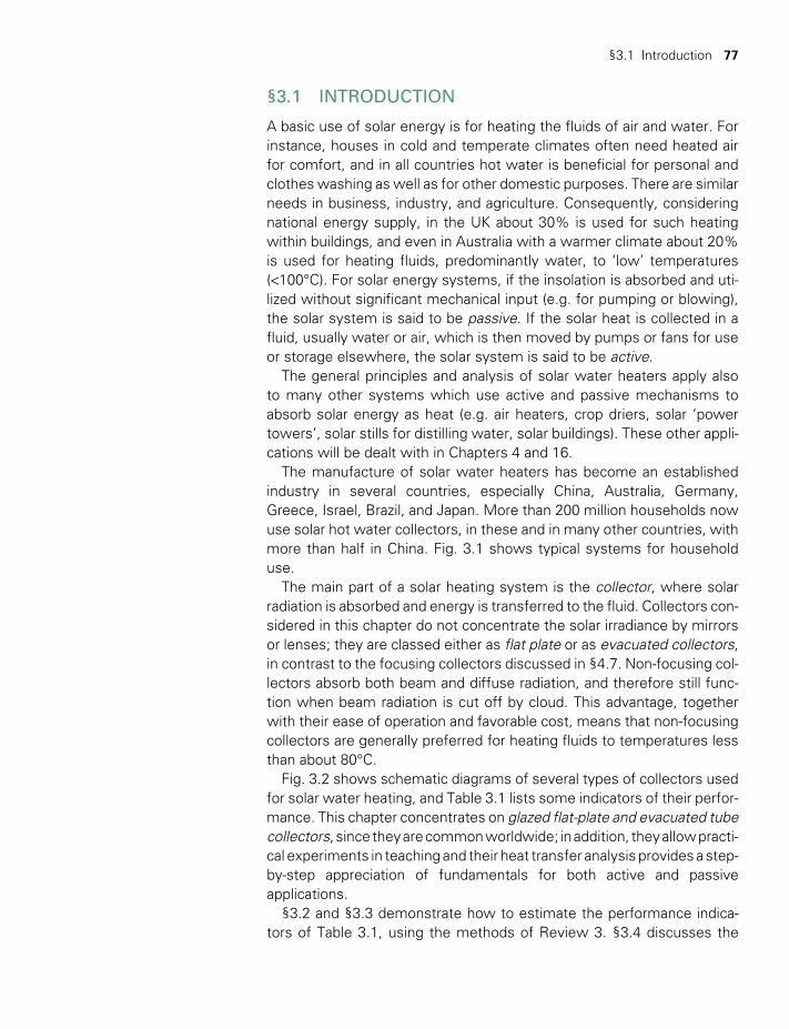
§3.1 Introduction 77
§3.1 INTRODUCTION
A basic use of solar energy is for heating the fluids of air and water. For instance, houses in cold and temperate climates often need heated air for comfort, and in all countries hot water is beneficial for personal and clothes washing as well as for other domestic purposes. There are similar needs in business, industry, and agriculture. Consequently, considering national energy supply, in the UK about 30% is used for such heating within buildings, and even in Australia with a warmer climate about 20% is used for heating fluids, predominantly water, to ‘low’ temperatures (<100°C). For solar energy systems, if the insolation is absorbed and uti-lized without significant mechanical input (e.g. for pumping or blowing), the solar system is said to be passive. If the solar heat is collected in a fluid, usually water or air, which is then moved by pumps or fans for use or storage elsewhere, the solar system is said to be active.
The general principles and analysis of solar water heaters apply also to many other systems which use active and passive mechanisms to absorb solar energy as heat (e.g. air heaters, crop driers, solar ‘power towers’, solar stills for distilling water, solar buildings). These other appli-cations will be dealt with in Chapters 4 and 16.
The manufacture of solar water heaters has become an established industry in several countries, especially China, Australia, Germany, Greece, Israel, Brazil, and Japan. More than 200 million households now use solar hot water collectors, in these and in many other countries, with more than half in China. Fig. 3.1 shows typical systems for household use.
The main part of a solar heating system is the collector, where solar radiation is absorbed and energy is transferred to the fluid. Collectors con-sidered in this chapter do not concentrate the solar irradiance by mirrors or lenses; they are classed either as flat plate or as evacuated collectors, in contrast to the focusing collectors discussed in §4.7. Non-focusing col-lectors absorb both beam and diffuse radiation, and therefore still func-tion when beam radiation is cut off by cloud. This advantage, together with their ease of operation and favorable cost, means that non-focusing collectors are generally preferred for heating fluids to temperatures less than about 80°C.
Fig. 3.2 shows schematic diagrams of several types of collectors used for solar water heating, and Table 3.1 lists some indicators of their perfor-mance. This chapter concentrates on glazed flat-plate and evacuated tube collectors, since they are common worldwide; in addition, they allow practi-cal experiments in teaching and their heat transfer analysis provides a step- by-step appreciation of fundamentals for both active and passive applications.
§3.2 and §3.3 demonstrate how to estimate the performance indica-tors of Table 3.1, using the methods of Review 3. §3.4 discusses the
TWIDELL PAGINATION.indb 77 01/12/2014 11:36
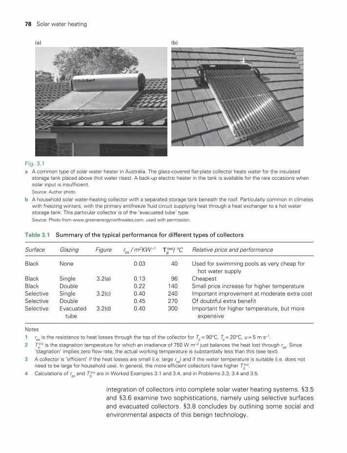
78 Solar water heating
Fig. 3.1a A common type of solar water heater in Australia. The glass-covered flat-plate collector heats water for the insulated
storage tank placed above (hot water rises). A back-up electric heater in the tank is available for the rare occasions when solar input is insufficient.
Source: Author photo.
b A household solar water-heating collector with a separated storage tank beneath the roof. Particularly common in climates with freezing winters, with the primary antifreeze fluid circuit supplying heat through a heat exchanger to a hot water storage tank. This particular collector is of the ‘evacuated tube’ type.
Source: Photo from www.greenenergynorthwales.com, used with permission.
(a) (b)
Table 3.1 Summary of the typical performance for different types of collectors
Surface Glazing Figure rpa / m2KW –1 Tp
(m)/ ºC Relative price and performance
Black None 0.03 40 Used for swimming pools as very cheap for hot water supply
Black Single 3.2(a) 0.13 96 CheapestBlack Double 0.22 140 Small price increase for higher temperatureSelective Single 3.2(c) 0.40 240 Important improvement at moderate extra costSelective Double 0.45 270 Of doubtful extra benefitSelective Evacuated
tube3.2(d) 0.40 300 Important for higher temperature, but more
expensive
Notes1 rpa is the resistance to heat losses through the top of the collector for Tp = 90°C, Ta = 20°C, u = 5 m s–1.2 Tp
(m) is the stagnation temperature for which an irradiance of 750 W m–2 just balances the heat lost through rpa. Since ‘stagnation’ implies zero flow rate, the actual working temperature is substantially less than this (see text).
3 A collector is ‘efficient’ if the heat losses are small (i.e. large rpa) and if the water temperature is suitable (i.e. does not need to be large for household use). In general, the more efficient collectors have higher Tp
(m). 4 Calculations of rpa and Tp
(m) are in Worked Examples 3.1 and 3.4, and in Problems 3.3, 3.4 and 3.5.
integration of collectors into complete solar water heating systems. §3.5 and §3.6 examine two sophistications, namely using selective surfaces and evacuated collectors. §3.8 concludes by outlining some social and environmental aspects of this benign technology.
TWIDELL PAGINATION.indb 78 01/12/2014 11:36
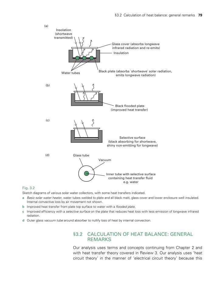
§3.2 Calculation of heat balance: general remarks 79
Fig. 3.2Sketch diagrams of various solar water collectors, with some heat transfers indicated. a Basic solar water heater, water tubes welded to plate and all black matt, glass cover and lower enclosure well insulated.
Internal convective loss by air movement not shown.b Improved heat transfer from plate top surface to water with a flooded plate.c Improved efficiency with a selective surface on the plate that reduces heat loss with less emission of longwave infrared
radiation.d Outer glass vacuum tube around absorber to nullify loss of heat by internal convection.
(b)
Black flooded plate(improved heat transfer)
(c)
Selective surface(black absorbing for shortwave,
shiny non-emitting for longwave)
(d) Glass tubeVacuum
Inner tube with selective surfacecontaining heat transfer fluid
e.g. water
Insulation
Insolation(shortwavetransmitted)
Glass cover (absorbs longwave infrared radiation and re-emits)
(a)
Water tubes Black plate (absorbs `shortwave´ solar radiation, emits longwave radiation)
§3.2 CALCULATION OF HEAT BALANCE: GENERAL REMARKS
Our analysis uses terms and concepts continuing from Chapter 2 and with heat transfer theory covered in Review 3. Our analysis uses ‘heat circuit theory’ in the manner of ‘electrical circuit theory’ because this
TWIDELL PAGINATION.indb 79 01/12/2014 11:36
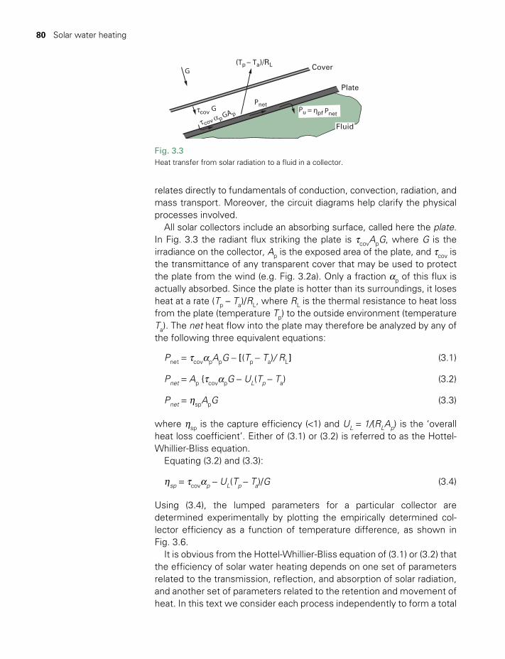
80 Solar water heating
relates directly to fundamentals of conduction, convection, radiation, and mass transport. Moreover, the circuit diagrams help clarify the physical processes involved.
All solar collectors include an absorbing surface, called here the plate. In Fig. 3.3 the radiant flux striking the plate is τcovApG, where G is the irradiance on the collector, Ap is the exposed area of the plate, and τcov is the transmittance of any transparent cover that may be used to protect the plate from the wind (e.g. Fig. 3.2a). Only a fraction αp of this flux is actually absorbed. Since the plate is hotter than its surroundings, it loses heat at a rate (Tp – Ta)/RL, where RL is the thermal resistance to heat loss from the plate (temperature Tp) to the outside environment (temperature Ta). The net heat flow into the plate may therefore be analyzed by any of the following three equivalent equations:
Pnet = τcovαpApG − [(Tp − Ta)/ RL] (3.1)
Pnet = Ap τcovαpG − UL(Tp − Ta) (3.2)
Pnet = ηspApG (3.3)
where ηsp is the capture efficiency (<1) and UL = 1/(RLAp) is the ‘overall heat loss coefficient’. Either of (3.1) or (3.2) is referred to as the Hottel-Whillier-Bliss equation.
Equating (3.2) and (3.3):
ηsp = τcovαp − UL(Tp − Ta)/G (3.4)
Using (3.4), the lumped parameters for a particular collector are determined experimentally by plotting the empirically determined col-lector efficiency as a function of temperature difference, as shown in Fig. 3.6.
It is obvious from the Hottel-Whillier-Bliss equation of (3.1) or (3.2) that the efficiency of solar water heating depends on one set of parameters related to the transmission, reflection, and absorption of solar radiation, and another set of parameters related to the retention and movement of heat. In this text we consider each process independently to form a total
Fig. 3.3Heat transfer from solar radiation to a fluid in a collector.
G Cover
Plate
GGAp
Pnet
αp
τcov
(Tp – Ta)/RL
τcov
Pu = ηpf Pnet
Fluid
TWIDELL PAGINATION.indb 80 01/12/2014 11:36
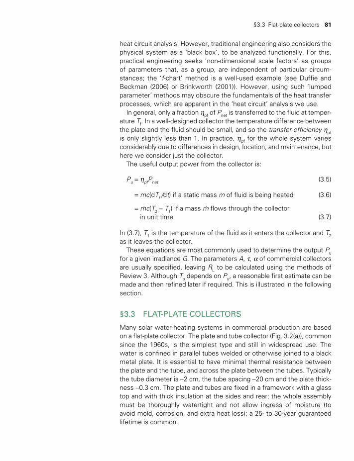
§3.3 Flat-plate collectors 81
heat circuit analysis. However, traditional engineering also considers the physical system as a ‘black box’, to be analyzed functionally. For this, practical engineering seeks ‘non-dimensional scale factors’ as groups of parameters that, as a group, are independent of particular circum-stances; the ‘f-chart’ method is a well-used example (see Duffie and Beckman (2006) or Brinkworth (2001)). However, using such ‘lumped parameter’ methods may obscure the fundamentals of the heat transfer processes, which are apparent in the ‘heat circuit’ analysis we use.
In general, only a fraction ηpf of Pnet is transferred to the fluid at temper-ature Tf. In a well-designed collector the temperature difference between the plate and the fluid should be small, and so the transfer efficiency ηpf is only slightly less than 1. In practice, ηpf for the whole system varies considerably due to differences in design, location, and maintenance, but here we consider just the collector.
The useful output power from the collector is:
Pu = ηpfPnet (3.5)
= mc(dTf /dt) if a static mass m of fluid is being heated (3.6)
= m. c(T2 − T1) if a mass m. flows through the collector in unit time (3.7)
In (3.7), T1 is the temperature of the fluid as it enters the collector and T2 as it leaves the collector.
These equations are most commonly used to determine the output Pu for a given irradiance G. The parameters A, τ, α of commercial collectors are usually specified, leaving RL to be calculated using the methods of Review 3. Although Tp depends on Pu, a reasonable first estimate can be made and then refined later if required. This is illustrated in the following section.
§3.3 FLAT-PLATE COLLECTORS
Many solar water-heating systems in commercial production are based on a flat-plate collector. The plate and tube collector (Fig. 3.2(a)), common since the 1960s, is the simplest type and still in widespread use. The water is confined in parallel tubes welded or otherwise joined to a black metal plate. It is essential to have minimal thermal resistance between the plate and the tube, and across the plate between the tubes. Typically the tube diameter is ~2 cm, the tube spacing ~20 cm and the plate thick-ness ~0.3 cm. The plate and tubes are fixed in a framework with a glass top and with thick insulation at the sides and rear; the whole assembly must be thoroughly watertight and not allow ingress of moisture (to avoid mold, corrosion, and extra heat loss); a 25- to 30-year guaranteed lifetime is common.
TWIDELL PAGINATION.indb 81 01/12/2014 11:36
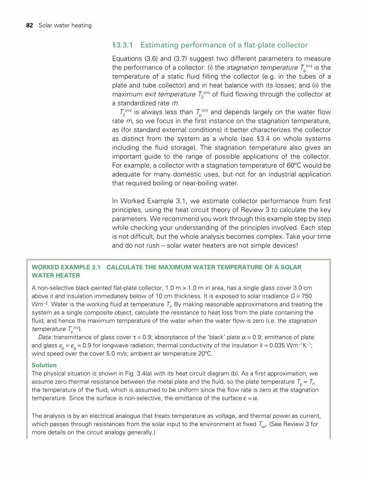
82 Solar water heating
§3.3.1 Estimating performance of a flat-plate collector
Equations (3.6) and (3.7) suggest two different parameters to measure the performance of a collector: (i) the stagnation temperature Tp
(m) is the temperature of a static fluid filling the collector (e.g. in the tubes of a plate and tube collector) and in heat balance with its losses; and (ii) the maximum exit temperature T2
(m) of fluid flowing through the collector at a standardized rate m. .
T2(m) is always less than Tp
(m) and depends largely on the water flow rate m. , so we focus in the first instance on the stagnation temperature, as (for standard external conditions) it better characterizes the collector as distinct from the system as a whole (see §3.4 on whole systems including the fluid storage). The stagnation temperature also gives an important guide to the range of possible applications of the collector. For example, a collector with a stagnation temperature of 60ºC would be adequate for many domestic uses, but not for an industrial application that required boiling or near-boiling water.
In Worked Example 3.1, we estimate collector performance from first principles, using the heat circuit theory of Review 3 to calculate the key parameters. We recommend you work through this example step by step while checking your understanding of the principles involved. Each step is not difficult, but the whole analysis becomes complex. Take your time and do not rush – solar water heaters are not simple devices!
WORKED EXAMPLE 3.1 CALCULATE THE MAXIMUM WATER TEMPERATURE OF A SOLAR WATER HEATER
A non-selective black-painted flat-plate collector, 1.0 m × 1.0 m in area, has a single glass cover 3.0 cm above it and insulation immediately below of 10 cm thickness. It is exposed to solar irradiance G = 750 Wm−2. Water is the working fluid at temperature Tf. By making reasonable approximations and treating the system as a single composite object, calculate the resistance to heat loss from the plate containing the fluid, and hence the maximum temperature of the water when the water flow is zero (i.e. the stagnation temperature Tp
(m)).Data: transmittance of glass cover τ = 0.9; absorptance of the ‘black’ plate α = 0.9; emittance of plate
and glass ep = eg = 0.9 for longwave radiation; thermal conductivity of the insulation k = 0.035 Wm−1K−1; wind speed over the cover 5.0 m/s; ambient air temperature 20ºC.
SolutionThe physical situation is shown in Fig. 3.4(a) with its heat circuit diagram (b). As a first approxim ation, we assume zero thermal resistance between the metal plate and the fluid, so the plate temperature Tp = Tf, the temperature of the fluid, which is assumed to be uniform since the flow rate is zero at the stagnation temperature. Since the surface is non-selective, the emittance of the surface e = α.
The analysis is by an electrical analogue that treats temperature as voltage, and thermal power as current, which passes through resistances from the solar input to the environment at fixed Tref. (See Review 3 for more details on the circuit analogy generally.)
TWIDELL PAGINATION.indb 82 01/12/2014 11:36
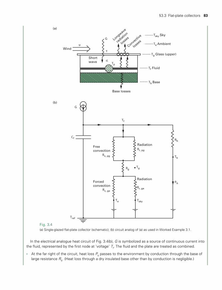
§3.3 Flat-plate collectors 83
In the electrical analogue heat circuit of Fig. 3.4(b), G is symbolized as a source of continuous current into the fluid, represented by the first node at ‘voltage’ Tf. The fluid and the plate are treated as combined.
• At the far right of the circuit, heat loss Pb passes to the environment by conduction through the base of large resistance Rb. (Heat loss through a dry insulated base other than by conduction is negligible.)
Fig. 3.4(a) Single-glazed flat-plate collector (schematic); (b) circuit analog of (a) as used in Worked Example 3.1.
Wind
(a)
(b)
Freeconvection
Forcedconvection
Radiation
Radiation
Shortwave
Longwave
radiatio
n
losses
Convective
losses
u
G
G
τ
Tb Base
Cf
RgTg
Tf
TskyTa
Tref
Rr, pg
Rr, ga
Rb
Tb
Pb
Rv, pg
Rv, ga
Tg Glass (upper)
Tf Fluid
Ta Ambient
Tsky Sky
Base losses
Tp
TWIDELL PAGINATION.indb 83 01/12/2014 11:36
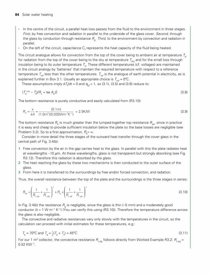
84 Solar water heating
• In the centre of the circuit, a parallel heat loss passes from the fluid to the environment in three stages. First, by free convection and radiation in parallel to the underside of the glass cover. Second, through the glass by conduction through resistance Rg. Third, to the environment by convection and radiation in parallel.
• On the left of the circuit, capacitance Cf represents the heat capacity of the fluid being heated.
The circuit analogue allows for convection from the top of the cover being to ambient air at temperature Ta, for radiation from the top of the cover being to the sky at temperature Tsky and for the small loss through insulation being to its outer temperature Tb. These different temperatures (cf. voltages) are maintained in the circuit analogy by ‘batteries’ that maintain the required temperature with respect to a reference temperature Tref less than the other temperatures. Tref is the analogue of earth potential in electricity, as is explained further in Box 3.1. Usually an appropriate choice is Tref = 0ºC.
These assumptions imply dTf/dt = 0 and ηpf = 1, so (3.1), (3.5) and (3.6) reduce to:
(Tp(m) − Ta)/RL = τα ApG (3.8)
The bottom resistance is purely conductive and easily calculated from (R3.10):
= = − −Rx
kA(0.1m)
(1.0m )(0.035Wm K )= 2.9K/Wb 2 1 1 (3.9)
The bottom resistance Rb is much greater than the lumped-together top resistance Rpa, since in practice it is easy and cheap to provide sufficient insulation below the plate so the base losses are negligible (see Problem 3.2). So to a first approximation, Rb= ∞.
Consider in more detail the three stages of the outward heat transfer through the cover glass in the central path of Fig. 3.4(b):
1 Free convection by the air in the gap carries heat to the glass. In parallel with this the plate radiates heat at wavelengths ~10 mm. At these wavelengths, glass is not transparent but strongly absorbing (see Fig. R3.12). Therefore this radiation is absorbed by the glass.
2 The heat reaching the glass by these two mechanisms is then conducted to the outer surface of the glass.
3 From here it is transferred to the surroundings by free and/or forced convection, and radiation.
Thus, the overall resistance between the top of the plate and the surroundings is the three stages in series:
= +
+ + +
− −
RR R
RR R
1 1 1 1
v pg r pg v ga r gapa
, ,
1
g, ,
1
(3.10)
In Fig. 3.4(b) the resistance Rg is negligible, since the glass is thin (~5 mm) and a moderately good conductor (k ≈ 1 W m−1 K−1) (You can verify this using (R3.10)). Therefore the temperature difference across the glass is also negligible.
The convective and radiative resistances vary only slowly with the temperatures in the circuit, so the calculation can proceed with initial estimates for these temperatures, e.g.:
Tp = 70ºC and Tg = 12(Tp + Ta) = 45ºC (3.11)
For our 1 m2 collector, the convective resistance Rv,pg follows directly from Worked Example R3.2: Rv,pg = 0.52 KW−1.
TWIDELL PAGINATION.indb 84 01/12/2014 11:36
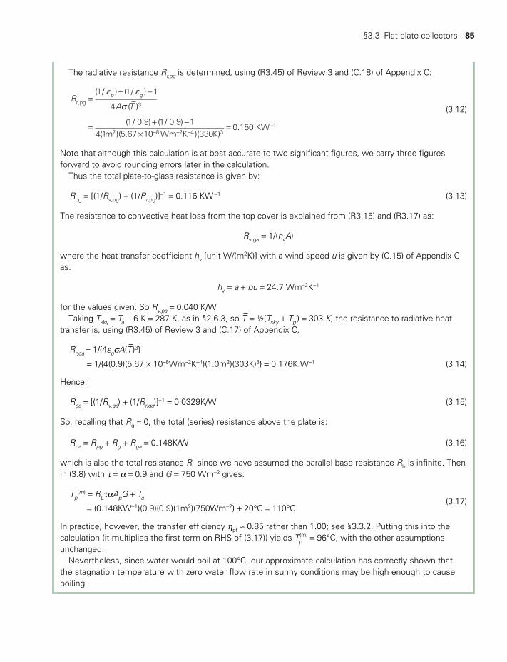
§3.3 Flat-plate collectors 85
The radiative resistance Rr,pg is determined, using (R3.45) of Review 3 and (C.18) of Appendix C:
RA T
(1/ ) (1/ ) 1
4 ( )
(1/ 0.9) (1/ 0.9) 14(1m )(5.67 10 Wm K )(330K)
0.150 KW
p gr,pg 3
2 8 2 4 31
e e
σ=
+ −
= + −×
=− − −
−
(3.12)
Note that although this calculation is at best accurate to two significant figures, we carry three figures forward to avoid rounding errors later in the calculation.
Thus the total plate-to-glass resistance is given by:
Rpg = [(1/Rv,pg) + (1/Rr,pg)]−1 = 0.116 KW −1 (3.13)
The resistance to convective heat loss from the top cover is explained from (R3.15) and (R3.17) as:
Rv,ga = 1/(hvA)
where the heat transfer coefficient hv [unit W/(m2K)] with a wind speed u is given by (C.15) of Appendix C as:
hv = a + bu = 24.7 Wm−2K−1
for the values given. So Rv,pa = 0.040 K/WTaking Tsky
= Ta − 6 K = 287 K, as in §2.6.3, so T– = ½(Tsky + Tg ) = 303 K, the resistance to radiative heat
transfer is, using (R3.45) of Review 3 and (C.17) of Appendix C,
Rr,ga = 1/4egσA(T–)3
= 1/4(0.9)(5.67 × 10−8Wm−2K−4)(1.0m2)(303K)3 = 0.176K.W−1 (3.14)
Hence:
Rga = [(1/Rv,ga) + (1/Rr,ga)]−1 = 0.0329K/W (3.15)
So, recalling that Rg ≈ 0, the total (series) resistance above the plate is:
Rpa = Rpg + Rg + Rga = 0.148K/W (3.16)
which is also the total resistance RL since we have assumed the parallel base resistance Rb is infinite. Then in (3.8) with τ = α = 0.9 and G = 750 Wm−2 gives:
Tp(m) = RLταApG + Ta (3.17)
= (0.148KW−1)(0.9)(0.9)(1m2)(750Wm−2) + 20°C = 110°C
In practice, however, the transfer efficiency ηpf ≈ 0.85 rather than 1.00; see §3.3.2. Putting this into the calculation (it multiplies the first term on RHS of (3.17)) yields Tp
(m) = 96°C, with the other assumptions unchanged.
Nevertheless, since water would boil at 100°C, our approximate calculation has correctly shown that the stagnation temperature with zero water flow rate in sunny conditions may be high enough to cause boiling.
TWIDELL PAGINATION.indb 85 01/12/2014 11:36
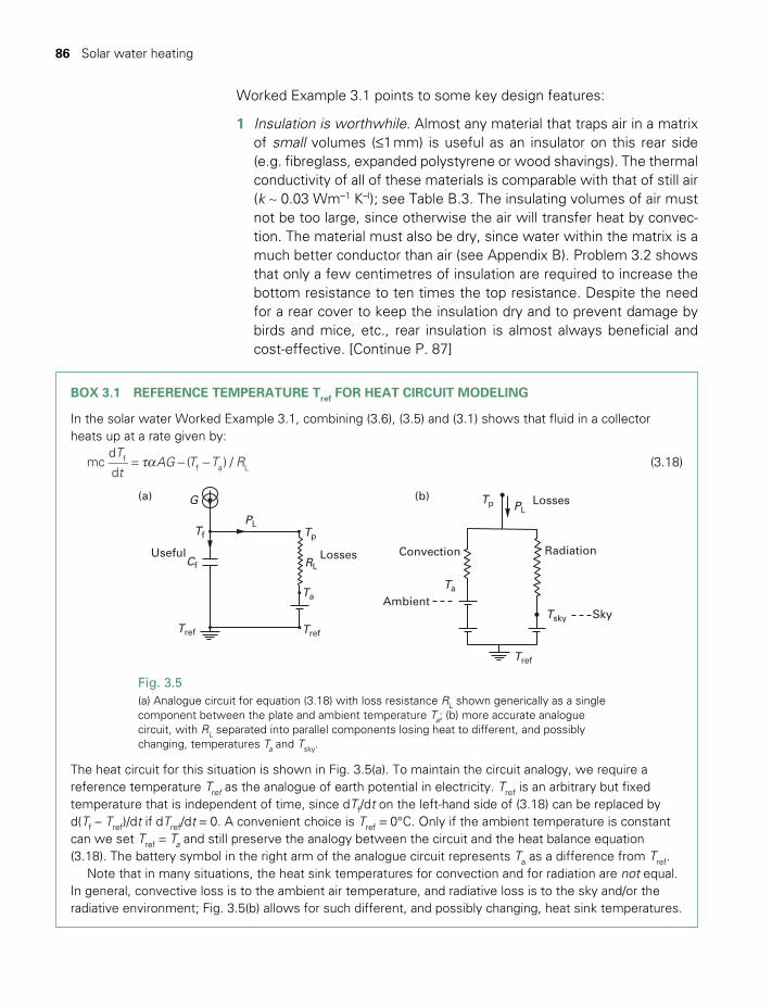
86 Solar water heating
Worked Example 3.1 points to some key design features:
1 Insulation is worthwhile. Almost any material that traps air in a matrix of small volumes (≤1 mm) is useful as an insulator on this rear side (e.g. fibreglass, expanded polystyrene or wood shavings). The thermal conductivity of all of these materials is comparable with that of still air (k ~ 0.03 Wm–1 K–l); see Table B.3. The insulating volumes of air must not be too large, since otherwise the air will transfer heat by convec-tion. The material must also be dry, since water within the matrix is a much better conductor than air (see Appendix B). Problem 3.2 shows that only a few centimetres of insulation are required to increase the bottom resistance to ten times the top resistance. Despite the need for a rear cover to keep the insulation dry and to prevent damage by birds and mice, etc., rear insulation is almost always beneficial and cost-effective. [Continue P. 87]
BOX 3.1 REFERENCE TEMPERATURE Tref FOR HEAT CIRCUIT MODELING
In the solar water Worked Example 3.1, combining (3.6), (3.5) and (3.1) shows that fluid in a collector heats up at a rate given by:
τα= − −T
tAG T T Rmc
d
d( ) /f
f a L (3.18)
Fig. 3.5(a) Analogue circuit for equation (3.18) with loss resistance RL shown generically as a single component between the plate and ambient temperature Ta; (b) more accurate analogue circuit, with RL separated into parallel components losing heat to different, and possibly changing, temperatures Ta and Tsky.
G
Useful
Tf
Cf
PLTp
RL
TaTa
Tp PL
Tsky Sky
Tref
TrefTref
Convection Radiation
Ambient
Losses
Losses(b)(a)
The heat circuit for this situation is shown in Fig. 3.5(a). To maintain the circuit analogy, we require a reference temperature Tref as the analogue of earth potential in electricity. Tref is an arbitrary but fixed temperature that is independent of time, since dTf/dt on the left-hand side of (3.18) can be replaced by d(Tf – Tref)/dt if dTref/dt = 0. A convenient choice is Tref = 0°C. Only if the ambient temperature is constant can we set Tref = Ta and still preserve the analogy between the circuit and the heat balance equation (3.18). The battery symbol in the right arm of the analogue circuit represents Ta as a difference from Tref.
Note that in many situations, the heat sink temperatures for convection and for radiation are not equal. In general, convective loss is to the ambient air temperature, and radiative loss is to the sky and/or the radiative environment; Fig. 3.5(b) allows for such different, and possibly changing, heat sink temperatures.
TWIDELL PAGINATION.indb 86 01/12/2014 11:36
§3.3 Flat-plate collectors 87
2 Avoid excessive pressure and other dangers from very hot water and boiling. Even simple solar water heaters produce dangerous condi-tions if elementary safeguards are not taken (e.g. pressure release valves, warning signs, child entry prevention). Avoiding boiling is one reason why thermosyphon systems (§3.4.2) are preferred in very sunny climates (since their water flow is not subject to pump failure).
§3.3.2 Efficiency of a flat-plate collector
A collector of efficiency ηc and area Ap, exposed to irradiance G (meas-ured in the plane of the collector), gives a useful output:
Pu = ηcApG (3.19)
According to (3.3) and (3.5), the collector efficiency ηc can be divided into two stages, the capture efficiency ηsp and the transfer efficiency ηpf:
ηc = ηspηpf (3.20)
It follows from (3.2) that:
ηsp = τcovαp − UL(Tp − Ta)/G (3.21)
which shows that as the plate gets hotter, the losses increase until ηsp decreases to zero at the ‘equilibrium’ temperature Tp
(m) (also called the stagnation temperature).
Because the plate temperature Tp of an operating collector is not usually known, it is more convenient to relate the useful energy gain to the mean fluid temperature T–f. Hence:
ηc = Pu /(AG) = ηpfτcovαp − ηpf UL(T–
f − Ta)/G (3.22)
In a well-designed collector, the temperature difference between the plate and the fluid is small and the value of ηpf is nearly one (see Problem 3.8). Typically, ηpf = 0.85 and is almost independent of the operating conditions, and, since pipes and storage tanks should be well insulated, T–
f ≈ Tp, the collector plate temperature. Hence the UL in (3.22) is numeri-cally almost the same as that in (3.21). The capture efficiency ηsp (and therefore also the collector efficiency ηc) would vary linearly with tem-perature if UL = 1/(APRL) is constant in (3.21) and (3.22), but in practice the radiative resistance decreases appreciably as Tp increases. Therefore a plot of ηc against operating temperature is curved, as in Fig. 3.6.
The performance of a flat-plate collector, and in particular its efficiency at high temperatures, can be substantially improved by one or both of the following:
1 Reducing the convective transfer between the plate and the outer glass cover, with a double-glazed top cover (see Fig. 5.1(b) and Problem 3.5).
TWIDELL PAGINATION.indb 87 01/12/2014 11:36
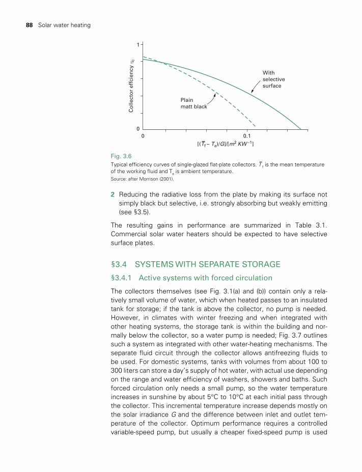
88 Solar water heating
2 Reducing the radiative loss from the plate by making its surface not simply black but selective, i.e. strongly absorbing but weakly emitting (see §3.5).
The resulting gains in performance are summarized in Table 3.1. Commercial solar water heaters should be expected to have selective surface plates.
§3.4 SYSTEMS WITH SEPARATE STORAGE
§3.4.1 Active systems with forced circulation
The collectors themselves (see Fig. 3.1(a) and (b)) contain only a rela-tively small volume of water, which when heated passes to an insulated tank for storage; if the tank is above the collector, no pump is needed. However, in climates with winter freezing and when integrated with other heating systems, the storage tank is within the building and nor-mally below the collector, so a water pump is needed; Fig. 3.7 outlines such a system as integrated with other water-heating mechanisms. The separate fluid circuit through the collector allows antifreezing fluids to be used. For domestic systems, tanks with volumes from about 100 to 300 liters can store a day’s supply of hot water, with actual use depending on the range and water efficiency of washers, showers and baths. Such forced circulation only needs a small pump, so the water temperature increases in sunshine by about 5°C to 10°C at each initial pass through the collect or. This incremental temperature increase depends mostly on the solar irradiance G and the difference between inlet and outlet tem-perature of the collector. Optimum performance requires a controlled variable-speed pump, but usually a cheaper fixed-speed pump is used
Fig. 3.6Typical efficiency curves of single-glazed flat-plate collectors. T
–f is the mean temperature
of the working fluid and Ta is ambient temperature. Source: after Morrison (2001).
0.1C
olle
cto
r ef
fcie
ncy
ηc
Plainmatt black
Withselectivesurface
00
1
[(Tf – Ta)/G]/[m2 KW –1]
TWIDELL PAGINATION.indb 88 01/12/2014 11:36
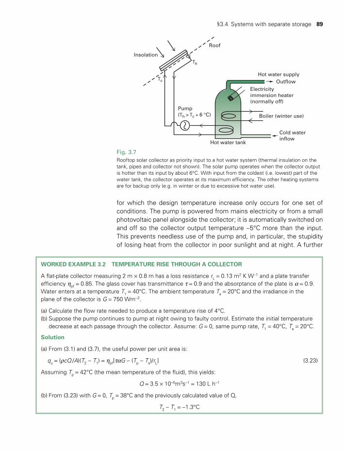
§3.4 Systems with separate storage 89
for which the design temperature increase only occurs for one set of conditions. The pump is powered from mains electricity or from a small photovoltaic panel alongside the collector; it is automatically switched on and off so the collector output temperature ~5°C more than the input. This prevents needless use of the pump and, in particular, the stupidity of losing heat from the collector in poor sunlight and at night. A further
Fig. 3.7Rooftop solar collector as priority input to a hot water system (thermal insulation on the tank, pipes and collector not shown). The solar pump operates when the collector output is hotter than its input by about 6°C. With input from the coldest (i.e. lowest) part of the water tank, the collector operates at its maximum efficiency. The other heating systems are for backup only (e.g. in winter or due to excessive hot water use).
Hot water supply
Electricityimmersion heater(normally off)
Boiler (winter use)
Cold waterinflow
Hot water tank
Pump(Th > Tc + 6 °C)
Insolation
Roof
Th
Tc Outf low
WORKED EXAMPLE 3.2 TEMPERATURE RISE THROUGH A COLLECTOR
A flat-plate collector measuring 2 m × 0.8 m has a loss resistance rL = 0.13 m2 K W−1 and a plate transfer efficiency ηpf = 0.85. The glass cover has transmittance τ = 0.9 and the absorptance of the plate is α = 0.9. Water enters at a temperature T1 = 40°C. The ambient temperature Ta = 20°C and the irradiance in the plane of the collector is G = 750 Wm−2.
(a) Calculate the flow rate needed to produce a temperature rise of 4°C.(b) Suppose the pump continues to pump at night owing to faulty control. Estimate the initial temperature
decrease at each passage through the collector. Assume: G = 0, same pump rate, T1 = 40°C, Ta = 20°C.
Solution
(a) From (3.1) and (3.7), the useful power per unit area is:
qu = (ρcQ /A)(T2 − T1) = ηpf[ταG − (Tp − Ta)/rL] (3.23)
Assuming Tp = 42°C (the mean temperature of the fluid), this yields:
Q = 3.5 × 10⁻⁵m3s−1 = 130 L h−1
(b) From (3.23) with G = 0, Tp = 38°C and the previously calculated value of Q,
T2 – T1 = −1.3°C
TWIDELL PAGINATION.indb 89 01/12/2014 11:36
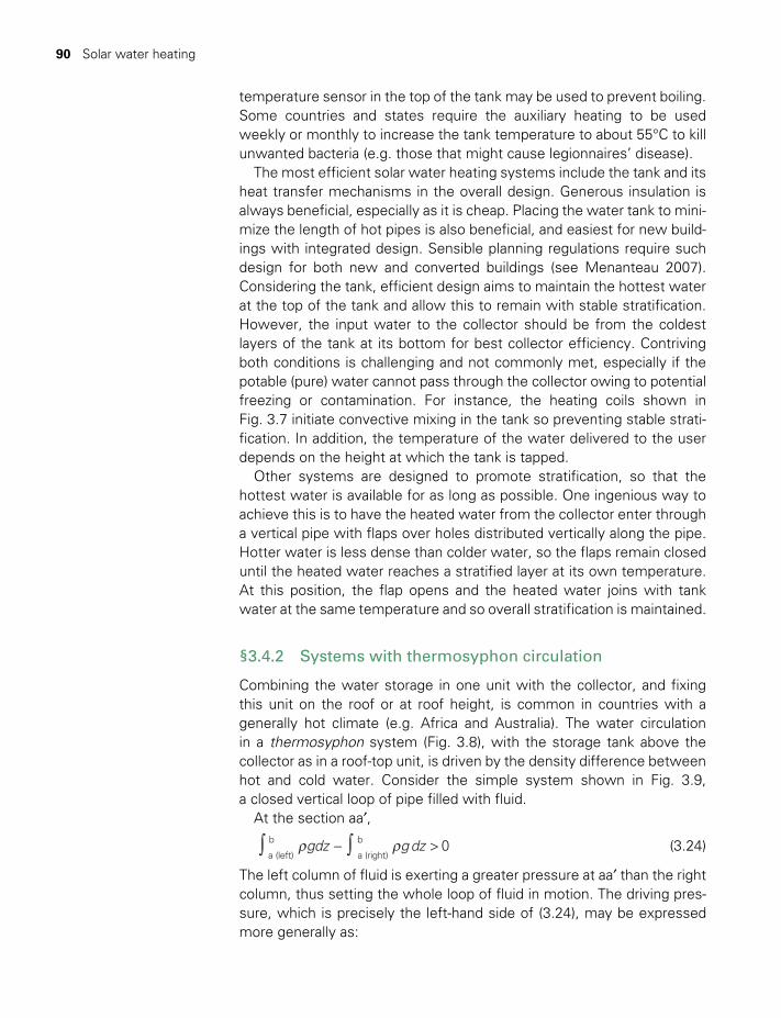
90 Solar water heating
temperature sensor in the top of the tank may be used to prevent boiling. Some countries and states require the auxiliary heating to be used weekly or monthly to increase the tank temperature to about 55°C to kill unwanted bacteria (e.g. those that might cause legionnaires’ disease).
The most efficient solar water heating systems include the tank and its heat transfer mechanisms in the overall design. Generous insulation is always beneficial, especially as it is cheap. Placing the water tank to mini-mize the length of hot pipes is also beneficial, and easiest for new build-ings with integrated design. Sensible planning regulations require such design for both new and converted buildings (see Menanteau 2007). Considering the tank, efficient design aims to maintain the hottest water at the top of the tank and allow this to remain with stable stratification. However, the input water to the collector should be from the coldest layers of the tank at its bottom for best collector efficiency. Contriving both conditions is challenging and not commonly met, especially if the potable (pure) water cannot pass through the collector owing to potential freezing or contamination. For instance, the heating coils shown in Fig. 3.7 initiate convective mixing in the tank so preventing stable strati-fication. In addition, the temperature of the water delivered to the user depends on the height at which the tank is tapped.
Other systems are designed to promote stratification, so that the hottest water is available for as long as possible. One ingenious way to achieve this is to have the heated water from the collector enter through a vertical pipe with flaps over holes distributed vertically along the pipe. Hotter water is less dense than colder water, so the flaps remain closed until the heated water reaches a stratified layer at its own temperature. At this position, the flap opens and the heated water joins with tank water at the same temperature and so overall stratification is maintained.
§3.4.2 Systems with thermosyphon circulation
Combining the water storage in one unit with the collector, and fixing this unit on the roof or at roof height, is common in countries with a generally hot climate (e.g. Africa and Australia). The water circulation in a thermosyphon system (Fig. 3.8), with the storage tank above the collect or as in a roof-top unit, is driven by the density difference between hot and cold water. Consider the simple system shown in Fig. 3.9, a closed vertical loop of pipe filled with fluid.
At the section aa′,
gdz gdz 0a (left)
b
a (right)
b∫ ∫ρ ρ− > (3.24)
The left column of fluid is exerting a greater pressure at aa′ than the right column, thus setting the whole loop of fluid in motion. The driving pres-sure, which is precisely the left-hand side of (3.24), may be expressed more generally as:
TWIDELL PAGINATION.indb 90 01/12/2014 11:36
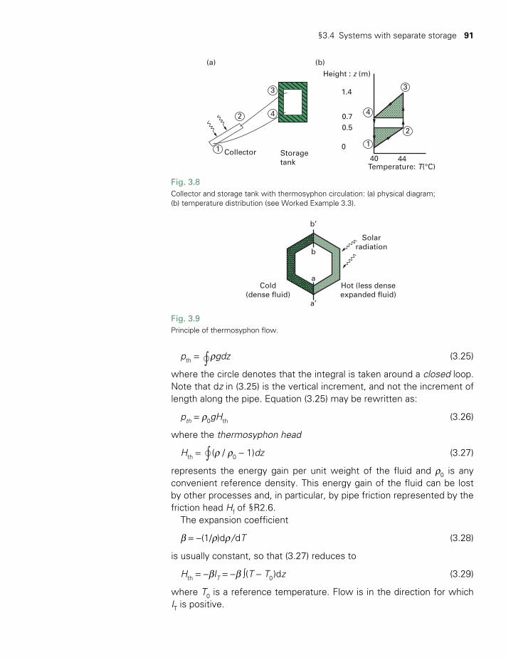
§3.4 Systems with separate storage 91
pth = ∫ ρgdz (3.25)
where the circle denotes that the integral is taken around a closed loop. Note that dz in (3.25) is the vertical increment, and not the increment of length along the pipe. Equation (3.25) may be rewritten as:
pth = ρ0gHth (3.26)
where the thermosyphon head
Hth = ∫ (ρ / ρ0 − 1)dz (3.27)
represents the energy gain per unit weight of the fluid and ρ0 is any convenient reference density. This energy gain of the fluid can be lost by other processes and, in particular, by pipe friction represented by the friction head Hf of §R2.6.
The expansion coefficient
β = −(1/ρ)dρ / dT (3.28)
is usually constant, so that (3.27) reduces to
Hth = −βIT = −β ∫(T − T0 )dz (3.29)
where T0 is a reference temperature. Flow is in the direction for which IT is positive.
Fig. 3.8Collector and storage tank with thermosyphon circulation: (a) physical diagram; (b) temperature distribution (see Worked Example 3.3).
Height : z (m)
1.4
0.70.5
0Storagetank
Collector1
2 4 4
1
2
33
40 44Temperature: T(°C)
(b)(a)
Fig. 3.9Principle of thermosyphon flow.
Cold(dense fluid)
Hot (less denseexpanded fluid)
Solarradiation
a’
b’
a
b
TWIDELL PAGINATION.indb 91 01/12/2014 11:36
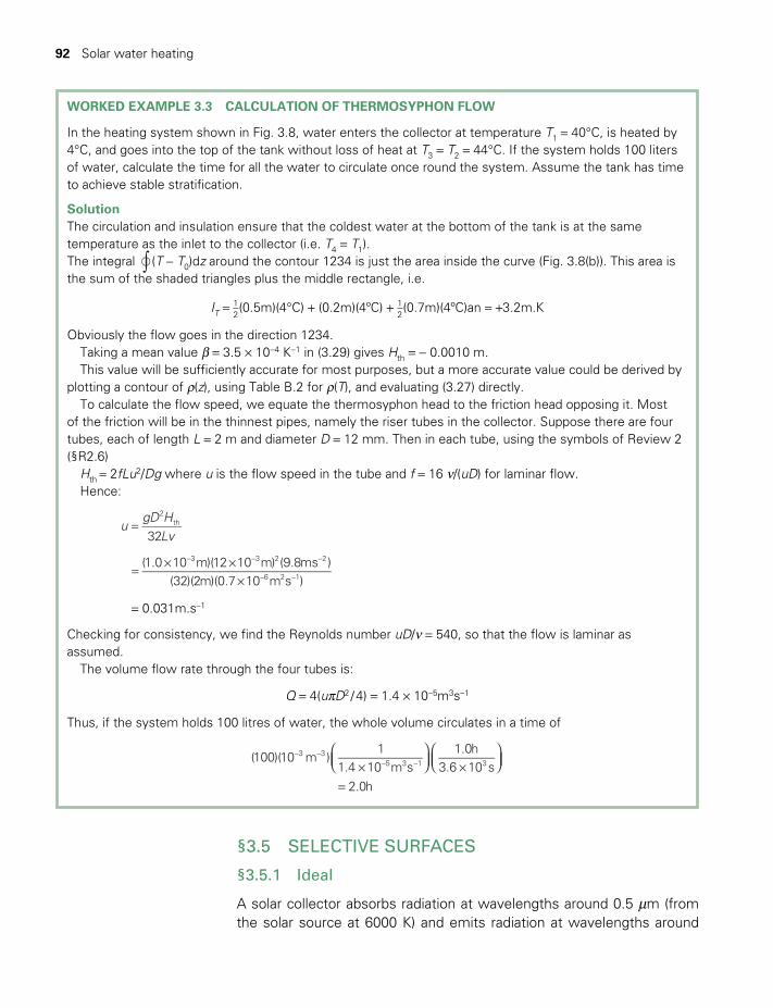
92 Solar water heating
§3.5 SELECTIVE SURFACES
§3.5.1 Ideal
A solar collector absorbs radiation at wavelengths around 0.5 mm (from the solar source at 6000 K) and emits radiation at wavelengths around
WORKED EXAMPLE 3.3 CALCULATION OF THERMOSYPHON FLOW
In the heating system shown in Fig. 3.8, water enters the collector at temperature T1 = 40°C, is heated by 4°C, and goes into the top of the tank without loss of heat at T3 = T2 = 44°C. If the system holds 100 liters of water, calculate the time for all the water to circulate once round the system. Assume the tank has time to achieve stable stratification.
SolutionThe circulation and insulation ensure that the coldest water at the bottom of the tank is at the same temperature as the inlet to the collector (i.e. T4 = T1). The integral ∫ (T − T0)dz around the contour 1234 is just the area inside the curve (Fig. 3.8(b)). This area is the sum of the shaded triangles plus the middle rectangle, i.e.
IT = 12(0.5m)(4°C) + (0.2m)(4ºC) + 1
2(0.7m)(4ºC)an = +3.2m.K
Obviously the flow goes in the direction 1234. Taking a mean value β = 3.5 × 10⁻⁴ K−1 in (3.29) gives Hth = − 0.0010 m. This value will be sufficiently accurate for most purposes, but a more accurate value could be derived by
plotting a contour of ρ(z), using Table B.2 for ρ(T), and evaluating (3.27) directly.To calculate the flow speed, we equate the thermosyphon head to the friction head opposing it. Most
of the friction will be in the thinnest pipes, namely the riser tubes in the collector. Suppose there are four tubes, each of length L = 2 m and diameter D = 12 mm. Then in each tube, using the symbols of Review 2 (§R2.6)
Hth = 2fLu2/Dg where u is the flow speed in the tube and f = 16 ν/(uD) for laminar flow.Hence:
=u
gD HLv32
2th
= × ×
×
− − −
− −
(1.0 10 m)(12 10 m) (9.8ms )(32)(2m)(0.7 10 m s )
3 3 2 2
6 2 1
= 0.031m.s–1
Checking for consistency, we find the Reynolds number uD/ν = 540, so that the flow is laminar as assumed.
The volume flow rate through the four tubes is:
Q = 4(uπD2 / 4) = 1.4 × 10⁻⁵m3s–1
Thus, if the system holds 100 litres of water, the whole volume circulates in a time of
(100)(10 m )1
1.4 10 m s1.0h
3.6 10 s2.0h
3 35 3 1 3×
×
=
− −− −
TWIDELL PAGINATION.indb 92 01/12/2014 11:36
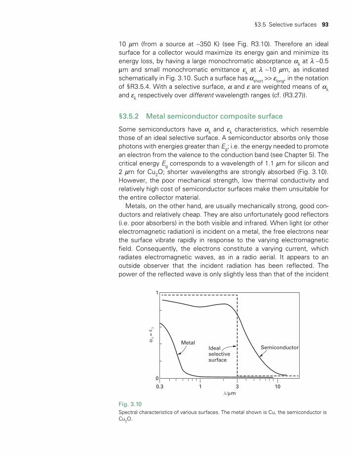
§3.5 Selective surfaces 93
10 mm (from a source at ~350 K) (see Fig. R3.10). Therefore an ideal surface for a collector would maximize its energy gain and minimize its energy loss, by having a large monochromatic absorptance αl at l ~0.5 mm and small monochromatic emittance el at l ~10 mm, as indicated schematic ally in Fig. 3.10. Such a surface has αshort >> elong, in the notation of §R3.5.4. With a selective surface, α and e are weighted means of αl and el respectively over different wavelength ranges (cf. (R3.27)).
§3.5.2 Metal semiconductor composite surface
Some semiconductors have αl and el characteristics, which resemble those of an ideal selective surface. A semiconductor absorbs only those photons with energies greater than Eg; i.e. the energy needed to promote an electron from the valence to the conduction band (see Chapter 5). The critical energy Eg corresponds to a wavelength of 1.1 mm for silicon and 2 mm for Cu2O; shorter wavelengths are strongly absorbed (Fig. 3.10). However, the poor mechanical strength, low thermal conductivity and relatively high cost of semiconductor surfaces make them unsuitable for the entire collector material.
Metals, on the other hand, are usually mechanically strong, good con-ductors and relatively cheap. They are also unfortunately good reflectors (i.e. poor absorbers) in the both visible and infrared. When light (or other electromagnetic radiation) is incident on a metal, the free electrons near the surface vibrate rapidly in response to the varying electromagnetic field. Consequently, the electrons constitute a varying current, which radiates electromagnetic waves, as in a radio aerial. It appears to an outside observer that the incident radiation has been reflected. The power of the reflected wave is only slightly less than that of the incident
Fig. 3.10Spectral characteristics of various surfaces. The metal shown is Cu, the semiconductor is Cu2O.
SemiconductorIdealselectivesurface
Metal
0
1
0.3 1 3 10λ /µm
α λ =
λ∋
TWIDELL PAGINATION.indb 93 01/12/2014 11:36
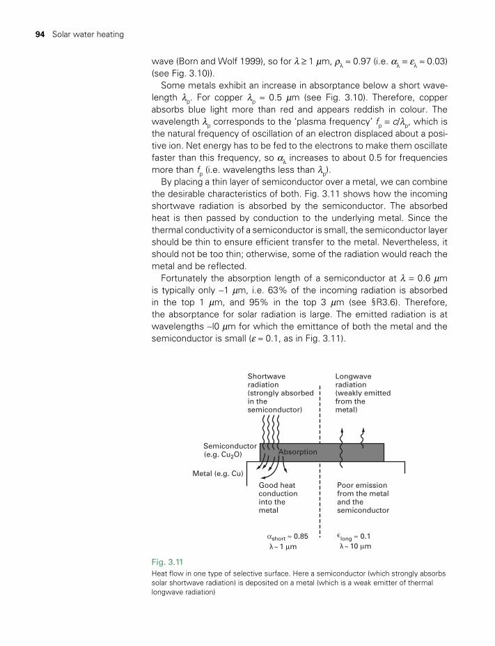
94 Solar water heating
wave (Born and Wolf 1999), so for l ≥ 1 mm, ρl ≈ 0.97 (i.e. αl = el ≈ 0.03) (see Fig. 3.10)).
Some metals exhibit an increase in absorptance below a short wave-length lp. For copper lp ≈ 0.5 mm (see Fig. 3.10). Therefore, copper absorbs blue light more than red and appears reddish in colour. The wavelength lp corresponds to the ‘plasma frequency’ fp = c/lp, which is the natural frequency of oscillation of an electron displaced about a posi-tive ion. Net energy has to be fed to the electrons to make them oscillate faster than this frequency, so αl increases to about 0.5 for frequencies more than fp (i.e. wavelengths less than lp).
By placing a thin layer of semiconductor over a metal, we can combine the desirable characteristics of both. Fig. 3.11 shows how the incoming shortwave radiation is absorbed by the semiconductor. The absorbed heat is then passed by conduction to the underlying metal. Since the thermal conductivity of a semiconductor is small, the semiconductor layer should be thin to ensure efficient transfer to the metal. Nevertheless, it should not be too thin; otherwise, some of the radiation would reach the metal and be reflected.
Fortunately the absorption length of a semiconductor at l = 0.6 mm is typically only ~1 mm, i.e. 63% of the incoming radiation is absorbed in the top 1 mm, and 95% in the top 3 mm (see §R3.6). Therefore, the absorptance for solar radiation is large. The emitted radiation is at wavelengths ~l0 mm for which the emittance of both the metal and the semiconductor is small (e ≈ 0.1, as in Fig. 3.11).
Fig. 3.11Heat flow in one type of selective surface. Here a semiconductor (which strongly absorbs solar shortwave radiation) is deposited on a metal (which is a weak emitter of thermal longwave radiation)
Shortwaveradiation(strongly absorbedin thesemiconductor)
Longwaveradiation(weakly emittedfrom themetal)
Absorption
Good heatconductioninto themetal
Poor emissionfrom the metaland thesemiconductor
αshort ≈ 0.85λ~ 1 µm λ~ 10 µm
∋
long ≈ 0.1
Semiconductor(e.g. Cu2O)
Metal (e.g. Cu)
TWIDELL PAGINATION.indb 94 01/12/2014 11:36
§3.5 Selective surfaces 95
The result is a composite surface that has much lower radiative loss than a simple black-painted surface (which is black to both visible and infrared radiation, and therefore has α = e ≈ 0.9). The absorptance is not quite as large as that of a pure black surface, because αl of the selective surface decreases for l≥ 1 mm (see Fig. 3.10), and 30% of the solar radia-tion is at wavelengths greater than 1 mm (see Fig. 4.1).
The small emittance of the selective surface becomes more of an advantage initially as the working temperature increases, since the radia-tive losses increase as eT4. For example, at a plate temperature of 40°C with e >0.9, radiative losses are typically only 20% of the total (e.g. cal-culate these in Worked Example 3.1); however, at a plate temperature of 400°C they would be 50% if e = 0.9 but only 10% if e = 0.1 (but see caution after (4.24) for T> 1000°C). Nevertheless, if the surface tempera-ture becomes extremely hot, for instance, for a collector in a concen-trated solar array (§4.8) at perhaps 1000ºC or more, then the wavelength range for both absorption (from the Sun) and emission (from the col-lector) overlap so that the monochromatic absorptance αl and mono-chromatic emittance el are no longer significantly different and selective surfaces cannot be obtained.
§3.5.3 Manufacture of selective surfaces
One method for preparing an actual selective surface involves dipping a sheet of copper into an alkaline solution, so that a film of Cu2O (which is a semiconductor) is formed on it. Many other surface coating types have been successfully developed, including black chrome (Cr/CrOx), metal pigmented aluminum oxide (e.g. Ni/ Al2O3) and oxidized stainless steel. Most commercial production of selective surfaces is now by sputtering, rather than by electrochemical dipping. Sputtering allows the preparation of water-free composite coatings within which chemical composition, compositional grading, metal particle size and volume fill factor can be carefully controlled. Such selective absorbers readily achieve α >0.95 and e <0.10.
The absorbing thin-film layer is usually a metal: dielectric composite, often with graded refractive index increasing with depth. A favored composition is a fine-grained dispersion of submicron-sized conducting particles embedded in an insulating matrix of low dielectric constant that is transparent to infrared radiation. Many physical processes can contribute to the large solar absorptance (e.g. plasma resonance of free electrons (as in Cu), resonant scattering by discrete conduct-ing particles, textural discontinuities and surface roughness, inter-band transitions (as in semiconductors), and interference effects). Theoretical models of such dispersions using Maxwell’s equations go back to 1904, but have recently been refined into ‘effective medium theories’ which allow computer modeling to be used to evaluate
TWIDELL PAGINATION.indb 95 01/12/2014 11:36
96 Solar water heating
candidate media and optimize designs (Wackelgard et al. 2001; Hutchins 2003).
Selective surfaces continue to be an active area of research and devel-opment (R&D), as manufacturers of solar thermal equipment strive to improve efficiency, reduce manufacturing cost, and improve robust-ness (especially for applications at temperatures >~200°C). Much of this R&D focuses on production techniques and on the nanostructure of the surface.
§3.6 EVACUATED COLLECTORS
Using a selective absorbing surface substantially reduces radiative losses from a collector. To improve efficiency further and obtain larger tempera-ture differences (e.g. for heat supply at temperatures >~70°C, for which there is substantial industrial demand) convective losses must also be reduced. One method for moderate improvement of a flat-plate collector is to use ‘double-glazing’ (see Problem 3.3). However, undoubtedly the best method is to evacuate the space between the plate and its glass cover. This requires a very strong structural configuration to prevent the large air pressure forces from breaking the glass, which is best provided with the collector within an outer glass tube of circular cross-section. A less common method for flat-plate collectors is to have strong transpar-ent ‘spacers’ in the partially evacuated space between the plate and cover to counteract the external air pressure.
One type of evacuated collector uses a double tube, as shown in Fig. 3.12(a), with the inner tube containing either the potable water to be heated directly or another the heat transfer fluid. The outer tube is made of glass because it is transparent to solar shortwave radiation but not to thermal, longwave, radiation, and because glass is relatively strong compared with transparent plastic materials. The inner tube is usually made of glass since glass holds a vacuum better than most other materials. The out-gassing rate from baked Pyrex glass is such that the pressure can be held less than 0.1 N m–2 for 300 years, which is about 10l2 times longer than for a copper tube. The inner tube has a circular cross-section. This helps the weak glass withstand the tension forces produced in it by the pressure difference between the fluid inside and the vacuum outside. Typically the tubes have an outer diameter D = 5 cm and an inner diameter d = 4 cm. By suitably connecting an array of these tubes, perhaps with back reflectors, such collectors receive both direct and diffuse solar radiation. Other variations are also marketed successfully, especially single glass tube systems with the interior col-lector a metal tube in contact with a long plate, behind which is fixed a woven cloth wick as a ‘heat pipe’ (Fig 3.12(c), see §R3.7.2). Here the combined tubes are sloped and the fluid within the wick evaporates. The vapor condenses within the horizontal manifold of a header heat
TWIDELL PAGINATION.indb 96 01/12/2014 11:36
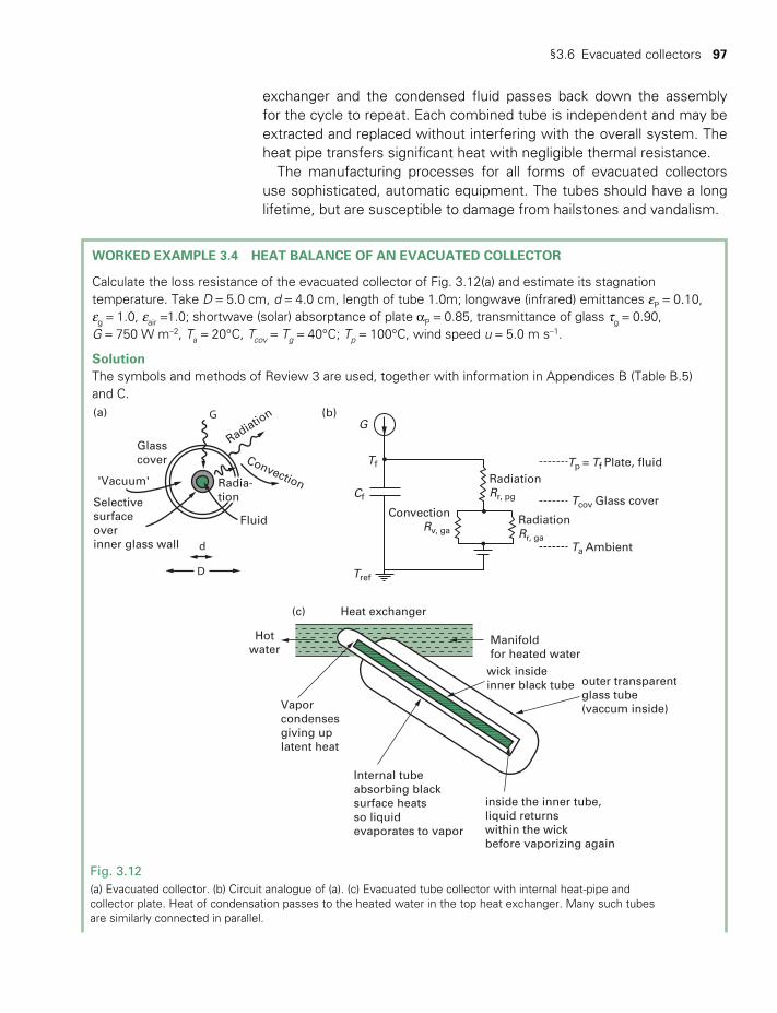
§3.6 Evacuated collectors 97
exchanger and the condensed fluid passes back down the assembly for the cycle to repeat. Each combined tube is independent and may be extracted and replaced without interfering with the overall system. The heat pipe transfers significant heat with negligible thermal resistance.
The manufacturing processes for all forms of evacuated collectors use sophisticated, automatic equipment. The tubes should have a long lifetime, but are susceptible to damage from hailstones and vandalism.
WORKED EXAMPLE 3.4 HEAT BALANCE OF AN EVACUATED COLLECTOR
Calculate the loss resistance of the evacuated collector of Fig. 3.12(a) and estimate its stagnation temperature. Take D = 5.0 cm, d = 4.0 cm, length of tube 1.0m; longwave (infrared) emittances eP = 0.10, eg = 1.0, eair =1.0; shortwave (solar) absorptance of plate αP = 0.85, transmittance of glass τg = 0.90, G = 750 W m–2, Ta = 20°C, Tcov = Tg = 40°C; Tp = 100°C, wind speed u = 5.0 m s–1.
SolutionThe symbols and methods of Review 3 are used, together with information in Appendices B (Table B.5) and C.
Fig. 3.12(a) Evacuated collector. (b) Circuit analogue of (a). (c) Evacuated tube collector with internal heat-pipe and collector plate. Heat of condensation passes to the heated water in the top heat exchanger. Many such tubes are similarly connected in parallel.
Glasscover
Fluid
Convection'Vacuum'
Radiation
Selectivesurfaceoverinner glass wall d
G(a)
D
Radia-tion
Heat exchanger
Manifoldfor heated water
Hotwater
Vapor condensesgiving uplatent heat
Internal tubeabsorbing blacksurface heatsso liquidevaporates to vapor
(c)
inside the inner tube,liquid returnswithin the wickbefore vaporizing again
outer transparentglass tube(vaccum inside)
wick insideinner black tube
(b)G
Tf
RadiationRr, pg
RadiationRr, ga
ConvectionRv, ga
Cf
Tref
Tp = Tf Plate, fluid
Ta Ambient
Tcov Glass cover
TWIDELL PAGINATION.indb 97 01/12/2014 11:36
98 Solar water heating
The circuit analogue is shown in Fig. 3.12(b). It has no convective pathway between the ‘plate’ (inner tube) and glass (outer tube) because of the vacuum. The only convection is from the outer glass to the environment. Consider a unit length of tube. Tp = 100°C = 373 K, Tg = 40°C = 313 K. Treating the two tubes as close parallel surfaces, then by (C.18), (R3.2), (R3.5) and (R3.43) we obtain by algebraic factorization:
1/rpg = σepeg(Tp2 + Tg
2) (Tp + Tg) = 0.92 Wm–2K–1
Taking the characteristic area Apg to be that of a cylinder of length 1 m and mean diameter 4.5 cm:
Apg = 2π(0.045m)(1.0m) = 0.28 m2
hence: R r A/ 1(0.92 Wm K )(0.28m ) 3.88 KWpg pg pg 2 1 2
1= = =− −−
For the convective loss per unit area of the outside surface, for an approximate answer we may use (C.15) with area Ag = 2π (0.050 m)(1.0 m) = 0.31 m2. Thus the convective loss coefficient per unit area is approximately
hv,ga = a + bu = [(5.7Wm–2K–1) + (3.8 Wm–2 K–1m–1s) × 5.0 ms–1) 25 Wm–2 K–1
By (R3.45), since eg = eair = 1.0, and F ’12 = 1.0, the radiative loss coefficient for the outer surface is
hr,ga = 4σ [(Tg + Ta )/2]3 = 6.2 Wm–2K–1
The losses by convection and radiation from the external glass to the environment are in parallel, and since by (R3.6) h = 1/r, the combined thermal resistance is
Rga = 1/[(hv.ga + hr.ga )Ag ] = 1/[(24.7 + 6.2)Wm–2K–1 × 0.28 m2]
= 1/[8.65WK–1] = 0.12KW–1
and
Rpa = Rga + Rpg = (0.12 + 7.7)KW–1 = 7.8 KW–1
Note how the radiation resistance Rpg dominates, since there is no convection to ‘short-circuit’ it. It is not significant that the mixed convection formula (C.15) applies to a flat surface, since it will underestimate the resistance from a curved surface.
Since each 1 m of tube occupies the same collector area as a flat plate of area 0.05 m2, we could say that the equivalent resistance of unit area of this collector is rpa = Rpa. 0.05 m2 = .0.39 m2 KW–1, although this figure does not have the same significance as for true flat plates.
To calculate the heat balance on a single tube, we note that the heat input is to the projected area of the inner tube, whereas the losses are from the entire outside of the larger outer tube. With no heat removed by a stagnant fluid, input solar energy equals output from losses, so
τgαpGd (1.0m) = (Tp − Ta)/Rpa
Tp − Ta = 0.90 × 0.85 × 750 Wm–2 × 0.04 m × 1.0 m × 7.8 KW–1 = 180 K
giving Tp = (180 + 293)K= 473K = 200ºC for the maximum (stagnation) temperature.
Note: This temperature is less than that listed for the double-glazed flat plate in Table 3.1. However, Tp
(m) and, more importantly, the outlet temperature T2 when there is flow in the tubes, can be increased by increasing the energy input into each tube (e.g. by placing a white or reflective surface behind the tubes), which increases radiant input by reflecting shortwave radiation and reducing the effect of wind.
TWIDELL PAGINATION.indb 98 01/12/2014 11:36

§3.7 Instrumentation and monitoring 99
§3.7 INSTRUMENTATION AND MONITORING
All machines require monitoring to check they are functioning correctly, which requires instruments and warning devices to inform the operator/householder. This principle is universally accepted for cars and other vehicles with a range of indicators in front of the driver. The same principle applies to solar heaters, although their operation is much simpler. Instruments and indicator lights should be placed at eye level in a position often noticed by the householder, for instance, on a wall adjacent to the opening side of a regularly used door. Hidden instruments are useless. In addition, a copy of the original instruction details, plans and operational note should be safeguarded in an obvious position. Over the 30 years or more lifetime of the device, operators and householders will change and need to be re-informed. Once constructed, solar water heaters are simple devices, but even so many owners fail to check their operation and may fail to benefit fully from the free heat.
Useful instrumentation includes the following:
• Display of temperatures.*• Temperature sensors (usually thermistors) for the display: collector
outlet,* top of the tank,* bottom of the tank,* bottom of the collector, middle of the tank.
• Pump-enabled* on/off colored lights.• Pump hours run. • Back-up heating on* (especially important for electric immersers for
which sensors and time clocks may fail or be mistimed, and so unnec-essary electricity is used).
* indicates the most desirable instruments for a diligent householder.
Faults (and remedial actions) that may occur during the long lifetime of a solar water heater include the following:
• Dirty cover glass (inspect at least twice per year and if necessary clean; note that self-cleaning glass may be used: see Box 5.1).
• Pump failure (indicated by temperature difference across the collector being too large).
• Sensor failure (often mice and rodents nibble the cables!).• Fuses blown (not itself a fault, but indicates a probable fault).• Frozen and burst pipes (inadequate insulation and/or bad positioning).• Metal corrosion from poor design using mixed metals (should not
occur with reliable design; annual inspection recommended with remedial action if necessary).
Very few solar water heaters are fitted with heat metres (propor-tional to the product of water flow rate and temperature increase) and so the value of heating is not usually measured. It may be inferred
TWIDELL PAGINATION.indb 99 01/12/2014 11:36

100 Solar water heating
however if the pumping rate is known and the pump running hours are measured.
§3.8 SOCIAL AND ENVIRONMENTAL ASPECTS
Solar water heating is an extremely benign and acceptable tech nology. The collectors are not obtrusive, especially when integrated into roof design. There are no harmful emissions in operation and manufacture involves no especially dangerous materials or techniques. Installations may be expected to be effective with very little service cost for at least 25 to 35 years. Installation requires the operatives to be trained conven-tionally in plumbing and construction, and to have had a short course in the solar-related principles. The technology is now developed and com-mercial in most countries, either extensively (e.g. China, Turkey, Brazil, Greece, Cyprus, Germany, Israel) or without widespread deployment (e.g. the USA, France and the UK). It works best everywhere in summer and especially in sunny climates (e.g. the Mediterranean), and where alternatives, such as gas or electricity, are most expensive (e.g. Israel). Units designed for colder climates with the threat of freezing conditions are more sophisticated and expensive than those made for countries where freezing does not occur. The solar water heaters discussed in this chapter may be used at larger scale for space heating as well as for water heating, especially if linked to large-scale inter-seasonal thermal storage.
It is important to stress that in locations with relatively small daily inso-lation, whether due to latitude or cloudiness (see Fig. 2.18), solar water heaters are still beneficial for preheating water (say, to 30ºC) when there is a second system to complete the heating (to, say, 50ºC). In the UK, for instance, a 4 m2 collector is sufficient for nearly 100% supply to a family of two to four, with careful use, from mid-April to late September, and will preheat in other months, so saving on other fuels throughout the year.
Unglazed solar water heating systems are cheap and provide useful heat in certain circumstances (e.g. for slightly boosting the temperature of water in swimming pools, as is widespread in the USA).
In almost all cases, using solar energy for water heating replaces brown (fossil) energy at source. This gives the benefits of improved sustainabil-ity and fewer greenhouse gas emissions, as described in §1.2. For this reason, some governments partially subsidize household purchase of solar water heaters in an attempt to offset the ‘external costs’ of brown energy (see Chapter 17 for a general discussion of external costs and policy tools). The fossil fuel use replaced may be direct (e.g. gas heating) or indirect (e.g. gas or coal-fired electricity). Especially in colder countries, the replacement is likely to be seasonal, with the ‘solar deficit’ in the cooler months being supplied by electric heating, central heating boilers, or district heating.
TWIDELL PAGINATION.indb 100 01/12/2014 11:36
§3.8 Social and environmental aspects 101
By the end of 2011, total global solar water heating capacity (glazed) had reached 232 GW (thermal), with net annual addition (i.e. less retire-ments) of 50 GWth (REN-21 Status Report 2012). (In reckoning installed capacity for statistical purposes, 1 million m2 of collector is equated to 1GW of thermal capacity; see Problem 3.8.) The significant annual increase indicates that the medium- to long-term outlook for solar water heating is positive, although growth may not be steady owing to short-term policy changes and ‘financial crises’.
A solar water heating system can be installed by practical household-ers, although most people employ trained and certified tradespersons. The collectors (and for some systems the water tank also) are usually fixed on roofs of sufficient strength. In most situations, a ‘conventional’ water heating system is available as back-up and for winter conditions. Nevertheless, the payback time in fuel saving against the operational cost of a conventional system is usually five to ten years, which is sub-stantially less than the lifetime of the solar system itself (see Worked Examples 17.1 and 17.2).
Solar water heaters, even relatively sophisticated ones, can be manu-factured in most countries on a small or medium scale, thus giving employment and providing useful products. They do not need to be imported and there is usually a demand, especially from the middle class and members of ‘green’ organizations. The technology is modular and can be scaled up for commercial uses, such as laundries and hotels. Early experience from the 1970s onward provided the market incen-tive for modern manufacturing. The largest national production of solar water heaters is in China, which accounts for more than 75% of world production. Here basic low-priced systems mostly provide domestic hot water, even if only for half the year in the winter climate and high latitude of China. More recently evacuated tube collectors form much of the Chinese production, contributing to significant exports.
All of these features are examples of the benefits of renewable energy systems generally, as set out in Chapter 1.
CHAPTER SUMMARY
Solar water heaters are a widely used and straightforward application of solar energy, in use in over 200 million households worldwide. There are relatively few homes and businesses that would not benefit from such installations, yet their use is still far from universal. Most systems use glazed, non-concentrating collectors, which typically raise the water temperature to 30 to 60°C above ambient, depending on insolation and flow rate. The performance of such collectors may be estimated using standard formulae of heat transfer, as is demonstrated in this chapter. The general principles and analysis that apply to solar water heaters apply also to many other systems that use active and passive mechanisms to absorb the Sun’s energy as heat. Selective surfaces and evacuated collectors enhance the performance of collectors at acceptable cost.
TWIDELL PAGINATION.indb 101 01/12/2014 11:36

102 Solar water heating
QUICK QUESTIONS
Note: Answers to these questions are in the text of the relevant section of this chapter, or may be readily inferred from it.
1 What substance occupies the greatest volume in a good non- evacuated thermal insulator?
2 What type of collector is most suitable for supply of water at (i) ~60ºC; (ii) boiling temperature?
3 What type of solar water heater is most economic for giving extra heat to a swimming pool?
4 Why do most solar collectors include a glass cover? Why glass and not polythene?
5 What is the difference between an ‘active’ and a ‘passive’ solar system for heating water?
6 What is a selective surface, and why is it useful in solar water heating?
7 Name the device used in some evacuated solar collectors that transfers heat very easily, i.e. that has very small thermal resistance.
8 Why is the efficiency of a typical solar collector less at 80ºC than at 20ºC?
9 What is the importance of basic instrumentation for solar water heaters and where should it be placed?
10 Name three heat-loss mechanisms present in all solar water heaters and describe methods to reduce each one.
PROBLEMS
3.1 The collector of Worked Example 3.1 had a resistivity to losses from the top of rpa = 0.13 m2 KW–1. Suppose the bottom of the plate is insulated from the ambient (still) air by glass wool insu-lation with k = 0.034 Wm–1 K–1. What thickness of insulation is required to ensure that the resistance to heat loss at the bottom is (a) equal to and (b) 10 times the resistance of the top?
Tg Ta Tsky
RgaRpg
Rpa
Tp
Fig. 3.13Thermal resistances for Problem 3.2.
3.2 In a sheltered flat-plate collector, the heat transfer between the plate and the outside air above it may be represented by the
TWIDELL PAGINATION.indb 102 01/12/2014 11:36
Problems 103
network shown in Fig. 3.13, where Tp, Tg and Ta are the mean temperatures of plate, glass and air respectively.
(a) Show that:
Tg = Ta + (Rga / Rpa) (Tp – Ta)
Verify that, for Tp = 70°C and the resistances calculated in Worked Example 3.1, this implies Tg = 32°C.
(b) Recalculate the resistances involved, using this second approximation for Tg instead of the first approximation of 1
2 (Tp + Ta) = 45°C used in the example, and verify that the effect on the overall resistance rpa is small.
3.3 A certain flat-plate collector has two glass covers. Draw a resist-ance diagram showing how heat is lost from the plate to the sur-roundings, and calculate the resistance (for unit area) rpa for losses through the covers. (Assume the standard conditions of Worked Example 3.1.) Why will this collector need thicker rear insulation than a single-glazed collector?
3.4 Calculate the top resistance rpa of a flat-plate collector with a single glass cover and a selective surface. (Assume the standard condi-tions of Worked Example 3.1.) See Fig. 3.2(d).
3.5 Calculate the top resistance of a flat-plate collector with double-glazing and a selective surface. (Again assume the standard condi-tions.) See Fig. 3.2(c).
3.6 Bottled beer is pasteurized by passing 50 liters of hot water (at 70°C) over each bottle for 10 minutes. The water is recycled, so that its minimum temperature is 40°C.
(a) A brewery in Kenya proposes to use solar energy to heat this water. What form of collector would be most suitable for this purpose? Given that the brewery produces 65,000 filled bottles in an 8-hour working day, and that the irradi-ance at the brewery may be assumed to be always at least 20 MJ m–2 day–1 (on a horizontal surface), calculate the minimum collect or area required, assuming no heat supply losses.
(b) Refine your estimate of the required collector area by allowing for the usual losses from a single-glazed flat-plate collector. (Make suitable estimates for G, Ta, u.)
(c) For this application, would it be worthwhile using collectors with (i) double-glazing; (ii) selective surface?
Justify your case as quantitatively as you can.Hint: Use the results summarized in Table 3.1.
TWIDELL PAGINATION.indb 103 01/12/2014 11:36
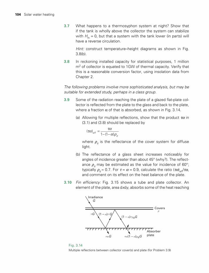
104 Solar water heating
3.7 What happens to a thermosyphon system at night? Show that if the tank is wholly above the collector the system can stabilize with Hth = 0, but that a system with the tank lower (in parts) will have a reverse circulation.
Hint: construct temperature–height diagrams as shown in Fig. 3.8(b).
3.8 In reckoning installed capacity for statistical purposes, 1 million m2 of collector is equated to 1GW of thermal capacity. Verify that this is a reasonable conversion factor, using insolation data from Chapter 2.
The following problems involve more sophisticated analysis, but may be suitable for extended study, perhaps in a class group.
3.9 Some of the radiation reaching the plate of a glazed flat-plate col-lector is reflected from the plate to the glass and back to the plate, where a fraction α of that is absorbed, as shown in Fig. 3.14.
(a) Allowing for multiple reflections, show that the product τα in (3.1) and (3.8) should be replaced by
( )1 (1 )eff
d
τα ταα ρ
=− −
where ρd is the reflectance of the cover system for diffuse light.
(b) The reflectance of a glass sheet increases noticeably for angles of incidence greater than about 45° (why?). The reflect-ance ρd may be estimated as the value for incidence of 60°; typically ρd ≈ 0.7. For τ = α = 0.9, calculate the ratio (τα)eff/τα, and comment on its effect on the heat balance of the plate.
3.10 Fin efficiency: Fig. 3.15 shows a tube and plate collector. An element of the plate, area dxdy, absorbs some of the heat reaching
Irradiance
Covers
Absorberplate
G
(1 – α)τ G(1 – α)τρdG
τα(1 – α)ρdGταG
ρτG
Fig. 3.14Multiple reflections between collector cover(s) and plate (for Problem 3.9)
TWIDELL PAGINATION.indb 104 01/12/2014 11:36

Problems 105
it from the sun, loses some to the surroundings, and passes the rest by conduction along the plate (in the x direction) to the bond region above the tube. Suppose the plate has conductivity k and thickness d, and the section of plate above the tube is at constant temperature Tb.
(a) Show that in equilibrium the energy balance on the element of the plate can be written
kd Tdx
T T Gr r( ) /pa pa
2
2 ad τα= − −
(b) Justify the boundary conditions:dTdx
at x
T T at x W D
0 0
( ) / 2b
= =
= = −
(c) Show that the solution of (a), (b) is
T T Gr
T T Grmx
m W Dcosh
cosh ( ) / 2a pa
b a pa
τατα
− −− −
=−
where m2 = 1/(kdrpa), and that the heat flowing into the bond region from the side is
(W – D)F [ταG – (Tb – Ta)/rpa]
where the fin efficiency is given by
Fm W D
m W Dtanh ( ) / 2
( ) / 2= −
−(d) Evaluate F for k = 385 Wm–1 K–1, d = 1 mm, W = 100 mm,
D = 10 mm.
Bond region
W/2
z
y
x
dx
D
W
(T − Ta)/rpa
Tb
τG
δ
Fig. 3.15Cross-section of a tube and plate collector (for Problem 3.10).
TWIDELL PAGINATION.indb 105 01/12/2014 11:36

106 Solar water heating
BIBLIOGRAPHY
General
Duffie, J.A. and Beckman, W.A. (2006) Solar Engineering of Thermal Processes, 3rd edn. John Wiley and Sons, New York. The standard work on this subject, including not just the collectors but also the systems of which they form part.
Gordon, J. (ed.) (2001) Solar Energy – the state of the art, James & James, London. Ten chapters by solar thermal, photovoltaic and glazing experts; plus single chapters on policy and wind power. See in particular: Wackelgard, E., Niklasson, G. and Granqvist, C. on ‘Selectively solar-absorbing coatings’, and Morrison, G.L. on ‘Solar collectors’ and ‘Solar water heating’.
Goswami, D.Y., Kreith, F. and Kreider, J.F. (2000), Principles of Solar Engineering, 2nd edn, Taylor and Francis, London. Another standard textbook at postgraduate level, though by now a little dated.
Laughton, C. (2010) Solar Domestic Water Heating: The Earthscan expert handbook for planning, design and installation, Earthscan, London. Principles and practicalities.
Martin, C.L. and Goswami, D.Y. (2005) Solar Energy Pocket Reference, International Solar Energy Society/Earthscan, London. Handy compilation of data and formulae, covering insolation, materials properties, collector types, PV configurations, and more.
Specific references
Born, M. and Wolf, W. (1999, 7th edn) Principles of Optics, Cambridge University Press, Cambridge. Electromagnetic theory of absorption, etc. Heavy going!
Brinkworth B.J. (2001) ‘Solar DHW system performance correlation revisited’, Solar Energy, 71 (6), 377–387. A thorough review of ‘black box’ comparative analysis and standards for domestic hot water (DHW) systems, including storage; based on the search for comprehensive non-dimensional groups of parameters which provide generalized reference methods of performance.
Close, D.J. (1962) ‘The performance of solar water heaters with natural circulation’, Solar Energy, 5, 33–40. A seminal paper of theory and experiments on thermosyphon systems. Many ongoing articles in the same journal elaborate on this.
Hutchins, M.G. (2003) ‘Spectrally selective materials for efficient visible, solar and thermal radiation control’, in M. Santamouris (ed.), Solar Thermal Technologies for Buildings, James & James, London, pp. 33–63.
Laughton, C. (2010) Solar Domestic Water Heating: The Earthscan expert handbook for planning, design and installation, Earthscan, London. Principles and practicalities.
Morrison, G.L. (2001) ‘Solar collectors’, in Gordon (2001), pp. 145–221.
Peuser, F.A., Remmmers, K-H. and Schnauss, M. (2002) Solar Thermal Systems, James and James, London, with Solarpraxis, Berlin. Predominantly considering large solar water-heating plant, this book demonstrates the complex learning curve of commercial experience in Germany; read this to appreciate the engineering demands of successful large installations.
Policy and regulation
Menanteau, P. (2007) Policy Measures to Support Solar Water Heating: Information, incentives and regulations, World Energy Council and ADEME project on energy efficiency policies (author at LEPII/ CNRS, Université de Grenoble).
TWIDELL PAGINATION.indb 106 01/12/2014 11:36

Bibliography 107
Websites and journals
IEA-SHC (www.iea-shc.org) The Solar Heating and Cooling Working Group of the International Energy Agency is a long-running international collaboration, which pools and publishes research. Among its free publications is a Technology Roadmap for Solar Heating and Cooling (2012).
REN-21 (ren21.net) The Renewable Energy Policy Network for the 21st century publish annually a Global Status Report, which gives data and comment on installed capacity (by technology), national policies on RE, etc.
Solar Energy. The research journal of the International Solar Energy Society, now published by Elsevier.
TWIDELL PAGINATION.indb 107 01/12/2014 11:36
Other solar thermal applications
CHAPTER
4
CONTENTS
Learning aims 108
§4.1 Introduction 110
§4.2 Air heaters 110
§4.3 Crop driers 112§4.3.1 Water vapor and air 113§4.3.2 Water content of crop 114§4.3.3 Energy balance and temperature
for drying 115
§4.4 Solar thermal refrigeration and cooling 117
§4.5 Water desalination 120
§4.6 Solar salt-gradient ponds 122
§4.7 Solar concentrators 123§4.7.1 Basics 123§4.7.2 Thermodynamic limit to
concentration ratio 125§4.7.3 Derivation: Performance
of linear concentration 128§4.7.4 Parabolic bowl concentrator 129§4.7.5 Fresnel concentrating
lenses and mirrors 130§4.7.6 Non-imaging concentrators 130
§4.8 Concentrated solar thermal power (CSTP) for electricity generation 132§4.8.1 Introduction 132§4.8.2 CSTP system types 135§4.8.3 Adding storage, so matching
solar input to electricity demand 138§4.8.4 Thermochemical closed-loop
storage 139§4.8.5 Small-scale CSTP
microgeneration 140
§4.9 Fuel and chemical synthesis from concentrated solar 140§4.9.1 Introduction 140§4.9.2 Hydrogen production 141
§4.10 Social and environmental aspects 141
Chapter summary 142
Quick questions 142
Problems 143
Notes 148
Bibliography 148
Box 4.1 Solar desiccant cooling 120
LEARNING AIMS
• Appreciate the many uses of solar thermal energy.
• Understand solar concentration.
• Hence to consider electricity generation.
TWIDELL PAGINATION.indb 108 01/12/2014 11:36
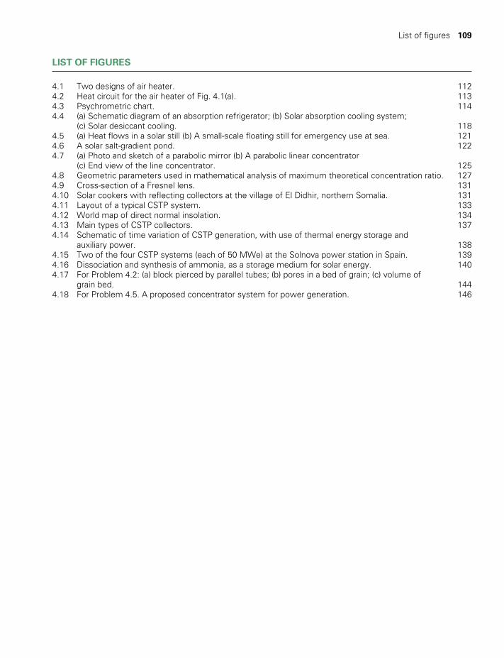
List of figures 109
LIST OF FIGURES
4.1 Two designs of air heater. 1124.2 Heat circuit for the air heater of Fig. 4.1(a). 1134.3 Psychrometric chart. 1144.4 (a) Schematic diagram of an absorption refrigerator; (b) Solar absorption cooling system;
(c) Solar desiccant cooling. 1184.5 (a) Heat flows in a solar still (b) A small-scale floating still for emergency use at sea. 1214.6 A solar salt-gradient pond. 1224.7 (a) Photo and sketch of a parabolic mirror (b) A parabolic linear concentrator
(c) End view of the line concentrator. 1254.8 Geometric parameters used in mathematical analysis of maximum theoretical concentration ratio. 1274.9 Cross-section of a Fresnel lens. 1314.10 Solar cookers with reflecting collectors at the village of El Didhir, northern Somalia. 1314.11 Layout of a typical CSTP system. 1334.12 World map of direct normal insolation. 1344.13 Main types of CSTP collectors. 1374.14 Schematic of time variation of CSTP generation, with use of thermal energy storage and
auxiliary power. 1384.15 Two of the four CSTP systems (each of 50 MWe) at the Solnova power station in Spain. 1394.16 Dissociation and synthesis of ammonia, as a storage medium for solar energy. 1404.17 For Problem 4.2: (a) block pierced by parallel tubes; (b) pores in a bed of grain; (c) volume of
grain bed. 1444.18 For Problem 4.5. A proposed conce n trator system for power generation. 146
TWIDELL PAGINATION.indb 109 01/12/2014 11:36

110 Other solar thermal applications
§4.1 INTRODUCTION
Solar radiation has many applications other than heating water, so in this chapter we progress incrementally by analyzing some other thermal applications, using the basic principles of heat transfer and storage from Review 3. Solar buildings are probably the most important such applica-tion, but as they integrate solar heating and cooling with the efficient use of energy, they are included as a key aspect of Chapter 16.
Solar air-heaters, §4.2 are the basis of solar crop dryers (§4.3). Much of the world’s grain harvest is lost to fungal attack, which is prevented by proper drying. Crop drying requires the transfer not only of heat but also of water vapor; so too does solar distillation of saline or brackish impure water for irrigation and drinking (potable) water, §4.5. Absorption refrigerators use heat to produce cold; their use in solar refrigeration and cooling is explained in §4.4. An interesting method to capture solar heat is the solar salt-gradient pond, §4.6. However, practical application of these three applications has been very limited, largely due to their costs relative to alternatives, not least refrigeration and desalination driven by solar electricity from photovoltaics.
The maximum intensity on Earth of solar radiation without concentra-tion is about 1 kW/m2; this intensity is compatible with life processes, but insufficient for thermal input to machines or for chemical process-ing. Therefore in clear-sky climates we concentrate beam radiation with concentrating mirrors by factors of up to ~100 in linear concentrators and up to ~3000 in point concentrators, while at the same time raising the temperature at the focus to maxima of ~750°C in linear concentra-tors and ~3,500°C in point concentrators. However, a dispersed focus that spreads energy over a receiver surface to maximize energy capture operates at a smaller temperature. §4.7 considers these concentrators and §4.8 explains how the increased energy flux and increased tem-perature are used for heat engines to power electricity generation (con-centrating solar thermal power). Note that focusing collectors of §4.7 have numerous other uses, including photovoltaic electricity generation (Chapter 5) and synthesis of chemicals and fuels, such as hydrogen (§4.9).
The chapter concludes with a brief review of some of the social and environmental aspects of the technologies discussed.
§4.2 AIR HEATERS
Hot air is required to warm buildings (§16.4) and dry crops (§4.3). Solar air heaters are similar to the solar water heaters described in Chapter 3 because a fluid is warmed by contact with an irradiated surface in a col-lector. In particular, the effects of orientation and the mechanisms of heat loss are very similar.
TWIDELL PAGINATION.indb 110 01/12/2014 11:36
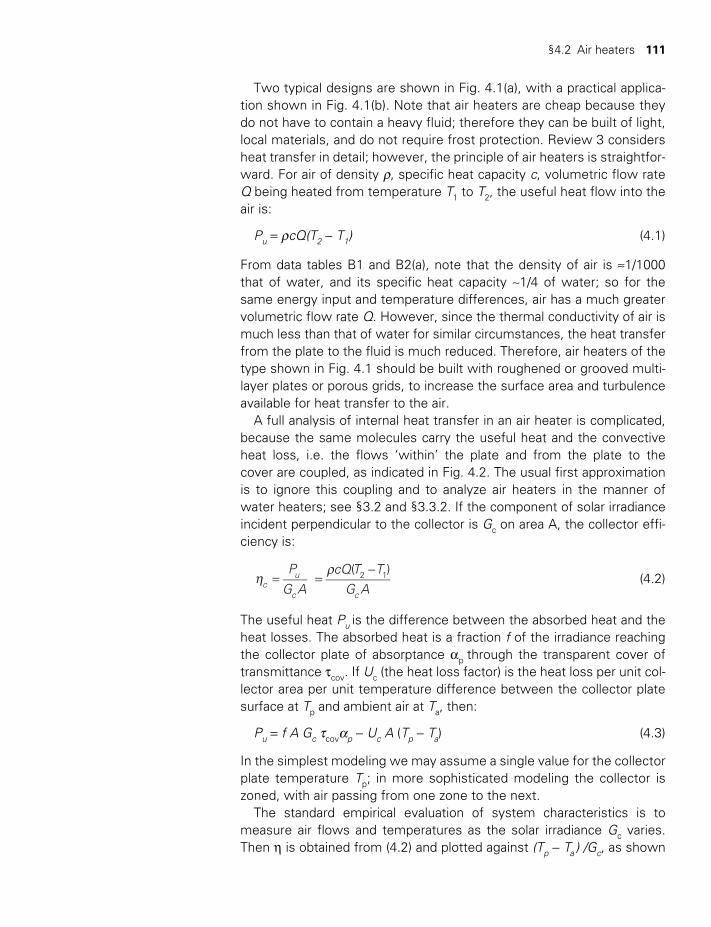
§4.2 Air heaters 111
Two typical designs are shown in Fig. 4.1(a), with a practical applica-tion shown in Fig. 4.1(b). Note that air heaters are cheap because they do not have to contain a heavy fluid; therefore they can be built of light, local materials, and do not require frost protection. Review 3 considers heat transfer in detail; however, the principle of air heaters is straightfor-ward. For air of density ρ, specific heat capacity c, volumetric flow rate Q being heated from temperature T1 to T2, the useful heat flow into the air is:
Pu = ρcQ(T2 − T1) (4.1)
From data tables B1 and B2(a), note that the density of air is ≈1/1000 that of water, and its specific heat capacity ~1/4 of water; so for the same energy input and temperature differences, air has a much greater volumetric flow rate Q. However, since the thermal conductivity of air is much less than that of water for similar circumstances, the heat transfer from the plate to the fluid is much reduced. Therefore, air heaters of the type shown in Fig. 4.1 should be built with roughened or grooved multi-layer plates or porous grids, to increase the surface area and turbulence available for heat transfer to the air.
A full analysis of internal heat transfer in an air heater is complicated, because the same molecules carry the useful heat and the convective heat loss, i.e. the flows ‘within’ the plate and from the plate to the cover are coupled, as indicated in Fig. 4.2. The usual first approximation is to ignore this coupling and to analyze air heaters in the manner of water heaters; see §3.2 and §3.3.2. If the component of solar irradiance incident perpendicular to the collector is Gc on area A, the collector effi-ciency is:
ηρ
= =−P
G AcQ T T
G A( )
cu
c c
2 1 (4.2)
The useful heat Pu is the difference between the absorbed heat and the heat losses. The absorbed heat is a fraction f of the irradiance reaching the collector plate of absorptance ap through the transparent cover of transmittance tcov. If Uc (the heat loss factor) is the heat loss per unit col-lector area per unit temperature difference between the collector plate surface at Tp and ambient air at Ta, then:
Pu = f A Gc tcovap − Uc A (Tp − Ta) (4.3)
In the simplest modeling we may assume a single value for the collect or plate temperature Tp; in more sophisticated modeling the collector is zoned, with air passing from one zone to the next.
The standard empirical evaluation of system characteristics is to measure air flows and temperatures as the solar irradiance Gc varies. Then η is obtained from (4.2) and plotted against (Tp − Ta ) /Gc, as shown
TWIDELL PAGINATION.indb 111 01/12/2014 11:36

112 Other solar thermal applications
in Fig. 3.6. Further information is obtained using (4.1) to obtain Pu and plotting this against (Tp − Ta), as in (4.3). If the material properties tcov and ap are known, then the overall loss factor Uc and the collection fraction f are obtained from the slope and ordinate intercept.
§4.3 CROP DRIERS
Grain and many other agricultural products must be dried before storing; otherwise insects and fungi, which thrive in moist conditions, ruin them. Examples include wheat, rice, coffee, copra (coconut flesh), certain
T2
Rough, blackabsorbing surface
Glass cover
(a)
(b)
T1
Fig. 4.1Two designs of air heater. a with air passing over a black surface; b a solar collector in Minnesota, USA, constructed as a black grid through which air is
sucked, thereby heating, and then passes into the house.
TWIDELL PAGINATION.indb 112 01/12/2014 11:36
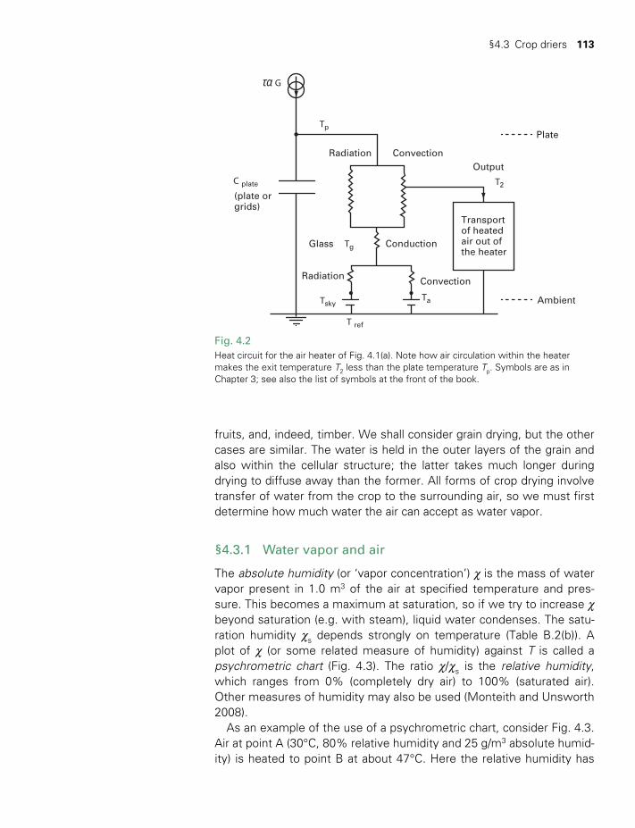
§4.3 Crop driers 113
fruits, and, indeed, timber. We shall consider grain drying, but the other cases are similar. The water is held in the outer layers of the grain and also within the cellular structure; the latter takes much longer during drying to diffuse away than the former. All forms of crop drying involve transfer of water from the crop to the surrounding air, so we must first determine how much water the air can accept as water vapor.
§4.3.1 Water vapor and air
The absolute humidity (or ‘vapor concentration’) c is the mass of water vapor present in 1.0 m3 of the air at specified temperature and pres-sure. This becomes a maximum at saturation, so if we try to increase c beyond saturation (e.g. with steam), liquid water condenses. The satu-ration humidity cs depends strongly on temperature (Table B.2(b)). A plot of c (or some related measure of humidity) against T is called a psychrometric chart (Fig. 4.3). The ratio c/cs is the relative humidity, which ranges from 0% (completely dry air) to 100% (saturated air). Other measures of humidity may also be used (Monteith and Unsworth 2008).
As an example of the use of a psychrometric chart, consider Fig. 4.3. Air at point A (30°C, 80% relative humidity and 25 g/m3 absolute humid-ity) is heated to point B at about 47°C. Here the relative humidity has
Radiation
(plate orgrids)
Output
Plate
Ambient
Transportof heatedair out ofthe heater
Convection
Convection
ConductionGlass
Radiation
TskyTa
T2
Tg
Tp
C plate
T ref
Gta
Fig. 4.2Heat circuit for the air heater of Fig. 4.1(a). Note how air circulation within the heater makes the exit temperature T2 less than the plate temperature Tp. Symbols are as in Chapter 3; see also the list of symbols at the front of the book.
TWIDELL PAGINATION.indb 113 01/12/2014 11:36
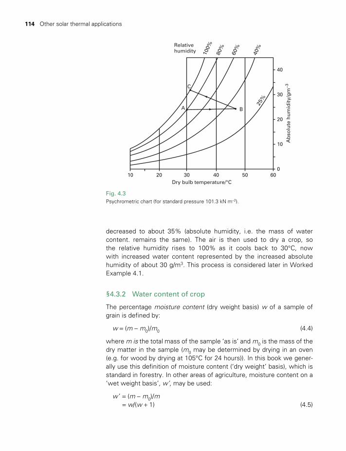
114 Other solar thermal applications
decreased to about 35% (absolute humidity, i.e. the mass of water content. remains the same). The air is then used to dry a crop, so the relative humidity rises to 100% as it cools back to 30°C, now with increased water content represented by the increased absolute humidity of about 30 g/m3. This process is considered later in Worked Example 4.1.
§4.3.2 Water content of crop
The percentage moisture content (dry weight basis) w of a sample of grain is defined by:
w = (m − m0)/m0 (4.4)
where m is the total mass of the sample ‘as is’ and m0 is the mass of the dry matter in the sample (m0 may be determined by drying in an oven (e.g. for wood by drying at 105°C for 24 hours)). In this book we gener-ally use this definition of moisture content (‘dry weight’ basis), which is standard in forestry. In other areas of agriculture, moisture content on a ‘wet weight basis’, w’, may be used:
w ’ = (m − m0)/m = w/(w + 1) (4.5)
10 20
A
C
B
30 40 50 60
40
100%
80%
60%
40%
25%
Relativehumidity
30
20
10
0
Dry bulb temperature/°C
Ab
solu
te h
um
idit
y/g
m−3
Fig. 4.3Psychrometric chart (for standard pressure 101.3 kN m–2).
TWIDELL PAGINATION.indb 114 01/12/2014 11:36
§4.3 Crop driers 115
The accurate determination of m0 requires care, and ideally should be measured in a laboratory according to the standard procedures for each crop or product. For routine measurement to less accuracy, a variety of relatively cheap instruments may be used, for instance, depending on the electrical resistance of the material. It is also important to realize that there are maximum temperatures for drying crops for storage so that the product does not crack and allow bacteria and other microbes to enter, producing decay and toxins. Further details are in the reference section at the end of this chapter.
If left for long enough, a moist grain will give up water to the sur-rounding air until the grain reaches its equilibrium moisture content we. The value of we depends partly on the crop, but mostly on the temperature and humidity of the surrounding air. For example, rice in air at 30°C and 80% relative humidity (typical of rice-growing areas) has we ≈ 16%.
Note that the rate of drying is not uniform. Much of the moisture within the material of a crop is ‘free water’ held in the cell pores, which after harvest diffuses relatively easily to surfaces and evapo-rates (e.g. from dispersed grain spread in the dry). All other parameters remaining constant, the moisture content reduces at a constant rate as this loosely held water is removed. The remaining water (usually 30 to 40%) is bound to the cell walls by hydrogen bonds, and is therefore harder to remove; this moisture is lost at a decreasing rate. It is impor-tant that grain be dried as quickly as possible without cracking (i.e. within a few days of harvest) to about 14% to 16% moisture content to prevent the growth of fungi that thrive in moist or partly moist grain. Even if the fungi die, the waste chemicals that remain can be poison-ous to cattle and humans. Once dried, the grain has to remain dry in ventilated storage.
Fuel-wood is best dried in stacks with rain cover, but through which air can move easily. Drying timber to equilibrium moisture content without heating usually takes between one and two years.
§4.3.3 Energy balance and temperature for drying
If unsaturated air is passed over wet material, the air will take up water from the material as described in the previous section. This water has to be evaporated, and the heat to do this comes from the air and the material. The air is thereby cooled. In particular, if a volume V of air is cooled from T1 to T2 in the process of evaporating a mass mw of water, then
mw L = ρcV(T1 − T2) (4.6)
where L is the latent heat of vaporization of water and ρ and c are the density and specific heat of the ‘air’ (i.e. including the water vapor) at
TWIDELL PAGINATION.indb 115 01/12/2014 11:36
116 Other solar thermal applications
WORKED EXAMPLE 4.1
Rice is harvested at a dry basis moisture content w = 0.28. Ambient conditions are 30°C and 80% relative humidity, at which the equilibrium moisture content for rice (dry basis) is given as we = 0.16. Calculate how much air at 45°C is required for drying 1000 kg of rice if the conditions are as shown in Fig. 4.3.
SolutionFrom (4.4), m/m0 = w + 1.
For 1000 kg of rice at w = 0.28, the dry mass ism0 = m/(w+1) = 1000 kg/1.28 = 781 kg. At w = 0.28, the mass of water present = 1000 kg − 781 kg = 219 kg.At w = 0.16, the mass of the crop m is given by 0.16 = (m − 781 kg)/781 kg,
so m = 1.16 × 781 kg = 906 kg, and the water present = (906 − 781) kg = 125 kg.The mass of water to be evaporated is therefore (219–125) kg = 94 kg which equals 94/220 = 42% of the
total water present.Note that moist air is less dense than drier air at the same temperature and pressure. This is because
water molecules have less mass than either oxygen or nitrogen molecules (and it is why moist air rises to form clouds). We neglect this small effect.
We can obtain the absolute humidity, c, of the ambient air entering the drier in two ways:
a from Fig. 4.3 (point A), where the ordinate scale gives c≈ 25 g/m3
b more accurately from Table B.2(b) at 30°C, for saturated air c = 30.3 g/m3, so at 80% c = 0.8 × 30.3 g/m3 = 24.2 g/m3.
The absolute humidity of the same air after heating to 45°C (point B) has about 35% relative humidity, as given from Fig. 4.3. This air passes through the rice and extracts 94 kg of water, so increasing its absolute humidity and then cooling to the 30°C ambient temperature (point C).
Then from (4.6):
Vm
c T T( )(94kg) (2.4MJkg )
(1.15kg.m ) (1.0kJkg K ) (45 30) C
13 000 m
w
1 2
1
3 1 1
3
ρ=
L−
=− °
=
−
− − −
where the latent heat of vaporization of water at this temperature range is 2.4 MJ/kg; other data come from Appendix B.
constant pressure at the mean temperature, for moderate temperature differences.
The basic challenge in designing a crop drier is to have a suitable T1 and V to remove a specified amount of water mw. The temperature T1 must not be too large, which would crack the grain, but must be sufficient to prevent conditions of high relative humidity lasting for periods long enough for microbial growth.
Exact calculation would consider the variations in the parameters L, ρ and c as the air passes through the crop bed. However, the overall con-clusion would be the same; drying requires relatively large volumes of warm, dry air to pass through the crop in the drier. Drying with forced air flow is an established and technological subject, producing safe products
TWIDELL PAGINATION.indb 116 01/12/2014 11:36
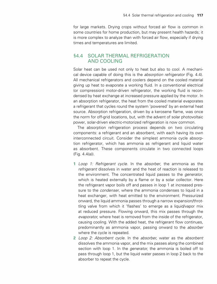
§4.4 Solar thermal refrigeration and cooling 117
for large markets. Drying crops without forced air flow is common in some countries for home production, but may present health hazards; it is more complex to analyze than with forced air flow, especially if drying times and temperatures are limited.
§4.4 SOLAR THERMAL REFRIGERATION AND COOLING
Solar heat can be used not only to heat but also to cool. A mechani-cal device capable of doing this is the absorption refrigerator (Fig. 4.4). All mechanical refrigerators and coolers depend on the cooled material giving up heat to evaporate a working fluid. In a conventional electrical (or compression) motor-driven refrigerator, the working fluid is recon-densed by heat exchange at increased pressure applied by the motor. In an absorption refrigerator, the heat from the cooled material evaporates a refrigerant that cycles round the system ‘powered’ by an external heat source. Absorption refrigeration, driven by a kerosene flame, was once the norm for off-grid locations, but, with the advent of solar photovoltaic power, solar-driven electric-motorized refrigeration is now common.
The absorption refrigeration process depends on two circulating components: a refrigerant and an absorbent, with each having its own interconnected circuit. Consider the simplest ammonia cycle absorp-tion refrigerator, which has ammonia as refrigerant and liquid water as absorbent. These components circulate in two connected loops (Fig. 4.4(a)).
1 Loop 1: Refrigerant cycle. In the absorber, the ammonia as the refrigerant dissolves in water and the heat of reaction is released to the environment. The concentrated liquid passes to the generator, which is heated externally by a flame or by a solar collector. Here the refrigerant vapor boils off and passes in loop 1 at increased pres-sure to the condenser, where the ammonia condenses to liquid in a heat exchanger, with heat emitted to the environment. Pressurized onward, the liquid ammonia passes through a narrow expansion/throt-tling valve from which it ‘flashes’ to emerge as a liquid/vapor mix at reduced pressure. Flowing onward, this mix passes through the evaporator, where heat is removed from the inside of the refrigerator, causing cooling. With the added heat, the refrigerant flow continues, predominantly as ammonia vapor, passing onward to the absorber where the cycle is repeated.
2 Loop 2: Absorbent cycle. In the absorber, water as the absorbent dissolves the ammonia vapor, and the mix passes along the combined section with loop 1. In the generator, the ammonia is boiled off to pass through loop 1, but the liquid water passes in loop 2 back to the absorber to repeat the cycle.
TWIDELL PAGINATION.indb 117 01/12/2014 11:36
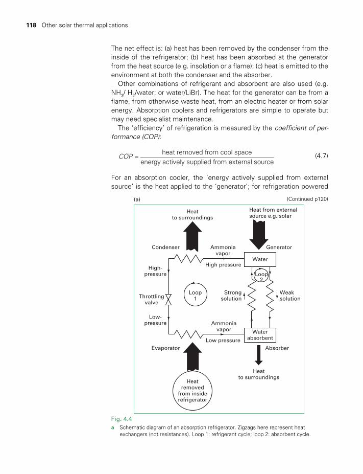
118 Other solar thermal applications
The net effect is: (a) heat has been removed by the condenser from the inside of the refrigerator; (b) heat has been absorbed at the generator from the heat source (e.g. insolation or a flame); (c) heat is emitted to the environment at both the condenser and the absorber.
Other combinations of refrigerant and absorbent are also used (e.g. NH3/ H2/water; or water/LiBr). The heat for the generator can be from a flame, from otherwise waste heat, from an electric heater or from solar energy. Absorption coolers and refrigerators are simple to operate but may need specialist maintenance.
The ‘efficiency’ of refrigeration is measured by the coefficient of per-formance (COP):
=COPheat removed from cool space
energy actively supplied from external source (4.7)
For an absorption cooler, the ‘energy actively supplied from external source’ is the heat applied to the ‘generator’; for refrigeration powered
Heatto surroundings
(a)
Condenser Ammoniavapor
Heat from externalsource e.g. solar
Generator
Loop2
Loop1
WaterHigh pressure
Weaksolution
Ammoniavapor Water
absorbent
AbsorberLow pressure
Heatto surroundings
High-pressure
Low-pressure
Evaporator
Heatremoved
from insiderefrigerator
Throttlingvalve
Strongsolution
Fig. 4.4a Schematic diagram of an absorption refrigerator. Zigzags here represent heat
exchangers (not resistances). Loop 1: refrigerant cycle; loop 2: absorbent cycle.
(Continued p120)Heatto surroundings
(a)
Condenser Ammoniavapor
Heat from externalsource e.g. solar
Generator
Loop2
Loop1
WaterHigh pressure
Weaksolution
Ammoniavapor Water
absorbent
AbsorberLow pressure
Heatto surroundings
High-pressure
Low-pressure
Evaporator
Heatremoved
from insiderefrigerator
Throttlingvalve
Strongsolution
TWIDELL PAGINATION.indb 118 01/12/2014 11:36
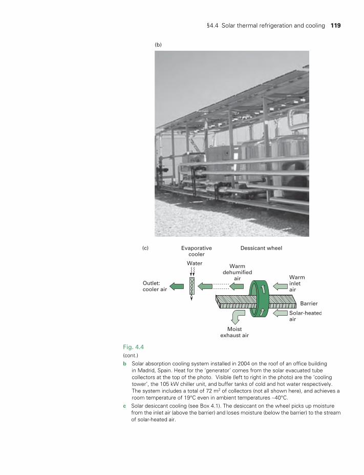
§4.4 Solar thermal refrigeration and cooling 119
(b)
Outlet:cooler air
Water
Moistexhaust air
Dessicant wheel
Warminletair
Barrier
Solar-heatedair
Warmdehumified
air
Evaporativecooler
(c)
Fig. 4.4(cont.)b Solar absorption cooling system installed in 2004 on the roof of an office building
in Madrid, Spain. Heat for the ‘generator’ comes from the solar evacuated tube collectors at the top of the photo. Visible (left to right in the photo) are the ‘cooling tower’, the 105 kW chiller unit, and buffer tanks of cold and hot water respectively. The system includes a total of 72 m2 of collectors (not all shown here), and achieves a room temperature of 19°C even in ambient temperatures ~40°C.
c Solar desiccant cooling (see Box 4.1). The desiccant on the wheel picks up moisture from the inlet air (above the barrier) and loses moisture (below the barrier) to the stream of solar-heated air.
TWIDELL PAGINATION.indb 119 01/12/2014 11:36
120 Other solar thermal applications
by electric motors, this is the electrical energy used. Electrical refrigera-tion is the norm worldwide, with such refrigerators and coolers normally having COP >1.5. Absorption coolers in practice have COP ~0.7, and so are less efficient technically. Their value, however, is not their COP, but their use in situations where there is no electricity supply or, at a larger scale, where low-cost heat can be used at input despite their relatively large capital cost (see e.g. Fig. 4.4(b)).
BOX 4.1 SOLAR DESICCANT COOLING
Desiccants are materials that absorb moisture from the air and then release the moisture when heated; silica gel is a common example. In the example given here, solar heat is used for drying. We want fresh air in a room that is drier than outside; Fig 4.4(c) shows one method. The incoming air passes first through a slowly turning wheel in the section containing the dried desiccant. As the moist air passes around the desiccant, the latent heat of absorption (similar to condensation) is released, so partly heating the air, which nevertheless has had significant water vapor removed. The section in the desiccant wheel slowly rotates and next passes through a hot stream of solar-heated air, so becoming dry again (‘regenerated’) ready to repeat the cycle. Meantime, the warm, dried (dehumidified) air passes through an evaporative cooler and then into the room. The system works because the moisture added in the evaporative cooling is less than that removed in the initial drying by the desiccant.
Other solar-related methods of refrigeration and coolingIn practice, conventional electricity-driven motorized refrigerators and coolers dominate the market, with off-grid operation increasingly powered by solar photovoltaic panels (Chapter 5). For buildings in hot cli-mates, cooling is an integral aspect of passive solar design (cf. §16.4.3). We may note that evaporative cooling in hot, dry climates is simple and reliable where water is available for the evaporation. Even in warm, humid climates, evaporative cooling can be effective if coupled with solar desiccation (see Box 4.1).
§4.5 WATER DESALINATION
For communities in arid and desert conditions, a potable (safe to drink) water supply is essential. In addition, improved water may be needed for crops and general purposes. For instance, many desert regions have nearby supplies of sea water or brackish water that may be cheaper to purify locally than to transport in fresh water. These same regions usually have reliable insolation for solar desalination technology.
One such technology is solar distillation. Fig. 4.5(a) indicates the heat flows which can be described by the heat circuit. A commercial example is the small-scale floating still, designed for shipwrecked mariners (Fig. 4.5(b)). At its base is an internally blackened ‘basin’ that can be filled with a shallow depth of salty/brackish water. Over this
TWIDELL PAGINATION.indb 120 01/12/2014 11:36
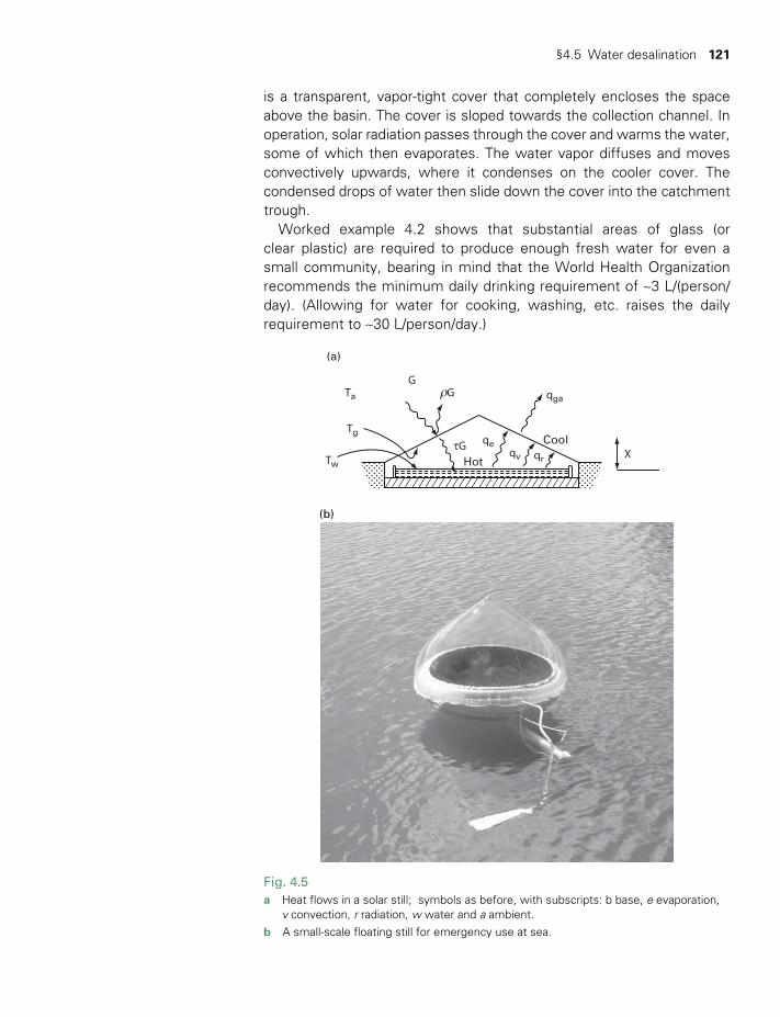
§4.5 Water desalination 121
is a transparent, vapor-tight cover that completely encloses the space above the basin. The cover is sloped towards the collection channel. In operation, solar radiation passes through the cover and warms the water, some of which then evaporates. The water vapor diffuses and moves convectively upwards, where it condenses on the cooler cover. The condensed drops of water then slide down the cover into the catchment trough.
Worked example 4.2 shows that substantial areas of glass (or clear plastic) are required to produce enough fresh water for even a small community, bearing in mind that the World Health Organization recommends the minimum daily drinking requirement of ~3 L/(person/day). (Allowing for water for cooking, washing, etc. raises the daily requirement to ~30 L/person/day.)
Tw
Tg
Ta
qeqv qr
qga
GG
Hot
CoolX
τG
ρ
(a)
Fig. 4.5a Heat flows in a solar still; symbols as before, with subscripts: b base, e evaporation,
v convection, r radiation, w water and a ambient.b A small-scale floating still for emergency use at sea.
(b)
TWIDELL PAGINATION.indb 121 01/12/2014 11:36
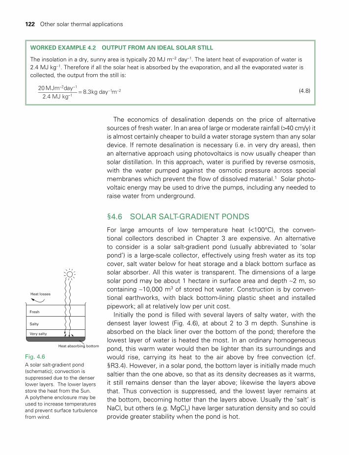
122 Other solar thermal applications
The economics of desalination depends on the price of alternative sources of fresh water. In an area of large or moderate rainfall (>40 cm/y) it is almost certainly cheaper to build a water storage system than any solar device. If remote desalination is necessary (i.e. in very dry areas), then an alternative approach using photovoltaics is now usually cheaper than solar distillation. In this approach, water is purified by reverse osmosis, with the water pumped against the osmotic pressure across special membranes which prevent the flow of dissolved material.1 Solar photo-voltaic energy may be used to drive the pumps, including any needed to raise water from underground.
§4.6 SOLAR SALT-GRADIENT PONDS
For large amounts of low temperature heat (<100°C), the conven-tional collectors described in Chapter 3 are expensive. An alternative to consider is a solar salt-gradient pond (usually abbreviated to ‘solar pond’) is a large-scale collector, effectively using fresh water as its top cover, salt water below for heat storage and a black bottom surface as solar absorber. All this water is transparent. The dimensions of a large solar pond may be about 1 hectare in surface area and depth ~2 m, so containing ~10,000 m3 of stored hot water. Construction is by conven-tional earthworks, with black bottom- lining plastic sheet and installed pipework; all at relatively low per unit cost.
Initially the pond is filled with several layers of salty water, with the densest layer lowest (Fig. 4.6), at about 2 to 3 m depth. Sunshine is absorbed on the black liner over the bottom of the pond; therefore the lowest layer of water is heated the most. In an ordinary homogeneous pond, this warm water would then be lighter than its surroundings and would rise, carrying its heat to the air above by free convection (cf. §R3.4). However, in a solar pond, the bottom layer is initially made much saltier than the one above, so that as its density decreases as it warms, it still remains denser than the layer above; likewise the layers above that. Thus convection is suppressed, and the lowest layer remains at the bottom, becoming hotter than the layers above. Usually the ‘salt’ is NaCl, but others (e.g. MgCl2) have larger saturation density and so could provide greater stability when the pond is hot.
WORKED EXAMPLE 4.2 OUTPUT FROM AN IDEAL SOLAR STILL
The insolation in a dry, sunny area is typically 20 MJ m−2 day−1. The latent heat of evaporation of water is 2.4 MJ kg−1. Therefore if all the solar heat is absorbed by the evaporation, and all the evaporated water is collected, the output from the still is:
20 MJm day2.4 MJ kg
8.3kg day m2 1
11 2=
− −
−− − (4.8)
Heat absorbing bottom
Very salty
Salty
Fresh
Heat losses
Fig. 4.6A solar salt-gradient pond (schematic); convection is suppressed due to the denser lower layers. The lower layers store the heat from the Sun. A polythene enclosure may be used to increase temperatures and prevent surface turbulence from wind.
TWIDELL PAGINATION.indb 122 01/12/2014 11:36
§4.7 Solar concentrators 123
Of course, the bottom layer does not heat up indefinitely but equil-ibrates at a temperature determined by the heat lost by conduction, mainly through the stationary water above. Calculation shows that the resistance to this heat loss is comparable to that in a conventional plate collector (Problem 4.3). Equilibrium temperatures of 90°C or more have been achieved in the lowest layer. Filling a solar pond may take several months, because if the upper layers are added too quickly the resulting turbulence stirs up the lower layers and destroys the desired stratification.
With a large solar pond, the thermal capacitance and resistance can be sufficiently large to retain the heat in the bottom layer from summer to winter (Problem 4.3). Such interseasonal heat storage may be used for heating buildings. Solar ponds have many potential applications in industry as a steady source of heat at a moderately high temperature, and it is possible to produce electricity from a solar pond by using a special ‘low temperature’ heat engine coupled to an electric generator (see Box 13.1). Prototype solar ponds were first constructed in India; a solar pond at Beit Ha’Harava in Israel produced a steady and reliable 5 MW(e) electricity supply at a levelized cost of around 30 USc/kWh (Tabor and Doron 1990); a solar pond at El Paso, in Texas, gained many years of operational experience, producing heat, electricity and desalinated water for a nearby fruit canning factory (Lu et al. 2004). Development continues at several international projects, but solar ponds have not achieved wide commercial use because the laborious construction and long time-constants of operation require many years of experience to obtain satisfactory results.
§4.7 SOLAR CONCENTRATORS
§4.7.1 Basics
Many applications of solar heat require hotter temperatures than those achievable by even the best flat-plate collectors. For instance, a working fluid at ~500°C can drive a conventional heat engine to produce mechani-cal work for electricity generation. Even hotter temperatures (to ~2000°C) are useful for the production of refractory materials in pure conditions. The aim is to collect insolation over a large area and concentrate this flux onto a small receiver; in practice, mirrors are used to concentrate the direct solar beam in cloudless conditions. Since only the beam radiation can be con-centrated, concentrators are useful only in places like California and North Africa which have long periods of bright sunshine; solar energy applica-tions in cloudier climates like Northern Europe or the ‘wet tropics’ have to rely on flat-plate collectors and photovoltaic panels with no concentration.
The theory of such solar energy concentration originally derived from optical imaging devices (e.g. telescopes); however, modern research and development has developed non-imaging concentrators as more
TWIDELL PAGINATION.indb 123 01/12/2014 11:36
124 Other solar thermal applications
beneficial for solar energy concentration for both thermal and photo-voltaic power (see Roland Winston’s publications at the University of California). Applications need a specific raised temperature that is not too large and not too small, and a large flux of energy; therefore non- imaging solar concentrators are designed to give the required temperature with the energy flux spread evenly over the absorber with minimal loss. A sharp optical quality image is not desired. The solar cooker shown in Fig. 4.10 is one such application.
A concentrator comprises a collector that directs beam radiation onto a receiver, where the radiation is absorbed and converted to some other energy form. So in this text:
concentrator = collector (subscript c) + receiver (subscript r)
Concentrators have collectors that focus onto a single focal area, either onto the ‘point’ entry to a cavity, or onto a line of pipe. The former are point concentrators (Fig 4.7(a)); the latter are linear concentrators (Fig. 4.7(b)). Point concentrators must be orientated to follow the Sun in two dimensions: east/west and north/south. Line concentrators rotate around the horizontal north/south axis of the receiver to follow the elevation of the Sun through the day; tracking in only one dimension is mechanically simpler and cheaper than tracking in two dimensions.
The receiver is the heat-absorbing component. This is usually a con-tainer through which a fluid passes to transport the energy to a heat engine. However, R&D progresses on alternative receivers, such as a falling stream of particles (e.g. sand) that passes through the focused beam, becomes heated to perhaps 1000°C and then passes into a heat transfer container from which the heat is transported to an engine. The benefit is the higher temperature of the energy transfer and the greater efficiency of the heat engine.
Concentrated solar thermal power (§4.8) may be the most prominent application of solar concentrators.
However, some solar applications need a large flux of energy at a tem-perature that is not too high but significantly more than ambient; these non-imaging solar concentrators (§4.7.6) are appropriate and cheaper than focusing concentrators, especially because they achieve sufficient con-centration ( X~5) without the mechanical complexity for tracking the Sun.
The aperture of the collector has area Ac and the irradiated area of the receiver is Ar. The area concentration ratio Xa is defined as the ratio of Aa to the absorbing area Ar of the receiver:
Xa = Ac / Ar (4.9)
However, in practice, these areas are not easy to define accurately, espe-cially since the concentrated beam will not be uniform over the receiver and since support structures interfere. A more meaningful parameter is the flux concentration ratio2 Xf, being the ratio of the flux density at the
TWIDELL PAGINATION.indb 124 01/12/2014 11:36
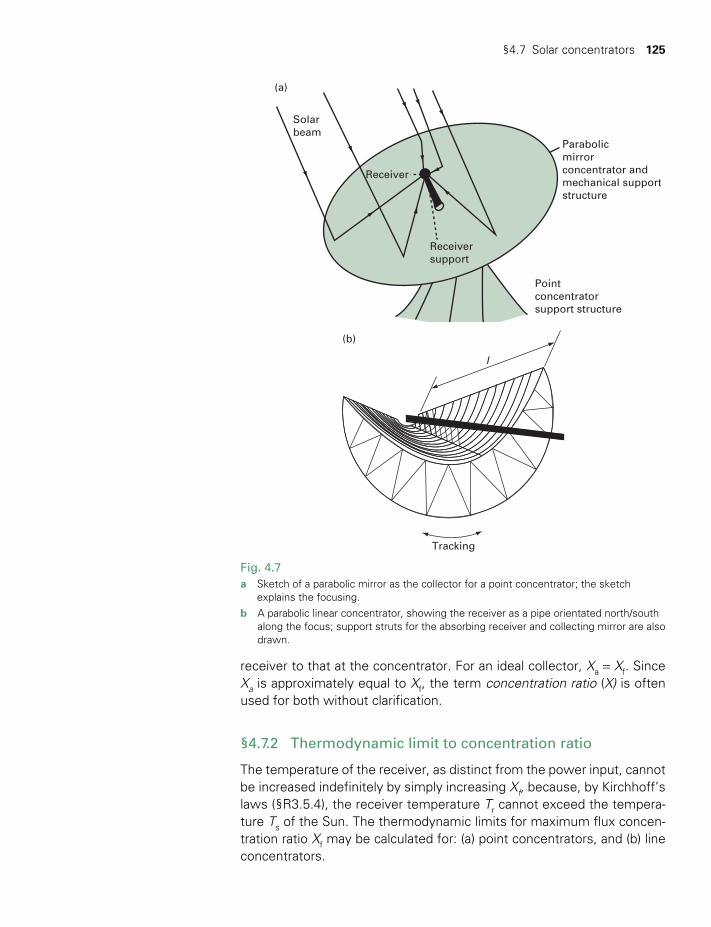
§4.7 Solar concentrators 125
Tracking
l
(b)
Solarbeam
(a)
Receiver
Receiversupport
Pointconcentratorsupport structure
Parabolicmirrorconcentrator andmechanical supportstructure
Fig. 4.7a Sketch of a parabolic mirror as the collector for a point concentrator; the sketch
explains the focusing. b A parabolic linear concentrator, showing the receiver as a pipe orientated north/south
along the focus; support struts for the absorbing receiver and collecting mirror are also drawn.
receiver to that at the concentrator. For an ideal collector, Xa = Xf. Since Xa is approximately equal to Xf, the term concentration ratio (X) is often used for both without clarification.
§4.7.2 Thermodynamic limit to concentration ratio
The temperature of the receiver, as distinct from the power input, cannot be increased indefinitely by simply increasing Xf, because, by Kirchhoff’s laws (§R3.5.4), the receiver temperature Tr cannot exceed the tempera-ture Ts of the Sun. The thermodynamic limits for maximum flux concen-tration ratio Xf may be calculated for: (a) point concentrators, and (b) line concentrators.
TWIDELL PAGINATION.indb 125 01/12/2014 11:36
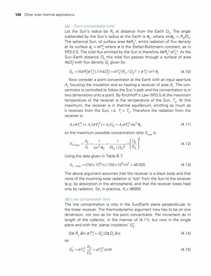
126 Other solar thermal applications
(a) Point concentrator limit Let the Sun’s radius be RS at distance from the Earth DS. The angle subtended by the Sun’s radius at the Earth is θS, where sinθS, = RS/DS. The spherical Sun, of surface area 4pRS
2, emits radiation of flux density at its surface fs = sT 4s where s is the Stefan-Boltzmann constant, as in §R3.5.5. The total flux emitted by the Sun is therefore 4pRS
2 sTS4. At the
Sun–Earth distance DS, this total flux passes through a surface of area 4pDS
2 with flux density GE given by:
p s p s s θ= = =G R T D T R D T(4 ) / (4 ) ( / ) sinE S S S S S S S S2 4 2 4 2 4 2 (4.10)
Now consider a point concentrator at the Earth with an input aperture Ac focusing the insolation and so heating a receiver of area Ar. The con-centrator is controlled to follow the Sun’s path and the concentration is in two dimensions onto a point. By Kirchhoff’s Law (§R3.5.4) the maximum temperature of the receiver is the temperature of the Sun, TS. At this maximum, the receiver is in thermal equilibrium, emitting as much as it receives from the Sun, i.e. Tr = TS. Therefore the radiation from the receiver is:
s s s θ= = =A T A T A G A T( ) ( ) sinr r r S c E c S S4 4 4 2 (4.11)
so the maximum possible concentration ratio Xmax is
θ= = = =
X
AA R D
DR
1
sin
1
( / )f
c
r S S S
S
S,max 2 2
2
(4.12)
Using the data given in Table B.7:
= × × =X (150 10 m / 700 10 m) 46 000f , max9 6 2 (4.13)
The above argument assumes that the receiver is a black body and that none of the incoming solar radiation is ‘lost’ from the Sun to the receiver (e.g. by absorption in the atmosphere), and that the receiver loses heat only by radiation. So, in practice, Xf < 46000.
(b) Line concentrator limit The line concentration is only in the Sun/Earth plane perpendicular to the linear receiver. The thermodynamic argument now has to be on one dimension, not two as for the point concentrator. Per increment ∆x in length of the collector, in the manner of (4.11), but now in the single plane and with the ‘planar insolation’ G ′E.
(2p Rs dx ) s T 4s = G ′E (2p Ds d x) (4.14)
so
G TRD
T. sinE SS
SS
4 4s s θ= =′ (4.15)
TWIDELL PAGINATION.indb 126 01/12/2014 11:36
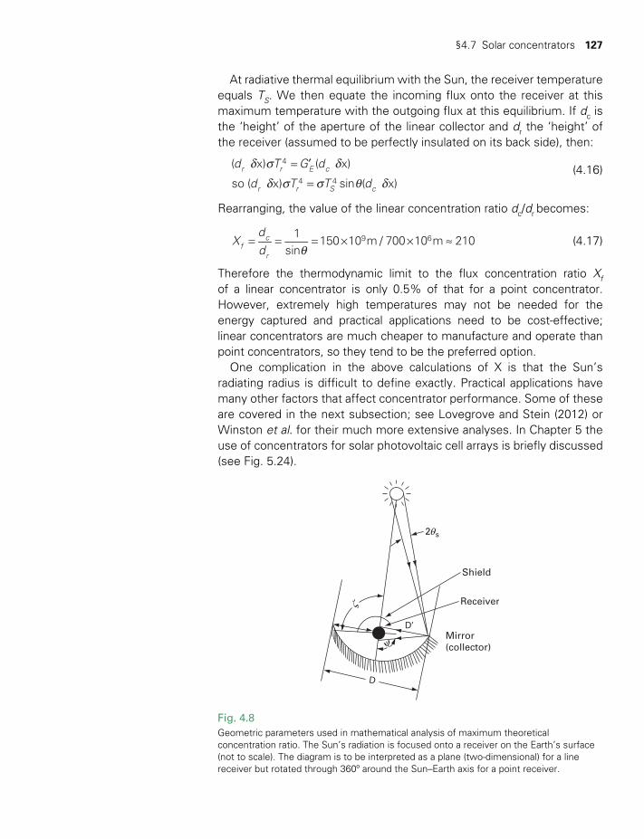
§4.7 Solar concentrators 127
Shield
Receiver
D
Mirror(collector)
D’
2 s
ψ
ζ
θ
Fig. 4.8Geometric parameters used in mathematical analysis of maximum theoretical concentration ratio. The Sun’s radiation is focused onto a receiver on the Earth’s surface (not to scale). The diagram is to be interpreted as a plane (two-dimensional) for a line receiver but rotated through 360º around the Sun–Earth axis for a point receiver.
At radiative thermal equilibrium with the Sun, the receiver temperature equals TS. We then equate the incoming flux onto the receiver at this maximum temperature with the outgoing flux at this equilibrium. If dc is the ‘height’ of the aperture of the linear collector and dr the ‘height’ of the receiver (assumed to be perfectly insulated on its back side), then:
d s dd s s θ d
= ′
=
d T G d
d T T d
( x) ( x)
so ( x) sin ( x)r r E c
r r S c
4
4 4 (4.16)
Rearranging, the value of the linear concentration ratio dc/dr becomes:
θ= = = × × ≈X
d
d1
sin150 10 m / 700 10 m 210f
c
r
9 6 (4.17)
Therefore the thermodynamic limit to the flux concentration ratio Xf of a linear concentrator is only 0.5% of that for a point concentrator. However, extremely high temperatures may not be needed for the energy captured and practical applications need to be cost-effective; linear concentrators are much cheaper to manufacture and operate than point concentrators, so they tend to be the preferred option.
One complication in the above calculations of X is that the Sun’s radiating radius is difficult to define exactly. Practical applications have many other factors that affect concentrator performance. Some of these are covered in the next subsection; see Lovegrove and Stein (2012) or Winston et al. for their much more extensive analyses. In Chapter 5 the use of concentrators for solar photovoltaic cell arrays is briefly discussed (see Fig. 5.24).
TWIDELL PAGINATION.indb 127 01/12/2014 11:36

128 Other solar thermal applications
§4.7.3 DERIVATION: PERFORMANCE OF LINEAR CONCENTRATORS
Fig. 4.8 shows a typical trough linear concentrator. The collector drawn has a parabolic section as mirror of length L with the absorbing receiver along its axis. To understand this, mentally extend that slice (thin plane) all the way back to the Sun, as in the derivation of Xf
(max) above. Only radiation in this thin slice is focused onto that length of collector.
The axis is aligned north/south, and the trough is rotated automatically about its axis, so following the Sun in tilt only. If we personify the Sun, we realize that for a perfectly aligned concentrator, the Sun looks at the collector and sees only the image of the black absorber filling the collector area. Therefore the power absorbed by the absorbing tube is:
ρ a=P A Gabs c c b (4.18)
where ρc is the reflectance of the concentrator, a is the absorptance of the absorber, θ=A DLcosc is the collector area as ‘seen’ by the Sun, θ is the angle of incidence (defined in Fig. 2.9) and Gb is beam irradiance from the direction of the Sun. (These symbols are as in Chapter 2 and Review 3, and are in the list of symbols at the front of the book; because of the tracking, at solar noon when the trough points vertically, θ equals the angle at which the Sun is below the vertical.)
The shield shown in Fig. 4.8 reduces heat losses from the receiver. It also removes the entry of some direct irradiation, but this is insignificant compared with the concentrated reflected radiation absorbed from the collector. The receiver loses radiation only in directions unprotected by the shield, i.e. the radiative loss is a fraction (1− ζ/p) of that which would be emitted from its whole surface area 2prl. Therefore radiated power loss from the receiver is:
e s p ζ p= −P T rL( ) (2 )(1 / )rrad4 (4.19)
where Tr, e, r and L are respectively the temperature, emittance, radius and length of the receiver tube, and ζ p/ is the radian angle fraction for which the shield prevents radiative loss. For each reflected ray, the angle of reflection is equal to the angle of incidence, so that the reflected Sun subtends the same angle as the Sun viewed directly, i.e. 2θS. To minimize the losses from the receiver we want small r, but to gain the full absorbed power Pabs the tube must be at least as big as the Sun’s image.
Therefore for high temperatures we choose
θ= ′ ×r D S (4.20)
in the notation of Fig. 4.8. However, D’ varies from lf at the vertex of the mirror to 2lf (at points level with the receiver) where lf is the focal length of the parabola.
In principle, other heat losses can be eliminated, but radiative losses cannot. Therefore by setting Prad = Pabs we find the stagnation temperature Tr:
TG D
rcos
2 1 /rc b
1/4 1/4aρ θ
es p ζ p( )=
−
(4.21)
where a is the absorptance of the receiver, equal for a non-selective surface to the emittance e. Tr is a maximum when the shield allows outward radiation only to the mirror, i.e. ζ → p − ψ. In practice,
trough collectors usually have subtended half-angle ψ ≈ p/2, so that the average distance from mirror to focus is ≈D D' 0.3 and ζ p≈ / 2 . With these values for D’ and ζ, and using (4.20) to substitute for r, the geometric term inside the second bracket of (4.21) becomes:
TWIDELL PAGINATION.indb 128 01/12/2014 11:36
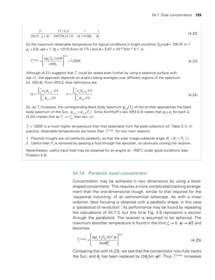
§4.7 Solar concentrators 129
p ζ p p θ p θ θ−≈
′′
≈× 0.3
≈D
rDD2 (1 / )
/ 0.32 ( )(1/ 2)
1( )
1
S S S
(4.22)
So the maximum obtainable temperature for typical conditions in bright sunshine Gbcosθ = 700 W m−2, ρc = 0.8, a/e = 1, θs = 1/210 (from (4.17) ) and s = 5.67 × 10⁻⁸ Wm−2 K−4, is:
TG cos
1200Krc b
S
(max)
1/4aρ θ
esθ=
= (4.23)
Although (4.21) suggests that Tr could be raised even further by using a selective surface with a /e >1, this approach depends on a and e being averages over different regions of the spectrum (cf. §R3.6). From §R3.5, their definitions are:
∫∫
∫∫
aa f l
f le
e f l
f l= =l l
l
l l
l
∞
∞
∞
∞
d
d
d
d
, ,in0
,in0
B0
,B0
(4.24)
So, as Tr increases, the corresponding black body spectrum fl,B(Ts) of the emitter approaches the black body spectrum of the Sun, f f=l l T( )in B s, , . Since Kirchhoff’s law (§R3.5.4) states that al= el for each l, (4.24) implies that as Tr → Ts, then a/e →1.
Tr = 1200K is a much higher temperature than that obtainable from flat-plate collectors (cf. Table 3.1). In practice, obtainable temperatures are lower than Tr
(max) for two main reasons:
1 Practical troughs are not perfectly parabolic, so that the solar image subtends angle R L/s s sθ θ′ > = .2 Useful heat Pu is removed by passing a fluid through the absorber, so obviously cooling the receiver.
Nevertheless, useful input heat may be obtained for an engine at ~700°C under good conditions (see Problem 4.5).
§4.7.4 Parabolic bowl concentrator
Concentration may be achieved in two dimensions by using a bowl-shaped concentrator. This requires a more complicated tracking arrange-ment than the one-dimensional trough, similar to that required for the ‘equatorial mounting’ of an astronomical telescope. As with a linear collector, best focusing is obtained with a parabolic shape, in this case a ‘paraboloid of revolution’. Its performance may be found by repeating the calculations of §4.7.3, but this time Fig. 4.8 represents a section through the paraboloid. The receiver is assumed to be spherical. The maximum absorber temperature is found in the limit ζ → 0, ψ → p/2 and becomes
TG sin
4rc
s
(max) a 02
2
1/4aρ t ψ
esθ=
(4.25)
Comparing this with (4.23), we see that the concentrator now fully tracks the Sun, and θs has been replaced by (2θs/sin ψ)2. Thus Tr
(max) increases
TWIDELL PAGINATION.indb 129 01/12/2014 11:36

130 Other solar thermal applications
substantially. Indeed, for the ideal case, sin ψ = a = ρc = ta = e = 1, the lim-iting temperature Tr = TS ≈ 6000 K. In practice, temperatures approaching 3000K can be achieved, despite the ever-present imperfections in track-ing, shaping the mirror, and designing the receiver.
§4.7.5 Fresnel concentrating lenses and mirrors
The principle of a Fresnel lens is illustrated in Fig. 4.9. On the right is a conventional ‘plano convex’ lens in which parallel rays of light entering from the right are focused to a point on the left by the curved surface. The shaded area is solid glass, which on a large scale makes the lens very heavy. The ingenious lens on the left, designed by Fresnel in the 1820s, achieves the same optical effect with much less glass, by having the curvature of each of its curved segments (on the right-hand side of diagram) precisely matching the curvature of the corresponding section of the thick lens.
A Fresnel mirror is an arrangement of nearly flat reflecting seg-ments, with each segment matching the curvature of a corresponding focusing mirror in either three or two dimensions, the latter being a linear mirror. The Fresnel linear mirror in Fig. 4.9 shows the key features:
• The mirror as a whole is in one place.• Each strip segment of the mirror may be individually focused, in this
case on the linear absorbing receiver.• The strip segments may be long, flat mirrors, since exact line focusing
is not wanted and the non-imaging spread averaged over the receiver is better.
• Wind speed at low level is less than higher above ground, so wind damage is less likely than for a parabolic mirror.
• Cleaning, with the strip segments vertical, is far easier than for a para-bolic mirror.
Therefore Fresnel mirrors have some important benefits for large con-centrators over conventional mirror concentrators, as will be explained in §4.8.2 for concentrating solar power.
§4.7.6 Non-imaging concentrators
The previous sections describe how large concentration ratios may be achieved with geometric precision and accurate tracking. Nevertheless, concentrators with smaller concentration ratio and with non-imaging char-acteristics may be preferred, for instance, to avoid ‘hot spots’ of exces-sive or uneven intensity across photovoltaic modules (see Chapter 5) and to simplify tracking. For example, it may be cheaper and equally satisfactory to use a 5 m2 area non-tracking concentrator of concentra-
TWIDELL PAGINATION.indb 130 01/12/2014 11:36
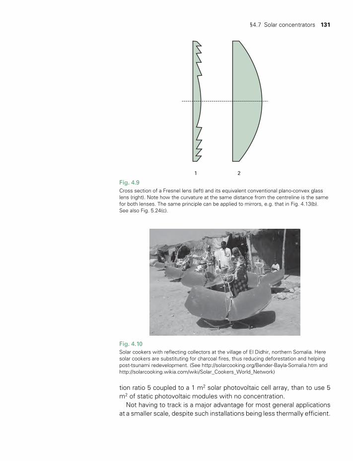
§4.7 Solar concentrators 131
Fig. 4.10Solar cookers with reflecting collectors at the village of El Didhir, northern Somalia. Here solar cookers are substituting for charcoal fires, thus reducing deforestation and helping post-tsunami redevelopment. (See http://solarcooking.org/Bender-Bayla-Somalia.htm and http://solarcooking.wikia.com/wiki/Solar_Cookers_World_Network)
tion ratio 5 coupled to a 1 m2 solar photovoltaic cell array, than to use 5 m2 of static photovoltaic modules with no concentration.
Not having to track is a major advantage for most general applications at a smaller scale, despite such installations being less thermally efficient.
Fig. 4.9Cross section of a Fresnel lens (left) and its equivalent conventional plano-convex glass lens (right). Note how the curvature at the same distance from the centreline is the same for both lenses. The same principle can be applied to mirrors, e.g. that in Fig. 4.13(b). See also Fig. 5.24(c).
1 2
TWIDELL PAGINATION.indb 131 01/12/2014 11:36
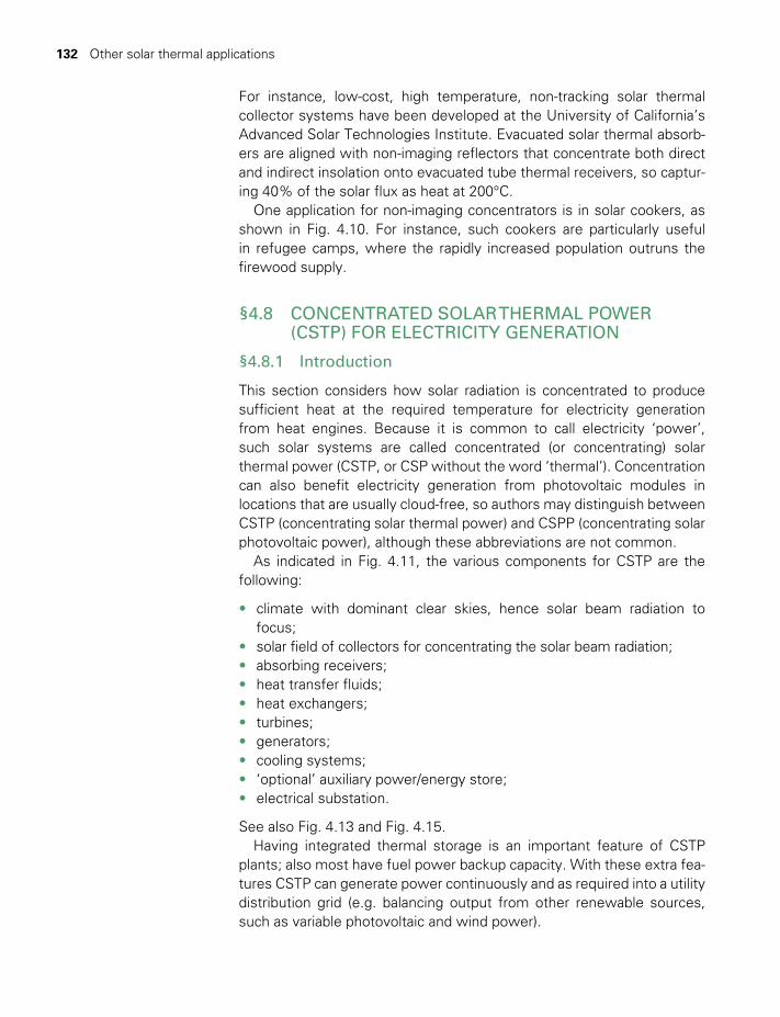
132 Other solar thermal applications
For instance, low-cost, high temperature, non-tracking solar thermal collector systems have been developed at the University of California’s Advanced Solar Technologies Institute. Evacuated solar thermal absorb-ers are aligned with non-imaging reflectors that concentrate both direct and indirect insolation onto evacuated tube thermal receivers, so captur-ing 40% of the solar flux as heat at 200°C.
One application for non-imaging concentrators is in solar cookers, as shown in Fig. 4.10. For instance, such cookers are particularly useful in refugee camps, where the rapidly increased population outruns the firewood supply.
§4.8 CONCENTRATED SOLAR THERMAL POWER (CSTP) FOR ELECTRICITY GENERATION
§4.8.1 Introduction
This section considers how solar radiation is concentrated to produce sufficient heat at the required temperature for electricity generation from heat engines. Because it is common to call electricity ‘power’, such solar systems are called concentrated (or concentrating) solar thermal power (CSTP, or CSP without the word ‘thermal’). Concentration can also benefit electricity generation from photovoltaic modules in locations that are usually cloud-free, so authors may distinguish between CSTP (concentrating solar thermal power) and CSPP (concentrating solar photovoltaic power), although these abbreviations are not common.
As indicated in Fig. 4.11, the various components for CSTP are the following:
• climate with dominant clear skies, hence solar beam radiation to focus;
• solar field of collectors for concentrating the solar beam radiation;• absorbing receivers;• heat transfer fluids;• heat exchangers;• turbines;• generators;• cooling systems;• ‘optional’ auxiliary power/energy store;• electrical substation.
See also Fig. 4.13 and Fig. 4.15. Having integrated thermal storage is an important feature of CSTP
plants; also most have fuel power backup capacity. With these extra fea-tures CSTP can generate power continuously and as required into a utility distribution grid (e.g. balancing output from other renewable sources, such as variable photovoltaic and wind power).
TWIDELL PAGINATION.indb 132 01/12/2014 11:36
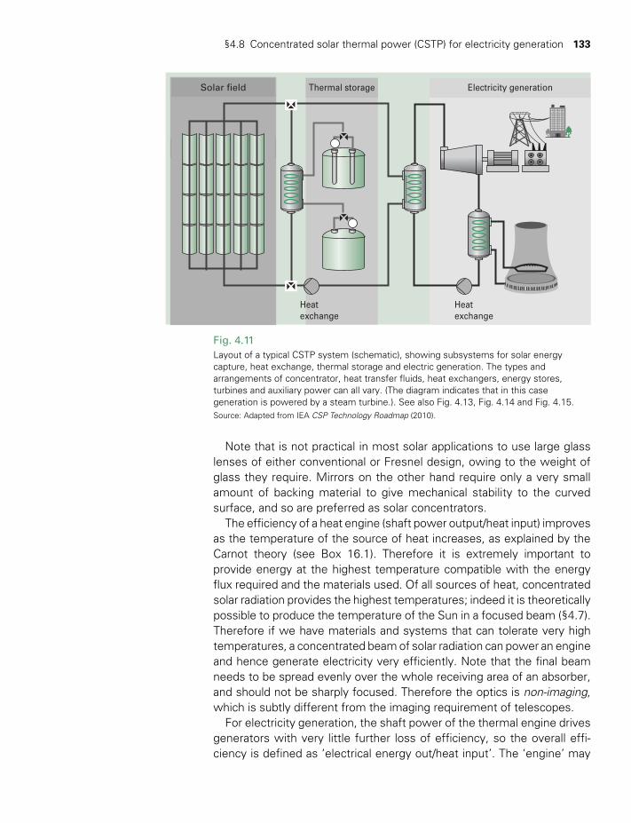
§4.8 Concentrated solar thermal power (CSTP) for electricity generation 133
Note that is not practical in most solar applications to use large glass lenses of either conventional or Fresnel design, owing to the weight of glass they require. Mirrors on the other hand require only a very small amount of backing material to give mechanical stability to the curved surface, and so are preferred as solar concentrators.
The efficiency of a heat engine (shaft power output/heat input) improves as the temperature of the source of heat increases, as explained by the Carnot theory (see Box 16.1). Therefore it is extremely important to provide energy at the highest temperature compatible with the energy flux required and the materials used. Of all sources of heat, concentrated solar radiation provides the highest temperatures; indeed it is theoretically possible to produce the temperature of the Sun in a focused beam (§4.7). Therefore if we have materials and systems that can tolerate very high temperatures, a concentrated beam of solar radiation can power an engine and hence generate electricity very efficiently. Note that the final beam needs to be spread evenly over the whole receiving area of an absorber, and should not be sharply focused. Therefore the optics is non-imaging, which is subtly different from the imaging requirement of telescopes.
For electricity generation, the shaft power of the thermal engine drives generators with very little further loss of efficiency, so the overall effi-ciency is defined as ‘electrical energy out/heat input’. The ‘engine’ may
Fig. 4.11Layout of a typical CSTP system (schematic), showing subsystems for solar energy capture, heat exchange, thermal storage and electric generation. The types and arrangements of concentrator, heat transfer fluids, heat exchangers, energy stores, turbines and auxiliary power can all vary. (The diagram indicates that in this case generation is powered by a steam turbine.). See also Fig. 4.13, Fig. 4.14 and Fig. 4.15.Source: Adapted from IEA CSP Technology Roadmap (2010).
Solar field Thermal storage Electricity generation
Heatexchange
Heatexchange
TWIDELL PAGINATION.indb 133 01/12/2014 11:36
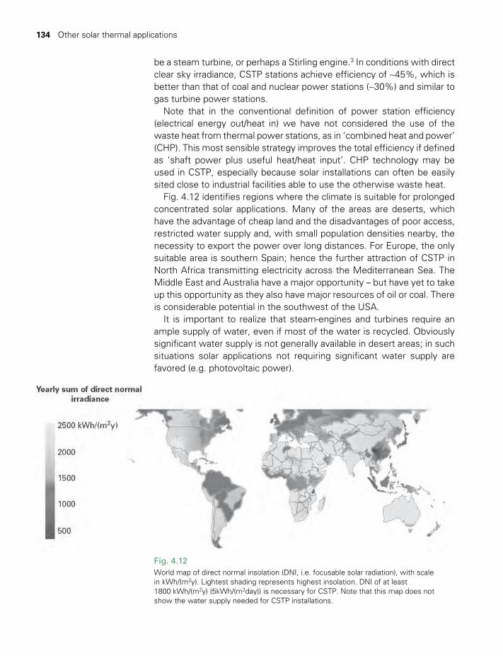
134 Other solar thermal applications
be a steam turbine, or perhaps a Stirling engine.3 In conditions with direct clear sky irradiance, CSTP stations achieve efficiency of ~45%, which is better than that of coal and nuclear power stations (~30%) and similar to gas turbine power stations.
Note that in the conventional definition of power station efficiency (electrical energy out/heat in) we have not considered the use of the waste heat from thermal power stations, as in ‘combined heat and power’ (CHP). This most sensible strategy improves the total efficiency if defined as ‘shaft power plus useful heat/heat input’. CHP technology may be used in CSTP, especially because solar installations can often be easily sited close to industrial facilities able to use the otherwise waste heat.
Fig. 4.12 identifies regions where the climate is suitable for prolonged concentrated solar applications. Many of the areas are deserts, which have the advantage of cheap land and the disadvantages of poor access, restricted water supply and, with small population densities nearby, the necessity to export the power over long distances. For Europe, the only suitable area is southern Spain; hence the further attraction of CSTP in North Africa transmitting electricity across the Mediterranean Sea. The Middle East and Australia have a major opportunity – but have yet to take up this opportunity as they also have major resources of oil or coal. There is considerable potential in the southwest of the USA.
It is important to realize that steam-engines and turbines require an ample supply of water, even if most of the water is recycled. Obviously significant water supply is not generally available in desert areas; in such situations solar applications not requiring significant water supply are favored (e.g. photovoltaic power).
Fig. 4.12World map of direct normal insolation (DNI, i.e. focusable solar radiation), with scale in kWh/(m2y). Lightest shading represents highest insolation. DNI of at least 1800 kWh/(m2y) (5kWh/(m2day)) is necessary for CSTP. Note that this map does not show the water supply needed for CSTP installations.
TWIDELL PAGINATION.indb 134 01/12/2014 11:36

§4.8 Concentrated solar thermal power (CSTP) for electricity generation 135
CSTP power stations have progressed rapidly from R&D projects to commercial-scale investments. Individual stations (plants) have electric-ity generating capacity from ~10 kW (microgeneration) to more than 200 MW. The world installed electricity generating capacity from CSTP is significant, increasing from 1,600 MW in 2009 to 10,000 MW (10 GW) from about 25 multi-megawatt (of electricity capacity) plants worldwide by 2012 (according to the European Solar Thermal Electricity Association). CSTP is now adopted as one form of utility ‘mainstream generation’, especially in southern Spain and California. In some countries, CSTP is already cost-competitive at times of peak electricity demand. With further increase in scale of use and successive incremental technology improvements, CSTP is expected to become a competitive source of bulk power in peak and intermediate loads by 2020, and of baseload power by 2025 to 2030.
§4.8.2 CSTP system types
There are four main types of CSTP systems in commercial development and use, as named by their type of collector: (1) parabolic trough; (2) linear Fresnel; (3) central receiver (power tower); and (4) dish (parabo-loid) (see Fig. 4.13). In addition, there are many variations, for instance, for the structures, control systems, heat transfer fluids, heat exchang-ers, couplings and operational temperatures. Additional features to extend the time of generation include: (5) auxiliary power and heat storage.
(a) Parabolic trough, line-focused CSTPParabolic trough concentrators rotate the collector and receiver together through the day on a horizontal fixed north – south axis, i.e. there is just one axis of orientation in comparison with the two axes of a dish or tower system. The system aperture is therefore never perpendicular to the beam (except twice per year within the Tropics) and so extended mirror areas are needed in comparison with dishes. The movements are however simple and robust. The mirrors focus the solar beam radiation onto a central linear receiver, which essentially is a pipe containing a heat transfer fluid (usually an oil, although systems using water/steam, molten salts or compressed air have been developed). In practice the receiver has a sophisticated structure to reduce heat loss, likely to include an evacuated inner space, insulating and reflective shields, and perhaps selective surfaces. The transfer fluid passes to a central position where the heat is transferred to an engine, which powers the electricity gen-erator. If the transfer fluid is steam, it may be used directly in a Rankine cycle steam turbine (Box 13.1), or if a mineral oil, the heat may be trans-ferred to heat steam indirectly, as in the Kramer Junction solar power station shown in Fig. 4.13(a).
TWIDELL PAGINATION.indb 135 01/12/2014 11:36

136 Other solar thermal applications
(b) Linear Fresnel CSTPFresnel lenses and mirrors (Fig. 4.9) are segmented to have a flat profile, while maintaining the optical effects of conventional lenses and mirrors. They are lightweight and low-cost. Fig. 4.13(b) shows a Fresnel reflecting concentrator focused onto a linear receiver; the concentrator is formed by having long horizontal segments of flat or slightly curved mirrors. Each mirror is rotated independently to focus on the fixed central horizon-tal receiver. Since non-imaging optics is preferable, the Fresnel method allows fine tuning to obtain dispersed concentration across the receiver. The receiver is stationary, permanently down-facing (so otherwise insulated) and fixed separately from the concentrator (so not requiring movable joints for its thermal transfer fluid; an advantage in practice over many parabolic concentrating systems). Since the mirrors are in a hori-zontal plane close to the ground, maintenance and cleaning are easier than for parabolic concentrators, and wind perturbations and damage should be significantly reduced.Since their optics are equivalent, the analysis of a parabolic trough con-centrator in §4.7.3 applies also for a Fresnel mirror concentrator.
(c) Central receiver (power tower)Fig. 4.13(c) shows an array of mirrors (heliostats) reflecting the solar direct beam into an elevated receiver cavity at the top of a central tower. The mirrors are usually flat (for simplicity and cheapness) but may be slightly parabolic by stressing the fixing points. Each mirror has to be individually controlled in two axes to focus on the cavity as the Sun’s position moves through the days and year. Strict safety procedures and careful design are necessary to prevent accidental focusing on other components or personnel. With time there are many variations in tem-perature, wind and other environmental conditions, so the design and maintenance challenge is considerable. An advantage of the central small aperture receiver is that very high temperatures ≥1000°C may be obtained; for instance, to directly power gas turbines, for combined cycle systems (i.e. with first-stage ‘waste heat’ being used to power a sequen-tial turbine or for materials testing).
(d) Dish CSTPDish CSTP systems have an individual receiver, engine and genera-tor positioned permanently at the focus of each paraboloid mirror, as shown in Fig. 4.13(d). As with power towers, receiver temperatures can be very high ( > ~ 1000 Co ). The engine is usually a Stirling Engine, since this can be powered from an external heat source and is, in prin-ciple, simple and efficient. Overall efficiency is likely to be definitely better than line concentrators and in practice better than power towers. However, the heavy machinery has to be suspended at the focus of each mirror, so requiring a strong and expensive dynamic structure.
TWIDELL PAGINATION.indb 136 01/12/2014 11:36

§4.8 Concentrated solar thermal power (CSTP) for electricity generation 137
(c) (d)
Fig. 4.13Main types of CSTP collectorsa Parabolic trough. Picture shows part of the facility at Kramer Junction, California,
which has a total capacity of 354 MWe and covers more than 400 ha. With an annual output ~660 GWh/y, its 24-hour capacity factor is 21%. Each tracking collector has five segments and is about 10 m along its two-dimensional tracking axis. (Compare the size of the technicians in the photo.) Working fluid is heated to 400°C in the receiver absorbing pipe at the focus of each parabolic trough. Built between 1984 and 1991, this complex comprised most of the CSP in the world until about 2005.
b Linear Fresnel reflector system. Part of the 5 MW Kimberlina station at Bakersfield, California, built in 2008. Working fluid is steam at 400°C.
c Power tower. Photo shows PS10 near Seville, Spain. Commissioned in 2000, it is the world’s first commercial power tower. It is rated at 11 MW, is 115 m high, has 624 heliostats each of 120 m2, to produce saturated steam at 275°C in the receiver. It includes 1 hour of energy storage as pressurized water.
d Dish. Photo shows the 500 m2 ‘big dish’ at the Australian National University, built in 2010 which is made up of 384 small mirrors, each with a reflectivity of 93%. Compared to an earlier prototype, built in 1994, it has improved systems for tracking, mirrors, and receiver.
(a) (b)
TWIDELL PAGINATION.indb 137 01/12/2014 11:36
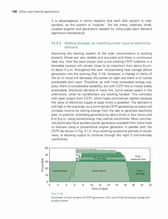
138 Other solar thermal applications
It is advantageous in some respects that each dish system is inde-pendent, so the system is ‘modular’. Yet the many, relatively small, coupled engines and generators needed for utility-scale plant demand significant maintenance.
§4.8.3 Adding storage, so matching solar input to electricity demand
Assuming the tracking system of the solar concentrators is working properly (these are very reliable and accurate) and there is continuous clear sky, then the input power onto a sun-tracking CSTP collector in a favorable location will remain close to its maximum from about 9 a.m. to about 5 p.m. throughout the year. Incorporating heat storage allows generation into the evening (Fig. 4.14). However, a change in clarity of the air or cloud will decrease this power at night and there is of course predictable zero input. Therefore, as with most renewable energy sup-plies, there is considerable variability, but with CSTP this is mostly totally predictable. Electricity demand in many hot, sunny places peaks in the afternoons, when air conditioners are working hardest. This coincides with peak output from CSTP, which helps commercial viability because the value of electricity supply at peak times is greatest. The demand is still high in the evenings, so a commercial CSTP generating company will increase income by storing energy from the day to generate electricity later. In practice, extending generation by about three or four hours until 8 to 9 p.m. using stored energy may well be worthwhile. Most commer-cial plants also have auxiliary power generation available from fossil fuels or biofuels using a conventional engine generator in parallel with the CSTP (as shown in Fig. 4.11), thus covering occasional periods of cloudi-ness, or allowing output to continue through the night if commercially worthwhile.
Fig. 4.14Schematic of time variation of CSTP generation, with use of thermal energy storage and auxiliary power.
0
50
40
30
20
10
062 4 8 10 14 16 20 22
Firmcapacity lineTo storage
Fromstorage
12 18 24
Fuel backup Solar direct
Time of day/h
Po
wer
/MW
TWIDELL PAGINATION.indb 138 01/12/2014 11:36
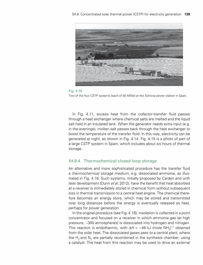
§4.8 Concentrated solar thermal power (CSTP) for electricity generation 139
In Fig. 4.11, excess heat from the collector-transfer fluid passes through a heat exchanger where chemical salts are melted and the liquid salt held in an insulated tank. When the generator needs extra input (e.g. in the evenings), molten salt passes back through the heat exchanger to boost the temperature of the transfer fluid. In this way, electricity can be generated at night, as shown in Fig. 4.14. Fig. 4.15 is a photo of part of a large CSTP system in Spain, which includes about six hours of thermal storage.
§4.8.4 Thermochemical closed-loop storage
An alternative and more sophisticated procedure has the transfer fluid a thermochemical storage medium, e.g. dissociated ammonia, as illus-trated in Fig. 4.16. Such systems, initially proposed by Carden and with later development (Dunn et al. 2012), have the benefit that heat absorbed at a receiver is immediately stored in chemical form without subsequent loss in thermal transmission to a central heat engine. The chemical there-fore becomes an energy store, which may be stored and transmitted over long distances before the energy is eventually released as heat, perhaps for power generation.
In the original procedure (see Fig. 4.16), insolation is collected in a point concentrator and focused on a receiver in which ammonia gas (at high pressure, ~300 atmospheres) is dissociated into hydrogen and nitrogen. This reaction is endothermic, with ∆H = − 46 kJ (mole NH3)
−1 obtained from the solar heat. The dissociated gases pass to a central plant, where the H2 and N2 are partially recombined in the synthesis chamber, using a catalyst. The heat from this reaction may be used to drive an external
Fig. 4.15Two of the four CSTP systems (each of 50 MWe) at the Solnova power station in Spain.
TWIDELL PAGINATION.indb 139 01/12/2014 11:36
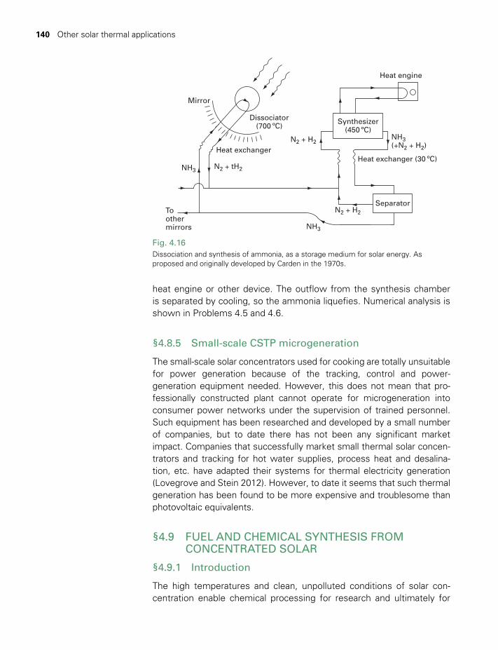
140 Other solar thermal applications
heat engine or other device. The outflow from the synthesis chamber is separated by cooling, so the ammonia liquefies. Numerical analysis is shown in Problems 4.5 and 4.6.
§4.8.5 Small-scale CSTP microgeneration
The small-scale solar concentrators used for cooking are totally unsuitable for power generation because of the tracking, control and power- generation equipment needed. However, this does not mean that pro-fessionally constructed plant cannot operate for microgeneration into consumer power networks under the supervision of trained personnel. Such equipment has been researched and developed by a small number of companies, but to date there has not been any significant market impact. Companies that successfully market small thermal solar concen-trators and tracking for hot water supplies, process heat and desalina-tion, etc. have adapted their systems for thermal electricity generation (Lovegrove and Stein 2012). However, to date it seems that such thermal generation has been found to be more expensive and troublesome than photovoltaic equivalents.
§4.9 FUEL AND CHEMICAL SYNTHESIS FROM CONCENTRATED SOLAR
§4.9.1 Introduction
The high temperatures and clean, unpolluted conditions of solar con-centration enable chemical processing for research and ultimately for
Fig. 4.16Dissociation and synthesis of ammonia, as a storage medium for solar energy. As proposed and originally developed by Carden in the 1970s.
Heat engine
NH3(+N2 + H2)
N2 + H2
N2 + tH2
N2 + H2
NH3
NH3
Toothermirrors
Separator
Heat exchanger (30 ºC)Heat exchanger
Mirror
Dissociator(700 ºC)
Synthesizer(450 ºC)
TWIDELL PAGINATION.indb 140 01/12/2014 11:36
§4.10 Social and environmental aspects 141
commercial products and processes (Konstandopoulos et al. 2012). Manufacturing fuels is one main aim, thereby capturing and storing the transient energy of the Sun. Such thermochemical processes overall are endothermic (absorbing energy) and proceed faster at high temperature; hence the benefit of solar concentration.
The main fuels are: (1) hydrogen from the thermochemical dissocia-tion of water; and (2) carbon fuels from the thermochemical dissociation of wastes to CO and H2, with subsequent production of synthetic liquid fuels. The ammonia synthesis/dissociation (Fig. 4.16) is a special case, in which the chemical reaction is used as an energy store.
§4.9.2 Hydrogen production
Single-step (direct) water splitting to hydrogen and oxygen in one stage requires temperatures >2000°C, and could be dangerous. Therefore a multi-step process is preferred; usually a two-step process using metal oxides as ‘system catalysts’ (i.e. chemicals that are essential reactants, but which cycle continuously in the process between a reduced (e.g. SnO) and an oxidized state (e.g. SnO2)). In such ways the reaction tem-peratures may be <1500°C and more easily attained. A very large range of metal oxides (MOs) have been researched in solar hydrogen synthe-sis. The two reactions simplify, for example, to:
At smaller ‘high temperature’ MO + H2O → MO2 + H2 + heat (4.26)
At larger ‘higher temperature’ 2MO2 + heat → 2MO + O2 (4.27)
R&D to date has explored such processes in operational solar concentra-tors. The European HYDROSOL program has demonstrated the concept at ever-increasing scales, and with various multi-chamber solar reac-tors with the aim of continuous production, including the Hydrosol-2 100-kilowatt pilot plant at the Plataforma Solar de Almería in Spain, oper-ational from 2008. (See Bibliography.)
§4.10 SOCIAL AND ENVIRONMENTAL ASPECTS
Solar crop driers and concentrating solar thermal power (CSTP) can have widespread benefits in suitable climates. The other solar technologies examined in this chapter (water distillation, absorption refrigerators, salt-gradient ponds, fuel and chemical synthesis) are less common. Where these technologies are appropriate, they can contribute to clean, sustaina-ble economies. As with all renewables, a beneficial impact is to substitute for fossil fuels, and so abate pollution, both locally and globally. Several of the technologies may use potentially harmful or dangerous chemicals, so procedures established in conventional industries for health and safety must be followed. Concentrated solar radiation is a serious danger for per-sonal harm and for fire, so adequate site safety procedures are essential.
TWIDELL PAGINATION.indb 141 01/12/2014 11:36
142 Other solar thermal applications
Given the arid/semi-arid nature of environments suitable for CSTP, a key challenge usually is obtaining cooling water for the thermal engines. Otherwise dry or hybrid dry/wet cooling has to be used, but with loss of efficiency. Another limitation for CSTP plants is the distance between areas suitable for power production and major consumption centers. Several proposed large-scale proposals (e.g. Desertec, which aims to use CSTP in North Africa to supply Central European demand) therefore incorporate low-loss, very high-voltage, electricity transmission.
Some solar applications are so obviously beneficial that it seems unnecessary to emphasize them here; examples are the benefits of ‘solar buildings’ (§16.4), clothes drying and salt production (by evapora-tion of salt water in large salt pans). It is unfortunate that in many affluent households and organizations, washed clothes are routinely dried by heat from electricity in clothes driers rather than using sunshine whenever possible. Even when the driers reuse heat recovered from water vapor condensation, such electrically heated drying is frequently unnecessary.
CHAPTER SUMMARY
Basic analysis is explained here for many solar applications other than water heating (Chapter 3) and buildings (Chapter 16). Crop drying after harvest is vital for food security and is greatly assisted by solar energy. Closed crop driers are air heaters that work on similar principles to solar water heaters, but are usually of much simpler construction. Concentrated solar thermal power (CSTP) has progressed rapidly from R&D projects to commercial-scale investments, especially in southern Spain and California. Because only direct (beam) radiation can be concentrated by factors >10, CSTP is applicable only in sunny, nearly cloud-free locations. Integrated thermal storage is an important feature of CSTP plants, and so such systems extend generation into the evening and also may have fuel power backup capacity. Thus, CSTP offers firm, flexible electrical production capacity to utilities, and is already cost-competitive at times of peak electricity demand, especially in summer. The main limitations to the expansion of CSTP plants are accessing the necessary cooling water and the distance between these areas and major consumption centers. CSTP systems may use any of the four main types of concentrating collector: (1) parabolic trough; (2) linear Fresnel; (3) central receiver (power tower); and (4) ‘dish’ (paraboloid). Types (1) and (2) track the Sun in only one dimension (east–west) and typically achieve receiver temperatures ~400°C, but are mechanically simpler and cheaper than types (3) and (4), which track the Sun in two dimensions. The latter, with point concentration, can achieve maximum temperatures of ~2000°C, for chemical production and materials testing. The other solar technologies examined in this chapter (water distillation, absorption refrigerators, salt-gradient ponds, solar cookers) all have specific benefits in appropriate climates and locations, but have not generally replaced conventional technology.
QUICK QUESTIONS
Note: Answers to these questions are in the text of the relevant section of this chapter, or may be readily inferred from it.
1 Why is it important to dry crops soon after harvest? 2 What is the difference between absolute humidity and relative
humidity?
TWIDELL PAGINATION.indb 142 01/12/2014 11:36

Problems 143
3 Why does an absorption cooler require heat to be added? 4 How much fresh water per day could be produced by a solar still of
10 m2 area? 5 What is a ‘solar pond’? 6 Why is a selective surface important for a solar water heater but not
for a CSTP receiver? 7 Name three types of solar concentrator. Which of these achieves
the highest output temperature? Which is the easiest to keep clean?
8 Outline the principle of a Fresnel mirror. 9 Why do most commercial CSTP systems include some energy
storage? What is the most common form of such storage? 10 List three constraints on the location of CSTP plants.
PROBLEMS
4.1 Theory of the chimney
A vertical chimney of height h takes away hot air at temperature Th from a heat source. By evaluating the integral (3.25) inside and outside the chimney, calculate the thermosyphon pressure pth for the following conditions:
(a) Ta = 30°C, Th = 45 °C, h = 4 m (corresponding to a solar crop drier).(b) Ta = 5°C, Th = 300°C, h = 100 m (corresponding to an industrial
chimney).
4.2 Flow through a bed of grain
Flow of air through a bed of grain is analogous to fluid flow through a network of pipes.
(a) Fig. 4.17(a) shows a cross-section of a solid block pierced by n paral-lel tubes, each of radius a. As a is small, the flow is laminar (why?), in which case it may be shown that according to Poiseuille’s law, the volume of fluid flowing through each tube is:
pm
=
Q
a dpdx81
4 (4.28)
where m is the dynamic viscosity (see Review 2) and dp/dx is the pressure gradient driving the flow. Use this to show that the bulk fluid flow speed through the solid block of cross-section A0 is:
e= =vQ a dp
dxA 8total
0
2
TWIDELL PAGINATION.indb 143 01/12/2014 11:36
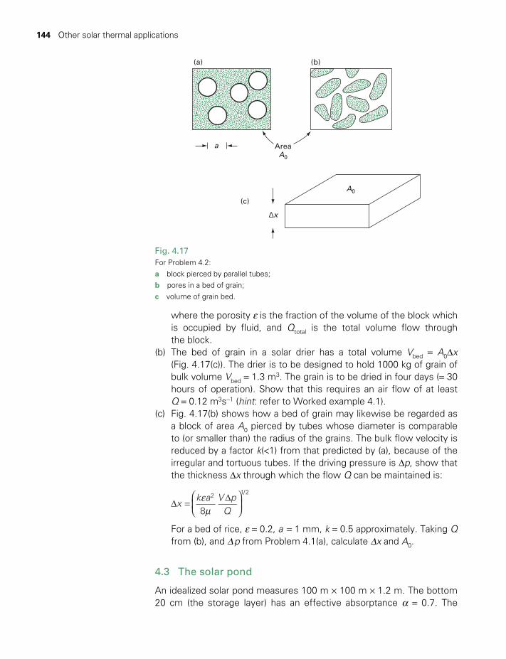
144 Other solar thermal applications
Fig. 4.17For Problem 4.2: a block pierced by parallel tubes; b pores in a bed of grain; c volume of grain bed.
AreaA0
a
(a) (b)
(c)
∆x
A0
where the porosity e is the fraction of the volume of the block which is occupied by fluid, and Qtotal is the total volume flow through the block.
(b) The bed of grain in a solar drier has a total volume Vbed = A0∆x (Fig. 4.17(c)). The drier is to be designed to hold 1000 kg of grain of bulk volume Vbed = 1.3 m3. The grain is to be dried in four days (= 30 hours of operation). Show that this requires an air flow of at least Q = 0.12 m3s−1 (hint: refer to Worked example 4.1).
(c) Fig. 4.17(b) shows how a bed of grain may likewise be regarded as a block of area A0 pierced by tubes whose diameter is comparable to (or smaller than) the radius of the grains. The bulk flow velocity is reduced by a factor k(<1) from that predicted by (a), because of the irregular and tortuous tubes. If the driving pressure is ∆p, show that the thickness ∆x through which the flow Q can be maintained is:
em
∆ = ∆
x
k a V pQ8
2 1/2
For a bed of rice, e = 0.2, a = 1 mm, k = 0.5 approximately. Taking Q from (b), and ∆ p from Problem 4.1(a), calculate ∆x and A0.
4.3 The solar pond
An idealized solar pond measures 100 m × 100 m × 1.2 m. The bottom 20 cm (the storage layer) has an effective absorptance a = 0.7. The
TWIDELL PAGINATION.indb 144 01/12/2014 11:36
Problems 145
1.0 m of water above (the insulating layer) has a transmittance t = 0.7, and its density increases downwards so that convection does not occur (see Fig. 4.6). The designer hopes to maintain the storage layer at 80°C. The temperature at the surface of the pond is 27°C (day and night).
(a) Calculate the thermal resistance of the insulating layer, and compare it with the top resistance of a typical flat--plate collector.
(b) Calculate the thermal resistance of a similar layer of fresh water, subject to free convection. Compare this value with that in (a), and comment on any improvement.
(c) The density of NaCl solution increases by 0.75 g/liter for every 1.0 g of NaCl added to 1.0 kg H2O. A saturated solution of NaCl con-tains about 370 g NaCl per kg H2O. The volumetric coefficient of thermal expansion of NaCl solution is about 4 × 10− 4/K. Calculate the minimum concentration Cmin of NaCl required in the storage layer to suppress convection, assuming the water layer at the top of the pond contains no salt. How easy is it to achieve this concentration in practice?
(d) Calculate the characteristic time scale for heat loss from the storage layer, through the resistance of the insulating layer. If the tempera-ture of the storage layer is 80°C at sunset (6 p.m.) what is its tem-perature at sunrise (6 a.m.)?
(e) Diffusion of a solute depends on its molecular diffusivity D, analogous to thermal diffusivity κ of §R3.3. For NaCl in water, D = 1.5 × 10⁻⁹ m2s−1.The pond is set up with the storage layer having twice the critical concentration of NaCl, i.e. double the value Cmin cal-culated in (c). Estimate the time for molecular diffusion to decrease this concentration to Cmin.
Note: Molecular diffusion of salt (solute) from a region of strong concentration to a weak concentration is analogous to the diffusion of heat from a region of high temperature to a region of low tempera-ture by conduction, as described in §R3.3. In fact, the same equa-tions apply with molecular diffusivity D in place of thermal diffusivity κ and concentration C in place of temperature T.
(f) According to your answers to (c)–(e), discuss the practicability of building such a pond, and the possible uses to which it could be put.
4.4
Fig. 4.18 shows the key feature of a system for the large-scale use of solar energy similar to one implemented in California in the 1980s. Sunlight is concentrated on a pipe perpendicular to the plane of the diagram and is absorbed by the selective surface on the outside of the
TWIDELL PAGINATION.indb 145 01/12/2014 11:36
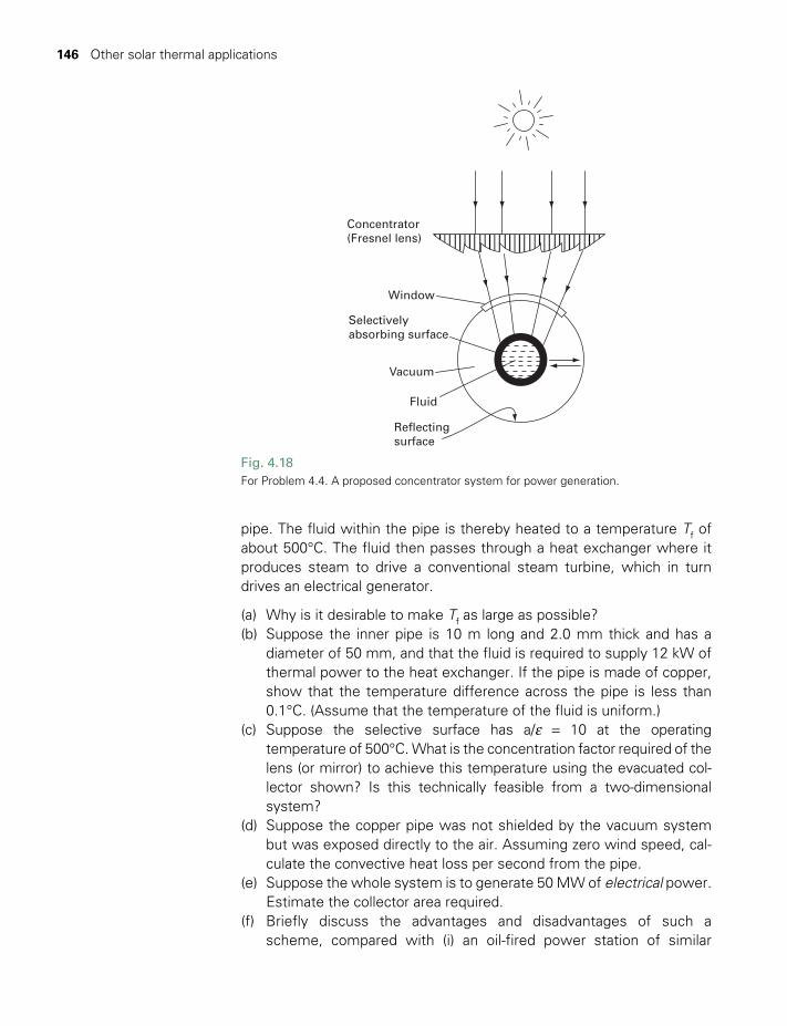
146 Other solar thermal applications
pipe. The fluid within the pipe is thereby heated to a temperature Tf of about 500°C. The fluid then passes through a heat exchanger where it produces steam to drive a conventional steam turbine, which in turn drives an electrical generator.
(a) Why is it desirable to make Tf as large as possible?(b) Suppose the inner pipe is 10 m long and 2.0 mm thick and has a
diameter of 50 mm, and that the fluid is required to supply 12 kW of thermal power to the heat exchanger. If the pipe is made of copper, show that the temperature difference across the pipe is less than 0.1°C. (Assume that the temperature of the fluid is uniform.)
(c) Suppose the selective surface has a/e = 10 at the operating temperature of 500°C. What is the concentration factor required of the lens (or mirror) to achieve this temperature using the evacuated col-lector shown? Is this technically feasible from a two-dimensional system?
(d) Suppose the copper pipe was not shielded by the vacuum system but was exposed directly to the air. Assuming zero wind speed, cal-culate the convective heat loss per second from the pipe.
(e) Suppose the whole system is to generate 50 MW of electrical power. Estimate the collector area required.
(f) Briefly discuss the advantages and disadvantages of such a scheme, compared with (i) an oil-fired power station of similar
Fig. 4.18For Problem 4.4. A proposed concentrator system for power generation.
Concentrator(Fresnel lens)
Window
Vacuum
Fluid
Reflectingsurface
Selectivelyabsorbing surface
TWIDELL PAGINATION.indb 146 01/12/2014 11:36
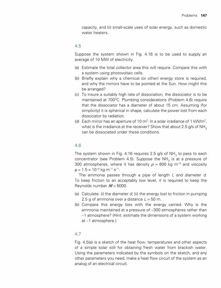
Problems 147
capacity, and (ii) small-scale uses of solar energy, such as domestic water heaters.
4.5
Suppose the system shown in Fig. 4.16 is to be used to supply an average of 10 MW of electricity.
(a) Estimate the total collector area this will require. Compare this with a system using photovoltaic cells.
(b) Briefly explain why a chemical (or other) energy store is required, and why the mirrors have to be pointed at the Sun. How might this be arranged?
(c) To insure a suitably high rate of dissociation, the dissociator is to be maintained at 700°C. Plumbing considerations (Problem 4.6) require that the dissociator has a diameter of about 15 cm. Assuming (for simplicity) it is spherical in shape, calculate the power lost from each dissociator by radiation.
(d) Each mirror has an aperture of 10 m2. In a solar irradiance of 1 kW/m2, what is the irradiance at the receiver? Show that about 2.5 g/s of NH3 can be dissociated under these conditions.
4.6
The system shown in Fig. 4.16 requires 2.5 g/s of NH3 to pass to each concentrator (see Problem 4.5). Suppose the NH3 is at a pressure of 300 atmospheres, where it has density ρ = 600 kg m−3 and viscosity m = 1.5 × 10⁻⁴ kg m−1 s−1.
The ammonia passes through a pipe of length L and diameter d. To keep friction to an acceptably low level, it is required to keep the Reynolds number R < 6000.
(a) Calculate: (i) the diameter d; (ii) the energy lost to friction in pumping 2.5 g of ammonia over a distance L = 50 m.
(b) Compare this energy loss with the energy carried. Why is the ammonia maintained at a pressure of ~300 atmospheres rather than ~1 atmosphere? (Hint: estimate the dimensions of a system working at ~1 atmosphere.)
4.7
Fig. 4.5(a) is a sketch of the heat flow, temperatures and other aspects of a simple solar still for obtaining fresh water from brackish water. Using the parameters indicated by the symbols on the sketch, and any other parameters you need, make a heat flow circuit of the system as an analog of an electrical circuit.
TWIDELL PAGINATION.indb 147 01/12/2014 11:36

148 Other solar thermal applications
NOTES
1 See §13.8 for an outline of ‘osmosis’.2 This may also be called the ‘optical concentration ratio’.3 At excellent explanation with dynamic diagrams may be found at http://en.wikipedia.org/wiki/Stirling_engine
(accessed September 14, 2011).
BIBLIOGRAPHY
General
Duffie, J.A. and Beckman, W.A. (2006, 3rd edn) Solar Engineering of Thermal Processes, John Wiley & Sons, New York. The classic text, especially for solar thermal theory and application. Covers most of the topics of this chapter by empirical engineering analysis.
Gordon, J. (ed.) (2001) Solar Energy − The state of the art, James & James, London. Ten chapters by experts in solar thermal, photovoltaic and glazing.
Goswami, D.Y., Kreith, F. and Kreider, J.F. (2000, 2nd edn) Principles of Solar Engineering, Taylor and Francis, London. Another standard textbook on solar thermal systems.
Journals
The most established journal, covering all aspects of solar (sunshine) energy, is Solar Energy, published by Elsevier in cooperation with the International Solar Energy Society (ISES).
Air heaters and crop drying
Brenndorfer, B., Kennedy, L., Bateman, C.O., Mrena, G.C. and Wereko-Brobby, C. (1985) Solar Dryers: Their role in post-harvest processing, Commonwealth Secretariat, London.
Monteith, J. and Unsworth, K. (2008, 3rd edn) Principles of Environmental Physics, Academic Press, London. Includes a full discussion of humidity.
Water desalination
Delyannis, E. and Belessiotis,V. (2001) ‘Solar energy and desalination’, Advances in Solar Energy, 14, 287. Useful review with basic physics displayed; notes that ‘almost all large state-of-the-art stills have been dismantled’.
Rizzutti, L., Ettouney, H. and Cipollina, A. (eds) (2007) Solar Desalination for the 21st Century, Springer, New York. Proceedings of a conference sponsored by NATO.
Solar absorption cooling
Wang, R.Z. (2003) ‘Solar refrigeration and air conditioning research in China’, Advances in Solar Energy, 15, 261. Clear explanation of principles; notes that there have been few commercial applications as yet.
TWIDELL PAGINATION.indb 148 01/12/2014 11:36

Bibliography 149
Solar ponds
El-Sebaii, A.A., Ramadan, M.R.I., Aboul-Enein, S. and Khallaf, A.M. (2011) ‘History of the solar ponds: a review study’, Renewable and Sustainable Energy Reviews, 15, 3319–3325. What its title suggests.
Leblanc, J., Akbarzadeh, A., Andrews, J., Lu, H. and Golding, P. (2011) ‘Heat extraction methods from salinity-gradient solar ponds and introduction of a novel system of heat extraction for improved efficiency’, Solar Energy, 85(12), 3103–3142.
Lu, H., Swift, A.H.P., Hein, H.D.and Walton J.C. (2004) ‘Advancements in salinity gradient solar pond technology based on sixteen years of operational experience’, Journal of Solar Energy Engineering, 126, 759–767. Careful review, including technical detail and operational experience.
Tabor, H. and Doron, B. (1990) ‘The Beit Ha’Harava 5 MW(e) solar pond’, Solar Energy, 45, 247–253. Describes the earliest – and largest at the time – operational solar pond.
Concentrators and their applications
Dunn, R., Lovegrove, K. and Burgess, G. (2012) ‘A review of ammonia-based thermochemical energy storage for Concentrating Solar Power’, IEEE Journal, 100(2), 391–400.
HYDROSOL: successive European Union funded R&D programmes for hydrogen production from water. For example, see http://160.40.10.25/hydrosol/ (accessed March 23, 2013).
Konstandopoulos, A.G. and Lorentzou, S. (2010) ‘Novel monolithic reactors for solar thermochemical water split-ting’, in L. Vayssieres (ed.), On Solar Hydrogen and Nanotechnology, John Wiley & Sons, Singapore.
Konstandopoulos, A.G., Pagkoura, C. and Lorentzou, S. (2012) ‘Solar fuels and industrial solar chemistry’, ch. 20 in Lovegrove and Stein (2012). Excellent survey from a chemical point of view.
Lovegrove, K. and Stein, W. (eds) (2012) Concentrating Solar Power Technology: Principles, developments and applications, Woodhead Publishing, Cambridge. Comprehensive and authoritative integrated chapters by experts; includes solar, physical, chemical, economic and manufacturing reviews.
Winston, R. (2011) Thermodynamically efficient solar concentrator technology, Lecture series, UC Davis. Available at http://solar.ucdavis.edu/files/education/2011-minicourse-winston.pdf (accessed March 2013).
Winston, R., Minano, J.C. and Beniez, P.G. (2005) Nonimaging Optics, Elsevier Academic Press, San Diego, CA.
See also University of California’s Advanced Solar Technologies Institute. Research Center on non-imaging con-centrators led by Professor Winston. See http://ucsolar.org/research-projects/solar-thermal.
Solar thermal electricity generation
Carden, P.O. (1977) ‘Energy co-radiation using the reversible ammonia reaction’, Solar Energy, 19, 365–378. First of a long series of articles; see also Luzzi, A. and Lovegrove, K. (1997) ‘A solar thermochemical power plant using ammonia as an attractive option for greenhouse gas abatement’, Energy, 22, 317–325. See also Dunn et al. (2012).
Mills, D.R. (2001) Solar Thermal Electricity, in Gordon (2001), pp. 577– 651.
Winter, C.J., Sizmann, R.L. and Vant-Hull, L.L. (eds) (1991) Solar Power Plants: Fundamentals, technology, systems, economics, Springer Verlag, Berlin. Detailed engineering review.
TWIDELL PAGINATION.indb 149 01/12/2014 11:36

150 Other solar thermal applications
Websites
There are countless websites dealing with applications in solar energy, some excellent and many of dubious academic value. Use a search engine to locate these and give most credence to the sites of official organizations, as with the examples cited below.
ESTELA (the European Solar Thermal Electricity Association) <www.estelasolar.eu/> Site includes the ESTELA/Kearney Report of June 2010, Solar Thermal Electricity 2025.
International Solar Energy Society (ISES) <www.ises.org>. The largest, oldest, and most authoritative profes-sional organization dealing with the technology and implementation of solar energy. ISES sponsors the research-level journal Solar Energy, which covers all the topics in this chapter.
IEA Solar Heating and Cooling Program <www.iea-shc.org> Reports international research and projects in these fields.
IEA program on Concentrated Solar Power <www.solarpaces.org> Reports international research and projects in this field, along with outlines of the relevant technologies. Publications available on this site include CSP Technology Roadmap (2010–2050).
TWIDELL PAGINATION.indb 150 01/12/2014 11:36
Photovoltaic (PV) power technology
CONTENTS
Learning aims 152
§5.1 Introduction 153§5.1.1 Background 153§5.1.2 Uses and rapid growth 154§5.1.3 Basics 155§5.1.4 Chapter sections 156
§5.2 Photovoltaic circuit properties 156
§5.3 Applications and systems 161§5.3.1 Stand-alone applications 161§5.3.2 Grid-connected systems 162§5.3.3 Balance of system (BoS)
components 165
§5.4 Maximizing cell efficiency (Sicells) 167§5.4.1 Top-surface electrical-contact
obstruction area (intrinsic loss ~3%) 168
§5.4.2 Optical losses, top and rear surfaces 169
§5.4.3 Photon energy less than band gap (loss ~23%) 172
§5.4.4 Excess photon energy (loss ~33%) 172§5.4.5 Capture efficiency (loss ~0.4%) 172§5.4.6 Collection efficiency 173§5.4.7 Voltage factor Fv (loss ~20%) 173§5.4.8 Fill factor (curve factor) Fc
(intrinsic loss ~12%) 174§5.4.9 Ideality factor A (loss ~5%) 174§5.4.10 Series resistance (loss ~0.3%) 175§5.4.11 Shunt resistance (negligible
loss ~0.1%) 175§5.4.12 Delivered power 175
§5.5 Solar cell and module manufacture 176
§5.6 Types and adaptations of photovoltaics 179§5.6.1 Variations in Si material 180§5.6.2 Variations in junction geometry 183§5.6.3 Other substrate materials;
chemical groups III/V and II/VI 184§5.6.4 Other semiconductor
mechanisms, classifications and terminologies 186
§5.6.5 Variation in system arrangement 189
§5.7 Social, economic and environmental aspects 191§5.7.1 Prices 191§5.7.2 Grid-connected systems 192§5.7.3 Stand-alone systems 193§5.7.4 PV for rural electrification,
especially in developing countries 193§5.7.5 Environmental impact 196§5.7.6 Outlook 196
Chapter summary 197
Quick questions 197
Problems 198
Note 200
Bibliography 200
Box 5.1 Self-cleaning glass on module PV covers 167
Box 5.2 Solar radiation absorption at the p–n junction 171
Box 5.3 Manufacture of silicon crystalline cells and modules 176
Box 5.4 An example of a sophisticated Si solar cell 185
CHAPTER
5
TWIDELL PAGINATION.indb 151 01/12/2014 11:36
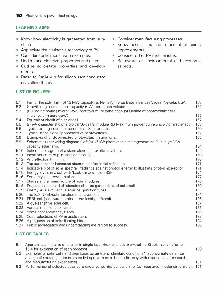
152 Photovoltaic power technology
LIST OF TABLES
5.1 Approximate limits to efficiency in single-layer (homo-junction) crystalline Si solar cells (refer to §5.4 for explanation of each process) 169
5.2 Examples of solar cells and their basic parameters, standard conditions* (approximate data from a range of sources; there is a steady improvement in best efficiency with experience of research and manufacturing experience) 181
5.3 Performance of selected solar cells under concentrated ‘sunshine’ (as measured in solar simulators). 191
LIST OF FIGURES
5.1 Part of the solar farm of 13 MW capacity, at Nellis Air Force Base, near Las Vegas, Nevada, USA. 1535.2 Growth of global installed capacity (GW) from photovoltaics. 1545.3 (a) Diagrammatic (‘micro-view’) portrayal of PV generation (b) Outline of photovoltaic cells
in a circuit (‘macro-view’). 1555.4 Equivalent circuit of a solar cell. 1575.5 (a) I–V characteristic of a typical 36-cell Si module. (b) Maximum power curve and I-V characteristic. 1585.6 Typical arrangements of commercial Si solar cells. 1605.7 Typical stand-alone applications of photovoltaics. 1625.8 Examples of grid-connected photovoltaic installations. 1635.9 Schematics (not wiring diagrams) of: (a) ~5 kW photovoltaic microgeneration (b) a large MW
capacity solar farm. 1645.10 Schematic diagram of a stand-alone photovoltaic system. 1655.11 Basic structure of p–n junction solar cell. 1685.12 Antireflection thin film. 1705.13 Top surfaces for increased absorption after initial reflection. 1715.14 Indicative plot of solar spectral irradiance against photon energy to illustrate photon absorption. 1715.15 Energy levels in a cell with ‘back surface field’ (BSF). 1745.16 Some crystal growth methods. 1775.17 Stages in the manufacture of solar modules. 1785.18 Projected costs and efficiencies of three generations of solar cell. 1805.19 Energy levels of various solar cell junction types. 1835.20 The SJ3 NREL/solar junction multilayer cell. 1845.21 PERL cell (passivated emitter, rear locally diffused). 1855.22 A dye-sensitive solar cell. 1875.23 Vertical multi-junction cells. 1885.24 Some concentrator systems. 1905.25 Cost reductions of PV in application. 1925.26 A progression of solar lighting kits. 1945.27 Public appreciation and understanding are critical to success. 196
LEARNING AIMS
• Know how electricity is generated from sun- shine.
• Appreciate the distinctive technology of PV.• Consider applications, with examples.• Understand electrical properties and uses.• Outline solid-state properties and develop -
ments.• Refer to Review 4 for silicon semiconductor
crystalline theory.
• Consider manufacturing processes.• Know possibilities and trends of efficiency
improvements.• Consider other PV mechanisms.• Be aware of environmental and economic
aspects.
TWIDELL PAGINATION.indb 152 01/12/2014 11:36

§5.1 Introduction 153
Fig. 5.1Part of the solar farm of 13 MW capacity, at Nellis Air Force Base, near Las Vegas, Nevada, USA. The photovoltaic modules are fixed to nearly 6000 Sun-tracking frames, at which the DC power is transformed (inverted) into conventional AC mains power for electricity throughout the Base, peaking at 13 MW. The solar electricity integrates with the supply from the Base’s diesel generators, thus giving considerable reduction in fuel use.
§5.1 INTRODUCTION
§5.1.1 Background
There are only two methods to generate significant electric power. The first is electromagnetic dynamic generation discovered by Michael Faraday in 1821 and in commercial production by 1890; this is the domi-nant method today, requiring the relative movement of a magnetic field and a conductor powered by an external engine or turbine.
The second method is photovoltaic generation with no moving parts using solar cells (technically photovoltaic cells), which produce electric-ity from the absorption of electromagnetic radiation, especially light, predominantly within semiconductor materials, as shown in Fig. 5.1. The photovoltaic (PV) effect1 was discovered by Becquerel in 1839 but was not developed as a power source until 1954 by Chapin, Fuller and Pearson using doped semiconductor silicon; the physical mechanism is explained in Review 4. There are many different types of PV cell, but for practical application it is not essential to understand their internal operation, since they can be described by their external electrical circuit characteristics (§5.2).
TWIDELL PAGINATION.indb 153 01/12/2014 11:36
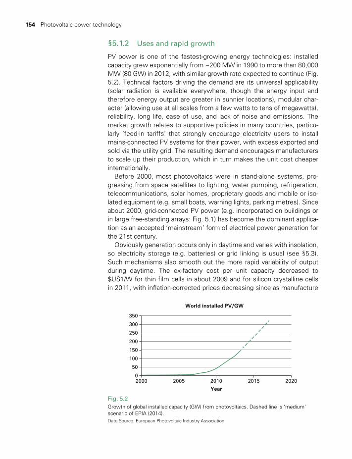
154 Photovoltaic power technology
§5.1.2 Uses and rapid growth
PV power is one of the fastest-growing energy technologies: installed capacity grew exponentially from ~200 MW in 1990 to more than 80,000 MW (80 GW) in 2012, with similar growth rate expected to continue (Fig. 5.2). Technical factors driving the demand are its universal applicability (solar radiation is available everywhere, though the energy input and therefore energy output are greater in sunnier locations), modular char-acter (allowing use at all scales from a few watts to tens of megawatts), reliability, long life, ease of use, and lack of noise and emissions. The market growth relates to supportive policies in many countries, particu-larly ‘feed-in tariffs’ that strongly encourage electricity users to install mains-connected PV systems for their power, with excess exported and sold via the utility grid. The resulting demand encourages manufacturers to scale up their production, which in turn makes the unit cost cheaper internationally.
Before 2000, most photovoltaics were in stand-alone systems, pro-gressing from space satellites to lighting, water pumping, refrigeration, telecommunications, solar homes, proprietary goods and mobile or iso-lated equipment (e.g. small boats, warning lights, parking metres). Since about 2000, grid-connected PV power (e.g. incorporated on buildings or in large free-standing arrays: Fig. 5.1) has become the dominant applica-tion as an accepted ‘mainstream’ form of electrical power generation for the 21st century.
Obviously generation occurs only in daytime and varies with insolation, so electricity storage (e.g. batteries) or grid linking is usual (see §5.3). Such mechanisms also smooth out the more rapid variability of output during daytime. The ex-factory cost per unit capacity decreased to $US1/W for thin film cells in about 2009 and for silicon crystalline cells in 2011, with inflation-corrected prices decreasing since as manufacture
Fig. 5.2Growth of global installed capacity (GW) from photovoltaics. Dashed line is ‘medium’ scenario of EPIA (2014).Date Source: European Photovoltaic Industry Association
50
100
150
200
250
300
350
02000 2005
Year
World installed PV/GW
2015 20202010
TWIDELL PAGINATION.indb 154 01/12/2014 11:36
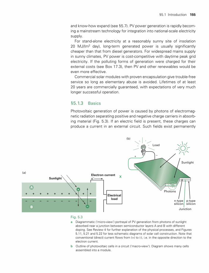
§5.1 Introduction 155
and know-how expand (see §5.7). PV power generation is rapidly becom-ing a mainstream technology for integration into national-scale electricity supply.
For stand-alone electricity at a reasonably sunny site of insolation 20 MJ/(m2 day), long-term generated power is usually significantly cheaper than that from diesel generators. For widespread mains supply in sunny climates, PV power is cost-competitive with daytime peak grid electricity. If the polluting forms of generation were charged for their external costs (see Box 17.3), then PV and other renewables would be even more effective.
Commercial solar modules with proven encapsulation give trouble-free service so long as elementary abuse is avoided. Lifetimes of at least 20 years are commercially guaranteed, with expectations of very much longer successful operation.
§5.1.3 Basics
Photovoltaic generation of power is caused by photons of electromag-netic radiation separating positive and negative charge carriers in absorb-ing material (Fig. 5.3). If an electric field is present, these charges can produce a current in an external circuit. Such fields exist permanently
+ + ++
– – – – – – –
–
– – –
+
A
B
+ + + + +
X
+
Electricalload
Electron currentSunlight e–
(a)
–+
Load
Photons
n-typesilicon
p-typesilicon
Junction
Sunlight
(b)
Fig. 5.3a Diagrammatic (‘micro-view’) portrayal of PV generation from photons of sunlight
absorbed near a junction between semiconductor layers A and B with different doping. See Review 4 for further explanation of the physical processes, and Figures 5.11, 5.21 and 5.22 for less schematic diagrams of solar cell construction. Note that conventional (direct) current flows from (+) to (-), i.e. in the opposite direction to the electron current.
b Outline of photovoltaic cells in a circuit (‘macro-view’). Diagram shows many cells assembled into a module.
TWIDELL PAGINATION.indb 155 01/12/2014 11:36
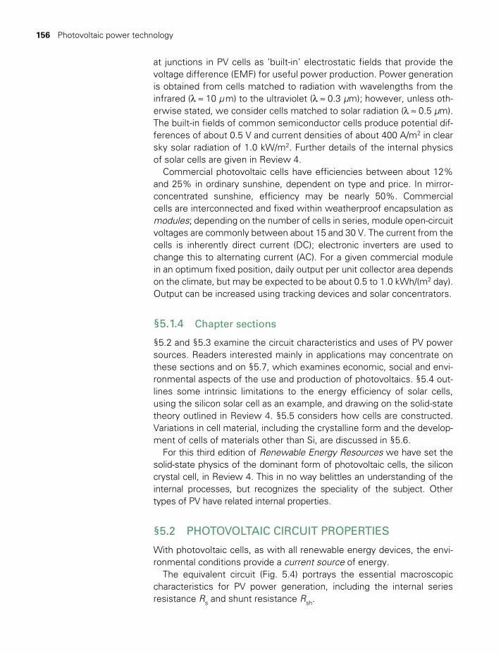
156 Photovoltaic power technology
at junctions in PV cells as ‘built-in’ electrostatic fields that provide the voltage difference (EMF) for useful power production. Power generation is obtained from cells matched to radiation with wavelengths from the infrared (l ≈ 10 μ m) to the ultraviolet (l ≈ 0.3 μm); however, unless oth-erwise stated, we consider cells matched to solar radiation (l ≈ 0.5 μm). The built-in fields of common semiconductor cells produce potential dif-ferences of about 0.5 V and current densities of about 400 A/m2 in clear sky solar radiation of 1.0 kW/m2. Further details of the internal physics of solar cells are given in Review 4.
Commercial photovoltaic cells have efficiencies between about 12% and 25% in ordinary sunshine, dependent on type and price. In mirror- concentrated sunshine, efficiency may be nearly 50%. Commercial cells are interconnected and fixed within weatherproof encapsulation as modules; depending on the number of cells in series, module open-circuit voltages are commonly between about 15 and 30 V. The current from the cells is inherently direct current (DC); electronic inverters are used to change this to alternating current (AC). For a given commercial module in an optimum fixed position, daily output per unit collector area depends on the climate, but may be expected to be about 0.5 to 1.0 kWh/(m2 day). Output can be increased using tracking devices and solar concentrators.
§5.1.4 Chapter sections
§5.2 and §5.3 examine the circuit characteristics and uses of PV power sources. Readers interested mainly in applications may concentrate on these sections and on §5.7, which examines economic, social and envi-ronmental aspects of the use and production of photovoltaics. §5.4 out-lines some intrinsic limitations to the energy efficiency of solar cells, using the silicon solar cell as an example, and drawing on the solid-state theory outlined in Review 4. §5.5 considers how cells are constructed. Variations in cell material, including the crystalline form and the develop-ment of cells of materials other than Si, are discussed in §5.6.
For this third edition of Renewable Energy Resources we have set the solid-state physics of the dominant form of photovoltaic cells, the silicon crystal cell, in Review 4. This in no way belittles an understanding of the internal processes, but recognizes the speciality of the subject. Other types of PV have related internal properties.
§5.2 PHOTOVOLTAIC CIRCUIT PROPERTIES
With photovoltaic cells, as with all renewable energy devices, the envi-ronmental conditions provide a current source of energy.
The equivalent circuit (Fig. 5.4) portrays the essential macroscopic characteristics for PV power generation, including the internal series resistance Rs and shunt resistance Rsh.
TWIDELL PAGINATION.indb 156 01/12/2014 11:36
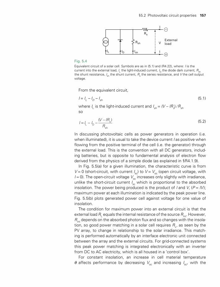
§5.2 Photovoltaic circuit properties 157
From the equivalent circuit,
I = IL – ID – Ish (5.1)
where IL is the light-induced current and Ish = (V – IRs) / Rshso
= - --
I I IV IR
R
( )L D
s
sh
(5.2)
In discussing photovoltaic cells as power generators in operation (i.e. when illuminated), it is usual to take the device current I as positive when flowing from the positive terminal of the cell (i.e. the generator) through the external load. This is the convention with all DC generators, includ-ing batteries, but is opposite to fundamental analysis of electron flow derived from the physics of a simple diode (as explained in §R4.1.9).
In Fig. 5.5(a) for a given illumination, the characteristic curve is from V = 0 (short-circuit, with current Isc) to V = Voc (open circuit voltage, with I = 0). The open-circuit voltage Voc increases only slightly with irradiance, unlike the short-circuit current Isc which is proportional to the absorbed insolation. The power being produced is the product of I and V, (P = IV ); maximum power at each illumination is indicated by the peak power line. Fig. 5.5(b) plots generated power cell against voltage for one value of insolation.
The condition for maximum power into an external circuit is that the external load RL equals the internal resistance of the source Rint. However, Rint depends on the absorbed photon flux and so changes with the insola-tion, so good power matching in a solar cell requires RL, as seen by the PV array, to change in relationship to the solar irradiance. This match-ing is performed automatically by an interface electronic unit connected between the array and the external circuits. For grid-connected systems this peak power matching is integrated electronically with an inverter from DC to AC electricity, which is all housed in a ‘control box’.
For constant insolation, an increase in cell material temperature θ affects performance by decreasing Voc and increasing Isc, with the
Fig. 5.4Equivalent circuit of a solar cell. Symbols are as in (5.1) and (R4.22), where: I is the current into the external load, IL the light-induced current, ID the diode dark current, Rsh the shunt resistance, Ish the shunt current, Rs the series resistance, and V the cell output voltage.
IL ID Ish
I
ExternalloadV
–
+I
Rsh
Rs
TWIDELL PAGINATION.indb 157 01/12/2014 11:36
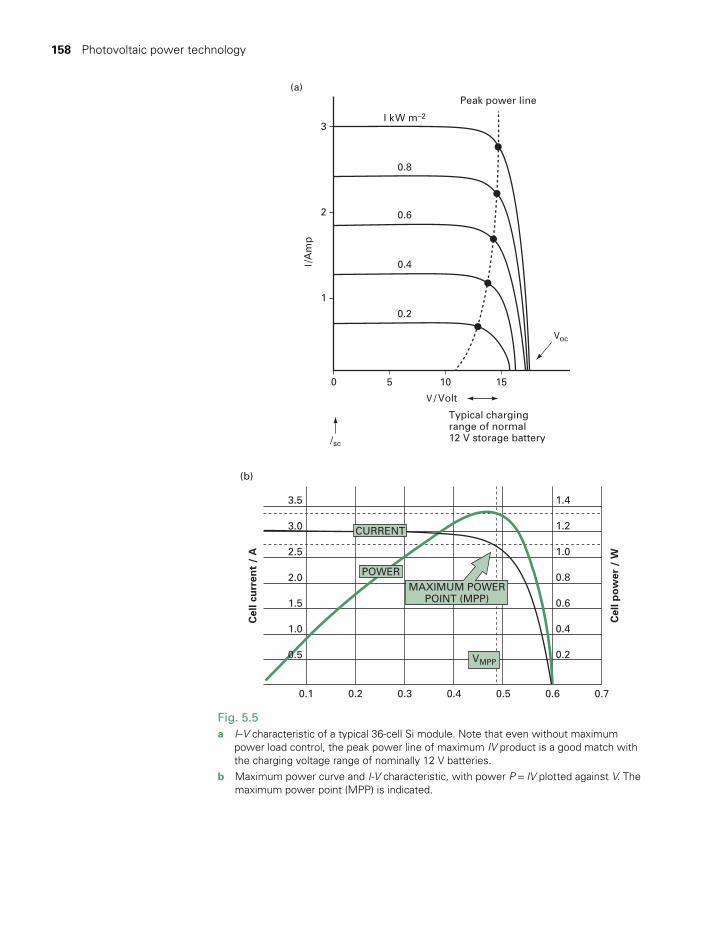
158 Photovoltaic power technology
3I kW m–2
0.8
Peak power line
V / Volt
0.6
0.4
0.2
2
1
0
I/A
mp
5
Typical chargingrange of normal12 V storage battery
10 15
/sc
Voc
(a)
Fig. 5.5a I–V characteristic of a typical 36-cell Si module. Note that even without maximum
power load control, the peak power line of maximum IV product is a good match with the charging voltage range of nominally 12 V batteries.
b Maximum power curve and I-V characteristic, with power P = IV plotted against V. The maximum power point (MPP) is indicated.
3.5
0.5
0.1 0.2 0.3 0.4 0.5 0.6 0.7
1.0
Cel
l cu
rren
t /
A
Cell voltage / V
Cel
l po
wer
/ W
VMPP
POWERMAXIMUM POWER
POINT (MPP)
2.0
3.0
1.5
2.5
1.4
0.2
0.4
0.8
1.2
0.6
1.0
CURRENT
(b)
TWIDELL PAGINATION.indb 158 01/12/2014 11:36
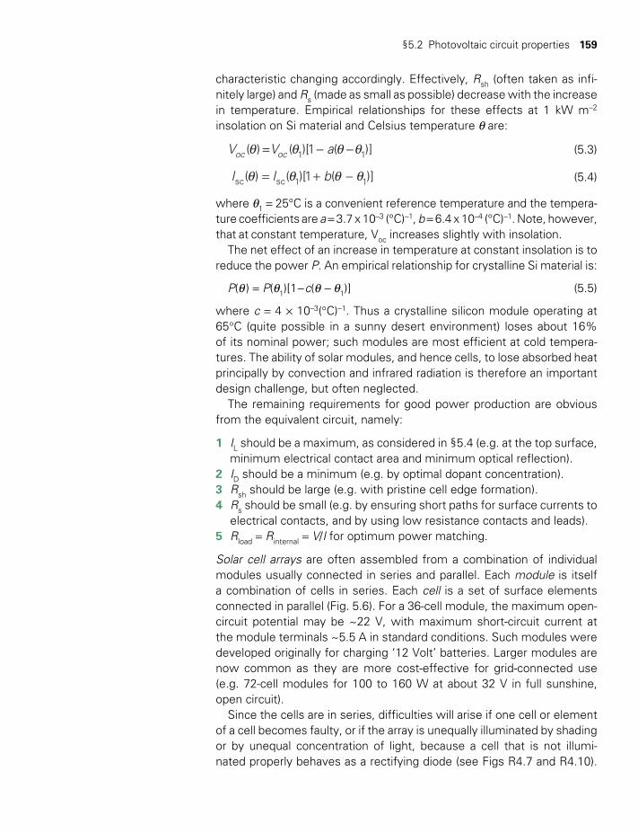
§5.2 Photovoltaic circuit properties 159
characteristic changing accordingly. Effectively, Rsh (often taken as infi-nitely large) and Rs (made as small as possible) decrease with the increase in temperature. Empirical relationships for these effects at 1 kW m–2 insolation on Si material and Celsius temperature θ are:
V V a( ) ( )[1 ( )]oc oc 1 1θ θ θ θ= - - (5.3)
I I b( ) ( )[1 ( )]sc sc 1 1θ θ θ θ= + - (5.4)
where θ1 = 25°C is a convenient reference temperature and the tempera-ture coefficients are a = 3.7 x 10⁻³ (°C)–1, b = 6.4 x 10⁻⁴ (°C)–1. Note, however, that at constant temperature, Voc increases slightly with insolation.
The net effect of an increase in temperature at constant insolation is to reduce the power P. An empirical relationship for crystalline Si material is:
P(θ ) = P(θ1)[1- c(θ - θ1)] (5.5)
where c = 4 × 10⁻³(°C)–1. Thus a crystalline silicon module operating at 65°C (quite possible in a sunny desert environment) loses about 16% of its nominal power; such modules are most efficient at cold tempera-tures. The ability of solar modules, and hence cells, to lose absorbed heat principally by convection and infrared radiation is therefore an important design challenge, but often neglected.
The remaining requirements for good power production are obvious from the equivalent circuit, namely:
1 IL should be a maximum, as considered in §5.4 (e.g. at the top surface, minimum electrical contact area and minimum optical reflection).
2 ID should be a minimum (e.g. by optimal dopant concentration).3 Rsh should be large (e.g. with pristine cell edge formation).4 Rs should be small (e.g. by ensuring short paths for surface currents to
electrical contacts, and by using low resistance contacts and leads).5 Rload = Rinternal = V/I for optimum power matching.
Solar cell arrays are often assembled from a combination of individual modules usually connected in series and parallel. Each module is itself a combination of cells in series. Each cell is a set of surface elements connected in parallel (Fig. 5.6). For a 36-cell module, the maximum open-circuit potential may be ~22 V, with maximum short-circuit current at the module terminals ~5.5 A in standard conditions. Such modules were developed originally for charging ‘12 Volt’ batteries. Larger modules are now common as they are more cost-effective for grid-connected use (e.g. 72-cell modules for 100 to 160 W at about 32 V in full sunshine, open circuit).
Since the cells are in series, difficulties will arise if one cell or element of a cell becomes faulty, or if the array is unequally illuminated by shading or by unequal concentration of light, because a cell that is not illumi-nated properly behaves as a rectifying diode (see Figs R4.7 and R4.10).
TWIDELL PAGINATION.indb 159 01/12/2014 11:36
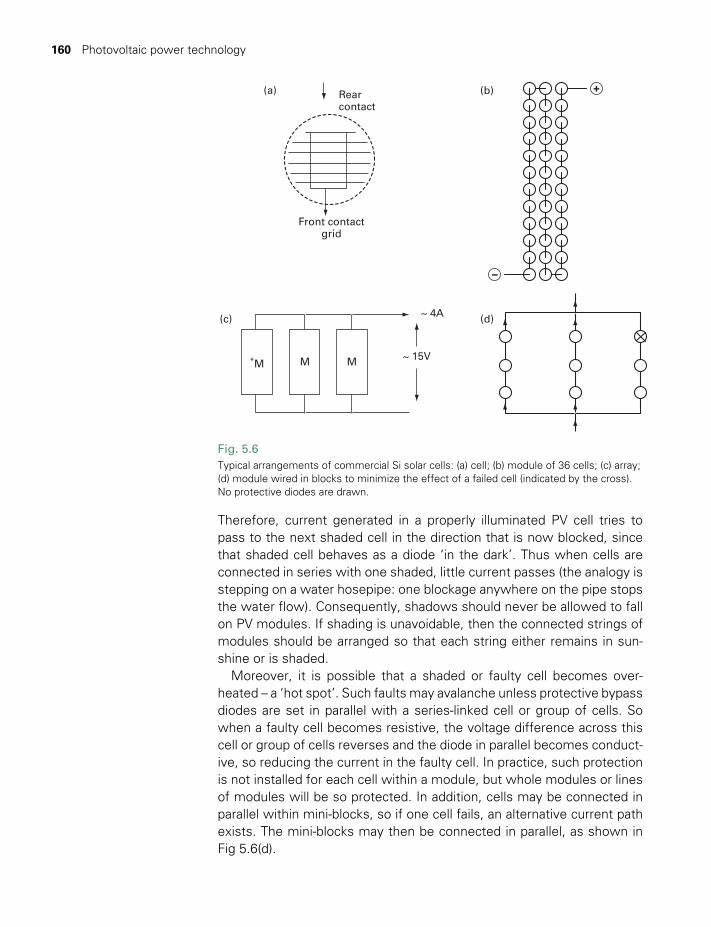
160 Photovoltaic power technology
Therefore, current generated in a properly illuminated PV cell tries to pass to the next shaded cell in the direction that is now blocked, since that shaded cell behaves as a diode ‘in the dark’. Thus when cells are connected in series with one shaded, little current passes (the analogy is stepping on a water hosepipe: one blockage anywhere on the pipe stops the water flow). Consequently, shadows should never be allowed to fall on PV modules. If shading is unavoidable, then the connected strings of modules should be arranged so that each string either remains in sun-shine or is shaded.
Moreover, it is possible that a shaded or faulty cell becomes over-heated – a ‘hot spot’. Such faults may avalanche unless protective bypass diodes are set in parallel with a series-linked cell or group of cells. So when a faulty cell becomes resistive, the voltage difference across this cell or group of cells reverses and the diode in parallel becomes conduct-ive, so reducing the current in the faulty cell. In practice, such protection is not installed for each cell within a module, but whole modules or lines of modules will be so protected. In addition, cells may be connected in parallel within mini-blocks, so if one cell fails, an alternative current path exists. The mini-blocks may then be connected in parallel, as shown in Fig 5.6(d).
Rearcontact
Front contactgrid
(a) +
−
(b)
~ 4A
~ 15VM*M M
(c) (d)
Fig. 5.6Typical arrangements of commercial Si solar cells: (a) cell; (b) module of 36 cells; (c) array; (d) module wired in blocks to minimize the effect of a failed cell (indicated by the cross). No protective diodes are drawn.
TWIDELL PAGINATION.indb 160 01/12/2014 11:36
§5.3 Photovoltaic circuit properties 161
§5.3 APPLICATIONS AND SYSTEMS
PV applications are of two types: (1) stand-alone (independent) equip-ment; and (2) systems interconnected with utility electricity grids. A benefit of using PV electricity from single modules is safety owing to the low voltage and lack of damage to the module if the output short-circuits. Therefore PV power from single cells or modules provides essential hands-on educational experience, both indoors and outdoors. However, great care is needed with interconnected arrays of modules since their terminals are ‘live’ in daylight; even experienced electricians may forget this.
§5.3.1 Stand-alone applications
Photovoltaic modules are very reliable, have no moving parts and require no maintenance or fuel supply other than a flux of solar energy.
Thus photovoltaics offer one of the technically best solutions for bring-ing widespread modern energy to the rural and remote parts of devel-oping countries, where systems of only a few dozen Watts can offer lighting and telecommunication, which are of great social benefit. This is the more so as their cost decreases. However, success in these applica-tions depends at least as much on social and institutional factors as on the technology (see §5.7 and §17.2.2).
The same technical advantages meant that in general the first signifi-cant uses of PV were in applications where a small quantity of electric power was essential but where it was difficult or expensive to bring in fuel for conventional generators. The first major example was for space satellites, which led to considerable early development. Many other uses, usually connected with batteries for electricity storage and voltage regulation, benefitted from this; examples include ‘solar homes’, isolated communities, remote medical centers (especially for refrigerators for pharmaceutical drugs), meteorological measurement, marine warning lights, telecommunication repeater stations (Fig. 5.7), torches, portable radios and other electronic devices, traffic and warning signs, parking metres, etc. If a stand-alone system does not need battery storage (e.g. for water pumping), then a load-matching and voltage regulation inter-face is important. Stand-alone applications often operate automatically, but need periodic cleaning and battery maintenance by trained personnel (but see Box 5.1, §5.3.3, about self-cleaning glass).
As the cost of PV systems has decreased, so has the distance from the electric grid at which the installations are cost-competitive. For example, it is often cheaper, and always safer, to install traffic signs, car-parking metres or lighting for footpaths as stand-alone solar-powered systems than to install grid connection and metering for the small amounts of power required. Moreover, the latest electronic devices, including LED
TWIDELL PAGINATION.indb 161 01/12/2014 11:36

162 Photovoltaic power technology
Fig. 5.7Typical stand-alone applications of photovoltaics. (a) Powering a railway signal box in a remote area of Australia. (b) PV module powering lights for a house in the Solomon Islands.
(a)
(b)
(light emitting diode) lighting, always tend to use less power than their predecessors, so PV power is even more likely to be used.
§5.3.2 Grid-connected systems
Since 2000, grid-connected systems, as shown in Figs 5.1 and 5.8, have been the largest, and fastest-growing, use of photovoltaics. In general there are two classes of such grid ‘distributed/embedded’ generation:
1 ‘Microgeneration’ at or on a building, whereby the PV power connects to the consumer side of the utility metre, with excess power exported to the local grid distribution lines.
2 ‘Solar farms’ of a large array of modules connect directly to the appro-priately scaled grid distribution lines.
Fig. 5.9(a) shows the power flows and connections of typical microgen-eration at a building. The solar modules (panels) are fixed on or integrated with the roof, or on a free-standing framework near the building. The microgenerated power usually connects to the user side of the utility metre, since the owners benefit mostly from using their own power and so reducing imported (purchased) power. Excess power flows away from the building as export into the utility distribution grid lines, for which the owners expect to be paid. In the happy circumstance that the payment per unit for exported power is greater than the unit price of imported power, the microgenerated power should be connected on the utility side of the utility metre to maximize income. A combination of the utility metre and the owners’ metres enables at least three power flows to be measured: (i) generated power, (ii) exported power; and (iii) imported power. The financial arrangements for imported and exported power (usually called a ‘feed-in tariff’, §17.5.1) vary widely by country and utility.
TWIDELL PAGINATION.indb 162 01/12/2014 11:36

§5.3 Photovoltaic circuit properties 163
(a)
Fig. 5.8Examples of grid-connected photovoltaic installations. a Apartments in Freiburg, Germany; PV arrays of 11 modules provide both shade to
windows and electricity to each apartment. Photo: author.
b A transport service station in Australia with PV roof. Photo by courtesy of BP Solar.
(b)
In some places, the feed-in tariff even includes some credit for ‘abated-carbon’ and ‘clean-power’.
Fig. 5.9(b) shows the connection of a megawatt-scale solar farm (e.g. that shown in Fig. 5.1) to the distribution grid; generally there is no local
TWIDELL PAGINATION.indb 163 01/12/2014 11:36
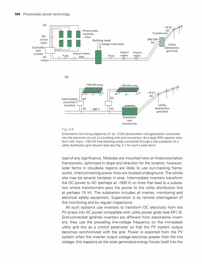
164 Photovoltaic power technology
load of any significance. Modules are mounted here on fixed-orientation frameworks, optimized in slope and direction for the location; however, solar farms in cloudless regions are likely to use sun-tracking frame-works. Interconnecting power lines are located underground. The whole site may be several hectares in area. Intermediate inverters transform the DC power to AC (perhaps at ~500 V) on lines that lead to a substa-tion where transformers pass the power to the utility distribution line at perhaps 15 kV. The substation includes all metres, monitoring and electrical safety equipment. Supervision is by remote interrogation of the monitoring and by regular inspections.
All such systems use inverters to transform DC electricity from the PV arrays into AC power compatible with utility power grids (see §R1.3). Grid-connected (grid-tie) inverters are different from stand-alone invert-ers; they use the prevailing line-voltage frequency on the immediate utility grid line as a control parameter so that the PV system output becomes synchronized with the grid. Power is exported from the PV system when the inverter output voltage becomes greater than the line voltage; this happens as the solar-generated energy forces itself into the
∞ ∞
Photovoltaicmodules~ 5 kw
Building loadsUsage metre kwh
FuseFuseACoutput
Controllerwith
inverter
DCcircuitinput
Exportmetre
Export metrekwh
Importmetre
240/120vAC
Utilitydistributiongrid lines
~100 kW array ~100 kW array
~15 kVAC
Utilitydistributiongrid lines
Substationand
transformer
ACAC
DCDC
Transformer
~ 15 kVAC
~ 300 V
Intermediatecontroller/inverters
(a)
(b)
Fig. 5.9Schematics (not wiring diagrams) of: (a) ~5 kW photovoltaic microgeneration connected into the electricity circuits of a building with grid connection, (b) a large MW capacity solar farm with many ~100 kW free-standing arrays connected through a site substation to a utility distribution grid network (see also Fig. 5.1 for such a solar farm).
TWIDELL PAGINATION.indb 164 01/12/2014 11:36
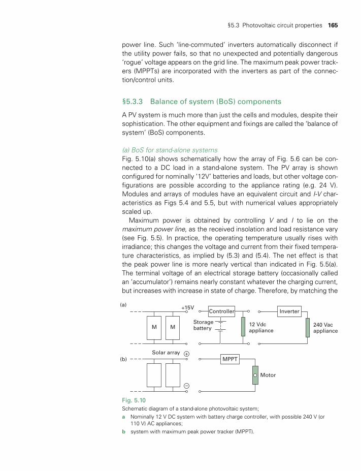
§5.3 Photovoltaic circuit properties 165
power line. Such ‘line-commuted’ inverters automatically disconnect if the utility power fails, so that no unexpected and potentially dangerous ‘rogue’ voltage appears on the grid line. The maximum peak power track-ers (MPPTs) are incorporated with the inverters as part of the connec-tion/control units.
§5.3.3 Balance of system (BoS) components
A PV system is much more than just the cells and modules, despite their sophistication. The other equipment and fixings are called the ‘balance of system’ (BoS) components.
(a) BoS for stand-alone systemsFig. 5.10(a) shows schematically how the array of Fig. 5.6 can be con-nected to a DC load in a stand-alone system. The PV array is shown configured for nominally ‘12V’ batteries and loads, but other voltage con-figurations are possible according to the appliance rating (e.g. 24 V). Modules and arrays of modules have an equivalent circuit and I-V char-acteristics as Figs 5.4 and 5.5, but with numerical values appropriately scaled up.
Maximum power is obtained by controlling V and I to lie on the maximum power line, as the received insolation and load resistance vary (see Fig. 5.5). In practice, the operating temperature usually rises with irradiance; this changes the voltage and current from their fixed tempera-ture characteristics, as implied by (5.3) and (5.4). The net effect is that the peak power line is more nearly vertical than indicated in Fig. 5.5(a). The terminal voltage of an electrical storage battery (occasionally called an ‘accumulator’) remains nearly constant whatever the charging current, but increases with increase in state of charge. Therefore, by matching the
MPPT
Inverter
240 Vacappliance
M M
Controller
Motor
(a)
(b)
12 Vdcappliance
Storagebattery
Solar array
−
+
+15V
Fig. 5.10Schematic diagram of a stand-alone photovoltaic system;a Nominally 12 V DC system with battery charge controller, with possible 240 V (or
110 V) AC appliances; b system with maximum peak power tracker (MPPT).
TWIDELL PAGINATION.indb 165 01/12/2014 11:36

166 Photovoltaic power technology
array optimum voltage and the nominal battery voltage, the V/I load line for battery charging can be matched near to the maximum power line of the array if a more sophisticated controller is not incorporated. In such a case, the battery controls the voltage.
Nearly all stand-alone PV systems require battery storage of electricity, most obviously for lighting at night but also to cope with load surges such as for radio transmission. Batteries are discussed in §15.5. The lifetime and reliability of a PV system are improved using a purpose-designed deep-discharge ‘solar battery’ and not a vehicle battery. A controller pro-vides the specified maximum charge rate and depth of discharge, and is almost essential for reliable operation. Even with a controller, battery lifetime is usually only three to six years – very much less than module lifetime, and often less than the system designers imply! The controller may incorporate a maximum peak power tracker (MPPT) in a single unit.
Direct electrical loads cannot directly regulate the voltage and current, as does a battery. Therefore an intermediate controller is used to sepa-rate (decouple) the voltage and current optimization of the PV array from the voltage requirement of the load. The controller may incorporate an electronic MPPT so the DC voltage and current from the array are con-trolled so that maximum power is generated as the insolation changes (Fig. 5.10(b)). MPPTs are often built into stand-alone solar pumping systems with names like ‘maximizer’ or ‘linear current booster’ and can enable 95% of the maximum output to reach the water pump under varying solar conditions.
To operate AC appliances (240 V/50 Hz or 110 V/60 Hz) from a DC PV supply requires an inverter, as shown on the left of Fig. 5.9(a). A stand-alone inverter uses an internal frequency generator and switching circuitry to transform the low voltage DC power to higher voltage AC power. The shape of the AC waveform may be a square wave (cheap inverter) or an almost pure sine wave (sophisticated solid-state electronic inverter). The inverter should be sized for the surge currents associated with motor-starting (if applicable) but not so large that it normally operates at a small fraction of its rated power (say, <15%) and therefore at poor efficiency (<85%). Solid-state electronic inverters are commercially available with excellent reliability and 95% to 99% efficiency at reasonable cost.
(b) BoS for grid-connected PV For microgeneration at buildings, in addition to fixings and cabling, balance of system equipment consists of a control unit for the con-nection to the mains power lines, extra metering, fuses and safety switches. The control unit normally includes one or more inverters to transform the PV DC to the AC of the building mains electricity, which in turn is connected to the utility local supply lines at usually 110V/60 Hz or 240 V/50 Hz. The inverter is always ‘grid-tied’ so that its output main-tains synchronism with the grid electricity; if the grid supply fails, then
TWIDELL PAGINATION.indb 166 01/12/2014 11:36

§5.4 Maximizing cell efficiency (si cells) 167
the inverter immediately cuts out, but will automatically cut in when the grid supply returns. Owners may add extra monitoring equipment for records of performance and for information to make use of the on-site power.
Module covers may require cleaning, especially in dry environments, but covers of ‘self-cleaning glass’ accumulate less deposits and self-clean in rain (see Box 5.1).
BOX 5.1 SELF-CLEANING GLASS ON MODULE PV COVERS
So-called ‘self-cleaning’ glass is used for the front sloping cover of many modules. It is manufactured with a ~25 nm monolayer of titanium dioxide (TiO2) on its outward-facing surface that has two associated beneficial effects for loosening organic dirt and dust: (1) a catalytic effect that decomposes organic dirt in solar ultraviolet (photocatalysis); and (2) a reduction in the surface tension and surface contact angle of water on the cover (hydrophilic effect) that allows rain or hose water to run off as a sheet film, so carrying away the decomposed dirt. The process was developed and patented by Pilkington Glass.
§5.4 MAXIMIZING CELL EFFICIENCY (SI CELLS)
The efficiency and cost-effectiveness of photovoltaic cells are being continuously improved by research, development and manufacturing know-how, but the many variables and types of cell make the subject exceedingly complex. In this section, we mostly explain key aspects of the dominant form of Si cells, occasionally referring to the basic physics of photovoltaics in Review 4. At the very least, this section should indi-cate the extreme sophistication of solar cell manufacture.
Photovoltaic cells are limited in efficiency by many losses; some of these are avoidable but others are intrinsic to the system. Some limits are obvious and may be controlled independently, but others are complex and cannot be controlled without producing interrelated effects. For instance, increasing dopant concentration can have both advantageous and harmful effects. Table 5.1 portrays typical losses for commercial Si p–n junction single-crystal solar cells in AM1 irradiance, taken in order from the top of the cell to the bottom (see Fig. 5.11). Unfortunately there is no standard convention for the names of the loss factors, which will be considered later.
Note that the most significant inefficiencies are the intrinsic mismatch of the solar spectrum to the single-layer band gap (Box 5.2, §5.4.2). One strategy to reduce these inefficiencies is to have multilayer (heterojunc-tion) devices with layers matched to different regions of the solar spec-trum (§5.6.2); such improvements of efficiency usually allow the cell to be thin, to ~2mm thick rather than ~200mm, so reducing the amount of expensive material, and thus the cost of the cell and its output power.
TWIDELL PAGINATION.indb 167 01/12/2014 11:36
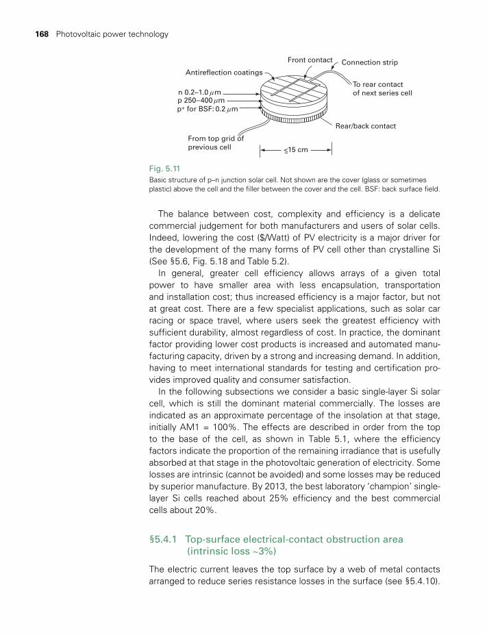
168 Photovoltaic power technology
The balance between cost, complexity and efficiency is a delicate commercial judgement for both manufacturers and users of solar cells. Indeed, lowering the cost ($/Watt) of PV electricity is a major driver for the development of the many forms of PV cell other than crystalline Si (See §5.6, Fig. 5.18 and Table 5.2).
In general, greater cell efficiency allows arrays of a given total power to have smaller area with less encapsulation, transportation and installation cost; thus increased efficiency is a major factor, but not at great cost. There are a few specialist applications, such as solar car racing or space travel, where users seek the greatest efficiency with sufficient durability, almost regardless of cost. In practice, the dominant factor providing lower cost products is increased and automated manu-facturing capacity, driven by a strong and increasing demand. In addition, having to meet international standards for testing and certification pro-vides improved quality and consumer satisfaction.
In the following subsections we consider a basic single-layer Si solar cell, which is still the dominant material commercially. The losses are indicated as an approximate percentage of the insolation at that stage, initially AM1 = 100%. The effects are described in order from the top to the base of the cell, as shown in Table 5.1, where the efficiency factors indicate the proportion of the remaining irradiance that is usefully absorbed at that stage in the photovoltaic generation of electricity. Some losses are intrinsic (cannot be avoided) and some losses may be reduced by superior manufacture. By 2013, the best laboratory ‘champion’ single-layer Si cells reached about 25% efficiency and the best commercial cells about 20%.
§5.4.1 Top-surface electrical-contact obstruction area (intrinsic loss ~3%)
The electric current leaves the top surface by a web of metal contacts arranged to reduce series resistance losses in the surface (see §5.4.10).
Antireflection coatings
n 0.2–1.0 m p 250–400 m p+ for BSF: 0.2 m
To rear contactof next series cell
From top grid ofprevious cell <~15 cm
Rear/back contact
Front contact Connection strip
µµ
µ
Fig. 5.11Basic structure of p–n junction solar cell. Not shown are the cover (glass or sometimes plastic) above the cell and the filler between the cover and the cell. BSF: back surface field.
TWIDELL PAGINATION.indb 168 01/12/2014 11:36
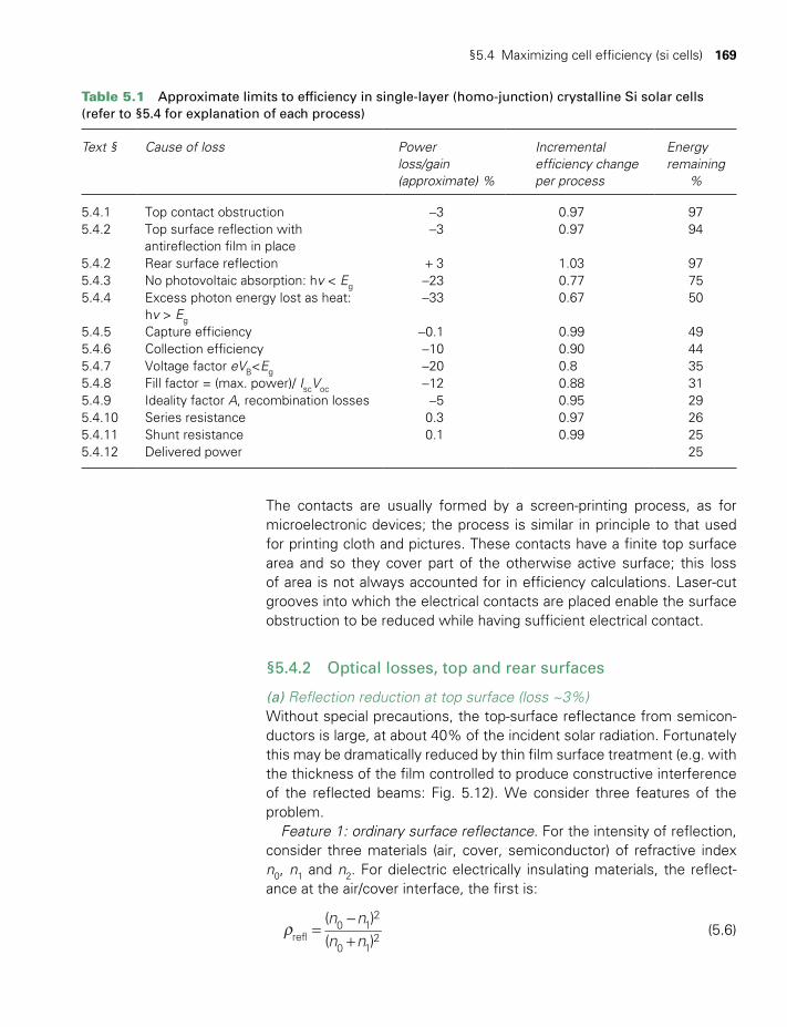
§5.4 Maximizing cell efficiency (si cells) 169
The contacts are usually formed by a screen-printing process, as for microelectronic devices; the process is similar in principle to that used for printing cloth and pictures. These contacts have a finite top surface area and so they cover part of the otherwise active surface; this loss of area is not always accounted for in efficiency calculations. Laser-cut grooves into which the electrical contacts are placed enable the surface obstruction to be reduced while having sufficient electrical contact.
§5.4.2 Optical losses, top and rear surfaces
(a) Reflection reduction at top surface (loss ~3%) Without special precautions, the top-surface reflectance from semicon-ductors is large, at about 40% of the incident solar radiation. Fortunately this may be dramatically reduced by thin film surface treatment (e.g. with the thickness of the film controlled to produce constructive interference of the reflected beams: Fig. 5.12). We consider three features of the problem.
Feature 1: ordinary surface reflectance. For the intensity of reflection, consider three materials (air, cover, semiconductor) of refractive index n0, n1 and n2. For dielectric electrically insulating materials, the reflect-ance at the air/cover interface, the first is:
r =-+
n nn n( )( )refl
0 12
0 12
(5.6)
Table 5.1 Approximate limits to efficiency in single-layer (homo-junction) crystalline Si solar cells (refer to §5.4 for explanation of each process)
Text § Cause of loss Power loss/gain (approximate) %
Incremental efficiency change per process
Energyremaining
%
5.4.1 Top contact obstruction -3 0.97 975.4.2 Top surface reflection with
antireflection film in place-3 0.97 94
5.4.2 Rear surface reflection + 3 1.03 975.4.3 No photovoltaic absorption: hv < Eg -23 0.77 755.4.4 Excess photon energy lost as heat:
hv > Eg
-33 0.67 50
5.4.5 Capture efficiency -0.1 0.99 495.4.6 Collection efficiency -10 0.90 445.4.7 Voltage factor eVB<Eg -20 0.8 355.4.8 Fill factor = (max. power)/ IscVoc -12 0.88 315.4.9 Ideality factor A, recombination losses -5 0.95 295.4.10 Series resistance 0.3 0.97 265.4.11 Shunt resistance 0.1 0.99 255.4.12 Delivered power 25
TWIDELL PAGINATION.indb 169 01/12/2014 11:36
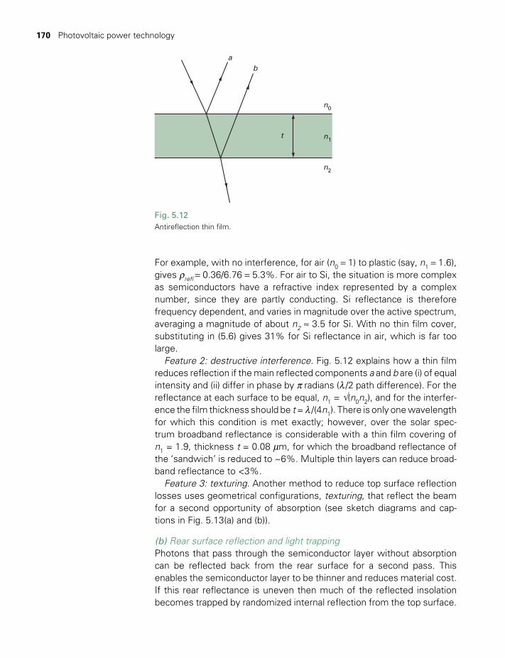
170 Photovoltaic power technology
For example, with no interference, for air (n0 = 1) to plastic (say, n1 = 1.6), gives rrefl = 0.36/6.76 = 5.3%. For air to Si, the situation is more complex as semiconductors have a refractive index represented by a complex number, since they are partly conducting. Si reflectance is therefore frequency dependent, and varies in magnitude over the active spectrum, averaging a magnitude of about n2 ≈ 3.5 for Si. With no thin film cover, substituting in (5.6) gives 31% for Si reflectance in air, which is far too large.
Feature 2: destructive interference. Fig. 5.12 explains how a thin film reduces reflection if the main reflected components a and b are (i) of equal intensity and (ii) differ in phase by p radians (l /2 path difference). For the reflectance at each surface to be equal, n1 = √(n0n2), and for the interfer-ence the film thickness should be t = l /(4n1). There is only one wavelength for which this condition is met exactly; however, over the solar spec-trum broadband reflectance is considerable with a thin film covering of n1 = 1.9, thickness t = 0.08 mm, for which the broadband reflectance of the ‘sandwich’ is reduced to ~6%. Multiple thin layers can reduce broad-band reflectance to <3%.
Feature 3: texturing. Another method to reduce top surface reflection losses uses geometrical configurations, texturing, that reflect the beam for a second opportunity of absorption (see sketch diagrams and cap-tions in Fig. 5.13(a) and (b)).
(b) Rear surface reflection and light trapping Photons that pass through the semiconductor layer without absorption can be reflected back from the rear surface for a second pass. This enables the semiconductor layer to be thinner and reduces material cost. If this rear reflectance is uneven then much of the reflected insolation becomes trapped by randomized internal reflection from the top surface.
ab
n0
n1t
n2
Fig. 5.12Antireflection thin film.
TWIDELL PAGINATION.indb 170 01/12/2014 11:36
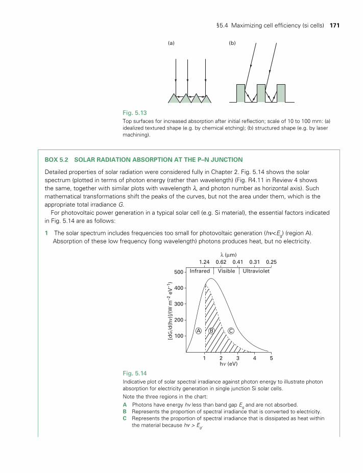
§5.4 Maximizing cell efficiency (si cells) 171
BOX 5.2 SOLAR RADIATION ABSORPTION AT THE P–N JUNCTION
Detailed properties of solar radiation were considered fully in Chapter 2. Fig. 5.14 shows the solar spectrum (plotted in terms of photon energy (rather than wavelength) (Fig. R4.11 in Review 4 shows the same, together with similar plots with wavelength l, and photon number as horizontal axis). Such mathematical transformations shift the peaks of the curves, but not the area under them, which is the appropriate total irradiance G.
For photovoltaic power generation in a typical solar cell (e.g. Si material), the essential factors indicated in Fig. 5.14 are as follows:
1 The solar spectrum includes frequencies too small for photovoltaic generation (hn<Eg) (region A). Absorption of these low frequency (long wavelength) photons produces heat, but no electricity.
λ (µm)
1 2 3 4 5
1.24
500
400
300
200
A B C100
Infrared Visible Ultraviolet
0.62 0.41 0.31 0.25
h (eV)ν
[dG
/d(h
)]/
(W m
–2 e
V–1
)ν
Fig. 5.14Indicative plot of solar spectral irradiance against photon energy to illustrate photon absorption for electricity generation in single junction Si solar cells.Note the three regions in the chart: A Photons have energy hv less than band gap Eg and are not absorbed.B Represents the proportion of spectral irradiance that is converted to electricity.C Represents the proportion of spectral irradiance that is dissipated as heat within
the material because hn > Eg.
Fig. 5.13Top surfaces for increased absorption after initial reflection; scale of 10 to 100 mm: (a) idealized textured shape (e.g. by chemical etching); (b) structured shape (e.g. by laser machining).
(a) (b)
TWIDELL PAGINATION.indb 171 01/12/2014 11:36
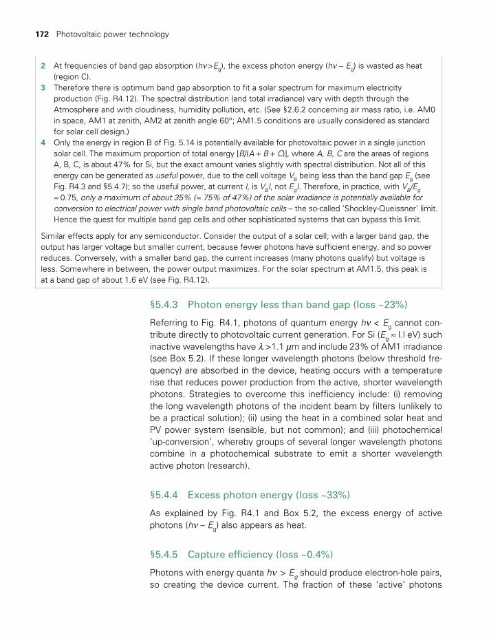
172 Photovoltaic power technology
2 At frequencies of band gap absorption (hn >Eg), the excess photon energy (hn - Eg) is wasted as heat (region C).
3 Therefore there is optimum band gap absorption to fit a solar spectrum for maximum electricity production (Fig. R4.12). The spectral distribution (and total irradiance) vary with depth through the Atmosphere and with cloudiness, humidity pollution, etc. (See §2.6.2 concerning air mass ratio, i.e. AM0 in space, AM1 at zenith, AM2 at zenith angle 60°; AM1.5 conditions are usually considered as standard for solar cell design.)
4 Only the energy in region B of Fig. 5.14 is potentially available for photovoltaic power in a single junction solar cell. The maximum proportion of total energy [B/(A + B + C)], where A, B, C are the areas of regions A, B, C, is about 47% for Si, but the exact amount varies slightly with spectral distribution. Not all of this energy can be generated as useful power, due to the cell voltage VB being less than the band gap Eg (see Fig. R4.3 and §5.4.7); so the useful power, at current I, is VBI, not EgI. Therefore, in practice, with VB/Eg ≈ 0.75, only a maximum of about 35% ( = 75% of 47%) of the solar irradiance is potentially available for conversion to electrical power with single band photovoltaic cells – the so-called ‘Shockley-Queissner’ limit. Hence the quest for multiple band gap cells and other sophisticated systems that can bypass this limit.
Similar effects apply for any semiconductor. Consider the output of a solar cell; with a larger band gap, the output has larger voltage but smaller current, because fewer photons have sufficient energy, and so power reduces. Conversely, with a smaller band gap, the current increases (many photons qualify) but voltage is less. Somewhere in between, the power output maximizes. For the solar spectrum at AM1.5, this peak is at a band gap of about 1.6 eV (see Fig. R4.12).
§5.4.3 Photon energy less than band gap (loss ~23%)
Referring to Fig. R4.1, photons of quantum energy hn < Eg cannot con-tribute directly to photovoltaic current generation. For Si (Eg ≈ l.l eV) such inactive wavelengths have l >1.1 mm and include 23% of AM1 irradiance (see Box 5.2). If these longer wavelength photons (below threshold fre-quency) are absorbed in the device, heating occurs with a temperature rise that reduces power production from the active, shorter wavelength photons. Strategies to overcome this inefficiency include: (i) removing the long wavelength photons of the incident beam by filters (unlikely to be a practical solution); (ii) using the heat in a combined solar heat and PV power system (sensible, but not common); and (iii) photochemical ‘up-conversion’, whereby groups of several longer wavelength photons combine in a photochemical substrate to emit a shorter wavelength active photon (research).
§5.4.4 Excess photon energy (loss ~33%)
As explained by Fig. R4.1 and Box 5.2, the excess energy of active photons (hn – Eg) also appears as heat.
§5.4.5 Capture efficiency (loss ~0.4%)
Photons with energy quanta hn > Eg should produce electron-hole pairs, so creating the device current. The fraction of these ‘active’ photons
TWIDELL PAGINATION.indb 172 01/12/2014 11:36
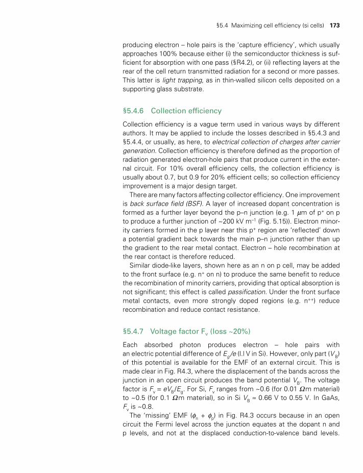
§5.4 Maximizing cell efficiency (si cells) 173
producing electron – hole pairs is the ‘capture efficiency’, which usually approaches 100% because either (i) the semiconductor thickness is suf-ficient for absorption with one pass (§R4.2), or (ii) reflecting layers at the rear of the cell return transmitted radiation for a second or more passes. This latter is light trapping, as in thin-walled silicon cells deposited on a supporting glass substrate.
§5.4.6 Collection efficiency
Collection efficiency is a vague term used in various ways by different authors. It may be applied to include the losses described in §5.4.3 and §5.4.4, or usually, as here, to electrical collection of charges after carrier generation. Collection efficiency is therefore defined as the proportion of radiation generated electron-hole pairs that produce current in the exter-nal circuit. For 10% overall efficiency cells, the collection efficiency is usually about 0.7, but 0.9 for 20% efficient cells; so collection efficiency improvement is a major design target.
There are many factors affecting collector efficiency. One improvement is back surface field (BSF). A layer of increased dopant concentration is formed as a further layer beyond the p–n junction (e.g. 1 mm of p+ on p to produce a further junction of ~200 kV m–1 (Fig. 5.15)). Electron minor-ity carriers formed in the p layer near this p+ region are ‘reflected’ down a potential gradient back towards the main p–n junction rather than up the gradient to the rear metal contact. Electron – hole recombination at the rear contact is therefore reduced.
Similar diode-like layers, shown here as an n on p cell, may be added to the front surface (e.g. n+ on n) to produce the same benefit to reduce the recombination of minority carriers, providing that optical absorption is not significant; this effect is called passification. Under the front surface metal contacts, even more strongly doped regions (e.g. n++) reduce recombination and reduce contact resistance.
§5.4.7 Voltage factor Fv (loss ~20%)
Each absorbed photon produces electron – hole pairs with an electric potential difference of Eg /e (l.l V in Si). However, only part (V B) of this potential is available for the EMF of an external circuit. This is made clear in Fig. R4.3, where the displacement of the bands across the junction in an open circuit produces the band potential VB. The voltage factor is Fv = eVB /Eg. For Si, Fv ranges from ~0.6 (for 0.01 W m material) to ~0.5 (for 0.1 W m material), so in Si VB ≈ 0.66 V to 0.55 V. In GaAs, Fv is ~0.8.
The ‘missing’ EMF (fn + fp) in Fig. R4.3 occurs because in an open circuit the Fermi level across the junction equates at the dopant n and p levels, and not at the displaced conduction-to-valence band levels.
TWIDELL PAGINATION.indb 173 01/12/2014 11:36
174 Photovoltaic power technology
Increased dopant concentration increases Fv (0.01 W m Si has greater VB and Voc than 0.1 W m Si), but other effects limit the maximum dopant concentrations in Si to ~1022 m–3 of 0.0l W m materials.
When producing current on load, the movement of carriers under forward bias produces heat as resistive internal impedance heating. This may be included as voltage factor loss, as ideality factor loss (§5.4.9) or, as here, by series resistance heating (§5.4.10).
§5.4.8 Fill factor (curve factor) Fc (intrinsic loss ~12%)
The maximum power produced by a cell is not the product IscVoc but the smaller amount Pmax at the maximum power point. This is because the I–V characteristic is strongly influenced by the p–n diode biasing charac-teristic (Fig. R4.6).
Thus as the solar cell output voltage is raised towards Voc the diode becomes increasingly forward biased, so increasing the internal recom-bination current Ir across the junction. This necessary behavior is treated as a fundamental loss in the system, measured by the fill factor:
=F P I V/ ( )sc ocmax (5.7)
The maximum value of F in Si is 0.88.
§5.4.9 Ideality factor A (loss ~5%)
In practice the cell characteristic does not exactly follow equation (R4.23), derived from diode properties, and is better represented by (R4.2.4):
= --I I I eV AkT[exp( / ) 1]0L (5.8)
where here IL, and therefore I, is considered positive for the PV cell. The ideality factor A (>2 for many commercial cells) allows for the
Front grid
e–
h+n p p+
h+
e–
e–
Metal contact
Fig. 5.15Energy levels in a cell with ‘back surface field’ (BSF) indicated as p+ at the rear metal contact. This extra layer lessens diffusion leakage of electron current carriers at the rear of cells, shown here as an ‘n on p’ cell.
TWIDELL PAGINATION.indb 174 01/12/2014 11:36

§5.4 Maximizing cell efficiency (si cells) 175
electron-hole recombination loss in the junction. This effect also tends to change Voc and 10, so in general optimum output would only occur if A = 1.
Unwanted electron-hole recombination has already been mentioned for back surface field (§5.4.6). Within the cell, recombination is lessened if:
1 Diffusion paths are long (in Si from ~50 to ~100 mm). This requires long minority carrier lifetimes (in Si up to 100 ms).
2 The junction is near the top surface (within 0.15 mm, rather than 0.35 mm as in normal Si cells).
3 The material has few defects other than the dopant.
Surface recombination effects are influential owing to defects and imper-fections introduced at crystal slicing or at material deposition.
§5.4.10 Series resistance (loss ~0.3%)
The solar cell current passes through the bulk material to front and rear contacts. The rear contact area can cover the whole cell and its con-tribution to series ‘ohmic’ resistance is very small. However, the top surface should be exposed to the maximum amount of light with the top contact area minimized, thus causing relatively long current path lengths with significant series resistance. Improvements have been made to the front contacts (e.g. by having narrow laser-cut channels within which contacts may be formed), and by arranging the contact layout to minimize resistance to ~0.1 W in a cell resistance of ~20 W at peak power.
§5.4.11 Shunt resistance (negligible loss ~0.1%)
Shunt resistance in parallel with the bulk resistance is caused by struc-tural defects across the surface and at the edge of the cell. Improved technology has reduced these to a negligible effect, so shunt resistance may be considered infinite in single-crystal Si cells. This may not be so in polycrystalline cells, however.
§5.4.12 Delivered power
For ‘high-efficiency’ crystalline Si cells, after the losses listed in the above sections, Table 5.1 estimates the percentage power as 25% of the incident insolation. This assumes optimum load matching at full insolation, without overheating, to produce peak power on the I–V char-acteristic. Note that the losses relating to the intrinsic mismatch of solar radiation with the single band gap set a theoretical limit for the efficiency of even a ‘perfect’ Si cell of about - × - ≈(100 33)% (100 23)% 50%. Therefore, one obvious way to increase efficiency is to have multilayer
TWIDELL PAGINATION.indb 175 01/12/2014 11:36

176 Photovoltaic power technology
cells, with each layer matched to a different region of the solar spec-trum, as in §5.6.2.
§5.5 SOLAR CELL AND MODULE MANUFACTURE
The majority of solar cells manufactured worldwide is with silicon cells, so we first outline the construction of standard single-crystal Si cells and their fabrication into modules. There are many variations, and commer-cial competition produces the continued improvement of cell type and of manufacturing methods. A general design of Si cells is shown in Fig. 5.11, with schematics of module and array assemblies shown in Fig. 5.6.
§5.5.1 General design criteria
1 Initial materials must be of excellent chemical purity with consistent properties.
2 The cell design should improve the efficiency of electricity generation.3 Cells are mass produced with minimum cost; so in practice they
must be thinner (less material) and of larger area (fewer connections and less empty module area), with rapid manufacturing speed (more manu facture per unit of labor and overheads) using ‘robotic’ control of the processes and excellent precision (high-efficiency cells), i.e. thinner, larger, faster, cheaper.
4 Tested and graded cells are interconnected and then encapsulated as modules.
5 The design must allow for some faults to occur without failure of the complete system. Thus redundant electrical contacts are useful and modules may be connected in parallel strings so that if one string fails, there is still generation.
6 Modules are usually guaranteed for at least 20 years. The design caters for the potential damage from transportation and on-site build-ing construction, and from exposure in hostile environments with sig-nificant changes of temperature (even without solar concentration, the cell temperature may range between –30 and +100°C). Electrical contacts must survive and all forms of corrosion avoided, in particular water must not enter the module.
Box 5.3 gives a more detailed outline of the production process.
BOX 5.3 MANUFACTURE OF SILICON CRYSTALLINE CELLS AND MODULES
Step 1: Raw materials to polycrystalline ingots
‘Pure’ SiO2 sand is reduced to metallurgical grade Si (~98.5% purity, i.e. <1.5% impurity) in coke (carbon) furnaces, and then purified further into either expensive electronic-grade Si (<10-7% impurity) or cheaper solar-grade Si (<10-3% impurity). Waste electronic-grade Si is used for PV manufacture, but limited
TWIDELL PAGINATION.indb 176 01/12/2014 11:36
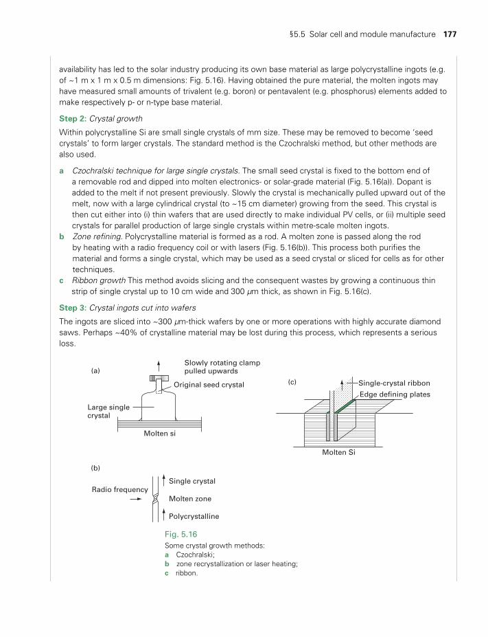
§5.5 Solar cell and module manufacture 177
availability has led to the solar industry producing its own base material as large polycrystalline ingots (e.g. of ~1 m x 1 m x 0.5 m dimensions: Fig. 5.16). Having obtained the pure material, the molten ingots may have measured small amounts of trivalent (e.g. boron) or pentavalent (e.g. phosphorus) elements added to make respectively p- or n-type base material.
Step 2: Crystal growth
Within polycrystalline Si are small single crystals of mm size. These may be removed to become ‘seed crystals’ to form larger crystals. The standard method is the Czochralski method, but other methods are also used.
a Czochralski technique for large single crystals. The small seed crystal is fixed to the bottom end of a removable rod and dipped into molten electronics- or solar-grade material (Fig. 5.16(a)). Dopant is added to the melt if not present previously. Slowly the crystal is mechanically pulled upward out of the melt, now with a large cylindrical crystal (to ~15 cm diameter) growing from the seed. This crystal is then cut either into (i) thin wafers that are used directly to make individual PV cells, or (ii) multiple seed crystals for parallel production of large single crystals within metre-scale molten ingots.
b Zone refining. Polycrystalline material is formed as a rod. A molten zone is passed along the rod by heating with a radio frequency coil or with lasers (Fig. 5.16(b)). This process both purifies the material and forms a single crystal, which may be used as a seed crystal or sliced for cells as for other techniques.
c Ribbon growth This method avoids slicing and the consequent wastes by growing a continuous thin strip of single crystal up to 10 cm wide and 300 μm thick, as shown in Fig. 5.16(c).
Step 3: Crystal ingots cut into wafers
The ingots are sliced into ~300 μm-thick wafers by one or more operations with highly accurate diamond saws. Perhaps ~40% of crystalline material may be lost during this process, which represents a serious loss.
Molten Si
Molten si
Single crystal
Polycrystalline
Molten zoneRadio frequency
Large singlecrystal
Slowly rotating clamppulled upwards
Original seed crystal Single-crystal ribbon
Edge defining plates
(a)
(c)
(b)
Fig. 5.16Some crystal growth methods: a Czochralski; b zone recrystallization or laser heating; c ribbon.
TWIDELL PAGINATION.indb 177 01/12/2014 11:36
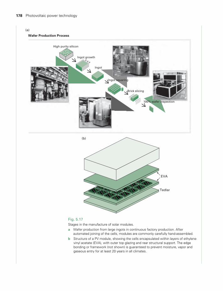
178 Photovoltaic power technology
Tedlar
EVA
(b)
High purity silicon
(a)
Wafer Production Process
Ingot growth
Ingot
Brick slicing
Ingot squaring
100% wafer inspection
Fig. 5.17Stages in the manufacture of solar modules.a Wafer production from large ingots in continuous factory production. After
automated joining of the cells, modules are commonly carefully hand-assembled. b Structure of a PV module, showing the cells encapsulated within layers of ethylene
vinyl acetate (EVA), with outer top glazing and rear structural support. The edge bonding or framework (not shown) is guaranteed to prevent moisture, vapor and gaseous entry for at least 20 years in all climates.
TWIDELL PAGINATION.indb 178 01/12/2014 11:36
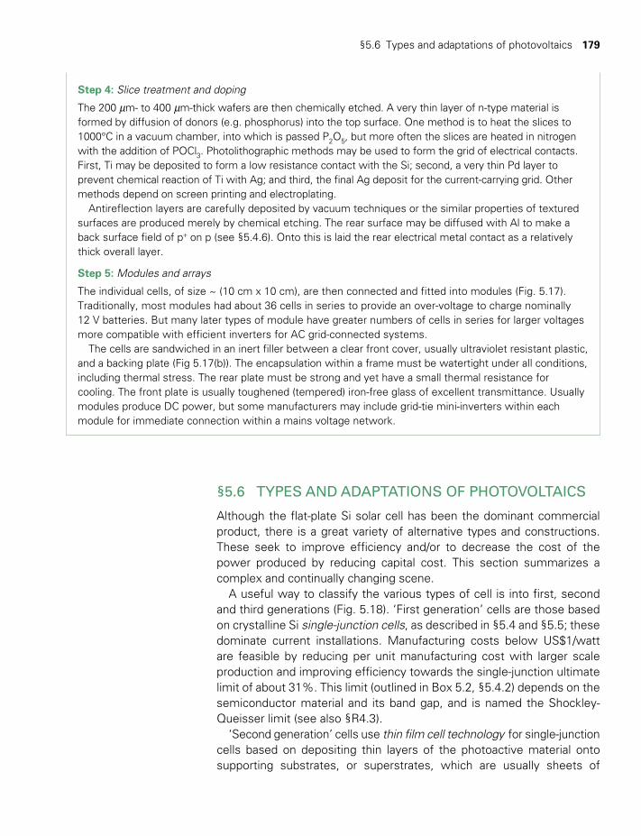
§5.6 Types and adaptations of photovoltaics 179
§5.6 TYPES AND ADAPTATIONS OF PHOTOVOLTAICS
Although the flat-plate Si solar cell has been the dominant commercial product, there is a great variety of alternative types and constructions. These seek to improve efficiency and/or to decrease the cost of the power produced by reducing capital cost. This section summarizes a complex and continually changing scene.
A useful way to classify the various types of cell is into first, second and third generations (Fig. 5.18). ‘First generation’ cells are those based on crystalline Si single-junction cells, as described in §5.4 and §5.5; these dominate current installations. Manufacturing costs below US$1/watt are feasible by reducing per unit manufacturing cost with larger scale production and improving efficiency towards the single-junction ultimate limit of about 31%. This limit (outlined in Box 5.2, §5.4.2) depends on the semiconductor material and its band gap, and is named the Shockley-Queisser limit (see also §R4.3).
‘Second generation’ cells use thin film cell technology for single-junction cells based on depositing thin layers of the photoactive material onto supporting substrates, or superstrates, which are usually sheets of
Step 4: Slice treatment and doping
The 200 mm- to 400 mm-thick wafers are then chemically etched. A very thin layer of n-type material is formed by diffusion of donors (e.g. phosphorus) into the top surface. One method is to heat the slices to 1000°C in a vacuum chamber, into which is passed P2O5, but more often the slices are heated in nitrogen with the addition of POCl3. Photolithographic methods may be used to form the grid of electrical contacts. First, Ti may be deposited to form a low resistance contact with the Si; second, a very thin Pd layer to prevent chemical reaction of Ti with Ag; and third, the final Ag deposit for the current-carrying grid. Other methods depend on screen printing and electroplating.
Antireflection layers are carefully deposited by vacuum techniques or the similar properties of textured surfaces are produced merely by chemical etching. The rear surface may be diffused with Al to make a back surface field of p+ on p (see §5.4.6). Onto this is laid the rear electrical metal contact as a relatively thick overall layer.
Step 5: Modules and arrays
The individual cells, of size ~ (10 cm x 10 cm), are then connected and fitted into modules (Fig. 5.17). Traditionally, most modules had about 36 cells in series to provide an over-voltage to charge nominally 12 V batteries. But many later types of module have greater numbers of cells in series for larger voltages more compatible with efficient inverters for AC grid-connected systems.
The cells are sandwiched in an inert filler between a clear front cover, usually ultraviolet resistant plastic, and a backing plate (Fig 5.17(b)). The encapsulation within a frame must be watertight under all conditions, including thermal stress. The rear plate must be strong and yet have a small thermal resistance for cooling. The front plate is usually toughened (tempered) iron-free glass of excellent transmittance. Usually modules produce DC power, but some manufacturers may include grid-tie mini-inverters within each module for immediate connection within a mains voltage network.
TWIDELL PAGINATION.indb 179 01/12/2014 11:36
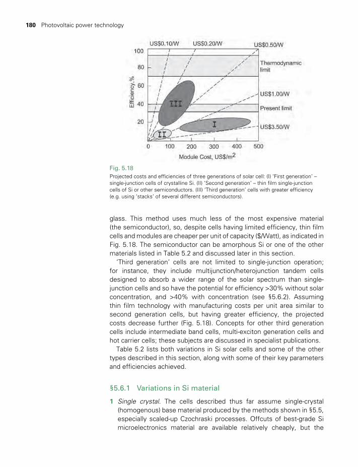
180 Photovoltaic power technology
glass. This method uses much less of the most expensive material (the semiconductor), so, despite cells having limited efficiency, thin film cells and modules are cheaper per unit of capacity ($/Watt), as indicated in Fig. 5.18. The semiconductor can be amorphous Si or one of the other materials listed in Table 5.2 and discussed later in this section.
‘Third generation’ cells are not limited to single-junction operation; for instance, they include multijunction/heterojunction tandem cells designed to absorb a wider range of the solar spectrum than single-junction cells and so have the potential for efficiency >30% without solar concentration, and >40% with concentration (see §5.6.2). Assuming thin film technology with manufacturing costs per unit area similar to second generation cells, but having greater efficiency, the projected costs decrease further (Fig. 5.18). Concepts for other third generation cells include intermediate band cells, multi-exciton generation cells and hot carrier cells; these subjects are discussed in specialist publications.
Table 5.2 lists both variations in Si solar cells and some of the other types described in this section, along with some of their key parameters and efficiencies achieved.
§5.6.1 Variations in Si material
1 Single crystal. The cells described thus far assume single-crystal (homogenous) base material produced by the methods shown in §5.5, especially scaled-up Czochraski processes. Offcuts of best-grade Si microelectronics material are available relatively cheaply, but the
Fig. 5.18Projected costs and efficiencies of three generations of solar cell: (I) ‘First generation’ – single-junction cells of crystalline Si. (II) ‘Second generation’ – thin film single-junction cells of Si or other semiconductors. (III) ‘Third generation’ cells with greater efficiency (e.g. using ‘stacks’ of several different semiconductors).
TWIDELL PAGINATION.indb 180 01/12/2014 11:36
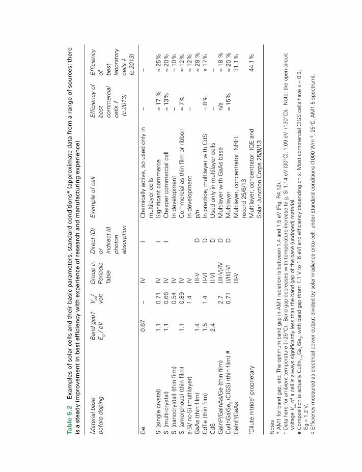
Tab
le 5
.2
Exa
mp
les
of
sola
r ce
lls a
nd
th
eir
bas
ic p
aram
eter
s, s
tan
dar
d c
on
dit
ion
s* (
app
roxi
mat
e d
ata
fro
m a
ran
ge
of
sou
rces
; th
ere
is a
ste
ady
imp
rove
men
t in
bes
t ef
fici
ency
wit
h e
xper
ien
ce o
f re
sear
ch a
nd
man
ufa
ctu
rin
g e
xper
ien
ce)
Mat
eria
l bas
ebe
fore
dop
ing
Ban
d ga
p†E
g / e
V
V oc/
volt
Gro
up in
P
erio
dic
Tabl
e
Dire
ct (D
)or In
dire
ct (I
)ph
oton
ab
sorp
tion
Exa
mpl
e of
cel
lE
ffic
ienc
y of
be
st
com
mer
cial
ce
lls ‡
(c.2
013)
Eff
icie
ncy
of
best
labo
rato
ryce
lls ‡
(c.2
013)
Ge
0.67
-IV
IC
hem
ical
ly a
ctiv
e, s
o us
ed o
nly
in
mul
tilay
er c
ells
--
Si (
sing
le c
ryst
al)
1.1
0.71
IVI
Sig
nific
ant
com
mer
ce≈
17 %
≈ 25
%S
i (m
ulti-
crys
tal)
1.1
0.66
IVI
Che
aper
com
mer
cial
cel
l≈
13%
≈ 20
%S
i (na
nocr
ysta
l) (t
hin
film
)0.
54IV
In d
evel
opm
ent
-≈
10%
Si (
amor
phou
s) (t
hin
film
)1.
10.
89IV
Com
mer
cial
as
thin
film
or
ribbo
n≈
7%≈
12%
a-S
i/ nc
-Si (
mul
tilay
er)
1.4
IVIn
dev
elop
men
t-
≈ 12
%G
aAs
(thi
n fil
m)
1.4
III-V
Dp/
n≈
28 %
CdT
e (t
hin
film
)1.
51.
4II-
VI
DIn
pra
ctic
e, m
ultil
ayer
with
CdS
≈ 8%
» 17
%C
dS2.
4II-
VI
DU
sed
only
in m
ultil
ayer
cel
ls-
-G
aInP
/GaI
nAs/
Ge
(thi
n fil
m)
2.7
(III-V
)/IV
DM
ultil
ayer
with
GaA
s ba
sen/
a≈
18 %
Cu(
InG
a)S
e 2 (C
IGS
) (th
in f
ilm) #
0.71
(I/III
)-VI
DM
ultil
ayer
≈
15%
≈ 20
%G
aInP
/GaA
sIII
-VM
ultil
ayer
, con
cent
rato
r. N
RE
L re
cord
25/
6/13
31.1
%
‘Dilu
te n
itrid
e’ p
ropr
ieta
ryM
ultil
ayer
, con
cent
rato
r: IQ
E a
nd
Sol
ar J
unct
ion
Cor
ps 2
5/8/
1344
.1%
Not
es*
AM
1 fo
r ba
nd g
ap, e
tc. T
he o
ptim
um b
and
gap
in A
M1
radi
atio
n is
bet
wee
n 1.
4 an
d 1.
5 eV
(Fig
. R4.
12).
† D
ata
here
for
am
bien
t te
mpe
ratu
re (~
25°C
). B
and
gap
decr
ease
s w
ith t
empe
ratu
re in
crea
se (e
.g. S
i 1.1
4 eV
(30°
C),
1.09
eV
(13
0°C
)). N
ote:
the
ope
n-ci
rcui
t vo
ltage
Voc
of
a ce
ll is
alw
ays
sign
ifica
ntly
less
tha
n th
e ba
nd g
ap o
f th
e ba
se (u
ndop
ed) m
ater
ial.
# C
ompo
sitio
n is
act
ually
Cu(
In1–
xGa x)S
e 2, w
ith b
and
gap
(fro
m 1
.1 V
to
1.6
eV) a
nd e
ffic
ienc
y de
pend
ing
on x
. Mos
t co
mm
erci
al C
IGS
cel
ls h
ave
x ≈
0.3,
E
g ≈
1.2
V.
‡ E
ffic
ienc
y m
easu
red
as e
lect
rical
pow
er o
utpu
t di
vide
d by
sol
ar ir
radi
ance
ont
o ce
ll, u
nder
sta
ndar
d co
nditi
ons
(100
0 W
m-2
, 25°
C, A
M1.
5 sp
ectr
um).
TWIDELL PAGINATION.indb 181 01/12/2014 11:36

182 Photovoltaic power technology
quantities are insufficient for the modern PV industry, which increas-ingly produces its own base material. The latter need to be less pure than for microelectronics and may be cut from metre-scale ingots with multi-seeded segments from which both single and polycrystalline wafers may be obtained.
2 Mixed crystalline (irregular juxtaposition of single-crystal ‘grains’ within a solid). The PV industry uses a range of Si material, described by increasing crystal grain size as: microcrystalline <~1 mm, polycrys-talline <~1 mm, multicrystalline <~3 cm, and single crystal of one large grain. However, commonly the word ‘polycrystalline’ includes all forms other than single crystalline. Such polycrystalline material is cheaper and easier to obtain than single crystals and is not necessarily structurally weak. However, photovoltaic currents are reduced when electron-hole pairs recombine internally at the grain boundaries, so reducing overall efficiency. By having the typical grain size dimension at least equal to the thickness of cell, it becomes unlikely that the current crosses a grain boundary, so there is little loss of efficiency. Therefore thinner cells are cheaper by having less material and may be designed for improved efficiency.
Note that controlled crystal growth at micron (mm) scale is an aspect of nanotechnology, so such microcrystalline cells may be called nanocrystalline.
3 Amorphous. Amorphous materials are solids with short-range order of only a relatively few atoms and therefore are not crystalline (e.g. solid glass). Amorphous silicon (α-Si) can be produced by thin film deposi-tion with Si vapor deposition techniques and retains its basic tetra-hedral semiconductor properties; in particular n- and p-type dopants allow photovoltaic junctions to be formed as in crystalline material. However, the amorphous structure produces a very large proportion of unattached ‘dangling’ chemical bonds that trap electron and hole current carriers, thereby drastically reducing photovoltaic efficiency. To counteract this, the amorphous material is initially formed in an atmosphere of silane (SiH4 ) so that hydrogen atoms bond chemically at the previously unattached sites, thus greatly reducing the number of electron-hole traps. Amorphous Si is used in thin film solar cells of low cost with total thickness of semiconductor about 1 μm (i.e. ~1/100 of the thickness of a conventional single-crystal cell). The band gap of α-Si is 1.7 eV, as compared with crystalline Si of 1.1 eV, which is a better fit to the solar spectrum (see Fig. R4.12). Development with multiple junctions within that 1 μm has increased efficiency to about 10%. A practical difficulty may be reduced efficiency with age, especially in the first few years of operation. An advantage is that the output of α-Si cells does not change significantly with an increase of temperature.
TWIDELL PAGINATION.indb 182 01/12/2014 11:36
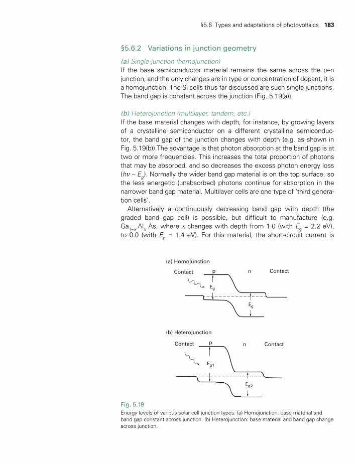
§5.6 Types and adaptations of photovoltaics 183
§5.6.2 Variations in junction geometry
(a) Single-junction (homojunction) If the base semiconductor material remains the same across the p–n junction, and the only changes are in type or concentration of dopant, it is a homojunction. The Si cells thus far discussed are such single junctions. The band gap is constant across the junction (Fig. 5.19(a)).
(b) Heterojunction (multilayer, tandem, etc.) If the base material changes with depth, for instance, by growing layers of a crystalline semiconductor on a different crystalline semiconduc-tor, the band gap of the junction changes with depth (e.g. as shown in Fig. 5.19(b)).The advantage is that photon absorption at the band gap is at two or more frequencies. This increases the total proportion of photons that may be absorbed, and so decreases the excess photon energy loss (hn – Eg ). Normally the wider band gap material is on the top surface, so the less energetic (unabsorbed) photons continue for absorption in the narrower band gap material. Multilayer cells are one type of ‘third genera-tion cells’.
Alternatively a continuously decreasing band gap with depth (the graded band gap cell) is possible, but difficult to manufacture (e.g. Ga1– x Alx As, where x changes with depth from 1.0 (with Eg = 2.2 eV), to 0.0 (with Eg = 1.4 eV). For this material, the short-circuit current is
Fig. 5.19Energy levels of various solar cell junction types: (a) Homojunction: base material and band gap constant across junction. (b) Heterojunction: base material and band gap change across junction.
(a) Homojunction
(b) Heterojunction
p
p
n Contact
n Contact
Contact
Contact
Eg
Eg1
Eg2
Eg
TWIDELL PAGINATION.indb 183 01/12/2014 11:36
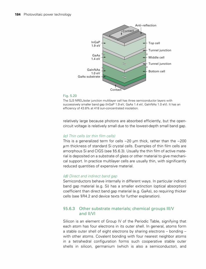
184 Photovoltaic power technology
relatively large because photons are absorbed efficiently, but the open-circuit voltage is relatively small due to the lowest-depth small band gap.
(c) Thin cells (or thin film cells) This is a generalized term for cells ~20 µm thick, rather than the ~200 m m thickness of standard Si crystal cells. Examples of thin film cells are amorphous Si and CIGS (see §5.6.3). Usually the thin film of active mate-rial is deposited on a substrate of glass or other material to give mechani-cal support. In practice multilayer cells are usually thin, with significantly reduced quantities of expensive material.
(d) Direct and indirect band gap Semiconductors behave internally in different ways. In particular indirect band gap material (e.g. Si) has a smaller extinction (optical absorption) coefficient than direct band gap material (e.g. GaAs), so requiring thicker cells (see §R4.2 and device texts for further explanation).
§5.6.3 Other substrate materials; chemical groups III/V and II/VI
Silicon is an element of Group IV of the Periodic Table, signifying that each atom has four electrons in its outer shell. In general, atoms form a stable outer shell of eight electrons by sharing electrons – bonding – with other atoms. Covalent bonding with four nearest neighbor atoms in a tetrahedral configuration forms such cooperative stable outer shells in silicon, germanium (which is also a semiconductor), and
Fig. 5.20The SJ3 NREL/solar junction multilayer cell has three semiconductor layers with successively smaller band gap (InGaP 1.9 eV, GaAs 1.4 eV, GaInNAs 1.0 eV). It has an efficiency of 43.8% at 418 sun-concentrated insolation.
Top cell
Contact
Anti–reflection
Tunnel junction
Tunnel junction
Middle cell
Bottom cell
InGaP1.9 eV
GaAs1.4 eV
GalnNAs1.0 eV
GaAs substrate
Contact
TWIDELL PAGINATION.indb 184 01/12/2014 11:36
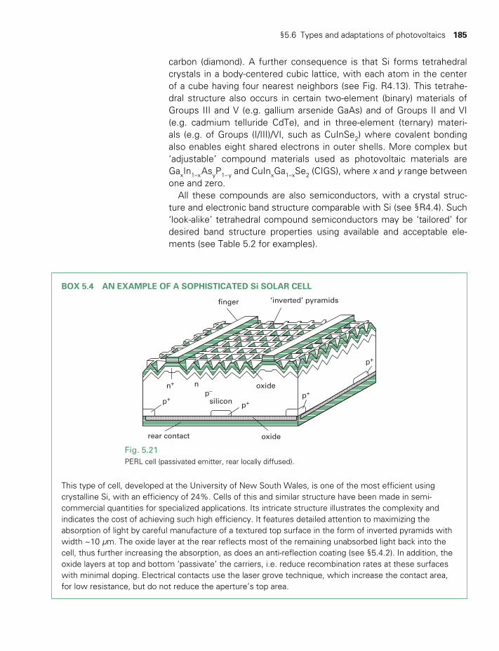
§5.6 Types and adaptations of photovoltaics 185
carbon (diamond). A further consequence is that Si forms tetrahedral crystals in a body-centered cubic lattice, with each atom in the center of a cube having four nearest neighbors (see Fig. R4.13). This tetrahe-dral structure also occurs in certain two-element (binary) materials of Groups III and V (e.g. gallium arsenide GaAs) and of Groups II and VI (e.g. cadmium telluride CdTe), and in three-element (ternary) materi-als (e.g. of Groups (I/III)/VI, such as CuInSe2) where covalent bonding also enables eight shared electrons in outer shells. More complex but ‘adjustable’ compound materials used as photovoltaic materials are GaxIn1–x AsyP1– y and CuInxGa1–xSe2 (CIGS), where x and y range between one and zero.
All these compounds are also semiconductors, with a crystal struc-ture and electronic band structure comparable with Si (see §R4.4). Such ‘look-alike’ tetrahedral compound semiconductors may be ‘tailored’ for desired band structure properties using available and acceptable ele-ments (see Table 5.2 for examples).
BOX 5.4 AN EXAMPLE OF A SOPHISTICATED Si SOLAR CELL
Fig. 5.21PERL cell (passivated emitter, rear locally diffused).
finger
oxide
silicon
rear contact oxide
p+p+p–
n+ n
‘inverted’ pyramids
p+
p+
This type of cell, developed at the University of New South Wales, is one of the most efficient using crystalline Si, with an efficiency of 24%. Cells of this and similar structure have been made in semi-commercial quantities for specialized applications. Its intricate structure illustrates the complexity and indicates the cost of achieving such high efficiency. It features detailed attention to maximizing the absorption of light by careful manufacture of a textured top surface in the form of inverted pyramids with width ~10 μm. The oxide layer at the rear reflects most of the remaining unabsorbed light back into the cell, thus further increasing the absorption, as does an anti-reflection coating (see §5.4.2). In addition, the oxide layers at top and bottom ‘passivate’ the carriers, i.e. reduce recombination rates at these surfaces with minimal doping. Electrical contacts use the laser grove technique, which increase the contact area, for low resistance, but do not reduce the aperture’s top area.
TWIDELL PAGINATION.indb 185 01/12/2014 11:36

186 Photovoltaic power technology
§5.6.4 Other semiconductor mechanisms, classifications and terminologies
So far we have considered PV generation from semiconductors with tetrahedral structure (e.g. Si and GaAs), because these are the most common PV materials. However, there are other systems and configura-tions. Examples are as follows.
(a) ‘PV thermal’ collectors This name is used for constructions that combine PV electricity gen-eration with heat production (e.g. hot water). The supposed advantages include: (i) the PV efficiency is increased if the PV material is cooled; (ii) better use is made of the collection area; and (iii) construction and instal-lation costs are less than for equivalent separated systems. However, despite these advantages, mixed systems of this sort are unusual. In practice, the well-established KISS principle operates (‘keep it simple stupid’).
(b) Organic photovoltaics (OPV)s It is common for light to be absorbed in certain organic compounds so producing separated electrons and holes as excited states of the molecu-lar structure, but paired close enough to form a bound state as ‘exci-tons’. The molecular structure often has a dimension of a relatively few repeated molecules, i.e. of an oligomer as opposed to a polymer. Such processes and oligomers are the basis of photosynthesis (Chapter 9). The essence of an OPV device is to allow the electron and hole of the exciton to be separated and pass to an external circuit. This requires two layers of different conducting materials that have an intrinsic electric field between them, i.e. a voltage. An early example is a layer of indium tin oxide and a layer of low work-function metal (e.g. Al), with organic material between these layers (e.g. the macromolecular dye compound phthalocyanine). The extensive knowledge of organic chemistry and the possible cheap-ness of organic materials make developments in this area of great inter-est. Efficiencies of 10% have been achieved (Green et al. 2012).
(c) Quantum-dot devices Quantum dots are semiconductor nanocrystals (e.g. Si, of diameter about 5 mm (5 x 10⁻⁶ m). Absorbed solar photons create one or more electron – hole pairs (‘excitons’) in the nanocrystal that are ‘quantum confined’ and only able to recombine with the emission of photons of wavelength defined by the nanocrystal dimension. Hence quantum dots of the same size all luminesce at the same frequency. Luminescence occurs when solar photons are absorbed, leading to the emission of one or more photons with less quantized energy at longer wavelength. By contain-ing the luminescent material in a thin glass ‘tank’, most of the emitted
TWIDELL PAGINATION.indb 186 01/12/2014 11:36
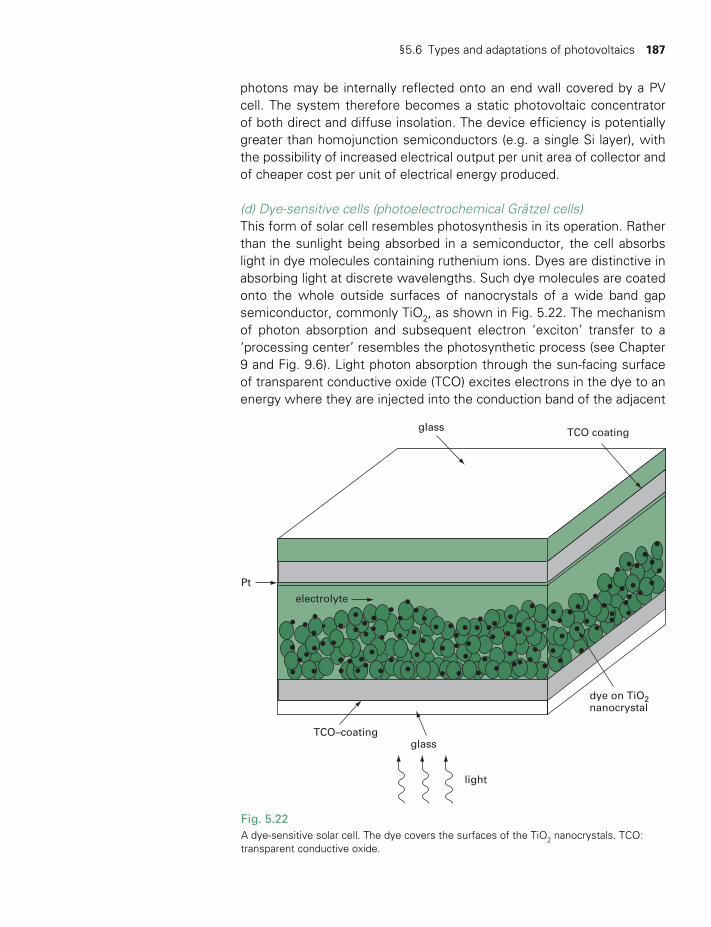
§5.6 Types and adaptations of photovoltaics 187
photons may be internally reflected onto an end wall covered by a PV cell. The system therefore becomes a static photovoltaic concentrator of both direct and diffuse insolation. The device efficiency is potentially greater than homojunction semiconductors (e.g. a single Si layer), with the possibility of increased electrical output per unit area of collector and of cheaper cost per unit of electrical energy produced.
(d) Dye-sensitive cells (photoelectrochemical Grätzel cells) This form of solar cell resembles photosynthesis in its operation. Rather than the sunlight being absorbed in a semiconductor, the cell absorbs light in dye molecules containing ruthenium ions. Dyes are distinctive in absorbing light at discrete wavelengths. Such dye molecules are coated onto the whole outside surfaces of nanocrystals of a wide band gap semiconductor, commonly TiO2, as shown in Fig. 5.22. The mechanism of photon absorption and subsequent electron ‘exciton’ transfer to a ‘processing center’ resembles the photosynthetic process (see Chapter 9 and Fig. 9.6). Light photon absorption through the sun-facing surface of transparent conductive oxide (TCO) excites electrons in the dye to an energy where they are injected into the conduction band of the adjacent
Fig. 5.22A dye-sensitive solar cell. The dye covers the surfaces of the TiO2 nanocrystals. TCO: transparent conductive oxide.
electrolyte
glass
glass
light
Pt
TCO–coating
TCO coating
dye on TiO2nanocrystal
TWIDELL PAGINATION.indb 187 01/12/2014 11:36
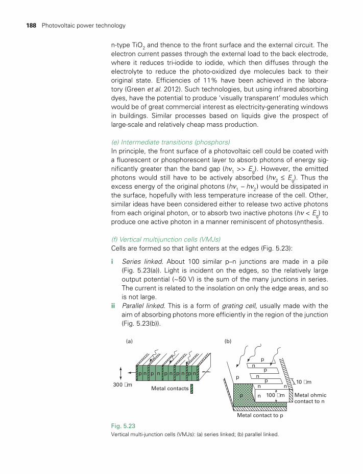
188 Photovoltaic power technology
n-type TiO2 and thence to the front surface and the external circuit. The electron current passes through the external load to the back electrode, where it reduces tri-iodide to iodide, which then diffuses through the electrolyte to reduce the photo-oxidized dye molecules back to their original state. Efficiencies of 11% have been achieved in the labora-tory (Green et al. 2012). Such technologies, but using infrared absorbing dyes, have the potential to produce ‘visually transparent’ modules which would be of great commercial interest as electricity-generating windows in buildings. Similar processes based on liquids give the prospect of large-scale and relatively cheap mass production.
(e) Intermediate transitions (phosphors) In principle, the front surface of a photovoltaic cell could be coated with a fluorescent or phosphorescent layer to absorb photons of energy sig-nificantly greater than the band gap (hn1 >> Eg). However, the emitted photons would still have to be actively absorbed (hn2 ≤ Eg). Thus the excess energy of the original photons (hn1 - hn2 ) would be dissipated in the surface, hopefully with less temperature increase of the cell. Other, similar ideas have been considered either to release two active photons from each original photon, or to absorb two inactive photons (hn < Eg) to produce one active photon in a manner reminiscent of photosynthesis.
(f) Vertical multijunction cells (VMJs)Cells are formed so that light enters at the edges (Fig. 5.23):
i Series linked. About 100 similar p–n junctions are made in a pile (Fig. 5.23(a)). Light is incident on the edges, so the relatively large output potential (~50 V) is the sum of the many junctions in series. The current is related to the insolation on only the edge areas, and so is not large.
ii Parallel linked. This is a form of grating cell, usually made with the aim of absorbing photons more efficiently in the region of the junction (Fig. 5.23(b)).
Fig. 5.23Vertical multi-junction cells (VMJs): (a) series linked; (b) parallel linked.
Metal contacts
Metal contact to p
(a) (b)
p p p p pp
p
n n n n nn
p
p
pn
n n
n Metal ohmiccontact to n
100 µm
10 µm300 µm
TWIDELL PAGINATION.indb 188 01/12/2014 11:36
§5.6 Types and adaptations of photovoltaics 189
(g) Thermo-photovoltaics These devices produce electricity after the absorption of longwave infra-red radiation as from sources at, say, about 1000°C. Small band gap semiconductors are used (e.g. GaSb with 0.7 eV band gap), which are mostly under laboratory development. Possible uses include generating electricity from otherwise waste heat (e.g. at metal foundries). Another option is to concentrate solar radiation onto a black absorbing surface, which then re-radiates to a thermo-photovoltaic device. Effectively the peak frequency of the concentrated solar radiation is shifted into the infrared to obtain a better match with a small band gap photovoltaic cell.
(h) Nanotechnology As with solid-state electronic devices, PV processes depend on atomic and molecular scale processes, at a corresponding scale of about 1 to 100 nanometers (10-9 to 10-7 m) . Materials can be ‘seen’ at this scale by electron microscopes; in particular surfaces and surface layers can be investigated at atomic scale using a range of scanning electron micro-scopes. Such tools have facilitated very precise ‘engineering’ of PV devices (e.g. deposition of semiconductor layers and contacts at near atomic scale as anti-reflection surface layers). Manufacturing processes at such precision can be operated for accurate replicated production of millions of products (i.e. large-scale manufacture of nano-scale devices).
(i) Water splitting for hydrogen and oxygen production Active research in photoelectrochemistry seeks to use solar irradiation to produce commercial hydrogen from direct ‘water-splitting’ processes. An example is a joint nanoscale structure of hematite (Fe2O3) with a dye-sensitive photovoltaic layer attached (a ‘hematite photoelectrode’), which in effect produces sufficient voltage to electrolyze water within the ‘tandem’ structure.
§5.6.5 Variation in system arrangement
(a) Concentrators (see Fig. 5.24 and §4.8) The benefits of concentrating solar radiation onto photovoltaic cells are: (i) fewer cells are needed, hence reducing costs per unit of power gen-erated; (ii) hence the cells that are used can be the best available (likely to be multilayer cells with perhaps 40% efficiency); (iii) less site area is needed; (iv) total frameworks and construction costs may reduce. Disadvantages are: (i) long periods of clear sky are essential; (ii) to follow the Sun, the concentrator is expensive and requires maintenance; (iii) cell efficiency is reduced at increased temperature, so active or passive cooling is needed (however, the heat removed in active cooling may be useful).
TWIDELL PAGINATION.indb 189 01/12/2014 11:36
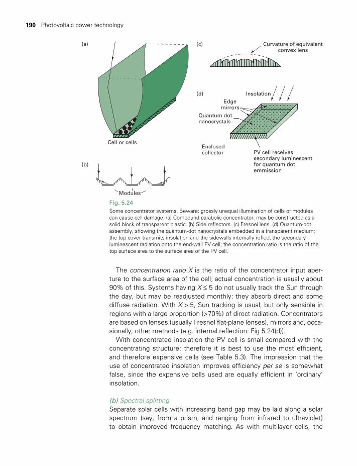
190 Photovoltaic power technology
The concentration ratio X is the ratio of the concentrator input aper-ture to the surface area of the cell; actual concentration is usually about 90% of this. Systems having X ≤ 5 do not usually track the Sun through the day, but may be readjusted monthly; they absorb direct and some diffuse radiation. With X > 5, Sun tracking is usual, but only sensible in regions with a large proportion (>70%) of direct radiation. Concentrators are based on lenses (usually Fresnel flat-plane lenses), mirrors and, occa-sionally, other methods (e.g. internal reflection: Fig 5.24(d)).
With concentrated insolation the PV cell is small compared with the concentrating structure; therefore it is best to use the most efficient, and therefore expensive cells (see Table 5.3). The impression that the use of concentrated insolation improves efficiency per se is somewhat false, since the expensive cells used are equally efficient in ‘ordinary’ insolation.
(b) Spectral splitting Separate solar cells with increasing band gap may be laid along a solar spectrum (say, from a prism, and ranging from infrared to ultraviolet) to obtain improved frequency matching. As with multilayer cells, the
Fig. 5.24Some concentrator systems. Beware: grossly unequal illumination of cells or modules can cause cell damage: (a) Compound parabolic concentrator: may be constructed as a solid block of transparent plastic. (b) Side reflectors. (c) Fresnel lens. (d) Quantum-dot assembly, showing the quantum-dot nanocrystals embedded in a transparent medium; the top cover transmits insolation and the sidewalls internally reflect the secondary luminescent radiation onto the end-wall PV cell; the concentration ratio is the ratio of the top surface area to the surface area of the PV cell.
(a)
Cell or cells
Curvature of equivalentconvex lens
(c)
(b)
Modules
InsolationEdge
mirrors
(d)
Enclosedcollector
Quantum dotnanocrystals
PV cell receivessecondary luminescentfor quantum dotemmission
TWIDELL PAGINATION.indb 190 01/12/2014 11:36
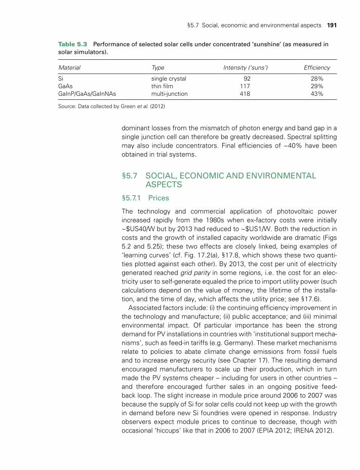
§5.7 Social, economic and environmental aspects 191
dominant losses from the mismatch of photon energy and band gap in a single junction cell can therefore be greatly decreased. Spectral splitting may also include concentrators. Final efficiencies of ~40% have been obtained in trial systems.
§5.7 SOCIAL, ECONOMIC AND ENVIRONMENTAL ASPECTS
§5.7.1 Prices
The technology and commercial application of photovoltaic power increased rapidly from the 1980s when ex-factory costs were initially ~$US40/W but by 2013 had reduced to ~$US1/W. Both the reduction in costs and the growth of installed capacity worldwide are dramatic (Figs 5.2 and 5.25); these two effects are closely linked, being examples of ‘learning curves’ (cf. Fig. 17.2(a), §17.8, which shows these two quanti-ties plotted against each other). By 2013, the cost per unit of electricity generated reached grid parity in some regions, i.e. the cost for an elec-tricity user to self-generate equaled the price to import utility power (such calculations depend on the value of money, the lifetime of the installa-tion, and the time of day, which affects the utility price; see §17.6).
Associated factors include: (i) the continuing efficiency improvement in the technology and manufacture; (ii) public acceptance; and (iii) minimal environmental impact. Of particular importance has been the strong demand for PV installations in countries with ‘institutional support mecha-nisms’, such as feed-in tariffs (e.g. Germany). These market mechanisms relate to policies to abate climate change emissions from fossil fuels and to increase energy security (see Chapter 17). The resulting demand encouraged manufacturers to scale up their production, which in turn made the PV systems cheaper – including for users in other countries – and therefore encouraged further sales in an ongoing positive feed-back loop. The slight increase in module price around 2006 to 2007 was because the supply of Si for solar cells could not keep up with the growth in demand before new Si foundries were opened in response. Industry observers expect module prices to continue to decrease, though with occasional ‘hiccups’ like that in 2006 to 2007 (EPIA 2012; IRENA 2012).
Table 5.3 Performance of selected solar cells under concentrated ‘sunshine’ (as measured in solar simulators).
Material Type Intensity (‘suns’) Efficiency
Si single crystal 92 28%GaAs thin film 117 29%GaInP/GaAs/GaInNAs multi-junction 418 43%
Source: Data collected by Green et al. (2012)
TWIDELL PAGINATION.indb 191 01/12/2014 11:36
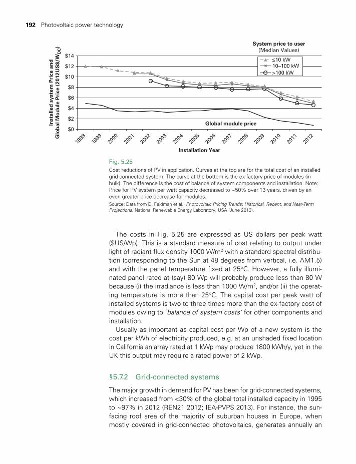
192 Photovoltaic power technology
The costs in Fig. 5.25 are expressed as US dollars per peak watt ($US/Wp). This is a standard measure of cost relating to output under light of radiant flux density 1000 W/m2 with a standard spectral distribu-tion ( corresponding to the Sun at 48 degrees from vertical, i.e. AM1.5) and with the panel temperature fixed at 25°C. However, a fully illumi-nated panel rated at (say) 80 Wp will probably produce less than 80 W because (i) the irradiance is less than 1000 W/m2, and/or (ii) the operat-ing temperature is more than 25°C. The capital cost per peak watt of installed systems is two to three times more than the ex-factory cost of modules owing to ‘balance of system costs’ for other components and installation.
Usually as important as capital cost per Wp of a new system is the cost per kWh of electricity produced, e.g. at an unshaded fixed location in California an array rated at 1 kWp may produce 1800 kWh/y, yet in the UK this output may require a rated power of 2 kWp.
§5.7.2 Grid-connected systems
The major growth in demand for PV has been for grid-connected systems, which increased from <30% of the global total installed capacity in 1995 to ~97% in 2012 (REN21 2012; IEA-PVPS 2013). For instance, the sun-facing roof area of the majority of suburban houses in Europe, when mostly covered in grid-connected photovoltaics, generates annually an
Fig. 5.25Cost reductions of PV in application. Curves at the top are for the total cost of an installed grid-connected system. The curve at the bottom is the ex-factory price of modules (in bulk). The difference is the cost of balance of system components and installation. Note: Price for PV system per watt capacity decreased to ~50% over 13 years, driven by an even greater price decrease for modules. Source: Data from D. Feldman et al., Photovoltaic Pricing Trends: Historical, Recent, and Near-Term Projections, National Renewable Energy Laboratory, USA (June 2013).
$14
$12
$10
$8
$6
$4
Inst
alle
d s
yste
m P
rice
an
dG
lob
al M
od
ule
Pri
ce (
2012
US
$/W
DC)
$2
$0
1998
1999
2000
2001
2002
2003
2004
2005
2006
2007
2008
2009
2010
2011
2012
Global module price
Installation Year
System price to user(Median Values)
>100 kW10–100 kW≤10 kW
TWIDELL PAGINATION.indb 192 01/12/2014 11:36

§5.7 Social, economic and environmental aspects 193
amount of electricity equal to 50 to 100% of the household’s electricity demand. Such householders use their own microgenerated electricity in the daytime, while selling any excess to the grid utility, then at night they buy imported power. The grid thus acts as their ‘virtual storage’. Because household electricity use is erratic and insolation varies, a rule-of-thumb is that 50% of microgenerated power is used in the building and 50% is exported to the grid. The same principle applies to busi-ness and commercial buildings; however, if loads are large and continu-ous, a much greater proportion of the microgenerated power is used on site. Government institutional support mechanisms help microgenera-tors establish cost-effective systems by one or more of: (a) mandating utilities to pay for microgenerated electricity at preferential rates (feed-in tariffs and legal obligations); (b) subsidizing the initial capital cost of the solar array; and (c) establishing payments for carbon-abatement ‘credits’ obtained in proportion to the renewable energy generated. The modular nature of PV generation and the lightweight of the static modules make such distributed (embedded) generation relatively easy to install, either on new-build and established buildings, or on independent structures.
The economics and ease of construction are improved by the devel-opment of ‘structural’ PV panels incorporated within the outer fabric of buildings and roofs, with their installed cost reduced by savings on con-ventional materials. It is reasonable to expect that within a few decades PV will become as incorporated into standard roof structures as glass is into windows now.
§5.7.3 Stand-alone systems
Stand-alone systems which depend on storage batteries are typically twice as expensive per unit capacity as grid-connected systems, owing to the added cost of the batteries. For stand-alone applications, the most important measure is the relative cost of service delivered at a particular site (e.g. comparing a PV-powered light of a certain light intensity with a kerosene-fueled light of similar intensity). Regarding the efficiency-of-use of the solar electricity, there is a trade-off between system compo-nents (e.g. better energy-efficient appliances require smaller panels and less balance of system cost), so investing in energy efficiency nearly always gives long-term reductions in lifetime expenditure, as empha-sized in Chapter 16.
§5.7.4 PV for rural electrification, especially in developing countries
PV use and demand have continued for off-grid rural electrification – vital for social and economic development, particularly in the rural areas of developing countries, where billions of people live without access to grid
TWIDELL PAGINATION.indb 193 01/12/2014 11:36
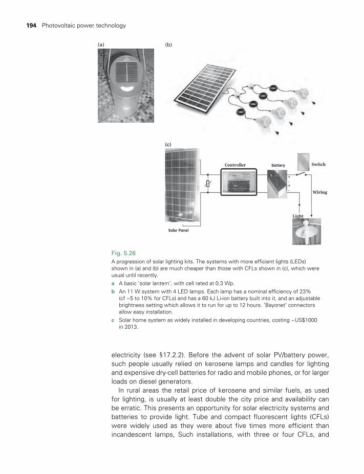
194 Photovoltaic power technology
Fig. 5.26A progression of solar lighting kits. The systems with more efficient lights (LEDs) shown in (a) and (b) are much cheaper than those with CFLs shown in (c), which were usual until recently. a A basic ‘solar lantern’, with cell rated at 0.3 Wp. b An 11 W system with 4 LED lamps. Each lamp has a nominal efficiency of 23%
(cf ~5 to 10% for CFLs) and has a 60 kJ Li-ion battery built into it, and an adjustable brightness setting which allows it to run for up to 12 hours. ‘Bayonet’ connectors allow easy installation.
c Solar home system as widely installed in developing countries, costing ~US$1000 in 2013.
(a) (b)
(c)
electricity (see §17.2.2). Before the advent of solar PV/battery power, such people usually relied on kerosene lamps and candles for lighting and expensive dry-cell batteries for radio and mobile phones, or for larger loads on diesel generators.
In rural areas the retail price of kerosene and similar fuels, as used for lighting, is usually at least double the city price and availability can be erratic. This presents an opportunity for solar electricity systems and batteries to provide light. Tube and compact fluorescent lights (CFLs) were widely used as they were about five times more efficient than incandescent lamps, Such installations, with three or four CFLs, and
TWIDELL PAGINATION.indb 194 01/12/2014 11:36

§5.7 Social, economic and environmental aspects 195
usually also powering chargers for radios and mobile phones, are called solar home systems (see Fig. 5.26(c)). Typically they cost ~US$1000 installed. Since about 2008, LED lamps have become widely available, producing the same amount of usable light (lumens) for one-third of the electricity (kWh), so that an equivalent system can use much smaller PV panels for the same output of light (Fig. 5.26(b)). Coupled with the decrease in module prices this has substantially reduced the cost of a solar home system to US$300, which is more easily financed. Such systems of < ~10 Wp are called Solar Pico Systems. They include port-able solar lanterns (Fig. 5.26(a)), which have the electronics and a Li-ion battery built in and cost only ~US$10 to US$40 depending on quality and light output, which makes them accessible even to the very poor; by 2013, about 0.5 million LED lanterns had been sold in Africa. As with all technology, increased markets allow improved technical support and hence more sustainable systems (IEA-PVPS 2013).
The key challenges in making such systems sustainable are no longer technical, but institutional and financial. Appropriate solutions to these non-technical challenges depend on local culture and social factors (e.g. whether people operate as individuals or cooperatively in a community, the extent of education and practical aptitude (including for maintenance), cash income, and the ease of transport for suppliers) (Chaurey and Kanpal 2010). Sometimes where a community has a cooperative infrastructure and culture, a centralized ‘microgeneration’ mini-grid system serves a whole village.
Often with support from multilateral banks and bilateral aid donors, many million solar home systems (SHS) have been installed worldwide, especially in Africa, the Far East and South America, together with market structures for further dissemination. Several developing countries have innovative business models for PV microgeneration based on ‘fee for service’, ‘pay as you go’ or ‘prepaid metering’ to improve affordabil-ity. The Government of China distributed about 400,000 SHS between 2005 and 2011, complementing its 2800 MW of grid-connected PV. In a similar period, about 1.3 million SHS were distributed in Bangladesh by 30 partner organizations, with finance from the World Bank and other agencies (REN21 2012).
In richer countries, solar home systems are used at remote farm-steads, etc., too far from the grid to warrant connection; such systems usually have larger installed capacity (>5 kW) for more electrical appli-ances than are affordable in poorer countries.
As markets for small-scale renewables increase, the differences between stand-alone and grid-connected microgeneration systems are less contrasting; it is obviously beneficial if as many components as possible are in common, so presenting a larger total market and less dif-ferentiation between ‘developing’ and ‘developed’ regions.
TWIDELL PAGINATION.indb 195 01/12/2014 11:36

196 Photovoltaic power technology
§5.7.5 Environmental impact
In operation, photovoltaics are environmentally benign, with no emis-sions and no noise, although manufacture involves some fully controlled noxious chemicals and uses energy. Module guaranteed life by manu-facturers is typically at least 20 years, but most modules will generate acceptably for very much longer, perhaps to ~100 years for modules with crystalline cells in good encapsulation. At end-of-life, modules should be returned for specialist recycling; sadly such facilities are not (yet) common The time for a given PV module to generate electricity equal in energy to that used in its manufacture (its energy payback) depends on the site insolation and the method of manufacture. For a typical temperate climate, this energy payback time for single-crystal silicon encapsulated modules is about two to three years (see refer-ences at the end of this chapter); for thin film technologies and for sunnier locations it is less.
§5.7.6 Outlook
Mass production of PV modules continues to increase dramatically in scale and quality, with associated decrease in price, so a future where the majority of new roofs on buildings generate electricity is predictable. As a mechanism for such electricity generation, PV power is peerless – there are no emissions, there is no noise, almost no running costs, life-time is at least several decades, new costs are reducing and it keeps out the rain!
Fig. 5.27Public appreciation and understanding is critical to success.a Householders with a small house-lighting system in Bhutan. Training local people
in basic maintenance of such systems is vital to their success.b Members of Westmill Solar Cooperative in the UK at the opening of their 5 MW
electricity-generating plant; all the many cooperative shareholders have equal rights, whatever their investment.
(a) (b)
TWIDELL PAGINATION.indb 196 01/12/2014 11:36

Quick questions 197
QUICK QUESTIONS
Note: Answers to these questions are in the text of the relevant section of this chapter, or may be readily inferred from it.
1 What is the name of an entity of quantized light? 2 What is the approximate open-circuit voltage of a Si p–n junction? 3 You have the choice of short-circuiting either a battery or an illumi-
nated photovoltaic module; which are dangerous, which are safe, and why?
CHAPTER SUMMARY
Solar cells produce electricity from the photovoltaic (PV) effect, i.e. the absorption of light within semi-conductor materials. An account of the solid-state physics underlying this process is given in Review 4.
Technical advantages of PV include its universal applicability (although energy output is greater in sunnier locations), modular character (allowing use at all scales from ~1 W to ~100 MW), reliability and long life (because there are no moving parts), ease of use, and lack of noise and emissions. The main technical disadvantage is that electricity generation is only during daytime. Therefore electricity storage (e.g. batteries) or grid linking is usual. Such mechanisms also smooth out the more rapid variability of output during daytime.
PV has been strongly encouraged in several countries by economic policies, such as feed-in tariffs. The resulting demand encouraged manufacturers to scale up production, which in turn made PV systems cheaper worldwide, including for stand-alone systems in rural areas of developing countries – and thus encouraged further sales in an ongoing positive feedback loop. Consequently PV power is one of the fastest-growing energy technologies: installed capacity had grown exponentially from ~200 MW in 1990 to more than 80,000 MW (80 GW) in 2012 (97% of which was grid-connected systems), with a similar growth rate expected to continue. In sunny climates, PV power is now cost-competitive with daytime peak grid electricity.
The efficiency and cost-effectiveness of photovoltaic cells are being continuously improved by R&D and manufacturing experience. ‘First generation’ cells based on crystalline or multi-crystalline Si single-junction cells dominate present installations. ‘Second generation’ cells use thin film cell technology for single-junction cells, but based on depositing thin layers of the photoactive material onto a supporting substrate (e.g. glass). By using much less of the most expensive material (the semiconductor), thin film cells and modules are cheaper per unit of capacity ($/Watt). Some of them use chemically more complex semiconductors such as CuInxGa1–xSe2 (CIGS) or certain organic oligomers. The intrinsic mismatch of the solar spectrum to the band gap limits the efficiency of single-band photovoltaic cells to <35%. ‘Third generation’ cells are not limited to single-junction operation; for instance, they include multi-junction/heterojunction tandem cells designed to absorb a wider range of the solar spectrum than single-junction cells and so having the potential for efficiency >30% without solar concentration, and >40% with concentration.
Commercial photovoltaic cells now have efficiencies of about 12 to 25% in ordinary sunshine. PV cells are usually sold as weatherproof modules, with open-circuit voltages between about 15 and 30 V. The current from the cells is inherently direct current (DC); electronic inverters are used to change this to alternating current (AC) if required. Daily output is typically ~0.5 to ~1.0 kWh/( m2 day), depending on climate.
TWIDELL PAGINATION.indb 197 01/12/2014 11:36
198 Photovoltaic power technology
4 As temperature increases in constant insolation, does PV power increase or decrease?
5 PV modules generate DC, yet most grids are AC; how can they be connected?
6 Name three components of a PV balance of system (BoS). 7 How can radiation absorption into a PV cell be increased? 8 What is the dominant factor limiting the efficiency of a single-band
gap PV cell? 9 Name one way in which the intrinsic lack of efficiency of QQ 8 may
be overcome. 10 Give two reasons why PV module cost has decreased dramatically
over the past 20 years.
PROBLEMS
5.1 The band gap of GaAs is 1.4 eV. Calculate the optimum wave-length of light for photovoltaic generation in a GaAs solar cell.
5.2 (a) Give the equation for the I–V characteristic of a p–n junction diode in the dark.
(b) If the saturation current is 10- 8 Am-2, calculate and draw the I–V characteristic as a graph to 0.2 V.
5.3 (a) What is the approximate photon flux density (photon s- l m- 2) for AM1 solar radiation at 0.8 kW m- 2?
(b) AM1 insolation of 0.8 kW m-2 is incident on a single Si solar cell of area l00 cm2. Assume 10% of photons cause electron – hole separation across the junction leading to an external current. What is the short-circuit current Isc of the cell? Sketch the I–V characteristic for the cell.
5.4 A small household lighting system is powered from a nominally 8 V (i.e. 4 cells at 2 V) storage battery having a 30 Ah supply when charged. The lighting is used for 4.0 h each night at 3.0 A.
Design a suitable photovoltaic power system that will charge the battery from an arrangement of Si solar cells.
(a) How will you arrange the cells?
(b) How will the circuit be connected?
(c) How will you test the circuit and performance?
5.5 (a) Calculate the approximate time to a single-crystalline PV module to generate electricity equal in energy terms to the primary energy used in its manufacture. Consider: a typical Japanese climate with 1450 kWh/(m2y) of insolation; modules
TWIDELL PAGINATION.indb 198 01/12/2014 11:36
Problems 199
of 15% efficiency; per 1.0 kWp peak power of modules. The total direct manufacturing and processing energy (includes refining, etc.) is 1350 kWh/kWp, plus a further 1350 kWh/kWp of factory ‘overhead energy’, with 90% of both from electricity (generated thermally at 55% efficiency from fuels in combined cycle generation).
(b) Straightforward energy payback of (a) assumes that electric-ity has the same ‘worth’ or ‘value’ as heat. Is this correct? What result would be obtained if PV cells and modules were manufactured entirely from, say, hydroelectricity? How can manufacture be more energy-efficient?
5.6 What is the best fixed orientation for power production from a photovoltaic module located at the South Pole?
5.7 (a) The band gap of intrinsic Si at 29°C is 1.14 eV. Calculate the probability function exp(-Eg/(2kT) for electrons to cross the full band gap by thermal excitation.
(b) If the Fermi level in n-type Si is about 0.1 eV below the con-duction band, calculate the probability function for electrons to be thermally excited into the conduction band. Compare your answers for (a) and (b).
5.8 Einstein won the Nobel Physics prize in 1905 for explaining the photoelectric effect, in which light incident on a surface can lead to the emission of an electron from that surface with energy
E = hn - Φ
where hn is the energy of a photon of light and Φ is a property of the surface.
(a) What are the main differences and similarities between the photoelectric effect and the photovoltaic effect?
(b) Discuss how, if at all, the photoelectric effect could be used to yield useful energy.
5.9 A Si photovoltaic module is rated at 50 W with insolation 1000 W/m2, as for peak insolation on Earth. What would be its peak output on Mars? (Note: mean distance of the Sun from Earth 1.50 x 10¹¹ m and from Mars 2.28 x 10¹¹ m; there is no significant atmosphere on Mars.)
5.10 By differentiation of (R4.28) by parts, prove (R4.29).
5.11 A solar array rated at 1 kW produces about 1800 kWh annually in California. What is its capacity factor?
TWIDELL PAGINATION.indb 199 01/12/2014 11:36

200 Photovoltaic power technology
NOTE
1 The photovoltaic effect should not be confused with the photoelectric effect whereby electrons are emitted from surfaces, as explained in 1905 by Einstein (see Problem 5.8).
BIBLIOGRAPHY
Comprehensive books
Goetzberger, A. and Hoffmann, V.U. (2005) Photovoltaic Solar Energy Generation, Springer Series in Optical Science, Springer. Excellent review of PV development, generation principles, manufacture, installation and market deployment. Quantitative and informative but non-mathematical. Well referenced.
Luque, A. and Hegedus, S. (eds) (2011, 2nd edn) Handbook of Photovoltaic Science and Engineering, Wiley, New York. Comprehensive reference covering physics, construction, testing, systems, applications, economics and implications for rural development. Includes an excellent and readable overview by the editors of the state of the art in all of the above, and in-depth chapters on each of the major device technologies.
McEvoy, A., Markvart, T. and Castañer, L. (eds) (2011) Practical Handbook of Photovoltaics: Fundamentals and applications, Elsevier, Oxon. A multi-author survey similar to Luque and Hegedus (2011).
Principally device physics
Green, M.A. (1998) Solar Cells: Operating principles, technology and system application, Prentice-Hall, New York. Reprinted by the University of New South Wales, Australia. A basic text from nearly first principles. Excellent text, with later revisions, by an outstanding researcher. See Wenham et al. (2011) for a companion applied text.
Green, M.A. (2001) Photovoltaic Physics and Devices, in J.E. Gordon (ed.), Solar Energy: The state of the art, James & James, London, pp. 291–355. Concise and comprehensive review in an excellent general solar text.
Green, M.A. (2006), Third Generation Photovoltaics, Springer, New York. Focuses on advanced types still at the conceptual or early laboratory stage.
Islam, S., Woyte, A., Belmans, R., Heskes, P., Rooij, P.M. and Hogedoorn, R. (2006) ‘Cost effective second generation AC-modules: development and testing aspects’, Energy, 31(12), 1897–1920. Comprehensive study, including technological options and costs.
Principally applications
Boxwell, M. (2012, 6th edn) Solar Electricity Handbook, Greenstream Publishing, UK. Well described by its sub-title, ‘A simple practical guide to solar energy: how to design and install photovoltaic solar electric systems’. See also www.SolarElectricityHandbook.com.
Chaurey, A. and Kandpal, T.C. (2010) ‘Assessment and evaluation of PV based decentralized rural electricifica-tion: an overview’, Renewable and Sustainable Energy Reviews, 14, 2266–2278. Excellent worldwide review, focusing on the social and institutional issues and the various ways used to meet them in different parts of the world.
IEA-PVPS (2013) Pico Solar PV Systems for Remote Homes. Useful summary, also including some history of ‘solar home systems’ for developing countries; available from www.iea-pvps.org.
TWIDELL PAGINATION.indb 200 01/12/2014 11:36

Bibliography 201
Krauter, S. (2006) Solar Electric Power Generation, Springer, New York. Useful on basic circuits, etc.; also some modeling of uses.
Labouret, A. and Viloz, M. (2011) Solar Photovoltaic Energy, The Institution of Engineering and Technology, London. Translated from 4th edn of an accessible French work.
Loos, G. and van Hemert, B. (eds) (1999) Stand-alone Photovoltaic Applications: Lessons learned, International Energy Agency, Paris, and James & James, London.
Weir, T. and Prasad, S. (2012) ‘Adoption of climate-smart technologies: the case of rural solar electricity in the Pacific Islands’, available at www.climate2012.de.
Wenham, S.R., Green, M.A., Watt, M.E., Corkish, R. and Sproul, A. (2011, 3rd edn) Applied Photovoltaics, Routledge, Oxon. Written by experienced experts for university and college students, but with basic theory and application detail.
Specific references
European Photovoltaic Industry Association (2012) Global Market Outlook for Photovoltaics until 2016, available at www.epia.org.
Feldman, D. et al. (2013) Photovoltaic Pricing Trends: Historical, recent, and near-term projections, National Renewable Energy Laboratory, USA (June).
Green, M.A., Emery, K., Hishikawa, Y., Warta, W. and Dunlop, E.D. (2012) ‘Solar cell efficiency tables (version 39)’, Prog. Photovolt:Res. Appl., 20, 12–20. Continuing series of reports; see e.g. http://onlinelibrary.wiley.com/doi/10.1002/pip.2163/full.
IRENA (2012) Renewable Energy Cost-analysis Series: Issue 4, Photovoltaics, International Renewable Energy Agency, www.irena.org.
Knapp, K. and Jester, T. (2001) ‘Empirical investigation of the energy payback time for photovoltaic modules’, Solar Energy, 71, 165–172. See also the more optimistic estimates of energy payback times by Alsema, E. (1998) Renewable and Sustainable Energy Reviews, 2, 387–415; also Fthenak, V. et al. (2005) Progress in Photovoltaics, 13, 713–723, and (2008) Environment, Science and Technology, 42, 2168–2174.
REN21 (2012) Global Status Report 2012. This is an annual survey of RE use and policies around the world, avail-able at www.ren21.org. The 2012 Report includes a special chapter on ‘rural renewable energy’.
Journals and websites
Progress in Photovoltaics, bimonthly by Wiley, Chichester. An important journal with world leaders in photovolta-ics on the Board of Editors.
www.solarbuzz.com. Includes industry statistics and news, outlines of technologies and their status, etc.
www.solarserver.com/. International Solar Energy information. Has excellent reports on technology and uptake.
www.nrel.gov/pv/. US National Center for Photovoltaics. Strong on R&D, US government programs, and case studies.
www.iea-pvps.org. Website of IEA Task Force on Photovoltaic Power Systems; has many useful reports, includ-ing annual reports on state of industry and applications.
TWIDELL PAGINATION.indb 201 01/12/2014 11:36

Hydropower
CHAPTER
6
CONTENTS
Learning aims 202
§6.1 Introduction 204
§6.2 Principles 208
§6.3 Assessing the resource 209§6.3.1 Measurement of head H 210§6.3.2 Measurement of flow rate Q 210
§6.4 Impulse turbines 212
§6.5 Reaction turbines 217
§6.6 Hydroelectric systems 220§6.6.1 Power regulation and control:
grid-connected 222§6.6.2 Power regulation and control:
stand-alone systems 223§6.6.3 System efficiency 223§6.6.4 Scope for technology upgrades 224
§6.7 Pumped hydro energy storage 224
§6.8 Social and environmental aspects 225
Chapter summary 227
Quick questions 228
Problems 228
Bibliography 231
Box 6.1 Measurement of flow rate Q: principles as described for small systems 210
Box 6.2 ‘Specific speed’ 216
Box 6.3 The Three Gorges dam, Yangtze River, Hubei Province, China: the world’s largest hydroelectric installation 221
LEARNING AIMS
• Appreciate the large extent of worldwide gen-eration of electricity from falling water.
• Understand how the energy transformations occur.
• Perform fundamental calculations. • Estimate hydropower potential at a site.
• Consider small-scale applications and so be able to perform practical experiments and field studies.
• Apply scaling laws that extend laboratory studies to large-scale application. Appreciate environmental impacts.
TWIDELL PAGINATION.indb 202 01/12/2014 11:36

List of tables 203
LIST OF FIGURES
6.1 Growth of world hydroelectricity generation (TWh/y) and capacity (GW). 2046.2 Layout of a typical hydroelectric power station. 2076.3 Measuring water flow. 2116.4 Schematic diagram of a Pelton wheel impulse turbine. 2136.5 Photo of Pelton wheel. 2136.6 Speed of cup and fluid 2146.7 Methods of increasing the power from a given size of machine, working at the same water
pressure. 2186.8 Illustrative peak efficiencies. 2196.9 Layout of a micro hydroelectric system using a Pelton wheel. 2206.10 The Three Gorges hydroelectric dam in China: the world’s largest. 2216.11 Typical layout of a pumped hydro energy storage system. 2256.12 A U-weir. 229
LIST OF TABLES
6.1 Hydropower potential, capacity and output by region and by sample countries (2008). Note the variation in capacity factor by country, and the significant potential for development in Africa and Asia. 205
TWIDELL PAGINATION.indb 203 01/12/2014 11:36
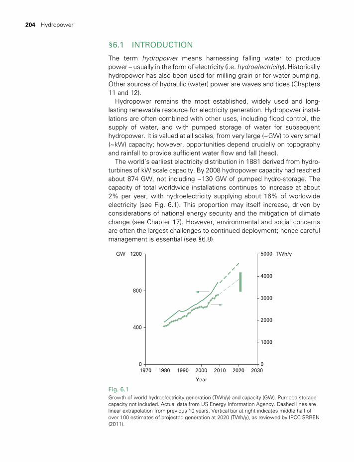
204 Hydropower
§6.1 INTRODUCTION
The term hydropower means harnessing falling water to produce power – usually in the form of electricity (i.e. hydroelectricity). Historically hydropower has also been used for milling grain or for water pumping. Other sources of hydraulic (water) power are waves and tides (Chapters 11 and 12).
Hydropower remains the most established, widely used and long- lasting renewable resource for electricity generation. Hydropower instal-lations are often combined with other uses, including flood control, the supply of water, and with pumped storage of water for subsequent hydropower. It is valued at all scales, from very large (~GW) to very small (~kW) capacity; however, opportunities depend crucially on topography and rainfall to provide sufficient water flow and fall (head).
The world’s earliest electricity distribution in 1881 derived from hydro-turbines of kW scale capacity. By 2008 hydropower capacity had reached about 874 GW, not including ~130 GW of pumped hydro-storage. The capacity of total worldwide installations continues to increase at about 2% per year, with hydroelectricity supplying about 16% of worldwide electricity (see Fig. 6.1). This proportion may itself increase, driven by considerations of national energy security and the mitigation of climate change (see Chapter 17). However, environmental and social concerns are often the largest challenges to continued deployment; hence careful management is essential (see §6.8).
Fig. 6.1Growth of world hydroelectricity generation (TWh/y) and capacity (GW). Pumped storage capacity not included. Actual data from US Energy Information Agency. Dashed lines are linear extrapolation from previous 10 years. Vertical bar at right indicates middle half of over 100 estimates of projected generation at 2020 (TWh/y), as reviewed by IPCC SRREN (2011).
5000 TWh/yGW
4000
3000
2000
1000
019700
800
1200
400
1980 1990 2000 2010 2020 2030
Year
TWIDELL PAGINATION.indb 204 01/12/2014 11:36
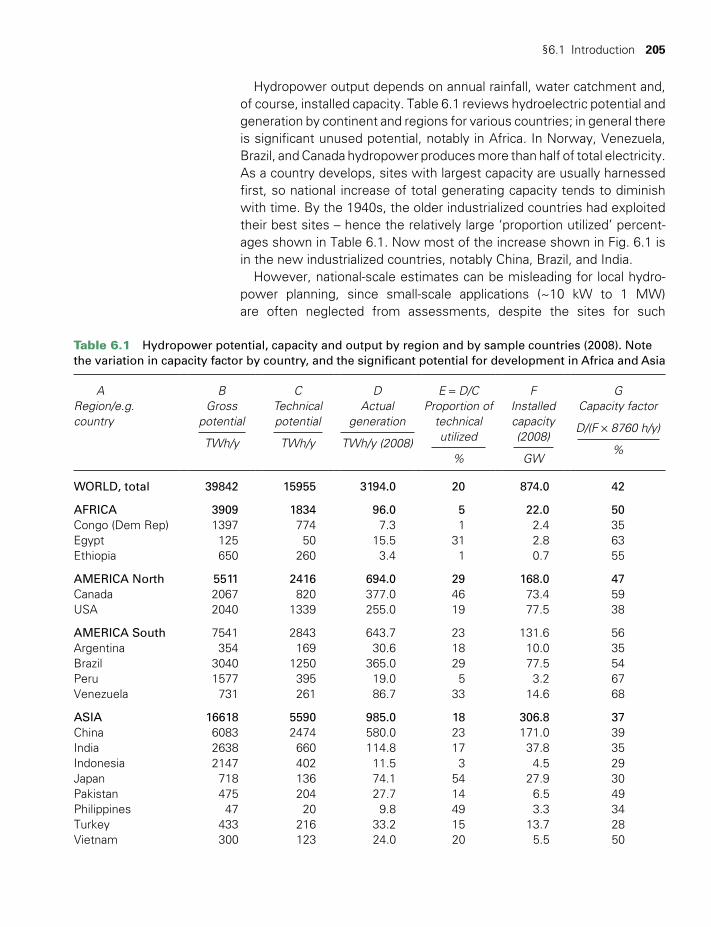
§6.1 Introduction 205
Hydropower output depends on annual rainfall, water catchment and, of course, installed capacity. Table 6.1 reviews hydroelectric potential and generation by continent and regions for various countries; in general there is significant unused potential, notably in Africa. In Norway, Venezuela, Brazil, and Canada hydropower produces more than half of total electricity. As a country develops, sites with largest capacity are usually harnessed first, so national increase of total generating capacity tends to diminish with time. By the 1940s, the older industrialized countries had exploited their best sites – hence the relatively large ‘proportion utilized’ percent-ages shown in Table 6.1. Now most of the increase shown in Fig. 6.1 is in the new industrialized countries, notably China, Brazil, and India.
However, national-scale estimates can be misleading for local hydro-power planning, since small-scale applications (~10 kW to 1 MW) are often neglected from assessments, despite the sites for such
Table 6.1 Hydropower potential, capacity and output by region and by sample countries (2008). Note the variation in capacity factor by country, and the significant potential for development in Africa and Asia
ARegion/e.g. country
BGross
potential
TWh/y
CTechnical potential
TWh/y
DActual
generation
TWh/y (2008)
E = D/CProportion of
technical utilized
%
FInstalled capacity (2008)
GW
GCapacity factor
D/(F × 8760 h/y)
%
WORLD, total 39842 15955 3194.0 20 874.0 42
AFRICA 3909 1834 96.0 5 22.0 50Congo (Dem Rep) 1397 774 7.3 1 2.4 35Egypt 125 50 15.5 31 2.8 63Ethiopia 650 260 3.4 1 0.7 55
AMERICA North 5511 2416 694.0 29 168.0 47Canada 2067 820 377.0 46 73.4 59USA 2040 1339 255.0 19 77.5 38
AMERICA South 7541 2843 643.7 23 131.6 56Argentina 354 169 30.6 18 10.0 35Brazil 3040 1250 365.0 29 77.5 54Peru 1577 395 19.0 5 3.2 67Venezuela 731 261 86.7 33 14.6 68
ASIA 16618 5590 985.0 18 306.8 37China 6083 2474 580.0 23 171.0 39India 2638 660 114.8 17 37.8 35Indonesia 2147 402 11.5 3 4.5 29Japan 718 136 74.1 54 27.9 30Pakistan 475 204 27.7 14 6.5 49Philippines 47 20 9.8 49 3.3 34Turkey 433 216 33.2 15 13.7 28Vietnam 300 123 24.0 20 5.5 50
TWIDELL PAGINATION.indb 205 01/12/2014 11:36
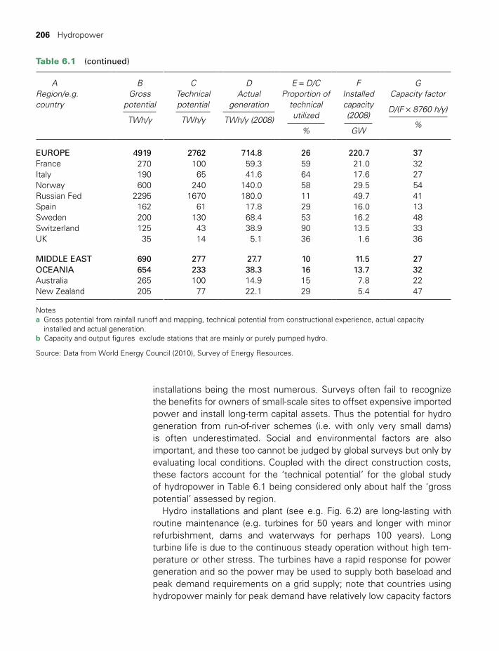
206 Hydropower
installations being the most numerous. Surveys often fail to recognize the benefits for owners of small-scale sites to offset expensive imported power and install long-term capital assets. Thus the potential for hydro generation from run-of-river schemes (i.e. with only very small dams) is often underestimated. Social and environmental factors are also important, and these too cannot be judged by global surveys but only by evaluating local conditions. Coupled with the direct construction costs, these factors account for the ‘technical potential’ for the global study of hydropower in Table 6.1 being considered only about half the ‘gross potential’ assessed by region.
Hydro installations and plant (see e.g. Fig. 6.2) are long-lasting with routine maintenance (e.g. turbines for 50 years and longer with minor refurbishment, dams and waterways for perhaps 100 years). Long turbine life is due to the continuous steady operation without high tem-perature or other stress. The turbines have a rapid response for power generation and so the power may be used to supply both baseload and peak demand requirements on a grid supply; note that countries using hydropower mainly for peak demand have relatively low capacity factors
Table 6.1 (continued)
ARegion/e.g. country
BGross
potential
TWh/y
CTechnical potential
TWh/y
DActual
generation
TWh/y (2008)
E = D/CProportion of
technical utilized
%
FInstalled capacity (2008)
GW
GCapacity factor
D/(F × 8760 h/y)
%
EUROPE 4919 2762 714.8 26 220.7 37France 270 100 59.3 59 21.0 32Italy 190 65 41.6 64 17.6 27Norway 600 240 140.0 58 29.5 54Russian Fed 2295 1670 180.0 11 49.7 41Spain 162 61 17.8 29 16.0 13Sweden 200 130 68.4 53 16.2 48Switzerland 125 43 38.9 90 13.5 33UK 35 14 5.1 36 1.6 36
MIDDLE EAST 690 277 27.7 10 11.5 27OCEANIA 654 233 38.3 16 13.7 32Australia 265 100 14.9 15 7.8 22New Zealand 205 77 22.1 29 5.4 47
Notesa Gross potential from rainfall runoff and mapping, technical potential from constructional experience, actual capacity
installed and actual generation. b Capacity and output figures exclude stations that are mainly or purely pumped hydro.
Source: Data from World Energy Council (2010), Survey of Energy Resources.
TWIDELL PAGINATION.indb 206 01/12/2014 11:36

§6.1 Introduction 207
(Table 6.1). Moreover, turbines can be designed for reverse operation as pumps for pumped storage schemes (§6.7).
Hydropower systems have among the best conversion efficiencies of all known energy sources (up to 90% efficiency, water to wire). The relatively expensive initial investment is offset by long lifespan, together with low-cost operation and maintenance. Consequently, the levelized production cost of electricity from hydropower (i.e. the cost of genera-tion averaged over the life of the project: see Chapter 17) can be as cheap as 3 to 5 US cents/kWh under good conditions, compared with utility selling prices to the public of ~15 to 20 US cents/kWh.
One almost unique characteristic of hydropower is the continuous range of applicable scales, from less than 1 kW to more than 500 MW. The adjectives ‘small’, ‘large’, etc. used to describe the projects depend on the organization or person involved; there is no international code. Nevertheless, we distinguish four main scales; Large (>100 MW), Medium (15 to 100 MW), Mini (0.1 to 15 MW), and Micro (<100 kW).
The major disadvantages of hydropower are associated with effects other than the generating equipment, particularly for large systems. These
Fig. 6.2Layout of a typical hydroelectric power station. Water is stored behind a dam (near top of photo), flows down the pipes (middle of photo) to turbines (in the housings near bottom of photo), and is then released downstream. Photo shows the 1500 MW Tumut 3 power station in Australia, with head of 150 m. In this particular installation, the output water passes through a tunnel (not shown in the photo) to augment agricultural irrigation – thus illustrating how hydro installations may have multiple societal and economic benefits. This station may also be used as a pumped hydro energy storage system (see § 6.7).
TWIDELL PAGINATION.indb 207 01/12/2014 11:36

208 Hydropower
include possible adverse environmental impacts, the effect on fish, silting of dams, corrosion of turbines in certain water conditions, social impact of displacement of people from the reservoir site, loss of potentially productive land (often balanced by the benefits of irrigation on other land), and relatively large capital costs compared with those of fossil power sta-tions. For instance, there has been extensive international debate on the benefits and disadvantages of the Aswan Dam for Egypt and the Three Gorges project for China. All of these issues are discussed further in §6.8.
This chapter considers fundamental aspects of hydropower and does not attempt to be comprehensive in such a developed subject. In par-ticular, we have considered small-scale applications, since students can use these in laboratory and field conditions for practical learning. We refer readers to the bibliography for comprehensive works at established engineering level.
The fundamental equation (6.1) is sufficient for estimating hydropower potential at a particular location; the methods described in §6.3 give a more accurate assessment. Turbines are of two types: (a) impulse tur-bines, where the flow hits the turbine as a jet in an open environment, with the power deriving from the kinetic energy of the flow (see §6.4); and (b) reaction turbines, where the turbine is totally embedded in the fluid and powered from the pressure drop across the device (see §6.5). The mechanical turbines then drive machinery (historical use) or elec-tricity generators (dominant use). Reaction turbine generators may be reversed, so water is pumped to high levels for pumped storage and sub-sequent generation (§6.7), at an overall efficiency of ~70%. §6.6 consid-ers other technical aspects of hydroelectric systems, and §6.8 reviews the social and environmental aspects of hydropower. The eResource and the Bibliography at the end of the chapter give further information on applications, including the purely mechanical hydraulic ram pump.
§6.2 PRINCIPLES
Water of volume per second Q and density ρ falls down a slope. The mass falling per unit time is ρQ, and the rate of potential energy lost by the falling fluid is
ρ=P QgH0 (6.1)
where g is the acceleration due to gravity and H is the vertical compo-nent of the water path.
The turbines convert this power to shaft power. Unlike thermal power sources, there is no fundamental thermodynamic or dynamic reason why the output power of a hydro system should be less than the input power P0, apart from frictional losses that can be proportionately very small. For a site with a water reservoir, H is fixed and Q is adjustable. Hence the power output is quickly controlled at, or less than, the design output,
TWIDELL PAGINATION.indb 208 01/12/2014 11:36
§6.3 Assessing the resource 209
provided that there is sufficient water supply. Note that the density of fresh water at ambient temperatures is 1000 kg/m3 and of air only about 1.2 kg/m3, which is a major reason for the difference in diameter between water and wind turbines of the same nominal output power.
The main disadvantage of hydropower is also clear from (6.1): the site must have sufficient Q and H. In general this requires a rainfall > ~ 40 cm/y dispersed through the year, a suitable elevated catchment or river (if possible with water storage) and a final steep fall of the water onto the turbines. This combination of conditions is not common, so hydropower is far from universally available. However, where available, hydropower is almost certainly the most suitable electricity-generating source, as suggested in Worked Example 6.1.
Nevertheless, considerable civil engineering (in the form of dams, pipework, etc.) is always required to direct the flow through the tur-bines. These civil works often cost more than the mechanical and electri-cal components. However, for large, high-head, hydropower, tunneling technology has improved greatly due to the introduction of increasingly efficient equipment. Consequently, excavation costs have reduced by 25% over the past 30 years. Note that the cost per unit power of turbines tends to increase with Q. Therefore costs per unit power output of high-head installations are less than low-head, unless pipework costs become excessive. For small installations at old water-mill sites, conversion to electricity generation can be very cost-effective.
§6.3 ASSESSING THE RESOURCE
Suppose we have a stream available which may be useful for hydro-power. At first, only approximate data, with an accuracy of about ±50%,
WORKED EXAMPLE 6.1
Water from a moderately sized river flows at a rate of 100 m3/s down a perfectly smooth pipe, falling 50 m into a turbine.
(a) How much power is available? (b) If in practice 10% of the power is lost by friction, transformation and distribution, how many houses having average electricity use of about 0.5 kW (i.e. 12 kWh/day) could this power supply?
SolutionFrom (6.1),
P (1000kg/m ) (100m /s) (9.81m/s ) 50m
49 10 kg.m/s 49MJ/s 49MW0
3 3 2
6 3
= × × ×= × = =
The number of houses is (49,000 – 4,900) kW/(0.5 kW per house) ≈ 88,000 houses, i.e. a large town with a population of about 220,000.
TWIDELL PAGINATION.indb 209 01/12/2014 11:36

210 Hydropower
are needed to estimate the power potential of the site. If this survey proves promising, then a detailed investigation will be necessary involv-ing data, for instance, rainfall taken over several years. It is clear from (6.1) that to estimate the input power P0 we have to measure the flow rate Q and the available vertical fall H (usually called the head). For example, with Q = 40 liter/s and H = 20 m, the maximum power available at source is 8 kW. This might be very suitable for a household supply.
§6.3.1 Measurement of head H
For nearly vertical falls, trigonometric survey methods (perhaps even using the lengths of shadows) are suitable; whereas for more gentle slopes, level and pole surveying is straightforward. Note that the power input to the turbine depends not on the geometric (or ‘total’) head Ht as surveyed, but on the available head Ha:
H H Ha t f= − (6.2)
where the head loss Hf allows for friction losses in the pipe and chan-nels leading from the source to the turbine (see §R2.6). With suitable pipework fH < ~ Ht /3; however, by (R2.11) Hf increases in proportion to the total length of pipe, so the best sites for hydropower have steep slopes.
§6.3.2 Measurement of flow rate Q
The flow through the turbine produces the power, and this flow will usually be less than the flow in the stream. However, the flow in the stream varies with time, for example, between drought and flood periods. For power generation we usually want to know the minimum (dry season) flow, since a turbine matched to this will produce power all the year round without overcapacity of machinery. Such data are also necessary for environmental impact (e.g. maintaining a minimum flow for aquatic life). We also need to know the maximum flow and flood levels to avoid damage to installations.
The measurement of Q is more difficult than the measurement of H. Box 6.1 outlines some possible methods. The method chosen will depend on the size and speed of the stream concerned. For large instal-lations, the ‘sophisticated method’ is always used.
BOX 6.1 MEASUREMENT OF FLOW RATE Q: PRINCIPLES AS DESCRIBED FOR SMALL SYSTEMS
As in § R2.2,
Q t tflow rate (volume passing in time ) /= ∆ ∆ (6.3)
u A(mean speed ) (cross-sectional area ) = × (6.4)
= ∫ u d A (6.5)
TWIDELL PAGINATION.indb 210 01/12/2014 11:36

§6.3 Assessing the resource 211
where u is the streamwise velocity (normal to the elemental area dA ). The measurement methods relating to each equation we call basic (6.3), refined (6.4) and sophisticated (6.5). A further method may be used if the water falls freely over a ledge or weir.
Fig. 6.3Measuring water flow: (a) basic method; (b) refined method (i); (c) refined method (ii); (d) sophisticated method; (e) weir method, see also Fig. 6.12.
Stop watch
Speed uArea dA
d
∆x
h
Notch
Stream
Dam
(e)
(d)
(c)
(b)
0
(a)
Barrel
Surface
Diversionpipe
12 3
4y
y1 z1z2
z3
Stream
TWIDELL PAGINATION.indb 211 01/12/2014 11:36
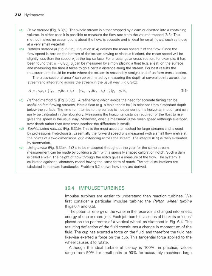
212 Hydropower
(a) Basic method (Fig. 6.3(a)). The whole stream is either stopped by a dam or diverted into a containing volume. In either case it is possible to measure the flow rate from the volume trapped (6.3). This method makes no assumptions about the flow, is accurate and is ideal for small flows, such as those at a very small waterfall.
(b) Refined method (i) (Fig. 6.3(b)). Equation (6.4) defines the mean speed u of the flow. Since the flow speed is zero on the bottom of the stream (owing to viscous friction), the mean speed will be slightly less than the speed us at the top surface. For a rectangular cross-section, for example, it has been found that u ≈ 0.8us. us can be measured by simply placing a float (e.g. a leaf) on the surface and measuring the time it takes to go a certain distance along the stream. For best results the measurement should be made where the stream is reasonably straight and of uniform cross-section. The cross-sectional area A can be estimated by measuring the depth at several points across the stream and integrating across the stream in the usual way (Fig 6.3(b)):
A y z (y y )(z z ) (y y )(z z ) (y y )z12 1 1
12 2 1 1 2
12 3 2 2 3
12 4 3 3≈ + − + + − + + − (6.6)
(c) Refined method (ii) (Fig. 6.3(c)). A refinement which avoids the need for accurate timing can be useful on fast-flowing streams. Here a float (e.g. a table tennis ball) is released from a standard depth below the surface. The time for it to rise to the surface is independent of its horizontal motion and can easily be calibrated in the laboratory. Measuring the horizontal distance required for the float to rise gives the speed in the usual way. Moreover, what is measured is the mean speed (although averaged over depth rather than over cross-section: the difference is small).
(d) Sophisticated method (Fig. 6.3(d)). This is the most accurate method for large streams and is used by professional hydrologists. Essentially the forward speed u is measured with a small flow metre at the points of a two-dimensional grid extending across the stream. The integral (6.5) is then evaluated by summation.
(e) Using a weir (Fig. 6.3(e)). If Q is to be measured throughout the year for the same stream, measurement can be made by building a dam with a specially shaped calibration notch. Such a dam is called a weir. The height of flow through the notch gives a measure of the flow. The system is calibrated against a laboratory model having the same form of notch. The actual calibrations are tabulated in standard handbooks. Problem 6.2 shows how they are derived.
§6.4 IMPULSE TURBINES
Impulse turbines are easier to understand than reaction turbines. We first consider a particular impulse turbine: the Pelton wheel turbine (Figs 6.4 and 6.5).
The potential energy of the water in the reservoir is changed into kinetic energy of one or more jets. Each jet then hits a series of buckets or ‘cups’ placed on the perimeter of a vertical wheel, as sketched in Fig. 6.4. The resulting deflection of the fluid constitutes a change in momentum of the fluid. The cup has exerted a force on the fluid, and therefore the fluid has likewise exerted a force on the cup. This tangential force applied to the wheel causes it to rotate.
Although the ideal turbine efficiency is 100%, in practice, values range from 50% for small units to 90% for accurately machined large
TWIDELL PAGINATION.indb 212 01/12/2014 11:36
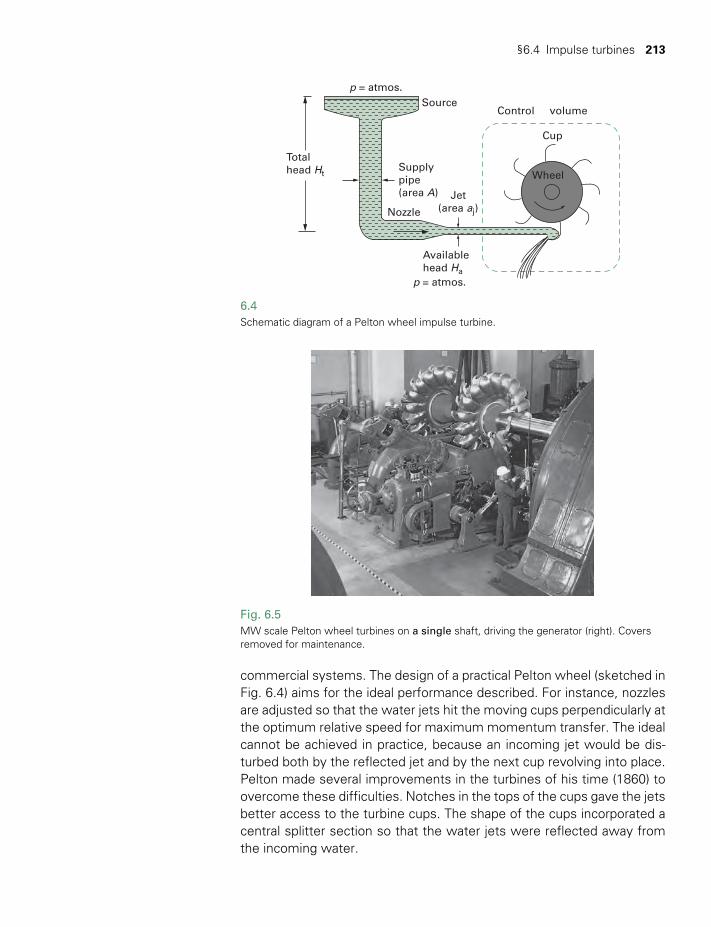
§6.4 Impulse turbines 213
commercial systems. The design of a practical Pelton wheel (sketched in Fig. 6.4) aims for the ideal performance described. For instance, nozzles are adjusted so that the water jets hit the moving cups perpendicularly at the optimum relative speed for maximum momentum transfer. The ideal cannot be achieved in practice, because an incoming jet would be dis-turbed both by the reflected jet and by the next cup revolving into place. Pelton made several improvements in the turbines of his time (1860) to overcome these difficulties. Notches in the tops of the cups gave the jets better access to the turbine cups. The shape of the cups incorporated a central splitter section so that the water jets were reflected away from the incoming water.
6.4Schematic diagram of a Pelton wheel impulse turbine.
Source
Supplypipe(area A) Jet
(area aj)
Wheel
Control
Cup
volume
Nozzle
Totalhead Ht
Availablehead Ha
p = atmos.
p = atmos.
Fig. 6.5MW scale Pelton wheel turbines on a single shaft, driving the generator (right). Covers removed for maintenance.
TWIDELL PAGINATION.indb 213 01/12/2014 11:36
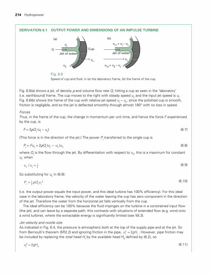
214 Hydropower
DERIVATION 6.1 OUTPUT POWER AND DIMENSIONS OF AN IMPULSE TURBINE
Fig. 6.6Speed of cup and fluid: in (a) the laboratory frame; (b) the frame of the cup.
(a)
Jet of water Jet of waterCup
(b)
Q
uj
ucuc
ur1 = uj – uc
ur2 = u2 – uc u2
Fig. 6.6(a) shows a jet, of density ρ and volume flow rate Q, hitting a cup as seen in the ‘laboratory’ (i.e. earthbound) frame. The cup moves to the right with steady speed uc and the input jet speed is uj. Fig. 6.6(b) shows the frame of the cup with relative jet speed uj − uc; since the polished cup is smooth, friction is negligible, and so the jet is deflected smoothly through almost 180° with no loss in speed.
ForcesThus, in the frame of the cup, the change in momentum per unit time, and hence the force F experienced by the cup, is
F = 2ρQj (uj − uc) (6.7)
(This force is in the direction of the jet.) The power Pj transferred to the single cup is
Pj = Fuc = 2ρQj (uj − uc )uc (6.8)
where Qj is the flow through the jet. By differentiation with respect to uc, this is a maximum for constant uj, when
u u/c j12= (6.9)
So substituting for uc in (6.8):
P Q uj j j12
2ρ= (6.10)
(i.e. the output power equals the input power, and this ideal turbine has 100% efficiency). For this ideal case in the laboratory frame, the velocity of the water leaving the cup has zero component in the direction of the jet. Therefore the water from the horizontal jet falls vertically from the cup.
The ideal efficiency can be 100% because the fluid impinges on the turbine in a constrained input flow (the jet), and can leave by a separate path; this contrasts with situations of extended flow (e.g. wind onto a wind turbine), where the extractable energy is significantly limited (see §8.3).
Jet velocity and nozzle sizeAs indicated in Fig. 6.4, the pressure is atmospheric both at the top of the supply pipe and at the jet. So from Bernoulli’s theorem (§R2.2) and ignoring friction in the pipe, u gH2j
2t= . However, pipe friction may
be included by replacing the total head Ht by the available head Ha defined by (6.2), so
u gH2j2
a= (6.11)
TWIDELL PAGINATION.indb 214 01/12/2014 11:36

§6.4 Impulse turbines 215
In practice, the size of the pipes is chosen so that uj is independent of the nozzle area. If there are n nozzles, each of area a, then the total flow from all jets is
Q = nauj = nQj (6.12)
If the efficiency of transforming the water jet power into mechanical rotational power is ηm ,then the mechanical power output Pm from the turbine with n jets is, from (6.9) and (6.10),
P nP n Qu n au u
na gH
( )( ) ( )( )
(2 )
m m j m j m j j
m a
12
2 12
2
12
3/2
η η ρ η ρ
η ρ
= = =
=
(6.13)
This shows the importance of obtaining the maximum available head Ha between turbine and reservoir. The output power is proportional to the total jet cross-sectional area A = n a. However, a is limited by the size of cup, so if a is to be increased, a larger turbine is needed. It is usually easier to increase the number of nozzles n than to increase the overall size of the turbine, but the arrangement becomes unworkably complicated for n ≥ 4. For small wheels, n = 2 is the most common.
Of course, the total flow Q through the turbine cannot be more than the flow in the stream Qstream. Using (6.11) and (6.12),
na Q gHa/ (2 )j stream1/2≤ (6.14)
Angular velocity and turbine sizeSuppose we have chosen the nozzle size and number in accordance with (6.12) and (6.13) to give the maximum power available. The nozzle size has fixed the size of the cups, but not the overall size of the wheel. The latter is determined by geometric constraints, and also by the required rotational speed. For electrical generation, the output variables (e.g. voltage, frequency and efficiency) depend on the angular speed of the generator. Most electric generators have greatest efficiency at large rotational speed (frequency), commonly ~1500 rpm. To avoid complicated and lossy gearing, it is important that the turbine should also operate at such large speed; the Pelton wheel is particularly suitable in this respect.
If the wheel has radius R and turns at angular velocity ω, by (6.7) and (6.8),
P = FR ω (6.15)
Thus, for a given output power, the larger the wheel the smaller its angular velocity. Since uc = Rω, and uc = 0.5 uj by (6.9), and using (6.11),
RgH0.5(2 )a
1/2
ω= (6.16)
The nozzles usually give circular cross-section jets of area a and radius r. So a = π r2 and from (6.13),
rP
n gH( )2 m
jm a3/2η ρ π
=√ 2 (6.17)
Combining (6.16) and (6.17), we find
ηω
ρ
η
=
=
−
−
r R n PgH
n
/ 0.68( )( )
0.68( )
m1/2 m
1/2
1/2a
5/4
m1/2S
(6.18)
TWIDELL PAGINATION.indb 215 01/12/2014 11:36
216 Hydropower
In (6.18) S is a non-dimensional measure of the operating conditions, called the shape number of the turbine:
ωρ
= PgH( )m1/2
1/2a
5/4S (6.19)
Such non-dimensional factors are powerful functions in engineering (e.g. allowing the results of measurement and optimization of laboratory-scale physical models to be applied to full-scale plant).
From (6.18), the mechanical efficiency ηm at any instant is a function of: (i) the fixed geometry of a particular Pelton wheel (measured by the non-dimensional parameters r/R and n), and (ii) the non-dimensional ‘shape number’ S which characterizes the operating conditions at that time.
WORKED EXAMPLE 6.2
Determine the dimensions of a single jet Pelton wheel to develop 160 kW under a head of: (i) 81 m, and (ii) 5.0 m. What is the angular speed at which these wheels will perform best?
SolutionAssume that water is the working fluid. Let r be the nozzle radius and R the wheel radius. It is difficult to operate a wheel with r > R/10, since the cups would then be so large that they would interfere with each
BOX 6.2 ‘SPECIFIC SPEED’
Beware! Instead of the dimensionless shape number S of (6.19), some engineering texts use a dim en -sioned characteristic called ‘specific speed’, Ns, defined from the variables P, ν (= ω /2π) and Ha:
NPHs
a
1/2
5/4
ν= (6.20)
‘Specific speed’ does not include g and ρ, since these are effectively constants. Consequently, Ns has dimensions and units, and so, disturbingly, its numerical value depends on the particular units used. In practice, these units vary between the USA (e.g. rpm, shaft horsepower, ft) and Europe (e.g. rpm, metric horsepower, m), with a standard version for SI units yet to become common.
Implicit in (6.18) is the relation between the speed of the moving parts uc and the speed of the jet uj. If the ratio uc /uj is the same for two wheels of different sizes but the same shape, then the whole flow pattern is also the same for both. It follows that all non-dimensional measures of hydraulic performance, such as ηm and S, are the same for impulse turbines with the same ratio of uc/uj. Moreover, for a particular shape of Pelton wheel (specified here by r/R and n), there is a particular combina-tion of operating conditions (specified by S ) for maximum efficiency.
TWIDELL PAGINATION.indb 216 01/12/2014 11:36
§6.5 Reaction turbines 217
Comparing cases (i) and (ii) in Example 6.2, Pelton wheels at low heads should rotate slowly and have large radius. Such installations would be unwieldy and costly, especially because the size of framework and housing increases with size of turbine. In practice therefore, Pelton wheels are used predominantly for high-head and relatively small-flow installations.
§6.5 REACTION TURBINES
Low-head situations (6.1), require a greater flow Q through the turbine than for high-head. Likewise, considering the shape number S of (6.19), to maintain the same ω and P with lower H, we require a turbine with larger S. For instance, by increasing the number of nozzles on a Pelton wheel: see (6.18) and Fig. 6.7(a). However, the pipework becomes unduly complicated if n > 4, and the efficiency decreases because the many jets of water interfere with each other.
To maintain a larger flow through a turbine, design changes are needed, as in the Francis reaction turbine of Figs 6.7(b) and 6.7(c). In effect, the entire periphery of the wheel is made into one large ‘slot’ jet for water to enter and then turn in a vortex to push against the rotor vanes. Such turbines are called reaction machines because the fluid
other’s flow; therefore we assume r = R/12 in (6.18), and from Fig. 6.8 with the optimum operating conditions ηm ≈ 0.9, the characteristic shape number in (6.18) becomes:
S = 0.11
(i) With Ha = 81 m, (6.17) from the angular speed for best performance is
ω ρ=
=×
=
−
− −
−
gH P( )0.11(10 kgm ) [(9.8 ms )(81m)]
(16 10 W)36 rad s
11/2
a5/4 1/2
3 3 1/2 2 5/4
4 1/21
S
From (6.11)
u gH(2 ) 40 msj a1/2 1= = −
Therefore:
ω= =R u / 0.55 m12 j
(ii) Similarly, with Ha = 5 m,
ω ω= ===
−
−uR
(5 / 81) 1.1rad s10 ms
4.5 m
2 15/4 1
j1
TWIDELL PAGINATION.indb 217 01/12/2014 11:36

218 Hydropower
pushes (or ‘reacts’) continuously against the blades. This contrasts with impulse machines (e.g. Pelton wheels), where the blades (cups) receive a series of impulses. For a reaction turbine, the wheel, called the runner, must be adapted so that the fluid enters radially perpendicular to the turbine axis, but turns and leaves parallel to this axis. Consequently, the fluid velocity has a radial component in addition to the tangential veloc-ity, which complicates the analysis (see textbooks in the Bibliography at the end of this chapter).
A larger water flow may be obtained by making the incoming water ‘jet’ almost as large in cross-section as the wheel itself. This concept leads to a turbine in the form of a propeller, with the flow mainly along the axis of rotation (e.g. the Kaplan turbine shown in Fig. 6.7(d)).
Fig. 6.7Methods of increasing the power from a given size of machine, working at the same water pressure.a A four-jet Pelton wheel, the power of which is four times greater than that from a one-
jet wheel of the same size and speed. (For simplicity not all the cups are shown.) b A Francis turbine seen from above; the jets supplying water to the rotor now exist all
around the circumference as a slot. c Francis turbine (cut-away side view) with water entering at high pressure from the
left and right input tubes around the vertical axis turbine, before entering the spaces between the vanes, and dropping vertically down through the center.
d A propeller (Kaplan) turbine; here large shape number, S, is obtained if the jet is made the same size as the rotor and there is no radial flow over the rotor.
Rotatingvanes
Stationaryguide vanes
Scrollcase
Inflow
Pelton (impulse) Francis (impulse)(b)(a)
Guidevanes
Turbine blades
Turbinegenerator shaft
(d) Kaplan (propeller) (c) Francis (side view)
WaterflowGuide
vanes
Turbine blades
Turbinegenerator shaft
(d) Kaplan (propeller) (c) Francis (side view)
Waterflow
TWIDELL PAGINATION.indb 218 01/12/2014 11:36
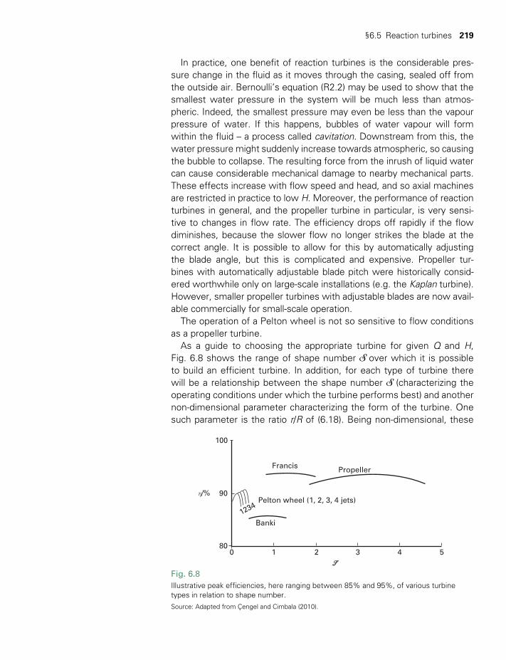
§6.5 Reaction turbines 219
In practice, one benefit of reaction turbines is the considerable pres-sure change in the fluid as it moves through the casing, sealed off from the outside air. Bernoulli’s equation (R2.2) may be used to show that the smallest water pressure in the system will be much less than atmos-pheric. Indeed, the smallest pressure may even be less than the vapour pressure of water. If this happens, bubbles of water vapour will form within the fluid – a process called cavitation. Downstream from this, the water pressure might suddenly increase towards atmospheric, so causing the bubble to collapse. The resulting force from the inrush of liquid water can cause considerable mechanical damage to nearby mechanical parts. These effects increase with flow speed and head, and so axial machines are restricted in practice to low H. Moreover, the performance of reaction turbines in general, and the propeller turbine in particular, is very sensi-tive to changes in flow rate. The efficiency drops off rapidly if the flow diminishes, because the slower flow no longer strikes the blade at the correct angle. It is possible to allow for this by automatically adjusting the blade angle, but this is complicated and expensive. Propeller tur-bines with automatically adjustable blade pitch were historically consid-ered worthwhile only on large-scale installations (e.g. the Kaplan turbine). However, smaller propeller turbines with adjustable blades are now avail-able commercially for small-scale operation.
The operation of a Pelton wheel is not so sensitive to flow conditions as a propeller turbine.
As a guide to choosing the appropriate turbine for given Q and H, Fig. 6.8 shows the range of shape number S over which it is possible to build an efficient turbine. In addition, for each type of turbine there will be a relationship between the shape number S (characterizing the operating conditions under which the turbine performs best) and another non-dimensional parameter characterizing the form of the turbine. One such parameter is the ratio r/R of (6.18). Being non-dimensional, these
Fig. 6.8Illustrative peak efficiencies, here ranging between 85% and 95%, of various turbine types in relation to shape number.Source: Adapted from Çengel and Cimbala (2010).
0
100
90
Francis Propeller
Pelton wheel (1, 2, 3, 4 jets)
Banki1234
801 2 3 4 5
η/%
TWIDELL PAGINATION.indb 219 01/12/2014 11:36

220 Hydropower
relationships may be established both theoretically and experimentally, and are used to optimize design. Details are given in the recommended texts and engineering handbooks at the end of this chapter.
§6.6 HYDROELECTRIC SYSTEMS
Overwhelmingly, hydropower generates electricity, although very occasionally water-mills, hydraulic lifts and ram pumps provide useful mechanical power (see references at the end of this chapter). All hydro-electric systems, whether large scale (as in Fig. 6.2 or Box 6.3) or small scale (Fig. 6.9), must include a water source, enclosed pressure pipe (penstock), flow control, turbine, electric generator, electrical control, and reticulation (cables and wiring) for electricity distribution.
The dam insures a steady supply of water without fluctuations, and, most importantly, enables energy storage in the reservoir. It may also provide benefits other than generating electricity (e.g. flood control, water supply, a road crossing). Small run-of-the-river systems from a reasonably steady flow may require only a retaining wall of low height (i.e. enough to keep the penstock fully immersed), but this does not provide storage.
The supply pipe (penstock) is usually a relatively major construction cost. It is cheaper if thin walled, short and of small diameter; but these conditions are seldom possible. In particular the diameter D cannot be small due to excessive head loss Hf ∝D–5 (see Problem 6.7). The greater cost of a larger pipe has to be compared with the continued loss of power by using a small pipe. A common compromise is to make Hf ≤ 0.1 Ht . For larger systems, the ‘pipe’ may include underground tunnels.
The material of the penstock needs to be both smooth (to reduce fric-tion) and strong (to withstand the static pressures, and the considerably
Fig. 6.9Layout of a micro hydroelectric system using a Pelton wheel. Note that this diagram does not indicate the water head H required.
Electricgenerator
Belt
Turbine
Nozzle
Dam
Pipe
Valve
Screen
Water
TWIDELL PAGINATION.indb 220 01/12/2014 11:36

§6.6 Hydroelectric systems 221
larger dynamic ‘water hammer’ pressures from sudden changes in flow). For small installations, PVC plastic is suitable for the main length of the pipe, perhaps with a short steel section at the bottom to withstand the larger pressures there. A screen is needed at the top of the supply pipe to intercept rubbish (e.g. leaves) before it blocks the pipe. This screen must be regularly checked and cleared of debris; however, screens utilizing
Fig. 6.10The Three Gorges hydroelectric dam in China: the world’s largest. See Box 6.3 for a more detailed description.
BOX 6.3 THE THREE GORGES DAM, YANGTZE RIVER, HUBEI PROVINCE, CHINA: THE WORLD’S LARGEST HYDROELECTRIC INSTALLATION
Completed in 2012, the dam is 2335 m long and rises 181 m above the river bed (rock). The normal level of water in the dam is 170 m above low-flow level (see Fig. 6.10). Catchment has area ~1,000,000 km2 and extends ~600 km upstream. Reservoir water surface area ~1,000 km2.
Embedded in the dam are 32 Francis turbines, each 700 MW (diameter 10 m; head 81 m; max flow 950 m3/s). There is one generator per turbine, each with rated power 700 MW at 20 kV, maximum generator electrical efficiency 96.5%. Hence, total installed electrical capacity is 22,500 MW (i.e. ≈30% of UK total capacity of all forms of electricity generation).
Power output depends on the river flow, which varies strongly with season. Output is typically ≤ 5000 MW during the November to May dry season; when there is enough flow (typically July to September) power output is limited by plant-generating capacity to 22,500 MW. The expected annual generation output is 100 TWh, implying a capacity factor of (100 X 103 GWh/ 8760 h)/(22.5 GW) = 50%.
Other benefits: flood control, year-round shipping and barge traffic above dam, ship lifts (locks) alongside dam; 190 million t/y fossil carbon potentially abated in comparison to building coal plant and 10 million t/y by using river transport instead of road.
Negative impacts include: 1300 million people displaced; 1300 archeological sites drowned (however, some have been repositioned); removal of silt increases likelihood of flooding downstream; built on an earthquake region (huge potential risk if dam breaks).
Source: http://en.wikipedia.org/wiki/Three_Gorges_Dam.
TWIDELL PAGINATION.indb 221 01/12/2014 11:36

222 Hydropower
the Coanda effect (the tendency of a fluid jet to be attracted to a nearby surface) are the least troublesome.
Small systems (~10 kW) generally use off-the-shelf generators or induction motors operated as generators (see §R1.6). If the turbine speed is not large enough to match the generator, then gearing is used. A V-belt is a common gearing mechanism, which unfortunately may give power losses of 10 to 20% in very small systems. Large systems usually have several turbines, each with one or more purpose-built generators running from the same shaft as its turbine, which minimizes both con-struction cost and power losses.
§6.6.1 Power regulation and control: grid-connected
With any hydro installation feeding electricity into a utility transmission grid, it is important that the voltage and frequency of the output match that of the rest of the grid. Although the primary generation is always at a relatively low voltage, the AC voltage may easily be increased by trans-formers, both to match the grid voltage and to minimize I2R losses in transmission. It is important that the voltage and frequency be controlled to maintain common standards and electrical device requirements. (See related discussions of electricity grids (§15.4), grid-connected wind power (§8.8) and control system principles (§1.5.3.)
With hydropower, this is done traditionally by mechanical feedback systems which control the flow through the turbine, so that it maintains constant frequency (‘speed’). For example, with a Pelton wheel, a spear valve is made to move in and out of the nozzle (as indicated in Fig. 6.9), thus regulating Q. For propeller turbines it may be possible to adjust the blade angles in addition to the flow rate. All such mechanical systems are relatively complicated and expensive, especially for smaller scale application.
Hydroelectric systems, once the turbines and generators are set up for voltage and frequency, are easy to integrate into an electricity grid. Indeed, they have several significant advantages over other generating systems:
1 If the catchment area, rainfall and dammed reservoir are large enough (or river flow is very consistent), approximately constant power can be generated day and night as ‘baseload’ plant.
2 With less water availability, stored hydropower is likely to be most valuable as ‘peak’ utility power when demand is large (e.g. morning and evening). The rapid start-up time (~1 minute) and relatively easy control are most beneficial compared with thermal power generation plant.
3 They give operating flexibility, start generating with very short notice and minimal start-up cost, and provide rapid changes in generated power over a wide range while maintaining excellent full- and part-load
TWIDELL PAGINATION.indb 222 01/12/2014 11:36

§6.6 Hydroelectric systems 223
efficiency. Within a national electricity grid network, pumped hydro-power storage (§6.7) is an asset for inflexible power plant, such as nuclear, and variable plant, such as wind power.
§6.6.2 Power regulation and control: stand-alone systems
Stand-alone, autonomous, hydro systems (e.g. for electricity supply to a village or farm) also require speed and power regulation; however, the devices they power, such as lights and small electric motors in refrig-erators, generally tolerate variations in voltage and frequency to ±10%. Moreover the currents involved are easily switched by power electronic devices, such as thyristors. This gives the possibility of a much cheaper control than the conventional mechanical systems.
With an electronic load control system, major variations in output are accomplished by manually switching nozzles completely in or out, or by manually controlling the total flow through the turbine. Finer control is achieved by an electronic feed-forward control which shares the output of the generator between the main loads (e.g. house lights) and a ballast (or ‘off-peak’) heating circuit which can tolerate a varying or intermittent supply (see Fig. 1.4(d)). The generator thus always sees a constant total load (= main + ballast); therefore it can run at constant power output, and so too can the turbine from which the power comes. The flow through the turbine does not therefore have to be continually automatically adjusted, which greatly simplifies its construction.
§6.6.3 System efficiency
Even though the efficiency of each individual power transformation step is large, there is still a significant energy loss in passing from the original potential power P0 of the water, to the electrical output Pe from the gen-erator, through the mechanical (m), electricity generation (g) and trans-mission (t) stages. These considerations of course apply to all forms of power generation. Considering the successive energy transformations, approximate systems overall efficiencies may be:
Small autonomous systems:
P
P(0.8)(0.8)(0.8) 0.5
g te
0m
η η=
≈ ≈
η (6.21)
Large utility systems:
η η=
≈ ≈
ηP
P(0.95)(0.95)(0.95) 0.86
g te
0m (6.22)
TWIDELL PAGINATION.indb 223 01/12/2014 11:36
224 Hydropower
§6.6.4 Scope for technology upgrades
Modern large hydropower turbines are close to the theoretical limit for efficiency, with up to 96% efficiency possible in optimum conditions, but continued research is needed for efficient operation over a broader range of flows. Older turbines may have smaller efficiency because of inadequate design or reduced efficiency due to corrosion and cavitation damage.
Potential therefore exists to increase energy output by retrofitting with new equipment of improved efficiency and perhaps increased capacity. For example, an estimate for the USA is that a 6% increase in output (TWh/y) might be achieved from efficiency improvements if hydro plant, fabricated in 1970 or prior years, having a total capacity of 30 GW, are replaced (Kumar et al. 2011).
There is much ongoing research aiming to extend the operational range in terms of head and discharge, and also to improve environmental per-formance and reliability and reduce costs. Most of the new technologies under development aim at utilizing low-head (<15 m) or very low-head (<5 m) sites, so allowing many more sites for hydropower.
Computational fluid dynamics (CFD) facilitates turbine design for high efficiency over a broad range of flows. There is also scope for the hydro-kinetic devices initially designed for tidal steam power (Chapter 12) to be used inland in both free-flowing rivers and in engineered waterways, such as canals and tailraces of existing water-supply dams. These devel-opments can significantly increase the technical potential for hydropower in some countries. For example, in 2004 the potential for cost-effective new mini-hydro (i.e. <10 MW) in Norway was calculated to be ~25 TWh/y (T. Jensen, www.HydroWorld.com, accessed August 31, 2012).
§6.7 PUMPED HYDRO ENERGY STORAGE
For utility supply companies, hydroelectricity provides an extremely flex-ible and reliable method of generating electricity, only constrained by lack of rainfall. The key feature is that power can be increased or decreased rapidly within seconds to fine-tune the power balance on a grid. If hydro-power is offline, it can be brought fully online within a few minutes from a ‘standing start’. If it is offline, no resource is being wasted.
A further benefit of hydropower is that a system powered from water in a reservoir and feeding water into a river or lake can be reversed. In this way excess power on the grid (e.g. from wind farms and at night from nuclear power stations) may be used to pump water uphill to the reservoir. Later, when peak electricity is needed, the water can be returned downhill to generate the necessary ‘extra’ power. Often the same machines are used as both turbines and pumps. This is a form of electricity storage – but usually on a much larger scale than other forms of electrical storage (see §15.6). Fig. 6.11 shows the layout of
TWIDELL PAGINATION.indb 224 01/12/2014 11:36
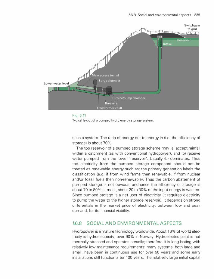
§6.8 Social and environmental aspects 225
such a system. The ratio of energy out to energy in (i.e. the efficiency of storage) is about 70%.
The top reservoir of a pumped storage scheme may (a) accept rainfall within a catchment (as with conventional hydropower), and (b) receive water pumped from the lower ‘reservoir’. Usually (b) dominates. Thus the electricity from the pumped storage component should not be treated as renewable energy such as; the primary generation labels the classification (e.g. if from wind farms then renewable, if from nuclear and/or fossil fuels then non-renewable). Thus the carbon abatement of pumped storage is not obvious, and since the efficiency of storage is about 70 to 80% at most, about 20 to 30% of the input energy is wasted. Since pumped storage is a net user of electricity (it requires electricity to pump the water to the higher storage reservoir), it depends on strong differentials in the market price of electricity, between low and peak demand, for its financial viability.
§6.8 SOCIAL AND ENVIRONMENTAL ASPECTS
Hydropower is a mature technology worldwide. About 16% of world elec-tricity is hydroelectricity; over 90% in Norway. Hydroelectric plant is not thermally stressed and operates steadily; therefore it is long-lasting with relatively low maintenance requirements: many systems, both large and small, have been in continuous use for over 50 years and some early installations still function after 100 years. The relatively large initial capital
Fig. 6.11Typical layout of a pumped hydro energy storage system.
Switchgearto grid
Main access tunnel
Surge chamberLower water level
Turbine/pump chamber
Breakers
Transformer vault
ReservoirIntake
TWIDELL PAGINATION.indb 225 01/12/2014 11:36

226 Hydropower
cost has been long since written off, with the ‘levelized’ cost of electric-ity produced (i.e. the cost per kWh averaged over the life of the system) much less than other sources, especially thermal plant which requires expenditure on fuel and more frequent replacement of machinery. If the external costs are internalized (see Chapter 17), non-renewable sources become even more expensive. For hydro plant with an ample supply of water, the flow can be controlled to produce either baseload or rapidly peaking power as demanded; if the water supply is limited, then sale of electricity at only peak demand is easy and most profitable. Nevertheless, the initial capital cost of hydropower is always relatively large, so it has been observed that ‘all power producers wish they had invested in hydro-power 20 years ago, but unfortunately cannot afford to do so now – and they said the same thing 20 years ago!’
The complications of hydropower systems arise mostly from associ-ated dams and reservoirs, particularly on the large-scale projects. Most rivers, including large rivers with continental-scale catchments, such as the Nile, the Zambesi and the Yangtze, have large seasonal flows, making floods a major characteristic. Therefore most large dams (i.e. those >15 m high) are built for multiple purposes: electricity generation, water for potable supply and irrigation, controlling river flow, mitigating floods, and providing road crossings, leisure activities, fisheries, etc. Social and economic development always requires electricity and water supply, so large-scale projects appeal to politicians and financiers seeking cen-tralized national development that is conceptually and administratively ‘simple’. However, the enormous investments and widespread impacts of hydropower have made large dams hotly contested issues in sustain-able development (World Commission on Dams 2000). Countering the benefits of large hydro, referred to above, are certainly adverse impacts; examples are debt burden (dams are often the largest single investment project in a country), cost overruns, displacement and impoverishment of people, destruction of ecosystems and fishery resources, and the inequi-table sharing of costs and benefits. For example, over one million people were displaced by the construction of the Three Gorges dam in China (Box 6.3), which has a capacity of over 22500 MW; yet these displaced people may never consider that they are, on balance, beneficiaries of the increased power capacity and industrialization. Some dams have been built on notoriously silt-laden rivers, resulting in the depletion of reser-voir volume. Various major funding agencies (including the World Bank) and stakeholder groups (e.g. UNEP, IEA, IHA) have followed the World Commission on Dams, by developing their own guidelines on sustain-ability, which hopefully will limit such mistakes in future.
Hydropower, like all renewable energy sources, mitigates emissions of the greenhouse gas CO2 by displacing fossil fuel that would otherwise have been used. However, in some dam projects, in an effort to save construction time and cost, rotting vegetation (mostly trees) has been
TWIDELL PAGINATION.indb 226 01/12/2014 11:36
§6.8 Social and environmental aspects 227
left in place as the dam fills up, which results in significant emissions of methane, another greenhouse gas. Even so, nearly all estimates of the life cycle greenhouse gas (GHG) impact of hydropower systems are less than 40 gCO2-eq/ kWh, which is an order of magnitude less than for fossil systems (see Chart D3 in Appendix D).
In many industrialized countries the technically most attractive sites were developed decades ago and so the building of large dams has all but ceased. Moreover, in the USA, dams have been decommissioned to allow increased ecological benefit from ‘environmental flow’ through downstream ecosystems. Yet hydroelectric capacity may be increased by adding turbine generators to water supply reservoirs and, for older hydropower stations, installing additional turbines and/or replacing old turbines by more efficient or larger capacity modern plant. Such devel-opments have a positive environmental impact, with no new negative impact, and is an example of using an otherwise ‘wasted’ flow of energy (cf. §1.4). Likewise, the installation of small ‘run-of-river’ hydroelectric systems, with only very small dams, is generally considered a positive development; for example, the output of such systems in China is greater than the total hydropower capacity of most other countries.
CHAPTER SUMMARY
Hydropower is the most established, widely used and long-lasting renewable resource for electricity generation. It supplies about 16% of worldwide electricity. Hydropower systems in use range from very large (~GW) to very small (~kW) capacity.
Hydropower requires topography and rainfall that can provide sufficient water flow Q and fall (head H). A first estimate of power potentially available at a site is
P0 = ρQgH
where ρ is the density of water and g is the acceleration due to gravity. Hydropower systems have excellent energy efficiency (to 95%, water to wire for large commercial plant).
The relatively expensive initial investment is offset by long lifespan (turbines and generators to ~40 y, dams >100 y), together with low-cost operation and maintenance.
Turbines are of two types: (a) impulse turbines, where the flow hits the turbine as a jet in an open environment, with the power deriving from the kinetic energy of the flow; and (b) reaction turbines, where the turbine is totally embedded in the fluid and powered from the pressure drop across the device. Impulse turbines are usually used when H is high, even if Q is low. Reaction turbines are usual when H is relatively low. The choice is governed by a non-dimensional shape number of the form
ωρ
= PgH( )
1/2
1/2 5/4S .
All hydroelectric systems must include a water source, enclosed pressure pipe (penstock), flow control, turbine, electric generator, electrical control, and reticulation (cables and wiring) for electricity distribution. The dam ensures a steady supply of water without fluctuations, and, most importantly, enables energy
TWIDELL PAGINATION.indb 227 01/12/2014 11:36

228 Hydropower
QUICK QUESTIONS
Note: Answers to these questions are in the text of the relevant section of this chapter, or may be readily inferred from it.
1 Water from a reservoir flows at 2 m3/s down a smooth and vertical penstock pipe of length 10 m before entering a turbine generator of overall efficiency 80%. What is the maximum power generated?
2 What factors affect the length, diameter and material of a penstock pipe?
3 What is an essential difference between the shape number and spe-cific speed of a hydro turbine?
4 Explain the difference in method of operation between an impulse turbine and a reaction turbine.
5 Briefly explain ‘cavitation’ that may occur in a reaction turbine. 6 Hydroelectric generation may approach 100% efficiency, whereas
thermal power generation is about 30 to 45%. Why is there such a difference?
7 List at least three benefits of hydropower generation to an electric power utility.
8 List at least three common negative environmental impacts of hydropower.
9 Why do electricity utilities in Norway fear a very cold winter?10 Which electricity-generating technologies are most likely to benefit
from pumped storage on a national network, and why?
PROBLEMS
Note: *indicates a ‘problem’ that is particularly suitable for class discus-sion or group tutorials.
*6.1 Use an atlas to estimate the hydro potential of your country or state, as follows:
(a) Call the place in question X. What is the lowest altitude in X? What area of X lies more than 300 metres above the lowest
storage in the reservoir. It may also provide benefits other than generating electricity (e.g. flood control, water supply, a road crossing).
Pumped hydro systems are used by utilities for large-scale energy storage. Excess power on the grid at a time of low demand is used to pump water uphill to a reservoir. Later, when electricity demand is greater, the water is returned downhill to generate the necessary ‘extra’ power.
The major disadvantages of hydropower are associated with effects other than the generating equipment, particularly for large systems. These include possible adverse environmental impact by the effects on fish, silting of dams, corrosion of turbines in certain water conditions, social impact of displacement of people from the reservoir site, and loss of potentially productive land. Consequently the role of large dams in promoting sustainable development is hotly contested.
TWIDELL PAGINATION.indb 228 01/12/2014 11:36
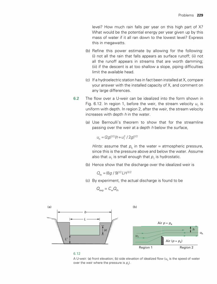
Problems 229
level? How much rain falls per year on this high part of X? What would be the potential energy per year given up by this mass of water if it all ran down to the lowest level? Express this in megawatts.
(b) Refine this power estimate by allowing for the following: (i) not all the rain that falls appears as surface runoff; (ii) not all the runoff appears in streams that are worth damming; (iii) if the descent is at too shallow a slope, piping difficulties limit the available head.
(c) If a hydroelectric station has in fact been installed at X, compare your answer with the installed capacity of X, and comment on any large differences.
6.2 The flow over a U-weir can be idealized into the form shown in Fig. 6.12. In region 1, before the weir, the stream velocity u1 is uniform with depth. In region 2, after the weir, the stream velocity increases with depth h in the water.
(a) Use Bernoulli’s theorem to show that for the streamline passing over the weir at a depth h below the surface,
u g h u g(2 ) ( / 2 )h1/2
12 1/2= +
Hints: assume that ph in the water = atmospheric pressure, since this is the pressure above and below the water. Assume also that u1 is small enough that p1 is hydrostatic.
(b) Hence show that the discharge over the idealized weir is
Q g LH(8 / 9)th1/2 3/2=
(c) By experiment, the actual discharge is found to be
Qexp = CwQth
6.12A U-weir: (a) front elevation; (b) side elevation of idealized flow (uh is the speed of water over the weir where the pressure is ph).
H
L’
b
Air p = pa
Region 2Region 1
(a) (b)
Air (p = pa)
L
huh
u1
TWIDELL PAGINATION.indb 229 01/12/2014 11:36
230 Hydropower
where Cw ≈ 0.6. (The precise value of Cw varies with H/L’ and L/b.) Explain why Cw<1.
(d) Calculate Qexp for the case L’ = 0.3 m, L = l m, b = 4 m, H = 0.2 m. Calculate also u1 and justify the assumptions about u1 used in (a) and (b).
6.3 Verify that S defined by (6.19) is dimensionless. What are the advantages of presenting performance data for turbines in dimen-sionless form?
6.4 A propeller turbine has shape number S = 4 and produces 100 kW (mechanical) at a working head of 6 m. Its efficiency is about 70%. Calculate:
(a) The flow rate.
(b) The angular speed of the shaft.
(c) The gear ratio required if the shaft is to drive a four-pole alter-nator to produce a steady 50 Hz.
6.5 A Pelton wheel cup is so shaped that the exit flow makes an angle θ with the incident jet, as seen in the cup frame. As shown in Fig. 6.6, uc is the tangential velocity of the cup, measured in the laboratory frame. The energy lost by friction between the water and the cup may be measured by a loss coefficient k such that
u u k(1 )r r12
22= +
Show that the power transferred is
P Q u u uk
( ) 1cos(1 )c j cρ θ= − +
√ +
Derive the mechanical efficiency ηm.
What is the reduction in efficiency from the ideal when θ = 7°, k = 0.1? What is the angle of deflection seen in the laboratory frame?
6.6 A Pelton wheel is to be installed in a site with H = 20 m, Qmin = 0.05 m3s–1.
(a) Neglecting friction, find: (i) the jet velocity; (ii) the maximum power available, and (iii) the radius of the nozzles (assuming there are two nozzles).
(b) Assuming the wheel has shape number
PgH( )
0.111/2
1/2 5/4
ωρ
= =S
TWIDELL PAGINATION.indb 230 01/12/2014 11:36

Bibliography 231
where P1 is the power per nozzle, find: (iv) the number of cups; (v) the diameter of the wheel, and (vi) the angular speed of the wheel in operation.
(c) If the main pipe (the penstock) had a length of 100 m, how would your answers to (a) and (b) be modified by fluid friction using: (vii) PVC pipe with a diameter of 15 cm; (viii) common plastic hosepipe with a diameter of 5 cm? In each case determine the Reynolds number in the pipe.
6.7 A steel pipe of diameter D and length L is to carry a flow Q. Assuming that the pipe friction coefficient f varies only slowly with the Reynolds number, show that the head loss due to friction is proportional to D–5 (for fixed L and Q). (Hint: Refer to §R2.6.)
*6.8 Sudan is a flat country with very little rainfall, but its own power supply is dominated by hydroelectricity. How can this be? Why does this example of Sudan differ from that of the (equally flat) country of Denmark?
BIBLIOGRAPHY
General articles and books on hydropower
Kumar, A., Schei, T., Ahenkorah, A., Caceres Rodriguez, R., Devernay, J-M., Freitas, M., Hall, D., Killingtveit, Å. and Liu, Z. (2011) ‘Hydropower’, in O. Edenhofer, R. Pichs-Madruga, Y. Sokona, K. Seyboth, P. Matschoss, S. Kadner, T. Zwickel, P. Eickemeier, G. Hansen, S. Schlömer and C. von Stechow (eds) IPCC Special Report on Renewable Energy Sources and Climate Change Mitigation, Cambridge University Press, Cambridge. Authoritative review of state of the art and potential for wider use, including sustainability issues (often referred to as SRREN).
Ramage, J. (2004, 2nd edn) ‘Hydroelectricity’, ch. 5 in G. Boyle (ed.), Renewable Energy: Power for a sustainable future, Oxford University Press, Oxford. Non-technical survey, with many photos and illustrations.
Mechanics of turbines
Most engineering textbooks on fluid mechanics include a chapter on turbomachinery; for example:
Çengel, Y.A. and Cimbala, J. (2009, 2nd edn) Fluid Mechanics: Fundamentals and applications, McGraw-Hill, New York. Clear and detailed explanations with emphasis on physical principles. Very student-friendly with exemplary accompanying learning aids.
Dixon, S.L.B. and Hall, C. ( 2010, 6th edn) Fluid Mechanics and Thermodynamics of Turbomachinery, Butterworth-Heinemann, London. An established textbook for professional engineers.
Massey, B. and Ward-Smith, J. (2011, 9th edn) Mechanics of Fluids,, CRC Press, London. Longer account of turbomachinery than some other general textbooks, but still at student level.
Wagner, H-J. and Mathur, J. (2011) Introduction to Hydro Energy Systems: Basics, technology and operation, Springer, New York. Textbook for students.
TWIDELL PAGINATION.indb 231 01/12/2014 11:36

232 Hydropower
Small-scale (mini) hydropower (~1 to 100 kW)
Bhatti, T.S., Bansal, R.C. and Kothari, D.P. (eds) (2004) Small Hydro Power Systems, Dhanpat Rai & Co, Delhi, India. General principles and illuminating case studies, based on experience in India.
Khennas, S. and Barnett, A. (2000) Best Practices for Sustainable Development of Micro Hydro Power in Developing Countries, ITDG, London. Available on the web at www.microhydropower.net; see also (much shorter) ITDG technical brief on micro hydro power at www.itdg.org.
Moniton, L., Le Nir, M. and Roux, J. (1984) Micro Hydroelectric Power Stations, Wiley, Chichester. Translation of a French text of 1981.
Tong Jiandong et al. (1996) Mini Hydropower, UNESCO/ Wiley, Chichester. Useful summary of extensive Chinese experience.
US Department of Energy (1988) Small-scale Hydropower Systems, NCIS, Washington, DC. Non-technical account with many good line drawings.
Water Power and Dam Construction (1990) ‘Micro hydro: current practice and future development’, Scottish Seminar, special issue.
Pumped hydro systems
Deane, J.P., O’Gallachoir, B.P. and McKeogh, E.J. (2010) ‘Techno-economic review of existing and new pumped hydro energy storage plant’, Renewable and Sustainable Energy Reviews, 14, 1293–1302.
Mechanical uses: hydraulic ram
The hydraulic ram is a mechanical device which uses a flow with high Q and low H to pump water to a higher site (with higher H and lower Q).
Inverson, A.R. (1978) Hydraulic Ram Pump, Volunteers in Technical Assistance, Maryland, USA, Technical Bulletin no. 32. Construction plans of the ram itself.
Jeffrey, T.D., Thomas, T.H., Smith, A.V., Glover, P.B. and Fountain, P.D. (1992) Hydraulic Ram Pumps: A guide to ram pump water supply systems, ITDG Publishing, UK. See also ITDG technical brief ‘hydraulic ram pumps’, online at www.itdg.org.
Krol, J. (1951) ‘The automatic hydraulic ram’, Proceedings of the Institute of Mechanical Engineering, 165, 53–65. Mathematical theory and some supporting experiments. Clumsy writing makes the analysis seem difficult.
Twidell, J. and Weir, T. (2006, 2nd edn) Renewable Energy Resources,, Taylor & Francis, Oxon. §8.7 gives a brief account of the hydraulic ram and is reproduced in the online supplementary material for this book. See eResource S6.1 on the publisher’s website: www.routledge.com/books/details/9780415584388.
Watt, S.B. (1975) A Manual on the Hydraulic Ram for Pumping Water, Intermediate Technology Publications, London. Plans for an alternative design of home-made ram, plus details of installation and operation.
Institutional and environmental issues
International Energy Agency (1993) Hydropower, Energy and the Environment. Conference proceedings, but with a useful overview. Focuses on implications of upgrades to existing facilities.
TWIDELL PAGINATION.indb 232 01/12/2014 11:36

Bibliography 233
Moreira, J.R. and Poole, A.D. (1993) ‘Hydropower and its constraints’, in T. Johansson et al. (eds), Renewable Energy: Sources for fuels and electricity, Earthscan, London, pp. 71–119. Good survey of global issues and potential, with focus on social and environmental constraints, and case studies from Brazil.
World Commission on Dams (2000) Dams and Development: A new framework for decision making (at www.dams.org). The Commission was set up by the World Bank and the International Union for the Conservation of Nature to review the effectiveness of large dams in fostering economic and social development and to develop new criteria for assessing proposals for such dams.
See also Kumar et al. (2011), listed above under ‘General articles’.
Journals and websites
Water Power and Dam Construction, monthly, Quadrant House, Sutton, UK. General journal including production information, conference reports, articles, etc.
World Energy Council (2010) Survey of Energy Resources 2010 (chapter on hydropower). Available on web at www.worldenergy.org/wec-geis/publications/reports/ser/hydro/hydro.asp. Data on installed capacity and techni-cal potential for numerous countries, compiled by utilities and energy agencies; publication covers other energy resources as well, including fossil and even OTEC (usually updated every three years).
http://en.wikipedia.org/wiki/Hydroelectricity (excellent summary with important links).
http://hydroelectric-energy.blogspot.com/ News on new hydro developments.
http://www.eia.gov/ US Energy Information Administration offers vast reservoir of energy statistics, including hydropower, from around the world.
www.Indexmundi.com. Has some conveniently plotted graphs based on EIA data.
TWIDELL PAGINATION.indb 233 01/12/2014 11:36

Wind resource
CHAPTER
7
CONTENTS
Learning aims 234
§7.1 Introduction 236
§7.2 World wind 237§7.2.1 Global effects 237§7.2.2 Planetary boundary layer
and turbulence 240§7.2.3 Regional wind power
resource assessment 240
§7.3 Characteristics of the wind 242§7.3.1 Basic meteorological data
and wind speed time series 242§7.3.2 Variation with height 243§7.3.3 Wind speed analysis, probability
and prediction 248§7.3.4 Wind speed probability
distributions: Weibull and Rayleigh 248
§7.3.5 Wind speed and direction: variation with time and distance 254
§7.4 Wind instrumentation, measurement and computational tools for prediction 258§7.4.1 Traditional established
instruments 258§7.4.2 Instrument towers 259§7.4.3 Wind speed and direction
instruments for commercial and research use 259
§7.4.4 Other indicators and instruments 262
§7.4.5 Computational tools for assessing wind power potential 262
§7.4.6 Short-term predictions 263
Chapter summary 264
Quick questions 264
Problems 265
Bibliography 266
LEARNING AIMS
• Appreciate how wind occurs and how it is measured.
• Appreciate the variation of wind speed: – over time on scales of years, months,
hours, and seconds; – from region to region and from site to
site within a region (i.e. the effect of local terrain and obstructions);
– with height.
• Appreciate the probability distribution of wind speed, including the Weibull and Rayleigh distributions.
TWIDELL PAGINATION.indb 234 01/12/2014 11:36
List of tables 235
LIST OF FIGURES
7.1 Circulation of the Earth’s Atmosphere (schematic). 2377.2 Average wind speeds across the world in January and July. 2397.3 Regional wind speed map for the USA. 2417.4 Wind speed time and frequency plots. 2467.5 Wind rose from accumulated data. 2477.6 Wind speed variation with height; ‘wind shear’. 2477.7 Probability distribution of wind speed against wind speed. 2507.8 Probability of wind speeds greater than a particular speed u’. 2517.9 Distribution of power in the wind, for example, of North Ronaldsay. 2517.10 Power per unit area in the wind against probability of wind speeds greater than a particular
speed u’. 2527.11 Weibull distribution curves. 2537.12 Some instruments for measuring wind speed and/or direction. 260
LIST OF TABLES
7.1 Wind speed relationships based on the Beaufort scale. 2447.2 Wind speed analysis for North Ronaldsay. 250
TWIDELL PAGINATION.indb 235 01/12/2014 11:36

236 Wind resource
§7.1 INTRODUCTION
The extraction of power from the wind with modern turbines and energy conversion systems is an established global industry. This chapter focuses on the wind power resource and its measurement; the technol-ogy to extract this power follows in Chapter 8. We are particularly inter-ested in average and above-average wind speeds, because the power in the wind is proportional to the cube of the wind speed, as shown in §8.3.1. We are also interested in (a) how wind occurs; (b) measure-ment; (c) variation with time, because of output power fluctuations; (d) increase of wind speed with height above the ground, since blade tips of very large machines may be 200 metres high; (e) turbulence and gusts; (f) local site conditions and obstructions, including other turbines, which affect generated output, and (g) prediction, so that electricity grid operators can plan ahead.
Wind results from expansion and convection of air as solar radiation is absorbed on Earth. On a global scale these thermal effects combine with dynamic effects from the Earth’s rotation to produce prevailing wind pat-terns. The kinetic energy stored in the winds is about 0.7 × 10²¹ J, and this is dissipated by friction, mainly in the air but also by contact with the ground and the sea. About 1% of absorbed solar radiation, 1200 TW (1200 × 1012 W), is dissipated in this way. In addition to this general syn-optic behavior of the Atmosphere there is considerable regional and local variation caused by geographical and environmental factors. In general, wind speeds increase with height, with the horizontal components sig-nificantly greater than the vertical components.
Wind speed varies significantly with time over periods from seconds to seasons and years, and over distances ~1 km, especially in hilly terrain. Therefore it is important to make measurements at the nomi-nated site at several heights for at least 12 months and compare these with official meteorological data and wind atlas information. The infor-mation enables the prediction of power generation from nominated tur-bines for the site.
A major design criterion for turbines is the need to protect the machine against damage in very strong and turbulent winds, even though such gale-force winds are relatively infrequent. Wind forces tend to increase as the square of the wind speed and the amplitude of turbulent varia-tion increase similarly. Therefore fatigue damage may occur, especially related to the blades and drive train; so wind speed variation of one minute and less must be understood across the area of turbine rotor.
Fortunately there are other industries and services that need to know about wind conditions and so information can be shared; this includes meteorological services, agriculture, aircraft and airports, building and bridge construction, and road safety.
TWIDELL PAGINATION.indb 236 01/12/2014 11:36
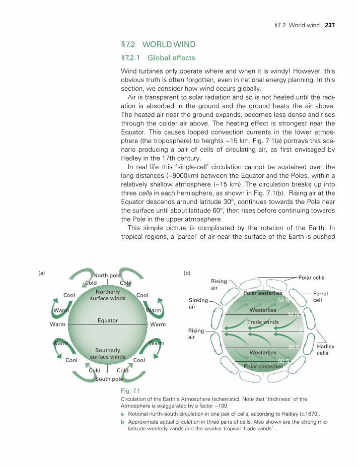
§7.2 World wind 237
§7.2 WORLD WIND
§7.2.1 Global effects
Wind turbines only operate where and when it is windy! However, this obvious truth is often forgotten, even in national energy planning. In this section, we consider how wind occurs globally.
Air is transparent to solar radiation and so is not heated until the radi-ation is absorbed in the ground and the ground heats the air above. The heated air near the ground expands, becomes less dense and rises through the colder air above. The heating effect is strongest near the Equator. This causes looped convection currents in the lower atmos-phere (the troposphere) to heights ~15 km. Fig. 7.1(a) portrays this sce-nario producing a pair of cells of circulating air, as first envisaged by Hadley in the 17th century.
In real life this ‘single-cell’ circulation cannot be sustained over the long distances (~9000km) between the Equator and the Poles, within a relatively shallow atmosphere (~15 km). The circulation breaks up into three cells in each hemisphere, as shown in Fig. 7.1(b). Rising air at the Equator descends around latitude 30°, continues towards the Pole near the surface until about latitude 60°, then rises before continuing towards the Pole in the upper atmosphere.
This simple picture is complicated by the rotation of the Earth. In tropical regions, a ‘parcel’ of air near the surface of the Earth is pushed
Fig. 7.1Circulation of the Earth’s Atmosphere (schematic). Note that ‘thickness’ of the Atmosphere is exaggerated by a factor ~100.a Notional north–south circulation in one pair of cells, according to Hadley (c.1670).b Approximate actual circulation in three pairs of cells. Also shown are the strong mid-
latitude westerly winds and the weaker tropical ‘trade winds’.
Northerlysurface winds
Equator
North pole
South pole
ColdCold
Cold Cold
Cool
(a)
Cool
Cool
Cool
WarmWarm
Warm Warm
WarmWarmSoutherly
surface winds
(b)
Polar easterlies
Westerlies
60 N
Polar cellsRisingair
Risingair
Sinkingair
Ferrelcell
Hadleycells
30 N
30 S
0
Trade winds
Westerlies
Polar easterlies60 S
TWIDELL PAGINATION.indb 237 01/12/2014 11:36

238 Wind resource
towards the Equator by the thermal circulation, thus moving to a region where the rotational speed of the Earth is greater than that where the air came from, so the ‘parcel’ of air is ‘left behind’ by the surface under-neath and arrives at a point to the west of where it would have been if it moved purely from north to south. Thus the ‘wind’ (i.e. the air move-ment near surface level) appears to an observer on the surface of the Earth to be coming from the northeast (in the northern hemisphere) or from the southeast (in the southern hemisphere) (see Fig.7.1(b)). This usually moderate prevailing NE or SE wind is called a ‘trade wind’, owing to the use sailing ships made of it. Similarly, the polar cell sets up strong easterly winds.
In the mid-latitudes, where surface air is going towards the Poles, it is moving into regions of slower rotational speeds, and is therefore traveling faster than the new surface. An observer here senses the wind blowing from the west – the so-called westerlies (a westerly wind is one coming from the west). The westerly component of this mid-latitude wind is stronger than that of the easterly component in the trade winds, because the difference in rotation speed across latitude is greater; hence the name ‘roaring forties’.
The maps in Fig. 7.2 show that the strongest prevailing winds occur over the ocean in the ‘roaring forties’ and weaken over continents. Successful harnessing of wind power requires strong, steady winds and a population with a demand for energy. The maps indicate that north-western USA, northwestern Europe (including Britain and Ireland), New Zealand and Chile are all such favorable regions. Fig. 7.2 also illustrates that in summer the ‘roaring forties’ are further towards the Pole, and in winter they move into the mid-latitudes; this is because the declination of the Earth (§2.4) implies that the region of rising air near the Equator moves north to south with the seasons.
Understanding wind within the whole discipline of meteorology is a major analytical challenge in association with comprehensive meas-urement and data recording (see this chapter’s bibliography for further and in-depth information). In addition to the global circulation described so far, there are a multitude of other effects with significant seasonal, regional and local variation.
(a) Effect of oceans and continentsSolar radiation heats land quickly but oceans slowly; however, the thermal capacity of ocean near-surface water is large and so contrasts with con-tinental land mass. The relative effects are seasonal as solar inclination and other effects change through the year. Extreme winds occur in hur-ricanes (tropical cyclones) and monsoons as moisture, mostly taken from the ocean, condenses to water (rain) with the release of latent heat. Similar effects, but less extreme, occur in all cyclonic weather as air not only circulates, but moves upwards and downwards. These movements
TWIDELL PAGINATION.indb 238 01/12/2014 11:36
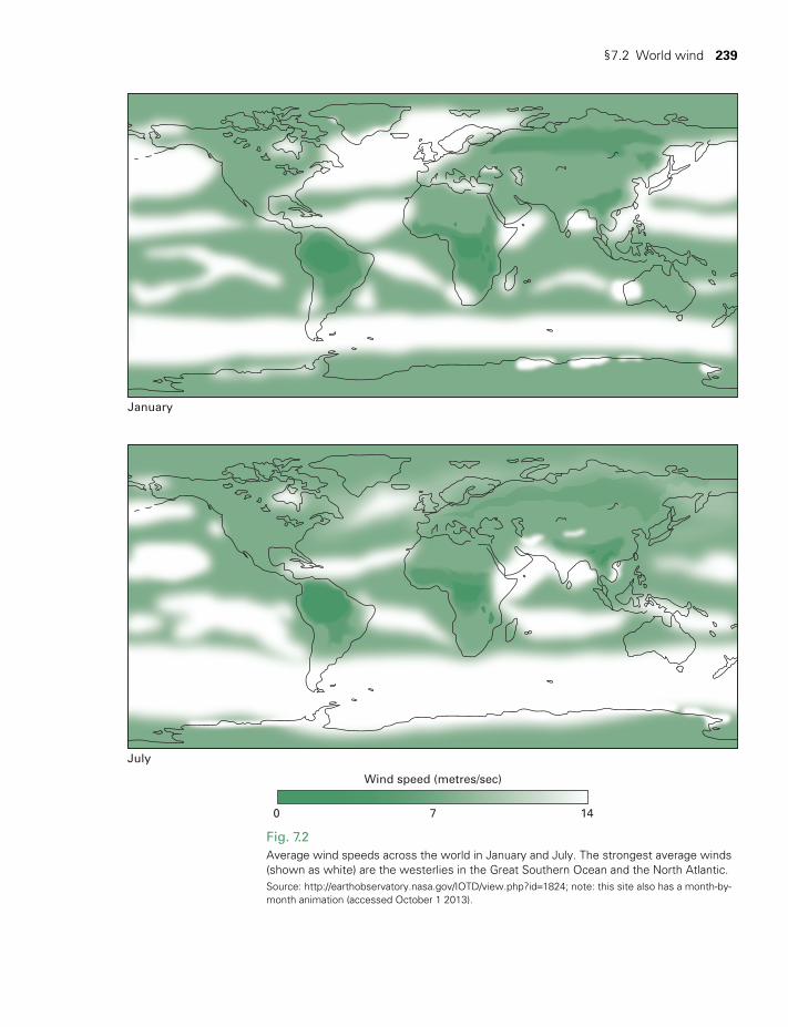
§7.2 World wind 239
Fig. 7.2 Average wind speeds across the world in January and July. The strongest average winds (shown as white) are the westerlies in the Great Southern Ocean and the North Atlantic.Source: http://earthobservatory.nasa.gov/IOTD/view.php?id=1824; note: this site also has a month-by-month animation (accessed October 1 2013).
Wind speed (metres/sec)
July
January
0 7 14Wind speed (metres/sec)
July
January
0 7 14
TWIDELL PAGINATION.indb 239 01/12/2014 11:36
240 Wind resource
are experienced as wind. On a smaller scale, the uneven heating of land and sea produces local diurnal sea breezes.
(b) Effects of land shape The complex terrain of hills and mountains deflects and concentrates air movement, with significant effect on wind. Daily variation of such winds occurs due to uneven solar absorption and height differences, and with concentration, as in valleys. Movement of air over mountains may lead to deposition of rain on windward sides and air warmed by its increasing pressure on the leeward side (Föhn wind).
(c) Effects by season and timeIn the great majority of locations, average wind speed and direction depend on the season in the year, and in many locations on the time of the day. Meteorological services know these effects well and can make reasonably reliable forecasts. However, there is almost complete igno-rance about predicting variation from year to year, which for wind power can cause significant variation affecting the economics of installations.
Such comprehensive knowledge is needed to be able to choose pro-ductive wind turbine sites and to predict wind conditions and hence wind-generated power, as, for instance, in wind atlases, as described in §7.2.3.
§7.2.2 Planetary boundary layer and turbulence
Turbulence is change of wind speed and wind direction in both the hori-zontal plane and the vertical direction. Meteorologists speak of the plan-etary boundary layer as the lowest region of the Earth’s Atmosphere where there is marked turbulence caused by friction with the ground and disturbance by obstructions, such as trees, large buildings, cities and hills. This boundary layer varies in thickness from about 250 m over sea to about 500 m over cities and craggy country. Above the boundary layer, air movement is smooth (laminar), unless there are major storms or hurricanes; an unusual feature are the jet streams at heights between about 10 to 15 km, affecting weather and aircraft, but not wind tur-bines directly. The largest wind turbines have top blade-tip heights of about 150 m, so definitely all wind turbines operate within the planetary boundary layer and always experience turbulence in the wind. This has significant impact on the design of the turbines, especially regarding the strength and toughness of the blades and the drive-train components.
§7.2.3 Regional wind power resource assessment
There are many publications, websites and software tools to help deter-mine the wind power potential of countries, regions and local areas.
TWIDELL PAGINATION.indb 240 01/12/2014 11:36

§7.2 World wind 241
Fig. 7.3(a) Southern France; Note the localised regional windiness of the Rhone valley and western Mediterranean coast.Credit: European Wind Atlas, DTU Wind Energy, formerly RISO National Laboratory.
(b) Regional wind speed map for the USA. Note the distinctive strong winds associated with mountain and valley regions of the central west. The contours represent average wind power (proportional to wind speed cubed; see §8.3), with dark green the largest (u- >7/m/s).Source: http://rredc.nrel.gov/wind/pubs/atlas/maps/chap2/2-01m.html.
> 6,0
Sheltered terrain
Wind resource at 50 metres above ground levelfor five different topographic conditions m/s.
(a)
(b)UNITED STATES ANNUAL AVERAGE WIND POWER
Open plan At a sea coast Open sea Hills and ridges
< 3,5
5,0–6,0
4,5–5,0
3,5–4,5
> 7,5
< 4,5
6,5–7,5
5,5–6,5
4,5–5,5
> 8,5 > 9,0
< 5,0 < 5,5
7,0–8,5 8,0–9,0
7,0–8,0
5,5–7,0
> 11,5
< 7,0
10,0–11,5
8,5–10,0
7,0–8,5
6,0–7,0
5,0–6,0
Windpowerclass
1
2
3
4
5
6
7
0
100
150
200
250
300
400
1000
Ridge crest estimates (local relief > 1000 ft)
Classes of windpower density
0
4.4
5.1
5.6
6.0
6.4
7.0
9.4
0
9.8
11.5
12.5
13.4
14.3
15.7
21.1
0
200
300
400
500
600
800
2000
0
5.6
6.4
7.0
7.5
8.0
8.8
11.9
0
12.5
14.3
15.7
16.8
17.9
19.7
26.6
Wind powerW/m2
Wind powerW/m2
10m (33 f t) 50m (164 f t)Speed
m / s mphSpeed
m / s mph
0 100 200 300miles
0 100 200 300kilometres
Alaska
Principal Hawaiian Islands
0 100 200miles
0 100 200kilometres
0 100 200miles
0 100 200kilometres
0 100 200miles
PUERTO RICO
0 100 200kilometres
TWIDELL PAGINATION.indb 241 01/12/2014 11:37

242 Wind resource
Of basic importance are wind power atlases associated with software tools, of which the most international are those produced by the WAsP program (see www.windatlas.dk). The atlases and software specify and derive wind speed seasonal averages that may be applied to regional areas with different geographical features within the general area, for instance, ‘sheltered terrain’ (e.g. near forest), ‘open plain’, ‘sea coast’, ‘open sea’ and ‘hills and ridges’. See §7.4.5.
Fig. 7.3 shows wind maps of southern France and of the United States from such atlases. Both show strong wind speed locations at lower ground near mountains, and/or where wind is channeled by synoptic weather patterns and/or diurnal solar heating gives strong wind speeds in mountain valleys, and/or near large stretches of open water. Such local effects can be extremely important for regional wind power.
§7.3 CHARACTERISTICS OF THE WIND
§7.3.1 Basic meteorological data and wind speed time series
All countries have national meteorological services that record and publish weather-related data, including wind speeds and directions. The methods are well established and coordinated within the World Meteorological Organisation in Geneva, with the main aim of providing continuous runs of data for many years. Data tend to be recorded at a relatively few per-manently staffed official stations using robust and trusted equipment. Unfortunately for wind power prediction, official measurements of wind speed tend to be measured only at the one standard height of 10 m, and at stations near to airports or towns where shielding from the wind may be a natural feature of the site. Such data are, however, important as basic ‘anchors’ for computerized wind modeling, but are not suit-able to apply directly to predict wind power conditions at a specific site. Standard meteorological wind data from the nearest official station are only useful as first-order estimates; they are not sufficient for detailed planning, especially in hilly (complex) terrain. Measurements at the nomi-nated site at several heights are needed to predict the power produced by particular turbines. Such measurements, even for a few months but best for a year, are compared with standard meteorological data so that the short-term comparison may be used for longer term prediction; the technique is called ‘measure-correlate-predict’. In addition, information is held at specialist wind power data banks that are obtained from aircraft measurements, wind power installations and mathematical modeling, etc. Such organized and accessible information is increasingly available on the Internet. Wind power prediction models (§7.4.5) (e.g. the propri-etary WAsP models developed in Denmark) enable detailed wind power prediction for prospective wind turbine sites from relatively sparse local data, even in hilly terrain.
TWIDELL PAGINATION.indb 242 01/12/2014 11:37
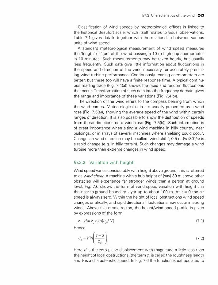
§7.3 Characteristics of the wind 243
Classification of wind speeds by meteorological offices is linked to the historical Beaufort scale, which itself relates to visual observations. Table 7.1 gives details together with the relationship between various units of wind speed.
A standard meteorological measurement of wind speed measures the ‘length’ or ‘run’ of the wind passing a 10 m high cup anemometer in 10 minutes. Such measurements may be taken hourly, but usually less frequently. Such data give little information about fluctuations in the speed and direction of the wind necessary for accurately predict-ing wind turbine performance. Continuously reading anemometers are better, but these too will have a finite response time. A typical continu-ous reading trace (Fig. 7.4(a)) shows the rapid and random fluctuations that occur. Transformation of such data into the frequency domain gives the range and importance of these variations (Fig. 7.4(b)).
The direction of the wind refers to the compass bearing from which the wind comes. Meteorological data are usually presented as a wind rose (Fig. 7.5(a)), showing the average speed of the wind within certain ranges of direction. It is also possible to show the distribution of speeds from these directions on a wind rose (Fig. 7.5(b)). Such information is of great importance when siting a wind machine in hilly country, near buildings, or in arrays of several machines where shielding could occur. Changes in wind direction may be called ‘wind shift’; 0.5 rad/s (30°/s) is a rapid change (e.g. in hilly terrain). Such changes may damage a wind turbine more than extreme changes in wind speed.
§7.3.2 Variation with height
Wind speed varies considerably with height above ground; this is referred to as wind shear. A machine with a hub height of (say) 30 m above other obstacles will experience far stronger winds than a person at ground level. Fig. 7.6 shows the form of wind speed variation with height z in the near-to-ground boundary layer up to about 100 m. At z = 0 the air speed is always zero. Within the height of local obstructions wind speed changes erratically, and rapid directional fluctuations may occur in strong winds. Above this erratic region, the height/wind speed profile is given by expressions of the form
z − d = z0 exp(uz / V ) (7.1)
Hence
u Vz d
zlnz
0
=−
(7.2)
Here d is the zero plane displacement with magnitude a little less than the height of local obstructions, the term z0 is called the roughness length and V is a characteristic speed. In Fig. 7.6 the function is extrapolated to
TWIDELL PAGINATION.indb 243 01/12/2014 11:37
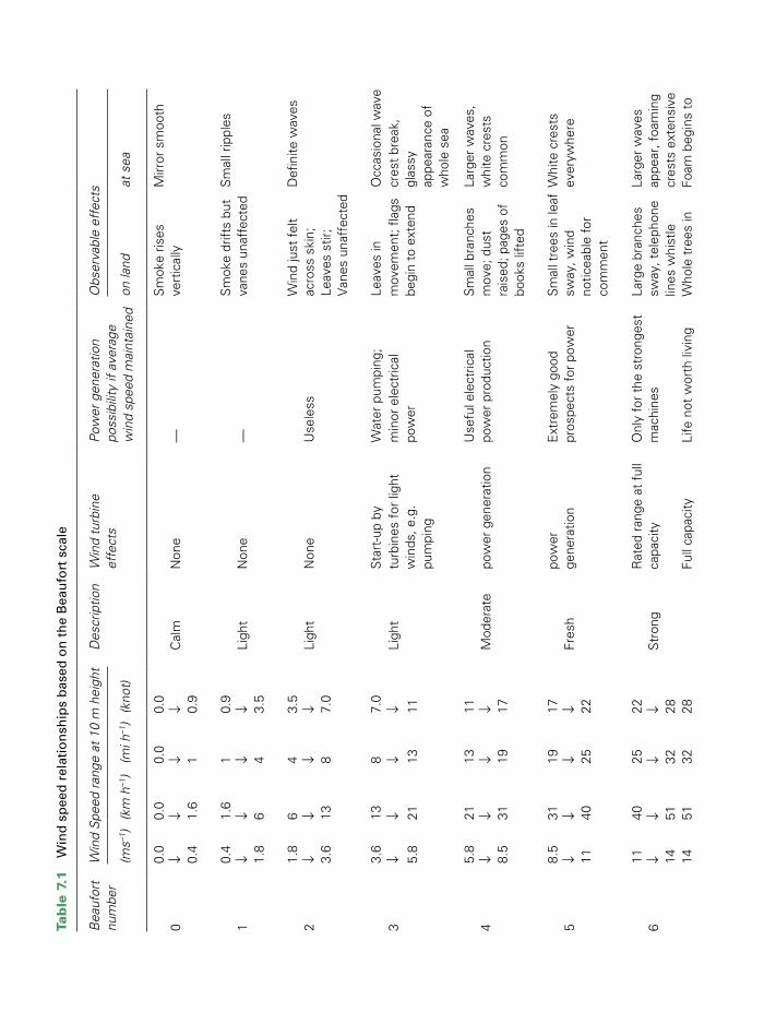
Tab
le 7
.1
Win
d s
pee
d r
elat
ion
ship
s b
ased
on
th
e B
eau
fort
sca
le
Bea
ufor
t nu
mbe
rW
ind
Spe
ed r
ange
at
10 m
hei
ght
Des
crip
tion
Win
d tu
rbin
e
effe
cts
Pow
er g
ener
atio
n po
ssib
ility
if a
vera
ge
win
d sp
eed
mai
ntai
ned
Obs
erva
ble
effe
cts
(ms–1
)(k
m h
–1)
(mi h
–1)
(kno
t)on
land
at s
ea
0.0
0.0
0.0
0.0
Sm
oke
rises
ve
rtic
ally
Mirr
or s
moo
th0
↓↓
↓↓
Cal
mN
one
—0.
41.
61
0.9
0.4
1.6
10.
9S
mok
e dr
ifts
but
vane
s un
affe
cted
Sm
all r
ippl
es1
↓↓
↓↓
Ligh
tN
one
—1.
86
43.
5
1.8
64
3.5
Win
d ju
st f
elt
Def
inite
wav
es2
↓↓
↓↓
Ligh
tN
one
Use
less
acro
ss s
kin;
3.6
138
7.0
Leav
es s
tir;
Van
es u
naff
ecte
d
3.6
138
7.0
Sta
rt-u
p by
Wat
er p
umpi
ng;
Leav
es in
Occ
asio
nal w
ave
3↓
↓↓
↓Li
ght
turb
ines
for
ligh
t w
inds
, e.g
. pu
mpi
ng
min
or e
lect
rical
pow
erm
ovem
ent;
fla
gsbe
gin
to e
xten
dcr
est
brea
k,
glas
sy
appe
aran
ce o
f w
hole
sea
5.8
2113
11
5.8
2113
11U
sefu
l ele
ctric
alS
mal
l bra
nche
sLa
rger
wav
es,
4↓ 8.
5↓ 31
↓ 19↓ 17
Mod
erat
epo
wer
gen
erat
ion
pow
er p
rodu
ctio
nm
ove;
dus
t ra
ised
; pag
es o
f bo
oks
lifte
d
whi
te c
rest
s co
mm
on
8.5
3119
17po
wer
Ext
rem
ely
good
Sm
all t
rees
in le
afW
hite
cre
sts
5↓ 11
↓ 40↓ 25
↓ 22Fr
esh
gene
ratio
npr
ospe
cts
for
pow
ersw
ay, w
ind
notic
eabl
e fo
rev
eryw
here
com
men
t
1140
2522
Rat
ed r
ange
at
full
Onl
y fo
r th
e st
rong
est
Larg
e br
anch
esLa
rger
wav
es6
↓↓
↓↓
Str
ong
capa
city
mac
hine
ssw
ay, t
elep
hone
appe
ar, f
oam
ing
1451
3228
lines
whi
stle
cres
ts e
xten
sive
1451
3228
Full
capa
city
Life
not
wor
th li
ving
Who
le t
rees
inFo
am b
egin
s to
TWIDELL PAGINATION.indb 244 01/12/2014 11:37
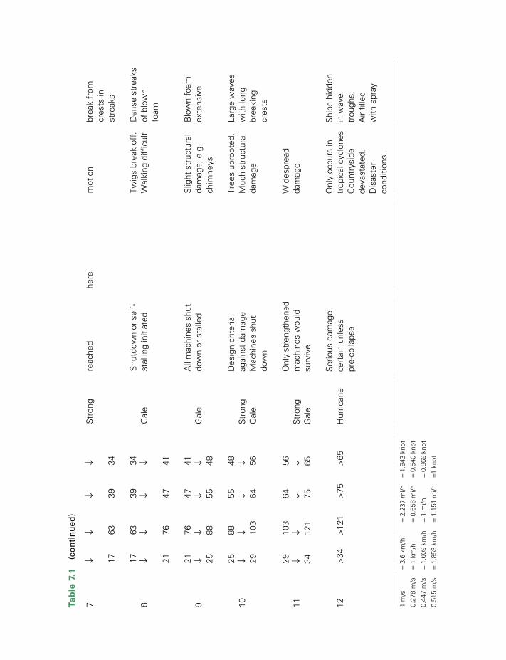
7↓
↓↓
↓S
tron
gre
ache
dhe
rem
otio
nbr
eak
from
cr
ests
in17
6339
34st
reak
s
1763
3934
Shu
tdow
n or
sel
f-st
allin
g in
itiat
edTw
igs
brea
k of
f.D
ense
str
eaks
of
blo
wn
fo
am8
↓↓
↓↓
Gal
eW
alki
ng d
iffic
ult
2176
4741
2176
4741
All
mac
hine
s sh
utS
light
str
uctu
ral
Blo
wn
foam
9↓
↓↓
↓G
ale
dow
n or
sta
lled
dam
age,
e.g
.ex
tens
ive
2588
5548
chim
neys
2588
5548
Des
ign
crite
riaTr
ees
upro
oted
. M
uch
stru
ctur
al
dam
age
Larg
e w
aves
w
ith lo
ng
brea
king
cres
ts
10↓
↓↓
↓S
tron
gag
ains
t da
mag
e29
103
6456
Gal
eM
achi
nes
shut
do
wn
2910
364
56O
nly
stre
ngth
ened
Wid
espr
ead
11↓
↓↓
↓S
tron
gm
achi
nes
wou
ldda
mag
e34
121
7565
Gal
esu
rviv
e
Ser
ious
dam
age
cert
ain
unle
ss
pre-
colla
pse
Onl
y oc
curs
intr
opic
al c
yclo
nes
Cou
ntry
side
de
vast
ated
. D
isas
ter
cond
ition
s.
Shi
ps h
idde
n
in w
ave
trou
ghs.
A
ir fil
led
with
spr
ay
12>
34>
121
>75
>65
Hur
rican
e
1 m
/s
= 3.
6 km
/h
= 2.
237
mi/h
=
1.94
3 kn
ot
0.27
8 m
/s
= 1
km/h
=
0.65
8 m
i/h
= 0.
540
knot
0.44
7 m
/s
= 1.
609
km/h
=
1 m
i/h
= 0.
869
knot
0.51
5 m
/s
= 1.
853
km/h
=
1.15
1 m
i/h
=1 k
not
Tab
le 7
.1
(co
nti
nu
ed)
TWIDELL PAGINATION.indb 245 01/12/2014 11:37
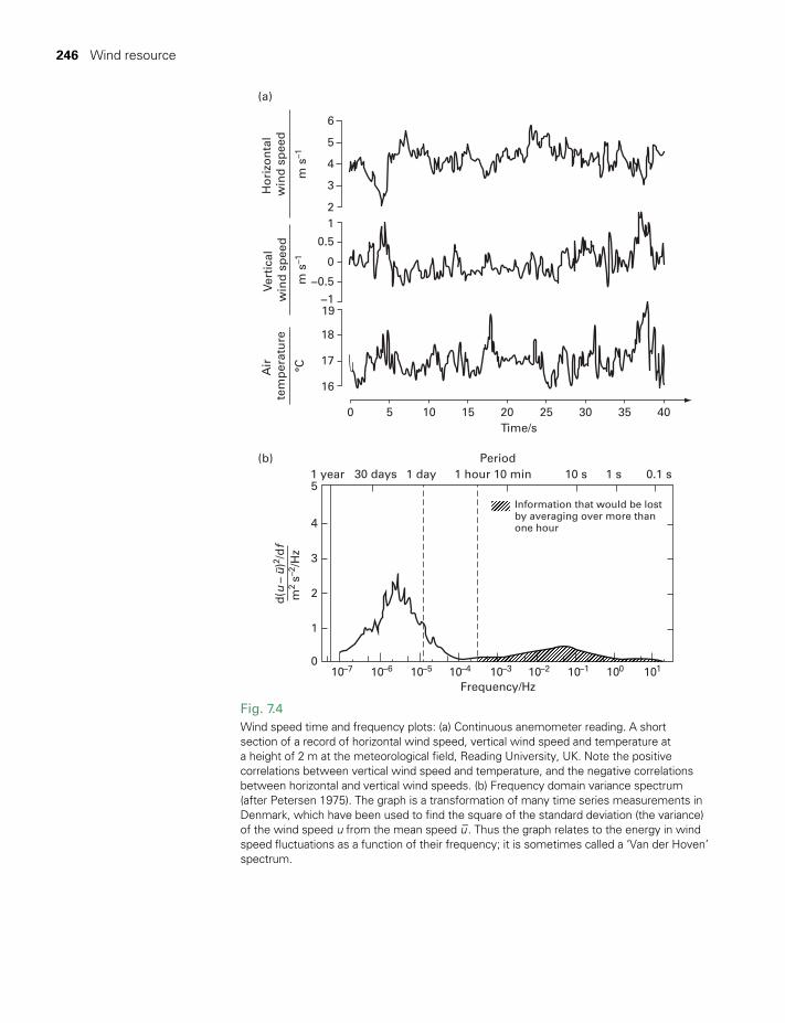
246 Wind resource
Fig. 7.4Wind speed time and frequency plots: (a) Continuous anemometer reading. A short section of a record of horizontal wind speed, vertical wind speed and temperature at a height of 2 m at the meteorological field, Reading University, UK. Note the positive correlations between vertical wind speed and temperature, and the negative correlations between horizontal and vertical wind speeds. (b) Frequency domain variance spectrum (after Petersen 1975). The graph is a transformation of many time series measurements in Denmark, which have been used to find the square of the standard deviation (the variance) of the wind speed u from the mean speed u–. Thus the graph relates to the energy in wind speed fluctuations as a function of their frequency; it is sometimes called a ‘Van der Hoven’ spectrum.
6
5
4
3
21
0.5
−0.5
−119
18
17
16
0 5 10
10–7 10–6 10–5 10–4 10–3
Frequency/Hz10–2 10–1 100 101
15 20 25 30 35 40Time/s
1 year5
4
3
2
1
0
1 day 1 hour 10 min 10 s 1 s 0.1 sPeriod
Information that would be lostby averaging over more thanone hour
(b)
(a)
30 days
Air
te
mp
erat
ure
°C
0Ve
rtic
al
win
d s
pee
d
m s
–1
Ho
rizo
nta
l w
ind
sp
eed
m s
–1
d(u
– u
)2 /d
fm
2 s–2
/Hz
TWIDELL PAGINATION.indb 246 01/12/2014 11:37
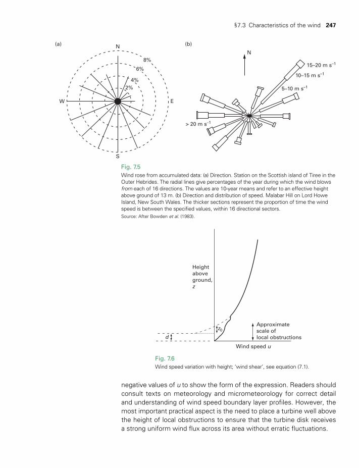
§7.3 Characteristics of the wind 247
Fig. 7.5Wind rose from accumulated data: (a) Direction. Station on the Scottish island of Tiree in the Outer Hebrides. The radial lines give percentages of the year during which the wind blows from each of 16 directions. The values are 10-year means and refer to an effective height above ground of 13 m. (b) Direction and distribution of speed. Malabar Hill on Lord Howe Island, New South Wales. The thicker sections represent the proportion of time the wind speed is between the specified values, within 16 directional sectors.Source: After Bowden et al. (1983).
N
2%
W
S
E
(a)
4%
6%
8%
(b)
N
> 20 m s–1
5–10 m s–1
10–15 m s–1
15–20 m s–1
Fig. 7.6Wind speed variation with height; ‘wind shear’, see equation (7.1).
d
Wind speed u
Approximatescale oflocal obstructions
Heightaboveground,z
z0
negative values of u to show the form of the expression. Readers should consult texts on meteorology and micrometeorology for correct detail and understanding of wind speed boundary layer profiles. However, the most important practical aspect is the need to place a turbine well above the height of local obstructions to ensure that the turbine disk receives a strong uniform wind flux across its area without erratic fluctuations.
TWIDELL PAGINATION.indb 247 01/12/2014 11:37
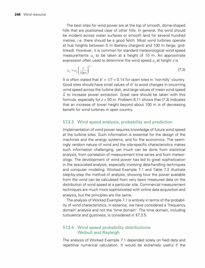
248 Wind resource
The best sites for wind power are at the top of smooth, dome-shaped hills that are positioned clear of other hills. In general, the wind should be incident across water surfaces or smooth land for several hundred metres, i.e. there should be a good fetch. Most wind turbines operate at hub heights between 5 m (battery chargers) and 100 m (large, grid-linked). However, it is common for standard meteorological wind speed measurements us to be taken at a height of 10 m. An approximate expression often used to determine the wind speed uz at height z is
=
′
u uz
10mz s
b
(7.3)
It is often stated that b’ = 1/7 = 0.14 for open sites in ‘non-hilly’ country. Good sites should have small values of b’ to avoid changes in oncoming wind speed across the turbine disk, and large values of mean wind speed u– to increase power extraction. Great care should be taken with this formula, especially for z > 50 m. Problem 8.11 shows that (7.3) indicates that an increase of tower height beyond about 100 m is of decreasing benefit for wind turbines in open country.
§7.3.3 Wind speed analysis, probability and prediction
Implementation of wind power requires knowledge of future wind speed at the turbine sites. Such information is essential for the design of the machines and the energy systems, and for the economics. The seem-ingly random nature of wind and the site-specific characteristics makes such information challenging, yet much can be done from statistical analysis, from correlation of measurement time series and from meteor-ology. The development of wind power has led to great sophistication in the associated analysis, especially involving data-handling techniques and computer modeling. Worked Example 7.1 and Table 7.2 illustrate step-by-step the method of analysis, showing how the power available from the wind can be calculated from very basic measured data on the distribution of wind speed at a particular site. Commercial measurement techniques are much more sophisticated with online data acquisition and analysis, but the principles are the same.
The analysis of Worked Example 7.1 is entirely in terms of the probabil-ity of wind characteristics; in essence, we have considered a ‘frequency domain’ analysis and not the ‘time domain’. The time domain, including turbulence and gustiness, is considered in §7.3.5.
§7.3.4 Wind speed probability distributions: Weibull and Rayleigh
The analysis of Worked Example 7.1 depended solely on field data and repetitive numerical calculation. It would be extremely useful if the
TWIDELL PAGINATION.indb 248 01/12/2014 11:37
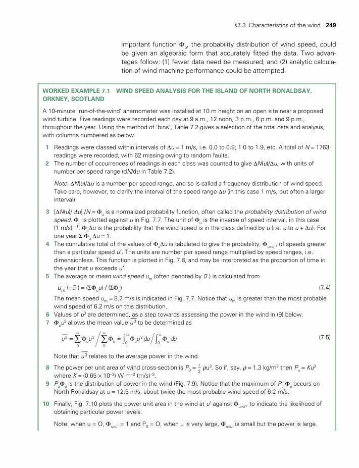
§7.3 Characteristics of the wind 249
WORKED EXAMPLE 7.1 WIND SPEED ANALYSIS FOR THE ISLAND OF NORTH RONALDSAY, ORKNEY, SCOTLAND
A 10-minute ‘run-of-the-wind’ anemometer was installed at 10 m height on an open site near a proposed wind turbine. Five readings were recorded each day at 9 a.m., 12 noon, 3 p.m., 6 p.m. and 9 p.m., throughout the year. Using the method of ‘bins’, Table 7.2 gives a selection of the total data and analysis, with columns numbered as below.
1 Readings were classed within intervals of Du = 1 m/s, i.e. 0.0 to 0.9; 1.0 to 1.9, etc. A total of N = 1763 readings were recorded, with 62 missing owing to random faults.
2 The number of occurrences of readings in each class was counted to give DN(u)/Du, with units of number per speed range (dN/du in Table 7.2).
Note: DN(u)/Du is a number per speed range, and so is called a frequency distribution of wind speed. Take care, however, to clarify the interval of the speed range Du (in this case 1 m/s, but often a larger interval).
3 [DN(u)/ Du] /N = Fu is a normalized probability function, often called the probability distribution of wind speed. Fu is plotted against u in Fig. 7.7. The unit of Fu is the inverse of speed interval, in this case (1 m/s)—1. FuDu is the probability that the wind speed is in the class defined by u (i.e. u to u + Du). For one year S Fu Du = 1.
4 The cumulative total of the values of FuDu is tabulated to give the probability, Fu>u’, of speeds greater than a particular speed u′. The units are number per speed range multiplied by speed ranges, i.e. dimensionless. This function is plotted in Fig. 7.8, and may be interpreted as the proportion of time in the year that u exceeds u′.
5 The average or mean wind speed um (often denoted by u– ) is calculated from
um (≡u– ) = (SFuu) / (SFu) (7.4)
The mean speed um = 8.2 m/s is indicated in Fig. 7.7. Notice that um is greater than the most probable wind speed of 6.2 m/s on this distribution.
6 Values of u3 are determined, as a step towards assessing the power in the wind in (9) below. 7 Fuu
3 allows the mean value u—
3 to be determined as
∑ ∑ ∫ ∫= F F = F F∞ ∞ ∞ ∞
u u u u ud du u u u3 3
0 0
30 0
(7.5)
Note that u—
3 relates to the average power in the wind.
8 The power per unit area of wind cross-section is P0 = 12 ru3. So if, say, r = 1.3 kg/m3 then Pu = Ku3
where K = (0.65 × 10⁻³) W m−2 (m/s)−3. 9 PuFu is the distribution of power in the wind (Fig. 7.9). Notice that the maximum of Pu Fu occurs on
North Ronaldsay at u = 12.5 m/s, about twice the most probable wind speed of 6.2 m/s.
10 Finally, Fig. 7.10 plots the power unit area in the wind at u’ against Fu>u’, to indicate the likelihood of obtaining particular power levels.
Note: when u = O, Fu>u’ = 1 and P0 = O, when u is very large, Fu>u’ is small but the power is large.
important function Fu, the probability distribution of wind speed, could be given an algebraic form that accurately fitted the data. Two advan-tages follow: (1) fewer data need be measured; and (2) analytic calcula-tion of wind machine performance could be attempted.
TWIDELL PAGINATION.indb 249 01/12/2014 11:37
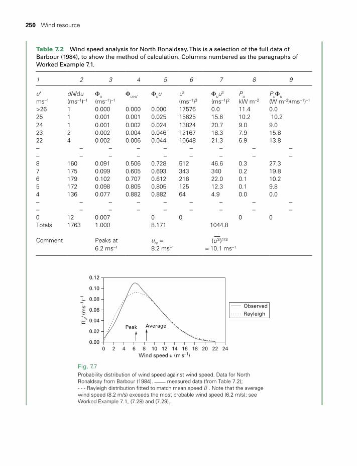
250 Wind resource
Table 7.2 Wind speed analysis for North Ronaldsay. This is a selection of the full data of Barbour (1984), to show the method of calculation. Columns numbered as the paragraphs of Worked Example 7.1.
1 2 3 4 5 6 7 8 9
u′ dN/du Fu Fu>u’ Fuu u3 Fuu3 Pu PuFu
ms−1 (ms−1)−1 (ms−1)−1 (ms−1)3 (ms−1)2 kW m−2 (W m−2)(ms−1)−1
>26 1 0.000 0.000 0.000 17576 0.0 11.4 0.025 1 0.001 0.001 0.025 15625 15.6 10.2 10.2 24 1 0.001 0.002 0.024 13824 20.7 9.0 9.023 2 0.002 0.004 0.046 12167 18.3 7.9 15.822 4 0.002 0.006 0.044 10648 21.3 6.9 13.8− − − − − − − − −− − − − − − − − −8 160 0.091 0.506 0.728 512 46.6 0.3 27.37 175 0.099 0.605 0.693 343 340 0.2 19.86 179 0.102 0.707 0.612 216 22.0 0.1 10.25 172 0.098 0.805 0.805 125 12.3 0.1 9.84 136 0.077 0.882 0.882 64 4.9 0.0 0.0− − − − − − − − −− − − − − − − − −0 12 0.007 0 0 0 0Totals 1763 1.000 8.171 1044.8
Comment Peaks at um = (u—
3 )1/ 3
6.2 ms−1 8.2 ms−1 = 10.1 ms−1
0.00
0.02
0.04
0.06
0.08
0.10
0.12
0 2 4 6 8 10 12 14 16 18 20 22 24Wind speed u (m s–1)
Πu
/ (m
s–1)–1
Observed
Rayleigh
Peak Average
Fig. 7.7Probability distribution of wind speed against wind speed. Data for North Ronaldsay from Barbour (1984). measured data (from Table 7.2); - - - Rayleigh distribution fitted to match mean speed u– . Note that the average wind speed (8.2 m/s) exceeds the most probable wind speed (6.2 m/s); see Worked Example 7.1, (7.28) and (7.29).
TWIDELL PAGINATION.indb 250 01/12/2014 11:37
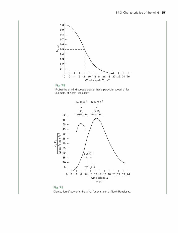
§7.3 Characteristics of the wind 251
1.0
0.9
0.8
0.7
0.6
0.5
0.4
0 2 4 6 8 10 12 14 16 18Wind speed u’/m s–1
Φu
> u
’
20 22 24 26
0.3
0.2
0.1
Fig. 7.8Probability of wind speeds greater than a particular speed u’, for example, of North Ronaldsay.
60 maximum maximum
55
50
45
40
35
30
25
20
15
10
0 2 4 6 8 10 12
8.2
6.2 m s–1
Φu
12.5 m s–1
10.1
13um (u3)
14 16 18Wind speed u
P0 Φu
m s–1
20 22 24 26
5
(W m
–2)
(m s
–1)–1
P0
Φu
Fig. 7.9Distribution of power in the wind, for example, of North Ronaldsay.
TWIDELL PAGINATION.indb 251 01/12/2014 11:37
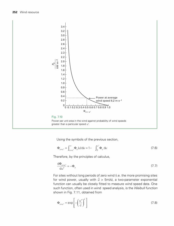
252 Wind resource
00
0.2
0.4
0.6
0.9
1.0
1.2
1.4
Power at averagewind speed 8.2 m s−1
1.6
1.8
2.0
2.2
2.3
2.4
2.6
2.8
3.0
3.2
3.4
0.1 0.2 0.3 0.4 0.5 0.6Φu > u’
0.7 0.8 0.9 1.0
P0
kW m
−2
Fig. 7.10Power per unit area in the wind against probability of wind speeds greater than a particular speed u’.
Using the symbols of the previous section,
u u u( )d 1 du u u u
u
u u 0∫∫F = F = − F> ′
′
= ′
∞ (7.6)
Therefore, by the principles of calculus,
u
d
du u
u
F′
= −F> ′ (7.7)
For sites without long periods of zero wind (i.e. the more promising sites for wind power, usually with u– > 5m/s), a two-parameter exponential function can usually be closely fitted to measure wind speed data. One such function, often used in wind speed analysis, is the Weibull function shown in Fig. 7.11, obtained from
uc
expu u
k
F = −′
> ′ (7.8)
TWIDELL PAGINATION.indb 252 01/12/2014 11:37
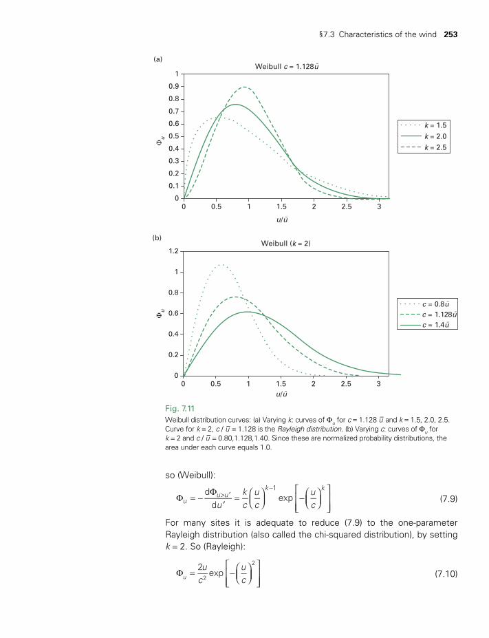
§7.3 Characteristics of the wind 253
so (Weibull):
F = −F
′=
−
> ′−
ukc
uc
uc
dd
expuu u
k k1
(7.9)
For many sites it is adequate to reduce (7.9) to the one-parameter Rayleigh distribution (also called the chi-squared distribution), by setting k = 2. So (Rayleigh):
uc
uc
2expu 2
2
F = −
(7.10)
0
0.1
0.2
0.3
0.4
0.5
0.6
0.7
0.8
0.9
1
0 0.5 1 1.5 2 2.5 3
u/u
Weibull c = 1.128u
Φu
k = 1.5
k = 2.0
k = 2.5
0
0.2
0.4
0.6
0.8
1
1.2
c = 0.8uc = 1.128uc = 1.4u
0 0.5 1 1.5 2 2.5 3
Φu
u/u
Weibull (k = 2)(b)
(a)
Fig. 7.11Weibull distribution curves: (a) Varying k: curves of Fu for c = 1.128 u– and k = 1.5, 2.0, 2.5. Curve for k = 2, c / u– = 1.128 is the Rayleigh distribution. (b) Varying c: curves of Fu for k = 2 and c / u– = 0.80,1.128,1.40. Since these are normalized probability distributions, the area under each curve equals 1.0.
TWIDELL PAGINATION.indb 253 01/12/2014 11:37
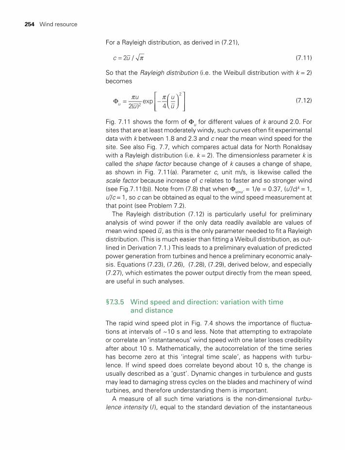
254 Wind resource
For a Rayleigh distribution, as derived in (7.21),
c u2 / p= (7.11)
So that the Rayleigh distribution (i.e. the Weibull distribution with k = 2) becomes
uu
uu2( )
exp4u 2
2p pF = −
(7.12)
Fig. 7.11 shows the form of Fu for different values of k around 2.0. For sites that are at least moderately windy, such curves often fit experimental data with k between 1.8 and 2.3 and c near the mean wind speed for the site. See also Fig. 7.7, which compares actual data for North Ronaldsay with a Rayleigh distribution (i.e. k = 2). The dimensionless parameter k is called the shape factor because change of k causes a change of shape, as shown in Fig. 7.11(a). Parameter c, unit m/s, is likewise called the scale factor because increase of c relates to faster and so stronger wind (see Fig.7.11(b)). Note from (7.8) that when Fu>u' = 1/e = 0.37, (u’/c)k = 1, u’/c = 1, so c can be obtained as equal to the wind speed measurement at that point (see Problem 7.2).
The Rayleigh distribution (7.12) is particularly useful for preliminary analysis of wind power if the only data readily available are values of mean wind speed u–, as this is the only parameter needed to fit a Rayleigh distribution. (This is much easier than fitting a Weibull distribution, as out-lined in Derivation 7.1.) This leads to a preliminary evaluation of predicted power generation from turbines and hence a preliminary economic analy-sis. Equations (7.23), (7.26), (7.28), (7.29), derived below, and especially (7.27), which estimates the power output directly from the mean speed, are useful in such analyses.
§7.3.5 Wind speed and direction: variation with time and distance
The rapid wind speed plot in Fig. 7.4 shows the importance of fluctua-tions at intervals of ~10 s and less. Note that attempting to extrapolate or correlate an ‘instantaneous’ wind speed with one later loses credibility after about 10 s. Mathematically, the autocorrelation of the time series has become zero at this ‘integral time scale’, as happens with turbu-lence. If wind speed does correlate beyond about 10 s, the change is usually described as a ‘gust’. Dynamic changes in turbulence and gusts may lead to damaging stress cycles on the blades and machinery of wind turbines, and therefore understanding them is important.
A measure of all such time variations is the non-dimensional turbu-lence intensity (I ), equal to the standard deviation of the instantaneous
TWIDELL PAGINATION.indb 254 01/12/2014 11:37
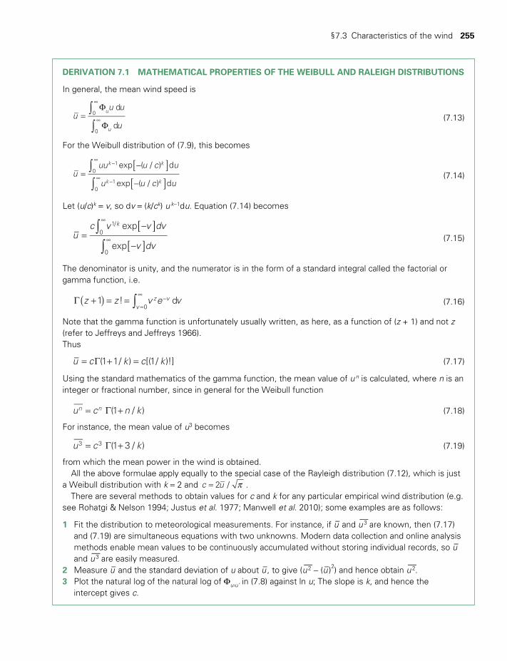
§7.3 Characteristics of the wind 255
DERIVATION 7.1 MATHEMATICAL PROPERTIES OF THE WEIBULL AND RALEIGH DISTRIBUTIONS
In general, the mean wind speed is
∫∫
=F
F
∞
∞uu u
u
d
d
u
u
0
0
(7.13)
For the Weibull distribution of (7.9), this becomes
∫∫
[ ][ ]
=−
−
−∞
−∞uuu u c u
u u c u
exp ( / ) d
exp ( / ) d
k k
k k
10
10
(7.14)
Let (u/c)k = v, so dv = (k/ck) u k−1du. Equation (7.14) becomes
uc v v dv
v dv
exp
exp
k1/0
0
∫∫
[ ][ ]
=−
−
∞
∞ (7.15)
The denominator is unity, and the numerator is in the form of a standard integral called the factorial or gamma function, i.e.
z z v e v1 ! dz vv 0∫( )Γ + = = −
=
∞ (7.16)
Note that the gamma function is unfortunately usually written, as here, as a function of (z + 1) and not z (refer to Jeffreys and Jeffreys 1966).Thus
u c k c k(1 1/ ) [(1/ )!]= Γ + = (7.17)
Using the standard mathematics of the gamma function, the mean value of u n is calculated, where n is an integer or fractional number, since in general for the Weibull function
u c n k(1 / )n n= Γ + (7.18)
For instance, the mean value of u3 becomes
u c k(1 3 / )3 3= Γ + (7.19)
from which the mean power in the wind is obtained.All the above formulae apply equally to the special case of the Rayleigh distribution (7.12), which is just
a Weibull distribution with k = 2 and p=c u2 / . There are several methods to obtain values for c and k for any particular empirical wind distribution (e.g.
see Rohatgi & Nelson 1994; Justus et al. 1977; Manwell et al. 2010); some examples are as follows:
1 Fit the distribution to meteorological measurements. For instance, if u– and u—3 are known, then (7.17)
and (7.19) are simultaneous equations with two unknowns. Modern data collection and online analysis methods enable mean values to be continuously accumulated without storing individual records, so u– and u
—3 are easily measured.2 Measure u– and the standard deviation of u about u–, to give (u
—2 − (u–)2) and hence obtain u—2.
3 Plot the natural log of the natural log of Fu›u’ in (7.8) against ln u; The slope is k, and hence the intercept gives c.
TWIDELL PAGINATION.indb 255 01/12/2014 11:37
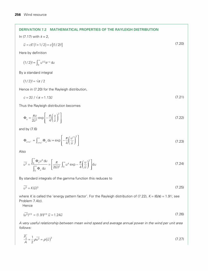
256 Wind resource
DERIVATION 7.2 MATHEMATICAL PROPERTIES OF THE RAYLEIGH DISTRIBUTION
In (7.17) with k = 2,
[ ]( )= Γ + =u c c1 1/ 2 (1/ 2)! (7.20)
Here by definition
∫( ) = −∞u e u1/ 2 ! du1/2
0
By a standard integral
p( ) = √1/ 2 ! / 2
Hence in (7.20) for the Rayleigh distribution,
p= √ =c u u2 / 1.13 (7.21)
Thus the Rayleigh distribution becomes
p pF = −
uu
uu2
exp4u 2
2
(7.22)
and by (7.6)
∫p
F = F = −′
> ′ = ′
∞u
uu
d exp4u u uu u
2
(7.23)
Also
∫∫
∫p p
=F
F= −
∞
∞
∞u
u u
u uu
uu
ud
d 2( )exp
4d
u
u
3
30
0
24
2
0 (7.24)
By standard integrals of the gamma function this reduces to
=u K u( )3 3 (7.25)
where K is called the ‘energy pattern factor’. For the Rayleigh distribution of (7.22), K = (6/p) = 1.91; see Problem 7.4(c).
Hence
= =u u u( ) (1.91) 1.243 1/3 1/3 (7.26)
A very useful relationship between mean wind speed and average annual power in the wind per unit area follows:
r r ( )= ≈P
Au u
12
0 3 3 (7.27)
TWIDELL PAGINATION.indb 256 01/12/2014 11:37
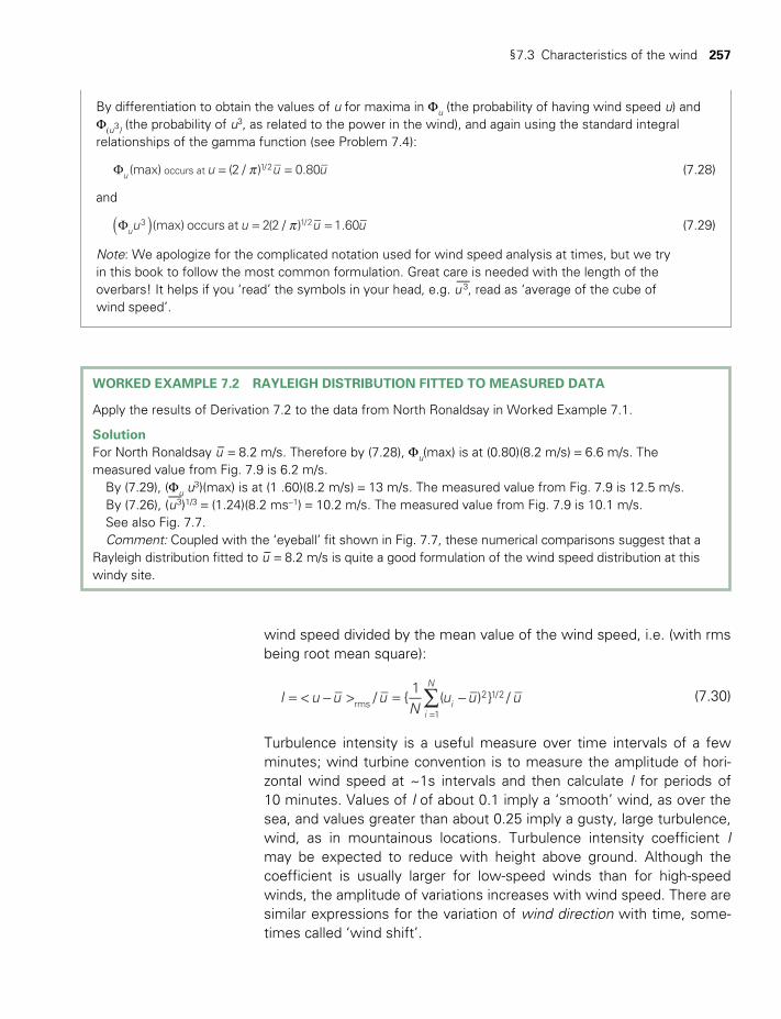
§7.3 Characteristics of the wind 257
wind speed divided by the mean value of the wind speed, i.e. (with rms being root mean square):
u uii
N
∑= < − > = −I u u uN
u/ 1
( ) /rms2
=1
1/2 (7.30)
Turbulence intensity is a useful measure over time intervals of a few minutes; wind turbine convention is to measure the amplitude of hori-zontal wind speed at ~1s intervals and then calculate I for periods of 10 minutes. Values of I of about 0.1 imply a ‘smooth’ wind, as over the sea, and values greater than about 0.25 imply a gusty, large turbulence, wind, as in mountainous locations. Turbulence intensity coefficient I may be expected to reduce with height above ground. Although the coefficient is usually larger for low-speed winds than for high-speed winds, the amplitude of variations increases with wind speed. There are similar expressions for the variation of wind direction with time, some-times called ‘wind shift’.
By differentiation to obtain the values of u for maxima in Fu (the probability of having wind speed u) and F(u3) (the probability of u3, as related to the power in the wind), and again using the standard integral relationships of the gamma function (see Problem 7.4):
pF = =u u u(max) (2 / ) 0.80occurs atu1/2 (7.28)
and
p( )F = =u u u u(max) occurs at 2(2 / ) 1.60u3 1/2 (7.29)
Note: We apologize for the complicated notation used for wind speed analysis at times, but we try in this book to follow the most common formulation. Great care is needed with the length of the overbars! It helps if you ‘read’ the symbols in your head, e.g. u
—3, read as ‘average of the cube of wind speed’.
WORKED EXAMPLE 7.2 RAYLEIGH DISTRIBUTION FITTED TO MEASURED DATA
Apply the results of Derivation 7.2 to the data from North Ronaldsay in Worked Example 7.1.
SolutionFor North Ronaldsay u– = 8.2 m/s. Therefore by (7.28), Fu(max) is at (0.80)(8.2 m/s) = 6.6 m/s. The measured value from Fig. 7.9 is 6.2 m/s.
By (7.29), (Fu u3)(max) is at (1 .60)(8.2 m/s) = 13 m/s. The measured value from Fig. 7.9 is 12.5 m/s.
By (7.26), (u—3)1/3 = (1.24)(8.2 ms−1) = 10.2 m/s. The measured value from Fig. 7.9 is 10.1 m/s.
See also Fig. 7.7.Comment: Coupled with the ‘eyeball’ fit shown in Fig. 7.7, these numerical comparisons suggest that a
Rayleigh distribution fitted to u– = 8.2 m/s is quite a good formulation of the wind speed distribution at this windy site.
TWIDELL PAGINATION.indb 257 01/12/2014 11:37
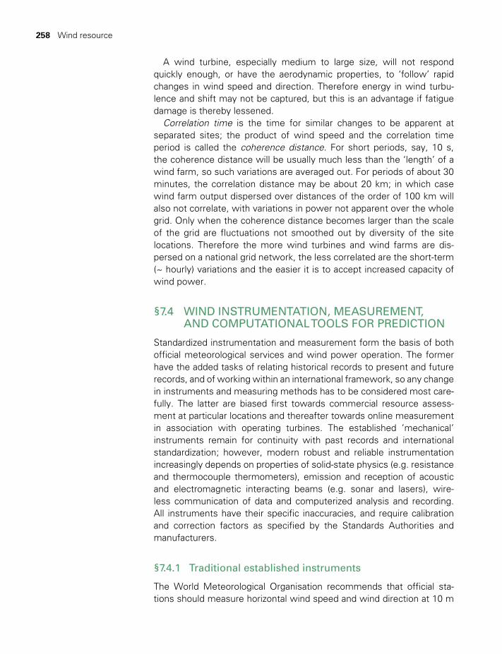
258 Wind resource
A wind turbine, especially medium to large size, will not respond quickly enough, or have the aerodynamic properties, to ‘follow’ rapid changes in wind speed and direction. Therefore energy in wind turbu-lence and shift may not be captured, but this is an advantage if fatigue damage is thereby lessened.
Correlation time is the time for similar changes to be apparent at separated sites; the product of wind speed and the correlation time period is called the coherence distance. For short periods, say, 10 s, the coherence distance will be usually much less than the ‘length’ of a wind farm, so such variations are averaged out. For periods of about 30 minutes, the correlation distance may be about 20 km; in which case wind farm output dispersed over distances of the order of 100 km will also not correlate, with variations in power not apparent over the whole grid. Only when the coherence distance becomes larger than the scale of the grid are fluctuations not smoothed out by diversity of the site locations. Therefore the more wind turbines and wind farms are dis-persed on a national grid network, the less correlated are the short-term (~ hourly) variations and the easier it is to accept increased capacity of wind power.
§7.4 WIND INSTRUMENTATION, MEASUREMENT, AND COMPUTATIONAL TOOLS FOR PREDICTION
Standardized instrumentation and measurement form the basis of both official meteorological services and wind power operation. The former have the added tasks of relating historical records to present and future records, and of working within an international framework, so any change in instruments and measuring methods has to be considered most care-fully. The latter are biased first towards commercial resource assess-ment at particular locations and thereafter towards online measurement in association with operating turbines. The established ’mechanical’ instruments remain for continuity with past records and international standardization; however, modern robust and reliable instrumentation increasingly depends on properties of solid-state physics (e.g. resistance and thermocouple thermometers), emission and reception of acoustic and electromagnetic interacting beams (e.g. sonar and lasers), wire-less communication of data and computerized analysis and recording. All instruments have their specific inaccuracies, and require calibration and correction factors as specified by the Standards Authorities and manufacturers.
§7.4.1 Traditional established instruments
The World Meteorological Organisation recommends that official sta-tions should measure horizontal wind speed and wind direction at 10 m
TWIDELL PAGINATION.indb 258 01/12/2014 11:37

§7.4 Wind instrumentation, measurement, and computational tools for prediction 259
height at sites with no obstructions within at least 100 m (WMO 2008). The recommended instruments and recording methods are as follows:
• cup anemometers for wind speed• wind vanes for wind direction• records may be written, on chart recorders or with digital data stores.
Both types of instrument have been so used for over 100 years and items may be purchased to standard replicable designs. The rotational rate of a standard cup anemometer with a clean and undamaged bearing is directly proportional to wind speed; and so both sets of instrument give linear readings of the measured variable. Nevertheless, cup anemometers must be calibrated initially and at annual or biannual intervals, since the bearing may be faulty or worn. The WMO recognizes that other instru-ments exist, but is loath to make changes for the sake of international cooperation and consistency with historical records. Both type of instru-ment may be on the same tower, as shown in Fig. 7.12.
§7.4.2 Instrument towers
Wind speed and direction are measured preferably to the top blade-tip height of the intended wind turbine. However, a large turbine may be more than 150 m high, which height is unrealistic for an instrument tower, usually limited by cost and site to at most between 50 m and 100 m high. Offshore, an instrument tower requires an independent sub sea foundation, warning lights, etc., which makes it extremely expensive. Sets of wind speed, wind direction and temperature sensors will be placed at successive heights up the tower at about 15 m intervals. Connection to data recorders may be by cable, but more likely by wire-less. The tower structure distorts the wind flow in certain directions, and so corrections are needed.
§7.4.3 Wind speed and direction instruments for commercial and research use
Utility-scale wind turbines generally have an anemometer, wind vane and thermometer located on the topside and rear end of the turbine nacelle.
(a) Mechanical instrumentsMechanical cup anemometers and wind vanes mounted on towers are common, but mechanical propeller anemometers are often favored, which have three propellers at right-angles; online analysis calculates wind speed, wind direction and vertical components of wind speed.
TWIDELL PAGINATION.indb 259 01/12/2014 11:37
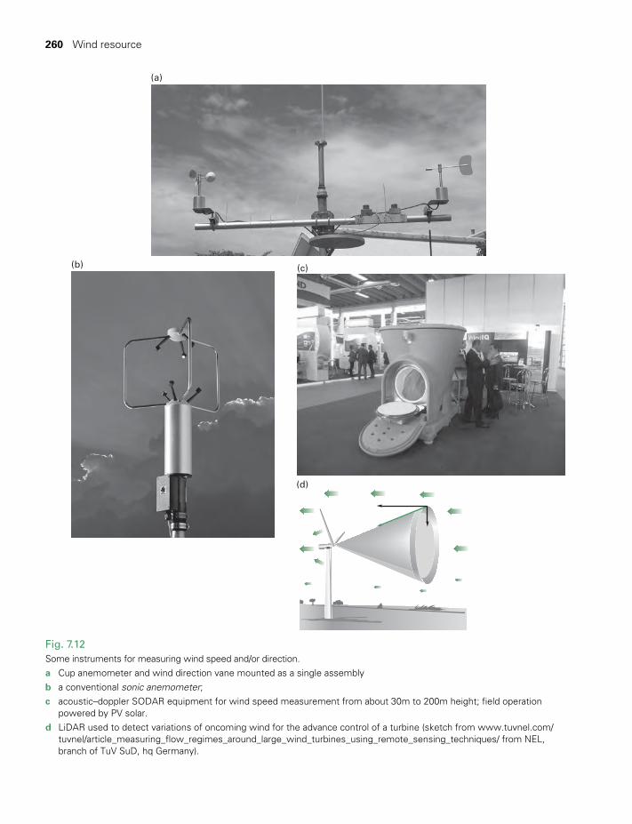
260 Wind resource
(b)
Fig. 7.12Some instruments for measuring wind speed and/or direction.a Cup anemometer and wind direction vane mounted as a single assemblyb a conventional sonic anemometer; c acoustic–doppler SODAR equipment for wind speed measurement from about 30m to 200m height; field operation
powered by PV solar.d LiDAR used to detect variations of oncoming wind for the advance control of a turbine (sketch from www.tuvnel.com/
tuvnel/article_measuring_flow_regimes_around_large_wind_turbines_using_remote_sensing_techniques/ from NEL, branch of TuV SuD, hq Germany).
(c)
(d)
(a)
(b)
TWIDELL PAGINATION.indb 260 01/12/2014 11:37
§7.4 Wind instrumentation, measurement, and computational tools for prediction 261
(b) Sonic instruments These include the following (see Fig. 7.12(b)):
• The ultrasonic (sonic) anemometer which has a set of three displaced sound emitters and a separated set of three recei vers. The time of flight of emitted sound pulses between paired emitters and receivers depends on the speed and direction of air flowing through the device.
• The acoustic resonance anemometer, which also uses ultrasonic waves, but forms these into a standing wave pattern in the horizontal gap between two disks. Wind passing through the gap distorts the standing wave pattern and wind speed, and direction may be obtained from the phase-shifted output of the receivers. The acoustic reso-nance anemometer is a robust instrument, so is suitable for fixing on operating wind turbines.
(c) Doppler back-scatter effect beam instruments (see Fig. 7.12(c) and (d))
Sensing and thereby measuring electromagnetic radiation (either visible or infrared) or sound back scattered from dust or temperature inhomo-geneities in the air provide several methods of measuring wind speed and direction. Common methods are based on the Doppler Effect, since both acoustic and electromagnetic beams are changed in frequency if they are reflected from a moving object. The acoustic instruments are called Sonic Detection and Ranging (SODAR), and the infrared/visible-red laser instruments Light Detection and Ranging (LiDAR). The sophisti-cated instruments propagate signals from ground level (not necessarily always vertical, but able to scan in different directions) and record the ‘back-scattered’ signal back from dust that is always in the air. The‘time of flight’ between emission of a pulse and its return, together with the angle to the vertical, gives the distance of the sampling. The frequency shift of the back-scattered beam relates to the relative speed of the dust (i.e. the air), and is measured by interference with the unperturbed out-going beam. The equipment can be transported (and stolen!) relatively easily. Such instrumentation is indispensable at sea, since wind speed and direction measurement to heights of about 250 m can be used to monitor the oncoming wind to a wind turbine to control the blade set-tings and other variables in advance. The rate of sampling can be very large; for example, SODAR sampling at 200 ms intervals allows air turbu-lence to be measured. The benefits are the absence of towers, the large range of measurement heights and angular positions, and the imme-diacy of the analyzed data. However, such equipment is expensive and requires expert calibration. LiDAR instrumentation is used from satellites to produce maps, as shown in Fig. 7.2.
TWIDELL PAGINATION.indb 261 01/12/2014 11:37

262 Wind resource
§7.4.4 Other indicators and instruments
There are many other ways of assessing wind speed, some of which may be useful for education and students’ practical work (see Problem 7.5). The Beaufort visual scale in Table 7.1 is one method. Instrumental methods include: (i) the Pitot tube used to measure aircraft speed; (ii) hot-wire sensor (temperature and therefore resistance varies with heat loss in the airflow); (iii) Tela kites with calibrated tether force; (iv) tatter flags (left out for months and comparisons and rates of ‘tatter’ noted, as used by foresters to identify sheltered spots for planting); (v) drag spheres, e.g. in wind tunnels. Less formal but revealing methods include: (a) ping-pong balls on strings as drag spheres, and (b) running downwind holding out a handkerchief which becomes vertical when running at the wind speed (great fun, never forgotten).
§7.4.5 Computational tools for assessing wind power potential
The impossibility of comprehensive wind measurements for a whole region or country means that computer modeling (simulation) is the only method of assessment and prediction, with the model calibrated from relatively few sets of measured data. Likewise for the complicated wind properties of an actual site, including within a wind farm. Two examples are as follows:
• NOABL (Numerical Objective Analysis Boundary Layer) modeling. The basic model maintains the constancy of air mass as the modeled wind fronts move across complex terrain. Therefore, relatively few calibration points allow average wind to be predicted at any other position in the network; for an example, see www.rensmart.com. Note, however, that local disturbance (e.g. trees and buildings) is not considered, which is a major handicap.
• WAsP (Wind Atlas Analysis and Application Program) is an interna-tionally used set of software packages (models) for PCs produced by the Wind Energy Department (ex Riso) at the Technical University of Denmark. The basic method is to accept trustworthy wind data from an established meteorological station, remove the effects of local topography and elevation, transfer these data to the required site, add the effects of site altitude, topography and obstructions (e.g. buildings) and finally predict wind-related parameters (e.g. average wind speeds month by month). The full set of programs offers many more simulated aspects of wind power.
Such modeling is essential. However, take care to experience real wind conditions, especially the force of gale-force wind. Computer modeled wind will never frighten you; the real wind will.
TWIDELL PAGINATION.indb 262 01/12/2014 11:37

§7.4 Wind instrumentation, measurement, and computational tools for prediction 263
§7.4.6 Short-term predictions
Knowledge of future wind speed is needed for a range of purposes and over a range of times ahead. With significant wind power installed capac-ity, such predictions are needed: (i) minutes ahead providing information for individual wind turbine control systems; (ii) hours ahead for elec-trical network operators’ short-term planning markets; (iii) days ahead for network operators’ power station scheduling; (iii) months ahead for power maintenance scheduling; (iv) years ahead for wind farm financing. Also needing predictions from hours to months ahead are financial opera-tors buying and selling electricity in power markets.
Correlation of monthly and annual wind speeds between a wind power site and standard meteorological stations (as shown in §7.4.5) enables estimates to be made of power generation and resulting finance; this usually satisfies the needs of the owners and financiers.
However, electricity grid network operators need information to plan ahead for inputs of generation to ensure that total generation supplies the varying demand (§15.4). Such networks cover large regional, national and international areas, so significant averaging occurs (see Box 15.5). In practice the network need is to predict the input from many wind farms distributed over areas of about 300 km x 300 km or greater. Much information about wind conditions from hours to several days ahead is available from meteorological services; this is usually available as maps on websites free of charge. The same information may be purchased digitally and online for input for computer analysis and, if necessary, control. With, say, 10 to perhaps 100 wind farms spread across a large region, the total wind turbine operation is very reliable and dependable, unlike the supply from a central power station which can cut out sud-denly by, for example, grid connection faults and operational failures. The uncertainty about such wind power is not the condition of the machines, but the state of the wind.
The meteorological services use very large computing capacity for weather prediction from hours to several days ahead using established models. Such models range from post-prediction correlations with past recorded wind speed (for instance, using auto regression moving average (ARMA), mathematics, and artificial neural network theory (ANN)) to hydrodynamic models calculating how air pressure differences and heat inputs cause masses of air to move. Such analysis provides generally very reliable information for the areas covered by grid networks.
TWIDELL PAGINATION.indb 263 01/12/2014 11:37

264 Wind resource
QUICK QUESTIONS
Note: Answers to these questions are in the text of the relevant section of this chapter, or may be readily inferred from it.
1 For wind power, what range of wind speeds is most productive? 2 Pinpoint the populated regions of the world with best wind power
resource. 3 What other factors benefit wind power resource? 4 Why is the wind onto wind turbines always classed as turbulent? 5 Is the increase of wind speed with height linear? If not, what is the
relationship? 6 Describe the effects of trees and buildings on nearby wind turbines,
and hence summarize your advice about siting wind turbines. 7 What is the role of the World Meteorological Organisation regarding
wind power? 8 It is not possible to predict accurately future wind speed by time, so
how is it possible to predict annual wind power electricity sales so that a financial return can be offered to investors?
CHAPTER SUMMARY
To properly assess the power likely to be produced by particular turbines at particular sites requires careful measurements at that site over at least 12 months at several heights. This is because wind speed varies strongly with time over periods from seconds to seasons and years, and over distances ~1 km generally and ~100 m in hilly (complex) terrain. Prediction of such winds is possible with information from official meteorological stations using the ‘measure-correlate-predict’ methodology, and from using ‘Wind Atlas’ computational techniques. In practice, annual wind speed assessment may lead to uncertainty of at least 20% year by year, owing to a combination of ‘natural’ variation and climate change.
A key indicator is the mean wind speed u ; a good site for wind power will have u > ~ 5 m / s at 10 m
height. Published wind atlases give a preliminary guide to good sites. Globally, such sites are particularly plentiful in latitudes ~40° where the prevailing winds are strong (e.g. western North America, Northwest Europe including Britain and Ireland, and New Zealand).
The probability distribution of wind speed is important because the power in the wind is proportional to wind speed cubed (u 3) and because above-average winds contribute disproportionately more power. For a given mean wind speed, relatively simple mathematical functions (the Weibull or Rayleigh distributions) give an acceptable fit to the probability distribution at most sites, thus enabling a preliminary analysis of monthly and annual wind power potential.
Meteorological services have routine measurements of land-based wind speed and direction over many years, using cup anemometers, but often at sites not suitable for wind power (e.g. airports) and at heights lower than those of many turbines (wind speed increases significantly with height above the ground in the height regions of turbine rotors). Offshore information is not so well established, so further measurement is needed, usually requiring more sophisticated instrumentation (e.g. with sonic and radar back-scatter), as do measurements at short (~second) time intervals, as for analysis of turbulence. Such sophisticated instrumentation allows the near-field wind approaching a turbine to be measured for turbine control.
Computer models (e.g. WAsP) are widely used to interpolate from a few measurement sites to proposed turbine sites nearby. Wind prediction is important, especially for electricity network operators.
TWIDELL PAGINATION.indb 264 01/12/2014 11:37
Problems 265
9 Why are more site data needed to fit a Weibull distribution than a Rayleigh distribution? In what circumstances does this make the Rayleigh distribution particularly useful?
10 What are the traditional wind instruments for meteorological stations and what instrumental methods have been added to these for the wind power industry?
PROBLEMS
Note: *indicates a ‘problem’ that is particularly suitable for class discus-sion or group tutorials.
7.1 Using equation (7.3), with b’ = 1/7 = 0.14, compare the propor-tional increases in expected wind speed by adding 50 m to a 50 m and a 100 m-high tower.
7.2 Refer to Table 7.2 column 4, and Fig. 7.8. Explain how a graph of u uF > ′ against u’ is obtained from field data using online data collection. Then from (7.8) and (7.9) prove that when
e1/ 1/ 2.72 0.368u uF = = => ′ then u c′ = , where c is the scale factor.
7.3 The flow of air in the wind will be turbulent if the Reynolds number R ≥ 2000 (see §R2.5). Calculate the maximum wind speed for laminar flow around an obstruction of dimension 1.0 m. Is laminar flow realistic for wind turbines?
7.4 For a wind speed pattern following a Rayleigh distribution, prove that:
(a) The most probable wind speed is u0.80 .
(b) The most probable power in the wind occurs at a wind speed of u1.60 .
(c) u u6
( )3 3
p=
where u—
3 is the mean of u 3, and u is the mean of u , and so
u u( ) 1.243 1/3 =
Note: Requires maths at level of Derivation 7.2.
*7.5 Experiment with cheaper methods of measuring wind speed, such as: (i) tatter flags (left out for months and comparisons and rates of ‘tatter’ noted); (ii) a ping-pong ball hanging on a string in the wind as an educational exercise to calibrate; (iii) running downwind holding out a handkerchief vertically when running at the wind speed (great fun, never forgotten).
TWIDELL PAGINATION.indb 265 01/12/2014 11:37

266 Wind resource
BIBLIOGRAPHY
General
Manwell, J.F., McGowan, J.G. and Rogers, A.L. (2010, 2nd edn) Wind Energy Explained, John Wiley & Sons, New York. Has a complete chapter on wind characteristics and resources.
Rohatgi, J.S. and Nelson, V. (1994) Wind Characteristics: An Analysis for the Generation of Power, Burgess Publishing, Edina, MA. A seminal text.
Specifically referenced
Barbour, D. (1984) Energy Study of the Island of North Ronaldsay, Orkney, MSc thesis, University of Strathclyde.
Bowden, G.J., Barker, P.R., Shestopal, V.O. and Twidell, J.W. (1983) ‘The Weibull distribution function and wind power statistics’, Wind Engineering, 7, 85–98.
Jeffreys, H. and Jeffreys, B. (1966) Methods of Mathematical Physics, Cambridge University Press, Cambridge. Carefully presented text of advanced maths for engineers, etc.
Justus, C.G., Hargreaves, W.R., Mikherl, A.S. and Graves, D. (1977) ‘Methods for estimating wind speed fre-quency distribution’, Journal of Applied Meteorology, 17, 673–678.
Petersen, E.L. (1975) On the Kinetic Energy Spectrum of Atmospheric Motions in the Planetary Boundary Layer, Report 285 of the Wind Test site, Riso, Denmark.
World Meteorological Organisation (WMO) (1981) Meteorological Aspects of the Utilization of Wind as an Energy Source, Technical Note No. 175, WMO, Geneva, Switzerland.
WMO (2008) Guide to Meteorological Instruments and Methods of Observation, World Meteorological Organisation, Geneva, Switzerland.
Global climatology of wind
Chatfield, R. (2000) ‘Atmospheric motions and the greenhouse effect’, in W.G. Ernst (ed.), Earth Systems – Processes and issues, Cambridge University Press, Cambridge.
Peixoto, J.P. and Oort, A.H. (1992) The Physics of Climate, American Institute of Physics, New York.
Journals and websites
Wind atlases; background, methods and availability (www.windatlas.dk/).
TWIDELL PAGINATION.indb 266 01/12/2014 11:37
CONTENTS
Learning aims 268
§8.1 Introduction 269
§8.2 Turbine types and terms 272§8.2.1 Horizontal axis wind turbines
(HAWTs) 274§8.2.2 Vertical axis wind turbines
(VAWTs) 276§8.2.3 Concentrators, diffusers and
shrouds 277
§8.3 Linear momentum theory 277§8.3.1 Energy extraction; Lanchester-
Betz-Zhukowsky theory 277§8.3.2 Thrust (axial force) on wind
turbines 281§8.3.3 Torque 283§8.3.4 Drag machines 285
§8.4 Angular momentum theory 286 §8.4.1 Concepts 286§8.4.2 Torque, power and tip-speed
ratio from considering angular momentum 287
§8.5 Dynamic matching 289§8.5.1 Optimal rotation rate; tip-speed
ratio λ 289§8.5.2 Extensions of linear momentum
theory 293
§8.6 Blade element theory 295§8.6.1 Calculation of lift and drag
forces on a blade element 295§8.6.2 Calculation of forces and turning
torque on a whole blade 298§8.6.3 Implications 298
§8.7 Power extraction by a turbine 299
§8.8 Electricity generation 303§8.8.1 Basics 303§8.8.2 Classification of electricity
systems using wind power 305§8.8.3 Wind farms: inland and
offshore 308§8.8.4 Technical aspects for grid-connected
wind turbines 311§8.8.5 Wind power contribution to
national electricity generation 311§8.8.6 Smaller scale systems and
independent owners 312
§8.9 Mechanical power 314§8.9.1 Sea transport 314§8.9.2 Grain milling 314§8.9.3 Water pumping 315§8.9.4 Heat production by friction 316
§8.10 Social economic and environmental considerations 316
Chapter summary 318
Quick questions 318
Problems 319
Notes 322
Bibliography 322
Box 8.1 Experiencing lift and drag forces 290
Box 8.2 Multimode wind power system with load-management control at Fair lsle, Scotland 313
CHAPTER
8Wind power technology
TWIDELL PAGINATION.indb 267 01/12/2014 11:37
268 Wind power technology
LEARNING AIMS
• Identify the main type of wind turbines.• Understand the physical reasons why the
power in the wind is proportional to the cube of the wind speed, but no more than 60% of the power in the approaching wind can be extracted by a turbine.
• Understand the meaning of cut-in speed, rated power, and cut-out speed of a turbine.
• Appreciate the reasons behind the rapid increase of installed wind power systems, especially in wind farms.
• Appreciate the potential of more advanced methods to better model turbine performance.
LIST OF FIGURES
8.1 Growth in wind power: world installed capacity (GW) and annual electricity generation (TWh). 2698.2 Velocities and forces at a section of a rotating turbine blade. 2728.3 Classification of wind machines and devices: (a) horizontal axis; (b) vertical axis; (c) concentrators. 2758.4 Power in the wind. 2788.5 Lanchester-Betz-Zhukowsky model of the expanding airstream through the turbine rotor, modeled
as an actuator disk. 2788.6 Power coefficient Cp as a function of induction factor a. 2808.7 Thrust on wind turbines. 2818.8 Torque coefficient CG vs. tip-speed ratio λ. 2858.9 (a) A sailing yacht using the drag force of its spinnaker to sail downwind. (b) Yacht sailing into the
wind utilizing lift force (c) Idealized drag machine with hinged flaps on a rotating belt. 2858.10 Actuator disk, showing some of its key parameters. 2878.11 (a) Hand in the airstream of a moving car. (b) Lift and drag forces on a smooth airplane wing. 2908.12 Definition sketch of angles and forces, looking along a wind turbine blade from its tip as it rotates
in a plane perpendicular to the far oncoming (upstream) wind. 2908.13 Turbine speed (frequency) and power capture. 2928.14 Indicative sketch of power coefficient Cp as a function of tip-speed ratio λ for a range of wind
turbine types. 2938.15 Power coefficient CP versus induction factor a = 1 – u1/u0, as given by the linear momentum model. 2948.16 (a) Element section of a blade (b) Lift and drag forces (c) Showing blade twist. (d) Vector triangle
of velocities at the blade element. (e) Commercial turbine. 2968.17 Modeled airspeeds at rotor at distance r from axis. 2998.18 Wind turbine power curve for operating regions and power performance. 3008.19 Power coefficient Cp. 3028.20 Microgeneration. 3058.21 Some supply options for stand-alone systems. 3068.22 Wind/diesel supply modes. 3078.23 Part of the Buffalo Ridge wind farm in Minnesota, USA. 3098.24 Offshore wind farms. 3108.25 Water pumping by direct mechanical link to a multi-blade turbine. 315
LIST OF TABLES
8.1 Typical wind turbine–generating characteristics at rated power in 12 m/s wind speed. 2718.2 Comparison of airplane wing to blade of a wind turbine 2898.3 A classification of wind turbine electricity systems 305
TWIDELL PAGINATION.indb 268 01/12/2014 11:37
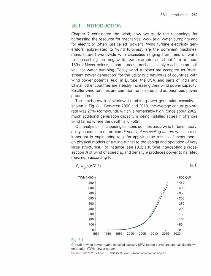
§8.1 Introduction 269
1,000
900
800
700
600
500
TWh
400
300
200
100
100
01985 1990 1995 2000 2005 2010 2015 2020
0
50
150
200
250
GW
300
350
400
450
500
Fig. 8.1Growth in wind power: world installed capacity (GW) (upper curve) and annual electricity generation (TWh) (lower curve).Source: Data to 2012 from BP. Statistical Review; linear extrapolation beyond.
§8.1 INTRODUCTION
Chapter 7 considered the wind; now we study the technology for harnessing the resource for mechanical work (e.g. water pumping) and for electricity (often just called ‘power’). Wind turbine electricity gen-erators, abbreviated to ‘wind turbines’, are the dominant machines, manufactured worldwide with capacities ranging from tens of watts to approaching ten megawatts, with diameters of about 1 m to about 150 m. Nevertheless, in some areas, mechanical-only machines are still vital for water pumping. Today wind turbines are accepted as ‘main-stream power generation’ for the utility grid networks of countries with wind power potential (e.g. in Europe, the USA, and parts of India and China); other countries are steadily increasing their wind power capacity. Smaller wind turbines are common for isolated and autonomous power production.
The rapid growth of worldwide turbine power generation capacity is shown in Fig. 8.1. Between 2000 and 2010, the average annual growth rate was 27% (compound), which is remarkably high. Since about 2002, much additional generation capacity is being installed at sea in offshore wind farms where the depth is < ~50m.
Our analysis in succeeding sections outlines basic wind turbine theory; a key aspect is to determine dimensionless scaling factors which are so important in engineering (e.g. for applying the results of experiments on physical models of a wind tunnel to the design and operation of very large structures). For instance, see §8.3; a turbine intercepting a cross-section A of wind of speed u0 and density r produces power to its rated maximum according to
r p=P D u C( / 4)( )T P12
2 03 (8.1)
TWIDELL PAGINATION.indb 269 01/12/2014 11:37
270 Wind power technology
Here Cp is a dimensionless efficiency factor called the power coefficient. Note that the power PT is proportional to A and to the cube of wind speed u0. Thus, whereas doubling A may produce twice the power, a doubling of wind speed produces eight times the power potential. The power coefficient Cp also varies with wind speed for individual machines. Since wind speed distribution is skewed (see Fig. 7.11), at any one time speeds less than average are more likely than speeds greater than average. Therefore, the optimum design size of rotor and generator at a particular site depends on the power requirement, either to maximize generated energy per year or to provide frequent power. As apparent from (7.27) for common wind speed distributions, the average annual power from a wind turbine approximates to
P C A u( )T P 03r≈ (8.2)
where u0 is the mean wind speed.1
The whole assembly comprising the rotor, its matched electricity gen-erator and other equipment is usually called a wind turbine, as in this book.2 The maximum rated power capacity of a wind turbine is given for a specified ‘rated’ wind speed, commonly about 12 m/s. At this speed, power production of about 0.3 kW/m2 of cross-section would be expected with power coefficients Cp of between 35 and 45%. The optimum rotation rate depends on the ratio of the blade-tip speed to the wind speed, so small machines rotate rapidly and large machines rotate slowly. Table 8.1 gives outline details of machine size. Machines are expected to last for at least 20 to 25 years and cost about Euro 1200 (about $US1500) per kW rated capacity, ex-factory. When installed in windy locations and given financial credit for not polluting, power pro-duction is competitive with the cheapest forms of other generation (see Appendix D).
Wind power for mechanical purposes, i.e. milling and water pumping, has been established for many hundreds of years. Wind electricity gen-erators date from around 1890, with most early development from about 1930 to about 1955. At this time development almost ceased due to the availability of cheap oil, but interest reawakened and increased rapidly from about 1973. A few of the older machines kept operating for several tens of years (e.g. the Gedser 100 kW, 24 m-diameter machine in Denmark, built in 1957). Manufacturing growth since about 1980 has benefited greatly from the use of solid-state electronics, composite materials, computer-aided design and site optimization.
A major design criterion is the need to protect the machine against damage in very strong winds, even though such gale-force winds are relatively infrequent. Wind forces tend to increase as the square of the wind speed. Since the 1-in-50-year gale speed will be five to ten times the average wind speed, considerable overdesign has to be incorporated
TWIDELL PAGINATION.indb 270 01/12/2014 11:37
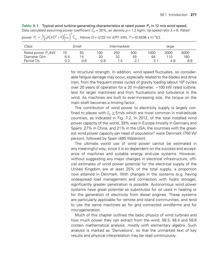
§8.1 Introduction 271
Table 8.1 Typical wind turbine-generating characteristics at rated power PT in 12 m/s wind speed. Data calculated assuming power coefficient CP = 30%, air density r = 1.2 kg/m, tip-speed ratio λ = 6. Rated
power r ( )( )p= 12 CP D u/ 4T
20
3
p . Hence D = (2.02 m) √(P/1 kW), T = (0.0436 s m−1)D.
Class Small Intermediate large
Rated power PT /kW 10 50 100 250 500 1000 3000 6000Diameter D/m 6.4 14 20 32 49 64 110 160Period T/s 0.3 0.6 0.9 1.4 2.1 3.1 4.8 6.8
for structural strength. In addition, wind speed fluctuates, so consider-able fatigue damage may occur, especially related to the blades and drive train, from the frequent stress cycles of gravity loading (about 108 cycles over 20 years of operation for a 20 m-diameter, ~100 kW rated turbine, less for larger machines) and from fluctuations and turbulence in the wind. As machines are built to ever-increasing size, the torque on the main shaft becomes a limiting factor.
The contribution of wind power to electricity supply is largely con-fined to places with u0 5 m/s which are most common in mid-latitude countries, as indicated in Fig. 7.2. In 2012, of the total installed wind power capacity of the world, 39% was in Europe (mostly in Germany and Spain), 27% in China, and 21% in the USA; the countries with the great-est wind power capacity per head of population3 were Denmark (750 W/person), followed by Spain (485 W/person).
The ultimate world use of wind power cannot be estimated in any meaningful way, since it is so dependent on the success and accept-ance of machines and suitable energy end-use systems. However, without suggesting any major changes in electrical infrastructure, offi-cial estimates of wind power potential for the electrical supply of the United Kingdom are at least 25% of the total supply, a proportion now attained in Denmark. With changes in the systems (e.g. having widespread load management and connection with hydro storage), significantly greater penetration is possible. Autonomous wind power systems have great potential as substitutes for oil used in heating or for the generation of electricity from diesel engines. These systems are particularly applicable for remote and island communities, and tend to use the same machines as for grid connected windfarms and for microgeneration.
Much of this chapter outlines the basic physics of wind turbines and how much power they can extract from the wind. §8.3, §8.4 and §8.6 contain mathematical analysis, mostly with elementary algebra. Such analysis is marked as ‘Derivations‘, so that the unmarked text of key results and physical interpretation may be read continuously.
<
TWIDELL PAGINATION.indb 271 01/12/2014 11:37
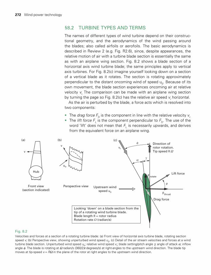
272 Wind power technology
§8.2 TURBINE TYPES AND TERMS
The names of different types of wind turbine depend on their construc-tional geometry, and the aerodynamics of the wind passing around the blades; also called airfoils or aerofoils. The basic aerodynamics is described in Review 2 (e.g. Fig. R2.6), since, despite appearances, the relative motion of air with a turbine blade section is essentially the same as with an airplane wing section. Fig. 8.2 shows a blade section of a horizontal axis wind turbine blade; the same principles apply to vertical axis turbines. For Fig. 8.2(c) imagine yourself looking down on a section of a vertical blade as it rotates. The section is rotating approximately perpendicular to the distant oncoming wind of speed u0. Because of its own movement, the blade section experiences oncoming air at relative velocity vr. The comparison can be made with an airplane wing section by turning the page so Fig. 8.2(c) has the relative air speed vr horizontal.
As the air is perturbed by the blade, a force acts which is resolved into two components:
• The drag force FD is the component in line with the relative velocity vr. • The lift force FL is the component perpendicular to FD. The use of the
word ‘lift’ does not mean that FL is necessarily upwards, and derives from the equivalent force on an airplane wing.
Front view(section indicated)
Hub
v
v
uo
Perspective view
(a) (b)
Lift force
α
φ
φ
γ
Direction ofrotor rotation.Tip speed R
Drag force
Fthrust
Frotate
Upstream windspeed uo
vr
Looking ‘down’ on a blade section from thetip of a rotating wind turbine blade.Blade length R = rotor radiusRotation rate (radian/s)
(c)
W
Ω
Fig. 8.2Velocities and forces at a section of a rotating turbine blade: (a) Front view of horizontal axis turbine blade, rotating section speed v; (b) Perspective view, showing unperturbed wind speed u0. (c) Detail of the air stream velocities and forces at a wind turbine blade section. Unperturbed wind speed u0; relative wind speed vr; blade setting/pitch angle g; angle of attack a; inflow angle f. The blade is rotating at W radian/s (360/2p degrees/s) at right-angles to the upstream wind direction. The blade tip moves at tip-speed v = RW in the plane of the rotor at right angles to the upstream wind direction.
TWIDELL PAGINATION.indb 272 01/12/2014 11:37

§8.2 Turbine types and terms 273
The next steps are to resolve (‘split’) both FL and FD:
1 Along the axis of the rotor, with the sum of resolved components being the overturning axial thrust Fthrust . Because drag is small due to the smooth aerodynamic surfaces, and lift is maximized from the shape of the airfoil, the net force in the plane of the rotor, Frotate, is in the direction of rotation.
2 In the plane of the rotor, with the algebraic sum (actually their differ-ence in magnitude, since the resolved components have opposite directions) being the rotational force Frotate. The force Frotate turns the shaft of the turbine and enables power to be extracted from the con-nected generator.
It may seem strange that the rotor turns in a direction against the incom-ing relative wind. However, the same situation is met with racing yachts; yachts can sail into a wind at a speed faster than the speed of the wind owing to the resolution of lift forces on the sails. If the yacht sails with the wind behind, for instance, with a spinnaker sail, then the boat can never go faster than the wind (see §8.3.4).
Some other factors which affect the interaction between the blade and the wind include the following:
1 Unseen by the eye, rotational movement of the air occurs as the air-stream flows around the blade. Consequently, distinct vortices and eddies (whirlpools of air) are created near the surface; vortex shedding occurs as these rotating masses of air break free from the surface and move away, still rotating, with this airstream. In addition, signifi-cant angular momentum is imparted to the blade, so equal and oppo-site angular momentum is given to the airstream, which circulates downwind as wakes. These disturbances are dissipated after traveling about 10 to 30 turbine diameters downwind.
2 The air is disturbed by the blade movement and by wind gusts, and the flow becomes erratic and perturbed. This turbulence (see §R2.5) occurs before and after the rotating blades, so each individual blade may often be moving in the turbulence created by other blades.
3 The aerodynamic characteristics of the blades are crucial; roughness and protrusions should be avoided. Note that the predominantly two-dimensional airflow over an airplane wing becomes three- dimensional, and therefore more complex, for a rotating wind turbine blade.
The characteristics of a particular wind turbine are described by the answers to a number of questions (see Fig. 8.3). The theoretical justifica-tion for these criteria will be given in later sections.
1 Is the axis of rotation parallel or perpendicular to the airstream? The former is a horizontal axis machine, the latter usually a vertical axis machine in a cross-wind configuration.
TWIDELL PAGINATION.indb 273 01/12/2014 11:37

274 Wind power technology
2 Is the predominant force lift or drag? Drag machines can have no part moving faster than the wind, but lift machines can have blade sections moving considerably faster than the wind speed. This is similar to a keeled sail boat which can sail faster than the wind.
3 What is the solidity? ‘Solidity’ is the ratio of the total area of the blades at any one moment in the direction of the airstream to the swept area across the airstream. For many turbines this is described by giving the number of blades. Large solidity machines (many blades) start easily with large initial torque, but soon reach maximum power at small rotational frequency. Small solidity devices may require starting, but reach maximum power at faster rotational frequency. Thus large solid-ity machines are used for water pumping even in light winds. Small solidity turbines are used for electricity generation, since fast shaft rotational frequency is needed.
4 What is the purpose of the turbine? Historic grain windmills and water-pumping wind turbines produce mechanical power. The vast majority of modern wind turbines are for electricity generation; generally large (>2.5 MW) for utility grid power and intermediate or small for autono-mous, stand-alone power and for grid-linked microgeneration.
5 Is the frequency of rotation constant, or does it vary with wind speed? A wind turbine whose generator is connected directly to a strong AC electrical grid will rotate only at nearly constant frequency. However, a turbine of variable frequency can be matched more efficiently to the varying wind speed than a constant frequency machine, but this requires special generators with an indirect connection through a power–electronic interface (see Review 1).
A classification of wind machines and devices can now be given in association with Fig. 8.3. This includes the main types, but numerous other designs and adaptations occur.
§8.2.1 Horizontal axis wind turbines (HAWTs)
Two- and three-bladed HAWTs are by far the most common for electricity generation (see Fig. 8.3(a)), with the rotor consisting of both the hub and the blades. Three-bladed rotors operate more ‘smoothly’ and, generally, more quietly than two-bladed rotors. Visually, three-bladed tur-bines rotate smoothly, but two-bladed turbines may appear to ‘wobble’. Single-bladed rotors, with a counterweight, have been field tested at full scale, but the asymmetry produced too many difficulties for commercial prospects. Gearing and generators are usually at the top of the tower in a nacelle. Multi-blade rotors, having large starting torque in light winds, are used for water pumping and other low-frequency mechanical power.
All wind turbines have blades similar in operation to airplane wings (and also, but less so, to airplane propellers). The dominant driving force
TWIDELL PAGINATION.indb 274 01/12/2014 11:37
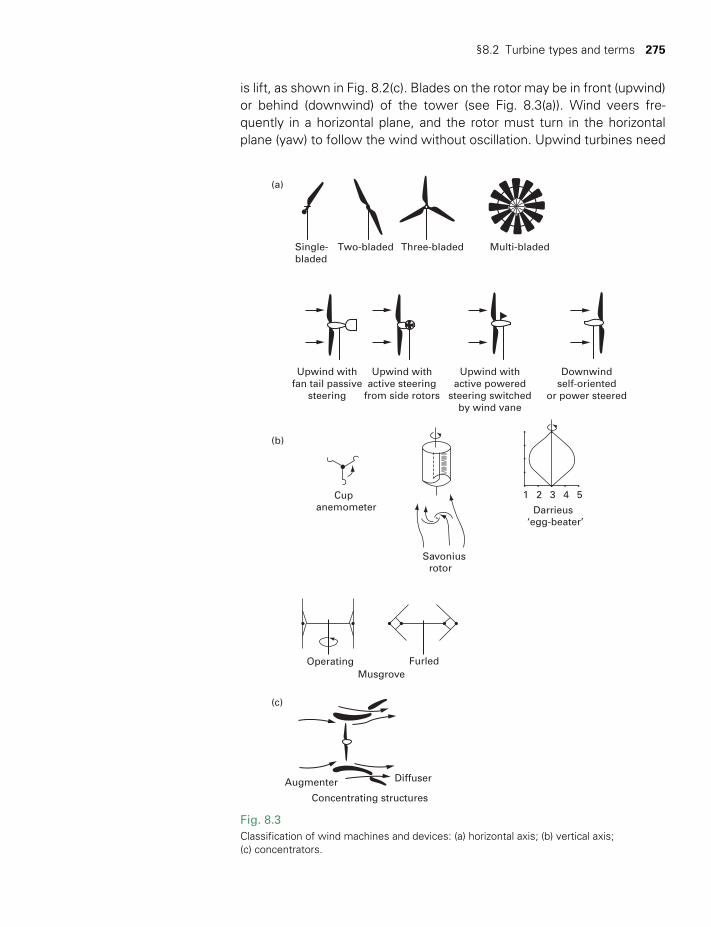
§8.2 Turbine types and terms 275
is lift, as shown in Fig. 8.2(c). Blades on the rotor may be in front (upwind) or behind (downwind) of the tower (see Fig. 8.3(a)). Wind veers fre-quently in a horizontal plane, and the rotor must turn in the horizontal plane (yaw) to follow the wind without oscillation. Upwind turbines need
Cupanemometer
(b)
Savoniusrotor
FurledMusgrove
Operating
Darrieus‘egg-beater’
1 2 3 4 5
Single-bladed
Upwind withfan tail passive
steering
Upwind withactive steering
from side rotors
Upwind withactive powered
steering switchedby wind vane
Downwindself-oriented
or power steered
Two-bladed Three-bladed Multi-bladed
(a)
Augmenter
(c)
Diffuser
Concentrating structures
Fig. 8.3Classification of wind machines and devices: (a) horizontal axis; (b) vertical axis; (c) concentrators.
TWIDELL PAGINATION.indb 275 01/12/2014 11:37

276 Wind power technology
a tail or some other yawing mechanism, such as electric motor drives, to maintain orientation. Downwind turbines are, in principle, self- orienting, but are more affected by the tower, which produces wind shadow and extra turbulence in the blade path. Perturbations of this kind cause cyclic stresses on the structure, additional noise and output fluctuations. Upwind and downwind machines of rotor diameter of more than about 10 m use electric motors to control yaw.
§8.2.2 Vertical axis wind turbines (VAWTs)
By turning about a vertical axis, a machine can accept wind from any direction without adjustment, whereas a horizontal axis machine must yaw (i.e. turn in the horizontal plane to face the wind). An expectation for vertical axis wind turbine generators is to have gearboxes and genera-tors at ground level. Examples, from the smallest devices, are sketched in Fig. 8.3(b):
1 Cup anemometer. This device rotates by drag force. The shape of the cups produces a nearly linear relationship between rotational frequency and wind speed, so that measurement of the number of rotations per time period correlates to average wind speed over that period. The device is a standard anemometer for meteorological data (§7.4.1).
2 Savonius rotor (turbo machine). There is a complicated motion of the wind through and around the two curved sheet airfoils. The driving force is principally drag. The construction is simple and inexpensive. The large solidity produces large starting torque, so Savonius rotors may be used for water pumping.
3 Darrieus rotor. This has two or three thin curved blades with an airfoil section. The rotor shape is a catenary, with the aim of the rotating blades being only stressed along their length.
4 Musgrove rotor. The blades of this form of rotor are vertical for normal power generation, but tip or turn about a horizontal point for control or shutdown. There are several variations, which are all designed to have the advantage of fail-safe shutdown in strong winds.
For the Darrieus and Musgrove rotors, the driving wind forces are lift, with maximum turbine torque occurring when a blade moves twice per rotation across the wind, so pulsing the rotation. Uses are for electricity generation. The rotor is not usually self-starting, so may be initiated with the generator operating as a motor.
A major advantage of vertical axis machines is to eliminate gravity-induced stress/strain cycles on blades (which occurs every rotation in the blades of horizontal axis turbines); thus, in principle, vertical axis blades may be very large. For small machines, gearing and generators may be directly coupled to the vertical main shaft at ground level. However, for large machines this would require a long main shaft transmitting very
TWIDELL PAGINATION.indb 276 01/12/2014 11:37
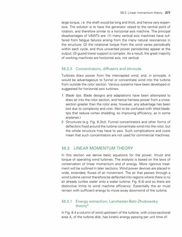
§8.3 Linear momentum theory 277
large torque, i.e. the shaft would be long and thick, and hence very expen-sive. The solution is to have the generator raised to the central point of rotation, and therefore similar to a horizontal axis machine. The principal disadvantages of VAWTs are: (1) many vertical axis machines have suf-fered from fatigue failures arising from the many natural resonances in the structure; (2) the rotational torque from the wind varies periodically within each cycle, and thus unwanted power periodicities appear at the output; (3) guyed tower support is complex. As a result, the great majority of working machines are horizontal axis, not vertical.
§8.2.3 Concentrators, diffusers and shrouds
Turbines draw power from the intercepted wind, and, in principle, it would be advantageous to funnel or concentrate wind into the turbine from outside the rotor section. Various systems have been developed or suggested for horizontal axis turbines:
1 Blade tips. Blade designs and adaptations have been attempted to draw air into the rotor section, and hence harness power from a cross-section greater than the rotor area; however, any advantage has been lost due to complexity and cost. (Not to be confused with tilted blade-tips that reduce vortex shedding, so improving efficiency, as in some airplanes.)
2 Structures (e.g. Fig. 8.3(c)). Funnel concentrators and other forms of deflectors fixed around the turbine concentrate wind into the rotor, but the whole structure may have to yaw. Such complications and costs mean that such concentrators are not used for commercial machines.
§8.3 LINEAR MOMENTUM THEORY
In this section we derive basic equations for the power, thrust and torque of operating wind turbines. The analysis is based on the laws of conservation of linear momentum and of energy. More rigorous treat-ment will be outlined in later sections. Wind power devices are placed in wide, extended, fluxes of air movement. The air that passes through a wind turbine cannot therefore be deflected into regions where there is no air already (unlike water onto a water turbine: Fig. 6.4) and so there are distinctive limits to wind machine efficiency. Essentially the air must remain with sufficient energy to move away downwind of the turbine.
§8.3.1 Energy extraction; Lanchester-Betz-Zhukowsky theory4
In Fig. 8.4 a column of wind upstream of the turbine, with cross-sectional area A1 of the turbine disk, has kinetic energy passing per unit time of:
TWIDELL PAGINATION.indb 277 01/12/2014 11:37
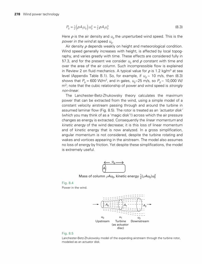
278 Wind power technology
P A u u A u012 1 0 0
2 12 1 0
3r r( )= = (8.3)
Here r is the air density and u0 the unperturbed wind speed. This is the power in the wind at speed u0.
Air density r depends weakly on height and meteorological condition. Wind speed generally increases with height, is affected by local topog-raphy, and varies greatly with time. These effects are considered fully in §7.3, and for the present we consider u0 and r constant with time and over the area of the air column. Such incompressible flow is explained in Review 2 on fluid mechanics. A typical value for r is 1.2 kg/m3 at sea level (Appendix Table B.1). So, for example, if u0 ~ 10 m/s, then (8.3) shows that P0 = 600 W/m2, and in gales, u0~25 m/s, so P0 ~ 10,000 W/m2; note that the cubic relationship of power and wind speed is strongly non-linear.
The Lanchester-Betz-Zhukowsky theory calculates the maximum power that can be extracted from the wind, using a simple model of a constant velocity airstream passing through and around the turbine in assumed laminar flow (Fig. 8.5). The rotor is treated as an ‘actuator disk’ (which you may think of as a ‘magic disk’!) across which the air pressure changes as energy is extracted. Consequently the linear momentum and kinetic energy of the wind decrease; it is this loss of linear momentum and of kinetic energy that is now analyzed. In a gross simplification, angular momentum is not considered, despite the turbine rotating and wakes and vortices appearing in the airstream. The model also assumes no loss of energy by friction. Yet despite these simplifications, the model is extremely useful.
A0
u0 u1 u2
A1 A2
Upstream Turbine(as actuator
disc)
Downstream
Fig. 8.5Lanchester-Betz-Zhukowsky model of the expanding airstream through the turbine rotor, modeled as an actuator disk.
A
u0
Mass of column ρAu0, kinetic energy (ρAu0)u02
21
Fig. 8.4Power in the wind.
TWIDELL PAGINATION.indb 278 01/12/2014 11:37

§8.3 Linear momentum theory 279
DERIVATION 8.1 LINEAR MOMENTUM THEORY: CALCULATION OF u1 AND PT
Step 1: Calculate u1 by conservation of energy
The rate of air mass flow in the column is m.
. This moving air applies a force F to the turbine rotor and, by Newton’s third law, itself experiences an equal and opposite force, so slowing from u0 to u2. By Newton’s second law, F equals the reduction in momentum of the air per unit time:
= −F mu mu. .
0 2 (8.4)
The power PT (energy per unit time) extracted from the wind and passing into the turbine is
= = −P Fu m u u u.( )T 1 0 2 1 (8.5)
Consequently, the air slows as kinetic energy is removed from the wind at a rate (power) Pw given by:
P m u u.( )w
12 0
222= − (8.6)
By conservation of energy, the power extracted from the wind equals the power gained by the turbine; so equating (8.5) and (8.6):
m u u u m u u m u u u u.( )
.( )
.( )( )0 2 1
12 0
222 1
2 0 2 0 2− = − = + − (8.7)
Hence:
= +u u u( )112 0 2 (8.8)
Note that according to this linear momentum theory, the air speed through the actuator disk cannot be less than half the unperturbed wind speed.
Step 2: Knowing u1, calculate the power extracted from the wind
The mass of air flowing through the disk per unit time is given by:
r=m Au.
1 1 (8.9)
So that in (8.5),
r= −P Au u u( )T 1 12
0 2 (8.10)
Substituting for = −u u u22 1 0 from (8.8) in (8.10) gives:
r r= − − = −P Au u u u Au u u[ (2 )] 2 ( )T 1 12
0 1 0 1 12
0 1 (8.11)
The axial induction factor a (also in some texts called the ‘axial interference factor’) is the fractional wind speed decrease at the turbine. Thus,
= −a u u u( ) /0 1 0 (8.12)
We consider air approaching and passing through and by the turbine disk. Area A1 is the rotor swept area, and areas A0 and A2 enclose the stream of air passing through A1. A0 is positioned in the oncoming wind front unaffected by the turbine; A2 is at the position of minimum wind speed downwind before the wind front reforms. A0 and A2 can be located
TWIDELL PAGINATION.indb 279 01/12/2014 11:37
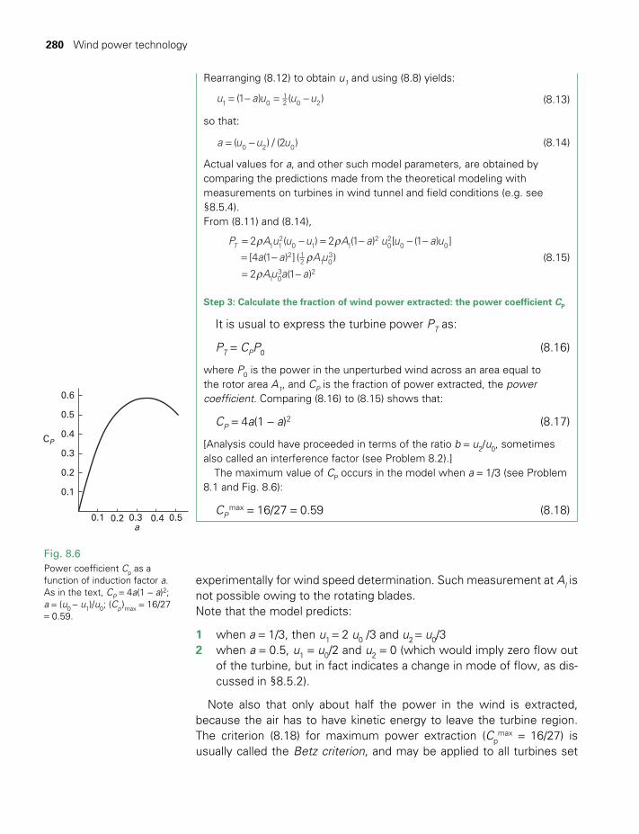
280 Wind power technology
experimentally for wind speed determination. Such measurement at Al is not possible owing to the rotating blades.Note that the model predicts:
1 when a = 1/3, then u1 = 2 u0 /3 and u2 = u0/3 2 when a = 0.5, u1 = u0/2 and u2 = 0 (which would imply zero flow out
of the turbine, but in fact indicates a change in mode of flow, as dis-cussed in §8.5.2).
Note also that only about half the power in the wind is extracted, because the air has to have kinetic energy to leave the turbine region. The criterion (8.18) for maximum power extraction (Cp
max = 16/27) is usually called the Betz criterion, and may be applied to all turbines set
Rearranging (8.12) to obtain u1 and using (8.8) yields:
= − = −u a u u u(1 ) ( )1 012 0 2 (8.13)
so that:
= −a u u u( ) / (2 )0 2 0 (8.14)
Actual values for a, and other such model parameters, are obtained by comparing the predictions made from the theoretical modeling with measurements on turbines in wind tunnel and field conditions (e.g. see §8.5.4).From (8.11) and (8.14),
r rr
r
= − = − − −= −= −
P A u u u A a u u a u
a a A u
Au a a
2 ( ) 2 (1 ) [ (1 ) ]
[4 (1 ) ] ( )
2 (1 )
T 1 12
0 1 12
02
0 02 1
2 1 03
1 03 2
(8.15)
Step 3: Calculate the fraction of wind power extracted: the power coefficient CP
It is usual to express the turbine power PT as:
PT = CPP0 (8.16)
where P0 is the power in the unperturbed wind across an area equal to the rotor area A1, and CP is the fraction of power extracted, the power coefficient. Comparing (8.16) to (8.15) shows that:
CP = 4a(1 − a)2 (8.17)
[Analysis could have proceeded in terms of the ratio b = u2/u0, sometimes also called an interference factor (see Problem 8.2).]
The maximum value of CP occurs in the model when a = 1/3 (see Problem 8.1 and Fig. 8.6):
CP max = 16/27 = 0.59 (8.18)
0.1
0.2
0.3
0.1 0.2 0.3 0.4a
0.5
0.4CP
0.5
0.6
Fig. 8.6 Power coefficient Cp as a function of induction factor a. As in the text, CP = 4a(1 − a)2; a = (u0 − u1)/u0; (Cp )max = 16/27 = 0.59.
TWIDELL PAGINATION.indb 280 01/12/2014 11:37
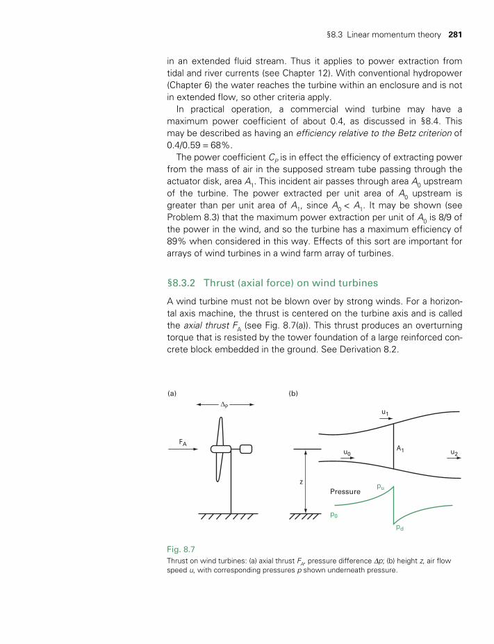
§8.3 Linear momentum theory 281
∆P
FA
z
(a) (b)
A1
p0
u0
u1
u2
pd
puPressure
Fig. 8.7 Thrust on wind turbines: (a) axial thrust FA, pressure difference Dp; (b) height z, air flow speed u, with corresponding pressures p shown underneath pressure.
in an extended fluid stream. Thus it applies to power extraction from tidal and river currents (see Chapter 12). With conventional hydropower (Chapter 6) the water reaches the turbine within an enclosure and is not in extended flow, so other criteria apply.
In practical operation, a commercial wind turbine may have a maximum power coefficient of about 0.4, as discussed in §8.4. This may be described as having an efficiency relative to the Betz criterion of 0.4/0.59 = 68%.
The power coefficient CP is in effect the efficiency of extracting power from the mass of air in the supposed stream tube passing through the actuator disk, area A1. This incident air passes through area A0 upstream of the turbine. The power extracted per unit area of A0 upstream is greater than per unit area of A1, since A0 < A1. It may be shown (see Problem 8.3) that the maximum power extraction per unit of A0 is 8/9 of the power in the wind, and so the turbine has a maximum efficiency of 89% when considered in this way. Effects of this sort are important for arrays of wind turbines in a wind farm array of turbines.
§8.3.2 Thrust (axial force) on wind turbines
A wind turbine must not be blown over by strong winds. For a horizon-tal axis machine, the thrust is centered on the turbine axis and is called the axial thrust FA (see Fig. 8.7(a)). This thrust produces an overturning torque that is resisted by the tower foundation of a large reinforced con-crete block embedded in the ground. See Derivation 8.2.
TWIDELL PAGINATION.indb 281 01/12/2014 11:37
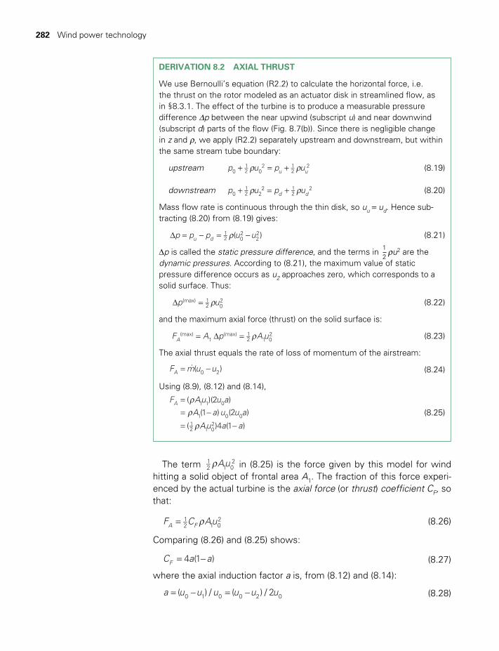
282 Wind power technology
The term Au12 1 0
2r in (8.25) is the force given by this model for wind hitting a solid object of frontal area A1. The fraction of this force experi-enced by the actual turbine is the axial force (or thrust) coefficient CF, so that:
F C AuA F12 1 0
2r= (8.26)
Comparing (8.26) and (8.25) shows:
C a a4 (1 )F = − (8.27)
where the axial induction factor a is, from (8.12) and (8.14):
a u u u u u u( ) / ( ) / 20 1 0 0 2 0= − = − (8.28)
DERIVATION 8.2 AXIAL THRUST
We use Bernoulli’s equation (R2.2) to calculate the horizontal force, i.e. the thrust on the rotor modeled as an actuator disk in streamlined flow, as in §8.3.1. The effect of the turbine is to produce a measurable pressure difference Dp between the near upwind (subscript u) and near downwind (subscript d) parts of the flow (Fig. 8.7(b)). Since there is negligible change in z and r, we apply (R2.2) separately upstream and downstream, but within the same stream tube boundary:
upstream r r+ = +p u p uu u012 0
2 12
2 (8.19)
downstream r r+ = +p u p ud d012 2
2 12
2 (8.20)
Mass flow rate is continuous through the thin disk, so uu = ud. Hence sub-tracting (8.20) from (8.19) gives:
rD = − = −p p p u u( )u d12 0
222 (8.21)
Dp is called the static pressure difference, and the terms in ru2 are the dynamic pressures. According to (8.21), the maximum value of static pressure difference occurs as u2 approaches zero, which corresponds to a solid surface. Thus:
rD =p u(max) 12 0
2 (8.22)
and the maximum axial force (thrust) on the solid surface is:
r= D =F A p A uA(max)
1(max) 1
2 1 02 (8.23)
The axial thrust equals the rate of loss of momentum of the airstream:
= −F m u u.( )A 0 2 (8.24)
Using (8.9), (8.12) and (8.14),
rr
r
== −= −
F Au u a
A a u u a
Au a a
( )(2 )
(1 ) (2 )
( )4 (1 )
A 1 1 0
1 0 012 1 0
2
(8.25)
12
TWIDELL PAGINATION.indb 282 01/12/2014 11:37
§8.3 Linear momentum theory 283
By the model, the maximum value of CF = 1.0 when a = ½, equivalent to u2 = 0 (i.e. the wind is stopped). Compare the maximum power extrac-tion, which, by the Betz criterion, occurs when a = 1/3 (Fig. 8.6 and (8.17)), corresponding to CF = 8/9 = 0.89.
In practice, the maximum value of CF on a solid disk is not 1.0 but about 1.2 owing to edge effects. Nevertheless, the linear momentum theory shows that the turbine appears to the wind as a near-solid disk when extract-ing power. It is quite misleading to estimate the forces on a rotating wind turbine by picturing the wind passing unperturbed through the gaps between the blades. If the turbine is extracting power efficiently, these gaps are not apparent to the wind and extremely large thrust forces occur.
Since wind turbine thrust forces increase as A u1 02 in (8.26), control
strategies are used to protect the machines at wind speeds of more than about 15 to 20 m/s; these include: (1) to turn (yaw) the rotor out of the wind; (2) to lessen power extraction and hence thrust by pitching the blades or extending spoil flaps; (3) if blade pitch is fixed, the blades are designed to become inefficient and self-stalling in large wind speed; (4) to stop the rotation by blade pitching and/or braking. Method (3) is perhaps the safest and cheapest; however, self-stalling blades have a reduced power coefficient and do not give optimum power extraction or smooth power control. Therefore, method (2) is preferred for large com-mercial machines by blade pitching (not spoil flaps), since power perfor-mance can be optimized and controlled in strong winds, and the rotation stopped if necessary. In areas prone to hurricanes, turbines may have special towers that can be tilted (lowered) to the ground and so out of the wind; the extra cost of these more than repays what would otherwise be the loss of the whole wind power system.
§8.3.3 Torque
The previous calculation of axial thrust on a wind turbine provides an oppor-tunity to introduce definitions for the torque causing the shaft to rotate. At this stage no attempt is made to analyze angular momentum exchange between the air and the turbine. However, it is obvious that if the turbine turns one way the air must turn the other; full analysis must eventually consider the vortices of air circulating downwind of the turbine (see §8.4).
The maximum conceivable torque, Gmax, on a turbine rotor would occur if the maximum thrust could somehow be applied in the plane of the turbine blades at the blade-tip furthest from the axis. For a propeller turbine of radius R, this ‘baseline’ criteria would be:
G = F Rmax max (8.29)
For a working machine producing an actual shaft torque G, the torque coefficient CG is defined by reference to the benchmark torque Gmax:
G G= GC max (8.30)
TWIDELL PAGINATION.indb 283 01/12/2014 11:37
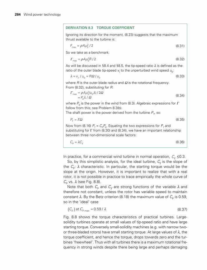
284 Wind power technology
In practice, for a commercial wind turbine in normal operation, CG 0.3.So, by this simplistic analysis, for the ideal turbine, CG is the slope of
the CP: λ characteristic. In particular, the starting torque would be the slope at the origin. However, it is important to realize that with a real rotor, it is not possible in practice to trace empirically the whole curve of CP vs. λ (see Fig. 8.8).
Note that both CP and CG are strong functions of the variable λ and therefore not constant, unless the rotor has variable speed to maintain constant λ. By the Betz criterion (8.18) the maximum value of CP is 0.59, so in the ‘ideal’ case
C Cat 0.59 /P.max λ( ) =G (8.37)
Fig. 8.8 shows the torque characteristics of practical turbines. Large-solidity turbines operate at small values of tip-speed ratio and have large starting torque. Conversely small-solidity machines (e.g. with narrow two- or three-bladed rotors) have small starting torque. At large values of λ, the torque coefficient, and hence the torque, drops towards zero and the tur-bines ‘freewheel’. Thus with all turbines there is a maximum rotational fre-quency in strong winds despite there being large and perhaps damaging
> ~
DERIVATION 8.3 TORQUE COEFFICIENT
Ignoring its direction for the moment, (8.23) suggests that the maximum thrust available to the turbine is:
r=F Au / 2max 1 02 (8.31)
So we take as a benchmark:
G r= Au R / 2max 1 02 (8.32)
As will be discussed in §8.4 and §8.5, the tip-speed ratio λ is defined as the ratio of the outer blade tip-speed vt to the unperturbed wind speed u0:
λ W= =v u R u/ /t 0 0 (8.33)
where R is the outer blade radius and W is the rotational frequency.From (8.32), substituting for R:
G r λ Wλ W
==
Au uP
( ) / 2/
max 1 02
0
0 (8.34)
where P0 is the power in the wind from (8.3). Algebraic expressions for G follow from this; see Problem 8.3(b).The shaft power is the power derived from the turbine PT, so:
GW=PT (8.35)
Now from (8.16) PT = CPP0. Equating the two expressions for PT and substituting for G from (8.30) and (8.34), we have an important relationship between three non-dimensional scale factors:
λ= GC CP (8.36)
TWIDELL PAGINATION.indb 284 01/12/2014 11:37
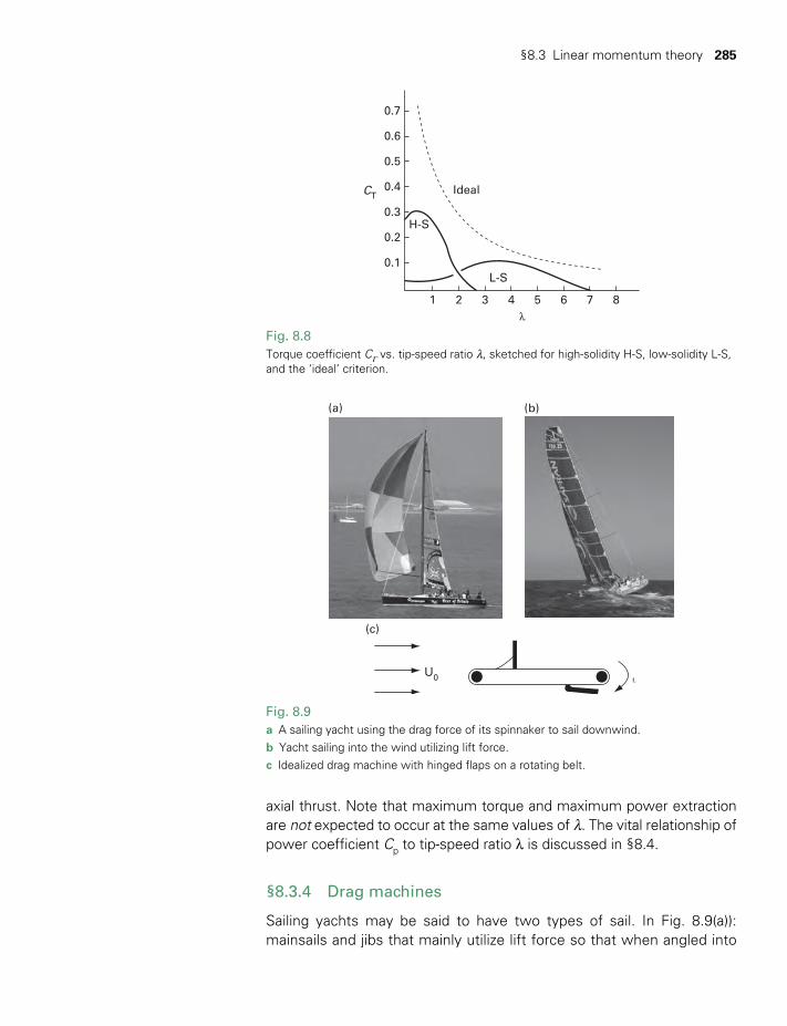
§8.3 Linear momentum theory 285
0.1
1 2 3 4 5 6 7 8
0.2
0.3
IdealCT
H-S
L-S
l
0.4
0.5
0.6
0.7
Fig. 8.8Torque coefficient CG vs. tip-speed ratio λ, sketched for high-solidity H-S, low-solidity L-S, and the ‘ideal’ criterion.
(a) (b)
U0
(c)
υ
Fig. 8.9 a A sailing yacht using the drag force of its spinnaker to sail downwind. b Yacht sailing into the wind utilizing lift force. c Idealized drag machine with hinged flaps on a rotating belt.
axial thrust. Note that maximum torque and maximum power extraction are not expected to occur at the same values of λ. The vital relationship of power coefficient Cp to tip-speed ratio λ is discussed in §8.4.
§8.3.4 Drag machines
Sailing yachts may be said to have two types of sail. In Fig. 8.9(a)): mainsails and jibs that mainly utilize lift force so that when angled into
TWIDELL PAGINATION.indb 285 01/12/2014 11:37
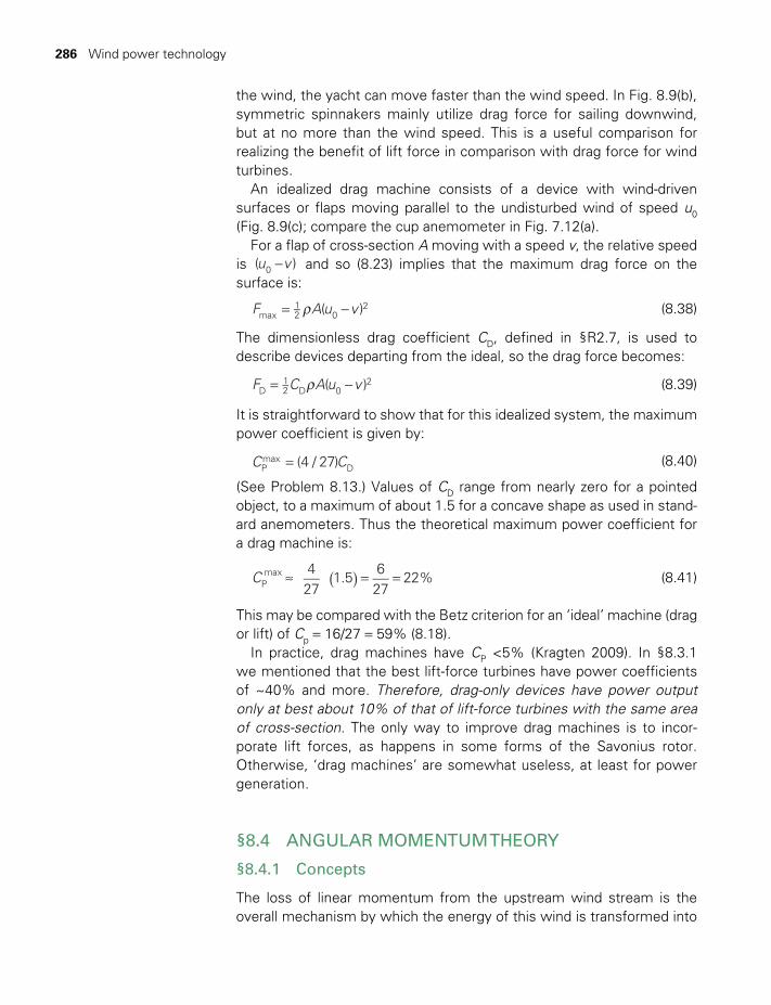
286 Wind power technology
the wind, the yacht can move faster than the wind speed. In Fig. 8.9(b), symmetric spinnakers mainly utilize drag force for sailing downwind, but at no more than the wind speed. This is a useful comparison for realizing the benefit of lift force in comparison with drag force for wind turbines.
An idealized drag machine consists of a device with wind-driven surfaces or flaps moving parallel to the undisturbed wind of speed u0 (Fig. 8.9(c); compare the cup anemometer in Fig. 7.12(a).
For a flap of cross-section A moving with a speed v, the relative speed is u v( )0 − and so (8.23) implies that the maximum drag force on the surface is:
r= −F A u v( )max12 0
2 (8.38)
The dimensionless drag coefficient CD, defined in §R2.7, is used to describe devices departing from the ideal, so the drag force becomes:
r= −F C A u v( )D12 D 0
2 (8.39)
It is straightforward to show that for this idealized system, the maximum power coefficient is given by:
C C(4 / 27)Pmax
D= (8.40)
(See Problem 8.13.) Values of CD range from nearly zero for a pointed object, to a maximum of about 1.5 for a concave shape as used in stand-ard anemometers. Thus the theoretical maximum power coefficient for a drag machine is:
( )≈ = =C4
271.5
627
22%Pmax (8.41)
This may be compared with the Betz criterion for an ‘ideal’ machine (drag or lift) of Cp = 16/27 = 59% (8.18).
In practice, drag machines have CP <5% (Kragten 2009). In §8.3.1 we mentioned that the best lift-force turbines have power coefficients of ~40% and more. Therefore, drag-only devices have power output only at best about 10% of that of lift-force turbines with the same area of cross-section. The only way to improve drag machines is to incor-porate lift forces, as happens in some forms of the Savonius rotor. Otherwise, ‘drag machines’ are somewhat useless, at least for power generation.
§8.4 ANGULAR MOMENTUM THEORY
§8.4.1 Concepts
The loss of linear momentum from the upstream wind stream is the overall mechanism by which the energy of this wind is transformed into
TWIDELL PAGINATION.indb 286 01/12/2014 11:37
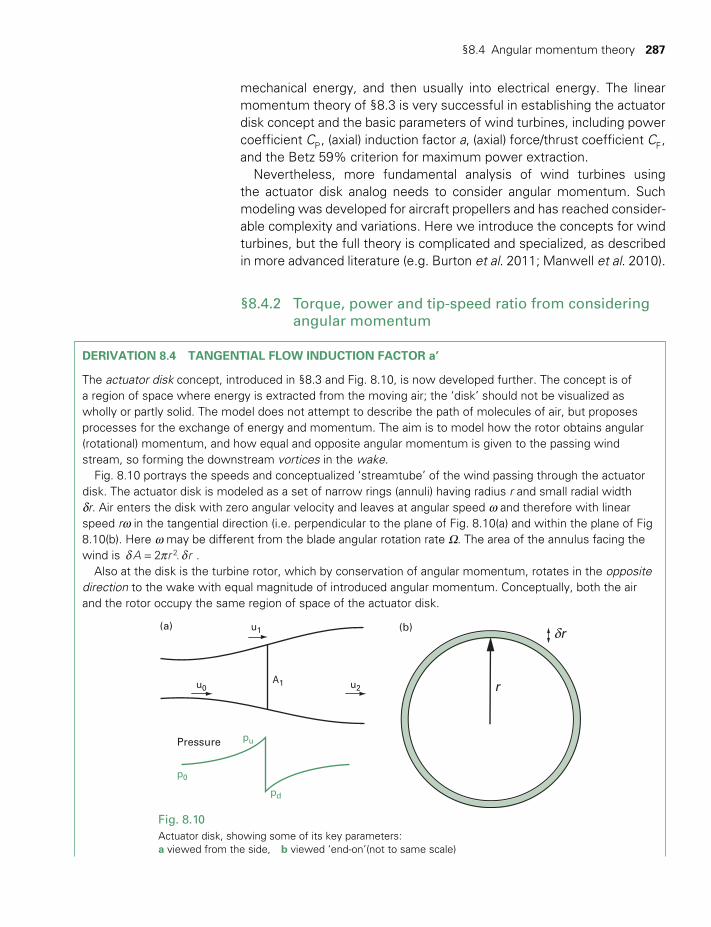
§8.4 Angular momentum theory 287
DERIVATION 8.4 TANGENTIAL FLOW INDUCTION FACTOR a’
The actuator disk concept, introduced in §8.3 and Fig. 8.10, is now developed further. The concept is of a region of space where energy is extracted from the moving air; the ‘disk’ should not be visualized as wholly or partly solid. The model does not attempt to describe the path of molecules of air, but proposes processes for the exchange of energy and momentum. The aim is to model how the rotor obtains angular (rotational) momentum, and how equal and opposite angular momentum is given to the passing wind stream, so forming the downstream vortices in the wake.
Fig. 8.10 portrays the speeds and conceptualized ‘streamtube’ of the wind passing through the actuator disk. The actuator disk is modeled as a set of narrow rings (annuli) having radius r and small radial width dr. Air enters the disk with zero angular velocity and leaves at angular speed w and therefore with linear speed rw in the tangential direction (i.e. perpendicular to the plane of Fig. 8.10(a) and within the plane of Fig 8.10(b). Here w may be different from the blade angular rotation rate W. The area of the annulus facing the wind is d p d=A r r2 .2 .
Also at the disk is the turbine rotor, which by conservation of angular momentum, rotates in the opposite direction to the wake with equal magnitude of introduced angular momentum. Conceptually, both the air and the rotor occupy the same region of space of the actuator disk.
(a)
A1
p0
u0
u1
u2
pd
puPressure
δr
r
(b)
Fig. 8.10 Actuator disk, showing some of its key parameters: a viewed from the side, b viewed ‘end-on’(not to same scale)
mechanical energy, and then usually into electrical energy. The linear momentum theory of §8.3 is very successful in establishing the actuator disk concept and the basic parameters of wind turbines, including power coefficient CP , (axial) induction factor a, (axial) force/thrust coefficient CF , and the Betz 59% criterion for maximum power extraction.
Nevertheless, more fundamental analysis of wind turbines using the actuator disk analog needs to consider angular momentum. Such modeling was developed for aircraft propellers and has reached consider-able complexity and variations. Here we introduce the concepts for wind turbines, but the full theory is complicated and specialized, as described in more advanced literature (e.g. Burton et al. 2011; Manwell et al. 2010).
§8.4.2 Torque, power and tip-speed ratio from considering angular momentum
TWIDELL PAGINATION.indb 287 01/12/2014 11:37
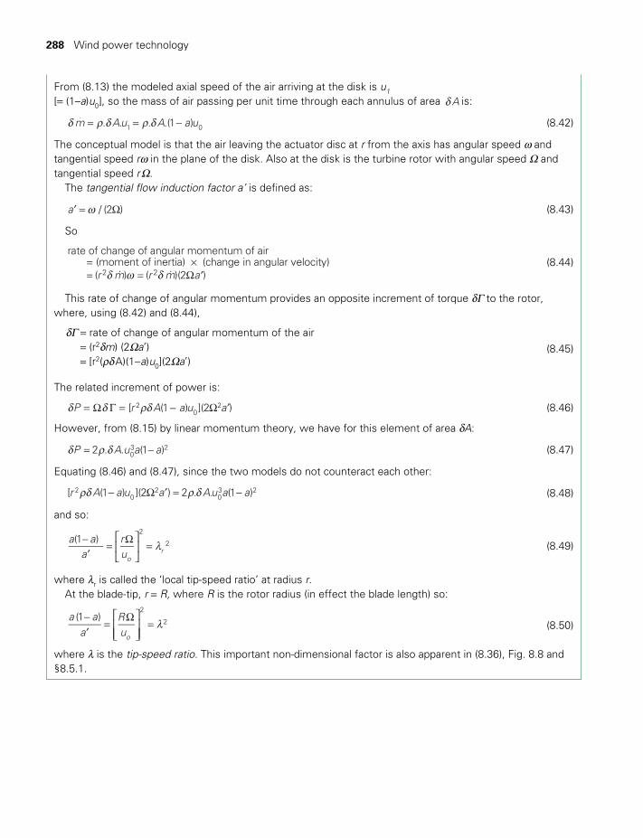
288 Wind power technology
From (8.13) the modeled axial speed of the air arriving at the disk is u1
[= (1–a)u0], so the mass of air passing per unit time through each annulus of area d A is:
d r d r d= = −m Au A a u. . . .(1 ).
1 0 (8.42)
The conceptual model is that the air leaving the actuator disc at r from the axis has angular speed w and tangential speed rw in the plane of the disk. Also at the disk is the turbine rotor with angular speed W and tangential speed r W.
The tangential flow induction factor a’ is defined as:
w′ = Wa / (2 ) (8.43)
So
r m r m a
rate of change of angular momentum of air= (moment of inertia) (change in angular velocity)= (
.) (
.)(2 )2 2d w d
×= W ′
(8.44)
This rate of change of angular momentum provides an opposite increment of torque dG to the rotor, where, using (8.42) and (8.44),
(8.45)
The related increment of power is:
d d rd= W G = − W ′P r A a u a[ (1 ) ](2 )20
2 (8.46)
However, from (8.15) by linear momentum theory, we have for this element of area dA:
d r d= −P A u a a2 . . (1 )03 2 (8.47)
Equating (8.46) and (8.47), since the two models do not counteract each other:
r A a u a Au a a[ (1 ) ](2 ) 2 . . (1 )20
203 2rd r d− W ′ = − (8.48)
and so:
λ−′
= W
=a a
aru
(1 )
or
2
2 (8.49)
where λr is called the ‘local tip-speed ratio’ at radius r.At the blade-tip, r = R, where R is the rotor radius (in effect the blade length) so:
λ−′
=W
=a a
aRu
(1 )
o
2
2 (8.50)
where λ is the tip-speed ratio. This important non-dimensional factor is also apparent in (8.36), Fig. 8.8 and §8.5.1.
dG = rate of change of angular momentum of the air = (r2dm) (2Wa’) = [r2(rd A)(1−a)u0](2Wa’)
TWIDELL PAGINATION.indb 288 01/12/2014 11:37
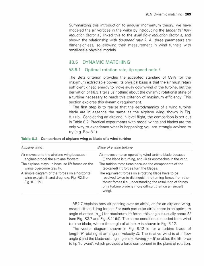
§8.5 Dynamic matching 289
Table 8.2 Comparison of airplane wing to blade of a wind turbine
Airplane wing Blade of a wind turbine
Air moves onto the airplane wing because engines propel the airplane forward.
Air moves onto an operating wind turbine blade because (i) the blade is turning, and (ii) air approaches in the wind.
The airplane stays up because lift forces on the wings overcome gravity.
The turbine rotor turns because the components of the (so-called) lift forces turn the blades.
A simple diagram of the forces on a horizontal wing explain lift and drag (e.g. Fig. R2.6 or
Fig. 8.11(b)).
The equivalent forces on a rotating blade have to be resolved twice to distinguish the turning forces from the
thrust forces (i.e. understanding the resolution of forces on a turbine blade is more difficult than on an aircraft wing).
Summarizing this introduction to angular momentum theory, we have modeled the air vortices in the wake by introducing the tangential flow induction factor a’, linked this to the axial flow induction factor a, and shown the relationship with tip-speed ratio λ. All three parameters are dimensionless, so allowing their measurement in wind tunnels with small-scale physical models.
§8.5 DYNAMIC MATCHING
§8.5.1 Optimal rotation rate; tip-speed ratio λ
The Betz criterion provides the accepted standard of 59% for the maximum extractable power. Its physical basis is that the air must retain sufficient kinetic energy to move away downwind of the turbine, but the derivation of §8.3.1 tells us nothing about the dynamic rotational state of a turbine necessary to reach this criterion of maximum efficiency. This section explores this dynamic requirement.
The first step is to realize that the aerodynamics of a wind turbine blade are in essence the same as the airplane wing shown in Fig. 8.11(b). Considering an airplane in level flight, the comparison is set out in Table 8.2. Practical experiments with model wings and blades are the only way to experience what is happening; you are strongly advised to try (e.g. Box 8.1).
§R2.7 explains how air passing over an airfoil, as for an airplane wing, creates lift and drag forces. For each particular airfoil there is an optimum angle of attack (aopt ) for maximum lift force; this angle is usually about 5° (see Fig. R2.7 and Fig. 8.11(b)). The same condition is needed for a wind turbine blade, where the angle of attack a is shown in Fig. 8.12.
The vector diagram shown in Fig. 8.12 is for a turbine blade of length R rotating at an angular velocity W. The relative wind is at inflow angle f and the blade-setting angle is g. Having g ~ 5° enables the lift force to tip ‘forward’, which provides a force component in the plane of rotation,
TWIDELL PAGINATION.indb 289 01/12/2014 11:37

290 Wind power technology
Drag force
Upstream windspeed uo
Lift force
Direction ofrotor rotation.Tip speed RΩ
Looking ‘down’ on a blade section
Blade length R = rotor radiusRotation rate Ω (radian/s)
from the tip of a rotation wind turbine blade.
vr
α γ
Fthrust
Frotate
f
f
Fig. 8.12Definition sketch of angles and forces, looking along a wind turbine blade from its tip as it rotates in a plane perpendicular to the far oncoming (upstream) wind.
BOX 8.1 EXPERIENCING LIFT AND DRAG FORCES
In a safe location on a private road, as a passenger in the back seat of a car traveling at about 50 km/h, hold your arm out of the window with your hand flat, as in the photograph (Fig. 8.11(a)). As you rotate your hand you will feel drag force and, with the hand angled about 5° from the horizontal you will sense your arm rising with the lift force. The lift and drag forces on a smooth wing (see diagram, Fig.8.11(b)) are similar, but far more efficient!
(a) Lift, L
Drag, D
Centre of Lift
Chord line from tip to tip
Direction of flight
u0
Similar situation for anairplane wing
(b)
Air flow a
For an airplane wing (an airfoil),lift and drag forces L and D are functions of the angle of attack a.
L needs to be largeD needs to be small
Fig. 8.11 a Hand in the airstream of a moving car. b Lift and drag forces on a smooth airplane wing.
TWIDELL PAGINATION.indb 290 01/12/2014 11:37
§8.5 Dynamic matching 291
so turning the rotor. The relative wind is at an angle of attack a to the blade, in a similar manner to the air meeting the airplane wing (Fig. 8.11(b)).
The speed of the tip is RW in a direction at right angles to the far oncoming wind of speed u0; therefore the inflow angle f is given by:
R ucotan cotan( ) / 0f a g λ= + = W = (8.51)
In (8.51) the dimensionless parameter λ = RW/u0 is the tip-speed ratio. This important parameter has appeared in angular momentum theory of the actuator disk (§8.4), and may now be understood in relation to the angle of attack.
Maximum lift force, as with an airplane wing, occurs when the angle of attack is constant at aopt (usually about 5° for lift with small drag away from stall: see Fig. R2.7(a)); this is the condition for optimum rotor efficiency. We therefore conclude that for a wind turbine to operate effi-ciently, the rotor should rotate at an angular speed such that the angle of attack a remains constant at its optimum. This implies that as the upstream wind speed u0 changes, so too should the rotational speed W change so that a, and therefore f, remain constant. The blade-setting angle (i.e. the pitch) at the tip, g, is usually held constant (unless changed to stop or otherwise control the machine), so the condition for optimum power capture is that the non-dimensional tip-speed ratio λ be controlled constant and optimized as the upstream wind speed changes. This is the condition for optimum dynamic matching of the turbine to the wind.
In (8.51), if, for example, a ≈ 5° and b ≈ 3°, then λ = cotan f = cotan 8° = 7.1; so keeping the angle of attack constant at the tip requires λ to remain constant at this value. Thus, if the upstream wind speed u0 increases, then the rotational rate W has to increase to obtain optimum energy capture, and vice versa. (8.51) explains why, in the same wind speed, large-radius rotors turn more slowly than small radius rotors of similar geometry; each has the same value of RW/u0, i.e. the same tip-speed ratio.
Our basic analysis above has considered only an individual blade. In practice as the rotor turns, blades move into the position occupied previ-ously by other blades. In simple terms: (i) if the rotor turns slowly, more air can move through the plane of the rotor without any interaction with a blade and so not transfer energy, and (ii) if the rotor turns very rapidly, the rotor appears to the wind more like a solid disk, and again energy is not transferred efficiently. This is outlined in Fig. 8.13.
An order-of-magnitude calculation based on Fig. 8.13 (Problem 8.5) correctly suggests that for a turbine with n blades of radius R: (i) the rota-tional speed Wm for maximum power extraction is inversely proportional to n; and (ii) significant perturbation of the oncoming air stream begins only at a fairly short distance (< ~R ) upstream from the rotor. Problem 8.5 also suggests that maximum power coefficient for a three-bladed turbine occurs at λ ≈ 4.
TWIDELL PAGINATION.indb 291 01/12/2014 11:37
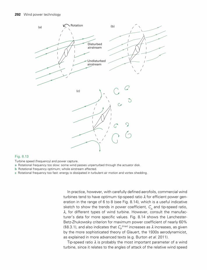
292 Wind power technology
In practice, however, with carefully defined aerofoils, commercial wind turbines tend to have optimum tip-speed ratio λ for efficient power gen-eration in the range of 6 to 8 (see Fig. 8.14), which is a useful indicative sketch to show the trends in power coefficient, Cp, and tip-speed ratio, λ, for different types of wind turbine. However, consult the manufac-turer’s data for more specific values. Fig. 8.14 shows the Lanchester-Betz-Zhukowsky criterion for maximum power coefficient of nearly 60% (§8.3.1), and also indicates that CP
(max) increases as λ increases, as given by the more sophisticated theory of Glauert, the 1930s aerodynamicist, as explained in more advanced texts (e.g. Burton et al. 2011).
Tip-speed ratio λ is probably the most important parameter of a wind turbine, since it relates to the angles of attack of the relative wind speed
Rotation(a) (b)
(c)
Disturbedairstream
Undisturbedairstream
Fig. 8.13Turbine speed (frequency) and power capture. a Rotational frequency too slow: some wind passes unperturbed through the actuator disk. b Rotational frequency optimum; whole airstream affected.c Rotational frequency too fast: energy is dissipated in turbulent air motion and vortex shedding.
TWIDELL PAGINATION.indb 292 01/12/2014 11:37
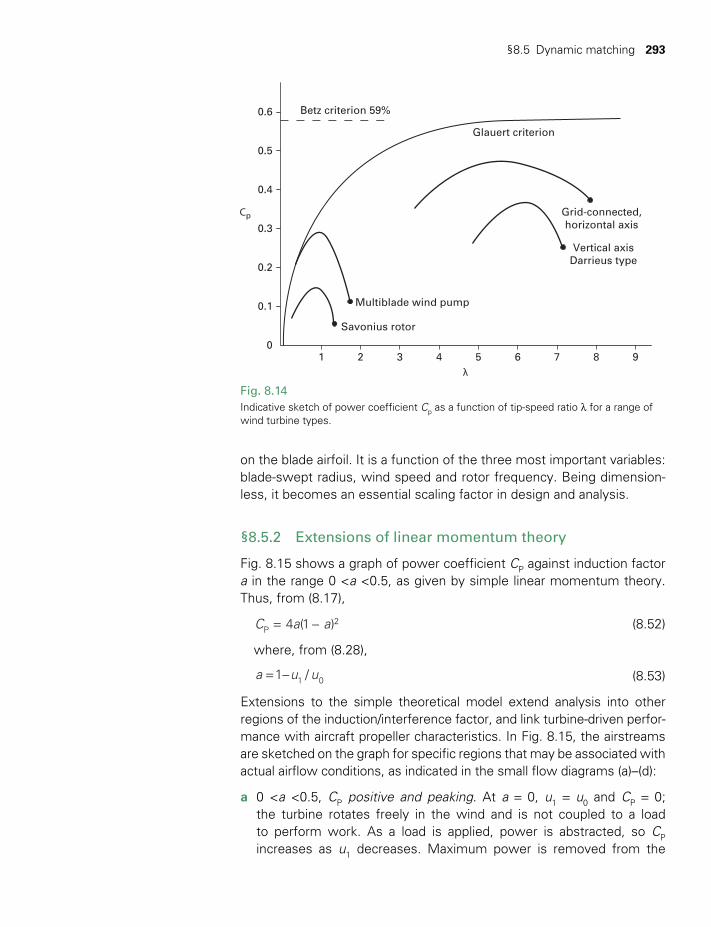
§8.5 Dynamic matching 293
on the blade airfoil. It is a function of the three most important variables: blade-swept radius, wind speed and rotor frequency. Being dimension-less, it becomes an essential scaling factor in design and analysis.
§8.5.2 Extensions of linear momentum theory
Fig. 8.15 shows a graph of power coefficient CP against induction factor a in the range 0 <a <0.5, as given by simple linear momentum theory. Thus, from (8.17),
= −C a a4 (1 )P2 (8.52)
where, from (8.28),
a u u1 /1 0= − (8.53)
Extensions to the simple theoretical model extend analysis into other regions of the induction/interference factor, and link turbine-driven perfor-mance with aircraft propeller characteristics. In Fig. 8.15, the airstreams are sketched on the graph for specific regions that may be associated with actual airflow conditions, as indicated in the small flow diagrams (a)–(d):
a 0 <a <0.5, CP positive and peaking. At a = 0, u1 = u0 and CP = 0; the turbine rotates freely in the wind and is not coupled to a load to perform work. As a load is applied, power is abstracted, so CP increases as u1 decreases. Maximum power is removed from the
Betz criterion 59%
Glauert criterion
Vertical axisDarrieus type
Grid-connected,horizontal axis
Cp
λ
Multiblade wind pump
Savonius rotor
1 2 3 4 5 6 7 8 9
0.6
0.5
0.4
0.3
0.2
0.1
0
Fig. 8.14Indicative sketch of power coefficient Cp as a function of tip-speed ratio λ for a range of wind turbine types.
TWIDELL PAGINATION.indb 293 01/12/2014 11:37
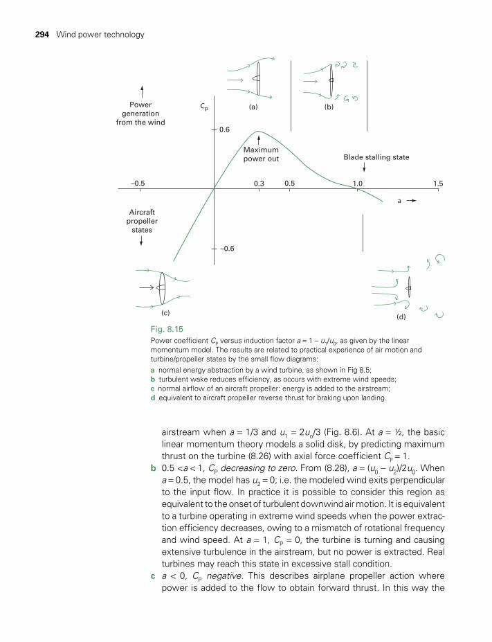
294 Wind power technology
airstream when a = 1/3 and u1 = 2uo/3 (Fig. 8.6). At a = ½, the basic linear momentum theory models a solid disk, by predicting maximum thrust on the turbine (8.26) with axial force coefficient CF = 1.
b 0.5 <a < 1, CP decreasing to zero. From (8.28), a = (u0 − u2)/2u0. When a = 0.5, the model has u2 = 0; i.e. the modeled wind exits perpendicular to the input flow. In practice it is possible to consider this region as equivalent to the onset of turbulent downwind air motion. It is equivalent to a turbine operating in extreme wind speeds when the power extrac-tion efficiency decreases, owing to a mismatch of rotational frequency and wind speed. At a = 1, CP = 0, the turbine is turning and causing extensive turbulence in the airstream, but no power is extracted. Real turbines may reach this state in excessive stall condition.
c a < 0, CP negative. This describes airplane propeller action where power is added to the flow to obtain forward thrust. In this way the
Powergeneration
from the wind
(a)
(c)
(b)
(d)
Maximumpower out Blade stalling state
Aircraftpropeller
states
0.6
0.3 0.5–0.5 1.0 1.5
a
Cp
–0.6
Fig. 8.15 Power coefficient CP versus induction factor a = 1 – u1/u0, as given by the linear momentum model. The results are related to practical experience of air motion and turbine/propeller states by the small flow diagrams: a normal energy abstraction by a wind turbine, as shown in Fig 8.5; b turbulent wake reduces efficiency, as occurs with extreme wind speeds; c normal airflow of an aircraft propeller: energy is added to the airstream; d equivalent to aircraft propeller reverse thrust for braking upon landing.
TWIDELL PAGINATION.indb 294 01/12/2014 11:37

§8.6 Blade element theory 295
propellers pull themselves into the incoming airstream and propel the airplane forward into the airstream.
d a >1. This implies negative u1 and is met if a propeller airplane reverses thrust by changing blade pitch on landing (e.g. the C-130 Hercules). Intense vortex shedding occurs in the airstream as the air passes the propellers. In the airplane, additional energy is being added to the air-stream and is apparent in the vortices, yet the total effect is a reverse thrust to increase braking.
§8.6 BLADE ELEMENT THEORY
Previous sections have established a basic understanding of wind power machines and their dynamics; in particular we have defined dimension-less scaling parameters for power coefficient CP, torque coefficient CG , and tip-speed ratio λ. However, we have not analyzed how, for each section of a blade, the relative wind speed and the forces of lift and drag vary along the blade. Such analysis is called blade element theory (also called ‘stream-tube theory’), of which we give only an outline in this section. See more advanced textbooks (e.g. Hansen 2007) for further details.
§8.6.1 Calculation of lift and drag forces on a blade element
We begin by considering blade elements (sections) and the cylinders of the airstream (stream-tubes) moving onto the rotor, as shown in Fig. 8.16. Each blade element of Fig. 8.16(a) is associated with a standard airfoil cross-section. The lift and drag forces on most common airfoil shapes have been measured and tabulated, notably by NASA,5 as a function of relative air speed vr and angle of attack a. From these data for each element, the force turning the rotor can be calculated by integration along each blade.
The most efficient wind turbines have twisted blades, with the ‘twist’ most pronounced near the hub (Fig. 8.16(c) and Fig. 8.16(d)). In opera-tion, this allows the angle of attack a along the blade to be closer to optimum, since vr increases and f decreases with distance from the hub (see Fig. 8.16(c)). At start-up rW is zero and, in practice, u0 ≥ 4 m/s, so having the largest twist near the hub gives an angle of attack that results in sufficient accelerating torque on the rotor to begin rotation. Once rotating, the contribution to torque from the inner parts of the blades is minimal, so the large twist near the hub is then unimportant.
The rotor with its blades rotates at frequency (angular speed) W; there-fore the elemental section moves at linear speed v = rW in the plane of the rotor. The linear speed of the horizontal wind far upstream is u0. By actuator disk theory (Fig. 8.5), as the airstream expands the horizontal wind speed in the model becomes u1 = u0(1–a) at the rotor plane; see
TWIDELL PAGINATION.indb 295 01/12/2014 11:37
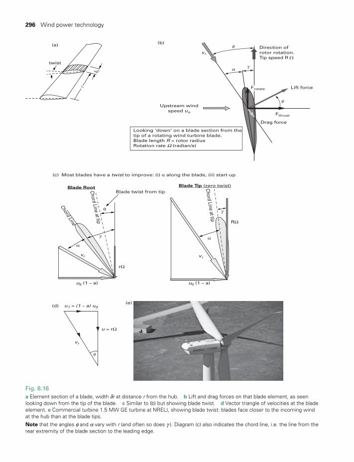
296 Wind power technology
twist
(a) (b)
(c)
(d)(e)
r
δ r
Lift force
α
φ
φ
φ
γ
γ
γ
Direction ofrotor rotation.Tip speed RΩ
Drag force
Fthrust
Frotate
Upstream windspeed uo
vr
Looking ‘down’ on a blade section from thetip of a rotating wind turbine blade.Blade length R = rotor radiusRotation rate Ω (radian/s)
Most blades have a twist to improve: (i) a along the blade, (ii) start-up
Blade Root Blade Tip (zero twist)Blade twist from tip
rΩ
RΩ
u0 (1 – a) u0 (1 – a)
θ
α
α
Chord Line
Chord Line at tip
Chord Line at tip
u1 = (1 – a) u0
u = rΩ
vr
vr vr
Fig. 8.16a Element section of a blade, width dr at distance r from the hub. b Lift and drag forces on that blade element, as seen looking down from the tip of the blade. c Similar to (b) but showing blade twist. d Vector triangle of velocities at the blade element. e Commercial turbine 1.5 MW GE turbine at NREL), showing blade twist: blades face closer to the incoming wind at the hub than at the blade tips.Note that the angles f and a vary with r (and often so does g ). Diagram (c) also indicates the chord line, i.e. the line from the rear extremity of the blade section to the leading edge.
TWIDELL PAGINATION.indb 296 01/12/2014 11:37
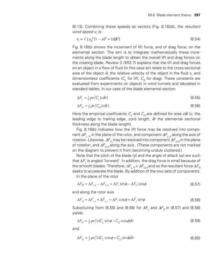
§8.6 Blade element theory 297
(8.13). Combining these speeds as vectors (Fig. 8.16(d)), the resultant wind speed vr is:
vr = √ u02 (1 − a )2 + (rW)2 (8.54)
Fig. 8.16(b) shows the increment of lift force, and of drag force, on the elemental section. The aim is to integrate mathematically these incre-ments along the blade length to obtain the overall lift and drag forces on the rotating blade. Review 2 (§R2.7) explains that the lift and drag forces on an object in a flow of fluid (in this case air) relate to the cross-sectional area of the object A; the relative velocity of the object in the fluid vr and dimensionless coefficients (CL for lift, CD for drag). These constants are evaluated from experiments on objects in wind tunnels and tabulated in standard tables. In our case of the blade elemental section:
F v C c r( )L r L12
2r dD = (8.55)
F v C c r( )D r D12
2r dD = (8.56)
Here the empirical coefficients CL and CD are defined for area cdr (c, the leading edge to trailing edge, cord length, dr the elemental sectional thickness along the blade length).
Fig. 8.16(b) indicates how the lift force may be resolved into compo-nent DFL, R in the plane of the rotor, and component DFL,A along the axis of rotation. Likewise, DFD may be resolved into component DFD,R in the plane of rotation, and DFD,A along the axis.. (These components are not marked on the diagram to prevent it from becoming unduly cluttered.)
Note that the pitch of the blade (g ) and the angle of attack (a ) are such that DFL is angled ‘forward’. In addition, the drag force is small because of the smooth blades. Therefore, DFL,R > DFD,R and so the resultant force DFR seeks to accelerate the blade. By addition of the two sets of components:
In the plane of the rotor
f fD = D − D = D − DF F F F Fsin cosR L R D R L D, , (8.57)
and along the rotor axis
f fD = D + D = D + DF F F F Fcos sinA L A D A L D, , (8.58)
Substituting from (8.55) and (8.56) for DFL and DFD in (8.57) and (8.58) yields:
F v c C C r( sin cos )R r L D12
2r f f dD = − (8.59)
and:
F v c C C r( cos sin )A r L D12
2r f f dD = + (8.60)
TWIDELL PAGINATION.indb 297 01/12/2014 11:37
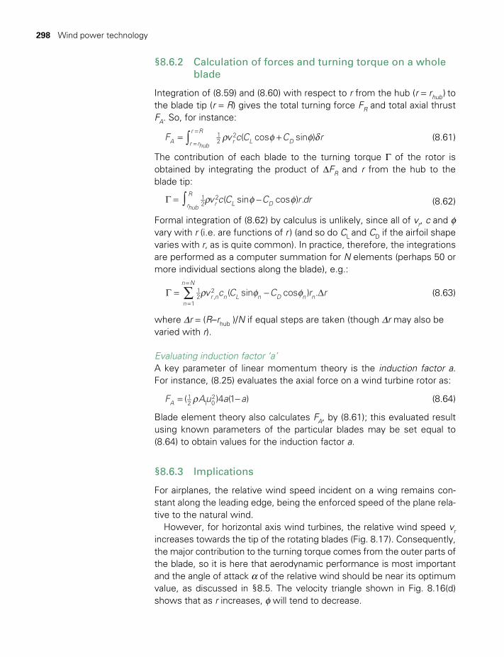
298 Wind power technology
§8.6.2 Calculation of forces and turning torque on a whole blade
Integration of (8.59) and (8.60) with respect to r from the hub (r = rhub ) to the blade tip (r = R) gives the total turning force FR and total axial thrust FA. So, for instance:
F v c C C r( cos sin )A r rhub
r R
r L D12
2∫ r f f d= +=
= (8.61)
The contribution of each blade to the turning torque G of the rotor is obtained by integrating the product of DFR and r from the hub to the blade tip:
v c C C r dr( sin cos ) .rhub
R
r L D12
2∫ r f fG = − (8.62)
Formal integration of (8.62) by calculus is unlikely, since all of vr, c and f vary with r (i.e. are functions of r ) (and so do CL and CD if the airfoil shape varies with r, as is quite common). In practice, therefore, the integrations are performed as a computer summation for N elements (perhaps 50 or more individual sections along the blade), e.g.:
v c C C r r( sin cos ) .n
n N
r n n L n D n n12
1,
2∑ r f fG = − D=
=
(8.63)
where Dr = (R–rhub )/N if equal steps are taken (though Dr may also be varied with r).
Evaluating induction factor ‘a’ A key parameter of linear momentum theory is the induction factor a. For instance, (8.25) evaluates the axial force on a wind turbine rotor as:
F Au a a( )4 (1 )A12 1 0
2r= − (8.64)
Blade element theory also calculates FA, by (8.61); this evaluated result using known parameters of the particular blades may be set equal to (8.64) to obtain values for the induction factor a.
§8.6.3 Implications
For airplanes, the relative wind speed incident on a wing remains con-stant along the leading edge, being the enforced speed of the plane rela-tive to the natural wind.
However, for horizontal axis wind turbines, the relative wind speed vr increases towards the tip of the rotating blades (Fig. 8.17). Consequently, the major contribution to the turning torque comes from the outer parts of the blade, so it is here that aerodynamic performance is most important and the angle of attack a of the relative wind should be near its optimum value, as discussed in §8.5. The velocity triangle shown in Fig. 8.16(d) shows that as r increases, f will tend to decrease.
TWIDELL PAGINATION.indb 298 01/12/2014 11:37
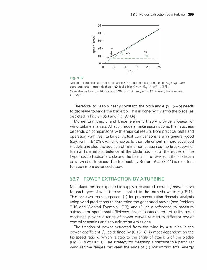
§8.7 Power extraction by a turbine 299
0
10
20
30
40
50
0 5 10 15 20 25
r / m
spee
d /(
m/s
)
u1rΩ
vr
Fig. 8.17 Modeled airspeeds at rotor at distance r from axis (long green dashes) u1 = u0(1–a) = constant; (short green dashes ) r W; (solid black) = √ − + Wv u a r[ (1 ) ( ) ]r 0
2 2 2 . Case shown has u0 = 10 m/s, a = 0.30, W = 1.78 rad/sec = 17 rev/min, blade radius R = 25 m.
Therefore, to keep a nearly constant, the pitch angle g (= f − a) needs to decrease towards the blade tip. This is done by twisting the blade, as depicted in Fig. 8.16(c) and Fig. 8.16(e).
Momentum theory and blade element theory provide models for wind turbine analysis. All such models make assumptions; their success depends on comparisons with empirical results from practical tests and operation with real turbines. Actual comparisons are in general good (say, within ± 10%), which enables further refinement in more advanced models and also the addition of refinements, such as the breakdown of laminar flow into turbulence at the blade tips (i.e. at the edges of the hypothesized actuator disk) and the formation of wakes in the airstream downwind of turbines. The textbook by Burton et al. (2011) is excellent for such more advanced study.
§8.7 POWER EXTRACTION BY A TURBINE
Manufacturers are expected to supply a measured operating power curve for each type of wind turbine supplied, in the form shown in Fig. 8.18. This has two main purposes: (1) for pre-construction financial analysis using wind predictions to determine the generated power (see Problem 8.10 and Worked Example 17.3); and (2) as a reference to measure subsequent operational efficiency. Most manufacturers of utility scale machines provide a range of power curves related to different power control scenarios and acoustic noise emissions.
The fraction of power extracted from the wind by a turbine is the power coefficient CP, as defined by (8.16). CP is most dependent on the tip-speed ratio λ, which relates to the angle of attack a of the blades (Fig. 8.14 of §8.5.1). The strategy for matching a machine to a particular wind regime ranges between the aims of (1) maximizing total energy
TWIDELL PAGINATION.indb 299 01/12/2014 11:37
300 Wind power technology
production during the year (e.g. for sale to a utility electricity network); and (2) providing a minimum supply even in light winds (e.g. for water pumping to a cattle trough or charging a battery for lighting). In addi-tion, secondary equipment, such as generators or pumps, has to be coupled to the turbine, so its power-matching response has to be linked to the turbine characteristic. The subject of power extraction is therefore complex, incorporating many factors, and in practice a range of strate-gies and types of system will be used according to different traditions and needs.
This section considers power extracted by the turbine, which will have a rated power capacity PR usually equal to the capacity of the generator that can be maintained continuously without overheating. The fraction of power in the wind captured by the turbine is CP(u), the power coefficient, defined from (8.16), which is a function of the wind speed u:
r=C u P A u( ) / ( )P T12 1
3 (8.65)
Note that for simplification of notation in this section, we sometimes use the symbol u for the unperturbed (upstream) wind speed, denoted by u0 in §8.3. As in §7.2.3, let Φu denote the normalized probability per wind speed interval that the unperturbed wind speed will be in the interval u to (u + du ), i.e. Φu du is the probability of wind speed between u and (u + du ). Then the average power extracted by the turbine of rotor area A1 from air of density r per interval of wind speed u is:
∫r Φ=
∞P A u C u u= ( )d1
2T uu13
P0 (8.66)
Let E be the total energy extracted in the period T, and let Eu be the corresponding energy extracted per unit of wind speed between wind speeds of u and (u + du). The capacity factor Z is defined generally for all
Turbineoutputpower PT
PR Rated power
Cut in
uci uRWind speed u
uR
Rated wind speed
Cut out
Fig. 8.18Wind turbine power curve for operating regions and power performance. Typical values are cut-in wind speed uci ≈ 5m/s, rated wind speed uR ≈ 13 m/s, cut-out wind speed uco ≈ 30m/s.
Standard characteristics; requiring exact blade pitch control.- - - - Actual operating characteristics of many machines, including stall regulation.
TWIDELL PAGINATION.indb 300 01/12/2014 11:37
§8.7 Power extraction by a turbine 301
energy generation plant in §1.5.4(b), as the energy actually generated in time period T, usually a year, as a proportion of the energy that would be produced if the turbine generated continuously at rated power:
So, in this case:
∫ ∫r= = = =
Φ=
∞
ZE
P T
E du
P TPP
A u C u u
P
( )d12
R
u
R
T
R
u Pu
R
13
0 (8.67)
where =P E T/T is the average power produced over the period T. Thus the capacity factor depends strongly on the wind regime. For a site with strong, steady wind (e.g. on the west coast of New Zealand) Z may be as large as 40%. For sites with weaker but still viable wind (e.g. parts of Germany), Z is typically in the range 15–25%. (See Table D.4 in Appendix D.)
It is usually considered that there are four distinct wind speed regions of operation (see. Fig. 8.18):
1 u0 less than cut-in speed uci
Eu = 0 for u0 < uci (8.68)
There is no power output because the generator is either stationary or rotating too slowly for meaningful power output; in practice, espe-cially for large machines, the rotor is braked automatically to prevent ‘rocking’ movements that cause wear in shafts and gearboxes. Accidents due to an unlocked rotor beginning to turn are prevented if automatic or manual locking occurs.
2 u0 greater than rated speed uR but less than cut-out speed uco In this range the turbine is producing constant power PR, so:
Eu = (Φu > uR − Φu > uco
) PRT (8.69)
where Φu > u' is the probability of the wind speed exceeding u’ (as in Fig. 7.8 of Worked Example 7.1. §7.3.4), and PR is the rated power output and T is the evaluation time.
3 u0 greater than cut-out speed uco By definition of the cut-out speed,
Eu = 0 for u0 > uco (8.70)
However, in practice, many machines do not fully cut out in high wind speeds because of stall regulation, but continue to operate at greatly reduced efficiency at reasonably large power.
4 u between uci and uR The turbine power output PT increases with u in a way that depends
on the operating conditions and type of machine. For many machines, PT in this range can be fitted by an equation of the form:
PT ≈ au 30 − bPR (8.71)
TWIDELL PAGINATION.indb 301 01/12/2014 11:37
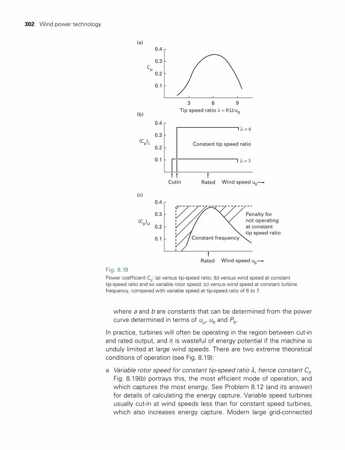
302 Wind power technology
where a and b are constants that can be determined from the power curve determined in terms of uci, uR and PR.
In practice, turbines will often be operating in the region between cut-in and rated output, and it is wasteful of energy potential if the machine is unduly limited at large wind speeds. There are two extreme theoretical conditions of operation (see Fig. 8.19):
a Variable rotor speed for constant tip-speed ratio λ, hence constant CP.Fig. 8.19(b) portrays this, the most efficient mode of operation, and which captures the most energy. See Problem 8.12 (and its answer) for details of calculating the energy capture. Variable speed turbines usually cut-in at wind speeds less than for constant speed turbines, which also increases energy capture. Modern large grid-connected
(a)0.4
0.3
0.2
0.1
3Tip speed ratio λ = R Ω/u0
Constant tip speed ratio
Cutin Rated Wind speed u0
Rated Wind speed u0
Penalty fornot operatingat constanttip speed ratio
Constant frequency
6 9
0.4
0.3
0.2
0.1
0.4
0.3
0.2
0.1
Cp
(Cp)λ
(Cp)Ω
(c)
(b)
λ = 6
λ = 3
Fig. 8.19 Power coefficient Cp: (a) versus tip-speed ratio; (b) versus wind speed at constant tip-speed ratio and so variable rotor speed; (c) versus wind speed at constant turbine frequency, compared with variable speed at tip-speed ratio of 6 to 7.
TWIDELL PAGINATION.indb 302 01/12/2014 11:37
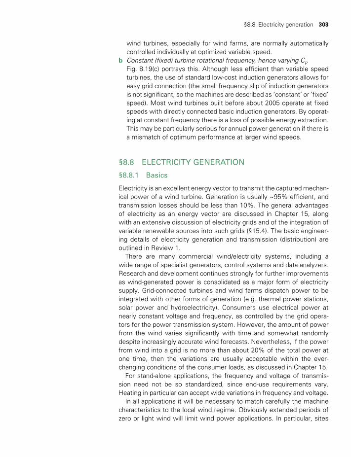
§8.8 Electricity generation 303
wind turbines, especially for wind farms, are normally automatically controlled individually at optimized variable speed.
b Constant (fixed) turbine rotational frequency, hence varying CP Fig. 8.19(c) portrays this. Although less efficient than variable speed turbines, the use of standard low-cost induction generators allows for easy grid connection (the small frequency slip of induction generators is not significant, so the machines are described as ‘constant’ or ‘fixed’ speed). Most wind turbines built before about 2005 operate at fixed speeds with directly connected basic induction generators. By operat-ing at constant frequency there is a loss of possible energy extraction. This may be particularly serious for annual power generation if there is a mismatch of optimum performance at larger wind speeds.
§8.8 ELECTRICITY GENERATION
§8.8.1 Basics
Electricity is an excellent energy vector to transmit the captured mechan-ical power of a wind turbine. Generation is usually ~95% efficient, and transmission losses should be less than 10%. The general advantages of electricity as an energy vector are discussed in Chapter 15, along with an extensive discussion of electricity grids and of the integration of variable renewable sources into such grids (§15.4). The basic engineer-ing details of electricity generation and transmission (distribution) are outlined in Review 1.
There are many commercial wind/electricity systems, including a wide range of specialist generators, control systems and data analyzers. Research and development continues strongly for further improvements as wind-generated power is consolidated as a major form of electricity supply. Grid-connected turbines and wind farms dispatch power to be integrated with other forms of generation (e.g. thermal power stations, solar power and hydroelectricity). Consumers use electrical power at nearly constant voltage and frequency, as controlled by the grid opera-tors for the power transmission system. However, the amount of power from the wind varies significantly with time and somewhat randomly despite increasingly accurate wind forecasts. Nevertheless, if the power from wind into a grid is no more than about 20% of the total power at one time, then the variations are usually acceptable within the ever-changing conditions of the consumer loads, as discussed in Chapter 15.
For stand-alone applications, the frequency and voltage of transmis-sion need not be so standardized, since end-use requirements vary. Heating in particular can accept wide variations in frequency and voltage.
In all applications it will be necessary to match carefully the machine characteristics to the local wind regime. Obviously extended periods of zero or light wind will limit wind power applications. In particular, sites
TWIDELL PAGINATION.indb 303 01/12/2014 11:37

304 Wind power technology
with an average wind speed of less than 4 m/s at 10 m height usually have unacceptably long periods at which generation would not occur, although water pumping into water storage may still be feasible. Usually, if the annual average wind speed at 10 m height is 5 m/s or more, elec-tricity generation from wind turbines is beneficial.
The distinctive features of wind/electricity generating systems are:
1 Turbines range in size from very large (e.g. ~130 m diameter, ~5 MW) for utility generation, to very small (e.g. ~1 m diameter, ~50 W) for battery charging.
2 There are always periods without wind. Most turbines are grid con-nected, so supply to consumers continues from other generation. For the relatively few, but important, stand-alone systems, wind turbines must be linked to energy storage and/or have parallel generation (e.g. diesel generators). Chapter 15 has more details.
3 Wind turbine efficiency is greatest if rotational frequency varies to maintain constant tip-speed ratio, yet electricity supply is at nearly constant frequency. Therefore interface electronics is needed, unless the wind turbine operates less efficiently at fixed speed.
4 Mechanical control of a turbine by blade pitch or other mechani-cal control increases efficiency, but also increases complexity and expense. An alternative method, usually cheaper and more efficient but seldom done, is to vary the electrical load on the turbine to control the rotational frequency.
5 The optimum rotational frequency of a turbine (its ‘speed’) in a par-ticular wind speed decreases with an increase in radius in order to maintain constant tip-speed ratio (§8.5). Thus only small (~2 m radius) turbines can be coupled directly to conventional four or six pole-pair generators. Larger machines require additional equipment, which may or may not include: (i) a gearbox to increase the generator drive fre-quency; (ii) special multipole or doubly fed generators; or (iii) interface electronics as rectifiers and inverters (refer to Review 1). Gearboxes are relatively expensive and heavy; they require regular maintenance and can be noisy. Special generators and electronic interfaces are also expensive, but become cheaper and more reliable in mass production.
6 Very short-term, but useful, ‘rotor inertia’ energy storage occurs which smooths wind turbulence. Even the provision of a ‘soft coupling’ using teetered blades, shock absorbers or other mechanical mechanisms is useful to reduce electrical spikes and mechanical strain.
7 Often, the best wind power sites are in remote rural, island or marine areas. Local energy requirements at such places are distinctive, and almost certainly do not require the much larger electrical power of urban and industrial complexes. Some of these locations are grid con-nected to regional or national networks and some are not. The techni-cal implications of this are outlined in §8.8.6.
TWIDELL PAGINATION.indb 304 01/12/2014 11:37
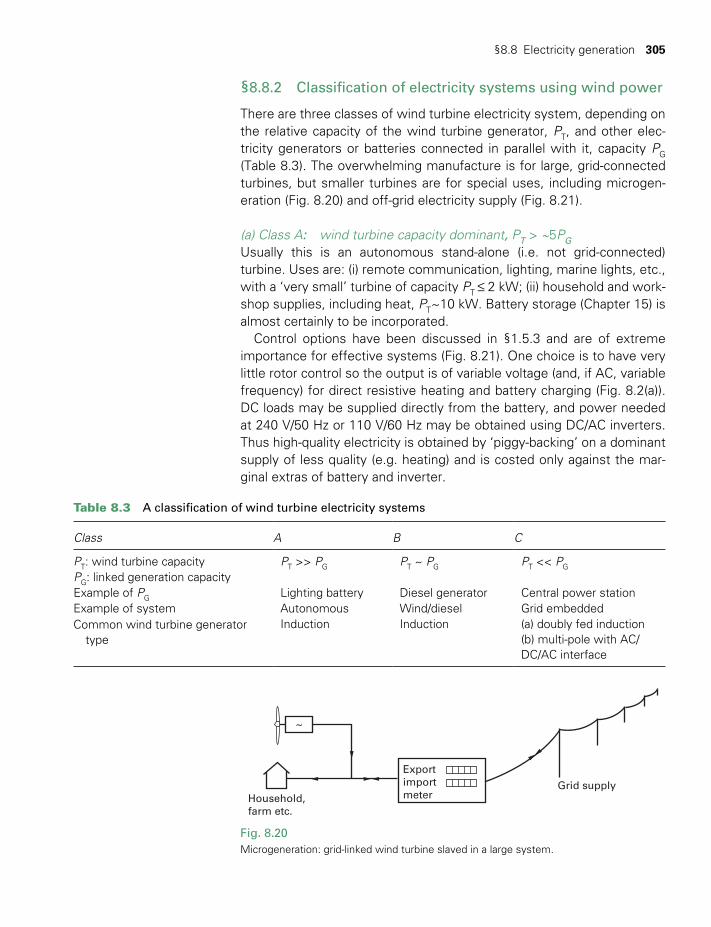
§8.8 Electricity generation 305
§8.8.2 Classification of electricity systems using wind power
There are three classes of wind turbine electricity system, depending on the relative capacity of the wind turbine generator, PT, and other elec-tricity generators or batteries connected in parallel with it, capacity PG (Table 8.3). The overwhelming manufacture is for large, grid-connected turbines, but smaller turbines are for special uses, including microgen-eration (Fig. 8.20) and off-grid electricity supply (Fig. 8.21).
(a) Class A: wind turbine capacity dominant, PT > ~5PG
Usually this is an autonomous stand-alone (i.e. not grid-connected) turbine. Uses are: (i) remote communication, lighting, marine lights, etc., with a ‘very small’ turbine of capacity PT ≤ 2 kW; (ii) household and work-shop supplies, including heat, PT~10 kW. Battery storage (Chapter 15) is almost certainly to be incorporated.
Control options have been discussed in §1.5.3 and are of extreme importance for effective systems (Fig. 8.21). One choice is to have very little rotor control so the output is of variable voltage (and, if AC, variable frequency) for direct resistive heating and battery charging (Fig. 8.2(a)). DC loads may be supplied directly from the battery, and power needed at 240 V/50 Hz or 110 V/60 Hz may be obtained using DC/AC inverters. Thus high-quality electricity is obtained by ‘piggy-backing’ on a dominant supply of less quality (e.g. heating) and is costed only against the mar-ginal extras of battery and inverter.
Household,farm etc.
~
Exportimportmeter
Grid supply
Fig. 8.20 Microgeneration: grid-linked wind turbine slaved in a large system.
Table 8.3 A classification of wind turbine electricity systems
Class A B C
PT: wind turbine capacity PT >> PG PT ~ PG PT << PGPG: linked generation capacityExample of PG Lighting battery Diesel generator Central power stationExample of system Autonomous Wind/diesel Grid embeddedCommon wind turbine generator type
Induction Induction (a) doubly fed induction(b) multi-pole with AC/DC/AC interface
TWIDELL PAGINATION.indb 305 01/12/2014 11:37
306 Wind power technology
However, it may be preferred to have the electricity directly at con-trolled frequency. There are two extreme options for this:
1 Mechanical control of the turbine blades. As the wind changes speed, the pitch of the blades or blade tips is adjusted to control the frequency of turbine rotation (Fig.8.21(b)). The disadvantages are that power in the wind is ‘spilt’ and therefore lost (see §1.5) and the control method may be expensive and unreliable.
2 Load control. As the wind changes speed, the electrical load is changed by rapid switching, so the turbine frequency is controlled (Fig. 8.21(c)). This method makes greater use of the power in the wind by optimiz-ing tip-speed ratio λ. Moreover, local control by modern electronic methods is cheaper and more reliable than control of mechanical com-ponents exposed in adverse environments.
Permanent magnet multipole generators are common for small machines. DC systems can be smoothed and the energy stored in batteries. AC systems may have synchronous generators producing uncontrolled variable frquency output for heat, or controlled output by mechanical or load control. AC induction generators can be self-excited with a capacitor bank to earth, or may operate with an idling synchro-nous generator as a compensator. (See Review 1 for further details of generator types.)
(a)Variable voltage
Resistive heating
Battery charging
Controlled AC~
~
DC/ACinverter
Controller
Feedback toblade pitch
(b)
(c) Priority loadController
Feedforwardto a rangeof loads
Controlledfixed voltageand frequency
and/or frequency
Fig. 8.21Some supply options for stand-alone systems with the wind turbine the dominant supply.
TWIDELL PAGINATION.indb 306 01/12/2014 11:37
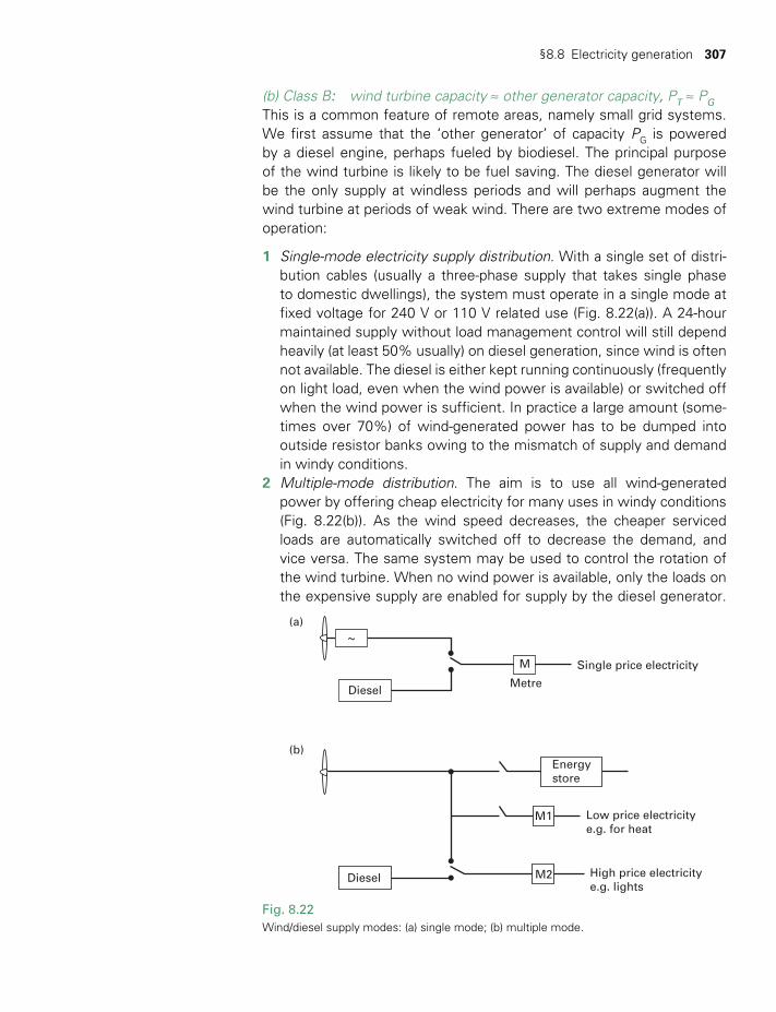
§8.8 Electricity generation 307
(a)
(b)
Diesel M2
M1
M
Metre
Single price electricity
Low price electricitye.g. for heat
High price electricitye.g. lights
Diesel
~
Energystore
Fig. 8.22Wind/diesel supply modes: (a) single mode; (b) multiple mode.
(b) Class B: wind turbine capacity ≈ other generator capacity, PT ≈ PG
This is a common feature of remote areas, namely small grid systems. We first assume that the ‘other generator’ of capacity PG is powered by a diesel engine, perhaps fueled by biodiesel. The principal purpose of the wind turbine is likely to be fuel saving. The diesel generator will be the only supply at windless periods and will perhaps augment the wind turbine at periods of weak wind. There are two extreme modes of operation:
1 Single-mode electricity supply distribution. With a single set of distri-bution cables (usually a three-phase supply that takes single phase to domestic dwellings), the system must operate in a single mode at fixed voltage for 240 V or 110 V related use (Fig. 8.22(a)). A 24-hour maintained supply without load management control will still depend heavily (at least 50% usually) on diesel generation, since wind is often not available. The diesel is either kept running continuously (frequently on light load, even when the wind power is available) or switched off when the wind power is sufficient. In practice a large amount (some-times over 70%) of wind-generated power has to be dumped into outside resistor banks owing to the mismatch of supply and demand in windy conditions.
2 Multiple-mode distribution. The aim is to use all wind-generated power by offering cheap electricity for many uses in windy conditions (Fig. 8.22(b)). As the wind speed decreases, the cheaper serviced loads are automatically switched off to decrease the demand, and vice versa. The same system may be used to control the rotation of the wind turbine. When no wind power is available, only the loads on the expensive supply are enabled for supply by the diesel generator.
TWIDELL PAGINATION.indb 307 01/12/2014 11:37
308 Wind power technology
The pragmatic economic advantage of successful multiple-mode operation is that the full capital value of the wind machine is used at all times, and since the initial power in the wind is free, the maximum benefit is obtained. It is also advantageous in using less fuel with the abatement of pollution and noise.
(c) Class C: grid linked, wind turbine embedded in a large system, PT ≤ 0.2 PG
This is the most common arrangement for large (>~1 MW), medium (~250 kW) and small (~50 kW) machines where a public utility or other large-capacity grid is available. In this case PG is usually from relatively very large (>~500 MW) central power stations that control the frequency across the network.. The bulk of new wind power capacity is for wind farms, in which a number (10 to 1000) of turbines in a group feed into the grid (§8.8.3). For smaller systems, the owner (microgenerator) may use the wind power directly and sell (export) excess to the grid, with electricity purchased (imported) from the grid at periods of weak or no wind (Fig. 8.20).
Review 1 considers electricity generation in more detail. The cheap-est type of generator is an induction generator connected directly to the grid. The turbine has to operate at nearly constant frequency, within a maximum slip usually less than 5% ahead of the mains-related fre-quency; this is usually called ‘fixed speed’. In weak wind, there is an automatic cut-out to prevent motoring. The disadvantage of a directly coupled induction generator is that the turbine frequency cannot change sufficiently to maintain even approximate constant tip-speed ratio.
However, there are several ways in which the system can be made to produce electricity at fairly constant frequency while allowing varia-tion in turbine frequency. They include: (1) multiple (usually two) com-bination windings in an induction generator to connect more pole-pairs in weak winds for smaller rotational frequency; (2) some intermediate scale machines use two generators in the same nacelle, say, 5 kW and 22 kW, for automatic connection to a two-speed gearbox in light and strong winds; (3) using a synchronous generator and rectifying its output to direct current and then producing the prescribed alternating current mains frequency with an inverter; (4) increasing the effective slip on an induction generator by active change of the current and phase in the gen-erator’s rotor (e.g. in a doubly fed induction generator); this requires exter-nal electrical connection to the rotor winding via slip rings and brushes.
§8.8.3 Wind farms: inland and offshore
(a) Why wind farms? Commercial wind turbines are an established ‘mainstream’ form of power generation into grid distribution and transmission networks, with most capacity in multi-turbine wind farms, mainly on land (as shown
TWIDELL PAGINATION.indb 308 01/12/2014 11:37

§8.8 Electricity generation 309
Fig. 8.23Part of the Buffalo Ridge wind farm in Minnesota, USA, with agricultural activity continuing underneath and around the turbines. The turbines shown are some of the 143 Zond Z-750s installed in 1998, each of height 78 m and rated at 750 kW. Many more turbines have been installed on Buffalo Ridge subsequently.
in Fig. 8.23), but with an increasing proportion offshore (as shown in Fig. 8.24). The growth of worldwide generating capacity has been, and continues to be, about 20%/y, which is remarkable for engineering structures (see Fig. 8.1).
Machines of multiple-megawatt capacity operate successfully, with lifetimes of 20 to 25 years, and more with renovation. Multiple numbers of machines installed in wind farms (typically with 10 to 100 turbines on land, and 50 to 300 offshore) make convenient and manageable units as distributed generation into regional and national electricity networks. Grouping machines in this way allows savings in planning applications, construction costs (e.g. having specialized cranes, etc. on site), grid con-nection (fewer substations and grid interface transformers), common management and maintenance. Wind farms are most likely in countries with (1) governmental commitment to sustainable, low-carbon energy supplies; (2) unmet electricity supply needs, and (3) open, rural or marine coastal areas with an average wind speed >6 m/s at 10 m height.
(b) Offshore wind farmsOffshore wind farms have increased rapidly in importance since about 2000. Although generally more expensive to install and operate than wind farms on land, they are favored in countries with marine coasts which have limited land available for wind farms and/or there are lobbies against wind power on land. Moreover, wind speed is usually greater off-shore than on land. Europe dominates offshore wind turbines in numbers and in the development of the technology; by mid-2013 total offshore wind capacity was 6 GW in 58 offshore wind farms in 10 countries, showing that the industry had become established.
> ~
TWIDELL PAGINATION.indb 309 01/12/2014 11:37

310 Wind power technology
The benefits of offshore wind farms compared with onshore therefore include the following:
• stronger and less turbulent wind, hence more power;• large areas available under single government-related ownership;• no nearby population that might be disturbed;• delivery and installation of heavy tower sections and long blades by
boat (delivery usually easier than onshore delivery by road); • large total generation capacity linked to high-voltage land transmission
grids;• output of individual wind farms controlled remotely by grid operators.
The disadvantages include the following:
• difficult access requiring special skills and safety provision;• more expensive installation and maintenance, including subsea
foundations;• corrosive saline environment.
Fig. 8.24 shows examples of construction and operation of offshore wind farms.
Special requirements for offshore turbines include the following:
• marine environmental impact assessment, including migratory birds, sea mammal communication, shipping lanes, fishing, sea views;
• wind speed assessment, probably including sonic and laser tech-niques (see §7.4);
• subsea foundations and anti-scour protection from subsea water currents;
• specialist marine installation ‘ship/platforms’ (see e.g. Fig. 8.24(b) and (c));
Fig. 8.24 Offshore wind farms. a Middelgrunden, Copenhagen harbour, early cooperative offshore wind farm: 20 × 2 MW turbines. b Wind farm offshore from Great Yarmouth England, at Scroby Sands, 30 × 2 MW turbines. c The jack-up vessel Resolution installing wind turbines offshore.
(a) (b) (c)
TWIDELL PAGINATION.indb 310 01/12/2014 11:37
§8.8 Electricity generation 311
• maintenance access by boat, including in bad weather;• marine substation large power connection to onshore power networks;• exceptionally thorough component standards to reduce faults and
maintenance;• large power density transmitted significant distances to integrate with
high-voltage onshore grids (see §R1.4). High-voltage direct current (HVDC) is the most efficient method, but requires high power AC/DC and DC/AC inverters for the connections. Therefore costs may be high.
§8.8.4 Technical aspects of grid-connected wind turbines
For all grid-connected wind turbines, the output power PT << PG, where the total power in the grid PG, is usually from relatively very large (>~500 MW) central power stations that control the frequency across the network.
§R1.6 considers electricity-generating machines in more detail. The cheapest and most robust type of generator is an induction generator connected directly to the grid. The turbine has to operate at nearly con-stant frequency, within a maximum slip usually less than 5% ahead of the mains-related frequency; this is usually called ‘fixed speed’. In weak wind, there is an automatic cut-out to prevent motoring. The disadvantage of a directly coupled induction generator is that the turbine frequency cannot change sufficiently to maintain even approximate constant tip-speed ratio.
However, there are several ways in which the system can be made to produce electricity at fairly constant frequency while allowing variation in turbine frequency. They include: (1) multiple (usually two) combination windings in an induction generator to connect more pole-pairs in weak winds for smaller rotational frequency; (2) using a synchronous generator and rectifying its output to direct current and then producing the prescribed alternating current mains frequency with an inverter; (3) increasing the effective slip on an induction generator by active change of the current and phase in the generator’s rotor (e.g. in a doubly fed induction genera-tor); this requires external electrical connection to the rotor winding via slip rings and brushes; and (4) some small-scale machines use two gen-erators in the same nacelle, say, 5 kW and 22 kW, which are automatically connected to a two-speed gearbox in light and strong winds respectively.
§8.8.5 Wind power contribution to national electricity generation
Because wind power generation is variable, adding wind capacity of, say, 100 MW capacity to a grid is not equivalent to adding 100 MW capac-ity from a thermal source (coal, gas, nuclear, biomass). In general the average capacity factor (sometimes called the ‘load factor’) of a wind turbine is 20 to 35%, whereas for a thermal power station it is about
TWIDELL PAGINATION.indb 311 01/12/2014 11:37

312 Wind power technology
70 to 90%. Yet, not all thermal sources are equivalent (e.g. nuclear power is suitable only for baseload and is shut down about every 18 months for refueling, whereas gas turbines are best for rapid response to peak demands). Network operators describe the contribution of different power sources in terms of capacity credit, namely the power rating of a network’s conventional plant that is displaced by the installation of wind power or other renewable energy (see Box 15.3). Theoretical studies indicate that 1000 MW (rated) wind power has a capacity credit of 250 to 400 MW, depending on long-term wind characteristics (Milborrow 2001). If the wind power comes from a diversity of sites, there is less chance of them all having reduced output at the same time, and so the predicted capacity credit is larger. (For a more extensive analysis of these issues see Twidell (2013), ‘Assessing Backup Requirements for Wind Power’, item S15.1 in the online supplementary material for this book.)
A utility network always has to have reserve generating capacity and load-reduction facilities available for all forms of generation, especially because the supply from large power stations can fail abruptly and unex-pectedly at times. As is also discussed in §15.4, this established reserve capacity from a mix of sources has proved in practice to be sufficient for variable renewables (notably wind power) to contribute up to 20 to 30% of total capacity. Box 15.4 describes such wind-powered supply in the joint Norweb system of Norway, Sweden and Denmark, and in Ireland.
Special provision is perhaps needed only if the share of wind capacity exceeds about 20 to 30% of total capacity. Such provision may not neces-sarily be only in the form of extra thermal or hydro-reservoir capacity, as traditionally, but may include significant load management, and/or a diver-sity of renewable sources (see Box 15.5). To the authors’ knowledge, no additional ‘back-up power’ has yet been needed or constructed anywhere solely because of the installation of extra wind power capacity.
§8.8.6 Smaller scale systems and independent owners
Although the wind turbine market is dominated by large grid-connected turbines for wind farms, other, usually smaller, turbines continue to be developed and sold in large numbers for special uses, including inde-pendent owners, microgeneration and off-grid electricity supply. Very small machines of capacity between about 50 W and 1 kW are common for yachts and, in windy regions, for holiday caravans and houses, for low-power public service (e.g. rural bus shelters), and for small meteor-ological and other measurement sites. Often solar photovoltaic power is used in parallel with such wind power, or independently. Slightly larger, but still ‘small’ are 5 kW to 100 kW wind turbines installed for household, farm and institutional use. By the term ‘independent owners’ we mean individuals and individual companies operating medium (>100 kW) to large (>1 MW) turbines singly or in a cluster of two or three machines,
TWIDELL PAGINATION.indb 312 01/12/2014 11:37

§8.8 Electricity generation 313
BOX 8.2 MULTIMODE WIND POWER SYSTEM WITH LOAD-MANAGEMENT CONTROL AT FAIR ISLE, SCOTLAND
Fair Isle is an isolated Scottish island in the North Sea between mainland Shetland and Orkney. The population of about 70 is well established and progressive within the limits of the harsh yet beautiful environment. Previously the people depended entirely on coal and oil for heat, petroleum for vehicles, and diesel fuel for electricity generation. Then in 1982 the community-led electricity cooperative installed a
but not wind farms). Cost-effectiveness is likely if other energy supplies are expensive or not available, if surplus power is sold and if government incentives, such as feed-in tariffs, are available.
Often, the best wind power sites are in remote rural, island or marine areas. Energy requirements in such places are distinctive, and almost certainly will not require the intense electrical power of large industrial complexes. Often end-use requirements for controlled electricity (e.g. 240 V/50 Hz or 110 V/60 Hz for lighting, machines and electronics) are likely to be only 5 to 10% of the total energy requirement for transport, cooking and heat. Therefore wind power may provide affordable energy for heat and transport, in addition to standard electrical uses. Such devel-opments occurred first in some remote area power systems (e.g. the Fair Isle system described in Box 8.2) but now are increasingly common and sophisticated (see also Box 15.7 for the example at Utsira, Norway). Moreover, rural grid systems are likely to be ‘weak’, since they carry relatively low-voltage electricity (e.g. 33 kV) over relatively long distances with complicated inductive and resistive power-loss problems. Interfacing a wind turbine in weak grids is acceptable with modern power electronic control and interfaces; indeed, the wind power may be used to strengthen the grid supply, for instance, by controlling reactive power and voltage.
As with most other supplies, grid connection benefits wind power instal-lations technically and may allow excess electricity to be sold. Indeed, the whole network benefits by such distributed generation and smaller scale microgeneration. If grid connection is not possible, then wind turbines for electricity supply can operate as an ‘autonomous stand-alone’ system mentioned in §8.8.2 for Classes A and B; this requires connection with batteries and/or controllable generation as from a diesel generator or, if possible, hydro power. In practice, independent operation encourages ‘smart technology’ to employ the electricity for all energy uses, including heat and transport, and with energy storage (see Chapter 15). The aim is to optimize the variable generation by having responsive loads that match demand to supply. Almost certainly this requires loads that store energy, of which the simplest are thermal capacities for heated water, refrigeration and space heating and cooling. Other likely stores are bat-teries (e.g. for lighting and electric vehicles). The multi-mode system at Fair Isle (Box 8.2) illustrates what can be achieved by taking an integrated whole-system approach, covering both supply and use of energy. Such smart technology occurs on much larger systems, but is still uncommon.
TWIDELL PAGINATION.indb 313 01/12/2014 11:37
314 Wind power technology
§8.9 MECHANICAL POWER
Historically the mechanical energy in the wind has been harnessed predominantly for transport with sailing ships, for milling grain and for pumping water. These uses still continue and may increase again in the future. This section briefly discusses those systems, bearing in mind that electricity can be an intermediate energy vector for such mechanical uses.
§8.9.1 Sea transport
The old square-rigged sailing ships operated by drag forces and were inef-ficient. Modern racing yachts, with a subsurface keel harnessing lift forces, are much more efficient and can sail faster than the wind (Fig. 8.9(c)). However, pure sail power for commercial carriage of people or freight is now obsolete except in niche applications (such as in developing countries with many scattered islands (Nuttall et al. 2013). Some developments to modern cargo ships have used fixed sails set by mechanical drives.
§8.9.2 Grain milling
The traditional windmill (commonly described as a Dutch windmill) has been eclipsed by engine- or electrical-driven machines. It is unlikely that the variable nature of wind over land will ever be suitable again for com-mercial milling in direct mechanical systems. It is better that wind tur-bines are used to generate electricity into a grid and the electricity then used in motors.
60 kW rated-capacity Danish-manufactured wind turbine having a simple induction generator. This operated in the persistent winds, with average speed at 10 m height of 10 m/s. The control system (Fig. 8.21(c)) depended on frequency sensitive switches that enabled and disabled individual loads (usually heaters, much needed in the cold winters!) according to the line frequency, so controlling the rotational rate of the turbine. At the frequent periods of excessive wind power, further heat became available (e.g. for growing food in a glasshouse). For a short time in the 1980s, an electric vehicle was charged from the system, but this use was found to be not viable with the technology of the time. Despite the strong winds, the total generating capacity was small for the population served, acceptable standards being only possible because the houses are well insulated and careful energy strategies are maintained. This community wind power was one of the world’s first examples of smart energy technology.
The initial load-controlled turbine operated successfully for more than 20 years, but an increase in network demand required in 1996 a second 100 kW turbine, operating in parallel with the reconditioned first machine and two 30 kW diesel generators. This arrangement required a more complex control and supply system, with a dual tariff system as shown in Fig. 8.22(b), and an additional central ‘dump’ load, which was needed to keep the system stable. The wind turbines supply a yearly average of 85% of the electricity and heat demand and 97% in the winter, when the wind is strongest despite demand being greatest.
Source: http://www.fairisle.org.uk/FIECo/ (which includes a detailed engineering description of the upgraded system operating since 1998). Accessed 23/08/2014.
TWIDELL PAGINATION.indb 314 01/12/2014 11:37
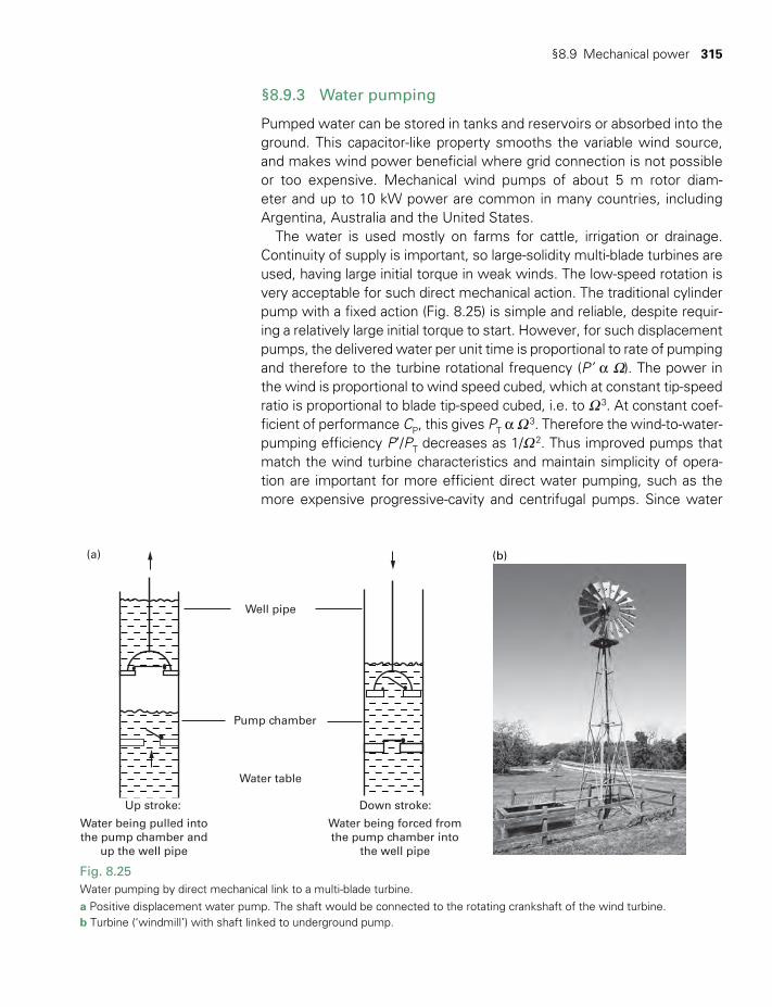
§8.9 Mechanical power 315
Well pipe
(a)
Pump chamber
Water table
Down stroke:Up stroke:
Water being pulled intothe pump chamber and
up the well pipe
Water being forced fromthe pump chamber into
the well pipe
(b)
Fig. 8.25 Water pumping by direct mechanical link to a multi-blade turbine.a Positive displacement water pump. The shaft would be connected to the rotating crankshaft of the wind turbine.b Turbine (‘windmill’) with shaft linked to underground pump.
§8.9.3 Water pumping
Pumped water can be stored in tanks and reservoirs or absorbed into the ground. This capacitor-like property smooths the variable wind source, and makes wind power beneficial where grid connection is not possible or too expensive. Mechanical wind pumps of about 5 m rotor diam-eter and up to 10 kW power are common in many countries, including Argentina, Australia and the United States.
The water is used mostly on farms for cattle, irrigation or drainage. Continuity of supply is important, so large-solidity multi-blade turbines are used, having large initial torque in weak winds. The low-speed rotation is very acceptable for such direct mechanical action. The traditional cylinder pump with a fixed action (Fig. 8.25) is simple and reliable, despite requir-ing a relatively large initial torque to start. However, for such displacement pumps, the delivered water per unit time is proportional to rate of pumping and therefore to the turbine rotational frequency (P’ a W). The power in the wind is proportional to wind speed cubed, which at constant tip-speed ratio is proportional to blade tip-speed cubed, i.e. to W 3. At constant coef-ficient of performance CP, this gives PT a W 3. Therefore the wind-to-water-pumping efficiency P’/PT decreases as 1/W 2. Thus improved pumps that match the wind turbine characteristics and maintain simplicity of opera-tion are important for more efficient direct water pumping, such as the more expensive progressive-cavity and centrifugal pumps. Since water
TWIDELL PAGINATION.indb 315 01/12/2014 11:37

316 Wind power technology
is usually available at low locations, and wind increases with height, it is often sensible to have an electricity-generating wind turbine placed on a hill operating an electric pump placed at the nearby water supply.
§8.9.4 Heat production by friction
The direct dissipation of the mechanical power from a wind turbine (e.g. by paddle wheel systems) produces heat with 100% efficiency, but matching the turbine to a mechanical ‘dissipater’ is extremely difficult. Since wind turbine electricity generators are so common and efficient, electricity is favored as the intermediate energy vector for electrically powered heating.
§8.10 SOCIAL, ECONOMIC AND ENVIRONMENTAL CONSIDERATIONS
The nation benefits from the use of wind power because electricity from wind power mitigates the emissions and costs of fossil fuels, and there-fore decreases impact causing climate change. There are also employ-ment and national energy security benefits. The owners and landlords of turbines benefit by income from exported power, and often by their own use of their power.
The key factor for successful wind power is the site wind speed. Generally u should be >5 m/s at 10 m height, but windier sites are very worthwhile owing to the u3 dependence of power output. For instance, an increase inu (at 10 m) from 6 m/s to 8.2 m/s may increase a turbine’s capacity factor from ~33% to ~49%, i.e. a 50% increase in output for the same input cost (see Problem 8.10). Technological improvements and economies of scale have resulted in the capital cost per unit capacity of wind turbines decreasing significantly since 1990 (see Fig. 17.2(b); see also chart D6 in Appendix D for ‘levelized costs’).
Supportive government policies that recognize the benefits of wind power, such as the feed-in tariffs and obligated purchases, support the growth of installations and manufacture, so establishing a viable industry.
The more local impacts of wind power may be summarized as follows:
• Visual: turbines have to be in open land or at sea, so that they are clearly visible in direct sight. Note that the larger the diameter, the slower and more ‘graceful’ the rotation and the higher the tower and blade tips. Turbine color can be chosen as the most acceptable, which is usually white. For the viewer, nearby obstruction by hills, buildings and trees, etc. can prevent sighting. Turbines may be considered detrimental if observable from historic sites or in areas of scenic beauty. Simulation
TWIDELL PAGINATION.indb 316 01/12/2014 11:37

§8.10 Social, economic and environmental considerations 317
software is used to give a dynamic visual impression of the wind farm from all viewpoints before permission is granted to construct.
• Sound: audible noise from machinery, blade tips, tower passing etc. is expected to be <40 dBA at 250 m, which is sleepable; infrasound from vibrations not audible or often detected, but contentious. Such impacts are not detectable from offshore wind farms. Modern machines are considerably quieter than early developments as manufacturers seek to respond to public comment and to improve efficiency: noise is often a sign of less efficient energy capture. (The online supplementary material eResource for this book includes our summary of noise from wind turbines and of the measurements and criteria needed for object-ive analysis access §8.1.)
• Bird and bat impact: generally very seldom (<house windows); avoid siting near hedges or other insect-feeding areas. Species vary consid-erably in their behavior and so expert investigation is needed before permitting construction.
• Agriculture: horses and cattle may be alarmed at first, but will become accustomed to the noise. In general, the previous use of the site for animals and crops continues unaffected apart from 1 to 2% of the area used by the tower bases, substations and unsurfaced roadways.
• TV and microwave: avoid line-of-sight with local transmitters.• Radar: possible interference for flight operators, who can use special
‘erasing’ software for their screens. • Sunshine shadows: may give ‘flicker’ through windows; turbines can
be automatically shut down if such flicker is likely.• Grid limitations: for exportable power may require grid upgrading.• Benefits to the local community as a whole may be offered by the
developer (e.g. cheaper electricity supplies, donations to schools).
Wind power impacts require consideration of many disciplines, including ecology, aesthetics, cultural heritage and public perceptions; Pasqualetti et al. in Wind Power in View (2002) consider these impacts in detail and their book is recommended reading.
Wind farm developers have to obtain local or national planning per-mission before installing a wind farm, which may involve consideration of all the above factors from independent experts. Consequently the process of preparing an application has become comprehensive and professional. All these procedures are necessary, but they are time-consuming and expensive. If an application is refused, then appeals may be made.
Yet the final outcome is that national and world wind power capacities are increasing, carbon and other emissions are abating, the technology is improving and most of the perceived adverse impacts are decreasing per unit of generated output.
TWIDELL PAGINATION.indb 317 01/12/2014 11:37
318 Wind power technology
QUICK QUESTIONS
Note: Answers to these questions are in the text of the relevant section of this chapter, or may be readily inferred from it.
1 For electricity generation by wind power into a utility grid network, why is a wind speed of less than 3 m/s of negligible benefit; yet a wind speed of 6 m/s is beneficial?
CHAPTER SUMMARY
Today, wind turbines are accepted as ‘mainstream power generation’ for the utility grid networks of regions with sufficient wind, notably in Europe, China and the USA. When installed in windy locations (mean wind speed at least ~5 m/s at 10 m height), wind power is cost-competitive with all other forms of electricity generation, especially when it is given financial credit for not polluting. Consequently, world installed capacity of wind power has grown at ≥20%/y for the past decade and continues to do so, almost all of it in multi-turbine wind farms on land and offshore.
For common wind speed distributions, the average annual power from a wind turbine of area A approximates to r≈P C A u( )T P 0
3 , where u0 is the upstream wind speed, r is the density of air and Cp is the [dimensionless] power coefficient. The maximum rated power capacity of a wind turbine is given for a specified rated wind speed, commonly about 12 m/s. At this speed, power production of about 0.3 kW/m2 of cross-section would be expected with Cp ~40%. A simple physical argument shows that there is a maximum value of CP because the air passing through the turbine has to retain sufficient kinetic energy to continue downstream; thus CP
(max) ~ 0.59 (the Lanchester-Betz-Zhukowsky criterion). The aerodynamics of wind turbine blades is very similar to that of airplane wings, with the aerofoil
shape carefully chosen to maximize lift force and minimize drag forces. By far the most common turbines for electricity generation are horizontal axis with two or three blades, with radius ranging from ~5 m to ~60 m. If the turbine is extracting power efficiently, the gaps between blades are not apparent to the wind and energy capture is maximized, while allowing the air to escape downwind. To prevent generators from overheating beyond their rated output, turbines are controlled passively or actively to this output in wind speeds of more than about 12 m/s. In gale-force winds, when violent turbulence might damage the machine, rotation is usually stopped for utility scale machines at the cut-out wind speed of ~30 m/s. To prevent wear for no benefit, turbines also have a cut-in wind speed, usually 3 m/s to 4 m/s.
The power coefficient CP depends strongly on the tip-speed ratio λ = RW /u0, where R is the blade radius and W is the angular speed of rotation (in radians/s). For a horizontal axis turbine to operate efficiently, the rotor should rotate at an angular speed such that λ ≈ 6 to 7. This is why small machines rotate rapidly and large machines slowly. It also implies that as the upstream wind speed u0 changes, so too should the rotational speed W change. This criterion is closely related to controlling the inflow angle f between the direction of rotation speed and the vector velocity of the air relative to the blade. Blade element theory considers how all these parameters vary along the rotating blade, and is used for accurate design calculations. It also explains why practical turbine blades have a twist, with the blade facing closer to the incoming wind at the hub than at the blade tip.
A well-managed grid can cope with the variation of wind power output as wind speed varies, provided the wind power ≤~20% of the total power in the grid, especially as there are several ways in which a wind turbine can be made to produce electricity at the frequency to the grid. Capacity credit is the power rating that network operators consider available from different forms of generation in the whole network; for national wind power, wind power rated at 1000 MW may have a capacity credit of 250–400 MW.
Smaller turbines continue to be developed and sold for special uses, including microgeneration and off-grid electricity supply.
TWIDELL PAGINATION.indb 318 01/12/2014 11:37

Problems 319
2 What is a wind farm? Why are many new wind farms built offshore? 3 A wind turbine has a rated power of 100 kW and rated speed of
12 m/s. Estimate its power output in a wind speed of (a) 9 m/s; (b) 18 m/s.
4 Name two uses of wind power other than electricity generation. 5 Define the power coefficient of a wind turbine. What (a) theoretically
and (b) usually, is the maximum value of this parameter? 6 Define the tip-speed ratio of wind turbines. Why is it important? 7 Most commercial wind turbines in use today have a horizontal
axis and three blades. Name two other types of commercial wind turbine.
8 Explain, with the use of sketch diagrams or a paper model, why the aerodynamic force on a blade has to be resolved twice to obtain the accelerating force on a wind turbine rotor.
9 Why are large wind turbine blades often twisted?10 What are the advantages and disadvantages of (a) fixed speed tur-
bines; (b) variable speed turbines?11 Name three factors that you would expect to be considered in a plan-
ning application for a new wind farm.
PROBLEMS
8.1 From (8.17) the fraction of power extracted from the wind is the power coefficient CP = 4a(1-a)2. By differentiating with respect to a, show that the maximum value of CP is 16/27 when a = 1/3.
8.2 The calculation of power coefficient CP by linear momentum theory (§8.3.1) can proceed in terms of b = u2/u0 instead of in terms of a = (u0 − u1)/u0. Show that (a) CP = (1 − b2)(1 + b)/2; (b) CP is a maximum at 16/27 when b = 1/3; (c) a b(1 ) / 2= − ; and (d) the drag coefficient CF = (1 − b2 ).
8.3 (a) By considering the ratio of the areas A0 and A1 of Fig. 8.5, show that the optimum power extraction (according to linear momentum theory) per unit of area A0 is 8/9 of the incident power in the wind.
(b) Prove that the torque produced by a wind turbine rotor of radius R can be expressed as C R u( / 2) /P
30
2p r λG = .
8.4 A large wind turbine has blades 50 m long. In gale-force winds of 20 m/s, calculate the rotational rate if the blade tips were to equal the speed of sound. Is this likely to happen?
8.5 Refer to the sketches in Fig. 8.13. Consider a wind, upstream speed u0, passing through the rotor of a turbine, with n blades each of length R turning at angular velocity W. Assume that this
TWIDELL PAGINATION.indb 319 01/12/2014 11:37

320 Wind power technology
movement disturbs a length d of the airflow, which passes in time tw:
(i) Calculate the time tb for a blade to move to the position of a previous blade.
(ii) If maximum power is extracted when tw ≈ tb, show that the tip-speed ratio λ ≈ (2pR/nd).
(iii) If wind tunnel tests on certain model turbines show that maximum power extraction occurs when approximately d ≈ R/2, show that the maximum power coefficient occurs at λ ≈ 6 for a two-bladed model, and at λ ≈ 3 for a four-bladed model.
(iv) What other general deductions can you make from your analysis?
8.6 The flow of air in the wind will be turbulent if Reynolds number R ≥ 2000 (see §2.5). Calculate the maximum wind speed for laminar flow around an obstruction of dimension 1.0 m. Is laminar flow realistic for wind turbines?
8.7 A number of designs of wind turbine pass the output wind from one set of blades immediately onto a second, identical set (e.g. two contrary rotating blades set on the same horizontal axis). By considering two actuator disks in series, and using linear momen-tum theory, show that the combined maximum power coefficient CP equals 0.64.
Note: this is only slightly larger than the maximum of 16/27 = 0.59 for a single pass of the wind through one set of blades. Thus in a tandem horizontal axis machine of identical blade sets, and indeed in a vertical axis turbine, little extra power is gained by the airstream passing a second set of blades at such close proximity.
8.8 (a) Calculate the possible maximum axial thrust per unit area of rotor for a wind turbine in a 20 m/s wind.
(b) The Danish standard for axial thrust design is 300 N/m2 of rotor area. What is the minimum possible wind speed that this corresponds to?
8.9 From Fig. 8.12 and equation (8.13), show that usually maximum power extraction occurs at tip-speed ratio λ ~ 1.5 cotan f. Hence explain in non-technical language why maximum power extraction in varying wind speed relates to maintaining λ constant.
8.10 A wind turbine rated at 600 kW has a cut-in speed of 5 m/s, a rated speed of 15 m/s and a cut-out speed of 22 m/s. Its power output as a function of wind speed at hub height is summarized in the following table. Its hub height is 45 m.
TWIDELL PAGINATION.indb 320 01/12/2014 11:37
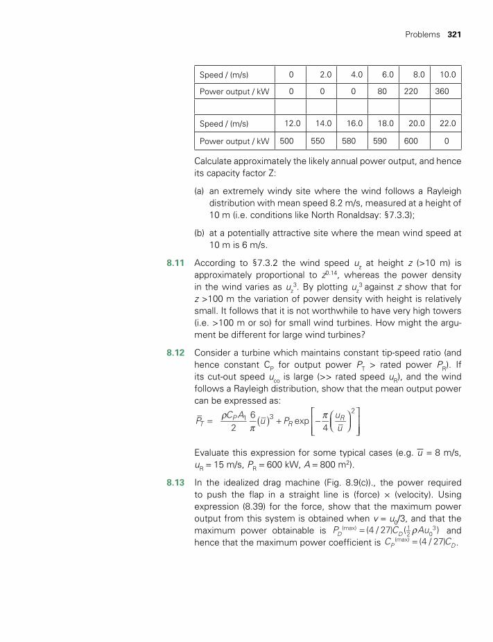
Problems 321
Speed / (m/s) 0 2.0 4.0 6.0 8.0 10.0
Power output / kW 0 0 0 80 220 360
Speed / (m/s) 12.0 14.0 16.0 18.0 20.0 22.0
Power output / kW 500 550 580 590 600 0
Calculate approximately the likely annual power output, and hence its capacity factor Z:
(a) an extremely windy site where the wind follows a Rayleigh distribution with mean speed 8.2 m/s, measured at a height of 10 m (i.e. conditions like North Ronaldsay: §7.3.3);
(b) at a potentially attractive site where the mean wind speed at 10 m is 6 m/s.
8.11 According to §7.3.2 the wind speed uz at height z (>10 m) is approximately proportional to z0.14, whereas the power density in the wind varies as uz
3. By plotting uz3 against z show that for
z >100 m the variation of power density with height is relatively small. It follows that it is not worthwhile to have very high towers (i.e. >100 m or so) for small wind turbines. How might the argu-ment be different for large wind turbines?
8.12 Consider a turbine which maintains constant tip-speed ratio (and hence constant CP for output power PT > rated power PR). If its cut-out speed uco is large (>> rated speed uR), and the wind follows a Rayleigh distribution, show that the mean output power can be expressed as:
rp
p( )= + −
PC A
u Puu2
6exp
4TP
RR1 3
2
Evaluate this expression for some typical cases (e.g. u = 8 m/s, uR = 15 m/s, PR = 600 kW, A = 800 m2).
8.13 In the idealized drag machine (Fig. 8.9(c))., the power required to push the flap in a straight line is (force) × (velocity). Using expression (8.39) for the force, show that the maximum power output from this system is obtained when v = u0/3, and that the maximum power obtainable is P C Au(4 / 27) ( )D D
(max) 12 0
3r= and hence that the maximum power coefficient is C C(4 / 27)P D
(max) = .
TWIDELL PAGINATION.indb 321 01/12/2014 11:37

322 Wind power technology
NOTES
1 An overbar denotes an average of whatever is under the bar.2 The term ‘wind energy conversion system’ (WECS) is used by a few authors to distinguish the whole assem-
bly from the actual turbine.3 Data from Global Wind Energy Council (2013).4 The theory was developed independently by Lanchester (1915 in the UK), Betz (1920 in Germany) and
Zhukowsky (1920 in Russia; often spelt as Joukowski). Many sources refer only to Betz.5 The US National Aeronautics and Space Administration.
BIBLIOGRAPHY
General
Burton, T., Sharpe, D., Jenkins, N. and Bossanyi, E. (2011, 2nd edn) Wind Energy Handbook, Wiley, Chichester. This is the wind turbine ‘bible’, with advanced fundamental theory and professional experience of designing, manufacturing and implementing wind power.
Gipe, P. (2004) Wind Power, James and James, London. Thorough and personal analysis of wind power develop-ment, especially in the USA; a bias to the independent owner.
Golding, E.W. (1976) The Generation of Electricity by Wind Power, reprinted with additional material by R.I. Harris, E. and F.N. Spon, London. The classic text that became a guide for much modern work.
Hansen, M.O (2007, 2nd edn) Aerodynamics of Wind Turbines, Routledge, London. Clearly presented but advanced text from an experienced lecturer; moves from fundamental aeronautics to blade element theory, with physical explanations of further intricacies and applications.
Manwell, J.F., McGowan, J.G. and Rogers, A.L. (2010, 2nd edn) Wind Energy Explained, John Wiley & Sons, Chichester. A major textbook for specialist study.
Milborrow, D. (2001) ‘Wind energy review’, in J. Gordon (ed.), Solar Energy: The state of the art, International Solar Energy Society and James & James, London.
Pasqualetti, M.J., Gipe, P. and Righter, R.W. (2002) Wind Power in View, Academic Press with Reed Elsevier, San Diego; Academic Press, London. An edited set of chapters, mostly by experts other than engineers, concerning the visual and other non-engineering impacts of wind power installations. Important insights into personal aes-thetics and cultural heritage.
Van Est, R. (1999) Winds of Change, International Books, Utrecht (in English). A comparative study of the politics and institutional factors of wind energy development in California and Denmark.
Specifically referenced
Bowden, G. J., Barker, P.R., Shestopal, V.O. and Twidell, J.W. (1983) ‘The Weibull distribution function and wind power statistics’, Wind Engineering, 7, 85–98.
Jeffreys, H. and Jeffreys, B. (1966) Methods of Mathematical Physics, Cambridge University Press, Cambridge. Carefully presented text of advanced maths for engineers, etc.
Justus, C.G., Hargreaves, W.R., Mikherl, A.S. and Graves, D. (1977) ‘Methods for estimating wind speed fre-quency distribution’, Journal of Applied Meteorology, 17, 673–678.
TWIDELL PAGINATION.indb 322 01/12/2014 11:37

Bibliography 323
Kaimal, J.C. and Finnigan, J.J. (1994) Atmospheric Boundary Layer Flows, Oxford University Press, Oxford. Fundamental analysis and explanation by leading experts.
Kragten, A. (2009) ‘Windmills using aerodynamic drag as propelling forces: a hopeless task’, web published at www.bidnetwork.org/en/plan/302071, Kragten Design, Populierenlaan 51, 5492 SG Sint-Oedenrode, The Netherlands.
Nuttall, P., Newell, A., Prasad, B., Veitayaki, J. and Holland, E. (2013) ‘A review of sustainable sea-transport for Oceania: providing context for renewable energy shipping for the Pacific’, Marine Policy, http://dx.doi.org/10.1016/j.marpol.2013.06.009.
Panofsky, H A. and Dutton, J A. (1984) Atmospheric Turbulence, Models and Methods for Engineering Applications, Wiley, New York. Useful an alysis and background for wind turbine generation.
Petersen, E.L. (1975) On the Kinetic Energy Spectrum of Atmospheric Motions in the Planetary Boundary Layer, Report no. 285 of the Wind Test site, Riso, Denmark.
Rohatgi, J.S. and Nelson, V. (1994) Wind Characteristics: An analysis for the generation of power, Burgess Publishing, Edina, MA, USA.
Journals and websites
Wind Power Monthly. Vrinners Hoved, Knebel, Denmark. In English; worldwide news and articles.
Wind Engineering. Multi-Science Publishing Co., 5 Wates Way, Brentwood, UK. Academic and research journal.
Wind Energy. Wiley. Academic and research journal.
World Wind Energy Association (www.wwindea.org/home/index.php). Excellent reports and data.
American Wind Energy Association (www.awea.org/).
Danish Wind Industry Association; education (www.windpower.org/en/knowledge/windpower_wiki.html). Excellent website for students; clear explanations, with video support.
RenewableUK (previously British Wind Energy Association) (www.renewableuk.com/). UK wind data and activi-ties; also wave and tidal power.
Spanish wind power generation and proportion of national supply in real time and for past dates (www.ree.es/ingles/operacion/curvas_eolica.asp#). Instructive and exciting.
Wind Atlases of the World (www.windatlas.dk/). Wind atlases; background, methods and availability.
Youtube video, What’s inside a wind turbine (2010) (www.youtube.com/watch?v=LNXTm7aHvWc). Instructive, especially for maintenance staff.
TWIDELL PAGINATION.indb 323 01/12/2014 11:37
Biomass resources from photosynthesis
CONTENTS
Learning aims 325
§9.1 Introduction 326
§9.2 Photosynthesis: a key process for life on Earth 327
§9.3 Trophic level photosynthesis 328
§9.4 Relation of photosynthesis to other plant processes 331
§9.5 Photosynthesis at the cellular and molecular level 332§9.5.1 Reaction overview 333§9.5.2 Thermodynamic considerations 335§9.5.3 Photophysics 338§9.5.4 Number of photons per
carbon fixed 341§9.5.5 Efficiency of photosynthesis
at photon level 341
§9.6 Energy farming: biomass production for energy 343§9.6.1 Energy farming 343§9.6.2 Wood resource 346§9.6.3 Crop yield and improvement 347§9.6.4 How much biomass is
available for energy? 347
§9.7 R&D to ‘improve’ photosynthesis 350§9.7.1 Plant physiology and biomass 350
§9.7.2 Bioengineered photosynthesis 351§9.7.3 Artificial photosynthesis 351
§9.8 Social and environmental aspects 351§9.8.1 Bioenergy in relation to
agriculture and forestry 351§9.8.2 Food versus fuel 352§9.8.3 Greenhouse gas impacts:
bioenergy and carbon sinks 352§9.8.4 Bioenergy in relation to
the energy system 353§9.8.5 Human impact on net
primary production (NPP) 353
Chapter summary 354
Quick questions 355
Problems 355
Notes 356
Bibliography 356
Box 9.1 Structure of plant leaves 334
Box 9.2 Sugar cane: an example of energy farming 344
Box 9.3 How is biomass resource assessed? 349
CHAPTER
9
TWIDELL PAGINATION.indb 324 01/12/2014 11:37
List of tables 325
LEARNING AIMS
• Know how solar energy forms biomass by photosynthesis.
• Realize that biomass is stored solar energy.• Be aware of photosynthetic growth rates for
the production of food crops and fuels.• Compare and contrast photovoltaics and pho
tosynthesis.
• Appreciate the ecological context of bioenergy.
• Relate human need for food to need for energy.
• Be aware of land use and productivity issues.• Consider biological carbon capture and relate
to climate forcing.
LIST OF FIGURES
9.1 Trophic level global photosynthesis. 3299.2 Plant level photosynthesis. 3329.3 Molecular level photosynthesis. 3339.4 Structure and scale of plant leaves. 3349.5 Electron excitation by (a) heat and (b) photon absorption. 3369.6 Reduction level R of carbon compounds. Enthalpy change per carbon atom. 3379.7 Reduction of water to oxygen and protons at reaction center of photosystem 2. 3389.8 FranckCondon diagram. 3399.9 Transfer of energy by pigment molecules of the lightharvesting system to the particular
reaction center. 3409.10 Absorption spectrum (solid curve) and action spectra (dashed curve) of a typical green plant leaf. 3429.11 Sugar cane agroindustry: process flow diagram. 3449.12 A sugar mill set up to produce sugar, ethanol, and surplus electricity. 345
LIST OF TABLES
9.1 Approximate photosynthetic efficiency for a range of circumstances. 3319.2 Energy losses at each stage of photosynthesis. 3439.3 Advantages and dangers of energy farming. 3459.4 Maximum practical biomass yields. 3489.5 An estimate of technical potential of bioenergy available from new plantations on land ‘available
and suitable’ for the selected plant species. 350
TWIDELL PAGINATION.indb 325 01/12/2014 11:37
326 Biomass resources from photosynthesis
§9.1 INTRODUCTION
The material of plants and animals, including their wastes and residues, is called biomass. It is organic, carbonbased material that reacts with oxygen in natural metabolic processes and in combustion to release heat that, especially if at temperatures >400°C, may be used to generate work and electricity. The initial material may be transformed by chemical and biological processes to produce biofuels, i.e. biomass processed into a more convenient form, particularly liquid fuels for transport. Examples of biofuels include methane gas, liquid ethanol, methyl esters, oils and solid charcoal. The term bioenergy is used to describe both biomass and biofuels.
Bioenergy is by far the most used renewable energy resource by energy value, being about 10% of global total primary energy supply if noncommercial firewood for cooking and commercial use of wastes are included (Edenhofer et al. 2011). Despite the historic use of biofuels, there is great potential for more energyefficient and sustainable use in both developing and developed countries. Technologies for doing this are described in the next chapter.
Biomass is formed naturally by photosynthesis, which is the driving function of all life, including of course human life via food; the underlying processes are outlined in §9.2 to §9.5, with an emphasis on the physical principles involved. Sustaining the subsequent processes is a key function of ecological systems; processes that occur naturally and successfully without the intervention of mankind. We are wise if we understand and participate in such processes without destroying the status quo.
One aspect of photosynthesis is that it is the dominant process for rapidly storing solar energy in a stable form. We should understand the process and learn from it with the expectation of technological applications (§9.7). An obvious comparison is with photovoltaic cells, but these have no inherent energy storage.
Macroscopic biomass resources are considered in §9.6. This assesses ‘energy farming’ (the production of fuels and energy as a main or subsidiary product of agriculture, forestry, aquaculture) and the processing of ‘organic waste’. This includes the potential energy resource from biomass.
In §9.8, we assess the extent and potential of biomass as an energy resource within the umbrella of sustainability. In particular, we look at its implications for greenhouse gases, and note that human activities already make direct use of more than 25% of the net photosynthetic output of all the landbased plants on Earth.
TWIDELL PAGINATION.indb 326 01/12/2014 11:37

§9.2 Photosynthesis: a key process for life on earth 327
§9.2 PHOTOSYNTHESIS: A KEY PROCESS FOR LIFE ON EARTH
Photosynthesis is the making (synthesis) of organic structures and chemical energy stores by the action of solar radiation. It is by far the most important renewable energy process, because living organisms are made from material fixed by photosynthesis, and our activities rely on photosynthetically produced oxygen with which the solar energy is mostly stored. For instance, the human metabolism continuously releases about 150 W per person from food. Thus, both the materials and the energy for all life are made available in gases circulating in the Earth’s atmosphere, namely carbon dioxide and oxygen.
Although photosynthesis is a physically induced process and the driving function of natural engineering, the subject is missing from most physics and engineering texts. Too often, photosynthesis is considered only as an aspect of biochemistry, which, although of considerable importance, is insufficient. We therefore gave a physicsbased description of its key processes, drawing attention to its analogies with photovoltaic generation (Chapter 5) and radioreceiving antennae, with further details on the website of this book at. www.routledge.com/books/details/9780415584388
Photosynthesis occurs in both landbased and marine plants, thereby influencing the concentration of CO2 in our Earth’s atmosphere and consequently the greenhouse effect (§2.9). However, applications of bioenergy mainly involve terrestrial biomass, on which this chapter focuses. Photosynthesis on land stores energy at a rate of about 0.8 × 10¹⁴ W (i.e. about 10 kW per person; see Problem 9.1). As biomass decays or combusts, the stored energy is released from reactions with oxygen. This is the energy equivalent of the power output of about a million large nuclear power stations and is about four times the present total commercial energy use by mankind.
Virtually all terrestrial photosynthesis occurs in the leaves of living plants. Solar radiation causes electrons to be excited in a key part of these leaves (the chloroplast), which through a complex series of chemical processes outlined in §9.4 to 9.5, leads to the production of oxygen and carbonbased structural material. These chemical processes are sensitive to the temperature of the leaf, so plants have evolved to ensure that some solar radiation is reflected or transmitted, rather than absorbed (which is why leaves are seldom black). The role of water transpiration in both the chemical reactions and the temperature control is an integrated aspect of the process.
The energy processes in photosynthesis depend on the photons (energy packets) of the solar radiation, each of energy hν, where h is Planck’s constant and ν is the frequency of the radiation. The organic material produced is mainly carbohydrate (e.g. cellulose, which is
TWIDELL PAGINATION.indb 327 01/12/2014 11:37
328 Biomass resources from photosynthesis
a longchain polymer of glucose C6Hl2O6). If this (dry) material is burnt in oxygen, the heat released is about 16 MJ/kg (4.8 eV per carbon atom, 460 kJ per mole of carbon). The fixation of one carbon atom from atmospheric CO2 to carbohydrate proceeds by a series of stages in green plants, including algae:
1 Reactions in light: the solar photons excite and separate electrons and protons in hydrogen atoms of water, with O2 as an important byproduct and with electrons excited in two stages to produce strong reducing chemicals.
2 Reactions not requiring light (called ‘dark’ reactions, but occurring at any time): the reducing chemicals from (1) reduce CO2 to carbohydrates, proteins and fats.
In the overall chemical equations (9.1) and (9.2), the oxygen atoms initially in CO2 and H2O
. are distinguished; the latter being shown with a
dot over the O. Thus, combining both the light and dark reactions and neglecting many intermediate steps:
CO + 2H2 2O. →light O
.2 + [CH O] + H O2 2 (9.1)
where the products have about 4.8 eV per C atom more enthalpy (energy production potential) than the initial material because of the absorption of at least eight photons. Here [CH2O] represents a basic unit of carbohydrate, so the reaction for sucrose production is:
12CO + 24H2 2 O. →light 12 O
.2 + C H O + 13H O12 22 11 2 (9.2)
There is extensive variety in all aspects of photosynthesis, from the scale of plants down to molecular level. It must not be assumed that any one system is as straightforward as described in this chapter, which concentrates on the general physical principles. However, the end result is that energy from the Sun is stored in stable chemicals for later use – a principal goal of renewable energy technology, yet happening all around us.
§9.3 TROPHIC LEVEL PHOTOSYNTHESIS
Animals exist by obtaining energy and materials directly or indirectly from plants. This is called the trophic (feeding) system. Fig. 9.1 is an extremely simplified diagram to emphasize the essential processes of natural ecology. We should remember, however, that the box labeled ‘animals’ may also include the human fossil fuelbased activities of industry, transport, heating, etc. Figs 9.2 and 9.3 give ‘closeup’ views of photosynthesis respectively at the plant level and the molecular level.
During photosynthesis CO2 and H2O are absorbed to form carbohydrates, proteins and fats. The generalized symbol [CH2O] is used to indicate the basic building block for these products. CO2 is released
TWIDELL PAGINATION.indb 328 01/12/2014 11:37
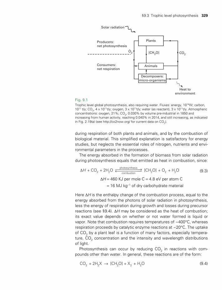
§9.3 Trophic level photosynthesis 329
during respiration of both plants and animals, and by the combustion of biological material. This simplified explanation is satisfactory for energy studies, but neglects the essential roles of nitrogen, nutrients and environmental parameters in the processes.
The energy absorbed in the formation of biomass from solar radiation during photosynthesis equals that emitted as heat in combustion, since:
∆ →← H + CO + 2H O [CH O] + O + H O2 2
photosynthesis
combustion 2 2 2 (9.3)
∆H = 460 KJ per mole C = 4.8 eV per atom C
≈ 16 MJ kg-1 of dry carbohydrate material
Here ∆H is the enthalpy change of the combustion process, equal to the energy absorbed from the photons of solar radiation in photosynthesis, less the energy of respiration during growth and losses during precursor reactions (see §9.4). ∆H may be considered as the heat of combustion; its exact value depends on whether or not water formed is liquid or vapor. Note that combustion requires temperatures of ~400°C, whereas respiration proceeds by catalytic enzyme reactions at ~20°C. The uptake of CO2 by a plant leaf is a function of many factors, especially temperature, CO2 concentration and the intensity and wavelength distributions of light.
Photosynthesis can occur by reducing CO2 in reactions with compounds other than water. In general, these reactions are of the form:
→CO + 2H X [CH O] + X + H O2 2 2 2 2 (9.4)
Fig. 9.1Trophic level global photosynthesis, also requiring water. Fluxes: energy, 1014W; carbon, 1011 t/y; CO2, 4 x 10¹¹t/y; oxygen, 3 x 10¹¹t/y; water (as reactant), 3 x 10¹¹t/y. Atmospheric concentrations: oxygen, 21%; CO2, 0.030% by volume preindustrial in 1850 and increasing from human activity, reaching 0.040% in 2014, and still increasing, as indicated in Fig. 2.19(a) (see http://co2now.org/ for current data on CO2).
Solar radiation
Producers:net photosynthesis
Consumers:net respiration
[CH2O]
Plants
Animals
Decomposers:micro-organisms
CO2
Heat toenvironment
O2
TWIDELL PAGINATION.indb 329 01/12/2014 11:37
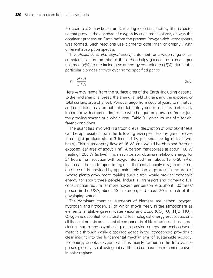
330 Biomass resources from photosynthesis
For example, X may be sulfur, S, relating to certain photosynthetic bacteria that grow in the absence of oxygen by such mechanisms, as was the dominant process on Earth before the present ‘oxygenrich’ atmosphere was formed. Such reactions use pigments other than chlorophyll, with different absorption spectra.
The efficiency of photosynthesis η is defined for a wide range of circumstances. It is the ratio of the net enthalpy gain of the biomass per unit area (H/A) to the incident solar energy per unit area (E/A), during the particular biomass growth over some specified period:
η =H AE A
//
(9.5)
Here A may range from the surface area of the Earth (including deserts) to the land area of a forest, the area of a field of grain, and the exposed or total surface area of a leaf. Periods range from several years to minutes, and conditions may be natural or laboratory controlled. It is particularly important with crops to determine whether quoted growth refers to just the growing season or a whole year. Table 9.1 gives values of η for different conditions.
The quantities involved in a trophic level description of photosynthesis can be appreciated from the following example. Healthy green leaves in sunlight produce about 3 liters of O2 per hour per kg of leaf (wet basis). This is an energy flow of 16 W, and would be obtained from an exposed leaf area of about 1 m2. A person metabolizes at about 100 W (resting), 200 W (active). Thus each person obtains metabolic energy for 24 hours from reaction with oxygen derived from about 15 to 30 m2 of leaf area. Thus in temperate regions, the annual bodily oxygen intake of one person is provided by approximately one large tree. In the tropics (where plants grow more rapidly) such a tree would provide metabolic energy for about three people. Industrial, transport and domestic fuel consumption require far more oxygen per person (e.g. about 100 trees/person in the USA, about 60 in Europe, and about 20 in much of the developing world).
The dominant chemical elements of biomass are carbon, oxygen, hydrogen and nitrogen, all of which move freely in the atmosphere as elements in stable gases, water vapor and cloud (CO2, O2, H2O, NOx). Oxygen is essential for natural and technological energy processes, and all these elements are essential components of life structure. Thus appreciating that in photosynthesis plants provide energy and carbonbased materials through easily dispersed gases in the atmosphere provides a clear insight into the fundamental mechanisms of sustainable ecology. For energy supply, oxygen, which is mainly formed in the tropics, disperses globally, so allowing animal life and combustion to continue even in polar regions.
TWIDELL PAGINATION.indb 330 01/12/2014 11:37
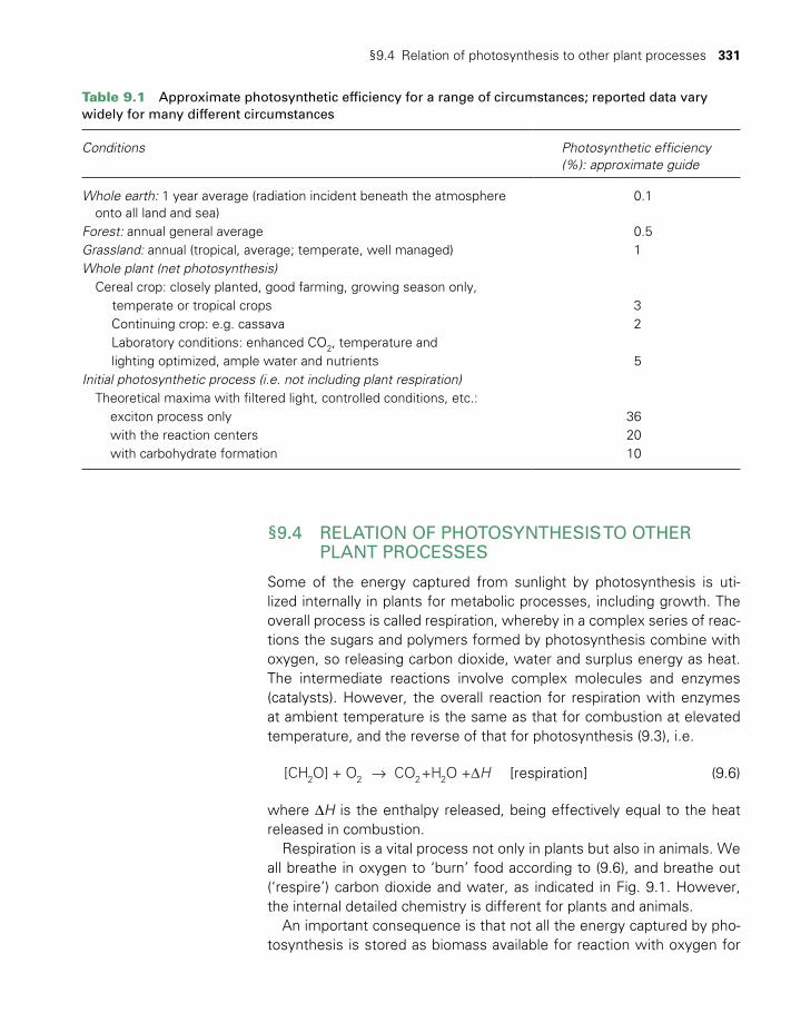
§9.4 Relation of photosynthesis to other plant processes 331
§9.4 RELATION OF PHOTOSYNTHESIS TO OTHER PLANT PROCESSES
Some of the energy captured from sunlight by photosynthesis is utilized internally in plants for metabolic processes, including growth. The overall process is called respiration, whereby in a complex series of reactions the sugars and polymers formed by photosynthesis combine with oxygen, so releasing carbon dioxide, water and surplus energy as heat. The intermediate reactions involve complex molecules and enzymes (catalysts). However, the overall reaction for respiration with enzymes at ambient temperature is the same as that for combustion at elevated temperature, and the reverse of that for photosynthesis (9.3), i.e.
→ ∆H[CH O] + O CO +H O +2 2 2 2 [respiration] (9.6)
where ∆H is the enthalpy released, being effectively equal to the heat released in combustion.
Respiration is a vital process not only in plants but also in animals. We all breathe in oxygen to ‘burn’ food according to (9.6), and breathe out (‘respire’) carbon dioxide and water, as indicated in Fig. 9.1. However, the internal detailed chemistry is different for plants and animals.
An important consequence is that not all the energy captured by photosynthesis is stored as biomass available for reaction with oxygen for
Table 9.1 Approximate photosynthetic efficiency for a range of circumstances; reported data vary widely for many different circumstances
Conditions Photosynthetic efficiency (%): approximate guide
Whole earth: 1 year average (radiation incident beneath the atmosphere onto all land and sea)
0.1
Forest: annual general average 0.5Grassland: annual (tropical, average; temperate, well managed) 1Whole plant (net photosynthesis) Cereal crop: closely planted, good farming, growing season only, temperate or tropical crops 3
Continuing crop: e.g. cassava 2Laboratory conditions: enhanced CO2, temperature andlighting optimized, ample water and nutrients 5
Initial photosynthetic process (i.e. not including plant respiration) Theoretical maxima with filtered light, controlled conditions, etc.: exciton process only 36 with the reaction centers 20 with carbohydrate formation 10
TWIDELL PAGINATION.indb 331 01/12/2014 11:37
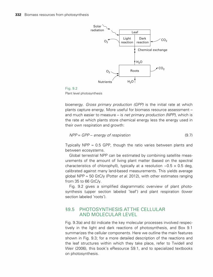
332 Biomass resources from photosynthesis
bioenergy. Gross primary production (GPP) is the initial rate at which plants capture energy. More useful for biomass resource assessment – and much easier to measure – is net primary production (NPP), which is the rate at which plants store chemical energy less the energy used in their own respiration and growth:
NPP = GPP - energy of respiration (9.7)
Typically NPP ≈ 0.5 GPP, though the ratio varies between plants and between ecosystems.
Global terrestrial NPP can be estimated by combining satellite measurements of the amount of living plant matter (based on the spectral characteristics of chlorophyll), typically at a resolution ~0.5 ×0.5 deg, calibrated against many landbased measurements. This yields average global NPP ≈ 50 GtC/y (Potter et al. 2012), with other estimates ranging from 35 to 66 GtC/y.
Fig. 9.2 gives a simplified diagrammatic overview of plant photosynthesis (upper section labeled ‘leaf’) and plant respiration (lower section labeled ‘roots’).
§9.5 PHOTOSYNTHESIS AT THE CELLULAR AND MOLECULAR LEVEL
Fig. 9.3(a) and (b) indicate the key molecular processes involved respectively in the light and dark reactions of photosynthesis, and Box 9.1 summarizes the cellular components. Here we outline the main features shown in Fig. 9.3; for a more detailed description of the reactions and the leaf structures within which they take place, refer to Twidell and Weir (2006), this book’s eResource S9.1, and to specialized textbooks on photosynthesis.
Fig. 9.2Plant level photosynthesis
Chemical exchange
Roots
Nutrients
Solarradiation
Leaf
CO2
CO2O2
Lightreaction
DarkreactionO2
H2O
H2O
TWIDELL PAGINATION.indb 332 01/12/2014 11:37
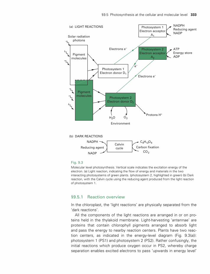
§9.5 Photosynthesis at the cellular and molecular level 333
§9.5.1 Reaction overview
In the chloroplast, the ‘light reactions’ are physically separated from the ‘dark reactions’.
All the components of the light reactions are arranged in or on proteins held in the thylakoid membrane. Lightharvesting ‘antennae’ are proteins that contain chlorophyll pigments arranged to absorb light and pass the energy to nearby reaction centers. Plants have two reaction centers, as indicated in the energylevel diagram (Fig. 9.3(a)): photosystem 1 (PS1) and photosystem 2 (PS2). Rather confusingly, the initial reactions which produce oxygen occur in PS2, whereby charge separation enables excited electrons to pass ‘upwards in energy level’
Fig. 9.3Molecular level photosynthesis. Vertical scale indicates the excitation energy of the electron. (a) Light reaction, indicating the flow of energy and materials in the two interacting photosystems of green plants. (photosystem 2, highlighted in green) (b) Dark reaction, with the Calvin cycle using the reducing agent produced from the light reaction of photosystem 1.
(a) LIGHT REACTIONS
(b) DARK REACTIONS
Solar radiationphotons
Pigmentmolecules
Photosystem 1Electron donor D1
Photosystem 2Electron acceptor
A2
Electrons e–
Electrons e–
Protons H+
NADPHReducing agentNADP
NADPH
Reducing agent
NADP
ATPEnergy storeADP
e–
Photosystem 2Electron donor D2
Environment
Calvincycle
H2O
C6H12O6
CO2
Carbon fixation
O2
Photosystem 1Electron acceptor
A1
Pigmentmolecules
TWIDELL PAGINATION.indb 333 01/12/2014 11:37

334 Biomass resources from photosynthesis
BOX 9.1 STRUCTURE OF PLANT LEAVES
In plants and algae, photosynthesis takes place in organelles of plant cells called chloroplasts. A typical plant cell contains about 10 to 100 chloroplasts (see Fig. 9.4). The chloroplast is enclosed by a membrane. Within the membrane is an aqueous fluid called the stroma. The stroma contains stacks of thylakoids, which are the site of photosynthesis. The thylakoids are flattened disks, bounded by a membrane. The site of photosynthesis is the thylakoid membrane, which contains integral and peripheral membrane protein complexes, including the pigments that absorb light energy, which form the photosystems.
Plants absorb light primarily using the pigment chlorophyll, which is the reason that most plants have a green colour, though most plants also use other pigments to some extent. These pigments are positioned in plants and algae as special ‘antennaproteins’ at the surfaces of the thylakoid membrane (see Twidell and Weir (2006) and cooperate as a lightharvesting complex.
Although all cells in the green parts of a plant have chloroplasts, most of the energy is captured in the leaves. The cells in the interior tissues of a leaf can contain between 450,000 and 800,000 chloroplasts per mm2 of leaf.
Fig. 9.4Structure and scale of plant leaves. a Section of a typical leaf of a broadleafed plant. Photosynthetically active green cells are shown dotted with
chloroplast organelles. Approximate scale only. Actual cells press together more closely than shown, i.e. do not have gaps as large as indicated in the figure for clarity.
b Section through chloroplast organelle. The thylakoid internal membranes are shown in the liquid stroma. Certain regions have stacked thylakoid membranes (the grana) which are connected by unstacked stroma lamellae membrane.
c Perspective of the stacked and unstacked thylakoid membrane structure. Stacked grana are linked by bridges of the stroma lamellae, all within the liquid stroma of the chloroplast organelle. Approximate scale only.
Upper cuticleUpper epidermisCells of palisade mesophyll
Lower epidermisLower cuticle
Cells of spongy mesophyll
CO2 O2 guard cellGas and vaporexchange throughthe stomata
~0.1 mm
(a)Leaf structure
= 100 mµ
Chloroplast organelleSide section
Broad section
10 µmOrganelles containlamellae
(b)
Thylakoid membranes are lined with photosynthetically active surfaces
1 µm
100nm = 0.1µm
Lamellae are madeof thylakoid membranes
(c)
TWIDELL PAGINATION.indb 334 01/12/2014 11:37
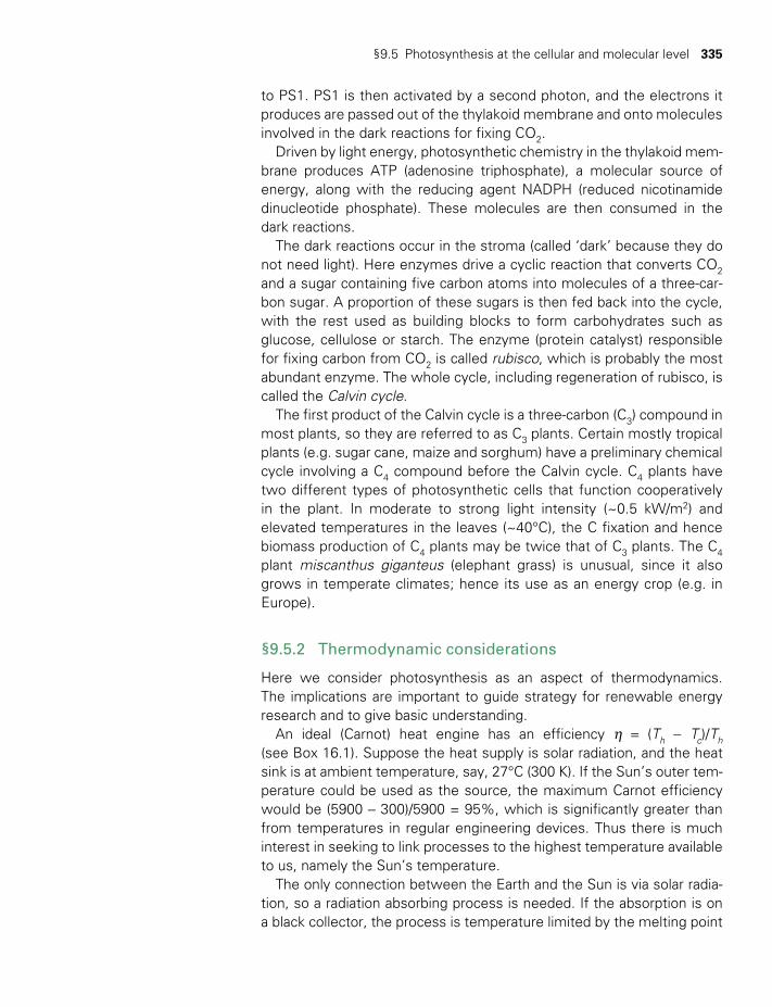
§9.5 Photosynthesis at the cellular and molecular level 335
to PS1. PS1 is then activated by a second photon, and the electrons it produces are passed out of the thylakoid membrane and onto molecules involved in the dark reactions for fixing CO2.
Driven by light energy, photosynthetic chemistry in the thylakoid membrane produces ATP (adenosine triphosphate), a molecular source of energy, along with the reducing agent NADPH (reduced nicotinamide dinucleotide phosphate). These molecules are then consumed in the dark reactions.
The dark reactions occur in the stroma (called ‘dark’ because they do not need light). Here enzymes drive a cyclic reaction that converts CO2 and a sugar containing five carbon atoms into molecules of a threecarbon sugar. A proportion of these sugars is then fed back into the cycle, with the rest used as building blocks to form carbohydrates such as glucose, cellulose or starch. The enzyme (protein catalyst) responsible for fixing carbon from CO2 is called rubisco, which is probably the most abundant enzyme. The whole cycle, including regeneration of rubisco, is called the Calvin cycle.
The first product of the Calvin cycle is a threecarbon (C3) compound in most plants, so they are referred to as C3 plants. Certain mostly tropical plants (e.g. sugar cane, maize and sorghum) have a preliminary chemical cycle involving a C4 compound before the Calvin cycle. C4 plants have two different types of photosynthetic cells that function cooperatively in the plant. In moderate to strong light intensity (~0.5 kW/m2) and elevated temperatures in the leaves (~40°C), the C fixation and hence biomass production of C4 plants may be twice that of C3 plants. The C4 plant miscanthus giganteus (elephant grass) is unusual, since it also grows in temperate climates; hence its use as an energy crop (e.g. in Europe).
§9.5.2 Thermodynamic considerations
Here we consider photosynthesis as an aspect of thermodynamics. The implications are important to guide strategy for renewable energy research and to give basic understanding.
An ideal (Carnot) heat engine has an efficiency η = (Th - Tc)/Th (see Box 16.1). Suppose the heat supply is solar radiation, and the heat sink is at ambient temperature, say, 27°C (300 K). If the Sun’s outer temperature could be used as the source, the maximum Carnot efficiency would be (5900 - 300)/5900 = 95%, which is significantly greater than from temperatures in regular engineering devices. Thus there is much interest in seeking to link processes to the highest temperature available to us, namely the Sun’s temperature.
The only connection between the Earth and the Sun is via solar radiation, so a radiation absorbing process is needed. If the absorption is on a black collector, the process is temperature limited by the melting point
TWIDELL PAGINATION.indb 335 01/12/2014 11:37
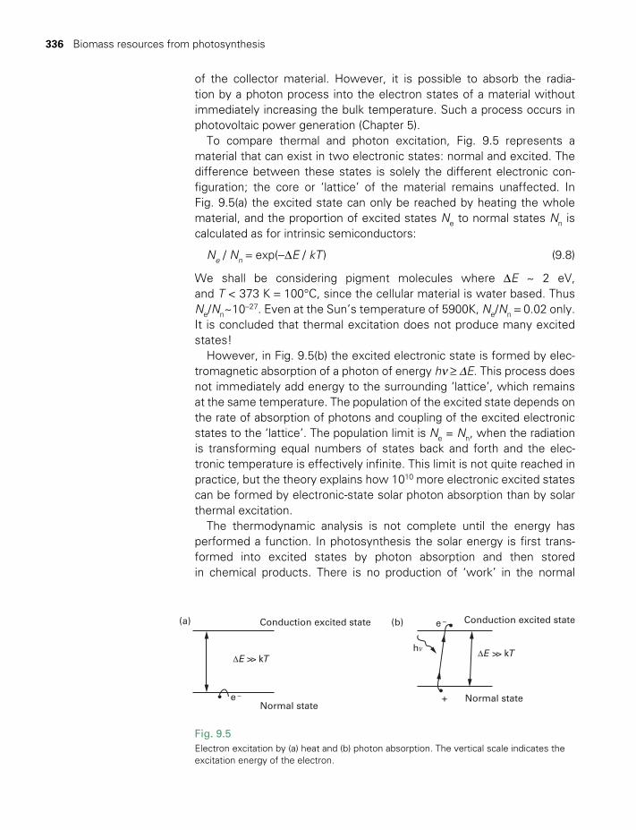
336 Biomass resources from photosynthesis
of the collector material. However, it is possible to absorb the radiation by a photon process into the electron states of a material without immediately increasing the bulk temperature. Such a process occurs in photovoltaic power generation (Chapter 5).
To compare thermal and photon excitation, Fig. 9.5 represents a material that can exist in two electronic states: normal and excited. The difference between these states is solely the different electronic configuration; the core or ‘lattice’ of the material remains unaffected. In Fig. 9.5(a) the excited state can only be reached by heating the whole material, and the proportion of excited states Ne to normal states Nn is calculated as for intrinsic semiconductors:
Ne / Nn = exp(-∆E / kT ) (9.8)
We shall be considering pigment molecules where ∆E ~ 2 eV, and T < 373 K = 100°C, since the cellular material is water based. Thus Ne/Nn~10–27. Even at the Sun’s temperature of 5900K, Ne/Nn = 0.02 only. It is concluded that thermal excitation does not produce many excited states!
However, in Fig. 9.5(b) the excited electronic state is formed by electromagnetic absorption of a photon of energy hν≥∆E. This process does not immediately add energy to the surrounding ‘lattice’, which remains at the same temperature. The population of the excited state depends on the rate of absorption of photons and coupling of the excited electronic states to the ‘lattice’. The population limit is Ne = Nn, when the radiation is transforming equal numbers of states back and forth and the electronic temperature is effectively infinite. This limit is not quite reached in practice, but the theory explains how 1010 more electronic excited states can be formed by electronicstate solar photon absorption than by solar thermal excitation.
The thermodynamic analysis is not complete until the energy has performed a function. In photosynthesis the solar energy is first transformed into excited states by photon absorption and then stored in chemical products. There is no production of ‘work’ in the normal
Fig. 9.5Electron excitation by (a) heat and (b) photon absorption. The vertical scale indicates the excitation energy of the electron.
Conduction excited state(a) (b) Conduction excited state
Normal state
DE kT DE kT
e –
e –
Normal state+
hn >>>>
TWIDELL PAGINATION.indb 336 01/12/2014 11:37
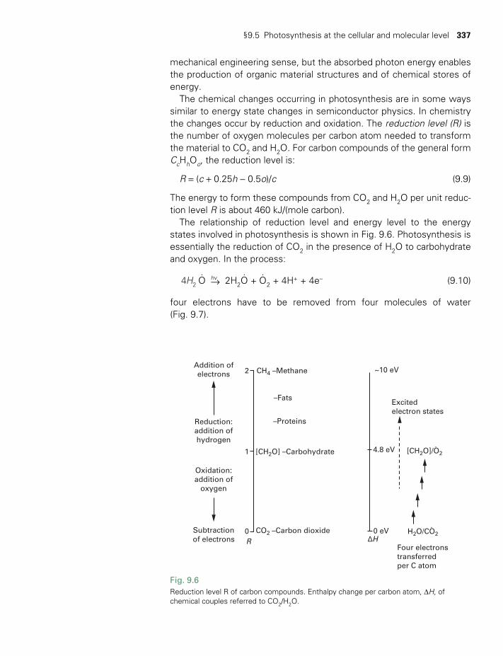
§9.5 Photosynthesis at the cellular and molecular level 337
mechanical engineering sense, but the absorbed photon energy enables the production of organic material structures and of chemical stores of energy.
The chemical changes occurring in photosynthesis are in some ways similar to energy state changes in semiconductor physics. In chemistry the changes occur by reduction and oxidation. The reduction level (R) is the number of oxygen molecules per carbon atom needed to transform the material to CO2 and H2O. For carbon compounds of the general form CcHhOo, the reduction level is:
R = (c + 0.25h - 0.5o)/c (9.9)
The energy to form these compounds from CO2 and H2O per unit reduction level R is about 460 kJ/(mole carbon).
The relationship of reduction level and energy level to the energy states involved in photosynthesis is shown in Fig. 9.6. Photosynthesis is essentially the reduction of CO2 in the presence of H2O to carbohydrate and oxygen. In the process:
H4 2 O. →hv 2H2O
. + O
. 2 + 4H+ + 4e– (9.10)
four electrons have to be removed from four molecules of water (Fig. 9.7).
Fig. 9.6Reduction level R of carbon compounds. Enthalpy change per carbon atom, ∆H, of chemical couples referred to CO2/H2O.
Addition ofelectrons 2
1
0R ∆H
CH4 –Methane
–Fats
–Proteins
[CH2O] –Carbohydrate
CO2 –Carbon dioxide
Excitedelectron states
~10 eV
4.8 eV
0 eV H2O/CO2
[CH2O]/O2
Four electronstransferredper C atom
Reduction:addition ofhydrogen
Oxidation:addition of
oxygen
Subtractionof electrons
TWIDELL PAGINATION.indb 337 01/12/2014 11:37
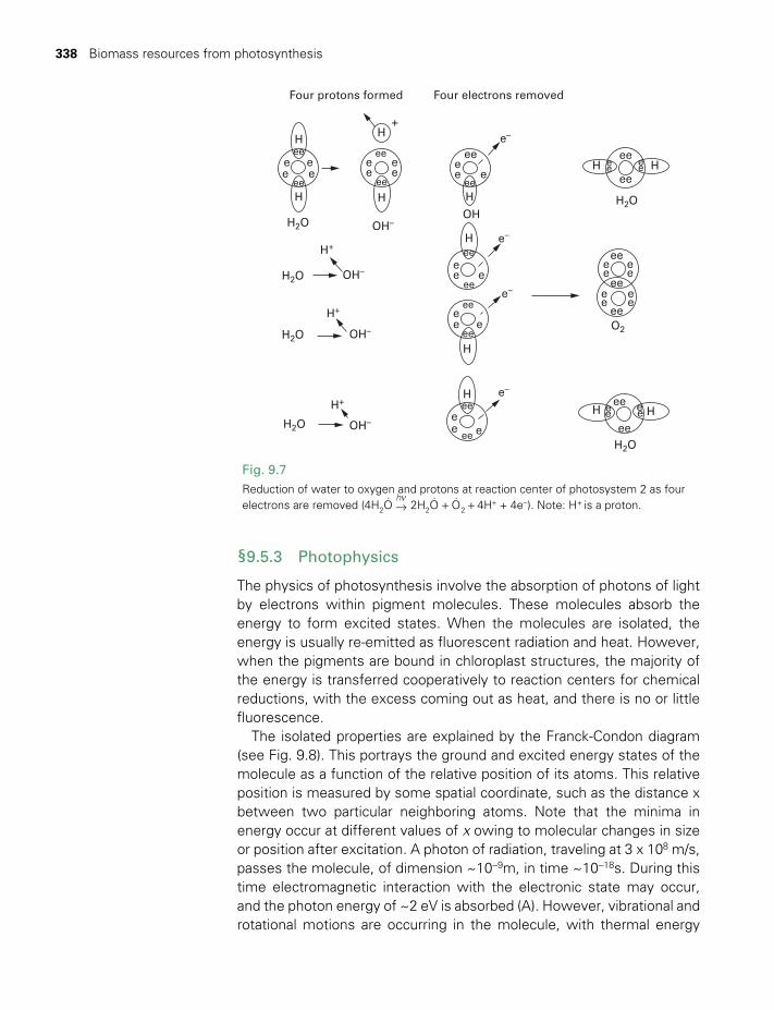
338 Biomass resources from photosynthesis
Fig. 9.7Reduction of water to oxygen and protons at reaction center of photosystem 2 as four electrons are removed (4H2O
. →
νh2H2O
. +O
. 2+4H+ + 4e-). Note: H+ is a proton.
H H
H H
H Hee
ee
ee
ee
ee
ee
ee
ee
ee
ee
eeee
ee
ee
H
H
H HH
+
H
Four protons formed Four electrons removed
H+
H+
H+
OH–
OH–
OH–
H2O
H2O
H2O
O2
H2O
H2O
H2O
OH–OH
ee eee–
e–
e–
e–
ee
ee
ee
ee
ee
ee
ee
ee
ee ee
ee
e e ee
ee
e
e
e
e
ee e
e e
e
e
eee
§9.5.3 Photophysics
The physics of photosynthesis involve the absorption of photons of light by electrons within pigment molecules. These molecules absorb the energy to form excited states. When the molecules are isolated, the energy is usually reemitted as fluorescent radiation and heat. However, when the pigments are bound in chloroplast structures, the majority of the energy is transferred cooperatively to reaction centers for chemical reductions, with the excess coming out as heat, and there is no or little fluorescence.
The isolated properties are explained by the FranckCondon diagram (see Fig. 9.8). This portrays the ground and excited energy states of the molecule as a function of the relative position of its atoms. This relative position is measured by some spatial coordinate, such as the distance x between two particular neighboring atoms. Note that the minima in energy occur at different values of x owing to molecular changes in size or position after excitation. A photon of radiation, traveling at 3 x 10⁸ m/s, passes the molecule, of dimension ~10-9m, in time ~10-18s. During this time electromagnetic interaction with the electronic state may occur, and the photon energy of ~2 eV is absorbed (A). However, vibrational and rotational motions are occurring in the molecule, with thermal energy
TWIDELL PAGINATION.indb 338 01/12/2014 11:37
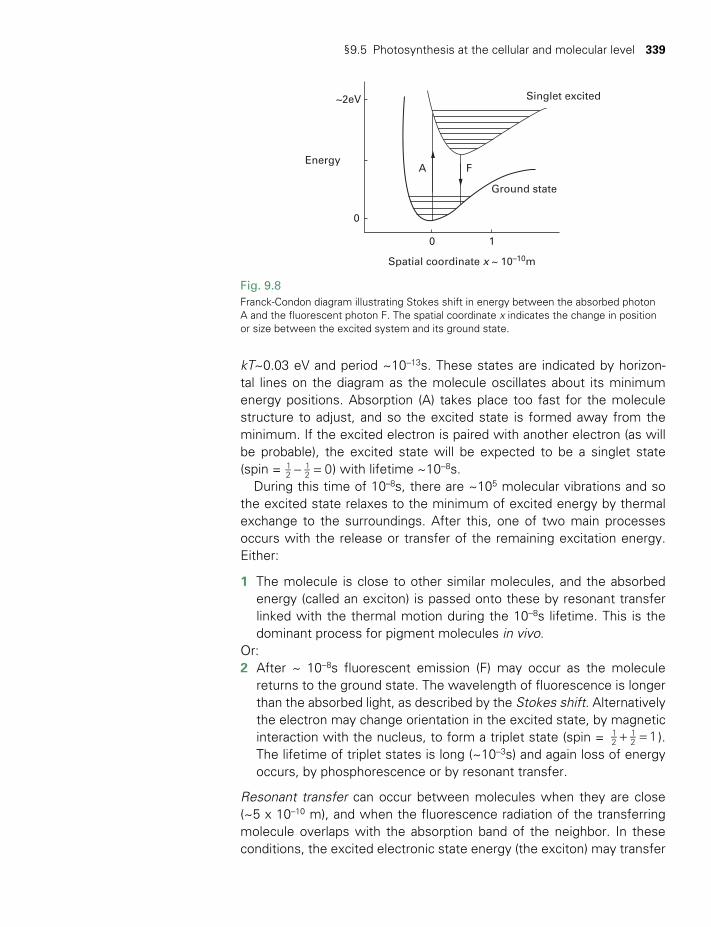
§9.5 Photosynthesis at the cellular and molecular level 339
kT~0.03 eV and period ~10-13s. These states are indicated by horizontal lines on the diagram as the molecule oscillates about its minimum energy positions. Absorption (A) takes place too fast for the molecule structure to adjust, and so the excited state is formed away from the minimum. If the excited electron is paired with another electron (as will be probable), the excited state will be expected to be a singlet state (spin = - = 01
212 ) with lifetime ~10-8s.
During this time of 10–8s, there are ~105 molecular vibrations and so the excited state relaxes to the minimum of excited energy by thermal exchange to the surroundings. After this, one of two main processes occurs with the release or transfer of the remaining excitation energy. Either:
1 The molecule is close to other similar molecules, and the absorbed energy (called an exciton) is passed onto these by resonant transfer linked with the thermal motion during the 10-8s lifetime. This is the dominant process for pigment molecules in vivo.
Or:2 After ~ 10-8s fluorescent emission (F) may occur as the molecule
returns to the ground state. The wavelength of fluorescence is longer than the absorbed light, as described by the Stokes shift. Alternatively the electron may change orientation in the excited state, by magnetic interaction with the nucleus, to form a triplet state (spin = 11
212+ = ).
The lifetime of triplet states is long (~10-3s) and again loss of energy occurs, by phosphorescence or by resonant transfer.
Resonant transfer can occur between molecules when they are close (~5 x 10⁻¹⁰ m), and when the fluorescence radiation of the transferring molecule overlaps with the absorption band of the neighbor. In these conditions, the excited electronic state energy (the exciton) may transfer
Fig. 9.8FranckCondon diagram illustrating Stokes shift in energy between the absorbed photon A and the fluorescent photon F. The spatial coordinate x indicates the change in position or size between the excited system and its ground state.
Energy
Singlet excited
Ground state
FA
~2eV
0
0 1
Spatial coordinate x ~ 10–10m
TWIDELL PAGINATION.indb 339 01/12/2014 11:37
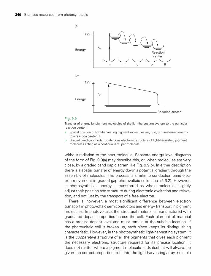
340 Biomass resources from photosynthesis
without radiation to the next molecule. Separate energy level diagrams of the form of Fig. 9.9(a) may describe this, or, when molecules are very close, by a graded band gap diagram like Fig. 9.9(b). In either description there is a spatial transfer of energy down a potential gradient through the assembly of molecules. The process is similar to conduction band electron movement in graded gap photovoltaic cells (see §5.6.2). However, in photosynthesis, energy is transferred as whole molecules slightly adjust their position and structure during electronic excitation and relaxation, and not just by the transport of a free electron.
There is, however, a most significant difference between electron transport in photovoltaic semiconductors and energy transport in pigment molecules. In photovoltaics the structural material is manufactured with graduated dopant properties across the cell. Each element of material has a precise dopant level and must remain at the suitable location. If the photovoltaic cell is broken up, each piece keeps its distinguishing characteristic. However, in the photosynthetic lightharvesting system, it is the cooperative structure of all the pigments that gives each pigment the necessary electronic structure required for its precise location. It does not matter where a pigment molecule finds itself; it will always be given the correct properties to fit into the lightharvesting array, suitable
Fig. 9.9Transfer of energy by pigment molecules of the lightharvesting system to the particular reaction center. a Spatial position of lightharvesting pigment molecules (m, n, o, p) transferring energy
to a reaction center R.b Graded band gap model: continuous electronic structure of lightharvesting pigment
molecules acting as a continuous ‘super molecule’.
2eV
2eV
Reactioncenter
Reaction center
(a)
hν
hνEnergy
(b)
Energy
m n o p R
TWIDELL PAGINATION.indb 340 01/12/2014 11:37
§9.5 Photosynthesis at the cellular and molecular level 341
for its position. So when the ‘array’ is broken up, each pigment reverts to its isolated properties. This accounts for the difference between in vivo and in vitro properties of pigment molecules during absorption and fluorescence.
§9.5.4 Number of photons per carbon fixed
The main requirement for light absorption is that individual photons can be absorbed and the energy stored for sufficient time to be used in later chemical reactions or further photon excitation. Each photosystem is triggered by the absorption of single solar photon in molecules of chlorophyll. Then the quantized energy passes as ‘excitons’, namely mobile excited electronic states, and so passes laterally along a chain of similar excitable molecules to molecules forming the reaction center. A minimum of four operations of PS2 are needed to produce one molecule of O2, i.e. four electrons have to be lifted off H2O (see Fig. 9.7). Four other photons are needed to produce the NADPH for CO2 reduction. Thus in green plants with coupled PS2 and PS1, at least eight photons are needed to fix one C atom as carbohydrate. In practice it seems that more photons are needed, either because an effective chemical saturation or loss occurs, or because further ATP is required. Thus most plants probably operate at about ten photons per C fixed in optimum conditions.
§9.5.5 Efficiency of photosynthesis at photon level
The minimum photon energy input at the outside antenna pigment molecules (i.e. not at the reaction center) may be given as four photons of 1.77 eV (PS2 absorption for D2 at 700 nm) and four of 1.82 eV (PS1 absorption for D1 at 680 nm), totaling 14.4 eV. The actual excitations D2 to A2, and D1 to A1, are about 1.1 eV each. Thus four operations of each require 8.8 eV. The outputs may be considered to be four electrons lifted from H2O to NADP over redox potential 1.15 eV (4.60 eV), plus three ATP molecules at 0.34 eV each (1.02 eV), to give a total output of 5.6 eV. The output may also be considered as one O2 molecule, and one C atom fixed in carbohydrate, requiring 4.8 eV.
A reasonable maximum theoretical efficiency from light absorption to final product may thus be taken as 4.8/14.4 = 33%. However, the larger proportions of 5.6/14.4 (38%), 5.6/8.8 (63%) and 4.8/8.8 (54%) are sometimes considered. Note that these theoretical efficiencies take no account of the distribution of radiation in the solar spectrum or of plant respiration; therefore they are all larger than practical values obtained from applying (9.5) to crops in sunlight.
Note that in discussing photon interactions, the unit of the einstein is often used. One einstein is Avogadro’s number of photons of the same frequency, i.e. one mole of identical or similar photons.
TWIDELL PAGINATION.indb 341 01/12/2014 11:37
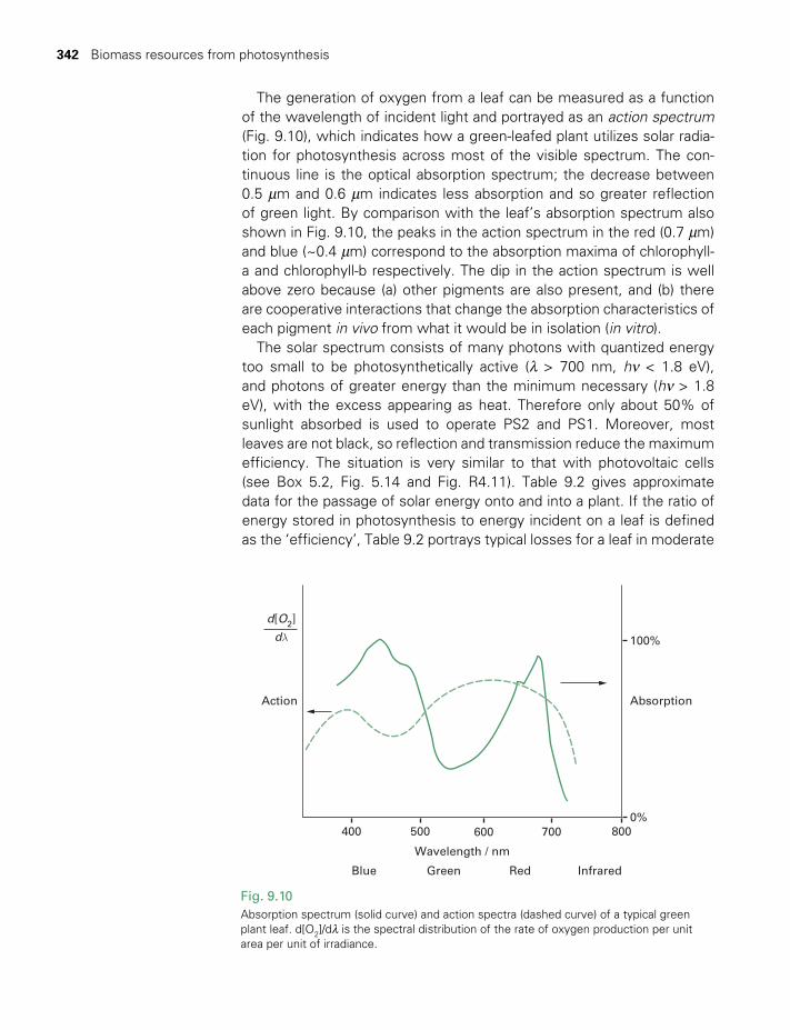
342 Biomass resources from photosynthesis
The generation of oxygen from a leaf can be measured as a function of the wavelength of incident light and portrayed as an action spectrum (Fig. 9.10), which indicates how a greenleafed plant utilizes solar radiation for photosynthesis across most of the visible spectrum. The continuous line is the optical absorption spectrum; the decrease between 0.5 mm and 0.6 mm indicates less absorption and so greater reflection of green light. By comparison with the leaf’s absorption spectrum also shown in Fig. 9.10, the peaks in the action spectrum in the red (0.7 mm) and blue (~0.4 mm) correspond to the absorption maxima of chlorophylla and chlorophyllb respectively. The dip in the action spectrum is well above zero because (a) other pigments are also present, and (b) there are cooperative interactions that change the absorption characteristics of each pigment in vivo from what it would be in isolation (in vitro).
The solar spectrum consists of many photons with quantized energy too small to be photosynthetically active (l > 700 nm, hν < 1.8 eV), and photons of greater energy than the minimum necessary (hν> 1.8 eV), with the excess appearing as heat. Therefore only about 50% of sunlight absorbed is used to operate PS2 and PS1. Moreover, most leaves are not black, so reflection and transmission reduce the maximum efficiency. The situation is very similar to that with photovoltaic cells (see Box 5.2, Fig. 5.14 and Fig. R4.11). Table 9.2 gives approximate data for the passage of solar energy onto and into a plant. If the ratio of energy stored in photosynthesis to energy incident on a leaf is defined as the ‘efficiency’, Table 9.2 portrays typical losses for a leaf in moderate
Fig. 9.10Absorption spectrum (solid curve) and action spectra (dashed curve) of a typical green plant leaf. d[O2]/dl is the spectral distribution of the rate of oxygen production per unit area per unit of irradiance.
AbsorptionAction
100%
d[O2]
dλ
Blue Green Red Infrared
400
Wavelength / nm
500 600 700 8000%
TWIDELL PAGINATION.indb 342 01/12/2014 11:37
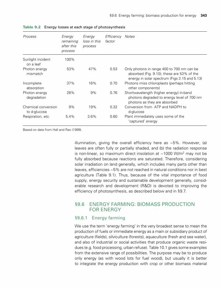
§9.6 Energy farming: biomass production for energy 343
illumination, giving the overall efficiency here as ~5%. However, (a) leaves are often fully or partially shaded, and (b) the radiation response is nonlinear, so maximum direct insolation at ~1000 W/m2 may not be fully absorbed because reactions are saturated. Therefore, considering solar irradiation on land generally, which includes many parts other than leaves, efficiencies ~5% are not reached in natural conditions nor in best agriculture (Table 9.1). Thus, because of the vital importance of food supply, energy security and sustainable development generally, considerable research and development (R&D) is devoted to improving the efficiency of photosynthesis, as described below and in §9.7.
§9.6 ENERGY FARMING: BIOMASS PRODUCTION FOR ENERGY
§9.6.1 Energy farming
We use the term ‘energy farming’ in the very broadest sense to mean the production of fuels or immediate energy as a main or subsidiary product of agriculture (fields), silviculture (forests), aquaculture (fresh and sea water), and also of industrial or social activities that produce organic waste residues (e.g. food processing, urban refuse). Table 10.1 gives some examples from the extensive range of possibilities. The purpose may be to produce only energy (as with wood lots for fuel wood), but usually it is better to integrate the energy production with crop or other biomass material
Table 9.2 Energy losses at each stage of photosynthesis
Process Energy remaining after this process
Energy loss in this process
Efficiency factor
Notes
Sunlight incident on a leaf
100%
Photon energy mismatch
53% 47% 0.53 Only photons in range 400 to 700 nm can be absorbed (Fig. 9.10); these are 53% of the
energy in solar spectrum (Figs 2.15 and 5.13) Incomplete absorption
37% 16% 0.70 Photons miss chloroplasts (perhaps hitting other components)
Photon energy degradation
28% 9% 0.76 Shortwavelength (higher energy) inband photons degraded to energy level of 700 nm
photons as they are absorbedChemical conversion to dglucose
9% 19% 0.32 Conversion from ATP and NADPH to dglucose
Respiration, etc. 5.4% 3.6% 0.60 Plant immediately uses some of the ‘captured’ energy
Based on data from Hall and Rao (1999).
TWIDELL PAGINATION.indb 343 01/12/2014 11:37
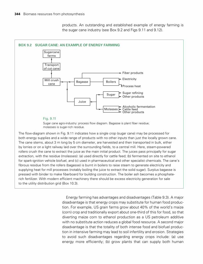
344 Biomass resources from photosynthesis
products. An outstanding and established example of energy farming is the sugar cane industry (see Box 9.2 and Figs 9.11 and 9.12).
BOX 9.2 SUGAR CANE: AN EXAMPLE OF ENERGY FARMING
Fig. 9.11Sugar cane agroindustry: process flow diagram. Bagasse is plant fiber residue; molasses is sugarrich residue.
Sugarcanefarms
Transportof cut cane
Mill crushcane
Bagasse Boilers
Sugar
MolassesAlcoholic fermentationCattle feed
Sugar refining
Process heat
Electricity
Fiber products
Other products
Other products
Juice
The flowdiagram shown in Fig. 9.11 indicates how a single crop (sugar cane) may be processed for both energy supplies and a wide range of products with no other inputs than just the locally grown cane. The cane stems, about 3 m long by 5 cm diameter, are harvested and then transported in bulk, either by lorries or on a light railway laid over the surrounding fields, to a central mill. Here, steampowered rollers crush the cane to extract the juice as the main initial product. The juices pass principally for sugar extraction, with the residue (molasses): (a) used directly for cattle feed; (b) fermented on site to ethanol for sparkignition vehicle biofuel, and (c) used in pharmaceutical and other specialist chemicals. The cane’s fibrous residue from the rollers (bagasse) is burnt in boilers to raise steam to generate electricity and supplying heat for mill processes (notably boiling the juice to extract the solid sugar). Surplus bagasse is pressed with binder to make fiberboard for building construction. The boiler ash becomes a phosphaterich fertilizer. With modern efficient machinery there should be excess electricity generation for sale to the utility distribution grid (Box 10.3).
Energy farming has advantages and disadvantages (Table 9.3). A major disadvantage is that energy crops may substitute for human food production. For example, US grain farms grow about 40% of the world’s maize (corn) crop and traditionally export about onethird of this for food, so that diverting maize corn to ethanol production as a US petroleum additive with no substitute action reduces a global food resource. A second major disadvantage is that the totality of both intense food and biofuel production in intensive farming may lead to soil infertility and erosion. Strategies to avoid such disadvantages regarding energy crops include: (a) use energy more efficiently; (b) grow plants that can supply both human
TWIDELL PAGINATION.indb 344 01/12/2014 11:37

§9.6 Energy farming: biomass production for energy 345
Fig. 9.12A sugar mill set up to produce sugar, ethanol, and surplus electricity. This photo shows the Costa Pinto mill in Brazil (São Paulo state). In the foreground is the receiving operation of the sugar cane harvest, with the mill immediately adjacent (at left). In the right background is the associated distillation facility for ethanol production.Photo by Mariordo, reproduced here under Creative Commons AttributionShare Alike 3.0 Unported License.
Table 9.3 Advantages and dangers of energy farming
Advantages Dangers and difficulties
Large potential supply May lead to soil infertility and erosionVariety of crops May compete with food productionVariety of uses (including transport fuel and electricity generation)Efficient use of byproducts, residues, wastes Bulky biomass material handicaps transport to
the processing factoryLink with established agriculture and forestry May encourage genetic engineering of
uncontrollable organismsEncourages integrated farming practiceEstablishes agroindustry that may include full range of technical processes, with the need for skilled
and trained personnelEnvironmental improvement by utilizing wastes Pollutant emissions from poorly controlled
processesFully integrated and efficient systems need have little water and air pollution (e.g. sulphur
content low)
Poorly designed and incompletely integrated systems may pollute water and air
Encourages rural development Largescale agroindustry may be socially disruptiveDiversifies the economy with respect to product, location and employee skillGreatest potential is in tropical countries, frequently of developing countries
Foreign capital may not be in sympathy with local or national benefit
TWIDELL PAGINATION.indb 345 01/12/2014 11:37

346 Biomass resources from photosynthesis
foods (e.g. grain) and energy from the waste products (e.g. straw); (c) do not burn residue biomass in the field, and (d) decrease feeding human food crops to animals.
Another related issue is: if the purpose of producing liquid biofuels is to decrease national consumption of fossil fuels, for reasons of ‘energy security’ (§17.2.1) or to reduce greenhouse gas emissions (§17.4), does the production of the biofuel require more fossil fuel than the biofuel would displace? This issue is addressed empirically in Boxes 10.3 and 10.4.
§9.6.2 Wood resource
Wood is a sustainable energy resource only if it is grown as fast as it is consumed. Moreover, there are ecological imperatives for the preservation of natural woodland and forests. The world’s wood resource is consumed not just for firewood, but for sawn timber, paper making and other industrial uses. In addition, much forest is cleared for agricultural land and not ‘harvested’, with its timber burnt as ‘waste’. FAO statistics estimate that the world harvest of wood as a utilized resource is about 3700 million m3 of wood per year, of which about 45% is noncommercial use for fuel and a further 6% is directly used as commercial fuel (FAO statistics for 2012). (The non commercial figure is subject to considerable uncertainty, and is probably an underestimate.)
In many countries, firewood consumption exceeds replacement growth, so fuelwood is a depleting resource. Fuelwood collection for household consumption, usually a task for women and children, is becoming more burdensome as fuelwood becomes scarcer. The proportion of rural women affected by fuelwood scarcity is around 60% in Africa, 80% in Asia, and 40% in Latin America. Moreover, gathering firewood may require one to five hours per day. Alleviating these difficulties requires both intensive reforestation and a switch to more efficient and alternative cooking methods (see §10.3.1 and Fig. 10.8).
Regeneration may occur in natural forest, or in manmade plantations (which usually grow faster, and are preferential for biofuels). For example: (i) from 2009, Brazil increased its 5 million hectares of sustainable eucalyptus plantations used for manufacturing steel from charcoal and for drying and processing soya;1 (ii) many Indian households are growing small private plantations for their own fuel use.2 Plantations grown specifically for energy supply need different management (silviculture) techniques than plantations grown primarily for timber (Sims 2002). Combustible wood need not be in large pieces, and can therefore be harvested at three to five years rather than ~30 years, so increasing productivity. The traditional method of coppicing (i.e. leaving the roots in the ground and periodically cropping only the abovesurface
TWIDELL PAGINATION.indb 346 01/12/2014 11:37

§9.6 Energy farming: biomass production for energy 347
branches) is successful with many tree species; it reduces labor for planting and weeding saplings, and also reduces soil erosion compared with repeated replanting.
§9.6.3 Crop yield and improvement
Predicting crop yields requires detailed knowledge of meteorological conditions, soil type, farming practice, fertilizer use, irrigation, etc.; moreover, unexpected weather conditions often counteract such predictions. Comparison between different crops and different places is difficult because of differences in growing seasons and harvesting methods. Some arable crops are planted annually (e.g. cereal grains), and may be cropped more than once (e.g. grasses). Others are planted every few years and harvested annually (e.g. sugar cane). Trees may grow for many years and be totally harvested (timber logging); other tree crops may grow from the continuing roots and be harvested as coppice every few years (e.g. willow, hazel and some eucalyptus). Table 9.4 estimates maximum biofuel potential of various crops in terms of heat of combustion and continuing energy supply. The data for aquatic crops assume abundant nutrients. Grasses are assumed to have frequent harvesting in the growing season.
As biomass energy becomes more important, plants are being selected and developed to optimize fuel supplies rather than just their fruit, grain or similar part product. For instance, propagation from clones of best plants and the application of genetic engineering has increased photosynthetic efficiency for biomass production.
§9.6.4 How much biomass is available for energy?
Box 9.3 outlines techniques for assessing how much biomass is potentially available for energy use. In such assessments, it is essential to focus on how much can be sustainably taken each year (i.e. with regrowth compensating for that used) without impinging on crops and land needed for food and without causing unacceptable ecological damage. Waste biomass (e.g. forest trimmings, coconut husks, timber offcuts, waste cardboard, sewage, etc.) should be the priority resource for combustion for energy. However, such resources are often difficult to quantify, and it is essential to leave significant amounts of rotting biomass for ecological sustainability of microflora and microfauna, and for soil structure. Therefore, many resource estimates, including Table 9.5, often include only biomass from new plantations. Table 9.5 (and the reports on which it is based) suggest that the greatest potential for energy farming of biomass perhaps occurs in tropical countries, especially those with adequate rainfall and soil condition.
TWIDELL PAGINATION.indb 347 01/12/2014 11:37
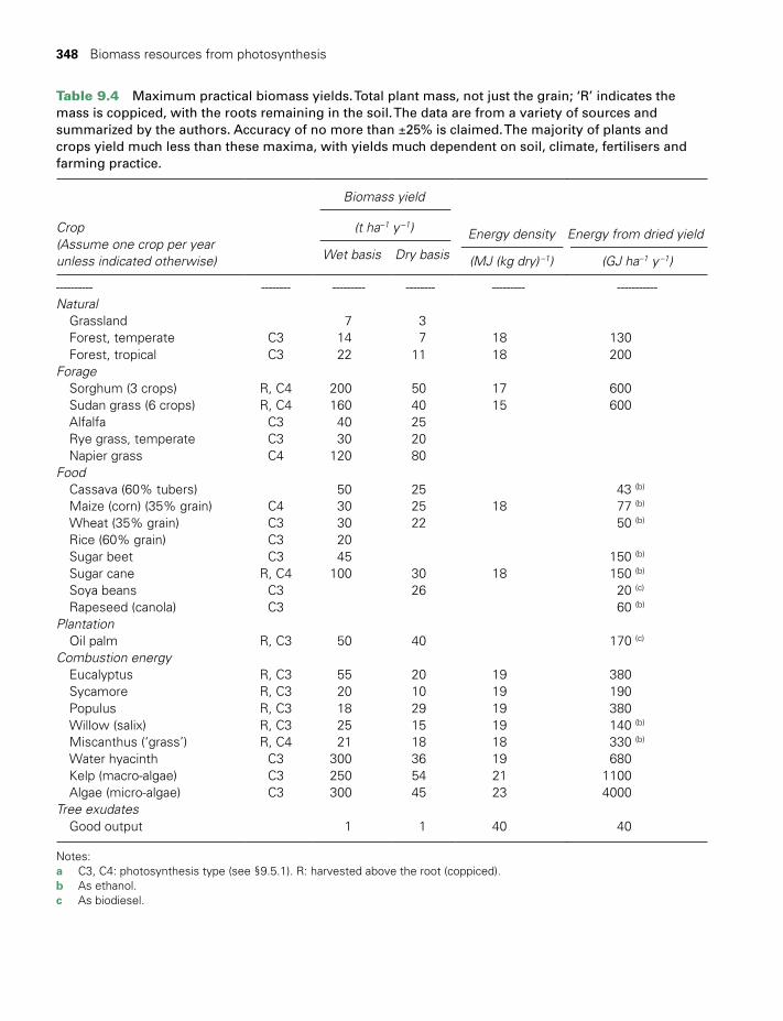
348 Biomass resources from photosynthesis
Table 9.4 Maximum practical biomass yields. Total plant mass, not just the grain; ‘R’ indicates the mass is coppiced, with the roots remaining in the soil. The data are from a variety of sources and summarized by the authors. Accuracy of no more than ±25% is claimed. The majority of plants and crops yield much less than these maxima, with yields much dependent on soil, climate, fertilisers and farming practice.
Biomass yield
Crop(Assume one crop per year unless indicated otherwise)
(t ha–1 y –1)
Wet basis Dry basis
Energy density
(MJ (kg dry) –1)
Energy from dried yield
(GJ ha–1 y –1)
Natural Grassland 7 3 Forest, temperate C3 14 7 18 130 Forest, tropical C3 22 11 18 200Forage Sorghum (3 crops) R, C4 200 50 17 600 Sudan grass (6 crops) R, C4 160 40 15 600 Alfalfa C3 40 25 Rye grass, temperate C3 30 20 Napier grass C4 120 80Food Cassava (60% tubers) 50 25 43 (b)
Maize (corn) (35% grain) C4 30 25 18 77 (b)
Wheat (35% grain) C3 30 22 50 (b)
Rice (60% grain) C3 20 Sugar beet C3 45 150 (b)
Sugar cane R, C4 100 30 18 150 (b)
Soya beans C3 26 20 (c)
Rapeseed (canola) C3 60 (b)
Plantation Oil palm R, C3 50 40 170 (c)
Combustion energy Eucalyptus R, C3 55 20 19 380 Sycamore R, C3 20 10 19 190 Populus R, C3 18 29 19 380 Willow (salix) R, C3 25 15 19 140 (b)
Miscanthus (‘grass’) R, C4 21 18 18 330 (b)
Water hyacinth C3 300 36 19 680 Kelp (macroalgae) C3 250 54 21 1100 Algae (microalgae) C3 300 45 23 4000Tree exudates Good output 1 1 40 40
Notes:a C3, C4: photosynthesis type (see §9.5.1). R: harvested above the root (coppiced).b As ethanol.c As biodiesel.
TWIDELL PAGINATION.indb 348 01/12/2014 11:37
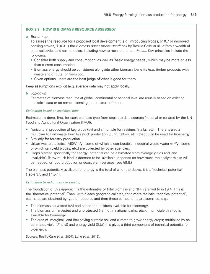
§9.6 Energy farming: biomass production for energy 349
BOX 9.3 HOW IS BIOMASS RESOURCE ASSESSED?
a Bottom-up To assess the resource for a proposed local development (e.g. introducing biogas, §10.7 or improved
cooking stoves, §10.3.1) the Biomass Assessment Handbook by RosilleCalle et al. offers a wealth of practical advice and case studies, including how to measure timber in situ. Key principles include the following:
• Consider both supply and consumption, as well as ‘basic energy needs’, which may be more or less than current consumption.
• Biomass energy should be considered alongside other biomass benefits (e.g. timber products with waste and offcuts for fuelwood).
• Given options, users are the best judge of what is good for them.
Keep assumptions explicit (e.g. average data may not apply locally).
b Top-down Estimates of biomass resource at global, continental or national level are usually based on existing
statistical data or on remote sensing, or a mixture of these.
Estimation based on statistical data
Estimation is done, first, for each biomass type from separate data sources (national or collated by the UN Food and Agricultural Organisation (FAO)).
• Agricultural production of key crops (t/y) and a multiple for residues (stalks, etc.). There is also a multiplier to find waste from livestock production (dung, tallow, etc.) that could be used for bioenergy.
• Similarly for forestry production. • Urban waste statistics (MSW (t/y), some of which is combustible, industrial waste water (m3/y), some
of which can yield biogas, etc.) are collected by other agencies.• Crops planted specifically for energy: potential can be estimated from average yields and land
‘available’. (How much land is deemed to be ‘available’ depends on how much the analyst thinks will be needed, or food production or ecosystem services: see §9.8.)
The biomass potentially available for energy is the total of all of the above; it is a ‘technical potential’ (Table 9.5 and §1.5.4).
Estimation based on remote sensing
The foundation of this approach is the estimates of total biomass and NPP referred to in §9.4. This is the ‘theoretical potential’. Then, within each geographical area, for a more realistic ‘technical potential’, estimates are obtained by type of resource and then these components are summed, e.g.:
• The biomass harvested (t/y) and hence the residues available for bioenergy.• The biomass unharvested and unprotected (i.e. not in national parks, etc.); in principle this too is
available for bioenergy.• The area of ‘marginal’ land (ha) having suitable soil and climate to grow energy crops; multiplied by an
estimated yield (t/(ha y)) and energy yield (GJ/t) this gives a third component of technical potential for bioenergy.
Sources: RosilloCalle et al. (2007); Long et al. (2013).
TWIDELL PAGINATION.indb 349 01/12/2014 11:37
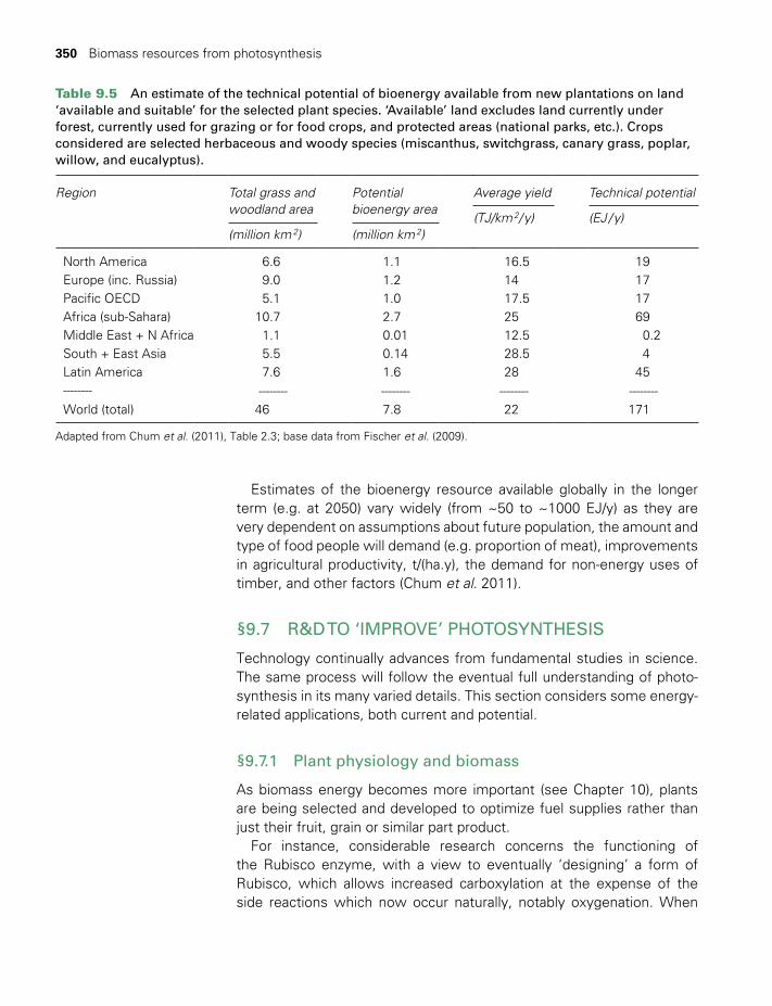
350 Biomass resources from photosynthesis
Estimates of the bioenergy resource available globally in the longer term (e.g. at 2050) vary widely (from ~50 to ~1000 EJ/y) as they are very dependent on assumptions about future population, the amount and type of food people will demand (e.g. proportion of meat), improvements in agricultural productivity, t/(ha.y), the demand for nonenergy uses of timber, and other factors (Chum et al. 2011).
§9.7 R&D TO ‘IMPROVE’ PHOTOSYNTHESIS
Technology continually advances from fundamental studies in science. The same process will follow the eventual full understanding of photosynthesis in its many varied details. This section considers some energyrelated applications, both current and potential.
§9.7.1 Plant physiology and biomass
As biomass energy becomes more important (see Chapter 10), plants are being selected and developed to optimize fuel supplies rather than just their fruit, grain or similar part product.
For instance, considerable research concerns the functioning of the Rubisco enzyme, with a view to eventually ‘designing’ a form of Rubisco, which allows increased carboxylation at the expense of the side reactions which now occur naturally, notably oxygenation. When
Table 9.5 An estimate of the technical potential of bioenergy available from new plantations on land ‘available and suitable’ for the selected plant species. ‘Available’ land excludes land currently under forest, currently used for grazing or for food crops, and protected areas (national parks, etc.). Crops considered are selected herbaceous and woody species (miscanthus, switchgrass, canary grass, poplar, willow, and eucalyptus).
Region Total grass and woodland area
(million km 2)
Potential bioenergy area
(million km 2)
Average yield
(TJ/km 2/ y)
Technical potential
(EJ / y)
North America 6.6 1.1 16.5 19Europe (inc. Russia) 9.0 1.2 14 17Pacific OECD 5.1 1.0 17.5 17Africa (subSahara) 10.7 2.7 25 69Middle East + N Africa 1.1 0.01 12.5 0.2South + East Asia 5.5 0.14 28.5 4Latin America 7.6 1.6 28 45 World (total) 46 7.8 22 171
Adapted from Chum et al. (2011), Table 2.3; base data from Fischer et al. (2009).
TWIDELL PAGINATION.indb 350 01/12/2014 11:37
§9.8 Social and environmental aspects 351
photosynthesis occurs in an atmosphere with an enlarged concentration of CO2, the ‘desirable’ carbohydrateforming reaction is promoted at the expense of the ‘undesirable’ side reaction of Rubisco with oxygen. A method for this has tanks of algae in polytunnels through which flue gas (which is ~10% CO2 and ~ 90% N2) passes from a power station.
§9.7.2 Bioengineered photosynthesis
The term ‘bioengineered’ refers to systems in which some of the key natural components of photosynthesis are artificially assembled into ‘engineered’ systems aimed at removing characteristics that may limit biomass productivity (e.g. the ability of plants to reproduce themselves). Some examples of bioengineered ‘photosynthesis’ systems under active investigation are reviewed by Blankenship et al. (2011).
§9.7.3 Artificial photosynthesis
The term artificial photosynthesis is used to describe processes in which laboratory materials are used to capture light energy and produce a chemical store of energy. Such processes are inspired by natural photosynthesis, but, unlike those of §9.7.2, do not use the same components as nature does. In particular, it refers to the production of hydrogen from water by lightinduced redox reactions Natural photosynthesis uses chlorophyll for the light antenna and hydrogenase enzymes for the hydrogen reaction, but current R&D focuses on the use of metal oxide semiconductors and metalbased catalysts for these actions (Jones 2012).
§9.8 SOCIAL AND ENVIRONMENTAL ASPECTS
§9.8.1 Bioenergy in relation to agriculture and forestry
Use and production of biomass for energy are intimately connected with wider policies and practices for agriculture and forestry. An overriding consideration is that such use and production should be ecologically sustainable, i.e. that the resource be used in a renewable manner, with (re)growth keeping pace with use. Moreover, for ethical reasons, it is vital that biomass production for energy is not at the expense of growing enough food to feed people.
Nevertheless, in the European Union and the USA, a major issue in agriculture is overproduction of food, as encouraged by agricultural financial subsidies. Such subsidies increase taxation on wage earners and the consequent surpluses of agricultural products distort world trade to the disadvantage of developing countries. As a partial response to such concerns, the European Union introduced financial incentives for
TWIDELL PAGINATION.indb 351 01/12/2014 11:37

352 Biomass resources from photosynthesis
its farmers to divert land from food production, and either to maintain it unproductively or for biomass for energy. Such policies retain the social benefits of an economically active agricultural population while also bringing the environmental benefits, described below, of substituting biofuels for fossil fuels.
Utilizing waste biomass increases the productivity of agriculture and forestry. This is especially so for the acceptable disposal of otherwise undesirable outputs (e.g. biodigestion of manure from intensive piggeries), so the integrated system brings both economic and environmental benefits. As emphasized in §9.6 and §10.1, successful biofuel production utilizes already concentrated flows of biomass, such as offcuts and sawdust from sawmilling, straw from crops, manure from penned animals and sewage from municipal works. Biofuel processes that depend upon first transporting and then concentrating diffuse biomass resources are less desirable.
Energy developments utilizing local crops and established skills are most likely to be socially acceptable. Thus the form of biomass most likely to be viable as an energy source will vary from region to region. Moreover, as with any crop, sustainable agriculture and forestry are required; for instance, extensive monocultures are vulnerable to disease and pests and unfriendly to native fauna. Note, too, that greenhouse gas benefits only occur when the biomass is used to replace fossil fuel use, so leaving the abated fossil fuel underground.
§9.8.2 Food versus fuel
Production of liquid biofuels has been based historically on biomass from grain, sugar and oil crops, all of which are essential food crops, generally grown on the best agricultural land available. Despite crop production surpluses in the USA and Europe, the increasing worldwide demand for food implies that these crops should not be diverted significantly from food to energy unless crop production becomes sufficient in the needy countries. Therefore, biofuel production as a major contribution to world energy supplies requires other feedstock and land than for food and other strategies. For instance, there is a need for cheaper, more energy efficient processes for producing ethanol from widely available lignocellusosic materials (e.g. corn stalks, straw, and wood), especially sawdust and other woody residues, rather than from foodrelated crops.
§9.8.3 Greenhouse gas impacts: bioenergy and carbon sinks
When a plant grows, carbon is extracted from the air as the CO2 is absorbed in photosynthesis, so becoming ‘locked into’ carbohydrate material both above and below ground. Significant amounts of CO2 are released in plant metabolism, but the net carbon flow is into the plant.
TWIDELL PAGINATION.indb 352 01/12/2014 11:37
§9.8 Social and environmental aspects 353
Carbon concentrations in the soil may also increase ‘indirectly’ from organic matter formed from plant detritus in fallen leaves and branches. Such removal of the greenhouse gas CO2 from the atmosphere is called a ‘carbon sink’. Consequently a dedicated program to increase plant growth will offset temporarily an increase in atmospheric CO2 from burning fossil fuels. However, all plants die and the vast majority of all such direct and indirect carbon eventually returns to the atmosphere, so joining a natural cycle which neither depletes nor increases atmospheric CO2 concentrations.
Only if the plant material is burnt to replace (abate) specific use of fossil fuel will there be a longterm benefit by preventing that fossil carbon from otherwise reaching the Atmosphere. It follows that such abated fossil carbon should always stay beneath the ground and never be extracted. In the national reports compiled for the UN Framework Convention on Climate Change, this abated fossil fuel shows as a reduction in the CO2 emissions from fossil fuel.
§9.8.4 Bioenergy in relation to the energy system
Biomass is currently a major part of the world energy system, although mainly in the form of inefficiently used firewood in rural areas, especially where cooking is over an open fire. A more sustainable energy system for the world will necessarily have to involve this widely distributed and versatile resource, but used in more efficient and more modern ways, as discussed in Chapter 10. For example, in the 160 energy scenarios reviewed by SRREN (2011), of those with significant input from renewable energy, half had bioenergy contributing at least 125 EJ/y to global total primary energy supply (TPES) by 2050, i.e. at least 25% of current TPES (see §17.8 for a general discussion of energy scenarios). Indeed, Chum et al. (2011) estimate that the technical potential of biomass for energy use may be as large as 500 EJ/y by 2050. However, such production of bioenergy requires sustainability and policy frameworks that ensure good governance of land use and improvements in forestry, agriculture and livestock management, and in associated bioenergy technologies.
§9.8.5 Human impact on net primary production (NPP)
Mapping from satellites and on the ground shows that 35% of the Earth’s icefree land surface is croplands (~10%) and grazing pastures for livestock (~25%); together these make perhaps the largest ecosystem on the planet, matching forest cover in extent. Meat production accounts for ~40% of global agricultural commercial output in industrialized countries and the equivalent impact in other countries (Steinfeld et al. 2006). Logged and managed forests add to the impact. Human appropriated net primary productivity (HANPP) is the proportion of global biological
TWIDELL PAGINATION.indb 353 01/12/2014 11:37
354 Biomass resources from photosynthesis
productivity that is used, managed, or coopted by human actions; this is estimated to be 20 ± 6% of global NPP (see e.g. Imhoff et al. 2004).
The conclusion is that by clearing natural ecosystems or by intensifying practices on existing croplands, grazing pastures and forests, present human landuse activities are consuming an everlarger share of the planet’s biological productivity and dramatically altering the Earth’s ecosystems in the process. It is important to realize that should all humans be vegetarian and all crop growth efficient, then land use would be far less. Now, however, there are large regions of the world where HANPP is between 60% and 100% of total NPP. Humans today already harvest over 8 Pg C/y for their own immediate food and for animals. This biomass amounts to an approximate gross calorific value of ≈300 exajoules (EJ) per year, of which ~50 EJ/y are used for the provision of energy services. The total is expected to increase in the next decades by an additional harvest of 4–7 Pg C/y, which would almost double the present biomass harvest and generate substantial additional pressure on ecosystems (Haberl et al. 2007).
Given the magnitude of these effects, it is clear that, as with greenhouse gases and climate change, human society with its present diet, lifestyle, economies and aspirations is approaching a fundamental environmental limit on its sustainability. How much more of the biosphere’s productivity can we appropriate before planetary systems begin to break
CHAPTER SUMMARY
All biological and economic life on Earth depends on photosynthesis as the process by which living plants (a) make their own structural material (biomass) from the main inputs of carbon dioxide and water, and (b) produce oxygen, as necessary for animal life and combustion generally. The biomass and the oxygen together become chemical stores of solar energy. This involves a series of complex physical and biochemical reactions, most of which take place in the leaves of a plant. The first stage (photon absorption, mainly by chlorophyll pigments) has analogies with photovoltaic cells, which can generate but not store electricity. About half of the energy captured by plants from sunlight is used for the plant’s own metabolism. About 3% of insolation on plants is stored as biomass, even for a wellcultivated crop in the growing season. Thus the dominant immediate effect of sunshine is to warm the Earth, with the biomass energy eventually transforming in use or decay to heat also. Nevertheless, the global net primary production (NPP, i.e. the energy stored by terrestrial plants as biomass) is about three times the current total commercial energy use by mankind.
About 20% of global NPP is used, managed, or coopted by human actions, although ‘only’ about 2% of global NPP is currently used for energy. Maintaining livestock for meat production has a major impact. Thus there are strong environmental and social constraints on the biomass resource available for energy purposes, including giving priority to food, animal feed and fiber products as global population increases, and to maintaining the natural environment. If biomass regrows at a rate at least as rapidly as it is used, then its net effect on CO2 concentration in the atmosphere is zero.
There is considerable potential for energy farming, notably through use for energy of agricultural and forestry residues and through new plantations on otherwise marginal lands. Enhanced productivity
TWIDELL PAGINATION.indb 354 01/12/2014 11:37

Problems 355
down: 30%? 40%? 50%? Perhaps we have already unknowingly crossed that threshold.
QUICK QUESTIONS
Note: Answers to these questions are in the text of the relevant section of this chapter, or may be readily inferred from it.
1 How is the energy of solar radiation stored? 2 What approximately is the heat of combustion of plant biomass? 3 Why is biomass heat of combustion less than that of, say, natural gas
(methane)? 4 What is the minimum number of absorbed solar photons needed to
produce one molecule of oxygen? 5 How is absorbed solar energy channeled for chemical reactions in
plants? 6 What are ‘photosystems’ and what do they do? 7 What is the efficiency of plant photosynthesis and what are the impli
cations of plant photosynthesis being ten times greater? 8 Define ‘energy farming’. 9 How many products can you identify from a sugar cane ‘mill/factory’?10 Describe the impact of human food and energy consumption on the
Earth’s land ecosystem.11 How is a carbon atom in biomass different in effect from a carbon
atom in fossil fuel?
PROBLEMS
9.1 According to (9.3), photosynthesis stores 460 kJ per mole C. Use this to calculate how much energy is stored per year by the global terrestrial net primary production. How much is this in Watts (J/s)?
9.2 Calculate very approximately how many trees are necessary to produce the oxygen used for (i) your own metabolism, and (ii) to maintain the per capita total fuel consumption of your country. Compare this with the approximate number of trees per person in your country.
through improved agricultural practices and plant breeding and selection can also add to the potential bioenergy resource.
Natural photosynthesis has inspired research in two directions that may lead to new renewable energy technologies: (i) ‘bioengineered photosynthesis’, in which some of the key natural components of photosynthesis are artificially assembled into ‘engineered’ systems aimed at overcoming some of the efficiency limits of natural photosynthesis, and (ii) ‘artificial photosynthesis’, processes in which inorganic materials are used to capture light energy and produce a chemical store of energy.
TWIDELL PAGINATION.indb 355 01/12/2014 11:37
356 Biomass resources from photosynthesis
NOTES
1 Rechargenews, August 7, 2009.2 ‘India’s firewood crisis reexamined’, Resources for the Future (2006).
BIBLIOGRAPHY
Photosynthesis: Undergraduate-level books and reviews
Archer, M. and Barber, J. (eds) (2005) Molecular to Global Photosynthesis, Imperial College Press, London. Part of a series on photoconversion of solar energy. See especially the editors’ introduction (similar level to this book) and the chapter by A. Holzworth on ‘Light absorption and harvesting’.
Cogdell, R. (2013) ‘Instant Expert #30: Photosynthesis’, New Scientist, supplement to issue of February 2.
Edenhofer, O., PichsMadruga R., Sokona, Y., Seyboth, K., Matschoss, P., Kadner, S., Zwickel, T., Eickemeier, P., Hansen, G., Schlömer, S. and von Stechow, C. (eds) (2011) IPCC Special Report on Renewable Energy Sources and Climate Change Mitigation. Cambridge University Press, Cambridge. Chapter 2 deals specifically with bioenergy; Chapter 1 is an overview of renewable energy.
Hall, D.O. and Rao, K.K. (1999, 6th edn) Photosynthesis, Edward Arnold, London. A short and stimulating introduction with more physical bias than many others.
Lawlor, D.W. (2001, 3rd edn) Photosynthesis: Molecular, physiological and environmental processes, BIOS Scientific Publications, Oxford. Concise text for biology undergraduates.
Monteith, J. and Unsworth, K. (1997, 2nd edn) Principles of Environmental Physics, Edward Amold, London. Considers the physical interaction of plant and animal life with the environment. Chemical aspects are not covered. Of background relevance to photosynthesis.
Morton, O. (2007) Eating the Sun: How plants power the planet, Fourth Estate, London. Popularlevel account, including lively character sketches of key scientists in the field.
Wrigglesworth J. (1997) Energy and Life, Taylor & Francis, London. The biochemistry of metabolism and photosynthesis, clearly presented.
Biomass resource
Chum, H., Faaij, A. Moreira, J., Berndes, G., Dhamija, P., Dong, H., Gabrielle, B., Goss Eng, A., Lucht, W., Mapako, M., Masera Cerutti, O., McIntyre, T., Minowa, T. and Pingoud, K. (2011) ‘Bioenergy’, Chapter 2 of IPCC Special Report on Renewable Energy Sources and Climate Change Mitigation, ed. O. Edenhofer, R. PichsMadruga, Y. Sokona, K. Seyboth, P. Matschoss, S. Kadner, T. Zwickel, P. Eickemeier, G. Hansen, S. Schlömer and C. von Stechow, Cambridge University Press, Cambridge. Recent authoritative review of both biomass resource and full range of bioenergy technologies (available online at http://srren.ipccwg3.de/report).
FAO Statistics (2012) Extracted from faostat3.fao.org (statistics website of UN Food and Agriculture Organisation). Contains official production statistics of crops, including yields for most countries and regions for each year since 1961; also similar for forestry statistics, including resource estimates – all freely downloadable.
9.3 The heat of combustion of sucrose C12H22O11 is 5646 kJ/mole. Calculate using the Avogadro constant, the energy per atom of carbon in units of eV.
TWIDELL PAGINATION.indb 356 01/12/2014 11:37
Bibliography 357
Long, H., Li, X. Wang, H. and Jia, J. (2013) ‘Biomass resources and their bioenergy potential estimation: a review’, Renewable and Sustainable Energy Reviews, 26, 344–352. Useful collection of the range of estimates for various regions.
RosilloCalle, F., de Groot, P., Hemstock, S. and Woods, J. (2007) The Biomass Assessment Handbook: Bioenergy for a sustainable environment, Earthscan, London. Practical methods for assessment of local biomass resource. Does not include any largescale resource estimates.
Sims, R.E. (2002) The Brilliance of Bioenergy in Business and in Practice, James & James, London. Illuminating text with emphasis on modern industrial production and applications; contains numerous illustrated case studies of power systems, including with biogas.
Specific references
Blankenship, R. et al. (2011) ‘Comparing photosynthetic and photovoltaic efficiencies and recognizing the potential for improvement’, Science, 332, 805–809. Includes an excellent summary of possible directions for enhanced natural photosynthesis and for engineered photosynthesis.
Fischer, G., Hizsnyik, E., Prieler, S., Shah, M. and van Velthuizen, H. (2009) Biofuels and Food Security, International Institute for Applied Systems Analysis, Vienna (available at www.iiasa.ac.at).
Haberl, H. et al. (2007) ‘Quantifying and mapping the human appropriation of net primary production in Earth’s terrestrial ecosystems’, Proceedings of the National Academy of Science (USA), 104, 12492–12947.
Imhoff, M., Bounoua, L., Ricketts, T., Loucks, C., Harriss, R. and Lawrence, W. (2004) ‘Global patterns of net primary production’, Nature, 429, 870–874. Estimates that humans are utilizing ~25% of global net primary production.
Jones, N. (2012) ‘New leaf: the promise of artificial photosynthesis’, New Scientist, April 16.
Potter, C., Klooster, S. and Genovese, V. (2012) ‘Net primary production of terrestrial ecosystems from 2000 to 2009’, Climatic Change, 115, 365–378.
Steinfeld, H., Gerber, P., Wassenaar, T., Castel, V., Rosales, M. and de Haan, C. (2006) Livestock’s Long Shadow: Environmental issues and options. Livestock, environment and development, FAO, Rome. A detailed study of the impact of animal livestock on the environment, with particular information on climate change impact.
Twidell, J.W. and Weir, A.D. (2006, 2nd edn) Renewable Energy Resources, Taylor & Francis, Oxon. Chapter 10 of the second edition contains much more detail on the physics and chemistry of photosynthesis at the molecular and plant level than we give here in this third edition. That chapter is reproduced on the eResource of the publisher’s website for this book, see S9.1.
Vitousek, P., Ehrlich, P., Ehrlich, A. and Matson, P. (1986) ‘Human appropriation of the products of photosynthesis’, Bioscience, 36, 368–373. Pioneering analysis, which has inspired much subsequent work.
Journals and websites
Photosynthesis is an extremely active area of scientific research, with most of that research (>1000 papers per year) reported in specialist scientific journals such as
Photosynthesis Research, Annual Review of Plant Physiology and Plant Molecular Biology, Nature, and Photochemistry and Photobiology.
TWIDELL PAGINATION.indb 357 01/12/2014 11:37

358 Biomass resources from photosynthesis
Much of this work is then distilled into graduatelevel monographs.
Many of the more generally interesting research results, including those on artificial or engineered photosynthesis, are summarized on the website (www.sciencedaily.com), which is both free and searchable.
http://greet.es.anl.gov/main The GREET model (Greenhouse gases, Regulated Emissions, and Energy use in Transportation), developed and continually updated by Argonne National Laboratory (USA), allows researchers and analysts to evaluate various vehicle and fuel combinations on a full fuel cycle/vehicle cycle basis. The model is freely available for download and draws on an extensive database of US agricultural and engineering practice.
TWIDELL PAGINATION.indb 358 01/12/2014 11:37
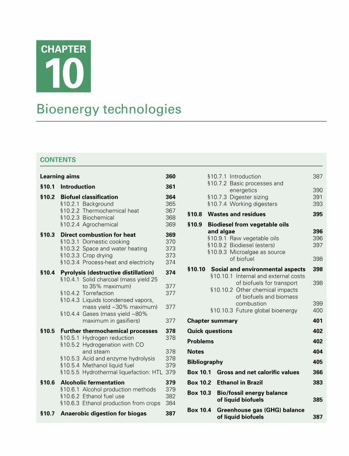
Bioenergy technologies
CONTENTS
Learning aims 360
§10.1 Introduction 361
§10.2 Biofuel classification 364 §10.2.1 Background 365 §10.2.2 Thermochemical heat 367 §10.2.3 Biochemical 368 §10.2.4 Agrochemical 369
§10.3 Direct combustion for heat 369 §10.3.1 Domestic cooking 370 §10.3.2 Space and water heating 373 §10.3.3 Crop drying 373 §10.3.4 Process-heat and electricity 374
§10.4 Pyrolysis (destructive distillation) 374 §10.4.1 Solid charcoal (mass yield 25
to 35% maximum) 377 §10.4.2 Torrefaction 377 §10.4.3 Liquids (condensed vapors,
mass yield ~30% maximum) 377 §10.4.4 Gases (mass yield ~80%
maximum in gasifiers) 377
§10.5 Further thermochemical processes 378 §10.5.1 Hydrogen reduction 378 §10.5.2 Hydrogenation with CO
and steam 378 §10.5.3 Acid and enzyme hydrolysis 378 §10.5.4 Methanol liquid fuel 379 §10.5.5 Hydrothermal liquefaction: HTL 379
§10.6 Alcoholic fermentation 379 §10.6.1 Alcohol production methods 379 §10.6.2 Ethanol fuel use 382 §10.6.3 Ethanol production from crops 384
§10.7 Anaerobic digestion for biogas 387
§10.7.1 Introduction 387 §10.7.2 Basic processes and
energetics 390 §10.7.3 Digester sizing 391 §10.7.4 Working digesters 393
§10.8 Wastes and residues 395
§10.9 Biodiesel from vegetable oils and algae 396
§10.9.1 Raw vegetable oils 396 §10.9.2 Biodiesel (esters) 397 §10.9.3 Microalgae as source
of biofuel 398
§10.10 Social and environmental aspects 398 §10.10.1 Internal and external costs
of biofuels for transport 398 §10.10.2 Other chemical impacts
of biofuels and biomass combustion 399
§10.10.3 Future global bioenergy 400
Chapter summary 401
Quick questions 402
Problems 402
Notes 404
Bibliography 405
Box 10.1 Gross and net calorific values 366
Box 10.2 Ethanol in Brazil 383
Box 10.3 Bio/fossil energy balance of liquid biofuels 385
Box 10.4 Greenhouse gas (GHG) balance of liquid biofuels 387
CHAPTER
10
TWIDELL PAGINATION.indb 359 01/12/2014 11:37
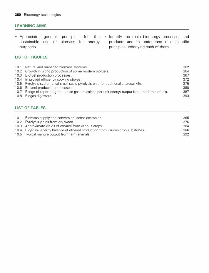
360 Bioenergy technologies
LEARNING AIMS
• Appreciate general principles for the sus tainable use of biomass for energy purposes.
• Identify the main bioenergy processes and products and to understand the scientific principles underlying each of them.
LIST OF FIGURES
10.1 Natural and managed biomass systems. 36210.2 Growth in world production of some modern biofuels. 36410.3 Biofuel production processes. 36710.4 Improved efficiency cooking stoves. 37210.5 Pyrolysis systems: (a) small-scale pyrolysis unit; (b) traditional charcoal kiln. 37510.6 Ethanol production processes. 38010.7 Range of reported greenhouse gas emissions per unit energy output from modern biofuels. 38710.8 Biogas digesters. 393
LIST OF TABLES
10.1 Biomass supply and conversion: some examples. 36510.2 Pyrolysis yields from dry wood. 37610.3 Approximate yields of ethanol from various crops. 38410.4 Bio/fossil energy balance of ethanol production from various crop substrates. 38610.5 Typical manure output from farm animals. 392
TWIDELL PAGINATION.indb 360 01/12/2014 11:37

§10.1 Introduction 361
§10.1 INTRODUCTION
The material of plants and animals, including their wastes and residues, is called biomass. It is organic, carbon-based material that reacts with oxygen in combustion and natural metabolic processes to release heat. Such heat, especially if at temperatures >400°C, may be used to gen-erate work and electricity. The initial material may be transformed by chemical and biological processes to produce biofuels, i.e. biomass pro-cessed into a more convenient form, particularly liquid fuels for transport. Examples of biofuels include methane gas, liquid ethanol, methyl esters, oils and solid charcoal. The term bioenergy is sometimes used to cover biomass and biofuels together.
The initial energy of the biomass oxygen system is captured from solar radiation in photosynthesis, as described in Chapter 9. When released in combustion, the biofuel energy is dissipated, but the elements of the material should be available for recycling in natural ecological or agricultural processes, as described in Chapter 1 and Fig. 10.1. Thus the use of industrial biofuels, when linked carefully to natural ecological cycles, may be non-polluting and sustainable. Such systems are called agro-industries (§9.6), of which the most established are the sugar cane and forest products industries; however, there are increasing examples of commercial products for energy and materials made from crops as a means of both diversifying and integrating agriculture.
The dry matter mass of biological material cycling in the biosphere is about 250 × 109 t/y incorporating about 100 × 109 t/y of carbon. The associated energy captured in photosynthesis is 2 × 10²¹ J/y (= 0.7 × 10¹⁴W). Of this, about 0.5% by weight is biomass as crops for human food. Biomass production varies with local conditions, and is about twice as great per unit surface area on land than at sea. The global resource of biomass is reviewed in Chapter 9, including the apparent competition of food and biofuels.
Biomass is the primary source for about 10% (50 EJ/y) of mankind’s energy use, which is similar to the global use of fossil gas. Uses in approximate proportions include (IPCC 2011): (i) ~70% as mostly non-commercial ‘traditional’ fuel-wood for domestic cooking and heating, pre-dominantly in developing countries but also including significant amounts in the rural areas of mature economies; (ii) ~10% as fuel for electricity generation, including ‘combined heat and power – CHP’; (iii) ~10% for non-domestic process heat, and (iv) ~10% for the biofuel component of vehicle fuel, which is rapidly increasing in both absolute and percentage terms. Some countries are notable for their use of bioenergy, including Brazil (31%), Sweden (23%) and Austria (18%).
If biomass is to be considered renewable, growth must at least keep pace with use. It is distressing for local ecology and global climate control
TWIDELL PAGINATION.indb 361 01/12/2014 11:37
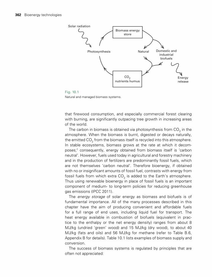
362 Bioenergy technologies
that firewood consumption, and especially commercial forest clearing with burning, are significantly outpacing tree growth in increasing areas of the world.
The carbon in biomass is obtained via photosynthesis from CO2 in the atmosphere. When the biomass is burnt, digested or decays naturally, the emitted CO2 from the biomass itself is recycled into this atmosphere. In stable ecosystems, biomass grows at the rate at which it decom-poses;1 consequently, energy obtained from biomass itself is ‘carbon neutral’. However, fuels used today in agricultural and forestry machinery and in the production of fertilizers are predominantly fossil fuels, which are not themselves ‘carbon neutral’. Therefore bioenergy, if obtained with no or insignificant amounts of fossil fuel, contrasts with energy from fossil fuels from which extra CO2 is added to the Earth’s atmosphere. Thus using renewable bioenergy in place of fossil fuels is an important component of medium- to long-term policies for reducing greenhouse gas emissions (IPCC 2011).
The energy storage of solar energy as biomass and biofuels is of fundamental importance. All of the many processes described in this chapter have the aim of producing convenient and affordable fuels for a full range of end uses, including liquid fuel for transport. The heat energy available in combustion of biofuels (equivalent in prac-tice to the enthalpy or the net energy density) ranges from about 8 MJ/kg (undried ‘green’ wood) and 15 MJ/kg (dry wood), to about 40 MJ/kg (fats and oils) and 56 MJ/kg for methane (refer to Table B.6, Appendix B for details). Table 10.1 lists examples of biomass supply and conversion.
The success of biomass systems is regulated by principles that are often not appreciated:
Solar radiation
Photosynthesis
Biomass energystore
CO2nutrients humus
Natural
Energyrelease
Domestic andindustrialbiofuels
Fig. 10.1Natural and managed biomass systems.
TWIDELL PAGINATION.indb 362 01/12/2014 11:37

§10.1 Introduction 363
1 Every biomass activity produces a wide range of products and ser-vices. For instance, where sugar is made from cane, many commer-cial products may be obtained from the otherwise waste molasses and fiber. If the fiber is burnt, then any excess process heat may be used to generate electricity. Washings and ash can be returned to the soil as fertilizer.
2 Some high-value energy supplies require a greater amount of low-value energy for their production (e.g. electricity from biomass thermal power, ethanol from starch crops, methane from animal slurry). Such apparent inefficiency is justifiable, especially if the process energy is from otherwise waste material (e.g. straw, crop fiber, forest trim-mings, animal slurry).
3 The full economic benefit of agro-industries is likely to be widespread and yet difficult to assess. One of many possible benefits is an increase in local ‘cash flow’ by trade and employment.
4 Biofuel production is likely to be most economic if the produc-tion process utilizes materials already concentrated, probably as a by-product, and so available at low cost or as extra income for the treatment and removal of waste. Thus there has to be a supply of biomass already passing near the proposed place of production, just as hydro-power depends on a natural flow of water already con-centrated by a catchment. Examples are the wastes from animal enclosures, offcuts and trimmings from sawmills, municipal sewage, husks and shells from coconuts, and straw from cereal grains. It is extremely important to identify and quantify these flows of biomass in a national or local economy before specifying likely biomass devel-opments. Unless concentrated biomass already exists from previ-ously established systems, then the cost of biomass growth and/or collection is often too great and too complex for economic benefit. Short-rotation crops may be grown primarily for energy production as part of intensive agriculture; however, within the widespread prac-tice of agricultural subsidies it is difficult to evaluate fundamental cost-effectiveness.
5 Negative and unjustifiable impacts of extensive biomass fuel produc-tion on a large scale include deforestation, soil erosion and the dis-placement of vital food crops by fuel crops.
6 Biofuels are organic materials, so there is always the alternative of using these materials as chemical feedstock or structural materials. For instance, palm oil is an important component of soaps; many plastic and pharmaceutical goods are made from natural products; and much building board is made from plant fibers constructed as composite materials.
7 Poorly controlled biomass processing or combustion can certainly pro- duce unwanted pollution, especially from relatively low-temperature combustion, wet fuels and lack of oxygen supply to the combustion
TWIDELL PAGINATION.indb 363 01/12/2014 11:37
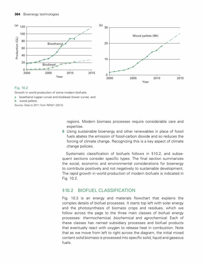
364 Bioenergy technologies
regions. Modern biomass processes require considerable care and expertise.
8 Using sustainable bioenergy and other renewables in place of fossil fuels abates the emission of fossil-carbon dioxide and so reduces the forcing of climate change. Recognizing this is a key aspect of climate change policies.
Systematic classification of biofuels follows in §10.2, and subse-quent sections consider specific types. The final section summarizes the social, economic and environmental considerations for bioenergy to contribute positively and not negatively to sustainable development. The rapid growth in world production of modern biofuels is indicated in Fig. 10.2.
§10.2 BIOFUEL CLASSIFICATION
Fig. 10.3 is an energy and materials flowchart that explains the complex details of biofuel processes. It starts top left with solar energy and the photosynthesis of biomass crops and residues, which we follow across the page to the three main classes of biofuel energy processes: thermochemical, biochemical and agrochemical. Each of these classes has named subsidiary processes and biofuel products that eventually react with oxygen to release heat in combustion. Note that as we move from left to right across the diagram, the initial mixed content solid biomass is processed into specific solid, liquid and gaseous fuels.
0
20
40
60
80
100
120
2000
(a)
2005 2010 2015Year
Pro
du
ctio
n (
GL)
Bioethanol
Biodiesel
0
10
20
30(b)
2000 2005 2010 2015Year
Wood pellets (Mt)
Fig. 10.2Growth in world production of some modern biofuels: a bioethanol (upper curve) and biodiesel (lower curve), and b wood pellets.Source: Data to 2011 from REN21 (2012).
TWIDELL PAGINATION.indb 364 01/12/2014 11:37
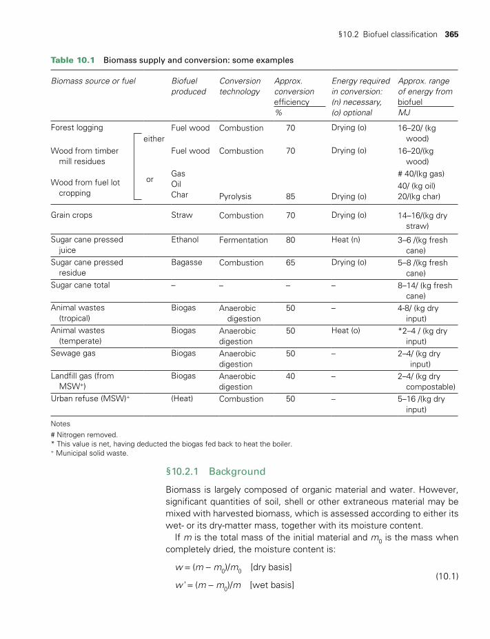
§10.2 Biofuel classification 365
Table 10.1 Biomass supply and conversion: some examples
Biomass source or fuel Biofuel produced
Conversion technology
Approx. conversion efficiency %
Energy required in conversion: (n) necessary, (o) optional
Approx. range of energy from biofuel MJ
Forest loggingeither
Fuel wood Combustion 70 Drying (o) 16–20/ (kg wood)
Wood from timber mill residues
Wood from fuel lot cropping
Fuel wood Combustion 70 Drying (o) 16–20/(kg wood)
orGasOil Char Pyrolysis
# 40/(kg gas)
85 Drying (o)40/ (kg oil) 20/(kg char)
Grain crops Straw Combustion 70 Drying (o) 14–16/(kg dry straw)
Sugar cane pressed juice
Ethanol Fermentation 80 Heat (n) 3–6 /(kg fresh cane)
Sugar cane pressed residue
Bagasse Combustion 65 Drying (o) 5–8 /(kg fresh cane)
Sugar cane total – – – – 8–14/ (kg fresh cane)
Animal wastes (tropical)
Biogas Anaerobic digestion
50 – 4-8/ (kg dry input)
Animal wastes (temperate)
Biogas Anaerobic digestion
50 Heat (o) *2–4 / (kg dry input)
Sewage gas Biogas Anaerobic digestion
50 – 2–4/ (kg dry input)
Landfill gas (from MSW+)
Biogas Anaerobic digestion
40 – 2–4/ (kg dry compostable)
Urban refuse (MSW)+ (Heat) Combustion 50 – 5–16 /(kg dry input)
Notes# Nitrogen removed.* This value is net, having deducted the biogas fed back to heat the boiler.+ Municipal solid waste.
§10.2.1 Background
Biomass is largely composed of organic material and water. However, significant quantities of soil, shell or other extraneous material may be mixed with harvested biomass, which is assessed according to either its wet- or its dry-matter mass, together with its moisture content.
If m is the total mass of the initial material and m0 is the mass when completely dried, the moisture content is:
w = (m − m0)/m0 [dry basis] (10.1)
w' = (m − m0)/m [wet basis]
TWIDELL PAGINATION.indb 365 01/12/2014 11:37
366 Bioenergy technologies
The moisture is in the form of both extracellular and intracellular water, which has to be mostly removed from the initial crop for preservation by drying (see §4.3). When harvested, the wet basis moisture content of plants is commonly 50%, and may be as large as 90% in aquatic algae, including seaweed (kelps). The material is considered ‘dry’ when it reaches long-term equilibrium with the environment, usually at about 10 to 15% water content by mass.
Carbon-based fuels may be classified by their reduction level (§9.5.2). When biomass is converted to CO2 and H2O, the energy made available is about 460 kJ per mole of carbon (38 MJ per kg of carbon; ~16 MJ per kg of dry biomass), per unit of reduction level R. This is not an exact quantity owing to other energy changes. Thus sugars (R = 1) have a heat of combustion of about 450 kJ per 12 g of carbon content. Fully reduced material (e.g. methane CH4 (R = 2)) has a heat of combustion of about 890 kJ per 12 g of carbon (i.e. per 16 g of methane).
BOX 10.1 GROSS AND NET CALORIFIC VALUES
Gross calorific value (GCV) is the heat evolved in a reaction of the type
CH2O + O2 CO2 (gas) + H2O (liquid).
(e.g. the output is liquid water and not steam or water vapor, as in a condensing boiler which so recovers the latent heat). Chemists often refer to GCV as only the heat of combustion. Unless stated otherwise, this is the measure used in this book.
Some authors quote the net (or lower) calorific value (LCV), which is the heat evolved if the final H2O is gaseous as a vapor, so there is no latent heat recovery (e.g. as in an internal combustion engine).
LCV is about 6 to 7% less than GCV for most biofuels, and ~8% less for fossil petroleum and diesel fuels.
If combusted, moisture in wet and damp biomass solid fuel causes significant reduction in useful thermal output, because (i) evapora-tion of water requires 2.3 MJ per kg which is generally not recovered; (ii) the temperature of the combustion is reduced; and (iii) polluting smoke emission is likely. In contrast, dry fuel is a delight. This affects how the heat value of the fuel is measured (Box 10.1). With condens-ing boilers, much of such latent heat can be recovered by condensing the water vapor in the emission so that the incoming cold water is preheated.
The density of biomass, and the bulk density of stacked fibrous biomass, are important, especially for transportation and storage. In general, three to four times the volume (not mass) of dry biological material has to be accumulated to provide the same energy as coal. Thus suitable transport and fuel handling is required if the biomass is not utilized at source.
TWIDELL PAGINATION.indb 366 01/12/2014 11:37
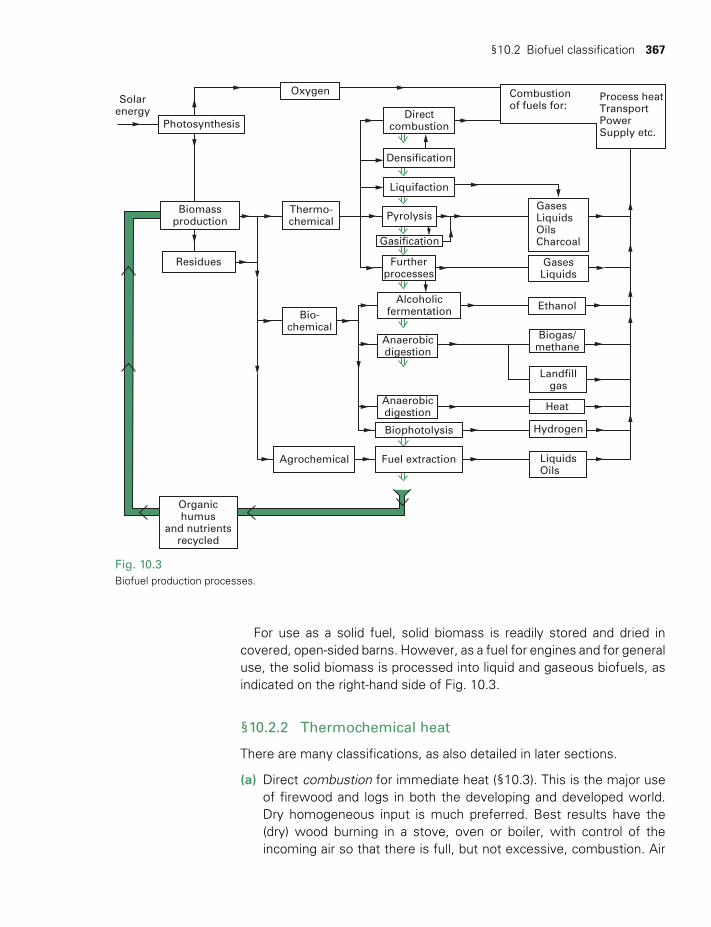
§10.2 Biofuel classification 367
For use as a solid fuel, solid biomass is readily stored and dried in covered, open-sided barns. However, as a fuel for engines and for general use, the solid biomass is processed into liquid and gaseous biofuels, as indicated on the right-hand side of Fig. 10.3.
§10.2.2 Thermochemical heat
There are many classifications, as also detailed in later sections.
(a) Direct combustion for immediate heat (§10.3). This is the major use of firewood and logs in both the developing and developed world. Dry homogeneous input is much preferred. Best results have the (dry) wood burning in a stove, oven or boiler, with control of the incoming air so that there is full, but not excessive, combustion. Air
Agrochemical
Bio-chemical
Thermo-chemical
Oxygen
Densification
Solarenergy Direct
combustion
Pyrolysis
Gasification
Furtherprocesses
Alcoholicfermentation
Anaerobicdigestion
Biophotolysis
Fuel extraction LiquidsOils
Liquifaction
Hydrogen
Landfillgas
Biogas/methane
Anaerobicdigestion Heat
Ethanol
GasesLiquids
GasesLiquidsOilsCharcoal
Combustionof fuels for:
Process heatTransportPowerSupply etc.
Photosynthesis
Residues
Organichumus
and nutrientsrecycled
Biomassproduction
Fig. 10.3 Biofuel production processes.
TWIDELL PAGINATION.indb 367 01/12/2014 11:37

368 Bioenergy technologies
entry is needed around the fuel for the initial combustion and into the hot exhaust for secondary combustion. Some biomass, such as sawmill waste or purposely produced sawdust, is ‘densified’ by only compression into pellets (~15 mm × ~5 mm) or briquettes (~100 mm × ~40 mm). This process makes the biomass easier and cheaper to transport and deliver to stores, easier to feed directly from the store into combustion chambers with auger screws, and it is easier to control the combustion with injected air; consequently there is now substantial regional and international trade in wood pellets. Municipal solid waste (MSW: §10.8) and dried sewage can be processed by densification to produce solid combustion fuels,
(b) Pyrolysis (§10.4). Biomass is heated either in the absence of air, or by the partial combustion of some of the biomass in a restricted air or oxygen supply. The products are extremely varied, consist-ing of gases, vapors, liquids and oils, and solid char and ash. The output depends on temperature, type of input material and treatment process. In some processes the presence of water is necessary and therefore the material need not be dry. If output of combustible gas is the main product, the process is called gasification. Traditional charcoal-making and modern torrefaction at moderate temperatures of ~200°C to ~300°C produce solid char as the desired product.
(c) Other thermochemical processes (§10.5). A wide range of pre- treatment and process operations are possible. These normally involve sophisticated chemical control and industrial scale of manu-facture; methanol production is such a process (e.g. for liquid fuel). Of particular importance are processes that break down cellulose and starches into sugars, for subsequent fermentation.
§10.2.3 Biochemical
(a) Aerobic digestion. In the presence of air, the microbial aerobic metabolism of biomass generates heat with the emission of CO2, but not methane. This process is of great significance for the biological carbon cycle (e.g. decay of forest litter), and for sewage processing, but is not used significantly for commercial bioenergy.
(b) Anaerobic digestion (§10.7). In the absence of free oxygen, certain micro-organisms can obtain their own energy supply by reacting with carbon compounds of medium reduction level (see §10.4) to produce both CO2 and fully reduced carbon as methane, CH4. The process (the oldest biological ‘decay’ mechanism) may also be called ‘fermentation’, but is usually called ‘digestion’ because of the similar process that occurs in the digestive tracts of ruminant animals. The evolved mix of CO2, CH4 and trace gases is called biogas as a general term, but may be called sewage-gas or landfill-gas as appropriate.
TWIDELL PAGINATION.indb 368 01/12/2014 11:37
§10.3 Direct combustion for heat 369
(c) Alcoholic fermentation (§10.6). Ethanol is a volatile liquid fuel that may be used in place of refined petrol (gasoline). It is manufactured by the action of micro-organisms and is therefore a fermentation process. Conventional (‘first generation’) ethanol has sugars as feedstock, which may have been produced from starch (e.g. maize, wheat, barley) by other micro-organisms in a preliminary process of malting.
(d) Biophotolysis. Photolysis is the splitting of water into hydrogen and oxygen by the action of light. Recombination occurs when hydro-gen is burnt or exploded as a fuel in air. Certain biological organ-isms produce, or can be made to produce, hydrogen in biophotolysis. Similar results can be obtained chemically, without living organisms, under laboratory conditions. Yields are small, so R&D continues for commercial exploitation (see §9.7).
§10.2.4 Agrochemical
(a) Fuel extraction. Occasionally, liquid or solid fuels may be obtained directly from living or freshly cut plants. The materials are called exu-dates and are obtained by cutting into (tapping) the stems or trunks of living plants or by crushing freshly harvested material. A well-known similar process is the production of natural rubber latex. Related plants to the rubber plant Herea, such as species of Euphorbia, produce hydrocarbons of less molecular weight than rubber, which may be used as petroleum substitutes and turpentine. Some varie-ties of algae likewise produce hydrocarbons directly at high yield per unit area; ongoing R&D seeks cost-effective biofuel.
(b) Biodiesel and esterification (§10.9). Concentrated vegetable oils from plants may be used directly as fuel in diesel engines; indeed, Rudolph Diesel designed his original 1892 engine to run on a variety of fuels, including natural plant oils. However, difficulties arise with direct use of plant oil due to the high-viscosity and combustion deposits as com-pared with standard diesel-fuel mineral oil, especially at low ambient temperature 5°C. Both difficulties are overcome by converting the vegetable oil to the corresponding ester, which is arguably a fuel better suited to diesel engines than conventional (petroleum-based) diesel oil.
§10.3 DIRECT COMBUSTION FOR HEAT
Biomass is burnt to provide heat for cooking, comfort heat (space heat), crop drying, factory processes, and raising steam for electricity produc-tion and transport. Traditional use of biomass combustion includes: (a) cooking with firewood, with the latter perhaps supplying about 15% of global energy use (a proportion extremely difficult to assess); and (b) commercial and industrial use for heat and power (e.g. for sugar
< ~
TWIDELL PAGINATION.indb 369 01/12/2014 11:37
370 Bioenergy technologies
cane milling, tea or copra drying, oil palm processing and paper- making). Efficiency and minimum pollution are aided by using dry fuel and con-trolled, high temperature combustion. Table B.6 gives the heat of com-bustion for a range of energy crops, residues, derivative fuels and organic products, assuming dry material. Such data are important for the indus-trial use of biomass fuel.
§10.3.1 Domestic cooking
A significant proportion of the world’s population depends on fuel-wood or other biomass for cooking, heating and other domestic uses. Average daily consumption of fuel is about 0.5 to 1 kg of dry biomass per person, i.e. 10–20 MJ d-1 ≈ 150 W. Multiplied by, say, 2 × 10⁹ people, this rep-resents energy usage at the very substantial rate of 300 GW. Most domestic fuel-wood use, but certainly not all, is in developing countries, with the majority not included in commercial energy statistics. Here we assume the fuel has dried thoroughly, since this is an essential first step for biomass combustion (see §4.3 and §10.3.3); using wet or damp fuel should be avoided.
An average consumption of 150 W ‘continuous’, solely for cooking, may seem surprisingly large. Such a large consumption arises from the widespread use of inefficient cooking methods, the most common of which is an open fire. Such methods may have a thermal efficiency of heating the food of only about 5%, although the ‘three-stone’ fireplace allows wood to be pushed in for controlled combustion and improved efficiency. The ‘lost energy’ includes incomplete combustion of the wood, wind dispersing heat away from the fire, and by radiation and convective losses from the mismatch of fire and pot size. Considerable energy is also wasted in evaporation from uncovered pots (as in kitch-ens worldwide) and from wet fuel. Smoke (i.e. unburnt carbon and tars) from a fire is evidence of incomplete combustion, and there may be little control over the rate at which wood is burnt. Moreover, the smoke is a health hazard unless there is an efficient extraction chimney. However, a reason for allowing internal smoke may be to deter vermin and pests from the roof, and to cure (‘smoke’) dried food. Efficiently burnt dry wood, in which the initially produced unburnt gases and tars burn in a secondary reaction, emits only CO2 and H2O with fully combusted ash.
Cooking efficiency and facilities can be improved by:
1 Using dry fuel.2 Introducing alternative foods and cooking methods (e.g. steam
cookers).3 Decreasing heat losses using enclosed burners or stoves, and well-
fitting pots with lids.4 Facilitating the secondary combustion of unburnt flue gases.
TWIDELL PAGINATION.indb 370 01/12/2014 11:37

§10.3 Direct combustion for heat 371
5 Introducing stove controls that are robust and easy to use.6 Explanation, training and management.
With these improvements, the best cooking stoves using fuel-wood and natural air circulation can place more than 20% of the combustion energy into the cooking pots. Designs using forced and actively controlled ven-tilation, say, with an electric fan, can be more than 80% efficient, but cooking may be slow. There are many scientifically based programs to improve cooking stoves, yet full market acceptability is not always reached, especially if cultural and gender factors are not considered ade-quately. By far the largest such program has been in China, with over 170 million new stoves in use, mostly in rural areas. In Rwanda, more than half of all households now have such stoves, with the proportion increas-ing. The World Bank (2010) has reviewed the lessons learnt from many such programs. Successful programs offer a wide range of efficient stove designs tailored to user requirements and sold commercially; the stoves have proven efficiency, the ability to reduce indoor air pollution, good durability and are safe.
The combustion of firewood is a complex and varying process. Much depends on the type of wood and its moisture content. Initial combus-tion releases CO, which itself should burn in surplus air. At temperatures greater than 370°C, calcium oxalate in the wood breaks down with the release of some oxygen, so improving combustion and reducing par-ticulate and combustible emissions. Good design ensures that (i) high temperature combustion is restricted to a ‘white-hot’ small volume by directed, perhaps forced, air entry; and (ii) that pyrolytic gases are them-selves burnt in a secondary combustion region where further air enters.
If space heating is needed, then the seemingly wasted heat from cooking becomes useful (§10.3.2).
A parallel method for reducing domestic fuel-wood demand is to encourage alternative renewable energy supplies, such as biogas (methane with CO2) (see §10.7); fuel from crop wastes; and small-scale hydro-power (§6.6). The need for such improvements is overwhelming when forests are dwindling and deserts increasing.
Fig. 10.4 shows two types of wood-burning stoves, designed to make better use of wood as a cooking fuel. Both designs are cheap enough to allow widespread use in developing countries. More expensive stoves (often called ranges) for both cooking and water heating are luxury items in many kitchens of Northern European and North American homes, where some designs allow wood burning.
In the stove shown in Fig. 10.4(a), the fire is completely enclosed in the firebox on the left. The iron (dark-colored) door is removed only when fuel is inserted. Air enters through a hole of adjustable size beneath the door (fully shut in the photo). Thus the rate of combustion can be closely controlled to match the type of cooking being done. Hot gases from
TWIDELL PAGINATION.indb 371 01/12/2014 11:37
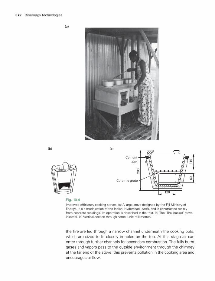
372 Bioenergy technologies
CementAsh
280
120
6011
0Ceramic grate
(b)
(a)
(c)
Fig. 10.4Improved efficiency cooking stoves. (a) A large stove designed by the Fiji Ministry of Energy. It is a modification of the Indian (Hyderabad) chula, and is constructed mainly from concrete moldings. Its operation is described in the text. (b) The ‘Thai bucket’ stove (sketch). (c) Vertical section through same (unit: millimetres).
the fire are led through a narrow channel underneath the cooking pots, which are sized to fit closely in holes on the top. At this stage air can enter through further channels for secondary combustion. The fully burnt gases and vapors pass to the outside environment through the chimney at the far end of the stove; this prevents pollution in the cooking area and encourages airflow.
CementAsh
280
12060
110
Ceramic grate
(b)
(a)
(c)
TWIDELL PAGINATION.indb 372 01/12/2014 11:37
§10.3 Direct combustion for heat 373
The stove shown in Fig. 10.4(b) is simpler and cheaper, but has less control and less flexibility. Nevertheless, its small mass means that it is transportable and little heat is used in heating the stove as distinct from the pot, which is an advantage for quick cooking. Air reaches the fuel from below, through a grate. Since the fire is contained, and the heat is chan-neled towards the pot, the efficiency is high. This stove is well suited for use with charcoal as a fuel, since charcoal burns cleanly without smoke.
§10.3.2 Space and water heating
For comfort (space) heat in buildings, as with cooking stoves, it is import-ant for the stove or central-heating boiler to have a controlled fire with good secondary combustion. Efficiency is improved if air for combus-tion is introduced directly to the combustion chamber from outside the building, which decreases internal draughts and heat loss. Sophisticated and efficient wood-burners for heating are in widespread use, especially in some wood-rich industrialized countries (e.g. Norway, Canada and New Zealand). If the useful heat is the heat delivered beneficially, then enclosed stoves and boilers with controlled primary and secondary com-bustion can be 80 to 90% efficient.
Some countries (e.g. in Northern Europe) encourage markets in (i) fuel-wood chips (machine-cut palm-sized wood); and (ii) pellets ( compressed sawdust from timber yards). Although the main market for these products may be for co-firing with coal in power stations (§10.3.4), they are used for space heat and hot water in individual buildings. For the latter, there are specially designed sophisticated stoves with automatic input of fuel, which are easy to use, have excellent fuel efficiency and are clean with minimum pollution.
§10.3.3 Crop drying
The drying of crops (e.g. fruit, copra, cocoa, coffee, tea), for storage and subsequent sale, is commonly accomplished by burning wood and the crop residues, or by using the waste heat from electricity generation. The material to be dried may be placed directly in the flue exhaust gases, but there is a danger of fire and contamination of food products. More com-monly, air is heated in a gas/air heat exchanger before passing through the crop. Drying theory is discussed in §4.3.
Combustion of harvest residues for crop drying is a rational use of biofuel, since the fuel is close to where it is needed. Combustion in an efficient furnace yields a stream of hot, clean exhaust gas (CO2 + H2O + excess air) at about 1000°C, which can be diluted with cold air to the required temperature. If the amount of biomass residue exceeds that required for crop drying, the excess may be used for other purposes, such as producing industrial steam.
TWIDELL PAGINATION.indb 373 01/12/2014 11:37
374 Bioenergy technologies
§10.3.4 Process-heat and electricity
Steam process-heat is commonly obtained for factories by burning wood or other biomass residues in boilers, perhaps operating with fluidized beds. It is physically sensible to use the steam first to generate electric-ity before the heat degrades to a lower useful temperature. The effi-ciency of electricity generation from the biomass may be only about 20 to 25% due to low temperature combustion, so 75 to 80% of the energy remains as process-heat and a useful final temperature is maintained. Frequently the optimum operation of such processes treats electricity as a by- product of process-heat generation, with excess electricity being sold to the local electricity supply agency, as in modern sugar cane mills (Figs 9.11 and 9.12).
A relatively easy way to use energy crops and biomass residues is co-firing in coal-burning power stations. The combustion method is adapted for the known mixture of coal and biomass. Having a uniform fuel gives the most reliable operation, so densified products such as wood pellets are favored. Torrefaction (controlled low temperature pyrolysis to produce char) of the mixed biomass before combustion improves the final combustion in the boilers. In recent years, a substantial international trade in wood pellets (>10 PJ/y) has arisen, notably from Russia and Canada into Western Europe. Such substitution (abatement) of coal is a realistic policy for biomass to reduce greenhouse gas emissions in the short term, despite the intrinsic efficiency of all such power stations without combined heat and power being only about 35%.
§10.4 PYROLYSIS (DESTRUCTIVE DISTILLATION)
Pyrolysis is a general term for all processes whereby organic material is heated or partially combusted with minimal air to produce secondary fuels and chemical products. The input may be wood, biomass residues, municipal waste, or, indeed, coal. The products are gases, condensed vapors as liquids, tars and oils, and solid residue as char (charcoal) and ash. Traditional charcoal making is pyrolysis at relatively low temperature with the vapors and gases not collected; the modern equivalent is torre-faction, but with the effluent gases being burnt for heating the process. Gasification is pyrolysis adapted to produce a maximum amount of sec-ondary fuel gases.
Various pyrolysis units are shown in Fig. 10.5. Vertical top-loading devices are usually considered to be the best. The fuel products are more convenient, clean and transportable than the original biomass. The chemical products are important as chemical feedstock for further processes, or as directly marketable goods. Partial combustion devices, which are designed to maximize the amount of combustible gas rather than char or volatiles, are usually called gasifiers. The process is essen-tially pyrolysis, but may not be described as such.
TWIDELL PAGINATION.indb 374 01/12/2014 11:37
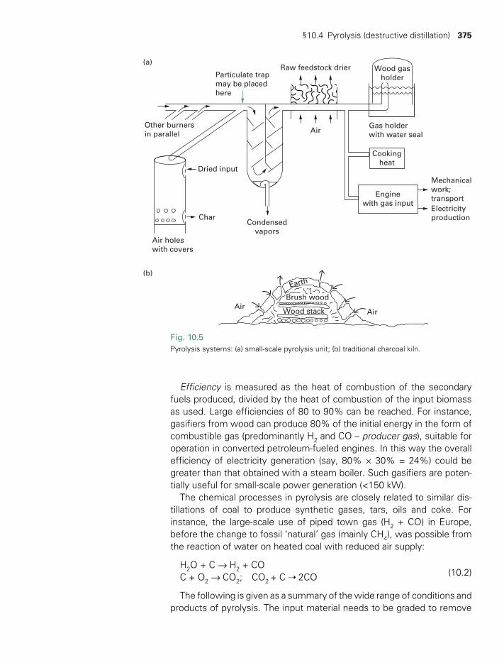
§10.4 Pyrolysis (destructive distillation) 375
Efficiency is measured as the heat of combustion of the secondary fuels produced, divided by the heat of combustion of the input biomass as used. Large efficiencies of 80 to 90% can be reached. For instance, gasifiers from wood can produce 80% of the initial energy in the form of combustible gas (predominantly H2 and CO – producer gas), suitable for operation in converted petroleum-fueled engines. In this way the overall efficiency of electricity generation (say, 80% × 30% = 24%) could be greater than that obtained with a steam boiler. Such gasifiers are poten-tially useful for small-scale power generation (<150 kW).
The chemical processes in pyrolysis are closely related to similar dis-tillations of coal to produce synthetic gases, tars, oils and coke. For instance, the large-scale use of piped town gas (H2 + CO) in Europe, before the change to fossil ‘natural’ gas (mainly CH4), was possible from the reaction of water on heated coal with reduced air supply:
H2O + C → H2 + CO (10.2)C + O2 → CO2; CO2 + C 2CO
The following is given as a summary of the wide range of conditions and products of pyrolysis. The input material needs to be graded to remove
Particulate trapmay be placedhere
Other burnersin parallel
(a)
(b)
Dried input
Char
Air holeswith covers
Condensedvapors
AirAir
Brush wood
Wood stack
Earth
Raw feedstock drier
Gas holderwith water seal
Mechanicalwork;transportElectricityproduction
Air
Wood gasholder
Cookingheat
Enginewith gas input
Fig. 10.5 Pyrolysis systems: (a) small-scale pyrolysis unit; (b) traditional charcoal kiln.
TWIDELL PAGINATION.indb 375 01/12/2014 11:37
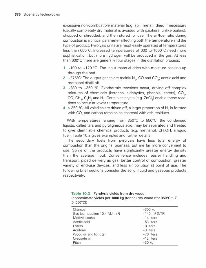
376 Bioenergy technologies
excessive non-combustible material (e.g. soil, metal), dried if necessary (usually completely dry material is avoided with gasifiers, unlike boilers), chopped or shredded, and then stored for use. The air/fuel ratio during combustion is a critical parameter affecting both the temperature and the type of product. Pyrolysis units are most easily operated at temperatures less than 600°C. Increased temperatures of 600 to 1000°C need more sophistication, but more hydrogen will be produced in the gas. At less than 600°C there are generally four stages in the distillation process:
1 ~100 to ~120 °C: The input material dries with moisture passing up through the bed.
2 ~275°C: The output gases are mainly N2, CO and CO2; acetic acid and methanol distill off.
3 ~280 to ~350 °C: Exothermic reactions occur, driving off complex mixtures of chemicals (ketones, aldehydes, phenols, esters), CO2, CO, CH4, C2H6 and H2. Certain catalysts (e.g. ZnCl2) enable these reac-tions to occur at lower temperature.
4 > 350 °C: All volatiles are driven off, a larger proportion of H2 is formed with CO, and carbon remains as charcoal with ash residues.
With temperatures ranging from 350°C to 550°C, the condensed liquids, called tars and pyroligneous acid, may be separated and treated to give identifiable chemical products (e.g. methanol, CH3OH, a liquid fuel). Table 10.2 gives examples and further details.
The secondary fuels from pyrolysis have less total energy of combustion than the original biomass, but are far more convenient to use. Some of the products have significantly greater energy density than the average input. Convenience includes: easier handling and transport, piped delivery as gas, better control of combustion, greater variety of end-use devices, and less air pollution at point of use. The following brief sections consider the solid, liquid and gaseous products respectively.
Table 10.2 Pyrolysis yields from dry wood (approximate yields per 1000 kg (tonne) dry wood (for 350°C < ~ T < ~ 550°C))
Charcoal ~300 kgGas (combustion 10.4 MJ m–3) ~140 m3 (NTP)Methyl alcohol ~14 litersAcetic acid ~53 litersEsters ~8 litersAcetone ~3 litersWood oil and light tar ~76 litersCreosote oil ~12 litersPitch ~30 kg
TWIDELL PAGINATION.indb 376 01/12/2014 11:37
§10.4 Pyrolysis (destructive distillation) 377
§10.4.1 Solid charcoal (mass yield 25 to 35% maximum)
Modern charcoal retorts operating at about 600°C produce 25 to 35% of the dry matter biomass as charcoal. Traditional earthen kilns usually give yields closer to 10%, since there is less control. Charcoal is 75 to 85% carbon, unless great care is taken to improve quality (as for chemical grade charcoal), and the heat of combustion is about 30 MJ/kg. Thus if charcoal alone is produced from wood, between 15 and 50% of the origi-nal chemical energy of combustion remains. Charcoal is useful as a clean controllable fuel. Chemical grade charcoal has many uses in laboratory and industrial chemical processes. Charcoal is superior to coal products for making high quality steel.
§10.4.2 Torrefaction
This is a form of pyrolysis at reduced temperature ~200°C to ~320°C, with the effluent gases being used for the heating. The product is a dry, non-rotting solid char, sometimes called ‘bio-coal’, that subsequently can be burnt efficiently with minimal pollution. ‘Bio-coal’ is very suitable for co-firing with fossil coal in boilers, etc., since it reduces proportionally the unwanted emissions from fossil coal, including fossil carbon dioxide. Typically the product retains 80% of the mass and 90% of the heating value of the original biomass. Its characteristics can be improved further by densification. Controlled torrefaction is a relatively new process, which is increasing into widespread use.
§10.4.3 Liquids (condensed vapors, mass yield ~30% maximum)
These divide between (1) a sticky phenolic tar (creosote), and (2) an aqueous liquid, pyroligneous acid, of mainly acetic acid, methanol (maximum 2%) and acetone. The liquids may be either separated or used together as a crude, potentially polluting and carcinogenic, fuel with a heat of combustion of about 22 MJ/kg. The maximum yield corresponds to about 400 liters of combustible liquid per tonne of dry biomass. The liquids are better used as a source of chemicals, but this requires rela-tively large-scale and sophisticated operation.
§10.4.4 Gases (mass yield ~80% maximum in gasifiers)
The mixed gas output with nitrogen is known as wood gas, synthesis gas, producer gas or water gas, and has a heat of combustion in air of 5 to 10 MJ/kg (4 to 8 MJ/m3 at STP). It may be used directly in diesel cycle or spark ignition engines with adjustment of the fuel injector or carburettor, but extreme care has to be taken to avoid intake of ash and condensable vapors. The gas is mainly N2, H2 and CO, with perhaps
TWIDELL PAGINATION.indb 377 01/12/2014 11:37
378 Bioenergy technologies
small amounts of CH4 and CO2. The gas may be stored in gasholders near atmospheric pressure, but is not conveniently compressed. A much cleaner and more uniform gas may be obtained by gasification of wet charcoal rather than wood, since the majority of the tars from the original wood have already been removed.
The Fischer-Tropsch process is a general term for a wide variety of methods that convert CO and H2, the main gases of synthesis gas (pro-ducer gas), into oil suitable for vehicle fuel. Often coal has been the starter material used to generate the initial producer gas, but biomass can also be the starter material. There have been many large-scale industrial establishments using variations of the process in several countries over the past 100 years, but none have widespread international replication.
§10.5 FURTHER THERMOCHEMICAL PROCESSES
In the previous sections, biomass has been used directly after preliminary sorting and cutting for combustion or pyrolysis. However, the biomass may be treated chemically: (1) to produce material suitable for alcoholic fermentation (§10.6); or, (2) to produce secondary or improved fuels.
Consider the following few important examples from the great number of possibilities.
§10.5.1 Hydrogen reduction
Dispersed, shredded or digested biomass (e.g. manure) is heated in hydrogen to about 600°C under pressure of about 50 atmospheres. Combustible gases, mostly methane and ethane, are produced that may be burnt to give about 6 MJ per kg of initial dry material.
§10.5.2 Hydrogenation with CO and steam
The process is as above, but heating is within an enclosure with CO and steam to about 400°C and 50 atmospheres. A synthetic oil is extracted from the resulting products that may be used as a fuel. A catalyst is needed to produce reactions of the following form:
CO + H2O → CO2 + H2 (10.3)Cn (H2O)n + (n + 1)H2 → nH2O + H(CH2)nH
where the latter reaction implies the conversion of carbohydrate material to hydrocarbon oils. The energy conversion efficiency is about 65%.
§10.5.3 Acid and enzyme hydrolysis
Cellulose is the major constituent (30 to 50%) of plant dry biomass and is very resistant to hydrolysis, and hence fermentation by
TWIDELL PAGINATION.indb 378 01/12/2014 11:37
§10.6 Alcoholic fermentation 379
micro- organisms (§10.6). Conversion to sugars, which can be fermented, is possible by heating in sulphuric acid or by the action of enzymes (cel-lulases) of certain micro-organisms (§10.6). The products may also be used as cattle feed.
§10.5.4 Methanol liquid fuel
Methanol, a toxic liquid, is made from the catalytic reaction of H2 and CO2 at 330°C and at 150 atmospheric pressure:
2H2 + CO → CH3OH (10.4)
The input gases are components of synthesis gas (§10.4.4), and may be obtained from gasification of biomass. Methanol may be used as a liquid fuel in petroleum spark-ignition engines with an energy density of 23 MJ/kg. It is also used as an ‘anti-knock’ fuel additive to enhance the octane rating, and is potentially a major fuel for fuel cells (§15.8).
§10.5.5 Hydrothermal liquefaction: HTL
HTL is a thermochemical process that seeks to imitate, at greatly increased speed, the processes that turned biomass into fossil fuels over geological periods within the crust of the Earth. Processes require heating the biomass, such as manures, sewage and crops, with water and possibly catalysis to temperatures ~300°C and pressures ~20 to ~50 MPa. At these conditions the chemical properties of water favor the biomass breaking down into oils and residues. The chemistry is varied and complex, and commercial viability for the oil products to compete generally with conventional biofuels already in the market has not occurred. See Zhang (2010) for further details.
§10.6 ALCOHOLIC FERMENTATION
§10.6.1 Alcohol production methods
Ethanol, C2H5OH, is produced naturally by certain micro-organisms from sugars under acidic conditions, pH 4 to 5. This alcoholic fermenta-tion process is used worldwide to produce alcoholic drinks. The most common micro-organism, the yeast Saccharomyces cerevisiae, is poi-soned by C2H5OH concentration greater than 10%, and so stronger concentrations up to 95% are produced by distilling and fractionating (Fig. 10.6). When distilled, the remaining constant boiling-point mixture is 95% ethanol, 5% water. Anhydrous ethanol is produced commer-cially with azeotropic removal of water by an extra process such as co-distillation with solvents such as benzene or (more recently) the use of ‘molecular sieves’ (Mousdale 2010). Only about 0.5% of the
TWIDELL PAGINATION.indb 379 01/12/2014 11:37
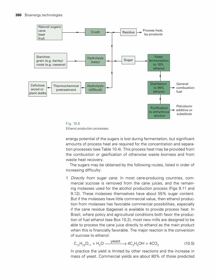
380 Bioenergy technologies
energy potential of the sugars is lost during fermentation, but significant amounts of process heat are required for the concentration and separa-tion processes (see Table 10.4). This process heat may be provided from the combustion or gasification of otherwise waste biomass and from waste heat recovery.
The sugars may be obtained by the following routes, listed in order of increasing difficulty:
1 Directly from sugar cane. In most cane-producing countries, com-mercial sucrose is removed from the cane juices, and the remain-ing molasses used for the alcohol production process (Figs 9.11 and 9.12). These molasses themselves have about 55% sugar content. But if the molasses have little commercial value, then ethanol produc-tion from molasses has favorable commercial possibilities, especially if the cane residue (bagasse) is available to provide process heat. In Brazil, where policy and agricultural conditions both favor the produc-tion of fuel ethanol (see Box 10.2), most new mills are designed to be able to process the cane juice directly to ethanol as the main product when this is financially favorable. The major reaction is the conversion of sucrose to ethanol:
C12H22O11 + H2O yeast 4C2H5OH + 4CO2 (10.5)
In practice the yield is limited by other reactions and the increase in mass of yeast. Commercial yields are about 80% of those predicted
Process heat, by-products
Natural sugars:canebeetfruit
Starches:grain (e.g. barley)roots (e.g. cassava)
Cellulosewood or
plant stalks
Crush Residue
Hydrolysis(easy)
Sugar
Thermochemicalpretreatment
Hydrolysis(difficult)
Yeast fermentation
to 10% ethanol
Distillation to 95%ethanol
Generalcombustionfuel
Petroleumadditive orsubstitute
Purification to anhydrous
alcohol
Fig. 10.6 Ethanol production processes.
TWIDELL PAGINATION.indb 380 01/12/2014 11:37
§10.6 Alcoholic fermentation 381
by (10.5). The fermentation reactions for other sugars (e.g. glucose, C6H12O6) are very similar.
2 Sugar beet is a mid-latitude root crop for obtaining major supplies of sugar. The sugar can be fermented, but obtaining process heat from the crop residues is, in practice, not as straightforward as with cane sugar, so ethanol production is more expensive.
3 Starch crops (e.g. grain and cassava) can be hydrolyzed to sugars. Starch is the main energy storage carbohydrate of plants, and is composed of two large molecular weight components: amylose and amylopectin. These relatively large molecules are essentially linear, but have branched chains of glucose molecules linked by distinctive carbon bonds. These links can be broken by enzymes from malts associated with specific crops (e.g. barley or corn), or by enzymes from certain molds (fungi). Such methods are common in whisky dis-tilleries, corn syrup manufacture, and ethanol production from cassava roots. The links can also be broken by acid treatment at pH 1.5 and 2 atmospheres pressure, but yields are small and the process more expensive than enzyme alternatives. An important by-product of the enzyme process is the residue used for cattle feed or soil conditioning.
All of the above processes are based on centuries-old technology and use feedstock that could also be food; their product is often called ‘first generation’ bioethanol.
4 Cellulose comprises about 40% of all biomass dry matter, including the crop residues remaining after the grains, juices and fruit have been removed. Previously we have noted its important use as a combustion fuel, but it also has the potential to be a major material for ethanol pro-duction. Such use would avoid the ‘fuel versus food’ issues discussed in §10.10 that limit benefits from processes (1) to (3) above. Ethanol from cellulose is therefore often called ‘second generation’ bioetha-nol. Cellulose (molecular weight ~500,000) has a polymer structure of linked glucose molecules, and forms the main mechanical-structure component of the woody parts of plants. These links are considerably more resistant to break down into sugars under hydrolysis than the equivalent links in starch. In plants, cellulose is found in close associa-tion with 15 to 25% by mass of lignin, a polymer which is even harder to break down than cellulose – thus these woody feedstocks (includ-ing grasses and stalks) are collectively called ‘ligno-cellulose’.
Mousdale (2010) gives a comprehensive review of the state of the art of this route to ethanol. Acid hydrolysis is possible as with starch, but the process is expensive and energy intensive. Hydrolysis is less expensive, and less energy input is needed if enzymes of natural wood-rotting fungi are used, but the process is uneconomically slow. However, biotech-nologically optimized enzymes give quicker results. For woody mate-rial, the initial physical breakdown is a difficult and expensive stage,
TWIDELL PAGINATION.indb 381 01/12/2014 11:37

382 Bioenergy technologies
requiring much electricity for the rolling and hammering machines. Consequently some prototype commercial processes have used as input: (i) pulped wood or old newspaper; (ii) corn stover (residue stalks and leaves of maize) and various grasses, which are more easily shred-ded and collected than wood. For all substrates, thermochemical pre-treatment of the lignocellulose increases processing rates (e.g. acidic or alkaline steaming at ~200°C for 10 to 60 minutes), which weakens the physical structure, so increasing the surface area available to the enzymes.
Substantial R&D in the USA and Scandinavia from the 1990s onwards has led to processes with improved yields and potentially cheaper pro-duction, key features of which are acid-catalyzed hydrolysis of hemicel-lulose, more effective enzymes to break down cellulose, and genetically engineered bacteria that ferment all biomass sugars (including 5-carbon sugars which resist standard yeasts) to ethanol with high yields. There are a few prototype plants that produce ethanol from lignocellulose, but in general more development funding is needed to progress to large-scale operation.
§10.6.2 Ethanol fuel use
Liquid fuels are of great importance because of their ease of handling and controllable combustion in engines. Azeotropic ethanol (i.e. the con-stant boiling-point mixture with 4.4% water) is a liquid between –114°C and +78°C, with a flashpoint of 9°C and a self-ignition (auto-ignition) tem-perature of 423°C; therefore it has the characteristics for a commercial liquid fuel, being used as a direct substitute or additive for petrol (gaso-line). It is used in three ways:
1 as azeotropic ethanol, used directly in modified and in purpose-built spark-ignition engines;
2 mixed as a solution with the fossil petroleum to produce gasohol; used at small ~5% concentrations in unmodified spark-ignition engines, and at larger concentrations in ‘flexi-car’ and specially tuned engines;
3 as an emulsion with diesel fuel for diesel compression engines (this may be called diesohol, but is not common).
Fuel containing bioethanol 2 has the proportion of ethanol indicated as EX, where X is the percentage of ethanol (e.g. E10 has 10% ethanol and 90% fossil petroleum). Gasohol for unmodified engines is usually between E10 and E15; larger proportions of ethanol require moder-ate engine modification as ‘flexi-cars’. (Note that water does not mix with petrol, and so water is often present as an undissolved sludge in the bottom of petroleum vehicle fuel tanks without causing difficulty; if gasohol is added to such a tank, the water dissolves in the ethanol fraction and the fuel may become unsuitable for an unmodified engine.)
TWIDELL PAGINATION.indb 382 01/12/2014 11:37
§10.6 Alcoholic fermentation 383
Gasohol, with ethanol mostly from sugar cane, is now standard in Brazil (see Box 10.2) and in countries of Southern Africa. It is mandated, initially as E5, in Europe and also in the USA where the ethanol is predominantly from corn (maize) grain.
The ethanol additive has anti-knock properties and is preferable to the more common tetraethyl lead, which produces serious air pollution. The excellent combustion properties of ethanol enable a modified engine to produce up to 20% more power with ethanol than previously with petro-leum. The mass density and calorific value of ethanol are both less than those of petroleum, so the energy per unit volume of ethanol (24 GJ/m3) is 40% less than for petroleum (39 GJ/m3) (see Table B.6). However, the better combustion properties of ethanol almost compensate when measured as volume per unit distance (e.g. litre/100 km). Fuel consump-tion by volume in similar cars using petrol, gasohol or pure ethanol is in the ratio 1: 1: 1.2, i.e. pure ethanol is only 20% inferior by these criteria. We note, however, that the custom of measuring liquid fuel consump-tion per unit volume is deceptive, since measurement per unit mass relates better to the enthalpy of the fuel.
Production costs of ethanol fuels depend greatly on local condi-tions, and demand relates to the prices paid for alternative products. Government policy and taxation rates are extremely important in deter-mining the retail price and hence the scale of production (see §10.10 and Box 10.2).
BOX 10.2 ETHANOL IN BRAZIL
The Brazilian ethanol program is the most famous example of large-scale support for and production of biofuels. It was established in the 1970s to reduce the country’s dependence on imported oil and to help stabilize sugar production, and hence employment, in the context of unstable world prices for both sugar and petroleum. The program both increased employment in the sugar industry and generated several hundred thousand new jobs in processing and manufacturing. It led to economies of scale and technological development which reduced the production cost of ethanol from sugar, to the extent that in 2013, the unsubsidized cost of the production of azeotropic bioethanol in Brazil was ~25 USc/L. Consequently, even anhydrous ethanol was cheaper than fossil gasoline for crude oil prices more than ~US$45/bbl. In 2013 crude oil sold for ~US$110/bbl!
The program has evolved over time in response to changing conditions in the international markets for sugar and petroleum, notably the lower prices for fossil fuel in the 1990s. It has used both tax incentives (i.e. reduced taxes on some forms of fuel) and regulation (e.g. requiring refineries to take and market the entire bioethanol production, either as blends (usually E20 to E25) or as azeotropic ethanol), and strongly encouraging the use of ‘flexi-fuel’ vehicles, capable of operating on fuels ranging from E0 to E85, and on azeotropic ethanol. The success of the program has been helped by several local factors: (1) the coexistence of a sugar agro-industry and a national automobile industry, both having the ability for steady technology development; (2) an internal automobile market large enough to sustain new engine regulations, and (3) political willingness to pursue the program and force imported cars to be ‘flexi-fuel’.
TWIDELL PAGINATION.indb 383 01/12/2014 11:37
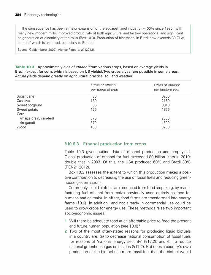
384 Bioenergy technologies
§10.6.3 Ethanol production from crops
Table 10.3 gives outline data of ethanol production and crop yield. Global production of ethanol for fuel exceeded 80 billion liters in 2010: double that in 2003. Of this, the USA produced 60% and Brazil 30% (REN21 2012).
Box 10.3 assesses the extent to which this production makes a posi-tive contribution to decreasing the use of fossil fuels and reducing green-house gas emissions.
Commonly, liquid biofuels are produced from food crops (e.g. by manu-facturing fuel ethanol from maize previously used entirely as food for humans and animals). In effect, food farms are transformed into energy farms (§9.6). In addition, land not already in commercial use could be used to grow crops for energy use. These methods raise two important socio-economic issues:
1 Will there be adequate food at an affordable price to feed the present and future human population (see §9.8)?
2 Two of the most often-stated reasons for producing liquid biofuels in a country are: (a) to decrease national consumption of fossil fuels for reasons of ‘national energy security’ (§17.2); and (b) to reduce national greenhouse gas emissions (§17.2). But does a country’s own production of the biofuel use more fossil fuel than the biofuel would
The consequence has been a major expansion of the sugar/ethanol industry (~400% since 1980), with many new modern mills, improved productivity of both agricultural and factory operations, and significant co-generation of electricity at the mills (Box 10.3). Production of bioethanol in Brazil now exceeds 30 GL/y, some of which is exported, especially to Europe.
Source: Goldemberg (2007); Alonso-Pippo et al. (2013).
Table 10.3 Approximate yields of ethanol from various crops, based on average yields in Brazil (except for corn, which is based on US yields). Two crops a year are possible in some areas. Actual yields depend greatly on agricultural practice, soil and weather.
Litres of ethanolper tonne of crop
Litres of ethanolper hectare year
Sugar cane 86 6200Cassava 180 2160Sweet sorghum 86 3010Sweet potato 125 1875Corn (maize grain, rain-fed) 370 2300 (irrigated) 370 4600Wood 160 3200
TWIDELL PAGINATION.indb 384 01/12/2014 11:37
§10.6 Alcoholic fermentation 385
displace? And does it in fact reduce the nation’s GHG emissions? Boxes 10.3 and 10.4 consider these questions empirically.3
Table 10.4 highlights the crucial importance for bioenergy systems of using low-cost biomass residues for process heat and electricity produc-tion. New processes are entering commercial use that produce bioetha-nol from cellulosic inputs, such as corn stalks (‘stover’), specially grown plants (e.g. miscanthus), and forest residues (see §10.6.1). Since these products all use biomass residues for process energy, as defined in Box 10.3, their fossil fuel energy ratios R and fossil fuel net energy gains G will be much larger than those of corn ethanol produced with the use of fossil fuels. If by-products and the use of the biofuel are included (e.g. displacing coal-based electricity), then for ethanol from corn stover or from miscanthus, R becomes extremely large and G2 exceeds the enthalpy of ethanol (Wang et al. 2011). One lesson to learn from such analyses on commercial products is that the whole system has to be carefully defined and scrutinized to assess their environmental impact, carbon footprint and sustainability, etc.
BOX 10.3 BIO/FOSSIL ENERGY BALANCE OF LIQUID BIOFUELS
Inputs considered are traded energy used in agricultural machines, drying, processing, transport, manufacture of equipment and fertilizers, etc. As with the established discipline of Energy Analysis (which defines terms differently), we do not consider solar energy as an input. The analysis here is restricted to biofuels produced entirely within the specific country and used entirely to replace (abate) fossil fuels – which is close to reality for both Brazilian cane ethanol and for corn ethanol in the USA. We use two parameters as indicators for the specific nation:
• The national bio/fossil energy ratio R (= energy content (enthalpy) of fuel output divided by the fossil fuel input used to produce it).
• The national bio/fossil net energy gain G (= the enthalpy of the fuel output minus the enthalpy of the fossil fuel input used to produce it).
If no fossil fuel is used, then R equals infinity and G equals the enthalpy (taken to be the heat of combustion) of the biofuel. The aim for sustainability is that both R and G should be as large as possible.
If G is negative, so R <1, the contribution of the biofuel as a replacement for fossil fuels in that country is negative. Two variants of R and G appear in the literature, designated in Table 10.4 as R1 and G1 and as R2 and G2. R1 considers only the enthalpy of the liquid biofuel as the output, while R2 includes also the enthalpy in some co-products as an output.
Because calculating R involves the energy used in prior processes (e.g. fertilizer manufacture), energy balance calculations relate to life cycle analysis (§17.4). As an example, Table 10.4 summarizes published calculations for the production of fuel ethanol from sugar cane in Brazil and from corn (maize) in the USA.
Although both indicate a positive net energy gain, that for sugar cane is much larger. The main reason is that sugar cane milling uses zero fossil fuel (row (6)), since the process heat and electricity are from the combustion of residue cane stalks (bagasse) (see Figs 9.11 and 9.12). In modern sugar mills, as in Brazil, the cogeneration process produces not just the process heat and electricity for the mill itself, but also a
TWIDELL PAGINATION.indb 385 01/12/2014 11:37
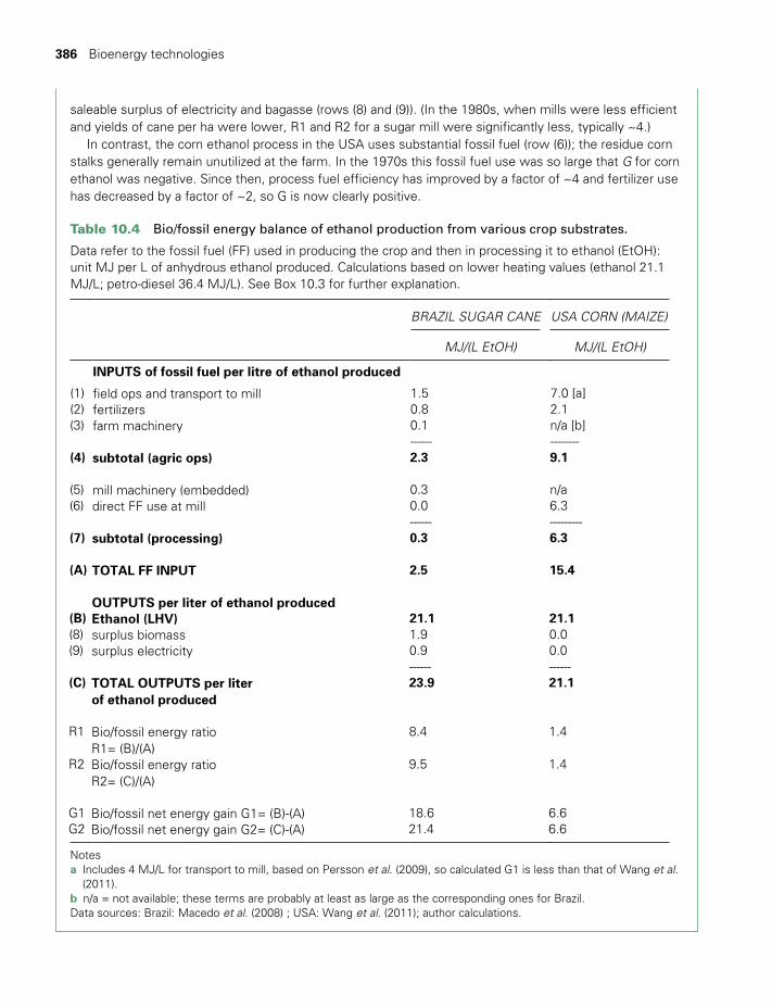
386 Bioenergy technologies
Table 10.4 Bio/fossil energy balance of ethanol production from various crop substrates.
Data refer to the fossil fuel (FF) used in producing the crop and then in processing it to ethanol (EtOH): unit MJ per L of anhydrous ethanol produced. Calculations based on lower heating values (ethanol 21.1 MJ/L; petro-diesel 36.4 MJ/L). See Box 10.3 for further explanation.
BRAZIL SUGAR CANE USA CORN (MAIZE)
MJ/(L EtOH) MJ/(L EtOH)
INPUTS of fossil fuel per litre of ethanol produced
(1) field ops and transport to mill 1.5 7.0 [a](2) fertilizers 0.8 2.1(3) farm machinery 0.1 n/a [b]
------ -------- (4) subtotal (agric ops) 2.3 9.1
(5) mill machinery (embedded) 0.3 n/a(6) direct FF use at mill 0.0 6.3
------ ---------(7) subtotal (processing) 0.3 6.3
(A) TOTAL FF INPUT 2.5 15.4
OUTPUTS per liter of ethanol produced(B) Ethanol (LHV) 21.1 21.1(8) surplus biomass 1.9 0.0(9) surplus electricity 0.9 0.0
------ ------(C) TOTAL OUTPUTS per liter
of ethanol produced23.9 21.1
R1 Bio/fossil energy ratio R1= (B)/(A)
8.4 1.4
R2 Bio/fossil energy ratio R2= (C)/(A)
9.5 1.4
G1 Bio/fossil net energy gain G1= (B)-(A) 18.6 6.6G2 Bio/fossil net energy gain G2= (C)-(A) 21.4 6.6
Notesa Includes 4 MJ/L for transport to mill, based on Persson et al. (2009), so calculated G1 is less than that of Wang et al.
(2011). b n/a = not available; these terms are probably at least as large as the corresponding ones for Brazil. Data sources: Brazil: Macedo et al. (2008) ; USA: Wang et al. (2011); author calculations.
saleable surplus of electricity and bagasse (rows (8) and (9)). (In the 1980s, when mills were less efficient and yields of cane per ha were lower, R1 and R2 for a sugar mill were significantly less, typically ~4.)
In contrast, the corn ethanol process in the USA uses substantial fossil fuel (row (6)); the residue corn stalks generally remain unutilized at the farm. In the 1970s this fossil fuel use was so large that G for corn ethanol was negative. Since then, process fuel efficiency has improved by a factor of ~4 and fertilizer use has decreased by a factor of ~2, so G is now clearly positive.
TWIDELL PAGINATION.indb 386 01/12/2014 11:37
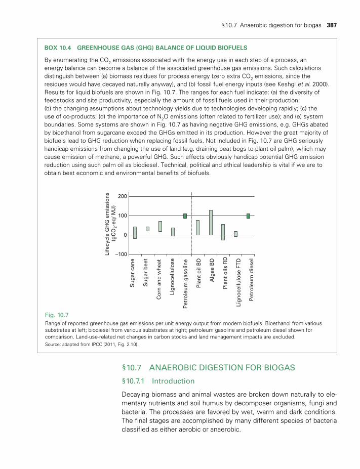
§10.7 Anaerobic digestion for biogas 387
BOX 10.4 GREENHOUSE GAS (GHG) BALANCE OF LIQUID BIOFUELS
By enumerating the CO2 emissions associated with the energy use in each step of a process, an energy balance can become a balance of the associated greenhouse gas emissions. Such calculations distinguish between (a) biomass residues for process energy (zero extra CO2 emissions, since the residues would have decayed naturally anyway), and (b) fossil fuel energy inputs (see Keshgi et al. 2000). Results for liquid biofuels are shown in Fig. 10.7. The ranges for each fuel indicate: (a) the diversity of feedstocks and site productivity, especially the amount of fossil fuels used in their production; (b) the changing assumptions about technology yields due to technologies developing rapidly; (c) the use of co-products; (d) the importance of N2O emissions (often related to fertilizer use); and (e) system boundaries. Some systems are shown in Fig. 10.7 as having negative GHG emissions, e.g. GHGs abated by bioethanol from sugarcane exceed the GHGs emitted in its production. However the great majority of biofuels lead to GHG reduction when replacing fossil fuels. Not included in Fig. 10.7 are GHG seriously handicap emissions from changing the use of land (e.g. draining peat bogs to plant oil palm), which may cause emission of methane, a powerful GHG. Such effects obviously handicap potential GHG emission reduction using such palm oil as biodiesel. Technical, political and ethical leadership is vital if we are to obtain best economic and environmental benefits of biofuels.
Life
cycl
e G
HG
em
issi
on
s (g
CO
2-eq
/ MJ)
Lig
no
cellu
lose
FT
D
Pet
role
um
die
sel
Su
gar
can
e
Su
gar
bee
t
Co
rn a
nd
wh
eat
Lig
no
cellu
lose
Pet
role
um
gas
olin
e
Pla
nt
oil
BD
Alg
ae B
D
Pla
nt
oils
RD
200
100
–100
0
Fig. 10.7 Range of reported greenhouse gas emissions per unit energy output from modern biofuels. Bioethanol from various substrates at left; biodiesel from various substrates at right; petroleum gasoline and petroleum diesel shown for comparison. Land-use-related net changes in carbon stocks and land management impacts are excluded. Source: adapted from IPCC (2011, Fig. 2.10).
§10.7 ANAEROBIC DIGESTION FOR BIOGAS
§10.7.1 Introduction
Decaying biomass and animal wastes are broken down naturally to ele-mentary nutrients and soil humus by decomposer organisms, fungi and bacteria. The processes are favored by wet, warm and dark conditions. The final stages are accomplished by many different species of bacteria classified as either aerobic or anaerobic.
TWIDELL PAGINATION.indb 387 01/12/2014 11:37
388 Bioenergy technologies
Aerobic bacteria are favored in the presence of oxygen with the biomass carbon being fully oxidized to CO2. This composting process releases some heat slowly and locally, but is not a useful process for energy supply. To be aerobic, air has to permeate, so a loose ‘heap’ of biomass is essential. Domestic composting is greatly helped by including layers of rumpled newspaper and cardboard, which allows air pockets and introduces beneficial carbon from the carbohydrate material. Such aerobic digestion has minimal emission of methane, CH4, which, per additional molecule, is about eight times more potent as a greenhouse gas than CO2 (see §2.9).
In closed conditions, with no oxygen available from the environment, anaerobic bacteria exist by breaking down carbohydrate material. The carbon may be ultimately divided between fully oxidized CO2 and fully reduced CH4 (see Fig. 9.6). Nutrients such as soluble nitrogen com-pounds remain available in solution, so providing excellent fertilizer and humus. Being accomplished by micro-organisms, the reactions are all classed as fermentations, but in anaerobic conditions the term ‘diges-tion’ is preferred.
It should be emphasized that both aerobic and anaerobic decom-position are fundamental processes of natural ecology that affect all biomass irrespective of human involvement. As with all other forms of renewable energy, we are able to interface with the natural process and channel energy and resources for our economy. The decomposed waste should then be released for natural ecological processes to continue.
Biogas is the CH4/CO2 gaseous mix evolved from anaerobic digesters, including waste and sewage pits; to utilize this gas, the digesters are constructed and controlled to favor methane production and extraction from liquid slurries (Fig. 10.8). The energy available from the combustion of biogas is between 60% and 90% of the dry-matter heat of combustion of the input material. However, the gas is obtainable from slurries of up to 95% water, so in practice the biogas energy is often available where none would otherwise have been obtained. Another benefit is that the digested effluent forms significantly less of a health hazard than the input material. However, not all parasites and pathogens are destroyed in the digestion. For the intensive animal enclosures of ‘industrial agriculture’, the opportunity to treat waste feces and effluents to make them environmentally acceptable and the need to avoid penal-ties for pollution are major incentives to incorporate anaerobic digesters and to utilize the biogas.
The economics and general benefits of biogas are always most favora-ble when the digester is placed in a flow of waste material already present. Examples are sewage systems, piggery washings, cattle shed slurries, abattoir wastes, food-processing residues, sewage and munici-pal refuse landfill dumps. The economic benefits are that input material
TWIDELL PAGINATION.indb 388 01/12/2014 11:37

§10.7 Anaerobic digestion for biogas 389
does not have to be specially collected, administrative supervision is already present, waste disposal is improved, and uses are likely to be available for the biogas and nutrient-rich effluent. However, in high and middle latitudes, tank digesters have to be heated for fast digestion (especially in the winter); usually such heat would come from burning the output gas, hence reducing net yield significantly. Slow digestion does not require such heating. Obviously obtaining biogas from, say, urban landfill waste is a different engineering task than from cattle slur-ries. Nevertheless, the biochemistry is similar. Most of the following refers to tank digesters, but the same principles apply to other biogas systems.
Biogas generation is suitable for small- to large-scale operation. By 2013, several million household-scale systems had been installed in developing countries, especially in China (>40 million) and India (>4 million), with the gas used for cooking and lighting. Rural systems in India mostly use cow dung as input, but ~1 million systems are ‘urban’, fed mainly on kitchen waste (see e.g. §10.7.4). Successful long-term operation requires: (a) trained maintenance and repair technicians; (b) the users to perceive benefits; (c) alternative fuels (e.g. kerosene and bottle gas), not to be subsidised, and (d) a sustainable source of organic input and of water. Unfortunately many biogas systems have failed because one or more of these factors was missing.
Most biogas systems in industrialized countries operate at intensive livestock farms (Fig. 10.8(d)), at large breweries and similar crop-using industries, at urban sewage plants and as part of municipal landfills (‘rubbish tips’). Biogas from these sites may be injected for sale into gas-grid distribution networks (either directly as mixed CH4/ CO2, or as only CH4, having removed the CO2, e.g. by bubbling through water). More usually, however, the biogas becomes the fuel for spark-ignition engines generating electricity for both on-site use and for export to a utility grid network. In Europe especially, such systems may operate as combined heat and power (CHP), especially if close to towns where the heat can be used for district heating (§15.3.3). Germany has significant generation capacity from biogas (>5000 systems with a total electricity-generating capacity ~2300 MW),
Biogas systems on farms are a step towards ‘integrated farming’, which emulate a full ecological cycle on the single farm. The best exam-ples are where plant and animal wastes are anaerobically digested to biogas and the digested effluent passes for aerobic digestion in open tanks before dispersal. The biogas may be (a) used directly for domestic and process heat, for export to a utility gas main, and possibly for light-ing, or (b) as fuel for engines and electricity generators, with perhaps export to a utility grid. Algae may be grown on the open-air tanks and removed for cattle feed. From the aerobic digestion, the treated effluent passes through reed beds, perhaps then to fish tanks and duck ponds
TWIDELL PAGINATION.indb 389 01/12/2014 11:37

390 Bioenergy technologies
before finally being passed to the fields as fertilizer. The success of such schemes depends on a favorable site, integrated design, good standards of construction, and the enthusiasm and commitment of the operator, not least for the regular maintenance required.
§10.7.2 Basic processes and energetics
The general equation for anaerobic digestion in the input of slurry is:
CxHyOz + (x − y/4 − z/2)H2O (10.6)
→ (x/2 − y/8 + z/4)CO2 + (x/2 + y/8 − z/4)CH4
For cellulose, this becomes:
(C6H10O5)n + nH2O → 3nCO2 + 3nCH4 (10.7)
Some organic material (e.g. lignin) and all inorganic inclusions are not digested in the process. These add to the bulk of the material, form a scum and can easily clog the system. In general, 95% of the mass of the material is water.
The reactions are slightly exothermic, with typical heats of reaction being about 1.5 MJ per kg dry digestible material, equal to about 250 kJ per mole of C6H10O5. This is not sufficient to significantly affect the tem-perature of the bulk material, but does indicate that most enthalpy of reaction is passed to the product gas.
If the input material of the slurry had been dried and burnt, the heat of combustion would have been about 16 MJ/kg. In complete anaerobic digestion only about 10% of the potential heat of combustion is lost in the digestion process, so giving 90% conversion efficiency to biogas. Moreover, very wet input is processed to give this convenient and con-trollable gaseous fuel, whereas drying the aqueous slurry would have required much energy (about 40 MJ/kg of solid input). In practice, diges-tion seldom goes to completion because of the long time involved, so 60% conversion is common. Gas yield is about 0.2 to 0.4 m3 per kg of dry digestible input at STP, with throughput of about 5 kg dry digestible solid per m3 of liquid.
It is generally considered that three ranges of temperature favor par-ticular types of bacteria. Digestion at higher temperature proceeds more rapidly than at lower temperature, with gas yield rates doubling at about every 5°C of increase. The temperature ranges are: (a) psicrophilic, about 20°C; (b) mesophilic, about 35°C, and (c) thermophilic, about 55°C. In tropical countries, unheated digesters are likely to be at average ground temperature between 20 and 30°C. Consequently the digestion is psicro-philic, with retention times being at least 14 days. In colder climates, the psicrophilic process is significantly slower, so it may be decided to heat the digesters, probably by using part of the biogas output; a temperature
TWIDELL PAGINATION.indb 390 01/12/2014 11:37
§10.7 Anaerobic digestion for biogas 391
of about 35°C is likely to be chosen for mesophilic digestion. Few digest-ers operate at 55°C unless the purpose is to digest material rather than produce excess biogas. In general, the greater the temperature, the faster the process time.
The biochemical processes occur in three stages, each facilitated by distinct sets of anaerobic bacteria:
1 Insoluble biodegradable materials (e.g. cellulose, polysaccharides and fats) are broken down to soluble carbohydrates and fatty acids (hydro-genesis). This occurs in about a day at 25°C in an active digester.
2 Acid-forming bacteria produce mainly acetic and propionic acid (acido-genesis). This stage likewise takes about one day at 25°C.
3 Methane-forming bacteria slowly, in about 14 days at 25°C, complete the digestion to a maximum ~70% CH4 and minimum ~30% CO2 with trace amounts of H2 and perhaps H2S (methanogenesis). H2 may play an essential role, and indeed some bacteria (e.g. Clostridium) are distinctive in producing H2 as the final product.
The methane-forming bacteria are sensitive to pH, and conditions should be mildly acidic (pH 6.6 to 7.0) but not more acidic than pH 6.2. Nitrogen should be present at 10% by mass of dry input, and phospho-rus at 2%. A golden rule for successful digester operation is to maintain constant conditions of temperature and suitable input material; conse-quently a suitable population of bacteria becomes established to suit these conditions.
§10.7.3 Digester sizing
The energy available from a biogas digester is given by:
E = ηHbVb (10.8)
where η is the combustion efficiency of burners, boilers, etc. (~60%). Hb is the heat of combustion per unit volume biogas (20 MJm–3 at 10 cm water gauge pressure, 0.01 atmosphere) and Vb is the volume of biogas. Note that some of the heat of combustion of the methane goes to heating the CO2 present in the biogas, and is therefore unavailable for other purposes, so decreasing the efficiency.
An alternative analysis is:
E = ηHmfmVb (10.9)
where Hm is the heat of combustion of methane (56 MJ/kg, 28 MJ/m3 at STP) and fm is the fraction of methane in the biogas. For biogas directly from the digester, fm should be between 0.5 and 0.7, but it is not difficult to pass the gas through a counterflow of water to dissolve the CO2 and increase fm to nearly 1.0.
TWIDELL PAGINATION.indb 391 01/12/2014 11:37
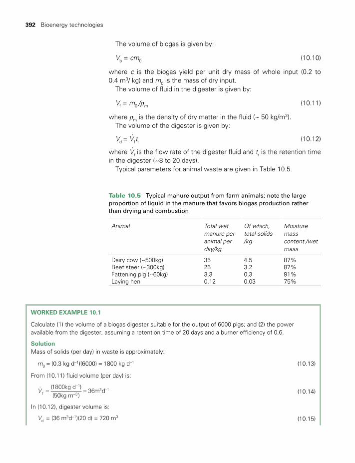
392 Bioenergy technologies
The volume of biogas is given by:
Vb = cm0 (10.10)
where c is the biogas yield per unit dry mass of whole input (0.2 to 0.4 m3/ kg) and m0 is the mass of dry input.
The volume of fluid in the digester is given by:
Vf = m0 /rm (10.11)
where rm is the density of dry matter in the fluid (~ 50 kg/m3).The volume of the digester is given by:
Vd = V.
ftr (10.12)
where V.f is the flow rate of the digester fluid and tr is the retention time
in the digester (~8 to 20 days).Typical parameters for animal waste are given in Table 10.5.
Table 10.5 Typical manure output from farm animals; note the large proportion of liquid in the manure that favors biogas production rather than drying and combustion
Animal Total wet manure per animal per day/kg
Of which, total solids /kg
Moisture mass content /wet mass
Dairy cow (~500kg) 35 4.5 87%Beef steer (~300kg) 25 3.2 87%Fattening pig (~60kg) 3.3 0.3 91%Laying hen 0.12 0.03 75%
WORKED EXAMPLE 10.1
Calculate (1) the volume of a biogas digester suitable for the output of 6000 pigs; and (2) the power available from the digester, assuming a retention time of 20 days and a burner efficiency of 0.6.
SolutionMass of solids (per day) in waste is approximately:
m0 = (0.3 kg d−1)(6000) = 1800 kg d−1 (10.13)
From (10.11) fluid volume (per day) is:
= = −−
−V. (1800kg d )
(50kg m )36m df
1
33 1 (10.14)
In (10.12), digester volume is:
−V = (36 m d )(20 d) = 720 md3 1 3 (10.15)
TWIDELL PAGINATION.indb 392 01/12/2014 11:37

§10.7 Anaerobic digestion for biogas 393
From (10.10), volume of biogas is:
V = (0.24 m kg )(1800 kg d ) = 430m db3 1 1 3 1− − − (10.16)
So, from (10.8), energy output is:− −
− −E = (0.6)(20 MJ m )(430 m d )
= 5200 MJ d = 1400 kWh d= 60 kW (continuous, thermal)
3 3 1
1 1 (10.17)
If continuously converted to electricity, this would yield about 20 kWe of electricity from a biogas-fired generator set at 25% overall efficiency.
§10.7.4 Working digesters
Fig. 10.8 shows a range of biogas digesters from the elementary to the sophisticated, allowing principles to be explained.
a Rural household digester (Figs 10.8(a) and 10.8(b)). This is a recom-mended design in the Republic of China for households and village communes, where several million have been installed; similar designs are now common in India and Nepal. The main input is usually pig dung in China and cow dung in India. The main feature of the design is the concrete cap which enables pressurized gas to be obtained, although part of the cap is removable for maintenance. This top is much cheaper than the heavy metal floating gasholder of older Indian systems. The flow moves slowly through the buried brick tank in about 14 to 30 days to the outlet, from which nutrient-rich fertilizer is obtained. As the gas evolves, its volume replaces digester fluid and the pressure increases. Frequent (~daily) inspection of pipes, etc. and
Materialinlet
(a)Gaspipe Removable cover
Outlet
Separatingwall
Anaerobicdigestion
Gas storage tank
(b)
Fig. 10.8Biogas digesters.a Chinese ‘dome’ for small-scale use. Diluted dung flows underground to the digester, which also holds the biogas at
moderate pressure (adapted from Van Buren (1979)).b Photo of similar in use in rural India; the ‘dome’ is just visible behind the flowers to the right of the inlet (author photo).
TWIDELL PAGINATION.indb 393 01/12/2014 11:37
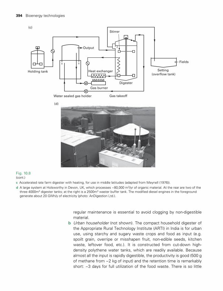
394 Bioenergy technologies
Holding tank
(c)Stirrer
Output
Heat exchanger
Gas burner
Digester
Gas takeoff
Fields
Setting (overflow tank)
Water sealed gas holder(d)
Fig. 10.8 (cont.)c Accelerated rate farm digester with heating, for use in middle latitudes (adapted from Meynell (1976)).d A large system at Holsworthy in Devon, UK, which processes ~80,000 m3/yr of organic material. At the rear are two of the
three 4000m3 digester tanks; at the right is a 2500m3 waster buffer tank. The modified diesel engines in the foreground generate about 20 GWh/y of electricity (photo: AnDigestion Ltd.).
regular maintenance is essential to avoid clogging by non-digestible material.
b Urban householder (not shown). The compact household digester of the Appropriate Rural Technology Institute (ARTI) in India is for urban use, using starchy and sugary waste crops and food as input (e.g. spoilt grain, overripe or misshapen fruit, non-edible seeds, kitchen waste, leftover food, etc.). It is constructed from cut-down high-density polythene water tanks, which are readily available. Because almost all the input is rapidly digestible, the productivity is good (500 g of methane from ~2 kg of input) and the retention time is remarkably short: ~3 days for full utilization of the food waste. There is so little
(d)
TWIDELL PAGINATION.indb 394 01/12/2014 11:37
§10.8 Wastes and residues 395
residue that ARTI recommend simply mixing it with the next batch of input to maintain the culture of anaerobic bacteria.
c Industrial design (Fig 10.8(c)). The diagram shows a design for com-mercial operation in mid-latitudes for accelerated digestion under fully controlled conditions. The digester tank is usually heated to at least 35°C. The main purpose of such a system is often the treatment of the otherwise unacceptable waste material, with biogas being an additional benefit.
d Case study (Fig 10.8(d)). The photograph shows the centralized anaerobic digestion power station at Holsworthy in Devon, UK. Three 4000m3 digesters (of which only two are shown in the photo) can process 80,000m3 per year of organic material. The incoming waste stream is heated by heat exchange with the outgoing residue and with the ‘waste’ heat of the engines used for electricity generation. The plant has 3.9 MW of installed generating capacity. The amount of electricity being generated at any one time depends on the quantity and nature of the feedstocks being supplied to the plant. Typically, the plant produces ~1700 MWh of electricity per month, of which 10% is used in the plant operation and 90% is sold to the local grid. The feed-stocks for the plant come from various local sources, including dairy farms, industrial bakeries and food processors, abattoirs, fish proces-sors, cheese producers, biodiesel manufacturers and councils. After pasteurization and digestion, the sludge is returned to local farms as a bio-fertilizer for use on both arable and grassland.
§10.8 WASTES AND RESIDUES
Wastes and residues from human activity and economic production are a form of ‘indirect’ renewable energy, since they are unstoppable flows of energy potential in our environment. Wastes and residues arise from: (a) primary economic activity (e.g. forestry, timber mills, harvested crops, abattoirs, food processing); and (b) urban, municipal and domestic refuse, including sewage. The energy generation potential from such wastes is primarily from the biomass content. However, there is usually a significant proportion of combustible waste from mineral sources (e.g. most plastics); however, such combustion requires regulation to reduce unacceptable emissions. A key factor regarding wastes and refuse is that they are usually available at points of concentration, where they easily become an environmental hazard. Dealing with this ‘problem’ becomes a necessity. The wastes operator will therefore be paid for the material and so be subsidized in later energy production.
Major wastes are: (a) municipal solid waste (MSW); (b) landfill; (c) sewage. MSW is the wastes removed by municipal authorities from domestic and industrial sources; it usually contains significant amounts of metal, glass and plastic (i.e. non-biomass) material. Recycling of most
TWIDELL PAGINATION.indb 395 01/12/2014 11:37

396 Bioenergy technologies
plastics, metal, glass and other materials should occur before landfill or combustion. Nevertheless, non-biomass materials usually remain in significant amounts. MSW is loose, solid material of variable composi-tion, available directly for combustion or pyrolysis. If the composition is acceptable, it may be pressurized and extruded as ‘refuse-derived fuel, RDF’, usually available as dried pellets of about 5 cm dimension for com-bustion in domestic-scale boilers.
‘Landfill’ is waste, usually municipal solid waste (MSW), deposited in large pits. A large proportion of municipal solid waste (MSW) is biological material that, once enclosed in landfill, decays anaerobically to biogas, emitted as a mix of CH4 and CO2, often contaminated with air (O2 and especially N2), usually called ‘landfill gas’. The process is slower than in most biogas digesters, because of the reduced ground temperature, but when stabilized after many months, the gas composition is similar (see §10.7). If not collected, the gas leaks slowly into the Atmosphere, along with various smellier gases such as H2S, so causing unpleasant environ-mental pollution and being potentially explosive. Regulations in several countries require capture of at least 40% of the methane from landfill, in order to reduce greenhouse gas emissions and hazard. Therefore, the landfill site is constructed carefully to prevent ground contamination and after filling is capped (e.g. with clay) so that the gas may be collected (e.g. by an array of perforated pipes laid horizontally as the landfill is com-pleted or drilled vertically into the buried refuse of an existing site). Apart from wastefully flaring the gas to avoid accidents, there are three ways to use landfill gas: (a) in a gas turbine or modified spark-ignition engine to generate on-site electricity and sell the excess; (b) sold directly to a nearby industrial facility for direct combustion in boilers for process heat and/or in engines for electricity generation; (c) injected and sold into a utility gas supply, probably after bubbling through water to remove CO2.
With limited land for landfills and increasing sorting and recycling of waste, many municipalities motivate and assist households to place food waste and garden plant waste in labeled bins that are collected for turning into garden and horticultural compost by chopping and then aerobic digestion (Fig.10.2).
Energy production globally from waste incineration and landfill gas exceeds 1.5 EJ/y globally and is often a significant proportion of national commercial renewable energy.
§10.9 BIODIESEL FROM VEGETABLE OILS AND ALGAE
§10.9.1 Raw vegetable oils
Vegetable oils are extracted from biomass on a substantial scale for use in soap-making, other chemical processes and, in more refined form, for cooking.
TWIDELL PAGINATION.indb 396 01/12/2014 11:37
§10.9 Biodiesel from vegetable oils and algae 397
Categories of suitable materials are as follows:
1 Seeds (e.g. sunflower, rape, jatropha, soya beans).2 Nuts (e.g. oil palm, coconut copra); ~50% of dry mass of oil (e.g. the
Philippines’ annual production of coconut oil is ~1.5 million t/y). 3 Fruits (e.g. world olive production ~3 Mt/y).4 Leaves (e.g. eucalyptus).5 Tapped exudates (e.g. rubber latex, jojoba (Simmondsia chinensis)
tree oil).6 By-products of harvested biomass, for instance, oils and solvents to
15% of the plant dry mass (e.g. turpentine, oleoresins from pine trees, oil from Euphorbia).
§10.9.2 Biodiesel (esters)
Concentrated vegetable oils may be used directly as fuel in diesel engines, but difficulties arise from the high viscosity and from the combustion deposits, as compared with conventional (fossil) petroleum-based diesel oil, especially at low ambient temperature (≤ 5°C).
Both difficulties are considerably eased by reacting the extracted veg-etable oil with ethanol or methanol to form the equivalent ester. Such esters, called biodiesel, have technical characteristics as fuels that are better suited to diesel engines than petroleum-based diesel oil. The reac-tion yields the equivalent ester and glycerine (also called glycerol). The process usually uses KOH as a catalyst. The glycerol is also a useful and saleable product.
The esterification process is straightforward for those with basic chem-ical knowledge, and, with due regard for safety, can be undertaken as a small batch process. Continuous commercial production obviously needs more sophistication, and uses whatever oil is most readily and cheaply available in the country concerned (e.g. rapeseed oil in Europe (called ‘canola’ in some other countries) and soya oil in USA). Biodiesel can also be made from waste (used) cooking oil and from animal fat (tallow). Thus Argentina, with its large livestock industry, has become a substantial exporter of biodiesel (>1 GL/y). The use of waste cooking oil as the raw material is attractive in both environmental and cost terms, especially on a small scale; the cost of collection is an issue on a larger scale.
When some governments removed institutional barriers to the pro-duction and sale of biodiesel, world commerce grew dramatically from near-zero in 1995 to over 20 GL/y by 2011, two-thirds of which was produced in the EU, which has RE targets and a supportive institutional framework. The fuel is sold either as 100% biodiesel or blended with petroleum-based diesel. Although the production cost of biodiesel sub-stantially exceeds that of conventional diesel fossil fuel, such govern-ments justified the policy in terms of the ‘external’ benefits for the environment (e.g. absence of sulfur emissions, abating fossil carbon).
TWIDELL PAGINATION.indb 397 01/12/2014 11:37
398 Bioenergy technologies
Similar considerations apply to many other biofuels, notably bioethanol (see §10.6 and §10.10).
The energy density of biodiesel as an ester varies with composition and is typically about 38 MJ/kg, which is greater than for the raw oil and near to petroleum-based diesel fuel at about 46 MJ/kg. Nevertheless, in practice, fuel consumption per unit volume of a diesel-engine vehicle running on biodiesel is little different from that on fossil diesel. Quality standards have been established for the compatibility of biodiesel with most vehicles. A minor benefit of using biodiesel is that the exhaust smell is reminiscent of cooking (e.g. of popcorn).
Energy balance calculations for biodiesel produced from soya oil and methanol in the general US economy indicate that the production of 1 MJ of the fuel may use about 0.3 MJ of fossil fuel input. The produc-tion of methanol from (fossil) natural gas accounts for nearly half of the 0.3 MJ, so the analysis would be even more favorable if the methanol (or ethanol) came from biomass, see Table 10.4 and Box 10.4.
§10.9.3 Microalgae as source of biofuel
Growing energy crops should not reduce necessary food crops, espe-cially on a global scale. One strategy is to utilize microalgae grown in water; single cellular photosynthetic plants from ~10–6 m to ~10–4 m in diameter. They grow rapidly, generally doubling numbers within 24 hours, and some species contain oils, as do larger plants. Oil content ranges from 15 to 75% (dry weight); consequently potential annual oil production from oil-rich microalgae is 50,000 to 150,000 L/ha, which is ~10 times more per unit area than from vegetable sources. Commercial growth is usually in open ponds at 20°C to 30°C, with input of sunlight, CO2 and nutrients (N, P, and minerals). Biodiesel from algae is some-times referred to as a ‘second generation’ biofuel.
Producing biodiesel from microalgae is a proven process, but expen-sive, being ~10 times more than crude palm oil (probably the cheapest vegetable oil) or fossil-petro-diesel (Cheng and Timilsina 2011). In open ponds, the oil-bearing microalgae become contaminated by local algae and bacteria, so transparent enclosures are needed. These and other challenges drive the considerable R&D for a commercial product.
§10.10 SOCIAL AND ENVIRONMENTAL ASPECTS
§10.10.1 Internal and external costs of biofuels for transport
The cost of producing bioethanol and biodiesel is generally more expensive than extracting and refining fossil fuels. However, automo-tive petroleum fuels are usually heavily taxed, with perhaps 70% of the wholesale price being tax. Such taxation raises revenue and discourages unnecessary driving to reduce pollution, road congestion and, usually,
TWIDELL PAGINATION.indb 398 01/12/2014 11:37
§10.10 Social and environmental aspects 399
imports costing foreign exchange. Governments may therefore encour-age the inclusion of biofuels as a percentage of vehicle fuel: (a) with a smaller tax on biofuels than on fossil petroleum, and/or (b) mandate that all transport fuel must contain a certain percentage of biofuel (see Box 10.2 on Brazil’s ethanol program). Of course, such measures are only feasible if motor manufacturers are required to produce biofuel- compatible vehicles, which is technically not difficult. Subsidies awarded to the agricultural producers of biofuels, as with the EU Common Agricultural Policy, are another policy tool.
Environmentally, substituting biofuel for fossil petroleum reduces greenhouse gas emissions, provided the biofuel comes from a suitable process (see Box 10.3). Biofuel combustion under properly controlled conditions is usually more complete than for fossil petroleum so that unhealthy emissions of particulates are less. Moreover, (a) all biofuels have a larger proportion of oxygen and a smaller proportion of sulphur impurities in their chemical composition than fossil petroleum hydro-carbons, so SO2 pollution is negligible; and (b) the biofuel of one plant species tends to have the identical chemical composition, whereas fossil petroleum is a complex mix of different chemicals, so the biofuel com-bustion process can be tuned more efficiently.
§10.10.2 Other chemical impacts of biofuels and biomass combustion
Every country has regulations concerning the permitted and the forbid-den emissions of gases, vapors, liquids and solids. This is a huge and complex subject within environmental studies.
The most vital aspect for the optimum combustion of any fuel is to control temperature and input of oxygen, usually as air. The aim with biomass and biofuel combustion, as with all fuels, is to have emissions with minimum particulates (unburnt and partially burnt material), with fully oxidized carbon to CO2 and not CO or CH4, and with minimum con-centration of nitrogen oxides (usually resulting from excessive air tem-perature). Therefore, in practice, the combustion should be confined to a relatively small space at almost white-hot temperature; this volume has to be fed with air and fresh fuel. In addition, only fully burnt ash should remain (at best a fine powder that moves almost as a liquid). Useful heat is extracted by radiation from the combustion and by conduction from the flue gases through a heat exchanger, usually to water. Combustion of biofuels in engines, including turbines, has similar basic requirements, but occurs with much greater sophistication. Such combustion is pos-sible according to different circumstances, for example:
• With firewood: position the wood so that the fire is contained within two or three burning surfaces (e.g. at the tips of three logs (the classic
TWIDELL PAGINATION.indb 399 01/12/2014 11:37

400 Bioenergy technologies
‘three-stone fire’), or in the lengthwise space between three parallel logs.
• With wood chips or pellets: feed the fuel by conveyor or slope from a hopper to a relatively small combustion zone, onto which compressed air is blown and from which the ash falls.
• With general timber and forest waste: feed the fuel as above, but probably with a moving or shaking grate.
• With liquid and gaseous biofuels, the combustion should be controlled in boilers and engines as with liquid and gaseous fossil fuels, but with different air flow and fuel-/air-mixing requirements.
Combustion of contaminated biomass (e.g. when mixed with plastics, etc., in municipal solid waste) or under less controlled conditions (most notably cooking over an open fire in a confined space) has considerable adverse environmental impact, unless great care is taken.
Over a million deaths per year of women and children in develop-ing countries have been attributed to kitchen smoke, ‘the killer in the kitchen’. Improving domestic air quality is a major motivation for the improved cooking stoves described in §10.3.1.
On an industrial scale, particulates may be removed by improved com-bustion, filters, cyclones and flue condensation, which also recovers the latent heat of the condensate and increases efficiency. Nitrogen oxides, NOx formation may be alleviated by controlling combustion temperature. Straw from cereal crops may contain relatively large concentrations of potassium and chlorine, which can cause corrosion in boiler grates; this may be reduced by installing rotating grates to prevent a solid mass of ash forming. Nevertheless, the ash from the complete combustion of any biomass is always a valued fertilizer, especially for the phosphate content.
Although the natural carbon cycle of plant growth fully renews the carbon in a crop or plantation, there may be a net loss of nitrogen and possibly other nutrients when the biomass is burnt or otherwise pro-cessed. That is, nitrogen is not returned sufficiently to the soil ‘automati-cally’ and has to be put back as a chemical input, possibly in the form of manure or by rotation with nitrogen-fixing crops, such as beans, clover or leucaena.
Finally, we extol the benefits of composting waste biomass: (a) nutri-ents and soil conditioners return to the soil; (b) carbon is added to the soil rather than being immediately emitted as CO2 (compost is a ‘carbon sink’); or (c) artificial fertilizers become unnecessary.
§10.10.3 Future global bioenergy
Biomass is a major part of the world energy system now, especially in rural areas for cooking and heating. This dependency will increase for a more sustainable global energy system, involving widely distributed
TWIDELL PAGINATION.indb 400 01/12/2014 11:37
§10.10 Social and environmental aspects 401
and versatile resources, but used ever more efficiently and in more modern ways. Already ~35% of the ~53 EJ/y of bioenergy used glob-ally is for modern energy uses (REN21 2012). By 2050, global biomass energy use may be 500 EJ/y (Chum et al. in IPCC 2011). However, as discussed in §9.8, this requires not only the technologies described in this chapter but also sustainability and policy frameworks that ensure good governance of land use, improvements in forestry, agriculture and livestock management, and above all, sufficient food supply.
CHAPTER SUMMARY
Biomass is plant material, including animal wastes and residues. Biomass now provides about 13% of mankind’s energy consumption, of which about two-thirds is the use of wood fuel in developing countries for cooking and lighting. Biofuels are biomass processed into a more convenient form, particularly liquid fuels for transport. The term bioenergy covers both biomass and biofuels, relating to Chapter 9 (photosynthesis and biomass resource potential) and Chapter 10 (the technologies to produce and use biofuels).
Important general principles for bioenergy include the following:
• Use of co-products and residues for energy or other purposes (e.g. fertilizer, composting). • Biofuel production is most likely to be economic if the production process uses materials already
concentrated, probably as a by-product and so available at low cost or as extra income for the treatment and removal of waste.
• Biofuels are organic materials, so there is always the alternative of using these materials as chemical feedstock or structural materials.
• The use of sustainable bioenergy in place of fossil fuels abates the emission of fossil carbon dioxide and so reduces the forcing of climate change.
• The main dangers of extensive biomass fuel use are deforestation, soil erosion and the displacement of food crops by fuel crops.
• Poorly controlled biomass processing or combustion can certainly produce unwanted pollution (e.g. from open fires for cooking, ‘the killer in the kitchen’).
The main bioenergy processes and products are as follows:
• Direct combustion for heat (and often for cogeneration of electricity). • Pyrolysis (heating in a restricted or null air supply) especially to produce useful gases and char.• Anaerobic digestion of biodegradable waste in constructed digesters and landfill to produce biogas (a
mixture of CH4 and CO2), used for cooking and heat, process heat, electricity generation and export of gas into utility mains.
• Fermentation by micro-organisms to produce bioethanol (liquid) vehicle fuel from sugars or starch (first generation, now commercial) or from ligno-cellulose (‘second generation’ from plant stalks, etc.) material.
• Biodiesel (transport fuel) made by esterification of vegetable oils.
Most of these ‘modern’ applications have continued to increase production rapidly over the past 20 years. So, by 2013, production of bioethanol was >80 GL/y and of biodiesel >20 GL/y; there were more than 170 million ‘improved’ wood cooking stoves, 40 million household biogas systems, and 6000 industrial-scale biogas systems worldwide.
TWIDELL PAGINATION.indb 401 01/12/2014 11:37

402 Bioenergy technologies
QUICK QUESTIONS
Note: Answers to these questions are in the text of the relevant section of this chapter, or may be readily inferred from it.
1 Give a chemical explanation of the term ‘biomass’. 2 Explain two differences between carbon in CO2 from burning coal
and from burning biomass. 3 Compare the heat of combustion (MJ/kg) of dry wood and of petro-
leum oil. 4 For a given sample of biomass, which is the larger: its dry-basis or its
wet-basis moisture content? 5 What is a ‘wood pellet’ and how big is it likely to be? 6 Which biofuel is safest for a policeman to drink and why? 7 For cooking, what are the advantages and disadvantages of using a
cooking stove as compared to an open fire? 8 How might you obtain hydrogen from wood? 9 List as many saleable products from a cane sugar mill as you can.10 What is ‘second generation’ bioethanol?11 What is the main benefit of a Brazilian ‘flexi-car’?12 What is ‘national fossil fuel energy ratio’ and why is it important?13 Which biomass energy crops and products are (a) most likely, and
(b) least likely to affect food supplies?14 What benefits may occur if an anaerobic digester is installed at a
cattle farm?15 Name and quantify anaerobic digestion temperature ranges.16 What can happen to landfill gas?17 What is biodiesel and in what ways does it differ from bioethanol?18 Identify two social advantages and two disadvantages of utilizing
biofuels.
PROBLEMS
Note: *indicates a ‘problem’ that is particularly suitable for class discus-sion or group tutorials.
10.1 A farmer with 50 pigs proposed to use biogas generated from their wastes to power the farm’s motor car.
(a) Discuss the feasibility of doing this. You should calculate both the energy content of gas and the energy used in compress-ing the gas to a usable volume, and compare these with the energy required to run the car.
(b) Briefly comment on what other benefits (if any) might be gained by installing a digester.
TWIDELL PAGINATION.indb 402 01/12/2014 11:37
Problems 403
You may assume that a 100 kg pig excretes about 0.5 kg of vola-tile solid (VS) per day (plus 6 kg water), and that 1 kg of VS yields 0.4 m3 of biogas at STP.
10.2 Studies show that the major energy consumption in Fijian villages is wood which is used for cooking over open fires. Typical consumption of wood is 1 kg person–1day–1.
(a) Estimate the heat energy required to boil a 2-liter pot full of water. Assuming this to be the cooking requirement of each person, compare this with the heat content of the wood, and thus estimate the thermal efficiency of the open fire.
(b) How much timber has to be felled each year to cook for a village of 200 people?
Assuming systematic replanting, what area of crop must the village therefore set aside for fuel use if it is not to make a net deforestation? Hint: refer to Table 10.4.
(c) Comment on the realism of the assumptions made, and revise your estimates accordingly.
10.3 (a) A butyl rubber bag of total volume 3.0 m3 is used as a biogas digester. Each day it is fed an input of 0.20 m3 of slurry, of which 4.0 kg is volatile solids, and a corresponding volume of digested slurry is removed. (This input corresponds roughly to the waste from 20 pigs.)
Assuming that a typical reaction in the digestion process is bacteria:
C12H22O11 + H2O → 6CH4 + 6CO2
and that the reaction takes seven days to complete, calculate: (i) the volume of gas; (ii) the heat obtainable by combustion of this gas for each day of operation of the digester; and (iii) how much kerosene would have the same calorific value as one day’s biogas.
(b) The reaction rate in the digester can be nearly doubled by raising the temperature of the slurry from 28°C (ambient) to 35°C. (i) What would be the advantage of doing this? (ii) How much heat per day would be needed to achieve this? (iii) What proportion of this could be contributed by the heat evolved in the digestion reaction?
10.4 (a) Write down a balanced chemical equation for the conversion of sucrose (Cl2H22O11) to ethanol (C2H5OH). Use this to calculate how much ethanol could be produced in theory from one tonne of sugar. What do you think would be a realistic yield?
TWIDELL PAGINATION.indb 403 01/12/2014 11:37

404 Bioenergy technologies
(b) Fiji is a small country in the South Pacific, whose main export crop is sugar. Fiji produces 300,000 t/y of sugar, and imports 300,000 t of fossil petroleum fuel. If all this sugar were con-verted to ethanol, what proportion of petroleum imports could it replace?
10.5 Consider a pile of green wood chips at 60% moisture content (wet basis) and weighing 1 tonne. What is the oven-dry mass of biomass in the pile?
The biomass has a heat of combustion of 16 MJ per oven-dry kg. This is the ‘gross calorific value’ corresponding to the heat output in a reaction of the type:
[CH2O] +O2 → CO2 (gas) + H2O (liq)
The net calorific value (or ‘lower heating value’) is the heat evolved when the final water is gaseous; in practice, this is the maximum thermal energy available for use when biomass is burnt.
(i) The pile is left to dry to 50% moisture content (wet basis), when it looks much the same but has less water in it.
(ii) The pile is left to dry for a few more weeks, and reaches 20% m.c. (w.b.), at which stage it has shrunk a little in volume and greatly in mass.
For each situation calculate the total mass of the pile, the net heat energy available from burning the pile, and its net calorific value per wet kg.
The following questions are particularly suitable for class discussion:
10.6* ‘Powered by biofuels’ is the name of a television program showing your own family group living entirely on biological resources; describe how such a family might live.
10.7* List the five most important reasons for ‘why’ and ‘why not’ com-mercial biomass energy should or should not increase. Discuss these reasons.
NOTES
1 This ‘biological’ carbon has a larger proportion of the isotope 14C than carbon in fossil fuels; this enables iso-topic analysis of air to clarify the proportion of atmospheric CO2 that is from fossil fuels (see Box 2.3).
2 Here, the term ‘bioethanol’ denotes ethanol made by any of the routes (1) to (4) of §10.6.1, but some authors use the term in different senses. Note that much industrial alcohol is made from fossil petroleum.
3 The ‘energy balance’ calculations outlined here may appear similar to those of the ‘energy analysis’ of Leach (1976), Kumar and Twidell (1981) and Twidell and Pinney (1985). However, here we narrow the analysis
TWIDELL PAGINATION.indb 404 01/12/2014 11:37

Bibliography 405
to only fossil fuel inputs, with the biomass growth and biofuel production all within the specific country. Consequently, the analysis is indicative, but still very policy-relevant.
BIBLIOGRAPHY
Overviews
Chum, H.L. and Overend, R.P. (2003) ‘Biomass and bioenergy in the United States’, Advances in Solar Energy, 15, 83–148. Comprehensive review of commercial and near-commercial technologies, and supporting policies and R&D, with emphasis on large and medium scale.
IEA Bioenergy (2009) Bioenergy – A Sustainable and Reliable Energy Source: A review of status and prospects, International Energy Organisation, Paris (available online at http://www.ieabioenergy.com/. Comprehensive review aimed at ‘policy-makers’, so not very detailed technically.
IPCC (2011) (H. Chum, A. Faaij, J. Moreira, G. Berndes, P. Dhamija, H. Dong, B. Gabrielle, A. Goss Eng, W. Lucht, M. Mapako, O. Masera Cerutti, T. McIntyre, T. Minowa, K. Pingoud), ‘Bioenergy’, ch. 2 in O. Edenhofer, R. Pichs-Madruga, Y. Sokona, K. Seyboth, P. Matschoss, S. Kadner, T. Zwickel, P. Eickemeier, G. Hansen, S. Schlömer and C. von Stechow (eds), IPCC Special Report on Renewable Energy Sources and Climate Change Mitigation Cambridge University Press, Cambridge. Recent authoritative review of both biomass resource and full range of bioenergy technologies (available online at http://srren.ipcc-wg3.de/report).
Klass, D.L. (1998) Biomass for Renewable Energy, Heat and Chemicals, Academic Press, London. An extremely comprehensive and reliable text. Based on chemical principles, but aware of all appropriate disciplines, including economics. Uses S.I. units.
Sims, R.E. (2002) The Brilliance of Bioenergy in Business and in Practice, James & James, London. Illuminating text with emphasis on modern industrial production and applications; includes numerous illustrated case studies of power systems, including with biogas.
Resource estimates
See bibliography for Chapter 9.
Direct combustion, especially wood fuel
De Lepeleire, G., Prasad, K.K., Verhaart, P. and Visser, P. (1981) A Woodstove Compendium, Eindhoven University, Holland. Gives principles of wood burning, and technical descriptions of many stoves designed for domestic cooking in developing countries.
Kammen, D.M. (1995) ‘Cookstoves for the developing world’, Scientific American, 273, 64–67.
Wahlund, B., Yan, J. and Westermark, M. (2004) ‘Increasing biomass utilisation in energy systems: a compara-tive study of CO2 reduction and cost for different bioenergy processing options’, Biomass and Bioenergy, 26, 531–544. Focuses on wood in Sweden; concludes that pelletization for coal substitution is best option in that case.
World Bank (2010) Improved Cookstoves and Better Health in Bangladesh: Lessons from household energy and sanitation programs (final report). World Bank, Washington. Reviews many other programs besides those in Bangladesh.
TWIDELL PAGINATION.indb 405 01/12/2014 11:37

406 Bioenergy technologies
Biofuels
Cheng, J.J. and Timilsina, G.R. (2011) ‘Status and barriers of advanced biofuel technologies: a review’, Renewable Energy, 36, 3541–3549. Useful review, especially on lignocellusosic ethanol and algae.
Goldemberg, J. (2007) ‘Ethanol for a sustainable energy future’, Science, 315: 808–810.
Keshgi H.S., Prince, R.C. and Marland, G. (2000) ‘The potential of biomass fuels in the context of global climate change: focus on transportation fuels’, Annual Review of Energy and the Environment, 25, 199–244. Wide back-ground, plus energy analysis of bioethanol in the USA and Brazil.
Marc Londo, et al. (2010) ‘The REFUEL EU road map for biofuels in transport: Application of the project’s tools to some short-term policy issues’, Biomass and Bioenergy, 34, 244–250.
Mousdale, D. (2010) Introduction to Biofuels, CRC Press, London. Especially good on the biochemistry involved, and the likely costs of various routes.
Wyman, C.E. (1999) ‘Biomass ethanol: technical progress, opportunities, and commercial challenges’, Annual Review of Energy and the Environment, 24, 189–226. Emphasizes potential of new technology to produce ethanol from cellulose, (e.g. ‘waste’ from food crops).
Zhang, Y. (2010) ‘Hydrothermal liquefaction to convert biomass into crude oil’, ch. 10 in Biofuels from Agricultural Wastes and Byproducts, H.P. Blaschek, T. C. Ezeji and J. Scheffran (eds), Blackwell Publishing, Oxford.
Zuubier, P. and van der Vooren, J. (eds) (2008) Sugarcane Ethanol: Contributions to climate change mitigation and the environment, Wageningen Academic Publishers, The Netherlands. Multi-author work, focussing on Brazilian experience.
Biogas
Chynoweth, D.P., Owens, J.M. and Legrand, R. (2001) ‘Renewable methane from anaerobic digestion of biomass’, Renewable Energy, 22, 1–8. Advocates anaerobic digestion as the principal pathway to the use of energy crops.
Meynell, P.J. (1976) Methane – Planning a Digester, Prism Press, Dorchester, UK. An old but still useful short and practical book with basic technical and biochemical explanations.
Muller, C. (2007) Anaerobic Digestion of Biodegradable Solid Waste in Low- and Middle-income Countries, EAWAG aquatic research, Switzerland (available at www.eawag.ch). Reviews systems for household and munic-ipal waste.
Van Buren, A. (1979) A Chinese Biogas Manual, Intermediate Technology Publications, London. A stimulating and useful handbook, based on the considerable experience of small-scale digesters in rural China. Reprinted several times.
Wellinger, A., Murphy, J. and Baxter, D. (eds) (2013) The Biogas Handbook: Science, production and applications, Woodhead Publishing, Cambridge. A serious engineering monograph.
Specific references
Alonso-Pippo, W., Luengo, C.A., Alberteris, L.A.M., del Pino, G.C. and Duvoirsin, S. (2013) ‘Practical implementa-tion of liquid biofuels: the transferability of the Brazilian experiences’, Energy Policy, 60, 70–80.
TWIDELL PAGINATION.indb 406 01/12/2014 11:37

Bibliography 407
Kumar, M. and Twidell, J.W. (1981) ‘Energy analysis of some sugarcane farms in Fiji: considering labour and machine use’, Energy, 6, 139–152.
Leach, G. (1976) Energy and Food Production., IPS Science and Technology Press for the International Institute for Environment and Development, Guildford. Seminal early text on ‘energy analysis’.
Macedo, I.C., Seabra, J.E. and Silva, J.E. (2008) ‘Greenhouse gas emissions in the production and use of ethanol from sugarcane in Brazil: the 2005/2006 averages and a prediction for 2020’, Biomass and Bioenergy, 32, 582–595.
Meynell, P.J. (1976) Methane – Planning a Digester, Prism Press, Dorchester, UK. An old but still useful short and practical book with basic technical and biochemical explanations.
Persson, T., Garcia, A., Paz, J., Jones, J. and Hoogenboom, G. (2009) ‘Net energy value of maize ethanol, as a response to different climate and soil conditions in the southeastern USA’, Biomass and Bioenergy, 33, 1055–1064.
REN21 (2012) Renewables 2012: Global status report, Renewable Energy Policy Network for the 21st century, Paris. Report is updated annually; the latest is at www.ren21.net.
Twidell, J.W. and Pinney, A.A. (1985) ‘The quality and exergy of energy systems, using conventional and renew-able resources’, in L.F. Jesch (ed.), Sun-at-Work in Britain, UK-ISES. Comments on ‘energy analysis’.
Van Buren, A. (1979) A Chinese Biogas Manual, Intermediate Technology Publications, London. A stimulating and useful handbook, based on the considerable experience of small-scale digesters in rural China. Reprinted several times.
Wang, M.Q., Han, J., Haq, Z., Tyner W.E., Wu M. and Elgowainy, A. (2011) ‘Energy and greenhouse gas emis-sion effects of corn and cellulosic ethanol with technology improvements and land use changes’, Biomass and Bioenergy, 35, 1885–1896.
Journals and websites
Biomass and Bioenergy, monthly, Elsevier. Covers a wide range of basic science and applications.
http://journeytoforever.org. A guide to do-it-yourself- biodiesel.
www.biodiesel.org. Basics of biodiesel technology, and lots of links onwards to news and developments; emphasis on the USA.
www.ieabioenergy.com. Reports of international collaborative research on technology and policy.
www.hedon.info. Household Energy Network, with prime focus on developing countries, brings together infor-mation on biogas, wood cooking stoves, and related topics.
www.Ren21.net. Annually reports market data and policy on all forms of renewable energy, including bioenergy.
www.iea/org/statistics/. Energy statistics freely accessible online, for all industrialized countries and most large developing countries, from 1990 to the latest year available.
http://greet.es.anl.gov/main. The GREET model (Greenhouse gases, Regulated Emissions, and Energy use in Transportation) developed and continually updated by Argonne National Laboratory (USA) allows researchers and analysts to evaluate various vehicle and fuel combinations on a full fuel-cycle/vehicle-cycle basis. Model is freely available for download and draws on an extensive database of US agricultural and engineering practice.
TWIDELL PAGINATION.indb 407 01/12/2014 11:37
Wave power
CONTENTS
Learning aims 409
§11.1 Introduction 410
§11.2 Wave motion 413
§11.3 Wave energy and power 417 §11.3.1 Derivation: Energy in
the wave at particular location 417 §11.3.2 Formulae for power extraction
from waves 418
§11.4 Real (irregular) sea waves: patterns and power 421
§11.5 Energy extraction from devices 427 §11.5.1 Classification of devices 427 §11.5.2 Capture width and tuned
energy capture 428
§11.6 Wave power devices 430 §11.6.1 On-shore terminator,
Tapchan, overtopping wave capture 430
§11.6.2 The Wave Dragon: floating overtopping terminator 431
§11.6.3 Oscillating water column (OWC) terminator: first generation on-shore and near shore 432
§11.6.4 Pelamis attenuator, offshore, second and third generation 436
§11.6.5 Summary of operational devices 437
§11.7 Social, economic and environmental aspects 437
Chapter summary 439
Quick questions 440
Problems 440
Notes 442
Bibliography 443
Acknowledgment 444
Box 11.1 Satellite measurement of wave height, etc. 423
Box 11.2 Wave energy in the UK 430
Box 11.3 Basic theory of an OWC device 434
CHAPTER
11
TWIDELL PAGINATION.indb 408 01/12/2014 11:37
List of figures 409
LEARNING AIMS
• Appreciate the large energy fluxes and formi-dable conditions of sea waves.
• Analyze and evaluate wave propagation in terms of wavelength, wave height, frequency and period.
• Be aware of the hydrodynamic characteristics of waves and wave power extraction.
• Know the main classes of wave power devices.
• Appreciate how successful devices absorb wave power from a wider distance than their own width, hence defining the term ‘capture width’.
• Appreciate the development of commer-cial electricity generation from prototype devices.
LIST OF FIGURES
11.1 (a) Maximum wave heights worldwide; (b) Average annual wave energy. 41111.2 Particle motion in water waves. 41311.3 Water surface perpendicular to resultant of gravitational and centrifugal force acting
on an element of water, mass m. 41411.4 Wave characteristics. 41411.5 Resultant forces on surface particles. 41511.6 Accelerations and velocities of a surface water particle. 41511.7 Elemental motion of water in a deep-water wave. 41711.8 Local pressure fluctuations in the wave. 41911.9 Simulated wave-height record. 42211.10 (a) Wave-power map for sea west of Norway from satellite-derived data.
(b) Contours of average wave energy off Northwest Europe. 42411.11 Distribution of power per frequency interval in a typical Atlantic deep-water wave pattern. 42511.12 Illustrative scatter diagram of significant wave height Hs against zero crossing period Tz. 42611.13 Wave device classification by method of capturing wave energy. 42711.14 Schematic diagram of the Tapchan wave energy plant. 43111.15 Wave Dragon floating wave power device. 43311.16 Schematic diagram of an on-shore wave power system using an oscillating water column. 43411.17 Simplistic model of an oscillating water column wave power device. 43511.18 Sketch curve showing power extracted from an oscillating column wave power device
as a function of damping in the air turbine. 43511.19 Pelamis attenuator wave power device. 43611.20 Wells turbine. 44111.21 (a) A hinged flap oscillates as waves impinge on it from the left; (b) a more efficient device
(Salter’s ‘duck’). 442
TWIDELL PAGINATION.indb 409 01/12/2014 11:37
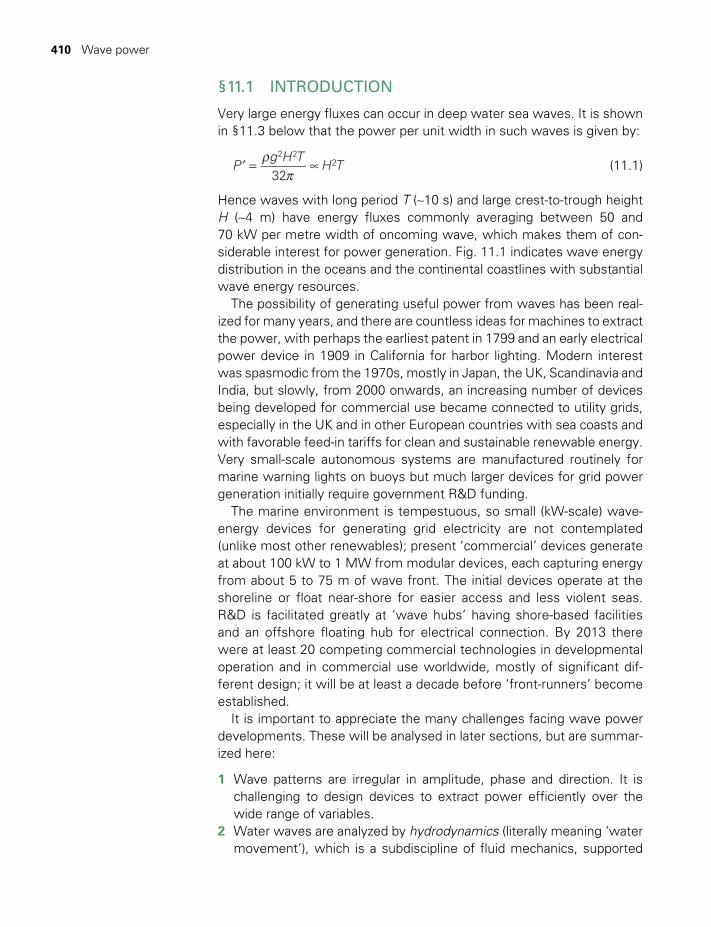
410 Wave power
§11.1 INTRODUCTION
Very large energy fluxes can occur in deep water sea waves. It is shown in §11.3 below that the power per unit width in such waves is given by:
rp
′ = ∝Pg H T
H T32
2 22 (11.1)
Hence waves with long period T (~10 s) and large crest-to-trough height H (~4 m) have energy fluxes commonly averaging between 50 and 70 kW per metre width of oncoming wave, which makes them of con-siderable interest for power generation. Fig. 11.1 indicates wave energy distribution in the oceans and the continental coastlines with substantial wave energy resources.
The possibility of generating useful power from waves has been real-ized for many years, and there are countless ideas for machines to extract the power, with perhaps the earliest patent in 1799 and an early electrical power device in 1909 in California for harbor lighting. Modern interest was spasmodic from the 1970s, mostly in Japan, the UK, Scandinavia and India, but slowly, from 2000 onwards, an increasing number of devices being developed for commercial use became connected to utility grids, especially in the UK and in other European countries with sea coasts and with favorable feed-in tariffs for clean and sustainable renewable energy. Very small-scale autonomous systems are manufactured routinely for marine warning lights on buoys but much larger devices for grid power generation initially require government R&D funding.
The marine environment is tempestuous, so small (kW-scale) wave-energy devices for generating grid electricity are not contemplated (unlike most other renewables); present ‘commercial’ devices generate at about 100 kW to 1 MW from modular devices, each capturing energy from about 5 to 75 m of wave front. The initial devices operate at the shoreline or float near-shore for easier access and less violent seas. R&D is facilitated greatly at ‘wave hubs’ having shore-based facilities and an offshore floating hub for electrical connection. By 2013 there were at least 20 competing commercial technologies in developmental operation and in commercial use worldwide, mostly of significant dif-ferent design; it will be at least a decade before ‘front-runners’ become established.
It is important to appreciate the many challenges facing wave power developments. These will be analysed in later sections, but are summar-ized here:
1 Wave patterns are irregular in amplitude, phase and direction. It is challenging to design devices to extract power efficiently over the wide range of variables.
2 Water waves are analyzed by hydrodynamics (literally meaning ‘water movement’), which is a subdiscipline of fluid mechanics, supported
TWIDELL PAGINATION.indb 410 01/12/2014 11:37
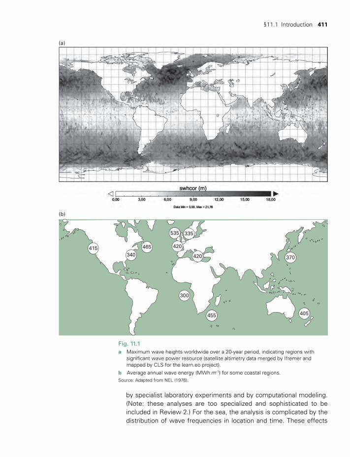
§11.1 Introduction 411
Fig. 11.1a Maximum wave heights worldwide over a 20-year period, indicating regions with
significant wave power resource (satellite altimetry data merged by Ifremer and mapped by CLS for the learn.eo project).
b Average annual wave energy (MWh.m-1) for some coastal regions.Source: Adapted from NEL (1976).
(a)
(b)
535
300
455
370
405
465415340
335
420
420
by specialist laboratory experiments and by computational modeling. (Note: these analyses are too specialized and sophisticated to be included in Review 2.) For the sea, the analysis is complicated by the distribution of wave frequencies in location and time. These effects
TWIDELL PAGINATION.indb 411 01/12/2014 11:37
412 Wave power
are modeled to obtain the dynamic forces on wave-energy devices and structures that must survive for at least 25 years. A key part of the hydrodynamic analysis is the ability of a successful device to pull power into itself from a larger region of sea than its own footprint; a measure of this ability is the device capture width (§11.5).
3 There is always a probability of extreme gales or hurricanes producing waves of freak intensity. The wave-power devices must be able to survive in such conditions. Commonly, the 50-year peak wave is 10 times the height of the average wave. Thus the structures have to survive in seas with ~100 times the power intensity to which they are normally matched. Allowing for this requires sophisticated design and testing, and adds greatly to the initial cost of wave-power systems.
4 Peak power is generally available in deep-water waves from open-sea swells produced from long fetches of prevailing wind (e.g. beyond the Western Islands of Scotland in one of the most tempestuous areas of the North Atlantic and in regions of the Pacific Ocean). The difficulties of constructing power devices for these types of wave regimes, of maintaining and fixing or mooring them in position, and of transmitting power to land, are formidable. Therefore more protected and acces-sible areas near to the shore are used for prototype development and initial commercialization.
5 Wave periods are commonly ~5 to 10 s (frequency ~0.1 Hz). It is chal-lenging to couple this irregular slow motion for electricity generation at ~500 times greater frequency.
6 Many types of device have been suggested for wave-power extrac-tion and so the task of selecting and developing a particular method has been somewhat arbitrary. The dedication and ability of pioneer engineers and financiers are vital to success.
7 The development and application of wave power have occurred with spasmodic and changing government interest, largely without the benefit of market incentives. Wave power needs the same learning curve of steadily enlarging application from small beginnings that has occurred with wind power.
The distinctive advantages of wave power are the large energy fluxes available and the predictability of wave conditions over periods of days ahead. Waves are created by wind, and effectively store the energy for transmission over great distances. For instance, large waves appearing off Europe will have been initiated in stormy weather in the mid-Atlantic or as far away as the Caribbean.
The following sections aim to give a general basis for understanding wave energy devices. First, we outline the theory of deep-water waves and calculate the energy fluxes available in single-frequency waves. Then we review the patterns of sea waves that actually occur. Finally we describe wave-power devices and their commercial development.
TWIDELL PAGINATION.indb 412 01/12/2014 11:37
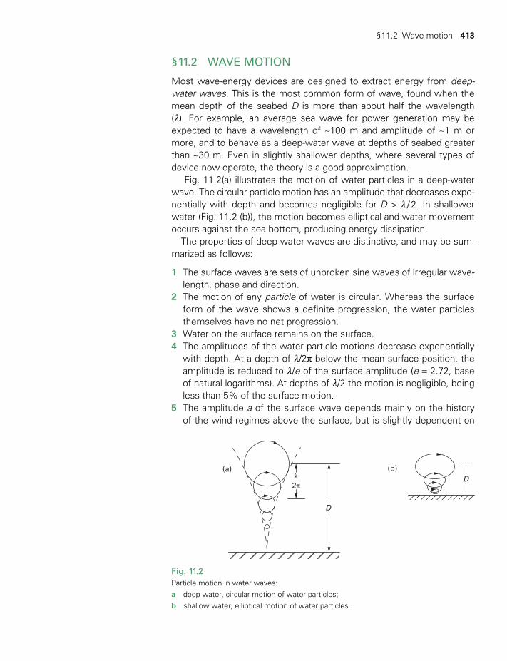
§11.2 Wave motion 413
§11.2 WAVE MOTION
Most wave-energy devices are designed to extract energy from deep-water waves. This is the most common form of wave, found when the mean depth of the seabed D is more than about half the wavelength (l). For example, an average sea wave for power generation may be expected to have a wavelength of ~100 m and amplitude of ~1 m or more, and to behave as a deep-water wave at depths of seabed greater than ~30 m. Even in slightly shallower depths, where several types of device now operate, the theory is a good approximation.
Fig. 11.2(a) illustrates the motion of water particles in a deep-water wave. The circular particle motion has an amplitude that decreases expo-nentially with depth and becomes negligible for D > l / 2. In shallower water (Fig. 11.2 (b)), the motion becomes elliptical and water movement occurs against the sea bottom, producing energy dissipation.
The properties of deep water waves are distinctive, and may be sum-marized as follows:
1 The surface waves are sets of unbroken sine waves of irregular wave-length, phase and direction.
2 The motion of any particle of water is circular. Whereas the surface form of the wave shows a definite progression, the water particles themselves have no net progression.
3 Water on the surface remains on the surface.4 The amplitudes of the water particle motions decrease exponentially
with depth. At a depth of l/2p below the mean surface position, the amplitude is reduced to l/e of the surface amplitude (e = 2.72, base of natural logarithms). At depths of l/2 the motion is negligible, being less than 5% of the surface motion.
5 The amplitude a of the surface wave depends mainly on the history of the wind regimes above the surface, but is slightly dependent on
Fig. 11.2Particle motion in water waves:a deep water, circular motion of water particles; b shallow water, elliptical motion of water particles.
D
(a)
2pl D
(b)
TWIDELL PAGINATION.indb 413 01/12/2014 11:37
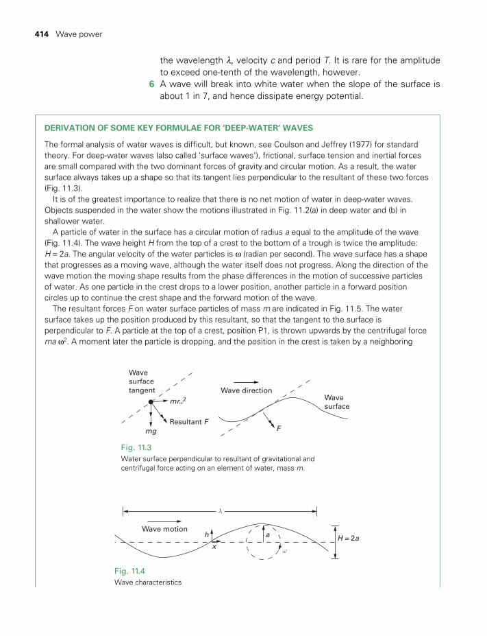
414 Wave power
the wavelength l, velocity c and period T. It is rare for the amplitude to exceed one-tenth of the wavelength, however.
6 A wave will break into white water when the slope of the surface is about 1 in 7, and hence dissipate energy potential.
DERIVATION OF SOME KEY FORMULAE FOR ‘DEEP-WATER’ WAVES
The formal analysis of water waves is difficult, but known, see Coulson and Jeffrey (1977) for standard theory. For deep-water waves (also called ‘surface waves’), frictional, surface tension and inertial forces are small compared with the two dominant forces of gravity and circular motion. As a result, the water surface always takes up a shape so that its tangent lies perpendicular to the resultant of these two forces (Fig. 11.3).
It is of the greatest importance to realize that there is no net motion of water in deep-water waves. Objects suspended in the water show the motions illustrated in Fig. 11.2(a) in deep water and (b) in shallower water.
A particle of water in the surface has a circular motion of radius a equal to the amplitude of the wave (Fig. 11.4). The wave height H from the top of a crest to the bottom of a trough is twice the amplitude: H = 2a. The angular velocity of the water particles is w (radian per second). The wave surface has a shape that progresses as a moving wave, although the water itself does not progress. Along the direction of the wave motion the moving shape results from the phase differences in the motion of successive particles of water. As one particle in the crest drops to a lower position, another particle in a forward position circles up to continue the crest shape and the forward motion of the wave.
The resultant forces F on water surface particles of mass m are indicated in Fig. 11.5. The water surface takes up the position produced by this resultant, so that the tangent to the surface is perpendicular to F. A particle at the top of a crest, position P1, is thrown upwards by the centrifugal force ma w2. A moment later the particle is dropping, and the position in the crest is taken by a neighboring
Fig. 11.3Water surface perpendicular to resultant of gravitational and centrifugal force acting on an element of water, mass m.
Wave directionWavesurface
F
Wavesurfacetangent
Resultant F
mrω2
mg
Fig. 11.4Wave characteristics
Wave motionh
x
a H = 2a
ω
λ
TWIDELL PAGINATION.indb 414 01/12/2014 11:37
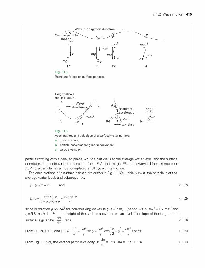
§11.2 Wave motion 415
particle rotating with a delayed phase. At P2 a particle is at the average water level, and the surface orientates perpendicular to the resultant force F. At the trough, P3, the downward force is maximum. At P4 the particle has almost completed a full cycle of its motion.
The accelerations of a surface particle are drawn in Fig. 11.6(b). Initially t = 0, the particle is at the average water level, and subsequently:
φ p w= − t( / 2) and (11.2)
w φw φ
w φ=
+≈s
ag a
ag
tansin
cossin2
2
2
(11.3)
since in practice g >> aw 2 for non-breaking waves (e.g. a = 2 m, T (period) = 8 s, a w 2 = 1.2 ms–2 and g = 9.8 ms–2). Let h be the height of the surface above the mean level. The slope of the tangent to the
surface is given by: =hx
sdd
tan (11.4)
From (11.2), (11.3) and (11.4), w φ w p φ w w= = −
=hx
ag
ag
ag
tdd
sin cos2
cos2 2 2
(11.5)
From Fig. 11.5(c), the vertical particle velocity is: w φ w w= − = −ht
a a tdd
sin cos (11.6)
Fig. 11.5Resultant forces on surface particles.
Wave propagation direction
Circular particlemotion
P1 P3 P2 P4
F
FF F
maω 2
maω 2 maω 2
maω 2
mg
mg mg mg
Fig. 11.6Accelerations and velocities of a surface water particle: a water surface; b particle acceleration; general derivation; c particle velocity.
Height abovemean level, h
(a) (b) (c)
Wavedirection x Resultant
acceleration
sin φ
g
g
s
s
aω 2ωt
ωt
aω 2
aωaω 2
φ
φ
φ
TWIDELL PAGINATION.indb 415 01/12/2014 11:37
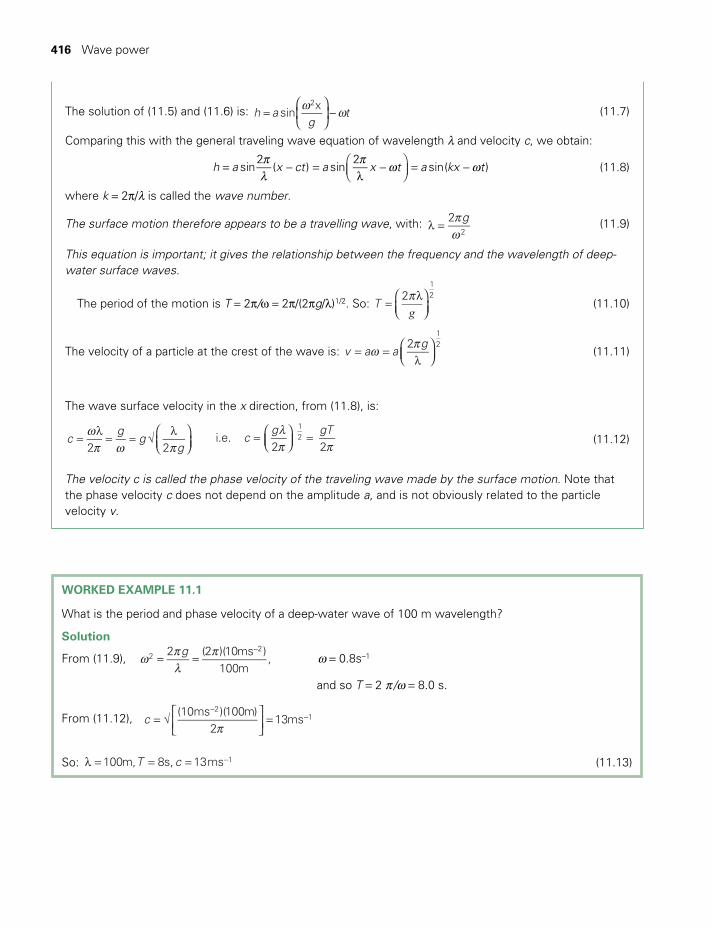
416 Wave power
The solution of (11.5) and (11.6) is: h ag
tsinx2w w=
− (11.7)
Comparing this with the general traveling wave equation of wavelength l and velocity c, we obtain:
πλ
π ω ω= − =λ
−
= −h a x ct a x t a kx tsin2
( ) sin2
sin( ) (11.8)
where k = 2p/l is called the wave number.
The surface motion therefore appears to be a travelling wave, with: pw
l =g22
(11.9)
This equation is important; it gives the relationship between the frequency and the wavelength of deep-water surface waves.
The period of the motion is T = 2p/w = 2p/(2pg/l)1/2. So: g
p=
l
T2
12
(11.10)
The velocity of a particle at the crest of the wave is: w p= =
l
v a ag2
12
(11.11)
The wave surface velocity in the x direction, from (11.8), is:
wp w p
=l
= = √l
cg
gg2 2
lp p
=
=cg gT
i.e.2 2
12
(11.12)
The velocity c is called the phase velocity of the traveling wave made by the surface motion. Note that the phase velocity c does not depend on the amplitude a, and is not obviously related to the particle velocity v.
WORKED EXAMPLE 11.1
What is the period and phase velocity of a deep-water wave of 100 m wavelength?
Solution
From (11.9), g2 (2 )(10ms )
100m, 0.8s2
21w p
lp w= = =
−− w = 0.8s–1
and so T = 2 p /w = 8.0 s.
From (11.12), p
= √
=−
−c(10ms )(100m)
213ms
21
So: l = = = −T c100m, 8s, 13ms 1 (11.13)
TWIDELL PAGINATION.indb 416 01/12/2014 11:37
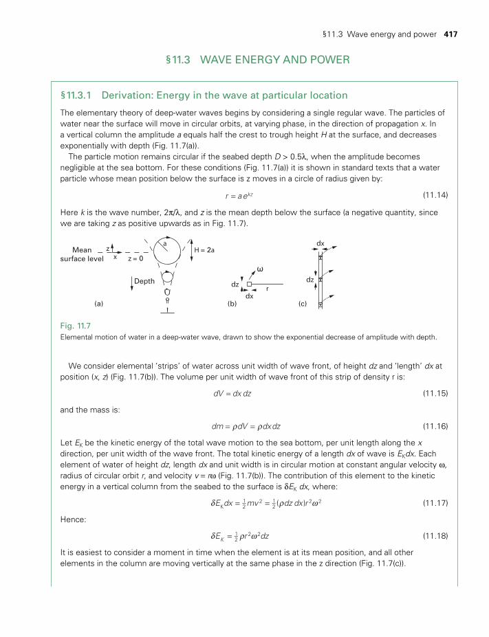
§11.3 Wave energy and power 417
§11.3 WAVE ENERGY AND POWER
§11.3.1 Derivation: Energy in the wave at particular location
The elementary theory of deep-water waves begins by considering a single regular wave. The particles of water near the surface will move in circular orbits, at varying phase, in the direction of propagation x. In a vertical column the amplitude a equals half the crest to trough height H at the surface, and decreases exponentially with depth (Fig. 11.7(a)).
The particle motion remains circular if the seabed depth D > 0.5l, when the amplitude becomes negligible at the sea bottom. For these conditions (Fig. 11.7(a)) it is shown in standard texts that a water particle whose mean position below the surface is z moves in a circle of radius given by:
=r aekz (11.14)
Here k is the wave number, 2p/l, and z is the mean depth below the surface (a negative quantity, since we are taking z as positive upwards as in Fig. 11.7).
We consider elemental ‘strips’ of water across unit width of wave front, of height dz and ‘length’ dx at position (x, z) (Fig. 11.7(b)). The volume per unit width of wave front of this strip of density r is:
=dV dx dz (11.15)
and the mass is:
r r= =dm dV dxdz (11.16)
Let EK be the kinetic energy of the total wave motion to the sea bottom, per unit length along the x direction, per unit width of the wave front. The total kinetic energy of a length dx of wave is EKdx. Each element of water of height dz, length dx and unit width is in circular motion at constant angular velocity w, radius of circular orbit r, and velocity v = rw (Fig. 11.7(b)). The contribution of this element to the kinetic energy in a vertical column from the seabed to the surface is dEK dx, where:
d r w= =E dx mv dz dx r( )K12
2 12
2 2 (11.17)
Hence:
d r w=E r dzK12
2 2 (11.18)
It is easiest to consider a moment in time when the element is at its mean position, and all other elements in the column are moving vertically at the same phase in the z direction (Fig. 11.7(c)).
Fig. 11.7Elemental motion of water in a deep-water wave, drawn to show the exponential decrease of amplitude with depth.
Meansurface level
Depth
(a) (b) (c)
z = 0H = 2az
dz
dxr
dx
dzω
x
a
TWIDELL PAGINATION.indb 417 01/12/2014 11:37
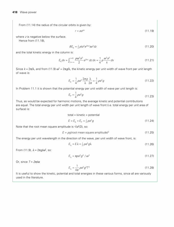
418 Wave power
From (11.14) the radius of the circular orbits is given by:
=r aekz (11.19)
where z is negative below the surface.Hence from (11.18),
d r w=E a e dz( )kzK
12
2 2 2 (11.20)
and the total kinetic energy in the column is:
∫rw r w
= ==−∞
=E dx
ae dz dx
ak
dx2
14
kzz
z
K
2 22
2 20 (11.21)
Since k = 2p/l, and from (11.9) w2 = 2pg/l, the kinetic energy per unit width of wave front per unit length of wave is:
r pp
r=l
l=E a
ga g
14
22
14K
2 2 (11.22)
In Problem 11.1 it is shown that the potential energy per unit width of wave per unit length is:
E a g14P
2r= (11.23)
Thus, as would be expected for harmonic motions, the average kinetic and potential contributions are equal. The total energy per unit width per unit length of wave front (i.e. total energy per unit area of surface) is:
total = kinetic + potential
r= + =E E E a gK P12
2 (11.24)
Note that the root mean square amplitude is √(a2/2), so:
r=E g (root mean square amplitude)2 (11.25)
The energy per unit wavelength in the direction of the wave, per unit width of wave front, is:
l r= = llE E a g12
2 (11.26)
From (11.9), l = 2pg/w2, so:
pr w=lE a g /2 2 2 (11.27)
Or, since T = 2p/w:
p
r=lE a g T1
42 2 2 (11.28)
It is useful to show the kinetic, potential and total energies in these various forms, since all are variously used in the literature.
TWIDELL PAGINATION.indb 418 01/12/2014 11:37
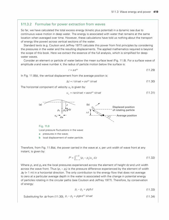
§11.3 Wave energy and power 419
§11.3.2 Formulae for power extraction from waves
So far, we have calculated the total excess energy (kinetic plus potential) in a dynamic sea due to continuous wave motion in deep water. The energy is associated with water that remains at the same location when averaged over time. However, these calculations have told us nothing about the transport of energy (the power) across vertical sections of the water.
Standard texts (e.g. Coulson and Jeffrey 1977) calculate this power from first principles by considering the pressures in the water and the resulting displacements. The applied mathematics required is beyond the scope of this book. Here we extract the essence of the full analysis, which is simplified for deep-water waves.
Consider an element or particle of water below the mean surface level (Fig. 11.8). For a surface wave of amplitude a and wave number k, the radius of particle motion below the surface is:
=r aekz (11.29)
In Fig. 11.8(b), the vertical displacement from the average position is:
w wΔ = =z r t ae tsin sinkz (11.30)
The horizontal component of velocity ux is given by:
w w w w= =u r t ae tsin sinxkz (11.31)
Therefore, from Fig. 11.8(a), the power carried in the wave at x, per unit width of wave front at any instant, is given by:
' ∫= −=−∞
=P p p u dz( ) xz
z
1 2
0 (11.32)
Where p1 and p2 are the local pressures experienced across the element of height dz and unit width across the wave front. Thus (p1 − p2) is the pressure difference experienced by the element of width Δy (= 1 m) in a horizontal direction. The only contribution to the energy flow that does not average to zero at a particular average depth in the water is associated with the change in potential energy of particles rotating in the circular paths (see Coulson and Jeffrey 1977). Therefore, by conservation of energy:
r− = Δp p g z1 2 (11.33)
Substituting for Δz from (11.30), r w− =p p gae tsinkz1 2 (11.34)
Fig. 11.8Local pressure fluctuations in the wave: a pressures in the wave; b local displacement of water particle.
Displaced positionof rotating particle
z
dx
dzrω
ωtux
p1 p2
Average position
(b)(a)
z∇ r
TWIDELL PAGINATION.indb 419 01/12/2014 11:37
420 Wave power
In (11.32), and with (11.31) and (11.34), ' ∫∫
r w w w
r w w
=
=
= −∞
=
= −∞
=
P gae t ae t z
ga e t z
( sin )( sin )d
sin d
kzz
zkz
kzz
z
0
2 20
2
(11.35)
The time average over many periods of sin2wt equals 1/2, so:
' ∫r w r w
= == −∞
=P
gae dz
gak2 21
2kz
z
z22
0 2 (11.36)
The velocity of the wave (strictly the phase velocity) as visible to the eye is, from (11.8),
w
= =l
ck T
(11.37)
So the power carried forward in the wave per unit width across the wave front becomes in terms of wave amplitude a, period T and wavelength l:
'r r
= =l
Pga c ga
T2 2 4
2 2
(11.38)
From (11.24) and (11.38) the power P ‘ equals the total energy (kinetic plus potential) E in the wave per unit area of surface, times c/2. c/2 is called the group velocity (u) of the deep-water wave, i.e. the velocity at which the unseen energy in the group of waves is carried forward,
=u c / 2 (11.39)
so, from (11.38), 'r r
= = =P ga c gau Eu
2 2 2.
2 2
(11.40)
where from (11.24), E = rga2/2. But from (11.9), p l w= =k g2 / /2 , so the phase velocity c and group velocity u are:
w
w p p= = = =c
kg g
TgT
(2 / ) 2 (11.41)
p
= =uc gT2 4
(11.42)
This difference between the group velocity and the phase velocity is common to all waves where the velocity depends on the wavelength. Such waves are called dispersive waves and are well described in the literature. Substituting for c from (11.12) into (11.38) gives:
the power carried in the wave across a vertical plane, per unit width of wave front as:
r
p′ =P
g a T8
2 2 (11.43)
That is, the power in the wave increases directly as the square of the wave amplitude and directly as the period. The attraction of long-period, large-amplitude ocean swells to wave-power engineers is apparent. We note that long-period waves can equally well be characterized as long-wavelength waves, with (11.43) written in terms of wavelength and amplitude using (11.10):
rp
pl′ =
Pg a
g822 2
12
(11.44)
TWIDELL PAGINATION.indb 420 01/12/2014 11:37
§11.4 Real (irregular) sea waves: patterns and power 421
WORKED EXAMPLE 11.2
What is the power in a deep-water wave of wavelength 100 m and amplitude 1.5 m?
SolutionFrom (11.44):
′ = =− −
−−P
(1025kg.m ).(9.8m.s ).(1.5m)8
.2 .100m9.8m.s
72kWm3 2 2
2
1/21
ππ
Alternatively from Worked Example 11.1, c = 13 m/s. With (11.40),
u = c/2 = 6.5ms−1
where u is the group velocity of the energy and c is the phase velocity.The sea water waves have an amplitude a = 1.5 m (H = 3 m), not unrealistic for Atlantic waves, so in
(11.38):
′ = =− − − −P (1025 kgm )(9.8 ms )(1.5 m) (6.5 ms ) 72 kWm12
3 2 2 1 1
From Worked Example 11.2, we can appreciate that there may be extremely large power densities available in the deep-water waves of real-istic ocean swells.
§11.4 REAL (IRREGULAR) SEA WAVES: PATTERNS AND POWER
Wave systems are not in practice the single sine wave patterns moving in one direction as idealized in the previous sections. Very occasion-ally natural or contrived wave diffraction patterns, or channeled waves, approach this condition, but normally a sea will be an irregular pattern of waves of varying period, direction and amplitude. Under the stimulus of a prevailing wind the wave trains may show a preferred direction (e.g. the southwest to northeast direction of Atlantic waves off the British Isles), and produce a significant long period sea ‘swell’. Winds that are more erratic produce irregular water motion typical of shorter periods, called a ‘sea’. At sea bottom depths ~30 m or less, significant focussing and directional effects may occur, possibly producing more regular or enhanced power waves at local sites. Wave-power devices must there-fore match a broad band of natural conditions, and be designed to extract the maximum power averaged over a considerable time for each particu-lar deployment position. In designing these devices, it will first be neces-sary to understand the wave patterns of the particular site that may arise over a 50-year period; this requires statistical and other modeling if such long-term measurements are unavailable.
The height of waves at one position was traditionally monitored on a wave-height analogue recorder. Separate measurements and analyses
TWIDELL PAGINATION.indb 421 01/12/2014 11:37
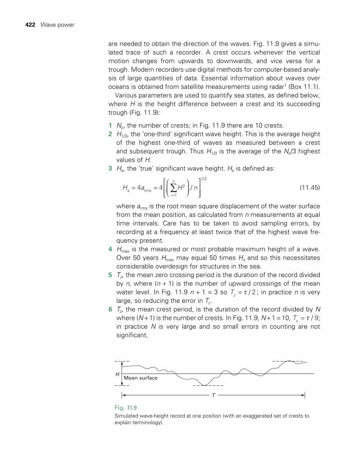
422 Wave power
are needed to obtain the direction of the waves. Fig. 11.9 gives a simu-lated trace of such a recorder. A crest occurs whenever the vertical motion changes from upwards to downwards, and vice versa for a trough. Modern recorders use digital methods for computer-based analy-sis of large quantities of data. Essential information about waves over oceans is obtained from satellite measurements using radar1 (Box 11.1).
Various parameters are used to quantify sea states, as defined below, where H is the height difference between a crest and its succeeding trough (Fig. 11.9):
1 Nc, the number of crests; in Fig. 11.9 there are 10 crests.2 H1/3, the ‘one-third’ significant wave height. This is the average height
of the highest one-third of waves as measured between a crest and subsequent trough. Thus H1/3 is the average of the Nc/3 highest values of H.
3 Hs, the ‘true’ significant wave height. Hs is defined as:
∑= =
=
H a H n4 4 /i
n
s rms2
1
1/2
(11.45)
where arms is the root mean square displacement of the water surface from the mean position, as calculated from n measurements at equal time intervals. Care has to be taken to avoid sampling errors, by recording at a frequency at least twice that of the highest wave fre-quency present.
4 Hmax is the measured or most probable maximum height of a wave. Over 50 years Hmax may equal 50 times Hs and so this necessitates considerable overdesign for structures in the sea.
5 Tz, the mean zero crossing period is the duration of the record divided by n, where (n + 1) is the number of upward crossings of the mean water level. In Fig. 11.9 n + 1 = 3 so τ=T / 2z ; in practice n is very large, so reducing the error in Tz.
6 Tc, the mean crest period, is the duration of the record divided by N where (N + 1) is the number of crests. In Fig. 11.9, N + 1 = 10, τ=T / 9c ; in practice N is very large and so small errors in counting are not significant,
Fig. 11.9Simulated wave-height record at one position (with an exaggerated set of crests to explain terminology).
Mean surfaceH
T
TWIDELL PAGINATION.indb 422 01/12/2014 11:37
§11.4 Real (irregular) sea waves: patterns and power 423
7 The spectral width parameter e gives a measure of the variation in wave pattern:
e = − T T1 ( / )c z2 2 (11.46)
For a uniform single frequency motion, Tc = Tz, so e = 0. In our example e = [1 − (0.3)2]1/2 = 0.9, implying a mix of many frequencies. The full infor-mation is displayed by Fourier transformation to a frequency spectrum (e.g. Fig. 11.11).
From the power per unit width of the wave front in a pure sinusoidal a deep water wave is:
'r
pr
p= =P
g a T g H T8 32
2 2 2 2 (11.47)
where the trough to crest height is H = 2a. The root mean square (rms) wave displacement for a pure sinusoidal wave is amax = a / √2, so in (11.47):
'r
p=P
g a T
4
2rms2
(11.48)
BOX 11.1 SATELLITE MEASUREMENT OF WAVE HEIGHT, ETC.
Remote sensing from satellites is the only method of measuring the Earth’s whole ocean surface; there are two types of measurement: (i) radar altimeter; (ii) synthetic aperture radar (SAR). Both methods are used with Low Earth Orbiting (LEO) satellites that orbit at heights of ~1000 km and periods of ~15 orbits/day over the rotating Earth below. Data are available for free access (e.g. from www.globwave.org), with explanations and accuracies of the methods used.
Radar altimeter data: Sea-surface height (with respect to satellite distance from Earth). Sea-surface height is derived from the ‘time of flight’ of radar pulses emitted vertically downwards by the instruments (altimeters) and reflected off ocean and inland sea surface. Sophisticated averaging of this time allows average wave-height measurement over ‘sea patches’ about 5 km in diameter along the satellite path round the Earth. Accuracy to ~1 cm is sufficient to measure averages for wave height of sea waves as defined in this chapter.
Synthetic aperture radar is emitted in high-power pulses in narrow beams at right angles to the satellite path and at controllable angles from vertical. The reflected beam returns with its frequency changed by the Doppler effect if the reflection is from a moving surface (e.g. water rotation of sea waves). Sophisticated analysis allows wave heights to be measured to accuracies ~1 mm; such accuracy is more than adequate for sea-wave analysis, and sufficient to measure the small amplitude capillary waves relating to wind speed.
Use of wave data. The satellite-derived data from a variety of instrument types are important for many purposes, including meteorological services, sea and land temperature, shipping and fisheries, geological prospecting, offshore construction, ice formations, wave energy assessment for renewable energy, wind speed assessment for offshore windfarms and recreational sailing. Fig. 11.10 illustrates the value of such data for wave energy resource assessment.
TWIDELL PAGINATION.indb 423 01/12/2014 11:37
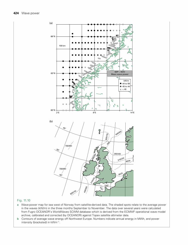
424 Wave power
Fig. 11.10a Wave-power map for sea west of Norway from satellite-derived data. The shaded spots relate to the average power
in the waves (kW/m) in the three months September to November. The data over several years were calculated from Fugro OCEANOR’s WorldWaves SCWM database which is derived from the ECMWF operational wave model archive, calibrated and corrected (by OCEANOR) against Topex satellite altimeter data.
b Contours of average wave energy off Northwest Europe. Numbers indicate annual energy in MWh, and power intensity (bracketed) in kWm−1.
(a)
66°N
100 km
63°N
60°N2°E
(b)
8°E 14°E
SEP − NOVMean wave power
kW/m44 to 5840 to 44< 40
45°
55°
50°
620(70)
440(
50)
210(
24)
(24)
(30)
30(3)
80(9)210(24)
350(40)
440
440(
50)
620(
70)
440(50)
700(80)
700(80)
TWIDELL PAGINATION.indb 424 01/12/2014 11:37
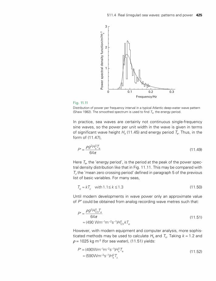
§11.4 Real (irregular) sea waves: patterns and power 425
Fig. 11.11Distribution of power per frequency interval in a typical Atlantic deep-water wave pattern (Shaw 1982). The smoothed spectrum is used to find Te, the energy period.
Frequency/HzP
ow
er s
pec
tral
den
sity
fu
nct
ion
/m2 H
z–1
3
2
1
0 0.1 0.2 0.3
In practice, sea waves are certainly not continuous single-frequency sine waves, so the power per unit width in the wave is given in terms of significant wave height Hs (11.45) and energy period Te. Thus, in the form of (11.47),
'r
p=P
g H T64
2s2
e (11.49)
Here Te, the ‘energy period’, is the period at the peak of the power spec-tral density distribution like that in Fig. 11.11. This may be compared with Tz the ‘mean zero crossing period’ defined in paragraph 5 of the previous list of basic variables. For many seas,
≈ ≤ ≤T kT kwith1.1 1.3e z (11.50)
Until modern developments in wave power only an approximate value of P ′ could be obtained from analog recording wave metres such that:
'r
p≈
≈ − − −
Pg H T
H kT64
(490 Wm m s )
e
e
21/32
1 2 11/32
(11.51)
However, with modern equipment and computer analysis, more sophis-ticated methods may be used to calculate Hs and Te. Taking k ≈ 1.2 and r = 1025 kg m-3 (for sea water), (11.51) yields:
' =≈
− − −
− −
P H T
H T
(490Wm m s )
(590Wm s )
1 2 1s2
e3 1
s2
z (11.52)
TWIDELL PAGINATION.indb 425 01/12/2014 11:37
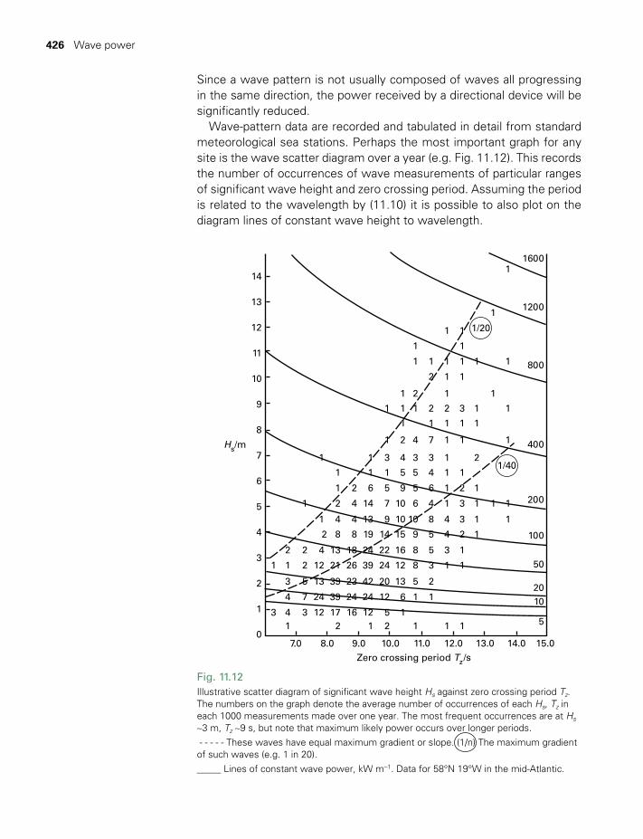
426 Wave power
Fig. 11.12Illustrative scatter diagram of significant wave height Hs against zero crossing period Tz. The numbers on the graph denote the average number of occurrences of each Hs, Tz in each 1000 measurements made over one year. The most frequent occurrences are at Hs ~3 m, Tz ~9 s, but note that maximum likely power occurs over longer periods. - - - - - These waves have equal maximum gradient or slope. (1/n) The maximum gradient of such waves (e.g. 1 in 20). _____ Lines of constant wave power, kW m−1. Data for 58°N 19°W in the mid-Atlantic.
1/20
1/40
14
13
12
11
10
9
8
7
6
5
4
3
2
1
07.0 8.0 9.0 10.0
Zero crossing period Tz
/s
Hs/m
11.0 12.0 13.0 14.0 15.0
1600
1200
800
400
200
100
50
2010
5
1
1
1 1
1
1 1 1
1
1
3221
21
1 1
2 1
1
1
1
1
1
1
2
3146714421
1
1
1
1
1
1
1 1
1 1 1 1
1 1
12 4 7 1
3 4 3 3 1
1 5 5 4 1
2 6 5 9 5 6 1 1
2
3
2459151419882
1 4 4 13 9 10
10
10 8 4
1
13 4
4
3
1 1
2 2 4 13 18 24 22 16 8 5 3
1
1 1
11 1
2 12 21 26 39 24 12 8 3 1 1
5 13 39 23 42 20 13 5 2
7 24 39 24 24 12 6 1 1
3 12 17 16 12 5 12 1 2 1 1 1
Since a wave pattern is not usually composed of waves all progressing in the same direction, the power received by a directional device will be significantly reduced.
Wave-pattern data are recorded and tabulated in detail from standard meteorological sea stations. Perhaps the most important graph for any site is the wave scatter diagram over a year (e.g. Fig. 11.12). This records the number of occurrences of wave measurements of particular ranges of significant wave height and zero crossing period. Assuming the period is related to the wavelength by (11.10) it is possible to also plot on the diagram lines of constant wave height to wavelength.
TWIDELL PAGINATION.indb 426 01/12/2014 11:37
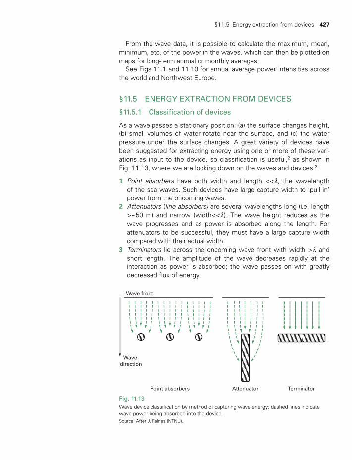
§11.5 Energy extraction from devices 427
Fig. 11.13Wave device classification by method of capturing wave energy; dashed lines indicate wave power being absorbed into the device.Source: After J. Falnes (NTNU).
Wave front
Wave direction
Point absorbers Attenuator Terminator
From the wave data, it is possible to calculate the maximum, mean, minimum, etc. of the power in the waves, which can then be plotted on maps for long-term annual or monthly averages.
See Figs 11.1 and 11.10 for annual average power intensities across the world and Northwest Europe.
§11.5 ENERGY EXTRACTION FROM DEVICES
§11.5.1 Classification of devices
As a wave passes a stationary position: (a) the surface changes height, (b) small volumes of water rotate near the surface, and (c) the water pressure under the surface changes. A great variety of devices have been suggested for extracting energy using one or more of these vari-ations as input to the device, so classification is useful,2 as shown in Fig. 11.13, where we are looking down on the waves and devices:3
1 Point absorbers have both width and length <<l, the wavelength of the sea waves. Such devices have large capture width to ‘pull in’ power from the oncoming waves.
2 Attenuators (line absorbers) are several wavelengths long (i.e. length >~50 m) and narrow (width<<l). The wave height reduces as the wave progresses and as power is absorbed along the length. For attenuators to be successful, they must have a large capture width compared with their actual width.
3 Terminators lie across the oncoming wave front with width >l and short length. The amplitude of the wave decreases rapidly at the interaction as power is absorbed; the wave passes on with greatly decreased flux of energy.
TWIDELL PAGINATION.indb 427 01/12/2014 11:37
428 Wave power
Devices are further classified by their location, as on-shore (i.e. on land), near-shore (i.e. in relatively shallow water, depth ~l ), or offshore (i.e. in deep water, depth >>l ).
A further classification relates to the development of wave power devices:
1 First generation: these are oscillating water column (OWC) devices as described in §11.6.3, having been the most straightforward devices to construct onshore and near-shore. Air above the water column is forced through a turbine generator for electricity.
2 Second generation: developmental floating devices taking power from the waves to pump internal fluids through a turbine generator.
3 Third generation: very large single devices or as large arrays of smaller devices operating commercially when the particular technologies are considered proven and financed. Very few devices had reached this stage by 2013.
§11.5.2 Capture width and tuned energy capture
Wave energy devices extract an average power PD (unit W) from the oncoming power flux of the waves P ′ (unit W/m); P ′ is calculated from (11.43) or (11.52). The ratio of these two parameters has dimensions of length (m) and is the capture width Cw:
= ′C P P/w D (11.53)
If Cw is divided by the device width w, we have the non-dimensional or relative capture width:
= = ′C C w P P w/ ( / ) /w r w D, (11.54)
Capture width (sometimes called ‘absorption width’) is used as a ‘measure of the efficacy’ of a device and depends on: (a) the wave conditions, especially of wave frequency, height and direction; (b) the boundaries of the wave pattern (e.g. open sea or wave tank), and (c) the device’s fixed or variable position. The averaging criteria need to be defined most carefully (e.g. per wave period for ‘regular’ single frequency waves, which are unlikely to occur at sea, or per period of repeated wave energy fluxes in ‘irregular’ waves of repeating pattern, approximately repeating every five to ten waves, or per year for a specific location). Successful devices have Cw r,
> ~ 3 because the device absorbs power from a wave front wider than the device itself; for this reason it is not helpful to consider Cw,r an efficiency in the normal sense.
We can, however, define the efficiency of the device as the ratio of the useful power output from the device to the power incident immediately
TWIDELL PAGINATION.indb 428 01/12/2014 11:37

§11.5 Energy extraction from devices 429
on the device. In practice, this efficiency depends greatly on the wave-length and amplitude of the oncoming waves and the characteristics of the device.
An important principle for the design of a floating wave energy absorber was first expressed by Falnes (2002); it may be stated as ‘a successful wave energy absorber is a successful wave energy maker’. To understand this, we imagine the wave device forced to oscillate in a calm sea; it will make waves of pattern A. In operation, waves of pattern B are incident on the device, which then oscillates. If pattern B is in anti-phase with pattern A, then the water around the device becomes calm, i.e. the device has absorbed 100% of the surrounding incoming wave power. This concept is vital for designing a tunable wave power-absorbing device.
Cruz (2008) applies Falnes’ principle to both a point absorber and a line attenuator/absorber.
• A point absorber (constrained to move in heave only, i.e. vertically) in still water generates pattern A as circular waves in all directions. However, incoming waves with pattern B with wavelength l are from only one direction, so pattern A can never cancel pattern B. The maximum theoretical capture width may be shown to be l/2p (i.e. about 16 m for large 100 m wavelength waves irrespective of the size of the ‘point’).
• However, a line attenuator with coupled sections moving out of phase with each other (as does the Pelamis wave power device of §11.6.4) can be controlled to produce pattern A as a unidirectional wave train propagated in line with itself. This is because the patterns from each out-of-phase section cancel each other in all other direc-tions. Cruz (2008) points out that this is the same wave mechanism used to produce directed ‘phased array’ radar beams with no moving antennae. By suitable scaling and design of the coupled sections and by ‘tuning’ the hydraulic actuators, pattern A can be made to be the anti-phase equivalent of the incoming sea wave, for which the theoretical capture width is l/2 (i.e. 50 m for large 100 m wavelength waves).
The Falnes principle is very important in explaining why and how optimum wave power devices need to be dynamic tunable structures, and certainly not fixed static structures. Yet this criterion is far from easy to attain for operational devices surviving for many years in open oceans, even if the tuning is adjusted hourly or daily rather than fresh for every incoming wave. In practice, tunable efficiency is less important than sur-vival; the hope is to have both.
TWIDELL PAGINATION.indb 429 01/12/2014 11:37
430 Wave power
BOX 11.2 WAVE ENERGY IN THE UK
Located at the east side of the North Atlantic, the United Kingdom (of England, Scotland, Wales and Northern Ireland) is an island nation with major opportunities to develop and use wave power. (The waves approaching the west coasts of Ireland and Scotland are even more powerful than those approaching the west coast of Norway (Fig. 11.10); the contour of 70 kW/m annual average lies only ~50 km off the western coast of Ireland.) Present policy is for an independent government-established agency, the Carbon Trust, to manage ‘The Marine Challenge’ for the promotion of both wave and tidal power. Studies and manufactured devices are fully or cooperatively funded with the aim of establishing a major UK energy supply at realistic costs. Results to date include the following:
• The total wave power entering UK coastal waters is about 350 TWh/y, equal in energy terms to UK annual electricity supply.
• The most economic developments would be placed in the Atlantic Ocean ~100 km off the west coast of Scotland.
• From this location only, delivered power would be about 35 TWh/y from about 10 GW of installed wave power capacity, i.e. at 35% capacity factor.
• This would be about 10% of UK total annual electricity supply.• With devices as performing in 2012, the generation cost would be about 23 p/kWh (about 36 c/kWh).• Development and experience are expected to reduce costs significantly to be a competitive carbon-
free power supply.• Offshore wave hubs for R&D projects exist near to the shore off Orkney main island (north Scotland)
and off southwest England.• In May 2013, the Scottish government approved a 40 MW wave farm off the Isle of Lewis (west coast
of Scotland) with Aquamarine ‘Oyster’ ~1 MW devices.
Sources: The Carbon Trust (2006); Cruz (2008).
§11.6 WAVE POWER DEVICES
In this section we review a selected range of devices to illustrate the classification criteria above.
§11.6.1 On-shore terminator, Tapchan, overtopping wave capture
The principle of wave capture is simple, as observed in many shoreline lagoons and swimming pools. Waves rise up a channeled sea wall and the overspilling water is impounded in a reservoir above the mean sea level. Controlled outlet water returns to the sea through a conventional low-head hydroelectric turbine generator.
Fig. 11.14 is a schematic diagram of the 350 kW Tapchan system dem-onstrated in Norway in 1985 and since replicated at a few sites world-wide. The incoming waves funnel up a narrowing (tapered) channel, whose concrete walls reached 2 to 3 m above mean sea level. The peaks of these waves increase in height above the troughs as the waves progress along the tapered channel, so water spills over into the reser-voir as the wave arrives at the wall. Larger waves may overtop the wall
TWIDELL PAGINATION.indb 430 01/12/2014 11:37
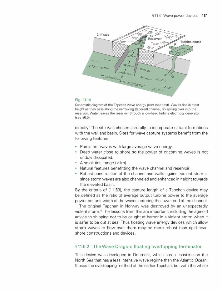
§11.6 Wave power devices 431
Fig. 11.14Schematic diagram of the Tapchan wave energy plant (see text). Waves rise in crest height as they pass along the narrowing (tapered) channel, so spilling over into the reservoir. Water leaves the reservoir through a low-head turbine electricity generator (see §6.5).
Cliff faceReservoir
P
Q
Turbine house
directly. The site was chosen carefully to incorporate natural formations with the wall and basin. Sites for wave capture systems benefit from the following features:
• Persistent waves with large average wave energy.• Deep water close to shore so the power of oncoming waves is not
unduly dissipated.• A small tidal range (<1m).• Natural features benefitting the wave channel and reservoir.• Robust construction of the channel and walls against violent storms,
since storm waves are also channeled and enhanced in height towards the elevated basin.
By the criteria of (11.53), the capture length of a Tapchan device may be defined as the ratio of average output turbine power to the average power per unit width of the waves entering the lower end of the channel.
The original Tapchan in Norway was destroyed by an unexpectedly violent storm.4 The lessons from this are important, including the age-old advice to shipping not to be caught at harbor in a violent storm when it is safer to be out at sea. Thus floating wave energy devices which allow storm waves to flow over them may be more robust than rigid near-shore constructions and devices.
§11.6.2 The Wave Dragon: floating overtopping terminator
This device was developed in Denmark, which has a coastline on the North Sea that has a less intensive wave regime than the Atlantic Ocean. It uses the overtopping method of the earlier Tapchan, but with the whole
TWIDELL PAGINATION.indb 431 01/12/2014 11:37
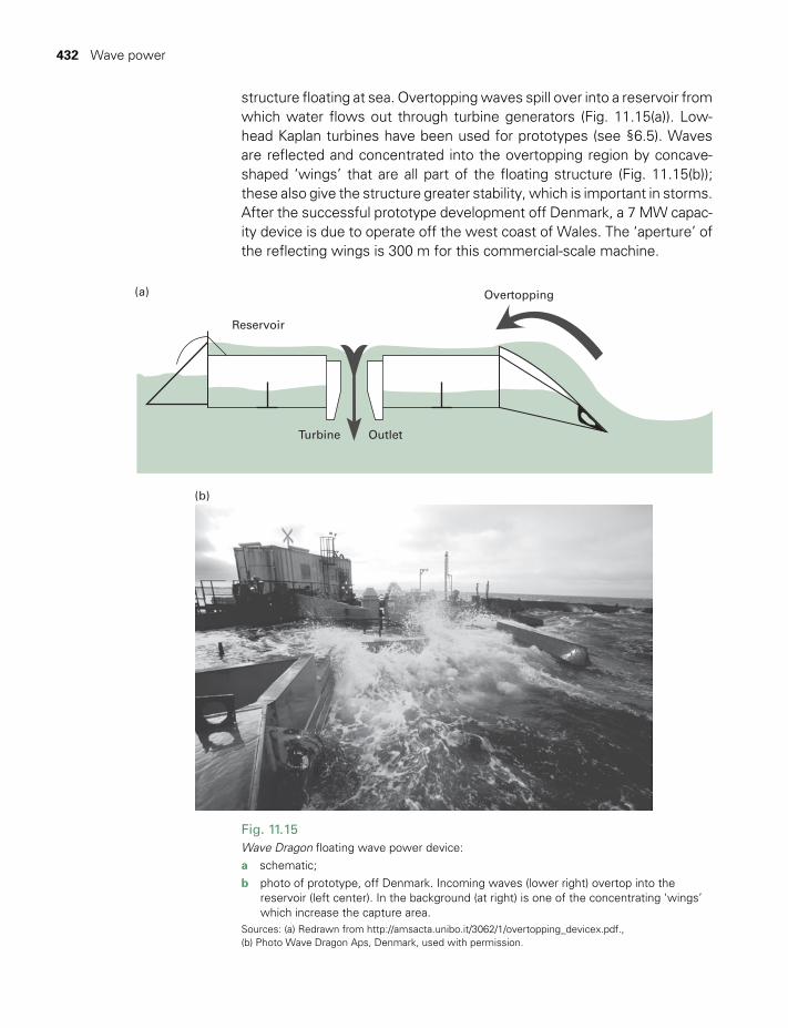
432 Wave power
Fig. 11.15Wave Dragon floating wave power device: a schematic; b photo of prototype, off Denmark. Incoming waves (lower right) overtop into the
reservoir (left center). In the background (at right) is one of the concentrating ‘wings’ which increase the capture area.
Sources: (a) Redrawn from http://amsacta.unibo.it/3062/1/overtopping_devicex.pdf., (b) Photo Wave Dragon Aps, Denmark, used with permission.
Reservoir
(a)
Turbine
Overtopping
Outlet
(b)
structure floating at sea. Overtopping waves spill over into a reservoir from which water flows out through turbine generators (Fig. 11.15(a)). Low-head Kaplan turbines have been used for prototypes (see §6.5). Waves are reflected and concentrated into the overtopping region by concave-shaped ‘wings’ that are all part of the floating structure (Fig. 11.15(b)); these also give the structure greater stability, which is important in storms. After the successful prototype development off Denmark, a 7 MW capac-ity device is due to operate off the west coast of Wales. The ‘aperture’ of the reflecting wings is 300 m for this commercial-scale machine.
TWIDELL PAGINATION.indb 432 01/12/2014 11:38
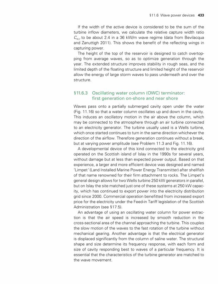
§11.6 Wave power devices 433
If the width of the active device is considered to be the sum of the turbine inflow diameters, we calculate the relative capture width ratio Cw,r to be about 2.4 in a 36 kW/m wave regime (data from Bevilacqua and Zanuttigh 2011). This shows the benefit of the reflecting wings in capturing power.
The height of the top of the reservoir is designed to catch overtop-ping from average waves, so as to optimize generation through the year. The extended structure improves stability in rough seas, and the limited depth of the floating structure and limited height of the reservoir allow the energy of large storm waves to pass underneath and over the structure.
§11.6.3 Oscillating water column (OWC) terminator: first generation on-shore and near shore
Waves pass onto a partially submerged cavity open under the water (Fig. 11.16) so that a water column oscillates up and down in the cavity. This induces an oscillatory motion in the air above the column, which may be connected to the atmosphere through an air turbine connected to an electricity generator. The turbine usually used is a Wells turbine, which once started continues to turn in the same direction whichever the direction of the airflow. Therefore generation continues without a break, but at varying power amplitude (see Problem 11.3 and Fig. 11.16).
A developmental device of this kind connected to the electricity grid operated on the Scottish island of Islay in the 1990s for several years, without damage but at less than expected power output. Based on that experience, a larger and more efficient device was designed and named ‘Limpet’ (Land Installed Marine Power Energy Transmitter) after shellfish of that name renowned for their firm attachment to rocks. The Limpet’s general design allows for two Wells turbine 250 kW generators in parallel, but on Islay the site matched just one of these systems at 250 kW capac-ity, which has continued to export power into the electricity distribution grid since 2000. Commercial operation benefitted from increased export price for the electricity under the Feed-in Tariff legislation of the Scottish Administration (see §17.5).
An advantage of using an oscillating water column for power extrac-tion is that the air speed is increased by smooth reduction in the cross-sectional area of the channel approaching the turbine. This couples the slow motion of the waves to the fast rotation of the turbine without mechanical gearing. Another advantage is that the electrical generator is displaced significantly from the column of saline water. The structural shape and size determine its frequency response, with each form and size of cavity responding best to waves of a particular frequency. It is essential that the characteristics of the turbine generator are matched to the wave movement.
TWIDELL PAGINATION.indb 433 01/12/2014 11:38
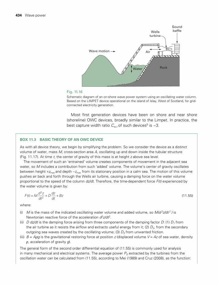
434 Wave power
BOX 11.3 BASIC THEORY OF AN OWC DEVICE
As with all device theory, we begin by simplifying the problem. So we consider the device as a distinct volume of water, mass M, cross-section area A, oscillating up and down inside the tubular structure (Fig. 11.17). At time t, the center of gravity of this mass is at height z above sea level.
The movement of such an ‘entrained’ volume creates components of movement in the adjacent sea water, so M includes a contribution from such ‘added’ volume. The volume’s center of gravity oscillates between height +zmax and depth −zmax from its stationary position in a calm sea. The motion of this volume pushes air back and forth through the Wells air turbine, causing a damping force on the water volume proportional to the speed of the column dz/dt. Therefore, the time-dependent force F(t) experienced by the water volume is given by:
= + +F t Md zdt
Ddzdt
Bz( )2
2 (11.55)
where:
(i) M is the mass of the indicated oscillating water volume and added volume, so M(d 2z/dt 2 ) is Newtonian reactive force of the acceleration d2z/dt2.
(ii) D dz/dt is the damping force arising from three components of the damping factor D: (1) D1 from the air turbine as it resists the airflow and extracts useful energy from it; (2) D2, from the secondary outgoing sea waves created by the oscillating volume; (3) D3 from unwanted friction.
(iii) B = Arg is the gravitational restoring force at position z (displaced volume V = Az of sea water, density r, acceleration of gravity g).
The general form of the second order differential equation of (11.55) is commonly used for analysis in many mechanical and electrical systems. The average power PD extracted by the turbines from the oscillation water can be calculated from (11.55), according to Mei (1989) and Cruz (2008), as the function:
Fig. 11.16Schematic diagram of an on-shore wave power system using an oscillating water column. Based on the LIMPET device operational on the island of Islay, West of Scotland, for grid-connected electricity generation.
Wellsturbine
Soundbaffle
Air
Water
Wave motion
Rock
Most first generation devices have been on shore and near shore (shoreline) OWC devices, broadly similar to the Limpet. In practice, the best capture width ratio Cw,r of such devices5 is ~3.
TWIDELL PAGINATION.indb 434 01/12/2014 11:38
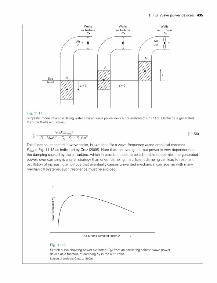
§11.6 Wave power devices 435
ww w
=− + + +
PD F
B M D D D/
( ) ( )D
12 1 mod
2
2 21 2 3
2 2 (11.56)
This function, as tested in wave tanks, is sketched for a wave frequency w and empirical constant Fmod in Fig. 11.18 as indicated by Cruz (2008). Note that the average output power is very dependent on the damping caused by the air turbine, which in practice needs to be adjustable to optimize the generated power; over-damping is a safer strategy than under-damping. Insufficient damping can lead to resonant oscillation of increasing amplitude that eventually causes unwanted mechanical damage; as with many mechanical systems, such resonance must be avoided.
Fig. 11.18Sketch curve showing power extracted (PD) from an oscillating column wave power device as a function of damping D1 in the air turbine. Source of analysis: Cruz, J. (2008).
Air turbine damping factor D1
Po
wer
ext
ract
ed P
D
Fig. 11.17Simplistic model of an oscillating water column wave power device, for analysis of Box 11.3. Electricity is generated from the Wells air turbine.
Wellsair turbine
Sealevel
z < 0 z = 0
z
Wellsair turbine
Wellsair turbine
A
A
A
Airin
Airout
TWIDELL PAGINATION.indb 435 01/12/2014 11:38
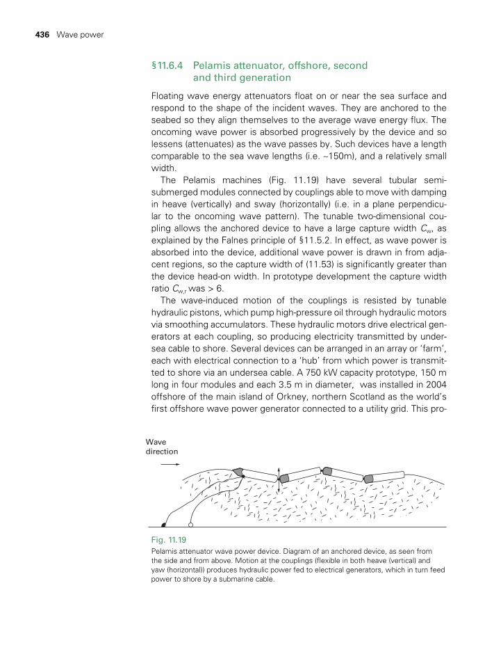
436 Wave power
§11.6.4 Pelamis attenuator, offshore, second and third generation
Floating wave energy attenuators float on or near the sea surface and respond to the shape of the incident waves. They are anchored to the seabed so they align themselves to the average wave energy flux. The oncoming wave power is absorbed progressively by the device and so lessens (attenuates) as the wave passes by. Such devices have a length comparable to the sea wave lengths (i.e. ~150m), and a relatively small width.
The Pelamis machines (Fig. 11.19) have several tubular semi- submerged modules connected by couplings able to move with damping in heave (vertically) and sway (horizontally) (i.e. in a plane perpendicu-lar to the oncoming wave pattern). The tunable two-dimensional cou-pling allows the anchored device to have a large capture width Cw, as explained by the Falnes principle of §11.5.2. In effect, as wave power is absorbed into the device, additional wave power is drawn in from adja-cent regions, so the capture width of (11.53) is significantly greater than the device head-on width. In prototype development the capture width ratio Cw,r was > 6.
The wave-induced motion of the couplings is resisted by tunable hydraulic pistons, which pump high-pressure oil through hydraulic motors via smoothing accumulators. These hydraulic motors drive electrical gen-erators at each coupling, so producing electricity transmitted by under-sea cable to shore. Several devices can be arranged in an array or ‘farm’, each with electrical connection to a ‘hub’ from which power is transmit-ted to shore via an undersea cable. A 750 kW capacity prototype, 150 m long in four modules and each 3.5 m in diameter, was installed in 2004 offshore of the main island of Orkney, northern Scotland as the world’s first offshore wave power generator connected to a utility grid. This pro-
Fig. 11.19Pelamis attenuator wave power device. Diagram of an anchored device, as seen from the side and from above. Motion at the couplings (flexible in both heave (vertical) and yaw (horizontal)) produces hydraulic power fed to electrical generators, which in turn feed power to shore by a submarine cable.
Wavedirection
TWIDELL PAGINATION.indb 436 01/12/2014 11:38
§11.7 Social, economic and environmental aspects 437
totype machine was developed into a similar-sized and capacity model P2 for commercial experience and utility generation. In use in moderate sea conditions of ‘normal’ (i.e. irregular) waves, electrical power output reaches 400 kW in bursts and averages about 270 kW.6 Pelamis devel-opment is progressing to wave power farms of ~10 MW capacity from arrays of about 15 P2-scale machines.
The electricity generated ‘immediately’ by wave power devices (i.e. without some form of averaging or storage as in overtopping devices) varies in amplitude with time. Such variability is similar, and perhaps greater than, the variability of individual wind turbines. In both cases, aver-aging the output of multiple machines in arrays considerably decreases the variability of the combined output.
§11.6.5 Summary of operational devices
There are many developmental wave power devices, several of which are in commercial deployment for grid-compatible electricity generation. Table §11.1 in the supplementary online eResource for this book sum-marizes the situation as at 2013.
§11.7 SOCIAL, ECONOMIC AND ENVIRONMENTAL ASPECTS
As with all development, careful and comprehensive environmen-tal impact scrutiny is essential. Wave power is a renewable energy resource and so shares the general characteristics of sustainability, energy security, minimal chemical pollution, local employment and natural variability – characteristics that mostly contrast with those of fossil fuels and nuclear power. There are distinctive characteristics of wave power systems, the main one being the essential marine circum-stance and the relevance only to countries with shorelines and offshore rights. Clearly, safety of personnel at sea is of paramount importance, especially as the devices and the work on them in operation are individu-ally new and distinctive.
National policies may favor wave power because of the positive ben-efits of:
• The mitigation of greenhouse gas emissions by substituting for fossil fuel use (as with all renewable energy).
• Increasing national energy security with local generation of electricity.• Increased employment and investment, especially in marine-related
industries of construction and servicing. • Cooperation and integration with offshore wind farms and other
marine resources.
TWIDELL PAGINATION.indb 437 01/12/2014 11:38

438 Wave power
With only a few wave power systems having many years of opera-tion, experience is limited, but potential negative impacts of wave power devices include the following:
• Air turbines operating with wave periodicities may be acoustically noisy. However, wind and breaking waves are likely to mask such noise. Nevertheless, noise reduction at source is always needed.
• Underwater noise, possibly confusing fish and, especially, marine mammals.
• On-shore structural and visual damage to coastlines at points of contact (on-shore structures, submarine cable connections to grid lines, maintenance depots, etc.).
• Leaks of hydraulic oils and anti-fouling chemicals may damage marine life.
• Obstruction to fishing.• Distraction by lights at night to birds, including migrating birds.• Danger at all times to boats and shipping, especially from half-
submerged or broken floating structures with poor visibility and radar profile.
• Danger of floating devices breaking their moorings and becoming an unknown hazard to shipping.
• At a very large scale of implementation, changes to marine currents and energy fluxes may be detrimental to marine ecology.
Impact on fish is usually neutral and may be positive, since the structures provide breeding areas and protection from commercial fishing. Most designs of wave power plant do not harm individual fish. In a similar manner, marine birds may well find the structures welcome. Conceivable negative impacts from electric fields around submarine cables have been suggested, but to date no evidence has been obtained.
As with all impacts, recognition at the design stage allows for planned minimization of negative impacts and increased benefit of positive impacts.
National and international marine and shipping law has a long history, being both complex and comprehensive. Near-shore and off-shore wave power devices are included within this, as are boats and ships. Examples are the need to include warning lights and devices for other shipping, and the need for safety of personnel. Wave power devel-opers expect, and usually welcome, the express inclusion of wave power devices in such legislation so that they can plan accordingly. International norms in such matters are important, since manufactur-ers expect to market devices worldwide. The clear trend is for much increased ‘constructional activity’ at sea (e.g. offshore oil and gas explo-ration and extraction, wind farms, wave farms, tidal-current power arrays, tidal-range power barriers). Comprehensive planning is essential
TWIDELL PAGINATION.indb 438 01/12/2014 11:38

§11.7 Social, economic and environmental aspects 439
CHAPTER SUMMARY
Ocean waves contain considerable mechanical power which can be harnessed especially in those locations where the resource is large and relatively near to the shore for long periods (e.g. the North Atlantic coasts of America, Canada and Europe, and the coasts of northeast Asia and southern Australia). In such locations, the resource is commonly ~30 to 50 kW per metre width of wave front. Devices may be classified as point absorbers, attenuators and terminators. Among the challenges of accessing and utilizing wave power are the possibility of damage to devices from exceptionally powerful waves and the difficulties of bringing the electrical power to shore; challenges that add to complexity and cost. However, success is possible, especially as designers and regulators benefit from experience with other established offshore structures of offshore oil and gas extraction and of offshore wind farms.
The mathematical theory of water waves is well developed; it shows that the power available in deep-water waves is proportional to the period of the wave and to the square of the wave height. Satellites now measure such parameters worldwide for ocean waves, which also benefits shipping and meteorological understanding.
There are many mechanisms by which the mechanical power of the waves is extracted and converted to useful (electrical) power. Their state of development ranges from laboratory studies to increasing deployment of commercial-scale products, but none are yet established in global use. Offshore, deployment of multiple devices in ‘hubs’ makes power extraction easier and reduces costs.
if all such activities are to exist alongside the established practices of shipping and fishing.
In terms of costs and development status, wave power today is at roughly the stage that wind power was 30 years ago. From the experi-ence of the initial plants, the projected cost of wave power-generated electricity power encourages optimism. For example, even before 2006, the Limpet and Pelamis installations both accepted contracts to supply electricity for 15 years at less than 7 p/kWh (≈ US$0.15/kWh). It is rea-sonable to project that with greater deployment, which spreads devel-opment costs over multiple units, and with incremental engineering improvements from the pilot plants, these costs may halve within tens of years (an example of the ‘learning curves’ discussed in §17.8).
Reliability and low operational costs are the most critical factors in achieving low average costs per kWh for systems which are capital inten-sive (see Chapter 17). This is particularly true for wave power systems, which necessarily operate in vigorous sea conditions. If a system is destroyed by a storm in its first few years of operation, it will not pay its way, and power suppliers will not want to invest in further, similar devices. Fortunately, engineers can now draw on the experience of the offshore oil and windpower industries to ‘ruggedize’ their designs and allow more confident installation and operation.
TWIDELL PAGINATION.indb 439 01/12/2014 11:38

440 Wave power
QUICK QUESTIONS
Note: Answers to these questions are in the text of the relevant section of this chapter, or may be readily inferred from it.
1 Sketch the movement of small elemental water volumes in a deep-water wave; then from the sketches explain how the totality of such movements produces a forward-moving wave.
2 What is the relationship between group and phase (wave) velocity of a deep-water wave?
3 (i) What is the mathematical relationship between the frequency and wavelength of a deep-water wave? (ii) Is there a mathematical relationship between the wavelength and amplitude of deep-water waves, and if not, why not?
4 Does the energy carried forward in a deep-water wave travel at the same speed as the wave?
5 How does the power transmitted forward in a deep-water wave relate to the amplitude and wavelength of the wave?
6 Sea waves are irregular in amplitude. How is ‘significant wave height’ defined?
7 How does the power per unit wave front of deep-water waves relate to their significant wave height?
8 Name three main classes of wave energy devices and three main locations.
9 In a Tapchan wave energy device, does sea water enter a reservoir mainly because the entry channel changes in width or in depth?
10 List three legal or planning issues that are important for the deploy-ment of wave power devices.
PROBLEMS
Note: *indicates a ‘problem’ that is particularly suitable for class discus-sion or group tutorials.
11.1 By considering elements of water lifted from depth z below the mean sea level to a height z above this level in a crest, show that the potential energy per unit length per unit width of wave front in the direction of the wave is:
r=E a gP14
2
11.2 How do Fig. 11.11 (distribution of sea wave power with respect to frequency) and equation (11.9) (relation of wavelength to fre-quency) relate to the design of a Pelamis wave energy device?
11.3 Fig. 11.20(a) shows a perspective sketch of a Wells turbine; Fig. 11.20(b) shows (schematically) a cross-section of its symmetrical blade and its movement as seen by a fixed observer.
TWIDELL PAGINATION.indb 440 01/12/2014 11:38
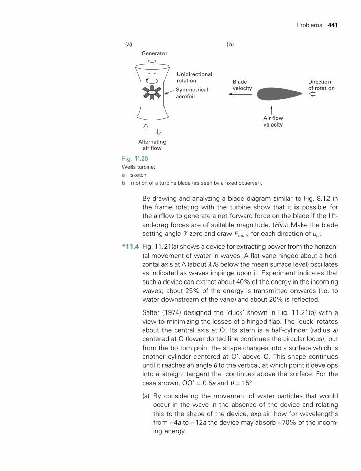
Problems 441
Fig. 11.20Wells turbine: a sketch, b motion of a turbine blade (as seen by a fixed observer).
Alternatingair flow
(b)(a)
Symmetricalaerofoil
Unidirectionalrotation Blade
velocity
Air flowvelocity
Directionof rotation
Generator
By drawing and analyzing a blade diagram similar to Fig. 8.12 in the frame rotating with the turbine show that it is possible for the airflow to generate a net forward force on the blade if the lift-and-drag forces are of suitable magnitude. (Hint: Make the blade setting angle γ zero and draw Frotate for each direction of u0 .
*11.4 Fig. 11.21(a) shows a device for extracting power from the horizon-tal movement of water in waves. A flat vane hinged about a hori-zontal axis at A (about l /8 below the mean surface level) oscillates as indicated as waves impinge upon it. Experiment indicates that such a device can extract about 40% of the energy in the incoming waves; about 25% of the energy is transmitted onwards (i.e. to water downstream of the vane) and about 20% is reflected.
Salter (1974) designed the ‘duck’ shown in Fig. 11.21(b) with a view to minimizing the losses of a hinged flap. The ‘duck’ rotates about the central axis at O. Its stern is a half-cylinder (radius a) centered at O (lower dotted line continues the circular locus), but from the bottom point the shape changes into a surface which is another cylinder centered at O’, above O. This shape continues until it reaches an angle θ to the vertical, at which point it develops into a straight tangent that continues above the surface. For the case shown, OO’ = 0.5a and θ = 15°.
(a) By considering the movement of water particles that would occur in the wave in the absence of the device and relating this to the shape of the device, explain how for wavelengths from ~4a to ~12a the device may absorb ~70% of the incom-ing energy.
TWIDELL PAGINATION.indb 441 01/12/2014 11:38
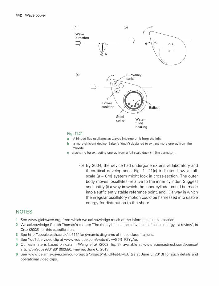
442 Wave power
(b) By 2004, the device had undergone extensive laboratory and theoretical development. Fig. 11.21(c) indicates how a full-scale (a ~ 8m) system might look in cross-section. The outer body moves (oscillates) relative to the inner cylinder. Suggest and justify (i) a way in which the inner cylinder could be made into a sufficiently stable reference point, and (ii) a way in which the irregular oscillatory motion could be harnessed into usable energy for distribution to the shore.
NOTES
1 See www.globwave.org, from which we acknowledge much of the information in this section.2 We acknowledge Gareth Thomas’s chapter ‘The theory behind the conversion of ocean energy – a review’, in
Cruz (2008) for this classification.3 See http://people.bath.ac.uk/sb515/ for dynamic diagrams of these classifications.4 See YouTube video clip at www.youtube.com/watch?v=vG6R_R2YyAo.5 Our estimate is based on data in Wang et al. (2002, fig. 3), available at www.sciencedirect.com/science/
article/pii/S0029801801000580, (viewed June 6, 2013).6 See www.pelamiswave.com/our-projects/project/1/E.ON-at-EMEC (as at June 5, 2013) for such details and
operational video clips.
Fig. 11.21a A hinged flap oscillates as waves impinge on it from the left; b a more efficient device (Salter’s ‘duck’) designed to extract more energy from the
waves; c a scheme for extracting energy from a full-scale duck (~10m diameter).
(a) (b)
Buoyancytanks
Ballast
Water-filledbearing
Steelspine
Powercanister
Wavedirection
(c)
o' +
o +A
θ
TWIDELL PAGINATION.indb 442 01/12/2014 11:38

Bibliography 443
BIBLIOGRAPHY
General
Brooke, J. (ed.) for Engineering Committee on Oceanic Resources (2003) Wave Energy Conversion, Elsevier, Oxford. Excellent survey of the then state of the art with supporting theory and descriptions of installations and prototypes.
Carbon Trust (2006) Ocean Energy and Wave Energy Device Design; and (2012) UK Wave Energy Resource. These and numerous other reports on wave power and tidal power, with special reference to the UK, are avail-able at http://www.carbontrust.com/resources/reports/technology/marine-energy/.
Cruz, J. (2008) Ocean Wave Energy: Current status and future perspectives, Springer-Verlag, Berlin. In English: a series of edited chapters by experts currently working on operational devices; includes both theory and practical detail.
Enferad, E. and Nazarpour, D. (2013) Case Study Waves, ch. 12 in Ocean’s Renewable Power and Review of Technologies, pp. 273–300, Intech Open Source at: http://cdn.intechopen.com/pdfs/42182/, viewed June 6, 2013. Excellent review outlining theory and describing influential applications.
Falnes, J. (2002) Ocean Waves and Oscillating Systems, Cambridge University Press, Cambridge. Thorough physical analysis of waves and the extraction of wave power; research level.
McCormick, M. (1971) Ocean Wave Energy Conversion, Wiley, Chichester (1981) (reprinted in 2007 by Dover Books). Engineering guide, with basic physical analysis.
Mei, C.C. (1989, revised edn 2005) The Applied Dynamics of Ocean Surface Waves, World Scientific Publishing Co. Pte. Ltd., Singapore. Rigorous theory.
Stevens, C., Smith, M. and Gorman, R. (2005) ‘Ocean bounty: energy from waves and tides’., Water & Atmosphere, 13(4).
Historical interest
Energy Technology Support Unit (1992) Wave Energy Review, ETSU, AEA Harwell, UK.
NEL (1976) The Development of Wave Power – A techno-economic Study, by Leishman, J.M. and Scobie, G. of the National Engineering Laboratory, East Kilbride, Glasgow, Report EAU M25.
Ross, D. (1995) Power from the Waves, Oxford University Press, Oxford. Journalistic account of the history of wave energy, especially including the machinations of wave energy politics in the UK. Incorporates and extends the author’s earlier book Energy from the Waves (1979), Pergamon, Oxford.
Specific references
Bevilacqua, G. and Zanuttigh, B. (2011) ‘Overtopping wave energy converters: general aspects and stage of development’, AMS Acta ISSN: 2038-7954 Contributi di ricerca dell’Alma Mater Studiorum – Università di Bologna; see http://amsacta.unibo.it/3062/1/overtopping_devicex.pdf (viewed June 6, 2013).
Coulson, C.A. and Jeffrey, A. (1977) Waves, Longman, London. Didactic theoretical text, partly considering water waves; beautifully written and clear. Available as free download on internet in 2013.
Glendenning, I. (1977) ‘Energy from the sea’, Chemistry and Industry, 592–599.
TWIDELL PAGINATION.indb 443 01/12/2014 11:38

444 Wave power
Salter, S.H. (1974) ‘Wave power’, Nature, 249, 720–724. Now seen as a classic paper for wave power. Later papers deal with the ‘Salter duck’ developments.
Shaw, R. (1982) Wave Energy – A Design Challenge, Ellis Horwood, Chichester, and Halstead Press, New York.
Wang, D.J., Katory, M. and Li, Y.S. (2002) ‘Analytical and experimental investigation on the hydrodynamic perfor-mance of onshore wave-power devices’, Ocean Engineering, 29, 871–885.
Journals and websites
Wave power development is published in a range of engineering and marine science journals. In addition, most analysis is reported in conferences and specialist seminars. Particularly useful are the biennial European Wave and Tidal Energy Conferences (EWTEC, www.ewtec.org). Commercial activity is being encouraged within the ambit of RenewableUK (previously the British Wind Energy Association (BWEA) (www.bwea.com). The websites of device developers are often informative (e.g. Ocean Power Delivery (re the Pelamis) at www.oceanpd.com, and Wavegen (re the Limpet) at www.wavegen.co.uk. Other useful sites include: wikipedia (http://en.wikipedia.org/wiki/Wave_power).
Falnes’ lecture on mechanics of waves and power extraction is at http://folk.ntnu.no/falnes/teach/wave/JF_intro-duction2010-06-28.pdf.
ACKNOWLEDGMENT
The authors thank Professor Falnes of Norway for his helpful comments on this chapter.
TWIDELL PAGINATION.indb 444 01/12/2014 11:38
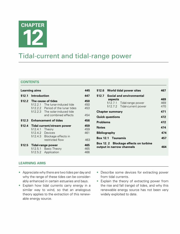
Tidal-current and tidal-range power
CONTENTS
Learning aims 445
§12.1 Introduction 447
§12.2 The cause of tides 450 §12.2.1 The lunar-induced tide 450 §12.2.2 Period of the lunar tides 453 §12.2.3 The solar-induced tide
and combined effects 454
§12.3 Enhancement of tides 456
§12.4 Tidal current/stream power 459 §12.4.1 Theory 459 §12.4.2 Devices 461 §12.4.3 Blockage effects in
restricted flow 463
§12.5 Tidal-range power 465 §12.5.1 Basic Theory 465 §12.5.2 Application 466
§12.6 World tidal power sites 467
§12.7 Social and environmental aspects 469
§12.7.1 Tidal-range power 469 §12.7.2 Tidal-current power 470
Chapter summary 471
Quick questions 472
Problems 472
Notes 474
Bibliography 474
Box 12.1 Tsunamis 457
Box 12. 2 Blockage effects on turbine output in narrow channels 464
CHAPTER
12
LEARNING AIMS
• Appreciate why there are two tides per day and why the range of these tides can be consider-ably enhanced in certain estuaries and bays.
• Explain how tidal currents carry energy in a similar way to wind, so that an analogous theory applies to the extraction of this renew-able energy source.
• Describe some devices for extracting power from tidal currents.
• Explain the theory of extracting power from the rise and fall (range) of tides, and why this renewable energy source has not been very widely exploited to date.
TWIDELL PAGINATION.indb 445 01/12/2014 11:38

446 Tidal-current and tidal-range power
LIST OF FIGURES
12.1 Regions of high tidal range. 44912.2 Motion of the Moon and the Earth. 45112.3 Basic physical explanation of the semi-diurnal and diurnal tide. 45212.4 Comparison of three different ‘days’ that may be observed from Earth: (a) sidereal and solar day;
(b) sidereal and lunar. 45312.5 (a) Sinusoidal variation of tidal range.
(b) Tidal range variation for one month for a regular semi-diurnal tide. (c) Positions of the Sun, Moon, and Earth. 455
12.6 Motion of water in a tidal wave. 45712.7 Resonant enhancement of a tidal wave in an estuary. 45812.8 Some representative devices for harnessing tidal current power. 46212.9 Illustrating the effect on mean flow of blockage by a turbine in a channel. 46412.10 Power generation from tidal range. 465
LIST OF TABLES
12.1 Major world tidal power sites and stations 467
TWIDELL PAGINATION.indb 446 01/12/2014 11:38
§12.1 Introduction 447
§12.1 INTRODUCTION
The level of water in oceans rises and falls predictably as tides due to the relative positions of the Sun, Earth and Moon. Since the astronomical periodicities are known accurately and the effects of particular coast-lines remain constant, the prediction of tidal rhythms and amplitudes is mathematically exact. The main periods t of tides are diurnal at about 24 hours and semi-diurnal at about 12 hours 25 minutes. The change in height between successive high and low tides is the tidal range, R. This varies between about 0.6 m in mid-ocean to about 10 m at a few locations of continental land masses. The movement of the water pro-duces periodic tidal currents, which may reach peak speeds of ~5 m/s in coastal and inter-island channels. The increased tidal flow and tidal range at specific locations permit two distinct technologies for electricity gen-eration, namely (a) tidal-current power (also called tidal-stream power), and (b) tidal-range power. We consider both technologies in this chapter, despite their considerable differences.
Tidal currents may be harnessed with some devices in a manner similar to wind, though, unlike wind, tidal currents are predictable in amplitude and frequency. Thus, as is shown in §12.4.1, for peak flow rate umax, sea water density r and assuming 40% conversion to electricity, the average power generated per unit area of capture is:
r≈q u0.1 max3 (12.1)
For example, for umax = 3 m/s, q ~14 kW/m2. Power generation is only attractive where tidal currents are relatively rapid because of (a) relatively large tidal range, and/or (b) enhanced speed of water movement in straits near islands, or at estuarine or lagoon inlets. Thus tidal current power is very site specific.
Tidal-current generating plant may be constructed offsite as a standard module. This may then be positioned on site without significant civil works to operate individually or as a group across a tidal flow. Various tidal-current systems are being developed with financial support from governments and venture capital, as outlined in §12.4.2. Many projects have been supported by the European Union and by UK authorities.
Tidal-current technological development today may be compared with that of wind technology in the late 1970s and early 1980s, when many different forms of wind turbine were being studied and before standard commercial models evolved. As the push for sustainable, emission-free electricity generation continues, the next 20 years will clarify the technol-ogy choices and see increased application.
Tidal range is harnessed for power generation by trapping water behind a dam (usually called a barrage) at high tide in an estuarine basin of area A behind a dam or barrier. If the water of density r runs out
TWIDELL PAGINATION.indb 447 01/12/2014 11:38

448 Tidal-current and tidal-range power
through turbines at low tide of period t, the average power produced (§12.5.1) is:
P = rAR 2g/(2t) (12.2)
For example, if A = 10 km2, R = 4 m, t = 12 h 25 min, then P = 17 MW. Obviously sites of large range give the greatest potential for tidal power, but other vital factors are the opportunities to integrate the power within a network, and the costs and secondary benefits of the construction. Thus the development of tidal range power is also very site-specific.
Tidal-range power was used historically for small mechanical power devices (e.g. in medieval England and in China), but modern interest focuses on large-scale electricity production. The best-known system is the 240 MWe ‘La Rance’ system at an estuary into the Gulf of St. Malo in Brittany, France, which has operated reliably since 1967, so proving the technical feasibility of this technology on a large scale. Usually the barrage extends completely across the tidal inlet, but may be used as a road or rail crossing, as at ‘La Rance’. If ships have to pass, a lock is built into the barrage. Therefore upfront costs, especially for the civil engi-neering, are large and usually require government funding, but opera-tional costs are small for a lifetime of at least 100 years. The effect of a barrage is likely to have considerable environmental impact as estuar-ies with large tidal range tend at low water to have extensive mudflats and wetlands with distinctive flora and fauna, especially wading birds. Despite feasibility studies over the past 100 years concluding that sub-stantial electricity generation is possible from the relatively few sites with large tidal range (e.g. the Severn Estuary in Britain could produce 10% of national electricity: see Fig. 12.1), the implications of capital cost and environmental impact have meant that very few tidal range systems have been implemented at a significant scale.
The range, flow and periodic behavior of tides at most coastal regions are well documented and analyzed because of the demands of naviga-tion and oceanography. The behavior may be predicted accurately, within an uncertainty of less than ±4%, and so tidal power is a very reliable and sustainable source of clean power, which is a major advantage compared with other energy sources.
The major challenges for all forms of tidal power are as follows:
1 Only a few sites are suitable, and these may be distant from the demand for power.
2 The mismatch of the principal lunar-driven periods of 12 hours 25 minutes and 24 hours 50 minutes with the human (solar) period of 24 hours, so that optimum tidal power generation is not in phase with demand.
As noted above, tidal-range power (but not tidal-current power) also suffers from the following:
TWIDELL PAGINATION.indb 448 01/12/2014 11:38

§12.1 Introduction 449
3 The requirement for large water volume flow at low head, necessitat-ing many specially constructed turbines set in parallel.
4 The very large capital costs of most potential installations.5 Potential ecological harm and disruption to extensive estuaries or
marine regions.
For optimum electrical power generation from tides, the turbines should be operated in a regular and repeatable manner. The mode of operation will depend on the scale of the power plant, and the demand and avail-ability of other sources. Very many variations are possible, but certain generalizations apply:
a If the tidal generated electricity is for local use, then other assured power supplies must exist when the tidal power is unavailable.
b If the generated electricity can feed into a large grid and so form a proportionately minor source within a national system, then the pre-dictable tidal power variations can be submerged into the national demand.
–90180 90
Lati
tud
e ø
/deg
rees
Latitude λ /degrees
0 90 180
–60
–30
0
30
609m
57 GW 11m29 GW
10m2 GW 8m
11 GW
7m16 GW
6m6 GW
5m
5m
7m
6m
5m
7m
90
Fig. 12.1Regions of high tidal range (in dark green). For some regions, also indicated is the mean tidal range and mean technical potential for tidal power in bays and estuaries (black dots) along that coast. Regions of high tidal range are necessarily also regions of high tidal current, but some specific sites (e.g. between islands, as in Indonesia) have strong tidal currents even without high tidal range.Source: Adapted from OpenHydro.com and Sørensen (2011).
TWIDELL PAGINATION.indb 449 01/12/2014 11:38
450 Tidal-current and tidal-range power
c If the immediate demand is not fixed to the human (solar) period of 24 hours, then the tidal power can be used whenever available. For instance, if the electrical power produces a fuel (e.g. hydrogen) or provides water desalination (e.g. by reverse osmosis), then such a decoupling of supply and use may occur.
The following sections outline the physical understanding of tides and tidal power. Readers interested only in power generating installations should turn directly to §12.4 and §12.5. Social and environmental aspects of the technologies are outlined in §12.7.
§12.2 THE CAUSE OF TIDES1
The analysis of tidal behavior has been developed by many notable mathematicians and applied physicists, including Newton, Airy, Laplace, George Darwin (son of Charles Darwin) and Kelvin. We shall use Newton’s physical theory to explain the phenomena of tides. However, present-day analysis and prediction depend on the mathematical method of harmonic analysis developed by Lord Kelvin in Glasgow. A complete physical understanding of tidal dynamics has not yet been attained, owing to the topological complexity of the ocean basins. This section gives only a basic account.
The seas are liquids held on the solid surface of the rotating Earth by gravity. The gravitational attraction of the Earth with the Moon and the Sun perturbs these forces and motions so that tides are produced. Tidal power is derived from turbines set in this liquid, so harnessing the kinetic energy of the rotating Earth. Even if all the world’s major tidal power sites were utilized, this would lead to an extra slowing of the Earth’s rotation by no more than one day in 2000 years; this is not a significant extra effect.
§12.2.1 The lunar-induced tide
The Moon and the Earth revolve about each other in space (Fig. 12.2), but since the mass of the Earth is nearly 100 times greater than the Moon’s mass, the Moon’s motion is more apparent. The center of revolution is at O, such that:
= ′ ′ML M L
′ = ′ +L MD M M/ ( ) (12.3)
′ =L 4670 km.
The Earth’s mean radius is 6371 km, so the point of revolution O is inside the surface of the Earth.
TWIDELL PAGINATION.indb 450 01/12/2014 11:38
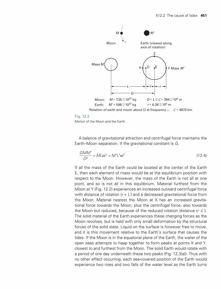
§12.2 The cause of tides 451
A balance of gravitational attraction and centrifugal force maintains the Earth–Moon separation. If the gravitational constant is G,
w w′= = ′ ′
GMMD
ML M L2
2 2 (12.4)
If all the mass of the Earth could be located at the center of the Earth E, then each element of mass would be at the equilibrium position with respect to the Moon. However, the mass of the Earth is not all at one point, and so is not all in this equilibrium. Material furthest from the Moon at Y (Fig. 12.2) experiences an increased outward centrifugal force with distance of rotation (r + L’) and a decreased gravitational force from the Moon. Material nearest the Moon at X has an increased gravita-tional force towards the Moon, plus the centrifugal force, also towards the Moon but reduced, because of the reduced rotation distance (r -L’). The solid material of the Earth experiences these changing forces as the Moon revolves, but is held with only small deformation by the structural forces of the solid state. Liquid on the surface is however free to move, and it is this movement relative to the Earth’s surface that causes the tides. If the Moon is in the equatorial plane of the Earth, the water of the open seas attempts to heap together to form peaks at points X and Y, closest to and furthest from the Moon. The solid Earth would rotate with a period of one day underneath these two peaks (Fig. 12.3(a)). Thus with no other effect occurring, each sea-covered position of the Earth would experience two rises and two falls of the water level as the Earth turns
Fig. 12.2Motion of the Moon and the Earth.
Moon:
Moon
X
Z
O E Y Mass M’
M
M
M’
Mass
Earth (viewed alongaxis of rotation)
M = 7.35 × 10²² kg
M’ = 598 × 1022 kg
D = L + L’ = 384 × 106 m
r = 6.38 × 10⁶ mEarth:
L’ = 4670 kmRotation of earth and moon about O at frequency ω.
L
D
rL’
ω
TWIDELL PAGINATION.indb 451 01/12/2014 11:38
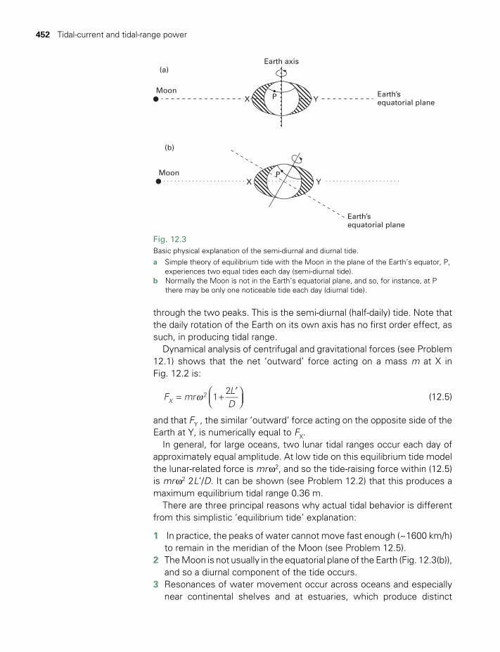
452 Tidal-current and tidal-range power
through the two peaks. This is the semi-diurnal (half-daily) tide. Note that the daily rotation of the Earth on its own axis has no first order effect, as such, in producing tidal range.
Dynamical analysis of centrifugal and gravitational forces (see Problem 12.1) shows that the net ‘outward’ force acting on a mass m at X in Fig. 12.2 is:
w= +′
F mrLD
12
X2 (12.5)
and that FY , the similar ‘outward’ force acting on the opposite side of the Earth at Y, is numerically equal to FX.
In general, for large oceans, two lunar tidal ranges occur each day of approximately equal amplitude. At low tide on this equilibrium tide model the lunar-related force is mr w2, and so the tide-raising force within (12.5) is mr w2 2L’/D. It can be shown (see Problem 12.2) that this produces a maximum equilibrium tidal range 0.36 m.
There are three principal reasons why actual tidal behavior is different from this simplistic ‘equilibrium tide’ explanation:
1 In practice, the peaks of water cannot move fast enough (~1600 km/h) to remain in the meridian of the Moon (see Problem 12.5).
2 The Moon is not usually in the equatorial plane of the Earth (Fig. 12.3(b)), and so a diurnal component of the tide occurs.
3 Resonances of water movement occur across oceans and especially near continental shelves and at estuaries, which produce distinct
Fig. 12.3Basic physical explanation of the semi-diurnal and diurnal tide. a Simple theory of equilibrium tide with the Moon in the plane of the Earth’s equator, P,
experiences two equal tides each day (semi-diurnal tide).b Normally the Moon is not in the Earth’s equatorial plane, and so, for instance, at P
there may be only one noticeable tide each day (diurnal tide).
Moon
(a)
(b)
X
X
Y
Y
P
PMoon
Earth axis
Earth’sequatorial plane
Earth’sequatorial plane
TWIDELL PAGINATION.indb 452 01/12/2014 11:38
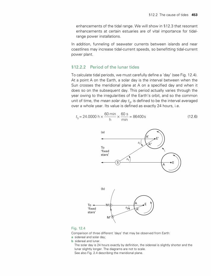
§12.2 The cause of tides 453
enhancements of the tidal range. We will show in §12.3 that resonant enhancements at certain estuaries are of vital importance for tidal-range power installations.
In addition, funneling of seawater currents between islands and near coastlines may increase tidal-current speeds, so benefitting tidal-current power plant.
§12.2.2 Period of the lunar tides
To calculate tidal periods, we must carefully define a ‘day’ (see Fig. 12.4). At a point A on the Earth, a solar day is the interval between when the Sun crosses the meridional plane at A on a specified day and when it does so on the subsequent day. This period actually varies through the year owing to the irregularities of the Earth’s orbit, and so the common unit of time, the mean solar day tS, is defined to be the interval averaged over a whole year. Its value is defined as exactly 24 hours, i.e.
× ×t = 24.0000 h60 min
h60 smin
= 86400sS (12.6)
Fig. 12.4Comparison of three different ‘days’ that may be observed from Earth:a sidereal and solar day;b sidereal and lunar. The solar day is 24 hours exactly by definition, the sidereal is slightly shorter and the
lunar slightly longer. The diagrams are not to scale. See also Fig. 2.4 describing the meridional plane.
To‘fixedstars’
To‘fixedstars’
M
(a)
(b)
A’θ2
θ1
θ1
EA
SA
E
E’
A’’
A’
M’
TWIDELL PAGINATION.indb 453 01/12/2014 11:38
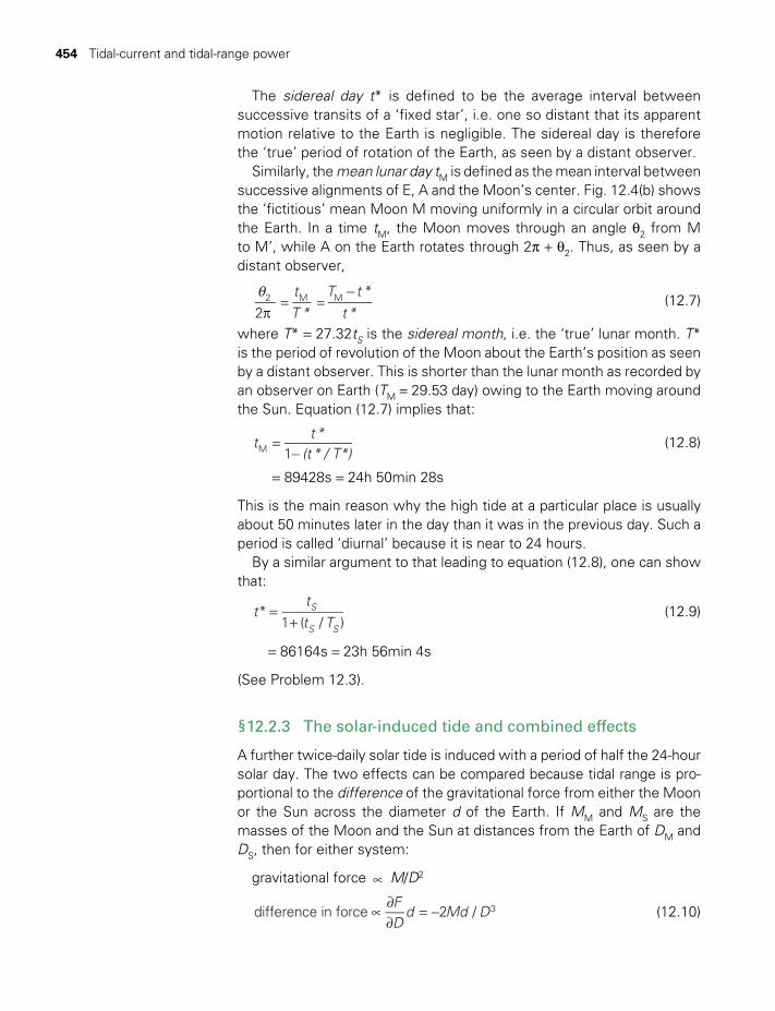
454 Tidal-current and tidal-range power
The sidereal day t* is defined to be the average interval between successive transits of a ‘fixed star’, i.e. one so distant that its apparent motion relative to the Earth is negligible. The sidereal day is therefore the ‘true’ period of rotation of the Earth, as seen by a distant observer.
Similarly, the mean lunar day tM is defined as the mean interval between successive alignments of E, A and the Moon’s center. Fig. 12.4(b) shows the ‘fictitious’ mean Moon M moving uniformly in a circular orbit around the Earth. In a time tM, the Moon moves through an angle q2 from M to M’, while A on the Earth rotates through 2p + q2. Thus, as seen by a distant observer,
qp
−tT *
T t*t*2
= =2 M M (12.7)
where T* = 27.32tS is the sidereal month, i.e. the ‘true’ lunar month. T* is the period of revolution of the Moon about the Earth’s position as seen by a distant observer. This is shorter than the lunar month as recorded by an observer on Earth (TM = 29.53 day) owing to the Earth moving around the Sun. Equation (12.7) implies that:
−t
t*(t* / T*)
=1M (12.8)
= 89428s = 24h 50min 28s
This is the main reason why the high tide at a particular place is usually about 50 minutes later in the day than it was in the previous day. Such a period is called ‘diurnal’ because it is near to 24 hours.
By a similar argument to that leading to equation (12.8), one can show that:
=+
tt
t T*
1 ( / )S
S S
(12.9)
= 86164s = 23h 56min 4s
(See Problem 12.3).
§12.2.3 The solar-induced tide and combined effects
A further twice-daily solar tide is induced with a period of half the 24-hour solar day. The two effects can be compared because tidal range is pro-portional to the difference of the gravitational force from either the Moon or the Sun across the diameter d of the Earth. If MM and MS are the masses of the Moon and the Sun at distances from the Earth of DM and DS, then for either system:
gravitational force ∝ M/D2
∝∂∂
= −FD
d Md Ddifference in force 2 / 3 (12.10)
TWIDELL PAGINATION.indb 454 01/12/2014 11:38
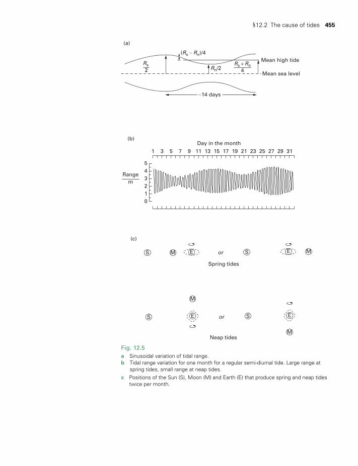
§12.2 The cause of tides 455
(a)
(b)
(c)
S
S
Sor
M
Neap tidesM
M S
Spring tides
EE
E E
Mor
1
012345
3 5 7 9 11 13 15 17 19 21 23 25 27 29 31
Day in the month
∼14 days
Mean sea level
Mean high tide(Rs − Rn)/4
Rn/2 4Rs + Rn
mRange
2Rs
Fig. 12.5a Sinusoidal variation of tidal range. b Tidal range variation for one month for a regular semi-diurnal tide. Large range at
spring tides, small range at neap tides. c Positions of the Sun (S), Moon (M) and Earth (E) that produce spring and neap tides
twice per month.
TWIDELL PAGINATION.indb 455 01/12/2014 11:38
456 Tidal-current and tidal-range power
The ratio of the lunar range RM and solar range RS is therefore:
=
RR
(M / D )(M / D )
=D
DMM
M
S
M M3
S S3
S
M
3
M
S
(12.11)
××
××
==1.50 10 m3.84 10 m
7.35 10 kg1.99 10 kg
2.211
8
3 22
30
i.e. the range of the solar tide is 2.2 times less than the range of the lunar tide, which therefore predominates.
The solar tide moves in and out of phase with the lunar tide. When the Sun, Earth and Moon are aligned in conjunction, the lunar and solar tides are in phase, so producing tides of maximum range. These are named ‘spring tides’ of maximum range occurring twice per lunar (synodic) month at times of both full and new Moons (Fig. 12.5).
When the Sun/Earth and Moon/Earth directions are perpendicular (in quadrature) the ranges of the tides are least. These are named ‘neap tides’ that again occur twice per synodic month. If the spring tide is con-sidered to result from the sum of the lunar and solar tides, and the neap tide from the difference, then the ratio of spring to neap ranges might be expected to be:
=+−
=R
R
(spring)
(neap)1 (1/ 2.2)1 (1/ 2.2)
2.6s
n
(12.12)
In practice, dynamical and local effects alter this rather naive model, and the ratio of spring to neap range is more frequently about 2.0. Spring tides at the Moon’s perigee have greater range than spring tides at apogee, and a combination of effects, including wind, may occur to cause unusu-ally high tides.
§12.3 ENHANCEMENT OF TIDES
In mid-ocean the tidal range is only about 0.6 m and tidal currents are negligible, so power generation is totally unrealistic. However, near many estuaries and some other natural features, enhancement of the tidal range and tidal currents may occur by: (1) funneling of the tides (as with soundwaves in an old-fashioned trumpet-shaped hearing aid); (2)˛flow perturbation near islands and irregular coastlines, and (3) resonant cou-pling to natural frequencies of water movement in coastal contours and estuaries. This local enhancement is essential for tidal power potential; we stress this point most strongly.
Ordinary tidal-induced movement of water in the sea has the form of a particular type of perturbation called a ‘tidal wave’. The whole column of water from surface to sea bed may propagate in unison (Fig. 12.6). The
TWIDELL PAGINATION.indb 456 01/12/2014 11:38
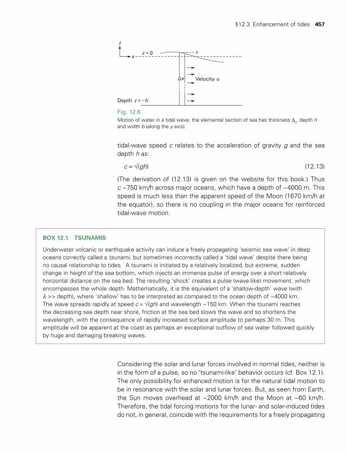
§12.3 Enhancement of tides 457
tidal-wave speed c relates to the acceleration of gravity g and the sea depth h as:
c = √(gh) (12.13)
(The derivation of (12.13) is given on the website for this book.) Thus c ~750 km/h across major oceans, which have a depth of ~4000 m. This speed is much less than the apparent speed of the Moon (1670 km/h at the equator), so there is no coupling in the major oceans for reinforced tidal-wave motion.
Fig. 12.6Motion of water in a tidal wave; the elemental section of sea has thickness Dx, depth h and width b (along the y axis).
Depth
Velocity u∆x
z = −h
z
zx
z = 0
BOX 12.1 TSUNAMIS
Underwater volcanic or earthquake activity can induce a freely propagating ‘seismic sea wave’ in deep oceans correctly called a tsunami, but sometimes incorrectly called a ‘tidal wave’ despite there being no causal relationship to tides. A tsunami is initiated by a relatively localized, but extreme, sudden change in height of the sea bottom, which injects an immense pulse of energy over a short relatively horizontal distance on the sea bed. The resulting ‘shock’ creates a pulse (wave-like) movement, which encompasses the whole depth. Mathematically, it is the equivalent of a ‘shallow-depth’ wave (with l >> depth), where ‘shallow’ has to be interpreted as compared to the ocean depth of ~4000 km. The wave spreads rapidly at speed c = √(gh) and wavelength ~150 km. When the tsunami reaches the decreasing sea depth near shore, friction at the sea bed slows the wave and so shortens the wavelength, with the consequence of rapidly increased surface amplitude to perhaps 30 m. This amplitude will be apparent at the coast as perhaps an exceptional outflow of sea water followed quickly by huge and damaging breaking waves.
Considering the solar and lunar forces involved in normal tides, neither is in the form of a pulse, so no ‘tsunami-like’ behavior occurs (cf. Box 12.1). The only possibility for enhanced motion is for the natural tidal motion to be in resonance with the solar and lunar forces. But, as seen from Earth, the Sun moves overhead at ~2000 km/h and the Moon at ~60 km/h. Therefore, the tidal forcing motions for the lunar- and solar-induced tides do not, in general, coincide with the requirements for a freely propagating
TWIDELL PAGINATION.indb 457 01/12/2014 11:38
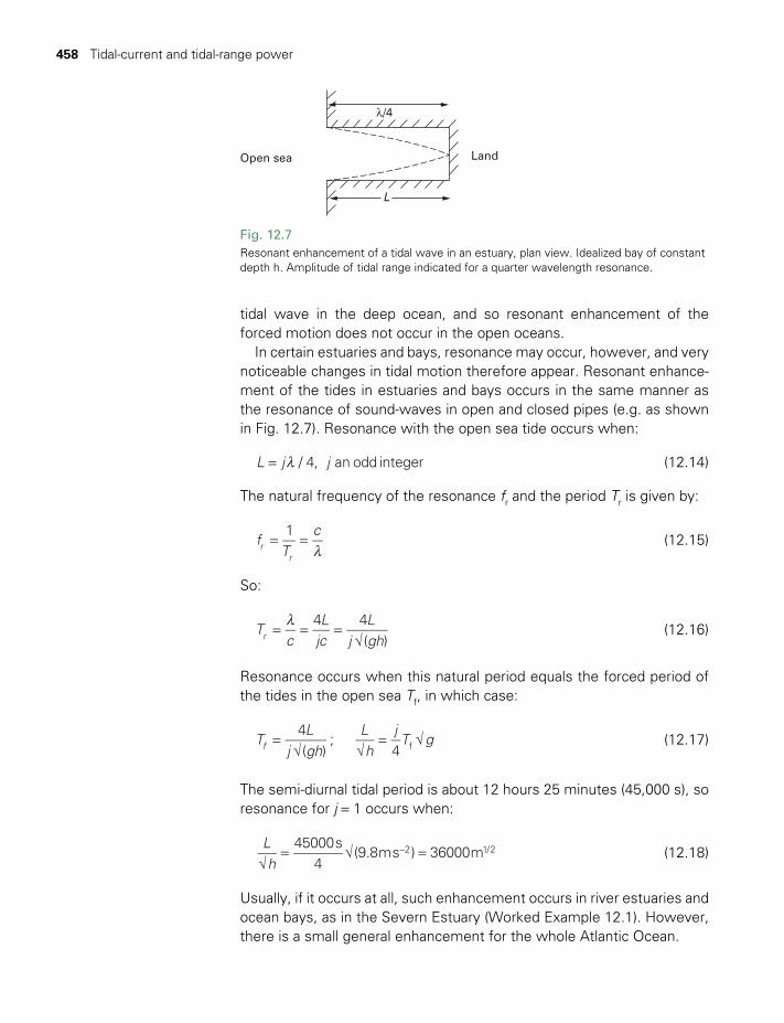
458 Tidal-current and tidal-range power
tidal wave in the deep ocean, and so resonant enhancement of the forced motion does not occur in the open oceans.
In certain estuaries and bays, resonance may occur, however, and very noticeable changes in tidal motion therefore appear. Resonant enhance-ment of the tides in estuaries and bays occurs in the same manner as the resonance of sound-waves in open and closed pipes (e.g. as shown in Fig. 12.7). Resonance with the open sea tide occurs when:
l=L j j/ 4, an odd integer (12.14)
The natural frequency of the resonance fr and the period Tr is given by:
l= =f
Tc1
rr
(12.15)
So:
l= = =
√T
cL
jcL
j gh4 4
( )r (12.16)
Resonance occurs when this natural period equals the forced period of the tides in the open sea Tf, in which case:
=√ √
= √TL
j ghLh
jT g
4( )
;4f f (12.17)
The semi-diurnal tidal period is about 12 hours 25 minutes (45,000 s), so resonance for j = 1 occurs when:
√= √ =−L
h45000s
4(9.8ms ) 36000m2 1/2 (12.18)
Usually, if it occurs at all, such enhancement occurs in river estuaries and ocean bays, as in the Severn Estuary (Worked Example 12.1). However, there is a small general enhancement for the whole Atlantic Ocean.
Open sea Land
L
λ/4
Fig. 12.7Resonant enhancement of a tidal wave in an estuary, plan view. Idealized bay of constant depth h. Amplitude of tidal range indicated for a quarter wavelength resonance.
TWIDELL PAGINATION.indb 458 01/12/2014 11:38
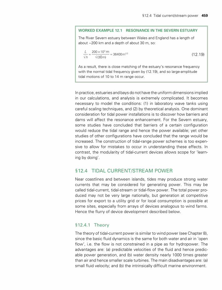
§12.4 Tidal current/stream power 459
WORKED EXAMPLE 12.1 RESONANCE IN THE SEVERN ESTUARY
The River Severn estuary between Wales and England has a length of about ~200 km and a depth of about 30 m, so:
√≈
×√
≈L m
0h
200 10
(3 m)36400m
31/2 (12.19)
As a result, there is close matching of the estuary’s resonance frequency with the normal tidal frequency given by (12.19), and so large-amplitude tidal motions of 10 to 14 m range occur.
In practice, estuaries and bays do not have the uniform dimensions implied in our calculations, and analysis is extremely complicated. It becomes necessary to model the conditions: (1) in laboratory wave tanks using careful scaling techniques, and (2) by theoretical analysis. One dominant consideration for tidal power installations is to discover how barriers and dams will affect the resonance enhancement. For the Severn estuary, some studies have concluded that barriers of a certain configuration would reduce the tidal range and hence the power available; yet other studies of other configurations have concluded that the range would be increased. The construction of tidal-range power schemes is too expen-sive to allow for mistakes to occur in understanding these effects. In contrast, the modularity of tidal-current devices allows scope for ‘learn-ing by doing’.
§12.4 TIDAL CURRENT/STREAM POWER
Near coastlines and between islands, tides may produce strong water currents that may be considered for generating power. This may be called tidal-current, tidal-stream or tidal-flow power. The total power pro-duced may not be very large nationally, but generation at competitive prices for export to a utility grid or for local consumption is possible at some sites, especially from arrays of devices analogous to wind farms. Hence the flurry of device development described below.
§12.4.1 Theory
The theory of tidal-current power is similar to wind power (see Chapter 8), since the basic fluid dynamics is the same for both water and air in ‘open flow’, i.e. the flow is not constrained in a pipe as for hydropower. The advantages are: (a) predictable velocities of the fluid and hence predic-able power generation, and (b) water density nearly 1000 times greater than air and hence smaller scale turbines. The main disadvantages are: (a) small fluid velocity; and (b) the intrinsically difficult marine environment.
TWIDELL PAGINATION.indb 459 01/12/2014 11:38
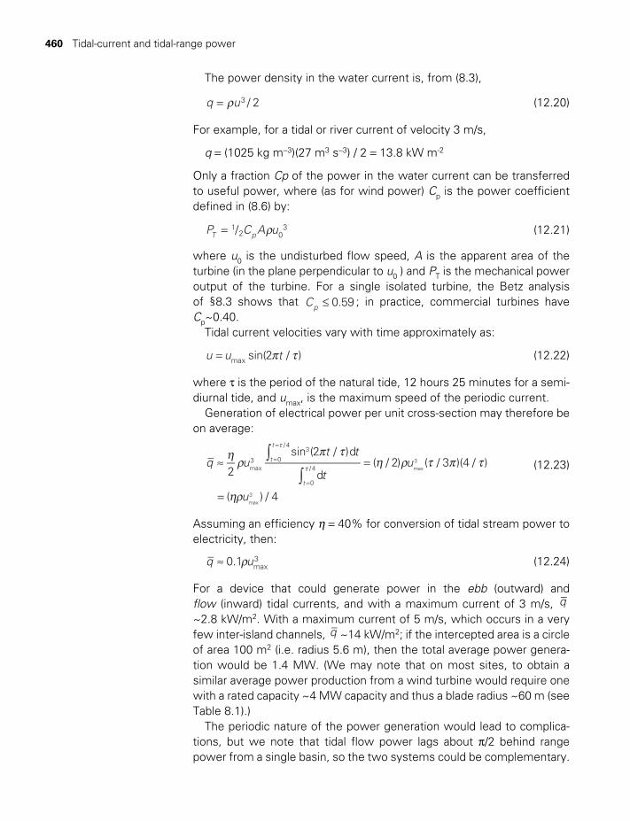
460 Tidal-current and tidal-range power
The power density in the water current is, from (8.3),
r=q u / 23 (12.20)
For example, for a tidal or river current of velocity 3 m/s,
q = (1025 kg m−3)(27 m3 s−3) / 2 = 13.8 kW m-2
Only a fraction Cp of the power in the water current can be transferred to useful power, where (as for wind power) Cp is the power coefficient defined in (8.6) by:
r=P C A u/T p1
2 03 (12.21)
where u0 is the undisturbed flow speed, A is the apparent area of the turbine (in the plane perpendicular to u0 ) and PT is the mechanical power output of the turbine. For a single isolated turbine, the Betz analysis of §8.3 shows that ≤C 0.59p ; in practice, commercial turbines have Cp~0.40.
Tidal current velocities vary with time approximately as:
p t=u u tsin(2 / )max (12.22)
where t is the period of the natural tide, 12 hours 25 minutes for a semi-diurnal tide, and umax, is the maximum speed of the periodic current.
Generation of electrical power per unit cross-section may therefore be on average:
∫∫
h rp t
h r t p t≈ =
t
t=
=
=
q ut t
tu
2
sin (2 / )d
d( / 2) ( / 3 )(4 / )t
t
t
max3
3
0
/ 4
0
/ 4 max3 (12.23)
hr= u( ) / 4max3
Assuming an efficiency h = 40% for conversion of tidal stream power to electricity, then:
r≈q u0.1 max3 (12.24)
For a device that could generate power in the ebb (outward) and flow (inward) tidal currents, and with a maximum current of 3 m/s, q ~2.8 kW/m2. With a maximum current of 5 m/s, which occurs in a very few inter-island channels, q ~14 kW/m2; if the intercepted area is a circle of area 100 m2 (i.e. radius 5.6 m), then the total average power genera-tion would be 1.4 MW. (We may note that on most sites, to obtain a similar average power production from a wind turbine would require one with a rated capacity ~4 MW capacity and thus a blade radius ~60 m (see Table 8.1).)
The periodic nature of the power generation would lead to complica-tions, but we note that tidal flow power lags about p/2 behind range power from a single basin, so the two systems could be complementary.
TWIDELL PAGINATION.indb 460 01/12/2014 11:38

§12.4 Tidal current/stream power 461
§12.4.2 Devices
At the present time, tidal current power is not a generally proven com-mercial technology. Most types of device are developmental; however, some prototypes with capacities up to ~2 MW have been generating into a grid routinely, with plans to scale up into arrays similar to wind farms (see Table 12.1 in §12.6). Examples are given below of each of several device classes.
Many of the water current energy conversion systems resemble wind turbine generators. However, marine turbines must be designed for reversing flows, cavitation and harsh underwater marine conditions (e.g. salt water corrosion, debris, fouling, etc.). Axial-flow turbines must be able to respond to reversing flow directions, while cross-flow turbines in an adjustable enclosure continue to operate regardless of current flow direction. Axial-flow turbines either reverse nacelle direction about 180° with alternate tides or, alternatively, the nacelle has a fixed position with the rotor blades changing pitch to accept reversing flow. An important design consideration is allowing for maintenance (e.g. having the active part of the system rise out of the water on its supports).
(a) Class 1: Horizontal axisThe majority of tidal-current devices in operation are of this type, with several of the more promising start-up companies now taken over by major suppliers of electricity-generating equipment, whose engineers and financiers use their previous experience of wind and hydro turbines.
The world’s first commercial tidal-current turbine exporting electric-ity to the grid network has operated at the sea mouth of Strangford Lough in Northern Ireland since 2008. In essence there are two horizon-tal axis twin-bladed turbine generators held on a horizontal arm that can be raised out of the water for installation and maintenance (Fig. 12.8(a)). The pitch of the blades is adjusted to suit either the ebb or flow condi-tions of the tidal cycle. The fluid-dynamics of this water turbine is similar to that of a horizontal axis wind turbine (see Chapter 8). For instance, the tip-speed ratio (ratio of blade-tip speed in the water to the speed of the water current) has to be optimized and remain constant as the water speed changes.
Rotor shrouds (also known as cowlings or ducts) enhance hydro-dynamic performance by increasing the flow velocity through the rotor and reducing tip losses (for the reasons given in Box 12.2). Several prom-ising devices (e.g. that of OpenHydro (Fig. 12.8(b)) incorporate such ducts. To be economically beneficial, the additional energy capture must offset the cost of the shroud over the life of the device.
TWIDELL PAGINATION.indb 461 01/12/2014 11:38
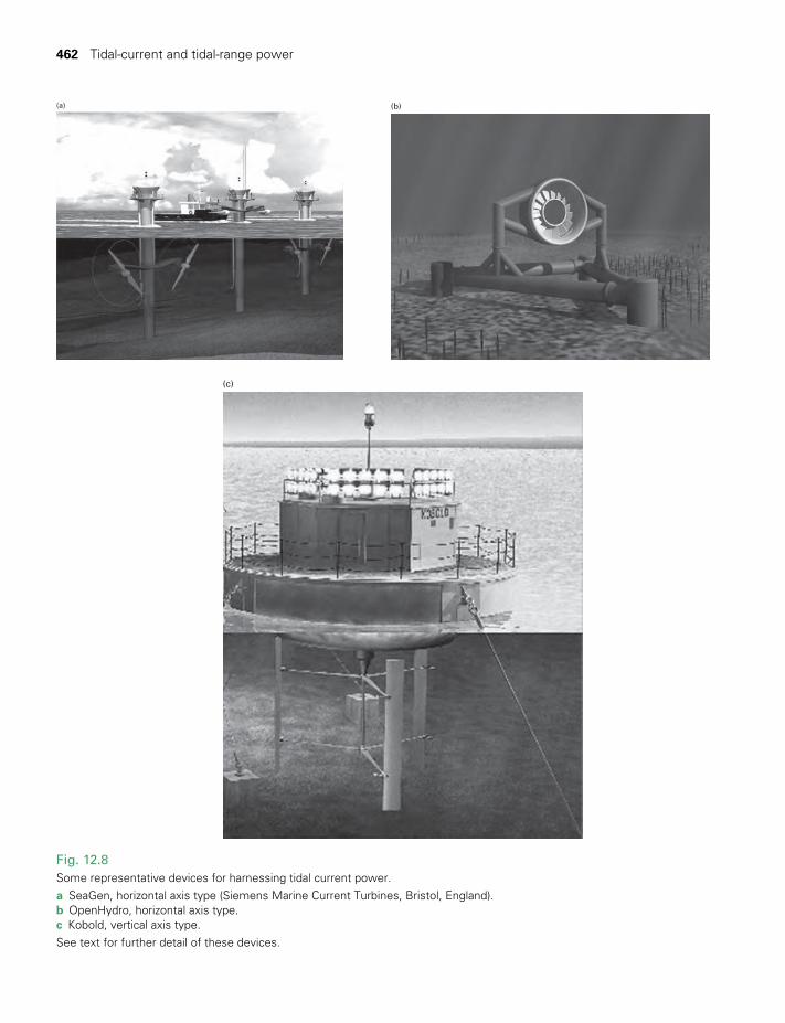
462 Tidal-current and tidal-range power
(a) (b)
Fig. 12.8 Some representative devices for harnessing tidal current power. a SeaGen, horizontal axis type (Siemens Marine Current Turbines, Bristol, England).b OpenHydro, horizontal axis type.c Kobold, vertical axis type. See text for further detail of these devices.
(c)
TWIDELL PAGINATION.indb 462 01/12/2014 11:38

§12.4 Tidal current/stream power 463
(b) Class 2: Vertical axisThere have been far fewer proposals for vertical-axis tidal devices than horizontal axis (as with wind power). The Kobold turbine (Fig.12.8(c)) developed in Italy is one such device, with prototypes operating since 2009 in Italy (Straits of Messina), China (Jintang Strait) and the Philippines (Cebu, with a maximum current of 4 m/s). It features a specially designed hydrofoil, with the blade angles controlled by a series of levers to main-tain an optimum angle of attack.2
(c) Class 3: Reciprocating blade The principle is that the water forces a plate or ‘blade’ up and down, or from side to side, in a current. This actuates a gear or hydraulic pump to pass the power to a generator.
In the Pulse Tidal device, each of the two blades is horizontal and moves vertically in the stream, connected through a gearbox to a gen-erator. The advantage is claimed to be that the system will operate with large blades in relatively shallow water to produce significant power (e.g. 1.2 MW in 18 m depth, 5 MW in 35 m depth). During operation, the system sits on the sea bed and is fully submerged even in shallow water. However, for maintenance, the system can come to the surface without the need for cranes and complicated offshore vessels – making maintenance work straightforward. A demonstration device of 100 kW capacity has operated in the Humber estuary, eastern England, since 2007. Deployment of a ‘full-scale’ 1.2 MW machine is expected.
12.4.3 Blockage effects in restricted flow
Because tidal currents tend to be strongest in narrow channels, an array of turbines in the channel may occupy an appreciable fraction of the channel cross-section. The turbines may thus constitute an appreciable blockage to the undisturbed flow, to a much greater extent than occurs for wind farms. This restricted flow may result in a turbine (or array of turbines) producing more power than indicated by the Betz analysis of §8.3, i.e. Cp >0.6. In effect, the flow is ‘pushed’ strongly from upstream and only a limited proportion can divert around the turbine, so the remain-der is forced through the turbine at a faster speed than would be the case for an isolated turbine, as illustrated in Fig. 12.9. (This is the reason why hydropower turbines, encased by pipework, are also not subject to the Betz ‘limit’.)
Box 12.2 outlines some results from one of the many laboratory or numerical simulations that aim to quantify these effects. Not surprisingly, the effect increases with the proportion of the flow that is ‘blocked’ by turbines, so this ‘enhancement’ is likely to be more significant in narrow channels (<~100 m ) than in wide estuaries such as the Bay of Fundy.
TWIDELL PAGINATION.indb 463 01/12/2014 11:38
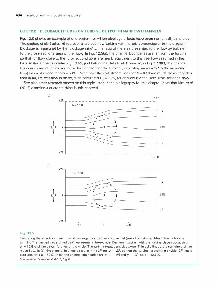
464 Tidal-current and tidal-range power
BOX 12.2 BLOCKAGE EFFECTS ON TURBINE OUTPUT IN NARROW CHANNELS
Fig. 12.9 shows an example of one system for which blockage effects have been numerically simulated. The dashed circle (radius R) represents a cross-flow turbine with its axis perpendicular to the diagram. Blockage is measured by the ‘blockage ratio’ b, the ratio of the area presented to the flow by turbine to the cross-sectional area of the flow. In Fig. 12.9(a), the channel boundaries are far from the turbine, so that for flow close to the turbine, conditions are nearly equivalent to the free flow assumed in the Betz analysis; the calculated Cp = 0.52, just below the Betz limit. However, in Fig. 12.9(b), the channel boundaries are much closer to the turbine, so that the turbine (presenting an area 2R to the incoming flow) has a blockage ratio b = 50%. Note how the exit stream lines for b = 0.50 are much closer together than in (a), i.e. exit flow is faster, with calculated Cp = 1.25, roughly double the Betz ‘limit’ for open flow.
See also other research papers on this topic listed in the bibliography for this chapter (note that Kim et al. (2012) examine a ducted turbine in this context).
+2R
–2R
+2R
–2R–2R +2R0
b = 0.125
(a)
(b)
b = 0.50
+ 8R
– 8R
1.1R
1.1R 2.1R
2.9R0
0
Fig. 12.9Illustrating the effect on mean flow of blockage by a turbine in a channel (seen from above). Mean flow is from left to right. The dashed circle of radius R represents a three-blade ‘Darrieus’ turbine, with the turbine blades occupying only 12.5% of the circumference of the circle. The turbine rotates anticlockwise. Thin solid lines are streamlines of the mean flow. In (b), the channel boundaries are at y = +2R and y = −2R, so that the turbine (presenting a width 2R) has a blockage ratio b = 50%. In (a), the channel boundaries are at y = +8R and y = −8R, so b = 12.5%. Source: After Consul et al. (2013, Fig. 8.)
TWIDELL PAGINATION.indb 464 01/12/2014 11:38
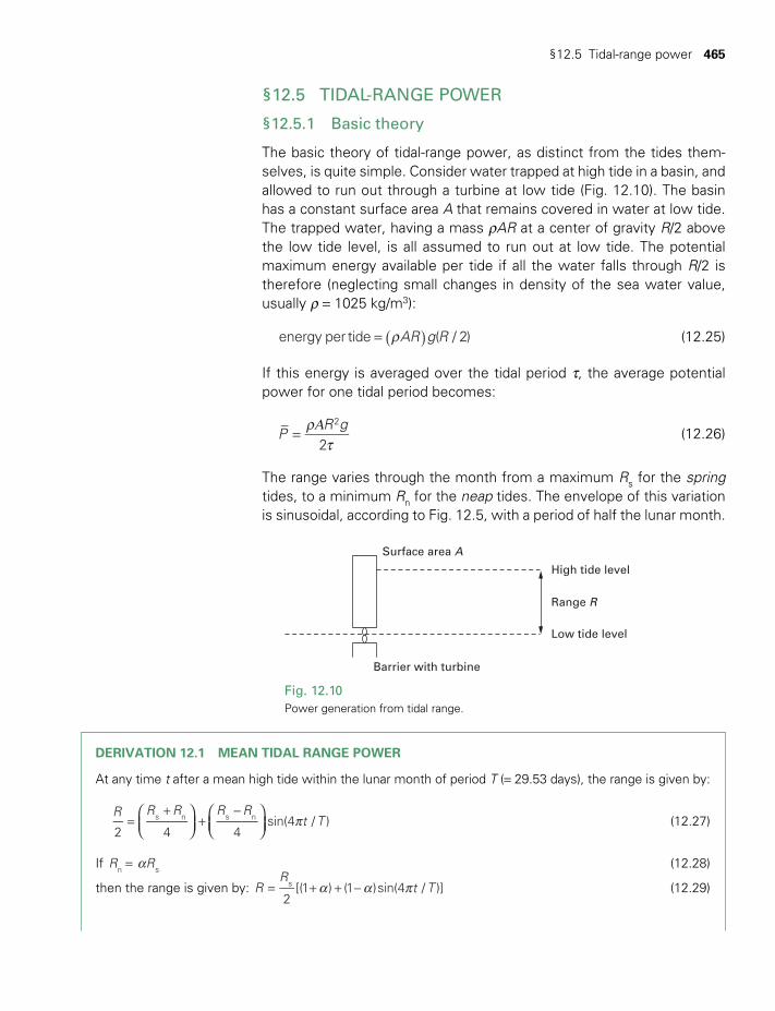
§12.5 Tidal-range power 465
§12.5 TIDAL-RANGE POWER
§12.5.1 Basic theory
The basic theory of tidal-range power, as distinct from the tides them-selves, is quite simple. Consider water trapped at high tide in a basin, and allowed to run out through a turbine at low tide (Fig. 12.10). The basin has a constant surface area A that remains covered in water at low tide. The trapped water, having a mass rAR at a center of gravity R/2 above the low tide level, is all assumed to run out at low tide. The potential maximum energy available per tide if all the water falls through R/2 is therefore (neglecting small changes in density of the sea water value, usually r = 1025 kg/m3):
r( )= AR g Renergy per tide ( / 2) (12.25)
If this energy is averaged over the tidal period t, the average potential power for one tidal period becomes:
rΑt
=PR g
2
2 (12.26)
The range varies through the month from a maximum Rs for the spring tides, to a minimum Rn for the neap tides. The envelope of this variation is sinusoidal, according to Fig. 12.5, with a period of half the lunar month.
Surface area A
High tide level
Low tide level
Barrier with turbine
Range R
Fig. 12.10 Power generation from tidal range.
DERIVATION 12.1 MEAN TIDAL RANGE POWER
At any time t after a mean high tide within the lunar month of period T (= 29.53 days), the range is given by:
p=+
+−R R R R R
t T2 4 4
sin(4 / )s n s n (12.27)
If a=R Rn s (12.28)
then the range is given by: a a p= + + −RR
t T2
[(1 ) (1 )sin(4 / )]s (12.29)
TWIDELL PAGINATION.indb 465 01/12/2014 11:38
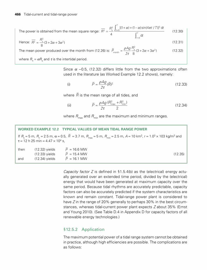
466 Tidal-current and tidal-range power
Since a ~0.5, (12.32) differs little from the two approximations often used in the literature (as Worked Example 12.2 shows), namely:
(i)
r2t
≈PAg
R( )2 (12.33)
where R is the mean range of all tides, and
(ii)
r2t
≈+
PAg R R( )
2max2
min2
(12.34)
where Rmax and Rmin are the maximum and minimum ranges.
The power is obtained from the mean square range: ∫
∫
a a p=
+ + −=
=
RR t T t
t4
[(1 ) (1 )sin(4 / )] d
d
t
T
t
T2 s
2 2
0
0
(12.30)
Hence: a a= + +RR
8(3 2 3 )2 s
22 (12.31)
The mean power produced over the month from (12.26) is: r2t
a a= + +PAg R
8(3 2 3 )month
s2
2 (12.32)
where Rn = aRs and t is the intertidal period.
WORKED EXAMPLE 12.2 TYPICAL VALUES OF MEAN TIDAL RANGE POWER
If Rs = 5 m, Rn = 2.5 m, a = 0.5, R = 3.7 m, Rmax = 5 m, Rmin = 2.5 m, A = 10 km2, r = 1.03 × 10³ kg/m3 and t = 12 h 25 min = 4.47 × 10⁴ s,
then (12.32) yields P = 16.6 MW (12.33) yields P = 15.4 MW (12.35)and (12.34) yields P = 16.1 MW
Capacity factor Z is defined in §1.5.4(b) as the (electrical) energy actu-ally generated over an extended time period, divided by the (electrical) energy that would have been generated at maximum capacity over the same period. Because tidal rhythms are accurately predictable, capacity factors can also be accurately predicted if the system characteristics are known and remain constant. Tidal-range power plant is considered to have Z in the range of 20% generally to perhaps 30% in the best circum-stances, whereas tidal-current power plant expects Z about 35% (Ernst and Young 2010). (See Table D.4 in Appendix D for capacity factors of all renewable energy technologies.)
§12.5.2 Application
The maximum potential power of a tidal range system cannot be obtained in practice, although high efficiencies are possible. The complications are as follows:
TWIDELL PAGINATION.indb 466 01/12/2014 11:38
§12.6 World tidal power sites 467
1 Power generation cannot be maintained near to low tide conditions and so some potential energy is not harnessed.
2 The turbines must operate at low head with large flow rates, a condition that is uncommon in conventional hydropower practice, but similar to
‘run-of-the-river’ hydropower. The French have most experience of such turbines, having developed low-head, large-flow bulb turbines for generation from rivers and the La Rance tidal scheme. The turbines are least efficient at lowest head.
3 The electrical power may be needed at a near constant rate, and so there is a constraint to generate at times of less than maximum head.
Efficiency can be improved if the turbines are operated as pumps at high tide to increase the head. Consider a system where the range is 5 m. Water lifted 1 m at high tide can be let out for generation at low tide when the head becomes 6 m. Even if the pumps and generators are 50% efficient, there will be a net energy gain of ~200% (see Problem 12.6).
In Fig. 12.10, note that power can be produced as water flows both with the incoming (‘flow’) and outgoing (‘ebb’) tide. Thus a carefully optimized tidal power system that uses reversible turbines to generate at both ebb and flow, and where the turbine can operate as pumps to increase the head, can produce energy of 90% of the potential given by (12.32).
§12.6 WORLD TIDAL POWER SITES
The greatest experience by far of tidal-range power is from the La Rance 240 MW capacity station in Brittany, France, which has operated as planned since 1966. Table 12.1 shows other working plant of significantly lower capacity, and also the recent (2010) large plant of 254 MW capacity at Siwha in South Korea.
The total dissipation of energy by water tides on the Earth is estimated to be 3000 GW, of which no more than about 1000 GW occurs in shallow sea areas accessible for large civil engineering works. Sites of great-est resource potential throughout the world are indicated in Fig. 12.1; they have a combined technical potential of about 120 GW, which is approximately 10% of the total world hydropower (river) potential. This is a significant power potential and of great potential importance for certain countries (e.g. the UK, where, in principle, about 25% of annual electricity could be generated by tidal power from known estuaries with enhanced tidal range).
Further details of some of the more promising sites are given in Table 12.1. The very large (GW) resource in some locations has tempted proponents to develop proposals for gigantic range-power stations, none of which have been actually constructed, mostly due to large capital cost compared to small short-term financial gains, and to social and envi-ronmental factors discussed below. For example, the Severn estuary
TWIDELL PAGINATION.indb 467 01/12/2014 11:38
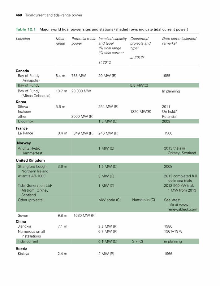
468 Tidal-current and tidal-range power
Table 12.1 Major world tidal power sites and stations (shaded rows indicate tidal current power)
Location Mean range
Potential mean power
Installed capacity and typea (R) tidal range(C) tidal current
at 2012
Consented projects and typeb
at 2013 a
Date commissioned/ remarksb
CanadaBay of Fundy (Annapolis)
6.4 m 765 MW 20 MW (R) 1985
Bay of Fundy 5.5 MW(C)
Bay of Fundy (Minas-Cobequid)
10.7 m 20,000 MW In planning
KoreaSihwa 5.6 m 254 MW (R) 2011Incheon 1320 MW(R) On hold?other 2000 MW (R) PotentialUldolmok 1.5 MW (C) 2009
FranceLa Rance 8.4 m 349 MW (R) 240 MW (R) 1966
NorwayAndritz Hydro Hammerfest
1 MW (C) 2013 trials in Orkney, Scotland
United Kingdom
Strangford Lough, Northern Ireland
3.6 m 1.2 MW (C) 2008
Atlantis AR-1000 3 MW (C) 2012 completed full scale sea trials
Tidal Generation Ltd/ Alstrom, Orkney,
Scotland
1 MW (C) 2012 500 kW trial, 1 MW from 2013
Other (projects) MW scale (C) Numerous (C) See latest info at www.
renewableuk.com
Severn 9.8 m 1680 MW (R)
ChinaJiangxia 7.1 m 3.2 MW (R) 1980Numerous small installations
0.7 MW (R) 1961–1978
Tidal current 0.1 MW (C) 3.7 (C) in planning
RussiaKislaya 2.4 m 2 MW (R) 1966
TWIDELL PAGINATION.indb 468 01/12/2014 11:38
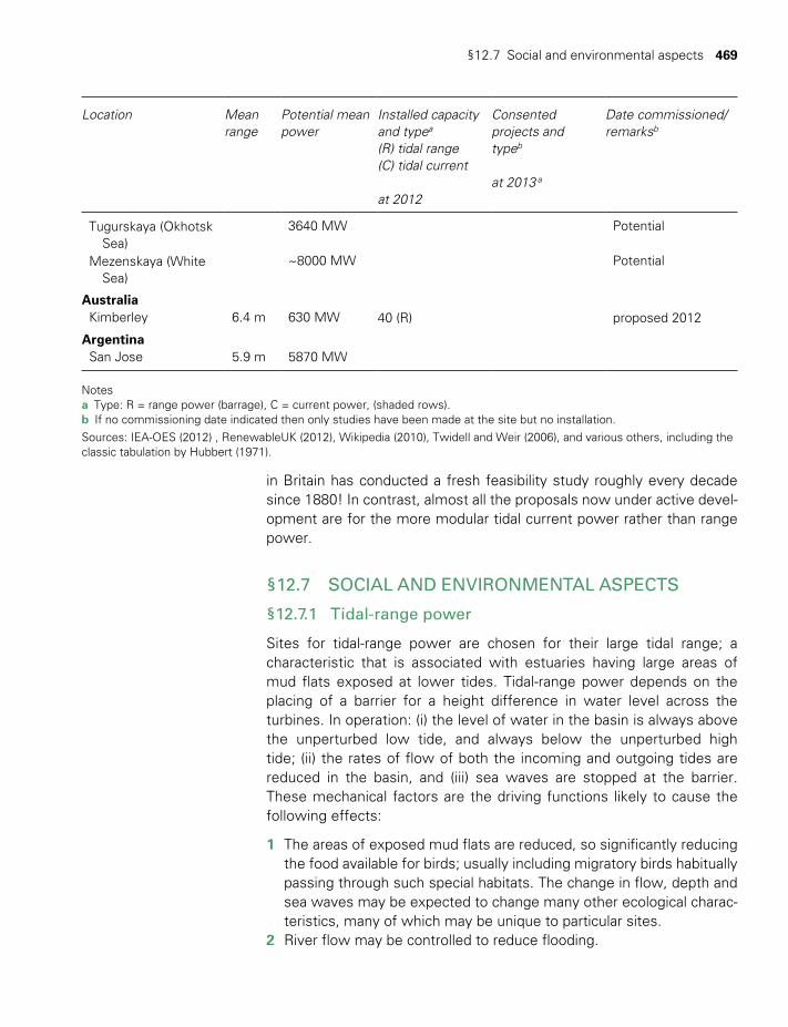
§12.7 Social and environmental aspects 469
in Britain has conducted a fresh feasibility study roughly every decade since 1880! In contrast, almost all the proposals now under active devel-opment are for the more modular tidal current power rather than range power.
§12.7 SOCIAL AND ENVIRONMENTAL ASPECTS
§12.7.1 Tidal-range power
Sites for tidal-range power are chosen for their large tidal range; a characteristic that is associated with estuaries having large areas of mud flats exposed at lower tides. Tidal-range power depends on the placing of a barrier for a height difference in water level across the turbines. In operation: (i) the level of water in the basin is always above the unperturbed low tide, and always below the unperturbed high tide; (ii) the rates of flow of both the incoming and outgoing tides are reduced in the basin, and (iii) sea waves are stopped at the barrier. These mechanical factors are the driving functions likely to cause the following effects:
1 The areas of exposed mud flats are reduced, so significantly reducing the food available for birds; usually including migratory birds habitually passing through such special habitats. The change in flow, depth and sea waves may be expected to change many other ecological charac-teristics, many of which may be unique to particular sites.
2 River flow may be controlled to reduce flooding.
Location Mean range
Potential mean power
Installed capacity and typea (R) tidal range(C) tidal current
at 2012
Consented projects and typeb
at 2013 a
Date commissioned/ remarksb
Tugurskaya (Okhotsk Sea)
3640 MW Potential
Mezenskaya (White Sea)
~8000 MW Potential
AustraliaKimberley 6.4 m 630 MW 40 (R) proposed 2012
ArgentinaSan Jose 5.9 m 5870 MW
Notesa Type: R = range power (barrage), C = current power, (shaded rows). b I f no commissioning date indicated then only studies have been made at the site but no installation.Sources: IEA-OES (2012) , RenewableUK (2012), Wikipedia (2010), Twidell and Weir (2006), and various others, including the classic tabulation by Hubbert (1971).
TWIDELL PAGINATION.indb 469 01/12/2014 11:38
470 Tidal-current and tidal-range power
3 Access for boats to harbors in the basin is possible if suitable lock(s) are included in the barrage; indeed, the restricted tidal range within the basin may be advantageous.
4 Controlled depth and flow of the basin allows for leisure activities such as sailing.
5 Visual impact is changed, but with a barrier the only necessary construction.
6 The barrier may be used as a viaduct for transport and for placing other constructions (e.g. wind turbines).
Tidal barriers are large and expensive structures that may require years to construct. No power may be produced, and hence no income generated, until the last section of the barrier is complete. Difficulties in finance may lead to lack of environmental care. Although the installation at La Rance now features a flourishing natural ecosystem, it is noticeably different from that which was there before the dam, and took some years to re-establish itself. Therefore, it has been observed that La Rance may not have been constructed if it had had to face today’s environmental impact procedures.
A developer’s main criterion for the success of a tidal power plant is the cost per kWh of the power produced. As with other capital- intensive energy technologies, the economic cost per kWh generated can be reduced (a) if other advantages can be costed as benefit to the project, including fossil-carbon abatement; (b) if interest rates of money bor-rowed to finance the high capital cost are small, and (c) if the output power may be used to decrease consumption of expensive fuels such as oil. (See Chapter 17 for a more general discussion of these issues.) For example, the only large-scale (>50 MW) tidal-range power plant commis-sioned since 1970, the Sihwa system in Korea, was built into a barrage constructed earlier for flood mitigation and agricultural purposes.
12.7.2 Tidal-current power
The social and environmental aspects are very different for tidal-current power. For tidal-current systems, unlike for tidal-range systems, it is not necessary to block an entire tidal flow, so that the obstruction to the passage of fish and boats is much less. For the same reason, con-struction can proceed in a modular fashion, with only a few turbines being put in place initially, and others added later. As with wind power systems, this greatly simplifies the capital cost requirement, especially as useful power can be generated and income earned step-by-step as portions of the capital cost are expended. This modularity also enables rapid technology development through ‘learning by doing’.
A particular concern regarding the early installation at Strangford Lough (Fig. 12.8) was the potential impact on fish, seals, sea-birds and boats.
TWIDELL PAGINATION.indb 470 01/12/2014 11:38
§12.7 Social and environmental aspects 471
CHAPTER SUMMARY
The change in height between successive high and low tides (the range) varies at coastlines between about 0.5 m in general and about 10 m at particular favorable sites (e.g. certain river estuaries). The movement of the water produces tidal currents, which may be harnessed in a manner similar to wind power. In practice, tidal currents are likely to be attractive for power generation only where they are naturally strong (>~3 m/s) because of large tidal range, and/or enhanced in speed by water movement in narrow straits between islands and mainland or between islands.
The high tide in an estuarine basin can be trapped behind a dam or barrier to produce tidal-range power, using low-head ‘hydropower’ turbines. The 240 MWe ‘La Rance’ system in France has operated reliably since 1967, thereby proving the technical feasibility of this technology at scale. Unfortunately, to be effective for this purpose, the barrage has to extend nearly or completely across the whole tidal estuary. This not only entails very large civil engineering costs, but is likely to also block shipping, and to produce large environmental impacts, notably in tidal wetlands. Numerous feasibility studies over the past 100 years suggest that substantial range power is in principle available at the few sites with large tidal range (e.g. the Severn estuary in Britain and the Bay of Fundy at the US/Canadian border); these factors have meant that very few tidal-range systems have been implemented for power generation per se on any significant scale. It is noteworthy that the 254 MW tidal-range power plant at Siwha, South Korea, utilized a pre-existing water catchment dam to ‘insert’ its turbines; thus emphasizing the importance of multi-purpose installations.
Most tidal-current power devices are similar in principle to horizontal-axis wind turbines that operate in extended fluid flow. A major aspect is that they do not block the entire tidal flow, so having significantly less impact than tidal-range plant. Also, large ‘systems’ can be built in a modular manner, so producing useful output incrementally. Consequently, the economic, social and environmental aspects of tidal-current power are in many ways more favorable than those for tidal-range systems. Consequently a variety of prototype tidal-current systems are being explored vigorously with financial support from governments and venture capital.
The range, flow and periodic behavior of tides at most coastal regions are well documented and analyzed owing to the demands of navigation and oceanography. The variability arises from the mismatch of the principal lunar-driven tidal periods of 12 hours 25 minutes and 24 hours 50 minutes with the human (solar) period of 24 hours, so that optimum tidal power generation is not in phase with demand. This variation handicaps the use of tidal power, but the predictability, to +/- 4%, allows pre-planned integration into large electrical grid networks, perhaps also with large storage facilities. Thus tidal power, especially tidal-range power which may be combined with other capital assets, presents a very assured source of significant sustainable energy, which is probably its major advantage compared with other energy sources. The major drawbacks for all forms of tidal power are: (a) only a few sites are suitable, and these may be distant from the demand for power; and (b) the variability of power generation.
Therefore underwater video cameras recorded the movement of fish and other animals past the rotating blades and showed that no harm had been caused. No other adverse impacts of significance have been recorded, the public accepts the visual impact and, as with most renew-able energy projects, the device adds to tourist attraction – all of which is encouraging for future projects.
TWIDELL PAGINATION.indb 471 01/12/2014 11:38
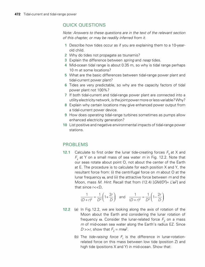
472 Tidal-current and tidal-range power
QUICK QUESTIONS
Note: Answers to these questions are in the text of the relevant section of this chapter, or may be readily inferred from it.
1 Describe how tides occur as if you are explaining them to a 10-year-old child.
2 Why do tides not propagate as tsunamis? 3 Explain the difference between spring and neap tides. 4 Mid-ocean tidal range is about 0.35 m, so why is tidal range perhaps
10 m at some locations? 5 What are the basic differences between tidal-range power plant and
tidal-current power plant? 6 Tides are very predictable, so why are the capacity factors of tidal
power plant not 100%? 7 If both tidal-current and tidal-range power plant are connected into a
utility electricity network, is the joint power more or less variable? Why? 8 Explain why certain locations may give enhanced power output from
a tidal-current power device. 9 How does operating tidal-range turbines sometimes as pumps allow
enhanced electricity generation?10 List positive and negative environmental impacts of tidal-range power
stations.
PROBLEMS
12.1 Calculate to first order the lunar tide-creating forces FX at X and
Fy at Y on a small mass of sea water m in Fig. 12.2. Note that our seas rotate about point O, not about the center of the Earth at E. The procedure is to calculate for each position X and Y, the resultant force from: (i) the centrifugal force on m about O at the lunar frequency w, and (ii) the attractive force between m and the Moon, mass M. Hint: Recall that from (12.4) [GM/D2]= L’w2] and that since r<<D,
D r Dr
D D r Dr
D1
( )1
12
and1
( )1
12
2 2 2 2+= +
+
= −
12.2 (a) In Fig. 12.2, we are looking along the axis of rotation of the Moon about the Earth and considering the lunar rotation of frequency w. Consider the lunar-related force FZ on a mass m of mid-ocean sea water along the Earth’s radius EZ. Since D >>r, show that FZ = mrw2.
(b) The tide-raising force Ft is the difference in lunar-rotation-related force on this mass between low tide (position Z) and high tide (positions X and Y) in mid-ocean. Show that:
TWIDELL PAGINATION.indb 472 01/12/2014 11:38
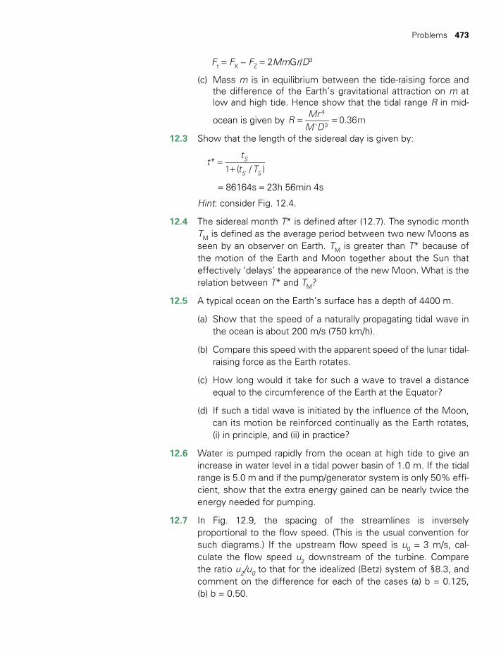
Problems 473
Ft = FX − FZ = 2MmGr/D3
(c) Mass m is in equilibrium between the tide-raising force and the difference of the Earth’s gravitational attraction on m at low and high tide. Hence show that the tidal range R in mid-
ocean is given by = =RMr
M D'0.36m
4
3
12.3 Show that the length of the sidereal day is given by:
=
+t
t
t T*
1 ( / )S
S S
= 86164s = 23h 56min 4s
Hint: consider Fig. 12.4.
12.4 The sidereal month T* is defined after (12.7). The synodic month TM is defined as the average period between two new Moons as seen by an observer on Earth. TM is greater than T* because of the motion of the Earth and Moon together about the Sun that effectively ‘delays’ the appearance of the new Moon. What is the relation between T* and TM?
12.5 A typical ocean on the Earth’s surface has a depth of 4400 m.
(a) Show that the speed of a naturally propagating tidal wave in the ocean is about 200 m/s (750 km/h).
(b) Compare this speed with the apparent speed of the lunar tidal-raising force as the Earth rotates.
(c) How long would it take for such a wave to travel a distance equal to the circumference of the Earth at the Equator?
(d) If such a tidal wave is initiated by the influence of the Moon, can its motion be reinforced continually as the Earth rotates, (i) in principle, and (ii) in practice?
12.6 Water is pumped rapidly from the ocean at high tide to give an increase in water level in a tidal power basin of 1.0 m. If the tidal range is 5.0 m and if the pump/generator system is only 50% effi-cient, show that the extra energy gained can be nearly twice the energy needed for pumping.
12.7 In Fig. 12.9, the spacing of the streamlines is inversely proportional to the flow speed. (This is the usual convention for such diagrams.) If the upstream flow speed is u0 = 3 m/s, cal-culate the flow speed u2 downstream of the turbine. Compare the ratio u2/u0 to that for the idealized (Betz) system of §8.3, and comment on the difference for each of the cases (a) b = 0.125, (b) b = 0.50.
TWIDELL PAGINATION.indb 473 01/12/2014 11:38
474 Tidal-current and tidal-range power
NOTES
1 A more detailed discussion of the causes of tides is given in Chapter 13 of the second edition of this book, which is available via the publishers’ website (www.routledge.com/books/details/9780415584388).
2 Source: http://energiesdelamer.blogspot.com/2011/01/enermar-un-projet-hydrolien-italien.html (report of January 13, 2011).
BIBLIOGRAPHY
Bahaj, A.S. (2013) ‘Marine current energy conversion: the dawn of a new era in electricity production’, Philosophical Transactions of the Royal Society A, vol. 371 (part of a special issue on this subject). Focus on UK developments.
Charlier, R.C. (2003) ‘Sustainable co-generation from the tides: a review’, Renewable and Sustainable Energy Reviews, 7, 187–213. Comprehensive review of range power, including work before 1980 and up until 2002; contrasts ‘dreams and reality’.
Clare, R. (ed.) (1992) Tidal Power: Trends and developments, Thomas Telford, London. Conference papers, mostly studies of potential sites and installations in UK, but also including M. Rodier, ‘The Rance tidal power station: a quarter of a century in operation’. Indicates that there was not much progress between the 1970s and 1990s.
Hardisty, J. (2009) An Analysis of Tidal Stream Power, Wiley-Blackwell, Oxford. This considers: (i) fluid dynamical theory of tides, fluids and power turbines backed with historical information, with application for recent devices; (ii) practical advice and economic analysis for operational projects and for siting worldwide; and (iii) supporting material on its website includes a model for estimating potential power at a site.
Hubbert, M.K. (1971) Scientific American, September, 60–87. Classic estimates of global tidal power potential.
Lewis, A., Estefen, S., Huckerby, J., Musial, W., Pontes, T. and Torres Martinez, J. (2011) ‘Ocean energy’. In O. Edenhofer, R. Pichs Madruga, Y. Sokona, K. Seyboth, P. Matschoss, S. Kadner, T. Zwickel, P. Eickemeier, G. Hansen, S. Schlömer and C. von Stechow (eds), IPCC Special Report on Renewable Energy Sources and Climate Change Mitigation, Cambridge University Press, Cambridge. Reviews current state of the art and future potential of all forms of ocean energy, including tidal.
Specific references
Consul, C.A., Willden, R.H. and McIntosh, S.C. (2013) ‘Blockage effects on the hydrodynamic performance of a marine cross-flow turbine’, Philosophical Transactions of the Royal Society A, vol. 371 (part of a special issue on this subject).
Ernst and Young LLP (2010) Cost and Support of Wave, Tidal-stream and Tidal-range Generation in the UK, Report to the (UK government) Department of Energy and Climate Change, and the Scottish government.
Kim, K-P., Ahmed, M.R. and Lee, Y-H. (2012) ‘Efficiency improvement of a tidal current turbine utilizing a larger area of channel’, Renewable Energy, 48, 557–564.
Sørensen, B. (2011, 4th edn) Renewable Energy, Academic Press, London. Includes a useful but short summary of tidal power potential.
Twidell, J. and Weir, A. (2006, 2nd edn) Renewable Energy Resources; ch. 13, ‘Tidal power’, is on the website for the current (third) edition.
TWIDELL PAGINATION.indb 474 01/12/2014 11:38

Bibliography 475
Vennell, R. (2012) ‘Realising the potential of tidal currents and the efficiency of turbine farms in a channel’, Renewable Energy, 47, 95–102.
Wikipedia (2010) ‘List of tidal power stations’ (last updated November 2010).
Websites
IEA Ocean Energy Systems. International collaboration with useful reports of progress and policies; see esp. their ‘Annual Reports’ (www.ocean-energy-systems.org).
http://energiesdelamer.blogspot.com/2011/01/enermar-un-projet- hydrolien-italien.html. A newsletter on marine energy, mainly in French.
http://social.tidaltoday.com. A newsletter specifically on tidal power.
leeds-faculty.colorado.edu/lawrence/.../Lectures/Oceanic%20Energy.ppt. Lectures on ocean energy.
TWIDELL PAGINATION.indb 475 01/12/2014 11:38
Ocean gradient energy: OTEC and osmotic power
CONTENTS
Learning aims 476
§13.1 General introduction 478
§13.2 Ocean thermal energy conversion (OTEC): introduction 478
§13.3 OTEC principles 479
§13.4 Practical considerations about OTEC 483 §13.4.1 Heat exchangers 483 §13.4.2 Biofouling and corrosion 483 §13.4.3 Pumping requirements 484 §13.4.4 Land-based plant and
floating platforms 484 §13.4.5 Construction of the cold
water pipe 484 §13.4.6 Power connections 485 §13.4.7 The turbine generator 485 §13.4.8 Summary of advantages and
disadvantages of OTEC 485
§13.5 OTEC Devices 486
§13.6 Related technologies 487
§13.7 Social, economic and environmental aspects of OTEC 488
§13.8 Osmotic power from salinity gradients 489
Chapter summary 491
Quick questions 492
Problems 492
Note 493
Bibliography 493
Box 13.1 Rankine cycle engine 482
LEARNING AIMS
• Understand the principles of two differ-ent ocean energy extraction technologies. The first, ocean thermal energy conversion (OTEC), depends on the temperature gradi-ent below the surface of tropical oceans. The second, osmotic power, depends on gradi-ents of salt concentration between sea and fresh water.
• Understand the basic principles and limita-tions of each of these technologies.
• Review the progress of applications.
CHAPTER
13
TWIDELL PAGINATION.indb 476 01/12/2014 11:38

List of tables 477
LIST OF FIGURES
13.1 Schematic diagram of an OTEC system. 48013.2 Seasonal average of temperature difference DT between sea surface and a depth of 1000 m. 48113.3 Temperature profile with depth of typical tropical seas. 48213.4 Pressure-volume chart of the Rankine cycle. 48213.5 Shell-and-tube heat exchanger. 48313.6 Some of the systems (devices) designed to demonstrate OTEC. 48713.7 Illustrating osmotic pressure. 49013.8 Schematic diagram of an osmotic power system, using pressure retarded osmosis. 491
LIST OF TABLES
13.1 Summary of OTEC Demonstration Plants (based on Ravindran (1999), Nihous (2008) and R&D reports of Delft University (the Netherlands), the National Institute of Ocean Technology (India), the Natural Energy Laboratory of Hawaii Authority (USA), etc.) 486
TWIDELL PAGINATION.indb 477 01/12/2014 11:38
478 Ocean gradient energy:
§13.1 GENERAL INTRODUCTION
In this chapter we consider two significantly different technologies, neither of which to date have progressed beyond research and develop-ment activity into profitable commercial application as energy supplies. However, should such R&D be successful, then the potential is wide-spread for relatively large-scale installations. The common link is variation in the ocean, one of surface temperature and the other of salinity. Both depend on well-established science, but both have considerable engi-neering challenges to overcome before becoming established industries.Most of this chapter (§13.2 to §13.6) deals with ocean thermal energy conversion (OTEC) as this has been widely studied; §13.7 outlines the principles of osmotic power.
§13.2 OCEAN THERMAL ENERGY CONVERSION (OTEC): INTRODUCTION
The ocean is the world’s largest solar collector. In tropical seas, tempera-ture differences of about 20°C occur between the warm near-surface water and the cold ‘deep’ water at 500 to 1000 m depth. Heat engines can operate between thermal sources and sinks with such relatively small temperature difference, but their intrinsic efficiency is small due to the laws and practicalities of thermodynamics. Ocean thermal energy conversion (OTEC) is the extraction and conversion of this thermal energy into useful work for electricity generation. Given sufficient scale of efficient equipment, electricity power generation could be sustained day and night at ~200 kWe/km2 in areas of tropical sea. Such power equals about 0.07% of the absorbed solar irradiation input to that area.
The earliest OTEC demonstration plant was in 1930. R&D effort was resourced from France pre-1970s and then from the USA, Japan and Taiwan in the 1980s and with continuing very moderate activity since then; see §13.5. Avery and Wu (1994) give a detailed history, updated by Nihous (2008, 2013). The demonstration plants described in §13.5 confirmed that to achieve cost per unit of power output competitive with other renewable energy sources requires large-scale (> ~100MW) and improved energy efficiency. It follows that privately funded develop-ment and commercialization are unlikely without continuing government funding. It is also clear that the economics would be improved if benefits in addition to electricity generation are included (e.g. water desalination, building cooling, nutrient addition for fish farming), as indicated in §13.6.
The attractiveness of OTEC from successful plant is the effectively limitless energy of the hotter surface water in relation to the colder deep water and its potential for constant, baseload electricity generation; i.e. plant has the potential for large capacity factor approaching 100%. However, OTEC faces three fundamental limitations:
TWIDELL PAGINATION.indb 478 01/12/2014 11:38
§13.3 Otec principles 479
1 Pumping. Heat engines depend on energy passing down a tempera-ture gradient from a hotter source to a colder sink (e.g. in steam from ~150°C to ambient temperature ~25°C). For OTEC the hot source is the tropical surface water at ~25°C and the cold sink is water from the deep ocean at ~5°C. This cold saline watert has to be pumped up to surface level to become a colder thermal sink for the heat engine, for which considerable pumping power is required. In practice, pumping is at a rate of about 6 m3/s of water per MWe of electricity generated, which may require up to 50% of the generated power. Such systems require large pumps, large-diameter pipes and large heat exchangers, all of which are expensive.
2 Small efficiency. In practice, the temperature difference available to operate the heat engine is small (<20°C) and so the efficiency of even a ‘perfect’ engine is small at > ~5%.
3 Remote location. Sites with OTEC potential are either at tropical coastlines or offshore using large floating installations. Such sites are usually far from habitations having the capacity to utilize OTEC output.
To tackle the technical limitations, OTEC designers use methods of estab-lished industries for energy recovery (e.g. from large flows of heated discharge from metal refining, power stations and food industries). In addition, OTEC can combine with other applications using deep water as explained in §13.6; the general term for such development is deep ocean water applications (DOWA). It is probable that only joint OTEC/DOWA schemes are ever likely to be commercially successful.
§13.3 OTEC PRINCIPLES
Fig. 13.1 outlines a system for OTEC; and with a heat engine operating a closed-cycle Rankine process (see also Box 13.1). The working fluid (e.g. ammonia) boils in the ‘evaporator’ at the ~25°C to ~30°C temperature of the surface water, so driving a turbine generator for electricity supply. On the output side of the turbine, the vapor condenses to a liquid at the ~5°C temperature of the pumped deep water.1 Alternative open-cycle systems have sea water as incoming working fluid, which evaporates at reduced pressure before passing through a turbine. The condensate is ‘distilled water’, which may be used as both potable and irrigation water. The essential thermodynamic principles and limitations of the open cycle and closed cycle are the same.
In an idealized system with perfect heat exchangers, volume flow Q of warm water passes into the system at temperature Th and leaves at Tc (the cold water temperature of lower depths). The power given up from the warm water in such an ideal system is:
ρ DP cQ T=0 (13.1)
TWIDELL PAGINATION.indb 479 01/12/2014 11:38
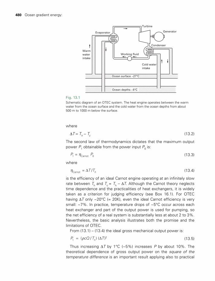
480 Ocean gradient energy:
where
DT = Th - Tc (13.2)
The second law of thermodynamics dictates that the maximum output power P1 obtainable from the power input P0 is:
ηP P=1 Carnot 0 (13.3)
where
η DT T= / hCarnot (13.4)
is the efficiency of an ideal Carnot engine operating at an infinitely slow rate between Th and Tc = Th – DT. Although the Carnot theory neglects time dependence and the practicalities of heat exchangers, it is widely taken as a criterion for judging efficiency (see Box 16.1). For OTEC having DT only ~20°C (= 20K), even the ideal Carnot efficiency is very small: ~7%. In practice, temperature drops of ~5°C occur across each heat exchanger and part of the output power is used for pumping, so the net efficiency of a real system is substantially less at about 2 to 3%. Nevertheless, the basic analysis illustrates both the promise and the limitations of OTEC.
From (13.1) – (13.4) the ideal gross mechanical output power is:
ρ= DP cQ T T( / ) ( )h12 (13.5)
Thus increasing DT by 1°C (~5%) increases P by about 10%. The theoretical dependence of gross output power on the square of the temperature difference is an important result applying also to practical
Evaporator
Working fluid
Ocean surface ~27°C
Ocean depths ~5°C
Turbine
Condenser
Generator
Cold waterintake
Warmwaterintake
Fig. 13.1 Schematic diagram of an OTEC system. The heat engine operates between the warm water from the ocean surface and the cold water from the ocean depths from about 500 m to 1000 m below the surface.
TWIDELL PAGINATION.indb 480 01/12/2014 11:38
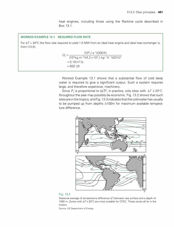
§13.3 Otec principles 481
WORKED EXAMPLE 13.1 REQUIRED FLOW RATE
For DT = 20°C the flow rate required to yield 1.0 MW from an ideal heat engine and ideal heat exchanger is, from (13.5):
=×
==
-
- - -Q
(10 J s )(300K)(10 kg m )(4.2 10 J kg K )(20 K)0.18 m /s650 t/h
1
6 1
3 3 3 1 1 2
3
N40°
20°
20°
22°
24°
22°
22°20°18°16°
40°
20°
20°
40°S
Eq.
N
20°
24°
20°18°
16°
22°
20°
40°
16°18°
20°22°
22° 16°18°20°
22°
22°20° 18°
16°
20°
20°18°
16°
S
Eq.
Fig. 13.2 Seasonal average of temperature difference DT between sea surface and a depth of 1000 m. Zones with DT ≥ 20°C are most suitable for OTEC. These zones all lie in the tropics. Source: US Department of Energy.
heat engines, including those using the Rankine cycle described in Box 13.1.
Worked Example 13.1 shows that a substantial flow of cold deep water is required to give a significant output. Such a system requires large, and therefore expensive, machinery.
Since P1 is proportional to (DT)2, in practice, only sites with D ≥T 20 Co throughout the year may possibly be economic. Fig. 13.2 shows that such sites are in the tropics, and Fig. 13.3 indicates that the cold water has usually to be pumped up from depths > ~100m for maximum available tempera-ture difference.
TWIDELL PAGINATION.indb 481 01/12/2014 11:38
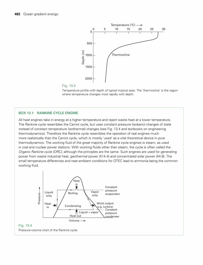
482 Ocean gradient energy:
BOX 13.1 RANKINE CYCLE ENGINE
All heat engines take in energy at a higher temperature and reject waste heat at a lower temperature. The Rankine cycle resembles the Carnot cycle, but uses constant pressure (isobaric) changes of state instead of constant temperature (isothermal) changes (see Fig. 13.4 and textbooks on engineering thermodynamics). Therefore the Rankine cycle resembles the operation of real engines much more realistically than the Carnot cycle, which is mostly ‘used’ as a vital theoretical device in pure thermodynamics. The working fluid of the great majority of Rankine cycle engines is steam, as used in coal and nuclear power stations. With working fluids other than steam, the cycle is often called the Organic Rankine cycle (ORC), although the principles are the same. Such engines are used for generating power from waste industrial heat, geothermal power (§14.4) and concentrated solar power (§4.8). The small temperature differences and near-ambient conditions for OTEC lead to ammonia being the common working fluid.
Pre
ssu
re
Volume
Liquid + vapor
Work outpute.g. turbine
Liquidonly
Vaporonly
Constantpressureevaporator
Constantpressurecondenser
Boiling
Heatin
Heatin
Heat out
Condensing
Fig. 13.4Pressure-volume chart of the Rankine cycle.
00 5 10 15
Thermocline
20 25 30
500
1000
1500
2000D
epth
(m
)
Temperature (°C)
Fig. 13.3Temperature profile with depth of typical tropical seas. The ‘thermocline’ is the region where temperature changes most rapidly with depth.
TWIDELL PAGINATION.indb 482 01/12/2014 11:38

§13.4 Practical considerations about otec 483
§13.4 PRACTICAL CONSIDERATIONS ABOUT OTEC
There are no fundamental thermodynamic reasons preventing OTEC systems from working successfully, but there are definite technical chal-lenges, the main ones of which are outlined below. (For more details and some relevant calculations, see the online supplementary material for this chapter.)
§13.4.1 Heat exchangers
Fig. 13.5 shows the outline design of a shell and tube heat exchanger suit-able for closed-circuit OTEC, but, for 1 MW thermal output at the small temperature differences, this would require several thousand internal tubes with a total surface area >>2000 m2. Thus OTEC heat exchan-gers must be relatively large to provide sufficient area for heat transfer at low temperature difference, and are therefore expensive (perhaps 50% of total costs). Moreover, the calculation of ideal output power P1 in assumes perfect heat transfer between the external ocean water and the internal working fluid; this is unrealistic, especially owing to bio-fouling outside and inside the pipes. Therefore development of OTEC includes improvements in existing heat exchangers to decrease the thermal resistance between the water and the working fluid. The aim is for more efficient, and therefore smaller, heat exchangers, which with less metal may give significant cost reduction.
§13.4.2 Biofouling and corrosion
The inside especially of the pipes become encrusted by marine organ-isms, which increase the thermal resistance, so reducing efficiency. Such biofouling is one of the major problems in OTEC design, since increasing
Working fluid (hot)
Working fluid (cold)
Water(cold)
Water(hot)
Fig. 13.5 Shell-and-tube heat exchanger (cut-away view).
TWIDELL PAGINATION.indb 483 01/12/2014 11:38

484 Ocean gradient energy:
the surface area available for heat transfer also increases the opportunity for organisms to attach themselves. Among the methods tried to keep this fouling under control are mechanical cleaning by continual circulation of close-fitting balls and chemical cleaning by additives to the water. In addition, serious corrosion can occur with metal structures, including the inner heat transfer tubing of heat exchangers.
§13.4.3 Pumping requirements
Work is required to move large quantities of hot and cold water around the system against friction; this power is supplied from the gross power output, so reducing the ideal power output P1 of (13.5). Although the cold water pipe can be built large enough to avoid significant friction (because the head loss varies as diameter D –5: see R2.6 and Problem 6.7), friction loss may become appreciable within connections and in the smaller pipes inside the heat exchangers. Biofouling within the heat exchanger tubes increases friction with roughness and decreases the tube diameter, making the situation worse. Consequently over 50% of the pumping power may be lost due to fluid friction.
§13.4.4 Land-based plant and floating platforms
Land-based systems are only possible at certain favorable tropical loca-tions, where the sea bed slopes sharply downward. Their main advan-tage is reduced cost, since the links to shore, assembly and maintenance are much simplified. The cold water pipe is not unduly stressed, since it rests on the sea bottom; however, it is still vulnerable to storm damage from wave motion to a depth of about 20 m.
Very large purpose-designed floating offshore platforms for OTEC could potentially generate electricity at ~500 MWe. Such power would be brought to land by cables or might be used on board (e.g. for produc-ing hydrogen as a fuel, §15.9.1).
§13.4.5 Construction of the cold water pipe
The suspended cold water pipe is subject to many forces, including those due to drag by currents, vortex shedding, motion of buoys and plat-forms, and the dead weight of the pipe itself. In addition, there are sub-stantial difficulties involved in assembling and positioning the pipe. Some engineers favor bringing out a prefabricated pipe and slowly sinking it into place; however, transporting an object several meters in diameter and perhaps a kilometre long is difficult. Premature failure of the cold water pipe (e.g. from storm damage) has caused the failure of several demonstration projects (see Table 13.1).
TWIDELL PAGINATION.indb 484 01/12/2014 11:38

§13.4 Practical considerations about otec 485
§13.4.6 Power connections
High-voltage, large power submarine cables are standard components of electrical power transmission systems. Cables to 500 km in length are practicable, with power loss about 0.05% per km for AC and 0.01% per km for DC. There is now considerable experience for underwater connections in power-grid networks and for offshore wind power. Large OTEC plants located far from energy demand could, in principle, use the electricity to produce a chemical store of energy (e.g. H2: §15.6).
§13.4.7 The turbine generator
The turbine has to operate between small temperature differences at near-ambient temperature. Therefore the working fluid has to enter the turbine as a heated gas or evaporated vapor and then be cooled or con-densed at the exit. Box 13.1 outlines the Rankine cycle of suitable tur-bines and shows the layout for a closed system of working fluid. For the OTEC conditions, there are several common fluids having an appro-priate boiling point (e.g. ammonia, freon and propane). Unfortunately many such fluids are not acceptable for safety or environmental reasons; ammonia is therefore a common choice.
By applying a partial vacuum (i.e. reducing the pressure), the boiling point of water can be reduced to the temperature of the warm water intake, so enabling water to be the working fluid. This is the basis of the open cycle system, in which the warm sea water itself is used as the working fluid. Such a system provides not only power but also significant quantities of distilled water from the turbine output.
§13.4.8 Summary of advantages and disadvantages of OTEC
Advantages: (i) steady output; (ii) uses conventional engineering hard-ware of turbines, pipes and heat exchangers; (iii) limited only by the size of the machinery; (iv) quiet; (v) seemingly small environmental impact; (vi) may be linked with associated deep ocean water applications (DOWAs).
Disadvantages: (i) extremely small thermodynamic efficiency; (ii) hence large installations needed for meaningful power output; (iii) hence expensive; (iv) surface and near-surface equipment exposed to cyclones and storm waves; (v) biofouling within pipes restricts flows, increases pumping pressure and reduces heat exchanger efficiency, thereby decreasing overall efficiency; (vi) biofouling can be overcome with bursts of chemical herbicide, but have unwanted environmental impact; (vii) undersea and above-sea pipes are difficult to insulate at large scale, hence unwanted heat entry and loss of power potential; (viii) inter-national cooperation is limited to only a few interested countries.
TWIDELL PAGINATION.indb 485 01/12/2014 11:38
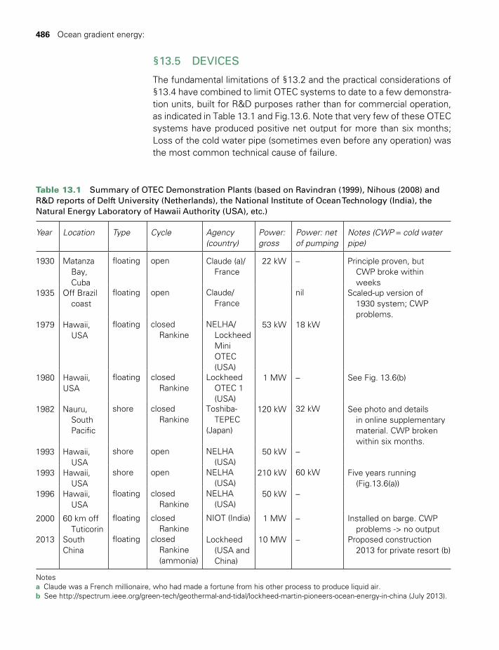
486 Ocean gradient energy:
§13.5 DEVICES
The fundamental limitations of §13.2 and the practical considerations of §13.4 have combined to limit OTEC systems to date to a few demonstra-tion units, built for R&D purposes rather than for commercial operation, as indicated in Table 13.1 and Fig.13.6. Note that very few of these OTEC systems have produced positive net output for more than six months; Loss of the cold water pipe (sometimes even before any operation) was the most common technical cause of failure.
Table 13.1 Summary of OTEC Demonstration Plants (based on Ravindran (1999), Nihous (2008) and R&D reports of Delft University (Netherlands), the National Institute of Ocean Technology (India), the Natural Energy Laboratory of Hawaii Authority (USA), etc.)
Year Location Type Cycle Agency (country)
Power: gross
Power: net of pumping
Notes (CWP = cold water pipe)
1930 Matanza Bay,
Cuba
floating open Claude (a)/ France
22 kW – Principle proven, but CWP broke within
weeks1935 Off Brazil
coastfloating open Claude/
Francenil Scaled-up version of
1930 system; CWP problems.
1979 Hawaii, USA
floating closed Rankine
NELHA/ Lockheed
Mini OTEC (USA)
53 kW 18 kW
1980 Hawaii, USA
floating closed Rankine
Lockheed OTEC 1
(USA)
1 MW – See Fig. 13.6(b)
1982 Nauru, South
Pacific
shore closed Rankine
Toshiba- TEPEC (Japan)
120 kW 32 kW See photo and details in online supplementary
material. CWP broken within six months.
1993 Hawaii, USA
shore open NELHA (USA)
50 kW –
1993 Hawaii, USA
shore open NELHA (USA)
210 kW 60 kW Five years running (Fig.13.6(a))
1996 Hawaii, USA
floating closed Rankine
NELHA (USA)
50 kW –
2000 60 km off Tuticorin
floating closed Rankine
NIOT (India) 1 MW – Installed on barge. CWP problems -> no output
2013 South China
floating closed Rankine
(ammonia)
Lockheed (USA and
China)
10 MW – Proposed construction 2013 for private resort (b)
Notes a Claude was a French millionaire, who had made a fortune from his other process to produce liquid air. b See http://spectrum.ieee.org/green-tech/geothermal-and-tidal/lockheed-martin-pioneers-ocean-energy-in-china (July 2013).
TWIDELL PAGINATION.indb 486 01/12/2014 11:38

13.6 Related technologies 487
§13.6 RELATED TECHNOLOGIES
OTEC is one of several possible deep ocean water applications (DOWAs) associated with pumping sea water from depths of at least 100 m. Others are listed below. Like OTEC itself, they all have dimensional scaling factors encouraging large equipment, unlike the modular operation and smaller scale of many renewable energy options. However, if OTEC, or similar technologies, are ever to become accepted commercially, it seems inevitable that an integrated set of operations will be used for a combination of several benefits.
1 Marine farming. Sea water from the depths below about 500 m is rich in nutrients, and these may be pumped to the surface, as from an OTEC plant. This encourages the growth of algae (phytoplankton), which feed other marine creatures higher up the food chain and so provide a basis for commercial fish farming.
2 Cooling. Deep, cool water pumped to the surface may be used to cool buildings, tropical horticultural ‘greenhouses’ or engineering plant as in chemical refineries.
3 Fresh water/desalination. Flash evaporation of upper-surface sea water onto condensers cooled by deep water produces ‘distilled’ ‘fresh’ water for drinking, horticulture, etc. This process may be inte-grated with solar distillation. For OTEC an open-cycle Rankine engine inputs water vapor and outputs a mist of partly condensed water; this output is in effect distilled water and may be used for potable and agricultural water.
(a)
Mixedwaterdrain
Warmwaterintake
Buoy
Cold waterpipe
Sea floor(1000 m)
Anchorleg
(b)
Fig. 13.6 Some of the systems (devices) designed to demonstrate OTEC: (a) on-shore system at Hawaii (big island) in the 1990s: cold water pipe from ocean is at the top of the photo; (b) floating barge system (schematic, based on NIOT c. 2003).
TWIDELL PAGINATION.indb 487 01/12/2014 11:38

488 Ocean gradient energy:
4 CO2 injection. The aim is to absorb CO2 emitted from large-scale fossil fuel combustion by absorption in sea water and then pumping this to depth. This is one type of carbon capture and storage (CCS). It is almost the reverse of the technology for the OTEC cold water pipe, and potentially would be on a very large scale. If combined with OTEC, the evaporator output would absorb the CO2 and then be pumped down for discharge at depth. However, there are significant unre-solved issues with such suggestions, including the environmental impact on the biota at depth, cost and the long-term stability of the capture.
5 Floating industrial complexes. Concepts exist to match the large scale of OTEC and DOWA with industry on very large floating rafts of km scale (e.g. for hydrogen production for shipping to land-based markets as energy storage). Talk is cheap!
§13.7 SOCIAL, ECONOMIC AND ENVIRONMENTAL ASPECTS OF OTEC
As illustrated in Fig.13.2, the resource for OTEC is effectively limited to coasts or islands in the tropics. However, most such places are in poorer countries which lack the funds to bear the risk and burden associated with novel capital-intensive technologies, with a few notable exceptions such as Hawaii, Florida and Brazil. In such places, the social impacts of an OTEC plant would be similar to operating an offshore oil rig or an onshore power station (e.g. providing employment and nearby industry, including marine service activities).
The economics of OTEC are dominated by the high projected capital costs arising from the large size of OTEC components and the demands imposed by offshore environments on equipment survival and power production logistics. This, as well as the relatively small power outputs, result in analyses based on the levelized cost of electricity generation (§17.6) and consistently find OTEC projects have too small a cost/benefit ratio to be economically worthwhile. Even though the cost-effectiveness gap between OTEC and the most expensive fossil fuel power-generation technologies (e.g., oil) has steadily declined, since 2000, OTEC market penetration has not yet succeeded. Because of a lack of experimental and operational data in running OTEC systems however, taking advantage of this purported economy of scale presents a large financial and engineering risk, with capital outlays as high as US$300 million for power outputs of the order of 10 MW. Hence, it remains likely that any meaningful demonstration of scalable OTEC systems will be accomplished only with a strong commitment of public funds.
The main environmental impacts of OTEC and DOWA technologies relate to the following:
TWIDELL PAGINATION.indb 488 01/12/2014 11:38

§13.8 Osmotic power from salinity gradients 489
• leakage, and likely pollution, from engineering plant, especially of the working fluids and antifouling chemicals;
• large volumes of pumped marine water; • mixing of deep nutrient-rich (nitrate, phosphate and silicate) water
with upper, solar irradiated, water;• operation of engineering plant, usually in pristine marine locations.
A dominant harmful threat is local onshore, near-shore and offshore pollution from leaks of working fluids. The mixing of nutrient-rich deep water with surface water has ecological impacts, which may be benefi-cial for fisheries but not otherwise. The thermal mixing of water is not considered harmful from developmental or single isolated OTEC plant; even the hypothetical location of about 1000 stations of 200 MWe each in the Gulf of Mexico has been calculated to reduce surface sea tempera-ture by only 0.3°C, which is not considered significant. Large deployment of OTEC plant, say, 100 stations at 10 km separation, would cause the upwelling of nitrate to a concentration found naturally off Peru, where fish populations are much increased. The prospect of enriching fisheries with deep-water nutrients is generally favored.
If cold deep water is discharged into the ocean surface, a proportion of its otherwise stable dissolved CO2 passes into the atmosphere. If 50% of the excess CO2 is emitted, the rate would be about 0.1 kg/kWe, as compared with about 0.8 kg/kWe from electricity generation by fossil fuel. This not insignificant impact leads to discussion whether OTEC is indeed an environmentally sustainable source of power (in the sense discussed in Chapter 1).
§13.8 OSMOTIC POWER FROM SALINITY GRADIENTS
Osmotic power is the extraction of useful energy from the difference in salt concentration between the ocean and a nearby source of fresh water (e.g. a river). The technique uses the osmotic pressure that is apparent when two volumes of a solvent (e.g. water) having different concentra-tions of solute (e.g. salt) are separated by a semi-permeable membrane, as shown in Fig. 13.7. Microscopically the molecules of the solvent are able to diffuse back and forth through the membrane, but the molecules of the solute cannot do this. Consequently, the more concentrated solu-tion becomes less concentrated because more solvent passes one way than the other. This causes a macroscopic pressure difference across the membrane. Eventually equilibrium is reached, for which the static pressure difference across the membrane is termed the osmotic pres-sure. Osmotic pressures are very large (e.g. 30 atmospheres between fresh water and sea water). (For further detail see textbooks on physical chemistry.) Osmotic pressure differences and movement of solvents is an essential process in life systems (e.g. kidney function and water movement through semi-permeable cell walls).
TWIDELL PAGINATION.indb 489 01/12/2014 11:38

490 Ocean gradient energy:
For reverse osmosis, external pressure forces water from the salty/brackish side to the fresh side of a semi-permeable membrane against the osmotic pressure. The technique is used for desalination of brackish water and sea water, for instance, on a large scale in parts of the Middle East, usually powered by fossil fuels, but on a small scale for rural areas, usually powered by solar photovoltaic or wind power.
Techniques to harness osmotic processes for useful energy are con-sidered ‘renewable’, as defined in §1.1, as they depend only on the natural hydrological cycle, but have only relatively recently been consid-ered for commercial energy supply. The first pilot system was built in 2009 by Statkraft, a hydro-electricity-generating utility of Norway; this led to initiating the construction of a 2 MW osmotic power plant in the Sunndalsøra fjord in 2013.
(a) Pressure retarded osmosis (PRO) for powerFig. 13.8 shows a flow diagram of the PRO power system piloted by Statkraft (Norway). Fresh water from a hydro catchment or nearby river is fed into the plant and filtered before entering the membrane modules. Each membrane module contains spiral wound or hollow fibre membranes, across which 80 to 90% of the fresh water transfers by osmosis. This pressurizes the sea water pipes (dark green) and increases the volumetric flow at high pressure. The ‘pressure exchanger’ is in effect a pump for the inflow of sea water.
The brackish water from the membrane module divides into two flows. About one-third of this water goes to the turbine to generate power, and two-thirds passes to the pressure exchanger to pressurize the feed of sea water. To optimize the power plant, the typical operating pressure is in the range of 11 to 15 atmospheres. This is equivalent to a water head of 100 to 145 metres in a hydropower plant, thus generating about 1 MW for each m3s-1 of fresh water (see §6.2).
Some pre-treatment of both the fresh water and sea water is neces-sary. Experience from Norwegian water treatment plants shows that mechanical filtration down to 50 µm in combination with a standard cleaning and maintenance cycle is enough to sustain the membrane performance for 7 to 10 years.
As with OTEC, the concept of salinity gradient power is simple, proven at pilot plant level and has a resource potential wherever a fresh-water river runs into the ocean. Therefore its global resource level is very large. The present difficulty is that the value of the net power output remaining after pumping is small in relation to the large capital cost, especially of the membranes. However, membrane systems are being improved and becoming cheaper as R&D responds to the demand for desalination by reverse osmosis.
Solution
Semipermeablemembrane
Pure solvent
h
Fig. 13.7 Illustrating osmotic pressure: osmotic equilibrium across a semi-permeable membrane. Osmotic pressure from the ‘pure solvent’ side (at right) of the membrane is balanced by the weight (‘gravity pressure’) of the extra height h of liquid on the solute-rich side (at left).
TWIDELL PAGINATION.indb 490 01/12/2014 11:38
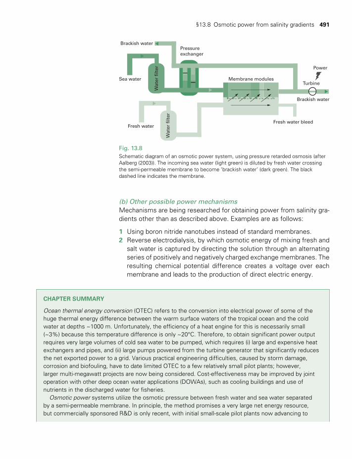
§13.8 Osmotic power from salinity gradients 491
(b) Other possible power mechanismsMechanisms are being researched for obtaining power from salinity gra-dients other than as described above. Examples are as follows:
1 Using boron nitride nanotubes instead of standard membranes. 2 Reverse electrodialysis, by which osmotic energy of mixing fresh and
salt water is captured by directing the solution through an alternating series of positively and negatively charged exchange membranes. The resulting chemical potential difference creates a voltage over each membrane and leads to the production of direct electric energy.
Brackish water
Sea water
Fresh water
Wat
er f
ilter
Wat
er f
ilter
Membrane modules
Power
Turbine
Brackish water
Fresh water bleed
Pressureexchanger
Fig. 13.8 Schematic diagram of an osmotic power system, using pressure retarded osmosis (after Aalberg (2003)). The incoming sea water (light green) is diluted by fresh water crossing the semi-permeable membrane to become ‘brackish water’ (dark green). The black dashed line indicates the membrane.
CHAPTER SUMMARY
Ocean thermal energy conversion (OTEC) refers to the conversion into electrical power of some of the huge thermal energy difference between the warm surface waters of the tropical ocean and the cold water at depths ~1000 m. Unfortunately, the efficiency of a heat engine for this is necessarily small (~3%) because this temperature difference is only ~20°C. Therefore, to obtain significant power output requires very large volumes of cold sea water to be pumped, which requires (i) large and expensive heat exchangers and pipes, and (ii) large pumps powered from the turbine generator that significantly reduces the net exported power to a grid. Various practical engineering difficulties, caused by storm damage, corrosion and biofouling, have to date limited OTEC to a few relatively small pilot plants; however, larger multi-megawatt projects are now being considered. Cost-effectiveness may be improved by joint operation with other deep ocean water applications (DOWAs), such as cooling buildings and use of nutrients in the discharged water for fisheries.
Osmotic power systems utilize the osmotic pressure between fresh water and sea water separated by a semi-permeable membrane. In principle, the method promises a very large net energy resource, but commercially sponsored R&D is only recent, with initial small-scale pilot plants now advancing to
TWIDELL PAGINATION.indb 491 01/12/2014 11:38

492 Ocean gradient energy:
QUICK QUESTIONS
Note: Answers to these questions are in the text of the relevant section of this chapter, or may be readily inferred from it.
1 What do the abbreviations OTEC and DOWA stand for? 2 Why is OTEC not feasible outside the tropics? 3 Describe the OTEC thermodynamic limit on efficiency. 4 How does OTEC power potential vary with the temperature difference
of surface and deep water? 5 What is biofouling and why is it a challenge for OTEC systems? 6 Why are large corrosion-resistant heat exchangers needed for
OTEC? 7 What are two main reasons why OTEC has yet to progress beyond a
few pilot plants? 8 What is osmotic pressure? 9 Is osmotic power confined to the tropics and why? 10 Why is OTEC favored offshore and osmotic power favored
onshore?11 Why is it important to differentiate ‘net power’ from ‘gross power’ in
both OTEC and osmotic power, but not so important for most other generating technologies?
PROBLEMS
13.1 If P ∝ DT2 / Th (13.5) calculate the rate of change of efficiency with respect to temperature difference DT. What is the percentage improvement in power production if DT increases from 20°C to 21°C?
13.2 Consider the definition of the term ‘renewable energy’ in §1.1, and discuss how both OTEC and osmotic power fit or do not fit these definitions.
Note: Further problems from Chapter 14 in Twidell and Weir (2006) Renewable Energy Resources, 2nd edn, are available on the website of this third edition. They relate to extended quantitative analysis of some engineering aspects of OTEC.
MW scale application. Costs may decrease substantially in future, as membrane technology improves in throughput and reliability, driven largely by the increasing demand for desalination by reverse osmosis using similar membranes.
TWIDELL PAGINATION.indb 492 01/12/2014 11:38
Bibliography 493
NOTE
1 Deep-water ocean currents of cold water circulate globally, driven from sinking cold sea water at the Poles.
BIBLIOGRAPHY
OTEC
Avery, W.H. and Wu, C. (1994) Renewable Energy from the Ocean – A guide to OTEC, Oxford University Press, Oxford (Johns Hopkins University series). A substantial and authoritative study of the science, engineering and history of OTEC.
Curzon, F.L. and Ahlborn, B. (1975) `Efficiency of a Carnot engine at maximum power output’, American Journal of Physics, 43, 22–24.
d’Arsonval, J. (1881) Revue Scientifique, 17, 370–372. Perhaps the earliest published reference to the potential of OTEC.
Gauthier, M., Golman, L. and Lennard, D. (2000) ‘Ocean Thermal Energy Conversion (OTEC) and Deep Water Applications (DOWA) – market opportunities for European Industry’, in Proceedings of the European Conference, New and Renewable Technologies for Sustainable Development, Madeira, June. Excellent review of working plant since the 1930s to 2000, with future industrial market potential.
Johnson, F.A. (1992) ‘Closed cycle thermal energy conversion’, in R.J. Seymour (ed.), Ocean Energy Recovery: The state of the art, American Society of Civil Engineers. Useful summary of thermodynamics, economics and history.
Masutani, S.M. and Takahashi, P.K. (1999) ‘Ocean Thermal Energy Conversion’, in J.G. Webster (ed.), Encyclopaedia of Electrical and Electronics Engineering, 18, 93–103, Wiley, New York. Authoritative summary.
McGowan, J.G. (1976) ‘Ocean thermal energy conversion – a significant solar resource’, Solar Energy, 18, 81–92. Reviewed US design philosophy at a historically important time.
Meyer, M., Cooper, D. and Varley, R. (2011) ‘Are we there yet? A developer’s roadmap to OTEC commercializa-tion’, Hawaii National Marine Renewable Energy Center OTEC References, Lockheed Martin Mission Systems and Sensors, Manassas, VA, USA.
Nihous, G. (2008) Ocean Thermal Energy Conversion (OTEC) and Derivative Technologies: Status and prospects, report available at http://www.ocean-energy-systems.org/ocean_energy/ocean_ thermal_energy/.
Nihous, G. (2013) ‘Ocean Thermal Energy Conversion’, in G.M. Crawley (ed.), Handbook of Energy, World Scientific Publishing Co. Pte. Ltd., Singapore.
Ravidran, M. (1999) ‘Indian 1 MW floating plant: an overview’, in Proceedings of the IOA ‘99 Conference, IMARI, Japan.
Twidell, J.W. and Weir, T. (2006) Renewable Energy Resources, 2nd edn, ch. 14, ‘Ocean Thermal Energy Conversion’ (heat exchangers, pp. 461–463), Earthscan, London. This chapter, which is available on the website for the current edition of this book, has more detail of heat exchangers and biofouling than in this (third) edition, including some indicative calculations.
UN (1984) A Guide to Ocean Thermal Energy Conversion for Developing Countries, United Nations Publications, New York.
TWIDELL PAGINATION.indb 493 01/12/2014 11:38

494 Ocean gradient energy:
Osmotic power
This subject is so new that most of the literature on it is only in the form of magazine-style articles and technical reports, most of which appear only on the internet. See e.g.:
http://www.statkraft.com/energy-sources/osmotic-power/ (Statkraft is a major utility in Norway, and is actively developing osmotic power).
www.yuvaenegineers.com (a website compiled by Indian engineering students; see especially the 2010 article on ‘osmotic power’ by Rohini and Ahmed Beer).
Aaberg, R.J. (2003) ‘Osmotic power: a new and powerful renewable energy source?’, Refocus, 4, 48–50.
Siria, A. et al. (2013) 'Giant osmotic energy conversion measured in a single transmembrane boron nitride nano-tube', Nature, 494, 455. DOI: 10.1038/nature11876.
Websites
The newsletters and sites on ocean energy, cited in Chapters 11 and 12, also report on OTEC, although there are not many stories on OTEC compared to the more active fields of wave power and tidal currents. See in particular:
IEA Ocean Energy Systems. International collaboration with useful reports of progress and policies – see espe-cially their ‘Annual Reports’ (www.ocean-energy-systems.org).
http://energiesdelamer.blogspot.com/. (A newsletter on marine energy , mainly in French).
TWIDELL PAGINATION.indb 494 01/12/2014 11:38
Geothermal energy
CONTENTS
Learning aims 495
§14.1 Introduction 497
§14.2 Geophysics 500
§14.3 Dry rock and hot aquifer analysis 503 §14.3.1 Dry rock: algebra to calculate
potential heat output 503 §14.3.2 Hot aquifers: algebra to
calculate potential rate of heat extraction 505
§14.4 Harnessing geothermal resources 507 §14.4.1 Matching supply and
demand 507 §14.4.2 Extraction techniques:
hydrothermal 508
§14.4.3 Extraction techniques: ‘enhanced geothermal systems’ (EGS) 509
§14.4.4 Electricity-generating systems 510
§14.4.5 Direct uses of geothermal heat 510
§14.5 Ground-source heat pumps 512
§14.6 Social and environmental aspects 514
Chapter summary 516
Quick questions 517
Problems 518
Bibliography 519
LEARNING AIMS
• Identify the source of geothermal energy and appreciate issues around its sustainability.
• Identify requirements for geothermal energy to be potentially useful for electricity genera-tion and understand why suitable locations are geographically restricted.
• Appreciate potential for more geographically widespread use of geothermal energy for thermal applications.
• Understand operating principles of ground-source heat pumps.
CHAPTER
14
LIST OF FIGURES
14.1 Growth in world geothermal installations. 49714.2 Key named regions harnessing geothermal energy for heat production and/or electricity generation. 49814.3 Geothermal structure of the Earth. 500
TWIDELL PAGINATION.indb 495 01/12/2014 11:38

496 Geothermal energy
14.4 Geology of an aquifer in a hydrothermal region. 50214.5 (a) Profile of hot aquifer system for calculating the heat content; (b) a geyser, a common sight in
many hydrothermal regions. 50414.6 (a) Schematic diagram, not to scale, of hydrothermal power stations in a hyperthermal region
(e.g. the Geysers geothermal field, California). (b) Geology of an aquifer in a hydrothermal region and a region of hot, dry rock. 508
14.7 Schematic diagram of heat extraction from a hot, dry rock system. 50914.8 Schematic diagrams of two major applications of geothermal heat. 51114.9 ‘Geothermal’ heat pumps. 51314.10 The Wairakei geothermal power station in New Zealand. 516
LIST OF TABLES
14.1 Countries with significant use of geothermal energy. 49914.2 Direct applications of geothermal heat, 2010. 512
TWIDELL PAGINATION.indb 496 01/12/2014 11:38
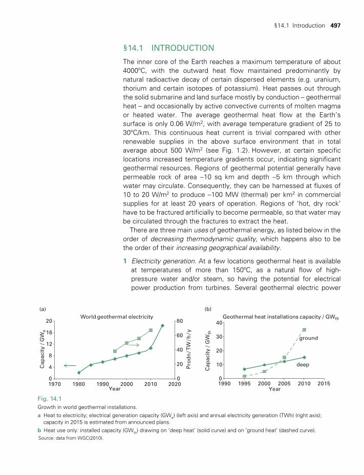
§14.1 Introduction 497
§14.1 INTRODUCTION
The inner core of the Earth reaches a maximum temperature of about 4000ºC, with the outward heat flow maintained predominantly by natural radioactive decay of certain dispersed elements (e.g. uranium, thorium and certain isotopes of potassium). Heat passes out through the solid submarine and land surface mostly by conduction – geothermal heat – and occasionally by active convective currents of molten magma or heated water. The average geothermal heat flow at the Earth’s surface is only 0.06 W/m2, with average temperature gradient of 25 to 30ºC/km. This continuous heat current is trivial compared with other renewable supplies in the above surface environment that in total average about 500 W/m2 (see Fig. 1.2). However, at certain specific locations increased temperature gradients occur, indicating significant geothermal resources. Regions of geothermal potential generally have permeable rock of area ~10 sq km and depth ~5 km through which water may circulate. Consequently, they can be harnessed at fluxes of 10 to 20 W/m2 to produce ~100 MW (thermal) per km2 in commercial supplies for at least 20 years of operation. Regions of ‘hot, dry rock’ have to be fractured artificially to become permeable, so that water may be circulated through the fractures to extract the heat.
There are three main uses of geothermal energy, as listed below in the order of decreasing thermodynamic quality, which happens also to be the order of their increasing geographical availability.
1 Electricity generation. At a few locations geothermal heat is available at temperatures of more than 150ºC, as a natural flow of high- pressure water and/or steam, so having the potential for electrical power production from turbines. Several geothermal electric power
0
20
40
60
80
0
4
8
12
16
20
(a)
1970 1980 1990 2000 2010 2020
Cap
acit
y / G
We
Year
World geothermal electricity
Pro
dn
/ TW
/ h / y
0
10
20
30
40
1990 1995 2000 2005 2010 2015Year
Geothermal heat installations capacity / GWth
ground
deep
(b)
Cap
acit
y / G
Wth
Fig. 14.1 Growth in world geothermal installations. a Heat to electricity; electrical generation capacity (GWe) (left axis) and annual electricity generation (TWh) (right axis);
capacity in 2015 is estimated from announced plans.b Heat use only: installed capacity (GWth) drawing on ‘deep heat’ (solid curve) and on ‘ground heat’ (dashed curve). Source: data from WGC(2010).
TWIDELL PAGINATION.indb 497 01/12/2014 11:38

498 Geothermal energy
complexes have operated for many years, especially in Italy, Iceland, New Zealand and the USA (see Fig. 14.2). The number of similar instal-lations has increased steadily since the 1970s (Fig 14.1(a)). As for hydro-power, hydrothermal power technology is mature and long-lasting when tailored to specific sites. The power may be used constantly for baseload at a cheap per unit cost. New developments have increased rapidly in the relatively unexploited geothermally active regions of the Philippines, Indonesia and western USA (see Table 14.1).
2 Hot water supply. In many more locations, geothermal heat is avail-able at ~50 to 70°C; for instance, for ‘medicinal’ bathhouses in the Roman Empire, and today for greenhouse heating for vegetable crops and soft fruits, for crop drying, for aquaculture of fish and algae, for district heating servicing buildings and for industrial process heat (e.g. for paper pulp from wood processing, and for leaching chemicals). More than 60 countries list such uses, many of which do not produce geothermal electricity (see Table 14.1 and Fig. 14.1(b)).
3 Heat pumps. Heat at ambient temperature from near-surface ground (to depths of usually about 3 m), or from rivers and lakes, is input to electrical-powered heat pumps, which provide heat to buildings at increased temperature. The systems are often called ‘geother-mal’, although the input heat arises from soil heated by sunshine and ambient air. Note that ground at depths of more than about 2 m has
Geysers
Matsukawa
Tiwi
CerroPrieto
Hawaii
Iceland
ParisLarderello
Wairakei
Fig. 14.2 Key named regions harnessing geothermal energy for heat production and/or electricity generation. Dashed lines indicate plate boundaries. Colored lines indicate areas of extra strain.
TWIDELL PAGINATION.indb 498 01/12/2014 11:38

§14.1 Introduction 499
In Chapter 1, renewable energy was defined as ‘energy obtained from naturally repetitive and persistent flows of energy occurring in the local environment’. By this definition, most supplies of geothermal energy may be classed as renewable, because the energy would otherwise be dissipated continuously in the local environment (e.g. from hot springs or geysers). In other geothermal supply, the current of heat is increased arti-ficially (e.g. by fracturing and actively cooling ‘hot’ rocks, which remain in place, but do not reheat except over the very long term, so the resource in practice has a finite lifetime). Such enhanced geothermal systems (EGS) definitely have the potential to supply energy without mining and extraction of materials, so ‘hot rocks’ technology is being researched and developed as a means of alternative energy (§14.4.3).
Table 14.1 Countries with significant use of geothermal energy. Table shows installed capacity for electricity generation (MWe), capacity factor Z for geothermal electricity, and installed capacity for direct heat use (excluding ‘surface’ ground- and air-sourced heat pumps) (MWth). All data are for 2010.
Country Electricity capacity
MWe
% of world geothermal
total
Electricity capacity factor Z
(%)
Direct heating capacity
(excluding heat pumps)
(MWth)
% of world total of direct
heating
USA 3093 29 61 611 4Philippines 1904 18 62 3Indonesia 1197 11 92 2Mexico 958 9 84 155 1Italy 843 8 75 636 4New Zealand 628 6 74 386 3Iceland 575 5 91 1822 12Japan 536 5 65 2093 14El Salvador 204 2 79 2Kenya 167 2 98 16Costa Rica 166 2 78 1Nicaragua 88 1 40 0Turkey 82 1 68 1548 10Russia 82 1 61 307 2China 24 71 3690 24others 168 2 4075 27
--------- -------- --------- ---------WORLD TOTAL 10715 100% 15347 100%
Source: Bertani (2010), Lund et al. (2010).
nearly constant temperature through the year. In reverse mode extract-ing heat from buildings, the same heat pumps may be used for cooling, i.e. they function as refrigerators. This technology is available world-wide and is by far the most rapidly growing ‘geothermal’ application (Fig. 14.1(b)). The relevant technology is outlined in §14.5.
TWIDELL PAGINATION.indb 499 01/12/2014 11:38
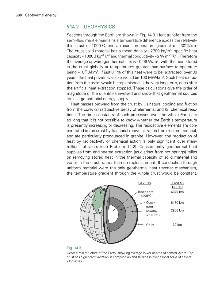
500 Geothermal energy
§14.2 GEOPHYSICS
Sections through the Earth are shown in Fig. 14.3. Heat transfer from the semi-fluid mantle maintains a temperature difference across the relatively thin crust of 1000ºC, and a mean temperature gradient of ~30ºC/km. The crust solid material has a mean density ~2700 kg/m3, specific heat capacity ~1000 J kg-1 K-1 and thermal conductivity ~2 W m-1 K-1. Therefore the average upward geothermal flux is ~0.06 W/m2, with the heat stored in the crust globally at temperatures greater than surface temperature being ~1020 J/km2. If just 0.1% of this heat were to be ‘extracted’ over 30 years, the heat power available would be 100 MW/km2. Such heat extrac-tion from the rocks would be replenished in the very long term, eons after the artificial heat extraction stopped. These calculations give the order of magnitude of the quantities involved and show that geothermal sources are a large potential energy supply.
Heat passes outward from the crust by (1) natural cooling and friction from the core; (2) radioactive decay of elements; and (3) chemical reac-tions. The time constants of such processes over the whole Earth are so long that it is not possible to know whether the Earth’s temperature is presently increasing or decreasing. The radioactive elements are con-centrated in the crust by fractional recrystallization from molten material, and are particularly pronounced in granite. However, the production of heat by radioactivity or chemical action is only significant over many millions of years (see Problem 14.2). Consequently geothermal heat supplies from engineered extraction (as distinct from hot springs) relies on removing stored heat in the thermal capacity of solid material and water in the crust, rather than on replenishment. If conduction through uniform material were the only geothermal heat transfer mechanism, the temperature gradient through the whole crust would be constant.
Crust
LAYERS LOWESTDEPTH
Mantle~ 1000°C
Outercore
Inner core~ 4000°C
6370 km
5180 km
2900 km
30 km
Fig. 14.3 Geothermal structure of the Earth, showing average lower depths of named layers. The crust has significant variation in composition and thickness over a local scale of several kilometres.
TWIDELL PAGINATION.indb 500 01/12/2014 11:38
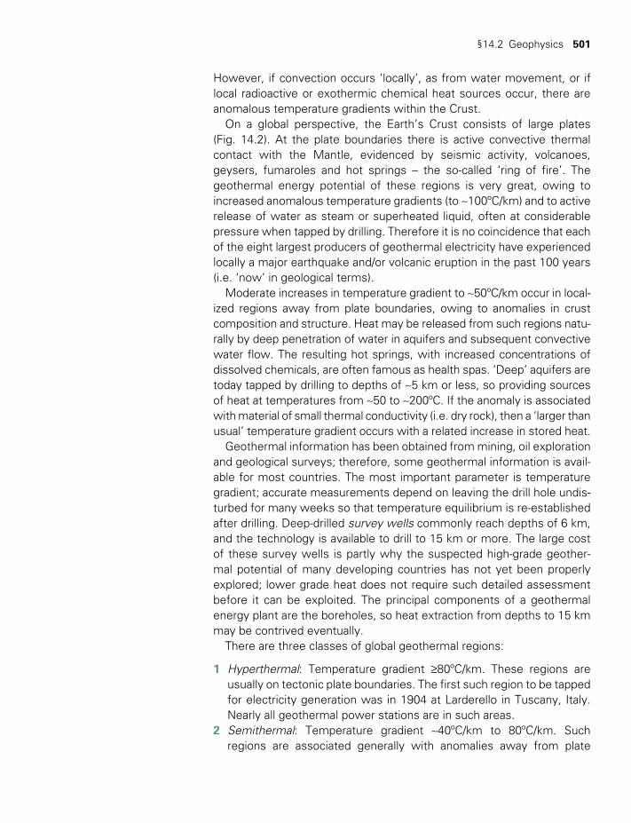
§14.2 Geophysics 501
However, if convection occurs ‘locally’, as from water movement, or if local radioactive or exothermic chemical heat sources occur, there are anomalous temperature gradients within the Crust.
On a global perspective, the Earth’s Crust consists of large plates (Fig. 14.2). At the plate boundaries there is active convective thermal contact with the Mantle, evidenced by seismic activity, volcanoes, geysers, fumaroles and hot springs – the so-called ‘ring of fire’. The geothermal energy potential of these regions is very great, owing to increased anomalous temperature gradients (to ~100ºC/km) and to active release of water as steam or superheated liquid, often at considerable pressure when tapped by drilling. Therefore it is no coincidence that each of the eight largest producers of geothermal electricity have experienced locally a major earthquake and/or volcanic eruption in the past 100 years (i.e. ‘now’ in geological terms).
Moderate increases in temperature gradient to ~50ºC/km occur in local-ized regions away from plate boundaries, owing to anomalies in crust composition and structure. Heat may be released from such regions natu-rally by deep penetration of water in aquifers and subsequent convective water flow. The resulting hot springs, with increased concentrations of dissolved chemicals, are often famous as health spas. ‘Deep’ aquifers are today tapped by drilling to depths of ~5 km or less, so providing sources of heat at temperatures from ~50 to ~200ºC. If the anomaly is associated with material of small thermal conductivity (i.e. dry rock), then a ‘larger than usual’ temperature gradient occurs with a related increase in stored heat.
Geothermal information has been obtained from mining, oil exploration and geological surveys; therefore, some geothermal information is avail-able for most countries. The most important parameter is temperature gradient; accurate measurements depend on leaving the drill hole undis-turbed for many weeks so that temperature equilibrium is re-established after drilling. Deep-drilled survey wells commonly reach depths of 6 km, and the technology is available to drill to 15 km or more. The large cost of these survey wells is partly why the suspected high-grade geother-mal potential of many developing countries has not yet been properly explored; lower grade heat does not require such detailed assessment before it can be exploited. The principal components of a geothermal energy plant are the boreholes, so heat extraction from depths to 15 km may be contrived eventually.
There are three classes of global geothermal regions:
1 Hyperthermal: Temperature gradient ≥80ºC/km. These regions are usually on tectonic plate boundaries. The first such region to be tapped for electricity generation was in 1904 at Larderello in Tuscany, Italy. Nearly all geothermal power stations are in such areas.
2 Semithermal: Temperature gradient ~40ºC/km to 80ºC/km. Such regions are associated generally with anomalies away from plate
TWIDELL PAGINATION.indb 501 01/12/2014 11:38
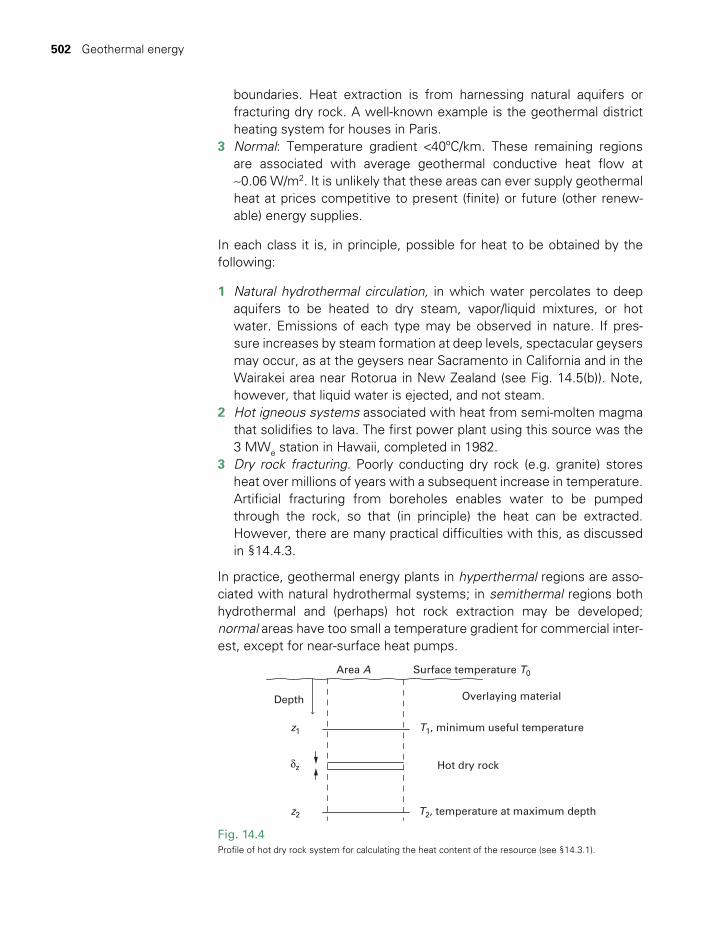
502 Geothermal energy
boundaries. Heat extraction is from harnessing natural aquifers or fracturing dry rock. A well-known example is the geothermal district heating system for houses in Paris.
3 Normal: Temperature gradient <40ºC/km. These remaining regions are associated with average geothermal conductive heat flow at ~0.06 W/m2. It is unlikely that these areas can ever supply geothermal heat at prices competitive to present (finite) or future (other renew-able) energy supplies.
In each class it is, in principle, possible for heat to be obtained by the following:
1 Natural hydrothermal circulation, in which water percolates to deep aquifers to be heated to dry steam, vapor/liquid mixtures, or hot water. Emissions of each type may be observed in nature. If pres-sure increases by steam formation at deep levels, spectacular geysers may occur, as at the geysers near Sacramento in California and in the Wairakei area near Rotorua in New Zealand (see Fig. 14.5(b)). Note, however, that liquid water is ejected, and not steam.
2 Hot igneous systems associated with heat from semi-molten magma that solidifies to lava. The first power plant using this source was the 3 MWe station in Hawaii, completed in 1982.
3 Dry rock fracturing. Poorly conducting dry rock (e.g. granite) stores heat over millions of years with a subsequent increase in temperature. Artificial fracturing from boreholes enables water to be pumped through the rock, so that (in principle) the heat can be extracted. However, there are many practical difficulties with this, as discussed in §14.4.3.
In practice, geothermal energy plants in hyperthermal regions are asso-ciated with natural hydrothermal systems; in semithermal regions both hydrothermal and (perhaps) hot rock extraction may be developed; normal areas have too small a temperature gradient for commercial inter-est, except for near-surface heat pumps.
Surface temperature T0
Overlaying material
Area A
z2
z1
δz Hot dry rock
T1, minimum useful temperature
T2, temperature at maximum depth
Depth
Fig. 14.4 Profile of hot dry rock system for calculating the heat content of the resource (see §14.3.1).
TWIDELL PAGINATION.indb 502 01/12/2014 11:38
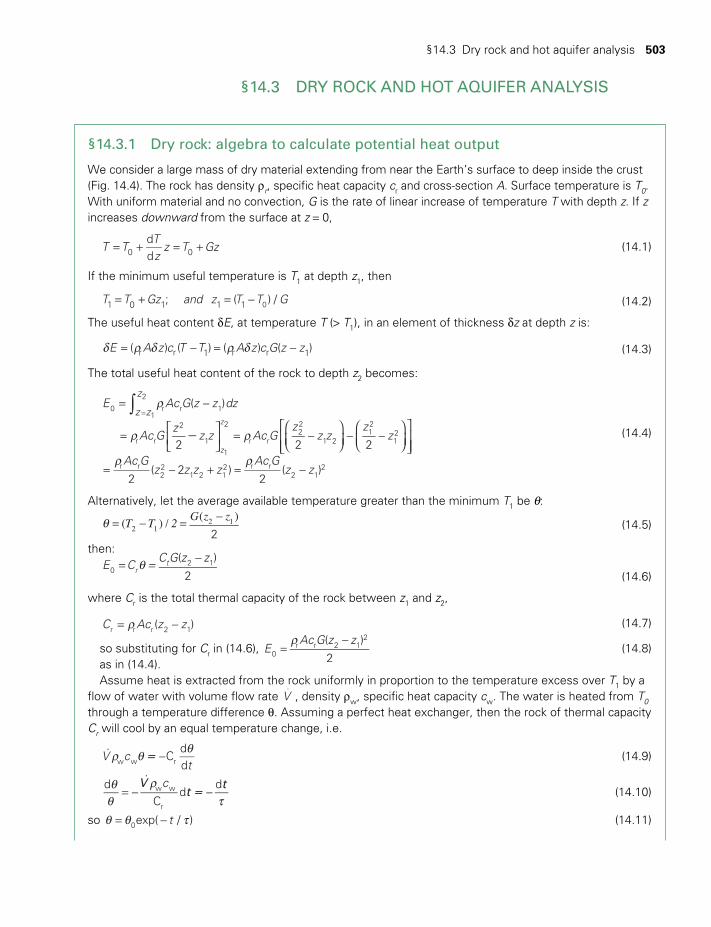
§14.3 Dry rock and hot aquifer analysis 503
§14.3 DRY ROCK AND HOT AQUIFER ANALYSIS
§14.3.1 Dry rock: algebra to calculate potential heat output
We consider a large mass of dry material extending from near the Earth’s surface to deep inside the crust (Fig. 14.4). The rock has density rr, specific heat capacity cr and cross-section A. Surface temperature is T0. With uniform material and no convection, G is the rate of linear increase of temperature T with depth z. If z increases downward from the surface at z = 0,
T TTz
z T Gzdd0 0= + = + (14.1)
If the minimum useful temperature is T1 at depth z1, then
T T Gz and z T T G; ( ) /1 0 1 1 1 0= + = - (14.2)
The useful heat content dE, at temperature T (> T1), in an element of thickness dz at depth z is:
E A z c T T A z c G z z( ) ( ) ( ) ( )r r 1 r r 1d r d r d= - = - (14.3)
The total useful heat content of the rock to depth z2 becomes:
E Ac G z z dz
Ac Gz
z z Ac Gz
z zz
z
Ac Gz z z z
Ac Gz z
( )
2 2 2
2( 2 )
2( )
z z
z
z
z
r r
2
11
2
r r22
1 212
12
r r22
1 2 12 r r
2 12
0 r r 11
2∫-
r
r r
r r
= -
=
= -
- -
= - + = -
=
(14.4)
Alternatively, let the average available temperature greater than the minimum T1 be q:
2q = - = -T T 2 G z z( ) / ( )
2 12 1 (14.5)
then:E C
C G z z( )
2rt
02 1q == -
(14.6)
where Cr is the total thermal capacity of the rock between z1 and z2,
C Ac z z( )r r r 2 1r= - (14.7)
so substituting for Cr in (14.6), EAc G z z( )
20r r 2 1
2r=
- (14.8)
as in (14.4).Assume heat is extracted from the rock uniformly in proportion to the temperature excess over T1 by a
flow of water with volume flow rate V.
, density rw, specific heat capacity cw. The water is heated from T0
through a temperature difference q. Assuming a perfect heat exchanger, then the rock of thermal capacity Cr will cool by an equal temperature change, i.e.
V ct
Cddw w r= r q - q
(14.9)
cdC
ddw w
r
Vt = tq
qr
t= - - (14.10)
so texp( / )0q q t= - (14.11)
TWIDELL PAGINATION.indb 503 01/12/2014 11:38
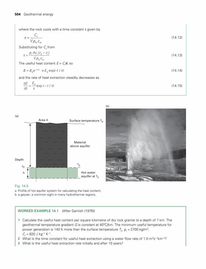
504 Geothermal energy
where the rock cools with a time constant t given by
C
V cr
w wtr
= (14.12)
Substituting for Ct from
Ac z z
V c
( )r r
w w
2 1t
rr
=-
(14.13)
The useful heat content E = Crq, so
E te exp( / )0t /
0Ε Ε t= ≡ -t- (14.14)
and the rate of heat extraction steadily decreases as
Et
Et
dd
exp ( / )0
tt= - (14.15)
Surface temperature T0
Materialabove aquifer
Depth
Hot wateraquifer at T2
Area A
T2z2
h
(a)
(b)
Fig. 14.5a Profile of hot aquifer system for calculating the heat content;b a geyser, a common sight in many hydrothermal regions.
WORKED EXAMPLE 14.1 (After Garnish (1976))
1 Calculate the useful heat content per square kilometre of dry rock granite to a depth of 7 km. The geothermal temperature gradient G is constant at 40ºC/km. The minimum useful temperature for power generation is 140 K more than the surface temperature T0. rr = 2700 kg/m3, Cr = 820 J kg-1 K-1.
2 What is the time constant for useful heat extraction using a water flow rate of 1.0 m3s-1km-2?3 What is the useful heat extraction rate initially and after 10 years?
TWIDELL PAGINATION.indb 504 01/12/2014 11:38
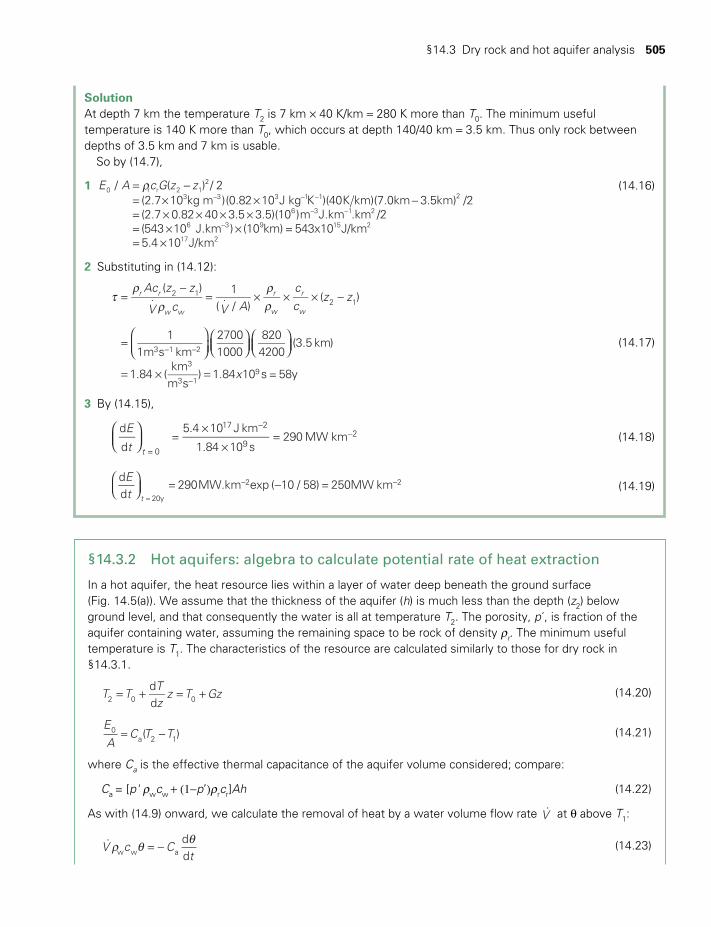
§14.3 Dry rock and hot aquifer analysis 505
SolutionAt depth 7 km the temperature T2 is 7 km × 40 K/km = 280 K more than T0. The minimum useful temperature is 140 K more than T0, which occurs at depth 140/40 km = 3.5 km. Thus only rock between depths of 3.5 km and 7 km is usable.
So by (14.7),
1 E A c G z z/ ( ) / 2(2.7 10 kg m )(0.82 10 J kg K )(40K km)(7.0km 3.5km) /2(2.7 0.82 40 3.5 3.5)(10 )m J.km .km /2(543 10 J.km ) (10 km) = 543x10 J/km5.4 10 J/km
0 r r 2 12
3 3 3 1 1 2
6 3 1 2
6 3 9 15 2
17 2
r= -= × × -= × × × ×= × ×= ×
- - -
- -
-
(14.16)
2 Substituting in (14.12):
Ac z z
V c V A
c
cz z
x
( ).
1(
./ )
( )
11m s km
27001000
8204200
(3.5 km)
1.84 (km
m s) 1.84 10 s = 58y
r r
w w
r
w
r
w
2 12 1
3 1 2
3
3 19
tr
rrr
=-
= × × × -
=
= × =
- -
-
(14.17)
3 By (14.15),
E
t
d
d=
5.4 10 J km
1.84 10 s290 MW km
t = 0
17 2
92
××
=-
- (14.18)
Et
dd
= 290MW.km exp ( 10 / 58) = 250MW kmt = 20y
2 2
-- - (14.19)
§14.3.2 Hot aquifers: algebra to calculate potential rate of heat extraction
In a hot aquifer, the heat resource lies within a layer of water deep beneath the ground surface (Fig. 14.5(a)). We assume that the thickness of the aquifer (h) is much less than the depth (z2) below ground level, and that consequently the water is all at temperature T2. The porosity, p´, is fraction of the aquifer containing water, assuming the remaining space to be rock of density rr. The minimum useful temperature is T1. The characteristics of the resource are calculated similarly to those for dry rock in §14.3.1.
T TTz
z T Gzdd2 0 0= + = + (14.20)
E
AC T T( )0
a 2 1= - (14.21)
where Ca is the effective thermal capacitance of the aquifer volume considered; compare:
Ca = [p' rwcw + (1-p’)rrcr]Ah (14.22)
As with (14.9) onward, we calculate the removal of heat by a water volume flow rate V at q above T1:
V c Ct
ddw w a
r q q= - (14.23)
TWIDELL PAGINATION.indb 505 01/12/2014 11:38
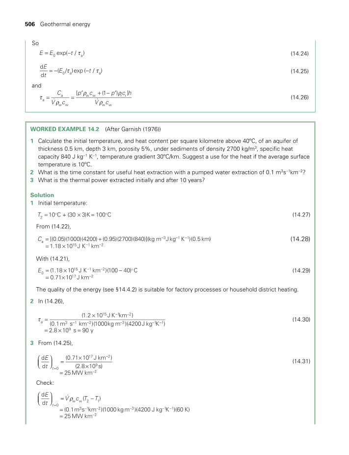
506 Geothermal energy
So
E E texp( / )0 at= - (14.24)
Et
E tdd
( / )exp ( / )0 a at t= - - (14.25)
andC
V c
p c p c h
V c
[ (1 ) ]a
a
w w
w w r r
w w tr
r rr
= =′ + - ′
(14.26)
WORKED EXAMPLE 14.2 (After Garnish (1976))
1 Calculate the initial temperature, and heat content per square kilometre above 40ºC, of an aquifer of thickness 0.5 km, depth 3 km, porosity 5%, under sediments of density 2700 kg/m3, specific heat capacity 840 J kg-1 K-1, temperature gradient 30ºC/km. Suggest a use for the heat if the average surface temperature is 10ºC.
2 What is the time constant for useful heat extraction with a pumped water extraction of 0.1 m3s-1km-2?3 What is the thermal power extracted initially and after 10 years?
Solution1 Initial temperature:
T 10 C + (30 3)K= 100 C2 = × (14.27)
From (14.22),
C [(0.05)(1000)(4200) (0.95)(2700)(840)](kg m Jkg K )(0.5 km)1.18 10 J K km
a3 1 1
15 1 2= += ×
- - -
- -
(14.28)
With (14.21),
E (1.18 10 J K km )(100 40) C0.71 10 J km
015 1 2
17 2
= × -= ×
- -
- (14.29)
The quality of the energy (see §14.4.2) is suitable for factory processes or household district heating.
2 In (14.26),
(1.2 10 J K km )(0.1m s km )(1000kg m )(4200J kg K )2.8 10 s 90 y
a
15 1 2
3 1 2 3 1 1
9
t =×
= × =
- -
- - - - -
(14.30)
3 From (14.25),
Et
dd
(0.71 10 J km )(2.8 10 s)
25 MW kmt 0
17 2
9
2
=×
×=
=
-
-
(14.31)
Check:
Et
V c T Tdd
( )
(0.1m s km )(1000 kg m )(4200 J kg K )(60 K)25 MW km
t 0w w 2 1
3 1 2 3 1 1
2
r
= -
==
=- - - - -
-
TWIDELL PAGINATION.indb 506 01/12/2014 11:38
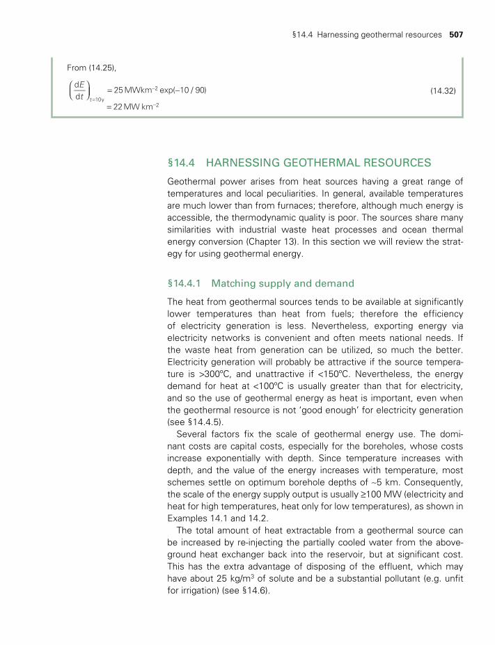
§14.4 Harnessing geothermal resources 507
§14.4 HARNESSING GEOTHERMAL RESOURCES
Geothermal power arises from heat sources having a great range of temperatures and local peculiarities. In general, available temperatures are much lower than from furnaces; therefore, although much energy is accessible, the thermodynamic quality is poor. The sources share many similarities with industrial waste heat processes and ocean thermal energy conversion (Chapter 13). In this section we will review the strat-egy for using geothermal energy.
§14.4.1 Matching supply and demand
The heat from geothermal sources tends to be available at significantly lower temperatures than heat from fuels; therefore the efficiency of electricity generation is less. Nevertheless, exporting energy via electricity networks is convenient and often meets national needs. If the waste heat from generation can be utilized, so much the better. Electricity generation will probably be attractive if the source tempera-ture is >300ºC, and unattractive if <150ºC. Nevertheless, the energy demand for heat at <100ºC is usually greater than that for electricity, and so the use of geothermal energy as heat is important, even when the geothermal resource is not ‘good enough’ for electricity generation (see §14.4.5).
Several factors fix the scale of geothermal energy use. The domi-nant costs are capital costs, especially for the boreholes, whose costs increase exponentially with depth. Since temperature increases with depth, and the value of the energy increases with temperature, most schemes settle on optimum borehole depths of ~5 km. Consequently, the scale of the energy supply output is usually ≥100 MW (electricity and heat for high temperatures, heat only for low temperatures), as shown in Examples 14.1 and 14.2.
The total amount of heat extractable from a geothermal source can be increased by re-injecting the partially cooled water from the above-ground heat exchanger back into the reservoir, but at significant cost. This has the extra advantage of disposing of the effluent, which may have about 25 kg/m3 of solute and be a substantial pollutant (e.g. unfit for irrigation) (see §14.6).
From (14.25),
Et
dd
25 MWkm exp( 10 / 90)
22MW kmt 10y
2
2
= -
==
-
-
(14.32)
TWIDELL PAGINATION.indb 507 01/12/2014 11:38

508 Geothermal energy
§14.4.2 Extraction techniques: hydrothermal
The most successful geothermal projects have boreholes sunk into natural water channels in hyperthermal regions (Fig. 14.6). This is the method used at Wairakei, New Zealand (Fig. 14.10), and at the geysers in California. Similar methods are used for extraction from hot aquifers in semithermal regions, where natural convection can be established from the borehole without extra pumping.
Naturalgeyser Power
plant Power plant
Hot rock
~ 30 km
Mantle magna
Deep bore~ 5 km
Steam/water reservoir~ 280° C
Geyser
(a)
Hot granite rocksHot granite rocks
Recharge area
Hot springor
steam vent
Hotfluids
Hotfluid
Coldfluid
Geothermalwell
Impermeable cap rock(thermal
conduction)
Impermeable rock
(thermal conduction)
Reservoir(thermal
convection)
(b)
Fig. 14.6a Schematic diagram, not to scale, of hydrothermal power stations in a hyperthermal region (e.g. the Geysers geothermal
field, California). b Geology of an aquifer in a hydrothermal region (left of diagram) and a region of hot, dry rock (right of diagram) (not
to scale). The diagram also indicates some of the flows of heat (‘broad’ arrows) and water (‘line’ arrows) relevant to geothermal power.
TWIDELL PAGINATION.indb 508 01/12/2014 11:38

§14.4 Harnessing geothermal resources 509
Power plant
Overlayingrock
Districtheating
Waterinjectionbore
Outflow
Artificiallyfractured region
Losses
Hot dry rock:e.g. granite
~300°C
~ 5−7 km
Fig. 14.7 Schematic diagram of heat extraction from a hot, dry rock system. Black arrows indicate the desired direction of water flow; green (dashed) arrows indicate water lost by ‘undesired’ paths through the fractured zone.
§14.4.3 Extraction techniques: ‘enhanced geothermal systems’ (EGS)
Sources of ‘hot, dry rock’ (HDR) are much more abundant than hydro-thermal regions: temperatures of 200°C are accessible under a signifi-cant proportion of the world’s landmass. This has motivated expensive research and development in the USA and Europe on techniques to harness this heat for electricity power generation. One result has been the recognition that few basement rocks are completely dry, but there are many regions where utilization of their geothermal heat requires ‘enhanced geothermal systems’, in which re-injection is necessary to maintain commercial production.
In the 1980s, the research group at the Los Alamos Scientific Laboratory, USA pioneered methods of fracturing the rock with pressurized cold water around the end of the injection borehole (Fig. 14.7). After initial fracturing, water was pumped down the injection bore to percolate upwards through the hot rock at depths of ~5 km and temperatures ~250°C before return-ing through shallower return pipes. Using such ‘enhanced geothermal systems’ (EGS), complex arrays of injection and return boreholes might, in principle, enable gigawatt supplies of heat to be obtained. However, it has proved difficult to constrain the fracturing so that a large enough frac-tion of the injected water emerges from the outflow pipes; the injected water leaks into other fractures and is lost, as indicated in Fig. 14.7.
TWIDELL PAGINATION.indb 509 01/12/2014 11:38

510 Geothermal energy
These technical difficulties and large costs of EGS have limited development to only a few pilot plants, mainly in Europe and the USA. Nevertheless, the 1.7 MWe ‘Desert Peak 2’ system in Nevada, USA operated commercially in 2013. For EGS to become a worldwide applica-tion with reasonable power output, the technology will have to be scaled up in stages from pilot plants of ~1 MWe to the range of 50 to 200 MWe. To achieve this by 2025, as envisaged by the IEA Geothermal Roadmap, will require strong policy and funding support.
§14.4.4 Electricity-generating systems
The choice of the heat exchange and turbine system for a particular geothermal source is complex, requiring specialist experience. Fig. 14.8 sketches some of the system configurations in common use. Nearly always the emerging bore water after use is re-injected into the reser-voir. The simplest systems pass ‘dry’ steam from the ground directly into a steam turbine (Fig. 14.8(a)), as used in the first-ever geothermal power plant in Italy in 1904, and subsequently in other places (e.g. Wairakei, New Zealand: Fig. 14.10). The geothermal reservoir contains superheated water at temperatures >180°C and at large pressure. As the water flows to the surface, the pressure decreases and some boils (‘flashes’) into steam, which is injected into steam turbines that power the generators (Fig. 14.8(b)). In other situations, water at lower temperatures (110°C to 180°C) heats other working fluids, usually organic compounds, in a heat exchanger; these generally boil at about 80°C, so providing the pressur-ized vapor to a turbine (Fig. 14.8(c)). The turbines operate with a Rankine cycle, as for OTEC and solar ponds (see Box 13.1). In the heat exchang-ers, the counter-flowing fluids are separate, yet nevertheless difficulties occur owing to deposits and corrosion from the chemicals in the cooling borehole water. Similar problems occur for ocean thermal energy conver-sion (Chapter 13).
§14.4.5 Direct uses of geothermal heat
Despite using insulated pipes, heat cannot be distributed effectively over distances greater than ~30 km, so use of geothermal must be near to the supply. In cold climates, household and business district- heating schemes have proved viable if the population density is ≥350 people/km2 (>100 premises/km2). Thus a 100 MWth geothermal plant can serve an urban area ~20 km × 20 km at ~ 2 kWth per premises. Other heating loads are for glasshouse heating, fish farming, food drying, factory processes, etc.
Table 14.2 lists some of the main direct uses of geothermal heat and the countries having the largest use. Only Iceland and Japan are
TWIDELL PAGINATION.indb 510 01/12/2014 11:38
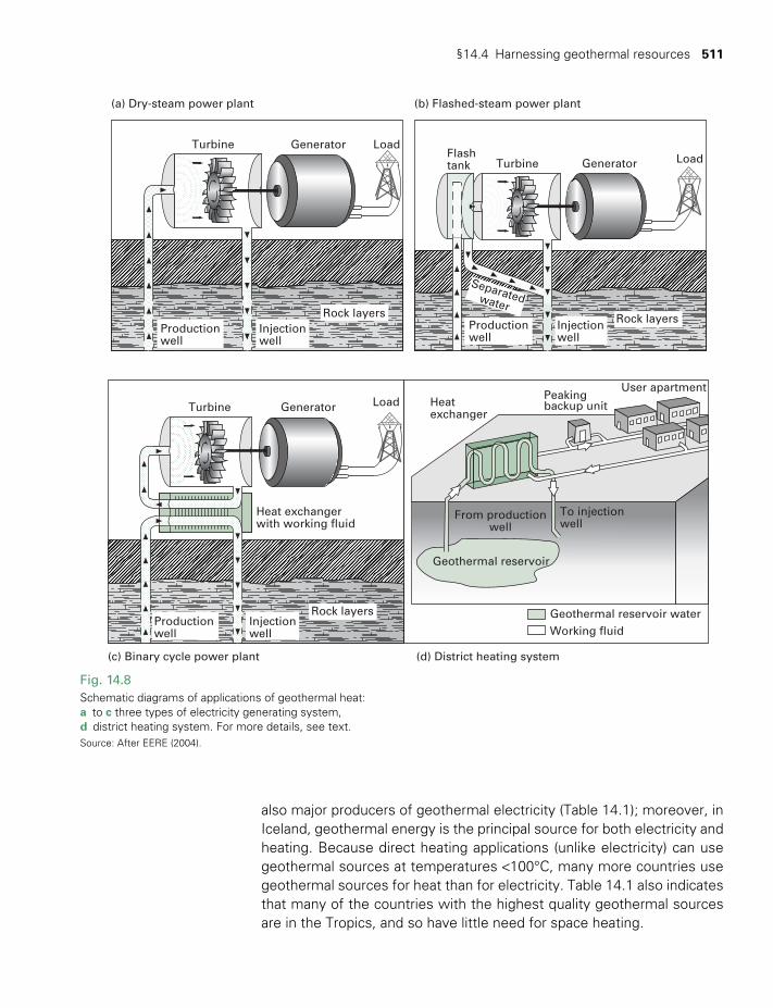
§14.4 Harnessing geothermal resources 511
Load
Geothermal reservoir waterWorking fluid
Turbine
Turbine Generator
Geothermal reservoir
Heat exchangerwith working fluid
From productionwell
To injectionwell
Heatexchanger
Peakingbackup unit
User apartment
(a) Dry-steam power plant
(c) Binary cycle power plant (d) District heating system
(b) Flashed-steam power plant
Generator LoadFlashtank Turbine
Separatedwater
Generator Load
Productionwell
Productionwell
Productionwell
Injectionwell
Injectionwell
Injectionwell
Rock layersRock layers
Rock layers
Fig. 14.8 Schematic diagrams of applications of geothermal heat:a to c three types of electricity generating system,d district heating system. For more details, see text. Source: After EERE (2004).
also major producers of geothermal electricity (Table 14.1); moreover, in Iceland, geothermal energy is the principal source for both electricity and heating. Because direct heating applications (unlike electricity) can use geothermal sources at temperatures <100°C, many more countries use geothermal sources for heat than for electricity. Table 14.1 also indicates that many of the countries with the highest quality geothermal sources are in the Tropics, and so have little need for space heating.
TWIDELL PAGINATION.indb 511 01/12/2014 11:38
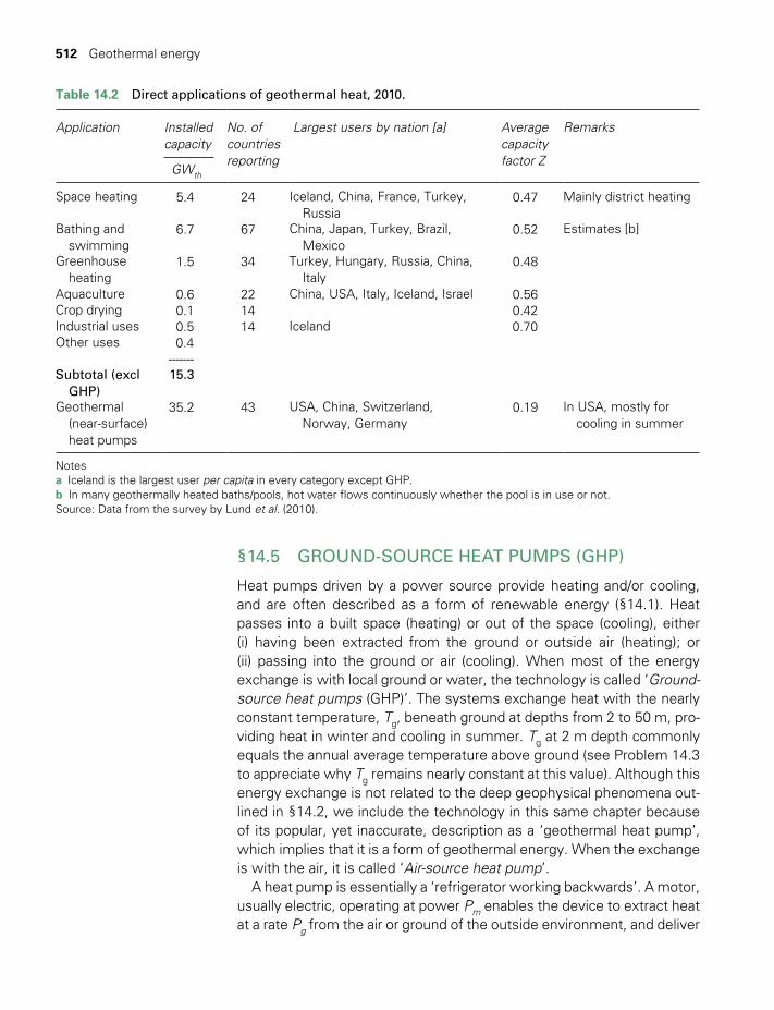
512 Geothermal energy
§14.5 GROUND-SOURCE HEAT PUMPS (GHP)
Heat pumps driven by a power source provide heating and/or cooling, and are often described as a form of renewable energy (§14.1). Heat passes into a built space (heating) or out of the space (cooling), either (i) having been extracted from the ground or outside air (heating); or (ii) passing into the ground or air (cooling). When most of the energy exchange is with local ground or water, the technology is called ‘Ground-source heat pumps (GHP)’. The systems exchange heat with the nearly constant temperature, Tg, beneath ground at depths from 2 to 50 m, pro-viding heat in winter and cooling in summer. Tg at 2 m depth commonly equals the annual average temperature above ground (see Problem 14.3 to appreciate why Tg remains nearly constant at this value). Although this energy exchange is not related to the deep geophysical phenomena out-lined in §14.2, we include the technology in this same chapter because of its popular, yet inaccurate, description as a ‘geothermal heat pump’, which implies that it is a form of geothermal energy. When the exchange is with the air, it is called ‘Air-source heat pump’.
A heat pump is essentially a ‘refrigerator working backwards’. A motor, usually electric, operating at power Pm enables the device to extract heat at a rate Pg from the air or ground of the outside environment, and deliver
Table 14.2 Direct applications of geothermal heat, 2010.
Application Installed capacity
GWth
No. of countries reporting
Largest users by nation [a] Average capacity factor Z
Remarks
Space heating 5.4 24 Iceland, China, France, Turkey, Russia
0.47 Mainly district heating
Bathing and swimming
6.7 67 China, Japan, Turkey, Brazil, Mexico
0.52 Estimates [b]
Greenhouse heating
1.5 34 Turkey, Hungary, Russia, China, Italy
0.48
Aquaculture 0.6 22 China, USA, Italy, Iceland, Israel 0.56Crop drying 0.1 14 0.42Industrial uses 0.5 14 Iceland 0.70Other uses 0.4
-------Subtotal (excl GHP)
15.3
Geothermal (near-surface)
heat pumps
35.2 43 USA, China, Switzerland, Norway, Germany
0.19 In USA, mostly for cooling in summer
Notes a Iceland is the largest user per capita in every category except GHP.b In many geothermally heated baths/pools, hot water flows continuously whether the pool is in use or not. Source: Data from the survey by Lund et al. (2010).
TWIDELL PAGINATION.indb 512 01/12/2014 11:38
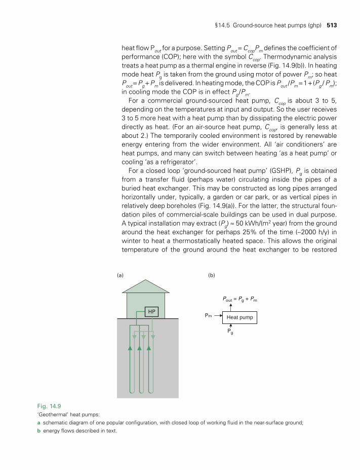
§14.5 Ground-source heat pumps (ghp) 513
heat flow Pout for a purpose. Setting Pout = CcopPm defines the coefficient of performance (COP); here with the symbol Ccop. Thermodynamic analysis treats a heat pump as a thermal engine in reverse (Fig. 14.9(b)). In heating mode heat Pg is taken from the ground using motor of power Pm; so heat Pout = Pg + Pm is delivered. In heating mode, the COP is Pout /Pm = 1 + (Pg / Pm); in cooling mode the COP is in effect Pg /Pm.
For a commercial ground-sourced heat pump, Ccop is about 3 to 5, depending on the temperatures at input and output. So the user receives 3 to 5 more heat with a heat pump than by dissipating the electric power directly as heat. (For an air-source heat pump, Ccop, is generally less at about 2.) The temporarily cooled environment is restored by renewable energy entering from the wider environment. All ‘air conditioners’ are heat pumps, and many can switch between heating ‘as a heat pump’ or cooling ‘as a refrigerator’.
For a closed loop ‘ground-sourced heat pump’ (GSHP), Pg is obtained from a transfer fluid (perhaps water) circulating inside the pipes of a buried heat exchanger. This may be constructed as long pipes arranged horizontally under, typically, a garden or car park, or as vertical pipes in relatively deep boreholes (Fig. 14.9(a)). For the latter, the structural foun-dation piles of commercial-scale buildings can be used in dual purpose. A typical installation may extract (Pg) ≈ 50 kWh/(m2 year) from the ground around the heat exchanger for perhaps 25% of the time (~2000 h/y) in winter to heat a thermostatically heated space. This allows the original temperature of the ground around the heat exchanger to be restored
(a) (b)
Heat pumpPm
Pg
Pout = Pg + Pm
HP
Fig. 14.9 ‘Geothermal’ heat pumps:a schematic diagram of one popular configuration, with closed loop of working fluid in the near-surface ground;b energy flows described in text.
TWIDELL PAGINATION.indb 513 01/12/2014 11:38

514 Geothermal energy
by thermal conduction through the soil and, possibly, by groundwater movement. The source of most of this restored heat is usually from sun-shine and ambient air above the ground, rather than from any significant thermal flow upwards from geothermal sources; the average geother-mal flux is <0.4 W/m2, which is insignificant. In practice, for heating an insulated building, the area needed for the capture of the heat through horizontal heat exchangers is about 1.5 times the outside wall area of the building.
When operating for cooling, the heat pump reverses flow to act as a refrigerator, so adding heat to the underground surroundings. For deep, vertically orientated heat exchangers (e.g. if combined with structural piling), the underground surroundings heat in summer and cool in winter, so becoming a heat store with a six-month reversible cycle.
The capacity factors for GHPs are small compared to other direct uses of geothermal heat (Table 14.2) because GHPs are rarely used throughout the year, and are often oversized for peak summer and/or winter use.
The optimum theoretical performance is as a Carnot cycle operating between input absolute temperature Tg, and output temperature Tout, so:
Ccop(carnot) = Pout /Pm = Tout /(Tout – Tg ). (14.33)
With Tout = 298 K (25°C) and Tg = 278 K (5°C), Ccop(carnot) = 15. However,
this ‘ideal’ is much larger than the values of 3 to 6 obtained in practice for ground-sourced heat pumps, since the Carnot analysis assumes infinitely slow, reversible processes.
§14.6 SOCIAL AND ENVIRONMENTAL ASPECTS
Geothermal power from hydrothermal regions has a proven record of providing generally safe and reliable electrical power generation at relatively low cost. Consequently its use has increased steadily during the past few decades (see Fig. 14.1). Capital costs of new systems are about US$2500 per installed kilowatt (electric) capacity, which are similar to those of nuclear and hydro power stations. Power is generated continuously at full rating, with reductions for maintenance and repair, so average capacity factors are ~70% (Table 14.1) and similar to coal and nuclear plant, i.e. annual output is ~70% of full rating for 8760 hours per year. Thus, in favorable sites, the levelized cost of electricity production is competitive with conventional (brown) sources, being especially so if external costs are included (see Table D.4 in Appendix D). Once utilized, the heat- extracting fluids are either discharged at surface level or re-injected. Surface discharge requires careful environmental monitoring and may be ecologically damaging. Re-injection of pressurized fluids into the reservoir generally improves the energy extraction, but may cause micro-earthquakes if forced into deep formations. Hydrogen sul-
TWIDELL PAGINATION.indb 514 01/12/2014 11:38

§14.6 Social and environmental aspects 515
phide gas may be emitted with the fluids, being unpleasant to smell yet not generally at concentrations to be dangerous. Water quality monitoring in the vicinity is essential to monitor dissolved chemicals.
Resources of ‘hot-dry-rock’ (HDR) are much more abundant than hydrothermal resources: temperatures of 200°C are accessible under a large proportion of the world’s landmass. Goldstein et al. (2011) indi-cate that if ‘enhanced geothermal systems’ (EGS) were to become suc-cessful at a commercial scale, then the electricity-generating capacity from geothermal sources could be comparable to global primary energy supply (i.e. >20 EJ/y). Unfortunately, even after several decades of tech-nical development, EGS are still only at a ‘pilot plant’ stage.
For geothermal power, the size of the resource is unconfirmed until drilling takes place, as with oil or mining projects. After such prospect-ing, successful geothermal projects take at least five to seven years to develop from resource discovery to commercial development. Long development times and the upfront financial risk of the cost of explora-tion make development of the resource particularly difficult in developing countries with visible geothermal activity at a plate boundary but limited power demand, such as the Solomon Islands, the smaller islands of Indonesia or parts of East Africa.
Ground-source heat pumps are a totally different technology from geothermal energy extraction. They are usually for small-scale supply of building space heat and hot water, and may be reversed for cooling. They are a mature and reliable technology, with millions of units operat-ing worldwide.
We illustrate the environmental impacts of geothermal power through the example of the 140 MWe Wairakei power station in New Zealand (Fig. 14.10). The station was built in the 1950s in one of the most geologically active areas in the world. The wells (top left of the photo) tap into a mixture of water and steam; the hot water is separated with the high-pressure steam being directed through the pipes to the power station at bottom right. At Wairakei there is a considerable overpressure in the boreholes. The clouds of steam at top left come from the hot water boiling as the pressure on it is released.
Removal of the hot water from the ground through the power station resulted in subsidence affecting some local buildings. Consequently, some of the output water flow was re-injected into the area, alleviating the difficulty. There has been a diminution in the intensity of some of the natural geysers of the area due to power stations, although most remain substantially unaffected. Note that such a negative impact on natural geo-thermal phenomena inhibits the wider use of geothermal power in Japan.
At the bottom of the photograph of Fig.14.10 is the Waikato River, which both provides cooling water and receives the condensed steam and other emissions at discharge. The inherent emission of H2S is treated before discharge. The Waikato is one of the largest rivers in the country,
TWIDELL PAGINATION.indb 515 01/12/2014 11:38
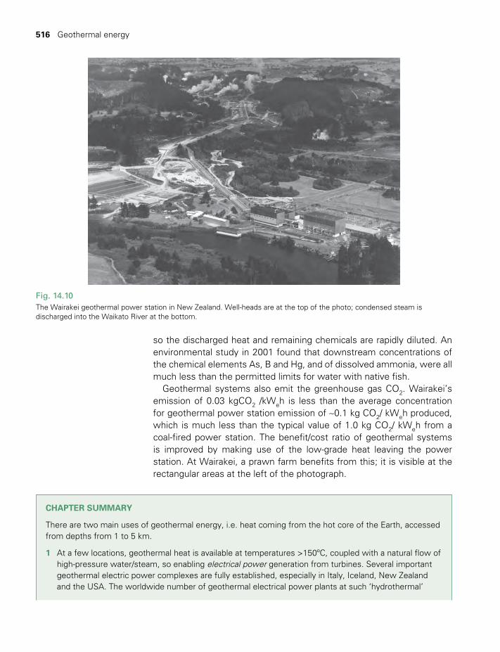
516 Geothermal energy
CHAPTER SUMMARY
There are two main uses of geothermal energy, i.e. heat coming from the hot core of the Earth, accessed from depths from 1 to 5 km.
1 At a few locations, geothermal heat is available at temperatures >150ºC, coupled with a natural flow of high-pressure water/steam, so enabling electrical power generation from turbines. Several important geothermal electric power complexes are fully established, especially in Italy, Iceland, New Zealand and the USA. The worldwide number of geothermal electrical power plants at such ‘hydrothermal’
Fig. 14.10The Wairakei geothermal power station in New Zealand. Well-heads are at the top of the photo; condensed steam is discharged into the Waikato River at the bottom.
so the discharged heat and remaining chemicals are rapidly diluted. An environmental study in 2001 found that downstream concentrations of the chemical elements As, B and Hg, and of dissolved ammonia, were all much less than the permitted limits for water with native fish.
Geothermal systems also emit the greenhouse gas CO2. Wairakei’s emission of 0.03 kgCO2 /kWeh is less than the average concentration for geothermal power station emission of ~0.1 kg CO2/ kWeh produced, which is much less than the typical value of 1.0 kg CO2/ kWeh from a coal-fired power station. The benefit/cost ratio of geothermal systems is improved by making use of the low-grade heat leaving the power station. At Wairakei, a prawn farm benefits from this; it is visible at the rectangular areas at the left of the photograph.
TWIDELL PAGINATION.indb 516 01/12/2014 11:38
Quick questions 517
locations had increased steadily to a capacity of ~15 GW(elec) by 2011, with further increase expected. The technology is mature and long-lasting, but has to be tailored to each site; it may be used for baseload grid supply at a per unit levelized cost of electricity among the cheapest available.
2 In a much wider set of locations, geothermal heat is available, but only at ~50 to 70°C. It is used in more than 60 countries for thermal applications, including hot water spas, district-space heating and industrial process heat.
Resources of ‘hot, dry rock’ (HDR) are much more abundant than hydrothermal resources, temperatures of 200°C being potentially accessible under a large proportion of the world’s landmass. Enhanced geothermal systems (EGS) exploit this resource by circulating water down to the HDR and then tapping into the heated water output. If EGS develops to commercial scale, the electricity-generating capacity from geothermal sources could be >20 EJ/y, i.e. comparable to global primary energy supply in 2008. However, after several decades of technical development, the technology is still only at the ‘pilot plant’ stage.Ground-source heat pumps (GHPs) – often misleadingly called ‘geothermal heat pumps’ – tap into the nearly constant temperature of the ground Tg at depths from 2 to 50 m for either heating (in winter, when the air temperature is significantly less than Tg) or for cooling (in summer, when the air temperature is significantly more than Tg ). This application is available worldwide and increasing rapidly, though not geothermal in the sense of the meanings of (1) and (2).
QUICK QUESTIONS
Note: Answers to these questions are in the text of the relevant section of this chapter, or may be readily inferred from it.
1 Lord Kelvin calculated the age of the Earth assuming it is a hot body cooling in a vacuum from a molten mass. Was he correct in the assumption, and if not, why not?
2 Where would you look on the Earth for most geothermal activity? 3 Temperature increases with depth of a borehole; how does the rate
of increase with depth indicate the type of geothermal region? 4 Describe at least two mechanisms for heat to leave a geothermal
resource. 5 Describe circumstances for geothermal water to ‘flash’ into steam. 6 What types of engine can operate from geothermal energy? Explain
how they function. 7 Give two reasons for the re-injection of effluent fluids back into geo-
thermal reservoirs and two reasons for not doing so. 8 From the point of view of a grid operator, compare electricity genera-
tion from geothermal sources with that from solar sources. 9 Heat emerges from a ground-source heat pump; where does it come
from?10 A heat pump is reversed to become an air cooler; is its coefficient of
performance unchanged? Explain your answer.
TWIDELL PAGINATION.indb 517 01/12/2014 11:38
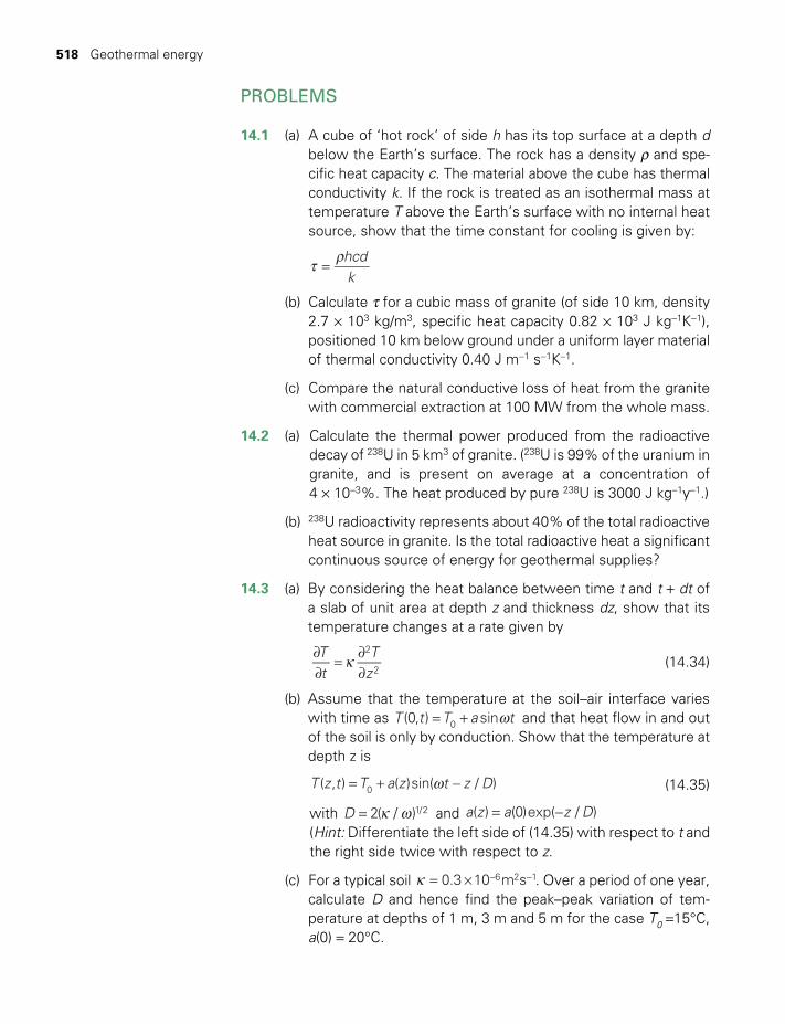
518 Geothermal energy
PROBLEMS
14.1 (a) A cube of ‘hot rock’ of side h has its top surface at a depth d below the Earth’s surface. The rock has a density r and spe-cific heat capacity c. The material above the cube has thermal conductivity k. If the rock is treated as an isothermal mass at temperature T above the Earth’s surface with no internal heat source, show that the time constant for cooling is given by:
t r=
hcdk
(b) Calculate t for a cubic mass of granite (of side 10 km, density 2.7 × 10³ kg/m3, specific heat capacity 0.82 × 10³ J kg-1K-1), positioned 10 km below ground under a uniform layer material of thermal conductivity 0.40 J m-1 s-1K-1.
(c) Compare the natural conductive loss of heat from the granite with commercial extraction at 100 MW from the whole mass.
14.2 (a) Calculate the thermal power produced from the radioactive decay of 238U in 5 km3 of granite. (238U is 99% of the uranium in granite, and is present on average at a concentration of 4 × 10⁻³%. The heat produced by pure 238U is 3000 J kg-1y-1.)
(b) 238U radioactivity represents about 40% of the total radioactive heat source in granite. Is the total radioactive heat a significant continuous source of energy for geothermal supplies?
14.3 (a) By considering the heat balance between time t and t + dt of a slab of unit area at depth z and thickness dz, show that its temperature changes at a rate given by
κ∂∂
=∂∂
Tt
Tz
2
2 (14.34)
(b) Assume that the temperature at the soil–air interface varies with time as ω= +T t T a t(0, ) sin0 and that heat flow in and out of the soil is only by conduction. Show that the temperature at depth z is
ω= + -T z t T a z t z D( , ) ( )sin( / )0 (14.35)
with κ ω=D 2( / )1/2 and = -a z a z D( ) (0)exp( / ) (Hint: Differentiate the left side of (14.35) with respect to t and
the right side twice with respect to z.
(c) For a typical soil κ = × - -0.3 10 m s6 2 1. Over a period of one year, calculate D and hence find the peak–peak variation of tem-perature at depths of 1 m, 3 m and 5 m for the case T0 =15°C, a(0) = 20°C.
TWIDELL PAGINATION.indb 518 01/12/2014 11:38

Bibliography 519
BIBLIOGRAPHY
General
Dickson, M. and Fanelli, M. (eds) (2005) Geothermal Energy: Utilization and technology, UNESCO and Routledge, Abingdon. Textbook level; has one chapter on power systems and four chapters on heating applications.
DiPippio, R. (2012, 3rd edn) Geothermal Power Plants: Principles, applications, case studies and environmental impact, Elsevier, New York. Excellent and up-to-date professional-level text, with coverage summarized by its title.
Goldstein, B., Hiriart, G., Bertani, R., Bromley, C., Gutiérrez‐Negrín, L., Huenges, E., Muraoka, H., Ragnarsson, A., Tester, J. and Zui, V. (2011) ‘Geothermal energy’, in O. Edenhofer, R. Pichs Madruga, Y. Sokona, K. Seyboth, P. Matschoss, S. Kadner, T. Zwickel, P. Eickemeier, G. Hansen, S. Schlömer and C. von Stechow (eds), IPCC Special Report on Renewable Energy Sources and Climate Change Mitigation, Cambridge University Press, Cambridge. An authoritative recent review of the state of the art in, and future prospects for, geothermal energy.
International Energy Agency (2011) Energy Roadmap: Geothermal heat and power, Paris (free for download from www. iea.org). Current status and outlook to ~2050; finds major growth requires significant development of EGS.
Tester, J.W., Drake, E.M., Driscoll, M.J., Golay, M.W. and Peters, W.A. (2012, 2nd edn) Sustainable Energy: Choosing among options, MIT Press, Boston, MA. Chapter 11 on geothermal energy draws on co-author Tester’s many publications on this subject.
Heat pumps
Banks, D. (2008) An Introduction to Thermogeology: Ground source heating and cooling, Oxford University Press, Oxford.
Ochsner, K. (2008) Geothermal Heat Pumps, Earthscan, London. Excellent summary of principles and applica-tions. Very clear presentation.
Specific references
Bertani, R. (2010) ‘Geothermal power generation in the world: 2005–2010 update’, in Proceedings of the World Geothermal Congress. Available online at www.geothermal-energy.org/pdf/IGAstandard/WGC/2010/0008.pdf (accessed June 4, 2013).
Chandrasekharam, D. and Bundschuh, J. (2008) Low-enthalpy Geothermal Resources for Power Generation: Exploration and economics, Taylor & Francis, Abingdon. Particularly good on small sites in developing countries.
EERE (2004) US Department of Energy Report DOE/GO-102004, ‘Buried treasure: the environmental, economic and employment benefits of geothermal energy’. Available online at www.nrel.gov/docs/fy05osti/35939.pdf (June 2013).
Environment Waikato (2004) Environmental Consent Hearing on Contact Energy – Wairakei geothermal opera-tions. Available online at: www.ew.govt.nz/resourceconsents/hearingsdecisions/contact.htm#Bookmark_tech appendices>. See especially the technical appendices which give details about its history and present operation.
Garnish, J.D. (1976) Geothermal Energy: The case for research in the UK, Department of Energy paper no. 9, HMSO, London. Succinct evaluation with basic analysis.
TWIDELL PAGINATION.indb 519 01/12/2014 11:38

520 Geothermal energy
Lund, J.W., Freeston, D.H. and Boyd, T.L. (2010) ‘Direct utilization of geothermal energy: 2010 worldwide review’. Available online at www.geothermal-energy.org/pdf/IGAstandard/WGC/2010/007.pdf (accessed June 4, 2013).
Websites and periodicals
Geothermal Energy Association (www.geo-energy.org), US-based but every few years publishes a useful International Market Report.
International Geothermal Association (www.geothermal-energy.org), c/o ENEL DP-PDG, Via A. Pisano 120, 56122 Pisa, Italy.
International Ground Source Heat Pump Association (www.ceat.okstate.edu/international-ground-source- heat-pump-association).
US Department of Energy Geothermal Technology Office (www1.eere.energy.gov/geothermal). Has many useful publications and updates.
World Geothermal Congress: Conference held every ~5years (e.g. 2010 Congress at Bali, Indonesia); proceed-ings available from the International Geothermal Association.
Geothermics – a specialist research journal covering both heat and power applications.
TWIDELL PAGINATION.indb 520 01/12/2014 11:38
Energy systems
Integration, distribution and storage
CONTENTS
Learning aims 522
§15.1 Introduction 523
§15.2 Energy systems 523 §15.2.1 Terminology 523 §15.2.2 Technological issues of
integrating RE into energy systems 525
§15.3 Distribution technologies 526 §15.3.1 Pipelines 528 §15.3.2 Batch transport 529 §15.3.3 Heat distribution 529
§15.4 Electricity supply and networks 530 §15.4.1 Electricity grids (networks) 530 §15.4.2 Balancing supply and
demand in a grid 533 §15.4.3 Smart grids and virtual
storage 537
§15.5 Comparison of technologies for energy storage 538
§15.6 Energy storage for grid electricity 541 §15.6.1 Pumped hydro 541 §15.6.2 Flywheels 541 §15.6.3 Compressed air 542 §15.6.4 High-power electrical storage 544
§15.7 Batteries 544 §15.7.1 The lead-acid battery 545 §15.7.2 Lithium-based batteries 550 §15.7.3 Other battery technologies 551
§15.8 Fuel cells 552
§15.9 Chemicals as energy stores 553
§15.9.1 Hydrogen 553 §15.9.2 Ammonia 555
§15.10 Storage for heating and cooling systems 555
§15.11 Transport systems 558
§15.12 Social and environmental aspects of energy supply and storage 559
Chapter summary 560
Quick questions 560
Problems 561
Note 563
Bibliography 563
Box 15.1 It’s a myth that energy storage is a challenge only for renewable energy 532
Box 15.2 Self-sufficient energy systems 532
Box 15.3 Capacity credit, dispatchability and predictablity 535
Box 15.4 Grid stability with high wind penetration: western Denmark and Ireland 536
Box 15.5 Combining many types of variable RE enables large RE penetration: two modeled cases 537
Box 15.6 Scaling up batteries: flow cells 550
Box 15.7 A small island autonomous wind-hydrogen energy system 554
CHAPTER
15
TWIDELL PAGINATION.indb 521 01/12/2014 11:38

522 Integration, distribution and storage
LEARNING AIMS
• Appreciate that wide application of renewable energy requires mechanisms to integrate vari-able supplies into energy systems.
• Understand why electricity networks can readily achieve such integration up to ~20% of total supply (and in some cases greater %).
• Understand the importance of energy storage as a component of such integration and the physical principles underlying storage tech-nologies.
LIST OF FIGURES
15.1 A general energy system. 52415.2 Wind energy, electricity demand, and instantaneous penetration levels in the electricity grids. 53415.3 Energy per unit cost versus energy per unit volume of storage methods. 53815.4 Compressed air energy storage and recovery system. 54315.5 Schematic diagram of lead-acid cell. 54515.6 Operating characteristics of a typical lead-acid battery. 54915.7 Flow cell battery (schematic). 55115.8 Schematic diagram of a fuel cell. 552
LIST OF TABLES
15.1 Summary of major means and flows for distributing energy 52715.2 Storage devices and their performance 539
TWIDELL PAGINATION.indb 522 01/12/2014 11:38
§15.2 Energy systems 523
§15.1 INTRODUCTION
Our demand for energy in usable forms is a major factor in human society and economies, requiring technological solutions (this chapter), manage-ment of demand (Chapter 16), and affordable and appropriately regulated supply (Chapter 17).
Taking energy to where it is wanted is called distribution or transmis-sion; keeping it available until when it is wanted is called storage. For example, within natural ecology, biomass is an energy store for animals, with fruit and seeds a form of distribution. Within human society, local distribution, long-distance transmission and storage are established energy services by a range of technologies, including transportation and pipelines for fuels, electricity grid networks, batteries, hydro-pumped storage and building mass for heat. Fossil and nuclear fuels are effectively ab initio long-lasting energy stores with large energy density; their use depends on mining, processing of ores and fuels, distribution by trans-portation and pipelines, and, after electricity generation, transmission and distribution by high-voltage cables. In contrast, renewable energy is ab initio a continuing supply from the natural environment requiring matched demand and, for abundant use, storage (recall Chapter 1).
This chapter begins with an overview of the technical issues in integrat-ing renewable energy (RE) into present and developing energy systems (§15.2), and then reviews mechanisms for distributing energy either as electricity (§15.4) or in other forms (§15.3). §15.5 gives an overview of technologies for energy storage, with later sections elaborating on spe-cific storage technologies and their physical principles, and §15.12 outlin-ing some of the associated social and environmental aspects.
§15.2 ENERGY SYSTEMS
§15.2.1 Terminology
Energy is useful only if it is available in the necessary form, when and where wanted. The ‘forms’ may be categorized as heat, fuel and elec-tricity. The energy is delivered by interlinked processes from resource to end-use, as influenced by many factors (see Fig. 15.1). The whole system at national and international scale is surprisingly complicated, indicated in the figure by:
(A) Primary resource; renewables, fossil fuel or nuclear fuel.(B) Conversion to manageable form (e.g. liquid fuel, electricity, gas).(C) Storage for later use (e.g. holding tanks, batteries).(D) Distribution (e.g. shipping, road and rail transport, electricity net-
works and grids, pipelines).(E) End-use sector classification (e.g. as transport fuel, industrial and
domestic heat supply, electricity).(F) Consumer (e.g. householder, shop, factory).
TWIDELL PAGINATION.indb 523 01/12/2014 11:38
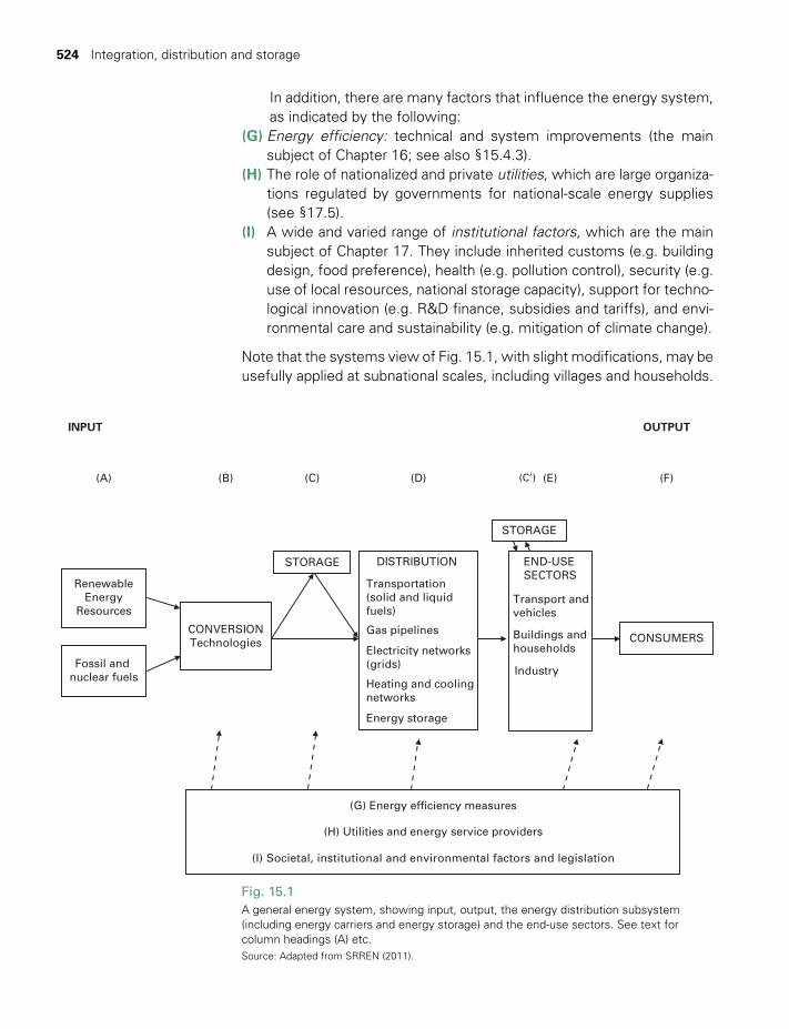
524 Integration, distribution and storage
In addition, there are many factors that influence the energy system, as indicated by the following:
(G) Energy efficiency: technical and system improvements (the main subject of Chapter 16; see also §15.4.3).
(H) The role of nationalized and private utilities, which are large organiza-tions regulated by governments for national-scale energy supplies (see §17.5).
(I) A wide and varied range of institutional factors, which are the main subject of Chapter 17. They include inherited customs (e.g. building design, food preference), health (e.g. pollution control), security (e.g. use of local resources, national storage capacity), support for techno-logical innovation (e.g. R&D finance, subsidies and tariffs), and envi-ronmental care and sustainability (e.g. mitigation of climate change).
Note that the systems view of Fig. 15.1, with slight modifications, may be usefully applied at subnational scales, including villages and households.
Fig. 15.1A general energy system, showing input, output, the energy distribution subsystem (including energy carriers and energy storage) and the end-use sectors. See text for column headings (A) etc.Source: Adapted from SRREN (2011).
RenewableEnergy
Resources
DISTRIBUTION
Transportation(solid and liquidfuels)
Gas pipelines
Electricity networks(grids)
Heating and coolingnetworks
Energy storage
END-USESECTORS
Transport andvehicles
Buildings andhouseholds
Industry
CONVERSIONTechnologies
Fossil and nuclear fuels
INPUT
(A) (B)
(G) Energy efficiency measures
(H) Utilities and energy service providers
(I) Societal, institutional and environmental factors and legislation
(C)
CONSUMERS
OUTPUT
STORAGE
(D) (E) (F)
STORAGE
(C’)
TWIDELL PAGINATION.indb 524 01/12/2014 11:38

§15.2 Energy systems 525
§15.2.2 Technological issues of integrating RE into energy systems
Technologies marked (C) and (D) in Fig. 15.1 enable the distribution and storage of RE, for which the technologies are mostly established and available. Most of this chapter analyzes these technologies and their basic physical principles.
Since the use of RE supplies requires a diversion of a continuing natural flow of energy, there are challenges in matching supply and demand in the time domain, i.e. in matching the rate at which energy is used. This varies with time on scales of months (e.g. house heating in cold and temperate climates), days (e.g. artificial lighting), hours (e.g. cooking) and seconds (e.g. starting motors). In contrast to fossil fuels, the initial primary inputs of renewable energy supplies are outside of our control. Thus, as discussed in Chapter 1, we must adjust (match) the demand (load) to the renewable supply and/or store some of the energy for subsequent benefit as biomass and biofuels, chemical form (e.g. bat-teries), heat (e.g. thermal mass), potential energy (e.g. pumped hydro), kinetic energy (e.g. flywheels) or as electrical potential (e.g. capacitors).
Uses of RE depend significantly on their type and scale. Some renew-able electricity supplies may be of relatively large scale with fully con-trollable output (e.g. large hydroelectric, biomass heat and/or power plant) and so used in a similar manner to fossil fuel plant. However, in general, as discussed in Chapter 1, renewable electricity supplies have different requirements for storage and distribution than traditional central power supplies. For instance, some large renewables have differing time dependence (e.g. tidal range, offshore wind farms, concentrated solar plant) and so require integration with other electricity generation in a common system, which may beneficially incorporate energy storage. However, all forms of renewable energy at relatively small and moderate intensity can be integrated into established systems (e.g. micro-gener-ation into electricity distribution grids and biogas into gas distribution pipelines). The low intensity and widespread location of most renewable sources favor decentralized generation and use.
All countries have national energy systems that have been established historically according to needs and resources; most, but not all, depend on fossil fuels and centralized provision. Thus, for the next few decades at least, we believe the issue is to modify this system to allow the smooth integration of an ever-increasing proportion of renewables, with the long-term goal of moving the entire system to renewables.
On the feasibility of doing this, we agree with the conclusion of the authoritative review by the IPCC (Sims et al. 2011, often referred to as SRREN):
The costs and challenges of integrating increasing shares of RE into an existing energy supply system depend on the system
TWIDELL PAGINATION.indb 525 01/12/2014 11:38

526 Integration, distribution and storage
characteristics, the current share of RE, the RE resources available and how the system evolves and develops in the future. Whether for electricity, heating, cooling, gaseous fuels or liquid fuels, RE integration is contextual, site specific and complex. […]
Existing energy infrastructure, markets and other institutional arrangements may need adapting, but there are few, if any, technical limits to the planned integration of RE technologies across the very broad range of present energy supply systems world-wide, though other barriers (e.g. economic and institutional) may exist.
Integration of RE into electricity networks (§15.4 and Review 1) is tech-nically straightforward, with the variable nature of some renewables, such as wind and solar power, much less of an issue than skeptics have alleged. This integration can be enhanced by energy storage, including by pumped water storage (§ 6.7), flywheel storage of kinetic energy (§15.6.2), com-pressed air storage (§15.6.3) and batteries (§15.7). If electric vehicles are used, their batteries can become a component of smart technologies to optimize grid distribution and management of variable RE supply.
Integration of RE into district heating and cooling networks, gas dis-tribution grids and liquid fuel systems is generally also straightforward once compatibility and technological standards have been met. This includes pumping hydrogen into piped distribution grids, provided that safety standards are met (§15.3, §15.9.1). Storing energy as heat is com-monly practiced today (§15.10), and is an option for heating and cooling networks that incorporate variable RE sources. Various RE technologies may also be utilized directly in all end-use sectors (e.g. fuel-wood, build-ing-integrated solar water heaters and photovoltaics, and smaller scale wind power).
§15.3 DISTRIBUTION TECHNOLOGIES
This section explains Table 15.1, which summarizes and compares various ways of distributing energy. The vital subject of electricity distri-bution is discussed separately in §15.4.
The distance and magnitude scales of RE distribution obviously depend on the capacity of the supply at source and the location of the demand. In general, the larger the supply capacity, the longer the dis-tribution network, as with most hydro power and with offshore wind power. However, an advantage of renewables is that local supply can often be matched to local demand, especially when the sources are widespread and perhaps of relatively small capacity. Worked examples are the short-haul carriage of biomass, and the distribution of heat to and within buildings. The renewable energy supplies that are mechani-cal in origin (e.g. hydro, wave and wind) are usually best distributed by
TWIDELL PAGINATION.indb 526 01/12/2014 11:38

Tab
le 1
5.1
S
um
mar
y o
f m
ajo
r m
ean
s an
d f
low
s fo
r d
istr
ibu
tin
g e
ner
gy
Long
dis
tanc
eFl
ow
Med
ium
dis
tanc
eFl
owS
hort
dis
tanc
eFl
ow
(>10
00 k
m)
------
---
------
--(1
–100
0 km
)---
-----
------
--(1
0m–1
km)
------
-----
-----
M
W M
JM
W M
J
MW
MJ
pe
r un
itus
er −1
day
−1
per
unit
user
-1da
y −1
pe
r un
itus
er −1
day
−1
cont
inuo
usoi
l pip
elin
e15
000
60oi
l pip
elin
e10
000
60
gas
pipe
line
(h
igh
pres
sure
)50
020
gas
pipe
line
(hig
h
pres
sure
)50
020
gas
pipe
line
(lo
w p
ress
ure)
7
elec
tric
ity
(h
igh
volta
ge)
100
20el
ectr
icity
(low
vol
tage
)10
heat
in g
as,
va
pour
or
liqui
d
batc
hoi
l tan
ker
1200
oil (
or s
ubst
itute
, e.
g. e
than
ol)
in v
ehic
le a
s
ca
rgo
200
in v
ehic
le a
s fu
el28
coal
in s
hips
coal
in t
rain
s
biom
ass
on lo
rry
15bi
omas
s on
lorr
y15
woo
d by
han
d 0
.03
15
TWIDELL PAGINATION.indb 527 01/12/2014 11:38
528 Integration, distribution and storage
electricity into regional and national networks, where, by the nature of electricity, power is utilized at the nearest available locations. Note that electricity is a carrier (a vector) of energy, and not necessarily the main end-use requirement. Movement of gas, perhaps on the large scale of natural gas pipelines today, will be required if hydrogen becomes a common supply and store of energy.
§15.3.1 Pipelines
In pipelines carrying fuel gases, the flow is turbulent but not supersonic. Therefore the pipe friction equations of §R2.6 apply, although their inter-pretation is affected by the compressibility of the gas, as follows.
Equation (R2.11) implies that the pressure gradient along a small length of pipe of diameter D is:
r= −px
fuD
dd
22
(15.1)
where f is the pipe friction factor, and r and u are respectively the density and mean speed of the fluid. In a steady flow of gas, both r and u vary along the length of a long pipe, but the mass flow rate
r=m uA. (15.2)
is constant; A = pD 2/4 is the cross-sectional area. In addition, the density r varies with the pressure p:
r r=
≡pR TM
K0 (15.3)
with K approximately constant for a given gas. R0 is the universal gas con-stant, T is absolute temperature, and M is the gram molecular mass/1000, (so having units of kg/mol). If the Reynolds number (R = uD/ν) (R2.10) is large, f will not vary appreciably along the pipe, and we can integrate (15.3) between stations x1 and x2 to get:
p− =
−p p
fR Tm x x
MD
64.
( )12
22 0
22 1
2 5 (15.4)
Thus the pressure falls off rapidly along the length of the pipe, and frequent pumping (recompression) stations are needed to maintain the flow. As a numerical example, a pipe of diameter 30 cm, carrying methane at a mean pressure about 40 times atmospheric, holds an energy flow of about 500 MW, which is very substantial (see Problem 15.7). According to (15.4), larger pipes (bigger D) will require much less pumping. The most economical balance between pipe size (capital cost) and pump separation (running cost) depends largely on the accessibility of the pipe.
TWIDELL PAGINATION.indb 528 01/12/2014 11:38
§15.3 Distribution technologies 529
The compressibility of the gas offers another benefit. The pipe itself may be used as a store of adjustable capacity by simply pumping gas in faster than it is taken out, so the compressed gas accumulates in the pipe. For the pipe considered above, the energy ‘stored’ in a 100 km length might be:
(32 kg/m3) (50 MJ/kg) (105 m) p (0.15 m)2 = 11 x 106 MJ
Such ‘virtual’ storage is very substantial.The rate of flow of energy (i.e. the power) can likewise be very large in
liquid fuel pipelines (see Table 15.1 and Problem 15.7).
§15.3.2 Batch transport
Biomass can be transported in suitable vehicles by road, rail, river or sea. However, the small density and bulky nature of most biomass as harvested mean that it is rarely economic without subsidies to distribute it over long distances (>~500 km). Even over medium distances (100 to 500 km), it is unlikely to be economic to distribute such biomass for its energy value alone. The guiding principle for the economic and ecological use of biomass is to interact with a ‘flow’ of harvested biomass which is already occurring for some other purpose. An excellent example is the extraction of sugar from sugar cane, so leaving the cane residue (bagasse) to fuel the factory, as described in Box 9.2. In this case the transport of the fuel may be regarded as ‘free’, or nearly so. Biofuels can, however, be transported over medium to long distances after chipping or pelleting or after conversion from raw biomass (e.g. by pyrolysis (§10.4), or as biodiesel (§10.9)). In all countries, firewood is usually used close to its source (<100 km).
§15.3.3 Heat distribution
The movement of heat within a building, either through hot air ‘ducts’ or open doorways, and through hot water or steam pipes is a major means of distributing energy over short distances. This is especially true in cold climates, where space heating dominates energy use (Fig. 16.3(b)). Heat distribution by steam is also used in many industrial processes. Obviously efficient piped or ducted heat distribution needs adequate insulation.
WORKED EXAMPLE 15.1 HEAT LOSS FROM A STEAM PIPE
A pipe 6 cm in diameter is to deliver heat over a distance of 100 m. It is insulated with glass wool of thickness Dx = 1.0 cm. Estimate the heat loss along the path. (Take ambient Ta = 10°C.)
TWIDELL PAGINATION.indb 529 01/12/2014 11:38
530 Integration, distribution and storage
The loss calculated in Worked Example 15.1 is independent of the flow rate in the pipe. Obviously, very large heat flows (~10 MW) in insulated pipes are needed if the losses are to be proportionately small. District heating of this kind operates successfully in many cities.
The heat pipe offers another way to move relatively large quantities of heat over very short distances, as in solar-evacuated tube collectors (§3.6) and Fig. 3.12. This is a tube containing vapor with the condensate recycled by a wick, which has an effective conductivity much greater than that of copper (Fig. R3.15).
§15.4 ELECTRICITY SUPPLY AND NETWORKS
§15.4.1 Electricity grids (networks)
Renewable energy supplies that are mechanical in origin (e.g. hydro, wave and wind) are usually best distributed by electricity. In this way electricity is a carrier or vector of energy, and not necessarily the main end-use requirement. Electricity is a convenient and adaptable form of energy for both consumers and suppliers, e.g. its proportion of total world energy use doubled from 11% in 1973 to 22% in 2011 (IEA statistics).
Electrical power generation usually links to the load demand by a common regional or national network, often called ‘the grid’. The generators may be centralized power stations or distributed smaller capacity embedded generation, such as gas turbines, wind farms and household micro-generation. The grid allows the sharing of generation and consumption, and so provides a reliable and most cost-effective general means of supply.
The basics of electrical generation and transmission are outlined in Review 1. Most electricity is generated as alternating current (AC), which is easily and efficiently transformed from low voltage to high voltage for reduced transmission losses and subsequently to lower voltage (typically 110 V or 240 V) for ‘end-use’.
Where energy is supplied by a network of wires, it is sensible for a region to have a single (monopoly) operator rather than competitors; this
SolutionAs a first approximation, assume the steam is at 100°C along the whole pipe. (Steam at higher pressure will actually be at higher temperature: see most books on engineering thermodynamics.) The conductivity of mineral wool is k = 0.04 W m−1 K−1 (similar to that of other insulators, using trapped air). The major resistance to heat loss is by conduction through the insulation, so from (R3.9), where the negative sign indicates mathematically heat flow from hot to cold.
P kA T x= /= (0.04 W m K )(100 m) (0.06 m)(10 100) °C/(0.01 m)= 6.8 kW
loss1 1 p
− D D− −− −
TWIDELL PAGINATION.indb 530 01/12/2014 11:38
§15.4 Electricity supply and networks 531
is also true for gas pipe networks. However, in many countries, although operation of the physical network may be a monopoly, private companies are licensed by governments to buy and sell the electricity competitively, as outlined in Chapter 17.
Generating and sending electricity to a constant load (demand) are straightforward, but for utility networks the demand changes all the time, so control of the generation, voltage and frequency is needed to change the generation to match the instantaneous alternating current demand. Reliable control strategies and methods have developed so that the demand variation is catered for and supply is not interrupted. The key to understanding the integration of variable renewables generation into the network is to realize that an increase in variable generation appears to the network controller as similar to a decrease in variable demand and vice versa; so the same control methods generally cater for both vari-able demand and variable generation. There are of course other factors that have to be assured, especially that the dispersed renewables auto-matically stop generating or disconnect if the local grid connection fails. However, none of these factors present significant difficulty. In general there is little difficulty and significant advantage in integrating into a network up to about 20% of generation from new dispersed renewables; the control systems in place that already cater for perhaps 50% change in demand are able to control the dispersed and variable input.
The advent of low-consumption and reliable digital electronics enables ‘smart technology’ whereby many small electrical loads can be switched remotely and locally to stop or start according to the generation avail-able, the tariff the consumer chooses, the needs of the device (e.g. temperature of refrigerators) and other factors. The total impact of many thousands of such devices in a ‘smart grid’ can have a most significant and positive impact on grid networks and produce reduced energy costs for consumers.
Generating electricity from renewables on a small scale (say, 1 to 100 kW) for households, farms, businesses, etc. is possible, safe and cost-effective, especially with photovoltaic (solar) panels, small-scale wind turbines and run-of-the-river hydro turbines; all such technology is of commercial quality and is usually licensed to be connected to utility grids, as well as for stand-alone power. Such systems are referred to as micro-generation. It is possible for tidal-current and tidal-range power, wave power and other renewables generation to operate on such a small scale, but opportunities are rare and commercial equipment is unlikely to be available.
To run a reliable large electricity supply network of many different units is a challenging task with or without RE in the mix (Box 15.1) because demand varies continually and the generation must always match demand. This requires a portfolio approach, including sophisti-cated distribution and control systems, control of voltage and frequency,
TWIDELL PAGINATION.indb 531 01/12/2014 11:38

532 Integration, distribution and storage
smart grids, energy storage, generation ‘reserves’ (some of which must respond within minutes, and others be available for outages and planned maintenance), and close attention to changes in demand on time scales ranging from minutes to months. Integrating a geographically dispersed mix of renewable energy sources with differing time variability can both complicate and ease network management (Box 15.5). Moreover, the inherent characteristics of some RE systems can contribute positively to stabilizing the grid, as listed in §15.4.2.
BOX 15.1 IT’S A MYTH THAT ENERGY STORAGE IS A CHALLENGE ONLY FOR RENEWABLE ENERGY
Energy storage is often described as a particular challenge for renewable energy, for two main reasons:
• Most renewable energy supplies are variable at source (sunshine, wind, seasonal crops, etc.) and not in synchronism with our changeable needs.
• Many renewables are used for electricity, where supply must be balanced instantaneously by load for a stable system.
However, the similar challenges for nuclear energy (or for large coal-fired power stations) are not so often recognized:
• Nuclear energy generation should remain constant and continuous and so is not in synchronism with our changeable needs.
• Nuclear energy is used overwhelmingly for electricity, where supply must be balanced instantaneously by load for a stable system.
When a nuclear power station ‘drops out’ (usually due to an electrical fault), 1000 MW of power generation disappears from the network within seconds. This happens randomly at intervals of about 18 months per station, yet the grid adjusts and national supply is maintained. Since grid operators cope with outages of normally unchanging nuclear supply, we can be confident that they will also cope with a large amount of renewables power from different technologies.
The mechanisms for maintaining grid stability are discussed further in §15.4.2 and Review 1.
BOX 15.2 SELF-SUFFICIENT ENERGY SYSTEMS
Due to supply constraints, environmental impact and costs of fossil fuel, especially at remote locations, there is a growing trend in all countries towards using local RE resources. Self-sufficient energy systems (also called autonomous energy supply) are not connected to a utility electricity grid or gas supply network and do not use imported fuels, unless as standby. Such systems are typically small scale and are often located in remote areas, small islands, or individual buildings where the provision of commercial energy is not readily available through grids and networks. Per unit of energy produced, such systems may be expensive to establish, but are usually cheap in operation.. For electricity supply from 100% variable renewables generation (e.g. wind and solar), balancing supply with demand is a significant challenge, usually requiring electrical storage (e.g. batteries) and/or controllable demand. Efficient use of the electricity (e.g. LED lights) is in practice very beneficial. Electrical balancing may utilize battery
TWIDELL PAGINATION.indb 532 01/12/2014 11:38

§15.4 Electricity supply and networks 533
storage and/or (bio)diesel generators and load management control (e.g. with resistive water heating) to absorb surplus energy. Two examples on small islands are Fair Isle in Scotland (Box 8.2) and Utsira in Norway (Box 15.7). The use of local wood and other biomass waste for heat, solar photovoltaic electricity generation and hydro run-of-the-river (if available) is particularly straightforward.
Financial viability of autonomous RE systems depends upon the local RE resources available, capital and installation costs, running costs and grants; as contrasted with supply from central facilities. In addition, the commitment and underlying motivation of the operators and owners have value.
§15.4.2 Balancing supply and demand in a grid
Electricity demand varies with the needs of the user; typically at a minimum at night and increasing to a peak during working hours (see Fig. 15.2). In addition, there are normally differences between working days and weekends/holidays and also between seasons; most systems also show an annual growth in consumption from year to year. Therefore, generation on a system must be scheduled (dispatched) to match these variations throughout the year and have appropriate network infrastruc-ture to transfer that power to be available. A natural passive corrective mechanism is that reduction in frequency and voltage reduces the load, so accommodating short intervals of insufficient generation. However, it is not good practice that voltage and frequency vary, so active balancing is carried out by the system operator.
Matching demand and supply (balancing) on a minute-to-minute basis has traditionally been done mainly by control of generation. This is known as regulation/load following with small to medium variations in the output of the power stations. It is usually controlled automatically or by a central electricity system operator, who is responsible for monitoring and oper-ating equipment in the transmission system and in power-generating stations. If it is already operating below its maximum output (so-called ‘spinning reserve’), the output of a suitable fossil fuel and biomass thermal generating unit can be increased or decreased smoothly in a few minutes, though start-up from cold may take hours. Gas (fossil or biogas) turbines are much more flexible and can be rapidly started in a few seconds. Hydro power systems, with their energy storage inherent in the reservoir, are equally flexible; no other storage systems currently in use in electrical networks have such large capacity, though R&D is proceeding (§15.5). Modern electronic controls and telecommunication allow ‘feed-forward’ control (§1.5.3) through demand management, even on a large scale using ‘smart grids’, which facilitates the integration of variable RE resources.
Over slightly longer time periods (e.g. 30 minutes to 24 hours), speci-fied power stations turn on/turn off or ramp up/ramp down output to ensure balance. Some generation units run at maximum capacity all day (supplying baseload); nuclear stations are inflexible and can only
TWIDELL PAGINATION.indb 533 01/12/2014 11:38
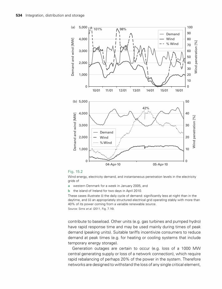
534 Integration, distribution and storage
Fig. 15.2Wind energy, electricity demand, and instantaneous penetration levels in the electricity grids of a western Denmark for a week in January 2005, and b the island of Ireland for two days in April 2010.These cases illustrate (i) the daily cycle of demand: significantly less at night than in the daytime, and (ii) an appropriately structured electrical grid operating stably with more than 40% of its power coming from a variable renewable source. Source: Sims et al. (2011, Fig. 7.16).
Dem
and
an
d w
ind
[M
W]
16/0115/0114/0113/0112/0111/0110/01
101% 98% 100
90
80
70
60
50
40
30
20
10
0
Win
d p
enet
rati
on
[%
]
5,000 (a)
4,000
3,000
2,000
1,000
0
Demand
% Wind Wind
Dem
and
an
d w
ind
[M
W]
05-Apr-1004-Apr-10
42%
50
40
30
20
10
0
Win
d p
enet
rati
on
[%
]
5,000(b)
4,000
3,000
2,000
1,000
0
Demand
% Wind
Wind
contribute to baseload. Other units (e.g. gas turbines and pumped hydro) have rapid response time and may be used mainly during times of peak demand (peaking units). Suitable tariffs incentivize consumers to reduce demand at peak times (e.g. for heating or cooling systems that include temporary energy storage).
Generation outages are certain to occur (e.g. loss of a 1000 MW central generating supply or loss of a network connection), which require rapid rebalancing of perhaps 20% of the power in the system. Therefore networks are designed to withstand the loss of any single critical element,
TWIDELL PAGINATION.indb 534 01/12/2014 11:38

§15.4 Electricity supply and networks 535
so no other element is overloaded and satisfactory supply continues. Since all major grid systems can cater for rapid demand fluctuations of ~20%, it is also possible for the same systems to cater for rapid supply fluctuations of ~20%. Thus the inclusion of variable supplies, such as wind power, is possible. (See online supplementary material for this chapter for more discussion of ‘how much back-up does grid-integrated wind power require?’)
Moreover, some RE systems can contribute positively to stabilizing the grid, for example:
• Small and medium-sized solar PV is typically installed near to demand and connected at the distribution level. At low penetrations on dis-tribution feeders (PV capacity <100% peak load on feeder), PV may offset the need for distribution upgrades (where peak demand on the feeder occurs in daylight) and reduce losses.
• Network-connected PV systems use inverters for grid interfacing, enabling in-principle control of electrical characteristics relevant for grid integration.
• Solar-based electric power systems (PV or CSP) both offer peak output power when peak demand occurs in hot, sunny places (e.g. California) where the demand peak is driven by air conditioning and other cooling systems.
• For reservoir-based hydro power, when water is available, the electrical output of the plants is highly controllable and can offer significant flexibility for system operation. The reservoir capacity can vary from short term to seasonal to multi-seasonal. The energy storage in the reservoir allows hydro plants to operate in baseload mode or as load following plants.
• Modern wind power plants are connected to the power system via power electronic converters, and can be equipped to provide grid services such as active power, reactive power and voltage control, fre-quency response (inertial type response) and power system support during network faults.
BOX 15.3 CAPACITY CREDIT, DISPATCHABILITY AND PREDICTABILITY
For grid operation, a ‘generating unit’ is an individual large electrical generator or a coupled group of smaller generators. Dispatchable units are those where the output can be readily varied directly or indirectly by the operator between a minimum and maximum level. The output of some units (e.g. most wind turbines) is not usually controlled and depends on the varying local energy resource. However, remote control is possible for larger units (e.g. offshore wind farms) through a reduction of the output or through an increase of previously de-rated capacity. Such units are ‘partially dispatchable’.
Generation from large hydro power (with dam), geothermal and biomass is fully dispatchable, whereas large wind power, PV, and wave or tidal power with remote control are only partially dispatchable. Concentrated solar power (CSP) generators may incorporate several hours of thermal storage, which
TWIDELL PAGINATION.indb 535 01/12/2014 11:38
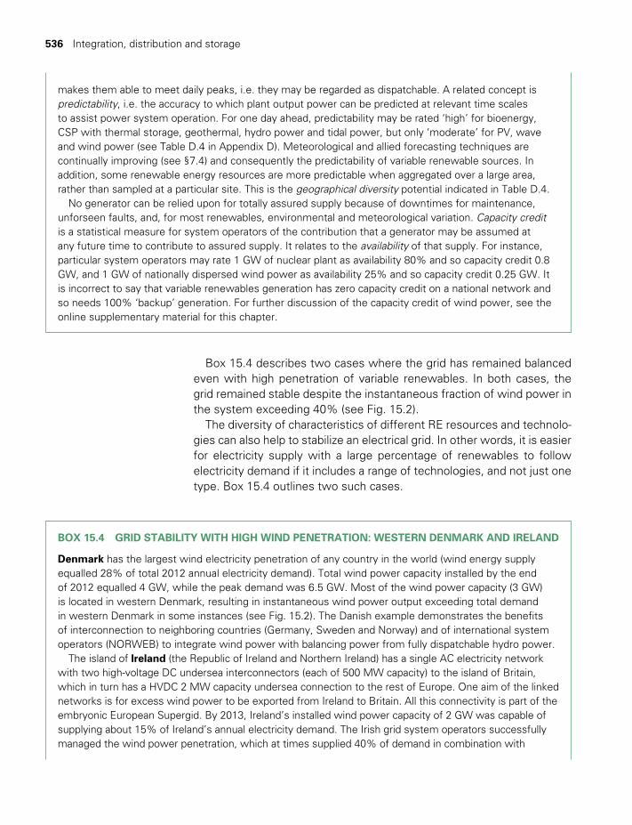
536 Integration, distribution and storage
makes them able to meet daily peaks, i.e. they may be regarded as dispatchable. A related concept is predictability, i.e. the accuracy to which plant output power can be predicted at relevant time scales to assist power system operation. For one day ahead, predictability may be rated ‘high’ for bioenergy, CSP with thermal storage, geothermal, hydro power and tidal power, but only ‘moderate’ for PV, wave and wind power (see Table D.4 in Appendix D). Meteorological and allied forecasting techniques are continually improving (see §7.4) and consequently the predictability of variable renewable sources. In addition, some renewable energy resources are more predictable when aggregated over a large area, rather than sampled at a particular site. This is the geographical diversity potential indicated in Table D.4.
No generator can be relied upon for totally assured supply because of downtimes for maintenance, unforseen faults, and, for most renewables, environmental and meteorological variation. Capacity credit is a statistical measure for system operators of the contribution that a generator may be assumed at any future time to contribute to assured supply. It relates to the availability of that supply. For instance, particular system operators may rate 1 GW of nuclear plant as availability 80% and so capacity credit 0.8 GW, and 1 GW of nationally dispersed wind power as availability 25% and so capacity credit 0.25 GW. It is incorrect to say that variable renewables generation has zero capacity credit on a national network and so needs 100% ‘backup’ generation. For further discussion of the capacity credit of wind power, see the online supplementary material for this chapter.
Box 15.4 describes two cases where the grid has remained balanced even with high penetration of variable renewables. In both cases, the grid remained stable despite the instantaneous fraction of wind power in the system exceeding 40% (see Fig. 15.2).
The diversity of characteristics of different RE resources and technolo-gies can also help to stabilize an electrical grid. In other words, it is easier for electricity supply with a large percentage of renewables to follow electricity demand if it includes a range of technologies, and not just one type. Box 15.4 outlines two such cases.
BOX 15.4 GRID STABILITY WITH HIGH WIND PENETRATION: WESTERN DENMARK AND IRELAND
Denmark has the largest wind electricity penetration of any country in the world (wind energy supply equalled 28% of total 2012 annual electricity demand). Total wind power capacity installed by the end of 2012 equalled 4 GW, while the peak demand was 6.5 GW. Most of the wind power capacity (3 GW) is located in western Denmark, resulting in instantaneous wind power output exceeding total demand in western Denmark in some instances (see Fig. 15.2). The Danish example demonstrates the benefits of interconnection to neighboring countries (Germany, Sweden and Norway) and of international system operators (NORWEB) to integrate wind power with balancing power from fully dispatchable hydro power.
The island of Ireland (the Republic of Ireland and Northern Ireland) has a single AC electricity network with two high-voltage DC undersea interconnectors (each of 500 MW capacity) to the island of Britain, which in turn has a HVDC 2 MW capacity undersea connection to the rest of Europe. One aim of the linked networks is for excess wind power to be exported from Ireland to Britain. All this connectivity is part of the embryonic European Supergid. By 2013, Ireland’s installed wind power capacity of 2 GW was capable of supplying about 15% of Ireland’s annual electricity demand. The Irish grid system operators successfully managed the wind power penetration, which at times supplied 40% of demand in combination with
TWIDELL PAGINATION.indb 536 01/12/2014 11:38
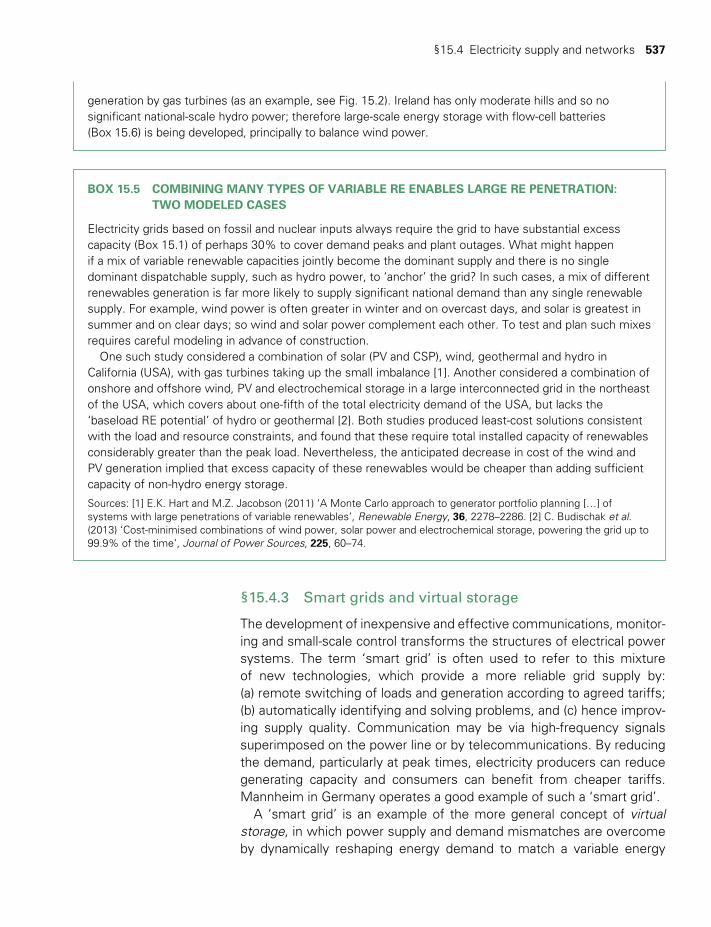
§15.4 Electricity supply and networks 537
§15.4.3 Smart grids and virtual storage
The development of inexpensive and effective communications, monitor-ing and small-scale control transforms the structures of electrical power systems. The term ‘smart grid’ is often used to refer to this mixture of new technologies, which provide a more reliable grid supply by: (a) remote switching of loads and generation according to agreed tariffs; (b) automatically identifying and solving problems, and (c) hence improv-ing supply quality. Communication may be via high-frequency signals superimposed on the power line or by telecommunications. By reducing the demand, particularly at peak times, electricity producers can reduce generating capacity and consumers can benefit from cheaper tariffs. Mannheim in Germany operates a good example of such a ‘smart grid’.
A ‘smart grid’ is an example of the more general concept of virtual storage, in which power supply and demand mismatches are overcome by dynamically reshaping energy demand to match a variable energy
generation by gas turbines (as an example, see Fig. 15.2). Ireland has only moderate hills and so no significant national-scale hydro power; therefore large-scale energy storage with flow-cell batteries (Box 15.6) is being developed, principally to balance wind power.
BOX 15.5 COMBINING MANY TYPES OF VARIABLE RE ENABLES LARGE RE PENETRATION: TWO MODELED CASES
Electricity grids based on fossil and nuclear inputs always require the grid to have substantial excess capacity (Box 15.1) of perhaps 30% to cover demand peaks and plant outages. What might happen if a mix of variable renewable capacities jointly become the dominant supply and there is no single dominant dispatchable supply, such as hydro power, to ‘anchor’ the grid? In such cases, a mix of different renewables generation is far more likely to supply significant national demand than any single renewable supply. For example, wind power is often greater in winter and on overcast days, and solar is greatest in summer and on clear days; so wind and solar power complement each other. To test and plan such mixes requires careful modeling in advance of construction.
One such study considered a combination of solar (PV and CSP), wind, geothermal and hydro in California (USA), with gas turbines taking up the small imbalance [1]. Another considered a combination of onshore and offshore wind, PV and electrochemical storage in a large interconnected grid in the northeast of the USA, which covers about one-fifth of the total electricity demand of the USA, but lacks the ‘baseload RE potential’ of hydro or geothermal [2]. Both studies produced least-cost solutions consistent with the load and resource constraints, and found that these require total installed capacity of renewables considerably greater than the peak load. Nevertheless, the anticipated decrease in cost of the wind and PV generation implied that excess capacity of these renewables would be cheaper than adding sufficient capacity of non-hydro energy storage.
Sources: [1] E.K. Hart and M.Z. Jacobson (2011) ‘A Monte Carlo approach to generator portfolio planning […] of systems with large penetrations of variable renewables’, Renewable Energy, 36, 2278–2286. [2] C. Budischak et al. (2013) ‘Cost-minimised combinations of wind power, solar power and electrochemical storage, powering the grid up to 99.9% of the time’, Journal of Power Sources, 225, 60–74.
TWIDELL PAGINATION.indb 537 01/12/2014 11:38
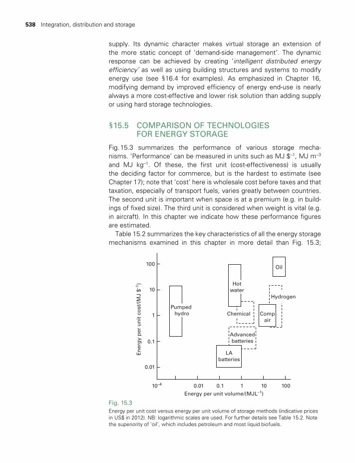
538 Integration, distribution and storage
supply. Its dynamic character makes virtual storage an extension of the more static concept of ‘demand-side management’. The dynamic response can be achieved by creating ‘intelligent distributed energy efficiency’ as well as using building structures and systems to modify energy use (see §16.4 for examples). As emphasized in Chapter 16, modifying demand by improved efficiency of energy end-use is nearly always a more cost-effective and lower risk solution than adding supply or using hard storage technologies.
§15.5 COMPARISON OF TECHNOLOGIES FOR ENERGY STORAGE
Fig. 15.3 summarizes the performance of various storage mecha-nisms. ‘Performance’ can be measured in units such as MJ $−1, MJ m−3 and MJ kg−1. Of these, the first unit (cost-effectiveness) is usually the deciding factor for commerce, but is the hardest to estimate (see Chapter 17); note that ‘cost’ here is wholesale cost before taxes and that taxation, especially of transport fuels, varies greatly between countries. The second unit is important when space is at a premium (e.g. in build-ings of fixed size). The third unit is considered when weight is vital (e.g. in aircraft). In this chapter we indicate how these performance figures are estimated.
Table 15.2 summarizes the key characteristics of all the energy storage mechanisms examined in this chapter in more detail than Fig. 15.3;
Fig. 15.3Energy per unit cost versus energy per unit volume of storage methods (indicative prices in US$ in 2012). NB: logarithmic scales are used. For further details see Table 15.2. Note the superiority of ‘oil’, which includes petroleum and most liquid biofuels.
0.01
10–4 0.01 0.1 1 10 100
0.1
1
10Hot
water
Oil
Hydrogen
Chemical Compair
Advancedbatteries
LAbatteries
En
erg
y p
er u
nit
co
st/(
MJ
$–1)
Energy per unit volume/(MJL–1)
100
Pumped hydro
TWIDELL PAGINATION.indb 538 01/12/2014 11:38
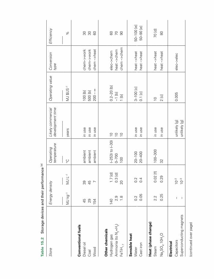
Tab
le 1
5.2
S
tora
ge
dev
ices
an
d t
hei
r p
erfo
rman
ce [a
]
Sto
reE
nerg
y de
nsity
Ope
ratin
gLi
kely
com
mer
cial
O
pera
ting
valu
eC
onve
rsio
nE
ffic
ienc
yte
mpe
ratu
re
deve
lopm
ent
time
type
------
-----
----
------
----
------
------
----
------
-----
-----
M
J kg
–1M
J L–1
°Cye
ars
MJ
$US
–1
%
Co
nve
nti
on
al f
uel
sD
iese
l oil
4539
ambi
ent
in u
se10
0 [b
]ch
em–>
wor
k30
Coa
l29
45am
bien
tin
use
500
[b]
chem
–>w
ork
30W
ood
154
7am
bien
tin
use
200
– ∞
chem
–>
heat
60
Oth
er c
hem
ical
sH
ydro
gen
gas
140
1.7
[d]
(–25
3) t
o (–
30)
100.
2–20
[b]
elec
–>ch
em60
Am
mon
ia (t
o N
2+H
2)2.
90.
3 [d
]0–
700
10~
1 [b
]he
at –
>ch
em70
FeTi
H1.
71.
820
100
101
[b]
chem
–>
chem
90
Sen
sib
le h
eat
Wat
er0.
20.
220
–100
in u
se3–
100
[c]
heat
–>
heat
50–1
00 [e
]C
ast
iron
0.05
0.4
20–4
00in
use
0.1
[c]
heat
–>
heat
50–9
0 [e
]
Hea
t (p
has
e ch
ang
eS
team
2.2
0.02
[f]
100–
300
in u
se10
heat
–>
heat
70 [d
]
Na 2S
O4.
10H
2O0.
250.
2932
in u
se2
[c]
heat
–>
heat
80
Ele
ctri
cal
Cap
acito
rs–
10–2
unlik
ely
[g]
0.00
5el
ec–>
elec
Sup
erco
nduc
ting
mag
nets
–10
–3un
likel
y [g
]
(con
tinue
d ov
er p
age)
TWIDELL PAGINATION.indb 539 01/12/2014 11:38
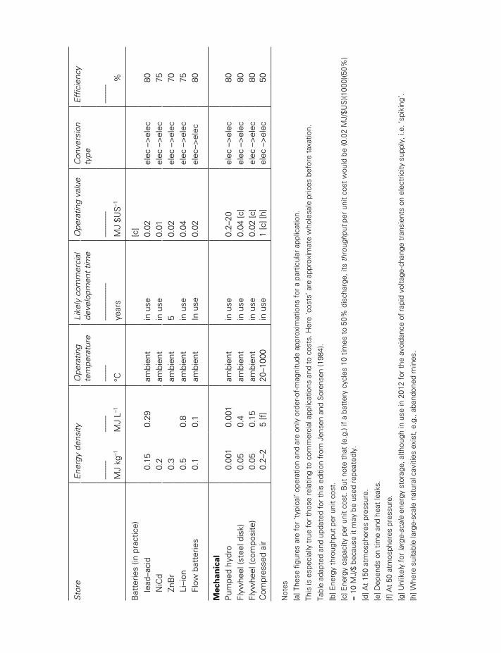
Sto
reE
nerg
y de
nsity
Ope
ratin
gLi
kely
com
mer
cial
O
pera
ting
valu
eC
onve
rsio
nE
ffic
ienc
yte
mpe
ratu
re
deve
lopm
ent
time
type
------
-----
----
------
----
------
------
----
------
-----
-----
M
J kg
–1M
J L–1
°Cye
ars
MJ
$US
–1
%
Bat
terie
s (in
pra
ctic
e)[c
]
lead
–aci
d0.
150.
29am
bien
tin
use
0.02
elec
–>
elec
80
NiC
d0.
2am
bien
tin
use
0.01
elec
–>
elec
75
ZnB
r0.
3am
bien
t5
0.02
elec
–>
elec
70
Li–i
on0.
50.
8am
bien
tin
use
0.04
elec
–>
elec
75
Flow
bat
terie
s0.
10.
1am
bien
tIn
use
0.02
elec
–>el
ec80
Mec
han
ical
Pum
ped
hydr
o0.
001
0.00
1am
bien
tin
use
0.2–
20el
ec –
>el
ec80
Flyw
heel
(ste
el d
isk)
0.05
0.4
ambi
ent
in u
se0.
04 [c
]el
ec –
>el
ec80
Flyw
heel
(com
posi
te)
0.05
0.15
ambi
ent
in u
se0.
02 [c
]el
ec –
>el
ec80
Com
pres
sed
air
0.2–
25
[f]
20–1
000
in u
se1
[c] [
h]el
ec –
>el
ec50
Not
es
[a] T
hese
fig
ures
are
for
‘typ
ical
’ ope
ratio
n an
d ar
e on
ly o
rder
-of-
mag
nitu
de a
ppro
xim
atio
ns f
or a
par
ticul
ar a
pplic
atio
n.
This
is e
spec
ially
tru
e fo
r th
ose
rela
ting
to c
omm
erci
al a
pplic
atio
ns a
nd t
o co
sts.
Her
e ‘c
osts
’ are
app
roxi
mat
e w
hole
sale
pric
es b
efor
e ta
xatio
n.
Tabl
e ad
apte
d an
d up
date
d fo
r th
is e
ditio
n fr
om J
ense
n an
d S
oren
sen
(198
4).
[b] E
nerg
y th
roug
hput
per
uni
t co
st.
[c] E
nerg
y ca
paci
ty p
er u
nit
cost
. But
not
e th
at (e
.g.)
if a
batt
ery
cycl
es 1
0 tim
es t
o 50
% d
isch
arge
, its
thr
ough
put
per
unit
cost
wou
ld b
e (0
.02
MJ/
$US
)(100
0)(5
0%)
= 1
0 M
J/$
beca
use
it m
ay b
e us
ed r
epea
tedl
y.
[d] A
t 15
0 at
mos
pher
es p
ress
ure.
[e] D
epen
ds o
n tim
e an
d he
at le
aks.
[f] A
t 50
atm
osph
eres
pre
ssur
e.
[g] U
nlik
ely
for
larg
e-sc
ale
ener
gy s
tora
ge, a
lthou
gh in
use
in 2
012
for
the
avoi
danc
e of
rap
id v
olta
ge-c
hang
e tr
ansi
ents
on
elec
tric
ity s
uppl
y, i.
e. ‘s
piki
ng’.
[h] W
here
sui
tabl
e la
rge-
scal
e na
tura
l cav
ities
exi
st, e
.g.,
aban
done
d m
ines
.
TWIDELL PAGINATION.indb 540 01/12/2014 11:38
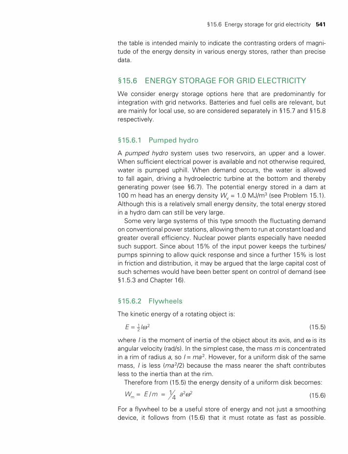
§15.6 Energy storage for grid electricity 541
the table is intended mainly to indicate the contrasting orders of magni-tude of the energy density in various energy stores, rather than precise data.
§15.6 ENERGY STORAGE FOR GRID ELECTRICITY
We consider energy storage options here that are predominantly for integration with grid networks. Batteries and fuel cells are relevant, but are mainly for local use, so are considered separately in §15.7 and §15.8 respectively.
§15.6.1 Pumped hydro
A pumped hydro system uses two reservoirs, an upper and a lower. When sufficient electrical power is available and not otherwise required, water is pumped uphill. When demand occurs, the water is allowed to fall again, driving a hydroelectric turbine at the bottom and thereby generating power (see §6.7). The potential energy stored in a dam at 100 m head has an energy density Wv = 1.0 MJ/m3 (see Problem 15.1). Although this is a relatively small energy density, the total energy stored in a hydro dam can still be very large.
Some very large systems of this type smooth the fluctuating demand on conventional power stations, allowing them to run at constant load and greater overall efficiency. Nuclear power plants especially have needed such support. Since about 15% of the input power keeps the turbines/pumps spinning to allow quick response and since a further 15% is lost in friction and distribution, it may be argued that the large capital cost of such schemes would have been better spent on control of demand (see §1.5.3 and Chapter 16).
§15.6.2 Flywheels
The kinetic energy of a rotating object is:
w=E I12
2 (15.5)
where I is the moment of inertia of the object about its axis, and w is its angular velocity (rad/s). In the simplest case, the mass m is concentrated in a rim of radius a, so I = ma 2. However, for a uniform disk of the same mass, I is less (ma 2/2) because the mass nearer the shaft contributes less to the inertia than at the rim.
Therefore from (15.5) the energy density of a uniform disk becomes:
w= =W E m a/ 14m
2 2 (15.6)
For a flywheel to be a useful store of energy and not just a smoothing device, it follows from (15.6) that it must rotate as fast as possible.
TWIDELL PAGINATION.indb 541 01/12/2014 11:38
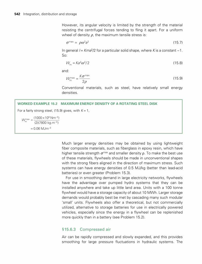
542 Integration, distribution and storage
However, its angular velocity is limited by the strength of the material resisting the centrifugal forces tending to fling it apart. For a uniform wheel of density r, the maximum tensile stress is:
s rw= amax 2 2 (15.7)
In general I = Kma2/2 for a particular solid shape, where K is a constant ~1. So:
w=W Ka / 2m2 2 (15.8)
and:s
r=W
K2m
maxmax
(15.9)
Conventional materials, such as steel, have relatively small energy densities.
WORKED EXAMPLE 15.2 MAXIMUM ENERGY DENSITY OF A ROTATING STEEL DISK
For a fairly strong steel, (15.9) gives, with K = 1,
= ×
=
−
−
−
W(1000 10 Nm )(2)(7800 kg.m )
0.06 MJm
mmax
6 2
3
3
Much larger energy densities may be obtained by using lightweight fiber composite materials, such as fiberglass in epoxy resin, which have higher tensile strength s max and smaller density r. To make the best use of these materials, flywheels should be made in unconventional shapes with the strong fibers aligned in the direction of maximum stress. Such systems can have energy densities of 0.5 MJ/kg (better than lead-acid batteries) or even greater (Problem 15.3).
For use in smoothing demand in large electricity networks, flywheels have the advantage over pumped hydro systems that they can be installed anywhere and take up little land area. Units with a 100 tonne flywheel would have a storage capacity of about 10 MWh. Larger storage demands would probably best be met by cascading many such modular ‘small’ units. Flywheels also offer a theoretical, but not commercially utilized, alternative to storage batteries for use in electrically powered vehicles, especially since the energy in a flywheel can be replenished more quickly than in a battery (see Problem 15.2).
§15.6.3 Compressed air
Air can be rapidly compressed and slowly expanded, and this provides smoothing for large pressure fluctuations in hydraulic systems. The
TWIDELL PAGINATION.indb 542 01/12/2014 11:38
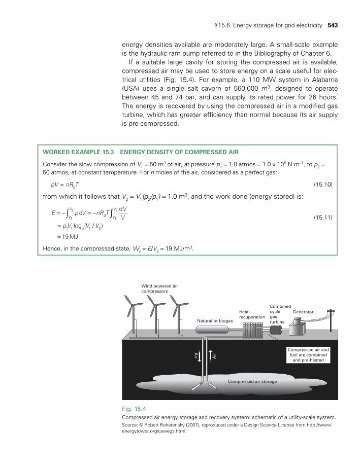
§15.6 Energy storage for grid electricity 543
energy densities available are moderately large. A small-scale example is the hydraulic ram pump referred to in the Bibliography of Chapter 6.
If a suitable large cavity for storing the compressed air is available, compressed air may be used to store energy on a scale useful for elec-trical utilities (Fig. 15.4). For example, a 110 MW system in Alabama (USA) uses a single salt cavern of 560,000 m3, designed to operate between 45 and 74 bar, and can supply its rated power for 26 hours. The energy is recovered by using the compressed air in a modified gas turbine, which has greater efficiency than normal because its air supply is pre-compressed.
Fig. 15.4Compressed air energy storage and recovery system: schematic of a utility-scale system. Source: © Robert Rohatensky (2007), reproduced under a Design Science License from http://www.energytower.org/cawegs.html.
Wind powered aircompressors
Natural or biogas
Compressed air storage
Air
Air
Heatrecuperation
GeneratorCombinedcyclegasturbine
Compressed air andfuel are combined
and pre-heated
WORKED EXAMPLE 15.3 ENERGY DENSITY OF COMPRESSED AIR
Consider the slow compression of V1 = 50 m3 of air, at pressure p1 = 1.0 atmos = 1.0 x 10⁵ N m–2, to p2 = 50 atmos, at constant temperature. For n moles of the air, considered as a perfect gas:
=pV nR T0 (15.10)
from which it follows that V2 = V1(p2/p1) = 1.0 m3, and the work done (energy stored) is:
E p V nR TV
VpV V V
dd
log ( / )
19 MJ
V
V
V
V
e
1
20
1
2
1 1 1 2
∫ ∫= − = −
=
=
(15.11)
Hence, in the compressed state, Wv = E/V2 = 19 MJ/m3.
TWIDELL PAGINATION.indb 543 01/12/2014 11:38
544 Integration, distribution and storage
For systems operating under less idealized conditions the energy stored per unit volume, Wv will be less but of similar magnitude. A major difficulty is to decrease the energy loss from heat production during the compression. Kreith and Kreider (2011) give a more detailed descrip-tion of the engineering aspects of such systems.
§15.6.4 High-power electrical storage
A superconducting electromagnetic energy storage (SMES) system is a device for storing and very quickly discharging large quantities of elec-tric power (e.g. 10 MW in ~1 s). It stores energy in the magnetic field created by the flow of DC in a coil of superconducting material that has been cryogenically cooled to ~4 K. At these very low temperatures, certain materials have essentially zero resistance to electric current and can maintain a DC current for years without appreciable loss. SMES systems have been in use for some years to improve industrial power quality and to provide a premium quality service for those electricity users who are particularly vulnerable to voltage fluctuations. An SMES recharges within minutes and can repeat the charge/discharge cycle thousands of times without any degradation of the magnet. Although there have been proposals to use SMES more generally for storing large amounts of electrical energy, the cost appears to be prohibitive (see Table 15.2).
Other large systems with fast response are being developed for similar power-conditioning uses. In particular, electrochemical capacitors (ECs) store electrical energy in the two series capacitors that exist in the electric double layer (EDL) at the interface of each electrode and the electrolyte solution. The distance over which the charge separation occurs is just a few angstroms. The capacitance and energy density of these devices are thousands of times larger than for ‘standard’ electrolytic capacitors. Compared to lead-acid batteries, ECs have less energy density but they can be cycled tens of thousands of times and are much more functional than batteries (fast charge and discharge capability). While small electrochemical capacitors are a fairly mature technology, products with larger energy densities are still under development.
§15.7 BATTERIES
Electricity is a high-quality form of energy, and therefore a great effort has been made to find a cheap and efficient means for storing it. A device that has electricity both as input and output is called an (electrical) storage battery or – occasionally – an electrical ‘accumulator’. Batteries are an essential component of most autonomous power systems (especially with photovoltaic and small wind turbine generation), of standby and emergency power systems, and of electric vehicles.
TWIDELL PAGINATION.indb 544 01/12/2014 11:38
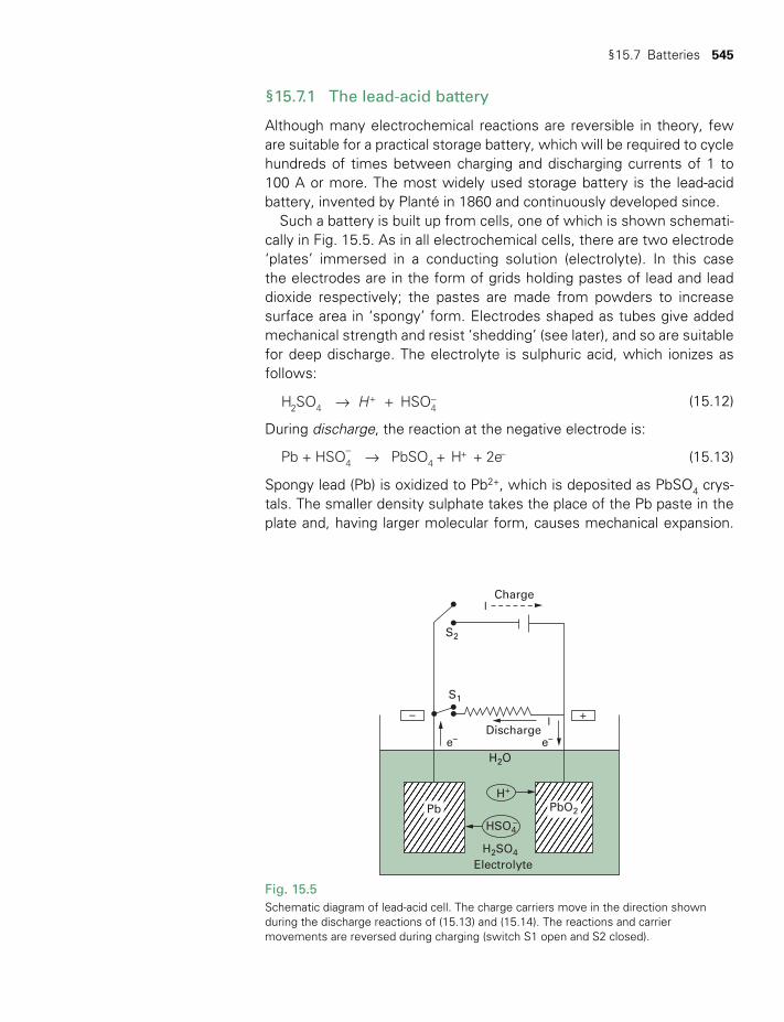
§15.7 Batteries 545
§15.7.1 The lead-acid battery
Although many electrochemical reactions are reversible in theory, few are suitable for a practical storage battery, which will be required to cycle hundreds of times between charging and discharging currents of 1 to 100 A or more. The most widely used storage battery is the lead-acid battery, invented by Planté in 1860 and continuously developed since.
Such a battery is built up from cells, one of which is shown schemati-cally in Fig. 15.5. As in all electrochemical cells, there are two electrode ‘plates’ immersed in a conducting solution (electrolyte). In this case the electrodes are in the form of grids holding pastes of lead and lead dioxide respectively; the pastes are made from powders to increase surface area in ‘spongy’ form. Electrodes shaped as tubes give added mechanical strength and resist ‘shedding’ (see later), and so are suitable for deep discharge. The electrolyte is sulphuric acid, which ionizes as follows:
HH SO HSO2 4 4→ ++ − (15.12)
During discharge, the reaction at the negative electrode is:
→− −Pb + HSO PbSO + H + 2e4 4+ (15.13)
Spongy lead (Pb) is oxidized to Pb2+, which is deposited as PbSO4 crys-tals. The smaller density sulphate takes the place of the Pb paste in the plate and, having larger molecular form, causes mechanical expansion.
Fig. 15.5Schematic diagram of lead-acid cell. The charge carriers move in the direction shown during the discharge reactions of (15.13) and (15.14). The reactions and carrier movements are reversed during charging (switch S1 open and S2 closed).
Charge
e– e–Discharge
Electrolyte
Pb
+–
PbO2
S2
S1
H2O
H2SO4
HSO4–
H+
I
I
TWIDELL PAGINATION.indb 545 01/12/2014 11:38
546 Integration, distribution and storage
WORKED EXAMPLE 15.4 THEORETICAL ENERGY DENSITY OF LEAD-ACID BATTERY
The reactions (15.12) and (15.13) show that to transfer 2 mol of electrons requires:
1 mol Pb = 207 g1 mol PbO2 = 239 g2 mol H2SO4 = 196 gTotal active material 642 g
But 2 mol of electrons represent a charge (unit of Coulomb):
(2 mol)(–1.60 x 10⁻¹⁹C)(6.02 x 10²³ mol–1) = –(2) (9.6 x 10⁴) C = –1.93 x 10⁵ Coulomb
The electrode potential, under standard conditions of concentration, for (Pb/PbSO4) is 0.30 V and for (PbSO4/Pb4
+) is –1.62 V. So the theoretical cell-EMF at standard conditions for (Pb/PbSO4/H2SO4/PbSO4/PbO2) is xcell = +1.92 V, with the PbO2 plate positive, according to the IUPAC sign convention.
The actual cell EMF depends on the concentration of reagents, and may be calculated by standard electrochemical methods. In general, the open-circuit voltage of a cell differs by only a few per cent from the theoretical cell voltage (Fig. 15.6). In particular, lead-acid batteries produce an open-circuit potential difference of 2.0 V per cell. If the internal resistance of the cell is much less than that of the external load (as may be expected with a new or ‘good’ cell), then the potential difference across the terminals will be close to the open-circuit value.
Therefore the work done in moving 2 mol of electrons is:
(1.93 x 10⁵ C) (2.0 V) = 0.386 x 10⁶ J
Thus the energy stored in 1.0 kg of active ingredients is, in theory,Wm
(0) = (0.386 x 10⁶ J)/(0.642 kg) = 0.60 MJ/kg.
The electrons so liberated travel through the external circuit to the posi-tive electrode, where they contribute to the reaction:
→− −PbO + HSO + 3H + 2 e PbSO + 2H O2 4+
4 2 (15.14)
Thus PbSO4 replaces the PbO2 in that plate, with similar, but less dis-ruptive, mechanical effects than in the negative plate. The electrical current through the solution is carried by H+ and HSO4
– ions from the sulphuric acid electrolyte, which themselves take part in the plate reac-tions. Transportable ‘gelled cells’ have this electrolyte immobilized in pyrogenic silica, with the fibrous glass mat separator giving open gas paths for the release of hydrogen and oxygen in overcharge. Although this makes them relatively expensive, they are safer to use and trans-port, since there is no danger of spilling highly corrosive sulphuric acid, and they are ‘maintenance free’.
Knowing the reactions involved and the corresponding standard elec-trode potentials (given in chemical tables), the theoretical energy density of any proposed battery can be calculated.
TWIDELL PAGINATION.indb 546 01/12/2014 11:38

§15.7 Batteries 547
Unfortunately, the energy density Wm of any practical battery is always much less than the theoretical value Wm
(0) based on the total active mass, as explained below for lead-acid batteries. Therefore most com-mercial batteries have Wm ~0.15 Wm
(0), although more careful (and more expensive!) designs may reasonably be expected to achieve energy den-sities up to 25% of the theoretical values.
In the specific case of the lead-acid battery, the main reasons for the ‘underachievement’ are as follows:
1 A working battery necessarily contains non-active materials (e.g. the case), the separators (which prevent the electrodes from short- circuiting) and the water in which the acid is dissolved. Moreover, the acid concentration must not be too large, since the battery would then discharge itself. Since the mass of actual battery contents exceeds the mass of the active ingredients, the energy density based on the mass of the whole battery is less than the theoretical value based on the active mass alone. However, this factor is not of great importance for stationary batteries.
2 The reactions cannot be allowed to go to completion. If all the lead were consumed by reaction (15.13) there would be no electrode left for the reverse reaction to operate, i.e. the battery could not be cycled. Similarly, if the concentration of H2SO4 is allowed to reduce too much, the electrolyte ceases to be an adequate conductor. In practice, many battery types should not be allowed to discharge more than about 50% of total potential stored energy, or they may be ruined. However, specially designed batteries do allow ‘deep discharge’ beyond 50%.
A further limitation of real batteries is that they do not last for ever. Solid Pb is almost twice as dense as the PbSO4 found in the discharge reaction (15.13). Therefore it is difficult to fit the PbSO4 crystals into the space originally occupied by the Pb paste in the negative electrode. After many charge/discharge cycles, the repeated expansion and contraction cause plate material and some PbSO4 to fall to the bottom of the cell. This consti-tutes an irreversible loss of active material. This loss is worse if the battery is allowed to fully discharge; indeed, it may rapidly become impossible to recharge the battery. In addition, the ‘shed’ material may provide an electrically conducting link between plates, so increasing ‘self-discharge’. Storage batteries should have a generous space below the plates so that debris can accumulate without short-circuiting the electrodes.
The other main factor limiting the life of even a well-maintained battery is self-discharge of the positive electrode. This is particularly acute in vehicle SLI (starting, lighting and ignition) batteries in which the grid is not pure Pb but usually a lead-antimony-calcium alloy. Electrode plates with antimony are physically stronger and better able to stand the mechanical stresses during motion. Unfortunately antimony promotes the reaction:
→5PbO + 2Sb + 6H SO (SbO ) SO + 5PbSO + 6H O2 2 4 2 2 4 4 2 (15.15)
TWIDELL PAGINATION.indb 547 01/12/2014 11:38
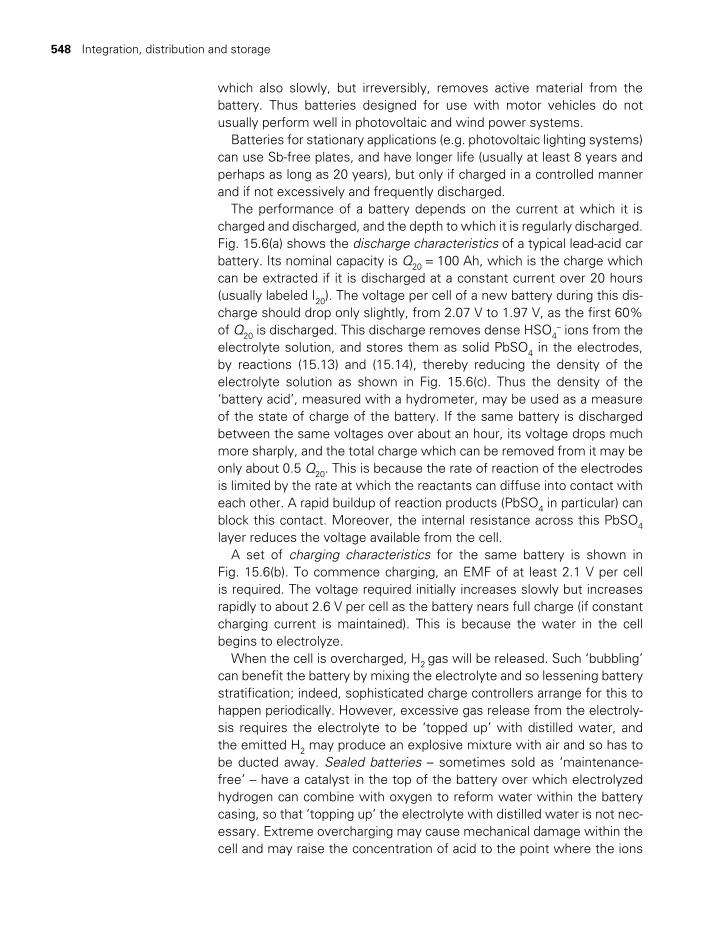
548 Integration, distribution and storage
which also slowly, but irreversibly, removes active material from the battery. Thus batteries designed for use with motor vehicles do not usually perform well in photovoltaic and wind power systems.
Batteries for stationary applications (e.g. photovoltaic lighting systems) can use Sb-free plates, and have longer life (usually at least 8 years and perhaps as long as 20 years), but only if charged in a controlled manner and if not excessively and frequently discharged.
The performance of a battery depends on the current at which it is charged and discharged, and the depth to which it is regularly discharged. Fig. 15.6(a) shows the discharge characteristics of a typical lead-acid car battery. Its nominal capacity is Q20 = 100 Ah, which is the charge which can be extracted if it is discharged at a constant current over 20 hours (usually labeled I20). The voltage per cell of a new battery during this dis-charge should drop only slightly, from 2.07 V to 1.97 V, as the first 60% of Q20 is discharged. This discharge removes dense HSO4
– ions from the electrolyte solution, and stores them as solid PbSO4 in the electrodes, by reactions (15.13) and (15.14), thereby reducing the density of the electrolyte solution as shown in Fig. 15.6(c). Thus the density of the ‘battery acid’, measured with a hydrometer, may be used as a measure of the state of charge of the battery. If the same battery is discharged between the same voltages over about an hour, its voltage drops much more sharply, and the total charge which can be removed from it may be only about 0.5 Q20. This is because the rate of reaction of the electrodes is limited by the rate at which the reactants can diffuse into contact with each other. A rapid buildup of reaction products (PbSO4 in particular) can block this contact. Moreover, the internal resistance across this PbSO4 layer reduces the voltage available from the cell.
A set of charging characteristics for the same battery is shown in Fig. 15.6(b). To commence charging, an EMF of at least 2.1 V per cell is required. The voltage required initially increases slowly but increases rapidly to about 2.6 V per cell as the battery nears full charge (if constant charging current is maintained). This is because the water in the cell begins to electrolyze.
When the cell is overcharged, H2 gas will be released. Such ‘bubbling’ can benefit the battery by mixing the electrolyte and so lessening battery stratification; indeed, sophisticated charge controllers arrange for this to happen periodically. However, excessive gas release from the electroly-sis requires the electrolyte to be ‘topped up’ with distilled water, and the emitted H2 may produce an explosive mixture with air and so has to be ducted away. Sealed batteries – sometimes sold as ‘maintenance-free’ – have a catalyst in the top of the battery over which electrolyzed hydrogen can combine with oxygen to reform water within the battery casing, so that ‘topping up’ the electrolyte with distilled water is not nec-essary. Extreme overcharging may cause mechanical damage within the cell and may raise the concentration of acid to the point where the ions
TWIDELL PAGINATION.indb 548 01/12/2014 11:38
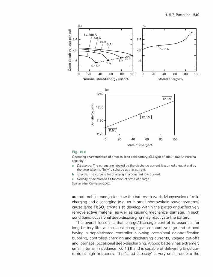
§15.7 Batteries 549
Fig. 15.6Operating characteristics of a typical lead-acid battery (SLI type of about 100 Ah nominal capacity). a Discharge. The curves are labeled by the discharge current (assumed steady) and by
the time taken to ‘fully’ discharge at that current. b Charge. The curve is for charging at a constant low current. c Density of electrolyte as function of state of charge. Source: After Crompton (2000).
1240
1200
1160
1120
0 20
11.5 V
12.0 V
12.5 V
40
State of charge/%
Den
sity
/(kg
/m3 )
60 80 100
(c)
0
1.6
Op
en c
ircu
it v
olt
age
per
cel
l
2.0
2.4
(a)
20
0.15 h
5 A15 A
50 AI = 200 A
I = 7 A
1 h5 h
20 h
40
Nominal stored energy used/% Stored energy/%
60 80 100 0
1.6
2.0
2.4
(b)
20 40 60 80 100
are not mobile enough to allow the battery to work. Many cycles of mild charging and discharging (e.g. as in small photovoltaic power systems) cause large PbSO4 crystals to develop within the plates and effectively remove active material, as well as causing mechanical damage. In such conditions, occasional deep-discharging may reactivate the battery.
The overall lesson is that charge/discharge control is essential for long battery life; at the least charging at constant voltage and at best having a sophisticated controller allowing occasional de-stratification bubbling, controlled charging and discharging currents, voltage cut-offs and, perhaps, occasional deep-discharging. A good battery has extremely small internal impedance (<0.1 Ω) and is capable of delivering large cur-rents at high frequency. The ‘farad capacity’ is very small, despite the
TWIDELL PAGINATION.indb 549 01/12/2014 11:38
550 Integration, distribution and storage
‘charge capacity’ being large, so do not be misled by the two distinct meanings of the word ‘capacity’.
Development of improved lead-acid batteries still continues, produc-ing a variety of models with performance optimized for different appli-cations, in terms of reliability, long life, cost, power/weight ratio, etc. Key developments over the past few decades include: polypropylene for inert, leak-proof enclosures; ‘absorbent glass mat’ technology for plate separators; valve-regulated lead-acid batteries (sealed to prevent air ingress but allowing excess gas to escape and having internal refor-mation of overcharge electrolyzed hydrogen and oxygen); a wide range of ‘recipes’ with small concentration additives for specialist plates and separators; and electronically controlled charging.
For applications requiring extra-large capacity (e.g. as part of an elec-tricity grid), lead-acid batteries may be scaled up in the form of flow cells (Box 15.6).
BOX 15.6 SCALING UP BATTERIES: FLOW CELLS
Flow cell batteries use a different geometry from conventional batteries to enable scale-up to utility level. Flow cell battery storage uses two chemical solutions to store electricity (Fig. 15.7) The chemicals are held in adjacent tanks and then pumped when needed through an electrolytic ‘battery’ cell. Thus the volume of electrolyte, and hence the energy stored, are determined separately from the cell construction characteristics. Electricity is produced as with a conventional type of battery. The battery is charged in a reverse process.
Flow cells are technically very suitable for static installations storing significant quantities of electrical energy with fast response, as in national electricity grids.
For example, the Notrees array of flow cells in Texas (USA), installed in 2012, can deliver 36 megawatt of power to the grid over a period of 15 minutes. It comprises bus-sized, lead-acid battery modules with high surface area electrodes and multiple terminals, so that electricity flows in and out quickly, and is used to smooth out the supply of electricity from the 153 MW Notrees wind farm nearby. It also makes the entire grid more resilient to spikes in demand, because battery arrays can respond almost instantly, whereas natural gas power plants take about 15 minutes to boost their output.
Electrolyte combinations other than lead-acid are the subject of active flow cell development, notably Vanadium redox flow cells and zinc bromine flow cells.
Source: H. Hodson, ‘Texas mega-battery aims to green up the grid’, New Scientist, February 1, 2013.
15.7.2 Lithium-based batteries
Development of other electrochemical systems for storage batteries is also active. The major factor contributing to the relatively small energy density of a lead-acid battery is the large atomic weight of lead (207). This has driven active development of batteries based on lighter elements, notably lithium (Li, atomic weight 7), especially for applications where weight is a greater constraint than cost, in particular for electric vehicles (see §16.5.5(b)).
Modern lithium-based batteries do not use lithium metal as such, since it ignites easily and reacts violently with water. Instead, the lithium is
TWIDELL PAGINATION.indb 550 01/12/2014 11:38
§15.7 Batteries 551
combined with other elements into more benign compounds which do not react with water. The typical lithium-ion cell uses carbon for its anode and a compound such as lithium cobalt dioxide or lithium iron phosphate as the cathode. Lithium ions are intercalated into the positive electrode in the discharged state and into the negative electrode in the charged state, and move from one to the other across the electrolyte. The electrolyte is usually based on a lithium salt in an organic solvent.
Volume production has reduced the price, so lithium rechargeable batteries dominate for portable consumer electronics equipment (e.g. mobile phones and portable computers). By 2012, these advances in energy density and price had led to almost all electric vehicles (EVs) using Li-ion batteries. However, active development of variants continues as the price of the batteries needs to decrease further, and their useful life increase, before EVs compete for distance travel with similar sized conventional vehicles.
However, Li is a fairly rare element, and the batteries for even a single EV obviously require much more Li than do those for hundreds of laptop computers. Therefore there is a danger that widespread use of EVs using Li-based batteries may be resource – and therefore price – limited. This factor is a significant incentive for the development of other novel battery types.
§15.7.3 Other battery technologies
Numerous other types of storage batteries have been and are being developed for special applications; some are listed in Table 15.2 of §15.5. For further details see, e.g. www.electropaedia.com. Research
Fig. 15.7Flow cell battery (schematic).Source: http://www.mpoweruk.com/flow.htm (which links to www.electropaedia.com).
Ion exchangemembrane
Power out
Electrode Electrode
Electrolyteflow
Electrolyte Tanks
+ –
TWIDELL PAGINATION.indb 551 01/12/2014 11:38
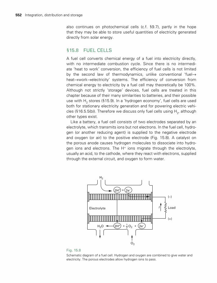
552 Integration, distribution and storage
also continues on photochemical cells (c.f. §9.7), partly in the hope that they may be able to store useful quantities of electricity generated directly from solar energy.
§15.8 FUEL CELLS
A fuel cell converts chemical energy of a fuel into electricity directly, with no intermediate combustion cycle. Since there is no intermedi-ate ‘heat to work’ conversion, the efficiency of fuel cells is not limited by the second law of thermodynamics, unlike conventional ‘fuel→ heat→work→electricity’ systems. The efficiency of conversion from chemical energy to electricity by a fuel cell may theoretically be 100%. Although not strictly ‘storage’ devices, fuel cells are treated in this chapter because of their many similarities to batteries, and their possible use with H2 stores (§15.9). In a ‘hydrogen economy’, fuel cells are used both for stationary electricity generation and for powering electric vehi-cles (§16.5.5(b)). Therefore we discuss only fuel cells using H2, although other types exist.
Like a battery, a fuel cell consists of two electrodes separated by an electrolyte, which transmits ions but not electrons. In the fuel cell, hydro-gen (or another reducing agent) is supplied to the negative electrode and oxygen (or air) to the positive electrode (Fig. 15.8). A catalyst on the porous anode causes hydrogen molecules to dissociate into hydro-gen ions and electrons. The H+ ions migrate through the electrolyte, usually an acid, to the cathode, where they react with electrons, supplied through the external circuit, and oxygen to form water.
Fig. 15.8Schematic diagram of a fuel cell. Hydrogen and oxygen are combined to give water and electricity. The porous electrodes allow hydrogen ions to pass.
Electrolyte
2H+
2H+
2e–
2e–
LoadI
(–)
(+)
H2O
H2
O2
O2+
+
+21
TWIDELL PAGINATION.indb 552 01/12/2014 11:38

§15.9 Chemicals as energy stores 553
The efficiencies of practical fuel cells, whether hydrogen/oxygen or some other gaseous ‘couple’, are much less than the theoretical 100%, for much the same reasons as for batteries. In practice, the efficiency is perhaps 40% for the conversion of chemical energy to electricity, but this is not dependent on whether or not the cell is working at its full rated power. This contrasts with most diesel engines, gas turbines and other engines.
Since the efficiency of an assembly of fuel cells is nearly equal to that of a single cell, there are few economies of large scale. Therefore small localized plants of 1 to 100 kW capacity are a promising proposi-tion. Using the fuel cell as a combined heat and power source, a single building could be supplied with both electricity and heat (from the waste heat of the cells), for the same amount of fuel ordinarily required for the thermal demand alone. The main reason why fuel cells are not in wider use for such applications is their capital cost ~$700/ kW.
§15.9 CHEMICALS AS ENERGY STORES
$15.9.1 Hydrogen
Hydrogen can be made from water by electrolysis, using any source of DC electricity. The gas can be stored, distributed and burnt to release heat. The only product of combustion is water, so at end-use no pollu-tion results. The enthalpy change is DH = –242 kJ/mol; i.e. 242 kJ are released for every mole (18 g) of H2O formed.
Hydrogen (with CO in the form of ‘town gas’ made from coal) was used for many years as an energy store and supply, and there is no over-riding technical reason why hydrogen-based systems could not come into wide use again. Note, however, that most hydrogen is made now from fossil fuels.
Electrolysis is a well-established commercial process yielding pure hydrogen, but generally efficiencies have been only ~60%. Some of this loss is due to electrical resistance in the circuit, especially around the electrodes where the evolving bubbles of gas block the current carry-ing ions in the water. Electrodes with ‘bubble-removing mechanisms’ should be advantageous. The best electrodes have large porosity, so giving a greater effective area and thus allowing a larger current density, which implies having fewer cells and reduced cost for a given gas output. Efficiencies ~80% have been so obtained, and can be increased further by using – usually expensive – catalysts.
A technical difficulty in the electrolysis of sea water is that chlorine may also be evolved at the ‘oxygen’ electrode. Approximate chemical calculations suggest that the O2 can be kept pure if the applied voltage per cell is less than 1.8 V, but unfortunately this limits the current density, so electrodes of large surface area would be needed.
TWIDELL PAGINATION.indb 553 01/12/2014 11:38
554 Integration, distribution and storage
High temperatures also promote the chemical decomposition of water. The change in Gibbs free energy associated with a reversible electro-chemical reaction at absolute temperature T is:
xD = = D − DG nF H T S (15.16)
where x is the electrical potential, DH is the enthalpy change and DS is the entropy change, F = 96,500 Coulomb mol–1 is Faraday’s constant, and n is the number of moles of reactant.
The decomposition reaction
H2O → H2 + 1 2 O2 (15.17)
has DG, DH, DS all positive. Therefore from (15.16), increasing T decreases the electric potential x required for decomposition. Problem 15.10 shows that x = 0 for T >~2000 K, so it is impracticable to decom-pose water solely by straightforward heating. A more promising strategy is to reduce the input electrical energy needed for electrolysis by heating from a cheaper source. Heat at T ~1000 K from solar concentrators may be cheaper than just using electricity, and this may be the cheapest route to produce hydrogen.
Several other methods of producing hydrogen without using fossil fuels have been tried in the laboratory, including special algae, which ‘photosynthesize’ H2 (see §9.7.3); but none has yet shown worthwhile efficiencies.
BOX 15.7 A SMALL ISLAND AUTONOMOUS WIND-HYDROGEN ENERGY SYSTEM
An autonomous wind/hydrogen energy demonstration system located on the island of Utsira, Norway, was officially launched by Norsk Hydro (now Statoil) and Enercon (a German wind turbine manufacturer) in July 2004. The main components of the system are a 600 kWe rated wind turbine, a water electrolyzer to produce about 10 Nm3/h of hydrogen, with about 2400 Nm3 of hydrogen storage (at 20,000 kPa), a hydrogen-powered internal combustion engine driving a 55 kWe generator, and a 10 kWe proton exchange membrane (PEM) fuel cell. This innovative demonstration system supplies 10 households on the island providing two to three days of full energy autonomy (Ulleberg et al. 2010).
Operational experience and data collected from the plant over four to five years showed that the overall efficiency of the wind to AC-electricity to hydrogen to AC-electricity system, assuming no storage losses, is only about 10%. If the hydrogen engine was to be replaced by a 50 kWe PEM fuel cell, the overall efficiency would increase to 16 to 18%. Replacing the present electrolyzer with a more efficient unit (such as a PEM or a more advanced alkaline design) would increase the overall system efficiency to around 20% (Ulleberg et al. 2010).
The relatively low efficiency of the system illustrates the challenge for commercial hydrogen developments. More compact hydrogen storage systems and more robust and less costly fuel cells need to be developed before autonomous wind/hydrogen systems can become technically and economically viable.
Sources: SRREN (2011, §8.2.5.5); O. Ulleberg, T. Nakken and A. Ete (2010) “The wind/hydrogen demonstration system at Utsira in Norway: evaluation of system performance”, International Journal of Hydrogen Energy, 35, 1841–1852.
TWIDELL PAGINATION.indb 554 01/12/2014 11:38
§15.10 Storage for heating and cooling systems 555
To store hydrogen in large quantities is not trivial. Most promising is the use of underground caverns, such as those from which natural gas is now extracted, but storage of gas, even if compressed, is bulky. Hydrogen can be liquefied, but since its boiling point is 20 K (i.e. –253°C), such cold stores are expensive to build and to operate, requiring contin-ued refrigeration. Chemical storage as metal hydrides, from which the hydrogen can be released by heating, is more manageable and allows large volumes of H2 to be stored (see Table 15.2). For example,
FeTiH1.7 T~50°C
+FeTiH 0.8H0.1 2 (15.18)
This reaction is reversible, so a portable hydride store can be replen-ished with hydrogen at a central ‘filling station’. The heat released in this process may be used for district heating, and the portable hydride store may be used as the ‘fuel tank’ of a vehicle. The main difficulty is the weight and cost of the metals used (see Table 15.2). Hydrogen could also be distributed through the extensive pipeline networks already used deliver natural gas in many countries, although hydrogen carries less energy per unit volume than methane.
Some writers envisage a ‘hydrogen economy’ in which hydrogen becomes the main means of storing and distributing energy. But the benefits of this are dubious unless the H2 itself is produced from RE, so that the cost of the major new infrastructure required would seem to be unwarranted.
§15.9.2 Ammonia
Unlike water, ammonia can be dissociated at realizable temperatures:
+ →←N H NH3 22 2 3 (15.19)
In conjunction with a heat engine, these reactions form the basis of systems that may be the most efficient way to generate continuous electrical power from solar heat (see §4.8.3).
Similar systems have also been proposed based on the reaction
→←CO + 2H O CH + 2O2 2 4 2 (15.20)
using electricity to bias the reaction to the right (e.g. from periods when wind power generation exceeds demand). This is sometimes referred to as ‘power to gas’ (P2G) storage.
§15.10 STORAGE FOR HEATING AND COOLING SYSTEMS
A substantial fraction of world energy use is as low temperature heat. For example, Fig. 16.3(b) shows the demand in Britain for total energy and for space heating. Although details change from year to year, this
TWIDELL PAGINATION.indb 555 01/12/2014 11:38
556 Integration, distribution and storage
suggests that in winter over half of the national energy consumption is for space heating in buildings at temperatures of about 18 ± 3°C. It is usually not sensible to meet this demand for heat from the best thermo-dynamic quality energy supplies (§1.4.2), since these should be saved for electricity generation, engines and motor drives. Thus, for example, it is better to capture solar heat gains, and then to keep buildings within comfortable temperatures using the averaging and heat-storage charac-teristics of the building mass (see §16.4). Heat storage also provides a way of fruitfully using ‘waste’ energy utilized or recovered from other processes (e.g. by load control devices: §1.5.3).
In the higher latitudes, solar heat supply is significantly greater in summer than in winter (see Figs 2.7 and 2.10), yet the demand for heat is greatest in winter. Therefore the maximum benefit from solar heat requires heat storage for at least three months, say, in hot water in an underground enclosure. To consider this possibility, we estimate the time, tloss, for such a heat store to have 50% of its content withdrawn while maintaining a uniform temperature Ts. Assuming that the immedi-ate environment (e.g. the soil temperature) has constant temperature Ta, the heat balance equation is:
= −−
mcdTdt
T TR
s s a (15.21)
where mc is its heat capacity, and R is the thermal resistance between the store and the surroundings. The solution of (15.21) is:
T T
T Tt
mcR(0)exps a
s a
−−
= −
(15.22)
from which it follows that the ‘time constant’
=t mcR1.3loss (15.23)
If the store is a sphere of radius a, the thermal resistance is R = r/4pa2, where r is the thermal resistivity of unit area, and m = 4pa3 r/3, so for a sphere,
r=t cra0.43loss (15.24)
WORKED EXAMPLE 15.5 SIZE AND INSULATION OF A DOMESTIC HEAT STORE
Assume a well-insulated, house requires in winter an average internal heat supply of 1.0 kW. Together with the free gains of lighting, etc., this will maintain an internal temperature of 20°C. It is decided to build a hot water store in a rectangular tank whose top forms the floor of the house, of area 200 m2. The heating must be adequate for 100 days, as all the heat loss from the tank passes by conduction through the floor, and as the water cools from an initial 60°C to a final 40°C.
TWIDELL PAGINATION.indb 556 01/12/2014 11:38
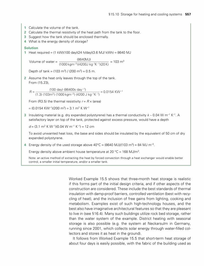
§15.10 Storage for heating and cooling systems 557
Worked Example 15.5 shows that three-month heat storage is realistic if this forms part of the initial design criteria, and if other aspects of the construction are considered. These include the best standards of thermal insulation with damp-proof barriers, controlled ventilation (best with recy-cling of heat), and the inclusion of free gains from lighting, cooking and metabolism. Examples exist of such high-technology houses, and the best also have imaginative architectural features so that they are pleasant to live in (see §16.4). Many such buildings utilize rock bed storage, rather than the water system of the example. District heating with seasonal storage is also possible (e.g. the system at Neckarsulm in Germany, running since 2001, which collects solar energy through water-filled col-lectors and stores it as heat in the ground).
It follows from Worked Example 15.5 that short-term heat storage of about four days is easily possible, with the fabric of the building used as
1 Calculate the volume of the tank.2 Calculate the thermal resistivity of the heat path from the tank to the floor.3 Suggest how the tank should be enclosed thermally.4 What is the energy density of storage?
Solution1 Heat required = (1 kW)(100 day)(24 h/day)(3.6 MJ/ kWh) = 8640 MJ
Volume of water = − − −
(8640MJ)(1000 kgm )(4200J kg K )(20 K)3 1 1
= 103 m3
Depth of tank = (103 m3) / (200 m2) = 0.5 m.
2 Assume the heat only leaves through the top of the tank.From (15.23),
= =−
− − −−R
(100 day) (86400s day )(1.3) (103m ) (1000 kgm ) (4200 J kg K )
0.0154 KW1
3 3 1 11
From (R3.5) the thermal resistivity r = R × (area)
= (0.0154 KW–1)(200 m2) = 3.1 m2 K W–1
3 Insulating material (e.g. dry expanded polystyrene) has a thermal conductivity k ~ 0.04 W m–1 K–1. A satisfactory layer on top of the tank, protected against excess pressure, would have a depth
d = (3.1 m2 K W–1)(0.04 W m–1 K–1) = 12 cm
To avoid unwanted heat loss, the base and sides should be insulated by the equivalent of 50 cm of dry expanded polystyrene.
4 Energy density of the used storage above 40°C = (8640 MJ)/(103 m3) = 84 MJ m–3.
Energy density above ambient house temperature at 20 °C = 168 MJ/m3.
Note: an active method of extracting the heat by forced convection through a heat exchanger would enable better control, a smaller initial temperature, and/or a smaller tank.
TWIDELL PAGINATION.indb 557 01/12/2014 11:38
558 Integration, distribution and storage
the store. Similarly, thermal capacity and cold storage can have important implications for building design in hot-weather conditions.
Materials that change phase offer a much larger heat capacity, over a limited temperature range, than systems using sensible heat. For example, Glauber’s salt (Na2SO4. 10H2O) has been used as a store for room heating. It decomposes at 32°C to a saturated solution of Na2 SO4 plus an anhydrous residue of Na2SO4. This reaction is reversible and evolves 250 kJ/kg ~650 MJ/m3. Since much of the cost of a store for house heating is associated with the construction, such stores may be cheaper overall than simple water tanks of less energy density per unit volume. Nevertheless, this seemingly simple method requires prac-tical difficulties to be overcome. In particular, the solid and liquid phases often eventually separate spatially so that recombination is prevented; consequently, without mixing, the system becomes inefficient after many cycles.
§15.11 TRANSPORT SYSTEMS
In many countries, transport accounts for around 30% of national use of commercial energy, with the dominant primary energy input to trans-portation being from fossil fuels, especially oil (see Figs 16.3, 16.9 and §16.5). Electric railway systems with primary energy from hydro power are a small exception. The steam trains which were dominant in the 19th century are now rare; likewise commercial sail-boats, except in niche applications such as in developing countries with many scattered islands. Hence transportation is the most difficult sector for RE to replace fossil fuel use.
In §16.5 we consider reducing fossil fuel use for transport by improv-ing the transport system as a whole, and in particular looking at the more efficient ways of managing the demand (e.g. through urban plan-ning that is not based around the private motor car) and of meeting the demand (e.g. through more attractive mass transit systems). Short term strategies discussed in §16.5 are resigned to something like the current pattern of vehicle use, and focus on improving the fuel efficiency of the vehicles themselves and/or on alternative fuels or engines. Alternative fuels that can be supplied from renewable rather than fossil sources include liquid biofuels (Chapter 10) or hydrogen (§15.9.1 below). The alternative engines under most active development are electric vehicles, the key to which are improved batteries and perhaps fuel cells.
Considerable R&D funding has gone into the development of vehicles that use hydrogen (H2) as a fuel (i.e. as an energy store, see §15.9.1. This is because the combustion of H2 or its reaction in a fuel cell for elec-tricity (Fig. 15.8) produces only H2O, thus avoiding ‘tail pipe’ pollution. However, pollution is shifted elsewhere, since most hydrogen today is produced as a by-product of petroleum refining. Pollution can only be
TWIDELL PAGINATION.indb 558 01/12/2014 11:38

§15.12 Social and environmental aspects of energy supply and storage 559
eliminated by using hydrogen from electrolysis of water with electricity from non-thermal renewable energy.
§15.12 SOCIAL AND ENVIRONMENTAL ASPECTS OF ENERGY SUPPLY AND STORAGE
Energy delivery and storage are important. The world economy depends on the distribution of energy on a very large scale. International trade in fossil fuels (coal, oil and gas) from the relatively few countries that export in large quantities exceeded 11% of world trade in 2012.1 The concen-trated lines of supply are vulnerable to disruption, so several wars are attributed to oil-consuming counties seeking to secure their supplies (see Yergin 1992). The fact that oil and coal are cheap stores of large quanti-ties of easily accessible energy (see Fig. 15.3) allowed the rapid growth of cities. There was little initial attention to the environmental conse-quences (McNeill 2000) and to the overall efficiency with which energy was used (Chapter 16). Occasional failures of the distribution systems have severe environmental consequences, notably large-scale oil spills.
National governments accept responsibility to oversee and secure energy supplies at all levels of society (§17.2). For example, energy dis-tribution routes receive priority planning permissions and in severe dis-ruptions military personnel are used to maintain supplies.
As discussed in Chapter 1, the less concentrated and dispersed nature of renewable energy sources allows a major shift away from international and centralized energy delivery and its vulnerable distribution. Therefore it is generally recognized that renewable energy supplies have a favor-able impact, especially regarding security of supply. However, the con-siderable vested interests in the status quo handicap the wholehearted development and use of renewables.
Methods of storing energy are important to support continuity of supply (as with pumped hydro for electricity and national oil reserve stores) and vital for autonomous power (as in batteries for vehicle start-ing and lighting, and for stand-alone and emergency power).
There are relatively minor environmental hazards to some of the storage mechanisms described in this chapter. In particular, batteries of all kinds are filled with noxious chemicals, so that their safe disposal is necessary. Lead-acid batteries are so widespread for vehicles that there is a thriving recycling business in most countries, with lead especially recycled from ‘dead’ batteries. Operational hazards are always important to safeguard against, and dangers of mechanical failure, fire and explosion, leakage and electrical shock must be recognized and guarded against.
Contrary to popular impression, hydrogen gas is no more hazardous regarding fire and explosion than the more familiar natural gas (methane). Of course, two wrongs do not make a right, so care is needed by using established safety criteria. Thus safety and social issues do not negate a
TWIDELL PAGINATION.indb 559 01/12/2014 11:38

560 Integration, distribution and storage
‘hydrogen economy’, which is much more restricted by the economics, the infrastructure and the need to adapt most end-use devices.
Thermal mass in buildings is a form of energy storage. ‘Heavy con-struction’, with appropriate external insulation, allows passive solar and other variable (perhaps variably priced also) heat gains to be stored intrin-sically from at least day to night and from day to day. Alternatively, the ‘coolness’ of a building from losing heat in the night can be ‘stored’ through the day. Such simple energy storage has major implications for comfort and more efficient energy supplies in buildings, which gener-ally utilize at least 30% of national energy supplies, as considered in §16.4. The widespread reintroduction of such ‘heavy’ and appropriately insulated buildings has considerable implications for energy efficiency, planning regulations and constructional resources.
CHAPTER SUMMARY
The efficient distribution and storage of energy are linked themes for all energy supplies, including fuel and electricity. The variable nature of most renewables sources requires both integration with other supplies and energy storage. However, most of the technologies and methods for this are already in use and needed for conventional supplies. This chapter demonstrates that there are no technical reasons to prevent the integration of a significant increase of renewable energy (RE) in the supply of fuels and electricity.
Storing energy as heat is commonly practiced now in cold climates. Hydrogen and methane produced from RE are fairly straightforward to integrate into gas distribution grids. Small-scale storage of electricity in batteries is widespread. Some RE technologies may also be utilized directly in end-use sectors (such as first generation biofuels and building-integrated solar water heaters).
The proportion of energy delivered as electricity is increasing in most countries, and may increase further as electricity is used for transport and as distributed generation to be shared among consumers. Integration of RE into electricity networks, even with variable renewable sources such as wind and solar power, is now standard practice. This integration may be enhanced by energy storage, including pumped water storage, flywheel storage of kinetic energy and compressed air storage. Modern microelectronics and communications, used in smart grids and in micro-generation, can also enhance integration, including through dynamic management of electricity demand. Substituting renewable energy for fossil fuel stored energy in transportation is a major challenge.
QUICK QUESTIONS
Note: Answers to these questions are in the text of the relevant section of this chapter, or may be readily inferred from it.
1 Name three main systems used for distributing energy to consumers. 2 What is an electricity grid, and why are such grids so widely used? 3 Explain why ‘matching supply to demand’ is a challenge for electric-
ity suppliers (a) generally; (b) when wind power is a major proportion of the supply mix.
4 What is micro-generation?
TWIDELL PAGINATION.indb 560 01/12/2014 11:38
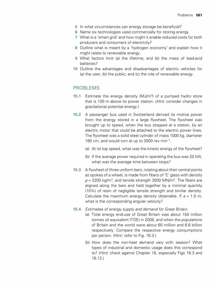
Problems 561
5 In what circumstances can energy storage be beneficial? 6 Name six technologies used commercially for storing energy. 7 What is a ‘smart grid’ and how might it enable reduced costs for both
producers and consumers of electricity? 8 Outline what is meant by a ‘hydrogen economy’ and explain how it
might relate to renewable energy. 9 What factors limit (a) the lifetime; and (b) the mass of lead-acid
batteries? 10 Outline the advantages and disadvantages of electric vehicles for
(a) the user; (b) the public; and (c) the role of renewable energy.
PROBLEMS
15.1 Estimate the energy density (MJ/m3) of a pumped hydro store that is 100 m above its power station. (Hint: consider changes in gravitational potential energy.)
15.2 A passenger bus used in Switzerland derived its motive power from the energy stored in a large flywheel. The flywheel was brought up to speed, when the bus stopped at a station, by an electric motor that could be attached to the electric power lines. The flywheel was a solid steel cylinder of mass 1000 kg, diameter 180 cm, and would turn at up to 3000 rev min–1.
(a) At its top speed, what was the kinetic energy of the flywheel?
(b) If the average power required in operating the bus was 20 kW, what was the average time between stops?
15.3 A flywheel of three uniform bars, rotating about their central points as spokes of a wheel, is made from fibers of ‘E’ glass with density r = 2200 kg/m3, and tensile strength 3500 MN/m2. The fibers are aligned along the bars and held together by a minimal quantity (10%) of resin of negligible tensile strength and similar density. Calculate the maximum energy density obtainable. If a = 1.0 m, what is the corresponding angular velocity?
15.4 Estimates of energy supply and demand for Great Britain.(a) Total energy end-use of Great Britain was about 150 million
tonnes oil equivalent (TOE) in 2008, and when the populations of Britain and the world were about 60 million and 6.6 billion respectively. Compare the respective energy consumptions per person. (Hint: refer to Fig. 16.3.)
(b) How does the non-heat demand vary with season? What types of industrial and domestic usage does this correspond to? (Hint: check against Chapter 16, especially Figs 16.3 and 16.12.)
TWIDELL PAGINATION.indb 561 01/12/2014 11:38
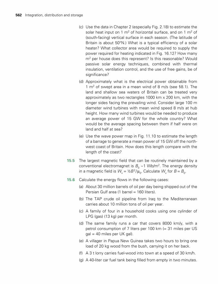
562 Integration, distribution and storage
(c) Use the data in Chapter 2 (especially Fig. 2.18) to estimate the solar heat input on 1 m2 of horizontal surface, and on 1 m2 of (south-facing) vertical surface in each season. (The latitude of Britain is about 50°N.) What is a typical efficiency of a solar heater? What collector area would be required to supply the power required for heating indicated in Fig. 16.12? How many m2 per house does this represent? Is this reasonable? Would passive solar energy techniques, combined with thermal insulation, ventilation control, and the use of free gains, be of significance?
(d) Approximately what is the electrical power obtainable from 1 m2 of swept area in a mean wind of 8 m/s (see §8.1). The land and shallow sea waters of Britain can be treated very approximately as two rectangles 1000 km x 200 km, with the longer sides facing the prevailing wind. Consider large 100 m diameter wind turbines with mean wind speed 8 m/s at hub height. How many wind turbines would be needed to produce an average power of 15 GW for the whole country? What would be the average spacing between them if half were on land and half at sea?
(e) Use the wave power map in Fig. 11.10 to estimate the length of a barrage to generate a mean power of 15 GW off the north-west coast of Britain. How does this length compare with the length of the coast?
15.5 The largest magnetic field that can be routinely maintained by a conventional electromagnet is B0 ~1 Wb/m2. The energy density in a magnetic field is Wv = ½B 2 / m0. Calculate Wv for B = B0.
15.6 Calculate the energy flows in the following cases:
(a) About 30 million barrels of oil per day being shipped out of the Persian Gulf area (1 barrel = 160 liters).
(b) The TAP crude oil pipeline from Iraq to the Mediterranean carries about 10 million tons of oil per year.
(c) A family of four in a household cooks using one cylinder of LPG (gas) (13 kg) per month.
(d) The same family runs a car that covers 8000 km/y, with a petrol consumption of 7 liters per 100 km (= 31 miles per US gal = 40 miles per UK gal).
(e) A villager in Papua New Guinea takes two hours to bring one load of 20 kg wood from the bush, carrying it on her back.
(f) A 3 t lorry carries fuel-wood into town at a speed of 30 km/h.
(g) A 40-liter car fuel tank being filled from empty in two minutes.
TWIDELL PAGINATION.indb 562 01/12/2014 11:38
Bibliography 563
15.7 A steel pipeline of diameter 30 cm carries methane gas (CH4). Recompression stations are sited at 100 km intervals along the pipeline. The gas pressure is boosted from 3 to 6 MN/m2 at each station. (These are typical commercial conditions.) Calculate (a) the mass flow; and (b) the energy flow. (c) What volume per day of gas at STP would this correspond to? (Hint: refer to (15.4) and Fig. R2.5 (in Review 2), then make a first estimate of f, assuming R is ‘high enough’. Then find m
. and check for consistency. Iterate if necessary. Viscosity of methane at these pressures is:
m = × − −10 10 N s m .6 2
15.8 An electrical transmission line links a 200 MW hydroelectric installation A to a city B 200 km away, at 220 kV. The cables are designed to dissipate 1% of the power carried. Calculate the dimensions of wire required, and explain why losses of 1% may be economically preferable to losses of 10% or 0.1%.
15.9 Considering a six pole-pair induction generator (§R1.6), if s = –0.1 at generation into a 50 Hz grid, determine the induced rotor current frequency f2 and fs.
15.10 The changes in enthalpy, free energy and entropy in the formation of water
H2 + ½O2 → H2O(gas)
are respectively
DH = –242 kJ/molDG = –228 kJ/molDS = –47 J K–1 mol–1
Estimate the temperature above which H2O is thermodynamically unstable. (Hint: consider (15.16)).
NOTE
1 UN International Trade Statistics (www.comtrade.un.org).
BIBLIOGRAPHY
General
Institution of Mechanical Engineers (2000) Renewable Energy Storage: Its role in renewables and future electricity markets, Professional Engineering Publications, Bury St. Edmunds. Set of conference papers, includ-ing short articles on ‘regenerative fuel cells’, flywheels and superconducting magnetic energy storage.
Jensen, J. and Sorensen, B. (1984) Energy Storage, Wiley, Chichester. Still one of the few books specifically on this topic. Good coverage at about the same level as this book.
TWIDELL PAGINATION.indb 563 01/12/2014 11:38

564 Integration, distribution and storage
Kreith, F. and Kreider, J.F. (2011) Principles of Sustainable Energy, CRC Press, London. Chapter 10 covers energy storage, with particular detail on compressed air systems.
Sims, R., Mercado, P., Krewitt, W., Bhuyan, G., Flynn, D., Holttinen, H., Jannuzzi, G., Khennas, S., Liu, Y., O’Malley, M., Nilsson, L.J.,Ogden, J., Ogimoto, K., Outhred, H., Ulleberg, O. and van Hulle, F. (2011) ‘Integration of renewable energy into present and future energy systems’, in O. Edenhofer, R. Pichs-Madruga, Y. Sokona, K. Seyboth, P. Matschoss, S. Kadner, T. Zwickel, P. Eickemeier, G. Hansen, S. Schlömer and C.von Stechow (eds), IPCC Special Report on Renewable Energy Sources and Climate Change Mitigation, Cambridge University Press, Cambridge. Reviews state of the art and future prospects, especially from an energy systems perspective.
US Electricity Storage Association. A trade association with much useful technical information on its website (www.electricitystorage.org/technology/storage_technologies/technology_comparison).
Most books on particular renewable energy sources (referred to in the appropriate chapters) include some dis-cussion of storage media applicable to that source (e.g. heat stores for solar, batteries for wind).
Chemical storage
Carden, P.O. (1977) ‘Energy corradiation using the reversible ammonia reaction’, Solar Energy, 19, 365–378. Sets out the main features of a solar/ammonia system using distributed collectors. Many later papers elaborate on details and similar systems
Dunn, R., Lovegrove, K. and Burgess, G. (2012) ‘A review of ammonia-based thermochemical energy storage for concentrating solar power’, IEEE Journal, 100, 391–400).
Goel, N., Miraball, S., Ingley, H.A. and Goswami, D.Y. (2003) ‘Hydrogen production’, Advances in Solar Energy, 15, 405–451. Emphasis on production by renewable energy; includes cost estimates.
National Research Council [USA] (2004) The Hydrogen Economy: Opportunities, costs barriers and R&D needs, National Academies Press, New York. Available online at nap.edu.
Wald, M.L. (2004) ‘Questions about a hydrogen economy’, Scientific American, 290, 42–48. Looks at ‘wells to wheels’ energy analysis.
Any of the many textbooks on physical chemistry will give a thermodynamic analysis of the heat release in chemical reactions (e.g. Atkins, P.W. and de Paul, J. (2002) Atkins’ Physical Chemistry, Oxford University Press, Oxford).
Heat storage
Duffie, J.A. and Beckman, W.A. (2006, 3rd edn) Solar Engineering of Thermal Processes, Wiley, New York. Chapter 9 is specifically concerned with heat storage.
Ryle, M. (1977) ‘Economics of alternative energy sources’, Nature, 267, 111–116. Classic paper, cogently arguing that storage for about seven days enables wind/wave/solar to match most fluctuations in UK demand.
Electrical storage
Any of the many textbooks on physical chemistry will give an introduction to the elementary electrochemistry used in this chapter (e.g. Atkins, P.W. and de Paul, J. (2002) Atkins’ Physical Chemistry, Oxford University Press, Oxford).
TWIDELL PAGINATION.indb 564 01/12/2014 11:38

Bibliography 565
Crompton, T.R. (2000. 3rd edn) Battery Reference Book, Newnes, Oxford.
Electropaedia (www.mpoweruk.com/index.htm). A useful source of basic technical information about batteries of all types, compiled by Woodbank Communications.
ITDG (2004) Batteries, ITDG technical brief. Available online at www.itdg.org. Very down-to-earth guide on how to use and look after batteries.
Lindsay, T.J. (1999) Secrets of Lead Acid Batteries, Lindsay Publications Inc., Il 60915, USA. Forty-eight pages of practical explanations and guidance that is hard to find elsewhere.
Rand, D.A.J., Woods, R. and Dell, R.M. (1998) Batteries for Electric Vehicles, Society of Automotive Engineers, Pennsylvania. Covers all types of storage batteries.
Yuan, X., Liu, H. and Zhang, J. (eds) (2012) Lithium-ion Batteries: Advanced materials and technologies, CRC Press, London. Multi-author compilation with detailed analysis of materials and technical challenges for anodes, cathodes, electrolytes, etc.
Fuel cells
Alleau, T. (2003) ‘A state of the art of hydrogen and fuel cell technologies: diffusion perspectives and barriers’, in A. Avadikyan, P. Cohendet and J-A. Heraud (eds), The Economic Dynamics of Fuel Cell Technologies, Springer, Berlin.
Hoogers, G. (ed.) (2003) Fuel Cell Technology Handbook, CRC Press, London. Review of technology and its appli-cations in power systems and vehicles.
Srinivasan, S. (2006) Fuel Cells: From fundamentals to applications, Springer, Berlin. Comprehensive textbook of >600pages.
Flywheels
Genta, G. (1985) Kinetic Energy Storage: Theory and practice of advanced flywheel systems, Butterworths, London. Book-length detail.
Distribution and transmission and social aspects
Boyle, G. (ed.) (2007) Renewable Energy and the Grid, Earthscan, London.
BP Statistical Review of World Energy (annual). Data and maps showing production, consumption and trade, especially in fossil fuels.
El-Sharkawi, M.A. (2012, 3rd edn) Electric Energy: An introduction, CRC Press, London. Engineering textbook covering both electric machines and power distribution systems.
Freris, L. and Infield, D. (2008) Renewable Energy in Power Systems, Wiley, Chichester. Usual power systems mechanics, but with special emphasis on RE.
Galan, E.M. et al. (2012) ‘Rural renewable energy’, Chapter 5 in REN21 (2012) Global Status Report 2012. Available online at www.ren21.org.
McNeill, J.R. (2000) Something New Under the Sun: An environmental history of the twentieth century, Penguin, London. The growth of fossil fuel-fired cities and their impacts on water, air and the biosphere.
TWIDELL PAGINATION.indb 565 01/12/2014 11:38

566 Integration, distribution and storage
Nuttall, P. et al. (2013) ‘A review of sustainable sea-transport for Oceania: providing context for renewable energy shipping for the Pacific’, Marine Policy, http://dx.doi.org/10.1016/j.marpol.2013.06.009i.
Yergin, D. (1992) The Prize: The epic quest for oil money and power, Simon & Schuster, New York. This book won the Pulitzer Prize for non- fiction in 1992 for its authoritative reporting and comment on the oil industry.
TWIDELL PAGINATION.indb 566 01/12/2014 11:38
Using energy efficiently
CHAPTER
16
CONTENTS
Learning aims 568
§16.1 Introduction 569
§16.2 Energy services 571
§16.3 Energy end-use by sector 574
§16.4 Energy-efficient (solar) buildings 576§16.4.1 General concepts 576§16.4.2 Space heating: principles 576§16.4.3 Passive solar buildings 578§16.4.4 Active solar building
systems 581§16.4.5 Cold climates 582§16.4.6 Temperate climates 584§16.4.7 Hot, dry climate 587§16.4.8 Warm, humid tropical
climate 589§16.4.9 Composite climates 591
§16.5 Transport 591§16.5.1 Background 591§16.5.2 Vehicles 591§16.5.3 An unsustainable transport
system? 593§16.5.4 Transport and urban form 593§16.5.5 Improved vehicles 596§16.5.6 Freight transport 598§16.5.7 Aviation 599
§16.6 Manufacturing industry 599
§16.7 Domestic energy use 601
§16.8 Social and environmental aspects 602§16.8.1 Negawatts are cheaper than
megawatts! 602§16.8.2 Impact on renewable energy 603
§16.8.3 Paths of economic development 603
§16.8.4 Buildings 604§16.8.5 Environmental implications of
energy efficiency 604
Chapter summary 605
Quick questions 606
Problems 606
Notes 608
Bibliography 608
Box 16.1 Maximum efficiency of heat engines 573
Box 16.2 The impact of technology change in lighting in England, 1500–2000 573
Box 16.3 Summary of RE applications in selected end-use sectors 575
Box 16.4 Building codes 578
Box 16.5 The Solar Decathlon 586
Box 16.6 Electrochromic windows 589
Box 16.7 Curitiba: a case study of urban design for sustainability and reduced energy demand 595
Box 16.8 Proper sizing of pipes and pumps saves energy 600
Box 16.9 Energy use in China 604
TWIDELL PAGINATION.indb 567 01/12/2014 11:38
568 Using energy efficiently
LEARNING AIMS
• Appreciate that energy systems include both end-uses (demand) and generation (supply).
• Realize that consumers want energy services, not energy as such.
• Define and quantify end-use efficiency and overall (system) efficiency.
• Realize that efficient use of energy improves consumer satisfaction.
• Understand why energy efficiency and renew-able energy are complementary.
• Appreciate that greenhouse gas emissions are thereby reduced.
• Examine examples of how solar energy, insula-tion, advanced materials and other aspects of building design give energy-efficient and com-fortable living in both hot and cold climates.
• Consider how the economy benefits from energy efficiency in the sectors of transport, energy supply and buildings.
• Consider the social and environmental issues for implementing energy efficiency.
LIST OF FIGURES
16.1 Energy flow from source to end–use service. 57016.2 Progression of lighting services in England during the period from 1500 to 2000, indicating
dominant lighting technology. 57416.3 (a) World primary energy use by end-use sector. (b) Energy demand by service. 57516.4 Direct gain passive solar heating. 57916.5 Buildings suitable for a cold climate. 58316.6 Four buildings suitable for a temperate climate. 58516.7 Hot, dry climate zone. 58816.8 Warm, humid zone. 59016.9 Liquid fuel use by sector 2008 to 2035 (million barrels oil/day). 59216.10 Transport energy use per capita in a range of cities. 59416.11 One of the bus stops in the integrated transport system used by 85% of the population of the
Brazilian city of Curitiba. 59616.12 Energy savings in UK residences. 60116.13 Heat loss through a window. 607
LIST OF TABLES
16.1 Possible performance of some future ‘advanced’ motor cars 597
TWIDELL PAGINATION.indb 568 01/12/2014 11:38
§16.1 Introduction 569
§16.1 INTRODUCTION
Motivation for this chapter in a book about renewable energy is that improved efficiency of energy use and thus less energy demand increases opportunities for renewable energy systems. This presents opportunities to reduce the use of fossil fuels and shift to clean sustainable systems – a double opportunity for greenhouse gas reduction.
Energy supply is costly, requiring infrastructure (e.g. transportation, electricity grids, maintenance) and equipment to convert the primary energy to a usable form. Therefore reducing energy demand without loss of benefit reduces ongoing costs for the consumer. For example, the capacity, and hence the cost, of photovoltaic panels and ancillary equipment for daytime internal lighting depend on the control of the required illumination and the efficiency of the lights; better control and efficiency require less capacity and hence less PV capital cost. For the energy supplier, less demand means less capital expenditure on plant capacity and the opportunity to integrate renewable energy sources. However, the supplier’s income from consumer bills reduces unless per unit charges are increased, so governmental regulation is needed for a fair and energy-efficient system.
One general principle is that we do not require energy as such, but the energy services provided, such as lighting, heating, communication and transport. These services are also called end-uses.
In supplying energy for a service, the primary energy is, for example, the chemical energy content of fuel or the energy from solar radiation onto a photovoltaic device. There are many conversion and supply steps along the way, as indicated in Fig. 16.1. The whole process and each of the intermediate conversion stages in Fig. 16.1 have an energy efficiency defined generally by:
η =energy outputenergy input
(16.1)
There are always some losses in any energy conversion, so η ≤ 1. Since the output of one stage is the input to the next, it follows that the effi-ciency in going from, for example, stage 1 to stage 3 is:
η13 = η12 η23 (16.2)
and so on. In particular, we can calculate an overall system energy effi-ciency of:
ηpu = Eu / Ep (16.3)
where Ep is the primary energy utilized in providing the service and Eu is the energy delivered by the end-use for a service.
In practice, the efficiency of all such stages can be improved (e.g. improved turbine generators, vehicles that are more fuel efficient, better
TWIDELL PAGINATION.indb 569 01/12/2014 11:38
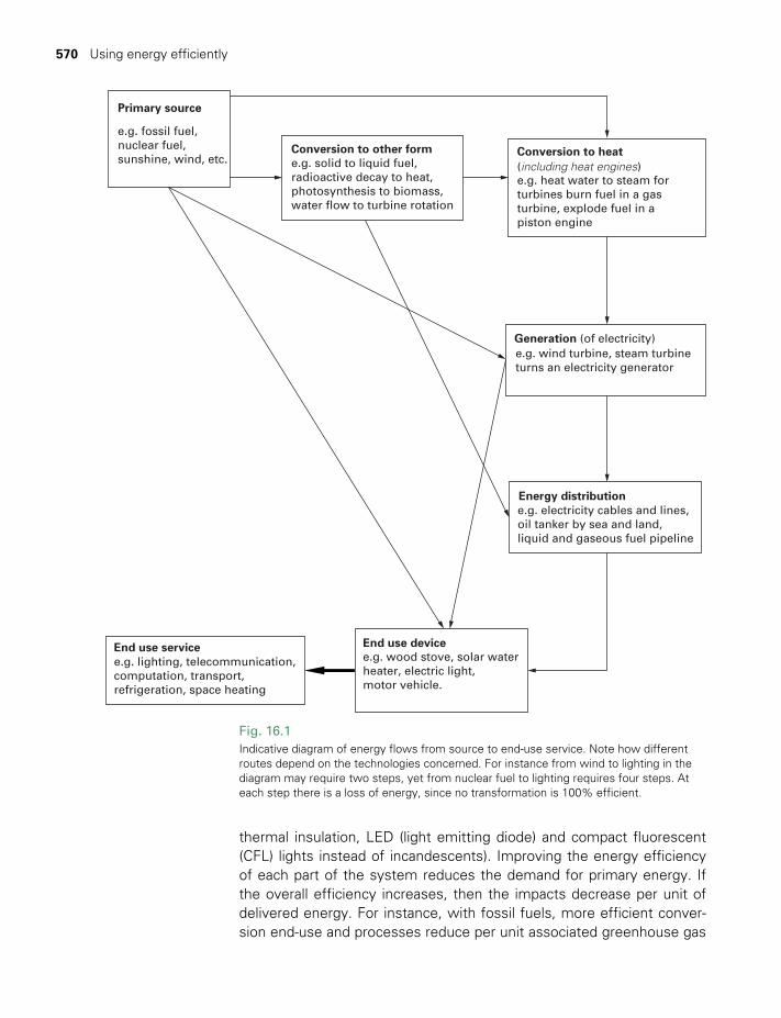
570 Using energy efficiently
thermal insulation, LED (light emitting diode) and compact fluorescent (CFL) lights instead of incandescents). Improving the energy efficiency of each part of the system reduces the demand for primary energy. If the overall efficiency increases, then the impacts decrease per unit of delivered energy. For instance, with fossil fuels, more efficient conver-sion end-use and processes reduce per unit associated greenhouse gas
Fig. 16.1Indicative diagram of energy flows from source to end-use service. Note how different routes depend on the technologies concerned. For instance from wind to lighting in the diagram may require two steps, yet from nuclear fuel to lighting requires four steps. At each step there is a loss of energy, since no transformation is 100% efficient.
Primary source
e.g. fossil fuel,nuclear fuel,sunshine, wind, etc.
Conversion to other forme.g. solid to liquid fuel,radioactive decay to heat,photosynthesis to biomass,water flow to turbine rotation
Conversion to heat (including heat engines) e.g. heat water to steam forturbines burn fuel in a gasturbine, explode fuel in apiston engine
Generation (of electricity) e.g. wind turbine, steam turbineturns an electricity generator
Energy distribution e.g. electricity cables and lines,oil tanker by sea and land,liquid and gaseous fuel pipeline
End use service e.g. lighting, telecommunication,computation, transport,refrigeration, space heating
End use device e.g. wood stove, solar waterheater, electric light,motor vehicle.
TWIDELL PAGINATION.indb 570 01/12/2014 11:38
§16.2 Energy services 571
emissions and thus incrementally the risk of global climate change (see Box 17.1). With wind turbines (Chapter 8) per unit of delivered electricity, the greater their turbine and system efficiencies, the less the number of turbines, their impact, and the capital and operational costs (see §17.6).
Every energy supply we use has environmental impact and costs money. Therefore using energy more efficiently requires less for the same benefit, so reducing impact and saving on the recurrent and capital cost of the service. Moreover, using less energy for the same benefit increases energy security for individuals and for their nation (see §17.2).
It is vital therefore that we manage the efficient use of energy. This necessity applies to all forms of energy supply; however, the manner of application may differ according to the type of supply; for example:.
• Nuclear reactors in practice produce a constant supply of heat and hence of electricity, so integration with other controllable supplies and energy storage is essential.
• Renewable energy supplies vary significantly according to the environ-mental source; consequently their output requires matching loads or integration with other supplies and energy storage (Chapter 15).
• Fossil fuels produce atmospheric and water pollution; using less more efficiently is therefore vital.
In practice, most users do not know the primary source of their energy so leaving the management of their demand to the government regulators and suppliers (e.g. the price of fuel, the tariff prices for electricity, obliga-tions on suppliers to provide a mix of supplies, energy efficiency cam-paigns, building codes and standards, banning inefficient products (e.g. incandescent electric lamps), reduced taxes and/or grants for energy effi-ciency products (e.g. thermal insulation, solar water heaters; see §17.5). However, individual consumers can and should still take seriously their responsibility for their energy use (see §17.2.3).
This book is primarily about renewable energy, so in this chapter we pay particular attention to energy use in buildings (§16.4) where savings in purchased energy may come from passive solar structures and micro-generation. Subsequent sections outline the potential for energy savings in transport (§16.5) and industry (§16.6), as these sectors account for more than half of total energy use worldwide. §16.7 focuses on the residential sector (i.e. energy used in houses), particularly on electrical appliances, as subjects most open to action by individuals. The chapter concludes with a brief examination of the social issues, benefits and costs of energy efficiency (§16.8).
§16.2 ENERGY SERVICES
It is the service function from energy that matters, not the energy itself. We need heating, lighting, delivery of goods, movement of people,
TWIDELL PAGINATION.indb 571 01/12/2014 11:38
572 Using energy efficiently
communication of information and many other such benefits. Fig. 16.1 gives examples of the multi-step process as primary energy is converted into a service, usually via intermediate conversion (e.g. to electricity, to shaft power of an engine) and by energy ‘vectors’ (e.g. via heating pipes, electricity distribution networks, gas pipelines). The figure shows impor-tant terminology, such as ‘conversion’, ‘generation’ and ‘distribution’.
The thermodynamic limitations of thermal conversion by heat engines are particularly important, as with vehicle combustion engines and with power station turbines for electricity generation. Carnot theory explains that only a fraction of input heat energy can be transformed into mechan-ical work output, with the remainder emitted to the environment as lower temperature heat (see Box 16.1). The practical consequence is that whenever heat is converted to work, as in engines and turbines, the mechanical efficiency is at best about 45% (high-temperature gas turbine), often about 35% (coal, nuclear power stations) and commonly less (biomass combustion and geothermal power stations, most vehicle engines). The largest energy output is therefore not useful work (e.g. as shaft power for electricity generators) but the waste heat in the exhaust or cooling tower! Of course, if the output heat can itself be used benefi-cially (e.g. for local district heating), it is no longer waste and the overall efficiency should be improved considerably.
Direct energy conversions from solar PV, hydro, ocean, and wind energy to work and electricity do not have the thermodynamic limitations of heat engines. However, they experience other conversion inefficien-cies in extracting energy from natural energy flows, as explained in the relevant subject chapters.
Note that most specific energy services may be provided in alternative ways, e.g. lighting from direct daylight through windows and via sun-pipes through roofs to rooms, from candles and oil lamps, and, mostly, from electric lights of many types; transport by walking, cycling, and by electric and combustion-engine vehicles. The efficiencies of the multiple energy conversions and individual devices vary greatly; likewise their impacts. Lighting is an excellent example of a steady progression in technological improvement and widening application. Box 16.2 gives an example.
Energy savings arise from changing the activities that require energy inputs, for example, turning off lights when not needed, walking instead of using a car, changing the controls for heating or air conditioning to avoid excessive heating or cooling, or eliminating a particular appliance and performing a task in a less energy-intensive manner. Energy savings can be realized by technical, organizational, institutional, structural and behavioral changes.
Increasing the efficiency of energy services can reduce the primary energy required from all forms of energy supply. However, this may be particularly important for renewables if the available supply is limited (e.g. household micro-generation from solar photovoltaic modules may
TWIDELL PAGINATION.indb 572 01/12/2014 11:38
§16.2 Energy services 573
BOX 16.2 THE IMPACT OF TECHNOLOGY CHANGE IN LIGHTING IN ENGLAND, 1500–2000
In a seminal work of economic history, Fouquet (2008) analyzed transitions between energy technologies. He tracked energy services in England over the 500 years from 1500 to 2000, and examined the main technologies and primary energy sources used. He analyzed prices (in real terms, i.e. adjusted for inflation), efficiencies and how socio-economic changes affected the use of such services. He did this separately for heating, lighting, mechanical power and transport; we summarize here his findings for lighting. Candles made from tallow (animal fat) were the dominant technology for lighting at night and remained essentially unchanged for centuries (Fig. 16.2). A tax on candles in 1820 prompted candle-makers to use technological improvements (e.g. plaited wicks) for improved efficiency so that users had more light from the more expensive product. Lighting from producer-gas (carbon monoxide and hydrogen mostly from coal, but also biomass) was introduced at about that time, but was expensive and did not come into
BOX 16.1 MAXIMUM EFFICIENCY OF HEAT ENGINES
A heat engine is a device that converts heat into work by a cyclic process. The efficiency of the engine is given by (16.1), with the input energy being the energy content of the fuel used, and the output energy the mechanical power output of the engine.
The theoretical maximum efficiency of a heat engine is shown in textbooks on thermodynamics to be that of a Carnot engine, which is:
T T T( ) /h hCarnot cη = − (16.4)
where Th and Tc are respectively the maximum and minimum temperatures of the working fluid during its cycle. (Note that the working fluid in a gasoline or diesel engine is the air/fuel mixture in the cylinder.)
The full thermodynamic arguments justifying such theory are given in the textbooks and acceptable websites referenced at the end of this chapter. Carnot theory is of immense conceptual value for heat engines (e.g. heat cannot be converted entirely to work and the hotter the input, the more efficient the engine), but this ‘simple’ theory has intrinsic quantitative limitations. For instance, the theory requires rever sible changes with zero friction and of infinite time; both are totally unrealistic in practice. Maximum power theorems tackle such issues, but are beyond the remit of this book. See Chen et al. (1999) for more detail.
In practice, the efficiency for real engines is always less than half of ηCarnot, i.e. between about 35% and 50% efficient from fuel to shaft power for internal combustion engines, with the remaining energy being emitted as heat of no value in a vehicle, other than for comfort heating in cold conditions. Diesel compression engines operate at higher temperatures than spark-ignition engines; therefore their intrinsic efficiency is greater. However, the latest spark-ignition engines with fuel injection, etc. may be as fuel efficient as diesel engines.
benefit from controlled switching of electrical end-use devices). Likewise biofuel supply is inadequate now to power all present-day vehicles, but if all vehicles had the fuel efficiency of the best demonstration models, a much larger fraction could run on biofuels. Electricity distribution and management is simplified and system-balancing costs are lower if the energy demands become smaller (Synapse 2008). The importance of end-use efficiency in buildings for renewable technology optimization is considered in §16.4.
TWIDELL PAGINATION.indb 573 01/12/2014 11:38
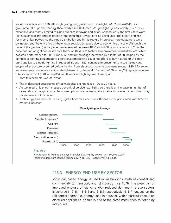
574 Using energy efficiently
wider use until about 1850. Although gas lighting gave much more light (~0.07 lumen / W)1 for a given amount of primary energy than candles (~0.03 lumen / W), gas lighting was initially much more expensive and mostly limited to piped supplies in towns and cities. Consequently the first users were rich households and large factories of the Industrial Revolution also using coal-fired steam-engines for mechanical power. As the piped distribution and infrastructure improved, more customers were connected and the unit price of the energy supply decreased due to economies of scale. Although the price of the gas fuel (primary energy) decreased between 1850 and 1900 by only a factor of 2, (a) the price per unit of light decreased by a factor of 10, due to technical improvement in mantles, etc. which boosted performance to ~0.5 lumen / W; and (b) the usage increased by a factor of 50 (helped by the companies renting equipment to poorer customers who could not afford to buy it outright). A similar story applies to electric lighting introduced around 1880; continual improvements in technology and supply infrastructure occurred before lighting from electricity became dominant around 1920. Moreover, improvements continue as solid-state light-emitting diodes (LEDs, with ~100 lumen/W) replace vacuum-tube incandescent (~10 lumen / W) and fluorescent lighting (~40 lumen / W).
From this example, we learn that:
• The widespread acceptance of technological change takes ~20 to 30 years.• As technical efficiency increases per unit of service (e.g. light), so there is an increase in number of
users; thus although a particular consumption may decrease, the total national energy consumed may not decrease but increase.
• Technology and manufacture (e.g. lights) become ever more efficient and sophisticated with time as markets increase.
Fig. 16.2Progression of lighting services in England during the period from 1500 to 2000, indicating dominant lighting technology. N.B. LED – Light Emitting Diode.
Main lighting technology
1500 1700 18001600 1900 2000
Candles (tallow)
Candles (improved)
Gaslight
Kerosene
Electric (filament)
Electric (fluorescent)
Electric (LED)
§16.3 ENERGY END-USE BY SECTOR
Most purchased energy is used in (a) buildings (both residential and commercial), (b) transport, and (c) industry (Fig. 16.3). The potential for improved end-use efficiency and/or reduced demand in these sectors is covered in §16.4, §16.5 and §16.6 respectively. §16.7 focuses on the residential sector (i.e. energy used in houses), with a particular focus on electrical appliances, as this is one of the areas most open to action by individuals.
TWIDELL PAGINATION.indb 574 01/12/2014 11:38

§16.3 Energy end-use by sector 575
Fig. 16.3a World primary energy use by end-use sector. These data are for 2008 (total = 531 EJ)
but the percentages change only slowly over time. Note the large proportion lost in generation and distribution of electricity.
b Energy demand by service. These data are for the UK in 2010, but the percentages are similar for most countries in temperate climates and change only slowly over time.
Source: Data for (a) from US-EIA International Energy Outlook 2011; data for (b) from UK Department of Energy and Climate Change, Energy Consumption in the UK (2012 update).
Commercial6%
Industrial38%
Residential10%
Transport19%
Electricity losses27%
(a)
Space heat23%
Other heat 14%
Lighting6%
Transport29%
Other28%
(b) UK energy demand by service (2010)
BOX 16.3 SUMMARY OF RE APPLICATIONS IN SELECTED END-USE SECTORS
Buildings (including residential)
Micro-generation of electricity by photovoltaics (§5.3.2). Solar water heating (Chapter 3). Passive solar design (for space heating and cooling) (§16.4). Active solar space heating (§16.4). Active solar cooling (§4.4). Biomass for cooking and space heating (§10.3).
Transport
Liquid biofuels (for vehicles) (§10.6.2, §10.9). Electric vehicles (§15.11) and batteries (§15.7). Hydrogen-fueled vehicles (if H2 produced by RE) (§15.11).
Industry
Hydroelectricity for aluminum smelting (Chapter 6).Mixed fuels Industries combusting coal are able to incorporate biomass for ‘co-firing’ within the raw fuel mix
without great difficulty, yet with important adjustments to air flow and combustion control (§10.3). Similarly, biogas (§10.7) can be mixed into piped supplies of ‘natural gas’ and liquid biofuels mixed with petroleum fuels, especially as diesel fuel (§10.9).
The potential deployment of renewable energy supplies in each of these sectors is summarized in Box 16.3, including references to more detail in the technology chapters of this book.
TWIDELL PAGINATION.indb 575 01/12/2014 11:38

576 Using energy efficiently
§16.4 ENERGY-EFFICIENT (SOLAR) BUILDINGS
§16.4.1 General concepts
Keeping buildings warm in winter, and cool in summer, accounts for about one-quarter of the energy requirements of many countries (e.g. the UK: Fig.16.3(b)). Therefore designing and adapting buildings to utilize solar energy reduces recurrent costs and abates significant amounts of fossil fuel, and also usually improves comfort and well-being. This section considers the design and construction of energy-efficient, solar-friendly, comfortable and cost-effective buildings that should be an essen-tial aspect of modern architecture. Best results require an integrated approach, optimizing (a) solar energy inputs for heat and solar shading for cooling; (b) the thermal mass and insulation; (c) the internal heat gains in the building from the appliances and metabolic heat of the occu-pants; (d) other renewable sources if needed and available (e.g. biomass heating); and (e) aspects of control, both active and passive. Moreover, the building should be visually attractive, comfortable and stimulating to live in. Careful site-specific energy design requires creative and innova-tive architecture, which usually leads to stimulating design.
Thermal comfort in different climatic conditions requires these princi-ples to be applied in different ways, depending on whether the dominant need is for heating or cooling, and also on the prevailing humidity. We look first at the requirements for space heating, since that is the largest energy use for buildings, not least because most of the richer countries of the world enjoy a ‘temperate’ climate in which occupant overheat-ing is rarely an issue. Successive later subsections look at examples of energy-efficient buildings for cold climates, temperate climates, hot, dry climates and warm, humid climates.
Although this chapter focuses on direct energy use, the sustainability parameters for buildings are not just the energy use of the occupants. For instance, the embodied energy sequestered in the manufacture of the building components and in construction is important (see discus-sions of sustainable development in Chapter 1 and of ‘life-cycle costing’ in Chapter 17). Likewise, electricity and heat micro-generation at the site should be considered (e.g. by photovoltaic arrays on the walls or roof: see e.g. Fig. 5.8, Fig. 16.6(d) and by small wind turbines: e.g. §8.8.6) as a step towards making the building self-sufficient (i.e. not depleting outside resources) and indeed an energy supplier via local grids.
§16.4.2 Space heating: principles
A major use of energy is to heat buildings in cold periods, which certainly usually include winter but may also include cold evenings in otherwise warm periods. Comfort depends on air temperature, humidity, received
TWIDELL PAGINATION.indb 576 01/12/2014 11:38
§16.4 Energy-efficient (solar) buildings 577
radiation flux, speed of moving air, clothing, and each person’s activity, metabolism and lifestyle. Consequently, inside (room) temperature Tr may be considered comfortable in the range of about 15°C to 25°C. The internal built environment should be at such a ‘comfort temperature’ while using the minimum artificial heating or cooling (Pboost), even when the external (ambient) temperature Ta is well outside the comfort range. The heat balance of the inside of a building with solar input is described by equations similar to (3.1). The simplest formulation considers solar gain and lumped parameters of mass m, specific heat capacity c and whole fabric thermal resistance R (unit: W/K), as in Review 3 (Box R3.1). Note that here R is not the ‘R-value’ (unit: m2K/W) used in the building trade (see Box R3.1).
Since energy is conserved:
mcTt
GA PT T
Rdd
( )r arboostτa= + −
− (16.5)
Detailed mathematical modeling of a building is most complex and is undertaken with specialist software packages. Nevertheless (16.5), con-tains the basis of all such modeling, namely energy fluxes and heat capacities.
The best results are achieved by allowing for energy considerations at the design and construction stage. These include the following:
• Suitable orientation of the building (with windows, conservatories and other glazed spaces facing the Equator to catch the sunshine in winter but with shades to mitigate unwanted vertical solar input in summer). Incorporation of such site-specific features also makes the buildings architecturally interesting (see e.g. Fig. 16.6).
• Optimum glazing and window construction (double-glazing or better in colder climates with cold winters).
• Considering ground temperature (which remains nearly constant throughout the year at depths of about 2 m) and the need for ample underfloor insulation, which is cheap.
• External insulation and large interior thermal mass, which provide energy storage and avoid daily temperature variation, yet may limit room size at some sites.
• Above-ceiling insulation, which is cheap but may limit loft space.• Roof outer surface, which may include grass roofs, solar electric (PV)
and solar thermal (water heating) panels, and reflective surfaces.• Rain water catchment (water supply is otherwise energy intensive
and expensive).• Internal daylight by windows and sun-pipes.• Airtightness, yet ventilation; forced extract ventilation from kitchens,
bathrooms, showers, toilets, etc.• Calculation, probably with specialist software, of the thermal and
TWIDELL PAGINATION.indb 577 01/12/2014 11:38

578 Using energy efficiently
daylight characteristics, and including ‘free energy gains’ from cooking, powered devices and metabolism.
• Opportunities for on-site micro-generation of electricity and heat.
Governments provide guidance on energy features required, notably minimum levels of insulation, by means of building codes, and regula-tions to enforce compliance with them (see Box 16.4 for an example).
BOX 16.4 BUILDING CODES
The UK has codes 1 to 6 (best) for buildings. Below is the code 6 summary which in practice can only be met with new buildings.
UK Code Level 6 standard for buildings
The home must be completely zero carbon (i.e. zero net emissions of CO2 from all energy use in the home) as achieved by all or some of the following measures:
• Using low and zero carbon technologies such as solar thermal panels, photovoltaic micro-generation, biomass boilers, wind turbines, and combined heat and power systems (CHP).
• Improving the thermal efficiency of the walls, windows and roof.• Reducing air permeability to the minimum consistent with health requirements.• Installing a high-efficiency condensing boiler for heat, or being on a district heating system.• Carefully designing the fabric of the home to reduce thermal bridging (e.g. at roof edges, corners of
walls).• Use no more than about 80 liters of water per person per day, including about 30% for non-potable
water from rain water harvesting and/or gray water recycling systems.• Materials – low resource impact.• Maximum, accessible provision for recycling domestic food and material wastes.• Energy-efficient appliances and lighting.• Improved daylighting, sound insulation and security.• Assessing and minimizing the ecological impact of construction.
Passivhaus standard for buildings with ultra-low energy use
Passivhaus is a rigorous voluntary standard for energy efficiency in a building, reducing its ecological footprint. It results in ultra-low energy buildings that require little energy for space heating or cooling. More than 10,000 such buildings have been constructed in Germany and Scandinavia. Passivhaus standards emphasize superinsulation, triple-glazed advanced-technology windows with specialist coatings and filling, solar gain from carefully orientated glazing, ventilation heat recovery from ‘free’ heat gains (e.g. from electric lights and devices, and from cooking), airtightness, and many other factors of integrated design and excellent building skills.
See www.planningportal.gov.uk/uploads/code_for_sust_homes.pdf.See http://en.wikipedia.org/wiki/Passive_house.
§16.4.3 Passive solar buildings
Passive solar design in all climates consists of arranging the lumped building mass m, the sun-facing area A and the loss resistance R of (16.5) to achieve optimum solar benefit by structural design. The first step is
TWIDELL PAGINATION.indb 578 01/12/2014 11:38

§16.4 Energy-efficient (solar) buildings 579
to insulate the building thoroughly (large R: insulation is cheap), includ-ing draught prevention and, if necessary, controlled ventilation with heat recovery. The orientation, size and position of windows and conservato-ries should allow a sufficient product of GA (perpendicular to the glazing) for significant passive solar heating in winter, with active and passive shading preventing overheating in summer. The windows themselves should have advanced, multi-surface construction so their resistance to heat transfer, other than incoming shortwave solar radiation, is large.
For passive solar buildings at higher latitudes, solar heat gain in winter is possible because the insolation on vertical sun-facing glazing and walls is significantly more than on horizontal surfaces: see Fig. 2.18. The sun-facing internal mass surfaces should have a dark color with a > 0.8 (Fig. 16.4(a)) and the building should be designed to have a large mass of interior walls and floors (large m) for heat storage within the insulation, thereby limiting the variations in Tr. Overheating may be prevented by fitting external shades and shutters, which also provide extra thermal insulation at night. Constructing a glazed conservatory on the sun-facing sides of a building enables solar heat to be captured; the adjoining mass of the building therefore gives benefits for heating if there is controlled air flow (e.g. through doors). However, such glazed spaces oscillate in temperature rapidly with and without sunshine, so active or passive ven-tilation control is essential. Conservatories should be used when their conditions are comfortable, and not used otherwise; it is poor practice to install heaters or coolers in conservatories.
Worked Example 16.1 illustrates that most of the heating load of a well-designed house can be from solar energy, but the design of practi-cal passive solar systems is more difficult than the example suggests. A more recent and much more sophisticated house (the ‘Meridian First Light House’) for similar conditions is shown in Fig.16.6(b). For example,
Fig. 16.4Direct gain passive solar heating: note the orientation and massive dark-colored surfaces to absorb and store the insolation. Note the importance of building orientation and use of massive, dark-colored, rear-insulated surfaces to absorb and to store the radiation.a basic system; b clerestory window (to give direct gain on the back wall of the house).
(a) (b)
TWIDELL PAGINATION.indb 579 01/12/2014 11:38
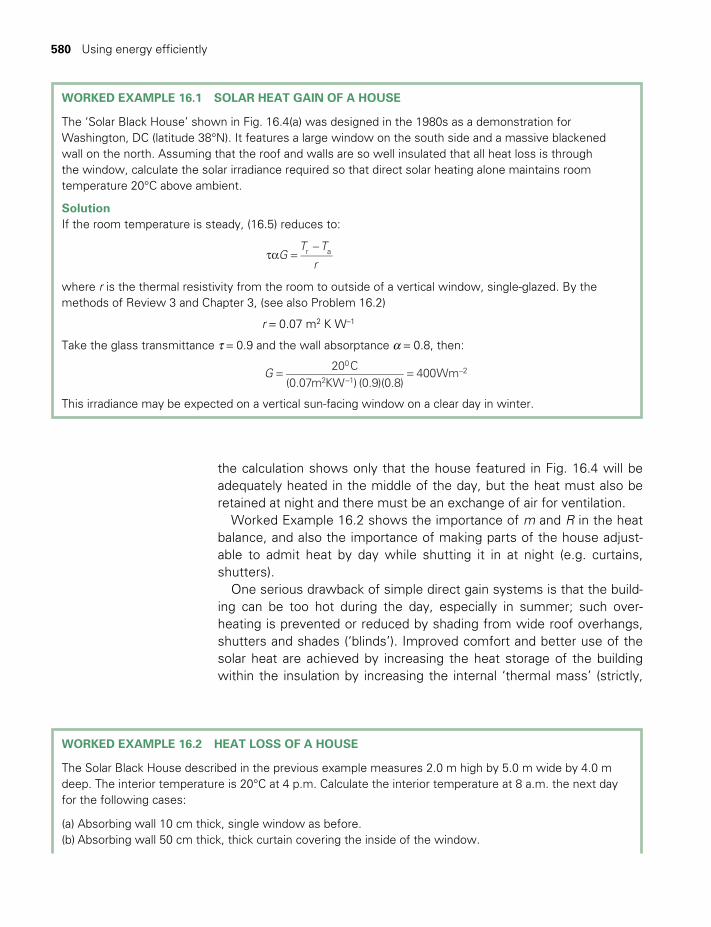
580 Using energy efficiently
WORKED EXAMPLE 16.1 SOLAR HEAT GAIN OF A HOUSE
The ‘Solar Black House’ shown in Fig. 16.4(a) was designed in the 1980s as a demonstration for Washington, DC (latitude 38°N). It features a large window on the south side and a massive blackened wall on the north. Assuming that the roof and walls are so well insulated that all heat loss is through the window, calculate the solar irradiance required so that direct solar heating alone maintains room temperature 20°C above ambient.
SolutionIf the room temperature is steady, (16.5) reduces to:
GT T
rr aτa =
−
where r is the thermal resistivity from the room to outside of a vertical window, single-glazed. By the methods of Review 3 and Chapter 3, (see also Problem 16.2)
r = 0.07 m2 K W–1
Take the glass transmittance τ = 0.9 and the wall absorptance a = 0.8, then:
G20 C
(0.07m KW ) (0.9)(0.8)400Wm
0
2 12= =
−−
This irradiance may be expected on a vertical sun-facing window on a clear day in winter.
WORKED EXAMPLE 16.2 HEAT LOSS OF A HOUSE
The Solar Black House described in the previous example measures 2.0 m high by 5.0 m wide by 4.0 m deep. The interior temperature is 20°C at 4 p.m. Calculate the interior temperature at 8 a.m. the next day for the following cases:
(a) Absorbing wall 10 cm thick, single window as before.(b) Absorbing wall 50 cm thick, thick curtain covering the inside of the window.
the calculation shows only that the house featured in Fig. 16.4 will be adequately heated in the middle of the day, but the heat must also be retained at night and there must be an exchange of air for ventilation.
Worked Example 16.2 shows the importance of m and R in the heat balance, and also the importance of making parts of the house adjust-able to admit heat by day while shutting it in at night (e.g. curtains, shutters).
One serious drawback of simple direct gain systems is that the build-ing can be too hot during the day, especially in summer; such over-heating is prevented or reduced by shading from wide roof overhangs, shutters and shades (‘blinds’). Improved comfort and better use of the solar heat are achieved by increasing the heat storage of the building within the insulation by increasing the internal ‘thermal mass’ (strictly,
TWIDELL PAGINATION.indb 580 01/12/2014 11:38
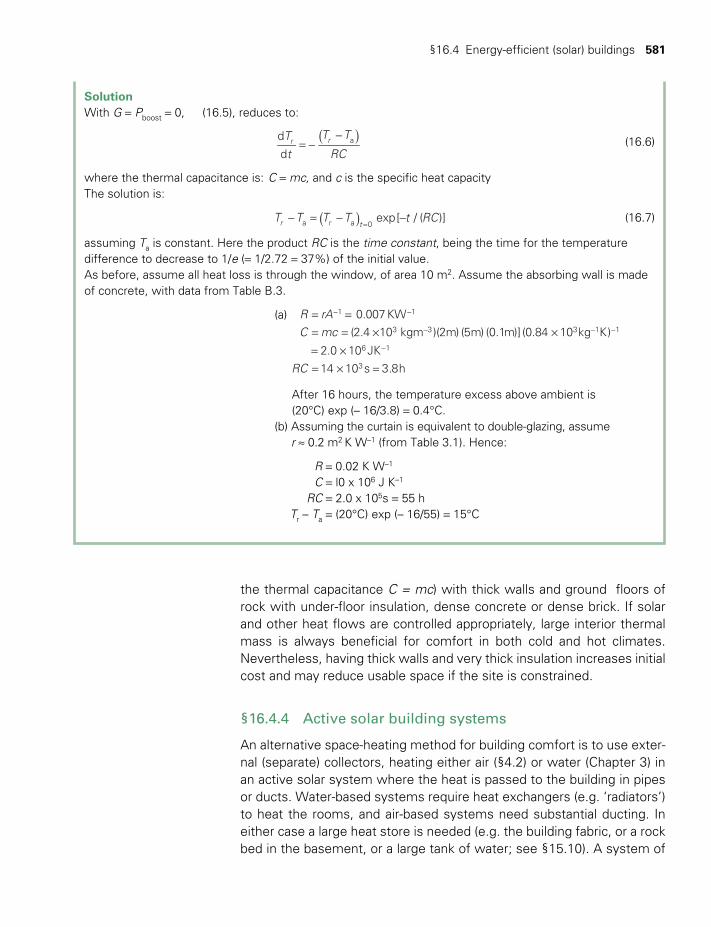
§16.4 Energy-efficient (solar) buildings 581
the thermal capacitance C = mc) with thick walls and ground floors of rock with under-floor insulation, dense concrete or dense brick. If solar and other heat flows are controlled appropriately, large interior thermal mass is always beneficial for comfort in both cold and hot climates. Nevertheless, having thick walls and very thick insulation increases initial cost and may reduce usable space if the site is constrained.
§16.4.4 Active solar building systems
An alternative space-heating method for building comfort is to use exter-nal (separate) collectors, heating either air (§4.2) or water (Chapter 3) in an active solar system where the heat is passed to the building in pipes or ducts. Water-based systems require heat exchangers (e.g. ‘radiators’) to heat the rooms, and air-based systems need substantial ducting. In either case a large heat store is needed (e.g. the building fabric, or a rock bed in the basement, or a large tank of water; see §15.10). A system of
SolutionWith G = Pboost = 0, (16.5), reduces to:
T
t
T T
RC
d
dr r a( )
= −− (16.6)
where the thermal capacitance is: C = mc, and c is the specific heat capacityThe solution is:
T T T T t RCexp[ / ( )]r r ta a 0( )− = − −=
(16.7)
assuming Ta is constant. Here the product RC is the time constant, being the time for the temperature difference to decrease to 1/e (= 1/2.72 = 37%) of the initial value.As before, assume all heat loss is through the window, of area 10 m2. Assume the absorbing wall is made of concrete, with data from Table B.3.
(a) R rAC mc
RC
0.007 KW(2.4 10 kgm )(2m) (5m) (0.1m)] (0.84 10 kg K)
2.0 10 JK14 10 s 3.8h
1 1
3 3 3 1 1
6 1
3
= == = × ×= ×= × =
− −
− − −
−
After 16 hours, the temperature excess above ambient is(20°C) exp (– 16/3.8) = 0.4°C.
(b) Assuming the curtain is equivalent to double-glazing, assume r ≈ 0.2 m2 K W–1 (from Table 3.1). Hence:
R = 0.02 K W–1
C = l0 x 106 J K–1
RC = 2.0 x 10⁵s = 55 hTr – Ta = (20°C) exp (– 16/55) = 15°C
TWIDELL PAGINATION.indb 581 01/12/2014 11:38

582 Using energy efficiently
pumps or fans is needed to circulate the working fluid, which is easier to control than purely passive systems, and may, in principle, be fitted to existing houses. However, the collectors have to be large and retrofitting is usually far less satisfactory than correct design at initial construction.
Like passive systems, active solar systems will work well only if heat losses have been minimized. In practice so-called passive houses are much improved with electric fans controlled to pass air between rooms and heat stores. Thus the term ‘passive’ tends to be used when the Sun’s heat is first trapped in rooms or conservatories behind windows, even if controlled ventilation is used in the building. ‘Active’ tends to be used if the heat is first trapped in a purpose-built exterior collector.
The analysis for real houses is complicated because of the complex absorber geometry, heat transfer through the walls, the presence of people in the house, and the considerable ‘free gains’ from lighting, cooking, etc. People make independent adjustments, such as opening windows or drawing curtains, that cannot be easily predicted. In addi-tion, their metabolism contributes appreciably to the heat balance of an ‘energy-conscious’ building with 100 to 150 W per person in the term Pboost of (16.5). A reasonable number of air changes (between one and three per hour) are required for ventilation, and this will usually produce significant heat loss unless heat exchangers are fitted. Computer pro-grams such as Energy plus (USA) and performance assessment methods such as BREEAM (UK) are designed to assess the interactions between all the factors affecting the energy performance of a building and are widely used, but it is still essential for analysts to appreciate the impor-tance of the individual effects through simplified, order of magnitude, calculations such as those in Worked Examples 16.1 and 16.2.
§16.4.5 Cold climates
In distinctly cold climates, where the dominant problem is lack of heating, and even the best energy-conscious buildings will need some active heating, the main concern is to minimize heat loss. A compact building form, which minimizes the surface-to-volume ratio, is desirable, as are the many factors mentioned above.
The Inuit igloo, made of snow, exemplifies minimum surface-to- volume ratio and heat gain from the metabolic and living activity of the inhabitants (Fig. 16.5(a)).
More modern buildings have a wider range of construction mater-ials available, and can use the passive solar gain from Equator-facing windows, provided that the window is well protected against heat loss at night (e.g. by double- or triple-glazing and/or curtains), thick wall insula-tion (e.g. r = 4m2K/W or better; refer to Box R3.1) and thermal mass to store the heat input (see Worked Example 16.1). The airtightness of the building envelope is important in minimizing heat loss, but inadequate
TWIDELL PAGINATION.indb 582 01/12/2014 11:38

§16.4 Energy-efficient (solar) buildings 583
Fig. 16.5Buildings suitable for a cold climate. a An Inuit village in 1865: igloos made from snow.
Source: reproduced from C.F. Hall, Arctic Researches and Life Among the Esquimaux, Harper Brothers, New York (1865).
b The Minto Roehampton apartment building in mid-town Toronto. Completed in 2007, this was the first multi-residential building to achieve LEED-Canada Gold certification. Source: Photo courtesy of UrbanDB.com.
(a) (b)
ventilation may lead to the accumulation of undesirable gases from some construction materials.
The Minto Roehampton multi-residential building in downtown Toronto (Fig. 16.5(b)) utilizes the aspects of energy-conscious design we have considered above, with passive solar energy to preheat fresh corridor air. It was designed to be 40% more energy efficient than the Canadian Model National Energy Code for Buildings at that time. A heat-recovery ventilation system delivers fresh, filtered air to each suite and circulates fresh air throughout the suites. An energy-saving ‘all-off switch’ installed in each of the 148 apartments allows residents to turn off all ceiling lights and exhaust fans from one switch as they leave. The opaque walls have high thermal resistivity (‘R-value’ = r ) with r = 15m2K/W, and the windows r = 0.3m2K/W without curtains. (Compare the smaller values of r for ‘standard’ walls and windows in Table B.7 of Appendix B.) The complex also incorporates other features to make it more ‘sustainable’ than common practice: easy walking distance to shops and amenities, covered bicycle storage, and a car-pool program for residents (compare §16.5), energy-efficient appliances (§16.7), a rigorous waste manage-ment system and careful management of water supplies.
TWIDELL PAGINATION.indb 583 01/12/2014 11:38

584 Using energy efficiently
§16.4.6 Temperate climates
In ‘temperate’ climates (e.g. most of Europe), the winter conditions approach those for cold climates, but for shorter periods of the year. Building solutions must allow for both winter and summer conditions (e.g. any large Equator-facing windows for winter solar heating may cause overheating in summer, thus requiring appropriate shading eaves, as visible in Fig.16.6(b) and (d)). Shading angles may be calculated from the formulas given in Chapter 2, or obtained in charts for architects, as in Szokolay (2008). In many temperate climates, the night temperatures even in summer are often below ‘comfort’ levels, so a large thermal capacity construction may be preferable. For instance, the thermal time constant of a solar-heated ‘mass-wall’, as shown in Worked Example 16.2, may be designed to match the time difference between maximum solar input and when heating is needed. Insulation is mandated in EU countries and in most states of the USA by building codes appropriate for each region (see Box 16.4). Sadly, such national building standards usually lag far behind standards of known best practice, since the build-ing industries are conservative and fear increased construction costs. The long-term costs of the future occupants’ energy needs are often not considered seriously.
Fig. 16.6 shows photographs and outlines of some solar-conscious buildings to give an idea of the architectural variety and the opportunities for stimulating design. Fig. 16.6(a) shows a large complex of student accommodation in Scotland, featuring transparent insulation and shade-blinds over the walls, and windows with individual blinds. Transparent insulation allows solar gain while still retaining heat produced inside the building. The south faces of the building have a monthly net gain of energy into the building throughout the year, even in midwinter in Glasgow.
The ‘First Light House’ in Fig. 16.6(b) was designed to meet the requirements of the Solar Decathlon (Box 16.5) for an affordable, energy-efficient family dwelling. It features an indoor top-glazed ‘deck’ (middle of photo) acting as a cooking and dining space, and bridging the sleep-ing and study areas. The building envelope is highly insulated, but is also flexible to climatic conditions, with sliding shutters to maximize or reduce solar gain as needed. An external timber canopy housing the photovoltaic panels and solar water heaters provides an elegant solution to the often cumbersome integration of solar panels. The canopy forms part of both the active and passive solar strategy, shading the glazing in summer months and aiding the passive cooling of the PV panels. The house integrates energy-efficient appliances, including LED lighting and a reverse-cycle heat pump with a high coefficient of performance. The users of the home can both monitor and optimize their energy usage with an intuitive home-monitoring system.
TWIDELL PAGINATION.indb 584 01/12/2014 11:38

§16.4 Energy-efficient (solar) buildings 585
Fig. 16.6Four buildings suitable for a temperate climate.a Student Solar Residences, University of Strathclyde, Glasgow, Scotland (latitude
56°N). South façade showing transparent insulation. Source: Twidell et al. (1994).
b ‘Meridian First Light House’ built for conditions at Washington, DC, USA (latitude 38°N) by students from Victoria University of Wellington for Solar Decathlon 2011. (Photo by Jim Tetro for the US Department of Energy Solar Decathlon.)Source: www.solardecathlon.gov.
c Refurbished office block in South Melbourne, Australia (latitude 38°S): front façade (facing east),
d detail of rear of same building, showing PV panels used for shading of west-facing windows).Source for (c) and (d): reproduced from Baird (2010).
(a) (b)
(c) (d)
TWIDELL PAGINATION.indb 585 01/12/2014 11:38

586 Using energy efficiently
The climate of Melbourne (Australia) is at the warmer boundary of ‘tem-perate climate’ with summer temperatures exceeding 34°C on ~10% of summer days but a mean minimum temperature in winter of +8°C. The office building shown in Fig.16.6(c) to (d) was extensively refurbished (retrofitted) in 2005 to reach a five-star energy rating (the best at that time). The former concrete façade was replaced by full-height, clear, low-emittance double-glazing, designed to maximize light transmission and reduce solar heat gain, supplemented by shading from the steel-perforated mesh visible in Fig.16.6(c). The rear (western) windows have the same glass but are shaded by neighboring buildings for much of the year. Although the building is ~5 times as deep as the width of its façade, natural light is maximized by fitting a central stairwell with a skylight, having open plan offices at both ends (on each of the five floors), and glazing the few internal walls. Natural ventilation is achieved by openable windows at both façades and using the stack effect in the open-tread stairwell to draw the air across the office and exit through louvres at roof level. In summer this system also allows the building to cool down at night before the next working day. There is also a Heating Ventilating and Air Conditioning (HVAC) system for periods when additional heating or cooling is required. All aspects are usually ‘automatically’ controlled by a building management system. Solar water heaters and PV arrays are mounted on the roof (in addition to the array shown in Fig. 16.6(d)).
The homes of the Hockerton Housing Association in Nottinghamshire, England are built to classic solar-conscious design. Thick external insu-lation encapsulates the west, north and east walls; inside this is thick, dense building block and a conventional brick wall. Conservatories cover
BOX 16.5 THE SOLAR DECATHLON
The U.S. Department of Energy Solar Decathlon challenges collegiate teams to design, build and operate solar-powered houses that are cost-effective, energy-efficient and attractive. The winner of the competition is the team that best blends affordability, consumer appeal and design excellence with optimal energy production and maximum efficiency.
A team typically takes two years to design and document its house at ‘home’ before re-erecting it on the competition showground alongside those from the other competitors. The design is required to work well as a ‘family dwelling’ on site. Ideally it should be energy self-sufficient, and cost <US$250,000, including fittings and appliances.
The competition shows consumers how to save money and energy with affordable clean energy products that are available today. The Solar Decathlon also provides participating students with hands-on experience and unique training that prepares them to enter the clean energy workforce. The Solar Decathlon has been held ‘biennially’ since 2005. Open to the public free of charge, the Solar Decathlon gives visitors the opportunity to tour the houses, gather ideas to use in their own homes, and learn how energy-saving features can help them save money today.
For more information, see www.solardecathlon.org. A similar competition is also held in Europe.
TWIDELL PAGINATION.indb 586 01/12/2014 11:38

§16.4 Energy-efficient (solar) buildings 587
the south façades, with internal windows and doors leading to the rooms. In addition, the north walls are buried within an earth rampart with grass and shrub cover. (See www.hockertonhousingproject.org.uk/ for informa-tion about the present activities.)
§16.4.7 Hot, dry climate
In hot, dry climates daytime temperatures may be very high (>40°C) but the diurnal range is often large (>20°C), so that night temperatures can be uncomfortably cool (e.g. ~0°C in winter in central Australia). Consequently large thermal mass is a most important characteristic for a comfortable building, with massive shaded walls and ceiling structures under a reflective roof. The windows should be shaded and are best kept closed during the day and opened at night for cooling (burglar bars may be needed!). External surfaces should be matt white, so reflect-ing solar radiation but allowing infrared heat radiation to be emitted to the (usually clear) night sky. Ground temperature at about 2 m depth is constant through the year in all climates; in hot, dry climates this temperature is likely to be around 20°C to 25°C. Therefore the floors of buildings should be in good thermal contact with the ground and not insulated. Indeed, underground rooms and cellars may be thermally very comfortable.
Places with this climate often have a hot, dusty and generally ‘hostile’ outdoor environment, so buildings with an inward-facing courtyard are pleasant, for instance, as is traditional in Egypt and northern India. The air in the courtyard can be evaporatively cooled by a pond or fountain, so providing cooled air to adjacent rooms with inward-facing doors and windows. Shade trees and other vegetation in the courtyard enhance this effect and create a pleasant semi-outdoor living space. In these dry climates, electrically powered table and ceiling fans enable forced evapo-rative cooling from the skin, so bringing both fresh air and welcome relief from heat. Evaporative coolers are similarly welcome, whereby external dry air is blown by fans through pads of loose wetted straw and then into rooms, from which air can exit. Evaporative cooling with fans requires significantly less electrical power than air-conditioning with refrigerants (~150 W compared with ~1500 W).
Fig. 16.7 shows a modern research complex in Gujarat (India) which uses these principles. Electricity for air-conditioning and artificial light is expensive and often unreliable, so the design aims to be energy-efficient. The passive solar features provide natural light and ventilation, while controlling the ingress of dust. Thermal mass is provided by the reinforced concrete construction from local materials, with brick infill in the walls and hollow concrete blocks in the roof coffers for addi-tional thermal mass. Vermiculite is the main insulating material where appropriate. The exterior is white, including the roof. In the hot, dry
TWIDELL PAGINATION.indb 587 01/12/2014 11:38

588 Using energy efficiently
Fig. 16.7Hot, dry climate zone. The Torrent Research Centre, Ahmedabad, Gujarat, India. a Exterior view of one block showing one of the evaporative coolers (large structure on
roof) and multiple exhaust towers. b Cross-section showing the ventilation system. Source: Photo and sketch from Baird (2010).
(a)
Laboratory
Exhaust(b)
Exhaust
Exhaust Exhaust
Inlet
Micronisers
Offices
TWIDELL PAGINATION.indb 588 01/12/2014 11:38
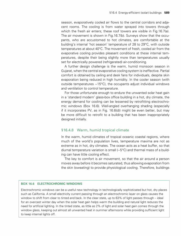
§16.4 Energy-efficient (solar) buildings 589
season, evaporatively cooled air flows to the central corridors and adja-cent rooms. The cooling is from water sprayed into towers through which the fresh air enters; these roof towers are visible in Fig.16.7(a). The air movement is shown in Fig.16.7(b). Surveys show that the occu-pants, who are accustomed to hot climates, are comfortable at the building’s internal ‘hot season’ temperature of 28 to 29°C, with outside temperatures at about 40°C. The movement of fresh, cooled air from the evaporative cooling provides pleasant conditions at these internal tem-peratures, despite their being slightly more than temperatures usually set for electrically powered (refrigerated) air-conditioning.
A further design challenge is the warm, humid monsoon season in Gujarat, when the central evaporative cooling system is ineffective. Partial comfort is obtained by ceiling and desk fans for individuals, despite skin evaporation being reduced in high humidity. In the cooler season (with outside temperatures ~15°C), the occupants adjust individual windows and ventilation to control temperature.
For those unfortunate enough to endure the unwanted solar heat gain in a ‘standard modern’ glass-box office building in a hot, dry climate, the energy demand for cooling can be lessened by retrofitting electrochro-mic windows (Box 16.6). Well-angled overhanging shading (especially if it incorporates PV, as in Fig. 16.6(d)) might be even better, but may be more difficult to retrofit to a building that has been inappropriately designed initially.
§16.4.8 Warm, humid tropical climate
In the warm, humid climates of tropical oceanic coastal regions, where much of the world’s population lives, temperature maxima are not as extreme as in hot, dry climates. The ocean acts as a heat buffer, so that diurnal temperature variation is small (~5°C) and thermal mass of a build-ing can have little cooling effect.
The key to comfort is air movement, so that the air around a person moves away before it becomes saturated, thus allowing evaporation from the skin (sweating) to provide physiological cooling. Therefore, buildings
BOX 16.6 ELECTROCHROMIC WINDOWS
Electrochromic windows can be a useful new technology in technologically sophisticated but hot, dry places such as California. A small electricity current passing through an electrochromic layer on glass causes the window to shift from clear to tinted and back. In the clear state, up to 63% of light passes through – ideal for an overcast winter day when the solar heat gain helps warm the building and natural light reduces the need for artificial lighting. In the tinted state, as little as 2% of light and solar heat gain comes through the window glass, keeping out almost all unwanted heat in summer afternoons while providing sufficient light to keep internal lights off.
TWIDELL PAGINATION.indb 589 01/12/2014 11:38

590 Using energy efficiently
are traditionally constructed with numerous openings facing the prevail-ing wind, few internal impediments to the breeze (as in Fig. 16.8), and also often raised off the ground to catch a stronger breeze (recall the variation of wind speed with height: §7.3.2). If a natural breeze is absent, low-velocity fans provide welcome air movement.
Another consideration is that in tropical locations the Sun’s path is near the zenith, so the roof receives very strong insolation, which can increase ceiling temperatures with heat radiating strongly into the inte-rior. Therefore roof surfaces should be highly reflective or otherwise white, with adequate ventilation beneath and thermal insulation above ceilings. Windows that face east or west should be shaded, to avoid heat from low-angle insolation.
Electrically powered air-conditioning can also provide comfort, but its power consumption (and initial cost) is at least 10 times that of an elec-tric fan – more if the temperature setting is too low. If its use is deemed absolutely necessary (e.g. in some laboratories), whole buildings or rooms should be thoroughly insulated as in cold climates; unfortunately this is seldom done.
Fig. 16.8Warm, humid zone. a A ‘traditional’ fale in Upolu, Samoa (a tropical island in the Pacific Ocean (latitude
13°S)), with no walls to block the breeze. This one incorporates galvanized iron in the roof, because it is easier to maintain than thatch (author photo).
b A traditional ‘Queenslander’ house in Brisbane, Australia (latitude 27°S) showing elevation for breeze, wide verandahs for shading, and lightweight construction for rapid cooling at night.
Source: Photo by Wade Johanson, cropped and used here under Creative Commons Attribution Generic 2.0 License.
(a) (b)
TWIDELL PAGINATION.indb 590 01/12/2014 11:38
§16.5 Transport 591
§16.4.9 Composite climates
Although the simple classification of climates outlined by Szokolay (2008) and used above describes most places adequately for architectural pur-poses, some places have significant seasonal variation. Ahmedabad in Gujarat is an example: as noted in §16.4.7 it has a hot, dry season fol-lowed by a warm, humid season, which makes building design more complicated. Washington, DC, is another example, with warm, humid summers and cold winters – a challenge met by the First Light House shown in Fig.16.6(b).
§16.5 TRANSPORT
§16.5.1 Background
Transport is generally considered as the movement of goods and people by powered vehicles. Thus, despite their importance, walking and cycling tend to be neglected by transport planners and statisticians. Powered vehicles account for between 20% and 30% of primary energy use within most economies. However, within official statistics (see Fig 16.3), such data often does not include international journeys and inter-national trade by air and sea. The movements of people, and of goods and commodities (including fossil fuels), are major components of the global economy.
§16.5.2 Vehicles
The motive-power mechanisms for common modes of land transport are as follows:
1 Metabolism (walking, running, cycling, animal power) (§17.2.3). 2 Wind (sailing-boats). 3 Electric motor, grid-connected (electric trains and trams) (§15.4).4 Electric motor from onboard rechargeable battery or fuel cell (elec-
tric cars, lightweight vans/lorries, cycles and hybrid vehicles) (see §15.7).
5 Internal combustion engines with liquid or liquified fuel (spark-ignition, compression-ignition/diesel, jet engines). (see Ch. 10).
6 Internal combustion with gaseous fuel (spark-ignition engine for road vehicles with tanks of compressed methane or hydrogen) (for biogas, §10.8).
Method (5) is overwhelmingly dominant today, with fossil petroleum the main fuel (Fig. 16.9). Renewable energy is able to power all of mecha-nisms (1) to (6), and therefore presents considerable choice, as indicated by the section references in the list above; see also Box 16.3.
TWIDELL PAGINATION.indb 591 01/12/2014 11:38
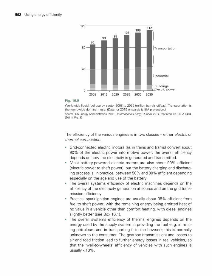
592 Using energy efficiently
The efficiency of the various engines is in two classes – either electric or thermal combustion:
• Grid-connected electric motors (as in trains and trams) convert about 90% of the electric power into motive power; the overall efficiency depends on how the electricity is generated and transmitted.
• Most battery-powered electric motors are also about 90% efficient (electric power to shaft power), but the battery charging and discharg-ing process is, in practice, between 50% and 80% efficient depending especially on the age and use of the battery.
• The overall systems efficiency of electric machines depends on the efficiency of the electricity generation at source and on the grid trans-mission efficiency.
• Practical spark-ignition engines are usually about 35% efficient from fuel to shaft power, with the remaining energy being emitted heat of no value in a vehicle other than comfort heating, with diesel engines slightly better (see Box 16.1).
• The overall systems efficiency of thermal engines depends on the energy used by the supply system in providing the fuel (e.g. in refin-ing petroleum and in transporting it to the bowser); this is normally unknown to the consumer. The gearbox (transmission) and losses to air and road friction lead to further energy losses in real vehicles, so that the ‘well-to-wheels’ efficiency of vehicles with such engines is usually <10%.
Fig. 16.9Worldwide liquid fuel use by sector 2008 to 2035 (million barrels oil/day). Transportation is the worldwide dominant use. (Data for 2015 onwards is EIA projection.) Source: US Energy Administration (2011), International Energy Outlook 2011, reprinted. DOE/EIA-0484 (2011), Fig. 33.
112108
103
93 98
120
80
86
40
02008 2015 2020 2025 2030 2035
Industrial
Transportation
BuildingsElectric power
TWIDELL PAGINATION.indb 592 01/12/2014 11:38
§16.5 Transport 593
§16.5.3 An unsustainable transport system?
Several components of present transport systems make them problematic in environmental, economic and social terms:
1 Diminishing fossil oil reserves (the present system is almost entirely fueled by petroleum products).
2 Global atmospheric impacts (CO2 emissions from fossil fuels are driving climate change: see §2.9).
3 Local air quality impacts (urban smog caused largely by vehicle exhausts is a health hazard, as lead was from leaded petrol).
4 Noise, especially from motorways and freeways, and in cities.5 Fatalities from road accidents (a significant cause of death, e.g. USA
~40,000/y at 14 per 100,000 people per year, Namibia 53/100,000, Japan 3.8/100,000).
6 Inadequate mobility in developing countries (poor infrastruc-ture prevents many people from bringing their produce to market and from accessing what facilities there are for health care and education).
RE (particularly biofuels, but also with electric vehicles) contributes to mitigating (1) and (2) (see Box 10.3), and possibly (3) and (4). The other issues are reduced by improved resources, better control technology and public responsibility.
When travel was severely restricted in Britain by the Second World War, there was a slogan: ‘Is your journey really necessary?’ The same question can and should be asked today of much of the growing – but almost certainly unsustainable – demand for travel.
Telecommunication technologies are often promoted as a way to lessen the need to physically bring co-workers together, and thereby reduce the demand both for daily commuter travel and for longer jour-neys (often by air) to business conferences and the like. Nevertheless, the high growth in remote information exchange, especially via the inter-net, is itself a significant energy use, with power consumption by data centers amounting to about 2% of total electricity use in the USA and about 1.3% of global electricity use, with these proportions continuing to increase (Koomey 2011). Moreover, the increased telecommunica-tion activity may actually stimulate an increase in travel, and increasing wealth in countries indicates that even if individuals may travel less, the sum total of all travel will increase. Therefore the need for sustainable travel and transport mechanisms is vital.
§16.5.4 Transport and urban form
Urban design for sustainability promotes energy-efficient communal modes of transport to replace journeys in personal motor vehicles.
TWIDELL PAGINATION.indb 593 01/12/2014 11:38
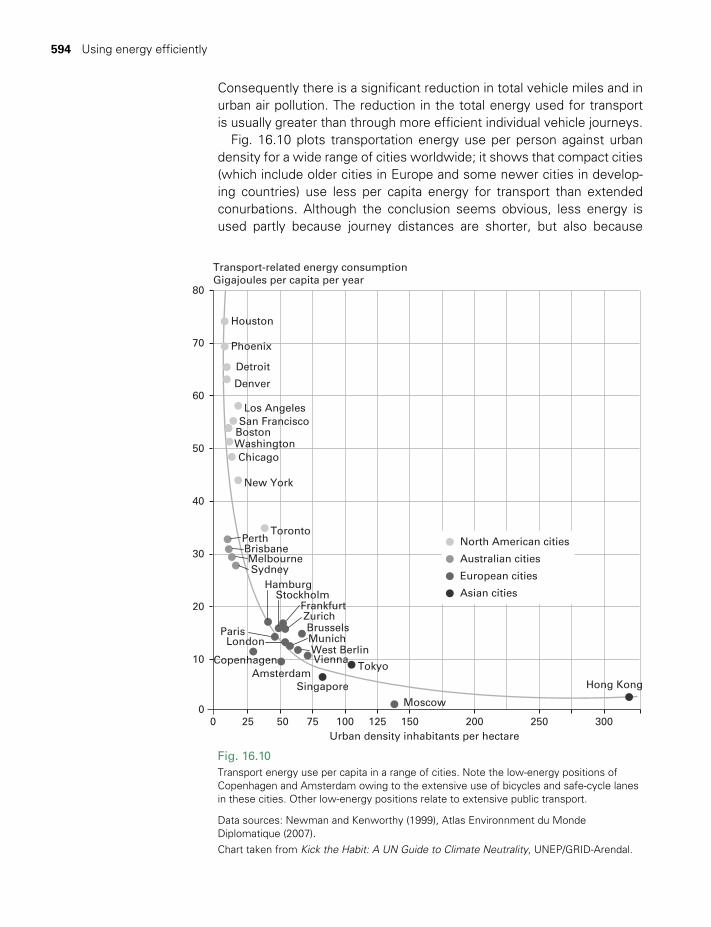
594 Using energy efficiently
Consequently there is a significant reduction in total vehicle miles and in urban air pollution. The reduction in the total energy used for transport is usually greater than through more efficient individual vehicle journeys.
Fig. 16.10 plots transportation energy use per person against urban density for a wide range of cities worldwide; it shows that compact cities (which include older cities in Europe and some newer cities in develop-ing countries) use less per capita energy for transport than extended conurbations. Although the conclusion seems obvious, less energy is used partly because journey distances are shorter, but also because
80
Transport-related energy consumptionGigajoules per capita per year
Houston
70
60
50
40
30
20
10
00 25 50 75 100 125 150 200 250 300
Phoenix
Detroit
Denver
Los AngelesSan Francisco
BostonWashingtonChicago
New York
TorontoPerthBrisbaneMelbourneSydney
HamburgStockholm
ParisLondon
CopenhagenAmsterdam
Singapore
Moscow
Hong Kong
Urban density inhabitants per hectare
FrankfurtZurichBrusselsMunichWest BerlinVienna
Tokyo
North American cities
Australian cities
European cities
Asian cities
Fig. 16.10Transport energy use per capita in a range of cities. Note the low-energy positions of Copenhagen and Amsterdam owing to the extensive use of bicycles and safe-cycle lanes in these cities. Other low-energy positions relate to extensive public transport.
Data sources: Newman and Kenworthy (1999), Atlas Environnment du Monde Diplomatique (2007). Chart taken from Kick the Habit: A UN Guide to Climate Neutrality, UNEP/GRID-Arendal.
TWIDELL PAGINATION.indb 594 01/12/2014 11:38

§16.5 Transport 595
people walk, cycle and use public transport without the need for private vehicles. Walking and cycling are always by renewable energy (food metabolism) and increasingly public transport uses biofuels and other renewables-orientated technologies. The urban sprawl of 20th-century cities, like Los Angeles where ‘planning’ (if any) has been based around private motor vehicles, is a major factor contributing to extravagant fuel use in transport; nevertheless, such cities may present the best oppor-tunities for electric vehicles, perhaps charged from RE-based electricity from the grid or from domestic micro-generation.
By 2010, about 50% of the world population lived in cities and urban areas; this is projected to be 60% by 2030, mainly because of the rapid growth of megalopolises in developing countries, such as Shanghai, Mumbai and Cairo. From a global energy and sustainability perspective, it is therefore vital to get good urban planning in place in the megalopolises before they sprawl out of control as many cities in the USA and elsewhere have done. Likewise, in rapidly growing mid-sized cities such as Curitiba (Box 16.7), many of which still have sur-rounding land available on which new development can be controlled. Proper planning presents opportunities for the acceptance of renewable energy technologies, not only for transport but also for buildings (see Box 16.7).
BOX 16.7 CURITIBA: A CASE STUDY OF URBAN DESIGN FOR SUSTAINABILITY AND REDUCED ENERGY DEMAND
The city of Curitiba in Brazil (population ~2.3 million) set new standards of sustainable urban planning, under its long-term mayor, Jaime Lerner. The city acted pro-actively in the 1970s, to avoid urban sprawl and slum development over its natural surroundings.
Curitiba has an integrated transportation system, which includes dedicated lanes on major streets for buses. Although the city has doubled in population since the system was developed, residential development (much of it high-density multi-storey) and commercial development have been carefully zoned to allow easy access to the bus system (which was cheaper and more flexible to develop than alternatives such as an underground railway). The system is used by 85% of Curitiba’s population (2.3 million passengers a day), The bus stops (Fig. 16.11) are near bicycle paths of total length 160 km in the city. The buses, manufactured by Volvo in Brazil, are 28 m long, split into three sections (bi-articulated) and fueled by biodiesel from soybeans.
The sustainability and livability of the city are enhanced by a network of almost 30 parks and urban forested areas, making it one of the greenest cities in the world. Back in 1970, each of the city’s inhabitants had less than 1 m² of green area. A goal-directed effort has since boosted this area to 52 m² per inhabitant and the city is still actively improving its natural environment. The city has succeeded in introducing a Green Exchange employment program to the benefit of the environment and socially deprived groups. 70% of Curitiba’s waste is recycled. The city’s recycling of paper alone accounts for the equivalent of 1200 trees a day.
Source: Danish Architecture Center, http://www.dac.dk.
TWIDELL PAGINATION.indb 595 01/12/2014 11:38
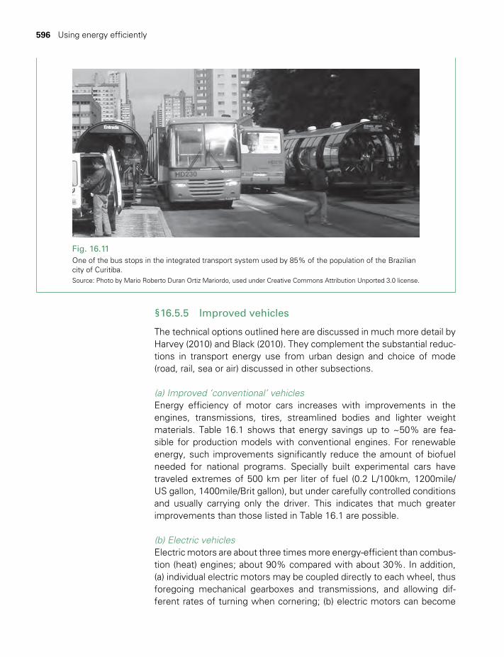
596 Using energy efficiently
Fig. 16.11One of the bus stops in the integrated transport system used by 85% of the population of the Brazilian city of Curitiba. Source: Photo by Mario Roberto Duran Ortiz Mariordo, used under Creative Commons Attribution Unported 3.0 license.
§16.5.5 Improved vehicles
The technical options outlined here are discussed in much more detail by Harvey (2010) and Black (2010). They complement the substantial reduc-tions in transport energy use from urban design and choice of mode (road, rail, sea or air) discussed in other subsections.
(a) Improved ‘conventional’ vehicles Energy efficiency of motor cars increases with improvements in the engines, transmissions, tires, streamlined bodies and lighter weight materials. Table 16.1 shows that energy savings up to ~50% are fea-sible for production models with conventional engines. For renewable energy, such improvements significantly reduce the amount of biofuel needed for national programs. Specially built experimental cars have traveled extremes of 500 km per liter of fuel (0.2 L/100km, 1200mile/US gallon, 1400mile/Brit gallon), but under carefully controlled conditions and usually carrying only the driver. This indicates that much greater improvements than those listed in Table 16.1 are possible.
(b) Electric vehicles Electric motors are about three times more energy-efficient than combus-tion (heat) engines; about 90% compared with about 30%. In addition, (a) individual electric motors may be coupled directly to each wheel, thus foregoing mechanical gearboxes and transmissions, and allowing dif-ferent rates of turning when cornering; (b) electric motors can become
TWIDELL PAGINATION.indb 596 01/12/2014 11:38
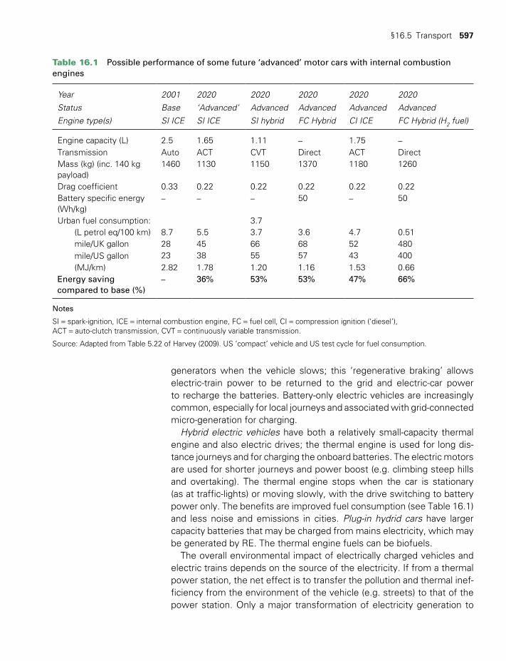
§16.5 Transport 597
Table 16.1 Possible performance of some future ‘advanced’ motor cars with internal combustion engines
Year 2001 2020 2020 2020 2020 2020
Status Base ‘Advanced’ Advanced Advanced Advanced Advanced
Engine type(s) SI ICE SI ICE SI hybrid FC Hybrid CI ICE FC Hybrid (H2 fuel)
Engine capacity (L) 2.5 1.65 1.11 – 1.75 –Transmission Auto ACT CVT Direct ACT DirectMass (kg) (inc. 140 kg payload)
1460 1130 1150 1370 1180 1260
Drag coefficient 0.33 0.22 0.22 0.22 0.22 0.22Battery specific energy (Wh/kg)
– – – 50 – 50
Urban fuel consumption: 3.7 (L petrol eq/100 km) 8.7 5.5 3.7 3.6 4.7 0.51 mile/UK gallon 28 45 66 68 52 480 mile/US gallon 23 38 55 57 43 400 (MJ/km) 2.82 1.78 1.20 1.16 1.53 0.66Energy saving compared to base (%)
– 36% 53% 53% 47% 66%
Notes
SI = spark-ignition, ICE = internal combustion engine, FC = fuel cell, CI = compression ignition (‘diesel’), ACT = auto-clutch transmission, CVT = continuously variable transmission.
Source: Adapted from Table 5.22 of Harvey (2009). US ‘compact’ vehicle and US test cycle for fuel consumption.
generators when the vehicle slows; this ‘regenerative braking’ allows electric-train power to be returned to the grid and electric-car power to recharge the batteries. Battery-only electric vehicles are increasingly common, especially for local journeys and associated with grid- connected micro-generation for charging.
Hybrid electric vehicles have both a relatively small-capacity thermal engine and also electric drives; the thermal engine is used for long dis-tance journeys and for charging the onboard batteries. The electric motors are used for shorter journeys and power boost (e.g. climbing steep hills and overtaking). The thermal engine stops when the car is stationary (as at traffic-lights) or moving slowly, with the drive switching to battery power only. The benefits are improved fuel consumption (see Table 16.1) and less noise and emissions in cities. Plug-in hydrid cars have larger capacity batteries that may be charged from mains electricity, which may be generated by RE. The thermal engine fuels can be biofuels.
The overall environmental impact of electrically charged vehicles and electric trains depends on the source of the electricity. If from a thermal power station, the net effect is to transfer the pollution and thermal inef-ficiency from the environment of the vehicle (e.g. streets) to that of the power station. Only a major transformation of electricity generation to
TWIDELL PAGINATION.indb 597 01/12/2014 11:38
598 Using energy efficiently
renewable energy sources can make such vehicles part of a truly sus-tainable energy system. Plug-in electric vehicles will contribute to this transformation, as their intermittent load on the grid can in principle help match the demand for electricity to the variable input from wind power, etc. (see §15.4.2).
(c) Hydrogen-powered vehiclesHydrogen gas may be used as the fuel for (a) spark-ignition engines, and (b) fuel cells producing the electricity for electric vehicles. (Although H2 is lightweight, the car indicated in Table 16.1 is heavy due to the fuel tank required: see §15.11.) When and where used, the only emission is water vapor, since the overall chemical reaction at the vehicle is:
2H + O 2H O +142MJ / (kg of hydrogen)2 2 2 (16.8)
Therefore hydrogen-powered vehicles are suitable in towns and cities if the necessary refueling infrastructure is in place, which requires major investment. The global impact depends on how the hydrogen has been produced for which there are two categories of manufacture: (1) by chemical reaction, or (2) by electrolysis of water. The chemical reaction route is normally from the fossil fuels of ‘natural’ gas (methane), oil or coal, but could in principle be from biogas (methane) or biomass.2 Further details of a ‘hydrogen economy’ are given in §15.9.1.
§16.5.6 Freight transport
Transport of goods accounts for 30% of transport energy use in OECD countries, and perhaps more in developing countries. Transport by sea dominates international movement of goods (over 95% measured by tonne-km; about 50% by value), with ship engines using poorly refined, but relatively cheap, fossil oil. For all modes of freight transport, energy use per tonne-km is large for distances less than 200 km because of the energy used for loading and unloading, but approximately proportional to distance for longer distances. Energy intensities (MJ per tonne-km) for long-distance cargo containers are ~0.7 for road, ~0.3 for rail and ~0.2 for sea transport.3 Energy intensities for bulk cargoes (e.g. wheat or oil) by sea are even less. Sea transport is energy efficient, reliable and safe, but often polluting; however, it is slow, which is why valued (in $/kg) or perishable cargoes may be transported by road, rail or air. Although increases in ship size and improvements in design and engines have improved energy efficiency markedly over the past 30 years, there is still scope for further improvement. An important factor is that – other things being equal – the energy to propel a ship increases as the fluid drag (i.e. with the square of its speed), so slow boats are the most energy efficient.
TWIDELL PAGINATION.indb 598 01/12/2014 11:38
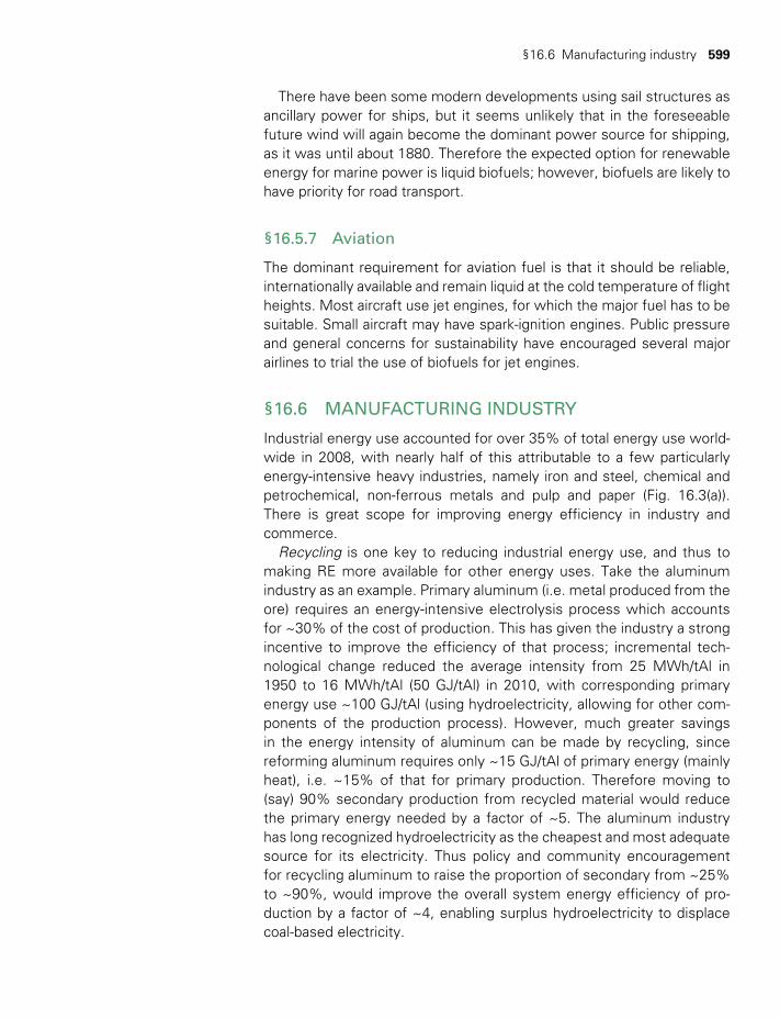
§16.6 Manufacturing industry 599
There have been some modern developments using sail structures as ancillary power for ships, but it seems unlikely that in the foreseeable future wind will again become the dominant power source for shipping, as it was until about 1880. Therefore the expected option for renewable energy for marine power is liquid biofuels; however, biofuels are likely to have priority for road transport.
§16.5.7 Aviation
The dominant requirement for aviation fuel is that it should be reliable, internationally available and remain liquid at the cold temperature of flight heights. Most aircraft use jet engines, for which the major fuel has to be suitable. Small aircraft may have spark-ignition engines. Public pressure and general concerns for sustainability have encouraged several major airlines to trial the use of biofuels for jet engines.
§16.6 MANUFACTURING INDUSTRY
Industrial energy use accounted for over 35% of total energy use world-wide in 2008, with nearly half of this attributable to a few particularly energy-intensive heavy industries, namely iron and steel, chemical and petrochemical, non-ferrous metals and pulp and paper (Fig. 16.3(a)). There is great scope for improving energy efficiency in industry and commerce.
Recycling is one key to reducing industrial energy use, and thus to making RE more available for other energy uses. Take the aluminum industry as an example. Primary aluminum (i.e. metal produced from the ore) requires an energy-intensive electrolysis process which accounts for ~30% of the cost of production. This has given the industry a strong incentive to improve the efficiency of that process; incremental tech-nological change reduced the average intensity from 25 MWh/tAl in 1950 to 16 MWh/tAl (50 GJ/tAl) in 2010, with corresponding primary energy use ~100 GJ/tAl (using hydroelectricity, allowing for other com-ponents of the production process). However, much greater savings in the energy intensity of aluminum can be made by recycling, since reforming aluminum requires only ~15 GJ/tAl of primary energy (mainly heat), i.e. ~15% of that for primary production. Therefore moving to (say) 90% secondary production from recycled material would reduce the primary energy needed by a factor of ~5. The aluminum industry has long recognized hydroelectricity as the cheapest and most adequate source for its electricity. Thus policy and community encouragement for recycling aluminum to raise the proportion of secondary from ~25% to ~90%, would improve the overall system energy efficiency of pro-duction by a factor of ~4, enabling surplus hydroelectricity to displace coal-based electricity.
TWIDELL PAGINATION.indb 599 01/12/2014 11:38
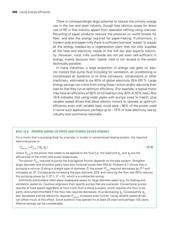
600 Using energy efficiently
There is correspondingly large potential to reduce the primary energy use in the iron and steel industry, though less obvious scope for direct use of RE in that industry appart from specialist refining using charcoal. Recycling of paper products reduces the pressure on world forests for fiber, and also the energy required for paper-making. Furthermore, in modern pulp and paper mills there is sufficient biomass ‘waste’ to supply all the energy needed by a cogeneration plant that not only supplies all the heat and electricity needs of the mill but also exports electric-ity. However, most mills worldwide are not yet even self-sufficient in energy, mainly because their ‘waste’ heat is not reused to the extent technically possible.
In many industries, a large proportion of energy use goes on elec-tric motors that pump fluid (including for ventilation, air conditioning or compressed air systems) or to drive conveyors, compressors or other machinery, estimated to be 40% of global electricity (IEA 2011). Large energy savings can come from sizing these motors and/or adjusting their load so that they run at optimum efficiency. (For example, a typical motor may have an efficiency of 80% at full load but only 30% at 50% load.) Box 16.8 indicates that using wider pipes with pumps sized to match, plus variable speed drives that allow electric motors to operate at optimum efficiency even with variable load, could save ~90% of the power used in some such applications; perhaps up to ~15% of total electricity use by industry and commerce nationally.
BOX 16.8 PROPER SIZING OF PIPES AND PUMPS SAVES ENERGY
For a motor that is pumping fluid, for example, in a solar or conventional heating system, the required electrical power is:
η η=P P / ( )m pelectric fluid (16.9)
where Pfluid is the power that needs to be applied to the fluid (i.e. the load) and ηm and ηp are the efficiencies of the motor and pump respectively.
The power Pfluid required to pump the fluid against friction depends on the pipe system. Straighter, larger diameter and smoother pipes have less frictional losses (see §R2.6). Problem 6.7 shows that in pumping a volume Q along a straight pipe of diameter D, the power Pfluid required decreases as D –5 and increases as Q3. Consequently increasing the pipe diameter 20% and reducing the flow rate 50% reduces the pumping power by (1.2) 2 205 3× = , which is a substantial saving.
Architects and builders often allow inadequate space for large diameter pipes (e.g. for heating and ventilation systems). Cautious engineers then specify pumps that are oversized. Conventional pumps operate at fixed speed regardless of how much fluid is being pumped, which requires the flow to be partly obstructed (throttled) if the flow rate required decreases, thus decreasing ηp. Consequently ηm also decreases and the electricity required Pelectric increases even further. Using variable speed drives can offset much of this effect. Since systems may operate for at least 20 years and perhaps 100 years, lifetime savings can be considerable.
TWIDELL PAGINATION.indb 600 01/12/2014 11:38
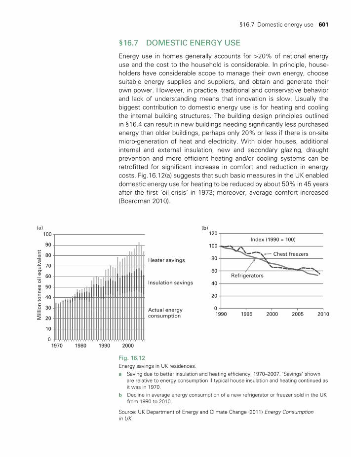
§16.7 Domestic energy use 601
§16.7 DOMESTIC ENERGY USE
Energy use in homes generally accounts for >20% of national energy use and the cost to the household is considerable. In principle, house-holders have considerable scope to manage their own energy, choose suitable energy supplies and suppliers, and obtain and generate their own power. However, in practice, traditional and conservative behavior and lack of understanding means that innovation is slow. Usually the biggest contribution to domestic energy use is for heating and cooling the internal building structures. The building design principles outlined in §16.4 can result in new buildings needing significantly less purchased energy than older buildings, perhaps only 20% or less if there is on-site micro-generation of heat and electricity. With older houses, additional internal and external insulation, new and secondary glazing, draught prevention and more efficient heating and/or cooling systems can be retrofitted for significant increase in comfort and reduction in energy costs. Fig.16.12(a) suggests that such basic measures in the UK enabled domestic energy use for heating to be reduced by about 50% in 45 years after the first ‘oil crisis’ in 1973; moreover, average comfort increased (Boardman 2010).
Fig. 16.12Energy savings in UK residences. a Saving due to better insulation and heating efficiency, 1970–2007. ‘Savings’ shown
are relative to energy consumption if typical house insulation and heating continued as it was in 1970.
b Decline in average energy consumption of a new refrigerator or freezer sold in the UK from 1990 to 2010.
Source: UK Department of Energy and Climate Change (2011) Energy Consumption in UK.
(a)
0
10
20
30
40
50
60
70
80
90
100
1970 1980 1990 2000
Mill
ion
ton
nes
oil
equ
ival
ent
Actual energy consumption
Insulation savings
Heater savings
(b)
0
20
40
60
80
100
120
1990 1995 2000 2005 2010
Index (1990 = 100)
Refrigerators
Chest freezers
TWIDELL PAGINATION.indb 601 01/12/2014 11:38

602 Using energy efficiently
Many heating and cooling systems worldwide are controlled by ther-mostats set by the user. It is important to realize that substantial cost savings can be made in buildings by setting the thermostat appropriately. Generally, without loss of comfort or convenience, one can easily put on an extra layer of clothing in winter or take one off in summer.
Electricity consumption can be reduced significantly with compact fluorescent (CFL) and light-emitting-diode (LED) lighting, with improved ‘white goods’, especially refrigerators and washing machines, with solid state television and computer screens, and by avoiding standby power. Clearly visible instruments and regular monitoring promote behavioral changes that frequently reduce consumption by at least 10%.
As with lighting (Box 16.2), the energy efficiency of appliances has been greatly improved, driven by policy measures such as Minimum Energy Performance Standards. Fig. 16.12(b) indicates that the average energy consumption of new refrigerators and freezers has halved over the past 20 years. Most OECD countries require the power rating of products to be clearly indicated so that consumers can make informed choices.
Micro-generation of on-site electricity, especially by rooftop PV panels, and of heat, especially by solar water heaters, wood stoves and heat pumps, has increased rapidly since about 2000 with successful institu-tional policy mechanisms (e.g. feed-in tariffs). By 2011, Germany had 3400 MW of installed solar PV capacity on nearly a million residential buildings. In general, the range and number of micro-generation installa-tions are increasing significantly worldwide, with the result that houses with such technology can reduce their purchased energy considerably.
§16.8 SOCIAL AND ENVIRONMENTAL ASPECTS
§16.8.1 Negawatts are cheaper than megawatts!
Amory Lovins, in his 1970s analysis of demand-side actions, coined the term ‘negawatt’ (negative watt) for ‘power not consumed’ and so ‘saved’. Such analyses of actions reducing energy consumption and hence costs (in terms of payback times: see Chapter 17) and GHG emissions (in terms of $/tCO2 reduction) established the efficient use of energy as a recog-nized discipline. The net cost over a few years of successful negawatt measures is negative, i.e. there is both energy and financial saving. For example, manually switching off unused electric lights costs nothing, with immediate savings on power bills. Installing automatic lighting control in offices (e.g. light-intensity switching, a time switch or a motion sensor) may repay investment within a year. There are many such examples.
A key policy question is why such opportunities are not always imple-mented. We disregard as demonstrably absurd the contention of some economists that such opportunities cannot exist because, in their ideal-ized economic models, everyone has perfect information and therefore
TWIDELL PAGINATION.indb 602 01/12/2014 11:38
§16.8 Social and environmental aspects 603
any opportunities to make money in this way are automatically taken up. However, it is evident that many people and businesses are not aware of the technological possibilities for energy efficiency, and do not monitor the amounts and costs of their energy use. This may be because they believe energy is a small part of their overall costs. For successful demand-side action, clear information is essential; but stronger policy tools, such as minimum energy performance standards, etc., are also needed (see §17.5). Box 17.5 indicates that without such policy measures global energy demand is likely to increase by ~40% by 2030, but that strong policy measures to accelerate technological improvement in energy efficiency could limit the increase in demand to ≤ 5%, while not limiting prosperity.
§16.8.2 Impact on renewable energy
Reducing end user's demand for energy reduces their costs and thereby increases the practical feasibility of using a renewable energy source to meet that demand. For example, the cost of photovoltaic panels and ancillary equipment to supply electricity to a household depends on both the service required and the efficiency of use. The continuing techno-logical improvement of the energy efficiency of appliances reduces elec-tricity consumption, and thus the size and cost of the PV panels (and perhaps batteries) required. This cost reduction is complementary to that arising from the improved efficiency of the panels themselves (Chapter 5) and the economies of scale from massively increased production (Fig. 17.2). All of this results in positive feedback and a further increase in the use of solar energy for micro-generation in both developed and develop-ing countries. This opens the door to social benefits to health, education and telecommunication of a modern energy supply to millions of people in the rural areas of developing countries.
§16.8.3 Paths of economic development
A key consideration in future global energy demand is the nature of economic development and whether and to what extent developing countries need to follow the historic development pathways of industri-alized countries. The ‘lock-in’ effects of infrastructure, technology and product design choices made by rich countries in the mid-20th century and earlier (e.g. commitment to coal-fired power stations, urban layouts dependent on motor cars, etc.) set the frame for energy use per person ranging from around 125 kWh/day per person in Europe to 250 kWh/day per person in the USA. Such established and often energy-inefficient procedures are responsible for much of the recent increase in world energy use.
In developing countries, where much infrastructure is still to be built, the spectrum of future options is considerably wider. In particular,
TWIDELL PAGINATION.indb 603 01/12/2014 11:38
604 Using energy efficiently
developing countries can bypass energy-inefficient practices and proceed directly to cleaner technologies and more sustainable built environments (see Boxes 16.7 and 16.9).
§16.8.4 Buildings
The marginal cost of passive solar features for buildings such as orien-tation, window placement and shading is relatively small at design and construction. For an established building, change in orientation is impos-sible, but significant benefits may come from retrofitting with insulation, shading, curtains, skylights, improved appliances, etc . There are definite improvements in comfort, with financial payback often within one to five years. Micro-generation is a responsible action for both new and estab-lished buildings, with payback over five to 20 years likely, depending on government incentives.
The paybacks for rented buildings are often equally short, but the ‘landlord-tenant problem’ applies: landlords are often reluctant to pay the capital cost of energy-efficiency measures when the financial savings accrue to the tenant. Therefore government regulation is necessary, man-dating appropriate minimum standards for energy performance in rented property, see Chapter 17 regarding institutional factors.
§16.8.5 Environmental implications of energy efficiency
The major positive environmental impact of improved energy efficiency is to reduce the greenhouse gas emissions associated with fossil fuel
BOX 16.9 ENERGY USE IN CHINA
Linked to the numerical model of §1.2 is the following identity:
Total national energy demandenergy demand
GDPGDP
personpopulation= × × (16.10)
In China, GDP/person has increased at the rapid rate of ~8%/y for more than a decade. The population has remained approximately constant at ~1 billion owing to strong governmental policy. Energy demand per GDP (effectively a measure of national energy efficiency) has not decreased significantly to offset the growth of GDP/person, so national energy demand is accelerating strongly.
Much of present energy supply is from fossil fuels, which will become unsustainable in the near future owing to pollution and limitation of supply. For instance, if only 20% of China’s population own ordinary cars, the world’s oil supply would become seriously restricted.
By 2012, China had more renewable electricity power capacity (and more solar water heaters) than any other nation (280 GW, of which 25% was non-hydro). China led the world in the rate of increase of renewable energy supply at~30 GW/y (REN21 2012). Nevertheless, this increase of 30 GW/y in 2012 was overwhelmed by the increase in energy demand, and was less than the increase in coal-fired power stations. China’s increasing emphasis on renewable energy relates to the conundrum of balancing the increasing demand for energy services against the need for a clean and sustainable environment.
TWIDELL PAGINATION.indb 604 01/12/2014 11:38
§16.8 Social and environmental aspects 605
use. Numerous analysts, following Lovins, have emphasized opportuni-ties for low or even negative net costs per tonne of CO2 abated. The numbers in this chapter suggest that savings of at least 20% of global CO2 emissions are potentially available; the ER scenario described in Box 17.5 suggests that strong measures could save 40%.
In general, the adverse environmental impact of any structure or action (including the supply and use of energy) is less if structures become smaller and actions less resource-intensive, i.e. if the structures and actions are efficient. Environmental impact is complex and varied; there are many other parameters than just efficiency; however, the need for efficiency combined with increase of RE is probably universal.
CHAPTER SUMMARY
Energy systems include both end-uses (demand) and generation (supply). People do not require energy as such, but the energy services provided, such as lighting, heating, communication and transport. There are usually several steps from the primary energy input (e.g. chemical energy in biomass) to the end-use (e.g. transport in a vehicle powered by biodiesel). Each step has an energy efficiency = (energy output)/(energy input) which is usually historically poor but which can be improved by technology and user understanding. Energy savings can occur through alternative methods (e.g. travel on safe tracks by bicycle instead of by car). In general, energy efficiency decreases the total cost of purchased energy for users and decreases global emissions of greenhouse gases from fossil fuels. Energy-saving measures are usually more cost-effective in the medium to long range than changes in energy supply. Efficient use of energy favors the introduction of renewable energy systems.
The efficient use of energy is not simple or obvious, requiring education, information, the labeling of goods and monitoring. Governmental legislation and obligations are always important.
Keeping buildings warm in winter, and cool in summer, accounts for about one-quarter of the energy requirements of many countries, but careful design and layout can yield very substantial energy savings. Key factors are solar energy gain, thermal mass, insulation and micro-generation; such benefits should be compulsory in building codes. It is far easier to incorporate solar gain and other energy-efficiency benefits in new buildings than in established buildings. Nevertheless, retrofitted improvements have significant benefits for older buildings. Different climates require different building styles (e.g. in hot, humid climates, air movement and minimal solar gain give comfort, whereas in cold climates draught-proofing, solar gain and thermal insulation are necessary.
Energy demand for transport relates to the form of conurbations (urban density, location of facilities, public transport, etc.). Careful planning now can substantially reduce the future demand in many rapidly growing cities. Complementary energy savings can come from incremental technological improvements to vehicles which improve their energy efficiency and allow wider use of renewable energy through liquid biofuels or the electricity grid.
A few energy-intensive industries account for most of the energy use by industry, which totals ~30% of global energy demand. Substantial energy savings can accrue from process improvements, greater recycling of products (e.g. steel, aluminum and paper) and from more careful sizing of motors and pumps. In the domestic sector, individuals gain saving in energy and cost by home renovations, careful choice of appliances and micro-generation with renewables.
TWIDELL PAGINATION.indb 605 01/12/2014 11:38

606 Using energy efficiently
QUICK QUESTIONS
Note: Answers to these questions are in the text of the relevant section of this chapter, or may be readily inferred from it.
1 Name the energy services provided in your immediate environ-ment now, and clarify which are from renewable sources (include biomass).
2 What energy measuring and monitoring methods do you use; how might you improve them?
3 What is the theoretical Carnot efficiency of a simple steam-engine working in an environmental temperature of 20°C?
4 Name at least five types of lighting and list these in order of efficient use of energy.
5 For buildings, what is ‘a non-solar free energy gain’? Give five examples.
6 In which direction(s) should windows face to maximize solar heat gain? What features benefit the glazing?
7 Why are evaporative coolers effective in Alice Springs (central Australia) but not in Singapore?
8 Name five methods for utilizing renewable energy in vehicles. 9 Why are bicycles energy efficient?10 Although renewable energy arrives at source without cost, explain
why the managing the use of renewable energy is necessary.
PROBLEMS
Note: *indicates a ‘problem’ that is particularly suitable for class discus-sion or group tutorials.
16.1 For each of the following cases, identify the steps in moving from a primary energy source to the end-use service. For each step, indicate the approximate efficiency of the energy conversion involved, and comment on how it might be improved.
(a) A householder uses PV on the roof to generate electricity to power her refrigerator.
(b) A motorist in a diesel-powered automobile sets the ‘automatic throttle’ to maintain speed at 80 km/h up and down hill.
(c) Another motorist has an electric car, for which he recharges the batteries from mains electricity supplied by a coal-fired power station.
16.2 Heat loss through windowsA room has two glass windows each 1.5 m high, 0.80 m wide and 5.0 mm thick (Fig. 16.13). The temperature of the air and wall surface inside the room is 20°C. The temperature of the outside air
TWIDELL PAGINATION.indb 606 01/12/2014 11:38
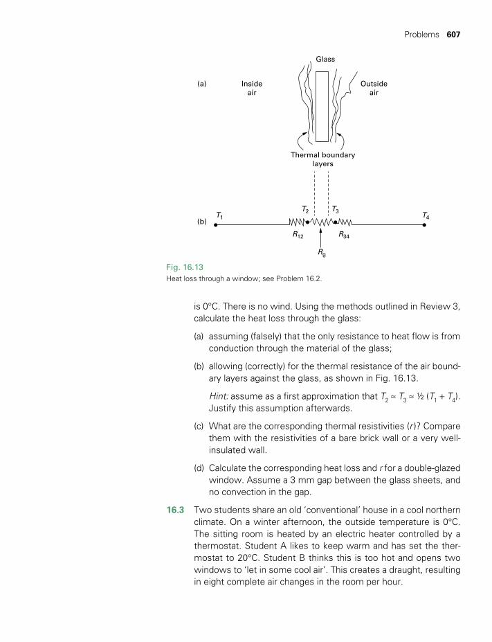
Problems 607
is 0°C. There is no wind. Using the methods outlined in Review 3, calculate the heat loss through the glass:
(a) assuming (falsely) that the only resistance to heat flow is from conduction through the material of the glass;
(b) allowing (correctly) for the thermal resistance of the air bound-ary layers against the glass, as shown in Fig. 16.13.
Hint: assume as a first approximation that T2 ≈ T3 ≈ ½ (T1 + T4). Justify this assumption afterwards.
(c) What are the corresponding thermal resistivities (r )? Compare them with the resistivities of a bare brick wall or a very well-insulated wall.
(d) Calculate the corresponding heat loss and r for a double-glazed window. Assume a 3 mm gap between the glass sheets, and no convection in the gap.
16.3 Two students share an old ‘conventional’ house in a cool northern climate. On a winter afternoon, the outside temperature is 0°C. The sitting room is heated by an electric heater controlled by a thermostat. Student A likes to keep warm and has set the ther-mostat to 20°C. Student B thinks this is too hot and opens two windows to ‘let in some cool air’. This creates a draught, resulting in eight complete air changes in the room per hour.
Glass
Insideair
T1T2
R12 R34
Rg
T3 T4
(a)
(b)
Outsideair
Thermal boundarylayers
Fig. 16.13 Heat loss through a window; see Problem 16.2.
TWIDELL PAGINATION.indb 607 01/12/2014 11:38

608 Using energy efficiently
(a) If the room measures 6 m × 4 m × 3 m, calculate the rate of heat loss from this draught.
(b) Calculate how much energy it would take to maintain the tem-perature at 20°C against this loss. If electricity costs 15 cents per kWh, how much money would this cost per hour?
*16.4 (a) In your country, what is a typical rated power for each of the following domestic appliances: (i) television set; (ii) refrigerator; (iii) ‘desk-top’ fan; (iv) air conditioner (per room serviced). (Hint: the rated power is usually listed on a manufacturer’s sticker some-where on the appliance.) (b) Estimate (or measure!) for how many hours per day each of these appliances runs at its rated power. (c) Comment on their relative energy use.
NOTES
1 The lumen is a unit measuring radiant power, as perceived by the human eye. (The energy from a light source in each wavelength band weighted by the average sensitivity of a human eye in that band.)
2 Further details at http://en.wikipedia.org/wiki/Hydrogen_production.3 Data in Harvey (2009) based on an IMO report of 2000.
BIBLIOGRAPHY
Books on energy management generally
Beggs, C. (2009, 2nd edn) Energy: Management, supply and conservation, Butterworth-Heinemann, London. Not too technical.
GEA (2012) Global Energy Assessment: Towards a more sustainable future, ed. T. Johansson, N. Nakicenovic, A. Patwardhan and L. Gomez-Echeverri, Cambridge University Press, Cambridge. Large-scale international review, including chapters on energy use in industry, transport, buildings and urban systems. Some chapters are avail-able online at www.globalenergyassessment.org.
Harvey D. (2010) Energy and the New Reality 1: Energy efficiency and the demand for energy services, Earthscan, London. Excellent overview, covering ‘energy basics’ and energy use in buildings, industry, transport, agriculture, etc. Most of the numbers used in §s16.5 and 16.6 are based on data collated in this book.
IEA (2011) Wade, P. and Brunner, C.V., Energy-Efficiency Policy Options for Electric Motor-Drive Systems, IEA Press, Paris.
Kreith, F. and Goswami, D.Y. (eds) (2007) Handbook of Energy Efficiency and Renewable Energy, CRC, London. Multi-author tome; slightly US focussed.
MacKay, D. (2009) Sustainable Energy – Without the Hot Air, UIT, Cambridge. Clearly relates familiar household services/energy uses to the national and global scale, using exemplary diagrams and order of magnitude calcula-tions. Full text available online at www. withouthotair.com.
REN21 (2012) Renewables Global Status Report 2012, Renewable Energy Network (REN21). Available online at www.ren21.org. Includes a special feature on the synergies between renewable energy and energy efficiency.
TWIDELL PAGINATION.indb 608 01/12/2014 11:38

Bibliography 609
Buildings
ASRAE (2006, 2nd edn) Green Guide: The design construction and operation of sustainable buildings, Butterworth-Heinemann, London. Terse reference book, intended to help an engineer decide ‘could this technology be useful on this project?’.
Baird, G. (2010) Sustainable Buildings in Practice: What the users think, Routledge, Abingdon. Case studies with focus on architecture and energy services to each building; many photos and plans.
Balcomb, J.D. (ed.) (1991) Passive Solar Buildings, MIT Press, Cambridge, MA. One of a series on ‘solar heat technologies’ summarizing US research in the 1970s and 1980s.
Eicker, U. (2003) Solar Technologies for Buildings, Wiley, New York. Translated from a German original of 2001. Includes chapters on solar heating and cooling, and on absorption cooling.
Givoni, B. (1998) Climate Considerations in Building and Urban Design, Van Nostrand Reinhold, New York. A classic review by one of the modern pioneers in his field.
Griffiths, N. (2007) Eco-house Manual, Haynes Publishing, London. Full of stimulating good sense and practical advice for householders seeking to live sustainably. Particularly applicable for the UK.
Harvey, L.D. (2006) A Handbook of Low-energy Buildings and District Energy Systems: Fundamentals, techniques and examples, Earthscan, London. A technology compendium, which successfully explains how energy-saving technologies and an integrated approach can achieve large reductions in energy use without compromising on building comfort or services.
Mumovic, D. and Santamouris, M. (eds) (2009) A Handbook of Sustainable Building Design and Energy, Earthscan, London. Multi-author, readable level but still with good technical detail.
Nicholls, R. and Hall, K. (eds) (2008) Green Building Bible, Vol. 2, Green Building Press, Llandysul (www.green-building press.co.uk). Concentrates on the construction and renovation of buildings for energy efficiency and water conservation; excellent technical explanations and illustrations.
Salmon, C. (1999) Architectural Design for Tropical Regions, Wiley, New York. Includes selected climate profiles, climate and design considerations, and design guidelines.
Santamouris, M. (ed.) (2003) Solar Thermal Technologies for Buildings: The state of the art, James & James, London. Part of a series on buildings, energy and solar technology.
Snell, C. and Callahan, T. (2005) Building Green, Lark Books of Sterling Publishing, Ontario, Canada. Superbly illustrated for architects and builders, including self-build; of international application.
Szokolay, S. (2008, 2nd edn) Introduction to Architectural Science, Architectural Press/Elsevier, New York. Includes concise treatment of energy-efficient designs (often traditional) for a range of climates, along with many useful charts and tables.
Vale, B. and Vale, R. (2000) The New Autonomous House, Thames & Hudson, London. Design and construction of low-energy, solar-conscious and sustainable-materials housing, with specific UK examples. A serious study of a common subject.
Weiss, W. (ed.) (2003) Solar Heating Systems for Houses, James & James, London. One of a series of publi-cations emerging from the Solar Heating and Cooling Program of the International Energy Agency. This book focusses on combi-systems (i.e. the use of solar water heaters integrated with other heating for buildings).
TWIDELL PAGINATION.indb 609 01/12/2014 11:38
610 Using energy efficiently
Transport
Black, W.R. (2010) Sustainable Transportation: Problems and solutions, Guilford Press, New York. Very readable student-level text, though largely based on American data and thin on urban planning.
http://en.wikipedia.org/wiki/Alternative_fuel_vehicle. Useful source on alternative fuel vehicles, updated from time to time.
Historical
Fouquet, R. (2008) Heat Power and Light: Revolutions in energy services, Edward Elgar, Cheltenham. A tour de force of economic history, tracing costs and usage of energy services (heat, light, mechanical power, transport) in England from 1300 to 2000!
Personal
There are numerous books and even more websites with advice on how individuals can reduce their energy demand and with a more sustainable lifestyle (which necessarily includes reduced energy use). These are mostly aimed at those in ‘Western’ economies and include many typical (and sometimes surprising) numerical examples.
Goodall, C. (2007) How to Live a Low-carbon Life, Earthscan, London.
Vale, R. and Vale, B. (2009) Time to Eat the Dog? The real guide to sustainable living, Thames & Hudson, London.
Specific references
Boardman, B. (2010) Fixing Fuel Poverty, Earthscan, London. An authoritative text, most detail aimed at the UK but the principles apply internationally.
Chen, L. et al. (1999) ‘Effect of heat transfer law on the performance of a generalized irreversible Carnot engine’, Journal of Physics D: Applied Physics, 32, 99–105.
Fouquet, R. (2008) Heat Power and Light: Revolutions in energy services, Edward Elgar, Cheltenham.
Koomey, J. (2011) Growth in Data Center Electricity Use 2005 to 2010, Analytics Press, Oakland, CA. Available online at http://www. analyticspress.com/datacenters.html.
Synapse (2008) Costs and Benefits of Electric Utility Energy Efficiency in Massachusetts, Synapse Energy Economics for the (Massachusetts) North East Energy Efficiency Council. Available at www.synapse-energy.com/Downloads/SynapseReport.2008-08.0.MA-Electric-Utility-Energy-Efficiency.08-075.pdf.
Twidell, W., Johnstone, C., Zuhdy, B. and Scott, A. (1994) ‘Strathclyde University’s passive solar, low-energy, residences with transparent insulation’, Solar Energy, 52, 85–109.
Journals and websites
Some relevant technical journals include: Energy and Buildings, Energy Conversion and Management, International Journal of Sustainable Energy and Solar Energy. There are countless websites dealing with the topics of this chapter, some excellent and many of dubious aca-demic value. Use a search engine to locate these and give most credence to the sites of official organizations, as
TWIDELL PAGINATION.indb 610 01/12/2014 11:38

Bibliography 611
with the examples cited below. Useful search terms could include ‘energy use in buildings’, ‘sustainable cities’, etc.
American Council for an Energy Efficient Economy. www.aceee.org/. Includes many concrete hints, plus discus-sion of policies, and a set of further links.
Association of Environment Conscious Buildings (UK) www.aecb.net; literature and practical information.
Australian Green Development Forum. www.agdf.com.au/ showcase.asp. Formerly Australian Building Energy Council (http://www.netspeed.com.au/abeccs/). Case studies from Australia.
Interactive Database for Energy-efficient Architecture (IDEA). nesa1.uni-siegen.de/projekte/idea/idea_1_e.htm. Numerous case studies from Europe, both residential and commercial buildings.
International Solar Energy Society (ISES). www.ises.org. The largest, oldest, and most authoritative professional organization dealing with the technology and implementation of solar energy.
UK energy consumption statistics.www.decc.gov.uk/en/content/cms/statistics/publications/ecuk/ecuk.aspx.
TWIDELL PAGINATION.indb 611 01/12/2014 11:38
CHAPTER
17Institutional and economic factors
CONTENTS
Learning aims 612
§17.1 Introduction 614
§17.2 Socio-political factors 614§17.2.1 National energy policy 614§17.2.2 Developing countries 618§17.2.3 Role of the individual 619
§17.3 Economics 620§17.3.1 Basics 620
§17.4 Life cycle analysis 622
§17.5 Policy tools 623§17.5.1 Governmental policies 623§17.5.2 Governmental procedures 625
§17.6 Quantifying choice 626§17.6.1 Basic analysis 626§17.6.2 Discounted cash flow
(DCF) techniques: net present value 630
§17.7 Present status of renewable energy 635
§17.8 The way ahead 635
Chapter summary 641
Quick questions 642
Problems 642
Note 643
Bibliography 643
Box 17.1 Climate change projections and impacts 615
Box 17.2 External costs of energy 621
Box 17.3 Environmental impact assessment (EIA) matrix 625
Box 17.4 Some definitions 627
Box 17.5 Contrasting energy scenarios: ‘Business As Usual’ vs. ‘Energy Revolution’ 640
LEARNING AIMS
• Appreciate socio-economic factors for new energy developments.
• Understand varieties of economic and life-cycle analysis.
• Know policy tools for encouraging renewable energy.
• Understand discounted cash flows.• Know how modern renewables started and
are likely to continue.
TWIDELL PAGINATION.indb 612 01/12/2014 11:38
List of tables 613
LIST OF FIGURES
17.1 Projected temperature rises for a range of emission scenarios. 61617.2 Some examples of ‘learning curves’, showing the falling cost of renewable energy as usage
increases. 63817.3 Schematic cost curves for renewable energy, conventional (brown) energy (costed conventionally),
and brown energy including external (social) costs. 63917.4 Two illustrative scenarios to 2050 for the development of (a) energy demand, (b) CO2 emissions
from energy sources, (c) proportion of renewable energy (RE) in the global energy supply. 640
LIST OF TABLES
17.1 Some estimates of the external costs of electricity generation from coal or nuclear (in USc/kWh). 62217.2 Tabulation of environmental impacts of wind power. 62617.3 Present value of solar water heater factor in year n. 63217.4 Cost and benefit streams from a wind farm. 63417.5 Evolution of the technological, economic and political environment for ‘new’ renewable energy
systems. 637
TWIDELL PAGINATION.indb 613 01/12/2014 11:38

614 Institutional and economic factors
§17.1 INTRODUCTION
Previous chapters may have been given the impression that innovation and application depend only on science and engineering. However, such an opinion is extremely naïve; practical developments depend about 75% on ‘institutional factors’ and only about 25% on science and engineering. The ‘institutional factors’ are driven by politicians, planners, financiers, lawyers, social scientists, the media, the public and, because of ethical, religious and cultural values, artists, authors, theologians and philoso-phers. Scientists and engineers become more influential when they par-ticipate in these other areas.
Here, we review some of the socio-political and economic factors influencing energy systems. Usually the full external and societal costs of conventional energy are not included in its price (e.g. pollution, see Box 17.2), which biases choice against more sustainable energy systems, including renewables. Policy tools that redress this are explained. §17.6 outlines economic and accounting methods quantifying choice, including discounted cash flows. Finally we examine how the technological, socio-political and economic environment for renewable energy evolved and is still evolving. Renewables are growth sectors of economies, with the potential to supply sustainably most of the world’s energy from many millions of sites; this requires knowledge, vision, experience, finance, markets and choice, as based on good science and technology.
§17.2 SOCIO-POLITICAL FACTORS
Action within society depends on many factors, including culture, tradi-tions, political frameworks and financing. Such influences vary greatly and change with time; they also relate to the availability and awareness of technology.
§17.2.1 National energy policy
Socio-political factors influencing energy policy, especially for renewables, including, in approximate order of importance:
1 Energy security. Economies cannot function without reliable and con-tinuously available supplies of energy as fuels, heat and electricity. Imported energy supply is vulnerable to disruption by war, trade sanc-tions and price rises, as instanced historically many times. For instance, many countries import fuel oil costing 30% or more of GDP, making them economically vulnerable (§17.2.2). However, every country has its own distinctive set of renewable energy resources within its ter-ritorial boundaries; thus utilizing these to abate imported fossil fuels increases security of supply against hostile and market disruptions, and diversifies options.
TWIDELL PAGINATION.indb 614 01/12/2014 11:38
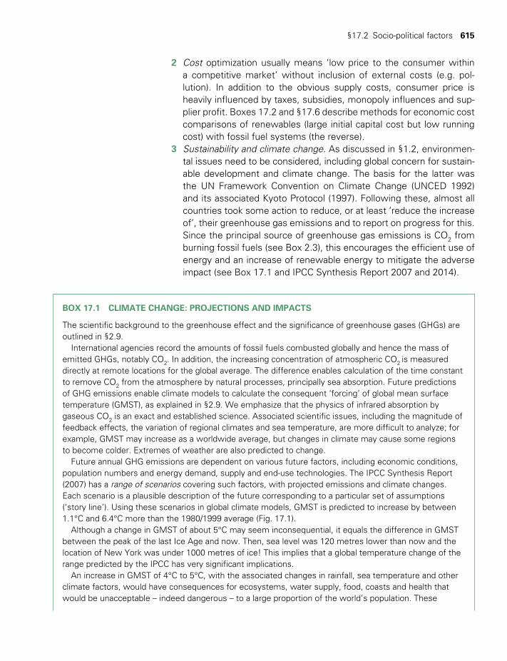
§17.2 Socio-political factors 615
2 Cost optimization usually means ‘low price to the consumer within a competitive market’ without inclusion of external costs (e.g. pol-lution). In addition to the obvious supply costs, consumer price is heavily influenced by taxes, subsidies, monopoly influences and sup-plier profit. Boxes 17.2 and §17.6 describe methods for economic cost comparisons of renewables (large initial capital cost but low running cost) with fossil fuel systems (the reverse).
3 Sustainability and climate change. As discussed in §1.2, environmen-tal issues need to be considered, including global concern for sustain-able development and climate change. The basis for the latter was the UN Framework Convention on Climate Change (UNCED 1992) and its associated Kyoto Protocol (1997). Following these, almost all countries took some action to reduce, or at least ‘reduce the increase of’, their greenhouse gas emissions and to report on progress for this. Since the principal source of greenhouse gas emissions is CO2 from burning fossil fuels (see Box 2.3), this encourages the efficient use of energy and an increase of renewable energy to mitigate the adverse impact (see Box 17.1 and IPCC Synthesis Report 2007 and 2014).
BOX 17.1 CLIMATE CHANGE: PROJECTIONS AND IMPACTS
The scientific background to the greenhouse effect and the significance of greenhouse gases (GHGs) are outlined in §2.9.
International agencies record the amounts of fossil fuels combusted globally and hence the mass of emitted GHGs, notably CO2. In addition, the increasing concentration of atmospheric CO2 is measured directly at remote locations for the global average. The difference enables calculation of the time constant to remove CO2 from the atmosphere by natural processes, principally sea absorption. Future predictions of GHG emissions enable climate models to calculate the consequent ‘forcing’ of global mean surface temperature (GMST), as explained in §2.9. We emphasize that the physics of infrared absorption by gaseous CO2 is an exact and established science. Associated scientific issues, including the magnitude of feedback effects, the variation of regional climates and sea temperature, are more difficult to analyze; for example, GMST may increase as a worldwide average, but changes in climate may cause some regions to become colder. Extremes of weather are also predicted to change.
Future annual GHG emissions are dependent on various future factors, including economic conditions, population numbers and energy demand, supply and end-use technologies. The IPCC Synthesis Report (2007) has a range of scenarios covering such factors, with projected emissions and climate changes. Each scenario is a plausible description of the future corresponding to a particular set of assumptions (‘story line’). Using these scenarios in global climate models, GMST is predicted to increase by between 1.1°C and 6.4°C more than the 1980/1999 average (Fig. 17.1).
Although a change in GMST of about 5°C may seem inconsequential, it equals the difference in GMST between the peak of the last Ice Age and now. Then, sea level was 120 metres lower than now and the location of New York was under 1000 metres of ice! This implies that a global temperature change of the range predicted by the IPCC has very significant implications.
An increase in GMST of 4°C to 5°C, with the associated changes in rainfall, sea temperature and other climate factors, would have consequences for ecosystems, water supply, food, coasts and health that would be unacceptable – indeed dangerous – to a large proportion of the world’s population. These
TWIDELL PAGINATION.indb 615 01/12/2014 11:38
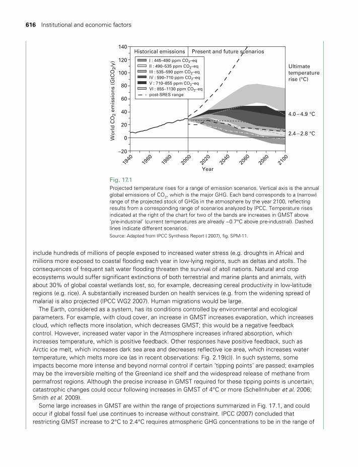
616 Institutional and economic factors
include hundreds of millions of people exposed to increased water stress (e.g. droughts in Africa) and millions more exposed to coastal flooding each year in low-lying regions, such as deltas and atolls. The consequences of frequent salt water flooding threaten the survival of atoll nations. Natural and crop ecosystems would suffer significant extinctions of both terrestrial and marine plants and animals, with about 30% of global coastal wetlands lost, so, for example, decreasing cereal productivity in low-latitude regions (e.g. rice). A substantially increased burden on health services (e.g. from the widening spread of malaria) is also projected (IPCC WG2 2007). Human migrations would be large.
The Earth, considered as a system, has its conditions controlled by environmental and ecological parameters. For example, with cloud cover, an increase in GMST increases evaporation, which increases cloud, which reflects more insolation, which decreases GMST; this would be a negative feedback control. However, increased water vapor in the Atmosphere increases infrared absorption, which increases temperature, which is positive feedback. Other responses have positive feedback, such as Arctic ice melt, which increases dark sea area and decreases reflective ice area, which increases water temperature, which melts more ice (as in recent observations: Fig. 2.19(c)). In such systems, some impacts become more intense and beyond normal control if certain ‘tipping points’ are passed; examples may be the irreversible melting of the Greenland ice shelf and the widespread release of methane from permafrost regions. Although the precise increase in GMST required for these tipping points is uncertain, catastrophic changes could occur following increases in GMST of 4°C or more (Schellnhuber et al. 2006; Smith et al. 2009).
Some large increases in GMST are within the range of projections summarized in Fig. 17.1, and could occur if global fossil fuel use continues to increase without constraint. IPCC (2007) concluded that restricting GMST increase to 2°C to 2.4°C requires atmospheric GHG concentrations to be in the range of
140
120
100
Historical emissions Present and future scenarios
80
60
40
20
–20
1940
1960
1980
2000
2020
2040
2060
2080
2100
0
Year
Ultimatetemperaturerise (°C)
4.0 – 4.9 °C
2.4 – 2.8 °C
Wo
rld
CO
2 em
issi
on
s (G
tCO
2/y)
I : 445–490 ppm CO2–eq II : 490–535 ppm CO2–eq III : 535–590 ppm CO2–eq IV : 590–710 ppm CO2–eq V : 710–855 ppm CO2–eq VI : 855–1130 ppm CO2–eq post-SRES range
Fig. 17.1Projected temperature rises for a range of emission scenarios. Vertical axis is the annual global emissions of CO2, which is the major GHG. Each band corresponds to a (narrow) range of the projected stock of GHGs in the atmosphere by the year 2100, reflecting results from a corresponding range of scenarios analyzed by IPCC. Temperature rises indicated at the right of the chart for two of the bands are increases in GMST above ‘pre-industrial’ (current temperatures are already ~0.7°C above pre-industrial). Dashed lines indicate different scenarios.Source: Adapted from IPCC Synthesis Report ( 2007), fig. SPM-11.
TWIDELL PAGINATION.indb 616 01/12/2014 11:38
§17.2 Socio-political factors 617
4 Health and safety. Like other energy installations, such as nuclear power stations, oil refineries and high-voltage transmission lines, renewable energy installations can be dangerous, with recognizable difficulty in maintaining safety at the many and dispersed locations. Working near rotating machinery and electrical power systems, climb-ing structures and handling combustible materials present dangers. In practice, many renewable installations have relatively small-scale operations, so personnel are involved in many varied tasks. Although these provide interesting and responsible work, such variation pre-sents dangers.
Pollution may be defined as negative impacts, usually chemical emis-sions, not present in the natural environment. Fossil and nuclear energy processes (brown energy: Chapter 1) concentrate and then emit chemicals and ionizing radiation as pollution. The precursors of this pollution were already present in the primary materials, which were, however, ‘safe’ underground. In general, renewables (whose energy derives from natural energy flows) avoid the widespread pol-lution hazards to health associated with brown energy supplies. An exception is incomplete combustion of biomass, which is common from burning firewood or in poorly regulated machines using biofuels (see §10.10).
5 Vested interests. A potent political factor in many countries is the legacy of fossil fuel and nuclear industries, which seek to protect their assets and preserve their dominance in the energy infrastructure. The money from this ‘energy industrial complex’ of motor vehicle companies, coal industries, unenlightened utilities, and oil and gas companies has obscured the ecological truth of the situation we are in, and has undermined our ability to engineer the smart policies needed to establish sustainable energy supplies.
6 Economic conditions. The relatively large capital costs and initial loans for renewables require relatively long payback periods (often 10 to 15 years and more). Economic uncertainty, such as the ‘Global Financial Crisis’ of 2008, discourages potential investors; however, settled economies, with small rates of inflation and of loan interest, favor such capital investment. Policy tools available to governments include legislation to shape the structure of energy markets and planning pro-cedures (§17.5).
445 to 490 ppm CO2-eq. This requires global emissions of CO2: (i) to decrease by 50 to 85% from those in 2000 by 2050; and (ii) to begin to decrease no later than 2015, as indicated in Fig. 17.1. Such decreases in related fossil fuel use require a huge, but possible, expansion of renewable energy.
TWIDELL PAGINATION.indb 617 01/12/2014 11:38

618 Institutional and economic factors
§17.2.2 Developing countries
The factors outlined above are important for policy everywhere; however, some extra societal and institutional factors apply to developing coun-tries. Developing countries have no historical inheritance of large-scale established energy infrastructures (e.g. national electricity grids), nor the economic and technical support to immediately establish and maintain such an infrastructure. Energy supplies tend to be installed primarily in the major cities as contrasted with the rural areas, yet even in the cities, supply may be irregular and unable to meet demand. For example, sub-Saharan Africa (excluding RSA) with a population of around 800 million currently generates about as much electricity as Switzerland that has a population of 8 million. Thus, although national consumption of commer-cial energy may be relatively small on a per capita basis, potential and projected growth in energy consumption raises issues of economic and ecological sustainability, as considered in Chapter 1. The cost of imported fuel can be a significant macroeconomic constraint. Government subsi-dies reducing the price of fossil fuels to consumers probably decrease expenditure on health, education and rural development. A sustainable path to the future with renewable energy and energy efficiency should alleviate many such difficulties in the longer term.
Usually, a large proportion of the population live in rural communi -ties needing improved energy supply (e.g. because of inefficient fuel-wood and lighting). Often the women in rural villages walk many miles every day to fetch water and firewood. Such ‘energy poverty’ handi-caps the provision of clean water, telecommunications and home study. This perpetuates social inequality and denies social and economic advancement.
The potential small demand for electricity from rural and island house-holds often does not justify governments paying the cost of grid electrifica-tion for essential services, such as lights, television, radio and appliances (e.g. hand tools, sewing machines and water pumps). However, appro-priate renewable energy supplies can usually provide these services if combined with energy-efficient devices. Photovoltaic power is almost always applicable (§5.7), with small wind (§8.8.6) and hydro (§6.6) tur-bines most beneficial if local conditions are favorable. Diesel generators fueled by biofuels are also possible, but not (yet) common. Microfinancing arrangements provide low-interest loans to spread the cost over time; repayment is usually met by savings on purchased fuels (e.g. kerosene), and earnings on business activities powered by the new renewables power supply (e.g. machine tools and sewing machines). It is important to appreciate that the worldwide increase of micro-generation with grid connection encourages similar scale technology with battery storage replacing the grid.
TWIDELL PAGINATION.indb 618 01/12/2014 11:38

§17.2 Socio-political factors 619
§17.2.3 Role of the individual
The rise of renewables since the ‘oil crisis’ of 1973 (when the Organisation of Petroleum Exporting Countries (OPEC) drastically curtailed fuel exports for political reasons) owes much to actions by individuals and small communities seeking independence and creativity for their own energy supply from fledgling renewables. Much of their aspiration related to the use of appropriate and intermediate technology, which was foreseen to benefit both the ‘overdeveloped’ and ‘underdeveloped’ world. Over the next 10 years their ideas and successes permeated upward through society, becoming strong influences in universities, wider communities and emerging technology. This was helped by collective action through the strengthening and initiation of professional and trade associations, and through specialist publications and journals. Thus, by the late 1980s, large companies and governments were becoming seriously involved. This growth blended in the 1990s with the need to abate the use of fossil fuels because of their GHG emissions, so that by 2000 the great majority of governments (especially including those in the European Union) had targeted policies to promote renewables; nevertheless, many govern-ments still maintain policies assisting the production of brown energy. By 2010, it was apparent in most countries that modern renewables are ‘here to stay’.
Yet the work and role of the individual and small organizations are still vital. Technologies are available for individuals, small businesses, coop-eratives and communities to produce and/or purchase all their energy needs from renewables. Many are able to export excess, especially elec-tricity, and all are likely to increase their efficiency of energy use. Such ‘self-sufficiency and independence’ usually provide significant long-term cost savings, especially where governments provide incentives (e.g. subsidies and feed-in tariffs). These ‘informed citizens’ can have zero and negative carbon footprints, can ease their concern about fossil and nuclear fuels, can raise their morale and can give themselves greater security for the future.
Experience shows that such sustainability is helped by the following:
• Measuring and monitoring resource use, so enumerating carbon foot-print; the mere act of monitoring with feedback of information almost always leads to less resource (e.g. electricity) being used; with the saving of ~10% justifying the necessary instrumentation and effort.
• Using energy-efficient appliances and, especially, improving the energy efficiency of homes and businesses.
• Traveling by public transport, bicycling and walking.• Choosing low-consumption vehicles, including those with electric and
biofuel engines.• Limiting air travel and using electronic communications (e.g. via the
internet).
TWIDELL PAGINATION.indb 619 01/12/2014 11:38
620 Institutional and economic factors
• Steadily using financial savings to increase investment in renewables (e.g. biomass-burning stoves and boilers, micro-generation, building insulation, LED lighting, electric car, membership of self-help energy cooperatives, etc.).
• Joining appropriate local and national groups, not least to continue ‘bottom-up’ lobbying on governments.
• Exporting and selling excess micro-generated electricity and fuels, so subtracting carbon footprint.
§17.3 ECONOMICS
§17.3.1 Basics
Economics seeks to analyze and develop tools for individuals, organi-zations and governments to make rational decisions about their allo-cation of scarce resources. The dominant parameter used is money, with all actions having both costs and benefits; the evaluations seek to find which of several alternative choices, including the status quo, has the most favorable balance. Several questions immediately arise in the context of renewable energy systems:
1 Whose financial costs and benefits are to be assessed: the owners, the end-users or those of the nation or the world as a whole? For example, the actual costs of damage from pollution emitted by a cen-tralized coal-burning electricity power station (corrosion from acid rain, climate change from greenhouse gases, cleaning contaminated efflu-ents, etc.) are mostly not included in the internal financial accounts of the electricity-generating company or its customers, but are paid by others. These are called ‘external’ costs, as described in Box 17.2 concerning energy. Moreover, there are other unwanted effects of emissions (e.g. loss of biodiversity) which may not be identifiable in any financial accounting. In contrast, photovoltaic power produces no emissions and has low external costs. If the PV power substitutes for the use of coal, then real savings are made in society; yet these savings may not accrue to the PV generator whose financial challenge is to pay for the capital costs of the PV system. This comparison favors the fossil fuel power station because its external costs are not included.
There is much controversy about how to put a monetary value on many of the factors relevant to renewable energy sources, such as having a cleaner environment than otherwise. Because such factors have been hard to quantify, they have often been left out of account, to the detriment of those promoting renewable energy systems.
2 Which parameters or systems should be assessed: the primary energy sources or the end-use service? For example, householders
TWIDELL PAGINATION.indb 620 01/12/2014 11:38
§17.3 Economics 621
lighting their houses at night are interested in the cost and amount of illumination rather than energy as such. The cost of a clock battery is never considered in terms of Wh delivered, but always in terms of the service provided to know the time.
3 Where does the assessment apply? The costs of installed renewable energy systems (RES) are site-specific. Since they are designed to tap into existing natural flows of energy (Chapter 1), it is obvious that a particular RES will be favorable where the appropriate flow already exists, and unfavorable otherwise. Thus hydroelectric systems are only practical and economically viable where there is sufficient flow of water. The cost of a biomass-based system depends on the avail-ability and cost of the biomass; if this is already on site as waste, as in a sugar cane mill (Box 9.2), the operation is much cheaper than when biomass has to be purchased and transported to site.
4 When are the costs and benefits to be assessed? Renewable energy systems generally have small operational costs and large initial, capital, cost. Fossil fuel plant has the reverse, especially if there is no emissions prevention. Economists have developed tools for combin-ing future and continuing known costs with initial costs, as discussed in §17.6.
From a longer term economic perspective, a critical question is: what extra cost should be attributed to the use now of a resource which may become severely limited for future generations? There are as yet no agreed answers.
Varying the points of reference (1) to (4) gives very different answers to the question of whether a particular renewable energy system is ‘eco-nomic’. As one economics professor is reported to have said (when challenged about repeating identical examination questions from year to year): ‘In economics, it’s the answers that change each year, not the questions!’
BOX 17.2 EXTERNAL COSTS OF ENERGY
External costs are actual and real costs resulting from a process, but which are not included in the price of the product and therefore have to be paid by the public. Electricity generation from coal or nuclear can have significant external costs. For example, burning high-sulphur coal produces SO2 emissions, which give ‘acid rain’, which causes damage to forests, metal structures and heritage stone buildings. Particulate emissions can cause lung diseases. The costs of disposal and long-term storage of nuclear waste are usually a significant external cost (since in practice significant costs are paid by subsequent governments from general taxation and not from the sale of electricity), as are the research and development costs of reactors (which in many countries drew on defense and research budgets). Using motor vehicles similarly has major external costs, arising from climate change, smog, the productive land ‘lost’ to roads, and the health and productivity losses caused by injuries and deaths in road accidents.
In the early 1990s there were several large studies that attempted to evaluate numerically such externalities, especially in electricity production. Some indicative results are shown in Table 17.1. The
TWIDELL PAGINATION.indb 621 01/12/2014 11:38
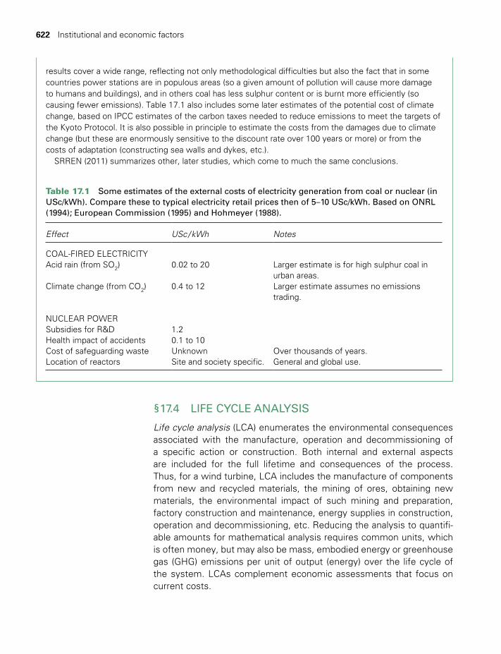
622 Institutional and economic factors
§17.4 LIFE CYCLE ANALYSIS
Life cycle analysis (LCA) enumerates the environmental consequences associated with the manufacture, operation and decommissioning of a specific action or construction. Both internal and external aspects are included for the full lifetime and consequences of the process. Thus, for a wind turbine, LCA includes the manufacture of components from new and recycled materials, the mining of ores, obtaining new materials, the environmental impact of such mining and preparation, factory construction and maintenance, energy supplies in construction, operation and decommissioning, etc. Reducing the analysis to quantifi-able amounts for mathematical analysis requires common units, which is often money, but may also be mass, embodied energy or greenhouse gas (GHG) emissions per unit of output (energy) over the life cycle of the system. LCAs complement economic assessments that focus on current costs.
results cover a wide range, reflecting not only methodological difficulties but also the fact that in some countries power stations are in populous areas (so a given amount of pollution will cause more damage to humans and buildings), and in others coal has less sulphur content or is burnt more efficiently (so causing fewer emissions). Table 17.1 also includes some later estimates of the potential cost of climate change, based on IPCC estimates of the carbon taxes needed to reduce emissions to meet the targets of the Kyoto Protocol. It is also possible in principle to estimate the costs from the damages due to climate change (but these are enormously sensitive to the discount rate over 100 years or more) or from the costs of adaptation (constructing sea walls and dykes, etc.).
SRREN (2011) summarizes other, later studies, which come to much the same conclusions.
Table 17.1 Some estimates of the external costs of electricity generation from coal or nuclear (in USc/kWh). Compare these to typical electricity retail prices then of 5–10 USc/kWh. Based on ONRL (1994); European Commission (1995) and Hohmeyer (1988).
Effect USc / kWh Notes
COAL-FIRED ELECTRICITYAcid rain (from SO2) 0.02 to 20 Larger estimate is for high sulphur coal in
urban areas.Climate change (from CO2) 0.4 to 12 Larger estimate assumes no emissions
trading.
NUCLEAR POWERSubsidies for R&D 1.2Health impact of accidents 0.1 to 10Cost of safeguarding waste Unknown Over thousands of years.Location of reactors Site and society specific. General and global use.
TWIDELL PAGINATION.indb 622 01/12/2014 11:38

§17.5 Policy tools 623
The full extent of the factors to take into account is enormous, but the ‘per unit’ impact becomes less, the further removed the factor. In practice, only significant influences are included, but usually there is debate about what these are and how they are valued and quantified; for example, (a) visual impact, assessed perhaps by change in local house prices, or (b) employment, assessed perhaps by changes in government payments to the ‘unemployed’. A particular difficulty for finite resources is to assess the value of not using them, since leaving the resource underground abates pollution, and yet the resource could be used by future genera-tions. For renewables, the difficulty is how to assess the implications of the natural variability of the resource (e.g. for wind power being absent on windless days1). Assumptions and changing characteristics of the background energy system (e.g. its carbon intensity) affect LCAs of most RE technologies, since their life cycle impacts stem almost entirely from component manufacturing. Further challenges include the potential for double-counting when assessing large interconnected energy systems, and system boundary problems.
Chart D3 in Appendix D shows estimates of life cycle GHG emis-sions (g CO2eq /kWh) for broad categories of electricity generation tech-nologies, including both ‘green’ and ‘brown’ technologies. Two features stand out: (a) GHG emissions from fossil fuel systems are greater by an order of magnitude than those from any renewable systems; neverthe-less, it is important to quantify the difference. (b) For each technology, the estimates cover a wide range because of the issues raised in the previous paragraph and because of different technological characteristics (e.g. design, capacity factor, variability, service lifetime and vintage, geo-graphic location, background energy system characteristics, data source, LCA technique, co-product allocation, avoided emissions, and system boundaries). Economics is not an exact science!
§17.5 POLICY TOOLS
Table 17.1 indicates that the external costs of non-renewables electricity generation from fossil and nuclear fuels are in the ballpark of prices of electricity charged to the consumer, i.e. internalizing them would perhaps double the consumer price. Consequently, not internalizing externalities does not fully encourage consumers to use electricity efficiently and does not encourage utilities to generate from renewables.
§17.5.1 Governmental policies
Governments use various policy tools. We consider three ‘methods’ here. Method 1: external costs are included by non-renewables gen-erators in their prices. Method 2: (a) subsidies are given to renewables
TWIDELL PAGINATION.indb 623 01/12/2014 11:38
624 Institutional and economic factors
generators; also (b) subsidies may be removed from non-renewables. Method 3: grants are awarded. Examples are as follows:
1 Technological removal of the pollutant: Method 1. Fossil fuel genera-tors may pay for the extraction of pollution at source, so reducing the external costs. This internalizes the external cost and raises the con-sumer price. For example, in many countries legislation compelling ‘flue gas desulphurization’ has significantly reduced SO2 emissions and hence ‘acid rain’. Market competition for electricity benefits the generator that removes the pollution at least cost.
2 Environmental taxes: Method 1. Imposing a carbon tax on fossil fuel electricity generation and perhaps using the revenue to subsidize renewables. The subsidy is in effect a payment to renewables for abating the pollution. Difficulties include: (a) determining an appropri-ate numerical charge, given the ranges in Table 17.1; (b) reluctance of consumers (voters) to pay more; (c) international business competi-tiveness if some countries have a carbon tax and others do not; (d) if the charge is too small, the pollution continues.
3 Tradable emission permits (certificates): Method 1. Government gives permits as certificates to industry for target amounts of their pollution, with the total reducing each year. These certificates are returned to a central agency as the pollution is emitted. An industry that pollutes beyond its permitted target either pays a fine to government or pur-chases spare permits from industries that have managed to reduce their pollution and so have spare permits to sell.
4 Removal of subsidies to polluting sources: Method 2b. In many coun-tries, electricity generation from fossil fuels and/or nuclear power is subsidized for societal reasons (e.g. by tax reductions or grants). Decreasing these subsidies reduces a barrier to renewables. The social objectives may then be met through welfare payments.
5 Subsidies to renewable: Method 2a. Time-limited subsidies aim to increase the market for renewables, so allowing trade to grow and mature, while at the same time recognizing that these renewables abate polluting generation. Mechanisms include: (i) tax concessions for renewable energy generators, as often used in the USA; (ii) legislation obligating utilities that a certain proportion of electricity generation has to be supplied from renewables (e.g. the UK and Australia), for instance, by competitive tendering so least-cost renewables are preferentially adopted, and/or a mechanism to provide a maximum ‘ceiling’ price; (iii) feed-in tariffs allow renewables generators to be paid increased amounts for electricity exported to the grid and gener-ated for themselves; utilities are obliged to cooperate and the method is administratively straightforward.
6 Public research and development grants: Method 3. In common with most innovation, companies and research organizations are awarded
TWIDELL PAGINATION.indb 624 01/12/2014 11:38
§17.5 Policy tools 625
grants for renewables research, development and demonstration. Helpful for renewables in the 1970s to 1980s, this measure proved insufficient to overcome the institutional and financial biases against renewables (see §17.8).
Such mechanisms promote a ‘learning curve’ for establishing renewables technology (§17.6). Our examples all refer to electricity generation, but related mechanisms exist for biofuels in transportation, and for energy-efficient buildings. A mix of policies is generally needed to address the various barriers to RE. There is no ‘one-size-fits-all’ policy suitable for all countries at all times. The extensive review by IPCC SRREN (2011) shows that different policies or combinations of policies can be more effective and efficient depending on factors such as the level of techno-logical maturity, availability of affordable capital, and the local and national RE resource base.
§17.5.2 Governmental procedures
Legislation. All governments have laws about energy supply. These laws should regulate security, diversity, costs, safety, market structure and some environmental impacts.
Planning procedures. Governments establish planning legislation and procedures, which vary greatly between nations and states. Although it may involve itself closely in large and influential developments (e.g. large-scale hydropower and offshore wind power), the decisions about medium and small developments tend to reside with local government. These days, an important part of planning procedures is consideration of an Environmental Impact Assessment (Box 17.3). Democratic rights may give individual citizens considerable influence within planning pro-cedures, but usually only to present arguments to the decision-makers.
BOX 17.3 ENVIRONMENTAL IMPACT ASSESSMENT (EIA) MATRIX
In practice, an EIA will relate to national and local environmental laws and regulations, which vary greatly from one jurisdiction to another, but usually require much detail. Here we simply categorize key impacts in a matrix, using wind power as an example.
Impacts may be positive or negative, or may be neutral.Table 17.2 shows a 3 x 4 matrix of factors, with one ‘axis’ for the scale of the impact (Global
~100,000 km, Regional ~200 km, Local ~500 m), and the other axis for the type of impact (chemical, physical, ecological and ‘emotional’). These categories are obvious, apart from ‘emotional’, which covers personal and psychological responses from individuals made because of their own feelings and personal opinions. Into each of the 12 categories is entered the relevant impacts for the particular technology. Table 17.2 shows these for wind power.
Note how such an analysis sets positive factors (e.g. energy security) alongside negative factors (e.g. acoustic noise). All too often, positive factors are underrated as anger takes over about the negative.
TWIDELL PAGINATION.indb 625 01/12/2014 11:38
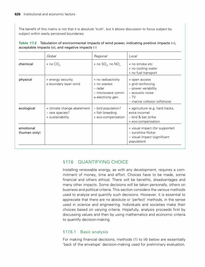
626 Institutional and economic factors
§17.6 QUANTIFYING CHOICE
Installing renewable energy, as with any development, requires a com-mitment of money, time and effort. Choices have to be made, some financial and others ethical. There will be benefits, disadvantages and many other impacts. Some decisions will be taken personally, others on business and political criteria. This section considers the various methods used to analyze and quantify such decisions. However, it is essential to appreciate that there are no absolute or ‘perfect’ methods, in the sense used in science and engineering. Individuals and societies make their choices based on varying criteria. Hopefully, analysis proceeds first by discussing values and then by using mathematics and economic criteria to quantify decision-making.
§17.6.1 Basic analysis
For making financial decisions, methods (1) to (4) below are essentially ‘back of the envelope’ decision-making used for preliminary evaluation.
The benefit of this matrix is not that it is absolute ‘truth’, but it allows discussion to focus subject by subject within easily perceived boundaries.
Table 17.2 Tabulation of environmental impacts of wind power, indicating positive impacts (+), acceptable impacts (o), and negative impacts (-)
Global Regional Local
chemical + no CO2 + no SO2, no NO× + no smoke etc+ no cooling water+ no fuel transport
physical + energy securityo boundary layer wind
+ no radioactivity + no wastes − radar − microwave commo electricity gen.
+ open access+ grid reinforcing− power variability− acoustic noise− TV− marine collision (offshore)
ecological + climate change abatement− rare species?+ sustainability
− bird population?+ fish breeding+ eco-compensation
+ agriculture (e.g. hard tracks, extra income)− bird & bat strike+ eco-compensation
emotional (human only)
+ visual impact (for supporter)− sunshine flicker− visual impact (significant population)
TWIDELL PAGINATION.indb 626 01/12/2014 11:38

§17.6 Quantifying choice 627
Only if a project looks promising on those bases is it worth turning to the mathematically more sophisticated methods involving discounted cash flows as used by accountants and bankers. These latter techniques are always used for commercial-scale projects that require borrowing from a bank. Box 17.4 lists some definitions used in such analyses.
1 Gut-feel. Most personal and family decisions, and a surprising number of business and political choices, are taken because an indi-vidual or group reach a conclusion instinctively or after discussion. Usually, but not always, the consequences of failure are small, so other methods are needless. Having a vegetable garden or installing a wood-burning stove in a sitting room may be an example; but another
BOX 17.4 SOME DEFINITIONS
Developer: person or organization planning and coordinating a project (in this case, the supply and use of renewable energy).Discounted value: the worth of future financial transaction from the point of view of the present.Embodied energy (of a product or service, i.e. of a ‘good’): the total of commercial energy expended in all processes and supplies for a good, calculated per unit of that good. Note: By this definition sunshine onto crops is not part of embodied energy, but the heat of combustion of commercial biofuels is included.Energy payback (time): the embodied energy of energy-producing equipment divided by its annual energy production.Equity: funds in the ownership of the developer; usually obtained from shares sold to shareholders by a limited company. Loans are not equity, so project finance is the sum of equity and loans.External costs: actual and real costs resulting from a process, which are not included in the price of the product and so have to be paid by the public otherwise (e.g. acid rain from coal-burning power stations damaging metal structures). (See Box 17.2.) Footprint: the impact of an action (e.g. carbon footprint): the carbon emissions from fossil fuels arising by the action, usually per year.Inflation: a general decrease in the value of money (rise in prices), usually measured by a national average annual rate of inflation i.Internal costs: costs included in the price of a product or service.Levelized cost (e.g. for the production of electricity): the average cost of production per unit over the life of the system, allowing for discounting over time. Loan: money made available to a developer and requiring, usually, the payment of loan interest to the lender in addition to repayment of the sum borrowed. The contracts usually stipulate that, in the event of bankruptcy, loaned money has to be repaid as a priority over the interests of others (e.g. banks providing loans are repaid in preference to shareholders and suppliers of goods).Operation and maintenance costs (O&M): these may be fixed (e.g. ground rent, regular staff) or variable (e.g. replacement parts, contract staff).Price = cost + profit + taxes.Rate: in accounting, this means a proportion of money exchanged per time period, usually per year. Accountants and economists usually leave out the ‘per year’ (e.g. ‘interest rate of 5%’ means ‘5%/y’).Retail price index: a measure of inflation (or deflation) made by the periodic costing of a fixed set of common expenditures.
TWIDELL PAGINATION.indb 627 01/12/2014 11:38
628 Institutional and economic factors
was the decision in Paris to construct the Eiffel Tower. Satisfaction and pleasure are obtained, in addition to perceived benefit. Often, a ‘statement’ is made to the general public by the development (e.g. having photovoltaic modules on the entrance roof of a prestigious office as a mark of autonomy and sustainability). Such non-analytical decision-making may well be influenced by ethical opinion as ‘the right thing to do’.
2 Non-dimensional matrix analysis. Decide on n criteria or ‘values’ (e.g. price, noise, aesthetics, lifetime, etc.), each with weight wj (say, 1 to 10). Then assess each possibility by awarding a mark mj within each criterion. The total score for each possible choice is:
∑==
S w mj jj
n
1
(17.1)
Then accept the choice with the largest score, or reassess the weight-ings and criteria for a further score. Such non-dimensional methods are useful if the criteria cannot all have the same unit of account (e.g. happiness or money).
3 Capital payback time Tp. The first step is to decide the actual (internal-ized) money benefit per year, Bi, gained or saved (abated) by a project of capital cost C (e.g. a solar water heater substituting for (abating) purchased electricity). Then:
T C B/p i= (17.2)
This provides an initial criterion, usually leading to further discus-sion or analysis. Usually payback time is calculated by comparison with an alternative, including continuing with current practice. The ‘savings’ and ‘costs’ needed to calculate payback in (17.2) are the dif-ference between the two possible paths (as in Worked Example 17.1). Business may expect Tp of two years, whereas a private individual may accept 10 years.
4 Simple return on investment (simple rate of return) Rs. Expressed as a percentage per year, this is the inverse of payback time:
=R T1/s p (17.3)
For example: Tp of 10y gives Rs of 10% /y. However, there are more meaningful and ‘professional’ methods for calculating financial return, so use of Rs may be misleading.
5 External payback and benefit criteria. There may be other benefits or non-benefits (e.g. reduction in pollution) than actual internalized money gain or loss. It is entirely reasonable for the developer to include such non-monetary factors in choice, perhaps for ethical values alone or to proclaim a good example. If the factors can be quantified in monetary
TWIDELL PAGINATION.indb 628 01/12/2014 11:38
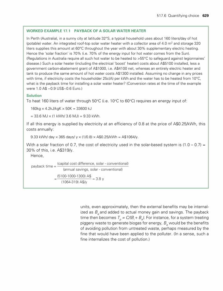
§17.6 Quantifying choice 629
units, even approximately, then the external benefits may be internal-ized as Be and added to actual money gain and savings. The payback time then becomes Tp = C/(Bi + Be). For instance, for a system treating piggery waste to generate biogas for energy, Be would be the benefits of avoiding pollution from untreated waste, perhaps measured by the fine that would have been applied to the polluter. (In a sense, such a fine internalizes the cost of pollution.)
WORKED EXAMPLE 17.1 PAYBACK OF A SOLAR WATER HEATER
In Perth (Australia), in a sunny city at latitude 32°S, a typical household uses about 160 liters/day of hot (potable) water. An integrated roof-top solar water heater with a collector area of 4.0 m2 and storage 320 liters supplies this amount at 60°C throughout the year with about 30% supplementary electric heating. Hence the ‘solar fraction’ is 70% (i.e. 70% of the energy input for hot water comes from the Sun). (Regulations in Australia require all such hot water to be heated to >55°C to safeguard against legionnaires’ disease.) Such a solar heater (including the electrical ‘boost’ heater) costs about A$5100 installed, less a government carbon-abatement grant of A$1000, i.e. A$4100 net, whereas an entirely electric heater and tank to produce the same amount of hot water costs A$1300 installed. Assuming no change in any prices with time, if electricity costs the householder 25c(A) per kWh and the water has to be heated from 10°C, what is the payback time for installing a solar water heater? (Conversion rates at the time of the example were 1.0 A$ ~0.9 US$~0.6 Euro.)
SolutionTo heat 160 liters of water through 50°C (i.e. 10°C to 60°C) requires an energy input of:
160kg × 4.2kJ/kgK × 50K = 33600 kJ
= 33.6 MJ × (1 kWh/ 3.6 MJ) = 9.33 kWh.
If all this energy is supplied by electricity at an efficiency of 0.8 at the price of A$0.25/kWh, this costs annually:
9.33 kWh/ day × 365 days/ y × (1/0.8) × A$0.25/kWh = A$1064/y.
With a solar fraction of 0.7, the cost of electricity used in the solar-based system is (1.0 – 0.7) = 30% of this, i.e. A$319/y.
Hence,
=
payback time =(capital cost difference, solar - conventional)
(annual savings, solar - conventional)
=(5100-1000-1300) A$
(1064-319) A$/y3.8 y
TWIDELL PAGINATION.indb 629 01/12/2014 11:38
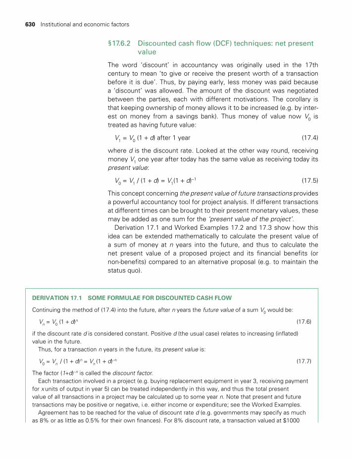
630 Institutional and economic factors
§17.6.2 Discounted cash flow (DCF) techniques: net present value
The word ‘discount’ in accountancy was originally used in the 17th century to mean ‘to give or receive the present worth of a transaction before it is due’. Thus, by paying early, less money was paid because a ‘discount’ was allowed. The amount of the discount was negotiated between the parties, each with different motivations. The corollary is that keeping ownership of money allows it to be increased (e.g. by inter-est on money from a savings bank). Thus money of value now V0 is treated as having future value:
V1 = V0 (1 + d) after 1 year (17.4)
where d is the discount rate. Looked at the other way round, receiving money V1 one year after today has the same value as receiving today its present value:
V0 = V1 / (1 + d) = V1(1 + d)−1 (17.5)
This concept concerning the present value of future transactions provides a powerful accountancy tool for project analysis. If different transactions at different times can be brought to their present monetary values, these may be added as one sum for the ‘present value of the project’.
Derivation 17.1 and Worked Examples 17.2 and 17.3 show how this idea can be extended mathematically to calculate the present value of a sum of money at n years into the future, and thus to calculate the net present value of a proposed project and its financial benefits (or non-benefits) compared to an alternative proposal (e.g. to maintain the status quo).
DERIVATION 17.1 SOME FORMULAE FOR DISCOUNTED CASH FLOW
Continuing the method of (17.4) into the future, after n years the future value of a sum V0 would be:
Vn = V0 (1 + d)n (17.6)
if the discount rate d is considered constant. Positive d (the usual case) relates to increasing (inflated) value in the future.
Thus, for a transaction n years in the future, its present value is:
V0 = Vn / (1 + d)n = Vn (1 + d)−n (17.7)
The factor (1+d)−n is called the discount factor.Each transaction involved in a project (e.g. buying replacement equipment in year 3, receiving payment
for x units of output in year 5) can be treated independently in this way, and thus the total present value of all transactions in a project may be calculated up to some year n. Note that present and future transactions may be positive or negative, i.e. either income or expenditure; see the Worked Examples.
Agreement has to be reached for the value of discount rate d (e.g. governments may specify as much as 8% or as little as 0.5% for their own finances). For 8% discount rate, a transaction valued at $1000
TWIDELL PAGINATION.indb 630 01/12/2014 11:38
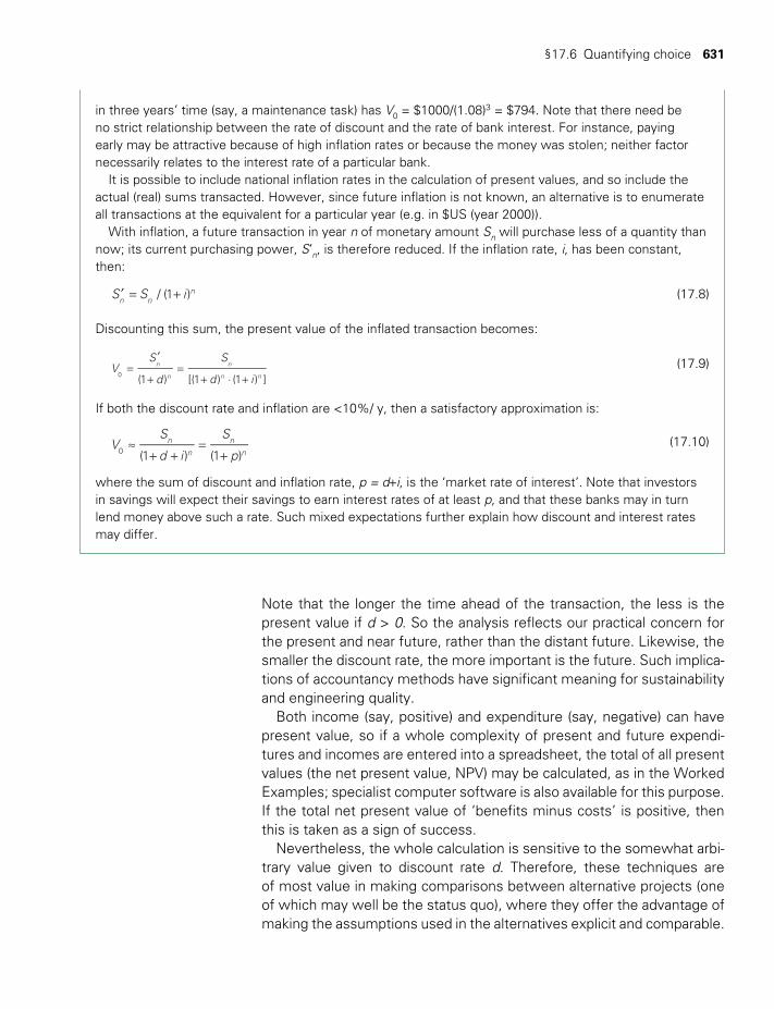
§17.6 Quantifying choice 631
Note that the longer the time ahead of the transaction, the less is the present value if d > 0. So the analysis reflects our practical concern for the present and near future, rather than the distant future. Likewise, the smaller the discount rate, the more important is the future. Such implica-tions of accountancy methods have significant meaning for sustainability and engineering quality.
Both income (say, positive) and expenditure (say, negative) can have present value, so if a whole complexity of present and future expendi-tures and incomes are entered into a spreadsheet, the total of all present values (the net present value, NPV) may be calculated, as in the Worked Examples; specialist computer software is also available for this purpose. If the total net present value of ‘benefits minus costs’ is positive, then this is taken as a sign of success.
Nevertheless, the whole calculation is sensitive to the somewhat arbi-trary value given to discount rate d. Therefore, these techniques are of most value in making comparisons between alternative projects (one of which may well be the status quo), where they offer the advantage of making the assumptions used in the alternatives explicit and comparable.
in three years’ time (say, a maintenance task) has V0 = $1000/(1.08)3 = $794. Note that there need be no strict relationship between the rate of discount and the rate of bank interest. For instance, paying early may be attractive because of high inflation rates or because the money was stolen; neither factor necessarily relates to the interest rate of a particular bank.
It is possible to include national inflation rates in the calculation of present values, and so include the actual (real) sums transacted. However, since future inflation is not known, an alternative is to enumerate all transactions at the equivalent for a particular year (e.g. in $US (year 2000)).
With inflation, a future transaction in year n of monetary amount Sn will purchase less of a quantity than now; its current purchasing power, S’n, is therefore reduced. If the inflation rate, i, has been constant, then:
′ = +S S i/ (1 )n nn (17.8)
Discounting this sum, the present value of the inflated transaction becomes:
VS
d
S
d i(1 ) [(1 ) (1 ) ]n
n
n
n n0=
′
+=
+ ⋅ + (17.9)
If both the discount rate and inflation are <10%/ y, then a satisfactory approximation is:
≈+ +
=+
VS
d i
S
p(1 ) (1 )n
n
n
n0 (17.10)
where the sum of discount and inflation rate, p = d+i, is the ‘market rate of interest’. Note that investors in savings will expect their savings to earn interest rates of at least p, and that these banks may in turn lend money above such a rate. Such mixed expectations further explain how discount and interest rates may differ.
TWIDELL PAGINATION.indb 631 01/12/2014 11:38
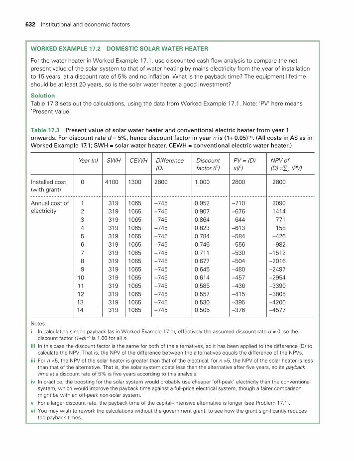
632 Institutional and economic factors
WORKED EXAMPLE 17.2 DOMESTIC SOLAR WATER HEATER
For the water heater in Worked Example 17.1, use discounted cash flow analysis to compare the net present value of the solar system to that of water heating by mains electricity from the year of installation to 15 years, at a discount rate of 5% and no inflation. What is the payback time? The equipment lifetime should be at least 20 years, so is the solar water heater a good investment?
SolutionTable 17.3 sets out the calculations, using the data from Worked Example 17.1. Note: ‘PV’ here means ‘Present Value’
Table 17.3 Present value of solar water heater and conventional electric heater from year 1 onwards. For discount rate d = 5%, hence discount factor in year n is (1+ 0.05)−n. (All costs in A$ as in Worked Example 17.1; SWH = solar water heater, CEWH = conventional electric water heater.)
Year (n) SWH CEWH Difference (D)
Discount factor (F)
PV = (D)x(F)
NPV of (D) =∑n (PV)
Installed cost (with grant)
0 4100 1300 2800 1.000 2800 2800
Annual cost of electricity
1 319 1065 −745 0.952 −710 20902 319 1065 −745 0.907 −676 14143 319 1065 −745 0.864 −644 7714 319 1065 −745 0.823 −613 1585 319 1065 −745 0.784 −584 −4266 319 1065 −745 0.746 −556 −9827 319 1065 −745 0.711 −530 −15128 319 1065 −745 0.677 −504 −20169 319 1065 −745 0.645 −480 −2497
10 319 1065 −745 0.614 −457 −295411 319 1065 −745 0.585 −436 −339012 319 1065 −745 0.557 −415 −380513 319 1065 −745 0.530 −395 −420014 319 1065 −745 0.505 −376 −4577
Notes:i In calculating simple payback (as in Worked Example 17.1), effectively the assumed discount rate d = 0, so the
discount factor (1+d) –n is 1.00 for all n.iii In this case the discount factor is the same for both of the alternatives, so it has been applied to the difference (D) to
calculate the NPV. That is, the NPV of the difference between the alternatives equals the difference of the NPVs. iii For n <5, the NPV of the solar heater is greater than that of the electrical; for n >5, the NPV of the solar heater is less
than that of the alternative. That is, the solar system costs less than the alternative after five years, so its payback time at a discount rate of 5% is five years according to this analysis.
iv In practice, the boosting for the solar system would probably use cheaper ‘off-peak’ electricity than the conventional system, which would improve the payback time against a full-price electrical system, though a fairer comparison might be with an off-peak non-solar system.
v For a larger discount rate, the payback time of the capital−intensive alternative is longer (see Problem 17.1).vi You may wish to rework the calculations without the government grant, to see how the grant significantly reduces
the payback times.
TWIDELL PAGINATION.indb 632 01/12/2014 11:38

§17.6 Quantifying choice 633
WORKED EXAMPLE 17.3 LEVELIZED COST OF A WIND FARM
A wind farm is located on an open plain in New South Wales (Australia). It comprises 10 turbines, each rated at 3.0 MW and with a cut-in speed of 4 m/s. The average wind speed at 10 m height is u = 6.0 m/s; the on-site capacity factor of the turbines is 0.22. For each turbine, the ex-factory cost is US$5.4 million and the cost of installation (including civil and electrical engineering) is US$1.1 million. Operation and maintenance costs are constant at US$150,000/y per turbine. (These costs exclude the cost of land.
Use discounted cash flow analysis for the following calculations.
a Calculate the average (‘levelized’) cost of production of electricity at the site for a discount rate of 5% and an assumed future life of the system of 20 years.
b Under the emissions trading regime agreed at installation, the generator receives credit for carbon dioxide saved at US$30/tCO2. What is now the effective cost of production?
c The farmers on whose grazing land the wind farm is constructed continue to graze their cows there. Three maintenance workers are employed on the cattle farm, and 100 extra visitors come per year to the district to view the installation. Discuss the ‘cost’ (actually the benefit) to the local region.
d A similar system is installed at another site where the wind is stronger (similar to Orkney, Scotland, see Fig. 7.7). The capacity factor there is 0.40. What is the cost of electricity generated under similar financial assumptions?
Solution
a A capacity factor of 0.22 means that each turbine produces a fraction 0.22 of what it would produce if run at full rating for a full year. Thus the electricity produced per year per turbine
= 3.0 MW × 8760 h/y × 0.22 = 5780 MWh/y
If this electricity is sold at q $/kWh, then the stream of costs and benefits from the system will be as shown in Table 17.4 with ready cost benefit of
(q$/kWh × 5780 MWh/y) × (103 kWh/MWh) × (1 M$/106$)
Therefore the levelized price at which the total benefits to the wind farm owners will match their total costs in present value terms after 20 years if
q = 8.313/69.87 = $0.119/kWh
Note that the price to consumers should be higher than this, to allow for some profit to the wind farm owners.
b For electricity produced from coal, Problem 17.4 shows that each kWh produced entails the emission of approximately 1.0 kg CO2. Therefore, the annual carbon credit from each turbine in this system is:
5800 MWh × (1.0 tCO2/MWh) × ($30/tCO2) = $173,000
This may be taken into account in Table 17.4 by subtracting this amount from the annual running cost (i.e. by replacing 0.15 by (0.15 − 0.173 = −0.023). By doing this, the PV of costs changes from $8.113m to $5.932m, and the cost per unit becomes:
q’ = 6.22/69.87 = $0.089 $/kWh.
c Since normal agricultural activity can continue underneath the turbines, rental charge for the facility is entirely a gain to the landholder. Consequently, land rental costs are substantially less than operation and maintenance costs, which are the principal annual running cost. If maintenance staff live locally, wages represent a benefit to the local community from the (extra) cash flow.
TWIDELL PAGINATION.indb 633 01/12/2014 11:38
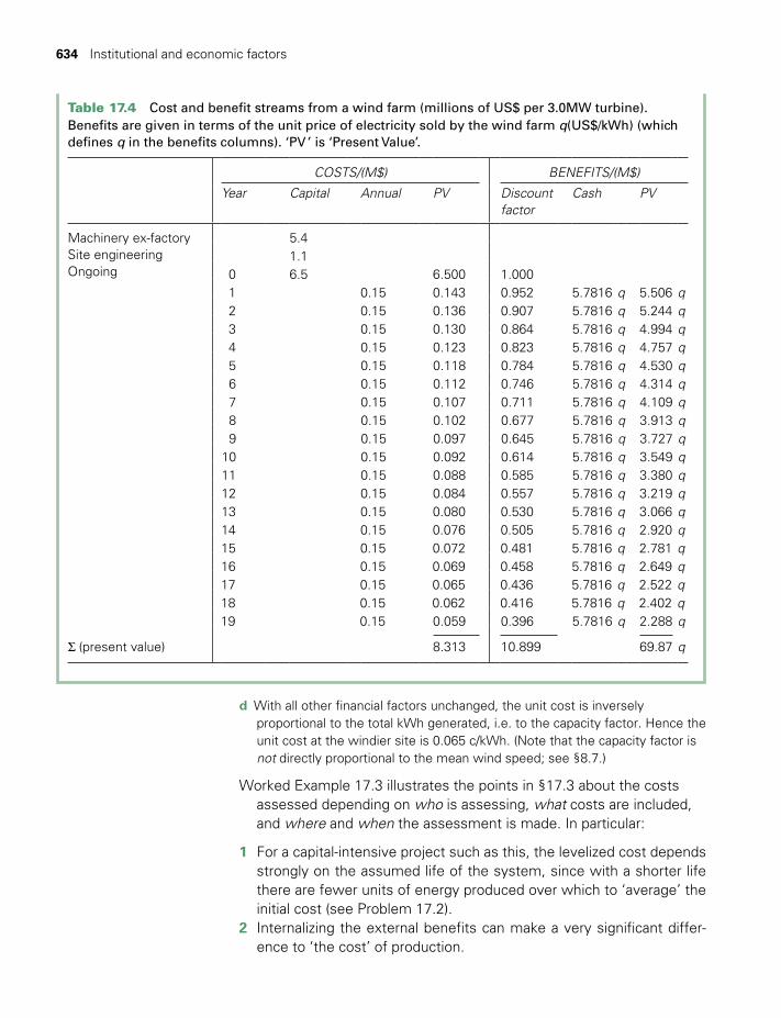
634 Institutional and economic factors
Table 17.4 Cost and benefit streams from a wind farm (millions of US$ per 3.0MW turbine). Benefits are given in terms of the unit price of electricity sold by the wind farm q(US$/kWh) (which defines q in the benefits columns). ‘PV ’ is ‘Present Value’.
COSTS/(M$) BENEFITS/(M$)
Year Capital Annual PV Discount factor
Cash PV
Machinery ex-factorySite engineeringOngoing
5.41.1
0 6.5 6.500 1.0001 0.15 0.143 0.952 5.7816 q 5.506 q2 0.15 0.136 0.907 5.7816 q 5.244 q3 0.15 0.130 0.864 5.7816 q 4.994 q4 0.15 0.123 0.823 5.7816 q 4.757 q5 0.15 0.118 0.784 5.7816 q 4.530 q6 0.15 0.112 0.746 5.7816 q 4.314 q7 0.15 0.107 0.711 5.7816 q 4.109 q8 0.15 0.102 0.677 5.7816 q 3.913 q9 0.15 0.097 0.645 5.7816 q 3.727 q
10 0.15 0.092 0.614 5.7816 q 3.549 q11 0.15 0.088 0.585 5.7816 q 3.380 q12 0.15 0.084 0.557 5.7816 q 3.219 q13 0.15 0.080 0.530 5.7816 q 3.066 q14 0.15 0.076 0.505 5.7816 q 2.920 q15 0.15 0.072 0.481 5.7816 q 2.781 q16 0.15 0.069 0.458 5.7816 q 2.649 q17 0.15 0.065 0.436 5.7816 q 2.522 q18 0.15 0.062 0.416 5.7816 q 2.402 q19 0.15 0.059 0.396 5.7816 q 2.288 q
Σ (present value) 8.313 10.899 69.87 q
d With all other financial factors unchanged, the unit cost is inversely proportional to the total kWh generated, i.e. to the capacity factor. Hence the unit cost at the windier site is 0.065 c/kWh. (Note that the capacity factor is not directly proportional to the mean wind speed; see §8.7.)
Worked Example 17.3 illustrates the points in §17.3 about the costs assessed depending on who is assessing, what costs are included, and where and when the assessment is made. In particular:
1 For a capital-intensive project such as this, the levelized cost depends strongly on the assumed life of the system, since with a shorter life there are fewer units of energy produced over which to ‘average’ the initial cost (see Problem 17.2).
2 Internalizing the external benefits can make a very significant differ-ence to ‘the cost’ of production.
TWIDELL PAGINATION.indb 634 01/12/2014 11:38
§17.8 The way ahead 635
3 A table like Table 17.3 is easily adapted to the situation where the annual costs vary significantly from year to year (e.g. if major components are replaced every five years).
§17.7 PRESENT STATUS OF RENEWABLE ENERGY
Renewable energy sources in 2012 accounted for about 13% of global primary energy supply, but by far the biggest portion of this was traditional biomass use (i.e. mainly firewood) in developing countries (10% of global TPES), followed by hydropower (2.3%). (See data in Part D2 of Appendix D.)
Global energy use continues to increase, driven by increasing population, and economic development, especially in the large developing countries of China, India and Brazil, associated with increasing industrialization. Global energy use rose at an average rate of 2.5% p.a. (compound) between 2000 and 2010. However, the increase in the use of renewable energy was much faster, especially that of ‘new renewables’, albeit from a low base: elec-tricity generation from wind, PV and geothermal for electricity (combined) grew at 12% p.a., and liquid biofuels increased at 20% pa (see Appendix D).
An encouraging indicator is that total new investment in renewables (including hydropower) has exceeded that in fossil fuel generation every year since 2008, and the excess is increasing; likewise the excess over nuclear power investment. Over the same period, the proportion of global investment in renewable power systems in developing countries (where the need is arguably greatest) increased from about 30% in 2007 to about 45% since 2007; the proportion for small (<1 MW) distributed capacity (mainly PV) has also increased from about 10% to about 30% (UNEP 2013).
The current state of technological maturity of the various technologies has been examined in earlier chapters of this book. A few RE technolo-gies (e.g. hydropower, and hydrothermal geothermal power) have been competing favorably with fossil fuel systems for decades. By 2013, wind power and concentrating solar power had become commercially viable without subsidies in favorable locations, and even more so where pref-erential payments are made, in effect for internalizing external costs of abated fossil fuels. A much wider range of RE technologies are available commercially year by year. (See Fig. D.5 in Appendix D, which compares a range of costs for renewable and fossil sources.) Most, however, need supporting policies that increase their scale of deployment, so benefit-ting from economies of scale and so decreasing cost. The aim every-where is sustainable energy systems (see §17.5 and §17.8).
§17.8 THE WAY AHEAD
The modern history of renewable energy systems, summarized in Table 17.5, shows their evolution in status. Apart from hydropower, 40 years
TWIDELL PAGINATION.indb 635 01/12/2014 11:38

636 Institutional and economic factors
ago most of these technologies were considered ‘small-scale curiosi-ties promoted by idealists’, but today modern renewables have become mainstream technologies, produced and operated by companies com-peting in an increasingly open market.
Overall, the global energy scene in the early 21st century is one of good news and bad news. The bad news is: (a) about 80% of the world’s energy use is from fossil fuels, hence forcing climate change and creat-ing a dependency that in the medium term is unsustainable; (b) 10% is based on scare firewood, often used inefficiently and hastening deforest-ation; (c) nuclear power from fission has no agreed method to dispose of high-level radioactive waste and is expensive where used and is banned in several countries; (d) nuclear fusion as a power source remains only a research aspiration. The good news is that renewable energy and the efficient use of energy are increasingly accepted as technically capable of providing the global population with sustainable heat, electricity and fuel in equitable and satisfactory lifestyles.
Implicit in Table 17.5 is the way in which the costs of energy from the more promising renewable energy technologies have steadily decreased. Fig. 17.2 illustrates this for the cases of wind power and photovoltaics. Such decreases in cost per unit of output are common as new technologies are developed from the stage of research prototypes to wide commercial use in a competitive environment. Curves like those shown in Fig. 17.2 are learning curves because they reflect how produc-ers learn by experience how to make the technology more reliable, more efficient, and users learn how to integrate the new technology into their practices; in this case into electricity grids.
In the case of renewable energy systems, much of this technological learning stems from R&D funded in the 1970s and 1980s, which has led to the technical developments described in earlier chapters, many of them involving new materials and microelectronic control (see Table 17.5). These have contributed to the ‘push’ for such modern technology. The realization that the substantial application of renewable energy systems produces a cleaner environment by the abatement of fossil and nuclear fuels has provided a matching ‘pull’. Political and economic measures to encourage wide take-up of a technology can have positive feedback: as more are used, the price comes down. This is due to ‘economies of scale’; for instance, the cost of designing and tooling up for a new wind turbine model is much the same whether 1 or 100 turbines are being produced, but if more are sold, the cost can be spread more thinly so that the price per unit is less, so more users find it ‘economic’. Consequently, yet more systems are brought into production, in turn driving further technical and economic improvement in a virtuous cycle.
The steadily improving technologies described in this book are needed urgently to bring renewables into the dominant position required to make global energy systems sustainable. Often it has taken about 25 years
TWIDELL PAGINATION.indb 636 01/12/2014 11:38
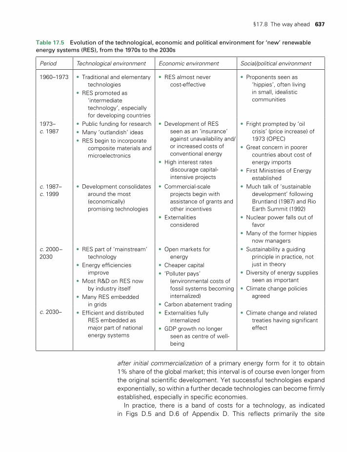
§17.8 The way ahead 637
after initial commercialization of a primary energy form for it to obtain 1% share of the global market; this interval is of course even longer from the original scientific development. Yet successful technologies expand exponentially, so within a further decade technologies can become firmly established, especially in specific economies.
In practice, there is a band of costs for a technology, as indicated in Figs D.5 and D.6 of Appendix D. This reflects primarily the site
Table 17.5 Evolution of the technological, economic and political environment for ‘new’ renewable energy systems (RES), from the 1970s to the 2030s
Period Technological environment Economic environment Social/political environment
1960–1973 • Traditional and elementary technologies
• RES promoted as ‘intermediate
technology’, especially for developing countries
• RES almost never cost-effective
• Proponents seen as ‘hippies’, often living
in small, idealistic communities
1973– c. 1987
• Public funding for research• Many ‘outlandish’ ideas• RES begin to incorporate
composite materials and microelectronics
• Development of RES seen as an ‘insurance’
against unavailability and/or increased costs of conventional energy
• High interest rates discourage capital-
intensive projects
• Fright prompted by ‘oil crisis’ (price increase) of
1973 (OPEC) • Great concern in poorer
countries about cost of energy imports
• First Ministries of Energy established
c. 1987– c. 1999
• Development consolidates around the most
(economically) promising technologies
• Commercial-scale projects begin with
assistance of grants and other incentives
• Externalities considered
• Much talk of ‘sustainable development’ following
Bruntland (1987) and Rio Earth Summit (1992)
• Nuclear power falls out of favor
• Many of the former hippies now managers
c. 2000 – 2030
• RES part of ‘mainstream’ technology
• Energy efficiencies improve
• Most R&D on RES now by industry itself
• Many RES embedded in grids
• Open markets for energy
• Cheaper capital• ‘Polluter pays’
(environmental costs of fossil systems becoming internalized)
• Carbon abatement trading
• Sustainability a guiding principle in practice, not
just in theory• Diversity of energy supplies
seen as important• Climate change policies
agreed
c. 2030– • Efficient and distributed RES embedded as
major part of national energy systems
• Externalities fully internalized
• GDP growth no longer seen as centre of well-
being
• Climate change and related treaties having significant
effect
TWIDELL PAGINATION.indb 637 01/12/2014 11:38
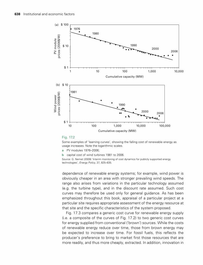
638 Institutional and economic factors
dependence of renewable energy systems; for example, wind power is obviously cheaper in an area with stronger prevailing wind speeds. The range also arises from variations in the particular technology assumed (e.g. the turbine type), and in the discount rate assumed. Such cost curves may therefore be used only for general guidance. As has been emphasized throughout this book, appraisal of a particular project at a particular site requires appropriate assessment of the energy resource at that site and the specific characteristics of the system proposed.
Fig. 17.3 compares a generic cost curve for renewable energy supply (i.e. a composite of the curves of Fig. 17.2) to two generic cost curves for energy supplied from conventional (‘brown’) sources. While the costs of renewable energy reduce over time, those from brown energy may be expected to increase over time. For fossil fuels, this reflects the producer’s preference to bring to market first those resources that are more readily, and thus more cheaply, extracted. In addition, innovation in
$ 1001976
1 10 100
Cumulative capacity (MW)
PV
mo
du
lep
rice
s (2
006$
/W)
1,000 10,000
1980
19902000
2006
$ 10
(a)
$ 1
$ 10(b)
$ 110 100
Cumulative capacity (MW)
Win
d p
ow
erp
rice
s (2
006$
/W)
1,000 10,000 100,000
1981
1990
2000 2006
Fig. 17.2Some examples of ‘learning curves’, showing the falling cost of renewable energy as usage increases. Note the logarithmic scales. a PV modules 1976–2006; b capital cost of wind turbines 1981 to 2006. Source: G. Nemet (2009) ‘Interim monitoring of cost dynamics for publicly supported energy technologies’, Energy Policy, 37, 825–835.
TWIDELL PAGINATION.indb 638 01/12/2014 11:38
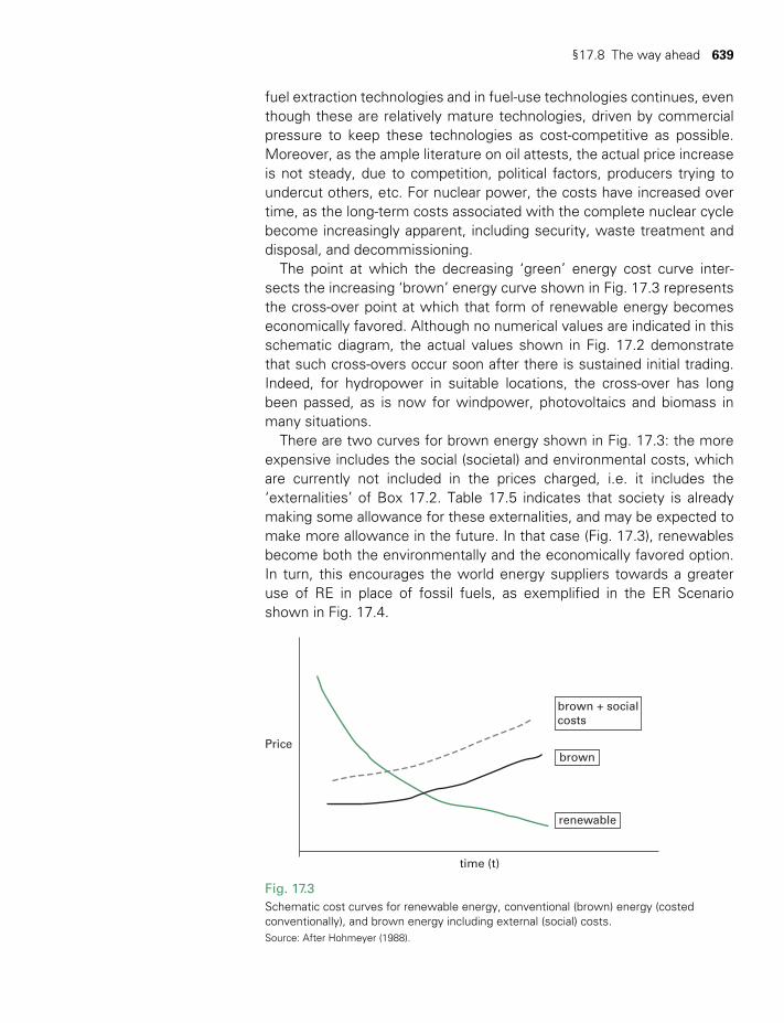
§17.8 The way ahead 639
fuel extraction technologies and in fuel-use technologies continues, even though these are relatively mature technologies, driven by commercial pressure to keep these technologies as cost-competitive as possible. Moreover, as the ample literature on oil attests, the actual price increase is not steady, due to competition, political factors, producers trying to undercut others, etc. For nuclear power, the costs have increased over time, as the long-term costs associated with the complete nuclear cycle become increasingly apparent, including security, waste treatment and disposal, and decommissioning.
The point at which the decreasing ‘green’ energy cost curve inter-sects the increasing ‘brown’ energy curve shown in Fig. 17.3 represents the cross-over point at which that form of renewable energy becomes economically favored. Although no numerical values are indicated in this schematic diagram, the actual values shown in Fig. 17.2 demonstrate that such cross-overs occur soon after there is sustained initial trading. Indeed, for hydropower in suitable locations, the cross-over has long been passed, as is now for windpower, photovoltaics and biomass in many situations.
There are two curves for brown energy shown in Fig. 17.3: the more expensive includes the social (societal) and environmental costs, which are currently not included in the prices charged, i.e. it includes the ‘externalities’ of Box 17.2. Table 17.5 indicates that society is already making some allowance for these externalities, and may be expected to make more allowance in the future. In that case (Fig. 17.3), renewables become both the environmentally and the economically favored option. In turn, this encourages the world energy suppliers towards a greater use of RE in place of fossil fuels, as exemplified in the ER Scenario shown in Fig. 17.4.
Price
time (t)
brown + socialcosts
brown
renewable
Fig. 17.3Schematic cost curves for renewable energy, conventional (brown) energy (costed conventionally), and brown energy including external (social) costs. Source: After Hohmeyer (1988).
TWIDELL PAGINATION.indb 639 01/12/2014 11:38
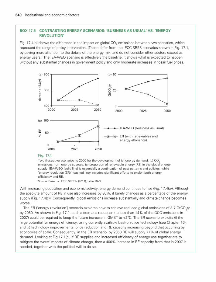
640 Institutional and economic factors
BOX 17.5 CONTRASTING ENERGY SCENARIOS: ‘BUSINESS AS USUAL’ VS. ‘ENERGY REVOLUTION’
Fig. 17.4(b) shows the difference in the impact on global CO2 emissions between two scenarios, which represent the range of policy intervention. (These differ from the IPCC-SRES scenarios shown in Fig. 17.1, by paying more attention to the details of the energy mix, and do not consider other sectors except as energy users.) The IEA-WEO scenario is effectively the baseline: it shows what is expected to happen without any substantial changes in government policy and only moderate increases in fossil fuel prices.
With increasing population and economic activity, energy demand continues to rise (Fig. 17.4(a)). Although the absolute amount of RE in use also increases by 80%, it barely changes as a percentage of the energy supply (Fig. 17.4(c)). Consequently, global emissions increase substantially and climate change becomes worse.
The ER (‘energy revolution’) scenario explores how to achieve reduced global emissions of 3.7 GtCO2/y by 2050. As shown in Fig. 17.1, such a dramatic reduction (to less than 14% of the GCC emissions in 2007) could be required to keep the future increase in GMST to <2°C. The ER scenario exploits (i) the large potential for energy efficiency, using currently available best-practice technology (see Chapter 16), and (ii) technology improvements, price reduction and RE capacity increasing beyond that occurring by economies of scale. Consequently, in the ER scenario, by 2050 RE will supply 77% of global energy demand. Looking at Fig.17.1(c), if RE supplies and increased efficiency of energy use together are to mitigate the worst impacts of climate change, then a 400% increase in RE capacity from that in 2007 is needed, together with the political will to do so.
(a)
400
600
800
2000 2025 2050
dem
and
(E
J/y)
(b)
0
25
50
2000 2025 2050G
tCO
2/y
(c)
0
50
100
2000 2025 2050
IEA-WEO (business as usual)
ER (with renewables and energy efficiency)
% R
E
Fig. 17.4Two illustrative scenarios to 2050 for the development of (a) energy demand, (b) CO2 emissions from energy sources, (c) proportion of renewable energy (RE) in the global energy supply. IEA-WEO (solid line) is essentially a continuation of past patterns and policies, while ‘energy revolution (ER)’ (dashed line) includes significant efforts to exploit both energy efficiency and RE. Source: Based on IPCC SRREN (2011), table 10–3.
TWIDELL PAGINATION.indb 640 01/12/2014 11:38

§17.8 The way ahead 641
To achieve deep policy change, it is necessary to change not only the answers (as in economics: see §17.3) but also to persuade those in charge to change the question. This is difficult because the fundamental question (e.g. ecological sustainability) often runs counter to the training, experience and philosophical stance of those who have risen through the existing institutions of power.
We conclude that renewables are growth areas of development, with the potential to supply most of the world’s energy from millions of local and appropriate sites. Such success requires knowledge, vision, experi-ence, finance, markets, and individual and collective choice. However, we caution that for a national energy system to be truly sustainable, not only must its energy sources be sustainable but so must its energy con-sumption. Consequently, the efficiency and purposes of energy end-use are vital (see Chapter 16). This is a key point in the energy revolution scenario described in Box 17.5 and other similar low-emission scenarios. Renewable energy sources are sufficient to meet the growing global demand for energy services, but only if combined with the efficient use of energy. Is such success possible? We believe it is.
CHAPTER SUMMARY
This chapter reviews socio-political and economic factors influencing the development of renewable energy systems (RES). These include national energy policy, economic conditions, consumer prices, external costs, climate change, energy security, and the corporate and market mechanisms of energy supply. RES development depends about 75% on such ‘institutional factors’ and about 25% on science and engineering.
Methods for quantifying choices between systems include matrix analysis, ‘payback time’, and discounted cash flows. Economic assessment of ‘costs’ depends greatly on whose costs are assessed (consumers or producers) and on time periods and location. Supply of renewable energy is generally site-specific with dominant upfront capital costs, unlike fossil fuel supplies. Policy tools making sustainable energy supplies more cost-effective and widespread over the past 40 years include regulatory limits to pollution, grants for RD&D, decreased subsidies for non-sustainable systems, subsidies for renewables, taxation adjustments, tradable permits, renewables obligations, feed-in tariffs. Even so, the full external and societal costs of conventional fossil fuel and nuclear energy supplies are still usually not fully included in their price, which biases choice against sustainable renewable energy.
Technological improvements and economies of scale from their increasing production and use continue to reduce the costs of RES. Renewables are now strongly growing in most countries, with potential to supply sustainably most of the world’s energy from many millions of sites. To achieve this potential requires knowledge, vision, experience, finance, markets and choice, all based on good science and technology.
TWIDELL PAGINATION.indb 641 01/12/2014 11:38

642 Institutional and economic factors
QUICK QUESTIONS
Note: Answers to these questions are in the text of the relevant section of this chapter, or may be readily inferred from it.
1 List and clarify at least five ‘institutional factors’ affecting growth of renewable energy.
2 What factors influence national policies for energy supply? 3 For your own country, name five factors favoring the uptake of
renewable energy, and five factors discouraging such uptake. 4 In your opinion, who benefits most from renewable energy, the rich
or the poor? Discuss. 5 Give examples of ‘external costs’ in your own country; have any of
these been ‘internalized’, and if so, how? 6 Define ‘life cycle analysis’. 7 Describe five methods used by governments to encourage the
uptake of renewable energy. 8 Summarize three methods used to quantify choice for decision-making. 9 Is economics an exact science, and if not, why not?10 Will you increase your use of renewable energy, and if so, how?
PROBLEMS
17.1 For the solar water heating system shown in Worked Example 17.2, calculate the payback time against the conventional electric system:
(a) using a discount rate of 10%.
(b) using a discount rate of 5%, but with no government grant.
(Hint: construct a spreadsheet similar to Table 17.3.)
17.2 For the wind farm shown in Worked Example 17.3, calculate the levelized cost of electricity under the following assumptions:
(a) a discount rate of 10% and a system life of 20 years;
(b) discount rate of 5% and a system life of six years (as might happen if an inadequately protected system was destroyed by a very severe storm);
(c) a discount rate of 10% and a system life of six years.
Comment on the relative effects on the levelized cost of discount rate and system life.
(Hint: construct a spreadsheet similar to Table 17.4).
17.3 Discuss how your country stands in relation to the socio-political factors outlined in §17.2. Identify any forces that are acting to change this position.
TWIDELL PAGINATION.indb 642 01/12/2014 11:38

Bibliography 643
17.4 Estimate the CO2 emissions per unit of electricity produced by a conventional coal-fired power station. (Hint: Coal is about 80% carbon. Make reasonable assumptions about the efficiency of conversion from heat to power.)
NOTE
1 See Box 15.3 and the supplementary web information on grid- integrated wind power.
BIBLIOGRAPHY
Policy and institutional issues
Edinger, R. and Kaul, S. (2000) Renewable Resources for Electric Power, Quorum Books, Connecticut, USA. Non-technical account of technologies, emphasizing the importance of institutional factors and end-use efficiency.
Flavin, C. and Lenssen, N. (1995) Power Surge: A guide to the coming energy revolution, Earthscan/James & James, London. Argues that, contrary to most ‘incremental analysis’, an energy revolution to a sustainable system based on greater efficiency and renewable sources is both possible and desirable.
Friedman, T.L. (2008) Hot, Flat and Crowded: Why the world needs a green revolution and how we can renew our global future, Allen Lane, London. Lively polemic, full of good quotes.
GEA (2011) Global Energy Assessment: Towards a sustainable energy future, Cambridge University Press, Cambridge. Authoritative and comprehensive international review of the framework and resources for today’s energy system and how they need to change to ensure sustainability. Extent > 2000 pages (several chapters available online at www.globalenergyassessment.org).
Geller, H. (2003) Energy Revolution: Policies for a sustainable future, Island Press, Washington, DC. Emphasizes three themes: current sources and patterns of energy use are unsustainable; an ‘energy revolution’ is possible and desirable through much greater energy efficiency and RE; the barriers to this may be overcome through enlightened public policies.
Glasson, J., Therival, R. and Chadwick, A., (2011, 4th edn) Introduction to Environmental Impact Assessment, Routledge/Taylor & Francis, Abingdon. Structured approach for professional standards and methods; examples include wind farms.
Goldemberg, J. and Lucon, J. (2009, 2nd edn) Energy, Environment and Development, Routledge, London. Wide-ranging and readable exposition of the links between energy and social and economic development and sustain-ability, with consideration of equity within and between countries by a Brazilian expert.
Hunt, S. and Shuttleworth, G. (1996) Competition and Choice in Electricity, Wiley, Chichester. Explains how national electricity supply industries were changed by liberalization and privatization.
International Solar Energy Society (2004) Transitioning to a Renewable Energy Future – A White Paper. Available online at www.ises.org. Focuses on technology commercialization and policy shifts required.
IPCC WG2 (2007) Climate Change 2007: Contribution of Working Group II to the Fourth Assessment Report of the IPCC: Summary for Policymakers, Intergovernmental Panel on Climate Change. Available online at www.ipcc.ch. IPCC Working Group 2 covers impacts, adaptation and vulnerability aspects of climate change.
IPCC WG1 (2013) Climate Change 2013: Contribution of Working Group II to the Fifth Assessment Report of the IPCC: The Physical Science Basis: Summary for Policymakers, Intergovernmental Panel on Climate Change, available online at www.ipcc.ch.
TWIDELL PAGINATION.indb 643 01/12/2014 11:38
644 Institutional and economic factors
Laird, F.N. (2001) Solar Energy,Technology Policy and Institutional Values, Cambridge University Press, Cambridge. Scholarly study of US energy policy 1946 to 1979, showing how institutional factors blocked RE from becoming a major part of the US energy system during that period.
Mallon, K. (2006) Renewable Energy Policy and Politics – A handbook for decision makers, Earthscan, London. Structured chapters by experts, analyzing governmental strategies and implications for renewable energy devel-opment and implementation at national scales. Includes case studies. Seeks general quantified conclusions, but without mathematical analysis.
Mitchell, C. (2008) The Political Economy of Sustainable Energy, Macmillan, London. Placing the UK in compara-tive perspective, Mitchell argues for a new way of approaching policy towards energy and sustainability.
Mitchell, C., Sawin, J., Pokharel, G.R., Kammen, D., Wang, Z., Fifita, S., Jaccard, M., Langniss, O., Lucas, H., Nadai, A., Trujillo Blanco, R., Usher, E., Verbruggen, A., Wüstenhagen, R. and Yamaguchi, K. (2011) ‘Policy, financing and implementation’, in O. Edenhofer, R. Pichs Madruga, Y. Sokona, K. Seyboth, P. Matschoss, S. Kadner, T. Zwickel, P. Eickemeier, G. Hansen, S. Schlömer and C. von Stechow (eds), IPCC Special Report on Renewable Energy Sources and Climate Change Mitigation, ch.11, Cambridge University Press, Cambridge. Authoritative review of international experience with RE policies; often referred to as SRREN.
Scheer, H. (2001) The Solar Economy: Renewable energy for a sustainable global future, Earthscan/James & James, London. A well-phrased polemic arguing that an energy system based almost totally on renewables is feasible but will require ‘creative destruction’ of the old fossil-based system.
SRREN (2011) See Mitchell et al. (2011).
UNCED (1992) The Earth Summit. Several resulting United Nations publications including: Agenda 21, the Rio Declaration on Environment and Development, the Statement of Forest Principles, the United Nations Framework Convention on Climate Change, and the United Nations Convention on Biological Diversity.
Wilkins, G. (2002) Technology Transfer for Renewable Energy, Earthscan/James & James, London. Examines the practicalities of bringing renewable energy into wider use in developing countries, with reference to the Kyoto Protocol mechanisms and case studies of biomass co-generation and household photovoltaic systems.
Yergin, D. (1992) The Prize: The epic quest for oil money and power, Simon & Schuster, New York. Entertaining account of the politics and personalities of the oil world.
Environmental economics textbooks
Common, M. and Stagl, S. (2005) Ecological Economics: An introduction, Cambridge University Press, Cambridge. Clear exposition at introductory level of relevant economic principles and tools.
Tietenberg, T. and Lewis, L. (2009, 8th edn) Environmental and Natural Resource Economics, Pearson/Addison-Wesley, Reading, MA. A standard text at slightly more advanced level than Common and Stagl.
Externalities
European Commission (1995) ExternE: Externalities of energy, 7 vols, E.C., Brussels.
Hohmeyer, O. (1988) Social Costs of Energy Consumption: External effects of electricity generation in the Federal Republic of Germany, Springer Verlag, Berlin.
Oak Ridge National Laboratory & Resources for the Future (1994) Fuel Cycle Externalities, USA.
See also Fischedick et al. (2011).
TWIDELL PAGINATION.indb 644 01/12/2014 11:38

Bibliography 645
Tools for present value analysis
Awerbuch, S. (1996) ‘The problem of valuing new energy technologies’, Energy Policy, 24, 127–128. Introduction to new valuation techniques going beyond ‘traditional’ utility and present value techniques.
Boyle, G. (ed.) (2004, 2nd edn) Renewable Energy, Oxford University Press, Oxford. The appendix on ‘investing in renewable energy’ is strongly recommended.
International Energy Agency (1991) Guidelines for the Economic Analysis of Renewable Energy Technology Applications, IEA, Paris. Very detailed account with worked examples, though ignoring externalities.
Scenarios for the future
Aitken, D.W,, Billman, L.L. and Bull, S.R. (2004) ‘The climate stabilization challenge: can renewable energy sources meet the target?’, Renewable Energy World, December, 56–69. A review of various published sce-narios, which concludes that RE could make 50% of all energy supply by 2050.
Fischedick, M., Schaeffer, R., Adedoyin, A., Akai, M., Bruckner, T., Clarke, L., Krey, V., Savolainen, I., Teske, S., Ürge-Vorsatz, D. and Wright, R. (2011) ‘Mitigation potential and costs’ in O. Edenhofer et al. (eds), IPCC Special Report on Renewable Energy Sources and Climate Change Mitigation, ch. 10, Cambridge University Press, Cambridge. Reviews a wide range of energy scenarios.
IPCC (2007) Climate Change 2007: Synthesis report, Intergovernmental Panel on Climate Change/Cambridge University Press, Cambridge. Summarizes and integrates the three separate IPCC volumes on physical science, impacts and adaptation, and mitigation. Available online at www.ipcc.ch.
Krey, V. and Clarke, L. (2011) ‘Role of renewable energy in climate mitigation: a synthesis of recent scenarios’, Climate Policy, 11,1131–1158. A major source for Fischedick et al. (2011).
Schellnhuber, H.J., Cramer, W., Nakicenovic, N., Wigley, T. and Yohe, G. (eds) (2006) Avoiding Dangerous Cimate Change, Cambridge University Press, Cambridge.
Smith, J.B., Schneider, S.H. et al. (2009) ‘Assessing dangerous climate change through an update of the Intergovernmental Panel on Climate Change (IPCC) “reasons for concern”’, Proceedings of the National Academy of Sciences, 106, 4133–4137.
Teske, S., Pregger, T., Simon, S., Naegler, T., Graus, W. and Lins, C. (2011) ‘Energy [R]evolution 2010 – a sustain-able world energy outlook’, Energy Efficiency, 4, 409–433. Presents a radical low-carbon energy scenario.
Weir, T. (2012) ‘Climate change and renewable energy: implications for the Pacific Islands of a global perspec-tive’, Journal of Pacific Studies, 32(2), 4–30.
Some case studies
Ling, S., Twidell, J. and Boardman, B. (2002) ‘Household photovoltaic market in Xining, Qinghai Province, China: the role of local PV business’, Solar Energy, 73, 227–240.
Lipp, J. (2001) ‘Micro-financing solar power: the Sri Lankan SEEDS model’, Refocus, October, 18–21.
Mandela, M. (2000) ‘Support for renewables: a perspective of the Development Bank of Southern Africa’, Refocus, August, 15–17.
TWIDELL PAGINATION.indb 645 01/12/2014 11:38

646 Institutional and economic factors
Journals and websites
Energy Policy (published by Elsevier) is an academic journal focussed on economic, policy and institutional aspects, (e.g. the impact of climate change policies) of all forms of energy, including renewable energy.
Refocus magazine (published by Elsevier on behalf of the International Solar Energy Society) has numerous articles on rural electrification.
Renewable Energy Network (REN21) (www.ren21.org), a worldwide network of experts who publish annual surveys of RE use and policies around the world (Renewables Global Status Report).
UNEP (2013) Global Trends in Sustainable Energy Investment 2013, United Nations Environment Programme (http://www.unep.org/sefi-ren21/). Updated annually.
TWIDELL PAGINATION.indb 646 01/12/2014 11:38
Review 1 Electrical power for renewables
CONTENTS
Learning aims 647
§R1.1 Introduction 648
§R1.2 Electricity transmission: principles 648
§R1.3 Electricity grids (networks) 650
§R1.4 DC grids 651
§R1.5 AC active and reactive power: transformers 651
§R1.6 Electric machines (generators and motors) 652
§R1.7 Special challenges and opportunities for renewables electricity 656
Quick questions 659
Bibliography 659
LEARNING AIMS
Most renewables technologies are used to gen-erate electricity. From this Review you should be able to explain (a) the basics of the various
electricity generators included in this book, (b) the operation of the grids distributing the power, and (c) some applications.
LIST OF FIGURES
R1.1 Electrical transmission. 649R1.2 Synchronous generator: principle. 653R1.3 Doubly fed induction generator. 656R1.4 Energy flow diagram for the USA in 2011. 658
TWIDELL PAGINATION.indb 647 01/12/2014 11:38
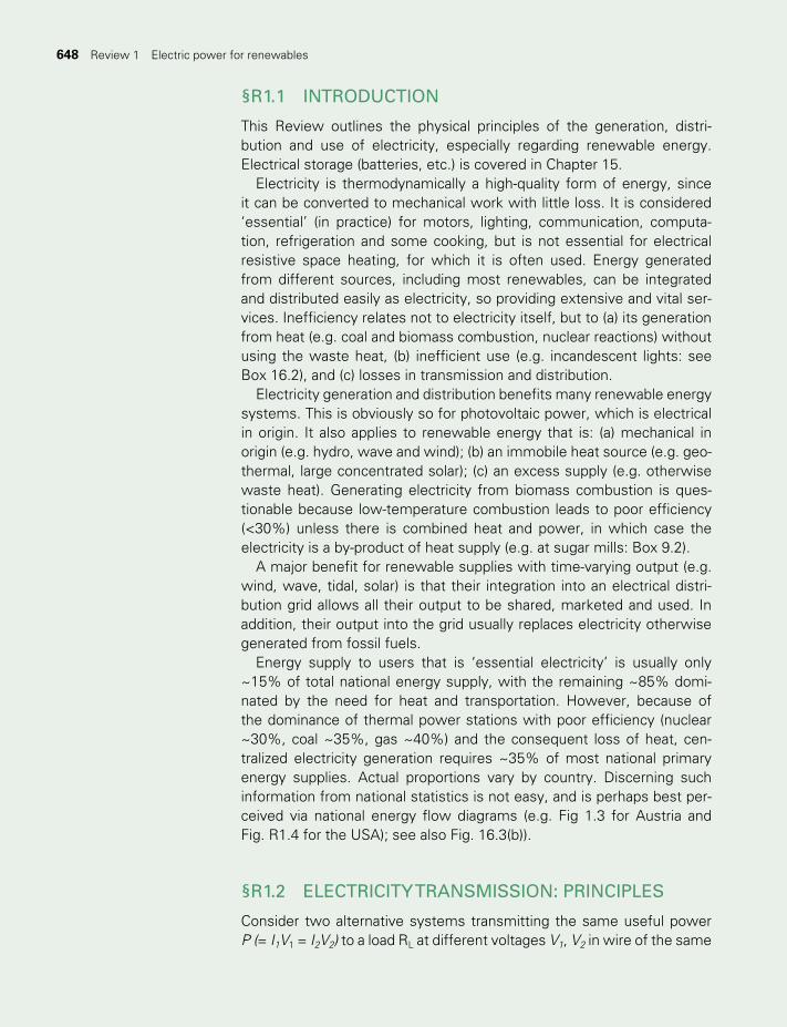
648 Electrical power for renewables648 Review 1 Electric power for renewables
§R1.1 INTRODUCTION
This Review outlines the physical principles of the generation, distri-bution and use of electricity, especially regarding renewable energy. Electrical storage (batteries, etc.) is covered in Chapter 15.
Electricity is thermodynamically a high-quality form of energy, since it can be converted to mechanical work with little loss. It is considered ‘essential’ (in practice) for motors, lighting, communication, computa-tion, refrigeration and some cooking, but is not essential for electrical resistive space heating, for which it is often used. Energy generated from different sources, including most renewables, can be integrated and distributed easily as electricity, so providing extensive and vital ser-vices. Inefficiency relates not to electricity itself, but to (a) its generation from heat (e.g. coal and biomass combustion, nuclear reactions) without using the waste heat, (b) inefficient use (e.g. incandescent lights: see Box 16.2), and (c) losses in transmission and distribution.
Electricity generation and distribution benefits many renewable energy systems. This is obviously so for photovoltaic power, which is electrical in origin. It also applies to renewable energy that is: (a) mechanical in origin (e.g. hydro, wave and wind); (b) an immobile heat source (e.g. geo-thermal, large concentrated solar); (c) an excess supply (e.g. otherwise waste heat). Generating electricity from biomass combustion is ques-tionable because low-temperature combustion leads to poor efficiency (<30%) unless there is combined heat and power, in which case the electricity is a by-product of heat supply (e.g. at sugar mills: Box 9.2).
A major benefit for renewable supplies with time-varying output (e.g. wind, wave, tidal, solar) is that their integration into an electrical distri-bution grid allows all their output to be shared, marketed and used. In addition, their output into the grid usually replaces electricity otherwise generated from fossil fuels.
Energy supply to users that is ‘essential electricity’ is usually only ~15% of total national energy supply, with the remaining ~85% domi-nated by the need for heat and transportation. However, because of the dominance of thermal power stations with poor efficiency (nuclear ~30%, coal ~35%, gas ~40%) and the consequent loss of heat, cen-tralized electricity generation requires ~35% of most national primary energy supplies. Actual proportions vary by country. Discerning such information from national statistics is not easy, and is perhaps best per-ceived via national energy flow diagrams (e.g. Fig 1.3 for Austria and Fig. R1.4 for the USA); see also Fig. 16.3(b)).
§R1.2 ELECTRICITY TRANSMISSION: PRINCIPLES
Consider two alternative systems transmitting the same useful power P (= I1V1 = I2V2) to a load RL at different voltages V1, V2 in wire of the same
TWIDELL PAGINATION.indb 648 01/12/2014 11:38
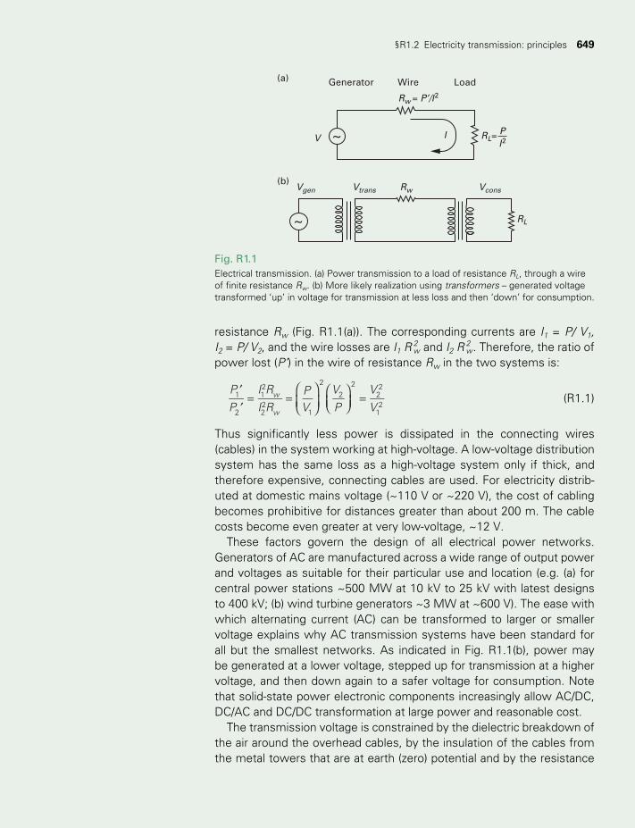
§R1.2 Electricity transmission: principles 649
resistance Rw (Fig. R1.1(a)). The corresponding currents are I1 = P/ V1, I2 = P/ V2, and the wire losses are I1 R
2w and I2 R
2w. Therefore, the ratio of
power lost (P’) in the wire of resistance Rw in the two systems is:
PP
I RI R
PV
VP
VV
w
w
1
2
12
22
1
2
22
22
12
′′
= =
= (R1.1)
Thus significantly less power is dissipated in the connecting wires (cables) in the system working at high-voltage. A low-voltage distribution system has the same loss as a high-voltage system only if thick, and therefore expensive, connecting cables are used. For electricity distrib-uted at domestic mains voltage (~110 V or ~220 V), the cost of cabling becomes prohibitive for distances greater than about 200 m. The cable costs become even greater at very low-voltage, ~12 V.
These factors govern the design of all electrical power networks. Generators of AC are manufactured across a wide range of output power and voltages as suitable for their particular use and location (e.g. (a) for central power stations ~500 MW at 10 kV to 25 kV with latest designs to 400 kV; (b) wind turbine generators ~3 MW at ~600 V). The ease with which alternating current (AC) can be transformed to larger or smaller voltage explains why AC transmission systems have been standard for all but the smallest networks. As indicated in Fig. R1.1(b), power may be generated at a lower voltage, stepped up for transmission at a higher voltage, and then down again to a safer voltage for consumption. Note that solid-state power electronic components increasingly allow AC/DC, DC/AC and DC/DC transformation at large power and reasonable cost.
The transmission voltage is constrained by the dielectric breakdown of the air around the overhead cables, by the insulation of the cables from the metal towers that are at earth (zero) potential and by the resistance
Generator
VPI2
I RL=
RL
Rw
Rw = P’/I2
Vgen Vtrans Vcons
(a)
(b)
Wire Load
Fig. R1.1Electrical transmission. (a) Power transmission to a load of resistance RL, through a wire of finite resistance Rw. (b) More likely realization using transformers – generated voltage transformed ‘up’ in voltage for transmission at less loss and then ‘down’ for consumption.
TWIDELL PAGINATION.indb 649 01/12/2014 11:38

650 Electrical power for renewables650 Review 1 Electric power for renewables
of the cables. Most transmission is AC because of using conventional transformers, but DC systems have advantages for efficient transmis-sion because there are no inductive losses and the constancy of peak voltage allows maximum power flow. Overhead transmission voltages for long lines are commonly about 200 kV to 500 kV, with ‘ultra-high- voltage’ of about 1000 kV (AC) and 800 kV (DC). Superconducting wires of zero resistance operating at very low ‘cryogenic’ temperature are used in some equipment (e.g. intense electromagnets) but not as yet for trans-mission lines owing to cost and complexity.
§R1.3 ELECTRICITY GRIDS (NETWORKS)
Community and national electrical power generation links to the load demand by a common network, often called ‘the grid’. The generation may be from centralized power stations or from smaller capacity embed-ded generation, such as photovoltaic micro-generation or wind turbines. The grid allows the sharing of generation and consumption, and so pro-vides a reliable and most cost-effective supply.
Despite their name and original intention, since about 1930 electric-ity ‘grids’ became characterized by centralized despatch of electricity at very high voltage (>~100 kV) from a small number of interconnected very large power stations of ~1000 MW capacity. Near the point of end-use, the electricity is transformed down to ~10 kV (e.g. for a suburb), and then to ~230 V or ~110 V (e.g. for a street of houses). Older rural grids from central dispatch may lose 10 to 20% of power in transmis-sion, distribution and transformation, with the best urban grids having about 5% losses. Despite the dominance of central generation, most grids can incorporate a significant spread of decentralized sources (e.g. micro-generation from individual householders with ‘grid-connected’ PV systems (§5.3) or dispersed wind farms (Chapter 8)). With modern solid-state power electronic control and remote supervision, grids are increas-ingly able to both accept and distribute dispersed power, including from a wide range of renewables generation. Some of the technical features of such grids are outlined in §15.4.
Electricity on a grid is predominantly an instantaneous carrier or vector of energy, since to date its storage in batteries and fuel cells is negligible on national scales. Therefore, the balance on a network of supply with demand (and of demand with supply) has to be controlled. Renewable energy generators (e.g. wind turbines) have output that matches their changing environmental input, so their output varies continuously and may cease. Likewise, demand (the ‘load’) from consumers on a network varies. The transmission control operators have always managed this balance minute by minute through slight changes in line voltage and frequency, by integrating variable demand with variable input, and by using controllable generation (e.g. hydro and gas turbine power) and
TWIDELL PAGINATION.indb 650 01/12/2014 11:38

§R1.5 Ac active and reactive power: transformers 651
controllable loads (e.g. water heaters, metal refineries). Conventionally, all major grid systems cater for rapid demand fluctuations of ~20%, principally by having extra generation capacity available; consequently the same methods cater for rapid supply fluctuations also of ~20% (e.g. sudden disconnection of a central generating plant). These techniques accommodate variable, and mostly predictable, renewables supply. When the variable generation component exceeds ~20% of total supply, then special strategies may have to be used, such as increased standby generation, remote control of generators and control of specified loads (see §15.4).
Note that an electrical grid may be much smaller than national scale (e.g. a ‘micro-grid’ for a single isolated village or a small island).
§R1.4 DC GRIDS
The voltage of a grid is limited by the breakdown from sparks and dis-charges occurring at peak voltage, which is transitory within each AC cycle. However, the peak voltage on a DC grid is constant, so allowing a cable to carry more power as DC than AC. In addition: (a) AC currents tend to pass along the outer region of a cable (the skin effect), so increas-ing the effective resistance, whereas DC currents pass throughout the cable cross-section; (b) there are induction and capacitance losses with AC, which are absent for DC. Power transmission as DC is used for many large-power transmission lines that are long or under water; often these integrate inter-state and international generation and demand. In particu-lar, such long and large-power ‘electricity highways’ are used to transmit hydropower (e.g. (a) 2000 MW for ~1000 km at 450 kV (DC) between Quebec (Canada) and Boston (USA), and (b) 1900 MW for 1420 km at 500 kV (DC) from Cambora Bassa (Mozambique) to Johannesburg (South Africa)). Similar schemes have been proposed for transmitting offshore wind power from UK waters to Mainland Europe, and solar power from North Africa to Central Western Europe.
§R1.5 AC ACTIVE AND REACTIVE POWER: TRANSFORMERS
If there is only resistance in the external circuit, then the voltage and current are in phase, in which case the power dissipated as heat in the external circuit is P = VpIp sin2 ωt and the average power is Pav = VpIp/2. This is the active power, which, in this case, peaks at a frequency twice that of the voltage and current (half the period). It is common practice to call Vp /√2 = V the voltage (strictly, the root-mean-square voltage) and Ip /√2 = I the current, so that the power P = VI as for direct current.
If the external circuit is purely inductive with zero resistance, then the AC voltage (push) and current (flow) are φ = 90° out of phase
TWIDELL PAGINATION.indb 651 01/12/2014 11:38

652 Electrical power for renewables652 Review 1 Electric power for renewables
(push maximum with zero flow; flow maximum with zero push). In general, if the phase difference is φ, then the product of Vp sinωt and Ip sin(ωt + φ) has frequency 2ωt and amplitude Q, where:
Q V I sinφ= (R1.2)
This function Q has the units of power, but is not dissipated as heat; it is power oscillating backwards and forwards in the magnetic field of the inductance. The time-averaged power into the external circuit is zero, and is called the reactive power; it cannot appear as heat or work.
If the external circuit is inductive and also resistive, then φ is not 90°. The product of Vp sin ωt and Ip sin(ωt + φ) can now be separated into a reactive part (oscillating with equal amplitude between positive and negative) and an active part (always positive). The average value of the active power
Pav = V I cosφ (R1.3)
and the average value of the reactive power is zero as before.Similar effects occur with capacitance in the external circuit, but
with the current leading the voltage. It is common practice to adjust a compensating capacitance to negate the reactive power effects of inductance, and vice versa. Electrical engineers speak of ‘active’ and ‘reactive’ power as separate parameters; each separately instrumented and quantified. In general, reactive power is not wanted, and so grid-connected users may be charged for reactive power consumption that they cause or utilize, despite it not being usable power.
The reason that AC is so widely used is that the voltage of an alter-nating current can easily be altered by a transformer (see Fig. R1.1(b)). Essentially, a transformer consists of two coils of wire (with different number of turns N ) on the same ferromagnetic core. Since the magnetic flux Φ is effectively confined to the core, for each loop Φ is the same, and so from (R1.4) the voltage V in each winding is proportional to N. Because of this ease of transformation, and also ease of generation and its suitability for electric motors, AC is usual for grid systems.
§R1.6 ELECTRIC MACHINES (GENERATORS AND MOTORS)
(a) Basics
The basic operation of all generators is simple, but many complexities and variations are used to give particular properties and improvements in efficiency. Essentially a magnetic field is arranged to cut a wire with a relative velocity, so inducing an electric current by the Faraday Effect. Every generator has a stator (coils of wire or permanent magnets that stay static) and a rotor (magnets or coils of wire that rotate within the
TWIDELL PAGINATION.indb 652 01/12/2014 11:38
§R1.6 Electric machines (generators and motors) 653
stator); one of these has a coil (winding) within which the generated current is produced, and the other has other windings or permanent magnets to produce the magnetic fields. We give a brief account here; for further details see textbooks and websites on electrical machines in the Bibliography at the end of this Review.
A magnet moved across an electrical conductor will induce an electri-cal potential difference in the conductor (an electro-motive force (EMF); or a ‘voltage’). If the conductor forms a closed circuit, then an electrical current is induced. The EMF/voltage is:
V N d dt/Φ = − (R1.4)
where there are N conductors in series, each cut by a magnetic flux Φ of rate of change dΦ/ dt. A coil of wire (solenoid) carrying an electric current produces a magnet field, as does a magnet. If the coil has a fer-romagnetic core (e.g. iron), then the magnetic field is very considerably enhanced (by a factor of ~1000). Therefore, coils with ferromagnetic cores (electromagnets) are used in most electric machines, i.e. gen-erators and motors. The equivalent north and south poles of such coils are called ‘salient poles’. Limitations of space and simplicity encourage the use of permanent magnets instead of electromagnets, as in some multipole generators for large wind turbines.
(b) Synchronous generators (alternators)
Fig. R1.2 illustrates the basic AC synchronous generator; here with two permanent magnets on the stator producing a stationary magnetic field. A single coil turning in this field has an induced EMF, which produces a
Sinusoidalvoltage output
The mechanical energy input toa generator turns the coil in themagnetic field.
Magnetic polesSlip rings
A voltage proportional tothe rate of change of thearea facing magneticfield is generated in thecoil. This is an exampleof Faraday’s law.
Fig. R1.2Synchronous generator: principle.
TWIDELL PAGINATION.indb 653 01/12/2014 11:38
654 Electrical power for renewables654 Review 1 Electric power for renewables
current in an external circuit connected by brushes on circular slip rings at the commutator. Because the wires of the coil alternately cut the mag-netic field up and down, alternating current (AC) is generated at the same frequency as the shaft’s rotation.
The induced current in the rotating coil (winding) itself produces a magnetic field, Brotor, which rotates. The shaft is driven by the external mechanical torque Γm (e.g. as in a hydro-turbine shaft). However, the induced rotor magnetic field Brotor sets up an opposing torque Γem from the electromechanical effects. Equilibrium is reached when the shaft mechanically driven torque, Γm, equals the induced electromagnetic torque Γem. The mechanical power input equals the electrical power gen-erated, less frictional and electrical losses. The AC electricity generated has voltage and current varying sinusoidally with time in synchronism with the shaft rotational speed. Commercial AC generators operate on this principle, but with multiple magnetic fields forming many ‘pole-pairs’ with their magnetic fields crossing multiple coils. Generating efficiency from mechanical power to electricity is usually ~97%, i.e. only 3% lost as heat.
Because the magnetic fields are created by permanent magnets or DC currents, the generated sinusoidal current has an AC frequency (f1) in synchronization with the rotating shaft frequency (fs) of the generator. With n pole-pairs, each acting as a single magnetic ‘north/south pole- pair’, nfs = f1 exactly. Such a generator is a synchronous AC generator with the output frequency locked to the shaft frequency. This requires the shaft frequency to be closely controlled.
Usually power will be taken from grid-connected stationary coils on the stator, and the coils on the rotor producing the magnetic field are connected, via slip rings, to a DC generator. Note that power is extracted from the stator, which is connected to the grid. A benefit of synchronous generators is that the reactive power can be controlled and minimized, so maximizing real power. In the most common arrangement, the stator coils are directly connected to the grid, in which case power is only exported when the rotor turns exactly so nfs = f1. Consequently, f1 has to be controlled exactly equal to the grid network frequency (e.g. 50 Hz in most countries, or 60 Hz in North America). Obtaining synchronism at start-up and in operation is not difficult for utility-scale thermal and hydro plant, where synchronous generators are the norm. However, this control requirement initially discouraged synchronous generators for vari-able speed wind turbines. However, if a synchronous generator is decou-pled from the grid through a convertor (rectifier to DC linked to inverter to grid AC), then the exact speed synchronism is not necessary at any stage.
An important variation is the basic DC generator. Here the stator magnets produce a stationary magnetic field, but the rotor coils are con-nected by semicircular slip rings at the commutator so that the current reverses direction as each rotor coil passes perpendicular to the stator
TWIDELL PAGINATION.indb 654 01/12/2014 11:38
§R1.6 Electric machines (generators and motors) 655
field. Thus the output current is unidirectional; varying in amplitude as the modulus of sinωt. This varying DC current can be smoothed electronically to steady/constant DC. Such generators produce the DC current for the electromagnets of larger AC synchronous generators, being mounted on the same shaft.
(c) Induction generators (asynchronous generators)
The induction AC generator is strictly an induction machine, since the same device may be a motor or a generator, and is easily connected to the grid without any concern for synchronism. This generality of design allows induction generators to be cheaper than synchronous generators. The usual arrangement is that the stator windings (coils) are connected to the AC grid, so producing a rotating magnetic field around the shaft of the machine. The rotor is a ‘squirrel cage’ with copper bars set paral-lel to the axis, and connected together by rings at each end. Currents are thereby induced within the short-circuited coils on the shaft. These induced currents themselves produce magnetic fields, which in turn generate power into the stator coils, but only if the rates of rotation of the shaft magnetic field and the stator coils differ. The phase relationships are such that power may be transferred between the mechanical rotor shaft and electrical power in the stator circuit.
For the induction machine: (a) there are sets of windings on the stator simulating n pole-pairs; (b) if the grid frequency is fg and the rotor frequency is fr, then synchronism occurs when nfr = fg; (c) slip s is defined as:
s = (fg – nfr) /fg; (R1.5)
(d) when s = 0, there is synchronism and no power is generated or used; (e) when s is negative (nfr faster than fg) the machine is a generator; (f) when s is positive (nfr slower than fg) the machine is a motor. Generator slip magnitude is usually less than 10%, and between 0.5% and 5% for a motor.
An induction generator can only generate when the induced closed loop rotor currents have been initiated at connection; thereafter they continue automatically. There are generally two methods for this: (a) for grid-connected machines, reactive power is drawn from the live grid to which the generator output is connected; or (b) for autonomous opera-tion, self-excited generation is made possible by capacitors connected between the output and earth. The benefits of method (a) (grid linking) are: (i) the simplicity and cheapness of the system; (ii) safety, since the generator should not generate if the grid power is off, and (iii) the grid may be used to export power when there is surplus and import power at other times. In method 2 there has to be some residual magnetism in the framework or surroundings of the generator to provide the initial current, with the capacitors maintaining the correct phase relationships.
TWIDELL PAGINATION.indb 655 01/12/2014 11:38

656 Electrical power for renewables656 Review 1 Electric power for renewables
Because of cheapness and ease of operation, basic induction gen-erators are common for small- (~10 kW) to medium- (~100 kW) scale generation from mechanical power (e.g. hydro and diesel generators). Synchronism at grid frequency is difficult with wind turbines, and indeed not wanted to allow improved wind energy capture with varying turbine rotor speed (see Fig. 8.19(b)). For wind turbines, it is possible to increase the slip of the induction generator and thus allow an increased variation of rotor speed to maintain more constant blade-tip to wind speed ratio (tip-speed-ratio). The earliest method involves impedance change of the otherwise unconnected rotor windings, but at the expense of increased generator heating. The more modern method (doubly fed induction gen-erator) has the rotor windings connected through slip rings to an external power-electronic control of the voltage and phase (Fig. R1.3). In this way: (a) the rotational speed of the rotor may vary considerably from synchro-nism with the grid AC frequency, and (b) power may then be taken from the rotor circuits as well as the stator. Such doubly fed induction gen-erators, with the associated power electronics, allow wind turbines to have variable rotor speed and hence match the wind speed for the most efficient power extraction.
§R1.7 SPECIAL CHALLENGES AND OPPORTUNITIES FOR RENEWABLES ELECTRICITY
‘Renewables electricity’ may be defined as electricity initially generated from a renewable source and then either immediately used, or distrib-uted on a grid or stored for later supply (as in a battery). This definition covers a very wide range of applications, varying:
Rotor
StatorThree–phase
AC DC
AC/DC/AC converter
AC
Fig. R1.3Doubly fed induction generator with power generated both from the stator (as in a simple induction generator) and also from the rotor that has slip-ring connection to an AC/DC/AC convertor that controls the magnitude and phase of the AC power connection to the rotor. Consequently, the rotor frequency (speed) can be independent of the grid frequency (e.g. in a wind turbine).
TWIDELL PAGINATION.indb 656 01/12/2014 11:38
§R1.7 Special challenges and opportunities for renewables electricity 657
(i) By power: from watts (e.g. PV standby security) and kW (e.g. house-hold micro-generation) to GW (large-scale hydro).
(ii) By location: from isolated and autonomous (e.g. remote village, Earth satellite) to metropolis (e.g. Oslo).
(iii) By variability: from constant (e.g. hydro with substantial reservoir, stored biofuel) to variable (e.g. wind power).
(iv) By opportunity: from excess (e.g. hurricanes) to minimal (e.g. hydro in a desert).
(vi) By impact: from harm (e.g. flooded valley for hydro reservoir) to acceptable (e.g. PV barn roof).
(vii) By mitigation: from reducing carbon emissions (e.g. when substi-tuting electricity from coal power stations) to legacy (e.g. installing renewables sustains the future).
Such characteristics are considered generally in §1.4 and Table 1.1 for all forms of energy, but they are the most profound for electricity because of the universality of application. See Fig. R1.4 for the proportion of renewables electricity in total energy supply of a nation – the USA.
The great variation in form and location of renewables generation con-trasts with ‘traditional’ central generation in large networks, especially from large thermal plant of GW capacity. Consequently the traditional hierarchy of electrcity supply tends to oppose distributed generation, especially from relatively small-capacity private generators and micro-generators. However, generally, ‘what can go one way’ in an electrical power ditribu-tion network ‘can go the other way’. So the grid is there to ‘share’ electric-ity rather than having a one-way system from central generation outward. Obviously grid lines must not be overloaded and all connected equipment must be ‘type approved’. Modern commercial renewables equipment uses solid-state electronic controllers and interconnectors for safe and reliable connection to grids, so, as conditions change, power may be either imported (purchased) or exported (sold) by customers (traditionally called ‘consumers’, even when they are micro-generation exporters!).
There are considerable variations in power flow with time in all parts of a reliable network, as discussed in §15.4.2 etc. This is principally because demand changes with time of day and night, and with season. The grid operators have to maintain a continuous balance of supply and demand. For small, temporary variations, it is usual practice to allow the grid volt-ages and frequency to change slightly to maintain this balance automati-cally. For longer periods, there is a surplus of generation of a range of types so that the network controllers can cater for faults, unexpected generator disconnections and routine maintenance outages. In addition, and as a rule of thumb, 20% surplus generation capacity and low-tariff disconnectable load are available to cover such eventualities. Pumped hydro provision, if available, is valuable in this respect for rapidly provid-ing power or extra load as needed.
TWIDELL PAGINATION.indb 657 01/12/2014 11:39
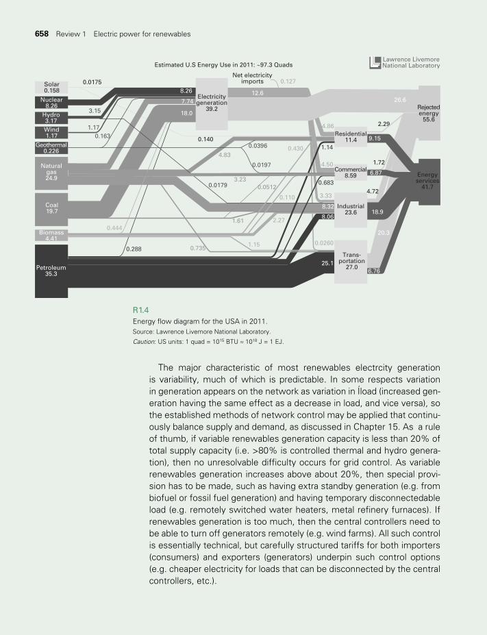
658 Electrical power for renewables658 Review 1 Electric power for renewables
Solar0.158
0.01758.26
7.74
18.0
12.6
4.83
3.23
0.0396 0.430
0.0197
0.0512
0.110
0.140
0.0179
3.15
1.170.163
Rejectedenergy
55.6
Energyservices
41.7
Commercial8.59
Residential11.4
Industrial23.6
Nuclear8.26
Hydro3.17Wind1.17
Geothermal0.226
Naturalgas24.9
Coal19.7
0.444
0.288 0.735
1.61
1.15
2.27
0.0260
25.16.76
20.3
18.98.06
8.32
3.33
4.50
4.86
1.14
4.72
1.72
9.15
2.29
26.6
0.683
Biomass4.41
Petroleum35.3
Electricitygeneration
39.2
Net electricityimports 0.127
Estimated U.S Energy Use in 2011: ~97.3 QuadsLawrence LivemoreNational Laboratory
Trans-portation
27.0
6.87
R1.4Energy flow diagram for the USA in 2011. Source: Lawrence Livemore National Laboratory.
Caution: US units: 1 quad = 1015 BTU ≈ 1018 J = 1 EJ.
The major characteristic of most renewables electrcity generation is variability, much of which is predictable. In some respects variation in generation appears on the network as variation in Íload (increased gen-eration having the same effect as a decrease in load, and vice versa), so the established methods of network control may be applied that continu-ously balance supply and demand, as discussed in Chapter 15. As a rule of thumb, if variable renewables generation capacity is less than 20% of total supply capacity (i.e. >80% is controlled thermal and hydro genera-tion), then no unresolvable difficulty occurs for grid control. As variable renewables generation increases above about 20%, then special provi-sion has to be made, such as having extra standby generation (e.g. from biofuel or fossil fuel generation) and having temporary disconnectedable load (e.g. remotely switched water heaters, metal refinery furnaces). If renewables generation is too much, then the central controllers need to be able to turn off generators remotely (e.g. wind farms). All such control is essentially technical, but carefully structured tariffs for both importers (consumers) and exporters (generators) underpin such control options (e.g. cheaper electricity for loads that can be disconnected by the central controllers, etc.).
TWIDELL PAGINATION.indb 658 01/12/2014 11:39

Bibliography 659
QUICK QUESTIONS
Note: Answers to these questions are in the text of the relevant section of this chapter, or may be readily inferred from it.
1 Why is electricity considered a high-quality form of energy? 2 What are the technical benefits of an electricity grid network? 3 What is ‘essential electricity’? 4 What characterisitcs benefit a long-distance transmission line? 5 How is alternating current electricity usually changed in voltage? 6 Explain reactive power. 7 What are the distinctive characteristics of a synchronous generator? 8 What are the distinctive characteristics of an asynchronous generator? 9 What are the distinctive characteristics of a doubly fed induction
generator?10 List the types of renewables generators that when generating
the electrical power are: (a) constant or as controlled, (b) periodic, (c) variable.
BIBLIOGRAPHY
El-Sharkawi, M.A. (2012, 3rd edn) Electric Energy – An Introduction, CRC Press / Taylor & Francis, Abingdon.
The Danish Wind Industry Association website (www.windpower wiki.dk/ ).
TWIDELL PAGINATION.indb 659 01/12/2014 11:39

660 Essentials of fluid dynamics
Review 2 Essentials of fluid dynamics
CONTENTS
Learning aims 660
§R2.1 Introduction 661
§R2.2 Conservation of energy: Bernoulli’s equation 661
§R2.3 Conservation of momentum 663
§R2.4 Viscosity 664
§R2.5 Turbulence 665
§R2.6 Friction in pipe flow 666
§R2.7 Lift and drag forces 668
Quick questions 671
Bibliography 671
LEARNING AIMS
After reading this Review, you should be familiar with the basic equations and terminology of fluid mechanics that are used in other chapters of this
book, and with the physical principles that lie behind those equations.
LIST OF FIGURES
R2.1 Illustrating conservation of energy in fluid flow. 662R2.2 A turbine in a pipe. 663R2.3 Flow between two parallel plates. 664R2.4 Path lines of flow in a pipe: (a) laminar, (b) turbulent. 665R2.5 Chart of friction factor f for pipe flow. 667R2.6 Sketches to illustrate forces on an object immersed in a fluid flow. 669R2.7 Variation of lift and drag coefficients with angle of attack α for a typical aerofoil in its working range. 670
LIST OF TABLES
R2.1 Approximate pipe roughness ξ 667
TWIDELL PAGINATION.indb 660 01/12/2014 11:39
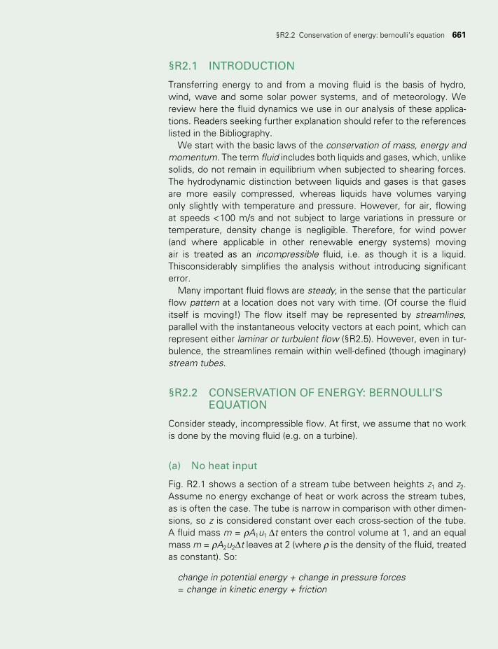
§R2.2 Conservation of energy: bernoulli’s equation 661
§R2.1 INTRODUCTION
Transferring energy to and from a moving fluid is the basis of hydro, wind, wave and some solar power systems, and of meteorology. We review here the fluid dynamics we use in our analysis of these applica-tions. Readers seeking further explanation should refer to the references listed in the Bibliography.
We start with the basic laws of the conservation of mass, energy and momentum. The term fluid includes both liquids and gases, which, unlike solids, do not remain in equilibrium when subjected to shearing forces. The hydrodynamic distinction between liquids and gases is that gases are more easily compressed, whereas liquids have volumes varying only slightly with temperature and pressure. However, for air, flowing at speeds <100 m/s and not subject to large variations in pressure or temperature, density change is negligible. Therefore, for wind power (and where applicable in other renewable energy systems) moving air is treated as an incompressible fluid, i.e. as though it is a liquid. Thisconsiderably simplifies the analysis without introducing significant error.
Many important fluid flows are steady, in the sense that the particular flow pattern at a location does not vary with time. (Of course the fluid itself is moving!) The flow itself may be represented by streamlines, parallel with the instantaneous velocity vectors at each point, which can represent either laminar or turbulent flow (§R2.5). However, even in tur-bulence, the streamlines remain within well-defined (though imaginary) stream tubes.
§R2.2 CONSERVATION OF ENERGY: BERNOULLI’S EQUATION
Consider steady, incompressible flow. At first, we assume that no work is done by the moving fluid (e.g. on a turbine).
(a) No heat input
Fig. R2.1 shows a section of a stream tube between heights z1 and z2. Assume no energy exchange of heat or work across the stream tubes, as is often the case. The tube is narrow in comparison with other dimen-sions, so z is considered constant over each cross-section of the tube. A fluid mass m = rA1u1 Dt enters the control volume at 1, and an equal mass m = rA2u2Dt leaves at 2 (where r is the density of the fluid, treated as constant). So:
change in potential energy + change in pressure forces = change in kinetic energy + friction
TWIDELL PAGINATION.indb 661 01/12/2014 11:39
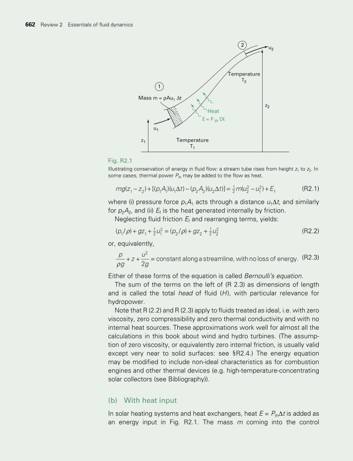
662 Essentials of fluid dynamics662 Review 2 Essentials of fluid dynamics
mg z z p A u t p A u t m u u E( ) [( )( ) ( )( )] ( )1 2 1 1 1 2 2 212 2
212
f- + D - D = - + (R2.1)
where (i) pressure force p1A1 acts through a distance u1Dt, and similarly for p2A2, and (ii) Ef is the heat generated internally by friction.
Neglecting fluid friction Ef and rearranging terms, yields:
p gz u p gz u( / ) ( / )1 112 1
22 2
12 2
2r r+ + = + + (R2.2)
or, equivalently,
pg
zug
+ +2
= constant along a streamline, withno loss of energy.2
r (R2.3)
Either of these forms of the equation is called Bernoulli’s equation. The sum of the terms on the left of (R 2.3) as dimensions of length
and is called the total head of fluid (H ), with particular relevance for hydropower.
Note that R (2.2) and R (2.3) apply to fluids treated as ideal, i.e. with zero viscosity, zero compressibility and zero thermal conductivity and with no internal heat sources. These approximations work well for almost all the calculations in this book about wind and hydro turbines. (The assump-tion of zero viscosity, or equivalently zero internal friction, is usually valid except very near to solid surfaces: see §R2.4.) The energy equation may be modified to include non-ideal characteristics as for combustion engines and other thermal devices (e.g. high-temperature-concentrating solar collectors (see Bibliography)).
(b) With heat input
In solar heating systems and heat exchangers, heat E = PthDt is added as an energy input in Fig. R2.1. The mass m coming into the control
Fig. R2.1Illustrating conservation of energy in fluid flow: a stream tube rises from height z1 to z2. In some cases, thermal power Pth may be added to the flow as heat.
Mass m = ρAu1 ∆t
u1
u2
z1
z2Heat
E = P th Dt
TemperatureT1
TemperatureT2
1
2
TWIDELL PAGINATION.indb 662 01/12/2014 11:39
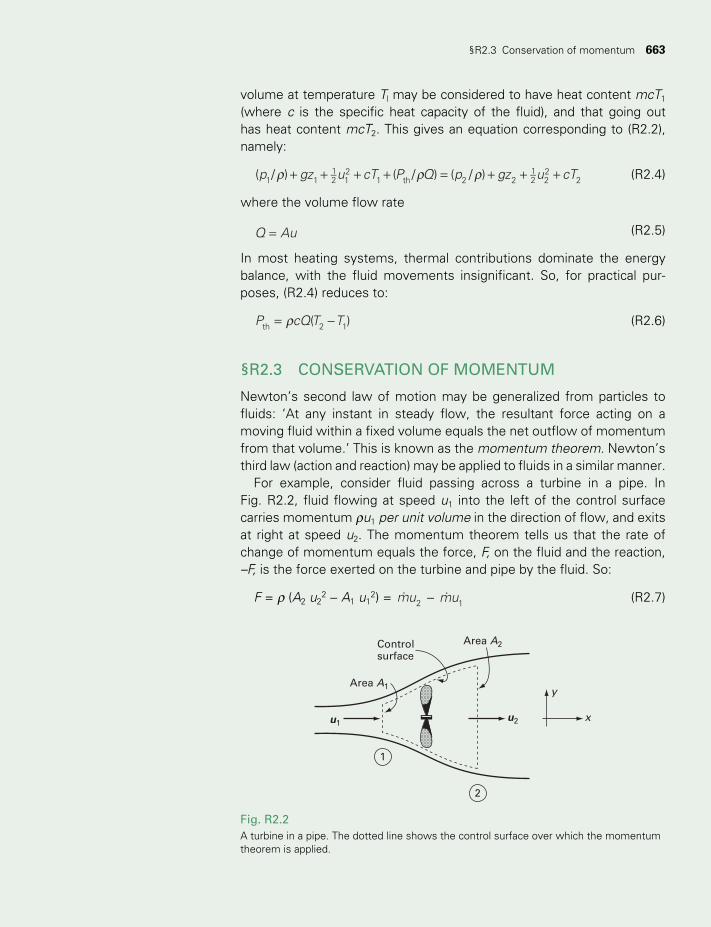
§R2.3 Conservation of momentum 663
volume at temperature Tl may be considered to have heat content mcT1 (where c is the specific heat capacity of the fluid), and that going out has heat content mcT2. This gives an equation corresponding to (R2.2), namely:
p gz u cT P Q p gz u cT( / ) ( / ) ( / )1 112 1
21 th 2 2
12 2
22r r r+ + + + = + + + (R2.4)
where the volume flow rate
Q Au= (R2.5)
In most heating systems, thermal contributions dominate the energy balance, with the fluid movements insignificant. So, for practical pur-poses, (R2.4) reduces to:
P cQ T T( )th 2 1r= - (R2.6)
§R2.3 CONSERVATION OF MOMENTUM
Newton’s second law of motion may be generalized from particles to fluids: ‘At any instant in steady flow, the resultant force acting on a moving fluid within a fixed volume equals the net outflow of momentum from that volume.’ This is known as the momentum theorem. Newton’s third law (action and reaction) may be applied to fluids in a similar manner.
For example, consider fluid passing across a turbine in a pipe. In Fig. R2.2, fluid flowing at speed u1 into the left of the control surface carries momentum ru1 per unit volume in the direction of flow, and exits at right at speed u2. The momentum theorem tells us that the rate of change of momentum equals the force, F, on the fluid and the reaction, –F, is the force exerted on the turbine and pipe by the fluid. So:
F = r (A2 u22 - A1 u1
2) = mu2 - mu1
(R2.7)
Area A2
u2
y
xu1
Area A1
Controlsurface
1
2
Fig. R2.2A turbine in a pipe. The dotted line shows the control surface over which the momentum theorem is applied.
TWIDELL PAGINATION.indb 663 01/12/2014 11:39
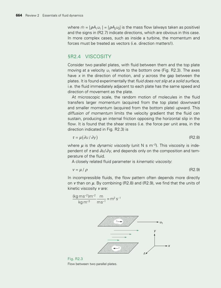
664 Essentials of fluid dynamics664 Review 2 Essentials of fluid dynamics
where m = | rA1u1 | = | rA2u2| is the mass flow (always taken as positive) and the signs in (R2.7) indicate directions, which are obvious in this case. In more complex cases, such as inside a turbine, the momentum and forces must be treated as vectors (i.e. direction matters!).
§R2.4 VISCOSITY
Consider two parallel plates, with fluid between them and the top plate moving at a velocity u1 relative to the bottom one (Fig. R2.3). The axes have x in the direction of motion, and y across the gap between the plates. It is found experimentally that fluid does not slip at a solid surface, i.e. the fluid immediately adjacent to each plate has the same speed and direction of movement as the plate.
At microscopic scale, the random motion of molecules in the fluid transfers larger momentum (acquired from the top plate) downward and smaller momentum (acquired from the bottom plate) upward. This diffusion of momentum limits the velocity gradient that the fluid can sustain, producing an internal friction opposing the horizontal slip in the flow. It is found that the shear stress (i.e. the force per unit area, in the direction indicated in Fig. R2.3) is
u y/t m ∂ ∂( )= (R2.8)
where m is the dynamic viscosity (unit N s m-2). This viscosity is inde-pendent of t and ∂u / ∂y, and depends only on the composition and tem-perature of the fluid.
A closely related fluid parameter is kinematic viscosity:
/n m r= (R2.9)
In incompressible fluids, the flow pattern often depends more directly on n than on m. By combining (R2.8) and (R2.9), we find that the units of kinetic viscosity n are:
- -
- --(kg ms )m
kg mm
ms= m s
2 2
3 12 1
Fig. R2.3Flow between two parallel plates.
τ
τ
u1
x
z
y
TWIDELL PAGINATION.indb 664 01/12/2014 11:39
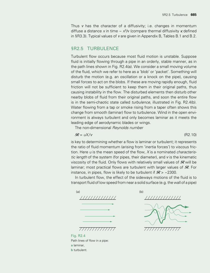
§R2.5 Turbulence 665
Thus n has the character of a diffusivity; i.e. changes in momentum diffuse a distance x in time ~ x2/n (compare thermal diffusivity k defined in §R3.3). Typical values of n are given in Appendix B, Tables B.1 and B.2.
§R2.5 TURBULENCE
Turbulent flow occurs because most fluid motion is unstable. Suppose fluid is initially flowing through a pipe in an orderly, stable manner, as in the path lines shown in Fig. R2.4(a). We consider a small moving volume of the fluid, which we refer to here as a ‘blob’ or ‘packet’. Something will disturb the motion (e.g. an oscillation or a knock on the pipe), causing small forces to act on the blobs. If these are moving rapidly enough, fluid friction will not be sufficient to keep them in their original paths, thus causing instability in the flow. The disturbed elements then disturb other nearby blobs of fluid from their original paths, and soon the entire flow is in the semi-chaotic state called turbulence, illustrated in Fig. R2.4(b). Water flowing from a tap or smoke rising from a taper often shows this change from smooth (laminar) flow to turbulence. Wind in the open envi-ronment is always turbulent and only becomes laminar as it meets the leading edge of aerodynamic blades or wings.
The non-dimensional Reynolds number
R = uX / n (R2.10)
is key to determining whether a flow is laminar or turbulent; it represents the ratio of fluid momentum (arising from ‘inertia forces’) to viscous fric-tion. Here u is the mean speed of the flow, X is a nominated characteris-tic length of the system (for pipes, their diameter), and n is the kinematic viscosity of the fluid. Only flows with relatively small values of R will be laminar; most practical flows are turbulent with larger values of R. For instance, in pipes, flow is likely to be turbulent if R > ~2300.
In turbulent flow, the effect of the sideways motions of the fluid is to transport fluid of low speed from near a solid surface (e.g. the wall of a pipe)
Fig. R2.4Path lines of flow in a pipe: a laminar, b turbulent.
(a) (b)
TWIDELL PAGINATION.indb 665 01/12/2014 11:39
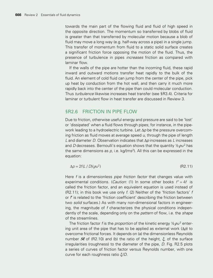
666 Essentials of fluid dynamics666 Review 2 Essentials of fluid dynamics
towards the main part of the flowing fluid and fluid of high speed in the opposite direction. The momentum so transferred by blobs of fluid is greater than that transferred by molecular motion because a blob of fluid may move a long way (e.g. half-way across a pipe) in a single jump. This transfer of momentum from fluid to a static solid surface creates a significant friction force opposing the motion of the fluid. Thus, the presence of turbulence in pipes increases friction as compared with laminar flow.
If the walls of the pipe are hotter than the incoming fluid, these rapid inward and outward motions transfer heat rapidly to the bulk of the fluid. An element of cold fluid can jump from the center of the pipe, pick up heat by conduction from the hot wall, and then carry it much more rapidly back into the center of the pipe than could molecular conduction. Thus turbulence likewise increases heat transfer (see §R3.4). Criteria for laminar or turbulent flow in heat transfer are discussed in Review 3.
§R2.6 FRICTION IN PIPE FLOW
Due to friction, otherwise useful energy and pressure are said to be ‘lost’ or ‘dissipated’ when a fluid flows through pipes; for instance, in the pipe-work leading to a hydroelectric turbine. Let Dp be the pressure overcom-ing friction as fluid moves at average speed u, through the pipe of length L and diameter D. Observation indicates that Dp increases as L increases and D decreases. Bernoulli’s equation shows that the quantity ½ ru 2 has the same dimensions as p, i.e. kg/(ms2). All this can be expressed in the equation:
p f L D u2 ( / )( )2rD = (R2.11)
Here f is a dimensionless pipe friction factor that changes value with experimental conditions. (Caution: (1) In some other books f f4′ = is called the friction factor, and an equivalent equation is used instead of (R2.11); in this book we use only f. (2) Neither of the ‘friction factors’ f or f′ is related to the ‘friction coefficient’ describing the friction between two solid surfaces.) As with many non-dimensional factors in engineer-ing, the magnitude of f characterizes the physical conditions indepen-dently of the scale, depending only on the pattern of flow, i.e. the shape of the streamlines.
The friction factor f is the proportion of the kinetic energy ½ ru 2 enter-ing unit area of the pipe that has to be applied as external work (Dp) to overcome frictional forces. It depends on (a) the dimensionless Reynolds number R of (R2.10) and (b) the ratio of the height, ξ, of the surface irregularities (roughness) to the diameter of the pipe, D. Fig. R2.5 plots a series of curves of friction factor versus Reynolds number, with one curve for each roughness ratio ξ/D.
TWIDELL PAGINATION.indb 666 01/12/2014 11:39
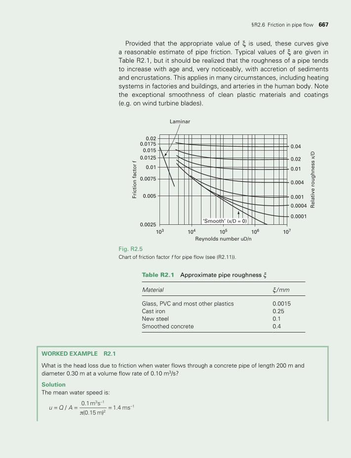
§R2.6 Friction in pipe flow 667
Table R2.1 Approximate pipe roughness ξ
Material ξ/ mm
Glass, PVC and most other plastics 0.0015Cast iron 0.25New steel 0.1Smoothed concrete 0.4
0.02
0.04
0.02
0.01
0.004
0.001
0.0004
0.0001‘Smooth’ (x/D = 0)
Rel
ativ
e ro
ug
hn
ess x/
D
Fric
tio
n f
acto
r f
0.01750.015
0.0125
0.0075
0.005
0.0025103 104 105 106 107
Laminar
Reynolds number uD/n
0.01
Fig. R2.5Chart of friction factor f for pipe flow (see (R2.11)).
Provided that the appropriate value of ξ is used, these curves give a reasonable estimate of pipe friction. Typical values of ξ are given in Table R2.1, but it should be realized that the roughness of a pipe tends to increase with age and, very noticeably, with accretion of sediments and encrustations. This applies in many circumstances, including heating systems in factories and buildings, and arteries in the human body. Note the exceptional smoothness of clean plastic materials and coatings (e.g. on wind turbine blades).
WORKED EXAMPLE R2.1
What is the head loss due to friction when water flows through a concrete pipe of length 200 m and diameter 0.30 m at a volume flow rate of 0.10 m3/s?
SolutionThe mean water speed is:
u Q A/0.1m s
(0.15 m)1.4 ms
3 1
21= = =
--
π
TWIDELL PAGINATION.indb 667 01/12/2014 11:39
668 Essentials of fluid dynamics668 Review 2 Essentials of fluid dynamics
From (R2.10), the Reynolds number
n= =
×= ×
-
- -
uD (1.4 ms )(0.3 m)
1.0 10 m s0.4 10
1
6 2 16R
where the value of n is taken from Appendix B, Table B.2. Since R >> 2000, flow is turbulent.For concrete (from Table R2.1), ξ = 0.4 mm. Thus the ratio
D/0.4 mm
300 mm0.0013ξ = =
For these values of R and ξ/ D, Fig. R2.5 gives
f = 0.0050,
Expressing (R2.11) in terms of the head loss due to friction,
H p g fLu Dg/ 2 /f2r= D = (R2.12)
Hence:
H(2)(5.0 10 )(200 m)(1.4 ms )
(0.3 m)(9.8 ms )1.3 m
f
3 1 2
2=
×
=
- -
-
Fig. R2.5 shows only one curve for R < 2000 indicating the flow is laminar; the ‘pattern’ of the moving water is independent of the pipe internal surface in this range of Reynolds number. In laminar flow it is possible to calculate the pressure drop Dp explicitly from (R2.8), and hence it may be shown that the friction factor is:
n=f uD16 / ( ) (laminar) (R2.13)
§R2.7 LIFT AND DRAG FORCES
Lift and drag forces apply to any solid object immersed in a fluid flow (e.g. wings on an aircraft or blades on a wind turbine rotor).
In Fig. R2.6(a) a solid object is immersed in a fluid flowing from left to right (relative to the object). However, due to intricacies of the flow pattern passing the object, the resulting force on the object is unlikely to be parallel to the upstream flow. If the total (vector) force exerted on the body is F, the drag force FD is the component of that force in the direction of the upstream flow and the lift force FL is the component normal to the flow. It is the lift force that twists and turns the object.
An important special case is an airfoil. This is a smooth structure of width (chord) much less than its length (span), and thickness much less
TWIDELL PAGINATION.indb 668 01/12/2014 11:39
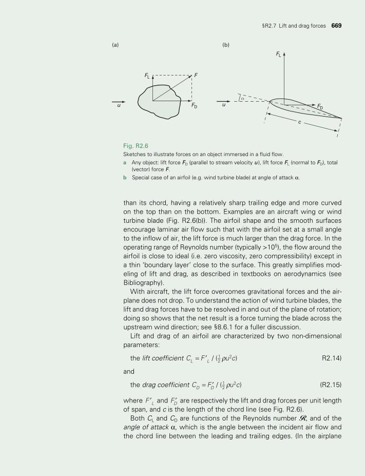
§R2.7 Lift and drag forces 669
than its chord, having a relatively sharp trailing edge and more curved on the top than on the bottom. Examples are an aircraft wing or wind turbine blade (Fig. R2.6(b)). The airfoil shape and the smooth surfaces encourage laminar air flow such that with the airfoil set at a small angle to the inflow of air, the lift force is much larger than the drag force. In the operating range of Reynolds number (typically >105), the flow around the airfoil is close to ideal (i.e. zero viscosity, zero compressibility) except in a thin ‘boundary layer’ close to the surface. This greatly simplifies mod-eling of lift and drag, as described in textbooks on aerodynamics (see Bibliography).
With aircraft, the lift force overcomes gravitational forces and the air-plane does not drop. To understand the action of wind turbine blades, the lift and drag forces have to be resolved in and out of the plane of rotation; doing so shows that the net result is a force turning the blade across the upstream wind direction; see §8.6.1 for a fuller discussion.
Lift and drag of an airfoil are characterized by two non-dimensional parameters:
the lift coefficient r= ′C F u c/ ( )L L12
2 R2.14)
and
the drag coefficient C F u c/ ( )D D12
2r= ′ (R2.15)
where ′F L and FD′ are respectively the lift and drag forces per unit length of span, and c is the length of the chord line (see Fig. R2.6).
Both CL and CD are functions of the Reynolds number R, and of the angle of attack α, which is the angle between the incident air flow and the chord line between the leading and trailing edges. (In the airplane
FL
FFL
FDFD u
c
αu
(a) (b)
Fig. R2.6Sketches to illustrate forces on an object immersed in a fluid flow. a Any object: lift force FD (parallel to stream velocity u ), lift force FL (normal to FD), total
(vector) force F. b Special case of an airfoil (e.g. wind turbine blade) at angle of attack α.
TWIDELL PAGINATION.indb 669 01/12/2014 11:39
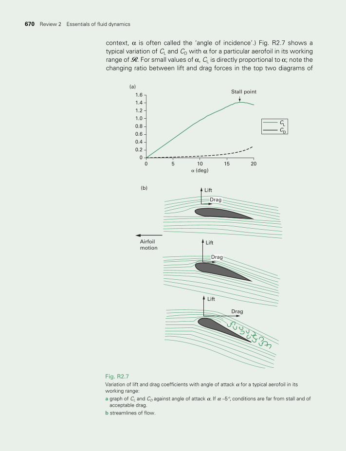
670 Essentials of fluid dynamics670 Review 2 Essentials of fluid dynamics
Airfoilmotion
Lift
Lift
Drag
Lift(b)
Drag
Drag
0
0.2
0.4
0.6
0.8
1.0
1.2
1.4
1.6
(a)
0 5 10 15 20a (deg)
CL CD
Stall point
Fig. R2.7Variation of lift and drag coefficients with angle of attack α for a typical aerofoil in its working range: a graph of CL and CD against angle of attack α.If α∼5°,conditions are far from stall and of
acceptable drag.b streamlines of flow.
context, α is often called the ‘angle of incidence’.) Fig. R2.7 shows a typical variation of CL and CD with α for a particular aerofoil in its working range of R. For small values of α, CL is directly proportional to α; note the changing ratio between lift and drag forces in the top two diagrams of
TWIDELL PAGINATION.indb 670 01/12/2014 11:39

Bibliography 671
Fig. R2.7(b). For some value of α between 10° and 20°, the lift decreases, and the aerofoil becomes stalled, with the flow separating from the top surface and the drag increasing substantially, as in the bottom diagram of Fig. R2.7(b).
QUICK QUESTIONS
Note: Answers to these questions are in the text of the relevant section of this chapter, or may be readily inferred from it.
1 Why can air be treated as incompressible in most renewable energy applications?
2 Write down Bernouilli’s equation. Does it relate primarily to the speed, the momentum, or the energy of a fluid?
3 Distinguish dynamic viscosity from kinenatic viscosity. 4 Define Reynolds number. Why is it so important in calculations of
fluid flow? 5 What is the difference between turbulent flow and laminar flow? 6 Why is pipe friction greater in than in laminar flow? 7 Define lift and drag. 8 Why are aircraft wings usually thin compared to their length or width? 9 Compare the density of air and water, and discuss the effect on
turbine design.10 What is the speed of a moving fluid at a smooth boundary surface?
BIBLIOGRAPHY
The following selection from the many books and websites on fluid mechanics may prove useful. There are many other good books besides those listed. For work on turbo-machinery, books written for engineers are usually more useful than those written for mathematicians, who too often ignore friction and forces. Since the basics of fluid dynamics have not changed, old textbooks may still be useful, especially if they use SI units (which many older books do not). However, modern engineering practice makes much use of computer software packages, with the danger of misuse if basic principles are not understood by the user.
Books
Batchelor, G.K. (1967) An Introduction to Fluid Dynamics, Cambridge University Press, Cambridge. Classic text, reissued unchanged in 2000. A most precise statement of the foundations (see especially ch. 3), with many examples. Repays careful reading, but perhaps unsuitable for beginners.
Çengel, Y.A. and Cimbala, J. (2009, 2nd edn) Fluid Mechanics: Fundamentals and applications, McGraw-Hill, New York. Clear and detailed explanations with emphasis on physical principles. Very student-friendly with exemplary accompanying learning aids.
Francis, J.R. (1974, 4th edn) A Textbook of Fluid Mechanics, Edward Arnold, London. Clear writing makes this easy reading for beginners. More engineering detail than Kay and Nedderman.
TWIDELL PAGINATION.indb 671 01/12/2014 11:39

672 Essentials of fluid dynamics672 Review 2 Essentials of fluid dynamics
Kay, J.M. and Nedderman, R.M. (1985) Fluid Mechanics and Transfer Processes, Cambridge University Press, Cambridge. A concise and wide-ranging introduction.
Mott, R.L. (2005, 6th edn) Applied Fluid Mechanics, Prentice Hall, Englewood Cliffs, NJ. Widely used student text at beginner level, with exceptionally clear explanations.
Potter, M. and Wiggert, D. (2007) Fluid Mechanics, Schaum’s Outline Series. Multitude of worked examples. One of numerous similar books in this student-friendly series.
Tritton, D.J. (1988) Physical Fluid Dynamics, Oxford Science Publications, Oxford University Press, Oxford. Careful mathematical formulation, related closely to physical reality.
Webber, N. (1971) Fluid Mechanics for Civil Engineers, Chapman and Hall, London. Delightfully simple but useful introduction for students with little knowledge of physics or engineering.
Websites
en.wikipedia.org/wiki/Fluid_dynamics. As usual for basic science, the Wikipedia article is excellent, but quickly enters developments not needed for this book.
www.youtube.com/watch?v=dY3daNK1Tek&feature=related. An old mili tary training film with exceptionally clear explanations of basic aerodynamics.
TWIDELL PAGINATION.indb 672 01/12/2014 11:39
Review 3 Heat transfer
CONTENTS
§R3.1 Introduction 675
§R3.2 Heat circuit analysis and terminology 675
§R3.3 Conduction 679
§R3.4 Convection 681§R3.4.1 Free and forced convection 681§R3.4.2 Nusselt number N 682§R3.4.3 Forced convection 684§R3.4.4 Free convection 685§R3.4.5 Calculation of convective
heat transfer 686
§R3.5 Radiative heat transfer 688§R3.5.1 Introduction 688§R3.5.2 Radiant flux density (RFD) 688§R3.5.3 Absorption, reflection and
transmission of radiation 690§R3.5.4 Black bodies, emittance
and Kirchhoff’s laws 693§R3.5.5 Radiation emitted by a
body 693§R3.5.6 Radiative exchange
between black surfaces 695
§R3.5.7 Radiative exchange between gray surfaces 696
§R3.5.8 Thermal resistance formulation 696
§R3.6 Properties of ‘transparent’ materials 697
§R3.7 Heat transfer by mass transport 698§R3.7.1 Single-phase heat transfer 698§R3.7.2 Phase change, including
heat pipes 699
§R3.8 Multimode transfer and circuit analysis 701§R3.8.1 Resistances only 701§R3.8.2 Thermal capacitance 701§R3.8.3 Thermal time constant 703§R3.8.4 Heat exchangers 704
Quick questions 705
Notes 706
Bibliography 706
Box R3.1 Heat transfer terminology 678
LIST OF FIGURES
R3.1 Worked Example of a heat circuit. surface, the wall surfaces 676R3.2 Fluid movement by free convection, away from the hotter surface. 682R3.3 Idealized thermal boundary layer in free convection. 683R3.4 Fluid flow over a hot plate. 684R3.5 Schematic diagram of a blob of fluid moving upward in free convection. 685R3.6 Diagram for Worked Example R3.2 on convection. 687
TWIDELL PAGINATION.indb 673 01/12/2014 11:39

674 Heat transfer674 Review 3 Heat transfer
R3.7 Measurements of various radiation parameters using a small totally absorbing plane. 689R3.8 Reflection, absorption and transmission of radiation. 690R3.9 Data for Worked Example R3.3. 692R3.10 Spectral distribution of black body radiation. 694R3.11 Exchange of radiation between two (black) surfaces. 695R3.12 Monochromatic transmittance of: (a) glass. (b) polythene. 698R3.13 Mass flow through a heated pipe. 699R3.14 Heat transfer by phase change. 700R3.15 Schematic diagram of a heat pipe. 700R3.16 A hot object loses heat to its surroundings. 702R3.17 (a) Equivalent circuit of a heated (or cooled) material. (b) Corresponding decay of temperature of
mass in (a). 703R3.18 Sketch of counter-flow heat exchanger principle. 704
LIST OF TABLES
R3.1 Heat transfer terminology 678R3.2 Comparable electrical and thermal quantities 702
TWIDELL PAGINATION.indb 674 01/12/2014 11:39
§R3.2 Heat circuit analysis and terminology 675
§R3.1 INTRODUCTION
Using energy implies that it is transferred from one form to another (e.g. from solar radiation to the temperature increase of water, or from solar radiation to electricity). When the transfer is from a hot body to a cooler body, the processes are called heat transfer. Heat transfer pro-cesses are dominant in utilizing direct solar, geothermal and biomass sources.
Heat transfer is a well-established yet complex subject. In this Review, we outline the basic physics with the key definitions and formulae needed in this book. The main formulae needed for practical calcula-tions are summarized in Appendix C. Specialized textbooks justify this approach, as listed in the Bibliography.
Our recommended analysis uses heat transfer circuits of the intercon-nected processes (see e.g. Fig. R3.1(c)); these are analogs of electri-cal circuits. After sketching the circuit, we then calculate each transfer process according to its classification as conduction, radiation, convection or mass transfer. At this stage insignificant processes may be neglected, and the dominant transfers analyzed to greater accuracy. Even so, it is unlikely that overall accuracy of complex processes will be better than ±25% of actual performance. This, however, is sufficient to suggest design improvements.
§R3.2 HEAT CIRCUIT ANALYSIS AND TERMINOLOGY
As a simple example, consider a large tank of hot water standing in a cool, enclosed room, with a colder environment outside. The floor and ceiling are so well insulated that heat passes predominantly through the walls. Therefore net heat transfer is down a temperature gradient from the hot tank to the cold outside environment (Fig. R3.1(a)). Heat is transferred from the tank by radiation and convection to the room walls, by —conduction through the walls, and then by radiation and convec-tion to he environment (Fig. R3.1(b)). This complex transfer of parallel and series connections is described in the heat circuit shown in Fig. R3.1(c).
Each process may be described by an equation of the form:
= − = DP T T R T R( ) / /ij i j ij ij (R3.1)
where the power Pij is the heat flow between surfaces at temperatures Ti (hotter) and Tj (colder), and Rij is called the thermal resistance1 (see Appendix A for units). This equation is analogous to Ohm’s Law in elec-tricity, with heat flow analogous to electrical current, temperature to voltage and thermal resistance to electrical resistance. As with electrical resistance, thermal resistance is not necessarily a constant.
TWIDELL PAGINATION.indb 675 01/12/2014 11:39

676 Heat transfer676 Review 3 Heat transfer
The thermal resistance method allows each step of a complex of heat transfers to be added together as a set of series and parallel connections, as in electrical circuits. In our example of Fig. R3.1:
= −P T T R( ) /14 1 4 14 (R3.2)
where
= + +R R R R14 12 23 34
and
= +R R R1 1
(convection)1
(radiation)12 12 12
=R R (conduction)23 23
= +R R R
1 1(convection)
1(radiation)34 34 34
Fig. R3.1Worked Example of a heat circuit. a Physical situation. A hot tank is in a cool room with cold air outside. The roof and the
floor are well insulated. T1, T2, T3 and T4 are the temperatures of the tank surface, the wall surfaces and the outside environment respectively.
b Energy flow mechanisms. c Analog circuit.
T2
(a)
Convection ConvectionConduction
RadiationRadiation
(b)
(c)
T3 T4
Source(tank)
Sink(environment)
T1 T2Rv,12
Rr,12
Rn,23
Rr,34
T3Rv, 34
T4
T1
TWIDELL PAGINATION.indb 676 01/12/2014 11:39
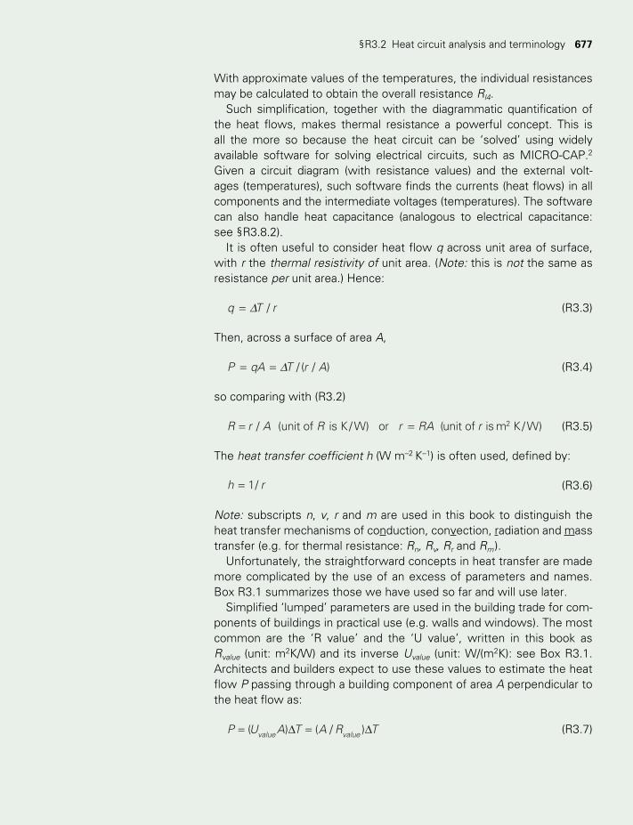
§R3.2 Heat circuit analysis and terminology 677
With approximate values of the temperatures, the individual resistances may be calculated to obtain the overall resistance Rl4.
Such simplification, together with the diagrammatic quantification of the heat flows, makes thermal resistance a powerful concept. This is all the more so because the heat circuit can be ‘solved’ using widely available software for solving electrical circuits, such as MICRO-CAP.2 Given a circuit diagram (with resistance values) and the external volt-ages (temperatures), such software finds the currents (heat flows) in all components and the intermediate voltages (temperatures). The software can also handle heat capacitance (analogous to electrical capacitance: see §R3.8.2).
It is often useful to consider heat flow q across unit area of surface, with r the thermal resistivity of unit area. (Note: this is not the same as resistance per unit area.) Hence:
D=q T r/ (R3.3)
Then, across a surface of area A,
D= =P qA T r A/ ( / ) (R3.4)
so comparing with (R3.2)
= =R r A R r RA r/ (unit of is K/W) or (unit of is m K/W)2 (R3.5)
The heat transfer coefficient h (W m–2 K–1) is often used, defined by:
=h r1/ (R3.6)
Note: subscripts n, v, r and m are used in this book to distinguish the heat transfer mechanisms of conduction, convection, radiation and mass transfer (e.g. for thermal resistance: Rn, Rv, Rr and Rm ).
Unfortunately, the straightforward concepts in heat transfer are made more complicated by the use of an excess of parameters and names. Box R3.1 summarizes those we have used so far and will use later.
Simplified ‘lumped’ parameters are used in the building trade for com-ponents of buildings in practical use (e.g. walls and windows). The most common are the ‘R value’ and the ‘U value’, written in this book as Rvalue (unit: m2K/W) and its inverse Uvalue (unit: W/(m2K): see Box R3.1. Architects and builders expect to use these values to estimate the heat flow P passing through a building component of area A perpendicular to the heat flow as:
= D = DP U A T A R T( ) ( / )value value (R3.7)
TWIDELL PAGINATION.indb 677 01/12/2014 11:39
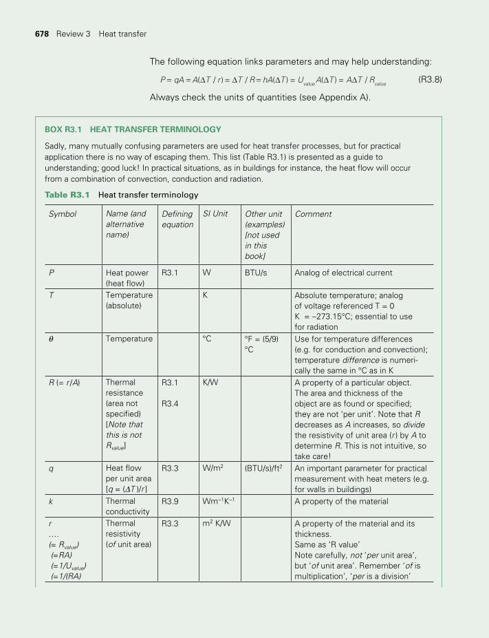
678 Heat transfer678 Review 3 Heat transfer
BOX R3.1 HEAT TRANSFER TERMINOLOGY
Sadly, many mutually confusing parameters are used for heat transfer processes, but for practical application there is no way of escaping them. This list (Table R3.1) is presented as a guide to understanding; good luck! In practical situations, as in buildings for instance, the heat flow will occur from a combination of convection, conduction and radiation.
Table R3.1 Heat transfer terminology
Symbol Name (and alternative name)
Definingequation
SI Unit Other unit(examples)[not used in this book]
Comment
P Heat power (heat flow)
R3.1 W BTU/s Analog of electrical current
T Temperature (absolute)
K Absolute temperature; analog of voltage referenced T = 0 K = −273.15°C; essential to use for radiation
θ Temperature °C °F = (5/9) °C
Use for temperature differences (e.g. for conduction and convection); temperature difference is num eri-cally the same in °C as in K
R (= r /A) Thermal resistance(area not specified)[Note that this is not Rvalue]
R3.1
R3.4
K/W A property of a particular object.The area and thickness of the object are as found or specified; they are not ‘per unit’. Note that R decreases as A increases, so divide the resistivity of unit area (r ) by A to determine R. This is not intuitive, so take care!
q Heat flow per unit area[q = (DT )/r ]
R3.3 W/m2 (BTU/s)/ft2 An important parameter for practical measurement with heat meters (e.g. for walls in buildings)
k Thermal conductivity
R3.9 Wm−1K−1 A property of the material
r…. (= Rvalue) (=RA) (=1/Uvalue) (=1/(RA)
Thermal resistivity (of unit area)
R3.3 m2 K/W A property of the material and its thickness.Same as ‘R value’Note carefully, not ‘per unit area’, but ‘of unit area’. Remember ‘of is multiplication’, ‘per is a division’
The following equation links parameters and may help understanding:
P qA A T r T R hA T U A T A T R( / ) = / ( ) = ( ) = /value value= = D D = D D D (R3.8)
Always check the units of quantities (see Appendix A).
TWIDELL PAGINATION.indb 678 01/12/2014 11:39
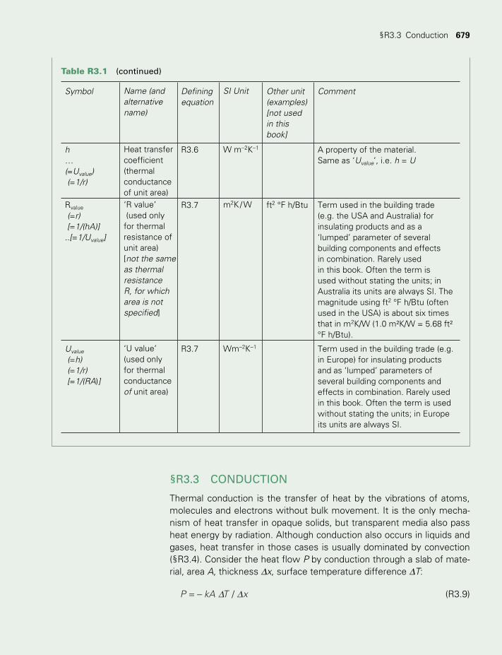
§R3.3 Conduction 679
§R3.3 CONDUCTION
Thermal conduction is the transfer of heat by the vibrations of atoms, molecules and electrons without bulk movement. It is the only mecha-nism of heat transfer in opaque solids, but transparent media also pass heat energy by radiation. Although conduction also occurs in liquids and gases, heat transfer in those cases is usually dominated by convection (§R3.4). Consider the heat flow P by conduction through a slab of mate-rial, area A, thickness Dx, surface temperature difference DT:
D D = − P kA T x/ (R3.9)
Symbol Name (and alternative name)
Definingequation
SI Unit Other unit(examples)[not used in this book]
Comment
h… (=Uvalue) (=1/r)
Heat transfer coefficient(thermal conductance of unit area)
R3.6 W m−2K−1 A property of the material.Same as ‘Uvalue’, i.e. h = U
Rvalue
(=r) [=1/(hA)]..[=1/Uvalue]
‘R value’ (used only for thermal resistance of unit area)[not the same as thermal resistance R, for which area is not specified]
R3.7 m2K / W ft2 °F h/Btu Term used in the building trade (e.g. the USA and Australia) for insulating products and as a ‘lumped’ parameter of several building components and effects in combination. Rarely used in this book. Often the term is used without stating the units; in Australia its units are always SI. The magnitude using ft2 °F h/Btu (often used in the USA) is about six times that in m2K/W (1.0 m²K/W = 5.68 ft² °F h/Btu).
Uvalue
(=h) (=1/r) [=1/(RA)]
‘U value’(used only for thermal conductance of unit area)
R3.7 Wm−2K−1 Term used in the building trade (e.g. in Europe) for insulating products and as ‘lumped’ parameters of several building components and effects in combination. Rarely used in this book. Often the term is used without stating the units; in Europe its units are always SI.
Table R3.1 (continued)
TWIDELL PAGINATION.indb 679 01/12/2014 11:39
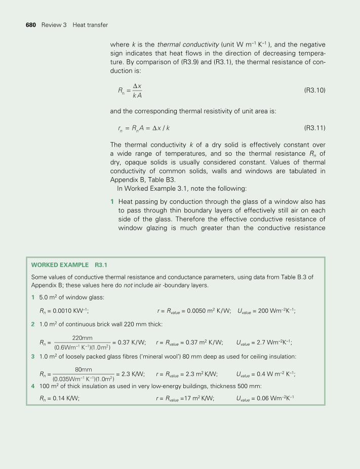
680 Heat transfer680 Review 3 Heat transfer
where k is the thermal conductivity (unit W m–1 K–1 ), and the negative sign indicates that heat flows in the direction of decreasing tempera-ture. By comparison of (R3.9) and (R3.1), the thermal resistance of con -duction is:
=D
Rx
k An (R3.10)
and the corresponding thermal resistivity of unit area is:
= = Dr R A x k/n n (R3.11)
The thermal conductivity k of a dry solid is effectively constant over a wide range of temperatures, and so the thermal resistance Rn of dry, opaque solids is usually considered constant. Values of thermal conductivity of common solids, walls and windows are tabulated in Appendix B, Table B3.
In Worked Example 3.1, note the following:
1 Heat passing by conduction through the glass of a window also has to pass through thin boundary layers of effectively still air on each side of the glass. Therefore the effective conductive resistance of window glazing is much greater than the conductive resistance
WORKED EXAMPLE R3.1
Some values of conductive thermal resistance and conductance parameters, using data from Table B.3 of Appendix B; these values here do not include air -boun dary layers.
1 5.0 m2 of window glass:
Rn = 0.0010 KW–1; r = Rvalue = 0.0050 m2 K / W; Uvalue = 200 Wm−2K−1;
2 1.0 m2 of continuous brick wall 220 mm thick:
Rn = 220mm
(0.6Wm K )(1.0m )1 1 2− −= 0.37 K / W; r = Rvalue = 0.37 m2 K / W; Uvalue = 2.7 Wm–2K–1;
3 1.0 m2 of loosely packed glass fibres (‘mineral wool’) 80 mm deep as used for ceiling insulation:
Rn =80mm
(0.035Wm K )(1.0m )1 1 2− −= 2.3 K/W; r = Rvalue = 2.3 m2 K/W; Uvalue = 0.4 W m–2 K–1;
4 100 m2 of thick insulation as used in very low-energy buildings, thickness 500 mm:
Rn = 0.14 K/W; r = Rvalue =17 m2 K/W; Uvalue = 0.06 Wm−2K−1
TWIDELL PAGINATION.indb 680 01/12/2014 11:39
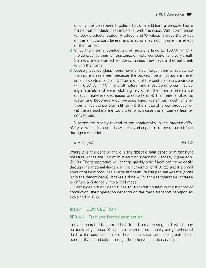
§R3.4 Convection 681
of only the glass (see Problem 16.2). In addition, a window has a frame that conducts heat in parallel with the glass. With commercial window products, stated ‘R values’ and ‘U values’ include the effect of the air boundary layers, and may or may not include the effect of the frames.
2 Since the thermal conductivity of metals is large (k~100 W m–1K–1), the conductive thermal resistance of metal components is very small. So avoid metal-framed windows, unless they have a thermal break within the frame.
3 Loosely packed glass fibers have a much larger thermal resistance than pure glass sheet, because the packed fibers incorporate many small pockets of still air. Still air is one of the best insulators available (k ~ 0.03 W m–1K–1), and all natural and most commercial insulat-ing materials and warm clothing rely on it. The thermal resistance of such materials decreases drastically if: (i) the material absorbs water and becomes wet, because liquid water has much smaller thermal resistance than still air; (ii) the material is compressed, or (iii) the air pockets are too big (in which case the air carries heat by convection).
A parameter closely related to the conductivity is the thermal diffu-sivity κ, which indicates how quickly changes in temperature diffuse through a material:
κ ρ= k c/ ( ) (R3.12)
where ρ is the density and c is the specific heat capacity at constant pressure. κ has the unit of m2/s as with kinematic viscosity ν (see eqn. (R2.9)). The temperature will change quickly only if heat can move easily through the material (large k in the numerator of (R3.12)) and if a small amount of heat produces a large temperature rise per unit volume (small ρc in the denominator). It takes a time ~y2 /κ for a temperature increase to diffuse a distance y into a cold mass.
Heat pipes are enclosed tubes for transferring heat in the manner of conduction; their operation depends on the mass transport of vapor, as explained in §3.6.
§R3.4 CONVECTION
§R3.4.1 Free and forced convection
Convection is the transfer of heat to or from a moving fluid, which may be liquid or gaseous. Since the movement continually brings unheated fluid to the source or sink of heat, convection produces greater heat transfer than conduction through the otherwise stationary fluid.
TWIDELL PAGINATION.indb 681 01/12/2014 11:39
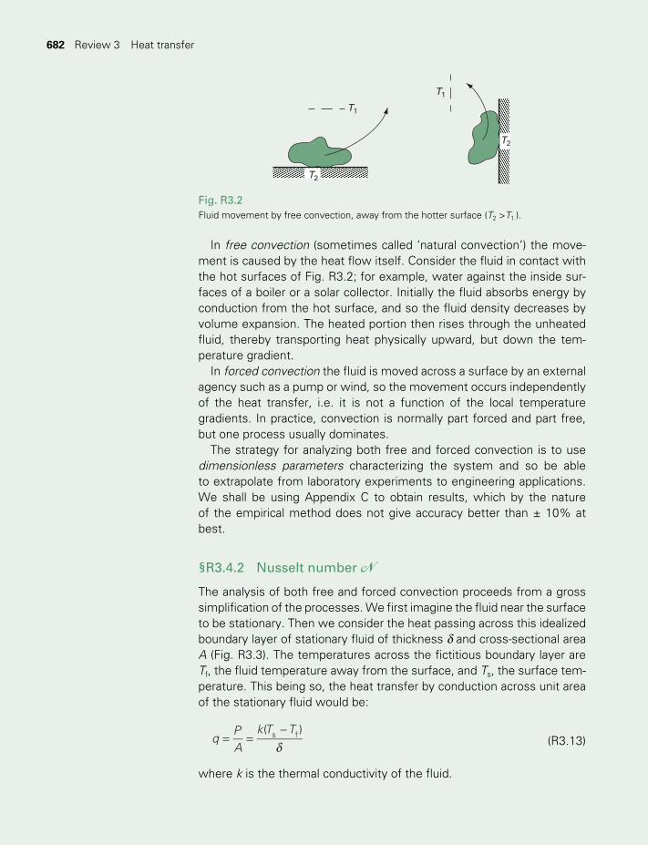
682 Heat transfer682 Review 3 Heat transfer
In free convection (sometimes called ‘natural convection’) the move-ment is caused by the heat flow itself. Consider the fluid in contact with the hot surfaces of Fig. R3.2; for example, water against the inside sur-faces of a boiler or a solar collector. Initially the fluid absorbs energy by conduction from the hot surface, and so the fluid density decreases by volume expansion. The heated portion then rises through the unheated fluid, thereby transporting heat physically upward, but down the tem-perature gradient.
In forced convection the fluid is moved across a surface by an external agency such as a pump or wind, so the movement occurs independently of the heat transfer, i.e. it is not a function of the local temperature gradients. In practice, convection is normally part forced and part free, but one process usually dominates.
The strategy for analyzing both free and forced convection is to use dimensionless parameters characterizing the system and so be able to extrapolate from laboratory experiments to engineering applications. We shall be using Appendix C to obtain results, which by the nature of the empirical method does not give accuracy better than ± 10% at best.
§R3.4.2 Nusselt number N
The analysis of both free and forced convection proceeds from a gross simplification of the processes. We first imagine the fluid near the surface to be stationary. Then we consider the heat passing across this idealized boundary layer of stationary fluid of thickness d and cross-sectional area A (Fig. R3.3). The temperatures across the fictitious boundary layer are Tf, the fluid temperature away from the surface, and Ts, the surface tem-perature. This being so, the heat transfer by conduction across unit area of the stationary fluid would be:
d= =
−q
PA
k T T( )s f (R3.13)
where k is the thermal conductivity of the fluid.
Fig. R3.2Fluid movement by free convection, away from the hotter surface (T2 >T1 ).
T2
T1
T1
T2
TWIDELL PAGINATION.indb 682 01/12/2014 11:39
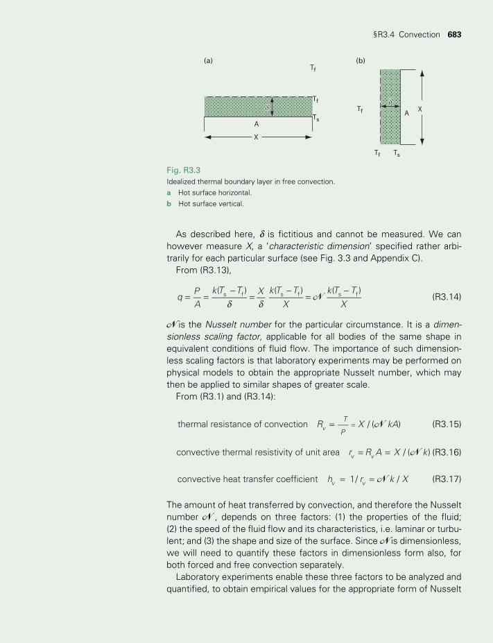
§R3.4 Convection 683
As described here, d is fictitious and cannot be measured. We can however measure X, a ‘characteristic dimension’ specified rather arbi-trarily for each particular surface (see Fig. 3.3 and Appendix C).
From (R3.13),
NqPA
k T T X k T T
X
k T T
X
( ) ( ) ( )s f s f s f
d d= =
−=
−=
− (R3.14)
N is the Nusselt number for the particular circumstance. It is a dimen-sionless scaling factor, applicable for all bodies of the same shape in equivalent conditions of fluid flow. The importance of such dimension-less scaling factors is that laboratory experiments may be performed on physical models to obtain the appropriate Nusselt number, which may then be applied to similar shapes of greater scale.
From (R3.1) and (R3.14):
= = NR X kAthermal resistance of convection / ( )T
Pv (R3.15)
= = Nr R A X kconvective thermal resistivity of unit area / ( )v v (R3.16)
= = Nh r k Xconvective heat transfer coefficient 1/ /v v (R3.17)
The amount of heat transferred by convection, and therefore the Nusselt number N , depends on three factors: (1) the properties of the fluid; (2) the speed of the fluid flow and its characteristics, i.e. laminar or turbu-lent; and (3) the shape and size of the surface. Since N is dimensionless, we will need to quantify these factors in dimensionless form also, for both forced and free convection separately.
Laboratory experiments enable these three factors to be analyzed and quantified, to obtain empirical values for the appropriate form of Nusselt
Fig. R3.3Idealized thermal boundary layer in free convection. a Hot surface horizontal. b Hot surface vertical.
Tf
TfTf
Tf Ts
TsA
A X
(a) (b)
X
δδδδ
TWIDELL PAGINATION.indb 683 01/12/2014 11:39
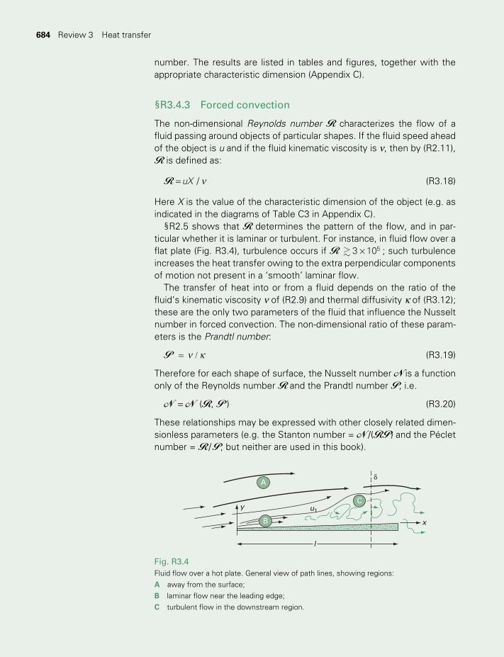
684 Heat transfer684 Review 3 Heat transfer
number. The results are listed in tables and figures, together with the appropriate characteristic dimension (Appendix C).
§R3.4.3 Forced convection
The non-dimensional Reynolds number R characterizes the flow of a fluid passing around objects of particular shapes. If the fluid speed ahead of the object is u and if the fluid kinematic viscosity is ν, then by (R2.11), R is defined as:
R uX / ν= (R3.18)
Here X is the value of the characteristic dimension of the object (e.g. as indicated in the diagrams of Table C3 in Appendix C).
§R2.5 shows that R determines the pattern of the flow, and in par-ticular whether it is laminar or turbulent. For instance, in fluid flow over a flat plate (Fig. R3.4), turbulence occurs if R 3 105× ; such turbulence increases the heat transfer owing to the extra perpendicular components of motion not present in a ‘smooth’ laminar flow.
The transfer of heat into or from a fluid depends on the ratio of the fluid’s kinematic viscosity ν of (R2.9) and thermal diffusivity κ of (R3.12); these are the only two parameters of the fluid that influence the Nusselt number in forced convection. The non-dimensional ratio of these param-eters is the Prandtl number:
P ν κ= / (R3.19)
Therefore for each shape of surface, the Nusselt number N is a function only of the Reynolds number R and the Prandtl number P, i.e.
N = N (R, P ) (R3.20)
These relationships may be expressed with other closely related dimen-sionless parameters (e.g. the Stanton number = N /(RP) and the Péclet number = R / P, but neither are used in this book).
Fig. R3.4Fluid flow over a hot plate. General view of path lines, showing regions: A away from the surface; B laminar flow near the leading edge; C turbulent flow in the downstream region.
B
y
x
l
A
C
d
u1
TWIDELL PAGINATION.indb 684 01/12/2014 11:39
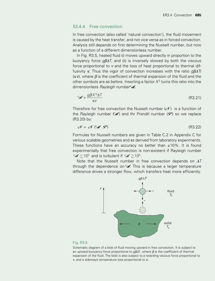
§R3.4 Convection 685
§3.4.4 Free convection
In free convection (also called ‘natural convection’), the fluid movement is caused by the heat transfer, and not vice versa as in forced convection. Analysis still depends on first determining the Nusselt number, but now as a function of a different dimensionless number.
In Fig. R3.5, heated fluid (i) moves upward directly in proportion to the buoyancy force gbDT, and (ii) is inversely slowed by both the viscous force proportional to ν and the loss of heat proportional to thermal dif-fusivity κ. Thus the vigor of convection increases with the ratio gbDT/(κ ν), where b is the coefficient of thermal expansion of the fluid and the other symbols are as before. Inserting a factor X 3 turns this ratio into the dimensionless Rayleigh number A.
g X T3A b
ν= D
κ (R3.21)
Therefore for free convection the Nusselt number (N ) is a function of the Rayleigh number ( A ) and thr Prandtl number (P ) so we replace (R3.20) by:
N = N ( A P ) (R3.22)
Formulas for Nusselt numbers are given in Table C.2 in Appendix C for various scalable geometries and as derived from laboratory experiments. These functions have an accuracy no better than ±10%. It is found experimentally that free convection is non-existent if Rayleigh number
103A and is turbulent if 105A .Note that the Nusselt number in free convection depends on DT
through the dependence on A. This is because a larger temperature difference drives a stronger flow, which transfers heat more efficiently.
Fig. R3.5Schematic diagram of a blob of fluid moving upward in free convection. It is subject to an upward buoyancy force proportional to gbDT, where b is the coefficient of thermal expansion of the fluid. The blob is also subject to a retarding viscous force proportional to ν, and a sideways temperature loss proportional to κ.
fluidTf
g ∆T
solidTs
X
υ
κz
β
TWIDELL PAGINATION.indb 685 01/12/2014 11:39
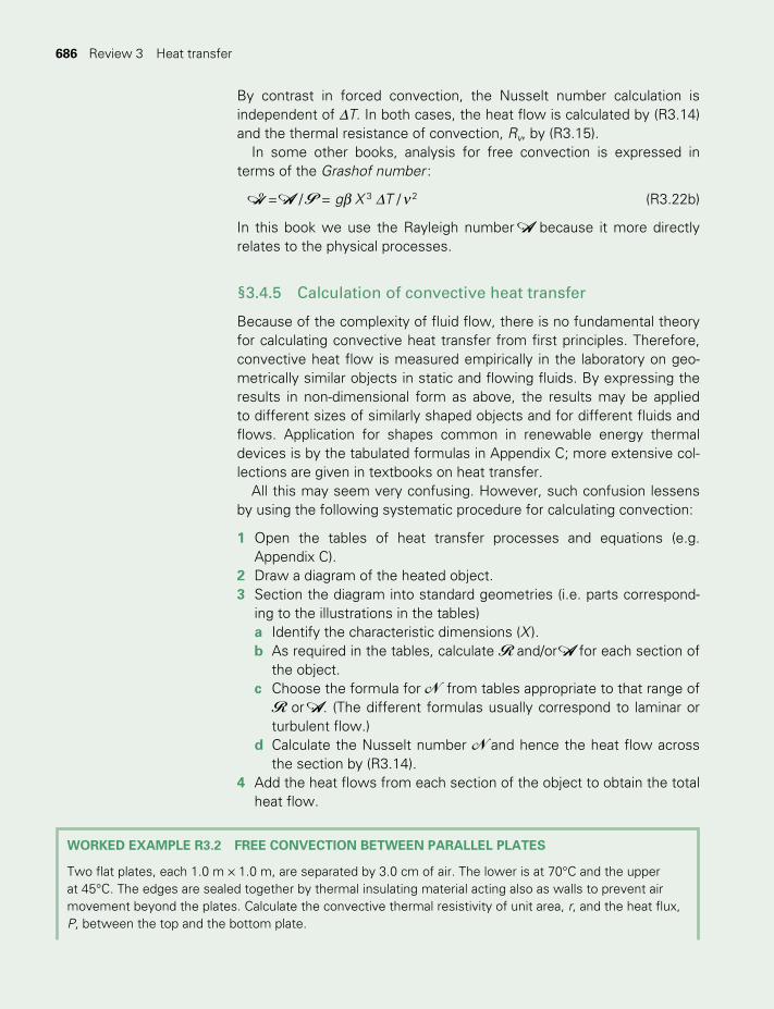
686 Heat transfer686 Review 3 Heat transfer
By contrast in forced convection, the Nusselt number calculation is independent of DT. In both cases, the heat flow is calculated by (R3.14) and the thermal resistance of convection, Rv, by (R3.15).
In some other books, analysis for free convection is expressed in terms of the Grashof number :
G = A / P = gb X 3 DT / ν 2 (R3.22b)
In this book we use the Rayleigh number A because it more directly relates to the physical processes.
§3.4.5 Calculation of convective heat transfer
Because of the complexity of fluid flow, there is no fundamental theory for calculating convective heat transfer from first principles. Therefore, convective heat flow is measured empirically in the laboratory on geo-metrically similar objects in static and flowing fluids. By expressing the results in non-dimensional form as above, the results may be applied to different sizes of similarly shaped objects and for different fluids and flows. Application for shapes common in renewable energy thermal devices is by the tabulated formulas in Appendix C; more extensive col-lections are given in textbooks on heat transfer.
All this may seem very confusing. However, such confusion lessens by using the following systematic procedure for calculating convection:
1 Open the tables of heat transfer processes and equations (e.g. Appendix C).
2 Draw a diagram of the heated object.3 Section the diagram into standard geometries (i.e. parts correspond-
ing to the illustrations in the tables)a Identify the characteristic dimensions (X ).b As required in the tables, calculate R and/or A for each section of
the object.c Choose the formula for N from tables appropriate to that range of
R or A. (The different formulas usually correspond to laminar or turbulent flow.)
d Calculate the Nusselt number N and hence the heat flow across the section by (R3.14).
4 Add the heat flows from each section of the object to obtain the total heat flow.
WORKED EXAMPLE R3.2 FREE CONVECTION BETWEEN PARALLEL PLATES
Two flat plates, each 1.0 m × 1.0 m, are separated by 3.0 cm of air. The lower is at 70°C and the upper at 45°C. The edges are sealed together by thermal insulating material acting also as walls to prevent air movement beyond the plates. Calculate the convective thermal resistivity of unit area, r, and the heat flux, P, between the top and the bottom plate.
TWIDELL PAGINATION.indb 686 01/12/2014 11:39
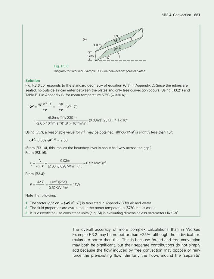
§R3.4 Convection 687
SolutionFig. R3.6 corresponds to the standard geometry of equation (C.7) in Appendix C. Since the edges are sealed, no outside air can enter between the plates and only free convection occurs. Using (R3.21) and Table B.1 in Appendix B, for mean temperature 57°C (= 330 K):
A κν κν
( )b b= =
g X T gX T
33
=× ×
= ×−
− − − −
(9.8ms )(1/ 330K)
(2.6 10 m s )(1.8 10 m s )(0.03m) (25K) 4.1 10
1
5 2 1 5 2 13 4
Using (C.7), a reasonable value for N may be obtained, although A is slightly less than 105:
N = 0.062 A 0.33 = 2.06
(From (R3.14), this implies the boundary layer is about half-way across the gap.)From (R3.16):
rX 0.03m
(2.06)(0.028 Wm K )0.52 KW mv 1 1
1 2
kN= = =
− −−
From (R3.4):
PA T (1m )(25K)
0.52KW m48W
2
1 2r=
D= =
−
Note the following:
1 The factor (gb / κ ν) = (A / X 3 DT ) is tabulated in Appendix B for air and water.2 The fluid properties are evaluated at the mean temperature (57°C in this case).3 It is essential to use consistent units (e.g. SI) in evaluating dimensionless parameters like A.
1.0
45° C
70° C
30°
1.0 m
3 cm
(a)
Fig. R3.6Diagram for Worked Example R3.2 on convection: parallel plates.
The overall accuracy of more complex calculations than in Worked Example R3.2 may be no better than ±25%, although the individual for-mulas are better than this. This is because forced and free convection may both be significant, but their separate contributions do not simply add because the flow induced by free convection may oppose or rein-force the pre-existing flow. Similarly the flows around the ‘separate’
TWIDELL PAGINATION.indb 687 01/12/2014 11:39
688 Heat transfer688 Review 3 Heat transfer
sections of the object interact with each other. If in doubt whether a forced or free flow is laminar or turbulent, it is best to assume turbulent, since it is difficult to smooth out streamlines which have become tangled by turbulence. The only sure way to accurately evaluate a convective heat transfer, allowing for all these interactions, is by actual measurement of temperatures with visualization of fluid flows and of temperatures, which is not realistic in most applications. Nevertheless, calculation of convec-tion by the methods described is essential to give order-of-magnitude evaluation and understanding.
§R3.5 RADIATIVE HEAT TRANSFER
§R3.5.1 Introduction
Surfaces emit energy by electromagnetic radiation according to the fun-damental laws of physics. Absorption of radiation is a closely related process. Sadly, the literature and terminology concerning radiative heat transfer are confusing; symbols and names for the same quan-tities vary, and the same symbol and name may be given for totally different quantities. Here, we have tried to follow the recommenda-tions of the International Solar Energy Society (ISES), while maintaining unique symbols throughout the whole book, as in the List of Symbols on page xxiii. The good news is that radiative heat transfer is an exact and well-understood subject, with the physical processes backed by estab-lished theory. With simple shapes and accurate data, the accuracy of calculations can be better than ±10%. This is in marked contrast with convective heat transfer that depends on empirical relationships and many approximations, with accuracy of practical calculations often no better than ±25%.
§R3.5.2 Radiant flux density (RFD)
Radiation is energy transported by electromagnetic propagation through space or transparent media. Its properties relate to its wavelength l. The regions of the electromagnetic spectrum important for renewable energy are named in Fig. 2.13(a). The flux of energy per unit area is the radiant flux density (abbreviation RFD, unit W/m2, symbol f). The varia-tion of RFD with wavelength is described by the spectral RFD (symbol fl, unit (W/ m2) m–1 or more usually W m–2 mm–1); it is the derivative df/dl. Thus fl Dl gives the power per unit area in a (narrow) wavelength range Dl. The integration of fl with respect to wavelength gives the total RFD, i.e. f = ∫ f lld . Radiation coming onto a surface is usually called irradiance (unit: W/(m2 of receiving area); from a surface as source it is called radiance, but we do not use this term.
TWIDELL PAGINATION.indb 688 01/12/2014 11:39

§R3.5 Radiative heat transfer 689
It is obvious that radiation has directional properties, and that these need to be specified. Understanding is always helped by:
1 Drawing pictures of the radiant fluxes and the methods of measurement.
2 Clarifying the units of the parameters.
Consider a small test instrument for measuring radiation parameters in an ideal manner. This could consist of a small, totally absorbing, black plane (Fig. R3.7) that may be adapted to (a) absorb on both sides, (b) absorb on one side only, (c) absorb from one direction only, and (d) absorb from one three-dimensional solid angle only.
The energy DE absorbed in time Dt could be measured from the tem-perature rise of the plane of area of one side, D A, knowing its thermal capacity. From Fig. R3.7(a) the radiant flux density from all directions would be f = DE (2D A) / Dt. In Fig. R3.7(b) the radiation is incident from the hemisphere above one side of the test plane (which may be labeled + or –), so:
D D Df = E A t/ ( ) (R3.23)
In Fig. R3.7(c), a vector quantity is now measured with the direction of the radiation flux perpendicular to the receiving plane. In Fig. R3.7(d), the radiation flux is measured within a solid angle Dw, centered perpendicu-lar to the plane of measurement and with the unit of W/( m2 sr).
The wavelength(s) of the received radiation need not be specified, since the absorbing surface is assumed to be totally black. However, if a dispersing device is placed in front of the instrument which passes only a small range of wavelength from l – Dl / 2 to l + Dl / 2, then the spectral radiant flux density may be measured as:
f =D
D D Dl l
− −E
A t(unit: Wm m )2 1 (R3.24)
Fig. R3.7Measurements of various radiation parameters using a small totally absorbing plane. a Absorbs all directions. b Absorbs from hemisphere above one side only. c Absorbs from one direction only. d Absorbs from one solid angle only.
(a) (b) (c) (d)
TWIDELL PAGINATION.indb 689 01/12/2014 11:39
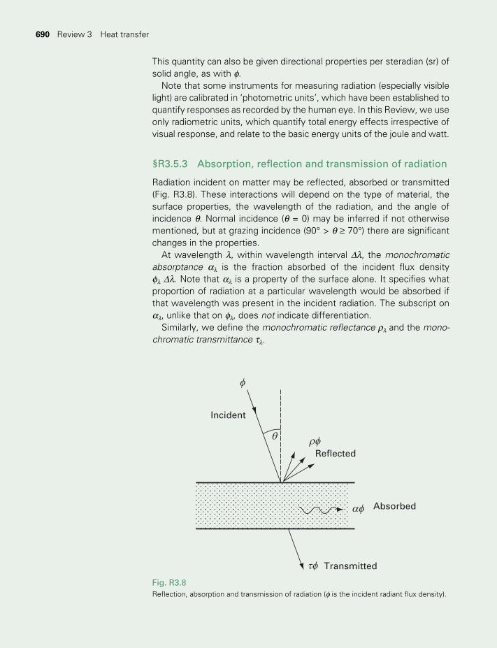
690 Heat transfer690 Review 3 Heat transfer
This quantity can also be given directional properties per steradian (sr) of solid angle, as with f.
Note that some instruments for measuring radiation (especially visible light) are calibrated in ‘photometric units’, which have been established to quantify responses as recorded by the human eye. In this Review, we use only radiometric units, which quantify total energy effects irrespective of visual response, and relate to the basic energy units of the joule and watt.
§R3.5.3 Absorption, reflection and transmission of radiation
Radiation incident on matter may be reflected, absorbed or transmitted (Fig. R3.8). These interactions will depend on the type of material, the surface properties, the wavelength of the radiation, and the angle of incidence θ. Normal incidence (θ = 0) may be inferred if not otherwise mentioned, but at grazing incidence (90° > θ ≥ 70°) there are significant changes in the properties.
At wavelength l, within wavelength interval Dl, the monochromatic absorptance al is the fraction absorbed of the incident flux density fl Dl. Note that al is a property of the surface alone. It specifies what proportion of radiation at a particular wavelength would be absorbed if that wavelength was present in the incident radiation. The subscript on al, unlike that on fl, does not indicate differentiation.
Similarly, we define the monochromatic reflectance ρl and the mono-chromatic transmittance tl.
Fig. R3.8Reflection, absorption and transmission of radiation (f is the incident radiant flux density).
Incident
Reflected
Absorbed
Transmitted
θ
φ
αφ
τφ
ρφ
TWIDELL PAGINATION.indb 690 01/12/2014 11:39
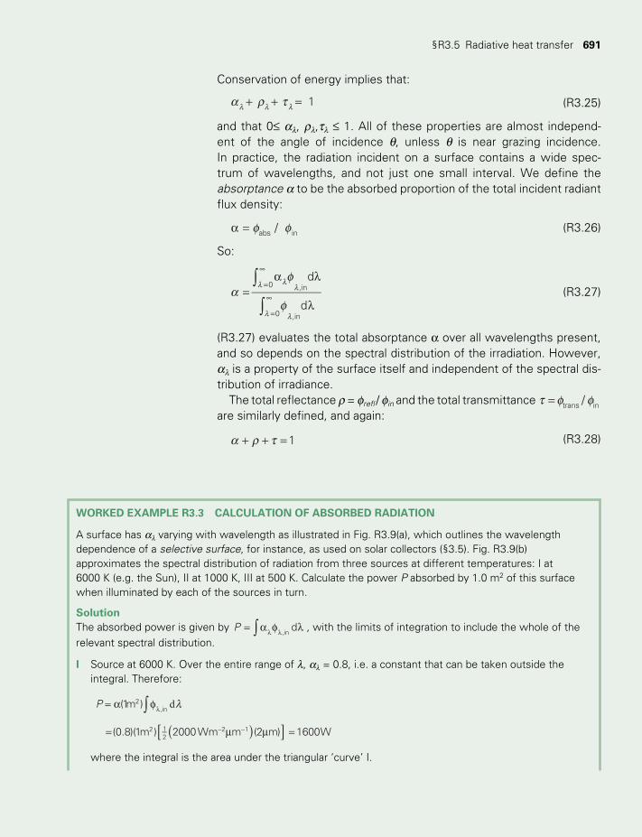
§R3.5 Radiative heat transfer 691
Conservation of energy implies that:
a ρ t + + =l l l 1 (R3.25)
and that 0≤ al, ρl,tl ≤ 1. All of these properties are almost independ-ent of the angle of incidence θ, unless θ is near grazing incidence. In practice, the radiation incident on a surface contains a wide spec-trum of wavelengths, and not just one small interval. We define the absorptance a to be the absorbed proportion of the total incident radiant flux density:
f fa = /abs in (R3.26)
So:
∫∫
af
f=
a l
l
ll l
l l
=
∞
=
∞
d
d
0 ,in
0 ,in
(R3.27)
(R3.27) evaluates the total absorptance a over all wavelengths present, and so depends on the spectral distribution of the irradiation. However, al is a property of the surface itself and independent of the spectral dis-tribution of irradiance.
The total reflectance ρ = frefl / fin and the total transmittance t f f= /trans in are similarly defined, and again:
a ρ t + + = 1 (R3.28)
WORKED EXAMPLE R3.3 CALCULATION OF ABSORBED RADIATION
A surface has al varying with wavelength as illustrated in Fig. R3.9(a), which outlines the wavelength dependence of a selective surface, for instance, as used on solar collectors (§3.5). Fig. R3.9(b) approximates the spectral distribution of radiation from three sources at different temperatures: I at 6000 K (e.g. the Sun), II at 1000 K, III at 500 K. Calculate the power P absorbed by 1.0 m2 of this surface when illuminated by each of the sources in turn.
SolutionThe absorbed power is given by P d,in∫= a f ll l , with the limits of integration to include the whole of the relevant spectral distribution.
I Source at 6000 K. Over the entire range of l, al = 0.8, i.e. a constant that can be taken outside the integral. Therefore:
∫[ ]( )
l= a f
= m m =
l
− −
dP (1m )
(0.8)(1m ) 2000Wm m (2 m) 1600W
2,in
2 12
2 1
where the integral is the area under the triangular ‘curve’ I.
TWIDELL PAGINATION.indb 691 01/12/2014 11:39
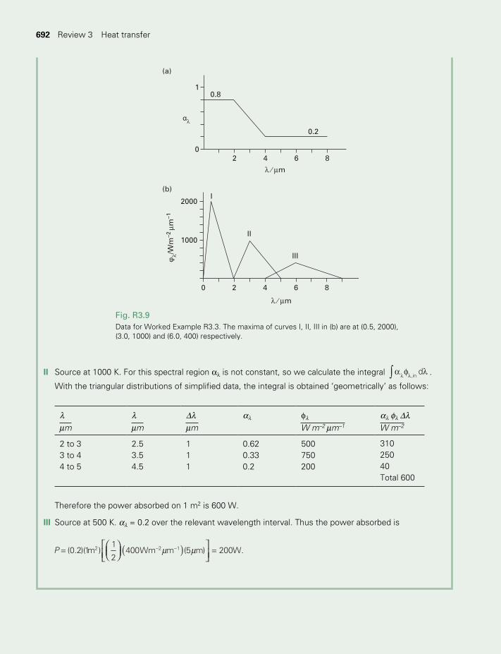
692 Heat transfer692 Review 3 Heat transfer
II Source at 1000 K. For this spectral region al is not constant, so we calculate the integral d,in∫ a f ll l .
With the triangular distributions of simplified data, the integral is obtained ‘geometrically’ as follows:
l l Dl al fl al fl Dl mm mm mm W m–2 mm–1 W m–2
2 to 3 2.5 1 0.62 500 3103 to 4 3.5 1 0.33 750 2504 to 5 4.5 1 0.2 200 40
Total 600
Therefore the power absorbed on 1 m2 is 600 W.
III Source at 500 K. al = 0.2 over the relevant wavelength interval. Thus the power absorbed is
( )
m m= =− − .P (0.2)(1m )1
2400Wm m (5 m) 200W2 2 1
1
0
(a)
(b)
2 4 6 8
0.8
0.2
αλ
λ ⁄ µm
λ ⁄ µm
2 4 6 8
2000
1000
0
φλ/
Wm
–2 µm
–1
II
I
III
Fig. R3.9Data for Worked Example R3.3. The maxima of curves I, II, III in (b) are at (0.5, 2000), (3.0, 1000) and (6.0, 400) respectively.
TWIDELL PAGINATION.indb 692 01/12/2014 11:39
§R3.5 Radiative heat transfer 693
R3.5.4 Black bodies, emittance and Kirchhoff’s laws
An idealized surface absorbing all incident irradiation, visible and invisible, is called a black body. A black body has al = 1 for all l, and therefore also has total absorptance a = 1. Nothing can absorb more radiation than a similarly dimensioned black body placed in the same incident irradi-ance. Moreover, Kirchhoff proved by logical argument that no body can emit more radiation than a similarly dimensioned black body at the same temperature. This link between absorption and emission is important, as used below.
The emittance e of a particular surface is the ratio of the radiant flux density, RFD, emitted by this surface, to the RFD emitted by a black body at the same temperature, T:
e =f
f
T
T
( )
( )from surface
from blackbody
(R3.29)
The monochromatic emittance, el, of any real surface is similarly defined by comparison with the ideal black body, as the corresponding ratio of RFD in the wavelength range Dl (from l − Dl/2 to l + Dl / 2). It follows that:
0 , 1e e≤ ≤l (R3.30)
Note that the emittance e of a surface may vary with temperature.Kirchhoff extended his theoretical argument to prove Kirchhoff’s law :
‘for any surface at a specified temperature, and for the same wave-length, the monochromatic emittance and monochromatic absorptance are equal:
a e=l l (R3.31)
For solar energy devices, the incoming radiation is expected from the Sun’s surface at temperature 5800 K, emitting with peak intensity at l ~ 0.5 mm. However, the receiving surface may be at about 350 K, emit-ting with peak intensity at about l ~ 10 mm. The dominant monochromatic absorptance is therefore al = 0.5 mm and the dominant monochromatic emittance is el = 10 mm. These two coefficients need not be equal (see §3.5 about selective surfaces). Nevertheless, Kirchhoff’s Law is important for the determination of such parameters (e.g. at the same wavelength of 10mm, el = 10 mm = al = 10 mm).
R3.5.5 Radiation emitted by a body
The monochromatic radiant flux density fBl, emitted by a black body of absolute temperature T, is derived from quantum mechanics as Planck’s radiation law :
f =l l −l T
C[exp(C ) 1]B
15
2
(R3.32)
TWIDELL PAGINATION.indb 693 01/12/2014 11:39
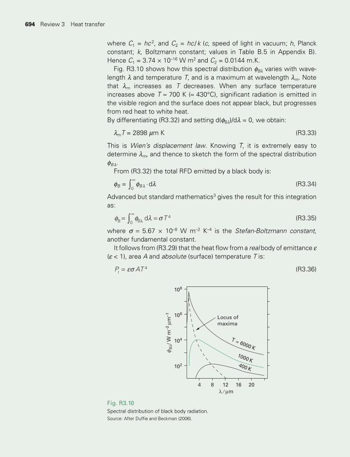
694 Heat transfer694 Review 3 Heat transfer
where C1 = hc 2, and C2 = hc / k (c, speed of light in vacuum; h, Planck constant; k, Boltzmann constant; values in Table B.5 in Appendix B). Hence C1 = 3.74 × 10⁻¹⁶ W m2 and C2 = 0.0144 m.K.
Fig. R3.10 shows how this spectral distribution fBl varies with wave-length l and temperature T, and is a maximum at wavelength lm. Note that lm increases as T decreases. When any surface temperature increases above T ≈ 700 K (≈ 430°C), significant radiation is emitted in the visible region and the surface does not appear black, but progresses from red heat to white heat.By differentiating (R3.32) and setting d(fBl)/dl = 0, we obtain:
lmT = 2898 mm K (R3.33)
This is Wien’s displacement law. Knowing T, it is extremely easy to determine lm, and thence to sketch the form of the spectral distribution fB l.
From (R3.32) the total RFD emitted by a black body is:
fB = ∫f f l s= =l
∞TdB B0
4fB l ⋅ dl (R3.34)
Advanced but standard mathematics3 gives the result for this integration as:
∫f f l s= =l
∞TdB B0
4 (R3.35)
where s = 5.67 × 10⁻⁸ W m–2 K–4 is the Stefan-Boltzmann constant, another fundamental constant.
It follows from (R3.29) that the heat flow from a real body of emittance e (e < 1), area A and absolute (surface) temperature T is:
es= P ATr4 (R3.36)
108
106
104
102
4 8 12 20
Locus ofmaxima
Βλ/
W m
–2 µm
–1
T = 6000 K
1000 K400 K
16
φ
λ ⁄ µm
Fig. R3.10Spectral distribution of black body radiation. Source: After Duffie and Beckman (2006).
TWIDELL PAGINATION.indb 694 01/12/2014 11:39
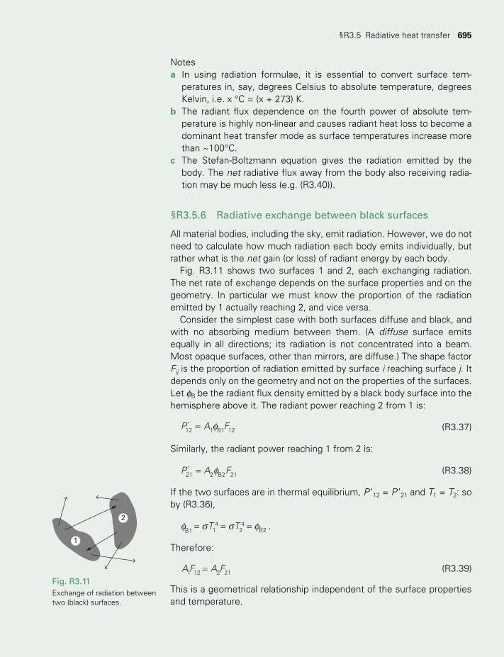
§R3.5 Radiative heat transfer 695
Notesa In using radiation formulae, it is essential to convert surface tem-
peratures in, say, degrees Celsius to absolute temperature, degrees Kelvin, i.e. x °C = (x + 273) K.
b The radiant flux dependence on the fourth power of absolute tem-perature is highly non-linear and causes radiant heat loss to become a dominant heat transfer mode as surface temperatures increase more than ~100°C.
c The Stefan-Boltzmann equation gives the radiation emitted by the body. The net radiative flux away from the body also receiving radia-tion may be much less (e.g. (R3.40)).
§R3.5.6 Radiative exchange between black surfaces
All material bodies, including the sky, emit radiation. However, we do not need to calculate how much radiation each body emits individually, but rather what is the net gain (or loss) of radiant energy by each body.
Fig. R3.11 shows two surfaces 1 and 2, each exchanging radiation. The net rate of exchange depends on the surface properties and on the geometry. In particular we must know the proportion of the radiation emitted by 1 actually reaching 2, and vice versa.
Consider the simplest case with both surfaces diffuse and black, and with no absorbing medium between them. (A diffuse surface emits equally in all directions; its radiation is not concentrated into a beam. Most opaque surfaces, other than mirrors, are diffuse.) The shape factor Fij is the proportion of radiation emitted by surface i reaching surface j. It depends only on the geometry and not on the properties of the surfaces. Let fB be the radiant flux density emitted by a black body surface into the hemisphere above it. The radiant power reaching 2 from 1 is:
f=′P A F12 1 B1 12 (R3.37)
Similarly, the radiant power reaching 1 from 2 is:
f=′P A F21 2 B2 21 (R3.38)
If the two surfaces are in thermal equilibrium, P ’12 = P ’21 and T1 = T2: so by (R3.36),
f s s f= = =T TB1 14
24
B2 .
Therefore:
=AF A F1 12 2 21 (R3.39)
This is a geometrical relationship independent of the surface properties and temperature.
1
2
Fig. R3.11Exchange of radiation between two (black) surfaces.
TWIDELL PAGINATION.indb 695 01/12/2014 11:39
696 Heat transfer696 Review 3 Heat transfer
If the surfaces are not at the same temperature, then the net radiative heat flow from 1 to 2, using (R3.39) is:
f f s s
s
= −
= − = −
= −
′ ′P P P
AF A F T AF T A F
T T AF( )
B B
12 12 21
1 1 12 2 2 21 14
1 12 24
2 21
14
24
1 12
(R3.40)
In general, the calculation of Fij requires a complicated integration, and results are tabulated in handbooks. However, solar collector configu-rations frequently approximate to the top two cases in Table C.5 in Appendix C, where the shape factor becomes unity.
§R3.5.7 Radiative exchange between gray surfaces
A gray body has a diffuse opaque surface with e = a = 1 – ρ = constant, independent of surface temperature, wavelength and angle of incidence. This is a reasonable approximation for most opaque surfaces in common solar energy applications where maximum temperatures are ~200°C and wavelengths are between 0.3 mm and 15 mm.
The radiation exchange between any numbers of gray bodies may be analyzed allowing for absorption, re-emission and reflection. The result-ing system of equations can be solved to yield the heat flow from each body if the temperatures are known, or vice versa. If there are only two bodies, the heat flow from body 1 to body 2 may be expressed in the form:
s= −′P A F T T( )12 1 12 14
24 (R3.41)
where the exchange factor F ’12 depends on the geometric shape factor F12, the area ratio (A1/A 2) and the surface properties e1, e2. Comparison with (R3.40) shows that for black bodies only, F ’l2 = F12.
A common situation is parallel plates with D << L and L’, as with heat exchange in flat-plate solar water heaters, in which case:
F ′ 12 ≈ 1/ [(1/e1) + (1/e2) – 1] R3.42)
Exchange factors for this and other commonly encountered geometries are listed in Table C.5 in Appendix C. More exhaustive lists are given in specialized handbooks (e.g. Wong 1977; Rohsenow et al. 1998).
§R3.5.8 Thermal resistance formulation
Equation (R3.41) may be factorized into the form:
= s + + −′P A F T T T T T T( )( )( )12 1 12 12
22
1 2 1 2 (R3.43)
TWIDELL PAGINATION.indb 696 01/12/2014 11:39
§R3.6 Properties of ‘transparent’ materials 697
Comparing this with (R3.41) we see that the resistance to radiative heat flow from body 1 is:
= s + +′ −R AF T T T T[ ( )( )]r 1 12 12
22
1 21 (R3.44)
In general, Rr depends strongly on temperature. However, T1 and T2 in are absolute temperatures, so that it is often true that (T1 – T2) << T1, T2. In this case may be simplified to:
≈ s ′R A F T1/ (4 )r 1 12
3 (R3.45)
where = +T T T( )12 1 2 is the mean temperature.
WORKED EXAMPLE R3.4 DERIVE TYPICAL VALUES OF Rr , Pr
Two parallel plates of area 1.0 m2 have emittances of 0.9 and 0.2 respectively. If T1 = 350 K and T2 = 300 K then, using (R3.45) and (C.18), Appendix C,
=+ −
×=
− −2 −−R
(1/ 0.9) (1/ 0.2) 1
4(1m )(5.67 10 Wm K )(325K)0.66 K Wr 2 8 4 3
1 .
This is comparable to the typical convective resistances of Worked Example R3.2. The corresponding heat flow is:
P r = 50 K/(0.66 K/W) = 75 W
§R3.6 PROPERTIES OF ‘TRANSPARENT’ MATERIALS
In visible light an ideal transparent material would have transmittance t = 1, reflectance ρ = 0 and absorptance a = 0. However, in practice a ‘transparent’ material (e.g. clean glass) has t ~ 0.9, ρ ~ 0.08 and a ~ 0.02 at the important angles of incidence with the normal of ≤ 70°, and rapidly reducing t and increasing ρ as angles of incidence approach 90°, i.e. grazing incidence. These properties are fully explained by Maxwell’s equations of electromagnetism.
Irradiation reaching a depth x below the surface decreases with x according to the Bouger-Lambert law; the transmitted proportion at x is:
eaxKxt = − (R3.46)
where the extinction coefficient K varies from about 0.04 cm–1 (for good-quality ‘water white’ glass) to about 0.30 cm–1 for common window glass (with iron impurity, having greenish edges).
Fig. R3.12(a) shows the variation with wavelength and thickness of the overall monochromatic transmittance, tl, for a typical glass. Note the very small transmittance (and hence large absorptance) in the thermal infrared region (l >3 mm). Glass is a good absorber in this waveband,
TWIDELL PAGINATION.indb 697 01/12/2014 11:39
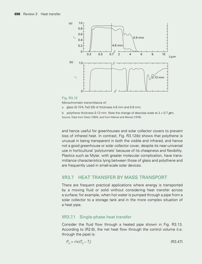
698 Heat transfer698 Review 3 Heat transfer
and hence useful for greenhouses and solar collector covers to prevent loss of infrared heat. In contrast, Fig. R3.12(b) shows that polythene is unusual in being transparent in both the visible and infrared, and hence not a good greenhouse or solar collector cover, despite its near-universal use in horticultural ‘polytunnels’ because of its cheapness and flexibility. Plastics such as Mylar, with greater molecular complication, have trans-mittance characteristics lying between those of glass and polythene and are frequently used in small-scale solar devices.
§R3.7 HEAT TRANSFER BY MASS TRANSPORT
There are frequent practical applications where energy is transported by a moving fluid or solid without considering heat transfer across a surface; for example, when hot water is pumped through a pipe from a solar collector to a storage tank and in the more complex situation of a heat pipe.
§R3.7.1 Single-phase heat transfer
Consider the fluid flow through a heated pipe shown in Fig. R3.13. According to (R2.6), the net heat flow through the control volume (i.e. through the pipe) is:
= −P mc T T( )m 3 1 (R3.47)
Fig. R3.12Monochromatic transmittance of: a glass (0.15% Fe2 03) of thickness 4.8 mm and 0.9 mm;
b polythene thickness 0.13 mm. Note the change of abscissa scale at l = 0.7 mm. Source: Data from Dietz (1954), and from Meinel and Meinel (1976).
1.0
0.8
0.6
(a)
(b)
0.4τλ
τλ
0.2
0.3 0.5 0.7 2 4 6
4.8 mm
0.9 mm
0.13 mm
8 10λ/µm
0
1.0
0
TWIDELL PAGINATION.indb 698 01/12/2014 11:39
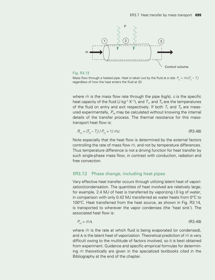
§R3.7 Heat transfer by mass transport 699
where m is the mass flow rate through the pipe (kg/s), c is the specific heat capacity of the fluid (J kg–1 K–1), and T1, and T3 are the temperatures of the fluid on entry and exit respectively. If both T1 and T3 are meas-ured experimentally, Pm may be calculated without knowing the internal details of the transfer process. The thermal resistance for this mass-transport heat flow is:
= − =R T T P mc( ) / 1/m m3 1 (R3.48)
Note especially that the heat flow is determined by the external factors controlling the rate of mass flow m , and not by temperature differences. Thus temperature difference is not a driving function for heat transfer by such single-phase mass flow, in contrast with conduction, radiation and free convection.
§R3.7.2 Phase change, including heat pipes
Very effective heat transfer occurs through utilizing latent heat of vapori-zation/condensation. The quantities of heat involved are relatively large; for example, 2.4 MJ of heat is transferred by vaporizing l.0 kg of water, in comparison with only 0.42 MJ transferred as water heats from 0°C to 100°C. Heat transferred from the heat source, as shown in Fig. R3.14, is transported to wherever the vapor condenses (the ‘heat sink’). The associated heat flow is:
= ΛP mm (R3.49)
where m is the rate at which fluid is being evaporated (or condensed), and Λ is the latent heat of vaporization. Theoretical prediction of m is very difficult owing to the multitude of factors involved, so it is best obtained from experiment. Guidance and specific empirical formulas for determin-ing m theoretically are given in the specialized textbooks cited in the Bibliography at the end of the chapter.
Fig. R3.13Mass flow through a heated pipe. Heat is taken out by the fluid at a rate P mc T T( )
m 3 1= −
regardless of how the heat enters the fluid at (2).
Control volume
32
P
1
m
TWIDELL PAGINATION.indb 699 01/12/2014 11:39
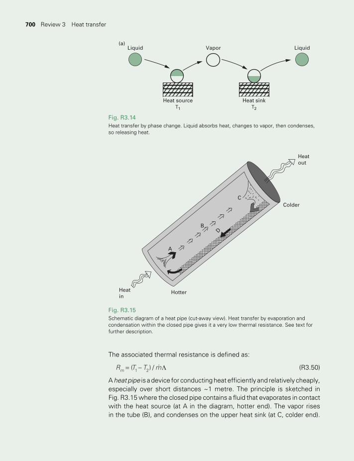
700 Heat transfer700 Review 3 Heat transfer
The associated thermal resistance is defined as:
= − ΛR T T m( ) /m 1 2 (R3.50)
A heat pipe is a device for conducting heat efficiently and relatively cheaply, especially over short distances ~1 metre. The principle is sketched in Fig. R3.15 where the closed pipe contains a fluid that evaporates in contact with the heat source (at A in the diagram, hotter end). The vapor rises in the tube (B), and condenses on the upper heat sink (at C, colder end).
LiquidVaporLiquid(a)
Heat sourceT1
Heat sinkT2
Fig. R3.14Heat transfer by phase change. Liquid absorbs heat, changes to vapor, then condenses, so releasing heat.
Fig. R3.15Schematic diagram of a heat pipe (cut-away view). Heat transfer by evaporation and condensation within the closed pipe gives it a very low thermal resistance. See text for further description.
Heatout
A
B
D
CColder
HotterHeatin
TWIDELL PAGINATION.indb 700 01/12/2014 11:39
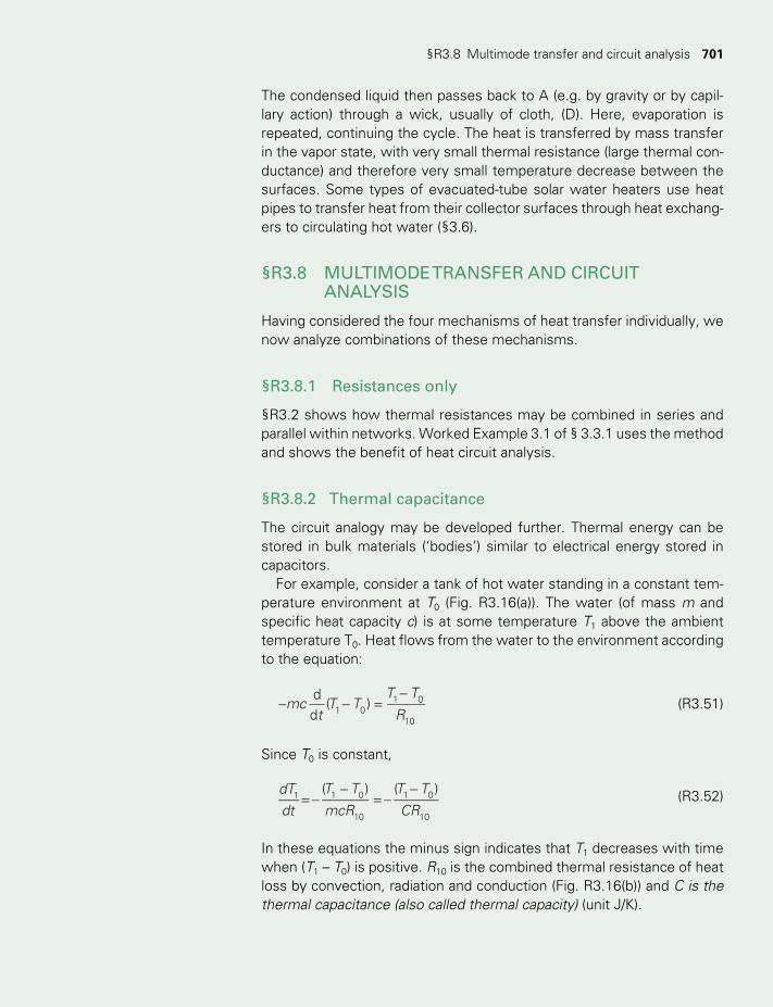
§R3.8 Multimode transfer and circuit analysis 701
The condensed liquid then passes back to A (e.g. by gravity or by capil-lary action) through a wick, usually of cloth, (D). Here, evaporation is repeated, continuing the cycle. The heat is transferred by mass transfer in the vapor state, with very small thermal resistance (large thermal con-ductance) and therefore very small temperature decrease between the surfaces. Some types of evacuated-tube solar water heaters use heat pipes to transfer heat from their collector surfaces through heat exchang-ers to circulating hot water (§3.6).
§R3.8 MULTIMODE TRANSFER AND CIRCUIT ANALYSIS
Having considered the four mechanisms of heat transfer individually, we now analyze combinations of these mechanisms.
§R3.8.1 Resistances only
§R3.2 shows how thermal resistances may be combined in series and parallel within networks. Worked Example 3.1 of § 3.3.1 uses the method and shows the benefit of heat circuit analysis.
§R3.8.2 Thermal capacitance
The circuit analogy may be developed further. Thermal energy can be stored in bulk materials (‘bodies’) similar to electrical energy stored in capacitors.
For example, consider a tank of hot water standing in a constant tem-perature environment at T0 (Fig. R3.16(a)). The water (of mass m and specific heat capacity c) is at some temperature T1 above the ambient temperature T0. Heat flows from the water to the environment according to the equation:
− − =−
mct
T TT T
Rdd
( )1 01 0
10
(R3.51)
Since T0 is constant,
= −−
= −−dT
dt
T T
mcR
T T
CR
( ) ( )1 1 0
10
1 0
10
(R3.52)
In these equations the minus sign indicates that T1 decreases with time when (T1 – T0) is positive. R10 is the combined thermal resistance of heat loss by convection, radiation and conduction (Fig. R3.16(b)) and C is the thermal capacitance (also called thermal capacity) (unit J/K).
TWIDELL PAGINATION.indb 701 01/12/2014 11:39
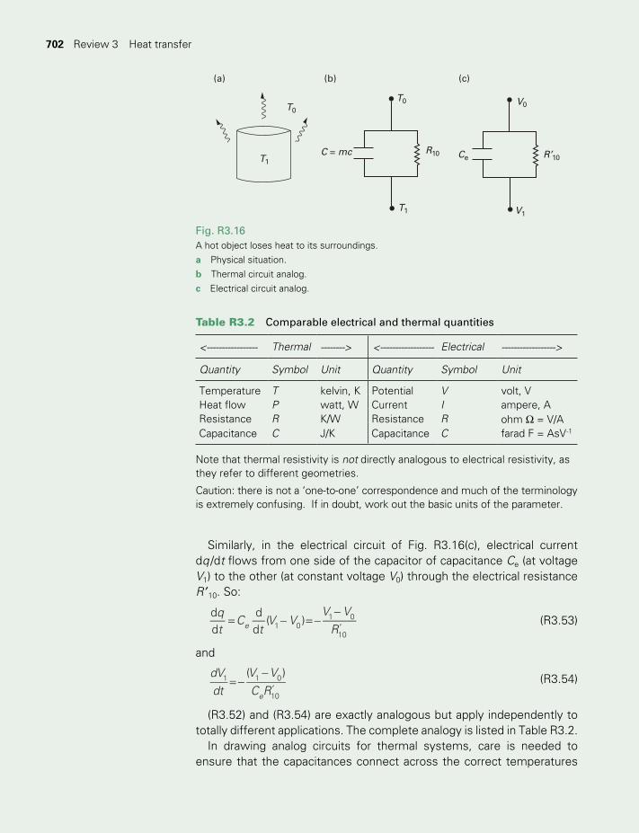
702 Heat transfer702 Review 3 Heat transfer
Similarly, in the electrical circuit of Fig. R3.16(c), electrical current dq /dt flows from one side of the capacitor of capacitance Ce (at voltage V1) to the other (at constant voltage V0) through the electrical resistance R ′10. So:
= − = −−
′
qt
Ct
V VV V
Rdd
dd
( )e 1 01 0
10
(R3.53)
and
= −−
′
dVdt
V V
C R
( )
e
1 1 0
10
(R3.54)
(R3.52) and (R3.54) are exactly analogous but apply independently to totally different applications. The complete analogy is listed in Table R3.2.
In drawing analog circuits for thermal systems, care is needed to ensure that the capacitances connect across the correct temperatures
V1
V0
R’10Ce
(c)
T0
T1
R10C = mc
(b)
T0
T1
(a)
Fig. R3.16A hot object loses heat to its surroundings. a Physical situation. b Thermal circuit analog. c Electrical circuit analog.
Table R3.2 Comparable electrical and thermal quantities
<----------------- Thermal --------> <------------------ Electrical ------------------>
Quantity Symbol Unit Quantity Symbol Unit
Temperature T kelvin, K Potential V volt, VHeat flow P watt, W Current I ampere, AResistance R K/W Resistance R ohm Ω = V/ACapacitance C J/K Capacitance C farad F = AsV-1
Note that thermal resistivity is not directly analogous to electrical resistivity, as they refer to different geometries.
Caution: there is not a ‘one-to-one’ correspondence and much of the terminology is extremely confusing. If in doubt, work out the basic units of the parameter.
TWIDELL PAGINATION.indb 702 01/12/2014 11:39
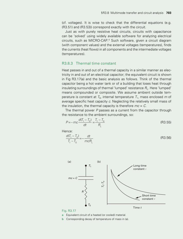
§R3.8 Multimode transfer and circuit analysis 703
(cf. voltages). It is wise to check that the differential equations (e.g. (R3.51) and (R3.53)) correspond exactly with the circuit.
Just as with purely resistive heat circuits, circuits with capacitance can be ‘solved’ using widely available software for analyzing electrical circuits, such as MICRO-CAP.4 Such software, given a circuit diagram (with component values) and the external voltages (temperatures), finds the currents (heat flows) in all components and the intermediate voltages (temperatures).
R3.8.3 Thermal time constant
Heat passes in and out of a thermal capacity in a similar manner as elec-tricity in and out of an electrical capacitor; the equivalent circuit is shown in Fig R3.17(a) and the basic analysis as follows. Think of the thermal capacitor being a hot water tank or of a building that loses heat through insulating surroundings of thermal ‘lumped’ resistance RL. Here ‘lumped’ means compounded or composite. We assume ambient outside tem-perature is constant at T0, internal temperature T1, mass enclosed m of average specific heat capacity c. Neglecting the relatively small mass of the insulation, the thermal capacity is therefore mc = C.
The thermal power P passes as a current from the capacitor through the resistance to the ambient surroundings, so:
= −−
=−
P mcd T T
dt
T T
R
( )
L
1 0 1 0 (R3.55)
Hence:−
−= −
d T T
T Tdt
mcR
( )
L
1 0
1 0
(R3.56)
Long timeconstant τ
Short timeconstant τ
Time t
T1-
To
T1
T0
R
mc = C
(a) (b)
Fig. R3.17a Equivalent circuit of a heated (or cooled) material. b Corresponding decay of temperature of mass in (a).
TWIDELL PAGINATION.indb 703 01/12/2014 11:39
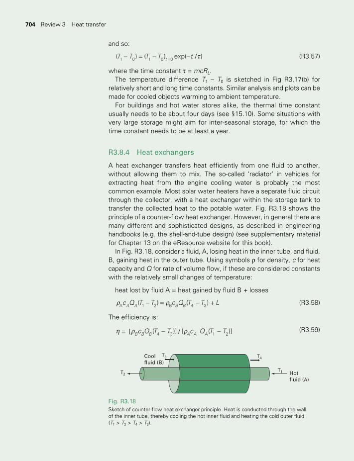
704 Heat transfer704 Review 3 Heat transfer
and so:
t− = − −=T T T T t( ) ( ) exp( / )t1 0 1 0 0 (R3.57)
where the time constant t = mcRL.The temperature difference T1 – T0 is sketched in Fig R3.17(b) for
relatively short and long time constants. Similar analysis and plots can be made for cooled objects warming to ambient temperature.
For buildings and hot water stores alike, the thermal time constant usually needs to be about four days (see §15.10). Some situations with very large storage might aim for inter-seasonal storage, for which the time constant needs to be at least a year.
R3.8.4 Heat exchangers
A heat exchanger transfers heat efficiently from one fluid to another, without allowing them to mix. The so-called ‘radiator’ in vehicles for extracting heat from the engine cooling water is probably the most common example. Most solar water heaters have a separate fluid circuit through the collector, with a heat exchanger within the storage tank to transfer the collected heat to the potable water. Fig. R3.18 shows the principle of a counter-flow heat exchanger. However, in general there are many different and sophisticated designs, as described in engineering handbooks (e.g. the shell-and-tube design) (see supplementary material for Chapter 13 on the eResource website for this book).
In Fig. R3.18, consider a fluid, A, losing heat in the inner tube, and fluid, B, gaining heat in the outer tube. Using symbols ρ for density, c for heat capacity and Q for rate of volume flow, if these are considered constants with the relatively small changes of temperature:
heat lost by fluid A = heat gained by fluid B + losses
c Q T T c Q T T L( ) ( )A A B BA 1 2 B 4 3ρ ρ− = − + (R3.58)
The efficiency is:
c Q T T c Q T T( )] / [ ( )]B B B A A A4 3 1 2η ρ ρ= [ − − (R3.59)
Fig. R3.18Sketch of counter-flow heat exchanger principle. Heat is conducted through the wall of the inner tube, thereby cooling the hot inner fluid and heating the cold outer fluid (T1 > T2 > T4 > T3).
T4
T2
T3
T1
Coolfluid (B)
Hotfluid (A)
TWIDELL PAGINATION.indb 704 01/12/2014 11:39
Quick questions 705
The simplest air-to-air heat-recovery heat exchangers operate as ventila-tion units for rooms in buildings, in which case usually volume flow rate QA = QB. With air as the common fluid, and changes in temperature < 50°C, the fluid density and heat capacity are considered equal. So:
η = − / −( ) ( )4 3 1 2T T T T (R3.60)
In winter, the incoming fresh air is preheated from the outgoing stale air. If the external fresh air is at temperature T0, and the internal stale air at T1, and if, in practice, T2 ≈ T3 ≈ T0, then:
T T T T( ) / ( )4 0 1 0η ≈ − − (R3.61)
Commonly T0 ≈ 5 °C, T1 ≈ 22 °C and, in practice, T4 ≈ 17 °C, so:
η ≈ − − ≈(17 5) / (22 5) 70% (R3.62)
In summer in hot weather, the same flows can pre-cool incoming ventila-tion air.
Such counter-flow heat exchangers are relatively cheap to purchase and to operate. They provide an excellent example of energy saving and more efficient use of energy.
QUICK QUESTIONS
Note: Answers to these questions are in the text of the relevant section of this Review, or may be readily inferred from it.
I Name and explain the various mechanisms of heat transfer; how many are there?
2 Explain how each heat transfer mechanism varies with temperature difference.
3 How is thermal resistance analogous to electrical resistance? Why is this analogy useful?
4 Define thermal conductivity k and thermal diffusivity κ. In what sense is κ a “diffusivity” (i.e. what diffuses?)
5 Define Nusselt number of N Is it most useful for calculations of con-duction, convection or radiation?
6 What is the difference between forced and free convection? 7 Define absorptance a and monochromatic absorptance al. Explain,
with examples, why each is needed in calculations. 8 Is the radiative flux density from a black body proportional to tem-
perature T, T 2, T 3, T 4 or something else? What is the unit of T here, and how does it relate to Celsius temperature?
9 What is a heat pipe? Why and where are these devices useful?10 What is a heat exchanger? Why and where are such devices useful?
TWIDELL PAGINATION.indb 705 01/12/2014 11:39

706 Heat transfer706 Review 3 Heat transfer
NOTES
1 This is not the same as ‘R value’, as used for labeling thermal insulation (see Box 3.1).2 Micro-Cap software may be downloaded from http://www.spectrum-soft.com/demodownnew.shtm.3 See e.g. Joos and Freeman, Theoretical Physics, p. 616.4 Micro-Cap software may be downloaded from http://www.spectrum-soft.com/demodownnew.shtm.
BIBLIOGRAPHY
General textbooks on heat transfer
There are many good texts written for engineering students and practicing engineers. Without exception these will include heat transfer under large temperature differences using complex situations. Non-focusing solar energy systems seldom require such complex analysis since temperature differences are relatively small and simple conditions exist. Therefore do not be daunted by the fearsome format of some of these books (many run to >800 pages!), of which a small but representative sample follows. The more modern ones have a greater emphasis on computer-aided solutions, but many of the older books are still very useful.
Bergman, T.L., Lavine, A.S., Incropera, F.P. and deWitt, D.P. (2011, 7th edn) Fundamentals of Heat and Mass transfer, Wiley, Chichester. Includes some solar energy applications as examples.
Çengel, Y.A. and Ghajar, A.J. (2011, 4th edn) Heat and Mass Transfer: Fundamentals and applications, McGraw-Hill, New Jersey. Comprehensive and clear, emphasizing physical principles, with many aids to students – some editions even include software for solving the equations!
Holman, J.P. (2010, 10th edn), Heat Transfer, McGraw-Hill, New Jersey. A widely used text for beginning engi-neering students, emphasizing electrical analogies.
Kay, J.M. and Nedderman, R.M. (1985) Fluid Mechanics and Transfer Processes, Cambridge University Press, Cambridge. A terse but clear account for engineering students.
Kreith, F.R., Manglik, R. and Bohn, S. (2010, 7th edn) Principles of Heat Transfer, Cengage, New York. Detailed but clear textbook for would-be specialists.
Rohsenow, W.R., Hartnett, J.P. and Cho, Y.I. (eds) (1998, 3rd edn) Handbook of Heat Transfer, McGraw-Hill, New York. Comprehensive and detailed handbook for practitioners.
Wong, H.Y. (1977) Handbook of Essential Formulae and Data on Heat Transfer for Engineers, Longmans, London. A gem of a book, if you can still find it. Easy to use, with comprehensive data expanding Appendices B and C of this book.
Heat transfer for solar energy applications
Most books on solar thermal applications include useful chapters on heat transfer formulas. These chapters mostly assume that the basics are known already. For example:
11 An insulated hot water tank has a time constant of 7 days. Ambient temperature is 20°C. Initially the water is at 80°C. No water is extracted and there is no further heat input. Estimate by drawing a graph the time for the water temperature to decrease to 40°C.
TWIDELL PAGINATION.indb 706 01/12/2014 11:39

Bibliography 707
Duffie, J.A. and Beckman, W.A. (2006, 3rd edn) Solar Engineering of Thermal Processes, John Wiley & Sons, New York. Very thorough in a mechanical engineering tradition and widely used. Uses SI units. Heat transfer is treated from functional relationships, as in many engineering texts, rather than from fundamental physical principles.
Specific references in text
Dietz, A.G.H. (1954) ‘Diathermanous materials and properties of surfaces’, in R.W. Hamilton (ed.), Space Heating with Thermal Energy, MIT Press, Boston.
International Solar Energy Society (ISES) (1978) ‘Units and symbols in solar energy’, Solar Energy, 21, 65–68.
Joos, G. and Freeman, X. (1987) Theoretical Physics, Dover Publications, New York. Reprint of classic text of 1958.
Meinel, A.B. and Meinel, M.P. (1976) Applied Solar Energy, Addison-Wesley, Reading, MA.
TWIDELL PAGINATION.indb 707 01/12/2014 11:39
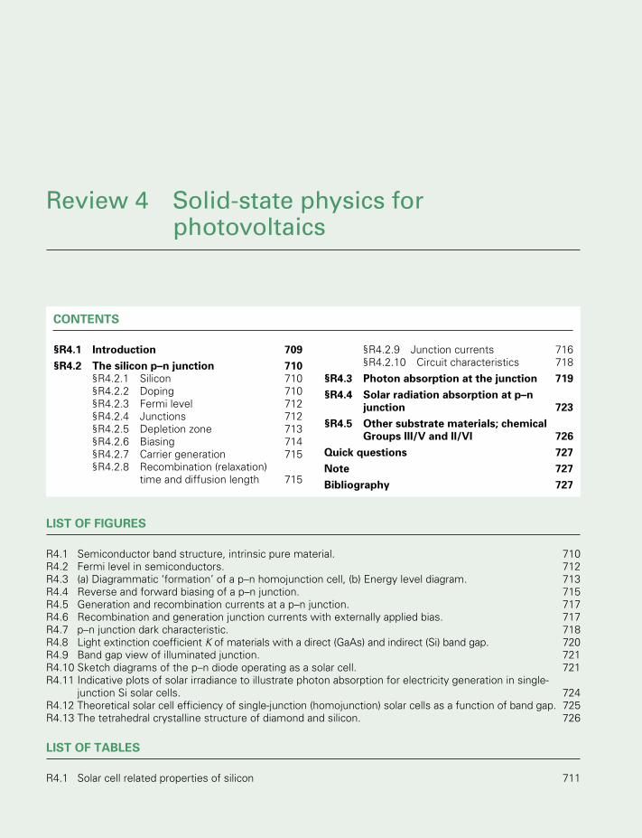
708
Review 4 Solid-state physics for photovoltaics
CONTENTS
§R4.1 Introduction 709§R4.2 The silicon p–n junction 710
§R4.2.1 Silicon 710§R4.2.2 Doping 710§R4.2.3 Fermi level 712§R4.2.4 Junctions 712§R4.2.5 Depletion zone 713§R4.2.6 Biasing 714§R4.2.7 Carrier generation 715§R4.2.8 Recombination (relaxation)
time and diffusion length 715
§R4.2.9 Junction currents 716§R4.2.10 Circuit characteristics 718
§R4.3 Photon absorption at the junction 719§R4.4 Solar radiation absorption at p–n
junction 723§R4.5 Other substrate materials; chemical
Groups III/V and II/VI 726Quick questions 727Note 727Bibliography 727
LIST OF FIGURES
R4.1 Semiconductor band structure, intrinsic pure material. 710R4.2 Fermi level in semiconductors. 712R4.3 (a) Diagrammatic ‘formation’ of a p–n homojunction cell, (b) Energy level diagram. 713R4.4 Reverse and forward biasing of a p–n junction. 715R4.5 Generation and recombination currents at a p–n junction. 717R4.6 Recombination and generation junction currents with externally applied bias. 717R4.7 p–n junction dark characteristic. 718R4.8 Light extinction coefficient K of materials with a direct (GaAs) and indirect (Si) band gap. 720R4.9 Band gap view of illuminated junction. 721R4.10 Sketch diagrams of the p–n diode operating as a solar cell. 721R4.11 Indicative plots of solar irradiance to illustrate photon absorption for electricity generation in single-
junction Si solar cells. 724R4.12 Theoretical solar cell efficiency of single-junction (homojunction) solar cells as a function of band gap. 725R4.13 The tetrahedral crystalline structure of diamond and silicon. 726
LIST OF TABLES
R4.1 Solar cell related properties of silicon 711
TWIDELL PAGINATION.indb 708 01/12/2014 11:39

§R4.1 Introduction 709
§R4.1 INTRODUCTION
Photovoltaic power generation is caused by electrons and their counter-part holes being excited by photons (quanta) of electromagnetic radiation (e.g. sunlight), within the intrinsic voltage difference of a semiconductor junction. Applications are considered in Chapter 5. This Review concen-trates on the dominant material: silicon.
How should we picture solids (e.g. semiconductors) formed by atoms of only elements? There are two ‘views’:
1 Bond model. Chemistry explains that the outer atomic electrons are not firmly bound in complete shells and so tend to form covalent bonds with neighboring atoms; some of these outer electrons are able to ‘hop’ through the material as free electrons, so allowing the material to conduct electricity. This bond model is helpful for explain-ing how the ‘hole’ left by the ‘hopping’ electrons becomes in effect a charge carrier in the opposite direction, so doubling the current; the analogy is a bubble of air moving in the opposite direction to its envel-oping liquid.
2 Band model. Physics, however, sees the whole material as one large molecule of identical atoms, with the wave-mechanical nature of the outer atomic electrons determining the cooperative properties. Thus, just as a single isolated atom has discrete (quantized) energy states for its electrons, so electrons of the whole single-element array cooperate to have quantized energy states throughout the material. These allowed electron states are in discrete bands, which are equivalent, for the whole material, to the electron states of an isolated atom. The most energetic occupied band (i.e. of the outer atomic electrons) is called the valence band. Electrons absorbing quanta from incoming radiation (e.g. from light) are excited into the next unoccupied band called the conduction band and so allow the material to conduct electricity. The energy difference between these bands is the band gap, Eg.
Band gap Eg is an energy difference. Instead of quantifying this with the unit of joule, it is usual to use the energy unit ‘electron volt’ (abbreviated to eV), where -e is the charge of an electron.1 eV = 1.602 × 10⁻¹⁹ Coulomb × 1 Volt = 1.602 × 10⁻¹⁹ J.
But what about very dilute ‘impurities’ in the otherwise pure semicon-ductor, for instance, Group III and V atoms in a Group IV semiconductor such as silicon? The bond model sees these impurity atoms as capturing (‘accepting’) or releasing (‘donating’) free electrons in the otherwise pure lattice. The band model sees the impurities as allowing extra narrow bands between the valence and conduction bands of the dominant semi-conductor material.
TWIDELL PAGINATION.indb 709 01/12/2014 11:39
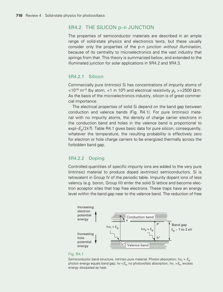
710 710 Review 4 Solid-state physics for photovoltaics
§R4.2 THE SILICON p–n JUNCTION
The properties of semiconductor materials are described in an ample range of solid-state physics and electronics texts, but these usually consider only the properties of the p–n junction without illumination, because of its centrality to microelectronics and the vast industry that springs from that. This theory is summarized below, and extended to the illuminated junction for solar applications in §R4.2 and §R4.3.
§R4.2.1 Silicon
Commercially pure (intrinsic) Si has concentrations of impurity atoms of <1018 m–3 (by atom, <1 in 109) and electrical resistivity re >>2500 W m. As the basis of the microelectronics industry, silicon is of great commer-cial importance.
The electrical properties of solid Si depend on the band gap between conduction and valence bands (Fig. R4.1). For pure (intrinsic) mate-rial with no impurity atoms, the density of charge carrier electrons in the conduction band and holes in the valence band is proportional to exp(–Eg / 2kT). Table R4.1 gives basic data for pure silicon; consequently, whatever the temperature, the resulting probability is effectively zero for electron or hole charge carriers to be energized thermally across the forbidden band gap.
§R4.2.2 Doping
Controlled quantities of specific impurity ions are added to the very pure (intrinsic) material to produce doped (extrinsic) semiconductors. Si is tetravalent in Group IV of the periodic table. Impurity dopant ions of less valency (e.g. boron, Group III) enter the solid Si lattice and become elec-tron acceptor sites that trap free electrons. These traps have an energy level within the band gap near to the valence band. The reduction of free
Fig. R4.1Semiconductor band structure, intrinsic pure material. Photon absorption; hv2 = Eg, photon energy equals band gap; hv <Eg, no photovoltaic absorption; hv1 >Eg, excess energy dissipated as heat.
Increasingelectronpotentialenergy
e–e–
h+
Valence bandh+
Band gapEg ~ 1 to 2 eV
h 1 > Eg h 2 = Eg
Increasingholepotentialenergy
Conduction band
νν
TWIDELL PAGINATION.indb 710 01/12/2014 11:39
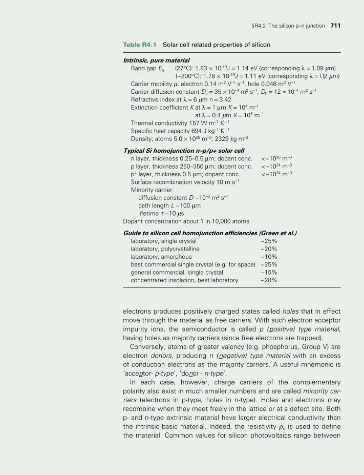
§R4.2 The silicon p–n junction 711
Table R4.1 Solar cell related properties of silicon
Intrinsic, pure material Band gap Eg (27°C): 1.83 × 10⁻¹⁹J = 1.14 eV (corresponding l = 1.09 mm) (~200°C): 1.78 × 10⁻¹⁹J = 1.11 eV (corresponding l = l.l2 mm) Carrier mobility m, electron 0.14 m2 V–1 s–1, hole 0.048 m2 V–1
Carrier diffusion constant De = 35 × 10–4 m2 s–1, Dh = 12 = 10–4 m2 s–1
Refractive index at l = 6 mm n = 3.42 Extinction coefficient K at l = 1 mm K = 104 m–1
at l = 0.4 mm K = 105 m–1
Thermal conductivity 157 W m–1 K – 1
Specific heat capacity 694 J kg–1 K – 1
Density; atoms 5.0 × 1028 m–3; 2329 kg m–3
Typical Si homojunction n–p/p+ solar cell n layer, thickness 0.25–0.5 mm; dopant conc. <~1026 m–3 p layer, thickness 250–350 mm; dopant conc. <~1024 m–3
p+ layer, thickness 0.5 mm; dopant conc. <~1024 m–3
Surface recombination velocity 10 m s–1
Minority carrier: diffusion constant D ~10–3 m2 s–1
path length L ~100 mm lifetime t ~10 ms
Dopant concentration about 1 in 10,000 atoms
Guide to silicon cell homojunction efficiencies (Green et al.) laboratory, single crystal ~25% laboratory, polycrystalline ~20% laboratory, amorphous ~10% best commercial single crystal (e.g. for space) ~25% general commercial, single crystal ~15% concentrated insolation, best laboratory ~28%
electrons produces positively charged states called holes that in effect move through the material as free carriers. With such electron acceptor impurity ions, the semiconductor is called p ( positive) type material, having holes as majority carriers (since free electrons are trapped).
Conversely, atoms of greater valency (e.g. phosphorus, Group V) are electron donors, producing n ( negative) type material with an excess of conduction electrons as the majority carriers. A useful mnemonic is ‘acceptor- p-type’, ‘donor - n-type’.
In each case, however, charge carriers of the complementary polarity also exist in much smaller numbers and are called minority car-riers (electrons in p-type, holes in n-type). Holes and electrons may recombine when they meet freely in the lattice or at a defect site. Both p- and n-type extrinsic material have larger electrical conductivity than the intrinsic basic material. Indeed, the resistivity re is used to define the material. Common values for silicon photovoltaics range between
TWIDELL PAGINATION.indb 711 01/12/2014 11:39
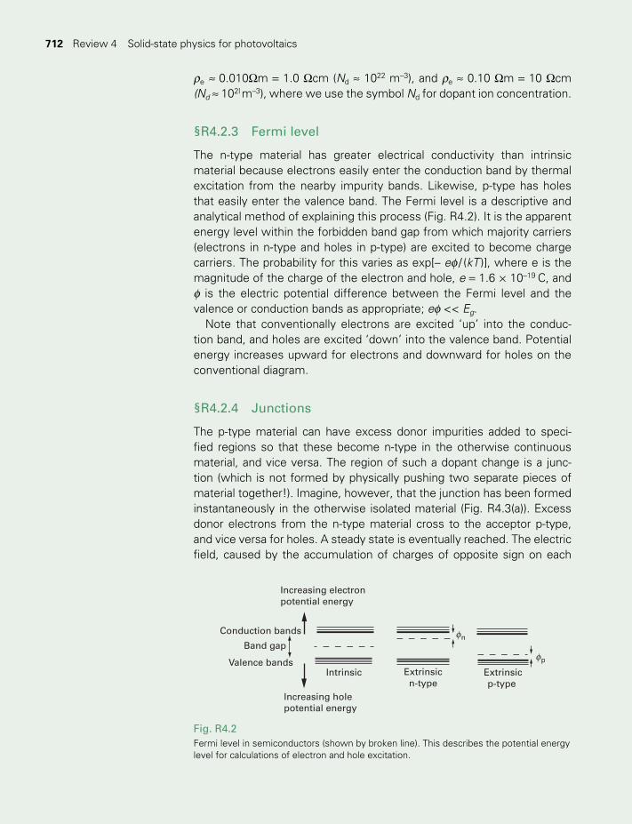
712 712 Review 4 Solid-state physics for photovoltaics
re ≈ 0.010Wm = 1.0 Wcm (Nd ≈ 1022 m–3), and re ≈ 0.10 Wm = 10 Wcm (Nd ≈ 102l m–3), where we use the symbol Nd for dopant ion concentration.
§R4.2.3 Fermi level
The n-type material has greater electrical conductivity than intrinsic material because electrons easily enter the conduction band by thermal excitation from the nearby impurity bands. Likewise, p-type has holes that easily enter the valence band. The Fermi level is a descriptive and analytical method of explaining this process (Fig. R4.2). It is the apparent energy level within the forbidden band gap from which majority carriers (electrons in n-type and holes in p-type) are excited to become charge carriers. The probability for this varies as exp[– ef / (kT )], where e is the magnitude of the charge of the electron and hole, e = 1.6 × 10⁻¹⁹ C, and f is the electric potential difference between the Fermi level and the valence or conduction bands as appropriate; ef << Eg.
Note that conventionally electrons are excited ‘up’ into the conduc-tion band, and holes are excited ‘down’ into the valence band. Potential energy increases upward for electrons and downward for holes on the conventional diagram.
§R4.2.4 Junctions
The p-type material can have excess donor impurities added to speci-fied regions so that these become n-type in the otherwise continuous material, and vice versa. The region of such a dopant change is a junc-tion (which is not formed by physically pushing two separate pieces of material together!). Imagine, however, that the junction has been formed instantaneously in the otherwise isolated material (Fig. R4.3(a)). Excess donor electrons from the n-type material cross to the acceptor p-type, and vice versa for holes. A steady state is eventually reached. The electric field, caused by the accumulation of charges of opposite sign on each
Fig. R4.2Fermi level in semiconductors (shown by broken line). This describes the potential energy level for calculations of electron and hole excitation.
Conduction bands
Band gap
Valence bands
Increasing electronpotential energy
Increasing holepotential energy
Intrinsic Extrinsicn-type
Extrinsicp-type
φn
φp
TWIDELL PAGINATION.indb 712 01/12/2014 11:39
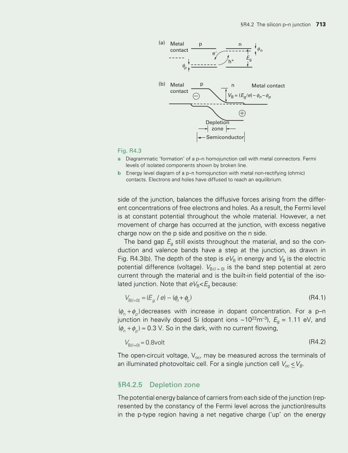
§R4.2 The silicon p–n junction 713
side of the junction, balances the diffusive forces arising from the differ-ent concentrations of free electrons and holes. As a result, the Fermi level is at constant potential throughout the whole material. However, a net movement of charge has occurred at the junction, with excess negative charge now on the p side and positive on the n side.
The band gap Eg still exists throughout the material, and so the con-duction and valence bands have a step at the junction, as drawn in Fig. R4.3(b). The depth of the step is eVB in energy and VB is the electric potential difference (voltage). VB (I = 0) is the band step potential at zero current through the material and is the built-in field potential of the iso-lated junction. Note that eVB<Eg because:
φ φ= − +=V E e( / ) ( )I g n pB( 0) (R4.1)
φ φ+( )n p decreases with increase in dopant concentration. For a p–n junction in heavily doped Si (dopant ions ~1022m–3), Eg = 1.11 eV, and φ φ+( )n p ≈ 0.3 V. So in the dark, with no current flowing,
V 0.8voltIB( 0) ≈= (R4.2)
The open-circuit voltage, Voc, may be measured across the terminals of an illuminated photovoltaic cell. For a single junction cell Voc <~VB.
§R4.2.5 Depletion zone
The potential energy balance of carriers from each side of the junction (rep-resented by the constancy of the Fermi level across the junction)results in the p-type region having a net negative charge (‘up’ on the energy
Fig. R4.3a Diagrammatic ‘formation’ of a p–n homojunction cell with metal connectors. Fermi
levels of isolated components shown by broken line. b Energy level diagram of a p–n homojunction with metal non-rectifying (ohmic)
contacts. Electrons and holes have diffused to reach an equilibrium.
Metalcontact
(a)
Metal contact
VB = (Eg /e) – n – p
Metalcontact
p
pφ
φ
φ φ
n
n
e–
h+
np
(b)
Semiconductor
Eg
Depletionzone
TWIDELL PAGINATION.indb 713 01/12/2014 11:39
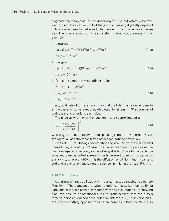
714 714 Review 4 Solid-state physics for photovoltaics
diagram) and vice versa for the donor region. The net effect is to draw electron and hole carriers out of the junction, leaving it greatly depleted in total carrier density. Let n and p be the electron and hole carrier densi-ties. Then the product np = C is a constant, throughout the material. For example,
1 p region:
= = =− − −np C (10 m )(10 m ) 10 m10 3 22 3 32 6 (R4.3)
+ = −n p 10 m22 3
2 n region:
= = =− − −np C (10 m )(10 m ) 10 m22 3 10 3 32 6 (R4.4)
+ = −n p 10 m22 3
3 Depletion zone: n = p by definition. So:
= = = −n p C 10 m2 2 32 6
= = −n p 10 m16 3
+ = × −n p 2 10 m16 3
(R4.5)
The typical data of this example show that the total charge carrier density at the depletion zone is reduced (depleted) by at least ~105 as compared with the n and p regions each side.
The physical width w of the junction may be approximated to:
ε≈
ε√
w
V
e np
2
( )0 r B
1/2
(R4.6)
where ε0 is the permittivity of free space, εr is the relative permittivity of the material, and the other terms have been defined previously.
For Si at 1022/m3 doping concentration and w ≈ 0.5 mm, the electric field intensity VB / w is ~2 × 10⁶ V/m. The current-carrying properties of the junction depend on minority carriers being able to diffuse to the depletion zone and then be pulled across in the large electric field. This demands that w < L, where L ≈ 100 mm is the diffusion length for minority carriers, and this is a criterion easily met in solar cell p–n junctions (see (R4.11)).
§R4.2.6 Biasing
The p–n junction may be fitted with metal contacts connected to a battery (Fig. R4.4). The contacts are called ‘ohmic’ contacts, i.e. non-rectifying junctions of low resistance compared with the bulk material. In ‘forward bias’ the positive conventional circuit current passes from the p to n material across a reduced band potential difference VB. In ‘reverse bias’, the external battery opposes the internal potential difference VB and so
TWIDELL PAGINATION.indb 714 01/12/2014 11:39
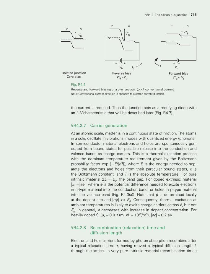
§R4.2 The silicon p–n junction 715
the current is reduced. Thus the junction acts as a rectifying diode with an I –V characteristic that will be described later (Fig. R4.7).
§R4.2.7 Carrier generation
At an atomic scale, matter is in a continuous state of motion. The atoms in a solid oscillate in vibrational modes with quantized energy (phonons). In semiconductor material electrons and holes are spontaneously gen-erated from bound states for possible release into the conduction and valence bands as charge carriers. This is a thermal excitation process with the dominant temperature requirement given by the Boltzmann probability factor exp [– E/(kT)], where E is the energy needed to sep-arate the electrons and holes from their particular bound states, k is the Boltzmann constant, and T is the absolute temperature. For pure intrinsic material 2E = Eg, the band gap. For doped extrinsic material
φ=E e , where f is the potential difference needed to excite electrons in n-type material into the conduction band, or holes in p-type material into the valence band (Fig. R4.3(a)). Note that f is determined locally at the dopant site and |ef | << Eg. Consequently, thermal excitation at ambient temperatures is likely to excite charge carriers across f, but not Eg. In general, f decreases with increase in dopant concentration. For heavily doped Si (re ≈ 0.01Wm, Nd ≈ 1022/m3), |ef| ≈ 0.2 eV.
§R4.2.8 Recombination (relaxation) time and diffusion length
Electron and hole carriers formed by photon absorption recombine after a typical relaxation time t, having moved a typical diffusion length L through the lattice. In very pure intrinsic material recombination times
Fig. R4.4Reverse and forward biasing of a p–n junction. I0<<I, conventional current.Note: Conventional current direction is opposite to electron current direction.
+ −+−I VbVb
Isolated junctionZero bias
Reverse biasV’B >Vb
Forward biasV’’B < Vb
VBV’B
P n
V’’B
nPnP
I0
TWIDELL PAGINATION.indb 715 01/12/2014 11:39
716 716 Review 4 Solid-state physics for photovoltaics
can be long (t ~1 s), but for commercial doped material recombination times are much shorter (t ~10–2 to 10–8 s). The shorter lifetime is because the carriers recombine at sites of impurities, crystal imperfections, front and rear surfaces, irregularities, and other defects. Thus highly doped material tends to have short relaxation times and diffusion lengths. Surface recombination is a persistent difficulty in solar cells because of the large area and constructional techniques. It is characterized by the surface recombination velocity Sv, typically ~10 m/s for Si, as defined by:
=J S Nv (R4.7)
where J is the recombination current number density perpendicular to the surface (m–2 s–1) and N is the carrier concentration in the material (m–3).The probability per unit time of a carrier recombining is 1/t. For n elec-trons the number of recombinations per unit time is n/tn, and for p holes is p/tp. In the same material at equilibrium these must be equal, so:
τ ττ τ τ τ= = =n p n
ppn, ,
n pn p p n (R4.8)
In p material, if p ~ 1022/m3 as the majority carrier and n~l011/m3 as the minority carrier, then tn<<tp and vice versa. Therefore in solar cell materials, minority carrier lifetimes are many orders of magnitude shorter than majority carrier lifetimes (i.e. minority carriers have many majority carriers with which to recombine).
Carriers diffuse through the lattice down a concentration gradient dN / dx to produce a number current density (in the direction x) of:
= −
J DdNdxx (R4.9)
where D is the diffusion constant, for which a typical value for Si is 35 × 10–4 m2 s–1 for electrons, 12 × 10–4 m2 s–1 for holes.
Within the relaxation time t, the diffusion distance L is given by Einstein’s relationship:
τ=L D( )1/2 (R4.10)
Therefore a typical diffusion length for minority carriers in p-type Si (D~10–3 m2/s, τ ~ 10–5 s) is:
µ≈ ≈− −L (10 10 ) m 100 m3 5 1/2 (R4.11)
Note that L >> w, the junction width of a typical p–n junction, see (R4.6).
§R4.2.9 Junction currents
Electrons and holes may be generated thermally or by light, and so become carriers in the material. Minority carriers, once in the built-in field of the
TWIDELL PAGINATION.indb 716 01/12/2014 11:39
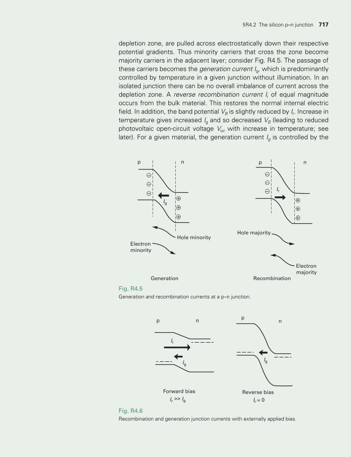
§R4.2 The silicon p–n junction 717
depletion zone, are pulled across electrostatically down their respective potential gradients. Thus minority carriers that cross the zone become majority carriers in the adjacent layer; consider Fig. R4.5. The passage of these carriers becomes the generation current Ig, which is predominantly controlled by temperature in a given junction without illumination. In an isolated junction there can be no overall imbalance of current across the depletion zone. A reverse recombination current Ir of equal magnitude occurs from the bulk material. This restores the normal internal electric field. In addition, the band potential VB is slightly reduced by Ir. Increase in temperature gives increased Ig and so decreased VB (leading to reduced photovoltaic open-circuit voltage Voc with increase in temperature; see later). For a given material, the generation current Ig is controlled by the
Fig. R4.5Generation and recombination currents at a p–n junction.
–
–
–
–
–
–+
n
Ig
Ir
Hole minorityHole majority
Electronmajority
Recombination
Electronminority
Generation
p np
+
+
+
+
+
Fig. R4.6Recombination and generation junction currents with externally applied bias.
p
Forward bias Reverse bias
n
Ir
Ir = 0Ir
Ig
Ig>>
Ig
np
TWIDELL PAGINATION.indb 717 01/12/2014 11:39
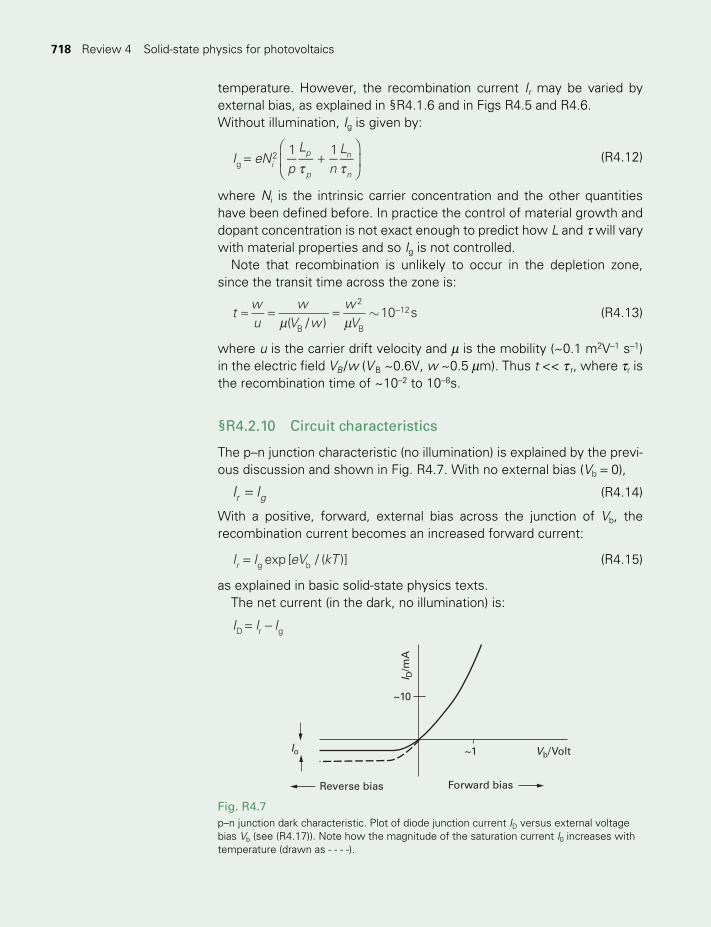
718 718 Review 4 Solid-state physics for photovoltaics
temperature. However, the recombination current Ir may be varied by external bias, as explained in §R4.1.6 and in Figs R4.5 and R4.6.Without illumination, Ig is given by:
τ τ= +
I eN
p
L
nL1 1
ip
p
n
ng
2 (R4.12)
where Ni is the intrinsic carrier concentration and the other quantities have been defined before. In practice the control of material growth and dopant concentration is not exact enough to predict how L and t will vary with material properties and so Ig is not controlled.
Note that recombination is unlikely to occur in the depletion zone, since the transit time across the zone is:
Vµ µ≈ = = −t
wu
wV w
w( / )
10 sB
2
B
12∼ (R4.13)
where u is the carrier drift velocity and m is the mobility (~0.1 m2V–1 s–1) in the electric field VB /w (V B ~0.6V, w ~0.5 mm). Thus t << t r, where tr is the recombination time of ~10–2 to 10–8s.
§R4.2.10 Circuit characteristics
The p–n junction characteristic (no illumination) is explained by the previ-ous discussion and shown in Fig. R4.7. With no external bias (Vb = 0),
=I Ir g (R4.14)
With a positive, forward, external bias across the junction of Vb, the recombination current becomes an increased forward current:
=I I eV kTexp [ / ( )]r g b (R4.15)
as explained in basic solid-state physics texts.The net current (in the dark, no illumination) is:
= −I I ID r g
Fig. R4.7p–n junction dark characteristic. Plot of diode junction current ID versus external voltage bias Vb (see (R4.17)). Note how the magnitude of the saturation current I0 increases with temperature (drawn as - - - -).
Reverse bias Forward bias
Vb/ Volt
I D/m
A
~10
~1Io
TWIDELL PAGINATION.indb 718 01/12/2014 11:39
§R4.3 Photon absorption at the junction 719
[ ] −= I eV kTexp / ( 1g (R4.16)
This is the Shockley equation for the junction diode, usually written as:
= −I I eV kTexp[ / ( )] 1D 0 b (R4.17)
where I0( = Ig) is the saturation current in the dark under full reverse bias before avalanche breakdown. It is also called the leakage or diffusion current. For good quality solar cells I0 ~10–8 A m–2.
§R4.3 PHOTON ABSORPTION AT THE JUNCTION
So far, we have considered the junction ‘in the dark’; now let light appear. The dominant process causing the absorption of electromagnetic radia-tion in semiconductors is the generation of electron–hole pairs. This occurs in direct transitions of electrons across the band gap Eg when
h Egν ≥ (R4.18)
where h is the Planck constant (6.63 × 10⁻³⁴ J s) and ν is the radiation frequency. The semiconductor material of solar cells has Eg ≈ 1 eV.
Absorption of photons near this condition occurs in indirect band gap transitions (e.g. as in silicon) owing to interaction within the crystal lattice with a lattice vibration phonon of energy hW ≈ 0.02 eV, where W is the phonon frequency. In this case the radiation absorption is not ‘sharp’ because the condition for photon absorption is:
h h Egν ± Ω ≥ (R4.19)
Direct band gap semiconductors (e.g. GaAs) absorb photons without lattice phonon interaction. Therefore they have sharp absorption band transitions with relatively large values of extinction coefficient K for light of frequencies ν > Eg /h (Fig. R4.8). This contrasts with the indirect band gap semiconductors (e.g. Si) that have less sharp absorption bands and smaller extinction coefficients K.
Band gap absorption for semiconductors occurs at frequencies within the solar spectrum; for Si this occurs across the whole visible spectrum for frequencies
E h/(1.1eV)(1.6 10 JeV )
6.63 10 Js0.27 10 Hzg
19 1
3415ν > ≈
××
= ×− −
− (R4.20)
and wavelengths
λ µ<×
×=
−
−
3.0 10 m.s0.27 10 s
1.1 m8 1
15 1 (R4.21)
The number flux of photons in the solar spectrum is large
TWIDELL PAGINATION.indb 719 01/12/2014 11:39
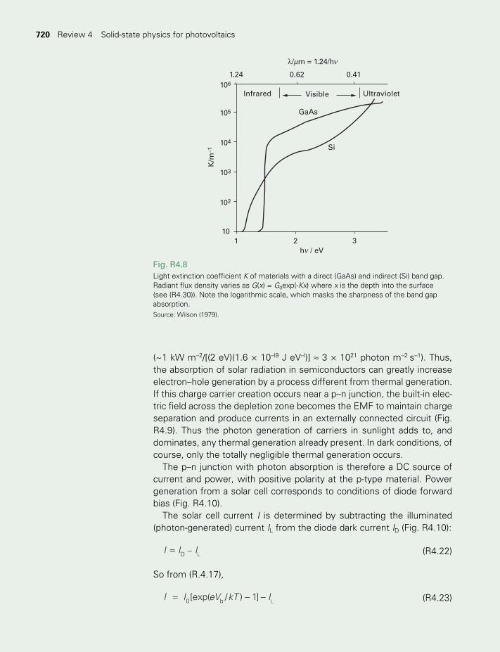
720 720 Review 4 Solid-state physics for photovoltaics
(~1 kW m–2/[(2 eV)(1.6 × 10–l9 J eV–l)] ≈ 3 × 10²¹ photon m–2 s–1). Thus, the absorption of solar radiation in semiconductors can greatly increase electron–hole generation by a process different from thermal generation. If this charge carrier creation occurs near a p–n junction, the built-in elec-tric field across the depletion zone becomes the EMF to maintain charge separation and produce currents in an externally connected circuit (Fig. R4.9). Thus the photon generation of carriers in sunlight adds to, and dominates, any thermal generation already present. In dark conditions, of course, only the totally negligible thermal generation occurs.
The p–n junction with photon absorption is therefore a DC source of current and power, with positive polarity at the p-type material. Power generation from a solar cell corresponds to conditions of diode forward bias (Fig. R4.10).
The solar cell current I is determined by subtracting the illuminated (photon-generated) current IL from the diode dark current ID (Fig. R4.10):
= −I I ID L (R4.22)
So from (R.4.17),
I I eV kT I[exp( / ) 1]0 b L= − − (R4.23)
Fig. R4.8Light extinction coefficient K of materials with a direct (GaAs) and indirect (Si) band gap. Radiant flux density varies as G(x) = G0exp(-Kx) where x is the depth into the surface (see (R4.30)). Note the logarithmic scale, which masks the sharpness of the band gap absorption. Source: Wilson (1979).
Infrared Visible
GaAs
Si
K/m
–1
λ/ m = 1.24/h
h / eV1
10
102
103
104
105
106
1.24 0.62 0.41
2 3
Ultraviolet
ν
νµ
TWIDELL PAGINATION.indb 720 01/12/2014 11:39
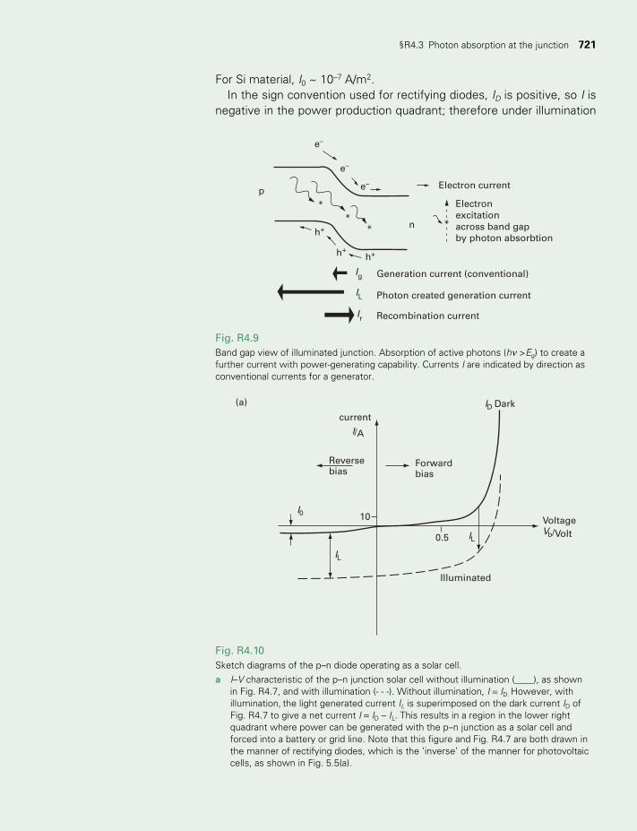
§R4.3 Photon absorption at the junction 721
Fig. R4.9Band gap view of illuminated junction. Absorption of active photons (hν >Eg) to create a further current with power-generating capability. Currents I are indicated by direction as conventional currents for a generator.
Electron current
n
p
h+
h+h+
e–
e–
e–
Generation current (conventional)
***
*
Ig
IL
Ir
Photon created generation current
Recombination current
Electronexcitationacross band gapby photon absorbtion
Fig. R4.10Sketch diagrams of the p–n diode operating as a solar cell.a I–V characteristic of the p–n junction solar cell without illumination (____), as shown
in Fig. R4.7, and with illumination (- - -). Without illumination, I = ID. However, with illumination, the light generated current IL is superimposed on the dark current ID of Fig. R4.7 to give a net current I = ID – IL. This results in a region in the lower right quadrant where power can be generated with the p–n junction as a solar cell and forced into a battery or grid line. Note that this figure and Fig. R4.7 are both drawn in the manner of rectifying diodes, which is the ‘inverse’ of the manner for photovoltaic cells, as shown in Fig. 5.5(a).
Forwardbias
Reversebias
current
VoltageI0
I/A
Vb/Volt
ID Dark
IL
IL
ID
IL
Illuminated
Illumination
Vb ≈ 0.5 V
10
0.5
p
+ _
n
(a)
(b)
For Si material, I0 ~ 10–7 A/m2.In the sign convention used for rectifying diodes, ID is positive, so I is
negative in the power production quadrant; therefore under illumination
TWIDELL PAGINATION.indb 721 01/12/2014 11:39
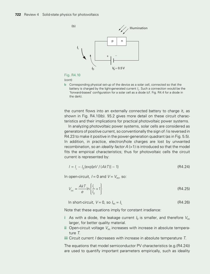
722 722 Review 4 Solid-state physics for photovoltaics
the current flows into an externally connected battery to charge it, as shown in Fig. R4.10(b). §5.2 gives more detail on these circuit charac-teristics and their implications for practical photovoltaic power systems.
In analyzing photovoltaic power systems, solar cells are considered as generators of positive current, so conventionally the sign of I is reversed in R4.23 to make it positive in the power-generation quadrant (as in Fig. 5.5). In addition, in practice, electron/hole charges are lost by unwanted recombination, so an ideality factor A (>1) is introduced so that the model fits the empirical characteristics; thus for photovoltaic cells the circuit current is represented by:
= − −I I I eV AkTexp[ / ( )] 10L (R4.24)
In open-circuit, I = 0 and V = Voc, so:
= +
V
AkTe
II
ln 1ocL
0
(R4.25)
In short-circuit, V = 0, so Isc = IL (R4.26)
Note that these equations imply for constant irradiance:
i As with a diode, the leakage current I0 is smaller, and therefore Voc
larger, for better quality material.ii Open-circuit voltage Voc increases with increase in absolute tempera-
ture T. iii Circuit current I decreases with increase in absolute temperature T.
The equations that model semiconductor PV characteristics (e.g.(R4.24)) are used to quantify important parameters empirically, such as ideality
Forwardbias
Reversebias
current
VoltageI0
I/A
Vb/Volt
ID Dark
IL
IL
ID
IL
Illuminated
Illumination
Vb ≈ 0.5 V
10
0.5
p
+ _
n
(a)
(b)
Fig. R4.10(cont)b Corresponding physical set-up of the device as a solar cell, connected so that the
battery is charged by the light-generated current IL. Such a connection would be the ‘forward-biased’ configuration for a solar cell as a diode (cf. Fig. R4.4 for a diode in the dark).
TWIDELL PAGINATION.indb 722 01/12/2014 11:39

§R4.4 Solar radiation absorption at p–n junction 723
factor A, by comparison with experimental results. For instance, maxi-mum power occurs when:
= =dPdV
d IVdV( )
0 (R4.27)
From (R4.24):
= + −IV I V I V I V eV AkTexp[( / )]L 0 0 (R4.28)
then differentiating by parts to obtain d(IV)/dV and equating this function to zero (see Problem 5.10) yields the voltage at maximum power:
= − +
V V
AkTe
eV
AkTln 1mpp oc
mpp (R4.29)
From this non-linear equation, A is determined by best fit from substitut-ing empirical values for Vmpp and Voc from measurements at constant insolation.
Photocurrent generation depends on photon absorption near the junc-tion region. If the incident solar radiant flux density is G0, then at depth x the radiant flux density is:
= −G x G Kx( ) exp( )0 (R4.30)
where K(ν ) is the extinction coefficient of Fig. R4.8, and is critically dependent upon frequency. Thus the cumulative absorbed power per unit area Gabs is:
= − = − −G G G G Kx1 exp[ ]abs x0 0 (R4.31)
For Si, photons in the infrared of energy less than the band gap are trans-mitted with zero or very little absorption. For Si at frequencies equal to the band gap of 1.14 eV, K ≈ 2 × 10⁻⁴ m−1, so (R4.31) from 90% absorp-tion occurs at a depth of about 500 mm, which gives approximately the minimum thickness for solar cell material, unless back-surface reflection and light-trapping techniques are used (§5.4.5).
§R4.4 SOLAR RADIATION ABSORPTION AT p–n JUNCTION
Detailed properties of solar radiation were considered fully in Chapter 2. Fig. R4.11 indicates the spectral distributions of solar irradiance (i.e. inso-lation) plotted in terms of (a) wavelength l, (b) photon energy hν, and (c) photon number. These mathematical transformations shift the peaks of the curves, but not the area under them, which is the appropriate total irradiance G.
TWIDELL PAGINATION.indb 723 01/12/2014 11:39
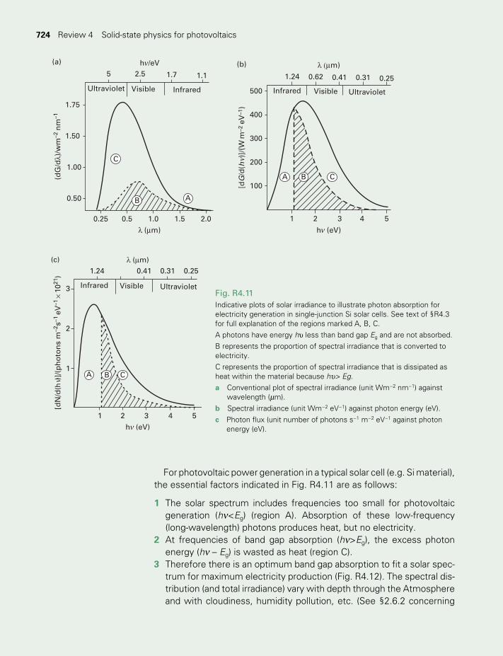
724 724 Review 4 Solid-state physics for photovoltaics
Fig. R4.11 Indicative plots of solar irradiance to illustrate photon absorption for electricity generation in single-junction Si solar cells. See text of §R4.3 for full explanation of the regions marked A, B, C.A photons have energy hu less than band gap Eg and are not absorbed.B represents the proportion of spectral irradiance that is converted to electricity. C represents the proportion of spectral irradiance that is dissipated as heat within the material because hu> Eg.a Conventional plot of spectral irradiance (unit Wm−2 nm−1) against
wavelength (mm).b Spectral irradiance (unit Wm−2 eV−1) against photon energy (eV).c Photon flux (unit number of photons s−1 m−2 eV−1 against photon
energy (eV).
A
(a)
5
1.75
1.50
1.00
0.50
2.5 1.7 1.1
Ultraviolet Visible Infrared
(dG
/dλ)
/wm
–2 n
m–1
C
h /eV
0.25 0.5 1.0 1.5 2.0
λ (µm)
B
ν
500
400
300
200
100
(b)
1.24 0.62 0.41 0.31 0.25
Infrared Visible Ultraviolet
[dG
/d(h
)]/
(W m
–2 e
V–1
)
A B C
1 2 3 4 5
h (eV)
λ (µm)
νν
A B
(c)
1.24 0.41 0.31 0.25
Infrared Visible Ultraviolet
[dN
/d(h
)]/
(ph
oto
ns
m–2
s–1 e
V–1
× 10
21)
C
h (eV)
1 2 3 4 5
3
2
1
λ (µm)
ν
ν
For photovoltaic power generation in a typical solar cell (e.g. Si material), the essential factors indicated in Fig. R4.11 are as follows:
1 The solar spectrum includes frequencies too small for photovoltaic generation (hν<Eg) (region A). Absorption of these low-frequency (long-wavelength) photons produces heat, but no electricity.
2 At frequencies of band gap absorption (hν>Eg), the excess photon energy (hν – Eg) is wasted as heat (region C).
3 Therefore there is an optimum band gap absorption to fit a solar spec-trum for maximum electricity production (Fig. R4.12). The spectral dis-tribution (and total irradiance) vary with depth through the Atmosphere and with cloudiness, humidity pollution, etc. (See §2.6.2 concerning
TWIDELL PAGINATION.indb 724 01/12/2014 11:39
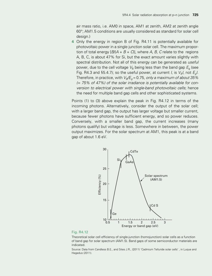
§R4.4 Solar radiation absorption at p–n junction 725
air mass ratio, i.e. AM0 in space, AM1 at zenith, AM2 at zenith angle 60°; AM1.5 conditions are usually considered as standard for solar cell design.)
4 Only the energy in region B of Fig. R4.11 is potentially available for photovoltaic power in a single junction solar cell. The maximum propor-tion of total energy [B/(A + B + C)], where A, B, C relate to the regions A, B, C, is about 47% for Si, but the exact amount varies slightly with spectral distribution. Not all of this energy can be generated as useful power, due to the cell voltage VB being less than the band gap Eg (see Fig. R4.3 and §5.4.7); so the useful power, at current I, is VBI, not EgI. Therefore, in practice, with VB/Eg ≈ 0.75, only a maximum of about 35% ( = 75% of 47%) of the solar irradiance is potentially available for con-version to electrical power with single-band photovoltaic cells; hence the need for multiple band gap cells and other sophisticated systems.
Points (1) to (3) above explain the peak in Fig. R4.12 in terms of the incoming photons. Alternatively, consider the output of the solar cell; with a larger band gap, the output has larger voltage but smaller current, because fewer photons have sufficient energy, and so power reduces. Conversely, with a smaller band gap, the current increases (many photons qualify) but voltage is less. Somewhere in between, the power output maximizes. For the solar spectrum at AM1, this peak is at a band gap of about 1.6 eV.
Fig. R4.12Theoretical solar cell efficiency of single-junction (homojunction) solar cells as a function of band gap for solar spectrum (AM1.5). Band gaps of some semiconductor materials are indicated. Source: Data from Candless B.E., and Sites J.R., (2011) ‘Cadmium Telluride solar cells’ , in Luque and Hegedus (2011).
30
25
20
15
Ge
SiGaAs
CdTe
Solar spectrum(AM1.5)
Cd S
100.5 1 1.5
Energy or band gap (eV)
Eff
icie
ncy
(%
)
2 2.5 3
TWIDELL PAGINATION.indb 725 01/12/2014 11:39
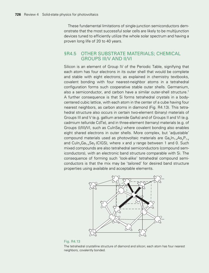
726 726 Review 4 Solid-state physics for photovoltaics
These fundamental limitations of single-junction semiconductors dem-onstrate that the most successful solar cells are likely to be multijunction devices tuned to efficiently utilize the whole solar spectrum and having a proven long life of 20 to 40 years.
§R4.5 OTHER SUBSTRATE MATERIALS; CHEMICAL GROUPS III/V AND II/VI
Silicon is an element of Group IV of the Periodic Table, signifying that each atom has four electrons in its outer shell that would be complete and stable with eight electrons; as explained in chemistry textbooks, covalent bonding with four nearest-neighbor atoms in a tetrahedral configuration forms such cooperative stable outer shells. Germanium, also a semiconductor, and carbon have a similar outer-shell structure.1 A further consequence is that Si forms tetrahedral crystals in a body-centered cubic lattice, with each atom in the center of a cube having four nearest neighbors, as carbon atoms in diamond (Fig. R4.13). This tetra-hedral structure also occurs in certain two-element (binary) materials of Groups III and V (e.g. gallium arsenide GaAs) and of Groups II and VI (e.g. cadmium telluride CdTe), and in three-element (ternary) materials (e.g. of Groups (I/III)/VI, such as CuInSe2) where covalent bonding also enables eight shared electrons in outer shells. More complex, but ‘adjustable’ compound materials used as photovoltaic materials are GaxIn1-xAsyP1-y
and CuInxGa1-xSe2 (CIGS), where x and y range between 1 and 0. Such mixed compounds are also tetrahedral semiconductors (compound sem-iconductors), with an electronic band structure comparable with Si. The consequence of forming such ‘look-alike’ tetrahedral compound semi-conductors is that the mix may be ‘tailored’ for desired band structure properties using available and acceptable elements.
Fig. R4.13The tetrahedral crystalline structure of diamond and silicon; each atom has four nearest neighbors, covalently bonded.
TWIDELL PAGINATION.indb 726 01/12/2014 11:39

Bibliography 727
QUICK QUESTIONS
Note: Answer to these questions are in the text of the relevant section of this Review, or can be readily inferred from it.
1 What do the terms ‘conduction band’ and band gap’ refer to? 2 What is the difference between an n-type and a p-type semiconductor? 3 What is a p-n junction and why are these important for electronics?4 Which photons can in principle be absorbed at a p-n junction? How
may such absorption give rise to DC power? 5 Why does a Si solar cell absorb light only in a certain range of wave-
length? What is this range (approximately) and how does it relate to the band gap of Si?
6 What is the theoretical maximum efficiency of a Si solar cell? Why is <100%?
7 Si is a chemical element. How can some chemical compounds be semiconductors similar to Si? Name one such compound.
NOTE
1 See http://highered.mcgraw-hill.com/sites/dl/free/0073529 583/897250/Sample_Chapter.pdf for an excellent explanation of these crystal structures.
BIBLIOGRAPHY
Goetzberger, A. and Hoffmann, V.U. (2005) Photovoltaic Solar Energy Generation, Springer Series in Optical Science, Springer, Berlin. Excellent review of PV development, generation principles, manufacture, installation and market deployment. Quantitative and informative but non-mathematical. Well referenced.
Green, M.A. (1998) Solar Cells: Operating principles, technology and system application, Prentice-Hall, New York. Reprinted by the University of New South Wales, Australia. A basic text from nearly first principles. Excellent text, with later revisions, by an outstanding researcher.
Luque, A. and Hegedus, S. (eds) (2011, 2nd edn) Handbook of photovoltaic science and engineering, Wiley, Chichester.
Wilson, I. I. B. (1979) Solar Energy, Wykeham, London.
TWIDELL PAGINATION.indb 727 01/12/2014 11:39

728 The ‘algebraic’ method
Review 5 Units, labelling and conversions: the ‘algebraic’ method
This book uses the convention of ‘algebraic’ use of units, i.e.:
as a sentence ‘a quantity is a number of units’
so as an equation quantity = number × unit
hence number = quantity ÷ unit = quantity / unit
Thus, with symbols for quantities:
symbol = number × unit
number = symbol/unit = symbol
unit
Since entries in tables and graphs are numbers, the headings for columns and rows of numbers are labeled as:
(symbol of quantity) divided by unit i.e. as: (symbol of quantity) / unit
For example, column headings and a sample line of data, as in Table B.2, are headed as:
Table R5.1
Temperature Density Kinematic viscosity
Thermal diffusivity
Thermal conductivity
Prandtl number
Expansion coefficient
Specific heat capacity
T
°C
r
(103kg m−3) 10 m s6 2 1− −
ν = (µ /ρ)(10 m s )6 2 1
κ− − (Wm K )1 1
k− −
P β10 K )4 1− − − −
c
Jkg Kp1 1
20 0.9982 1.01 0.143 0.60 7.0 1.0 4182
TWIDELL PAGINATION.indb 728 01/12/2014 11:39
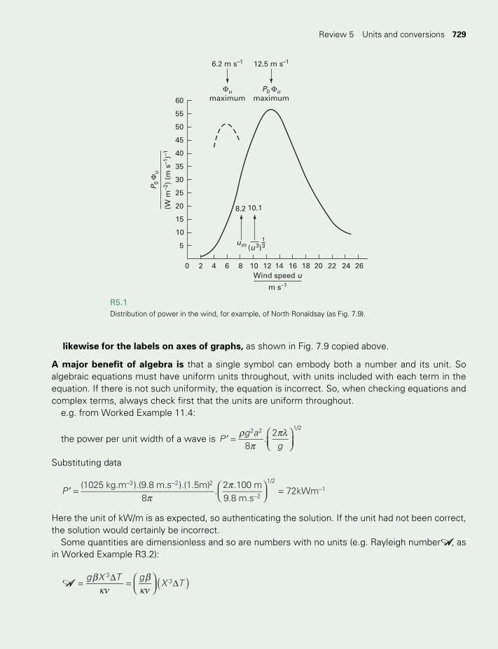
Review 5 Units and conversions 729
likewise for the labels on axes of graphs, as shown in Fig. 7.9 copied above.
A major benefit of algebra is that a single symbol can embody both a number and its unit. So algebraic equations must have uniform units throughout, with units included with each term in the equation. If there is not such uniformity, the equation is incorrect. So, when checking equations and complex terms, always check first that the units are uniform throughout.
e.g. from Worked Example 11.4:
the power per unit width of a wave is Pg a
g8.
22 2 1/2rπ
πλ′ =
Substituting data
P(1025 kg.m ).(9.8 m.s ).(1.5m)
8.
2 .100 m9.8 m.s
72kWm3 2 2
2
1/21
ππ
′ =
=− −
−−
Here the unit of kW/m is as expected, so authenticating the solution. If the unit had not been correct, the solution would certainly be incorrect.
Some quantities are dimensionless and so are numbers with no units (e.g. Rayleigh number A, as in Worked Example R3.2):
A βκν
βκν
( )= ∆ =
∆g X T gX T
33
60 maximum maximum
55
50
45
40
35
30
25
20
15
10
0 2 4 6 8 10 12
8.2
6.2 m s–1
Φu
12.5 m s–1
10.1
13um (u3)
14 16 18Wind speed u
P0 Φu
m s–1
20 22 24 26
5
(W m
–2)
(m s
–1)–1
P0
Φu
R5.1Distribution of power in the wind, for example, of North Ronaldsay (as Fig. 7.9).
TWIDELL PAGINATION.indb 729 01/12/2014 11:39
730 The ‘algebraic’ method730 Review 5 Units and conversions
(9.8ms )(1/ 330K)
(2.6 10 m s )(1.8 10 m s )(0.03m) (25K) 4.1 10
1
5 2 1 5 2 13 4=
× ×= ×
−
− − − −
The solution has no units, hence authenticating the dimensionless solution.In calculations there is often confusion about whether to multiply or divide by a numerical conver-
sion factor, but the technique shown below (and used in the examples throughout this book) is virtu-ally foolproof. In brief:
• Express all physical quantities as (number) × (unit); i.e. retain units explicitly throughout the working. • Cancel out the same unit in the denominator and numerator to simplify.• Multiply quantities in such a way that only the desired units remain, with the undesired ones
‘canceled out’.
The method depends on using an appropriate expression for ‘1’. For example, the equality 1kW = 103 W may be expressed as:
11kW10 W
10 W1kW3
3
=
=
(R5.1)
or as 11Js1W
1
=
− (R5.2)
or as 13600 s
1h= (R5.3)
or as 11MJ10 J6
=
(R5.4)
In Worked Example R5.1, each of the expressions in parentheses is 1.0, since the numerator and denominator are identical, by definition of the units involved. With practice, one can go directly to the long expression at the end. Notice how the expressions are arranged so that the ‘undesired’ units (in this case, J, s, etc.) ‘cancel out’ (i.e. appear in the numerator of one bracket and the denominator of another).
TWIDELL PAGINATION.indb 730 01/12/2014 11:39
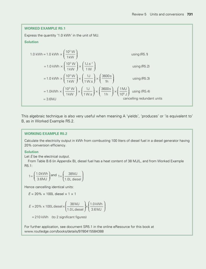
Review 5 Units and conversions 731
This algebraic technique is also very useful when meaning A ‘yields’, ‘produces’ or ‘is equivalent to’ B, as in Worked Example R5.2.
WORKED EXAMPLE R5.1
Express the quantity ‘1.0 kWh’ in the unit of MJ.
Solution
= ×
= × ×
= × × ×
= × × × ×
=
−
1.0 kWh 1.0 kWh10 W
1kWusing (R5.1)
1.0 kWh10 W
1kW
1J.s
1 Wusing (R5.2)
1.0 kWh10 W
1kW
1J
1 W.s
3600s
1husing (R5.3)
1.0kWh10 W
1kW
1J
1 W.s
3600s
1h
1MJ
10 Jusing (R5.4)
3.6MJ cancelling redundant units
3
3 1
3
3
6
WORKING EXAMPLE R5.2
Calculate the electricity output in kWh from combusting 100 liters of diesel fuel in a diesel generator having 20% conversion efficiency.
SolutionLet E be the electrical output.
From Table B.6 (in Appendix B), diesel fuel has a heat content of 38 MJ/L, and from Worked Example R5.1:
11.0kWh
3.6MJ
= and
1
38MJ
1.0L diesel
=
Hence cancelling identical units:
E = 20% × 100L diesel × 1 × 1
E 20% x 100Ldiesel38 MJ
1.0 Ldiesel
1.0 kWh
3.6 MJ
210 kWh (to 2 significant figures)
= × ×
=
For further application, see document SR5.1 in the online eResource for this book at www.routledge.com/books/details/9780415584388
TWIDELL PAGINATION.indb 731 01/12/2014 11:39

Appendix A Units and conversions
A.1 NAMES AND SYMBOLS FOR THE SI UNITS
Base units
Physical quantity Name of SI unit Symbol for SI unit
Length metre mMass kilogram kgTime second sElectric current ampere AThermodynamic temperature kelvin KAmount of substance mole molLuminous intensity candela cd
Supplementary units
Physical quantity Name of SI unit Symbol for SI unit
Plane angle radian radSolid angle steradian sr
A.2 SPECIAL NAMES AND SYMBOLS FOR SI DERIVED UNITS
Physical quantity Name of SI unit Symbol for SI unit Definition of SI unit Equivalent form(s) of SI unit
Energy joule J m2 kg s−2 N mForce newton N m kg s−2 J m−1
Pressure pascal Pa m−1 kg s−2 N m−2, J m−3
Power watt W m2 kg s−3 J s−1
Electric charge coulomb C s A A sElectric potential difference
volt V m2 kg s−3 A−1 J A−1 s−1, J C−1
TWIDELL PAGINATION.indb 732 01/12/2014 11:39
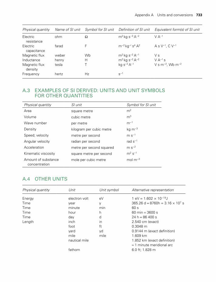
Appendix A Units and conversions 733
Physical quantity Name of SI unit Symbol for SI unit Definition of SI unit Equivalent form(s) of SI unit
Electric resistance
ohm Ω m2 kg s−3 A−2 V A−1
Electric capacitance
farad F m−2 kg−l s4 A2 A s V−1, C V−1
Magnetic flux weber Wb m2 kg s−2 A−1 V sInductance henry H m2 kg s−2 A−2 V A−1 sMagnetic flux density
tesla T kg s−2 A−1 V s m−2, Wb m−2
Frequency hertz Hz s−1
A.3 EXAMPLES OF SI DERIVED: UNITS AND UNIT SYMBOLS FOR OTHER QUANTITIES
Physical quantity SI unit Symbol for SI unit
Area square metre m2
Volume cubic metre m3
Wave number per metre m−1
Density kilogram per cubic metre kg m−3
Speed; velocity metre per second m s−1
Angular velocity radian per second rad s−1
Acceleration metre per second squared m s−2
Kinematic viscosity square metre per second m2 s−1
Amount of substance concentration
mole per cubic metre mol m−3
A.4 OTHER UNITS
Physical quantity Unit Unit symbol Alternative representation
Energy electron volt eV 1 eV = 1.602 × 10⁻¹⁹JTime year y 365.26 d = 8760h = 3.16 × 10⁷ sTime minute min 60 sTime hour h 60 min = 3600 sTime day d 24 h = 86 400 sLength inch in 2.540 cm (exact)
foot ft 0.3048 myard yd 0.9144 m (exact definition)mile mile 1.609 kmnautical mile 1.852 km (exact definition)
≈ 1 minute meridional arcfathom 6.0 ft; 1.828 m
TWIDELL PAGINATION.indb 733 01/12/2014 11:39
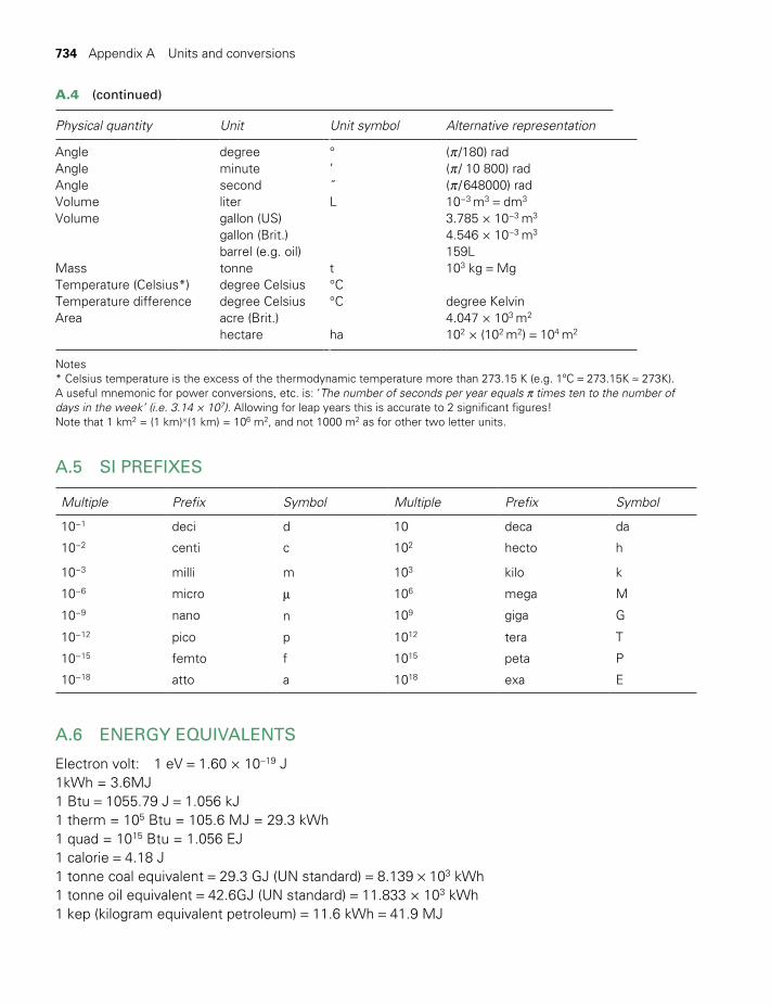
734 Appendix A Units and conversions
Physical quantity Unit Unit symbol Alternative representation
Angle degree ° (π /180) radAngle minute ’ (π / 10 800) radAngle second ˝ (π / 648000) radVolume liter L 10−3 m3 = dm3
Volume gallon (US) 3.785 × 10⁻³ m3
gallon (Brit.) 4.546 × 10⁻³ m3
barrel (e.g. oil) 159LMass tonne t 103 kg = MgTemperature (Celsius*) degree Celsius °CTemperature difference degree Celsius °C degree KelvinArea acre (Brit.) 4.047 × 10³ m2
hectare ha 102 × (102 m2) = 104 m2
Notes * Celsius temperature is the excess of the thermodynamic temperature more than 273.15 K (e.g. 1ºC = 273.15K ≈ 273K). A useful mnemonic for power conversions, etc. is: ‘The number of seconds per year equals π times ten to the number of days in the week’ (i.e. 3.14 × 10⁷). Allowing for leap years this is accurate to 2 significant figures!Note that 1 km2 = (1 km)×(1 km) = 106 m2, and not 1000 m2 as for other two letter units.
A.5 SI PREFIXES
Multiple Prefix Symbol Multiple Prefix Symbol
10−1 deci d 10 deca da
10−2 centi c 102 hecto h
10−3 milli m 103 kilo k
10−6 micro m 106 mega M
10−9 nano n 109 giga G
10−12 pico p 1012 tera T
10−15 femto f 1015 peta P
10−18 atto a 1018 exa E
A.6 ENERGY EQUIVALENTS
Electron volt: 1 eV = 1.60 × 10⁻¹⁹ J1kWh = 3.6MJ 1 Btu = 1055.79 J = 1.056 kJ1 therm = 105 Btu = 105.6 MJ = 29.3 kWh1 quad = 1015 Btu = 1.056 EJ1 calorie = 4.18 J1 tonne coal equivalent = 29.3 GJ (UN standard) = 8.139 × 10³ kWh1 tonne oil equivalent = 42.6GJ (UN standard) = 11.833 × 10³ kWh1 kep (kilogram equivalent petroleum) = 11.6 kWh = 41.9 MJ
A.4 (continued)
TWIDELL PAGINATION.indb 734 01/12/2014 11:39

Appendix A Units and conversions 735
A.7 POWER EQUIVALENTS
1 Btu s−1 = 1.06 kW 1Btu h−1 = 0.293 W1 horsepower = 746 W1 (tonne oil equivalent) / y = 1.350 kW
A.8 SPEED EQUIVALENTS
1 m/s = 3.6 km / h = 2.237 mi / h = 1.943 knot0.278 m/ s = 1 km / h = 0.658 mi / h = 0.540 knot0.447 m/s = 1.609 km / h = 1 mi / h = 0.869 knot0.515 m/ s = 1.853 km / h = 1.151 mi / h = 1 knot
TWIDELL PAGINATION.indb 735 01/12/2014 11:39

BIBLIOGRAPHY
Engineering toolbox (online at www.engineeringtoolbox.com) (comprehensive and inclusive; tabulates with several systems of units, so take care).
Handbook of Physics and Chemistry, CRC Press, London (annual). Chemical emphasis, but useful for all scien-tists, yet often complicated to use.
Kaye and Laby (online at www.kayelaby.npl.co.uk) Tables of Physical and Chemical Constants (user–friendly and authoritative; careful use of SI units).
Mills, A.F. (1999, 2nd edn) Basic Heat and Mass Transfer, Prentice-Hall, New York. Includes a full appendix of accessible data.
Monteith, J. and Unsworth , M. (2007, 3rd edn) Principles of Environmental Physics, Academic Press, London. Extremely useful set of tables for data on air and water vapor, and on heat transfer with elementary geometrical shapes.
Rohsenow, W.M., Hartnett, J.P. and Cho, J. (eds) (1997, 3rd edn) Handbook of Heat Transfer, McGraw-Hill, New York. Chapter 2 by T.F. Irvine is an extensive compilation of thermophysical data.
Unit conversion (online at www.unitconversion.org). Always check the balance of units in equations yourself, as explained in Review 5, since this forces you to understand the analysis. However, this unit conversion website is an important check.
Appendix B Data and fundamental constants
The following tables give sufficient physical data and information to follow the examples and problems in this book. They are not intended to take the place of the standard handbooks listed in the following bib-liography, from which the data have been extracted. These handbooks themselves use databases, such as those maintained by the US National Institute of Standards and Technology.
Only two or three significant figures are given, except in the few cases where the data and their use in this book justify more accuracy.
TWIDELL PAGINATION.indb 736 01/12/2014 11:39
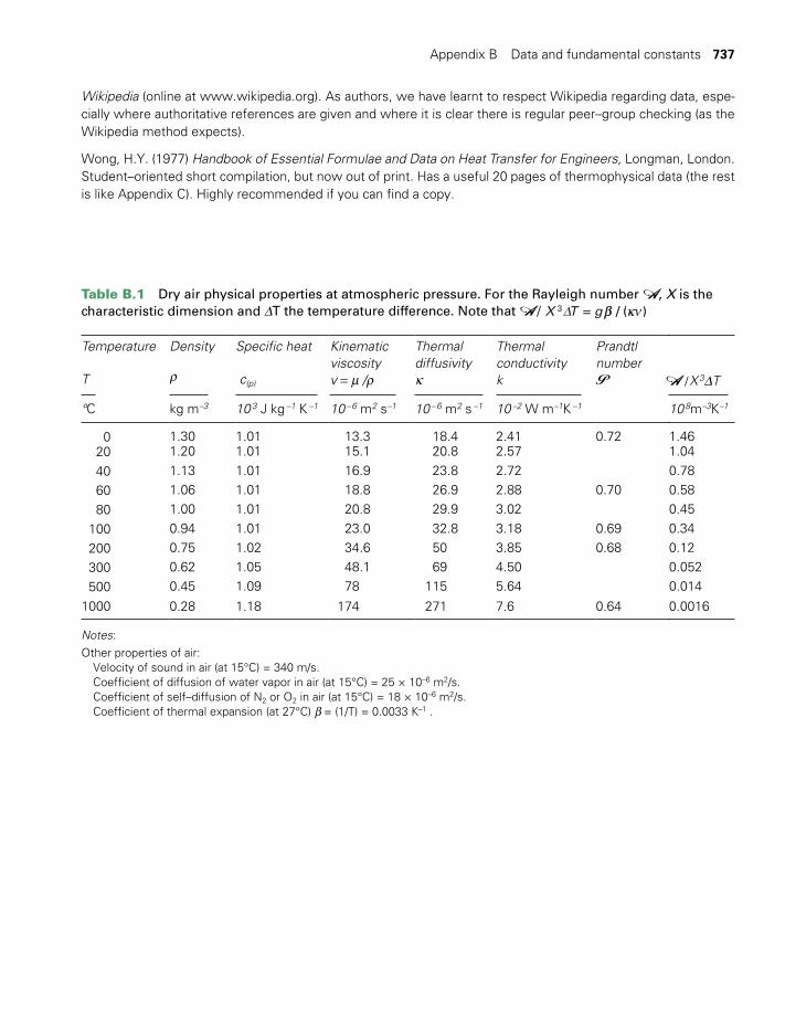
Appendix B Data and fundamental constants 737
Wikipedia (online at www.wikipedia.org). As authors, we have learnt to respect Wikipedia regarding data, espe-cially where authoritative references are given and where it is clear there is regular peer–group checking (as the Wikipedia method expects).
Wong, H.Y. (1977) Handbook of Essential Formulae and Data on Heat Transfer for Engineers, Longman, London. Student–oriented short compilation, but now out of print. Has a useful 20 pages of thermophysical data (the rest is like Appendix C). Highly recommended if you can find a copy.
Table B.1 Dry air physical properties at atmospheric pressure. For the Rayleigh number A, X is the characteristic dimension and DT the temperature difference. Note that A / // (( ))X T g3 bb kkD n==
Temperature
T
Density
r
Specific heat
c(p)
Kinematicviscosityv = m /r
Thermaldiffusivityk
Thermalconductivityk
PrandtlnumberP
A / X 3DT
°C kg m–3 10 3 J kg –1 K –1 10 – 6 m2 s–1 10 – 6 m2 s –1 10 –2 W m–1K –1 10 8m–3K–1
0 1.30 1.01 13.3 18.4 2.41 0.72 1.46 20 1.20 1.01 15.1 20.8 2.57 1.04
40 1.13 1.01 16.9 23.8 2.72 0.78 60 1.06 1.01 18.8 26.9 2.88 0.70 0.58 80 1.00 1.01 20.8 29.9 3.02 0.45
100 0.94 1.01 23.0 32.8 3.18 0.69 0.34 200 0.75 1.02 34.6 50 3.85 0.68 0.12 300 0.62 1.05 48.1 69 4.50 0.052 500 0.45 1.09 78 115 5.64 0.014
1000 0.28 1.18 174 271 7.6 0.64 0.0016
Notes:Other properties of air: Velocity of sound in air (at 15°C) = 340 m/s. Coefficient of diffusion of water vapor in air (at 15°C) = 25 × 10–6 m2/s. Coefficient of self–diffusion of N2 or O2 in air (at 15°C) = 18 × 10–6 m2/s. Coefficient of thermal expansion (at 27°C) b = (1/T) = 0.0033 K–1 .
TWIDELL PAGINATION.indb 737 01/12/2014 11:39
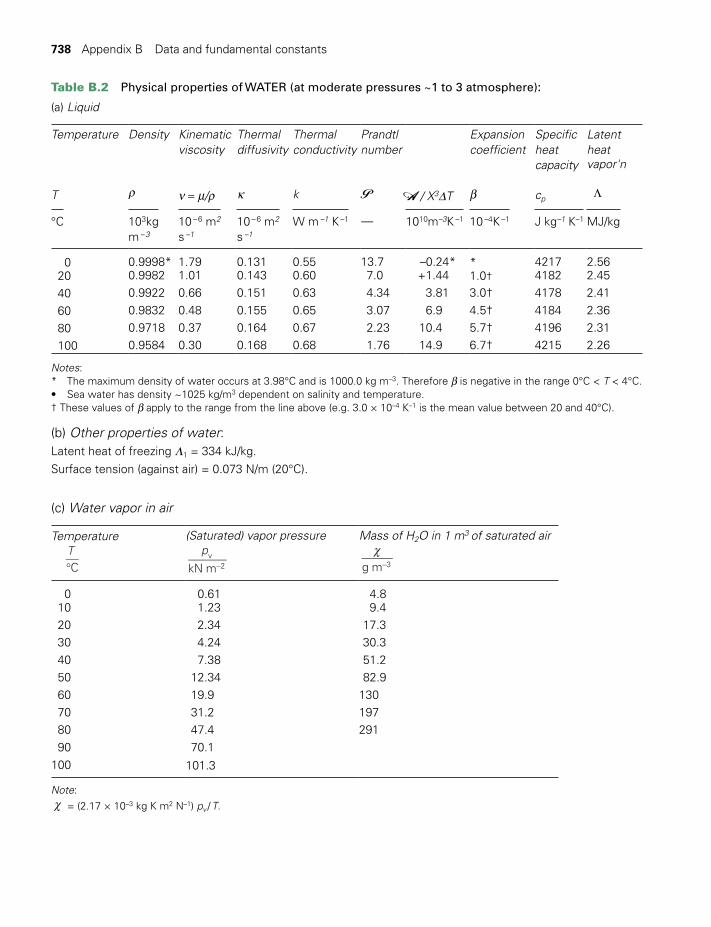
738 Appendix B Data and fundamental constants
Table B.2 Physical properties of WATER (at moderate pressures ~1 to 3 atmosphere):
(a) Liquid
Tempe rature
T
Density
r
Kinematicviscosity
n = m/r
Thermaldiffusivity
k
Thermalconductivity
k
Prandtlnumber
P
A / X3DT
Expansioncoefficient
b
Specific heat capacity
cp
Latent heatvapor'n Λ
°C 103kg m – 3
10 – 6 m2 s –1
10 – 6 m2 s –1
W m –1 K –1 — 1010m–3K –1 10 –4K –1 J kg–1 K–1 MJ/kg
0 0.9998* 1.79 0.131 0.55 13.7 –0.24* * 4217 2.56 20 0.9982 1.01 0.143 0.60 7.0 +1.44 1.0† 4182 2.45 40 0.9922 0.66 0.151 0.63 4.34 3.81 3.0† 4178 2.41
60 0.9832 0.48 0.155 0.65 3.07 6.9 4.5† 4184 2.36 80 0.9718 0.37 0.164 0.67 2.23 10.4 5.7† 4196 2.31 100 0.9584 0.30 0.168 0.68 1.76 14.9 6.7† 4215 2.26
Notes:* The maximum density of water occurs at 3.98°C and is 1000.0 kg m–3. Therefore b is negative in the range 0°C < T < 4°C.• Sea water has density ~1025 kg/m3 dependent on salinity and temperature.† These values of b apply to the range from the line above (e.g. 3.0 × 10⁻⁴ K–1 is the mean value between 20 and 40°C).
(b) Other properties of water:Latent heat of freezing Λ1 = 334 kJ/kg. Surface tension (against air) = 0.073 N/m (20°C).
(c) Water vapor in air
Temperature
°TC
(Saturated) vapor pressure
−
p
kN mv
2
Mass of H2O in 1 m3 of saturated airχ
−g m 3
0 0.61 4.8 10 1.23 9.4 20 2.34 17.3 30 4.24 30.3 40 7.38 51.2 50 12.34 82.9 60 19.9 130 70 31.2 197 80 47.4 291 90 70.1100 101.3
Note:χ = (2.17 × 10⁻³ kg K m2 N–1) pv / T.
TWIDELL PAGINATION.indb 738 01/12/2014 11:39
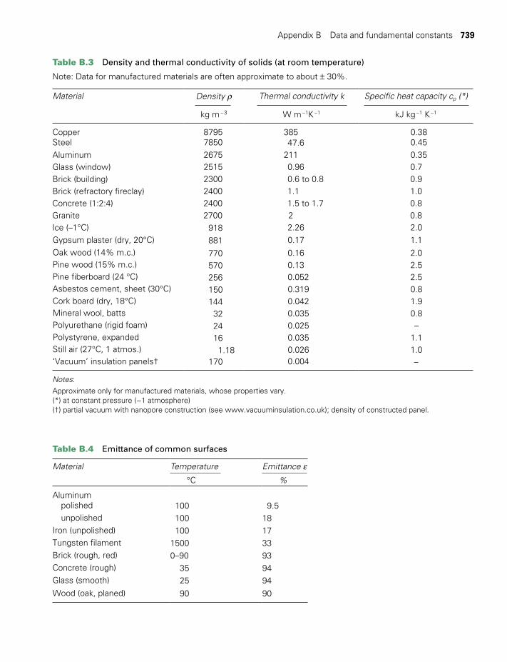
Appendix B Data and fundamental constants 739
Table B.3 Density and thermal conductivity of solids (at room temperature)
Note: Data for manufactured materials are often approximate to about ± 30%.
Material Density r Thermal conductivity k Specific heat capacity cp (*)
kg m – 3 W m –1K –1 kJ kg –1 K –1
Copper 8795 385 0.38Steel 7850 47.6 0.45Aluminum 2675 211 0.35Glass (window) 2515 0.96 0.7Brick (building) 2300 0.6 to 0.8 0.9Brick (refractory fireclay) 2400 1.1 1.0Concrete (1:2:4) 2400 1.5 to 1.7 0.8Granite 2700 2 0.8Ice (–1°C) 918 2.26 2.0Gypsum plaster (dry, 20°C) 881 0.17 1.1Oak wood (14% m.c.) 770 0.16 2.0Pine wood (15% m.c.) 570 0.13 2.5Pine fiberboard (24 °C) 256 0.052 2.5Asbestos cement, sheet (30°C) 150 0.319 0.8Cork board (dry, 18°C) 144 0.042 1.9Mineral wool, batts 32 0.035 0.8Polyurethane (rigid foam) 24 0.025 –Polystyrene, expanded 16 0.035 1.1Still air (27°C, 1 atmos.) 1.18 0.026 1.0‘Vacuum’ insulation panels† 170 0.004 –
Notes:Approximate only for manufactured materials, whose properties vary.(*) at constant pressure (~1 atmosphere)(†) partial vacuum with nanopore construction (see www.vacuuminsulation.co.uk); density of constructed panel.
Table B.4 Emittance of common surfaces
Material Temperature °C
Emittance e %
Aluminum polished 100 9.5 unpolished 100 18Iron (unpolished) 100 17Tungsten filament 1500 33Brick (rough, red) 0–90 93Concrete (rough) 35 94Glass (smooth) 25 94Wood (oak, planed) 90 90
TWIDELL PAGINATION.indb 739 01/12/2014 11:39
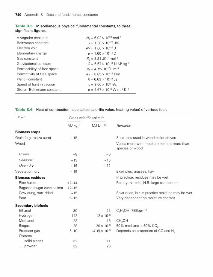
740 Appendix B Data and fundamental constants
Table B.5 Miscellaneous physical fundamental constants, to three significant figures.
A vogadro constant N0 = 6.02 × 10²³ mol–1
Boltzmann constant k = 1.38 × 10⁻²³ J/KElectron volt eV = 1.60 × 10⁻¹⁹ JElementary charge e = 1.60 × 10⁻¹⁹ CGas constant R0 = 8.31 JK–1 mol–1
Gravitational constant G = 6.67 × 10⁻¹¹ N M2 kg–2
Permeability of free space m0 = 4 p × 10–7H m–1 Permittivity of free space ∈0 = 8.85 × 10⁻¹² F/mPlanck constant h = 6.63 × 10⁻³⁴ JsSpeed of light in vacuum c = 3.00 × 10⁸m/sStefan–Boltzmann constant s = 5.67 × 10⁻⁸ W m–2 K– 4
Table B.6 Heat of combustion (also called calorific value, heating value) of various fuels
Fuel Gross calorific value (a)
RemarksMJ kg–1 MJ L–1 (b)
Biomass crops
Grain (e.g. maize corn) ~15 Surpluses used in wood pellet stoves
Wood Varies more with moisture content more than species of wood
Green ~8 ~6
Seasonal ~13 ~10 Oven dry ~16 ~12
Vegetation: dry ~15 Examples: grasses, hay
Biomass residues In practice, residues may be wet Rice husks 12–14 For dry material, N.B. large ash content Bagasse (sugar cane solids) 12–15 Cow dung, sun–dried ~15 Solar dried, but in practice residues may be wet Peat 6–15 Very dependent on moisture content
Secondary biofuels Ethanol 30 25 C2H5OH: 789kgm–3
Hydrogen 142 12 × 10–3
Methanol 23 18 CH3OH Biogas 28 20 × 10–3 50% methane + 50% CO2
Producer gas 5–10 (4–8) × 10–3 Depends on proportion of CO and H2
Charcoal ….. …..solid pieces 32 11 …..powder 32 20
TWIDELL PAGINATION.indb 740 01/12/2014 11:39

Appendix B Data and fundamental constants 741
Fuel Gross calorific value (a) Remarks
MJ kg –1 MJ L–1 (b)
Coconut and most other crop oils 39.5 ± 0.5 36 Biodiesel (1) 39 33 Ethyl esters of coconut oil Biodiesel (2) 40 35 Methyl esters of soya oil
Fossil fuels Methane 56 38 × 10–3 Also called ‘natural gas’ Petrol/gasoline 47 34 Motor spirit Kerosene 46 37 Diesoline 46 38 Automotive distillate, derv, diesel Crude oil 44 35 Coal 27 Black, coking grade
Notes:a Gross calorific value (GCV also called heat of combustion) is the heat evolved in a reaction of the type
CH2O + O2 → CO2 (gas) + H2O (liquid). Some authors quote instead the net (or lower) calorific value LCV, which is the heat evolved when the final H2O is
gaseous. LCV is 6% less than GCV for most biofuels and 8% less than GCV for petroleum and diesel fuels.b At 15°C.
Table B.7 U–values of walls and windows
The heat transfer is by conduction and also by convection and radiation. The U–values shown here are for the combined processes. See Box R3.1 for other associated heat transfer terminology.
WALLS U–values, unit of W/(m2 °C)
Single brick Cavity between brick Cavity filled with insulation External insulation (100 mm) U ~2.2 U ~1.0 U ~0.5 U ~0.2
Roof, 400 mm insulation U ~0.1
WINDOWS AND GLAZING
(a) Shading is extremely important to reduce solar input causing overheating. (b) U–values (heat transfer coefficient of unit area) of only the glazing and not the frame.
single double triple double+IR reflection coating K glass, gas filled (…………no coating………......…) (K glass; Kappa glass) (e.g. argon, krypton)
U~5 ~3 ~2 ~1.8 ~1.5 W/(m2 K) (measured in a laboratory with no solar radiation)
TWIDELL PAGINATION.indb 741 01/12/2014 11:39
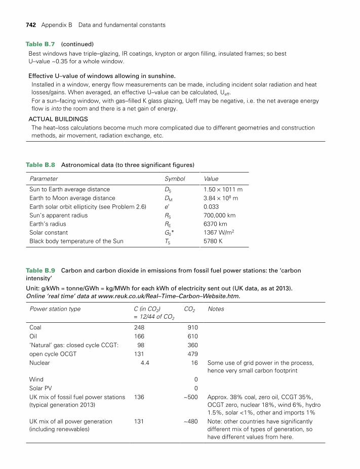
742 Appendix B Data and fundamental constants
Best windows have triple–glazing, IR coatings, krypton or argon filling, insulated frames; so best U–value ~0.35 for a whole window.
Effective U–value of windows allowing in sunshine. Installed in a window, energy flow measurements can be made, including incident solar radiation and heat losses/gains. When averaged, an effective U–value can be calculated, Ueff.
For a sun–facing window, with gas–filled K glass glazing, Ueff may be negative, i.e. the net average energy flow is into the room and there is a net gain of energy.
ACTUAL BUILDINGS The heat–loss calculations become much more complicated due to different geometries and construction methods, air movement, radiation exchange, etc.
Table B.8 Astronomical data (to three significant figures)
Parameter Symbol Value
Sun to Earth average distance DS 1.50 × 10¹¹ mEarth to Moon average distance DM 3.84 × 10⁸ mEarth solar orbit ellipticity (see Problem 2.6) e’ 0.033Sun’s apparent radius RS 700,000 kmEarth’s radius RE 6370 kmSolar constant G0* 1367 W/m2
Black body temperature of the Sun TS 5780 K
Table B.9 Carbon and carbon dioxide in emissions from fossil fuel power stations: the ‘carbon intensity’
Unit: g/kWh = tonne/GWh = kg/MWh for each kWh of electricity sent out (UK data, as at 2013).Online ‘real time’ data at www.reuk.co.uk/Real–Time–Carbon–Website.htm.
Power station type C (in CO2) = 12/44 of CO2
CO2 Notes
Coal 248 910Oil 166 610‘Natural’ gas: closed cycle CCGT: 98 360 open cycle OCGT 131 479Nuclear 4.4 16 Some use of grid power in the process,
hence very small carbon footprintWind 0Solar PV 0UK mix of fossil fuel power stations(typical generation 2013)
136 ~500 Approx. 38% coal, zero oil, CCGT 35%, OCGT zero, nuclear 18%, wind 6%, hydro 1.5%, solar <1%, other and imports 1%
UK mix of all power generation (including renewables)
131 ~480 Note: other countries have significantly different mix of types of generation, so have different values from here.
Table B.7 (continued)
TWIDELL PAGINATION.indb 742 01/12/2014 11:39
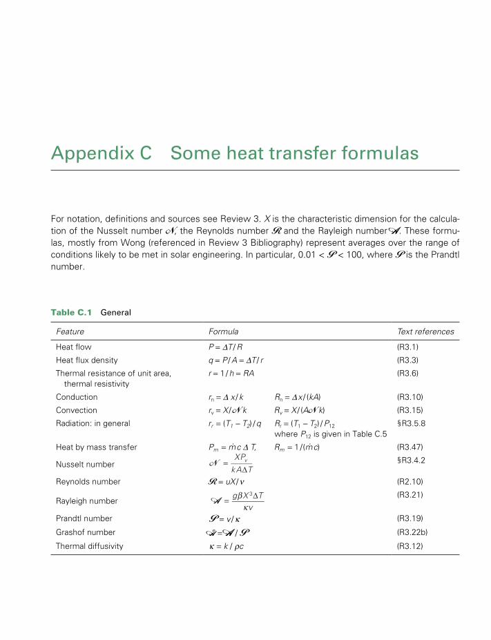
Appendix C Some heat transfer formulas
For notation, definitions and sources see Review 3. X is the characteristic dimension for the calcula-tion of the Nusselt number N, the Reynolds number R and the Rayleigh number A. These formu-las, mostly from Wong (referenced in Review 3 Bibliography) represent averages over the range of conditions likely to be met in solar engineering. In particular, 0.01 < P < 100, where P is the Prandtl number.
Table C.1 General
Feature Formula Text references
Heat flow P = DT / R (R3.1)
Heat flux density q = P / A = DT / r (R3.3)
Thermal resistance of unit area, thermal resistivity
r = 1 / h = RA (R3.6)
Conduction rn = D x / k Rn = D x / (kA) (R3.10)
Convection rv = X / N k Rv = X / (AN k) (R3.15)
Radiation: in general rr = (T1 - T2) / q Rr = (T1 - T2) / P12
where P12 is given in Table C.5§R3.5.8
Heat by mass transfer Pm = m. c D T, Rm = 1 / (m
. c) (R3.47)
Nusselt number §R3.4.2
Reynolds number R = uX / ν (R2.10)
Rayleigh number(R3.21)
Prandtl number P = v / k (R3.19)
Grashof number G = A / P (R3.22b)
Thermal diffusivity k = k / rc (R3.12)
NXP
kA Tv=
D
A g X Tv
3βk
= D
TWIDELL PAGINATION.indb 743 01/12/2014 11:39
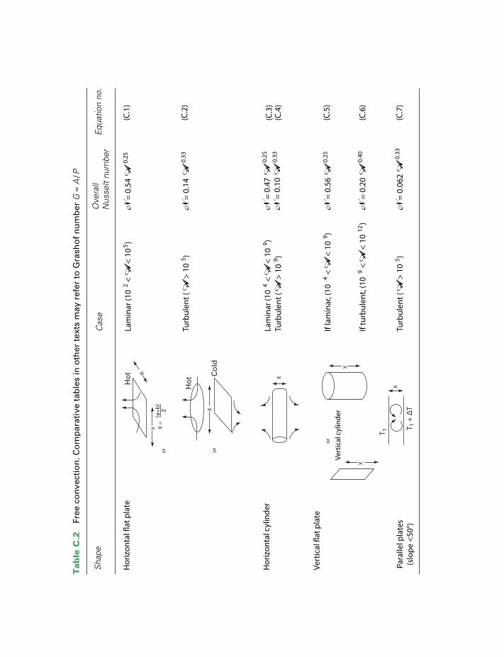
Hor
izon
tal
at p
late
Shap
eC
ase
Lam
inar
(10
2 < A
< 1
05 )N
= 0
.54
A 0.
25(C
.1)
(C.2
)
(C.3
)(C
.4)
(C.5
)
(C.6
)
(C.7
)
N =
0.1
4 A
0.33
Turb
ulen
t ( A
> 1
05 )
Lam
inar
(10
4 < A
< 1
09 )
Turb
ulen
t (A
> 1
09 )
If la
min
ar, (
104 <
A <
10
9 )
If tu
rbul
ent,
(10
9 < A
< 1
012
)
Turb
ulen
t (A
> 1
05 )
N =
0.0
62 A
0.33
N =
0.2
0 A
0.40
N =
0.5
6 A
0.25
N =
0.4
7 A
0.25
N =
0.1
0 A
0.33
Ove
rall
Nus
selt
num
ber
Equa
tion
no.
Hor
izon
tal c
ylin
der
Vert
ical
cyl
inde
r
Para
llel p
late
s(s
lope
<50
°)
Vert
ical
at
pla
te
Ho
t
(a+b
)2
b
a
orX
=
Ho
t Co
ldor
X
X
or
X
X
T 1
T 1 +
∆T
X
Tab
le C
.2
Free
co
nvec
tio
n. C
om
par
ativ
e ta
ble
s in
oth
er t
exts
may
ref
er t
o G
rash
of
nu
mb
er G
= A
/ P
TWIDELL PAGINATION.indb 744 01/12/2014 11:39

x x
or
DT 2
T 1L
Shap
eC
ase
Ove
rall
Nus
selt
num
ber
Equa
tion
no.
Flow
ove
r a
t pl
ate
Flow
ove
r ci
rcul
ar c
ylin
der
Flow
insi
de a
circ
ular
pip
e:
Indi
cate
s se
ctio
n of
an
exte
nded
sha
pe
Gen
eral
P =
cQ
(T2
– T
1)
N =
0.0
27R
0.8 P
0.33
Gra
etz
num
ber
= R
P(D
/L)
Turb
ulen
t (1
03 <
R <
5 ×
104 )
Lam
inar
ow
,sh
ort
pipe
(R<
2300
,G
1>10
)Tu
rbul
ent
ow
( R>
2300
)
Lam
inar
(0.1
< R
< 1
000)
Lam
inar
(R <
5 ×
105 )
Turb
ulen
t ( R
> 5
× 1
05 )
N =
1.8
6 G
10.33
= 4
Q/κ
πL
N =
(0.3
5 +
0.5
6R
0.52
)P0.
3
N =
0.3
7R0.
8 P0.
33
N =
0.6
64R
0.5 P
0.33
(C.8
)
(C.1
0)
(C.1
1)
(C.1
2)(C
.13)
(C.1
4)
(R2.
6)
(C.9
)
N =
0.2
6R0.
6 P0.
3
ρ
Tab
le C
.3
Forc
ed c
onv
ecti
on
TWIDELL PAGINATION.indb 745 01/12/2014 11:39

746 Appendix C Some heat transfer formulas
Air over flat plate
General
Case Formula
(C.15)
(C.16)
X > 0.1mh = a + bu[a = 5.7Wm−2 K−1
b = 3.8 (Wm−2K−1)/(ms−1)]N1 = max(Nforced, Nfree)
N1 < Nmixed < Nforced + Nfree
1 m/s < u < 20m/s
Shape
X
u
Table C.4 Mixed convection (forced and free together)
System Schematic presentation Net radiative heat flow Equation no.
(C.17)
(C.18)
(C.19)
(3.36)
(C.20)
F12 = shape factor
Gray surface tosurroundings (A1 << A2)
Two closely spacedparallel planes(L / D → ∞)
Closure formed by twosurfaces (surface1 convex or at)
General two-body system(neither surface receivesradiation from a thirdsurface) P12 =
σ(T14 4
− T2 )1 − 1 1A1
1 − 2 2A2
1A1F12
+ +
P12 = σA1(T1
4 – T24)
(1/ 1) + (1/ 2) − 1
P12 = σA1(T1 − T2 )
4 4
P12 = 1σA1(T14 – T2
4)
1 + 1A1A2
−2
1 1
ε
ε ε
ε
ε εεε
ε
2
2
2D
L
T1
T2
A1
1
1
1
Table C.5 Net radiative heat flow between two diffuse gray surfaces. For definitions and notation, see Chapter 3, especially §3.5.6 and §3.5.7. In general P12 = s A1 F ’12(T 41 - T 42), where F ’12 is the exchange factor of (3.46). NB In these formulas T is the absolute temperature (i.e in kelvin, unit K)
TWIDELL PAGINATION.indb 746 01/12/2014 11:39
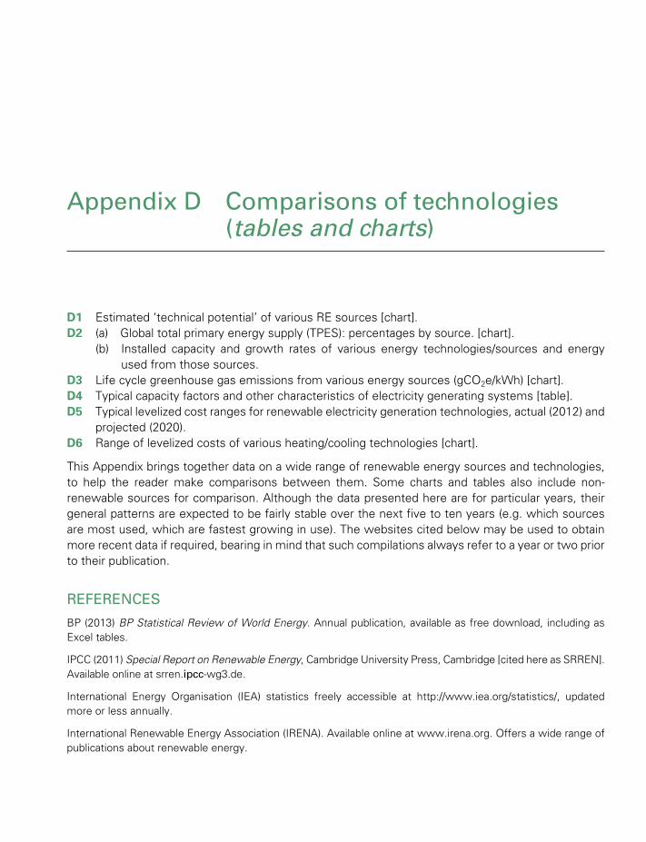
Appendix D Comparisons of technologies (tables and charts)
D1 Estimated ‘technical potential’ of various RE sources [chart].D2 (a) Global total primary energy supply (TPES): percentages by source. [chart]. (b) Installed capacity and growth rates of various energy technologies/sources and energy
used from those sources.D3 Life cycle greenhouse gas emissions from various energy sources (gCO2e/kWh) [chart].D4 Typical capacity factors and other characteristics of electricity generating systems [table].D5 Typical levelized cost ranges for renewable electricity generation technologies, actual (2012) and
projected (2020).D6 Range of levelized costs of various heating/cooling technologies [chart].
This Appendix brings together data on a wide range of renewable energy sources and technologies, to help the reader make comparisons between them. Some charts and tables also include non-renewable sources for comparison. Although the data presented here are for particular years, their general patterns are expected to be fairly stable over the next five to ten years (e.g. which sources are most used, which are fastest growing in use). The websites cited below may be used to obtain more recent data if required, bearing in mind that such compilations always refer to a year or two prior to their publication.
REFERENCES
BP (2013) BP Statistical Review of World Energy. Annual publication, available as free download, including as Excel tables.
IPCC (2011) Special Report on Renewable Energy, Cambridge University Press, Cambridge [cited here as SRREN]. Available online at srren. ipcc-wg3.de.
International Energy Organisation (IEA) statistics freely accessible at http://www.iea.org/statistics/, updated more or less annually.
International Renewable Energy Association (IRENA). Available online at www.irena.org. Offers a wide range of publications about renewable energy.
TWIDELL PAGINATION.indb 747 01/12/2014 11:39
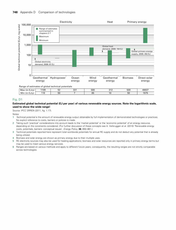
748 Appendix D Comparison of technologies
100,000
Glo
bal
tec
hn
ical
po
ten
tial
[E
J/yr
, lo
g s
cale
]Electricity
Maximum
Minimum
Range of estimatessummarized inchapters 2-7
Geothermalenergy
Global electricitydemand, 2008: 61 EJ
Global heatdemand, 2008: 164 EJ
Global primary energysupply, 2008: 492 EJ
Geothermalenergy
Direct solarenergy
Hydropower
Range of estimates of global technical potentials
85 10580 312 500 49837
157550750118331521109Max (in EJ/y)
Min (in EJ/y)
BiomassOceanenergy
Windenergy
Heat Primary energy
10,000
1,000
100
10
0
Fig. D1Estimated global technical potential (EJ per year) of various renewable energy sources. Note the logarithmic scale, used to show the wide range!Source: IPCC SRREN (2011, fig. 1.17).
Notes1 Technical potential is the amount of renewable energy output obtainable by full implementation of demonstrated technologies or practices.
No explicit reference to costs, barriers or policies is made. 2 Taking such ‘practical’ considerations into account leads to the ‘market potential’ or the ‘economic potential’ of an energy resource,
depending on the constraints considered. (For further discussion of these concepts see A. Verbruggen et al. (2010) ‘Renewable energy costs, potentials, barriers: conceptual issues’, Energy Policy, 38, 850–861.)
3 Technical potentials reported here represent total worldwide potentials for annual RE supply and do not deduct any potential that is already being utilized.
4 Biomass and solar energy are shown as primary energy due to their multiple uses. 5 RE electricity sources may also be used for heating applications; biomass and solar resources are reported only in primary energy terms but
may be used to meet various energy services.6 Ranges are based on various methods and apply to different future years; consequently, the resulting ranges are not strictly comparable
across technologies.
TWIDELL PAGINATION.indb 748 01/12/2014 11:39
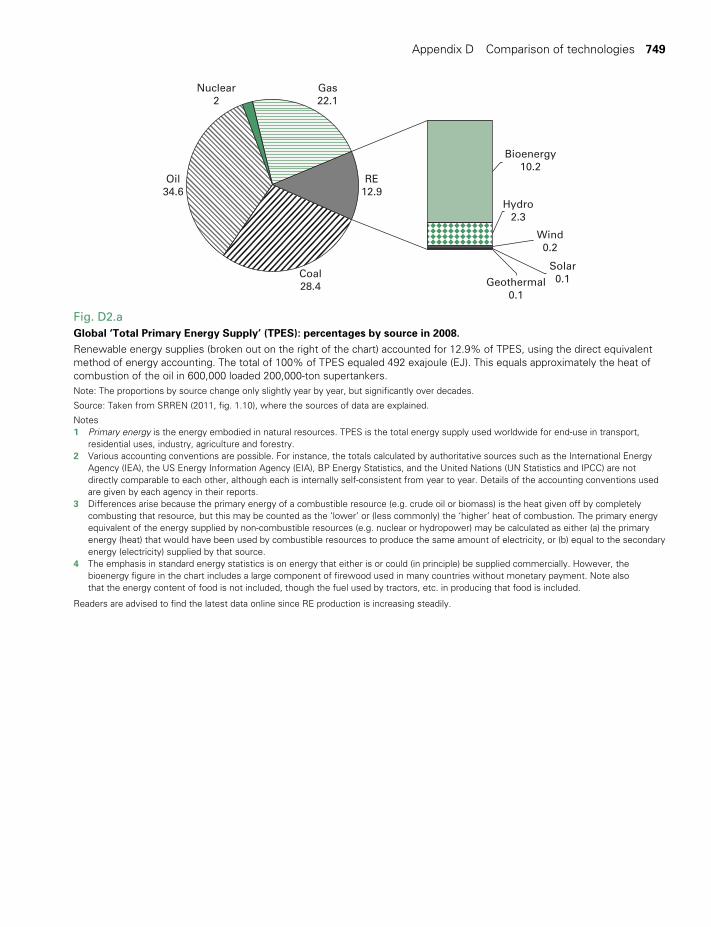
Appendix D Comparison of technologies 749
Nuclear2
Gas22.1
RE12.9
Bioenergy10.2
Hydro2.3
Wind0.2
Solar0.1Geothermal
0.1
Coal28.4
Oil34.6
Fig. D2.aGlobal ‘Total Primary Energy Supply’ (TPES): percentages by source in 2008. Renewable energy supplies (broken out on the right of the chart) accounted for 12.9% of TPES, using the direct equivalent method of energy accounting. The total of 100% of TPES equaled 492 exajoule (EJ). This equals approximately the heat of combustion of the oil in 600,000 loaded 200,000-ton supertankers.Note: The proportions by source change only slightly year by year, but significantly over decades.
Source: Taken from SRREN (2011, fig. 1.10), where the sources of data are explained.
Notes1 Primary energy is the energy embodied in natural resources. TPES is the total energy supply used worldwide for end-use in transport,
residential uses, industry, agriculture and forestry.2 Various accounting conventions are possible. For instance, the totals calculated by authoritative sources such as the International Energy
Agency (IEA), the US Energy Information Agency (EIA), BP Energy Statistics, and the United Nations (UN Statistics and IPCC) are not directly comparable to each other, although each is internally self-consistent from year to year. Details of the accounting conventions used are given by each agency in their reports.
3 Differences arise because the primary energy of a combustible resource (e.g. crude oil or biomass) is the heat given off by completely combusting that resource, but this may be counted as the ‘lower’ or (less commonly) the ‘higher’ heat of combustion. The primary energy equivalent of the energy supplied by non-combustible resources (e.g. nuclear or hydropower) may be calculated as either (a) the primary energy (heat) that would have been used by combustible resources to produce the same amount of electricity, or (b) equal to the secondary energy (electricity) supplied by that source.
4 The emphasis in standard energy statistics is on energy that either is or could (in principle) be supplied commercially. However, the bioenergy figure in the chart includes a large component of firewood used in many countries without monetary payment. Note also that the energy content of food is not included, though the fuel used by tractors, etc. in producing that food is included.
Readers are advised to find the latest data online since RE production is increasing steadily.
TWIDELL PAGINATION.indb 749 01/12/2014 11:39
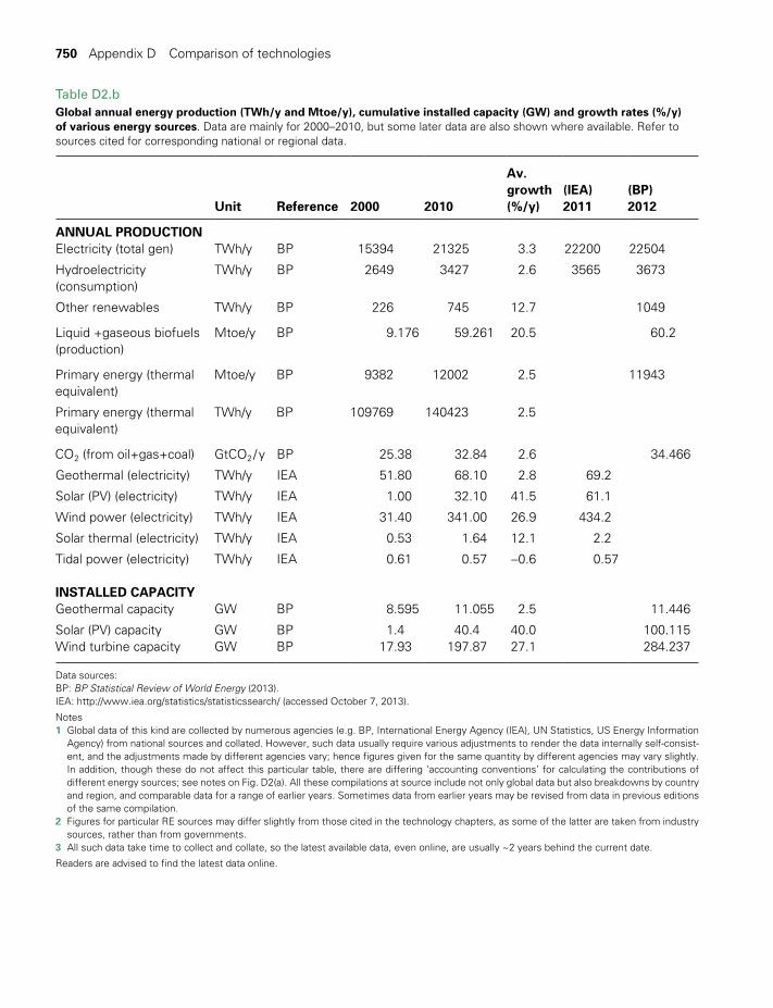
750 Appendix D Comparison of technologies
Unit
Reference
2000
2010
Av. growth (%/y)
(IEA) 2011
(BP) 2012
ANNUAL PRODUCTIONElectricity (total gen) TWh/y BP 15394 21325 3.3 22200 22504
Hydroelectricity (consumption)
TWh/y BP 2649 3427 2.6 3565 3673
Other renewables TWh/y BP 226 745 12.7 1049
Liquid +gaseous biofuels (production)
Mtoe/y BP 9.176 59.261 20.5 60.2
Primary energy (thermal equivalent)
Mtoe/y BP 9382 12002 2.5 11943
Primary energy (thermal equivalent)
TWh/y BP 109769 140423 2.5
CO2 (from oil+gas+coal) GtCO2 / y BP 25.38 32.84 2.6 34.466
Geothermal (electricity) TWh/y IEA 51.80 68.10 2.8 69.2
Solar (PV) (electricity) TWh/y IEA 1.00 32.10 41.5 61.1
Wind power (electricity) TWh/y IEA 31.40 341.00 26.9 434.2
Solar thermal (electricity) TWh/y IEA 0.53 1.64 12.1 2.2
Tidal power (electricity) TWh/y IEA 0.61 0.57 −0.6 0.57
INSTALLED CAPACITYGeothermal capacity GW BP 8.595 11.055 2.5 11.446
Solar (PV) capacity GW BP 1.4 40.4 40.0 100.115Wind turbine capacity GW BP 17.93 197.87 27.1 284.237
Data sources:BP: BP Statistical Review of World Energy (2013).IEA: http://www.iea.org/statistics/statisticssearch/ (accessed October 7, 2013).
Notes1 Global data of this kind are collected by numerous agencies (e.g. BP, International Energy Agency (IEA), UN Statistics, US Energy Information
Agency) from national sources and collated. However, such data usually require various adjustments to render the data internally self-consist-ent, and the adjustments made by different agencies vary; hence figures given for the same quantity by different agencies may vary slightly. In addition, though these do not affect this particular table, there are differing ‘accounting conventions’ for calculating the contributions of different energy sources; see notes on Fig. D2(a). All these compilations at source include not only global data but also breakdowns by country and region, and comparable data for a range of earlier years. Sometimes data from earlier years may be revised from data in previous editions of the same compilation.
2 Figures for particular RE sources may differ slightly from those cited in the technology chapters, as some of the latter are taken from industry sources, rather than from governments.
3 All such data take time to collect and collate, so the latest available data, even online, are usually ~2 years behind the current date.
Readers are advised to find the latest data online.
Table D2.bGlobal annual energy production (TWh/y and Mtoe/y), cumulative installed capacity (GW) and growth rates (%/y) of various energy sources. Data are mainly for 2000–2010, but some later data are also shown where available. Refer to sources cited for corresponding national or regional data.
TWIDELL PAGINATION.indb 750 01/12/2014 11:39
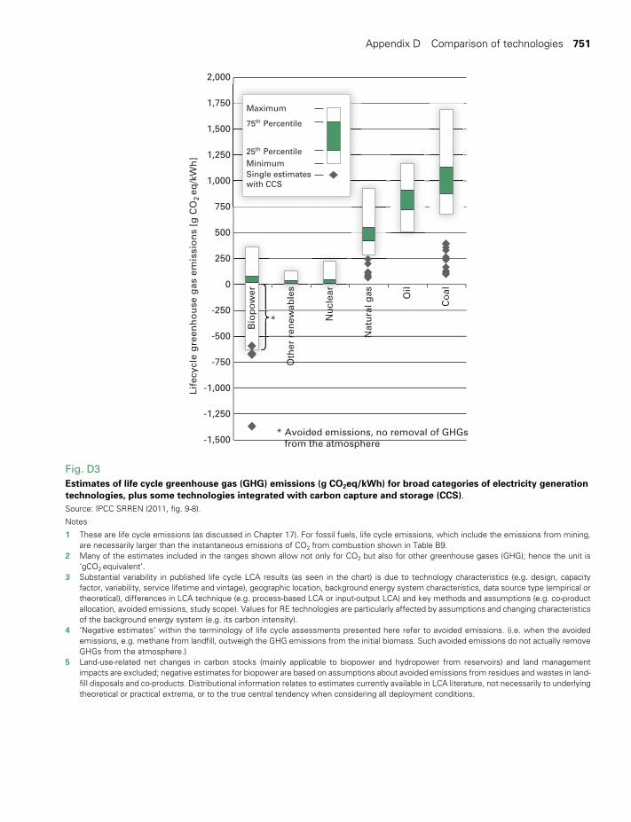
Appendix D Comparison of technologies 751
Fig. D3Estimates of life cycle greenhouse gas (GHG) emissions (g CO2eq/kWh) for broad categories of electricity generation technologies, plus some technologies integrated with carbon capture and storage (CCS).Source: IPCC SRREN (2011, fig. 9-8).
Notes
1 These are life cycle emissions (as discussed in Chapter 17). For fossil fuels, life cycle emissions, which include the emissions from mining, are necessarily larger than the instantaneous emissions of CO2 from combustion shown in Table B9.
2 Many of the estimates included in the ranges shown allow not only for CO2 but also for other greenhouse gases (GHG); hence the unit is ‘gCO2 equivalent’.
3 Substantial variability in published life cycle LCA results (as seen in the chart) is due to technology characteristics (e.g. design, capacity factor, variability, service lifetime and vintage), geographic location, background energy system characteristics, data source type (empirical or theoretical), differences in LCA technique (e.g. process-based LCA or input-output LCA) and key methods and assumptions (e.g. co-product allocation, avoided emissions, study scope). Values for RE technologies are particularly affected by assumptions and changing characteristics of the background energy system (e.g. its carbon intensity).
4 ‘Negative estimates’ within the terminology of life cycle assessments presented here refer to avoided emissions. (i.e. when the avoided emissions, e.g. methane from landfill, outweigh the GHG emissions from the initial biomass. Such avoided emissions do not actually remove GHGs from the atmosphere.)
5 Land-use-related net changes in carbon stocks (mainly applicable to biopower and hydropower from reservoirs) and land management impacts are excluded; negative estimates for biopower are based on assumptions about avoided emissions from residues and wastes in land-fill disposals and co-products. Distributional information relates to estimates currently available in LCA literature, not necessarily to underlying theoretical or practical extrema, or to the true central tendency when considering all deployment conditions.
0
*
* Avoided emissions, no removal of GHGs from the atmosphere
Life
cycl
e g
reen
ho
use
gas
em
issi
on
s [g
CO
2 eq
/kW
h]
-1,250
-1,500
-250
-750
-1,000
-500
250
750
500
1,750
1,250
1,000
1,500
2,000
Bio
po
wer
Co
alOil
Nat
ura
l gas
Nu
clea
r
Oth
er r
enew
able
s
Maximum
75th Percentile
25th Percentile Minimum Single estimates with CCS
TWIDELL PAGINATION.indb 751 01/12/2014 11:39

Tec
hn
olo
gy
Typ
ical
p
lan
t-si
te
cap
acit
y ra
ng
e (e
.g.
win
dfa
rm)
Var
iab
ility
: ch
arac
teri
stic
ti
me
scal
es f
or
po
wer
sys
tem
o
per
atio
n
Dis
pat
chab
ility
Geo
gra
ph
ical
d
iver
sity
p
ote
nti
al
Pre
dic
tab
ility
Cap
acit
y fa
cto
r ra
ng
eC
apac
ity
cred
it
ran
ge
Act
ive
po
wer
, fr
equ
ency
co
ntr
ol
Vo
ltag
e,
reac
tive
p
ow
er
con
tro
l
(MW
)se
e no
tes
see
note
sse
e no
tes
see
note
s%
%se
e no
tes
see
note
s---
------
------
------
------
----
------
------
----
------
------
------
------
------
------
------
------
----
------
------
----
------
-----
------
------
----
------
----
------
------
-bi
oene
rgy
0.1–
100
seas
ons
++
++
++
50–9
0si
mila
r to
th
erm
al+
++
+
sola
rP
V0.
004–
100,
m
odul
arm
inut
es t
o ye
ars
++
++
12–2
7<
25 t
o 75
++
sola
r (s
unny
re
gion
)C
SP
with
th
erm
al
stor
age
50–2
50ho
urs
to y
ears
++
++
+35
–42
90+
++
+
geot
herm
al2–
100
year
s to
dec
ades
++
+n/
a+
+60
–90
sim
ilar
to
ther
mal
++
++
hydr
opow
erru
n of
riv
er0.
1–15
00ho
urs
to y
ears
++
++
+20
–95
0-90
++
++
hydr
opow
erre
serv
oir
1–20
,000
days
to
year
s+
++
++
+30
–60
sim
ilar
to
ther
mal
++
++
tidal
ran
ge0.
1–30
0ho
urs
to d
ays
++
++
22–2
8<
10+
++
+tid
alcu
rren
t1–
200
hour
s to
day
s+
++
+19
–60
10 t
o 20
++
+w
ave
1–20
0m
inut
es t
o ye
ars
++
++
22–3
116
++
win
d5–
300
min
utes
to
year
s+
++
+18
–40
onsh
ore,
30
–45
offs
hore
5 to
40
++
+
Sou
rce:
Ada
pted
fro
m IP
CC
SR
RE
N (2
011,
Tab
le 8
.1).
Not
es1
Sev
eral
col
umns
of
this
tab
le a
re d
iscu
ssed
in §
15.2
, esp
ecia
lly B
ox 1
5.3.
2
Pla
nt s
ite s
ize:
ran
ge o
f ty
pica
l rat
ed w
hole
pla
nt c
apac
ity (e
.g. w
ind
farm
).3
Cha
ract
eris
tic t
ime
scal
es: t
ime
scal
es w
here
var
iabi
lity
sign
ifica
nt f
or p
ower
sys
tem
inte
grat
ion
occu
rs
4 D
ispa
tcha
bilit
y (i.
e. c
ontr
olle
d ex
port
to
grid
): de
gree
of
plan
t di
spat
chab
ility
: + lo
w p
artia
l dis
patc
habi
lity,
++
par
tial d
ispa
tcha
bilit
y, +
++
goo
d di
spat
chab
le.
5 G
eogr
aphi
cal d
iver
sity
pot
entia
l: de
gree
to w
hich
siti
ng o
f the
tech
nolo
gy m
ay m
itiga
te v
aria
bilit
y an
d im
prov
e pr
edic
tabi
lity,
with
out s
ubst
antia
l nee
d fo
r add
ition
al n
etw
ork:
+ m
oder
ate
pote
ntia
l, +
+ h
igh
dive
rsity
pot
entia
l.6
Pre
dict
abili
ty: a
ccur
acy
to w
hich
pla
nt o
utpu
t po
wer
may
be
pred
icte
d at
tim
e sc
ales
rel
evan
t to
ass
istin
g po
wer
sys
tem
ope
ratio
n: +
mod
erat
e, +
+ h
igh.
7
Act
ive
pow
er a
nd f
requ
ency
con
trol
: tec
hnol
ogy
poss
ibili
ties
enab
ling
plan
t to
par
ticip
ate
in a
ctiv
e po
wer
con
trol
and
fre
quen
cy r
espo
nse
durin
g no
rmal
situ
atio
ns a
nd d
urin
g ne
twor
k fa
ult
situ
a-tio
ns: +
goo
d po
ssib
ilitie
s, +
+ f
ull c
ontr
ol p
ossi
bilit
ies.
8 Vo
ltage
and
reac
tive
pow
er c
ontr
ol: t
echn
olog
y po
ssib
ilitie
s en
ablin
g pl
ant t
o pa
rtic
ipat
e in
vol
tage
and
reac
tive
pow
er c
ontr
ol d
urin
g no
rmal
situ
atio
ns a
nd d
urin
g ne
twor
k fa
ult s
ituat
ions
: + g
ood
poss
ibili
ties,
++
ful
l con
trol
pos
sibi
litie
s.
Tab
le D
4C
apac
ity
fact
ors
an
d o
ther
ch
arac
teri
stic
s o
f R
E e
lect
rici
ty s
yste
ms.
TWIDELL PAGINATION.indb 752 01/12/2014 11:39

Appendix D Comparison of technologies 753
2011
US
D/k
Wh
0
2012
2020
2012
2020
2012
2020
2012
2020
2012
2020
2012
2020
2012
2020
2012
2020
2012
2020
2012
2020
2012
2020
2012
2020
2012
2020
Geoth
erm
al
Hydro
power
Biom
ass n
on-OECD
Biom
ass-c
o-firin
g
Biom
ass-A
D
Biom
ass-g
asifi
catio
n
Biom
ass-s
toke
r/BFB
/CFB
CSP ST (6
–15 h
stora
ge)
CSP PT (6
h st
orage)
CSP PT (n
o stora
ge)
Solar P
V-grid
Win
d offs
hore
Win
d onsh
ore
0.1Range of fossil
fuel power OECD
0.2
0.3
0.4
Fig. D5Typical levelized cost1 ranges for renewable electricity generation technologies: actual (2012) and projected (2020), compared with that from fossil fuel (ignoring externalities).Light-green horizontal shading indicates generaton from fossil fuels within OECD countries in 2012.Source: IRENA (2013), Renewable Power Generation Costs in 2012: An overview.
Note
1 Levelized cost is the average cost of production per unit over the life of the system, allowing for discounting over time. For further explanation and an example of calculation, see §17.5.
TWIDELL PAGINATION.indb 753 01/12/2014 11:39
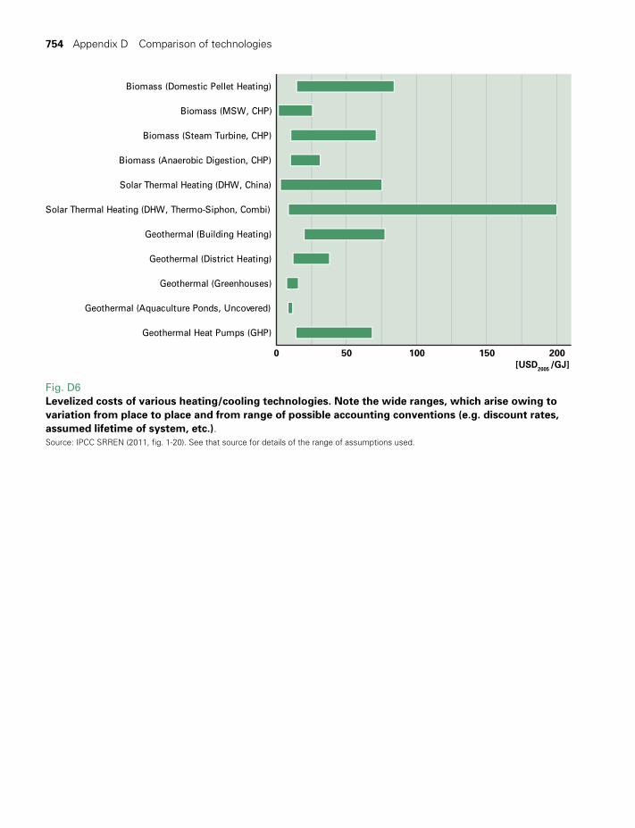
754 Appendix D Comparison of technologies
Fig. D6Levelized costs of various heating/cooling technologies. Note the wide ranges, which arise owing to variation from place to place and from range of possible accounting conventions (e.g. discount rates, assumed lifetime of system, etc.).Source: IPCC SRREN (2011, fig. 1-20). See that source for details of the range of assumptions used.
Solar Thermal Heating (DHW, Thermo-Siphon, Combi)
Biomass (Domestic Pellet Heating)
Biomass (MSW, CHP)
Biomass (Steam Turbine, CHP)
Biomass (Anaerobic Digestion, CHP)
Solar Thermal Heating (DHW, China)
Geothermal (Building Heating)
Geothermal (District Heating)
Geothermal (Greenhouses)
Geothermal (Aquaculture Ponds, Uncovered)
Geothermal Heat Pumps (GHP)
150100500 200[USD2005 /GJ]
TWIDELL PAGINATION.indb 754 01/12/2014 11:39
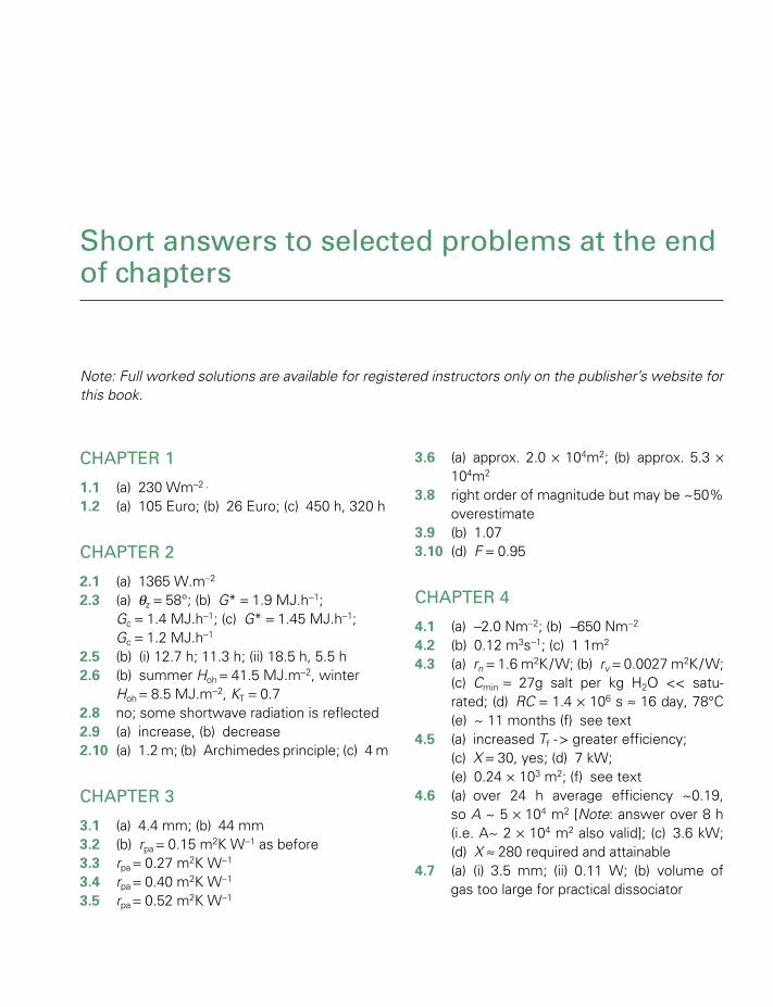
Short answers to selected problems at the end of chapters
Note: Full worked solutions are available for registered instructors only on the publisher’s website for this book.
CHAPTER 1
1.1 (a) 230 Wm-2 .
1.2 (a) 105 Euro; (b) 26 Euro; (c) 450 h, 320 h
CHAPTER 2
2.1 (a) 1365 W.m-2 2.3 (a) qz = 58°; (b) G* = 1.9 MJ.h-1;
Gc = 1.4 MJ.h-1; (c) G* = 1.45 MJ.h-1; Gc = 1.2 MJ.h-1
2.5 (b) (i) 12.7 h; 11.3 h; (ii) 18.5 h, 5.5 h 2.6 (b) summer Hoh = 41.5 MJ.m-2, winter
Hoh = 8.5 MJ.m-2, KT = 0.7 2.8 no; some shortwave radiation is reflected2.9 (a) increase, (b) decrease2.10 (a) 1.2 m; (b) Archimedes principle; (c) 4 m
CHAPTER 3
3.1 (a) 4.4 mm; (b) 44 mm3.2 (b) rpa = 0.15 m2K W-1 as before3.3 rpa = 0.27 m2K W-1
3.4 rpa = 0.40 m2K W-1
3.5 rpa = 0.52 m2K W-1
3.6 (a) approx. 2.0 × 10⁴m2; (b) approx. 5.3 × 10⁴m2
3.8 right order of magnitude but may be ~50% overestimate
3.9 (b) 1.073.10 (d) F = 0.95
CHAPTER 4
4.1 (a) -2.0 Nm-2; (b) -650 Nm-2
4.2 (b) 0.12 m3s-1; (c) 1 1m2 4.3 (a) rn = 1.6 m2K / W; (b) rv = 0.0027 m2K / W;
(c) Cmin = 27g salt per kg H2O << satu-rated; (d) RC = 1.4 × 10⁶ s ≈ 16 day, 78°C (e) ~ 11 months (f) see text
4.5 (a) increased Tf - > greater efficiency; (c) X = 30, yes; (d) 7 kW; (e) 0.24 × 10³ m2; (f) see text
4.6 (a) over 24 h average efficiency ~0.19, so A ~ 5 × 10⁴ m2 [Note: answer over 8 h (i.e. A~ 2 × 10⁴ m2 also valid]; (c) 3.6 kW; (d) X ≈ 280 required and attainable
4.7 (a) (i) 3.5 mm; (ii) 0.11 W; (b) volume of gas too large for practical dissociator
TWIDELL PAGINATION.indb 755 01/12/2014 11:39
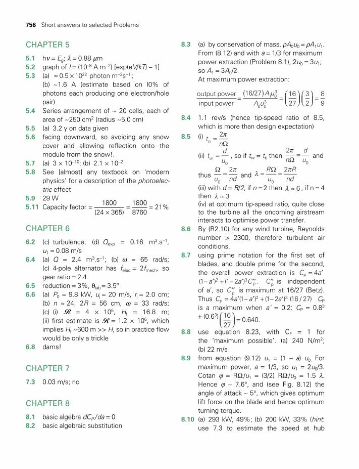
756 Short answers to selected Problems
CHAPTER 5
5.1 hν = Eg; l = 0.88 mm5.2 graph of I = (10–8 A m-2) [exp(eV/kT) – 1]5.3 (a) ≈ × - -0.5 10 photon m s22 2 1 ; (b) ~1.6 A (estimate based on l0% of
photons each producing one electron/hole pair)
5.4 Series arrangement of ~ 20 cells, each of area of ~250 cm2 (radius ~5.0 cm)
5.5 (a) 3.2 y on data given 5.6 facing downward, so avoiding any snow
cover and allowing reflection onto the module from the snow!.
5.7 (a) 3 × 10⁻¹⁰; (b) 2.1 × 10⁻²
5.8 See [almost] any textbook on ‘modern physics’ for a description of the photoelec-tric effect
5.9 29 W 5.11 Capacity factor =
1800 (24 × 365)
= 1800 8760
= 21%
CHAPTER 6
6.2 (c) turbulence; (d) Qexp = 0.16 m3.s-1, u1 = 0.08 m/s
6.4 (a) Q = 2.4 m3.s-1; (b) ω = 65 rad/s; (c) 4-pole alternator has felec = 2fmech, so gear ratio = 2.4
6.5 reduction = 3%, qlab = 3.5° 6.6 (a) P0 = 9.8 kW, uj = 20 m/s, rj = 2.0 cm;
(b) n ≈ 24, 2R = 56 cm, ω = 33 rad/s; (c) (i) R = 4 × 10⁵, Hf = 16.8 m; (ii) first estimate is R = 1.2 × 10⁶, which implies Hf ~600 m >> H, so in practice flow would be only a trickle
6.8 dams!
CHAPTER 7
7.3 0.03 m/s; no
CHAPTER 8
8.1 basic algebra dCP / da = 0 8.2 basic algebraic substitution
8.3 (a) by conservation of mass, rA0u0 = rA1u1. From (8.12) and with a = 1/3 for maximum
power extraction (Problem 8.1), 2u0 = 3u1; so A1 = 3A0/2.
At maximum power extraction:
( )=
=A u
A uoutput powerinput power
=16/27 16
2732
89
1 03
0 03
8.4 1.1 rev/s (hence tip-speed ratio of 8.5, which is more than design expectation)
8.5 (i) p=Ω
tn2
b
(ii) =tduw
0
, so if tw = tb then pΩ
=n
du
2
0 and
thus u nd2
0
pΩ = and Ru
Rnd
2
0
l p= Ω =
(iii) with d = R/2, if n = 2 then l ≈ 6 , if n = 4 then l ≈ 3
(iv) at optimum tip-speed ratio, quite close to the turbine all the oncoming airstream interacts to optimise power transfer.
8.6 By (R2.10) for any wind turbine, Reynolds number > 2300, therefore turbulent air conditions.
8.7 using prime notation for the first set of blades, and double prime for the second, the overall power extraction is = ′C a4P
- ′ + - ′ ′′a a C(1 ) (1 2 )2 3P . ′′Cp is independent
of a’, so ′′C p is maximum at 16/27 (Betz). Thus = ′ - ′ + - ′C a a a4 (1 ) (1 2 ) (16 / 27)P
2 3 CP
is a maxi mum when a’ = 0.2: CP = 0.83 + (0.63)
=1627
0.640.
8.8 use equation 8.23, with CF = 1 for the ‘maximum possible’. (a) 240 N/m2; (b) 22 m/s
8.9 from equation (9.12) u1 = (1 - a) u0. For maximum power, a = 1/3, so u1 = 2u0/3. Cotan ϕ = RΩ /u1 = (3/2) RΩ /u0 = 1.5 l. Hence ϕ ∼ 7.6°, and (see Fig. 8.12) the angle of attack ∼ 5°, which gives optimum lift force on the blade and hence optimum turning torque.
8.10 (a) 293 kW, 49%; (b) 200 kW, 33% (hint: use 7.3 to estimate the speed at hub
TWIDELL PAGINATION.indb 756 01/12/2014 11:39
Short answers to selected Problems 757
height, and then construct a table similar to Table 7.2 to calculate the power obtained in each speed range)
8.11 Hint: Sketch graphs of (i) wind speed with height, (ii) turbine power with nacelle height. If installed tower costs increase approximately in proportion to height, con-sider the limitations of taller towers.
8.12 Algebraic analysis, then substitute reason-able values to obtain PT ∼ 130 kW for the conditions specified.
8.13 Basic calculus to find ν for which dPD /du =0. Then apply (8.16).
CHAPTER 9
9.1 50 GtC/y -> 1.9 × 10²¹ J/y = 6.1 × 10¹³ W9.2 ~1 large tree/person in temperate regions
(less in tropical) several methods yield this approximate result.
9.3 4.8 eV/atomC
CHAPTER 10
10.1 (a) key points: gas yield 200 MJ day–1. Car requires 4 liters petrol day–1 = 160 MJ day–1. Compressor work pV 30MJ∼ ; (b) see text
10.2 (a) mcDT ≈ 0.6 MJ (heat losses from pot imply actual requirement is higher). h ≈ 3%. (b) 70 tonnes; 7 ha.
10.3 (a) (i) ∼3 m3; (ii) ∼63 MJ; (iii) ∼1.7 liters kerosene. (b) (i) smaller tank, smaller cost; (ii) heat required 6 MJ day -1; (iii) heat evolved: 0.3 MJ (mole sucrose)–1 day -1 = 3.6 MJ day -1.
10.4 (a) 680 L at 100% yield. (b) about 27%, allowing for less energy per kg with ethanol.
10.5 note that the oven dry mass remains 400 kg throughout. (o) 1000 kg, 4.7GJ, 6.4 MJ/wet kg; (i) total 800 kg, 5.2 GJ, 6.4 MJ/wet kg; (ii) total 500 kg, 5.9 GJ, 11.8 MJ/wet kg.
CHAPTER 11
11.1 ∫∫ r=l
l /
=
=
=
=E g z( dxdz) (2 )
z
z h
x
x
p, 00
2
11.2 Use (11.9) to relate to the Pelamis con-nected ‘tube’ sections.
11.3 ‘Forward’ push on the turbine blades if FL sinf - FD cosf > 0 in the notation of blade theory (Fig. 8.12).
11.4 (a) Make sketches to match the device as a wave generator to the same device absorb-ing power from real sea waves.
b) Possibilities: (i) Connect many ‘ducks’, each oscillating out of phase with each other, so the common axis (the spine) maintains a relative stable position for each duck to work against;
ii) generate hydraulic power at each duck into a common pipe within the spine, using non-return valves to ‘rectify’ the fluid flow.
CHAPTER 12
12.1, 12.2, 12.3 Algebraic manipulation from first principles
12.4 =-
=TTT T
t*
1 ( * / )29.53m
ss
12.5 (a) v = √ (gh) = [ (10 m s–2)(4400 m)]1/2 = 210 m s–1 (b) t = 2pr/v = 2p(64 × 106 m)/(210 m s–1) = 53 h (N.B. 53 h >> 24 h) (c) (i) the freely traveling tidal wave propagates at less than half the speed necessary for continual reinforcement by the Moon’s tidal influence; (ii) no
12.6 for data given, (Energy gain)/(energy input) = 1.7
12.7 (a) 1.1 m/s (b) 1.6 m/s
CHAPTER 13
13.1 (i) Dh = D (DT) / Th (ii) about 10%
TWIDELL PAGINATION.indb 757 01/12/2014 11:39
758 Short answers to selected Problems
CHAPTER 14
14.1 (b) 17 million years (c) 6 MW / 100 MW14.2 (a) 52 kW; (b) no14.3 (c) 22°C at 1 m, 6.8°C at 3 m, 2.1°C at 5 m
CHAPTER 15
15.1 0.98 kJ/m3
15.2 (a) 5.6 kWh; (b) 16 min15.3 11,500 rev/min15.4 (a) UK 106 GJ.person-1y -1; (b) world ~58
GJ.person-1y-1; (c) ~400 MJ.day -1 house-hold-1, requiring ~ 40 m2 per household; (d) ~10,000 turbines, average spacing ~5 km; (e) 600 km
15.5 0.4 MJm-3 15.6 (a) 2000 GW; (b) 14 GW; (c) 250 W;
(d) 610 W; (e) 28 kW; (f) ~8 MW; (g) 11 MW
15.7 mass flow 1.5 kg/s, energy flow 84 MW15.8 diameter 21 mm for each of the 4 wires15.9 shaft frequency 9.2 Hz15.10 5100 K
CHAPTER 16
16.1 Overall approximately (a) ~3%, (b) ~10%, (c) ~10%, but improvements possible
16.2 (a) 1.1 kW; (b) 0.36 kW; (c) 0.045 m2K.W-1, 0.13 m2K.W-1, bare brick ~0.14 m2K.W-1, ‘good’ wall ~5 m2K.W-1; (d) 0.30 m2K.W-1, 160 W
16.3 (a) 0.4 kW; (b) 6¢/h
CHAPTER 17
17.1. (Hint: draw up a spreadsheet like Table 17.3) (a) 5 years [NPV of (SWH-CEWH) is negative for n ≥ 5]); (b) 7 years
17.2 (Hint: draw up a spreadsheet like Table 17.4) (a) 16 c/kWh (for n = 19) (b) 29 c/kWh (c) 32 c/kWh (for n = 5)
17.4 About 1.2 kg CO2 / [kWh (electricity)]. (Answer depends on coal quality and efficiency of power station).
TWIDELL PAGINATION.indb 758 01/12/2014 11:39

INDEX
Figures and Tables are indicated by italic page numbers; Boxes, Derivations and Worked Examples by bold numbers; notes by suffix ‘n’.
Abbreviations: GHG = greenhouse gases; OTEC = ocean thermal energy conversion; PV = photovoltaic; RE = renewable energy; RES = renewable energy systems; Si = silicon
Abbreviations [listed] xxx–xxxiAbsolute humidity 113, 114Absolute temperature 693, 694,
695, 746Absorber of solar concentrator
see Receiver of solar concentrating collector; Solar collectors
Absorptance 691of selective surface 92–5, 691,
692see also Monochromatic
absorptanceAbsorption coefficient see
AbsorptanceAbsorption of radiation
by atmosphere 50, 54–5general 690–2by plants 333, 335–7, 342by PV cell 171–2, 723–6thermal versus electronic 93–4
Absorption refrigerators 110, 117–19, 120
Absorption width see Capture width
AC see Alternating currentAcceptor atom/ion 711Acceptor molecule 333Accumulators see BatteriesAcid rain 621, 622Acronyms [listed] xxx–xxxi
Actinometers see Pyroheliometers; Solarimeters
Action spectrum 342Active cavity radiometers 57Active power 651–2, 752Active solar heating 77, 581–2Actuator disk concept, applied
to wind turbines 278, 282, 287–8
Additional curve factor see Ideality factor
Aerobic digestion of biomass 368, 388, 400
Aerodynamics see Drag; Fluid dynamics
Aerofoils 272, 289, 668–71Aerogenerator see Wind turbineAgriculture
and biomass energy 351–2and wind farms 309, 317, 633see also Energy farming
Agrochemical energy processes 369, 396–8
Agro-industries 343–6, 361, 363Air
compressed 526, 540, 542–4as insulating material 681properties [table] 737
Air conditioningpower consumption 587, 590see also Solar space cooling
Air heaters, solar 110–12see also Solar crop driers
Air mass ratio 52–3, 172, 725Airfoils see AerofoilsAirplane wing, lift on 289, 290,
669Albedo 52
see also ReflectanceAlcohol see Ethanol; MethanolAlgae, as source of biofuel 369,
398Algebraic method 728–30Alternating current (AC) 649
generators 649, 653–4, 655–6
preferred for transmission 530, 650
Alternators 653–4Ammonia
as energy store 139–40, 141, 147, 539, 555
as refrigerant 117as working fluid in OTEC system
479, 485Amplitude see Deep water wave,
Wave heightAnaerobic digestion of biomass
368, 387–95chemistry 390digester design 391–5see also Biogas
TWIDELL PAGINATION.indb 759 01/12/2014 11:39
760 Index
Analog circuit for heat transfer 675–8
for air heater 113with capacitance 701–3comparable electrical and
thermal quantities 702for evacuated solar collector
97for flat-plate solar collector 83general concept 675physically constructed 675, 676,
702reference temperature for 86for solar collector 83thermal resistance method
675–7Anemometers 249, 259–61Angle of attack [of aerofoil]
669–70Angle of incidence 46, 690
little effect on absorption 691of solar beam 47–8
Angular momentum theory [for wind turbines] 286–9
Antenna-proteins [for photosynthesis] 333, 334
Anti-knock additives 383Antireflection coating 170, 179Apogee 456Appropriate technology 28, 30,
619Aquaculture 343, 487Aquifers [geothermal] 501, 505–7Arctic ice melt 65, 66, 616Area concentration ratio 124Array of solar cells 159, 160Artificial photosynthesis 351Assessment of resource
biomass 332, 347, 349general requirements 18–19hydropower 209–12wave power 423–7see also Hydropower; Solar
radiationAstronomical data 742Aswan Dam [Egypt] 208Asynchoronous generator 655–6Atlantic ocean waves 412, 421,
430Atmosphere, effect on solar
radiation 45, 49–56, 62–7
ATP [chemical in photosynthesis] 335
Attenuator [wave power device] 427, 429, 436–7
Australiahydroelectric power station 207PV installations 163solar architecture 585, 586,
590solar power generation 137solar water heaters 77, 78
Austria 13, 361Autonomous energy systems see
Stand-alone energy systemsAutonomous house see Solar
homesAvailable head see Head of fluidAviation, energy use by 599Axial-flow marine turbines 461Axial force [on wind turbine] 273,
281–3coefficient 282–3
Azimuth of solar collector 46optimum 48–9
Back surface field (BSF) 173, 174Bacteria
anaerobic [for biogas] 390–1photosynthetic 330
Bagasse 344, 345, 740Balance of system [photovoltaics]
165–7Band gap in semiconductors 700,
713direct 184, 719graded 183indirect 184, 719and solar cell performance 172
Banki turbine 219Base load
in electricity grid 533–4see also Load (electrical)
Batteries 58, 166, 305, 526, 540, 544–52
lead–acid battery 545–50noxious chemicals in 559other types 540, 550–2use with solar cells 166see also Lead–acid battery
Bay of Fundy tidal power station [Canada] 463, 467
Beam radiation 41, 60direction of 47–8as proportion of total 60
Beaufort scale [of wind speed] 243, 244–5, 262
Bernoulli’s equation 662applied 214, 282
Betz criterion 280–1, 284, 286, 289, 463, 464
see also Lanchester–Betz–Zhukowsky theory
Bio/fossil balance of biofuels 385–6
Biochemical energy processes 368–9, 379–96
Bio-coal 377Biodiesel 369, 396–8
calorific value 741energy required to produce 398world energy potential 364
Bioenergycapacity factors 25, 26, 752carbon-neutral 362in global energy system 400–1global estimate 350greenhouse gas impacts 352–3relation to agriculture and
forestry 351–2relation to global energy system
353technologies 359–407see also Biofuels; Biomass
Bioethanol see EthanolBiofouling in OTEC systems 483Biofuels
calorific values 362, 365, 366, 740–1
as chemical feedstock 363classification of 364–9energy balance of 385–6food crops used in production
344, 352GHG balance of 387growth in world production 364liquid transport fuels 558, 599
economics 398–9technical aspects 379, 382–3
meaning of term 361periodic variations 15preferred biomass in production
352
TWIDELL PAGINATION.indb 760 01/12/2014 11:39
Index 761
production processes 367transport of 529world energy potential 364see also Biodiesel; Biogas;
Biomass; Ethanol; Fuelwood
Biogas 368, 387–95biochemical processes 391chemistry 390digester designs 391–5economics 388–9see also Landfill gas
Biological energy conversion see Biofuels; Photosynthesis
Biomass 324–58assessment of resource 332,
347, 349calorific values 740chemical elements in 330co-firing with coal 373, 374combustion of 366, 367–8,
369–74, 399–400composting of 400costs 621digested to biogas 368, 387–95energy potential 362, 365as energy store 326, 523environmental implications
352–4fermented to ethanol 344, 345,
384–5formation of 361gasification of 368, 374heat of combustion [table] 740liquid fuel from 379, 383–4,
384meaning of term 326, 361moisture content 365–6production on energy farms
343–50pyrolysis of 374–8requirements for best use 352,
363social issues 344, 345thermal power station 24, 25,
26transported in batches 526,
527, 529yields 346, 347see also Biofuels; Fuelwood;
Photosynthesis
Biophotolysis 369Birds, impact on wind farms 317Black body 693
Earth as 51, 52, 63radiation emitted by 693–5Sun as 40
Blade element theory [for wind turbine] 295–9
Boreholes [geothermal] 501, 507BoS see Balance of systemBouger–Lambert law 697Boundary layer of fluid 682–3Brackish water, desalination of
110, 120–1, 490Brazil
bioenergy/biofuels 361, 383–4, 385–6
energy farming 345, 346, 380ethanol program 383–4hydropower 205OTEC 488solar water heating 77, 100
Britainenergy demand in 555–6, 575see also Scotland; United
KingdomBrown (non-renewable) energy 3
compared with green energy 10, 751
costs increasing over time 638–9
pollution from 29, 617see also Fossil fuels; Nuclear
powerBruntland report (1987) 5
see also World Commission on Environment and Development
Building codes and standards 578, 584
Buildingscooling of 120, 487, 587–9energy-efficient 123, 576–91heating of: see Heating‘heavy’ [as energy store] 560
Burning see Combustion
C3/C4 mechanisms in photosynthesis 335
Cadmium telluride (CdTe) 181, 185, 725
Calorific values of fuels [table] 740–1
Calvin cycle 333, 335Campbell–Stokes radiometers 59Capacitance, electrical [in analog
circuit] 701–3Capacitors as energy stores 539,
544Capacity credit 312, 536, 752Capacity factor [by technology]
16, 24–5factors affecting 26geothermal energy 512, 514,
752tidal power plant 466, 752values for various RE systems
24–5, 26, 752wind turbines 25, 26, 311, 633,
752Capture efficiency
PV cell 169, 172–3solar collector 80, 87
Capture width [of wave power device] 412, 428, 433, 434, 436
Carbohydrates 327–8Carbon
capture and storage of 488energy release per mole 328isotopes 66–7
Carbon abatement, by biomass use 353, 374
Carbon credit 163, 193, 633see also Renewable energy,
policiesCarbon cycle 329, 368, 400Carbon dioxide
abatement of 364absorption spectrum 54emissions from fossil fuels 6,
64, 66–7, 570, 742as greenhouse gas 63injection into deep ocean 488and plants 328–32see also Greenhouse gas
emissionsCarbon monoxide, in producer gas
378, 379Carbon sink 353, 400Carbon tax 624Carbon Trust 430
TWIDELL PAGINATION.indb 761 01/12/2014 11:39
762 Index
Carnot engine 335, 482, 573Carnot theory 16, 133, 572, 573Cavitation in water 219Cellulose 327–8, 378–9, 381Centralized versus dispersed
energy sources 17Characteristic dimension in heat
transfer 683, 684formulas 743
Charcoal 346, 368, 376, 377Charging of battery 549Chi square distribution of
windspeed see Rayleigh distribution
Chimney, thermosyphon pressure in 143
Chinabiogas digesters 389, 393cooking stoves 371hydropower 205, 208, 221, 226mini-hydro schemes 227national energy use and supply
604solar water heaters 77, 101Three Gorges hydro project
208, 221, 226Chlorophyll 334Chloroplasts 334Choice, quantification of 626–34Chord of aerofoil 296CHP see Combined heat and
powerCircuit analysis of heat transfer
see Analog circuitCities, energy use in 593–5Civil time 43Clear sky radiation 45Clearness Index 60Climate change
causes 6, 19, 39, 63–4external costs 620, 622observations 64–7policies 364projected 67, 615–17treaties on 6, 64, 615see also Greenhouse effect;
Greenhouse gas emissionsClimate models 67Closed cycle system for OTEC
479, 485Clothes drying 142
Clouds 41, 45, 52CO2 see Carbon dioxideCoal
calorific value 741co-firing with biomass 373, 374external costs 621–2reserves 5transport of 527see also Brown energy; Fossil
fuelsCoanda effect 222Coconut oil as fuel 397Coefficient of performance
heat pumps 513refrigerators and coolers 118,
120see also Power coefficient
Cogeneration see Combined heat and power
Coherence distance [of wind] 258Cold water pipe for OTEC 484Collection efficiency
solar cell 169, 173solar collector 87–8
Collectors, solar see Solar collectors
Combined heat and power systems 12, 14, 361, 389
Combustionof biofuels 400of biomass [wood] 366, 367–8,
369–74, 399–400energy release in 329, 740–1partial, in gasifier 374, 375–6
Comfort, thermal 373, 576, 577Compact fluorescent lamps (CFLs)
14, 194, 602Comparisons of technologies
747–54Composting 388, 400
see also Aerobic digestionCompressed air as energy store
526, 540, 542–4Computational fluid dynamics
(CFD) 224Concentrated Solar Power (CSP)
see Concentrated Solar Thermal Power
Concentrated Solar Thermal Power (CSTP) 110, 124, 132–40
small-scale microgeneration 140
system types 135–8thermal storage 138–9
Concentration ratio of solar collector 124–5, 190
theoretical maximum 125–7Concentrators see Solar
concentrators; Wind concentrators
Condensation see Phase changeCondensing boiler 366Conduction band [in
semiconductor] 709Conduction of heat 679–81Conductivity see Thermal
conductivityConservation of energy in fluid
flow 661–3see also Energy conservation
Conservation of momentum in fluid flow 663–4
Consumption of energy see End uses
Control of energy flow 20–2feedback 21feedforward 21load 21, 306, 307–8, 313–14mechanical 306wind-electric systems 305–6see also Storage of energy
Convection of heat 681–8between parallel plates 686–7,
744calculations [worked examples]
686–8accuracy of 687–8
forced 682, 684formulas 744–5free [natural] 122, 682, 685–6,
687suppressed in solar pond 122suppressed in vacuum 96
Conventional energy supplies see Brown energy; Fossil fuels
Conversions between units 734–5in algebraic method 730
Cookingby solar concentrators 124, 131,
132by wood-burning stoves 370–3
Cooking oil waste, biofuel using 397, 398
TWIDELL PAGINATION.indb 762 01/12/2014 11:39

Index 763
Cooking pots, heat loss from 370Cooling see Energy-efficient
buildings; Heat pumps; Refrigerators; Solar space cooling
COP see Coefficient of performance
Coppicing of trees 346–7Copra oil see Coconut oilCord see ChordCorn as bioenergy feedstock 18,
344, 381Correlation time, for wind turbines
258Cost optimization 615Costs of RE systems
decrease over time 636, 638, 639
tools to analyze 622–34see also Economics; External
costsCrest of wave 414, 422Crop drying
by biomass 373energy balance and temperature
115–17with forced air flow 116–17by solar crop driers 110, 112–17
Crop residues as fuel 344, 365Crop yields 348Cross-flow marine turbines 461Crust of Earth 500–1Crystal growth [of Si] 177CSP see Concentrated Solar
[Thermal] PowerCuritiba [Brazil] 595–6Curve factor of solar cell 169, 174
see also Ideality factorCut-in speed of wind turbine 300,
301Cut-out speed of wind turbine
300, 301Czochralski technique 177, 180
Daily insolation see InsolationDams 220, 221
decommissioned in USA 227methane emissions 227multiple purposes 226social impact 226World Commission on 226, 233
Dark reactions in photosynthesis 328, 333, 335
Darrieus rotor 275, 276, 464Day
clear, radiation in 45length of 44–5mean lunar 454mean solar 453sidereal 454, 473
Daylighting [in buildings] 572, 577, 578
DC see Direct currentDCF see Discounted cash flowDecentralization (of society) 28Declination 44Deep Ocean Water Applications
(DOWA) 479, 487, 488Deep-water waves 413
frequency and wavelength 416group velocity 420height 414observed patterns 421–7particle motion in 413–18phase velocity 416, 420properties 413–14theory of regular waves 414–18total energy (power) in 417–18see also Ocean waves; Period;
Wave powerDeforestation 361–2, 363Demand for energy 5, 19
in Austria 13matching to supply 15, 19–22,
525, 533–7, 650, 657in UK 575
Denmarkwave power installations 431–2wind power in 27, 271, 534,
536Density
air [table] 737sea water 425, 465various solids [table] 739water [table] 738
Depletion zone [in semiconductor] 712–13
Desalination of water 110, 120–2, 487, 490
Developing countriesenergy needs and supply 604,
618
extensive use of biomass 346, 361
gender issues 371hydro-electricity in 205, 618microfinancing in 618photovoltaics in 193–6, 618potential for renewables 595–6,
603–4, 618small wind turbines 618see also Economic
developmentDiesel, Rudolph 369Diesel engines
with biofuel 369, 382–3, 396–8in small electrical grid 307
Diesohol 382Diesoline [petroleum product]
398–9, 741Diffuse radiation 41, 60, 61
and Clearness Index 60, 61Diffuse surface 695Diffusion of carriers in
semiconductors 716Diffusivity
of momentum 664thermal 681
Digestion of biomass see BiogasDimensional analysis
convection 685–6pipe friction 667
Dimensionless flow parameters 666, 682, 683, 684, 685
see also Nusselt number; Prandtl number; Rayleigh number; Reynolds number
Diode [semiconductor]Direct current (DC) 153, 156,
651generator 654–5power transmission 651
Direct [solar] radiation see Beam radiation
Discount factor 630Discount rate 630Discounted cash flow 630–4
examples 632–4Dispatchability 535–6, 752Dispersed energy supplies 28
versus centralized energy sources 17
see also Embedded generation
TWIDELL PAGINATION.indb 763 01/12/2014 11:39
764 Index
Dispersed living see Decentralization; Soft technology
Dispersed versus centralized energy sources 17
Dispersive waves 420Distillation
of ethanol 379of water see Desalinationof wood see Pyrolysis
Distributed generation see Embedded generation; Microgeneration
Distribution of energy 523, 524, 526–38
by electricity 530–8, 650–1environmental aspects 559as heat 529–30by hydrogen 555by mass transport 526, 529by pipeline 528–9, 555
Distribution of wind speed see Wind speed probability distribution
District heating 510, 512, 529–30, 557
integration of RE into 526, 557
Diversity of energy supply 615Domestic heat store 556–8Domestic uses of energy 601–2
UK statistics 601see also Cooking; Heating
Donor atom 179, 711, 712Donor molecule 333Doping of semiconductors 179,
710–12Doppler back-scatter effect beam
instruments 260, 261Doubly-fed generator 656Drag force 272, 295–7, 668–71
wind machines based on 274, 276, 285–6, 314
Drinking water, WHO recommendations 121
Dry rock [geothermal] 503–5see also Hot dry rock
Drying of crops see Crop drying
Ducted rotors see Wind concentrators
Dungin biogas digesters 389, 393calorific value 740
Dye sensitive [solar] cell 187–8Dynamic characteristics of RES
15–16Dynamic pressure 282Dynamic tunable wave power
devices 429, 436–7Dynamic viscosity of fluid, see also
Kinematic viscosity; Viscosity
Earthastronomical data 742as black body 51, 52, 63crust of 500–1eccentricity of orbit 40, 43energy balance of 52, 62–3geothermal heat flow through
497, 500movement around Sun 40,
43–6rotation on axis 42
Economic conditions, impact on investment 617
Economic development 4–5paths to 603–4requires more than electricity
226see also Sustainable
developmentEconomics
changing ‘answers’ in 621terminology 627
Economics of RESbiofuels 398–9biogas 388–9general considerations 4–5,
620–1, 626–34hydropower 207, 225–6wind power 316see also External costs
Economies of scale 636Efficiency 22–4
of combustion 375electrolysis 553of end-use 567–611fuel cell 552hydroelectric system 207OTEC systems 479photosynthesis 330, 331, 341–3
photovoltaic cell 156, 167–76, 181
solar collector 80–1, 87–8of system 14, 19of various devices 23–4wave energy devices 428–9wind system see Power
coefficientwind turbines 270, 280, 281
EGS see Enhanced Geothermal System
EIA see Environmental Impact Assessment
Einstein [unit] 341Einstein’s relationship 716Electric motors 596–7, 600, 655Electric vehicles 558, 596–8Electrical contacts in solar cell
168–9, 175, 185Electrical generators
AC 649, 653–4, 655–6asynchronous 655–6DC 654–5doubly-fed 656induction 655–6synchronous 653–4variable speed 656for wind power 656
Electrical grid [for transmission and distribution] 530–8, 650–1
centralizes society 17DC grid 651decouples supply and demand
22with hydro systems 222–3, 533large [national] 22, 311–12microgeneration in see
Embedded generationphotovoltaics in 154, 155,
162–5, 166–7, 192–3, 195with RE systems 22, 526, 530,
535–7small [for remote area] 307,
312–13stability 535, 536–7storage in 22, 193, 537–8,
541–4with wind systems 263, 308,
311, 534, 536–7Electricity
external costs of 622
TWIDELL PAGINATION.indb 764 01/12/2014 11:39
Index 765
grid see Electrical gridnetwork see Electrical gridtransmission of 485, 530–8,
648–51Electricity generation
biomass 374embedded 162, 313, 530external costs of 621–2fossil fuels 523geothermal energy 497–8, 507,
510, 511hydro 220–4ocean waves 428, 432, 433,
436–7OTEC 485outages 534–5photovoltaics 151–201solar cells 156–60solar concentrators 132–40solar pond 123solar thermal 123wind 269, 270, 303–14see also Brown energy;
Electrical generatorsElectrochromic windows 589Electrolysis 553–4Electromagnetic dynamic
generation 153Electromagnetic radiation see
RadiationElectromagnetic spectrum 54, 688Electron volt 709, 740Electronic load control, in hydro
systems 223Electrons
energy levels in semiconductors 183, 710
movement in Si 716–17Ellipticity of Earth’s orbit 40, 43Embedded energy see Embodied
energyEmbedded generation [in electrical
grid] 162, 313, 530Embodied energy
of biofuel 385–6of building 576
Emission permits 624Emissivity see EmittanceEmittance 693
of selective surface 92–5typical values [table] 739
Employment benefits of renewables 101, 316, 383, 437
End uses of energy 574–605in Austria 13buildings 576–91classification of 523, 524, 575conservation measures 14, 19,
595–6domestic 601–2
see also Cooking; Heatingefficiency is important 19, 570efficiency not always pursued
602–3impact on RE 603manufacturing industry
599–600percent by sector 575time variation 556transport 591–9
Energyequivalents 734forms of 523growth in use 5as proportion of GNP 5and sustainable development
see Sustainable Development
Energy analysisof biodiesel 398of ethanol production 385–6see also Bio/fossil balance; Life
cycle analysisEnergy balance
global 52of liquid biofuels 385–6, 398
Energy conservation [minimizing waste] 14, 19, 595–6
reduces GHG emissions 570–1, 604–5
see also Conservation of energy in fluid flow
Energy demand 575, 640in Austria 13factors affecting 603–4matching to supply 15, 19–22,
523, 533–5rapid fluctuations 535, 651by sector 575
Energy densityof biofuels 365, 379, 398
of storage media 541, 542, 543, 544, 546, 550
see also Batteries; Flywheels; Storage of energy
Energy efficiency 524, 538, 569environmental implications
604–5see also Efficiency
Energy-efficient buildings 576–91for cold climate 582–3for composite climate 591for hot dry climate 587–9social benefits 604–5for temperate climate 584–7for warm humid climate
589–90Energy end-use 12, 13, 574–602
see also End uses of energyEnergy farming 343–50, 384Energy flow diagrams
Austria 13USA 658
Energy flow(s)to and from Earth 11flux density of 11of nonrenewable sources 9of renewable sources 9from sources to uses in an
economy 523–4, 570see also Control of energy flow;
Distribution of energyEnergy management 14, 533–7,
571Energy markets, evolution of 636,
637Energy pattern factor [of wind]
256Energy planning 7, 12, 14Energy policy 614–17Energy production, global data
750Energy quality 16Energy ratio [of crop] 385‘Energy revolution’ (ER) 640Energy savings 572
from improved heating and cooling 600, 601–2
Energy security 7, 204, 346, 384, 437, 559, 571, 614
Energy services 569, 571–4Energy sources 9, 11
TWIDELL PAGINATION.indb 765 01/12/2014 11:39
766 Index
Energy storage see Storage of energy
Energy systems 12, 19, 523–6, 569–70
integration of RE into 525–6terminology 523–4see also Combined heat and
power; Control [of energy flow]; Matching supply and demand; Renewable energy systems; Stand-alone energy systems
Energy transmission see Distribution of energy; Electrical grid
Engines see Diesel engines; Heat engine
Enhanced geothermal systems (EGS) 499, 509–10
Enthalpybiofuels 362, 383, 385photosynthesis 328, 330
Environmental energy flows 11–12
see also Energy flowsEnvironmental Impact Assessment
(EIA) 614–25Environmental impact of
renewables 29see also Biomass; Hydropower;
Photovoltaic systems; Sustainable development; Wave power; Wind power
Equation of time 43Equatorial plane of Earth 42Equilibrium moisture content 115Equilibrium theory of tides 450–4Equivalent circuit of solar cell, see
also Analogue circuitEsterification [for biodiesel] 369,
397–8Ethanol [as fuel]
as anti-knock additive 383economics 398–9energy required to produce 386for esterification of vegetable
oil 397production, use, and yield 344,
345, 369, 379–85as transport fuel 382–3
Ethyl alcohol see Ethanol
EU (European Union)biodiesel 397policies to promote renewables
619Euphorbia 369, 397European Wind Energy Association
36Evacuated solar collector 96–8,
701heat-balance calculations 97–8
Evaporative cooling 119, 120, 587, 589
Evaporative heat transfer 120, 699–701
thermal resistance of 700Exchange factor for radiation 696
formulas 746Excitons 186, 341Exergy 16Expansion coefficient, water
[table] 738External costs of energy 620,
621–2internalising of 7, 226, 623, 624,
635, 637External payback and benefit
criteria 628–9Externalities see External costsExtinction coefficient 697
of glass 697–8of semiconductors 184, 711,
719, 720Exudates from plants348 369, 397
f-chart method 81Fair Isle [Scotland], multi-mode
wind-power system 22, 313–14, 533
Falnes principle [for wave power devices] 429, 436
Faraday Effect 652Farming
for energy see Energy farmingintegrated see Integrated
farmingsee also Agriculture
Fatigue in wind turbines 236, 258, 271, 277
Feed-in tariffs [to encourage RE] 154, 162–3, 191, 193, 316, 433, 602, 624
Feedback 21, 61unsuitable as control for
renewables 21see also Feedforward control
Feedforward control 22, 533see also Electronic load control
Fermentation 344, 345, 365, 369, 384–5
see also Biogas; EthanolFermi level in semiconductor
712Fertilizer from biogas digester
393, 395FF see Fossil fuelFiji 372Fill factor of solar cell see Curve
factor of solar cellFin efficiency [of solar collector]
104–5Financial aspects of RE
analytical tools 626–34see also Costs of RE systems;
Economics; MicrofinancingFinite energy sources see Brown
energyFire see Combustion; Open fire;
Wood-burning stovesFirewood see FuelwoodFischer–Tropsch process 378Fish farming see AquacultureFlat plate, flow over 684, 745,
746Flat plate solar collectors 77, 78,
79, 81–8classification of 79efficiency 87–8exchange factor for 696optimum orientation 48–9performance calculated 82–7plate-and-tube type 79, 81
Floating industrial platforms 484, 488
Floating wave power devices 428, 431–3, 436–7
Flow cell battery 540, 550, 551Flow of energy see Energy flowFlow rate of fluid
magnitude required for OTEC 479, 481
in river, measurement of 210–12
TWIDELL PAGINATION.indb 766 01/12/2014 11:39
Index 767
Fluiddefined 661ideal 662
Fluid dynamicsprinciples 660–72tidal-current power compared
with wind power 459–60, 461
Fluorescence 338, 339Flux concentration ratio 124–5Flux density 17
see also Radiant flux densityFlywheels 526, 540, 541–2
compared with pumped hydro systems 542
Focussingocean waves 421solar radiation see Solar
concentratorswind see Wind concentrators
Food production, displaced by energy farming 344, 352, 384
Force coefficient of wind machine 294
Forced circulation in solar water heaters 88–90
Forced convection 682formulas 745Reynolds number and 684
Forestry see AgricultureForests
biomass yields 348depletion of 346, 361–2, 363,
371photosynthetic efficiency 331
Fossil fuels 5–6calorific values [table] 741CO2 emissions 6, 64, 66–7, 570,
742costs [low but increasing] 559as energy stores 523, 539external costs 100heat of combustion [table] 741life-cycle GHG emissions 751non-renewability of 5reserves 5SO2 emissions 621substitution by biomass/biofuels
346, 353, 362trade in 559urbanization encouraged by 28
see also Coal; Natural gas; Oil (petroleum)
Fourier analysis see Spectral distribution
Francetidal power 448, 467, 468wind map 241, 242
Francis turbine 217–18, 218, 219, 221
Franck–Condon diagram 338, 339
Free [natural] convection 122, 682, 685–6, 687
formulas 744see also Rayleigh number
Freight transport, energy use by 598
Frequencyanalysis of wind speed 243,
246rotation of water turbine 215,
222rotation of wind turbine 304,
315water wave 425
see also Water wavesFresnel concentrator 130Fresnel lens 130, 131, 133, 190Fresnel mirror concentrator 130,
190electricity generation using 136,
137Friction-caused heat production
316Friction factor [for flow in pipe]
666–8Friction in fluid flow 664
in hydro systems 209in OTEC systems 484in pipes 666–8in solar collectors 91, 92
Fuel cells 379, 552–3, 558Fuels
calorific values [table] 740–1synthesis using solar reactor
140–1see also Biofuels; Fossil fuels
Fuelwoodas charcoal 346combustion process 371drying of 115
in gasifiers 368, 374, 376importance in developing
countries 361, 370regeneration of 346scarcity 346, 636world energy potential 364see also Biomass
Full load hours 24values for various RE systems
24–5Fundamental constants 740Furnaces 17, 373
Gallium arsenide (GaAs) 181, 185, 719, 720, 725
Gamma function 255Gas
concentration units 65distinguished from liquid 661transmission by pipeline 527,
528–9, 555see also Biogas; Hydrogen;
Natural gas; Producer gas; Town gas
Gas turbines, flexibility 533, 534Gasification of biomass 368, 374,
376see also Furnace; Producer gas;
PyrolysisGasohol 382Gasoline see PetrolGDP see Gross Domestic ProductGearbox [for wind turbine] 304Gender issues 371Generators, electrical see Electrical
generatorsGeophysics 500–2Geostationary Environmental
Satellite (GOES) 59–60Geothermal energy 495–520
best sites for 497–8costs 514enhanced systems see Hot dry
rockenvironmental impacts 515–16extraction of 508–10installed capacity 512low quality of 497renewable? 499stored in Earth’s crust 500time scale for depletion 499
TWIDELL PAGINATION.indb 767 01/12/2014 11:39
768 Index
Geothermal energy (cont.)use for electricity 497–8, 507,
510, 511use as heat 498–9, 510–11, 512
Geothermal heat flow 497enhanced artificially 499,
509–10Geothermal heat pumps 498–9,
512–14Geothermal regions 498, 501–2Germanium 184, 725, 726Germany
biogas digesters 389feed-in tariff [for RE] 191PV installations 163, 602solar water heating 77, 100wind power 271, 301
Geysers 502, 504, 508GHG see Greenhouse gas
[emissions]GHP see Ground-source heat
pumpGibbs free energy 554Glass
as cover on PV module 167as cover on solar collector 78,
79, 83, 698holds vacuum 96‘self-cleaning’ 167transmittance of 96, 697–8
Glauber’s salt [as heat store] 539, 558
Glauert theory [of wind turbine] 292
Global climate models 67Global irradiance [total irradiance]
see Solar irradianceGlobal Mean Surface Temperature
(GMST) 65, 66, 615, 616Global warming 65
see also Climate changeGlobal warming potential (GWP)
64Gobar gas see BiogasGOES see Geostationary
Environmental SatelliteGovernment’s role in energy
614–17, 623–5see also Energy policy;
Institutional factorsGraetz number 745
Grain [rice, wheat, etc]air flow through 115–17, 143–4drying of 113, 115, 144makes alcohol 344, 369, 381,
384milling of 270, 314
Grana 334Grashof number 686, 744Grasses, as biomass 335, 347,
348Grätzel [photovoltaic] cell see Dye
sensitive cellGray body 696Grazing incidence [of radiation]
690, 691Green energy
compared with brown energy 10, 638–9
see also Renewable energyGreenhouse effect 6, 39, 63–4
enhanced 63see also Climate change
Greenhouse gas (GHG) emissionsabated by carbon sinks
[biomass] 352–3abated by renewables 204, 346,
384, 437, 615from biofuel production 387from fossil fuels 6, 64from geothermal systems 516from hydropower systems 227human impact on 64–5, 66–7
Greenhouse gases (GHGs) 39, 63life cycle emissions 623, 751
Greenwich mean time 42Grid see Electrical gridGross national product, relation to
energy use 5Ground-source heat pumps
512–14Group velocity of deep-water wave
420‘Gut-feel’ [decision making]
627–8
Hawaiigeothermal power plant 502OTEC system 486, 487
HDR see Hot dry rockHead of fluid 662
available for hydropower 210
loss in pipe 668thermosyphon 91
Health aspects of energy systems 617
smoke 370, 400see also Pollution
Heat capacity see Specific heat capacity
Heat circuit see Analog circuitHeat of combustion, fuels [table]
740–1Heat engines 335, 482, 572
efficiency 335, 573see also Carnot engine; Diesel
engines; Solar thermal power; Steam engines; Turbines
Heat exchangers 704–5in geothermal systems 510, 511for OTEC 483in solar water heater 88, 89, 90,
704in ventilation systems 705
Heat flow 675per unit area 678see also Energy flow(s);
Geothermal heat flowHeat loss
from building 580–1from solar water heater 80from steam pipe 529–30through window 582, 606–7,
680–1, 741–2see also Heat transfer; Thermal
resistanceHeat pipe 530, 681, 699–701Heat pumps 512–13
cooling using 499, 513, 514from ground heat 498–9,
512–14Heat storage
in buildings 514, 556–7, 560, 581–2
in Earth’s crust 500by hot water 58, 88–92, 556–7time-scale required 557
Heat supplies [for RE] 16Heat transfer 673–707
analog circuits for 675–8by conduction 679–81by convection 681–8
TWIDELL PAGINATION.indb 768 01/12/2014 11:39

Index 769
formulas for 743–6by mass transport 698–701by radiation 688–97terminology 678–9see also Analog circuits;
Conduction; Convection; Radiation
Heat transfer coefficient 679relation to Nusselt number 683walls and windows 741–2
Heatingof air 110–12as ‘ballast’ load for electronic
load controls 223, 313of buildings 498, 576–8demand for 575by fuelwood 373by geothermal energy 498,
510–11, 512as percentage of energy
demand 575residential 576–87, 601–2seasonal demand for 555–6of water see Hot water; Solar
water heatersHeating value see Heat of
combustionHeller method see Matrix analysisHeterojunctions [in
semiconductors] 183see also p-n junction
Hills, as sites for wind power systems 248
Hockerton Housing Association [UK] 586–7
Holes [in semiconductor] 709, 711
Holsworthy [Devon, UK], anaerobic digestion power station 394, 395
Homojunctions [in semiconductors] see p-n junction
Horizontal-axis tidal-current devices 461, 462
Horizontal-axis wind machine 275–6, 275
Hot dry rock 497, 509, 515Hot water
as energy store 58, 88–92, 556–7
geothermal 498, 505–7see also Solar water heaters
Hottel–Whillier–Bliss equation 80Hour angle 43, 47Hours of bright sunshine see
Sunshine hoursHousehold energy use see
Domestic energy useHouses
heating requirements 576–8see also Solar buildings
Human impacton climate 6, 19, 64–5, 66–7on net primary production
353–4Humber Estuary [UK], tidal-current
power system 463Humidity
absolute 113relative 113solar irradiance affected by 59temperature dependence 113,
114, 738Hybrid electric vehicles 597Hydraulic power see Hydropower;
OTEC; Tidal power; Wave power
Hydrides as portable energy store 539, 555
Hydrodynamics 410–11Hydroelectric systems 220–4
advantages 222–3, 533, 535capacity factors 24, 26, 205–6,
752costs 621grid-connected 222–3long life of 206overall efficiency 23, 207pumped storage system 224–5stand-alone system 223see also Hydropower
Hydrogenas energy store 539, 553–5in fuel cells 552, 554, 558in lead–acid battery 548produced biologically 351, 369,
554produced from biomass 376,
377production on OTEC platforms
488
production by solar devices 141, 189, 554
reduction of biomass by 378safety issues 559storage of 555transmission by pipeline 526,
527, 555vehicles using 558, 598see also Producer gas
Hydrogen economy 552, 555, 598
Hydrogenation of biomass 378Hydro-kinetic devices 224Hydrolysis of biomass 378–9Hydropower 202–33
advantages 206–7, 225assessment of resource
209–12civil engineering works required
209, 220classification of 207disadvantages 207–8, 209, 221,
226economics 207, 225–6in electricity grid 222–3environmental factors 226–7global capacity 204hydroelectric systems 220–4installed capacity (by region)
205–6mechanical systems 222periodic variations 15potential [technical and
economic] 205–6, 224principles 208–9scope for technology upgrades
224small-scale installations 205–6,
209, 220, 221social and environmental
aspects 225–7turbines 208, 212–20see also Turbines for water
HYDROSOL [solar reactor] program 141
Hydrothermal circulation 502, 504
Hydrothermal liquefaction (HTL) 379
Hyperthermal region(s) of Earth 501, 502, 508
TWIDELL PAGINATION.indb 769 01/12/2014 11:39
770 Index
Iceland, geothermal energy 499, 510, 511
Ideality factor of solar cell 169, 174–5, 722
Igloo 582, 583Impulse turbines 208, 212–20
see also Pelton wheelInclined surface, irradiance on
46–9Incompressible fluid 661India
biogas digesters 389, 393energy–efficient buildings
587–9fuelwood use 346hydropower 205solar ponds 123wave power 410
Induction factor [of wind turbine] 279–80, 287–8, 298
power coefficient affected by 293–5
Induction generators 655–6in hydro systems 222in wind systems 303, 306, 308,
311Industry, energy use in 599–600Inflation rate [economic] 631Infrared radiation 40, 55
see also Longwave radiationInsolation
factors affecting 44–5on inclined surface 45, 60–2satellite measurements
59–60and sunshine hours 59see also Solar radiation
Institutional influences on RES 524, 614–26
changes from 1970s to 2030s 635–6, 637
policy tools 623–5socio-political factors 614–20unrecognized costs of brown
energy 621–2see also Political influences;
Social influencesInstrument towers [for wind
turbines] 259Instrumentation
solar radiation 99–100
wind speed and direction 258–62
see also Solar radiation; Wind speed
Insulation, thermal 681in buildings 579, 580–1, 584,
587for heat store 556–7materials 557, 587, 681in solar heaters 86, 90
Integrated farming 17, 389–90Integration of RE into energy
systems 525–6, 648Interference factor [aerodynamics]
279, 280Intergovernmental Panel on
Climate Change (IPCC) 35on greenhouse gases 65on integration of RE
technologies 30, 525–6on sustainable RE resources
6International Electrochemical
Commission (IEC) 27International Energy Agency (IEA)
35International Renewable Energy
Agency 35International Solar Energy Society,
recommended terminology 688
Interseasonal heat storage 123, 704
Inverters 153, 156, 166line-commuted 164–5, 166–7
Investment, return on 628IPCC see Intergovernmental Panel
on Climate ChangeIreland, wind power in grid 534,
536–7Irradiance 688
solar see Solar irradiance; Solar radiation
Irradiation see InsolationIslay [Scotland], wave power 433,
434Israel
solar pond 123solar water heating 77, 100
Italy, geothermal energy 498, 499, 510
Japangeothermal energy 499, 510,
512OTEC 478, 486solar water heaters 77wave power 410
Joukowski [Zhukowsky] see Betz-Lanchester-Zhukowsky criterion
Junction see p-n junction
Kaplan turbine 218, 218, 219, 219, 432
Kimberlina solar power station [USA] 137
Kinematic viscosity 664–5values 737, 738see also Friction in fluid flow;
Rayleigh number; Reynolds number; Viscosity
Kirchhoff’s laws of radiation 125, 126, 693
Kobold marine turbine 462, 463Kramer Junction solar power
station [USA] 135, 137Kyoto Protocol [on climate change]
64, 615
La Rance tidal power station [France] 448, 467, 468, 470
Labelling of graphs 729Lambert’s law see Bouger–
Lambert lawLamellae [in leaf] 334Laminar flow of fluid 661, 668Lanchester–Betz–Zhukowsky
theory for wind turbines 277–81, 322n4
Land-based OTEC systems 484Land-based wave power devices
428, 430–1, 433–5Land shape, effect on winds 240,
248Landfill gas 365, 368, 396‘Landlord–tenant problem’ 604Latent heat
of vaporization/condensation 699
water [table] 738Latitude 42
insolation affected by 44, 45
TWIDELL PAGINATION.indb 770 01/12/2014 11:39
Index 771
LCA see Life cycle analysisLead–acid battery 545–50
limitations 547operating characteristics 548,
549recycling of 559
Learning curve [of cost] 625, 636, 638
Leaves [plant]as site of photosynthesis 330,
334structure 334
LEDs see Light-emitting diodesLegislation on energy 624, 625
see also Energy policyLess developed countries see
Developing countriesLeucaena [timber species] 400Levelized cost
hydropower compared with other sources 226
various RE electricity generation technologies compared 753
various RE heating/cooling compared 754
wind farm 633–4LiDAR (Light Detection And
Ranging) instrument 260, 261Life cycle analysis (LCA) 576,
622–3see also Energy analysis
Lifestyle 27–30Lift force 272, 295–7, 668–71Lift [wind] machines 274, 275,
276, 285–6, 314Light see Solar radiationLight-emitting diodes (LEDs) 14,
194, 195, 574, 602Light-harvesting system in plants
333, 334, 335Light reactions in photosynthesis
328, 333, 335Light trapping [in PV cell] 170, 173Lighting
energy efficiency of 14, 194–5, 602
history of 573–4as percentage of energy
demand 575small PV systems 193–6
Ligno-cellulose [for bioethanol] 381–2
Limpet wave-power device 433, 434, 439
Line absorber [wave power device] 427, 429, 436–7
Linear momentum theory, applied to wind machine 277–86, 293–4
Linear solar concentrator 124, 125, 126–7, 128–9
Liquid biofuels see BiofuelsLiquid fuels
advantages 382synthesis by solar concentrators
141worldwide use [by sector] 592
Lithium-based batteries 540, 550–1
Load control see Control of energy flows; Electronic load control
Load [electrical] 19Load hours, full 24Load matching 19–22Local government 625Local time 43Long-wave radiation 50, 54, 55,
63see also Infrared radiation
Long-wavelength waves 420Longitude 42Lord Howe Island [Australia] 247Lunar day 453, 454Lunar-induced tide 450–3
period of 453–4
Maize see CornMalting [sugars production from
starch] 369, 381Management of energy see
Energy managementManufacturing industry, energy
use by 599–600Manure 392
see also Dung‘Marine Challenge’ 430Marine farming 487Market incentives
agricultural 351–2, 383for biofuels 383for brown energy 624
for green energy 619, 624see also Feed-in tariffs
Marketselectricity 624energy 614
Mass transport, heat transfer by 698–701
Matching supply and demand 15, 19–22, 525, 533–7, 650, 657
by control 21–2by decoupling 22, 313–14, 450
see also Electrical gridgeothermal systems 507by storage 22, 132, 138–9,
532–3wind power systems 263, 313see also Control [of energy
flow]; Energy systems; Feedback; Storage of energy
Matrix analysis 628Maximum peak power tracker
(MPPT) 165, 166Maximum power load control 157,
158Mechanical means of storing
energy 526, 540, 541–4Mechanical power from wind
turbine 269, 270, 274, 314–16Mechanical supplies [for RE] 16Mediterranean countries, solar
water heaters in 100MEPS see Minimum Energy
Performance Standards‘Meridian First Solar House’ 579,
584, 585Meridional plane of Earth 42Meteorological records 18–19
solar radiation 57–8wind 242–3
Meteorological services, for wind power systems 242, 263
Methaneabsorption spectrum 54calorific value 741emissions caused by dams 227from H-reduction of biomass
378as greenhouse gas 63, 227main constituent of biogas 388,
391
TWIDELL PAGINATION.indb 771 01/12/2014 11:39

772 Index
Methane (cont.)piped as ‘natural gas’ 528, 555safety issues 559see also Biogas; Gas [fossil];
Natural gasMethanol 368, 376, 379, 740
for esterification of vegetable oil 397, 398
Methyl alcohol see MethanolMicrofinancing 618Microgeneration 17, 531, 604
PV system 162, 166–7solar concentrator used 140wind system 313see also Embedded generation
Microhydropower 220–2Mini-hydro systems 22, 220–2
numerous in China 227Minimum Energy Performance
Standards 602Minto Roehampton building
[Toronto, Canada] 583Mitchell turbine see Banki turbineModule of solar cells 159, 160
manufacture of 178, 179recycling of 196wired in blocks 160
Moisture content of plant matter 114–15, 365–6
equilibrium 115Molasses 344, 380Molecules in photosynthesis
332–5Moment of inertia 541Momentum, conservation of
663–4Momentum theorem 663
applied to impulse [water] turbine 214
applied to wind machine 277–89
see also Angular momentum theory
Monochromatic absorptance 690equals emittance 693selective surface 93see also Absorptance;
Kirchhoff’s lawsMonochromatic emittance 693
equals absorptance 693selective surface 93
see also Emittance; Kirchhoff’s laws
Monochromatic radiant flux density see Spectral radiant flux density
Monochromatic reflectance 690Monochromatic transmittance 690
of glass 96, 697, 698Month
sidereal 454, 473synodic [observed lunar] 456,
473Montreal Protocol 55Moon, as cause of tides 450–4Multimode wind-power system
[Fair Isle, Scotland] 22, 313–14, 533
Municipal solid waste (MSW) 365, 368, 395–6
Musgrove rotor 275, 276Mylar [transparent plastic] 698
n-type semiconductor 711, 712NADPH [chemical in
photosynthesis] 335Nagler turbine see Propeller
[water] turbineNanocrystalline [solar] cells 181,
182Nanotechnology, PV devices 189NASA 295National energy policy see Energy
policyNatural convection see Free
convectionNatural gas 375
pipelines 528, 555see also Methane
Nauru, OTEC system 486Neap tide 455, 456Near-shore wave power devices
428, 433–5, 438‘Negawatts’ 602–3Net present value (NPV) 631, 632Net Primary Production (NPP)
332human appropriation of 353–4
Network, electrical see Electricity grid
New Zealand, geothermal energy 499, 515–16
Newton’s laws [motion/action–reaction] 663
Nitrogen, lost by crop use 400Nitrogen oxides emissions 400Nitrous oxide
absorption spectrum 54as greenhouse gas 63
NOABL (Numerical Objective Analysis Boundary Layer) model 262
Noise see SoundNoncommercial energy sources
see Fuelwood; Renewable energy sources
Non-imaging solar concentrators 124, 130–1, 132, 133
Non-renewable energycontrasted with renewable
energy 3, 9, 10, 226, 751definitions 3, 9see also Brown energy; Fossil
fuels; Nuclear powerNon-tracking concentrators 131–2North Ronaldsay [Scotland], wind
speeds at 249–52Norway
hydropower in 27wave power data 424wave power installations 430–1
NPP see Net Primary ProductionNPV see Net present valueNuclear fuel, as energy store 523Nuclear fusion 40, 636Nuclear power
costs rise over time 636external costs 621, 622inflexibility 533–4, 541see also Brown energy
Nusselt number 682–4, 685formulas for specific cases
744–5
O&M see Operation and maintenance
Ocean energy see Ocean thermal energy; Tidal power; Wave power
Ocean thermal energy, periodic variations 15
Ocean thermal energy conversion (OTEC) 478–89
TWIDELL PAGINATION.indb 772 01/12/2014 11:39
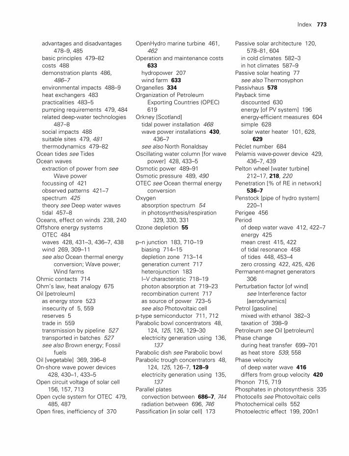
Index 773
advantages and disadvantages 478–9, 485
basic principles 479–82costs 488demonstration plants 486,
486–7environmental impacts 488–9heat exchangers 483practicalities 483–5pumping requirements 479, 484related deep-water technologies
487–8social impacts 488suitable sites 479, 481thermodynamics 479–82
Ocean tides see TidesOcean waves
extraction of power from see Wave power
focussing of 421observed patterns 421–7spectrum 425theory see Deep water wavestidal 457–8
Oceans, effect on winds 238, 240Offshore energy systems
OTEC 484waves 428, 431–3, 436–7, 438wind 269, 309–11see also Ocean thermal energy
conversion; Wave power; Wind farms
Ohmic contacts 714Ohm’s law, heat analogy 675Oil [petroleum]
as energy store 523insecurity of 5, 559reserves 5trade in 559transmission by pipeline 527transported in batches 527see also Brown energy; Fossil
fuelsOil [vegetable] 369, 396–8On-shore wave power devices
428, 430–1, 433–5Open circuit voltage of solar cell
156, 157, 713Open cycle system for OTEC 479,
485, 487Open fires, inefficiency of 370
OpenHydro marine turbine 461, 462
Operation and maintenance costs 633
hydropower 207wind farm 633
Organelles 334Organization of Petroleum
Exporting Countries (OPEC) 619
Orkney [Scotland]tidal power installation 468wave power installations 430,
436–7see also North Ronaldsay
Oscillating water column [for wave power] 428, 433–5
Osmotic power 489–91Osmotic pressure 489, 490OTEC see Ocean thermal energy
conversionOxygen
absorption spectrum 54in photosynthesis/respiration
329, 330, 331Ozone depletion 55
p–n junction 183, 710–19biasing 714–15depletion zone 713–14generation current 717heterojunction 183I–V characteristic 718–19photon absorption at 719–23recombination current 717as source of power 723–5see also Photovoltaic cell
p-type semiconductor 711, 712Parabolic bowl concentrators 48,
124, 125, 126, 129–30electricity generation using 136,
137Parabolic dish see Parabolic bowlParabolic trough concentrators 48,
124, 125, 126–7, 128–9electricity generation using 135,
137Parallel plates
convection between 686–7, 744radiation between 696, 746
Passification [in solar cell] 173
Passive solar architecture 120, 578–81, 604
in cold climates 582–3in hot climates 587–9
Passive solar heating 77see also Thermosyphon
Passivhaus 578Payback time
discounted 630energy [of PV system] 196energy-efficient measures 604simple 628solar water heater 101, 628,
629Péclet number 684Pelamis wave-power device 429,
436–7, 439Pelton wheel [water turbine]
212–17, 218, 220Penetration [% of RE in network]
536–7Penstock [pipe of hydro system]
220–1Perigee 456Period
of deep water wave 412, 422–7energy 425mean crest 415, 422of tidal resonance 458of tides 448, 453–4zero crossing 422, 425, 426
Permanent-magnet generators 306
Perturbation factor [of wind] see Interference factor [aerodynamics]
Petrol [gasoline]mixed with ethanol 382–3taxation of 398–9
Petroleum see Oil [petroleum]Phase change
during heat transfer 699–701as heat store 539, 558
Phase velocityof deep water wave 416differs from group velocity 420
Phonon 715, 719Phosphates in photosynthesis 335Photocells see Photovoltaic cellsPhotochemical cells 552Photoelectric effect 199, 200n1
TWIDELL PAGINATION.indb 773 01/12/2014 11:39
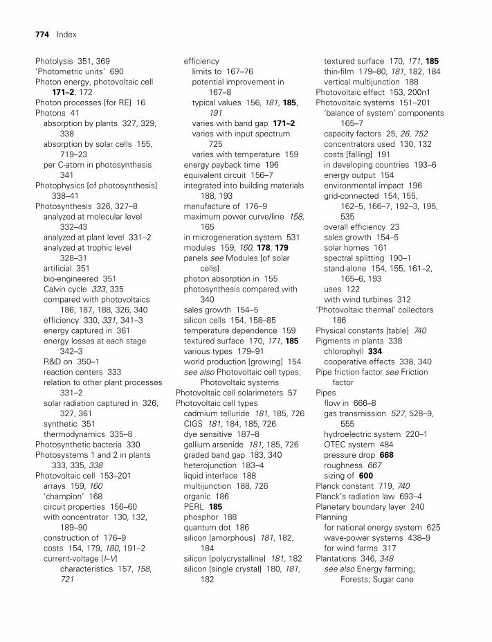
774 Index
Photolysis 351, 369‘Photometric units’ 690Photon energy, photovoltaic cell
171–2, 172Photon processes [for RE] 16Photons 41
absorption by plants 327, 329, 338
absorption by solar cells 155, 719–23
per C-atom in photosynthesis 341
Photophysics [of photosynthesis] 338–41
Photosynthesis 326, 327–8analyzed at molecular level
332–43analyzed at plant level 331–2analyzed at trophic level
328–31artificial 351bio-engineered 351Calvin cycle 333, 335compared with photovoltaics
186, 187, 188, 326, 340efficiency 330, 331, 341–3energy captured in 361energy losses at each stage
342–3R&D on 350–1reaction centers 333relation to other plant processes
331–2solar radiation captured in 326,
327, 361synthetic 351thermodynamics 335–8
Photosynthetic bacteria 330Photosystems 1 and 2 in plants
333, 335, 338Photovoltaic cell 153–201
arrays 159, 160‘champion’ 168circuit properties 156–60with concentrator 130, 132,
189–90construction of 176–9costs 154, 179, 180, 191–2current-voltage [I–V]
characteristics 157, 158, 721
efficiencylimits to 167–76potential improvement in
167–8typical values 156, 181, 185,
191varies with band gap 171–2varies with input spectrum
725varies with temperature 159
energy payback time 196equivalent circuit 156–7integrated into building materials
188, 193manufacture of 176–9maximum power curve/line 158,
165in microgeneration system 531modules 159, 160, 178, 179panels see Modules [of solar
cells]photon absorption in 155photosynthesis compared with
340sales growth 154–5silicon cells 154, 158–85temperature dependence 159textured surface 170, 171, 185various types 179–91world production [growing] 154see also Photovoltaic cell types;
Photovoltaic systemsPhotovoltaic cell solarimeters 57Photovoltaic cell types
cadmium telluride 181, 185, 726CIGS 181, 184, 185, 726dye sensitive 187–8gallium arsenide 181, 185, 726graded band gap 183, 340heterojunction 183–4liquid interface 188multijunction 188, 726organic 186PERL 185phosphor 188quantum dot 186silicon [amorphous] 181, 182,
184silicon [polycrystalline] 181, 182silicon [single crystal] 180, 181,
182
textured surface 170, 171, 185thin-film 179–80, 181, 182, 184vertical multijunction 188
Photovoltaic effect 153, 200n1Photovoltaic systems 151–201
‘balance of system’ components 165–7
capacity factors 25, 26, 752concentrators used 130, 132costs [falling] 191in developing countries 193–6energy output 154environmental impact 196grid-connected 154, 155,
162–5, 166–7, 192–3, 195, 535
overall efficiency 23sales growth 154–5solar homes 161spectral splitting 190–1stand-alone 154, 155, 161–2,
165–6, 193uses 122with wind turbines 312
‘Photovoltaic thermal’ collectors 186
Physical constants [table] 740Pigments in plants 338
chlorophyll 334cooperative effects 338, 340
Pipe friction factor see Friction factor
Pipesflow in 666–8gas transmission 527, 528–9,
555hydroelectric system 220–1OTEC system 484pressure drop 668roughness 667sizing of 600
Planck constant 719, 740Planck’s radiation law 693–4Planetary boundary layer 240Planning
for national energy system 625wave-power systems 438–9for wind farms 317
Plantations 346, 348see also Energy farming;
Forests; Sugar cane
TWIDELL PAGINATION.indb 774 01/12/2014 11:39
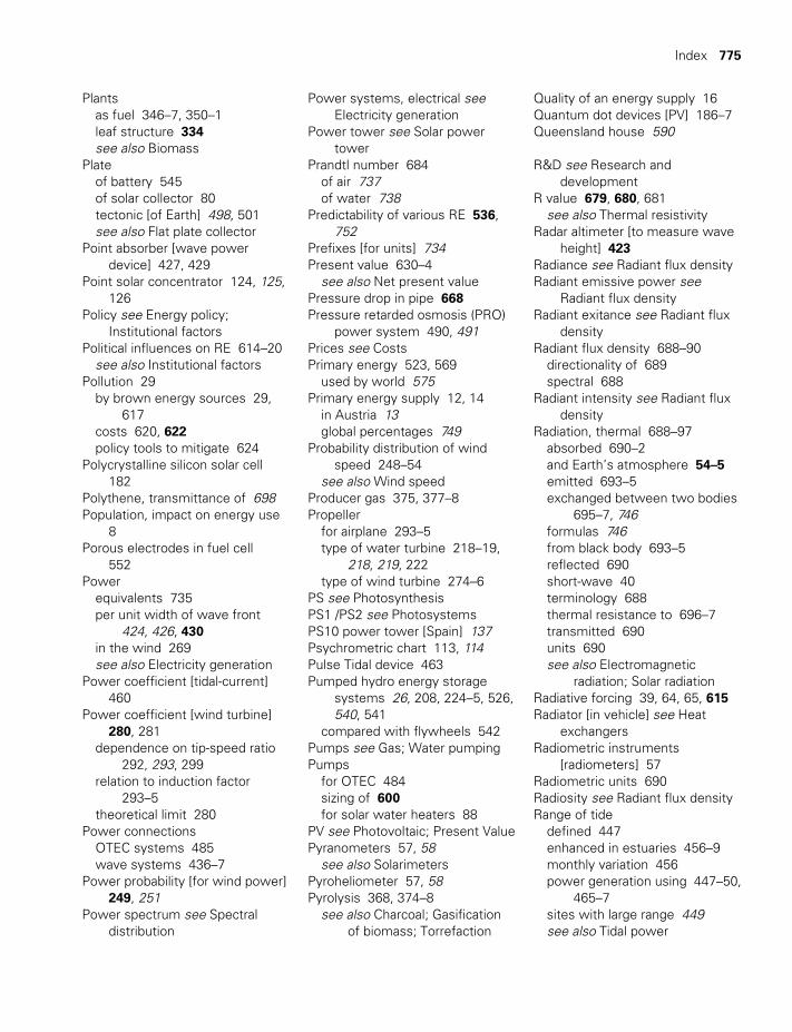
Index 775
Plantsas fuel 346–7, 350–1leaf structure 334see also Biomass
Plateof battery 545of solar collector 80tectonic [of Earth] 498, 501see also Flat plate collector
Point absorber [wave power device] 427, 429
Point solar concentrator 124, 125, 126
Policy see Energy policy; Institutional factors
Political influences on RE 614–20see also Institutional factors
Pollution 29by brown energy sources 29,
617costs 620, 622policy tools to mitigate 624
Polycrystalline silicon solar cell 182
Polythene, transmittance of 698Population, impact on energy use
8Porous electrodes in fuel cell
552Power
equivalents 735per unit width of wave front
424, 426, 430in the wind 269see also Electricity generation
Power coefficient [tidal-current] 460
Power coefficient [wind turbine] 280, 281
dependence on tip-speed ratio 292, 293, 299
relation to induction factor 293–5
theoretical limit 280Power connections
OTEC systems 485wave systems 436–7
Power probability [for wind power] 249, 251
Power spectrum see Spectral distribution
Power systems, electrical see Electricity generation
Power tower see Solar power tower
Prandtl number 684of air 737of water 738
Predictability of various RE 536, 752
Prefixes [for units] 734Present value 630–4
see also Net present valuePressure drop in pipe 668Pressure retarded osmosis (PRO)
power system 490, 491Prices see CostsPrimary energy 523, 569
used by world 575Primary energy supply 12, 14
in Austria 13global percentages 749
Probability distribution of wind speed 248–54
see also Wind speedProducer gas 375, 377–8Propeller
for airplane 293–5type of water turbine 218–19,
218, 219, 222type of wind turbine 274–6
PS see PhotosynthesisPS1 /PS2 see PhotosystemsPS10 power tower [Spain] 137Psychrometric chart 113, 114Pulse Tidal device 463Pumped hydro energy storage
systems 26, 208, 224–5, 526, 540, 541
compared with flywheels 542Pumps see Gas; Water pumpingPumps
for OTEC 484sizing of 600for solar water heaters 88
PV see Photovoltaic; Present ValuePyranometers 57, 58
see also SolarimetersPyroheliometer 57, 58Pyrolysis 368, 374–8
see also Charcoal; Gasification of biomass; Torrefaction
Quality of an energy supply 16Quantum dot devices [PV] 186–7Queensland house 590
R&D see Research and development
R value 679, 680, 681see also Thermal resistivity
Radar altimeter [to measure wave height] 423
Radiance see Radiant flux densityRadiant emissive power see
Radiant flux densityRadiant exitance see Radiant flux
densityRadiant flux density 688–90
directionality of 689spectral 688
Radiant intensity see Radiant flux density
Radiation, thermal 688–97absorbed 690–2and Earth’s atmosphere 54–5emitted 693–5exchanged between two bodies
695–7, 746formulas 746from black body 693–5reflected 690short-wave 40terminology 688thermal resistance to 696–7transmitted 690units 690see also Electromagnetic
radiation; Solar radiationRadiative forcing 39, 64, 65, 615Radiator [in vehicle] see Heat
exchangersRadiometric instruments
[radiometers] 57Radiometric units 690Radiosity see Radiant flux densityRange of tide
defined 447enhanced in estuaries 456–9monthly variation 456power generation using 447–50,
465–7sites with large range 449see also Tidal power
TWIDELL PAGINATION.indb 775 01/12/2014 11:39
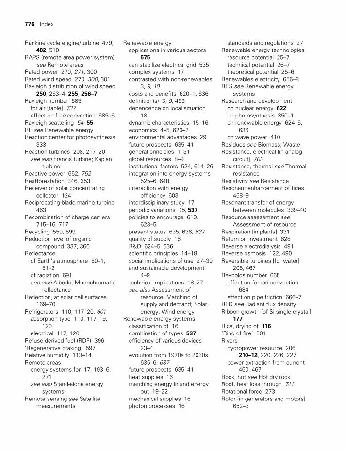
776 Index
Rankine cycle engine/turbine 479, 482, 510
RAPS (remote area power system) see Remote areas
Rated power 270, 271, 300Rated wind speed 270, 300, 301Rayleigh distribution of wind speed
250, 253–4, 255, 256–7Rayleigh number 685
for air [table] 737effect on free convection 685–6
Rayleigh scattering 54, 55RE see Renewable energyReaction center for photosynthesis
333Reaction turbines 208, 217–20
see also Francis turbine; Kaplan turbine
Reactive power 652, 752Reafforestation 346, 353Receiver of solar concentrating
collector 124Reciprocating-blade marine turbine
463Recombination of charge carriers
715–16, 717Recycling 559, 599Reduction level of organic
compound 337, 366Reflectance
of Earth’s atmosphere 50–1, 51–2
of radiation 691see also Albedo; Monochromatic
reflectanceReflection, at solar cell surfaces
169–70Refrigerators 110, 117–20, 601
absorption type 110, 117–19, 120
electrical 117, 120Refuse-derived fuel (RDF) 396‘Regenerative braking’ 597Relative humidity 113–14Remote areas
energy systems for 17, 193–6, 271
see also Stand-alone energy systems
Remote sensing see Satellite measurements
Renewable energyapplications in various sectors
575can stabilize electrical grid 535complex systems 17contrasted with non-renewables
3, 9, 10costs and benefits 620–1, 636definition(s) 3, 9, 499dependence on local situation
18dynamic characteristics 15–16economics 4–5, 620–2environmental advantages 29future prospects 635–41general principles 1–31global resources 8–9institutional factors 524, 614–26integration into energy systems
525–6, 648interaction with energy
efficiency 603interdisciplinary study 17periodic variations 15, 537policies to encourage 619,
623–5present status 635, 636, 637quality of supply 16R&D 624–5, 636scientific principles 14–18social implications of use 27–30and sustainable development
4–9technical implications 18–27see also Assessment of
resource; Matching of supply and demand; Solar energy; Wind energy
Renewable energy systemsclassification of 16combination of types 537efficiency of various devices
23–4evolution from 1970s to 2030s
635–6, 637future prospects 635–41heat supplies 16matching energy in and energy
out 19–22mechanical supplies 16photon processes 16
standards and regulations 27Renewable energy technologies
resource potential 25–7technical potential 26–7theoretical potential 25–6
Renewables electricity 656–8RES see Renewable energy
systemsResearch and development
on nuclear energy 622on photosynthesis 350–1on renewable energy 624–5,
636on wave power 410
Residues see Biomass; WasteResistance, electrical [in analog
circuit] 702Resistance, thermal see Thermal
resistanceResistivity see ResistanceResonant enhancement of tides
458–9Resonant transfer of energy
between molecules 339–40Resource assessment see
Assessment of resourceRespiration [in plants] 331Return on investment 628Reverse electrodialysis 491Reverse osmosis 122, 490Reversible turbines [for water]
208, 467Reynolds number 665
effect on forced convection 684
effect on pipe friction 666–7RFD see Radiant flux densityRibbon growth [of Si single crystal]
177Rice, drying of 116‘Ring of fire’ 501Rivers
hydropower resource 206, 210–12, 220, 226, 227
power extraction from current 460, 467
Rock, hot see Hot dry rockRoof, heat loss through 741Rotational force 273Rotor [in generators and motors]
652–3
TWIDELL PAGINATION.indb 776 01/12/2014 11:39
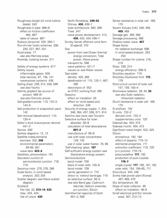
Index 777
Roughness length [of wind turbine blade] 243
Roughness in pipe 666–8effect on friction coefficient
484, 667table of values 667
Rubisco [enzyme] 335, 350–1Run-of-river hydro schemes 206,
220, 227, 467, 531Rural areas 17
see also Remote areasRwanda, cooking stoves 371
Safety of energy systems 617Safety issues
inflammable gases 559solar devices 87, 136, 141wave-power systems 438
Sailing ships 238, 314, 558, 599see also Yachts
Salinity gradient [as source of power] 489–91
see also Osmotic powerSalt-gradient ponds 110, 122–3,
144–5Salt production in evaporation pans
142Salt removal [desalination] 110,
120–4Salter’s duck [wave-power device]
441–2Samoa 590Sankey diagrams 12, 13Satellite measurements
biomass 332, 349environmental parameters
59–60, 261wave data 423–4
Satellites, photovoltaics 161Saturation current of
semiconductor junction 718, 719
Savonius rotor 275, 276, 286Scale factor, in wind speed
analysis 253, 254Scatter diagram see Wave scatter
diagramScotland
Fair Isle 22, 313–14, 533Islay 433, 434Isle of Lewis 430
North Ronaldsay 249–52Orkney 430, 436–7solar architecture 584, 585Tiree 247wave power development 412,
430, 433, 434, 436–7Scroby Sands offshore wind farm
[England] 310Sea
power from see Ocean thermal energy conversion; Tidal power; Wave power
transport by 598wave patterns 421–7waves on see Water waves
Sea waterdensity 425, 465desalination of 110, 120–1, 487,
490electrolysis of 553as OTEC working fluid 485
Seasonseffect on insolation 45effect on wind speed and
direction 240Security of energy supply 7, 204,
346, 384, 437, 559, 571, 614Seismic sea wave see TsunamiSelective surface for solar
absorber 92–6calculation of total absorptance
691–2manufacture of 95–6use with solar concentrator
129, 135use in solar water heater 78, 88
‘Self-cleaning’ glass 167Self-sufficient energy system see
Stand-alone energy systemSemiconductors
band model 709basis of solar cells 155–6bond model 709carrier generation in 715direct vs. indirect band-gap 719as selective surface 93–5see also Band gap; Cadmium
telluride; Gallium arsenide; p-n junction; Silicon
Semithermal region(s) of Earth 501–2, 508
Series resistance in solar cell 169, 175
Severn Estuary [UK] 448, 458, 459, 469
Sewage gas 365, 368Sewage processing 368Shallow-water wave 457Shape factor
for radiative exchange 696in wind speed analysis 253,
254Shape number for turbine 216,
219Ships 238, 314
energy efficiency 598–9Shockley equation 719Shockley–Queissner limit 172,
179Short-circuit current of solar cell
157, 159, 183–4Shortwave radiation 39, 40, 55
see also Solar radiation; Ultraviolet radiation
Shunt resistance in solar cell 169, 175
SI prefixes 734SI units 732–3
derived units 732–3supplementary units 732
Sidereal day 454, 473Sidereal month 454, 473Significant wave height 422, 425Silicon
amorphous 182, 184effect of dopants 710–12elemental properties 711extinction coefficient 719, 720p–n junction 710–19polycrystalline 177, 182production of pure crystals
176–7single crystal 177, 180, 181, 182solar cells 154, 158–85, 711
Silviculture 343, 346Siwha tidal power plant [Korea]
467, 469, 470Sky temperature 56Slope of solar collector 46
effect on insolation 46–9Small electrical grid [for remote
area] 307, 312–13
TWIDELL PAGINATION.indb 777 01/12/2014 11:39

778 Index
Small hydro schemes 205–6, 209, 220–2, 227, 467, 531
Small PV systems 162, 166–7, 193–6, 576
Small thermal solar generators 140
Small wave-power devices 410Small wind turbines 312–14, 531,
576, 618Smart grids 537–8Smart technology 19, 313, 314,
526, 531Smoke [as health hazard] 370, 400Social aspects
of energy end-use efficiency 602–4
of energy policy 619–20of RE technologies 27–30see also Decentralization [of
society]; Hydropower; Photovoltaics; Soft technology; Sustainable development; Wind power, etc
Social costs see External costsSocial development see
Sustainable developmentSocio-political influences on RE
614–20SoDAR (Sonic Detection And
Ranging) instrument 260, 261Sodium sulfate as heat store 539,
558Soil erosion 345, 363Solar air-conditioning 120
see also Solar architectureSolar air-heaters 110–12
see also Solar crop driers, Solar space heating
Solar altitude 46Solar architecture 110, 142,
578–91‘Solar Black House’ 580Solar buildings 110, 142, 576–91Solar cell see Photovoltaic cellSolar collectors
air 110–12concentrating see Solar
concentratorscosts 78covers 78, 79, 83, 698
distributed 110, 124efficiency 80–1, 87–8evacuated 77, 96–8flat plate see Flat plate
collectorsheat-balance calculations 79–81the ocean as 478orientation 45, 46–9, 60–1performance of different types
78selective surfaces for 79, 92–6,
691solar pond 110, 122–3, 144–5temperature calculations 89water 75–107
Solar concentrators 110, 123–32electricity generation using
132–40fuel and chemical synthesis
using 140–1linear concentrator 124, 125,
126–7, 128–9non-imaging 124, 130–1, 132,
133non-tracking 130, 131–2parabolic bowl 129–30parabolic trough 128–9point concentrator 124, 125,
126use with solar cells 130, 132,
189–90Solar constant 40Solar cooking 124, 131, 132Solar cooling see Solar
architecture; Solar space cooling
Solar crop driers 110, 112–17Solar day 453Solar Decathlon 584, 586Solar desiccant cooling 119, 120,
144–7Solar distillation 110, 120–4Solar energy see Solar cells; Solar
concentrators; Solar radiation; Solar water heaters
Solar flux density 11, 51, 63, 110Solar gain of a house 578, 579,
580Solar heating see Solar air heaters;
Solar crop driers; Solar space heating; Solar water heaters
Solar home systems (SHS) 194–5, 196
Solar homes 161, 578–81Solar-induced tide 454–6Solar irradiance
beam 41, 47–8, 60diffuse 41, 60, 61effect of orientation 48–9extraterrestrial 40–1horizontal 42variation with air mass [zenith
angle] 52–3variation with time 49, 50variation with wavelength 40see also Insolation; Solar
radiationSolar lantern 194, 195Solar panel see Flat plate collector;
Module of solar cellsSolar Pico Systems 195Solar ponds 110, 122–3, 144–5Solar power tower [for generation
of electricity] 136, 137Solar radiation 39–62
beam and diffuse 41, 47–8, 60, 61
components 41–2daily see Insolationeffect of earth’s atmosphere
41, 49–56estimation from other data
57–62extra-terrestrial 40–1instruments 57, 58meteorological records 57–8periodic variations 15, 40promotes photosynthesis 326,
327, 361site estimation of 57–62spectral distribution 39, 40statistical variation 58–9see also Insolation; Solar
irradianceSolar reactors 141Solar sea power see Ocean
thermal energy conversionSolar space cooling
absorption refrigerator 110architectural design 120,
587–9compression refrigerator 120
TWIDELL PAGINATION.indb 778 01/12/2014 11:39
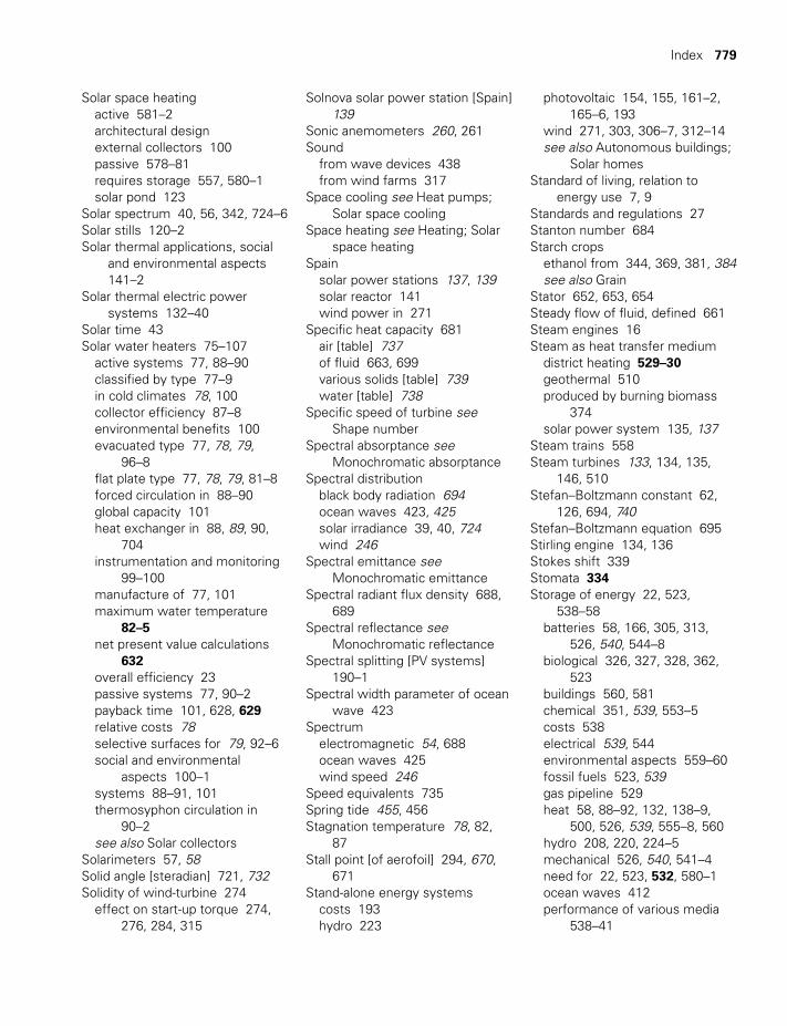
Index 779
Solar space heatingactive 581–2architectural designexternal collectors 100passive 578–81requires storage 557, 580–1solar pond 123
Solar spectrum 40, 56, 342, 724–6Solar stills 120–2Solar thermal applications, social
and environmental aspects 141–2
Solar thermal electric power systems 132–40
Solar time 43Solar water heaters 75–107
active systems 77, 88–90classified by type 77–9in cold climates 78, 100collector efficiency 87–8environmental benefits 100evacuated type 77, 78, 79,
96–8flat plate type 77, 78, 79, 81–8forced circulation in 88–90global capacity 101heat exchanger in 88, 89, 90,
704instrumentation and monitoring
99–100manufacture of 77, 101maximum water temperature
82–5net present value calculations
632overall efficiency 23passive systems 77, 90–2payback time 101, 628, 629relative costs 78selective surfaces for 79, 92–6social and environmental
aspects 100–1systems 88–91, 101thermosyphon circulation in
90–2see also Solar collectors
Solarimeters 57, 58Solid angle [steradian] 721, 732Solidity of wind-turbine 274
effect on start-up torque 274, 276, 284, 315
Solnova solar power station [Spain] 139
Sonic anemometers 260, 261Sound
from wave devices 438from wind farms 317
Space cooling see Heat pumps; Solar space cooling
Space heating see Heating; Solar space heating
Spainsolar power stations 137, 139solar reactor 141wind power in 271
Specific heat capacity 681air [table] 737of fluid 663, 699various solids [table] 739water [table] 738
Specific speed of turbine see Shape number
Spectral absorptance see Monochromatic absorptance
Spectral distributionblack body radiation 694ocean waves 423, 425solar irradiance 39, 40, 724wind 246
Spectral emittance see Monochromatic emittance
Spectral radiant flux density 688, 689
Spectral reflectance see Monochromatic reflectance
Spectral splitting [PV systems] 190–1
Spectral width parameter of ocean wave 423
Spectrumelectromagnetic 54, 688ocean waves 425wind speed 246
Speed equivalents 735Spring tide 455, 456Stagnation temperature 78, 82,
87Stall point [of aerofoil] 294, 670,
671Stand-alone energy systems
costs 193hydro 223
photovoltaic 154, 155, 161–2, 165–6, 193
wind 271, 303, 306–7, 312–14see also Autonomous buildings;
Solar homesStandard of living, relation to
energy use 7, 9Standards and regulations 27Stanton number 684Starch crops
ethanol from 344, 369, 381, 384see also Grain
Stator 652, 653, 654Steady flow of fluid, defined 661Steam engines 16Steam as heat transfer medium
district heating 529–30geothermal 510produced by burning biomass
374solar power system 135, 137
Steam trains 558Steam turbines 133, 134, 135,
146, 510Stefan–Boltzmann constant 62,
126, 694, 740Stefan–Boltzmann equation 695Stirling engine 134, 136Stokes shift 339Stomata 334Storage of energy 22, 523,
538–58batteries 58, 166, 305, 313,
526, 540, 544–8biological 326, 327, 328, 362,
523buildings 560, 581chemical 351, 539, 553–5costs 538electrical 539, 544environmental aspects 559–60fossil fuels 523, 539gas pipeline 529heat 58, 88–92, 132, 138–9,
500, 526, 539, 555–8, 560hydro 208, 220, 224–5mechanical 526, 540, 541–4need for 22, 523, 532, 580–1ocean waves 412performance of various media
538–41
TWIDELL PAGINATION.indb 779 01/12/2014 11:39
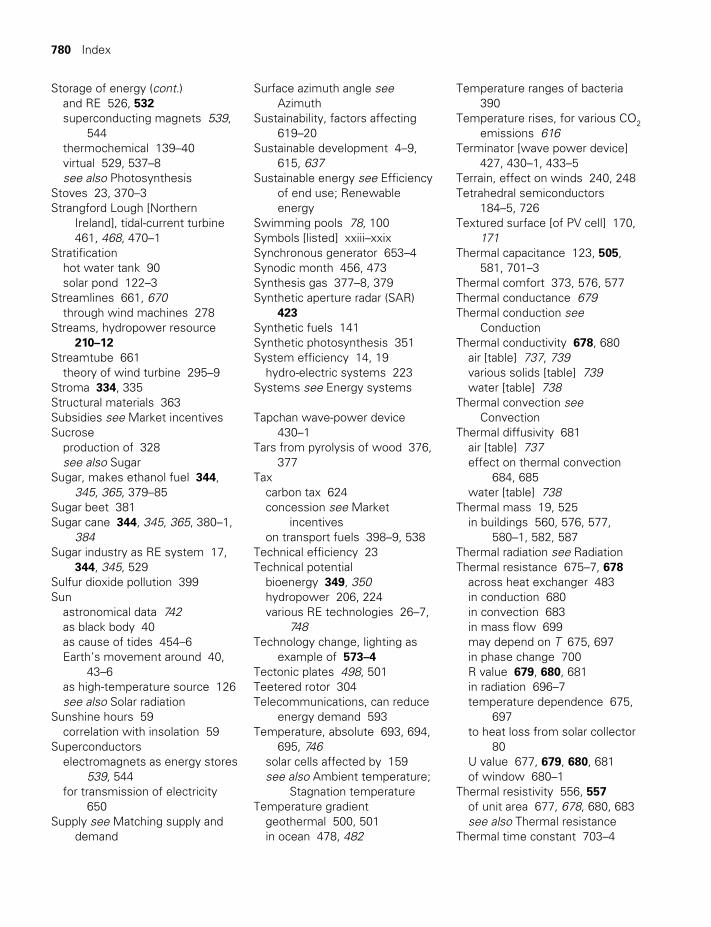
780 Index
Storage of energy (cont.)and RE 526, 532superconducting magnets 539,
544thermochemical 139–40virtual 529, 537–8see also Photosynthesis
Stoves 23, 370–3Strangford Lough [Northern
Ireland], tidal-current turbine 461, 468, 470–1
Stratificationhot water tank 90solar pond 122–3
Streamlines 661, 670through wind machines 278
Streams, hydropower resource 210–12
Streamtube 661theory of wind turbine 295–9
Stroma 334, 335Structural materials 363Subsidies see Market incentivesSucrose
production of 328see also Sugar
Sugar, makes ethanol fuel 344, 345, 365, 379–85
Sugar beet 381Sugar cane 344, 345, 365, 380–1,
384Sugar industry as RE system 17,
344, 345, 529Sulfur dioxide pollution 399Sun
astronomical data 742as black body 40as cause of tides 454–6Earth’s movement around 40,
43–6as high-temperature source 126see also Solar radiation
Sunshine hours 59correlation with insolation 59
Superconductorselectromagnets as energy stores
539, 544for transmission of electricity
650Supply see Matching supply and
demand
Surface azimuth angle see Azimuth
Sustainability, factors affecting 619–20
Sustainable development 4–9, 615, 637
Sustainable energy see Efficiency of end use; Renewable energy
Swimming pools 78, 100Symbols [listed] xxiii–xxixSynchronous generator 653–4Synodic month 456, 473Synthesis gas 377–8, 379Synthetic aperture radar (SAR)
423Synthetic fuels 141Synthetic photosynthesis 351System efficiency 14, 19
hydro-electric systems 223Systems see Energy systems
Tapchan wave-power device 430–1
Tars from pyrolysis of wood 376, 377
Taxcarbon tax 624concession see Market
incentiveson transport fuels 398–9, 538
Technical efficiency 23Technical potential
bioenergy 349, 350hydropower 206, 224various RE technologies 26–7,
748Technology change, lighting as
example of 573–4Tectonic plates 498, 501Teetered rotor 304Telecommunications, can reduce
energy demand 593Temperature, absolute 693, 694,
695, 746solar cells affected by 159see also Ambient temperature;
Stagnation temperatureTemperature gradient
geothermal 500, 501in ocean 478, 482
Temperature ranges of bacteria 390
Temperature rises, for various CO2 emissions 616
Terminator [wave power device] 427, 430–1, 433–5
Terrain, effect on winds 240, 248Tetrahedral semiconductors
184–5, 726Textured surface [of PV cell] 170,
171Thermal capacitance 123, 505,
581, 701–3Thermal comfort 373, 576, 577Thermal conductance 679Thermal conduction see
ConductionThermal conductivity 678, 680
air [table] 737, 739various solids [table] 739water [table] 738
Thermal convection see Convection
Thermal diffusivity 681air [table] 737effect on thermal convection
684, 685water [table] 738
Thermal mass 19, 525in buildings 560, 576, 577,
580–1, 582, 587Thermal radiation see RadiationThermal resistance 675–7, 678
across heat exchanger 483in conduction 680in convection 683in mass flow 699may depend on T 675, 697in phase change 700R value 679, 680, 681in radiation 696–7temperature dependence 675,
697to heat loss from solar collector
80U value 677, 679, 680, 681of window 680–1
Thermal resistivity 556, 557of unit area 677, 678, 680, 683see also Thermal resistance
Thermal time constant 703–4
TWIDELL PAGINATION.indb 780 01/12/2014 11:39
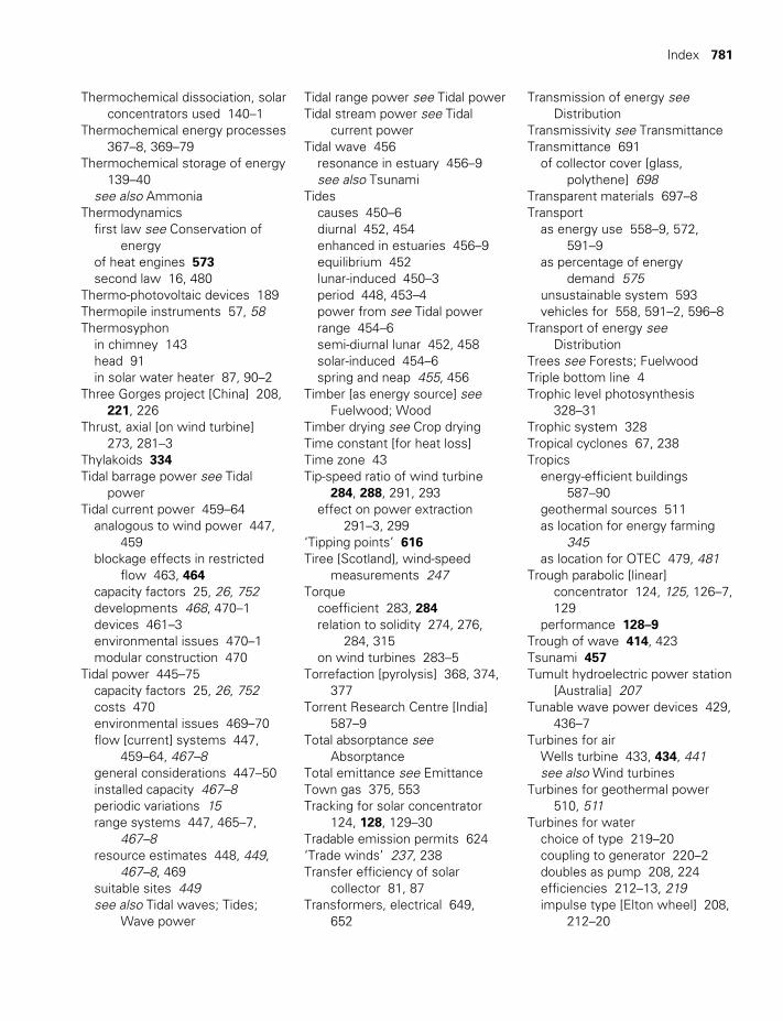
Index 781
Thermochemical dissociation, solar concentrators used 140–1
Thermochemical energy processes 367–8, 369–79
Thermochemical storage of energy 139–40
see also AmmoniaThermodynamics
first law see Conservation of energy
of heat engines 573second law 16, 480
Thermo-photovoltaic devices 189Thermopile instruments 57, 58Thermosyphon
in chimney 143head 91in solar water heater 87, 90–2
Three Gorges project [China] 208, 221, 226
Thrust, axial [on wind turbine] 273, 281–3
Thylakoids 334Tidal barrage power see Tidal
powerTidal current power 459–64
analogous to wind power 447, 459
blockage effects in restricted flow 463, 464
capacity factors 25, 26, 752developments 468, 470–1devices 461–3environmental issues 470–1modular construction 470
Tidal power 445–75capacity factors 25, 26, 752costs 470environmental issues 469–70flow [current] systems 447,
459–64, 467–8general considerations 447–50installed capacity 467–8periodic variations 15range systems 447, 465–7,
467–8resource estimates 448, 449,
467–8, 469suitable sites 449see also Tidal waves; Tides;
Wave power
Tidal range power see Tidal powerTidal stream power see Tidal
current powerTidal wave 456
resonance in estuary 456–9see also Tsunami
Tidescauses 450–6diurnal 452, 454enhanced in estuaries 456–9equilibrium 452lunar-induced 450–3period 448, 453–4power from see Tidal powerrange 454–6semi-diurnal lunar 452, 458solar-induced 454–6spring and neap 455, 456
Timber [as energy source] see Fuelwood; Wood
Timber drying see Crop dryingTime constant [for heat loss]Time zone 43Tip-speed ratio of wind turbine
284, 288, 291, 293effect on power extraction
291–3, 299‘Tipping points’ 616Tiree [Scotland], wind-speed
measurements 247Torque
coefficient 283, 284relation to solidity 274, 276,
284, 315on wind turbines 283–5
Torrefaction [pyrolysis] 368, 374, 377
Torrent Research Centre [India] 587–9
Total absorptance see Absorptance
Total emittance see EmittanceTown gas 375, 553Tracking for solar concentrator
124, 128, 129–30Tradable emission permits 624‘Trade winds’ 237, 238Transfer efficiency of solar
collector 81, 87Transformers, electrical 649,
652
Transmission of energy see Distribution
Transmissivity see TransmittanceTransmittance 691
of collector cover [glass, polythene] 698
Transparent materials 697–8Transport
as energy use 558–9, 572, 591–9
as percentage of energy demand 575
unsustainable system 593vehicles for 558, 591–2, 596–8
Transport of energy see Distribution
Trees see Forests; FuelwoodTriple bottom line 4Trophic level photosynthesis
328–31Trophic system 328Tropical cyclones 67, 238Tropics
energy-efficient buildings 587–90
geothermal sources 511as location for energy farming
345as location for OTEC 479, 481
Trough parabolic [linear] concentrator 124, 125, 126–7, 129
performance 128–9Trough of wave 414, 423Tsunami 457Tumult hydroelectric power station
[Australia] 207Tunable wave power devices 429,
436–7Turbines for air
Wells turbine 433, 434, 441see also Wind turbines
Turbines for geothermal power 510, 511
Turbines for waterchoice of type 219–20coupling to generator 220–2doubles as pump 208, 224efficiencies 212–13, 219impulse type [Elton wheel] 208,
212–20
TWIDELL PAGINATION.indb 781 01/12/2014 11:39
782 Index
Turbines for Water (cont.)propeller type [Kaplan] 218–19,
218, 219, 432reaction type [Francis] 208,
217–20reversible 208, 467shape number 216specific speed 216for tidal power systems 467
Turbines for wind see Wind turbines
Turbulence intensity 254, 257Turbulence of wind 240, 273, 665Turbulent flow of fluid 661
around wind turbine 240promotes fluid friction 666promotes heat transfer 666,
684
U value 677, 679, 680, 681typical values for walls and
windows 741–2see also Thermal conductance;
Thermal resistivityUK see United KingdomUltraviolet radiation 40, 55
see also Solar radiationUnited Kingdom
Building Code 578energy demand 575solar water heaters 100wave energy potential 424, 430
United Nations Framework Convention on Climate Change (UNFCCC) 353, 625
Units 732–4in algebraic method 728conversions between 734–5
Urban form, effect on energy demand 593–5
US[A] (United States of America)decommissioning of dams 227energy flow diagram 658geothermal energy 499, 502,
508solar pond 123solar power stations 135, 137solar water heaters 100wind map 241, 242
Use of energy see End usesUtilities, role of 524
Utility grid [network] see Electrical grid
Utsira island [Norway], wind/hydrogen energy system 533, 554
Valence band [in semiconductor] 709
Van der Hoven spectrum [of wind fluctuations] 246
Vapor concentration see HumidityVegetable oils 369, 396–8
see also Biodiesel; OilVehicles 591–2
electric 596–8energy efficiency of 596, 597hydrogen-powered 558, 598improved 596–8
Velocity see Wave velocity; Wind speed
Ventilation 586, 587–9, 589–90Vertical-axis tidal-current devices
462, 463Vertical-axis wind machines 275,
276–7Vested interests, energy policy
affected by 617Virtual storage
gas pipeline as 529grid as 22, 193, 537–8
Viscosity of fluid 664–5dynamic 664kinematic 664–5see also Friction in fluid flow
Visible radiation 40, 694see also Solar radiation
Visual impact, wind turbines 316–17
Voltage of electrical transmission 164
Voltage factor of solar cell 169, 173–4
Vorticesaround wind turbines 273, 289cavitation in water 219
Wairakei [New Zealand] geothermal system 502, 515–16
Walls, heat loss through 741WAsP (Wind Atlas Analysis and
Application Program) 242, 262
Waste heat, recovery of see Combined heat and power
‘Waste’ material as energy source 344, 345, 352, 395–6
Wateraquifers 505–7effect on thermal resistance
681, 699electrolysis of 189, 553injected into hot rock 509properties [table] 738splitting of 141, 189, 554as working fluid in heat engine
510see also Seawater
Water content of plant matter see Moisture content
Water desalination see Desalination
Water gas 377–8‘Water hammer’ 221Water heating
as ‘ballast-load’ 223, 313see also Solar water heaters
Water level in oceans 447see also Tidal range
Water power see Hydropower; OTEC; Tidal power; Wave power
Water pumpingOTEC system 479, 484for solar heater 88–9by wind power 269, 270, 274,
276, 315–16see also Pumped hydro storage
Water resources, environmental impact on 29
Water storage see Dam; Hot waterWater vapor
properties 54, 738see also Humidity
Water waves see Ocean waves; Shallow water wave; Tidal waves; Wave power
Waterfall, hydropower resource of 210, 212
Wave capture systems 430–3Wave Dragon [wave power device]
431–3
TWIDELL PAGINATION.indb 782 01/12/2014 11:39
Index 783
Wave energyglobal data 411northwest Europe data 424
Wave heightmeasured by satellites 423–4‘one-third’ 422significant 422, 425worldwide data 41120-/50-year maximum 411, 422
Wave length see WavelengthWave number 416Wave power 408–44
advantages and disadvantages 412, 437–8
assessment of resource 423–7capacity factors 25, 26, 752costs 439devices [operational] 430–7difficulties of harnessing 412environmental issues 438–9formulas for 418–20government support fluctuates
412natural fluxes of 424periodic variations 15, 752possible sites 411, 412, 431,
434potential for 411, 424see also Deep water waves;
Ocean waves; Wave power devices
Wave power devices 430–7attenuator [line absorber] 427,
429, 436–7capture width 412, 428, 433,
434, 436classification of 427–8dynamic tunable 429, 436–7efficiency 428–9energy extraction from 427–30floating 428, 431–3, 436–7focussing in 430–3Limpet device 433, 434, 439near-shore 428, 433–5, 438noise 438off-shore 428, 431–3, 436–7,
438on-shore 428, 430–1, 433–5oscillating water column (OWC)
428, 433–5Pelamis device 429, 436–7, 439
point absorber 427, 429reliability 439Salter’s duck 441–2Tapchan device 430–1terminator 427, 430–5tunable 429, 436–7wave capture systems 430–3Wave Dragon device 431–3wave profile device 436–7
Wave scatter diagram 426Wave velocity
energy propagation see Group velocity
particles in 419water wave surface see Phase
velocityWavelength
of deep-water wave 416, 420of maximum emitted RFD 694of radiation 689
Waves see Deep water waves; Ocean waves; Radiation (electromagnetic); Shallow water waves; Wave power
WECS see Wind turbinesWeibull distribution of wind speed
252–3, 255Weir [for measuring flow] 211,
212Wells [air] turbine 433, 434, 441‘westerlies’ [winds] 237, 238, 239Wien’s displacement law [of
radiation] 694Wind atlases 240–2Wind, characteristics of 242–58
direction 237, 238global pattern 237–40speed see Wind speed
Wind concentrators 275, 277Wind energy conversion system
(WECS) 322n2see also Wind power; Wind
turbinesWind farms 308–11, 633–4
compatibility with agriculture 309, 317, 633
discounted cash flow [example] 633–4
environmental issues 316–17offshore 269, 309–11
Wind power 267–323
autonomous [stand-alone] systems 271
classification of electricity systems 305–8
costs 270, 316, 633economics 270, 316, 633–4electricity production from 269,
270, 303–14, 535environmental impacts 316–17,
626installed capacity 269, 271matches seasonal demand
313–14mechanical power from 269,
270, 274, 314–16multi-mode system 307–8,
313–14periodic variations 15with photovoltaics 312potential 240–2, 270prediction models 242, 262relationship to wind speed 236,
270, 278resource see Wind resourcerural applications 307–8,
313–14water pumping by 269, 270,
274, 315–16see also Wind turbines
Wind resource 234–66instruments to measure 258–62models to estimate 262
Wind rose 243, 247Wind shear 243, 247Wind shift 243Wind speed
average 249Beaufort scale 243, 244–5, 262cut-in 300, 301cut-out 300, 301distribution around world 238,
239distribution in time 243, 246effect on solar heater 85, 98factors affecting 236, 243–8meteorological records 242–3minimum for electrical
generation 271, 304, 316prediction of 263probability distribution 248–54rated power 271
TWIDELL PAGINATION.indb 783 01/12/2014 11:39

784 Index
Wind speed (cont.)short-term predictions 263spectrum 246variation with height 243,
247–8, 278wind power related to 236, 270,
278Wind turbine
anemometer as 275, 276annual power output 269axial thrust on 281–3blade element theory 295–9capacity factors 25, 26, 311,
752classified by geometry and use
274–7concentrators 275, 277constant/fixed-speed 303, 308control systems 305–6costs 270, 316, 638Darrieus rotor 275, 276design criteria 236, 270–1efficiency [power coefficient]
270, 280, 281electricity generation from 271,
274, 303–14energy and power extracted
277–86, 289–95, 299–303, 656
gearbox 304horizontal axis types 274–6matching to wind regime
289–93, 299–300maximum [theoretical] power
coefficient 280mechanical power from 269,
270, 274, 314–16
momentum theory applied 277–89
Musgrove rotor 275, 276noise 317operated in series 320operating height 304, 316overall efficiency 23power coefficient 270, 280,
281, 299power curve 299, 300rated power 270, 271, 300Savonius rotor 275, 276, 286siting of 248solidity 274, 276, 284, 315stream tube theory 295–9thrust on 273, 281–3torque on 285, 298with twisted blades 295, 296,
299types 272–7typical operating characteristics
284–5, 300variable-speed 302–3, 304, 656vertical axis types 275, 276–7visual impact 316–17
Wind turbine blade, lift force on 295–7, 669–71
Wind vanes 259, 260Windfarms see Wind farmsWindmills 270, 314
see also Wind turbinesWindows
electrochromic 589heat loss through 582, 606–7,
680–1, 741–2Women and fuelwood 346Wood-burning stoves 23, 370–3
Wood consumption and production 346–7
see also FuelwoodWood gas 377–8Working fluids
in geothermal systems 510in OTEC system 479, 485in solar concentrators 123,
137World Commission on Dams 226,
233World Commission on
Environment and Development 2
World Energy Council (WEC) 35World Health Organization
(WHO), drinking-water recommendations 121
World Meteorological Organization (WMO)
meteorological methods 242standards for radiometers 57
Yachts 273, 285–6, 314Yaw [horizontal motion of wind
turbine] 275–6Yield of crops 348
Zenith angle 46, 47, 52see also Air mass ratio
Zero crossing period [of ocean waves] 422, 425, 426
Zhukowsky theory see Lanchester–Betz–Zhukowsky theory
Zone refining [of Si single crystal] 177
TWIDELL PAGINATION.indb 784 01/12/2014 11:39
Related Documents


![Resources [renewable and non renewable]](https://static.cupdf.com/doc/110x72/55643cd7d8b42ad3308b522b/resources-renewable-and-non-renewable.jpg)