REMUS AUV

Verification of a Six-Degree of Freedom Simulation Modelfor the REMUS Autonomous Underwater Vehicle

byTimothy Prestero

B.S., Mechanìcal EngineeringUniversity of California at Davis (1994)

Submitted to the Joint Program in Applied Ocean Science and Engineering

in partial fulfillment of the requirements for the degrees ofMaster of Science in Ocean Engineering

andMaster of Science in Mechanical Engineering

at theMASSACHUSETTS INSTITUTE OF TECHNOLOGY

and theWOODS HOLE OCEANOGRAPHIC INSTITUTION

September 200 iCS 2001 Timothy Prestero. All rights reserved.

The author hereby grants MIT and WHOI permission to reproduce paperelectronic copies of this thesis in whole or in part and to distribute them pu

) " ~1 L)l

--:fa?~L

If rnm _" ;, ,

Verification of a Six-Degree of Freedom Simulation Model for theREMUS Autonomous Underwater Vehicle

byTimothy Prestero

Submitted to the Joint Program in Applied Ocean Science and Engineering

on 10 August 2001, in partial fulfillment of therequirements for the degrees of

Master of Science in Ocean Engineeringand

Master of Science in Mechanical Engineering

AbstractImproving the performance of modular, low-cost autonomous underwater vehicles (AUVs) in suchapplications as long-range oceanographic survey, autonomous docking, and shallow-water mine coun-termeasures requires improving the vehicles' maneuvering precision and battery life. These goals

can be achieved through the improvement of the vehicle control system. A vehicle dynamics modelbased on a combination of theory and empirical data would provide an effcient platform for vehi-cle control system development, and an alternative to the typical trial-and-error method of vehiclecontrol system field tuning. As there exists no standard procedure for vehicle modeling in industry,the simulation of each vehicle system represents a new challenge.

Developed by von Alt and associates at the Woods Hole Oceanographic Institute, the REMUSAUV is a small, low-cost platform serving in a range of oceanographic applications. This thesisdescribes the development and verification of a six degree of freedom, non-linear simulation modelfor the REMUS vehicle, the first such model for this platform. In this model, the external forcesand moments resulting from hydrostatics, hydrodynamic lift and drag, added mass, and the controlinputs of the vehicle propeller and fins are all defined in terms of vehicle coeffcients. This thesisdescribes the derivation of these coeffcients in detaiL. The equations determining the coeffcients,as well as those describing the vehicle rigid-body dynamics, are left in non-linear form. to bettersimulate the inherently non-linear behavior of the vehicle. Simulation of the vehicle motion is

achieved through numeric integration of the equations of. motion. The simulator output is thenchecked against vehicle dynamics data collected in experiments performed at sea. The simulator isshown to accurately model the motion of the vehicle.

Thesis Supervisor: Jerome MilgramTitle: Professor of Ocean Engineering, MIT

Thesis Supervisor: Kamal Youcef-ToumiTitle: Professor of Mechanical Engineering, MIT

Thesis Supervisor: Christopher von AltTitle: Principal Engineer, WHOI

Candide had been wounded by some splinters of stone; he was stretched out in thestreet and covered with debris. He said to Pangloss: "Alas, get me a little wine and oil,I am dying."

"This earthquake is not a new thing," replied Pangloss. "The town of Lima sufferedthe same shocks in America last year; same causes, same effects; there is certainly a veinof sulfur underground from Lima to Lisbon."

"Nothing is more probable," said Candide, "but for the love of God, a little oil andwine."

"What do you mean, probable?" replied the philosopher. "I maintain that the matteris proved." Candide lost consciousness.

~Candide, Voltaire

Did I possess all the knowledge in the world, but had no love, how would this help mebefore God, who will judge me by my deeds?

~The Imitation of Christ, Thomas à Kempis

AcknowledgmentsIf not for the assistance and support of the following people, this work would have been much morediffcult, if not impossible to accomplish.

At MIT, I would first like to thank my advisor Prof. Jerry Milgram, for giving me a chance, forhelping me to get started on such an interesting problem, and for allowing me the room to figurethings out on my own. I would like to thank Prof. Kamal Youcef- Toumi for agreeing to read thisthesis on top of what was already a very busy schedule. I would like to thank Prof. John Leonard forhis humanity and his excellent advice. And finally, I have to thank the department administrators,Beth TUths and Jean Sucharewicz, for their unfailing patience and courtesy in answering about amilion emails from Africa.

At Woods Hole, I would like to thank Chris von Alt for his sage advice, and for his patienceas I figured out how to assemble this Heath Kit. I would like to thank Ben Allen for not tellnganyone that I dropped the digital camera into the tow tank. I would like to thank Roger Stokey,

Tom Austin, Ned Forrester, Mike Purcell and Greg Packard for all of their help with the vehicleexperiments, and for swatting their share of the green flies in TUckerton. I would like to thankMarga McElroy for helping me navigate the WHOI bureaucracy, and I have to thank Butch Grantfor inducting me into the mysteries of the circuit board and soldering iron.

I would like to thank Nuno Cruz for the excellent discussions about experimental methods,

Oscar Pizarro, Chris Roman, and Fabian Tapia for solving the world's problems over dinner, andTom Fulton and Chris Cassidy for the water-skiing lessons. And wherever he is now in Brooklyn, Ihave to thank Alexander Terry for that first kick in the pants.

At home, I have to thank my family for their confidence and constant support, and Sheridan forfirst giving me the good news. And finally, I would like to thank Elizabeth for absolutely everything.

TIMOTHY PRESTEROCambridge, Massachusetts

4

Contents

1 Introduction

1.1 Motivation .........1.2 Vehicle Model Development

1.3 Research Platform . . .1.4 Model Code . . . . . . . . .1.5 Modeling Assumptions . . .

1.5.1 Environmental Assumptions.

1.5.2 Vehicle/Dynamics Assumptions.

121212121313

1313

2 The REMUS Autonomous Underwater Vehicle2.1 Vehicle Profile. . .2.2 Sonar Transducer. . . . . . . .2.3 Control Fins. . . . . . . . . . .2.4 Vehicle Weight and Buoyancy.

2.5 Centers of Buoyancy and Gravity .

2.6 Inertia Tensor. . . .2.7 Final Vehicle Profile . . . . . . . .

141415

1515171718

3 Elements of the Governing Equations3.1 Body-Fixed Vehicle Coordinate System Origin

3.2 Vehicle Kinematics . . . . . .3.3 Vehicle Rigid-Body Dynamics

3.4 Vehicle Mechanics ......

2020202223

4 Coeffcient Derivation

4.1 Hydrostatics.....4.2 Hydrodynamic Damping .

4.2.1 Axial Drag . .4.2.2 Crossflow Drag

4.2.3 Rollng Drag .4.3 Added Mass . . . . . .

4.3.1 Axial Added Mass

4.3.2 Crossflow Added Mass

4.3.3 Rollng Added Mass .

4.3.4 Added Mass Cross-terms

4.4 Body Lift . . . . . . . . .4.4.1 Body Lift Force. .4.4.2 Body Lift Moment

4.5 Fin Lift . . . . . .4.6 Propulsion Model. . . . .

24242525262727282829293030313133

5

4.6.1 Propeller Thrust

4.6.2 Propeller Torque

4.7 Combined Terms . . . .4.8 Total Vehicle Forces and Moments

5 Vehicle Tow Tank Experiments5.1 Motivation ...........5.2 Laboratory Facilities and Equipment

5.2.1 Flexural Mount. . . . . . .5.2.2 Tow Tank Carriage. . . . .

5.3 Drag Test Experimental Procedure

5.3.1 Instrument Calibration

5.3.2 Drag Runs

5.3.3 Signal Processing. . . .5.4 Experimental Results. . . . . .5.5 Component-Based Drag Model

33333434

3737373838414142424243

6 Vehicle Simulation

6.1 Combined Nonlinear Equations of Motion . . . . .6.2 Numerical Integration of the Equations of Motion.

6.2.1 Euler's Method . . . . . .6.2.2 Improved Euler's Method

6.2.3 Runge-Kutta Method

6.3 Computer Simulation.

45454747474848

7 Field Experiments7.1 Motivation

7.2 Measured States

7.3 Vehicle Sensors .

7.3.1 Heading: Magnetic Compass

7.3.2 Yaw Rate: TUning Fork Gyro

7.3.3 Attitude: Tilt Sensor. .7.3.4 Depth: Pressure Sensor

7.4 Experimental Procedure . . . .7.4.1 Pre-launch Check List .

7.4.2 Trim and Ballast Check

7.4.3 Vehicle Mission Programming.7.4.4 Compass Calibration.

7.4.5 Vehicle Tracking . . . . . .7.5 Experimental Results. . . . . . . .

7.5.1 Horizontal-Plane Dynamics

7.5.2 Vertical-Plane Dynamics. .

494949505050505151

5151515353535355

8 Comparisons of Simulator Output and Experimental Data8.1 Model Preparation . . . . . . .

8.1.1 Initial Conditions. . . . . . .8.1.2 Coeffcient Adjustments . . .

8.2 Uncertainties in Model Comparison.8.3 Horizontal Plane Dynamics

8.4 Vertical Plane Dynamics. . . .8.4.1 Vehicle Pitching Up . .8.4.2 Vehicle Pitching Down.

6060606061

61616767

6

9 Linearized Depth Plane Model and Controller

9.1 Linearizing the Vehicle Equations of Motion

9.1.1 Vehicle Kinematics. . . . . . .9.1.2 Vehicle Rigid-Body Dynamics.

9.1.3 Vehicle Mechanics . . . .9.2 Linearized Coeffcient Derivation

9.2.1 Hydrostatics .9.2.2 Axial Drag . .9.2.3 Crossflow Drag

9.2.4 Added Mass. .9.2.5 Body Lift Force and Moment

9.2.6 Fin Lift . . . . . . . .9.2.7 Combined Terms . . . .9.2.8 Linearized Coeffcients .

9.3 Linearized Equations of Motion

9.3.1 Equations of Motion . .9.3.2 Four-term State Vector

9.3.3 Three-term State Vector.

9.4 Control System Design. . . . . .9.4.1 Vehicle Transfer Functions.

9.4.2 Control Law ........9.4.3 Controller Design Procedure

9.4.4 Pitch Loop Controller Gains

9.4.5 Depth Loop Controller Gains9.5 Real-World Phenomena . .9.6 Controller Implementation. . . . . .

7878787979808080808182828383848485868687878789898993

10 Conclusion10.1 Expanded Tow Tank Measurements10.2 Future Experiments at Sea .....

10.2.1 Improved Vehicle Instrumentation10.2.2 Measurement of Vehicle Parameters10.2.3 Isolation of Vehicle Motion .

10.3 Controller-Based Model Comparison10.4 Vehicle Sensor Model. . . . . . . .

10.5 Improved Coeffcient-Based Model

9999

100100100100100101101

A Tables of Parameters 102

B Tables of Combined Non-Linear Coeffcients 104

C Tables of Non-Linear Coeffcients by Type 106

D Tables of Linearized Model Parameters 112

E MATLAB CodeE.l Vehicle Simulation

E.i. REMUS_SIM.m.E.1.2 REMUS.m '"

114114114117

F Example REMUS Mission FileF.l REMUS Mission Code. . . . .

120120

7

List of Figures

2-1 Myring Profile ................ . . . . . .2-2 REMUS Low-Frequency Sonar Transducer (XZ-plane)2-3 REMUS Tail Fins (XY- and XZ-plane) . . . . .2-4 STD REMUS Profile (XZ-plane) . . . . . . . .2-5 The REMUS Autonomous Underwater Vehicle

15

1616

19

19

3-1 REMUS Body-Fixed and Inertial Coordinate Systems 21

4-1 Effective Rudder Angle of Attack. . .

4-2 Effective Stern Plane Angle of Attack

3232

5- 1 URI Tow Tank Layout . . . . . . . . .5-2 URI Tow Tank . . . . . . . . . . . . .5-3 Carriage Setup and Vehicle Mounting

5-4 URI Tow Tank Carriage . . . . . .5-5 URI Tow Tank Carriage . . . . . . . .5-6 Unfiltered and Filtered Drag Data . .5-7 Forward Speed vs. Vehicle Axial and Lateral Drag

38394040414344

7-1 Vehicle Experiments at the Rutgers Marine Field Station7-2 REMUS Pre-Launch Checklist (Page One) .7-3 REMUS Mission Data: Crash Plot7-4 Vehicle Experiments at WHOI ... . . . .

7-5 The REMUS Ranger. . . . . . . . . . . . .7-6 REMUS Mission Data: Closed-Loop Control7-7 REMUS Mission Data: Rudder . . . . .7-8 REMUS Mission Data: Pitching Up ..7-9 REMUS Mission Data: Pitching Down.

495254555556575859

8-1 Horizontal Plane Simulation: Linear . .8-2 Horizontal Plane Simulation: Angular .

8-3 Horizontal Plane Simulation: Forces and Moments8-4 Horizontal Plane Simulation: Vehicle Trajectory

8-5 Horizontal Plane Simulation: Model Comparison8-6 Vertical Plane Simulation: Linear. . . . . . . . .

8-7 Vertical Plane Simulation: Angular. . . . . . . .

8-8 Vertical Plane Simulation: Forces and Moments.8-9 Vertical Plane Simulation: Vehicle Trajectory .

8-10 Vertical Plane Simulation: Model Comparison.8-11 Vertical Plane Simulation: Linear. .8-12 Vertical Plane Simulation: Angular. . . . . . .

626364656668697071

727374

8

8-13 Vertical Plane Simulation: Forces and Moments.8-14 Vertical Plane Simulation: Vehicle Trajectory .8-15 Vertical Plane Simulation: Model Comparison.

757677

9-1 Perturbation Velocity Linearization. . . . . .9-2 Depth-Plane Control System Block Diagram.

9-3 Ge Pole-Zero Plot .......9-4 Ge Open-Loop Step Response.

9-5 Ge Root-Locus Plot . . . . . .9-6 Ge Closed-Loop Step Response

9-7 Gz * He Pole-Zero Plot. . . . .9-8 Gz * He Root-Locus Plot

9-9 Gz * He Closed-Loop Step Response

9- 10 Modified Depth Plane Control System Block Diagram9-11 Vehicle Simulation: Case One .9-12 Vehicle Simulation: Case Two.9-13 Vehicle Simulation: Case Three9-14 Vehicle Simulation: Case Four .

8188909091919292949495969798

10-1 Forces on the vehicle at an angle of attack.

10-2 Vehicle performance limits as a function of depth and sea state99

101

9

List of Tables

2.1 Myring Parameters for STD REMUS.2.2 REMUS Fin Parameters . . . . . . .2.3 STD REMUS Weight and Buoyancy2.4 STD REMUS Center of Buoyancy2.5 STD REMUS Center of Gravity. .2.6 STD REMUS Moments of Inertia.2.7 STD REMUS Hull Parameters . .

15171717181818

4.1 Axial Added Mass Parameters Q and ß

4.2 STD REMUS Non-Linear Maneuvering Coeffcients: Forces4.3 STD REMUS Non-Linear Maneuvering Coeffcients: Moments

283536

5.1 REMUS Drag Runs .......................5.2 REMUS Component-Based Drag Analysis - Standard Vehicle5.3 REMUS Component-Based Drag Analysis - Sonar Vehicle

424444

7.1 Vehicle Field Experiments . . . . . . . 51

8.1 REMUS Simulator Initial Conditions.8.2 Vehicle Coeffcient Adjustment Factors.

6061

9.1 Linearized Velocity Parameters . . .9.2 Combined Linearized Coeffcients . .9.3 Linearized Maneuvering Coeffcients

9.4 Percent Overshoot and Damping Ratio.

81848588

A.l STD REMUS Hull Parameters . . . . .A.2 Hull Coordinates for Limits of IntegrationA.3 STD REMUS Center of BuoyancyA.4 STD REMUS Center of Gravity.A.5 REMUS Fin Parameters. . .

102102103103103

B. 1 N on- Linear Force CoeffcientsB.2 Non-Linear Moment Coeffcients

104105

C.l Axial Drag Coeffcient . . . .C.2 Crossflow Drag Coeffcients

C.3 Rolling Resistance CoeffcientC.4 Body Lift and Moment Coeffcients.C.5 Added Mass Coeffcients . . . . . . .C.6 Added Mass Force Cross-term Coeffcients

106106106107107108

10

C.7 Added Mass K-Moment Cross-term Coeffcients. . .C.8 Added Mass M-, N-Moment Cross-term CoeffcientsC.9 Propeller Terms. . . . .C.l0 Control Fin Coeffcients . . . . .

D.l Linearized Combined Coeffcients

D.2 Linearized Maneuvering Coeffcients

109110110111

112113

11

Chapter i

Introd uction

i. i Motivation

Improving the performance of modular, low-cost autonomous underwater vehicles (AUVs) in suchapplications as long-range oceanographic survey, autonomous docking, and shallow-water mine coun-termeasures requires improving the vehicles' maneuvering precision and battery life. These goals

can be achieved through the improvement of the vehicle control system. A vehicle dynamics modelbased on a combination of theory and empirical data would provide an effcient platform for vehi-cle control system development, and an alternative to the typical trial-and-error method of vehiclecontrol system field tuning. As there exists no standard procedure for vehicle modeling in industry,the simulation of each vehicle system represents a new challenge.

1.2 Vehicle Model Development

This thesis describes the development and verification of a simulation model for the motion of theREMUS vehicle in six degrees of freedom. In this model, the external forces and moments resultingfrom hydrostatics, hydrodynamic lift and drag, added mass, and the control inputs of the vehiclepropeller and fins are all defined in terms of vehicle coeffcients.

This thesis describes the derivation of these coeffcients in detail, and describes the experimentalmeasurement of the vehicle axial drag.

The equations determining the coeffcients, as well as those describing the vehicle rigid-bodydynamics, are left in non-linear form to better simulate the inherently non-linear behavior of thevehicle. Simulation of the vehicle motion is achieved through numeric integration of the equationsof motion. The simulator output is then checked against open-loop data collected in the field. Thisfield data measured the vehicle response to step changes in control fin angle. The simulator is shownto accurately model the vehicle motion in six degrees of freedom.

To demonstrate the intended application of this work, this thesis demonstrates the use of alinearized version of the vehicle model to develop a vehicle depth-plane control system.

In closing, this thesis discusses plans for further experimental verification of the vehicle coeff-cients, including tow tank lift and drag measurements, and precision inertial measurements of thevehicle open-water motion and sensor dynamics.

1.3 Research Platform

The platform for this research is the REMUS AUV, developed by von Alt and associates at theOceanographic Systems Laboratory at the Woods Hole Oceanographic Institution ¡31l. REMUS

12

(Remote Environmental Monitoring Unit) is a low-cost, modular vehicle with applications in au-tonomous docking, long-range oceanographic survey, and shallow-water mine reconnaissance ¡30l.See Chapter 2 for the specifications of the REMUS vehicle.

REMUS currently uses a field-tuned PID controller; previous attempts to apply more advancedcontrollers to REMUS have been hampered by the lack of a mathematical model to describe thevehicle dynamics.

i.4 Model Code

The author developed the simulator code using MAT LAB. Although MATLAB runs slowly comparedto other compilers, the program greatly facilitates data visualization. In developing the code, theauthor did not use any MATLAB-specific functions, so exporting the model code to another, fasterlanguage for controller development wil be easy.

1.5 Modeling Assumptions

In order to simplify the challenge of modeling an autonomous underwater vehicle, it is necessary tomake some assumptions on which to base the model development.

1.5.1 Environmental Assumptions

The author made the following assumptions about the vehicle with respect to its environment:

· The vehicle is deeply submerged in a homogeneous, unbounded fluid. In other words, the vehicleis located far from free surface (no surface effects, i.e. no sea wave or vehicle wave-makingloads), walls and bottom.

· The vehicle does not experience memory effects. The simulator neglects the effects of thevehicle passing through its own wake.

. The vehicle does not experience underwater currents.

1.5.2 Vehicle/Dynamics Assumptions

The author made the following assumptions about the vehicle itself:

· The vehicle is a rigid body of constant mass. In other words, the vehicle mass and massdistribution do not change during operation.

· Control surface assumptions: We assume that the control fins do not stall regardless of angleof attack. We also assume an instantaneous fin response, meaning that that vehicle actuatortime response is small in comparison with the vehicle attitude time response.

· Thruster assumptions: We will be using an extremely simple propulsion model, which treatsthe vehicle propeller as a source of constant thrust and torque.

· There exist no significant vehicle dynamics faster than 45 Hz (the modeling time step).

13

Chapter 2

The REMUS AutonomousU nderwater Vehicle

In order to calculate the vehicle coeffcients, we must first define the profile of the vehicle, determineits mass, mass distribution, and buoyancy, and finally identify the necessary control fin parameters.

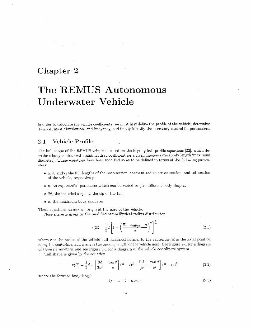
2.1 Vehicle Profile

The hull shape of the REMUS vehicle is based on the Myring hull profie equations ¡22J, which de-scribe a body contour with minimal drag coeffcient for a given fineness ratio (body length/maximumdiameter). These equations have been modified so as to be defined in terms of the following param-eters:

. a, b, and' c, the full Ìengths of the nose-section, constant-radius center-section, and tail~sectionof the vehicle, respectively

. n, an exponential parameter which can be varied to give different body shapes.

. 2e, the included angle at the tip of the tail

. d, the maximum body diameter

These equations assume an origin at the nose of the vehicle.Nose shape is given by the modified semi-elliptical radius distribution

1

1'(3) = ~d (1 - (3 + ao:set - a rr (2.1)

where l' is the radius of the vehicle hull measured normal to the centerline, 3 is the axial positionalong the centerline, and aoffset is the missing length of the vehicle nose. See Figure 2-1 for a diagramof these parameters, and see Figure 3-1 for a diagram of the vehicle coordinate system.

Tail shape is given by the equation

~ 1 i3d taneJ - 2 id taneJ ~ 3r(.:)=-d- --- (.:-1) + --- (.:-11)2 2c2 c c3 c2 (2.2)

where the forward body lengthIi = a + b - aoffset (2.3)

14

and again, l' is the vehicle hull radius and B is the axial position along the centerline. Note inFigure 2-1 that Coffset is the missing length of the vehicle tail, where C is the full Myring tail length.

~l=S,-i:-a: c . ; ..

td

b

¡ r(S)~i Coff,,': -::-, "ie'. ," .:

Figure 2- 1: Myring Profile: vehicle hull radius as a function of axial position

For reference, Myring (22, p. 1891 assumes a total body length of 100 units, and classifies bodytypes by a code of the form a/b/n/(j nd, where (j is given in radians. REMUS is based on theMyring B hull contour, which is given by the code 15/55/1.25/0.4363/5. Table 2.1 gives thedimensionalized Myring parameters.

Table 2.1: Myring Parameters for STD REMUSParameter Value Units Description

a +1.91e-001 m Nose Lengthaoffset +1.65e-002 m Nose Offsetb +6. 54e-001 m Midbody LengthC +5. 41e-001 m Tail Length

Coffset +3. 68e-002 m Tail Offsetn +2 . 00 n/ a Exponential Coeffcient(j +4. 36e-001 radians Included Tail Angled +1. 91e-001 m Maximum Hull DiameterL f +8. 28e-001 m Vehicle Forward LengthI +1. 33e+000 m Vehicle Total Length

2.2 Sonar Transducer

The REMUS vehicle is equipped with a forward sonar transducer, which is a cylinder 10.1 cm (4.0in) diameter. The remaining transducer dimensions are given in Figure 2-2.

2.3 Control Fins

The REMUS vehicle is equipped with four identical control fins, mounted in a cruciform patternnear the aft end of the hulL. These fins have a NACA 0012 cross-section; their remaining dimensionsare given in Figure 2-3. The relevant fin parameters are given in Table 2.2.

2.4 Vehicle Weight and Buoyancy

The weight of the REMUS vehicle can change between missions, depending on the type of batteriesused in the vehicle and the amount of ballast added. REMUS is typically ballasted with around

15

't---I

I

II

I

II

I

I

I

I

I

I ..I

't

I

i

I

i

14.2 em

i

~I'"

II

I

~: 5.0 em R12.6 em

Figure 2-2: REMUS Low-Frequency Sonar Transducer (XZ-plane)

r---------- -

13.1 em

- -f- - - - ~2.9 em

i:.. . 5.3emi

, I,I 1~ ~i 11.2 em

,1~,

~14.2 em

Figure 2-3: REMUS Tail Fins (XY- and XZ-plane)

16

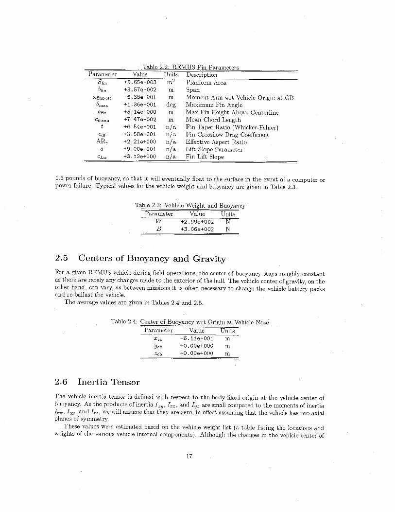
Table 2.2: REMUS Fin ParametersParameter Value Units Description

8fin +6.65e-003 m2 Planform Areabfin +8.57 e-002 m Span

Xfinpost -6.38e-00l m Moment Arm wrt Vehicle Origin at CBbmax +1.36e+00l deg Maximum Fin Angleafin +5. 14e+000 m Max Fin Height Above Centerline

cmean +7.47e-002 m Mean Chord Lengtht +6.54e-00l n/a Fin Taper Ratio (Whicker-FeIner)

Cdf +5.58e-00l n/a Fin Crossflow Drag Coeffcient

ARe +2.21e+000 n/a Effective Aspect Ratioa +9.00e-00l n/a Lift Slope Parameter

CLa +3. 12e+000 n/a Fin Lift Slope

1.5 pounds of buoyancy, so that it wil eventually float to the surface in the event of a computer orpower failure. Typical values for the vehicle weight and buoyancy are given in Table 2.3.

Table 2.3: Vehicle Weight and BuoyancyParameter Value Units

VV +2. 9ge+002 NB +3. 06e+002 N

2.5 Centers of Buoyancy and Gravity

For a given REMUS vehicle during field operations, the center of buoyancy stays roughly constantas there are rarely any changes made to the exterior of the hulL. The vehicle center of gravity, on theother hand, can vary, as between missions it is often necessary to change the vehicle battery packsand re-ballast the vehicle.

The average values are given in Tables 2.4 and 2.5.

Table 2.4: Center of Buoyancy wrt Origin at Vehicle NoseParameter Value Units

Xcb -6.11e-00l mYcb +0. OOe+OOO mZcb +0. OOe+OOO m

2.6 Inertia Tensor

The vehicle inertia tensor is defined with respect to the body-fixed origin at the vehicle center ofbuoyancy. As the products of inertia 1xy, 1xz, and 1yz are small compared to the moments of inertia1xx, 1yy, and 1zz, we wil assume that they are zero, in effect assuming that the vehicle has two axialplanes of symmetry.

These values were estimated based on the vehicle weight list (a table listing the locations andweights of the various vehicle internal components). Although the changes in the vehicle center of

17

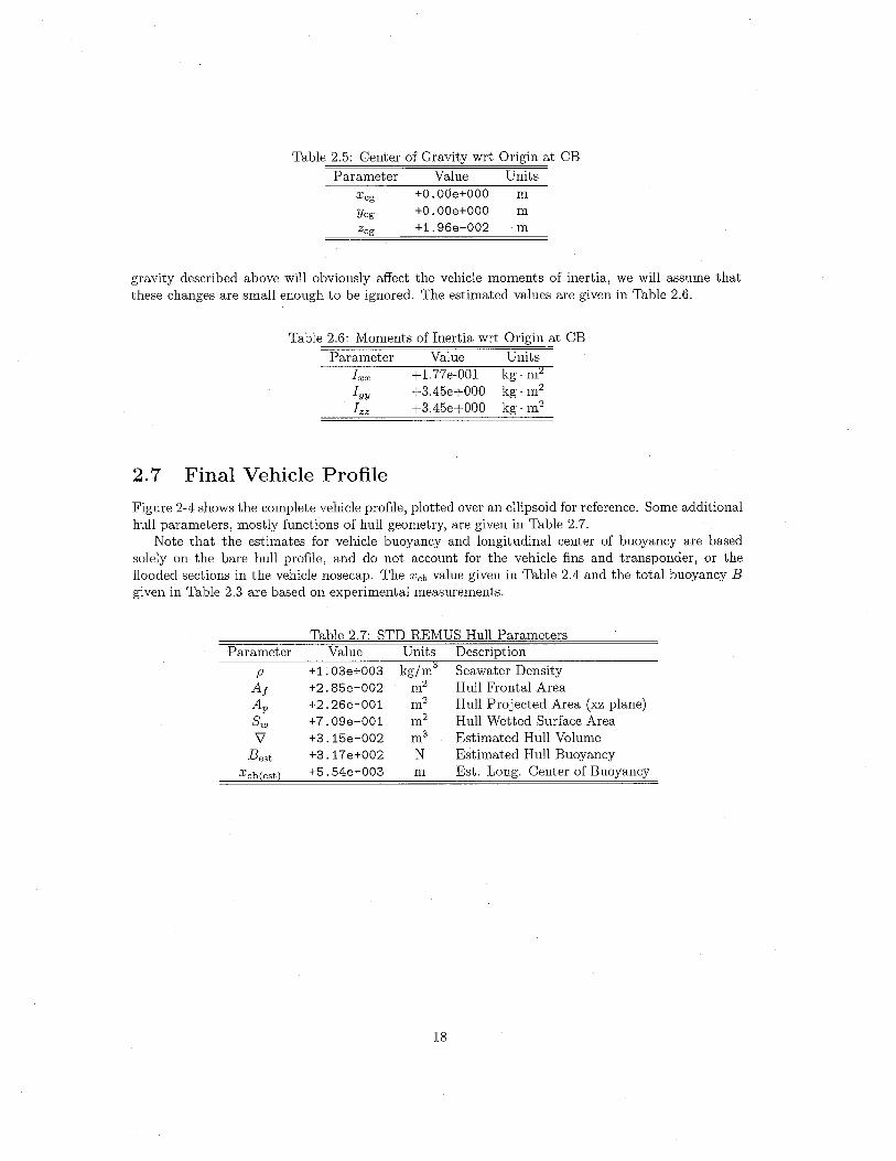
Table 2.5: Center of Gravity wrt Origin at CBParameter Value Units

xcg +0. OOe+OOO mYcg +0. OOe+OOO mZcg +1. 96e-002 m

gravity described above wil obviously affect the vehicle moments of inertia, we wil assume thatthese changes are small enough to be ignored. The estimated values are given in Table 2.6.

Table 2.6: Moments of Inertia wrt Origin at CBParameter

1xx

1yy

1zz

Value+1.77e-00I+3.45e+000+3.45e+000

Unitskg.m2kg. m2

kg. m2

2.7 Final Vehicle Profile

Figure 2-4 shows the complete vehicle profile, plotted over an ellipsoid for reference. Some additionalhull parameters, mostly functions of hull geometry, are given in Table 2.7.

Note that the estimates for vehicle buoyancy and longitudinal center of buoyancy are based

solely on the bare hull profile, and do not account for the vehicle fins and transponder, or theflooded sections in the vehicle nosecap. The Xcb value given in Table 2.4 and the total buoyancy Bgiven in Table 2.3 are based on experimental measurements.

Table 2.7: STD REMUS Hull Parameters

PAjApSw\l

BestXcb(est)

Value+1.03e+003+2.85e-002+2.26e-001+ 7. 0ge-001+3. 15e-002+3. 17e+002+5.54e-003

Unitskg/m::

m2m2m2m3N

DescriptionSeawater Density

Hull Frontal AreaHull Projected Area (xz plane)Hull Wetted Surface AreaEstimated Hull VolumeEstimated Hull BuoyancyEst. Long. Center of Buoyancy

Parameter

m

18

-0.2

-0.1

0

Æ 0.1in'xIII

N 0.2

0.3

0.4

0.5

.....~

- Hull Profie- Ellpsoid, lId = 6.99

+ Center of Gravity

o Center of Suo anc

-0.6 -0.4 -0.2 0x-axis (m)

0.2 0.4 0.6

Figure 2-4: STD REMUS Profile (XZ-plane)

Figure 2-5: The REMUS Autonomous Underwater Vehicle

19

Chapter 3

Elements of the GoverningEquations

In this chapter, we define the equations governing the motion of the vehicle. These equations consistof the following elements:

. Kinematics: the geometric aspects of motion

. Rigid-body Dynamics: the vehicle inertia matrix

. Mechanics: forces and moments causing motion

These elements are addressed in the following sections.

3.1 Body-Fixed Vehicle Coordinate System Origin

Please note that in all future calculations, the origin of the vehicle body-fixed coordinate system islocated at the vehicle center of buoyancy, as defined in Section 2.5 and ilustrated in Figure 2-4.

3.2 Vehicle Kinematics

The motion of the body-fixed frame of reference is described relative to an inertial or earth-fixedreference frame. The general motion of the vehicle in six degrees of freedom can be described by thefollowing vectors:

'li = ¡ x y z f;Vi = ¡ u v W jT;

7i = ¡ X Y Z f;

'l2 = ¡ cP e 7j j TV2 = ¡ P q l' j T

72 = ¡ K M N jT

where 'l describes the position and orientation of the vehicle with respect to the inertial or earth-fixed reference frame, v the translational and rotational velocities of the vehicle with respect to thebody-fixed reference frame, and 7 the total forces and moments acting on the vehièIe with respectto the body-fixed reference frame. See Figure 3-1 for a diagram of the vehicle coordinate system.

20

Figure 3-1: REMUS Body-Fixed and Inertial Coordinate Systems

The following coordinate transform relates translational velocities between body-fixed and iner-tial or earth-fixed coordinates:

IXj rUjl~ =Ji(T12)l:

(3.1)

where

¡ COs'i cos B - sin 'i cos ø + cos'i sin B sin øJ i (r¡2) = sin'i cos B cos'i cos ø + sin 'i sin B sin ø

- sin B cos B sin ø

sin 'i sin ø + cos 'i sin B cos ø j

- cos 'i sin ø + sin 'i sin B cos ø

cos B cos ø(3.2)

Note that J i (T12) is orthogonal:

(Ji (r¡2) ri = (Ji (T12) f (3.3)

The second coordinate transform relates rotational velocities between body-fixed and earth-fixedcoordinates:

¡ n ~ J, (~,) ¡ n(3.4)

where

J,(~,)~ ¡ ¡

sin øtan Bcosø

sin Ø/ cos B

cos øtan B j- sin ø

cos Ø/ cos B(3.5)

21

Note that J2 (172) is not defined for pitch angle e = ::90°. This is not a problem, as the vehiclemotion does not ordinarily approach this singularity. If we were in a situation where it becamenecessary to model the vehicle motion through extreme pitch angles, we could resort to an alternatekinematic representation such as quaternions or Rodriguez parameters ¡i 7J.

3.3 Vehicle Rigid-Body Dynamics

The locations of the vehicle centers of gravity and buoyancy are defined in terms of the body-fixedcoordinate system as follows:

rG ~ ¡ ~: J rB ~ ( ~: J (3.6)

Given that the origin of the body-fixed coordinate system is located at the center of buoyancy asnoted in Section 3.1, the following represent equations of motion for a rigid body in six degrees offreedom, defined in terms of body-fixed coordinates:

m (u - vr + wq - xg(q2 + 1'2) + Yg(pq - r) + zg(pr + g)J = ¿Xext

m (v - wp + ur - Yg(r2 + p2) + zg(qr - p) + xg(qp + r)J = ¿ Yext

m ('l - uq + vp - Zg(p2 + q2) + xg(rp - g) + Yg(rq + p)J = ¿ Zext

1xxp + (Izz - 1yy)qr - (r + pq)lxz + (1'2 - q2)lyz + (pr - g)lxy

+mlYg('l - uq + vp) - Zg(v - wp + ur)j = L Kext (3.7)

1yyg + (Ixx - 1zz)rp - (p + qr)lxy + (p2 - r2)lxz + (qp - r)lyz

+m¡zg(u - vr + wq) - xg('l - uq + vp)j = ¿Mext

1zzr + (Iyy - 1xx)pq - (g + rp)lyz + (q2 - p2)IXY + (rq - p)lxz

+m¡xg(v - wp + ur) - Yg(u - vr + wq)j = ¿ Next

where m is the vehicle mass. The first three equations represent translational motion, the secondthree rotational motion. Note that these equations neglect the zero-valued center of buoyancy terms.

Given the body-fixed coordinate system centered at the vehicle center of buoyancy, we have thefollowing, diagonal inertia tensor.

r 1xx10 = L ~o 0 J1yy 0o 1zz

This is based on the assumption, stated in Section 2.6, that the vehicle products of inertia of inertiaare smalL.

22

This simplifies the equations of motion to the following:

m ¡U - vr + wq - xg(q2 + 1'2) + Yg(pq - r) + Zg(pr + g)) = ¿ Xext

m ¡'U - wp + ur - Yg(r2 + p2) + Zg(qr - p) + xg(qp + r)) = ¿ Yext

m ¡W - uq + vp - Zg(p2 + q2) + xg(rp - g) + Yg(rq + p)) = ¿ Zext

1xxp + (Izz - 1yy)qr + m ¡Yg(w - uq + vp) - Zg('U - wp + ur)j = ¿ Kext

1yyg + (Ixx - 1zz)rp + m ¡Zg(u - vr + wq) - xg(w - uq + vp)j = ¿ Mext

1zzr + (Iyy - 1xx)pq + m ¡xg('U - wp + ur) - Yg(u - vr + wq)j = ¿ Next

(3.8)

We can further simply these equations by assuming that Yg is small compared to the other terms.Given the layout of the internal components of the REMUS vehicle, unless the vehicle is speciallyballasted Yg is in fact negligible. This results in the following equations for the vehicle rigid bodydynamics:

m ¡u - vr + wq - xg(q2 + 1'2) + zg(pr + g)) = ¿Xext

m ¡'U - wp + ur + zg(qr - p) + xg(qp + r)J = ¿Yext

m ¡w - uq + vp - Zg(p2 + q2) + xg(rp - g)) = ¿ Zext

1xxp + (Izz - 1yy)qr + m ¡-Zg('U - wp + ur)j = ¿ Kext

1yyg + (Ixx - Izz)rp + m ¡Zg(u - vr + wq) - xg(w - uq + vp)j = ¿ Mext

1zzr + (Iyy - Ixx)pq + m ¡xg('U - wp + ur)J = L Next

(3.9)

3.4 Vehicle lVíechanIcs

In the vehicle equations of motion, external forces and moments

¿ Fext = Fhydrostatic + Fìif + Fdrag + + Fcontrol

are described in terms of vehicle coeffcients. For example, axial drag

Fd = - GpCdA¡) u lul = xu1u1u lul == öFd 1Xu1ul = ö(u lul) = -2PCdA¡

These coeffcients are based on a combination of theoretical equations and empirically-derived for-mulae. The actual values of these coeffcients are derived Chapter 4.

23

Chapter 4

Coeffcient Derivation

In this chapter, we derive the coeffcients defining the forces and moments on the vehicle. Thevehicle and fluid parameters necessary for calculating each coeffcient are included either in thesection describing the coeffcient, or are listed in Appendix A.

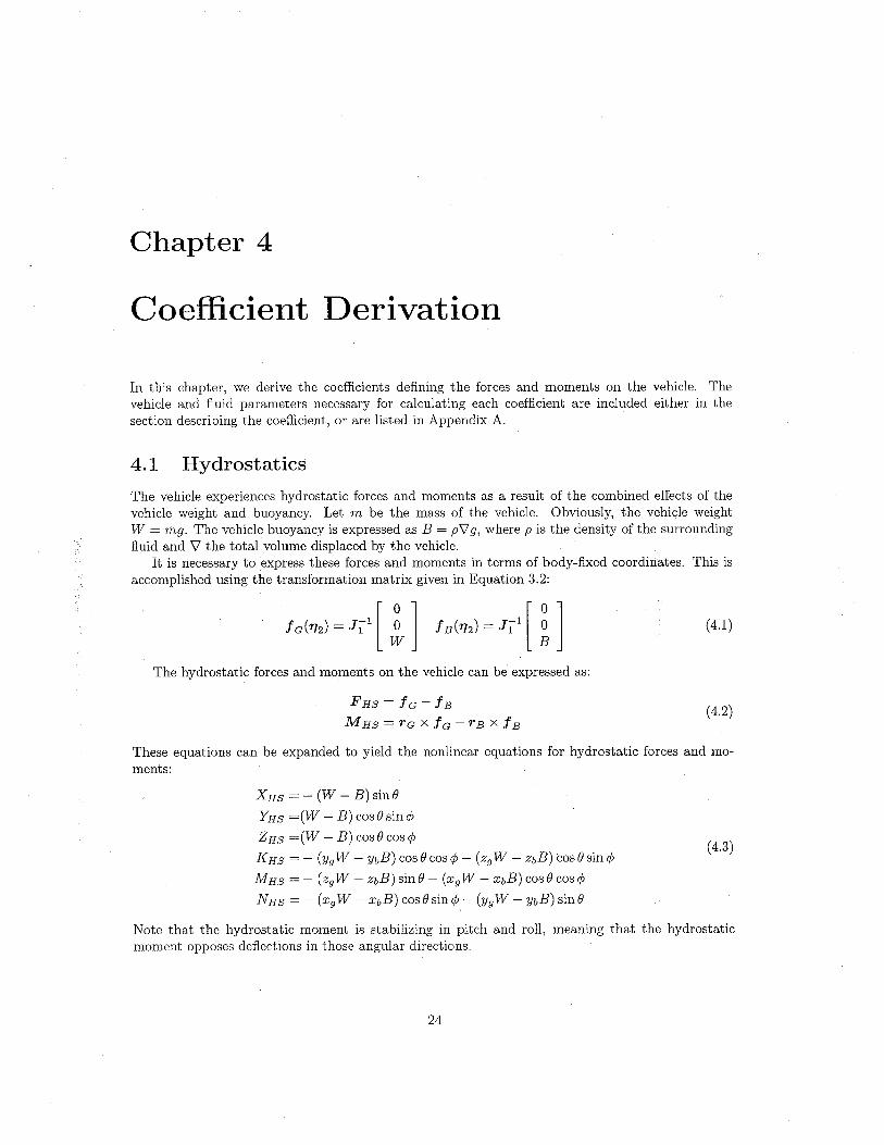
4.1 Hydrostatics

The vehicle experiences hydrostatic forces and moments as a result of the combined effects of thevehicle weight and buoyancy. Let m be the mass of the vehicle. Obviously, the vehicle weightW = mg. The vehicle buoyancy is expressed as B = pY' g, where p is the density of the surroundingfluid and Y' the total volume displaced by the vehicle.

It is necessary to\"xpress these forces and moments in terms of body-fied coordinates. This isaccomplished using the transformation matrix given in Equation 3.2:

fG(~') ~ J,' ¡ ! J fB(~') ~ J,' ¡ i J (4.1)

The hydrostatic forces and moments on the vehicle can be expressed as:

FHs=fe-fBMHs=Texfe-TBXfB (4.2)

These equations can be expanded to yield the nonlinear equations for hydrostatic forces and mo-ments:

XHS = - (W - B) sineYHS =(W - B) cosesinøZHS =(W - B) cos e cos ø

KHS = - (Yg W - YbB) cos ecos ø - (Zg W - ZbB) cose sin ø

MHS = - (Zg W - ZbB) sine - (xg W - XbB) cose cos øNHS = - (xgW - XbB) cosesinø - (ygW - YbB) sine

(4.3)

Note that the hydrostatic moment is stabilizing in pitch and roll, meaning that the hydrostaticmoment opposes deflections in those angular directions.

24

4.2 Hydrodynamic Damping

It is well known that the damping of an underwater vehicle moving at a high speed in six degrees offreedom is coupled and highly non-linear. In order to simplify modeling the vehicle, we wil makethe following assumptions:

· We will neglect linear and angular coupled terms. We wil assume that terms such as Yrv andMrv are relatively small. Calculating these terms is beyond the scope of this work.

· We will assume the vehicle is top-bottom (xy-plane) and port-starboard (xz-plane) symmetric.We wil ignore the vehicle asymmetry caused by the sonar transducer. This allows us to neglectsuch drag-induced moments as Kvlvl and Mulul'

· We will neglect any damping terms greater than second-order. This wil allow us to drop suchhigher-order terms as Yvvv.

The principal components of hydrodynamic damping are skin friction due to boundary layers,which are partially laminar and partially turbulent, and damping due to vortex shedding. Non-dimensional analysis helps us predict the type of flow around the vehicle. Reynolds number representsthe ratio of inertial to viscous forces, and is given by the equation

Re = Ulv (4.4)

where U is the vehicle operating speed, which for REMUS is typically 1.5 m/s (3 knots); i thecharacteristic length, which for REMUS is 1.7 meters; and v the fluid kinematic viscosity, which forseawater at 15°C, Newman ¡24J gives a value of 1.190 x 10-6 m2 Is.

This yields a Reynolds number of 1.3 x 106, which for a body with a smooth surface falls in thetransition zone between laminar and turbulent flow. However, the hull of the REMUS vehicle isbroken up by a number of seams, pockets, and bulges, which more than likely trip the flow aroundthe vehicle into the turbulent regime. We can use this information to estimate the drag coeffcientof the vehicle.

Note that viscous drag always opposes vehicle motion. In order to result in the proper sign, it isnecessary in all equations for drag to consider v Iv I, as opposed to v2.

4.2.1 Axial Drag

Vehicle axial drag can. be expressed by the following empirical relationship:

x = - (~PCdAf) u lul (4.5)

This equation yields the following non-linear axial drag coeffcient:

1Xu1ul = -2'pcdA¡ (4.6)

where P is the density of the surrounding fluid, Af the vehicle frontal area, and Cd the axial dragcoeffcient of the vehicle.

Bottaccini ¡7, p. 26j, Hoerner ¡15, pg. 3-12J and Triantafyllou ¡29J offer empirical formulae for

calculating the axial drag coeffcient. For example, Triantafyllou:

Cd = cs~¡Ap (1 + 60 ( ~) 3 + 0.0025 (~) J ( 4.7)

25

where Css is Schoenherr's value for flat plate skin friction, Ap = ld is the vehicle plan area, and Aiis the vehicle frontal area. From Principles of Naval Architecture l20J, we get an estimate for Css of3.397 x 10-3.

These empirical equations yield a value for Cd in the range of 0.11 to 0.13. Experiments conductedat sea by the Oceanographic Systems Lab measuring the propulsion effciency of the vehicle resultedin an estimate for Cd of 0.2.

Full-scale tow tank measurements of the vehicle axial drag-conducted by the author at theUniversity of Rhode Island and described in Chapter 5-yielded an axial drag coeffcient of 0.27.This higher value reflects the drag of the vehicle hull plus the drag of sources neglected in the

empirical estimate, such as the vehicle fins and sonar transponder, and the pockets in the vehiclenose section. We wil use this higher, experimentally-measured value in the vehicle simulation.

See Table C. 1 for the final value of Xulul'

4.2.2 Crossflow Drag

Vehicle crossflow drag is considered to be the sum of the hull crossflow drag plus the fin crossflowdrag. The method used for calculating the hull drag is analogous to strip theory, the method usedto calculate the hull added mass: the total hull drag is approximated as the sum of the drags on thetwo-dimensional cylindrical vehicle cross-sections.

Slender body theory is a reasonably accurate method for calculating added mass, but for viscousterms it can be off by as much as 100% l29J. This method does, however, allow us to include all of theterms in the equations of motion. In conducting the vehicle simulation, we wil attempt to correctany errors in the crossflow drag terms through comparison with experimental data and observationsof the vehicle at sea.

The nonlinear crossflow drag coeffcients are expressed as follows:

1 rXb2 (1)Yv1vl = Zwlwl = -"2PCde lx, 2R(x)dx - 2. "2pSfinCdf1 ixb2 (1)

Mwlwl = -Nv1vl = "2PCde 2xR(x)dx - 2Xfin' -pSfinCdfx, 21 rXb2 (1)Yrlrl = -Zqlql = -"2PCde lx, 2xlxIR(x)dx - 2Xfin IXfinl' "2 pSfinCdf1 ¡Xb2 (1)Mq1qi = Nr1ri = --PCde 2x3 R(x)dx - 2xïn' -pSfinCdf2 x, 2

(4.8)

where p is the seawater density, Cde the drag coeffcient of a cylinder, R(x) the hull radius as a

function of axial position as given by Equations 2.1 and 2.2, Sfin the control fin planform area, andCdf the crossflow drag coeffcient of the control fins. See Table A.2 for the limits of integration.

Hoerner l15J estimates the crossflow drag coeffcient of a cylinder Cde to be 1.1. The crossflowdrag coeffcient Cdf is derived using the formula developed by Whicker and Fehlner l32J:

Cdf = 0.1 + 0.7t (4.9)

where t is the fin taper ratio, or the ratio of the widths of the top and bottom of the fin along thevehicle long axis. From this formula, we get an estimate for Cdf of 0.56.

See Table C.2 for the final coeffcient values.

26

4.2.3 Rollng Drag

We wil approximate the rollng resistance of the vehicle by assuming that the principle componentcomes from the crossflow drag of the fins.

F = (Yvvjrmean) r~eanP Ipi ( 4.10)

where Yvvj is the fin component of the vehicle crossflow drag coeffcient, and rmean is the mean finheight above the vehicle centerline. This yields the following equation for the vehicle rollng dragcoeffcient:

Kplpl = Yvvjr~ean (4.11)This is at best a rough approximation for the actual value. It would be better to use experimentaldata.

See Table C.3 for the coeffcient value based on this rough approximation.

4.3 Added Mass

Added mass is a measure of the mass of the moving water when the vehicle accelerates. Ideal fluidforces and moments can be expressed by the equations:

Fj = -Uimji - EjklUinkmli

Mj = -Uimj+3,i - EjkIUinkml+3,i - EjklUkUimli

where i = 1,2,3,4,5,6and jkl=I,2,3

( 4.12)

and where the alternating tensor Ejkl is equal to +1 if the indices are in cyclic order (123, 231,312), -1 if the indices are acyclic (132, 213,321), and zero if any pair of the indices are equal. See

Newman ¡24J or Fossen ¡10J for the expansion of these equations.Due to body top-bottom and port-starboard symmetry, the vehicle added mass matrix reduces

to:mll 0 0 0 0 0

0 m22 0 0 0 m260 0 m33 0 m35 0

(4.13)0 0 0 m44 0 00 0 m53 0 m55 00 m62 0 0 0 m66

which is equivalent to:Xu 0 0 0 0 00 Yil 0 0 0 Nil0 0 Zw 0 Mw 0

(4.14)0 0 0 K. 0 0p0 0 Z. 0 M. 0a a0 Y" 0 0 0 N"

Substituting these remaining terms into the expanded equations for fluid forces and moments

27

from Equation 4.12 yields the following equations:

XA = Xu'U + Zwwq + Zqq2 - Yiivr - Yrr2

YA = Yiiv + Y"r + Xuur - Zwwp - ZqpqZA = Zww + Zqg - Xuuq + Yiivp + Y"rpKA = Kpp

MA = Mww + Mqg - (Zw - Xu)uw - Y"vp + (Kp - N" )rp - ZquqNA = Niiv + N"r - (Xu - Yii)uv + Zqwp - (Kp - Mq)pq + Yrur

(4.15)

4.3.1 Axial Added Mass

To estimate axial added mass, we approximate the vehicle hull shape by an ellpsoid for which themajor axis is half the vehicle length I, and the minor axis half the vehicle diameter d. See Figure 2-4for a comparison of the two shapes. Blevins ¡6, p.407J gives the following empirical formula for theaxial added mass of an ellpsoid:

Xu = -mii = - 4a:n (~) (~r ( 4.16)

or

Xu = -mii = _ 4ß:n (~) 3 (4.17)

where p is the density of the surrounding fluid, and a and ß are empirical parameters measured byBlevins and determined by the ratio of the vehicle length to diameter as shown in Table 4.1.

Table 4.1: Axial Added Mass Parameters a and ßlid a ß

0.01 0.63480.1 6.148 0.61480.2 3.008 0.60160.4 1.428 0.57120.6 0.9078 0.54470.8 0.6514 0.52111.0 0.5000 0.50001.5 0.3038 0.45572.0 0.2100 0.42002.5 0.1563 0.39083.0 0.1220 0.36605.0 0.05912 0.29567.0 0.03585 0.2510

10.0 0.02071 0.2071


4.3.2 Crossflow Added Mass

Vehicle added mass is calculated using strip theory on both cylindrical and cruciform hull crosssections. From Newman ¡24J, the added mass per unit length of a single cylindrical slice is given as:

ma(x) = 7rpR(x)2 (4.18)

28

where p is the density of the surrounding fluid, and R(x) the hull radius as a function of axial positionas given by Equations 2.1 and 2.2. The added mass of a circle with fins is given in Blevins ¡6J as:

( 2 2 R(x)4)maj(x) = 7rp afin - R(x) + ~

afin (4.19)

where afin, as defined in Table 2.2, is the maximum height above the centerline of the vehicle fins.Integrating Equations 4.18 and 4.19 over the length of the vehicle, we arrive at the following

equations for crossflow added mass:

¡Xf ¡Xf2 ¡Xb2Yv = -m22 = - ma(x)dx - maj(x)dx - ma(x)dxXt Xf Xf2Zw = -m33 = -m22 = Yv¡Xf ¡Xf2 ¡Xb2Mw = -m53 = xma(x)dx - xmaj(x)dx - xma(x)dxXt Xf Xf2Nv = -m62 = m53 = -MwYr = -m26 = -m62 = NvZe¡ = -m35 = -m53 = Mw

rXfin rXfin2 rXbOW2Me¡ = -m55 = - JXtail x2ma(x)dx - JXfin x2maj(x)dx - JXfin2 x2ma(x)dx

Nr = -m66 = -m55 = Me¡

(4.20)

See Table A.2 for the limits of integration.See Table C.5 for the final coeffcient values.

4.3.3 Rollng Added Mass

To estimate rolling added mass, we wil assume that the relatively smooth sections of the vehicle hulldo not generate any added mass in rolL. We wil also neglect the added mass generated by the sonartransponder and any other small protuberances. Given those assumptions, we need only consider

the hull section containing the vehicle control fins.Blevins ¡6J offers the following empirical formula for the added mass of a rollng circle with fins:

¡Xfin2 2

Kp = - -pa4dxXfin 1T

(4.21 )

where a is the fin height above the vehicle centerline, in this case averaged to be 0.1172 m. SeeTable A.2 for the limits of integration.

See Table C.5 for the final coeffcient value.

4.3.4 Added Mass Cross-terms

The remaining cross-terms result from added mass coupling, and are listed below:

Xwq = Zw

Yur = XuZuq = -Xu

Muwa = -(Zw - Xu)

Nuva = -(Xu - Yv)

Xqq = Ze¡

Ywp = -Zw

Zvp = Yv

Mvp = -Yr

Nwp = Ze¡

Xvr = -YvYpq = -Ze¡

Zrp = Yr

Mrp = (Kp - Nr)Npq = -(Kp - Me¡)

Xrr = -Yr (4.22)

( 4.23)

( 4.24)

( 4.25)

( 4.26)

Muq = -Ze¡

Nur = If

29

The added mass cross-terms Muwa and Nuva are known as the Munk Moment, and relates tothe pure moment experienced by a body at an angle of attack in ideal, inviscid flow.

See Tables C.6, C.7 and C.8 for the final coeffcient values.

4.4 Body LiftVehicle body lift results from the vehicle moving through the water at an angle of attack, causingflow separation and a subsequent drop in pressure along the aft, upper section of the vehicle hulL.This pressure drop is modeled as a point force applied at the center of pressure. As this center ofpressure does not line up with the origin of the vehicle-fixed coordinate system, this force also leadsto a pitching moment about the origin.

In determining the best method for calculating body lift, the author compared three empiricalmethods based on torpedo data ¡7, 9, 16J, and one theoretical method ¡23J. Unfortunately, theestimates for body lift from the four methods ranged over an order of magnitude. Given the lackof agreement between the empirical methods, it would be preferable to base the body lift estimateson actual REMUS data, from perhaps tow tank tests or measurements of the vehicle mounted on arotating arm.

Until that happens, the author decided to use Hoerner's estimates ¡16J, which appeared the mostreliable.

4.4.1 Body Lift ForceTo calculate body lift, we wil use the empirical formula developed by Hoerner ¡16J, which states:

1 2 2Lbody = -"2 pd CydU ( 4.27)

where p is the density of the surrounding fluid, Ap the projected area of the vehicle hull, u thevehicle forward velocity, and Cyd the body lift coeffcient, which by Hoerner's notation is expressedas:

() dCydCyd = Cyd ß = dß ß

where ß is the vehicle angle of attack in radians and is given by the relationship:

(4.28)

wtanß = -

U~ ß~:!

U(4.29)

Hoerner gives the following relationship for lift slope:

dC~d 0 ( I )dßo = cydß = d c~ß ( 4.30)

where I is the vehicle length and d the maximum diameter. Hoerner ¡16, pg. 13-3J states that

Ifor 6.7:: d :: 10, c~ß = 0.003 (4.31)

Note that in Equation 4.30 it is necessary to convert the Hoerner lift slope coeffcients c~dß and c~ßfrom degree to radians. This results in the Hoerner lift slope coeffcient Cydß, defined in terms ofradians as follows:

° (180)Cydß = cydß -- (4.32)

30

Substituting into Equation 4.27 the relationships given above, we are left with the followingequation for vehicle body lift:

1 2Lbody = ~ - pd CydßUW

2

which results in the following body lift coeffcients:

(4.33)

1 . 2Yuvl = Zuwl = - - pd Cydß. 2 (4.34)


4.4.2 Body Lift MomentHoerner estimates that for a body of revolution at an angle of attack, the viscous force is centeredat a point between 0.6 and 0.7 of the total body length from the nose. His experimental findingssuggest that the flow goes smoothly around the forward end of the hull, and that the lateral forceonly develops on the leeward side of the rear half of the hull.

Following these findings, we wil assume that, in body-fixed coordinates:

Xcp = ~0.65l - Xzero ( 4.35)

This results in the following equation for body lift moment:

1 2Muwl = -Nuvl = --pd CydßXcp

2 (4.36)


4.5 Fin LiftThe attitude of the REMUS vehicle is controlled by two horizontal fins, or stern planes, and twovertical fins, or rudders. The pairs of fins move together; in other words the stern planes do notmove independently of each other, nor do the rudder planes.

For the vehicle control fins, the empirical formula for fin lift is given as:

1 2Lfin = 'iPCLSfinfieve

Mfin = XfinLfin( 4.37)

where CL is the fin lift coeffcient, Sfin the fin planform area, fie the effective fin angle in radians, Vethe effective fin velocity, and Xfin the axial position of the fin post in body-referenced coordinates.

Fin lift coeffcient CL is a function of the effective fin angle of attack a. Hoerner ¡16, pg. 3-2Jgives the following empirical formula for fin lift as a function of a in radians:

dCI I 1 1 J -1CLo: = da = l2ei1T + 1T(ARe) (4.38)

where the factor ei was found by Hoerner to be of the order 0.9, and (ARe) is the effective fin aspectratio, which is given by the formula:

ARe = 2(AR) = 2 (~ti) ( 4.39)

31

As the fin is located at some offset from the origin of the vehicle coordinate system, it experiencesthe following effective velocities:

Ufin = U + Zfinq - Yfinr

Vfin = v + Xfinr - ZfinP

Wfin = W + YfinP - Xfina

( 4.40)

where Xfin, Yfin, and Zfin are the body-referenced coordinates of the fin posts. For the REMUSvehicle, we wil drop the terms involving Yfin and Zfin as they are small compared to the vehicle

translational velocities.The effective fin angles ose and Ore can be expressed as

Ore = Or - ßre

ose = Os + ßse(4.41 )

where Os and Or are the fin angles referenced to the vehicle hull, ßse and ßre the effective angles ofattack of the fin zero plane, as shown in Figures 4-1 and 4-2. Assuming small angles, these effectiveangles can be expressed as:

Vfin 1ßre = - ;: - (v + Xfin 1')Ufin U

Wfin 1ßse = -;: - (w - xfinq)Ufin U

( 4.42)

based on Equation 4.40

t-xy

u

L,Vfluid

Figure 4- 1: Effective Rudder Angle of Attack

VII"id~' C

Figure 4-2: Effective Stern Plane Angle of Attack

Substituting the results of Equations 4.40, 4.41 and 4.42 into Equation 4.44 results in the following

32

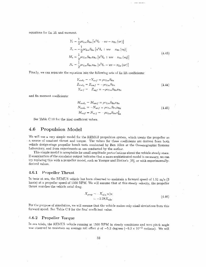
equations for fin lift and moment:

Yr = ~PCL",Sfin (U2Or - UV - Xfin (ur)J2

Zs = -~PCL",Sfin (u2Os + UW - Xfin (uq)J2

Ms = ~PCL",SfinXfin (u2Os + UW - Xfin (uq)J

Nr = ~PCL",SfinXfin (u2Or - UV - Xfin (ur)J

Finally, we can separate the equation into the following sets of fin lift coeffcients:

( 4.43)

YUUÓr = -Yuvj = PCL",Sfin

Zuuós = Zuwj = -PCL",Sfin

Yurj = -Zuqj = -PCL",SfinXfin

(4.44 )

and fin moment coeffcients:

Muuós = Muwj = PCL",SfinXfin

Nuuór = -Nuvj = PCL",SfinXfin

Muqj = Nurj = -PCL",SfinX~n

( 4.45)

See Table C.I0 for the final coeffcient values.

4.6 Propulsion Model

We wil use a very simple model for the REMUS propulsion system, which treats the propeller asa source of constant thrust and torque. The values for these coeffcients are derived from bothvehicle design-stage propeller bench tests conducted by Ben Allen at the Oceanographic SystemsLaboratory, and from experiments at sea conducted by the author.

This simple model is acceptable for small amplitude perturbations about the vehicle steady state.If examination of the simulator output indicates that a more sophisticated model is necessary, we can

try replacing this with a propeller model, such as Yoerger and Slotine's ¡35J, or with experimentally-

derived values.

4.6.1 Propeller Thrust

In tests at sea, the REMUS vehicle has been observed to maintain a forward speed of 1.51 m/s (3knots) at a propeller speed of 1500 RPM. We wil assume that at this steady velocity, the propellerthrust matches the vehicle axial drag.

Xprop = -Xuluiu lul= -2.28Xuiul (4.46)

For the purpose of simulation, we wil assume that the vehicle makes only small deviations from this

forward speed. See Table C.9 for the final coeffcient value.

4.6.2 Propeller Torque

In sea trials, the REMUS vehicle running at 1500 RPM in steady conditions and zero pitch anglewas observed to maintain an average roll offset ø of -5.3 degrees (~9.3 x 10-2 radians). We wil

33

assume that under these conditions, the propeller torque matches the hydrostatic roll moment.

Kprop = -KHS = (ygW - YbB) cosecosq; + (zgW - ZbB) cosesinq;= 0.995(ygW - YbB) - 0.093(zgW - ZbB)

(4.47)

See Table C.9 for the final coeffcient value.

4.7 Combined Terms

Combining like terms from Equations 4.22, 4.34, 4.36, 4.44 and 4.45, we get the following:

Yuv = Yuv1 + Yuvj

Yur = Yura + Yur j

Zuw = Zuwl + Zuwj

Zuq = Zuqa + Zuqj

Muw = Muwa + Muw1 + Muwj

Muq = Muqa + Muqj

Nuv = Nuva + Nuvl + Nuvj

Nur = Nura + Nurj

(4.48 )

4.8 Total Vehicle Forces and Moments

Combining the coeffcient equations for the vehicle

. Hydrostatics: Equation 4.3

e Hydrodynamic Damping: Equations 4.6,4.8 and 4.11

. Added Mass: Equations 4.16, 4.20, 4.21 and 4.22

. Body Lift and Moment: Equations 4.34 and 4.36

. Pin Lift and Moment: Equations 4.44 and 4.45

. Propeller Thrust and Torque: Equations 4.46 and 4.47

34

the sum of the depth-plane forces and moments on the vehicle can be expressed as:

L Xext =XHS + Xu1ulU lul + Xuu + Xwqwq + Xqqaq + Xvrvr + Xrrrr+ Xprop

L Yext =YHS + Yv1vlV ivl + Yr1r1r 11'1 + Y"v + Yrr

+ Yurur + Ywpwp + Ypqpa + Yuvuv + YUUÖr u2Ór

L Zext =ZHS + Zwlwlw iwl + Zqlqla lal + zww + Zi¡q+ Zuquq + Zvpvp + Zrprp + Zuwuw + ZUUÖs u2Ós

LKext =KHS + Kp1plP ¡pi + Kf;,p + Kprop

L Mext =MHS + Mw1w1w Iwl + Mq1q1q Iql + Mww + Mi¡q+ Muquq + Mvpvp + Mrprp + Muwuw + Muuös u2Ós

L Next =NHS + Nv1v1v ivl + Nr1r1r 11'1 + N"v + NTr+ Nurur + Nwpwp + Npqpq + Nuvuv + Nuuör u2Ór

See Tables 4.2 and 4.3 for a list of the non-zero vehicle coeffcients.

Table 4.2: STD REMUS Non-Linear Maneuvering Coeffcients: ForcesParameter

XuuXu

XwqXqqXvrXrr

XpropYvv

YrrYuv

Y"

YT

YurYwp

Ypq

YuudrZww

Zqq

ZuwZwZ.q

ZuqZvpZrp

Zuuds

Value-1.62e+000-9.30e-001-3.55e+001-1.93e+000+3.55e+001-1.93e+000+3.86e+000-1. 31e+002+6.32e-001-2. 86e+00 1

-3.55e+001+1.93e+000+5.22e+000+3.55e+001+1.93e+000+9.64e+000-1. 31e+002-6.32e-001-2. 86e+00 1

-3.55e+001-1.93e+000-5.22e+000-3. 55e+00 1

+1.93e+000-9.64e+000

Unitskg/m

kgkg/rad

kg. m/radkg/rad

kg. m/radN

kg/m2kg. m/rad

kg/mkg

kg. m/radkg/radkg/rad

kg. m/radkg/(m. rad)

kg/mkg. m/rad2

kg/mkg

kg. m/radkg/radkg/radkg/rad

kg/(m. rad)

DescriptionCross-flow DragAdded Mass

Added Mass Cross-termAdded Mass Cross-termAdded Mass Cross-termAdded Mass Cross-termPropeller ThrustCross-flow DragCross-flow DragBody Lift Force and Fin LiftAdded Mass

Added MassAdded Mass Cross Term and Fin LiftAdded Mass Cross-termAdded Mass Cross-termFin Lift Force

Cross- flow DragCross-flow DragBody Lift Force and Fin LiftAdded Mass

Added Mass

Added Mass Cross-term and Fin LiftAdded Mass Cross-termAdded Mass Cross-termFin Lift Force

35

(4.49 )

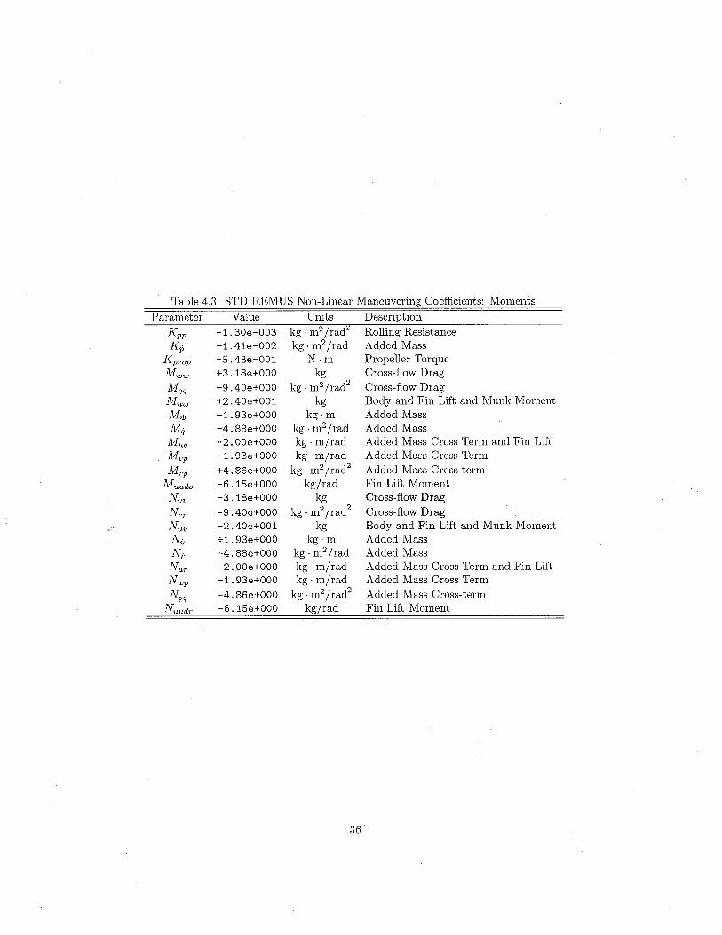
Table 4.3: STD REMUS Non-Linear Maneuvering Coeffcients: MomentsParameter

KppK-p

KpropMww

MqqMuwMwM.qMuqMvp

MrpMuuds

Nvv

NrrNuvNi;NrNurNwp

NpqNuudr

Value-1.30e-003-1.41e-002-5.43e-001+3. 18e+000-9.40e+000+2.40e+001-1.93e+000-4.88e+000-2.00e+000-1.93e+000+4.86e+000-6. 15e+000-3. 18e+000-9.40e+000-2.40e+001+1.93e+000-4 . 88e+000-2.00e+000-1.93e+000-4.86e+000-6. 15e+000

Unitskg. m2/rad:¿

kg. m2/radN'm

kgkg. m2/rad2

kgkg.m

kg. m2/radkg. m/radkg. m/rad

kg. m2/rad2kg/rad

kgkg. m2/rad2

kgkg.m

kg. m2/radkg . m/radkg. m/rad

kg. m2/rad2kg/rad

DescriptionRollng Resistance

Added Mass

Propeller TorqueCross-flow DragCross-flow DragBody and Fin Lift and Munk MomentAdded Mass

Added MassAdded Mass Cross Term and Fin LiftAdded Mass Cross TermAdded Mass Cross-termFin Lift MomentCross-flow DragCross-flow DragBody and Fin Lift and Munk MomentAdded Mass

Added Mass

Added Mass Cross Term and Fin LiftAdded Mass Cross TermAdded Mass Cross-termFin Lift Moment

36

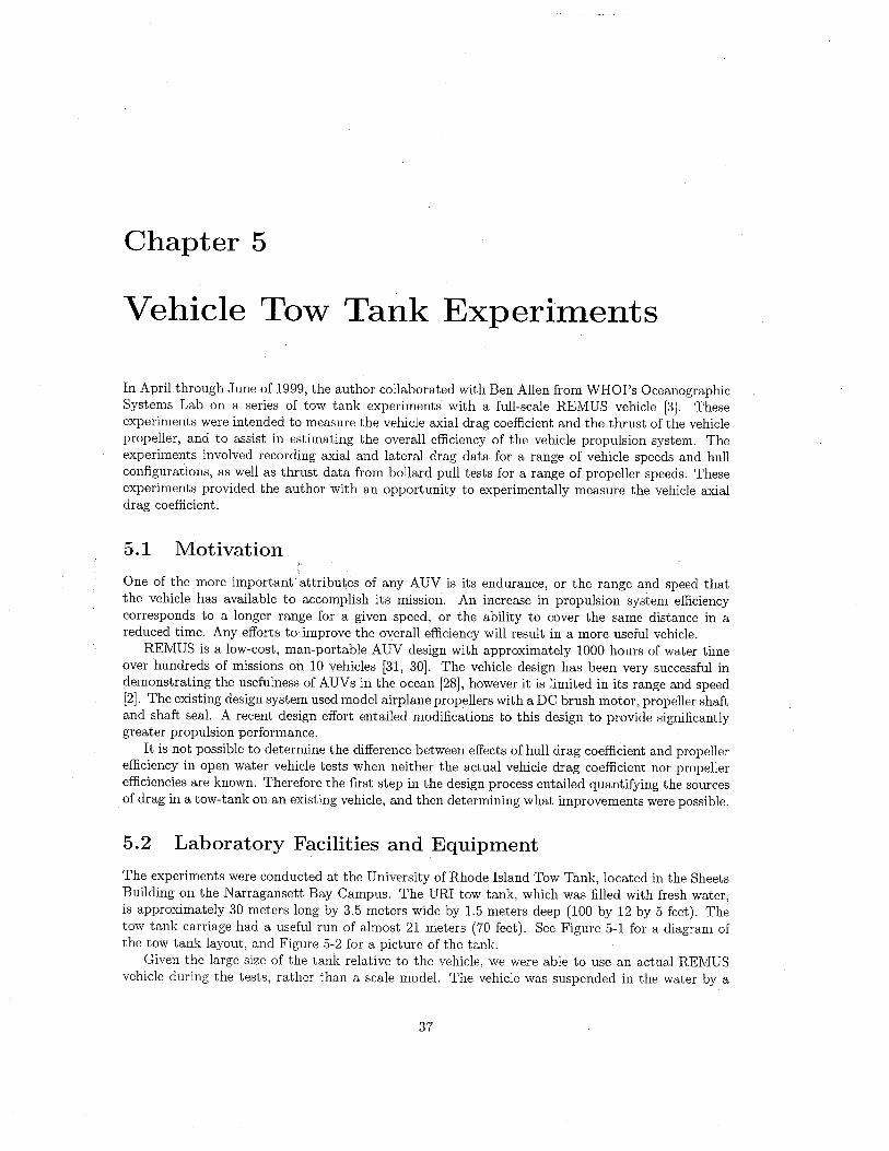
Chapter 5

Vehicle Tow Tank Experiments

In April through June of 1999, the author collaborated with Ben Allen from WHOI's OceanographicSystems Lab on a series of tow tank experiments with a full-scale REMUS vehicle (3J. Theseexperiments were intended to measure the vehicle axial drag coeffcient and the thrust of the vehiclepropeller, and to assist in estimating the overall effciency of the vehicle propulsion system. Theexperiments involved recording axial and lateral drag data for a range of vehicle speeds and hull

configurations, as well as thrust data from bollard pull tests for a range of propeller speeds. Theseexperiments provided the author with an opportunity to experimentally measure the vehicle axialdrag coeffcient.

5.1 Motivation

One of the more importantattributes of any AUV is its endurance, or the range and speed thatthe vehicle has available to accomplish its mission. An increase in propulsion system effciencycorresponds to a longer range for a given speed, or the abilty to cover the same distance in a

reduced time. Any efforts to improve the overall effciency wil result in a more useful vehicle.REMUS is a low-cost, man-portable AUV design with approximately 1000 hours of water time

over hundreds of missions on 10 vehicles (31, 301. The vehicle design has been very successful indemonstrating the usefulness of AUVs in the ocean (281, however it is limited in its range and speed(2J. The existing design system used model airplane propellers with a DC brush motor, propeller shaftand shaft seaL. A recent design effort entailed modifications to this design to provide significantlygreater propulsion performance.

It is not possible to determine the difference between effects of hull drag coeffcient and propellereffciency in open water vehicle tests when neither the actual vehicle drag coeffcient nor propellereffciencies are known. Therefore the first step in the design process entailed quantifying the sourcesof drag in a tow-tank on an existing vehicle, and then determining what improvements were possible.

5.2 Laboratory Facilities and Equipment

The experiments were conducted at the University of Rhode Island Tow Tank, located in the SheetsBuilding on the Narragansett Bay Campus. The URI tow tank, which was filled with fresh water,is approximately 30 meters long by 3.5 meters wide by 1.5 meters deep (100 by 12 by 5 feet). Thetow tank carriage had a useful run of almost 21 meters (70 feet). See Figure 5-1 for a diagram ofthe tow tank layout, and Figure 5-2 for a picture of the tank.

Given the large size of the tank relative to the vehicle, we were able to use an actual REMUSvehicle during the tests, rather than a scale modeL. The vehicle was suspended in the water by a

37

=Laser

Laser target range-finder

J~

Tow tank carriage with ID D I Data Statio~ with carriage Carriage brakeREMUS vehicle suspended

from flexural mountcontrols, strip-chart recorderand DAQ-equipped laptop PC

Figure 5-1: URI Tow Tank Layout

faired strut, which was connected to the towing carriage by the bottom plate of a flexural mount.See Figure 5-3 for a diagram of the carriage setup and vehicle mounting, and Figure 5-4 for a photoof the vehicle on the strut.

5.2.1 Flexural MountThe flexural mount was a box consisting of two parallel, horizontal plates connected by flat verticalsprings. The springs allowed the lower plate to move in the horizontal plane. The motion of platerelative to the carriage was measured with two orthogonally-mounted linear variable differentialtransformers (LVDTs), electromechanical transducers which converted the rectilinear motion of theplate along each horizontal axis into corresponding electrical signals.

The LVDT output signals were amplified and electronically filtered, then transmitted to the datastation where they were plotted on a strip chart recorder and sampled by an analog-to-digital boardconnected to a laptop PC.

We were able to calibrate the axially-mounted LVDT to a significantly greater level of accuracythan the laterally-mounted instrument, due to the poor condition of the latter. As such, we only

'used the laterally-mounted LVDT for gross measurements of lateral drag, as an indicator of strut,yehicle or fin misalignment.

5.2.2 Tow Tank Carriage

The tow tank carriage was a large flat cart with hard rubber wheels driven by an electric motor.Instead of rails, the carriage rolled along the flat tops of the tank walls.

See Figure 5-5 for a picture of the tow tank carriage.The desired carriage speed was set by a rheostat at the data station. A simple motor controller

measured the carriage speed using an encoder wheel and light sensor mounted on the axle of themotor shaft. On forward runs, the carriage was stopped when a protruding trigger switch wasthrown by a flange mounted on the tank walL. On backing up, the cart was stopped only by thealert operators stabbing at the motor kil switch mounted at the data station.

The speed at which we operated the carriage was limited more by the length of the tow tankthan by the torque of the carriage motor. Our maximum speed was roughly 1.5 meters per secondor 3 knots, the operating speed of the vehicle. At that velocity, the strut vibrations generated by

the impulsive start took several seconds to damp out, leaving us with only a few seconds of useful

data before the carriage began decelerating.

The actual carriage speed was measured using a laser range finder mounted at the far end ofthe tank. The range finder, a Nova Ranger NR-I00, did not measure time-of-flight; instead, it wascalibrated to measure distance based on the location of the projected dot. For a given distance, theinstrument output a corresponding voltage.

38

Figure 5-2: URI Tow Tank ¡Photo courtesy of URI Ocean Engineering DepartmentJ

39

Laser TargetTow Tank Carriage

Flexural Pivotwith LVOT

Faired Strut

Mounting Plate withHose Clamps

0.432 m(2.3 diameters)

____ _1_

Figure 5-3: Carriage Setup and Vehicle Mounting

Figure 5-4: URI Tow Tank Carriage

40

Figure 5-5: URI Tow Tank Carriage

The analog range finder signal was transmitted to the data station, where it too was sampledby the laptop PC's analog-to-digital board. Both digital signals were logged with data acquisitionsoftware, then processed with MATLAB.

5;3 Drag Test Experimental Procedure

The drag test experimental procedure involved the following steps:

. LVDT and strut pre-calibration

. vehicle mount and alignment check

. fin alignment check

. vehicle drag runs

. LVDT and strut post-calibration

5.3.1 Instrument Calibration

In calibrating the LVDT, we would apply a range of known loads to the flexural carriage and recordthe output voltage. This was accomplished by hanging weights from a line tied to the aft end of thebottom flexural plate and run over a pulley. Given that there was a small amount of friction in theLVDT shaft, after hanging the weights we would whack the flexural mount and allow the vibrationsto damp out, recording the average steady value after several whacks.

41

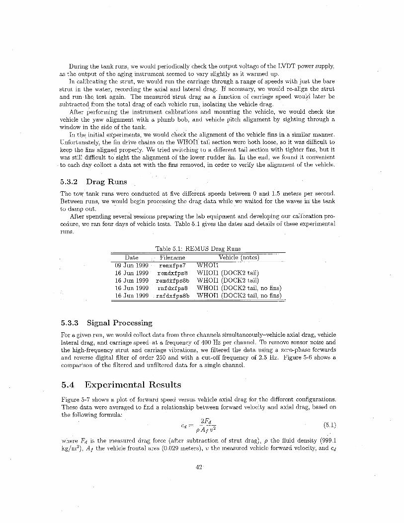
During the tank runs, we would periodically check the output voltage of the LVDT power supply,as the output of the aging instrument seemed to vary slightly as it warmed up.

In calibrating the strut, we would run the carriage through a range of speeds with just the barestrut in the water, recording the axial and lateral drag. If necessary, we would re-align the strut

and run the test again. The measured strut drag as a function of carriage speed would later besubtracted from the total drag of each vehicle run, isolating the vehicle drag.

After performing the instrument calibrations and mounting the vehicle, we would check thevehicle the yaw alignment with a plumb bob, and vehicle pitch alignment by sighting through awindow in the side of the tank.

In the initial experiments, we would check the alignment of the vehicle fins in a similar manner.Unfortunately, the fin drive chains on the WHOIl tail section were both loose, so it was diffcult tokeep the fins aligned properly. We tried switching to a different tail section with tighter fins, but itwas still diffcult to sight the alignment of the lower rudder fin. In the end, we found it convenientto each day collect a data set with the fins removed, in order to verify the alignment of the vehicle.

5.3.2 Drag Runs

The tow tank runs were conducted at five different speeds between 0 and 1.5 meterS per second.Between runs, we would begin processing the drag data while we waited for the waves in the tankto damp out.

After spending several sessions preparing the lab equipment and developing our calibration pro-cedure, we ran four days of vehicle tests. Table 5.1 gives the dates and details of these experimentalruns.

Date09 Jun 1999

16 Jun 1999

16 Jun 1999

16 Jun 1999

16 Jun 1999

Table 5.1: REMUS Drag RunsFilename Vehicle (notes)remxfps7 WHOIlremdxfps8 WHOIl (DOCK2 tail)remdxfps8b WHOIl (DOCK2 tail)rnfdxfps8 WHOIl (DOCK2 tail, no fins)rnfdxfps8b WHOIl (DOCK2 tail, no fins)

5.3.3 Signal Processing

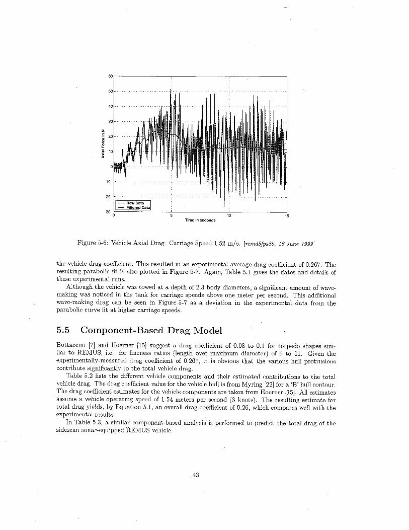
For a given run, we would collect data from three channels simultaneously-vehicle axial drag, vehiclelateral drag, and carriage speed-at a frequency of 400 Hz per channeL. To remove sensor noise andthe high-frequency strut and carriage vibrations, we filtered the data using a zero-phase forwards

and reverse digital filter of order 250 and with a cut-off frequency of 2.5 Hz. Figure 5-6 shows acomparison of the filtered and unfitered data for a single channeL.

5.4 Experimental Results

Figure 5-7 shows a plot of forward speed versus vehicle axial drag for the different configurations.These data were averaged to find a relationship between forward velocity and axial drag, based onthe following formula:

2FdCd = - (5.1)P Ai v2

where Fd is the measured drag force (after subtraction of strut drag), p the fluid density (999.1kg/m3), Ai the vehicle frontal area (0.029 meters), v the measured vehicle forward velocity, and Cd

42

60

10

10 15

20

Time in seconds

Figure 5-6: Vehicle Axial Drag. Carriage Speed 1.52 m/s. ¡remd5fps8b, 16 June 1999J

the vehicle drag coeffcient. This resulted in an experimental average drag coeffcient of 0.267. Theresulting parabolic fit is also plotted in Figure 5-7. Again, Table 5.1 gives the dates and details ofthese experimental runs.

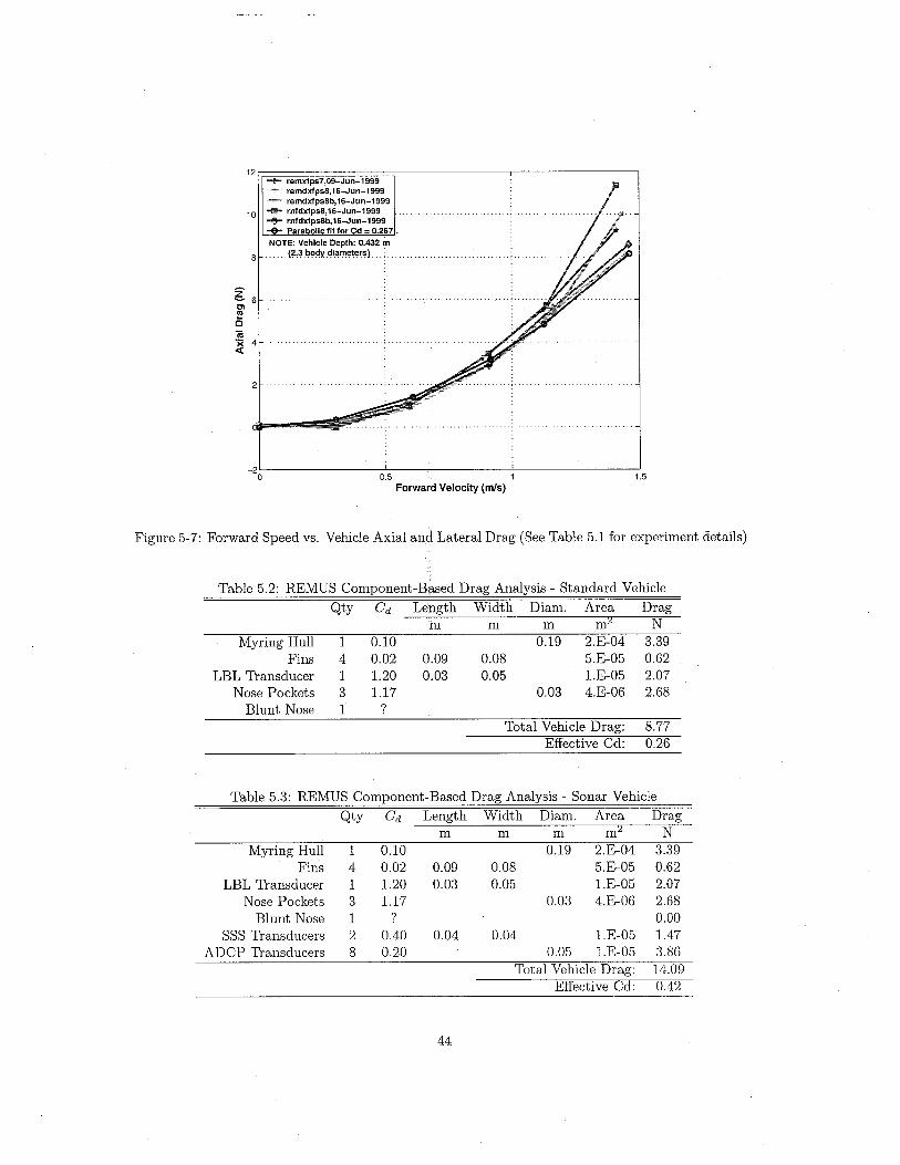
Although the vehicle was towed at a depth of 2.3 body diameters, a significant amount of wave-making was noticed in the tank for carriage speeds above one meter per second. This additionalwave-making drag can be seen in Figure 5-7 as a deviation in the experimental data from theparabolic curve fit at higher carriage speeds.

5.5 Component-Based Drag Model

Bottaccini ¡7j and Hoerner ¡15j suggest a drag coeffcient of 0.08 to 0.1 for torpedo shapes sim-ilar to REMUS, i.e. for fineness ratios (length over maximum diameter) of 6 to 11. Given theexperimentally-measured drag coeffcient of 0.267, it is obvious that the various hull protrusionscontribute significantly to the total vehicle drag.

Table 5.2 lists the different vehicle components and their estimated contributions to the totalvehicle drag. The drag coeffcient value for the vehicle hull is from Myring ¡22j for a 'B' hull contour.The drag coeffcient estimates for the vehicle components are taken from Hoerner ¡15j. All estimatesassume a vehicle operating speed of 1.54 meters per second (3 knots). The resulting estimate fortotal drag yields, by Equation 5.1, an overall drag coeffcient of 0.26, which compares well with theexperimental results.

In Table 5.3, a similar component-based analysis is performed to predict the total drag of thesidescan sonar-equipped REMUS vehicle.

43

2

12-l remxlps7,09-Jun-1999

remdxlps8,16-Jun-1999remdxlps8b,16-Jun-1999

10 .. rnldxlps8,16-Jun-1999-+ rnldxlps8b,16-Jun-1999.. Parabolic lit lor Cd - 0.267 .NOTE: Vehicle Depth: 0.432 in

8 .... (2, .I?!'~y. .di.alTet~rsl.. :

g 6CIos

Cëã'x 4c:

-2o 0.5 1

Forward Velocity (m1s)1.5

Figure 5-7: Forward Speed vs. Vehicle Axial and Lateral Drag (See Table 5.1 for experiment details)

Table 5.2: REMUS Component-Based Drag Analysis - Standard Vehicle

Qty Cd Length Width Diam. Area Dragil m m m4 N

Myring Hull 1 0.10 0.19 2.E-04 3.39Fins 4 0.02 0.09 0.08 5.E-05 0.62

LBL Transducer 1 1.20 0.03 0.05 1.E-05 2.07Nose Pockets 3 1.17 0.03 4.E-06 2.68Blunt Nose 1 ?

Total Vehicle Drag: 8.77Effective Cd: 0.26

Table 5.3: REMUS Component-Based Drag Analysis - Sonar Vehicle

Qty Cd Length Width Diam. Area Dragm m m m4 N

Myring Hull 1 0.10 0.19 2.E-04 3.39Fins 4 0.02 0.09 0.08 5.E-05 0.62

LBL Transducer 1 1.20 0.03 0.05 l.E-05 2.07Nose Pockets 3 1.17 0.03 4.E-06 2.68Blunt Nose 1 ? 0.00

SSS Transducers 2 0.40 0.04 0.04 1.E-05 1.47ADCP Transducers 8 0.20 0.05 I.E-05 3.86

Total Vehicle Drag: 14.09Effective Cd: 0.42

44

Chapter 6

Vehicle Simulation

In this chapter, we begin by completing the equations governing vehicle motion. We then derive anumerical approximation for equations of motion and for the kinematic equations relating motionin the body-fixed coordinate frame to that of the inertial or Earth-fixed reference frame. Finally, weuse that numerical approximation to write a computer simulation of the vehicle motion.

6.1 Combined Nonlinear Equations of MotionCombining the equations for the vehicle rigid-body dynamics (Equation 3.8) with the equationsfor the forces and moments on the vehicle (Equation 4.49), we arrive at the combined nonlinearequations of motion for the REMUS vehicle in six degrees of freedom.

Surge, or translation along the x-axis:

m ¡u - vr + wq - xg(q2 + 1'2) + Yg(pq - r) + Zg(pr + a)) =

XHS + Xu1u1u lul + xuu + Xwqwq + Xqqqq

+ Xvrvr + Xrrrr + Xprop

(6.1)

Sway, or translation along the y-axis:

m ¡v - wp + ur - Yg(r2 + p2) + Zg(qr - p) + xg(qp + r)) =

YHS + Yvlviv ivl + Yririr 11'1 + Y"v + Y"r

+ Yurur + Ywpwp + Ypqpq + Yuvuv + YUUÓr u215r

(6.2)

Heave, or translation along the z-axis:

m ¡w - uq + vp - Zg(p2 + q2) + xg(rp - a) + Yg(rq + p)) =

ZHS + Zwlwlw Iwl+ Zqlqiq Iql + Z1iW + Zqa

+ Zuquq + Zvpvp + Zrprp + Zuwuw + ZUUÓs u215s

(6.3)

Roll, or rotation about the x-axis:

Ixxp + (Izz - 1yy)qr + m ¡Yg(w - uq + vp) - Zg(v - wp + ur)J =

KHS + Kp1plP Ipi + Kpp + Kprop (6.4)

45

Pitch, or rotation about the y-axis:

Iyyq + (Ixx - 1zz)rp + m ¡Zg(u - vr + wq) - xg(w - uq + vp)J =

MHs + Mw1wlw iwl + Mqiqiq Iql + Mww + Mqq

+ Muquq + Mvpvp + Mrprp + Muwuw + Muu¿;s u2Os

(6.5)

Yaw, or rotation about the z-axis:

1zzr + (lyy - 1xx)pq + m ¡xg(v - wp + ur) - Yg(u - vr + wq)J =

NHS + Nvlvlv ivl + Nr1r1r 11'1 + Nvv + N¡.r

+ Nurur + Nwpwp + Npqpq + Nuvuv + Nuu¿;r u2Or

(6.6)

We wil find it convenient to separate the acceleration terms from the other terms in the vehicleequations of motion. The equations can thus be re-written as:

(m - X,,)u + mzgq - mygr = XHS + Xululu lul

+ (Xwq - m)wq + (Xqq + mxg)q2 + (Xvr + m)vr + (Xrr + mxg)r2- mYgpq - mzgpr + Xprop

(m - Yv)v - mzgp + (mxg - Y¡.)r = YHS + Yvlvlv ivl + Yr1r1r 11'1+ mygr2 + (Yur - m)ur + (Ywp + m)wp + (Ypq - mxg)pq

+ Yuvuv + mYgp2 + mzgqr + YUU¿;r u2or

(m - Zw)w + mYgp - (mxg + Zq)q = ZHS + Zwlwiw iwl + Zqlqiq Iql

+ (Zuq + m)uq + (Zvp - m)vp + (Zrp - mxg)rp + Zuwuw+ mzg(p2 + q2) - mygrq + Zuu¿;s u2os (6.7)

- mzgv + mygw + (lxx - Kp)p = KHS + KplplP ¡pi

- (Izz - 1yy)qr + m(uq - vp) - mzg(wp - ur) + Kpropmzgu - (mxg + Mw)w + (lyy - Mq)q = MHS + Mwlwlw iwl + Mqiqiq Iql

+ (Muq - mxg)uq + (Mvp + mxg)vp + ¡Mrp - (Ixx - 1zz)J rp+ mzg(vr - wq) + Muwuw + Muu¿;s u2os

- mygu + (mxg - Nv)v + (Izz - N¡.)r = NHS + Nvlvlv ivl + Nririr 11'1

+ (Nur - mxg)ur + (Nwp + mxg)wp + ¡Npq - (Iyy - 1xx)Jpq- mYg(vr - wq) + Nuvuv + Nuu¿;r u2or

Finally, these equations can be summarized in matrix form as follows:

rmt

a a a mZg -m, i u EX jm-Yv a -mzg a

='(''U ¿Y

a m-Zw mYg -mxg - Zq W ¿z(6.8)-mZg mYg Ixx - Kp a p ¿K

mZg a -mxg - Mw a Iyy - Mq c¡ ¿M-mYg mXg - Nv a a a Izz - Ni- T ¿N

or

U

rmt

a a a mZg -mYg

r¿X

'U m-Yv a -mzg a mXg - Y¡. ¿YW a m-Zw mYg -mxg - Zq a ¿z

(6.9)p -mZg mYg Ixx - Kp a a ¿Kc¡ mZg a -mxg - Mw a Iyy - Mq a ¿MT -mYg mXg - Nv a a a Izz - Ni- ¿N

46

6.2 Numerical Integration of the Equations of MotionThe nonlinear differential equations denning the vehicle accelerations (Equation 6.9) and the kine-matic equations ( Equations 3.1 and 3.4) give us the vehicle accelerations in the different referenceframes. Given the complex and highly non-linear nature of these equations, we wil use numericalintegration to solve for the vehicle speed, position, and attitude in time.

Consider that at each time step, we can express Equation 6.9 as follows:

Xn = f (Xn, un) (6.10)

where x is the vehicle state vector:

X= L U v w p q l' X Y z q; e '1 f (6.11)

and Un is the input vector:Un = L Js Jr Xprop Kprop J T (6.12)

Refer back to Section 3.2 for the definitions of the vehicle states and inputs, and to Figtires 4-1 and4-2 for the fin angle sign conventions.

The following sections summarize three methods of numerical integration in order of increasingaccuracy.

6.2.1 Euler's MethodWe wil first consider Euler's method, a simple numerical approximation which consists of applyingthe iterative formula:

Xn+1 = Xn + f (Xn, un) . ßt (6.13)

where ßt is the modeling time step. Euler's method, although the least computationally intensivemethod, is unacceptable as it can lead to divergent solutions for large time steps.

6.2.2 Improved Euler's MethodThe following method improves the accuracy of Euler's method by averaging the tangent slope fortwo points along the line. We first calculate the following:

ki = Xn + f (Xn, un) . ßtk2 = f (ki, un+i) (6.14)

And then combine them to calculate the new state vector:

ßtXn+1 = Xn + 2 (f (Xn, un) + k2) (6.15)

This method is significantly more accurate than Euler's method.

47

6.2.3 Runge-Kutta Method

This method further improves the accuracy of the approximation by averaging the slope at fourpoints. We first calculate the following:

ki = Xn + f (Xn, un)

k2 = f (x + ~t ki, un+!)

k3 = f (x + ~t k2, un+!)

k4 = f (x + t:tk3, UnH)

(6.16)

where the interpolated input vector

1Un+! = '2 (un + un+i) (6.17)

We combine the above equations to yield:

t:tXnH = Xn + - (ki + 2k2 + 2k3 + k4)

6(6.18)

This method is is the most accurate of the three. This is what we shall use in the vehicle modelcode.

6.3 Computer Simulation

As described in the Introduction, the author implemented this numerical approximation using MAT-LAB. The model code can be seen in Appendix E. The model code works by calculating for eachtime step the forces and moments on the vehicle as a function of vehicle speed and attitude. Theseforces determine the vehicle body-fixed accelerations and earth-relative rates of change. These ac-celerations are then used to approximate the new vehicle velocities, which become the inputs for thenext modeling time step.

The vehicle model requires two inputs:

. Initial conditions, or the starting vehicle state vector.

. Control inputs, or the vehicle pitch fin and stern plane angles, either given as a pre-determinedvector, when comparing the model output with field data, or calculated at each time step, inthe case of control system design.

48

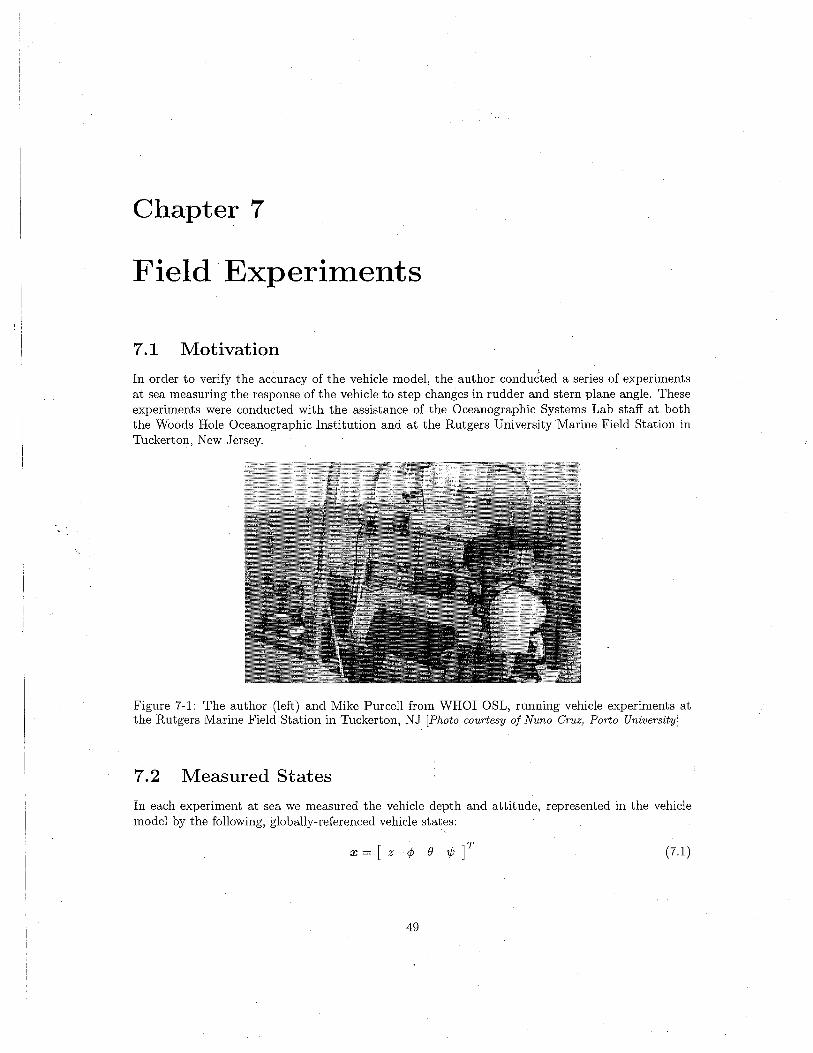
Chapter 7

Field Experiments

7.1 Motivation

In order to verify the accuracy of the vehicle model, the author conducted a series of experimentsat sea measuring the response of the vehicle to step changes in rudder and stern plane angle. Theseexperiments were conducted with the assistance of the Oceanographic Systems Lab staff at boththe Woods Hole Oceanographic Institution and at the Rutgers University Marine Field Station inTUckerton, New Jersey.

Figure 7-1: The author (left) and Mike Purcell from WHOI OSL, running vehicle experiments atthe Rutgers Marine Field Station in TUckerton, NJ ¡Photo courtesy of Nuno Cruz, Pono UniversityJ

7.2 Measured States

In each experiment at sea we measured the vehicle depth and attitude, represented in the vehiclemodel by the following, globally-referenced vehicle states:

x = ¡ z rP e 1/ JT (7.1)

49

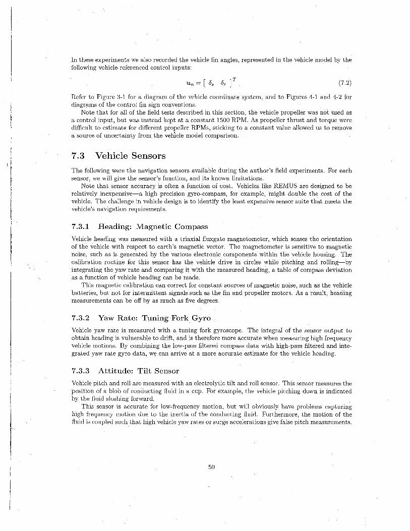
In these experiments we also recorded the vehicle fin angles, represented in the vehicle model by thefollowing vehicle-referenced control inputs:

Un = ¡ Os Or f (7.2)

Refer to Figure 3-1 for a diagram of the vehicle coordinate system, and to Figures 4-1 and 4-2 fordiagrams of the control fin sign conventions.

Note that for all of the field tests described in this section, the vehicle propeller was not used asa control input, but was instead kept at a constant 1500 RPM. As propeller thrust and torque werediffcult to estimate for different propeller RPMs, sticking to a constant value allowed us to removea source of uncertainty from the vehicle model comparison.

7. 3 Vehicle SensorsThe following were the navigation sensors available during the author's field experiments. For eachsensor, we wil give the sensor's function, and its known limitations.

Note that sensor accuracy is often a function of cost. Vehicles like REMUS are designed to berelatively inexpensive-a high precision gyro-compass, for example, might double the cost of thevehicle. The challenge in vehicle design is to identify the least expensive sensor suite that meets thevehicle's navigation requirements.

7.3.1 Heading: Magnetic Compass

Vehicle heading was measured with a triaxial fluxgate magnetometer, which senses the orientationof the vehicle with respect to earth's magnetic vector. The magnetometer is sensitive to magneticnoise, such as is generated by the various electronic components within the vehicle housing. Thecalibration routine for this sensor has the vehicle drive in circles while pitching and rolling-byintegrating the yaw rate and comparing it with the measured heading, a table of compass deviationas a function of vehicle heading can be made.

This magnetic calibration can correct for constant sources of magnetic noise, such as the vehiclebatteries, but not for intermittent signals such as the fin and propeller motors. As a result, headingmeasurements can be off by as much as five degrees.

7.3.2 Yaw Rate: Tuning Fork Gyro

Vehicle yaw rate is measured with a tuning fork gyroscope. The integral of the sensor output toobtain heading is vulnerable to drift, and is therefore more accurate when measuring high frequencyvehicle motions. By combining the low-pass filtered compass data with high-pass filtered and inte-grated yaw rate gyro data, we can arrive at a more accurate estimate for the vehicle heading.

7.3.3 Attitude: Tilt Sensor

t

Vehicle pitch and roll are measured with an electrolytic tilt and roll sensor. This sensor measures theposition of a blob of conducting fluid in a cup. For example, the vehicle pitching down is indicatedby the fluid sloshing forward.

This sensor is accurate for low-frequency motion, but will obviously have problems capturinghigh frequency motion due to the inertia of the conducting fluid. Furthermore, the motion of thefluid is coupled such that high vehicle yaw rates or surge accelerations give false pitch measurements.

50

7.3.4 Depth: Pressure Sensor

The vehicle depth is measured by a pressure sensor. This instrument is somewhat sensitive tochanges in the surrounding sea water temperature, but its errors are small in magnitude relative tothe error in the compass and attitude sensors.

7.4 Experimental Procedure

In this section, we describe the procedure used in the field experiment listed in Table 7.1. Theseexperiments were run in roughly ten meters of water, both in Hadley's Cove near the Woods HoleOceanographic Institution, and off the Atlantic coast near the Rutgers Marine Field Station inRutgers, New Jersey.

Date29 Jul 1998

29 Jul 1998

27 Oct 1998

28 Oct 1998

26 Jul 1999

27 Jul 1999

Table 7.1: Vehicle Field ExperimentsFilename Vehicled980729a STD REMUS (Dockl)d980729b STD REMUS (Dockl)d981027 STD REMUS (Dockl)d981028 STD REMUS (Dockl)a990726 NSW REMUS (NSW)a990727 NSW REMUS (NSW)

LocationRUMFSRUMFSHadley'sHadley'sRUMFSRUMFS

7.4.1 Pre-launch Check List

Before each mission, the author ran through the checklist shown in Figure 7-2 to check the vehiclehousing seals, and to verify operation of the vehicle sensors and communications.

7.4.2 Trim and Ballast Check

Following the pre-launch checklist, the author weighted the vehicle and measured the longitudinalcenter of gravity, xcg, on a balance. The vehicle buoyancy was measured in a sea water tank, andthe vehicle ballast adjusted to achieve 1.5 pounds of positive buoyancy as described in Section 2A

7.4.3 Vehicle Mission ProgrammingThe REMUS vehicle uses a component-based mission programming architecture. Each elementin the mission is called an objective. The following types of objectives were used in the thesis

experiments:

· SET POSITION: This command gives the vehicle its starting position as a range and bearingfrom a given latitude and longitude.

· WAIT PROP: This command tells the vehicle to remain on standby until it detects the givenpropeller RPM. This allows us to start the vehicle mission by reaching into the water andspinning the vehicle propeller. The mission program starts, the propeller starts spinning onits own, we push the vehicle underwater and it is on its way.

· LONG BASELINE: This command tells the vehicle to navigate to the given latitude and longitude,using the given transponder beacons. In this mode, the vehicle uses long baseline navigation,dead-reckoning its position between acoustic fixes. See Roger Stokey's paper ¡28J for detailson REMUS navigation.

51

THESIS EXPERIMENT PRE-lAUNCH OlECKtlST

DUE:

MISSION:

OPERATOR:

M ISSIONOBJ B:TIVÉ:

REMUS: HOUSING OPEN

(J \Hicle en sme ¡:r.D Check MU aig- mant in rrinng I:ckE.

(J ~i;n b;;ry side to rroo on chæ:sis=au heles.

(J. Check Si s' Cf chasss bird.ÌTe oonril- rrin1ing ¡:at.

D Check ltullJseri3land pOO€! oonrecns, 1iewr.p oorrassseralo)nri.

(J Check MU c~ssC3lbraCf

AS ai corirds.tl'ugi senal detiJg:h: - ckiar. h3' roncai!:abn"nal' stp$ p:lirg .'cc' cl:aÍ5 cCfss cal'resrt' - resla; oorr=

o Check MIJ O¡:r.Cf h heæhg, ¡:h, and rel

(; rrass li;ht GREEN?

o Check Wscmr ~k.ûp ætEfvdge. Rè¡:aæ if ~e=ry.

D Check rom ard ard.¡¡ O.nrq fCl- rH-s, ILbmae if rp-esay.

(J l-b Ai:1ail sectbn:

REMUS: HOUSING CLOSE(i

o Check rrcbody housirg fff aid ard ¡¡ fu phèt-dO-rigs

0' ~ sure 1hat eld 1il:s h¡¡,,I,,beff ~ICIde: 'and arol-va.(èl~eC:ierrs.rl(:cp.daC\s.datk

ÓJ mssicn'rissbn ri

~do,tr:.,s~iCflfli;tSon.rtC\;,adoJ) ""rrs v iniQajcpto -

D fet ban/t~'Pe h rEm _ v.hi 1i1:IJe3" b;;ry if nav Cl- frh charge

D Check ¡:esure g;lle: shOJld have\ifide athi:e' l:.3lrn

(J Check 1ha CTD daa rrs sens in ;¡r:

(;nd: Terr: Prss:(J R!c((d ooriass ~iÍh and rel ooe1:

Plch:

D Check.A P cperaCfLin rorlrnsrsion ~ngsEherrbles !:if( colecte: in text w hdcui .

I (J Check æouslbs on bffch.l.cçm dag-oslbs in rrsbn 1ile.Se rerr (r.g€! IftoTAAI£PONDimeAacètí fto 2 ii)hes a:31 . ..Chick ru

SINAtt

Pe;; ~ 23.000Ti. RANGffoff. \,tri3lnua((drc bÔ¡;I:OJ) 26.CO mrht A TS di"lnCGcs back olI Ctrrsbrí'1il:.

o \kri R8iUS r3"g€! O¡:raCf on 5 s€!Cfds.

\kri RÉMUS r3"g€! aooft.

t.13ke'sù'tl' pmp iscl:ar,tl- serd1i'1 pirgs

o Set cEar:¡ to maXÍnLm hrEmu~u!ini

Se "le ewy nth sts mg" = 1

(J Check Çih ard rí.d€!1in aigff.

R!c((d oo~ fr rerrs j iní

Ridær:Plch:

f'r.m LOCATION1iI:.

Trfle ct-èk all bu:y LA T/LO m,l¡e 3n are ot Òfæ¡ andaw ay lEe 1he -re Btobng 1~:3Cf i\dbatd in theLOCÂTIO N INFO pull dOO n.

f'r.mMISS.IJN1i1:

Check rrssicn ushg Fl UTE I.t- O.

\kri D8'TH, (ktnce and FPMf(( each I:g

\kritcta tire of rrsbn.(J Oe3" al taut massages.

DD

i:D

REST ART ve ticle.

a-ieck 1ha alights are GR EEt.i

R!ad ami falt J1s"les 1hat ap¡:3".

o Check æteryvclge byMring Ct~m31 iXers~ph/.

Sloijd be ?: 24 \,fil.R!cO:l-d æt€l/lJge:

Figure 7-2: REMUS Pre-Launch Checklist (Page One)

52

· TIMER: This command tells the vehicle to maintain the given depth or heading using feed-back control, or to maintain a given, fixed fin angle or propeller RPM. The timer commandsrepresent the experimental sections of each mission.

These objectives are edited and sent to the vehicle as a text files. See Appendix F for an examplemission file.

In order to measure the vehicle response to step changes in fin angle, the vehicle was given thefollowing commands:

· Timer to desired depth For "pitch up", the vehicle was commanded to six meters depth, toavoid breaking the surface. For "pitch down" commands, the vehicle was commanded to 2meters depth.

· Step change in fin angle Upon achieving depth, the vehicle was commanded to hold a certainfin angle for two seconds in the case of vertical plane response, or longer for horizontal planeresponse.

The fin angle duration of two seconds was chosen as a result of the experimental run shown inFigure 7-3. In the depth plot right around the seven-second mark, you can see that the vehicle raninto and bounced off the bottom. Given the unpredictable vehicle open-loop response, the authorthought it wise to use short periods.

7.4.4 Compass CalibrationAs described in Section 7.3.1, it was periodically necessary to update the vehicle compass calibration.The compass calibration objective could be included at the start of any mission file.

7.4.5 Vehicle Tracking

During the mission, the vehicle was tracked using a sonar transponder. See Figure 7-5 for a photoof the tracking equipment.

At the end of the mission, the vehicle would be recovered from the surface, and reprogrammedand relaunched if necessary.

7.5 Experimental Results

From these vehicle experiments, we get measurements for the vehicle response to temporary stepchanges in rudder and stern plane angle. It is important to note that during straight and level flight,the vehicle operates at a roll offset of negative five degrees (cP = -5) due to the propeller torque. Asa result, we never get pure vertical- or horizontal-plane motion. That said, the vehicle roll is smallenough that we are stil able identify the vehicle behavior in pitch and yaw.

See Figure 7-6 for REMUS motion while operating under closed-loop control, for comparisonwith the open-loop, step response data. In the example shown, the vehicle was commanded tomaintain a depth of two meters.

7.5.1 Horizontal-Plane Dynamics

The vehicle response to a step change in rudder angle is shown in Figure 7-7. For the objective shown,the rudder fin was fixed at four degrees, and the vehicle was commanded to maintain constant depththrough closed-loop control.

The relevant information in this set of plots is that, for a rudder angle (or) of roughly fourdegrees, the vehicle yaw rate was approximately 10 degrees/second.

53

Fin Angles vs. Time

W 20'"

~ 15'":s

Figure 7-3: REMUS Mission Data: Vehicle bounces off the bottom ¡d980729a, Dbj. 6j

54

Figure 7-4: Launching and recovering the REMUS vehicle. ¡Photo courtesy of Rob Goldsborough, WHO!

08LJ

Figure 7-5: The REMUS Ranger

7.5.2 Vertical-Plane Dynamics

Figures 7-8 and 7-9 show the vehicle response to different temporary step changes in fin angle. Inboth cases, the vehicle was operating under closed-loop depth control until the step change commandwas given. The time scale on each plot has been shifted such that the step change command occursat time t = 2 seconds.

In Figure 7-8, the vehicle pitch fin (stern plane) angle D8 was fixed at negative two degrees. Thevehicle is seen to rise roughly 0.5 meters, and that the pitch change is roughly 20 degrees. At theend of the interval, both the depth and pitch rates were increasing. The vehicle is show to have aslightly negative depth rate (rising at roughly 0.5 meters per second) at the instant of the fin stepchange.

In Figure 7-9, the vehicle pitch fin angle D8 was fixed at eight degrees. The vehicle is seen to diveroughly 0.4 meters, and the pitch change is roughly 18 degrees. Again, at the end of the interval,both the depth and pitch rates were increasing.

Also in Figure 7-9, the vehicle is shown to require a fin angle of positive four degrees in orderto maintain a constant depth in the first two seconds. This suggests that the vehicle was ballastedslightly nose-down. This may be due to internal ballast weights shifting during the launch of thevehicle.

Despite the fact that the vehicle was operating under closed-loop heading control at all times,you wil notice some heading drift in the data. It is not clear whether this reflects actual vehiclemotion, or instrument error.

55

Fin Angies vs. Time

êi 2Q)Q)OiQ)~

0E -30Ü -4

0 5 10 15 20 25

Vehicle Depth vs. Time-0.1

1.~.d~Pthl.'~Q)ãí -0.05

SQ)'"c'".cÜ.c 0.0515Q)0

0.10 5 10 15 20 25

Vehicle Yaw VS. Time10

ûìQ)Q)OiQ)~'"'")-Q)ëi:ëQ)).

-50 5 10 15 20 25

Vehicle Pitch and Roll vs. Time...........êiQ)Q)OiQ)~0a:'0c'"

..c.tl -1D.

-20 5 10 15 20 25

Time (seconds)

Figure 7-6: REMUS Mission Data: Vehicle under closed-loop control. ld990'l2'l, Obj. 4J

56

Cñ 6'"'"Oi'" 4~'"c;c'"cü:

ecoÜ -2

o

Fin Angles vs. Time

"',"""',"":"..'i~'¡.,."":~,,*,,w,.w..,,,,¡4"''':'¡~~~,..,~~-"...

0.5 1.5 2 2.5 3 3.5 4 4.5 5

oVehicle Depth vs. Time

Cñ

20.02'"E'ä 0.04tncoi

B 0.06.cg- 0.08o

... .1 ~'d~pih'l

0.1o 0.5 1.5 2 2.5 3 3.5 4 4.5 5

Vehicle Yaw vs. Timeo

~ -10~gi -20~~ -30)-~ -40:e~ -50

-60o 0.5 1.5 2 2.5 3 3.5

Vehicle t):ii ~~Jo~gins. Time

4 4.5 5

oCñæ -1Oi

:2 -2~ -3'0æ -4.c..g -5ci

0.5 1.5 2 2.5 3Time (seconds)

3.5 4 4.5 5-6

o

Figure 7-7: REMUS Mission Data: Step change in rudder angle. ¡d981028, Obj. 25J

57

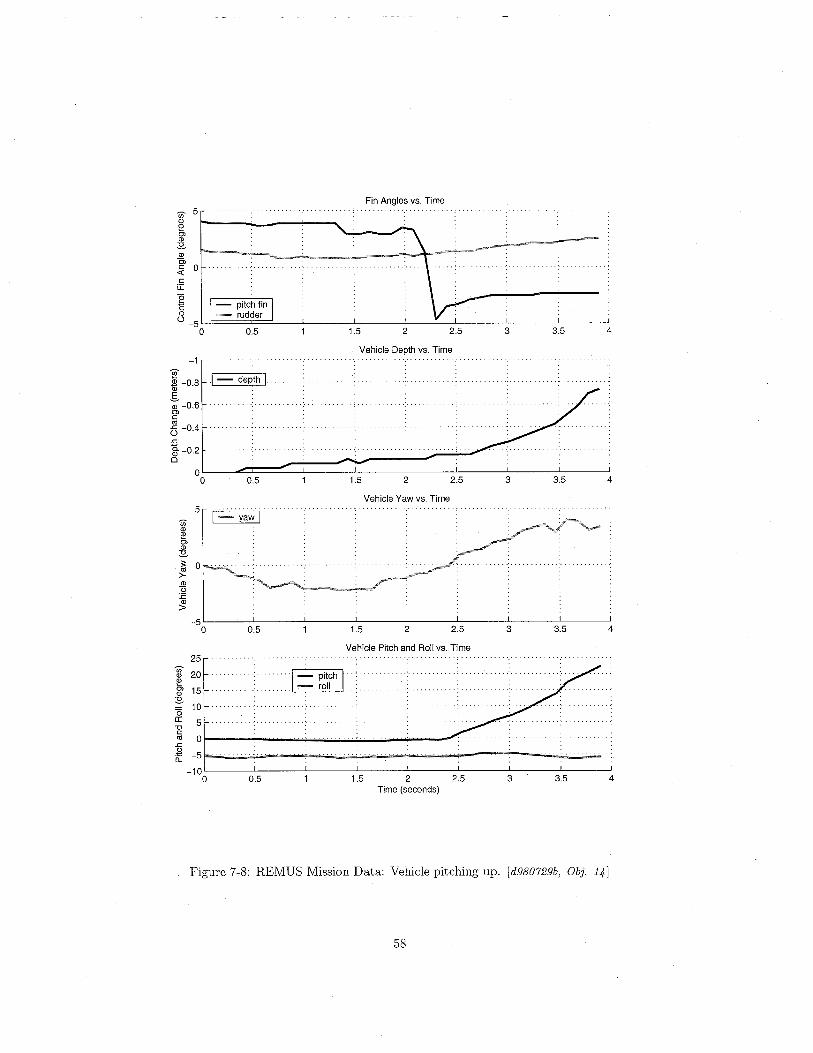
Figure 7-8: REMUS Mission Data: Vehicle pitching up. ¡d980729b, Dbj. 14J

58

Figure 7-9: REMUS Mission Data: Vehicle pitching down. ¡d980'l29b, Obj. 22J

59

Chapter 8

Comparisons of Simulator Outputand Experimental Data

In this chapter, we wil compare the simulator output with the vehicle response data described inChapter 7. We discuss the discrepancies between the two data sets, and the coeffcient adjustmentsused to correct for them.

8.1 Model Preparation

The model was given initial conditions and fin inputs matching the experimental data. Early modelcomparisons lead the author to adjust some of the vehicle coeffcients.

8.1.1 Initial Conditions

Each run of the model was given the following initial conditions:

Table 8.1: REMUS Simulator Initial ConditionsParameter Value Units Description

Zg +1. 96e-002 m vertical center of gravityu +1.54e+000 m/s Forward velocitycj -5. OOe+OOO deg Roll Angle

-The forward velocity of 1.54 m/s (3 knots) is the operating speed of the vehicle at a propellerRPM of 1500. The initial roll angle is the experimentally-measured steady-state roll offset due topropeller torque.

The remaining angles, angular rates, and velocities were entered as zero. Although vehicle ratesand velocities were not measured directly in the experiments, it is assumed that they were small.

8.1.2 Coeffcient Adjustments

The author found it necessary to adjust a subset of the vehicle coeffcients derived in Chapter 4 bythe factors listed below in Table 8.2.

These adjustments were based on comparisons with the experimental data, and were not entirelyunexpected. The methods used in Sections 4.2.3 and 4.3.3 to calculate rolling resistance had ahigh degree of uncertainty. More accurate methods to calculate this rollng resistance and added

60

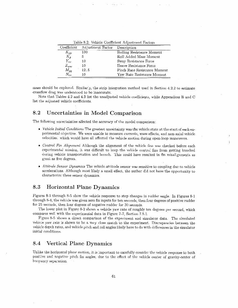
Table 8.2: Vehicle Coeffcient Adjustment FactorsCoeffcient Adjustment Factor Description

Kpp 100 Rollng Resistance MomentKp 5 Roll Added Mass MomentYvv 10 Sway Resistance ForceZww 10 Heave Resistance ForceMqq 12.5 Pitch Rate Resistance MomentNrr 10 Yaw Rate Resistance Moment

mass should be explored. Similarly, the strip integration method used in Section 4.2.2 to estimatecrossflow drag was understood to be inaccurate.

Note that Tables 4.2 and 4.3 list the unadjusted vehicle coeffcients, while Appendices Band Clist the adjusted vehicle coeffcients.

8.2 Uncertainties in Model ComparisonThe following uncertainties affected the accuracy of the model comparison:

. Vehicle Initial Conditions The greatest uncertainty was the vehicle state at the start of each ex-perimentalobjective. We were unable to measure currents, wave effects, and non-axial vehiclevelocities. which would have all affected the vehicle motion during open-loop maneuvers.

. Control Pin Alignment Although the alignment of the vehicle fins was checked before eachexperimental mission, it was diffcult to keep the vehicle control fins from getting knockedduring vehicle transportation and launch. This could have resulted in fin misalignments as

great as five degrees.

. Attitude Sensor Dynamics The vehicle attitude sensor was sensitive to coupling due to vehicleaccelerations. Although most likely a small effect, the author did not have the opportunity tocharacterize these sensor dynamics.

8.3 Horizontal Plane Dynamics

Figures 8- 1 through 8-5 show the vehicle response to step changes in rudder angle. In Figures 8- 1through 8-4, the vehicle was given zero fin inputs for ten seconds, then four degrees of positive rudderfor 25 seconds, then four degrees of negative rudder for 30 seconds.

The lower plot in Figure 8-2 shows a vehicle yaw rate of roughly ten degrees per second, whichcompares well with the experimental data in Figure 7-7, Section 7.5.I.

Figure 8-5 shows a direct comparison of the experiment and simulator data. The simulatedvehicle yaw rate is shown to be a very close match to the experiment. Discrepancies between thevehicle depth rates, and vehicle pitch and roll angles likely have to do with differences in the simulatorinitial conditions.

8.4 Vertical Plane Dynamics

Unlike the horizontal plane motion, it is important to carefully consider the vehicle response to bothpositive and negative pitch fin angles, due to the effect of the vehicle center of gravity-center ofbuoyancy separation.

61

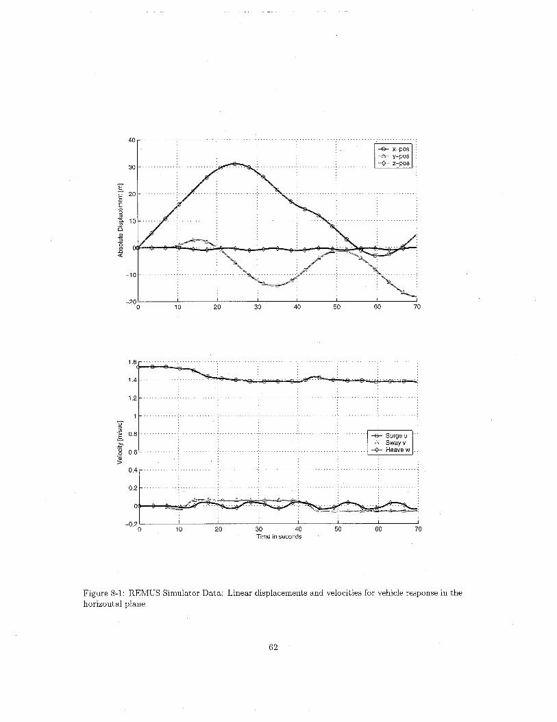
40

ëCDECDü'"ëi(JoCD:;o(J.0-i

I

10 20 30 40 50 60 70

1.6

1.4

1.2

ÜCDi 0.8

.i'13 0.60ID~

0.4

0.2

~&

-0.2o 10 20 30 40

Time in seconds50 60 70

Figure 8-1: REMUS Simulator Data: Linear displacements and velocities for vehicle response in thehorizontal plane

62

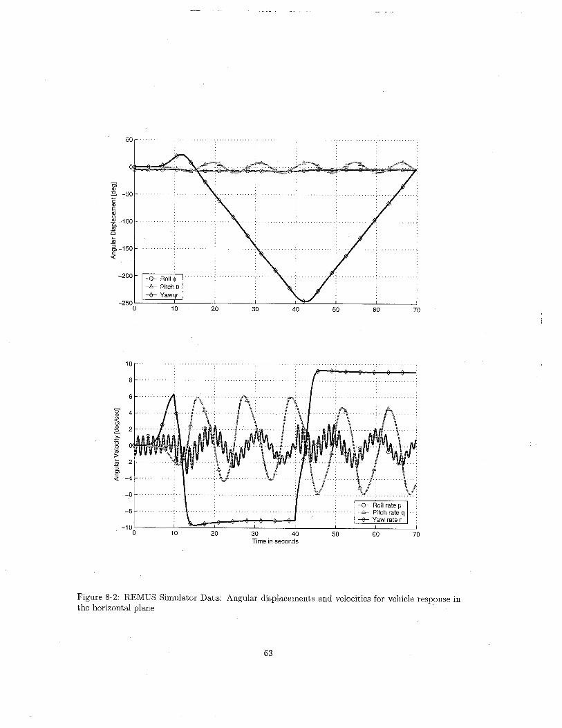
50

-200

10 20 30 40 50 60 70

OìOJ~ -50ëOJEOJüt -100U)ëi(¡

g, -150c:..

10

üOJ~Q)OJ~.i'(3om~(¡'SQ)c:..

10 20 30 40Time in seconds

50 60 70

Figure 8-2: REMUS Simulator Data: Angular displacements and velocities for vehicle response inthe horizontal plane

63

4

3 . (;".. -e X

-,¿'s Y .....,..~z .:

~UlQ)()isLLQ)Ü:eQ):;

-3a 10 20 30 40 50 60 70

1.5 ..~..: -e K ..: -8.... M :. .:. ~N .:

E 0.5kUlëQ)Eo:2Q)Ü:e~ -0.5

-1

-1.5a 10 20 30 40

Time in seconds50 60 70

Figure 8-3: REMUS Simulator Data: Forces and moments for vehicle response in the horizontalplane

64

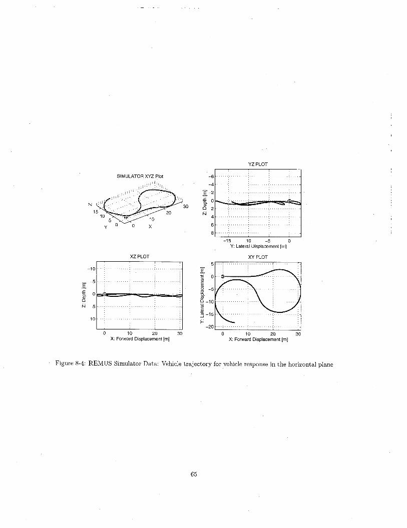
YZ PLOT

SIMULATOR XYZ Plot -6-4

I-2.L 0ë.N 30 Q)0 2N

4

0 6

8

-15 -10 -5 0Y: Lateral Displacement (mj

XZ PLOT XY PLOT

5-10 I

ë 0-5 Q)

I EQ)Ü

.L coë. 0 -aQ) '"0 is -10N 5 ~

Q)j -15

10 :;-20

0 10 20 30 0 10 20 30X: Forward Displacement (m) X: Forward Displacement (m)

Figure 8-4: REMUS Simulator Data: Vehicle trajectory for vehicle response in the horizontal plane

65

-1'è:;1D -0.5.SOlOl

0 _..........,;. ~.c " '-. " ._,..,_._.'".cÜ.c 0.5ã.Ol0

10 0.5 1.5 2 2.5 3 3.5 4 4.5 5

20

'èOlOl0,Ol:E;: -20'")-Olü -40:EOl;:

-600 0.5 1.5 2 2.5 3 3.5 4 4.5 5

20

'è 10Olil0,Ol 0:E .-._....-._..c.Bö: -10

-200 0.5 1.5 2 2.5 3 3.5 4 4.5 5

Vehicle Pitch and Roll YS. Time0

-2'è .'- .;. /:'Ol ...-Ol -4 ./. ........':,:. ".J' -' .- '- ;:-._, - :.....:-...~...~.. .::,....0,Ol:E -60a:

-8

-100 0.5 1.5 2 2.5 3 3.5 4 4.5 5

Time (seconds)

Figure 8-5: REMUS Simulator Data: Comparison plots for vehicle response in the yaw plane

66

8.4.1 Vehicle Pitching Up

Figures 8-6 through 8-10 show the vehicle response to a step change in pitch fin angle. As shown

in Figure 8-10, the vehicle was given zero fin inputs for two seconds, then four degrees of negative

pitch fin for two seconds.Figure 8-10 shows a vehicle depth change of roughly 0.5 meters and a pitch change of twenty

degrees, which both compare well with the experimental data in Figure 7-8, Section 7.5.2.

8.4.2 Vehicle Pitching DownFigures 8-11 through 8-15 show the vehicle response to a step change in pitch fin angle. As shownin Figure 8-15, the vehicle was given zero fin inputs for two seconds, then eight degrees of positivepitch fin for two seconds.

Figure 8-15 shows a vehicle depth change of roughly 0.6 meters and a pitch change of thirtydegrees, which both compare well with the experimental data in Figure 7-9, Section 7.5.2. Themodel pitch rate is slightly higher than the experimental data, but this could be due a difference ininitial conditions.

67

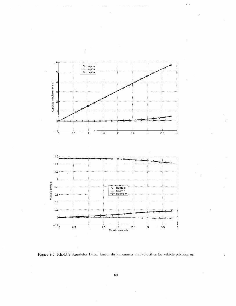
6

5

I 4

ëQlEQl 3u'"a.UJis

2Ql:;0UJ.0.i

-1o 0.5 1.5 2 2.5 3 3.5 4

1.6

1.4

1.2

0'Qli 0.8

~ë3 0.60a;~

0.4

0.2

-0.2o

. . . . . ~.

0.5 1.5 2 2.5Time in seconds

3 3.5 4

Figure 8-6: REMUS Simulator Data: Linear displacements and velocities for vehicle pitching up

68

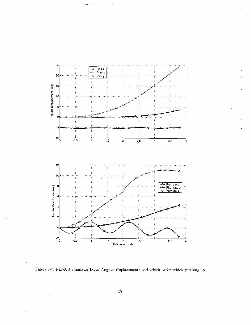
25

20

C; 15()~ë()E 10()"Clëieni: 5æ:;ClC~

-10o 0.5 1.5 2 2.5j 3 3.5 4

12

10

U 8().!Cl()~ 6,¡'(30ãi:;æ:;Clc~

0.5 1.5 2 2.5Time in seconds

3 3.5 4

Figure 8-7: REMUS Simulator Data: Angular displacements and velocities for vehicle pitching up

69

5

4

3

~ 2(/CD()(;u.CDU:ECD:;

-1

-2

-30 0.5

.~x:. i'=; i ':

.15 2 2.5 3 3.5 4

.14

Ek 0.8(/ëCDEo:2CDU:ECD:;

1.2

.~.:-eK:... =: ~ ..

-0.2o 0.5 1.5 2 2.5

Time in seconds3 3.5 4

Figure 8-8: REMUS Simulator Data: Forces and moments for vehicle pitching up

70

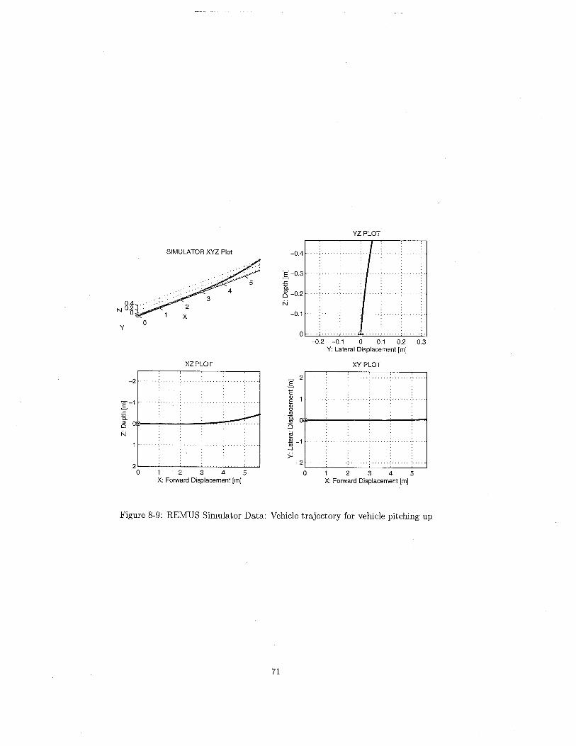
SIMULATOR XYZ Plot

8.4N '6

Yo

XZ PLOT

-2

I-1.cã.()oN

2o 1 2 3 4 5

X: Forward Displacement (mJ

-0.4

I-O.3.cã.c3 -0.2

N

-0.1

2Ic()E()t.Cle.(Jis(ï2 -1Cl..;;

-2o

YZ PLOT

o . t!i¡..

-0.2 -0.1 0 0.1 0.2 0.3Y: Lateral Displacement (mJ

XY PLOT

1 2 3 4 5X: Forward Displacement (mJ

Figure 8-9: REMUS Simulator Data: Vehicle trajectory for vehicle pitching up

71

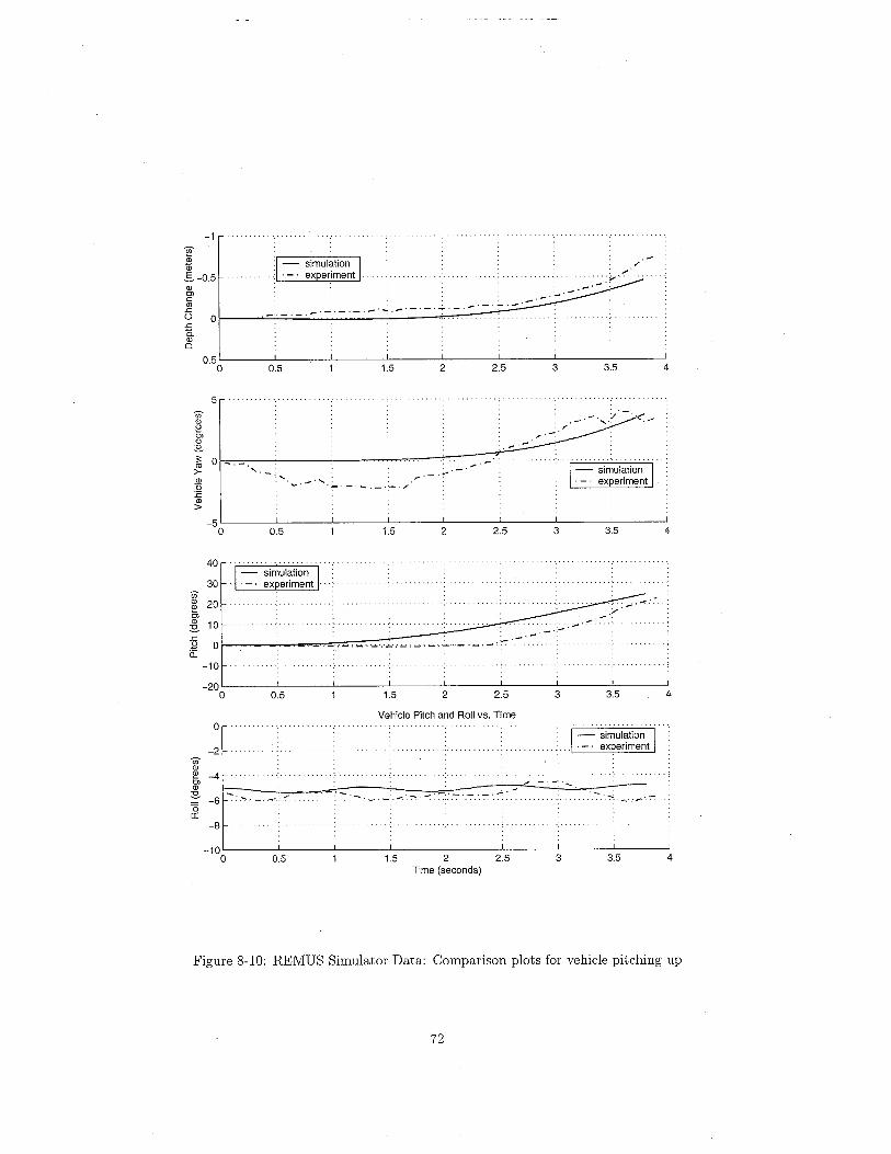
-1'&Q;1iÉ. -0.5Q)0)c'".cU a.c15Q)o

simulationexperiment

/'

.-'-.- ._._.~,-,-'-

..

0.5a 0.5 1.5 2 2.5 3 3.5 4

5

'&Q)Q)OiQ):::; a'")0Q)Ü:eQ):0

-5a

40

30'&Q) 20~0)Q) 10::.c.8 aö:

-10

-20a

"'. ,-,~.............:.. ~-'-._,--.'/

0.5 1.5 2 2.5 3 3.5 4

_.:-'.... '._'.'_r~' _.~:-. -'

0.5 1.5 2 2.5 3 3.5 4

Vehicle Pitch and Roll vs. Timea

-2- simulation. _. experiment

'&Q)~ -4Q)

~ -6oa:

.. ...."::~._.,....:..--.. ""*"'_"'_:A~"7": -,-.'_. ......

-8

-10a 0.5 1.5 2 2.5

Time (seconds)3 3.5 4

Figure 8-10: REMUS Simulator Data: Comparison plots for vehicle pitching up

72

6

5

I 4

ëilEil 3()C1ëiU)ëi

2il'50U).!..

-1o 0.5 1.5 2 2.5 3 3.5 4

1.6

1.4

1.2

'0 0.8il

f~ 0.6'(30a; 0.4:;

0.2

-0.2

-0.40 0.5 1ß 2 2ß


Figure 8-11: REMUS Simulator Data: Linear displacements and velocities for vehicle pitching down

73

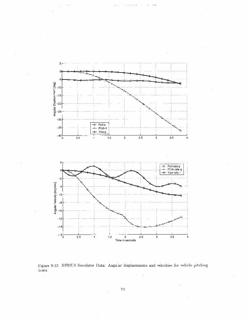
5

-5(

4

OìQ):2-10ëQ)

~ -15ü'"-ais -20(i~-25c-0

-30

-35-e Roll ip

-A Pitch e-G Yawll

-40o 1.5 3 3.52 2.50.5

2

-e Roll rate p

-.£- Pitch rate q-G Yaw rate r

-2

0'Q) -4~Q):2.i -6'50ãi -8:;(i:igi -10-0

-12

-14

-160 0.5 3 3.5 41ß 2 2ß

Time in seconds

Figure 8-12: REMUS Simulator Data: Angular displacements and velocities for vehicle pitchingdown

74

2

~-16'"

~ -2oLL

.g -3:eOJ;, -4

..............~.. -e X: : _.¿,.... y.... -+ z .

-5

0.5 1.5 2 2.5 3 3.5 4

0.5

EZ7; -0.5ëOJEo:2

~ -1:eOJ;, .~.~

-1.5

-2o 0.5 1.5 2 2.5


Figure 8-13: REMUS Simulator Data: Forces and moments for vehicle pitching down

75

YZ PLOT

SIMULATOR XYZ Plot0

0.1

iO.2.c0.0.3Q)0NO.4

0.5

0 0.6Y

-0.4 -0.2 0 0.2Y: Lateral Displacement (m)

XZ PLOT XY PLOT2

-1.5 I-1 ë

Q)~-0.5 EoS Q)ü.c Cl

0. ã. OLUJQ) 0.5 is0N '"

.$ -11.5 Cl-'

2 ;;-2

0 1 2 3 4 5 0 1 2 3 4 5X: Forward Displacement (m) X: Forward Displacement (m)

Figure 8-14: REMUS Simulator Data: Vehicle trajectory for vehicle pitching down

76

-0.5

'§'"ãi§. a'"OlC'"-'Ü 0.5-'õ.'"0

1a 0.5

5

(ñ'"'"Oi

a'":E;;'")0'" -5ë3:e'":;

0.5

20

(ñ a'"'"Oi

2- -20-'.8ë: -40

-60a 0.5

a

-2 ..............(ñ'"~ -4'"

~ -6oa:

-8

-10a 0.5

1.5 2 2.5 3 3.5 4

,-,- . .;'._._.-; ,'-._. -;. -, '. -..-

...:......'".'.~

1.5 2 2.5 3 3.5 4

. . ............................. _. _. -. -. -, - ,"-. . '-.

1.5 2 2.5 3 3.5 4

Vehicle Pitch and Roll VS. Time

.-.-............._....

1.5 2 2.5Time (seconds)

3 3.5 4

Figure 8-15: REMUS Simulator Data: Comparison plots for vehicle pitching down

77

Chapter 9

Linearized Depth Plane Model andController

This chapter describes the depth-plane linearization of the vehicle equations of motion and thecoeffcients used in those equations. It demonstrates the use of that model to design a simple inner-and-outer (pitch-and-depth) loop PD depth controller. Finally, this chapter shows how real worldeffects such as environmental disturbances, sensor noise and actuator non-linearities can be addedto the modeL.

Although this chapter covers only the depth-plane model, the equations of motion and vehi-

cle coeffcients are explained in suffcient detail to allow the development of a more sophisticatedlinearized, decoupled model in five degrees of freedom (disallowing vehicle roll).

9.1 Linearizing the Vehicle Equations of Motion

The equations governing the motion of the vehicle are described in Chapter 3. We wil brieflydescribe the linearization of the vehicle kinematics, rigid-body dynamics, and mechanics.

9.1.1 Vehicle Kinematics

The vehicle kinematic equations are developed in Section 3.2. Note that the rotational coordinate

transform matrix J2 (""2)' described in Equation 3.5, is not defined for cose = ~. This wil not bea problem, given that when we linearize the model we wil be assuming small vehicle perturbationsabout e = o.

As we are assuming pure depth-plane motion, we need only consider the body-relative surgevelocity u, heave velocity w, and pitch rate q, and the earth-relative vehicle forward position x,depth z, and pitch angle e. We wil set to zero all other velocities (v, p, 1'), and drop the equationsfor any out-of-plane terms.

By these assumptions, Equation 3.1 and Equation 3.4 result in the following relationships betweenbody- and earth-fixed vehicle velocities:

:i = cos eu + sinewz = - sin eu + cos ew (9.1)

e = q

We wil linearize these equations by assuming that the vehicle motion consists of small perturbationsaround a steady point. U in this case represents the steady-state forward velocity of the vehicle;

78

heave and pitch are linearized about zero.

u = U + ulIw=w

q = ql(9.2)

We wil also use the Maclaurin expansion of the trigonometric terms:

03 05sinO = 0 - -31 + -i +...

. 5.02 04

cosO = 1 - -21 + -i +.... 4.

(9.3)

Applying these linearizations and dropping any higher-order terms results in the following linearizedkinematic relationships between earth- and body-fixed velocities:

x = u + Ow

z=-UO+w0= q

(9.4)

9.1.2 Vehicle Rigid-Body Dynamics

The vehicle kinematic equations are developed in Section 3.3. As in the equations for vehiclekinematics, we wil simplify the equations for the rigid body dynamics (Equation 3.8) to a descriptionof pure depth-plane motion. We wil set to zero all unrelated terms (v, p, 1', Yg), and drop theequations for out-of-plane vehicle motion:

LX=LZ=LM=

m (u + wq - Xgq2 + Zga)( . 2.)m w - uq - Zgq - xgq (9.5)

1yya + m¡Zg(u + wq) - Xg(1. - uq)J

Substituting the linearized velocities from Equation 9.2 and dropping any higher-order termsresults in the following linearized equations of motion:

LX = m¡u+zgaJ

L Z = m ¡1. - Xga - U qJ

L M = 1yya + m¡zgu - Xg(1. - U q)J

(9.6)

9.1.3 Vehicle Mechanics

Our assumptions about the vehicle mechanics are identical to those developed in Section 3.4. In thelinearized vehicle equations of motion, external forces and moments

L Fext = Fhydrostatic + Rift + Fdrag + Fcontrol + Fdisturbance

are described in terms of vehicle coeffcients. For example, linearized axial drag

Fd = - (~PCdAfU) u = Xuu =* 8Fd 1Xu = - = --pcdAfU8u 2

79

These linearized coeffcients are based on a combination of theoretical equations and empirically-derived formulae. Note that we neglect the forward force due to body lift as it is a nonlinear term.

9.2 Linearized Coeffcient Derivation

The various parameters necessary to derive the vehicle coeffcients are either included in the sectiondescribing the coeffcient, or are listed in the Appendix.

9.2.1 Hydrostatics

The nonlinear equations for hydrostatic forces and moments (see Equation 4.3) are developed inSection 4.1. We wil simplify these by dropping the out-of-plane terms, assuming that xg ~ Xb, andusing the Maclaurin expansion of the trigonometric terms (see Equation 9.3). We then drop thehigher-order terms, as well as any resulting constant terms. This yields the following linearizedhydrostatic equations:

Xe = - (W - B)e

Me = - (zgW - ZbB)B(9.7)

9.2.2 Axial Drag

Vehicle axial drag can be expressed in Equation 4.6. Linearizing this equation using the relationshipgiven in Equation 9.2, results in the following:

1X = --pcdAj (U + u) IU + ul

21 ( 2 2)X = --pcdAj U +2Uu+u2

(9.8)

Assuming

u -(-( U, U? 0 (9.9)

and dropping any constant terms results in the following linearized axial drag coeffcient:

Xu = -pcdAjU (9.10)

9.2.3 Crossflow Drag

Vehicle crossflow drag is discussed in Section 4.2.2. In order to linearize the quadratic crossflow dragcoeffcients described in Equation 4.8, we must linearize the heave and pitch perturbation velocitiesabout zero. This is accomplished by fitting a slope to the parabolic velocity-squared curve, as showin Figure 9- 1.

w2 ~ mwwq2 ~~ mqq

(9.11)

The actual values used in this parameterization are given in Table 9.1. The estimates for maxi-mum expected heave and pitch velocity were taken from field data.

80

0.04

0.035

0.03

'"l!§ 0.025'"en

~ 0.02"o;g

0.015

0.01

0.005

oo

LinearVelocily (mls)

Figure 9-1: Perturbation Velocity Linearization

Table 9.1: Linearized Velocity ParametersParameter Value Units Description

Wmax +2. 00e-001 m/s Maximum Heave Perturbationamax +5. 00e-001 rad/s Maximum Pitch Perturbationmw +1.20e-001 m/s Heave Coeffcientmq +3. 00e-001 rad/s Pitch Coeffcient

Substituting these parameters results in the following linear equations for cross flow drag:1 tb2 ( 1 )Zwc = -"2pcdcmw lx, 2R(x)dx - 2. "2 pSfinCdfmw1 ¡Xb2 ( 1 )Mwc = --PCdcmw 2xR(x)dx - 2Xfin' -pSfinCdfmw2 ~ 21 rXb2 ( 1 )Zqc = -"2pcdcmq lx, 2xlxIR(x)dx - 2Xfin IXfinl' "2pSfinCdfmq

1 rXb2 (1)Mqc = -"2pcdcmq lx, 2x3 R(x)dx - 2x~n' "2pSfinCdfmq

(9.12)

See Table A.2 for the limits of integration.

9.2.4 Added Mass

Vehicle added mass is discussed in Section 4.3. By substituting linearized velocities and droppingthe out-of-plane and higher-order terms, the non-linear equations (see Equation 4.15) reduce to thefollowing:

XA = Xuu + Zqmqa

ZA = Zti/w + Zqq - XuU q

MA = M'Úw + Mqq - (Z'Ú - Xu)Uw - ZqUq(9.13)

81

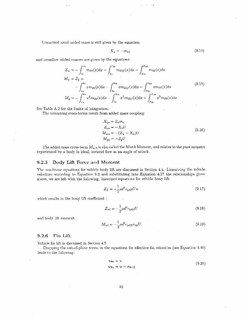
Linearized axial added mass is stil given by the equation:

Xu = -mii (9.14)

and crossflow added masses are given by the equations:

¡Xf lXf2 ixb2Zw = - m22(x)dx - m22f(x)dx - m22(x)dxXt. Xf Xf2Mw = Zq =¡Xf ixf2 ixb2

- xm22(x)dx - xm22f(x)dx - xm22 (x)dxXt Xf Xf2Lxf ixf2 ixb2Mq = - x2m22(x)dx - x2m22f(x)dx - x2m22(x)dxIt Xf Xf2

(9.15)

See Table A.2 for the limits of integration.The remaining cross-terms result from added mass coupling:

Xqa = Zqmq

Zqa = -XuUMwa = -(Zw - Xu)U

Mqa = -ZqU

(9.16)

The added mass cross-term MwA is also called the Munk Moment, and relates to the pure momentexperienced by a body in ideal, inviscid flow at an angle of attack.

9.2.5 Body Lift Force and MomentThe non-linear equations for vehicle body lift are discussed in Section 4.4. Linearizing the vehiclevelocities according to Equation 9.2 and substituting into Equation 4.27 the relationships givenabove, we are left with the following, linearized equations for vehicle body lift:

1 2ZL = --pd CydßUw

2(9.17)

which results in the body lift coeffcient:

1 2Zwl = --pd CydßU

2(9.18)

and body lift moment:1 2

Mwl = - - pd CydßXcpU2

(9.19)

9.2.6 Fin LiftVehicle fin lift is discussed in Section 4.5

Dropping the out-of-plane terms in the equations for effective fin velocities (see Equation 4.40)leads to the following:

Ufin = U(9.20)

Wfin = W - Xfin q

82

Effective fin angle oe can be expressed as

Oe = o8 + ße (9.21 )

where o8 is the stern plane angle, and ße the effective angle of attack of the fin zero plane, as shownin Figure 4-2. This effective angle is expressed as

Wfin 1ße = -:: - (w - Xfina)

Ufin U (9.22)

After linearizing the velocities in Equations 4.44 and 4.45 according to Equation 9.2 results inthe following sets of fin lift coeffcients:

Z,ss = -PCLexSfinU2

1Zwf = -'2PCLexSfinU

1Zqf = -PCLexSfinXfinU

2

and fin moment coeffcients:

M,ss = PCLexSfinXfinU2

1Mwf = -PCLexSfinXfinU

21 2Mqf = --PCLexSfinxfinU

2

9.2.7 Combined Terms

The sum of the depth-plane forces and moments on the vehicle can be expressed as:

LX = Xuu+Xuu+Xqa+Xea

L Z = Zww + Zqg + Zww + Zqq + Z,sso8

L M = Mww + Mqg + Mww + Mqq + Mea + M,sso8

where

Zw = Zwc + Zwl + Zwf

Mw = Mwc+ Mwa +Mwl +MwfZq = Zqc + Zqa + Zqf

Mq = Mqc + Mqa + Mqf

The values for these combined terms are given in Table 9.2.

9.2.8 Linearized Coeffcients

The final values for the linearized coeffcients are given below in Table 9.3.

83

(9.23)

(9.24)

(9.25)

(9.26)

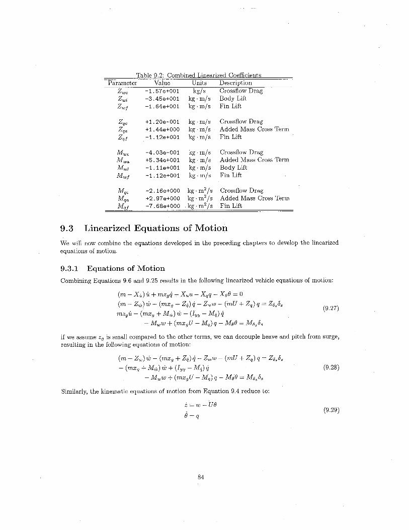
Table 9.2: Combined Linearized CoeffcientsParameter Value Units Description

Zwc -1.57e+001 kg/s Crossflow DragZwl -3.45e+001 kg. m/s Body LiftZwj -1.64e+001 kg. m/s Fin Lift

Zqc +1.20e-001 kg. m/s Crossflow DragZqa +1.44e+OOO kg. m/s Added Mass Cross TermZqj -1.12e+OO1 kg. m/s Fin Lift

Mwc -4.03e-001 kg. m/s Crossflow DragMwa +5.34e+OO1 kg. m/s Added Mass Cross TermMwl -1.11e+OO1 kg. m/s Body LiftMwj -1.12e+OO1 kg. m/s Fin Lift

Mqc -2. 16e+OOO kg. m2 Is Crossflow DragMqa +2.97 e+OOO kg.m2/s Added Mass Cross TermMqj -7 . 68e+OOO kg. m2/s Fin Lift

9.3 Linearized Equations of Motion

We wil now combine the equations developed in the preceding chapters to develop the linearizedequations of motion.

9.3.1 Equations of Motion

Combining Equations 9.6 and 9.25 results in the following linearized vehicle equations of motion:

(m - Xu)u + mzgq - Xuu - Xqq - XeB = 0

(m - Zw) 'I - (mxg + Zq) q - Zww - (mU + Zq) q = Zósósmzgu - (mxg + Mw) 'I + (Iyy - Mq) q

- Mww + (mxgU - Mq) q - MeB = Mósós

(9.27)

if we assume Zg is small compared to the other terms, we can decouple heave and pitch from surge,resulting in the following equations of motion:

(m - Zw) 'I - (mxg + Zq) q - Zww - (mU + Zq) q = Zósós- (mxg + Mw) 'I + (Iyy - Mq) q

- Mww + (mxgU - Mq) q - MeB = Mósós(9.28)

Similarly, the kinematic equations of motion from Equation 9.4 reduce to:

z = w - UB

B = q(9.29)

84

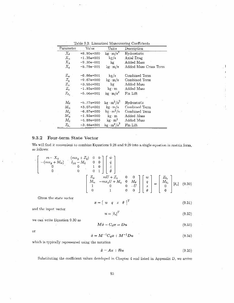
Table 9.3: Linearized Maneuvering CoeffcientsParameter Value Units Description

Xe +8.90e+OOO kg. m/s'2 HydrostaticXu -1.35e+OO1 kg/s Axial DragXu -9.30e-001 kg Added MassXq -5.78e-001 kg. m/s Added Mass Cross Term

Zw -6.66e+OO1 kg/s Combined TermZq -9.67 e+OOO kg. m/s Combined TermZw -3.55e+OO1 kg Added MassZ. -1.93e+OOO kg.m Added Massq

ZÓs -5.06e+OO1 kg. m/s2 Fin Lift

Me -5.77 e+OOO kg. m2/s2 HydrostaticMw +3.07e+OO1 kg. m/s Combined TermMq -6.87 e+OOO kg. m2/s Combined TermMw -1.93e+OOO kg.m Added MassM. -4.88e+OOO kg. m2 Added Massq

ZÓs ~3. 46e+OO1 kg . m2 I S2 Fin Lift

9.3.2 Four-term State Vector"-

We wil find it convenient to combine Equations 9.28 and 9.29 into a single equation in matrix form,as follows:

r

m-Xu -(mxg + Zq) 0

n rn-(mxg + Mw) Iyy - Mq 0

0 0 1

0 0 0

r Zw

mU + Zq~ i, ir ~ J

r Z"1

Mw -mxgU + Mq Mós¡Ósl

1 0 o -U z 00 1 o 0 () 0

Given the state vectorx=(w q z () JT

and the input vector

u = ¡Ósr

we can write Equation 9.30 asMx-Cdx=Du

orx = M-1Cdx + M-1 Du

which is typically represented using the notation

x = Ax + Bu

(9.30)

(9.31 )

(9.32)

(9.33)

(9.34)

Substituting the coeffcient values developed in Chapter 4 and listed in Appendix D, we arrive

(9.35)

85

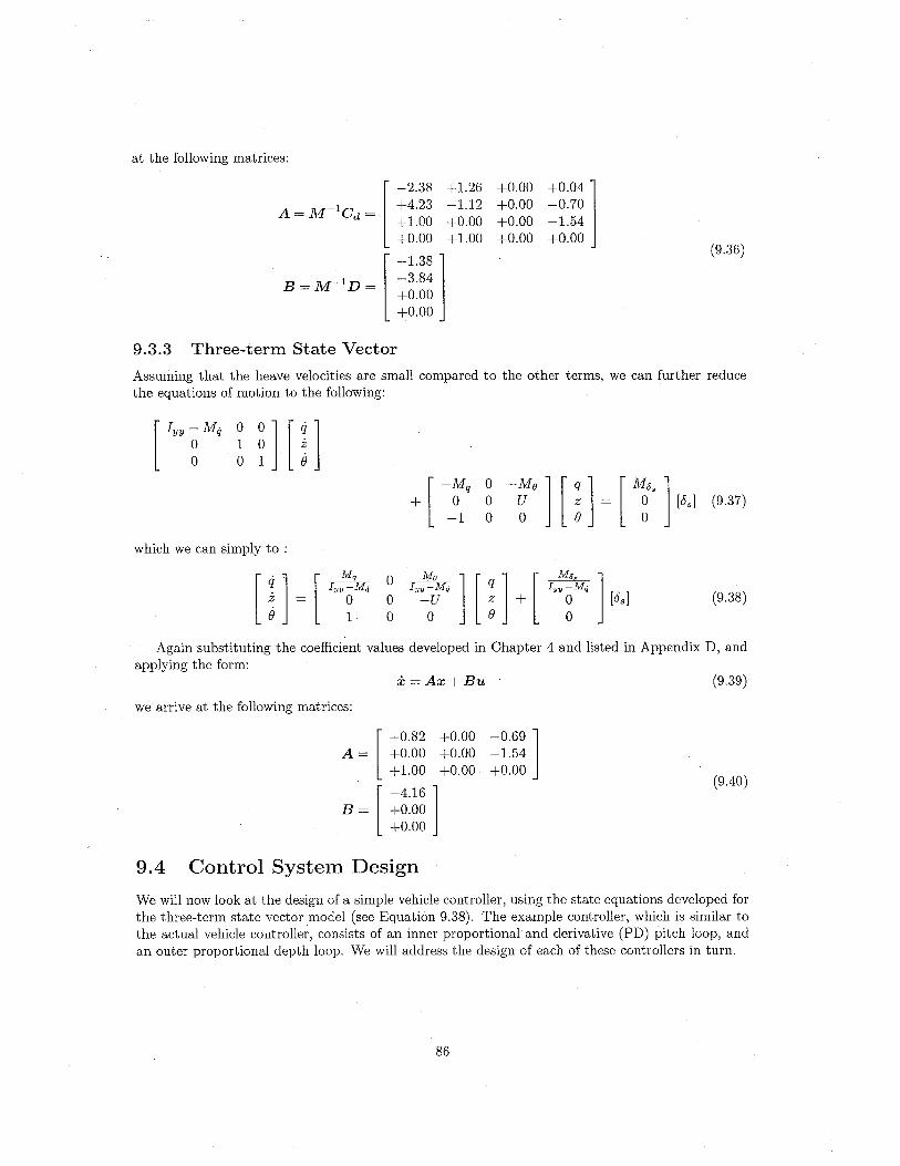
at the following matrices:

r -2.38 +1.26

A = M-1Cd = +4.23 -1.2+1.00 +0.00+0.00 +1.00

B = M-1 D = r =;:~~ i+0.00+0.00

9.3.3 Three-term State Vector

+0.00+0.00+0.00+0.00

+0.04 i-0.70-1.54+0.00

(9.36)

Assuming that the heave velocities are small compared to the other terms, we can further reducethe equations of motion to the following:

¡ I" t' ~ ~ H l i

¡ -Mq+ 0

-1

which we can simply to :

¡ n ¡

Mq 0Iyy -Mqo 01 0

MeIyy -Mq-u

o

~ -t i u i ¡ 1" i 18,1(9.37)

H n + ¡ "1M. i 18.1(9.38)

x = Ax + Bu'

Again substituting the coeffcient values developed in Chapter 4 and listed in Appendix D, andapplying the form:

(9.39)

we arrive at the following matrices:

¡ -0.82 +0.00

A = +0.00 +0.00+1.00 +0.00

¡ -4.16 iB = +0.00

+0.00

9.4 Control System Design

-0.69 i-1.54+0.00

(9.40)

We wil now look at the design of a simple vehicle controller, using the state equations developed forthe three-term state vector model (see Equation 9.38). The example controller, which is similar tothe actual vehicle controller, consists of an inner proportional and derivative (PD) pitch loop, andan outer proportional depth loop. We will address the design of each of these controllers in turn.

86

9.4.1 Vehicle Transfer Functions

The first step in designing the vehicle control system is to derive the vehicle transfer fuiictions. First,we want to derive the transfer function for the inner pitch loop, relating input stern plane angleÒs to the output vehicle pitch angle e. By taking the Laplace transform of Equation 9.38, we can

express this open-loop transfer function as:

e(s)Ge(s) = òs(s) =

~Iyy-Mqs2_~s-~Iyy-Mq Iyy-Mq

(9.41)

Next we want to find the transfer function of the outer depth loop, which relates the input vehiclepitch angle ed to the output vehicle depth z. In actuality, the inner pitch loop responds suffciently

fast enough compared tothe outer depth loop that we can consider the desired vehicle pitch ed tobe the same as the actual vehicle pitch e. Again taking the Laplace transform of the vehicle stateequations, Equation 9.38, we arrive at the desired open-loop transfer function:

Gz(s) = ;~;~ = -~ (9.42)

9.4.2 Control Law

We wil now define the control law for the inner and outer loops. As stated in at the beginningof this chapter, we wil design a proportional-derivative (PD) inner loop, and a proportional outerloop. The control law, then, for the inner loop can be expressed as:

Òs(s)

-() =-Kp(Tds+l)ee s(9.43)

whereee = ed - e (9.44)

Kp is the proportional gain, and Td the derivative time constant in seconds.There is a minus sign applied to the proportional gain due to the difference in sign conventions

between the stern plane angle and vehicle pitch angle. Positive stern plane angle wil generate anegative moment about the y-axis, forcing the vehicle to pitch down (negative pitch rate).

The control law for the outer loop can be expressed as:

e(s)-=ryeAs) (9.45)

whereez = Zd - Z (9.46)

and ry is the proportional gain.We can express the vehicle control system as a block diagram:

9.4.3 Controller Design Procedure

Before getting into the specifics of selecting the vehicle controller gains, we wil first review a generalcontroller design procedure.

This procedure assumes that the system has a second order response. Given that we have chosen

to work with the three-term state vector, this is true for the inner pitch loop. This assumption isalso valid for higher-order systems, provided the higher order poles are at least five times furtherfrom the origin of the s-plane than the two dominant poles.

87

Outer Depth Loop (Slow)

i-- ------ - -- ------ ------ - ------- ---- -----¡1 Inner Pitch Loop (Fast)~_______________________, 11 1 1Zd:: : Z

-~( 'tdS+ 1)1+ 11 1 PO Controller Plant1 1 111 1______------------______1 11____ __ _ _ _ _ _ _ _ _ _ _ _ _ _ _ _ ___ _ _ _ _ _ _ __ _ _ _ _ _ _ _ __ J

Plant

Figure 9-2: Depth-Plane Control System Block Diagram

We wil design our controller to have a specific second-order response in terms of natural frequencyWn and damping ratio (, where, for a second order system:

KG(s) =

s2 + 2(wns + w~ (9.47)

Percent Overshoot and Settling or Peak Time

Our primary consideration in choosing a system response wil be the percentage overshoot, %OS,and peak or settling time, Tp or Ts' See Nise (25J for a graphical explanation of these terms.

Our desired damping ratio is a function of percent overshoot, and is given by the equation:

(=-In (%os)100

i

(1T2 + In2 (~~os) J 2

(9.48)

Table 9.4 gives a range of values. One can also plot lines of constant damping ratio on thepole-zero diagram.

Given the desired damping ratio, our desired natural frequency can be found through the equa-tion:

1T

(9.49)Wn = Tp .¡or

4(9.50)Wn=-

(Ts

Desired Poles

From Equation 9.47, the second order transfer function, we can now find the desired pole locationsthrough the quadratic formula:

1Si,2 = -(wn :l '2 vi 4(2w~ - 4w~ (9.51 )

88

9.4.4 Pitch Loop Controller Gains

Substituting the coeffcient values from Table 9.3 into Equation 9.41 results in the following open-loop transfer function:

-3.18Ge(s) = s2 + L09s + 0.52 (9.52)

and the following open-loop poles.

Si,2 = -0.55:l 0.47i (9.53)

Figure 9-3 plots these open-loop poles. Figure 9-4 shows the open-loop step response.Given that the REMUS vehicle operates in shallow water and cannot tolerate significant depth

overshoot, I chose the following parameters in designing the vehicle pitch controller:

%OS = 0.05

Tp = 0.75 seconds (9.54)

These values resulted in the damping ratio (; and natural frequency Wn, shown in the legend of theroot-locus plot on Figure 9-5.

There are many systematic methods for generating the necessary controller gains-in this case, Iset the derivative time constant Td, and used the root-locus plot to find the necessary gaiii Kp. Theresulting controller values are also shown in the legend of Figure 9-5.

The resulting closed loop response of the pitch loop transfer function plus controller, He, is shownin Figure 9-6.

9.4.5 Depth Loop Controller GainsThe method used to find the depth loop controller gains is similar to that of the previous section.The depth transfer function Gz adds a third pole, as shown in the pole-zero plot in Figure 9-7.

In order to ensure that the pitch loop response is suffciently faster than the depth loop response,we must ensure that the pitch loop poles end up at least five times further away from the originthan the depth loop pole.

This was accomplished using a root-locus plot to identify the appropriate proportional gain 'Y.The resulting value can be found in the legend of the root-locus plot shown in Figure 9-8. Theresulting closed loop response can be seen in Figure 9-9.

9.5 Real-World Phenomena

Although this controller appears to exhibit ideal performance characteristics, it is not of much use inthe real world. For example, if the controller was given a suffciently large depth error, there wouldbe nothing to prevent it from commanding preposterous pitch and stern plane angles of greater than180 degrees. In other words, as designed, the controller assumes the transfer function relationshipsto be linear out to infinity. In reality, the stern planes wil stall at an effective fin angle of greater

than about 12 degrees. Similarly, the REMUS vehicle shuts down at greater than 30 degrees of pitchangle, as the software assumes that something has gone disastrously wrong with the vehicle mission.

Furthermore, the simulation assumes that the vehicle sensors are free from noise, and the vehicleexperiences no unmodeled disturbances. In reality, this is rarely the case.

It is an interesting exercise to discretize the transfer functions, and attempt to incorporatesome of these real-world effects into the vehicle modeL. Figure 9-10 shows a block diagram whichincorporates the saturation of the commanded stern plane and vehicle pitch angles, as well as pitchsensor noise and environmental disturbances. Figures 9-11 and 9-14 show the results of this kind of

89

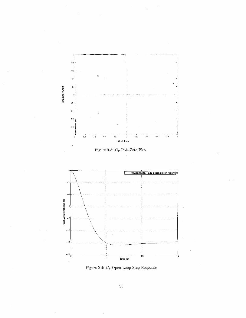
In'xc:~'"r='ei'".§ ".,.

x

x

0,8

0.5

C\.ô ,)6 ¡)A o.~? G.4 O.ß 0.8

Real Axis

Figure 9-3: Ge Pole-Zero Plot

íiCICI¡;CI~'"CIeir=c:.i.i¡;

-12

-14o 10 15

Time(s)

Figure 9-4: Ge Open-Loop Step Response

90

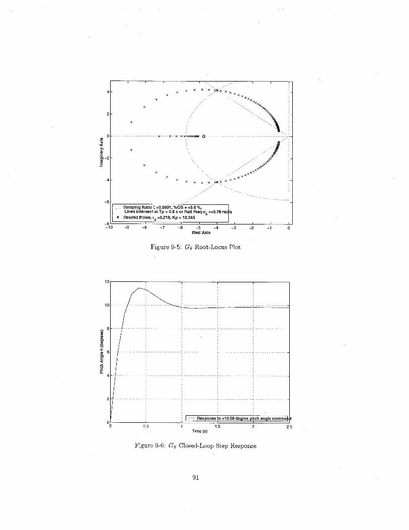
4 x x x x x ..Xx'.~. x....x x x Xxd'~x

x

x

2

x

o ............x ....x...)(.x.x:x.~..o...'";¡c(,.æc15,-2..oS x /;/

.... xxxxx xx x

x

-4

Damping Ratio ç =0.6901, %05 = +5.0 %,Lines intersect at Tp = 0.8 s or Natl Freq "'n =+5.79 ra s

.. Desired Poles"d =0.210, Kp = 10.345

-9 -8 -7 -6 -5 -4Real Axis

-3 -2 -1 o

Figure 9-5: Ce Root-Locus Plot

12

10

Uì8

""Ci":!ø

6"ëicc(.r.sii

4

2

00 0.5 1.5 2 2.5

Time (s)

Figure 9-6: Ce Closed-Loop Step Response

91

Ul.;¡

'"::..i:'5...É

4

2

oUl.;¡

'"",æi:'5-2...É

-4

-6

-8-7

x

o

x

Real Axis

Figure 9-7: Gz * He Pole-Zero Plot

.........:.~xx".....

...0.

. .. .. .. .. .""xxx..

Damping Ratio ç =0.6901, %OS = +5.0 %,Lines intersect at Tp = 0.8 s or Natl Freq ùJn =+5.79 ra s

x Desired Poles, y =-0.772

-6 -5 -4 -3Real Axis

-2

Figure 9-8: Gz * He Root-Locus Plot

92

x.

. .. .'. .. .x. .x.)(.x.x~:~.

-1 o

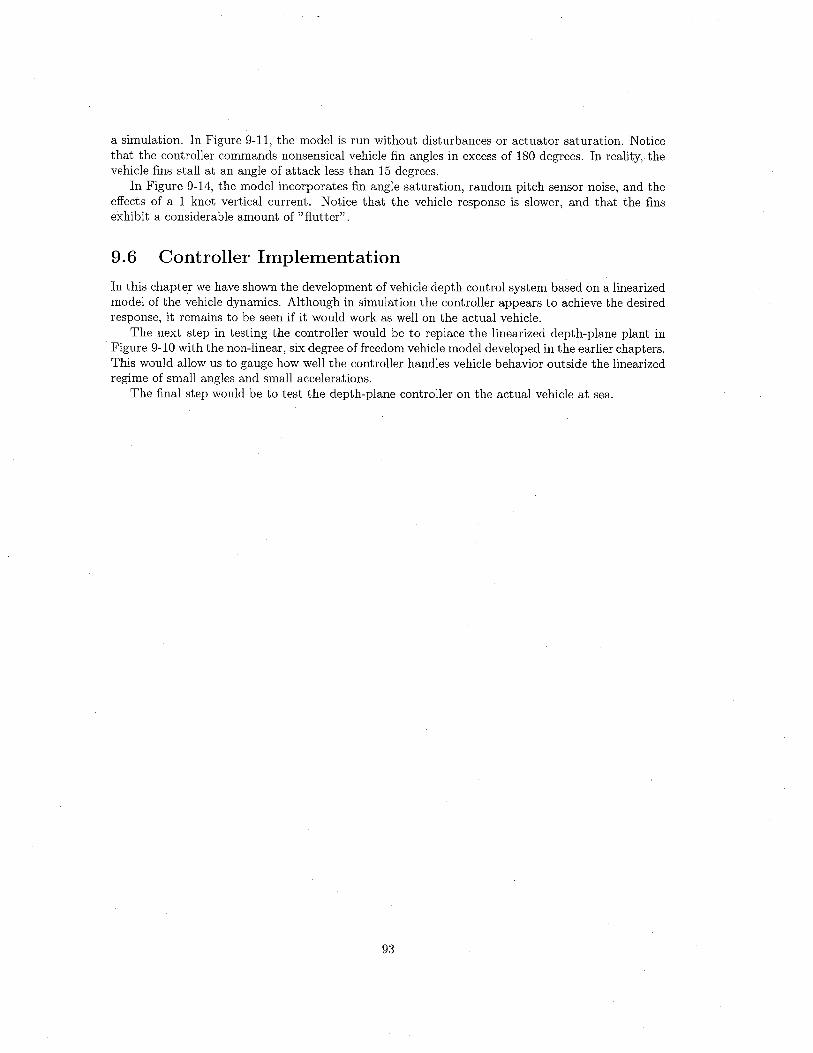
a simulation. In Figure 9-11, the model is run without disturbances or actuator saturation. Noticethat the controller commands nonsensical vehicle fin angles in excess of 180 degrees. In reality, thevehicle fins stall at an angle of attack less than 15 degrees.

In Figure 9-14, the model incorporates fin angle saturation, random pitch sensor noise, and theeffects of a 1 knot vertical current. Notice that the vehicle response is slower, and that the fins

exhibit a considerable amount of "flutter".

9.6 Controller Implementation

In this chapter we have shown the development of vehicle depth control system based on a linearizedmodel of the vehicle dynamics. Although in simulation the controller appears to achieve the desiredresponse, it remains to be seen if it would work as well on the actual vehicle.

The next step in testing the controller would be to replace the linearized depth-plane plant inFigure 9-10 with the non-linear, six degree of freedom vehicle model developed in the earlier chapters.This would allow us to gauge how well the controller handles vehicle behavior outside the linearizedregime of small angles and small accelerations.

The final step would be to test the depth-plane controller on the actual vehicle at sea.

93

o

2

3

4

gN

5.c15"c

6

7

8

9

100 2 3 4 5 6 7 8 9 10

Time (5)

Figure 9-9: Cz * He Closed-Loop Step Response

d EnvironmentalDisturbance

SensorNoise

Figure 9-10: Depth-Plane Control System Block Diagram with Actuator Limits, Environmental

Disturbance, and Sensor Noise

94

-0.60 2 3 4 5 6 7 8 9 10

600

I - Fin Angle I

êì 400Cl:iClëi 200i:~i:ü: 0

-2000 2 3 4 5 6 7 8 9 10

Time

Figure 9-11: Vehicle Simulation, based on basic block diagram

95

0

'êl-0.5.c~ë: -1Q)Ü~ -1.5

theta actual;:-- theta command

-20 2 3 4 5 6 7 8 9 10

-1

~-05 -------- depth actual

.§ . ._. depth command

.c 0ë.Q) 0.5cQ)Ü:eQ)

1.5;:

20 2 3 4 5 6 7 8 9 10

0.2 1- Heave Rate I

.! 0.1

.§~'"iigi -0.1'"Q):i -0.2

-0.30 2 3 4 5 6 7 8 9 10

10

'ê 5Q)~Q)Õl 0i:o:i:ü: -5

1 - Fin Angle I

II\

, ,-10o 2 3 4 5

Time6 7 8 9 10

Figure 9-12: Vehicle Simulation, with fin angle saturation

96

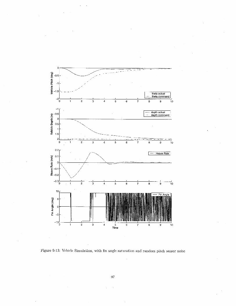
"ë! -0.5.s.lii -1Cli:t -1.5;:

-1

g-0.5.s 0ë.~ 0.5Cli::E

~ 1.5

~ 0.1

.§$ 0'"ii~ -0.1'"Cl:i -0.2

"ë 5Cl~Clei 0i:cii:¡¡ -5

o ~~-2

o

2o

0.2

/\ /,/\//-0.3

o

10

-10o

.._.- theta actual

..- theta command

2 3 4 5 6 7 8 9 10

depth actual. _. depth command

2 3 4 5 6 7 8 9 10

i -- Heave Rate I

2 3 4 5 6 7 8 9 10

2 3 4 5Time

6 7 8 9 10

Figure 9-13: Vehicle Simulation, with fin angle saturation and random pitch sensor noise

97

0.5

êì 0Q) --" . . ---- - ,J~ ~-- ..-~ -0.5 -' -' -ë:Q) ~1

/Õ /:e~ -1.5 -- -- theta actual

theta command-2

0 2 3 4 5 6 7 8 9 10

-1

~-05depth actual

g . depth command

.s 0..- ~ -----..,..

ë.Q) 0.50Q)Õ:eQ)

1.5;:

20 2 3 4 5 6 7 8 9 10

0.1 I-- Heave Rate I

~0

i -0.1'"a:

gi -0.2'"Q):i -0.3

-0.40 2 3 4 5 6 7 8 9 10

10

êì 5Q)~Q)ei 0cc(cii -5

-100 2 3 4 5 6 7 8 9 10

Time

Figure 9-14: Vehicle Simulation, incorporating fin angle saturation, random pitch sensor noise, and1 knot vertical current

98

Chapter 10

Conclusion

In the preceding chapters, we have demonstrated the development of a mathematical model forthe dynamics of an autonomous underwater vehicle. We have examined methods for validatingthe performance of this modeL. Finally, we have seen how such a model can be applied to thedevelopment of a vehicle control system.

In the following sections, we outline a series of recommendations for expanding upon this work.

10.1 Expanded Tow Tank Measurements

In the previous chapter, the author outlined the limitations of vehicle coeffcients based solely upon

semi-empirical formulae. The most significant source of error is in the way coeffcients are used tomodel the vehicle moving at some angle of attack, as shown in Figure 10-1. The fluid effects are

AxialDrag~

CrossflowDrag \ Î

BodyLift

..Fluid

Velocity

Figure 10-1: Forces on the vehicle at an angle of attack

broken up into vehicle body lift, vehicle crossflow drag, and vehicle axial drag. Of these, the authorhad the most diffculty estimating body lift.

The semi-empirical methods of calculating the body lift coeffcient used by Hoerner (161, Bottac-cini ¡71, and Nahon ¡231, explored in the development of this thesis, were found to differ by an order

of magnitude. It will therefore be important to experimentally measure forces and moments on thevehicle moving at an angle of attack, in order to verify the empirical estimates.

99

10.2 Future Experiments at Sea

The following are recommendations for future experiments at sea, derived from the author's expe-rience and consultation with experts in the field.

10.2.1 Improved Vehicle Instrumentation

The vehicle dynamics data collected in the experiments described in Chapter 7 were limited in thenumber of vehicle states recorded, and the accuracy of those measurements. This made it extremelydiffcult to judge the validity of the model comparison.

For future experiments, the author has augmented the standard REMUS sensors described inSection 7.3 with an inertial measurement unit: the Crossbow DMU-AHRS (Dynamic MeasurementUnit-Attitude and Heading Reference System). This instrument outputs magnetic orientation,accelerations and angular rates on three axes. From this instrument, we wil be able to accuratelymeasure or derive the following vehicle states.

r. . . .. e ./,)Tx=iuvwuvwpqr'f 'f (10.1)

This wil significantly improve our abilty to measure the vehicle initial conditions in particular, andthe vehicle motion in general.

10.2.2 Measurement of Vehicle ParametersWith the exception of the longitudinal center of gravity xcg, which was measured before each exper-iment using a balance, the author's estimates for the vehicle mass distribution were calculated usingthe vehicle weight list. Similarly, the estimates for the vehicle center of buoyancy were calculatedusing the Myring hull shape.

To reduce uncertainty in future experiments, it wil be necessary to measure these values exper-

imentally, preferably before each experiment.

10.2.3 Isolation of Vehicle MotionOne limitation of the experimental step response data used in the model validation was imperfect

knowledge of the vehicle initial conditions. At the time of the experiments, the author had no wayof measuring the vehicle accelerations and angular rates prior to the changes in fin angles.

These vehicle motions resulted from two sources: vehicle control inputs and external disturbances.In future experiments, every effort should be made to minimize these motions.

To minimize vehicle control motions, it is important to understand the vehicle steady-stateconditions. AUVs like REMUS can be unstable when operating without control. Using the inertialmeasurement unit, it wil be possible to identify the propeller RPM and fixed fin angles whichresult in straight and level vehicle flight. These settings should then be used at the start of everyexperimental run.

To minimize environmental disturbances, the experiments could be run in an area known to befree of currents, and at suffcient depth to avoid free surface interactions. Two locations meetingthese criteria would be deep lakes and flooded sinkholes.

10.3 Controller-Based Model ComparisonThe vehicle model is particularly useful as a tool in developing vehicle control systems. To that end,rather than comparing the model output to vehicle data collected during open-loop maneuvers, itwould be more useful to compare the model to the vehicle behavior during closed-loop control. This

100

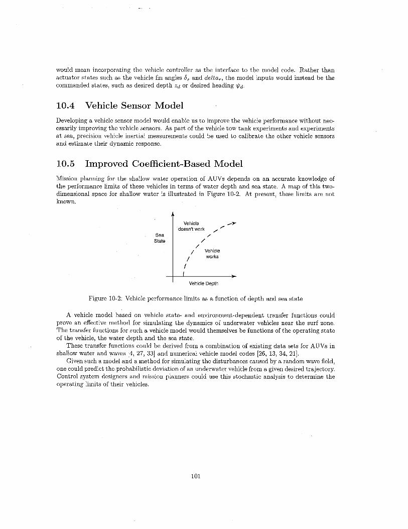
would mean incorporating the vehicle controller as the interface to the model code. Rather thanactuator states such as the vehicle fin angles 65 and deltar, the model inputs would instead be thecommanded states, such as desired depth Zd or desired heading i/d.

10.4 Vehicle Sensor ModelDeveloping a vehicle sensor model would enable us to improve the vehicle performance without nec-essarily improving the vehicle sensors. As part of the vehicle tow tank experiments and experimentsat sea, precision vehicle inertial measurements could be used to calibrate the other vehicle sensorsand estimate their dynamic response.

10.5 Improved Coeffcient-Based ModelMission planning for the shallow water operation of AUVs depends on an accurate knowledge ofthe performance limits of these vehicles in terms of water depth and sea state. A map of this two-dimensional space for shallow water is ilustrated in Figure 10-2. At present, these limits are not

known.

SeaState

Vehicledoesn't work ./ ./

.////I

I

_'r

Vehicleworks

Vehicle Depth

Figure 10-2: Vehicle performance limits as a function of depth and sea state

A vehicle model based on vehicle state- and environment-dependent transfer functions couldprove an effective method for simulating the dynamics of underwater vehicles near the surf zone.The transfer functions for such a vehicle model would themselves be functions of the operating stateof the vehicle, the water depth and the sea state.

These transfer functions could be derived from a combination of existing data sets for AUVs inshallow water and waves ¡4, 27, 33J and numerical vehicle model codes ¡26, 13,34, 21j.

Given such a model and a method for simulating the disturbances caused by a random wave field,one could predict the probabilistic deviation of an underwater vehicle from a given desired trajectory.Control system designers and mission planners could use this stochastic analysis to determine theoperating limits of their vehicles.

101

Appendix A

Tables of Parameters

Table A.I: STD REMUS Hull ParametersParameter Value Units Description

+1.03e+003 kg/m:;Seawater Densityp

At +2 . 85e~002 m2 Hull Frontal AreaAp +2.26e-001 m2 Hull Projected Area (xz plane)Sw + 7. 0ge-001 m2 Hull Wetted Surface Area'i +3. 15e-002 m3 Estimated Hull VolumeW +2.9ge+002 N Measured Vehicle WeightB +3.08e+002 N Measured Vehicle Buoyancy

Best +3. 17e+002 N Estimated Hull BuoyancyXcb(est) +5.54e-003 m Est. Long. Center of Buoyancy

Cd +3.00e-001 n/a REMUS Axial Drag Coeff.Cdc +1.10e+000 n/a Cylinder Crossflow Drag Coeff.

Cydß +1.20e+000 n/a Hoerner Body Lift Coeff.xcp -3.21e-001 n/a Center of Pressurea +3.5ge-002 n/a Ellipsoid Added Mass Coeff.

Table A.2: Hull Coordinates for Limits of IntegrationParameter Value Units Description

Xt -7. 21e-001 m Aft End of Tail SectionXt2 -2. 18e-001 m Forward End of Tail SectionXf -6. 85e-001 m Aft End of Fin SectionXf2 -6. 11e-001 m Forward End of Fin SectionXb +4. 37 e -00 1 m Aft End of Bow SectionXb2 +6.10e-001 m Forward End of Bow Section

102

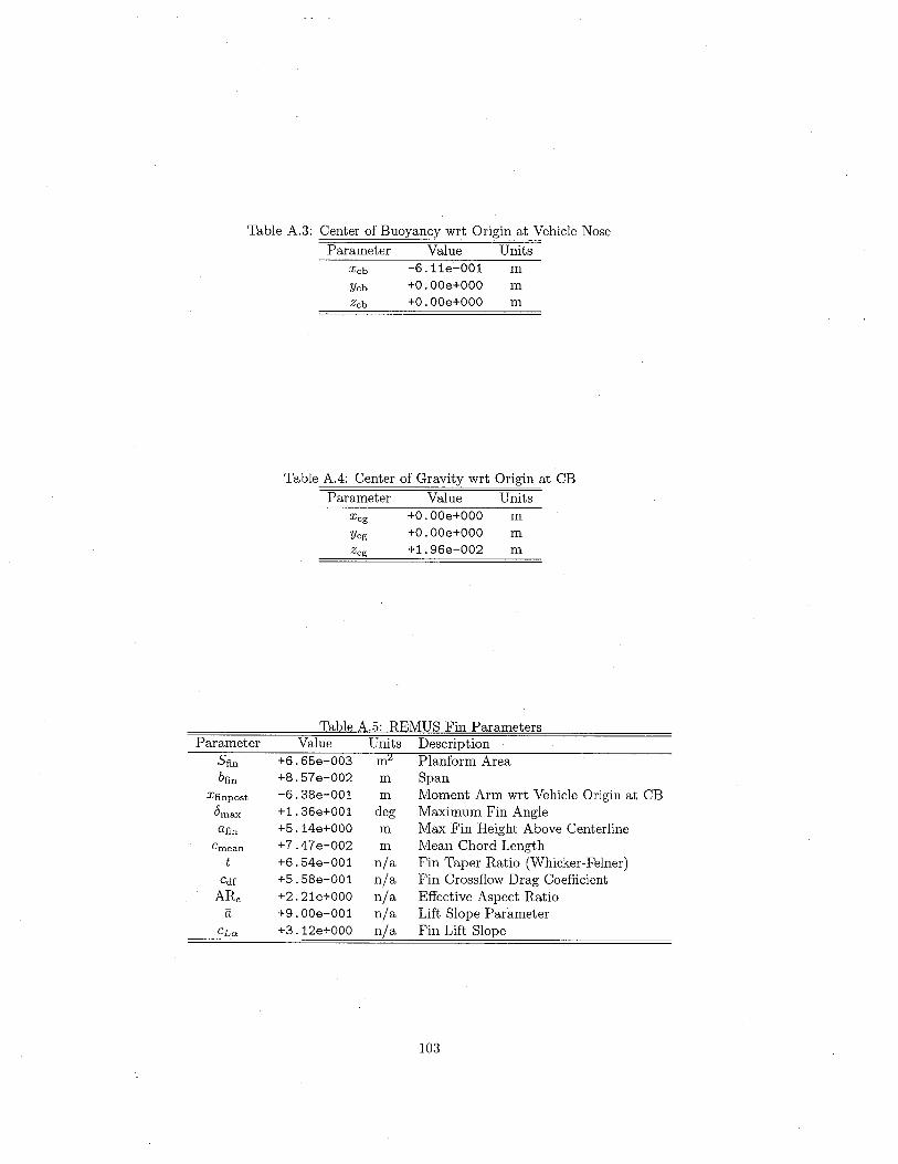
Table A.3: Center of Buoyancy wrt Origin at Vehicle Nose

Parameter Value UnitsXcb -6. 11e-001 mYcb +0 . OOe+OOO mZcb +0. OOe+OOO m

Table A.4: Center of Gravity wrt Origin at CBParameter Value Units

xcg +0. OOe+OOO mYcg +0 .00e+000 mZcg +1.96e-002 m

Table A.5: REMUS Fin ParametersParameter Value Units Description

Sfin +6. 65e-003 m:¿ Planform Areabfin +8.57 e-002 m Span

Xfinpost -6.38e-001 m Moment Arm wrt Vehicle Origin at CBOmax +1.36e+OO1 deg Maximum Fin Angleafin +5. 14e+OOO m Max Fin Height Above Centerline

Cmean +7.47e-002 m Mean Chord Lengtht +6.54e-001 n/a Fin Taper Ratio (Whicker-FeIner)

Cdf +5.58e-001 n/a Fin Crossflow Drag Coeffcient

ARe +2.21e+OOO n/a Effective Aspect Ratioa +9.00e-001 n/a Lift Slope Parameter

CLCY +3. 12e+OOO n/a Fin Lift Slope

103

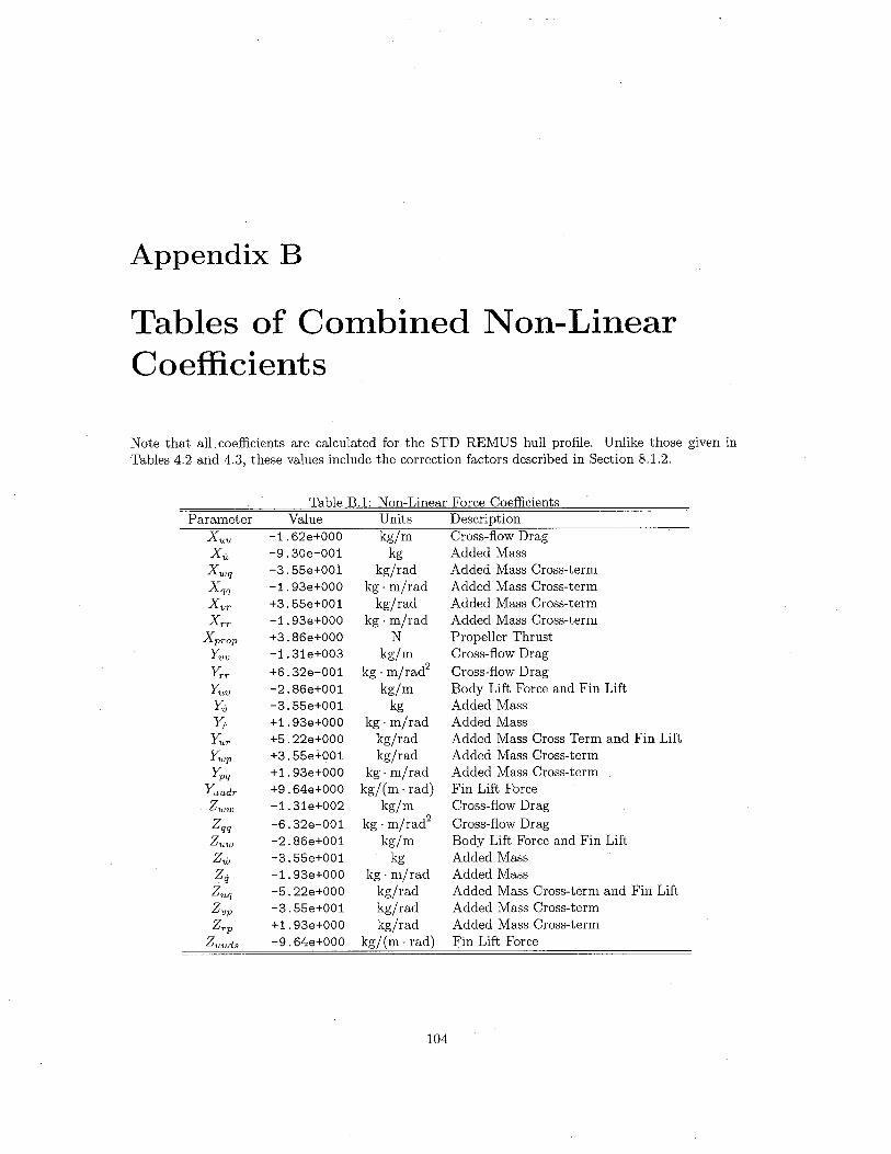
Appendix B

Tables of Combined Non-LinearCoeffcients

Note that all coeffcients are calculated for the STD REMUS hull profie. Unlike those given inTables 4.2 and 4.3, these values include the correction factors described in Section 8.1.2.

Table B.1: Non-Linear Force CoeffcientsParameter

XuuXu

XwqXqqXvrXrr

XpropYvv

YrrYuv

Yv

Y"

YurYwp

Ypq

YuudrZww

ZqqZuwZ,¡Z.q

ZuqZvpZrp

Zuuds

Value-1.62e+000-9.30e-001-3.55e+001-1.93e+000+3.55e+001-1 . 93e+000+3.86e+000-1.31e+003+6.32e-001-2.86e+001-3.55e+001+1.93e+000+5.22e+000+3.55e+001+1.93e+000+9 .64e+000-1. 31e+002-6.32e-001-2.86e+001-3.55e+001-1.93e+000-5.22e+000-3.55e+001+1.93e+000-9.64e+000

Unitskg/m

kgkg/rad

kg. m/radkg/rad

kg. m/radN

kg/mkg. m/rad2

kg/mkg


kg. m/radkg/(m. rad)

kg/mkg. m/rad2

kg/mkg


kg/(m. rad)

DescriptionCross-flow DragAdded Mass

Added Mass Cross-termAdded Mass Cross-termAdded Mass Cross-termAdded Mass Cross-termPropeller ThrustCross-flow DragCross-flow DragBody Lift Force and Fin LiftAdded Mass

Added Mass

Added Mass Cross Term and Fin LiftAdded Mass Cross-termAdded Mass Cross-termFin Lift Force

Cross-flow DragCross-flow DragBody Lift Force and Fin LiftAdded Mass

Added Mass

Added Mass Cross-term and Fin LiftAdded Mass Cross-termAdded Mass Cross-termFin Lift Force

104

Table B.2: Non-Linear Moment CoeffcientsParameter

KppK.p

KpropMww

MqqMuwMwM.q

MuqMvp

MrpMuuds

Nvv

NrrNuvNi;NrNurNwp

NpqNuudr

Value-1.30e-001-7.04e-002-5.43e-001+3. 18e+OOO

-1.88e+002+2.40e+001-1.93e+OOO-4. 88e+OOO

-2.00e+OOO-1.93e+OOO+4. 86e+OOO-6. 15e+OOO

-3. 18e+OOO

-9.40e+001-2.40e+001+1.93e+OOO-4. 88e+OOO

-2.00e+OOO-1.93e+OOO-4 . 86e+OOO-6. 15e+OOO

Unitskg. m2/rad4kg. m2/rad

N.mkg

kg. m2/rad2kg

kg.mkg. m2/radkg . m/radkg . m/rad

kg . m2/rad2kg/rad

kgkg . m2/rad2

kgkg.m

kg. m2/radkg . m/radkg. m/rad

kg. m2/rad2kg/rad

DescriptionRolling ResistanceAdded Mass

Propeller TorqueCross-flow DragCross-flow DragBody and Fin Lift and Munk MomentAdded Mass

Added Mass

Added Mass Cross Term and Fin LiftAdded Mass Cross TermAdded Mass Cross-termFin Lift MomentCross-flow DragCross-flow DragBody and Fin Lift and Munk MomentAdded Mass

Added Mass

Added Mass Cross Term and Fin LiftAdded Mass Cross TermAdded Mass Cross-termFin Lift Moment

105

Appendix C

Tables of Non-Linear Coeffcientsby Type

Note that all coeffcients are calculated for the STD REMUS hull profile. Unlike those given inTables 4.2 and 4.3, these values include the correction factors described in Section 8.1.2.

Table C.!: Axial Drag CoeffcientParameter Value Units

Xuu -1.62e+000 kg/m

Table C.2:Parameter

Yvv

YrrdZww

Zqqd

Mwwd

MqqNvvd

Nrr

Crossflow Drag Coeffcients

Value Units-1.31e+003 kg/m+6.32e-001 kg. m/rad2-1.31e+002 kg/m-6.32e-001 kg. m/rad2+3. 18e+000 kg-1.88e+002 kg. m2/rad2-3. 18e+000 kg-9.40e+001 kg. m2/rad2

Table C.3: Rollng Resistance Coeffcient

Parameter Value UnitsKpp -1.30e-001 kg. m2/rad'2

106

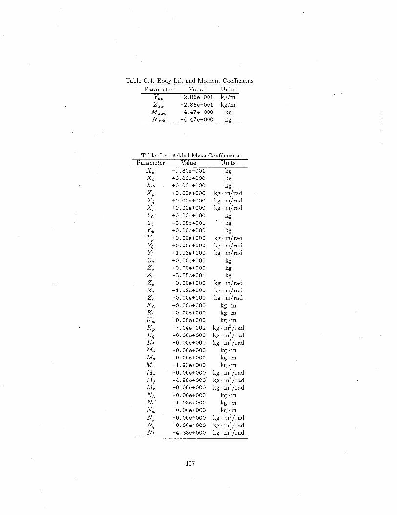
Table C.4: Body Lift and Moment CoeffcientsParameter Value Units

Yuv -2. 86e+001 kg/mZuw -2.86e+001 kg/IlMuwb -4 .47 e+OOO kgNuvb +4.47e+000 kg

Table C.5: Added Mass CoeffcientsParameter

XuX.¡

X,;X.pX.qXi-Yu

Y.¡

Y,;Yo.pY.qYfZuZ.¡

Z,;Z.pZ.qZi-

KuK.¡

K,;K.pK-qKi-MuM.¡

M,;M.pM.qMi-

NuN.¡

N,;N.pN.qNi-

Value-9.30e-001+0 . OOe+OOO

+0 . OOe+OOO

+0 . OOe+OOO

+0 . OOe+OOO

+0 . OOe+OOO

+0 . OOe+OOO

-3.55e+001+O.OOe+OOO

+O.OOe+OOO

+0 . OOe+OOO

+1.93e+000+0 . OOe+OOO

+0 . OOe+OOO

-3.55e+001+0 . OOe+OOO

-1.93e+000+0 . OOe+OOO

+0 . OOe+OOO

+0 . OOe+OOO

+0 . OOe+OOO

-7 . 04e-002+O.OOe+OOO

+O.OOe+OOO+O.OOe+OOO

+0 . OOe+OOO

-1.93e+000+0 . OOe+OOO

-4. 88e+000+0 . OOe+OOO

+0 . OOe+OOO

+1.93e+000+0 . OOe+OOO

+0 . OOe+OOO

+O.OOe+OOO

-4.88e+000

Unitskgkgkg

kg. m/radkg. m/radkg. m/rad

kgkgkg


kgkgkg


kg.mkg.mkg.m

kg. m2/radkg. m2/radkg. m2/rad

kg.mkg.mkg.m

kg. m2/radkg. m2/radkg. m2/rad

kg.mkg.mkg.m

kg . m2/radkg. m2/radkg. m2/rad

107

Table C.6: Added Mass Force Cross-term CoeffcientsParameter

XuqXwqXqqXvrXrpXrrXurXwrXvqXpqXqrYvr

Yvp

YrraYrpYpp

Yup

Ywr

YuraYwp

Ypq

Yqr

Zwq

ZuqaZqqaZvpZrpZppZupZwpZvqZpq

Zqr

Value+0 . OOe+OOO

-3.55e+001-1.93e+000+3.55e+001+0 . OOe+OOO

-1. 93e+000+0 .00e+000+0 .00e+000+O.OOe+OOO+0 .00e+000+0 . OOe+OOO

+O.OOe+OOO

+O.OOe+OOO

+O.OOe+OOO

+0 . OOe+OOO

+O.OOe+OOO

+0 .00e+000+O.OOe+OOO-9.30e-001+3.55e+001+1.93e+000+0 .00e+000+0 . OOe+OOO

+9.30e-001+0 .00e+000-3.55e+001+1.93e+000+O.OOe+OOO

+0 . OOe+OOO

+0 . OOe+OOO

+O.OOe+OOO

+O.OOe+OOO

+0 . OOe+OOO

108

Unitskg/radkg/rad

kg. m/radkg/rad

kg. m/radkg. m/rad

kgl radkg/radkg/rad

kg. m/radkg. m/rad

kg/radkgl rad

kg. m/radkg/rad

kg. m/radkg/radkgl radkg/radkg/rad

kg. m/radkg. m/rad

kg/radkg/rad



kg. m/radkg. m/rad

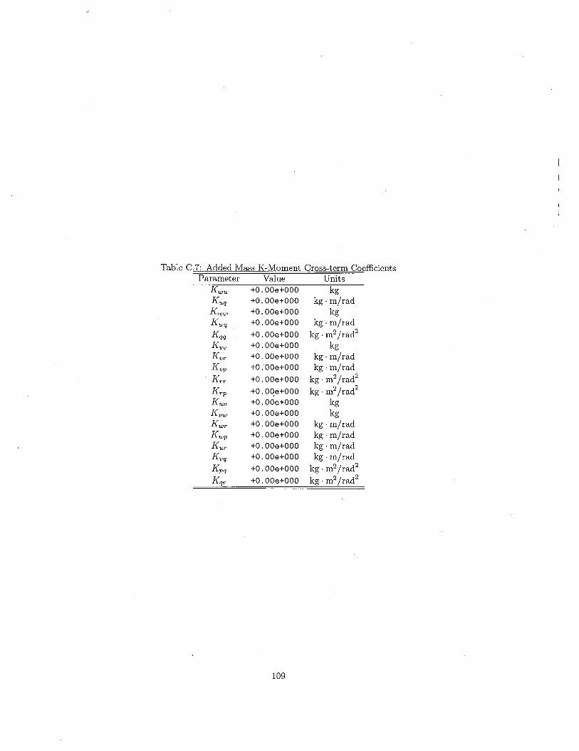
Table C.7: Added Mass K-Moment Cross-term CoeffcientsParameter

KwuKuqKwwKwq

KqqKvvKvrKvp

KrrKrpKuvKvwKwrKwpKurKvq

Kpq

Kqr

Value+O.OOe+OOO

+O.OOe+OOO



+0 . OOe+OOO

+0 . OOe+OOO

+0 . OOe+OOO

+O.OOe+OOO+0 . OOe+OOO

+0 . OOe+OOO

+O.OOe+OOO

+O.OOe+OOO

+O.OOe+OOO

+O.OOe+OOO

+O.OOe+OOO

+0. OOe+OOO

109

Unitskg

kg. m/radkg

kg. m/radkg. m2/rad2

kgkg. m/radkg. m/rad

kg. m2/rad2kg. m2/rad2

kgkg

kg. m/radkg. m/radkg. m/radkg. m/rad


Table C.8: Added Mass M-, N-Moment Cross-term CoeffcientsParameter

MwqMuqaMuu

MwwaMuwaMvrMvp

Mpp

MrrMrpMuvMvwMupMwrMwpMurMpq

JllqrNuuNwuNuqNwq

NqqNvvaNvrNvp

NrpNpp

NuvaNvwNupNuraNwpNvq

Npq

Nqr

Value+O.OOe+OOO

+1.93e+000+0 .00e+000+O.OOe+OOO

+3.46e+001+0 . OOe+OOO

-1. 93e+000+O.OOe+OOO

+0 . OOe+OOO

+4.86e+000+O.OOe+OOO

+0. OOe+OOO

+O.OOe+OOO

+O.OOe+OOO+0 .00e+000+O.OOe+OOO

+0. OOe+OOO

+0 . OOe+OOO

+O.OOe+OOO+0 .00e+000+0 . OOe+OOO

+O.OOe+OOO

+0 .00e+000+O.OOe+OOO


+0 . OOe+OOO

+O.OOe+OOO

-3.46e+001+0 . OOe+OOO

+O.OOe+OOO+1.93e+000-1.93e+000+O.OOe+OOO

-4 .86e+000+O.OOe+OOO

Unitskg. m/radkg . m/rad

kgkgkg

kg. m/radkg. m/rad

kg. m2/rad2kg. m2/rad2kg. m2/rad2

kgkg

kg. m/radkg . m/radkg. m/radkg. m/rad


kgkg

kg. m/radkg. m/rad

kg. m2/rad2kg

kg. m/radkg. m/rad


kgkg

kg. m/radkg. m/radkg. m/radkg. m/rad


Table C.9: Propeller TermsParameter Value Units

Xprop +3. 86e+000 NKprop '-5. 43e-001 N. m

110

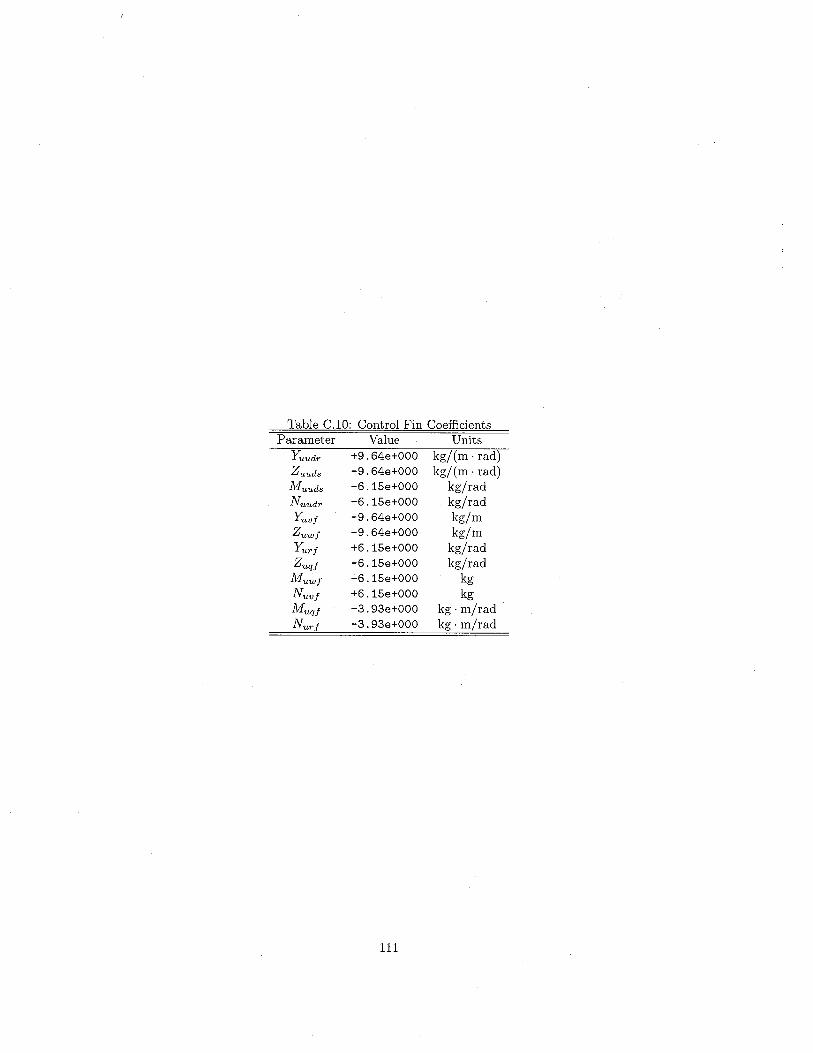
Table C.I0: Control Fin Coeffcients

ParameterYuudrZuudsMuudsNuudrYuvtZuwtYurtZuqtMuwtNuvtMuqtNurt

Value+9 . 64e+OOO-9 . 64e+OOO-6. 15e+OOO

-6. 15e+OOO

-9 . 64e+OOO-9 . 64e+OOO+6. 15e+OOO-6.15e+OOO-6. 15e+OOO

+6. 15e+OOO-3.93e+OOO-3.93e+OOO

Unitskg/(m. rad)kg/(m. rad)

kgl radkgl radkg/mkg/m

kg/radkg/rad

kgkg

kg. m/radkg. m/rad

111

Appendix D

Tables of Linearized ModelParameters

Note that all coeffcients are calculated for the STD REMUS hull profile.

Table D.l: Linearized Combined CoeffcientsParameter Value Units Description

Zwc -1. 57e+001 kg/s Crossflow DragZwl -3.45e+001 kg. m/s Body LiftZwf -1.64e+001 kg. m/s Fin Lift

Zqc +1.20e-001 kg. m/s Crossflow DragZqa +1.44e+000 kg. m/s Added Mass Cross TermZqf -1.12e+001 kg. m/s Fin Lift

Mwc -4.03e-001 kg. m/s Crossflow DragMwa +5.34e+001 kg. m/s Added Mass Cross TermMwl -1. 11e+001 kg. m/s Body LiftMwf -1.12e+001 kg. m/s Fin Lift

Mqc -2. 16e+000 kg.m2/s Crossflow DragMqa +2.97 e+OOO kg. m2 Is Added Mass Cross TermMqf -7 .68e+000 kg.m2/s Fin Lift

112

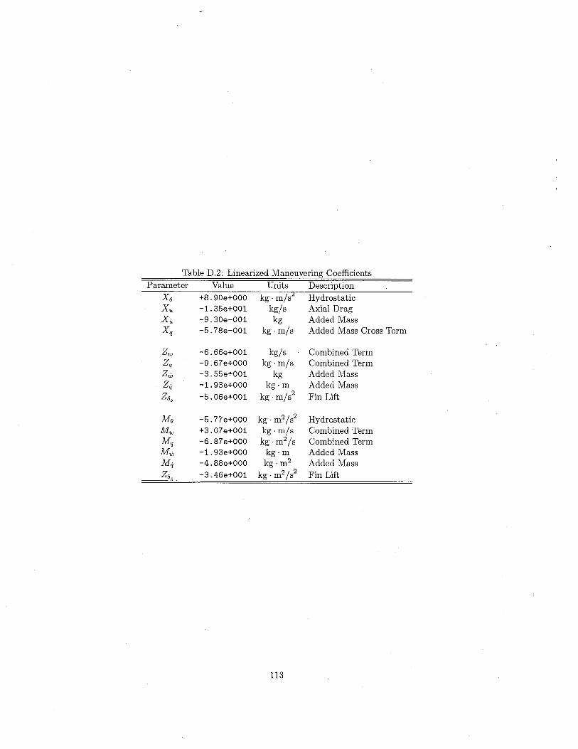
Table D.2: Linearized Maneuvering CoeffcientsParameter Value Units Description

Xe +8.90e+000 kg. m/s'2 HydrostaticXu -1.35e+001 kg/s Axial DragXu -9.30e-001 kg Added MassXq -5.78e-001 kg. m/s Added Mass Cross Term

Zw -6.66e+001 kg/s Combined TermZq -9.67 e+OOO kg. m/s Combined TermZw -3.55e+001 kg Added MassZ. -1.93e+000 kg.m Added Massq

ZÓs -5.06e+001 kg. m/s2 Fin Lift

Me -5.77 e+OOO kg. m2/s2 HydrostaticMw +3.07 e+001 kg. m/s Combined TermMq -6.87 e+OOO kg.m2/s Combined TermMw -1.93e+OOO kg.m Added MassM. -4.88e+OOO kg. m2 Added Massq

ZÓs -3.46e+OO1 kg.m2/s2 Fin Lift

113

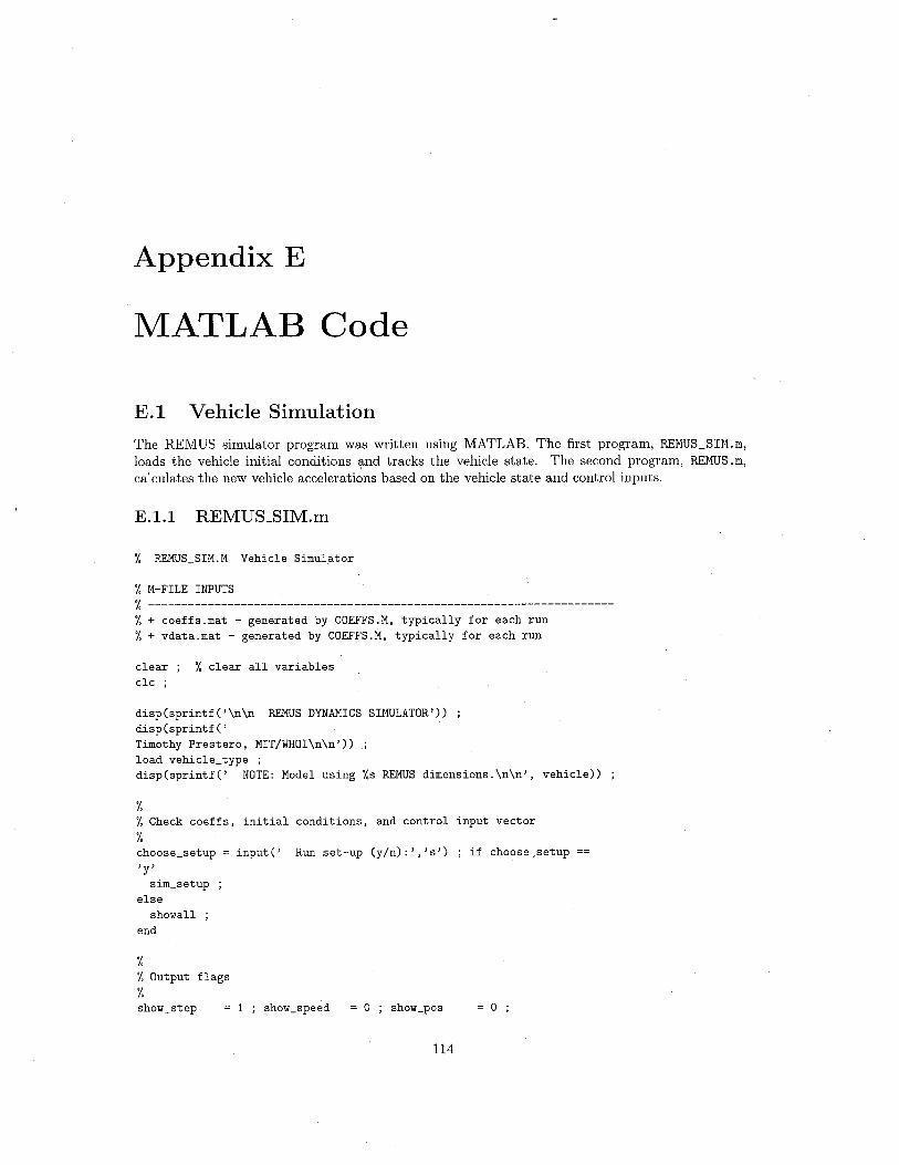
Appendix E

MATLAB Code

E.1 Vehicle SimulationThe REMUS simulator program was written using MATLAB. The first program, REMUS_S1M.m,

loads the vehicle initial conditions and tracks the vehicle state. The second program, REMUS. m,

calculates the new vehicle accelerations based on the vehicle state and control inputs.

E.!.! REMUS_SIM.m

% REMUS_SIM.M Vehicle Simulator

% M-FILE INPUTS

% ------------------------------- ---------------------------------------% + coeffs . mat - generated by COEFFS .M, typically for each run

% + vdata.mat - generated by COEFFS.M, typically for each run

clearclc ;

% clear all variables

disp (sprintf ( ) \n \n REMS DYNAMICS SIMULATOR'))disp (sprintf ( ,Timothy Prestero, MIT/WHOI\n\n'))

load vehicle_type ;disp (sprintf ( , NOTE: Model using %s REMS dimensions. \n \n', vehicle))

%

% Check coeffs, initial conditions, and control input vector

%

choose_setup = input ( , Run set-up (y In) : ) , ) s') ; if choose_setup'y'

sim_setupelse

show allend

%

% Output flags

%

show_step 1 show_speed o show _pos o

114

run_savedata = 0 ; run_plots

%choose_setup = 1 ;o choose int o

%

% SET INTEGRATION METHOD

%

int_list = t'Basic Euler' 'Improved Euler' 'Fourth-Order

Runge-Kutta'l ; int_methods = t'euler' 'imp_euler' 'rkutta' 1; if

c):oose_intdisp(sprintf (' Integration Method: \n')) ;

for i = 1:size(int_list,2) ;disp(sprintf(' %i - %s', i, char(int_list(i))))

endd = input ( '\n Enter a number: ') ;

elsed 3;

end int_method = char (int_methods (d))

% check working directory

cd_outputs ;

% create .mat files

d = clock ; yy = d(l) ; mo = d(2) ; dd = d(3) ; hh = d(4) ; mm =

d(5) ; ss = d(6) ; date_string = datestr (datenum(yy ,mo, dd) ,1)

time~string = datestr(datenum(yy,mo,dd,hh,mm,ss) ,13) ;

%% generate random filename

% (dumy, file_string, dumy, dumyJ = fileparts(tempname)%disp(sprintf('\nCurrent simulator data files: '));%ls * . mat ;%file_string = input (sprintf (' \nEnter name for data file: '), 's')

temp_str = datestr(now, 0) ; file_string =

strcat (' sim-' , temp_str(l: 2) , temp_str(4: 6) , temp_str(10: 11) , '-' , . . .temp_str(13:14), temp_str(16:17)) ;

disp(sprintf('\nData file saved as\n %s\\%s.mat', cd, file_string));

% EXPERIMENTAL/ASSIGNED VALUES: initial conditions, input vector

% ------------------------------------------------------------------------------% loading model inputs, generated in SIM_SETUP. M

load input_ vec~or % data from FIN_INPUTS. M on mission files

load time_step

load initial_state % data from INITIAL_CONDITIONS.M on above

pitch_max = 90 ;

% RUN MODEL

% ------------------------------------------------------------------------------% Initialize number of steps and storage matrix

if strcmp(int_method,' euler')

n_steps size (ui, 2) ;else

n_steps size (ui, 2)-1end output_table = zeros (n_steps, size (x, l)+size (ui, 1) +7) ;disp (sprintf ( '\n Simulator running...'));

115

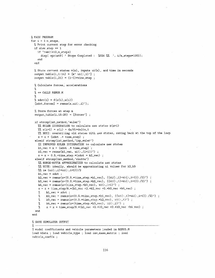
% MAIN PROGRAM

for i = 1:n_steps,

% Print current step for error checking

if show_step == 1

if -rem(i*10 ,n_steps)

disp( sprintf ( , Steps Completed %02d %%end

end

i/n_steps*100)) ;

% Store current states x (n), inputs ui (n), and time in seconds

output_table(i,1:14) = (x' ui(:,i)'J

output_table (i ,21) = (i -1) *time_step

% Calculate forces, accelerations

%

% * * CALLS REMS. M

%

% xdot(i) = f(x(i) ,u(i))

(xdot , f orcesJ = remus (x, uiC : , i) ') ;

% Store forces at step n

output_table(i,15:20) = (forces'J

if strcmp(int_method, 'euler')

%% EULER INTEGRATION to calculate new states x(n+1)

%% x(i+1) = xCi) + dx/dt*delta_t

%% NOTE: overwriting old states with new states, saving back at the top of the loop

x = x + (xdot . * time_step) ;elseif strcmp (int_method, , imp_euler')

%% IMPROVED EULER INTEGRATION to calculate new states

k1_ vec = x + (xdot . * time_step) ;

k2_vec = remus(k1_vec, ui(:,(i+1))') ;

x = x + 0.5. *time_step. * (xdot + k2_ vec)

elseif strcmp(int_method, 'rkutta')

%% RUNGE-KUTTA APPROXIMATION to calculate new states

%% NOTE: ideally, should be approximating ui values for k2,k3

%% ie (ui(: ,i)+ui(: ,i+1))/2

k1_ vec xdot;k2_vec remus(x+(O.5.*time_step.*k1_vec), ((ui(: ,i)+ui(: ,i+1)) ./2)')k3_vec remus(x+(O.5.*time_step.*k2_vec), ((ui(: ,i)+ui(: ,i+1)) ./2)')k4 vec remus (x+(time_step. *k3_vec) , ui(: ,i+1)') ;

x x + time_step/6.*(k1_vec +2.*k2_vec +2.*k3_vec +k4_vec) ;

% k1_ vec xdot;% k2_vec remus(x+(O.5.*time_step.*k1_vec), ((ui(: ,i)+ui(: ,i+1)) ./2)')% k3_vec remus(x+(O.5.*time_step.*k2_vec), ui(: ,i)') ;% k4 vec remus (x+ (time_step. *k3_ vec), ui (: , i) ') ;% x = x + time_step/6.*(k1_vec +2.*k2_vec +2.*k3_vec +k4_vec)

endend

% SAVE SIMULATOR OUTPUT

% ------------------------------------------------------------------------------% model coefficients and vehicle parameters loaded in REMUS.M

load vdata ; load vehicle_type ; load inv_mass_matrix ; load

vehicle coeffs

116

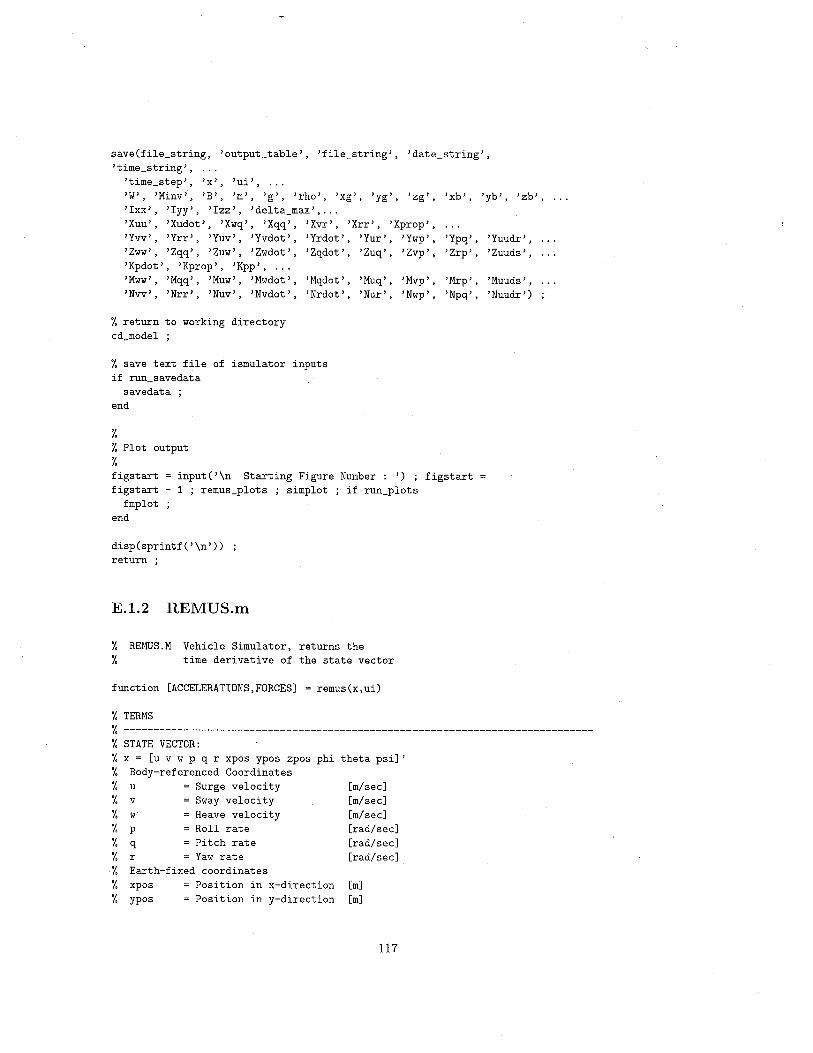
save(file_string, 'output_table', 'file_string', 'date_string',

'time_string' ,'time_step', 'x', 'ni', ...

'W', 'Minv', 'B', 'm', 'g', 'rho', 'xg', 'yg', 'zg', 'xb', 'yb', 'zb', ...

'lxx', 'Iyy', 'Izz', 'delta_max',...

'Xuu', 'Xudot', 'Xwq', 'Xqq', 'Xvr', 'Xrr', 'Xprop',

'Yvv', 'Yrr', 'Yuv', 'Yvdot', 'Yrdot', 'Yur', 'Ywp',

'Zww', 'Zqq', 'Zuw', 'Zwdot', , Zqdot , , 'Zuq', 'Zvp';'Kpdot', 'Kprop', 'Kpp', ...'Mww', 'Mqq', 'Muw', , Mwdot, ,'Nvv', 'Nrr', 'Nuv', 'Nvdot',

, Mqdot " 'Muq',, Nrdot " 'Nur' ,

% return to working directory

cd_model

% save text file of ismulator inputs

if run_savedata

savedataend

%

% Plot output

%

figstartfigstart -

fmplotend

'Mvp' ,'Nwp' ,

'Ypq' ,'Zrp' ,

'Yuudr' ,'Zuuds' ,

'Mrp', 'Muuds' ,'Npq', 'Nuudr')

input ( , \n Starting Figue Number : ' ) ; f igstart1 ; remus_plots ; simplot ; if run_plots

disp (sprintf ( , \n' ) )return ;

E.1.2 REMUS.m

% REMUS.M

%

Vehicle Simulator, returns thetime deri vati ve of the state vector

function (ACCELERATIONS, FORCES) = remus (x, ui)

% TERMS

%

%

%

%

%

%

%

%

%

%

%

%

%

STATE VECTOR:

x = (u v w p q r xpos ypos zpos phi theta psi) ,Body-referenced Coordinates

u Surge velocityv Sway velocityW' Heave velocityp Roll rateq Pitch rater Yaw rateEarth-fixed coordinates

xpos Posi tion in x-directionypos = Position in y-direction

(m/ see)(m/ see)(m/ see)(rad/sec)(rad/sec)(rad/ see)

(m)

(m)

117

% zpos Posi tion in z-direction (mJ

% phi Roll angle (radJ% theta Pi tch angle (radJ% psi Yaw angle (radJ%

% INPUT VECTOR

% ui = (delta_s delta_rJ'% Control Fin Angles

% del ta_s angle of stern planes (radJ% delta_r = angle of rudder planes (radJ

% Initialize global variables

% ------------------------------------------------------------------------------load vdata % W and B, CG and CB coordsload inv_mass_matrix % Minv matrixload vehicle coeffs % non-zero vehicle coefficients only

% Output flags

show_forces = 10

% Get and check state variables and control inputs

% ------------------------------------------------------------------------------% Get state variablesu x(1) vxes) r = x(6)

x (2) wphi = x(10)

x(3)theta

px (11)

x(4) qpsi = x (12)

% Get control inputs

delta_s = ui(U ; delta_r = ui(2) ;

% Check control inputs (useful later)

if del ta_s ) del ta_max

del ta_s = sign (del ta_s) *del ta_max

end ifdelta_r ) delta_max

delta_r = sign(delta_r)*delta_max

end

% Initialize elements of coordinate system transform matrix

% ---------------------------------------- --------------------------------------

c1 = cos(phi); c2 = cos(theta); c3 = cos(psi); s1 = sin(phi); s2 =

sin (theta) ; s3 = sin (psi) ; t2 = tan(theta) ;

% Set total forces from equations of motion

% ----------------------------------------------------- -------------------------

X = -(W-B)*sin(theta) + Xuu*u*abs(u) + (Xwq-m)*w*q + (Xqq +

m*xg) *qn2 ...

+ (Xvr+m) *v*r + (Xrr + m*xg) *rn2 -m*yg*p*q - m*zg*p*r ...

+ Xprop ;

Y (W-B)*cos(theta)*sin(phi) + Yvv*v*abs(v) + Yrr*r*abs(r) +Yuv*u*v ...

+ (Ywp+m) *w*p + (Yur-m) *u*r - (m*zg) *q*r + (Ypq - m*xg) *p*q

+ Yuudr*un2*delta_r ;

Z = (W-B)*cos(theta)*cos(phi) + Zww*w*abs(w) + Zqq*q*abs(q)+

Zuw*u*w

118

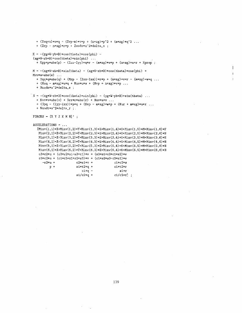
+ (Zuq+m) *u*q + (Zvp-m) *v*p + (m*zg) *p~2 + (m*zg) *q~2 ...

+ (Zrp - m*xg)*r*p + Zuuds*u~2*deita_s

K = -(yg*W-yb*B) *cos (theta) *cos (phi) -

(zg*W-zb*B) *cos (theta) *sin(phi) ...+ Kpp*p*abs (p) - (Izz- Iyy) *q*r - (m*zg) *w*p + (m*zg) *u*r + Kprop

M = -(zg*W-zb*B)*sin(theta) - (xg*W-xb*B)*cos(theta)*cos(phi) +

Mww*w*abs (w) ...

+ Mqq*q*abs(q) + (Mrp - (Ixx-Izz))*r*p + (m*zg)*v*r - (m*zg)*w*q

+ (Muq - m*xg)*u*q + Muw*u*w + (Mvp + m*xg)*v*p ...+ Muuds*u~2*deita_s ;

N -(xg*W-xb*B) *cos (theta) *sin(phi) - (yg*W-yb*B) *sin(theta) ...+ Nvv*v*abs(v) + Nrr*r*abs(r) + Nuv*u*v ...+ (Npq - (Iyy- Ixx)) *p*q + (Nwp - m*xg) *w*p + (Nux + m*xg) *u*r ...

+ Nuudr*u~2*deita_r ;

FORCES = (X Y Z K M NJ '

ACCELERATIONS = ...

(Minv(1, 1) *X+Minv(1, 2) *Y+Minv(1, 3) *Z+Minv(1 ,4) *K+Minv(1 ,5) *M+Minv(1, 6)*NMinv(2, 1) *X+Minv(2, 2) *Y+Minv(2 ,3)*Z+Minv(2,4) *K+Minv(2 ,5) *M+Minv(2, 6)*NMinv(3, 1) *X+Minv(3 ,2) *Y+Minv(3 ,3) *Z+Minv(3 ,4) *K+Minv(3 ,5) *M+Minv(3, 6) *N

Minv(4, 1) *X+Minv(4, 2) *Y+Minv(4 ,3) *Z+Minv(4,4) *K+Minv (4 ,5) *M+Minv(4, 6) *NMinv(5, 1)*X+Minv(5, 2) *Y+Minv(5, 3) *Z+Minv(5 ,4) *K+Minv(5 ,5) *M+Minv(5, 6) *NMinv(6, 1) *X+Minv(6, 2) *Y+Minv(6, 3) *Z+Minv(6 ,4) *K+Minv(6 ,5) *M+Minv(6, 6) *N

c3*c2*u + (c3*s2*s1-s3*c1) *v + (s3*s1 +c3*c1*s2) *w

s3*c2*u + (c1*c3+s1*s2*s3) *v + (c1*s2*s3-c3*s1) *w

-s2*u + c2*s1*v + c1*c2*wp + s1*t2*q + c1*t2*rc1*q - s1*r

s1/c2*q + c1/c2*rJ

119

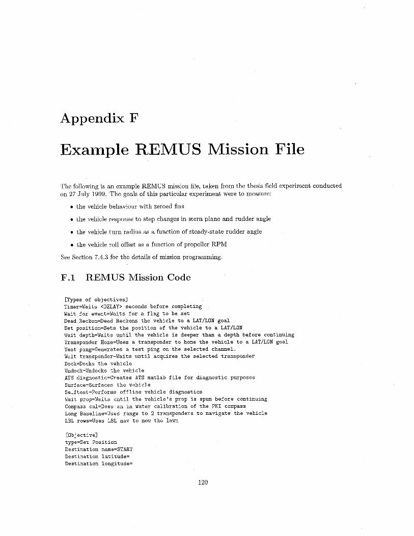
Appendix F

Example REMUS Mission File

The following is an example REMUS mission file, taken from the thesis field experiment conductedon 27 July 1999. The goals of this particular experiment were to measure:

. the vehicle behaviour with zeroed fins

. the vehicle response to step changes in stern plane and rudder angle

. the vehicle turn radius as a function of steady-state rudder angle

. the vehicle roll offset as a function of propeller RPM

See Section 7.4.3 for the details of mission programming.

F.i REMUS Mission Code

(Types of obj ecti vesJTimer=Wai ts ~DELAY) seconds before completing

Wait for event=Waits for a flag to be set

Dead Reckon=Dead Reckons the vehicle to a LAT/LON goal

Set posi tion=Sets the position of the vehicle to a LAT /LON

Wait depth=Waits until the vehicle is deeper than a depth before continuing

Transponder Home=Uses a transponder to home the vehicle to a LAT/LON goal

Test ping=Generates a test ping on the selected chanel.

Wait transponder=Waits until acquires the selected transponder

Dock=Docks the vehicle

Undock=Undocks the vehicle

ATS diagnostic=Creates ATS matlab file for diagnostic purposes

Surface=Surfaces the vehicle

Selftest=Performs offline vehicle diagnostics

Wait prop=Waits until the vehicle's prop is spun before continuing

Compass cal=Does an in water calibration of the PNI compass

Long Baseline=Uses range to 2 transponders to navigate the vehicle

LBL rows=Uses LBL nav to mow the lawn

(ObjectiveJtype=Set Position

Destination name=START

Destination lati tude=Destination longi tude=

120

Offset direction=131

Offset distance (Meters) =0

Offset Y axis (Meters)=O

(Obj ecti ve)

type=Wait prop

Required rpm=60

Auto calibrate depth sensor=NO

(Objective) ## GET TO START DEPTH (2M) AND HEADING (130) ##########type=Long baseline

Destination name=START

Destination lati tude=Destination longi tude=

Offset direction=130

Offset distance (Meters)=200

Offset Y axis (Meters)=O

Minimum range (M. )=10Depth control mode=normal #normal triangle altitude

Depth=2.0RPM=1500timeout (seconds) =-1

Trackline follow meters=200

Track ping interval (sees.) =5.0Transponder #1=NOPP _Ai

Transponder #2=NOPP _A2

(Objective) ## CONTROLLED LEVEL FLIGHT ##########type=TimerDelay in seconds=180. 0

Keep current commands=NO

Direct (pitch rudder thruster)=none

RPM command=1500. 0Depth command=2. 0

Heading command=130. 0

(Db j ecti ve) ## ZERO ALL FINS ##########type=TimerDelay in seconds=2. 0


Direct (pitch rudder thruster)=pitch rudder

Direct pitch command=O

Direct rudder command=O

RPM command=1500. 0

(Obj ecti ve) ## TIMER TO DEPTH 2M

type=TimerDelay in seconds=60. 0


Direct (pitch rudder thruster) =none



(Obj ecti ve) #### PITCH DOWN 2, HEADING ##########

121



Direct (pitch rudder thruster)=pitch

Direct pitch command=10


RPM command=1500. 0

CObjectiveJ ## TIMER TO DEPTH 6Mtype=TimerDelay in seconds=90. 0





CObj ecti veJ ## PITCH UP 2, HEADINGtype=TimerDelay in seconds=10. 0



Direct pitch command=-10


RPM command=1500. 0

CObjectiveJ ## TIMER TO DEPTH 2Mtype=TimerDelay in seconds=90. 0





CObjectiveJ #### PITCH DOWN 4, HEADING ##########type=TimerDelay in seconds=6. 0





RPM command=1500. 0

CObj ectiveJ ## TIMER TO DEPTH 6Mtype=TimerDelay in seconds=90. 0





CObj ecti veJ ## PITCH UP 4, HEADINGtype=Timer

122

Delay in seconds=8. 0





RPM command=1500. 0

(Objective) ## TIMER TO DEPTH 3Mtype=TimerDelay in seconds=90. 0





(Obj ecti ve) #### PITCH DOWN 6, HEADING ##########






RPM command=1500. 0

(Objective) ## TIMER TO DEPTH 6Mtype=TimerDelay in seconds=90. 0





(Objective) ## PITCH UP 6, HEADINGtype=TimerDelay in seconds=4. 0





RPM command=1500. 0

(Obj ecti ve) ## TIMER TO DEPTH 3M






(Obj ecti ve) #### RUDDER CIRCLE PORT, FIXED PITCH ##########type=TimerDelay in seconds=20. 0

123




Direct rudder command=40

RPM command=1500. 0

(Obj ecti veJ ## TIMER TO DEPTH 3M, HEADING 130






(ObjectiveJ ## RUDDER CIRCLE STBD, FIXED PITCHtype=TimerDelay in seconds=20. 0



Direct pitch command=O

Direct rudder command=-40

RPM command=1500. 0

(ObjectiveJ ## TIMER TO DEPTH 3M, HEADING 130type=TimerDelay in seconds=120. 0





(ObjectiveJ ## ZERO RUDDER, DEPTH- type=Timer

Delay in seconds=120. 0


Direct (pitch rudder thruster)=rudder

Direct rudder command=O

Depth command=3. 0

RPM command=1500. 0

(ObjectiveJ ## SPIN DOWN PROP 1250 ##########type=TimerDelay in seconds=120. 0





(ObjectiveJ ## SPIN DOWN PROP 1000type=TimerDelay in seconds=120. 0


124




(Obj ecti ve) ## SPIN DOWN PROP 750






(Objective) ## SPIN DOWN PROP 500type=TimerDelay in seconds=120. 0





(Objective)type=END

125

Bibliography

¡I) Martin Abkowitz. Stability and Motion Control of Ocean Vehicles. MIT Press, Cambridge,MA, 1972.

(2) B. Allen, R. Stokey, T. Austin, N. Forrester, R. Goldsborough, M. Purcell, and C. von Alt.REMUS: A small, low cost AUV; system description, field trials and performance results. InProceedings MTS/1EEE Oceans 1997, Halifax, Canada, 1997. 37

¡3) B. Allen, W. Vorus, and T. Prestero. Propulsion system performance enhancements on REMUSAUVs. In Proceedings MTS/1EEE Oceans 2000, Providence, Rhode Island, September 2000.37

(4) P. Edgar An. An experimental self-motion study of the Ocean Explorer AUV in controlled seastates. IEEE Journal of Oceanic Engineering, 23(3):274-284, 1998. 101

¡5) P. Ananthakrishnan. Dynamic response of an underwater body to surface waves. In ProceedingsASME Forum on Advances in Free Surface and Interface Fluid Dyanamics, San Francisco, CA,1999.

(6) Robert D. Blevins. Formulas for Natural Frequency and Mode Shape. Kreiger Publishing,Florida, 1979. 28, 29

¡7) M. R. Bottaccini. The stability coeffcients of standard torpedoes. NAVORD Report 3346, U.S.Naval Ordnance Test Station, China Lake, CA, 1954. 25, 30, 43, 99

(8) J. Feldman. Revised standard submarine equations of motion. Report DTNSRDC/SPD-0393-09, David W. Taylor Naval Ship Research and Development Center, Bethesda, MD, June 1979.

¡9) John E. Fidler and Charles A. Smith. Methods for predicting submersible hydrodynamic char-acteristics. Report NCSC TM-238-78, Naval Coastal Systems Laboratory, Panama City, FL,1978. 30

(10) Thor 1. Fossen. Guidance and Control of Ocean Vehicles. John Wiley & Sons, New York, 1994.27

¡11) R. W. Fox and A. T. McDonald. Introduction to Fluid Mechanics. J. Wiley and Sons, NewYork, 4th edition, 1992.

¡12) M. Gertler and G. Hagen. Standard equations of motion for submarine simulation. ReportDTNSRDC 2510, David W. Taylor Naval Ship Research and Development Center, Bethesda,MD, June 1967.

¡131 Michael J. Griffn. Numerical prediction of the forces and moments on submerged bodiesoperating near the free surface. In Proceedings of the 2000 SNAME/ ASNE Student PaperNight, Massachusetts Institute of Technology, January 2000. SNAME. 101

126

¡14J Michael F. Hajosy. Six Degree of Freedom Vehicle Controller Design for the Operation of an

Unmanned Underwater Vehicle in a Shallow Water Environment. Ocean Engineer's thesis,Massachusetts Institute of Technology, Department of Ocean Engineering, May 1994.

¡15J Sighard F. Hoerner. Fluid Dynamic Drag. Published by author, 1965. 25,26, 43

¡16J Sighard F. Hoerner and Henry V. Borst. Fluid Dynamic Lift. Published by author, second

edition, 1985. 30, 31, 99

¡i 7j P. C. Hughes. Spacecraft Attitude Dynamics. John Wiley and Sons, New York, 1986. 22

¡18j D. E. Humphreys. Development of the equations of motion and transfer functions for underwatervehicles. Report NCSL 287-76, Naval Coastal Systems Laboratory, Panama City, FL, July1976.

¡19J D. E. Humphreys. Dynamics and hydrodynamics of ocean vehicles. In Proceedings MTSj1EEEOceans 2000, Providence, Rhode Island, September 2000.

¡20J E. V. Lewis, editor. Principles of Naval Architecture. Society of Naval Architects and MarineEngineers, Jersey City, New Jersey, second edition, 1988. 26

¡21j Woei-Min Lin and Dick Y. P. K. Yue. Numerical solutions for large-amplitude ship motions inthe time domain. In Proceedings Eighteenth Symposium on Naval Hydrodynamics, Ann Arbor,Michigan, 1990. 101

¡22j D. F. Myring. A theoretical study of body drag in subcritical axisymmetric flow. AeronauticalQuarterly, 27(3):186-94, August 1976. 14, 15, 43

¡23J Meyer Nahon. A simplified dynamics model for autonomous underwater vehicles. In Proceedings1996 Symposium on Autonomous Underwater Vehicle Technology, pages 373-379, June 1996.30,99

¡24J J. N. Newman. Marine Hydrodynamics. MIT Press, Massachusetts, 1977. 25, 27, 28

¡25J Norman S. Nise. Control Systems Engineering. Benjamin/Cummings, San Francisco, CA, firstedition, 1992. 88

¡26j Wiliam D. Ramsey. Boundary Integral Methods for Lifting Bodies with Vortex Wakes. PhDdissertation, Massachusetts Institute of Technology, Department of Ocean Engineering, May1996. 101

¡27j Jeffery S. RiedeL. Seaway Learning and Motion Compensation in Shallow Waters for SmallA UVs. PhD dissertation, Naval Postgraduate School, Department of Ocean Engineering, June1999. 101

¡28J R. Stokey and T. Austin. Sequential long baseline navigation for REMUS, an autonomousunderwater vehicle. In Proceedings Information Systems for Navy Divers and A UVs Operatingin Very Shallow Water and Surf Zone Regions, April 1999. 37, 51

¡29j Michael S. Triantafyllou. Maneuvering and control of surface and underwater vehicles. LectureNotes for MIT Ocean Engineering Course 13.49, 1996. 25, 26 .

¡30j C. von Alt, B. Allen, T. Austin, and R. Stokey. Remote environmental monitoring units. InProceedings MTSj1EEE Oceans 1994, Cambridge, MA, 1994. 13,37

¡31j C. von Alt and J.F. Grassle. LEO-15: An unmanned long term environmental observatory. InProceedings MTSj1EEE Oceans 1992, Newport, RI, 1992. 12, 37

127ii

r

'i

l32j L. F. Whicker and L. F. Fehlner. Free-stream characteristics of a family of low-aspect ratiocontrol surfaces. Technical Report 933, David Taylor Model Basin, 1958. NC. 26

l33j Christopher J. Wily. Attitude Control of an Underwater Vehicle Subjected to Waves. OceanEngineer's thesis, Massachusetts Institute of Technology, Department of Ocean Engineering,May 1994. 101

l34j Ming Xue. Three-dimensional fully non-linear simulation of waves and wave-body interactions.PhD dissertation, Massachusetts Institute of Technology, Department of Ocean Engineering,May 1997. 101

¡35J D. R. Yoerger, J.G. Cooke, and J.-J. E. Slotine. The influence of thruster dynamics~ on un-

derwater vehicle behavior and their incorporation into control system design. IEEE Journal ofOceanic Engineering, 15:167-178, July 1990. 33

128

REMUS AUV

Documents

tuning fork

fin liftzqc

r2 p2

xt xf xf2

termfin lift

oceanographic

p2 q2

mu zq