Remote sensing of seagrasses in a patchy multi-species environment

PLEASE SCROLL DOWN FOR ARTICLE

This article was downloaded by: [Nordlund, Lina]On: 22 April 2011Access details: Access Details: [subscription number 936694830]Publisher Taylor & FrancisInforma Ltd Registered in England and Wales Registered Number: 1072954 Registered office: Mortimer House, 37-41 Mortimer Street, London W1T 3JH, UK

International Journal of Remote SensingPublication details, including instructions for authors and subscription information:http://www.informaworld.com/smpp/title~content=t713722504

Remote sensing of seagrasses in a patchy multi-species environmentAnders Knudbya; Lina Nordlundb

a Department of Geography, University of Waterloo, Waterloo, ON, Canada b Department of SystemsEcology, Stockholm University, Stockholm, Sweden

Online publication date: 20 April 2011

To cite this Article Knudby, Anders and Nordlund, Lina(2011) 'Remote sensing of seagrasses in a patchy multi-speciesenvironment', International Journal of Remote Sensing, 32: 8, 2227 — 2244To link to this Article: DOI: 10.1080/01431161003692057URL: http://dx.doi.org/10.1080/01431161003692057

Full terms and conditions of use: http://www.informaworld.com/terms-and-conditions-of-access.pdf

This article may be used for research, teaching and private study purposes. Any substantial orsystematic reproduction, re-distribution, re-selling, loan or sub-licensing, systematic supply ordistribution in any form to anyone is expressly forbidden.

The publisher does not give any warranty express or implied or make any representation that the contentswill be complete or accurate or up to date. The accuracy of any instructions, formulae and drug dosesshould be independently verified with primary sources. The publisher shall not be liable for any loss,actions, claims, proceedings, demand or costs or damages whatsoever or howsoever caused arising directlyor indirectly in connection with or arising out of the use of this material.

http://www.informaworld.com/smpp/title~content=t713722504

http://dx.doi.org/10.1080/01431161003692057

http://www.informaworld.com/terms-and-conditions-of-access.pdf

Remote sensing of seagrasses in a patchy multi-species environment

ANDERS KNUDBY*† and LINA NORDLUND‡

†Department of Geography, University of Waterloo, 200 University Avenue West,

Waterloo, ON, N2L3G1 Canada

‡Department of Systems Ecology, Stockholm University, S-106 91 Stockholm, Sweden

(Received 2 June 2009; in final form 14 December 2009)

We tested the utility of IKONOS satellite imagery to map seagrass distribution and

biomass in a 4.1 km2 area around Chumbe Island, Zanzibar, Tanzania. Considered

to be a challenging environment to map, this area is characterized by a diverse mix

of inter- and subtidal habitat types. Our mapped distribution of seagrasses corre-

sponded well to field data, although the total seagrass area was underestimated due

to spectral confusion and misclassification of areas with sparse seagrass patches as

sparse coral and algae-covered limestone rock. Seagrass biomass was also accu-

rately estimated (r2 ¼ 0.83), except in areas with Thalassodendron ciliatum (r2 ¼0.57), as the stems of T. ciliatum change the relationship between light interception

and biomass from that of other species in the area. We recommend the use of

remote sensing over field-based methods for seagrass mapping because of the

comprehensive coverage, high accuracy and ability to estimate biomass. The

results obtained with IKONOS imagery in our complex study area are encoura-

ging, and support the use of this data source for seagrass mapping in similar areas.

1. Introduction

Seagrass beds can be found in most shallow nearshore areas around the world (den

Hartog 1970). Seagrasses are important for coastal processes because of their role asecosystem engineers (Jones et al. 1994), and because they provide nursery habitat for

numerous juvenile fish and invertebrates, feeding grounds for dugongs and sea turtles

and protection against coastal erosion (Orth et al. 1984, Bell and Pollard 1989,

Costanza et al. 1997, Nagelkerken et al. 2000). However, natural and anthropogenic

disturbances have led to a worldwide decline of seagrasses (Green and Short 2003),

and an associated loss of ecosystem services and functions in the coastal zone

(Hemminga and Duarte 2000). This problem is especially pressing in areas of the

Western Indian Ocean (WIO), where the livelihoods of local people are immediatelydependent on invertebrates collected from seagrass beds (Gossling et al. 2004).

Observations and concerns over current losses of seagrass areas around Zanzibar

are beginning to be voiced by local fishermen and park rangers, but the existing

knowledge of the distribution and biomass of seagrasses in the region is limited

(Dahdouh-Guebas et al. 1999, Gullstrom et al. 2002, 2006). With local seagrass

beds under increasing pressure from economic development and population growth,

there is a growing need to monitor changes in the distribution, biomass and species

composition of seagrass areas. Given that seagrasses may function as an indicator of

*Corresponding author. Email: [email protected]

International Journal of Remote SensingISSN 0143-1161 print/ISSN 1366-5901 online # 2011 Taylor & Francis

http://www.tandf.co.uk/journalsDOI: 10.1080/01431161003692057

International Journal of Remote Sensing

Vol. 32, No. 8, 20 April 2011, 2227–2244

Downloaded By: [Nordlund, Lina] At: 15:20 22 April 2011

anthropogenic disturbance, such monitoring may also provide useful information for

conservation of closely associated environments in the area, such as coral reefs.

A cost-effective approach to nearshore monitoring is essential in the region because

of the limited resources available for such monitoring. Remote sensing, with its large

spatial coverage, has been used effectively to create baseline maps and to determinetemporal change in the spatial extent of seagrass areas (Ferguson et al. 1993),

percentage cover (Gullstrom et al. 2006) and aboveground biomass (Mumby et al.

1997b). Individual seagrass species have even been identified spectrally and mapped

using hyperspectral data (Fyfe 2003, Dekker et al. 2005), albeit with low overall

accuracy (Phinn et al. 2008). High accuracy of remotely sensed maps of seagrasses

has been obtained in areas with clear and shallow water and large homogeneous

seagrass meadows (Robbins 1997, Mumby et al. 1997b). In contrast to such ideal

conditions, nearshore areas in the WIO region are often characterized by small andpatchy seagrass areas with a mix of dominant species, each patch sometimes only a

few metres across and reaching depths greater than 5 m in areas with limited visibility.

This kind of environment is challenging to map, but if remote sensing is to contribute

to seagrass monitoring in the wider region, it is essential first to determine the

accuracy with which it can be used to map seagrasses in such environments.

In this study, we used established methods (Mumby et al. 1997b) to investigate the

potential of mapping seagrass distribution and biomass using high-resolution satellite

remote sensing in a complex WIO nearshore environment. We used IKONOS data(4 m multispectral resolution) because of their availability from the area and their

known ability to map nearshore environments (Andrefouet et al. 2003). We mapped

seagrass distribution and biomass in the area around Chumbe Island, Zanzibar,

Tanzania. Seagrasses here reach depths of 7 m in water with a typical visibility of

10–12 m. Seven different species of seagrass exist in the area, six of which can dominate

in any seagrass patch. We compare the results of imagery analyses with those of a

previous study (Hayford and Perlman 2006) that relied entirely on field observation,

and discuss the use of IKONOS imagery for mapping and monitoring seagrasses.

2. Methods

2.1 Study area

Chumbe Island is located off southwestern Unguja, the main island of Zanzibar,Tanzania (figure 1). An area of 0.3 km2 west of Chumbe Island has been formally

protected since 1994, when the Zanzibari government gazetted it as a no-take zone.

Effective management of the no-take zone is provided by Chumbe Island Coral Park

(Muthiga et al. 2000). The island is 1.1 km from north to south and 0.3 km from east

to west. It is composed of fossil coral rock, and the majority is covered by coral rag

forest. It is bordered on the western side by a fringing reef, and a shallow lagoon

extends east and south from the island. Coral cover ranges from very low on the inner

reef flat and in patches south and east of the island, to very high (. 90%) on parts ofthe reef crest. Rocky substrates are common in the intertidal zone, with occasional

stands of erect brown macroalgae, mainly Turbinaria sp., Hormophysa sp. and

Sargassum sp. Seagrass patches vary in size all around the island. Of the 13 seagrass

species known from the region (Bandeira and Bjork 2001), seven are found around

Chumbe Island: Cymodocea rotundata Ehrenb. & Hempr. ex Aschers, Halodule sp.

(Forsk.) Aschers. in Bossier, Thalassia hemprichii (Ehrenberg) Asherson,

Thalassodendron ciliatum (formerly Cymodocea ciliata) (Forskal) den Hartog,

2228 A. Knudby and L. Nordlund


Halophila ovalis (R. Br.) Hook. f., Syringodium isoetifolium (Ascherson) Dandy and

Cymodocea serrulata (R. Br.). Abbreviations for species names are used in the

remainder of this paper, as outlined in table 1.

2.2 Field methods

2.2.1 Seagrass data collection. Fieldwork was carried out from November to

December 2007, by both observers (AK and LN), in two parts: (i) development of a

visual scale of aboveground seagrass biomass (hereafter: biomass) and (ii) use of this

scale to collect biomass estimates along with depth and species composition data from

the areas around Chumbe Island. All data were collected while snorkelling.

(i) We developed a visual scale for biomass estimation by modifying the method

of Mumby et al. (1997b). For each calibration point, we placed a 0.25 m2

quadrat in a seagrass patch, and both observers visually estimated the amount

Figure 1. The location of Chumbe Island, Zanzibar.

Table 1. List of abbreviations of seagrass species used in this study.

Scientific name Abbreviation

Cymodocea rotundata CrHalodule sp. HThalassia hemprichii ThThalassodendron ciliatum TcHalophila ovalis HoSyringodium isoetifolium SiCymodocea serrulata Cs

Remote sensing of seagrasses 2229


of aboveground seagrass biomass inside the quadrat on a scale from 1 (only a

few blades present) to 6 (maximum biomass seen in the area). Because of the

large difference in biomass between species, and the species-dependent distri-

bution of aboveground biomass into stems and leaves, we developed two

separate scales. The first scale was used when one of the six smaller seagrassspecies, Si, Th, Cs, Cr, Ho and H, were dominant (i.e. when Tc was not

present); the second was used whenever Tc was present. Minimum increments

of 0.1 were used for both scales. When our estimates differed by more than 0.5,

we discussed the difference and reached a consensus value. At the end of the 2-

day calibration period, the average difference in estimates was 0.2, and no

estimates were more than 0.5 apart on either scale. We then collected 17

biomass samples, covering the range from , 1.5 to . 5.5 for each visual

scale, by harvesting all the aboveground seagrass biomass from a 625 cm2

quadrat placed in one corner of the larger quadrat. We cleaned the samples of

epiphytes and sediment with freshwater and oven dried them for a minimum of

48 h at 90�C until no further weight loss was recorded (method adopted from

Short and Coles (2001)). We then weighed each sample to the nearest 0.1 g on

an electronic scale.

We developed the visual scales without assumptions about the statistical

nature of the relationship between biomass and visual scale values. We there-

fore explored linear, power and exponential models, using half the data pointsfor model parameter calibration and the other half for accuracy assessment.

We chose the model with the lowest root mean square error (RMSE) as the

regression function for the given scale and repeated the calibration procedure

after data collection to check for ‘drift’ in the visual scales.

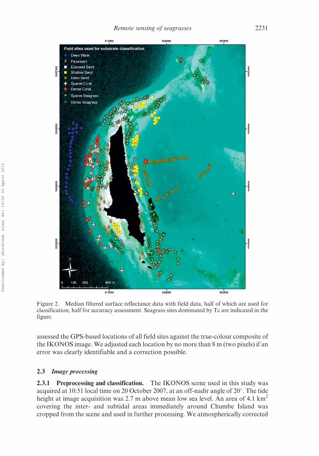
(ii) Using the visual scales, we then collected biomass data by snorkelling to areas

visually identified on the IKONOS image as probably containing seagrass

(figure 2). For each data point, each observer estimated the biomass, using

the appropriate visual scale, within a randomly thrown 0.25 m2 quadrat. Ifestimates differed by , 0.5 we recorded the average estimate, otherwise the

point was discarded. We noted the dominant and additional species in order of

relative cover, location, time, depth, whether the area was near the edge of the

seagrass patch and proximity and direction to features potentially recogniz-

able in the satellite imagery. We used the noted time to calibrate each depth

measurement to the tide height at the time of IKONOS image acquisition,

using local tide tables from Zanzibar Port. A total of 167 data points were

collected.

2.2.2 Non-seagrass data collection. To distinguish seagrass from non-seagrassareas through an image-based classification, we also collected field data from non-

seagrass areas (figure 2). These data were collected as georeferenced substrate photo-

graphs covering a minimum of 4 m2 (multiple photographs were taken if necessary),

processed in CPCe (Kohler and Gill 2006). Time and depth were again collected for

calibration of tide height.

2.2.3 Note on geolocation of field sites. Our Global Positioning System (GPS) had

an estimated horizontal accuracy of 7–8 m, typical of handheld GPS units. Many

substrate patches in the area are small compared to this accuracy. We therefore



assessed the GPS-based locations of all field sites against the true-colour composite of

the IKONOS image. We adjusted each location by no more than 8 m (two pixels) if an

error was clearly identifiable and a correction possible.

2.3 Image processing

2.3.1 Preprocessing and classification. The IKONOS scene used in this study was

acquired at 10:51 local time on 20 October 2007, at an off-nadir angle of 20�. The tide

height at image acquisition was 2.7 m above mean low sea level. An area of 4.1 km2

covering the inter- and subtidal areas immediately around Chumbe Island was

cropped from the scene and used in further processing. We atmospherically corrected

Figure 2. Median filtered surface reflectance data with field data, half of which are used forclassification, half for accuracy assessment. Seagrass sites dominated by Tc are indicated in thefigure.



the image using the Atcor2 algorithm in Geomatica 9 (PCI Geomatics 2003),

deglinted it using the algorithm of Hedley et al. (2005) and georectified it to , 2 m

RMSE. We then applied a 3� 3 kernel median filter to eliminate image noise. Finally,

we calculated the depth-invariant indices of Lyzenga (1978), and estimated bathyme-

try using the method of Stumpf et al. (2003). We classified the image using supervisedMaximum Likelihood Classification on the three depth-invariant indices using nine

classes: deep water (negligible substrate reflectance), deep sand (. 5 m), shallow sand

(, 5 m), exposed sand (above water), pavement (hard substrate with a low density of

filamentous algae), sparse coral (, 40% coral cover), dense coral (. 40% coral cover),

sparse seagrass (, 250 g m–2) and dense seagrass (. 250 g m–2). The 250 g m–2

threshold for seagrass equals the value 4.5 on visual scale 1, and 3 on visual scale 2.

A total of 425 data points were available for the nine substrate classes (figure 2), half

of which we used to train the classifier, reserving the other half for accuracy assess-ment. We used contextual editing to relabel seagrass and coral classes in reef zones

where one or neither occurs (Mumby et al. 1998) and ultimately merged the separate

sparse and dense seagrass classes into a unique ‘seagrass’ class.

We compared our seagrass distribution map to the results of a purely field-based

study from November 2006 (Hayford and Perlman 2006). This study had initially

located all seagrass areas around Chumbe by systematically searching areas of less

than 10 m depth. A map of seagrass distribution had then been produced by walking,

snorkelling or boating around the perimeter of each patch with a GPS. For thecomparison we assumed that change in the distribution of seagrass had been insig-

nificant in the period between November 2006 and 2007.

2.3.3 Biomass mapping. For each data point, we extracted a depth estimate and the

depth-invariant bottom index derived from bands 1 and 2 from the imagery. We then

developed two linear regression models, one for each visual scale (scale 1 used when

Tc was not present; scale 2 used when Tc was present). Estimated biomass was entered

as the dependent variable and the depth-invariant index as the independent variable.We developed scale-specific regression models not only because of the different

relationships between visual estimates (1–6) and biomass for each scale but also

because of the different distribution of aboveground biomass in Tc and in the other

species. Tc is characterized by a long stem that reaches above ground, sometimes

approaching 1 m in height and more than 1 cm in diameter. This stem adds substan-

tially to the aboveground biomass recorded for Tc, while contributing little to the

interception of light that influences the depth-invariant index. By contrast, the above-

ground biomass of the other six species consists entirely of leaves. An illustration ofthis important difference between Tc and the other species is given in figure 3.

As residuals from the linear regression model for scale 1 showed depth dependence,

we added depth as a second linear term in the model, and used the Akaike

Information Criterion (AIC; Akaike 1974) to ensure that this constituted a significant

improvement of the model. We used 10-fold cross-validation (Efron and Tibshirani

1993) to provide an estimate of prediction error. Finally, we produced a map of

seagrass biomass by applying the models to the depth-invariant index in the areas

classified as seagrass. To attempt mapping of individual seagrass species within thearea classified as seagrass, we applied a Maximum Likelihood Classification based on

seagrass species.



3. Results

3.1 Spatial distribution of seagrass areas

The result of the Maximum Likelihood Classification is shown in figure 4, depicting

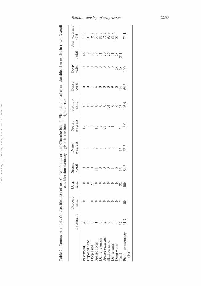
seagrass areas in two shades of green. The user and producer accuracies of the

classification, for the two seagrass classes combined, were 93.5% and 57.0%, respec-

tively, with an overall accuracy of 77.7%. This indicates a substantial underestimation

of the seagrass area. An investigation of the problematic seagrass areas revealed that

89% of the misclassified seagrass pixels were attributable to seagrass being classified

as either pavement or sparse coral. The complete confusion matrix is shown in table 2.

3.2 Biomass estimates based on the visual scales

Visual estimates and aboveground biomass (dry weight) are shown for each species in

figure 5. Based on our visual estimates and field samples, the range of aboveground

biomass found in the area around Chumbe Island is comparable with amounts inseagrass meadows on northern Zanzibar (Nordlund, unpublished data). For scale 1

(all species except Tc), a power function produced the best fit for a regression function,

whereas an exponential function produced the best fit for scale 2 (used for Tc).

Biomass predictions based on the visual scales have RMSE values of 35.1 g m–2

(r2¼ 0.83) and 227.3 g m–2 (r2¼ 0.57) for scales 1 and 2, respectively. This corresponds

to a precision (SE/mean) of 0.24 and 0.41, respectively.

3.3 Biomass estimates based on the satellite imagery

Linear regression models proved useful for predicting biomass at scales 1 and 2 from the

depth-invariant index derived from IKONOS bands 1 and 2 (Lyzenga 1978). Visual

Figure 3. Illustration of the difference between seagrass species without aboveground stems(Th in the foreground), and Tc with its higher canopy (in the background). Although the stemsthemselves are not visible in the image, the height of Tc plants, which they cause, is clearly seen.



biomass estimates at the two scales could be predicted from the depth-invariant index

with RMSE values of 52.5 g m–2 (r2 ¼ 0.47) and 136.2 g m–2 (r2 ¼ 0.56), respectively.

The residuals for scale 1 were depth dependent, and a multiple linear regression model

was therefore developed for this scale, adding remotely sensed depth as a second

independent variable, which reduced the RMSE value to 40.0 g m–2 (r2 ¼ 0.70).

Relationships between the depth-invariant index and biomass values support the

use of a separate biomass scale for Tc. The smaller seagrass species (all except Tc) fitwell in the same linear relationship between the depth-invariant index and biomass,

although, based on the limited amount of data available, Cr, Cs and Si individually

exhibit non-significant relationships. Tc, as expected, exhibits a very different rela-

tionship between the depth-invariant index and biomass compared to the other

species (figure 6).

Figure 4. The result of the Maximum Likelihood Classification.



Ta

ble

2.

Co

nfu

sio

nm

atr

ixfo

rcl

ass

ific

ati

on

of

nea

rsh

ore

ha

bit

ats

aro

un

dC

hu

mb

eIs

lan

d.

Fie

ldd

ata

inco

lum

ns,

cla

ssif

ica

tio

nre

sult

sin

row

s.O

ver

all

cla

ssif

ica

tio

na

ccu

racy

isg

iven

inth

eb

ott

om

rig

ht

corn

er.

Pa

vem

ent

Ex

po

sed

san

dD

eep

san

dS

pa

rse

cora

lD

ense

sea

gra

ssS

pa

rse

sea

gra

ssS

ha

llo

wsa

nd

Den

seco

ral

Dee

pw

ate

rT

ota

lU

ser

acc

ura

cy(%

)

Pa

vem

ent

34

00

00

12

00

04

67

3.9

Ex

po

sed

san

d0

70

00

00

00

71

00

Dee

psa

nd

00

22

00

00

10

23

95

.7S

pa

rse

cora

l1

00

11

21

00

40

29

37

.9D

ense

sea

gra

ss0

00

09

20

00

11

81

.8S

pa

rse

sea

gra

ss2

00

05

23

00

03

07

6.7

Sh

all

ow

san

d0

00

00

22

40

02

69

2.3

Den

seco

ral

00

01

01

09

01

18

1.8

Dee

pw

ate

r0

00

00

00

02

82

81

00

To

tal

37

72

21

31

65

02

51

42

82

11

Pro

du

cer

acc

ura

cy(%

)9

1.9

10

01

00

84

.65

6.3

46

.09

6.0

64

.31

00

79

.1



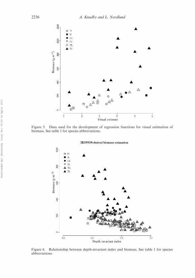
Figure 5. Data used for the development of regression functions for visual estimation ofbiomass. See table 1 for species abbreviations.

Figure 6. Relationship between depth-invariant index and biomass. See table 1 for speciesabbreviations.



Because of the inability to separate the different species in the imagery, it was not

possible to determine which of the two regression models should be used for biomass

estimation in a given seagrass pixel. As Tc did not occur in a unique area or depth

zone, these characteristics did not enable separation either. The image-based biomass

estimation resulting from this study (figure 7) was therefore based on scale 1, andinterpretation must be made with the knowledge that large underestimates of biomass

exist in areas where Tc is the dominant species. Our field data suggest that this is

10.8% of the total seagrass area.

Figure 7. IKONOS-based estimation of seagrass biomass around Chumbe Island and field-mapped seagrass areas (November 2006). Arrows indicate areas that are covered by seagrassand correctly identified in the field-based study but misclassified as non-seagrass substrate bythe satellite imagery.



3.4 Comparison with the field-based method

Results from the field-based study (Hayford and Perlman 2006) were overlaid on the

map of seagrass distribution obtained from the classification (figure 7). Some bound-

aries between seagrass areas and surrounding sandy substrates correspond well in the

two studies, but several differences were noted. Seagrass patches that were either small

or located far from the island were not mapped by the field-based study, and the large

polygon southeast of Chumbe was used to denote an area of many small seagrass

patches, too complex to map using the field-based method, but mappable with the

satellite imagery. For seagrass areas identified in the field study, the methods agreedon the location of the seaward edges of most seagrass patches, but not the landward

edges (examples are indicated by arrows in figure 7). Our field data indicate that the

areas of disagreement were sparsely covered by seagrass and misclassified as pave-

ment or sparse coral.

4. Discussion

4.1 Mapping seagrass distribution

Mapping the distribution of seagrasses around Chumbe Island is challenging for two

main reasons: spectral similarity between seagrasses and other substrates, and fine-

scale spatial heterogeneity.The area has seven seagrass species, six of which can dominate a given area, often

occurring in mixed-species meadows with densities ranging from a few Ho plants to

dense stands of Tc. This creates an environment where the ‘seagrass’ substrate is not

spectrally distinct, but rather displays a range of spectral responses. In addition,

seagrass meadows are located close to, sometimes directly bordering, other substrate

types. Like the seagrass itself, these substrates do not fit neatly into spectrally distinct

classes, but instead display a range of gradually changing and overlapping character-

istics. This complexity is illustrated by aboveground seagrass biomass values rangingfrom near 0 to more than 700 g m–2, coral-dominated areas ranging from just above 0 to

almost 100% coral cover and rocky substrates ranging from nearly void of algae to

supporting dense stands of erect brown macroalgae. Combined with the influence of a

light background (sand or coral rock) and reflectance spectra dominated by chlorophyll a

absorption from both the seagrass, corals and algae growing on the pavement, the

separation of these classes on a purely spectral basis is problematic. The influence of

seagrass biomass on misclassifications between these substrate types is illustrated by

our field data. The seagrass areas misclassified as pavement contained an averagebiomass of 84.6 � 33.6 g m–2, compared to an average of 174.9 � 153.1 g m–2 for all

seagrass sites. This shows that it is the areas with low seagrass biomass that suffer from

this type of misclassification. In addition, the contextual editing was unable to separate

sparse seagrass from pavement as they rarely occur in separate reef zones. The seagrass

areas misclassified as sparse coral also contained biomass values lower than the overall

average: 128.5� 102.7 g m–2. Contextual editing was able to separate these two classes in

areas with well-defined reef development. However, large areas around Chumbe Island

have no clear reef zones, and small patches of seagrass can occur in between coralbommies of similar sizes, making any further contextual editing unfeasible.

Misclassification between sparse seagrass and sparse coral is most frequent in the area

immediately southeast of Chumbe Island, where the two substrate types are found

together (see figure 4). These misclassifications are reflected in the user and producer



accuracies for seagrass areas (93.5% and 57.0%, respectively) and the overall accuracy of

77.7%. This indicates that the complexity of the environment directly affects map

accuracy.

Reliable comparisons with studies conducted in less complex environments are

complicated by differences in both the kind and spatial scale of field and remotelysensed data, processing techniques used and the statistical treatment and reporting of

results. Nevertheless, a few studies clearly illustrate what can be achieved under more

favourable conditions. In a study of Tampa Bay, a shallow 1000 km2 estuary with no

other substrates spectrally similar to seagrasses, Robbins (1997) achieved user accura-

cies of 95–99% for two classes (patchy and continuous seagrass) using 1:24 000 scale

aerial photography. Similarly, Ward et al. (1997) used Landsat Multispectral Scanner

(MSS) data (resampled to 50 m pixel size) to map eelgrass (Zostera marina) in

Izembek Lagoon, a 340 km2 Alaskan lagoon with no other substrates spectrallysimilar to eelgrass. Although Ward et al. (1997) did not quantify the resulting map

accuracy, they concluded that their classification, which used only three classes

(eelgrass, unvegetated and water) was ‘probably robust in Izembek Lagoon due to

good spectral distinction between the habitats’ (p. 237). Together these two studies

suggest that spatial and spectral resolution is of limited importance when mapping

seagrasses in environments with little potential for misclassification with spectrally

similar substrate types. High classification accuracies in similarly simple environ-

ments have also been reported from studies using IKONOS data (4 m pixel size) inthe Mediterranean (three classes) (Fornes et al. 2006) and in Japan (three classes)

(Sagawa et al. 2008). Other studies illustrate the challenges of mapping seagrasses in

complex environments. Working with Landsat Thematic Mapper (TM) data (30 m

pixel size) and three classes (dense seagrass, medium/sparse seagrass and other), using

a standardized methodology at multiple locations in the Caribbean, Wabnitz et al.

(2008) achieved the lowest classification accuracy (46%) at a site characterized by a

variety of spectrally similar habitats, while they achieved high accuracies (88%) where

the seagrass beds were found in geomorphologic zones that typically have few or nospectrally similar substrate types. Dekker et al. (2005) applied advanced processing

methods to Landsat TM data, mapping a total of 15 substrate classes in Wallis Lake,

Australia (94 km2). Substrates here range from sparsely to densely vegetated patches

composed of three species of seagrass and several species of macroalgae, all occurring

in both mixed and monospecific stands. Classification accuracies depended on the

spectral similarity between substrate types at different densities; for example, sparse

stands of Posidonia were often misclassified as Ruppia, and Chara was often misclas-

sified as macroalgae.The issue associated with fine-scale spatial heterogeneity arises from the combined

errors in geolocation of field observations and individual pixels in remotely sensed

data, causing misregistration between the two data sets. If this misregistration is larger

than the typical patch size in the environment, this can drastically reduce map

accuracy. We addressed this issue by manually adjusting the GPS-derived location

of field sites if a misregistration was clearly identifiable and a correction possible. By

contrast, Dekker et al. (2005) addressed this problem by allowing neighbouring pixels

of the correct class to contribute towards the accuracy measure. The issue is alsoillustrated in a study by Vela et al. (2008), focusing on El Bibane lagoon in northern

Tunisia (230 km2), which achieved higher classification accuracies for seagrasses with

fused Satellite Pour l’Observation de la Terre (SPOT) 5 data (2.5 m pixel size) than

with fused IKONOS data (0.6 m pixel size) (four classes). Vela et al. (2008) explained



these counterintuitive results with the fact that the coarser spatial resolution of SPOT

5 masked the heterogeneous spatial structure of the seagrasses and sediments in the

lagoon. All studies highlight the need to match the spatial resolution of field and

remotely sensed data with their geolocation accuracy (Wabnitz et al. 2008), and in

turn match these with the spatial scale of heterogeneity in the environment.

4.2 Mapping seagrass biomass

The accuracy of our in situ biomass estimates using the visual scales is comparable to

the r2 ¼ 0.94 found by Mumby et al. (1997a) in a two-species environment, and the

r2¼ 0.88 for subtidal and r2¼ 0.91 for intertidal seagrasses found by Mellors (1991) in

a five-species environment more similar to ours. Both of these studies dealt only with

small-leaved species similar to those comprising scale 1 in our study. However, thepresence of Tc caused two problems for accurate mapping of seagrass biomass in our

study area. First, the in situ biomass estimates for this species were less accurate than

for scale 1, which can probably be attributed to the distribution of biomass in Tc. In

Tc, a substantial part of the biomass is located in the stem, which is visually unassum-

ing and partly hidden from the view of a snorkeler by the leaves of the plants. Second,

Tc has a markedly different relationship between biomass and the depth-invariant

index used for its estimation (figure 6), probably also due to long and heavy stems,

which strongly influence the biomass, but not the interception of light relevant to thecalculation of the depth-invariant index. The inability to distinguish Tc from the other

species in the imagery led us to estimate biomass exclusively using scale 1, which

markedly reduced the accuracy of biomass estimates in area dominated by Tc.

Considering only scale 1, the accuracy of our IKONOS-based biomass estimates are

comparable to those obtained with other multispectral sensors in simpler environ-

ments. Working in the Turks and Caicos, Mumby et al. (1997b) achieved coefficients

of determination of r2¼ 0.79 and r2 ¼ 0.74 with SPOT XS and Landsat TM,

respectively, and Armstrong (1993) achieved r2¼ 0.80 using Landsat TM data inBahamas. Phinn et al. (2008) suffered from insufficient geolocation accuracy of their

field sites while working in a highly complex environment, and obtained a coefficient

of determination of only r2 ¼ 0.35 using Quickbird imagery from Moreton Bay,

Australia.

An additional consideration in interpretation of seagrass biomass maps is that

biomass estimates are only produced for areas classified as seagrass. Misclassification

of sparsely vegetated seagrass areas as sparse coral or pavement in our study therefore

reduces the overall area where seagrass biomass was mapped around Chumbe. Themisclassified areas had low biomass values and thus only had limited influence on the

biomass maps. Nevertheless, the classification accuracy in itself is an important con-

sideration when assessing the usefulness of seagrass biomass maps. Based on the

discussion above, it is clear that the presence of a seagrass species with a significantly

different structure limits the accuracy with which seagrass biomass can be mapped

using remote sensing. Accurate identification and mapping of such a species (Tc in our

study) would be necessary to improve biomass estimation. This problem is likely to exist

in other mixed species environments, where the different species have substantialstructural differences. Despite spectral differentiation being at least theoretically possi-

ble for some seagrass species (Fyfe 2003), a practical solution is not currently available,

even under the best possible conditions. Phinn et al. (2008), mapping seagrass species in

shallow areas (, 3 m) using airborne hyperspectral imagery at high spatial resolution



(4 m), achieved an overall classification accuracy of only 28.1%, low even considering

the nine classes used in the classification. Dekker et al. (2005) achieved nominally higher

classification accuracies with species-based classes using Landsat TM data, possibly

because of the coarser spatial resolution, and the elevated accuracy measure. Better

mapping of seagrass biomass is likely to depend on further improvement in thedifferentiation, spectral or otherwise, of species with substantially different structure.

4.3 Remote sensing vs. field-based seagrass mapping

The field-based study showed each of the identified seagrass patches as larger than thecorresponding patches mapped with satellite imagery. This less-than-perfect accuracy

of the IKONOS-based maps is an obvious disadvantage compared to field-based

studies, and reduces the value of these maps as baselines for future comparison

studies. In addition, remote sensing requires a greater investment in terms of imagery,

hardware, software and technical expertise, all of which may be costly. In comparison,

low cost and little training are required to map seagrass beds using snorkelling and a

GPS, and field-based studies can therefore be the best option in some situations. The

advantage of the remote sensing approach lies in the cost-effectiveness it achieveswhen used repeatedly or over large areas, but this is relatively poorly illustrated by the

one-off mapping of a relatively small area described in our study. Even so, the amount

of fieldwork for this study was limited to seven days, of which four were spent

calibrating the visual scales for biomass estimates and two were spent on image

processing. Importantly, extending this area to a full IKONOS scene (11 � 11 km)

would have taken no extra time. Compared to the three weeks of fieldwork used for

the field-based study that did not investigate biomass and achieved a smaller spatial

coverage, our comparison adds to the existing evidence of remote sensing’s utility forseagrass mapping (Mumby et al. 1999, Phinn et al. 2008).

Seagrass maps produced with either method can provide an important baseline

against which to measure future changes in seagrass distribution. However, in the

absence of field data from the past, a historical perspective on seagrass cover

dynamics relies either on interpretable remotely sensed data from the past (Dekker

et al. 2005, Gullstrom et al. 2006) or on local knowledge. In the case of Chumbe

Island, the park rangers, some of whom have worked on the island since 1992, are the

best source of local knowledge. The general opinion of four park rangers interviewedis that the total seagrass distribution around the island decreased from the time of the

park’s inception in 1992 to 1998, and has slowly recovered since then but not yet

reached the 1992 extent, particularly in the northern end of the protected area as well

as in the patchy areas south and southeast of the island. The cause of the initial

decline, mentioned by the rangers, was strong winds burying seagrass meadows north

of the island with sand, as well as a large number of sea urchins grazing on the

seagrass. The trajectory of decline and subsequent slow recovery is supported by

time-series analysis of Landsat TM imagery (Knudby et al. 2010), although thesatellite imagery suggests a rapid decrease in seagrass extent around 2001, rather

than a steady decline from 1992 to 1998.

5. Conclusion

The nearshore environment around Chumbe Island is complex, with seagrasses, algae

and corals in different densities, patch sizes and at different depths. This kind of

environment presents a challenge for remote sensing of nearshore resources, but is not



uncommon in Zanzibar or elsewhere in East Africa. Our results indicate that even in

this environment, maps of both seagrass distribution and biomass can be produced

with reasonable accuracy using IKONOS data. However, the presence of

Thalassodendron ciliatum and the inability to separate this species in the imagery

caused reduced accuracy of biomass estimates, although the limited extent of thisspecies around Chumbe Island reduces the problem in this study. Remote sensing is

the only feasible way to produce extensive maps of seagrass distribution and biomass,

and to discover seagrass meadows in areas not covered directly by fieldwork. It is also

the only feasible method for accurately quantifying change in seagrass distribution

and biomass over time. In an area where tourism development, increasingly unsus-

tainable fishing pressure and population explosions of seagrass-consuming sea urch-

ins put unprecedented pressure on seagrasses, such information can be crucial for

environmental campaigners and decision makers.

Acknowledgements

We thank the staff of Chumbe Island Coral Park for their cooperation and good

company, and the Institute of Marine Sciences on Zanzibar for access to laboratory

facilities. Funding for satellite imagery was provided by Ellsworth LeDrew, and

sound advice was provided by Martin Gullstrom and Bengt Lunden. Constructive

comments were provided by two anonymous reviewers.

References

AKAIKE, H., 1974, A new look at the statistical model identification. IEEE Transactions on

Biomedical Engineering, 19, pp. 716–723.

ANDREFOUET, S., KRAMER, P., TORRES-PULLIZA, D., JOYCE, K.E., HOCHBERG, E.J., GARZA-

PEREZ, R., MUMBY, P.J., RIEGL, B., YAMANO, H., WHITE, W.H., ZUBIA, M., BROCK,

J.C., PHINN, S.R., NASEER, A., HATCHER, B.G. and MULLER-KARGER, F.E., 2003, Multi-

site evaluation of IKONOS data for classification of tropical coral reef environments.

Remote Sensing of Environment, 88, pp. 128–143.

ARMSTRONG, R.A., 1993, Remote-sensing of submerged vegetation canopies for biomass esti-

mation. International Journal of Remote Sensing, 14, pp. 621–627.

BANDEIRA, S.O. and BJORK, M., 2001, Seagrass research in the Eastern Africa region: emphasis

on diversity ecology and ecophysiology. South African Journal of Botany, 67, pp.

420–425.

BELL, J. and POLLARD, D., 1989, Ecology of fish assemblages and fisheries associated with

seagrasses. In Biology of Seagrasses: A Treatise on the Biology of Seagrasses with Special

Reference to the Australian Region, A. Larkum, A. McComb and S. Shephard (Eds.),

pp. 565–609 (Amsterdam: Elsevier).

COSTANZA, R., D’ARGE, R., DE GROOT, R., FARBER, S., GRASSO, M., HANNON, B., LIMBURG, K.,

NAEEM, S., O’NEILL, R.V., PARUELO, J., RASKIN, R.G., SUTTON, P. and VAN DEN BELT,

M., 1997, The value of the world’s ecosystem services and natural capital. Nature, 387,

pp. 253–260.

DAHDOUH-GUEBAS, F., COPPEJANS, E. and VAN SPEYBROECK, D., 1999, Remote sensing and

zonation of seagrasses and algae along the Kenyan coast. Hydrobiologia, 400, pp.

63–73.

DEKKER, A.G., BRANDO, V.E. and ANSTEE, J.M., 2005, Retrospective seagrass change detection

in a shallow coastal tidal Australian lake. Remote Sensing of Environment, 97, pp.

415–433.

DEN HARTOG, C., 1970, The Seagrasses of the World (Amsterdam: North Holland).

EFRON, B. and TIBSHIRANI, R., 1993, An Introduction to the Bootstrap (New York: Chapman &

Hall).



FERGUSON, R., WOOD, L. and GRAHAM, D., 1993, Monitoring spatial change in seagrass habitat

with aerial photography. Photogrammetric Engineering and Remote Sensing, 59, pp.

1033–1038.

FORNES, A., BASTERRETXEA, G., ORFILA, A., JORDI, A., ALVAREZ, A. and TINTORE, J., 2006,

Mapping Posidonia oceanica from IKONOS. ISPRS Journal of Photogrammetry and

Remote Sensing, 60, pp. 315–322.

FYFE, S.K., 2003, Spatial and temporal variation in spectral reflectance: are seagrass species

spectrally distinct? Limnology and Oceanography, 48, pp. 464–479.

GOSSLING, S., KUNKEL, T., SCHUMACHER, K. and ZILGER, M., 2004, Use of molluscs, fish, and

other marine taxa by tourism in Zanzibar, Tanzania. Biodiversity and Conservation, 13,

pp. 2623–2639.

GREEN, E. and SHORT, F., 2003, World Atlas of Seagrasses (Berkeley: University of California

Press).

GULLSTROM, M., DE LA TORRE CASTRO, M., BANDEIRA, S.O., BJORK, M., DAHLBERG, M.,

KAUTSKY, N., RONNBACK, P. and OHMAN, M.C., 2002, Seagrass ecosystems in the

Western Indian Ocean. AMBIO, 31, pp. 588–596.

GULLSTROM, M., LUNDEN, B., BODIN, M., KANGWE, J., OHMAN, M., MTOLERA, M. and BJORK,

M., 2006, Assessment of changes in the seagrass-dominated submerged vegetation of

tropical Chwaka Bay (Zanzibar) using satellite remote sensing. Estuarine, Coastal and

Shelf Science, 67, pp. 399–408.

HAYFORD, J. and PERLMAN, M., 2006, Chumbe Seagrass Distribution and Composition. School

for International Training. Unpublished report.

HEDLEY, J.D., HARBORNE, A.R. and MUMBY, P.J., 2005, Simple and robust removal of sun glint

for mapping shallow-water benthos. International Journal of Remote Sensing, 26, pp.

2107–2112.

HEMMINGA, M. and DUARTE, C., 2000, Seagrass Ecology (Cambridge: Cambridge University

Press).

JONES, C.G., LAWTON, J.H. and SHACHAK, M., 1994, Organisms as ecosystem engineers. OIKOS,

69, pp. 373–386.

KNUDBY, A., NEWMAN, C., SHAGHUDE, Y. and MUHANDO, C., 2010, Simple and effective

monitoring of historic changes in nearshore environments using the free archive of

Landsat imagery. International Journal of Applied Earth Observation and

Geoinformation, 12 (Suppl. 1), pp. S116–S122.

KOHLER, K.E. and GILL, S.M., 2006, Coral Point Count with Excel extensions (CPCe): a Visual

Basic program for the determination of coral and substrate coverage using random

point count methodology. Computers and Geosciences, 32, pp. 1259–1269.

LYZENGA, D.R., 1978, Passive remote-sensing techniques for mapping water depth and bottom

features. Applied Optics, 17, pp. 379–383.

MELLORS, J.E., 1991, An evaluation of a rapid visual technique for estimating seagrass biomass.

Aquatic Botany, 42, pp. 67–73.

MUMBY, P., EDWARDS, A., GREEN, E.P., ANDERSON, C.W., ELLIS, A.C. and CLARK, C.D., 1997a,

A visual assessment technique for estimating seagrass standing crop. Aquatic

Conservation: Marine and Freshwater Ecosystems, 7, pp. 239–251.

MUMBY, P., GREEN, E., EDWARDS, A. and CLARK, C., 1997b, Measurement of seagrass standing

crop using satellite and digital airborne remote sensing. Marine Ecology Progress

Series, 159, pp. 51–60.

MUMBY, P.J., CLARK, C.D., GREEN, E.P. and EDWARDS, A.J., 1998, Benefits of water column

correction and contextual editing for mapping coral reefs. International Journal of

Remote Sensing, 19, pp. 203–210.

MUMBY, P.J., GREEN, E.P., EDWARDS, A.J. and CLARK, C.D., 1999, The cost-effectiveness of

remote sensing for tropical coastal resources assessment and management. Journal of

Environmental Management, 55, pp. 157–166.



MUTHIGA, N., RIEDMILLER, S., CARTER, E., VAN DER ELST, R., MANN-LANG, J., HORRILL, C.,

MCCLANAHAN, T.R., 2000, Management status and case studies. In Coral Reefs of the

Indian Ocean, T.R. McClanahan, C.R.C. Sheppard and D.O. Obura (Eds.), pp.

473–505 (Oxford: Oxford University Press).

NAGELKERKEN, I., DORENBOSCH, M., VERBERK, W., DE LA MORINIERE, E.C. and VAN DER VELDE,

G., 2000, Importance of shallow-water biotopes of a Caribbean bay for juvenile coral

reef fishes: patterns in biotope association, community structure and spatial distribu-

tion. Marine Ecology Progress Series, 202, pp. 175–192.

ORTH, R.J., HECK, K.L. and VANMONTFRANS, J., 1984, Faunal communities in seagrass beds: a

review of the influence of plant structure and prey characteristics on predator prey

relationships. Estuaries, 7, pp. 339–350.

PCI GEOMATICS, 2003, Geomatica Focus 9.1.0 (Richmond Hill: PCI Geomatics).

PHINN, S., ROELFSEMA, C., DEKKER, A., BRANDO, V. and ANSTEE, J., 2008, Mapping seagrass

species, cover and biomass in shallow waters: an assessment of satellite multi-spectral

and airborne hyper-spectral imaging systems in Moreton Bay (Australia). Remote

Sensing of Environment, 112, pp. 3413–3425.

ROBBINS, B.D., 1997, Quantifying temporal change in seagrass areal coverage: the use of GIS

and low resolution aerial photography. Aquatic Botany, 58, pp. 259–267.

SAGAWA, T., MIKAMI, A., KOMATSU, T., KOSAKA, N., KOSAKO, A., MIYAZAKI, S. and TAKAHASHI,

M., 2008, Mapping seagrass beds using IKONOS satellite image and side scan sonar

measurements: a Japanese case study. International Journal of Remote Sensing, 29, pp.

281–291.

SHORT, F. and COLES, R. (Eds.), 2001, Global Seagrass Research Methods (Amsterdam:

Elsevier).

STUMPF, R.P., HOLDERIED, K. and SINCLAIR, M., 2003, Determination of water depth with high-

resolution satellite imagery over variable bottom types. Limnology and Oceanography,

48, pp. 547–556.

VELA, A., PASQUALINI, V., LEONI, V., DJELOULI, A., LANGAR, H., PERGENT, G., PERGENT-

MARTINI, C., FERRAT, L., RIDHA, M. and DJABOU, H., 2008, Use of SPOT 5 and

IKONOS imagery for mapping biocenoses in a Tunisian Coastal Lagoon

(Mediterranean Sea). Estuarine Coastal and Shelf Science, 79, pp. 591–598.

WABNITZ, C.C., ANDREFOUET, S., TORRES-PULLIZA, D., MULLER-KARGER, F.E. and KRAMER,

P.A., 2008, Regional-scale seagrass habitat mapping in the Wider Caribbean region

using Landsat sensors: applications to conservation and ecology. Remote Sensing of

Environment, 112, pp. 3455–3467.

WARD, D.H., MARKON, C.J. and DOUGLAS, D.C., 1997, Distribution and stability of eelgrass

beds at Izembek Lagoon, Alaska. Aquatic Botany, 58, pp. 229–240.



Remote sensing of seagrasses in a patchy multi-species environment

Documents