Remote Response of the Indian Ocean to Interannual SST Variations in the Tropical Pacific

362 VOLUME 17J O U R N A L O F C L I M A T E

q 2004 American Meteorological Society

Remote Response of the Indian Ocean to Interannual SST Variations in theTropical Pacific

TOSHIAKI SHINODA AND MICHAEL A. ALEXANDER

NOAA–CIRES Climate Diagnostics Center, Boulder, Colorado

HARRY H. HENDON

Bureau of Meteorology Research Centre, Melbourne, Australia

(Manuscript received 14 February 2003, in final form 12 June 2003)

ABSTRACT

Remote forcing of sea surface temperature (SST) variations in the Indian Ocean during the course of El Nino–Southern Oscillation (ENSO) events is investigated using NCEP reanalysis and general circulation model (GCM)experiments. Three experiments are conducted to elucidate how SST variations in the equatorial Pacific influencesurface flux variations, and hence SST variations, across the Indian Ocean. A control experiment is conductedby prescribing observed SSTs globally for the period 1950–99. In the second experiment, observed SSTs areprescribed only in the tropical eastern Pacific, while climatological SSTs are used elsewhere over the globaloceans. In the third experiment, observed SSTs are prescribed in the tropical eastern Pacific, while a variable-depthocean mixed layer model is used at all other ocean grid points to predict the SST.

Composites of surface fluxes and SST over the Indian Ocean are formed based on El Nino and La Nina eventsduring 1950–99. The surface flux variations in the eastern Indian Ocean in all three experiments are similar andrealistic, confirming that much of the surface flux variation during ENSO is remotely forced from the Pacific.Furthermore, the SST anomalies in the eastern tropical Indian Ocean are well simulated by the coupled model,which supports the notion of an ‘‘atmospheric bridge’’ from the Pacific. During boreal summer and fall, whenclimatological winds are southeasterly over the eastern Indian Ocean, remotely forced anomalous easterlies actto increase the local wind speed. SST cools in response to increased evaporative cooling, which is partiallyoffset by increased solar radiation associated with reduced rainfall. During winter, the climatological windsbecome northwesterly and the anomalous easterlies then act to reduce the wind speed and evaporative cooling.Together with increased solar radiation and a shoaling mixed layer, the SST warms rapidly. The model is lesssuccessful at reproducing the ENSO-induced SST anomalies in the western Indian Ocean, suggesting thatdynamical ocean processes contribute to the east–west SST dipole that is often observed in boreal fall duringENSO events.

1. Introduction

An important attribute of El Nino–Southern Oscil-lation (ENSO) is that it drives changes in the globalatmospheric circulation. ENSO-induced anomalies overthe landmasses surrounding the Indian Ocean includereduced rainfall in the Indian summer monsoon, reducedrainfall in the late dry season (August–October) in In-donesia, and enhanced rainfall during the wet season(November–January) in eastern Africa (e.g., Roplewskiand Halpert 1987; Kiladis and Diaz 1989). There isgrowing evidence that these rainfall anomalies are driv-en both by remotely forced circulation changes from theequatorial Pacific and by sea surface temperature (SST)anomalies in the Indian Ocean (e.g., Hastenrath et al.

Corresponding author address: Dr. Toshiaki Shinoda, NOAA–CI-RES Climate Diagnostics Center, 325 Broadway, Boulder, CO 80303.E-mail: [email protected]

1993; Goddard and Graham 1999; Lau and Nath 2000;Rowell 2001). While typical SST anomalies in the In-dian Ocean during ENSO are only 1/2 to 1/3 as largeas those in the equatorial central and eastern Pacific, thehigh mean temperatures in the former imply that smallSST changes can drive significant rainfall and circula-tion anomalies (e.g., Palmer and Mansfield 1984).

It is difficult to attribute the cause of observed rainfallanomalies during ENSO to SSTs in a particular region,since SST anomalies in the Indian Ocean coevolve withthose in the Pacific. The typical evolution during theENSO cycle (e.g., Rassmusson and Carpenter 1982) arefor cold anomalies to develop in the equatorial easternIndian Ocean/Indonesian region when warm anomaliesare becoming prominent in the equatorial central Pacific(June–July). The western Indian Ocean then begins towarm and by boreal autumn, as warm anomalies beginto peak in the central Pacific, an anomalously negativezonal gradient of SST across the equatorial Indian Ocean

15 JANUARY 2004 363S H I N O D A E T A L .

develops (Baquero-Bernal et al. 2002). At the peakphase of ENSO in the Pacific (December–January), thewestern Indian Ocean continues to warm and the coldSST anomalies in the eastern Indian Ocean rapidly de-cay and even change sign (Nicholls 1981). The resultantbasin-scale warming in the Indian Ocean typically peakssome 3–4 months after the peak warming in the centralPacific (Klein et al. 1999).

The ENSO-related rainfall anomalies during the east-ern African wet season (December–March) have beenattributed to the basin-scale warming that is typicallyevident by December during a warm event (e.g., God-dard and Graham 1999). On the other hand, the mostdramatic rainfall impacts in the eastern Indian Ocean–Indonesian region occur during boreal autumn (e.g.,Flohn 1986; Hendon 2003), when the anomalous zonalSST gradient in the Indian Ocean is most developed.The strong negative correlation of Indonesian rainfallwith ENSO tends to disappear after SSTs warm in theeastern Indian Ocean in late boreal autumn.

The mechanism for generation of the SST anomaliesin the Indian Ocean that develop in conjunction withENSO is unclear. The eastward shift of the Walker cir-culation results in anomalous surface easterlies and re-duced cloud cover over the equatorial eastern Indianand far western Pacific Oceans (e.g., Rassmusson andCarpenter 1982). These wind and cloud cover changesimpact the latent heat flux, surface shortwave radiation,and wind stress. Klein et al. (1999) and Venzke et al.(2000) argue that the basin-scale warming of the IndianOcean primarily results from a combination of reducedlatent heat flux, associated with anomalous easterlies,and increased shortwave radiation, stemming from thereduction in cloud cover. Hendon (2003) argues furtherthat the negative SST anomalies that develop in theeastern Indian Ocean during boreal autumn and theirrapid demise once the Australian summer monsooncommences in early boreal winter can be accounted forby changes in the surface heat flux. The same easterlyanomalies, which reduce the surface wind speed duringDecember–March, increase the wind speed in the In-donesian region during August–November (e.g., Hack-ert and Hastenrath 1986). Hence, the easterly anomaliesinitially act to cool the eastern Indian Ocean and workagainst the warming associated with increased short-wave radiation produced by reduced cloud cover.

The same easterly anomalies also drive a dynamicalresponse in the Indian Ocean, whereby the equatorialthermocline is elevated in the east and suppressed in thewest, and upwelling is promoted off the west coast ofthe Indonesian archipelago (e.g., Chambers et al. 1999;Murtugudde and Bussalacchi 1999). Together, these dy-namical mechanisms will act to warm (cool) the western(eastern) equatorial Indian Ocean. These dynamicalmechanisms appear to be especially important duringlate 1997 (e.g., Murtugudde et al. 2000), when SSTanomalies at opposite sides of the Indian Ocean ex-

ceeded 28C—reversing the mean zonal SST gradient(e.g., Yu and Rienecker 1999).

Out-of-phase SST anomalies across the Indian Ocean,together with drought in Indonesia and floods in easternAfrica, occasionally develop during boreal autumn inthe absence of well-defined ENSO events in the Pacific,such as occurred in 1961 (Reverdin et al. 1986; Flohn1987). Coupled air–sea dynamics in the Indian Oceanappear to explain this interannual variability (e.g., Rev-erdin et al. 1986; Saji et al. 1999; Webster et al. 1999).Forced ocean model experiments and coupled GCMs,however, suggest that, while coupled behavior existswith some degree of independence from ENSO, remoteforcing by ENSO in the Pacific provides the main ex-citation of the zonally out-of-phase behavior (e.g., Mur-tugudde et al. 2000; Baquero-Bernal et al. 2002).

While many questions remain with regard to the dy-namics of interannual variability in the Indian Ocean,here we will focus on the generation of SST anomaliesby surface heat flux variations and mixed layer pro-cesses remotely forced from the Pacific. Previously Lauand Nath (2003) focused on the basinwide warmingduring boreal winter and spring associated with ENSOusing an AGCM coupled to an ocean mixed layer model.Observed SSTs were prescribed in the central and east-ern tropical Pacific Ocean and the ocean mixed layermodel was used to predict the SST elsewhere. Theirresults indicate that SST variations in the central andeastern Pacific associated with ENSO can perturb theWalker circulation, and that observed SST anomalies inthe Indian–western Pacific Oceans several months afterthe peak in ENSO can be developed by the anomaloussurface atmospheric circulation.

Using a similar experimental design as in Lau andNath (2003), we will focus on the seasonal evolutionof SST anomalies in the Indian Ocean that can be drivenby surface heat flux variations remotely forced from thePacific. In particular, we will focus on the seasonalityof the development of the anomalous zonal SST gradientin the Indian Ocean, which, during ENSO tends to peakin boreal autumn and then rapidly decay, giving way tobasin-scale warming. We will also look at other mixedlayer processes, such as variations in the mixed layerdepth, entrainment heat flux, and penetrative shortwaveradiation.

This paper is organized as follows: The models andexperimental design are described in section 2. In sec-tion 3, ENSO-based composite surface heat flux vari-ations from the model are compared to observations.The evolution of the remotely forced SST variations arediscussed in section 4. Finally, conclusions are providedin section 5.

2. Experiment design

a. Model experiments

Three sets of GCM experiments with different oceanconfigurations were conducted to elucidate how SST


variations in the tropical Pacific may influence air–seafluxes, and hence, SSTs in the Indian Ocean. In the firstexperiment, SSTs at all ocean grid points between 608Nand 408S were prescribed to evolve according to ob-servations (Smith et al. 1996) for the period 1950–99.Climatological SSTs were specified over the remainderof the oceans. An ensemble of four integrations wereconducted with slightly different initial conditions takenfrom a control run. These simulations, referred to asglobal ocean–global atmosphere (GOGA) runs, are usedto infer how the surface fluxes evolve over the IndianOcean given ‘‘perfect’’ boundary conditions.

The second experiment used the same observed SSTsin the tropical eastern and central Pacific (158S–158N,1728E–South American coast), but with climatologicalSSTs specified over the remainder of the world’s oceans.An ensemble of eight integrations were performed.These eastern–central Pacific ocean–global atmosphere(EPOGA) runs were designed to determine how muchof the surface heat flux anomalies produced in theGOGA run are driven by remote SST variations in thetropical eastern and central Pacific, in particular thosevariations associated with ENSO. Zonal shifts of con-vective activity during ENSO events are not largely af-fected by the zonal SST gradient at the artificial bound-ary at 1728E (not shown).

The third experiment is similar to the EPOGA con-figuration except that a one-dimensional mixed layerocean model was coupled to the atmospheric model ateach grid point outside of the tropical east Pacific. Theocean model simulates the mixed layer temperature,equivalent to the SST, while in the eastern and centraltropical Pacific SSTs were prescribed as in the EPOGAexperiment. An ensemble of 16 integrations were per-formed. These mixed layer model (MLM) runs explic-itly demonstrate how SST anomalies in the Indian Oceancan be remotely driven by SST variations in the easternand central Pacific. They also allow for local air–seafeedback, which we find to be modest and will be pre-sented in a later study.

b. Atmosphere and ocean models

The experiments were performed with an atmosphericGCM developed at the Geophysical Fluid DynamicsLaboratory (GFDL). The model has 14 sigma levels inthe vertical and is truncated rhomboidally at wavenum-ber 30. The physical grid, where for instance, surfacefluxes are computed, has a horizontal resolution of ap-proximately 2.258 latitude 3 3.758 longitude. Detaileddescription of the model physics is found in Manabeand Hahn (1981), Lau (1981), and Gordon and Stern(1982). Many features of the model’s climate are de-scribed in Alexander and Scott (1997). Lau and Nath(2000) discuss in detail the ability of the model to sim-ulate interannual variability of the Asian and Australiansummer monsoons.

The one-dimensional ocean mixed layer model used

in the MLM experiments consists of a bulk mixed layeratop a layered model extending down to 1000 m or tothe ocean bottom, whichever is shallower. The modeland coupling procedure are described in detail in Al-exander et al. (2000, 2002). The bulk model is basedon the formulation of Gaspar (1988) and simulates themixed layer depth, temperature, and salinity. It respondsto air–sea fluxes of heat, momentum, and freshwater. Itaccounts for penetrative shortwave radiation, and tur-bulent entrainment into the mixed layer, but not hori-zontal and vertical advective processes. Beneath thebulk mixed layer, heat is redistributed via vertical dif-fusion and convective adjustment. There are 31 levelsfrom the surface to 1000 m with 15 layers in the upper100 m. All layers completely within the mixed layer areset to the bulk model values. The flux adjustment, de-scribed in Alexander et al. (2000), guarantees a stableand realistic seasonally varying mean state. The mag-nitude of the flux correction is 10–25 W m22 over mostof the tropical Indian Ocean. The net surface heat fluxin the subsequent sections includes the flux adjustment.Note that the ENSO composite of surface heat fluxesare not affected by the flux correction since the correc-tion values are exactly the same during warm eventsand cold events.

3. ENSO composite of SST and surface fluxes

In this section, we develop an ENSO-based compositeevolution of observed SSTs and surface heat fluxesbased on National Centers for Environmental Prediction(NCEP) reanalyses (Kalnay et al. 1996) and from theGOGA experiment to examine the realism of surfaceheat fluxes produced by the model when given perfectboundary conditions.

Composites are formed based on nine El Nino events(1957, 1965, 1969, 1972, 1976, 1982, 1987, 1991, 1997)and nine La Nina events (1950, 1954, 1955, 1964, 1970,1973, 1975, 1988, 1998). The first eight El Nino andLa Nina events were identified by Lau and Nath (2000)based on the monthly SST anomaly in the 58S–58N,1208–1508W region, to which we have added the 1997El Nino and 1998 La Nina events. We refer to theseyears as year (0), and the following years as year (1).Over the Indian Ocean composite El Nino anomaliesare nearly but not exactly opposite to the La Nina anom-alies (e.g., Baquero-Bernal et al. 2002). However, wewill treat them as opposites and form composites basedon El Nino years minus La Nina years (also referred toas warm 2 cold in the subsequent figures). For bothmodel and observations, composites are formed fromanomalies that were created by subtracting the respec-tive mean seasonal cycles.

For reference, the composite evolution of Nino-3.4SST (observed SST averaged 58N–58S, 1208E–1708W)is shown in Fig. 1. Nino-3.4 SST peaks in early borealwinter and then declines through spring. The associatedevolution of SST across the equatorial Indian Ocean


FIG. 1. Composite SST anomalies (warm 2 cold) averaged for theNino-3.4 (58N–58S, 1208E–1708W, solid line, square), eastern IndianOcean (158–58S, 1008–1208E dashed line, open circle) and westernIndian Ocean (108S–108N, 508–608E, dotted line, closed circle).

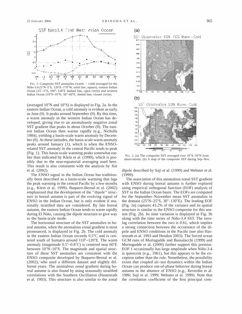
FIG. 2. (a) The composite SST averaged over 108S–108N fromobservations. (b) A map of the composite SST during Sep–Nov.

(averaged 108N and 108S) is displayed in Fig. 2a. In theeastern Indian Ocean, a cold anomaly is evident as earlyas June (0). It peaks around September (0). By this time,a warm anomaly in the western Indian Ocean has de-veloped, giving rise to an anomalously negative zonalSST gradient that peaks in about October (0). The east-ern Indian Ocean then warms rapidly (e.g., Nicholls1984), yielding a basin-scale warm anomaly by Decem-ber (0). At these latitudes, the basin-scale warm anomalypeaks around January (1), which is when the ENSO-related SST anomaly in the central Pacific tends to peak(Fig. 1). This basin-scale warming peaks somewhat ear-lier than indicated by Klein et al. (1999), which is pos-sibly due to the near-equatorial averaging used here.This result is also consistent with the analysis by Xieet al. (2002).

The ENSO signal in the Indian Ocean has tradition-ally been described as a basin-scale warming that lagsthe peak warming in the central Pacific by a few months(e.g., Klein et al. 1999). Baquero-Bernal et al. (2002)emphasized that the development of the ‘‘dipole’’ struc-ture in boreal autumn is part of the evolving signal ofENSO in the Indian Ocean, but is only evident if sea-sonally stratified data are considered. By late borealautumn, the eastern Indian Ocean tends to warm rapidlyduring El Nino, causing the dipole structure to give wayto the basin-scale mode.

The horizontal structure of the SST anomalies in bo-real autumn, when the anomalous zonal gradient is mostpronounced, is displayed in Fig. 2b. The cold anomalyin the eastern Indian Ocean exceeds 0.58C and is cen-tered south of Sumatra around 1108–1208E. The warmanomaly (magnitude 0.58–0.88C) is centered near 608Ebetween 108N–108S. The magnitude and spatial struc-ture of these SST anomalies are consistent with theENSO composite developed by Baquero-Bernal et al.(2002), who used a different dataset and slightly dif-ferent years. The anomalous zonal gradient during bo-real autumn is also found by using seasonally stratifiedcorrelations with the Southern Oscillation (Hastenrathet al. 1993). This structure is also similar to the zonal

dipole described by Saji et al. (1999) and Webster et al.(1999).

The association of this anomalous zonal SST gradientwith ENSO during boreal autumn is further exploredusing empirical orthogonal function (EOF) analysis ofSST in the Indian Ocean basin. The EOFs are computedfor the September–November mean SST anomalies inthe domain (258N–258S, 308–1308E). The leading EOF(Fig. 3a) captures 43.2% of the variance and its spatialstructure is similar to the ENSO composite for this sea-son (Fig. 2b). Its time variation is displayed in Fig. 3balong with the time series of Nino-3.4 SST. The zero-lag correlation between the two is 0.61, which impliesa strong connection between the occurrence of the di-pole and ENSO conditions in the Pacific (see also Has-tenrath et al. 1993 and Hendon 2003). The forced oceanGCM runs of Murtugudde and Bussalacchi (1999) andMurtugudde et al. (2000) further support this premise.EOF 1 occasionally has large amplitude when Nino-3.4is quiescent (e.g., 1961), but this appears to be the ex-ception rather than the rule. Nonetheless, the possibilityexists that coupled air–sea dynamics within the IndianOcean can produce out-of-phase behavior during borealautumn in the absence of ENSO (e.g., Reverdin et al.1986; Saji et al. 1999; Webster et al. 1999). Note thatthe correlation coefficient of the first principal com-


FIG. 3. (a) First eigenvector of the observed SST during Sep–Nov.The eigenvector has been scaled for a one standard deviation anomalyof the principal component. (b) Time series of the PC-1 (solid line)and the Nino-3.4 SST anomaly (dashed line) during Sep–Nov. Thesign of the Nino-3.4 SST is changed for the comparison. Both timeseries are normalized by the std dev.

FIG. 4. (a) Composite net surface heat flux (solid lines) and ob-served SST (dashed lines) averaged for the area (158–58S, 1008–1208E). Closed (open) circles indicate surface heat fluxes from theNCEP reanalysis (GOGA experiments). Positive values of the surfaceheat flux indicate warming. (b) Same as in (a) except for the area(108S–108N, 508–608E).

ponent (PC-1) with the Nino-3.4 SST during June–July–August (JJA) is almost same (0.61) as that with theSeptember–October–November (SON) Nino-3.4 SST.

Composite surface fluxes

The possible role that surface heat flux variations mayhave in driving the observed ENSO-related SST vari-ations in the Indian Ocean is now addressed. We willfocus on the development of both the anomalous zonalgradient (the dipole), which peaks in boreal autumn,and the basin-scale anomaly, which peaks in the fol-lowing boreal winter. The relationship between SST andsurface heat flux variations is examined in detail for thetropical eastern Indian Ocean (58–158S, 1008–1208E)and for the tropical western Indian Ocean (108N–108S,508–608E). For reference, the composite SST anomaliesin these two boxes are shown in Fig. 1. Consistent withthe discussion of Fig. 2, the anomalous zonal gradientis seen to peak in October (0), followed by rapid warm-ing in the eastern box, yielding a zonally in-phase warmanomaly beginning in December (0).

The net surface heat flux composites from the NCEPreanalysis and the ensemble mean of the GOGA ex-periments are shown for the eastern and western boxesin Fig. 4. Note that positive surface heat fluxes alwaysindicate heating of the ocean in the subsequent figures.In the eastern box, the surface heat flux from the GOGAexperiments and NCEP reanalysis show similar coolingduring boreal summer and fall and subsequent warmingduring winter. The heat flux leads the SST variation,consistent with the notion that the SST variation is beingdriven by the heat flux. Hendon (2002) argues that themagnitude of the surface heat flux is sufficient to drivethe observed SST variation, assuming the heat is de-posited into a mixed layer of typical depth (25–40 m,e.g., Monterey and Levitus 1997).

The heat flux variation in the western Indian Oceanis much smaller, and the flux variations from the GOGAexperiment and NCEP reanalysis are dissimilar. Fur-thermore, there appears to be little correspondence be-tween the heat flux and observed SST variations, sug-gesting that the SST variation during ENSO in the west-ern Indian Ocean may not be primarily controlled bythe surface heat. Previous studies also suggest that SSTsin the western Indian Ocean are strongly affected byocean dynamics (e.g., Schott and McCreary 2001).

The two dominant terms of the surface heat flux var-iation are latent heat flux and net shortwave radiation(Fig. 5). In the eastern box, both the model and obser-


FIG. 5. Composite surface latent heat flux (solid lines) and short-wave radiation (dashed lines) averaged for the area (158–58S, 1008–1208E) from the NCEP reanalysis (closed circle) and the GOGAexperiments (open circle). Positive values indicate warming.

FIG. 6. (a) Composite zonal winds at the surface averaged for thearea (158–58S, 1008–1208E) from the GOGA experiments (open cir-cle) and NCEP reanalysis (closed circle). (b) Composite precipitationaveraged for the area (158–58S, 1008–1208E) from the GOGA ex-periments (open circle) and NCEP reanalysis (closed circle).

vations indicate that the cooling in boreal summer andautumn stems from enhanced upward latent heat flux(increased evaporative cooling), which initially domi-nates over increased shortwave radiation. The subse-quent warming in late autumn and into winter resultsfrom decreased latent heat flux (reduced evaporativecooling) in conjunction with increased shortwave ra-diation (see also Hackert and Hastenrath 1986 and Hen-don 2003). While latent heat flux from the model agreesfairly well with observations, the agreement of short-wave radiation is not as good as the latent heat flux.This is probably due to the model deficiency to simulateconvective anomalies.

In the paradigm of the atmospheric bridge (e.g., Kleinet al. 1999), the anomalous latent heat flux and short-wave radiation are driven by an eastward shift of theWalker circulation, which results in anomalous easter-lies and reduced rainfall over the eastern Indian Ocean(Fig. 6). The easterlies are associated with increasedlatent heat flux in the summer and fall and reduced latentheat flux in winter (Fig. 5). This change in sign of thelatent heat flux, while the zonal wind anomaly retainsthe same sign, reflects the monsoonal circulation in thisregion (discussed in detail later). Decreased rainfall, be-ginning in boreal summer and peaking in autumn (Fig.6), is associated with decreased cloudiness and resultsin increased shortwave radiation (Fig. 5). The evolutionof zonal wind and rainfall from GOGA agrees reason-ably well with observed, however, the anomalies in themodel are weaker than observations, especially in No-vember and December. Note that the spread of com-posite precipitation is 0.1–0.2 cm day21, and all ensem-ble members underestimate negative precipitationanomaly during this period. Despite the weaker surfacewind anomaly, the latent heat flux in the model doesnot show a corresponding deficiency. The weaker sur-face wind anomalies in late autumn in the model wouldbe expected to have a deleterious impact on any dy-namical response in the ocean, which could affect theSST evolution if and where advective processes are im-portant (see further discussion in section 5).

4. Remotely forced surface fluxes and SST

In the previous section, we demonstrated that the at-mospheric model can generate the observed surface fluxvariations across the Indian Ocean (more so in the eastthan in the west) during ENSO, given ‘‘perfect’’ bound-ary forcing. In this section, we examine how much ofthis surface flux variation can be generated by remoteforcing from the Pacific, and whether these flux varia-tions are adequate to generate realistic SST anomaliesin the Indian Ocean.

The evolution of the surface flux anomalies in theeastern Indian Ocean is similar in the three model ex-periments (Fig. 7) with oceanic cooling in July–October,followed by warming that persists through the followingwinter. The amplitude and phasing of the SST variationfrom the MLM run (Fig. 7) also agrees well with ob-servations (Fig. 4a), suggesting that the observedENSO-induced SST variations in the eastern IndianOcean are driven by surface flux anomalies associatedwith the atmospheric bridge.

The initial surface cooling during boreal summer inthe model experiments and in observations (see Fig. 5)are predominantly due to increased latent heat flux,while the subsequent warming in late autumn–early win-ter results from a combination of reduced latent heatflux and increased shortwave radiation (not shown). Thelatent heat flux variations are primarily caused by windspeed anomalies, which are similar in all three runs (Fig.8). During boreal summer and fall, the wind speed is


FIG. 7. Composite net surface heat flux (solid lines) and SST fromthe MLM experiments (dashed lines) averaged for the area (158–58S,1008–1208E). Net surface heat flux values are plotted for the GOGAexperiments (open circle), EPOGA experiments (closed circle) andthe MLM experiments (square). Positive values indicate warming.

FIG. 9. (a) Composite zonal winds averaged for the area (158–58S,1008–1208E) from the GOGA (open circle), EPOGA (closed circle),and the MLM (square) experiments. (b) Annual cycle of zonal winds.The area and marks are the same as in (a).

FIG. 8. Composite wind speed (solid lines) and latent heat flux(dashed lines) averaged for the area (158–58S, 1008–1208E) from theGOGA experiments (open circle), the EPOGA experiments (closedcircle), and the MLM experiments (square).

FIG. 10. (a) Composite mixed layer depth for El Nino years (opencircle) and La Nina years (closed circle). (b) Composites of (1/rc)(Qw/Hm 2 Qc/Hm) (open circle); (1/rc) (Qw/Han 2 Qc/Han) (closedcircle); (1/rc) (Qw/Hw 2 Qc/Hc) (open square); and 2(1/rc) (Qswhw/Hw 2 Qswhc/Hc) (closed square).

greater than normal in all three experiments, producinganomalous evaporative cooling, while the reverse occursin winter. The wind speed anomalies reverse sign overthe ENSO cycle even though the anomalous zonal windsare always easterly (Fig. 9a and also Fig. 6a). This isdue to the interaction between the annual cycle of localwinds and the anomalous winds associated with ENSO.The easterly anomalies over the eastern Indian Oceanare maintained by the eastward shift of the Walker cir-culation (e.g., Hendon 2003). During boreal summer andfall the climatological winds are easterly (Fig. 9b) andthus the remotely forced anomalous easterlies enhancethe wind speed. During winter, the climatological winds,associated with Australian summer monsoon, becomewesterly and so the remotely forced easterly anomalyreduces the wind speed. Thus, the rapid developmentof the Australian summer monsoon is vital to the sea-sonality of the SST anomalies in the eastern IndianOcean during ENSO.

Annual and interannual wind speed fluctuations alsoimpact the mixed layer depth (MLD), which affects thesensitivity of the SST to surface heat flux forcing (e.g.,Alexander et al. 2000; Lau and Nath 2003). The MLDin the eastern Indian Ocean in the MLM run varies from;70 m in boreal summer to ;20 m in winter (Fig. 10a),


FIG. 11. (a) The composite SST averaged over 108S–108N fromthe MLM experiments. (b) A map of the composite SST during Sep–Nov.

which is consistent with observations (e.g., Montereyand Levitus 1997). Climatologically, the mixed layer isdeepest in boreal summer when the mean easterlies arethe strongest and shallowest in boreal winter when themonsoonal westerlies are relatively weak. The MLDalso varies over the course of the ENSO cycle in as-sociation with the wind speed anomalies discussed ear-lier. During boreal summer, when easterly anomaliesenhance the total wind speed, the mixed layer is anom-alously deep, while the opposite occurs in winter.

To quantify the impact of MLD variations on SST,the following quantities are computed from the com-posite net surface heat flux and MLD (Fig. 10b):

(1/rc)(Q /H 2 Q /H )w m c m

(1/rc)(Q /H 2 Q /H )w an c an

(1/rc)(Q /H 2 Q /H ),w w c c

where Qw and Qc are the average net surface heat fluxduring warm events and cold events, respectively; Hw

and Hc are MLD during warm events and cold events,respectively; Han is the annually varying MLD; Hm isthe annual mean MLD; and r and c are the density andspecific heat of seawater, respectively. The influence ofthe annual cycle in MLD on the anomalous SST can bequantified by comparing (Qw/Hm 2 Qc/Hm) with (Qw/Han 2 Qc/Han). The maximum value of (Qw/Hm 2 Qc/Hm) during boreal winter is about a half of (Qw/Han 2Qc/Han), indicating that the ENSO-induced warming isincreased by about a factor of 2 due to the annual shoal-ing of the mixed layer in winter.

The impact of interannual variations in MLD on SSTanomalies can be quantified by comparing (Qw/Han 2Qc/Han) with (Qw/Hw 2 Qc/Hc). The interannual vari-ation of MLD during boreal fall significantly affects theSST (Fig. 10b). Since the mixed layer during warmevents is deeper in fall, (Qw/Hw 2 Qc/Hc) tends to bemore negative, which enhances anomalous cooling dur-ing this season. During boreal winter, (Qw/Han 2 Qc/Han) is about 10% smaller than (Qw/Hw 2 Qc/Hc) sincethe mixed layer is shallower during warm events.

The shallow mixed layer in winter (;20 m) also im-plies that penetration of solar radiation through the baseof the mixed layer may be significant. The effect ofincreased solar radiation passing through the base of themixed layer, when the mixed layer is warming rapidlyin winter during El Nino, would be to reduce the sen-sitivity of the mixed layer temperature to the anomaloussurface heat flux forcing. This effect is quantified bycomputing 2(Qswhw/Hw 2 Qswhc/Hc), where Qswhw andQswhc are the penetrative component of solar radiationat the depth of the mixed layer during warm and coldevents, respectively. During boreal winter, the magni-tude of 2(Qswhw/Hw 2 Qswhc/Hc) is about 1/3 of (Qw/Hw

2 Qc/Hc) (Fig. 10b), indicating that ENSO-inducedwarming is significantly reduced due to the penetrationof solar radiation. Note that (Qw/Hw 2 Qc/Hc) 2 (Qswhw/

Hw 2 Qswhc/Hc) is close to the actual SST tendency (notshown, but can be inferred from Fig. 7).

The anomalous entrainment heat flux at the base ofthe mixed layer (not shown) acts together with the sur-face heat flux to cool the mixed layer in boreal summer(when the mixed layer deepens) and to warm the mixedlayer in winter (when the mixed layer shoals). The am-plitude never exceeds 3 W m22, which is much smallerthan the surface heat flux in winter but is comparableto the surface cooling in summer.

The composite SST anomalies from the MLM ex-periment averaged over 108N–108S across the IndianOcean are shown in Fig. 11a. The model reproduces theobserved seasonally phase-locked behavior in the east-ern Indian Ocean (see Fig 2) and the development ofthe basinwide warm anomaly by midwinter. In the west,the anomalous surface flux forcing creates positive SSTanomalies in winter that contribute to the basinwidewarming. However, the simulated warming of the west-ern Pacific Ocean is weaker than observed and occurstwo seasons too late. As a result, the cold SST anomalyextends too far to the west along the equator duringautumn (Fig. 11b).

The observed anomalous zonal SST gradient along


FIG. 12. Time series of the area average SST difference betweenthe eastern box and the western box shown in Fig. 2b during Sep–Nov from (top) observations and (bottom) the MLM experiments.Asterisk indicates El Nino years and plus sign indicates La Ninayears. Positive values indicate that the SST in the western box iswarmer than in the eastern box.

the equator in the Indian Ocean, that is, the ‘‘IndianOcean dipole,’’ is at its maximum in boreal autumn. Ameasure of the dipole is obtained here from the differ-ence between SSTs in the western and eastern boxes,shown in Figs. 2b and 11b. The time series of the dipoleindex from the observed SST and the MLM experimentsare shown in Fig. 12. The observed index is positive inall El Nino years and negative in all La Nina years,confirming that the anomalous zonal gradient is highlyinfluenced by ENSO. The correlation (r) with Nino-3.4SST is 0.77, which is also consistent with the EOFanalysis described in section 3 (Fig. 3). The index fromthe MLM experiments is also highly correlated with theNino-3.4 SST index (r 5 0.75) and with the observeddipole index (r 5 0.62). The correlation of observedSSTs in the eastern box with those from MLM exper-iments is 0.38 (after removing linear trends). The cor-relation is much higher (r 5 0.78) for El Nino and LaNina years, confirming that ENSO-induced anomaloussurface fluxes are responsible for explaining much ofobserved SST anomalies in the eastern Indian Oceanassociated with ENSO.

The standard deviation (SD) of the index from the

MLM experiment (SD 5 0.21) is more than 50% smallerthan observed (SD 5 0.50). This difference stems main-ly from lack of amplitude in the western box in themodel, where the warming is not generated in earlyautumn during El Nino. In the following section wehypothesize that the exclusion of a dynamical responseto the remotely forced surface wind variations in thesource of this discrepancy in the western Indian Ocean.

5. Discussion and conclusions

In this study, we examined the SST anomalies in thetropical Indian Ocean during ENSO, including the pro-cesses that create the anomalies and their evolution overthe seasonal cycle. We explored the extent to which SSTanomalies are generated by the atmospheric bridge, thatis, atmospheric changes associated with El Nino con-ditions in the Pacific drive Indian Ocean SST anomaliesvia surface heat fluxes and other vertical processes. Theatmospheric bridge hypothesis was tested using NCEPreanalysis and three sets of AGCM experiments: (i)GOGA 2 observed SSTs specified globally; (ii) EPO-GA 2 observed SSTs specified in the eastern tropicalPacific and climatological SSTs elsewhere; and (iii)MLM 2 observed SSTs specified in the eastern tropicalPacific and the AGCM coupled to a mixed layer modelelsewhere over the global oceans.

During the developing stages of El Nino in borealsummer and autumn, SSTs warm in the central Pacificand convection shifts eastward toward the data line. TheWalker circulation weakens, resulting in anomalouseasterlies and reduced rainfall over the eastern IndianOcean (e.g., Rassumusson and Carpenter 1982). Re-duced rainfall is associated with increased surface short-wave radiation, while the anomalous surface easterliesact to enhance the climatological easterly winds. Evap-orative cooling increases and the mixed layer deepens.The enhanced evaporative cooling dominates over in-creased shortwave radiation, hence the remotely forcedsurface flux acts to cool the eastern Indian Ocean.

During boreal winter, the climatological winds acrossthe southeastern Indian Ocean become westerly, asso-ciated with the onset of the Australian summer mon-soon. The persistent anomalous easterlies then act toreduce the wind speed and thus the evaporative cooling.Hence the reduced evaporative cooling and increasedshortwave radiation warm the underlying ocean. One-dimensional oceanic processes, especially shoaling ofthe mixed layer due to the weak winds significantlyenhances the warming.

The evolution of the anomalous surface flux forcingis well simulated in all three experiments and the SSTanomalies in the MLM experiment resemble observa-tions in the eastern Indian Ocean. The remotely forcedSST anomaly during boreal fall in the eastern part ofthe basin significantly contributes to the Indian Oceandipole. In addition, the basin-scale warm anomaly thatpeaks in late boreal winter, a few months after Nino-


3.4 peaks (e.g., Klein et al. 1999), also appears to begoverned by remotely forced surface heat fluxes.

While capturing some of the important features of theevolution of SST in the Indian Ocean during the ENSOcycle, some features are not well simulated by the one-dimensional mixed layer model employed here. For in-stance, the net surface heat flux in both reanalysis andthe AGCM experiments act to cool the western IndianOcean from August to October when the observed SSTsin the western Indian Ocean warm rapidly. The absenceof surface warming in the western Indian Ocean in theMLM results in a weak anomalous zonal SST gradientacross the basin in boreal autumn. Venzke et al. (2000),based on analysis of a coupled GCM, suggested thatSST changes in the western Indian Ocean associatedwith ENSO are primarily caused by latent heat fluxanomalies. However, Klein et al. (1999), using long-term ship and satellite data, indicated that the net surfaceheat flux associated with ENSO appears to be negative(cooling) in the southwestern Indian Ocean. Ocean dy-namics, which are not included in the MLM experiment,likely play an important role in the SST changes in thewestern Indian Ocean (e.g., Murtugudde and Busalacchi1999). During boreal summer and early autumn, theremotely driven surface easterlies should drive a dy-namical response in the equatorial Indian Ocean. Theadjustment to these easterlies takes the form of a down-welling Rossby wave to the west and upwelling Kelvinwave to the east. The downwelling Rossby wave wouldbe expected to cause anomalous warming once it reachesthe central Indian Ocean, where the mean thermoclineis shallow (e.g., Xie et al. 2002). This downwellingRossby wave, would also be expected to arrest the trop-ical cooling driven by the surface heat flux, which leadsto simulation of an overly extensive cold tongue ex-tending into the western Indian Ocean (Fig. 11).

The upwelling Kelvin wave would likely contributeto the cooling in the east during boreal summer andautumn. In addition, the easterlies would promote coast-al upwelling along the northwest- to southeast-tiltedcoasts of Sumatra and Java (e.g., Murtugudde and Bus-alacchi 1999). However, the change in sign of the evap-orative cooling, and the rapid shoaling of the mixedlayer once the Australian summer monsoon commencesseems to be critical for the rapid demise of the anom-alous zonal gradient in early winter, since the easternIndian Ocean warms rapidly while the anomalous windsare still easterly (Fig. 9).

While we have demonstrated the importance of sea-sonal evolution of surface heat fluxes using the ensem-ble mean, there is the spread among the ensemble mem-bers. Alexander et al. (2002) discussed the spreadamong 16 ensemble members in the MLM experiments.They demonstrated that the size of the ensemble is ad-equate to obtain significant results in the central NorthPacific Ocean. We have also calculated the compositesurface fluxes in the tropical Indian Ocean for the 16individual MLM simulations (not shown). The spread

of the latent heat flux (5–10 W m22) is similar to thatin the central North Pacific. In addition, all 16 ensemblemembers indicate cooling during boreal fall and warm-ing during the winter in the eastern Indian Ocean.

An issue that we have not addressed is the possiblefeedback of the induced SST anomalies onto the localcirculation and rainfall. Evidence for a feedback is seenin Fig. 8, where the latent heat flux in the eastern IndianOcean from the EPOGA experiment is stronger than theMLM experiments during boreal autumn and weakerduring winter. This difference results from using cli-matological SST boundary conditions in the IndianOcean in the EPOGA experiment, which are too warmin the eastern Indian Ocean in autumn and too cold inwinter. The feedback on the latent heat flux and localrainfall anomalies are modest, as will be discussed in aforthcoming study.

In summary, much of the observed SST variation inthe tropical Indian Ocean during ENSO can be account-ed for by one-dimensional ocean processes forced bysurface flux variations remotely driven from the tropicalPacific. In particular, the behavior in the eastern IndianOcean, where during El Nino SSTs initially cool in bo-real summer and early autumn and then abruptly warmin early winter, is well explained. So too is the devel-opment of a basinwide warm anomaly that lags the peakwarming in the eastern Pacific by a few months. Thedevelopment of a strong anomalous zonal SST gradientin boreal autumn is not well simulated, mainly due tothe lack of development of an opposite-signed anomalyin the western Indian Ocean. Allowing the dynamicalresponse in the ocean to affect the SST would seem toalleviate much of this deficiency and should be a futurearea of study.

Acknowledgments. Constructive comments by two re-viewers are gratefully acknowledged. Support for thiswork was provided by CLIVAR-Pacific Grants fromNOAA’s office of Global Programs.

REFERENCES

Alexander, M. A., and J. D. Scott, 1997: Surface flux variability overthe North Pacific and North Atlantic Oceans. J. Climate, 10,2963–2978.

——, ——, and C. Deser, 2000: Processes that influence sea surfacetemperature and ocean mixed layer depth variability in a coupledmodel. J. Geophys. Res., 105C, 16 823–16 842.

——, I. Blade, M. Newman, J. R. Lanzante, and N.-C. Lau, 2002:The atmospheric bridge: The influence of ENSO teleconnectionson air–sea interaction over the global oceans. J. Climate, 15,2205–2231.

Baquero-Bernal, A., M. Latif, and S. Legutke, 2002: On dipolelikevariability of sea surface temperature in the tropical IndianOcean. J. Climate, 15, 1358–1368.

Chambers, D. P., B. D. Tapley, and R. H. Stewart, 1999: Anomalouswarming in the Indian Ocean coincident with El Nino. J. Geo-phys. Res., 104, 3035–3047.

Flohn, H., 1986: Indonesian droughts and their teleconnections. Berl.Geogr. Stud., 20, 251–265.


Gaspar, P., 1988: Modeling the seasonal cycle of the upper ocean. J.Phys. Oceanogr., 18, 161–180.

Goddard, L., and N. E. Graham, 1999: Importance of the Indian Oceanfor simulating rainfall anomalies over eastern and southern Af-rica. J. Geophys. Res., 104, 19 099–19 116.

Gordon, H. B., and W. Stern, 1982: A description of the GFDL globalspectral model. Mon. Wea. Rev., 110, 625–644.

Hackert, E. C., and S. Hastenrath, 1986: Mechanisms of Java rainfallanomalies. Mon. Wea. Rev., 114, 745–757.

Hastenrath, S., A. Nicklis, and L. Greischar, 1993: Atmospheric-hydrospheric mechanisms of climate anomalies in the westernequatorial Indian Ocean. J. Geophys. Res., 98, 20 219–20 235.

Hendon, H. H., 2003: Indonesian rainfall variability: Impacts ofENSO and local air–sea interaction. J. Climate, 16, 1775–1790.

Kalnay, E., and Coauthors, 1996: The NCEP/NCAR 40-Year Re-analysis Project. Bull. Amer. Meteor. Soc., 77, 437–471.

Klein, S. A., B. J. Soden, and N. C. Lau, 1999: Remote sea surfacetemperature variations during ENSO: Evidence for a tropicalatmospheric bridge. J. Climate, 12, 917–932.

Kiladis, G. N., and H. F. Diaz, 1989: Global climatic anomalies as-sociated with extremes in the Southern Oscillation. J. Climate,2, 1069–1090.

Lau, N. C., 1981: A diagnostic study of recurrent meteorologicalanomalies appearing in a 15-year simulation with a GFDL gen-eral circulation model. Mon. Wea. Rev., 109, 2287–2311.

——, and M. J. Nath, 2000: Impact of ENSO on the variability ofthe Asian–Australian monsoons as simulated in GCM experi-ments. J. Climate, 13, 4287–4309.

——, and ——, 2003: Atmosphere–ocean variations in the Indo-Pacific sector during ENSO episodes. J. Climate, 16, 3–20.

Manabe, S., and D. G. Hahn 1981: Simulation of atmospheric vari-ability. Mon. Wea. Rev., 109, 2260–2286.

Monterey, G. I., and S. Levitus, 1997: Climatological cycle of mixedlayer depth in the world ocean. U.S. Government Printing Office,NOAA NESDIS, 5 pp.

Murtugudde, R., and A. J. Bussalacchi, 1999: Interannual variabilityof the dynamics and thermodynamics of the tropical IndianOcean. J. Climate, 12, 2300–2326.

——, J. P. McCreary Jr., and A. J. Bussalacchi, 2000: Oceanic pro-cesses associated with anomalous events in the Indian Oceanwith relevance to 1997–1998. J. Geophys. Res., 105, 3295–3306.

Nicholls, N., 1981: Air–sea interaction and the possibility of long-range weather prediction in the Indonesian Archipelago. Mon.Wea. Rev., 109, 2435–2443.

——, 1984: The Southern Oscillation and Indonesian sea surfacetemperature. Mon. Wea. Rev., 112, 424–432.

Palmer, T. N., and D. A. Mansfield, 1984: Response of two atmo-spheric general circulation models to sea-surface temperatureanomalies in the tropical east and west Pacific. Nature, 310, 483–485.

Rasmusson, E. M., and T. H. Carpenter, 1982: Variations in tropicalsea surface temperature and surface wind fields associated withthe Southern Oscillation/El Nino. Mon. Wea. Rev., 110, 354–384.

Reverdin, G., D. Cadet, and D. Gutzler, 1986: Interannual displace-ments of convection and surface circulation over the equatorialIndian Ocean. Quart. J. Roy. Meteor. Soc., 112, 43–67.

Ropelewski, C. F., and M. S. Halpert, 1987: Global and regional scaleprecipitation patterns associated with the El Nino/Southern Os-cillation. Mon. Wea. Rev., 115, 1606–1626.

Rowell, D. P., 2001: Teleconnections between the tropical Pacific andthe Sahel. Quart. J. Roy. Meteor. Soc., 127, 1683–1706.

Saji, N. H., B. N. Goswami, P. N. Vinayachandran, and T. Yamagata1999: A dipole mode in the tropical Indian Ocean. Nature, 401,360–363.

Schott, F. A., and J. P. McCreary, 2001: The monsoon circulation ofthe Indian Ocean. Progress in Oceanography, Vol. 51, Perga-mon, 1–123.

Smith, T. M., R. W. Reynolds, R. E. Livezey, and D. C. Strokes,1996: Reconstruction of historical sea surface temperatures usingempirical orthogonal functions. J. Climate, 9, 1403–1420.

Venzke, S., M. Latif, and A. Villwock, 2000: The coupled ECHO-2.Part II: Indian Ocean response to ENSO. J. Climate, 13, 1371–1383.

Webster, P. J., A. M. Moore, J. P. Loschnig, and R. R. Leben, 1999:Coupled ocean–atmosphere dynamics in the Indian Ocean during1997–98. Nature, 401, 356–360.

Xie, S. P., H. Annamalai, F. A. Schott, and J. P. McCreary, 2002:Structure and mechanisms of South Indian Ocean climate var-iability. J. Climate, 15, 864–878.

Yu, L., and M. M. Rienecker, 1999: Mechanisms for the Indian Oceanwarming during the 1997–1998 El Nino. Geophys. Res. Lett.,26, 735–738.

Remote Response of the Indian Ocean to Interannual SST Variations in the Tropical Pacific

Documents