RemittancesandtheRedistributiveTaxPolicyinGhana: A ... · Remittances and the Redistributive Tax Policy in Ghana: A Computable General Equilibrium Approach Isaac Dadson∗ Ryuta Ray

Economics & Management Series EMS-2015-05

Remittances and the Redistributive Tax Policy in Ghana:A Computable General Equilibrium Approach

Isaac DadsonGhana Statistical Service, Economic Statistics Division, Ghana

Ryuta Ray KatoInternational University of Japan

October 2015

IUJ Research InstituteInternational University of Japan

These working papers are preliminary research documents published by the IUJ research institute. To facilitate prompt distribution, they havenot been formally reviewed and edited. They are circulated in order to stimulate discussion and critical comment and may be revised. The viewsand interpretations expressed in these papers are those of the author(s). It is expected that the working papers will be published in some otherform.

Remittances and the Redistributive Tax Policy inGhana: A Computable General Equilibrium Approach

Isaac Dadson∗ Ryuta Ray Kato†

October 12, 2015

AbstractThis paper numerically explores the distributive tax policy for improving both ef-

ficiency and equity with increased remittances in Ghana within a computable generalequilibrium (CGE) framework. The generalized framework with the latest Ghanaianinput-output table of year 2005 with 59 different production sectors provides the fol-lowing results: First, the government can improve both efficiency and equity by usinga government surplus generated by increased remittances without additional tax rev-enue. Second, if the government is concerned about equity, then a surplus used formore direct transfers to the rural households results in the best outcome in terms ofequity. Third, such a policy also results in the improvement in efficiency. Welfare ofnot only rural but also urban households improves by such a policy through its strongstimulation effect on the demand side. Fourth, while the impact through the sup-ply side is relatively smaller, an introduction of subsidies to production of the ’CocoaBeans’ sector results in the best outcome for the improvement in efficiency and equityamong all supply side tax policies. Fifth, if the government is concerned only aboutefficiency, then a policy to use a surplus for more government spending on education orhealth achieves the highest efficiency through its direct demand effect. Under such apolicy, the positive impact on equity is limited. Finally, while the Ghanaian economycan enjoy the largest benefits in improved efficiency as a whole when a surplus is usedfor more government spending on education or health, increased efficiency gain will bemore distributed to the government sector in comparison with the case when a surplusis used for more direct transfers to the rural households.

Keywords: Ghana, Remittance, Efficiency, Equity, Taxation, Computable General Equi-librium (CGE) Model, Simulation

JEL Classification: C68, D58, H20, and O15

∗Ghana Statistical Service, Economic Statistics Division, Ghana (email: [email protected]).†Corresponding Author: Graduate School of International Relations, International University of Japan,

777 Kokusai-cho, Minami-Uonuma, Niigata 949-7277, Japan (email: [email protected], phone: +81-(0)25-779-1510).

1

1 Introduction

This paper explores the impact of several tax policies on economic growth and income in-

equality in Ghana with its increasing trend of international remittances within a computable

general equilibrium (CGE) framework with its latest Input-Output Table1.

Remittances in Ghana keep increasing in accordance with an increase in the number of

emigrants, as shown in Figure 1. The increasing trend of inflows of remittances has resulted

in its relatively more importance and its growing impact on the whole Ghanaian economy.

The World Bank (2015) forecasts that the global flows of remittances will again recover in

year 2016 and 2017 in line with the expected global economic recovery. The increasing trend

of remittances and an expectation of global economic recovery both imply that remittances

will play a more important role as the Ghanaian economy stably grows in the future.

Dadson and Kato (2015) examined the impact of international remittances and the brain

drain on the Ghanaian economy, and found out that the overall impact of both international

remittances and the brain drain has resulted in poverty reduction but more income inequality

in Ghana2. Indeed income inequality has been becoming wider in Ghana recently, as Ghana

Statistical Service (2014) reported in its latest survey3. Furthermore, Dadson and Kato

(2015) suggested a possibility of the current tax system of Ghana to induce more income

inequality when more international remittances expand the Ghanaian economy through its

strong impact on the demand side.

The purpose of this paper is to explore the current tax system when more international

remittances stimulate the Ghanaian economy. Since a stimulated economy pays more taxes

through an expansion of taxable income and production, the Ghanaian government can

obtain a surplus in its budget through the stimulation impact of remittances even if the

1FORTRAN programmes have been used for the numerical calculation in this paper.2They also pointed out that international remittances to the rural households would work to reduce

income inequality.3All survey data conducted in the past (Ghana Living Standards Survery (GLSS) round 3 (1991/1992), 4

(1998/1999), and 5 (2005/2006) showed the Gini Coefficient improved over time until GLSS 6 (2012/2013)was produced.

1

current tax system remains unchanged, as long as the government maintains its expenditure

level. Then the government can use the surplus for several tax polices to more stimulate an

economy and/or to reduce income inequality without any new revenue resources. As Lipsey

and Lancaster (1956) demonstrated, the direction of the tax system towards the first best

environment does necessarily not give an economy a better outcome as long as distortionary

taxes already exist. Furthermore, if there are several taxes available for the government to

improve efficiency and equity, then it seems more difficult to select a tax policy, since different

taxes affect a whole economy through several different channels. Thus, this paper employs a

general equilibrium framework to capture the whole impact of tax policies on efficiency and

equity in Ghana. The latest Input-Output Table is used to specify parameter values in our

CGE model, and our benchmark model can perfectly capture the actual Ghanaian economy

within the model.

In order to examine the impact of tax policies on income inequality, this paper explicitly

considers several different inputs in production such as skilled labor, unskilled labor, capital

for agriculture, general capital, and land. This paper also takes into account heterogeneity

of households in the rural and urban areas, since Djiofack et al (2013) pointed out for the

Cameroon case that an increase in remittances would result in more income inequality due

to the fact that a larger ratio of remittances will be sent to relatively richer households,

which live in the urban area.

In addition to careful parameter estimation for our realistic benchmark model, this pa-

per explicitly takes into account the following key issue argued in the current literature on

remittances: This paper explicitly considers how households use increased remittances. As

Adams and Cuecuecha (2010, 2013) empirically pointed out recently, remittances would be

used for particular goods; investment goods, and the receipt of remittances can cause behav-

ioral changes at the household level. Adams and Cuecuecha (2013) empirically found out

further that increased remittances would be used for more consumption of education, hous-

ing, and health in Ghana. Thus, this paper focuses on the case when increased remittances

2

are used only for more consumption of education, housing, and health4.

Our simulations show the following results. First of all, increased international remit-

tances induce a government surplus due to the fact that an increase in remittances stimulates

an economy, thus resulting in an expansion of taxable income and production, as long as

the government expenditure remains unchanged. Secondly, the government can improve

both efficiency and equity by using the surplus without additional tax revenue. Thirdly,

while the government can improve both efficiency and equity, there is a trade-off between

efficiency and equity among tax policies. Fourthly, if the government is concerned more

about equity, then a surplus used for more direct transfers to the rural households results in

the best outcome in terms of equity. Fifthly, such a policy also results in the improvement

in efficiency. This is because increased direct transfers stimulate consumption of the rural

households, and thus more income of all sectors. Welfare of not only rural but also urban

households improves by such a policy through its strong stimulation effect on the demand

side. As Agbola (2013) pointed out, our simulation result also indicates that the Ghanaian

economy is driven by its strong effect on the demand side. Sixthly, while the impact of a tax

policy through the supply side of the economy is relatively smaller than that through the

demand side, an introduction of subsidies to production of the ’Cocoa Beans’ sector results

in the best outcome for the improvement in efficiency and equity among all supply side tax

policies. Seventhly, if the government is concerned only about efficiency, then, a policy to use

a surplus for more government spending on education or health sector achieves the highest

efficiency through its direct demand effect. Under such a policy, the positive impact on eq-

uity is limited. Finally, while such a policy to use a surplus for more government spending on

education or health results in the best achievement in efficiency, the distribution of efficiency

gain between the government and the private sectors differs between the case of more direct

transfers to the rural households and the case of more government spending on education or

health. While the Ghanaian economy can enjoy the largest benefits in improved efficiency as

4Dadson and Kato (2015) investigated other cases, and they found out that the impact in this case is thelargest.

3

a whole when a surplus is used for more government spending, increased efficiency gain will

be more distributed to the government sector in comparison with the case when a surplus is

used for more direct transfers to the rural households. While a tax policy to provide the rural

households with more direct transfers induces the second best outcome in terms of efficiency,

it achieves the best outcome in terms of equity, so that both rural and urban households

can enjoy the highest welfare. In this case, efficiency gain is more distributed to the private

sector. While both policies with more government spending and with more direct transfers

can achieve more efficiency as well as more equity, there is still a trade-off between efficiency

and equity.

The paper is organized as follows. The next section reviews the literature on remittances,

and then Section 3 explains the data and benchmark model. Section 4 simulates several

scenarios with results and evaluations. Section 5 concludes the paper.

2 The Literature

The impact of international remittances and migration on economic growth, poverty, and

income inequality in the countries of origin has growingly received great attention in the

literature. By distinguishing remittances from migration, Rapoport et al (2006) surveyed

the literature from macro and micro perspectives. They pointed out that the full impact

of remittances on economic growth, capital accumulation, and income inequality is very

complicated, and also that remittances have direct and indirect effects as well as different

impact over time. Adams (2011) also surveyed the recent empirical literature which is based

on the household survey data, and he summarized the impact of remittances on poverty,

income inequality, health, investment, labor supply, and economic growth. As both Rapoport

et al (2006) and Adams (2011) pointed out, the results are quite mixed while a number of

research have been conducted.

On the impact of remittances on poverty reduction, however, it is rather more straight-

4

forward: Remittances seem to reduce poverty. Adams and Page (2005) concluded with a

wide range of the data set of 71 developing countries that remittances reduce poverty in

developing countries, and also provided a suggestion that the government should implement

a policy to decrease the transaction cost of remittances, so that increased remittances would

reduce more poverty in developing countries5. Acosta et al (2008) investigated the impact

of international remittances on poverty reduction in Latin American and Caribbean coun-

tries, and they also concluded that remittances reduce poverty in such countries. Gupta et

al (2009) explored the impact of remittances on poverty reduction in Sub-Saharan African

countries, and they also found the positive effect of remittances on poverty reduction. They

also pointed out the positive impact of remittances for the development of financial sectors6

as well as the bad influence of the high transaction cost in the formal financial sector for

remittances in Sub-Saharan Africa. Adams and Cuecuecha (2013) studied the impact of re-

mittances on investment and poverty in Ghana with 2005-6 Ghana Living Standard Survey

(GLSS 5), and they also concluded the positive impact on poverty reduction. They explic-

itly distinguished remittances between internal and international ones, and concerned how

to spend remittances. They found out that households in Ghana would spend more at the

margin on three investment goods: education, housing, and health. Adams and Cuecuecha

(2010) also investigated the same topic for Guatemala, and they reached the same result:

Remittances would be spent more on investment goods. As Rapoport et al (2006) pointed

out the importance of how to spend remittances7, more expenditure of remittances on in-

vestment goods would lead to higher economic growth, which would also result in further

poverty reduction in the future.

5Freund and Spatafora (2008) argued the impact of the transaction cost on remittances, and they foundout that the higher transaction cost would result in the smaller amount of remittances. They also pointedout a possibility of the negative impact of the higher transaction cost to use more informal channels ofsending remittances to the countries of origin.

6Mamun et al (2015) recently argued that the development of the financial sector is important for stimu-lating remittances. They also empirically found no evidence of the negative impact of remittances on laborproductivity.

7Kabki et al (2004) investigated the behavior of households regarding how to spend remittances forNetherlands-based Ghananian migrants based on interviews, and they also concluded that remittances wouldbe spent mainly on investment goods such as housing and family business in the country of origin.

5

In terms of the impact of remittances on income inequality, results are really mixed

(Lipton (1980), Stark et al (1988), and Taylor (1992)). While Lipton (1980) pointed out

a possibility of the effect of remittances on an expansion of inequality between rural and

urban areas, Stark et al (1988) argued the sensitivity of results of the effect of remittances

on inequality by using their extended Gini Index. Taylor (1992) explicitly took into account

the indirect and the long run effects to investigate the full impact of remittances on inequal-

ity, and they found an inverted U-shaped curve between remittances and inequality over

time8: Due to both the direct and the indirect effects in the short run, inequality would

expand at the beginning, but the externality effect starts to reduce inequality in the long

run9. As Barham and Boucher (1998) pointed out, the results of impact of remittances on

income inequality would depend on two key issues; the specific economic question and the

econometric or statistical techniques. They studied the impact of remittances on income

inequality for Nicaragua, and they reached their conclusion that the result differs depending

upon the specific economic question: They estimated two cases when remittances are simply

treated as exogenous transfers and also when they are treated as a potential substitute for

home earnings, and in the former case remittances reduces inequality, while in the latter

case they would oppositely increase inequality. Acosta et al (2008) found out the sensitivity

of the impact of remittances on inequality among different Latin American and Caribbean

countries, and they argued that the difference among countries matters for the impact on

inequality while they also found a small positive effect of remittances on inequality.

Regarding the research on Ghana and Africa in terms of remittances, in addition to Gupta

et al (2009) and Adams and Cuecuecha (2013), Agbola (2013) and Djiofack et al (2013)

should be noted. Agbola (2013) empirically found out the positive impact of remittances on

8While the context is different, Adams (2009) found an inverted U-shipaed relationship between per capitaGDP and per capita remittances by using the 76 developing country data. Adams (2009) investigated thereason why the amount of remittaces differs among different developing countries, and found out that moreskilled (educated) migrants remit less. Faini (2007) also obtained the same result in his paper where he alsoinvestigated the negative impact of migration of skilled workers (the so-called brain drain).

9Mckenzie anf Rapoport (2007) explicitly studied the network effect, which is smiliar to the externalityeffect in Taylor (1992), and they also found an inverted U-shaped curve between the number of migrantsand inequality.

6

economic growth through its stimulation effect on the demand side as well as the crowding out

effect of the conventional government policy on the private activities in Ghana. He argued

that the government spending should be shifted onto more production-enhancing sectors

such as education and health related sectors. Djiofack et al (2013) constructed a computable

general equilibrium (CGE) model10 for Cameroon with parameter values estimated with

the African country data set, and presented several suggestive results for African countries.

In particular, They found out that the effect of remittances on poverty reduction is quite

limited, and also that remittances would result in an expansion of income inequality due to

the fact that the amount of remittances sent by skilled workers abroad is much larger than

that by unskilled workers. Since households living in the urban area are richer than those

in the rural area, remittances would further widen the income gap between the urban and

rural areas.

This paper tries to develop a computable general equilibrium (CGE) model to numerically

measure the impact of several tax policies on efficiency and equity when more remittances

cause a wider income gap with higher GDP. As shown in the next section, more remittances

to the urban households indeed result in more income, but higher income inequality.

While the literature above consists of studies basically with econometrics techniques,

this paper employs a multisector general equilibrium model. While Djiofack et al (2013)

econometrically estimated parameter values for Cameroon with the African country data

set, this paper uses the latest Input-Output table of Ghana with 59 private sectors for

parameter specification, so that the benchmark model can perfectly re-produce the actual

Ghanaian economy within our model. Any simulations cannot be convincing without a good-

fitted benchmark model. Then this paper uses the well-fitted benchmark model to simulate

several scenarios about tax policies to explore the impact on efficiency and equity. To our

best knowledge, there is few work on the impact of tax policies on efficiency and equity

10Guha (2013) constructed a DSGE model to investigate the Dutch Disease effect of remittnaces, andpresented channels that remittances generates the similar impact on an economy, where a tradable goodindustry would negatively be affected by its spending effect on the exchange rate and the resource movementeffect on the tradable good industry.

7

with remittances, while current studies in the literature focus on the impact of remittances

itself. The main purpose of this paper is to investigate the best tax policy which achieves

the highest efficiency with the minimized income inequality, and thus our analysis would be

valuable to provide several policy implications as well.

3 Numerical Analysis

This paper uses the latest input-output table of Ghana within a general equilibrium frame-

work, in order to make the simulation analysis realistic. By using the actual input-output

table of Ghana, the paper has successfully realized the real economy within the model. This

paper employs the conventional static computable general equilibrium (CGE) model with

the actual input-output table of Ghana of year 2005. Note that all parameter values in the

model are calculated by using the actual data, so that the calculated values of endogenous

variables obtained within the model also become quite realistic.

3.1 Data

The latest input-output table of Ghana of year 2005 with 59 different intermediate sectors

has been used in order to construct the social accounting matrix (SAM), which is given in

Appendix 5.

The World Bank (2006) points out that the true size of international remittances flows

through formal and informal channels may be much higher than the formal size by perhaps 50

% or more. The Bank of Ghana reported that the total size of private transfers in year 2005

was 1549.76 million US dollars, and also that more than 80 % of the amount of received

remittances was sent privately and only 13 % was carried out through banks or money

transfer agencies. In the latest input-output table of Ghana of year 2005, while there are

items of official international remittances to rural and urban households through banks and

money transfer agencies, the values of these items are relatively too small compared to the

8

reported value by the Bank of Ghana. Then private transfers from abroad are categorized in

exports of sector 51 in the input-output table, and it is assumed in this paper that the amount

of private transfers is also included in international remittances, in order to capture the true

size of international remittances11. Table 1 shows the amount of international remittances

obtained from the input-output table of Ghana of year 2005 after the modification of the

treatment of exports of sector 51. As the table shows, the amount of international remittances

to the urban households is much higher than that to the rural households, and the total

income per capita in the urban area is also much higher than that in the rural area, as

shown in Table 2. This implies, as Djiofack et al (2013) pointed in the Cameroon case,

that more international remittances would result in more income inequality, since the more

amount of remittances would be sent to richer households in the urban area.

3.2 Benchmark Calibration

The general equilibrium model consists of 59 different production sectors, heterogenous

households, and the government. Each of 59 production sectors uses self-employed, unskilled

labor, skilled labor, land, agriculture specific capital, general capital, land, and intermediate

production goods in its production in order to maximize its profits. Each production sector

optimally determines how much it exports its own good, how much it imports goods for its

production, and how much it sells its own good domestically.

Households are heterogenous, depending on the place where they live; the rural area

household, and the urban area household. Each household maximizes its utility which is de-

fined over 59 different goods produced by 59 different production sectors. Disposal income of

rural and urban households consists of after tax labor and capital income, transfers from the

government, and remittances. Remittances include internal (from Ghana) and international

(from abroad) remittances. The government imposes taxes and tariffs on and gives subsidies

11The total value of exports of sector 51 was 7492.086 billion in GHC (old Ghana Cedis), which is equalto 173.21 million US dollors, in the original input-output table of year 2005. This size is relatively very largecompared to the amount of exports of other sectors due to the fact that it contains private transfers fromabroad. Then, this amount is assumed to be treated as informal remittances in the paper.

9

to 59 different production sectors. The government also imposes a labor income tax on the

households in the rural and urban areas, and gives transfers to them. The total tax revenue

is used for its expenditure. 59 different commodity markets, and factor markets are all fully

competitive, so that all prices are determined at the fully competitive level. 59 different

production sectors and the heterogenous households take all prices, tax rates, and subsidy

rates as given. The detailed explanation about the employed model is given in Appendix 1.

The benchmark case should reflect the real Ghanaian economy in order to make the

subsequent simulation scenarios realistic. Thus, the benchmark model should carefully be

calibrated until the calculated values of all endogenous variables within the model become

close to the actual values. Appendix 2-1 to Appendix 2-9 show the calculated model values

as well as the corresponding actual values in year 2005. Note that the tax rates shown in

Appendix 3-1 to Appendix 3-4 have been calculated by using the actual amount of taxes

collected, so that they can be interpreted as the average proportional rates. Appendix 4-1

to Appendix 4-7 present parameter values for the benchmark model.

4 Simulation Analysis

Since the benchmark case successfully re-produces the actual Ghanaian economy, it is now

used to compare the current Ghanaian economy with possible situations.

While the main purpose of this paper is to explore the impact of several tax policies

on efficiency and equity when inflows of remittances increase, it is important to show the

impact of more remittances on the Ghanaian economy. Adams and Cuecuecha (2010, 2013)

empirically pointed out recently that remittances would be used for particular goods; invest-

ment goods, and the receipt of remittances can cause behavioral changes at the household

level. Adams and Cuecuecha (2013) further found out that increased remittances would be

used for more consumption of education, housing, and health in Ghana. Thus, this paper

only focuses on the case when increased remittances are used only for more consumption of

10

education, housing, and health12.

Table 3 shows the impact of more remittances, depending on which households receive

them; rural households or urban households. In the table, the welfare change for the rural

and urban households are separately measured by the equivalent variation (EV). The total

impact on the whole economy is measured by GDP.

As Table 3 shows, while more remittances to the rural households improve income in-

equality, the magnitude of the impact is rather limited. Thus, in the following simulations,

only the case when the urban households receive more remittances is investigated. In such

a case, more remittances to the urban households result in more severe income inequality

with higher GDP. For instance, if remittances to the urban households increase by 30%, then

GDP is expected to increase by 4.7163%, but the Gini Coefficient increases from the current

level of 39.4 to 50.58, which corresponds to a 28.372% increase in income inequality from

the current level.

Note that a surplus for the government is also generated by more remittances, since

more remittances stimulate an economy, thus, eventuating in more tax revenue even if the

tax system remains unchanged, as long as the government maintains its expenditure level.

This is because taxable income and production increases in a stimulated economy. For

instance, when remittances to the urban households increase by 30%, then the government

can obtain a new government surplus of 35.188 million US dollars. This implies that the

government can modify the current tax rates without considering more tax revenue. In

particular, the government can increase direct transfers to households, and/or reduce several

tax rates in order to improve efficiency and equity. The government can even increase its

expenditure without trying to obtain new revenue when inflows of more remittances stimulate

an economy. Table 3 shows the impact of more remittances on tax revenue.

Before moving onto the next section, it should be noted that more remittances to the

urban households result in an increase in welfare not only of the urban households but also

12Dadson and Kato (2015) substantially investigated the impact of remittances and the brain drain to theGhanaian economy. See Dadson and Kato (2015) for more cases.

11

of the rural households. For instance, when remittances to the urban households increase

by 30%, then welfare of the rural households also increase by 0.3092 million US dollars.

This is because increased remittances to the urban households stimulate consumption of the

urban households, and their expanded consumption stimulates production. The stimulated

production then eventuates in more income of the rural households as well, and welfare of the

rural households increases. Such an impact can be captured only by a general equilibrium

framework, and in the following simulations regarding several tax policies it is assumed that

only urban households receive more international remittances.

4.1 The Direct Income Transfers (Simulation I)

The Ghanaian government provides both the rural and urban households with direct trans-

fers. The total amount of direct transfers to the rural and urban households reaches 251.1135

million US dollars, and 272.4138 million US dollars, respectively. In Simulation I, a surplus

generated by the stimulation impact of more remittances to the urban households is used to

increase direct transfers to either the rural or urban households until the surplus vanishes.

Note that an increase in direct transfers changes the optimal consumption behavior, thus

resulting in changes in consumption, income, production, and tax revenue through different

channels. Note also that tax revenue with each tax changes without any change in the tax

rate, and also that the government consumption changes even when the surplus vanishes

again. The general equilibrium framework can capture the overall impact of a policy change

on the behavior of all economic agents. Table 4 shows the results,which are summarized as

follows: First of all, the government can increase direct transfers to each household when

remittances to the urban households increases. For instance, the government can increase

direct transfers to either rural or urban households by 10.411% or 7.140%, respectively when

remittances to the urban households increase by 30%. This is because more remittances to

the urban households induce an expansion of taxable income and production, thus resulting

in additional tax revenue of 35.188 million US dollars. Secondly, more direct transfers only

12

to the rural households result in not only better outcome for income inequality, but also for

efficiency. While an economy (GDP) expands only by 1.5348% when a government surplus

is used for more direct transfers only to the urban households when remittances to the urban

households increase by 30%, an economy expands by 2.08% when the same surplus is used

for more direct transfers to the rural households. This surprising result can be explained as

follows: More direct transfers to the rural households strongly stimulate consumption of the

rural households. This strong impact on the demand by the rural households results in stim-

ulating production substantially, and then income of the urban households also increases.

As Agbola (2013) pointed out, the impact through the demand side seems very strong in

Ghana. Through its strong impact on the demand side, the direct transfers to the rural

households result in a better outcome in terms of welfare, and such a policy is justified not

only by equity, but also by efficiency. Finally, regarding the impact on savings, more direct

transfers to the rural households make the rural households save more. This implies that the

long-run effect reduces income inequality over time through the wealth effect under such a

policy. A smaller gap in savings between the rural and urban households results in a smaller

gap in their wealth, which eventuates in less income inequality in the future.

4.2 The Reduction of a Production Tax (Simulation II)

While the number of private sectors which pay a production (sales) tax is still limited in

Ghana, the amount of a production tax paid is quite biased. Only the top three sectors

(’Petroleum’, ’Diesel’, and ’Trade Services’) consist of nearly 60% of all production tax

revenue, and the average tax rate of a production tax applied to ’Petroleum’, ’Diesel’, and

’Trade Services’ sectors reaches 62.968%, 57.321%, and 16.047%, respectively. The reduction

of such very high and thus distortionary tax rates of these three sectors is simulated in this

section (Simulation II).

The results are shown in Table 5. First of all, the magnitude of the impact on efficiency is

rather limited. When remittances to the urban households increase by 30%, the distortionary

13

tax rate can be reduced by 6.26%, 8.729%, and 10.279% from the current level for the

’Petroleum’, ’Diesel’, and ’Trade Services’ sectors, respectively. However, the impact on the

improvement in efficiency (GDP) is unexpectedly quite small for all cases. This is because the

price elasticity in these three sectors seems quite small, so that the reduction of a production

tax rate has little impact on the Ghanaian economy. Secondly, the impact on welfare is

quite small and similar to both the rural and urban households. Finally, the magnitude of

the impact on income inequality is also small, while the reduction of a production tax on all

these three sectors result in a slight improvement in income inequality.

The above findings suggest that any tax policy to affect the supply side has relatively

little impact on both efficiency and equity in Ghana. Then, the next section is devoted to

investigate another tax to affect the supply side.

4.3 The Reduction of an Export Tax (Simulation III)

Among all 59 different sectors, only the ’Cocoa Beans (Sector number = 18)’ sector pays an

export tax in Ghana. This is because the ’Cocoa Beans’ sector has been very important for

the Ghanaian government to obtain stable government revenue by imposing an export tax

on its exports. Since an export tax is another distortionary tax and the ’Cocoa Bean’s sector

plays an important role in the Ghanaian economy, the reduction of the export tax rate is

expected to improve efficiency. If the government can maintain its stable revenue even after

the reduction of the tax rate of the export tax, then the reduction of the tax rate could be

justified.

Table 6 shows the results. First of all, when remittances to the urban households increase

by 30%, then the government can reduce its rate from the current level of 14.196% to

11.3652%, which reduction rate from the current level corresponds to nearly 20%. Secondly

the reduction of the export tax rate results in the improvement in not only efficiency (GDP)

but also in equity (Gini Coefficient). Finally, the magnitude of the positive impact on

efficiency and equity to the whole economy is larger than the case when any of production

14

tax rate of the top three sectors is reduced. Note that the ’Cocoa Beans’ sector has been

playing an important role in Ghana, not only in its contribution to the government revenue,

but also to income of households. Then, the following section investigates the impact of an

introduction of subsidies to production, particularly to the sectors which contribute relatively

more to income of the rural households, including the ’Cocoa Beans’ sector.

4.4 An Introduction of Subsidies (Simulation IV)

The above result showed that the magnitude of the positive impact of the reduction of the

export tax on the ’Cocoa Beans’ sector on both efficiency and equity is larger than the case

when a very high and distortionary production tax is reduced. This implies that the price

elasticities of these sectors such as the ’Petroleum’, ’Diesel’, and ’Trade Services’ sectors

are very small even though their tax rates are already very high. This finding suggests

the reduction of a production tax rate of other sectors. Furthermore, if the government

is trying to achieve the improvement in both efficiency and equity, the sectors should be

selected particularly based on income of the rural households. The result of Simulation I

also suggests that if income of the rural households increase by any tax policy change, then

increased income of the rural households also result in an expansion of an economy by its

strong stimulation impact on the demand side.

Then our SAM based on the latest Input-Output Table of Ghana of year 2005 indicates

the following three sectors to be explored; ’Cocoa Beans’, ’Vegetables’, and ’Yams’ sectors.

These three sectors pay relatively more income to the rural households, and the rural house-

holds consume more these goods compared to the urban households. However, any of these

three sectors has not paid a production tax. Then in this section, subsidies to their pro-

duction is introduced. Subsidies to production implies a negative tax rate of the production

tax.

Table 7 shows the results. In Table 7, the amount of subsidies to each sector is shown

when a surplus in the government budget is generated by more remittances to the urban

15

households. First of all, an introduction of subsidies, namely a negative production tax rate

for these sectors, results in better outcome in efficiency and equity compared to the case of the

reduction of a production tax rate of the top three sectors of ’Petroleum’, ’Diesel’, and ’Trade

Services’ sectors. This is because the price elasticities of the ’Cocoa Beans’, ’Vegetables’,

and ’Yams’ sectors are much higher. Secondly, an introduction of subsidies to production of

the ’Cocoa Beans’ sector results in the best outcome out of these sectors. When the urban

households receive more remittances by 30%, for instance, then the government can subsidy

the ’Cocoa Beans’ sector by 27.3223 million US dollars, and such subsidies result in the

substantial improvement in efficiency and equity. When the government uses its surplus for

the reduction of an export tax on the ’Cocoa Beans’ sector, efficiency and equity improve

by 1.9268% and 0.8443% from the current level, respectively. On the other hand, when the

government uses the surplus to subsidy production of the sector, then efficiency and equity

improve by 2.0468% and 3.4824%, respectively. In particular equity could be improved more

by an introduction of subsidies. This is because subsidies to production positively work

not only for exports but also for production of goods domestically consumed. The positive

impact on goods domestically consumed induces the stimulation effect on the Ghanaian

economy.

4.5 More Government Expenditure (Simulation V)

While the above result indicates that the ’Cocoa Beans’ sector is one of the key sectors if

the government tries to improve efficiency and equity through its impact on the supply side,

the results obtained in previous sections also show that the magnitude of the impact on

the demand side is much larger. Agbola (2013) pointed out that the impact through the

demand side is particularly strong in Ghana. He also mentioned that the government should

spend more money on the sectors such as education and health to stimulate the Ghanaian

economy. This final section then simulates the case when the government uses a surplus for

its consumption of education and health.

16

Table 8 shows the simulation results. The benchmark levels of government expenditure

on education and health are 289.2981 million US dollars and 56.7430 million US dollars,

respectively. Since the amount of government expenditure on health at the benchmark level

is much smaller than education, an increase in government expenditure on health is much

higher in each scenario. The first finding is that the impact on efficiency and equity is quite

similar in both education and health, while the amount of an increase in expenditure is quite

different. Secondly, the impact on income equality in both cases is quite limited, and income

inequality does not improve so much. Thirdly, however, the impact on efficiency is quite large

in both cases. Since more government expenditure directly stimulates the economy through

the demand side effect, a big expansion of the Ghanaian economy is achieved. Finally, while

the impact on efficiency is quite large, the distribution of the benefits generated by the policy

is different from other cases. While GDP expands, the improvement in welfare of both rural

and urban households is limited. Furthermore, increases in the amount of taxes paid by

the rural and urban households are much higher in this simulation. This implies that the

improvement in efficiency relatively more tributes to the government rather than an increase

in income of households, while the Ghanaian economy can enjoy benefits most as a whole,

when a surplus is used for more government expenditure.

4.6 An Overall Evaluation

This section summarizes the results obtained in the above sections. First of all, regarding

the impact on income inequality, direct transfers to the rural households result in the best

outcome. Secondly, direct transfers to the rural households also results in the improvement

in efficiency as well. This is because the impact on the demand side is very strong in Ghana,

and increased income of the rural households by more direct transfers to them results in

production being stimulated. Such a stimulation effect eventuates in the Ghanaian economy

to be expanded. An expansion of the direct transfers to the rural households induces the

improvement in not only equity but also efficiency in Ghana. The improvement in efficiency

17

is obtained by the strong impact of a policy change on the demand side. Thirdly, if the

government tries to improve efficiency and equity by a tax policy to affect the supply side

of the economy, then an introduction of subsidies to production of the ’Cocoa Beans’ sector

results in the best outcome among all supply side tax policies. Fourthly, the impact through

the supply side seems relatively small than through the demand side. if the magnitude of

the impact on efficiency is considered, however, more government expenditure on education

or health is more efficient than the case of direct transfers to the rural households. This is

because the stimulation on the demand side is quite strong in Ghana, and more government

expenditure on education or health directly stimulates the economy, thus resulting in a more

expansion of the economy. Finally, while the impact on efficiency is the largest when a

surplus is used for more government spending on education or health, the distribution of

increased efficiency is quite different between the case of more government spending and the

case of more direct transfers to the rural households. When the government uses a surplus

for more spending on education or health, increased efficiency is used for the government

relatively more than the case when it is used for more direct transfers to the rural households.

This implies that the distribution of efficiency gain between the government and the private

sectors differs among policies. If the government is willing to enjoy more revenue, then it

can spend more money on government spending with a slight improvement in equity. On

the other hand, if the government puts more weight on the improvement in equity, then the

government should spend more money on the direct transfers to the rural households.

Note again that in any policy the government can improve both efficiency and equity

from the current level when more remittances generates a surplus in the government budget,

by using the surplus for several tax policies without searching new tax revenue.

18

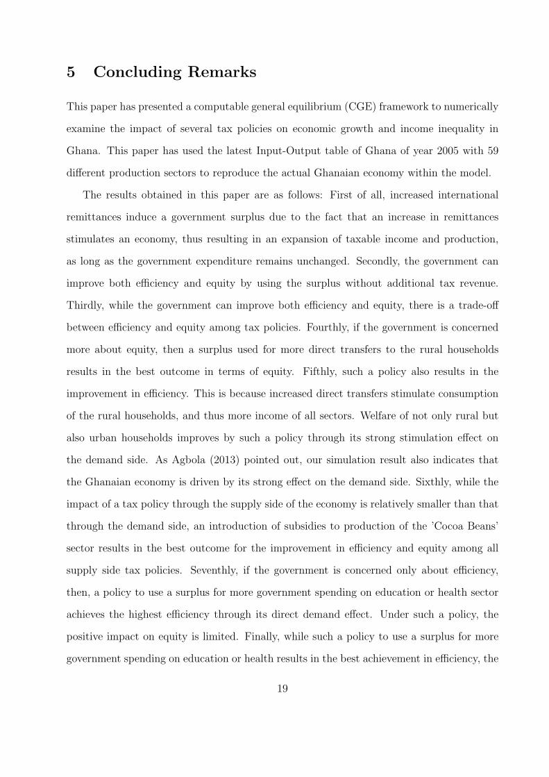
5 Concluding Remarks

This paper has presented a computable general equilibrium (CGE) framework to numerically

examine the impact of several tax policies on economic growth and income inequality in

Ghana. This paper has used the latest Input-Output table of Ghana of year 2005 with 59

different production sectors to reproduce the actual Ghanaian economy within the model.

The results obtained in this paper are as follows: First of all, increased international

remittances induce a government surplus due to the fact that an increase in remittances

stimulates an economy, thus resulting in an expansion of taxable income and production,

as long as the government expenditure remains unchanged. Secondly, the government can

improve both efficiency and equity by using the surplus without additional tax revenue.

Thirdly, while the government can improve both efficiency and equity, there is a trade-off

between efficiency and equity among tax policies. Fourthly, if the government is concerned

more about equity, then a surplus used for more direct transfers to the rural households

results in the best outcome in terms of equity. Fifthly, such a policy also results in the

improvement in efficiency. This is because increased direct transfers stimulate consumption

of the rural households, and thus more income of all sectors. Welfare of not only rural but

also urban households improves by such a policy through its strong stimulation effect on

the demand side. As Agbola (2013) pointed out, our simulation result also indicates that

the Ghanaian economy is driven by its strong effect on the demand side. Sixthly, while the

impact of a tax policy through the supply side of the economy is relatively smaller than that

through the demand side, an introduction of subsidies to production of the ’Cocoa Beans’

sector results in the best outcome for the improvement in efficiency and equity among all

supply side tax policies. Seventhly, if the government is concerned only about efficiency,

then, a policy to use a surplus for more government spending on education or health sector

achieves the highest efficiency through its direct demand effect. Under such a policy, the

positive impact on equity is limited. Finally, while such a policy to use a surplus for more

government spending on education or health results in the best achievement in efficiency, the

19

distribution of efficiency gain between the government and the private sectors differs between

the case of more direct transfers to the rural households and the case of more government

spending on education or health. While the Ghanaian economy can enjoy the largest benefits

in improved efficiency as a whole when a surplus is used for more government spending,

increased efficiency gain will be more distributed to the government sector in comparison

with the case when a surplus is used for more direct transfers to the rural households. While

a tax policy to provide the rural households with more direct transfers induces the second

best outcome in terms of efficiency, it achieves the best outcome in terms of equity, so that

both rural and urban households can enjoy the highest welfare. In this case, efficiency gain

is more distributed to the private sector.

Finally drawbacks of this paper should be mentioned: Since utility is defined only over

consumption and the optimal labor-leisure choice is not considered, the model cannot capture

the overall impact of taxation. In particular, if the impact of taxation on efficiency and

equity is considered, then the assumption of inelasitce labor supply would be inappropriate.

Furthermore, while it is conventional in the literature, the optimal behavior regarding savings

is not properly taken into account in the model. Thus, the impact on savings is not perfectly

captured with this model.

However, by using the latest Input-Output Table of Ghana, this paper has developed

a well-fitted benchmark model within a CGE framework, and it has numerically argued

the impact of several tax policies for the improvement in efficiency and equity within a

theoretical framework. It has also taken into account a key issue in the literature; behavioral

changes towards remittances. Since the benchmark model has successfully reproduced the

real Ghanaian economy within the model, the numerical results also seem realistic.

20

References

[1] Acosta, Pablo, C Calderon, P Fajnzylber, and H Lopez (2008), ’What is the Impact of

International Remittances on Poverty and Inequality in Latin America?,’ World Devel-

opment, Vol. 36 (1), pp. 89 - 114

[2] Adams, Richard H Jr (2009), ‘The Determinants of International remittances in Devel-

oping Countries,’ World Development, Vol. 37, No. 1, pp. 93 - 103

[3] Adams, Richard H Jr (2011), ‘Evaluating the Economic Impact of International Re-

mittances on Developing Countries Using Household Surveys: A Literature Review,’

Journal of Development Studies, Vol. 47, No. 6, pp. 809 - 828

[4] Adams, Richard H Jr, and A Cuecuecha (2010), ’Remittances, Household Expenditure

and Investment in Guatemala,’ World Development, Vol. 38, pp. 1626 - 1641

[5] Adams, Richard H Jr, and A Cuecuecha (2013), ’The Impact of Remittances on Invest-

ment and Poverty in Ghana,’ World Development, Vol. 50, pp. 24 - 40

[6] Adams, Richard H Jr, and J Page (2005), ’Do International Migration and Remittances

Reduce Poverty in Developing Countries?,’ World Development, Vol. 33, pp. 1645 - 1669

[7] Agbola, Frank Wogbe (2013), ’Does Human Capital Constrain the Impact of Foreign Di-

rect Investment and Remittances on Economic Growth in Ghana?,’ Applied Economics,

45, pp. 2853 - 2862

[8] Auerbach, Alan J and L J Kotlikoff (1987), Dynamic Fiscal Policy, Cambridge Univer-

sity Press

[9] Ballard, Charles L, D Fullerton, J B Shoven, and J Whalley (1985), A General Equilib-

rium Model for Tax Policy Evaluation, Chicago University Press

21

[10] Barham, Bradford, and S Boucher (1998), ’Migration, Remittances, and Inequality:

Estimating the Net effects of Migration on Income Distribution,’ Journal of Development

Economics, Vol. 55, pp. 307 - 331

[11] Dadson, Isaac, and R R Kato (2015), ’Remittances and the Brain Drain in Ghana:

A Computable General Equilibrium Approach, EMS-2015-04, Economics and Manage-

ment Series, IUJ Research Institute, International University of Japan

[12] Djiofack, Calvin Z, E W Djimeu, and M Boussichas (2013), ’Impact of Qualified Worker

Emigration on Poverty: A Macro-Micro-Simulation Approach for an African Economy,’

Journal of African Economies, Vol. 23, No.1, pp. 1 - 52

[13] Faini, Riccardo (2007), ‘Remittances and the Brain Drain: Do More Skilled Migrants

Remit More?,’ The World Bank Economic Review, Vol. 21, No.2, pp. 177 - 191

[14] Freund, Caroline and N Spatafora (2008), ‘Remittances, Transaction costs, and Infor-

mality,’ Journal of Development Economics, Vol. 86, pp. 356 - 366

[15] Ghana Statistical Service (2014), ’Poverty Profile in Ghana,’ Ghana Living Standards

Survey Round 6 (GLSS 6)

[16] Guha, Puja (2013), ‘Macroeconomic Effects of International Remittances: The Case of

Developing Countries,’ Economic Modelling, Vol. 33, pp. 292 - 305

[17] Gupta, Sanjeev, C A Pattillo, and S Wagh (2009), ’Effect of Remittances on Poverty

and Financial Development in Sub-Saharan Africa, World Development, Vol. 37, No.

1, pp. 104 - 115

[18] Hosoe, Nobuhiko, K Ogawa, and H Hashimoto (2010), Textbook of Computable General

Equilibrium Modeling, Palgrave

22

[19] Ihori, Toshihiro, R R Kato, M Kawade, and S Bessho (2006), ’Public Debt and Eco-

nomic Growth in an Aging Japan,’ in Tackling Japan’s Fiscal Challenges, eds by Keimei

Kaizuka and Anne O. Krueger, Palgrave

[20] Ihori, Toshihiro, R R Kato, M Kawade, and S Bessho (2011), ’Health Insurance Reform

and Economic Growth: Simulation Analysis in Japan,’ Japan and the World Economy,

Vol. 23 (4), pp. 227-239

[21] Kabki, Mirjam, V Mazzucato, and E Appiah (2004), ‘The Economic Impact of Remit-

tances of Netherlands-Based Ghanaian Migrants on Rural Ashanti,’ Population, Space

and Place, Vol. 10, pp. 85 - 97

[22] Kato, Ryuta Ray (1998), ’Transition to an Aging Japan: Public Pension, Savings and

Capital Taxation,’ Journal of the Japanese and International Economies 12, pp. 204-231

[23] Kato, Ryuta Ray (2002a), ’Government Deficits in an Aging Japan,’ Chapter 5 in Gov-

ernment Deficit and Fiscal Reform in Japan, eds by Ihori and Sato, Kluwer Academic

Publishers

[24] Kato, Ryuta Ray (2002b), ’Government Deficit, Public Investment, and Public Cap-

ital in the Transition to an Aging Japan,’ Journal of the Japanese and International

Economies, 16 (4), pp. 462-491

[25] Lipsey, R G, and K Lancaster (1956), ’The General Theory of Second Best,’ The Review

of Economic Studies, Vol. 24 (1), pp. 11-32

[26] Lipton, Michael (1980), ‘Migration from Rural Areas of Poor Countries: The Impact

on Rural Productivity and Income Distribution,’ World Development, Vol. 8, pp. 1 - 24

[27] Mamun, A, K Sohag, G S Uddin, and M Shahbaz (2015), ‘Remittance and Domestic

Labor Productivity: Evidence from Remittance Recipient Countries,’ Economic Mod-

elling, Vol. 47, pp. 207 - 218

23

[28] Mckenzie, David, and H Rapoport (2007), ‘Network Effects and the Dynamics of Mi-

gration and Inequality: Theory and Evidence from Mexico,’ Journal of Development


[29] Rapoport, Hillel, and F Docquier (2006), ‘The Economics of Migrants’ Remittances,’

Chapter 17, in Handbook of the Economics of Giving, Altruism and Reciprocity, Vol.

2, pp. 1135 - 1198

[30] Scarf, H E, and J B Shoven (2008), Applied General Equilibrium Analysis, Cambridge

University Press

[31] Shoven, John B, and J Whalley (1992), Applying General Equilibrium, Cambridge Uni-

versity Press

[32] Stark, Oded, J E Taylor, and S Yitzhaki (1988), ‘Migration, Remittances and Inequal-

ity: A Sensitivity Analysis Using the Extended Gini Index,’ Journal of Development


[33] Taylor, J Edward (1992), ‘Remittances and Inequality Reconsidered: Direct, Indirect,

and Intertemporal Effects,’ Journal of Policy Modeling, Vol. 14, No. 2, pp. 187 - 208

[34] World Bank (2006), ‘Global Economic Prospects: Economic Implications of Remit-

tances and Migration,’ pp. 1 - 182

[35] World Bank (2015), ’Remittances growth to slow sharply in 2015, as Eu-

rope and Russia stay weak; pick up expected next year,’ World Bank,

http://www.worldbank.org/en/news/press-release/2015/04/13/remittances-growth-to-

slow-sharply-in-2015-as-europe-and-russia-stay-weak-pick-up-expected-next-year

24

Appendix 1: Model

The computable general equilibrium model of this paper employs the conventional static

model13. The Ghanaian economy is assumed to consist of 59 different production sectors,

two different types of households, the government, and the investment firm sector. All 59

industries are allowed to have intermediate production processes, and they are assumed to

maximize their profit. Each production sector employes 6 factors in its production; self-

employed labor (Ls), unskilled employed labor (Lusk), skilled employed labor (Lsk), capital

specific for agriculture (Ka), general capital (Kn), and land (La). households are divided

into two groups based on their living place indexed by h; the household living in the rural area

(h = a) and the household living in the urban area (h = b). While households in different

areas are different, households living in the same area are assumed to be identical. The

household is assumed to maximize his/her utility over 59 different consumption goods.

The government is assumed to determine its tax revenue, its imports, its exports, income

transfers to households, and its consumption in order to satisfy its budget constraint. The

economy is assumed to be fully competitive, so that all prices are determined in the relevant

markets in order to equate the amount of demand to the amount of supply at its fully

competitive price level in equilibrium. Note that the model is static and thus the short-run

effect is only investigated. Thus, it is assumed for simplicity that factor inputs are not mobile

among different sectors in the short-run. All parameter values are presented in Table 6.

<household>

13In terms of the conventional static model, see Ballard et al (1985), Shoven and Whalley (1992), and Scarfand Shoven (2008). In particular, the model used in this paper is similar to Hosoe et al (2004). Regardingthe dynamic model, it is conventional to employ an overlapping generations model In terms of computableoverlapping generations model within a general equilibrium framework, see Auerbach and Kotlikoff (1987).Kato (1998, 2002a, 2002b), and Ihori et al (2006, 2011) also apply the dyanamic model to several policies inJapan.

25

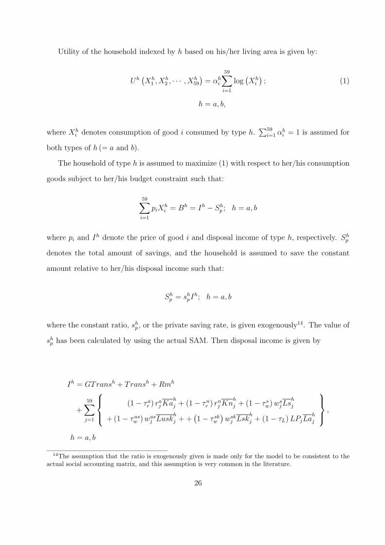
Utility of the household indexed by h based on his/her living area is given by:

Uh(Xh

1 , Xh2 , · · · , Xh

59

)= αh

i

59∑i=1

log(Xh

i

); (1)

h = a, b,

where Xhi denotes consumption of good i consumed by type h.

∑59i=1 αh

i = 1 is assumed for

both types of h (= a and b).

The household of type h is assumed to maximize (1) with respect to her/his consumption

goods subject to her/his budget constraint such that:

59∑i=1

piXhi = Bh = Ih − Sh

p ; h = a, b

where pi and Ih denote the price of good i and disposal income of type h, respectively. Shp

denotes the total amount of savings, and the household is assumed to save the constant

amount relative to her/his disposal income such that:

Shp = sh

pIh; h = a, b

where the constant ratio, shp , or the private saving rate, is given exogenously14. The value of

shp has been calculated by using the actual SAM. Then disposal income is given by

Ih = GTransh + Transh + Rmh

+59∑

j=1

(1 − τar ) ra

j Kah

j + (1 − τnr ) rn

j Knh

j + (1 − τ sw) ws

jLsh

j

+ (1 − τusw ) wus

j Luskh

j + +(1 − τ sk

w

)wsk

j Lskh

j + (1 − τL) LPjLah

j

,

h = a, b

14The assumption that the ratio is exogenously given is made only for the model to be consistent to theactual social accounting matrix, and this assumption is very common in the literature.

26

where GTransh, T ransh, and Rmh denote the government income transfers, net income

transfers from the other type of the household, and the remittance sent from the rest of

the world, respectively15. raj , and rn

j , denote the rental cost of capital specific for agriculture

(Ka), and general capital (Kn) in sector j (= 1, 2, · · · , 59), respectively. wsj , w

usj and wsk

j de-

note the wage rate of self-employed labor (Ls), unskilled employed labor (Lusk), and skilled

employed labor (Lsk) employed in sector j (= 1, 2, · · · , 59), respectively. LPj denotes the

unit price of land (La) . Each type is assumed to have endowments of Kah

j , Knh

j , Lsh

j , Luskh

j , Lskh

j ,

and Lah

j in sector j (= 1, 2, · · · , 59). Both types are also assumed to pay taxes, and

τar , τn

r , τ sw, τus

w , τ skw , and τL denote the capital income tax rate for agriculture, the capital

income tax rate for others, the wage income tax rate for self-employed worker, the wage

income tax rate for unskilled employed worker, the wage income tax rate for skilled em-

ployed worker, and the land tax rate, respectively. Note that all taxes are assumed to be

proportional, and the tax rates have been calculated by using the actual social accounting

matrix. The tax rate can be negative in the simulations if the effect of the case when the

government subsidizes a particular factor input is explored. Note also that all factors are

assumed to be immobile between different production sectors by assumption. The value of

factor payments can be obtained from the actual social accounting matrix16.

The first order conditions yield the demand functions such that:

Xhi = Xh

i

(p̃, ra

j , rnj , ws

j , wusj , wsk

j , LPj; τar , τn

r , τ sw, τus

w , τ skw , τL

)(2a)

=αh

i Ih(1 − sh

p

)pi

, (2b)

i = 1, 2, · · · , 59, h = a, b (2c)

15Preciously speaking, Transh also includes self-consumption within the same group.16The total number of self-employed as well as employed workers in each production sector can be obtained

from the IO table of year 2005. Since per capita wage income of employed workers and total wage incomecan also be obtained from the IO table of year 2005, wj,hLj

h can be calculated for both h = sw and h = ew.On rj,hK

j

h, the ratio of the number of each type of workers has simply been used to divide the total capitalincome of each production sector.

27

where p̃ = (p1,p2, · · · , p59). Note that αhi can be calculated by using (2b) and the actual

social accounting matrix so that:

αhi =

piXhi

Ih(1 − sh

p

) ; h = a, b

where both the values of the denominator and the numerator can be obtained from the actual

social accounting matrix.

<Production Sector>

Following the conventional assumption, the multiple decisions by each firm are described

by the tree structure, where each firm is assumed to make a decision over several different

items. In the tree structure, the optimal behavior of each firm which makes a decision over

different items is described as if the firm always makes a decision over two different items at

different steps. Each firm makes a decision over different items; exports of its own product,

the amount of imported goods and intermediate goods used for its production, and labor

and capital. This assumption simplifies a complicated decision over several items by each

firm. Each step is also shown in Figure 3.

At step 1, a private firm, i, is assumed to use labor and capital to produce its composite

goods, Yi. Then, the firm is assumed to produce its domestic goods, Zi, by using its own Yi

and Xi,k at the second step. Xi,k denotes the final consumption goods produced by firm k

used by firm i for its production. Thus, Xi,k is the amount of the final consumption goods

produced by firm k for the intermediate production process of firm i. At the third step,

the firm is assumed to decompose its domestic goods, Zi, into exported goods, Ei, and final

domestic goods, Di. This step is concerned about its optimal decision over the amount of its

product to be exported. At the final step (the fourth step), the firm is assumed to produce

its final consumption goods, Qi, by using its final domestic goods, Di, and imported goods,

Mi. This step corresponds to its optimal decision over how much it uses imported goods,

Mi, and its own goods, Di, to produce its final consumption goods, Qi, which are consumed

28

by domestic households. The assumption of this tree structure in terms of different decisions

can incorporate firm’s complicated decisions over exports of its own product, the amount of

imported goods and intermediate goods which the firm uses in its production process, and

the amount of factor inputs into the model in a tractable way.

Note that all market clearing conditions are used to determine all prices endogenously

in their corresponding markets, and also that at each step the private firm is assumed to

determine the amount of relevant variables in order to maximize its profit.

By the assumption of the above tree structure, all decision making processes can be

simplified, and the optimal behavior about all different decisions can be incorporated as

follows:

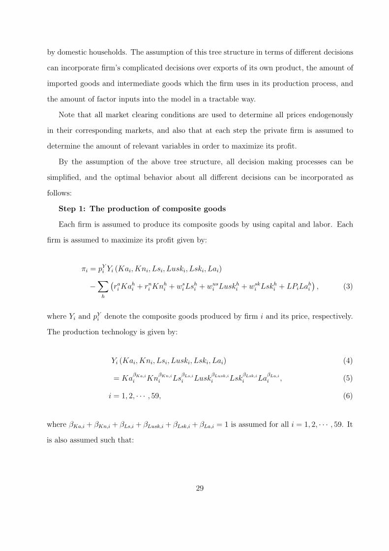
Step 1: The production of composite goods

Each firm is assumed to produce its composite goods by using capital and labor. Each

firm is assumed to maximize its profit given by:

πi = pYi Yi (Kai, Kni, Lsi, Luski, Lski, Lai)

−∑

h

(rai Kah

i + rni Knh

i + wsi Lsh

i + wusi Luskh

i + wski Lskh

i + LPiLahi

), (3)

where Yi and pYi denote the composite goods produced by firm i and its price, respectively.

The production technology is given by:

Yi (Kai, Kni, Lsi, Luski, Lski, Lai) (4)

= KaβKa,i

i KnβKn,i

i LsβLs,i

i LuskβLusk,i

i LskβLsk,i

i LaβLa,i

i , (5)

i = 1, 2, · · · , 59, (6)

where βKa,i + βKn,i + βLs,i + βLusk,i + βLsk,i + βLa,i = 1 is assumed for all i = 1, 2, · · · , 59. It

is also assumed such that:

29

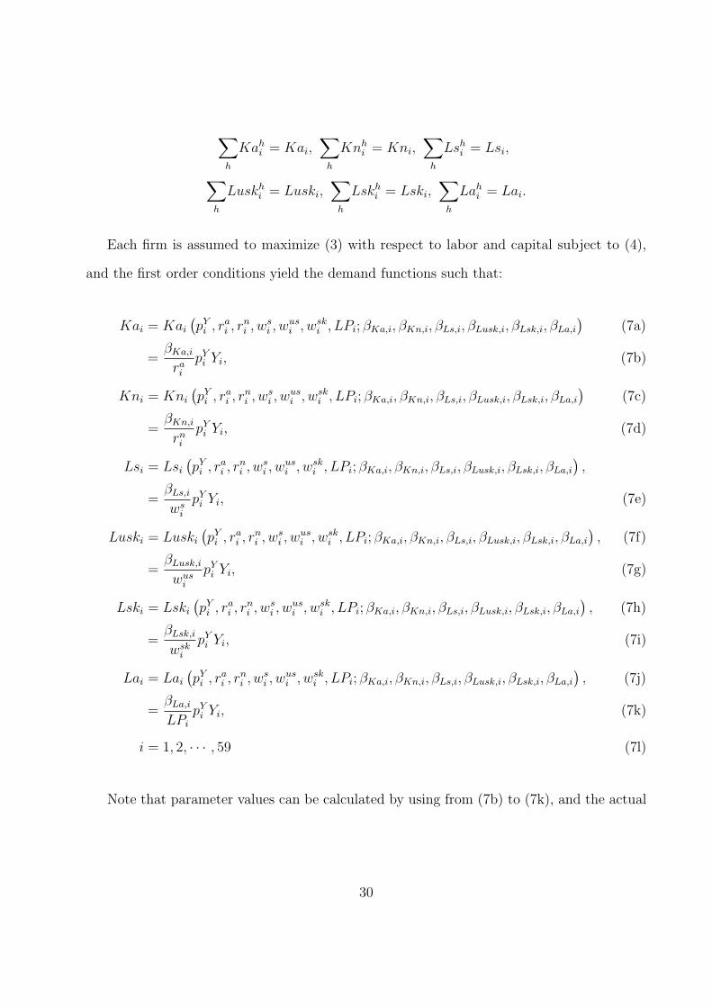
∑h

Kahi = Kai,

∑h

Knhi = Kni,

∑h

Lshi = Lsi,

∑h

Luskhi = Luski,

∑h

Lskhi = Lski,

∑h

Lahi = Lai.

Each firm is assumed to maximize (3) with respect to labor and capital subject to (4),

and the first order conditions yield the demand functions such that:

Kai = Kai

(pY

i , rai , r

ni , ws

i , wusi , wsk

i , LPi; βKa,i, βKn,i, βLs,i, βLusk,i, βLsk,i, βLa,i

)(7a)

=βKa,i

rai

pYi Yi, (7b)

Kni = Kni

(pY

i , rai , r

ni , ws

i , wusi , wsk


)(7c)

=βKn,i

rni

pYi Yi, (7d)

Lsi = Lsi

(pY

i , rai , r

ni , ws

i , wusi , wsk


),

=βLs,i

wsi

pYi Yi, (7e)

Luski = Luski

(pY

i , rai , r

ni , ws

i , wusi , wsk


), (7f)

=βLusk,i

wusi

pYi Yi, (7g)

Lski = Lski

(pY

i , rai , r

ni , ws

i , wusi , wsk


), (7h)

=βLsk,i

wski

pYi Yi, (7i)

Lai = Lai

(pY

i , rai , r

ni , ws

i , wusi , wsk


), (7j)

=βLa,i

LPi

pYi Yi, (7k)

i = 1, 2, · · · , 59 (7l)

Note that parameter values can be calculated by using from (7b) to (7k), and the actual

30

social accounting matrix so that:

βKa,i =rai Kai,

pYi Yi

, βKn,i =rni Kni,

pYi Yi

, βLs,i =ws

i Lsi

pYi Yi

,

βLusk,i =wys

i Luski

pYi Yi

, βLsk,i =wsk

i Lski

pYi Yi

, βLa,i =LPiLai

pYi Yi

,

i = 1, 2, · · · , 59

The estimated values of βK,i,h and βL,i,h are given in Table 6.

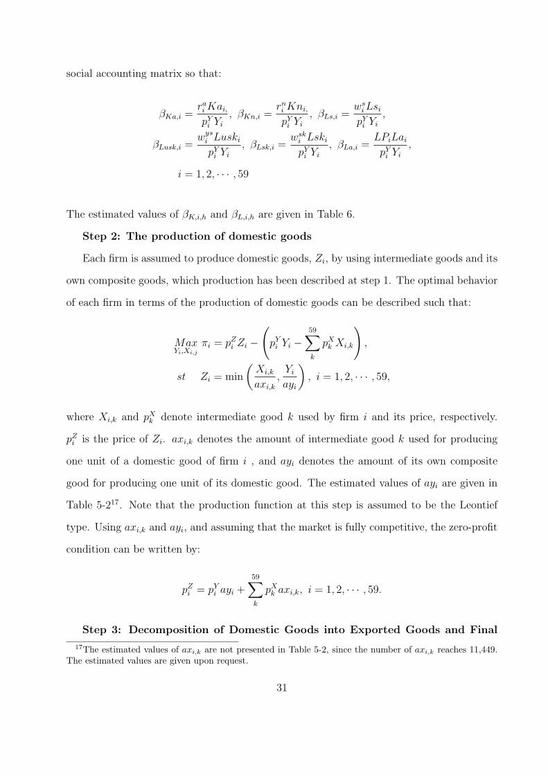
Step 2: The production of domestic goods

Each firm is assumed to produce domestic goods, Zi, by using intermediate goods and its

own composite goods, which production has been described at step 1. The optimal behavior

of each firm in terms of the production of domestic goods can be described such that:

MaxYi,Xi,j

πi = pZi Zi −

(pY

i Yi −59∑k

pXk Xi,k

),

st Zi = min

(Xi,k

axi,k

,Yi

ayi

), i = 1, 2, · · · , 59,

where Xi,k and pXk denote intermediate good k used by firm i and its price, respectively.

pZi is the price of Zi. axi,k denotes the amount of intermediate good k used for producing

one unit of a domestic good of firm i , and ayi denotes the amount of its own composite

good for producing one unit of its domestic good. The estimated values of ayi are given in

Table 5-217. Note that the production function at this step is assumed to be the Leontief

type. Using axi,k and ayi, and assuming that the market is fully competitive, the zero-profit

condition can be written by:

pZi = pY

i ayi +59∑k

pXk axi,k, i = 1, 2, · · · , 59.

Step 3: Decomposition of Domestic Goods into Exported Goods and Final

17The estimated values of axi,k are not presented in Table 5-2, since the number of axi,k reaches 11,449.The estimated values are given upon request.

31

Domestic Goods

The optimal decision made by firm i in terms of the amount of exports of its own goods

is described as the the decomposition of Zi (i = 1, 2, · · · , 59) into exported goods, Ei, and

final domestic goods, Di. Each firm is assumed to maximize its profit such that:

πi = pei (1 − τ e

i ) Ei + pdi Di − (1 + τ p

i ) pZi Zi, (8)

where pei and pd

i denote the price when the domestic goods are sold abroad, and the price

when the domestic goods are sold domestically, respectively. Note that pei is measured in the

domestic currency. τ pi and τ e

i are the tax rates of a production tax imposed on the production

of Zi, and the tax rate on exports, respectively. The values of τ pi and τ e

i are calculated by

using the actual social accounting matrix, and the calculated values are given in Table 2-1

and 2-2. The decomposition is assumed to follow the Cobb-Douglas technology18 such that:

Zi = Eκe

ii D

κdi

i , i = 1, 2, · · · , 59, (9)

where κdi +κe

i = 1 ( i = 1, 2, · · · , 59) is assumed. Each firm is assumed to maximize (8) with

respect to Ei and Di subject to (9), and the first order conditions yield

Ei = Ei

(pe

i , pdi , p

Zi ; τ p

i , τ si , κd

i , κei

)=

κei (1 + τ p

i ) pZi Zi

pei (1 − τ e

i ), (10a)

Di = Di

(pe

i , pdi , p

Zi ; τ p

i , τ si , κd

i , κei

)=

κdi (1 + τ p

i ) pZi Zi

pdi

, i = 1, 2, · · · , 59. (10b)

Note that κei and κd

i can be calculated by using (10a), (10b), and the actual social

18While it is common in the literature to assume (9) and (11) to be expressed by the CES technology, itis assumed in this paper that both technologies are expressed by the Cobb-Douglas technology. While theCobb-Douglas function is the special case of the CES function and thus the CES function provides moregenerality, our assumption gives us more advantages in terms of preciseness of our benchmark model. Asour benchmark results show, the assumption of the Cobb-Douglas technology substantially contributes toour perfectly well-fitted benchmark result. We believe that the benchmark model should be well-fitted to re-produce the actual economy within the model in any simulation anaylsis, and the Cobb-Douglas technology isassumed at the sacrifice of a certain level of genrerality, in order to obtain our perfectly well-fitted benchmarkmodel.

32

accounting matrix so that:

κei =

pei (1 − τ e

i ) Ei

(1 + τ pi ) pZ

i Zi

,

κdi =

pdi Di

(1 + τ pi ) pZ

i Zi

, i = 1, 2, · · · , 59,

where peiEi, pd

i Di, pZi Zi, τ s

i pZi Zi, and τ e

i peiEi can be obtained from the actual social accounting

matrix. The estimated values of κei and κd

i are given in Table 2.

Step 4: The Production of the final goods

Denote the final consumption goods by Qi (i = 1, 2, · · · , 59). The final consumption

goods are assumed to be produced by using the final domestic goods, Di, and the imported

goods, Mi. This step corresponds to the optimal decision making behavior of each firm

in terms of the amount of imported goods which are used in its production process. The

production technology at this final step is given by the following Cobb-Douglas function:

Qi = Mγm

ii D

γdi

i , i = 1, 2, · · · , 59, (11)

where γmi + γd

i = 1 ( i = 1, 2, · · · , 59) is assumed. Each firm is assumed to maximize its

profit with respect to Mi and Di subject to (11). Its profit is given by:

πi = pQi Qi − (1 + τm

i ) pmi Mi − pd

i Di, i = 1, 2, · · · , 59,

where pQi and τm

i denote the price of its final consumption goods, Qi, and the import tariff

rate, respectively. The import tariff rate is calculated by using the actual social accounting

matrix, and it is given in Table 2-4. Then, the first order conditions yield

Mi = Mi

(pm

i , pdi , p

Qi ; τm

i , γmi , γd

i

)=

γmi pQ

i Qi

(1 + τmi ) pm

i i

, (12a)

Di = Di

(pm

i , pdi , p

Qi ; τm

i , γmi , γd

i

)=

γdi p

Qi Qi

pdi

, i = 1, 2, · · · , 59. (12b)

33

Note that γmi and γd

i can be calculated by using (12a), (12b), and the actual social

accounting matrix so that:

γmi =

(1 + τmi ) pm

i Mi

pQi Qi

,

γdi =

pdi Di

pQi Qi

, i = 1, 2, · · · , 59,

where pmi Mi, pd

i Di, pQi Qi and τm

i pmi Mi can be obtained from the actual social accounting

matrix. The estimated values of γmi and γd

i are given in Table 6.

<The Government>

The government is assumed to impose several taxes to satisfy its budget constraint. Its

budget constraint is given by:

59∑i=1

pQi Xg

i + Sg + Gimp + GTrans = T I + T p + Tm + T e + Gex,

where the left hand side is the total government expenditure, and the right hand side is the

total government revenue. Xgi and Sg denote government consumption of final consumption

good i, and government savings, respectively. GTrans denotes the total amount of income

transfers to both types of h such that:

GTrans =∑

h

GTransh.

Gimp and Gex denote direct imports and exports by the government, respectively. The

34

total tax revenue is given by:

T I =59∑i=1

∑h

(τ swws

i Lshi + τus

w wusi Luskh

i + τ skw wsk

i Lskhi

)+

59∑i=1

∑h

(τar ra

i Kahi + τn

wrni Knh

i

),

TL =59∑i=1

∑h

(τLLPiLah

i

),

T p =59∑i=1

τ pi

(pZ

i Zi

),

Tm =59∑i=1

τmi (pm

i Mi) ,

T e =59∑i=1

τ ei (pe

iEi)

where T I , TL, T p, Tm, and T e denote the total income tax revenue, the total land tax

revenue, the total production tax revenue, the total import tariff revenue, and the total

export tax revenue, respectively. The government is assumed to save the constant amount

relative to the total amount of tax revenue, and the government savings are assumed to be

given by

Sg = sg(T I + T p + Tm + Gex

),

where the constant ratio, sg, is given exogenously, and .its value has been calculated by using

the actual SAM.

<Equilibrium Conditions>

There are two factor inputs, labour and capital. Since the model is static and thus the

short-run effect is explored, it is assumed that each factor cannot move among different sec-

tors (industries) in the short-run. This implies the equilibrium conditions of factor markets

35

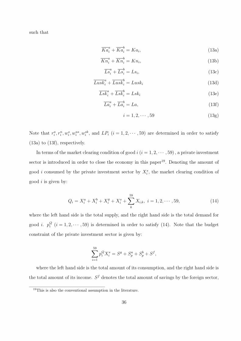
such that

Kaa

i + Kab

i = Kai, (13a)

Kna

i + Knb

i = Kni, (13b)

Lsa

i + Lsb

i = Lsi, (13c)

Luska

i + Luskb

i = Luski (13d)

Lska

i + Lskb

i = Lski (13e)

Laa

i + Lab

i = La, (13f)

i = 1, 2, · · · , 59 (13g)

Note that rai , r

ni , ws

i , wusi , wsk

i , and LPi (i = 1, 2, · · · , 59) are determined in order to satisfy

(13a) to (13f), respectively.

In terms of the market clearing condition of good i (i = 1, 2, · · · , 59) , a private investment

sector is introduced in order to close the economy in this paper19. Denoting the amount of

good i consumed by the private investment sector by Xsi , the market clearing condition of

good i is given by:

Qi = Xai + Xb

i + Xgi + Xs

i +59∑k

Xi,k, i = 1, 2, · · · , 59, (14)

where the left hand side is the total supply, and the right hand side is the total demand for

good i. pQi (i = 1, 2, · · · , 59) is determined in order to satisfy (14). Note that the budget

constraint of the private investment sector is given by:

59∑i=1

pQi Xs

i = Sg + Sap + Sb

p + Sf ,

where the left hand side is the total amount of its consumption, and the right hand side is

the total amount of its income. Sf denotes the total amount of savings by the foreign sector,

19This is also the conventional assumption in the literature.

36

or the deficits in the current account, and it is given by subtracting exports from imports20.

Since both the amount of exports and the amount of imports can be obtained from the actual

social accounting matrix, Sf can be calculated from the actual social accounting matrix, and

thus it is exogenously given in the model. Furthermore, the foreign trade balance is given

by

59∑i=1

pw,ei Ei + Sf + Gex +

∑h

Rmh =59∑i=1

pw,mi Mi + Gimp,

where pw,ei and pw,m

i denote the world price of export goods, and import goods of good

i, respectively, and both of them are assumed to be given exogenously. Since pei and pm

i are

both measured in the domestic currency, they are also expressed such that:

pei = εpw,e

i ,

pmi = εpw,m

i , i = 1, 2, · · · , 59,

where ε denotes the exchange rate. Note that the exogeneity assumption on the world

prices implies that the exchange rate is endogenously determined within the model.

20The FDI is assumed to be negiligible in this paper.

37

38

Figure 1: International Remittances

Data Source: World Bank

0.0000

20.0000

40.0000

60.0000

80.0000

100.0000

120.0000

140.0000

160.0000

1979

1980

1981

1982

1983

1984

1985

1986

1987

1988

1989

1990

1991

1992

1993

1994

1995

1996

1997

1998

1999

2000

2001

2002

2003

2004

2005

2006

2007

2008

2009

2010

2011

2012

2013

2014

e

Uni

t: m

illio

n U

SD

39

Table 1: International Remittances in year 2005 based on the IO Table year 2005

Unit: million USD

Formal Informal Total

To Rural houeholds 45.11181696 168.34958 213.46139Urban households 175.726162 655.77995 831.50611

total 220.8379789 824.12952 1044.9675

To Rural houeholds 3.268972244 12.199245 15.468217Urban households 20.91978119 78.069041 98.988822

total 24.18875343 90.268286 114.45704

Source: Input-Output Table of Year 2005

Per a million population

The amout of informal remittances is obtained based on the assumption that the amount ofexports in sector 51 is treated as informal international remittances

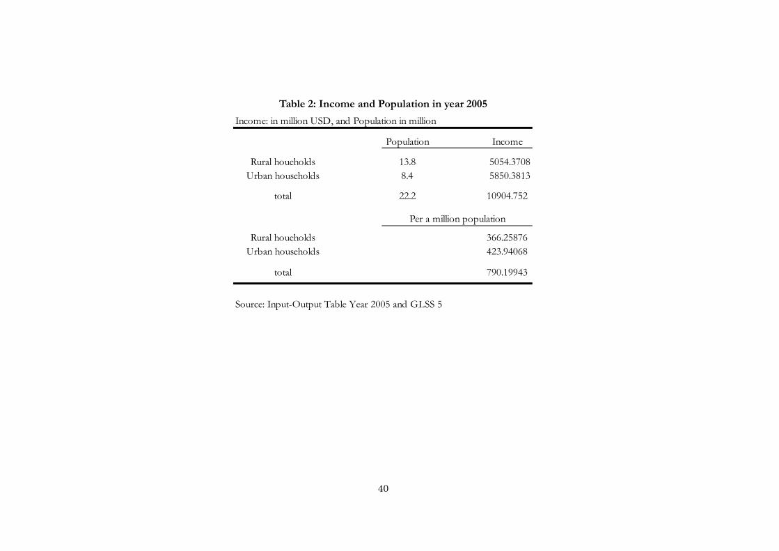
40

Table 2: Income and Population in year 2005

Income: in million USD, and Population in million

Population Income

Rural houeholds 13.8 5054.3708Urban households 8.4 5850.3813

total 22.2 10904.752

Rural houeholds 366.25876Urban households 423.94068

total 790.19943

Source: Input-Output Table Year 2005 and GLSS 5

Per a million population

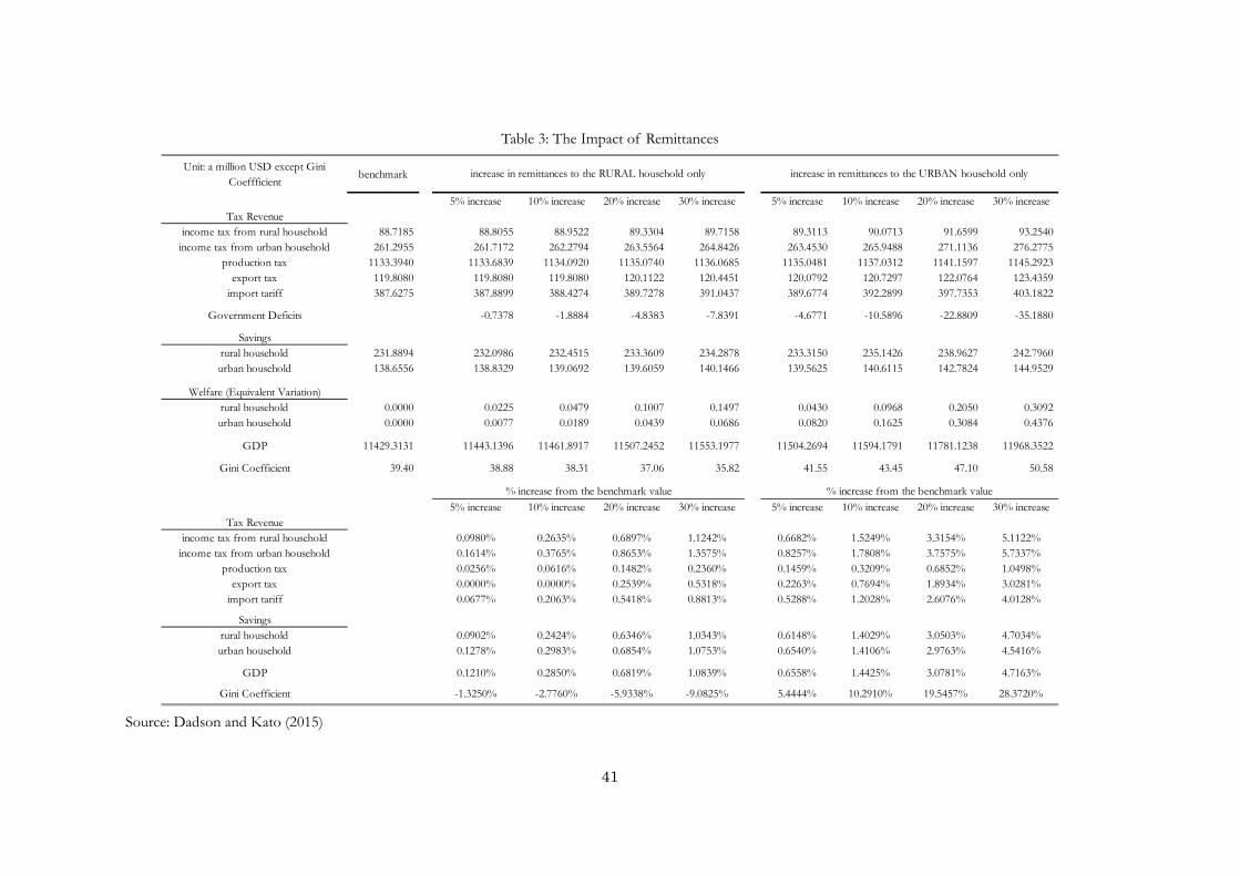
41

Table 3: The Impact of Remittances

Source: Dadson and Kato (2015)

Unit: a million USD except GiniCoeffficient

benchmark

5% increase 10% increase 20% increase 30% increase 5% increase 10% increase 20% increase 30% increaseTax Revenue

income tax from rural household 88.7185 88.8055 88.9522 89.3304 89.7158 89.3113 90.0713 91.6599 93.2540income tax from urban household 261.2955 261.7172 262.2794 263.5564 264.8426 263.4530 265.9488 271.1136 276.2775

production tax 1133.3940 1133.6839 1134.0920 1135.0740 1136.0685 1135.0481 1137.0312 1141.1597 1145.2923export tax 119.8080 119.8080 119.8080 120.1122 120.4451 120.0792 120.7297 122.0764 123.4359

import tariff 387.6275 387.8899 388.4274 389.7278 391.0437 389.6774 392.2899 397.7353 403.1822

Government Deficits -0.7378 -1.8884 -4.8383 -7.8391 -4.6771 -10.5896 -22.8809 -35.1880

Savingsrural household 231.8894 232.0986 232.4515 233.3609 234.2878 233.3150 235.1426 238.9627 242.7960urban household 138.6556 138.8329 139.0692 139.6059 140.1466 139.5625 140.6115 142.7824 144.9529

Welfare (Equivalent Variation)rural household 0.0000 0.0225 0.0479 0.1007 0.1497 0.0430 0.0968 0.2050 0.3092urban household 0.0000 0.0077 0.0189 0.0439 0.0686 0.0820 0.1625 0.3084 0.4376

GDP 11429.3131 11443.1396 11461.8917 11507.2452 11553.1977 11504.2694 11594.1791 11781.1238 11968.3522

Gini Coefficient 39.40 38.88 38.31 37.06 35.82 41.55 43.45 47.10 50.58

5% increase 10% increase 20% increase 30% increase 5% increase 10% increase 20% increase 30% increaseTax Revenue

income tax from rural household 0.0980% 0.2635% 0.6897% 1.1242% 0.6682% 1.5249% 3.3154% 5.1122%income tax from urban household 0.1614% 0.3765% 0.8653% 1.3575% 0.8257% 1.7808% 3.7575% 5.7337%

production tax 0.0256% 0.0616% 0.1482% 0.2360% 0.1459% 0.3209% 0.6852% 1.0498%export tax 0.0000% 0.0000% 0.2539% 0.5318% 0.2263% 0.7694% 1.8934% 3.0281%

import tariff 0.0677% 0.2063% 0.5418% 0.8813% 0.5288% 1.2028% 2.6076% 4.0128%

Savingsrural household 0.0902% 0.2424% 0.6346% 1.0343% 0.6148% 1.4029% 3.0503% 4.7034%urban household 0.1278% 0.2983% 0.6854% 1.0753% 0.6540% 1.4106% 2.9763% 4.5416%

GDP 0.1210% 0.2850% 0.6819% 1.0839% 0.6558% 1.4425% 3.0781% 4.7163%

Gini Coefficient -1.3250% -2.7760% -5.9338% -9.0825% 5.4444% 10.2910% 19.5457% 28.3720%

increase in remittances to the RURAL household only increase in remittances to the URBAN household only

% increase from the benchmark value % increase from the benchmark value

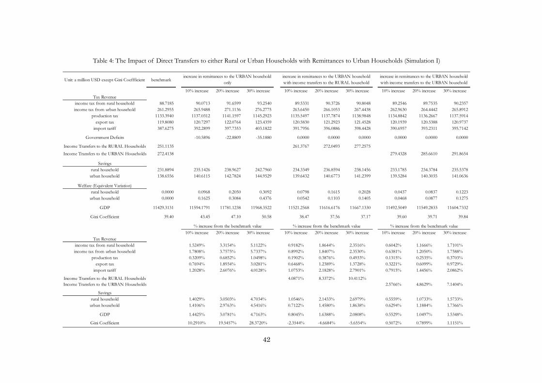
42

Table 4: The Impact of Direct Transfers to either Rural or Urban Households with Remittances to Urban Households (Simulation I)

Unit: a million USD except Gini Coeffficient benchmark

10% increase 20% increase 30% increase 10% increase 20% increase 30% increase 10% increase 20% increase 30% increaseTax Revenue

income tax from rural household 88.7185 90.0713 91.6599 93.2540 89.5331 90.3726 90.8048 89.2546 89.7535 90.2357income tax from urban household 261.2955 265.9488 271.1136 276.2775 263.6450 266.1053 267.4438 262.9630 264.4442 265.8912

production tax 1133.3940 1137.0312 1141.1597 1145.2923 1135.5497 1137.7874 1138.9848 1134.8842 1136.2667 1137.5914export tax 119.8080 120.7297 122.0764 123.4359 120.5830 121.2923 121.4528 120.1939 120.5388 120.9737

import tariff 387.6275 392.2899 397.7353 403.1822 391.7956 396.0886 398.4428 390.6957 393.2311 395.7142

Government Deficits -10.5896 -22.8809 -35.1880 0.0000 0.0000 0.0000 0.0000 0.0000 0.0000

Income Transfers to the RURAL Households 251.1135 261.3767 272.0493 277.2575Income Transfers to the URBAN Households 272.4138 279.4328 285.6610 291.8654

Savingsrural household 231.8894 235.1426 238.9627 242.7960 234.3349 236.8594 238.1456 233.1785 234.3784 235.5378

urban household 138.6556 140.6115 142.7824 144.9529 139.6432 140.6773 141.2399 139.5284 140.3035 141.0636

Welfare (Equivalent Variation)rural household 0.0000 0.0968 0.2050 0.3092 0.0798 0.1615 0.2028 0.0437 0.0837 0.1223

urban household 0.0000 0.1625 0.3084 0.4376 0.0542 0.1103 0.1405 0.0468 0.0877 0.1275

GDP 11429.3131 11594.1791 11781.1238 11968.3522 11521.2568 11616.6176 11667.1330 11492.5049 11549.2833 11604.7332

Gini Coefficient 39.40 43.45 47.10 50.58 38.47 37.56 37.17 39.60 39.71 39.84


income tax from rural household 1.5249% 3.3154% 5.1122% 0.9182% 1.8644% 2.3516% 0.6042% 1.1666% 1.7101%income tax from urban household 1.7808% 3.7575% 5.7337% 0.8992% 1.8407% 2.3530% 0.6381% 1.2050% 1.7588%

production tax 0.3209% 0.6852% 1.0498% 0.1902% 0.3876% 0.4933% 0.1315% 0.2535% 0.3703%export tax 0.7694% 1.8934% 3.0281% 0.6468% 1.2389% 1.3728% 0.3221% 0.6099% 0.9729%

import tariff 1.2028% 2.6076% 4.0128% 1.0753% 2.1828% 2.7901% 0.7915% 1.4456% 2.0862%

Income Transfers to the RURAL Households 4.0871% 8.3372% 10.4112%Income Transfers to the URBAN Households 2.5766% 4.8629% 7.1404%

Savingsrural household 1.4029% 3.0503% 4.7034% 1.0546% 2.1433% 2.6979% 0.5559% 1.0733% 1.5733%

urban household 1.4106% 2.9763% 4.5416% 0.7122% 1.4580% 1.8638% 0.6294% 1.1884% 1.7366%

GDP 1.4425% 3.0781% 4.7163% 0.8045% 1.6388% 2.0808% 0.5529% 1.0497% 1.5348%

Gini Coefficient 10.2910% 19.5457% 28.3720% -2.3544% -4.6684% -5.6554% 0.5072% 0.7899% 1.1151%

increase in remittances to the URBAN householdonly

increase in remittances to the URBAN householdwith income transfers to the RURAL household


increase in remittances to the URBAN householdwith income transfers to the URBAN household

% increase from the benchmark value

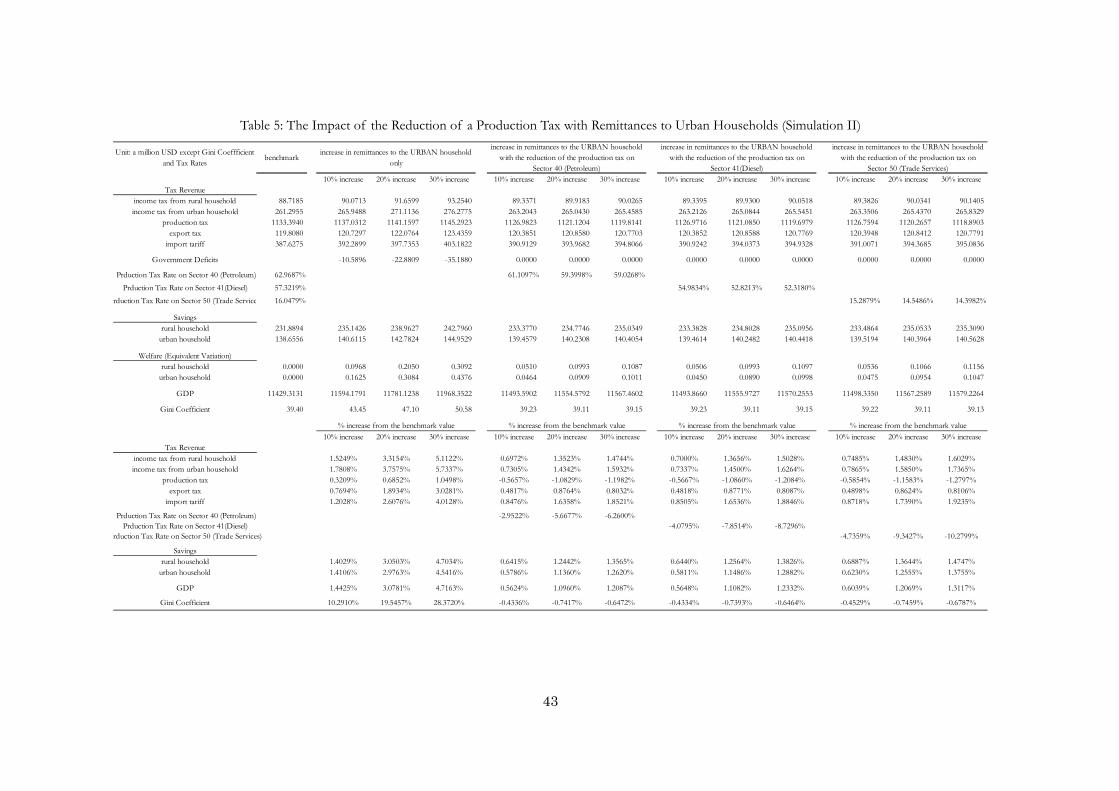
43

Table 5: The Impact of the Reduction of a Production Tax with Remittances to Urban Households (Simulation II)

Unit: a million USD except Gini Coeffficientand Tax Rates

benchmark

10% increase 20% increase 30% increase 10% increase 20% increase 30% increase 10% increase 20% increase 30% increase 10% increase 20% increase 30% increaseTax Revenue

income tax from rural household 88.7185 90.0713 91.6599 93.2540 89.3371 89.9183 90.0265 89.3395 89.9300 90.0518 89.3826 90.0341 90.1405income tax from urban household 261.2955 265.9488 271.1136 276.2775 263.2043 265.0430 265.4585 263.2126 265.0844 265.5451 263.3506 265.4370 265.8329

production tax 1133.3940 1137.0312 1141.1597 1145.2923 1126.9823 1121.1204 1119.8141 1126.9716 1121.0850 1119.6979 1126.7594 1120.2657 1118.8903export tax 119.8080 120.7297 122.0764 123.4359 120.3851 120.8580 120.7703 120.3852 120.8588 120.7769 120.3948 120.8412 120.7791

import tariff 387.6275 392.2899 397.7353 403.1822 390.9129 393.9682 394.8066 390.9242 394.0373 394.9328 391.0071 394.3685 395.0836

Government Deficits -10.5896 -22.8809 -35.1880 0.0000 0.0000 0.0000 0.0000 0.0000 0.0000 0.0000 0.0000 0.0000

Prduction Tax Rate on Sector 40 (Petroleum) 62.9687% 61.1097% 59.3998% 59.0268%Prduction Tax Rate on Sector 41(Diesel) 57.3219% 54.9834% 52.8213% 52.3180%

rduction Tax Rate on Sector 50 (Trade Service 16.0479% 15.2879% 14.5486% 14.3982%

Savingsrural household 231.8894 235.1426 238.9627 242.7960 233.3770 234.7746 235.0349 233.3828 234.8028 235.0956 233.4864 235.0533 235.3090

urban household 138.6556 140.6115 142.7824 144.9529 139.4579 140.2308 140.4054 139.4614 140.2482 140.4418 139.5194 140.3964 140.5628

Welfare (Equivalent Variation)rural household 0.0000 0.0968 0.2050 0.3092 0.0510 0.0993 0.1087 0.0506 0.0993 0.1097 0.0536 0.1066 0.1156

urban household 0.0000 0.1625 0.3084 0.4376 0.0464 0.0909 0.1011 0.0450 0.0890 0.0998 0.0475 0.0954 0.1047

GDP 11429.3131 11594.1791 11781.1238 11968.3522 11493.5902 11554.5792 11567.4602 11493.8660 11555.9727 11570.2553 11498.3350 11567.2589 11579.2264

Gini Coefficient 39.40 43.45 47.10 50.58 39.23 39.11 39.15 39.23 39.11 39.15 39.22 39.11 39.13


income tax from rural household 1.5249% 3.3154% 5.1122% 0.6972% 1.3523% 1.4744% 0.7000% 1.3656% 1.5028% 0.7485% 1.4830% 1.6029%income tax from urban household 1.7808% 3.7575% 5.7337% 0.7305% 1.4342% 1.5932% 0.7337% 1.4500% 1.6264% 0.7865% 1.5850% 1.7365%

production tax 0.3209% 0.6852% 1.0498% -0.5657% -1.0829% -1.1982% -0.5667% -1.0860% -1.2084% -0.5854% -1.1583% -1.2797%export tax 0.7694% 1.8934% 3.0281% 0.4817% 0.8764% 0.8032% 0.4818% 0.8771% 0.8087% 0.4898% 0.8624% 0.8106%

import tariff 1.2028% 2.6076% 4.0128% 0.8476% 1.6358% 1.8521% 0.8505% 1.6536% 1.8846% 0.8718% 1.7390% 1.9235%

Prduction Tax Rate on Sector 40 (Petroleum) -2.9522% -5.6677% -6.2600%Prduction Tax Rate on Sector 41(Diesel) -4.0795% -7.8514% -8.7296%

rduction Tax Rate on Sector 50 (Trade Services) -4.7359% -9.3427% -10.2799%

Savingsrural household 1.4029% 3.0503% 4.7034% 0.6415% 1.2442% 1.3565% 0.6440% 1.2564% 1.3826% 0.6887% 1.3644% 1.4747%

urban household 1.4106% 2.9763% 4.5416% 0.5786% 1.1360% 1.2620% 0.5811% 1.1486% 1.2882% 0.6230% 1.2555% 1.3755%

GDP 1.4425% 3.0781% 4.7163% 0.5624% 1.0960% 1.2087% 0.5648% 1.1082% 1.2332% 0.6039% 1.2069% 1.3117%

Gini Coefficient 10.2910% 19.5457% 28.3720% -0.4336% -0.7417% -0.6472% -0.4334% -0.7393% -0.6464% -0.4529% -0.7459% -0.6787%


increase in remittances to the URBAN householdwith the reduction of the production tax on

Sector 41(Diesel)


Sector 50 (Trade Services)



Sector 40 (Petroleum)


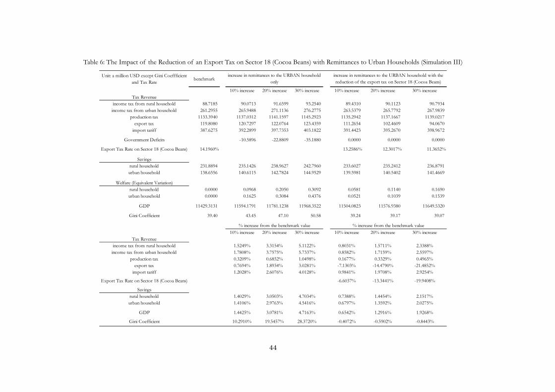
44

Table 6: The Impact of the Reduction of an Export Tax on Sector 18 (Cocoa Beans) with Remittances to Urban Households (Simulation III)

Unit: a million USD except Gini Coeffficientand Tax Rate

benchmark

10% increase 20% increase 30% increase 10% increase 20% increase 30% increaseTax Revenue

income tax from rural household 88.7185 90.0713 91.6599 93.2540 89.4310 90.1123 90.7934income tax from urban household 261.2955 265.9488 271.1136 276.2775 263.5379 265.7792 267.9839

production tax 1133.3940 1137.0312 1141.1597 1145.2923 1135.2942 1137.1667 1139.0217export tax 119.8080 120.7297 122.0764 123.4359 111.2654 102.4609 94.0670

import tariff 387.6275 392.2899 397.7353 403.1822 391.4423 395.2670 398.9672

Government Deficits -10.5896 -22.8809 -35.1880 0.0000 0.0000 0.0000

Export Tax Rate on Sector 18 (Cocoa Beans) 14.1960% 13.2586% 12.3017% 11.3652%

Savingsrural household 231.8894 235.1426 238.9627 242.7960 233.6027 235.2412 236.8791urban household 138.6556 140.6115 142.7824 144.9529 139.5981 140.5402 141.4669

Welfare (Equivalent Variation)rural household 0.0000 0.0968 0.2050 0.3092 0.0581 0.1140 0.1690urban household 0.0000 0.1625 0.3084 0.4376 0.0521 0.1039 0.1539

GDP 11429.3131 11594.1791 11781.1238 11968.3522 11504.0823 11576.9380 11649.5320

Gini Coefficient 39.40 43.45 47.10 50.58 39.24 39.17 39.07

10% increase 20% increase 30% increase 10% increase 20% increase 30% increaseTax Revenue

income tax from rural household 1.5249% 3.3154% 5.1122% 0.8031% 1.5711% 2.3388%income tax from urban household 1.7808% 3.7575% 5.7337% 0.8582% 1.7159% 2.5597%

production tax 0.3209% 0.6852% 1.0498% 0.1677% 0.3329% 0.4965%export tax 0.7694% 1.8934% 3.0281% -7.1303% -14.4790% -21.4852%

import tariff 1.2028% 2.6076% 4.0128% 0.9841% 1.9708% 2.9254%

Export Tax Rate on Sector 18 (Cocoa Beans) -6.6037% -13.3441% -19.9408%

Savingsrural household 1.4029% 3.0503% 4.7034% 0.7388% 1.4454% 2.1517%urban household 1.4106% 2.9763% 4.5416% 0.6797% 1.3592% 2.0275%

GDP 1.4425% 3.0781% 4.7163% 0.6542% 1.2916% 1.9268%

Gini Coefficient 10.2910% 19.5457% 28.3720% -0.4072% -0.5902% -0.8443%


increase in remittances to the URBAN household with thereduction of the export tax on Sector 18 (Cocoa Beans)


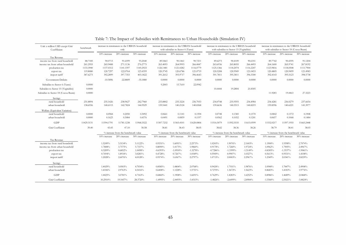
45

Table 7: The Impact of Subsidies with Remittances to Urban Households (Simulation IV)

Unit: a million USD except GiniCoeffficient

benchmark


income tax from rural household 88.7185 90.0713 91.6599 93.2540 89.5463 90.1461 90.7211 89.6273 90.4109 90.6351 89.7742 90.4395 91.1204income tax from urban household 261.2955 265.9488 271.1136 276.2775 263.4093 264.9993 266.4847 263.6936 265.8055 266.4493 264.1600 265.9741 267.8192

production tax 1133.3940 1137.0312 1141.1597 1145.2923 1126.1481 1121.0282 1116.0779 1125.1366 1118.2074 1116.2247 1123.9816 1118.0508 1111.7904export tax 119.8080 120.7297 122.0764 123.4359 120.3745 120.6786 121.0719 120.5208 120.9949 121.0453 120.4805 120.9499 121.4983

import tariff 387.6275 392.2899 397.7353 403.1822 391.2612 393.9717 396.4643 391.7811 395.3811 396.5300 392.4143 395.5123 398.5738

Government Deficits -10.5896 -22.8809 -35.1880 0.0000 0.0000 0.0000 0.0000 0.0000 0.0000 0.0000 0.0000 0.0000

Subsidies to Sector 6 (Yams) 0.0000 9.2003 15.7610 22.0942Subsidies to Sector 15 (Vegitables) 0.0000 10.4444 19.2804 21.8305

Subsidies to Sector 18 (Cocoa Beans) 0.0000 11.9283 19.4463 27.3223

Savingsrural household 231.8894 235.1426 238.9627 242.7960 233.8802 235.3224 236.7053 234.0748 235.9593 236.4984 234.4281 236.0279 237.6654urban household 138.6556 140.6115 142.7824 144.9529 139.5441 140.2124 140.8368 139.6636 140.5513 140.8219 139.8596 140.6221 141.3977

Welfare (Equivalent Variation)rural household 0.0000 0.0968 0.2050 0.3092 0.0661 0.1141 0.1594 0.0748 0.1385 0.1570 0.0842 0.1372 0.1908urban household 0.0000 0.1625 0.3084 0.4376 0.0491 0.0859 0.1197 0.0562 0.1052 0.1201 0.0657 0.1068 0.1484

GDP 11429.3131 11594.1791 11781.1238 11968.3522 11507.7232 11565.4101 11620.0806 11516.5079 11592.5535 11615.0599 11532.0217 11597.1955 11663.2448

Gini Coefficient 39.40 43.45 47.10 50.58 38.81 38.43 38.05 38.82 38.36 38.26 38.79 38.41 38.03


income tax from rural household 1.5249% 3.3154% 5.1122% 0.9331% 1.6091% 2.2573% 1.0243% 1.9076% 2.1603% 1.1900% 1.9398% 2.7074%income tax from urban household 1.7808% 3.7575% 5.7337% 0.8090% 1.4175% 1.9860% 0.9178% 1.7260% 1.9724% 1.0962% 1.7905% 2.4967%

production tax 0.3209% 0.6852% 1.0498% -0.6393% -1.0910% -1.5278% -0.7286% -1.3399% -1.5149% -0.8305% -1.3537% -1.9061%export tax 0.7694% 1.8934% 3.0281% 0.4728% 0.7267% 1.0549% 0.5949% 0.9907% 1.0327% 0.5613% 0.9531% 1.4108%

import tariff 1.2028% 2.6076% 4.0128% 0.9374% 1.6367% 2.2797% 1.0715% 2.0003% 2.2967% 1.2349% 2.0341% 2.8239%

Savingsrural household 1.4029% 3.0503% 4.7034% 0.8585% 1.4804% 2.0768% 0.9424% 1.7551% 1.9876% 1.0948% 1.7847% 2.4908%urban household 1.4106% 2.9763% 4.5416% 0.6408% 1.1228% 1.5731% 0.7270% 1.3672% 1.5623% 0.8683% 1.4183% 1.9776%

GDP 1.4425% 3.0781% 4.7163% 0.6860% 1.1908% 1.6691% 0.7629% 1.4283% 1.6252% 0.8986% 1.4689% 2.0468%

Gini Coefficient 10.2910% 19.5457% 28.3720% -1.4995% -2.4493% -3.4315% -1.4826% -2.6499% -2.8984% -1.5560% -2.5021% -3.4824%


increase in remittances to the URBAN householdwith subsidies to Sector 15 (Vegitables)

increase in remittances to the URBAN householdwith subsidies to Sector 18 (Cocoa Beans)


increase in remittances to the URBAN householdwith subsidies to Sector 6 (Yams)


46

Table 8: The Impact of More Government Expenditure with Remittances to Urban Households (Simulation V)

Unit: a million USD except Gini Coeffficient benchmark


income tax from rural household 88.7185 90.0713 91.6599 93.2540 89.4066 90.0790 90.7480 89.4168 90.0899 90.7636income tax from urban household 261.2955 265.9488 271.1136 276.2775 263.5339 265.8026 268.0321 263.5667 265.8316 268.0696

production tax 1133.3940 1137.0312 1141.1597 1145.2923 1135.2034 1137.0044 1138.7883 1135.2319 1137.0299 1138.8231export tax 119.8080 120.7297 122.0764 123.4359 120.3963 120.8268 121.3369 120.3964 120.8285 121.3385

import tariff 387.6275 392.2899 397.7353 403.1822 391.1983 394.6623 398.0663 391.2515 394.7137 398.1427

Government Deficits -10.5896 -22.8809 -35.1880 0.0000 0.0000 0.0000 0.0000 0.0000 0.0000

Government Expenditure on Sector 58 (Education) 289.2981 295.4315 301.6168 307.6272Government Expenditure on Sector 59 (Health) 56.7430 62.9180 69.1021 75.1224

Savingsrural household 231.8894 235.1426 238.9627 242.7960 233.5440 235.1612 236.7699 233.5687 235.1873 236.8074

urban household 138.6556 140.6115 142.7824 144.9529 139.5965 140.5501 141.4872 139.6103 140.5622 141.5029

Welfare (Equivalent Variation)rural household 0.0000 0.0968 0.2050 0.3092 0.0555 0.1098 0.1630 0.0555 0.1089 0.1615

urban household 0.0000 0.1625 0.3084 0.4376 0.0510 0.1024 0.1521 0.0512 0.1019 0.1513

GDP 11429.3131 11594.1791 11781.1238 11968.3522 11511.6902 11593.2405 11674.0463 11512.8987 11594.4071 11675.6473

Gini Coefficient 39.40 43.45 47.10 50.58 39.30 39.28 39.23 39.30 39.27 39.22


income tax from rural household 1.5249% 3.3154% 5.1122% 0.7756% 1.5336% 2.2876% 0.7871% 1.5458% 2.3052%income tax from urban household 1.7808% 3.7575% 5.7337% 0.8567% 1.7249% 2.5782% 0.8692% 1.7360% 2.5925%

production tax 0.3209% 0.6852% 1.0498% 0.1596% 0.3185% 0.4759% 0.1622% 0.3208% 0.4790%export tax 0.7694% 1.8934% 3.0281% 0.4911% 0.8504% 1.2761% 0.4911% 0.8518% 1.2775%

import tariff 1.2028% 2.6076% 4.0128% 0.9212% 1.8148% 2.6930% 0.9349% 1.8281% 2.7127%

Government Expenditure on Sector 58 (Education) 2.1201% 4.2581% 6.3357%Government Expenditure on Sector 59 (Health) 10.8825% 21.7809% 32.3906%

Savingsrural household 1.4029% 3.0503% 4.7034% 0.7135% 1.4109% 2.1046% 0.7242% 1.4222% 2.1208%

urban household 1.4106% 2.9763% 4.5416% 0.6786% 1.3663% 2.0421% 0.6885% 1.3751% 2.0535%

GDP 1.4425% 3.0781% 4.7163% 0.7208% 1.4343% 2.1413% 0.7313% 1.4445% 2.1553%

Gini Coefficient 10.2910% 19.5457% 28.3720% -0.2411% -0.3054% -0.4249% -0.2458% -0.3224% -0.4577%

% increase from the benchmark value

increase in remittances to the URBAN householdwith more government expenditure on Sector 59

(Health)


increase in remittances to the URBAN householdwith more government expenditure on Sector 58

(Education)


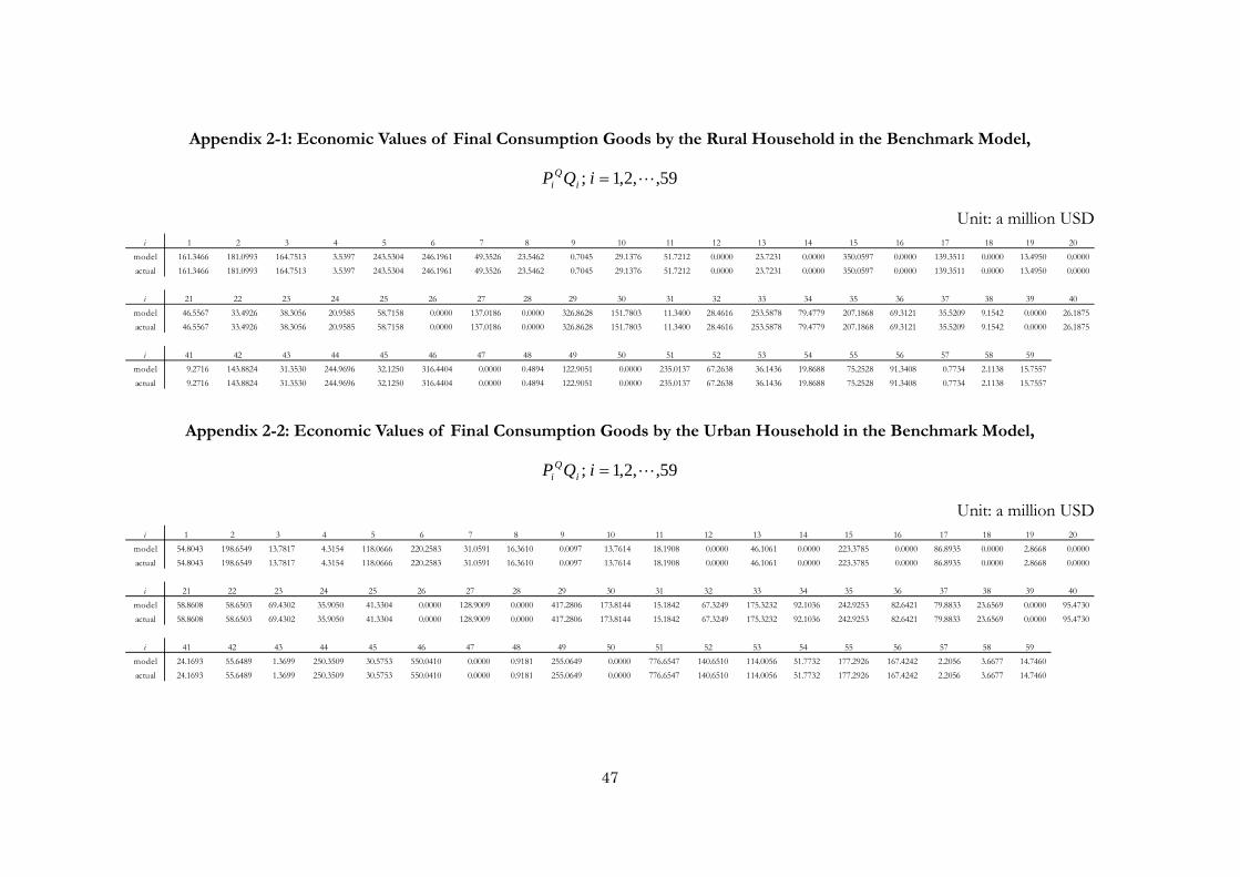
47

Appendix 2-1: Economic Values of Final Consumption Goods by the Rural Household in the Benchmark Model,

59,,2,1; iQP iQ

i

Unit: a million USD

Appendix 2-2: Economic Values of Final Consumption Goods by the Urban Household in the Benchmark Model,

59,,2,1; iQP iQ

i

Unit: a million USD

i 1 2 3 4 5 6 7 8 9 10 11 12 13 14 15 16 17 18 19 20model 161.3466 181.0993 164.7513 3.5397 243.5304 246.1961 49.3526 23.5462 0.7045 29.1376 51.7212 0.0000 23.7231 0.0000 350.0597 0.0000 139.3511 0.0000 13.4950 0.0000actual 161.3466 181.0993 164.7513 3.5397 243.5304 246.1961 49.3526 23.5462 0.7045 29.1376 51.7212 0.0000 23.7231 0.0000 350.0597 0.0000 139.3511 0.0000 13.4950 0.0000

i 21 22 23 24 25 26 27 28 29 30 31 32 33 34 35 36 37 38 39 40model 46.5567 33.4926 38.3056 20.9585 58.7158 0.0000 137.0186 0.0000 326.8628 151.7803 11.3400 28.4616 253.5878 79.4779 207.1868 69.3121 35.5209 9.1542 0.0000 26.1875actual 46.5567 33.4926 38.3056 20.9585 58.7158 0.0000 137.0186 0.0000 326.8628 151.7803 11.3400 28.4616 253.5878 79.4779 207.1868 69.3121 35.5209 9.1542 0.0000 26.1875

i 41 42 43 44 45 46 47 48 49 50 51 52 53 54 55 56 57 58 59model 9.2716 143.8824 31.3530 244.9696 32.1250 316.4404 0.0000 0.4894 122.9051 0.0000 235.0137 67.2638 36.1436 19.8688 75.2528 91.3408 0.7734 2.1138 15.7557actual 9.2716 143.8824 31.3530 244.9696 32.1250 316.4404 0.0000 0.4894 122.9051 0.0000 235.0137 67.2638 36.1436 19.8688 75.2528 91.3408 0.7734 2.1138 15.7557

i 1 2 3 4 5 6 7 8 9 10 11 12 13 14 15 16 17 18 19 20model 54.8043 198.6549 13.7817 4.3154 118.0666 220.2583 31.0591 16.3610 0.0097 13.7614 18.1908 0.0000 46.1061 0.0000 223.3785 0.0000 86.8935 0.0000 2.8668 0.0000actual 54.8043 198.6549 13.7817 4.3154 118.0666 220.2583 31.0591 16.3610 0.0097 13.7614 18.1908 0.0000 46.1061 0.0000 223.3785 0.0000 86.8935 0.0000 2.8668 0.0000

i 21 22 23 24 25 26 27 28 29 30 31 32 33 34 35 36 37 38 39 40model 58.8608 58.6503 69.4302 35.9050 41.3304 0.0000 128.9009 0.0000 417.2806 173.8144 15.1842 67.3249 175.3232 92.1036 242.9253 82.6421 79.8833 23.6569 0.0000 95.4730actual 58.8608 58.6503 69.4302 35.9050 41.3304 0.0000 128.9009 0.0000 417.2806 173.8144 15.1842 67.3249 175.3232 92.1036 242.9253 82.6421 79.8833 23.6569 0.0000 95.4730

i 41 42 43 44 45 46 47 48 49 50 51 52 53 54 55 56 57 58 59model 24.1693 55.6489 1.3699 250.3509 30.5753 550.0410 0.0000 0.9181 255.0649 0.0000 776.6547 140.6510 114.0056 51.7732 177.2926 167.4242 2.2056 3.6677 14.7460actual 24.1693 55.6489 1.3699 250.3509 30.5753 550.0410 0.0000 0.9181 255.0649 0.0000 776.6547 140.6510 114.0056 51.7732 177.2926 167.4242 2.2056 3.6677 14.7460

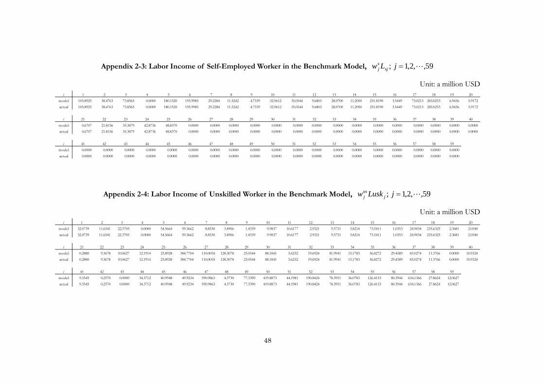
48

Appendix 2-3: Labor Income of Self-Employed Worker in the Benchmark Model, 59,,2,1; jLw sjsj

Unit: a million USD

Appendix 2-4: Labor Income of Unskilled Worker in the Benchmark Model, 59,,2,1; jLuskw jusj

Unit: a million USD

i 1 2 3 4 5 6 7 8 9 10 11 12 13 14 15 16 17 18 19 20model 105.8925 38.4763 73.8565 0.0000 180.1520 195.9985 29.2284 11.5242 4.7339 32.9612 35.0544 9.6803 28.0700 11.2050 251.8190 3.5449 73.0213 283.0253 6.9436 5.9172actual 105.8925 38.4763 73.8565 0.0000 180.1520 195.9985 29.2284 11.5242 4.7339 32.9612 35.0544 9.6803 28.0700 11.2050 251.8190 3.5449 73.0213 283.0253 6.9436 5.9172

i 21 22 23 24 25 26 27 28 29 30 31 32 33 34 35 36 37 38 39 40model 0.6707 21.8156 35.3879 42.8736 48.8370 0.0000 0.0000 0.0000 0.0000 0.0000 0.0000 0.0000 0.0000 0.0000 0.0000 0.0000 0.0000 0.0000 0.0000 0.0000actual 0.6707 21.8156 35.3879 42.8736 48.8370 0.0000 0.0000 0.0000 0.0000 0.0000 0.0000 0.0000 0.0000 0.0000 0.0000 0.0000 0.0000 0.0000 0.0000 0.0000

i 41 42 43 44 45 46 47 48 49 50 51 52 53 54 55 56 57 58 59model 0.0000 0.0000 0.0000 0.0000 0.0000 0.0000 0.0000 0.0000 0.0000 0.0000 0.0000 0.0000 0.0000 0.0000 0.0000 0.0000 0.0000 0.0000 0.0000actual 0.0000 0.0000 0.0000 0.0000 0.0000 0.0000 0.0000 0.0000 0.0000 0.0000 0.0000 0.0000 0.0000 0.0000 0.0000 0.0000 0.0000 0.0000 0.0000

i 1 2 3 4 5 6 7 8 9 10 11 12 13 14 15 16 17 18 19 20model 32.0739 11.6541 22.3705 0.0000 54.5664 59.3662 8.8530 3.4906 1.4339 9.9837 10.6177 2.9321 9.5731 3.8214 73.5411 1.0353 24.9034 235.6325 2.3681 2.0180actual 32.0739 11.6541 22.3705 0.0000 54.5664 59.3662 8.8530 3.4906 1.4339 9.9837 10.6177 2.9321 9.5731 3.8214 73.5411 1.0353 24.9034 235.6325 2.3681 2.0180

i 21 22 23 24 25 26 27 28 29 30 31 32 33 34 35 36 37 38 39 40model 0.2880 9.3678 10.0627 12.1914 25.8928 384.7704 110.0018 128.3078 23.0544 88.1841 5.6232 19.6924 81.9941 15.1783 56.8272 29.4589 83.0274 11.3766 0.0000 10.9324actual 0.2880 9.3678 10.0627 12.1914 25.8928 384.7704 110.0018 128.3078 23.0544 88.1841 5.6232 19.6924 81.9941 15.1783 56.8272 29.4589 83.0274 11.3766 0.0000 10.9324

i 41 42 43 44 45 46 47 48 49 50 51 52 53 54 55 56 57 58 59model 9.3545 0.2570 0.0000 34.3712 40.9948 49.9234 590.9863 4.3730 77.3390 419.8873 44.1981 190.8424 78.3951 36.0783 126.4153 80.3944 634.1366 27.8624 12.0627actual 9.3545 0.2570 0.0000 34.3712 40.9948 49.9234 590.9863 4.3730 77.3390 419.8873 44.1981 190.8424 78.3951 36.0783 126.4153 80.3944 634.1366 27.8624 12.0627

49

Appendix 2-5: Labor Income of Skilled Worker in the Benchmark Model, 59,,2,1; jLskw jskj

Unit: a million USD

Appendix 2-6: Capital Income in the Agriculture in the Benchmark Model, 59,,2,1; jKar jaj

Unit: a million USD

i 1 2 3 4 5 6 7 8 9 10 11 12 13 14 15 16 17 18 19 20model 0.0000 0.0000 0.0000 0.0000 0.0000 0.0000 0.0000 0.0000 0.0000 0.0000 0.0000 0.0000 0.0000 0.0000 0.0000 0.0000 0.0000 0.0000 0.0000 0.0000actual 0.0000 0.0000 0.0000 0.0000 0.0000 0.0000 0.0000 0.0000 0.0000 0.0000 0.0000 0.0000 0.0000 0.0000 0.0000 0.0000 0.0000 0.0000 0.0000 0.0000

i 21 22 23 24 25 26 27 28 29 30 31 32 33 34 35 36 37 38 39 40model 0.0000 0.0000 0.0000 0.0000 0.0000 19.4127 69.7719 30.8172 0.3714 0.0000 20.0733 6.8262 0.0000 0.0000 0.0000 0.0000 0.0000 3.9142 0.0000 0.0000actual 0.0000 0.0000 0.0000 0.0000 0.0000 19.4127 69.7719 30.8172 0.3714 0.0000 20.0733 6.8262 0.0000 0.0000 0.0000 0.0000 0.0000 3.9142 0.0000 0.0000

i 41 42 43 44 45 46 47 48 49 50 51 52 53 54 55 56 57 58 59model 0.0000 0.0000 0.0000 11.7311 0.0000 12.7006 87.6512 5.0142 36.2130 9.9256 0.8788 11.0618 21.8410 48.1011 0.0000 45.1715 377.3795 180.6854 49.0762actual 0.0000 0.0000 0.0000 11.7311 0.0000 12.7006 87.6512 5.0142 36.2130 9.9256 0.8788 11.0618 21.8410 48.1011 0.0000 45.1715 377.3795 180.6854 49.0762

i 1 2 3 4 5 6 7 8 9 10 11 12 13 14 15 16 17 18 19 20model 5.4798 2.7494 4.2129 0.0000 12.2215 21.4011 5.1579 1.8536 0.2564 2.3531 2.7171 2.2538 3.6592 1.4935 10.8366 0.3078 7.3163 19.5665 0.4618 0.8966actual 5.4798 2.7494 4.2129 0.0000 12.2215 21.4011 5.1579 1.8536 0.2564 2.3531 2.7171 2.2538 3.6592 1.4935 10.8366 0.3078 7.3163 19.5665 0.4618 0.8966

i 21 22 23 24 25 26 27 28 29 30 31 32 33 34 35 36 37 38 39 40model 0.2097 6.6148 6.3125 7.5228 10.9965 128.7726 31.8345 0.0000 0.0000 0.0000 0.0000 0.0000 0.0000 0.0000 0.0000 0.0000 0.0000 0.0000 0.0000 0.0000actual 0.2097 6.6148 6.3125 7.5228 10.9965 128.7726 31.8345 0.0000 0.0000 0.0000 0.0000 0.0000 0.0000 0.0000 0.0000 0.0000 0.0000 0.0000 0.0000 0.0000

i 41 42 43 44 45 46 47 48 49 50 51 52 53 54 55 56 57 58 59model 0.0000 0.0000 0.0000 0.0000 0.0000 0.0000 0.0000 0.0000 0.0000 0.0000 0.0000 0.0000 0.0000 0.0000 0.0000 0.0000 0.0000 0.0000 0.0000actual 0.0000 0.0000 0.0000 0.0000 0.0000 0.0000 0.0000 0.0000 0.0000 0.0000 0.0000 0.0000 0.0000 0.0000 0.0000 0.0000 0.0000 0.0000 0.0000

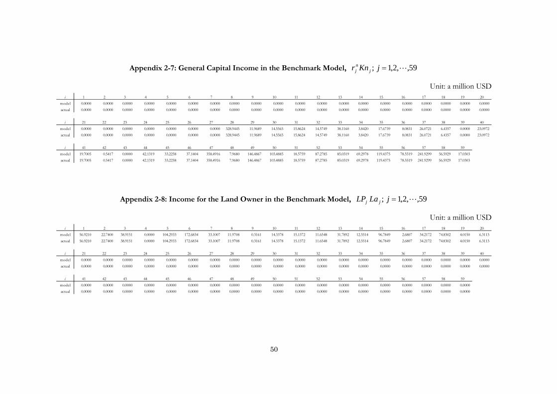
50

Appendix 2-7: General Capital Income in the Benchmark Model, 59,,2,1; jKnr jnj

Unit: a million USD

Appendix 2-8: Income for the Land Owner in the Benchmark Model, 59,,2,1; jLaLP jj

Unit: a million USD

i 1 2 3 4 5 6 7 8 9 10 11 12 13 14 15 16 17 18 19 20model 0.0000 0.0000 0.0000 0.0000 0.0000 0.0000 0.0000 0.0000 0.0000 0.0000 0.0000 0.0000 0.0000 0.0000 0.0000 0.0000 0.0000 0.0000 0.0000 0.0000actual 0.0000 0.0000 0.0000 0.0000 0.0000 0.0000 0.0000 0.0000 0.0000 0.0000 0.0000 0.0000 0.0000 0.0000 0.0000 0.0000 0.0000 0.0000 0.0000 0.0000

i 21 22 23 24 25 26 27 28 29 30 31 32 33 34 35 36 37 38 39 40model 0.0000 0.0000 0.0000 0.0000 0.0000 0.0000 0.0000 328.9445 11.9689 14.5565 15.8624 14.5749 38.1160 3.8420 17.6739 8.0831 26.0721 6.4357 0.0000 23.0972actual 0.0000 0.0000 0.0000 0.0000 0.0000 0.0000 0.0000 328.9445 11.9689 14.5565 15.8624 14.5749 38.1160 3.8420 17.6739 8.0831 26.0721 6.4357 0.0000 23.0972

i 41 42 43 44 45 46 47 48 49 50 51 52 53 54 55 56 57 58 59model 19.7005 0.5417 0.0000 42.1319 33.2258 37.1404 358.4916 7.9680 146.4867 103.4885 18.5759 87.2785 85.0319 69.2978 119.4375 78.5519 241.9299 56.5929 17.0303actual 19.7005 0.5417 0.0000 42.1319 33.2258 37.1404 358.4916 7.9680 146.4867 103.4885 18.5759 87.2785 85.0319 69.2978 119.4375 78.5519 241.9299 56.5929 17.0303

i 1 2 3 4 5 6 7 8 9 10 11 12 13 14 15 16 17 18 19 20model 56.9210 22.7400 38.9151 0.0000 104.2933 172.6834 33.1007 11.9708 0.3161 14.3378 15.1372 11.6548 31.7892 12.5514 96.7849 2.6807 34.2172 74.8302 4.0150 6.3113actual 56.9210 22.7400 38.9151 0.0000 104.2933 172.6834 33.1007 11.9708 0.3161 14.3378 15.1372 11.6548 31.7892 12.5514 96.7849 2.6807 34.2172 74.8302 4.0150 6.3113

i 21 22 23 24 25 26 27 28 29 30 31 32 33 34 35 36 37 38 39 40model 0.0000 0.0000 0.0000 0.0000 0.0000 0.0000 0.0000 0.0000 0.0000 0.0000 0.0000 0.0000 0.0000 0.0000 0.0000 0.0000 0.0000 0.0000 0.0000 0.0000actual 0.0000 0.0000 0.0000 0.0000 0.0000 0.0000 0.0000 0.0000 0.0000 0.0000 0.0000 0.0000 0.0000 0.0000 0.0000 0.0000 0.0000 0.0000 0.0000 0.0000

i 41 42 43 44 45 46 47 48 49 50 51 52 53 54 55 56 57 58 59model 0.0000 0.0000 0.0000 0.0000 0.0000 0.0000 0.0000 0.0000 0.0000 0.0000 0.0000 0.0000 0.0000 0.0000 0.0000 0.0000 0.0000 0.0000 0.0000actual 0.0000 0.0000 0.0000 0.0000 0.0000 0.0000 0.0000 0.0000 0.0000 0.0000 0.0000 0.0000 0.0000 0.0000 0.0000 0.0000 0.0000 0.0000 0.0000

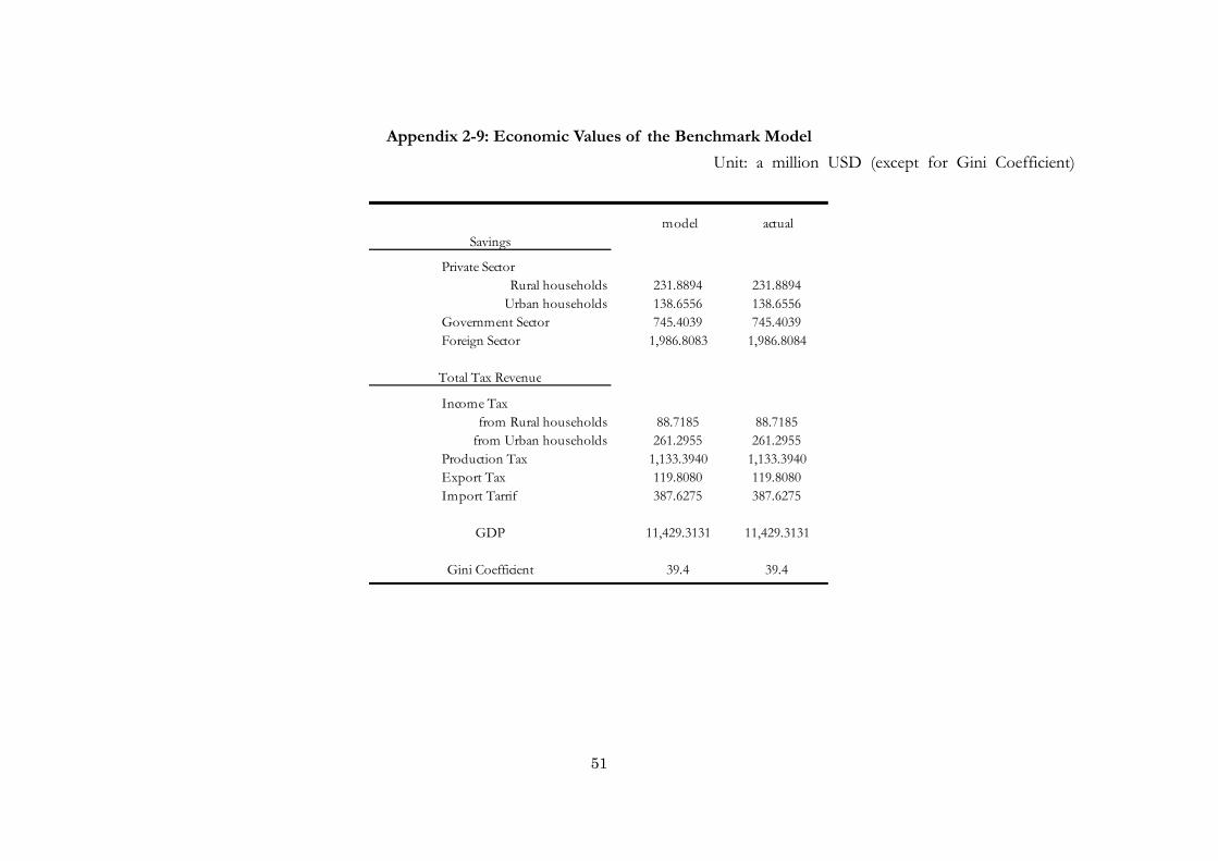
51

Appendix 2-9: Economic Values of the Benchmark Model

Unit: a million USD (except for Gini Coefficient)

model actual

Private SectorRural households 231.8894 231.8894

Urban households 138.6556 138.6556Government Sector 745.4039 745.4039Foreign Sector 1,986.8083 1,986.8084

Income Tax from Rural households 88.7185 88.7185from Urban households 261.2955 261.2955

Production Tax 1,133.3940 1,133.3940Export Tax 119.8080 119.8080Import Tarrif 387.6275 387.6275

11,429.3131 11,429.3131

39.4 39.4

GDP

Savings

Total Tax Revenue

Gini Coefficient

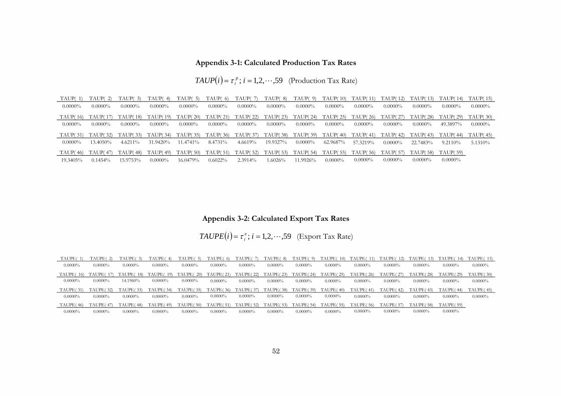
52

Appendix 3-1: Calculated Production Tax Rates

59,,2,1; iiTAUP pi (Production Tax Rate)

Appendix 3-2: Calculated Export Tax Rates

59,,2,1; iiTAUPE ei (Export Tax Rate)

TAUP( 1) TAUP( 2) TAUP( 3) TAUP( 4) TAUP( 5) TAUP( 6) TAUP( 7) TAUP( 8) TAUP( 9) TAUP( 10) TAUP( 11) TAUP( 12) TAUP( 13) TAUP( 14) TAUP( 15)0.0000% 0.0000% 0.0000% 0.0000% 0.0000% 0.0000% 0.0000% 0.0000% 0.0000% 0.0000% 0.0000% 0.0000% 0.0000% 0.0000% 0.0000%



TAUP( 46) TAUP( 47) TAUP( 48) TAUP( 49) TAUP( 50) TAUP( 51) TAUP( 52) TAUP( 53) TAUP( 54) TAUP( 55) TAUP( 56) TAUP( 57) TAUP( 58) TAUP( 59)19.3405% 0.1454% 15.9753% 0.0000% 16.0479% 0.6022% 2.3914% 1.6026% 11.9926% 0.0000% 0.0000% 0.0000% 0.0000% 0.0000%

TAUPE( 1) TAUPE( 2) TAUPE( 3) TAUPE( 4) TAUPE( 5) TAUPE( 6) TAUPE( 7) TAUPE( 8) TAUPE( 9) TAUPE( 10) TAUPE( 11) TAUPE( 12) TAUPE( 13) TAUPE( 14) TAUPE( 15)0.0000% 0.0000% 0.0000% 0.0000% 0.0000% 0.0000% 0.0000% 0.0000% 0.0000% 0.0000% 0.0000% 0.0000% 0.0000% 0.0000% 0.0000%



TAUPE( 46) TAUPE( 47) TAUPE( 48) TAUPE( 49) TAUPE( 50) TAUPE( 51) TAUPE( 52) TAUPE( 53) TAUPE( 54) TAUPE( 55) TAUPE( 56) TAUPE( 57) TAUPE( 58) TAUPE( 59)0.0000% 0.0000% 0.0000% 0.0000% 0.0000% 0.0000% 0.0000% 0.0000% 0.0000% 0.0000% 0.0000% 0.0000% 0.0000% 0.0000%

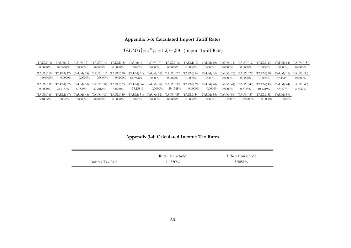
53

Appendix 3-3: Calculated Import Tariff Rates

59,,2,1; iiTAUM mi (Import Tariff Rate)

Appendix 3-4: Calculated Income Tax Rates

TAUM( 1) TAUM( 2) TAUM( 3) TAUM( 4) TAUM( 5) TAUM( 6) TAUM( 7) TAUM( 8) TAUM( 9) TAUM( 10) TAUM( 11) TAUM( 12) TAUM( 13) TAUM( 14) TAUM( 15)0.0000% 20.5630% 0.0000% 0.0000% 0.0000% 0.0000% 0.0000% 0.0000% 0.0000% 0.0000% 0.0000% 0.0000% 0.0000% 0.0000% 0.0000%



TAUM( 46) TAUM( 47) TAUM( 48) TAUM( 49) TAUM( 50) TAUM( 51) TAUM( 52) TAUM( 53) TAUM( 54) TAUM( 55) TAUM( 56) TAUM( 57) TAUM( 58) TAUM( 59)5.1803% 0.0000% 0.0000% 0.0000% 0.0000% 0.0000% 0.0000% 0.0000% 0.0000% 0.0000% 0.0000% 0.0000% 0.0000% 0.0000%

Rural Household Urban HouseholdIncome Tax Rate 1.9330% 5.5051%

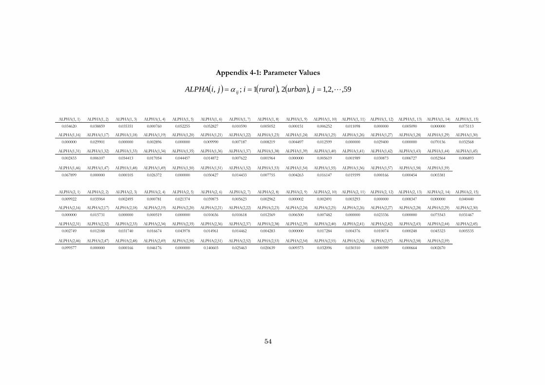
54

Appendix 4-1: Parameter Values

59,,2,1,2,1;, jurbanruralijiALPHA ij

ALPHA(1, 1) ALPHA(1, 2) ALPHA(1, 3) ALPHA(1, 4) ALPHA(1, 5) ALPHA(1, 6) ALPHA(1, 7) ALPHA(1, 8) ALPHA(1, 9) ALPHA(1, 10) ALPHA(1, 11) ALPHA(1, 12) ALPHA(1, 13) ALPHA(1, 14) ALPHA(1, 15)

0.034620 0.038859 0.035351 0.000760 0.052255 0.052827 0.010590 0.005052 0.000151 0.006252 0.011098 0.000000 0.005090 0.000000 0.075113

ALPHA(1,16) ALPHA(1,17) ALPHA(1,18) ALPHA(1,19) ALPHA(1,20) ALPHA(1,21) ALPHA(1,22) ALPHA(1,23) ALPHA(1,24) ALPHA(1,25) ALPHA(1,26) ALPHA(1,27) ALPHA(1,28) ALPHA(1,29) ALPHA(1,30)

0.000000 0.029901 0.000000 0.002896 0.000000 0.009990 0.007187 0.008219 0.004497 0.012599 0.000000 0.029400 0.000000 0.070136 0.032568


0.002433 0.006107 0.054413 0.017054 0.044457 0.014872 0.007622 0.001964 0.000000 0.005619 0.001989 0.030873 0.006727 0.052564 0.006893

ALPHA(1,46) ALPHA(1,47) ALPHA(1,48) ALPHA(1,49) ALPHA(1,50) ALPHA(1,51) ALPHA(1,52) ALPHA(1,53) ALPHA(1,54) ALPHA(1,55) ALPHA(1,56) ALPHA(1,57) ALPHA(1,58) ALPHA(1,59)

0.067899 0.000000 0.000105 0.026372 0.000000 0.050427 0.014433 0.007755 0.004263 0.016147 0.019599 0.000166 0.000454 0.003381

ALPHA(2, 1) ALPHA(2, 2) ALPHA(2, 3) ALPHA(2, 4) ALPHA(2, 5) ALPHA(2, 6) ALPHA(2, 7) ALPHA(2, 8) ALPHA(2, 9) ALPHA(2, 10) ALPHA(2, 11) ALPHA(2, 12) ALPHA(2, 13) ALPHA(2, 14) ALPHA(2, 15)

0.009922 0.035964 0.002495 0.000781 0.021374 0.039875 0.005623 0.002962 0.000002 0.002491 0.003293 0.000000 0.008347 0.000000 0.040440


0.000000 0.015731 0.000000 0.000519 0.000000 0.010656 0.010618 0.012569 0.006500 0.007482 0.000000 0.023336 0.000000 0.075543 0.031467


0.002749 0.012188 0.031740 0.016674 0.043978 0.014961 0.014462 0.004283 0.000000 0.017284 0.004376 0.010074 0.000248 0.045323 0.005535

ALPHA(2,46) ALPHA(2,47) ALPHA(2,48) ALPHA(2,49) ALPHA(2,50) ALPHA(2,51) ALPHA(2,52) ALPHA(2,53) ALPHA(2,54) ALPHA(2,55) ALPHA(2,56) ALPHA(2,57) ALPHA(2,58) ALPHA(2,59)

0.099577 0.000000 0.000166 0.046176 0.000000 0.140603 0.025463 0.020639 0.009373 0.032096 0.030310 0.000399 0.000664 0.002670

55


59,,2,1; iayiAY i


59,,2,1; iiGAMMAM Mi

AY( 1) AY( 2) AY( 3) AY( 4) AY( 5) AY( 6) AY( 7) AY( 8) AY( 9) AY( 10) AY( 11) AY( 12) AY( 13) AY( 14) AY( 15)

0.699884 0.540301 0.759805 0.000000 0.682745 0.705417 0.599342 0.697051 0.675917 0.624411 0.661131 0.678051 0.782935 0.753102 0.720244


0.539582 0.468256 0.704063 0.643535 0.565900 0.138829 0.326635 0.548247 0.803117 0.684946 0.697141 0.497900 0.564314 0.254799 0.262551


0.259156 0.513813 0.321418 0.317804 0.619382 0.402791 0.326870 0.430966 0.000000 0.075780 0.081231 0.032583 0.000000 0.370204 0.144098

AY( 46) AY( 47) AY( 48) AY( 49) AY( 50) AY( 51) AY( 52) AY( 53) AY( 54) AY( 55) AY( 56) AY( 57) AY( 58) AY( 59)

0.128848 0.704713 0.341918 0.354115 0.453133 0.092407 0.205930 0.713995 0.734131 0.654150 0.423139 0.706415 0.647720 0.695860

GAMMAM( 1) GAMMAM( 2) GAMMAM( 3) GAMMAM( 4) GAMMAM( 5) GAMMAM( 6) GAMMAM( 7) GAMMAM( 8) GAMMAM( 9) GAMMAM( 10) GAMMAM( 11) GAMMAM( 12) GAMMAM( 13) GAMMAM( 14) GAMMAM( 15)

0.043988 0.660226 0.000000 0.956640 0.000000 0.000000 0.000000 0.000000 0.000000 0.000000 0.000000 0.000000 0.000000 0.000000 0.000000


0.000000 0.000000 0.000000 0.321173 0.000000 0.931915 0.000000 0.328860 0.119340 0.181125 0.000000 0.000000 0.000000 0.732532 0.000000


0.000000 0.144923 0.393919 0.627147 0.705475 0.448160 0.000000 0.363574 0.956491 0.000000 0.000000 0.927479 0.874091 0.634572 0.256170

GAMMAM( 46) GAMMAM( 47) GAMMAM( 48) GAMMAM( 49) GAMMAM( 50) GAMMAM( 51) GAMMAM( 52) GAMMAM( 53) GAMMAM( 54) GAMMAM( 55) GAMMAM( 56) GAMMAM( 57) GAMMAM( 58) GAMMAM( 59)

0.786090 0.000000 0.000000 0.009678 0.000000 0.318108 0.000000 0.000000 0.000000 0.000000 0.000000 0.000000 0.000000 0.000000

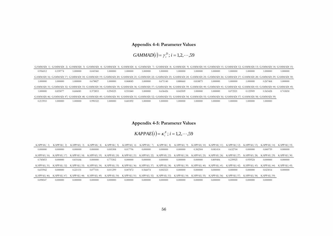
56


59,,2,1; iiGAMMAD Di


59,,2,1; iiKAPPAE Ei

GAMMAD( 1) GAMMAD( 2) GAMMAD( 3) GAMMAD( 4) GAMMAD( 5) GAMMAD( 6) GAMMAD( 7) GAMMAD( 8) GAMMAD( 9) GAMMAD( 10) GAMMAD( 11) GAMMAD( 12) GAMMAD( 13) GAMMAD( 14) GAMMAD( 15)

0.956012 0.339774 1.000000 0.043360 1.000000 1.000000 1.000000 1.000000 1.000000 1.000000 1.000000 1.000000 1.000000 1.000000 1.000000


1.000000 1.000000 1.000000 0.678827 1.000000 0.068085 1.000000 0.671140 0.880660 0.818875 1.000000 1.000000 1.000000 0.267468 1.000000


1.000000 0.855077 0.606081 0.372853 0.294525 0.551840 1.000000 0.636426 0.043509 1.000000 1.000000 0.072521 0.125909 0.365428 0.743830

GAMMAD( 46) GAMMAD( 47) GAMMAD( 48) GAMMAD( 49) GAMMAD( 50) GAMMAD( 51) GAMMAD( 52) GAMMAD( 53) GAMMAD( 54) GAMMAD( 55) GAMMAD( 56) GAMMAD( 57) GAMMAD( 58) GAMMAD( 59)

0.213910 1.000000 1.000000 0.990322 1.000000 0.681892 1.000000 1.000000 1.000000 1.000000 1.000000 1.000000 1.000000 1.000000

KAPPAE( 1) KAPPAE( 2) KAPPAE( 3) KAPPAE( 4) KAPPAE( 5) KAPPAE( 6) KAPPAE( 7) KAPPAE( 8) KAPPAE( 9) KAPPAE( 10) KAPPAE( 11) KAPPAE( 12) KAPPAE( 13) KAPPAE( 14) KAPPAE( 15)

0.000000 0.000000 0.000000 0.000000 0.005308 0.017796 0.000000 0.000000 0.000000 0.382504 0.081414 0.632704 0.000000 0.840759 0.000000


0.785853 0.000000 0.831646 0.000000 0.775302 0.000000 0.000000 0.000000 0.000000 0.000000 0.809406 0.239925 0.959524 0.000000 0.000000


0.653942 0.000000 0.221131 0.077101 0.011299 0.007872 0.566074 0.002323 0.000000 0.000000 0.000000 0.000000 0.000000 0.023014 0.000000

KAPPAE( 46) KAPPAE( 47) KAPPAE( 48) KAPPAE( 49) KAPPAE( 50) KAPPAE( 51) KAPPAE( 52) KAPPAE( 53) KAPPAE( 54) KAPPAE( 55) KAPPAE( 56) KAPPAE( 57) KAPPAE( 58) KAPPAE( 59)

0.098547 0.000000 0.000000 0.000000 0.000000 0.000000 0.000000 0.000000 0.000000 0.000000 0.000000 0.000000 0.000000 0.000000

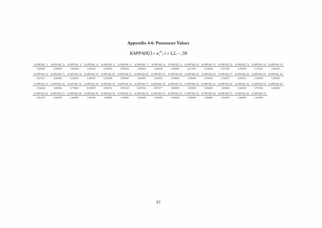
57


59,,2,1; iiKAPPAD Di

KAPPAD( 1) KAPPAD( 2) KAPPAD( 3) KAPPAD( 4) KAPPAD( 5) KAPPAD( 6) KAPPAD( 7) KAPPAD( 8) KAPPAD( 9) KAPPAD( 10) KAPPAD( 11) KAPPAD( 12) KAPPAD( 13) KAPPAD( 14) KAPPAD( 15)

1.000000 1.000000 1.000000 1.000000 0.994692 0.982204 1.000000 1.000000 1.000000 0.617496 0.918586 0.367296 1.000000 0.159241 1.000000


0.214147 1.000000 0.168354 1.000000 0.224698 1.000000 1.000000 1.000000 1.000000 1.000000 0.190594 0.760075 0.040476 1.000000 1.000000


0.346058 1.000000 0.778869 0.922899 0.988701 0.992128 0.433926 0.997677 1.000000 1.000000 1.000000 1.000000 1.000000 0.976986 1.000000

KAPPAD( 46) KAPPAD( 47) KAPPAD( 48) KAPPAD( 49) KAPPAD( 50) KAPPAD( 51) KAPPAD( 52) KAPPAD( 53) KAPPAD( 54) KAPPAD( 55) KAPPAD( 56) KAPPAD( 57) KAPPAD( 58) KAPPAD( 59)

0.901453 1.000000 1.000000 1.000000 1.000000 1.000000 1.000000 1.000000 1.000000 1.000000 1.000000 1.000000 1.000000 1.000000

58


59,,2,1,6,5,4,3,2,1,, jlandcapitalgeneraleagriculturincapitalskilledunskilleddselfemploeijiBETA ij

BETA( 1 1) BETA( 1 2) BETA( 1 3) BETA( 1 4) BETA( 1 5) BETA( 1 6) BETA( 1 7) BETA( 1 8) BETA( 1 9) BETA( 1 10) BETA( 1 11) BETA( 1 12) BETA( 1 13) BETA( 1 14) BETA( 1 15)0.528492 0.508813 0.529988 0.000000 0.512913 0.436086 0.382871 0.399602 0.702333 0.552709 0.551809 0.365006 0.384039 0.385432 0.581593



BETA( 1 46) BETA( 1 47) BETA( 1 48) BETA( 1 49) BETA( 1 50) BETA( 1 51) BETA( 1 52) BETA( 1 53) BETA( 1 54) BETA( 1 55) BETA( 1 56) BETA( 1 57) BETA( 1 58) BETA( 1 59)

0.000000 0.000000 0.000000 0.000000 0.000000 0.000000 0.000000 0.000000 0.000000 0.000000 0.000000 0.000000 0.000000 0.000000





0.500413 0.569829 0.251973 0.297413 0.787336 0.694362 0.659937 0.423144 0.235073 0.514191 0.393863 0.505915 0.105085 0.154315





0.127306 0.084513 0.288915 0.139260 0.018612 0.013807 0.038252 0.117889 0.313409 0.000000 0.221301 0.301074 0.681470 0.627821




BETA( 4 46) BETA( 4 47) BETA( 4 48) BETA( 4 49) BETA( 4 50) BETA( 4 51) BETA( 4 52) BETA( 4 53) BETA( 4 54) BETA( 4 55) BETA( 4 56) BETA( 4 57) BETA( 4 58) BETA( 4 59)0.000000 0.000000 0.000000 0.000000 0.000000 0.000000 0.000000 0.000000 0.000000 0.000000 0.000000 0.000000 0.000000 0.000000









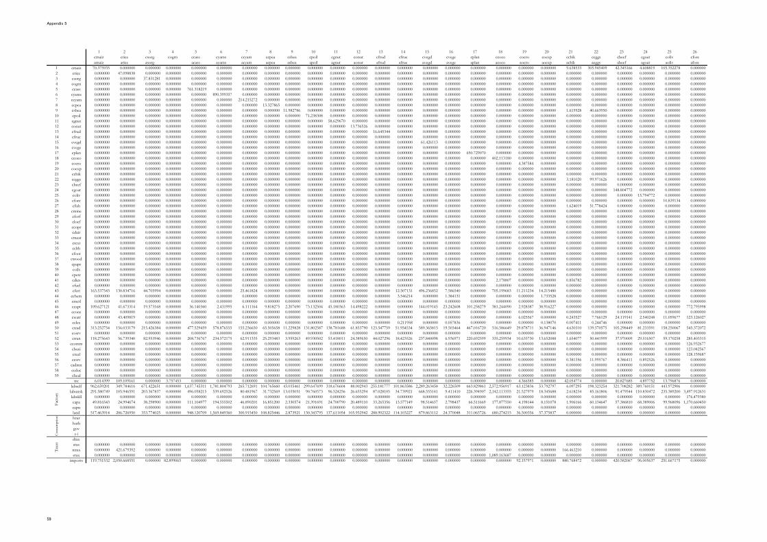
Appendix 5

1 2 3 4 5 6 7 8 9 10 11 12 13 14 15 16 17 18 19 20 21 22 23 24 25 26cmaiz crice csorg cogrn ccass cyams ccyam ccpea csbea cpoil cgnut conut cfrud cfrue cvegd cvege cplan ccoco cocro coexp cchik ceggs cbeef cgoat coliv cforeamaiz arice asorg acass ayams acyam acpea asbea apoil agnut aonut afrud afrue avegd avege aplan acoco aocro aoexp achik aeggs abeef agoat aoliv afore

1 cmaiz 70.375935 0.000000 0.000000 0.000000 0.000000 0.000000 0.000000 0.000000 0.000000 0.000000 0.000000 0.000000 0.000000 0.000000 0.000000 0.000000 0.000000 0.000000 0.000000 0.000000 9.638533 305.945409 42.345166 4.608819 105.352278 0.0000002 crice 0.000000 47.098838 0.000000 0.000000 0.000000 0.000000 0.000000 0.000000 0.000000 0.000000 0.000000 0.000000 0.000000 0.000000 0.000000 0.000000 0.000000 0.000000 0.000000 0.000000 0.000000 0.000000 0.000000 0.000000 0.000000 0.0000003 csorg 0.000000 0.000000 37.831281 0.000000 0.000000 0.000000 0.000000 0.000000 0.000000 0.000000 0.000000 0.000000 0.000000 0.000000 0.000000 0.000000 0.000000 0.000000 0.000000 0.000000 0.000000 0.000000 0.000000 0.000000 0.000000 0.0000004 cogrn 0.000000 0.000000 0.000000 0.000000 0.000000 0.000000 0.000000 0.000000 0.000000 0.000000 0.000000 0.000000 0.000000 0.000000 0.000000 0.000000 0.000000 0.000000 0.000000 0.000000 0.000000 0.000000 0.000000 0.000000 0.000000 0.0000005 ccass 0.000000 0.000000 0.000000 0.000000 761.318219 0.000000 0.000000 0.000000 0.000000 0.000000 0.000000 0.000000 0.000000 0.000000 0.000000 0.000000 0.000000 0.000000 0.000000 0.000000 0.000000 0.000000 0.000000 0.000000 0.000000 0.0000006 cyams 0.000000 0.000000 0.000000 0.000000 0.000000 890.399357 0.000000 0.000000 0.000000 0.000000 0.000000 0.000000 0.000000 0.000000 0.000000 0.000000 0.000000 0.000000 0.000000 0.000000 0.000000 0.000000 0.000000 0.000000 0.000000 0.0000007 ccyam 0.000000 0.000000 0.000000 0.000000 0.000000 0.000000 214.215272 0.000000 0.000000 0.000000 0.000000 0.000000 0.000000 0.000000 0.000000 0.000000 0.000000 0.000000 0.000000 0.000000 0.000000 0.000000 0.000000 0.000000 0.000000 0.0000008 ccpea 0.000000 0.000000 0.000000 0.000000 0.000000 0.000000 0.000000 13.327865 0.000000 0.000000 0.000000 0.000000 0.000000 0.000000 0.000000 0.000000 0.000000 0.000000 0.000000 0.000000 0.000000 0.000000 0.000000 0.000000 0.000000 0.0000009 csbea 0.000000 0.000000 0.000000 0.000000 0.000000 0.000000 0.000000 0.000000 11.982786 0.000000 0.000000 0.000000 0.000000 0.000000 0.000000 0.000000 0.000000 0.000000 0.000000 0.000000 1.615928 40.663950 0.000000 0.000000 0.000000 0.00000010 cpoil 0.000000 0.000000 0.000000 0.000000 0.000000 0.000000 0.000000 0.000000 0.000000 71.238308 0.000000 0.000000 0.000000 0.000000 0.000000 0.000000 0.000000 0.000000 0.000000 0.000000 0.000000 0.000000 0.000000 0.000000 0.000000 0.00000011 cgnut 0.000000 0.000000 0.000000 0.000000 0.000000 0.000000 0.000000 0.000000 0.000000 0.000000 58.629670 0.000000 0.000000 0.000000 0.000000 0.000000 0.000000 0.000000 0.000000 0.000000 0.000000 0.000000 0.000000 0.000000 0.000000 0.00000012 conut 0.000000 0.000000 0.000000 0.000000 0.000000 0.000000 0.000000 0.000000 0.000000 0.000000 0.000000 13.736526 0.000000 0.000000 0.000000 0.000000 0.000000 0.000000 0.000000 0.000000 0.000000 0.000000 0.000000 0.000000 0.000000 0.00000013 cfrud 0.000000 0.000000 0.000000 0.000000 0.000000 0.000000 0.000000 0.000000 0.000000 0.000000 0.000000 0.000000 16.645344 0.000000 0.000000 0.000000 0.000000 0.000000 0.000000 0.000000 0.000000 0.000000 0.000000 0.000000 0.000000 0.00000014 cfrue 0.000000 0.000000 0.000000 0.000000 0.000000 0.000000 0.000000 0.000000 0.000000 0.000000 0.000000 0.000000 0.000000 0.000000 0.000000 0.000000 0.000000 0.000000 0.000000 0.000000 0.000000 0.000000 0.000000 0.000000 0.000000 0.00000015 cvegd 0.000000 0.000000 0.000000 0.000000 0.000000 0.000000 0.000000 0.000000 0.000000 0.000000 0.000000 0.000000 0.000000 0.000000 61.426113 0.000000 0.000000 0.000000 0.000000 0.000000 0.000000 0.000000 0.000000 0.000000 0.000000 0.00000016 cvege 0.000000 0.000000 0.000000 0.000000 0.000000 0.000000 0.000000 0.000000 0.000000 0.000000 0.000000 0.000000 0.000000 0.000000 0.000000 0.000000 0.000000 0.000000 0.000000 0.000000 0.000000 0.000000 0.000000 0.000000 0.000000 0.00000017 cplan 0.000000 0.000000 0.000000 0.000000 0.000000 0.000000 0.000000 0.000000 0.000000 0.000000 0.000000 0.000000 0.000000 0.000000 0.000000 0.000000 650.729070 0.000000 0.000000 0.000000 0.000000 0.000000 0.000000 0.000000 0.000000 0.00000018 ccoco 0.000000 0.000000 0.000000 0.000000 0.000000 0.000000 0.000000 0.000000 0.000000 0.000000 0.000000 0.000000 0.000000 0.000000 0.000000 0.000000 0.000000 402.113180 0.000000 0.000000 0.000000 0.000000 0.000000 0.000000 0.000000 0.00000019 cocro 0.000000 0.000000 0.000000 0.000000 0.000000 0.000000 0.000000 0.000000 0.000000 0.000000 0.000000 0.000000 0.000000 0.000000 0.000000 0.000000 0.000000 0.000000 4.387584 0.000000 0.000000 0.000000 0.000000 0.000000 0.000000 0.00000020 coexp 0.000000 0.000000 0.000000 0.000000 0.000000 0.000000 0.000000 0.000000 0.000000 0.000000 0.000000 0.000000 0.000000 0.000000 0.000000 0.000000 0.000000 0.000000 0.000000 0.000000 0.000000 0.000000 0.000000 0.000000 0.000000 0.00000021 cchik 0.000000 0.000000 0.000000 0.000000 0.000000 0.000000 0.000000 0.000000 0.000000 0.000000 0.000000 0.000000 0.000000 0.000000 0.000000 0.000000 0.000000 0.000000 0.000000 0.000000 0.000000 0.000000 0.000000 0.000000 0.000000 0.00000022 ceggs 0.000000 0.000000 0.000000 0.000000 0.000000 0.000000 0.000000 0.000000 0.000000 0.000000 0.000000 0.000000 0.000000 0.000000 0.000000 0.000000 0.000000 0.000000 0.000000 0.000000 3.181020 99.971626 0.000000 0.000000 0.000000 0.00000023 cbeef 0.000000 0.000000 0.000000 0.000000 0.000000 0.000000 0.000000 0.000000 0.000000 0.000000 0.000000 0.000000 0.000000 0.000000 0.000000 0.000000 0.000000 0.000000 0.000000 0.000000 0.000000 0.000000 0.000000 0.000000 0.000000 0.00000024 cgoat 0.000000 0.000000 0.000000 0.000000 0.000000 0.000000 0.000000 0.000000 0.000000 0.000000 0.000000 0.000000 0.000000 0.000000 0.000000 0.000000 0.000000 0.000000 0.000000 0.000000 0.000000 0.000000 148.804772 0.000000 0.000000 0.00000025 coliv 0.000000 0.000000 0.000000 0.000000 0.000000 0.000000 0.000000 0.000000 0.000000 0.000000 0.000000 0.000000 0.000000 0.000000 0.000000 0.000000 0.000000 0.000000 0.000000 0.000000 0.000000 0.000000 0.000000 15.794772 0.000000 0.00000026 cfore 0.000000 0.000000 0.000000 0.000000 0.000000 0.000000 0.000000 0.000000 0.000000 0.000000 0.000000 0.000000 0.000000 0.000000 0.000000 0.000000 0.000000 0.000000 0.000000 0.000000 0.000000 0.000000 0.000000 0.000000 10.839134 0.00000027 cfish 0.000000 0.000000 0.000000 0.000000 0.000000 0.000000 0.000000 0.000000 0.000000 0.000000 0.000000 0.000000 0.000000 0.000000 0.000000 0.000000 0.000000 0.000000 0.000000 0.000000 1.624019 51.778424 0.000000 0.000000 0.000000 0.00000028 cmine 0.000000 0.000000 0.000000 0.000000 0.000000 0.000000 0.000000 0.000000 0.000000 0.000000 0.000000 0.000000 0.000000 0.000000 0.000000 0.000000 0.000000 0.000000 0.000000 0.000000 0.000000 0.000000 0.000000 0.000000 0.000000 0.00000029 cforf 0.000000 0.000000 0.000000 0.000000 0.000000 0.000000 0.000000 0.000000 0.000000 0.000000 0.000000 0.000000 0.000000 0.000000 0.000000 0.000000 0.000000 0.000000 0.000000 0.000000 0.000000 0.000000 0.000000 0.000000 0.000000 0.00000030 clocf 0.000000 0.000000 0.000000 0.000000 0.000000 0.000000 0.000000 0.000000 0.000000 0.000000 0.000000 0.000000 0.000000 0.000000 0.000000 0.000000 0.000000 0.000000 0.000000 0.000000 0.000000 0.000000 0.000000 0.000000 0.000000 0.00000031 ccopr 0.000000 0.000000 0.000000 0.000000 0.000000 0.000000 0.000000 0.000000 0.000000 0.000000 0.000000 0.000000 0.000000 0.000000 0.000000 0.000000 0.000000 0.000000 0.000000 0.000000 0.000000 0.000000 0.000000 0.000000 0.000000 0.00000032 cdair 0.000000 0.000000 0.000000 0.000000 0.000000 0.000000 0.000000 0.000000 0.000000 0.000000 0.000000 0.000000 0.000000 0.000000 0.000000 0.000000 0.000000 0.000000 0.000000 0.000000 0.000000 0.000000 0.000000 0.000000 0.000000 0.00000033 cmeat 0.000000 0.000000 0.000000 0.000000 0.000000 0.000000 0.000000 0.000000 0.000000 0.000000 0.000000 0.000000 0.000000 0.000000 0.000000 0.000000 0.000000 0.000000 0.000000 0.000000 0.000000 0.000000 0.000000 0.000000 0.000000 0.00000034 ctext 0.000000 0.000000 0.000000 0.000000 0.000000 0.000000 0.000000 0.000000 0.000000 0.000000 0.000000 0.000000 0.000000 0.000000 0.000000 0.000000 0.000000 0.000000 0.000000 0.000000 0.000000 0.000000 0.000000 0.000000 0.000000 0.00000035 cclth 0.000000 0.000000 0.000000 0.000000 0.000000 0.000000 0.000000 0.000000 0.000000 0.000000 0.000000 0.000000 0.000000 0.000000 0.000000 0.000000 0.000000 0.000000 0.000000 0.000000 0.000000 0.000000 0.000000 0.000000 0.000000 0.00000036 cfoot 0.000000 0.000000 0.000000 0.000000 0.000000 0.000000 0.000000 0.000000 0.000000 0.000000 0.000000 0.000000 0.000000 0.000000 0.000000 0.000000 0.000000 0.000000 0.000000 0.000000 0.000000 0.000000 0.000000 0.000000 0.000000 0.00000037 cwood 0.000000 0.000000 0.000000 0.000000 0.000000 0.000000 0.000000 0.000000 0.000000 0.000000 0.000000 0.000000 0.000000 0.000000 0.000000 0.000000 0.000000 0.000000 0.000000 0.000000 0.000000 0.000000 0.000000 0.000000 0.000000 0.00000038 cpapr 0.000000 0.000000 0.000000 0.000000 0.000000 0.000000 0.000000 0.000000 0.000000 0.000000 0.000000 0.000000 0.000000 0.000000 0.000000 0.000000 0.000000 0.000000 0.000000 0.000000 0.000000 0.000000 0.000000 0.000000 0.000000 0.00000039 coils 0.000000 0.000000 0.000000 0.000000 0.000000 0.000000 0.000000 0.000000 0.000000 0.000000 0.000000 0.000000 0.000000 0.000000 0.000000 0.000000 0.000000 0.000000 0.000000 0.000000 0.000000 0.000000 0.000000 0.000000 0.000000 0.00000040 cpetr 0.000000 0.000000 0.000000 0.000000 0.000000 0.000000 0.000000 0.000000 0.000000 0.000000 0.000000 0.000000 0.000000 0.000000 0.000000 0.000000 0.000000 0.000000 0.000000 0.000000 0.000000 0.000000 0.000000 0.000000 0.000000 0.00000041 cdies 0.000000 0.000000 0.000000 0.000000 0.000000 0.000000 0.000000 0.000000 0.000000 0.000000 0.000000 0.000000 0.000000 0.000000 0.000000 0.000000 0.000000 2.178807 0.000000 0.000000 0.856782 0.000000 0.000000 0.000000 0.000000 0.00000042 cfuel 0.000000 0.000000 0.000000 0.000000 0.000000 0.000000 0.000000 0.000000 0.000000 0.000000 0.000000 0.000000 0.000000 0.000000 0.000000 0.000000 0.000000 0.000000 0.000000 0.000000 0.000000 0.000000 0.000000 0.000000 0.000000 0.00000043 cfert 163.537543 130.834716 44.705994 0.000000 0.000000 0.000000 25.461824 0.000000 0.000000 0.000000 0.000000 0.000000 0.000000 12.507131 496.236852 7.586540 0.000000 705.199683 11.211234 14.215480 0.000000 0.000000 0.000000 0.000000 0.000000 0.00000044 cchem 0.000000 0.000000 0.000000 0.000000 0.000000 0.000000 0.000000 0.000000 0.000000 0.000000 0.000000 0.000000 0.000000 3.546214 0.000000 1.384131 0.000000 0.000000 0.000000 1.733528 0.000000 0.000000 0.000000 0.000000 0.000000 0.00000045 cmetl 0.000000 0.000000 0.000000 0.000000 0.000000 0.000000 0.000000 0.000000 0.000000 0.000000 0.000000 0.000000 0.000000 0.000000 0.000000 0.000000 0.000000 0.000000 0.000000 0.000000 0.000000 0.000000 0.000000 0.000000 0.000000 0.00000046 ccapt 109.627121 41.673314 19.573168 0.000000 36.140360 2.431995 6.111164 9.818275 2.207690 73.132504 45.180363 14.498222 0.000000 0.000000 144.019145 23.242608 101.258279 381.244090 2.928387 38.916227 0.000000 0.000000 0.000000 0.000000 0.000000 772.79599847 ccons 0.000000 0.000000 0.000000 0.000000 0.000000 0.000000 0.000000 0.000000 0.000000 0.000000 0.000000 0.000000 0.000000 0.000000 0.000000 0.000000 0.000000 0.000000 0.000000 0.000000 0.000000 0.000000 0.000000 0.000000 0.000000 0.00000048 cwatr 0.000000 43.409819 0.000000 0.000000 0.000000 0.000000 0.000000 0.000000 0.000000 0.000000 0.000000 0.000000 0.000000 0.000000 0.000000 0.000000 0.000000 0.000000 6.025567 0.000000 0.243527 7.766129 24.119141 2.540248 11.059677 123.12602749 celec 0.000000 0.000000 0.000000 0.000000 0.000000 0.000000 0.000000 0.000000 0.000000 0.000000 0.000000 0.000000 0.000000 0.211958 0.000000 0.057836 0.000000 0.000000 0.000000 0.138070 0.007411 0.244746 0.000000 0.000000 0.000000 0.00000050 ctrad 313.252754 156.033179 215.426384 0.000000 477.529459 578.876555 155.236650 65.505658 11.229828 131.802587 138.781688 61.853790 123.547759 51.954534 589.365815 19.503464 467.016720 516.586649 29.878711 36.947146 4.630310 139.570575 105.298449 81.233591 158.250067 545.37207251 cosrv 0.000000 0.000000 0.000000 0.000000 0.000000 0.000000 0.000000 0.000000 0.000000 0.000000 0.000000 0.000000 0.000000 0.000000 0.000000 0.000000 0.000000 0.000000 0.000000 0.000000 0.000000 0.000000 0.000000 0.000000 0.000000 0.00000052 ctran 118.275643 56.739340 82.953946 0.000000 208.736767 234.572175 62.911335 25.293483 3.959263 49.930502 53.418011 24.389650 44.027296 18.423526 237.840098 6.936971 220.692599 335.259934 10.635730 13.652088 1.654077 50.441999 37.970009 29.516507 59.170258 285.40331553 ccomm 0.000000 0.000000 0.000000 0.000000 0.000000 0.000000 0.000000 0.000000 0.000000 0.000000 0.000000 0.000000 0.000000 0.000000 0.000000 0.000000 0.000000 0.000000 0.000000 0.000000 0.000000 0.000000 0.000000 0.000000 0.000000 126.93267754 cbusi 0.000000 0.000000 0.000000 0.000000 0.000000 0.000000 0.000000 0.000000 0.000000 0.000000 0.000000 0.000000 0.000000 0.000000 0.000000 0.000000 0.000000 0.000000 0.000000 0.000000 0.000000 0.000000 0.000000 0.000000 0.000000 123.04256755 creal 0.000000 0.000000 0.000000 0.000000 0.000000 0.000000 0.000000 0.000000 0.000000 0.000000 0.000000 0.000000 0.000000 0.000000 0.000000 0.000000 0.000000 0.000000 0.000000 0.000000 0.000000 0.000000 0.000000 0.000000 0.000000 128.15968756 ccsrv 0.000000 0.000000 0.000000 0.000000 0.000000 0.000000 0.000000 0.000000 0.000000 0.000000 0.000000 0.000000 0.000000 0.000000 0.000000 0.000000 0.000000 0.000000 0.000000 0.000000 0.381356 11.995767 8.386411 0.892526 0.000000 0.00000057 cadmn 0.000000 0.000000 0.000000 0.000000 0.000000 0.000000 0.000000 0.000000 0.000000 0.000000 0.000000 0.000000 0.000000 0.000000 0.000000 0.000000 0.000000 0.000000 0.000000 0.000000 0.000000 0.000000 0.000000 0.000000 0.000000 0.00000058 ceduc 0.000000 0.000000 0.000000 0.000000 0.000000 0.000000 0.000000 0.000000 0.000000 0.000000 0.000000 0.000000 0.000000 0.000000 0.000000 0.000000 0.000000 0.000000 0.000000 0.000000 0.000000 0.000000 0.000000 0.000000 0.000000 0.00000059 cheal 0.000000 0.000000 0.000000 0.000000 0.000000 0.000000 0.000000 0.000000 0.000000 0.000000 0.000000 0.000000 0.000000 0.000000 0.000000 0.000000 0.000000 0.000000 0.000000 0.000000 0.000000 0.000000 0.000000 0.000000 0.000000 0.000000

trc 6.014399 109.109161 0.000000 3.757453 0.000000 0.000000 0.000000 0.000000 0.000000 0.000000 0.000000 0.000000 0.000000 0.000000 0.000000 0.000000 0.000000 0.000000 4.366585 0.000000 42.054774 0.000000 20.827685 4.897752 13.796876 0.000000labself 962.659201 349.784616 671.422651 0.000000 1,637.745311 1,781.804793 265.712691 104.765660 43.035461 299.647699 318.676604 88.002943 255.181777 101.863586 2,289.263458 32.226509 663.829861 2,572.956917 63.123836 53.792797 6.097295 198.323254 321.708282 389.760151 443.972906 0.000000

labunsk 291.580749 105.946591 203.367837 0.000000 496.058215 539.692526 80.481967 31.732569 13.035051 90.760573 96.524256 26.655294 87.028105 34.739921 668.555141 9.411410 226.394907 2,142.113355 21.527979 18.345688 2.618234 85.161806 91.479544 110.830472 235.389200 3,497.912631labskll 0.000000 0.000000 0.000000 0.000000 0.000000 0.000000 0.000000 0.000000 0.000000 0.000000 0.000000 0.000000 0.000000 0.000000 0.000000 0.000000 0.000000 0.000000 0.000000 0.000000 0.000000 0.000000 0.000000 0.000000 0.000000 176.479380capa 49.816543 24.994674 38.298900 0.000000 111.104977 194.555502 46.890201 16.851200 2.330574 21.391691 24.700790 20.489110 33.265356 13.577149 98.514657 2.798437 66.511669 177.877550 4.198144 8.151078 1.906166 60.134647 57.386810 68.389006 99.968096 1,170.660450capn 0.000000 0.000000 0.000000 0.000000 0.000000 0.000000 0.000000 0.000000 0.000000 0.000000 0.000000 0.000000 0.000000 0.000000 0.000000 0.000000 0.000000 0.000000 0.000000 0.000000 0.000000 0.000000 0.000000 0.000000 0.000000 0.000000land 517.463914 206.726950 353.774025 0.000000 948.120709 1,569.849360 300.915450 108.825446 2.873921 130.343795 137.611054 105.952942 288.992322 114.103227 879.863112 24.370048 311.065726 680.274215 36.500356 57.375837 0.000000 0.000000 0.000000 0.000000 0.000000 0.000000hrurhurbgovs-i

dtaxstax 0.000000 0.000000 0.000000 0.000000 0.000000 0.000000 0.000000 0.000000 0.000000 0.000000 0.000000 0.000000 0.000000 0.000000 0.000000 0.000000 0.000000 0.000000 0.000000 0.000000 0.000000 0.000000 0.000000 0.000000 0.000000 0.000000mtax 0.000000 421.679392 0.000000 0.000000 0.000000 0.000000 0.000000 0.000000 0.000000 0.000000 0.000000 0.000000 0.000000 0.000000 0.000000 0.000000 0.000000 0.000000 0.000000 0.000000 166.463210 0.000000 0.000000 0.000000 0.000000 0.000000etax 0.000000 0.000000 0.000000 0.000000 0.000000 0.000000 0.000000 0.000000 0.000000 0.000000 0.000000 0.000000 0.000000 0.000000 0.000000 0.000000 0.000000 1,089.163687 0.000000 0.000000 0.000000 0.000000 0.000000 0.000000 0.000000 0.000000

imports 119.751532 2,050.668551 0.000000 82.899065 0.000000 0.000000 0.000000 0.000000 0.000000 0.000000 0.000000 0.000000 0.000000 0.000000 0.000000 0.000000 0.000000 0.000000 92.157971 0.000000 880.768472 0.000000 420.582067 96.005637 251.667175 0.000000

Fact

ors

Cons

umpt

ion

Taxe

s

59

Appendix 5

27 28 29 30 31 32 33 34 35 36 37 38 39 40 41 42 43 44 45 46 47 48 49 50 51 52cfish cmine cforf clocf ccopr cdair cmeat ctext cclth cfoot cwood cpapr coils cpetr cdies cfuel cfert cchem cmetl ccapt ccons cwatr celec ctrad cosrv ctranafish amine aforf alocf acopr adair ameat atext aclth afoot awood apapr apetr adies afuel achem ametl acapt acons awatr aelec atrad aosrv atran0.000000 0.000000 7.843293 155.608260 0.000000 0.000000 0.000000 0.000000 0.000000 0.000000 0.000000 0.000000 0.000000 0.000000 0.000000 0.000000 0.000000 0.000000 0.000000 0.000000 0.000000 0.000000 0.000000 0.000000 55.629031 0.0000000.000000 0.000000 6.478499 155.310488 0.000000 0.000000 0.000000 0.000000 0.000000 0.000000 0.000000 0.000000 0.000000 0.000000 0.000000 0.000000 0.000000 0.000000 0.000000 0.000000 0.000000 0.000000 0.000000 0.000000 83.500282 0.0000000.000000 0.000000 6.495497 0.000000 0.000000 0.000000 0.000000 0.000000 0.000000 0.000000 0.000000 0.000000 0.000000 0.000000 0.000000 0.000000 0.000000 0.000000 0.000000 0.000000 0.000000 0.000000 0.000000 0.000000 0.000000 0.0000000.000000 0.000000 15.246855 0.000000 0.000000 0.000000 0.000000 0.000000 0.000000 0.000000 0.000000 0.000000 0.000000 0.000000 0.000000 0.000000 0.000000 0.000000 0.000000 0.000000 0.000000 0.000000 0.000000 0.000000 0.000000 0.0000000.000000 0.000000 0.000000 603.366809 0.000000 0.000000 0.000000 0.000000 0.000000 0.000000 0.000000 0.000000 0.000000 0.000000 0.000000 0.000000 0.000000 0.000000 0.000000 0.000000 0.000000 0.000000 0.000000 0.000000 0.000000 0.0000000.000000 0.000000 0.000000 558.208541 0.000000 0.000000 0.000000 0.000000 0.000000 0.000000 0.000000 0.000000 0.000000 0.000000 0.000000 0.000000 0.000000 0.000000 0.000000 0.000000 0.000000 0.000000 0.000000 0.000000 0.000000 0.0000000.000000 0.000000 0.000000 212.705573 0.000000 0.000000 0.000000 0.000000 0.000000 0.000000 0.000000 0.000000 0.000000 0.000000 0.000000 0.000000 0.000000 0.000000 0.000000 0.000000 0.000000 0.000000 0.000000 0.000000 0.000000 0.0000000.000000 0.000000 0.000000 0.000000 0.000000 0.000000 0.000000 0.000000 0.000000 0.000000 0.000000 0.000000 0.000000 0.000000 0.000000 0.000000 0.000000 0.000000 0.000000 0.000000 0.000000 0.000000 0.000000 0.000000 0.000000 0.0000000.000000 0.000000 29.899246 0.000000 0.000000 0.000000 0.000000 0.000000 0.000000 0.000000 0.000000 0.000000 0.000000 0.000000 0.000000 0.000000 0.000000 0.000000 0.000000 0.000000 0.000000 0.000000 0.000000 0.000000 0.000000 0.0000000.000000 0.000000 74.910473 0.000000 0.000000 0.000000 0.000000 0.000000 0.000000 0.000000 0.000000 0.000000 0.000000 0.000000 0.000000 0.000000 0.000000 0.000000 0.000000 0.000000 0.000000 0.000000 0.000000 0.000000 0.000000 0.0000000.000000 0.000000 108.211800 0.000000 0.000000 0.000000 0.000000 0.000000 0.000000 0.000000 0.000000 0.000000 0.000000 0.000000 0.000000 0.000000 0.000000 0.000000 0.000000 0.000000 0.000000 0.000000 0.000000 0.000000 0.000000 0.0000000.000000 0.000000 116.866126 0.000000 0.000000 0.000000 0.000000 0.000000 0.000000 0.000000 0.000000 0.000000 0.000000 0.000000 0.000000 0.000000 0.000000 0.000000 0.000000 0.000000 0.000000 0.000000 0.000000 0.000000 0.000000 0.0000000.000000 0.000000 0.000000 142.568755 0.000000 0.000000 0.000000 0.000000 0.000000 0.000000 0.000000 0.000000 0.000000 0.000000 0.000000 0.000000 0.000000 0.000000 0.000000 0.000000 0.000000 0.000000 0.000000 0.000000 54.663219 0.0000000.000000 0.000000 15.082687 0.000000 0.000000 0.000000 0.000000 0.000000 0.000000 0.000000 0.000000 0.000000 0.000000 0.000000 0.000000 0.000000 0.000000 0.000000 0.000000 0.000000 0.000000 0.000000 0.000000 0.000000 40.799324 0.0000000.000000 0.000000 0.000000 148.946963 0.000000 0.000000 0.000000 0.000000 0.000000 0.000000 0.000000 0.000000 0.000000 0.000000 0.000000 0.000000 0.000000 0.000000 0.000000 0.000000 0.000000 0.000000 0.000000 0.000000 41.636233 0.0000000.000000 0.000000 0.000000 0.000000 0.000000 0.000000 0.000000 0.000000 0.000000 0.000000 0.000000 0.000000 0.000000 0.000000 0.000000 0.000000 0.000000 0.000000 0.000000 0.000000 0.000000 0.000000 0.000000 0.000000 27.307615 0.0000000.000000 0.000000 0.000000 0.000000 0.000000 0.000000 0.000000 0.000000 0.000000 0.000000 0.000000 0.000000 0.000000 0.000000 0.000000 0.000000 0.000000 0.000000 0.000000 0.000000 0.000000 0.000000 0.000000 0.000000 0.000000 0.0000000.000000 0.000000 0.000000 0.000000 930.543598 0.000000 0.000000 0.000000 0.000000 0.000000 0.000000 0.000000 0.000000 0.000000 0.000000 0.000000 0.000000 0.000000 0.000000 0.000000 0.000000 0.000000 0.000000 0.000000 0.000000 0.0000000.000000 0.000000 39.690924 0.000000 0.000000 0.000000 0.000000 94.119995 0.000000 0.000000 0.000000 0.000000 0.000000 0.000000 0.000000 0.000000 0.000000 0.000000 0.000000 0.000000 0.000000 0.000000 0.000000 0.000000 0.000000 0.0000000.000000 0.000000 0.000000 0.000000 0.000000 0.000000 0.000000 54.661705 0.000000 0.000000 0.000000 0.000000 0.000000 0.000000 0.000000 0.000000 0.000000 0.000000 0.000000 0.000000 0.000000 0.000000 0.000000 0.000000 0.000000 0.0000000.000000 0.000000 0.000000 0.000000 0.000000 0.000000 0.000000 0.000000 0.000000 0.000000 0.000000 0.000000 0.000000 0.000000 0.000000 0.000000 0.000000 0.000000 0.000000 0.000000 0.000000 0.000000 0.000000 0.000000 165.400096 0.0000000.000000 0.000000 0.000000 0.000000 0.000000 0.000000 0.000000 0.000000 0.000000 0.000000 0.000000 0.000000 0.000000 0.000000 0.000000 0.000000 0.000000 0.000000 0.000000 0.000000 0.000000 0.000000 0.000000 0.000000 111.182823 0.0000000.000000 0.000000 0.000000 0.000000 0.000000 0.000000 244.057796 0.000000 0.000000 0.000000 0.000000 0.000000 0.000000 0.000000 0.000000 0.000000 0.000000 0.000000 0.000000 0.000000 0.000000 0.000000 0.000000 0.000000 55.434192 0.0000000.000000 0.000000 0.000000 0.000000 0.000000 0.000000 110.825204 0.000000 0.000000 0.000000 0.000000 0.000000 0.000000 0.000000 0.000000 0.000000 0.000000 0.000000 0.000000 0.000000 0.000000 0.000000 0.000000 0.000000 27.899207 0.0000000.000000 0.000000 7.613738 0.000000 0.000000 163.968868 264.619353 0.000000 0.000000 0.000000 0.000000 0.000000 0.000000 0.000000 0.000000 0.000000 0.000000 0.000000 0.000000 0.000000 0.000000 0.000000 0.000000 0.000000 27.957706 0.0000000.000000 0.000000 0.000000 0.000000 0.000000 0.000000 0.000000 12.900359 0.000000 0.000000 1,300.866575 0.000000 0.000000 0.000000 0.000000 0.000000 0.000000 0.000000 0.000000 0.000000 0.000000 0.000000 0.000000 0.000000 0.000000 0.0000000.000000 0.000000 7.613871 0.000000 0.000000 0.000000 307.267509 0.000000 0.000000 0.000000 0.000000 0.000000 0.000000 0.000000 0.000000 0.000000 0.000000 0.000000 0.000000 0.000000 0.000000 0.000000 0.000000 0.000000 150.929428 0.0000000.000000 0.000000 0.000000 0.000000 0.000000 0.000000 0.000000 0.000000 0.000000 0.000000 0.000000 0.000000 0.000000 0.000000 0.000000 0.000000 0.000000 0.000000 0.000000 72.371629 245.875180 0.000000 0.000000 0.000000 0.000000 0.0000000.000000 0.000000 25.239590 0.000000 0.000000 0.000000 40.166519 0.000000 0.000000 0.000000 0.000000 0.000000 0.000000 0.000000 0.000000 0.000000 0.000000 0.000000 0.000000 0.000000 0.000000 0.000000 0.000000 0.000000 223.037961 0.0000000.000000 0.000000 14.706688 228.616428 126.291047 0.000000 34.727084 0.000000 0.000000 0.000000 0.000000 0.000000 0.000000 0.000000 0.000000 0.000000 0.000000 0.000000 0.000000 0.000000 0.000000 0.000000 0.000000 0.000000 193.137198 0.0000000.000000 0.000000 82.996508 101.018479 0.000000 18.076880 0.000000 0.000000 0.000000 0.000000 0.000000 0.000000 0.000000 0.000000 0.000000 0.000000 0.000000 0.000000 0.000000 0.000000 0.000000 0.000000 0.000000 0.000000 61.278182 0.0000000.000000 0.000000 0.000000 0.000000 1.682763 8.994720 0.000000 0.000000 0.000000 0.000000 0.000000 0.000000 0.000000 0.000000 0.000000 0.000000 0.000000 0.000000 0.000000 0.000000 0.000000 0.000000 0.000000 0.000000 82.818670 0.0000000.000000 0.000000 0.000000 0.000000 0.000000 0.000000 414.016241 0.000000 0.000000 0.000000 0.000000 0.000000 0.000000 0.000000 0.000000 0.000000 0.000000 0.000000 0.000000 0.000000 0.000000 0.000000 0.000000 0.000000 254.191154 0.0000000.000000 102.477533 0.000000 0.000000 0.000000 0.000000 0.000000 8.990676 90.547602 0.000000 0.000000 0.000000 0.000000 0.000000 0.000000 0.000000 0.000000 0.000000 0.000000 15.059334 0.000000 0.000000 0.000000 0.000000 0.000000 0.0000000.000000 0.000000 0.000000 0.000000 0.000000 0.000000 0.000000 0.000000 0.000000 0.000000 0.000000 0.000000 0.000000 0.000000 0.000000 0.000000 0.000000 0.000000 0.000000 0.000000 0.000000 0.000000 0.000000 0.000000 0.000000 0.0000000.000000 0.000000 0.000000 0.000000 0.000000 0.000000 0.000000 0.000000 0.000000 271.022284 0.000000 0.000000 0.000000 0.000000 0.000000 0.000000 0.000000 0.000000 0.000000 0.000000 0.000000 0.000000 0.000000 0.000000 0.000000 0.0000000.000000 0.000000 0.000000 29.562531 0.000000 6.312596 34.711074 0.000000 0.000000 0.000000 67.695268 0.000000 0.000000 0.000000 0.000000 0.000000 0.000000 0.000000 0.000000 80.201735 0.000000 0.000000 0.000000 0.000000 110.421676 0.0000000.000000 0.000000 0.000000 0.000000 0.000000 0.000000 0.000000 0.000000 0.000000 0.000000 0.000000 137.539698 0.000000 0.000000 0.000000 0.000000 0.000000 70.219690 0.000000 0.000000 0.000000 0.000000 0.000000 0.000000 0.000000 0.0000000.000000 0.000000 0.000000 0.000000 0.000000 0.000000 0.000000 0.000000 0.000000 0.000000 0.000000 0.000000 0.000000 3,112.946333 2,426.966672 66.713429 0.000000 0.000000 0.000000 0.000000 0.000000 0.000000 339.191333 0.000000 0.000000 0.0000000.376696 4.315966 1.010428 3.420947 0.138717 4.377632 2.348076 0.185962 0.717089 0.364482 3.973024 6.280083 0.000000 0.745605 0.707033 0.009464 0.000000 8.671949 6.784936 2.513246 7.902090 3.149806 1.253181 14.017738 34.379024 5,323.2116417.349560 298.202024 4.374685 14.818870 0.600577 18.969919 10.163750 1.477146 5.697099 2.895726 205.012057 9.540091 0.000000 0.530309 0.502878 0.006731 0.000000 17.931404 30.652441 12.371616 149.693243 10.876990 73.382085 84.985059 21.526056 3,678.263226

403.027750 147.848998 5.565184 18.851714 0.764062 24.133831 12.927316 5.543889 21.389285 10.873536 0.168115 3.441679 0.000000 0.518709 0.491878 0.006584 0.000000 2.442802 79.230676 8.343146 14.114395 0.000000 0.000000 11.559687 0.000000 477.5818140.000000 0.000000 0.000000 0.000000 0.000000 0.000000 0.000000 0.000000 0.000000 0.000000 0.000000 0.000000 0.000000 0.000000 0.000000 0.000000 0.000000 0.000000 0.000000 0.000000 0.000000 0.000000 0.000000 0.000000 0.000000 0.0000000.000000 365.698893 0.000000 0.000000 0.000000 0.000000 0.000000 46.106731 31.583617 13.071175 0.000000 5.461377 0.000000 0.000000 0.000000 0.000000 0.000000 589.119901 0.000000 281.487792 0.000000 85.721069 0.000000 0.000000 70.690140 0.0000000.000000 126.658325 0.000000 0.000000 0.000000 0.000000 0.000000 0.000000 0.000000 0.000000 0.000000 0.000000 0.000000 0.000000 0.000000 0.000000 0.000000 0.000000 0.000000 3,576.496549 1,456.810396 0.000000 486.627028 0.000000 88.878399 0.000000

872.311919 1,120.579606 0.000000 0.000000 0.000000 0.000000 0.000000 6.554742 19.587892 11.560390 0.000000 0.000000 0.000000 0.000000 0.000000 0.000000 0.000000 45.769191 1,670.953791 212.377608 1,593.098135 95.479388 2,941.310549 1,715.156106 143.352915 0.0000000.000000 0.000000 0.000000 0.000000 0.000000 0.000000 0.000000 0.000000 0.000000 0.000000 0.000000 0.000000 0.000000 0.000000 0.000000 0.000000 0.000000 0.000000 0.000000 0.000000 0.000000 21.361971 301.847055 0.000000 0.000000 0.0000000.000000 0.000000 7.313372 31.438485 0.000000 6.391897 37.355224 0.000000 0.000000 0.000000 0.000000 0.000000 0.000000 0.000000 0.000000 0.000000 0.000000 0.000000 0.000000 0.000000 0.000000 0.000000 159.937042 0.000000 61.632817 0.0000000.071057 598.224546 5.014995 16.990659 0.735061 6.968358 28.967464 5.618107 21.681898 11.020252 70.673386 9.409739 0.000000 9.173896 8.697017 0.116399 0.000000 55.224474 1,888.511814 53.950606 1.346820 87.075148 8.237440 140.090107 59.500220 29.716686

387.413880 201.975737 103.287313 156.743918 17.237009 83.597813 626.011896 79.945162 95.265300 149.769833 394.074128 78.992055 0.000000 598.800206 507.086941 14.644993 0.000000 358.938759 261.712158 450.654057 0.000000 0.000000 0.000000 0.000000 1,837.800486 0.0000000.000000 0.000000 0.000000 0.000000 0.000000 0.000000 0.000000 0.000000 0.000000 0.000000 0.000000 0.000000 0.000000 0.000000 0.000000 0.000000 0.000000 0.000000 0.000000 0.000000 0.000000 0.000000 0.000000 0.000000 41.718862 0.000000

59.935412 77.201762 7.208632 45.247111 2.040257 6.311742 40.661186 6.001138 0.000000 8.516515 0.000000 0.000000 0.000000 50.255540 43.070610 1.183757 0.000000 20.915764 0.000000 20.703824 481.840104 0.000000 0.000000 3,885.275401 781.202272 0.00000070.082006 77.270999 0.000000 0.000000 0.000000 0.000000 0.000000 0.000000 0.000000 0.000000 0.000000 0.000000 0.000000 0.000000 0.000000 0.000000 0.000000 0.000000 0.000000 0.000000 0.000000 0.000000 0.000000 0.000000 123.738851 211.72100168.907235 149.622355 0.000000 0.000000 0.000000 0.000000 0.000000 0.000000 0.000000 0.000000 0.000000 0.000000 0.000000 0.000000 0.000000 0.000000 0.000000 0.000000 0.000000 0.000000 0.000000 0.000000 0.000000 0.000000 526.924616 201.78204170.463473 155.564622 0.000000 0.000000 0.000000 0.000000 0.000000 0.000000 0.000000 0.000000 0.000000 0.000000 0.000000 0.000000 0.000000 0.000000 0.000000 0.000000 0.000000 0.000000 0.000000 0.000000 0.000000 0.000000 124.852839 214.9581290.000000 0.000000 0.000000 0.000000 0.000000 0.000000 0.000000 0.000000 0.000000 0.000000 0.000000 0.000000 0.000000 0.000000 0.000000 0.000000 0.000000 0.000000 0.000000 0.000000 0.000000 0.000000 0.000000 0.000000 0.000000 0.0000000.000000 0.000000 0.000000 0.000000 0.000000 0.000000 0.000000 0.000000 0.000000 0.000000 0.000000 0.000000 0.000000 0.000000 0.000000 0.000000 0.000000 0.000000 0.000000 0.000000 0.000000 0.000000 0.000000 0.000000 0.000000 0.0000000.000000 0.000000 0.000000 0.000000 0.000000 0.000000 0.000000 0.000000 0.000000 0.000000 0.000000 0.000000 0.000000 0.000000 0.000000 0.000000 0.000000 0.000000 0.000000 0.000000 0.000000 0.000000 0.000000 0.000000 0.000000 0.0000000.000000 0.000000 0.000000 0.000000 0.000000 0.000000 0.000000 0.000000 0.000000 0.000000 0.000000 0.000000 0.000000 0.000000 0.000000 0.000000 0.000000 0.000000 0.000000 0.000000 0.000000 0.000000 0.000000 0.000000 0.000000 0.0000000.000000 0.000000 248.400001 0.000000 0.000000 5.388613 96.423283 49.065440 129.729318 26.930358 0.000000 10.126520 258.694674 0.000000 0.000000 132.891088 73.395188 195.360789 69.874342 1,345.407086 0.000000 0.000000 0.000000 0.000000 0.000000 0.0000000.000000 0.000000 0.000000 0.000000 0.000000 0.000000 0.000000 0.000000 0.000000 0.000000 0.000000 0.000000 0.000000 0.000000 0.000000 0.000000 0.000000 0.000000 0.000000 0.000000 0.000000 0.000000 0.000000 0.000000 0.000000 0.000000

1,000.016300 1,166.434762 209.585647 801.673270 51.120355 179.022025 745.400667 137.984635 516.611073 267.807821 754.794738 103.423982 0.000000 99.385252 85.041009 2.336001 0.000000 312.465667 372.679836 453.849518 5,372.603134 39.754894 703.081785 3,817.157658 401.801168 1,734.930524634.289547 280.156275 3.376392 0.000000 182.484924 62.056818 0.000000 0.000000 0.000000 0.000000 0.000000 35.583470 0.000000 0.000000 0.000000 0.000000 0.000000 106.646712 0.000000 115.460446 796.829166 45.583312 329.209264 90.232901 7.989365 100.561765289.404724 0.000000 0.000000 0.000000 0.000000 0.000000 0.000000 0.000000 0.000000 0.000000 0.000000 0.000000 0.000000 0.000000 0.000000 0.000000 0.000000 0.000000 0.000000 0.000000 0.000000 0.000000 0.000000 0.000000 0.000000 0.000000

0.000000 2,990.404682 108.808505 132.332055 144.203553 132.499521 346.508851 34.927056 160.671915 73.482612 237.019154 58.506225 0.000000 209.974972 179.095878 4.924489 0.000000 383.016973 302.052957 337.639955 3,259.014588 72.435916 1,331.697713 940.804849 168.871817 793.4409330.000000 0.000000 0.000000 0.000000 0.000000 0.000000 0.000000 0.000000 0.000000 0.000000 0.000000 0.000000 0.000000 0.000000 0.000000 0.000000 0.000000 0.000000 0.000000 0.000000 0.000000 0.000000 0.000000 0.000000 0.000000 0.000000

0.000000 0.000000 623.712777 0.000000 0.000000 97.464147 156.985501 173.790768 125.466893 71.793545 141.455682 91.352664 0.000000 2,570.589658 1,863.913607 0.000000 166.961605 199.575918 240.255443 1,361.352923 19.448648 73.716177 0.000000 1,717.009192 37.711669 305.2956200.000000 0.000000 270.062689 0.000000 0.000000 31.179231 104.276311 271.726464 192.779808 192.636319 0.000000 88.180511 0.000000 0.000000 0.000000 23.597078 157.488339 188.436592 44.822775 1,370.557958 0.000000 0.000000 0.000000 0.000000 0.000000 0.0000000.000000 0.000000 0.000000 0.000000 0.000000 0.000000 0.000000 0.000000 0.000000 0.000000 0.000000 0.000000 0.000000 0.000000 0.000000 0.000000 0.000000 0.000000 0.000000 0.000000 0.000000 0.000000 0.000000 0.000000 0.000000 0.0000000.000000 0.000000 4,896.767407 0.000000 0.000000 108.567636 1,694.910155 842.655474 2,693.971857 547.915106 0.000000 225.095225 5,687.123094 0.000000 0.000000 2,826.233373 1,511.133244 3,826.113637 1,650.521985 26,457.062017 0.000000 0.000000 65.242490 0.000000 2,938.909014 0.000000

59

Appendix 5

53 54 55 56 57 58 59ccomm cbusi creal ccsrv cadmn ceduc chealacomm abusi areal acsrv aadmn aeduc aheal trc labself labunsk labskll capa capn land hrur hurb gov s-i dtax stax mtax etax Exports0.000000 0.000000 0.000000 0.000000 0.000000 0.000000 0.000000 0.000000 1466.787293 498.221318 0.000000 0.000000 0.0000000.000000 0.000000 0.000000 0.000000 0.000000 0.000000 0.000000 0.000000 1646.357269 1805.953765 0.000000 0.000000 0.0000000.000000 0.000000 0.000000 0.000000 0.000000 0.000000 0.000000 0.000000 1497.739172 125.288235 0.000000 0.000000 0.0000000.000000 0.000000 0.000000 0.000000 0.000000 0.000000 0.000000 0.000000 32.178926 39.230737 0.000000 0.000000 0.0000000.000000 0.000000 0.000000 0.000000 0.000000 0.000000 0.000000 0.000000 2213.912980 1073.332353 0.000000 0.000000 24.8236560.000000 0.000000 0.000000 0.000000 0.000000 0.000000 0.000000 0.000000 2238.146091 2002.348172 0.000000 0.000000 103.0801030.000000 0.000000 0.000000 0.000000 0.000000 0.000000 0.000000 0.000000 448.659830 282.355880 0.000000 0.000000 0.0000000.000000 0.000000 0.000000 0.000000 0.000000 0.000000 0.000000 0.000000 214.056129 148.736162 0.000000 0.000000 0.0000000.000000 0.000000 0.000000 0.000000 0.000000 0.000000 0.000000 0.000000 6.404783 0.087880 0.000000 0.000000 0.0000000.000000 0.000000 0.000000 0.000000 0.000000 0.000000 0.000000 0.000000 264.887481 125.103384 0.000000 0.000000 332.1080150.000000 0.000000 0.000000 0.000000 0.000000 0.000000 0.000000 0.000000 470.193148 165.370535 0.000000 0.000000 71.1172830.000000 0.000000 0.000000 0.000000 0.000000 0.000000 0.000000 0.000000 0.000000 0.000000 0.000000 0.000000 224.9758260.000000 0.000000 0.000000 0.000000 0.000000 0.000000 0.000000 0.000000 215.664461 419.146179 0.000000 0.000000 0.0000000.000000 0.000000 0.000000 0.000000 0.000000 0.000000 0.000000 0.000000 0.000000 0.000000 0.000000 0.000000 295.0452350.000000 0.000000 0.000000 0.000000 0.000000 0.000000 0.000000 0.000000 3182.361080 2030.714002 0.000000 0.000000 0.0000000.000000 0.000000 0.000000 0.000000 0.000000 0.000000 0.000000 0.000000 0.000000 0.000000 0.000000 0.000000 100.2103370.000000 0.000000 0.000000 0.000000 0.000000 0.000000 0.000000 0.000000 1266.828578 789.941183 0.000000 0.000000 0.0000000.000000 0.000000 0.000000 0.000000 0.000000 0.000000 0.000000 0.000000 0.000000 0.000000 0.000000 0.000000 7672.3112900.000000 0.000000 0.000000 0.000000 0.000000 0.000000 0.000000 0.000000 122.681889 26.061691 0.000000 0.000000 0.0000000.000000 0.000000 0.000000 0.000000 0.000000 0.000000 0.000000 0.000000 0.000000 0.000000 0.000000 0.000000 188.6062340.000000 0.000000 0.000000 0.000000 0.000000 0.000000 0.000000 0.000000 423.242720 535.098300 0.000000 0.000000 0.0000000.000000 0.000000 0.000000 0.000000 0.000000 0.000000 0.000000 0.000000 304.478329 533.184533 0.000000 0.000000 0.0000000.000000 0.000000 0.000000 0.000000 0.000000 0.000000 0.000000 0.000000 348.233157 631.183193 0.000000 0.000000 0.0000000.000000 0.000000 0.000000 0.000000 0.000000 0.000000 0.000000 0.000000 190.531450 326.408846 0.000000 0.000000 0.0000000.000000 0.000000 0.000000 0.000000 0.000000 0.000000 0.000000 0.000000 533.779924 375.731306 0.000000 0.000000 0.0000000.000000 0.000000 0.000000 0.000000 0.000000 0.000000 0.000000 0.000000 0.000000 0.000000 0.000000 0.000000 5625.2787370.000000 0.000000 0.000000 0.000000 0.000000 0.000000 0.000000 0.000000 1245.624062 1171.826790 0.000000 0.000000 926.9854550.000000 0.000000 0.000000 0.000000 0.000000 0.000000 0.000000 0.000000 0.000000 0.000000 0.000000 0.000000 7544.3902770.000000 0.000000 0.000000 0.000000 0.000000 0.000000 0.000000 0.000000 2971.479815 3793.459938 0.000000 0.000000 0.0000000.000000 0.000000 0.000000 0.000000 0.000000 0.000000 0.000000 0.000000 1379.820809 1580.130603 0.000000 0.000000 0.0000000.000000 0.000000 0.000000 0.000000 0.000000 0.000000 0.000000 0.000000 103.090607 138.037905 0.000000 0.000000 953.3433620.000000 0.000000 0.000000 0.000000 0.000000 0.000000 0.000000 0.000000 258.741614 612.044478 0.000000 0.000000 0.0000000.000000 0.000000 0.000000 0.000000 0.000000 0.000000 0.000000 0.000000 2305.343196 1593.847652 0.000000 0.000000 785.9322170.000000 0.000000 0.000000 0.000000 0.000000 0.000000 0.000000 0.000000 722.526250 837.305553 0.000000 0.000000 55.3485010.000000 0.000000 0.000000 0.000000 0.000000 0.000000 0.000000 0.000000 1883.516757 2208.411536 0.000000 0.000000 13.7723530.000000 0.000000 0.000000 0.000000 0.000000 0.000000 0.000000 0.000000 630.110242 751.292088 0.000000 0.000000 7.2353390.000000 0.000000 0.000000 0.000000 0.000000 0.000000 0.000000 0.000000 322.917584 726.211542 0.000000 0.000000 1797.698121

106.269387 79.358095 169.987836 0.000000 0.000000 0.000000 0.000000 0.000000 83.219663 215.062290 0.000000 0.000000 1.2766600.000000 0.000000 0.000000 0.000000 0.000000 0.000000 0.000000 0.000000 0.000000 0.000000 0.000000 0.000000 0.0000002.111370 11.618680 43.497152 22.708935 25.505481 8.103304 2.516162 0.000000 238.067809 867.936774 0.000000 0.000000 0.000000

11.656752 4.973558 18.671323 41.739273 52.124786 14.913975 4.626536 0.000000 84.287687 219.720504 0.000000 0.000000 0.0000000.041094 0.008637 0.032453 6.706724 0.000000 2.387372 0.741536 0.000000 1308.021853 505.898664 0.000000 0.000000 0.0000000.000000 0.000000 0.000000 0.000000 0.000000 0.000000 0.000000 0.000000 285.027626 12.453754 0.000000 0.000000 0.0000000.000000 0.000000 0.000000 83.121521 183.079801 47.351757 14.321868 0.000000 2226.996424 2275.916901 0.000000 0.000000 54.4573850.000000 0.000000 0.000000 0.000000 0.000000 0.000000 0.000000 0.000000 292.045498 277.957567 0.000000 312.579392 0.000000

45.203578 32.969592 76.398172 0.000000 0.000000 0.000000 0.000000 0.000000 2876.731166 5000.373103 0.000000 15095.478399 827.81589180.938880 59.291764 136.309968 0.000000 0.000000 0.000000 0.000000 0.000000 0.000000 0.000000 0.000000 12798.826260 0.0000000.000000 0.000000 0.000000 0.000000 0.000000 0.000000 0.000000 0.000000 4.448964 8.346735 0.000000 0.000000 0.000000

14.865066 12.304441 46.143503 73.729634 5.592641 26.427283 8.187720 0.000000 1117.318859 2318.771649 0.000000 0.000000 0.0000000.000000 0.000000 0.000000 0.000000 0.000000 0.000000 0.000000 837.652656 0.000000 0.000000 0.000000 0.000000 0.0000000.000000 0.000000 0.000000 0.000000 0.000000 0.000000 0.000000 0.000000 2136.488150 7060.497518 0.000000 0.000000 0.000000

44.856743 32.740234 75.669657 290.442761 693.286613 172.987264 52.111233 2,008.858729 611.489451 1278.645147 0.000000 0.000000 0.000000123.636666 91.052187 207.292512 0.000000 0.000000 0.000000 0.000000 0.000000 328.577900 1036.414246 0.000000 0.000000 0.000000120.345194 89.331240 197.218829 0.000000 0.000000 0.000000 0.000000 0.000000 180.625441 470.665822 0.000000 0.000000 0.000000124.735427 91.645792 210.438793 0.000000 0.000000 0.000000 0.000000 0.000000 684.116267 1611.751352 0.000000 0.000000 0.000000

0.000000 0.000000 0.000000 2,011.293151 0.000000 0.000000 0.000000 0.000000 830.371076 1522.038174 0.000000 0.000000 0.0000000.000000 0.000000 0.000000 0.000000 3,776.133460 0.000000 0.000000 0.000000 7.030939 20.050767 12327.471313 0.000000 0.0000000.000000 0.000000 0.000000 0.000000 0.000000 1,038.772555 0.000000 0.000000 19.216081 33.342306 2629.982356 0.000000 0.0000000.000000 0.000000 0.000000 0.000000 0.000000 0.000000 228.090525 0.000000 143.233476 134.054623 515.845382 0.000000 0.0000000.000000 0.000000 0.000000 0.000000 0.000000 0.000000 0.0000000.000000 0.000000 0.000000 0.000000 0.000000 0.000000 0.000000

712.682338 327.984160 1,149.230439 730.858427 5,764.878008 253.294613 109.660528198.554276 437.282424 0.000000 410.649569 3,430.723028 1,642.594487 446.147147

0.000000 0.000000 0.000000 0.000000 0.000000 0.000000 0.000000773.017227 629.979751 1,085.795744 714.108467 2,199.362662 514.480689 154.820752

0.000000 0.000000 0.000000 0.000000 0.000000 0.000000 0.00000012424.788851 14086.383630 1711.853255 2704.168102 4023.221119 6775.002408 333.2991848 -333.2991848 2282.850147 1940.5581191490.569409 23498.510622 7821.037413 0.000000 10339.531615 0.000000 333.2991848 -333.299185 2476.489455 7559.146433

7293.093315 10303.58227 3523.886677 1089.163687 5714.2331972108.085608 1260.505794 6776.399027 18061.89362

4111.147726 806.5316991 2375.4138937.805048 227.924786 0.000000 0.000000 0.000000 0.000000 0.0000000.000000 0.000000 0.000000 0.000000 0.000000 0.000000 0.0000000.000000 0.000000 0.000000 0.000000 0.000000 0.000000 0.0000000.000000 0.000000 0.000000 0.000000 0.000000 0.000000 0.000000 914.9214655

59

RemittancesandtheRedistributiveTaxPolicyinGhana: A ... · Remittances and the Redistributive Tax Policy in Ghana: A Computable General Equilibrium Approach Isaac Dadson∗ Ryuta Ray

Documents