Remaining Useful Life Prognosis of Aircraft Brakes - PHM ...

International Journal of Prognostics and Health Management, ISSN 2153-2648, 2022

1

Remaining Useful Life Prognosis of Aircraft Brakes

Athanasios Oikonomou1*, Nick Eleftheroglou2*, Floris Freeman3, Theodoros Loutas4+, Dimitrios Zarouchas5+

1,4Department of Mechanical Engineering and Aeronautics, University of Patras, Patras GR-26500, Greece

[email protected] , [email protected]

2,5Faculty of Aerospace Engineering, Delft University of Technology, Kluyverweg 1, 2629HS, Delft, the Netherlands

[email protected] , [email protected]

3KLM Royal Dutch Airlines, Schiphol, 1117 ZL, The Netherlands

[email protected]

*Co-first authors: These authors contributed equally to this work; +corresponding authors: T. Loutas, D. Zarouchas

ABSTRACT

We investigate the performance of three different data-

driven prognostic methodologies towards the Remaining

Useful Life estimation of commercial aircraft brakes being

continuously monitored for wear. The first approach utilizes

a probabilistic multi-state deterioration mathematical model

i.e., a Hidden Semi Markov model whilst the second utilizes

a nonlinear regression approach through classical Artificial

Neural Networks in a Bootstrap fashion in order to obtain

prediction intervals to accompany the mean remaining life

estimates. The third approach attempts to leverage the

highly linear degradation data over time and uses a simple

linear regression in a Bayesian framework. All

methodologies, when properly trained with historical

degradation data, achieve excellent performance in terms of

early and accurate prediction of the remaining useful flights

that the monitored set of brakes can safely serve. The paper

presents a real-world application where it is demonstrated

that even in non-complex linear degradation data the

inherent data stochasticity prohibits the use of a simple

mathematical approaches and asks for methodologies with

uncertainty quantification.

1. INTRODUCTION

Aircraft maintenance ensures the airworthiness of the fleet

by preventively maintaining aircraft systems and structures

that are critical to safe and economic operations, and by

correctively maintaining systems and structures that are not

critical. Time-based maintenance (TBM) is the current

preventive practice for most of the aircraft components; they

are inspected and repaired if needed, based on fixed

intervals which are determined by flight hours, flight cycles

or calendar days, whichever comes first. Interval lengths

may vary from one cycle during pre-flight inspections to

several years during complete aircraft overhaul. Frequent

maintenance tasks increase the operational costs and the

downtime of an aircraft. Most inspections do not lead to any

required follow-up maintenance and could therefore have

been omitted if the state of the aircraft had been known a-

priori.

An alternative practice to TBM would be to execute

maintenance based on the real time health status of the

aircraft, the so-called condition-based maintenance (CBM).

CBM is a paradigm swift aiming to reliably assess the

condition of the aircraft’s systems and structures,

confidently estimate the future health state and

informatively support the operators for the decision making

on when maintenance should be performed (Lee & Mitici,

2020), (Kallen & Noortwijk, 2005), (Li, Verhagen &

Curran, 2020), (Ezhilarasu, Skaf & Jennions). The Advisory

Council for Aeronautical Research in Europe (ACARE)

envisages that, by 2050, all new aircraft will be designed for

CBM and it is expected that CBM will contribute to a

significant reduction in maintenance, repair and overhaul

process time (ACARE, 2005). To put CBM in practice

though, there is a need for assessing the current health state

of a component and estimating its future condition and

remaining useful life (RUL) in real-time (Li, Verhagen &

Curran, 2020), (Adhikari & Buderath, 2016). The latter falls

into the research field of prognostics; in particular,

prognostics aim to provide reliable predictions and

confidence to the operators for decision making that will

_____________________ Athanasios Oikonomou et al. This is an open-access article distributed

under the terms of the Creative Commons Attribution 3.0 United States

License, which permits unrestricted use, distribution, and reproduction in any medium, provided the original author and source are credited.

https://doi.org/10.36001/IJPHM.2022.v13i1.3072

INTERNATIONAL JOURNAL OF PROGNOSTICS AND HEALTH MANAGEMENT

2

convert health related information to values (Jia, Huang,

Feng, Cai & Lee, 2018).

In modern aircrafts, such as the BOEING 787 Dreamliner

and AIRBUS A350, thousands of sensors are integrated

within several systems, which record condition and health

parameters during the operational life of the fleet. One of

these sensorized systems are the aircraft’s brakes. The brake

system considered in this study is an electrically actuated

carbon disc brake system embedded in each of the 8 wheels

in the main landing gear of a wide-body aircraft. When

activated, four brake actuators on each brake create a

clamping force against the carbon-disc assembly, which

creates friction and eventually decelerates the aircraft.

Regular use of the brakes wears the pads and reduces their

thickness. Two wear pins per brake system act as a visual

indicator of the carbon thickness left. The aircraft itself

measures the position of the actuators when clamped to the

carbon discs and infers the carbon thickness from this

measurement. This thickness can be wirelessly transmitted

(as a percentage of original thickness) to the operator over

ACARS (Aircraft Communications Addressing and

Reporting System). A desirable thickness should be always

present to ensure that the brakes are in a condition to stop

the aircraft properly and are easily refurbished after

removal.

Currently, the maintenance of brakes is performed under

TBM. More specifically, two maintenance tasks are used; a

manual visual inspection of the brake wear pins by a ground

engineer at a fixed flight-cycle interval and the subsequent

replacement if needed. If a certain amount of wear is

observed, a pad replacement is scheduled but due to safety

reasons and regulations, the interval of inspection is much

shorter than the expected life cycle of the pad. As a result,

only a fraction of the inspections results in a requirement for

pad replacement. Real-time and remote estimation of the

brakes’ (future) condition would eliminate the need for these

manual inspections, leading to a reduction in maintenance

time. The electrical brakes could be one of the first

examples of an aircraft system where a TBM policy may be

substituted by CBM. The reason behind that is that the real-

time monitoring health parameter (pad thickness) is very

similar to the critical parameter that is manually inspected

today. Hence, the use-case presented in this paper can help

mature CBM in aircraft maintenance.

2. PROGNOSTICS IN AIRCRAFT SYSTEMS AND

STRUCTURES

Prognostics, and specifically RUL estimations, have been in

the epicenter of research and development for more than a

decade resulting in two main categories of methodologies

(Goebel, Daigle, Saxena, Sankararaman, Roychoudhury &

Celaya, 2017); model-based prognostics (Autin, De Martin,

Jacazio, Socheleau & Vachtsevanos, 2021), (Acuna &

Orchard, 2016), (Dalla Vedova, Germanà, Berri &

Maggiore, 2019) and data-driven prognostics (Rengasamy,

Jafari, Rothwell, Chen & Figueredo, 2020), (Verstraete,

Droguett & Modarres, 2020). In the field of aircraft systems

prognostics, few works have been published the last 10

years with most of them dealing with the famous C-MAPPS

simulation dataset from turbofan engines. In Autin et al.

(2021), a model-based prognostic methodology that utilizes

a high-fidelity dynamical model of flight control servo-

actuators and particle-filtering has proven very efficient in

fault detection and failure prognosis. Particle-filtering-based

prognostics has been indeed a popular approach in model-

based prognostics and gives excellent predictions when a

physical model exists. In Dalla Vedova et al. (2019), the

authors proposed a model-based fault detection and isolation

method, employing a Genetic Algorithm (GA) to identify

failure precursors before the performance of the system

starts being compromised. In the data-driven field, we can

indicatively mention (Rengasamy et al., 2020), (Verstraete

et al. 2020), (Che, Wang, Fu, & Ni, 2019) (Lu, Wu, Huang

& Qiu, 2019) where deep learning or logistic regression

approaches have been successfully implemented for aircraft

turbofan engine failure prognostics on simulated data. Both

data-driven and model-based methodologies have their merit

in the successful implementation of prognostics and their

employment should be done considering two factors; the

existence of a physical/phenomenological model that

describes the degradation process and the availability and

quality of condition or the existence of historical health

monitoring degradation data under the various health states.

While model-based methodologies are considered to be

more accurate as they capture the physical phenomenon and

they are easier to be understood by the operator/user, data-

driven methodologies become very popular nowadays as

they can be scaled to multiple systems without the need for

specific domain knowledge. The availability of vast amount

of data, the increase of computational power and the

capability of statistical models and/or Artificial Intelligence

(AI) algorithms to use and learn from real world degradation

data and train algorithms for reliable RUL estimations,

constitute the data-driven approaches a cost-effective

alternative to physics-based modelling (Dawn, Kim & Choi,

2015).

Data Analytics offer a wide range of mathematical

algorithms which can be employed in a prognostic

framework for RUL estimations; among them are artificial

neural networks, i.e. deep learning, LSTM and Bayesian

versions, logistic and Gaussian regression processes, Hidden

Markov models (Loutas, Eleftheroglou & Zarouchas, 2017),

(Eleftheroglou, Zarouchas, Loutas, Alderliesten &

Benedictus, 2018) have been utilized for developing data-

driven prognostics frameworks and demonstrating their

capabilities for aircraft systems as well as aircraft materials

and structures. There is no common rule for the selection of

an algorithm and it mainly depends on the knowledge about

the system’s operational behavior, the associated historical

INTERNATIONAL JOURNAL OF PROGNOSTICS AND HEALTH MANAGEMENT

3

data and the user’s experience and skillfulness to apply a

certain type of algorithm. Nevertheless, as the accuracy of

estimations is conditional to uncertainties, such as in-

complete knowledge of the future loading and

environmental conditions, noisy or faulty data and the use of

inaccurate models, it is essential that the algorithms can

express a confidence about their prediction. When designing

the prognostics framework, if uncertainty is not considered

or carefully interpreted, the predictions could be

meaningless compromising the mission of prognostics

(Sankararaman & Goebel, 2015).

The contribution of the present paper is to assess the

feasibility of real-time and remote RUL prognostication via

probabilistic data-driven methodologies in a new real-life

degradation dataset from aircraft brakes. A real-world

application is presented where we demonstrate that even in

non-complex linear degradation data the inherent data

stochasticity prohibits the use of a simple mathematical

approaches and methodologies with uncertainty

quantification are required. More specifically Artificial

Neural Networks (ANN) with bootstrapping, a Bayesian

approach to the classical Linear Regression (BLR) as well as

the Non-Homogeneous Hidden Semi Markov Model

(NHHSMM). ANN is a classical choice in regression

problems and the prediction problem might as well be

considered as such. The BLR is selected after observing the

highly linear nature of the data. The NHHSMM is a

statistical model more rich in structure and complex from a

mathematical point of view and was found to outperform

state-of-the-art machine learning algorithms in a series of

studies that the authors published (Loutas, Eleftheroglou &

Zarouchas, 2017), (Eleftheroglou, Zarouchas, Loutas,

Alderliesten & Benedictus, 2018), (Eleftheroglou, Mansouri,

Loutas, Karvelis, Georgoulas, Nikolakopoulos & Zarouchas,

2019), (Loutas, Eleftheroglou, Georgoulas, Loukopoulos,

Mba & Bennett, 2020) thus is believed to be a challenging

competitor to regression algorithms.

The remainder of the paper is organized as follows: Section

3 presents the dataset for the wear of the brake pads, the data

pre-processing and how the training/test data separation was

performed. Section 4 summarizes the basic principles of the

3 data-driven models. Section 5 presents and discusses the

results for the RUL estimations while section 6 compares

the performance of the models using several performance

metrics. The conclusions are given in section 7, along with a

discussion for future work.

3. METHODOLOGY

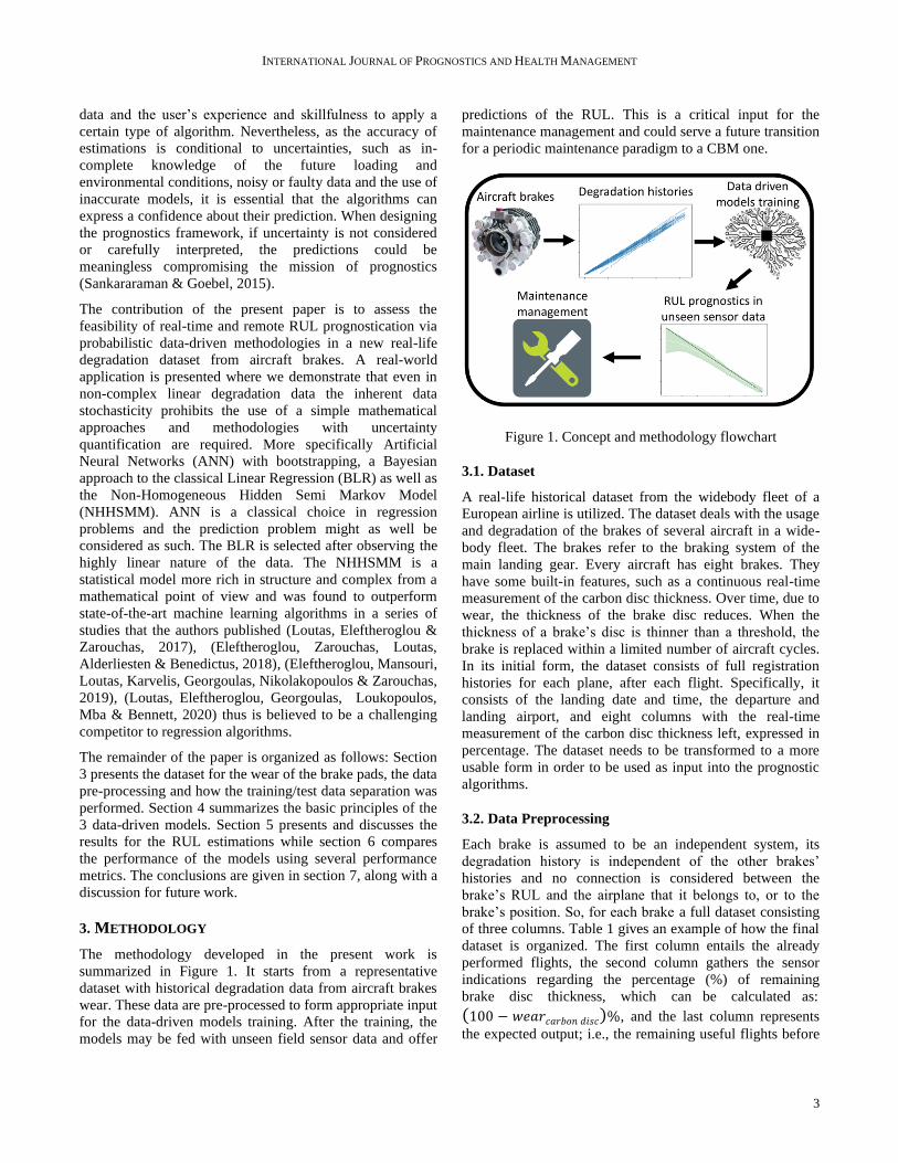
The methodology developed in the present work is

summarized in Figure 1. It starts from a representative

dataset with historical degradation data from aircraft brakes

wear. These data are pre-processed to form appropriate input

for the data-driven models training. After the training, the

models may be fed with unseen field sensor data and offer

predictions of the RUL. This is a critical input for the

maintenance management and could serve a future transition

for a periodic maintenance paradigm to a CBM one.

Figure 1. Concept and methodology flowchart

3.1. Dataset

A real-life historical dataset from the widebody fleet of a

European airline is utilized. The dataset deals with the usage

and degradation of the brakes of several aircraft in a wide-

body fleet. The brakes refer to the braking system of the

main landing gear. Every aircraft has eight brakes. They

have some built-in features, such as a continuous real-time

measurement of the carbon disc thickness. Over time, due to

wear, the thickness of the brake disc reduces. When the

thickness of a brake’s disc is thinner than a threshold, the

brake is replaced within a limited number of aircraft cycles.

In its initial form, the dataset consists of full registration

histories for each plane, after each flight. Specifically, it

consists of the landing date and time, the departure and

landing airport, and eight columns with the real-time

measurement of the carbon disc thickness left, expressed in

percentage. The dataset needs to be transformed to a more

usable form in order to be used as input into the prognostic

algorithms.

3.2. Data Preprocessing

Each brake is assumed to be an independent system, its

degradation history is independent of the other brakes’

histories and no connection is considered between the

brake’s RUL and the airplane that it belongs to, or to the

brake’s position. So, for each brake a full dataset consisting

of three columns. Table 1 gives an example of how the final

dataset is organized. The first column entails the already

performed flights, the second column gathers the sensor

indications regarding the percentage (%) of remaining

brake disc thickness, which can be calculated as:

(100 − 𝑤𝑒𝑎𝑟𝑐𝑎𝑟𝑏𝑜𝑛 𝑑𝑖𝑠𝑐)%, and the last column represents

the expected output; i.e., the remaining useful flights before

INTERNATIONAL JOURNAL OF PROGNOSTICS AND HEALTH MANAGEMENT

4

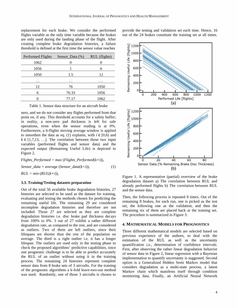
replacement for each brake. We consider the performed

flights variable as the only time variable because the brakes

are only used during the landing phase of the flight. After

creating complete brake degradation histories, a failure

threshold is defined at the first time the sensor value reaches

Performed Flights Sensor_Data (%) RUL (flights)

1062 0 0

1056 1 6

1050 1.5 12

… … …

12 76 1050

6 76.33 1056

0 77.17 1062

Table 1. Sensor data structure for an aircraft brake

zero, and we do not consider any flights performed from that

point on, if any. This threshold accounts for a safety buffer;

in reality, a non-zero pad thickness is left for safe

operations, even when the sensor reading is at 0%.

Furthermore, a 6-flights moving average window is applied

to smoothen the data as eq. (1) explains, with i ∈ [0,6) and

k ∈ [1,7,13, …]. The correlation between those two input

variables (performed flights and sensor data) and the

expected output (Remaining Useful Life) is depicted in

Figure 2.

Flights_Performed = max (Flights_Performed(k+i)),

Sensor_data = average (Sensor_data(k+i)), (1)

RUL = min (RUL(k+i)),

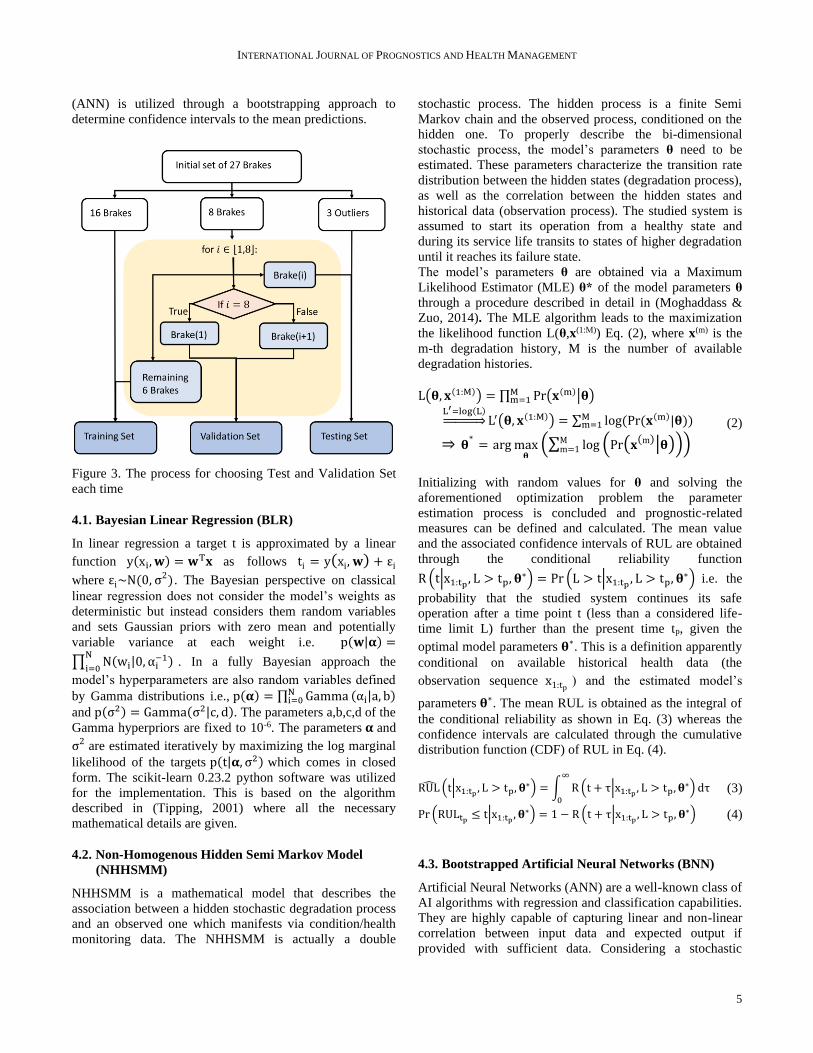
3.3. Training/Testing datasets preparation

Out of the total 56 available brake degradation histories, 27

histories are selected to be used as the dataset for training,

evaluating and testing the methods chosen for predicting the

remaining useful life. The remaining 29 are considered

incomplete degradation histories and therefore are not

included. Those 27 are selected as they are complete

degradation histories i.e. disc brake pad thickness decays

from 100% to 0%. 3 out of 27 exhibit a rather different

degradation rate, as compared to the rest, and are considered

as outliers. Two of them are left outliers, since their

lifespans are shorter than the rest of the population on

average. The third is a right outlier i.e. it has a longer

lifespan. The outliers are used only in the testing phase to

check the proposed algorithms’ predictive capabilities, since

one prognostic challenge is to be able to predict accurately

the RUL of an outlier without using it in the training

process. The remaining 24 histories represent complete

sensor data from 8 brake sets of 3 aircrafts. For the training

of the prognostic algorithms a k-fold leave-two-out method

was used. Randomly, one of those 3 aircrafts is chosen to

provide the testing and validation set each time. Hence, 16

out of the 24 brakes constitute the training set at all times.

Figure 1. A representative (partial) overview of the brake

degradation dataset a) The correlation between RUL and

already performed flights b) The correlation between RUL

and the sensor data.

Then, the following process is repeated 8 times. Out of the

remaining 8 brakes, for each run, one is picked as the test

set, the following one as the validation, and then the

remaining six of them are placed back at the training set.

The procedure is summarized in Figure 3.

4. MATHEMATICAL MODELS FOR PROGNOSTICS

Three different mathematical models are selected based on

previous experience of the authors, to deal with the

estimation of the RUL as well as the uncertainty

quantification i.e., determination of confidence intervals.

First, after observing the rather linear degradation behavior

of sensor data in Figure 2, linear regression with a Bayesian

implementation to quantify uncertainty is suggested. Second

option is a Generalized Hidden Semi Markov model that

considers degradation as a multi-state process, a latent

Markov chain which manifests itself through condition

monitoring data. Finally, an Artificial Neural Network

INTERNATIONAL JOURNAL OF PROGNOSTICS AND HEALTH MANAGEMENT

5

(ANN) is utilized through a bootstrapping approach to

determine confidence intervals to the mean predictions.

Figure 3. The process for choosing Test and Validation Set

each time

4.1. Bayesian Linear Regression (BLR)

In linear regression a target t is approximated by a linear

function y(xi, 𝐰) = 𝐰T𝐱 as follows ti = y(xi, 𝐰) + εi

where εi~Ν(0, σ2). The Bayesian perspective on classical

linear regression does not consider the model’s weights as

deterministic but instead considers them random variables

and sets Gaussian priors with zero mean and potentially

variable variance at each weight i.e. p(𝐰|𝛂) =

∏ N(wi|0, αi−1)

N

i=0. In a fully Bayesian approach the

model’s hyperparameters are also random variables defined

by Gamma distributions i.e., p(𝛂) = ∏ GammaNi=0 (αi|a, b)

and p(σ2) = Gamma(σ2|c, d). The parameters a,b,c,d of the

Gamma hyperpriors are fixed to 10-6. The parameters 𝛂 and

σ2 are estimated iteratively by maximizing the log marginal

likelihood of the targets p(t|𝛂, σ2) which comes in closed

form. The scikit-learn 0.23.2 python software was utilized

for the implementation. This is based on the algorithm

described in (Tipping, 2001) where all the necessary

mathematical details are given.

4.2. Non-Homogenous Hidden Semi Markov Model

(NHHSMM)

NHHSMM is a mathematical model that describes the

association between a hidden stochastic degradation process

and an observed one which manifests via condition/health

monitoring data. The NHHSMM is actually a double

stochastic process. The hidden process is a finite Semi

Markov chain and the observed process, conditioned on the

hidden one. To properly describe the bi-dimensional

stochastic process, the model’s parameters θ need to be

estimated. These parameters characterize the transition rate

distribution between the hidden states (degradation process),

as well as the correlation between the hidden states and

historical data (observation process). The studied system is

assumed to start its operation from a healthy state and

during its service life transits to states of higher degradation

until it reaches its failure state.

The model’s parameters θ are obtained via a Maximum

Likelihood Estimator (MLE) θ* of the model parameters θ

through a procedure described in detail in (Moghaddass &

Zuo, 2014). The MLE algorithm leads to the maximization

the likelihood function L(θ,x(1:Μ)) Eq. (2), where x(m) is the

m-th degradation history, M is the number of available

degradation histories.

L(𝛉, 𝐱(1:M)) = ∏ Pr(𝐱(m)|𝛉)Mm=1

L′=log(L)⇒ L′(𝛉, 𝐱(1:M)) = ∑ log(Pr(𝐱(m)|𝛉))M

m=1

⇒ 𝛉∗= arg max

𝛉(∑ log (Pr(𝐱(m)|𝛉))M

m=1 )

(2)

Initializing with random values for θ and solving the

aforementioned optimization problem the parameter

estimation process is concluded and prognostic-related

measures can be defined and calculated. The mean value

and the associated confidence intervals of RUL are obtained

through the conditional reliability function

R (t|x1:tp, L > tp, 𝛉∗) = Pr (L > t|x1:tp , L > tp, 𝛉

∗) i.e. the

probability that the studied system continues its safe

operation after a time point t (less than a considered life-

time limit L) further than the present time tp, given the

optimal model parameters 𝛉∗. This is a definition apparently

conditional on available historical health data (the

observation sequence x1:tp ) and the estimated model’s

parameters 𝛉∗. The mean RUL is obtained as the integral of

the conditional reliability as shown in Eq. (3) whereas the

confidence intervals are calculated through the cumulative

distribution function (CDF) of RUL in Eq. (4).

RUL̂ (t|x1:tp , L > tp, 𝛉∗) = ∫ R(t + τ|x1:tp , L > tp, 𝛉

∗) dτ∞

0

(3)

Pr (RULtp ≤ t|x1:tp , 𝛉∗) = 1 − R(t + τ|x1:tp , L > tp, 𝛉

∗) (4)

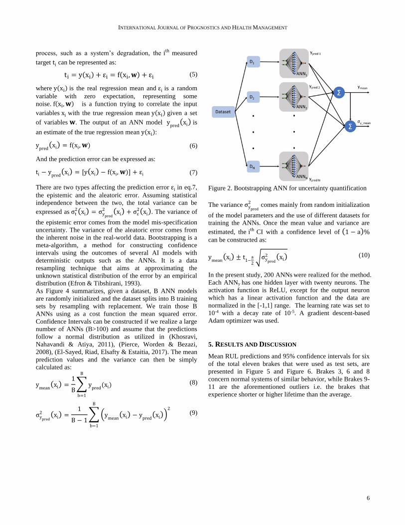
4.3. Bootstrapped Artificial Neural Networks (BNN)

Artificial Neural Networks (ANN) are a well-known class of

AI algorithms with regression and classification capabilities.

They are highly capable of capturing linear and non-linear

correlation between input data and expected output if

provided with sufficient data. Considering a stochastic

INTERNATIONAL JOURNAL OF PROGNOSTICS AND HEALTH MANAGEMENT

6

process, such as a system’s degradation, the ith measured

target ti can be represented as:

ti = y(xi) + εi = f(xi, 𝐰) + εi (5)

where y(xi) is the real regression mean and εi is a random

variable with zero expectation, representing some

noise. f(xi,𝐰) is a function trying to correlate the input

variables xi with the true regression mean y(xi) given a set

of variables 𝐰. The output of an ANN model ypred(xi) is

an estimate of the true regression mean y(xi):

ypred(xi) = f(xi,𝐰) (6)

And the prediction error can be expressed as:

ti − ypred(xi) = [y(xi) − f(xi,𝐰)] + εi (7)

There are two types affecting the prediction error εi in eq.7,

the epistemic and the aleatoric error. Assuming statistical

independence between the two, the total variance can be

expressed as σt2(xi) = σypred

2 (xi) + σε2(xi). The variance of

the epistemic error comes from the model mis-specification

uncertainty. The variance of the aleatoric error comes from

the inherent noise in the real-world data. Bootstrapping is a

meta-algorithm, a method for constructing confidence

intervals using the outcomes of several AI models with

deterministic outputs such as the ANNs. It is a data

resampling technique that aims at approximating the

unknown statistical distribution of the error by an empirical

distribution (Efron & Tibshirani, 1993).

As Figure 4 summarizes, given a dataset, B ANN models

are randomly initialized and the dataset splits into B training

sets by resampling with replacement. We train those B

ANNs using as a cost function the mean squared error.

Confidence Intervals can be constructed if we realize a large

number of ANNs (B>100) and assume that the predictions

follow a normal distribution as utilized in (Khosravi,

Nahavandi & Atiya, 2011), (Pierce, Worden & Bezazi,

2008), (El-Sayed, Riad, Elsafty & Estaitia, 2017). The mean

prediction values and the variance can then be simply

calculated as:

ymean(xi) =

1

B∑ y

pred(xi)

B

b=1

(8)

σypred2 (xi) =

1

B − 1∑(y

mean(xi) − ypred(xi))

2B

b=1

(9)

Figure 2. Bootstrapping ANN for uncertainty quantification

The variance σypred2 comes mainly from random initialization

of the model parameters and the use of different datasets for

training the ANNs. Once the mean value and variance are

estimated, the ith CI with a confidence level of (1 − a)%

can be constructed as:

ymean(xi) ± t1−a

2 √σypred

2 (xi)

(10)

In the present study, 200 ANNs were realized for the method.

Each ANNy has one hidden layer with twenty neurons. The

activation function is ReLU, except for the output neuron

which has a linear activation function and the data are

normalized in the [-1,1] range. The learning rate was set to

10-4 with a decay rate of 10-5. A gradient descent-based

Adam optimizer was used.

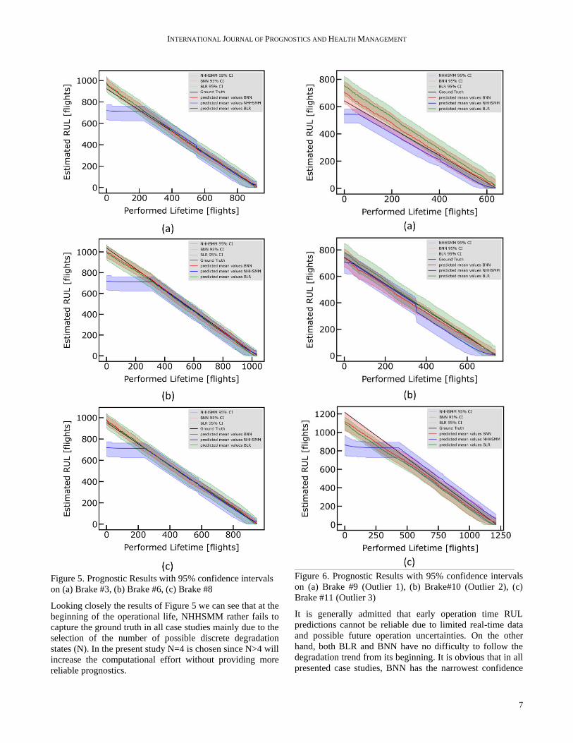
5. RESULTS AND DISCUSSION

Mean RUL predictions and 95% confidence intervals for six

of the total eleven brakes that were used as test sets, are

presented in Figure 5 and Figure 6. Brakes 3, 6 and 8

concern normal systems of similar behavior, while Brakes 9-

11 are the aforementioned outliers i.e. the brakes that

experience shorter or higher lifetime than the average.

INTERNATIONAL JOURNAL OF PROGNOSTICS AND HEALTH MANAGEMENT

7

Figure 5. Prognostic Results with 95% confidence intervals

on (a) Brake #3, (b) Brake #6, (c) Brake #8

Looking closely the results of Figure 5 we can see that at the

beginning of the operational life, NHHSMM rather fails to

capture the ground truth in all case studies mainly due to the

selection of the number of possible discrete degradation

states (N). In the present study N=4 is chosen since N>4 will

increase the computational effort without providing more

reliable prognostics.

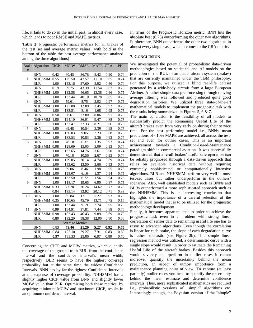
Figure 6. Prognostic Results with 95% confidence intervals

on (a) Brake #9 (Outlier 1), (b) Brake#10 (Outlier 2), (c)

Brake #11 (Outlier 3)

It is generally admitted that early operation time RUL

predictions cannot be reliable due to limited real-time data

and possible future operation uncertainties. On the other

hand, both BLR and BNN have no difficulty to follow the

degradation trend from its beginning. It is obvious that in all

presented case studies, BNN has the narrowest confidence

INTERNATIONAL JOURNAL OF PROGNOSTICS AND HEALTH MANAGEMENT

8

interval, while BLR and NHHSMM have wider CIs. It is

also worth mentioning that NHHSMM, for the majority of

the presented results, provides more conservative mean

estimates, while the mean estimates of BNN and BLR are,

in most cases, close to each other. While NHHSMM, after

overcoming the initial plateau, seems to have a clear

monotonic tendency, both BLRs and BNNs mean estimates

have some volatility. This volatility appears to be present at

the same x-values for both models, revealing the existence

of some possible abnormalities in the dataset. It is highly

notable that all three models mean predictions converge

very close to the ground truth as the end of lifetime

approaches and it is of paramount importance to have

successful predictions. The width of confidence intervals

decreases as well as operational time passes leading to

increasingly more confident mean estimates.

Figure 6 summarizes the prognostic result for the outlier

cases (Brake 9, Brake 10, Brake 11). Outliers as mentioned

previously are systems that degrade sooner than average or

later than average, and therefore experiencing shorter or

higher lifetime than average. In our case Brake 9 and Brake

10 are left outliers, as they degrade sooner than average,

whilst Brake 11 is considered as a right outlier since it

degrades later than average. From the results shown in

Figure 5 we can make the following comments. BNN

outperforms NHHSMM and BLR for both left and right

outliers, since ground truths seem to be within the predicted

CI and the mean values seem to be close to ground truth

even from the very beginning. The BNN estimated CIs are

wider regarding the outliers, than the predicted CIs for the

other eight brakes, while BLR and NHHSMM provide CIs

of almost the same width. To quantify even more these

qualitative observations, we proceed to a prognostic

performance assessment through special metrics.

6. PROGNOSTIC PERFORMANCE METRICS

The metrics used in our case study assess both the mean

value predictions as well as Confidence Intervals (CI). For

the assessment of the CI, the most important characteristic is

the coverage probability CICP (Confidence Interval

Coverage Probability). It is measured by counting every

target value that is in the defined confidence interval.

𝐶𝐼𝐶𝑃 =1

𝑛∑ 𝜉𝑖(𝐼𝑎(𝑥𝑖), 𝑡𝑖)

𝑛

𝑖=1,

where 𝜉𝑖(𝐼𝑎(𝑥𝑖), 𝑡𝑖) = {1, 𝑡𝑖 ∈ 𝐼𝑎(𝑥𝑖)

0, 𝑜𝑡ℎ𝑒𝑟𝑤𝑖𝑠𝑒

(11)

and where, 𝑛 is the number of target values that belong

inside the confidence interval 𝐼𝑎(𝑥𝑖), (1 − a)%. Another

crucial metric concerning the CI is the mean confidence

interval width (MCIW), which can be easily expressed as:

𝑀𝐶𝐼𝑊 =1

𝑛∑(𝑈𝑖 − 𝐿𝑖)

𝑛

𝑖=1

(12)

with 𝑈𝑖 and 𝐿𝑖 being the upper and lower value of the CI

respectively. For the assessment of the predicted mean

values several metrics as analyzed in the classical work of

(Saxena, Celaya, Saha, Saha & Goebel, 2010) are used. The

Root Mean Squared Error (RMSE), the Mean Absolute

Percentage Error (MAPE), the Prognostic Horizon (PH) and

the Cumulative Relative Accuracy (CRA) are defined in the

following:

𝑅𝑀𝑆𝐸 = √∑ (𝐸𝑚(𝑡𝑖))

2𝑛𝑖=1

𝑛

(13)

𝑀𝛢𝛲𝐸 =100

𝑛∑

|𝐸𝑚(𝑡𝑖)|

𝑦𝑡𝑟𝑢𝑒(𝑡𝑖)

𝑛

𝑖=1

(14)

𝑃𝐻 = 𝐸𝑂𝐿 − 𝑡𝑖 (15)

𝐶𝑅𝐴 =∑ 𝑅𝐴𝑛𝑖=1 (𝑡𝑖)

𝑁,𝑤ℎ𝑒𝑟𝑒 𝑅𝐴(𝑡𝑖) = 1 − |

𝐸𝑚(𝑡𝑖)

𝑦𝑡𝑟𝑢𝑒(𝑡𝑖)|,

𝑎𝑛𝑑 𝐸𝑚(𝑡𝑖) = 𝑦𝑡𝑟𝑢𝑒(𝑡𝑖) − 𝑦𝑚𝑒𝑎𝑛(𝑡𝑖)

(16)

Besides RMSE and MAPE which are well known and

widely used in prognostic results assessment, the Prognostic

Horizon is the difference between a time 𝑡𝑖 , when the

predictions meet specified performance criteria, and the time

corresponding to the end of life (EoL). Cumulative Relative

Accuracy is the normalized sum of relative prediction

accuracies at specific time instances. More details regarding

the metrics can be found in the classical paper of Saxena et

al. [30]. In Table 2 the prognostic performance metrics for

all the brakes of the test set are presented.

Although predictions are available from the very onset of

the operational phase of the brakes, we focus on the

performance at the 75% of the lifetime and thus we calculate

the metrics ignoring the first 25% of the lifetime of each

brake. It is desirable for CICP and CRA to get the maximum

value of 1 and for the PH a maximum value of 0.75 (since

we focus on the performance at the 75% of the lifetime),

while the rest of the presented metrics (MCIW, RMSE,

MAPE) are desirable to take as low values as possible.

The average metric values across all eleven brakes are also

calculated and presented in Table 2. Overall, the BNN

clearly outperforms the other two models with BLR

performing second best and NHHSMM being the worst of

the three. More specifically, regarding RMSE and MAPE

metrics, which represent the error of the predicted mean

RUL from the ground truth RUL, BNN outperforms the

other two methods in almost every single case. BLR

performs well in normal degradation scenarios, however, it

fails to accurately predict the RUL of the outliers. Although

NHHSMM performs quite well close to the brake’s end of

INTERNATIONAL JOURNAL OF PROGNOSTICS AND HEALTH MANAGEMENT

9

life, it fails to do so in the initial part, in almost every case,

which leads to poor RMSE and MAPE metrics.

Table 2: Prognostic performance metrics for all brakes of

the test set and average metric values (with bold in the

bottom of the table the best average performance attained

among the three algorithms)

Brake

#

Algorithm CICP MCIW RMSE MAPE CRA PH

1

BNN 0.42 60.45 36.78 8.42 0.90 0.74

NHHSMM 0.55 125.50 47.57 11.10 0.85 0.74

BLR 1.00 133.16 37.60 8.92 0.86 0.74

2

BNN 0.19 59.75 43.39 11.54 0.87 0.75

NHHSMM 1.00 132.58 46.65 13.38 0.66 0.75

BLR 1.00 133.44 40.10 10.78 0.85 0.75

3 BNN 1.00 59.61 8.75 2.02 0.97 0.75

NHHSMM 1.00 127.88 12.89 3.45 0.92 0.75

BLR 1.00 133.51 8.16 1.68 0.95 0.75

4 BNN 0.50 58.61 33.80 8.06 0.91 0.75

NHHSMM 1.00 124.10 36.01 9.47 0.85 0.75

BLR 1.00 132.47 32.33 8.21 0.86 0.75

5 BNN 1.00 69.48 10.54 2.39 0.95 0.75

NHHSMM 1.00 130.03 9.05 2.23 0.88 0.75

BLR 1.00 133.53 10.83 2.36 0.93 0.75

6 BNN 1.00 78.10 6.37 1.35 0.97 0.74

NHHSMM 0.98 128.09 15.05 3.09 0.93 0.74

BLR 1.00 132.65 14.76 3.61 0.90 0.74

7 BNN 1.00 70.18 10.56 2.67 0.95 0.74

NHHSMM 1.00 129.05 20.14 4.74 0.89 0.74

BLR 1.00 133.62 13.50 3.66 0.93 0.74

8 BNN 1.00 59.06 8.46 1.98 0.95 0.75

NHHSMM 1.00 128.07 6.16 1.37 0.94 0.75

BLR 1.00 133.50 6.72 1.56 0.94 0.75

9 BNN 1.00 118.17 19.65 6.90 0.87 0.75

NHHSMM 0.33 77.78 36.24 14.62 0.77 0.75

BLR 0.84 135.14 52.92 20.12 0.71 0.33

10 BNN 1.00 85.84 17.11 5.27 0.93 0.75

NHHSMM 0.35 110.65 45.79 13.71 0.75 0.15

BLR 1.00 133.44 9.19 2.74 0.95 0.75

11 BNN 0.99 154.91 37.81 7.44 0.88 0.75

NHHSMM 0.98 162.43 46.43 9.89 0.69 0.75

BLR 0.80 132.20 58.38 12.00 0.80 0.68

Average Metrics

BNN 0.83 79.46 21.20 5.27 0.92 0.75

NHHSMM 0.84 125.10 29.27 7.91 0.83 0.69

BLR 0.97 133.33 25.86 6.87 0.88 0.70

Concerning the CICP and MCIW metrics, which quantify

the coverage of the ground truth RUL from the confidence

interval and the confidence interval’s mean width,

respectively, BLR seems to have the highest coverage

probability but at the same time the widest Confidence

Intervals. BNN has by far the tightest Confidence Intervals

at the expense of coverage probability. NHHSMM has a

slightly higher CICP value from BNN and slightly lower

MCIW value than BLR. Optimizing both those metrics, by

acquiring minimum MCIW and maximum CICP, results in

an optimum confidence interval.

In terms of the Prognostic Horizon metric, BNN hits the

absolute best (0.75) outperforming the other two algorithms.

Furthermore, BNN outperforms the other two algorithms in

almost every single case, when it comes to the CRA metric.

7. CONCLUSION

We investigated the potential of probabilistic data-driven

methodologies based on statistical and AI models on the

prediction of the RUL of an actual aircraft system (brakes)

that are currently maintained under the TBM philosophy.

For this purpose, we utilized a blind real-life dataset

generated by a wide-body aircraft from a large European

Airliner. A rather simple data preprocessing through moving

average filtering was followed and produced quite good

degradation histories. We utilized three state-of-the-art

mathematical models to implement the prognostic task with

the results being summarized in Figures 5, 6 & 7.

The main conclusion is the feasibility of all models to

successfully predict the Remaining Useful Life of the

aircraft brakes even from very early on during their service

time. For the best performing model i.e., BNNs, mean

predictions of <10% MAPE are achieved, all across the test-

set and even for outlier cases. This is an important

achievement towards a Condition-Based-Maintenance

paradigm shift in commercial aviation. It was successfully

demonstrated that aircraft brakes’ useful safe operation can

be reliably prognosed through a data-driven approach that

relies on available historical data without requiring

extremely sophisticated or computationally intensive

algorithms. BLR and NHHSMM perform very well in most

test-set cases but rather underperform in the outliers’

scenarios. Also, well established models such as BNNs and

BLRs outperformed a more sophisticated approach such as

the NHHSMM. This is an interesting conclusion that

highlights the importance of a careful selection of the

mathematical model that is to be utilized for the prognostic

methodology development.

Finally, it becomes apparent, that in order to achieve the

prognostic task even in a problem with strong linear

correlation of sensor data to remaining useful life one has to

resort to advanced algorithms. Even though the correlation

is linear for each brake, the slope of each degradation curve

is rather stochastic (see Figure 2b). If a simple linear

regression method was utilized, a deterministic curve with a

single slope would result, in order to estimate the Remaining

Useful Life of the aircraft brakes. Besides this approach

would severely underperform in outlier cases it cannot

moreover quantify the uncertainty behind the mean

prediction, an aspect of utmost importance from a

maintenance planning point of view. To capture (at least

partially) outlier cases you need to quantify the uncertainty

behind the mean estimate and determine confidence

intervals. Thus, more sophisticated mathematics are required

i.e., probabilistic versions of “simple” algorithms etc.

Interestingly enough, the Bayesian version of the “simple”

INTERNATIONAL JOURNAL OF PROGNOSTICS AND HEALTH MANAGEMENT

10

linear regression is not the best performer as we

demonstrated in the paper. The transition to CBM of aircraft

systems fundamentally calls for reliable prognostics. The

present work demonstrates that this is feasible but the road

towards a Condition-Based-Maintenance paradigm shift in

commercial aviation has still several challenges ahead that

are beyond the objectives of the present work.

ACKNOWLEDGEMENT

The present work was financially supported by the European

Union’s Horizon 2020 research and innovation programme

ReMAP (Grant Agreement Number: 769288). The support

is sincerely appreciated by the authors.

REFERENCES

Acuna, D. E. & Orchard, M. E. (2017). Particle-filtering-

based failure prognosis via sigma-points: Application to

Lithium-Ion battery state-of-charge monitoring,

Mechanical Systems and Signal Processing, 85, pp.

827-848, https://doi.org/10.1016/j.mssp.2016.08.029

Adhikari, P.P. & Buderath, M. A framework for aircraft

maintenance strategy including CBM, Proceedings of

the European Conference Prognostics Health

Management Society 2016, pp. 1-10.

Autin, S.; De Martin, A.; Jacazio, G.; Socheleau, J.;

Vachtsevanos, G. (2021), International Journal of

Prognostics and Health Management, Results of a

Feasibility Study of a Prognostic System for Electro-

Hydraulic Flight Control Actuators, 12 (3), pp. 1-18.

https://doi.org/10.36001/ijphm.2021.v12i3.2935

Che, C.; Wang, H.; Fu, Q.; Ni, X. (2019) Combining

multiple deep learning algorithms for prognostic and

health management of aircraft, Aerospace Science and

Technology, 94, 105423.

https://doi.org/10.1016/j.ast.2019.105423

Dalla Vedova, M.D.L.; Germanà, A.; Berri, P.C.; Maggiore,

P. (2019). Model-Based Fault Detection and

Identification for Prognostics of Electromechanical

Actuators Using Genetic Algorithms. Aerospace 6 (94)

https://doi.org/10.3390/aerospace6090094

Dawn, A,; Kim, N.H.; Choi, J-H. (2015) Practical options

for selecting data-driven or physics-based prognostics

algorithms with reviews, Reliability Engineering &

System Safety, 133, pp. 223-236.

https://doi.org/10.1016/j.ress.2014.09.014

Efron, B.; Tibshirani, R.J. (1993) An Introduction to the

Bootstrap, Chapman and Hall, New York,

https://doi.org/10.1007/978-1-4899-4541-9

Eleftheroglou, N.; Mansouri, S.S.; Loutas, T.; Karvelis, P.;

Georgoulas, G.; Nikolakopoulos, G.; Zarouchas, D.

(2019). Intelligent data-driven prognostic

methodologies for the real-time remaining useful life

until the end-of-discharge estimation of the Lithium-

Polymer batteries of unmanned aerial vehicles with

uncertainty quantification, Applied Energy, 254,

113677.

https://doi.org/10.1016/j.apenergy.2019.113677

Eleftheroglou, N.; Zarouchas, D.; Loutas, T.; Alderliesten,

R.; Benedictus, R. (2018). Structural health monitoring

data fusion for in-situ life prognosis of composite

structures, Reliability Engineering & System Safety,

178, pp. 40-54.

https://doi.org/10.1016/j.ress.2018.04.031

El-Sayed, M.; Riad, F.; Elsafty, M.; Estaitia, Y. (2017).

Algorithms of Confidence Intervals of WG Distribution

Based on Progressive Type-II Censoring Samples.

Journal of Computer and Communications, 5, pp. 101-

116. https://doi: 10.4236/jcc.2017.57011.

Ezhilarasu, C.M.; Skaf, Z.; Jennions, I.K. (2019). The

application of reasoning to aerospace Integrated Vehicle

Health Management (IVHM): Challenges and

opportunities, Progress in Aerospace Sciences, 105 pp.

60-73, https://doi.org/10.1016/j.paerosci.2019.01.001

Goebel, K.; Daigle, M.; Saxena, A.; Sankararaman, S.;

Roychoudhury, I.; Celaya, (2017), Prognostics: The

science of prediction, CA, CreateSpace Independent

Publishing Platform; 1st ed.

Jia, X.; Huang, B.; Feng, J.; Cai, H.; Lee, J. (2018). A

Review of PHM Data Competitions from 2008 to 2017:

Methodologies and Analytics. Proceedings of the

Annual Conference of the Prognostics and Health

Management Society, Philadelphia, Pennsylvania, USA.

Kallen, M.J. & van Noortwijk, J.M. (2005) Optimal

maintenance decisions under imperfect inspection,

Reliability Engineering and System Safety, 90 (2-3), pp.

177-185. https://doi.org/10.1016/j.ress.2004.10.004

Khosravi, A., Nahavandi, S., Creighton, D. and Atiya, A. F.

(2011). Comprehensive Review of Neural Network-

Based Prediction Intervals and New Advances, IEEE

Transactions on Neural Networks, 22 (9) pp. 1341-

1356, doi: 0.1109/TNN.2011.2162110.

Lee, J. & Mitici, M. (2020). An integrated assessment of

safety and efficiency of aircraft maintenance strategies

using agent-based modelling and stochastic Petri nets,

Reliability Engineering & System Safety, 202, 107052.

https://doi.org/10.1016/j.ress.2020.107052

Li, R.; Verhagen, W.J.C.; Curran, R. (2020) Toward a

methodology of requirements definition for prognostics

and health management system to support aircraft

predictive maintenance, Aerospace Science and

Technology, 102, 105877.

https://doi.org/10.1016/j.ast.2020.105877

Loutas, T.; Eleftheroglou, N.; Zarouchas, D. (2017) A data-

driven probabilistic framework towards the in-situ

prognostics of fatigue life of composites based on

acoustic emission data, Composite Structures, 161, pp.

522-529.

https://doi.org/10.1016/j.compstruct.2020.112386

Loutas, T.; Eleftheroglou, N.; Georgoulas, G.; Loukopoulos,

P.; Mba D.; Bennett, I. (2020). Valve Failure

Prognostics in Reciprocating Compressors Utilizing

INTERNATIONAL JOURNAL OF PROGNOSTICS AND HEALTH MANAGEMENT

11

Temperature Measurements, PCA-Based Data Fusion,

and Probabilistic Algorithms, IEEE Transactions on

Industrial Electronics, 67 (6), pp. 5022-5029, doi:

10.1109/TIE.2019.2926048.

Lu, F.; Wu, J.; Huang, J.; Qiu, X. (2019). Aircraft engine

degradation prognostics based on logistic regression

and novel OS-ELM algorithm, Aerospace Science and

Technology, 84, pp. 661-671.

https://doi.org/10.1016/j.ast.2018.09.044

Moghaddass, R.; Zuo, M. J. (2014). An integrated

framework for online diagnostic and prognostic health

monitoring using a multistate deterioration process,

Reliability Engineering & System Safety, 124, pp. 92-

104. https://doi.org/10.1016/j.ress.2013.11.006

Nix, D.A.; Weigend, A.S. (1995). Learning local error bars

for nonlinear regression, Advances in Neural

Information Processing Systems, vol. 7, G. Tesauro, D.

Touretzky, and T. Leen, Eds. Cambridge, MA, USA:

MIT Press, pp. 489–496.

Pierce, S. G.; Worden, K.; Bezazi, A. (2008). Uncertainty

analysis of a neural network used for fatigue lifetime

prediction, Mechanical Systems Signal Processing, 22

(6), pp. 1395–1411.

https://doi.org/10.1016/j.ymssp.2007.12.004

Rengasamy, D.; Jafari, M.; Rothwell, B.; Chen X.;

Figueredo, G. (2020). Deep Learning with Dynamically

Weighted Loss Function for Sensor-Based Prognostics

and Health Management, Sensors, 20 (3), 723;

https://doi.org/10.3390/s20030723

Sankararaman, S. & Goebel, K. (2020) Uncertainty in

prognostics and systems health management,

International journal of prognostics and health

management, pp.1-14

https://doi.org/10.36001/ijphm.2015.v6i4.2319.

Strategic Research & Innovation Agenda, Vol. 2, Advisory

Council for Aviation Research and Innovation in

Europe (ACARE), September 2012,

www.acare4europe.com

Saxena A, Celaya J, Saha B, Saha S, Goebel K. (2020)

Metrics for offline evaluation of prognostic

performance, International. Journal Prognostics Health

Management, 1, pp.1–20.

Tipping, M. Sparse Bayesian learning and the relevance

vector machine, Journal of machine learning research 1,

2001, pp. 211-244.

Verstraete, D.; Droguett, E.; Modarres, M. A Deep

Adversarial Approach Based on Multi-Sensor Fusion

for Semi-Supervised Remaining Useful Life

Prognostics, Sensors 2020, 20(1), 176;

https://doi.org/10.3390/s20010176