Relief visualization techniques using free and open source ...

1. Introduction

There is a huge variety of relief visualization techniques, which is the consequence of long historical development and many technological innovations. The first pioneers who developed new techniques are well known, starting with the Renaissance polymath Leonardo da Vinci and followed by J. Murer, P. Apian and H. Gyger (the latter made revolutionary advance in topo-graphy but due to military secrecy of his maps unfortunately had no influence). Later, at the end of the 18th century, J. H. Weiss, J.E. Müller and J.R. Meyer in Atlas Suisse (“Meyer Atlas”) made the transition from oblique relief to plani-metric view, and J.G. Lehmann developed the technique of slope hachuring. In the 19th century the masterpiece Topographic Map of Switzer-land (“Dufour Map”) was published, combining different techniques in new shadow hachuring technique. During the late 19th and early 20th century F. Becker, the inventor of the so-called “Swiss Style” relief representation, introduced many new cartographic techniques. He was succeeded by E. Imhof who continued to im-prove the existing techniques and to develop new ones. In the second half of the 20th century first attempts in relief visualization and carto-graphy using digital technologies were made by P. Yoëli (E. Imhof 1982; B. Horn 1981; B. Jenny,

L. Hurni 2006; L. Hurni 2008; J. Siwek, W. Wa-cławik 2015; B. Jenny, S. Räber 2002; P. Ken-nelly 2017).

The digital era led to radical transformation in technologies which in the field of geography and cartography culminated in the advent and development of GIS. It has transformed the process of map making into more computational and less artistic, but at the same time opened the gates to new directions of development. One of them is the attempt to combine all clas-sical relief representation techniques with digital technologies and to develop new techniques. It is also a great challenge for modern carto-graphy to combine “together timeless principles of map making with the more temporal and technical expertise of making maps with soft-ware and data products” (J. Howarth 2017). Most of these techniques achieve high quality results when combining GIS with raster gra-phics software or combining automatic with manual techniques (T. Patterson 2002). Their implementation is difficult for non-cartographer GIS users because they are complex, time--consuming, and require a combination of seve-ral, mainly proprietary, software packages.

The aim of this article is to present some re-lief visualization techniques created using only free and open source GIS tools. The criteria for selection of these techniques are: (1) simple

Polish Cartographical ReviewVol. 50, 2018, no. 2, pp. 61–71

DOI: 10.2478/pcr-2018-0004

JORDAN TZVETKOVBulgarian Academy of Sciences, Space Research and Technology Institute Sofia, Bulgaria [email protected]

Relief visualization techniques using free and open source GIS tools

Abstract. The aim of the article is to present different relief visualization techniques created using only free and open source GIS tools, such as QGIS and RVT. The criteria for selection of these techniques are that they should be, on the one hand, simple and fast for implementation and on the other suitable for multiple visuali-zation purposes. Here we present several techniques which combine hillshade with other relief data layers derived from DEM and an assessment of advantages and disadvantages of their visualization.

Keywords: relief visualization, cartography, GIS, open source software, QGIS

62 Jordan Tzvetkov

and fast implementation, (2) multipurpose vi-sualization effectiveness.

Current development of free and open source GIS software is rapid and at present these software tools are capable of providing a vast range of opportunities, from data processing to cartography visualization and map design. Despite the existence of such opportunities, many experts and users in GIS field still prefer to use proprietary software. Here we will try to present some relief visualization techniques which can be useful in diverse fields where suitable visualization is needed (e.g. cartogra-phy, geomorphology, archaeology) and which are easy to implement as well as free to use.

2. Data and methods

There are several free and open source GIS tools and applications which can be used for processing DEM and for cartographic visuali-zation. For basic GIS software we used the well-known open source QGIS. This software is accompanied with many publications that include descriptions of relief visualization tech-niques, both for general (A. Bruy, D. Svidzinska 2015; K. Menke et al. 2015; A. Graser et al. 2017) and specific purposes (S. Eastmead 2017). We also used free Relief Visualization Tool (RVT, v. 1.3) which is specially designed to process raster elevation datasets (Ž. Kokalj et al. 2011; K. Zakšek et al. 2011). It is also accompanied with valuable practical publica-tions (Ž. Kokalj, R. Hesse 2017).

The basic initial data layer for DEM was derived from EU-DEM (source: European Environmental Agency) with raster resolution 25 × 25 m. The selected raster layer was pro-jected in UTM zone 35N coordinate system, datum WGS84. Then for the purpose of visual-ization we selected a part of Southwestern Bulgaria (including diverse relief with flat terrain,

hills, mountains and valleys) with extent: top 4736191.79, bottom 4706341.79, left 176968.92, and right 221268.92 (with approximate area of 1322 square km). This DEM raster layer has minimum value of 503 m and maximum value of 2277 m a.s.l.

From the basic initial DEM layer we derived several raster layers:

• Hillshade one direction – created with QGIS (GDAL function); parameters: Z factor 3.0, scale 1.0, azimuth of light 315 degrees, altitude of light 45 degrees, Horn’s method.

• Hillshade one direction – created with QGIS (GDAL function); parameters: Z factor 3.0, scale 1.0, azimuth of light 45 degrees, altitude of light 45 degrees, Horn’s method.

• Two directional hillshade – created with QGIS (raster calculator) and simple mean of the above two layers with the corresponding parameters: two light directions – 315 and 45 de-grees, altitude of light 45 degrees, Z factor 3.0.

• Slope gradient – created with QGIS (GDAL function); parameters: scale 1.0, Horn’s method.

• Simple Local Relief Model (SLRM) – created with RVT; parameters: radius for trend assess-ment 20 pixels, vertical exaggeration 1.0.

• Sky-View Factor (SVF) – created with RVT; parameters: 16 search directions, search radius 5 pixels, high level of noise removal, vertical exaggeration 1.0.

Although there exist more sophisticated and more precise methods for layer combination and visualization e.g. SVM method (D. Viljoen, J. Harri 2006) and NAGI method (R. Nagi, A. Bu-ckley 2013), here we used the most popular, simple and fast method: layer overlay with transparency. Significant visualization enhance-ment of this method is possible in QGIS with adjustment of blending mode.

Blending mode is a traditional function for graphic editing software (J. Beardsworth 2005;

Table 1. Comparison of popular GIS software by availability of blending modes

GIS software Blending modes

Free and open source Operating systems

GRASS • MS-Windows/Linux/MacOSXSAGA • MS-Windows/Linux/MacOSXgvSIG • MS-Windows/Linux/MacOSXQGIS • • MS-Windows/Linux/MacOSX

ArcGIS MS-WindowsGlobal Mapper • MS-Windows

63Relief visualization techniques using free and open source GIS tools

S. Valentine 2012). This function allows multiple layers to blend and to get new visual appearance of the top layer, based on the layers beneath it. The availability of blending modes in GIS soft-ware is a great advance for visualization pur-poses because it gives an opportunity to apply them without the need of using graphic design software for post-processing and visualization.

We compared (table 1) the availability of blend-ing modes in several popular GIS software packages, both open source and proprietary. A set of 12 blending modes is available in QGIS and a set of 18 is available in Global Mapper. The most important advantages of QGIS are that it is free and open source, and it is adapted to multiple operation systems. So this strongly

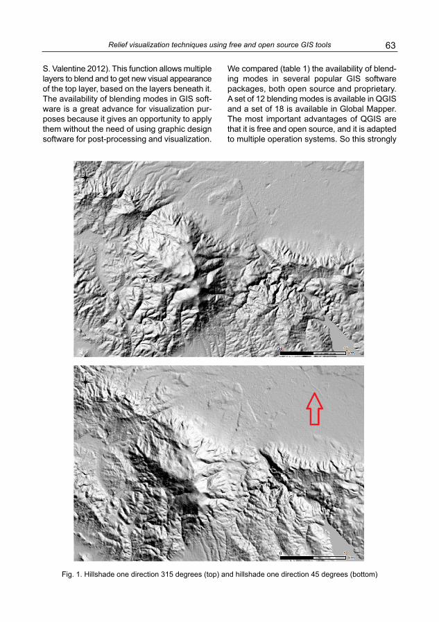
Fig. 1. Hillshade one direction 315 degrees (top) and hillshade one direction 45 degrees (bottom)

64 Jordan Tzvetkov

motivates us to use this software to perform relief visualization techniques.

3. Gray relief visualization

Gray relief visualization is common when vi-sualizing analytical hillshading because grey colors correspond to image raster values. Most

often one-directional analytical hillshading is used with lighting azimuth at 315 degrees (NW) and vertical angle at 45 degrees, which is enough to derive a 3D image of the terrain (fig. 1 – top).

Some well-known disadvantages of one-di-rectional hill shading are a consequence of its anisotropy (directional dependence). We will

Fig. 2. Two-directional hillshade (top) and multidirectional oblique-weighted hillshade (bottom)

65Relief visualization techniques using free and open source GIS tools

not discuss all of them in detail here. However, one of such disadvantages is that some small elongated landforms, the direction of which co-incides with the direction of light, are not well visible or sometimes even completely invisible. This is the case in the selected area even with vertical exaggeration at 3.0 and is illustrated in figure 1 – bottom, where the red arrow shows such a landform of a dike (levee) which became visible clear when the hillshade illumination azimuth is shifted to 45 degrees.

An interesting recent empirical study (J. Bi-land, A. Çöltekin 2016) investigating the relief inversion effect finds that from 16 light direc-tions the incident light at 337.5 degrees (NNW) yields the highest accuracy for correct land-form identification and this should be taken into account in the future when producing one--directional hillshading. It is also important to emphasize that the study finds the window between 337.5 and 0 degrees to be the best and the window between 315 and 45 degrees to be optimal. But it is important also to note that according to Imhof this technique was unsuitable for one-directional hillshading (pro-posed by H. Wiechel in the 1878) because “cartographic oblique hill shading provides satisfactory results only when light directions is varied locally and adapted to the shapes of

terrain” (E. Imhof 1982). Thus multidirectional hillshade is much better for relief visualization and more cartographically consistent. There exist several methods of creating multidirec-tional hillshade (R. Mark 1992; K. Hobbs 1995, 1999; B. Jenny 2001; P. Kennelly, J. Stewart 2006; S. Rusinkiewicz et al. 2006; T. Loisios et al. 2007; B. Devereux et al. 2008; T. Podob-nikar 2012; F. Veronesi, L. Hurni 2014, 2015; B. Marson, B. Jenny 2015), but their implemen-tation is difficult, time-consuming or requires expensive proprietary software. Here we used a very simple and fast multidirectional hillshade composed of only two one directional hillshade layers – with 315 and 45 degrees, chosen on the basis of empirical study mentioned above (J. Biland, A. Çöltekin, 2016). Such two-direc-tional hillshade (fig. 2 – top) we compared with the function for creating multidirectional hill-shade (Mark’s method for multidirectional ob-lique-weighted hillshade – MDOW) implemented in QGIS (after v. 2.16 in raster band rendering type). After generating a multidirectional hill-shade (with the following parameters: azimuth of light 315 degrees, altitude of light 45 degrees, Z factor 3.0), in order to enhance visualization, we adjusted brightness to 20 and contrast to 20, because the resulting image was too dim (fig. 2 – bottom). As expected we observed that the

Fig. 3. Relief visualization with two-directional hillshade and SLRM

66 Jordan Tzvetkov

main advantage of MDOW hillshade was less contrast compared to simple two-directional hillshade. This is an advantage predominantly for mountain terrains. But two-directional hill-shade presents small landforms in plain terrain more distinctly compared to MDOW. Therefore

the two-directional hillshade presented here is superior to one-directional hillshade (fig. 1) but still displays the traditional disadvantage of the method: contrast between shaded darkest parts (Southern slopes) and illuminated brightest parts (Northern slopes which appear too “shiny”).

Fig. 4. Relief visualization with two-directional hillshade and SLRM (with reverted gradient)

Fig. 5. Relief visualization with two-directional hillshade and SVF

67Relief visualization techniques using free and open source GIS tools

One way to avoid this is to adjust contrast and brightness. Another possibility is to use a com-bination of relief data layers which hold isotropy and demonstrate that they are suitable and effective for visualization (R. Bennett 2011; B. Štular et al. 2012; M. Doneus 2013; Ž. Ko-kalj, R. Hesse 2017).

In this case we combine two-directional hill-shade (stretch to min-max) with SLRM layer overlay (stretch with 2% clip, 70% transparency, and blending mode: multiply). This is illustrated in figure 3 where the SLRM layer overlay re-sults in more bright ridges and makes it possible to recognize some convexity and concavity of the terrain. One may see some visual similari-ties of this technique to an interesting method combining shaded relief with texture shading (L. Brown 2014; T. Patterson 2014). If needed for some purposes (e.g. geomorphology), the visualization of SLRM may turn to reverted gradient (from white to black) and this will em-phasize valleys (fig. 4). With additional adjust-ment of transparency, contrast and brightness such emphasis can be regulated. This technique shows similarity to the method combining shaded relief with curvature (P. Kennelly 2008).

A certain disadvantage of this visualization is that plains and flat terrains are a little darker and this results in poor impression of eleva-

tion. This can be avoided if instead of SLRM layer an SVF layer overlay is used (stretch with 2% clip, 70% transparency, and blending mode: multiply). This combination is shown in figure 5; it has some intermediate properties with lighter plains, darker slopes, with more contrast com-pared to figure 3, but with less contrast com-pared to single two-directional hillshade.

4. Red relief visualization

Red relief visualizations follow the most known Red Relief Image Map (RRIM) which is a combination of red slope and Ridge and Val-ley Index – RVI (T. Chiba et al. 2008; T. Chiba, B. Hasi 2016). Other versions of red relief are combination of hillshade (one direction) and slope (M. Doneus, T. Kühteiber 2013) and com-bination of SVF (gray) and red slope overlay (T. Inomata et al. 2017). Here we presented another version which is a combination of red slope base layer (stretch with 2% clip) with two directional hillshade overlay (stretch to min-max, 70% transparency, blending mode: normal) (fig. 6). In this visualization we prefer to use dark red colour (HSV: 0; 100; 80) for red slope but if it is not appropriative (e.g. when using for base map) it can be changed to dark brown (this can give a “bronze metal” impression). In

Fig. 6. Red relief visualization with red slope and two-directional hillshade

68 Jordan Tzvetkov

fact in cartography the basics of this method combining oblique shading and slope shading are not new – it is called “combined shading” (E. Imhof 1982). Advantages of such red relief visualization are connected with the red colour indicating the slope gradient and a fascinating 3D impression. The two colour combination of red for slopes and gray for hillshading makes it possible to avoid misinterpretation which occurs in specific cases when only gray color is used; “combined shading” method is well known for this disadvantage (E. Imhof 1982). In contrast to RRIM this visualization uses hill-shade to produce a 3D impression which loses one of the advantages of RRIM: isotropy – easy recognition of convexity and concavity independent from the direction of the light source (T. Chiba et al. 2008). If isotropy is one’s goal, the combination between red slope layer and SLRM will be very similar to RRIM. A disadvant-age of this type of visualization is the lack of elevation information, which can be overcome with a combination of contour lines (T. Chiba et al. 2008).

5. Colour relief visualization

Colour relief visualization is used to represent elevation with hypsometric tint. Even after long

discussions there is no universal technique for this, but the most common colour scheme is starting with green at lower elevations turning to brown at higher elevations (E. Imhof 1982).

For our purpose here we have designed a cus-tom gradient colour ramp in QGIS, continuous type with Colour 1 – HSV: 86; 65; 52; Colour 2 – HSV: 10; 85; 63; first stop colour at 25%, HSV: 60; 30; 97; second stop colour at 50%, HSV: 41; 48; 93; third stop colour at 75%, HSV: 28; 62; 87. The standard relief visualiza-tion is to combine a DEM layer with the colour hypsometric tint (stretch to min-max, linear inter-polation) with two directional hillshade overlay (stretch to min-max, 50% transparency, blending mode: multiply) (fig. 7). Additional improve-ment of this visualization can be achieved when the colour hypsometric tint is combined with two directional hillshade (stretch to min-max, 70% transparency, blending mode: multiply) and slope gradient (stretch with 2% clip, 70% transparency, blending mode: multiply) (fig. 8). This combination (“combined shading hypso-metric tint”) leads to remarkable improvement of the 3D impression of the mountainous and hilly terrain where slopes become darker and more distinguished in contrast to ridges and bottom valleys. The possibilities of further mo-dification and improvement of colour hypso-

Fig. 7. Colour hypsometric tint with two-directional hillshade

69Relief visualization techniques using free and open source GIS tools

metric tints in QGIS are diverse and convenient, with capability to apply an interactive plot and gradient stop adjustment.

6. Conclusion

As already mentioned the search for the best graphic effect is subjective (J. Drachal 2017), especially when the case is to perform an assessment of this graphic visualization. But keeping this in mind we can draw some general conclusions derived from the techniques pre-sented above.

Free and open source GIS software, which provides a vast range of visualization tech-niques, can be used on its own successfully for relief visualization.

With only a few simple and fast to implement techniques it is possible to significantly increase the quality of relief visualization.

Analytical hillshading is the basic technique to create an intuitive and easy to interpret 3D impression of the terrain, but instead of hillshade with one direction, multidirectional hillshading should be used because of its cartographic consistence and better results. This is valid even for the simplest version of two-directional hill-

shade (with two azimuths of 315 and 45 de-grees).

Two-directional hillshade is intermediate by quality (compared to more complex and better multidirectional hillshading methods) but simple and fast to produce. In combination with other layers such visualization can be significantly improved and applicable for multiple purposes.

The ability to apply blending mode function-ality in QGIS gives significant advantage to vi-sualization purposes when combining several layers. This functionality is traditional for graphic design and editing software and is not avail-able in ArcGIS, the most popular GIS software. It exists in Global Mapper, which is also a pro-prietary GIS software. This functionality gives an opportunity to perform high quality relief vi-sualizations in free and open source QGIS without using graphic design software for post-processing and visualization.

Relief visualization techniques presented in the article may be generally useful for broader audience who use GIS and maps to perform relief visualization beyond the community of professional cartographers. However, further development and improvement of such tech-niques is open to, and relies on, both these groups.

Fig. 8. Colour hypsometric tint with two directional hillshade and slope gradient

70 Jordan Tzvetkov

Acknowledgments

Literature

Beardsworth J., 2005, Photoshop Blending Modes Cookbook for Digital Photographers. Cambridge: Ilex.

Bennett R., 2011, Archaeological Remote Sensing: Visualization and Analysis of Grass-Dominated Environments Using Airborne Laser Scanning and Digital Spectra Data. Ph.D. Thesis. Bournemouth University.

Biland J., Çöltekin A., 2016, An empirical assessment of the impact of the light direction on the relief in-version effect in shaded relief maps: NNW is better than NW. “Cartography and Geographic Informa-tion Science” Vol. 44, no. 4, pp. 358−372.

Brown L., 2014, Texture shading: a new technique for depicting terrain relief. “Banff 2014: Papers and Slide Presentations. 9th ICA Mountain Cartography Workshop, 22−26 April, 2014”. Banff, Canada, pp. 1−14. www.mountaincartography.org/activities/workshops/banff_canada/papers/brown.pdf

Bruy A., Svidzinska D., 2015, QGIS by Example. Bir-mingham: Packt Publishing.

Chiba T., Kaneta S., Suzuki Y., 2008, Red relief image map: new visualization method for three dimensio-nal data. “The International Archives of the Photo-grammetry, Remote Sensing and Spatial Information Sciences” Vol. 37, Part B2, Beijing, pp. 1071−1076.

Chiba T., Hasi B., 2016, Ground surface visualization using red relief image map for a variety of map scales. “The International Archives of the Photogrammetry, Remote Sensing and Spatial Information Scien-ces” Vol. XLI-B2. XXIII ISPRS Congress, 12−19 July 2016, Prague, Czech Republic, pp. 393–397.

Devereux B., Amable G., Crow P., 2008, Visualization of LiDAR terrain models for archaeological feature detection. “Antiquity” Vol. 82, no. 316, pp. 470−479.

Doneus M., 2013, Openness as a visualization tech-nique for interpretative mapping of airborne LiDAR derived digital terrain models. “Remote Sensing” Vol. 5, no. 12, pp. 6427−6442.

Doneus M., Kühteiber T., 2013, Airborne laser scanning and archaeological interpretation – bringing back the people. In: Opitz R., Cowley D. Interpreting Ar-chaeological Topography: Lasers, 3D Data, Visuali-sation and Observation. Oxford, UK: Oxbow Books, pp. 32−50.

Drachal J., 2017, Combined shading used for small scale photographic maps. “Unbounded Mapping

of Mountains. Proceedings of the 10th ICA Mountain Cartography Workshop, 26−30 April 2016”. Berch-tesgaden, Germany, pp. 55−64.

Eastmead S., 2017, Use of QGIS Geographical In-formation System in Basic Field Archaeology and LiDAR Processing (Ed. 1, rev. 4, from 05.03.2018). E-book: https://eastmead.com/QGIS-LIDAR.htm

Graser A., Meams B., Mandel A., Olaya V., Bruy A., 2017, QGIS: Becoming a GIS Power User. Bir-mingham: Packt Publishing.

Hobbs K., 1995, The rendering of relief images from digital contour data. “The Cartographic Journal” Vol. 32, no. 2, pp. 111−116.

Hobbs K., 1999, An investigation of RGB multi-band shading for relief visualisation. “International Jour-nal of Applied Earth Observation and Geoinforma-tion” Vol. 1, no. 3/4, pp. 181−186.

Horn B., 1981, Hill shading and the reflectance map. “Proceedings of the IEEE” Vol. 69, no. 1, pp. 14−47.

Howarth J., 2017, Design patterns of naturalistic shaded relief for large-format maps with high-reso-lution data. “Unbounded Mapping of Mountains, Proceedings of the 10th ICA Mountain Cartogra-phy Workshop, 26–30 April 2016”. Berchtesgaden, Germany, pp. 215–231.

Hurni L., 2008, Cartographic mountain relief repre-sentation. 150 years of tradition and progress at ETH Zurich. “Mountain Mapping and Visualization, Proceedings of the 6th ICA Mountain Cartography Workshop, 11−15 February 2008”. Lenk, Switzer-land, pp. 85−91.

Imhof E., 1982, Cartographic Relief Presentation. Berlin, N. Y.: Walter de Gruyter.

Inomata T., Pinzón F., Ranchos J.L., Haraguchi T., Nasu H., Fernandez-Diaz J.C., Aoyama K., Yonen-obu H., 2017, Archaeological application of airborne LiDAR with object-based vegetation classification and visualization techniques at the lowland Maya site of Ceibal, Guatemala. “Remote Sensing” Vol. 9, pp. 1−27.

Jenny B., 2001, An interactive approach to analytical relief shading. “Cartographica” Vol. 38, no. 1-2, pp. 67−75.

Jenny B., Hurni L., 2006, Swiss-style colour relief shading modulated by elevation and by exposure to illumination. “The Cartographic Journal” Vol. 43, no. 3, pp. 198−207.

I would like to thank Asger Skovbo Petersen for providing me information about the multidi-rectional hillshading implemented in QGIS and to the two anonymous reviewers for their re-commendations.

This work has been carried out despite the negative attitude towards science in Bulgaria and the associated under-funding of authors’ institution.

71Relief visualization techniques using free and open source GIS tools

Kennelly P., Stewart J., 2006, A uniform sky model to enhance shading of terrain and urban elevation models. “Cartography and Geographic Informa-tion Science” Vol. 33, no. 1, pp. 21−36.

Kennelly P., 2008, Terrain maps displaying hill-shad-ing with curvature. “Geomorphology” Vol. 102, pp. 567−577.

Kokalj Ž., Zakšek K., Oštir K., 2011, Application of sky-view factor for the visualization of historic landscape features in Lidar-derived relief models. “Antiquity” Vol. 85, No. 327, pp. 263–273.

Kokalj Ž., Hesse R., 2017, Airborne Laser Scanning Raster Data Visualization: A Guide to Good Prac-tice. Ljubljana: Založba ZRC. E-book: http://zalo-zba.zrc-sazu.si/p/P14

Loisios T., Tzelepis N., Nakos B., 2007, A methodology for creating analytical hill-shading by combining different lighting directions. “ICA-CMC Session”, Russia, Moscow, pp. 1−10. http://www.mountain-cartography.org/publications/papers/ica_cmc_sessions/5_Moscow_Session_Mountain_Carto/moscow_loisios.pdf

Mark R., 1992, A multidirectional, oblique-weighted, shaded relief image of the Island of Hawaii. USGS Numbered Series, Open-File Report 92-422, pp. 1−5. https://pubs.er.usgs.gov/publication/ofr92422

Marson B., Jenny B., 2015, Improving the represen-tation of major landforms in analytical relief shading. “International Journal of Geographical Information Science” Vol. 29, no. 7, pp. 1144−1165.

Menke K., Smith R., Pirelli L., Van Hoesen J., 2015, Mastering QGIS. Birmingham: Packt Publishing.

Nagi R., Buckley A., 2013, The NAGI fusion method: A new technique to integrate color and grayscale raster layers. “Mapping Mountain Dynamics: From Glaciers to Volcanoes, Proceedings of the 8th ICA Mountain Cartography Workshop, 1−5 Septem-ber 2012”. Taurewa, New Zealand. CartoPRESS, pp. 39−47.

Patterson T., 2014, Enhancing shaded relief with terrain texture shader. “Banff2014: Papers and Presenta-tions. 9th ICA Mountain Cartography Workshop, 22−26 April, 2014”. Banff, Canada, pp. 1−10. www.mountaincartography.org/activities/workshops/banff_canada/papers/patterson.pdf

Podobnikar T., 2012, Multidirectional visibility index for analytical hillshading enhancement. “The Car-

tographic Journal” Vol. 49, no. 3, pp. 195−207.Rusinkiewicz S., Burns M., DeCarlo D., 2006, Exag-

gerated shading for depicting shape and detail. “ACM Transactions on Graphics (Proc. SIGGRAPH)” Vol. 25, no. 3, pp. 1199−1205. http://gfx.cs.prince-ton.edu/pubs/Rusinkiewicz_2006_ESF/index.php

Siwek J., Wacławik W., 2015, Can analytical shading be art? “Polish Cartographical Review” Vol. 47, no. 3, pp. 121−135.

Štular B., Kokalj Ž., Oštir K., Nuninger L., 2012, Visu-alization of lidar-derived relief models for detection of archaeological features. “Journal of Archaeolo-gical Science” Vol. 39, pp. 3354−3360.

Valentine S., 2012, The Hidden Power of Blend Mo-des in Adobe Photoshop. Berkeley: Adobe Press.

Veronesi F., Hurni L., 2014, Changing the light azi-muth in shaded relief representation by clustering aspect. “The Cartographical Journal” Vol. 51, no. 4, pp. 291−300.

Veronesi F., Hurni L., 2015, A GIS tool to increase the visual quality of relief shading by automatically changing the light direction. “Computers and Geo-sciences” Vol. 74, pp. 121−127.

Viljoen D., Harris J., 2006, Saturation and value mo-dulation (SVM): A new method for integrating color and grey-scale imagery. “Digital Mapping Techni-ques ‘06 − Workshop Proceedings, 11−14 June 2006”. Columbus, Ohio. U.S. Geological Survey Open-File Report 2007−1285, pp. 87−100. https://pubs.usgs.gov/of/2007/1285/contents.html

Zakšek K., Oštir K., Kokalj Ž., 2011, Sky-view factor as a relief visualization technique. “Remote Sensing” Vol. 3, no. 2, pp. 398−415.

Internet sources

Jenny B., Räber S., 2002, Relief Shading. Zürich, Institute of Cartography, ETH. http://www.relief-shading.com/

Kennelly P., 2017, Terrain representation. Wilson J.P. (ed.). The Geographic Information Science & Tech-nology Body of Knowledge. (4th Quarter 2017 Edition). https://gistbok.ucgis.org/bok-topics/terra-in-representation

Patterson T., 2002, Shaded Relief. http://www.sha-dedrelief.com/