International Journal of Rock Mechanics & Mining Sciences 43 (2006) 454–472 Reliability of numerical modelling predictions T.D. Wiles Mine Modelling (Pty) Limited, PO Box 637, Mt. Eliza, Vic., Australia 3930 Accepted 4 August 2005 Available online 28 September 2005 Abstract The accuracy of all predictions made using numerical modelling is strictly limited by the natural variability of geologic materials. In this paper, an attempt is made to quantify this accuracy through the straightforward application of probability and statistics. It is shown how the contributions from variability of the input parameters and also errors introduced by the modelling procedure can be combined into a single representative coefficient of variation C p . This parameter is a characteristic that quantifies how well the entire modelling procedure is performing. It includes contributions from the variability of the pre-mining stress and rock mass strength, material heterogeneity and also errors introduced by the modelling procedure (e.g. elastic versus inelastic), and represent the uncertainty one has in predictive capability. In the paper, a lower limit for C p of 30% is estimated for use with the conventional empirical approach (i.e. measurement of pre- mining in situ stress state, laboratory testing, and subsequent strength degradation to rock mass scale). Realistic values are most likely higher than this since some contributions have not been included and others are not known with any certainty. Various methods to reduce the magnitude of this parameter are then investigated. It is shown how this parameter can be evaluated by back-analysis of field observations. An example is detailed where a series of pillar failures are back analysed to calculate a site-specific value of 10%. This allows predictions to be made with greatly improved confidence and accuracy, and demonstrates why the back-analysis approach is so appealing. The paper presents a rational means for improving on existing empirical procedures for design of underground excavations. r 2005 Elsevier Ltd. All rights reserved. Keywords: Numerical modelling; Prediction reliability; Mine design; Back-analysis; Empirical failure criterion 1. Introduction It has long been recognized that geotechnical modelling problems are data limited. While it is not uncommon in the civil engineering environment to devote several percent of the project budget to rock mass characterization, in mining situations this figure is normally several orders of magnitude smaller. This necessitates a very different modelling approach from that developed in, e.g., civil, electrical or aerospace engineering [1]. The objective of this paper is to provide a methodology for determining quantitative accuracy limits and applying those in a meaningful, practical way to design problems. This paper is meant to take up the challenge posed by Hoek [2] to ‘‘find a better way’’ than conventional empirical procedures to design underground excavations. Rock failure occurs when stresses exceed the rock mass strength. There is considerable natural variability in the in situ pre-mining stress and rock lithology, deformation properties and strength. This results in uncertainty in both the accuracy of stress predictions and the strength to which these are compared. In addition to this ambiguity, the numerical model used, whether elastic, inelastic or other- wise, always represents an approximation to the actual rock mass behaviour. Even the most complex material models still require simplifying assumptions to be made about one or more parameters. As a consequence the accuracy of all failure predictions using numerical model- ling will be limited. Geological materials are naturally very non-uniform. Practical considerations limit the amount of information that can be determined about the geology and behavioural ARTICLE IN PRESS www.elsevier.com/locate/ijrmms 1365-1609/$ - see front matter r 2005 Elsevier Ltd. All rights reserved. doi:10.1016/j.ijrmms.2005.08.001 Tel.: +61 3 9787 0870; fax: +61 3 9787 9008. E-mail address: [email protected].

Welcome message from author
This document is posted to help you gain knowledge. Please leave a comment to let me know what you think about it! Share it to your friends and learn new things together.
Transcript

ARTICLE IN PRESS
1365-1609/$ - se
doi:10.1016/j.ijr
�Tel.: +61 3
E-mail addr
International Journal of Rock Mechanics & Mining Sciences 43 (2006) 454–472
www.elsevier.com/locate/ijrmms
Reliability of numerical modelling predictions
T.D. Wiles�
Mine Modelling (Pty) Limited, PO Box 637, Mt. Eliza, Vic., Australia 3930
Accepted 4 August 2005
Available online 28 September 2005
Abstract
The accuracy of all predictions made using numerical modelling is strictly limited by the natural variability of geologic materials. In
this paper, an attempt is made to quantify this accuracy through the straightforward application of probability and statistics. It is shown
how the contributions from variability of the input parameters and also errors introduced by the modelling procedure can be combined
into a single representative coefficient of variation Cp. This parameter is a characteristic that quantifies how well the entire modelling
procedure is performing. It includes contributions from the variability of the pre-mining stress and rock mass strength, material
heterogeneity and also errors introduced by the modelling procedure (e.g. elastic versus inelastic), and represent the uncertainty one has
in predictive capability.
In the paper, a lower limit for Cp of 30% is estimated for use with the conventional empirical approach (i.e. measurement of pre-
mining in situ stress state, laboratory testing, and subsequent strength degradation to rock mass scale). Realistic values are most likely
higher than this since some contributions have not been included and others are not known with any certainty. Various methods to
reduce the magnitude of this parameter are then investigated. It is shown how this parameter can be evaluated by back-analysis of field
observations. An example is detailed where a series of pillar failures are back analysed to calculate a site-specific value of 10%. This
allows predictions to be made with greatly improved confidence and accuracy, and demonstrates why the back-analysis approach is so
appealing. The paper presents a rational means for improving on existing empirical procedures for design of underground excavations.
r 2005 Elsevier Ltd. All rights reserved.
Keywords: Numerical modelling; Prediction reliability; Mine design; Back-analysis; Empirical failure criterion
1. Introduction
It has long been recognized that geotechnical modellingproblems are data limited. While it is not uncommon in thecivil engineering environment to devote several percent ofthe project budget to rock mass characterization, in miningsituations this figure is normally several orders ofmagnitude smaller. This necessitates a very differentmodelling approach from that developed in, e.g., civil,electrical or aerospace engineering [1]. The objective of thispaper is to provide a methodology for determiningquantitative accuracy limits and applying those in ameaningful, practical way to design problems. This paperis meant to take up the challenge posed by Hoek [2] to
e front matter r 2005 Elsevier Ltd. All rights reserved.
mms.2005.08.001
9787 0870; fax: +61 3 9787 9008.
ess: [email protected].
‘‘find a better way’’ than conventional empirical proceduresto design underground excavations.Rock failure occurs when stresses exceed the rock mass
strength. There is considerable natural variability in the insitu pre-mining stress and rock lithology, deformationproperties and strength. This results in uncertainty in boththe accuracy of stress predictions and the strength to whichthese are compared. In addition to this ambiguity, thenumerical model used, whether elastic, inelastic or other-wise, always represents an approximation to the actualrock mass behaviour. Even the most complex materialmodels still require simplifying assumptions to be madeabout one or more parameters. As a consequence theaccuracy of all failure predictions using numerical model-ling will be limited.Geological materials are naturally very non-uniform.
Practical considerations limit the amount of informationthat can be determined about the geology and behavioural

ARTICLE IN PRESS
Stress
ProbabilityDensity
StressPrediction
RockmassStrength
_ D
_ C
D C
Fig. 1. Capacity versus demand.
T.D. Wiles / International Journal of Rock Mechanics & Mining Sciences 43 (2006) 454–472 455
properties of the rock mass. Since real fracture systemgeometry and heterogeneity of the properties will never beknown, numerical models can only represent a very smallproportion of the system behaviour. For these reasons,numerical models can only simulate reality with limitedaccuracy. Owing to the irregularity of the rock mass, thereal behaviour of the later cannot be known with absoluteconfidence. Practical considerations limit the amount ofinformation that can be determined about the rock massresponse. Hence calibration of numerical models can onlybe conducted with limited accuracy.
Nevertheless, it is necessary to verify the reliability ofmodel predictions if designs based on these are also to bereliable. Here, it is considered that back-analysis is thebasis of model calibration for reliable failure prediction.However, since neither the model (geology, constitutivebehaviour, properties, pre-mining stress state) nor the truerock mass response can be determined with certainty, thereis no objective way to calibrate a model. The reliability ofthe back-analysis itself is relative and dependent on themodel and its parameters. Although back-analysis cannotguarantee unique solutions since different constitutivelaws, numerical methods and boundary conditions mayreach the same result; prediction reliability can beestablished by comparing results based on back-analysisof multiple predictions. Agreement in a few isolated cases isat best anecdotal. Reliability can only be established byusing statistical techniques to compare the difference ofmany individual predictions with their average behaviour.Well-clustered results under a wide range of conditionswould indicate reliable modelling predictions.
Since the reliability thus determined will depend on themodel, the model itself can be modified (i.e. the geology,constitutive behaviour, properties, pre-mining stress state)to improve the clustering and minimize the sum total of thedifferences between individual predictions and their aver-age behaviour. There is of course a limit to how good a fitthat can ever be achieved owing to the inherent variabilityof the rock mass. As the variability in the outcome is acombination of the variabilities in the input, in general, themore parameters involved in prediction, the more varia-bility should be anticipated in the outcome. This allows fordirect comparison of the benefit of utilizing alternativemodels (i.e. elastic, plastic, creep, dynamic, etc.), with thecost of running them and the ever-increasing effortrequired to better characterise the geology, behaviouralproperties of the rock mass, and quantify the rock massresponse.
The back-analysis approach described in this paper isrestricted to situations where some sort of observableresponse occurs repeatedly. Situations where ground fail-ure is routinely encountered (e.g. mining at high-extractionratios or in weak ground) are ideal. This approach istherefore limited in its application to ‘‘green-field’’ siteswhere no calibration data is available, or in projects wherethe ground response is primarily elastic. While theapplicability of the back-analysis method is limited, the
statistical approach described in this paper is moregenerally applicable and can be used with the conventionalempirical approach. The scope of this paper is limited to adiscussion of the use of modelling for quantitative design.There are many other possible uses that are not coveredhere including parametric studies and sensitivity analysis.
2. Prediction using the conventional empirical method for
rock mass strength estimation
Geological materials are often non-uniform, heteroge-neous and anisotropic, as a result the stress, strength andother characteristics will vary from point to point.Although a mean value can be defined, there will beuncertainty as to the value that would be found at anygiven location. Repeated measurements demonstrate thatthe likelihood of finding a given value can be quantified interms of probability. The range of variability is typicallydescribed by the coefficient of variation (Cv) for eachparameter.The reliability of a failure prediction can be determined
using the standard methodology of probability andstatistical analysis. To apply this, quantifying the meanand variability of both the rock mass strength (capacityfunction C) and stress predictions (demand function D) asshown in Fig. 1 is required.Here the vertical axis represents the likelihood that
various stress or strength levels will occur, and the width ofthe density distribution represents the variability. Predic-tion uncertainty is traditionally dealt with by applying acentral factor of safety defined as
SF ¼ C̄=D̄ (1)
where C_
and D_
represent, respectively, the mean capacityand demand.Alternatively, these two distributions can be subtracted
(i.e. the shaded area in Fig. 1) to provide a single functionrepresenting the overall probability of failure [3]. Althoughthis later approach appears to be quite straight forward,application to design problems is not so simple. Directdetermination of the probability distributions for stresspredictions and in situ strength is essentially impossible.Reliable quantification of local variability would requiredetailed in situ sampling and measurements of induced
ARTICLE IN PRESST.D. Wiles / International Journal of Rock Mechanics & Mining Sciences 43 (2006) 454–472456
stresses and rock mass strength. Owing to the large costsinvolved, this is an unrealistic objective particularly inmining environments. Hence, other means must be foundto account for variability and to measure how representa-tive or reliable a model prediction is.
In order to quantify the reliability of numericalmodelling predictions, the variability of the capacity anddemand functions needs to be estimated. The conventionalempirical method for application of numerical modellingrequires measurements of: (i) pre-mining in situ stress state;(ii) laboratory testing of rock samples; then, (iii) subse-quent degradation of the intact strength to rock massstrength. The uncertainty in each of these parameter sets iscombined with the uncertainty introduced by the numericalmodel to arrive at a coefficient of variation Cp for aprediction.
2.1. Estimating the capacity
The steps involved in estimating the capacity as shown inFig. 2.
2.1.1. Laboratory strength
The variability found when making laboratory strengthmeasurements can be expressed as a coefficient of varia-tion. Values ranging from a low of 10% to a high of 40%are often reported for hard rocks [4]. Harr [3] tabulatescoefficient of variation for a wide range of parameters andgives cohesive strength for soils at 40%. In the author’sexperience, values in the range of 20–30% can normally beachieved with good testing practices.
Although it is well known that the strength decreasesmarkedly with increasing sample size [5], what is notknown is whether the resulting coefficient of variationdecreases as well.
LaboratoryStrength
RockmassStrength
DegradationProcedure
Fig. 2. Steps required to estimate the capacity.
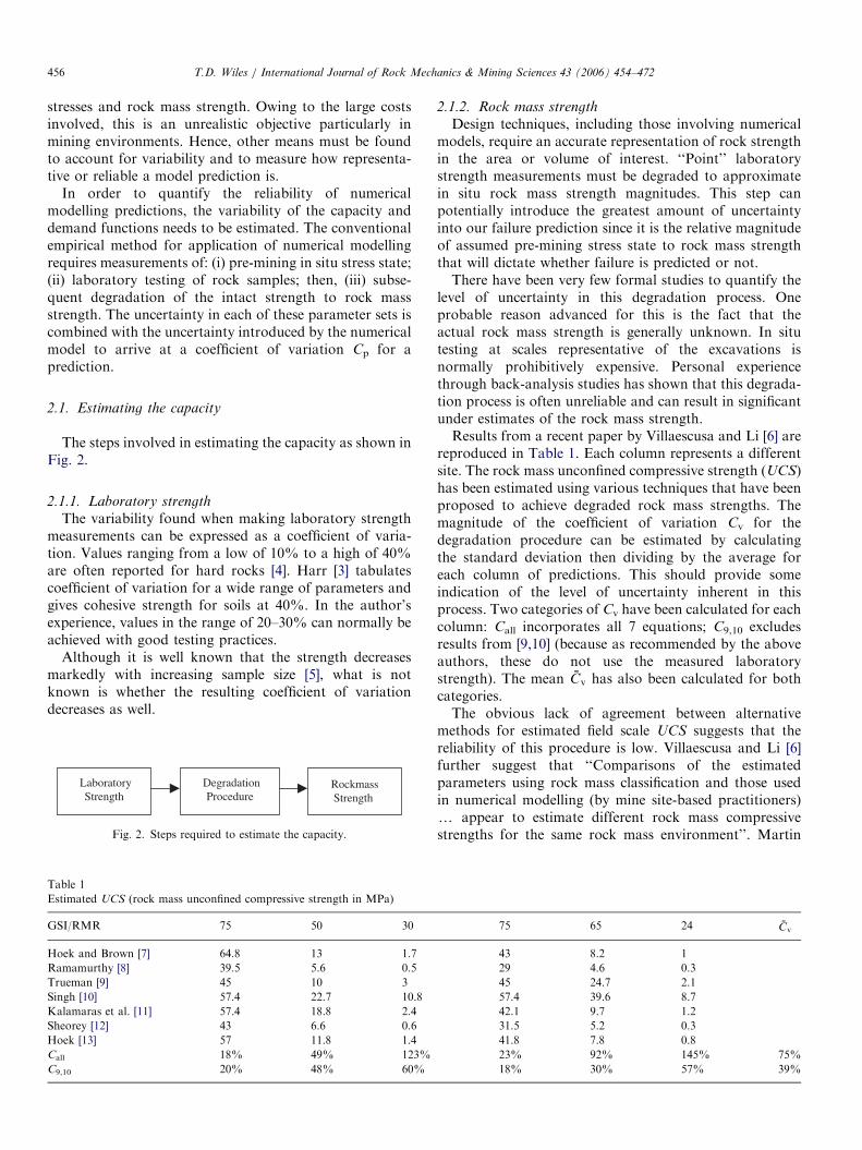
Table 1
Estimated UCS (rock mass unconfined compressive strength in MPa)
GSI/RMR 75 50 30
Hoek and Brown [7] 64.8 13 1.7
Ramamurthy [8] 39.5 5.6 0.5
Trueman [9] 45 10 3
Singh [10] 57.4 22.7 10.8
Kalamaras et al. [11] 57.4 18.8 2.4
Sheorey [12] 43 6.6 0.6
Hoek [13] 57 11.8 1.4
Call 18% 49% 123%
C9,10 20% 48% 60%
2.1.2. Rock mass strength
Design techniques, including those involving numericalmodels, require an accurate representation of rock strengthin the area or volume of interest. ‘‘Point’’ laboratorystrength measurements must be degraded to approximatein situ rock mass strength magnitudes. This step canpotentially introduce the greatest amount of uncertaintyinto our failure prediction since it is the relative magnitudeof assumed pre-mining stress state to rock mass strengththat will dictate whether failure is predicted or not.There have been very few formal studies to quantify the
level of uncertainty in this degradation process. Oneprobable reason advanced for this is the fact that theactual rock mass strength is generally unknown. In situtesting at scales representative of the excavations isnormally prohibitively expensive. Personal experiencethrough back-analysis studies has shown that this degrada-tion process is often unreliable and can result in significantunder estimates of the rock mass strength.Results from a recent paper by Villaescusa and Li [6] are
reproduced in Table 1. Each column represents a differentsite. The rock mass unconfined compressive strength (UCS)has been estimated using various techniques that have beenproposed to achieve degraded rock mass strengths. Themagnitude of the coefficient of variation Cv for thedegradation procedure can be estimated by calculatingthe standard deviation then dividing by the average foreach column of predictions. This should provide someindication of the level of uncertainty inherent in thisprocess. Two categories of Cv have been calculated for eachcolumn: Call incorporates all 7 equations; C9,10 excludesresults from [9,10] (because as recommended by the aboveauthors, these do not use the measured laboratorystrength). The mean C̄v has also been calculated for bothcategories.The obvious lack of agreement between alternative
methods for estimated field scale UCS suggests that thereliability of this procedure is low. Villaescusa and Li [6]further suggest that ‘‘Comparisons of the estimatedparameters using rock mass classification and those usedin numerical modelling (by mine site-based practitioners)y appear to estimate different rock mass compressivestrengths for the same rock mass environment’’. Martin
75 65 24 C̄v
43 8.2 1
29 4.6 0.3
45 24.7 2.1
57.4 39.6 8.7
42.1 9.7 1.2
31.5 5.2 0.3
41.8 7.8 0.8
23% 92% 145% 75%
18% 30% 57% 39%

ARTICLE IN PRESS
Table 2
Estimated and measured Coh (rock mass cohesive strength in MPa) [4]
Site CG1 CG2 FS1 M1 CH CM
GSI 74 65 65 54 60 46
Cohestimated 4.11 3.67 3.05 1.14 2.29 1.41
Cohmeasured 5.20 3.40 3.40 1.90 1.50 0.80 Coh ¼ 2:70DCoh �1.09 0.27 �0.35 �0.76 0.79 0.61 s ¼ 0:77
Table 3
Root mean square errors (RMSE) for estimated modulus of deformability
from the existing empirical equations [16]
Empirical equation RMSE (GPa) Number of tests
Bieniawski [17] 15.6 48
Asef et al. [18] 16.5 57
Serafim and Pereira [19] 8.9 9
Nicholson and Bieniawski [20] 5.6 57
Hoek and Brown [7] 8.9 33
T.D. Wiles / International Journal of Rock Mechanics & Mining Sciences 43 (2006) 454–472 457
and Maybee [14] find that the Hoek–Brown empiricalmethod over estimates hard rock pillar strengths. Hoek [2]states that his own degradation procedure ‘‘works, more bygood fortune than because of its inherent scientific merits’’.Furthermore, he states [15] ‘‘the user of the Hoek–Brownprocedure or of any other equivalent procedure forestimating rock mass properties should not assume thatthe calculations produce unique reliable numbers’’.
In a study conducted by Cai et al. [4], rock mass strengthis estimated using the Hoek–Brown method (Cohestimated)and measured using in situ block shear tests (Cohmeasured)at six different sites reported in Table 2.
The magnitude of the coefficient of variation for thedegradation procedure can be estimated by calculating astandard deviation s from the differences between theestimated and measured values (DCoh), then dividing by arepresentative stress magnitude. Here we could use theaverage of the measured values Coh or the working stresslevel of 0–5MPa suggested in the paper [4]. In either case,quite large values for Cv are indicated (i.e. 15–30%). Theauthors of this study conclude that the estimated cohesivestrengths ‘‘are generally in good agreement with field data’’despite the obvious large differences.
In a similar study by Kayabasi et al. [16], field scalevalues for the deformation modulus are estimated usingseveral different techniques and also measured using alarge number of plate loading tests. The reported rootmean square errors for the estimated and measured valuesare reproduced in Table 3.
The magnitude of the coefficient of variation can beestimated by dividing the RMSE by the measured fieldscale deformation moduli (these were mostly measured inthe range of 5–10GPa), suggesting quite large values (i.e.well over 50%). The authors of this study conclude that thelast three estimation techniques in the table ‘‘exhibitedacceptable results. In fact these results are typical’’.
Degradation techniques inherently involve subjectiveassumptions to derive a reasonable estimate of in situstrength. Uncertainty occurs because of simplification ofthe actual complex mechanisms responsible for thedegraded strength. Natural variability in the rock massdue to anisotropy, changing geology, pre-existing struc-ture, etc. is normally averaged across the mine site in anattempt to derive a single strength envelope or at best, aseries of strengths associated with broadly defined litholo-gical units. The examples that have been summarized heredemonstrate that existing empirical degradation techniques
do not agree with one another, and also do not agree withfield scale tests very well. Comments by the authors of thestudies suggest that the results they obtained are generallyexpected, acceptable and typical.From these results it would appear that the uncertainty
associated with degrading laboratory test results to fieldscale is generally unknown. It may be appropriate to assignvalues in the range of 15–30% for the coefficient ofvariation for the degradation procedure. However, thisnumber could be higher than this. It would appear thatmore work is required to confirm this.
2.2. Estimating the demand
The steps involved in estimating the demand are shownin Fig. 3.
2.2.1. Pre-mining stress state
Although the stress orientation and stress ratio can oftenbe measured with reasonable confidence, it is notoriouslydifficult to determine the pre-mining in situ stress statemagnitude by direct measurement. In addition, the localstress magnitudes can also vary quite widely across themine site [21] due to a number of factors such as structures,and variable geology within a unit, amongst others.Several hundred precision, temperature-controlled HI-
cell (CSIRO hollow inclusion cell) measurements weremade at Canada’s URL (AECL Underground ResearchLaboratory). Analysis of these very high-quality measure-ments demonstrates that the coefficient of variation forstress magnitude is in the order of 20% [22]. It was foundthat additional measurements do not reduce this varia-bility. At the same location, Martin et al. [23] calculate acoefficient of variation of approximately 20% for stress atdepth, and indicate that this increases near ground surface.

ARTICLE IN PRESS
Pre-MiningStress
Model Building
StressAnalysis
Induced Stresses
Fig. 3. Steps required to estimate the demand.
T.D. Wiles / International Journal of Rock Mechanics & Mining Sciences 43 (2006) 454–472458
One could expect even higher variability at sites where therock mass is not as uniform as at the URL.
Whether this uncertainty arises from natural variabilityof the rock mass or measurement error, this does representthe level of prediction uncertainty associated with the pre-mining stress state. The stress is normally averaged acrossthe mine site in an attempt to derive a single stress statevarying linearly with depth. Local deviations from theassumption of linearity are rarely taken into account inmodelling, even though marked improvement in accuracycan be obtained [24]. This is primarily because of the lackof detailed information regarding the pre-mining stressdistribution, but also because of the increase in complexitythis introduces to the model.
2.2.2. Model building
Model geometries can today be built quite accuratelyowing to the high quality of modern surveying and the easewith which complex 3D geometries can be built withmodern modelling packages such as Map3D [25]. Withcapacity to accommodate thousands of excavation units,there is no longer any reason for compromise in thisregard. Excavations cause stress magnifications, thusaccurate delineation of the geometry is necessary sincepillar widths, proximity of excavations and 3D spatiallocation directly affect the stress redistributions that will becalculated during the analysis. Inaccurate representation ofthe geometry can provide a large contribution to un-certainty in the final stress prediction.
2.2.3. Stress analysis
Stress analysis calculates how the pre-mining stresses aremodified due to mining. The relative magnitude of the pre-mining stress state with respect to the assumed rock massstrength directly controls the accuracy of the modellingpredictions since failure predictions require a comparisonof these to the strength. It is therefore necessary that themagnitude of both the pre-mining stress state and the rockmass strength be correctly specified to make accuratepredictions.
There will also be uncertainty in this part of the processparticularly if the rock mass is overstressed. Rock yieldingwill result in stress transfer that requires more complexinelastic models for correct simulation. This could beaccommodated through incorporation of slipping faults orgeneralized yielding of the rock mass. Unfortunately theuse of such models requires additional judgement andassumptions regarding a range of input parameters. Inelastic stress models the only significant contributingfactors are the geometry and pre-mining stress state; whilein elasto-plastic models, the strength and flow rule become
an integral part of the analysis. These assumptions changethe way the model responds and directly influences theanalysis results. Model results become loading pathdependant.It is unclear whether the increase in accuracy anticipated
by use of a more complex material model is offset by theuncertainty introduced by the additional input parameters.It is conceivable that one could obtain less reliablepredictions because of this (this is discussed in more detailin Section 5.6.2).
2.3. Combined effects—estimating Cp
It is timely to combine now the uncertainties associatedwith the laboratory strength, strength degradation to rockmass scale, pre-mining stress, and chosen modellingprocedure into a single measure of the uncertainty in ourpredictive capability. This can be expressed as a coefficientof variation Cp. The coefficients of variation from thevarious sources can be easily combined by taking thesquare root of the sum of the squares of the individualstandard deviations if it is assumed that normal distribu-tions apply and that the contributions are uncorrelated [26].Above it was shown that the uncertainty in laboratory
strength is near 20%. Uncertainty in the degradationprocedure may be in the range from 15% to 30% but couldbe higher than this. Combing these two figures gives anuncertainty in the rock mass strength estimate of 25–35%.Note that Hoek [13] calculates a value of 31% for the rockmass UCS. To determine Cp, the uncertainty in pre-miningstress (20%) and from the chosen modelling proceduremust be added. Unfortunately the later contribution isgenerally unknown. Taking square root of the sum of thesquares for all contributions it would appear that acoefficient of variation Cp of 30–40% should be expected.Realistic values are most likely higher than this, since somecontributions have not been included and others are notknown with any certainty.The implication of various magnitudes of coefficient of
variation on prediction accuracy is discussed in detailbelow.
3. Back-analysis approach
3.1. Background
To characterize the in situ variability of the stress andstrength, an alternative to attempting to quantify thevariability by actively conducting in situ measurements isto observe rock mass response during prior miningoperations. This approach can also be used to assess theapplicability of the chosen numerical modelling procedure(elastic, elasto-plastic, etc.) under similar conditions. Thisprocedure could be considered to be an application of theobservational approach to design [27].Back-analysis of observations of rock mass response to
advancing mining has the disadvantage that from an

ARTICLE IN PRESST.D. Wiles / International Journal of Rock Mechanics & Mining Sciences 43 (2006) 454–472 459
experimental perspective, the conditions are uncontrolled.‘‘It is futile ever to expect to have sufficient data to modelrock masses in the conventional (for example in electricalor aerospace engineering) way’’ [1]. This is rather unsettlingto practitioners who are used to conducting tests underwell-controlled laboratory conditions. ‘‘Our confidence inthe numerical models can be raised when they aresuccessfully calibrated against well-controlled laboratoryand in situ experiments’’ [28].
Under field conditions, precise measurements are oftennot possible or too expensive to be practical. However, inthe author’s opinion, this is more than offset by severalmajor advantages of the observational approach. A widerange of realistic shapes and loading conditions areroutinely exercised. A very large number of cases can beback analysed as part of the ongoing mining operation. Sitespecific values can be determined. Mining is of course truerock mass scale and uses the most representative shapes,stresses and conditions that are possible. Of course for thismethod to be viable, some sort of observable response mustoccur repeatedly. This can include (but is not limited to) avariety of stress-induced responses such as crack density,joint alteration, ground support requirements, blast-holecondition, ground stability, stand-up time, depth of over-break, dilution, micro-seismic activity, etc.
By using the same modelling tools for the back-analysesas will be used to make forward predictions, testing theapplicability of the chosen numerical modelling procedureis occurring. In addition, use of this method bypasses therequirement for a strength degradation procedure. Back-analysis can be viewed as a procedure for quantifying thereliability of the entire predictive system rather than any ofits individual components.
Table 4
3.2. Quantification of uncertainty
To demonstrate the proposed methodology, consider theseries of back-analyses of sill–pillar failures observedduring mining operations. These are shown as soliddiamond shapes in Fig. 4 [29–31].
0
50
100
150
200
250
300
0 10 20 30
Sigma 3 (MPa)
Sigm
a 1
(MP
a)
Linear best-fit
Fig. 4. Back-analysis of sill-pillar failures.
To obtain each of these points, a model was built and inthis case analysed elastically using Map3D [25] todetermine the stress state at the centre of each pillar atthe observed time of failure. From these back-analysesresults a best-fit strength envelope (shown as the solid-inclined line) using linear regression can easily bedetermined. It can be observed that the results are wellclustered, as the difference between individual predictionsand their average behaviour is small.It is now time to consider how the coefficient of variation
representing our predictive capability Cp from back-analysis results can be quantified. This is achieved bycalculating the mean distance from the predictions to thebest-fit line. For each back-analysis, the distance from anystress point to the best-fit line (excess stress) for a linear(Mohr–Coulomb) criterion is given by
Ds1 ¼ s1 �UCS � qs3, (2)
where s1 and s3 represent, respectively, the major andminor principal stresses, UCS and q represent, respectively,the rock mass unconfined compressive strength and slopeof the best-fit line. Ds1 is positive above the line andnegative below the line.The standard deviation s can be written
s ¼
ffiffiffiffiffiffiffiffiffiffiffiffiffiffiffiffiffiffiffiffiffiffiffiffiffiffiffiffiffiffiffiffiXDs21=ðn� 2Þ
q, (3)
where n represents the number of back-analysis points, andthe summation is taken for all n data points. Here, (n�2)represents the degrees of freedom used as a divisor to ensurean unbiased estimate. The best-fit line can be obtained byfinding that values UCS and q that minimize the magnitudeof s (i.e. linear regression) as shown in Table 4.
UCS and q can be related to the cohesion Coh andfriction angle j as follows:
UCS ¼ 2Coh tanð45þ j=2Þ,
q ¼ tan2ð45þ j=2Þ, ð4Þ
Sill–pillar back-analysis
s1 (Mpa) s3 (MPa) Ds1 (MPa)
216.9 16.9 +24.42
170.0 18.8 �30.22
218.9 20.4 +12.16
236.7 29.1 �5.49
227.3 24.5 +3.85
206.9 16.7 +15.24
145.1 10.6 �21.71
132.6 3.2 �4.05
146.2 2.0 +14.44
147.1 7.9 �8.70
s1 ¼ 184:77 UCS ¼ 123:61s3 ¼ 15:01 q ¼ 4:075s1 ¼ 40:29 Coh ¼ 30:61s3 ¼ 8:93 j ¼ 37:31s ¼ 18:39
ARTICLE IN PRESS
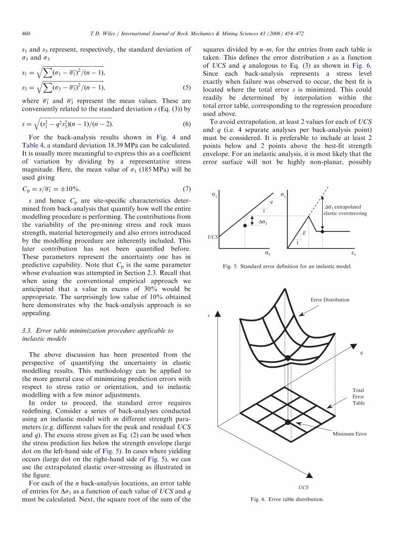
σ1
∆σ1 extrapolated elastic overstressing
σ3 ε1
σ1
UCS
1
q
1
E
∆σ1
Fig. 5. Standard error definition for an inelastic model.
UCS
q
s
Error Distribution
Minimum Error
TotalErrorTable
Fig. 6. Error table distribution.
T.D. Wiles / International Journal of Rock Mechanics & Mining Sciences 43 (2006) 454–472460
s1 and s3 represent, respectively, the standard deviation ofs1 and s3
s1 ¼
ffiffiffiffiffiffiffiffiffiffiffiffiffiffiffiffiffiffiffiffiffiffiffiffiffiffiffiffiffiffiffiffiffiffiffiffiffiffiffiffiffiffiffiffiXðs1 � s1Þ
2=ðn� 1Þq
,
s3 ¼
ffiffiffiffiffiffiffiffiffiffiffiffiffiffiffiffiffiffiffiffiffiffiffiffiffiffiffiffiffiffiffiffiffiffiffiffiffiffiffiffiffiffiffiffiXðs3 � s3Þ
2=ðn� 1Þq
, ð5Þ
where s1 and s3 represent the mean values. These areconveniently related to the standard deviation s (Eq. (3)) by
s ¼
ffiffiffiffiffiffiffiffiffiffiffiffiffiffiffiffiffiffiffiffiffiffiffiffiffiffiffiffiffiffiffiffiffiffiffiffiffiffiffiffiffiffiffiffiffiffiffiffiffiffiffiffiðs21 � q2s23Þðn� 1Þ=ðn� 2Þ
q. (6)
For the back-analysis results shown in Fig. 4 andTable 4, a standard deviation 18.39MPa can be calculated.It is usually more meaningful to express this as a coefficientof variation by dividing by a representative stressmagnitude. Here, the mean value of s1 (185MPa) will beused giving
Cp ¼ s=s1 ¼ �10%. (7)
s and hence Cp are site-specific characteristics deter-mined from back-analysis that quantify how well the entiremodelling procedure is performing. The contributions fromthe variability of the pre-mining stress and rock massstrength, material heterogeneity and also errors introducedby the modelling procedure are inherently included. Thislater contribution has not been quantified before.These parameters represent the uncertainty one has inpredictive capability. Note that Cp is the same parameterwhose evaluation was attempted in Section 2.3. Recall thatwhen using the conventional empirical approach weanticipated that a value in excess of 30% would beappropriate. The surprisingly low value of 10% obtainedhere demonstrates why the back-analysis approach is soappealing.
3.3. Error table minimization procedure applicable to
inelastic models
The above discussion has been presented from theperspective of quantifying the uncertainty in elasticmodelling results. This methodology can be applied tothe more general case of minimizing prediction errors withrespect to stress ratio or orientation, and to inelasticmodelling with a few minor adjustments.
In order to proceed, the standard error requiresredefining. Consider a series of back-analyses conductedusing an inelastic model with m different strength para-meters (e.g. different values for the peak and residual UCS
and q). The excess stress given as Eq. (2) can be used whenthe stress prediction lies below the strength envelope (largedot on the left-hand side of Fig. 5). In cases where yieldingoccurs (large dot on the right-hand side of Fig. 5), we canuse the extrapolated elastic over-stressing as illustrated inthe figure.
For each of the n back-analysis locations, an error tableof entries for Ds1 as a function of each value of UCS and q
must be calculated. Next, the square root of the sum of the
squares divided by n–m, for the entries from each table istaken. This defines the error distribution s as a functionof UCS and q analogous to Eq. (3) as shown in Fig. 6.Since each back-analysis represents a stress levelexactly when failure was observed to occur, the best fit islocated where the total error s is minimized. This couldreadily be determined by interpolation within thetotal error table, corresponding to the regression procedureused above.To avoid extrapolation, at least 2 values for each of UCS
and q (i.e. 4 separate analyses per back-analysis point)must be considered. It is preferable to include at least 2points below and 2 points above the best-fit strengthenvelope. For an inelastic analysis, it is most likely that theerror surface will not be highly non-planar, possibly

ARTICLE IN PRESST.D. Wiles / International Journal of Rock Mechanics & Mining Sciences 43 (2006) 454–472 461
discontinuous and loading path dependant, thereforemany more points may be required to identify thebest fit accurately. For example, considering 4 values foreach of value of UCS and q would require 4 to the power 2,or 16 separate analyses per back-analysis point. With 10back-analysis points, this requires 160 inelastic stressanalyses. Once the best-fit values for UCS and q aredetermined, the statistics given in Eq. (5), (6), and (7) arereadily calculated.
If a more complex strain softening material model isconsidered then there will be additional parameters thatmust be minimized. These can include: post-peak strength(2 parameters), dilation rate (1 parameter), strain-softeningrate (1 parameter), pre-peak moduli (2 parameters), post-peak moduli (2 parameters) and more. Sensitivity toloading path must also be considered. For each additionalparameter, a dimension to the error table must be added.For example with 6 parameters (i.e. m equals 6), generationof a 6 dimensional error table is needed. Requiring 4evaluations for each parameter, this would require 4 to thepower 6, or 2096 separate analyses per back-analysis point.With 10 back-analysis points, this requires 20,960 inelasticstress analyses. Realistically one may make-do with fewerback-analyses, however it is evident that error minimiza-tion will require many analyses.
This same approach could be used to minimize predic-tion errors with respect to stress ratio or orientation (orany other parameter) by specifying these later parametersas additional dimensions in the error table. This could bedone for either elastic or inelastic modelling. The approachprovides an opportunity to make use of detailed observa-tions of in situ response whether visual or from instru-mentation. This methodology can be considered to be ageneralization of direct error minimization techniques suchas under-excavation [32,33].
Even without investing any effort in error minimization,the statistics given in Eqs. (5), (6) and (7) can still be readilycalculated for any specific value of UCS and q. In this latercase only one analysis for each back-analysis point wouldneed to be conducted. Although in such a case the best-fitstrength parameters would not be used, predictions couldstill be made with these statistics.
Table 5
t distribution [26]
Pf (%) n ¼ 3 n ¼ 5
0.1 �318 �10.2
1 �31.8 �4.54
2.5 �12.7 �3.18
5 �6.31 �2.35
10 �3.08 �1.64
50 0 0
90 +3.08 +1.64
95 +6.31 +2.35
97.5 +12.7 +3.18
99 +31.8 +4.54
99.9 +318 +10.2
3.4. Probability of failure
If the assumption is that s1 is normally distributed, theprobability of failure Pf can be readily calculated byintegrating the overlapping area shown in Fig. 1
Pf ¼ NðDs1=sÞ, (8)
where N is a function that represents the area under thestandardized normal curve (Table 5 with n ¼ 1).For small data sets the calculated values for the best-fit
strength envelope and standard deviation are only un-certain estimates. This extra uncertainty can be incorpo-rated as a function of sample size n by using the t
distribution [26]
Pf ¼ TDs1sg
; n� 2
� �, (9)
where T is a function that represents the area under thestandardized t distribution curve for n�2 degrees offreedom and g is given by
g ¼
ffiffiffiffiffiffiffiffiffiffiffiffiffiffiffiffiffiffiffiffiffiffiffiffiffiffiffiffiffiffiffiffiffiffiffiffiffi1þ
1
nþðs3 � s3Þ
2
ðn� 1Þs23
s. (10)
This later factor quantifies the additional uncertaintyassociated with being at the extremities of the data range interms of s3. It represents an increasing lack of knowledgewhen s3 deviates a long way from the mean and thusprevents invalid interpolations.Given Pf, the confidence interval can be determined by
use of the inverse of this function
Ds1 ¼ sgT�1ðPf ; n� 2Þ. (11)
The 1%, 5%, 95% and 99% confidence intervalsdetermined using Eq. (11) are plotted for reference inFig. 7. Here the solid line represents the best fit (Pf of 50%)and the dashed lines represent the various confidenceintervals.The results for the t distribution are very similar to the
normal distribution except there is increased uncertainty(i.e. the confidence intervals are further from the mean)near the limits of the s3 range and for small values of n asshown in Table 5.
n ¼ 10 n ¼ 20 n ¼ 1
�4.50 �3.61 �3.09
�2.90 �2.55 �2.33
�2.31 �2.10 �1.96
�1.86 �1.73 �1.65
�1.40 �1.33 �1.28
0 0 0
+1.40 +1.33 +1.28
+1.86 +1.73 +1.65
+2.31 +2.10 +1.96
+2.90 +2.55 +2.33
+4.50 +3.61 +3.09

ARTICLE IN PRESS
0
50
100
150
200
250
300
350
0 10 20 30
Sigma 3 (MPa)
Sigm
a 1
(MP
a)
Pf = 1%
Pf = 95%
Pf = 99%
Pf = 5%
Pf = 50%
Fig. 7. Confidence intervals defined in Eq. (11).
0
50
100
150
200
250
300
0 10 20 30
Sigma 3 (MPa)
Sigm
a 1
(MP
a)
Linear best-fit
Fig. 8. Back-analysis of sill-pillar failures—fictitious data (Cv ¼ 40%).
T.D. Wiles / International Journal of Rock Mechanics & Mining Sciences 43 (2006) 454–472462
Note that for large values of n, the t distributionasymptotically approaches a normal distribution and g
asymptotically approaches unity, hence the probability offailure is given by Eq. (8).
3.5. Safety factor
The definition for safety factor from Eq. (1) can bewrittenSF ¼ ðUCS þ qs3Þ=s1. (12)
In Fig. 7 it is apparent that certain levels of stress can bedirectly associated with probability of failure. This can beexpressed by substituting for Eq. (2)SF ¼ ðUCS þ qs3Þ=ðUCS þ qs3 þ Ds1Þ. (13)
An approximate relation can be determined betweensafety factor and probability of failure by evaluating Eq.(13) at the mean (s1;s3,) and rearranging to obtain
SF ¼ 1=ð1þ Ds1=s1Þ. (14)
Now substituting Eq. (7), (10) and (11) the following can bederived
SF ¼ 1= 1þ CpT�1ðPf ; n� 2Þffiffiffiffiffiffiffiffiffiffiffiffiffiffiffiffi1þ 1=n
ph i. (15)
For large values of n this simplifies to
SF ¼ 1=½1þ CpN�1ðPf Þ�. (16)
These results demonstrate that safety factor, uncertainty(i.e. Cp), and probability of failure are closely linked. Safetyfactor determined in this way can be used as a simplifiedapproximation to the more rigorous calculation of prob-ability of failure described in the previous section.
3.6. Back-analysis approach
From the back-analysis results illustrated in Fig. 7, withenough data, it is possible to evaluate whether or not thefailure envelope should be a straight line, curved orotherwise. The goodness of fit can be readily assessed.From this simple procedure it is immediately obviouswhether the model is working or not. There is onecompelling advantage to approaching failure prediction inthis manner. If the magnitude specified for the pre-mining
stress state was too high or too low, the back-analysis results(and hence the best-fit line) would compensate simply byshifting up or down. This relieves the burden of attemptingto accurately determine the absolute magnitude of stress andstrength through direct measurement.The back-analysis results plotted with large scatter as
shown in Fig. 8 (coefficient of variation of 40%), it wouldindicate that the model is not working in this situation.This can result from technical modelling problems such as2D versus 3D, non-convergence, instability, chaotic beha-viour, geometric construction errors or numerical approx-imation errors. Perhaps, incorporation of importantgeological features such as changing lithology is required.It may be that the pre-mining stress state orientation orstress ratio assumption is incorrect. It is also possible thatan elasto-plastic, yielding model with slipping faults oryielding pillars is required. Another possibility is simplythat the back-analysis results have been collected fromdifferent lithological units and been superimposed on thesame s1 versus s3 plot. Creating a separate plot for eachlithological unit may be all that is required to resolve thedifferent strength clusters. In this case, we must decide ifthe extra costs involved with refining our procedure areworth the benefits of more accurate predictions.In any case, if results such as those pictured in Fig. 8
were obtained, it is obvious that there would be little basisfor prediction. For this reason, it is necessary to providevariability information with all modelling predictions. It isimportant to note that the fundamental difference betweenFigs. 7 and 8 is only the variability in the results. In bothfigures, the same solid line represents the best fit to theresults obtained by linear regression. This extreme has beenpresented to demonstrate the necessity of presentingvariability information along with the mean values.
4. Practical applications of variability concepts
With the failure envelope and the statistics representingpredictive uncertainty determined, it is now timely to applythis to a few examples to determine what the limits to theaccuracy of failure prediction are.

ARTICLE IN PRESST.D. Wiles / International Journal of Rock Mechanics & Mining Sciences 43 (2006) 454–472 463
4.1. Broken ground depth
This methodology can now be applied to ground supportdesign. The dead weight that the support needs to suspendis the ground that has undergone stress driven failure, and
Fig. 9. Highly stressed back.
Fig. 10. Contours of Pf—cross-section
Fig. 11. Contours of Pf—long-sectio
hence, should correspond to the ground that has beenstressed beyond the rock mass strength [34]. Consider thevertical section taken across the back of the 8m wide slotshown in Fig. 9. This figure illustartes only a small part ofthe mining excavations. Contours of probability of failureusing Eq. (9) are readily plotted as shown in Fig. 10 usingthe information determined in Table 4. In Fig. 11 it isshown how the depth of failure varies along the length ofthe same highly stressed back. Note the increaseduncertainty indicated by the thicker band of contours asyou approach the stope face.For the cross-section shown in Fig. 10, a prediction can
be made with 90% confidence (95% minus 5%) that thedepth of failure is between 1.54 and 3.0m. Otherconfidence intervals can easily be scaled off the contoursif desired. Note that the position of these contours isdirectly dependant on the magnitude of s used in Eq. (9).For a smaller value of s, a narrow range of uncertaintywould be found. Recall also that the value of s is a site-specific characteristic determined from back-analysis thatquantifies how well the modelling procedure is functioning.Details of the stresses in Fig. 10 are shown as solid
diamonds in Fig. 12, 13 and Table 6.
through the highly stressed back.
n along the highly stressed back.

ARTICLE IN PRESST.D. Wiles / International Journal of Rock Mechanics & Mining Sciences 43 (2006) 454–472464
Results in Fig. 13 confirm the predicted depth of failurebetween 1.54m and 3.0m made from the contours inFig. 10. This figure also illustrates that the results are wellrepresented by a normal distribution (shown as the hollowcircles) with a mean of 2.23m and standard deviation of0.442m.
4.2. Crown-pillar failure
The results provided in Fig. 7 and Table 4 show back-analyses of failures from the silling out stage at three
0
50
100
150
200
250
300
0 10 20 30
Sigma 3 (MPa)
Sigm
a 1
(MP
a)
Pf = 5%
Pf = 95%
Fig. 12. Stresses above the highly stressed back at 0.5m intervals.
Table 6
Details of stresses in the highly stressed back
Depth (m) s1 (MPa) s3 (MPa) Ds1/(sg) Pf
0.5 218.8 6.96 +3.31 99.5%
1 224.1 9.79 +3.07 99.2%
1.5 222.8 14.6 +2.04 96.2%
2 217.0 19.8 +0.62 72.5%
2.5 208.7 24.5 �0.74 24.0%
3 199.5 28.2 �1.85 5.12%
3.5 190.1 30.8 �2.68 1.40%
4 181.0 32.3 �3.30 0.54%
5 164.7 33.1 �4.10 0.17%
6 151.2 32.2 �4.60 0.09%
0%
20%
40%
60%
80%
100%
0Depth (m)
Pf
1 2 3 4
Fig. 13. Probability of failure above the highly stressed back.
different levels (over 2 km depth) of Inco’s Creighton Mineduring the mid-1980s (for example see Fig. 14). In all cases,the failures were obvious as the pillars failed by bursting.These bursts resulted in the displacement of considerablequantities of material varying from 7 to 200 ton.The initial silling created a 59m wide (in the vertical
direction), horizontally oriented crown-pillar as shown inFig. 15. After several years, the mechanized cut and fillmining had progressed to create a narrowing crown-pillarthat eventually failed violently at 35m width and approxi-mately a 2 to 1 height to width ratio. Let us now considerhow the above reliability concepts can be applied to predictthe onset of crown-pillar failure.Fig. 16 shows the stress state predicted from elastic
modelling for various crown-pillar widths. The soliddiamonds correspond to 8m intervals, representingtwo cuts each. Details are given in Table 7 and presentedin Fig. 17.Fig. 17 shows that a prediction can be made with 90%
confidence (95% minus 5%) that the crown-pillar will fail
Fig. 14. Geometry used for the sill-pillar back-analysis.
Fig. 15. Location of the crown-pillar failure.

ARTICLE IN PRESST.D. Wiles / International Journal of Rock Mechanics & Mining Sciences 43 (2006) 454–472 465
when its width is between 8 and 54m, or 723m. Otherconfidence intervals can be determined from Fig. 17 ifdesired. This figure also illustrates that although the resultsare skewed, they can be approximated by a normaldistribution (shown as the hollow circles) with a mean of38.3m and standard deviation of 13.8m.
Note that the positions of the confidence intervals inFig 16 are directly dependent on the magnitude of s used inEq. (9). For a smaller value of s, a narrow range ofuncertainty would be found. Recall also that the value of s
is a site-specific characteristic determined from back-analysis that quantifies how well the modelling procedure
0
50
100
150
200
250
300
0 10 20 30Sigma 3 (MPa)
Sigm
a 1
(MP
a)
Pf = 95%
Pf = 5%
Fig. 16. Stress in the crown-pillar for various pillar widths.
Table 7
Details of stresses in the crown–pillar
Width (m) s1 (MPa) s3 (MPa) Ds1/(sg) Pf
66 120.7 16.4 �3.57 0.36%
59 123.1 13.1 �2.78 1.20%
51 130.6 8.69 �1.46 9.10%
43 138.2 5.33 �0.36 36.6%
35* 141.3 3.17 +0.22 58.3%
27 150.6 2.76 +0.74 75.8%
19 164.8 4.56 +1.09 84.6%
11 183.4 6.82 +1.59 92.5%
*Failure.
0%
20%
40%
60%
80%
100%
0 10 20 30 40 50 60 70Width (m)
Pf
Fig. 17. Probability of failure in the crown-pillar.
is functioning. These results are discussed in more detailbelow.
5. Discussion
This paper has demonstrated how to quantify theaccuracy of failure predictions using numerical modelling.By considering the uncertainty of the various contributingfactors, many interesting and useful results have emerged.
5.1. Prediction reliability
The probability of failure that is acceptable is of coursedictated by the project. Harr [3] notes that most civilengineering systems are designed with a probability offailure between 1% and 5% (i.e. a reliability of 95–99%).Daehnke et al. [35] recommend using a 95% confidencelevel (5% probability of failure) for the South African goldmining industry. In non-entry mining operations it may bepossible to sustain higher probabilities of failure owing toshort-term stability requirements, or where failure maysimply mean rehabilitation rather than catastrophe.In the development of the methodology above, the
discussion thus far has been limited to the application ofnormal distributions. This simplicity has lead to manyintuitive insights. If there was a need to extend this to non-normal probability distributions, Rosenbleuth’s [36] pointestimate method, or Monte Carlo methods could beadopted. This has already been demonstrated in muchdetail [15,23].
5.2. Safety factor
Two problems can be identified with the definition ofsafety factor. The same magnitude of safety factorcorresponds to different probabilities of failure dependingon the magnitude of Cp. For example, consider twodifferent sites with two different sets of back-analysisresults. Using Eq. (10), (11) and (13), we can determine thatat s3 equals zero, a Pf of 5% requires a SF of 1.49 (with Cp
equal to 10% and n equal to 10). If at a different site (witha different set of back-analysis results) we determined thatCp was equal to 20%, the SF required would be 2.92.Widely different values for safety factor are required togive the same probability of failure depending on the localsite specific value of Cp.An additional problem is that the value of safety factor
required also depends on the magnitude of s3. Forexample, as above we can determine that at s3 equalszero, a Pf of 5% requires a SF of 1.49 (with Cp equal to10% and n equal to 10). With the same Cp, but at s3 equals15MPa, the SF required would be 1.24. This effect is toolarge to be ignored.These problems are a direct result of the definition of
safety factor and imply that the same numeric value ofsafety factor can represent different probabilities of failureand hence different levels of safety: definitely an oxymoron.

ARTICLE IN PRESST.D. Wiles / International Journal of Rock Mechanics & Mining Sciences 43 (2006) 454–472466
This safety factor only provides a unique measure of safetyunder very restrictive conditions. For these reasons it isrecommended that probability of failure be used.
5.3. Conventional empirical method for rock mass strength
estimation
The conventional numerical modelling approach re-quires measurement of the laboratory strength andsubsequent degradation to rock mass scale. The uncer-tainty in these later parameters is combined to determinean estimate of the coefficient of variation for our rock massfailure criterion. To this, the uncertainty associated withthe pre-mining in situ stress state and the stress analysisprocedure are combined to arrive at the coefficient ofvariation Cp for our predictive capability.
Taking into account these various contributions, a finalCp of 30% or more should be used. Using Eq. (16) we candetermine that this corresponds to a SF of 1.6, 2 and 3.3,respectively, for 10%, 5% and 1% probability of failure.This estimate for Cp would appear to be realistic, as theresulting safety factor does not appear to be out of linewith accepted practice. Safety factors of 2–2.5 are commonin building design. Obert and Duval [37] recommend usingvalues from 2–4 for mine pillars and sidewalls with arelatively short lifetime, and 4–8 for openings with a longlifetime. Lower values are generally recommended wherefrictional effects dominate. For rock slopes Hoek and Bray[38] quote 1.5 for cohesive strengths and 1.2 for frictionalstrength. Values from 2 to 4 are required for gravity dams,4 for concrete arch dams, and 1.2–1.5 for embankmentdams [39].
This large uncertainty does not allow for very welloptimised designs.
5.4. Back-analysis approach
An alternative methodology is proposed based on theobservational approach to design. Back-analysis results areused to determine a best-fit failure envelope that char-acterizes the combined uncertainty in pre-mining stress,rock mass strength and applicability of the chosenmodelling technique (elastic, elasto-plastic, etc.). Thecompelling advantages to this approach are many:
(1)
The ratio of pre-mining stress to rock mass strength isinherently determined as part of the calibrationprocess. This relaxes the sensitivity of predictions toassumptions regarding the pre-mining stress state andremoves the uncertainty involved with the procedurefor degradation of laboratory strength to field scalevalues.(2)
The uncertainty introduced by the chosen modellingprocedure is automatically included. Well-clusteredback-analysis results indicate when reliable modellingpredictions are obtained. Highly scattered resultsindicate problems with one or more assumptions.(3)
The coefficient of variation for the predictive capabilityis readily determined and can result in values for Cp aslow as 10%. This corresponds to a SF of 1.24 (for 5%probability of failure with n equal to 10). This isconsiderably lower than what is obtainable from theconventional empirical approach (Section 5.3), and is asite-specific value that needs to be determined throughback-analysis. This improved reliability allows forbetter-optimised designs.(4)
Back-analysis provides an opportunity to refine inputparameters by seeking values that reduce the scatter ofthe clustering about the best fit. Using the error tableminimization procedure, this can be applied to bothstrength parameters and far field stress state para-meters. With enough data, it should be possible toevaluate whether or not the failure envelope should be astraight line or curved. Local variations of the strengthand pre-mining stress state could be characterized.(5)
This can be applied to any situation where some sort ofobservable, stress-induced response occurs repeatedly.Situations where ground failure is routinely encountered(e.g. mining at high extraction ratios or in weak ground)are ideal. Envelopes corresponding to a variety ofresponses such as crack density, joint alteration, groundsupport requirements, blast-hole condition, groundstability, stand-up time, depth of over-break, dilution,micro-seismic activity, etc., can all be developed.5.5. Conclusive failure predictions
An important question here is whether the moment offailure can be predicted. In the earlier crown-pillar back-analysis, it was determined that the crown-pillar will failwhen its width is in the range of 8–54m or 723m (90%confidence, Cp of 10%, n equal to 10). This uncertaintyrepresents well over half the mining life of the pillar. Interms of predicting the exact moment of failure, this isclearly not a very useful prediction. It will be shown below(Fig. 19) that with a Cp greater than 20% we would noteven be able to predict with any certainty, whether thepillar would fail.In spite of our inability to predict the moment of failure,
we are quite certain that the crown-pillar is going to fail inthe middle 11 cuts. A more in-depth analysis [30,31]demonstrates that not only can we be confident inpredicting this failure, but by use of energy release ratecalculations, it can also be shown that the failure will be aviolent rock burst.
5.6. Refining accuracy of predictions
The accuracy of predictions can be refined in two ways,increase n and reduce Cp. If a larger number of back-analysis results were available (i.e. larger n), the results inTable 7 and Fig. 17 could be recalculated. From this itcould be predicted with 90% confidence that the crown-pillar will fail when its width is between 12 and 52m or

ARTICLE IN PRESS
0
10
20
30
40
50
60
70
80
0% 10% 20%
Cp
Wid
th (
m)
maximumpillar width
Fig. 19. Predicted crown-pillar failure width-range for various values of
Cp (90% confidence interval).
T.D. Wiles / International Journal of Rock Mechanics & Mining Sciences 43 (2006) 454–472 467
720m. This is not significantly different from theprediction made with n equal 10 (i.e. 723m). Closeexamination of Table 5 and Eq. (10) shows that the effectof sample size n is only dominant for very small samples orvery large confidence intervals. To demonstrate this, thewidth range has been calculated for a number of differentvalues for n as illustrated in Fig. 18.
There is very little to gain by back analysing more than10 data points in this case. If higher levels of confidencewere required, sensitivity to the magnitude of n would bemore pronounced.
Had the back-analysis results been more scattered givingfor example a Cp of 20%, the results in Table 7 and Fig. 17could be recalculated. From this it could be determinedthat the uncertainty would encompass the entire pillar, asshown in Fig. 19. This means that there is uncertainty as towhether the pillar is going to fail or not.
From this figure it can be observed that uncertainty as towhen the crown-pillar will fail is directly proportional tothe variability in our back-analysis results Cp (recall that inSection 2.3 we estimated a Cp of 30% or more for theconventional empirical approach).
From Fig. 19 it can be determined that in order todouble the prediction accuracy (i.e. from721 to710.5m),a Cp of 4.2% would be needed. A further reduction inuncertainty to 75m would require a Cp of 1.5%. It seemsunlikely that back-analysis results that matched observa-tions to the level of detail necessary to result in such a lowvalue are obtainable. This implies that high-accuracyconclusive predictions are not possible in this case.
5.6.1. Reducing Cp
For a given site, there is an inherent background level ofuncertainty due to the variability associated with the in situstress, strength and changing geology. The magnitude ofthis contribution could be reduced if we could spatiallycorrelate our rock mass failure criterion to match thesechanges.
Here, consideration could be given to incorporating non-homogeneous geological details into the model, aiming for
0
10
20
30
40
50
60
70
80
0 5 10 15 20n
Wid
th (
m)
large n
Fig. 18. Predicted crown-pillar failure width-range for various sample
sizes (90% confidence interval).
a better match with actual changing conditions across thesite. To achieve this it may be as simple as introducingzones with different stiffness or pre-mining stress states.Conversely, it could be as complicated as fault slipsimulation to model important structural features.A simpler alternative to modelling the geological
complexity is to determine a heterogenous rock massstrength distribution. Consistent success has been achieved[40] by broadly defining lithological units across a minesite. This benefit may arise due to actual varying rock massstrengths, or alternatively could reflect real but unknownvariations in the magnitude of the pre-mining stress state.This later explanation is quite likely if one keeps in mindthat numerical models actually calculate stress magnifica-tions of the pre-mining stress state rather than absolutevalues. In a study by the author [24], it was found thatwhen local deviations from assumed linear variation of thepre-mining stress magnitude with depth were measured andincluded in the model, remarkably accurate pillar stresspredictions were obtained.Recently, attempts have been made to reduce Cp by
directly modifying the simulated rock mass response byphysically loading the numerical model though incorpora-tion of seismicity [41,42]. This technique imposes theinelastic deformations implied by observed seismicitydirectly into the model. So far these have achieved limitedsuccess.
5.6.2. Numerical modelling technique
When large values of Cp are found from back-analysis, itis possible that this arises from use of an inappropriatemodelling technique. Obvious causes can include ill-posedmodels (2D versus 3D, non-converged, unstable, chaoticsystems), geometric construction errors or numericalapproximation errors (inadequate discretization). Thesetechnical problems while important, are not at issue here.In heavily loaded mines where significant stress transfer
occurs as a result of yielding ground, elastic models maynot provide accurate predictions. The rudiments of stresstransfer could be incorporated into an elastic model simply

ARTICLE IN PRESS
0
50
100
150
200
250
0 10 20 30
Sigma 3 (MPa)
Sigm
a 1
(MP
a)
Conventional empirical rock mass strength estimate?
Fig. 20. Conventional empirical rock mass strength estimate compared to
observed failures.
T.D. Wiles / International Journal of Rock Mechanics & Mining Sciences 43 (2006) 454–472468
by excavating failed pillars. Introducing either inelasticfault slip or elasto-plastic yielding to affect stress transfercould be considered. Block models could be used ifravelling is a dominant feature. However, caution isrequired if proceeding on this course. In addition to addingmore complex simulation capability, more assumptions areadded which can result in an increase in uncertainty.
With more parameters to adjust, it becomes progres-sively easier to achieve any specific desired result. However,this does not guarantee unique solutions since with moreparameters, many combinations of parameters may reachthe same result. Prediction reliability can only be estab-lished by comparing results based on back-analysis ofmultiple predictions under a wide range of conditions.Reliability can then be established using statistical techni-ques by comparing the difference of many individualpredictions with their average behaviour. Well-clusteredresults under a wide range of conditions would indicatereliable modelling predictions. Despite good intentions, it isentirely possible that less reliable predictions can be theoutcome. This often happens because the costs are simplytoo large to complete the number of back-analyses requiredto properly calibrate the large number of parameters usedwith inelastic models. Whereas a few dozen analyses maysuffice to test for good clustering and characterize theuncertainty in an elastic model, many thousands ofanalyses (Section 3.3) can be required for inelastic models.
Even though a complex model has the potential toprovide more accurate predictions, given a limited budgetand time, one must often choose between a well calibratedsimple model or a poorly calibrated complex one. Moreinformation may be gained by running many simplemodels rather than a few complex ones. The importanceof this issue is discussed by Starfield and Cundall [1] whosepaper focuses entirely on this issue.
If geological variability is primarily responsible for themismatch between back-analysis results and observed insitu response, then more complex inelastic modelling willnot improve prediction accuracy. Even though Creightonmine is one of the most highly stressed mines in the world(pre-mining stresses exceed 100MPa at depth), it isdoubtful that inelastic modelling would significantly reducethe Cp of 10% determined from elastic modelling for theback-analysis results presented in Fig. 7. The well-clusterednature of these results indicates very reliable modellingpredictions. Engineering effort would probably be betterdirected in attempting to spatially correlate our rock massfailure criterion to match the heterogenous rock massstrength distribution as discussed in Section 5.6.1 above.
5.7. Verification of conventional empirical strength
estimates
Once a rock mass strength estimate based on theconventional empirical method has been obtained, a com-parison between predictions and observed ground responsecan be made. The question here is how to proceed if in
doing this it was found that the strength estimate wasinaccurate and results as shown in Fig. 20 were obtained.The results shown in this figure appear to demonstrate a
possible systematic error. It is important to note that themodelling procedure is producing well-clustered consistentresults with a relatively small amount of variability (theseare the same back-analysis results considered above inFigs. 4 and 7 that give a Cp of only 10%), yet it is clear thatpredictions are unable to be made with any accuracy. Anerror should be declared in one or more of the modellingparameters.Although there are many possible sources of error, the
possibility of rock mass heterogeneity and inelastic effectscan be discounted due to well-clustered nature of thepredictions. The most likely cause would be that either thepre-mining stress magnitude or that the strength degrada-tion procedure is in error. It would be necessary at thispoint to either revise the strength estimate upwards, ordecrease the pre-mining stress magnitude until a match ofthe back-analysis results could be made.
5.8. Recommended procedure for making predictions
In view of the above discussion, recommendationsregarding application of modelling to design problemscan be made:
(1)
Accurate geometry. A good representation of thegeometry is necessary in order that stress redistribu-tions are accurately calculated during analysis. In anybut the simplest of problems this will require three-dimensional geometric representation since the proxi-mity of excavations and 3D spatial location directlyaffect the calculated stress concentrations.(2)
Simple model. Initially, the simplest possible modellingapproach should be adopted so that the least number ofparameters need to be estimated. Homogeneous, elasticmodelling is the best option since the only significantparameter that must be specified is the far-field stressstate. It is really only the stress orientation and ratio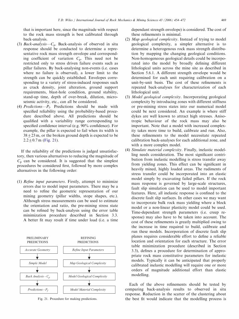
ARTICLE IN PRESST.D. Wiles / International Journal of Rock Mechanics & Mining Sciences 43 (2006) 454–472 469
that is important here, since the magnitude with respectto the rock mass strength is best calibrated throughback-analysis.
(3)
Back-analysis—Cp. Back-analysis of observed in situresponse should be conducted to determine a repre-sentative rock mass strength envelope and correspond-ing coefficient of variation Cp. This need not berestricted only to stress driven failure events such aspillar failures. By back-analysing non-events (i.e. caseswhere no failure is observed), a lower limit to thestrength can be quickly established. Envelopes corre-sponding to a variety of stress-induced responses suchas crack density, joint alteration, ground supportrequirements, blast-hole condition, ground stability,stand-up time, depth of over-break, dilution, micro-seismic activity, etc., can all be considered.(4)
Predictions—Pf. Predictions should be made withspecified reliability using the probability-based proce-dure described above. All predictions should bequalified with a variability range corresponding tospecified confidence interval (e.g. 90% confidence). Forexample, the pillar is expected to fail when its width is38723m, or the broken ground depth is expected to be2.270.7m (Fig. 21).If the reliability of the predictions is judged unsatisfac-tory, then various alternatives to reducing the magnitude ofCp can be considered. It is suggested that the simplestprocedures be considered first, followed by more complexalternatives in the following order:
(1)
Refine input parameters. Firstly, attempt to minimizeerrors due to model input parameters. There may be aneed to refine the geometric representation of ourmining geometry (pillar widths, stope shapes, etc.).Although stress measurements can be used to estimatethe orientation and ratio, the pre-mining stress statecan be refined by back-analysis using the error tableminimization procedure described in Section 3.3.A better fit may result if time under load (i.e. a timeAccurate Geometry
Simple Model
Back Analysis - Cp
Predictions - Pf
Refine Input Parameters
Map Geological Complexity
Model Geological Complexity
Model Material Complexity
PRELIMINARY PREDICTIONS
REFINING PREDICTIONS
Fig. 21. Procedure for making predictions.
dependant strength envelope) is considered. The cost ofthese refinements is minimal.
(2)
Map geological complexity. Instead of trying to modelgeological complexity, a simpler alternative is todetermine a heterogenous rock mass strength distribu-tion by mapping the changing geological conditions.Non-homogeneous geological details could be incorpo-rated into the model by broadly defining differentlithological units across the mine site as described inSection 5.6.1. A different strength envelope would bedetermined for each unit requiring calibration on aunit-by-unit basis. The cost of these refinements isrepeated back-analyses for characterization of eachlithological unit.(3)
Model geological complexity. Incorporating geologicalcomplexity by introducing zones with different stiffnessor pre-mining stress states into our numerical modelcould be next considered. An example is where stiffdykes are well known to attract high stresses. Aniso-tropic behaviour of the rock mass may also beimportant. Note that a model with increased complex-ity takes more time to build, calibrate and run. Also,these refinements to the model necessitate repeatedcalibration back-analyses for each additional zone, andwith a more complex model.(4)
Simulate material complexity. Finally, inelastic model-ling needs consideration. The most significant contri-bution from inelastic modelling is stress transfer awayfrom yielding zones. This effect can be significant inheavily mined, highly loaded areas. The rudiments ofstress transfer could be incorporated into an elasticmodel simply by excavating failed pillars. If the rockmass response is governed by large-scale structures,fault slip simulation can be used to model importantfeatures. Here, all inelastic response is confined to thediscrete fault slip surfaces. In other cases we may wantto incorporate bulk rock mass yielding where a blockmodel or a non-linear plasticity model could be used.Time-dependant strength parameters (i.e. creep re-sponse) may also have to be taken into account. Thecost of these refinements is greatly multiplied owing tothe increase in time required to build, calibrate andrun these models. Incorporation of discrete fault slipplanes requires considerable effort to define a reliablelocation and orientation for each structure. The errortable minimization procedure (described in Section3.3), defines a procedure for determination of appro-priate rock mass constitutive parameters for inelasticmodels. Typically it can be anticipated that properlycalibrated inelastic modelling will require one or moreorders of magnitude additional effort than elasticmodelling.Each of the above refinements should be tested bycomparing back-analysis results to observed in situresponse. Reduction in the scatter of the clustering aboutthe best fit would indicate that the modelling process is

ARTICLE IN PRESST.D. Wiles / International Journal of Rock Mechanics & Mining Sciences 43 (2006) 454–472470
performing better. This is the only definitive way ofdetermining whether the increased effort was justified.
Unless the effort of calibration (i.e. comparing back-analysis results to observed in situ response) is made, it isunclear whether the increase in accuracy anticipated by useof a more complex model is offset by the uncertaintyintroduced by the additional input parameters. Withoutthis calibration it is conceivable that one could obtain lessreliable predictions or at the very least, results withunknown reliability. At the very minimum, back-analysiswould be required for confirmation of model predictionsbefore any costly decisions were made based on these. Inthe final analysis, all efforts at modelling and calibrationcan only be justified if we are able to make better designdecisions. Often more questions can be answered and moreinformation can be obtained by running many simplermodels rather than a few complex ones.
In the above recommended procedure there has beenlittle emphasis placed on detailed in situ stress measure-ment, laboratory testing and degradation to rock massstrength. Whilst these procedures are the only techniquesfor gaining information under certain circumstances, theyshould only be relied on when back-analysis results are notavailable. These procedures are most appropriate inquantifying site variability, characterizing green-field sitesor anticipating changing conditions ahead of the miningface. If they are to be used, appropriate values for co-efficient of variation corresponding to each of these shouldbe combined in estimating Cp before making predictions.In all cases, the cost of using these procedures should beweighed against the benefit of conducting additional back-analyses. Many back-analyses can be completed for thesame cost as an in situ stress measurement.
6. Conclusions
Operators of underground mines are routinely facedwith decisions regarding both the safety of personnel andrisk of ore loss under limited stability ground conditions.Ultimately a ‘go–no–go’ decision must be made and this isusually done using a range of design tools, monitoring andengineering judgement. One common input in this processis from numerical models that often are used to identifypossible mechanisms of failure, and make relative compar-isons for various design alternatives. When modelling isused to make conclusive predictions, it is essential that themodelling system performance first be tested by compar-ison with back-analyses under similar conditions. In thisway, the uncertainty of the predictions can be estimatedand clearly stated. This allows appropriate assessment ofthe significance of their contribution to an overall decisionto be made relative to the many other factors therebycontributing to a cost effective, safe mining environment.
Reliability can be established by using statisticaltechniques to compare the difference of many individualpredictions with their average behaviour. Subjective agree-ment for a few isolated cases will not suffice: well-clustered
results under a wide range of conditions are required toestablish the reliability of modelling predictions. Simplerelastic models have the advantage that they can be built,executed, calibrated and interpreted with minimal effort.Although in many cases inelastic models have the potentialto provide more accurate predictions, they can requireorders of magnitude more effort for their implementation.With realistic time constraints and a limited budget, there isclearly more value in predictions from a well-calibratedsimple model, than from an inadequately calibratedcomplex model with unknown or poorly characterizedreliability. Reliable model predictions are mandatory ifdesigns based on these are also to be reliable. Better designdecisions may be made by running many simple modelsrather than a few complex ones.The observational approach is well defined and can be
easily used to quantify prediction variability with aminimum of engineering effort. This need not be restrictedonly to stress driven failure events such as pillar failures,since even non-events (i.e. cases where no failure isobserved) can be back-analysed to define a lower limit tothe strength. Envelopes corresponding to a variety ofstress-induced responses can be considered. This providessite-specific numbers that can be used to support engineer-ing judgement. Where this method can be applied, itrepresents the best way of estimating accuracy limits sinceit quantifies and demonstrates the predictive capability ofthe entire modelling system. This includes the rock massvariability, assumptions regarding input parameters, andapplicability of the chosen modelling technique.A generalized error table minimization methodology has
been described that allows field observations to be used tofind the value of any desired input parameter that results inthe best fit with modelling results. This can include bothstrength parameters and pre-mining stress state assump-tions, and is applicable to both elastic and inelasticmodelling. Using this procedure, the goodness of fit canbe determined and the prediction reliability can bequantified.An obvious limitation of the observational approach is
that observations of rock mass response are required for itsapplication. These are often not available in feasibilitystudies, ‘‘green-field’’ sites or in new mines. In such casesthe conventional empirical method for rock mass strengthestimation represents the best alternative. Efforts havebeen made here to quantify the uncertainty associated withthis method so that the uncertainty of these predictions canbe clearly stated. These estimates show that low-predictionreliability should be expected thus requiring large safetyfactors.Whether there is agreement or not as to the actual
magnitude of variability associated with the conventionalempirical approach, one thing is clear: there is largeuncertainty in the prediction accuracy obtained with thisapproach. More work needs to be done to firmly establishthe quantitative reliability associated with this method. Thelarge uncertainty associated with this procedure most likely

ARTICLE IN PRESST.D. Wiles / International Journal of Rock Mechanics & Mining Sciences 43 (2006) 454–472 471
results from errors in assumptions regarding the ratio ofpre-mining stress to rock mass strength. This can offsetcalculations from reality. This stress versus strengthmismatch is not due to any limitation of the modellingcapability, but rather, stems from an inability to accuratelyquantify the required input parameters.
High-accuracy conclusive predictions may not be possi-ble in a geological environment. It seems unlikely that thenecessary low values of Cp could ever be attained owing tothe natural variability of the rock mass. If geologicalvariability is primarily responsible for the mismatchbetween back-analysis results and observed in situresponse, then more complex inelastic modelling will notimprove prediction accuracy. Engineering effort wouldprobably be better directed in attempting to spatiallycorrelate the rock mass failure criterion to match theheterogenous rock mass strength distribution.
The definition of safety factor does not provide a uniquemeasure of safety and hence should not be used to compareone situation to another on an equal basis. Even thoughthe magnitude of safety factor can be adjusted to providethe same probability of failure depending on local siteconditions, the result will still be dependent on the localvalue of s3. This introduces unnecessary uncertainty intomodelling predictions that is readily avoided by use ofprobability methods.
The methodology proposed in this paper provides aquantitative, practical way to design underground excava-tions in a mining environment, with improved reliability.As a result, cost and safety related decisions could be madewith a known level of confidence providing us with realnumbers that can be used to backup our engineeringjudgement. The author believes that this work goes a longway towards improving on existing empirical proceduresfor design of underground excavations.
Acknowledgements
Inco is acknowledged for permitting publication ofdetails and analysis results from Creighton Mine. Theauthor is grateful for the comments from the formalreviewers and assistance of many colleagues who offeredsuggestions and constructive criticism.
References
[1] Starfield AM, Cundall PA. Towards a methodology for rock
mechanics modelling. Int J Rock Mech Min Sci 1988;25:99–106.
[2] Hoek E. The challenge of input data for rock engineering. ISRM
New J 1994;2:23–4.
[3] Harr ME. Reliability based design in civil engineering. New York:
McGraw-Hill Book Company; 1987.
[4] Cai M, Kaiser PK, Uno H, Tasaka Y, Minami M. Estimation of rock
mass deformation modulus and strength of jointed hard rock masses
using the GSI system. Int J Rock Mech Min Sci 2004;41:3–19.
[5] Martin CD. Seven years of stress measurements at the URL—an
overview, Rock mechanics contributions and challenges. In: Proceed-
ings of the 31st US Symposium. Colorado: Golden; 1990. p. 15–26.
[6] Villaescusa E, Li J. A review of empirical methods used to estimate
rock mass compressive strength and deformability in the mining
industry. MassMin Chile; 2004.
[7] Hoek E, Brown ET. Practical estimates of rock mass strength. Int
J Rock Mech Min Sci 1997;34:1165–86.
[8] Ramamurthy T. Stability of rock mass. Indian Geomech J 1986;16:1–74.
[9] Trueman R. An evaluation of strata support technique in dual life
gate roads. PhD. Thesis, University of Wales, Cardiff, 1988.
[10] Singh B. Indian case studies of squeezing grounds and experiences of
application of Barton’s Q-system. In: Workshop on Norwegian
method of tunnelling. New Delhi: CSMRS; 1993.
[11] Kalamaras GS, Bieniawski AT. A rock mass strength concept for
coal seams incorporating the effect of time. In: Proceedings of the
eighth international congress on rock mechanics, vol. 1. Rotterdam,
A.T.: ISRM, AA Balkema; 1995. p. 295–302.
[12] Sheorey PR. Empirical rock failure criteria. Rotterdam: AA
Balkema; 1997.
[13] Hoek E. Practical rock engineering. In: Hoek E, editor. Course notes.
Canada: Vancouver; 1998.
[14] Martin CD, Maybee WG. The strength of hard-rock pillars. Int
J Rock Mech Min Sci 2000;37:1239–46.
[15] Hoek E. Reliability of Hoek–Brown estimates of rock mass proper-
ties and their impact on design. Int J Rock Mech Min Sci
1998;35:63–8.
[16] Kayabasi A, Gokceoglu C, Ercanoglu M. Estimating the deformation
modulus of rock masses: A comparative study. Int J Rock Mech Min
Sci 2003;40:55–64.
[17] Bieniawski ZT. Determining rock mass deformability: Experience
from case histories. Int J Rock Mech Min Sci 1978;15:237–47.
[18] Asef MR, Reddish DJ, Lloyd PW, Mitri. Rock support interaction
analysis based on numerical modeling. Geotech Geol Eng
2000;18(1):23–37.
[19] Serafim JL, Pereira JP. Considerations on the geomechanical
classification of Bieniawski. In: Proceedings of the symposium on
engineering geology and underground openings. Portugal: Lisboa;
1983. p. 1133–44.
[20] Nicholson GA, Bieniawski ZT. A non-linear deformation modulus
based on rock mass classification. Int J Min Geol Eng 1990;8:
181–202.
[21] Hudson JA, Cooling CM. In situ rock stresses and their measurement
in the UK—Part I. The current state of knowledge. Int J Rock Mech
Min Sci 1988;25:363–9.
[22] Wiles TD, Kaiser PK. A new approach for statistical treatment of
stress tensors. Specialty Conference on Stress. Ottawa, Canada, 1990.
[23] Martin CD, Kaiser PK, Christiansson R. Stress, instability and
design of underground excavations. Int J Rock Mech Min Sci
2003;40:1027–47.
[24] Wiles TD. Accuracy and applicability of elastic stress analysis
methods in mining. In: 15th Canadian rock mechanics symposium,
Toronto, Canada, 1988, p. 207–220.
[25] Wiles TD. Map3D user’s manual, Mine modelling (Pty) report, 2005.
[26] Lipson C, Sheth NJ. Statistical design and analysis of engineering
experiments. New York: McGraw-Hill Book Company; 1973.
[27] Terzaghi K, Peck RB. Soil mechanics in engineering practice.
New York: Wiley; 1967.
[28] Jing L. A review of techniques, advances and outstanding issues in
numerical modelling for rock mechanics and rock engineering. Int
J Rock Mech Min Sci 2003;40:283–354.
[29] Marisett SD. Assessing pillar design at Inco’s Creighton mine using
the local energy release density method, MASc. Thesis, Queen’s
University, Kingston, Canada, 2001.
[30] Wiles TD, Marisett SD, Martin CD. Correlation between local
energy release density and observed bursting conditions at Creighton
mine. mine modelling report, Sudbury, Canada, 1998.
[31] Wiles TD. Rockburst prediction using numerical modelling: Realistic
limits for failure prediction Accuracy. In: Sixth international
symposium on rockbursts and seismicity in mines (RaSiM 6), Perth,
Australia, 2005.

ARTICLE IN PRESST.D. Wiles / International Journal of Rock Mechanics & Mining Sciences 43 (2006) 454–472472
[32] Wiles TD, Kaiser PK. In situ stress determination using the under-
excavation technique—I. Theory. Int J Rock Mech Min Sci 1994;
31:439–46.
[33] Wiles TD, Kaiser PK. In situ stress determination using the under-
excavation technique–II. Applications. Int J Rock Mech Min Sci
1994;31:447–56.
[34] Wiles TD, Villaescusa E, Windsor CR. Rock reinforcement design
for overstressed rock using three-dimensional numerical modeling.
In: Fifth international symposium on ground support in mining and
underground construction (ground support 2004). Australia: Perth;
2004.
[35] Daehnke A, Andersen LM, De Beer D, Esterhuizen GS, Glisson FJ,
Grodner MW, et al. Stope face support systems, SIMRAC GAP330
project report, Johannesburg, 1998.
[36] Rosenbleuth E. Two-point estimates in probabilities. J Appl Math
Modelling 1981;5:329–35.
[37] Obert L, Duval WI. Rock mechanics and the design of structures in
rock. London: Wiley; 1967.
[38] Hoek E, Bray JW. Rock slope engineering, Installation. London:
Mining and Metallurgy; 1977.
[39] Thomas HH. The engineering of large dams. London: Wiley; 1976.
[40] Nicholls D. personal communication, 1992.
[41] Lachenicht R, Wiles TD, van Aswegen G. Integration of determi-
nistic modelling with seismic monitoring for the assessment of rock
mass response to mining: Part II applications. In: Fifth international
symposium on rockbursts and seismicity in mines (RaSiM 5). South
Africa: Sandton; 2001. p. 389–96.
[42] Wiles TD, Lachenicht R, van Aswegen G. Integration of determi-
nistic modelling with seismic monitoring for the assessment of rock
mass response to mining: Part I theory. In: Fifth International
symposium on rockbursts and seismicity in Mines (RaSiM 5). South
Africa: Sandton; 2001. p. 379–88.
Related Documents