Reliability-Based Condition Assessment of Steel Containment ...

NUREG/CR-5442ORNL/TM-13244

Reliability-Based ConditionAssessment of SteelContainment and Liners

Prepared byB. Ellingwood, B. Bhattacharya, R. Zheng, JHU

The Johns Hopkins University

Oak Ridge National Laboratory

Prepared forU.S. Nuclear Regulatory Commission

RECEIVEDJ 7 (996

AVAILABILITY NOTICE

Availability of Reference Materials Cited in NRC Publications

Most documents cited in NRC publications will be available from one of the following sources:

1. The NRC Public Document Room, 2120 L Street, NW., Lower Level, Washington, DC 20555-0001

2. The Superintendent of Documents, U. S. Government Printing Office, P. O. Box 37082, Washington, DC20402-9328

3. The National Technical Information Service, Springfield, VA 22161-0002

Although the listing that follows represents the majority of documents cited in NRC publications, it is not in-tended to be exhaustive.

Referenced documents available for inspection and copying for a fee from the NRC Public Document Roominclude NRC correspondence and internal NRC memoranda; NRC bulletins, circulars, information notices, in-spection and investigation notices; licensee event reports; vendor reports and correspondence; Commissionpapers; and applicant and licensee documents and correspondence.

The following documents In the NUREG series are available for purchase from the Government Printing Office:formal NRC staff and contractor reports, NRC-sponsored conference proceedings, international agreementreports, grantee reports, and NRC booklets and brochures. Also available are regulatory guides, NRC regula-tions in the Code of Federal Regulations, and Nuclear Regulatory Commission Issuances.

Documents available from the National Technical Information Service include NUREG-series reports and tech-nical reports prepared by other Federal agencies and reports prepared by the Atomic Energy Commission,forerunner agency to the Nuclear Regulatory Commission.

Documents available from public and special technical libraries include all open literature items, such as books,journal articles, and transactions. Federal Register notices. Federal and State legislation, and congressionalreports can usually be obtained from these libraries.

Documents such as theses, dissertations, foreign reports and translations, and non-NRC conference pro-ceedings are available for purchase from the organization sponsoring the publication cited.

Single copies of NRC draft reports are available free, to the extent of supply, upon written request to the Officeof Administration, Distribution and Mail Services Section, U.S. Nuclear Regulatory Commission, Washington,DC 20555-0001.

Copies of Industry codes and standards used in a substantive manner in the NRC regulatory process are main-tained at the NRC Library, Two White Flint North, 11545 Rockville Pike, Rockville, MD 20852-2738, for use bythe public. Codes and standards are usually copyrighted and may be purchased from the originating organiza-tion or, if they are American National Standards, from the American National Standards Institute. 1430 Broad-way, New York, NY 10018-3308.

DISCLAIMER NOTICE

This report was prepared as an account of work sponsored by an agency of the United States Government.Neitherthe United States Government norany agency thereof, nor any of their employees, makes any warranty,expressed or implied, or assumes any legal liability or responsibility for any third party's use, or the results ofsuch use, of any information, apparatus, product, or process disclosed in this report, or represents that its useby such third party would not infringe privately owned rights.

Reliability-Based ConditionAssessment of SteelContainment and Liners


Manuscript Completed: October 1996Date Published: November 1996

Prepared byB. Ellingwood, B. Bhattacharya, R. Zheng, JHU

Oak Ridge National LaboratoryManaged by Lockheed Martin Energy Research CorporationOak Ridge, TN 37831

SubcontractorThe Johns Hopkins UniversityDepartment of Civil EngineeringBaltimore, MD 21218

W. E. Norris, NRC Project Manager

DISTRIBUTION OF THIS DOCUMENT IS UNLfifTED

Prepared forDivision of Engineering TechnologyOffice of Nuclear Regulatory ResearchU.S. Nuclear Regulatory CommissionWashington, DC 20555-0001NRC Job Code J6043

DISCLAIMER

This report was prepared as an account of work sponsored by an agency of theUnited States Government. Neither the United States Government nor any agencythereof, nor any of their employees, makes any warranty, express or implied, orassumes any legal liability or responsibility for the accuracy, completeness, or use-fulness of any information, apparatus, product, or process disclosed, or representsthat its use would not infringe privately owned rights. Reference herein to any spe-cific commercial product, process, or service by trade name, trademark, manufac-turer, or otherwise does not necessarily constitute or imply its endorsement, recom-mendation, or favoring by the United States Government or any agency thereof.The views and opinions of authors expressed herein do not necessarily state orreflect those of the United States Government or any agency thereof.

DISCLAIMER

Portions of this document may be illegiblein electronic image products. Images areproduced from the best available originaldocument

ABSTRACT

Steel containments and liners in nuclear power plants may be exposed to aggressive environments thatmay cause their strength and stiffness to decrease during the plant service life. Among the factors recognizedas having the potential to cause structural deterioration are uniform, pitting or crevice corrosion; fatigue,including crack initiation and propagation to fracture; elevated temperature; and irradiation. The evaluationof steel containments and liners for continued service must provide assurance that they are able to withstandfuture extreme loads during the service period with a level of reliability that is sufficient for public safety.Rational methodologies to provide such assurances can be developed using modern structural reliabilityanalysis principles that take uncertainties in loading, strength, and degradation resulting from environmentalfactors into account.

The research described in this report is in support of the Steel Containments and Liners Program beingconducted for the U.S. Nuclear Regulatory Commission by the Oak Ridge National Laboratory. The researchdemonstrates the feasibility of using reliability analysis as a tool for performing condition assessments andservice life predictions of steel containments and liners. Mathematical models that describe time-dependentchanges in steel due to aggressive environmental factors are identified, and statistical data supporting the useof these models in time-dependent reliability analysis are summarized. The analysis of steel containmentfragility is described, and simple illustrations of the impact on reliability of structural degradation are provided.The role of nondestructive evaluation in time-dependent reliability analysis, both in terms of defect detectionand sizing, is examined. A Markov model provides a tool for accounting for time-dependent changes indamage condition of a structural component or system.

iii NUREG/CR-5442

TABLE OF CONTENTS

PageABSTRACT iii

TABLE OF CONTENTS v

LKTOFTABLES vii

LISTOFFIGURES ix

ACKNOWLEDGEMENT xi

EXECUTIVE SUMMARY xiii

1. INTRODUCTION 1

1.1 Background 11.2 Project goals, objectives and scope 31.3 Organization of report 3

2. STRUCTURAL DETERIORATION AND ITS EVALUATION 52.1 Corrosion 6

2.1.1 General or uniform corrosion 62.1.2 Localized corrosion - pitting and crevice 82.1.3 Deterioration of coatings 9

2.2 Fatigue and fracture 102.2.1 Low-cycle fatigue 112.2.2 Crack propagation and fracture 132.2.3 Stress corrosion cracking 14

2.3 Elevated temperature and irradiation effects 152.4 Summary 15

3. NONDESTRUCTIVE EVALUATION METHODS 193.1 Detection of flaws 193.2 NDE techniques 22

3.2.1 Surface and near-surface methods 223.2.2 Ultrasonic inspection (UT) 233.2.3 Eddy current (EC) 233.2.4 Acoustic emission (AE) 243.2.5 Radiography (RT) 24

3.3 Flaw measurement errors 243.4 Summary 26

4. TIME-DEPENDENT RELIABILITY ANALYSIS 354.1 Probabilistic models of loads 354.2 Probabilistic models of resistance 36

4.2.1 Initial resistance 364.2.2 Time-dependent deterioration in resistance 374.2.3 Fragility modeling of steel containments and liners 38

NUREG/CR-5442

4.3 Time-dependent reliability analysis of degrading structures 414.3.1 Degradation independent of service loads 424.3.2 Illustration of time-dependent reliability - corrosion 434.3.3 Degradation dependent on service loads 454.3.4 Illustration of time-dependent reliability - fatigue 484.3.5 Reliability of Structural Systems 484.3.6 Appraisal of Structural Reliability Methods 50

4.4 Summary 51

5. TECHNIQUES FOR IN-SERVICE RISK MANAGEMENT 635.1 Overview of in-service inspection approaches 635.2 Impact of in-service inspection on reliability 645.3 Life-cycle cost analysis 665.4 Measures of risk 675.5 Summary 69

6. MARKOV PROCESS MODEL OF DAMAGE ACCUMULATION 75

7. RECOMMENDATIONS FOR FURTHER WORK 83

8. REFERENCES 85

NUREG/CR-5442 vi

LIST OF TABLES

PageTable 2.1 - Uniform corrosion parameters in Eqn 2.1 17Table 2.2 - Pitting corrosion parameters in Eqn 2.1 17

Table 4.1 - Summary of structural loads on NPPs 52Table 4.2 - Initial resistance of steel shapes and plates 53

vii NUREG/CR-5442

LIST OF FIGURES

PageFigure 2.1 Typical S-N curves for fatigue design 18

Figure 3.1 - POD curves for different models 27Figure 3.2-Probability of detection-PT and MT 28Figure 3.3 - Probability of detection - UT 29Figure3.4 Probability of detection-EC 30Figure3.5 Probability of detection-RT 31Figure 3.6 Actual vs measured crack length for PT and RT 32Figure 3.7 Actual vs measured crack depth including resolution limit 33

Figure 4.1 - Structural load stochastic models 54Figure 4.2 - Fragility family 55Figure 4.3 - Factors in fragility analysis 56Figure 4.4 - Sample functions representing structural loads and degrading resistance 57Figure 4.5 - Time-dependent reliability in tension (D + PJ:X = 0.0017/yr 58Figure 4.6 - Time-dependent reliability in tension (D + PJ ;X = 0.001/yr 59Figure 4.7 - Time-dependent reliability, with and without induction period for corrosion 60Figure 4.8 - Time-dependent reliability in flexure (D + L) 61Figure 4.9 - Time-dependent reliability in flexure, with and without induction period for corrosion . . . 62

Figure 5.1 - Bayesian updating of resistance 70Figure 5.2 - Effect of in-service inspection and maintenance on h(t) 71Figure 5.3 - CDF of corrosion depth at 10 and 40 years 72Figure 5.4 - CDF of corrosion depth, updated following inspection 73Figure 5.5 - Reliability for alternate ISI/M policies 74

ix NUREG/CR-5442

ACKNOWLEDGEMENT

The authors would like to acknowledge the advice throughout the research that has been provided by Dr. DanJ. Naus of the Oak Ridge National Laboratory, and the financial assistance through Lockheed-Martin EnergyResearch Corp. Contract No. 19X-SP638V. Appreciation also is extended to Mr. Wallace E. Norris of theDivision of Engineering Technology, U.S. Nuclear Regulatory Commission, and to Mr. C. Barry Oland ofORNL for helpful comments. The authors take full responsibility for the views expressed in this report.

xi NUREG/CR-5442

NUREG/CR-5442 Xll

EXECUTIVE SUMMARY

Steel containments and liners in nuclear power plants (NPPs) may be exposed to aggressiveenvironmental effects that may cause their strength and stiffness to decrease during the plant service life.Among the effects recognized as having the potential to cause structural deterioration are uniform, pitting orcrevice corrosion; fatigue, including crack initiation and propagation to fracture; and elevated temperaturesand irradiation. Such structural aging effects are well-recognized, at least qualitatively, in civil construction:bridges and highways, offshore structures, navigation infrastructure, and power plants. Although quantitativeevaluation of aging effects on structural behavior is possible in some areas, it remains novel in most others.In particular, the evaluation of steel containments and liners in NPPs for continued service must provideassurance that they are able to withstand future extreme loads during a service period with an acceptable levelof reliability. Rational methodologies to provide this assurance can be developed using modern structuralreliability analysis principles that take uncertainties in loading, strength and degradation resulting from theabove environmental effects into account.

The research described in this report supports the Steel Containments and Liners Program beingconducted for the U.S. Nuclear Regulatory Commission by Oak Ridge National Laboratory. The goals of theresearch are to identify mathematical models from principles of mechanics to evaluate structural degradation;to recommend statistically-based sampling plans for nondestructive evaluation (NDE) of complex structures;and to identify methods to assess the probability that containment or liner capacity has not degraded, or willnot degrade during a future service period. Section 2 reviews pertinent degradation mechanisms and associatedstatistical data, and proposes analytical methods for their treatment in condition assessment. Section 3identifies common NDE techniques, with specific regard to their usefulness in time-dependent reliabilityanalysis, flaw detection and measurement. Section 4 develops fundamental probabilistic methods for analyzingtime-dependent reliability of steel containments and liners, emphasizing corrosion and fatigue effects, andillustrates their application for simple idealized structures. Section 5 discusses the role of in-service inspection,NDE and maintenance in reliability assurance and risk management. Section 6 presents a Markov model fortracking the evolution of damage in a structure throughout its service life, making provision for the role ofperiodic in-service inspection and maintenance on time-dependent reliability. Section 7 presentsrecommendations for further work. A comprehensive bibliography on time-dependent relaiblity analysis, withparticular emphasis on reliability under conditions of corrosion and/or fatigue, concludes the report.

The first phase of this research has demonstrated the feasibility of using reliability analysis as a toolfor performing condition assessments, evaluations of existing margins of safety, and service life predictionsof steel containments and liners. Supporting statistical data and a demonstration of the application of themethodology to more complex structures are planned for the next phase of the research.

xiii NUREG/CR-5442

1. INTRODUCTION

1.1 Background

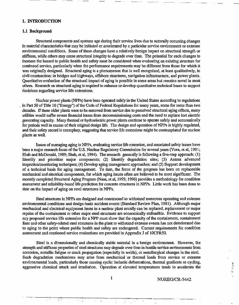
Structural components and systems age during their service lives due to naturally occurring changesin material characteristics that may be initiated or accelerated by a particular service environment or extremeenvironmental conditions. Some of these changes have a relatively benign impact on structural strength orstiffness, while others may cause structural integrity to degrade over time. The potential for such changes toincrease the hazard to public health and safety must be considered when evaluating an existing structure forcontinued service, particularly when the performance requirements may be different from those for which itwas originally designed. Structural aging is a phenomenon that is well recognized, at least qualitatively, incivil construction: in bridges and highways, offshore structures, navigation infrastructure, and power plants.Quantitative evaluation of the structural impact of aging is possible in some areas but remains novel in mostothers. Research on structural aging is required to enhance or develop quantitative technical bases to supportdecisions regarding service life extensions.

Nuclear power plants (NPPs) have been operated safely in the United States according to regulationsin Part 50 of Tide 10 ("Energy") of the Code of Federal Regulations for many years, some for more than twodecades. If these older plants were to be removed from service due to perceived structural aging effects, manyutilities would suffer severe financial losses from decommissioning costs and the need to replace lost electricgenerating capacity. Many thermal or hydroelectric power plants continue to operate safely and economicallyfor periods well in excess of their original design life. The design and operation of NPPs is highly regulated,and their safety record is exemplary, suggesting that service life extensions might be contemplated for nuclearplants as well.

Issues of managing aging in NPPs, evaluating service life extension, and associated safety issues havebeen a major research focus of the U.S. Nuclear Regulatory Commission for several years (Vora, et al, 1991;Shah and McDonald, 1989; Shah, et al, 1994). The research generally is following a five-step approach: (1)Identify and prioritize major components; (2) Identify degradation sites; (3) Assess advancedinspection/monitoring techniques; (4) Develop aging management approaches; and (5) Support developmentof a technical basis for aging management. To date, the focus of the program has been on replaceablemechanical and electrical components, for which aging issues often are believed to be most significant. Therecently completed Structural Aging Program (Naus, et al, 1993; 1996) provides a methodology for conditionassessment and reliability-based life prediction for concrete structures in NPPs. Little work has been done todate on the impact of aging on steel structures in NPPs.

Steel structures in NPPs are designed and constructed to withstand numerous operating and extremeenvironmental conditions and design-basis accident events (Standard Review Plan, 1981). Although majormechanical and electrical equipment items in a nuclear plant usually can be replaced, replacement or majorrepairs of the containment or other major steel structures are economically unfeasible. Evidence to supportany proposed service life extension for a NPP must show that the capacity of the containment, containmentliner and other safety-related steel structures in the plant to withstand extreme events has not deteriorated dueto aging to the point where public health and safety are endangered. Current requirements for conditionassessment and continued service evaluations are provided in Appendix J of 10CFR50.

Steel is a dimensionally and chemically stable material in a benign environment. However, thestrength and stiffness properties of steel structures may degrade over time in hostile service environments fromcorrosion, metallic fatigue or crack propagation (especially in welds), or metallurgical changes in the steel.Such degradation mechanisms may arise from mechanical or thermal loads from service or extremeenvironmental loads, particularly those causing cyclic inelastic deformations, thermal gradients or cycling,aggressive chemical attack and irradiation. Operation at elevated temperatures tends to accelerate the

1 NUREG/CR-5442

degradation processes. Moreover, operation at prolonged elevated temperatures can lead to synergistic effectsand accelerated damage (e.g. between creep and fatigue damage) that might not be apparent at lowertemperatures (Jaske, 1987). Steel structures that function in an aggressive environment require occasionalinspection and maintenance or repair to maintain their performance and reliability at an acceptable level (e.g.,Banon, 1994b).

An evaluation of the reliability of a steel containment or liner for a period of continued servicerequires, first of all, a knowledge of its initial design and construction. Challenges to its strength from itsservice history also must be taken into account The condition assessment and damage analysis methodologiesmust relate the significant material aging factors, environmental effects and structural loads to engineeringproperties that are needed for customary structural behavior evaluation and safety assessment. Finally, time-dependent strength and stiffness degradation, load history and inspection/maintenance policies must beintegrated into a decision tool to evaluate current and future safety or serviceability margins and to supportrational policy development. This decision tool should take into account the stochastic nature of past andfuture loads due to operating conditions and the environment, randomness in strength, and uncertainty innondestructive evaluation techniques. With these decision tools, the following issues could be addressed:

1. What aging factors are significant for steel containments and liners in terms of their futurereliability?

2. Has the original strength of the structure degraded over time as a result of corrosion, fatigue/crackgrowth, elevated operating temperatures, thermal cycling, or irradiation?

3. What is the residual structural safety margin or residual life of the containment and how would itrespond to a design-basis event?

4. Which NDE techniques (e.g., ultrasonic, acoustic emission, radiography) or in situ strengthmeasurement methods are most useful for locating strength-degrading defects and for demonstratingreliability of an existing containment?

5. What inspection procedures should be required, how frequently should they be conducted, andwhat statistically-based sampling plans should be implemented to provide the needed evidence ofreliability?

Structural reliability analysis methods provide the logical framework for decision analysis in thepresence of uncertainty (Melchers, 1987; Yao, 1986). Probability-based methods and technical data to supportcondition assessment have been developed for concrete structures in NPPs (Naus, et al, 1993; Ellingwood, andMori, 1992; Mori and Ellingwood, 1993,1994a, 1994b). Similar methods are required for steel containmentsand liners. Some rudimentary methods for making a quantitative evaluation of the residual strength orremaining service life of a steel structure based on a knowledge of its service history, present condition, andprojected use during a period of continued service already exist (Kameda and Koike, 1975; Ellingwood, 1976;Committee, 1982; DeKraker, et al, 1982; Siemes, et al, 1985; CIB, 1987; Ellingwood and Mori, 1992).Further development of such methods and their adaptation in decision-making for steel containments and linersare the subject of the proposed research.

Structural condition assessment may be required by the regulatory authority as a basis of criteria forfacility risk management. As an additional benefit, it also provides a NPP operator with cost-effective riskmanagement and decision-making tools. Such tools focus management attention on significant riskcontributors and minimize expenditures on items that have a negligible contribution to risk, thus optimizingefforts to maintain safety at a minimum cost.

NUREG/CR-5442

1.2 Project goals, objectives and scope

The overall goal of the research is to develop a methodology to permit quantitative assessments ofcurrent and future structural reliability of steel containments and liners in NPPs, taking into account serviceconditions and environmental factors that might diminish their residual safety margins during future design-basis events. This goal is supported by the following project objectives:

1. Identify mathematical models from principles of structural mechanics to evaluate degradation instrength of steel structures over time in terms of initial construction conditions, service load history,and aggressive environmental factors.

2. Recommend statistically-based sampling plans for nondestructive evaluation (NDE) of steelstructures to ensure that damage due to corrosion, fatigue cracking or other factors is detected witha specified level of confidence.

3. Develop methods to assess the probability that steel containment or liner capacity has degradedbelow a specified level or will do so during a future service period, taking into account initialconditions of the structure, service history, aging, nondestructive evaluation techniques, and in-serviceinspection/maintenance strategies.

The focus of the research is on steel containments, liners and other safety-related structuralcomponents and systems. Mechanical or electrical systems are not considered. It is assumed that the strengthdegradation and damage accumulation models and experimental data needed to support the structural reliabilityanalysis either are available or will be developed in concurrent research activities conducted in other tasks ofthe program. The research does not involve experimental testing.

1.3 Organization of report

This report summarizes the first phase of the research. Predictive models are identified from principlesof structural mechanics for assessing damage accumulation, residual strength and service life of steelcontainments and liners. Capabilities of current nondestructive evaluation methods are reviewed. Existingstructural loading data are summarized. Time-dependent reliability analysis methods for in-service conditionassessment are introduced.

Section 2 reviews degradation mechanisms that are potential contributors to deterioration of strengthor stiffness of steel structures in general and containments and liners in particular. Mathematical models arepresented for analyzing structural degradation over time.

Section 3 reviews common nondestructive evaluation techniques, with specific regard to characteristicsthat would be incorporated in a time-dependent reliability analysis or probability-based condition assessment.

Section 4 reviews fundamental probabilistic methods for analyzing time-dependent reliability of steelcontainments and liners in terms of component fragility, time-dependent limit state probability of failure, andcumulative probability of acceptable performance over a prescribed service interval.

Section 5 discusses the role of in-service inspection, nondestructive evaluation and maintenance inminimizing the impact of structural aging and in reliability assurance. Engineering decision analysis enablescompeting maintenance strategies to be evaluated in terms of risk and cost.

Section 6 presents a Markov model for tracking systematically the evolution of states of damage in

3 NUREG/CR-5442

a structure throughout its service life, including periodic in-service inspection and maintenance. Such a modelwould facilitate computerization of damage accumulation history and could provide an audit trail of facilityrisk management over a service life.

Section 7 presents recommendations for further work.

Section 8 lists references on condition assessment and reliability-based service life prediction ofcontainments and liners.

NUREG/CR-5442

2. STRUCTURAL DETERIORATION AND ITS EVALUATION

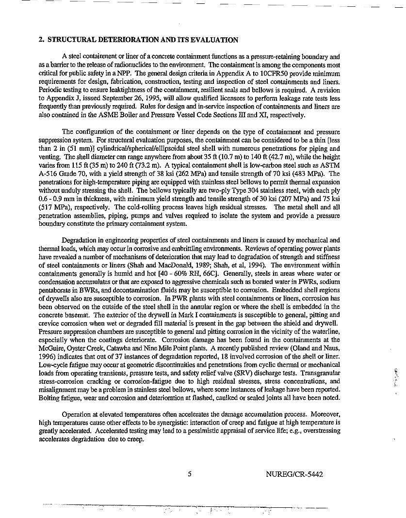
A steel containment or liner of a concrete containment functions as a pressure-retaining boundary andas a barrier to the release of radionuclides to the environment. The containment is among the components mostcritical for public safety in aNPP. The general design criteria in Appendix A to 10CFR50 provide minimumrequirements for design, fabrication, construction, testing and inspection of steel containments and liners.Periodic testing to ensure leaktightness of the containment, resilient seals and bellows is required. A revisionto Appendix J, issued September 26,1995, will allow qualified licensees to perform leakage rate tests lessfrequently than previously required. Rules for design and in-service inspection of containments and liners arealso contained in the ASME Boiler and Pressure Vessel Code Sections HI and XL respectively.

The configuration of the containment or liner depends on the type of containment and pressuresuppression system. For structural evaluation purposes, the containment can be considered to be a thin [lessthan 2 in (51 mm)] cylindrical/spherical/ellipsoidal steel shell with numerous penetrations for piping andventing. The shell diameter can range anywhere from about 35 ft (10.7 m) to 140 ft (42.7 m), while the heightvaries from 115 ft (35 m) to 240 ft (73.2 m). A typical containment shell is low-carbon steel such as ASTMA-516 Grade 70, with a yield strength of 38 ksi (262 MPa) and tensile strength of 70 ksi (483 MPa). Thepenetrations for high-temperature piping are equipped with stainless steel bellows to permit thermal expansionwithout unduly stressing the shell. The bellows typically are two-ply Type 304 stainless steel, with each ply0.6 - 0.9 mm in thickness, with minimum yield strength and tensile strength of 30 ksi (207 MPa) and 75 ksi(517 MPa), respectively. The cold-rolling process leaves high residual stresses. The metal shell and allpenetration assemblies, piping, pumps and valves required to isolate the system and provide a pressureboundary constitute the primary containment system.

Degradation in engineering properties of steel containments and liners is caused by mechanical andthermal loads, which may occur in corrosive and embrittling environments. Reviews of operating power plantshave revealed a number of mechanisms of deterioration that may lead to degradation of strength and stiffnessof steel containments or liners (Shah and MacDonald, 1989; Shah, et al, 1994). The environment withincontainments generally is humid and hot [40 - 60% RH, 66C]. Generally, steels in areas where water orcondensation accumulates or that are exposed to aggressive chemicals such as borated water in PWRs, sodiumpentaborate in BWRs, and decontamination fluids may be susceptible to corrosion. Embedded shell regionsof drywells also are susceptible to corrosion. In PWR plants with steel containments or liners, corrosion hasbeen observed on the outside of the steel shell in the annular region or where the shell is embedded in theconcrete basemat. The exterior of the drywell in Mark I containments is susceptible to general, pitting andcrevice corrosion when wet or degraded fill material is present in the gap between the shield and drywell.Pressure suppression chambers are susceptible to general and pitting corrosion in the vicinity of the waterline,especially when the coatings deteriorate. Corrosion damage has been found in the containments at theMcGuire, Oyster Creek, Catawba and Nine Mile Point plants. A recently published review (Oland and Naus,1996) indicates that out of 37 instances of degradation reported, 18 involved corrosion of the shell or liner.Low-cycle fatigue may occur at geometric discontinuities and penetrations from cyclic thermal or mechanicalloads from operating transients, pressure tests, and safety relief valve (SRV) discharge tests. Transgranularstress-corrosion cracking or corrosion-fatigue due to high residual stresses, stress concentrations, andmisalignment may be a problem in stainless steel bellows, where some instances of leakage have been reported.Bolting fatigue, wear and corrosion and deterioration at flashed, caulked or sealed joints all have been noted.

Operation at elevated temperatures often accelerates the damage accumulation process. Moreover,high temperatures cause other effects to be synergistic: interaction of creep and fatigue at high temperature isgreatly accelerated. Accelerated testing may lead to a pessimistic appraisal of service life; e.g., overstressingaccelerates degradation due to creep.

NUREG/CR-5442

The major mechanism of deterioration affecting steel structures in NPPs thus appears to be corrosion,with fatigue or corrosion/fatigue possible but less likely. Accordingly, these mechanisms are described in detailin the following sections. Since the probability distributions of damage or residual strength are required fortime-dependent reliability analysis, statistical descriptions of damage parameters also are provided, whereavailable.

2.1 Corrosion

Corrosion is an electrochemical reaction between a metal and its environment. Corrosion is the mostdamaging mechanism affecting metal containments and liners. Mechanisms that are of particular significancein carbon steels used for NPP containments, liners and other Category I steel structures are uniform corrosion,localized pitting and crevice corrosion. Intergranular or transgranular stress-corrosion may also occur, and maybe important in stainless steels. Corrosion impacts one structural limit state and one performance-related limitstate. At design load conditions, shell thinning from general corrosion may lead to gross inelastic deformationsin regions of tensile stress or instability in regions of compressive stress. Penetration of the shell by localizedcorrosion may lead to the development of a leak path and diminished pressure retention.

The electrochemistry of the corrosion process is reasonably well understood, and mathematical modelsof the electrochemical processes underlying corrosion are available (Berger, 1983). Here, we emphasize thoseaspects of the corrosion process that impact structural performance.

2.1.1 General or uniform corrosion

Uniform corrosion occurs over a large area of the surface of the component and is characterized byan essentially uniform thinning of the section. Excessive thinning due to uniform corrosion may lead to grossinelastic deformations or instability of the shell. The depth of corrosion in steel is modeled by,

X(t) = c(t-t ir (2.D

in which t = time, tj = induction or initiation time required to activate the process, C = rate parameter, and a= time-order parameter. It should be noted that Eqn 2.1 is empirical in nature. The associated corrosion rate(for purposes of comparison with experimental data) is,

dx/dt = aCtt-tj)*0 '0 (2.2)

The parameters C and a must be determined from experimental data, supplemented by knowledge of thephysics of the underlying mechanism of attack. For example, if the mechanism is diffusion-controlled, thena = 0.5. (In time-dependent reliability analysis, C, a and t; are modeled as random variables, as describedsubsequently).

An alternate expression for corrosion is (Porter, et al, 1994),

x(t) = aln(t) (2.3)

in which a is an experimental constant and the induction time has been ignored. The implied corrosion rateis proportional to 1/t.

Two general methods are recognized for estimating atmospheric corrosion-resistance of low-alloysteels (ASTM G101,1989) from test data. The first utilizes linear regression analysis of short-term data topredict long-term performance by extrapolation. The second determines a corrosion resistance index basedon chemical composition of the steel. The regression analysis presumes a log-linear relation between loss and

NUREG/CR-5442 6

time, leading to Eqn 2.1. The time-order parameter cc is invariably less than unity, indicating a decrease incorrosion rate with time. The idea of extrapolating beyond the realm of observed data violates one of the basictenets of regression analysis as a predictor. No convincing answer is provided to the question of long-termextrapolation or similitude of accelerated aging testing.

Corrosion testing is conducted mainly in the laboratory under carefully controlled conditions withsmall specimens. Corrosion'progression normally is measured by weighing and measuring material loss.Laboratory experiments often involve accelerated testing, or attempts to simulate a multi-year service life bya test of a few weeks or months. One must be cautious in using the results of such accelerated aging tests todetermine C and a, as the aging mechanisms may not scale properly from the laboratory to the serviceenvironment (Jaske, 1987; Natalie, 1987; Clifton, 1993). Physical factors that govern the corrosion processinclude temperature, residual stress, and cyclic loading rate, if cyclic loads are present. Temperature affectsoxygen solubility, pH, and corrosion product formation. In the presence of a moving fluid, the corrosion ratemay increase as fluid velocity increases. Degree of exposure - total, partial, or intermittent - also may changerate and mode of corrosion. On the other hand, the induction period normally is ignored in an acceleratedlaboratory test. Failure to include this (random) induction time has been shown to lead to a conservativeestimate of remaining service life or residual strength (Ellingwood and Mori, 1992).

Corrosion testing occasionally may be conducted in the field. Field tests may involve either smallspecimens or structural components. While environmental similitude is easier to maintain, accuratemeasurements of the corrosion process may be difficult to obtain under field conditions.

Table 2.1* summarizes average uniform corrosion parameters for carbon and weathering steels, someof which are similar to the low-carbon ferriu'c steels used for containments and liners, in several environments(Komp, 1987; Structural, 1989). These values were determined from tests of small specimens, and some errormay result from extrapolating these data to structural members. The constants C and a are such that x(t) ismeasured in |i-m when t is measured in years. Since no information or data were provided on the corrosioninduction period, it was assumed that corrosion initiated immediately and that t;= 0; this is a conservativeassumption. Some of the parameters provided by Komp (1987) have been used in reliability-based evaluationof bridge deterioration (Kayser and Nowak, 1989) and to devise bridge inspection strategies (Sommer, et al,1993). Uniform corrosion rates are dependent on the environment and ambient temperature. The uncertaintyin the corrosion rate is quite large; one reference reported a coefficient of variation of 0.7 for uniform corrosionin stainless steel containers (Porter, et al, 1994). A more typical coefficient of variation in C would be 0.3.

The time order parameter for uniform corrosion, a, is less than unity, indicating a decrease incorrosion rate with time. The initial corrosion rate in mild steels exposed to fresh or seawater is of the order200 u-m/yr (0.2mm/yr), decreasing parabolically to 100 u-m/yr after one year (Akashi, et al, 1990) as corrosionproduct film provides a protective barrier against further oxidation. The time-order parameter can be treatedas deterministic; its proximity to 0.5 suggests that corrosion might be modeled as a diffusion-type process.

m NPPs, estimated general corrosion rates from field surveys are (Shah, et al, 1994): 0.52 - 1.4 mm/yr(Oyster Creek exterior drywell shell); 0.08 mm/yr (Nine Mile Point torus interior above waterline); 1.15 mm/yr(McGuire 2, exterior of the containment); 0.33 mm/yr (McGuire 1 interior of containment). One must becautious about extrapolating such measurements to service life prediction since the corrosion rate decreaseswith time (cf Eqns 2.2 and 2.3), and corrosion measured early in a service period may not be indicative ofsubsequent performance. Coating degradation from temperature, condensation and immersion, radiation andimpact allows corrosion to initiate and spread, lifting the coating and accelerating deterioration.

* Tables and figures are placed at the end of each section.

7 NUREG/CR-5442

Possible structural degradation from uniform corrosion often is addressed in ordinary structural designby providing an extra thickness or "corrosion allowance" to the material. This allowance typically is on theorder of 1-3 mm (1/16-1/8 in) when no protective coating is provided. The maximum penetration of corrosionis a random variable and can be modeled by a Type I distribution of largest values or Gumbel distribution(Akashi, et al, 1990). Parameters of the extreme value distribution can be related empirically to the meancorrosion penetration; this then can be used to determine the 99-percentile value of loss of section due tocorrosion and thus a corrosion allowance (in mm) to ensure satisfactory performance during a service period.

The corrosion allowance approach has also been suggested for designing containers for long-termwaste storage (Marsh, 1985). Problems with long term extrapolation of data (out to 1000 years or more)necessitates very conservative assumptions regarding corrosion mechanisms. Making such assumptions,steady-state corrosion rate in low-carbon steel at 90 C is predicted to be 209 ji-m/yr. Experimental data (short-term) invariably fall below this level.

The presence of aggressive chemicals (e.g., boric acid, sodium pentaborate) can accelerate the rate ofmetallic corrosion (Czajkowski, 1990). Components known to have been affected by corrosive attack byborated water leaking through seals and valves include threaded fasteners, reactor coolant piping, pumps andvalves. Corrosion reported at the Catawba and McGuire plants was due to borated water leaking from aninstrumentation line which pooled against the metal shell. Corrosion rates up to 1.7 inches/yr (43 mm/yr) mayoccur in carbon or low-alloy steels exposed to borated water at 200 F (92 C); because of the high rate, suchcomponents cannot be designed using the corrosion allowance approach, and instead must be protected fromsuch aggressive attack.

2.1.2 Localized corrosion - pitting and crevice

Pitting and crevice corrosion are highly localized. Pits can be hidden under a surface of corrosionproducts, making detection difficult. Many nondestructive methods can locate relatively large pits but cannotdistinguish between pits and other surficial defects (Sprowls, 1987). Pitting corrosion is often identified bythe presence of surface nodulation. Problem areas usually represent only a small percentage of total surfacearea, and the local pitting usually is not accompanied by significant loss of material. However, evaluation ofthe depths of pitting corrosion is necessary to ensure the integrity of the pressure boundary. A single through-the-thickness crack is sufficient to cause leakage.

Pitting and crevice corrosion are similar in their mechanisms and descriptive mathematical models(Sprowls, 1987; Sharland, et al, 1989). The pitting process appears to be initiated by an electrochemicalbreakdown of the passive film from local acidity, inhomogeneities in the material, or other phenomena causinglocal disruption of the passive layer. Cyclic loading also can disrupt the passive layer, forming anodic areasat points of rupture and giving rise to corrosion-fatigue.

The initiation and growth of pits are not readily measured by methods that are used to evaluate uniformcorrosion. In fact, pits frequently become dormant following an initial period of growth and subsequentlyreinitiate (so-called pit birth and death - Williams, et al, 1985). However, mathematical modeling of growthof individual pits follows the same semi-empirical formulas as used for uniform corrosion (Eqns 2.1 - 2.3).In aluminum, it has been observed that pit depth is proportional to tI/3 (Sprowls, 1987). In steels, it has beenobserved (Kondo, 1989) that pit volume increases linearly with time. Assuming a hemispherical pit of radiusr and constant bulk dissolution rate B, pit volume (2/3) TCI3 = Bt, again implying that r is proportional to tm.This seems to agree well with experimental results. On the other hand, at least one study (Porter, et al, 1994)suggests that in stainless steels, pit growth is a linear function of time. Ahammed and Melchers (1995)proposed a pitting rate proportional to t "°-6. The pitting corrosion rate can be 3 x 105 to 106 times higher thangeneral corrosion (Joshi, 1994). Shibata (1994) reports an exponent of 3.42 in Eqn 2.1.

NUREG/CR-5442

Local pitting corrosion penetration is related to anodic current density (Marsh, et al, 1985). Maximumpit depths were measured over an area of approx 3 m2 in carbon steel specimens tested in NaHCO3 + Cl'forperiods of up to 1.1 years. These data were analyzed at different exposure times using statistics of extremes.Results indicated that maximum pitting depth was related to time by x,^ = 8.35 t0M, where t is in yr and x,în mm. Extrapolation of these data to a 1000-yr life yielded a pit depth of 200 mm; however, the validity ofthis extrapolation clearly is questionable and without doubt conservative.

Table 2.2 summarizes data on pitting corrosion identified by a literature search. Although only limiteddata were identified, it is clear that the rate of pit growth is potentially much higher than that of uniformcorrosion.

Limited statistical studies have been performed for pitting corrosion depth. When several pits arepresent, the maximum pit depth x ^ within an area is of more interest than the distribution of individual pitdepths. xmax has been reported to be a linear function of the log of exposed area (Aziz, 1956; Joshi, 1994).The distribution of maximum pit size can be determined from the individual pit depths using extreme valuestatistics (Sprowls, 1987; Kondo, 1989), assuming that the pit depths are statistically independent (Joshi, 1994;Scarf and Laycock, 1994; Shibata, 1994).

Mola, et al (1990) developed a stochastic model for pitting corrosion. They assumed that the number,N(t), of pits at time, t, is a Poisson process, dependent on the mean surface area and random initiation time.The growth in pit surface area is described by a stochastic finite difference equation. Provan and Rodriguez(1989) modeled the growth in maximum pit depth as a discrete-space, continuous-time Markov process. Theevolution of the probability density of pit depth in time was described by a Kolmogorov forward differentialequation. A laboratory program conducted as part of this study found that the mean and variance of maximumpit depth were proportional to f and P, respectively, where 0 < a,b< 1. The probability distribution ofmaximum pit depth was found to be Type I extreme value at different exposure periods, with mode and scaleparameters that increase linearly with time (Strutt, et al, 1985).

In a electrochemical rather than structural engineering approach (Gabrielli, et al, 1990), changes incurrent during corrosion were measured and analyzed statistically. The "survival probability" was theprobability that the electrode remained unpitted. The probability of survival was found to be,

L(t) = exp(-A(t)t) (2.4)

in which A(t) = time-dependent pit generation rate. IF the surface area is divided into small elementary areas,pitting in each area can be treated as statistically independent events. The maximum pit depth was describedby a Type I distribution of largest values. If depth increases by x = b log t + c, then dx/dt = b/t and time atwhich the maxmum pit penetrates the thickness of the component is described by a Weibull probabilitydistribution. This time-dependent model does not take into account birth and death processes of pits.Moreover, pit initiation cannot be modeled as a Poisson process with stationary increments, since the intervalsare not independent and occurrences have a tendency to cluster.

2.1.3 Deterioration of coatings

Coatings protect the structure from corrosion and facilitate decontamination. Coating degradation canoccur due to elevated temperatures, excessive moisture, radiation, and mechanical abrasion and chipping.Localized problems occur before general failure of the coating system. Once corrosion initiates, however,failure of the coating system accelerates.

Many plant owners already have found it necessary to perform local repairs of coating systems, andit seems likely that such repairs will continue to be needed at regular intervals during an extended service life.

9 NUREG/CR-5442

Fortunately, coating maintenance usually can be performed along with other required maintanance activities.Underwater-cured epoxy is a common solution for spot repairs of coatings in tanks and supression chambers.Coating performance thus does not appear to be a significant consideration in developing reliability-basedcondition assessment methodologies.

2.2 Fatigue and fracture

Metals contain voids and inclusions at the microscopic level. In addition, a structural component maycontain surficial geometric discontinuities (weld undercuts, reentrant corners, holes) or local damage (cracks,corrosion loss) that cause stress concentrations. In the presence of cyclic loads, these subcritical defects maygrow and cause fatigue in the metal, eventually leading to failure at loads much smaller than the staticallyapplied monotonic load causing failure.

The loads applied to a NPP structure may be cyclic in nature. Sources of operational cyclic thermaland mechanical loads in a containment include startup/shutdown thermal transients, pipe reactions, SRVdischarge test loads, crane and refueling loads. Although extreme environmental events such as earthquakesmay also induce cycling, the rate of occurrence and duration of such events is sufficiently small that they wouldnot cause fatigue damage to accumulate.

Early NPP steel structures and components were designed with little consideration for fatigue. Sincethe late 1960's, however, design requirements for RPVs and Class 1 piping have included fatigueconsiderations (Ware, et al, 1995). Current fatigue design analyses are aimed at demonstrating that acomponent has a cumulative use factor (computed from a Palmgren-Miner analysis, to be describedsubsequently) of less than 1.0 at the end of a 40-year design life. The analysis is made with conservativeassumptions regarding the number and magnitude of operating transients. Several fatigue monitoring programsare under development in the U. S., aimed at determining increases in the cumulative usage factor on-line asa function of operating transients.

Fatigue is not believed to be a significant problem in steel containments and liners except at pointsof structural discontinuities (weld undercuts, etc.), or heavy weldraents where residual stresses may approachyield. Most full-penetration thick welds in NPP containments are stress-relieved, so residual stresses are nota problem at such sites. Ductile carbon steels of the type used in containments and liners are not susceptibleto low-cycle fatigue, and can withstand numerous reversals of moderate inelastic strain without failure.However, general corrosion may cause the surface of the shell to become rough, causing local stressconcentrations, and corrosion pits also may serve as sites for fatigue crack initiation and growth. Crackinitiation time can be reduced by a factor of as much as three when pitting is present. An exception to thegeneral fatigue insensitivity of the containment is the stainless steel bellows at Mark I containmentpenetrations, which have high residual stresses from cold-rolling and are susceptible to low-cycle fatigue andstress-corrosion cracking.

It is convenient to envision three stages in the fatigue process: (1) crack initiation; (2) stable(subcritical) crack growth; and (3) unstable crack growth or fast fracture. The third stage occurs so rapidly incomparison with the first two that it can be ignored in service life predictions. Crack initiation and growthprocesses are driven by different factors. The initiation phase reflects interactions of the metal with the bulkenvironment. Dislocations due to slip lead to highly localized stresses that nucleate a macroscopic crack thatthen propagates. In the crack growth phase, the local crack tip environment, which may be different from bulkenvironment, determines the process. The relative contributions of these phases depend on the load spectrum,material characteristics, and initial condition of the component. If the structure is essentially defect-free andthe stress range is low, most of the life of the structure is consumed in initiating a detectable flaw. On the otherhand, many welded components contain initial flaws (lack of fusion, penetration), and in such components,there is essentially no initiation phase. A facility for analyzing both phases of fatigue is required in condition

NUREG/CR-5442 10

assessment. Fatigue often is thought of as having two domains: (1) low-cycle fatigue, with service life of100.000 cycles or less, and (2) high-cycle fatigue, with service life of more than 100,000 cycles. In the latter,the metal initially is essentially defect-free and cyclic stresses remain in the elastic range.

During a service load history involving time-varying or cyclic loads, failure can occur by singleoverload or by accumulation of damage (Madsen, 1982). In failure analysis, "damage" is an aggregatedparameter describing the macroscopic appearance or manifestation of functional impairment. There may beno immediate relation between damage and measurable physical quantities (this is the case prior to visiblecrack initiation, where microstructural changes cannot be detected by the usual field inspection methods), orthe relation may be quite obvious (crack propagation). Time-dependent reliability methods and conditionassessment procedures must be tailored to these realities. Sources of uncertainty in fatigue modeling includerandom load and material properties, system modeling, damage accumulation law, and defect size. The stateof the art of probabilistic fatigue analysis was reviewed in a series of four papers by the Committee on Fatigueand Fracture Reliability (Committee, 1982).

2.2.1 Low-cycle fatigue

All models used to analyze fatigue are empirical to a degree, with parameters that are dependent onthe metal and its service environment and are determined by testing small specimens under cyclic load. Theprimary load parameter affecting fatigue is the stress (or strain) range, A S = S,^ - S^ . Other factors that maybe important in varying degrees include mean stress (or stress ratio, R = SmiI/Smax), load sequence, and cyclicfrequency. Fatigue life to "failure" is defined in a number of ways: as time (or number of cycles) to completefracture of the specimen; as time required for a specified increase in specimen compliance; or as time toinitiation of detectable (and presumably repairable) cracking. When utilizing experimental data to developfatigue assessment procedures, it is essential to understand the relation between "failure" as it relates to thepeformance of the structure in service and "failure" as it is defined in the experimental fatigue database. It issurprising how often analysts ignore these differences.

The most common way of expressing the fatigue life of a component in terms of the number of cyclesto "failure," N, is through the well-known S-N relation between stress and cycles,

N(AS)m = C (2.5)

in which A S = applied stress range and m and C are experimental constants. When the fatigue testing isdeformation-controlled rather than load-controlled, stress range is often replaced with total strain range orplastic strain range. Eqn 2.5 is sometimes referred to as the Basquin equation. A more general model is theCoffin-Manson equation (discussed in Committee, 1982)

A e/2 = (o,/E) (2N)b + ef (2N)C (2.6)

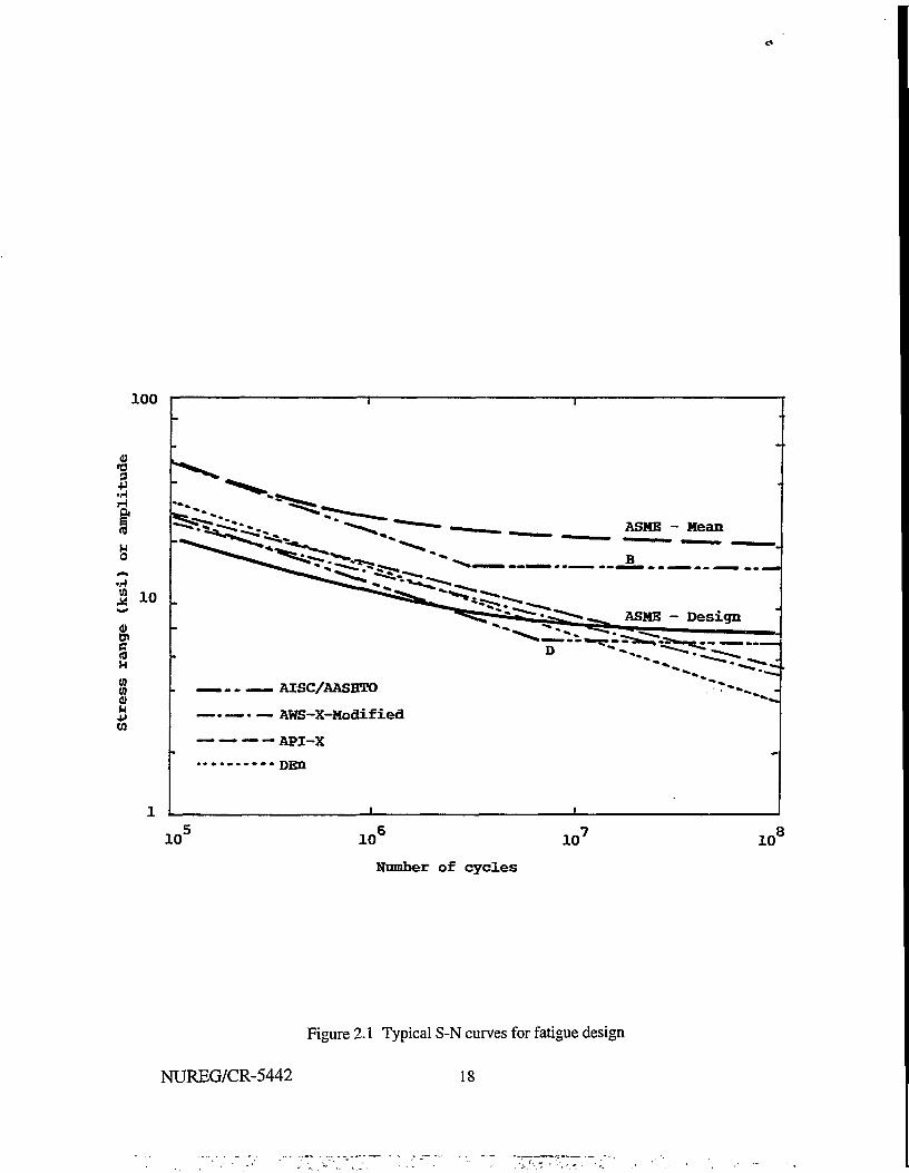
in which A e = strain range, E = modulus of elasticity, and of, ef, b and c = experimental constants. The firstterm is equivalent to Eqn 2.5, expressed in terms of elastic strain; the second term dominates in the low-cycleregime, where the cycling is inelastic. Several typical S-N curves used in design are illustrated in Figure 2.1.They are based on different testing conditions and load cycling. However, the tests were conducted in air. Thecurves labeled AISC/AASHTO B and D are based on fatigue tests of welded details found in buildings andbridges, and cycling was load-controlled and mainly from zero to maximum tension (R = 0). Curves AWS-X,API-X and DEn are found in design guides developed by the American Welding Society, America PetroleumInstitute, and the United Kingdom Department of Energy, respectively. In contrast, the curves labeled "ASMEmean" and "ASME design" are based on tests of small smooth polished specimens tested with fully reversedstrain-controlled cycling (R = -1). The ASME curves plot stress amplitude, computed as Sa = EAe/2 in whichA e is strain ranged defined in Eqn 2.6. Note that the exponent m is approximately 3 in all cases; in a corrosive

11 NUREG/CR-5442

environment, m increases to the range 3.5 - 4.0. The rate parameter, C, is dependent on the specimengeometry, yield strength of the material, and frequency at which the cyclic load is applied. Interestingly, thedependency of C on yield strength is not especially strong, implying that increases in yield strength and fatiguestrength are not commensurate with each other.

Fatigue test data presented in the form of S-N curves indicate a substantial inherent variability aboutthe median curve; coefficients of variation in fatigue life at a given stress commonly are on the order of 0.30 -0.60 (Committee, 1982). This inherent variability can be displayed by presenting the S-N curves as a/amityof curves at different cumulative probabilities, or P-S-N curves (Provan, 1987). In developing fatigue curvesfor design purposes, one might select a 5 percentile or 10 percentile curve. However, in developing fatiguecurves for design purposes from experimental data, it has been customary to divide the stress and/orcorresponding median life by deterministic factors of safety. For example, in ASME Code Section m, medianlow-cycle (controlled strain) fatigue curves were lowered by factors of 2 on stress and 20 on cycles to obtaindesign fatigue curves. These adjustments are intended to account for scatter in data, size effects, surface finish,and environmental effects. More recent studies indicate that these ASME curves may not addressenvironmental effects in the low-cycle (strain greater than 0.1%) range (Keisler, et al, 1994). Data fromseveral samples of smooth specimens tested under fully reversed strain cycling (R = -1) were analyzed.Temperature (in air), percentage dissolved oxygen and strain rate (in aqueous solution) had the most significantimpact. Strain rate in air or characteristics of load vs time had little effect on fatigue life.

Because of economic limitations, most fatigue data are determined by testing small, smooth specimensunder carefully controlled conditions. Most structural components that are susceptible to fatigue damage areneither small and smooth nor subject to constant amplitude cycling. Fatigue damage is most likely to initiateand develop at weld undercuts and other stress raisers (notches) where the local stress (or strain) is amplifiedby a significant factor above the "far-field stress" (or strain) computed from a finite element analysis. Suchlocal effects are not included within the normal factors of safety on smooth-specimen fatigue curves alludedto above. The question arises as to how to deal with such local effects.

One approach is to conduct fatigue tests of larger specimens containing representations of the fatigue-critical structural detail. This has, in fact, been done for civil structures; over a period of three decades fromthe 1950's to the 1980's, numerous fatigue tests of representative bolted and welded details mainlyrepresentative for bridge structures were conducted at Lehigh University, the University of Illinois, and otherinstitutions (reviewed by Keating and Fisher, 1986). The test results were collected in six main categories ofdetails (curves for two categories - B and D - are illustrated in Figure 2.1), and allowable cyclic stresses forfour main load conditions were determined with an appropriate factor of safety. The results can be seen inAppendix K of the new LRFD Specification (LRFD, 1993). Such an approach, while acceptable for routinedesign of civil structures where details are repetitive, may be unduly conservative when applied to a specificfatigue-critical detail. Thus, its use in condition assessment of a set of specific details in a structural systemmay not provide uniform or consistent reliability among these details. Moreover, in light of recent advancesin computational ability to analyze complex nonlinear stress-strain histories accurately, it is a highly inefficientmethod for condition assessment.

Smooth-specimen fatigue curves can be used to determine fatigue behavior of structural componentswith stress raisers, provided that the local stress-strain history at the notch can be analyzed. If the materialremains entirely elastic, the local maximum stress (or strain) at a notch is the product of the far-field stress anda stress concentration factor, IQ However, when the material local to the notch is stressed beyond the elasticrange, the local stresses and strains can no longer be determined from Kt. Studies (Ellingwood, 1976) haveshown that Neuber's rule (Topper, et al,1969 ) can be used in this case to determine the local stress-strainhistory at the notch needed to utilize smooth-specimen fatigue data. Neuber's rule postulates that the productof local stress and strain is proportional to the product of far-field elastic stress and strain, or,

NUREG/CR-5442 12

Aa Ae = k / AS Ae (2.7)

in which kf is an effective stress concentration factor and the elastic stress, AS, can be determined by finiteelement analysis or other conventional structural analysis procedure. The second condition needed fordetermining Aoand Ae is given by the constitutive model for the material. Assuming, for example, aRamberg-Osgood law,

e = K(o)n (2.8)

in which K = compliance and n = strain-hardening exponent, one would obtain,1

Ao = [(k fAS)2/KE]M (2.9)

Entering the S-N curve at this value of A o would give the fatigue life of the detail.

When the load amplitudes vary in time, the number of cycles to failure (or time to failure) must bedetermined from a cumulative damage law. Such laws relate fatigue behavior under variable amplitudeloading to the known behavior under constant amplitude cycling which can be determined from experiments.The most commonly used of these laws is the Palmgren-Miner hypothesis, which postulates that damageaccumulates linearly simply as a function of the number of cycles at a particular stress (or strain) level. Undervariable amplitude loading, then, damage accumulation, D, is described by,

D = £ A D i - £ C-1 (ASjT (2.10)i i-1

in which N = number of load cycles and, ADj = increment of damage in cycle i . If the load history consistsof k discrete load amplitudes, Eqn 2.10 takes the more familiar form,

D =

in which nj = number of cycles in the load history at stress level ASj, N(ASj) = number of cycles to failureunder constant amplitude loading AS;, determined from Eqns 2.5 or 2.6, andS n;=N. When the cycles arenot clearly defined, as is sometimes the case in broad-band excitation, rainflow cycle counting can be used todetermine ^ (Barson and Rolfe, 1987). (This necessitates a time-domain rather than frequency-domainanalysis.) The Palmgren-Miner hypothesis asserts that failure occurs when D > 1.0.

The Palmgren-Miner damage hypothesis does not account for stress sequence effects on fatigue life.However, reviews of other damage accumulation theories indicate that other, more complex, rules do notprovide consistently better results (Committee, 1982).

2.2.2 Crack propagation and fracture

Growth of an existing crack, once initiated, can be predicted by fracture mechanics analysis (Broek,1988). Under the domain of applicability of linear elastic fracture mechanics (LEFM), unstable crack growthleading to fracture initiates when,

K>KIC (2.12)

in which Kfc = (plane strain) fracture toughness and K = stress intensity. The plane strain fracture toughnessis a material-dependent parameter dependent on temperature, rate of loading, and the environment. For mild

13 NUREG/CR-5442

steel at ambient conditions, KIC typically is about 140 MNm"3/2, and its coefficient of variation typically is about0.15. The stress intensity is,

K = Y(a)ayfita. (2.13)

in which a = far-field stress, a = characteristic crack size, and Y(a) = correction factor based on relative cracksize and shape and far-field loading. For a large plate in tension with a center crack (through the platethickness) of length 2a, Y(a) = 1.0; for a penny-shaped crack within the plate with radius a, Y(a) = 2/n; andfor an edge crack loaded in tension or flexural tension with depth a less than half the thickness, Y(a) = 1.12.Procedures are also available for modeling nonlinear behavior; the J-integral and crack-opening displacementapproaches are two such procedures.

Fatigue crack growth (leading to increases in Kj up to Klc) is most commonly modeled using the Parisequation (Barsom and Rolfe, 1987),

da/dN = C(AK)m (2.14)

in which AK = range of fluctuating stress intensity factor, obtained by replacing a by A a in Eqn 2.13, andC and m are experimental constants (unrelated to the C, m in Eqn 2.5). With the stress history known, Eqn2.14 can be integrated to determine the crack size as a function of elapsed cycles, N. Refinements to Eqn 2.14for incorporating the mean stress or stress ratio^n/Sn^, the threshold for crack growth, K ,, and other factorsknown to affect crack growth rate, are available (Dowling, 1993)^ These effects generally have a second-ordereffect on predicted defect growth.

The crack growth analysis becomes difficult when several cracks grow simultaneously and interactionfor cracks in close proximity may occur. In this case, the rate at which fractured area is produced may be moremeaningful than crack growth rate. This suggests a "damage mechanics" approach, where multiple flaws aresmeared (Kachanov, 1986).

Current analysis and design procedures do not consider possible synergistic effects of corrosion froman aggressive environment and fatigue from mechanical or thermal loads. The corrosion-fatigue processconsists of several stages: pit formation and growth, crack formation from the pit (assuming corrosion pit canbe modeled as a sharp crack), coalescence and corrosion-fatigue crack propagation (Kondo, 1989). Post-failurefractographic investigations have revealed that a pit (or pits) is often the origin of the fracture surface, meaningthat pit initiation and coalescence is the trigger for fatigue crack initiation. The transition of a pit into a crackoccurs at a stress intensity of about K = 1.2 MPa(m)lc for low-alloy steel; this is below the threshold for a longplanar surface flaw (Kondo, 1989).

2.2.3 Stress corrosion cracking

Stress-corrosion cracking (SCC) and fatigue damage may occur in the bellows, which are subjectedto reversals in deformations due to heating and cooling during normal operation, pressure loads during leakrate tests, and high residual stresses. Maximum bellows deformations are 13 - 50 mm due to thermalexpansion; such cycles may occur on the order of 1000 - 5000 times during a 40-year service life.

The initiation of SCC on a surface appears to be primarily dependent on mechanically or chemically-induced rupture of the protective film (depassivation). This gives rise to acidity in occluded areas anddevelopment of local pitting or crevice corrosion at sites where cracking subsequently may initiate (Marsh,1985; Kobayashi, et al, 1991). Stress-corrosion cracking can also initiate at sites within the interior of acomponent, even in the presence of an aggressive external environment. Interior microcrack formation appearsto occur first where intergranular features are smooth rather than coarse, regardless of where such sites occur.

NUREG/CR-5442 14

The metal must be stressed in tension above a threshold stress or stress intensity level for SCC to initiate andprogress. Once initiated, stress-corrosion crack growth occurs at a much higher rate than either general orpitting corrosion, and even the minimum rate is too great for a corrosion allowance approach to design.

SCC is troublesome for time-dependent reliability analysis. It is difficult to analyze mathematicallyand to detect or repair prior to component failure. There is no unique definition of when localized corrosionchanges into a stress-corrosion crack. Several cracks may initiate and repassivate prior to the time at whicha dominant crack forms and propagates. Unexpected SCC problems in NPPs are costly to repair and raiseadditional safety concerns that are difficult to resolve. There are no satisfactory accelerated test methods(Kobayashi, et al, 1991) for SCC.

2.3 Elevated temperature and irradiation effects

Temperatures required for permanent degradation in strength or stiffness of carbon steel must be onthe order of 500 C. Similarly, embrittlement of reactor pressure vessel steels has been noted for neutronradiation with fluence greater than 1019n/cm2 (Chopra, et al, 1991). Since the containment is unlikely to seesuch levels of exposure, strength reduction due to prolonged elevated temperatures or radiation embrittlementof the metal containment shell is not generally a concern. Such effects may be of more, concern for the RPVand certain piping within the NPP. Neutron fluence of 1019 n/cm2 causes plane strain fracture toughness Klc

in the reactor pressure vessel material to reduce by about 20% during 40 years (Yoshimura, et al, 1993). Suchfluences do not occur in the containment. On the other hand, creep can occur at elevated temperatures,introducing residual stresses or deformations (Murakami and Mizuno, 1991).

2.4 Summary

Rogers (1990) laments that "it is surprising that in the literature of corrosion failure prediction thereare very few instances where statistical methods are applied." Commenting on fatigue crack growth two yearsearlier, Broek (1988) noted that "there are probably as many equations as there are researchers in the field,"and "no equation can fit all data." There is substantial uncertainty, both inherent variability and modelingerror, in modeling fatigue, corrosion, and their combinations, and in drawing inferences regarding their currentand future impact on structural behavior.

Fatigue analysis methodology for predicting service life and margins of safety must rely heavily onsmall specimen testing coupled with advanced (nonlinear) computational procedures. There seems to be littleprospect of using in-service data to develop models for predicting damage accumulation, other than in aqualitative sense. Failure rates in properly designed and fabricated structures are very small. Observationsof in-service data to infer actual failure rates either involve extreme censoring of data or accelerated life testing.In an accelerated test, failure mechanisms may not scale as in the prototype. Extrapolation of such data ishighly questionable. Moreover, early failures in service may derive from defects at assembly, error infabrication, etc. It has been suggested (Strelec, 1993) that an "acceleration function" could be developed tomake the time-dependent reliabilities the same under service and accelerated conditions. The accelerationfunction must be assumed; several have been proposed in which limited data have been used to estimate theempirical constants in the model statistically. However, this approach is empirical rather than mechanistic,as the scaling is done to preserve equal probabilities.

In modeling damage accumulation due to structural aging, it is important to measure microstructuralparameters that correlate with an engineering property useful for structural evaluation. A review of theliterature reveals that this often is not done, making much of the literature on material aging of limited use forstructural evaluation purposes. Damage parameters in structural condition assessment must be defined to beconsistent with detection parameters in common NDE methods. This is one difficulty in using the traditionalS-N/Palmgren-Miner approach to analyzing fatigue. "Damage" in this approach evolves with cycles (or with

15 NUREG/CR-5442

time) in a way that cannot be measured by conventional NDE methods. As a result, the residual strength ofa structure or component at some intermediate stage of damage evolution cannot be evaluated. Anotherexample of this is the use of half-cell potential measurements to evaluate corrosion; this method can detectlikely corrosion zones but cannot determine loss of section needed for structural calculations. In contrast, thedetectability of a particular crack size can be related to the NDE method selected, as will be shown in Section3. However, ignoring the crack initiation phase may lead to an overly pessimistic appraisal of residual strengthor remaining service life.

For accurate condition assessment and service life prediction, there is a need to track the evolution ofmicrostructural damage prior to the state where there is some detectable manifestation of deterioration. Therelatively new field of continuum damage mechanics (Kachanov, 1986; Chaboche, 1988; Lemaitre, 1992)provides one possible approach, which will be explored in a later phase of this research. A second is to takeadvantage of the apparently close correlation of magnetic and mechanical properties of ferromagnetic materials(Jiles, et al, 1994). Ware and Shah (1995) found that magnetic hysteresis measurements during cyclic loadingcould be used to track the evolution of fatigue damage. A533B steel (softening material) tension specimenswere cycled under both constant amplitude strain (low-cycle) and load (high-cycle) controlled conditions.Measurements of magnetic hysteresis during cycling indicated that the magnetic properties remained quitestable over 80 - 90 percent of the fatigue life, but changed dramatically as macrocracks formed.

NUREG/CR-5442 16

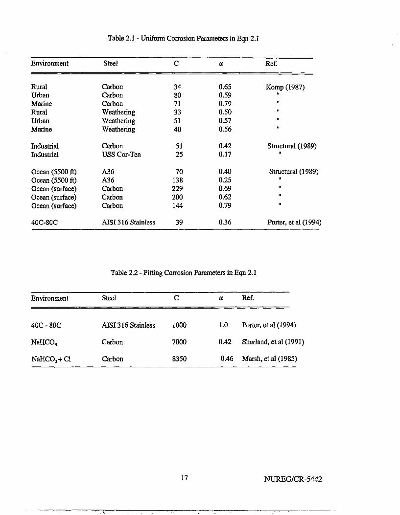
Table 2.1 - Unifonn Corrosion Parameters in Eqn 2.1

Environment

RuralUrbanMarineRuralUrbanMarine

IndustrialIndustrial

Ocean (5500 ft)Ocean (5500 ft)Ocean (surface)Ocean (surface)Ocean (surface)

40C-80C

Steel

CarbonCarbonCarbonWeatheringWeatheringWeathering

CarbonUSS Cor-Ten

A36A36CarbonCarbonCarbon

AISI316 Stainless

C

348071335140

5125

70138229200144

39

a

0.650.590.790.500.570.56

0.420.17

0.400.250.690.620.79

0.36

Ref.

Komp (1987)ll

tt

I I

tl

ll

Structural (1989)ll

Structural (1989)fl

ll

H

ll

Porter, et al (1994)

Table 2.2 - Pitting Corrosion Parameters in Eqn 2.1

Environment

40C - 80C

NaHCO3

NaHCOj+Cl

Steel

AISI 316 Stainless

Carbon

Carbon

C

1000

7000

8350

a

1.0

0.42

0.46

Ref.

Porter, et al (1994)

Sharland,etal(1991)

Marsh, etal (1985)

17 NUREG/CR-5442

100

43

in10

WM0

ASME - Mean

— AISC/AASHTO

— AWS-X-Modified

•— API-X-•DEn

1 0 ' 10 10

Number of cycles

10

Figure 2.1 Typical S-N curves for fatigue design

NUREG/CR-5442 18

3. NONDESTRUCTIVE EVALUATION METHODS

Nondestructive evaluation methods (NDE) are used to examine materials or components in ways thatdo not impair function in service. NDE is used to (1) locate and size flaws; (2) measure geometricalcharacteristics, and (3) assess composition. From an operational viewpoint, such inspections are required toidentify potential challenges to structural integrity in time to take remedial action. They also play an importantrole in structural reliability assessment, especially when combined with failure analysis techniques such asfracture mechanics. Factors that are important in areliability-based condition assessment include probabilityof detection, threshold of detection and flaw size distribution, and sizing accuracy. NDE provides anopportunity to revise and update the probability models used to determine current margins of safety and toforecast future reliability and performance. An ASME Research Task Force on risk-based inspection recentlyhas been created (ASME, 1992).

The most common NDE techniques in civil structures are Visual Inspection (VT), Eddy Current (EC),Magnetic Particle Inspection (MT), Liquid Penetrant (PT), Radiography (RT), Ultrasonic Inspection (UT) andAcoustic Emission (AE). However, no in-service inspection is perfect. NDE outputs depend on many factors,including the sensitivity of the instruments to different types of flaws, human factors such as education,training and proficiency of operators, geometry and microstructure of the component inspected, and size offlaws. Many of the NDE methods initially were developed to inspect components during relatively well-controlled manufacturing processes. They may be difficult to use in condition assessment and agingmanagement, where quantification of flaw size is necessary and limitations on the sensitivity of NDE areamplified by difficult field conditions. The procedures used in service frequently are manual and timeconsuming. A flaw of a given size can be detected only with a certain probability; for any but the largestdefects, however, there is a finite probability that the flaw escapes detection. Conversely, there is a possibilitythat NDE indicates a flaw when none is present (a so called false call); repair actions in such a case not onlywould be unnecessary but might damage the structure. Moreover, the actual flaw present may not be measuredaccurately by the NDE method chosen. Detection and measurement uncertainties arising from NDE must beincorporated in the reliability analysis.

Significant portions of NPP structures where damage might occur are not easily accessible toinspection. To maximize the efficiency of the inspection process, sampling plans must be devised that requireonly portions of the structure to be inspected, rather than the entire structure. The basic idea of such asampling plan is to focus initial inspection on a small (critical) portion (typically 5-10 percent) of the structure.If no problems are found in this first stage, the structure as a whole is deemed acceptable until the nextscheduled inspection. If flaws are located, an additional portion (say, 10-20 percent) is inspected. If no furtherproblems are evident in this second stage, the result of the initial stage is viewed as an anomaly; if, on the otherhand, problems are evident in the second stage as well, the entire structure may be inspected prior to continuedservice. Inspection is thus a living process. Obviously, a large portion of the structure may remain uninspected;any undetected flaws impact the time-dependent reliability.

In the following sections, common NDE methods will be assessed (Rummel, et al, 1989; Bray andStanley, 1989), with particular attention to quantifying detection and measurement uncertainties.

3.1 Detection of flaws

The probability of detecting a flaw depends on the NDE method employed, the size of the flaw andthe training of the operator. When NDE is performed, four outcomes are possible, as shown in the following:

19NUREG/CR-5442

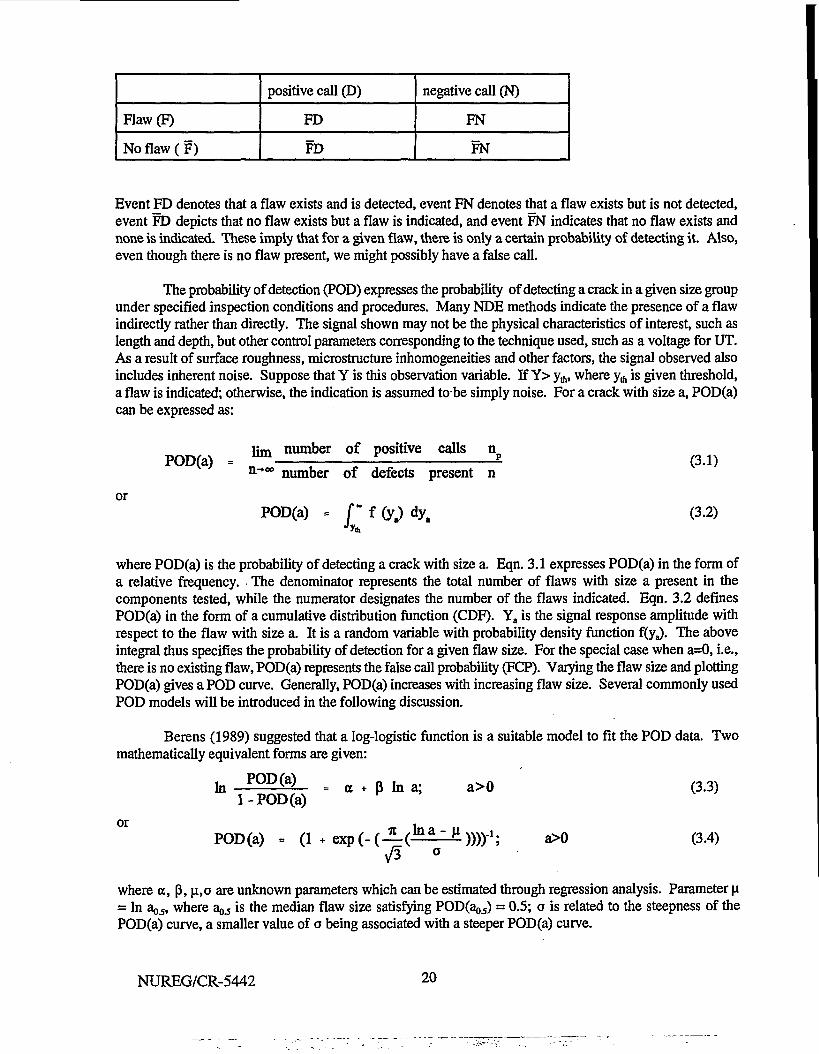
Flaw(F)

No flaw ( F )

positive call (D)

FD

FD

negative call (N)

FN

FN

Event FD denotes that a flaw exists and is detected, event FN denotes that a flaw exists but is not detected,event FD depicts that no flaw exists but a flaw is indicated, and event FN indicates that no flaw exists andnone is indicated. These imply that for a given flaw, there is only a certain probability of detecting it. Also,even though there is no flaw present, we might possibly have a false call.

The probability of detection (POD) expresses the probability of detecting a crack in a given size groupunder specified inspection conditions and procedures. Many NDE methods indicate the presence of a flawindirectly rather than directly. The signal shown may not be the physical characteristics of interest, such aslength and depth, but other control parameters corresponding to the technique used, such as a voltage for UT.As a result of surface roughness, microstructure inhomogeneities and other factors, the signal observed alsoincludes inherent noise. Suppose that Y is this observation variable. If Y> yft, where y , is given threshold,a flaw is indicated; otherwise, the indication is assumed to be simply noise. For a crack with size a, POD(a)can be expressed as:

i i m number of positive calls nPOD(a) = - ^ (3.1)n"+0° number of defects present n

orPOD(a) = f" f (yj dya (3.2)

where POD(a) is the probability of detecting a crack with size a. Eqn. 3.1 expresses POD(a) in the form ofa relative frequency. The denominator represents the total number of flaws with size a present in thecomponents tested, while the numerator designates the number of the flaws indicated. Eqn. 3.2 definesPOD(a) in the form of a cumulative distribution function (CDF). Ya is the signal response amplitude withrespect to the flaw with size a. It is a random variable with probability density function f(yj. The aboveintegral thus specifies the probability of detection for a given flaw size. For the special case when a=0, i.e.,there is no existing flaw, POD(a) represents the false call probability (FCP). Varying the flaw size and plottingPOD(a) gives a POD curve. Generally, POD(a) increases with increasing flaw size. Several commonly usedPOD models will be introduced in the following discussion.

Berens (1989) suggested that a log-logistic function is a suitable model to fit the POD data. Twomathematically equivalent forms are given:

In P 0 D ( a ) = a + p In a; a>0 (3.3)l -POD(a)

or tPOD(a) = (1 + e X p(- ( -^(- !^—£)) ) ) J ; a>0 (3.4)

where a, p, |i,o are unknown parameters which can be estimated through regression analysis. Parameter JJ= In a^, where a^ is the median flaw size satisfying PODta^) = 0.5; a is related to the steepness of thePOD(a) curve, a smaller value of a being associated with a steeper POD(a) curve.

NUREG/CR-5442 2 0

The relationship between (a, P) and (u,o) is,

H - - f (3-5)

o. - -?- (3.6)

The log-logistic model is similar to a lognormal distribution.

Others have suggested that the POD curve can be given by the exponential distribution,

{1 - exp (-c (a - a,.)) ; a h a,.0 ; a < a * ( 3 / 7 )

in which a^ = minimum detectable defect and c = constant, both of which depend on the NDE device and itsresolution (Tsai & Wu, 1993) or, more generally, a Weibull distribution (Kennedy, et al, 1991). If NDE isperfect, every defect above the threshold of detection, a ,, would be detected, and POD(a) would take on theappearance of a Heaviside function,

POD(a) = H ( a - a J (3.8)

Such is not the case, of course; however, one would like c to be as large as possible in order to approach thiscondition.

Both of the models mentioned above are consistent with the intuition that large defects almost certainlywill be detected while very small defects will almost certainly be missed, assuming that the entire componentis inspected. However this may not be the case. Considering that there may not be a certainty for detectingeven very large defects, an alternative expression for the probability of no detection is proposed (Staat, 1993),

1 - POD(a) = p + (1 - p) exp (-ca) (3.9)

in which p and c are parameters dependent on the NDE method. The corresponding POD is,

POD(a) = (1 - p)(l - exp (- ca)) ; a* 0 (3.10)

Note that this POD(a) is asymptotic to 1 - p for large values of a. There is no threshold of detection, i.e.,defects larger than zero have a finite POD. A model combining the best features of both Eqn 3.7 and 3.10would be,

POD(a) = (1 - p)(l - exp (-c(a - a j ) ) ; tea* (3.11)

The probability of detecting defects smaller than a^ would be zero, while the probability of detecting very largedefects would be 1 - p; typically p would be on the order of 0.001 - 0.05.

One disadvantage of the models represented by Eqns 3.7 - 3.11 is that none of them incorporates thefalse call probability (FCP) which may occur with some NDE methods. For example, in their pipe crackdetection round robin studies, Heasler et al (1990) found that the false call probability can be as high as 27%.

21 NUREG/CR-5442

Taking into account this FCP, Heasler, Taylor and Doctor (1993) proposed a logistic model using a insteadof In a in Berens1 model:

POD(a) = ( 1 + exp( - (a + pa)))1 (3.12)thus,

))"1 (3.13)

Generic POD curves using the above models are illustrated in Figure 3.1. Specific NDE methods areconsidered in the following sections.

3.2 NDE techniques

3.2.1 Surface and near-surface methods

Visual inspection (VT) is the oldest and still most widely used NDE method. In NPPs, accessiblesurfaces of the pressure-retaining boundary are inspected prior to each integrated leakrate test. Underwaterinspections for cracks usually are performed visually and are supplemented by magnetic particle inspectionafter cleaning (Kishi, 1988). Visual inspection can identify regions of corrosion, or peeling or blistering ofcoatings that may indicate damage to the substrate. Special attention must be paid to welds and heat-affectedzones of weldment.

Liquid penetrant (PT) is effective in locating surface flaws in essentially nonporous materials. Thefluorescent or visible penetrant seeps into various types of minute surface openings by capillary action, givingindications of defects. The advantage of this method is that it depends neither on ferromagnetism (as does,for example magnetic particle inspection) nor on defect orientation as long as only surficial flaws areconsidered. The major limitation of PT is that it cannot detect subsurface flaws and can be excessivelyinfluenced by the surface roughness or porosity. Studies (Chase, 1994) of application of NDE to the detectionof fatigue cracks in steel bridges have revealed that the crack length sensitivity range is 7-13 mm in welds andgreater than 24 mm in joints using PT; others have reported similar thresholds of detection (approximately9mm).

Figure 3.2(a) illustrates a POD curve for PT from analysis of data from 328 fatigue cracks in 118aluminum alloy specimens (Rummel, et al 1989). There is no false call probability indicated; the authorsclaimed that FCP was "not reflected by the POD curve" because in their experiment, no inspections wereconducted on unflawed areas. As will be seen later, the other three POD curves they obtained using EddyCurrent, Ultrasonic and X-ray inspection also indicated no FCP. The minimum flaw size here is about 0.5 mm.Using the model in Eqn. 3.4 we have u« 0, o » 0.3 mm; for the model of Eqn. 3.7, a^ = 0.5 mm, c - 2/mm.

Magnetic particle inspection (MT) is utilized to reveal surface and subsurface discontinuities inferro-magnetic materials. When the material is magnetized, a leakage field is generated by magneticdiscontinuities that lie in a direction transverse to the direction of the magnetic field. The leakage field gathersand holds some of the fine ferromagnetic particles applied over the surface. This forms an outline of thediscontinuity and indicates its location, size and shape. MT is capable of detecting fine, sharp and shallowsurface cracks in ferro-magnetic materials, but is not good for wide and deep defects. It cannot be used fornonferromagnetic materials. The magnetic field must be in a direction that intercepts the principal plane ofdiscontinuity for a good result. Thin coatings of paint and other nonmagnetic coverings will adversely affectthe sensitivity. MT is effective in detecting surficial defects in excess of about 6 mm (1/4 inch) long. Theprobability of detection is strongly dependent on field conditions.

Figure 3.2(b) illustrates a typical POD curve for MT obtained by Packman et al (1969). The materialwas AISI4330 vanadium modified heat treated steel.

NUREG/CR-5442 22

3.2.2 Ultrasonic inspection (UT)

UT is used to detect both surface and internal discontinuities in materials and can also be used toidentify areas of thinning due to corrosion. Beams of high frequency sound waves introduced into the materialattenuate due to wave scattering and are partially or completely reflected at interfaces. The reflected beam isdisplayed and analyzed to define the presence and location of defects such as cracks or voids. UT can also beused to measure thickness and extent of corrosion by monitoring the transit time of a sound wave through thecomponent or the attenuation of the energy. UT can be performed under water. The principal advantages ofUT are its portability and superior penetrating power and volumetric scanning ability which allow the detectionof deep flaws. Studies (Chase, 1994) show that its sensitivity to crack length is the highest among thecommonly used NDE techniques (detection thresholds between 3-7 mm in welds and 7-13 mm in joints), andits complexity and operator dependence are moderate. Its disadvantage is that defects in parts that have roughor irregular surfaces, or are very small, thin or non homogeneous are difficult to detect.

Research has been in progress for several years to determine reliability of in-service ultrasonicinspection and its capability for flaw sizing. The aim of this research is to establish reliability of the inspectionprocess for pressure vessels and primary coolant piping systems in NPPs (Doctor, et al, 1993). Techniquesother than UT are not being considered. Data are being obtained from an international round-robin test ofultrasonic inspection capabilities involving teams from the United States, several European countries andJapan. Data were gathered during an exercise called PISC II (Programme for the Inspection of SteelComponents, Phase 2). Human factors are being incorporated in the study. It was found that flaw length isthe best control parameter in determining probability of detection curves. Results of this activity are beinginterfaced with an ASME task force on reliability-based in-service inspection (ASME, 1992). Typical PODcurves developed as part of this study (Heasler, et al, 1993) are illustrated in Figure 3.3(a); points identifiedas H or L indicate potentially anomalous data As a comparison, the curve obtained by Rummel, et al (1989)is shown in Figure 3.3(b). Using the POD models in Eqn. 3.10 to fit the data in Figure 3.3(a), we have p =0.005, c = 0.1134/mm (Kennedy, et al, 1991; Staat, 1993); using Eqn. 3.12, a - -1.73, p - 1.5. A curvesimilar to Eqn. 3.7, in which c = 0.113/mm, was recommended by Tsai and Wu (1993). It is noted that FCPis significant for UT because it mainly deals with internal flaws and is not visually-assisted.

3.2.3 Eddy current (EC)

EC is effective in detecting defects at or within a few millimeters of the surface. It is based on theprinciple of electromagnetic induction. Taking a pipe as an example, a current is created by encircling thepipeline with induction coils, The presence of a crack in the pipe impedes the current flow and changes itsdirection, causing changes in the associated electromagnetic field which can be monitored. Thus surfacediscontinuities having a combination of predominantly longitudinal and radial dimensional components canreadily be detected.

A majority of surface discontinuities can be detected by EC with high speed and low cost. If a coatingis present, it need not be removed. However, the sensitivity of this method to defects beneath the surface isdecreased. Also, laminar defects may not alter the flow enough to be detected. Defects less than 6 mm (1/4in) at the toe of a weld reportedly cannot be detected by EC (Shah, et al, 1994), nor can defects more thanabout 13 mm (1/2 in) below the surface. The sensitivity ranges of fatigue cracks in steel bridges are 7-13 mmin welds and greater than 25 mm in joints (Chase, 1994), comparable to that of PT.

In one study (Bowen, et al, 1989), research was conducted on the reliability of eddy-current inspectiontechniques to detect and size flaws in steam generator tubes. Human factors also were taken into account inthis study, and performance of several inspection teams was considered. Typical POD data collected in thisstudy are shown in Figure 3.4(a); the lines correspond to lower bound and median trends. As a comparison,

23 NUREG/CR-5442

the curve obtained by Rummel, et al (1989) is shown in Figure 3.4(b).- Using the model in Eqn. 3.7 to fit thedata in Figure 3.4(a), we have

POD(a) = 1 - exp( -3.5 (a-0.10)) (3.14)

in which a=true flaw depth, expressed as a fraction of plate or weld thickness. Recognizing that the modeldoes not incorporate FCP, which appears to be apparent in the data, one might use the model in Eqn 3.12 witha «-2.94 and p - 9.

3.2.4 Acoustic emission (AE)

Sudden movement in stressed materials produces acoustic stress waves. The stress waves can bedetected on the surface of the structure by one or more piezoelectric transducers. One source of AE is defect-related active deformation processes such as fatigue crack growth. Thus, AE offers the possibility ofmonitoring growing defects during service. Research (Yeh, Enneking and Tsai, 1994) has been conducted torelate AE energy counts to stress intensity factor and strain energy release rate. However, difficulties stillremain in using acoustic transducers to locate or size growing defects accurately due to the noise resulted fromvarious sources, and the AE is better used in conjunction with other flaw detection methods. Efforts have beenmade (Ghorbanpoor, 1994) to improve signal discrimination techniques for AE evaluation of steel bridges.The sensitivity ranges for fatigue cracks in steel bridges are 7-13 mm in welds and 13-25 mm in joints,respectively. No further information on detection probability for AE could be located. The technique is stillrelatively new in its application to civil structures.

3.2.5 Radiography (RT)

RT methods are based on the differences in absorption by different portions of a component ofpenetrating radiation, such as X-ray or y-ray. The images produced can be analyzed to locate flaws. Planardefects cannot be detected unless their principal plane is essentially parallel to the radiation beam. Tight cracksare difficult to detect regardless of orientation. In contrast to the other methods above, access to both sides ofthe component is required. Safety protocols also must be followed. RT is relatively expensive. Figure 3.5illustrates a typical POD curve for X-ray inspection obtained by Rummel, et al (1989) by gathering data from328 fatigue cracks in 118 aluminum alloy specimens. Using the POD model in Eqn 3.7, we have a , - 0.51mm, c - 0.35/mm.

3.3 Flaw measurement errors

Error in sizing is also an important issue because the defect size identified is greatly affected by manyfactors such as education of operators, sensitivity of equipment, procedures conducted and materialimperfections. For example UT can be used to locate areas of corrosion in inaccessible regions, but may notcorrectly identify the extent of corrosion penetration if the surface roughness due to corrosion is high and wavescattering occurs as a result. Errors in measuring thickness ultrasonically for several commercially availableUT gauges (summarized in Figure 3.13 of Shah, et al, (1994)) and in sizing can be as high as 40 percent fora surface roughness of 0.2 mm RMS. The pipe inspection round robin conducted by Heasler, et al (1990) alsoshowed that sizing performance was not very good. Slopes of regressions of true sizes on measured sizes fromUT sometimes are close to 1 and other times deviate from 1; variability is high, with an average standard errorof 20 percent Other techniques such as EC and RT have similar sizing errors. Error in sizing by PT and MTseems to be less of a problem mainly because these techniques deal with surficial flaws where inspections arevisually assisted. Figure 3.6 illustrates the data scattering difference between PT and X-ray inspection.

After a flaw has been detected, it is necessary to estimate the true flaw size, a, from the measured size,a,,,. Usually, we are interested in P(A < ylAm = c), the probability that true flaw size, A, is less than y under

NUREG/CR-5442 24

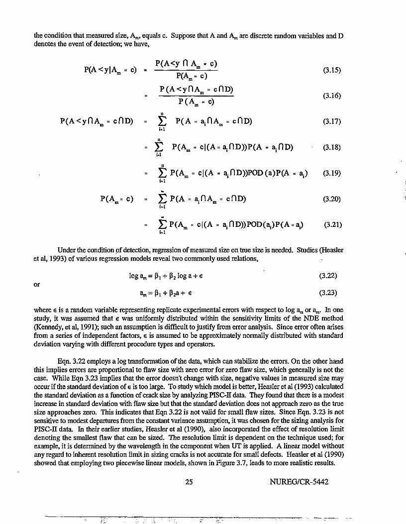
the condition that measured size, An,, equals c. Suppose that A and An, are discrete random variables and Ddenotes the event of detection; we have,

P(A<y D A = c)P(A<y|A. .o) • y

p ( A ^ c ) (3.15)

P(A<yflA = cflD)m

P(A<yriAm = cOD) = £ P(A = ajnAm = cflD) (3.17)i.i

= £ P(Am = c|(A= airiD))P(A = ajflD) (3.18)

ai) (3.19)i-l

P(Am=c) - E P ( A = ainAm = cnD) (3.20)i.l

= £ p ( Am = CKA = ainD))POD(a)P(A = ai) (3.21)

i.l

Under the condition of detection, regression of measured size on true size is needed. Studies (Heasleret al, 1993) of various regression models reveal two commonly used relations,

loga m =p, + p2 loga + e (3.22)or

a . ^ + Paa+e (3.23)

where e is a random variable representing replicate experimental errors with respect to log an, or a,,,. Li onestudy, it was assumed that e was uniformly distributed within the sensitivity limits of the NDE method(Kennedy, et al, 1991); such an assumption is difficult to justify from error analysis. Since error often arisesfrom a series of independent factors, e is assumed to be approximately normally distributed with standarddeviation varying with different procedure types and operators.

Eqn. 3.22 employs a log transformation of the data, which can stabilize the errors. On the other handthis implies errors are proportional to flaw size with zero error for zero flaw size, which generally is not thecase. While Eqn 3.23 implies that the error doesn't change with size, negative values in measured size mayoccur if the standard deviation of e is too large. To study which model is better, Heasler et al (1993) calculatedthe standard deviation as a function of crack size by analyzing PEJC-II data. They found that there is a modestincrease in standard deviation with flaw size but that the standard deviation does not approach zero as the truesize approaches zero. This indicates that Eqn 3.22 is not valid for small flaw sizes. Since Eqn. 3.23 is notsensitive to modest departures from the constant variance assumption, it was chosen for the sizing analysis forPISC-II data. In their earlier studies, Heasler et al (1990), also incorporated the effect of resolution limitdenoting the smallest flaw that can be sized. The resolution limit is dependent on the technique used; forexample, it is determined by the wavelength in the component when UT is applied. A linear model withoutany regard to inherent resolution limit in sizing cracks is not accurate for small defects. Heasler et al (1990)showed that employing two piecewise linear models, shown in Figure 3.7, leads to more realistic results.

25 NUREG/CR-5442

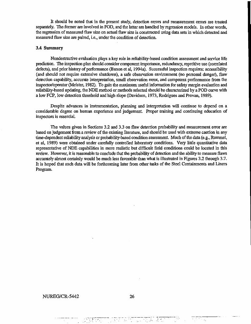
It should be noted that in the present study, detection errors and measurement errors are treatedseparately. The former are involved in POD, and the latter are handled by regression models. In other words,the regression of measured flaw size on actual flaw size is constructed using data sets in which detected andmeasured flaw size are paired, i.e., under the condition of detection.

3.4 Summary

Nondestructive evaluation plays a key role in reliability-based condition assessment and service lifeprediction. The inspection plan should consider component importance, redundancy, repetitive use (correlateddefects), and prior history of performance (Banon et al, 1994a). Successful inspection requires: accessibility(and should not require extensive shutdown), a safe observation environment (no personal danger), flawdetection capability, accurate interpretation, small observation error, and competent performance from theinspector/operator (Meister, 1982). To gain the maximum useful information for safety margin evaluation andreliability-based updating, the NDE method or methods selected should be characterized by a POD curve witha low FCP, low detection threshold and high slope (Davidson, 1973, Rodrigues and Provan, 1989).

Despite advances in instrumentation, planning and interpretation will continue to depend on aconsiderable degree on human experience and judgement. Proper training and continuing education ofinspectors is essential.

The values given in Sections 3.2 and 3.3 on flaw detection probability and measurement error arebased on judgement from a review of the existing literature, and should be used with extreme caution in anytime-dependent reliability analysis or probability-based condition assessment. Much of the data (e.g., Rummel,et al, 1989) were obtained under carefully controlled laboratory conditions. Very little quantitative datarepresentative of NDE capabilities in more realistic but difficult field conditions could be located in thisreview. However, it is reasonable to conclude that the probability of detection and the ability to measure flawsaccurately almost certainly would be much less favorable than what is illustrated in Figures 3.2 through 3.7.It is hoped that such data will be forthcoming later from other tasks of the Steel Containments and LinersProgram.

NUREG/CR-5442 26

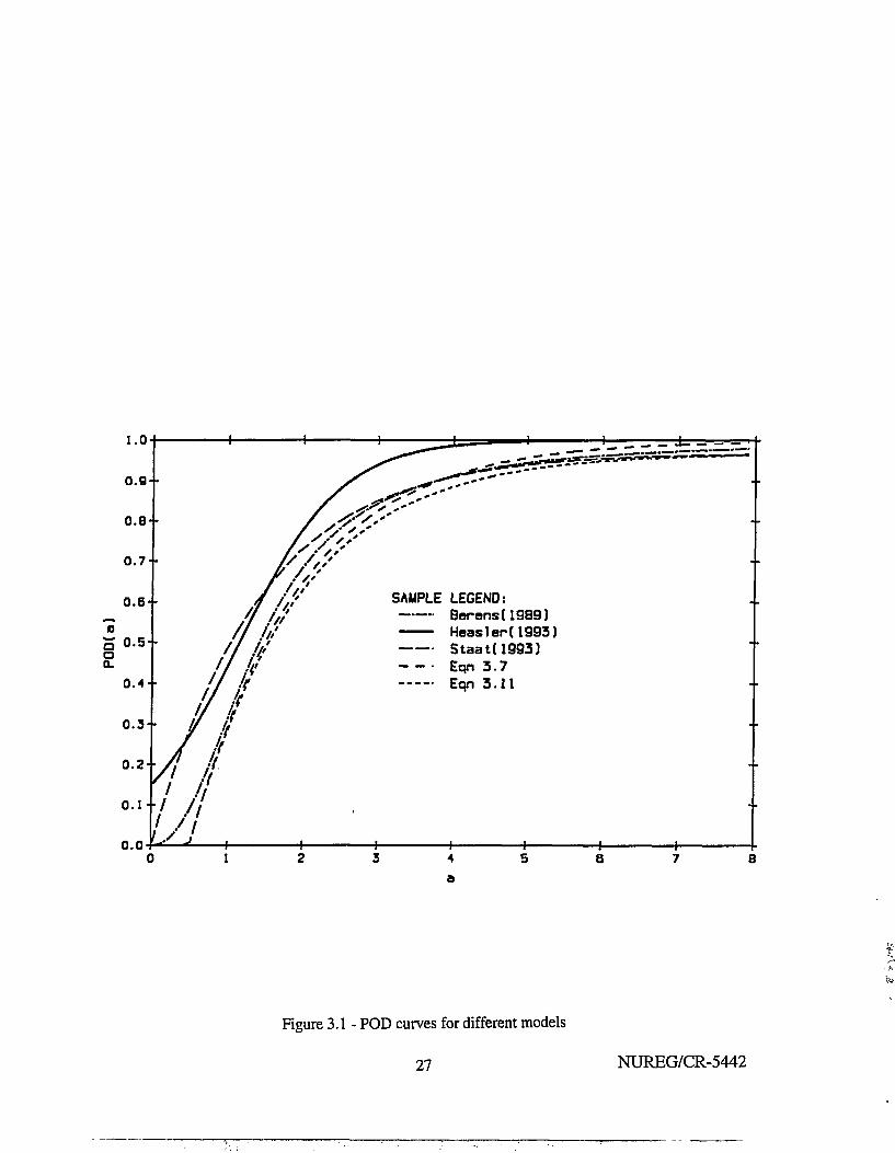
1.0

0.0

SAMPLE LEGEND:Berens(1989)Heasler(1993)Staat(1993)Eqn 3.7Eqn 3.11

Figure 3.1 - POD curves for different models

27 NUREG/CR-5442

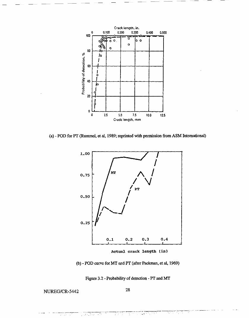
100

80

co

I 60•a"o

i f 40

1oIX

20

Crack length, in .0 0.100 0.200 0.300 0.400 0.500

<§fe/o/o

J.T

oI

i

f1

•> O —

» o o.

o

o

o0 O

r-mtm—mm

2.5 5.0 7.5 10.0Crack length, m m

12.5

(a) - POD for PT (Rummel, et al, 1989; reprinted with permission from ASM International)

1.00

0.75 "

0.50 -

0.25

0.1 0.2 0.3 0.4

Actual crack length (in)

(b) - POD curve for MT and PT (after Packman, et al, 1969)

Figure 3.2 - Probability of detection - PT and MT

NUREG/CR-5442 28

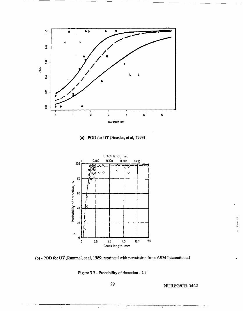
CO

d

tod

g

cvio

qd

(a) - POD for UT (Heasler, et al, 1993)

100

80

Crack length, in .

0.100 0.200 0.300 0.400

cgo2CD

•o**-o

f

60

•f 4015

20

/o

4a.

o o

2.5 5.0 7.5 10.0Crack length, m m

125

(b) - POD for UT (Rummel, et al, 1989; reprinted with permission from ASM International)

Figure 3.3 - Probability of detection - UT

29 NUREG/CR-5442

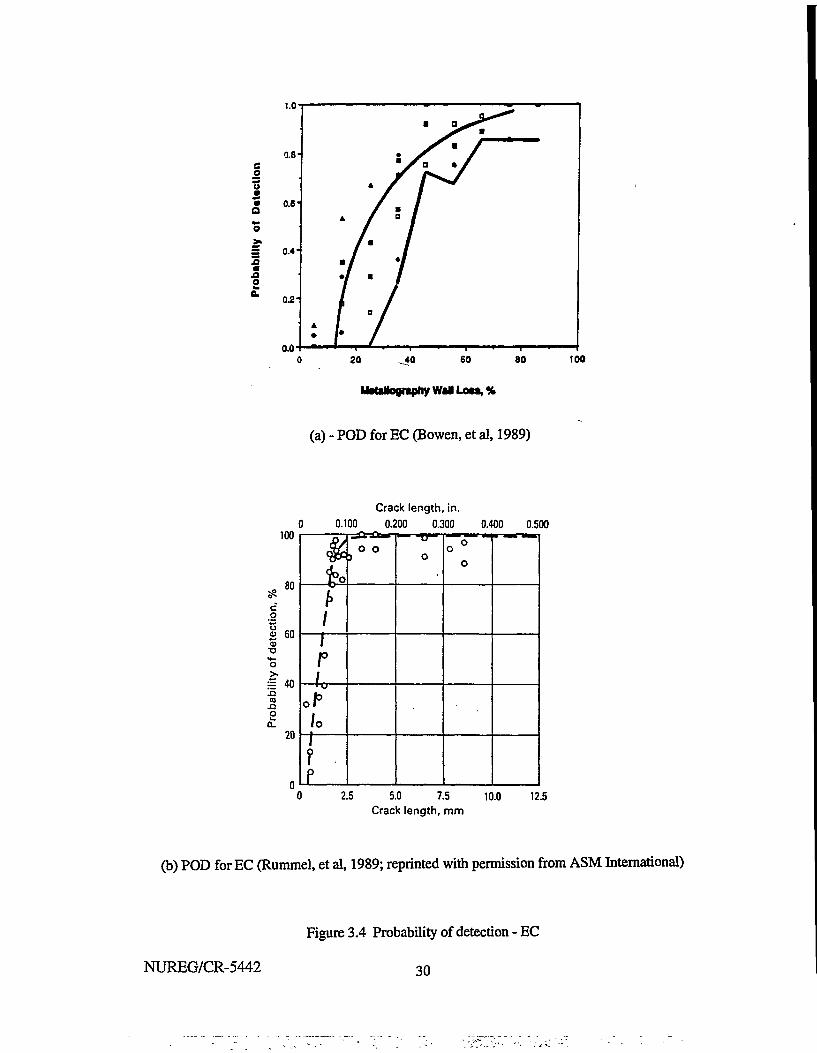
Ion

TimSa

>•

a2a.

1.0-

0.8-

0.8-

0.4-

02-

4•

A

• /

/

A

/

•

D ,

/

fa

• /

/

f

•

ri:/

20 _40 60 80

Urtaltognpiiy Wai Lota, %

(a) - POD for EC (Bowen, et al, 1989)

100

100

Crack length, in.

0.100 0.200 0.300 0.400 0.500

2 60

= 40

s20

*

\

plu

fo

1fp

o oo

o °o

2.5 5.0 7.5 10.0Crack length, mm

12.5

(b) POD for EC (Rummel, et al, 1989; reprinted with permission from ASM International)

Figure 3.4 Probability of detection - EC

NUREG/CR-5442 3 0

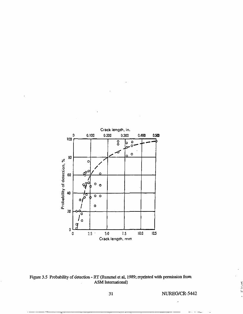
1G0

30

co

60

"o

I" 40A(0

O

20

Crack length, in.

0.100 0.200 0.300 0.400 0.500

o

#°/%°°IId

ori

o o

/ :

//

/ n

) ° O

0 O

o

oo o o

°*n °

- MM >

2.5 • 5.0 7.5 10.0Crack length, m m

115

Figure 3.5 Probability of detection - RT (Rummel et al, 1989; reprinted with permission fromASM International)

31 NUREG/CR-5442

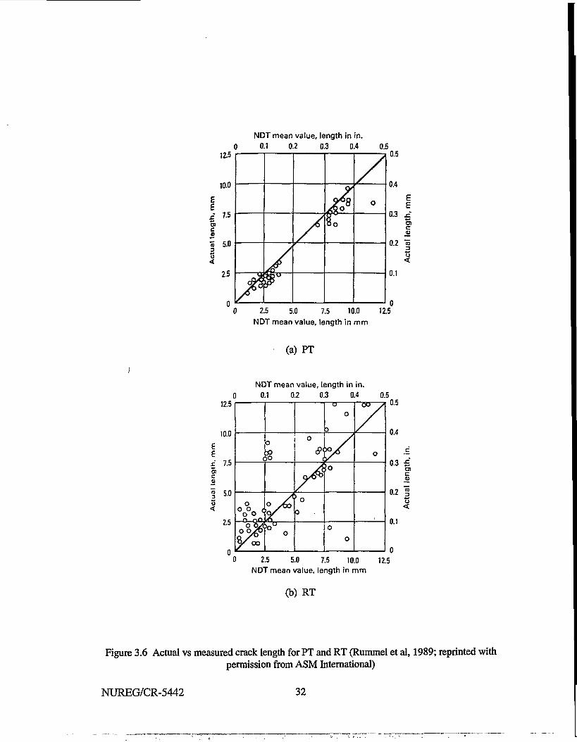
NDT mean value, length in in .0 0.1 0.2 0.3 0.4 0.5

10.0

eI 7-5oi 5.0

I2.5 A/

/.9^8

Oo

/

0

0.5

0.4

0.3

0.2

0.1

EE

c

00 2.5 5.0 7.5 10.0 12.5

NDT mean value, length in mm

(a)PT

NDT mean value, length in in.0 0.1 0.2 0.3 0.4 0.5

12.5 I 1 1 r-o nsj—n 0.5

10.0

£

£ 7-5

5£co

5.0

2.5

0oo. J

0 0O 0Ô "is0 0^0

Q/ÔO

0

°A0

0

c?'

0

yfto

(o0

0

0

70

0.4

0.3 £CDC

0.2 1

0.1

0 2.5 5.0 7.5 10.0 12.5NDT mean value, length in m m

(b) RT

Figure 3.6 Actual vs measured crack length for PT and RT (Rummel et al, 1989; reprinted withpermission from ASM International)

NUREG/CR-5442 32

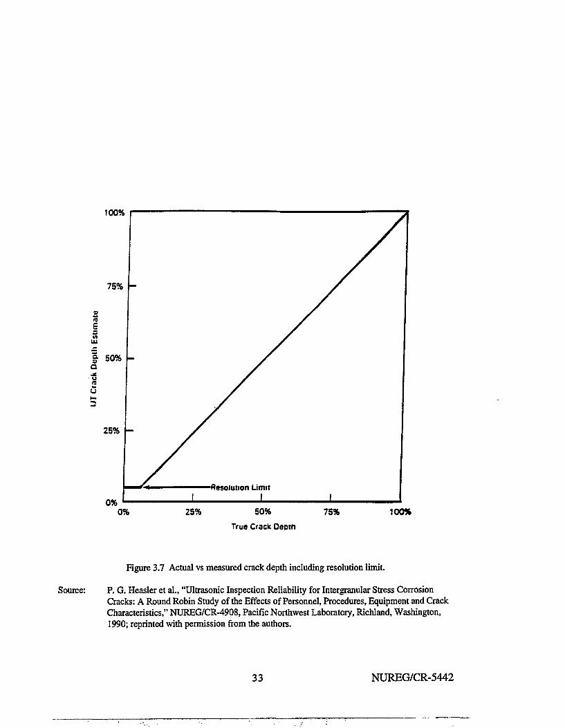
100%

0% 25% 50%

True Crack Depth

75% 100%

Figure 3.7 Actual vs measured crack depth including resolution limit.

Source: P. G. Heasler et al., "Ultrasonic Inspection Reliability for Intergranular Stress CorrosionCracks: A Round Robin Study of the Effects of Personnel, Procedures, Equipment and CrackCharacteristics," NUREG/CR-4908, Pacific Northwest Laboratory, Richland, Washington,1990; reprinted with permission from the authors.

33 NUREG/CR-5442

4. TIME-DEPENDENT RELIABILITY ANALYSIS

The evaluation of steel structures for continued service should provide quantitative evidence that theirstrength is sufficient to withstand future demands within the proposed service period with a level of reliabilitysufficient for public safety. Structural loads, engineering material properties, and strength degradationmechanisms are random in nature. Time-dependent reliability analysis methods provide the framework fordealing with uncertainties in performing condition assessments of existing and aging structures and fordetermining whether in-service inspection and maintenance is required to maintain their performance at thedesired level. Uncertainties that complicate the evaluation of aging effects arise from a number of sources:(1) inherent randomness in structural loads, initial strength, and degradation mechanisms; (2) lack of in-servicemeasurements and records; (3) limitations in available models for quantifying time-dependent material changesand their contribution to containment strength; (4) inadequacies in nondestructive evaluation; and (5)shortcomings in existing methods to account for repair.

4.1 Probabilistic models of loads

Structural loads occur randomly in time and are random in their intensity. Structural load models anddescriptive load statistics have been gathered in previous research to develop probability-based limit statesdesign and condition assessment procedures for NPP structures (Hwang, et al, 1987; Ellingwood and Mori,1993).

Discrete load models. The duration of structural loads that arise from rare operating or environmentalevents, such as accidental impact, earthquakes and tornadoes, is short and such events occupy a negligiblefraction of the service life of a structure. Such loads can be modeled as a sequence of short-duration loadpulses occurring randomly in time. One of the simplest pulse process models is illustrated by the samplefunction in Figure 4.1a. The occurrence in time of the loads (impulses) is described by a Poisson process, withmean (stationary) rate, of occurrence, A, random intensity Sj and duration x (Pearce and Wen, 1985). Thenumber of events, N(t), to occur during service life, t, is described by the probability mass function,

P[N(t) = n] = (k t)n exp (-At)/n! (4.1)

n = 0,1,2, . . .

The intensity of each load is a random variable, described by cumulative distribution function (CDF) Fj (x).One can generalize this process to one in which the load process is intermittent (Figure 4.1b) and the durationof each load pulse has an exponential distribution,

FTj(t) = 1 - exp [ - t/T]; t ^ 0 (4.2)

in which x = average duration of the load pulse. The probability that the load process is nonzero at anyarbitrary time is p = \x.

Continuous load models. Loads due to normal facility operation or climatic variations can bemodeled by continuous load processes. A Poisson process with rate X may be used to model changes in loadintensity if the loads are relatively constant for extended periods of time, as illustrated by the sample functionin Figure 4.1c. Here, the duration of each load is exponential, with average duration T= 1/k. Finally, loadsthat fluctuate with sufficient rapidity in time that they cannot be modeled by a sequence of discrete pulses canbe modeled as continuously parametered stochastic processes, a sample function of which is shown in Figure4.1d.

35 NUREG/CR-5442

Many of the loads for which nuclear power plant structures are designed can be modeled by suchprocesses (Ellingwood, 1983; Hwang, et al, 1987). A summary of load statistics obtained from prior researchis presented in Table 4.1. The operating load statistics were obtained from a consensus estimation survey(Delphi) of NPP loads (Hwang, et al, 1983). The subset of normal operating loads presented - dead, pressure,pipe reaction, restraint of thermal expansion - are typical for a variety of NPPs. The load statistics presentedin Table 4.1 are believed to be sufficient for developing and testing reliability-based condition assessmentmethods for NPPs. However, it is known that many operating loads are plant-dependent; moreover,environmental loads may well depend on the plant site. When plant-specific load statistics are available fromin-service monitoring programs or site-specific hazard analyses, they should be used in lieu of those in Table4.1.

4.2 Probabilistic models of resistance

4.2.1 Initial resistance

The properties of steel that are required in reliability analysis of steel structures include yield strength,tensile strength, Young's modulus of elasticity, and Poisson's ratio. The existing literature on this subject forcommon grades of structural steel was reviewed in depth as part of the effort to develop load and resistancefactor design procedures (Galambos and Ravindra, 1978; LRFD, 1993). These data are summarized in thetop portion of Table 4.2. A number of ASTM designations and grades of steel are represented in these data,but they all were construction grades and are designated simply as "carbon." A lognormal CDF

l ] (4.3)in which m and P = median and logarithmic standard deviation of random variable, X, and $ ( ) = CDF of astandard normal variate fits all data in Table 4.2 reasonably well.

Additional data were located on the strength of various grades of carbon steel plate used ascontainments or liners in NPPs. Statistical data for yield and ultimate tensile strengths for specific designationsof plate are presented in the lower part of Table 4.2 (Ellingwood and Hwang, 1985). In comparison with thegrades of carbon steel used for rolled shapes and plates that are common to civil construction, the meanstrengths are somewhat more conservative with respect to the nominal strengths while the coefficients ofvariation (COV) are smaller, indicating a higher standard of quality control in fabrication. There is a tendencyin these data for the mean strength to decrease with increasing plate thickness, a tendency that has beenobserved elsewhere. '

The resistance of a steel component depends on other factors besides the material strength. A simplemodel of resistance to a particular limit state is given by (Galambos and Ravindra, 1978),

R = R. .MFP (4.4)

in which Rn = nominal strength computed using material strengths, dimensions and analytical proceduresprescribed by the code; M = material factor; F = fabrication factor; and P = professional factor. M, F, and Pare random variables that, as a group, model the different sources of uncertainty in the resistance. To take aspecific example, one might model flexural strength as,

R = BF yZ x (4.5)

in which Fy = random yield strength (see Table 4.2), Z, = plastic section modulus, and B = bias factor. If thecode were to require the use of elastic analysis, the nominal strength would be,

NUREG/CR-5442 36

Rn=FynSxn (4.6)

in which F^ = specified yield strength and Sm= handbook elastic section modulus. With the notation in Eqs4.4 and 4.5, the random resistance would be,

R = R,, ( F / P ^ ( Z ^ J (B Z J S J (4.7a)

in which, using the notation in Eqn 4.3,

(4.7b)

(4.7c)

P = BZxn/Sxn (4.7d)

With a good quality control program, the mean of F is typically close to 1.0, and its COV is 0.05 or less. Themean and COV of P depend on the fundamental assumptions underlying the analysis - use of simple flexuraltheory, neglect of strain hardening, etc. - and its rigor in modeling the behavior of interest. Since suchassumptions usually are on the conservative side, the mean of P is usually greater than 1.0, while the COVtypically is on the order of 0.05 - 0.10.

4.2.2 Time-dependent deterioration in resistance

Reliability assessments of existing steel structures that may age in time require time-dependentstatistical models and descriptions of the structural resistance. Since aging has not been considered previouslyin probability-based design work, the available resistance statistics in Table 4.2 apply to new construction.In the absence of full-scale monitoring of structural performance, time-dependent resistance must be obtainedfrom mathematical models of degradation mechanisms described in Section 2, along with a knowledge of theinitial resistance.

The structural resistance is modeled as a time-dependent function (Ellingwood and Mori, 1993),

R(t) = R0G(t) (4.8)

in which R,, = R(0), the initial resistance, and G(t) is a time-dependent degradation function defining thefraction of initial strength remaining at time, t. Due to uncertainties in the structural impact on damageinitiation and growth from aggressive environmental attack, G(t) for a steel component will be a non-increasingrandom process unless there is some intervention in the form of in-service replacement or repair.

Conceptually, a degradation function for predicting time-dependent resistance can be associated witheach degradation mechanism. In the case of corrosion, for example, it has been shown that severely corrodedmaterial has virtually no strength, whereas uncorroded material retains its original strength properties. Thereduction in structural strength from corrosion comes primarily from loss of section, but also is affected bystress or strain concentrations that arise from general roughness of the corroded surface. Tests of simpletension specimens that have been uniformly corroded prior to testing have shown that their tensile strengthsbased on nominal area (in units of force) are proportional to the loss of section due to corrosion; however, theirstrains at fracture are reduced by approximately a factor of 2 (Cherry, 1995), apparently due to the strainconcentrations from local nonuniformities of the corroded surface.

As an example, consider a situation in which uniform corrosion penetrates to depth, x(t), in a plate ofthickness, W. Assuming that strength rather than ductility governs, when x(t) reaches the thickness W, the

37 NUREG/CR-5442

plate loses all capacity to carry load. The impact of this degradation depends on the nature of the behaviorallimit state. If the plate is in a state of simple tension,

R(t) = FyW(l-x(t)/W) . (4.9a)

and sample function g(t) is simply 1 - x(t)/W. On the other hand, if the plate is stressed in flexure, the bendingstrength per unit width is,

R(t) = Fy W2 (1 - x(t)/W)2/6 (4.9b)

and g(t) = (1 - x(t)/W)2. Thus, small errors in estimating x(t) would have a more significant impact on flexuralstrength than on tensile strength. Moreover, as damage progresses and x(t) increases, the governing limit statemay change during the service life of the component, creating an unanticipated and potentially dangeroussituation. Since x(t) actually is modeled as a random process, X(t) (eg., penetration of corrosion, modeled inSection 2), the probability distribution of X(t) plays a key role in the condition assessment.

4.2.3 Fragility modeling of steel containments and liners

Probabilistic models of resistance of steel containments and liners are integrated with stochastic loadmodels to develop fully-coupled time-dependent reliability assessement tools. An intermediate step in thedevelopment of fully-coupled reliability analysis procedures is the fragility modeling of the containment.Fragility analysis is a relatively simple but powerful technique for assessing the capability of a structuralsystem to withstand specified (sometimes referred to as screening or review-level) events in excess of thedesign-basis event. This process sometimes is referred to as a "safety margin analysis." During the lastdecade, it has been used to determine the capability of NPP structural components and systems to withstand,with high confidence, review-level earthquakes of a prescribed level in excess of the safe-shutdown earthquake(SSE). For example, the review earthquake might be set at 0.30g if the design-basis SSE were 0.17g. Thebasic idea is that if the system can be shown to perform safely at the review level, it is judged sufficient forpublic safety regardless of what the actual (unknown) hazard might be.

A margin analysis has at least three advantages over a fully coupled reliability analysis:

(1) The probability distribution of the hazard or the structural action caused by it is not required(although some general idea of the potential hazard must be available in order to arrive at a sensiblereview level event). Design-basis events for NPP structures are very rare, and determining theirprobability models is difficult because of the paucity of data. Extrapolating such probability modelswell beyond the realm of observation creates a large source of uncertainty. In analyzing seismichazards in the Eastern United States, for example, estimated probabilities that earthquakes in excessof the design basis occur annually can vary over two or more orders of magnitude, depending onwhich one of several (credible) hypotheses regarding seismic source zones is made.

(2) The convolution of hazard and resistance needed to determine probabilities of failure is avoided.

(3) The difficulty in interpreting the resulting probabilities is avoided. Because of the largeuncertainties in hazard analysis, these probabilities may span three or more orders of magnitude(Ellingwood, 1990,1992,1994). The selection of a numerical value for assessment purposes (e.g.,mean, median, mode), let alone its use as as a regulatory target, is very difficult.

A fragility analysis and margins assessment of a structure avoids these difficulties in interpretation, yet enablesvulnerabilities in the structure to be identified because of the supporting system analysis that underlies thefragility model. While a margins analysis is not as informative as the measure of safety obtained from a fully

NUREG/CR-5442 38

coupled PRA, it retains many of the desirable features of the structural system reliability analysis and is easierto perform.

The fragility of a component or system, such as a steel containment-or liner, is defined as itsprobability of "failure," conditioned on a level of demand (from ground motion, wind velocity, internalpressure, etc.) The definition of failure depends on the performance requirements of the component or systemconsidered. In a steel containment or liner, failure is assumed to occur when (generally inelastic) deformationsare large enough to interfere with the operation of attached equipment, when pressure retention is lost orleakage above a tolerable level occurs.

The lognormal distribution is the most common way to model fragility (Kennedy and Ravindra, 1984);

FR(x) = « | p " I (4.10)

in which mR = median capacity (expressed in units that are dimensionally consistent with the demandparameter) and pR = SD(ln R), or standard deviation in In R, describingJheJnherent randomness in thecapacity of the component to withstand the demand. Parameter pR= win (1 + VR), in which VR= coefficientof variation (COV) in capacity; when this COV is less than about 0.3, PR = VR.

Additional uncertainties in component capacity arise from assumptions made in the structural systemanalysis, limitations in the supporting statistical database, and similar factors. These modeling uncertaintiescan be taken into account, to first order, by assuming that the median capacity is a random variable.Accordingly, mR in Eqn 4.10 is replaced by random variable, MR, assumed to be lognormal with median mR

and logarithmic standard deviation, pw. The fragility thus becomes a random function of random variable, MR.A family of lognormal distributions, described by the fragility parameters (mR, PR, p0), displays the overalluncertainty in the conditional component failure probability at any value of x, as illustrated in Figure 4.2,where the graphs illustrate the 5 to 95 percentile fragility curves. The mean fragility can be shown to be(Ellingwood, 1994),

FR(x) -In (x/mR)

(4.11)

This mean fragility also is illustrated in Figure 4.2. Note that it has a different slope than the family of curves.

One uses the component fragility in a margins assessment to identify a level of demand at which thereis a high confidence that the component will survive. It has been common in structural design and safetychecking to use a nominal or characteristic strength that has a small probability, typically 0.05, of not beingattained. (This so-called 5 percentile value of strength, or 5 percent exclusion limit, is the basis forcharacteristic strengths now being recommended in the new limit state-based Eurocodes that are beingimplemented in Western Europe.) Figure 4.2 shows that in the presence of uncertainties arising frominsufficient data, the 5 percent exclusion limit has a frequency distribution, assumed to arise from uncertaintiesin estimating the median, mR. The lower a-fractile of this frequency distribution is a number, Ra; one mightsay that the probability of surviving an event with intensity Ra is 95 percent with confidence (1 - a) 100percent. Conversely, one can obtain Ra as,

Ra = mR exp (-1.645 pR + kap0) (4.12a)

39 NUREG/CR-5442

in which ktt = ®~\a). In seismic margins analysis, it has been customary to set a = 0.05 and refer to RB as theHCLPF, or "high-confidence, low probability of failure, value. This HCLPF can be expressed as,

HCLPF = mR exp [-1.645 (pR + pu)] (4.12b)

The HCLPF is akin to a lower tolerance limit, but in a Bayesian rather than a classical statistical sense.

Eqns 4.10 and 4.11 simply display the uncertainty in the component capacity. The fragility parametersmust be determined from structural analysis, examination of available statistical data, and expert judgement.To illustrate, suppose that it is desired to perform a margins analysis of a Mark I steel containment drywellsubjected to internal pressure, Pa. The capacity can be analyzed as the product of a series of factors (cf Eqn4.4 and 4.7),

R = ( H F i ) P a (4.13)

in which Pa = design-basis pressure (typically 40 - 60 psig for a BWR Mark 1) and F;= random factors which,collectively, represent the difference between strength of the containment in-service and the assumed designstrength. Assuming that the factors F; are mutually statistically independent, the median and variability in Rare,

mR = ErriiP, (4.14a)

PR = [ S Pi 2 ]" 2 (4.14b)

in which nij = median of factor i and p ; = logarithmic standard deviation describing inherent randomness oruncertainty in factor i. As the product of independent factors, R can be modeled by a lognormal distributionby virtue of the central limit theorem of probability theory.

At the current state-of-the-art, the starting point of the containment fragility analysis is the plant-specific elastic design calculations of containment strength, which usually are available. The product of factorsin Eqn 4.13 can be expressed as,

HF, = ? ,?„?„ (4.15)

Factor Fs = ~FJFai=Py/Pa, in which Fy = yield strength and F^, = allowable stress against which design-basispressure, Pa, was checked in design, and Py = pressure at which first yield occurs; F,, = P,/Py, in which Pu =pressure at which excessive inelastic deformation of the shell occurs; and Frs= structural response analysisfactor, describing the relative accuracy (bias) of the analysis used in the design calculations to determinecontainment response to internal pressure. These factors are illustrated in Figure 4.3, which shows internalpressures vs radial displacements measured in a test of a 1/6 scale model of a reinforced concrete containmentwith a steel liner (Walther, 1992). The behavior predicted by nonlinear finite element analyses conducted aspart of a containment reliability study (Rajashekhar and Ellingwood, 1995) is shown for comparison.

The determination of the median, inherent randomness and modeling uncertainty for each factor inEqn 4.13 requires an audit and supplemental analyses of the design calculations of a specific containment.Such a review is nontrivial and is outside the scope of the present report. For illustrative purposes, however,we might consider the following.

Structural analyses in support of containment design usually are elastic, and the design is based onallowable stress concepts:

NUREG/CR-5442 40

Effect of (PJ i FJFS (4.16)

in which FCT = limiting stress (yield, buckling) and FS is a factor of safety, typically about 1.6. The median ofF, thus would be approximately 1.7; the COV would equal the COV in yield strength, or about 0.07 - 0.11,depending on the type of steel considered.

The containment capacity is not reached when first yield occurs. Rather, stresses can redistribute dueto the ductility of the steel, while deformations increase in the radial and meridional directions. Eventuallya point is reached where radial (hoop) deformations reach an unacceptable level or the tensile strength at stressraisers is approached. The pressure at which this behavior occurs is well beyond the design basis, typicallyat 1.5 - 2.0 times the internal pressure at initial yield. A more precise value must be determined through anonlinear finite element analysis of the specific containment The median of F,, typically would be on the orderof 1.8, with modeling uncertainty of 0.15.

Structural response calculations nowadays are made almost exclusively using finite element analysis.Modern finite element codes are highly sophisticated, and are capable of analyzing nonlinear static anddynamic effects very accurately. For example, the ABAQUS finite element code was used recently (Casciatiand Columbi, 1993) to conduct numerical experiments and to propagate uncertainties through the model toconstruct a J-integral fragility (CDF) for an internally pressurized pipeline with a surface crack oriented in theaxial direction. Structural modeling assumptions in design tend to be conservative, however. A typical medianvalue of Fre might be 1.10, with modeling uncertainty pw = 0.05.

Collecting this information, one would have,

mR = 1.7 x 1.8 x 1.1 Pa = 3.37 Pa

PR =0.11

For a design-basis pressure of 40 psig(276 kPa), the median containment capacity would be 135 psig (931kPa). Independent nonlinear analyses of containments performed in other NRC-sponsored research havesuggested ultimate capacities of this order of magnitude. The HCLPF capacity, from Eqn 4.12b, would be 86psig (595 kPa), well above the design-basis pressure. The 86 psig capacity could be compared to the pressurefrom a review-level event to determine suitability for service.

In the presence of structural degradation, the fragility varies in time. If the containment were foundto be in a degraded condition during in-service inspection, the fragility analysis would be similar, except thatthe median factors would need to take into account the loss of section or other damage; this would entail afinite element analysis of the containment under observed or postulated degraded conditions. Correspondingly,the modeling uncertainties, Po, also would be increased. If Pu increased by a factor of 2, for example, a 40percent change in mR to 81 psig (558 kPa) would reduce the HCLPF to less than 40 psig (274 kPa).

4.3 Time-dependent reliability analysis of degrading structures

In this section, a time-dependent reliability analysis is considered, fully coupled in the sense thatknowledge of both stochastic loading and resistance are required. The areas of damage mechanics, stochasticcharacterization of the plant environment, service load history, and current strength are integrated to determineprobability distributions of future structural safety margins or additional useable life associated with aminimum required structural capacity.

41 NUREG/CR-5442

A schematic representation of time-dependent reliability analysis of a deteriorating structure ispresented in Figure 4.4 (Ellingwood and Mori, 1992). Sample functions of time-dependent resistance anddiscrete and continuous load processes are shown in Figures 4.4a and 4.4b; the scheme in Figure 4.4a was usedto evaluate concrete safety-related structures in NPPs in previous work (Ellingwood and Mori, 1992; 1993;Mori and Ellingwood, 1993,1994a, 1994b)

4.3.1 Degradation independent of service loads

It is assumed in this section that degradation is independent of the load history, and arises from adeterioration mechanism such as corrosion. To illustrate the reliability analysis of a degrading component ina simple way, the loads are modeled as a sequence of Poisson pulses and concurrently R(t) decreases due toenvironmental attack, as described earlier. At any time, the margin of safety, M(t), is,

M(t) = R(t)-S(t) (4.17)

Making the customary assumptions that R and S are statistically independent random variables, the(instantaneous) limit state probability of component failure is,

P,(t) = P[M(t)<0] = f" FR(x)fs(x)dx (4.18)Jo

in which FR(x) and fs(x) are CDF of R and PDF of S (Shinozuka, 1983). The P^t) so determined provides asnapshot of safety at time, t, but does not convey information on how Pf is evolving with t as degradationoccurs, nor on what information on future performance can be inferred from past performance. Suchinformation is required in service life predictions and to schedule in-service inspection and maintenance.Reliability and hazard functions provide the additional required information.

The reliability function is defined as the probability that the structure survives during interval of time(0,t). If n events occur within time interval (0,t), the reliability function for a structural component can berepresented as:

L(t) = P[R(t,) > SU...,R(Q > Sn] (4.19)

in which R(tj) = strength at time of load Sj. Taking into account the randomness in the number of loads andthe times at which they occur as well as in the initial strength, the reliability function becomes (Ellingwoodand Mori, 1992),

L(t) = p exp (-At [ 1 - f1 f * F s (gir)dt] ) £ (r) dr (4.20)Jo Jo

in which fj, (r) = PDF of the initial strength R,, (Table 4.2) and & = fraction of initial strength remaining attime of load Sj. The probability of failure during (0,t) is,

F(t) = l-L(t) (4.21)

The hazard function is defined as the probability of failure within time interval (t,t+dt), given that thecomponent has survived up to time t. This conditional probability can be expressed as,

h(t) = - dlnL(t)/dt (4.22)

NUREG/CR-5442 42

The reliability function and hazard function are integrally related:

L(t) = exp( - r 4 h(x )dx ) (4.23)Jo

If the structure has survived during interval (0,t,), it may be of interest in scheduling in-serviceinspections to determine the probability that it will fail before t . Such assessments can be performed if h(t)is known. If the time-to-failure is Tf, this probability can be expressed as,

P[Tf< tilTf> t j = 1 - exp ( - fh h(x) dx) (4.24)

The hazard function for failures occuring purely by chance is constant. When aging occurs, h(t)characteristically increases in time. Reliability assessments of nondegrading and degrading structuralcomponents can be distinguished by their hazard functions. Much of the challenge in structural reliabilityanalysis of deteriorating structures lies in relating h(t) to specific degradation mechanisms, such as corrosion.The common assumption in some time-dependent reliability studies that the failure rate increases linearly hasbeen shown to be invalid for aging structures in nuclear plants. When degradation mechanisms are synergistic,h(t) generally is unknown at the current state-of-the-art. In-service inspection and maintenance impact thehazard function, causing it to change discontinuously at the time that in-service maintenance is performed (seeFigure 4.4(c)).

The reliability functions L(t) and F(t) are cumulative, that is, they describe the probabilities ofsuccessful (or unsuccessful) performance during service interval (0,t). If h(t) is very small numerically, h(t)is approximately numerically equal to P^t) in Eqn 4.18. It should be emphasized that F(t) is not equal to P^t)in Eqn 4.18; the latter is simply the instantaneous probability of failure without regard to previous (or future)structural performance. Failure to recognize the difference between these probabilities is a fundamental butcommon interpretive error.

The methods summarized above have been extended to structures subjected to combinations ofstructural load processes and to structural systems (Ellingwood and Mori, 1992). The reliability function hasa similar appearance to that in Eqn 4.20, but the outer integral on resistance increases in dimension inaccordance with the number of components in the system. The system reliability may be evaluated by MonteCarlo simulation, using an adaptive importance sampling technique (Mori and Ellingwood, 1993) to enhancethe efficiency of the simulation.

4.3.2 Illustration of time-dependent reliability - corrosion

The effect of degradation in component strength due to corrosion on component reliability is illustratedfor a steel cylindrical shell. The sensitivity study herein identifies some of the more important parameters forcondition assessment purposes. Each reliability analysis is carried out for a period of 60 years, the sum of theinitial service period of 40 years and a tentative 20-year period of continued service. A cylindrical steel shellof radius 55 ft. (17m) and uniform wall thickness ho is subjected to accidental pressure whose nominal value,Pa is 40 psig (276 kPa). The shell is made of pressure vessel grade carbon steel A516/70, whose nominal yieldstress Fyn is 38 ksi (262 MPa) and ultimate strength is 70 ksi (483 MPa). The design basis is

Sm c*D + L + Pa (4.25)

where S^. = 19.5 ksi (134 MPa) for A516/70 steel, and D, L, Pa denote the stresses caused by the dead load,live load and pressure build-up respectively.

43 NUREG/CR-5442

According to elastic analysis, the maximum stress caused by the internal pressure inside the shell isPar/h0 which gives the required shell thickness as ho = 1.35 in (34mm). The shell wall is subject to generalcorrosion. The thickness at time t is

H(t) = ho ; t £ T ,

H(t) = ho - c(t - T,)m ; t > T, (4.26)

where Tjis the initiation time prior to which corrosion loss is zero.

The limit state for tensile failure due to yielding under accidental pressure is

py(t)-P(t) = O (4.27)where py(t) is the pressure corresponding to first yield and P(t) is the magnitude of the accidental pressure attime t This limit state is conservative, since after its first yield the cylindrical shell does not lose all its abilityto resist further pressure build-up (cf Section 4.2.3).

Normalizing this limit state with the above design equation, we obtain,

1 . 9 5 X S & - Y = 0 (4.28)ho

where X is the random yield stress and Y is the random accidental pressure magnitude, both normalized bytheir respective nominal values. X is lognormal with mean 1.1 and COV 0.07 (Table 4.2). The arrival of the(normalized) accidental pressure Y takes place according to a stationary Poisson pulse process, with anassumed mean rate of 0.0017 per year. The CDF of Y is Type I with mean 0.8 and COV 0.20 (Table 4.1).Rate parameter C is assumed to be either deterministic or lognormal, with mean 0.0091 in (231 um) and COVof 0.30, to illustrate the sensitivity of the reliability to randomness in C. The initiation time Tjis assumed tobe a lognormal random variable with mean of lOyr and COV 0.30. Time order parameter m is deterministicand equal to 0.7.

Figure 4.5(a) shows the hazard function h(t) and the failure probability F(t) = 1 - L(t) in Eqn 4.21(probability that life T of the structure is less than t) of the structure for periods of up to 60 years when C isdeterministic. It can be seen that if the corrosion loss is neglected, h(t) remains constant, implying that theinstantaneous failure probability does not increase with time. On the other hand, by taking corrosion intoaccount, the effect of aging can be seen clearly. Figure 4.5(b) compares reliability estimates for the two caseswhen corrosion rate parameter, C, is modeled as random or deterministic. Provided that C, as a fraction ofcomponent thickness, or the mean rate of occurrence of the significant load are small, the results are practicallythe same. When C = 500 um/yr (0.0236 in/yr), which is well above the rates indicated for uniform corrosionin Table 2.1, randomness in C has less than an order-of-magnitude effect after 60 years. The failureprobabilities in all these examples are estimated by Monte-Carlo simulation with sufficient samples to keepthe standard error in the estimates below 0.5%.

Figure 4.6 shows the effect of making the occurrences of Pa less frequent. By lowering the mean rateX to 0.0001 per year, both h(t) and F(t) decrease by more than one order of magnitude from the above case.Figure 4.7 compares the failure probabilities completed with and without an induction period prior to corrosioninitiation. The hazard functions in Figs. 4.5-4.7 clearly are nonlinear. The assumption of a linear failure ratemay be conservative for structural components subjected to corrosion.

The above tensile limit state is a linear function of the thickness H(t). By considering a flexural limitstate, which is a quadratic function of H(t), there is a more pronounced effect of section loss. Consider a plateof unit width made of the same material as described above, subject to the same corrosion mechanism, and

NUREG/CR-5442 44

having the same initial thickness of 1.35 in (34.3mm). ff the plate is subjected to live load (assume dead loadis negligible), the design basis then is,

O^S^L (4.29)

where Sxn is the nominal value of the elastic section modulus. The limit state is

FySx-L = 0 (4.30)

Upon normalization as before, this becomes

1.67X(-5S>)2-Y = 0 (4.31)

In this example, strength X is assumed to be a lognormal random variable with mean 1.1 and COV 0.11. Yis a Type I random variable with mean 0.3 and COV 0.50, which occurs as a stationary Poisson pulse processwith mean rate of 0.5 per year.

Figure 4.8 shows the effect of general corrosion is more pronounced on the flexural limit state thanon the tensile limit state. Hazard function h(t) at 60 years is more than one order magnitude lower if corrosionis not taken into account. Figure 4.9 shows the level of conservation in the reliability prediction if the timeto initiate corrosion is neglected.

4.3.3 Degradation dependent on service loads

Damage accumulation due to fatigue depends on the load history. Despite advances in fatigue andfracture analysis, the use of S/N diagrams for constant amplitude cycling, coupled with the Palmgren-Minerrule for dealing with variable amplitude cycling, still is state-of-the-art for predicting fatigue crack initiationor service life (Banon et al, 1994a; Kung and Wirsching, 1993).

If degradation occurs due to fatigue damage accumulation under variable amplitude loading duringinterval (0,t), we have from Eqn 2.10,

N(t)

D(t) = J j C1 S;1" • (4.32)i»l

in which N(t) = random number of load cycles. Failure is assumed to occur when D(t) > A, in which A =random variable that accounts for uncertainty in Miner's rule at failure. Parameter A often is assumed to belognormal, with median mA = 1.0 and SD (In A) = 0.30 to 0.60 (Committee, 1982; Yao, et al, 1986; Torng andWirsching, 1991). If the damage increments are small, N(t) is large, and the load (stress) process is stationaryand narrow band, the expected value of D(t) is,

E[D(t)] = E[N(t)] EtC"1 Sm] (4.33a)

= (v t) C 1 E[Sm] (4.33b)

in which E[N(t)] = v t, v = mean cycling rate, and E[Sm] is the mth moment of stress range A S. The latteris determined from,

E[Sm] = f~smfs(s)ds (4.34)J o

45 NUREG/CR-5442

in which fs(s) = PDF of stress range, which must be determined from the operating load history. The varianceof D(t) is more difficult to obtain, but is proportional to 1/t. Thus, assuming that t is large, the fatigue life canbe defined at the point where E[D(t)] = 1.0 (Lutes, et al, 1984). This assumption leads to the relation,

(vTf)E[Sm] = C (4.35)

which resembles the traditional Basquin equation, in which the deterministic parameters are replaced bymathematical expectations, and Tf = time to failure.

If the excitation S(t) is modeled as a narrow-band Gaussian process with zero mean and variance os2,

the peak amplitudes can be described by a Rayleigh distribution:

Fs(x) = 1 - exp(-x2/2 a2,); x * 0 (4.36)

Under these conditions, E[Sm] in Eqns 4.34 and 4.35 is,

E[Sm] =

Recent extensions of the Palmgren-Miner cumulative damage hypothesis have been made for bothbroad-band and narrow-band stochastic excitation (Sarkani, et al, 1994). Several power spectral densityfunctions (PSDs) have been suggested to model Gaussian excitations in the frequency domain; samplefunctions, s(t), in the time domain then can be determined by simulation. When the excitation is broad band,cycles are defined by the "rainflow" cycle-counting procedure. A damage correction factor for broad-band(rainflow, time domain analysis) damage accumulation was developed by simulation to enable the simplerRayleigh closed-form approximation in Eqs 4.30 and 4.31 to be used (Wirsching and Light, 1980).

Equations 4.32 - 4.37 can be used to predict time to initiate a detectable defect (say, 6 mm in size) orto predict overall fatigue life. However, the residual strength at an arbitrary time, t, in the interval 0 £ t £ Tf

cannot be determined. Fracture mechanics can be used to determine residual strength or time to failure afterinitiation of a crack.

Crack growth can be predicted from Eqn 2.14, repeated here for convenience:

da/dN = C ( Y A S V ^ a ) m (4.38)

in which a = crack size, A S = stress amplitude, and Y = geometric correction factor. Assuming that theloading can be modeled as a sequence of random loads, S{ (Casciati and Colombi, 1993),

(4.39)(YV5i)mda) = C £ Sii

in which a,, = initial crack size, and % - final crack size. It can be shown that if the load history is stationaryand narrow-band,

lim C ] £ S ^ = ( t) t )CE[Sm] (4.40)t - - frl

NUREG/CR-5442 46

The similarities of the right hand side of Eqn 4.40 to Eqn 4.35 should be noted. Other, more involvedequations for predicting crack growth are available. However, it is arguable whether they are any more usefulin time-dependent reliability analysis than this relatively simple approach because of the numerousuncertainties in the crack growth process and the ability of any equation to model it.

Statistical models of a,, and a, must be known for Eqn 4.39 to be useful in life prediction. The initialflaw size might be assumed to be the minimum detectable flaw size. This would depend on the NDEtechnology, since the resolutions of the different methods are different and, what is more important, dependon field conditions. Or, a,, might be the maximum size of flaw allowed to remain unrepaired in the structureif, following inspection, a decision is made to repair only those flaws larger than some "critical" size. The finalflaw size, a,, might be the size at the onset of unstable crack propagation, the component thickness(recommended in analyzing and ranking pipe welds for leak probabilities using the PRAISE code (Holman,1989) or for "leak-before-break" analysis), the crack size corresponding to an unacceptable increase incomponent compliance, or other performance-related definition. With a,, or % defined, the probability ofunacceptable defect growth can be determined from Eqn 4.39 (see, e.g. Oswald and Schueller, 1984; Ortiz andKiremidjian, 1986).

Fatigue crack growth is a random process. In applying the Paris-Erdogan law in fatigue reliabilityanalysis, some researchers have assumed either m or C to be the random variable or the random process (theother being deterministic), and some have taken them to be jointly distributed (eg, Ortiz and Kiremidjian,1986). Rocha et al (1993) found m and log C to be linearly dependent for high tensile steel. Diara and Misawa(1991) assumed C to be a non-stationary Gaussian process.

Deterministic models like Eqn. 2.14 also have been rendered stochastic by multiplying the right handside with a non-negative random process (Lin and Yang, 1983; Spencer and Tang, 1988) as in the following:

= C (AK)m X(t) (4.41)

where A(t) is the random crack size and X(t) is the random process. Alternately, arguing that uncertainty incrack growth rate arises out of inhomogeneity and randomness of material properties at or near the crack-tip,others (eg, Ditlevsen, 1986; Ortiz and Kiremedjian, 1986; Dolinski 1992) have introduced a multiplicativerandom function of the crack-tip position, a, rather than oft, in their stochastic models:

riA— = C(AK)mX(a) (4.42)dn

Fatigue crack growth has often been idealized as a Markov process. Li such an approach, Oswald andSchueller (1984) and Nienstedt (1990) have used probabilistic fracture mechanics to ascertain the transitionprobabilities. Lin and Yang (1983) adopted a diffusive Markov process to obtain the first passage time toreach the critical crack size. Ishikawa et al (1993) started with crack-growth as a general stochastic process,but subsequently approximated the process to be Markovian (continuous-time and continuous-state) assumingthat the correlation function vanishes at time intervals of practical interest. Spencer and Tang (1988) modeledcrack growth with a two-dimensional Markov vector process [A(t) Z(t)]T where A(t) is the crack size as in Eqn.4.41 and Z(t) is a stationary Gaussian process. Z(t) is related to X(t) of Eqn. 4.41 by the transformation Z(t)= oz$ '' (FJXft)}] where oz is the stationary standard deviation of the process Z(t) and $(.) is the standardnormal distribution function. Spencer and Tang (1988) used a Petrov-Galerkin finite element formulation toobtain a numerical solution for the time required to reach a critical crack-size. Lin and Yang (1983) and Zhuet al (1992) used the Fokker-Planck equation to determine the pdf of crack-size as a function of time.Bognadoff and Kozin (1985) used a discrete space and discrete time uni-directional unit-jump Markov modelfor damage growth. Zhao (1993) has sought to improve this cumulative damage model.

47 NUREG/CR-5442

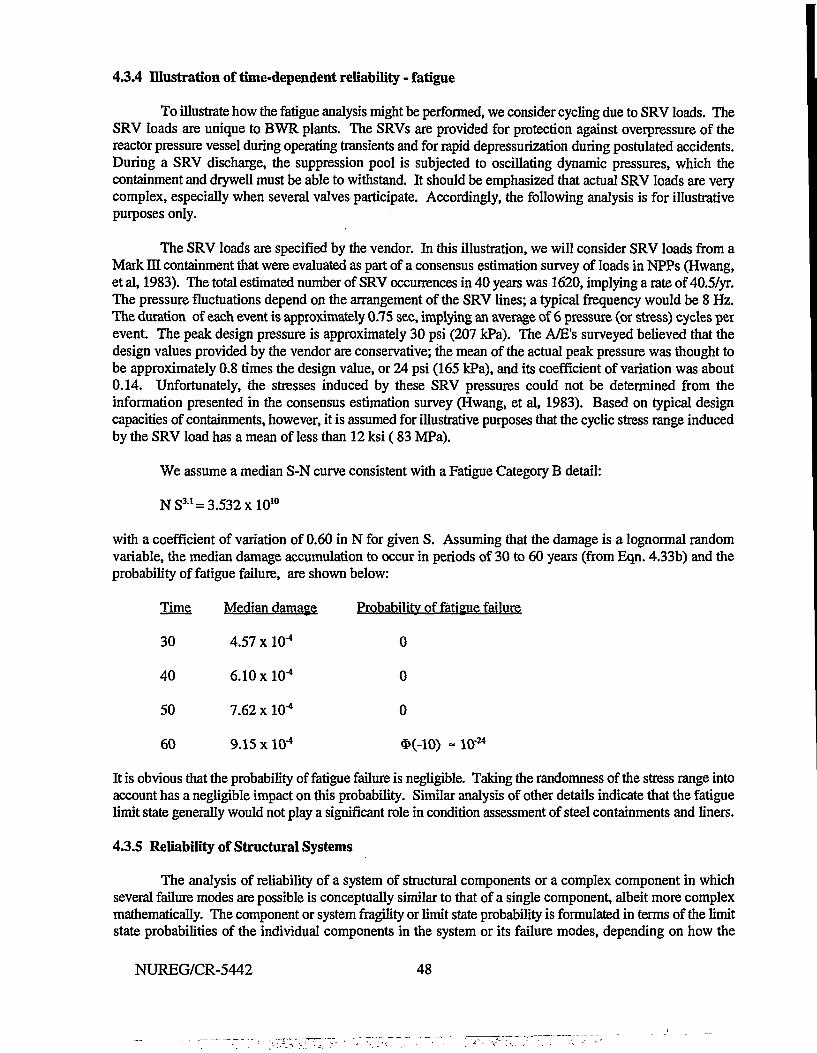
4.3.4 Illustration of time-dependent reliability - fatigue

To illustrate how the fatigue analysis might be performed, we consider cycling due to SRV loads. TheSRV loads are unique to BWR plants. The SRVs are provided for protection against overpressure of thereactor pressure vessel during operating transients and for rapid depressurization during postulated accidents.During a SRV discharge, the suppression pool is subjected to oscillating dynamic pressures, which thecontainment and drywell must be able to withstand. It should be emphasized that actual SRV loads are verycomplex, especially when several valves participate. Accordingly, the following analysis is for illustrativepurposes only.

The SRV loads are specified by the vendor. Li this illustration, we will consider SRV loads from aMark IE containment that were evaluated as part of a consensus estimation survey of loads in NPPs (Hwang,etal, 1983). The total estimated number of SRV occurrences in 40 years was 1620, implying a rate of 40.5/yr.The pressure fluctuations depend on the arrangement of the SRV lines; a typical frequency would be 8 Hz.The duration of each event is approximately 0.75 sec, implying an average of 6 pressure (or stress) cycles perevent. The peak design pressure is approximately 30 psi (207 kPa). The A/E's surveyed believed that thedesign values provided by the vendor are conservative; the mean of the actual peak pressure was thought tobe approximately 0.8 times the design value, or 24 psi (165 kPa), and its coefficient of variation was about0.14. Unfortunately, the stresses induced by these SRV pressures could not be determined from theinformation presented in the consensus estimation survey (Hwang, et al, 1983). Based on typical designcapacities of containments, however, it is assumed for illustrative purposes that the cyclic stress range inducedby the SRV load has a mean of less than 12 ksi ( 83 MPa).

We assume a median S-N curve consistent with a Fatigue Category B detail:

NS 3 1 = 3.532 xlO10

with a coefficient of variation of 0.60 in N for given S. Assuming that the damage is a lognormal randomvariable, the median damage accumulation to occur in periods of 30 to 60 years (from Eqn. 4.33b) and theprobability of fatigue failure, are shown below:

Time

30

40

50

60

Median damage

4.57 x 10-4

6.10 x 10"4

7.62 x 10"4

9.15 x 10"4

Probability of fatigue failure

0

0

0

$(-10) - 1024

It is obvious that the probability of fatigue failure is negligible. Taking the randomness of the stress range intoaccount has a negligible impact on this probability. Similar analysis of other details indicate that the fatiguelimit state generally would not play a significant role in condition assessment of steel containments and liners.

43.5 Reliability of Structural Systems

The analysis of reliability of a system of structural components or a complex component in whichseveral failure modes are possible is conceptually similar to that of a single component, albeit more complexmathematically. The component or system fragility or limit state probability is formulated in terms of the limitstate probabilities of the individual components in the system or its failure modes, depending on how the

NUREG/CR-5442 48

system is modeled mathematically (Moses, 1990; Karamchandani, et al, 1992; Rackwitz, 1985). There are twofundamental ways of modeling a system: as a series system and as a parallel system.

In a series system, failure occurs if any component fails (or if any mode occurs, depending on how thesystem is modeled). If, for example, a system consists of three components (or has three possible failuremodes) and if all three are necessary for proper functioning of the system (or if failure can occur in any oneof three modes), system failure will occur if any of the three components fails. The system failure event, Fsys,is described in terms of the component (mode) failure events, Fh as,

FSys = F i+F 2 + F3 (4.43)

in which "+" here denotes union of events. In a (strictly) parallel system, failure occurs only if all components(modes) fail. For the three-component system above,

Fsys = F , * F 2 * F 3 • (4.44)

in which "*" here denotes intersection of events. Most realistic engineered systems must be modeled ascombinations of unions and intersections; for example,

Fsys = F, + (F2*F3) (4.45)

meaning that the system fails if either component 1 fails or if components 2 and 3 fail together.

One generally analyzes the reliability of a system for a particular hazard, such as accidental pressureor earthquake, or collection of hazards. Such hazards are described by a CDF or complementary CDF(CCDF), several of which are summarized by the models listed in Table 4.1. The failures of the individualcomponents may be stochastically dependent. Stochastic dependence arises from several sources. First andperhaps most significant, the structural actions induced in each component from a common hazard are relatedby the laws of structural mechanics. To eliminate this source of dependence properly in the system reliabilityanalysis, the failure events in Eqns 4.41 - 4.43 must be analyzed as failures conditioned on a specific level ofhazard. Second, materials obtained from a common set of suppliers and common techniques employed by thecontractor in construction introduce dependence, although to a lesser degree. Finally, analysis assumptionsmade by the designer may affect several components simultaneously.

As a example, the fragility of the system in Eqn 4.43 for a specific accidental pressure, x, when theindividual component failures are statistically independent, is expressed in terms of the component fragilitiesas:

F ^ (x) = F^ (x) * [1 - F^ (x)] F^ (x) F^ (x) (4.46)

in which F;(x) is the fragility of component i, i = 1,2,3, the determination of which involves the considerationsdiscussed in Section 4.2.3. The individual (conditional) component (or mode) failure probabilities can bedetermined more easily than that of the system. The determination of component and system fragilities playsa key role in seismic margins analysis, as noted previously (Ellingwood, 1994). Once the (conditional) systemfailure probability is known, it can be convolved with the PDF of the hazard, as in Eqn 4.18, to determine theunconditional probability of system failure.

In the analysis of many complex facilities, it has been found that the COV in global system resistanceis on the order of component resistance COV, and thus is quite small in comparison with the COV in load(e.g., Banon, 1994a). Beneficial effects of redundancy often are offset by higher load variabilities. Failuremargins thus are highly correlated, and thus the failure mode and capacity found from a deterministic load-

49 NUREG/CR-5442

deformation analysis extended into the inelastic range often are adequate to establish the mean (or median) forprobabilistic analysis as well.

4.3.6 Appraisal of Structural Reliability Methods

In theory, component or system reliabilities can be computed from first-order reliability methods(FORM) or full-distribution methods (Shinozuka, 1983; Bjerager, 1990). In practice, this may not be as easyas it sounds. The determination of Fj(x) requires statistical data on material strengths, dimensions and otherbasic random variables, modeling errors, and a verifiable structural model of behavior based on principles ofmechanics to identify the limit condition (excessive inelastic deformation, instability, etc). There also is thenumerical problem in evaluating the probability integral for realistic systems.

In classical reliability analysis, there is a presumption that the limit state function (viz Eqn 4.17) isavailable in closed form, and therefore that the domain of integration of Eqn 4.18 is well-defined. However,modern structural analysis often is performed using finite element methods. In contrast to classical mechanics,finite element analysis (FEA) is algorithmic in nature, yielding structural responses (forces, displacements) atdiscrete points, but not a general closed-form expression for the limit state function. One can, however, useFEA to develop a "response surface" approximation to the limit state surface that is sufficiently accurate to beused in reliability analysis (Bucher and Borgund, 1990; Rajashekhar and Ellingwood, 1993). One firstperforms the FEA at a set of carefully selected experimental points in the domain of random variables. Next,a relatively simple function or response surface - commonly a second-order polynomial - is fitted to the FEAresults by regression or interpolation analysis. Once an adequate representation of the actual limit state hasbeen achieved (and this may involve some iteration in order to minimize statistical error), the reliabilityanalysis can be performed using the response surface.

The computation pf the probability integrals in Eqn 4.18 is numerically difficult when more than a fewrandom variables are involved. Monte Carlo methods can be used to perform these computations inapproximate form (Rubenstein, 1981). The Monte Carlo approach has a number of practical advantages,particularly in a structural system reliability analysis (e.g., Moses, 1990; Torng and Wirsching, 1991):complex structural behavior can be accommodated; stochastic dependency can be modeled; the possibleintroduction of new random variables due to inspection and repair can be dealt with; and several failure modescan be included, e.g., fracture from overload as opposed to fracture from crack growth. Perhaps one of themost useful features of Monte Carlo simulation is the way in which it facilites visualization of the damageevolution process.

The main disadvantage of Monte Carlo methods is their lack of numerical efficiency in structuralreliability analysis which involves small probabilities. If the event probabilities of interest are on the order of1O'N, an unmodified random sampling procedure requires approximately 10N+1 samples for the failureprobability estimate to be stable. The number of samples required to achieve a given sampling error, expressedby the standard deviation, SD(Pf), can be reduced by modifying the random sampling process. In structuralreliability analysis "importance sampling" often has been used for this purpose (Schueller and Stix, 1987;Melchers, 1990; Mori and Ellingwood, 1993). There are about 40 references on importance samplingtechniques (Engelund and Rackwitz, 1993). They can be categorized by: direct, updating, adaptive schemes,or spherical schemes/directional sampling. The efficiency of these approaches depends on the number of timesthe structural limit state must be calculated if the SD(Pf) < e; the efficiency thus is related more to the structuralanalysis than to the uncertainty analysis. In all methods except adaptive sampling, the positioning of theimportance sampling PDF must have been achieved with a suitable algorithm, often FORM. None of themethods is optimal under all circumstances, and some experimentation is required to determine the bestapproach for the particular problem at hand.

NUREG/CR-5442 50

4.4 Summary

Structural reliability analysis provides the framework for analyzing uncertainties in structural loads,operational demands on a structural component or system, and structural capacity to withstand demands. Thisinformation can be utilized on several levels: to identify a review level event to be used in a subsequentstructural analysis; to identify a high-confidence, low probability of failure capacity; to determine aninstantaneous probability of component or system failure; and to determine the probability of failure duringany service period.

A well-formulated system reliability analysis also can be used to evaluate fitness for continued serviceand to establish priorities for in-service inspection and maintenance. Existing internal events probabilistic riskassessments (PRAs) of existing plants have been used to establish priorities for inspection of the RPV andpiping (Doctor, et al, 1993). Inspection priorities were established by ranking importance measures based onthe contribution of component failures to core damage probability. While the information necessary to performsuch an importance analysis is a product of the structural reliability analysis, such an evaluation has not yetbeen attempted for steel containments and liners. In the next section, prospects for using reliability methodsin scheduling in-service inspection and maintenance will be considered.

51 NUREG/CR-5442

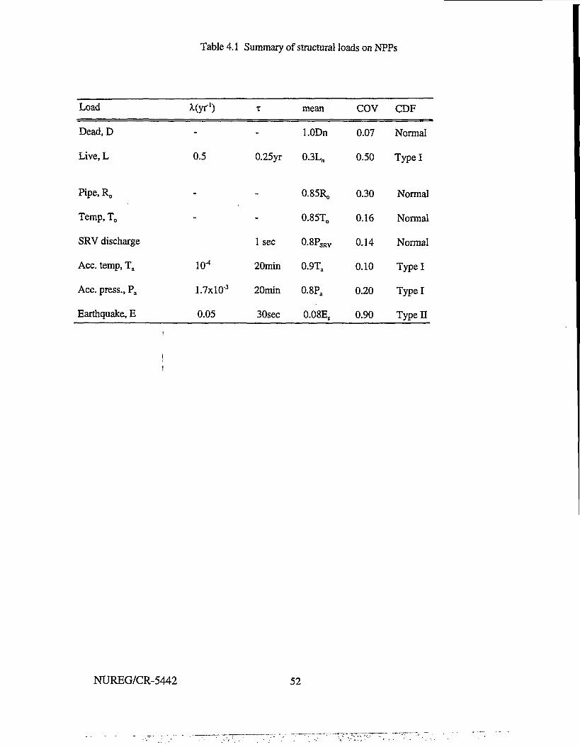
Table 4.1 Summary of structural loads on NPPs

Load

Dead, D

Live, L

Pipe, R,,

Temp, To

SRV discharge

Ace. temp, Ta

Ace. press., Pa

Earthquake, E

Myr"1)

-

0.5

-

-

lO"4

1.7xlO"3

0.05

X

-

0.25yr

-

-

1 sec

20min

20min

30sec

mean

l.ODn

0.3Ln

0.85R,

0.85To

0.8PSRV

0.9Ta

0.8Pa

0.08Es

COV

0.07

0.50

0.30

0.16

0.14

0.10

0.20

0.90

CDF

Normal

Type I

Normal

Normal

Normal

Type I

Type I

Typel!

NUREG/CR-5442 52

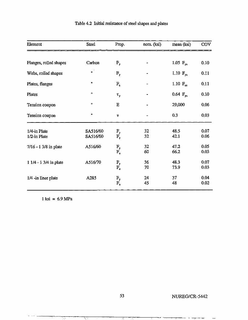
Table 4.2 Initial resistance of steel shapes and plates

Element Steel Prop. nom. (ksi) mean (ksi) COV

Flanges, rolled shapes

Webs, rolled shapes

Plates, flanges

Plates

Tension coupon

Tension coupon

Carbon -

-

-

-

-

-

3232

3260

3670

2445

1.05 F^

1.10 F^

1-10 Fun

0.64 F^

29,000

0.3

48.542.1

47.266.2

48.373.9

3748

0.10

0.11

0.11

0.10

0.06

0.03

0.070.06

0.050.03

0.070.03

0.040.02

1/4-in Plate1/2-in Plate

7/16 - 1 3/8 in plate

1 1/4-13/4 in plate

1/4 -in liner plate

SA516/60SA516/60

A516/60

A516/70

A285

1 ksi = 6.9 MPa

53 NUREG/CR-5442

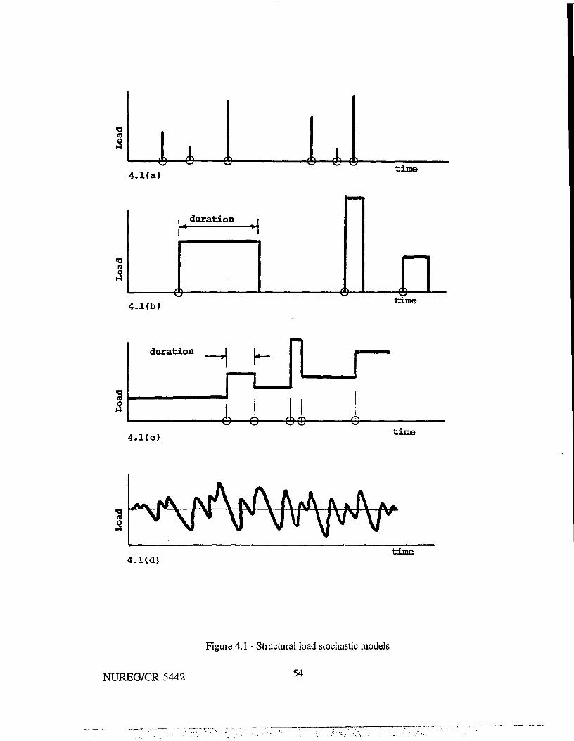
3 1time

4.Kb) time

is

duration H K-

A-itime

time

Figure 4.1 - Structural load stochastic models

NUREG/CR-5442 54

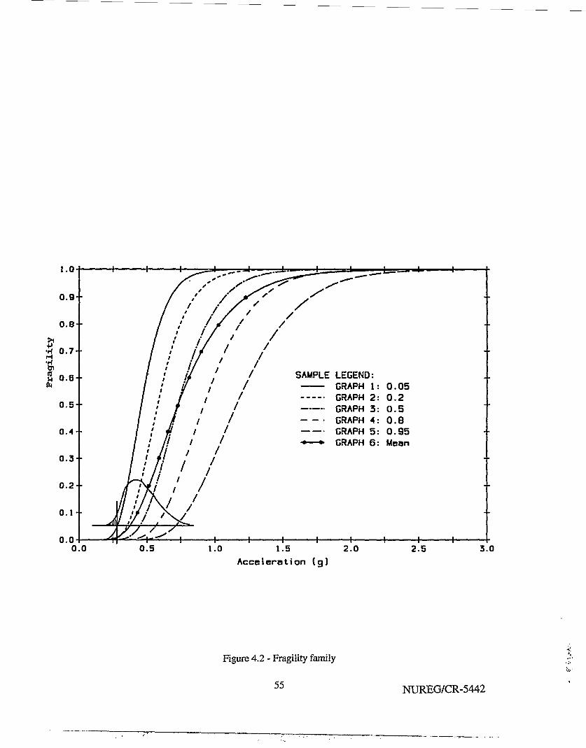
1.0-

0.9-

0.8-

•H 0.7-

(D - _U O . o "

0.5-

0.4-

0.3-

0.2-

0.1-

0.0-

h 1 1—

/ '

/ / •'

/ ' iJ/ / // / // : // ' // / /

Hi '£"'- -<^"^—1—

/ /

(/

1

11

1

11

1

/

h-

1 f1

I1

1f1

1

1

SAMPLE

.

H 1

LEGEND:GRAPH 1 :GRAPH 2 :GRAPH 3 :GRAPH 4 :GRAPH 5 :GRAPH 6 :

1

0.050 .20 .50 .80.95Mean

1 1 10.0 0.5 1.0 1.5 2.0

Accelerat ion (g)2.5 3.0

Figure 4.2 - Fragility family

55 NUREG/CR-5442

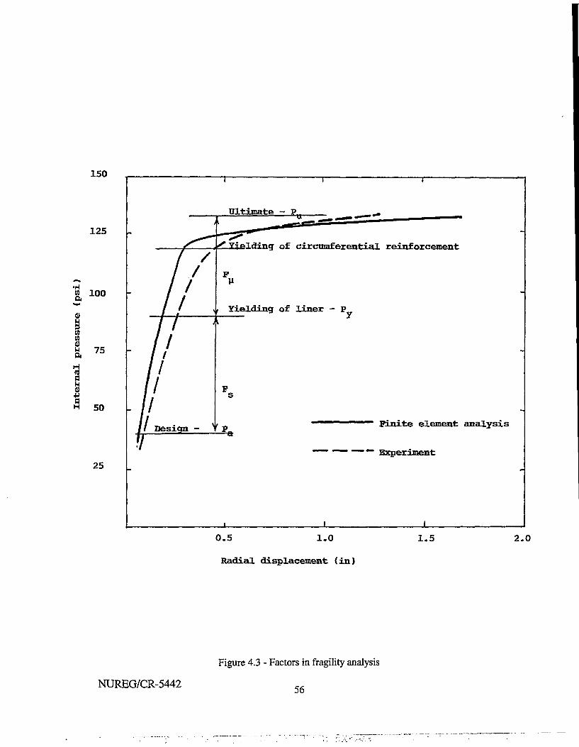
150

125

a

oww

ft

100

7 5

3H 50

25

Ultimate - P

Yielding of circmnferential reinforcement

Yielding of liner - P

Finite element analysis

*"~ """• ~~"" Experiment

0-5 1.0

Radial displacement (in)

1 . 5 2.0

NUREG/CR-5442

Figure 4.3 - Factors in fragility analysis

56

• .

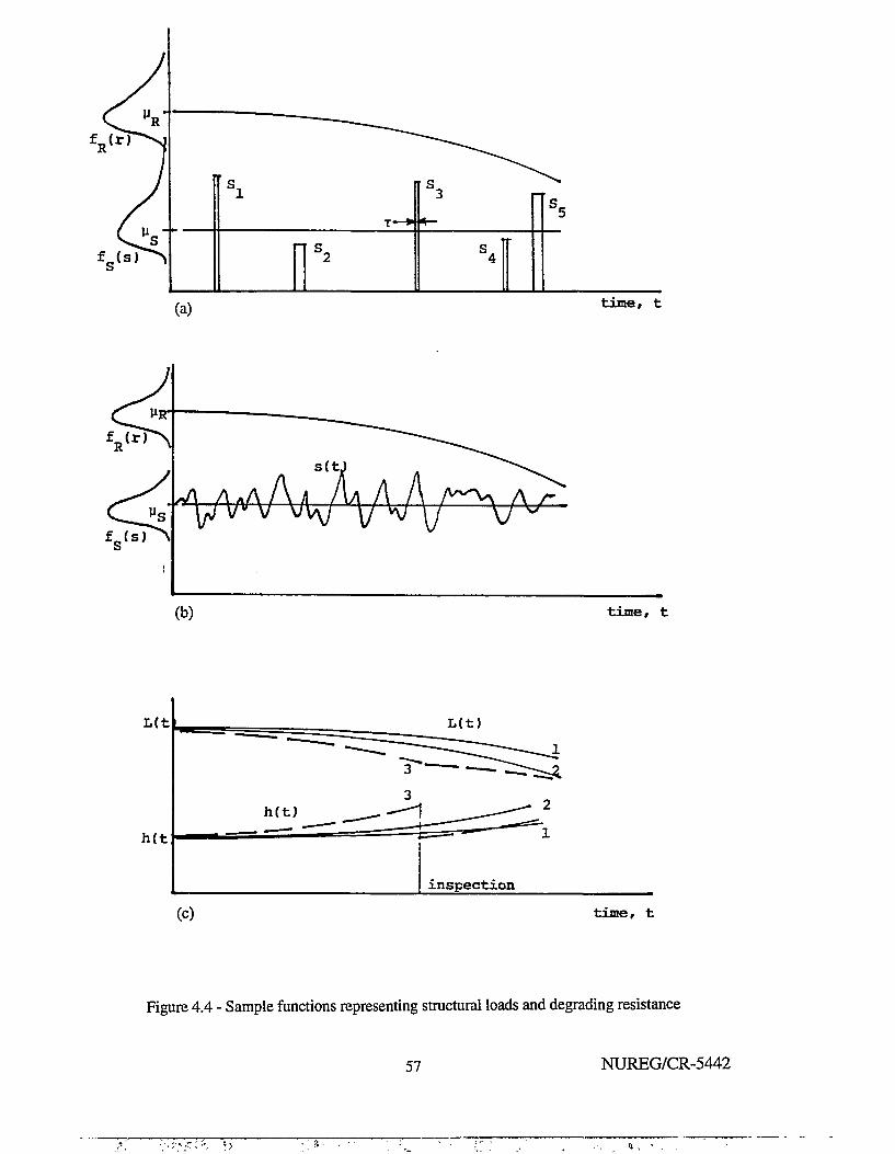
s1

— — - ~ _

1 S

s3

S 4

s5

(a) time, t

time, t

L(t

h(t

L(t)

inspection

(c) time, t

Figure 4.4 - Sample functions representing structural loads and degrading resistance

57 NUREG/CR-5442

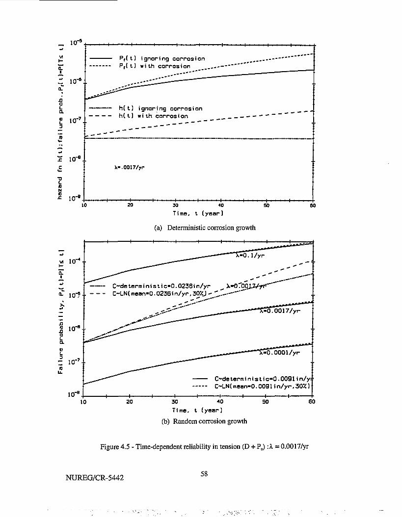
- 10"

VI

CLI

" 10*°..

oao 10"

2 10"9!

•o

nNn

Pf(t) ignoring corrosionPf( t) with corrosion

h(t) ignoring corrosionh(t) with corrosion

X-.0017/yr

10•+- •+-

20 30 40

Time, t (year)

(a) Deterministic corrosion growth

50 eo

vi 1CT--

Q.a

10"?

-0.1/yr

O d e term i n i s t i c-0.0236 i n/yrOLN(mean-0.0236 i n/yr. 30ZJ - .-—

.0001/yr

£>de term i n i s t i c-0.0091 i n/yiC~LN(mean-0.0091i n/yr .30*)

10 20 30 40Time, t (year)

(b) Random corrosion growth

50 60

Figure 4.5 - Time-dependent reliability in tension (D + Pa) :X = 0.0017/yr

NUREG/CR-5442 58

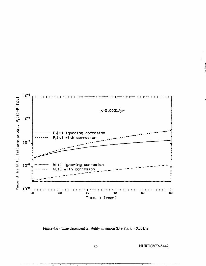
„ 10"5

VI» -

II

j 10-i

! • • • • !

X=0.0001/yr

oLaa)L

1 0 " 7 l

Pf(t) ignoring corrosionPf(t) with corrosion

JC 10"81 0 " B . . h(t) ignoring corrosionh(t) with corrosion

T)

N

10" •+- • + •

10 20 30 40

Time, t (year)50 60

Figure 4.6 - Time-dependent reliability in tension (D + Pa): A = 0.001/yr

59 NUREG/CR-5442

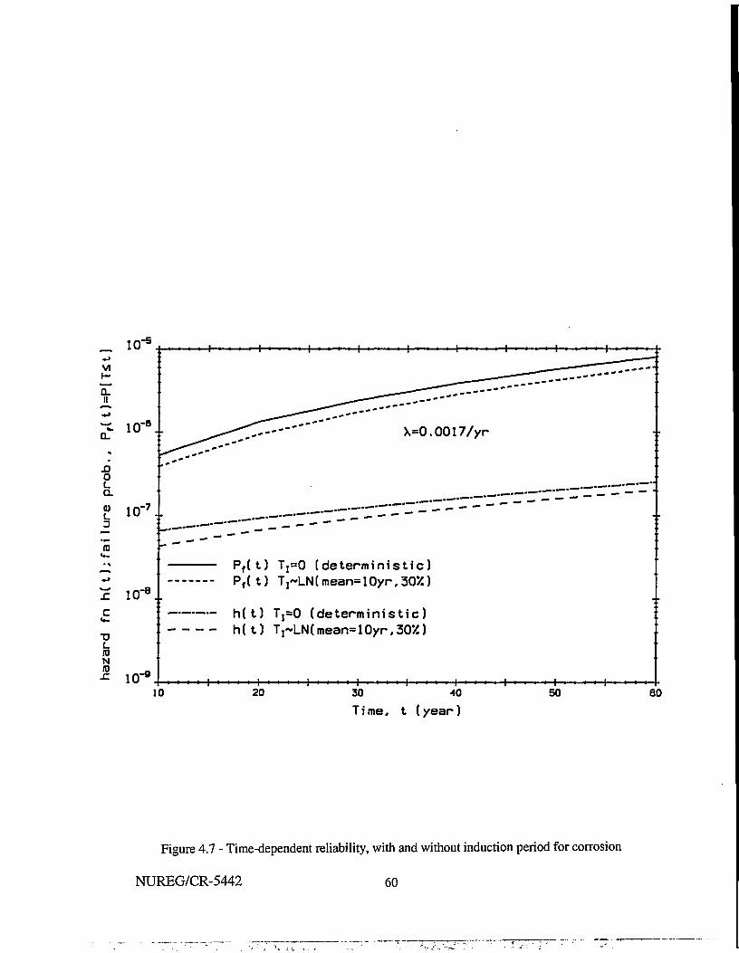
J3O

a0)L

D

IDNID

1O"71

£ 1 0 " 8 l

10"

\=0.0017/yr

P f( t ) T,=0 (determinis t ic)P f ( t ) T,~LN(mean=10yr,30Z)

h ( t ) Tj=0 (determinis t ic)h ( t ) T,"LN(mean=10yr<30/i)

10 20-f- •+- -t-30 40Time, t ( y e a r )

50 60

Figure 4.7 - Time-dependent reliability, with and without induction period for corrosion

NUREG/CR-5442 60

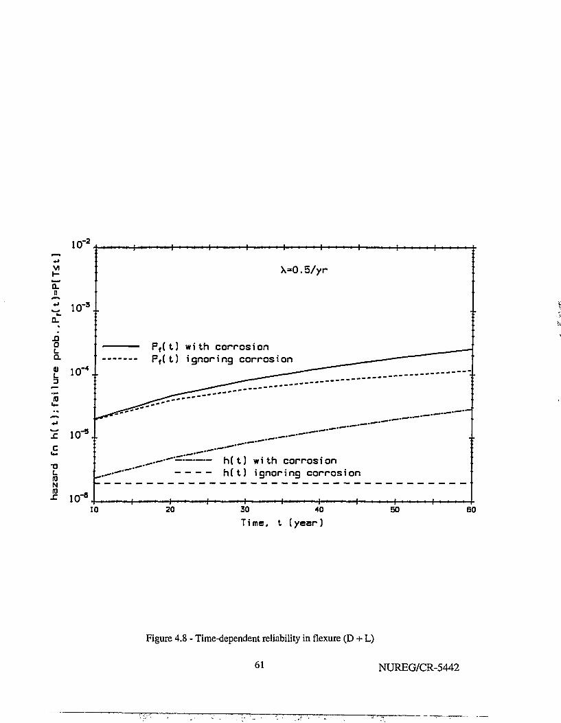
10',-2

VI

Q.II

X=0.5/yr

XIoaa

L.

10

10"4l

Pf(t) with corrosionPr(t) ignoring corrosion

JS 10"510" 5l

T3

N

— h(t) with corrosion- h(t) ignoring corrosion

10"10 20

•+• -f-30

Time,

•+• • • r •

4 0

t (year)

•+•50 B0

Figure 4.8 - Time-dependent reliability in flexure (D + L)

61 NUREG/CR-5442

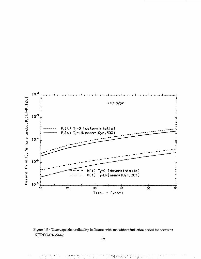
VI

Q.II

"3Z 10"a..

AO

a0)

5

IDNID

io-4 . .

r 1O"5!

10"

X=0.5/yr

P f( t) T,=O (determinist ic)P f( t) Tj~LN(mean=10yr,30X)

- h ( t ) Tj=O (determinist ic)— h ( t ) Ti~LN(mean=10yr,30/£)

10 201 l l

30 40Time, t ( y e a r )

50 80

Figure 4.9 - Time-dependent reliability in flexure, with and without induction period for corrosion

NUREG/CR-544262

5. TECHNIQUES FOR IN-SERVICE RISK MANAGEMENT

In-service inspection provides a means for minimizing the impact of aging on structural performance.Efficient and accurate nondestructive evaluation (NDE) methods, particularly those that are noninvasive anddo not disrupt the use of the structure, are essential for a properly designed condition assessment program tosupport facility risk management. Inspection and condition assessment identifies the cause and extent ofdamage, evaluates residual strength and serviceability, and provides recommendations on remedial measures(Chung, et al, 1993). Such remedial measures might include maintenance - actions that prevent or delaydamage or deterioration; repair - restoration of damaged structure for continued service; or rehabilitation -major modification of the structure to bring it up to current performance requirements (Wunderlich, 1991).

ASME Code Section XI Division 1, Subsection IWE currently sets inspection priorities for metalcontainments and liners of concrete containments. Insofar as can be determined, the ASME requirements arenot based on risk analysis, and a task force is considering revised risk-based guidelines (ASME, 1992). Thefocus of the ASME requirements is the RPV and various piping systems. NRC inspection guidelines call forpiping weld inspections based on material, heat treatment and service condition: e.g., 25% every 10 yrs; 50%every 10 yrs; 100% within two refueling cycles, etc (Holman, 1989). Most NPP facilities at present do notschedule general inspections of passive structural components regularly. Those that do inspect, do so atirregular intervals and rely almost exclusively on visual inspection. Condition assessments tend to be reactive,occurring only after there is some visible indication of damage or performance has been impaired. Operatingbudgets frequently do not provide for routine inspection. This attitude toward in-service inspection andmaintenance must change if life-cycle risk analysis is to evolve as a strategy for facility management.

Identification of deficiencies and detection of flaws in steel structures is difficult and demanding.Although large defects usually can be found visually if the structure is accessible, sophisticated methods maybe required to detect cracks or hidden defects. Incorporating this information into a reliability based structuralcondition assessment can have significant long-term economic and safety benefits.

5.1 Overview of in-service inspection approaches

A detailed condition survey is necessary at the initial stages of a inspection/maintenance/repairoperation. Design documentation and records of construction and repairs, service history and environmentalexposure should be reviewed at this time. The initial inspection, often performed visually, can documentinformation on cracking, spalling, leakage, evidence of chemical attack, and other factors that may lead tostructural deterioration, and indicates where to concentrate further quantitative testing procedures. Afundamental understanding of the structural performance requirements of the facility is required beforeinitiating any in-service inspection program. The inspection plan should consider component importance;structural redundancy; accessibility; repetitive use or correlations in behavior; severity of exposure; and priorhistory of performance (Banon et al, 1994a; Connolly, 1995).

In-service structural inspections should be oriented toward quantifying defects in a way that can beincorporated in calculations of the degraded strength of a structural component or system. Identifying thepresence of a defect without determining its size is not useful without further supplementary and quantitativeevaluation. Nondestructive evaluation methods, summarized in Section 3, should be used, if at all possible.To be useful in structural condition assessment, correlations must be established between the NDE parametermeasured (indentation diameter, pulse velocity, etc.) and the structural property of interest (tensile orcompression strength, crack size, etc.). These correlations customarily are established by regression analysisand there often is significant scatter in the data with respect to the regression relationship. In-situ structuralstrength varies over a structure or even within a large structural component, depending on the environmental

6 3 NUREG/CR-5442

conditions to which it is exposed. Thus, repetitive sampling is necessary to obtain reliable estimates of in-situstrength. It is, of course, desirable to sample at points where the strength requirements may be severe. Anappropriate sampling plan must specify the NDE procedure or procedures to be used, the zone of structure tobe sampled, and the number of samples to be taken.

In cases where NDE is noninformative or inconclusive, more invasive or destructive testing may berequired. Such methods have drawbacks. Destructive sampling makes post-inspection repair a critical issueand often militates against performing such tests. Small tensile coupons from steel components can be usedto estimate material strength and stiffness. However, steel coupon testing is not recommended unless it isbelieved that the steel has been accidentally overstressed, that there is evidence of fatigue or fire damage, orthat the original grade specified was not supplied. Such conditions seldom would occur in steel containmentsand liners in NPPs.

Load testing can be used in some cases to perform a strength evaluation of an existing structure (Hall,1988). In a typical test, the structure is loaded in stages to a relatively high fraction (say, 75 - 90 percent) ofits design strength, the load is held at each stage for a time, and deflections are measured at each stage (e.g.,ACI Standard 318,1989). The structure should show no signs of structural damage during the load test, andoften a limit is placed on maximum deflection. Following unloading, the recovery of deflection is used todetermine whether any permanent inelastic deformation has occurred, the occurrence of which might implynonvisible damage. Load testing should be used only when other methods lead to inconclusive results. Thetests are costly and disrupt the function of the facility unless performed during other scheduled maintenance.Moreover, recent reliability-based studies of proof load tests (Ellingwood, 1996) indicate that the test load mustexceed 80 percent of the design strength before one can conclude that passage of the load test implies ameasurable increase in reliability. At such load levels, there is a high probability that (repairable) damage tothe structure will occur. Destructive load testing (to failure) of components is useful only if the componentstested are mass-produced and easily replaced. The pressure imposed during the leakrate test performed onNPP containments is not sufficient in magnitude to verify the reliability of the containment for withstandingaccidental pressures in excess of the design-basis pressure, Pa.

5.2 Impact of in-service inspection on reliability

Forecasts of time-dependent reliability enable the analyst to determine the time period beyond whichthe desired reliability of the structure cannot be ensured. Conversely, intervals of in-service inspection andmaintenance (ISl/M)that may be required as a condition for continued operation can be determined from thetime-dependent reliability analysis (Madsen, 1987; Fujita, et al, 1989; Madsen, et al, 1989).

In-service inspection reveals information about the existing structure that can be used to revise theprior estimate of strength based on the materials in the structure, construction and methods of reliabilityanalysis described in Section 4. This change can be evaluated using Bayesian methods,

fR(rlD = CiK(Ilr)fR(r) (5.1)

in which K(Ilr) = likelihood function, fR(rlI) = updated (posterior) PDF of structural resistance, and c; =normalizing constant. The Bayesian updating process is illustrated in Figure 5.1. The likelihood functiondepends on the nature of the NDE technology employed. Maintenance or repair also cause the characteristicsof the strength to change by removing some of the larger defects from the structure, thereby (usually)upgrading its strength and shifting the PDF of resistance to higher strengths. This upgrading of the PDF canalso be determined from Bayes theorem:

fR(rlI,M) = cmK(Mlr,DfR(rlI) " (5.2)

NUREG/CR-5442 64

in which K(Mlr,I) = likelihood function and cm = normalizing constant The time-dependent reliability analysisthen is re-initialized following ISI/M using fR(rII) or fR(rII,M) in place of fR(r).

More generally, suppose that the margin of safety at time t is M(t) = R(t) - S(t), as in Eqn 4.17. Theinstantaneous probability of failure is P[M(t) < 0]. Additional information gained through ISI/M aboutstructural performance can be defined by another event, H < 0, expressed in terms of the structural variables.The revised failure probability following ISI/M is (Madsen, 1987),

P[M<0IH<0] = P[M<0,H<0]/P[H<0] (5.3)

For example, if the structure survives a load test with load magnitude S = q, then H = q - R < 0, and Eqn 5.3becomes,

fR(rlH) = [1 - FaCq)]"1 fR(r); r * q (5.4)

= 0 ; r < q

A similar approach can be taken if deflection or another structural response parameter is measured during astructural test. Moreover, if several response quantities are measured, the formulation of event H < 0 maybecome more complex or may be replaced by a joint event H = {Hj < 0,H2 < 0,..., Hk = 0,...} involving bothinequalities and equalities. In any event, the basic principle is the same. Subsequent reliability analysis shoulduse fR(rlH) in place of the prior estimate, fR(r).

In-service inspection and repair may cause the the hazard function, h(t), to change abruptly, dependingon how fR(rIH) differs from fR(r) as a result of what is learned about the current condition of the structure andwhat repair actions are taken. A conceptual illustration of the effect of this process on the hazard function ispresented in Figure 5.2. The removal of larger defects from the structure following repair reduces itsconditional failure rate. As the structure ages, the failure rate increases until another repair operation occurs.The probability of structural survival during interval (t,,^, given that the structure has survived until tu is

LCt,, ) = expf-p h(x)dxj (5.5)

The integrated effect of h(t) in Figure 5.2 must remaia below the target limit state probability.

Structures in a NPP are too complex and numerous to be completely monitored during their servicelife. There is a need to: (1) prioritize major components in terms of their impact on the performance of thefacility; (2) identify a limited set of potential degradation sites and modes for the current operating spectrum;and (3) develop an in-service inspection plan that is directed toward (but not focussed exclusively on) thoselimited sites. Some sort of adaptive learning process seems most desirable for NDE. A process is envisionedthat involves, first of all, inspecting a portion of structure using some noninvasive technique. If damage isfound, an additional portion is inspected, perhaps with a different technique, depending on what is learned atthe first inspection.

To illustrate the impact of NDE on the PDF of strength after inspection, we continue with the sameexample as in Section 4.3.2. Assume that rate C is a lognormal random variable, with mean equal to itsnominal value, and a COV of 20%. The exponent m remains deterministic. The randomness in corrosion lossD(t) arises out of the randomness in C and induction time, T,. Since D(t) is zero if t is less than tj, it has amixed distribution with a spike (probability mass function, or PMF) at 0. Figure 5.3 shows the distributionsof D(t) at 10 yr and 40 yr, with the mean, standard deviation and the value of the PMF at 0.

An inspection is carried out at t = 40 yr. The POD curve of the NDE instrument is

65 NUREG/CR-5442

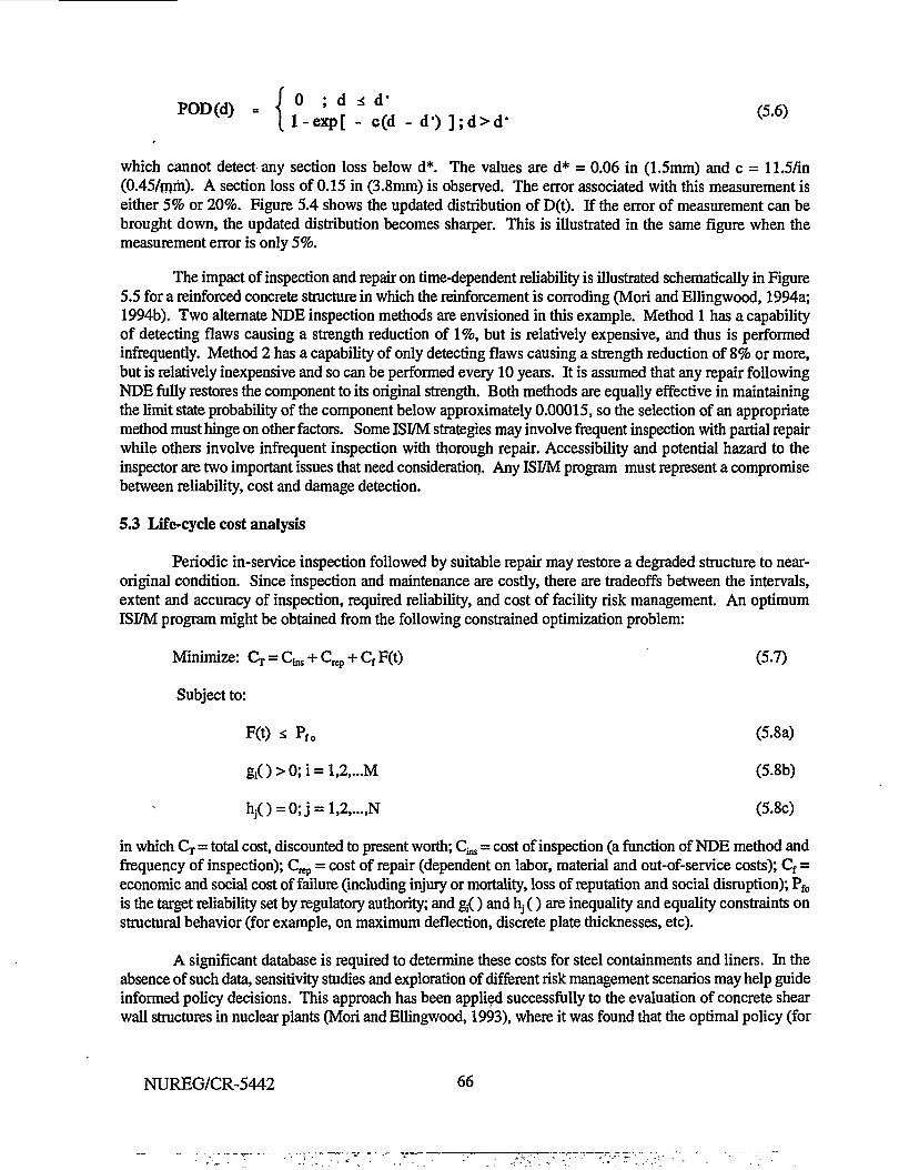
POD(d) = { ° ; d * d ' (56)w 1 l-exp[ - c(d - d') ];d>d* { }

which cannot detect any section loss below d*. The values are d* = 0.06 in (1.5mm) and c = 11.5/in(0.45/mm). A section loss of 0.15 in (3.8mm) is observed. The error associated with this measurement iseither 5% or 20%. Figure 5.4 shows the updated distribution of D(t). If the error of measurement can bebrought down, the updated distribution becomes sharper. This is illustrated in the same figure when themeasurement error is only 5%.

The impact of inspection and repair on time-dependent reliability is illustrated schematically in Figure5.5 for a reinforced concrete structure in which the reinforcement is corroding (Mori and Ellingwood, 1994a;1994b). Two alternate NDE inspection methods are envisioned in this example. Method 1 has a capabilityof detecting flaws causing a strength reduction of 1%, but is relatively expensive, and thus is performedinfrequently. Method 2 has a capability of only detecting flaws causing a strength reduction of 8% or more,but is relatively inexpensive and so can be performed every 10 years. It is assumed that any repair followingNDE fully restores the component to its original strength. Both methods are equally effective in maintainingthe limit state probability of the component below approximately 0.00015, so the selection of an appropriatemethod must hinge on other factors. Some IS1/M strategies may involve frequent inspection with partial repairwhile others involve infrequent inspection with thorough repair. Accessibility and potential hazard to theinspector are two important issues that need consideration. Any ISI/M program must represent a compromisebetween reliability, cost and damage detection.

5.3 Life-cycle cost analysis

Periodic in-service inspection followed by suitable repair may restore a degraded structure to near-original condition. Since inspection and maintenance are costly, there are tradeoffs between the intervals,extent and accuracy of inspection, required reliability, and cost of facility risk management. An optimumISI/M program might be obtained from the following constrained optimization problem:

Minimize: Q. = C ^ + Crep + Cf F(t) (5.7)

Subject to:

F(t) * Pf0 (5.8a)

= l,2,...M (5.8b)

= l,2,...,N (5.8c)

in which Cj = total cost, discounted to present worth; C^ = cost of inspection (a function of NDE method andfrequency of inspection); Crep = cost of repair (dependent on labor, material and out-of-service costs); Cf =economic and social cost of failure (including injury or mortality, loss of reputation and social disruption); Pf0

is the target reliability set by regulatory authority; and g;() and hj ( ) are inequality and equality constraints onstructural behavior (for example, on maximum deflection, discrete plate thicknesses, etc).

A significant database is required to determine these costs for steel containments and liners. In theabsence of such data, sensitivity studies and exploration of different risk management scenarios may help guideinformed policy decisions. This approach has been applied successfully to the evaluation of concrete shearwall structures in nuclear plants (Mori and Ellingwood, 1993), where it was found that the optimal policy (for

NUREG/CR-5442 66

degrading reinforced concrete structural components) was to perform 1SUM at essentially uniform intervalsover the service period.

Modern risk analysis focuses on the expected failure cost, Q F(t), the third term in Eqn 5.7, suggestingthat risk involves both probability and consequences. Low probability events can be very risky if associatedwith inordinate failure costs (e.g, ASME, 1992). There is more uncertainty in the likelihood of a rare eventthan in its consequences. While appearing to rationalize the decision process, minimum expected costdecision-making does have some shortcomings (Banon 1994b). Perhaps foremost is how to quantify intangiblecosts such as loss of life or environmental pollution associated with rare events. It also is difficult to compareevents with high-cost and low probability of failure to alternatives involving low cost but high probability offailure. The product Cf F(t) is the same in both cases, but the decision preference is not. The development ofpublic policies with regard to mitigation of fatalities from automobile vs commercial aviation is a case in point

5.4 Measures of risk

Risk assessment methods must be consistent for different applications in order to produce coherentpolicy and regulations. Proper facility risk management involves maintaining a level of safety in performancethat is acceptable to society and that is understood by the people that incur the risks. A sound risk managementstrategy requires (Pate-Cornell, 1994) economic efficiency; equity (no individual should incur excessive risk);maintains risk at or below de minimis levels (below regulatory concern); and distinguishes between risks thatpeople incur voluntarily or with informed consent and those that the do not. Unfortunately, this goal of riskmanagement currently is seldom achieved.

Structural reliability analysis in Section 4 yields the probability of failure as the quantitative measureof structural performance. In the absence of definitive data on failure costs, the probability of failure also isa surrogate for risk. This estimated failure probability must be compared to a target probability set byregulatory authority or by social custom. The target probability, Pf0, also furnishes one of the constraints inlife-cycle cost optimization (see Eqn 5.8), so its determination is a key consideration. There are essentiallythree points of view on how Pfo should be measured (Sorensen, et al, 1994):

(1) Single person acceptable risk: number of accidents or lives lost/number of participants, peopleexposed;

(2) Society risk: number of accidents or lives lost/number of people in society;

(3) Decision theoretical basis: economic optimum from minimizing the total cost, Ci(pf) + pf Cf,assuming that Cf is independent of pf.

Measures (1) and (2) can be quite different, since the relation between individual risk and social risk isnonlinear. Difficulties with measure (3) stemming from an inability to determine Cf have been discussedpreviously.

With a measurement agreed upon, it remains to determine a numerical measure of acceptable risk ofPf0. Risks associated with engineered structures, while unknown, certainly are very low. It generally is agreedthat the target value of Pf0 should depend on the type of structure, the mode of failure, its relative importanceto the facility, the residual life desired, and possible socioeconomic consequences of failure. Risks due tostructural failures should be much less than risks from operational failures. Structural failures affect manyfacility systems simultaneously, and thus the consequences are widespread. Moreover, repair of structuralcomponents that have failed invariably requires that the facility be taken out of service for an extended periodto time while repairs are made. Such downtimes may have severe economic consequences. Beyond these

6 7 NUREG/CR-5442

general observations, however, obtaining agreement on a precise numerical measure (or range of values) hasproved to be elusive.

One approach might be to determine levels of acceptable risk from an examination of existingengineering criteria that have led to facilities that are known to have performed acceptably in the past. Thosein support of this so-called calibration approach argue that if the current risks associated with a particulartechnology were unacceptable, public outrage would have forced corrective action. Indeed, this approach wasused to set the load and resistance factors used in the first-generation of probability-based limit states designspecifications for ordinary building construction (e.g., LRFD, 1993). The calibration approach works providedthat the technology to which the criteria are applied is established, relatively stable and is evolving at a slowenough rate that it is possible to learn from experience. However, historical data on actual failures provide anincomplete picture of acceptable structural risk because structural failure events are so rare. In the case ofunique facilities such as offshore platforms and NPPs, historical data on failures are virtually nonexistent.Morover, the calibration approach does not really provide a point estimate of acceptable risk but rather a lowerbound, since there is no way of knowing a posteriori whether less conservative criteria (with higher Pf0) wouldalso have proved to be acceptable. In fact, the large range in failure probabilities associated with existingdesign specifications is evidence to the contrary.

A second approach might be to establish reliability targets by considering comparable and presumablyacceptable risks in other human endeavors (Ellingwood, 1994). However, comparisons of structural failureprobabilities (assuming that they can be determined) with mortality statistics that have been reported elsewhereare inherently flawed. Such comparisons fail to take into account differences in the population at risk and thelarge uncertainties associated with reliability evaluation of structures. There currently is no generally acceptedmechanism for comparing risks from diverse hazards with low probabilities; nor is there a comprehensivedatabase to support such a comparative risk assessment. Accordingly, it has been suggested that civil engineersshould concentrate their efforts on managing hazards rather than on assessment of risks (Comerford andBlockley, 1993).

Determining an acceptable risk for an aging structure presents some unique challenges. It often is noteconomically feasible to restore an aging facility to its original condition. If the operation of the facility meetsan essential overall social objective, such as adequate electric power, the need remains even if the facility isclosed and alternatives will be sought. In this case, closing one facility may simply displace the risk to another.There does appear to be some willingness to accept lower reliabilities for older systems and not to require thatolder systems have the same reliability as new systems.

One can argue that if failure has the same consequences (e.g., involuntary offsite exposure), the risksfor an existing facility and a new facility should be the same. However, a sensible definition of risk involvestime of exposure as well as level of exposure, and it makes sense to differentiate between a short-term risk anda cumulative risk over an extended service period. The individual risk safety goal (on an annual basis) shouldbe approximately the same for old and new facilities but the cumulative risk for a service period may bedifferent. This is analogous to the difference between hazard h(t) and (cumulative) failure probability, F(t).

Target risks for critical facilities vary widely (Pate-Cornell, 1994). A review of risk targets for NPPsin the US and abroad suggests that the maximum annual probability of severe core damage is on the order of10"4; in addition, the maximum tolerable risk offsite individual = lO^/yr (Okrent, 1987). Core damageprobabilities computed from Level 1 PRAs generally are at or below these levels. There is no way ofvalidating such low levels of failure probability conclusively (Lewis, 1985). However, it should be noted thatthe computed risk of a structure is not an attribute of the structure but of the mathematical reliability modelused to analyze the structure. It can be used as an attribute to guide decision-making if the model isdependable (Comerford and Blockley, 1993). Moreover, a comparison of decision alternatives with such riskmodels used consistently may provide an improved basis for decision-making, irrespective of the absolute risks

NUREG/CR-5442 6 8

computed. Since this is a temporary answer to a perennial issue, an effort must be made to validate risk modelsof NPP facilities and to determine their limitations for risk analysis and life extension policies.

For example, Level 1 internal events PRAs of NPPs have been used recently to examine risk due tofailure of RPV and piping pressure boundary components, to rank their importance, and to establish inspectionpriorities (Vo, et al, 1994a, 1994b). ASME Section XI classifications and ISI requirements seem to be inquantitative agreement with rankings based on estimated mean core damage. It was recommended that theprobability of core damage due to failures of pressure boundary components be kept to 5% (or less) of the totalcore damage probability estimated by the PRA, and that the permitted increase should be allocated amongcomponents of a system in accordance with their relative importance. For example, if overall core damageprobability is 5 x 10"6, pressure-boundary component probability should be 2.5 x 10"7, distributed among thecomponents. Components making the greatest contribution to risk should have the most stringent inspectionrequirements. Steel structural components and systems were not considered in this study, nor were parameterand modeling uncertainties considered explicitly.

5.5 Summary

Probability-based criteria for facility risk management are being developed in other industries, mostnotably in the offshore industry. The American Petroleum Institute (API) is developing new guidelines thatcan be used for reassessment of offshore platforms (Banon, 1994b). Reassessment is aimed at answering thefollowing questions: Are design/construction drawings available? What is the physical condition of theplatform? What were previous inspection results? What level of structural analysis is necessary to assessresistance? Is all existing damage identified and included in the assessment? What are the potential failuremodes and consequences? How likely is each failure mode? What level of risk is acceptable? What repairmeasures are feasible for the damage observed? It seems clear that such generic questions are germane to theevaluation of aging in NPPs as well. In the nuclear industry, ASME has formed a research group to considerrisk-based inspection guidelines (ASME, 1992). In related research (Vo, 1994b), internal events Level 1(core damage) PRAs were used to identify the most significant pressurized systems for plant risk and thereforefor special attention during inspection. Seven PWRs and two BWRs were considered. Passive structuralcomponents were not considered.

The data to support risk-based inspection/maintenance programs for steel containments and liners arenot complete at present and will be developed in a later phase of this research program. Nondestructiveevaluation provides solutions to the lack of quantitative data. If the NDE information (generally at the localscale) can be incorporated into a rational structural condition and reliability assessment, the long-termeconomic benefits will be significant.

69 NUREG/CR-5442

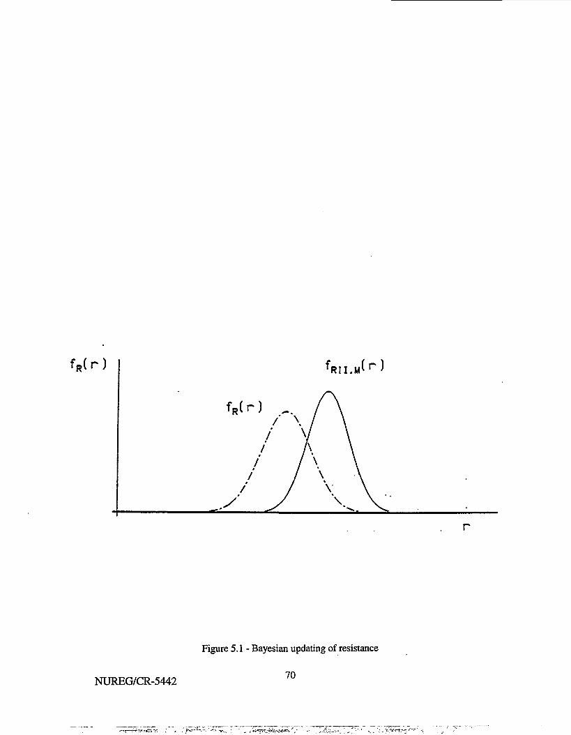
fp(r)

Figure 5.1 - Bayesian updating of resistance

NUREG/CR-544270

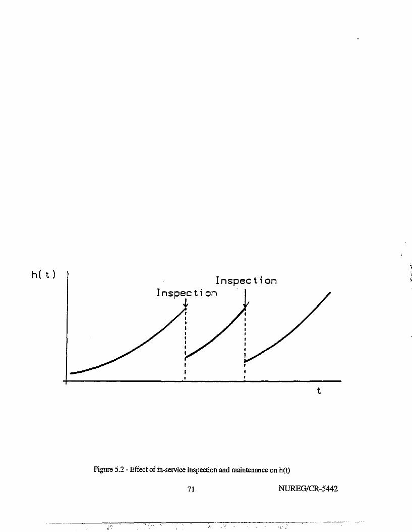
h(t) Inspecti onInspect!on

Figure 5.2 - Effect of in-service inspection and maintenance on h(t)

71 NUREG/CR-5442

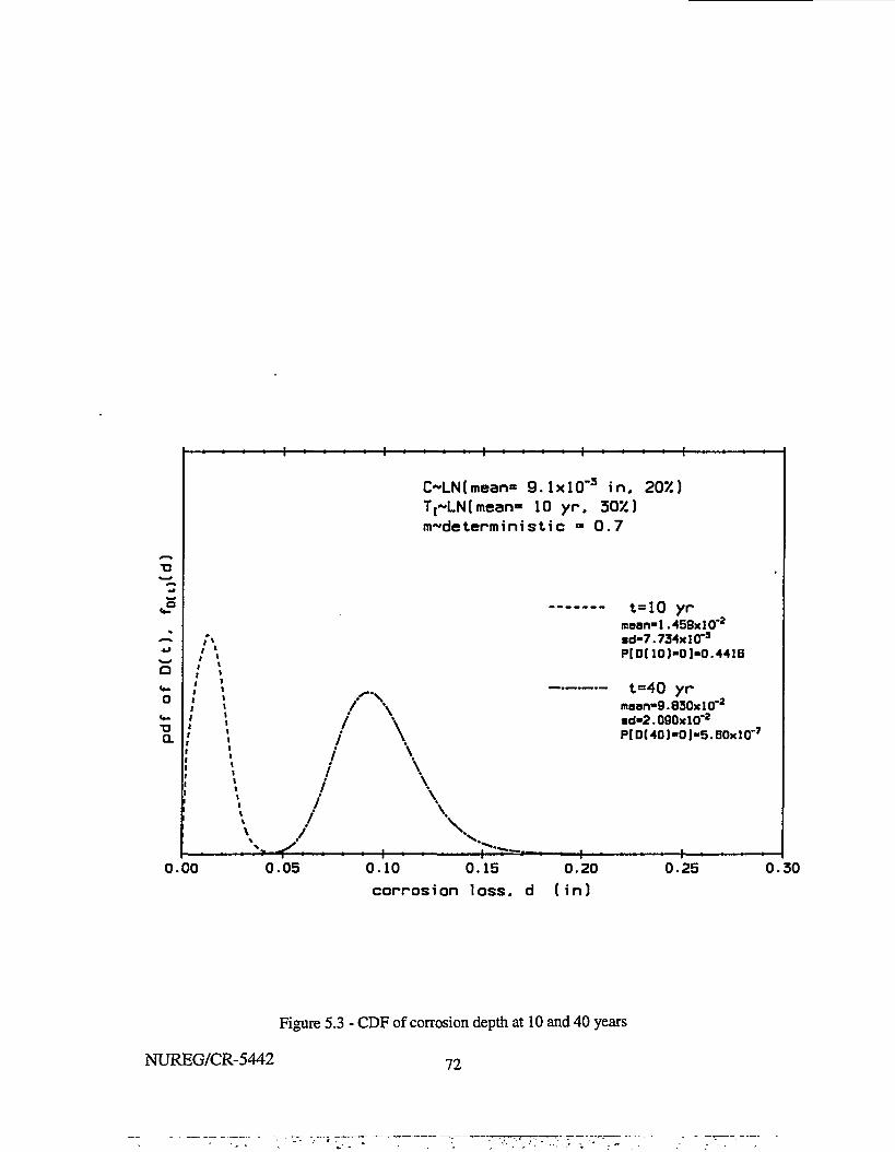
a«-O

a

• • • • i . . .

1 t, 1

/ \

•' l /

' 1 /1 /

I > /

1 /

/

/

/

s /

• ! • • • • — 1 • '

C~LN(mean»Tj~LN(mean»

' • • i • • • • i • • • •

g.lxlO"3 in. 20*/.)10 yr. 507.)

m^deterministic = 0 . 7

..'* \

\\

\

• i • • • • r * " ! — »

•

t=10 yrmean-1.458x10'2«d-7.734xlO"3

P[D(10)-0]-0.441B

t=40 yrmean-9.830xl0"2

«d-2.090xl0"2

PlDt40)-0j-5.B0xl0"7

— — • | • • • • I • • • • —

0.00 0.05 0.10 0.15 0.20 0.25 0.30

corrosion loss, d (in)

Figure 5.3 - CDF of corrosion depth at 10 and 40 years

NUREG/CR-5442 7 2

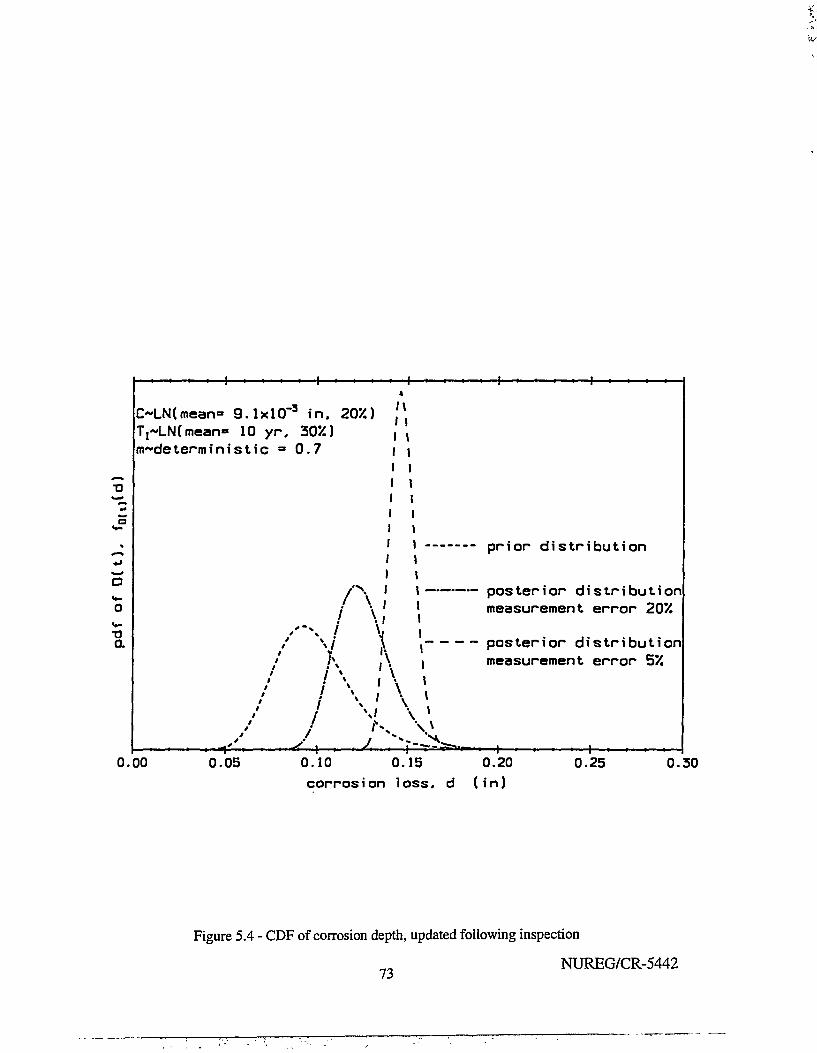
TJ« • ; ,

5«••

*>

Q<*-0

pdf

• • • • — I -

OLN(mean=TI~LN(mean»m~de term i n i

• • • • — I • •

9.1xlO"3 in. 20210 yr.stic =

I:

/

30X)0.7

j

>'m\ ivh1 \I \1

' • 1

' i\1 \

1 11111111

'1I

\!t/\*

i • • " •

iiii -------

iii

i•

i _

ii

prior distribution

posterior distributionmeasurement error 20X

posterior distributionmeasurement error 5%

1 • • • • 1 • < • •

0.00 0.05 0.10 0.15 0.20

corrosion loss, d (in)

0.25 0.30

Figure 5.4 - CDF of corrosion depth, updated following inspection

? 3 NUREG/CR-5442

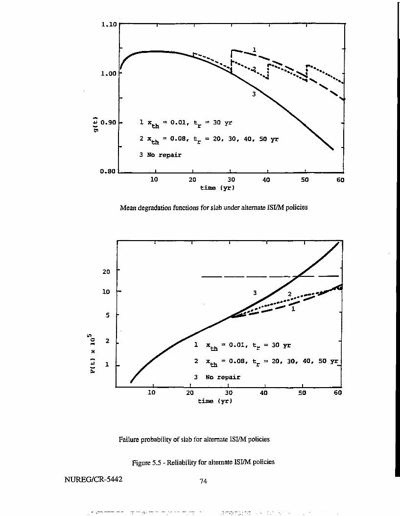
1.10

1.00 -

0.90 -

0.80

(

-

- 1

2

3

t I

Xth = °-01' fcr

xth = °-08' fcr

No repair

i i

= 30

= 20,

J

r-^>

yr

30,

t

. 1

3

40, 50 yr N.

10 20 30time (yr)

40 50

Mean degradation functions for slab under alternate ISI/M policies

60

m

10

20

10

5

2

1

• i

-

-

S^ 2 xth = °-08

No repair

r tr = 30 yr

, tr = 20, 30, 40, 50 yr_

i t

20 30time (yr)

40 50 60

Failure probability of slab for alternate ISI/M policies

Figure 5.5 - Reliability for alternate ISI/M policies

NUREG/CR-5442 7 4

6. MARKOV PROCESS MODEL OF DAMAGE ACCUMULATION

Damage accumulation in a large complex structure may be very difficult to track. The progressionof damage accumulation in a structure can be modeled as a Markov process (Bogdanoff and Kozin, 1985;Rahman and Grigoriu, 1993). The Markov model does not provide any insight into the mechanics of damageaccumulation. It simply provides a convenient framework for describing the evolution of damage stateprobabilities over time and, with its matrix formulation, provides a convenient algorithm for computerization.The Markov formulation can be viewed as operating on a number of levels. At the simplest level, it can beused to track "damage" when damage and effectiveness of in-service inspection and maintenance can only bedescribed linguistically. At the other extreme, the state of damage can be determined probabilistically usingstochastic computational mechanics formulations developed in the previous sections of this report.

We begin by envisioning a "duty cycle" (DC) for the structural system, which is some repetitivesequence of loads during the service life that arises from the operation of the facility and during which damagecan accumulate. At one extreme, loads from a standard cycle between refueling outages might be oneexample; at the other extreme, in the case of a broad-band load history, each distinct load might be considereda DC. The Markov model arises from the idea that the increment of damage that accumulates during each DCdepends only on the value of damage that has accumulated up to the start of that DC; the damage incrementis statistically independent of the process by which damage accumulated prior to the start of the DC. Underthese conditions, damage accumulation can be modeled as a Markov process, with time measured in DC units.If the damage state is discretized as well, the process is referred to as a Markov chain.

As a simple illustration of this concept, we might envision the structure to be in one of i = 1,2,...,Mdiscrete states of damage, D(t) = i at any time t (note that t can be an integer if time is measured in DC unitsor in cycles). The set {l,2...,m} is denoted the state space, and can be written for a structural component orsystem. One might say that the structure is undamaged if D(t) = 1 and that the structure has failed if D(t) =M. These definitions are completely arbitrary; the damage measure could be normalized as D(t) = (i-l)/(M-l)so that D(t) is consistent with the previous discussion of damage accumulation by the Palmgren-Minerhypothesis. The probability that the structure is in damage state, i, at time t is denoted,

P[D(t) = i] = Pi(t); i = l , 2 , . . , M (6.1)

The prior service history of structural behavior up to time t (here, t could be discrete or continuous) can beexpressed as the collection of observation times and damage states,

H t = {D(0),D(l),...,D(t-l)} (6.2)

The Markov property implies that the conditional probability that D(t) = i, conditioned on prior service history,is,

P[D(t) = ilHJ = P[D(t) = ilD(t-l) = j] (6.3a)

in which,

£ P[D(t) = i|D(t-l)=j] = 1.0 ; j = 1.2.....M (6.3b)i.i

In other words, if the immediate state of the structure is known, the future state is independent of past states.

7 5 NUREG/CR-5442

At some later time, v, the probability that the structure is in state j is,

PP(v)=j] - £ P (v|t) Pfi) (6.4)i.i

in which Py(vlt) = P[D(v)=jiD(t)=i] is the conditional probability that the structure is in state j at v, given thatit was in state i at t. Eqn 6.4 is simply a statement of the theorem of total probability. Considering all Mdamage states and collecting elements P;(t) into column vector, P(t), Eqn 6.5 can be expressed in matrix form:

P(v) = P(vlt)P(t) (6.5)

in which P(vlt) is denoted the "transition probability matrix" between stages t and v. With the Markovproperty, the elements of the transition probability in this summation are (the Chapman-Kolmogorov equation),

P [D(v )= j |D( t ) = i] = £ Pfc<y|ii)Py(u|t) (6.6)k-i

for t < u < v, and are independent of the history of damage accumulation prior to t.

According to Eqn 6.6, matrix P(vlt) can be constructed as the product of one-step transition matrices,TOO:

P(v|t) = E T(v-k) (6.7)k.0

Element PMM of T(v-k) is unity, the absorbing state of the chain (representing failure). In general, T(v-k) isa function of time (or index, k). However, in the case where P(vlt) depends only on v-t, the chain is said to behomogeneous (or have stationary increments), and

P(vlt) = T** (6.8)

in which T = stationary one-step transition probability matrix. Much of the mathematical literature on Markovchains has been developed for processes with stationary increments. It should be~noted that a process withstationary increments is not necessarily a stationary process, i.e., one in which the probability function P[D(t)= i] is invariant in time.

One can use Eqn 6.7 to track the evolution of damage accumulation through the service life of astructure, provided that the initial damage state vector, P(0), is known. Li general, we would have,

P(t) = H T( t -k) P(0) (6.9)

If the structure is undamaged in its initial condition, P(0) = (l,0,...,0)'. Since matrix multiplication is notcommutative, the order of damage cycles is important for damage accumulation. If the matrix T(t-k) isindependent of k and the process has stationary increments, then

P(t) = T'P(0) (6.10)

The elements of the transition matrix can be estimated by modeling the structural deteriorationmechanisms described in Section 3 as stochastic processes. The nature of structural degradation determinesthe characteristics of T. Since damage accumulation is assumed to be irreversible, T is a lower triangularmatrix in the absence of any in-service maintenance, repair, or other human intervention. If damage growthis gradual or if the time interval is small, only small changes of state are possible, and T is strongly diagonal.In the limiting case when damage accumulation can only increase by one state during a DC, T has only onediagonal and one off-diagonal term per row or column.

NUREG/CR-5442 76

The issue of whether the damage accumulation can be modeled as a process with stationary increments(with T independent of time) must be addressed in the context of the common damage accumulationmechanisms and their mathematical modeling. For example, in the case of stable propagation of a crack ina weldment exposed to a benign environment, the incremental crack growth during the application of the(i+l)th load in a sequence of statistically independent loads can be determined, approximately, from

Aa i 4 = C C Y A S J T C i c a ^ 1 (6.11)

It is clear that Aaj+1 is a function of the existing crack size, %, but the prior history of damage accumulationleading to a; does not affect Aa^,. Thus, damage accumulation manifested by a; could be modeled as a Markovprocess, and T should not depend on time. On the other hand, it is not obvious that the damage incrementsshould be stationary in the presence of a degrading structure. If the weldment were exposed to an aggressiveenvironmental factor, 0 (t), that caused cumulative time-dependent metallurgical changes leading to increasedembrittlement, it seems apparent that Aaî due to SM would depend not only on a; but on 9(t) as well. If 0(t)is constant or varies slowly in time, T would depend on the age at which SM occurred, i.e., other factors beingequal, Aa^., certainly would be larger if the exposure time were increased. If 8(t) fluctuated significantly intime, it is conceivable that crack growth could no longer be modeled as a Markov process.

If in-service inspection and/or maintenance is performed, the results can be incorporated in the damageevaluation process. As discussed in Section 5, there can be various levels of inspection, maintenance and repairor replacement. It is assumed that the duration of in-service inspection/maintenance is very short with respectto the service life.

When the structure is inspected at time r, something is learned about how damage has actually evolvedin time. However, no inspection is perfect. There is uncertainty in the ability of any NDE method to detecta defect and, if detected, to size the defect appropriately. The mathematical model of damage leading to (prior)estimate D(t) also is uncertain. This uncertainty can be expressed by an NDE matrix, E, with elements e^defined as,

eij = P[Dobs(r) = ilD(r)=j] (6.12)

in which Dobs(r) is the observed state of damage and D(r) is the prior (predicted) state. If the mathematicalmodel of damage evolution is accurate and in-service NDE is perfect, E is a unit matrix; otherwise, E has non-zero off-diagonal elements, reflecting uncertainties in modeling and NDE. The elements ey of E can bedetermined by Bayesian methods, dependent on the data collected during in-service inspection. As part of thisprocess, it may facilitate analysis to break the determination of E down into separate steps, depending onaccuracy of damage accumulation analysis, NDE, extent of structure inspected, and so forth. This more refinedoption will not be pursued at present for simplicity in presenting the overall concept.

Associated with the results of the in-service inspection is an "action" or decision space consisting ofK possible actions. This action space is denoted,

A = { a , ^ aK} (6.13a)

in which % = particular action. The space of actions may be as simple as {do nothing, repair, replace}, or maybe more complex, depending on the requirements of the problem. The action taken at the time of inspectiondepends on what is learned about the structure at that time, i.e., from the observations during the inspection.This can be expressed in probabilistic terms by a policy matrix, B, with elements by defined by the conditionalprobabilities,

77 NUREG/CR-5442

(r)=j] (6.13b)

If no damage was found, no maintenance or repair action would be taken. Typical elements of B might be:

P[repairlDobs(r) = 0 ] = 0

PtreplacelD^Cr) > 0.5] = 1.0

and so forth. The policy matrix generally would be nonstationary; if, for example, if the remaining serviceperiod was short, one probably would not replace or repair the component unless D(r) were relatively large.

Finally, one must consider the effectiveness of the action taken in mitigating damage accumulation.The effectiveness of repair can be modeled by the consequence matrix, C, defined at time t > r, (t-r issmall),with elements c;j defined by the conditional probabilities,

cy = P[D(t) = klA = a, n Dobs (r) = j] (6.14)

The consequence matrix reflects the fact that maintenance and repair operations are not perfect; indeed, certainrepairs, such as rewelding, can actually accelerate damage growth if not done properly. Typical elements ofC might be,

P[D(t) = 0.01A = replace n D (r) = 0.5] = 0.99

P[D(t) = 0.0IA = repair n D (r) = 0.5] = 0.95i

and so forth.i r

Combining these steps of inspection and repair (together or separately), their overall effectiveness inmitigating the damage states can be modeled by,

P(t) = CBEP(r) (6.15)

in which P(r) = state vector of damage prior to inspection at r, P(t) = state vector following repair at time tshortly after r, and the remaining matrices represent the effectiveness of in-service inspection and repair asdefined above. All human interaction with the structure and its behavior is encapsulated in matrices C, B andE. . .

When the necessary data to model stochastic deterioration quantitatively are unavailable, a simplerapproach can be taken, in which the states of damage are described linguistically. For example, a simple five-state representation might be,

Damage State P_

Undamaged 0.00Minor 0.25Moderate 0.50Major 0.75Unacceptable 1.00

NUREG/CR-5442 78

The transition probabilities would be estimated subjectively in this situation from the results of in-serviceinspection. Agreement on what is, e.g., "minor" damage; would be necessary in order to use the model tosupport a rational aging management strategy.

Illustration

To illustrate the above concepts in as simple way as possible, consider a structural system that issubjected to some unspecified degradation action. The state of the structural system can be described by thefive states in the above table. We will use the Markov model to view the progression of damage in incrementsof 10 years over a service life of 40 years and to determine the effectiveness of in-service inspection.

* ., The initial state of the structure is described stochastically by the probability mass function (PMF)P(0), which depends on the quality assurance and control programs in place at the time of design andconstruction. In this illustration, we will consider two different initial state vectors P(0):

(1) P(0) =(1,0,0,0,0)'

(2) P(0) = (0.95,0.049,0.001,0,0)t

The first corresponds to high-quality construction; the probability of any inherent initial damage is assumedto be zero. The second models construction with poor quality control.

In concept, the progression of damage in 10-year increments of time can be evaluated using the time-dependent reliability principles outlined in Section 4, and elements of the transition probability matrix, T (cfEqn 6.8) can be determined accordingly. The transition probability matrix for each 10-yr increment is assumedto be stationary in time; that is, the probability law describing damage growth in 10 years depends only on the.damage state at the beginning of the 10-yr period, not on the previous history. For illustrative purposes, thistransition probability matrix is assumed to be:

T1 —

The probability mass function describing the state of damage after 40 years can be evaluated from Eqn 6.10,in which

0.990.0090.00100

00.990.0090.0010

000.980.0150.005

0000.950.05

00001

rp40_

0.960590.034890.004390.000110.00002

0.00.960590.034380.004440.00051

0.00.00.922370.053930.02370

0.00.00.00.814510.18549

0.00.00.00.01.0

Substituting the two initial vectors P(0) into Eqn 6.10, we obtain:

(1) P(40) =(.96059,.03489,.00439,.00011,.00002)t

(2) P(40) = (.91256,.08021,.00678,.00038,.00007)t

79 NUREG/CR-5442

0.950.05000

0.0250.950.02500

00.0250.950.0250

000.0250.950.025

0000.050.95

where the time is understood to be prior to any ISI/M. Note that the impact of shoddy design/constructionpractice is to shift the probabilities toward the higher states of damage after 40 years.

An inspection now is performed at 40 years. The uncertainty in this inspection process is encapsulatedin matrix E (Eqn 6.12). The elements of this matrix can be determined using the NDE methodology describedin Sections 3 and 5. Here, we assume that:

E =

The high probabilities on the diagonal indicate that in 95% of the evaluations performed, the "observed"damage is the same as the "actual" damage; however, there is a margin for error in interpretation, measuredby the small off-diagonal probabilities. This margin is directly related to the sizing errors for a particular NDEmethod, as illustrated in Figures 3.6 - 3.7. The probability of the observed damage state for Case (1) from Eqn6.15 is,

(1) P(Dobs) = (.91343,.08128,.00505,.00022,.00002)t

(2) P(Dobs) = (.86894,.12200,.00846,.00053,.00007)t

Note that the observation error in this case tends to shift the observed damage states toward more conservativevalues.

The actions taken upon inspection are based on the states of damage that are observed. These actionsare determined by the inspection policy imposed by the facility owner or its regulator. Any one of severalactions may be taken, as indicated in Eqns 6.13. Suppose that the following deterministic policy is adopted:

Dobs(r) = undamaged: A = do nothingD ^ r ) = minor: A = repairDobs(r) = moderate: A = repairDobs(r) = major: A = replace

Dobs(r) = unacceptable: A = replace

The effectiveness of repair must be considered in developing terms in the consequence matrix, C, in Eqn 6.14.

For illustration,

c =

0.9990.001000

0.9950.0030.00200

0.9950.0030.00200

0.9950.005000

0.9950.005000

For example, the last two columns imply that if the component is severely or unacceptably damaged and isreplaced, the probability is 99.5% that following repair it will be "good-as-new," but there is a 0.5% probabilitythat the replacement will not be fully effective. Similarly (column 2), if the damage is minor and is repaired,there is a 0.3% probability that the repair is ineffective, and 0.2% probability that it actually worsens the

NUREG/CR-5442 80

condition of the component. Elements of matrix C would have to be determined from an examination of theeffectiveness of various in-service inspection and repair policies.

Finally, the damage state vector following inspection and repair is determined from Eqn 6.15. For thetwo cases, we have:

(1) P(40) = (.99865,.00118,.00017,0,0)t

(2) P(40) = (.99848,.00126,.00026,0,0)t

in which the time is immediately following ISI/M. Appropriate in-service inspection and maintenance policiescan be determined by selecting those policies that keep the probabilities of moderate (or greater) damageacceptably small. Note that if one starts off with a poorly designed and constructed structure (Case 2), this maybe practically impossible to accomplish.

Additional research is required to relate the elements of the transition probability and ISI/M matricesto the stochastic mechanics of structural degradation and the uncertainties in common NDE procedures.However, the formalism of the Markov model provides a simple and convenient way to visualize damageaccumulation in a NPP structure over its service life or a service life extension. It is recommended that thisapproach be developed further as a tool for facility life extension evaluations.

NUREG/CR-5442ol

7. RECOMMENDATIONS FOR FURTHER WORK

This report has reviewed published research on mechanisms of structural deterioration caused byoperation and aggressive environmental effects and on time-dependent reliability methods that can be used toperform condition assessments of steel containments and liners in nuclear power plants. Reliability-basedmethodologies and data currently are at a state where it should be possible to develop and institute risk-basedin-service inspection and maintenance policies for NPP facilities during the next several years. Themethodology leading to this policy should be relatively simple and should be consistent with construction andin-service inspection and maintenance databases currently maintained by the utilities and by the NRC.

Risk management policies should be developed by starting at the system level with a qualitativerequirement, followed by a quantitative criterion for acceptable performance expressed in probabilistic terms.Subsequent criteria to meet the system criterion should be addressed at the component level. Specific researchneeds have been collected into five groups below.

(1) Identification of degradation mechanisms and models

It is believed that most relevant degradation mechanisms have been identified in the current report.A survey of NPP operators should be conducted to obtain a sense of the relative importance of the mechanismsidentified, in terms of structural behavior, relative likelihood and economic impact on facility performance.

(2) Time-dependent reliability analysis procedures

The response of a steel containment or liner structure to combinations of operating loads, self-strainingthermal effects, and accidental loads is complex and unavailable in closed form. Nonlinear finite elementanalysis is required to determine structural response due to these effects. Response surface techniques can beused along with FEA to construct sufficiently accurate limit state models to perform reliability calculations ofdegraded containments.

Methods to analyze reliability of steel containments and liners subjected to combinations of fatigueand corrosion must be developed. In particular, little research is available on probabilistic aspects of corrosion,and techniques need to be developed for this purpose, requiring stochastic modeling of the initiation and activegrowth phases of corrosion discussed in Section 2. Existing probabilistic fatigue/fracture analysis methodsmust be adapted to consider the unique loading cases and environments found in steel containments and liners.Synergistic effects typical of corrosion/fatigue require further study.

Evaluation of damage accumulation through principles of damage mechanics shows great promise.Damage mechanics permits in-service assessment of residual strength or safety margins in situations wherethere may be no visible manifestation of damage that can be readily be detected by the usual NDE methodsdescribed in Section 3. Such situations would include: damage due to gross inelastic deformation; fatiguedamage prior to formation of a detectable crack; elevated temperature creep; and metallurgical embrittlementdue to irradiation. In addition, the damage mechanics formalism permits a variety of damage accumulationmechanisms to be evaluated by the same basic fundamental thermodynamics principles. Damage mechanicstheory indicates that the state of damage can be related directly to the modulus of elasticity, which can bemeasured or inferred from stress-wave or other easily performed tests.

(3) Data collection and evaluation

Research to obtain data to characterize aging in structural materials based on accelerated aging testshas shown that such data may be unreliable when extrapolated to field conditions. Field surveys and in-situ

83 NUREG/CR-5442

measurements of aging structures are required to identify the necessary descriptive parameters and to providerecommendations for any subsequent data collection in a later phase of the methodology development.

(4) Reliability measures and targets

One of the ingredients of a reliability-based condition assessment and service life prediction is thenotion of an acceptable risk or acceptable limit state probability. The selection and interpretation of suchquantitative reliability measures is difficult. Better estimates are required to support decision-making. In thepresence of limited data and little opportunity to validate risk analysis methods, any risk measure is more usefulin a comparative sense than as an absolute target. Research is required to investigate the feasibility ofdeveloping a framework for comparative risk assessment. This effort seems particularly important in view ofthe public nature and visibility of NPP facilities. Alternate maintenance strategies can be evaluated andcompared using probabilistic methods where the uncertainties can be dealt with explicitly and systematically.This method of comparative evaluation provides an audit trail for decision-making, which can be revised ina rational fashion if additional information subsequently becomes available.

The use of fragility modeling of steel containments and liners as an adjunct to risk management ofNPP facilities should be investigated further. A fragility analysis effectively uncouples the probabilisticanalysis of system performance from the analysis of the natural or man-made hazard. Focussing on thecomponent or system fragility allows the facility manager insight regarding the dominant contributors to riskwithout the need to resolve issues associated with the hazard determination, many of which are difficult orcontroversial and most of which are accompanied with high levels of uncertainty.

(5) Facility management policies

The reliability-based methodology can be used as a basis for developing rational in-service inspection,evaluation, and maintenance programs. However, the reliability methods are numerically intensive andcomplex and may be difficult to apply on a case-by-case basis. Accordingly, a set of requalification guidelinesshould be developed for in-service condition assessment. These guidelines should be reliability-based, butcouched in a form that would be relatively easy to use. The guidelines would address the following specificissues:

What inspections should be conducted?

What additional analyses should be performed? Can they be simple or must they be complex? Shouldthey be based on linear elastic analysis or nonlinear analysis? Can they be limited to static behavior,or must dynamic effects be considered explicitly

Should the requalification be done in terms of old or new structural codes?

What inspection and repair measures are consistent with performance objectives, acceptable risk orreliability, and cost?

What sort of documentation should be required?

It is important that the requalification guidelines be made understandable for field engineers.Communication, feedback and control (adaptive learning) are essential ingredients of risk management offacilities that evolve in time. Efforts should be made to formalize these processes so as to minimize the real-time learning process for NPP facilities.

NUREG/CR-5442 8 4

8. REFERENCES

ACI (1985). "Code requirements for nuclear safety related concrete structures (ACI349-1985V' AmericanConcrete Institute, Detroit, ML

ACI (1989). "Building code requirements for reinforced concrete (ACI 318-1989V American ConcreteInstitute, Detroit, ML

Ahammed, M. and Melchers, R.E. (1995). "Probabilistic analysis of pipelines subjected to pitting corrosionleaks." Engineering Structures, vol 17, no. 2, pp. 74-80.

Akashi, M., Fukuda T. and Yoneyama, H. (1990). "A corrosion localization assessment of the mild steel usedfor nuclear waste package." Mat. Res. Soc. Symp. Proc. vol. 176.

ASME Research task force on risk-based inspection guidelines (1992). "Risk-based inspection - developmentof guidelines." NUREG/GR-0005 (Vols. 1 and 2), US Nuclear Regulatory Commission, Washington, DC.

ASTM G101-89. "Standard guide for estimating atmospheric corrosion resistance of low-alloy steels." Am.Soc. For Testing and Mat., Philadelphia, PA.

Aziz, P.M. (1956). "Application of the statistical theory of extreme values to the analysis of maximum pitdepth data for aluminum." Corrosion. NACE, 12, (10), pp 495t-506t.

Banon, H., et al (1994a). "Assessing fitness for purpose of offshore platforms. I: Analytical methods andinspections." J. Struct. Engrg. ASCE 120(12):3595-3612.

Banon, H. (1994b). "Assessing fitness for purpose of offshore platforms. II: Risk management, maintenanceand repair." J. Struct. Engrg. ASCE 120(12):3613-3633.

Barsom, J. and Rolfe, S. (1987). Fatigue and fracture control in structures. Prentice-Hall, Englewood Cliffs,NJ.

Berens, A.P. (1989), "NDE reliability analysis," Metals Handbook. Vol. 17, ASM international, Metals Park,Ohio, 689-701,1989.

Berger, D.M. (1983). "Fundamentals and prevention of metallic corrosion." Corrosion and CorrosionProtection Handbook. Marcel Dekker, New York.

Bjerager, P. (1990). "On computation methods for structural reliability analysis." Struct. Safety. 9(2): 79-96.

Bogdanoff, J. and Kozin, F. (1985). Probabilistic models of damage accumulation. Wiley-Interscience, NewYork, NY.

Bowen, W.M., Heasler, P.G. and White, R.B. (1989). "Evaluation of sampling plans for in-service inspectionof steam generator tubes." NUREG/CR-5161, U.S. Nuclear Regulatory Commission, Washington, DC.

Bray, D.E. and Stanley, R.K. (1989). Nondestructive evaluation. McGraw-Hill, New York, NY.

Broek, D. (1988). The practical use of fracture mechanics. Dortrecht; Kluwer Academic Publishers, TheNetherlands.

85 NUREG/CR-5442

Bucher, C. and Bourgund, U. (1990). "A fast and efficient response surface approach for structural reliabilityproblems." Struct. Safety. 7(l):57-66.

Casciati, R, Colombi, P. and Faravelli, L. (1993). "Lifetime prediction of fatigue sensitive structural elements."Struct. Safety 12(2):105-lll.

Casciati, R, and Colombi, P. (1993). "Load combination and fatigue reliability problems." Struct, Safety

Chaboche, J.L. (1988). "Continuum damage mechanics, Parts I and TL" J. App. Mech. ASME 55(3):59-71.

Chase, S.B. (1994). "A New Fatigue Crack Detection System." Structural Materials Technology. (Scancellaet al, ed.), Atlantic City, New Jersey, pp 334-338,1994.

Cherry, J. L. (1995). "Interim report on capacity of degraded containments." Sandia National Laboratories,Albuquerque, NM.

Chopra, O.K., Shack, W.J. and Rosinski, S.T. (1991). "Radiation embrittlement of the neutron shield tank fromthe Shippingport Reactor." NUREG/CR-5748, Washington, DC.

Chung, H. M., et al (1993). "Environmentally assisted cracking in light water reactors." NUREG/CR-4667 (16Volumes), Washington, DC.

CIB (1987). "Prediction of service life of building materials and components.: CIB W80/RILEM 71-SPL,Materials and Structures20:55-77.

Clifton, J.R. (1993). "Predicting Service life of concrete." J. Materials. ACI 90(6):611-617.

Comerford, J.B. and Blockley, D. I. (1993). "Managing safety and hazard through dependability." Struct.Safety 12(l):21-33.

Committee on Fatigue and Fracture Reliability (1982). "Fatigue reliability, I - IV." J. Struct. Div. ASCE108(l):l - 88.

Connolly, M.P. (1995). "Reliability based assessment of inspection requirements." Materials Evaluation 10:pp. 1191-1197.

Czajkowski, C.J. (1990). "Survey of boric acid corrosion of carbon steel components in nuclear plants."NUREG/CR-5576, U.S. Nuclear Regulatory Commission, Washington, DC.

Davidson, J.R. (1973). "Reliability and structural integrity." 10th Anniversary Meeting of the Soc. of Engrg.Sci., Society of Engineering Science.

Dekraker, A., Tichler, S.W. and Vrouwenvelder, A. (1982). "Safety, reliability and service life of structures."HERON 27(l):Delft, The Netherlands.

Ditlevsen, O. (1986). "Random fatigue crack growth - a first passage problem." Engrg. Fract. Mech. 23(2467-477.

NUREG/CR-5442 8 6

Doctor, S. R., et al (1993). "Nondestructive examination (NDE) reliability for inservice inspection of lightwater reactors." NUREG/CR-4469 (15 Volumes), Washington, DC.

Dolinski, K. (1992). "Stochastic modeling and statistical verification of crack growth under constant amplitudeloading." Engrg. Fract. Mech.. 43(2) 195-216.

Dowling, N.E. (1993). Mechanical behavior of materials. Prentice-Hall, Englewood Cliffs, NJ.

Ellingwood, B. (1976). "Probabilistic assessment of low-cycle fatigue behavior of structural welds." J. PressureVessel Tech. ASME. 98(l):26-32.

Ellingwood, B. and Hwang, H.(1985). "Probabilistic descriptions of resistance of safety-related structures innuclear plants." Nuc. Engrg. and Des. 88(1):169-178.

Ellingwood, B. (1990). "Validation studies of seismic PRAs." Nuc. Engrg. and Des. 123(2):189-196.

Ellingwood, B. and Mori, Y. (1992). "Condition assessment and reliability-based life prediction of concretestructures in nuclear plants." Report ORNL/NRC/LTR-92/4, Oak Ridge National Laboratory, Oak Ridge, TN,147 pp.

Ellingwood, B. (1992). "Probabilistic risk assessment." in Engineering Safety (D. Blockley, ed.) McGraw-HillBook Company (UK) Ltd., pp. 89-116.

Ellingwood, B. and Mori, Y. (1993). "Probabilistic methods for condition assessment and life prediction ofconcrete structures in nuclear power plants." Nuc. Engrg. and Des. 142:155-166.

Ellingwood, B. (1983). "Probability based safety checking of nuclear plant structures." NUREG/CR-3628,U.S. Nuclear Regulatory Commission, Washington, DC.

Ellingwood, B. (1994). "Validation of seismic probabilistic risk assessments of nuclear power plants." ReportNUREG/GR-0008, Washington, DC, 130 pp.

Ellingwood, B. (1996). "Reliability-based condition assessment and LRFD for existing structures." Struct.Safety 18(2):27-45.

Engelund, S. and Rackwitz, R. (1993). "A benchmark study on importance sampling techniques in structuralreliability." Struct. Safety 12(4):255-276.

Fujita, M., Schall, G. and Rackwitz, R. (1989). "Adaptive reliability-based inspection strategies for structuressubjected to fatigue." Structural Safety and Reliability (ICOSSAR'89), Vol. IL ASCE, New York, pp. 1619-1626.

Gabrielli, C , et al (1990). "A review of the probabilistic aspects of localized corrosion." Corrosion Science46(4):266-278.

Galambos, T.V. and Ravindra, M.K. (1978). "Properties of steel for use in LRFD." J. Struct. Div. ASCE104(9): 1459-1468.

Ghorbanpoor, A. (1994). "An assessment of the current acoustic emission evaluation of steel bridges",Structural Materials Technology. (Scancella et al, ed.), Atlantic City, New Jersey, pp. 114-118.

87 NUREG/CR-5442

Hall, W.B. (1988). "Reliability of service-proven structures." J. Struct. Div. ASCE 114(3):608-623.

Heasler, P.G., Taylor, T.T., Spanner, J.C. et al. (1990). "Ultrasonic Inspection Reliability for IntergranularStress Corrosion Cracks.: NUREG/CR-4908, Washington, DC.

Heasler, P.G., Taylor, T.T. and Doctor, S.R. (1993). "Statistically Based Revaluation of PISC-II Round RobinTest Data," NUREG/CR-5410, Washington, DC.

Holman, G.S. (1989). "Application of reliability techniques to prioritize BWR recirculation loop welds for in-service inspection." NUREG/CR-5486, Washington, DC.

Hwang, H., et al (1983). "A consensus estimation study of nuclear power plant structural loads." NUREG/CR-3315, U.S. Nuclear Regulatory Commission, Washington, DC.

Hwang, H., Ellingwood, B., Shinozuka, M. and Reich, M. (1987). "Probability-based design criteria fornuclear plant structures." J. of Struct. Engrg. ASCE 113(5):925-942.

Hiara, C. and Misawa, T. (1991). "Stochastic models related to fatigue damage of materials". J. of EnergyResources Tech.. 113(4), pp 215-21.

Ishikawa, H., et al (1993). "Reliability assessment of structures based on probabilistic fracture mechanics."Probabilistic Engrg. Mech. 8(l):43-56.

Jaske, C. E. (1987). "Benefits of remaining life assessment." Chemical Engrg. Progress:37-46.

Jiles, D.C., Biner, S.B., Govindaraju, M.R. and Chen, ZJ. (1994). "Applications of anew magnetic monitoringtechnique to in situ evaluation of fatigue damage in ferrous components." NUREG/GR-0013, Washington, DC

Joshi, N.R. (1994). "Statistical analysis of UT corrosion data from floor plates of a crude oil abovegroundstorage tank." Materials Evaluation, vol 52, pp 846-9.

Kachanov, L.M. (1986). Introduction to continuum damage mechanics. Martinus Nijhoff, Dordrecht, theNetherlands.

Kameda, H.1 and Koike, T. (1975). "Reliability theory of deteriorating structures." J. Struct. Div. ASCE101(l):295-309.

Karamchandani, A., Dalane, J.I. and Bjerager, P. (1992). "System reliability approach to fatigue of structures."J. Struct. Engrg. ASCE 118(3):684-700.

Kayser, J.R. and Nowak, A.S. (1989). "Reliability of corroded steel girder bridges." Struct. Safety 6(l):53-63.

- Keating, and Fisher, J.W. (1986). "Evaluation of fatigue tests and design criteria on welded details." NCHRPReport 286, Transportation Research Board, Washington, DC.

Keisler, J., Chopra, O.K. and Shack, W.J. (1994). "Statistical analysis of fatigue strain-life data for carbon andlow-alloy steels." Report NUREG/CR-6237, Washington, DC, 36 pp.

Kennedy, E. L., Foulds, J.R. and Basin, S.L. (1991). "Nuclear reactor pressure vessel flaw distributiondevelopment Phase H - methodology and application." Report SAND91-7073, Sandia National Laboratories,Albuquerque, NM.

NUREG/CR-5442 8 8

Kennedy, R.P. and Ravindra, M.K. (1984). "Seismic fragilities for nuclear power plant studies." Nuc. Engrg.and_P_£§179(l):47-68.

Kishi, T. (1988). "Nondestructive Evaluation of Civil Structures in Japan." Proceedings of the InternationalWorkshop on Nondestructive Evaluation for Performance of Civil Structures. (Agbabian, M.S. and Masri, S.R,ed.) California, pp 63-79,1988.

Kobayashi, T., Shockey, D.A. and Jones, R.L. (1991). "Deriving SCC initiation times and growth rates fromposttest fractographic analysis." Corrosion Science 47(7^:528-535.

Komp, M.E. (1987). "Atmospheric corrosion ratings of weathering steels - calculation and significance."Materials Performance 26(7):42-44.

Kondo, Y. (1989). "Prediction of fatigue crack initiation life based on pit growth." Corrosion Science 45(1):7-11.

Kung, C.J. and Wirsching, P.H. (1993). "Fatigue/fracture reliability and maintainability process for structuralsystems." in Computational Stochastic Mechanics (Cheng and Yang, eds.), Elsevier, London, pp. 369 - 393.

LRFD specification for structural steel buildings (1993). American Institute of Steel Construction, Chicago,IL.

Lemaitre, Jean (1992). A course on damage mechanics. Springer-Verlag, Berlin, Germany.

Lewis, H.W. (1985). "Medians and means in probabilistic risk assessment" Nuc. Science and Engrg. 91:220-222.

Lin, Y.K. and Yang, J.Ni (1983). "On statistical moments of fatigue crack propagation", Engrg. Frac. Mech.Mechaqnics, vol. 18, no. 2, pp. 243-256,1983.

Lutes, L.D., Corazao, J., Hu, S.J., and Zimmerman, J (1984). "Stochastic fatigue damage accumulation." L.Struct. Engrg. ASCE 110(11): 2585-2601.

Madsen, H.O. (1982). "Deterministic and probabilistic models for damage accumulation due to time varyingloads." Dialog 5-82, Danish Engineering Academy, Lyngby.

Madsen, H.O. (1987). "Model updating in reliability theory." Reliability and Risk Analysis in CivilEngineering (TCASP 5.1987V University of Waterloo, pp. 564-577.

Madsen, H.O., Sorensen, J.D. and Olesen, R. (1989). "Optimal inspection planning for fatigue damage ofoffshore structures." Structural Safety and Reliability (TCOSSAR'Sg1). Vol. HJ, ASCE, New York, pp. 2099-2106.

Marsh, G.P., et al (1985). "Evaluation of localised corrosion of carbon steel overpacks for nuclear wastedisposal in granite environments." Symposium on Scientific Basis for Nuclear Waste Management DC,"Materials Research Society Symposium Proceedings Vol. 50, Pittsburgh, PA. pp. 421-428.

Meister, D. (1982). "Human factors in reliability." Reliability Handbook Oreson. ed.,) McGraw-Hill, NY.

Melchers, R.E. (1987). Structural reliability - analysis and prediction. Ellis Horwood, Chichester, UK.

89 NUREG/CR-5442

Melchers, R.G. (1990). "Search-based importance sampling." Struct. Safety 9(2):117-128.

Mola, E.E., Mellein, B., Rodriguez, E.M., Vicente, J.L., Salvarezza, R.C. and Arvia, A.J. (1990). "Stochasticapproach for pitting corrosion modeling I - The case of quasi-hemispherical pits." J. Electrochem. Soc. 137(5):1384-1390.

Mori,Y. and Ellingwood, B. (1993). "Reliability-based service life assessment of aging concrete structures."J. Struct. Engrg. ASCE 119(5):1600-1621.

Mori, Y and Ellingwood, B. (1993). "Methodology for reliability-based condition assessment - Applicationto concrete structures in nuclear plants." Report NUREG/CR-6052, ORNL/sub/93-SD684, U.S. NuclearRegulatory Commission, Washington, DC, 145 pp.

Mori, Y. and Ellingwood, B. (1994a). "Maintaining reliability of concrete structures I: Role ofinspection/repair." J. Struct. Engrg. ASCE 120(3):824-845.

Mori, Y. and Ellingwood, B. (1994b). "Maintaining reliability of concrete structures E: Optimum inspectionand repair." J. Struct. Engrg. ASCE 120(3):846-867.

Moses, F. (1990). "New directions and research needs in system reliability research." Struct. Safety 7C2V93-100.

Murakami, S. and Mizuno, M. (1991). "Elaborated constitutive equations for structural analysis for creep,swelling and damage under irradiation." Nuclear Technology 95:219-227 (August 1991)

Natalie, C.A. (1987). "Evaluation of uniform corrosion." ASM Handbook. Volume 13 - Corrosion. ASMInternational, pp. 229-230.

Naus, D.J. (1986). "Concrete component aging and its significance relative to life extension of nuclear po werplants." NUREG/CR-4652 (ORNL/TM-10059), Oak Ridge National Laboratory, Oak Ridge, TN.

Naus, D.J., Oland, C.B., Ellingwood, B., Mori, Y. and Arndt, E.G. (1993). "An overview of the ORNL/NRCprogram to address aging of concrete structures in nuclear power plants." Nuc. Engrg. and Des. 142:327-339.

Naus, D.J., Oland, C.B. and Ellingwood, B. (1996). "Final report on aging of nuclear power plant reinforcedconcrete structures." NUREG/CR-6424, U.S. Nuclear Regulatory Commission, Washington, DC.

Nienstedt, J., Tsurui, A., Tanaka, H. and Schueller, G.I. (1990). "Time-variant structural reliability analysisusing bivariate diffusive crack growth models." Int. J. Fatigue 12(2):83-89.

Okrent, D. (1987). "The safety goals of the U.S. Nuclear Regulatory Commission." Science 236(4799):233-364.

Oland, C.B. and Naus, DJ. (1996). "Degradation assessment methodology for application to steelcontainments and liners of reinforced concrete structures in nuclear power plants." Report ORNL/NRC/LTR-95/29, Oak Ridge National Laboratory, Oak Ridge, TN.

Ortiz, K. and Kiremidjian, A.S. (1986). "Time series analysis of fatigue crack growth rate data." Engrg. Fract.Mech.. vol. 24, no. 5, pp. 657-675.

NUREG/CR-5442 90

Oswald, G.F. and Schueller, G.I. (1984). "Reliability of deteriorating structures." Engrg. Fract. Mech.20(3):479-488.

Packman, P.F., Pearson, H.S., Owens, J.S. and Young, G. (1969). "Definition of Fatigue Cracks throughNondestructive Testing." Journal of Materials. Vol. 4,1969, pp. 666-700.

Pate-Cornell, E. (1994). "Numerical safety goals for engineering risk management." Risk Analysis. Univ. ofMichigan, Ann Arbor, MI, pp. 175-191.

Pearce, T.H. and Wen, Y.K. (1985). "Stochastic combinations of load effects." J. Struct. Engrg. ASCE110(7): 1613-1629.

Porter, F.M., Naish, C.C. and Sharland, S.M. (1994). "A probabilistic approach to assessing radioactive wastecontainer lifetimes." Proc. ANS Conf. on High-level Waste. Las Vegas, NV, May.

Provan, J.W. (1987). "Probabilistic approaches to the material-related reliability of fracture-sensitivestuctures." in Probabilistic Fracture Mechanics and Reliablity. (Dordrecht; Boston) Martinus NijhoffPublishers, The Netherlands.

Provan, J.W. and Rodriguez, E.S. (1989). "Part I: Development of a Markovian description of pittingcorrosion." Corrosion 45(31:178-192.

Rackwitz, R. (1985). "Reliability of systems under renewal pulse loading." J. Engrg. Mech. ASCE

Rahman S. and Grigoriu, M. (1993). "Markov model for seismic reliability analysis of degrading structures."J. Struct. Engrg. ASCE 119(6): 1844-1865.

Rajashekhar, M.R. and Ellingwood, B.R. (1995). "Reliability of reinforced-concrete cylindrical shells." 1Struct. Engrg. ASCE 121(2):336-347.

Rocha, M.M., Schueller, G.I. and Okamura, H. (1993). "The fitting of one- and two-dimensional fatigue crackgrowth laws." Engrg. Fract. Mech.. vol 44, no 3, pp 473-480,1993.

Rodrigues, E.S. and Provan, J.M. (1989). "Part JJ: development of a general failure control system forestimating the reliability of deteriorating structures." Corrosion 45(31:193-206.

Rogers, W.F. (1990). "Statistical prediction of corrosion failures." Materials Performance 29(6):40-44.

Rubenstein, R.Y. (1981). Simulation and the Monte Carlo Method. John Wiley, New York.

Rummel, W.D., Hardy, G.L. and Cooper, T.D. (1989). Metals Handbook. Ninth Edition. Vol. 17.Nondestructive Evaluation and Quality Control. ASM International, Materials Park, Ohio, 674-688.

Sarkani, S., Buresli, N. and Michaelov, G. (1994). "Fatigue damage accumulation under stochastic stresshistories." Proc. Structures Congress XII. Vol. 1. American Society of Civil Engineers, New York, NY, pp.833-838.

Scarf, P.A. and Laycock, P.J. (1994). "Application of extreme value theory in corrosion engineering", Journalof Research of the National Institute of Standards and Technology, vol 99, no 4, pp 313-20.

91 NUREG/CR-5442

Schueller, G.I. and Stix, R. (1987). "A critical appraisal of methods to determine failure probabilities." Struct.Safety 4(4):293-310.

Shah, V.N. and MacDonald, P.E., eds. (1989). "Residual life assessment of major light water reactorcomponents - overview." Report NUREG/CR-4731,2 Vols., Washington, DC.

Shah.V.N., Smith, S.K. and Sinha, U.P. (1994). "Insights for aging management of light water reactorcomponents - steel containments." NUREG/CR-5314, Vol. 5, U.S., Washington, DC.

Sharland, S.M., et al (1991). "The assessment of localised corrosion of carbon and stainless steel containersfor intermediate- and low-level radioactive waste under repository conditions." ANS Conf. on Nuclear WastePackaging. Las Vegas, NV, Sept.

Shibata, T. (1994). "Application of extreme value statistics to corrosion." J. of Research of the N.I.S.T. vol99, n»4,pp 327-36.

Shinozuka, M. (1983). "Basic analysis of structural safety." J. Struct. Engrg. ASCE 109(3):721-740.

Siemes, A.J.M., Vrouwenvelder, A. and van den Beukel, A. (1985). "Durability of buildings: a reliabilityanalysis." HERQN 30(3): 1-48.

Sommer, A., Nowak, A.S. and Thoft-Christensen, P. (1993). "Probabilisty-based bridge inspection strategy."J. Struct. Engrg. ASCE 119(12):3520-3536.

Sorensen, J.D., Kroon, IB . and Faber, M.H. (1994). "Optimal reliability-based code calibration." StructuralSafety. 15(3): 197-208.

Spencer, B.F. Jr. and Tang, J. (1988). "Markov process model for fatigue crack growth." J. of Engrg. Mech..ASCE114,(12):2134-57.

Sprowls, D.O. (1987). "Evaluation of pitting corrosion." ASM Handbook. Volume 13 - Corrosion. ASMInternational, pp. 231-233.

Staat, M. (1993). "Sensitivity of and influences on the reliability of an HTR-module primary circuit pressureboundary." Trans.. 12th Int Conf. on Struct. Mech. in Reactor Tech.. Vol. M. Elsevier, Amsterdam, theNetherlands, pp. 147 - 152.

"Standard Review Plan, Rev.l (1981)." NUREG-0800, U.S. Nuclear Regulatory Commission, Washington,DC.

Strelec, H. (1993). "A model for accelerated life testing." Struct. Safety 12(2):129-136.

Structural Alloys Handbook. Volume 3 (1989). Metals and Ceramics Information Center, Battelle, Columbus,OH.

Stratt, J.E., Nichells, J.R. and Barbier, M.E. (1985). "The prediction of corrosion by statistical analysis ofcorrosion profiles." Corrosion Sci. 25(5):

Topper, T.H., et al (1969). "Neuber's rule applied to fatigue of notched specimens." J. Materials JMLSA.4(l):200-209.

NUREG/CR-5442 92

Torng, T.Y. and Wirsching, P.H. (1991). "Fatigue and fracture reliability and maintainability process." L.Struct. Engrg. ASCE 117(12):3804-3822.

Tsai, C.-H. and Wu, W.-F. (1993). "Application of probabilistic fracture mechanics to risk assessment ofpressure vessels." Trans., 12th IntConf. on Struct. Mech. in Reactor Tech., Vol. M, Elsevier, Amsterdam, theNetherlands, pp. 135 -140.

Vo, T.V., et al (1994a). "Feasibility of developing risk-based rankings of pressure boundary systems forinservice inspection." NUREG/CR-6151, Washington, DC.

Vo, T.V., et al (1994b). "A pilot application of risk-based methods to establish in-service inspection prioritiesfor nuclear components at Surry Unit 1 nuclear power station." NUREG/CR-6181, Washington, DC.

Vora, J.P., et al (1991). "Nuclear plant aging research (NPAR) program plan." NUREG-1144, Rev. 2, U.S.Nuclear Regulatory Commission, Washington, DC.

Walther, H.P. (1992). "Evaluation of behavior and radial shear strength of a reinforced concrete containmentstructure." NUREG/CR-5674, Washington, DC.

Ware, A.G., Morton, D.K. and Nitzel, M.E. "Application of NUREG/CR-5999 interim fatigue curves toselected nuclear power plant components." NUREG/CR-6260, Washington, DC.

Williams, D.E., Westcott, C. and Fleishmann, M. (1985). "Stochastic models of pitting corrosion of stainlesssteels." J. Electrochem. Soc. 132(8): 1796-1804.

Wirsching, P. and Light, M. (1980). "Fatigue under wide band random stresses." J. Struct. Div. ASCE106(7): 1593-1607.

Wunderlich, W.O. (1991). "Probabilistic methods for maintenance." J. Engrg. Mech. ASCE 117(9):2065-2078.

Yao, J.T.P. et al (1986). "Stochastic Fatigue, Fracture and Damage Analysis." Struct. Safety 3(4):231 - 267.

Yeh, J.C. , Enneking, J.A. and Tsai, C.L. (1994). "Study of acoustic emission characteristics for fractureassessment of structural weldment." Review of Progress in Quantitative Nondestrcutive Evaluation. Vol. 13(Thompson et al, ed.). Plenum Press, New York, pp.477-483,1994.

Yoshimura, S., Zhang, M.-Y., and Yagawa, G. (1993). "Life extension simulation of aged RPV material usingprobabilistic fracture mechanics analysis on massively parallel computer." Trans.. 12th Int Conf. on Struct.Mech. in Reactor Tech.. Vol. M. Elsevier, Amsterdam, the Netherlands, pp. 165 - 176.

Zhao, H. (1993). "An improved probabilistic model of fatigue crack growth." Engrg. Fract. Mech. 46(5): 773-780.

Zhu, W.Q., Lin, Y.K. and Lei, Y. (1992). "On fatigue crack growth under random loading." Engrg. Fract.Mech.. 43(1), pp. 1-12.

93 NUREG/CR-5442


Dist. Category RD, R9

INTERNAL DISTRIBUTION

1. W. G. Craddick 23. ORNL Patent Section2. R. G. Gilliland 24. Central Research Library

3-12. D. J. Naus 25. Document Reference Section13-20. C. B. Oland 26-27. Laboratory Records

21. C. E. Pugh 28. Laboratory Records, ORNL-RC22. J. O. Stiegler

EXTERNAL DISTRIBUTION

29. H. G. Ashar, Division of Engineering, Office of Nuclear Reactor Regulation, NuclearRegulatory Commission, Washington, DC 20555-0001

30. G. Bagchi, Division of Engineering, Office of Nuclear Reactor Regulation, NuclearRegulatory Commission, Washington, DC 20555-0001

31. J. Carey, Electric Power Research Institute, 3412 Hillview Avenue, Palo Alto,CA 94304

32. K. N. Chao, Consumers Power Co., 1945 West Parnell Road, Jackson, MI 4920133. J. R. Clifton, National Institute of Standards of Technology, Building 226, Room

B-348, Gaithersburg, MD 2089934. Commander and Director, USAE Waterways Experiment Station, ATTN: CEWES-

IM-MI-R, Alfreda S. Clark, CD Dept. 1 #1072, 3909 Halls Ferry Road, Vicksburg,MS 39180-6199

35. J. F. Costello, Division of Engineering Technology, Office of Nuclear RegulatoryResearch, Nuclear Regulatory Commission, Washington, DC 20555-0001

36. K. Cozens, NUMARC, 17761 Street, NW, Washington, DC 2000637. C. Cragg, Ontario Hydro, 700 University Avenue, Toronto, Ontario MSG 1X6,

Canada38. J. W. Craig, Division of Engineering Technology, Office of Nuclear Regulatory

Research, Nuclear Regulatory Commission, Washington, DC 20555-000139. D. R. Eggett, Commonwealth Edison, 1400 Opus Place, Suite 500, Downers Grove,

EL 6051540-50. B. Ellingwood, Professor of Civil Engineering, The Johns Hopkins University,

3400 North Charles St., Baltimore, MD 21218-269951. G. Fordyce, HM Principal Inspector, Nuclear Installations Inspectorate, St. Peters

House, Balliol Road, Bootle, Merseyside L20 3LZ, England52. G. Frohnsdorff, National Institute of Standards of Technology, Building 226,

Room B-368, Gaithersburg, MD 2089953. W. L. Gamble, Professor of Civil Engineering, University of Illinois, 3122

Newmark Civil Engineering Laboratory, 205 N. Mathews, Urbana, JL 6180154. H. Graves, IE, Division of Engineering Technology, Office of Nuclear Regulatory

Research, Nuclear Regulatory Commission, Washington, DC 20555-000155. D. C. Jeng, Division of Engineering, Office of Nuclear Reactor Regulation, Nuclear

Regulatory Commission, Washington, DC 20555-0001

95 NUREG/CR-5442

56. R. Judge, AEA Technology, Bldg. 329, Harwell, Didcot, Oxford, 0X11 ORA, UnitedKingdom

57. D. Kluge, Swiss Federal Nuclear Safety Inspectorate (HSK), CH-5303, Wiirenlingen,Switzerland

58. P. Krauss, Wiss, Janney, Elstner Associates, Inc., 330 Pfingsten Road, Northbrook,IL 60062-2095

59. P-T. Kuo, Division of Reactor Program Management, Office of Nuclear ReactorRegulation, Nuclear Regulatory Commission, Washington, DC 20555-0001

60. T. C. Liu, Chief, Materials Engineering Section, Headquarters, U.S. Army Corps ofEngineers, 20 Massachusetts Ave., NW, HQUSACE (CECW-EG), Washington, DC20314

61. M. E. Mayfield, Division of Engineering Technology, Office of Nuclear RegulatoryResearch, Nuclear Regulatory Commission, Washington, DC 20555-0001

62. W. McCleese, U.S. Army Corps of Engineers, Waterways Experiment Station,(CEWES-SC-A), 3909 Halls Ferry Road, Vicksburg, MS 39180-6199

63. A. Murphy, Division of Engineering Technology, Office of Nuclear RegulatoryResearch, Nuclear Regulatory Commission, Washington, DC 20555-0001

64-68. W. Norris, Division of Engineering Technology, Office of Nuclear RegulatoryResearch, Nuclear Regulatory Commission, Washington, DC 20555-0001

69. J. Philip, Division of Regulatory Applications, Office of Nuclear Regulatory Research,Nuclear Regulatory Commission, Washington, DC 20555-0001

70. M. K. Ravindra, EQE International, 44 Montgomery Street, Suite 3200, SanFrancisco, CA 94104-4805

71. J. W. Reed, Jack R. Benjamin and Assoc, 444 Castro St., Suite 501, MountainView, CA 94041

72. R. F. Sammataro, Proto-Power Corporation, 591 Poquonnock Road, Groton, CT06340

73. L. C. Shao, Division of Engineering Technology, Office of Nuclear RegulatoryResearch, Nuclear Regulatory Commission, Washington, DC 20555-0001

74. R. E. Shewmaker, Office of Nuclear Materials Safety & Safeguards, Low-Level WasteManagement Branch, Nuclear Regulatory Commission, Washington, DC 20555-0001

75. M. Vagins, Division of Engineering Technology, Office of Nuclear RegulatoryResearch, Nuclear Regulatory Commission, Washington, DC 20555-0001

76. J. P. Vora, Division of Engineering Technology, Office of Nuclear RegulatoryResearch, Nuclear Regulatory Commission, Washington, DC 20555-0001

77. R. Winkel, Westinghouse Hanford Company, P.O. Box 1970-HF-57, Richland, WA99352

78. P. Zwicky, Basler & Hofmann, Forchstrasse 395, CH-8029 Zurich, Switzerland

NUREG/CR-5442 96

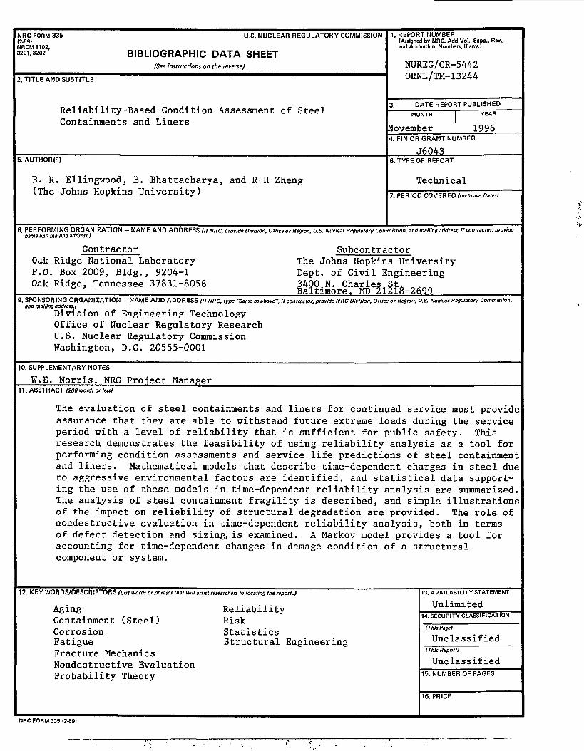
NRC FORM 335 U.S. NUCLEAR REGULATORY COMMISSION12-89)NR CM 1102,32013202 BIBLIOGRAPHIC DATA SHEET

(See Instructions on the reverse)

2, TITLE AND SUBTITLE

Reliability-Based Condition Assessment of SteelContainments and Liners

5, AUTHOR(S)

B. R. Ellingwood, B. Bhattacharya, and R-H Zheng(The Johns Hopkins University)

1. REPORT NUMBER(Assigned by NRC. Add Vol., Supp., Rev.,and Addendum Numbers, if 8ny.)


3. DATE REPORT PUBLISHED

MONTH 1 YEAR

November 19964. FIN OR GRANT NUMBER

J60436. TYPE OF REPORT

Technical7. PERIOD COVERED (InclusiveDates)

8. PERFORMING ORGANIZATION - NAME AND ADDRESS (If NRC, provide Division. Office or Region. U.S. Nuclear Regulatory Commission, and mailing address; if contractor, providename and mailing address.)

Contractor SubcontractorOak Ridge National Laboratory The Johns Hopkins UniversityP.O. Box 2009, Bldg., 9204-1 Dept. of Civil EngineeringOak Ridge, Tennessee 37831-8056 3400 N. Charles St.

Baltimore. MD 212IS-26999, SPONSORING ORGANIZATION - NAME AND ADDRESS (If NRC. type "Same as above"; if contractor, provide NRC Division. Office or Region. U.S. Nuclear Regulatory Commission,

and mailing address.!

Division of Engineering TechnologyOffice of Nuclear Regulatory ResearchU.S. Nuclear Regulatory CommissionWashington, D.C. 20555-0001

10, SUPPLEMENTARY NOTES

W.E. Norris, NRC Proiect Manager11. ABSTRACT (200 v/ords or less)

The evaluation of steel containments and liners for continued service must provideassurance that they are able to withstand future extreme loads during the serviceperiod with a level of reliability that is sufficient for public safety. Thisresearch demonstrates the feasibility of using reliability analysis as a tool forperforming condition assessments and service life predictions of steel containmentand liners. Mathematical models that describe time-dependent charges in steel dueto aggressive environmental factors are identified, and statistical data support-ing the use of these models in time-dependent reliability analysis are summarized.The analysis of steel containment fragility is described, and simple illustrationsof the impact on reliability of structural degradation are provided. The role ofnondestructive evaluation in time-dependent reliability analysis, both in termsof defect detection and sizing, is examined. A Markov model provides a tool foraccounting for time-dependent changes in damage condition of a structuralcomponent or system.

12, KEY WORDS/DESCRIPTORS (List words or phrases that will assist researchers in locating the report.)

Aging ReliabilityContainment (Steel) RiskCorrosion StatisticsFatigue Structural EngineeringFracture MechanicsNondestructive EvaluationProbability Theory

13. AVAILABILITY STATEMENT

Unlimited14. SECURITY CLASSIFICATION

(This Page)

Unclassified(This Report)

Unclassified

15. NUMBER OF PAGES

16. PRICE

NRC FORM 335 12-891

Printedon recycled

paper

Federal Recycling Program