Reliability-Aware Energy Management for Periodic Real-Time Tasks

Department of Computer Science, UTSA

Technical Report: CS-TR-2008-005

Reliability-Aware Energy Management for Periodic

Real-Time Tasks∗

Dakai Zhu Hakan Aydin

Department of Computer Science Department of Computer Science

University of Texas at San Antonio George Mason University

San Antonio, TX, 78249 Fairfax, VA 22030

[email protected] [email protected]

Abstract

Dynamic Voltage and Frequency Scaling (DVFS) has been widely used to manage energy

in real-time embedded systems. However, it was recently shown that DVFS has direct and

adverse effects on system reliability. In this work, we investigate static and dynamic reliability-

aware energy management schemes to minimize energy consumption for periodic real-time sys-

tems while preserving system reliability. Focusing on earliest deadline first (EDF) schedul-

ing, we first show that the static version of the problem is NP-hard and propose two task-level

utilization-based heuristics. Then, we develop a job-level online scheme by building on the idea

of wrapper-tasks, to monitor and manage dynamic slack efficiently in reliability-aware settings.

The feasibility of the dynamic scheme is formally proved. Finally, we present two integrated

approaches to reclaim both static and dynamic slack at run-time. To preserve system reliability,

∗A preliminary version of this paper appeared in IEEE RTAS 2007. This work is supported in part by NSF awardCNS-0720651, CNS-0720647 and NSF CAREER Award CNS-0546244.

1

the proposed schemes incorporate recovery tasks/jobs into the schedule as needed, while still

using the remaining slack for energy savings. The proposed schemes are evaluated through ex-

tensive simulations. The results confirm that all the proposed schemes can preserve the system

reliability and the ordinary (but reliability-ignorant) energy management schemes will result in

drastically decreased system reliability. For the static heuristics, the energy savings are close

to what can be achieved by an optimal solution by a margin of 5%. By effectively exploiting

the run-time slack, the dynamic schemes can achieve additional energy savings while preserving

system reliability.

1 Introduction

The phenomenal improvements in the performance of computing systems have resulted in drastic

increases in power densities. For battery-operated embedded devices with limited energy budget,

energy is now considered a first-class system resource. Many hardware and software techniques

have been proposed to manage power consumption in modern computing systems and power aware

computing has recently become an important research area. One common strategy to save energy is

to operate the system components at low-performance (thus, low-power) states, whenever possible.

For example, Dynamic Voltage and Frequency Scaling (DVFS) technique is based on scaling down

the CPU supply voltage and processing frequency simultaneously to save energy [34, 35].

For real-time systems where tasks have stringent timing constraints, scaling down the clock fre-

quency (i.e. processing speed) may cause deadline misses and special provisions are needed. In

the recent past, several research studies explored the problem of minimizing energy consumption

while meeting all the deadlines for various real-time task models. These include a number of

power management schemes which exploit the available static and/or dynamic slack in the system

[4, 11, 27, 30, 31]. For instance, the optimal static power management scheme for a set of periodic

tasks would scale down the execution of all tasks uniformly at a speed proportional to the system

utilization and employ the Earliest-Deadline-First (EDF) scheduling policy [4, 27].

Reliability and fault tolerance have always been major factors in computer system design. Due

to the effects of hardware defects, electromagnetic interferences and/or cosmic ray radiations, faults

may occur at run-time, especially in systems deployed in dynamic/vulnerable environments. Several

research studies reported that the transient faults occur much more frequently than the permanent

faults [9, 21]. With the continued scaling of CMOS technologies and reduced design margins for

higher performance, it is expected that, in addition to the systems that operate in electronics-hostile

2

environments (such as those in outer space), practically all digital computing systems will be re-

markably vulnerable to transient faults [15].

The backward error recovery techniques, which restore the system state to a previous safe state

and repeat the computation, can be used to tolerate transient faults [29]. It is worth noting that both

DVFS and backward recovery techniques are based on (and compete for) the active use of the system

slack. Thus, there is an interesting trade-off between energy efficiency and system reliability. More-

over, DVFS has been shown to have a direct and adverse effect on the transient fault rates, especially

for those induced by cosmic ray radiations [12, 15, 42], further complicating the problem. Hence,

for safety-critical real-time embedded systems (such as satellite and surveillance systems) where

reliability is as important as energy efficiency, reliability-cognizant energy management becomes a

necessity.

Fault tolerance through redundancy and energy management through DVFS have been exten-

sively (but, independently) studied in the context of real-time systems. Only recently, few research

groups began to investigate the implications of having both fault tolerance and energy efficiency

requirements [14, 26, 33, 36]. However, none of them considers the negative effects of DVFS on

system reliability. As the first effort to address the effects of DVFS on transient faults, we have

previously studied a reliability-aware power management (RA-PM) scheme. The central idea of the

scheme is to exploit the available slack to schedule a recovery task at the dispatch time of a task be-

fore utilizing the remaining slack for DVFS to save energy, thereby preserving the system reliability

[38]. The scheme has been extended to consider various task models and reliability requirements

[39, 41, 44, 45].

In this paper, we investigate both static and dynamic RA-PM schemes for a set of periodic real-

time tasks scheduled by the preemptive EDF policy. Specifically, we consider the problem of ex-

ploiting the system’s static and dynamic slack to save energy while preserving system reliability.

We show that the optimal static RA-PM problem is NP-hard and propose two efficient heuristics

for selecting a subset of tasks to use static slack (i.e., spare CPU capacity) for energy and reliabil-

ity management. Moreover, we develop a job-level dynamic RA-PM algorithm that monitors and

manages the dynamic slack which may be generated at run-time, again for these dual objectives.

The latter algorithm is built on the wrapper-task mechanism: the key idea is to conserve the dy-

namic slack allocated to scaled tasks for recovery across preemption points, which is essential for

preserving reliability. Integrated schemes for effectively exploiting both static and dynamic slack in

a uniform manner are also presented. To the best of our knowledge, this is the first research effort

that provides a comprehensive energy and reliability management framework for periodic real-time

3

tasks.

The remainder of this paper is organized as follows. The related work is summarized in Section 2.

Section 3 presents the system models. Section 4 focuses on the task-level static RA-PM schemes.

The wrapper-task mechanism and the job-level dynamic RA-PM scheme are studied in Section 5.

Section 6 presents the integrated slack reclamation mechanisms. Simulation results are discussed in

Section 7 and we conclude in Section 8.

2 Related Work

In [33], Unsal et al. proposed a scheme to postpone the execution of backup tasks to minimize the

overlap of primary and backup execution and thus, the energy consumption. The optimal number

of checkpoints, evenly or unevenly distributed, to achieve minimal energy consumption while toler-

ating a single fault was explored by Melhem et al. in [26]. Elnozahy et al. proposed an Optimistic

Triple Modular Redundancy (OTMR) scheme that reduces the energy consumption for traditional

TMR systems by allowing one processing unit to slow down provided that it can catch up and finish

the computation before the application deadline [14]. The optimal frequency settings for OTMR

was further explored in [43]. Assuming a Poisson fault model, Zhang et al. proposed an adaptive

checkpointing scheme that dynamically adjusts checkpoint intervals for energy savings while toler-

ating a fixed number of faults for a single task [36]. The work is further extended to a set of periodic

tasks [37].

For the existing DVFS-based research efforts, most of the research either focused on tolerating

fixed number of faults [14, 26] or assumed constant fault rate [36, 37]. However, it was shown that

there is a direct and negative effect of voltage scaling on the rate of transient faults [12, 15, 42].

Taking such effects into consideration, Ejlali et al. studied schemes that combine the information

(about hardware resources) and temporal redundancy to save energy and to preserve system reliabil-

ity [13]. Recently, Pop et al. studied the problem of energy and reliability trade-offs for distributed

heterogeneous embedded systems [28]. The main idea is to tolerate transient faults by switching

to pre-determined contingency schedules and re-executing processes. A novel, constrained logic

programming-based algorithm is proposed to determine the voltage levels, process start time and

message transmission time to tolerate transient faults and minimize energy consumption while meet-

ing the timing constraints of the application.

In our recent work, to address the problem of reliability degradation under DVFS, we have studied

a reliability-aware power management (RA-PM) scheme based on a single-task model. The central

4

idea of RA-PM is to reserve a portion of the available slack to schedule a recovery task for the task

whose execution is scaled down, to recuperate the reliability loss due to the energy management

[38]. The idea has been extended later to consider various task models [39, 44] as well as different

reliability requirements [45].

The work reported in this paper is different from all previous work in that, focusing on preemptive

EDF scheduling, we study the reliability-aware power management problem for a set of periodic

real-time tasks, where both task-level static schemes and job-level dynamic schemes are proposed.

In addition, integrated approaches with a uniform static and dynamic slack reclamation mechanism

are also explored.

3 System Models and Problem Description

3.1 Application Model

We consider a set of independent periodic real-time tasks Γ = {T1, . . . , Tn}. The task Ti is charac-

terized by the pair (pi, ci), where pi represents its period (which is also the relative deadline) and ci

denotes its worst case execution time (WCET). The first job of each task is assumed to arrive at time

0. The jth job of Ti, which is referred to as Jij , arrives at time (j− 1) · pi and has a deadline of j · pi.

In DVFS settings, it is assumed that the WCET ci of task Ti is given under the maximum process-

ing speed fmax. For simplicity, we assume that the execution time of a task scales linearly with the

processing speed1. That is, at the scaled speed f (≤ fmax), the execution time of task Ti is assumed

to be ci · fmax

f.

The system utilization is defined as U =∑n

i=1 ui, where ui = ci

piis the utilization for task Ti.

The tasks are to be executed on a uni-processor system according to the preemptive EDF policy.

Considering the well-known feasibility condition for EDF [25], we assume that U ≤ 1.

3.2 Power Model

The operating frequency for CMOS circuits is almost linearly related to the supply voltage [7].

DVFS reduces supply voltage for lower frequency requirements to save power/energy [34] and, in

what follows, we will use the term frequency change to stand for both supply voltage and frequency

1A number of studies have indicated that the execution time of tasks does not scale linearly with reduced processingspeed due to accesses to memory [32] and/or I/O devices [6]. However, exploring the full implications of this observationis beyond the scope of this paper and is left as our future work.

5

adjustments. Considering the ever-increasing static leakage power due to scaled feature size and

increased levels of integration [23], as well as the power-saving states provided in modern power-

efficient components (e.g., CPU [2] and memory [24]), in this work, we adopt the simple system-

level power model proposed in [42] (similar power models have been adopted in several previous

work [3, 11, 19, 23, 30]), where the power consumption P (f) of a computing system at frequency

f is given by:

P (f) = Ps + h(Pind + Pd) = Ps + h(Pind + Ceffm) (1)

Above, Ps is the static power, which includes the power to maintain basic circuits and to keep the

clock running. It can be removed only by powering off the whole system. Pind is the frequency-

independent active power, which is a constant and corresponds to the power that is independent of

CPU processing speed. It can be efficiently removed (in a couple of cycles) by putting systems into

sleep state(s) [2, 24]. Pd is the frequency-dependent active power, which includes the processor’s dy-

namic power and any power that depends on system processing frequency f (and the corresponding

supply voltage) [7, 24].

When there is computation in progress, the system is active and h = 1. Otherwise, when the

system is turned off or in power-saving sleep modes, h = 0. The effective switching capacitance

Cef and the dynamic power exponent m (in general, 2 ≤ m ≤ 3) are system-dependent constants

[7]. Despite its simplicity, this power model captures the essential components for system-wide

energy management.

Note that, the switching capacitance Cef may be different for different tasks [3, 10, 39]. For

simplicity, we assume that Cef is the average system switch capacitance. That is, the value of Cef

is the same for different tasks, as in most of the existing work [4, 11, 27, 31, 30]. Instead, we focus

in this paper on how to manage energy and reliability simultaneously. However, we would like to

emphasize that the RA-PM schemes proposed in this paper can be easily extended to consider the

task dependent Cef following a similar approach as in our previous work [3, 39].

Moreover, we assume that the normalized processing frequency is used with the maximum fre-

quency as fmax = 1 and the frequency f can be varied continuously from the minimum available

frequency fmin to fmax. The implications of having discrete speed levels are discussed in Sec-

tion 7.3. In addition, the overhead of frequency adjustment is assumed to be negligible or such

overhead can be incorporated into the WCET of tasks.

Minimum energy-efficient frequency: Considering that energy is the integral of power over time,

6

the energy consumption for executing a given job at the constant frequency f will be E(f) = P (f) ·t(f) = P (f) · c

f, where t(f) = c

fis the execution time of the job at frequency f . From Equation (1),

intuitively, lower frequencies result in less frequency-dependent active energy consumption. But

with reduced speeds, the job runs longer and thus consumes more static and frequency-independent

active energy. Therefore, a minimal energy-efficient frequency fee, below which DVFS starts to

consume more total energy, does exist [19, 23, 30]. Considering the prohibitive overhead of turning

on/off a system (e.g., tens of seconds), we assume that the system will is on and Ps is always

consumed during the operation interval considered (but it can be put into power-saving sleep states).

From the above equations, one can find that [42]:

fee = m

√Pind

Cef · (m− 1)(2)

Consequently, for energy efficiency, we limit the processing frequency to be fee ≤ f ≤ fmax.

3.3 Fault and Recovery Models

At run-time, faults may occur due to various reasons, such as hardware failures, electromagnetic

interferences as well as the effects of cosmic ray radiations. The transient faults occur much more

frequently than permanent faults [9, 21], especially with the continued scaling of CMOS technology

sizes and reduced design margins for higher performance [15]. Consequently, in this paper, we

focus on transient faults, which in general follow a Poisson distribution [36, 37]. Note that, DVFS

has been shown to have a direct and negative effect on system reliability due to increased number

of transient faults (especially the ones induced by cosmic ray radiations) at lower supply voltages

[12, 15]. Therefore, the average transient fault arrival rate for systems running at scaled frequency

f (and corresponding supply voltage) can be expressed as [42]:

λ(f) = λ0 · g(f) (3)

where λ0 is the average fault rate corresponding to fmax. That is, g(fmax) = 1. With reduced

processing speeds and supply voltages, the fault rate generally increases [42]. Therefore, we have

g(f) > 1 for f < fmax.

It is assumed that transient faults are detected by using sanity (or consistency) checks at the

completion of a job’s execution [29]. When faults are detected, backward recovery techniques will

be employed for fault tolerance and the recovery task is dispatched, in the form of re-execution

7

[26, 36, 38]. Again, for simplicity, the overhead for fault detection is assumed to be incorporated

into the WCETs of tasks.

3.4 Problem Description

Our primary objective in this paper is to develop power management schemes for periodic real-time

tasks executing on a uni-processor system and to preserve system reliability at the same time. The

reliability of a real-time system generally depends on the correct execution of all jobs. Although it is

possible to preserve the overall system reliability while sacrificing the reliability for some individual

jobs, for simplicity, we focus on maintaining the reliability of individual jobs in this work. Here, the

reliability of a real-time job is defined as the probability of its being correctly executed (considering

the possible recovery, if any) before its deadline.

Therefore, the problem to be addressed in this paper is, for a periodic real-time task set with

utilization U , how to efficiently use the spare CPU utilization (1 − U), as well as the dynamic

slack generated at run-time, in order to maximize energy savings while keeping the reliability

of any job of task Ti no less than R0i (i = 1, . . . , n), where R0

i = e−λ0ci (from Poisson fault arrival

pattern with the average fault rate λ0 at fmax [38]) represents the original reliability for Ti’s jobs,

when there is no power management and the jobs use their WCETs.

Here, to simplify the discussion, we assume that the achieved system reliability is satisfactory

when there is no pre-scheduled recovery and no power management scheme is applied (i.e., all tasks

are executed at fmax). We underline that the schemes to be studied in this paper can be applied to

systems where higher levels of reliability are required as well. Without loss of generality, suppose

that a recovery task RT needs to be pre-scheduled intentionally to achieve the desired high level of

reliability. Consider the augmented task set Γ′ = Γ ∪ {RT}, from the discussion in the next two

sections, applying the proposed schemes to Γ′ (where the recovery task RT is treated as a normal

task) will ensure that the reliabilities for all tasks in Γ′ will be preserved, which will in turn preserve

the required high level of system reliability.

In increasing level of sophistication and implementation complexity, we first introduce the task-

level static RA-PM schemes and then job-level dynamic RA-PM schemes in the next two sections.

The integration of static and dynamic schemes is further addressed in Section 6.

8

4 Task-Level Static RA-PM Schemes

4.1 Reliability-Aware Power Management (RA-PM)

Before presenting the proposed schemes, we first review the concept of reliability-aware power

management (RA-PM) [38]. Instead of utilizing all the available slack for DVFS to save energy as in

ordinary power management schemes which are reliability-ignorant (in the sense that no attention is

paid to the potential effects of DVFS on task reliabilities), the central idea of RA-PM is to reserve a

portion of the slack to schedule a recovery task (in the form of re-execution [29]) for any task whose

execution is scaled down, to recuperate the reliability loss due to energy management [38].

Here, for reliability preservation, the recovery task is dispatched at the maximum frequency fmax

only if transient fault(s) is detected at the end of the scaled task’s execution. With the help of the

recovery task, the overall reliability for a task will be the summation of the probability of the scaled

task being executed correctly and the probability of having transient fault(s) during the task’s scaled

execution and the recovery task being executed correctly. We have shown that, if the available

slack is more than the WCET of a task, by scheduling a recovery task (in the form of re-

execution), the RA-PM scheme can guarantee to preserve the reliability of a real-time job

while still obtaining energy savings using the remaining slack, regardless of increased fault

rates and scaled processing speeds [38].

4.2 Task-Level RA-PM

We start with considering static RA-PM schemes that make their decisions at the task-level. In this

approach, for simplicity, all the jobs of a task have the same treatment. That is, if a given task is

selected for energy management, all its jobs will run at the same scaled frequency; otherwise, they

will run at fmax. From the above discussion, to recuperate reliability loss due to scaled execution,

each scaled job2 will need a corresponding recovery job within its deadline, should a fault occur.

To provide the required recovery jobs, we construct a periodic recovery task (RT) by exploiting

the spare CPU capacity (i.e., static slack). The recovery task will have the same timing parameters

(i.e., WCET and period) as those of the task to be scaled. Therefore, with the recovery task, for

each primary job, a recovery job can be scheduled within its deadline. Note that a recovery job is

activated only when the corresponding primary job incurs a fault and that it is executed always at

2We use the expression scaled job to refer to any job whose execution is slowed down through DVFS, for energymanagement purposes.

9

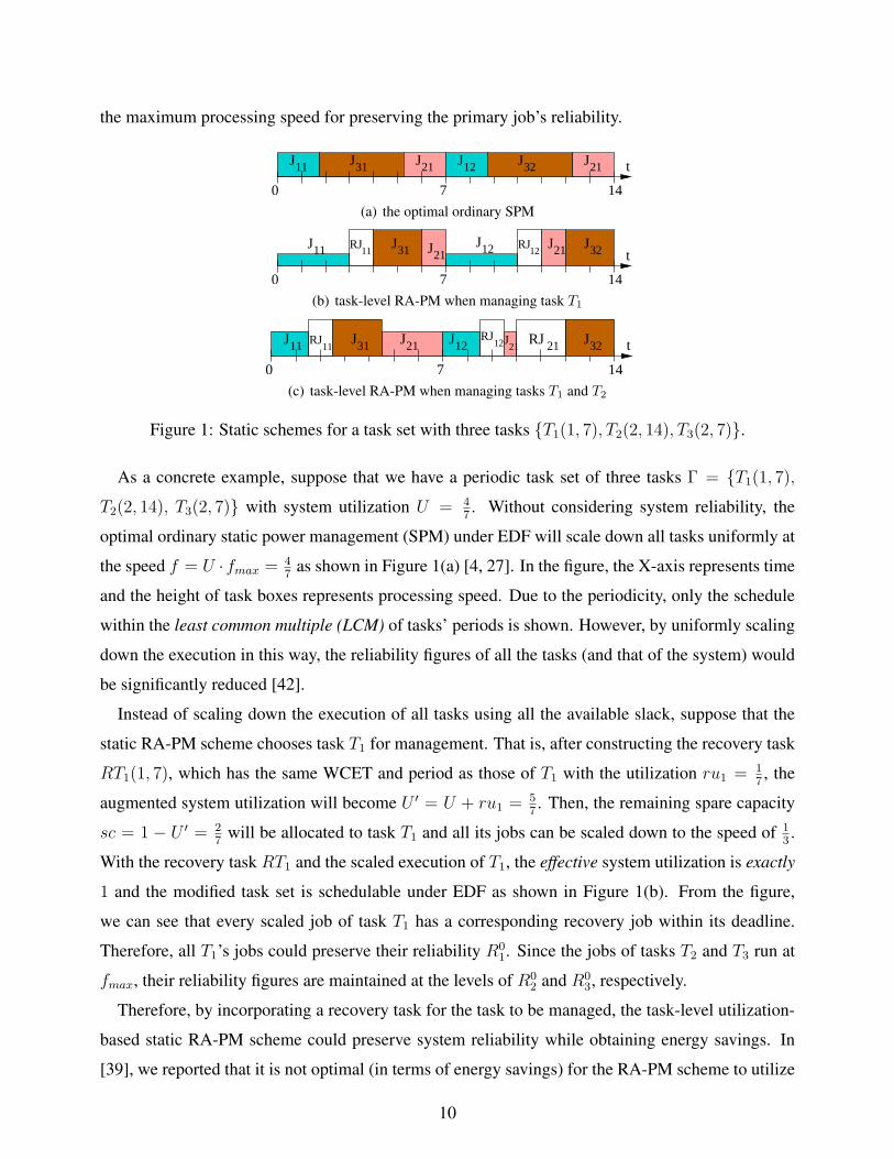
the maximum processing speed for preserving the primary job’s reliability.

7

J11 J31 J21

0 14

tJ12 J32 J21

(a) the optimal ordinary SPM

7

J11 J21J12

0 14

tRJ

11J31 RJ

12J21 J32

(b) task-level RA-PM when managing task T1

RJ11

RJ12

J12J21J11

70 14

tJ31 J21

RJ 21 J32

(c) task-level RA-PM when managing tasks T1 and T2

Figure 1: Static schemes for a task set with three tasks {T1(1, 7), T2(2, 14), T3(2, 7)}.

As a concrete example, suppose that we have a periodic task set of three tasks Γ = {T1(1, 7),

T2(2, 14), T3(2, 7)} with system utilization U = 47. Without considering system reliability, the

optimal ordinary static power management (SPM) under EDF will scale down all tasks uniformly at

the speed f = U · fmax = 47

as shown in Figure 1(a) [4, 27]. In the figure, the X-axis represents time

and the height of task boxes represents processing speed. Due to the periodicity, only the schedule

within the least common multiple (LCM) of tasks’ periods is shown. However, by uniformly scaling

down the execution in this way, the reliability figures of all the tasks (and that of the system) would

be significantly reduced [42].

Instead of scaling down the execution of all tasks using all the available slack, suppose that the

static RA-PM scheme chooses task T1 for management. That is, after constructing the recovery task

RT1(1, 7), which has the same WCET and period as those of T1 with the utilization ru1 = 17, the

augmented system utilization will become U ′ = U + ru1 = 57. Then, the remaining spare capacity

sc = 1 − U ′ = 27

will be allocated to task T1 and all its jobs can be scaled down to the speed of 13.

With the recovery task RT1 and the scaled execution of T1, the effective system utilization is exactly

1 and the modified task set is schedulable under EDF as shown in Figure 1(b). From the figure,

we can see that every scaled job of task T1 has a corresponding recovery job within its deadline.

Therefore, all T1’s jobs could preserve their reliability R01. Since the jobs of tasks T2 and T3 run at

fmax, their reliability figures are maintained at the levels of R02 and R0

3, respectively.

Therefore, by incorporating a recovery task for the task to be managed, the task-level utilization-

based static RA-PM scheme could preserve system reliability while obtaining energy savings. In

[39], we reported that it is not optimal (in terms of energy savings) for the RA-PM scheme to utilize

10

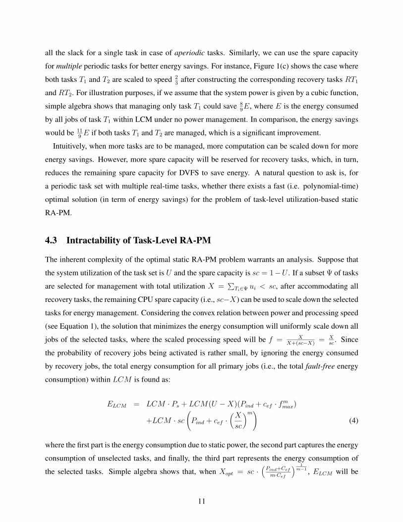
all the slack for a single task in case of aperiodic tasks. Similarly, we can use the spare capacity

for multiple periodic tasks for better energy savings. For instance, Figure 1(c) shows the case where

both tasks T1 and T2 are scaled to speed 23

after constructing the corresponding recovery tasks RT1

and RT2. For illustration purposes, if we assume that the system power is given by a cubic function,

simple algebra shows that managing only task T1 could save 89E, where E is the energy consumed

by all jobs of task T1 within LCM under no power management. In comparison, the energy savings

would be 119E if both tasks T1 and T2 are managed, which is a significant improvement.

Intuitively, when more tasks are to be managed, more computation can be scaled down for more

energy savings. However, more spare capacity will be reserved for recovery tasks, which, in turn,

reduces the remaining spare capacity for DVFS to save energy. A natural question to ask is, for

a periodic task set with multiple real-time tasks, whether there exists a fast (i.e. polynomial-time)

optimal solution (in term of energy savings) for the problem of task-level utilization-based static

RA-PM.

4.3 Intractability of Task-Level RA-PM

The inherent complexity of the optimal static RA-PM problem warrants an analysis. Suppose that

the system utilization of the task set is U and the spare capacity is sc = 1−U . If a subset Ψ of tasks

are selected for management with total utilization X =∑

Ti∈Ψ ui < sc, after accommodating all

recovery tasks, the remaining CPU spare capacity (i.e., sc−X) can be used to scale down the selected

tasks for energy management. Considering the convex relation between power and processing speed

(see Equation 1), the solution that minimizes the energy consumption will uniformly scale down all

jobs of the selected tasks, where the scaled processing speed will be f = XX+(sc−X)

= Xsc

. Since

the probability of recovery jobs being activated is rather small, by ignoring the energy consumed

by recovery jobs, the total energy consumption for all primary jobs (i.e., the total fault-free energy

consumption) within LCM is found as:

ELCM = LCM · Ps + LCM(U −X)(Pind + cef · fmmax)

+LCM · sc(Pind + cef ·

(X

sc

)m)

(4)

where the first part is the energy consumption due to static power, the second part captures the energy

consumption of unselected tasks, and finally, the third part represents the energy consumption of

the selected tasks. Simple algebra shows that, when Xopt = sc ·(

Pind+Cef

m·Cef

) 1m−1 , ELCM will be

11

minimized.

If sc > Xopt ≥ U , all tasks should be scaled down appropriately to minimize energy consumption.

Otherwise, the problem becomes essentially a task selection problem, where the summation of the

utilization for the selected tasks should be exactly equal to Xopt, if possible. In other words, such a

choice would definitely be the optimal solution. In what follows, we formally prove that the task-

level utilization-based static RA-PM problem is NP-hard by transforming the PARTITION problem,

which is known to be NP-hard [17], to a special case of the problem.

Theorem 1 For a set of periodic tasks, the problem of the task-level utilization-based static RA-PM

is NP-hard.

Proof We consider a special case of the problem with m = 2, Cef = 1 and Pind = 0; that is,

Xopt = sc2

. We show that even this special instance is intractable, by transforming the PARTITION

problem, which is known to be NP-hard [17], to that special case.

In the PARTITION problem, the objective is to find whether it is possible to partition a set of n

integers a1, . . . , an (where∑n

i=1 ai = S) into two disjoint subsets, such that the sum of numbers in

each subset is exactly S2

.

Given an instance of the PARTITION problem, we construct the corresponding static RA-PM

instance as follows: we have n periodic tasks, where ci = ai and pi = 2 · S. Note that, in this

case, U =∑ ci

pi= 1

2, sc = 1 − U = 1

2. Observe that, the energy savings will be maximized

if it is possible to find a subset of tasks whose total utilization is exactly Xopt = sc2

= 14. Since

pi = 2S ∀i, this is possible if and only if one can find a subset of tasks Ψ such that∑

i∈Ψ ci = S2

.

But this can happen only if the original PARTITION problem admits a YES answer. Therefore, if

the static RA-PM problem had a polynomial-time solution, one could also solve the PARTITION

problem in polynomial-time, by constructing the corresponding RA-PM problem, and checking if

the maximum energy savings that can be obtained correspond to the amount we could gain through

managing exactly Xopt = sc2

= 25% of the periodic workload.

4.4 Heuristics for Task-Level RA-PM

Considering the intractability of the problem, we propose two simple heuristics for selecting tasks

for energy management: largest-utilization-first (LUF) and smallest-utilization-first (SUF). Suppose

that the tasks in a given periodic task set are indexed in the non-decreasing order of their utilizations

(i.e., ui ≤ uj for 1 ≤ i < j ≤ n). SUF will select the first k tasks, where k is the largest integer that

12

satisfies∑k

i=1 ui ≤ Xopt. Similarly, LUF selects the task with the largest utilization first and, in the

reverse order of task’s utilization, tasks with smaller utilization are added to the selected subset Ψ

one by one as long as∑

Tk∈Ψ uk ≤ Xopt.

Here, SUF tries to manage as many tasks as possible. However, after selecting the first few

tasks, if the task with the next smallest utilization can not fit into Xopt, SUF may be forced to use a

significant portion of the spare capacity (i.e., much more than necessary) for energy management,

which may not be optimal. On the contrary, LUF tries to select larger utilization tasks first, and

the difference between Xopt and the total utilization of the selected tasks is less than the smallest

utilization among all tasks. The potential drawback of LUF is that, relatively few tasks might be

managed for energy savings. These heuristics are evaluated in Section 7.

5 Job-Level Dynamic RA-PM Algorithm

In our backward recovery framework, the recovery jobs are executed only if their corresponding

scaled primary jobs fail. Otherwise, the CPU time reserved for recovery jobs is freed and becomes

dynamic slack at run-time. Moreover, it is well-known that real-time tasks typically take a small

fraction of their WCETs [16]. Therefore, significant amount of dynamic slack can be expected at

run time, which should be exploited to further save energy and/or to enhance system reliability.

For ease of discussion, in this section, we first focus on the cases where no recovery task is stati-

cally scheduled. That is, for the task set with system utilization U ≤ 1, we exploit only the dynamic

slack that comes from the early completion of real-time jobs for energy and reliability management.

The integrated approaches, which combine static and dynamic schemes and collectively exploit

spare capacity and dynamic slack, will be discussed in Section 6.

Unlike the greedy RA-PM scheme which allocates all available dynamic slack for the next ready

task when the tasks share a common deadline [38], in periodic execution settings, the run-time dy-

namic slack will be generated at different priorities and may not be always reclaimable by the next

ready job [4]. Moreover, possible preemptions that a job could experience after it has reclaimed

some slack further complicate the problem. This is because, in RA-PM framework, once a job’s

execution is scaled through DVFS, additional slack must be reserved for the potential recovery op-

eration to preserve system reliability. Hence, conserving the reclaimed slack until the job completes

(at which point it may be used for recovery operation if faults occur, or freed otherwise) is essential

in reliability-aware settings.

13

5.1 Dynamic Slack Management with Wrapper-Tasks

The slack management problem for periodic tasks has been studied extensively (e.g., CASH-queue

[8] and α-queue [4] approaches) for different purposes. By borrowing and also extending some

fundamental ideas from these studies, we propose the wrapper-task mechanism to track/manage

dynamic slack, which guarantees the conservation of the reclaimed slack, thereby maintaining the

reliability figures.

Here, wrapper-tasks are used to represent dynamic slack generated at run-time. At the highest

level, we can distinguish three rules for managing dynamic slack with wrapper-tasks:

• Rule 1 (slack generation): When new slack is generated due to early completion of jobs

or removal of recovery jobs, a new wrapper-task is created with the following two timing

parameters: a size that equals the amount of dynamic slack generated and a deadline that

is equal to that of the job whose early completion gave rise to this slack. Then, the newly

created wrapper-task will be put into a wrapper-task queue (i.e., WT-Queue), which is used to

track/manage available dynamic slack. Here, the wrapper-tasks in WT-Queue are kept in the

increasing order of their deadlines and all wrapper-tasks in WT-Queue represent slack with

different deadlines. Thus, the newly created wrapper-task may be merged with an existing

wrapper-task in WT-Queue if they have the same deadline.

• Rule 2 (slack reclamation): The slack is reclaimed when: (a) a non-scaled job has the high-

est priority in Ready-Q and its reclaimable slack is larger than the WCET of the job’s task

(which ensures that a recovery, in the form of re-execution, can be scheduled to preserve reli-

ability); or, (b) the highest priority job in Ready-Q has been scaled (i.e., its recovery job has

already been reserved) but its speed is still higher than fee and there is reclaimable slack. After

reclamation, the corresponding wrapper-tasks are removed from WT-Queue and destroyed.

• Rule 3 (slack forwarding/wasting): After slack reclamation, the remaining wrapper-tasks

in WT-Queue compete for CPU along with ready jobs. When a wrapper-task has the highest

priority (i.e., the earliest deadline) and is “scheduled”: (a) if there are jobs in the ready queue

(Ready-Q), the wrapper-task will “fetch” the highest priority job in Ready-Q and “wrap” that

job’s execution during the interval when the wrapper-task is “executed”. In this case, the

corresponding slack is actually lended to the ready job and pushed forward (i.e. it is preserved

with a later deadline); (b) otherwise, if there is no ready job, the CPU will become idle,

and the wrapper-task is said to “execute no-ops” where the corresponding dynamic slack is

consumed/wasted during this time interval. Note that, when wrapped execution is interrupted

14

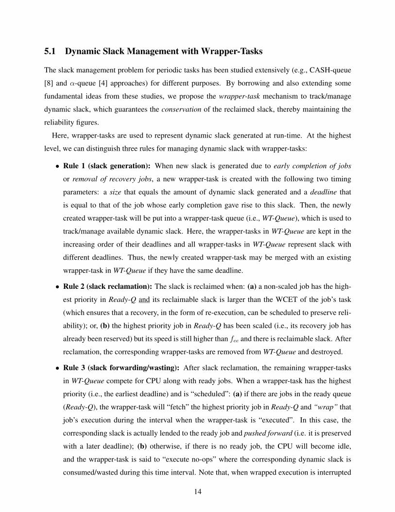
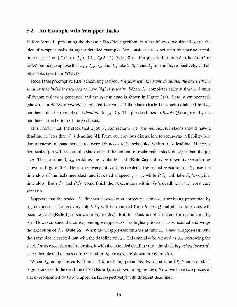
5 10 15 30

t

0

J11 21J

1531J

30

J41 4,10Ready−Q WT−Queue

(a) J21 completes early at time 3;5 10 15 30

t

0

J11 21J

Ready−Q WT−QueueJ4130

RJ3115

J31

15

(b) J31 reclaims the slack;

5 10 15 30

t

0

21J J3111J

Ready−Q WT−Queue

J12 J31

2,15J4130

(c) Scaled J31 finishes correctly, RJ31 is freed as slack;5 10 15 30

t

0

21J J3111J

Ready−Q WT−Queue

J12 J31

2,30

J41

41J30

J2220

(d) At time 10, the slack is pushed forward;

5 10 15 30

t

0

21J J3111J

Ready−Q

J12 J31J41 J1322J J22

J4130

2,30WT−Queue 3,20

(e) At time 14, more slack is generated from J22;5 10 15 30

t

0

21J J3111J

Ready−Q

J12 J31J41 J1322J J22

WT−QueueRJ41J41

3030

(f) Partial job J41 is scaled and needs a full recovery job RJ41;

21J J3111J J12 J31J41 J13J22 J22

5 10 150

t

30

41J

20 25

WT−QueueReady−Q 5,30J3230

(g) Scaled J41 finishes early, both its remaining time and RJ41 are released as slack at time 15, J32 arrives

21J J3111J J12 J31J41 J13J22 J22

5 10 150

t

30

41J

20 25

J32J14 J

32J23

WT−QueueReady−Q J1530

J32 RJ3230 30

2,30

(h) Scaled J32 is preempted (but its reclaimed slack is conserved) and more slack is generated from J22 at time 24;

21J J3111J J12 J31J41 J13J22 J22

5 10 150

t

30

41J

20 25

J32J14 J

32J23 J15 RJ15

J32 RJ 32

(i) J15 reclaimed the new slack and was scaled down; when it fails, RJ15 is executed; J32 and RJ32 meet their deadlines;

Figure 2: Using wrapper-tasks to manage dynamic slack.

by higher priority jobs, only part of slack will be pushed forward (if it is consumed by the

wrapped execution) or wasted, while the remaining part has the original deadline.

15

5.2 An Example with Wrapper-Tasks

Before formally presenting the dynamic RA-PM algorithm, in what follows, we first illustrate the

idea of wrapper-tasks through a detailed example. We consider a task-set with four periodic real-

time tasks Γ = {T1(1, 6), T2(6, 10), T3(2, 15), T4(3, 30)}. For jobs within time 30 (the LCM of

tasks’ periods), suppose that J21, J22, J23 and J41 take 2, 3, 4 and 213

time units, respectively, and all

other jobs take their WCETs.

Recall that preemptive EDF scheduling is used. For jobs with the same deadline, the one with the

smaller task index is assumed to have higher priority. When J21 completes early at time 3, 4 units

of dynamic slack is generated and the system state is shown in Figure 2(a). Here, a wrapper-task

(shown as a dotted rectangle) is created to represent the slack (Rule 1), which is labeled by two

numbers: its size (e.g., 4) and deadline (e.g., 10). The job deadlines in Ready-Q are given by the

numbers at the bottom of the job boxes.

It is known that, the slack that a job Jx can reclaim (i.e. the reclaimable slack) should have a

deadline no later than Jx’s deadline [4]. From our previous discussion, to recuperate reliability loss

due to energy management, a recovery job needs to be scheduled within Jx’s deadline. Hence, a

non-scaled job will reclaim the slack only if the amount of reclaimable slack is larger than the job

size. Thus, at time 3, J31 reclaims the available slack (Rule 2a) and scales down its execution as

shown in Figure 2(b). Here, a recovery job RJ31 is created. The scaled execution of J31 uses the

time slots of the reclaimed slack and is scaled at speed 24

= 12, while RJ31 will take J31’s original

time slots. Both J31 and RJ31 could finish their executions within J31’s deadline in the worst case

scenario.

Suppose that the scaled J31 finishes its execution correctly at time 8, after being preempted by

J12 at time 6. The recovery job RJ31 will be removed from Ready-Q and all its time slots will

become slack (Rule 1) as shown in Figure 2(c). But this slack is not sufficient for reclamation by

J41. However, since the corresponding wrapper-task has higher priority, it is scheduled and wraps

the execution of J41 (Rule 3a). When the wrapper-task finishes at time 10, a new wrapper-task with

the same size is created, but with the deadline of J41. This can also be viewed as J41 borrowing the

slack for its execution and returning it with the extended deadline (i.e., the slack is pushed forward).

The schedule and queues at time 10, after J22 arrives, are shown in Figure 2(d).

When J22 completes early at time 14 (after being preempted by J13 at time 12), 3 units of slack

is generated with the deadline of 20 (Rule 1), as shown in Figure 2(e). Now, we have two pieces of

slack (represented by two wrapper-tasks, respectively) with different deadlines.

16

Note that, as faults are assumed to be detected at the end of a job’s execution, a full recovery job

is needed to recuperate the reliability loss for an even partially scaled execution3. Thus, when the

partially-executed J41 reclaims all the available slack (since both wrapper-tasks have deadlines no

later than J41’s deadline), a full recovery job RJ41 is created and inserted into Ready-Q (Rule 2a).

J41 uses the remaining slack to scale down its execution appropriately as shown in Figure 2(f).

When the scaled J41 finishes early at time 15, both its unused CPU time and RJ41 are freed as

slack (Rule 1). After the arrival of J32 at time 15, the schedule and queues are shown in Figure 2(g).

Here, J32 will reclaim the slack and be scaled to speed 25

after reserving the slack for its recovery

job RJ32. After the scaled J32 is preempted by J14 and J23 (at time 18 and 20, respectively), and J23

completes early at time 24, Figure 2(h) shows the newly generated slack and the state of Ready-Q,

which contains J15 (with arrival time 24). Note that, the recovery job RJ32 (i.e., the slack time) is

conserved even after J32 is preempted by higher priority jobs.

J15 reclaims the new slack. Suppose that both of the scaled jobs J15 and J32 fail, then, RJ15 and

RJ32 will be executed as illustrated in Figure 2(i). It can be seen that all jobs (including recovery

jobs) finish their executions on time and no deadline is missed.

5.3 Job-level Dynamic RA-PM (RA-DPM) Algorithm

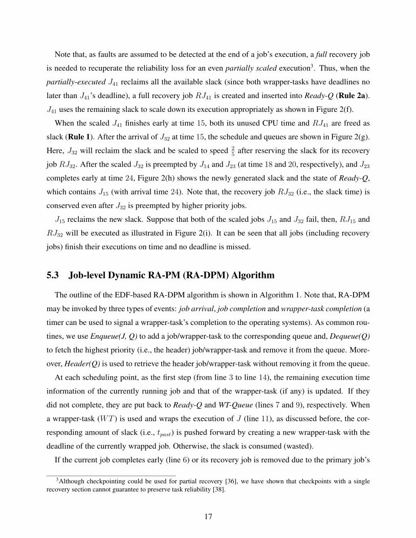
The outline of the EDF-based RA-DPM algorithm is shown in Algorithm 1. Note that, RA-DPM

may be invoked by three types of events: job arrival, job completion and wrapper-task completion (a

timer can be used to signal a wrapper-task’s completion to the operating systems). As common rou-

tines, we use Enqueue(J, Q) to add a job/wrapper-task to the corresponding queue and, Dequeue(Q)

to fetch the highest priority (i.e., the header) job/wrapper-task and remove it from the queue. More-

over, Header(Q) is used to retrieve the header job/wrapper-task without removing it from the queue.

At each scheduling point, as the first step (from line 3 to line 14), the remaining execution time

information of the currently running job and that of the wrapper-task (if any) is updated. If they

did not complete, they are put back to Ready-Q and WT-Queue (lines 7 and 9), respectively. When

a wrapper-task (WT ) is used and wraps the execution of J (line 11), as discussed before, the cor-

responding amount of slack (i.e., tpast) is pushed forward by creating a new wrapper-task with the

deadline of the currently wrapped job. Otherwise, the slack is consumed (wasted).

If the current job completes early (line 6) or its recovery job is removed due to the primary job’s

3Although checkpointing could be used for partial recovery [36], we have shown that checkpoints with a singlerecovery section cannot guarantee to preserve task reliability [38].

17

Algorithm 1 EDF-based RA-DPM Algorithm1: In the algorithm, tpast is the elapsed time since last scheduling point. J and WT represent the current job

and wrapper-task, respectively (each can have the value of NULL if there is no such a job or wrapper-task). J.rem and WT.rem denote the remaining time requirements; J.d and WT.d are the deadlines.

2: Step 1:3: if (J!=NULL and J.rem− tpast > 0) {4: J.rem − = tpast;5: if (J completes) //slack of early completion6: Create a wrapper-task with size J.rem and deadline J.d;7: else Enqueue(J , Ready-Q);}8: if (WT !=NULL and WT.rem− tpast > 0) {9: WT.rem − = tpast; Enqueue(WT , WT-Queue);}

10: if (WT !=NULL and J!=NULL) //push the slack forward;11: Create a wrapper-task with size tpast and deadline J.d;12: if (J is scaled and succeeds){13: RemoveRecoveryJob(J ,Ready-Q);//slack from free of recovery job;14: Create a wrapper-task with size J.c and deadline J.d;}15: Step 2:16: for (all newly arrived job NJ){ NJ.rem = NJ.c;17: NJ.f = fmax; Enqueue(NJ , Ready-Q);}18: Step 3://in the following, J and WT represent the next job and wrapper-task to be processed, respec-

tively;19: J=Dequeue(Ready-Q);20: if (J!=NULL) ReclaimSlack(J , WT-Queue);21: WT=Header(WT-Queue);22: if (J!=NULL){23: if (WT ! = NULL and WT.d < J.d)24: WT = Dequeue(WT-Queue);//WT wraps J’s execution25: else WT = NULL;//normal execution of J26: Execute(J);}27: else if (WT !=NULL)28: WT = Dequeue(WT-Queue);

successful scaled execution (lines 13 and 14), new slack is generated and corresponding wrapper-

tasks are created and added to the wrapper-task queue WT-Queue.

Secondly, if new jobs arrive at the current scheduling point, they are added to Ready-Q according

to their EDF priorities (line 17). The remaining timing requirements will be set as their WCETs at

the speed fmax. The last step is to choose the next highest priority ready job J (if any) for execution

(lines 19 to 28). J first tries to reclaim the available slack (line 20; details are shown in Algorithm 2).

Then, depending on the priority of the remaining wrapper-tasks, J’s execution may be wrapped (line

24) or executed normally (line 25). When a wrapper-task has the highest priority but no job is ready,

the wrapper-task executes no-ops (line 28).

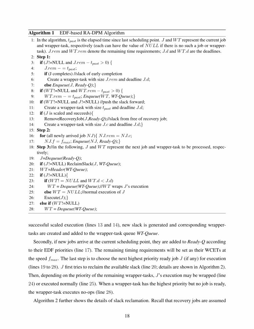
Algorithm 2 further shows the details of slack reclamation. Recall that recovery jobs are assumed

18

Algorithm 2 ReclaimSlack(J , WT-Queue)1: if(J is a recovery job) return; //recovery job is not scaled2: Step 1: //collect reclaimable slack3: slack = 0;4: for(WT ∈WT-Queue)5: if (WT.d ≤ J.d) slack+ = WT.rem;6: Step 2: //scale down J if the slack is sufficient7: if (!J.scaled && slack <= J.c) return;//J.c is the WCET of J’s task;8: if (!J.scaled) slack− = J.c; //reserve for recovery9: tmp = min(fee,

J.rem∗J.fslack+J.remfmax);

10: slack = J.rem∗J.ftmp − J.rem; //slack needed for energy management

11: J.f = tmp; //new speed12: if (!J.scaled){CreateRecoveryJob(J);slack+ = J.c;}13: J.scaled = true; //label the job as scaled14: //remove the reclaimed slack from WT-Queue;15: while (slack > 0){16: WT =Header(WT-Queue);17: if (slack ≥ WT.rem){slack− = WT.rem;18: WT =Dequeue(WT-Queue);}19: else{WT.rem− = slack; slack = 0;}20: }

to be executed at fmax and are not scaled (line 1). For a job J , by traversing WT-Queue, we can

find out the amount of reclaimable slack (lines 3 and 5). If J is not a scaled job (i.e., its recovery

job is not reserved yet) and the amount of reclaimable slack is no larger than the WCET of J (i.e.,

J.c), the available slack is not enough for reclamation (line 7). Otherwise, after properly reserving

the slack for recovery (line 8), J’s new speed is calculated, which is bounded by fee (line 9). The

actual amount of slack used by J includes those for energy management (line 10) as well as the

slack for recovery job (where the recovery job is created and added to Ready-Q in line 12). For the

reclaimed slack, the corresponding wrapper-task(s) will be removed from WT-Queue and destroyed

(lines 15 to 20), which ensures that this slack is conserved for the scaled job, even if higher-priority

jobs preempt the scaled job’s execution later.

5.4 Analysis of RA-DPM

Note that, when all jobs in a task set present their WCETs at run time, there will be no dynamic

slack and no wrapper-task will be created. In this case, RA-DPM will perform the same as EDF

and generate the same worst case schedule, which is feasible by assumption. However, as some

jobs complete early, RA-DPM will undertake slack reclamation and/or wrapped execution, and one

needs to show that the feasibility is preserved even after the changes in CPU time allocation of jobs.

19

Recall that, the elements of WT-Queue represent the slack of tasks that complete early. These slack

elements, while being reclaimed, may be entirely or partially re-transformed to actual workload. Our

strategy will consist in proving that, at any time t during execution, the remaining workload could

be feasibly scheduled by EDF, even if all the slack elements in WT-Queue were to be re-introduced

to the system, with their corresponding deadlines and remaining worst-case execution times (sizes).

This, in turn, will allow us to show the feasibility of the actual schedule, since the above-mentioned

property implies the feasibility even with an over-estimation of the actual workload, for any time t.

In RA-DPM, the slack is reclaimed for dual purposes of scheduling recovery jobs and slowing

down the execution of tasks to save energy with DVFS. Similarly, the slack may be added to the

WT-Queue as a result of early completion of a primary/recovery job, or de-activation of the recovery

job (in case of a successful, non-faulty completion of the corresponding primary job). However,

the feasibility of the resulting schedule is orthogonal to these details. Hence, we will not be further

concerned about whether the slack is obtained from a primary job or a recovery job, and for what

purpose (i.e. recovery or DVFS) it is used.

Before presenting the proof for the correctness of RA-DPM, we first introduce the concept of

processor demand and the fundamental result in the feasibility analysis of periodic real-time task

systems scheduled by preemptive EDF [5, 22].

Definition 1 The processor demand of a real-time job set Φ in an interval [t1, t2], denoted as

hΦ(t1, t2), is the sum of computation times of all jobs in Φ with arrival times greater than or equal

to t1 and deadlines less than or equal to t2.

Theorem 2 ([5, 22]) A set of independent real-time jobs Φ can be scheduled (by EDF) if and only

if hΦ(t1, t2) ≤ t2 − t1 for all intervals [t1, t2].

Let us denote by J(r, e, d) a job J that is released at time r, and that must complete its execution

by the deadline d, with worst-case execution time e. We next prove the following lemma that will

be instrumental in the rest of the proof.

Lemma 1 Consider a set Φ1 of real-time jobs which can be scheduled by preemptive EDF in a

feasible manner. Then, the set Φ2, obtained by replacing Ja(ra, ea, da) in Φ1 by two jobs Jb(ra, eb, db)

and Jc(ra, ec, dc), is still feasible if eb + ec ≤ ea, and da ≤ db ≤ dc.

Proof

20

Since the EDF schedule of Φ1 is feasible, from Theorem 2, we have hΦ1(t1, t2) ≤ t2− t1,∀ t1, t2.

We need to show that hΦ2(t1, t2) ≤ t2 − t1,∀ t1, t2.

It is well-known that, when evaluating the processor demand for a set of real-time jobs, one can

safely focus on intervals that start at a job release time and end at a job deadline [5, 22]. Noting

that the only difference between Φ1 and Φ2 consists in substituting two jobs Jb and Jc for Ja, we

first observe that hΦ2(rx, dy) = hΦ1(rx, dy) ≤ dy − rx, whenever rx is a job release time strictly

greater than ra, or dy is a job deadline strictly smaller than da. Hence, we need to consider only the

intervals [rx, dy] where rx ≤ ra and dy ≥ da. By taking into account the fact that da ≤ db ≤ dc, the

following properties can be easily derived for all possible positionings of dy with respect to these

three deadlines:

• hΦ2(rx, dy) = hΦ1(rx, dy)− (ea − eb − ec) if dc ≤ dy,

• hΦ2(rx, dy) = hΦ1(rx, dy)− (ea − eb) if da ≤ db ≤ dy < dc,

• hΦ2(rx, dy) = hΦ1(rx, dy)− ea if da ≤ dy < db ≤ dc.

Since ea ≥ eb + ec by assumption, in all three cases, hΦ2(rx, dy) ≤ hΦ1(rx, dy) ≤ dy − rx, and

the job set Φ2 is also feasible.

Now, we introduce some additional notations and definitions to reason about the execution state

of RA-DPM, at time t.

• JR(t) denotes the set of ready jobs at time t. Each job Ji ∈ JR(t) has a corresponding

remaining worst-case execution time ei at time t and deadline di. Note that Ji can be seen as

released at time t, and having the worst-case execution time ei and deadline di.

• JF (t) denotes the set of jobs that will arrive after t, with their corresponding worst-case re-

maining execution times and deadlines.

• JW (t) denotes the set of jobs obtained through the WT-Queue. Specifically, for every slack

element in WT-Queue with size si and deadline di, JW (t) will include a job Ji(t, si, di).

Definition 2 The Augmented Remaining Workload of RA-DPM at time t, denoted by ARW(t), is

defined as JR(t)⋃

JF (t)⋃

JW (t).

Informally, ARW(t) denotes the total workload obtained, if one re-introduces all the slack elements

in WT-Queue at time t to the ready-queue, with their corresponding deadlines. This is clearly an

21

over-estimation of the actual workload at time t, since the amount of workload re-introduced by

slack reclamation can never exceed JW (t).

Theorem 3 ARW(t) can be scheduled by EDF in a feasible manner during the execution of RA-

DPM, for every time t.

Proof The statement is certainly true at t = 0, when the WT-Queue is empty, and the workload

can be scheduled in a feasible manner by EDF even under the worst-case conditions.

Assume that the statement holds ∀ t ≤ t1. Note that for t = t1, t1 + 1, . . . , ARW(t) remains

feasible as long as there is no slack reclamation or ’wrapped execution’. This is because, under these

conditions, the task with highest priority in the ready queue is executed at every time slot according

to EDF – and being an optimal preemptive scheduling policy, EDF preserves the feasibility of the

remaining workload. Also note that, if the ready queue is empty for a given time slot, then the

slack at the head of WT-Queue is consumed, which corresponds to the fact that ARW(t) is updated

dynamically according to EDF execution rules.

Let t2 be the first time instant after t1, if any, where RA-DPM performs a slack reclamation or

starts the “wrapped execution”. We denote the head of WT-Queue by H at t = t2, with deadline

dH and size eH . We will show that ARW() remains feasible after such a point in both scenarios,

completing the proof.

• Case 1: At t = t2, slack reclamation is performed through the WT-Queue. Assume k units of

slack is transferred from H to the job JA which is about to be dispatched, with deadline dA ≥dH and remaining worst-case execution time eA. Note that this slack transfer can be seen as

replacing JH(t2, eH , dH) in ARW(t2) by two new jobs JH1(t2, k, dA) and JH2(t2, eH − k, dH);

and by the virtue of Lemma 1, ARW(t2) remains feasible after the slack transfer. If, the

slack is transferred from multiple elements in WT-Queue successively, then we can repeat

the argument for the following elements in the same order.

• Case 2: At t = t2, a ’wrapped execution’ starts, to end at t = t3 > t2. We will show that

ARW(t) remains feasible for t2 ≤ t ≤ t3, completing the proof.

The wrapped execution (i.e., slack forwarding) in the interval [t2, t3] is functionally equivalent

to the following: in every time slot [ti, ti+1] in the interval [t2, t3], one unit of slack from H

(the head of WT-Queue) is replaced by another item in WT-Queue with size 1, and deadline

dAi, which is the deadline of job JAi

that executes on the CPU in the interval [ti, ti+1]. On

22

the other hand, when seen from the perspective of changes in ARW(t), this is equivalent to the

reclamation by JAione unit of slack from H in slot [ti, ti+1] (even though, in actual execution,

this slack unit will not be used because of wrapped execution). As a conclusion, ARW(t)

remains feasible at every time slot in the interval [t2, t3] as slack reclamation on ARW(t) was

shown to be safe in Case 1 above.

Since ARW(t) is an over-estimation of the actual workload, we obtain the following result:

Corollary 1 RA-DPM preserves the feasibility of any periodic real-time task set under preemptive

EDF.

5.5 Complexity of RA-DPM

Note that, in the worst case (e.g., at t = 0), n jobs can arrive simultaneously, and the complexity of

building Ready-Q (lines 16 and 17 of Algorithm 1) will be O(n · log(n)). Moreover, the deadlines

of wrapper-tasks are actually the deadlines of corresponding real-time jobs. At any time t, there are

at most n different deadlines corresponding to jobs with release times on or before t and deadlines

on or after t. That is, the number of wrapper-tasks in WT-Queue is at most n. Therefore, slack

reclamation, where multiple wrapper-tasks may be reclaimed at the same time, can be performed

(by traversing WT-Queue; see Algorithm 2) in time O(n). Hence, the complexity of RA-DPM is at

most O(n · log(n)) at each scheduling point.

6 Integrated Schemes

We have studied separately, in the last two sections, the task-level static and job-level dynamic RA-

PM schemes that exploit system spare capacity (i.e., static slack) and dynamic slack, respectively.

In what follows, depending on how the static and dynamic slack are collectively reclaimed, we will

present two different approaches that integrate the static and dynamic schemes in reliability-aware

settings.

6.1 RA-DPM over Static Schemes

The intuitive approach, which follows the same idea of applying dynamic slack reclamation on top of

static power management [4], is to apply RA-DPM to a task set that has been statically managed. In

this case, a subset of tasks are statically selected to scale down and each of them has a corresponding

23

recovery task for reliability preservation utilizing the spare capacity, which is different from the

original task set (where all tasks run at the maximum frequency and no spare capacity is reclaimed).

Therefore, for jobs of different tasks, RA-DPM needs to treat them differently at the time of their

arrivals (i.e., at lines 16 and 17 of Algorithm 1).

Specifically, for jobs of tasks that are not scaled down, they will be handled in the same way as

shown in Algorithm 1. However, for jobs of scaled tasks, their initial speed will not be fmax but a

pre-determined scaled speed (e.g., NJ.f = f < fmax). The worst case remaining execution time

and flags should be set accordingly (e.g., NJ.rem = NJ.cf

; NJ.scaled = true;) and correspond-

ing recovery jobs should be created. After that, these pre-scaled jobs can be treated the same as

jobs that are scaled online. That is, if their scaled speed is higher than fee, they may reclaim addi-

tional dynamic slack and further slow down their executions. When they complete successfully, the

corresponding recovery jobs will be removed/released and become dynamic slack; otherwise, the

recovery jobs will be activated accordingly.

Note that, after a feasible task set (with system utilization U ≤ 1) is managed statically, the

effective total system utilization of the augmented task set (with scaled tasks and newly constructed

recovery tasks) should still be less than or equal to 1 (see Section 4). That is, the augmented task set

is schedulable under preemptive EDF. From previous discussion, we know that RA-DPM does not

introduce any additional workload to the augmented task set. Therefore, the approach of applying

RA-DPM over static RA-PM schemes is feasible in terms of meeting all the deadlines.

6.2 Slack Transformation using A Dummy Task

In the previous approach, spare capacity (i.e., static slack) and dynamic slack are reclaimed in two

separate steps. To simplify the process, in this section, we consider a single-step approach where the

spare capacity will be transformed into dynamic slack and is reclaimed at run time. The central idea

of such slack transformation relies on the creation of a dummy task T0 using the spare capacity. That

is, the utilization of T0 is u0 = sc = 1−U . At run time, all jobs of the dummy task will have the zero

actual execution time, which effectively transforms the spare capacity to dynamic slack periodically.

Therefore, with this approach, all available slack can be managed/reclaimed by the dynamic scheme

(i.e., RA-DPM) uniformly. In this approach, since a separate static component does not exist, at

system start time, all jobs will assume (implicitly) the speed fmax. However, at dispatch time, many

jobs will be able to slow down thanks to the dynamic slack periodically introduced by the dummy

task T0.

24

Note that, regardless of the period of T0, the task set augmented with the dummy task is schedu-

lable under preemptive EDF. Therefore, it is also schedulable under RA-DPM. However, we can see

that the period of the dummy task will lead to an interesting trade-off between the slack usage effi-

ciency and the overhead of RA-DPM. Intuitively, for smaller periods, the dummy task will distribute

the slack across the schedule more evenly and thus increase the chance of the slack being reclaimed.

However, with smaller periods, more preemptions, and scheduling points/activities can be expected

(thus resulting in higher scheduling overhead). Conversely, larger periods for the dummy task will

incur less scheduling overhead, but the chance of the corresponding slack being reclaimed will be

reduced and the slack is more likely to be wasted. The effects of the dummy task’s period on the

performance and overhead of RA-DPM will be evaluated in the next section.

7 Simulation Results and Discussion

To evaluate the performance of our proposed schemes, we developed a discrete event simulator

using C++. In the simulations, we consider the following different schemes. The scheme of no

power management (NPM), which executes all tasks/jobs at fmax and puts system to sleep states

when idle, is used as the baseline for comparison. The ordinary static power management (SPM)

scales all tasks uniformly at speed f = U · fmax (where U is the system utilization). For the task-

level static RA-PM schemes, after obtaining the optimal utilization (Xopt) that should be managed,

two heuristics are considered: smaller utilization task first (RA-SPM-SUF) and larger utilization

task first (RA-SPM-LUF). For dynamic schemes, we implemented our job-level dynamic RA-PM

(RA-DPM) algorithm and the cycle conserving EDF (CC-EDF) [27], a well-known but reliability-

ignorant DVFS algorithm, for periodic real-time tasks.

Transient faults are assumed to follow the Poisson distribution with an average fault rate of λ0 =

10−6 at fmax (and corresponding supply voltage), which corresponds to 100,000 FITs (failures in

time, in terms of errors per billion hours of use) per megabit. This is a realistic fault rate as reported

in [18, 46]. To take the effects of DVFS on fault rates into consideration, we adopt the exponential

fault rate model developed in [42], where λ(f) = λ0 · g(f) = λ010d(1−f)1−fmin . Here, the exponent d

(> 0) is a constant which indicates the sensitivity of fault rates to DVFS. The maximum fault rate is

assumed to be λmax = λ010d, which corresponds to the minimum frequency fee (and corresponding

supply voltage). In our simulations, we assume that the exponent d = 2. That is, the average fault

rate is assumed to be 100 times higher at the lowest speed fmin (and corresponding supply voltage).

The effects of different values of d were evaluated in our previous work [38, 39, 42].

25

As discussed in Section 3, the static power Ps will be always consumed for all schemes. Therefore,

we focus on active power in our evaluations. We further assume that m = 3, Cef = 1 and Pind = 0.1.

In these settings, the energy efficient frequency is found as fee = 0.37 (see Section 3). The effects of

these parameters on normalized energy consumption have been studied extensively in our previous

work [43].

We consider synthetic real-time task sets where each task set contains 5 or 20 periodic tasks. The

periods of tasks (p) are uniformly distributed within the range of [10, 20] (for short-period tasks) or

[20, 200] (for long-period tasks). The WCETs of tasks are uniformly distributed in the range of 1 and

their periods. Finally, the WCETs of tasks are scaled by a constant such that the system utilization

of tasks reaches a desired value [27]. The variability in the actual workload is controlled by theWCETBCET

ratio (that is, the worst-case to best-case execution time ratio), where the actual execution

time of tasks follows a normal distribution with mean and standard deviation being WCET+BCET2

and WCET−BCET6

, respectively [4].

We simulate the execution for 107 and 108 time units, for short- and long-period task sets, respec-

tively. That is, approximately 5 to 20 million jobs are executed during each run. Moreover, for each

result point in the graphs, 100 task sets are generated and the presented results correspond to the

average.

7.1 Performance of Task-Level Schemes

For different system utilization (i.e., spare capacity), we first evaluate the performance of the task-

level static schemes. It is assumed that all jobs take their WCETs. For task sets with short periods

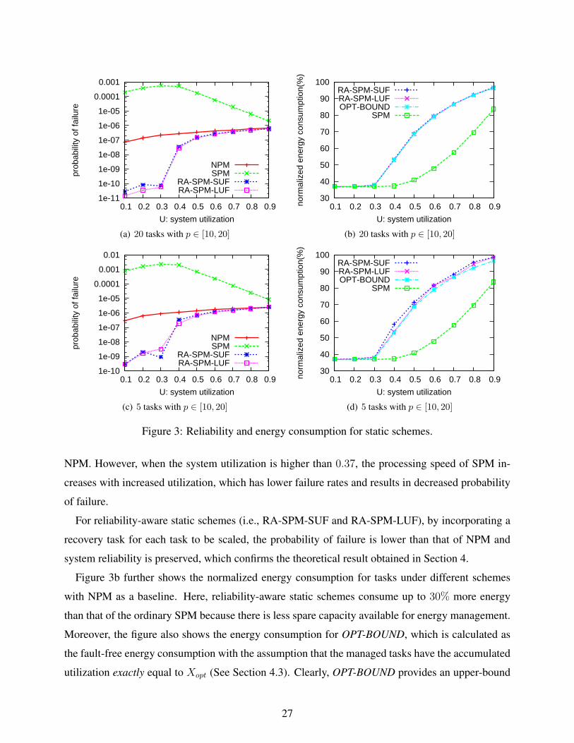
(i.e., p ∈ [10, 20]), where each set contains 20 tasks, Figure 3a first shows the probability of failure

(i.e., 1−reliability) for NPM and the static schemes. Here, the probability of failure shown is the

ratio of the number of failed jobs (recovery jobs have been incorporated, if any) over the total number

of jobs executed.

From the figure, we can see that, as the system utilization increases, for NPM, the probability

of failure increases slightly. The reason for this is that, with increased total utilization, the compu-

tation requirement for each task increases and tasks run longer, which increases the probability of

being subject to transient fault(s). The probability of failure for SPM increases drastically due to in-

creased fault rates and extended execution time. Note that, the minimum energy efficient frequency

is fee = 0.37. At low system utilizations (i.e., U < 0.37), SPM executes all tasks with fee. The

probability of failure for SPM increases slightly with increased utilization for the same reason as

26

1e-11

1e-10

1e-09

1e-08

1e-07

1e-06

1e-05

0.0001

0.001

0.1 0.2 0.3 0.4 0.5 0.6 0.7 0.8 0.9

prob

abili

ty o

f fai

lure

U: system utilization

NPMSPM

RA-SPM-SUFRA-SPM-LUF

(a) 20 tasks with p ∈ [10, 20]

30

40

50

60

70

80

90

100

0.1 0.2 0.3 0.4 0.5 0.6 0.7 0.8 0.9norm

aliz

ed e

nerg

y co

nsum

ptio

n(%

)

U: system utilization

RA-SPM-SUFRA-SPM-LUFOPT-BOUND

SPM

(b) 20 tasks with p ∈ [10, 20]

1e-10

1e-09

1e-08

1e-07

1e-06

1e-05

0.0001

0.001

0.01

0.1 0.2 0.3 0.4 0.5 0.6 0.7 0.8 0.9

prob

abili

ty o

f fai

lure

U: system utilization

NPMSPM

RA-SPM-SUFRA-SPM-LUF

(c) 5 tasks with p ∈ [10, 20]

30

40

50

60

70

80

90

100

0.1 0.2 0.3 0.4 0.5 0.6 0.7 0.8 0.9norm

aliz

ed e

nerg

y co

nsum

ptio

n(%

)

U: system utilization

RA-SPM-SUFRA-SPM-LUFOPT-BOUND

SPM

(d) 5 tasks with p ∈ [10, 20]

Figure 3: Reliability and energy consumption for static schemes.

NPM. However, when the system utilization is higher than 0.37, the processing speed of SPM in-

creases with increased utilization, which has lower failure rates and results in decreased probability

of failure.

For reliability-aware static schemes (i.e., RA-SPM-SUF and RA-SPM-LUF), by incorporating a

recovery task for each task to be scaled, the probability of failure is lower than that of NPM and

system reliability is preserved, which confirms the theoretical result obtained in Section 4.

Figure 3b further shows the normalized energy consumption for tasks under different schemes

with NPM as a baseline. Here, reliability-aware static schemes consume up to 30% more energy

than that of the ordinary SPM because there is less spare capacity available for energy management.

Moreover, the figure also shows the energy consumption for OPT-BOUND, which is calculated as

the fault-free energy consumption with the assumption that the managed tasks have the accumulated

utilization exactly equal to Xopt (See Section 4.3). Clearly, OPT-BOUND provides an upper-bound

27

even for the optimal static solution. From the figure, we can see that the normalized energy con-

sumption for the two heuristics is almost the same as that of the upper bound (within 2%). With 20

tasks in a task set, each task has a very small utilization, which leads to the close-to-optimal solution

for both static heuristics.

1e-10

1e-09

1e-08

1e-07

1e-06

1e-05

0.0001

0.001

0.01

0.1 0.2 0.3 0.4 0.5 0.6 0.7 0.8 0.9

prob

abili

ty o

f fai

lure

U: system utilization

NPMSPM

RA-SPM-SUFRA-SPM-LUF

(a) 20 tasks with p ∈ [20, 200]

30

40

50

60

70

80

90

100

0.1 0.2 0.3 0.4 0.5 0.6 0.7 0.8 0.9norm

aliz

ed e

nerg

y co

nsum

ptio

n(%

)U: system utilization

RA-SPM-SUFRA-SPM-LUFOPT-BOUND

SPM

(b) 20 tasks with p ∈ [20, 200]

1e-09

1e-08

1e-07

1e-06

1e-05

0.0001

0.001

0.01

0.1

0.1 0.2 0.3 0.4 0.5 0.6 0.7 0.8 0.9

prob

abili

ty o

f fai

lure

U: system utilization

NPMSPM

RA-SPM-SUFRA-SPM-LUF

(c) 5 tasks with p ∈ [20, 200]

30

40

50

60

70

80

90

100

0.1 0.2 0.3 0.4 0.5 0.6 0.7 0.8 0.9norm

aliz

ed e

nerg

y co

nsum

ptio

n(%

)

U: system utilization

RA-SPM-SUFRA-SPM-LUFOPT-BOUND

SPM

(d) 5 tasks with p ∈ [20, 200]

Figure 4: Reliability and energy consumption for static schemes.

When there are only 5 tasks in a task set, the utilization for each task becomes larger and Figure 3d

shows the normalized energy consumption for the static heuristics and the upper-bound. From the

results, we can see that RA-SPM-LUF outperforms RA-SPM-SUF for most cases since it selects

tasks to more closely match Xopt. However, even for RA-SPM-SUF, the normalized energy con-

sumption is within 5% of that of the upper-bound. For long-period tasks (i.e., p ∈ [20, 200]), similar

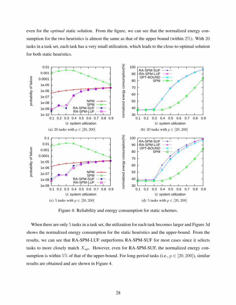
results are obtained and are shown in Figure 4.

28

1e-08

1e-07

1e-06

1e-05

0.0001

1 2 3 4 5 6 7 8 9 10

prob

abili

ty o

f fai

lure

WCET/BCET

NPMCC-EDFRA-DPM

50 55 60 65 70 75 80 85 90 95

100

1 2 3 4 5 6 7 8 9 10norm

aliz

ed e

nerg

y co

nsum

ptio

n(%

)

WCET/BCET

CC-EDFRA-DPM

RA-DPM-DISC

a. reliability for p ∈ [10, 20] b. energy for p ∈ [10, 20]

1e-07

1e-06

1e-05

0.0001

0.001

1 2 3 4 5 6 7 8 9 10

prob

abili

ty o

f fai

lure

WCET/BCET

NPMCC-EDFRA-DPM

50 55 60 65 70 75 80 85 90 95

100

1 2 3 4 5 6 7 8 9 10norm

aliz

ed e

nerg

y co

nsum

ptio

n(%

)

WCET/BCET

CC-EDFRA-DPM

RA-DPM-DISC

c. reliability for p ∈ [20, 200] d. energy for p ∈ [20, 200]

Figure 5: Reliability and energy consumption for dynamic schemes with 20 tasks.

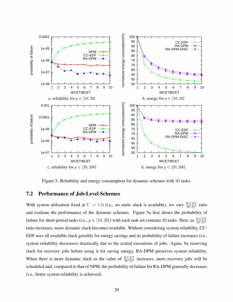
7.2 Performance of Job-Level Schemes

With system utilization fixed at U = 1.0 (i.e., no static slack is available), we vary WCETBCET

ratio

and evaluate the performance of the dynamic schemes. Figure 5a first shows the probability of

failure for short-period tasks (i.e., p ∈ [10, 20]) with each task set contains 20 tasks. Here, as WCETBCET

ratio increases, more dynamic slack becomes available. Without considering system reliability, CC-

EDF uses all available slack greedily for energy savings and its probability of failure increases (i.e.,

system reliability decreases) drastically due to the scaled executions of jobs. Again, by reserving

slack for recovery jobs before using it for saving energy, RA-DPM preserves system reliability.

When there is more dynamic slack as the value of WCETBCET

increases, more recovery jobs will be

scheduled and, compared to that of NPM, the probability of failure for RA-DPM generally decreases

(i.e., better system reliability is achieved).

29

Figure 5b shows the normalized energy consumption for short-period tasks. Initially, as the ratio

of WCETBCET

increases, additional dynamic slack becomes available and normalized energy consump-

tion decreases. Due to the limitation of fee (= 0.37), when WCETBCET

> 9, the normalized energy

consumption for both schemes stays roughly the same and RA-DPM consumes about 8% more en-

ergy than CC-EDF. However, for long-period tasks (i.e., p ∈ [20, 200]), as shown in Figure 5cd,

RA-DPM performs much worse than CC-EDF and consumes about 32% more energy. A possible

explanation is that, when the slack is pushed forward excessively by the long-period tasks, this pre-

vents other jobs from reclaiming it (due to reduced slack priorities), resulting in less energy savings.

Similar results are obtained for cases where each task set contains 5 tasks.

7.3 Effects of Discrete Speeds

So far, we have assumed that the clock frequency can be scaled continuously. However, current

DVFS-enabled processors (e.g., Intel XScale [1, 2]) only have a few speed levels. Nevertheless, our

schemes can be easily adapted to discrete speed settings. After obtaining the desired speed (e.g., Al-

gorithm 2 line 9), we can either use two adjacent frequency levels to emulate the task’s execution at

that speed [20], or use the next higher discrete speed to ensure the algorithm’s feasibility. Assuming

Intel XScale model [1] with 5 speed levels {0.15, 0.4, 0.6, 0.8, 1.0} and using the next higher speed,

we re-ran the simulations. The results for normalized energy consumption are represented as RA-

DPM-DISC and shown in Figure 5bd. Here, we can see that, although RA-DPM-DISC consumes

slightly less energy than that of RA-DPM for short period tasks; for long-period tasks, RA-DPM

performs slightly better than RA-DPM-DISC. However, the difference on the energy consumption

for discrete speeds and continuous speed is within 2%. The reason is that, with the next higher

discrete speed being utilized, the unused slack is not wasted but actually saved for future usage.

7.4 Evaluation of the Integrated Schemes

In the evaluation of the integrated schemes, we consider three different algorithms for comparison.

First, the static RA-SPM-SUF scheme, which executes selected tasks at statically determined scaled

frequency but does not reclaim dynamic slack at run time. SUF+RA-DPM is the second scheme

that will reclaim dynamic slack to further scale down the statically selected tasks or to manage more

unscaled tasks at run time. The last scheme, DUMMY+RA-DPM, uses a dummy task (as discussed

in Section 6) and does not select any task for scaling down statically. At run-time, together with the

transformed dynamic slack from the dummy task, all dynamic slack will be reclaimed appropriately

30

as in RA-DPM.

0.9 0.95

1 1.05 1.1

1.15 1.2

1.25 1.3

1.35 1.4

2 4 6 8 10 12 14 16 18 20

norm

aliz

ed #

of s

ched

ulin

g po

ints

dummy task period

RA-SPM-SUFSUF+RA-DPM

DUMMY+RA-DPM

50 52 54 56 58 60 62 64 66 68 70

2 4 6 8 10 12 14 16 18 20norm

aliz

ed e

nerg

y co

nsum

ptio

n(%

)

dummy task period

RA-SPM-SUFSUF+RA-DPM

DUMMY+RA-DPM

a. scheduling points for p ∈ [10, 20] b. energy for p ∈ [10, 20]

0.9

1

1.1

1.2

1.3

1.4

1.5

1.6

1.7

1.8

0 20 40 60 80 100 120 140 160 180 200

norm

aliz

ed #

of s

ched

ulin

g po

ints

dummy task period

RA-SPM-SUFSUF+RA-DPM

DUMMY+RA-DPM

55

60

65

70

75

80

85

0 20 40 60 80 100 120 140 160 180 200norm

aliz

ed e

nerg

y co

nsum

ptio

n(%

)

dummy task period

RA-SPM-SUFSUF+RA-DPM

DUMMY+RA-DPM

c. scheduling points for p ∈ [20, 200] d. energy for p ∈ [20, 200]

Figure 6: Effects of the dummy task’s period. Here, U = 0.5 and WCETBCET

= 1.

For task sets with 20 short-period tasks (i.e., p ∈ [10, 20]) with system utilization U = 0.5

and WCETBCET

= 1, Figure 6a first shows the normalized number of scheduling points with NPM

as the baseline for different periods of the dummy task. Note that, the dummy task only affects

DUMMY+RA-DPM scheme and the number of scheduling points for RA-SPM-SUF and SPM+RA-

DPM remain the same for different dummy task periods. Without managing and reclaiming the

dynamic slack (from early completion of jobs and the removal of statically scheduled recovery

jobs), the number of scheduling points for RA-SPM-SUF is almost the same as that of NPM. For

SUF+RA-DPM, it reclaims dynamic slack at run-time and the number of scheduling points is about

16% more than that of NPM. For DUMMY+RA-DPM, as the period of the dummy task increases,

less scheduling activities are expected and the normalized number of scheduling points decreases.

31

From the figure, we can see that, the minimum number of scheduling points is obtained when the

dummy period is 14 (which is around 10, the smallest period of tasks in the task set). For larger

dummy task periods, the transformed slack is aggregated and the job that reclaims the slack is

more likely executed at the minimum frequency fee, which leads to more preemption and thus more

scheduling points.

Figure 6b further shows the corresponding normalized energy consumption for the three schemes.

By reclaiming the dynamic slack, SUF+RA-DPM could save roughly 12% more energy than that

of RA-SPM-SUF. When the period of the dummy task is less than 10, the transformed slack is

uniformly distributed and can be effectively reclaimed, which leads to better energy savings for

DUMMY+RA-DPM than that of SUF+RA-DPM. However, for larger dummy task periods, the

transformed slack is aggregated under DUMMY+RA-DPM and leads to uneven execution for tasks,

where more energy is consumed under DUMMY+RA-DPM than that of SUF+RA-DPM. From

these results, we can see that, for short period tasks, the best period for the dummy task would be the

minimum period of all tasks in a task set, which is further confirmed for long-period tasks as shown

in Figure 6cd. However, for long-period tasks, the energy consumption for DUMMY+RA-DPM

is much worse than that of SUF+RA-DPM. This is because, the transformed dynamic slack under

DUMMY+RA-DPM may be pushed forward too much and wasted, which leads to inefficient usage

of the static slack and more energy consumption compared to that of SUF+RA-DPM.

For different values of WCETBCET

(i.e., different amounts of dynamic slack), Figure 7 further shows

the performance of the integrated schemes with 20 tasks in the task sets. For short-period (i.e.,

p ∈ [10, 20]) tasks with system utilization U = 0.5, Figures 7ab first show the probability of fail-

ure and normalized energy consumption for all the schemes, respectively. The same as before, all

reliability-aware schemes perform better than NPM with lower probability of failure. By reclaim-

ing dynamic slack and managing more jobs at run time, SUF+RA-DPM achieves better system

reliability (i.e., lower probability of failure values) than that of RA-SPM-SUF. With the dummy

task’s period being set as 10, DUMMY+RA-DPM performs slightly better (in terms of both relia-

bility and energy) than SUF+RA-DPM when WCETBCET

= 1. That is, when there is no dynamic slack

available from early completion (i.e., WCETBCET

= 1), by using a dummy task to transform all spare

capacity to dynamic slack, DUMMY+RA-DPM can use it more effectively to scale down the jobs

to fee for more energy savings and possibly re-use such slack to manage more jobs for better sys-

tem reliability. However, for cases where dynamic slack from early completion is significant (i.e.,WCETBCET

>= 2), DUMMY+RA-DPM could be too greedy when using the dynamic slack and the

slack transformed from spare capacity by the dummy task, and thus performs slightly worse (≤ 3%)

32

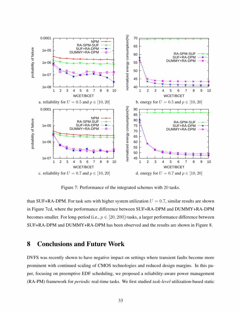
1e-08

1e-07

1e-06

1e-05

0.0001

1 2 3 4 5 6 7 8 9 10

prob

abili

ty o

f fai

lure

WCET/BCET

NPMRA-SPM-SUF

SUF+RA-DPMDUMMY+RA-DPM

40

45

50

55

60

65

70

1 2 3 4 5 6 7 8 9 10norm

aliz

ed e

nerg

y co

nsum

ptio

n(%

)

WCET/BCET

RA-SPM-SUFSUF+RA-DPM

DUMMY+RA-DPM

a. reliability for U = 0.5 and p ∈ [10, 20] b. energy for U = 0.5 and p ∈ [10, 20]

1e-07

1e-06

1e-05

0.0001

1 2 3 4 5 6 7 8 9 10

prob

abili

ty o

f fai

lure

WCET/BCET

NPMRA-SPM-SUF

SUF+RA-DPMDUMMY+RA-DPM

45

50

55

60

65

70

75

80

85

90

1 2 3 4 5 6 7 8 9 10norm

aliz

ed e

nerg

y co

nsum

ptio

n(%

)

WCET/BCET

RA-SPM-SUFSUF+RA-DPM

DUMMY+RA-DPM

c. reliability for U = 0.7 and p ∈ [10, 20] d. energy for U = 0.7 and p ∈ [10, 20]

Figure 7: Performance of the integrated schemes with 20 tasks.

than SUF+RA-DPM. For task sets with higher system utilization U = 0.7, similar results are shown

in Figure 7cd, where the performance difference between SUF+RA-DPM and DUMMY+RA-DPM

becomes smaller. For long-period (i.e., p ∈ [20, 200]) tasks, a larger performance difference between

SUF+RA-DPM and DUMMY+RA-DPM has been observed and the results are shown in Figure 8.

8 Conclusions and Future Work

DVFS was recently shown to have negative impact on settings where transient faults become more

prominent with continued scaling of CMOS technologies and reduced design margins. In this pa-

per, focusing on preemptive EDF scheduling, we proposed a reliability-aware power management

(RA-PM) framework for periodic real-time tasks. We first studied task-level utilization-based static

33

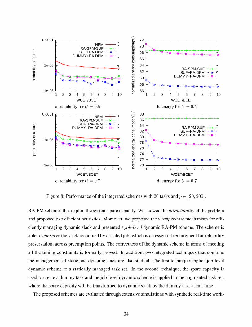
1e-06

1e-05

0.0001

1 2 3 4 5 6 7 8 9 10

prob

abili

ty o

f fai

lure

WCET/BCET

NPMRA-SPM-SUF

SUF+RA-DPMDUMMY+RA-DPM

56

58

60

62

64

66

68

70

72

1 2 3 4 5 6 7 8 9 10norm

aliz

ed e

nerg

y co

nsum

ptio

n(%

)

WCET/BCET

RA-SPM-SUFSUF+RA-DPM

DUMMY+RA-DPM

a. reliability for U = 0.5 b. energy for U = 0.5

1e-06

1e-05

0.0001

1 2 3 4 5 6 7 8 9 10

prob

abili

ty o

f fai

lure

WCET/BCET

NPMRA-SPM-SUF

SUF+RA-DPMDUMMY+RA-DPM

70

72

74

76

78

80

82

84

86

88

1 2 3 4 5 6 7 8 9 10norm

aliz

ed e

nerg

y co

nsum

ptio

n(%

)

WCET/BCET

RA-SPM-SUFSUF+RA-DPM

DUMMY+RA-DPM

c. reliability for U = 0.7 d. energy for U = 0.7

Figure 8: Performance of the integrated schemes with 20 tasks and p ∈ [20, 200].

RA-PM schemes that exploit the system spare capacity. We showed the intractability of the problem

and proposed two efficient heuristics. Moreover, we proposed the wrapper-task mechanism for effi-

ciently managing dynamic slack and presented a job-level dynamic RA-PM scheme. The scheme is

able to conserve the slack reclaimed by a scaled job, which is an essential requirement for reliability

preservation, across preemption points. The correctness of the dynamic scheme in terms of meeting

all the timing constraints is formally proved. In addition, two integrated techniques that combine

the management of static and dynamic slack are also studied. The first technique applies job-level

dynamic scheme to a statically managed task set. In the second technique, the spare capacity is

used to create a dummy task and the job-level dynamic scheme is applied to the augmented task set,

where the spare capacity will be transformed to dynamic slack by the dummy task at run-time.

The proposed schemes are evaluated through extensive simulations with synthetic real-time work-

34

loads. The results show that, compared to the ordinary energy management schemes, the new

schemes could achieve comparable amount of energy savings while preserving system reliability.

However, ordinary energy management schemes that are reliability-ignorant, often lead to dras-

tically decreased system reliability. For the static heuristics, the energy savings are close to the

upper-bound of the optimal solution by a margin of 5%. By effectively exploiting the run-time

slack, additional energy savings can be obtained through the dynamic schemes while preserving

system reliability. For the integrated technique with a dummy task, the period of the dummy task

should be set as the minimum period of tasks in a task set for the best performance. Although the

dummy task approach simplifies the slack reclamation, applying job-level dynamic scheme on top

of task-level static scheme generally gives better performance.

As our future work, we plan to extend the RA-PM framework for sporadic real-time tasks as

well as mixed workload with both aperiodic and periodic tasks. Another direction will be extending

the current RA-PM framework to consider parallel multicore-based systems and various system

reliability requirements.

References

[1] Intel xscale technology and processors. http://developer.intel.com/design/intelxscale/.

[2] Intel corp. mobile pentium iii processor-m datasheet. Order Number: 298340-002, Oct 2001.

[3] H. Aydin, V. Devadas, and D. Zhu. System-level energy management for periodic real-time

tasks. In Proc. of The 27th IEEE Real-Time Systems Symposium (RTSS), Piscataway, NJ, USA,

Dec. 2006. IEEE CS Press.

[4] H. Aydin, R. Melhem, D. Mosse, and P. Mejia-Alvarez. Power-aware scheduling for periodic

real-time tasks. IEEE Trans. on Computers, 53(5):584–600, 2004.

[5] S. Baruah, R. Howell, and L. Rosier. Algorithms and complexity concerning the preemptive

scheduling of periodic, real-time tasks on one processor. Real-Time Systems, 2, 1990.

[6] E. Bini, G.C. Buttazzo, and G. Lipari. Speed modulation in energy-aware real-time systems.

In Proc. of the 17th Euromicro Conference on Real-Time Systems, 2005.

[7] T. D. Burd and R. W. Brodersen. Energy efficient cmos microprocessor design. In Proc. of The

HICSS Conference, Jan. 1995.

35

[8] M. Caccamo, G. Buttazzo, and L. Sha. Capacity sharing for overrun control. In Proc. of

Real-Time Systems Symposium, 2000.

[9] X. Castillo, S. McConnel, and D. Siewiorek. Derivation and caliberation of a transient error

reliability model. IEEE Trans. on computers, 31(7):658–671, 1982.

[10] J.-J. Chen and T.-W. Kuo. Multiprocessor energy-efficient scheduling for real-time tasks with

different power characteristics. In Proc. of the 2005 International Conference on Parallel

Processing (ICPP), pages 13–20, Jun. 2005.

[11] J.-J. Chen and T.-W. Kuo. Procrastination determination for periodic real-time tasks in leakage-

aware dynamic voltage scaling systems. In Proc. of the 2007 IEEE/ACM Int’l Conference on

Computer-Aided Design (ICCAD), pages 289–294, 2007.

[12] V. Degalahal, L. Li, V. Narayanan, M. Kandemir, and M. J. Irwin. Soft errors issues in low-

power caches. IEEE Trans. on Very Large Scale Integration (VLSI) Systems, 13(10):1157–

1166, Oct. 2005.

[13] A. Ejlali, M. T. Schmitz, B. M. Al-Hashimi, S. G. Miremadi, and P. Rosinger. Energy efficient

seu-tolerance in dvs-enabled real-time systems through information redundancy. In Proc. of

the Int’l Symposium on Low Power and Electronics and Design (ISLPED), 2005.

[14] E. (Mootaz) Elnozahy, R. Melhem, and D. Mosse. Energy-efficient duplex and tmr real-time

systems. In Proc. of The 23rd IEEE Real-Time Systems Symposium, Dec. 2002.

[15] D. Ernst, S. Das, S. Lee, D. Blaauw, T. Austin, T. Mudge, N. S. Kim, and K. Flautner. Razor:

circuit-level correction of timing errors for low-power operation. IEEE Micro, 24(6):10–20,

2004.

[16] R. Ernst and W. Ye. Embedded program timing analysis based on path clustering and ar-

chitecture classification. In Proc. of The Int’l Conference on Computer-Aided Design, pages

598–604, 1997.

[17] M. R. Garey and D. S. Johnson. Computers and Intractability: A Guide to the Theory of

NP-Completeness. Mathematical Sciences Series. Freeman, 1979.

[18] P. Hazucha and C. Svensson. Impact of cmos technology scaling on the atmospheric neutron

soft error rate. IEEE Trans. on Nuclear Science, 47(6):2586–2594, 2000.

36

[19] S. Irani, S. Shukla, and R. Gupta. Algorithms for power savings. In Proc. of The 14th Sympo-

sium on Discrete Algorithms, 2003.

[20] T. Ishihara and H. Yauura. Voltage scheduling problem for dynamically variable voltage pro-

cessors. In Proc. of The Int’l Symposium on Low Power Electronics and Design, 1998.

[21] R.K. Iyer, D. J. Rossetti, and M.C. Hsueh. Measurement and modeling of computer reliability

as affected by system activity. ACM Trans. on Computer Systems, 4(3):214–237, Aug. 1986.

[22] K. Jeffay and D. L. Stone. Accounting for interrupt handling costs in dynamic priority task

systems. In Proc. of the IEEE Real-Time Systems Symposium, Dec. 1993.

[23] R. Jejurikar, C. Pereira, and R. Gupta. Leakage aware dynamic voltage scaling for real-time

embedded systems. In Proc. of the 41st Design automation conference, 2004.

[24] A. R. Lebeck, X. Fan, H. Zeng, and C. S. Ellis. Power aware page allocation. In Int’l Confer-

ence on Architectural Support for Programming Languages and Operating Systems, 2000.

[25] C. L. Liu and James W. Layland. Scheduling algorithms for multiprogramming in a hard

real-time environment. J. ACM, 20(1):46–61, 1973.

[26] R. Melhem, D. Mosse, and E. (Mootaz) Elnozahy. The interplay of power management and

fault recovery in real-time systems. IEEE Trans. on Computers, 53(2):217–231, 2004.

[27] P. Pillai and K. G. Shin. Real-time dynamic voltage scaling for low-power embedded operating

systems. In Proc. of 18th ACM Symposium on Operating Systems Principles, Oct. 2001.

[28] P. Pop, K.H. Poulsen, V. Izosimov, and P. Eles. Scheduling and voltage scaling for en-

ergy/reliability trade-offs in fault-tolerant time-triggered embedded systems. In Proc. of

the 5th IEEE/ACM Int’l Conference on Hardware/software codesign and System Synthesis

(CODES+ISSS), pages 233–238, 2007.

[29] D. K. Pradhan. Fault Tolerance Computing: Theory and Techniques. Prentice Hall, 1986.

[30] S. Saewong and R. Rajkumar. Practical voltage scaling for fixed-priority rt-systems. In Proc.

of the 9th IEEE Real-Time and Embedded Technology and Applications Symposium, 2003.

[31] C. Scordino and G. Lipari. A resrouce reservation algorithm for power-aware scheduling of

periodic and aperiodic real-time tasks. IEEE Trans. on Computers, 55(12):1509–1522, 2006.

37

[32] K. Seth, A. Anantaraman, F. Mueller, and E. Rotenberg. Fast: Frequency-aware static timing

analysis. In Proc. of the 24th IEEE Real-Time System Symposium, 2003.

[33] O. S. Unsal, I. Koren, and C. M. Krishna. Towards energy-aware software-based fault tolerance

in real-time systems. In Proc. of The Int’l Symposium on Low Power Electronics Design, 2002.

[34] M. Weiser, B. Welch, A. Demers, and S. Shenker. Scheduling for reduced cpu energy. In

Proc. of The First USENIX Symposium on Operating Systems Design and Implementation,

Nov. 1994.

[35] F. Yao, A. Demers, and S. Shenker. A scheduling model for reduced cpu energy. In Proc. of

The 36th Annual Symposium on Foundations of Computer Science, Oct. 1995.

[36] Y. Zhang and K. Chakrabarty. Energy-aware adaptive checkpointing in embedded real-time

systems. In Proc. of IEEE/ACM Design, Automation and Test in Europe Conference(DATE),

2003.

[37] Y. Zhang, K. Chakrabarty, and V. Swaminathan. Energy-aware fault tolerance in fixed-priority

real-time embedded systems. In Proc. of Int’l Conference on Computer Aided Design, Nov.

2003.

[38] D. Zhu. Reliability-aware dynamic energy management in dependable embedded real-time

systems. to appear in ACM Trans. on Embedded Computing Systems; A preliminary version

appeared in RTAS 2006.

[39] D. Zhu and H. Aydin. Energy management for real-time embedded systems with reliability

requirements. In Proc. of the Int’l Conf. on Computer Aidded Design, 2006.

[40] D. Zhu and H. Aydin. Reliability-aware energy management for periodic real-time tasks. Tech-

nical report, Dept. of Computer Science, Univ. of Texas at San Antonio, 2006. available at

http://www.cs.utsa.edu/˜dzhu/papers/CS-TR-2008-005-zhu.pdf.

[41] D. Zhu, H. Aydin, and J.-J. Chen. Optimistic reliability aware energy management for real-time

tasks with probabilistic execution times. In to appear in the Proc. of the 29th IEEE Real-Time

Systems Symposium (RTSS), 2008.

[42] D. Zhu, R. Melhem, and D. Mosse. The effects of energy management on reliability in real-

time embedded systems. In Proc. of the Int’l Conf. on Computer Aidded Design, 2004.

38

[43] D. Zhu, R. Melhem, D. Mosse, and E.(Mootaz) Elnozahy. Analysis of an energy efficient op-

timistic tmr scheme. In Proc. of the 10th Int’l Conference on Parallel and Distributed Systems,

2004.

[44] D. Zhu, X. Qi, and H. Aydin. Priority-monotonic energy management for real-time systems

with reliability requirements. In Proc. of the IEEE International Conference on Computer

Design (ICCD), 2007.

[45] D. Zhu, X. Qi, and H. Aydin. Energy management for periodic real-time tasks with variable

assurance requirements. In Proc. of the IEEE Int’l Conference on Embedded and Real-Time

Computing Systems and Applications (RTCSA), 2008.

[46] J. F. Ziegler. Trends in electronic reliability: Effects of terrestrial cosmic rays. available at

http://www.srim.org/SER/SERTrends.htm, 2004.

39