Release characteristics of highly pressurized hydrogen through a small hole

ww.sciencedirect.com

i n t e r n a t i o n a l j o u r n a l o f h y d r o g e n en e r g y 3 8 ( 2 0 1 3 ) 3 5 0 3e3 5 1 2

Available online at w

journal homepage: www.elsevier .com/locate/he

Release characteristics of highly pressurizedhydrogen through a small hole

Sang Heon Han a,*, Daejun Chang a,*, Jong Soo Kim b

aDivision of Ocean System Engineering, Korea Advanced Institute of Science and Technology, 373-1 Guseong-dong, Yuseong-gu,

Daejeon 305-701, South KoreabKorea Institute of Science and Technology, 39-1 Hawolgok-dong, Seongbuk-gu, Seoul, South Korea

a r t i c l e i n f o

Article history:

Received 18 September 2012

Received in revised form

13 November 2012

Accepted 16 November 2012

Available online 23 January 2013

Keywords:

High pressure hydrogen leakage

Jet dispersion

Small hole

Mass flux

* Corresponding authors. Tel.: þ82 42 350 157E-mail addresses: [email protected] (S.H

0360-3199/$ e see front matter Copyright ªhttp://dx.doi.org/10.1016/j.ijhydene.2012.11.0

a b s t r a c t

A hydrogen supplying system for hydrogen fuel cell cars is anticipated to utilize highly

pressurized hydrogen gas at pressures up to 700 bar. In this highly pressurized environ-

ment, large amount of hydrogen can be leaked from a relatively small hole caused by

material and mechanical defects. A leaked hydrogen jet can reach very far in distance and

the size of the leak plays an important role in determining the safety of hydrogen recharge

facilities. This study numerically investigated the concentration distribution and the mass

flux of hydrogen leaked from a highly pressurized source through a hole whose size is less

than 1.0 mm. Numerical analysis was performed in axisymmetric coordinates on the

assumption that the hydrogen jet has a huge Froude number and that buoyancy forces can

be negligible. The predicted hydrogen concentration along the centerline of a hydrogen jet

was compared with experimental data for verification of the numerical analysis and it

satisfied the hyperbolic decay characteristics and matched the experiment well. The mass

fluxes for the various hole lengths of this study were found to be 5%e20% less than those

predicted using an isentropic flow assumption.

Copyright ª 2012, Hydrogen Energy Publications, LLC. Published by Elsevier Ltd. All rights

reserved.

1. Introduction carbon energy strategy is significantly more costly than the

Transportation, which accounts for approximately 20% of CO2

emission from by fossil fuel combustion in typical industri-

alized countries, is the third major CO2 emission sector,

following the power and industry sectors. However, formu-

lating a CO2 reduction strategy for the transportation sector is

muchmore difficult becausemotor vehicles are nonstationary

and extremely small CO2 emission sources, emitting about

one millionth of the amount of large scale coal power plants

and blast furnaces. Consequently, in the Energy Technology

Perspectives 2008 [1], the International Energy Agency (IEA)

recommended a non-carbon energy strategy, i.e., employing

hydrogen or electricity to power motor vehicles. This non-

4; fax: þ82 42 350 1510.. Han), [email protected], Hydrogen Energy P71

CCS (CO2 Capture and Storage) strategy applicable for the

power and industry sectors, in that the marginal CO2 abate-

ment cost for the transportation sector range from 200e500$/

tCO2, whereas those for the power and industry sectors range

from 50e100$/tCO2 and 100e200$/tCO2, respectively. Never-

theless, a non-carbon energy strategy is still necessary to

achieve a deep CO2 reduction from the transportation sector

to stabilize the atmospheric CO2 level by 2050. The IEA-BLUE

Map scenario, developed with a specific target to CO2 stabili-

zation by 2050, calls for a 50%CO2 emission reduction globally,

which can be translated into an 80% CO2 emission reduction

for typical industrialized countries and a 90% CO2 emission

reduction for the USA.

u (D. Chang).ublications, LLC. Published by Elsevier Ltd. All rights reserved.

Nomenclature

A coefficient in Eq. (21)

a, b coefficients of line in Eq. (23)

CD discharge coefficient

Cp,k specific heat of k-th species, J/(kg K)

d diameter of hole, m

dps pseudo diameter of abrupt expansion, m

e!z; e!

r unit vectors, m

k turbulent kinetic energy or decay coefficient

h specific enthalpy, J/kg

L length of hole, m_m mass flux, kg/m2 s

Pr Prandtl number

p pressure, N/m2

r radial coordinate, m

R gas constant, J/(kg K)

Sc Schmit number

T temperature, K

uz, ur velocity components, m/s

XH2 hydrogen concentration

Yk mass fraction of k-th species

z axial coordinate, m

Greek symbols

3 turbulent dissipation

m, mt, meff molecular viscosity, turbulent viscosity, and

effective viscosity, kg/s m

r density, kg/m3

g ratio of specific heats

F dissipation function

Subscripts

k index for element or species

s isentropic

LFL lean flammability limit

i n t e rn a t i o n a l j o u r n a l o f h y d r o g e n en e r g y 3 8 ( 2 0 1 3 ) 3 5 0 3e3 5 1 23504

At this moment, it is unclear which will emerge as the

dominant non-carbon energy source for the transportation

sector among hydrogen and electricity. To win the competition

to become the dominant non-carbon transportation energy

system, it is necessary to develop not only the hydrogen or

electric vehicle technologies into a system capable of supplying

power in as large a quantity as that of gasoline engine vehicle,

but more importantly the corresponding energy infrastructure

from the energy producers to the terminal users. In this regard,

the hydrogen energy system is at a significant disadvantage

because it has yet to be built and the safety of the hydrogen

energy system needs to be fully addressed. In particular,

hydrogenfillingstationsareunder strict public scrutinybecause

it iswhere theenergysystemcomes intocontactwith thepublic.

Hydrogen is one of the most reactive compounds. On the

other hand, hydrogen has a very low volumetric energy

density and a great tendency to buoyantly disperse away from

a leaking source. Consequently, the safety of hydrogen filling

stations can be greatly improved by promoting the dispersion

of leaking hydrogen before exposure to an ignition source.

When developing the hydrogen station safety code that will

guarantee the safety for such station operators as well as for

the public, better quantified hydrogen jet characteristics will

enable us to maximize the safety potential by specifying

guidelines to promote the dispersion and dilution of the highly

reactive hydrogen. Therefore, it is the objective of this present

study to quantify the characteristics of hydrogen leaking from

a high pressure system through a small rupture hole.

Birch [2] demonstrated that the mean centerline concen-

tration profiles for various natural gas jets can be collapsed

into a single curve if the longitudinal distance from a virtual

point source is non-dimensionalized by a virtual diameter

derived from the mass balance. Birch’s approach for natural

gas jets was later extended to hydrogen jets by Ruffin et al. [3].

The concentration profile of hydrogen jets, established by

leakagewith constant pressures at up to 25 bar, wasmeasured

by Shirvill et al. [4] with an oxygen sensor. Takeno et al. [5]

measured the transient hydrogen concentration of a hypo-

thetical scenario for a large scale leakage from a pipeline.

Houf and Schefer [6,7] carried out experimental studies on the

dispersion of hydrogen jets arising from leakage with low

pressures.

Numerical studies on the release of highly pressurized

hydrogen have been performed in two ways. The first and

major concern of this study [8e14] is performed by analyzing

the dispersion of the hydrogen jet into ambient air in view of

safety. The domain sizes of theseworks are very large, such as

factory fields or urban sections. In this case, the precise

characteristics of the abrupt hydrogen expansion just after

exit through the cracked hole are neglected because of

numerical inappropriateness. The mass flow rate for the inlet

boundary is calculated using an isentropic flow assumption.

The second way [15,16] focuses on the abrupt expansion

characteristics of the jet. This way explores the expansion

length, pseudo diameter, and normal shock e essential data

for the Birch approach.

This study directly calculates both the mass flux and the

dispersion characteristics of a hydrogen jet leaked from

a highly pressurized source using numerical analysis. The

mass flux can be obtained by calculating the flow field inside

a source reservoir, which is almost stagnant, and a cracked

hole, which is being choked. The typical velocity and length

scales for high pressure hydrogen leakage are assumed to be

u w 1500 m/s, corresponding to the hydrogen sound speed,

and d w 1 mm, respectively. The resulting Froude number,

defined to be u2/gd, is on the order of 108, so that the buoyancy

effect, which is capable of bending the hydrogen jet upward, is

negligible and two dimensional axisymmetricity can be

assumed to significantly reduce numerical efforts.

2. Mathematical formulation

2.1. Isentropic approach

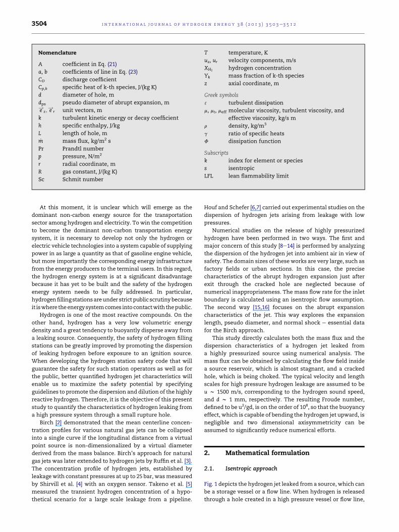
Fig. 1 depicts the hydrogen jet leaked from a source, which can

be a storage vessel or a flow line. When hydrogen is released

through a hole created in a high pressure vessel or flow line,

INFINITRESERVOIR

Fig. 1 e Schematics of abrupt expansion (Ref. [2]).

i n t e r n a t i o n a l j o u r n a l o f h y d r o g e n en e r g y 3 8 ( 2 0 1 3 ) 3 5 0 3e3 5 1 2 3505

the flow is choked near the exit of the hole. Neglecting viscous

dissipation and introducing an adiabatic wall assumption

inside the hole, the flow is isentropic. At the choking point, all

the flow variables can be obtained by combining the chocking

condition and the isentropic flow assumption:

P2;s ¼ P0

�2

gþ 1

�g=g�1

; T2;s ¼ T0

�2

gþ 1

�; r2;s ¼

P0

RT0

�2

gþ 1

� 1g�1

(1)

u2;s ¼ c2;s ¼ffiffiffiffiffiffiffiffiffiffiffiffiffiffigRT2;s

p ¼ffiffiffiffiffiffiffiffiffiffiffiffiffiffiffiffiffiffiffiffiffiffiffiffiffiffiffiRT0

�2g

gþ 1

�s(2)

The flow velocity is sonic velocity at the choking point. The

mass flux can be determined with the flow variables calcu-

lated at the choking point:

_ms ¼ CDr2;su2;s ¼ CDP0ffiffiffiffiffiffiffiffiRT0

p�

2gþ 1

� 1g�1

ffiffiffiffiffiffiffiffiffiffiffiffi2g

gþ 1

s(3)

Leaving the hole, the flow experiences an abrupt expansion

as shown in Fig. 1. The abrupt expansion is completed in

a very short distance (z10d), and it ends with a normal

shock. The flow becomes incompressible after the normal

shock. If the entrainment of air is neglected during the abrupt

expansion, the hydrogen concentration follows the mean

axial concentration hyperbolic decay rule after the normal

shock:

XH2¼ kdps

zþ z0

�rair

rH2

�12

¼ kdzþ z0

�rair

rH2

�12

ffiffiffiffiffiffiffiffiffiffiffiffiffiffiffiffiffiffiffiffiffiffiffiffiffiffiffiffiffiffiffiffiffiffiffiffiffiffiffiffiffiffiffiffiffiffiffiffiffiffiffiffiCD

�2

gþ 1

�ðgþ1Þ=2ðg�1Þ P0

Pair

s(4)

The derivation of Eq. (4) is described in Ref. [2]. In Eqs.

(1)e(4), z, z0, k, dps, g, CD are coordinates along the jet center-

line, virtual origin, decay coefficient, pseudo-diameter, ratio of

specific heats and the discharge coefficient, respectively.

2.2. Governing equations for flow, energy, and species

The numerical problem is formulated by simultaneously

solving for a high-pressure hydrogen reservoir, a choked

cracked hole and a hydrogen jet into the atmosphere. The

axisymmetric continuity, momentum, turbulent kinetic

energy and eddy dissipation rate equations governing the

thermo-fluidic characteristics can be written as:

v

vzðruzÞ þ 1

rv

vrðrrurÞ ¼ 0 (5)

v

vzðruzuzÞ þ 1

rv

vrðrruruzÞ ¼ �vp

vzþ vszz

vzþ 1

rv

vrðrsrzÞ (6)

v

vzðruzurÞ þ 1

r

v

vrðrrururÞ ¼ �vp

vrþ vszr

vzþ 1

r

v

vrðrsrrÞ � sqq

r(7)

v

vzðruzkÞþ1

rv

vrðrrurkÞ¼ v

vz

��mþmt

sk

�vkvz

�þ1rv

vr

�r

�mþmt

sk

�vkvr

�þG�r 3

(8)

v

vzðruz 3Þ þ 1

rv

vrðrrur 3Þ ¼ v

vz

��mþ mt

s 3

�v 3

vz

�þ 1

rv

vr

�r

�mþ mt

s 3

�v 3

vr

�

þ C 31G3

k� C 32r

32

kð9Þ

where

u ¼ uz e!

z þ ur e!

r (10)

meff ¼ mþ mt; mt ¼ rCm

k2

3(11)

G ¼ mt

��vuz

vzþ vur

vr

�2

þ2

�vuz

vz

�2

þ2

�vur

vr

�2

þ2�ur

r

�2�

(12)

szz ¼ meff

�2vuz

vz� 23V$u

�(13)

srr ¼ meff

�2vur

vr� 23V$u

�(14)

szr ¼ srz ¼ meff

�vuz

vrþ vur

vz

�(15)

sqq ¼ meff

�2ur

r� 23V$u

�(16)

The values of the model parameters are C1 3 ¼ 1.44,

C2 3¼ 1.92, Cm ¼ 0.09, sk ¼ 1.0 and s 3¼ 1.3. The conservation

equations of energy and species equations are as follows:

v

vzðruzhÞ þ 1

rv

vrðrrurhÞ ¼ v

vz

��m

Prþ mt

sh

�vhvz

�þ 1

rv

vr

�r

�m

Prþ mt

sh

�vhvr

�

þF�V$

�r

�12juj2þk

�u

�ð17Þ

v

vzðruzYiÞ þ1

rv

vrðrrurYiÞ ¼ v

vz

��m

Scþmt

ss

�vYi

vz

�þ1rv

vr

�r

�m

Scþmt

ss

�vYi

vr

�(18)

where:

h ¼Xk

Ykhk ¼Xk

Yk

ZT

Tref

Cp;kðTÞdT (19)

F ¼ v

vzðuzszz þ urszrÞ þ 1

rv

vr½rðuzsrz þ ursrrÞ� (20)

i n t e rn a t i o n a l j o u r n a l o f h y d r o g e n en e r g y 3 8 ( 2 0 1 3 ) 3 5 0 3e3 5 1 23506

Here, F denotes source terms of the energy equation due to

dissipation work. In this study, both the turbulent Prandtl

number sh and the turbulent Schmit number ss are taken to be

0.9. The ideal gas law is used for the state equation.

3. Results and discussion

3.1. Comparison between experiment and prediction

KIST (Korea Institute of Science and Technology) measured

the concentration of a released hydrogen jet from a highly

pressurized chamber, representing a high pressure vessel.

The hydrogen concentration was measured along the jet

centerline for three cases of small leak hole diameters

(d ¼ 0.5 mm, 0.7 mm and 1.0 mm). The hole diameters are

chosen in such a way that the hole area increases by

approximately two for each diameter increase. For each

diameter, the measurements are carried out for four cases of

chamber pressures (P0 ¼ 100 bar, 200 bar, 300 bar and 400 bar)

using a gas sampling method. However, KIST failed in

measuring the hydrogen concentration for d ¼ 1.0 mm and

P0 ¼ 400 bar because of the jet duration was too short to

complete the measurement. The concentration of hydrogen

was measured at five locations along the hydrogen jet

centerline e 1.0 m, 3.0 m, 5.0 m, 7.0 m and 9.0 m.

The geometrical model for this study is depicted in Fig. 2. It

has a pressure-inlet boundary at a distance enough far from

the leak hole. A fictitious slip wall is adopted for computa-

tional stability. The fictitious wall should be carefully located

in two reasons. The first reason is that the fictitious wall

should not disturb themain hydrogen jet flow by putting it too

close to the axis. The second reason is that computational

stability cannot be achieved by locating it too far from the axis.

Its location is different for different computational conditions.

In combination with the fictitious wall, an air intake inlet

boundary is added to the computation because it is necessary

to supply fresh air into the main flow. Consequently, the

actual boundary surrounding the jet is divided into the two

boundaries.

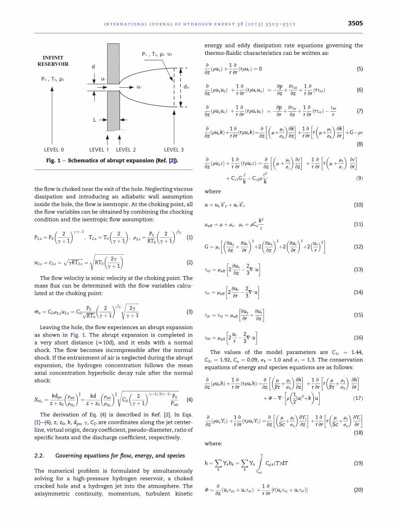
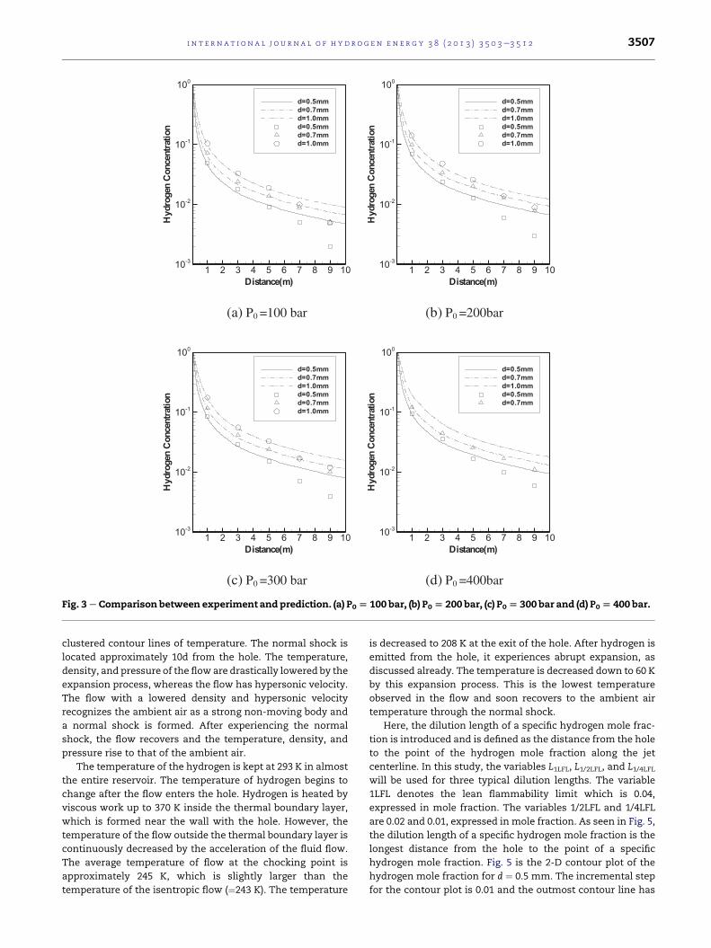
Fig. 3 shows the measurement and prediction. The

prediction was achieved by using FLUENT [17]. Both the

experimental and numerical results exhibit a gradual mono-

tonic decrease of the centerline hydrogen concentration with

excellent agreement until the 3rd probe at a 5m distance from

the exit for all diameters. Such an agreement indicates that

the experiment and the numerical simulation were carried

out in a physically reasonablemanner. The experimental data

for d ¼ 0.5 mm begin to show significant deviations from their

numerical counterparts from the 4th probe at a 7 m distance.

In the case of d ¼ 0.7 mm, both results still maintain

ReserviorInlet

Outlet

Axis

Fictitious Wall (Slip Boundary)Air intakeInlet

x

r

Fig. 2 e Geometric model used for the computation.

consistency at the 4th probe, but they show some deviation at

the 5th probe at a 9 m distance. The experimental data from

d ¼ 1.0 mm show some deviation from the 4th probe, but not

as severe as the d ¼ 0.5 mm case. The figure shows that the

downstream characteristics of the experiment aremuchmore

susceptible to disturbances by wind, especially for smaller

hole diameters and lower source pressures.

Among a number of causes contributing to the deviation

far downstream, the following three causes appear to be

outstanding. First, the virtual wall introduced for numerical

stability may have contributed to the over-prediction of the

hydrogen concentrations in the numerical analysis. As the jet

is being developed, the jet diameter becomes wide enough to

be affected by the virtual wall, which prevents the jet from

further expanding. Consequently, the numerical analysis

would over-predict the hydrogen concentration profiles,

particularly in the downstream region. Second, there is

measurement error associated with the alignment of the jet

centerline. The sampling probes might not be placed exactly

along the centerline of the jet exit. Third, because the exper-

iment was performed outside, the effects of wind could not be

totally eliminated. Consequently, such a small discrepancy in

the centerline alignment and wind effect could have resulted

in under-detecting the centerline hydrogen concentrations.

3.2. Dispersion of hydrogen jet

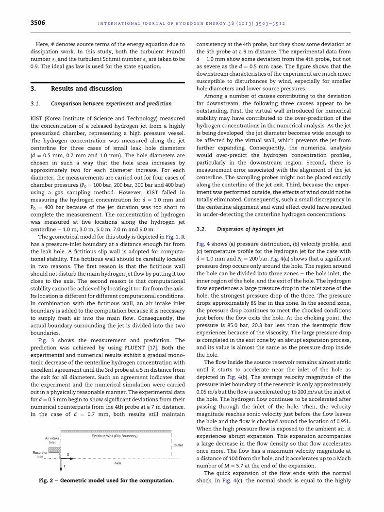
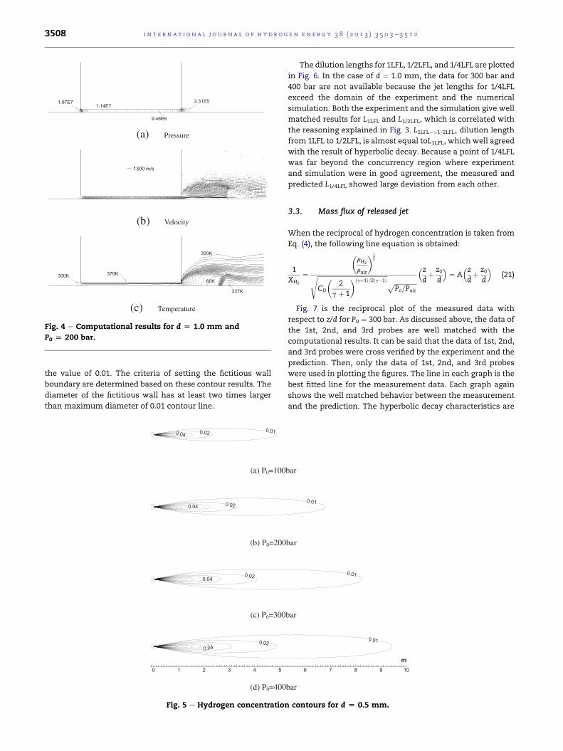
Fig. 4 shows (a) pressure distribution, (b) velocity profile, and

(c) temperature profile for the hydrogen jet for the case with

d ¼ 1.0 mm and P0 ¼ 200 bar. Fig. 4(a) shows that a significant

pressure drop occurs only around the hole. The region around

the hole can be divided into three zones e the hole inlet, the

inner region of the hole, and the exit of the hole. The hydrogen

flow experiences a large pressure drop in the inlet zone of the

hole; the strongest pressure drop of the three. The pressure

drops approximately 85 bar in this zone. In the second zone,

the pressure drop continues to meet the chocked conditions

just before the flow exits the hole. At the choking point, the

pressure is 85.0 bar, 20.3 bar less than the isentropic flow

experiences because of the viscosity. The large pressure drop

is completed in the exit zone by an abrupt expansion process,

and its value is almost the same as the pressure drop inside

the hole.

The flow inside the source reservoir remains almost static

until it starts to accelerate near the inlet of the hole as

depicted in Fig. 4(b). The average velocity magnitude of the

pressure inlet boundary of the reservoir is only approximately

0.05m/s but the flow is accelerated up to 200m/s at the inlet of

the hole. The hydrogen flow continues to be accelerated after

passing through the inlet of the hole. Then, the velocity

magnitude reaches sonic velocity just before the flow leaves

the hole and the flow is chocked around the location of 0.95L.

When the high pressure flow is exposed to the ambient air, it

experiences abrupt expansion. This expansion accompanies

a large decrease in the flow density so that flow accelerates

once more. The flow has a maximum velocity magnitude at

a distance of 10d from the hole, and it accelerates up to aMach

number of M ¼ 5.7 at the end of the expansion.

The quick expansion of the flow ends with the normal

shock. In Fig. 4(c), the normal shock is equal to the highly

(a) P0 =100 bar (b) P0 =200bar

(c) P0 =300 bar (d) P0 =400bar

Distance(m)

HydrogenConcentration

1 2 3 4 5 6 7 8 9 1010-3

10-2

10-1

100

d=0.5mm

d=0.7mm

d=1.0mm

d=0.5mm

d=0.7mm

d=1.0mm

Distance(m)

HydrogenConcentration

1 2 3 4 5 6 7 8 9 1010-3

10-2

10-1

100

d=0.5mm

d=0.7mm

d=1.0mm

d=0.5mm

d=0.7mm

d=1.0mm

Distance(m)

HydrogenConcentration

1 2 3 4 5 6 7 8 9 1010-3

10-2

10-1

100

d=0.5mm

d=0.7mm

d=1.0mm

d=0.5mm

d=0.7mm

d=1.0mm

Distance(m)

HydrogenConcentration

1 2 3 4 5 6 7 8 9 1010-3

10-2

10-1

100

d=0.5mm

d=0.7mm

d=1.0mm

d=0.5mm

d=0.7mm

Fig. 3 e Comparison between experiment and prediction. (a) P0[ 100 bar, (b) P0[ 200 bar, (c) P0[ 300 bar and (d) P0[ 400 bar.

i n t e r n a t i o n a l j o u r n a l o f h y d r o g e n en e r g y 3 8 ( 2 0 1 3 ) 3 5 0 3e3 5 1 2 3507

clustered contour lines of temperature. The normal shock is

located approximately 10d from the hole. The temperature,

density, and pressure of the flow are drastically lowered by the

expansion process, whereas the flow has hypersonic velocity.

The flow with a lowered density and hypersonic velocity

recognizes the ambient air as a strong non-moving body and

a normal shock is formed. After experiencing the normal

shock, the flow recovers and the temperature, density, and

pressure rise to that of the ambient air.

The temperature of the hydrogen is kept at 293 K in almost

the entire reservoir. The temperature of hydrogen begins to

change after the flow enters the hole. Hydrogen is heated by

viscous work up to 370 K inside the thermal boundary layer,

which is formed near the wall with the hole. However, the

temperature of the flow outside the thermal boundary layer is

continuously decreased by the acceleration of the fluid flow.

The average temperature of flow at the chocking point is

approximately 245 K, which is slightly larger than the

temperature of the isentropic flow (¼243 K). The temperature

is decreased to 208 K at the exit of the hole. After hydrogen is

emitted from the hole, it experiences abrupt expansion, as

discussed already. The temperature is decreased down to 60 K

by this expansion process. This is the lowest temperature

observed in the flow and soon recovers to the ambient air

temperature through the normal shock.

Here, the dilution length of a specific hydrogen mole frac-

tion is introduced and is defined as the distance from the hole

to the point of the hydrogen mole fraction along the jet

centerline. In this study, the variables L1LFL, L1/2LFL, and L1/4LFLwill be used for three typical dilution lengths. The variable

1LFL denotes the lean flammability limit which is 0.04,

expressed in mole fraction. The variables 1/2LFL and 1/4LFL

are 0.02 and 0.01, expressed in mole fraction. As seen in Fig. 5,

the dilution length of a specific hydrogen mole fraction is the

longest distance from the hole to the point of a specific

hydrogen mole fraction. Fig. 5 is the 2-D contour plot of the

hydrogen mole fraction for d ¼ 0.5 mm. The incremental step

for the contour plot is 0.01 and the outmost contour line has

(a) Pressure

(b) Velocity

(c) Temperature

2.31E51.97E71.14E7

9.46E6

1300 m/s

337K

300K

300K

370K60K

Fig. 4 e Computational results for d [ 1.0 mm and

P0 [ 200 bar.

i n t e rn a t i o n a l j o u r n a l o f h y d r o g e n en e r g y 3 8 ( 2 0 1 3 ) 3 5 0 3e3 5 1 23508

the value of 0.01. The criteria of setting the fictitious wall

boundary are determined based on these contour results. The

diameter of the fictitious wall has at least two times larger

than maximum diameter of 0.01 contour line.

(a) P0=100

(b) P0=200

(c) P0=300

(d) P0=400

0.010.04 0.02

0.04 0.02

0.040.02

0.040.02

0 1 2 3 4 5

Fig. 5 e Hydrogen concentration

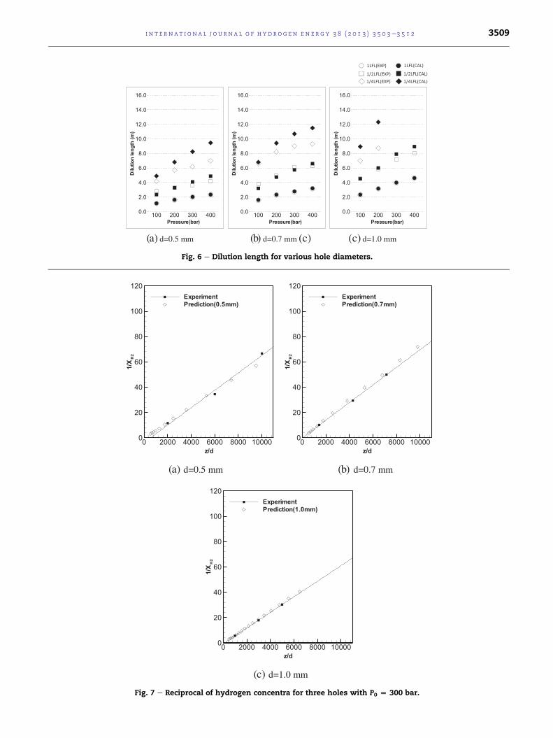
The dilution lengths for 1LFL, 1/2LFL, and 1/4LFL are plotted

in Fig. 6. In the case of d ¼ 1.0 mm, the data for 300 bar and

400 bar are not available because the jet lengths for 1/4LFL

exceed the domain of the experiment and the numerical

simulation. Both the experiment and the simulation give well

matched results for L1LFL and L1/2LFL, which is correlated with

the reasoning explained in Fig. 3. L1LFL�>1=2LFL, dilution length

from 1LFL to 1/2LFL, is almost equal toL1LFL, which well agreed

with the result of hyperbolic decay. Because a point of 1/4LFL

was far beyond the concurrency region where experiment

and simulation were in good agreement, the measured and

predicted L1/4LFL showed large deviation from each other.

3.3. Mass flux of released jet

When the reciprocal of hydrogen concentration is taken from

Eq. (4), the following line equation is obtained:

1XH2

¼

�rH2

rair

�12

ffiffiffiffiffiffiffiffiffiffiffiffiffiffiffiffiffiffiffiffiffiffiffiffiffiffiffiffiffiffiffiffiffiffiffiffiffiffiffiffiffiffiffiffiffiCD

�2

gþ 1

�ðgþ1Þ=2ðg�1Þs ffiffiffiffiffiffiffiffiffiffiffiffiffiffi

Po=Pair

p�zdþ z0

d

�¼ A

�zdþ z0

d

�(21)

Fig. 7 is the reciprocal plot of the measured data with

respect to z/d for P0 ¼ 300 bar. As discussed above, the data of

the 1st, 2nd, and 3rd probes are well matched with the

computational results. It can be said that the data of 1st, 2nd,

and 3rd probes were cross verified by the experiment and the

prediction. Then, only the data of 1st, 2nd, and 3rd probes

were used in plotting the figures. The line in each graph is the

best fitted line for the measurement data. Each graph again

shows the well matched behavior between the measurement

and the prediction. The hyperbolic decay characteristics are

bar

bar

bar

bar

0.01

0.01

0.01

6 7 8 9 10

m

contours for d [ 0.5 mm.

5 mm(a) d=0. (b) d=0.7 mm (c) (c) d=1.0 mm

Pressure(bar)

Dilutionlength(m)

100 200 300 4000.0

2.0

4.0

6.0

8.0

10.0

12.0

14.0

16.0

Pressure(bar)

Dilutionlength(m)

100 200 300 4000.0

2.0

4.0

6.0

8.0

10.0

12.0

14.0

16.0

Pressure(bar)

Dilutionlength(m)

100 200 300 4000.0

2.0

4.0

6.0

8.0

10.0

12.0

14.0

16.0

Fig. 6 e Dilution length for various hole diameters.

mm mm(a) d=0.5 (b) d=0.7

(c) d=1.0 mm

z/d

1/XH2

0 2000 4000 6000 8000 100000

20

40

60

80

100

120Experiment

Prediction(0.5mm)

z/d

1/XH2

0 2000 4000 6000 8000 100000

20

40

60

80

100

120Experiment

Prediction(0.7mm)

z/d

1/XH2

0 2000 4000 6000 8000 100000

20

40

60

80

100

120Experiment

Prediction(1.0mm)

Fig. 7 e Reciprocal of hydrogen concentra for three holes with P0 [ 300 bar.

i n t e r n a t i o n a l j o u r n a l o f h y d r o g e n en e r g y 3 8 ( 2 0 1 3 ) 3 5 0 3e3 5 1 2 3509

i n t e rn a t i o n a l j o u r n a l o f h y d r o g e n en e r g y 3 8 ( 2 0 1 3 ) 3 5 0 3e3 5 1 23510

valid up to relatively large axial distances. The z/d of the 3rd

probe for the three holes are 5,000, 7,000, and 10,000 in order of

hole diameter.

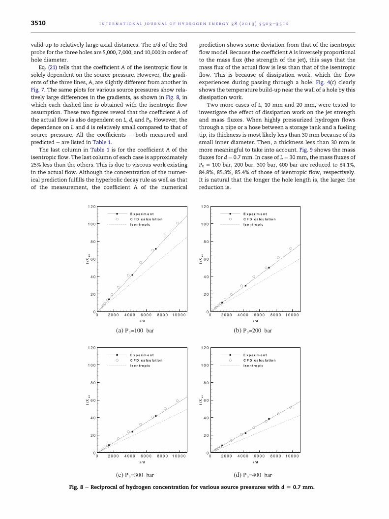
Eq. (21) tells that the coefficient A of the isentropic flow is

solely dependent on the source pressure. However, the gradi-

ents of the three lines, A, are slightly different from another in

Fig. 7. The same plots for various source pressures show rela-

tively large differences in the gradients, as shown in Fig. 8, in

which each dashed line is obtained with the isentropic flow

assumption. These two figures reveal that the coefficient A of

the actual flow is also dependent on L, d, and P0. However, the

dependence on L and d is relatively small compared to that of

source pressure. All the coefficients e both measured and

predicted e are listed in Table 1.

The last column in Table 1 is for the coefficient A of the

isentropic flow. The last column of each case is approximately

25% less than the others. This is due to viscous work existing

in the actual flow. Although the concentration of the numer-

ical prediction fulfills the hyperbolic decay rule as well as that

of the measurement, the coefficient A of the numerical

(a) P =100 bar

(c) P =300 bar

z /d

1/X

0 2 0 0 0 4 0 0 0 6 0 0 0 8 0 0 0 1 0 0 0 00

2 0

4 0

6 0

8 0

1 0 0

1 2 0

E xp e rim e n t

C F D ca lcu la tio n

Ise n tro p ic

z /d

1/X

0 2 0 0 0 4 0 0 0 6 0 0 0 8 0 0 0 1 0 0 0 00

2 0

4 0

6 0

8 0

1 0 0

1 2 0

E xp e rim e n t

C F D ca lcu la tio n

Ise n tro p ic

Fig. 8 e Reciprocal of hydrogen concentration for

prediction shows some deviation from that of the isentropic

flowmodel. Because the coefficientA is inversely proportional

to the mass flux (the strength of the jet), this says that the

mass flux of the actual flow is less than that of the isentropic

flow. This is because of dissipation work, which the flow

experiences during passing through a hole. Fig. 4(c) clearly

shows the temperature build-up near the wall of a hole by this

dissipation work.

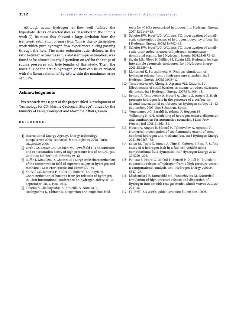
Two more cases of L, 10 mm and 20 mm, were tested to

investigate the effect of dissipation work on the jet strength

and mass fluxes. When highly pressurized hydrogen flows

through a pipe or a hose between a storage tank and a fueling

tip, its thickness is most likely less than 30 mm because of its

small inner diameter. Then, a thickness less than 30 mm is

more meaningful to take into account. Fig. 9 shows the mass

fluxes for d ¼ 0.7 mm. In case of L ¼ 30 mm, the mass fluxes of

P0 ¼ 100 bar, 200 bar, 300 bar, 400 bar are reduced to 84.1%,

84.8%, 85.3%, 85.4% of those of isentropic flow, respectively.

It is natural that the longer the hole length is, the larger the

reduction is.

(b) P =200 bar

(d) P =400 bar

z /d

1/X

0 2 0 0 0 4 0 0 0 6 0 0 0 8 0 0 0 1 0 0 0 00

2 0

4 0

6 0

8 0

1 0 0

1 2 0

E xp e rim e n t

C F D ca lcu la tio n

Ise n tro p ic

z /d

1/X

0 2 0 0 0 4 0 0 0 6 0 0 0 8 0 0 0 1 0 0 0 00

2 0

4 0

6 0

8 0

1 0 0

1 2 0

E xp e rim e n t

C F D ca lcu la tio n

Ise n tro p ic

various source pressures with d [ 0.7 mm.

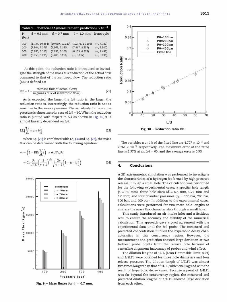
Table 1e Coefficient A (measurement, prediction),310L3.

P0(bar)

d ¼ 0.5 mm d ¼ 0.7 mm d ¼ 1.0 mm Isentropic

100 (11.34, 10.354) (10.069, 10.320) (10.778, 11.266) (e, 7.781)

200 (7.804, 7.379) (6.965, 7.380) (7.867, 8.257) (e, 5.502)

300 (6.880, 6.113) (5.796, 6.100) (6.155, 6.378) (e, 4.492)

400 (6.050, 5.235) (5.285, 5.266) (e, 5.617) (e, 3.891)

L/dReductionRatio

0 10 20 30 40 50 60 700

0.05

0.1

0.15

0.2

0.25

0.3

0.35

0.4

P0=100bar

P0=200bar

P0=300bar

P0=400bar

Fitted line

Fig. 10 e Reduction ratio RR.

i n t e r n a t i o n a l j o u r n a l o f h y d r o g e n en e r g y 3 8 ( 2 0 1 3 ) 3 5 0 3e3 5 1 2 3511

At this point, the reduction ratio is introduced to investi-

gate the strength of the mass flux reduction of the actual flow

compared to that of the isentropic flow. The reduction ratio

(RR) is defined as:

RR ¼ 1� _mðmass flux of actual flowÞ_msðmass flux of isentropic flowÞ : (22)

As is expected, the larger the L/d ratio is, the larger the

reduction ratio is. Interestingly, the reduction ratio is not as

sensitive to the source pressure. The sensitivity to the source

pressure is almost zero in case of L/d¼ 10.When the reduction

ratio is plotted with respect to L/d as shown in Fig. 10, it is

almost linearly dependent on L/d:

RR

�Ld

�yaþ b

Ld: (23)

When Eq. (22) is combinedwith Eq. (3) and Eq. (23), themass

flux can be determined with the following equation:

_m ¼�1� RR

�Ld

��� _msðT0;P0Þ

¼ CDP0ffiffiffiffiffiffiffiffiRT0

p�

2gþ 1

� 1g�1

ffiffiffiffiffiffiffiffiffiffiffiffi2g

gþ 1

s �1� a� b

Ld

�(24)

P re ssu re (b a r)

MassFlux(kg/m

s)

1 0 0 2 0 0 3 0 0 4 0 00

5 0 0 0

1 0 0 0 0

1 5 0 0 0

2 0 0 0 0

2 5 0 0 0

Is e n tro p ic

L = 2 0 m m

L = 1 0 m m

L = 3 0 m m

Fig. 9 e Mass fluxes for d [ 0.7 mm.

The variables a and b of the fitted line are 4.707 � 10�2 and

2.361 � 10�3, respectively. The maximum error of the fitted

line is 1.57% at an L/d ¼ 60, and the average error is 0.5%.

4. Conclusions

A 2D axisymmetric simulation was performed to investigate

the characteristics of a hydrogen jet formed by high pressure

release through a small hole. The calculation was performed

for the following experimental cases; a specific hole length

(L ¼ 30 mm), three hole sizes (d ¼ 0.5 mm, 0.77 mm and

1.0 mm) and four chamber pressures (P0 ¼ 100 bar, 200 bar,

300 bar, and 400 bar). In addition to the experimental cases,

calculations were performed for two more hole lengths to

analyze the mass flux characteristics through a small hole.

This study introduced an air intake inlet and a fictitious

wall to ensure the accuracy and stability of the numerical

calculation. This approach gave a good agreement with the

experimental data until the 3rd probe. The measured and

predicted concentration fulfilled the hyperbolic decay char-

acteristics in this concurrency region. However, the

measurement and prediction showed large deviation at two

farthest probe points from the release hole because of

centerline alignment inaccuracy of probes and wind effect.

The dilution lengths of 1LFL (Lean Flammable Limit, 0.04)

and 1/2LFL were obtained for three hole diameters and four

release pressures The dilution length of 1/2LFL was almost

two times longer than that of 1LFL, whichwell agreedwith the

result of hyperbolic decay curve. Because a point of 1/4LFL

was far beyond the concurrency region, the measured and

predicted dilution lengths of 1/4LFL showed large deviation

from each other.

i n t e rn a t i o n a l j o u r n a l o f h y d r o g e n en e r g y 3 8 ( 2 0 1 3 ) 3 5 0 3e3 5 1 23512

Although actual hydrogen jet flow well fulfilled the

hyperbolic decay characteristics as described in the Birch’s

work [2], its mass flux showed a large deviation from the

isentropic estimation of mass flux. This is due to dissipation

work which pure hydrogen flow experiences during passing

through the hole. The mass reduction ratio, defined as the

ratio between actual mass flux and isentropic estimation, was

found to be almost linearly dependent on L/d for the range of

source pressures and hole lengths of this study. Then, the

mass flux of the actual hydrogen jet flow can be calculated

with the linear relation of Eq. (24) within the maximum error

of 1.57%.

Acknowledgments

This research was a part of the project titled “Development of

Technology for CO2 Marine Geological Storage” funded by the

Ministry of Land, Transport and Maritime Affairs, Korea.

r e f e r e n c e s

[1] International Energy Agency. Energy technologyperspectives 2008: scenarios & strategies to 2050. Paris:OECD/IEA; 2008.

[2] Birch AD, Brown DR, Dodson MG, Swaffield F. The structureand concentration decay of high pressure jets of natural gas.Combust Sci Technol 1984;36:249e61.

[3] Ruffin E,Mouilleau Y, Chaineaux J. Large scale characterizationof the concentration field of supercritical jets of hydrogen andmethane. J Loss Prev Process Ind 1996;9:279e84.

[4] Shirvill LC, Roberts P, Butler CJ, Roberts TA, Royle M.Characterization of hazards from jet releases of hydrogen.In: First international conference on hydrogen safety; 8e10September, 2005. Pisa, Italy.

[5] Takeno K, Okabayashia K, Kouchia A, Nonaka T,Hashiguchia K, Chitose K. Dispersion and explosion field

tests for 40 MPa pressurized hydrogen. Int J Hydrogen Energy2007;32:2144e53.

[6] Schefer RW, Houf WG, Williams TC. Investigation of small-scale unintended releases of hydrogen: buoyancy effects. IntJ Hydrogen Energy 2008;33:4702e12.

[7] Schefer RW, Houf WG, Williams TC. Investigation of small-scale unintended releases of hydrogen: momentum-dominated regime. Int J Hydrogen Energy 2008;33:6373e84.

[8] Swain MR, Filoso P, Grilliot ES, Swain MN. Hydrogen leakageinto simple geometric enclosures. Int J Hydrogen Energy2003;28:229e48.

[9] Mohamed K, Paraschivoiu M. Real gas simulation ofhydrogen release from a high-pressure chamber. Int JHydrogen Energy 2005;30:903e12.

[10] Tchouveleva AV, Cheng Z, Agranat VM, Zhubrin SV.Effectiveness of small barriers as means to reduce clearancedistances. Int J Hydrogen Energy 2007;32:1409e15.

[11] Benard P, Tchouvelev A, Hourri A, Cheng Z, Angers B. Highpressure hydrogen jets in the presence of a surface. In:Second international conference on hydrogen safety; 11e13September, 2007. San Sebastian, Spain.

[12] Venetsanos AG, Baraldi D, Adams P, Heggem PS,Wilkening H. CFD modelling of hydrogen release, dispersionand combustion for automotive scenarios. J Loss PrevProcess Ind 2008;21:162e84.

[13] Hourri A, Angers B, Benard P, Tchouvelev A, Agranat V.Numerical investigation of the flammable extent of semi-confined hydrogen and methane jets. Int J Hydrogen Energy2011;36:2567e72.

[14] Salva JA, Tapia E, Iranzo A, Pino FJ, Cabrera J, Rosa F. Safetystudy of a hydrogen leak in a fuel cell vehicle usingcomputational fluid dynamics. Int J Hydrogen Energy 2012;37:5299e306.

[15] Peneau F, Pedro G, Oshkai P, Benard P, Djilali N. Transientsupersonic release of hydrogen from a high pressure vessel:a computational analysis. Int J Hydrogen Energy 2009;34:5817e27.

[16] Khaksarfard R, Kameshki MR, Paraschivoiu M. Numericalsimulation of high pressure release and dispersion ofhydrogen into air with real gas model. Shock Waves 2010;20:205e16.

[17] FLUENT. 6.3 user’s guide. Lebanon: Fluent Inc.; 2006.