Relativistic mass ejecta from phase-transition-induced collapse of neutron stars

arX

iv:0

908.

1834

v1 [

astr

o-ph

.HE

] 1

3 A

ug 2

009

Relativistic Mass Ejecta from Phase-transition-induced Collapse

of Neutron Stars

K. S. Cheng∗ and T. Harko

Department of Physics and Center for Theoretical and Computational Physics,

The University of Hong Kong, Pok Fu Lam Road, Hong Kong

Y. F. Huang

Department of Astronomy, Nanjing University, Nanjing, China

L. M. Lin

Department of Physics and Institute of Theoretical Physics,

The Chinese University of Hong Kong, Hong Kong, China

W. M. Suen

Department of Physics and Institute of Theoretical Physics,

The Chinese University of Hong Kong, Hong Kong, China and

McDonnell Center for the Space Sciences,

Department of Physics, Washington University, St. Louis, USA

X. L. Tian

Department of Physics, The University of Hong Kong, Pok Fu Lam Road, Hong Kong

(Dated: August 13, 2009)

1

Abstract

We study the dynamical evolution of a phase-transition-induced collapse neutron star to a hybrid

star, which consists of a mixture of hadronic matter and strange quark matter. The collapse

is triggered by a sudden change of equation of state, which result in a large amplitude stellar

oscillation. The evolution of the system is simulated by using a 3D Newtonian hydrodynamic

code with a high resolution shock capture scheme. We find that both the temperature and the

density at the neutrinosphere are oscillating with acoustic frequency. However, they are nearly

180◦ out of phase. Consequently, extremely intense, pulsating neutrino/antineutrino fluxes will

be emitted periodically. Since the energy and density of neutrinos at the peaks of the pulsating

fluxes are much higher than the non-oscillating case, the electron/positron pair creation rate can

be enhanced dramatically. Some mass layers on the stellar surface can be ejected by absorbing

energy of neutrinos and pairs. These mass ejecta can be further accelerated to relativistic speeds

by absorbing electron/positron pairs, created by the neutrino and antineutrino annihilation outside

the stellar surface. The possible connection between this process and the cosmological Gamma-ray

Bursts is discussed.

Keywords: dense matter : stars: neutron stars : stellar oscillations : phase transition- quark

stars : gamma ray bursts.

∗Electronic address: [email protected]

2

I. INTRODUCTION

Gamma-ray bursts (GRBs) are cosmic gamma ray emissions with typical fluxes of the

order of 10−5 to 5 × 10−4ergs cm−2 with the rise time as low as 10−4 s and the duration of

bursts from 10−2 to 103 s. The distribution of the bursts is isotropic and they are believed

to have a cosmological origin, with the observations showing that GRBs originate at extra-

galactic distances. The large inferred distances imply isotropic energy losses as large as

3 × 1053 ergs for GRB 971214 and 3.4 × 1054 ergs for GRB 990123. For detailed reviews

of GRBs properties see [1] and [2], respectively. The widely accepted interpretation of the

phenomenology of GRBs is that the observable effects are due to the dissipation of the

kinetic energy of a relativistically expanding fireball, whose primal cause is not yet known

[1].

One fundamental question related to GRBs is how many intrinsically different categories

they have. Each type may correspond to an intrinsically different type of progenitor, as

well as to a different type of central engine. From the GRB sample collected by BATSE,

a clear bimodal distribution of bursts was identified [2, 3]. Two criteria have been used

to classify the bursts. The primary criterion is duration, and a separation line of 2 s has

been adopted to separate the double-hump duration distribution of the BATSE bursts. The

second criterion is the hardness-usually denoted as the hardness ratio within the two energy

bands of the detector. On average, short GRBs are harder, while long GRBs are softer.

Hence the observations show the existence of two classes of GRBs, long-soft, and short-

hard, respectively. The short GRBs are hard because of the harder low-energy spectral

index of the GRB spectral function [4]. More interestingly, short GRB spectra are broadly

similar to those of long GRBs, if only the first 2 seconds of data of the long GRBs are

taken into account. Afterglows observation shed some light into the physical nature of these

two types of GRBs. The host galaxies of long GRBs are exclusively star forming galaxies,

predominantly irregular dwarf galaxies [5]. The observations suggest that most, if not all

of the long GRBs are produced during the core collapse of massive stars, called collapsars,

as has been also suggested theoretically [6, 7, 8]. Both the observations and the theoretical

models also support the idea that long GRBs are associated with supernova explosions [9].

The observations of SWIFT and of HETE led to a very different picture for the short

GRBs [1, 2]. The basic result of all these observations is that short GRBs are intrinsically

3

different from the long GRBs. Most of the short GRBs are found at the outskirts of elliptical

galaxies, where the star forming rate is very low. Even if they can be associated with star

forming regions, they are rather far away from the active zones [10]. In several cases a

robust host galaxy has not been identified, but the host galaxy is of early type. Deep

supernova searches have been performed, but with negative results [2]. This suggests that

short GRBs may be associated with mergers of compact objects, like neutron star-neutron

star or neutron star-black hole mergers, white-dwarf-neutron star or black hole mergers etc.

[11, 12, 13, 14, 15].

The possibility that the conversion of neutron stars to strange quark stars may be the

energy source for the cosmological gamma ray bursts was suggested in [16]. Neutron stars in

low-mass X-ray binaries can accrete sufficient mass to undergo a phase transition to become

strange stars. At the moment of its birth the strange star is very hot, with an interior

temperature of around ∼ 1011 K. By approximating the strange matter by a free Fermi gas,

the thermal energy of the star is Eth ≈ 5 × 1051 (ρ/ρ0)2/3 R3

6T211 ergs, where ρ is the average

mass density, ρ0 = 2.8×1014 g/cm3 is the nuclear density, R6 is the radius of the star in units

of 106 cm, and T11 is the temperature in units of 1011 K. For ρ = 8ρ0, R6 = 1, T11 = 1.5 the

thermal energy of the newly formed quark star is Eth ≈ 5 × 1052ergs. In the original model

of [16] it was assumed that the star would cool by emission of neutrinos and antineutrinos,

and that the neutrino pair annihilation process νν → e−e+ operates near the strange star

surface. The energy deposited due to this process is E1 ≈ 2 × 1048 (T0/1011K)4ergs ≈ 1049

ergs, where T0 is the initial temperature. The time scale for the deposition is around 1 s. On

the other hand, the processes n + νe → p + e− and p + νe → n + e+ play an important role

in the energy deposition. The integrated neutrino optical depth due to all these processes is

τ ≈ 4.5× 10−2ρ4/311 T 2

11, where ρ11 is the mass density in units of 1011 g/cm3. The deposition

energy can be estimated to be E2 ≈ Eth (1 − e−τ ) ≈ 2 × 1052 ergs. Here the value of the

neutron drip density, ρ11 = 4.3 has been used, and it has been assumed that all the thermal

energy of the star is lost in neutrinos. The process γγ → e−e+ inevitably leads to the

creation of a fireball, and this fireball will expand outward. The expanding shell interacts

with the surrounding interstellar medium, and its kinetic energy is radiated through non-

thermal processes in shocks. However, this model did not consider any internal dynamics,

e.g. heat transport, viscous damping, shock dissipation etc, which can affect the neutrino

emission dramatically. In fact the numerical simulations indicate that the temperature on

4

the neutrinosphere is rapidly changing with time, steady neutrino emission is not possible.

The presence of oscillations of the resulting quark star produced by the phase transition

induced collapse of a neutron star is one of the most intriguing features of the simulations

performed with our Newtonian numerical code introduced in [17]. Recently, the collapse

process with a conformally flat approximation to general relativity was also simulated in

[18]. The works of [17, 18] focus on the gravitational wave signals emitted by the collapse

process.

It is the purpose of the present paper to consider another important implication of this

result, namely, the effect of the oscillations of the newly formed quark star on the neutrino

emission. The oscillations can enhance the neutrino emission rate in a pulsating manner,

and the neutrinos are emitted in a much shorter time scale. Therefore the neutron-quark

phase transition in compact objects may be the energy source of GRBs.

This paper is organized as follows. The phase transition process from neutron stars to

hybrid stars, which consists of a mixture of strange quark matter and hadronic matter, is

summarized in Section II. We describe our numerical code, which is used to simulate the

dynamical evolution of star after phase transition in Section III. In Section IV, we calculate

the neutrino and antineutrino emission from the neutrinosphere and the electron/positron

pair creation rate due to neutrino and antineutrino annihilation process. In Section V, we

calculate mass ejection from stellar surface by absorbing neutrinos/pairs and their subse-

quent acceleration by the pairs outside the star. In Section VI we apply our model to GRBs.

Finally a brief summary and discussion is presented in Section VII.

II. DESCRIPTION OF THE PHASE TRANSITION

The quark structure of the nucleons, suggested by quantum chromodynamics, indicates

the possibility of a hadron-quark phase transition at high densities and/or temperatures, as

suggested by [19, 20, 21]. Theories of the strong interaction, like, for example, the quark

bag models, suppose that breaking of physical vacuum takes place inside hadrons. If the

hypothesis of the quark matter is true, then some of neutron stars could actually be strange

stars, built entirely of strange matter [22, 23, 31, 32, 33].

The central density of compact stellar objects may reach values of up to ten times nuclear-

matter saturation density, and therefore a phase transition to deconfined quark matter, or

5

pion and kaon condensates, should take place at least in the central region of the neutron

stars. In the case of the transition to quark matter, in addition to a phase of unpaired normal

quark matter, present at low densities, several superconducting phases, such as the two-

flavor color superconductor (2SC) phase or the gapless Color-flavor-lock (CFL) phase

can also occur at the large baryon densities reached at the central regions of a compact star.

The transition from the hadronic to the quark phase could proceed in two steps. In the first

step, a transition from hadronic matter to normal quark matter or to a 2SC phase takes

place, due to the increase of the baryonic density at the center of the star. This increase in

density may be due to mass accretion from the fall-back material or rapidly spin-down of the

star. The newly formed hybrid or quark star, containing some 2SC quark matter, can become

meta-stable, and decay into a star containing a CFL phase [24]. Pure hadronic compact

stars above a threshold value of their mass are metastable. The metastability of

hadronic stars originates from the finite size effects in the formation process of

the first strange quark matter drop in the hadronic environment [25].

A phase transition between the hadronic and quark phase occurs when the pressures and

the chemical potentials in the two phases are equal, Ph = Pq, µh = µq, where Ph, µh and Pq,

µq are the pressures and the chemical potentials in the hadron and quark phase, respectively.

In the present Section, unless otherwise explicitly specified, we use the natural

system of units with h = c = 1. If the transition pressure is less than that existing at

the center of the compact object, the transition can occur. For finite values of the surface

tension, complicated structures can develop in the mixed phase, such as drops, rods, and

slabs [28]. The formation of a mixed phase is the result of two competing processes: the size

of the barrier that the system has to overcome in order to form a structure, and the size of

the perturbation of the system. One method to see if the phase transition can proceed or

not is to compare the temperature reached by the system immediately after the conversion

with the height of the barrier. If the temperature is not much lower than the height of

the barrier, the structure formation proceeds thermally, and it is very rapid [29, 30]. If the

temperature is low, new structures can form only via quantum nucleation, which is a very

slow process [24].

The thermal nucleation rate of quark drops can be estimated in the frame-

work of the nucleation theory as Rnucl ≈ a exp (−Wc/T ), where the prefactor a (the

product of the dynamical prefactor and of the statistical prefactor) is the prod-

6

uct of a density and a growth factor, Wc = W (Rc) represents the work needed to

form the smallest drop capable of growing, and T is the temperature. Wc corre-

sponds to the maximum of the free energy of the drop in the new phase. The

dynamical prefactor for the nucleation rate of bubbles or droplets in first-order

phase transitions for the case where both viscous damping and thermal dissipa-

tion are significant has been obtained in [26]. This formalism was applied for

the study of the nucleation of quark-gluon plasma from hadronic matter in [27].

By taking into account the explicit forms of the temperature dependent quark

matter equation of state, of the dissipative factors and of the statistical prefac-

tor, one obtains a complicated dependence of the prefactor on the temperature.

However, the prefactor in this model is based on poorly known physical param-

eters (like, for example, the shear viscosity of the hadronic phase). In order

to obtain some qualitative estimates of the nucleation rate we use the thermo-

dynamical approach developed in [29, 30]. The form of the prefactor can be

obtained from general thermodynamical considerations as a ≈ T 4, and it is very

little dependent on some particular choices (for example in the low temperature

limit the prefactor in the expression for Rnucl can be replaced by the baryon

chemical potential). This form for the prefactor does not include any kinemat-

ics, e.g. the microscopic processes required to transform a gas of hadrons into

a gas of quarks. In the expression of the nucleation rate the dominant term is

the exponential. The free energy is given by W = −4πR3∆P/3+4πσR2 +8πγR+Nq∆µ,

where ∆P = Pq−Ph is the pressure difference, σ = σq +σh is the surface tension, γ = γq−γh

is the curvature energy density and ∆µ = µq −µh is the difference in the chemical potential.

Nq is the total baryon number in the quark drop [24, 29, 30, 34].

The free energy has a maximum at the critical radius Rc = σ(

1 +√

1 + b)

/C, where

C = ∆P − nq∆µ and b = 2γC/σ2. The corresponding free energy is

Wc = 8πσ3[

1 + (1 + b)3/2 + 3b/2]

/3C2. (1)

The number N of drops of the new phase formed inside the old phase in a volume V in a

time t is given by N = RnuclV t. Let λ be the spacing between two drops in the mixed phase.

The number of drops in a volume V is given by V/λ3. The number of drops produced while

the front moves over a distance λ must be of the order of the drops that are present in the

7

mixed phase, RnuclV t = RnuclS (λ/v) ≥ V/λ3 = S/λ2, where v is the velocity of the front

and S its surface area. Therefore in order for thermal nucleation take place the condition

Wc/T ≤ ln (T 4λ4/v) must be satisfied. The process of absorption of a hadron into a pure

quark matter phase can also be described phenomenologically as the fusion of a small drop

of quarks growing into a much larger drop.

The nature of the conversion process from the neutron to the quark matter

is not yet fully understood, and there is no clear theoretical evidence if it is a

deflagration or a detonation. Indeed, for realistic equations of state of quark and

neutron matter and when matter is assumed to be in β equilibrium, detonation

is difficult to achieve [35, 36]. However, it would be still possible to obtain a

detonation if the matter immediately after the front is not yet in β-equilibrium

[24]. It is also important to note that neutrino trapping delays β stability.

According to the analysis of [24], when the drop starts expanding, the process

of conversion can be extremely fast, within the layer in which deconfinement is

energetically favorable, even in the absence of the weak processes. In this case,

the conversion front moves at the velocity of the deflagration front vdf , which

approaches the velocity of sound. As the conversion layer moves outward, the

front enters the region of mixed phase, where vdf decreases until it vanishes at

the low density boundary of the mixed phase.

If the conversion is indeed extremely fast, taking place at speeds close to the

speed of sound, then the typical time scale for the transition can be estimated

as τtr = R/cs, where R is the radius of the neutron star and cs is the speed of

the sound. A simple phenomenological model for the evolution of the quark phase can be

obtained by assuming the relation dr/dt = (r − Rc) /τtr [34], which gives for the transition

time scale Ttr from a microscopic quark drop to a quark matter distribution of a macroscopic

size the expression

Ttr ≈ 10−4N−1/3q R6 ln

R

Rqs, (2)

where R6 is the neutron star radius in units of 106 cm, Rq ∼ 300Rc is the initial size of the

quark drop [34], and Nq, which could be as large as 1048 [37], is the number of quark drops

inside the core of the neutron star. In this case R in Eq. (2) is replaced by R/N1/3q . Therefore

the phase transition may take place in a time scale much shorter than submillisecond.

8

III. SIMULATION OF THE PHASE-TRANSITION INDUCED COLLAPSE

In this paper we focus on studying the phase-transition induced collapse of neutron star

to a hybrid quark star, which consists of a mixture of strange quark matter and hadronic

matter, and want to demonstrate that this process can produce relativistic ejecta, which

could be a mechanism for GRBs. In order to avoid other complications we would like to

simulate a non-rotating, phase-induced collapse of a compact object, with a mixed phase

of quark matter and nuclear matter. In this model gravitational radiation will not be

emitted. Hence we can focus on studying the neutrino and pair emissions and subsequently

gamma-ray emission via interaction between the interstellar medium from this system. In

our simulations, we will not simulate the phase transition process. Instead, we assume that

a fast phase transition has happened (e.g., via a detonation mode) so that the initial neutron

star has converted to a quark star in a timescale shorter than the dynamical timescale of

the system. We assume that the normal matter inside the initial neutron star has suddenly

changed to quark matter at t=0. This is achieved by changing the EOS at t=0 after the

initial hydrostatic equilibrium neutron star has been constructed. We then simulate the

resulting dynamics of the system triggered by the collapse.

A. Description of the numerical code

Our numerical code is based on the three-dimensional numerical simulation in Newtonian

hydrodynamics and gravity. The quark matter of the mixed phase is described by the MIT

bag model and the normal nuclear matter is described by an ideal fluid EOS. This code has

been used to study the gravitational wave emission from the phase-induced collapse of the

neutron stars [17]. Here we briefly summarize the main equations and the numerical scheme

involved. A detailed discussion can be found in [17].

The system of equations describing the non-viscous Newtonian fluid flow is given by

∂ρ

∂t+ ∇ · (ρv) = 0, (3)

∂

∂t(ρvi) + ∇ · (ρviv) +

∂P

∂xi

= −ρ∂Φ

∂xi

, (4)

∂τ

∂t+ ∇ · ((τ + P )v) = −ρv · ∇Φ, (5)

9

where ρ is the mass density of the fluid, v is the velocity with Cartesian components vi

(i = 1, 2, 3), P is the fluid pressure, Φ is the Newtonian potential and τ is the total energy

density, τ = ρǫ + ρv2/2, and ǫ is the internal energy per unit mass of the fluid, respectively.

The Newtonian potential Φ is obtained by solving the Poisson equation, ∇2Φ = 4πGρ. The

system is completed by specifying an equation of state P = P (ρ, ǫ).

The above hydrodynamics Eqs. (3)-(5) can be rewritten in the so-called flux-conservative

form, which can be solved numerically using quite standard high resolution shock capturing

(HRSC) schemes. A HRSC scheme, using either exact or approximate Riemann solvers, with

the characteristic fields (eigenvalues) of the system, obtains the solution of a local Riemann

problem at every cell interface of a finite-differencing grid. Such schemes have the ability

to resolve discontinuities in the solution (e.g., shock waves) by construction. Moreover,

they have high accuracy in regions where the fluid flow is smooth. In general, integrating

the hydrodynamics equations by a HRSC scheme involves the choices of an appropriate

numerical flux formula and a reconstruction method of the state variables (ρ, ǫ,v) for solving

the Riemann problems at the cell interfaces. In our code, we use the Roe’s approximate

Riemann solver [38] for the numerical fluxes and the third-order piecewise parabolic method

[39] for the reconstruction. For the temporal discretization, we use a basic two-step method

to achieve second-order accuracy in time.

In the simulations, we introduced a very low density atmosphere outside the star. The

”artificial” atmosphere is not physical, but it is important for the stability of the hydrody-

namical code. This is due to the problem that the hydrodynamical codes cannot in general

handle vacuum regions where the density is zero. In order to avoid a significant influence

of the atmosphere on the dynamics of the physical system, it is necessary to choose the

density of the atmosphere ρatm to be much smaller than the density scale of interest. For

the results reported in Section 3.4, we set ρatm to be 3 × 109 g/cm3. The effects of different

atmospherical values have been compared in [40].

B. Equation of state

The equation of state (EOS) for neutron stars is highly uncertain. We could try all

possible existing realistic EOS in our study. However, the main purpose of this paper is to

demonstrate that during the phase-transition induced collapse of a neutron star extremely

10

intense, pulsating and very high energy neutrinos can be emitted. The effect is governed

mainly by the amount of pressure reduction after the phase transition as compared to the

initial neutron star model. For simplicity we will use a polytropic EOS for the initial

equilibrium neutron star:

P = k0ρΓ0 , (6)

where k0 and Γ0 are constants. On the initial time slice, we also need to specify the specific

internal energy ǫ. For the polytropic EOS, the thermodynamically consistent ǫ is given by

ǫ =k0

Γ0 − 1ρΓ0−1. (7)

Note that the pressure in Eq. (6) can also be written as

P = (Γ0 − 1)ρǫ. (8)

In order to describe the physical properties of the neutron stars after the

phase transition, we consider that the star can be divided in three regions. At

the center of the star, where ρ > ρq, we have a pure quark core (Region I), which

is described by the MIT bag model equation of state, so that the pressure P is

given by

P = Pq =1

3(ρ + ρǫ − 4B) , ρ > ρq, (9)

where B is the bag constant, and ρq is a critical density for which all the hadrons

are deconfined into quarks. It should be noticed that Pq is not in the usual

form of P = (ρtot − 4B)/3, where ρtot is the (rest frame) total energy density. It is

because in our Newtonian simulations, we use the rest mass density ρ and specific

internal energy ǫ as fundamental variables in the hydrodynamics equations. We

assume that the quark core is absolutely stable. The quark core is surrounded

by a mixed phase of quark and nuclear matter (Region II) that can exist if the

density of the region is higher than a certain critical value ρtr (quark seeds can

spontaneously produce everywhere when ρ ≥ ρtr). Explicitly, the pressure in the

mixed phase is given by

P = αPq + (1 − α)Pn, ρq > ρ > ρtr (10)

where

Pn = (Γn − 1)ρǫ, (11)

11

and

α =

(ρ − ρtr)/(ρq − ρtr), for ρtr < ρ < ρq,

1, for ρq < ρ,

(12)

is defined to be the scale factor of the mixed phase [17]. Γn is not necessarily

equal to Γ0. Finally, we have a normal nuclear matter region (Region III),

extending from ρ < ρtr to the surface of the star, so that in this region

P = Pn, for ρ ≤ ρtr. (13)

A more detailed discussion about such hybrid quark stars can be found in [17].

The total energy density ρtot, which includes the rest mass contribution, is decomposed

as ρtot = ρ + ρǫ. We choose Γn < Γ0 in our simulations to take into account the possibility

that the nuclear matter may not be stable during the phase transition process, and hence

some quark seeds could appear inside the nuclear matter, or the convection, which can occur

during the phase transition process, can mix some quark matter with the nuclear matter. In

the presence of the quark seeds in the nuclear matter, the effective adiabatic index will be

reduced. The possible values of B1/4 range from 145 MeV to 190 MeV [41, 42, 43, 44]. For

ρ > ρq, the quarks will be deconfined from nucleons. The value of ρq is model dependent;

it could range from 4 to 8 ρnuc [44, 45, 46], where ρnuc = 2.8 × 1014 g cm−3 is the nuclear

density.

There are two issues regarding our EOS model to be addressed: (1) It should be noted

that, for simplicity, we do not include the change in the internal energy from the phase

transition when setting the initial data for the collapse. The binding energy released in

the phase transition effectively leads to a slightly harder EOS due to the thermal pressure.

This could be modeled by using a larger value of Γn (comparing to the one we used in this

work). However, as long as the EOS after the phase transition is softer than that of the

initial neutron star, the star will still collapse and stellar pulsations will be triggered. (2)

Furthermore, the parameter ρtr in our EOS model should be considered as the density below

which the matter is dominated by hadronic matter. It is noted that strange quark matter

(if it is more stable) cannot convert back to hadronic matter by decreasing the density.

However, when a fluid element originally in the mixed phase moves to the lower density

region (ρ < ρtr), the fluid element will mix with a large amount of hadronic matter. Hence,

12

14.4 14.6 14.8 15.0

33.5

34.0

34.5

35.0

logHΡL

logH

PL

FIG. 1: Comparison of the equation of state of the mixed quark-hadron phase proposed in [28] for

K = 240 MeV and effective mass m∗/m = 0.78 (dotted curve), and Eq. (10), the equation of state

if the mixed phase used in the present simulations (solid curve).

we approximate that the pressure in the outer region of the star is dominated by the hadronic

part, which is modeled by an ideal gas.

In the simulations, we choose Γ0 = 2, Γn = 1.85, B1/4 = 160 MeV and ρq = 9ρnuc. The

transition density ρtr is defined to be at the point where Pq vanishes initially.

In Eq. (10), we have used a very simple linear combination of strange quark matter EOS

and hadronic matter to represent the EOS of mixed phase, which consists of a mixture of

strange quark drops and hadronic matter. In fact, the properties of a mixed quark-hadron

phase and its implications for hybrid star structure were considered in [28]. In Fig. 1 we

compare the EOS of the mixed phase obtained in [28] for a compression modulus K = 240

MeV and an effective mass at saturation density of m ∗ /m = 0.78 with Eq. (10) used in

the present simulation. We can see that these EOSs are quite close to each other. Although

we use Eq. (10) in our simulation solely based on simplicity, we believe that the simulation

results will not be changed qualitatively if we replace Eq. (10) by the EOS given in [28].

In the mixed phase we have assumed that the effective bag constant B is a

linearly dependent function of the density. The equation of state used by us

reproduces quite well the EOS proposed in [28] to describe the mixed quark-

hadron phase. It is important to note that the main purpose of our paper

is to focus on the study of the dynamical response of the star after a sudden

13

phase transition, no matter what the fine details of the phase transition are. A

full and exact description of the phase transition would require a very precise

knowledge of the physical parameters describing both quark and hadronic mat-

ter. However, taking into account the uncertainties in our present knowledge of

the properties of matter at high densities, our investigations could certainly give

at least a qualitative picture of the astrophysical implications of hadron-quark

phase transitions in compact stars.

C. The Neutrinosphere

For a new born compact star, the internal temperature is so high that neutrinos will be

trapped inside the star for at least a few seconds (cf. [47] for a general review). However,

neutrinos very near the surface of the star can still escape from the star because the optical

depth near the stellar surface is low. Quantitatively we can define a surface called the

neutrinosphere with a radius Rν as follows, e.g. [47, 48],

τeff =∫ ∞

Rν

dr κeff (r) = 1, (14)

where the effective optical depth, τeff is defined as the inverse mean free path and the

effective opacity, κeff is given by

〈κeff 〉(r) = 1.202 × 10−7ρ10(r)(

Tν

4 MeV

)2 1

cm. (15)

It is clear that this surface is a function of the temperature and of the density.

D. Simulation Results

The total time span of the simulations is ∼5 ms, and the time step is 3.7× 10−4 ms. For

all the simulations we report in this paper, the grid spacing is set to be dx = 0.28 km and

the outer boundary of the computational domain is at 27.5 km, which is about two times

the stellar radius of our models. With the grid resolution we used for the simulations, we see

that numerical damping becomes important after about 3 ms. We shall thus only present

the numerical results up to 3 ms. During the simulations, a low-density atmosphere is added

outside the neutron star. The density and temperature of the atmosphere are 3× 109g/cm3

and 0.003 MeV respectively.

14

0 1 2 3Time / ms

0.8

0.85

0.9

0.95

1

1.05ρ 0 /

1015

g c

m-3

0 1 2 3Time / ms

0.9

0.95

1

1.05

1.1

ρ 0 / 10

15 g

cm

-3

0 1 2 3Time / ms

0.9

0.95

1

1.05

1.1

ρ 0 / 10

15 g

cm

-3

0 1 2 3Time / ms

0.95

1

1.05

1.1

1.15

ρ 0 / 10

15 g

cm

-3

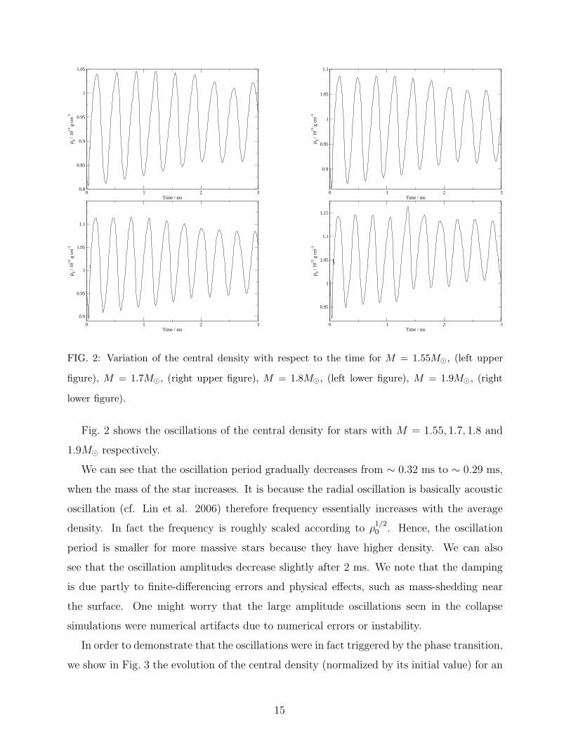
FIG. 2: Variation of the central density with respect to the time for M = 1.55M⊙, (left upper

figure), M = 1.7M⊙, (right upper figure), M = 1.8M⊙, (left lower figure), M = 1.9M⊙, (right

lower figure).

Fig. 2 shows the oscillations of the central density for stars with M = 1.55, 1.7, 1.8 and

1.9M⊙ respectively.

We can see that the oscillation period gradually decreases from ∼ 0.32 ms to ∼ 0.29 ms,

when the mass of the star increases. It is because the radial oscillation is basically acoustic

oscillation (cf. Lin et al. 2006) therefore frequency essentially increases with the average

density. In fact the frequency is roughly scaled according to ρ1/20 . Hence, the oscillation

period is smaller for more massive stars because they have higher density. We can also

see that the oscillation amplitudes decrease slightly after 2 ms. We note that the damping

is due partly to finite-differencing errors and physical effects, such as mass-shedding near

the surface. One might worry that the large amplitude oscillations seen in the collapse

simulations were numerical artifacts due to numerical errors or instability.

In order to demonstrate that the oscillations were in fact triggered by the phase transition,

we show in Fig. 3 the evolution of the central density (normalized by its initial value) for an

15

0 0.5 1 1.5 2 2.5 3Time / ms

0.998

0.999

1

1.001

ρ 0(t)

/ ρ0(t

=0)

FIG. 3: Evolution of the central density (normalized by its initial value) for an unperturbed

equilibrium neutron star with M = 1.8M⊙.

unperturbed equilibrium neutron star model with M = 1.8M⊙. We see that the amplitude

of the oscillations of the star triggered by finite-differencing errors is much smaller than that

seen in the collapse models. Furthermore, there is no obvious periodic features in Fig. 3.

With the simulated density and temperature profiles on a given time slice, we can calculate

the position of the neutrinosphere Rν (see Eq. (14)) with a trial-and-error method. Since

Rν is a function of both temperature and density (cf. previous Section), it also oscillates

with the same period as the central density. Figs. 4 and Figs. 5 show the temperatures and

the densities at the neutrinosphere as a function of time for neutron stars with masses of

1.55, 1.7, 1.8 and 1.9 M⊙, respectively.

We can see that both the temperature and the density at Rν are pulsating, with the same

period as that of the central density, but they are almost 180◦ out of phase to each other.

To show the origin of the pulse like temperature and density evolution, we pick 5 time

slices from t = 0 to t = 0.16 ms, and we focus on the temperature and density evolution at

the neutrinosphere. Figs. 6 show the time evolution of the temperature and of the density

profile of a star with 1.55M⊙ respectively.

We find that the core temperature is rising immediately after the phase transition, which

starts at t = 0, and the heat is moving outward. The neutrinosphere is moving inward

16

0 0.5 1 1.5 2 2.5 3

100

101

Time / ms

Tem

pera

ture

/ M

eV

0 0.5 1 1.5 2 2.5 3

100

101

Time / ms

Tem

pera

ture

/ M

eV

0 0.5 1 1.5 2 2.5 3

10−1

100

101

Time / ms

Tem

pera

ture

/ M

eV

0 0.5 1 1.5 2 2.5 3

100

101

Time / ms

Tem

pera

ture

/ M

eV

FIG. 4: Temperature at the neutrinosphere versus time for M = 1.55M⊙, (left upper figure),

M = 1.7M⊙, (right upper figure), M = 1.8M⊙, (left lower figure), M = 1.9M⊙, (right lower

figure).

because the matter is falling in. The star is shrinking until t ∼ 0.16 ms, which is half of

the oscillation period, and the density at the neutrinosphere is also at its minimum. Also at

t ∼ 0.16 ms, the outward heat pulse meets the infalling material density minimum. This can

also be understood from the definition of the radius of the neutrinosphere, which is defined

as the optical depth equal to unity. Therefore, when the temperature at the neutrinosphere

is maximum, the corresponding density must be at the minimum value.

While the resolutions we used in the simulations (which are limited by the computational

resource) are good enough to model the global dynamics of the star accurately, we note that

this is not the case near the stellar surface where the density is very small and changing

rapidly. In particular, the grid resolution near the neutrinosphere is not very high. We have

compared the numerical results obtained with a few different resolutions in order to examine

the effects of resolution.

17

0 0.5 1 1.5 2 2.5 3

101

102

103

Time / ms

Den

sity

/ 10

10 g

cm

−3

0 0.5 1 1.5 2 2.5 3

101

102

103

Time / ms

Den

sity

/ 10

10 g

cm

−3

0 0.5 1 1.5 2 2.5 3

101

102

103

Time / ms

Den

sity

/ 10

10 g

cm

−3

0 0.5 1 1.5 2 2.5 3

101

102

103

Time / ms

Den

sity

/ 10

10 g

cm

−3

FIG. 5: Density at the neutrinosphere versus time for M = 1.55M⊙, (left upper figure), M =

1.7M⊙, (right upper figure), M = 1.8M⊙, (left lower figure), M = 1.9M⊙, (right lower figure).

In Figs. 7, we show the evolutions of the temperature and density at the neutrinosphere

for the collapse model with M = 1.75M⊙. The figures show that the different resolution

results agree quite well qualitatively during about the first 1.5 ms. In particular, the period

of the pulses does not depend strongly on the resolution. The maximum variation in period

for different grid size is given by 0.28km/Cs, where Cs ∼ 109cm/s is sound speed near the

surface, and it gives the maximum shift in period ∼ 0.03ms.

IV. EMISSION OF NEUTRINOS AND e± PAIRS

A. Neutrino Luminosity

The neutrino luminosity is given by [49],

Lν = 4πr2c1

2πh2

∫

Eν d3pν

1 + exp(Eν − µν/kTν), (16)

18

0 2 4 6 8 10 12 14 1610

0

101

r / km

Tem

pera

ture

/ M

eV

0 ms0.037ms0.082ms0.12ms0.16ms

0 2 4 6 8 10 12 14 1610

0

101

102

103

104

105

r / km

Den

sity

/ 10

10 g

cm

−3

0 ms0.037ms0.082ms0.12ms0.16ms

FIG. 6: Temperature evolution (figure on the left) and density evolution (figure on the right).

The arrow indicates the position at which the temperature (density) change occurs at the neutri-

nosphere.

0 0.5 1 1.5 2 2.5 3

101

Time / ms

Tem

sper

atur

e / M

eV

0.56 km0.44 km0.28 km

0 0.5 1 1.5 2 2.5 3

101

102

103

Time / ms

Den

sity

/ 10

10 g

cm

−3

0.56 km0.44 km0.28 km

FIG. 7: Evolutions of the temperature (figure on the left) and density (figure on the right) at the

neutrinosphere for M = 1.75M⊙, with three different grid resolutions.

where µν is the neutrino chemical potential. Taking µν = 0, the neutrino luminosity emitted

from the neutrinosphere is given by Lν = 7πR2νacT 4

ν /16, where a = 4σ/c is the radiation con-

stant, σ is the Stefan-Boltzmann constant, and Tν is the temperature of the neutrinosphere.

If we assume equal luminosities for neutrinos and antineutrinos, the combined luminosity

for a single neutrino flavor is

Lν, ν = Lν + Lν =7

8πR2

νacT 4ν . (17)

The effect of coherent forward scattering must be taken into account when considering

19

the oscillations of neutrinos traveling through matter (author?) [50]. Although different

flavor neutrinos have different Rν , yet they have approximately the same value of luminosity

for all flavors [51, 52] (for general reviews and in depth discussions of the present status of

neutrino oscillations and their astrophysical implications see [53, 54, 55, 56]). Therefore the

total luminosity is around three times of a single neutrino flavor luminosity

L = Lνe, νe+ Lνµ, νµ

+ Lντ , ντ

=21

8πR2

νacT 4ν . (18)

Using Rν and Tν obtained from the last Section, we compute the neutrino luminosity as

a function of time. The results are shown in Fig. 8.

0 0.5 1 1.5 2 2.5 3

1049

1051

1053

Time / ms

Lν /

ergs

s−1

0 0.5 1 1.5 2 2.5 3

1050

1052

1054

Time / ms

Lν /

ergs

s−1

0 0.5 1 1.5 2 2.5 310

48

1050

1052

1054

Time / ms

Lν /

ergs

s−1

0 0.5 1 1.5 2 2.5 3

1050

1052

1054

Time / ms

Lν /

ergs

s−1

FIG. 8: Neutrino luminosity versus time for M = 1.55M⊙, (left upper figure), M = 1.7M⊙, (right

upper figure), M = 1.8M⊙, (left lower figure), M = 1.9M⊙, (right lower figure).

The peak luminosities range from 1052 to 1054 ergs/s; the pulsating period of the lumi-

nosity is the same as that of the temperature and of the density.

20

B. Pair Production Rate

Neutrinos and antineutrinos can become electron and positron pairs via the neutrino and

antineutrino annihilation process (ν + ν → e− + e+). The total neutrino and antineutrino

annihilation rate can be given as follows [57, 58]

Qνν→e± =7G2

Fπ3ζ(5)

2c5h6D [kTν(t)]

9∫

∞

Rν

Θ(r) 4πr2dr (19)

=7G2

FDπ3ζ(5)

2c5h6

8π3

9R3

ν(kTν)9, (20)

where Θ(r) = 2π2(1 − x)4(x2 + 4x + 5)/3, x =√

1 − R2ν/r

2, Tν(t) is the temperature at

the neutrinosphere at time t, G2F = 5.29 × 10−44 is the Fermi constant, ζ is the Riemann

zeta function, and D is a numerical value depending on the pair creation processes (e.g.

experimental results indicate that D1 = 1.23 for νe νe and D2 = 0.814 for νµ νµ and ντ ντ ).

To obtain the total neutrino annihilation rate from all species, νe νe, νµ νµ and ντ ντ , we sum

up the energy rate for each single flavor,

Q = Qνe νe+ Qνµ νµ

+ Qντ ντ

=28G2

Fπ6ζ(5)

9c5h6(D1 + 2D2)R

3ν(kTν)

9. (21)

Fig. 9 shows the rate of energy carried away by the electron/positron pairs produced

through neutrino annihilation, which varies from ∼ 1051ergs/s to ∼ 1053ergs/s.

It is interesting to note that almost all neutrinos can be annihilated into electron-positron

pairs at the peak because of the extremely high density and high energy of the neutrinos.

In particular the rest mass of the electrons/positrons is much smaller than kTν .

V. MASS EJECTION AND ACCELERATION

In order to calculate the mass ejected from the stellar surface by neutrinos/antineutrinos

and pairs, a very detailed knowledge of the mass distribution near the surface is required.

It was pointed out that the density profile in the crust plays a very important role in

determining how much mass can be ejected [59]. They use a static star model and an

assumed simple power law density profile to demonstrate that the mass ejection can be

significantly different. In our computer capability the minimum spacial grid size that can be

achieved is 0.28 km. In order to estimate a precise location we choose to use the Piecewise

21

0 0.5 1 1.5 2 2.5 3

1039

1041

1043

1045

1047

1049

1051

1053

Time / ms

Le±

/ erg

s s−

1

0 0.5 1 1.5 2 2.5 3

1040

1042

1044

1046

1048

1050

1052

1054

Time / ms

Le±

/ erg

s s−

1

0 0.5 1 1.5 2 2.5 310

40

1042

1044

1046

1048

1050

1052

1054

Time / ms

Le±

/ erg

s s−

1

0 0.5 1 1.5 2 2.5 310

40

1042

1044

1046

1048

1050

1052

1054

Time / ms

Le±

/ erg

s s−

1

FIG. 9: Electron-positron luminosity versus time for M = 1.55M⊙, (left upper figure), M = 1.7M⊙,

(right upper figure), M = 1.8M⊙, (left lower figure), M = 1.9M⊙, (right lower figure).

Cubic Hermite Interpolating Polynomial (PCHIP) method to interpolate the density and

the temperature data along the grids. The PCHIP method can provide a more accurate

representation of the physical reality [60]. As compared with other interpolation methods

(e.g., cubic spline data interpolation), the curve produced by the PCHIP method does not

contain extraneous ”bumps” or ”wiggles”, meaning that it could preserve the shape of the

density and of the temperature profile, even when they change dramatically. However, it

is unavoidable that even if we choose the best possible method, the true location might be

slightly different from the real one. In Fig. 10 we compare the original time evolution of

the position of the neutrinosphere (Rν), temperature at Rν , density at Rν , and the neutrino

luminosity with the results obtained by using the PCHIP method.

We can see that these quantities are qualitatively the same. We believe that the real

continuous mass distributions near the stellar surface can be approximated by a continuous

22

0 1 2 3

12

13

14

15

16

17

18

Time / ms

Rν

/ km

PCHIPNone

0 1 2 3

100

101

Time / ms

Tem

sper

atur

e / M

eV

PCHIPNone

0 1 2 3

101

102

103

Time / ms

Den

sity

/ 10

10 g

cm

−3

PCHIPNone

0 1 2 3

1048

1050

1052

Time / ms

Lum

inos

ity /

ergs

s−1

PCHIPNone

FIG. 10: Results with PCHIP method and without data interpolation for M=1.55M⊙.

mass distribution function, obtained from the numerical simulated data by using a PCHIP

method.

The mass ejection from a newly born quark stars was calculated in [59]. They argue

that neutrino-electron scattering is the most dominated process to deposit the neutrino

energy in the crust. In this paper we argue that the dominated energy deposition process

is the neutrino-antineutrino annihilation process. It should be noted that the optical depth

(τ), which is defined as τ = nσl, is the most important quantity to determine the energy

deposition instead of cross section (σ) alone. Here n is the scattered particle density and l

is the characteristic length. We can only eject mass above neutrinosphere, which is located

only several grid sizes below the stellar surface when the neutrino luminosity is maximum.

From Fig. 4 we can see that the density is several 1011g/cm3 when the neutrino luminosity is

maximum, where most of the mass is ejected. The density has dropped a factor of 10 in one

23

grid size from the neutrinosphere to the stellar surface. Therefore the scale length of density

is about half of grid size, i.e. l ∼ 0.14km. In a neutron rich matter, we can take electron

fraction as 0.2 then we obtain nel ∼ 1039cm−2. On the other hand, the neutrino density is

uniform from the neutrinosphere to the surface of the star and the density of neutrino is

given by nν = 11aT 4/4kT ∼ 1036 (kT/15 MeV)3, where a is the Stefan-Boltzmann constant

and k is the Boltzmann constant. At the neutrino luminosity maximum, kT ∼15 MeV and

the distance from the neutrinosphere to the stellar surface is several grid sizes, which is

∼1km. Then nνl ∼ 1041cm−2. Since neutrino-antineutrino annihilation cross section (cf.

Eq. 2 in [61]) and neutrino-electron scattering cross section (cf. Eq. 7 in [59]) are almost the

same so we will ignore this process in calculating the mass ejection.

A. Energy deposition in the crust and mass ejection

Although most of the neutrinos/antineutrinos created above the neutrinosphere can es-

cape, part of them can still be absorbed in the crust. We can estimate the amount of

neutrino energy Eν deposited in the crust due to the absorption in the following way. If we

define RM as RNS > RM > Rν , then the absorbed neutrino energy onto the surface mass

layer between RM and RNS could be expressed as

Eν(RM) =∫

[

1 − e−τ(RM)]

L(RM) dt, (22)

where τ(RM) =∫

∞

RMdr κeff (r) is the optical depth at RM, L(RM) = 21πR2

M a c T (RM)4/8 is

the neutrino luminosity above RM and T (RM) is the temperature at RM. Notice that we

only performed data output for every 20 iterations in our simulations, corresponding to a

time interval ∆T = 0.0075 ms. Hence, the time interval dt in the integral is taken to be

dt = ∆T .

The annihilated pairs created in the crust will be absorbed because of the much stronger

interaction matter than that of neutrinos, and the pair energy (El±) deposited in the crust

is given by

El± =∫

Q(RM) dt, (23)

Q(RM) =7 G2

F π3 ζ(5)

2 c5 h6(D1 + 2D2)(kTν)

9∫ RNS

RM

Θ(r) 4π r2 dr. (24)

Note that we only integrate r from RM to RNS instead of integrating from Rν to ∞.

24

The gravitational binding energy of the surface mass is

EG =G M ∆m

RM, (25)

where M = 4 π∫ RM

0 r2 ρ(r) dr, and ∆m(RM) = 4 π∫ RNS

RMr2 ρ(r) dr, respectively.

Since the neutrino and pair absorption inside the neutron star actually happen simulta-

neously, we combine the absorbed neutrino and pair energy together to be Eabsorbed

Eabsorbed = El± + Eν . (26)

As long as Eabsorbed(RM) > EG(RM), the surface layer of ∆m(RM) could be ejected from the

neutron star. Hence from this criteria we can obtain the maximum ejected mass.

B. Acceleration by pairs

As we have mentioned in Section 4.2, the neutrino and antineutrino annihilation is very

high at the peak of the neutrino pulses due to the extremely high density and the high

energy of neutrinos. In fact most pairs are created outside the star, and therefore after the

matter is ejected, it will be accelerated by absorbing the pairs created by the annihilation

processes. The annihilation energy created from the neutron star surface RNS to r > RNS

is given by El± =∫

Qνν→e±(r, t)dt, where

Q(r, t) =7G2

Fπ3ζ(5)

2c5h6(D1 + 2D2) [kTν(t)]

9∫ r

RNS

Θ(r′) 4πr′2dr′. (27)

In the following we will briefly describe how the pairs accelerate the ejected matter. Before

we present our calculations, we first describe the continuous mass ejection processes. The

time slice interval of our output data is ∆T = 0.0075 ms. We can calculate the maximum

amount of ejected mass only time slice by time slice.

At T1 (Fig. 11 upper left), a layer of mass ∆M(RM ) is ejected when Eabsorbed(RM) >

EG(RM). The outer surface RM1f of the ejected mass is approximately RNS, and the velocity

of the mass at the outer surface is almost c; the inner surface of the ejected mass is RM1s,

where the velocity of the mass at the inner surface is the escaping velocity, which is almost

half of the speed of light.

T2 is the next time step when another layer of mass could be ejected. Before T2 (Fig. 11

upper right), when the mass layer ejected at T1 is flying outwards from the star at T1+t < T2,

25

Rν1

RM1s

RNS1

(RM1f

)

T = T1

Rν1

RM1s

RNS1

T = T1+ dT < T

2

RM1f

Rν2

RM2s

RNS2

(RM2f

)

T = T2

RM1s

RM1f

Rν2

RM2s

RNS2

T = T2+ dT < T

3

RM2f

RM1s

RM1f

FIG. 11: Schematic illustration of mass ejection from the stellar surface.

the distance to the ejecta can be approximated as RNS1+ct and t is the elapsing time counted

from T1. In the space between RNS1 and RNS1+ct, pairs are created and they can move faster

than the ejected mass layer. Eventually they are absorbed by the ejecta and accelerates the

mass layer in front.

Another mass layer is ejected at T2 (Fig. 11 lower left). When this ejecta moves outward,

it will absorb pairs created between the stellar surface and this ejecta. However pairs created

in the space between these two ejecta can still be absorbed by the first ejecta (cf. Fig. 11

lower right). The total pair energy for accelerating the mass layer ejected at T1 is

Epair =T∞∑

Ti=T1

∫ Ti+∆T

Ti

QTi(r1, r2)dt, (28)

where

QTi(r1, r2) =

7G2Fπ3ζ(5)

2c5h6(D1 + 2D2)(kTν)

9∫ r2

r1

Θ(r) 4πr2dr, (29)

is always calculated between the stellar surface and the ejecta or between two ejecta.

26

Pulse Γ Energy(ergs) Mass (g) Time (s)

1 17 2.2 × 1046 1.5 × 1024 0.16

2 6.4 × 104 6.5 × 1045 1.1 × 1020 0.50

3 1.6 4.7 × 1048 9.1 × 1027 0.83

4 1.6 3.7 × 1049 7.1 × 1028 1.18

5 1 × 106 4.2 × 1046 4.6 × 1019 1.50

5 1.2 × 103 2.7 × 1048 2.4 × 1024 1.51

6 2.8 × 104 4.4 × 1048 1.7 × 1023 1.85

6 1.4 3.9 × 1049 1.1 × 1029 1.86

7 3.8 × 102 4.4 × 1051 1.3 × 1028 2.21

7 1.2 2.4 × 1049 1.6 × 1029 2.23

8 1.2 8.9 × 1048 5.0 × 1028 2.55

9 1.3 3.7 × 1048 1.3 × 1028 2.62

10 2.5 × 105 2.3 × 1048 1.1 × 1022 2.90

10 8.7 2.6 × 1050 3.8 × 1028 2.91

TABLE I: Properties of the ejected mass. Ejected mass in some pulses are divided

into two part: first part with sufficient mass and move faster; the later part moves

slower and cannot collide with first part. (M = 1.55M⊙, Γn=1.85 and B1/4=160

MeV).

The Lorentz factor of each ejecta can be estimated as

Γ =Epair + Eabsorbed

mc2+ 1. (30)

We summarize the results of the ejected masses in Tables 1-4. We can see that sometimes

more than one layer of mass can be ejected in one pulse.

VI. POSSIBLE CONNECTION WITH GAMMA-RAY BURSTS

A. Duration of mass ejection

We have pointed out that our numerical simulations are quite limited by the unphysical

numerical damping. However, in realistic situations, the oscillations triggered by the collapse

27

Pulse Γ Energy(ergs) Mass (g) Time (s)

1 21 1.6 × 1045 8.7 × 1022 0.15

2 2.6 × 102 1.0 × 1045 4.4 × 1021 0.47

3 3.4 × 102 3.2 × 1045 1.1 × 1022 0.79

4 1.3 × 102 5.3 × 1045 4.5 × 1022 1.10

5 2 × 104 3.6 × 1048 2.0 × 1023 1.41

6 2.2 6.9 × 1049 6.2 × 1028 1.74

7 4.8 2.0 × 1050 6.0 × 1028 1.89

8 2.3 × 102 3.1 × 1048 1.5 × 1025 1.91

9 1.6 × 106 2.9 × 1048 2.0 × 1021 2.08

9 5 4.7 × 1050 1.3 × 1029 2.09

10 1.1 4.2 × 1048 3.4 × 1028 2.13

11 8 1.2 × 1046 1.9 × 1024 2.41

12 31 2.5 × 1044 9.2 × 1021 2.73

TABLE II: Properties of the ejected mass. (M = 1.7M⊙, Γn=1.85 and B1/4=160

MeV).

must also be damped by some physical dissipation mechanisms. In this section, we would

like to estimate how long the oscillations could last.

First, we note that hydrodynamics effects (e.g., shock waves, mass-shedding etc.) which

can be modeled by our simulations certainly would play a role in the damping [17, 18].

In particular, the study of [18] suggests that the damping timescale due to hydrodynamics

effects seen in their simulations is typically a few tens to hundreds ms. Another damping

effect which exists in the case of rotational collapse is that due to gravitational radiation

back-reaction. However, the damping timescale of this process is much longer than that of

the hydrodynamics effects. The gravitational radiation damping is negligible and is in fact

not taken into account in the works of [17, 18]. There are still other damping mechanisms.

It was first pointed out in [62] that the dissipation due to nonleptonic reaction is of great

importance and the stellar pulsations of the quark stars would be strongly damped via

s + u ↔ u + d in a few milliseconds. On the other hand, it was shown in (author?) [63]

and [64] that in the high-temperature limit, which is exactly our case, the bulk viscosity is

28

Pulse Γ Energy(ergs) Mass (g) Time (s)

1 6.1 × 105 9.1 × 1045 1.7 × 1019 0.14

2 30 2.5 × 1046 9.5 × 1023 0.46

3 7.8 1.3 × 1046 2.1 × 1024 0.76

4 7.9 × 104 1.6 × 1047 2.2 × 1021 1.06

5 5.9 4.1 × 1047 9.3 × 1025 1.37

6 14 3.5 × 1048 3.1 × 1026 1.68

7 2.2 × 106 2.5 × 1048 1.3 × 1021 2.01

7 8.2 4.2 × 1050 6.4 × 1028 2.01

8 3.1 × 106 4.2 × 1048 1.5 × 1021 2.22

8 3.9 1.9 × 1050 7.4 × 1028 2.22

9 1.5 × 102 1.0 × 1045 7.3 × 1021 2.31

10 59 7.3 × 1043 1.4 × 1021 2.64

TABLE III: Properties of the ejected mass. (M = 1.8M⊙, Γn=1.85 and B1/4=160

MeV).

dramatically reduced. If we take ms ∼ 140 MeV, 〈ρ〉 ∼ 1015 g/cm3 and 〈T 〉 ∼ 50 MeV, the

damping time scale is ∼ 10 s [63].

If all of the above physical mechanisms cannot efficiently damp out the oscillations, then

the pulse neutrino emission and the produced mass ejection considered in this paper would

be the only processes to damp out the oscillations. In Tables 1-4 we can see that the energy

carried away by the ejecta in first 3 ms is of the order of ∼ 1050 ergs. The escaped neutrinos

will carry away comparable amount of energy. The total oscillation energy is of the order of

∆EG ∼ GM2∆R/R2, where ∆R is the change of radius before and after the phase transition.

For the models presented in this paper, ∆R/R is of the order of 10%, which gives oscillation

energy of the order of several 1052 ergs. In other words the oscillations cannot last longer

than several hundreds milliseconds even the neutrino emission and mass ejection are the

only mechanisms to damp out the oscillations.

29

Pulse Γ Energy(ergs) Mass (g) Time (s)

1 2.6 × 102 6.1 × 1046 2.6 × 1023 0.13

2 6.4 2.5 × 1047 5.2 × 1025 0.43

3 6.3 × 104 1.4 × 1046 2.4 × 1020 0.73

4 1 × 102 2.4 × 1047 2.7 × 1024 1.03

5 1.42 1.9 × 1049 4.9 × 1028 1.32

6 4.3 × 102 4.9 × 1048 1.3 × 1025 1.62

6 2.2 7.0 × 1049 6.5 × 1028 1.63

7 1 × 105 3.6 × 1049 4.0 × 1023 1.74

8 9.6 × 104 5.2 × 1048 6.0 × 1022 1.94

8 76 3.7 × 1051 5.6 × 1028 1.95

9 8.8 × 103 5.7 × 1048 7.2 × 1023 2.25

9 2.5 1.9 × 1050 1.4 × 1029 2.25

10 7.5 2.7 × 1047 4.6 × 1025 2.55

11 1.2 3.9 × 1048 2.0 × 1028 2.86

TABLE IV: Properties of the ejected mass. (M = 1.9M⊙, Γn=1.85 and B1/4=160

MeV).

B. Short GRBs

There are two kinds of GRBs, i.e., long GRBs with duration larger than ∼ 2 s and short

GRBs with duration less than ∼ 2 s [2, 3]. The isotropic γ-ray energy released by a short

GRB is usually in the range of 1049 — 1051 ergs, i.e., about two or three orders of magnitude

less than that of long GRBs [65]. Assuming that no more than ∼ 10% of the kinetic energy

can be converted to γ-ray radiation, then an amount of kinetic energy up to 1050 — 1052 ergs

should be produced by the central engine. An example that has a relatively large energy

release is GRB 051221A [66]. The isotropic γ-ray energy is 1.5× 1051 ergs, and an isotropic

kinetic energy of 8.4 × 1051 ergs has been estimated for this event [66].

It is widely believed that long GRBs may originate from the collapse of massive stars

[6], while short GRBs may be connected with the merger of binary compact stars [65,

67]. However, it is still possible that some GRBs may be produced by other mechanisms.

30

For example, GRB 060614, a special nearby long GRB that is not associated with any

supernovae, may be produced by an intermediate mass black hole that captured and tidally

disrupted a star [68]. Another interesting kind of central engine mechanism involves the

phase transition of normal neutron stars to strange stars [16, 69, 70, 71]. Since the phase

transition may be processed in a detonative mode, the details in this process are still largely

uncertain and need further investigation. Especially, numerical simulations are necessary to

help to understand the process.

1. Basic equations

The observations of X-ray, optical and radio afterglows from some well-localized GRBs

have proved their cosmological origin [10, 72, 73, 74, 75]. The so-called fireball model

[11, 76, 77, 78, 79, 80, 81, 82] can basically explain the observational facts well, and thus it

is strongly favored, and widely accepted today. In this model, the central engine gives birth

to some energetic ejecta intermittently, like a geyser, producing a series of ultra-relativistic

shells. The shells collide with each other at a radius of Rin and produce strong internal

shocks. The highly variable γ-ray emission in the main burst phase of GRBs should be

produced by these internal shocks. After the main burst phase, the shells merge into one

main shell and continue to expand outward. It sweeps up circum-burst medium, being

decelerated and producing external shocks. The observed long-lasting and steadily decaying

afterglows (with a much smoother light curve as compared with the γ-ray light curve) should

be due to these external shocks.

After examining the numerical results of our simulations, we believe that the gravitational

collapse of a neutron star induced by the phase transition from normal nuclear matter to

quark matter can be an ideal mechanism for producing GRBs. In this Section, we give some

detailed explanations.

Let us first consider the general case of the collision between two typical shells. Following

the description of [83], we assume that the first shell is ejected with a mass of M1, a bulk

velocity of β1 and a bulk Lorentz factor of γ1. The second shell is assumed to be ejected

after a time interval of ∆t, with the mass, velocity and Lorentz factor being M2, β2, and γ2,

respectively. Here, γ1 = (1 − β21)

−1/2, γ2 = (1 − β22)

−1/2, and they satisfy γ2 > γ1 ≫ 1. The

distance between the two shells is then initially c∆t. Since the second shell moves faster, it

31

will finally catch up with the first shell at a radius of [83],

Rin =β1β2

β2 − β1c∆t ≈ c∆t

β2 − β1=

2γ21γ

22

γ22 − γ2

1

c∆t. (31)

This is the place where the internal shock appears and the GRB takes place. At this point,

the total elapsed time measured in the static burster frame is

tin =Rin

β1c≈ ∆t

β2 − β1=

2γ21γ

22

γ22 − γ2

1

∆t. (32)

However, due to relativistic effect, the observed elapsed time since the beginning of the phase

transition is only tin/(2γ21) ≈ γ2

2∆t/(γ22 − γ2

1).

After the collision, the two shells will merge into one single shell and move at a new

bulk velocity of βbul (correspondingly, with the Lorentz factor γbul). During the process, a

portion of the initial bulk kinetic energy will be dissipated as random internal energy. We

denote the average Lorentz factor of the random internal energy as γi. Since momentum

and energy are conserved in the collision, we have [83],

M1γ1β1 + M2γ2β2 = (M1 + M2)γiγbulβbul, (33)

M1γ1 + M2γ2 = (M1 + M2)γiγbul. (34)

It is then easy to get the solution for βbul, γbul and γi as

βbul =M1γ1β1 + M2γ2β2

M1γ1 + M2γ2

, (35)

γbul =M1γ1 + M2γ2

√

M21 + M2

2 + 2M1M2γ1γ2(1 − β1β2)≈

√

M1γ1 + M2γ2

M1/γ1 + M2/γ2, (36)

γi =M1γ1 + M2γ2

(M1 + M2)γbul≈

√M1γ1 + M2γ2 ·

√

M1/γ1 + M2/γ2

M1 + M2. (37)

The efficiency of transferring bulk kinetic energy into internal energy is

ǫ = (γi − 1)/γi = 1 − γ−1i . (38)

When two shells collide, the emission from the shock-accelerated electrons will correspond

to a single pulse in the light curve of the GRB. The rising time of the pulse is mainly

32

determined by the time needed for the shocks to cross the two shells. Since the merged shell

is moving toward us ultra-relativistically with a Lorentz factor of γbul, only a small part of

the shell (with an opening angle of ∼ 1/γbul) will be seen by us. The decay time of the

pulse is then mainly determined by the arrival time lag of a photon emitted at the angle of

∼ 1/γbul as compared with the photon emitted simultaneously at the line of sight. Usually,

the decay time is longer than the rising time, so we can use the decay time to characterize

the width of the pulse, i.e. [84, 85]

τpulse ≈ Rin/(2γ2bulc). (39)

2. GRBs resulting from phase transition?

According to our simulations, at least more than 10 shells can be ejected during the phase

transition of a neutron star in the first 3 ms. Among these shells, a few will have isotropic

energies larger than 1048 ergs and expand ultra-relativistically with Lorentz factors larger

than > 100 (cf. Tables 1-4). Note that although our simulations only last for about 3 ms,

the actual duration of the oscillation process may last for several hundreds milliseconds, as

argued at the end of our Section 6.1 . During this period, tens or even hundreds of ultra-

relativistic shells might be ejected, each with an energy larger than ∼ 1048 ergs. The total

energy enclosed in these relativistic shells may be 1050 — 1051 ergs. We suggest that the

collision between these shells can give birth to a GRB.

To describe this process in a quantitative way, we first study the collision between two

specific (but typical) shells. We assume M1 = M2, γ1 = 300, γ2 = 2γ1 = 600. We further

assume that the second shell is ejected after a time interval of ∆t = 1 ms. It is then

straightforward to find that they will collide at a radius of Rin ∼ 8γ21c∆t/3 ≈ 7.2× 1012 cm,

and at the time of tin ∼ 8γ21∆t/3 ≈ 240 s. Note that due to relativistic effect, the observed

elapsed time since the beginning of the phase transition is only tin/(2γ21) ∼ 4∆t/3 ≈ 1.3 ms.

The merged shell will move at a Lorentz factor of γbul ∼√

2γ1 ≈ 420, with the co-moving

internal energy characterized by γi ≈ 3/2√

2 ≈ 1.06. The efficiency of transferring the bulk

kinetic energy into internal energy is ǫ = 1− 1/1.06 ≈ 5.6%. The pulse will have a width of

τpulse ≈ 2∆t/3 ≈ 0.6 ms.

In realistic cases, the shells are ejected with variable masses, variable Lorentz factors,

and variable time intervals, respectively. The conditions then become very complicated.

33

For example, if γ2 is much larger than γ1 (γ2 ≫ γ1, but we still assume M2 = M1), then

the solution can be expressed as Rin ∼ 2γ21c∆t, tin ∼ 2γ2

1∆t, γbul =√

γ1γ2, γi =√

γ2/4γ1,

τpulse = ∆tγ1/γ2. In this case, the pulse width will be very small. On the other hand, if γ2

is only slightly larger than γ1 (still with M2 = M1), then γbul ∼ γ1, γi ∼ 1, Rin and tin will

be very large so that a pulse much wider than ∆t can be generated. However, in this case,

the energy transfer efficiency will be extremely low (ǫ ≪ 1) for this single pulse.

In the standard fireball model, it is generally believed that the total duration of a GRB

reflects the active period of the central engine. In our simulations, the shells are ejected

mainly in a few hundred milliseconds. So, this mechanism is most proper for explaining

short GRBs. The duration may reasonably range between a few ms and several hundred

ms if the neutrino emission and the mass ejection are the only processes to damp out the

stellar oscillations. It is also possible for the duration to extent to more than 1 s. For

example, if we take γ1 = 350, γ2 = 400 and ∆t = 300 ms, then the observed elapsed time for

this pulse will be larger than tin/(2γ21) = γ2

2/(γ22−γ2

1)∆t ≈ 4.3∆t ∼ 1.3 s. Note that the total

isotropic energy of the shells can be 1050 — 1051 ergs, and this is also consistent with the

energy requirement of most short GRBs. If some extent of anisotropy exists in the process

(which is quite possible if the effects of strong magnetic field of the compact star are further

included, see the discussion in the last paragraph of this section), then the energy release

can even meet the requirement of those rigorous energetic events, such as GRB 051221A

[66]. Also, as noted above, if two shells are ejected with similar Lorentz factors, they may

collide at a very late time. We further notice from Tables 1 — 4 that there are many high

energy shells that moves at trans-relativistic speeds (with Lorentz factors significantly less

than ∼ 10). Late collisions can also be produced by these energetic shells when they finally

catch up with the decelerating external shock (that produces GRB afterglow). Such late

collisions may manifest themselves as flaring activities (emerged in the afterglow phase), as

frequently observed 1000 — 10000 s after the trigger of GRBs [86, 87].

In our simulations, the shells are ejected periodically, with a period of ∼ 0.3 ms. However,

it is quite unlikely that we could observe any obvious periodicity in the γ-ray light curve.

The reason is that the shells have different masses, velocities, and energies. The periodicity

will then be most likely smeared out at the time of collision.

The energy releases in our simulations are basically isotropic. The reason is that we did

not include the effects of rotation and macroscopical magnetic field in our calculations. When

34

these effects are considered, the energy releases should show some features of anisotropy.

This is an interesting point that needs to be investigated in further details.

VII. DISCUSSIONS

In this paper we have studied the possible consequences of the phase-induced collapse of

neutron stars to hybrid stars. We have found that both the density and the temperature

inside the star will oscillate with the same period, but almost 180◦ out of phase, which

will result in the emission of intense pulsating neutrinos. The temperatures at the peaks

of pulsating neutrino fluxes are 10-20 MeV, which are 2-3 times higher than non-oscillating

case. Since the electron/positron pair creation rate sensitively depends on the temperature

at neutrinosphere, the efficiency of pair creation increases dramatically. We want to point

out that the intense pulse neutrino and pair luminosity can be maintained due to the os-

cillatory fluid motion, which can carry thermal energy directly from the stellar core to the

surface. This process can replenish the energy loss of neutrino emission much quicker than

the neutrino diffusion process. Part of neutrino energy, roughly (1-1/e), and pairs inside

the star will be absorbed by the matter very near the stellar surface. When this amount

of energy exceeds the gravitational binding energy of matter, some mass near the stellar

surface will be ejected, and this mass will be further accelerated by absorbing pairs created

from the neutrino and antineutrino annihilation processes outside the star. Unlike inside the

star, the surface properties, e.g. position of the neutrinosphere, surface temperature etc.,

are very sensitive to the surface perturbation. The neutrino and pair luminosities can be

varied from pulse to pulse. This results in the large variation of the Lorentz factor of the

mass ejecta. The internal collisions among these mass ejecta may produce the short time

variabilities of the Gamma-ray Bursts, which can be as short as submilliseconds. Although

mass ejecta are ejected periodically, each ejecta can have different masses and Lorentz fac-

tors as explained before. Therefore, the intrinsic period could not be observed. Although

we can only simulate the oscillating stars for a few millisecond, we can speculate that this

may be a possible mechanism for short Gamma-ray Bursts based on the following reasons.

[89] have estimated that the viscous damping time for such oscillating system is of order of

10 s. By assuming that if neutrinos and pair emissions are the only damping mechanisms,

the pulsations can last less than ∼ 3s [89], which is roughly the characteristic time scale of

35

short Gamma-ray Bursts.

The phase-transition from a neutron star to a strange star was simulated in [88], with the

conclusion that this process is most likely not a gamma-ray burst mechanism. They mimic

the phase-transition by the arbitrary motion of a piston deep within the star, and they

have found that the mechanic wave will eject ∼ 10−2M⊙ baryons, which causes the baryon

contamination for the gamma-ray bursts. In our simulations, we assume a sudden change of

equation of state to mimic the phase-transition, and we use the Newtonian hydrodynamic

code to study the response of the stellar interior, after such a sudden change of the EOS. In

our simulations we find that the mass ejection by the motion of the fluid is very small. We

estimate that the major mass ejection would result from the heating of neutrinos and pairs

on the stellar crust, which is not modeled in the simulations. Our total energy output and

total mass in ejecta are close to that of [88] (cf. Tables 1-4). However, the neutrino energy

injection is pulsating, and hence the mass ejection is also pulsating. The masses of individual

ejecta range from ∼ 10−9M⊙ to ∼ 10−4M⊙, with output energy in the range of 1048 ergs

to 1050 ergs. Therefore, some ejecta cannot be relativistic, and they cannot contribute to

GRBs. However, there are still many relativistic ejecta in each simulation model, which can

have Lorentz factors >100, and with a total energy of ∼ 1050 — 1051 ergs. We conclude

that this could be a possible mechanism for short GRBs.

Finally, we want to remark that our numerical simulations describe a spherically symmet-

ric, non-rotating, and collapsing stellar object. Also the effect of the magnetic fields was not

taken into account. Therefore, the radiation emission produced in this model is isotropic.

However, a realistic neutron star should have finite angular momentum and strong magnetic

field, and hence these two factors could produce asymmetric mass ejection. This effect will

be considered in future work.

Acknowledgements

We thank M.C. Chu, Z.G. Dai, P. Haensel, T. Lu, K.B. Luk, V.V. Usov and K.W.

Wu for useful discussion, and the anonymous referee for very useful suggestions. KSC and

TH are supported by the GRF Grants of the Government of the Hong Kong SAR under

HKU7013/06P and HKU7025/07P respectively. YHF is supported by the National Science

Foundation of China (grant 10625313), and the National Basic Research Program of China

36

(grant 2009CB824800). LML is supported by the Hong Kong Research Grants Council

(Grant No. CUHK4018/07P) and the direct grant (Project IDs: 2060330) from the Chinese

University of Hong Kong. The computations were performed on the Computational Grid of

the Chinese University of Hong Kong and the High Performance Computing Cluster of the

University of Hong Kong.

[1] P. Meszaros, Rept. Prog. Phys. 69 (2006) 2259

[2] B. Zhang, Chin. J. Astron. Astrophys. 7 (2007) 1

[3] C. Kouveliotou et al., Astrophys. J. 413 (1993) L101

[4] G. Ghirlanda, G. Ghisellini and A. Celotti, Astron. Astrophys. 422 (2004) L5

[5] A. Fruchter et al., Nature 441 (2006) 436

[6] S. E. Woosley, Astrophys. J. 405 (1993) 273

[7] B. Paczynski, Astrophys. J. 494 (1998) L45

[8] A. I. MacFadyen and S. E. Woosley, Astrophys. J. 524 (1999) 262

[9] S. E. Woosley and J. S. Bloom, Ann. Rev. Astr. & Astrophys. 44 (2006) 507

[10] J. S. Bloom et al., Astrophys. J. 638 (2006) 354

[11] B. Paczynski, Astrophys. J. 308 (1986) L43

[12] M. Ruffert and H. T. Janka, Astron. Astrophys. 344 (1999) 573

[13] C. D. Dermer and A. Atoyan, Astrophys. J. 643 (2006) L13

[14] A. J. Levan et al. 2006, Month. Not. R. Ast. Soc. 368 (2006) L1

[15] A. King, E. Olsson and M. B. Davies, Month. Not. R. Ast. Soc. 374 (2007) L34

[16] K. S. Cheng and Z. G. Dai, Phys. Rev. Lett. 77 (1996) 1210

[17] L. M. Lin, K. S. Cheng, M. C. Chu and W. M. Suen, Astrophys. J 639 (2006) 382

[18] E. B. Abdikamalov, H. Dimmelmeier, L. Rezzolla, and J. C. Miller, Month. Not. R. Ast. Soc.

392 (2009) 52

[19] N. Itoh, Prog. Theor. Phys. 44 (1970) 291

[20] A. R. Bodmer, Phys. Rev. 4 (1971) 1601

[21] E. Witten, Phys. Rev. D30 (1984) 272

[22] C. Alcock, E. Farhi, and A. Olinto, Astrophys. J. 310 (1986) 261

[23] P. Haensel, J. L. Zdunik, and R. Schaeffer, Astron. Astrophys. 160 (1986) 121

37

[24] A. Drago, A. Lavagno, and I. Parenti, Astrophys. J. 659 (2007) 1519

[25] Z. Berezhiani, I. Bombaci, A. Drago, F. Frontera, and A. Lavagno, Astrophys. J.

586 (2003) 1250

[26] R. Venugopalan and A. P. Vischer, Phys. Rev. E49 (1994) 5849

[27] J. I. Kapusta, A. P. Vischer, and R. Venugopalan, Phys. Rev. C51 (1995) 901

[28] N. K. Glendenning, Compact stars, Nuclear Physics, Particle Physics and General Relativity,

(2000) Springer, New York

[29] M. L. Olesen and J. Madsen, Phys. Rev. D47 (1993) 2313

[30] M. L. Olesen and J. Madsen, Phys. Rev. D49 (1994) 2698

[31] K. S. Cheng, Z. G. Dai, and T. Lu, Int. J. Mod. Phys. D7 (1998) 139

[32] K. S. Cheng and Z. G. Dai, 1998, Phys. Rev. Lett. 80 (1998) 18

[33] K. S. Cheng, Z. G. Dai, D. M. Wei, and T. Lu, Science 280 (1998) 407

[34] T. Harko, K. S. Cheng, and P. S. Tang, Astrophys. J. 608 (2004) 945

[35] J. E. Horvath and O. G. Benvenuto, Phys. Lett. B 213 (1988) 516

[36] H. T. Cho, K. W. Ng, and A. D. Speliotopoulos, Phys. Lett. B326 (1994) 111

[37] K. Iida and K. Sato, Phys. Rev. C58 (1998) 2538

[38] P. L. Roe, 1981, J. Comput. Phys. 43 (1981) 357

[39] P. Collela and P. R. Woodward, 1984, J. Comput. Phys. 54 (1984) 174

[40] Tian, X. L., M.Phil. Thesis (2008) University of Hong Kong

[41] T. DeGrand, R. L. Jaffe, K. Johnson, and J. Kiskis, Phys. Rev. D12 (1975) 2060

[42] H. Satz, 1982, Phys. Lett. B113 (1982) 245

[43] F. M. Steffens, H. Holtmann, and A. W. Thomas, Phys. Lett. B358 (1995) 139

[44] P. Haensel, in Final Stages of Stellar Evolution, Ed. C. Match & J. M. Hamenry (Les Ulis:

EDP Sciences) (2003) 249

[45] K. S. Cheng and Z. G. Dai, 1998, Astrophys. J. 492 (1998) 281

[46] I. Bombaci, I. Parenti, and I. Vidana, Astrophys. J. 614 (2004) 314

[47] S. L. Shapiro and S. A. Teukolsky, Black Holes, White Dwarfs and Neutron Stars: The Physics

of Compact Objects (1983) (John Wiley & Sons)

[48] M. Jaroszynski, Astron. Astrophys. 305 (1996) 839

[49] A. B. Balantekin and H. Yuksel, New J. Phys. 7 (2005) 51

[50] L. Wolfenstein, 1978, Phys. Rev. D17 (1978) 2369

38

[51] H.-T. Janka, 1995, Astropart. Phys. 3 (1995) 377

[52] H.-T. Janka, Astron. Astrophys. 368 (2001) 527

[53] M. Maltoni, T. Schwetz, M. Tortola, and J. W. F. Valle, New Journal of Physics 6 (2004) 122

[54] O. Mena, I. Mocioiu, and S. Razzaque, Phys. Rev. D75 (2007) 063003

[55] E. Kh. Akhmedov and V. Niro, Journal of High Energy Physics 12 (2008) 106

[56] G. Altarelli and D. Meloni, 2009, Nucl. Phys. B809 (2009) 158

[57] J. Goodman, A. Dar, and S. Nussinov, Astrophys. J. 314 (1987) L7

[58] J. Cooperstein, L. J. V. D. Horn, and E. Baron, Astrophys. J. 321 (1987) L129

[59] P. Keranen, R. Ouyed, and P. Jaikumar, Astrophys. J. 618 (2005) 485

[60] F. N. Fritsch and R. E. Carlson, SIAM Journal on Numerical Analysis 17 (1980) 238

[61] K. Asano and T. Fukuyama, Astrophys. J. 531 (2000) 949

[62] Q. D. Wang and T. Lu, 1984, Physics Letters B148 (1984) 211

[63] R. F. Sawyer, 1989, Phys. Rev. D39 (1989) 3804

[64] J. Madsen, Phys. Rev. D46 (1992) 3290

[65] E. Nakar, Phys. Rept. 442 (2007) 166

[66] A. M. Soderberg, E. Berger, M. Kasliwal et al., Astrophys. J. 650 (2006) 261

[67] D. Eichler, M. Livio, T. Piran, and D. N. Schramm, Nature 340 (1989) 126

[68] Y. Lu, Y. F. Huang, and S. N. Zhang, Astrophys. J. 684 (2008) 1330

[69] I. Bombaci and B. Datta, Astrophys. J. 530 (2000) L69

[70] X. Y. Wang, Z. G. Dai, T. Lu, D. M. Wei, and Y. F. Huang, 2000, Astron. Astrophys. 357

(2000) 543

[71] R. Ouyed, J. Dey and M. Dey, Astron. Astrophys. 390 (2002) L39

[72] E. Costa et al., Nature 387 (1997) 783

[73] D. A. Frail, S. R. Kulkarni, L. Nicastro, M. Feroci, and G. B. Taylor, Nature 389 (1997) 261

[74] T. J. Galama, R. A. M. J. Wijers, M. Bremer, P. J. Groot, R. G. Strom, C. Kouveliotou, and

J. van Paradijs, Astrophys. J. 500 (1998) L97

[75] N. Gehrels et al., Nature 437 (2005) 851

[76] J. Goodman, 1986, Astrophys. J. 308 (1986) L47

[77] P. Meszaros and M. J. Rees, Astrophys. J. 397 (1992) 570

[78] M. J. Rees and P. Meszaros, Month. Not. R. Ast. Soc. 258 (1992) 41P

[79] M. J. Rees and P. Meszaros, Astrophys. J. 430 (1994) L93

39

[80] J. I. Katz, Astrophys. J. 422 (1994) 248

[81] R. Sari, R. Narayan, and T. Piran, Astrophys. J. 473 (1996) 204

[82] R. Sari, T. Piran, and R. Narayan, 1998, Astrophys. J. 497 (1998) L17

[83] B. Paczynski and G. Xu, Astrophys. J. 427 (1994) 708

[84] S. Kobayashi, T. Piran, and R. Sari, Astrophys. J. 490 (1997) 92

[85] T. Piran, Phys. Repts. 314 (1999) 575

[86] A. Burrows, R. Walder, C. D. Ott, and E. Livne, 2005, in The Fate of the Most Massive Stars,

ASP Conference Series, Edited by R. Humphreys and K. Stanek, San Francisco: Astronomical

Society of the Pacific, 332 (2005) 358

[87] P. Romano et al., Astron. Astrophys. 450 (2006) 59

[88] C. L. Fryer and S. E. Woosley, Astrophys. J. 501 (1988) 780

[89] T.C. Chan, K.S. Cheng, T. Harko, H.K. Lau, L.M. Lin, W.M. Suen and X. L. Tian, Astrophys.

J. 695 (2009) 732

40