Relativistic Hydrodynamics S.1 A brief introduction to general relativity The concept of manifold: A manifold is a topological space that can be continuously parameterized (i.e. differentiable), whose dimension is equal to the number of parameters required for specifying a point in this manifold. Locally, this manifold looks like the Euclidean four-space R 4 . Examples: 1- The circle S 1 = {(x,y)∈ IR 2 | x 2 +y 2 = 1} is a manifold of dimension one. 2- The circle S n = {(x 1 , x 2 , x 3 , …x n ,)∈ IR n+1 | x1 2 + x2 2 + x3 2 + …xn+1 2 = 1} is a manifold of dimension n. 3- The position coordinates of a particle (ξ 1 , ξ 2 , ξ 3 ) together with its three momentum coordinates (p 1 ,p 2 ,p 3 ) build up a 6-dimensional manifold. The geometry of a Riemannian manifold is defined through the metric that measures the distance between two arbitrary points in this manifold. In general relativity, the interval between two such points is given by the expression 2 , ds g dx dx where gμν is a set of coordinate functions that determines the geometry of the manifold. The intervals in Riemannian manifolds are positive definite and invariant under coordinate transformation. On manifolds, one may define scalar and vector fields. Φ on a manifold U is said to be a scalar field, if Φ associates to each point of U a unique real-value Φ(x μ ). Example: Φ(x 1, x 2 , x 3 ) = x 3 . Vector fields on manifolds are the assignment of a single vector to each point P of U. Each vector is a linear combination of the set of independent basis vectors e μ , whose number equal to the dimension of the manifold U, i.e., v( ) () () x v xe x , where () v x are the contravariant components (actually numbers) associated with each basis vector e μ . Similarly, the vector v(x) can be written as a linear combination of the dual basis vectors e (the reciprocal vectors of e μ ) : v( ) () () x v xe x , () v x here is the covariant components and . e e

Welcome message from author
This document is posted to help you gain knowledge. Please leave a comment to let me know what you think about it! Share it to your friends and learn new things together.
Transcript

Relativistic Hydrodynamics
S.1
A brief introduction to general relativity
The concept of manifold: A manifold is a topological space that can be continuously parameterized (i.e.
differentiable), whose dimension is equal to the number of parameters required
for specifying a point in this manifold.
Locally, this manifold looks like the Euclidean four-space R4.
Examples:
1- The circle S1 = {(x,y)∈ IR2 | x2+y2 = 1} is a manifold of dimension one.
2- The circle Sn = {(x1, x2, x3, …xn,)∈ IRn+1 | x12+ x2
2+ x32+ …xn+1
2 = 1} is a
manifold of dimension n.
3- The position coordinates of a particle (ξ 1, ξ 2, ξ 3) together with its three
momentum coordinates (p1,p2,p3) build up a 6-dimensional manifold.
The geometry of a Riemannian manifold is defined through the metric that
measures the distance between two arbitrary points in this manifold. In general
relativity, the interval between two such points is given by the expression 2 ,ds g dx dx
where gμν is a set of coordinate functions that determines the
geometry of the manifold. The intervals in Riemannian manifolds are positive
definite and invariant under coordinate transformation.
On manifolds, one may define scalar and vector fields.
Φ on a manifold U is said to be a scalar field, if Φ associates to each point of U
a unique real-value Φ(xµ).
Example: Φ(x1, x2, x3) = x3.
Vector fields on manifolds are the assignment
of a single vector to each point P of U.
Each vector is a linear combination of the set of
independent basis vectors eμ , whose number equal to the dimension of the manifold U, i.e.,
v( ) ( ) ( )x v x e x
, where ( )v x are the contravariant components
(actually numbers) associated with each basis vector eμ. Similarly, the vector v(x) can be written as a linear combination of the dual
basis vectors e𝝁 (the reciprocal vectors of eμ) : v( ) ( ) ( )x v x e x
,
( )v x here is the covariant components and .e e

Relativistic Hydrodynamics
S.2
This implies that v ,e v e e v v
but also
v .v e Now an infinitesimal interval between two arbitrary points on U, can be expressed as the inner product the two vectors:
2 ds×ds ( ) ( ) , .ds dx e dx e e e dx dx g dx dx where g e e
Equivalently, 2 , .ds g dx dx where g e e
Consequently, the inner product of two vectors should be the same, whether we use the contravariant or covariant versions of the vectors, i.e.,
( ) ( ) ( ) .V W v e w e e e v w g v w g v w
It can be easily
verified that the contavariant and covariant basis vectors can be
transformed from one to other using the metric gμν, i.e.,
, .e g e e g e
But as
.e e g g
Viewing as a matrix, then , is nothing but the inverse
matrix of and vice versa.
g g
g
Helpful notes:
1. A two dimensional table can be viewed as a matrix
2. Generalization of matrices are tensors
3. A 2D matrix ⟶ tensor of rank 2
4. A 3D matrix ⟶ tensor of rank 3
5. Tensors are transformable objects that could have geometrical meanings
Tensor products:
Let A, B, and C be matrices of arbitrary dimensions, so that AB = C.
An element of C reads:
ij in nj
n
c = a b

Relativistic Hydrodynamics
S.3
[ ]Cij
=
A B C
But in tensor world, the sum means a contraction. As in matrix algebra, we
introduce the inner product of two second-rank tensors as follows:
β β
αβ υ αβ αυ
β
A B = A B =T
We note that in matrix algebra, the products:
AB BA Example:
1 0 1 1 1 1=
1 2 1 1 3 3
1 1 1 0 2 2=
1 1 1 2 2 2
In tensor analysis the product of two tensors, such as:
β β
α βσ βσ αA B and B A
are sets of instructions that carry out the same process and, if carried out
correctly, will yield the same results.
Kummulativegesetzt???

Relativistic Hydrodynamics
S.4
2. Curvature in a manifold
Let us consider the following 3 shapes:
One way to determine the curvature of a surface is to take two
points, Pc and P2 on the surface, that are located at a distance d from each
other. Then to draw a cycle around Pc that goes through P2.
1. In flat space, the circumference of the resulting cycle is:
measured
FC = 2 d.
The distance d in this case is identical to the radius of the
cycle. The curvature is said to be zero, i.e., K=0.
2. If the shape is parabolic (dome-shaped surface), we obtain
measured
PC < 2 d. This corresponds to positive curvature, i.e., K> 0.
3. If the shape is hyperbolic (;saddle-shaped surface), then
measured
HC > 2 d. In this case the curvature is said to be negative.
Pc
P2

Relativistic Hydrodynamics
S.5
The degree of curvature may be approximated by osculating a
cycle whose circumference has maximum intersection points
with the sought-surface.
A strongly curved path would be approximated
by a smaller cycle, whereas cycles with large
radii would correspond to less curved paths.
Thus, a sphere with infinite radius
would correspond to a straight line.
Such a measure is conventionally called Gaussian curvature: and has the form:
2
1K =
R
The curvature of 2D surfaces can be measured by taking a point O, draw a
normal vector to the surface at O, where the two lines intersect perpendicularly,
then find the radii of the cycles corresponding to these two curves.
C1
C2
In this case the Gaussian curvature measure can be written as:
1 2
1K =
R R
In general the metric of a more general surface contains the full information on
the geometry of spacetime.
Under certain conditions, the Gaussian curvature can be calculated from the
metric coefficients as follows:
rr
2
rr
g / rK = f(g ) =
2rg
n
o
It is nor clear here, how
you calculate the
curvature? Why do you
need n and R1 and R2???

Relativistic Hydrodynamics
S.6
Example:
Consider the metric:
2 2 2 2 2 2 2 2
rr
2 2 2 2 2
rr
ds = c dt -g dr - r (dθ + sin θdφ )
= c dt -g dr - r dΩ ,
which is said to describe an isotropic and homogeneous space.
Let K designate the different curvature possibilities, then K=const.:
rrrr2 2
rr
g / r 1= 2rK g =
g 1-Kr
Riemann curvature tensor:
The metric tensor μυg of a flat space, or in curvilinear coordinates are known
a priori.
The physical world may, however, be different and a definitive procedure is
required to determine the components of the correct metric.
The Riemann curvature tensor,
λ
μνσR has been constructed to properly measure
the curvature of spacetime in multi-dimensions.
Let us consider the surface of a sphere and let A be a point on this surface,
where the vector V is located . It appears to be impossible to find two-
coordinate manifold (x1,x2) throughout the surface, such that 2 1 2 2 2ds = (dx ) + (dx ) = const.

Relativistic Hydrodynamics
S.7
By parallel-transporting the vector on the surface of the sphere, the vector may
undergo a significant change in its direction, depending upon the path followed
by the vector, as can be seen from the figure below:
θ φ
θ φ
V t=0 = (V ,V ) = (0,V)
V t= = (V ,V ) = (V,0)
This change is a consequence of the curvature of the spherical surface, and not
because of changing of the components of the vector.
The Riemann curvature tensor, RCT, measures the total variation of the
components of the contravariant vector μV parallel-transported through a
closed circuit of infinitesimal extend.
Without going into details of differential geometry, the RCT is found to have the
following form:
μ μ μ μ ν μ ν
σρλ σλ ρσ νρ σλ νλ ρσρ λR - + - ,
x x
Where
is the so called Christoffel symbol or connection coefficient.
These symbols are computed from the metric g describing the geometry of
the manifold as follows:
λ αλ1μν αμ,ν αν,μ μν,α2
Γ = g g +g -g

Relativistic Hydrodynamics
S.8
The tensor μ
σρλR has 44 components, but this number can be reduced
singnificantly, if the following general conditions are considered:
1. λ λ
μ νσ μ σνR = - R , i.e., antisymmetric with respect to the final two indices.
2. λμνσ μλσνR = - R
3. λμνσ νσλμR = R
4. μμνσ νσμμR = 0 = R
5. μνστ μτνσ μστνR + R + R = 0 cyclicity condition
With these conditions, the RCT reduces to just 20 independent
components.
The contracted RCT, is called Ricci tensor and it has the form:
λ λ ρ λ ρ1 1
αβ αβλ ρβ αβ αβ,λ αβ2 2,ρ ,α,βR = R = Γ Γ - Γ - Γ ln(-g) + ln(-g)
,
where λ 1αβ,λ 2 α
= - ln (-g)x
and μνg = g = det. g .
Bianchi identities:
Assuming the Christoffel’s symbols to vanish locally, we may compute the
covariant derivative of the RCT with respect to ηx as follows:
2 22 2
μν μκλν λκ
η κ μ κ λ μ ν ν λ
g gg g1λμνκ,η 2 x x x x x x x x x
R = - - +
By permuting ν,κ and η cyclically, the following equality can be obtained:
λμνκ,η λμην,κ λμκη,νR +R + R = 0
Taking symmetry into account and multiplying the latter equation by αμ βλg g ,
we get:
Relativistic Hydrodynamics
S.9
βλ μ αμ μ βλ
βλμ,ν ανλ;μ βνμ;λg R - g R - g R 0 . Carrying out the contraction and raising
operations, we finally obtain the equation of spacetime curvature in empty
space:
μ μ1 ν ν ;μ2
(R - g R) =0 , where μ
νR is called Ricci’s tensor and R is the Ricci
scalar.
The tensor μ μ μ1 ν ν ν2
G = R - g R is called the Einstein’s tensor.
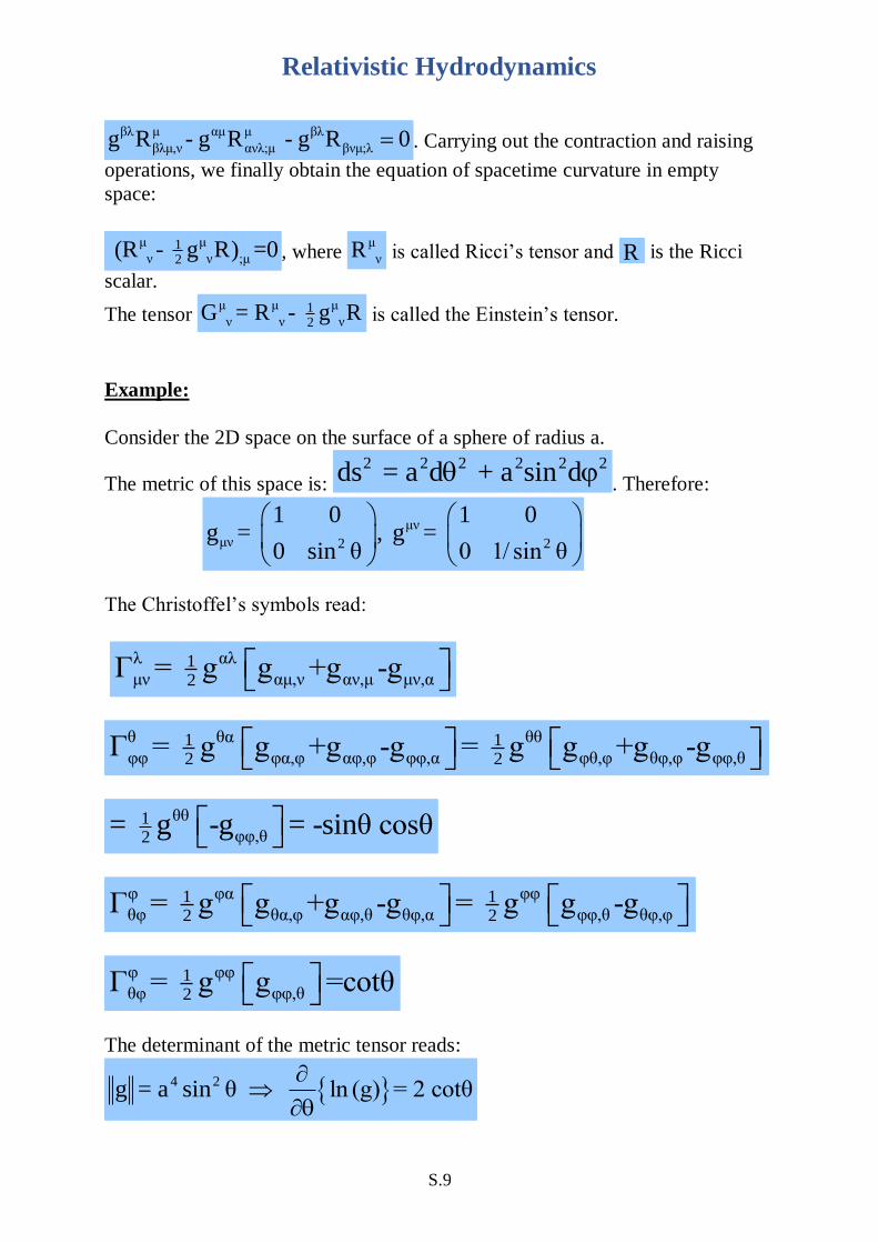
Example:
Consider the 2D space on the surface of a sphere of radius a.
The metric of this space is: 2 2 2 2 2 2ds = a d + a sin d
. Therefore:
μν
μν 2 2
1 0 1 0g = , g =
0 sin θ 0 1/ sin θ
The Christoffel’s symbols read:
λ αλ1μν αμ,ν αν,μ μν,α2
Γ = g g +g -g
θ θα θθ1 1φφ φα,φ αφ,φ φφ,α φθ,φ θφ,φ φφ,θ2 2
Γ = g g +g -g = g g +g -g
θθ1φφ,θ2
= g -g = -sinθ cosθ
φ φα φφ1 1θφ θα,φ αφ,θ θφ,α φφ,θ θφ,φ2 2
Γ = g g +g -g = g g -g
φ φφ1θφ φφ,θ2
Γ = g g =cotθ
The determinant of the metric tensor reads:
4 2g = a sin θ ln (g) = 2 cotθ

Relativistic Hydrodynamics
S.10
Thus, the θθ- component of the RCT is:
λ ρ θ θ1θθ ρθ θλ θθ,0 θθ ,θ2
R = Γ Γ - Γ - cotθΓ + cot θ
Summing over λ and ρ , we obtain then:
φ 0 2
θθ 0θ θφ ,θ 2
1R = Γ Γ - cot θ = cot θ - = -1
sin θ
and 2
φφR = -sin θ.
Therefore, the curvature invariant, R, is then:
θθ φφ 2
θθ φφR= g R + g R = -2/a
The curvature of a sphere decreases with increasing its radius.
Some useful connections:
1. The covariant derivative of a contravariant vector Vμ is composed of two
contributions: the change of the vector along a certain coordinate and its
change through parallel translation.
Mathematically, this reads:
: , ,V V V
where the semicolon refers to covariant differentiation and the comma to
ordinary partial differentiation.
On the other hand, the covariant derivative of a covariant vector V𝛍 reads:
: , .V V V
2. The covariant derivative of tensors of rank-2 reads:
HWQ: In the case of a scalar function, ; , . Explain why?
Γ has nothing to do with if a scalar or
a vector is to be Differentiated. Γ is a
property of the manifold. In the case of a scalar, the last term disappear all together, but not
because Γ=0, but because Vλ is zero.

Relativistic Hydrodynamics
S.11
: ,
If it is symmetric 1( )
T T T T
gT Tg
Whereas the covariant derivative of tensors of higher ranks:
: ,T T T T T T
The equation of the geodesic lines:
Assume we are given two events A and B on a surface S of a sphere.
The events correspond to the motion of a particle between the starting point A
and where the final point B located.
The motion of the particle is assumed to be field-free.
Therefore, we expect the particle to move along a
trajectory, that corresponds to the shortest distance
between the events A and B.
This choice of path has been experimentally observed,
and therefore, we may retain this hypothesis as a
principle for the future considerations.
Mathematically, such trajectories must fulfill the minimum variation principle:
ds= 0
A world-line satisfying this extremal condition is called a geodesic.
As a consequence, particles in free-fall through curved spacetime will also move
along the shortest possible length between events measured by the proper time.
In the absence of external forces, the Hamiltonian principle
states that the integral of the Lagrangian function describing the motion of a
particle must have an extremal values between two instants, i.e.,
L(q,q,t)dt = K(q,q,t) - (q,t) dt , where K,
denote the kinetic and potential energies of the system.
Q: Prove its
correctness!

Relativistic Hydrodynamics
S.12
As this applies for any system at arbitrary time, this integral
can be expanded to yield the Euler-Lagrange equation, i.e.,
2 2
1 1
t t
t t
L L L LL(q,q,t)dt= q+ q dt - =0.
q q t q q
Taking into account that =0(force free motion) , and using
the Euler-Lagrange equation of the calculation of variation, we obtain the so
called geodesic equation:
2
1
t 2 μ ν σ2 μ1
νσ2 2
t
d x dx dxmx dt + Γ =0
ds ds ds
μ
νσThe Christoffel symbols Γ and the Euler equations:
Consider a general metric of the form:
2 μ ν
μνds = g dx dx
Using the minimal variation principle, it appears that
geodesic lines fulfill the Euler-Lagrange equation:
L L- =0,
t q q
, where
μ ν
μνL= g dx dx
This relation between the Lagrangian function and the metric tensor can be used
to compute the Christoffel’s symbols.
Example:
Let
2 2 2 2 2 2 2 2ds = (c -a t )dt -2at dtdx-dx -dy -dz
The corresponding Lagrangian reads:
2 2 2 2 2 2 2L= (c -a t )t -2at tx-x -y -z
A
A

Relativistic Hydrodynamics
S.13
2 2 2L= 2(c -a t )t -2atx
t
L= -2att -2x
x
2
2 2 2 2
L= 2(-a 2t)t -2atx
t t t
= -4a tt + 2(c -a t )t-2axt-2atx
2L= -2at -2att -2x
t x
Putting terms together, i.e.,:
L LI. - =0
t t t
2 2 2 2 2 (c -a t )t = a tt +atx
2L LII. = at + att + x =0
t x x
2
t=0 I II
x+ at =0

Relativistic Hydrodynamics
S.14
2t t
tt tt2
22 x x
tt tt2
t t tt=0 + =0 =0
s s s
x t tx+ at =0 + =0 = a
s s s
Gravitation & Fields
Events in inertial frames cannot be formulated by means of transformation of
coordinates in the (3+1)-spacetime.
There is no transformation that relates the coordinates of an inertial frame to that
of a space with α
βγδR 0
This is a consequence of the fact that: α
βγδ ,R =f( ) = f( (g ))
.
In inertial frames α α
βγ βγδ = 0 R =0
Therefore the transformation of a curvilinear tensor from inertial frame into
other space with curvature would have
the form:
α ρ σ τα μ
βγδ ρστμ β γ δ
x x x xR = R .
x x x x
But if α α
βγδ βγδR =0 R =0 .
Gravitational fields, which are assumed to curve spacetime, are generically non-
symmetric. Therefore, it is almost impossible to get the curvature by means of
just coordinate transformation.
Example:
Let us assume that weak gravitational fields can be considered as small radial
perturbation in flat spacetime. Assuming spherical symmetry, the perturbed
metric reads:

Relativistic Hydrodynamics
S.15
2
00
11
μν 2
22
2 2
33
(1+f )c
-(1+f )g =
-(1+f )r
-(1+f )r sin
where μν μν μνf 1, f =f (r).
The geodesic equation of a particle in this field reads:
2 ν σr
νσ2
d r dx dx+ Γ =0
ds ds ds
The corresponding Lagrangian equation is:
r 2 r 2 r r 2
tt rr rθ φφr+ Γ t +Γ r + Γ rθ + + Γ φ =0
Since we consider just radial variations (θ=φ=0) , we end up with the equation:
r 2 r r 2
rr rt ttr+Γ r + 2Γ rt + + Γ t =0
The Christoffel symbols to be computed in this equation are:
r αr1rr rα,r rr,α2
Γ = g 2g -g
r αr1rt rα,t tα,r rt,α2
Γ = g g +g -g
r αr1tt tα,t tt,α2
Γ = g 2g -g
The metric tensor has no off-diagonal components and is assumed to be
independent of time. Therefore when the summations over α are carried out,
the expressions for the Christoffel symbols reduce to:
r rr1rr rr,r2
Γ = g g
r
rtΓ = 0
r rr1tt tt,r2
Γ = - g g
The contravariant metric tensor of μνg is:
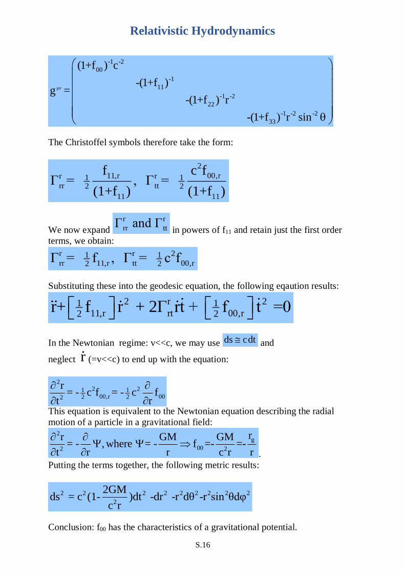
Relativistic Hydrodynamics
S.16
μν
-1 -2
00
-1
11
-1 -2
22
-1 -2 -2
33
(1+f ) c
-(1+f )g =
-(1+f ) r
-(1+f ) r sin
The Christoffel symbols therefore take the form:
2
11,r 00,rr r1 1rr tt2 2
11 11
f c fΓ = , Γ =
(1+f ) (1+f )
We now expand
r r
rr ttΓ and Γ in powers of f11 and retain just the first order
terms, we obtain:
r r 21 1rr 11,r tt 00,r2 2
Γ = f , Γ = c f
Substituting these into the geodesic equation, the following eqaution results:
2 r 21 111,r rt 00,r2 2
r+ f r + 2Γ rt + f t =0
In the Newtonian regime: v<<c, we may use ds cdt and
neglect r (=v<<c) to end up with the equation:
2
2 21 100,r 002 22
r= - c f = - c f
t r
This equation is equivalent to the Newtonian equation describing the radial
motion of a particle in a gravitational field: 2
g
002 2
rr GM GM= - , where = - f =- =-
t r r c r r
.
Putting the terms together, the following metric results:
2 2 2 2 2 2 2 2 2
2
2GMds = c (1- )dt -dr -r dθ -r sin θdφ
c r
Conclusion: f00 has the characteristics of a gravitational potential.

Relativistic Hydrodynamics
S.17
In general a perturbed Lorentz metric has the form:
μν μν μνg = g (Lorentz)+ (perturbation), where the latter term has the
characteristics of a gravitational potential.
The metric tensor equations in an empty space:
In Newtonian theory the gravitational potential satisfies the one of the following
equations:
= 0 in an empty space
= -4 G in gaseous clouds
.
The metric tensor of an Euclidian space is: μν μνg =
Here, we need to solve just a single equation to determine
In a curved spacetime, however, μνg may have 10 non-zero components, which
implies that 10 equations should be solved to determine .
Taking into account that α
βγδ ,λR =f( , ) , the requirement that λ
μνσR =0
can be fulfilled by only a flat spacetime.
However, a zero-contracted RCT, i.e., λ
μν μνλR = R =0 , which has 10
independent components, would certainly allow a much bigger degree of
freedom.
In the weak field approximation, μνR = 0 should lead to the Laplace’s
equation to determine the gravitational potential.
In rectangular coordinates, the metric may have the following form: 2 2 2 2
00ds = (1+f )c dt -d .
Now, as λ λα1μν μα,ν να,μ μν,α2
Γ = g g +g -g λ
μν 00, 00f f
Therefore,
00f <<12
, , 00 00 00 00R - + f -f + f f

Relativistic Hydrodynamics
S.18
, ,R - + =0
Noting that 2 2
00 00ln (-g)= ln c + ln(1+f )= ln c + f , we obtain that:
λσ1 1αβ ασ,β βσ,α αβ,σ 00,α,β2 2,λ
R =- g (g +g -g ) + f
This implies that:
λσ1 100 0σ,0 00, 00,0,02 2,λ
R =- g (g -g ) + f
But as =0t
, we obtain:
ij 11 22 331 100 00,j 00,1 00,2 00,32 2,i ,1 ,2 ,3
2
100,x,x 00,y,y 00,z,z 002
R =- g g = g g + g g + g g
c = - g +g +g = - f
2
Conclusion: In the weak field approximation, it is easy to verify that μνR = 0
actually correspond to the Laplace’s equation =0 in the Newtonian
regime.
The metric tensor equations in the presence of matter:
In presence of matter the gravitational potential in Newtonian theory satisfies
the Poisson equation:
= -4 G
In general relativity, the LHS is described by the Einstein tensor, μνG . In an
analogous manner, we may assume that the RHS to be described by matter-
tensor μνT . Hence the general equation to be solved is:
μν μνG = A T ,
(spatial operator).(potential)= matter

Relativistic Hydrodynamics
S.19
where A is a constant to be determined, and where μνT is said to have a
covariant derivative.
In an empty space, we have: 1
μν μν μν2G =0 R - g R=0
Note that if μνR =0 then its contraction R=0. This implies that
μν μνG =0 R =0 .
If the system has a non-zero density/energy 0 0 , then we may assume the
matter tensor to have the form: μν 0
dx dxT =
ds ds
, where ds is an element of
the worldline of the particle. dx
ds
has the character of a relative velocity
dx 1 dx v=
ds c dt c
. Thus, 00 0 0
2 2
dt dtT = =
c dt dt c
In order to find A, we multiply the general equation with μνg :
μσ μσ μσ1μν μν μν2
σ σ σ1ν ν ν2
g R - g g R= A g T
R - δ R= AT
Setting σ=ν and contract: 42
R - R= AT R = -AT , where λ
λT= T .
Substituting these back into the general equation, we obtain: 1
μν μν μν2R = A(T - g T) .
If T corresponds to a stationary dust cloud, then the only non-vanishing
component of this matter tensor is: 00 0
2
ρT =
c.
In this case,
2
00 00
cR =- f
2 ,
00 2 000 02
T =g T =c =c
and
2 00 2 2 2000 00 02
T =(g ) T =(c ) = cc
Therefore, the equation 1
00 00 002R = A(T - g T) is equivalent to

Relativistic Hydrodynamics
S.20
22 2 21
00 0 0 0 00 02
c A- f = A( c - c ) = c f = - A
2 2 .
Comparing this equation with the normal Poisson equation, it is easy to verify
that if GM
= -r
, then 00 2
2f = -
c
and therefore 2
8 GA= -
c
.
Consequently, in the presence of matter the metric equation
that describes the interaction of spacetime and matter is the
famous Einstein’s equation:
μν μν μν12 2
8 GR - g R= - T
c
, where
μνT
is the so called the energy-momentum tensor.
The Energy-Momentum Tensor μνT :
To describe the matter distribution at each point on a manifold or equivalently at
each event in spacetime, we need a tensor with special properties.
Due to the equivalence of matter and energy in special relativity, we may
intuitively assign for the matter-energy distribution at each event in spacetime the following tensor function:
0( ) ( ) ( ) ( )
energy-momentum tensor.
x x V x V x
v v
T
T
To see Tμν in a matrix form, consider the metric tensor of a Lorentz frame:
2 22 2 2 2 2 2 2 2 2 2
2
d V c dtds = c dt -d = c dt (1-( ) )=c dt (1-( ) )= ,
dt c
i.e.,
2 22
2
c dtds =

Relativistic Hydrodynamics
S.21
Now, using
μ ν μ νμν 2 2 μ ν μ ν0
0 0 2 2
dx dx dx dx dt ρT = = ( ) = x x = x x ,
ds ds dt dt ds c c
x y z
22x x x y x zμν
222y y x y y z
22z z x z y z
1 V V V1 x y z
V V V V V Vx x xy zxT = =
V V V V V Vy yx y zyc
V V V V V Vz zx yz z
The appearance of 2γ as coefficient in the stress energy tensor marks two
important effects of special relativity:
1. The volume of a moving matter shrinks by a factor γ as measured in
the observer frame.
2. The mass of a particle moving with a velocity V increases by a factor
γ .
Using the 4-velocity formulation:
00 0 0 2 2
0
0 0 0 2
0
2
0
( , ), then the components of T :
T = energy density of matter
T T energy flux in the j-direction
T material flux of the i-component of t
j j j j
ij i j i j
v c v read
v v c
v v cv
v v v v
he
momentum in the j-direction.

Relativistic Hydrodynamics
S.22
The conservative form of the hydro-equations in the non-relativistic regime
can be obtained from general relativity through the requirement that μνT
must have a vanishing covariant derivative, i.e., μν
;νT =0 .
Recalling that σ
μν =0 in Lorentz frames, we conclude that:
μνμν μν
;ν ,ν ν
TT = T = =0.
x
These expressions can then be expanded to yield the following equalities:
00 01 02 032 0ν 2
;ν 0 1 2 3
T T T Tc T =c + + + =0
x x x x
In this frame:
200 0 2 2
T = =c c
,
y01 02 01x z 2 2 2
VV VT = , T = ,T =
c c c
Putting the terms together, we obtain:
y2 0ν x z ;ν
VV Vc T = + + + = + V=0.
t x y z t
This equation is identical to the equation of mass conservation in normal fluid
dynamics.
The momentum equation is obtained by expanding the expression 2 1ν
;νc T =0
as follows: 10 11 12 13
2 1ν 2
;ν 0 1 2 3
1 1 1 1 2 1 3 xx0 1 2 3
T T T Tc T =c + + + =0
x x x x
V V V V V V V V + + + =0 + ( V V)=0,
x x x x t
where x y zV=(V ,V ,V ) is the 3-velocity vector of the flow.
However, the momentum equations in this form are said to describe the time-
evolution of non-interacting matter.
But why the modified differential operator: 1
( )gg
does not appear?

Relativistic Hydrodynamics
S.23
If the matter is interacting, but still non-dissipative, then the stress-energy tensor
must have the form: μ ν
μν μν
0 2 2
p dx dx pT = ( + ) - g
c ds ds c , where p is the pressure as measured in the
proper frame of the moving fluid and μνg corresponds to the contravariant
metric tensor.
If the flow is interacting and dissipative, then the stress energy tensor must be
modified to include the “highly complicated” viscous interaction tensor, Σμν and
heat conduction tensor Πμν:
μ νμν μν μν μν μ ν ν μ
0 2 2
p dx dx pT = ( + ) - g + af -2 + q u +q u .
c ds ds c
Related Documents