Relative density estimation and local bandwidth selection for censored data

Computational Statistics & Data Analysis 36 (2001) 497–510www.elsevier.com/locate/csda

Relative density estimation and localbandwidth selection for censored data

Ricardo Caoa ;∗, Paul Janssenb, No-el Veraverbekeb

aDepartamento de Matem�aticas, Facultade de Inform�atica, Universidade da Coruna,A Coruna 15071, Spain

bLimburgs Universitair Centrum, Universitaire Campus, B-3590, Belgium

Received 1 July 1999; accepted 1 June 2000

Abstract

This paper is concerned with local bandwidth selection for a kernel-type estimator of the relativedensity (or grade density) when the samples come from two populations under a right random cen-sorship mechanism. A two-stage smoothed plug-in local bandwidth selector with a beta reference isproposed. This estimation procedure is used to analyze the lifetime density in a two-sample problemrelated to breast cancer. A simulation study is carried out to examine the practical performance of thebandwidth selector. c© 2001 Elsevier Science B.V. All rights reserved.

Keywords: Grade density; Kaplan–Meier estimator; Kernel estimator; Plug-in bandwidth

1. Introduction

In the analysis of biomedical data the general two-sample problem of comparingthe cumulative distribution functions, F0 and F , of two random variables, Y0 and Y ,often arises. A possible tool for making such a comparison is the relative distributionfunction of Y with respect to Y0:

R(t)=P(F0(Y ) ≤ t)=F(F−10 (t)); 0¡t¡ 1; (1)

where L−1(t)= inf{x |L(x) ≥ t} denotes the quantile function of a general cumula-tive distribution function L. The function R is the cumulative distribution functionof F0(Y ) and has been used in ?elds like signal detection, in the evaluation ofdiagnostic tests or in statistical quality control under the name of receiver operating

∗ Corresponding author.

0167-9473/01/$ - see front matter c© 2001 Elsevier Science B.V. All rights reserved.PII: S 0167-9473(00)00055-4

498 R. Cao et al. / Computational Statistics & Data Analysis 36 (2001) 497–510

characteristic (ROC) curve (see Li et al., 1996). Denoting by TL = inf{x |L(x)= 1},it is easy to see that if TF0 ¡TF; R(t) has a jump of size 1− F(TF0) at t=1.

When the random variable F0(Y ) is absolutely continuous (or, at least, when ithas an absolutely continuous part) the relative density (or subdensity) can be de?ned

r(t)=R′(t)=f(F−1

0 (t))f0(F−1

0 (t)); 0¡t¡F0(TF);

where f and f0 are the densities pertaining to F and F0, respectively. Note thatwhen F and F0 are identical, r is the uniform density on (0; 1). An early referencein which the concept of relative distribution and relative density are used is Bell andDoksum (1966).

If we are given two independent random samples of i.i.d. observations Y1; Y2; : : : ; Ymand Y01; Y02; : : : ; Y0n, the relative distribution can be estimated by using in (1) theempirical distribution functions

Rm;n(t)=Fm(F−10n (t)); 0¡t¡ 1: (2)

This estimator has been studied by Gastwirth (1968), Hsieh and Turnbull (1996),GCwik and Mielniczuk (1993), Hsieh (1995) and Handcock and Morris (1999). GCwikand Mielniczuk (1993) also propose a kernel-type estimator for the relative density.

When the two samples are censored, Gastwirth and Wang (1988) give an asymp-totic normality result for the estimator similar to (2) but replacing the empirical dis-tribution functions with the Kaplan–Meier estimators (see Kaplan and Meier, 1958).Finally, also in the censored data case, Cao et al. (2000) present a kernel estimatorfor the relative density and ?nd its limit distribution.

In the rest of the paper we will focus on relative density estimation in the contextof random right censorship. In Section 2, some notation and technical background isintroduced and an algorithm for local bandwidth selection is presented. A medicalapplication to compare the lifetime for two groups of patients with adjuvant breastcancer is presented in Section 3. In Section 4 a simulation study is carried outto analyze the behavior of the local bandwidth selector. Some discussion and ?nalremarks are included in Section 5.

2. Statistical methods

2.1. Relative distribution and density estimation with censored data

Let us consider two random samples of right censored data

(X1; �1); : : : ; (Xm; �m) and (X01; �01); : : : ; (X0n; �0n);

where, Xi=min(Yi; Ci); �i=I(Yi ≤Ci) for i=1; : : : ; m and X0j=min(Y0j; C0j) and �0j =I(Y0j≤C0j) for j=1; : : : ; n. Our interest is in random variables Yi whose values maybe censored by the variables Ci. The Yi are i.i.d. with continuous distribution functionF and they are independent of the Ci, which are i.i.d. with continuous distributionfunction G. Similarly, in the second sample, the common continuous distributionfunction of the Y0j is F0, while the C0j are i.i.d. with continuous distribution function

R. Cao et al. / Computational Statistics & Data Analysis 36 (2001) 497–510 499

G0. Again Y0j and C0j are independent. We denote by H the distribution function ofXi and by H0 that of X0i. Due to the independence, we have 1−H =(1−F)(1−G)and 1− H0 = (1− F0)(1− G0).

Gastwirth and Wang (1988) proposed an obvious estimator for R(t) in this setup,given by

R(t)= Fm(F−10n (t)); (3)

where Fm is the Kaplan–Meier estimator for F , given by

1− Fm(t)=

1 if t ¡X(1);m∏i=1

X(i)≤t

(m− i

m− i + 1

)�(i)if t ≥ X(1)

and F0n is the Kaplan–Meier estimator for F0. These authors obtained the limitdistribution of R(t) whenever f0 is continuous and strictly positive at F−1

0 (t) and ifH (F−1

0 (t))¡ 1. Provided that m and n tend to in?nity, in such a way that, for someconstant 0¡�2¡∞; limm→∞m=n= �2, they prove that

m1=2(R(t)− R(t)) d→N(0; �2(F−10 (t)) + �2�20(F

−10 (t))r2(t)):

Here

�2(s)= (1− F(s))2∫ s

0

dF(y)(1− F(y))2(1− G(y))

and

�20(s)= (1− F0(s))2∫ s

0

dF0(y)(1− F0(y))2(1− G0(y))

:

Note that the asymptotic variance also involves the relative density r(t). The assump-tion H (F−1

0 (t))¡ 1 is classical in the right random censoring setup. It controls theamount of censoring in the F population at F−1

0 (t), needed to consistently estimateR(t).

In this context, Cao et al. (2000) proposed a kernel estimator for the relativedensity starting from the observation that r(t) is the (sub)density function of F0(Y ).If F0 were known, we could use a usual kernel density estimator (see, e.g., Lo etal., 1989) based on a censored sample of the “pseudovalues”

(F0(X1); �1); : : : ; (F0(Xm); �m):

Observe that this is indeed a censored sample, since F0(Xi)=min(F0(Yi); F0(Ci))and �i = I(Yi ≤ Ci)= I(F0(Yi) ≤ F0(Ci)).

Actually F0 is unknown and it has to be estimated by the Kaplan–Meier estimatorF0n. Hence, the estimator for r(t) proposed by Cao et al. (2000) is

rh(t)=1h

∫K(t − yh

)dR(y);

where the function K is a known probability density function and h= hm is a non-negative bandwidth sequence. In order to avoid the border eMect of the estimator att=0, the following simple boundary correction may be performed. Given the kernel


estimator, rh(t), we de?ne a boundary corrected version, rBCh (t), as follows: for all

t in a small neighborhood of zero, de?ne rBCh (t)= rh(t) + rh(−t), for every t ≥ 0 in

that neighborhood and rBCh (t)= 0 for t ¡ 0. Similar corrections may be done with

derivatives of rh(t).By using the Kaplan–Meier weights, an alternative expression for this estimator is

1h

m∑i=1

K

(t − F0i(Xi)

h

)(R(F0i(Xi))− R

−(F0i(Xi))); (4)

where R−

denotes the left limit of R. This expression uses the fact that the Gastwirthand Wang estimator in (3), R, coincides with the Kaplan–Meier estimator constructedfrom (F0n(X1); �1); : : : ; (F0n(Xm); �m).

Under certain regularity conditions on r and K and assuming H (F−10 (t))¡ 1, Cao

et al. (2000) showed that the bias and variance of the estimator in (4) are given by

E(rh(t))− r(t)= 12r

′′(t)dKh2 + o(h2) + o((mh)−1=2)

Var(rh(t))=#2(t)cKmh

+ o((mh)−1);

where

#2(t)=r(t)

1− G(F−10 (t))

+ �2 r2(t)1− G0(F−1

0 (t)); (5)

cK =∫K2(u) du and dK =

∫u2K(u) du. Under those assumptions they also obtained

the asymptotic normality of (mh)1=2(rh(t)− r(t)).

2.2. Local bandwidth selection

Using the asymptotic expressions for the bias and the variance, given above, andassuming that r(t) = 0 and r′′(t) = 0, it is easy to compute an asymptotic represen-tation for the mean-squared error:

MSE(h)=AMSE(h) + o(h4) + o((mh)−1);

where

AMSE(h)=14r′′(t)2d2

Kh4 +

#2(t)cKmh

:

The optimal bandwidth, hAMSE (minimizing AMSE(h)) takes the form hm =C(t)m−1=5

with

C(t)=

(#2(t)cKr′′(t)2d2

K

)1=5

: (6)

By examining expressions (5) and (6), it is clear that the relative density, r, andits second derivative have to be estimated in order to give a practical implementa-tion of the asymptotic optimal bandwidth hAMSE. The estimation of G(F−1

0 (t)) andG0(F−1

0 (t)) is also needed. The Kaplan–Meier estimators can be used to ?nd sam-ple versions of these two quantities, while the problem of estimating r′′(t) can be


treated by using a nonparametric kernel estimator with pilot bandwidth g. Generallyspeaking, g is just a preliminary bandwidth used to estimate some quantity that willbe used to select the ?nal bandwidth [see the book by Wand and Jones (1995) for anice review on pilot estimation in bandwidth selection for kernel density estimationin the uncensored case].

The second derivative of such an estimator, r′′g , will be used to estimate r′′.The same kind of techniques used in Cao et al. (2000) to compute the bias andthe variance of rh(t), can be employed to obtain an asymptotic expression for themean-squared error of r′′g (t) that resembles the corresponding formula for the uncen-sored one-sample case (see, for instance, Wand and Jones, 1995, Eq. (2:34), p. 49).Assume that r is bounded and four times continuously diMerentiable at t ¡F0(TF)with r(t) = 0 and r(4)(t) = 0, K is a symmetric density function with support[ − 1; 1], twice continuously diMerentiable and suppose that the pilot bandwidth gsatis?es g → 0 and mg3=(log logm)2 → ∞. Then, it holds

E[(r′′g (t)− r′′(t))2]=14r(4)(t)2d2

Kg4 +

#2(t)cK′′

mg5+ o(g4) + o(m−1g−5);

with cK′′ =∫K ′′(u)2 du. Taking all this into account, an asymptotic theoretical ex-

pression for the optimal value of the pilot bandwidth is

g0 =

(5#2(t)cK′′

r(4)(t)2d2Km

)1=9

: (7)

As shown in (7) the optimal pilot bandwidth depends on the fourth derivativeof the underlying relative density and, if we would keep going with this plug-inmechanism estimating the fourth derivative we would ?nd a prepilot bandwidth de-pending on the sixth derivative and so on. This yields to a never-ending process.A reasonable possibility is to stop the whole procedure at a given step by using aparametric reference, as already used by Silverman (1986). It is presented in moredetails (in the uncensored context for density estimation) in the books by Wand andJones (1995) and SimonoM (1996). This is precisely what we propose here for thesecond step by ?tting our data to a rescaled Beta distribution

r0(t;p; q; c)=

,(p+ q)c,(p),(q)

(tc

)p−1 (1− t

c

)q−1

if 0 ≤ t ≤ c;

0 if t ∈ [0; c]:(8)

In practice, the term r(t) appearing in #2(t) and r(4)(t) – both in (7) – are estimatedwith this Beta reference, using the relative data (F0n(X1); �1); : : : ; (F0n(Xm); �m). Thepilot bandwidth g0 is computed by substituting the estimators found for r(4)(t) and#2(t) in (7). Finally, the second derivative is estimated by means of the kernelestimator r′′g0 (t) and used (together with the estimated #2(t)) in (6) to end up withan empirical version of hAMSE.


2.3. The two-stage plug-in algorithm

One of the steps in the procedure sketched above to select the local bandwidthconsists of estimating the three parameters of the rescaled Beta distribution by meansof the relative data (D1; �1); : : : ; (Dm; �m), where Di = F0n(Xi); i=1; 2; : : : ; m. In thecase where the sample consists of uncensored observations D1; : : : ; Dm the maximumlikelihood estimator of c is

c= R−1

(1)=D(m): (9)

The principle of maximum likelihood estimation does not lead to unique estimatorsfor p and q and it would need some modi?cation in order to penalize the dominatingeMect that D(m) has in the likelihood function. The censored data case is even morecomplicated and has similar drawbacks. Since we only need some estimated valuesfor c; p and q to give a reasonable approximation of r(t), we decided to use c=D(m)

(the largest relative datum) and moment estimators for p and q.Under model (8) the ?rst and second noncentral moments are given by

.1 =p

p+ qc;

.2 =p(p+ 1)

(p+ q)(p+ q+ 1)c2:

Now, c is estimated by (9) (since the estimator is very simple) and the underlying?rst two moments are estimated by their empirical analogues,

.1 =m∑i=1

Di(R(Di)− R−(Di));

.2 =m∑i=1

D2i (R(Di)− R

−(Di)):

Although these estimators are biased (see Stute, 1994), they can be truncated toestimate consistently the truncated moments. In practice, due to the good perfor-mance of these moment estimators and the fact that the truncation approach leadsto very complicated formulas for the truncated versions of .1 and .2, we adopt theuntruncated estimators. Finally, the moment estimators for p and q can be computedeasily:

p=(.1 − .2=c).1

.2 − .21

;

q=(.1 − .2=c)(c − .1)

.2 − .21

: (10)

For a given t, such that H (F−10 (t))¡ 1 all the ideas presented above lead to the

following local bandwidth selection algorithm:

1. Compute the Kalpan–Meier estimator and ?nd the relative data(D1; �1); : : : ; (Dm; �m), where Di = F0n(Xi); i=1; 2; : : : ; m:


2. Using the censored sample of relative data compute the estimators c; p andq given in (9) and (10). These estimators are used for computing r0(·; p; q; c);r′′0 (·; p; q; c) and r(4)0 (·; p; q; c) at the given value t.

3. Obtain the pilot bandwidths

g0 =

(5#2

par(t)cK′′

r(4)0 (t; p; q; c)2d2Km

)1=9

and

g1 =

(#2par(t)cK

r′′0 (t; p; q; c)2d2Km

)1=5

;

where

#2par(t)=

r0(t; p; q; c)

1− G(F−10 (t))

+mn

r0(t; p; q; c)2

1− G0(F−10 (t))

and G; F0, and G0 are the Kaplan–Meier estimators of G; F0 and G0.4. Using

#2np(t)=

rg1 (t)

1− G(F−10 (t))

+mn

rg1 (t)2

1− G0(F−10 (t))

and the kernel estimator of the second derivative of the relative density withbandwidth g0,

r′′g0 (t)=1

g30

m∑i=1

K ′′(t − F0i(Xi)

g0

)(R(F0i(Xi))− R

−(F0i(Xi)));

compute

C(t)=

(#2np(t)cK

r′′g0 (t)2d2

K

)1=5

;

an estimator of the value C(t) de?ned in (6), and ?nally obtain hAMSE = C(t)m−1=5.The bandwidth obtained in this manner is not stable since it exhibits some high

peaks at several points [see Fig. 1 and the papers by M-uller and Stadtm-uller (1987)and Brockmann et al. (1993) on local bandwidth selection for kernel regressionestimators; see also the discussion in Section 3]. To remedy this, we modify ourprocedure by smoothing the denominator of hAMSE = hAMSE(t) in t. This is done bymeans of the convolution

rSg0′′(t)2 =

1b

∫K(u− tb

)r′′g0 (u)

2 du

or even better by

rSg0′′(t)2 =

1=b∫K((u− t)=b)r′′g0 (u)

2 du

1=b∫ c0 K((u− t)=b) du

;

since the local bandwidth is only computed at points t within the interval [0; c]. Theconstant b is a smoothing parameter that controls the amount of smoothing we useto get rid oM the Quctuation of the local bandwidth selection procedure.


Fig. 1. On the left vertical scale: kernel estimator of the relative density of ER− with respect to ER+lifetimes with unsmoothed (medium thickness line) and smoothed (thick line) local plug-in for thebreast cancer data analysed in Section 3. On the right vertical scale: their pertaining local bandwidths.

In practice the local bandwidth will be computed only at the values of a grid:t1; t2; : : : ; tM and hence the vector of smoothed local plug-in bandwidth selectors atthese points will be ?nally taken as

hS

AMSE(ti)=

(#2(ti)cK

rSg0′′(ti)2d2

Km

)1=5

with

rSg0′′(ti)2 =

∑Mj=1 K((tj − ti)=b)r

′′g0(tj)2∑M

j=1 K((tj − ti)=b); i=1; 2; : : : ; M:

Since the smoothing is needed here only to eliminate the high peaks of the localplug-in bandwidth only small values for b are advisable.

3. Application to the breast cancer data

In this section, we apply the two-stage local bandwidth selector presented aboveto estimate the relative density for a real data set concerned with breast cancer.

The data set corresponds to several studies (carried out by ECOG, the EasternCooperative Oncology Group) in which women with adjuvant breast cancer weretreated with various regimens (see Gray, 1992). The data set has a binary variablefor grouping: the estrogen receptor (ER) status, positive (+) or negative (−). Thereare 446 failure times and 410 censored in ER− group and 670 failures and 878censored in the ER+ group. In our case, the interest variable is the lifetime of thepatient (subject to right censoring). It roughly ranges between 0 and 12.5 years forevery group.

Using a Gaussian kernel, we have computed the relative density estimator, pre-sented in Section 2, for the lifetime of ER− patients with respect to the lifetime in


the ER+ group. This function may be helpful to regard the ER status as a prog-nostic indicator for breast cancer. To compute the estimator, we used as smoothingparameter the two-stage plug-in bandwidth selector and its smoothed version, pre-sented in the previous section. These two local bandwidths were computed in a gridof 200 equispaced points within the interval [0; 1]. We used a uniform kernel withbandwidth equal 0.025 to smooth the two-stage local pilot bandwidth and ?nallyobtained its smoothed version. The boundary eMect of the estimator was addressedby means of the boundary correction, rBC

h (t), presented in Section 2, with the choice(−0:1; 0:1) for the neighborhood of t=0.

The unsmoothed and smoothed local bandwidths and the resulting estimators arepresented in Fig. 1. It is remarkable how the local plug-in selector has very highpeaks at the points where the estimation of the second derivative of the relativedensity is close to zero. The practical eMect of these oversmoothed bandwidths is thatthe kernel estimator suddenly decreases around each of these points. The same ?gureshows how this feature disappears when performing the smoothed local bandwidth.

The estimated relative density of the ER− lifetime with respect to ER+ lifetime,shown in Fig. 1, deviates much from the baseline r(t) ≡ 1. It ?rst exhibits a very fastdecreasing tendency, within the interval [0:02; 0:12], and then a lower slope decreas-ing part, that roughly corresponds to the quantiles within the interval [0:15; 0:55].This is a visual way of analyzing the data that leads to the conclusion that the life-time of ER− patients tends to be smaller than that of ER+ patients. In other termsthe density function of ER− lifetimes is quite diMerent from the density of ER+lifetimes, since the second one is somehow shifted to the right with respect to the?rst one. The curve in Fig. 1 shows how large this diMerence is in terms of the ER+distribution quantiles. As a consequence of this plot, we can conclude, for example,that it is over twice more probable to ?nd a lifetime of an individual in the ER−group within a small neighborhood of the 5th percentile of the lifetime distributionfor ER+, than ?nding a lifetime of an ER+ patient within the same neighborhood.

4. Simulations

As an illustrative way of regarding the practical behavior of the relative densitykernel estimator proposed in Section 2, we present a series of simulations that canbe used to compare the results of the estimator with the true relative density in eachcase.

Along the simulations, we have used the following distribution function:

Qa;c(x)=

0 if x¡ 0;(x=c)a if x ∈ [0; c];1 if x¿c

with density given by

qa;c(x)=axa−1

cafor x ∈ [0; c]:


For the ?rst two models, the random variables of interest (Y and Y0) and thecensoring times (C and C0) were chosen to have the following distribution functions:F0 =Qa0 ;c0 ; G0 =Qb0 ;d0 ; F =Qa;c; G=Qb;d.

We made choices of c and c0 satisfying c0 ≥ c because otherwise the relativedistribution, R, would give a positive probability mass at t=1 (in such a case, r(t)would be a subdensity function). Under our condition, the relative density is givenby

r(t)=aa0

(c0c

)ata=a0−1 for t ∈

[0;(cc0

)a0]:

In order to be able to observe the variable of interest along its whole range,the condition c ≤ d has to be imposed. In the opposite case (c¿d), it would beimpossible to have uncensored observations in the interval (d; c). Under the conditionc ≤ d, the local probability of uncensored observations can be computed easily:

p(y) =P(�=1 |Y =y)

=f(y)(1− G(y))

f(y)(1− G(y)) + g(y)(1− F(y))

=adbya − aya+b

adbya + bcayb − (a+ b)ya+bfor y ∈ [0; c]; (11)

where g, in the previous formula, is the density function pertaining to G. Furthermore,the unconditional probability of having an uncensored observation is found to be

p=P(�=1)=∫ c

0p(y)h(y) dy

=∫ c

0f(y)(1− G(y)) dy

=∫ c

0

acaya−1

[1−

(yd

)b]dy

=1− acb

(a+ b)db: (12)

Using expressions (11) and (12) (and the corresponding similar expressions forthe baseline population (Y0; �0)) one can choose the values a; b; c; d; a0; b0; c0 andd0 in order to control the local and global amount of censoring.

Taking all this into account we tried two models. The combinations of parametersused, as well as the probabilities of uncensoring for these models are summarizedin Table 1.

A third model was considered by still using the previous parametric family for Yand C, but switching the other two to be Y0 ∼ exp (2) and C0 ∼ exp (3). In thiscase the probability of uncensoring for the baseline population is trivially computed:

p=P(Y0 ≤ C0)=∫ ∞

0(1− G0(x))f0(x) dx=

∫ ∞

0e−3x2 e−2x dx=

22+ 3

:

The values of the parameters and the probabilities of uncensoring for the third modelare given in Table 2.


Table 1Parameters chosen for models 1 and 2

Model a b c d a0 b0 c0 d0 p p0

1 6 2 3 3.2 2 1.1 4 4.1 0.3408 0.37212 6 2 3 4 2 3 4 4.1 0.5781 0.6286

Table 2Parameters chosen for model 3

Model a b c d 2 3 p p0

3 0.5 1.2 3 3.2 3 2.4 0.7278 0.5556

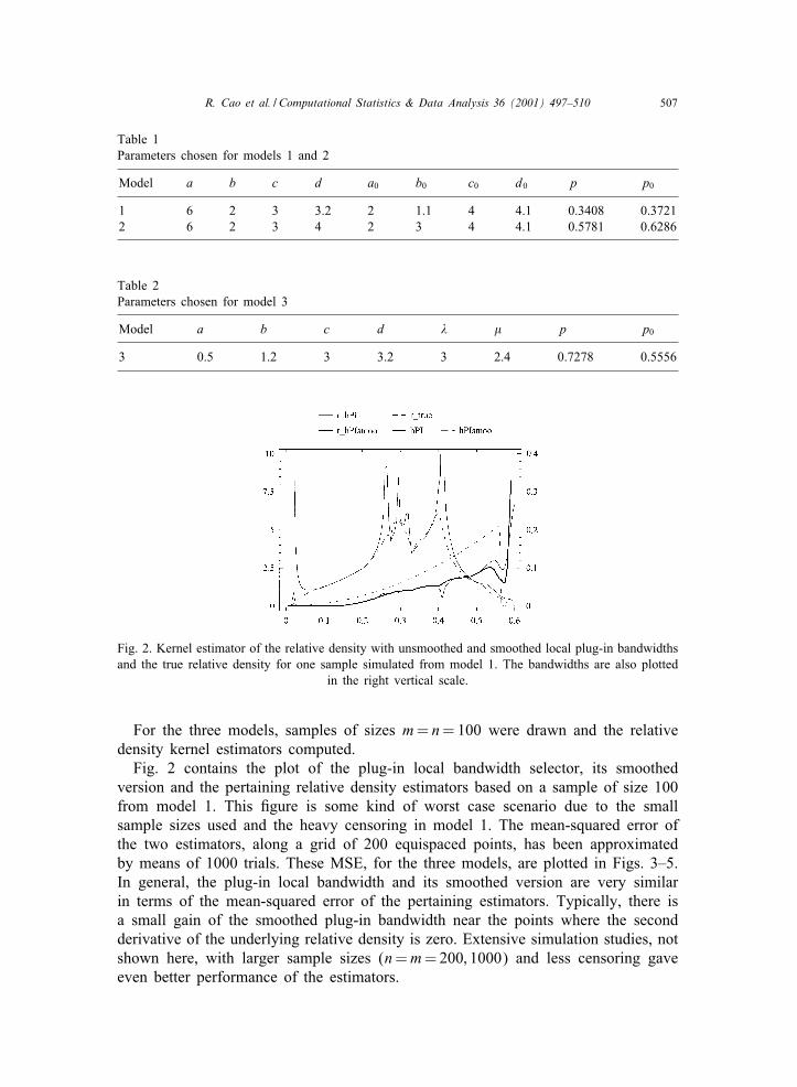
Fig. 2. Kernel estimator of the relative density with unsmoothed and smoothed local plug-in bandwidthsand the true relative density for one sample simulated from model 1. The bandwidths are also plotted

in the right vertical scale.

For the three models, samples of sizes m= n=100 were drawn and the relativedensity kernel estimators computed.

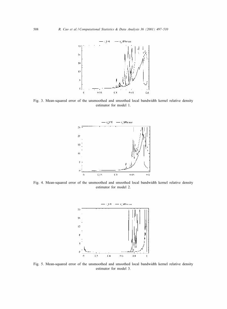
Fig. 2 contains the plot of the plug-in local bandwidth selector, its smoothedversion and the pertaining relative density estimators based on a sample of size 100from model 1. This ?gure is some kind of worst case scenario due to the smallsample sizes used and the heavy censoring in model 1. The mean-squared error ofthe two estimators, along a grid of 200 equispaced points, has been approximatedby means of 1000 trials. These MSE, for the three models, are plotted in Figs. 3–5.In general, the plug-in local bandwidth and its smoothed version are very similarin terms of the mean-squared error of the pertaining estimators. Typically, there isa small gain of the smoothed plug-in bandwidth near the points where the secondderivative of the underlying relative density is zero. Extensive simulation studies, notshown here, with larger sample sizes (n=m=200; 1000) and less censoring gaveeven better performance of the estimators.


Fig. 3. Mean-squared error of the unsmoothed and smoothed local bandwidth kernel relative densityestimator for model 1.




5. Final remarks

In a two-sample problem with censored data, one can apply smoothing techniquesto obtain a nonparametric kernel estimator of the relative density. This is a graphicalway of exploring a possible diMerence between the two underlying distributions. Oneof the important practical problems in this context is to ?nd an adequate selector ofthe smoothing parameter. In the spirit of local bandwidth selection, we have presenteda two-stage local plug-in bandwidth selector, as well as a smoothed version of it.The performance of these two is very similar in regions where the second derivativeof the underlying relative density is bounded away from zero. Near the zero secondderivative points, the smoothed local bandwidth produces a more stable and accurateestimator of the relative density. The application of this methodology to the breastcancer data presented in Section 3 shows that it is a Qexible graphical tool to examinethe diMerence between two populations.

One of the important steps in plug-in bandwidth selection is how to select a refer-ence parametric family from which to estimate some preliminary quantities to obtainthe pilot bandwidth. In this case, we used a Beta family because of its Qexibil-ity and the fact that the support of the relative density is contained in [0; 1]. Animportant open question is how much this choice aMects the ?nal properties of thelocal bandwidth selector. Some other aspect that deserves future research is to use asolve-the-equation rule (see Scott et al., 1977 or Scott and Factor, 1981) to modifythe two-stage plug-in selection rule presented in this paper.

Acknowledgements

The ?rst author’s research was sponsored by the Spanish DGICYT Grant PB94-0494, the DGES Grants PB95-0826 and PB98-0182-C02-01 and by the Xunta deGalicia Grant XUGA10501B97. The last two authors acknowledge partial support bythe Ministry of the Flemish Community (Project: BIL97=50, International Scienti?cand Technological Cooperation). Part of this research was carried out while the ?rstauthor visited the Center for Statistics, Limburgs Universitair Centrum, Belgium andalso while the second author visited the Department of Mathematics, Universidadeda Coruna, Spain. The authors greatly acknowledge constructive comments of twoanonymous referees.

References

Bell, C.B., Doksum, K.A., 1966. Optimal one-sample distribution-free tests and their two-sampleextensions. Ann. Math. Statist. 37, 120–132.

Brockmann, M., Gasser, T., Herrmann, E., 1993. Locally adaptive bandwidth choice for kernelregression estimators. J. Amer. Statist. Assoc. 88, 1302–1309.

Cao, R., Janssen, P., Veraverbeke, N., 2000. Relative density estimation with censored data. Can. J.Statist. 28, 97–111.

GCwik, J., Mielniczuk, J., 1993. Data-dependent bandwidth choice for a grade density kernel estimate.Statist. Probab. Lett. 16, 397–405.


Gastwirth, J.L., 1968. The ?rst-median test a two-sided version of the control median test. J. Amer.Statist. Assoc. 63, 692–706.

Gastwirth, J.L., Wang, J.-L., 1988. Control percentile test procedures for censored data. J. Statist.Planning Inf. 18, 267–276.

Gray, R.J., 1992. Flexible methods for analyzing survival data using splines, with applications to breastcancer prognosis. J. Amer. Statist. Assoc. 87, 942–951.

Handcock, M.S., Morris, M., 1999. Relative Distribution Methods in Social Sciences. Springer, NewYork.

Hsieh, F., 1995. The empirical process approach for semiparametric two-sample models withheterogeneous treatment eMect. J. Roy. Statist. Soc., Ser. B 57, 735–748.

Hsieh, F., Turnbull, B.W., 1996. Nonparametric and semiparametric estimation of the receiver operatingcharacteristic curve. Ann. Statist. 24, 25–40.

Kaplan, E.L., Meier, P., 1958. Nonparametric estimation from incomplete observations. J. Amer. Statist.Assoc. 53, 457–481.

Li, G., Tiwari, R.C., Wells, M.T., 1996. Quantile comparison functions in two-sample problems withapplications to comparisons of diagnostic markers. J. Amer. Statist. Assoc. 91, 689–698.

Lo, S.H., Mack, Y.P., Wang, J.-L., 1989. Density and hazard rate estimation for censored data viastrong representation of the Kaplan–Meier estimator. Probab. Theory Rel. Fields 80, 461–473.

M-uller, H.G., Stadtm-uller, U., 1987. Variable bandwidth kernel estimators of regression curves. Ann.Statist. 15, 182–201.

Scott, D.W., Factor, L.E., 1981. Monte Carlo study of three data-based nonparametric probabilitydensity estimators. J. Amer. Statist. Assoc. 76, 9–15.

Scott, D.W., Tapia, R.A., Thompson, J.R., 1977. Kernel density estimation revisited. Nonlinear Anal.Theory Meth. Appl. 1, 339–372.

Silverman, B.W., 1986. Density Estimation. Chapman and Hall, London.SimonoM, J.S., 1996. Smoothing Methods in Statistics. Springer, New York.Stute, W., 1994. The bias of Kaplan–Meier integrals. Scand. J. Statist. 21, 475–484.Wand, M.P., Jones, M.C., 1995. Kernel Smoothing. Chapman and Hall, London.

Relative density estimation and local bandwidth selection for censored data

Documents