Relationships Between Cloud Radiative Forcing and Local Meteorological Variables in Several Global Climate Models

Relationship between Shortwave Cloud Radiative Forcing and Local MeteorologicalVariables Compared in Observations and Several Global Climate Models

MARKUS STOWASSER AND KEVIN HAMILTON

International Pacific Research Center, University of Hawaii at Manoa, Honolulu, Hawaii

(Manuscript received 30 May 2005, in final form 27 December 2005)

ABSTRACT

The relations between local monthly mean shortwave cloud radiative forcing and aspects of the resolved-scale meteorological fields are investigated in hindcast simulations performed with 12 of the global coupledmodels included in the model intercomparison conducted as part of the preparation for IntergovernmentalPanel on Climate Change (IPCC) Fourth Assessment Report (AR4). In particular, the connection of thecloud forcing over tropical and subtropical ocean areas with resolved midtropospheric vertical velocity andwith lower-level relative humidity are investigated and compared among the models. The model results arealso compared with observational determinations of the same relationships using satellite data for the cloudforcing and global reanalysis products for the vertical velocity and humidity fields. In the analysis thegeographical variability in the long-term mean among all grid points and the interannual variability of themonthly mean at each grid point are considered separately. The shortwave cloud radiative feedback(SWCRF) plays a crucial role in determining the predicted response to large-scale climate forcing (such asfrom increased greenhouse gas concentrations), and it is thus important to test how the cloud representa-tions in current climate models respond to unforced variability.

Overall there is considerable variation among the results for the various models, and all models showsome substantial differences from the comparable observed results. The most notable deficiency is a weakrepresentation of the cloud radiative response to variations in vertical velocity in cases of strong ascendingor strong descending motions. While the models generally perform better in regimes with only modestupward or downward motions, even in these regimes there is considerable variation among the models inthe dependence of SWCRF on vertical velocity. The largest differences between models and observationswhen SWCRF values are stratified by relative humidity are found in either very moist or very dry regimes.Thus, the largest errors in the model simulations of cloud forcing are prone to be in the western Pacificwarm pool area, which is characterized by very moist strong upward currents, and in the rather dry regionswhere the flow is dominated by descending mean motions.

1. Introduction

Predictions of climate change due to increasinggreenhouse gases under a particular forcing scenariovary considerably among current climate models. Forexample, the Intergovernmental Panel on ClimateChange (IPCC) Third Assessment Report (TAR;Houghton et al. 2001) featured results of global warm-ing simulations from 19 different global coupled atmo-sphere–ocean models. The equilibrium climate sensitiv-ity to a doubling of atmospheric CO2 diagnosed fromglobal warming integrations varied by a factor of as

much as 3 among the models. Much of the variation inthe climate sensitivity of the global-mean surface tem-perature is attributable to differences in how the cloudsrespond to climate forcing (e.g., Senior 1999; Yao andDel Genio 1999). Cess et al. (1996) showed that therewas considerable variability in both the shortwave andlongwave cloud feedbacks in global warming simula-tions performed with a large number of different globalmodels. In a recent study Stowasser et al. (2006) per-formed a detailed diagnosis of the global and local feed-backs apparent in global warming simulations with ver-sions of the National Center for Atmospheric Research(NCAR) Climate System Model and the CanadianCentre for Climate Modelling and Analysis (CCCma)model. The clear-sky feedbacks were similar among themodels considered, but the cloud feedbacks varied con-siderably in both geographical pattern and global-mean

Corresponding author address: M. Stowasser, IPRC/SOEST,University of Hawaii at Manoa, 1680 East–West Rd., Post Bldg.401, Honolulu, HI 96822.E-mail: [email protected]

4344 J O U R N A L O F C L I M A T E VOLUME 19

© 2006 American Meteorological Society

JCLI3875

value. In terms of the sensitivity of the global-meansurface temperature, almost all the differences amongthe models could be attributed to differences in theshortwave cloud feedbacks in the tropical and subtropi-cal regions: the NCAR models have a net negativeshortwave cloud feedback while the CCCma model ex-amined has a positive shortwave cloud feedback. Theresult is a sensitivity of global-mean surface tempera-ture in the CCCma model that is almost twice that inthe NCAR models.

Given the importance of the cloud feedbacks for thesensitivity of local and global-mean climate, it would beuseful to understand why individual models differ in theregard and also to have some test of how realistic arethe cloud feedbacks simulated in a particular model.Conceptually it would be useful if the differences in thecloud feedbacks seen in warming simulations with twodifferent models could be separated into (i) a compo-nent due to differences in how the model circulationfields change, and (ii) a component attributable to thedifferent response of the cloud parameterizations to agiven circulation change. In practice, this kind of sepa-ration cannot be done cleanly since the way the cloudparameterization responds to changes in the resolvedmeteorological fields affects the way the circulation it-self changes in response to the imposed climate forcing.Despite this, however, there have been some recentpapers (e.g., Bony et al. 1997, 2004; Norris and Weaver2001; Williams et al. 2003) that have presented tech-niques to assess cloud behavior in particular dynamicalregimes in order to separate the effects of parameter-ized cloud physical processes and changes in the large-scale dynamical circulation.

Here we will attempt to use a somewhat similar ap-proach to assess in a simple manner the response of thecloud radiative forcing (CRF) in a number of coupledglobal climate model simulations meant to be represen-tative of the late twentieth century. The record of the

actual trends in climate and cloud fields over recentdecades is of rather limited value as a test of cloudeffects in climate models, since the trends have beenfairly modest and the satellite record of detailed cloudradiative effects is less than three decades in length. Wewill consider simulations and observations over just a5-yr period (1985–89) and so will investigate cloud be-havior in relation mainly to natural variability of thelarge-scale circulation. We will consider here just thebehavior of the clouds over tropical and subtropicalocean areas, but within this area we consider how cloudfeedbacks vary geographically, as a function of long-term mean circulation, and temporally, as a function ofthe interannual circulation fluctuations. In particular,the dependence of shortwave cloud radiative forcing(SWCRF) on midtropospheric vertical velocity andlower-tropospheric relative humidity are examined in alarge subset of the models participating in the intercom-parison being conducted as part of the preparation ofthe IPCC Fourth Assessment Report (AR4). The per-formance of the models is compared with observationsof the SWCRF from satellites and values of the meteo-rological fields from global reanalyses.

A brief description of the models and the observa-tional datasets used is given in section 2. Section 3 de-scribes the formalism employed to characterize the re-lationships between the SWCRF and the meteorologi-cal variables and shows some results for theobservational datasets. The results for the various mod-els are presented and compared in section 4. A discus-sion and the conclusions are given in section 5.

2. Models and observational data

Twelve models participating in the IPCC AR4 wereused for this study (see Table 1).

Segments of the so-called “twentieth century” runs(20c3m scenario) were analyzed. These runs began

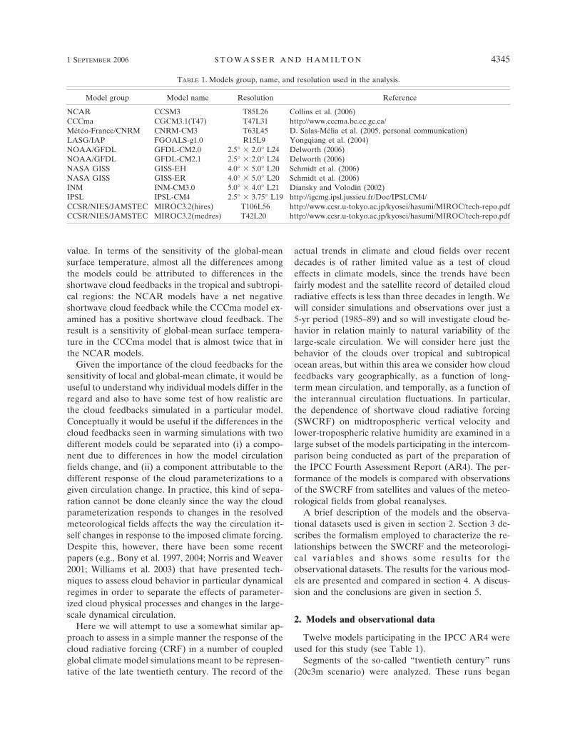
TABLE 1. Models group, name, and resolution used in the analysis.

Model group Model name Resolution Reference

NCAR CCSM3 T85L26 Collins et al. (2006)CCCma CGCM3.1(T47) T47L31 http://www.cccma.bc.ec.gc.ca/Météo-France/CNRM CNRM-CM3 T63L45 D. Salas-Mélia et al. (2005, personal communication)LASG/IAP FGOALS-g1.0 R15L9 Yongqiang et al. (2004)NOAA/GFDL GFDL-CM2.0 2.5° � 2.0° L24 Delworth (2006)NOAA/GFDL GFDL-CM2.1 2.5° � 2.0° L24 Delworth (2006)NASA GISS GISS-EH 4.0° � 5.0° L20 Schmidt et al. (2006)NASA GISS GISS-ER 4.0° � 5.0° L20 Schmidt et al. (2006)INM INM-CM3.0 5.0° � 4.0° L21 Diansky and Volodin (2002)IPSL IPSL-CM4 2.5° � 3.75° L19 http://igcmg.ipsl.jussieu.fr/Doc/IPSLCM4/CCSR/NIES/JAMSTEC MIROC3.2(hires) T106L56 http://www.ccsr.u-tokyo.ac.jp/kyosei/hasumi/MIROC/tech-repo.pdfCCSR/NIES/JAMSTEC MIROC3.2(medres) T42L20 http://www.ccsr.u-tokyo.ac.jp/kyosei/hasumi/MIROC/tech-repo.pdf

1 SEPTEMBER 2006 S T O W A S S E R A N D H A M I L T O N 4345

from spunup preindustrial initial conditions appropri-ate for some time in the late nineteenth century andthen were integrated forward through 1999, with theconcentration of long-lived greenhouse gases and atmo-spheric aerosols being specified with realistic time se-ries. The details of the climate forcing imposed wereleft to the individual modeling groups. So, for example,only some of the model 20c3m simulations includedvolcanic stratospheric aerosol.

The atmospheric components of six of the coupledmodels employ spectral numerics in the horizontal andfor these models the resolution ranges from R15 toT106 (see Table 1). The other six models have somekind of gridpoint representation of the atmospheric dy-namics and employ resolutions ranging from 2.5° � 2.0°to 4° � 5°. The various models use between 9 and 56vertical levels. The cloud fraction schemes employed bythe various models can be categorized broadly intothree groups: relative humidity–based schemes, statis-tical total water schemes, and prognostic cloud fractionschemes. Five models use a prognostic scheme [theGeophysical Fluid Dynamics Laboratory CoupledModel Versions 2.0/2.1 (GFDL-CM2.0/2.1), the Modelfor Interdisciplinary Research on Climate Version 3.2(MIROC3.2hires/medres), and the NCAR CommunityClimate System Model Version 3 (CCSM3)]; five userelative humidity–based schemes [the CCCma ThirdGeneration Coupled Global Climate Model (CGCM3.1),the Goddard Institute for Space Studies (GISS) modelsGISS-EH/ER, the Flexible Global Ocean–Atmosphere–Land System (FGOALS-g1.0), and the Instituto Nacio-nal de Meteorología Coupled Model Version 3.0 (INM-CM3.0)]; and only two use a statistical scheme [theCentre National de Recherches MeteorologiquesCoupled Model Version 3 (CNRM-CM3) and L’InstitutPierre-Simon Laplace Coupled Model Version 4 (IPSL-CM4)]. For detailed descriptions of the models andtheir physical parameterizations we refer to the refer-ences given in Table 1.

The IPCC models are evaluated through compari-sons with a combination of satellite and reanalysissets. The satellite observations are taken from theEarth Radiation Budget Experiment (ERBE) dataset(Barkstrom 1984), and our principal source of the cor-responding meteorological fields is the 40-yr Euro-pean Centre for Medium-Range Weather Forecasts(ECMWF) Re-Analysis (ERA-40) dataset (Simmonsand Gibson 2000). We also compare results obtainedwith the ERA-40 data with those from the NationalCenters for Environmental Prediction (NCEP) reanaly-sis-2 data, which is based on the widely used NCEP–NCAR reanalysis (Kalnay et al. 1996). These datasources provide values on 2.5° � 2.5° latitude–

longitude grids, but the grids are offset. To simplify theanalysis all data are interpolated to the grid of theERBE data. All analysis of observational and modeldata is based on monthly mean values interpolated tothis 2.5° � 2.5° grid. We analyze data at all grid pointsover the ocean and in the 30°S–30°N latitude band forthe 5-yr period from January 1985 to December 1989.This period starts over two years after the 1982 ElChichón volcanic eruption and ends before the 1991eruption of Mt. Pinatubo, and was selected to minimizeany complications from effects of stratospheric aero-sols.

Barkstrom et al. (1989) and Harrison et al. (1990)have attempted to quantify the error in the ERBE top-of-the-atmosphere (TOA) fluxes. For the shortwavefluxes Barkstrom et al. (1989) estimated accuracy forthe monthly mean values of shortwave flux of �5 Wm�2 while Harrison et al. (1990) suggest errors slightlylarger than this. Comparisons of fluxes using the ERBEand newer single scanner footprint algorithms with em-pirical angular distribution models (ADMs) foundlarger errors in the ERBE data. In a study by Loeb etal. (2003) the SW cloud radiative forcing differencesestimated from instantaneous ERBE-like and SSFTOA fluxes depend on the optical thickness of thecloud, and range from �10 to �15 W m�2. The root-mean-square error differences in CRF between theERBE-like and SSF TOA fluxes are typically 7–8 Wm�2 in the SW.

We will employ relative humidity and vertical veloc-ity fields from the ERA-40 and NCEP2 reanalyses. Theuse of gridded meterological reanalyses to provide thevertical velocity and humidity fields for our analysisintroduces some limitations. Over the ocean areaswhere our analysis will be applied, there are very few insitu observations of upper air available, and the fields inthe reanalyses are an indirect diagnostic produced usingan assimilation scheme in a particular numerical model.This is particularly the case for the vertical velocity,which is nowhere directly observed. The uncertainty inthe reanalyses products is one motivation for compar-ing the analysis for two different sets of reanalyses data.The differences between the ERA-40 and NCEP2 re-analysis fields provide at least a lower bound on theuncertainty.

Trenberth and Guillemot (1995, 1998) compared theprecipitable water over tropical and subtropical oceanareas measured by SSM/I satellite microwave observa-tions with ECMWF and NCEP analyses, and theNCEP–NCAR reanalyses. These datasets are predeces-sors of the reanalyses used in our present study. Thiscomparison provides a reasonably direct check on the


uncertainty in the lower-tropospheric humidity, as thisgenerally dominates the total precipitable water col-umn. Correlations of the time series of monthly meanwater column at individual grid points between theanalyses and the satellite observations are generallyhigh (more than 0.9 over much of the tropical and sub-tropical ocean areas). However, it should be noted thatthese correlations include the annual cycle as well asthe interannual fluctuations, which are the focus of thepresent analysis. Both the ECMWF and NCEP analy-ses do have some consistent, if modest, biases relativeto the satellite data, showing �10% lower columns thanthe satellites near the equator and about �10% largercolumns in the subtropics.

We have no comparable observational dataset for500-hPa vertical velocity �. One possibly useful point tomake, however, is that the overall distribution of boththe climatological mean and the interannual variationsof � is reasonably similar in the reanalyses and in theGCMs considered here. In fact we will demonstrate thislater in the present paper (see Fig. 7). So at least thereis no evidence for a significant systematic suppressionor enhancement of the actual vertical velocity in thereanalyses.

3. Analysis method

The basic idea is to stratify cloud data according tophysically based regime indicators X, such as the iso-baric coordinate vertical velocity �, and the relativehumidity h.

We define the SW component of the CRF as thedifference between the solar radiation absorbed in theatmospheric/surface column in actual and clear-sky

conditions; this can be determined from TOA observa-tions (e.g., Coakley and Baldwin 1984). Let C be theSW component of the CRF. Following Bony et al.(2004) the regime indicators are binned into a series ofregimes corresponding to different values of X:

C � �j

�jC for �j � �1 X ∈ Xj � �X

0 else. 1

Considering mean values Cj in the defined regime in-tervals (1) can be rewritten as

C � �j

pjCj 2

to give the area-averaged value C and the probabilitydistribution function (PDF) pj, which holds �jpj � 1.This decomposition can be done for all different kindsof representation of the climate (e.g., using a long-termaverage, monthly mean values, or interannual varia-tions).

We are interested in the relationship between thetime-mean value of X and C as well as the response ofC to deviations, X�, from this mean.

We want to consider only the interannual fluctua-tions, so the X� and C� values have been deseasonal-ized. We define mean values of C and X for every gridpoint and calendar month, [Xk

i ] and SWCRF [Cki ],

where i � 1, . . . , N, k � 1, . . . , 12, and N is the numberof grid points. The variations from the mean are con-structed by subtracting the monthly climatology fromeach month of the data X�i � Xk

i � [Xki ]. The corre-

sponding deviations C�i are constructed in a analogousway. Both variables [Xk

i ] and X�i are binned into inter-vals so that

C� � �l�m

�lmC�i for �lm � �1 �Xk ∈ �Xlk � �X and X� ∈ X�m � �X

0 else.

The C�i values are averaged for all 30°S–30°N oceanpoints falling within each ([Xl], X�m) category and foreach month in the 5-yr analysis period. The resultingaverage values of SWCRF, C�, can then be displayed ina contour plot as a function of the variations X� andmean [X ]. Figure 1a illustrates the approach, usingmonthly mean values of 500-hPa large-scale vertical ve-locities from ERA-40 and the SWCRF determinationsfrom the ERBE data.

The contours are plotted for each part of [�] and ��space that is occupied by at least a single grid point ofdata for at least one month in the full 5-yr period. Thecontours in Fig. 1b give the standard deviation � about

the mean values. Larger variations are generally foundfor large upward motion anomalies in regimes withmodest negative values of [�]. The smallest values of �are found in regions with strong downward mean mo-tions.

The ascending branches of the Hadley–Walker circu-lation, that occur mostly over the warmest portions ofthe Tropics, correspond to negative values of [�], whileregions of large-scale subsidence correspond to positivevalues of [�]. The bin interval used for both [�] and ��is 0.02 Pa s�1. For locations where there is a weak mean[�], the observations in Fig. 1 reveal a linear relation-ship between C� and ��. For either stronger mean as-


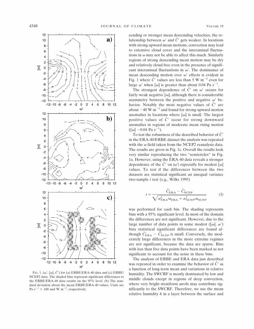
cending or stronger mean descending velocities, the re-lationship between �� and C� gets weaker. In locationswith strong upward mean motions, convection may leadto extensive cloud cover and the interannual fluctua-tions in � may not be able to affect this much. Similarlyregions of strong descending mean motion may be dryand relatively cloud free even in the presence of signifi-cant interannual fluctuations in ��. The dominance ofmean descending motion over �� effects is evident inFig. 1 where C� values are less than 5 W m�2 even forlarge �� when [�] is greater than about 0.04 Pa s�1.

The strongest dependence of C� on �� occurs forfairly weak negative [�], although there is considerableasymmetry between the positive and negative �� be-havior. Notably the most negative values of C� areabout �40 W m�2 and found for strong upward motionanomalies in locations where [�] is small. The largestpositive values of C� occur for strong downwardanomalies in regions of moderate mean rising motion([�] �0.04 Pa s�1).

To test the robustness of the described behavior of C�in the ERA-40/ERBE dataset the analysis was repeatedwith the � field taken from the NCEP2 reanalysis data.The results are given in Fig. 1c. Overall the results lookvery similar reproducing the two “semicircles” in Fig.1a. However, using the ERA-40 data reveals a strongerdependence of the C� on |��| especially for modest [�]values. To test if the differences between the twodatasets are statistical significant an unequal variancetwo-sample t test (e.g., Wilks 1995)

t �C�ERA � C�NCEP

��ERA2 �nERA � �NCEP

2 �nNCEP

3

was performed for each bin. The shading representsbins with a 95% significant level. In most of the domainthe differences are not significant. However, due to thelarge number of data points in some modest ([�], ��)bins statistical significant differences are found al-though C�ERA � C�NCEP is small. Conversely, the mod-erately large differences in the more extreme regimesare not significant, because the data are sparse. Binswith less than five data points have been marked as notsignificant to account for the noise in these bins.

The analysis of ERBE and ERA data just describedwas repeated in order to examine the behavior of C� asa function of long-term mean and variations in relativehumidity. The SWCRF is mostly dominated by low andmiddle clouds except in regions of deep convection,where very bright stratiform anvils may contribute sig-nificantly to the SWCRF. Therefore, we use the meanrelative humidity h in a layer between the surface and

FIG. 1. (��, [�], C�) for (a) ERBE/ERA-40 data and (c) ERBE/NCEP2 data. The shaded bins represent significant differences tothe ERBE/ERA-40 data results on the 95% level. (b) The stan-dard deviation about the mean ERBE/ERA-40 values. Units arePa s�1 � 100 and W m�2, respectively.


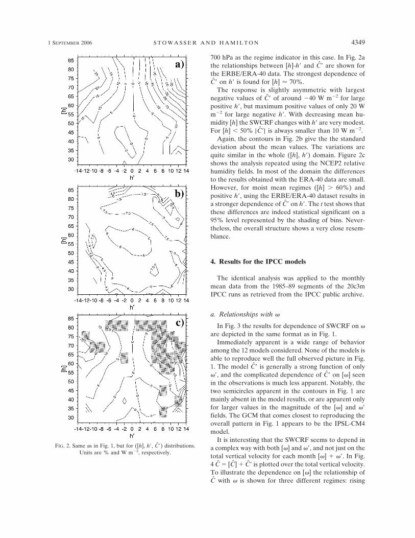
700 hPa as the regime indicator in this case. In Fig. 2athe relationships between [h]-h� and C� are shown forthe ERBE/ERA-40 data. The strongest dependence ofC� on h� is found for [h] � 70%.

The response is slightly asymmetric with largestnegative values of C� of around �40 W m�2 for largepositive h�, but maximum positive values of only 20 Wm�2 for large negative h�. With decreasing mean hu-midity [h] the SWCRF changes with h� are very modest.For [h] � 50% |C�| is always smaller than 10 W m�2.

Again, the contours in Fig. 2b give the the standarddeviation about the mean values. The variations arequite similar in the whole ([h], h�) domain. Figure 2cshows the analysis repeated using the NCEP2 relativehumidity fields. In most of the domain the differencesto the results obtained with the ERA-40 data are small.However, for moist mean regimes ([h] � 60%) andpositive h�, using the ERBE/ERA-40 dataset results ina stronger dependence of C� on h�. The t test shows thatthese differences are indeed statistical significant on a95% level represented by the shading of bins. Never-theless, the overall structure shows a very close resem-blance.

4. Results for the IPCC models

The identical analysis was applied to the monthlymean data from the 1985–89 segments of the 20c3mIPCC runs as retrieved from the IPCC public archive.

a. Relationships with �

In Fig. 3 the results for dependence of SWCRF on �are depicted in the same format as in Fig. 1.

Immediately apparent is a wide range of behavioramong the 12 models considered. None of the models isable to reproduce well the full observed picture in Fig.1. The model C� is generally a strong function of only��, and the complicated dependence of C� on [�] seenin the observations is much less apparent. Notably, thetwo semicircles apparent in the contours in Fig. 1 aremainly absent in the model results, or are apparent onlyfor larger values in the magnitude of the [�] and ��fields. The GCM that comes closest to reproducing theoverall pattern in Fig. 1 appears to be the IPSL-CM4model.

It is interesting that the SWCRF seems to depend ina complex way with both [�] and ��, and not just on thetotal vertical velocity for each month [�] � ��. In Fig.4 C � [C] � C� is plotted over the total vertical velocity.To illustrate the dependence on [�] the relationship ofC with � is shown for three different regimes: rising

FIG. 2. Same as in Fig. 1, but for ([h], h�, C�) distributions.Units are % and W m�2, respectively.


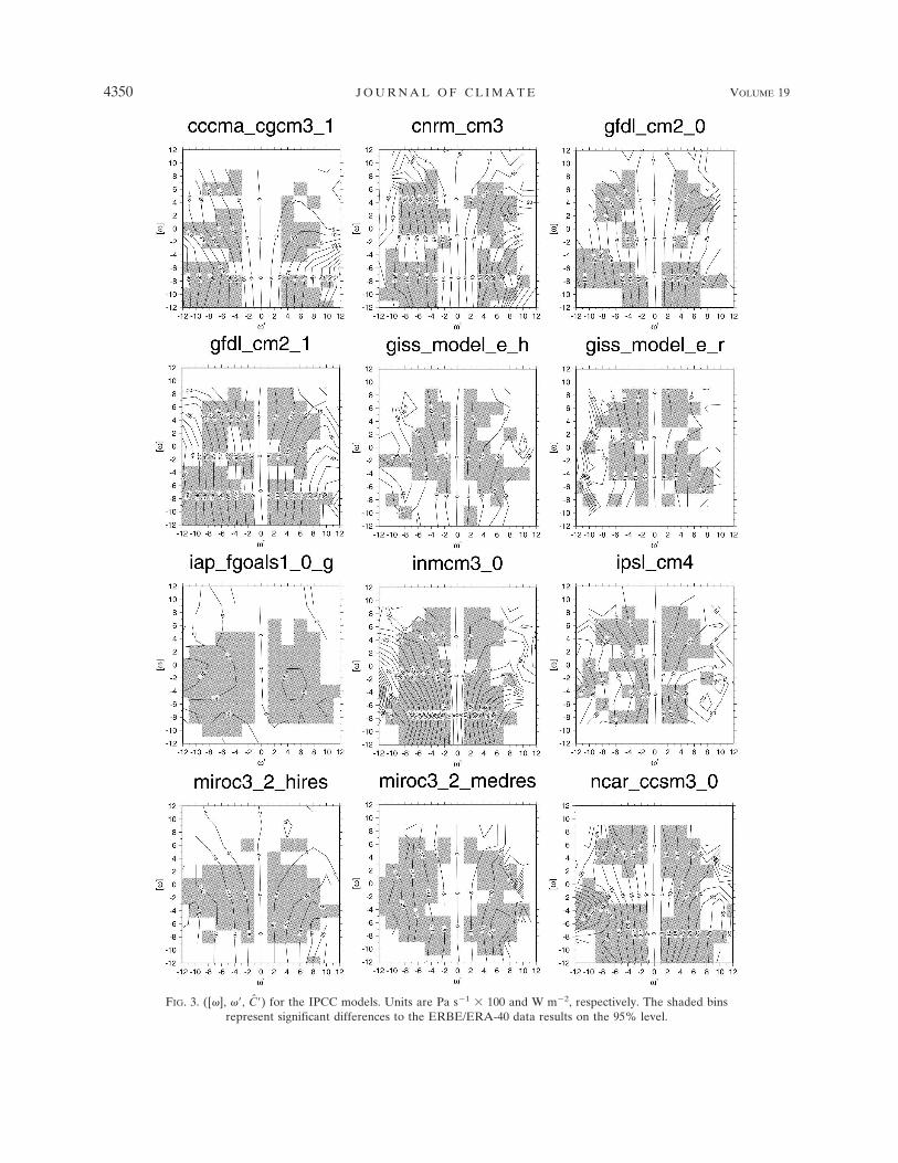
FIG. 3. ([�], ��, C�) for the IPCC models. Units are Pa s�1 � 100 and W m�2, respectively. The shaded binsrepresent significant differences to the ERBE/ERA-40 data results on the 95% level.


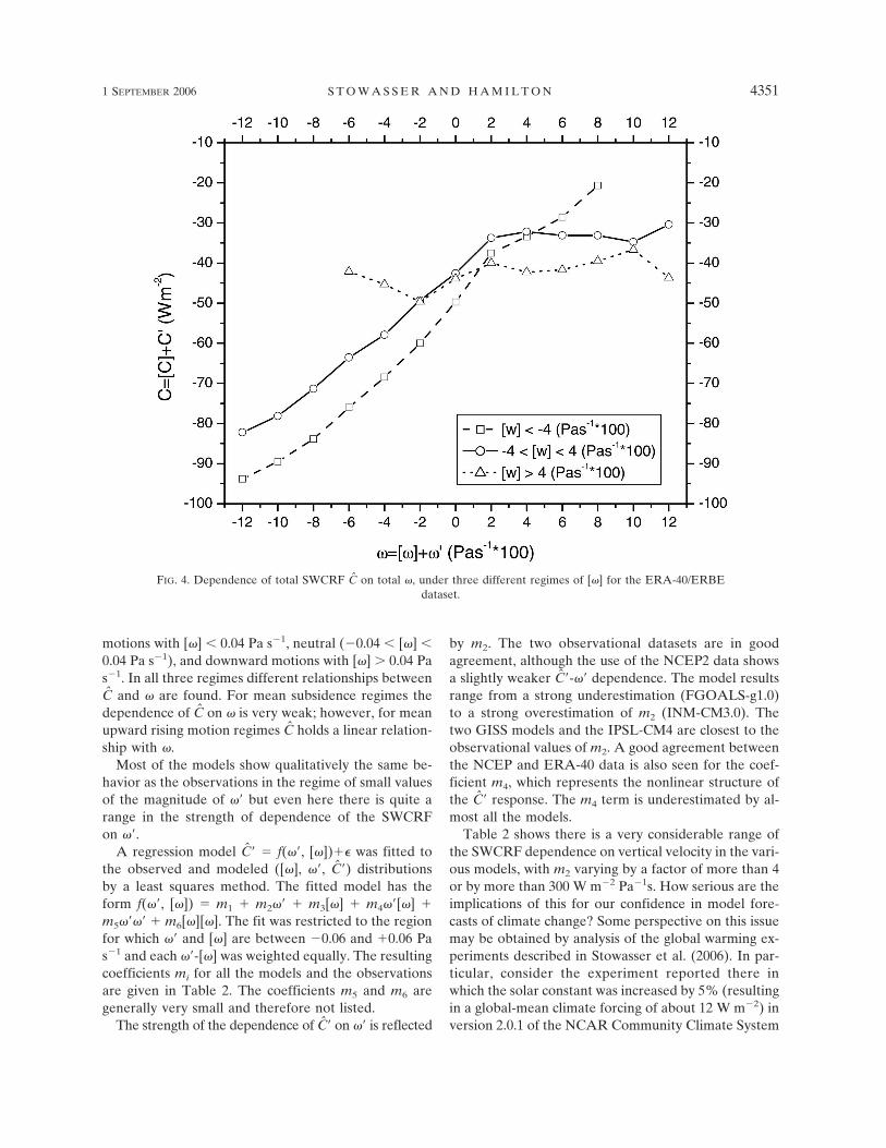
motions with [�] � 0.04 Pa s�1, neutral (�0.04 � [�] �0.04 Pa s�1), and downward motions with [�] � 0.04 Pas�1. In all three regimes different relationships betweenC and � are found. For mean subsidence regimes thedependence of C on � is very weak; however, for meanupward rising motion regimes C holds a linear relation-ship with �.

Most of the models show qualitatively the same be-havior as the observations in the regime of small valuesof the magnitude of �� but even here there is quite arange in the strength of dependence of the SWCRFon ��.

A regression model C� � f(��, [�])�� was fitted tothe observed and modeled ([�], ��, C�) distributionsby a least squares method. The fitted model has theform f(��, [�]) � m1 � m2�� m3[�] � m4��[�] �m5�� m6[�][�]. The fit was restricted to the regionfor which �� and [�] are between �0.06 and �0.06 Pas�1 and each ��-[�] was weighted equally. The resultingcoefficients mi for all the models and the observationsare given in Table 2. The coefficients m5 and m6 aregenerally very small and therefore not listed.

The strength of the dependence of C� on �� is reflected

by m2. The two observational datasets are in goodagreement, although the use of the NCEP2 data showsa slightly weaker C�-�� dependence. The model resultsrange from a strong underestimation (FGOALS-g1.0)to a strong overestimation of m2 (INM-CM3.0). Thetwo GISS models and the IPSL-CM4 are closest to theobservational values of m2. A good agreement betweenthe NCEP and ERA-40 data is also seen for the coef-ficient m4, which represents the nonlinear structure ofthe C� response. The m4 term is underestimated by al-most all the models.

Table 2 shows there is a very considerable range ofthe SWCRF dependence on vertical velocity in the vari-ous models, with m2 varying by a factor of more than 4or by more than 300 W m�2 Pa�1s. How serious are theimplications of this for our confidence in model fore-casts of climate change? Some perspective on this issuemay be obtained by analysis of the global warming ex-periments described in Stowasser et al. (2006). In par-ticular, consider the experiment reported there inwhich the solar constant was increased by 5% (resultingin a global-mean climate forcing of about 12 W m�2) inversion 2.0.1 of the NCAR Community Climate System

FIG. 4. Dependence of total SWCRF C on total �, under three different regimes of [�] for the ERA-40/ERBEdataset.


Model. The long-term mean response includes an ElNiño–like warming structure in the tropical Pacific,which involves significant geographical variations in theradiative and dynamical response. The change in 500-hPa vertical velocity along the equator has contrasts aslarge as 0.04 Pa s�1 while the TOA radiative responsehas variations of the order of 20 W m�2. The ratio ofthese two scales is of the order of 500 W m�2 Pa s �1.This is similar to the uncertainty in m2 among the mod-els considered here. This suggests that the degree ofuncertainty in the SWCRF documented here is quitesignificant.

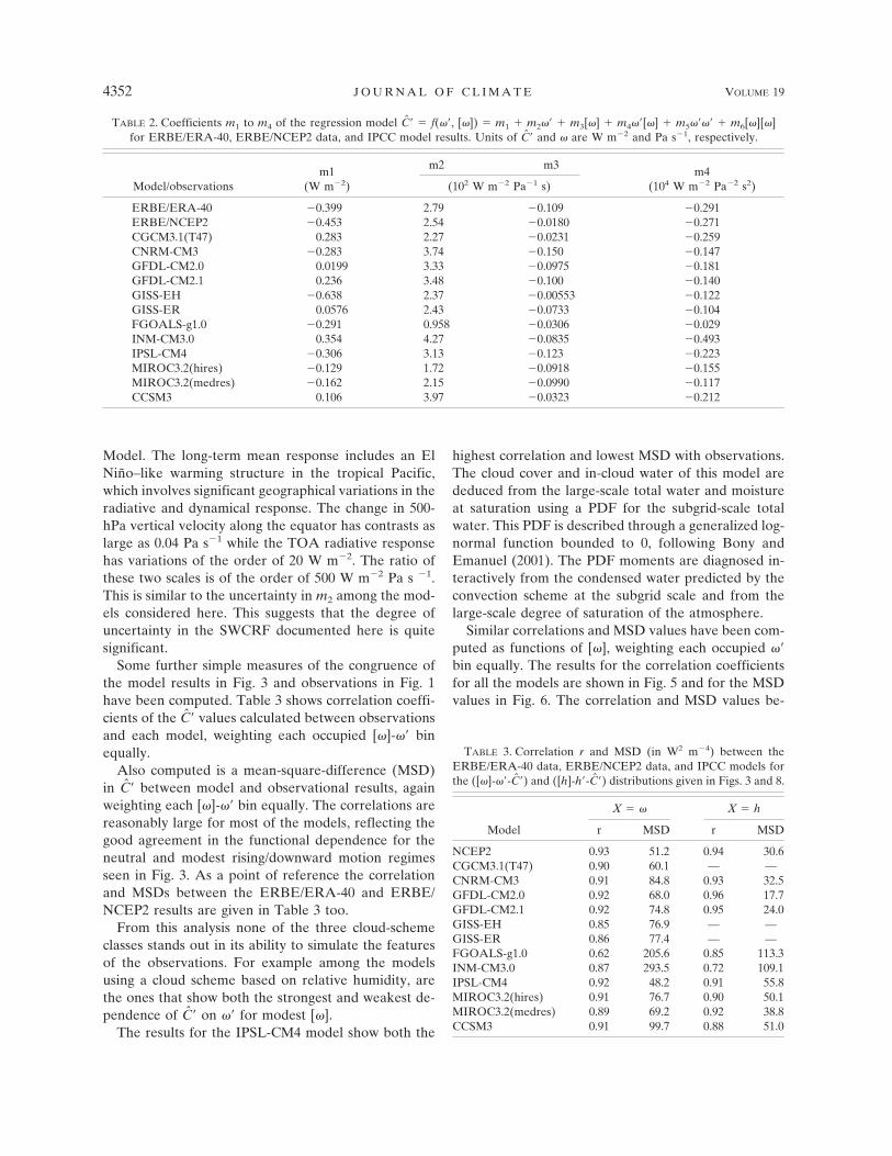
Some further simple measures of the congruence ofthe model results in Fig. 3 and observations in Fig. 1have been computed. Table 3 shows correlation coeffi-cients of the C� values calculated between observationsand each model, weighting each occupied [�]-�� binequally.

Also computed is a mean-square-difference (MSD)in C� between model and observational results, againweighting each [�]-�� bin equally. The correlations arereasonably large for most of the models, reflecting thegood agreement in the functional dependence for theneutral and modest rising/downward motion regimesseen in Fig. 3. As a point of reference the correlationand MSDs between the ERBE/ERA-40 and ERBE/NCEP2 results are given in Table 3 too.

From this analysis none of the three cloud-schemeclasses stands out in its ability to simulate the featuresof the observations. For example among the modelsusing a cloud scheme based on relative humidity, arethe ones that show both the strongest and weakest de-pendence of C� on �� for modest [�].

The results for the IPSL-CM4 model show both the

highest correlation and lowest MSD with observations.The cloud cover and in-cloud water of this model arededuced from the large-scale total water and moistureat saturation using a PDF for the subgrid-scale totalwater. This PDF is described through a generalized log-normal function bounded to 0, following Bony andEmanuel (2001). The PDF moments are diagnosed in-teractively from the condensed water predicted by theconvection scheme at the subgrid scale and from thelarge-scale degree of saturation of the atmosphere.

Similar correlations and MSD values have been com-puted as functions of [�], weighting each occupied ��bin equally. The results for the correlation coefficientsfor all the models are shown in Fig. 5 and for the MSDvalues in Fig. 6. The correlation and MSD values be-

TABLE 3. Correlation r and MSD (in W2 m�4) between theERBE/ERA-40 data, ERBE/NCEP2 data, and IPCC models forthe ([�]-��-C�) and ([h]-h�-C�) distributions given in Figs. 3 and 8.

Model

X � � X � h

r MSD r MSD

NCEP2 0.93 51.2 0.94 30.6CGCM3.1(T47) 0.90 60.1 — —CNRM-CM3 0.91 84.8 0.93 32.5GFDL-CM2.0 0.92 68.0 0.96 17.7GFDL-CM2.1 0.92 74.8 0.95 24.0GISS-EH 0.85 76.9 — —GISS-ER 0.86 77.4 — —FGOALS-g1.0 0.62 205.6 0.85 113.3INM-CM3.0 0.87 293.5 0.72 109.1IPSL-CM4 0.92 48.2 0.91 55.8MIROC3.2(hires) 0.91 76.7 0.90 50.1MIROC3.2(medres) 0.89 69.2 0.92 38.8CCSM3 0.91 99.7 0.88 51.0

TABLE 2. Coefficients m1 to m4 of the regression model C� � f(��, [�]) � m1 � m2�� m3[�] � m4��[�] � m5�� m6[�][�]for ERBE/ERA-40, ERBE/NCEP2 data, and IPCC model results. Units of C� and � are W m�2 and Pa s�1, respectively.

Model/observationsm1

(W m�2)

m2 m3m4

(104 W m�2 Pa�2 s2)(102 W m�2 Pa�1 s)

ERBE/ERA-40 �0.399 2.79 �0.109 �0.291ERBE/NCEP2 �0.453 2.54 �0.0180 �0.271CGCM3.1(T47) 0.283 2.27 �0.0231 �0.259CNRM-CM3 �0.283 3.74 �0.150 �0.147GFDL-CM2.0 0.0199 3.33 �0.0975 �0.181GFDL-CM2.1 0.236 3.48 �0.100 �0.140GISS-EH �0.638 2.37 �0.00553 �0.122GISS-ER 0.0576 2.43 �0.0733 �0.104FGOALS-g1.0 �0.291 0.958 �0.0306 �0.029INM-CM3.0 0.354 4.27 �0.0835 �0.493IPSL-CM4 �0.306 3.13 �0.123 �0.223MIROC3.2(hires) �0.129 1.72 �0.0918 �0.155MIROC3.2(medres) �0.162 2.15 �0.0990 �0.117CCSM3 0.106 3.97 �0.0323 �0.212


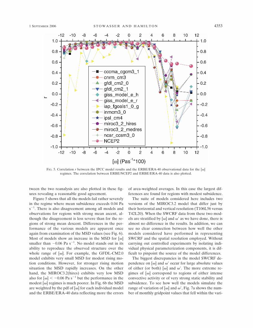
tween the two reanalysis are also plotted in these fig-ures revealing a reasonable good agreement.

Figure 5 shows that all the models fail rather severelyin the regime where mean subsidence exceeds 0.04 Pas�1. There is also disagreement among all models andobservations for regions with strong mean ascent, al-though the disagreement is less severe than for the re-gions of strong mean descent. Differences in the per-formance of the various models are apparent onceagain from examination of the MSD values (see Fig. 6).Most of models show an increase in the MSD for [�]smaller than �0.06 Pa s�1. No model stands out in itsability to reproduce the observed structure over thewhole range of [�]. For example, the GFDL-CM2.0model exhibits very small MSD for modest rising mo-tion conditions. However, for stronger rising motionsituation the MSD rapidly increases. On the otherhand, the MIROC3.2(hires) exhibits very low MSDalso for [�] � �0.06 Pa s�1 but the performance in themodest [�] regimes is much poorer. In Fig. 6b the MSDare weighted by the pdf of [�] for each individual modeland the ERBE/ERA-40 data reflecting more the errors

of area-weighted averages. In this case the largest dif-ferences are found for regions with modest subsidence.

The suite of models considered here includes twoversions of the MIROC3.2 model that differ just bytheir horizontal and vertical resolution (T106L56 versusT42L20). When the SWCRF data from these two mod-els are stratified by [�] and �� as we have done, there isalmost no difference in the results. In addition, we cansee no clear connection between how well the othermodels considered have performed in representingSWCRF and the spatial resolution employed. Withoutcarrying out controlled experiments by isolating indi-vidual physical parameterization components, it is dif-ficult to pinpoint the source of the model differences.

The biggest discrepancies in the model SWCRF de-pendence on [�] and �� occur for large absolute valuesof either (or both) [�] and ��. The more extreme re-gimes of [�] correspond to regions of either intenseconvective activity or of very strong static stability andsubsidence. To see how well the models simulate therange of variation of [�] and ��, Fig. 7a shows the num-ber of monthly gridpoint values that fell within the vari-

FIG. 5. Correlation r between the IPCC model results and the ERBE/ERA-40 observational data for the [�]regimes. The correlation between ERBE/NCEP2 and ERBE/ERA-40 data is also plotted.


Fig 5 live 4/C

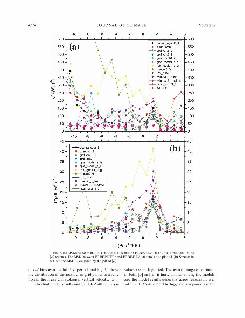
ous �� bins over the full 5-yr period, and Fig. 7b showsthe distribution of the number of grid points as a func-tion of the mean climatological vertical velocity, [�].

Individual model results and the ERA-40 reanalysis

values are both plotted. The overall range of variationin both [�] and �� is fairly similar among the models,and the model results generally agree reasonably wellwith the ERA-40 data. The biggest discrepancy is in the

FIG. 6. (a) MSDs between the IPCC model results and the ERBE/ERA-40 observational data for the[�] regimes. The MSD between ERBE/NCEP2 and ERBE/ERA-40 data is also plotted. (b) Same as in(a), but the MSD is weighted by the pdf of [�].


Fig 6 live 4/C

distribution of the time-mean vertical velocity, wherethe ERA-40 distribution appears shifted slightly topositive [�] values. Most of the grid points have [�]between �0.06 and �0.06 Pa s�1, but there are a fewpercent of grid points with stronger mean rising motionand [�] � �0.06 Pa s�1 (see Fig. 7c).

b. Relationship with relative humidity

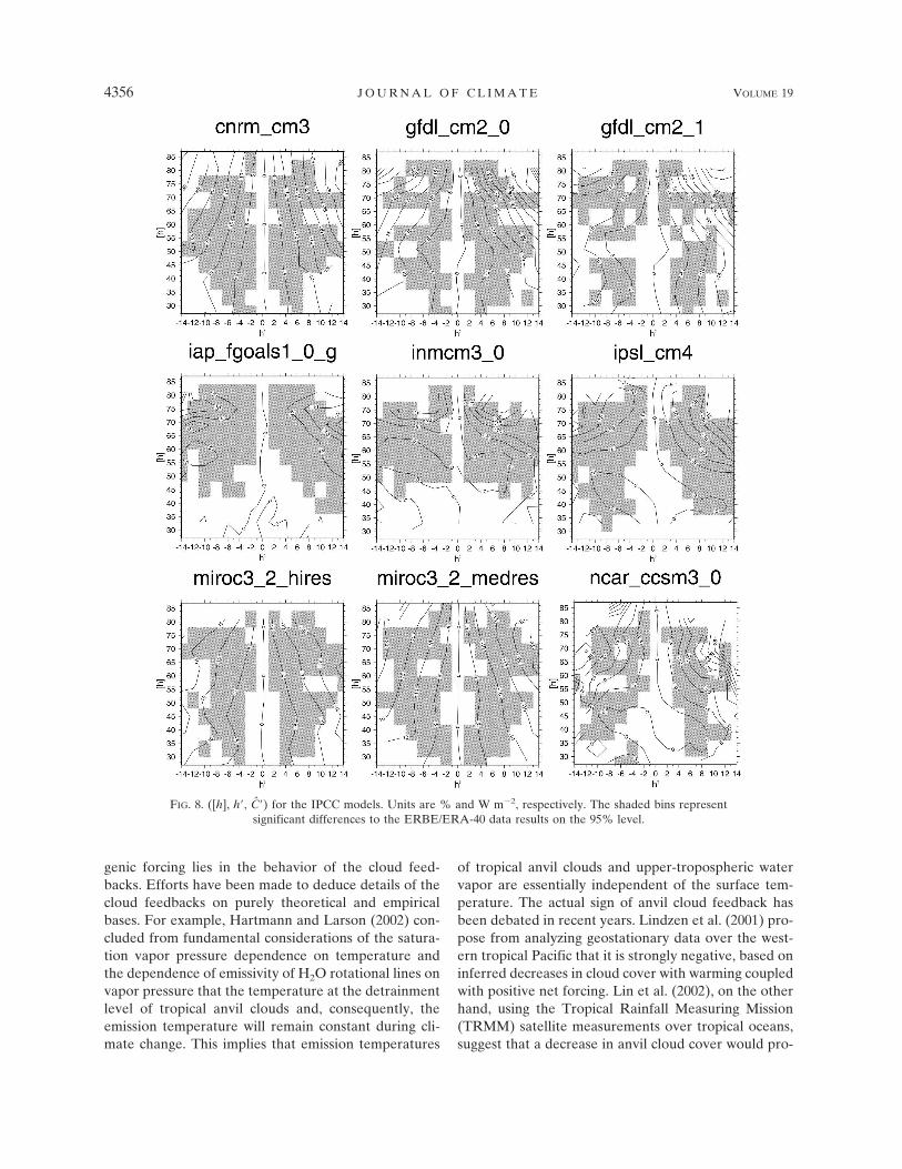
In Fig. 8 the results for the C� as a function of meanand variations in relative humidity are shown for 9 ofthe 12 models considered earlier.

These models were selected simply because therewere monthly mean relative humidity values available.In general the models are able to capture the basicstructure seen in Fig. 2. However, the maximum of C�for large [h] is clearly underestimated by five of themodels [FGOALS-g1.0, INM-CM3.0, IPSL-CM4,MIROC3.2(hi/medres)]. Most of these models also un-derestimate C� in the other [h] regimes. The other fourmodels tend to overestimate the response, especially inthe dry (small [h]) regimes.

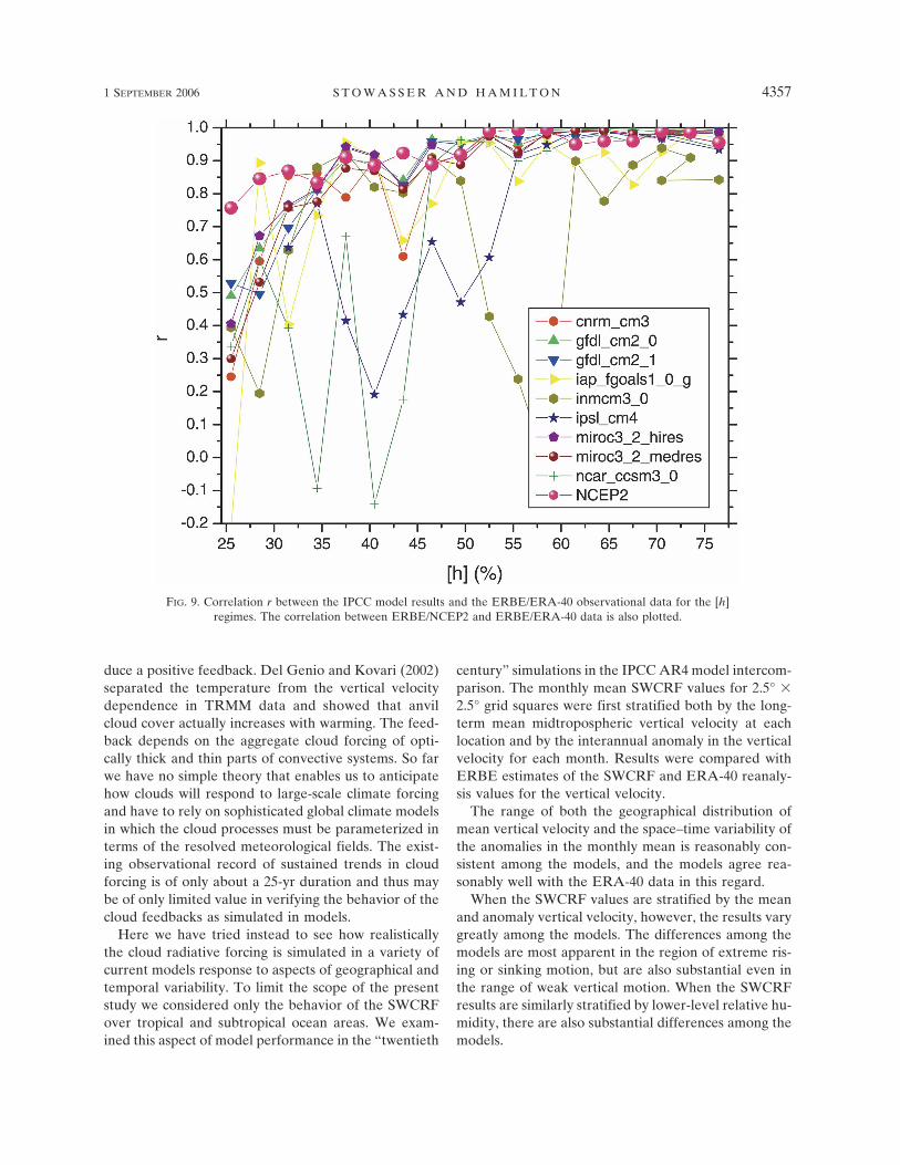
We calculate correlation coefficients and MSD be-tween model results and observations for the datastratified by h, in just the same manner as for the ver-tical velocity described above. The right columns inTable 3 give the r and MSD values when calculatedover all [h] and h�. In this case the two GFDL models,CM2.0 and CM2.1, appear to display the closest fit tothe observations in both the correlation and MSD mea-sures. These two models and the CNRM-CM3 revealsimilar or even smaller MSDs relative to the ERA-40/ERBE observations than in the ERBE-NCEP2/ERA-40 comparison. It is interesting to note that the IPSL-CM4 with its very good representation of the ([�], ��,C�) distribution shows a much less realistic behaviorwhen the SWCRF values are stratified by low-level hu-midity.

Figure 9 shows the spatial correlation r for all [h]regimes.

As stated above, a very good representation of the[h]-h�-C� relationships is generally found for [h] � 45%,but for dryer mean conditions the correlation dropsrapidly. Nevertheless, the corresponding MSD valuesremain rather small, since in this regime the simulatedand observed |C�| are small (not shown). The correla-tion between the ERA-40 and NCEP2 results showshigh correlation for the whole range of [h] regimes.

5. Conclusions

It seems likely that the biggest uncertainty involvedin forecasting climate response to expected anthropo-

FIG. 7. PDF of (a) �� and (b) the mean climatological verticalvelocity [�] for IPCC models (lines with symbols) and ERA-40data (black line). (c) The pdf � 100 of the ([�], ��) bins areplotted for the ERA-40 data.


Fig 7 live 4/C

genic forcing lies in the behavior of the cloud feed-backs. Efforts have been made to deduce details of thecloud feedbacks on purely theoretical and empiricalbases. For example, Hartmann and Larson (2002) con-cluded from fundamental considerations of the satura-tion vapor pressure dependence on temperature andthe dependence of emissivity of H2O rotational lines onvapor pressure that the temperature at the detrainmentlevel of tropical anvil clouds and, consequently, theemission temperature will remain constant during cli-mate change. This implies that emission temperatures

of tropical anvil clouds and upper-tropospheric watervapor are essentially independent of the surface tem-perature. The actual sign of anvil cloud feedback hasbeen debated in recent years. Lindzen et al. (2001) pro-pose from analyzing geostationary data over the west-ern tropical Pacific that it is strongly negative, based oninferred decreases in cloud cover with warming coupledwith positive net forcing. Lin et al. (2002), on the otherhand, using the Tropical Rainfall Measuring Mission(TRMM) satellite measurements over tropical oceans,suggest that a decrease in anvil cloud cover would pro-

FIG. 8. ([h], h�, C�) for the IPCC models. Units are % and W m�2, respectively. The shaded bins representsignificant differences to the ERBE/ERA-40 data results on the 95% level.


duce a positive feedback. Del Genio and Kovari (2002)separated the temperature from the vertical velocitydependence in TRMM data and showed that anvilcloud cover actually increases with warming. The feed-back depends on the aggregate cloud forcing of opti-cally thick and thin parts of convective systems. So farwe have no simple theory that enables us to anticipatehow clouds will respond to large-scale climate forcingand have to rely on sophisticated global climate modelsin which the cloud processes must be parameterized interms of the resolved meteorological fields. The exist-ing observational record of sustained trends in cloudforcing is of only about a 25-yr duration and thus maybe of only limited value in verifying the behavior of thecloud feedbacks as simulated in models.

Here we have tried instead to see how realisticallythe cloud radiative forcing is simulated in a variety ofcurrent models response to aspects of geographical andtemporal variability. To limit the scope of the presentstudy we considered only the behavior of the SWCRFover tropical and subtropical ocean areas. We exam-ined this aspect of model performance in the “twentieth

century” simulations in the IPCC AR4 model intercom-parison. The monthly mean SWCRF values for 2.5° �2.5° grid squares were first stratified both by the long-term mean midtropospheric vertical velocity at eachlocation and by the interannual anomaly in the verticalvelocity for each month. Results were compared withERBE estimates of the SWCRF and ERA-40 reanaly-sis values for the vertical velocity.

The range of both the geographical distribution ofmean vertical velocity and the space–time variability ofthe anomalies in the monthly mean is reasonably con-sistent among the models, and the models agree rea-sonably well with the ERA-40 data in this regard.

When the SWCRF values are stratified by the meanand anomaly vertical velocity, however, the results varygreatly among the models. The differences among themodels are most apparent in the region of extreme ris-ing or sinking motion, but are also substantial even inthe range of weak vertical motion. When the SWCRFresults are similarly stratified by lower-level relative hu-midity, there are also substantial differences among themodels.

FIG. 9. Correlation r between the IPCC model results and the ERBE/ERA-40 observational data for the [h]regimes. The correlation between ERBE/NCEP2 and ERBE/ERA-40 data is also plotted.


Fig 9 live 4/C

When the model results are compared with theERBE and ERA-40 data, it was found that there aresubstantial differences for all models. In terms of ver-tical velocity, the most notable deficiency is an unreal-istically linear dependence of the SWCRF on verticalvelocity even in regimes with strong ascending and de-scending motion. It was also found that for very humidregimes the majority of models tend to underestimatethe SWCRF response. At the other extreme, in loca-tions with dry mean conditions, the modeled SWCRFresponds too strongly to variations in humidity. Inter-estingly, the models with the most realistic dependenceof SWCRF on vertical velocity are among the less re-alistic in their simulation of the SWCRF dependence onrelative humidity.

The technique presented here is useful for evaluatingthe cloud radiative feedbacks in sophisticated globalclimate models. It seems reasonable to expect a modelto reproduce well the observed dependence of SWCRFon the meteorological variables discussed here, in orderto have much credibility in quantitative forecasting ofthe cloud responses to expected large-scale climateforcings. The fact that the models in the AR4 intercom-parison differ so widely in our measures of SWCRFdependence on meteorological fields is a matter of con-cern.

Acknowledgments. This research was supported bythe Japan Agency for Marine-Earth Science and Tech-nology (JAMSTEC) through its sponsorship of the In-ternational Pacific Research Center. The authors ben-efited from a number of illuminating discussions withGeorge Boer. We acknowledge the international mod-eling groups for providing their data for analysis, theProgram for Climate Model Diagnosis and Intercom-parison (PCMDI) for collecting and archiving themodel data, the JSC/CLIVAR Working Group onCoupled Modelling (WGCM) and their Coupled ModelIntercomparison Project (CMIP) and Climate Simula-tion Panel for organizing the model data analysis activ-ity, and the IPCC WG1 TSU for technical support. TheIPCC Data Archive at Lawrence Livermore NationalLaboratory is supported by the Office of Science, U.S.Department of Energy. The authors thank the editorand anonymous reviewers for a number of valuablecomments.

REFERENCES

Barkstrom, B. R., 1984: The earth radiation budget experiment(ERBE). Bull. Amer. Meteor. Soc., 65, 1170–1185.

——, E. Harrison, G. Smith, R. Green, J. Kibler, and R. Cess,1989: Earth Radiation Budget Experiment (ERBE) archival

and April 1985 results. Bull. Amer. Meteor. Soc., 70, 1254–1262.

Bony, S., and K. A. Emanuel, 2001: A parameterization of thecloudiness associated with cumulus convection; evaluationusing TOGA COARE data. J. Atmos. Sci., 58, 3158–3183.

——, K.-M. Lau, and Y. C. Sud, 1997: Sea surface temperatureand large-scale circulation influences on tropical greenhouseeffect and cloud radiative forcing. J. Climate, 10, 2055–2077.

——, J.-L. Dufresne, H. Le Treut, J.-J. Morcrette, and C. Senior,2004: On dynamic and thermodynamic components of cloudchanges. Climate Dyn., 22, 71–86.

Cess, R. D., and Coauthors, 1996: Cloud feedback in atmosphericgeneral circulation models: An update. J. Geophys. Res., 101,12 791–12 794.

Coakley, J. A., and D. G. Baldwin, 1984: Towards the objectiveanalysis of clouds from imagery data. J. Climate Appl. Me-teor., 23, 1065–1099.

Collins, W. D., and Coauthors, 2006: The Community ClimateSystem Model version 3 (CCSM3). J. Climate, 19, 2122–2143.

Del Genio, A. D., and W. Kovari, 2002: Climatic properties oftropical precipitating convection under varying environmen-tal conditions. J. Climate, 15, 2597–2615.

Delworth, T. L., 2006: GFDL’s CM2 global coupled climate mod-els. Part I: Formulation and simulation characteristics. J. Cli-mate, 19, 643–674.

Diansky, N. A., and E. M. Volodin, 2002: Simulation of present-day climate with a coupled atmosphere-ocean general circu-lation model. Izv. Atmos. Ocean Phys., 38, 732–747.

Harrison, E. F., P. M. Minnis, B. R. Barkstrom, V. Ramanathan,R. D. Cess, and G. G. Gibson, 1990: Seasonal variation ofcloud radiative forcing derived from the Earth RadiationBudget Experiment. J. Geophys. Res., 95, 18 687–18 703.

Hartmann, D. L., and K. Larson, 2002: An important constrainton tropical cloud-climate feedback. Geophys. Res. Lett., 29,1951, doi:10.1029/2002GL015835.

Houghton, J. T., Y. Ding, D. J. Griggs, M. Noguer, P. J. van derLinden, and D. Xiaosu, Eds., 2001: Climate Change 2001: TheScientific Basis. Cambridge University Press, 944 pp.

Kalnay, E., and Coauthors, 1996: The NCEP/NCAR 40-Year Re-analysis Project. Bull. Amer. Meteor. Soc., 77, 437–471.

Lin, B., B. A. Wielicki, L. H. Chambers, Y. Hu, and K. Xu, 2002:The seasonal cycle of low stratiform clouds. J. Climate, 15,3–7.

Lindzen, R. S., M. Chou, and A. Hou, 2001: Does the earth havean adaptive infrared iris? Bull. Amer. Meteor. Soc., 82, 417–432.

Loeb, N. G., K. Loukachine, N. Manalo-Smith, B. A. Wielicki,and D. F. Young, 2003: Angular distribution models for top-of-atmosphere radiative flux estimation from the Clouds andthe Earth’s Radiant Energy System instrument on the Tropi-cal Rainfall Measuring Mission Satellite. Part II: Validation.J. Appl. Meteor., 42, 1748–1769.

Norris, J. R., and C. P. Weaver, 2001: Improved techniques forevaluating GCM cloudiness applied to the NCAR CCM3. J.Climate, 14, 2540–2550.

Schmidt, G. A., and Coauthors, 2006: Present-day atmosphericsimulations using GISS ModelE: Comparison to in situ, sat-ellite, and reanalysis data. J. Climate, 19, 153–192.

Senior, C. A., 1999: Comparison of mechanisms of cloud-climatefeedbacks in GCMs. J. Climate, 12, 1480–1489.

Simmons, A. J., and J. K. Gibson, 2000: The ERA-40 Project Plan.ERA-40 Project Rep. Series 1, European Centre for Me-


dium-Range Weather Forecasts, Reading, United Kingdom,63 pp.

Stowasser, M., K. Hamilton, and G. J. Boer, 2006: Local and glob-al climate feedbacks in models with differing climate sensi-tivities. J. Climate, 19, 193–209.

Trenberth, K. E., and C. Guillemot, 1995: Evaluation of the globalatmospheric moisture budget as seen from analyses. J. Cli-mate, 8, 2255–2272.

——, and ——, 1998: Evaluation of the atmospheric moisture andhydrological cycle in the NCEP/NCAR reanalyses. ClimateDyn., 14, 213–231.

Wilks, D. S., 1995: Statistical Methods in the Atmospheric Sciences.Academic Press, 467 pp.

Williams, K. D., M. A. Ringer, and C. A. Senior, 2003: Evaluatingthe cloud response to climate change and current climatevariability. Climate Dyn., 20, 705–721.

Yao, M. S., and A. D. Del Genio, 1999: Effects of cloud param-eterization on the simulation of climate changes in the GISSGCM. J. Climate, 12, 761–779.

Yongqiang, Y., Z. Xuehong, and G. Yufu, 2004: Global coupledocean-atmosphere general circulation models in LASG/IAP.Adv. Atmos. Sci., 21, 444–455.


Relationships Between Cloud Radiative Forcing and Local Meteorological Variables in Several Global Climate Models

Documents