Relationship between Ionic Radius and Pressure Dependence of Ionic Conductivity in Water

Relationship between Ionic Radius and Pressure Dependence of IonicConductivity in Water

Parveen Kumar1, A.K. Shukla1,2 and S. Yashonath1,3

1 Solid State and Structural Chemistry Unit, Indian Institute of Science,

Bangalore-560012, India2 Central Electrochemical Research Institute, Karaikudi-630006 India

3 Center for Condensed Matter Theory, Indian Institute of Science,

Bangalore-560012, India and,

Jawaharlal Nehru Centre for Advanced Scientific Research,

Jakkur, Bangalore-560064, India

Abstract

Experimental measurements of ionic conductivity in water are analysed in order to

obtain insight into the pressure dependence of limiting ionic conductivity of individual

ions (λ0) for ions of differing sizes. Conductivities of individualions,λ0 do not exhibit

the same trend as a function of pressure for all ions. Our analysis suggests that the effect

of pressure on ionic conductivity depends on the temperature. At low temperatures, the

effect of pressure on relatively small ions such as Li+ exhibit an increase in conductivity

with pressure. Intermediate sized ions exhibit an increasein conductivity with increase

in pressure initially and then at still higher pressures, a decrease in ionic conductivity is

observed. Although there are data at low temperatures for ions of large radius, the effect

of increased pressure is expected to lower conductivity with increase in pressure over the

whole range. At higher temperatures, the dependence of conductivity on pressure changes

and these changes are discussed. Divalent ions such as SO2−4 exhibit different trends as a

function of pressure at different temperatures. Both the divalent ions (Ca2+ and SO2−4 ) for

which experimental data exists, exhibit an increase with pressure at lower temperatures. At

slightly higher temperatures, a maximum in conductivity isseen as a function of pressure

over the same range of pressure.

1. Introduction

Among the transport properties, the most accurately and relatively easily measured are

the ionic conductivities. These have been extensively investigated in different polar sol-

vents where different salts readily dissolve. The changes in conductivity with temperature,

pressure, size of the ion, concentration, etc. have been measured. Therefore a large amount

1

The Open-Access Journal for the Basic Principles of Diffusion Theory, Experiment and Application

© 2007, P. KumarDiffusion Fundamentals 6 (2007) 8.1 - 8.14

of data exists in the literature for different salts in a widevariety of solvents.

The importance of understanding the conductivity data in different polar solvents can

not be overemphasized. From a fundamental viewpoint it would lead to a capability to

predict and control as well as manipulate the conductivity.Further, a knowledge of the un-

derlying mechanism determining ionic motion can lead to increased understanding which

could lead to an ability to design new materials with better conductivity. The technological

spin-offs of all this development could be quite remarkable. Battery materials with higher

conductivity and lower dissipation are a possibility. Light materials for battery could reduce

the weight of the battery. Batteries under appropriate pressurized condition can probably

perform better. Some of these ideas could also be of importance in fuel cell technology.

The increased understanding can also lead to important advances in biochemistry and ion

conduction across biomembranes and may help unravel the reasons for selectivity observed

for potassium over sodium.

In spite of availability of a large amount of data, our understanding of the ionic con-

ductivity in water or other solvents still remains rudimentary. The reason for this is the

bewilderingly rich variety that the variation in conductivity exhibit as a function of the dif-

ferent conditions such as temperature, pressure, concentration, ion size, etc. It has been

very difficult, if not impossible, even to explain the variation of conductivity with just a

single variable such as ion size or pressure.

Influence of different variables on ionic conductivity havebeen investigated in the liter-

ature both experimentally and theoretically. Among the different variables that have been

studied, the most widely studied is the influence of size dependence on ionic conductivity.

These are discussed in most textbooks [1–5]. Solvents with hydrogen bonds such as water,

methanol, ethanol, etc. as well as a number of non-hydrogen bonded solvents such as ace-

tonitrile and pyridine are seen to exhibit a maximum in ionicconductivity as a function of

the ion radius. This maximum has been seen in all polar solvents. Positively charged ions

(e.g., alkali ions) as well as negatively charged ions (e.g., halide ions) show a maximum in

conductivity suggesting that such a maximum exists irrespective of the sign of the charge

on the ion or nature of the solvent. Thus, this maximum in conductivity is a universal

behaviour of ions in polar solvents.

This maximum is responsible for the breakdown in Walden’s rule which states that

the product of limiting ionic conductivity of a solutionΛ0 with solvent viscosityη0 is a

constant,Λ0η0 = c. It is generally seen that this product goes through a maximum when

plotted as a function of reciprocal of the ion radius. The maximum in Walden product

arises from a similar maximum in conductivity. This breakdown is probably related to any

2

breakdown in Stokes law.

Water being an important and well known solvent and due to itsimportance in many

chemical as well as biological processes, the conductivitymaximum has been most widely

studied in water as compared to other solvents [6]. The availability of measured conduc-

tivity data is extremely valuable, especially to verify thepredictions of theories or calcu-

lations. Further, existence of accurate potentials to model water and interactions between

water and the ion, has led to the detailed molecular dynamicssimulations whose results are

of great importance in relating the macroscopic behaviour with the microscopic properties

and understanding the cause of the many of the macroscopic behaviour.

Early work of Born [7] was responsible for increased interest in study of conductivity

maximum of ions in solution as a function of ionic radius. A number of groups have in-

vestigated the maximum in ionic conductivity in polar solvents [8–12]. These are aimed

at providing a theoretical framework to understand the underlying cause for the observed

size dependent maximum in ionic conductivity. The complexity of these electrolytic solu-

tions has meant that there are completely different theoretical approaches to understand the

maximum in conductivity.

One such theory is the solvent-berg model which put forward the suggestion

that smaller ions are strongly interacting with the nearestneighbour shell of solvent

molecules [13]. This was considered to be particularly trueof cations since these are gen-

erally smaller in size than the corresponding anions and have a higher charge density. The

ion essentially carries this shell of solvent molecules long enough that this leads to a larger

effective diameter which lowers its conductivity to a valuesmaller than the conductivity of

larger ions which have no strongly attached shells of solvent.

Another set of theoretical attempts to reproduce the observed conductivity variation

with ion radius is based on continuum models. Here dielectric friction arising from polar-

ization interaction between the ion field and the solvent is accounted for. Also accounted

for is the hydrodynamic friction arising from the viscosityof the solventη due to the van

der Waals interaction which is relatively short ranged. Born, Fuoss, Boyd, Zwanzig and

Hubbard and Onsager [7, 13–17] attempted to explain the observed maximum in terms of

the slow relaxation of the dielectric medium (solvent), induced by the electric field of the

ion as the ion diffuses. This gives rise to the dielectric friction,ζDF which is given by the

expression (see Zwanzig [17, 18])

ζDF = 3q2i (ǫ0 − ǫ∞)τD/(cr3

i (2ǫ0 + 1)ǫ0) (1)

whereτD is the dielectric relaxation time of the solvent associatedwith the dynamical

3

properties in continuum treatments. Hereǫ0 and ǫ∞ are the static and high frequency

dielectric constants of the solvent.ri and qi are the radius and charge of the ion. The

friction due to shear viscosity of the solvent, the hydrodynamic friction (which may arise

from the short-range interactions) is given by the Stokes law :

ζSR = 4π η ri (2)

for slip boundary condition. Thus, the total friction on theion, ζ is

ζ = ζSR + ζDF (3)

ζSR is higher, the larger the size of the ion. ButζDF has a 1/r3i dependence and is higher

for ions with smaller radius. The result is that at some intermediate size of the ion,ri, the

total friction ζ is lowest when both the termsζSR andζDF are not too large. This explains

the existence of a conductivity maximum. Hubbard and Onsager [16] have improved the

treatment which leads to better agreement with the experimental mobilities.

Although the maximum in ionic conductivity can be reproduced by the continuum treat-

ment for ions carrying a given type of charge – positive or negative – the theory does not

permit distinction between them asζDF depends onq2i . Thus, the theory can not account

for the two different curves in the plot of conductivity–1/ri obtained experimentally for

positive and negative ions and two different maxima [19]. Clearly there is a need for more

refined theories which treat the charge distribution of the solvent explicitly.

Wolynes proposed a microscopic theory to overcome some of the limitations of the

continuum theories. He separated the contribution into those from the hard replusive in-

teractionζHH and soft attractive interactionsζSS . The correlations between the soft and

hard interactions are neglected.ζHH is identified with the hydrodynamic friction. Both

solvent-berg and continuum treatments are limiting cases of this molecular theory. In this

sense, this may be considered to be more general than other theories.

More recently, Bagchi and coworkers [20–22] have extended the molecular theory to

permit self-motion of the ion. This provides a clearer picture of the various physical factors

responsible for the friction on the moving ion. These are based on mode coupling theory

and separate the overall friction into a microscopicζmicro and a hydrodynamic partζhyd :

1

ζ=

1

ζmicro

+1

ζhyd

(4)

Theζmicro has contributions from several terms. Direct binary collisions as well as the

isotropic fluctuations in density lead to friction that are represented respectively byζbinary

4

36

38

40

38

38.5

39

39.5

35

36

37

0 500 1000 1500 2000Pressure (bar)

16

17

18

19 Li+

K+

Cs+

Cl-

λo (

Scm

2 mol

-1)

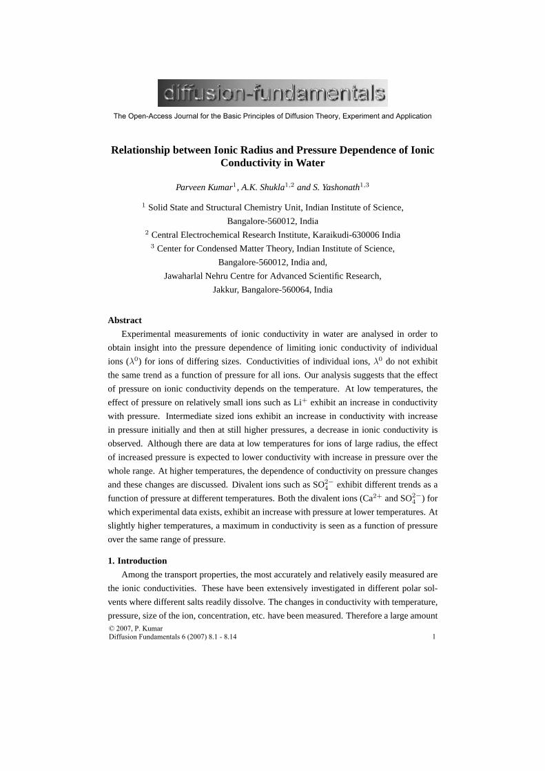
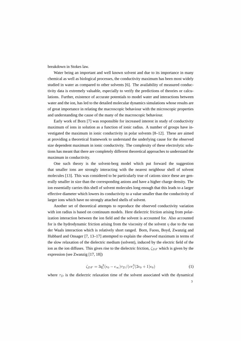
Figure 1: Variation of conductivity,λ0 with pressure for monovalent ions at -5◦C. Thedata have been taken from Takisawa et al. [26].

andζdensity. Coupling with polarization fluctuations is responsible for the dielectric fric-

tion ζDF . Thus,

ζmicro = ζbinary + ζdensity + ζDF (5)

ζhyd is the hydrodynamic friction. This can be usually determined from transverse current-

current correlation function. Although all these terms determine the overal friction on the

ion, often some of these terms are less important than others. Thus, for some ions, Bagchi

and coworkers suggest that some of these terms are small and can be neglected. More recent

studies by Bagchi and coworkers have shown the importance ofultrafast solvation. It leads

to a significant reduction in the contribution to friction experienced by the ion [23–25].

Fleming and coworkers [27], Barbara and coworkers [28] and Bagchi and cowork-

ers [29] have shown the relationship between the solvation energy time correlation function

and the dielectric friction. They have shown that both ion solvation dynamics and dielec-

tric friction are influenced by the dynamics of the ion and thesolvent. In other words, the

dynamics that influences the ion solvation dynamics is also responsible for the dielectric

friction. Bagchi and coworkers show that inclusion of the ultrafast mode in the dielec-

tric relaxation is necessary to obtain closer agreement with the experimentally measured

limiting ion conductivityΛ0.

5

72

74

76

78

18

18.5

19

19.5

76

77

78

22

23

48

49

50

29

30

31

32

0 500 1000 1500 2000

39

40

0 500 1000 1500 200040

42

44Li

+

Na+

Rb+

Cs+

Me4 N

+

Et4 N

+

Pr4 N

+

Bu4 N

+

Pressure (bar) Pressure (bar)

λo (

Scm

2 mol

-1)

λo (

Scm

2 mol

-1)

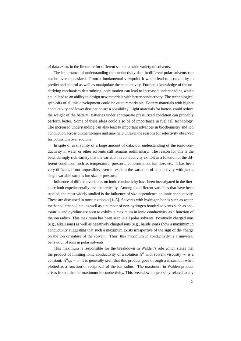
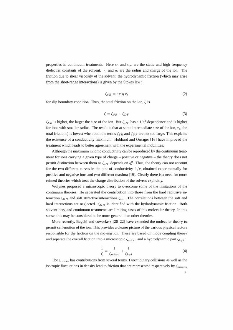
Figure 2: Variation of conducitivity,λ0 with pressure at 25◦C for monovalent cations. Datataken from Ueno et al. [35].

There have been computer simulation studies on diffusion ofions in water and other

solvents in the past two decades [30–33]. Computer simulations of Rasaiah and cowork-

ers and Lynden Bell and coworkers [32, 33] on ion motion in water have clarified some

aspects of this intriguing problem. Ion–water intermolecular potential was derived by fit-

ting them to solvation energies of ions in embedded water clusters. They have carried out

simulations to study the dependence of mobility on ion radius and charge. Their finding

that both positively and negatively charged ions exhibit a maximum in diffusivity confirms

the well known experimental results on alkali and halide ions which exhibit a maximum

for intermediate sized ions. Simulations suggest that the solvent coordination around the

ions depend crucially on the charge on the ion. However, theyfind no relation between the

solvent coordination and mobility; this supports the view that solvent-berg model does not

provide the required explanation to account for the maximumin conductivity. The precise

size of the ion at which the maximum in mobility is seen also depends on the charge. Their

calculations suggest that the dielectric friction model ismore appropriate for larger ions

while for small ions the solvent-berg model may be more appropriate. They obtained good

agreement with experimental results.

Chandra and coworkers [30] have studied the effect of ion concentration on the hydro-

gen bond dynamics. They find that water molecules participating in five hydrogen bonds

are more mobile as compared to four or fewer hydrogen bonds [31, 34]. They have also

studied the effect of pressure on aqueous solutions. Studies have also been carried out on

non-aqueous solutions.

6

Experimental studies date back to over several decades. Butmore recently, experi-

mental studies of ionic mobility in water, alcohols, acetonitrile and formamide by Kay

and Evans as well as Ueno and coworkers have shown the existence of a maximum in the

Walden’s product [35–40]. Investigations in D2O show that the ratio ofΛ0η0 in D2O to

that in H2O also exhibits a maximum when plotted againstr−1

ion. HereΛ0 is the limiting ion

conductivity of the solution andη0 is the viscosity of the solvent. Ionic mobility of cations

has also been studied in a series of monohydroxy alcohol [35,38]. It is generally observed

that the mobility is lower in these alcohols than found in water. Further, the mobility is still

lower in higher alcohols. Studies of ionic mobility also exist in solvents such as acetoni-

trile and formamide [35, 38, 39]. Both these solvents exhibit ultrafast solvation dynamics.

For acetonitrile, an inertial component with a relaxation time of 70 fs and for formamide

around 100 fs has been reported [41].

Recently, we proposed that the ionic conductivity maximum in polar solvents has its

origin in the Levitation Effect [42, 43]. The latter is an effect that was observed for guests

in zeolites and other porous solids. On increase in the size of the guest, the self diffusivity

decresed initially when the size of the guest was significantly smaller than the size of the

void and neck within the zeolites or other porous solids. However, the size of the guest

was comparable to the size of the neck then, a maximum in self diffusivity was seen. This

maximum has been shown to arise from the mutual cancellationof forces exerted on the

guest by the zeolite leading to lower net force on the guest when its size is comparable

to the size of the neck. The guest then is less confined relative to when it is smaller. A

similar effect leading to a maximum in self diffusivity exists in solutions dominated by van

der Waals interaction as well as in solutions with significant long-range interaction [44–

47]. Thus, it appears that while the previous theoretical frameworks proposed based on

continuum theories as well as microscopic theories providea reason for the size dependent

maximum in conducitivity, they do not even attempt to explain the variation of conductivity

with other variables such as pressure. Here we have collected all the conductivity data as a

function of pressure and analyse them so as to obtain a clear idea of how the conductivities

of ions in water are altered as a function of pressure. Such anunderstanding is necessary

before one can put forward theories to explain the pressure dependence of conductivity for

ions of different sizes.

2. Analysis of Experimental Measurements

Extensive amount of data is available in the literature for ionic conductivity in water

of different salts. There are also several groups who have studied the dependence of ionic

7

60

62

64

66

68

3030.5

3131.5

3232.5

78.5

79

79.5

34

34.5

35

35.5

0 500 1000 1500 2000Pressure (bar)

74

76

78

80

0 500 1000 1500 2000Pressure (bar)

39.5

40

40.5

41

41.5

λo (

Scm

2 mol

-1)

(a) I-

(a) Cl-

(a) Br-

(b) ClO4

-

(b) CH3 CO

2

-

(b) C2 H

5 CO

2

-

(b) C3 H

7 CO

2

-

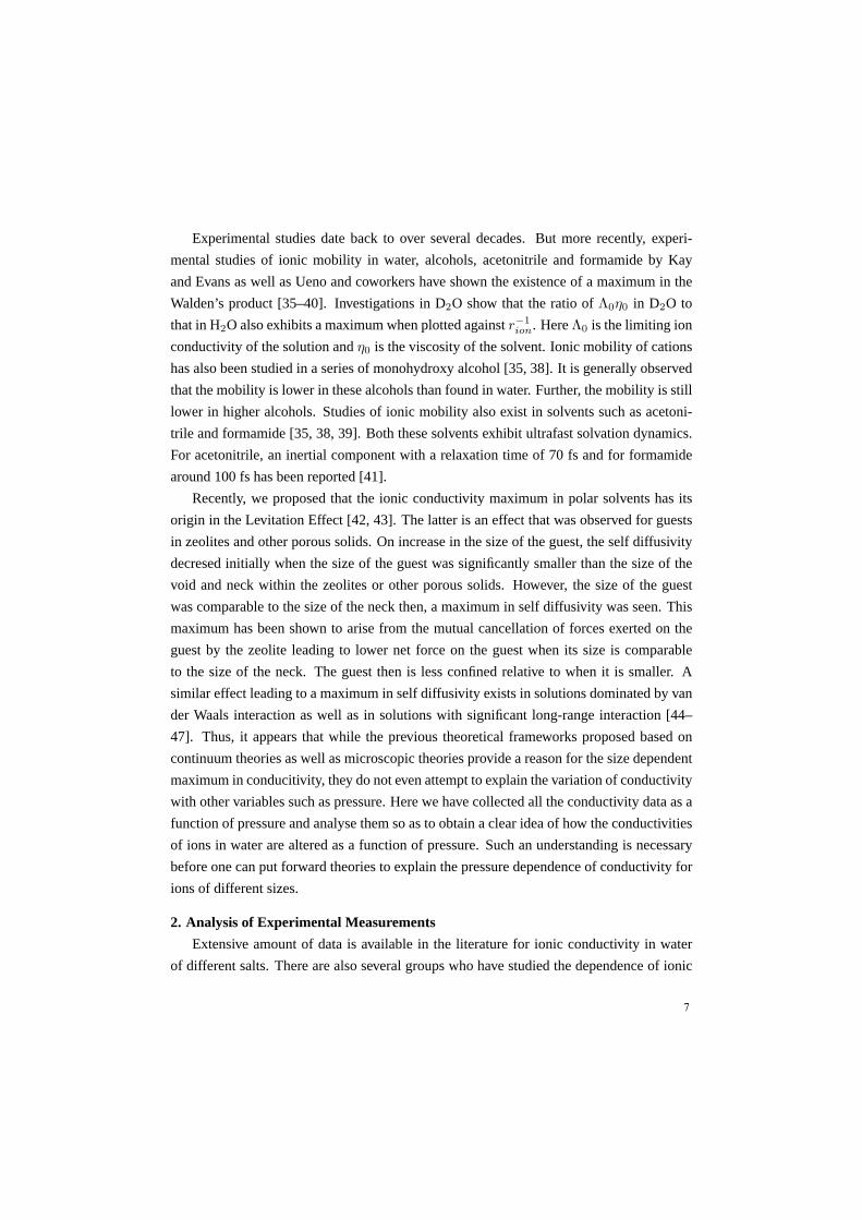
Figure 3: Variation of conducitivity,λ0 with pressure at 25◦C for monovalent anions. Datataken from Nakahara and Osugi [48] and Shimizu and Tsuchihashi [49].

conductivity as a function of pressure [26, 35, 49–53]. Usually, the conductivity of the

solution ,Λ, is measured at several concentrations. These are analysedby means of Fuoss-

Onsager equation [35, 51, 54]

Λ = Λ0− S

√

c + Ec log c + Jc

of conductance of unassociated electrolytes. Herec is molar concentration,S andE are

constants which are a function ofΛ0 and the solvent properties viscosity and dielectric

constant.J is a function of ion size taken as an adjustable parameter. From this,Λ0, the

limiting conductivity or conductivity at infinite dilutionof the solution is obtained:

λ0 = T 0+ Λ0 .

Here,T 0+ is the transference number at infinite dilution andλ0 is the limiting ion conduc-

tivity at infinite dilution of the specific ion. Experimentaldetails are not given here but

those interested can find it from the cited references.

An analysis ofλ0 of the specific ion is investigated here since this is a simplequantity.

In contrast,Λ0 is the conductivity of the solution and its value depends on the conductivities

of the cation as well as the anion. Although many studies in the literature reportΛ0 few

studies reportT 0+ or λ0. The available data for analysis is therefore not extensive.

8

0 500 1000 1500 200030

40

50

60

70

80

0 500 1000 1500 200010

15

20

25

30

35

40

45

50

Li+ / H

2 O

Li+ / D

2 O

Na+ / H

2 O

Na+ / D

2 O

Rb+ / H

2 O

Cs+ / H

2 O

Rb+ / D

2 O

Cs+ / D

2 O

Pressure (bar)

λo (

Scm

2 mol

-1)

Me4 N

+ / D

2 O

Me4 N

+ / H

2 O

Et4 N

+ / H

2 O

Et4 N

+ / D

2 O

Bu4 N

+ / D

2 O

Bu4 N

+ / H

2 O

Pr4 N

+ / D

2 O

Pr4 N

+ / H

2 O

Pressure (bar)

λo (

Scm

2 mol

-1)

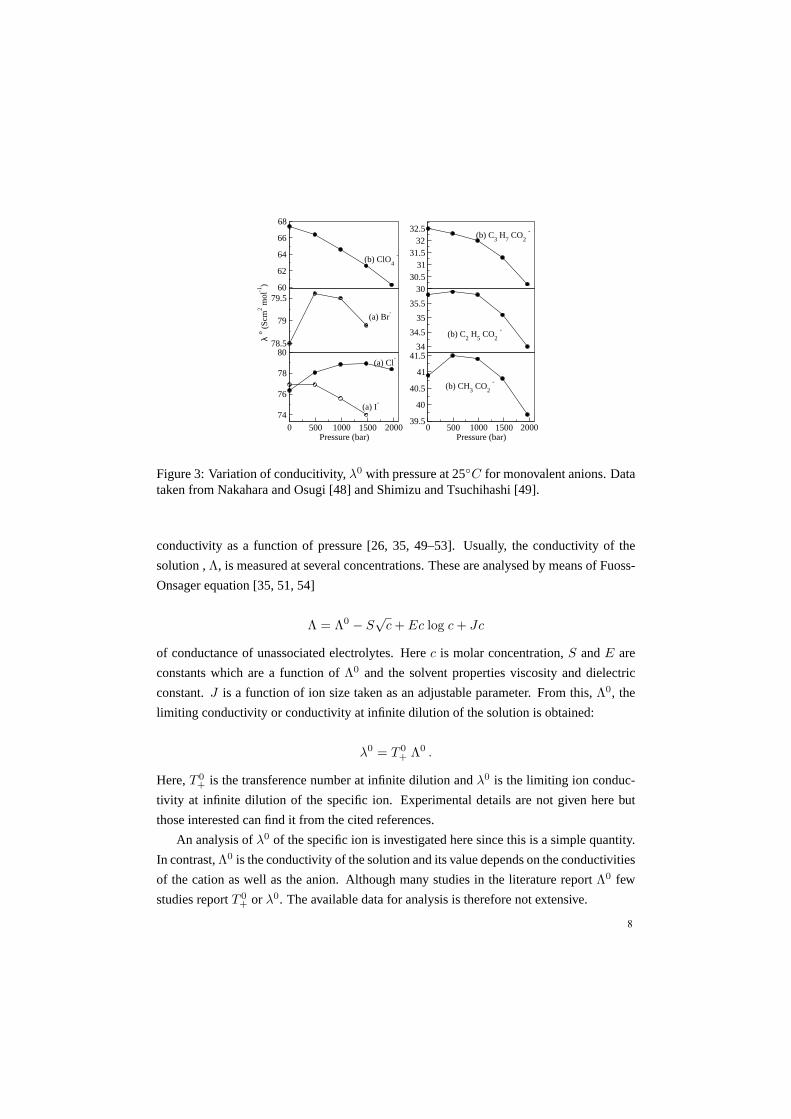
Figure 4: Variation of conductivity,λ0 with pressure in light and heavy water for cationsof differing sizes. Filled symbols are for light water and open symbols are for heavy water.Data taken from Ueno et al. [35].

Λ0− p plots for monovalent ions of different sizes at -5◦C: Figure 1 shows a plot

of the variation ofλ0 as a function of the pressure,p, for Li+, K+, Cs+ andCl− over

a pressure range of 1-2000 bars. The measurements have been made at -5◦C. We note

that forLi+, the conductivity increases with pressure. For intermediate-sized ions at low

temperatures,K+ andCs+, the conductivity increases initially and then subsequently de-

creases with pressure. Thus, a conductivity maximum is seenfor these ions. We could

not find any data for larger ions such tetraalkyl ammonium ions. ForCl− the behaviour is

similar to what is seen forLi+. These data have been taken from Takisawa et al. [26].

A plot of λ0 against pressure is shown for ions of different sizes of ionsfrom the work

of Ueno et al. [35] (see Figure 2). These measurements have been carried out at room

temperature, 298K. Note that the trends seen in the earlier Figure are valid here also : small

ions such asLi+exhibit an increase in conductivity with pressure. Intermediate sized ions

exhibit a maximum in ionic conductivity at some intermediate pressure but larger ions (such

asX4N+, whereX = Me, Et, Pr, Bu) show only a decrease in conductivity with pressure.

The data of Nakahara and Osugi and Shimizu and Tsuchihashi [48, 49] are shown in

Figure 3. This shows a plot ofλ0 versus pressure,p, for monovalent anions at 25◦C. For

the larger anions such asI−, ClO−

4 andC3H7CO−

2 conductivity decreases with increase

in pressure. But for anions of intermediate size (Br−, Cl−, CH3CO−

2 andC2H5CO−

2 ) a

maximum in conductivity with increase in pressure is seen. This behaviour is what we ob-

serve in case of monavalent cations. It therefore appears that the maximum in conductivity

9

38.8

39.2

39.6

40

72

73

74

72

74

76

78

76

77

78

79

0 1000 2000

14

16

18

20

22

0 1000 2000

30

33

36

39

42

0 1000 200032

36

40

44

0 1000 200034

36

38

40

42

44

46

Li+ Cl

-Cs

+K

+

(a) -5 o C

(a) -5 o C

(a) -5 o C

(a) -5 o C

(a) -10 o C

(a) -10 o C

(a) -10 o C

(a) 0 o C

(a) 0 o C

(a) 0 o C

(a) 0 o C

(b) 25 o C

(d) 25 o C

(b) 25 o C

(c) 25 o C

Pressure (bar)

λo (

Scm

2 mol

-1)

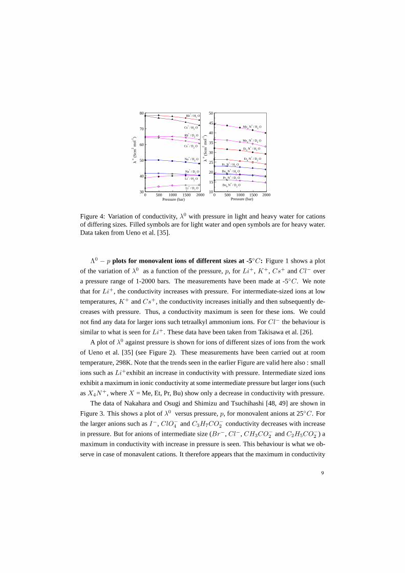
Figure 5: Variation of conductivity,λ0 with pressure for monovalent ions over a range oftemperature. The data have been taken from (a) Takisawa et al. [26] and (b) Nakahara etal. [55] and (c) Nakahara et al. [56] and (d) Ueno et al. [35].

depends on the size of the ion in a way that is independent of the nature of charge carried

by the ion.

Figure 4 shows a plot ofλ0 versus pressure,p, for monovalent cations of different

sizes in light and heavy water. From this figure, we can observe that conductivities in

heavy water show a similar trend as we observe in case of lightwater; only a uniform

lowering of conductivity is seen in heavy water as compared to light water. A reduction in

conductivity in heavy water is attributed to stronger hydrogen bonding in heavy water as

compared to light water. A sluggish solvent structure can lead to reduced mobility of the

ion and not just the solvent.

Temperature dependance of Λ0−p plots : In Figure 5 we show a plot of the variation

of λ0 with pressure over a range of temperatures. At higher temperatures, some changes

are seen in theλ0 -p curves. Firstly, for ions such asLi+ or Cl−, the increasing conductiv-

ity with pressure changes to an increasing and decreasing trend with pressure exhibiting a

maximum at some intermediate pressure. For the intermediate sized ions such asK+ and

Cs+ the trend is seen to remain the same; however, the pressure atwhich the conductivity

is maximum shifts to a lower pressure. For example, in the case K+ the maximum con-

ductivity is seen at a pressure of 1500 bars at -10◦C. By 25◦C the pressure at which the

conductivity is maximum shifts to 500 bars. ForCs+ the pressure at which the conductiv-

10

81.4

81.6

81.8

82

112.8

113.1

113.4

113.7

60

60.4

60.8

80.8

81.2

81.6

82

0 400 800 1200Pressure (bar)

47.2

47.6

48

48.4

48.8

0 400 800 1200Pressure (bar)

63.7

64.4

65.1

65.8

Ca2+ SO

4

2-

λo (

Scm

2 mol

-1 )

λo (

Scm

2 mol

-1 )

15o C

15o C

25o C

40o C

40o C

25o C

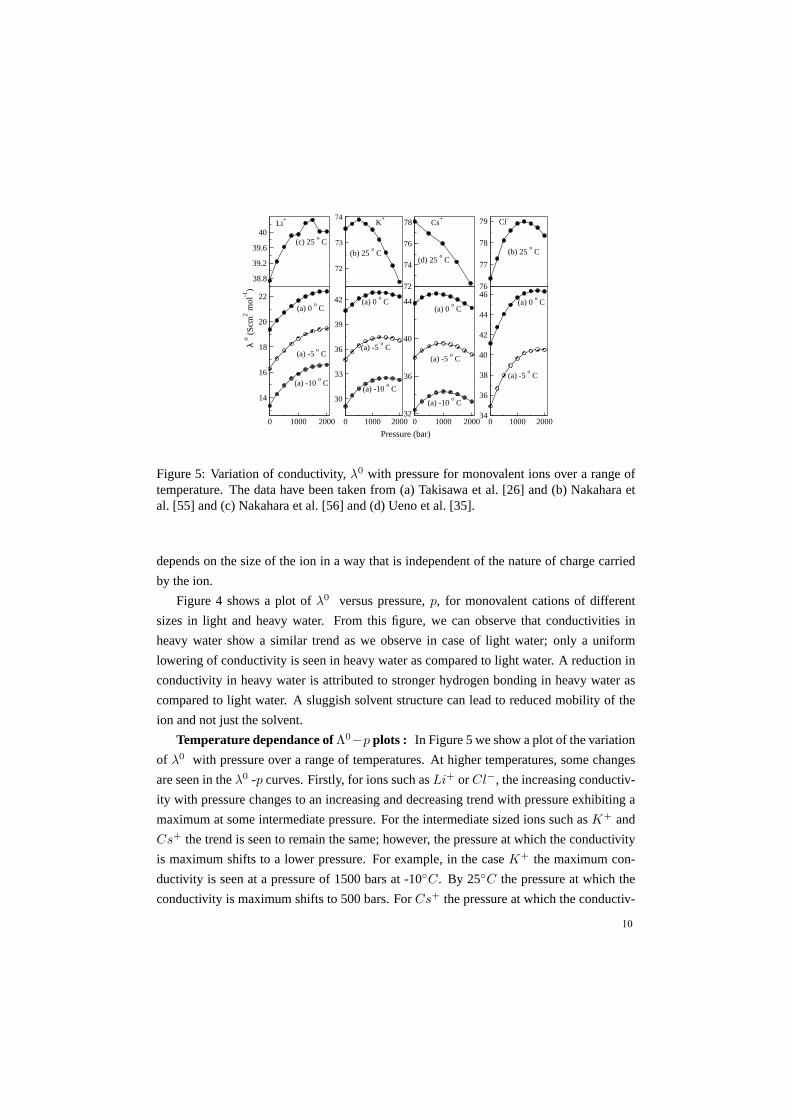
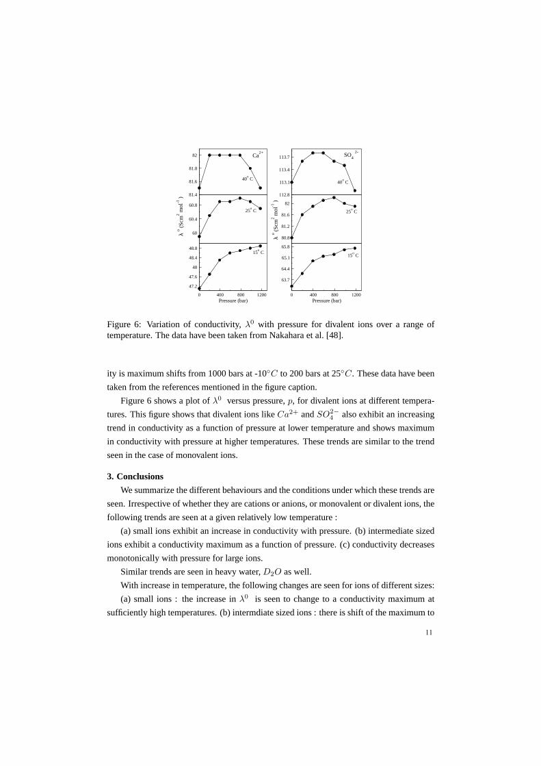
Figure 6: Variation of conductivity,λ0 with pressure for divalent ions over a range oftemperature. The data have been taken from Nakahara et al. [48].

ity is maximum shifts from 1000 bars at -10◦C to 200 bars at 25◦C. These data have been

taken from the references mentioned in the figure caption.

Figure 6 shows a plot ofλ0 versus pressure,p, for divalent ions at different tempera-

tures. This figure shows that divalent ions likeCa2+ andSO2−4 also exhibit an increasing

trend in conductivity as a function of pressure at lower temperature and shows maximum

in conductivity with pressure at higher temperatures. These trends are similar to the trend

seen in the case of monovalent ions.

3. Conclusions

We summarize the different behaviours and the conditions under which these trends are

seen. Irrespective of whether they are cations or anions, ormonovalent or divalent ions, the

following trends are seen at a given relatively low temperature :

(a) small ions exhibit an increase in conductivity with pressure. (b) intermediate sized

ions exhibit a conductivity maximum as a function of pressure. (c) conductivity decreases

monotonically with pressure for large ions.

Similar trends are seen in heavy water,D2O as well.

With increase in temperature, the following changes are seen for ions of different sizes:

(a) small ions : the increase inλ0 is seen to change to a conductivity maximum at

sufficiently high temperatures. (b) intermdiate sized ions: there is shift of the maximum to

11

lower pressures. (c) larger sized ions : no change; only a decreasing trend is seen.

Acknowledgement : We wish to thank Department of Science and Technology, and Coun-

cil of Scientific and Industrial Research, New Delhi for financial support.

References

[1] P. W. Atkins,Physical Chemistry, Oxford University Press, Oxford, 1994.

[2] J. M. Bockris and A. Reddy,Modern Electrochemistry 1 : Ionics, Litton Education

Publishing, New York, 1971.

[3] G. W. Castellan,Physical Chemistry, Addition-Wesley, Reading, MA, 1971.

[4] H. L. Falkenhagen,Electrolytes, Clarendon Press, Oxford, 1934.

[5] S. Glasstone,An Introduction to Electrochemistry, Litton Education Publishing, New

York, 1971.

[6] B. Bagchi and R. Biswas,Acc. Chem. Res., 31, 181 (1998).

[7] M. Born, Z. Phys., 1, 221 (1920).

[8] J. Barthel, L. Iberl, J. Rossmaier, H. J. Gores, and B. Kaukal,J. Sol. Chem., 19, 32

(1990).

[9] B. Das, N. Saha, and D. K. Hazra,J. Chem. Engg. data, 45, 353 (2000).

[10] D. F. Evans, C. Zawoyski, and R. L. Kay,J. Phy. Chem., 69, 3878 (1965).

[11] J. R. Graham, G. S. Kell, and A. R. Gordon,J. Am. Chem. Soc., 79, 2352 (1957).

[12] G. T. Hefter and M. Salomon,J. Sol. Chem., 25, 541 (1996).

[13] J. H. Chen and S. A. Adelman,J. Chem. Phys., 72, 2819 (1980).

[14] R. H. Boyd,J. Chem. Phys., 35, 1281 (1961).

[15] R. M. Fuoss,Proc. Natl. Acad. Sci., 45, 807 (1959).

[16] J. B. Hubbard and L. Onsager,J. Chem. Phys., 67, 4850 (1977).

[17] R. Zwanzig,J. Chem. Phys., 52, 3625 (1970).

12

[18] R. Zwanzig,J. Chem. Phys., 38, 1603 (1963).

[19] S. Koneshan, R. M. Lynden-Bell, and J. C. Rasaiah,J. Am. Chem. Soc., 120, 12041

(1998).

[20] R. Biswas and B. Bagchi,J. Chem. Phys., 106, 5587 (1997).

[21] R. Biswas and B. Bagchi,J. Am. Chem. Soc., 119, 5946 (1997).

[22] R. Biswas, S. Roy, and B. Bagchi,Phys. Rev. Lett., 75, 1098 (1995).

[23] S. Bhattacharya and B. Bagchi,J. Chem. Phys., 106, 1757 (1997).

[24] R. Biswas, N. Nandi, and B. Bagchi,J. Phys. Chem., 101, 2698 (1997).

[25] S. Roy and B. Bagchi,J. Chem. Phys., 99, 9938 (1993).

[26] N. Takisawa, J. Osugi, and M. Nakahara,J. Chem. Phys., 78, 2591 (1983).

[27] M. Maroncelli and G. Fleming,J. Chem. Phys., 89, 5044 (1988).

[28] P. F. Barbara and W. Jarzeba,Adv. Photochem., 15, 1 (1990).

[29] B. Bagchi,Annu. Rev. Phys. Chem., 40, 115 (1989).

[30] A. Chandra,Phys. Rev. Lett., 85, 768 (2000).

[31] A. Chandra and S. Chowdhury,Proc. Indian Acad. Sci. (Chem. Sci.), 113, 591 (2001).

[32] S. H. Lee and J. C. Rasaiah,J. Chem. Phys., 101, 6964 (1994).

[33] R. M. Lynden-Bell, R. Kosloff, S. Ruhman, D. Danovich, and J. Vala,J. Chem. Phys.,

109, 9928 (1998).

[34] S. C. A. Chandra,J. Chem. Phys., 115, 3732 (2001).

[35] M. Ueno, N. Tsuchihashi, K. Yoshida, and K. Ibuki,J. Chem. Phys., 105, 3662 (1996).

[36] T. Hoshina, N. Tsuchihashi, K. Ibuki, and M. Ueno,J. Chem. Phys., 120, 4355 (2004).

[37] K. Ibuki, M. Ueno, and M. Nakahara,J. Mol. Liq., 98-99, 129 (2002).

[38] R. Kay and D. F. Evans,J. Phys. Chem., 70, 2325 (1966).

[39] J. Thomas and D. F. Evans,J. Phys. Chem., 74, 3812 (1970).

13

[40] M. Ueno, K. Ito, N. Tsuchihashi, and K. Shimizu,Bull. Chem. Soc. Jpn., 59, 1175

(1986).

[41] M. L. Horng, J. A. Gardecki, A. Papazyan, and M. Maroncelli, J. Phys. Chem., 99,

17311 (1995).

[42] S. Yashonath and P. Santikary,J. Chem. Phys., 100, 4013 (1994).

[43] S. Yashonath and P. Santikary,J. Phys. Chem., 98, 6368 (1994).

[44] P. K. Ghorai and S. Yashonath,J. Phys. Chem. B, 109, 5824 (2005).

[45] P. K. Ghorai and S. Yashonath,J. Phys. Chem. B, 24, 12072 (2006).

[46] P. K. Ghorai and S. Yashonath,J. Phys. Chem. B, 110, 12179 (2006).

[47] P. K. Ghorai, S. Yashonath, and R. L. Bell,J. Phys. Chem. B, 109, 8120 (2005).

[48] M. Nakahara and J. Osugi,Rev. Phy. Chem. Jpn, 45, 1 (1975).

[49] K. Shimizu and N. Tsuchihashi,Rev. Phy. Chem. Jpn, 49, 18 (1979).

[50] R. A. Horne, B. R. Myers, and G. R. Frysinger,J. Chem. Phys., 39, 2666 (1963).

[51] E. Inada,Rev. Phy. Chem. Jpn, 46, 19 (1976).

[52] M. Nakahara,Rev. Phy. Chem. Jpn, 42, 75 (1972).

[53] M. Ueno, M. Nakahara, and J. Osugi,J. Sol. Chem., 8, 881 (1979).

[54] N. Takisawa, J. Osugi, and M. Nakahara,J. Chem. Phys., 77, 4717 (1982).

[55] M. Nakahara, M. Zenke, M. Ueno, and K. Shimizu,J. Chem. Phys., 83, 280 (1985).

[56] M. Nakahara, T. Torok, N. Takisawa, and J. Osugi,J. Chem. Phys., 76, 5145 (1982).

14