Relationship Banking and the Pricing of Financial Services Charles W. Calomiris and Thanavut Pornrojnangkool* This Version: February 2006 DRAFT: DO NOT QUOTE WITHOUT PERMISSION * Calomiris is the Henry Kaufman Professor of Financial Institutions at Columbia Business School, Professor of International and Public Affairs at Columbia’s SIPA, the Arthur Burns Fellow in International Economics at the American Enterprise Institute, and a Research Associate at the National Bureau of Economic Research. Pornrojnangkool is a Ph.D. candidate at Columbia Business School. We thank Paul Efron and seminar participants at the Columbia Business School, the New York Fed, the Federal Reserve Board, the University of Western Ontario, and George Mason University for helpful comments. Please address comments to: Charles W. Calomiris, email: [email protected]

Welcome message from author
This document is posted to help you gain knowledge. Please leave a comment to let me know what you think about it! Share it to your friends and learn new things together.
Transcript

Relationship Banking and the Pricing of Financial Services
Charles W. Calomiris and Thanavut Pornrojnangkool*
This Version: February 2006
DRAFT: DO NOT QUOTE WITHOUT PERMISSION
* Calomiris is the Henry Kaufman Professor of Financial Institutions at Columbia Business School, Professor of International and Public Affairs at Columbia’s SIPA, the Arthur Burns Fellow in International Economics at the American Enterprise Institute, and a Research Associate at the National Bureau of Economic Research. Pornrojnangkool is a Ph.D. candidate at Columbia Business School. We thank Paul Efron and seminar participants at the Columbia Business School, the New York Fed, the Federal Reserve Board, the University of Western Ontario, and George Mason University for helpful comments. Please address comments to: Charles W. Calomiris, email: [email protected]

ABSTRACT We investigate how banking relationships affect the terms of lending, through both supply- and demand-side effects, and the underwriting costs of debt and equity issues. We use micro- level loan and underwriting data to investigate pricing effects of the joint production of loans and security underwritings within the context of relationship banking. We capture and control for firm characteristics, including differences in the sequences of firm financing decisions, and assemble a database of the financial histories of 7,315 firms, comprising their loans, debt issues, and equity issues for the period 1992 to 2002. We address several shortcomings in prior studies, which results in significant improvement in the explanatory power of our regressions when compared to prior studies. We find no evidence that universal banks under-price loans to win underwriting business, which also rules out any possibility of illegal “tying.” We do find evidence that banks price loans and underwriting services in a strategic way to extract value from their relationships. In particular, we find that banks charge premiums for both loans and underwriting services to extract value from their combined lending and underwriting relationships. We also find that universal banks enjoy cost advantages in both lending and underwriting, irrespective of relationship benefits. Part of the advantages borrowers enjoy from bundling products within a banking relationship may include a reduced demand for borrowing, which takes the form of reduced demand for lines of credit. We find evidence of a “road show” effect from debt underwritings to loan pricing discounts.

1
1. Introduction
This paper focuses on the consequences for the pricing of financial transactions of
the bundling of those transactions within the same banking relationship. From the outset
it is important to distinguish bundling from illegal “tying.” Bundling is a well-established
practice within the banking industry whereby banks offer multiple financial products and
services to customers as a part of durable relationships. In theory, banks should price
related product offerings to meet their internal profitability standards on a total customer
relationship basis. In practice, banks generally offer arrays of products1 to customers, and
products may be bundled together. Laws do not prohibit this practice of relationship
banking or product bundling as long as customers have the option to refuse bundling.
Tying, on the other hand, is a different concept whereby the sale or price of a
“main” product, in which the seller potentially has market power, is conditioned upon the
requirement that customers also purchase the “other” products, with the goal of
leveraging market power in the “main” product to improve the performance of “other”
products.2
1 Bank regulators classify products that banks offer into traditional and non-traditional banking products. Traditional banking products are products that traditionally are offered by banks such as bank credit, deposit, custodian business, cash management, and trust service. Non-traditional banking products are, for example, insurance policy, wealth management service, and underwriting business. 2 Tying in this manner can be illegal in any product markets by general antitrust laws because of its anti-competitive effects. The Clayton Antitrust Act explicitly prohibits exclusive dealing arrangements or tying arrangements, where the seller conditions the sale of a desired product upon the buyer purchasing another product, where competition is likely to be lessened substantially. See Clayton Act, 15 U.S.C. § 14. In the banking industry, section 106 of the Bank Holding Company Act Amendment of 1970 explicitly prohibits the tying of traditional banking products to non-traditional banking products. Consistent with the intent of the law, regulators have adopted a strict interpretation of illegal tying to include only transactions that give rise to the potential extension of market power in traditional banking products to non-traditional banking products. According to a Federal Reserve interpretation (see Fed Reg. 52024 Aug 29,2003), the bundling of banking products constitutes illegal tying only when all of the following conditions are met: 1) tying is initiated by the bank, 2) tying involves at least two products, a borrower’s “desired” traditional banking product and another non-traditional banking product, 3) the pricing and/or availability of the “desired” product is conditioned on the borrower’s purchase of another non-traditional banking product (a tied product), and 4) at the time of negotiation, the bank does not present meaningful unbundled

2
Concerns about tying lending to security underwriting to win underwriting
business emerged only recently; until the 1980s the Glass-Steagall Act of 1933 was
interpreted as prohibiting banks from underwriting corporate securities. As the restriction
on underwritings was gradually lifted since 1987, regulatory interest in the consequences
of the bundling of lending and underwriting services has increased. The Glass-Steagall
Act was repealed by the Gramm-Leach-Bliley Act of 1999. The law allows the bundling
of lending and underwriting services by universal banks but the prohibition for tying
remains.3
Mullineaux (2003), among others, argues that the necessary conditions for illegal
tying by universal banks are unlikely to be met in the current market environment. The
corporate lending market for large firms is predominately a syndicated market, includes
many lenders, and is highly competitive. Banks have little apparent market power in this
market, so there is little potential to abuse power or to extend it to other (e.g.,
underwriting) services. A large firm is unlikely to hire a particular universal bank as
alternatives to the borrower. See Office of the Comptroller of the Currency (2003) for some legal perspective and some discussion regarding the original intents of the anti-tying laws. Closely related to anti-tying laws, section 23B of the Federal Reserve Act 1913 also prohibits any transactions that may benefit non-bank affiliates at the expense of insured banks. Effectively, this regulation prohibits banks from under-pricing loans to win underwriting businesses for their non-bank affiliates. The economic argument for this regulation is simple. Under-pricing loans might help weak banks increase their safety net subsidies by channeling income from insured banks to the uninsured security affiliates. 3 The in-roads made by universal banks into the securities underwriting business have prompted competitive concerns among specialized investment banks. Press coverage (e.g., The Economist, 1/9/2003, American Banker, 9/27/2002) and practitioner surveys (e.g., Association for Financial Professionals 2004 Credit Access Survey) worry that potential tying practices by universal banks may be used to compete unfairly for underwriting business against stand-alone investment banks. However, studies by regulators and government agencies indicate no widespread practice of illegal tying, despite the substantial increases in the market shares of universal banks in underwriting services. Regulators point to the need to distinguish between the illegal practice of tying and the legal practice of product bundling (e.g., General Accounting Office 2003). Not surprisingly, investment banks that are losing market share to universal banks may confound the two phenomena in their assessments of whether there is a “problem” of loan under-pricing by universal banks.

3
underwriter just to be able to get a loan from that bank when the lending market is
competitive.4
Of course, in some circumstances, market power may be an important issue.
Calomiris and Pornrojnangkool (2005) provide evidence that regional market power can
exist for some lending market segments, such as middle-market lending, when a single
lender dominates that segment of the market and borrowers are not large to obtain
sufficiently attractive terms from large lenders outside the region. However, the segment
of the market in which banking relationships are most likely to combine lending with
underwriting services is the large corporate segment, and these borrowers enjoy national
market access, so market power in lending is unlikely. Nonetheless, it is possible that
specific circumstances may exist that give banks an upper hand in negotiations with
clients, which may give rise to illegal tying.5
Even if the illegal tying of lending and underwriting are unlikely in the United
States today, it is still of interest to understand the consequences for lending and
underwriting costs of their joint production. Has the bundling of lending and
underwriting created net benefits from joint production, and if so, how have those
benefits been shared between banks and their clients? Do those net benefits show
themselves in the pricing of bundled lending and underwriting services?
4 Similarly, there are reasons to question whether violations of Section 23b are occurring, or that such violations could explain the growing market shares of universal banks in securities underwriting. Reforms of prudential regulation since 1991 (the FDICIA of 1991, and recent modifications of the Basel standards to emphasize internal risk controls at large banks), along with historically high bank capital ratios, should limit the incentives that large banks face to transfer income out of protected (deposit insured) commercial bank affiliates, even if regulators and supervisors were not able to observe and prevent safety net abuse. 5 On August 27, 2003, the Federal Reserve released a Combined Consent Order to Cease and Desist against WestLB AG and its New York branch, citing violations of anti-tying restrictions.

4
Another important question is whether universal banks enjoy a comparative
advantage in providing lending and underwriting services in comparison to stand-alone
investment banks. Universal banks have gained enormous market share in underwriting.
Does that reflect a fundamental cost advantage or an unfair competitive advantage related
to the possession of a commercial banking charter? Does the cost advantage of universal
banks show itself in both the lending function and the underwriting function? How do
cost advantages or disadvantages across banks affect strategic pricing behavior?
We compare banks’ pricing behavior for bundled and non-bundled transactions,
and compare the lending and underwriting costs charged by stand-alone investment banks
with those charged by universal banks. Our study of pricing policies across these types of
banks, and across different circumstances, provides new insights about the costs and
pricing strategies of different banks under different circumstances, and offers some
guidance to regulators about whether universal banks’ success should concern them.6
Section 2 provides a review of the literature. Section 3 reviews our data sources
and our empirical methodology. Section 4 presents our findings, including the estimation
of supply and demand functions for borrowing, and non-structural estimates of the cost of
underwriting services. Section 5 concludes.
2. Literature Review
An early line of research on the joint production of lending and underwriting
focused on conflicts of interest. A conflict can arise from a moral hazard problem, where
universal banks learn negative private information about a firm and induce the firm to
6 A 10/2/3003 letter from Board of Governors of the Federal Reserve System to the U.S. General Accounting Office indicates their current effort the study loan pricing behavior to potentially improve the enforcement of anti-tying and loan underpricing regulations.

5
issue debt in the market to repay outstanding loans to the bank before the negative
information is revealed to the market. Here, bankers harm securities purchasers by
withholding pertinent information from them. An adverse selection problem can also
create a conflict of interest in this setting. Universal banks may cherry-pick transactions
by lending to the best quality firms and bringing poor quality firms to the debt market.
Kroszner and Rajan (1994) focus on the pre-Glass Steagall era and compare the
ex-post performance of bonds underwritten by universal banks with bonds underwritten
by investment banks, after controlling for ex-ante risk profiles. They find that bonds
underwritten by universal banks default significantly less often than (ex-ante similar)
issues underwritten by investment banks. That finding indicates that potential conflicts of
interest either were absent or were overcome by other banking practices and reputational
considerations.
Focusing on bond issues from the same period, Kroszner and Rajan (1997)
investigate ex-ante pricing of bonds (i.e., yield spreads over Treasuries) and document
that the market rewards universal banks for placing their underwriting business within a
separate subsidiary (as opposed to an internal department) as one of the ways to mitigate
potential conflicts of interest, a finding that may help to explain the apparent lack of
conflict observed in Kroszner and Rajan (1994).
Joint production of multiple banking products can provide economies of scope
due to information reusability and efficiency gains associated with better portfolio
diversification, scale-related economies of scope in product delivery, and lower costs
(e.g. Calomiris 2000, Calomiris and Karceski 2000). There is a vast literature on the cost

6
functions in banks, which seeks to measure scope economies across activities, with little
success (e.g., Berger and Humphrey 1991, Pulley and Humphrey 1993).7
The joint production of lending and underwriting may give rise to bank quasi rent
creation and extraction in the context of relationship management (e.g., Greenbaum,
Kanatas and Venezia 1989, Sharpe 1990, Rajan 1992). In the case where it is costly for a
firm to credibly communicate its prospects to the public or to other banks, an informed
banker can gain market power that can potentially be translated into charging higher
prices for some loans and other services. This line of reasoning receives more attention in
our empirical discussion below. Some of our findings support the notion that bank-
borrower relationships entail the creation of quasi rents, and that banks are able to extract
some of those rents.
Puri (1996) investigates bond yield spreads over Treasuries for the pre-Glass
Steagall era and documents that universal banks obtain better prices for their customers
than investment banks do. This provides some evidence of net benefits from the joint
production of loans and debt underwriting. For the more recent period, Gande, Puri,
Saunders and Walter (1997) compare the yield spreads of bonds underwritten by
7 As pointed out by Rajan (1995), it can be difficult to detect scope economies due to difficulties in estimating bank cost functions precisely. A potentially more promising approach is to investigate micro-level data that enable researchers to measure interactions among various types of production activities directly. More recent studies pursue this line of analysis by comparing loan spreads, underwriting fees, and ex-ante performance of the security offerings between bundling and non-bundling transactions. Nonetheless, the results from these studies are not conclusive. In addition to reducing clients’ interest costs and fees, and increasing the securities prices clients are able to obtain from their issues, universal banking also may permit borrowers to save transaction costs (including “face time”) by establishing more efficient communication procedures with a smaller number of financial institutions. Information production is costly for both banks and borrowers. The larger the number of banking relationships, the larger the amount of the resources a borrower has to allocate to communicate and coordinate with banks. To our knowledge, there is no study that directly focuses on transaction cost savings from bundling services, and we are unaware of any data that would permit such a study. While we do not pursue this line of research in this study, transaction cost savings from universal banking would be consistent with some of our findings, as discussed further below.

7
investment banks with the spreads of bonds underwritten by subsidiaries of commercial
banks from 1993 to 1995. They find evidence that firms obtain better pricing for their
bonds when they have an existing relationship with the underwriting bank. Roten and
Mullineaux (2002) investigate the same question for bonds underwritten from 1995 to
1998 but find that an existing relationship with the underwriting bank has no impact on
bond pricing. However, they find that banks on average charge lower underwriting fees
(measured by gross underwriting spreads) than investment banks, regardless of
relationships.
Drucker and Puri (2005) investigate 2,301 seasoned equity underwritings during
the period 1996 to 2001. Of the 2,301 seasoned equity underwritings in their sample, 201
issues are bundled with 358 loans (that is, loans and underwriting services are provided
by the same institution). They estimate a gross underwriting spread equation and find that
investment banks offer a discount on their underwriting fees when an equity underwriting
is bundled with a loan. The discount only applies to non- investment grade issuers, where
the authors argue the gains from scope economies are relatively large. They find no
underwriting fee discount for bundled issues underwritten by universal banks. In
addition, they perform a matched sample analysis of bundled and non-bundled loans,
comparing their all- in-spreads, and find that universal banks give a pricing discount to
loans that are bundled with underwriting deals. They find no loan pricing discount on
bundled loans from investment banks. Their results are consistent with the existence of
economies of scope between lending and underwriting, although the authors find that
universal banks and investment banks pass on the associated cost savings to firms

8
through different channels, depending of the skills in which they have a comparative
advantage.
Several other studies, which differ from Drucker and Puri (2005) in their
methodologies, report somewhat contrary results. Fraser, Hebb and MacKinnon examine
1,633 revolving loans and 320 non-convertible debt issues from three large banks (Bank
of America, JP Morgan Chase, and Citibank) during the period 1997 to 2001. They first
run a regression controlling for the variables used in the matched sample analysis of
Drucker and Puri (2005) and find a similar result for loan interest cost discount when
banks bundle loans with underwritings. However, the discount disappears once fixed
effects for lenders and additional control variables are included. They conclude that
combining underwriting and lending in a single relationship has no impact on loan
pricing by universal banks.
Sufi (2004) studies the underwriting fees and yield spreads of bonds underwritten
by universal banks and investment banks from 1990 to 2003. The regression analysis
includes firm fixed effects to control for time-constant unobserved heterogeneity among
firms. The main finding of the paper is that universal banks provide a 10 to 15 percent
discount in underwriting fees for joint transactions of loans and debt underwriting.
However, there is no evidence of lower yields on bonds underwritten jointly with bank
loans. This paper demonstrates that OLS estimates of the bond spread equation are biased
and can lead to an incorrect inference when firm fixed effects are excluded or an
insufficient number of control variables are included in the regression.
Schenone (2004) focuses on the possible effect of an existing lending relationship
in reducing IPO underpricing. The study documents a substantial reduction in IPO

9
underpricing for firms that have existing lending relationship with banks with
underwriting capability (i.e., universal banks, as opposed to non-universal banks).
However, whether the firms go public with their relationship banks (or, alternatively,
choose to use another underwriter) has no incremental impact on IPO underpricing. One
interpretation of these findings, which we try to take into account in our own results
reported below, is that these results reflect selectivity bias. In particular, there may be
characteristics associated with the decision of a firm to establish a relationship with a
universal bank that are also associated with reduced IPO underpricing. The omitted
variables that are of our interest here may be related to a firm’s expected financing needs.
For example, a firm with exceptional business opportunities and a foreseeable need for a
future IPO may be more likely to establish a relationship with a universal bank. It might
be the case that the firm characteristic of exceptional business opportunities explains the
lower IPO underpricing found in the study; the firm’s relationship with a universal bank,
per se, may have no effect on underpricing. In the table below, we present a summary of
the relevant studies discussed above.
Our primary objective is to revisit the issue of how bank relationships (both
lending and underwriting) affect underwriting fees and the terms of loans. We employ a
comprehensive dataset and a research methodology designed to isolate the effects of
bundling on the supply functions for lending and underwriting. The distinguishing
features of this paper include the following methodological innovations.

10
Summary of Literature Review
Study Study Period Type of Relationship Variables of Interests Summary of Findings
Kroszner and Rajan 1994 1921-1929universal banks vs. investment banks debt underwritings bond default rate
Bonds underwritten by universal banks default significantly less.
Puri 1996 1927-1929universal banks vs. investment banks debt underwritings bond offering price
Universal bank underwritings obtain better offering prices.
Kroszner and Rajan 1997 1925-1929internal department vs. subsidiary underwriting structure bond offering price
Subsidiary underwritings obtain better offering prices.
Gande, Puri, Saunders and Walter 1997 1993-1995
joint production of loans and debt underwritings bond offering price
Underwriters with existing lending relationships obtain better offering prices.
bond offering priceExisting lending relationships have no impact on offering prices.
Roten and Mullineaux 2002 1995-1998joint production of loans and debt underwritings underwriting fee
Universal banks charge lower fees regardless of existence of relationship.
underwriting fee
Investment banks with existing lending relationships charge lower fees for non-investment grade issuers but no discount from universal banks.
Drucker and Puri 2005 1996-2001joint production of loans and SEO underwritings loan spread
Universal banks with existing lending relationships charge lower spread for loans but no discount from investment banks.
Fraser, Hebb and MacKinnon 20xx
1997-2001joint production of loans and debt underwritings loan spread
Underwriting relationships surrounding loan transaction has no impact on loan pricing.
underwriting feeUniversal banks with existing lending relationships charge lower fees.
Sufi 2004 1990-2003joint production of loans and debt underwritings bond offering price
Existing lending relationships have no impact on on offering prices.
Schenone 2004 1998-2000joint production of loans and IPO underwritings IPO underpricing
Prior relationships with propsective underwriters reduce IPO underpricings regardless of who actually underwrites.
First, our study is comprehensive in its treatment of firms’ financing decisions.
Previous studies focus on a pair of transaction types (i.e., loans vs. debts or loans vs.
equities) and usually investigate the pricing or fees of one type of transaction, ignoring
the other type of transaction (with the exception of Drucker and Puri 2005). For example,
Sufi (2004) and Roten and Mullineaux (2002) study the impact of an existing lending
relationship on underwriting fees and the pricing of bond underwritings but ignore any
pricing implication for the loan itself. The reason to examine all bank-borrower
interactions together is simple: Any discount of underwriting fees on bundled offerings
will have no impact on firm financing costs or on bank revenues if banks compensate for
that discount by charging higher spreads on bundled loans. We construct a complete

11
financing history of 7,315 firms (comprising of all loan, debt, and equity transactions8)
for the period 1992 to 2002, which spans a decade in which commercial banks gradually
entered the underwriting business and eventually were allowed to compete freely in the
market. We investigate the effects of relationships on underwriting fees (for both bonds
and equities) and on loan prices.
Second, our analysis of the loan market uses a structural modeling approach of the
price and quantity of the loan. We explicitly allow the price and quantity of the loans to
be determined jointly by the banks in our analysis. Our model posits determinants of loan
supply and loan demand, some of which we identify as only affecting supply or demand.
We utilize instruments to estimate loan supply and demand equations jointly using both
two-stage least squares and a more robust Generalized Method of Moments approach.
Previous studies have not tried to identify supply and demand, and thus have made strong
implicit assumptions about the orthogonality of demand and supply effects.
Third, existing studies suggest that model misspecification is a possible
explanation for the contradictory findings that appear in the various studies. Fraser, Hebb
and MacKinnon show that discounts for loans from relationship banks disappear once
sufficient variables controlling for risk and fixed effects for lenders are included in the
regressions. Sufi (2004) also shows that bond yield discounts disappear when fixed
effects for issuers are included in the regressions. We identify and take into account three
potential sources of model misspecification: (1) insufficient inclusion of balance sheet
and income statement characteristics of borrowers and issuers in the list of explanatory
variables that control for differences in firms’ riskiness; (2) insufficient controls for
8 We exclude private placements of securities and commercial paper offerings for reasons discussed in section 3.

12
possible heterogeneity in the cost functions of lenders and underwriters; and (3)
insufficient controls for heterogeneity in the financing strategies and objectives of
borrowers and issuers (which could be relevant for loan pricing because they capture
additional aspects of risk).
In our regressions, we employ larger sets of control variables than previously
studies, and include all variables previously found to be important either in the pricing of
loans or the setting of underwriting fees. In addition, we include variables that distinguish
the type of financial institutions in the transactions (i.e., universal banks vs. investment
banks) as well as proxies for lender reputation. Finally, we explicitly include variables
that capture patterns of firm financing strategie s in our regressions (in particular, the
specific combinations of financings in which firms engage within defined windows of
time). These variables capture otherwise omitted heterogeneity in firms that are likely
related to risk, and which could influence the terms of loans and the fees charged by
underwriters. The details of our regression specifications, and our dataset construction
methods, are presented in Section 3.
3. Data Sources and Research Methodology
In constructing our dataset, our objective is to measure the effects of relationship
formation on lending and underwriting behavior by capturing and controlling for firm
risk characteristics, including the dynamic nature of firm financing needs. The effects of
relationships have to be measured after controlling for the dynamic financing strategy of
the firm. For example, if relationships are more frequently formed by firms that engage in
many underwritings and loans at the same time, and if those firms have peculiar
(otherwise unobserved) risk characteristics, then failing to control for the combination of

13
financings chosen by the firm may lead to false inferences about the effects of
relationships, per se, on loan pricing or underwriting costs.
An ideal dataset would contain a complete and detailed history of firm financing
transactions, including bank loans and all public and private placements of securities.
Such a database is not readily available. To the extent that it can be approximated, one
must construct firm financing histories by combining multiple data sources.
This section details our approach to combining loan data from Loan Pricing
Corporation’s DealScan database and underwriting data from Securities Data
Corporation (SDC) into a single dataset that contains all available information on the
history of bank loans and public offerings for 7,315 U.S. firms during the period 1992 to
2002. Our data include deal pricing information, firm characteristics, and information
about the identity of lenders and underwriters for each deal.
We exclude private placements of securities from our dataset due to the lack of
pricing data for such deals. We do not regard the omission of private placements as a
major shortcoming since private placements constitute a small portion of listed firms’
financing transactions. Commercial paper offerings are also excluded, since these
offerings are generally part of a long-term financing program (making the timing of the
financing decision hard to measure) and because commercial paper offerings are
accessible only to a select group of firms (for further discussion, see Calomiris,
Himmelberg, and Wachtel 1995). To the best of our knowledge, we are the first to
construct such a complete dataset of bank loans and public offerings and to use it to
systematically address the issue of how relationship banking affects the pricing of
financing transactions.

14
Loan Data
We searched the DealScan database for all bank loan deals for U.S. borrowers
from 1992 to 2002. Since we are interested in industrial firms, we excluded all
transactions related to financial institutions (firms with SIC 6) from the search. We also
followed the precedent of many other studies by excluding regulated industries (those
with SIC code starting with 43, 45, and 49) 9 and government-related deals (those with
SIC code starting with 9) from the search. We further exclude borrowers with no stock
ticker information available from the dataset to restrict our study to listed borrowers. In
each deal, the data contain all loan facilities associated with the deal along with the list of
lenders and their roles for each facility in the deal. Data on the all- in-spread cost of loans
and other loan characteristics are also available from this source. Table I provides a
summary of loan observations in the study broken down by lender types, loan
classifications, and loan distribution method.
There are several points worth noting about the loan data. First, over the sample
period, 1992 to 2002, the lending market is dominated by commercial banks. Roughly
99% of loans in the sample have commercial banks in the leading roles. Investment banks
participate in the lending market primarily through relatively large loan syndications
where commercial banks act as joint lead lenders. Second, there is an increased usage of
short-term revolver facilities instead of longer-term ones as a result of a favorable
9 We do not exclude all firms with SIC 4 to ensure that some high-tech and telecom industry firms are included in our study. These firms are a focus of tying accusations in the financial press and were active issuers during our study period.

15
regulatory capital requirement rule for lines of credit with less than one year to
maturity. 10 Third, an increasing number of loans are syndicated over time.
Underwriting Data
Detailed data for all public offerings of common equity and bonds during 1992-
2002 are obtained from the SDC database. The data also contain information on the gross
underwriting spreads (total fees paid by the issuer to the underwriters) and the other
expenses associated with the offerings. As before, we exclude issuers with SIC codes
starting with 6, 9, 43, 45, and 49 from our sample. Table II provides a summary of
underwriting deals in our sample broken down by type of financial institutions.
It is very clear from the sample that investment banks have been losing a
significant amount of market share to universal banks, both for debt and equity
underwriting, during our sample period. This trend represents a combination of two
phenomena: in-roads by commercial banks into the underwriting business, and
consolidations between investment banks and commercial banks.
Combining the Datasets
To link data in the different datasets, by firm, we utilize a unique identification
number, namely GVKEY, assigned by Compustat to the each firm in its database. This
unique identification numbering system eliminates the problem associated with changes
in firms’ names and stock ticker symbols during the study period. It also facilitates our
matching of financing transaction data from SDC and DealScan with Compustat data on
firm characteristics and market pricing data in the CRSP database.
10 As we will show later, banks in fact charge lower spreads and provide larger credit lines for short-term revolving lines of credit.

16
To associate loan observations to the GVKEY variable in Compustat, we match
stock ticker information from the DealScan dataset to the ticker variable in Compustat
and combine data dated for the same quarter and year of the loan date, when available.
This approach ensures that loan deals are assigned to the current owner of the ticker
symbol at the time of the loan. 11 However, not all loan deals find a match in Compustat.
Borrowers that cannot be matched through the easy method are searched manually, by
name, for a possible match to the Compustat database. For underwriting deals from the
SDC database, the issuers’ CUSIP numbers are available and can be used to match with
firms in Compustat. When matching cannot be accomplished using this method, the
CUSIP numbers of the issuer’s immediate parent or ultimate parent is used to match
instead.
The resulting dataset can be used to track the history of financing transactions of a
firm by sorting all transactions associated with a particular GVKEY by loan and
underwriting dates. We have 7,315 firms with “complete” histories of financing
transactions (i.e., all bank loans and securities offerings from DealScan and SDC) in our
final dataset12. Once firms are matched, accounting information from Compustat and the
market equity price from CRSP are added to the final dataset.
Research Methodology
Our period of study begins in 1992 (a time at which commercial banks were able
to underwrite securities to a limited extent as the result of Federal Reserve actions).
11 More than one firm may use the same ticker symbol at the different point in time. Care is necessary to match the current owner of the symbol (in the DealScan data) with the correct firm in the Compustat data. 12 In matching loan and underwriting transactions, all observations from databases that can be matched to Compustat are included in order to obtain a complete history of financing transactions and matching relationships. However, not all transactions can be used in the regressions due to missing data for some variables used in those regressions.

17
Underwriting limits for commercial banks and “firewall” regulations were relaxed over
time, and all limits were eliminated in 1999 under the Gramm-Leach-Bliley Act.
Our objective is to study differences in lending terms (price and quantity) and
underwriting fees among borrowers that use different types of financial intermediaries,
have different financing needs (that are potentially driven by unobserved firm
characteristics), and have different banking relationship patterns. We thus classify firms’
financing patterns and banking relationship patterns through time. To this end, we
develop the concept of the “financing window” to capture differences in the dynamics of
firms’ financing needs, and to separate firm-level effects associated with combinations of
financings, per se, from the effects of different financial relationship choices and service
bundling decisions.
Defining Financing Windows
To capture the dynamic nature of financing transactions of a firm in a systematic
way,13 we define a financing window as a set of transactions that are temporally close
together. Specifically, a window is defined as a cluster of financing events14 that are at
most one year apart from their closest neighboring transaction, and for which there are no
other financing events (outside the window) happening within one year before or after the
13 Existing studies on the effects of relationships focus their attention on either lending or underwriting transactions and define banking relationships surrounding a particular transaction. This approach ignores other transactions in the close neighborhood and may affect the conclusion reached about relationships, per se. For example, when a study focuses on a debt underwriting transaction and defines the existing banking relationship as any lending transactions prior to the debt underwriting transaction, a fee discount on debt underwriting deal may not be a consequence of the existing lending relationship if, for example, there are other equity or debt offerings prior to the current debt underwriting deal, as well. That is, the discount may be a consequence of prior security offerings that are ignored in the construction of the proxies for banking relationship. We also distinguish between patterns of financing according to the sequence in which various transactions occur, as explained in more detail below. 14 Financial events can be a loan, a debt underwriting, or an equity underwriting.

18
window. 15 Using this definition, the window can have a length ranging from one year
(with two financing events, one at the beginning and one at the end of the window) to as
long as the total length of the study period (1992-2002). The vast majority of financing
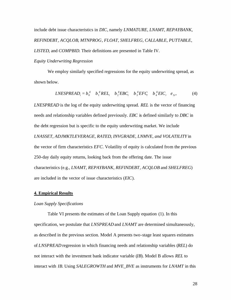
windows have a length of less than two years. Table III provides a summary of financing
windows constructed by this method.16 The last two rows of the table show the number of
windows in our dataset broken down by the number of events in the window and the
average length of the windows (in months). Not surprisingly, most of the windows have a
pair of events occurring less than one year apart. This fact explains why varying the
definition of windows has little effect on our findings.
Determining Lead Financial Institutions
The mergers, acquisitions, and reorganizations among financial institutions make
it difficult to identify all banks/subsidiaries within a bank holding structure through time.
To overcome this challenge, we develop an additional dataset containing the identities of
large bank holding companies, their subsidiaries, and merger histories, in order to
uniquely identify each financial institution in the dataset through time.17 We assign a
unique ID to all banks/subsidiaries within the same holding company. When mergers
occur, the IDs are updated to reflect the new holding company. Similarly, unique IDs are
assigned to all investment banks in our dataset.
In addition, several financial institutions usually participate in loan syndications
or joint security underwriting. However, the degree of participation and the influence in
15 We also defined the financing window with a 6-month events gap, as opposed to one year. The conclusions of the paper are insensitive to that alternative specification. 16 Because our dataset is left-truncated in 1992, we exclude all windows where the first event we observe occurs in 1992, since it is unclear whether those windows actually start in 1992 or at an earlier date. 17 Merger data are available from the BHC database provided at the Federal Reserve Bank of Chicago website. We also manually verify bank merger history and holding company structure with the website of the National Information Center of the Federal Reserve System for accuracy.

19
deal pricings vary according to their roles in the transaction. We credit a financial
institution with the transaction only if it has a leading role as the originator or underwriter
of the transaction. Specifically, the lead lenders for loans are defined as lenders with
agent title in loan syndication documentation (e.g., managing agent, syndication agent,
documentation agent, administrative agent) or act as the lender and arranger in non-
syndicated loans. For underwriting deals, we adopt the definition of lead managers from
the SDC database, where lead managers are defined as those with the role of book runner,
joint book runner, or joint lead manager. Therefore, it is possible in our dataset that a loan
or underwriting has multiple lead lenders or lead underwriters, which may give rise to
ambiguity in defining bank-firm relationship. We devise quite a robust approach to
handle this situation and will elaborate further below.
Constructing Control Variables for Firm Financing Needs
Having constructed financing windows that define combinations of transactions,
and their sequence, we proceed to define firm financing needs for each of the events
within the financing windows (loans, debt offerings, and equity offerings) according to
the existence of other events within the windows. We use the following six dummy
variables that are designed to capture patterns of firm financing strategies by describing
the temporal relationship between the current event and all the other events in the same
window: PL, PD, PE, SL, SD, and SE. The variables PL, PD, and PE equal one,
respectively, if there are other loan, debt, or equity events preceding the current event
within the financing window. Whereas SL, SD, and SE equal one, respectively, if there
are other loan, debt, and equity events subsequent to the current event within the
financing window. These six dummy variables are clearly defined for each event in a

20
financing window regardless of the identities of the lenders/underwriters involved in the
event and can be used in the regressions to control for unobserved heterogeneity among
firms related to differences in the patterns of their financial needs, per se.
Constructing Proxies for Relationship Variables
In the context of our ana lysis, we define a relationship between a bank and a firm
as the repetition of this bank-firm pairing in multiple events within the financing window.
Therefore, a bank-firm relationship can take the form of repeating loans, repeating debts,
repeating equities, or any combination of these transactions by this bank-firm pair within
a window.
When all of the lead lenders/underwriters for all events within a financing
window are unique, we identify this window as an unmatched window. In this case, a
firm uses different lenders/underwriters of all events in the window and there is no
identifiable relationship in the window. Clearly, a single-event window is an unmatched
window by definition. A financing window is a matched window when one or more lead
lenders/underwriters in the window (as identified by the ir unique IDs defined earlier) lead
more than one transaction within the window. Therefore, it is possible to have several
relationships embedded within a matched window. Figure 1 provides a diagram depicting
the classification of events for different type of windows and relationships.
First, consider the cases of unmatched windows. By construction, all events in the
unmatched windows are unmatched events. We use these events as a control group to
isolate the effects of relationship on deal pricings. When an unmatched event involves a
single lead financial institution, the identity and characteristic of lead institution to be
used in the regressions are obvious. However, it is less clear when there are multiple lead

21
bankers in the event. One possible approach for the regression analysis is to include all
possible bank-firm pairings from each event in the regressions. For example, a two-event
window comprised of a loan (with two lead lenders) followed by a debt underwriting
(with two lead underwriters) creates four possible observations for the regression analysis
(two observations for loan regressions and two observations for debt regressions). This
approach essentially double-counts some events, thus may suffer from non-random
sampling bias induced by the correlation among observations from the same event.
Instead, we handle unmatched loans with multiple lead institutions by randomly
assigning a lead institution to each event in order to create a unique bank-firm matching.
This approach to assigning bank-firm matches to our control (unmatched) group does not
introduce any systematic bias in measuring the effects of relationships on deal pricings,
which is evident in our robustness tests (not reported).18
In a matched window, if only one financial institution is involved in multiple
events in the window, then there is a unique relationship in this window. We simply
assign these matched events to the relationship bank in the regressions and discard any
unmatched events from the analysis. However, when more than one financial institution
leads (or jointly leads) multiple events in the window, we include only events from the
financial institution with the strongest relationship in the regressions, where the strength
18 In results not reported here, we perform the following robustness tests for our approach to randomly assigning a lead banker to each event. For the first robustness test, we redraw several trials of the random assignment of a banker-firm match for the set of unmatched loans. Our regression results are practically unchanged from one trial to another. For the second test, we average lender/underwriter characteristics across all banks and assign the average value to that event in the regressions. In our specification, the only lender/underwriter characteristic used in the regressions is the lending/underwriting market shares. In addition to the IB dummy variable, whose value indicates the fact that the event involves exclusively investment banks, we also include a dummy variable MIX to indicate mixed commercial and investment banks deal (the base case regression corresponds to deals that are done exclusively by commercial banks). The regression results for these robustness tests are very similar to the ones reported here in the paper.

22
of a bank-firm relationship is measured by the number of repeated transactions done by
that relationship bank within that window.19
In 2,377 of our 4,411 matched window observations for loans, we identify unique
matches within the window (that is, transactions involving a matched bank-firm
relationship where there is no other bank-firm matching occurring within the window). In
1,533 other transactions, there is more than one matched relationship within the window,
but we are able to identify a dominant matched relationship. In the remaining 501 cases
where more than one institution has the same number of repeated events in the window,
we randomly select one of the bank-firm relationships as the matched relationship for that
window. As in the case of the random assignment of unmatched bank-firm relationships,
this method avoids double counting of matched observations. We test, and confirm, the
robustness of our reported results to alternative random choices of bank-firm matches,
and also to the alternative sampling method of using only the 2,377 unique matches in
our sample.20
Once we identify the strongest relationship bank within the matched windows, we
define another set of six indicator variables, namely MPL, MPD, MPE, MSL, MSD, and
MSE, to capture the pattern of matching across transactions within the window. These
variables, MPL, MPD, MPE, MSL, MSD, and MSE, equal one when the corresponding
events (i.e. PL, PD, PE, SL, SD, and SE) involve the same financial institution as the one
in the current event. For instance, MPD as well as PD equals one if the current loan event 19 For an event with multiple lead bankers, it can simultaneously be part of several relationships within a window. Therefore, the approach we adopt here in defining the strongest relationship also handles the issues that arise from the events with multiple lead financial institutions. 20 In the Appendix Tables III , we present our loan spread regressions where we restrict our samples to include only events from unmatched windows and matched windows with a unique bank relationship, to test whether our conclusions are sensitive to our specific approach in assigning a relationship bank to a matched window with multiple relationships. The regression results in this case are similar to what we report in the next section of the paper.

23
is preceded by a debt offering that is underwritten by the same bank as the current loan.
Table IV provides descriptions for all twelve relationship variables defined earlier, along
with the definitions of other variables used in this study.
Table II in the Appendix provides two examples for matched windows to
illustrate how the relationship variables are determined. Example 1 illustrates the case
where there is only one lead banker for each event in a window with multiple
relationships. Example 2 in the same table illustrates the case of multiple lead bankers
within a window with multiple relationships. In both examples, bank B is involved in
three matched transactions compared to two transactions by bank A and one transaction
by bank C. We therefore include only the observations led by bank B in the regressions
based on the criteria that bank B has the highest number of repeated events within both
windows. In particular, we only include the second, the fourth and the fifth events in
example 1 in the regressions. Whereas, in example 2, we include all three events in the
regressions but only associate these events to bank B.
Loan Regressions
The endogenous variables of interest for the loan regressions are the loan spread
(all- in-spread) and the loan amount. We choose a log specification to be consistent with
positivity of loan spread and quantity and to transform these variables to be closer to a
normal distribution. 21 As discussed previously, we allow the loan spread and loan amount
to be determined jointly in the following system of simultaneous equations, where
equation (1) is the Loan Supply Equation, and equation (2) is the Loan Demand Equation.
0 1 2 3 4 5 1 1s s s s s s
i i i i i i i iLNSPREAD REL LEC LOC BC SUP LNAMTβ β β β β β γ ε= + + + + + + + (1)
21 Our results are not sensitive to this log transformation. We obtain very similar results using the basis point spread and the dollar loan amount.

24
0 1 2 3 4 5 2 2d d d d d d
i i i i i i i iLNAMT REL LEC LOC BC DEM LNSPREADβ β β β β β γ ε= + + + + + + + (2),
where:
- LNSPREAD is the natural log of the loan all- in-spread,
- LNAMT is the natural log of loan amount,
- REL is a vector of dummies for financing needs and relationship variables
(defined above) which can interact with dummies for the type of financial
institution,
- LEC is a vector of lender characteristics,
- LOC is a vector of loan characteristics,
- BC is a vector of borrower characteristics,
- SUP is a vector of loan supply shifters unrelated to loan demand, and
- DEM is a vector of loan demand shifters unrelated to loan supply.
Crucial to our ability to identify equations (1) and (2) as Loan Supply and Loan
Demand is our ability to construct plausible measures of SUP and DEM. We include
variables PRIME and SUBORDINATE in SUP. These variables are assumed to primarily
influence loan supply terms and to be unrelated to demand. Calomiris and
Pornrojnangkool (2005) and Beim (1996) document pricing premium for loans that are
indexed to the prime rate (instead of other, market-based indexes, such as Libor). Loan
subordination also reduces default risk to the lenders and should have negative impact on
loan prices but should be relatively unrelated to loan demand.
We include two measures of lender characteristics (LEC) in both the Loan Supply
and Loan Demand equations. These are the variables MULTIPLELENDER, and
LNTOTLENDING. MULTIPLELENDER is an indicator variable for syndicated loan. The

25
lead lender in a syndicated loan may have less pricing power due to the fact that other
members of the syndicate may insist that the loan is priced at market terms.
LNTOTLENDER is the log of the aggregate amount of lending made by the lead lender
for a given year. This variable is a proxy for the lender’s reputation and any lender size
effect. We expect these two LEC variables to have negative impacts on the loan spread.
For Loan Demand, the variables SALEGROWTH and MVE_BVE (the ratio of the
market value of equity to the book value equity) are used as proxies for growth and hence
the funding needs of borrowers, which drive demand. We assume that these two variables
do not influence loan pricing beyond the default risk that has already been captured by
other control variables in the system with which they may be correlated (which are
captured, inter alia, by debt ratings and leverage). If these identifying assumptions are
reasonable, then the coefficients of this system can be consistently estimated using two-
stage least square, where DEM is used to instrument LNAMT in equation (1) and SUP is
used to instrument LNSPREAD in equation (2). Alternatively, the coefficients of these
equations can potentially be estimated more efficiently by GMM. In the next section, we
report the results for both the 2SLS and GMM methods, together with various
specification tests for the endogeneity of LNAMT and LNSPREAD, the validity of the
instruments, and the overidentification restrictions.
The other control variables used are as follows. REL is a vector of variables which
consists of the variables PL, PD, PE, SL, SD, SE, MPL, MPD, MPE, MSL, MSD, MSE,
and their interaction with the variable IB (a dummy variable which equals one is the lead
financial institution in the event is an investment bank, and zero otherwise).

26
We include the following loan characteristic variables in LOC : LNMATURE,
TERMB, TERMBSUB, REVOLVER, STREVOLVER, BRIDGE, COMBODEAL,
PERFPRC, and SECURE, together with the following indicator variables that capture the
purpose use of loan: TAKEOVER, CAPRESTRUC, CPBACKUP, DEBTREPAY,
BUYOUT, and WORKCAP. Most of these are standard control variables for loan
characteristics that are used successfully in previous loan pricing studies (e.g., Calomiris
and Pornrojnangkool 2005). Their definitions are provided in Table IV, together with the
rest of the variables used in this paper. One point worth noting is that we distinguish
revolvers of less than one year from revolvers of greater than one year. Bank capital
regulation requires banks to hold additional capital against undrawn revolvers with a
maturity greater than one year. We thus expect STREVOLVER to have negative impact on
loan spread in the Loan Supply Equation.
The variables included in BC control for the borrower characteristics that
influence loan terms. LNASSET is used to capture the effect of borrower size.
ADJMKTLEVERAGE is the market value measure of leverage, and is adjusted for any
loan, debt, and equity transactions that have occurred since the last available financial
statements, in order to better reflect the borrower’s riskiness at the time of the loan event.
We use the market value of equity instead of the book value of equity in the calculation
of leverage. We also include dummies for S&P’s long-term senior credit ratings in the
regressions. Roughly one-third of our observations have no rating data. We employ an
ordered Probit model to impute credit ratings for observations where no rating data are

27
available.22 The indicator variable RATEFORE, which indicates whether ratings are
forecasted by the model rather than provided by the ratings agency, is included to capture
any systematic difference between firms that are rated and firms that are not.
Debt Underwriting Regression
We estimate the following, non-structural regression for total debt underwriting
spreads, where total spreads include management fees, underwriting fees, selling
concessions, and other direct expenses related to the administration and marketing of the
offering. We include these direct expenses into the definition of underwriting spreads to
better reflect total costs associated with security offerings.
0 1 2 3 4 3D D D D D
i i i i i iLNDSPREAD REL DBC DFC DICβ β β β β ε= + + + + + . (3)
LNDSPREAD is the natural log of the debt underwriting spread relative to the amount of
proceeds raised, expressed in basis points of the total amount of proceeds. REL is defined
similarly to the way it was defined in the loan regressions. DBC is a vector of underwriter
(bank) characteristics, which is comprised of MULTIPLEBANKER and
LNTOTDEBTUNDERWRITING. They are defined similarly to the control variables for
lender characteristics (LEC) in the Loan Supply equation, but are specific to the debt
underwriting market. DFC is a vector of firm characteristics, which includes the log of
firm assets (LNASSET), a market-value measure of adjusted leverage
(ADJMKTLEVERAGE) defined similarly to the measure used in the loan regressions, and
an indicator variable for an investment grade-rated firm (INVGRADE).23 Lastly, we
22 The Appendix includes the results of the ordered probit model used in this study, together with the results from the loan spread and loan amount regressions when observations with no rating information are excluded. Our findings are robust to such exclusion. 23 Calomiris and Himmelberg (1999) use these firm-level observable characteristics to estimate equity underwriting costs. They use these cost estimates as proxies for external financing costs and explore their impacts on the investment behavior of firms.
28
include debt issue characteristics in DIC, namely LNMATURE, LNAMT, REPAYBANK,
REFINDEBT, ACQLOB, MTNPROG, FLOAT, SHELFREG, CALLABLE, PUTTABLE,
LISTED, and COMPBID. Their definitions are presented in Table IV.
Equity Underwriting Regression
We employ similarly specified regressions for the equity underwriting spread, as
shown below.
0 1 2 3 4 3 ,E E E E Ei i i i i iLNESPREAD REL EBC EFC EICβ β β β β ε= + + + + + (4)
LNESPREAD is the log of the equity underwriting spread. REL is the vector of financing
needs and relationship variables defined previously. EBC is defined similarly to DBC in
the debt regression but is specific to the equity underwriting market. We include
LNASSET, ADJMKTLEVERAGE, RATED, INVGRADE, LNMVE, and VOLATILITY in
the vector of firm characteristics EFC. Volatility of equity is calculated from the previous
250-day daily equity returns, looking back from the offering date. The issue
characteristics (e.g., LNAMT, REPAYBANK, REFINDEBT, ACQLOB and SHELFREG)
are included in the vector of issue characteristics (EIC).
4. Empirical Results
Loan Supply Specifications
Table VI presents the estimates of the Loan Supply equation (1). In this
specification, we postulate that LNSPREAD and LNAMT are determined simultaneously,
as described in the previous section. Model A presents two-stage least squares estimates
of LNSPREAD regression in which financing needs and relationship variables (REL) do
not interact with the investment bank indicator variable (IB). Model B allows REL to
interact with IB. Using SALEGROWTH and MVE_BVE as instruments for LNAMT in this

29
regression seems to work well. At the bottom of the table, we display results for tests of
the significance of these instruments in the first-stage regression of LNAMT on all
exogenous variables. Individually and jointly, these instruments are correlated with
LNAMT. We also implement a Hausman (1978) procedure to test the null hypothesis that
instruments are exogenous. In doing so, we regress the residual from the second-stage
regression on the list of all exogenous variables and construct a test statistics (N times the
R-squared from this residual regression, where N is number of observations in the
regression). The test statistic has an asymptotic distribution of Chi-Square with 1 degree
of freedom (the number of instruments minus endogenous variables). As shown in the
overidentification tests in the table, the value of the test statistic is 0.37 for model A and
0.26 for model B, indicating that one cannot reject the null of instruments exogeneity.
In addition, we utilize the instruments to test for the endogeneity of LNAMT in the
spread regression. If LNAMT is exogenous in the spread equation, then ordinary least
squares and two-stage least squares estimates of all coefficients should differ only by
sampling error. The test is implemented by first regressing LNAMT on all exogenous
variables to obtain its residual. Then, we add the residuals from this regression to the
spread regression (1) to obtain the OLS estimate. The t-statistics of the residual term in
this augmented spread regression can be used as a test statistics for the null hypothesis
that LNAMT is exogenous. Our t statistic has a value of -12.77 for model A, and -11.51
for model B. Thus, we clearly reject the null hypothesis that LNAMT is exogenous.
In our sample, it is interesting to see how the coefficient of LNAMT from the two-
stage least squares estimate differs from the coefficient from the ordinary least squares
estimate. We include the ordinary least square estimates of equation (1) in the Appendix

30
(Appendix Table IV). The coefficient for LNAMT in the ordinary least squares regression
is significantly negative whereas the coefficient for LNAMT in the two-stage least squares
regression is positive and significant. Since we interpret our spread regression as a Loan
Supply equation (by including supply shifter variables (SUP) in the equation), we expect
an upward sloping supply curve (a positive coefficient for LNAMT ). The ordinary least
squares estimator clearly is not consistent and suffers from simultaneity bias. This result
therefore confirms the validity of our approach in modeling Loan Supply and Loan
Demand as a simultaneous system of equations.
The coefficients for most variables in the Loan Supply equation are of the
expected signs and significant. Having multiple lenders (MULTIPLELENDER)
participating in the syndication significantly reduces the costs of borrowing. Larger and
more diversified lenders (LNTOTLENDING) can lend to borrowers at lower costs. Loan
characteristics also affect loan pricing in expected ways. In tranch B term loans
(TERMB), where lenders carry lower seniority than other lenders in the same term loan,
loan pricing is higher. The pricing premium is even greater for loans in lower trenches
(TERMBSUB). Revolvers carry lower spreads than term loans (tranch A) and short-term
revolvers have even greater discounts, perhaps reflecting the lower regulatory capital
required for short-term revolvers. The indicator variable SECURE is significantly
positive, as found in previous studies. This reflects unobserved (higher) riskiness of
borrowers that borrow in the form of secured loans. In addition, borrowers are charged
higher rates when term and revolving loans are packaged together in one deal
(COMBODEAL). We document a substantial PRIME premium in our sample, as found in
Beim (1996). The coefficient for SUBORDINATE is also significant and positive in our

31
sample. In our sample, the discount for “performance pricing” of loans is significant but
smaller than the discount reported in prior studies (e.g., Beatty and Weber 2000). We
also include time and industry dummies, which are omitted from the table.
Table VII presents a GMM estimator for the Loan Supply equation, where we
utilize the cross-equation correlation of the error terms in the estimation and allow for a
general form of heteroskedasticity. The GMM estimator is asymptotically more efficient
if the model is correctly specified. The results are remarkably similar.
Effects of the Patterns of Financing Needs and Relationships on Loan Prices
As we discussed in our review of the literature, one potential shortcoming of
existing studies is their insufficient controls for heterogeneity among borrowers. In
particular, unobserved heterogeneity may drive patterns of borrowers’ financing needs,
which in turn may influence loan pricing, and may be correlated with relationship
indicator variables. Thus, omitting financing pattern variables from the regressions can
make estimates inconsistent and provide misleading estimates of the effects of bundling
on loan pricing. In our regressions, we include variables PL, PD, PE, SL, SD, and SE as
proxies for unobservable heterogeneity.
We find several consistent results across our specifications, which indicate the
importance of controlling for financing patterns. First, loans that occur around the time of
debt offerings receive pricing discounts from both universal and investment banks,
regardless of whether the lender and underwriter are matched (the coefficients of PD and
SD are negative). Interestingly, we do not find the same result for loans around the time
of equity offerings. This finding is consistent with a “road-show” effect, in which
information regarding creditworthiness of borrowers is transmitted to the market

32
surrounding a debt offering in a way that reduces information gathering costs for the
surrounding loans. Second, a loan that is followed by another loan (SL) is priced slightly
higher than a single loan. This occurs regardless of whether the loans are matched or not.
Third, investment banks price loans significantly higher than universal banks, in general
(the coefficient for IB is positive and significant). Investment banks’ loan spreads are
about 8% higher in model A, ceteris paribus, and the effect is even larger (11%) in model
B, where we allow the IB interactions. This finding indicates that investment banks suffer
a basic cost disadvantage relative to commercial banks in originating loans. It is possible
that commercial banks’ special access to the payment system reduces their costs of
originating loans.24
Turning to the effects of bundling lending and underwriting, our results for
matched loans (whose lenders also underwrite other transactions within the same
financing windows) differ from the results of existing studies. Matched loans, whose
lenders provide other loans or underwrite other debt issues within the same financing
windows, are priced similarly to unmatched loans, ceteris paribus. That finding is
consistent with the study of Fraser, Hebb and MacKinnon for the matching of loans and
debt underwritings. For loans that are matched to equity underwritings, we find that
matching has differing effects on loan pricing depending on the sequencing of the
transactions and the identities of the lenders. If matched loans occur before equity
underwritings, both universal banks and investment banks price these loans significantly
24 At least two possible influences may be important. First, the payment system may afford special information to banks about borrowers by virtue of the fact that banks can monitor debits and credits flowing in and out of the firm’s accounts. A second possibility, which applies to revolving lines of credit, is that linking the line with a checking account may economize on transaction costs of accessing the line.

33
higher than their unmatched counterparts. However, if loans are granted after matched
equity offerings, then there is a loan pricing discount that only investment banks provide.
Drucker and Puri (2005) utilize different econometric techniques in their analysis
and report evidence that only universal banks (not investment banks) provide discounts
for loans to the borrowers who also use their equity underwriting services around the
time of loans. They interpret their findings to be consistent with the existence of
economies of scope between the joint production of loans and underwritings, whose
benefits are passed on to borrowers in the form of a loan pricing discount. In their study,
however, they do not include our controls, model lending structurally, or consider
differences in loan pricing that result from differences in the sequences of loans and
equity offerings. Our results indicate that such distinctions result in qualitative
differences in estimated effects of bundling.
Our finding of a loan pricing premium preceding matched equity underwritings
does not support the notion that universal banks underprice their loans to win future
security underwriting business. Quite the opposite. Perhaps underwriters utilize their
ongoing equity underwriting relationship to over-price loans that immediately precede
equity offerings. Typically, equity underwritings are lengthy and complex processes. It is
not uncommon for a successful equity underwriting to take more than one year from
inception to completion. Therefore, it is possible that matched preceding loans are
granted after the firm has decided to underwrite equity. Because the debt underwriting
process is less complex and debt offerings are substitutes for loan, it may be more
difficult for debt underwriters to leverage their underwriting relationships to increase
their spreads in the lending market. Our findings suggest that illegal tying is not

34
prevalent, since a necessary condition for tying is the discounting of loans in anticipation
of underwritings – a phenomenon not apparent in the data.
Our finding that loan pricing discounts are offered only by investment banks, and
only when loans are preceded by matched equity underwritings, is consistent with the
notion that investment banks suffer cost disadvantages relative to commercial banks in
providing loans (i.e., the positive coefficient for the IB indicator). Investment banks may
compete with universal banks in the loan market by providing “rebates” through loan
pricing discounts only for loans that are closed after matched equity offerings. In this
regard, it is interesting to note that the coefficients on IB (0.11) and IB_MPE (-0.19) are
of roughly similar magnitude.
It is clear from our findings thus far that loan pricing in the presence of an
underwriting relationship does not merely reflect the physical scope economies between
lending and underwriting, as previous studies have posited. Banks also utilize loan
pricing in a strategic way to extract va lue from existing relationship with firms (by
selectively charging “premiums”), and also as a tool to compete with competitors (by
selectively offering “rebates”).
Universal banks seem to enjoy cost advantages in providing loans, in general.
This may explain universal banks’ growing share of the underwriting market. So long as
there are either expected savings to customers from bundling (which can take the form of
initial discounts to attract clients, partly offset by rent extraction in later years through the
charging of loan premia, as in Rajan 1922, or better price performance on securities
offerings, or physical, non-pecuniary savings of transaction costs to customers from
bundling), and as long as universal banks can perform underwriting services as

35
effectively as investment banks, then universal banks should attract a growing share of
the underwriting and lending markets. Given the fact that most universal banks acquired
existing investment banking franchises to participate in the underwriting market, there is
no obvious reason to presume that universal banks are not able to underwrite securities as
effectively as investment banks. Below, we investigate that question empirically.
We also report Loan Supply estimates using GMM estimators. The results are
similar and are presented in Table VII. Our instruments pass a GMM overidentification
test, which confirms our choice of instruments.
Loan Demand Specifications
Two-stage least squares estimates of the Loan Demand equation are presented in
models C to E in Table VI. The sign of LNSPREAD is negative and significant,
confirming the demand interpretation of the equation. Our instruments for LNSPREAD
also work well. In the first-stage regression, PRIME and SUBORDINATE are very
significant instruments in expla ining LNSPREAD, as shown at the bottom of the table. In
addition, we can not reject the null hypothesis that our instruments are exogenous in the
overidentification test, which validates our choices of instruments.
Our demand shifter variables (SALEGROWTH and MVE_BVE) are both positive
and significant. A higher growth firm has higher loan demand. Borrowers with higher
loan demand use larger lenders and often use loan syndication. Borrowers who use lower
tranch loans (TERMB and TERMBSUB) tend to have higher demand for funds. Revolvers
typically are associated with larger loan size than standard term loans. Borrowers who are
willing to have their loans secured tend to have larger demand for credit than those who
do not secure their loans. Borrowers tend to demand larger loans when the loans are for a

36
specific purpose such as a takeover, a bridge loan, or a debt repayment. Borrowers with
better credit ratings tend to have less demand for credit, and more leveraged borrowers
tend to have higher demand for credit. We include time and industry dummies, which are
omitted from the table. Results are similar using a GMM estimator and the instruments
for LNSPREAD in the Loan Demand regression pass GMM overidentification tests.
Effects of Patterns of Financing Needs and Relationships on Loan Demand
For the variables that capture patterns of financial need, we find that firms that
recently issued debts (PD) have lower demand for loans, and that firms that recently
issued equities or plan to issue equities (PE or SE) have higher demand for loans
regardless of whether the loans are matched.
For relationship variables, we observe consistently negative signs for the
coefficients of matched loans regardless of which particular transactions are matched
with these loans (i.e., negative signs for MPL, MPD, MPE, MSL, MSD, and MSE). In
model E, we restrict the model by requiring that all relationship dummies are equal (as
shown in MATCH and IB_MATCH variables at the bottom of the table). The result
indicates that bundling, in general, is associated with lower loan demand.25
Sub-Samples Analysis
Table VIII presents the GMM estimates of spread regressions broken down by
time and borrower sales.26 The evidence of a loan pricing premium on loans that precede
matched equity transactions holds when we split our sample pre- and post-1998, but
25 This finding may reflect another valuable aspect of banking relationships. Borrowers who maintain close relationships with their banks (as reflected in matched transactions) may have access to implicit “credit lines” from their relationship banks. They may consequently have less need for large explicit credit lines or large loans, which could result in substantial interest savings for borrowers through time. This result holds for both universal banks and investment banks. 26 The results are similar for the two -stage least squares estimators.

37
results are more significant post-1998, which corresponds to the period when the Glass-
Steagall Act was no longer in effect. This pricing premium applies across the borrower
size spectrum, although the coefficients for MSE are not significant for the smallest size
borrowers (with less than $250 million in annual sales) and the largest size borrowers
(with more than $10 billion in annual sales). This finding is consistent with our previous
interpretation that the MSE premium reflects bank quasi rent extraction by virtue of their
relationships. In our sample, there are few MSE transactions for the smallest size category
of borrowers, which can explain the larger standard errors for that coefficient. For the
largest borrowers, we hypothesize that the underwriting market is highly competitive
(i.e., lenders lack significant private information about these borrowers) so that banks
seeking to exploit their relationships to extract quasi rents (as in Rajan 1992) would fail
because they have no market power in the lending market.
The sign for the coefficients of IB*MPE is consistently negative pre- and post-
1998 and across borrower sizes. However, the coefficients are significant only for the
post-1998 period and for large borrowers (those with annual sales more than $1 billion).
This finding is also consistent with the hypothesis that investment banks suffer cost
disadvantages relative to universal banks in providing loans, and therefore, are forced to
compete in the loan market by providing “rebates” of their underwriting fees in the form
of pricing discounts for loans that follow equity offerings. Since this “rebate” is costly, it
is logical for them to offer it only when they have to do so (i.e., on deals where revenue is
large, and for which the competition from universal banks is strongest – namely loans to
large borrowers). Other regression results from the sub-samples are similar to those for
the whole sample, and thus we do not report them.

38
Debt Spread Regressions
Both our debt and equity underwriting spread regressions, shown in Table IX,
have high explanatory power, as is evident from the adjusted R-squareds of 0.78 and 0.74
for the debt and equity underwriting spread regressions, respectively. Our control
variables in the debt underwriting spread regressions shown in Table IX have the
expected signs and most are significant. Large underwriters
(LNTOTDEBTUNDERWRITING) appear to be able to underwrite debt issues more
efficiently and at lower cost, although it is also possible that the underwriter size effect
reflects unobserved heterogeneity of clients (riskier, and therefore, hard-to-underwrite
firms may be attracted to smaller underwriters). Larger firm size (LNASSET) is associated
with reduced underwriting costs for debt issuers. Higher leverage (ADJMKTLEVERAGE)
is associated with higher underwriting costs, while having long-term debt rated as
investment grade (INVGRADE) reduces underwriting costs. In addition, the underwriting
costs are lower when the proceeds of the debt offerings are used for existing debt
repayments or refinancings (REPAYBANK or REFINDEBT ). Having floating interest debt
(FLOAT), being registered in an MTN program (MTNPROG), or using a competitive
bidding process (COMPBID) for selecting underwriters reduces underwriting costs.
Finally, more complex debt structures such as callable and puttable features (CALLABLE
and PUTTABLE) increase underwriting costs for the issues.
With respect to bundling, we find that debt offering transactions that are
matched with loans are associated with higher spreads than unmatched counterparts (i.e.,
we find significantly positive coefficients for MPL and MSL) for both universal and
investment banks. This finding is consistent with the hypothesis that relationship banks

39
can extract value from their relationships. In this context, banks extract value from
relationships in the form of higher underwriting fees for matched loan and debt
transactions. Recall the results from the loan regressions, where we found significant
discounts for loans surrounding debt offerings due to a “road show” effect, whether these
loans are matched or not. Therefore, for matched debt and loan transactions, borrowers
pay less of an interest spread for their loans but the discounts are offset to some extent by
higher debt underwriting costs. In addition, we find that issuers pay less when debt
offerings are done consecutively, which we see as a variation on the “road show” effect.
Interestingly, we also find that, in general, it costs more to use specialized investment
banks than universal banks to underwrite debts.
Equity Spread Regressions
As in the debt regressions, we find that larger underwriters underwrite equity at
lower costs (LNTOTEQUNDERWRITING). Using joint underwriters
(MULTIPLEBANKER) increases total underwriting costs. We also find that market
capitalization (LNMVE), asset size (LNASSET), and the size of the equity offering
(LNAMT) are associated with significantly reduced underwriting costs, whereas leverage
(ADJMKTLEVERAGE) and equity volatility (VOLATILITY) are associated with higher
underwriting costs for equity offerings. The negative coefficient for SHELFREG and the
positive coefficient for ACQLOB are similar to those in the debt spread regressions.
With respect to the relationship variables, we find two results that are similar to
the debt underwriting regressions. First, investment banks in general underwrite equity
offerings at higher costs than universal banks, ceteris paribus (i.e., there is a significantly
positive coefficient for IB). Second, when there are matched loans surrounding equity

40
offerings, both universal banks and investment banks underwrite the issues at higher
costs than unmatched transactions. This finding together with the finding of a positive
coefficient for MSE in the loan spread regressions provide consistent evidence that both
universal and investment banks are able to extract value from their banking relationships
through higher loan and underwriting spreads in the matched windows in which loans are
followed by equity offerings. (Recall that we find a significant negative coefficient for
IB*MPE in the loan spread regressions.) It appears that investment banks provide a loan
pricing “rebate” after they capture an underwriting fee premium for matched transactions.
5. Conclusions
We investigate how the formation of banking relationships, and the bundling of
financial services that occurs within those relationships, affect the pricing of loans and
the underwriting costs of issuing securities. In particular, we investigate the alleged
practice of loan under-pricing (and potentially, illegal tying) as tools for universal banks
to compete more effectively as underwriters. In doing so, we revisit the existing literature
that uses micro- level loan and underwriting data to investigate the costs and benefits of
the joint production of loans and security underwritings within the context of relationship
banking.
Our research methodology addresses several shortcomings in current studies.
First, we incorporate important control variables into the analysis of the effects of
relationships on pricing, and in particular, we consider the pricing of financial
transactions within the context of the sequential patterns of financing transactions
undertaken by firms. Firm and deal characteristics, as well as the sequencing of
transactions, turn out to be important sources of firm heterogeneity, and incorporating

41
these effects has significant consequences for measuring the effects of relationships on
pricing. We construct a dataset that captures nearly complete financing transaction
histories for 7,315 firms comprising loan, debt, and equity transactions for the period of
1992 to 2002. Second, we explicitly identify the effects of bundling on loan supply by
imposing identifying restrictions on supply and demand that allow us to estimate loan
supply and loan demand functions. Third, we consider the pricing of several financial
services supplied within financial relationships, including loan pricing, debt underwriting
costs, and equity underwriting costs.
All of our regressions have high explanatory power. We report several interesting
findings. First, our findings contradict other studies that had found evidence that
universal banks under-price loans to gain an in-road into the underwriting market. Our
findings, therefore, also imply an absence of illegal loan tying.
Second, we find evidence of strategic aspects of the pricing of loans and
underwriting services. Banks are able to use their valuable relationships to over-price
loans (as predicted by Rajan 1992) that precede equity underwritings. We also find
pricing premiums for both debt and equity underwriting services that are matched with
loans within the same financing windows. Investment banks have different pricing
strategies than universal banks, reflecting the fact that investment banks apparently
operate at a cost disadvantage with respect to universal banks. That is, controlling for
other differences, investment banks price loans, and debt and equity underwriting
services, higher than universal banks. The cost disadvantage of investment banks may
explain why they price bundled transactions somewhat differently from universal banks,
too. Investment banks compete with universal banks in the loan market by providing loan

42
pricing discounts as “rebates” to borrowers who had employed them in preceding equity
underwriting transactions.
Our findings that banks appear to be able to extract quasi rents from their
relationships (charge premium on loans and underwritings) might seem to imply that
relationships are harmful to bank customers, but that is not the case. Unless there are
substantial benefits accruing to the borrowers from forming relationships and choosing to
bundle transactions, relationship banks should not be able to extract quasi rents from their
relationships through pricing premiums in bundled transactions. In the Rajan (1992)
model, customers freely choose and benefit from relationship formation, and receive up-
front concessions early on in their banking relationships which compensate for the quasi
rents banks later extract. Furthermore, relationships can entail benefits for customers
other than initial price discounts on loans and underwritings at the time of relationship
formation. One possibility is that bundling economizes on transaction costs (saved “face
time,” for example). Another possibility is that richer banking relationships increase the
prices of debt and equity securities underwritten by bankers. Still another possibility is
that relationships may reduce the need for some bank services. Our results from the
estimation of Loan Demand suggests that bundling may reduce the demand for loans,
possibly because stronger relationships entail an implicit “credit line,” which substitutes
for an explicit one. That reduction in the demand for credit could result in substantial
interest savings.
A more fundamental implication of our findings about the strategic pricing of
financial services is that empirical models of loan pricing and underwriting need to take
bank strategies into account, and not presume that physical scope economies will

43
necessarily be reflected in pricing decisions. Observed prices do not merely reflect the
cost functions of banks.
Third, we find evidence of “road show” effects for debt underwritings. The
similarity between the information produced in debt underwriting and loans seems to
result in pricing discounts for loans that occur near debt issues, and this result holds for
both universal and investment banks, whether the loans are bundled with the offerings
(matched with the same bank) or not. In addition, and similarly, we find that consecutive
debt offering have lower underwriting costs than stand alone debt offerings.
From the conclusions of this study, several questions remain and should be
addressed by further research. In particular, more investigation is warranted of the
possible advantages that customers receive from bundling, which could take the form of
improved prices on debt and equity securities, transaction costs savings that accompany
bundling, and possible savings from implicit “credit lines.” Second, further study is
needed to understand the relative efficiency of universal banks as compared with
investment banks – that is, why do investment banks systematically charge higher interest
rates on loans and higher fees for their underwriting services? The key difference
between the two intermediaries is the access to deposits and the payment system enjoyed
by commercial banks (which may provide favorable information processing capabilities
about borrowers, and lower transaction costs for providing revolving lines of credit), as
well as their access to the government safety net (i.e., deposit insurance, and access to
Fed overdrafts and the discount window).

This table presents the number and the dollar volume of loans to non-financial, non-regulated, and non-governmental borrowers in the U.S. from Loan Pricing Corporation's DealScan database. Specifically, we exclude all borrowers with first-digit SIC code 6 and 9 and highly regulated industries with first 2-digit SIC code 43, 45 and 49. In Panel A, the data are broken down by various types of lending financial institutions for the period from 1992 to 2002. Panel B classifies loans by type of loans. Panel C classifies loans by distribution method. Only loans from the borrowers that can be matched to financial data from Compustat are included in this table.
Type of lenders Data items 1992 1993 1994 1995 1996 1997 1998 1999 2000 2001 2002 TotalBanks Only Number of Loans(% of Total) 93% 95% 95% 94% 92% 88% 87% 83% 85% 80% 83% 88%
Dollar Volumn(% of Total) 88% 95% 96% 81% 89% 83% 83% 70% 70% 66% 71% 78%IBs Only Number of Loans(% of Total) 1% 1% 1% 1% 1% 1% 1% 1% 2% 1% 1% 1%
Dollar Volumn(% of Total) 1% 3% 1% 2% 2% 1% 1% 1% 2% 1% 0% 1%Joint Banks & IBs Number of Loans(% of Total) 0% 0% 0% 2% 3% 6% 7% 11% 9% 13% 12% 7%
Dollar Volumn(% of Total) 8% 0% 2% 17% 9% 15% 15% 28% 28% 32% 28% 19%Other Lenders Number of Loans(% of Total) 5% 4% 4% 3% 4% 4% 5% 5% 4% 6% 4% 4%
Dollar Volumn(% of Total) 3% 2% 1% 1% 1% 1% 1% 1% 1% 2% 1% 1%
1992 1993 1994 1995 1996 1997 1998 1999 2000 2001 2002 TotalBridge Loans Number of Loans(% of Total) 1% 1% 1% 1% 1% 1% 2% 2% 2% 2% 2% 1%
Dollar Volumn(% of Total) 1% 3% 0% 2% 1% 2% 4% 4% 3% 6% 6% 3%364 day Facility Number of Loans(% of Total) 1% 4% 7% 6% 4% 6% 9% 12% 16% 17% 18% 10%
Dollar Volumn(% of Total) 12% 15% 21% 17% 11% 14% 28% 36% 42% 36% 44% 28%Letter of Credit Number of Loans(% of Total) 4% 4% 3% 2% 2% 2% 1% 1% 1% 1% 1% 2%
Dollar Volumn(% of Total) 1% 1% 1% 1% 0% 2% 2% 2% 2% 2% 0% 1%Lease Number of Loans(% of Total) 0% 0% 0% 0% 1% 1% 1% 1% 2% 2% 1% 1%
Dollar Volumn(% of Total) 0% 0% 0% 0% 0% 0% 1% 0% 1% 1% 0% 0%Other Number of Loans(% of Total) 5% 4% 3% 2% 1% 1% 1% 4% 3% 3% 2% 3%
Dollar Volumn(% of Total) 1% 1% 1% 1% 1% 1% 1% 2% 2% 1% 1% 1%Revolver Number of Loans(% of Total) 67% 66% 65% 69% 71% 67% 61% 52% 51% 52% 50% 60%
Dollar Volumn(% of Total) 72% 71% 69% 73% 78% 71% 49% 40% 38% 44% 35% 55%Term Loan Number of Loans(% of Total) 22% 21% 21% 19% 21% 22% 26% 29% 26% 23% 26% 24%
Dollar Volumn(% of Total) 14% 9% 9% 7% 8% 9% 16% 16% 12% 10% 13% 11%
1992 1993 1994 1995 1996 1997 1998 1999 2000 2001 2002 TotalSole Lender Number of Loans(% of Total) 42% 36% 26% 18% 24% 23% 19% 15% 7% 8% 7% 18%
Dollar Volumn(% of Total) 3% 2% 1% 1% 1% 1% 1% 0% 0% 1% 0% 1%Syndication Number of Loans(% of Total) 58% 64% 74% 82% 76% 77% 81% 85% 93% 92% 93% 82%
Dollar Volumn(% of Total) 97% 98% 99% 99% 99% 99% 99% 100% 100% 99% 100% 99%Total Number of Loans 965 1,145 1,358 1,361 1,738 1,955 1,906 1,934 1,869 1,798 1,548 17,577
Dollar Volumn (Billion) 113 175 248 310 337 437 369 415 464 482 395 3,744
Panel B: Loans classified by loan type
Table ISummary of DealScan Loan Sample
Panel A: Loans classified by type of lender
Panel C: Loans classified by distributiion method

This table presents the number and the dollar volume of debt and public equity offerings (both IPO and SEO) by non-financial, non-regulated, and non-governmental borrowers inthe U.S. from Securities Data Corporation's underwriting database. Specifically, we exclude all borrowers with first-digit SIC code 6 and 9 and highly regulated industries with thefirst 2-digit SIC code 43, 45 and 49. The data are broken down by security type and types of underwriting financial institutions for the period 1992- 2002.
Security Underwriter Data items 1992 1993 1994 1995 1996 1997 1998 1999 2000 2001 2002 TotalDebt Banks Only Number of Offering(% of Total) 10% 11% 13% 20% 22% 16% 34% 33% 38% 47% 58% 26%
Dollar Volumn(% of Total) 7% 7% 7% 12% 16% 15% 24% 31% 34% 48% 57% 28%IBs Only Number of Offering(% of Total) 90% 89% 87% 80% 78% 84% 66% 66% 60% 49% 35% 72%
Dollar Volumn(% of Total) 93% 93% 93% 88% 84% 85% 74% 67% 63% 44% 28% 68%Joint Banks & IBs Number of Offering(% of Total) 0% 0% 0% 0% 0% 0% 1% 1% 2% 4% 8% 1%
Dollar Volumn(% of Total) 0% 0% 0% 0% 0% 0% 2% 2% 3% 7% 15% 4%Debt Total Number of Offering 417 511 315 397 565 657 749 403 308 401 340 5,063
Dollar Volumn (Billion) 70 84 44 58 78 84 114 114 100 169 122 1,039Equity Banks Only Number of Offering(% of Total) 0% 1% 3% 3% 5% 12% 29% 27% 33% 30% 30% 13%
Dollar Volumn(% of Total) 0% 2% 4% 3% 3% 8% 26% 22% 20% 18% 20% 13%IBs Only Number of Offering(% of Total) 100% 99% 97% 97% 95% 87% 70% 72% 62% 61% 64% 86%
Dollar Volumn(% of Total) 100% 98% 96% 97% 96% 90% 72% 75% 69% 62% 72% 82%Joint Banks & IBs Number of Offering(% of Total) 0% 0% 0% 0% 0% 0% 1% 2% 5% 8% 6% 1%
Dollar Volumn(% of Total) 0% 0% 0% 0% 1% 1% 2% 3% 10% 20% 8% 5%Equity Total Number of Offering 663 884 705 820 1,141 858 531 743 649 310 295 7,599
Dollar Volumn (Billion) 36 48 35 56 81 66 64 111 125 65 49 736
Table IISummary of SDC Public Offering Sample
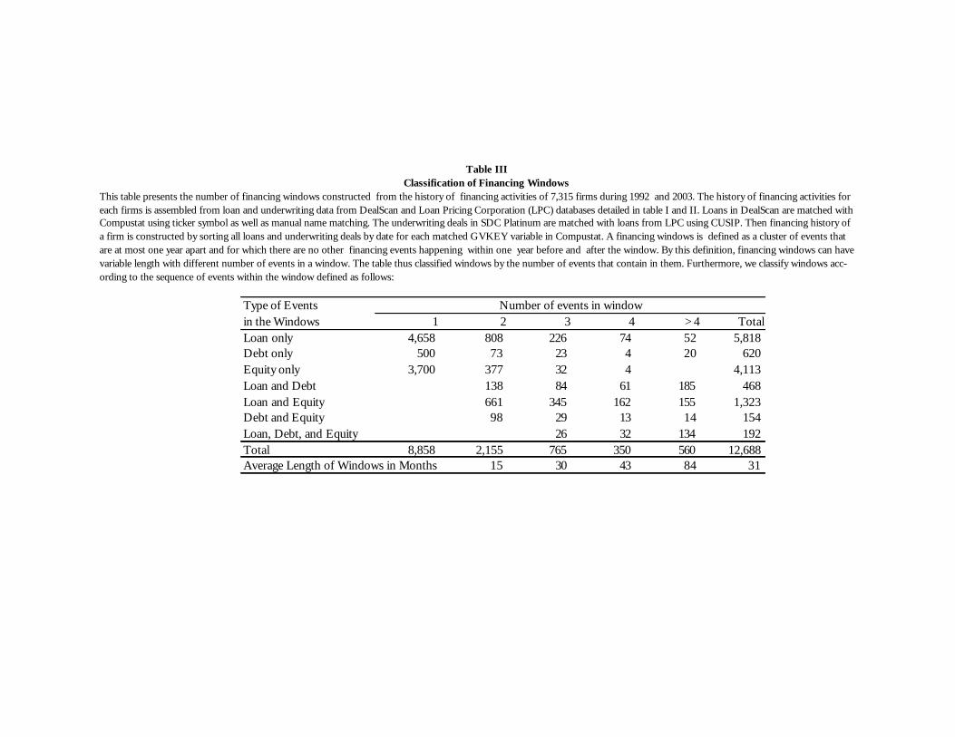
This table presents the number of financing windows constructed from the history of financing activities of 7,315 firms during 1992 and 2003. The history of financing activities for each firms is assembled from loan and underwriting data from DealScan and Loan Pricing Corporation (LPC) databases detailed in table I and II. Loans in DealScan are matched with Compustat using ticker symbol as well as manual name matching. The underwriting deals in SDC Platinum are matched with loans from LPC using CUSIP. Then financing history of a firm is constructed by sorting all loans and underwriting deals by date for each matched GVKEY variable in Compustat. A financing windows is defined as a cluster of events that are at most one year apart and for which there are no other financing events happening within one year before and after the window. By this definition, financing windows can have variable length with different number of events in a window. The table thus classified windows by the number of events that contain in them. Furthermore, we classify windows acc- ording to the sequence of events within the window defined as follows:
Type of Eventsin the Windows 1 2 3 4 >4 TotalLoan only 4,658 808 226 74 52 5,818 Debt only 500 73 23 4 20 620 Equity only 3,700 377 32 4 4,113 Loan and Debt 138 84 61 185 468 Loan and Equity 661 345 162 155 1,323 Debt and Equity 98 29 13 14 154 Loan, Debt, and Equity 26 32 134 192 Total 8,858 2,155 765 350 560 12,688 Average Length of Windows in Months 15 30 43 84 31
Classification of Financing Windows Table III
Number of events in window

Each transaction in a financing window defines an event. An event can be loan, debt offering, or equity offering. This tableprovides the definitions of dummy variables used to capture firm financing and bank relationship patterns. Table A1 in appendix provides an illustrative example of how the value of these dummy variables are assigned for a given event/transaction in a financing window.
Firm Financing and Bank Relationship Patterns
PL (has Preceding Loan)equals one if current event is preceded by at least one loan event in the same financing window.
PD (has Preceding Debt)equals one if current event is preceded by at least one debt event in the same financing window.
PE (has Preceding Equity)equals one if current event is preceded by at least one equity event in the same financing window.
MPL(has Matched Preceding Loan)
equals one if current event is preceded by at least one loan event in the same financing window and the preceding loan was from the same financial institution that is in the current event.
MPD(has Matched Preceding Debt)
equals one if current event is preceded by at least one debt event in the same financing window and the preceding offering was underwritted by the same financial institution that is in the current event.
MPE(has Matched Preceding Equity)
equals one if current event is preceded by at least one equity event in the same financing window and the preceding offering was underwritted by the same financial institution that is in the current event.
SL (has Subsequent Loan)equals one if current event is followed by at least one loan event in the same financing window.
SD (has Subsequent Debt)equals one if current event is followed by at least one debt event in the same financing window.
SE (has Subsequent Eq)equals one if current event is followed by at least one equity event in the same financing window.
MSL(has Matched Subsequent Loan)
equals one if current event is followed by at least one loan event in the same financing window and the subsequent loan is from the same financial institution that is in the current event.
MSD(has Matched Subsequent Debt)
equals one if current event is followed by at least one debt event in the same financing window and the subsequent offering is underwritten by the same financial institution that is in the current event.
MSE(has Matched Subsequent Equity)
equals one if current event is followed by at least one equity event in the same financing window and the subsequent offering was underwritten by the same financial institution that is in the current event.
IB equals one if the lender or runderwriter is investment bankLNTOTLENDING log of total dollar loan made by this lender last yearLNTOTDEBTUNDERWRITING log of total debt underwritten by this underwriter last yearLNTOTEQUNDERWRITING log of total equity underwritten by this underwriter last yearMULTIPLEBANKER equals one if the offering is joint underwritten by more than one underwriterMULTIPLELENDER equals one if loan is a syndicated loan with multiple lenders with agent titles
SIC2DEBTUNDERWRITERSHARE% share of debt offering done by this underwriter for companies with the same 2-digit SIC code
SIC2EQUNDERWRITERSHARE% share of eq offering done by this underwriter for companies with the same 2-digit SIC code
SIC2LENDINGSHARE % share of loans made by this lender to companies with the same 2-digit SIC code
Lenders or underwriters control variables
Definition of Variables that Capture Firm Financing and Bank Relationship PatternsTable IV
Variable Names (abb. For)

AAA,…,B are dummies for S&P senior debt credit ratingsLNAMT log of principle amount of loan or offeringACQLOB equals one if loan is acquisition line of creditBRIDGE equals one if loan is bridge loanCALLABLE equals one if debt issue is callable
COMBODEALequals one if multiple types of loans (eg term and revolver) are offered at the same time
COMPBID equals one if the underwriting fee is set by competitive bidding processFLOAT equals one if debt issue has floating rateLISTED equals one if company stocks are traded in the exchangeLNMATURE log of the number of days to maturity of loan or debt offeringLTREVOLVER equals one if loan is revolver loan with maturity more than 1 yearMTNPROG equals one if debt issue is a part of Medium-term Note programPUTTABLE equals one if debt issue is puttableREFINDEBT equals one if equity offering is for refinancing outstanding debtREPAYBANK equals one if equity or debt offering is used to repay bank loanSECURE equals one if loan is secured by assetsSHELFREG equals one if debt or equity offering has been shelf-registeredSUBORDINATE equals one if loan is a subordinated loanTERMB equals one if loan is tranch B term loanTERMBSUB equals one if loan is term loan with tranch lower than BPERFPRC equals one if loan has performance pricing provision (i.e. pricing grid)
ADJMKTLEVERAGE
(book debt+new debt+new loans)/(book debt+new debt+new loans+market value equity+new equity) where new transactioins are transactions that are yet to be reflected in latest accounting data
CURASSET_A current asssets/total assetsCURRATIO current ratioFWC_K financial working capital/fixed capitalINT_DEBT interest expenses/total debtsINTCOVER interest coverage ratioINVGRADE equals one if issuer's long-term senior debt is rated BBB or aboveINVTURNC sales/average cost of good soldINVTURNS sales/average inventoriesK_A properties, plant & equipment/total assetsLNAMT log of principle amount of loan or offeringLNASSET log of total assetsLNMVE log of market value of equityQUICKRATIO quick ratioRATED equals one if the issuer has credit rating
RATINGFORECASTequals one for borrower with no credit rating but uses forecasted rating in loan regressions
ROA return on assetROE return on equitySALEGROWTH growth of sales over the past yearMVE_BVE market value of equity/book value of equitySTD_A short-term debts/total assetsSTDEBTOVERDEBT short-term debts/total debtsSTREVOLVER equals one if loan is revolver loan with maturity equal or less than 1 yearVOL equity volatility calculated using last year daily equity returns
Definition of Variables that Capture Firm Financing and Bank Relationship PatternsTable IV (continue)
Loans or issue characteristics
Issuer/lenders control variables
Pricing Variables 25th pct Median 75th pct Mean Std CountLNSPREAD (loan) 3.9120 4.8283 5.4702 4.6322 0.9455 21579Loan all-in-spread (bps) 50 125 238 150 120 21579LNTOTSPREAD (debt) 4.2665 4.5312 5.0761 4.6859 0.7037 2132Debt total spread (bps of proceed amt) 71 93 160 143 133 2132LNTOTSPREAD (equity) 6.3120 6.5048 6.6898 6.5206 0.3801 1864Equity total spread (bps of proceed amt) 551 668 804 737 411 1864Loan Regressions 25th pct Median 75th pct Mean Std CountADJMKTLEVERAGE 0.2150 0.3540 0.5045 0.3690 0.1932 21579LNAMT 18.3153 19.3370 20.2533 19.1496 1.6906 21579LNASSET 19.9285 21.2252 22.5884 21.2093 1.9557 21579LNMATURE 5.8972 6.9994 7.5099 6.8425 0.8046 21579LNTOTLENDING 23.6742 24.8222 25.5747 24.3186 1.9696 21579MVE_BVE 1.3557 2.2643 3.8354 3.2726 1.8101 21579SALEGROWTH 0.0117 0.0909 0.2291 0.1519 0.3364 21579SALES (MILLION) 417 1568 5543 6532 14842 21579SIC2LENDINGSHARE 0.0189 0.0487 0.1003 0.0744 0.0898 21579Debt Underwriting Regressions 25th pct Median 75th pct Mean Std CountADJMKTLEVERAGE 0.1782 0.2733 0.4101 0.3060 0.1666 2132LNAMT 18.8261 19.3370 20.0301 19.4293 1.0198 2132LNASSET 21.0703 22.2074 23.3306 22.1268 1.6863 2132LNMATURE 7.8485 8.2039 8.3853 8.1576 0.8654 2132LNTOTDEBTUNDERWRITING 22.2887 22.9611 23.4945 22.6629 1.3806 2132MVE_BVE 1.5201 2.3330 3.6108 2.0611 4.1674 2132SALEGROWTH 0.0162 0.0764 0.1786 0.1347 0.2950 2132SALES 1214 4051 12144 11082 21123 2132SIC2DEBTUNDERWRITERSHARE 0.1111 0.2097 0.3752 0.2874 0.2504 2132Equity Underwriting Regressions 25th pct Median 75th pct Mean Std CountADJMKTLEVERAGE 0.0077 0.0879 0.2463 0.1502 0.1667 1864LNAMT 17.0841 17.7365 18.4000 17.7480 1.0855 1864LNASSET 17.5133 18.4171 19.6123 18.6313 1.6719 1864LNMVE 18.2538 19.0283 20.0088 19.1094 1.4457 1864LNTOTEQUNDERWRITING 19.5186 21.0705 22.0667 20.6364 1.8638 1864MVE_BVE 1.9889 3.1417 5.4753 2.9615 6.1149 1864SALEGROWTH 0.1017 0.2445 0.4810 0.3352 0.5839 1864SIC2EQUNDERWRITERSHARE 0.0241 0.0646 0.1653 0.1406 0.1944 1864VOLATILITY 0.4063 0.5256 0.6718 0.5655 0.2426 1864
PANEL A: VARIABLES USED IN REGRESSIONS
Table VSummary Statistics of Exogenous Variables Used in Regressions

IB 0.0467 IB 0.7617 IB 0.9152PL 0.4982 PL 0.4756 PL 0.2688PD 0.2605 PD 0.4146 PD 0.0708PE 0.1761 PE 0.1670 PE 0.2516SL 0.4413 SL 0.4784 SL 0.2307SD 0.2253 SD 0.4362 SD 0.0923SE 0.1303 SE 0.1196 SE 0.1164MPL 0.2790 MPL 0.1295 MPL 0.0134MPD 0.0260 MPD 0.2453 MPD 0.0418MPE 0.0080 MPE 0.0675 MPE 0.1711MSL 0.2713 MSL 0.1252 MSL 0.0123MSD 0.0305 MSD 0.2538 MSD 0.0494MSE 0.0073 MSE 0.0497 MSE 0.0740MULTIPLELENDER 0.9498 ACQLOB 0.0342 ACQLOB 0.0547COMBODEAL 0.3448 CALLABLE 0.3194 INVGRADE 0.0649BRIDGE 0.0189 COMPBID 0.0127 MULTIPLEBANKER 0.0461REVOLVER 0.4941 FLOAT 0.0239 RATED 0.3664STREVOLVER 0.3039 INVGRADE 0.7378 REFINDEBT 0.0655TERMB 0.0497 LISTED 0.1417 REPAYBANK 0.1964TERMBSUB 0.0117 MTNPROG 0.0038 SHELFREG 0.0456SECURE 0.4020 MULTIPLEBANKER 0.2223PRIME 0.0387 PUTTABLE 0.2167SUBORNINATE 0.0006 REFINDEBT 0.1998BUYOUT 0.0251 REPAYBANK 0.2688CAPRESTRUC 0.0241 SHELFREG 0.7758CPBACKUP 0.1857DEBTREPAY 0.2359TAKEOVER 0.2210WORKCAP 0.0921PERFPRC 0.4801AAA 0.0036AA 0.0329A 0.1686BBB 0.2893BB 0.2736B 0.2027
PANEL B: MEAN OF INDICATORS VARIABLES
Summary Statistics of Exogenous Variables Used in Regressions
Loan Regressions Debt Underwriting Regressions Equity Underwriting Regressions
Table V (continue)

This table presents two-stage least square estimates of a system of equations where log all-in-spread (LNSPREAD) and log loan amount (LNAMT) are allowed to be determined jointly. Model A and Cinclude IB dummy but does not interact with financing pattern and relationship variables. Model B and D allow IB interaction. Both LNSPREAD and LNAMT equations are overidentified with SALEGROWTH and MVE_BVE as instruments for LNAMT in LNSPREAD equation. Whereas PRIME and SUBORDINATE are instruments for LNSPREAD in LNAMT equations. A set of specification tests are listedat the end of the table. The first statistic tests the significance level of instruments (individually and jointly) in the first-stage regressions. The second test implements Hausman (1978) principle in a regression-base procedure by regressing the residual from the second-stage regression on all exogenous variables. The test statistic is constructed as N times R-sq of this residual regression. This statistic is distributed asymptotically as Chi-sq with degree of freedom equals to number of overidentifying instruments. The last test is also the regression-base Hausman test for endogeneity of LNSPREAD and LNAMT. To test for endogeneity of LNAMT in LNSPREAD regression, the OLS residuals from the first-stage regression of LNAMT are included in LNSPREAD regression. The test statistics is simply the t-stat of LNAMT residuals. The test for endogeneity of LNSPREAD in LNAMT regression is done similarly.
Coefficient Std Err Coefficient Std Err Coefficient Std Err Coefficient Std Err Coefficient Std ErrINTERCEPT 5.8358 0.3061 *** 5.8442 0.3062 *** Intercept 1 9.559070 0.569435 16.79 <.0001 InterceptINTERCEPT 9.5591 0.5694 *** 9.5672 0.5700 *** 9.5827 0.5677 ***LNAMT 0.0845 0.0228 *** 0.0850 0.0229 *** lnspread 1 -0.91335 0.078355 -11.66 <.0001LNSPREAD -0.9134 0.0784 *** -0.9132 0.0783 *** -0.9040 0.0782 ***PL 0.0224 0.0232 0.0169 0.0136 PL 1 0.005361 0.024071 0.22 0.8237PL 0.0054 0.0241 0.0015 0.0249 -0.0291 0.0202PD -0.0638 0.0115 *** -0.0593 0.0117 *** PD 1 -0.05849 0.021502 -2.72 0.0065PD -0.0585 0.0215 *** -0.0585 0.0217 *** -0.0599 0.0207 ***PE 0.0403 0.0299 0.0370 0.0302 PE 1 0.282011 0.020631 13.67 <.0001PE 0.2820 0.0206 *** 0.2817 0.0210 *** 0.2660 0.0200 ***MPL -0.0072 0.0138 0.0012 0.0143 MPL 1 -0.065243 0.023460 2.78 0.0054MPL -0.0652 0.0235 *** -0.0720 0.0244 ***MPD 0.0085 0.0218 0.0032 0.0243 MPD 1 -0.05166 0.039170 -1.32 0.1873MPD -0.0517 0.0392 -0.0702 0.0434MPE -0.0698 0.0295 ** -0.0127 0.0602 MPE 1 -0.22143 0.069711 -3.18 0.0015MPE -0.2214 0.0697 *** -0.1190 0.0590 **SL 0.0313 0.0146 ** 0.0329 0.0150 ** SL 1 0.002892 0.026615 0.11 0.9135SL 0.0029 0.0266 -0.0017 0.0274 -0.0127 0.0199SD -0.1697 0.0165 *** -0.1709 0.0166 *** SD 1 0.019050 0.024425 0.78 0.4354SD 0.0191 0.0244 0.0175 0.0248 0.0131 0.0234SE -0.0290 0.0262 -0.0275 0.0262 SE 1 0.133508 0.022490 5.94 <.0001SE 0.1335 0.0225 *** 0.1305 0.0228 *** 0.1251 0.0216 ***MSL -0.0011 0.0155 0.0027 0.0161 MSL 1 -0.08042 0.026358 3.05 0.0023MSL -0.0804 0.0264 *** -0.0868 0.0273 ***MSD -0.0307 0.0199 -0.0272 0.0212 MSD 1 -0.03675 0.016399 -1.01 0.3127MSD -0.0368 0.0164 ** -0.0244 0.0387MSE 0.1567 0.0411 *** 0.2133 0.0596 *** MSE 1 -0.02932 0.072883 -0.40 0.6874MSE -0.0293 0.0729 -0.0014 0.1073IB 0.0827 0.0241 *** 0.1105 0.0384 *** IB 1 0.233941 0.036361 6.43 <.0001IB 0.2339 0.0364 *** 0.2499 0.0682 *** 0.2075 0.0842 **IB_PL 0.0608 0.0536 IB_PL 0.0321 0.0979IB_PD -0.1417 0.0619 ** IB_PD -0.0249 0.1126IB_PE 0.0933 0.0590 IB_PE -0.0166 0.1071IB_MPL -0.1044 0.0896 IB_MPL -0.0711 0.0908IB_MPD 0.1398 0.0985 IB_MPD 0.1302 0.1255IB_MPE -0.1961 0.0909 ** IB_MPE -0.1821 0.1667IB_SL -0.0369 0.0625 IB_SL 0.0411 0.1137IB_SD 0.0165 0.0092 * IB_SD 0.0523 0.1154IB_SE -0.0669 0.0701 IB_SE 0.0870 0.1268IB_MSL -0.0383 0.0592 IB_MSL -0.0531 0.1080IB_MSD -0.0444 0.0739 IB_MSD -0.1497 0.1343IB_MSE -0.0556 0.0992 IB_MSE -0.1285 0.1809MULTIPLELENDER -0.1789 0.0566 *** -0.1788 0.0567 *** salegrowth 1 0.056371 0.020644 1.28 0.2015SALEGROWTH 0.0564 0.0206 *** 0.0574 0.0207 *** 0.0564 0.0206 ***LNTOTLENDING -0.0133 0.0028 *** -0.0135 0.0028 *** mve_bve 1 0.000997 0.000126 7.94 <.0001MVE_BVE 0.0010 0.0001 *** 0.0010 0.0001 *** 0.0010 0.0001 ***LNMATURE -0.1037 0.0162 *** -0.1038 0.0162 *** multiplelender 1 0.626629 0.037166 16.86 <.0001MULTIPLELENDER 0.6266 0.0372 *** 0.6273 0.0372 *** 0.6254 0.0370 ***
E: Constrained Matching EffectD: IB Interaction
Table VITwo-stage Least Square Estimates of Loan Pricing and Quantity Regressions
A: No IB Interaction B: IB Interaction C: No IB InteractionLNSPREAD Regressions LNAMT Regressions

Coefficient Std Err Coefficient Std Err Coefficient Std Err Coefficient Std Err Coefficient Std ErrTERMB 0.2364 0.0313 *** 0.2344 0.0314 *** LNTOTLENDING 0.0115 0.0044 *** 0.0113 0.0045 ** 0.0100 0.0044 **TERMBSUB 0.3905 0.0372 *** 0.3933 0.0372 *** LNMATURE 0.1041 0.0179 *** 0.1042 0.0179 *** 0.0996 0.0179 ***REVOLVER -0.0615 0.0284 ** -0.0612 0.0283 ** TERMB 0.5466 0.0442 *** 0.5467 0.0442 *** 0.5384 0.0442 ***STREVOLVER -0.2405 0.0348 *** -0.2402 0.0348 *** TERMBSUB 0.3326 0.0742 *** 0.3349 0.0744 *** 0.3146 0.0742 ***BRIDGE 0.0579 0.0643 0.0555 0.0643 REVOLVER 0.3357 0.0193 *** 0.3358 0.0193 *** 0.3356 0.0193 ***COMBODEAL 0.2484 0.0314 *** 0.2478 0.0314 *** STREVOLVER 0.2309 0.0350 *** 0.2307 0.0350 *** 0.2248 0.0349 ***SECURE 0.3556 0.0129 *** 0.3558 0.0128 *** BRIDGE 0.8695 0.0606 *** 0.8670 0.0606 *** 0.8598 0.0604 ***PERFPRC -0.0770 0.0184 *** -0.0769 0.0184 *** COMBODEAL -0.2093 0.0264 *** -0.2100 0.0263 *** -0.2126 0.0263 ***PRIME 0.5043 0.0372 *** 0.5051 0.0372 *** SECURE 0.2140 0.0345 *** 0.2142 0.0345 *** 0.2138 0.0344 ***SUBORNINATE 0.1509 0.0669 ** 0.1562 0.0669 ** PERFPRC -0.0325 0.0465 -0.0325 0.0465 -0.0380 0.0464TAKEOVER -0.0518 0.0441 -0.0521 0.0442 TAKEOVER 0.5693 0.0239 *** 0.5697 0.0239 *** 0.5678 0.0238 ***CAPRESTRUC 0.0177 0.0346 0.0172 0.0347 CAPRESTRUC 0.3246 0.0509 *** 0.3246 0.0510 *** 0.3268 0.0508 ***CPBACKUP -0.2521 0.0206 *** -0.2527 0.0206 *** CPBACKUP -0.0002 0.0309 0.0005 0.0310 0.0049 0.0309DEBTREPAY -0.0558 0.0190 *** -0.0555 0.0190 *** DEBTREPAY 0.1712 0.0218 *** 0.1713 0.0219 *** 0.1788 0.0218 ***BUYOUT 0.1571 0.0308 *** 0.1545 0.0309 *** BUYOUT 0.3723 0.0511 *** 0.3722 0.0512 *** 0.3914 0.0509 ***WORKCAP -0.0082 0.0152 -0.0088 0.0152 WORKCAP 0.0040 0.0277 0.0032 0.0278 0.0138 0.0277lnasset 1 -0.06930 0.029620 -1.75 0.0803LNASSET -0.0693 0.0296 ** -0.0699 0.0296 ** LNASSET 0.5198 0.0071 *** 0.5195 0.0071 *** 0.5186 0.0071 ***ADJMKTLEVERAGE 0.3532 0.0966 *** 0.3494 0.0967 *** ADJMKTLEVERAGE 1.7359 0.0593 *** 1.7357 0.0592 *** 1.7281 0.0592 ***AAA -1.6966 0.0698 *** -1.6971 0.0699 *** AAA -1.1858 0.1806 *** -1.1821 0.1806 *** -1.1724 0.1798 ***AA -1.6570 0.0591 *** -1.6605 0.0592 *** AA -0.7726 0.1434 *** -0.7730 0.1436 *** -0.7573 0.1427 ***A -1.2206 0.0363 *** -1.2216 0.0364 *** A -0.7433 0.1099 *** -0.7416 0.1099 *** -0.7401 0.1093 ***BBB -0.5949 0.0258 *** -0.5964 0.0258 *** BBB -0.4088 0.0674 *** -0.4083 0.0675 *** -0.4101 0.0670 ***BB -0.1997 0.0227 *** -0.2004 0.0227 *** BB -0.1421 0.0460 *** -0.1408 0.0460 *** -0.1445 0.0457 ***B -0.0785 0.0248 *** -0.0788 0.0248 *** B -0.2498 0.0415 *** -0.2493 0.0415 *** -0.2531 0.0413 ***RATEFORE 0.0202 0.0108 * 0.0212 0.0109 * FORECASTRATING -0.1541 0.0200 *** -0.1547 0.0200 *** -0.1435 0.0200 ***
MATCH -0.0890 0.0259 ***IB_MATCH -0.0076 0.0906
Adj R-sq 0.7886 0.7887 Adj R-sq 0.7996 0.7995 0.8005N 14439 14439 N 14439 14439 14439
Specification Tests1. Tests for significance of instruments in first-stage regression SALEGROWTH t(14380) 2.79 *** t(14368) 2.43 *** PRIME t(14380) 38.31 *** t(14368) 25.83 *** t(14384) 25.37 ***MVE_BVE t(14380) 11.48 *** t(14368) 10.41 *** SUBORDINATE t(14380) 2.30 ** t(14368) 2.97 ** t(14384) 2.67 **jointly F(2, 14380) 71.51 *** F(2, 14368) 71.36 *** jointly F(2, 14380) 274.42 *** F(2, 14368) 273.75 *** F(2,14384) 285.272. Overidentification test for validity of instruments (H0:instruments are exogenous)jointly Chi-sq(1) 0.37 Chi-sq(1) 0.26 jointly Chi-sq(1) 0.12 Chi-sq(1) 0.11 Chi-sq(1) 0.173. Hausman-type test for endogeneity of simultaneous variables (H0: simultaneous variable is exogenous)1-stage residual t(14379) -12.77 *** t(14367) -11.51 *** 1-stage residual t(14379) -3.93 *** t(14367) -3.43 *** t(14383) -3.41 ***
E: Constrained Matching EffectD: IB Interaction
Table VI (continue)Two-stage Least Square Estimates of Loan Pricing and Quantity Regressions
A: No IB Interaction B: IB Interaction C: No IB InteractionLNSPREAD Regressions LNAMT Regressions

This table presents the generalized method of moment estimates of a system of equations where log all-in-spread (LNSPREAD) and log loan amount (LNAMT) are allowed to be determined jointly. Model A and C include IB dummy but does not interact with financing pattern and relationship variables. Model B and D allow IB interaction. Both LNSPREAD and LNAMT equations are overidentified with SALEGROWTH and MVE_BVE as instruments for LNAMT in LNSPREAD equation. Whereas PRIME and SUBORDINATE are instruments for LNSPREAD in LNAMT equations. Under GMM framework, the estimators utilize cross equations correlation in estimation and are fully robust to heteroskdasticity. An overidentification test based on objective function of the GMM is reported at the end of the table.
Coefficient Std Err Coefficient Std Err Coefficient Std Err Coefficient Std ErrINTERCEPT 6.4170 0.2099 *** 6.5681 0.2190 *** INTERCEPT 10.7960 0.8346 *** 10.4716 0.8423 ***LNAMT 0.0631 0.0237 *** 0.0584 0.0235 ** LNSPREAD -1.1559 0.1102 *** -1.0700 0.1125 ***PL 0.0136 0.0153 0.0139 0.0154 PL -0.0093 0.0288 -0.0093 0.0280PD -0.0453 0.0185 ** -0.0423 0.0194 ** PD -0.0641 0.0346 * -0.0670 0.0335 **PE 0.0259 0.0185 0.0238 0.0180 PE 0.2721 0.0313 *** 0.2603 0.0300 ***MPL 0.0109 0.0125 0.0150 0.0125 MPL -0.0550 0.0210 *** -0.0513 0.0229 **MPD -0.0074 0.0261 -0.0058 0.0278 MPD -0.0750 0.0443 * -0.1068 0.0488 **MPE -0.0605 0.0256 ** 0.0140 0.0480 MPE -0.2235 0.0631 *** -0.2477 0.0951 ***SL 0.0344 0.0174 ** 0.0394 0.0278 SL 0.0230 0.0314 0.0250 0.0332SD -0.1804 0.0212 *** -0.1833 0.0199 *** SD -0.0255 0.0400 -0.0285 0.0412SE 0.0027 0.0195 0.0038 0.0202 SE 0.1725 0.0373 *** 0.1706 0.0388 ***MSL -0.0117 0.0145 -0.0091 0.0143 MSL -0.0669 0.0271 ** -0.0592 0.0284 **MSD -0.0265 0.0222 -0.0229 0.0225 MSD -0.0609 0.0355 * -0.0473 0.0402MSE 0.1121 0.0373 *** 0.1684 0.0532 *** MSE -0.0660 0.0784 -0.0730 0.1442IB 0.0741 0.0192 *** 0.1459 0.0317 *** IB 0.1895 0.0362 *** 0.1812 0.0635 ***IB_PL 0.0024 0.0468 IB_PL -0.0070 0.0797IB_PD -0.0548 0.0624 IB_PD 0.0440 0.0870IB_PE 0.0293 0.0637 IB_PE 0.0035 0.0937IB_MPL -0.0917 0.0783 IB_MPL 0.0287 0.0788IB_MPD 0.0739 0.0744 IB_MPD 0.0904 0.1087IB_MPE -0.1430 0.0662 ** IB_MPE -0.1868 0.1495IB_SL -0.0843 0.0553 IB_SL -0.0705 0.0925IB_SD 0.1104 0.0656 * IB_SD 0.1715 0.1036 *IB_SE -0.0570 0.0526 IB_SE -0.1514 0.1083IB_MSL -0.0359 0.0595 IB_MSL 0.1064 0.0948IB_MSD -0.1028 0.0862 IB_MSD -0.1271 0.1131IB_MSE -0.0403 0.0783 IB_MSE 0.1331 0.1908MULTIPLELENDER -0.1763 0.0451 *** -0.1713 0.0432 *** MULTIPLELENDER 0.7394 0.0543 *** 0.7323 0.0564 ***LNTOTLENDING -0.0149 0.0026 *** -0.0145 0.0026 *** LNTOTLENDING 0.0108 0.0050 ** 0.0108 0.0052 **
Table VIIGeneralized Method of Moments Estimates of Loan Pricing and Quantity Regressions
LNSPREAD Regressions LNAMT RegressionsA: No IB Interaction B: IB Interaction C: No IB Interaction D: IB Interaction

Coefficient Std Err Coefficient Std Err Coefficient Std Err Coefficient Std ErrLNMATURE -0.1160 0.0191 *** -0.1267 0.0179 *** LNMATURE 0.0850 0.0307 *** 0.0840 0.0311 ***TERMB 0.2407 0.0267 *** 0.2592 0.0273 *** TERMB 0.5704 0.0579 *** 0.5729 0.0614 ***TERMBSUB 0.4191 0.0419 *** 0.3927 0.0400 *** TERMBSUB 0.3053 0.0966 *** 0.2948 0.1010 ***REVOLVER -0.0757 0.0229 *** -0.0751 0.0233 *** REVOLVER 0.3556 0.0299 *** 0.3534 0.0291 ***STREVOLVER -0.2882 0.0331 *** -0.2925 0.0337 *** STREVOLVER 0.1290 0.0621 ** 0.1357 0.0613 **BRIDGE 0.0603 0.0683 0.0594 0.0714 BRIDGE 0.8325 0.1021 *** 0.8627 0.1111 ***COMBODEAL 0.2803 0.0241 *** 0.2836 0.0231 *** COMBODEAL -0.1073 0.0414 *** -0.1082 0.0432 **SECURE 0.3495 0.0163 *** 0.3460 0.0170 *** SECURE 0.3073 0.0499 *** 0.3063 0.0504 ***PERFPRC -0.1518 0.0362 *** -0.1489 0.0372 *** PERFPRC -0.0338 0.0643 -0.0317 0.0639PRIME 0.5512 0.0373 *** 0.5480 0.0352 *** SALEGROWTH 0.0556 0.0319 * 0.0563 0.0320 *SUBORDINATE 0.1485 0.0726 ** 0.1490 0.0750 ** MVE_BVE 0.0009 0.0001 *** 0.0009 0.0001 ***TAKEOVER -0.0530 0.0387 -0.0515 0.0378 TAKEOVER 0.7092 0.0384 *** 0.7378 0.0354 ***CAPRESTRUC 0.0175 0.0454 0.0169 0.0433 CAPRESTRUC 0.5897 0.0749 *** 0.5702 0.0794 ***CPBACKUP -0.2662 0.0236 *** -0.2580 0.0255 *** CPBACKUP -0.0015 0.0467 -0.0004 0.0497DEBTREPAY -0.0571 0.0212 *** -0.0556 0.0207 *** DEBTREPAY 0.2311 0.0326 *** 0.2200 0.0314 ***BUYOUT 0.2205 0.0444 *** 0.2165 0.0432 *** BUYOUT 0.4121 0.0882 *** 0.4110 0.0893 ***WORKCAP -0.0111 0.0204 -0.0110 0.0194 WORKCAP 0.1032 0.0380 *** 0.1059 0.0378 ***LNASSET -0.0618 0.0268 ** -0.0612 0.0272 ** LNASSET 0.5480 0.0135 *** 0.5463 0.0131 ***ADJMKTLEVERAGE 0.4285 0.0643 *** 0.4335 0.0614 *** ADJMKTLEVERAGE 1.9649 0.0953 *** 1.9054 0.0981 ***AAA -1.7708 0.0677 *** -1.7103 0.0642 *** AAA -1.5323 0.2481 *** -1.5034 0.2467 ***AA -1.7017 0.0535 *** -1.6607 0.0531 *** AA -0.9231 0.2078 *** -0.9337 0.2179 ***A -1.1536 0.0472 *** -1.1235 0.0480 *** A -0.8286 0.1569 *** -0.8243 0.1543 ***BBB -0.6222 0.0346 *** -0.6208 0.0342 *** BBB -0.3538 0.1080 *** -0.3667 0.1028 ***BB -0.2172 0.0293 *** -0.2083 0.0300 *** BB -0.0854 0.0757 -0.0866 0.0717B -0.0866 0.0299 *** -0.0825 0.0287 *** B -0.2243 0.0684 *** -0.2162 0.0633 ***RATEFORE 0.0316 0.0188 * 0.0326 0.0207 RATEFORE -0.1644 0.0306 *** -0.1563 0.0298 ***N 14439 14439 N 14439 14439GMM Obj Fn 1517.5 2515.3 GMM Obj Fn 1985.4 2207.7
Specification Tests1. Overidentification test for validity of instruments (H0:instruments are exogenous) based on GMM Objective Function/Njointly Chi-sq(2) 0.1051 0.1742 Chi-sq(2) 0.1375 0.1529
Table VII (continue)Generalized Method of Moments Estimates of Loan Pricing and Quantity Regressions
LNSPREAD Regressions LNAMT RegressionsA: No IB Interaction B: IB Interaction C: No IB Interaction D: IB Interaction
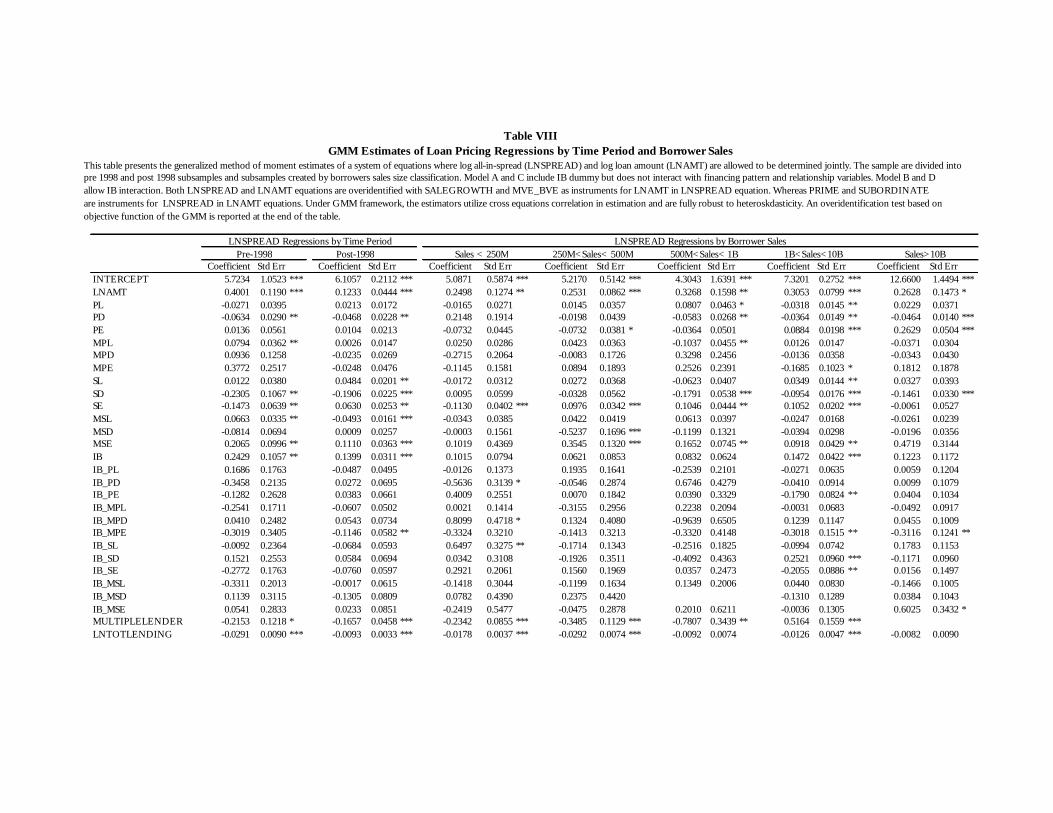
This table presents the generalized method of moment estimates of a system of equations where log all-in-spread (LNSPREAD) and log loan amount (LNAMT) are allowed to be determined jointly. The sample are divided intopre 1998 and post 1998 subsamples and subsamples created by borrowers sales size classification. Model A and C include IB dummy but does not interact with financing pattern and relationship variables. Model B and D allow IB interaction. Both LNSPREAD and LNAMT equations are overidentified with SALEGROWTH and MVE_BVE as instruments for LNAMT in LNSPREAD equation. Whereas PRIME and SUBORDINATE are instruments for LNSPREAD in LNAMT equations. Under GMM framework, the estimators utilize cross equations correlation in estimation and are fully robust to heteroskdasticity. An overidentification test based on objective function of the GMM is reported at the end of the table.
Coefficient Std Err Coefficient Std Err Coefficient Std Err Coefficient Std Err Coefficient Std Err Coefficient Std Err Coefficient Std Err b0 5.723449 1.0523 5.02 <.0001 InterceptINTERCEPT 5.7234 1.0523 *** b0 6.105729 0.2112 26.86 <.0001 Intercept6.1057 0.2112 *** Intercept 1 5.087055 0.587405 8.11 <.0001 Intercept5.0871 0.5874 *** Intercept 1 5.217008 0.514219 9.76 <.0001 Intercept5.2170 0.5142 *** Intercept 1 4.304305 1.639147 2.60 0.0094 Intercept4.3043 1.6391 *** Intercept 1 7.320052 0.275214 27.31 <.0001 Intercept7.3201 0.2752 *** Intercept 1 12.66003 1.449420 9.39 <.0001 Intercept12.6600 1.4494 *** b1 0.400107 0.1190 1.24 0.2142 lnamtLNAMT 0.4001 0.1190 *** b1 0.123297 0.0444 2.65 0.0080 lnamt0.1233 0.0444 *** lnamt 1 0.249826 0.127428 1.85 0.06450.2498 0.1274 ** lnamt 1 0.253095 0.086160 3.14 0.00170.2531 0.0862 *** lnamt 1 0.326827 0.159800 1.28 0.19930.3268 0.1598 ** lnamt 1 0.305308 0.079874 -4.07 <.00010.3053 0.0799 *** lnamt 1 0.262787 0.147313 -3.80 0.00010.2628 0.1473 * b2 -0.02709 0.0395 -0.70 0.4869 PLPL -0.0271 0.0395 b2 0.021314 0.0172 1.26 0.2077 PL0.0213 0.0172 PL 1 -0.01645 0.027079 -0.59 0.5555-0.0165 0.0271 PL 1 0.014517 0.035713 0.41 0.67870.0145 0.0357 PL 1 0.080660 0.046294 1.75 0.07970.0807 0.0463 * PL 1 -0.03180 0.014450 -2.21 0.0273-0.0318 0.0145 ** PL 1 0.022940 0.037133 0.64 0.52530.0229 0.0371 b3 -0.06335 0.0290 -1.25 0.2130 PDPD -0.0634 0.0290 ** b3 -0.04676 0.0228 -2.11 0.0346 PD-0.0468 0.0228 ** PD 1 0.214767 0.191415 2.58 0.00980.2148 0.1914 PD 1 -0.01980 0.043905 -0.45 0.6543-0.0198 0.0439 PD 1 -0.05833 0.026838 1.21 0.2252-0.0583 0.0268 ** PD 1 -0.03640 0.014917 -2.54 0.0111-0.0364 0.0149 ** PD 1 -0.04642 0.014019 1.31 0.1915-0.0464 0.0140 *** b4 0.013594 0.0561 0.23 0.8181 PEPE 0.0136 0.0561 b4 0.010446 0.0213 0.51 0.6116 PE0.0104 0.0213 PE 1 -0.07323 0.044533 -1.69 0.0909-0.0732 0.0445 PE 1 -0.07315 0.038121 -1.90 0.0570-0.0732 0.0381 * PE 1 -0.03637 0.050099 -0.70 0.4852-0.0364 0.0501 PE 1 0.088406 0.019809 4.48 <.00010.0884 0.0198 *** PE 1 0.262930 0.050378 5.48 <.00010.2629 0.0504 *** b5 0.079411 0.0362 2.17 0.0298 MPLMPL 0.0794 0.0362 ** b5 0.002582 0.0147 0.18 0.8555 MPL0.0026 0.0147 MPL 1 0.024992 0.028638 0.84 0.39870.0250 0.0286 MPL 1 0.042347 0.036337 1.10 0.27070.0423 0.0363 MPL 1 -0.10365 0.045508 -2.26 0.0237-0.1037 0.0455 ** MPL 1 0.012640 0.014726 0.83 0.40690.0126 0.0147 MPL 1 -0.03711 0.030396 -1.25 0.2107-0.0371 0.0304 b6 0.093635 0.1258 0.71 0.4758 MPDMPD 0.0936 0.1258 b6 -0.02353 0.0269 -0.80 0.4210 MPD-0.0235 0.0269 MPD 1 -0.27145 0.206378 -1.24 0.2164-0.2715 0.2064 MPD 1 -0.00834 0.172585 -0.05 0.9592-0.0083 0.1726 MPD 1 0.329750 0.245595 1.35 0.17800.3298 0.2456 MPD 1 -0.01358 0.035842 -0.39 0.6984-0.0136 0.0358 MPD 1 -0.03430 0.043021 -0.79 0.4307-0.0343 0.0430 b7 0.377153 0.2517 1.49 0.1362 MPEMPE 0.3772 0.2517 b7 -0.02480 0.0476 0.51 0.6100 MPE-0.0248 0.0476 MPE 1 -0.11451 0.158089 -0.75 0.4526-0.1145 0.1581 MPE 1 0.089415 0.189338 0.48 0.63350.0894 0.1893 MPE 1 0.252564 0.239129 1.11 0.26790.2526 0.2391 MPE 1 -0.16845 0.102286 -1.71 0.0874-0.1685 0.1023 * MPE 1 0.181224 0.187789 0.96 0.33670.1812 0.1878 b8 0.012209 0.0380 0.30 0.7606 SLSL 0.0122 0.0380 b8 0.048407 0.0201 2.33 0.0196 SL0.0484 0.0201 ** SL 1 -0.01724 0.031203 -0.55 0.5809-0.0172 0.0312 SL 1 0.027210 0.036833 0.69 0.48970.0272 0.0368 SL 1 -0.06227 0.040690 -1.51 0.1323-0.0623 0.0407 SL 1 0.034949 0.014394 2.31 0.02120.0349 0.0144 ** SL 1 0.032728 0.039279 0.85 0.39350.0327 0.0393 b9 -0.23050 0.1067 -2.23 0.0256 SDSD -0.2305 0.1067 ** b9 -0.19059 0.0225 -8.56 <.0001 SD-0.1906 0.0225 *** SD 1 0.009506 0.059917 0.16 0.86980.0095 0.0599 SD 1 -0.03275 0.056176 -0.63 0.5300-0.0328 0.0562 SD 1 -0.17910 0.053834 -3.31 0.0009-0.1791 0.0538 *** SD 1 -0.09544 0.017619 -5.63 <.0001-0.0954 0.0176 *** SD 1 -0.14612 0.032974 -4.30 <.0001-0.1461 0.0330 *** b10 -0.14729 0.0639 -2.27 0.0230 SESE -0.1473 0.0639 ** b10 0.062960 0.0253 2.61 0.0090 SE0.0630 0.0253 ** SE 1 -0.11304 0.040182 -2.89 0.0039-0.1130 0.0402 *** SE 1 0.097646 0.034169 3.00 0.00280.0976 0.0342 *** SE 1 0.104620 0.044401 2.54 0.01120.1046 0.0444 ** SE 1 0.105155 0.020231 5.47 <.00010.1052 0.0202 *** SE 1 -0.00609 0.052657 -0.12 0.9083-0.0061 0.0527 b11 0.066317 0.0335 1.95 0.0514 MSLMSL 0.0663 0.0335 ** b11 -0.04929 0.0161 -2.83 0.0047 MSL-0.0493 0.0161 *** MSL 1 -0.03426 0.038536 -0.91 0.3625-0.0343 0.0385 MSL 1 0.042230 0.041855 1.00 0.31870.0422 0.0419 MSL 1 0.061273 0.039669 1.48 0.13860.0613 0.0397 MSL 1 -0.02467 0.016829 -1.56 0.1193-0.0247 0.0168 MSL 1 -0.02605 0.023907 -1.16 0.2449-0.0261 0.0239 b12 -0.08135 0.0694 -1.16 0.2442 MSDMSD -0.0814 0.0694 b12 0.000944 0.0257 0.04 0.9691 MSD0.0009 0.0257 MSD 1 -0.00030 0.156117 -0.00 0.9983-0.0003 0.1561 MSD 1 -0.52374 0.169553 -3.19 0.0014-0.5237 0.1696 *** MSD 1 -0.11991 0.132115 -0.87 0.3860-0.1199 0.1321 MSD 1 -0.03943 0.029799 -1.33 0.1833-0.0394 0.0298 MSD 1 -0.01963 0.035582 -0.51 0.6079-0.0196 0.0356 b13 0.206521 0.0996 1.03 0.3020 MSEMSE 0.2065 0.0996 ** b13 0.111036 0.0363 1.93 0.0533 MSE0.1110 0.0363 *** MSE 1 0.101932 0.436903 -0.22 0.82740.1019 0.4369 MSE 1 0.354456 0.131956 1.94 0.05260.3545 0.1320 *** MSE 1 0.165201 0.074512 -0.29 0.76980.1652 0.0745 ** MSE 1 0.091814 0.042874 0.41 0.68190.0918 0.0429 ** MSE 1 0.471870 0.314357 -1.59 0.11240.4719 0.3144 b14 0.242860 0.1057 1.40 0.1603 ibIB 0.2429 0.1057 ** b14 0.139948 0.0311 4.65 <.0001 ib0.1399 0.0311 *** IB 1 0.101456 0.079435 1.28 0.1997 IB0.1015 0.0794 IB 1 0.062087 0.085323 0.76 0.4453 IB0.0621 0.0853 IB 1 0.083183 0.062421 1.37 0.1697 IB0.0832 0.0624 IB 1 0.147190 0.042168 3.66 0.0003 IB0.1472 0.0422 *** IB 1 0.122286 0.117231 1.02 0.3086 IB0.1223 0.1172 b15 0.168639 0.1763 1.01 0.3108 ib_PLIB_PL 0.1686 0.1763 b15 -0.04866 0.0495 -1.01 0.3117 ib_PL-0.0487 0.0495 ib_PL 1 -0.01255 0.137315 -0.09 0.9258-0.0126 0.1373 ib_PL 1 0.193457 0.164123 1.13 0.25920.1935 0.1641 ib_PL 1 -0.25393 0.210083 -1.19 0.2338-0.2539 0.2101 ib_PL 1 -0.02705 0.063522 -0.41 0.6828-0.0271 0.0635 ib_PL 1 0.005943 0.120443 0.05 0.96030.0059 0.1204 b16 -0.34584 0.2135 -1.60 0.1092 ib_PDIB_PD -0.3458 0.2135 b16 0.027234 0.0695 0.39 0.6958 ib_PD0.0272 0.0695 ib_PD 1 -0.56357 0.313898 -1.89 0.0587-0.5636 0.3139 * ib_PD 1 -0.05458 0.287416 -0.20 0.8391-0.0546 0.2874 ib_PD 1 0.674565 0.427929 1.55 0.12040.6746 0.4279 ib_PD 1 -0.04100 0.091444 -0.45 0.6550-0.0410 0.0914 ib_PD 1 0.009945 0.107865 0.09 0.93130.0099 0.1079 b17 -0.12818 0.2628 -0.50 0.6162 ib_PEIB_PE -0.1282 0.2628 b17 0.038268 0.0661 0.58 0.5626 ib_PE0.0383 0.0661 ib_PE 1 0.400878 0.255092 1.49 0.13600.4009 0.2551 ib_PE 1 0.007044 0.184240 0.04 0.96840.0070 0.1842 ib_PE 1 0.039016 0.332862 0.11 0.91080.0390 0.3329 ib_PE 1 -0.17898 0.082357 -2.11 0.0345-0.1790 0.0824 ** ib_PE 1 0.040436 0.103409 0.41 0.68290.0404 0.1034 b18 -0.25410 0.1711 -1.43 0.1539 ib_MPLIB_MPL -0.2541 0.1711 b18 -0.06065 0.0502 -1.22 0.2240 ib_MPL-0.0607 0.0502 ib_MPL 1 0.002086 0.141426 0.02 0.98740.0021 0.1414 ib_MPL 1 -0.31547 0.295613 -1.68 0.0935-0.3155 0.2956 ib_MPL 1 0.223810 0.209449 1.01 0.31370.2238 0.2094 ib_MPL 1 -0.00313 0.068307 -0.05 0.9630-0.0031 0.0683 ib_MPL 1 -0.04919 0.091669 -0.55 0.5804-0.0492 0.0917 b19 0.041000 0.2482 0.17 0.8662 ib_MPDIB_MPD 0.0410 0.2482 b19 0.054324 0.0734 0.73 0.4657 ib_MPD0.0543 0.0734 ib_MPD 1 0.809917 0.471800 1.88 0.06040.8099 0.4718 * ib_MPD 1 0.132398 0.408023 0.35 0.72820.1324 0.4080 ib_MPD 1 -0.96387 0.650507 -1.61 0.1080-0.9639 0.6505 ib_MPD 1 0.123942 0.114701 1.01 0.31330.1239 0.1147 ib_MPD 1 0.045504 0.100898 0.46 0.64770.0455 0.1009 b20 -0.30186 0.3405 -0.85 0.3937 ib_MPEIB_MPE -0.3019 0.3405 b20 -0.11457 0.0582 -1.30 0.1935 ib_MPE-0.1146 0.0582 ** ib_MPE 1 -0.33236 0.321045 -1.05 0.2950-0.3324 0.3210 ib_MPE 1 -0.14128 0.321286 -0.45 0.6504-0.1413 0.3213 ib_MPE 1 -0.33201 0.414752 -0.79 0.4292-0.3320 0.4148 ib_MPE 1 -0.30184 0.151470 0.33 0.7421-0.3018 0.1515 ** ib_MPE 1 -0.31156 0.124126 -1.58 0.1148-0.3116 0.1241 ** b21 -0.00923 0.2364 -0.04 0.9686 ib_SLIB_SL -0.0092 0.2364 b21 -0.06835 0.0593 -1.15 0.2494 ib_SL-0.0684 0.0593 ib_SL 1 0.649666 0.327479 2.10 0.03610.6497 0.3275 ** ib_SL 1 -0.17137 0.134302 -1.17 0.2424-0.1714 0.1343 ib_SL 1 -0.25162 0.182487 -1.42 0.1569-0.2516 0.1825 ib_SL 1 -0.09943 0.074223 -1.41 0.1599-0.0994 0.0742 ib_SL 1 0.178340 0.115338 1.53 0.12530.1783 0.1153 b22 0.152123 0.2553 0.58 0.5632 ib_SDIB_SD 0.1521 0.2553 b22 0.058371 0.0694 0.88 0.3796 ib_SD0.0584 0.0694 ib_SD 1 0.034191 0.310839 0.11 0.91280.0342 0.3108 ib_SD 1 -0.19260 0.351063 -0.57 0.5676-0.1926 0.3511 ib_SD 1 -0.40924 0.436315 -0.90 0.3667-0.4092 0.4363 ib_SD 1 0.252060 0.096001 2.60 0.00930.2521 0.0960 *** ib_SD 1 -0.11713 0.095975 -1.22 0.2236-0.1171 0.0960 b23 -0.27718 0.1763 -1.53 0.1249 ib_SEIB_SE -0.2772 0.1763 b23 -0.07601 0.0597 -1.26 0.2074 ib_SE-0.0760 0.0597 ib_SE 1 0.292084 0.206146 1.45 0.14830.2921 0.2061 ib_SE 1 0.155983 0.196947 0.84 0.39890.1560 0.1969 ib_SE 1 0.035653 0.247263 0.14 0.88540.0357 0.2473 ib_SE 1 -0.20546 0.088576 -2.43 0.0151-0.2055 0.0886 ** ib_SE 1 0.015585 0.149655 0.11 0.91130.0156 0.1497 b24 -0.33105 0.2013 -1.37 0.1719 ib_MSLIB_MSL -0.3311 0.2013 b24 -0.00171 0.0615 -0.03 0.9791 ib_MSL-0.0017 0.0615 ib_MSL 1 -0.14180 0.304442 -2.91 0.0036-0.1418 0.3044 ib_MSL 1 -0.11992 0.163425 -0.73 0.4638-0.1199 0.1634 ib_MSL 1 0.134878 0.200565 0.66 0.51100.1349 0.2006 ib_MSL 1 0.044040 0.083031 1.83 0.06790.0440 0.0830 ib_MSL 1 -0.14663 0.100512 -1.50 0.1338-0.1466 0.1005 b25 0.113860 0.3115 0.39 0.6999 ib_MSDIB_MSD 0.1139 0.3115 b25 -0.13048 0.0809 -1.72 0.0847 ib_MSD-0.1305 0.0809 ib_MSD 1 0.078180 0.438972 0.19 0.85160.0782 0.4390 ib_MSD 1 0.237542 0.441960 0.55 0.58450.2375 0.4420 ib_MSD 1 -0.13098 0.128946 -2.73 0.0064-0.1310 0.1289 ib_MSD 1 0.038385 0.104306 0.36 0.71950.0384 0.1043 b26 0.054119 0.2833 0.20 0.8433 ib_MSEIB_MSE 0.0541 0.2833 b26 0.023321 0.0851 0.27 0.7905 ib_MSE0.0233 0.0851 ib_MSE 1 -0.24193 0.547739 -0.46 0.6440-0.2419 0.5477 ib_MSE 1 -0.04746 0.287752 -0.16 0.8755-0.0475 0.2878 ib_MSE 1 0.200994 0.621136 0.32 0.74780.2010 0.6211 ib_MSE 1 -0.00361 0.130455 -0.03 0.9787-0.0036 0.1305 ib_MSE 1 0.602535 0.343156 1.76 0.07790.6025 0.3432 * b27 -0.21526 0.1218 -1.38 0.1680 multiplelenderMULTIPLELENDER -0.2153 0.1218 * b27 -0.16568 0.0458 -3.56 0.0004 multiplelender-0.1657 0.0458 *** multiplelender 1 -0.23421 0.085516 -2.75 0.0059-0.2342 0.0855 *** multiplelender 1 -0.34845 0.112889 -3.20 0.0014-0.3485 0.1129 *** multiplelender 1 -0.78070 0.343855 -2.16 0.0308-0.7807 0.3439 ** multiplelender 1 0.516402 0.155881 3.57 0.00040.5164 0.1559 *** b28 -0.02913 0.0090 -3.22 0.0013 lntotlendingLNTOTLENDING -0.0291 0.0090 *** b28 -0.00925 0.0033 -2.87 0.0041 lntotlending-0.0093 0.0033 *** lntotlending 1 -0.01781 0.003739 -4.46 <.0001-0.0178 0.0037 *** lntotlending 1 -0.02915 0.007430 -4.11 <.0001-0.0292 0.0074 *** lntotlending 1 -0.00917 0.007432 -1.24 0.2157-0.0092 0.0074 lntotlending 1 -0.01255 0.004742 -2.64 0.0084-0.0126 0.0047 *** lntotlending 1 -0.00820 0.009032 -0.88 0.3764-0.0082 0.0090
LNSPREAD Regressions by Time Period
GMM Estimates of Loan Pricing Regressions by Time Period and Borrower SalesTable VIII
LNSPREAD Regressions by Borrower Sales500M<Sales< 1B 1B<Sales<10B Sales>10BPre-1998 Post-1998 Sales < 250M 250M<Sales< 500M
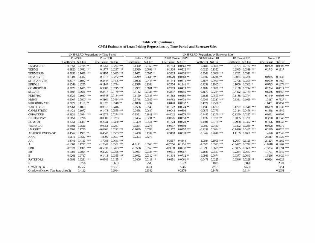
Coefficient Std Err Coefficient Std Err Coefficient Std Err Coefficient Std Err Coefficient Std Err Coefficient Std Err Coefficient Std Err b30 -0.15577 0.0718 -2.24 0.0253 lnmatureLNMATURE -0.1558 0.0718 ** b30 -0.12523 0.0227 -5.49 <.0001 lnmature-0.1252 0.0227 *** lnmature 1 -0.14699 0.035914 -4.07 <.0001-0.1470 0.0359 *** lnmature 1 -0.16130 0.036129 -4.60 <.0001-0.1613 0.0361 *** lnmature 1 -0.26061 0.080459 -3.37 0.0008-0.2606 0.0805 *** lnmature 1 -0.07043 0.016691 -4.24 <.0001-0.0704 0.0167 *** lnmature 1 -0.08292 0.030589 -2.73 0.0064-0.0829 0.0306 *** b31 0.392629 0.0892 4.15 <.0001 termBTERMB 0.3926 0.0892 *** b31 0.177709 0.0297 5.88 <.0001 termB0.1777 0.0297 *** termB 1 0.157977 0.069765 2.41 0.01590.1580 0.0698 ** termB 1 0.143816 0.051193 2.68 0.00730.1438 0.0512 *** termB 1 0.012558 0.135176 0.09 0.92530.0126 0.1352 termB 1 0.294549 0.031850 8.85 <.00010.2945 0.0319 *** termB 1 0.174296 0.111667 1.56 0.11890.1743 0.1117 b32 0.585326 0.1628 3.66 0.0003 termBsubTERMBSUB 0.5853 0.1628 *** b32 0.319712 0.0433 7.37 <.0001 termBsub0.3197 0.0433 *** termBsub 1 0.165216 0.090531 1.74 0.08150.1652 0.0905 * termBsub 1 0.332464 0.093322 3.77 0.00020.3325 0.0933 *** termBsub 1 0.336184 0.065960 5.11 <.00010.3362 0.0660 *** termBsub 1 0.228169 0.051102 4.46 <.00010.2282 0.0511 *** b33 -0.19080 0.1422 -1.42 0.1562 revolverREVOLVER -0.1908 0.1422 b33 -0.10172 0.0262 -4.10 <.0001 revolver-0.1017 0.0262 *** revolver 1 -0.12489 0.063281 -2.02 0.0436-0.1249 0.0633 ** revolver 1 -0.09286 0.038285 -2.43 0.0153-0.0929 0.0383 ** revolver 1 -0.24920 0.124571 -2.00 0.0461-0.2492 0.1246 ** revolver 1 0.006417 0.028642 0.22 0.82450.0064 0.0286 revolver 1 0.094507 0.113524 0.88 0.37640.0945 0.1135 b34 -0.27766 0.1087 -2.52 0.0116 strevolverSTREVOLVER -0.2777 0.1087 ** b34 -0.36469 0.0405 -8.52 <.0001 strevolver-0.3647 0.0405 *** strevolver 1 -0.10080 0.041831 -2.57 0.0101-0.1008 0.0418 ** strevolver 1 -0.15439 0.051134 -2.97 0.0030-0.1544 0.0511 *** strevolver 1 -0.48783 0.099119 -4.77 <.0001-0.4878 0.0991 *** strevolver 1 -0.27279 0.029930 -8.77 <.0001-0.2728 0.0299 *** strevolver 1 0.057933 0.146038 0.41 0.68210.0579 0.1460 b35 0.154213 0.2256 0.64 0.5231 bridgeBRIDGE 0.1542 0.2256 b35 -0.11467 0.0744 -1.62 0.1046 bridge-0.1147 0.0744 bridge 1 -0.19179 0.138834 -1.43 0.1533-0.1918 0.1388 bridge 1 0.275439 0.134101 2.03 0.04220.2754 0.1341 ** bridge 1 -0.42593 0.190544 -2.17 0.0303-0.4259 0.1905 ** bridge 1 0.104988 0.056294 1.76 0.07880.1050 0.0563 * bridge 1 0.672304 0.187406 3.64 0.00030.6723 0.1874 *** b36 0.382858 0.1480 2.41 0.0160 combodealCOMBODEAL 0.3829 0.1480 *** b36 0.338750 0.0245 13.37 <.0001 combodeal0.3388 0.0245 *** combodeal 1 0.290237 0.080094 3.57 0.00040.2902 0.0801 *** combodeal 1 0.291904 0.041259 7.18 <.00010.2919 0.0413 *** combodeal 1 0.263200 0.080065 3.23 0.00120.2632 0.0801 *** combodeal 1 0.213794 0.024406 9.20 <.00010.2138 0.0244 *** combodeal 1 0.278398 0.061446 4.52 <.00010.2784 0.0614 *** b37 0.560304 0.0666 8.45 <.0001 secureSECURE 0.5603 0.0666 *** b37 0.261733 0.0189 14.42 <.0001 secure0.2617 0.0189 *** secure 1 0.311173 0.032626 9.26 <.00010.3112 0.0326 *** secure 1 0.333667 0.025640 13.44 <.00010.3337 0.0256 *** secure 1 0.366959 0.026449 13.01 <.00010.3670 0.0264 *** secure 1 0.342185 0.016273 21.16 <.00010.3422 0.0163 *** secure 1 0.656606 0.055676 11.82 <.00010.6566 0.0557 *** b37p5 -0.27287 0.1040 -2.64 0.0084 perfprcPERFPRC -0.2729 0.1040 *** b37p5 -0.05477 0.0164 -3.46 0.0005 perfprc-0.0548 0.0164 *** perfprc 1 -0.11202 0.034583 -3.32 0.0009-0.1120 0.0346 *** perfprc 1 -0.15623 0.028026 -5.63 <.0001-0.1562 0.0280 *** perfprc 1 -0.18861 0.050297 -3.93 <.0001-0.1886 0.0503 *** perfprc1 1 -0.11883 0.074372 0.85 0.3934-0.1188 0.0744 perfprc1 1 0.104880 0.030822 3.19 0.00140.1049 0.0308 *** b38 0.600712 0.0800 7.89 <.0001 primePRIME 0.6007 0.0800 *** b38 0.516946 0.0484 11.04 <.0001 prime0.5169 0.0484 *** prime 1 0.574796 0.055244 10.02 <.00010.5748 0.0552 *** prime 1 0.878206 0.073426 11.73 <.00010.8782 0.0734 *** prime 1 0.930793 0.221680 4.39 <.00010.9308 0.2217 *** prime 1 0.633069 0.102924 6.69 <.00010.6331 0.1029 *** prime 1 1.311734 0.782674 1.80 0.07221.3117 0.7827 * b39 0.267652 0.1169 -2.55 0.0107 subordinateSUBORDINATE 0.2677 0.1169 ** b39 0.107813 0.0548 0.61 0.5423 subordinate0.1078 0.0548 ** suborninate 1 -0.18957 0.229368 0.80 0.4254-0.1896 0.2294 suborninate 1 0.042023 0.023189 -0.03 0.97280.0420 0.0232 * suborninate 1 0.477704 0.255630 -2.44 0.01460.4777 0.2556 * suborninate 1 -1.64513 0.515727 -3.26 0.0011-1.6451 0.5157 *** b40 -0.22626 0.1855 -1.23 0.2199 takeoverTAKEOVER -0.2263 0.1855 b40 -0.05178 0.0416 -1.22 0.2214 takeover-0.0518 0.0416 Takeover 1 0.058584 0.054880 1.11 0.2654 Takeover0.0586 0.0549 Takeover 1 -0.15220 0.062382 -2.59 0.0096 Takeover-0.1522 0.0624 ** Takeover 1 -0.19483 0.128320 -1.41 0.1574 Takeover-0.1948 0.1283 Takeover 1 0.172708 0.054757 3.18 0.0015 Takeover0.1727 0.0548 *** Takeover 1 0.635933 0.163849 3.71 0.0002 Takeover0.6359 0.1638 *** b41 -0.14206 0.1977 -0.76 0.4468 caprestrucCAPRESTRUC -0.1421 0.1977 b41 0.147767 0.0565 2.65 0.0080 caprestruc0.1478 0.0565 *** Caprestruc 1 0.045759 0.064713 0.67 0.5021 Caprestruc0.0458 0.0647 Caprestruc 1 0.004833 0.089829 0.05 0.9567 Caprestruc0.0048 0.0898 Caprestruc 1 0.087335 0.077274 1.09 0.2746 Caprestruc0.0873 0.0773 Caprestruc 1 0.211355 0.045641 4.55 <.0001 Caprestruc0.2114 0.0456 *** Caprestruc 1 0.186769 0.184926 1.01 0.3145 Caprestruc0.1868 0.1849 b42 -0.31204 0.0934 -3.40 0.0007 cpbackupCPBACKUP -0.3120 0.0934 *** b42 -0.25728 0.0274 -9.52 <.0001 cpbackup-0.2573 0.0274 *** Cpbackup 1 -0.93512 0.181056 -5.19 <.0001 Cpbackup-0.9351 0.1811 *** Cpbackup 1 -0.40116 0.087897 -4.59 <.0001 Cpbackup-0.4012 0.0879 *** Cpbackup 1 -0.44845 0.119970 -3.68 0.0002 Cpbackup-0.4485 0.1200 *** Cpbackup 1 -0.12993 0.022683 -5.94 <.0001 Cpbackup-0.1299 0.0227 *** Cpbackup 1 0.036132 0.080700 0.43 0.6651 Cpbackup0.0361 0.0807 b43 -0.11507 0.0796 -1.53 0.1269 debtrepayDEBTREPAY -0.1151 0.0796 b43 -0.03088 0.0223 -1.32 0.1873 debtrepay-0.0309 0.0223 Debtrepay 1 0.040367 0.023053 1.69 0.0909 Debtrepay0.0404 0.0231 * Debtrepay 1 -0.07263 0.035332 -2.06 0.0398 Debtrepay-0.0726 0.0353 ** Debtrepay 1 -0.17318 0.070132 -2.54 0.0111 Debtrepay-0.1732 0.0701 ** Debtrepay 1 -0.00349 0.023053 -0.16 0.8749 Debtrepay-0.0035 0.0231 Debtrepay 1 0.375987 0.104342 3.64 0.0003 Debtrepay0.3760 0.1043 *** b44 0.275102 0.1381 2.02 0.0439 buyoutBUYOUT 0.2751 0.1381 ** b44 0.204435 0.0470 4.71 <.0001 buyout0.2044 0.0470 *** Buyout 1 0.340877 0.051364 6.61 <.0001 Buyout0.3409 0.0514 *** Buyout 1 0.172420 0.082037 2.19 0.0286 Buyout0.1724 0.0820 ** Buyout 1 0.198052 0.077933 2.53 0.0115 Buyout0.1981 0.0779 ** Buyout 1 0.297837 0.039155 7.87 <.0001 Buyout0.2978 0.0392 *** Buyout 1 0.192575 0.094276 1.97 0.0490 Buyout0.1926 0.0943 ** b45 0.059091 0.0516 1.08 0.2786 WorkcapWORKCAP 0.0591 0.0516 b45 0.005388 0.0237 0.23 0.8205 Workcap0.0054 0.0237 Workcap 1 0.035400 0.027299 1.32 0.1854 Workcap0.0354 0.0273 Workcap 1 0.063702 0.039815 1.50 0.1345 Workcap0.0637 0.0398 Workcap 1 -0.05004 0.044296 -1.13 0.2603 Workcap-0.0500 0.0443 Workcap 1 0.049157 0.023868 2.11 0.0346 Workcap0.0492 0.0239 ** Workcap 1 -0.03279 0.077850 -0.43 0.6682 Workcap-0.0328 0.0779 b46 -0.27045 0.1776 -1.52 0.1297 lnassetLNASSET -0.2705 0.1776 b46 -0.09662 0.0272 -3.37 0.0008 lnasset-0.0966 0.0272 *** lnasset 1 -0.10991 0.070814 -1.68 0.0922-0.1099 0.0708 lnasset 1 -0.12772 0.045747 -2.69 0.0072-0.1277 0.0457 *** lnasset 1 -0.11990 0.063379 -1.28 0.1994-0.1199 0.0634 * lnasset 1 -0.14461 0.046722 3.01 0.0026-0.1446 0.0467 *** lnasset 1 0.202912 0.072038 2.90 0.00370.2029 0.0720 *** b47 0.456155 0.1951 -0.71 0.4758 adjmktleverageADJMKTLEVERAGE 0.4562 0.1951 ** b47 0.454265 0.0553 8.24 <.0001 adjmktleverage0.4543 0.0553 *** adjmktleverage 1 0.245822 0.118386 -1.15 0.24840.2458 0.1184 ** adjmktleverage 1 0.341779 0.082780 4.14 <.00010.3418 0.0828 *** adjmktleverage 1 0.646152 0.201003 3.34 0.00090.6462 0.2010 *** adjmktleverage 1 1.116895 0.106066 10.64 <.00011.1169 0.1061 *** adjmktleverage 1 1.451975 0.234752 5.91 <.00011.4520 0.2348 *** b48 -1.51104 0.3527 -4.47 <.0001 aaaAAA -1.5110 0.3527 *** b48 -1.87093 0.0667 -26.60 <.0001 aaa-1.8709 0.0667 *** aaa 1 0.230267 0.327269 0.66 0.50720.2303 0.3273 aaa 1 -2.53167 0.161983 -15.50 <.0001-2.5317 0.1620 *** b49 -1.87460 0.4115 -4.82 <.0001 aaAA -1.8746 0.4115 *** b49 -1.70880 0.0641 -28.65 <.0001 aa-1.7088 0.0641 *** aa 1 0.365677 0.484439 0.78 0.43840.3657 0.4844 aa 1 -1.00343 0.190517 -5.24 <.0001-1.0034 0.1905 *** aa 1 -1.26471 0.112489 -10.93 <.0001-1.2647 0.1125 *** aa 1 -2.12236 0.116179 -17.16 <.0001-2.1224 0.1162 *** b50 -1.15995 0.1717 -6.72 <.0001 aA -1.1600 0.1717 *** b50 -1.26466 0.0551 -23.30 <.0001 a-1.2647 0.0551 *** a 1 -1.01106 0.096321 -11.43 <.0001-1.0111 0.0963 *** a 1 -0.73564 0.125147 -6.19 <.0001-0.7356 0.1251 *** a 1 -1.05730 0.099319 -10.11 <.0001-1.0573 0.0993 *** a 1 -0.94270 0.074200 -12.37 <.0001-0.9427 0.0742 *** a 1 -1.86175 0.126226 -14.41 <.0001-1.8618 0.1262 *** b51 -0.76275 0.1391 -5.56 <.0001 bbbBBB -0.7628 0.1391 *** b51 -0.58320 0.0423 -14.26 <.0001 bbb-0.5832 0.0423 *** bbb 1 -0.55562 0.055777 -9.77 <.0001-0.5556 0.0558 *** bbb 1 -0.36386 0.073656 -4.61 <.0001-0.3639 0.0737 *** bbb 1 -0.62925 0.063486 -9.69 <.0001-0.6293 0.0635 *** bbb 1 -0.50552 0.065122 -7.59 <.0001-0.5055 0.0651 *** bbb 1 -1.32038 0.139093 -9.45 <.0001-1.3204 0.1391 *** b52 -0.19797 0.0864 -2.39 0.0170 bbBB -0.1980 0.0864 ** b52 -0.27197 0.0356 -7.26 <.0001 bb-0.2720 0.0356 *** bb 1 -0.30872 0.033384 -8.74 <.0001-0.3087 0.0334 *** bb 1 -0.06112 0.066678 -0.92 0.3586-0.0611 0.0667 bb 1 -0.28487 0.059650 -4.86 <.0001-0.2849 0.0597 *** bb 1 -0.22443 0.064679 -3.54 0.0004-0.2244 0.0647 *** bb 1 -1.17007 0.183980 -6.37 <.0001-1.1701 0.1840 *** b53 0.026145 0.0717 0.37 0.7096 bB 0.0261 0.0717 b53 -0.14178 0.0355 -4.08 <.0001 b-0.1418 0.0355 *** b 1 -0.10623 0.031223 -3.25 0.0011-0.1062 0.0312 *** b 1 0.141842 0.071187 2.09 0.03690.1418 0.0712 ** b 1 -0.09864 0.067377 -1.51 0.1316-0.0986 0.0674 b 1 -0.03768 0.064323 -0.58 0.5615-0.0377 0.0643 b 1 -1.52655 0.341980 -4.41 <.0001-1.5266 0.3420 *** b53p5 0.069052 0.0261 -3.93 <.0001 rateforeRATEFORE 0.0691 0.0261 *** b53p5 0.034927 0.0165 1.63 0.1035 ratefore0.0349 0.0165 ** Debtrepay 1 0.040643 0.011828 1.69 0.0909 Debtrepay0.0406 0.0118 *** Debtrepay 1 0.015125 0.006129 1.69 0.0909 Debtrepay0.0151 0.0061 ** Debtrepay 1 0.047840 0.022474 1.69 0.0909 Debtrepay0.0478 0.0225 ** Debtrepay 1 0.054638 0.022894 1.69 0.0909 Debtrepay0.0546 0.0229 ** Debtrepay 1 0.032438 0.022550 1.69 0.0909 Debtrepay0.0324 0.0226
N 3776 10663 2533 1572 1835 5878 2620GMM Obj Fn 1552.7 3160.5 350.1 373.5 270.8 672.4 537.4Overidentification Test Stats chisq(2) 0.4112 0.2964 0.1382 0.2376 0.1476 0.1144 0.2051
LNSPREAD Regressions by Time Period
GMM Estimates of Loan Pricing Regressions by Time Period and Borrower SalesTable VIII (continue)
LNSPREAD Regressions by Borrower Sales500M<Sales< 1B 1B<Sales<10B Sales>10BPre-1998 Post-1998 Sales < 250M 250M<Sales< 500M
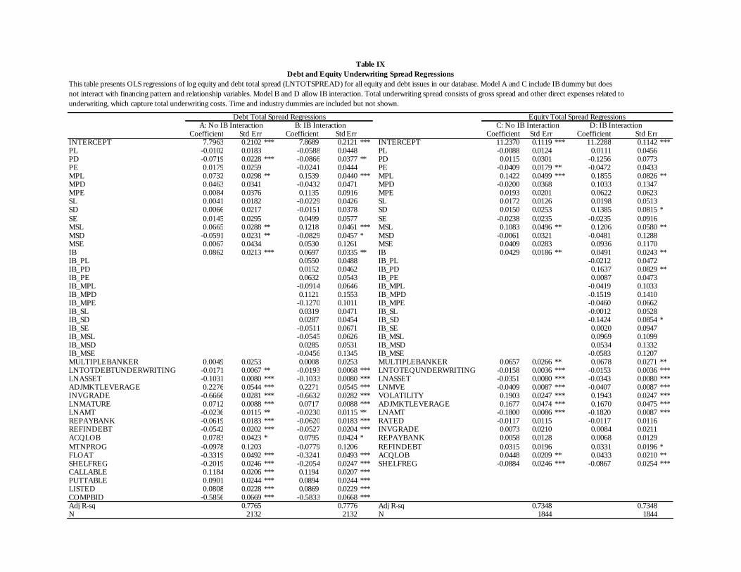
This table presents OLS regressions of log equity and debt total spread (LNTOTSPREAD) for all equity and debt issues in our database. Model A and C include IB dummy but doesnot interact with financing pattern and relationship variables. Model B and D allow IB interaction. Total underwriting spread consists of gross spread and other direct expenses related to underwriting, which capture total underwriting costs. Time and industry dummies are included but not shown.
Coefficient Std Err Coefficient Std Err Coefficient Std Err Coefficient Std ErrINTERCEPT 7.7963 0.2102 *** Intercept 1 7.868862 0.212121 37.10 <.00017.8689 0.2121 *** Intercept 1 11.23696 0.111855 100.46 <.0001INTERCEPT 11.2370 0.1119 *** Intercept 1 11.22878 0.114160 98.36 <.000111.2288 0.1142 ***PL -0.0102 0.0183 PL 1 -0.05884 0.044756 -1.31 0.1887-0.0588 0.0448 PL 1 -0.00875 0.012364 -0.71 0.4791PL -0.0088 0.0124 PL 1 0.011141 0.045565 0.24 0.80690.0111 0.0456PD -0.0719 0.0228 *** PD 1 -0.08660 0.037677 -2.30 0.0216-0.0866 0.0377 ** PD 1 0.011455 0.030059 0.38 0.7032PD 0.0115 0.0301 PD 1 -0.12555 0.077337 -1.62 0.1047-0.1256 0.0773PE 0.0179 0.0259 PE 1 -0.02409 0.044377 -0.54 0.5872-0.0241 0.0444 PE 1 -0.04094 0.017913 -2.29 0.0224PE -0.0409 0.0179 ** PE 1 -0.04715 0.043254 -1.09 0.2759-0.0472 0.0433MPL 0.0732 0.0298 ** MPL 1 0.153898 0.043985 3.50 0.00050.1539 0.0440 *** MPL 1 0.142215 0.049885 2.85 0.0044MPL 0.1422 0.0499 *** MPL 1 0.185521 0.082620 2.25 0.02490.1855 0.0826 **MPD 0.0463 0.0341 MPD 1 -0.04316 0.047108 -0.92 0.3597-0.0432 0.0471 MPD 1 -0.01999 0.036829 -0.54 0.5873MPD -0.0200 0.0368 MPD 1 0.103329 0.134672 0.77 0.44300.1033 0.1347MPE 0.0084 0.0376 MPE 1 0.113450 0.091613 1.24 0.21570.1135 0.0916 MPE 1 0.019259 0.020094 0.96 0.3380MPE 0.0193 0.0201 MPE 1 0.062158 0.062339 1.00 0.31890.0622 0.0623SL 0.0041 0.0182 SL 1 -0.02293 0.042623 -0.54 0.5906-0.0229 0.0426 SL 1 0.017213 0.012640 1.36 0.1734SL 0.0172 0.0126 SL 1 0.019841 0.051300 0.39 0.69900.0198 0.0513SD 0.0066 0.0217 SD 1 -0.01512 0.037758 -0.40 0.6888-0.0151 0.0378 SD 1 0.015009 0.025276 0.59 0.5527SD 0.0150 0.0253 SD 1 0.138531 0.081493 1.70 0.08930.1385 0.0815 *SE 0.0145 0.0295 SE 1 0.049890 0.057695 0.86 0.38730.0499 0.0577 SE 1 -0.02377 0.023516 -1.01 0.3122SE -0.0238 0.0235 SE 1 -0.02354 0.091609 -0.26 0.7973-0.0235 0.0916MSL 0.0665 0.0288 ** MSL 1 0.121770 0.046056 2.64 0.00830.1218 0.0461 *** MSL 1 0.108289 0.049629 2.18 0.0292MSL 0.1083 0.0496 ** MSL 1 00.12059 0.057995 -0.23 0.81510.1206 0.0580 **MSD -0.0591 0.0231 ** MSD 1 -0.08293 0.045688 -1.82 0.0696-0.0829 0.0457 * MSD 1 -0.00614 0.032091 -0.19 0.8483MSD -0.0061 0.0321 MSD 1 -0.04814 0.128755 -0.37 0.7085-0.0481 0.1288MSE 0.0067 0.0434 MSE 1 0.052991 0.126131 0.42 0.67440.0530 0.1261 MSE 1 0.040928 0.028308 1.45 0.1484MSE 0.0409 0.0283 MSE 1 0.093632 0.116966 0.80 0.42350.0936 0.1170IB 0.0862 0.0213 *** ib 1 0.069700 0.033527 1.27 0.20290.0697 0.0335 ** ib 1 0.042898 0.018589 2.31 0.0211IB 0.0429 0.0186 ** ib 1 0.049115 0.024296 2.02 0.04340.0491 0.0243 **IB_PL ib_PL 1 0.054952 0.048830 1.13 0.26060.0550 0.0488 IB_PL ib_PL 1 -0.02115 0.047187 -0.45 0.6540-0.0212 0.0472IB_PD ib_PD 1 0.015232 0.046219 0.33 0.74180.0152 0.0462 IB_PD ib_PD 1 0.163716 0.082936 1.97 0.04850.1637 0.0829 **IB_PE ib_PE 1 0.063243 0.054295 1.16 0.24420.0632 0.0543 IB_PE ib_PE 1 0.008710 0.047300 0.18 0.85390.0087 0.0473IB_MPL ib_MPL 1 -0.09140 0.064595 -2.50 0.0125-0.0914 0.0646 IB_MPL ib_MPL 1 -0.04193 0.103265 -0.41 0.6848-0.0419 0.1033IB_MPD ib_MPD 1 0.112092 0.155324 2.03 0.04290.1121 0.1553 IB_MPD ib_MPD 1 -0.15187 0.140985 -1.08 0.2815-0.1519 0.1410IB_MPE ib_MPE 1 -0.12699 0.101096 -1.26 0.2092-0.1270 0.1011 IB_MPE ib_MPE 1 -0.04599 0.066242 -0.69 0.4876-0.0460 0.0662IB_SL ib_SL 1 0.031911 0.047136 0.68 0.49850.0319 0.0471 IB_SL ib_SL 1 -0.00120 0.052777 -0.02 0.9818-0.0012 0.0528IB_SD ib_SD 1 0.028716 0.045420 0.63 0.52730.0287 0.0454 IB_SD ib_SD 1 -0.14237 0.085390 -1.67 0.0956-0.1424 0.0854 *IB_SE ib_SE 1 -0.05105 0.067075 -0.76 0.4467-0.0511 0.0671 IB_SE ib_SE 1 0.001960 0.094699 0.02 0.98350.0020 0.0947IB_MSL ib_MSL 1 -0.05451 0.062641 -0.87 0.3843-0.0545 0.0626 IB_MSL ib_MSL 1 0.096925 0.109882 1.79 0.07330.0969 0.1099IB_MSD ib_MSD 1 0.028488 0.053089 0.54 0.59160.0285 0.0531 IB_MSD ib_MSD 1 0.053390 0.133160 0.40 0.68850.0534 0.1332IB_MSE ib_MSE 1 -0.04557 0.134549 -0.34 0.7349-0.0456 0.1345 IB_MSE ib_MSE 1 -0.05831 0.120681 -0.48 0.6291-0.0583 0.1207MULTIPLEBANKER 0.0049 0.0253 multiplebanker 1 0.000827 0.025290 0.03 0.97390.0008 0.0253 multiplebanker 1 0.065698 0.026615 2.47 0.0137MULTIPLEBANKER 0.0657 0.0266 ** multiplebanker 1 0.067754 0.027113 2.50 0.01250.0678 0.0271 **LNTOTDEBTUNDERWRITING -0.0171 0.0067 ** lntotdebtunderwriting 1 -0.01925 0.006751 -2.85 0.0044-0.0193 0.0068 *** lntotequnderwriting 1 -0.01575 0.003586 -4.39 <.0001LNTOTEQUNDERWRITING -0.0158 0.0036 *** lntotequnderwriting 1 -0.01532 0.003598 -4.26 <.0001-0.0153 0.0036 ***LNASSET -0.1031 0.0080 *** lnasset 1 -0.10325 0.008029 -12.86 <.0001-0.1033 0.0080 *** lnasset 1 -0.03514 0.007992 -4.40 <.0001LNASSET -0.0351 0.0080 *** lnasset 1 -0.03429 0.008012 -4.28 <.0001-0.0343 0.0080 ***ADJMKTLEVERAGE 0.2276 0.0544 *** adjmktleverage 1 0.227053 0.054462 4.17 <.00010.2271 0.0545 *** lnmve 1 -0.04094 0.008652 -4.73 <.0001LNMVE -0.0409 0.0087 *** lnmve 1 -0.04068 0.008678 -4.69 <.0001-0.0407 0.0087 ***INVGRADE -0.6666 0.0281 *** invgrade 1 -0.66317 0.028206 -23.51 <.0001-0.6632 0.0282 *** volatility 1 0.190316 0.024654 7.72 <.0001VOLATILITY 0.1903 0.0247 *** volatility 1 0.194325 0.024730 7.86 <.00010.1943 0.0247 ***LNMATURE 0.0712 0.0088 *** lnmature 1 0.071679 0.008781 8.16 <.00010.0717 0.0088 *** adjmktleverage 1 0.167662 0.047411 3.54 0.0004ADJMKTLEVERAGE 0.1677 0.0474 *** adjmktleverage 1 0.166976 0.047491 3.52 0.00040.1670 0.0475 ***LNAMT -0.0236 0.0115 ** lnamt 1 -0.02298 0.011540 -1.99 0.0465-0.0230 0.0115 ** lnamt 1 -0.17998 0.008624 -20.87 <.0001LNAMT -0.1800 0.0086 *** lnamt 1 -0.18199 0.008669 -20.99 <.0001-0.1820 0.0087 ***REPAYBANK -0.0619 0.0183 *** repaybank 1 -0.06197 0.018322 -3.38 0.0007-0.0620 0.0183 *** rated 1 -0.01169 0.011534 -1.01 0.3110RATED -0.0117 0.0115 rated 1 -0.01171 0.011586 -1.01 0.3121-0.0117 0.0116REFINDEBT -0.0542 0.0202 *** refindebt 1 -0.05268 0.020358 -2.59 0.0097-0.0527 0.0204 *** invgrade 1 0.007292 0.020969 0.35 0.7281INVGRADE 0.0073 0.0210 invgrade 1 0.008370 0.021088 0.40 0.69150.0084 0.0211ACQLOB 0.0783 0.0423 * AcqLOB 1 0.079498 0.042352 1.88 0.06060.0795 0.0424 * repaybank 1 0.005835 0.012841 0.45 0.6496REPAYBANK 0.0058 0.0128 repaybank 1 0.006841 0.012873 0.53 0.59520.0068 0.0129MTNPROG -0.0978 0.1203 mtnprog 1 -0.07792 0.120564 -0.65 0.5182-0.0779 0.1206 refindebt 1 0.031450 0.019567 1.61 0.1082REFINDEBT 0.0315 0.0196 refindebt 1 0.033130 0.019639 1.69 0.09180.0331 0.0196 *FLOAT -0.3319 0.0492 *** float 1 -0.32409 0.049266 -6.58 <.0001-0.3241 0.0493 *** AcqLOB 1 0.044799 0.020908 2.14 0.0323ACQLOB 0.0448 0.0209 ** AcqLOB 1 0.043284 0.021047 2.06 0.03990.0433 0.0210 **SHELFREG -0.2019 0.0246 *** shelfreg 1 -0.20535 0.024715 -8.31 <.0001-0.2054 0.0247 *** shelfreg 1 -0.08842 0.024582 -3.60 0.0003SHELFREG -0.0884 0.0246 *** shelfreg 1 -0.08671 0.025416 -3.41 0.0007-0.0867 0.0254 ***CALLABLE 0.1184 0.0206 *** callable 1 0.119446 0.020659 5.78 <.00010.1194 0.0207 ***PUTTABLE 0.0901 0.0244 *** puttable 1 0.089425 0.024412 3.66 0.00030.0894 0.0244 ***LISTED 0.0808 0.0228 *** listed 1 0.086903 0.022917 3.79 0.00020.0869 0.0229 ***COMPBID -0.5856 0.0669 *** compbid 1 -0.58326 0.066845 -8.73 <.0001-0.5833 0.0668 ***Adj R-sq 0.7765 0.7776 Adj R-sq 0.7348 0.7348N 2132 2132 N 1844 1844
Table IXDebt and Equity Underwriting Spread Regressions
Debt Total Spread RegressionsA: No IB Interaction B: IB Interaction
Equity Total Spread RegressionsC: No IB Interaction D: IB Interaction

Figure 1 Classification of Events
All Events
Unmatched Windows: no identifiable relationship
Matched Windows: at least one relationship
Single Lead Banker
Multiple Lead Bankers: randomly
assign lead banker to the
event
Unmatched Events: do not
belong to any part of relationship, discarded from
regressions
Matched Events: belong to part of
relationship (repeated
transactions)
Part of the “strongest”
relationship*: the event is assigned to that relationship
bank in regressions
Part of “weak”relationships:
discarded from the
regressions
Note
* The strength of relationship is measured by the number of repeated transactions by a given financial institution in the window.

References
Association for Financial Professional, 2004 Credit Access Survey.
Basel Committee on Banking Supervision, 2003, “Markets for Bank Subordinated Debt and Equity in Basel Committee Member Countries,” August, Working Paper No. 12.
Beatty, Anne, and Joseph Weber, 2000, “Performance Pricing in Debt Contracts,” Social Science Research Network Electronic Paper Collection: http://papers.ssrn.com/paper.taf? abstract_id=249172.
Beim, David O., 1996, “The Prime Premium: Is Relationship Banking Too Costly for Some?,” Working Paper 1996, Columbia Business School.
Benston, George, 1989, The Separation of Commercial and Investment Banking: The Glass-Steagall Act Revisited and Reconsidered, Norwell: Kluwer Academic.
Berger, A., and Humphrey, D., 1991, “The dominance of inefficiencies of Scale and Product Mix Economies in Banking,” Journal of Monetary Economics 28, 117-148.
Calomiris, Charles W., 1997, The Postmodern Bank Safety Net: Lessons from Developed and Developing Economies, Washington, D.C.: AEI Press.
Calomiris, Charles W., 1999, “Building an Incentive-Compatible Safety Net,” Journal of Banking and Finance 23, October, 1499-520.
Calomiris, Charles W., 2000, U.S. Bank Deregulation in Historical Perspective, Cambridge: Cambridge University Press.
Calomiris, Charles W., and Charles P. Himmelberg, 2001, “Investment Banking Costs as a Measure of the Cost of External Finance”, Working Paper, Columbia Business School, Revised May 2001.
Calomiris, Charles W., and Jason Karceski, 2000, “Is the Bank Merger Wave of the 90s Efficient?,” in Mergers and Productivity, Steven Kaplan, ed., National Bureau of Economic Research, University of Chicago Press, 2000, 93-161.
Calomiris, Charles W., and Thanavut Pornrojnangkool, 2005, “Monopoly-Creating Bank Consolidation? The Merger of Fleet and BankBoston,” National Bureau of Economic Research, Working Paper w11351, 2005.
Calomiris, Charles W., Charles P. Himmelberg, and Paul Wachtel, 1995, “Commercial Paper, Corporate Finance, and the Business Cycle: A Microeconomic Perspective,” Carnegie-Rochester Series on Public Policy.
Covitz, D.M., D. Hancock, and M.L. Kwast, 2000, “Mandatory Subordinated Debt: Would Banks Face More Market Discipline?, Working Paper, Federal Reserve Board.

Drucker, Steve, and Manju Puri, 2005, “On the benefits of concurrent lending and underwriting,” Journal of Finance, forthcoming.
Evanoff, Douglas D., and Larry D. Wall, 2001, “Sub-Debt Yield Spreads as Bank Risk Measures,” Journal of Financial Services Research, 20, October, 121-46.
Evanoff, Douglas D., and Larry D. Wall, 2002, “Measures of the Riskiness of Banking Organizations: Subordinated Debt Yields, Risk-Based Capital, and Examination Ratings,” Journal of Banking and Finance, May, 989-1009.
Fraser, Donald, Greg Hebb, and Gregory H. MacKinnon, “Lending and Underwriting: Evidence on Tying Behaviour by Banks”, Working Paper, Saint Mary's University, undated.
Gande, Amar, Manju Puri, Anthony Saunders, and Ingo Walter, 1997, “Bank underwriting of debt securities: Modern evidence,” Review of Financial Studies 10, 1175-1202.
General Accounting Office, 2003, Bank Tying Additional Steps Needed to Ensure Effective Enforcement of Tying Prohibitions, Report to the Chairman and Ranking Minority Member, Committee on Financial Services, House of Representatives.
Greenbaum, Stuart, George Kanatas, and Itzhak Venezia, 1989, “Equilibrium Loan Pricing Under the Bank Client Relationship,” Journal of Banking and Finance 13, 221-235.
Hancock, D., and M.L Kwast, 2001, “Using Subordinated Debt to Monitor Bank Holding Companies: Is It Feasible?, Journal of Financial Services Research 20, October, 147-87.
Hausman, Jerry A., “Specification Tests in Econometrics,” Econometrica 46, 1251-1271.
Kroszner, Randall, and Raghuram G. Rajan, 1994, “Is the Glass-Steagall Act Justified? A Study of the U.S. Experience with Universal Banking Before 1933,” American Economic Review 84, September, 810-32.
Kroszner, Randall, and Raghuram G. Rajan, 1997, “Organization Structure and Credibility: Evidence from Commercial Bank Securitie s Activities before the Glass-Steagall Act,” Journal of Monetary Economics 39, 475-516.
Mullineaux, Donald J., 2003, “Tying and Subsidized Loans: A Doubtful Problem,” Working Paper, University of Kentucky.
Pulley, L., and Humphrey D., 1993, “The Role of Fixed Costs and Cost Complementarities in Determining Scope Economies and the Costs of Narrow Banking Proposals,” Journal of Business 66, 437-462.
Puri, Manju, 1994, “The Long-Term Default Performance of Bank Underwritten Securities Issues,” Journal of Banking and Finance 18, 397-481.

Puri, Manju, 1996, “Commercial Banks in Investment Banking Conflict of Interest or Certification Role?,” Journal of Financial Economics 40, 373-401.
Rajan, Raghuram, 1992, “Insiders and Outsiders: The Choice between Informed and Arm’s Length Debt,” Journal of Finance 47, 1367-1400.
Rajan, Raghuram, 1995, “The Entry of Commercial Banks into Securities Business: A Selective Survey of Theories and Evidence,” mimeo, University of Chicago.
Roten, Ivan C., and Donald Mullineaux, 2002, “Debt Underwriting by Commercial Bank-affiliated Firms and Investment Banks: More Evidence,” Journal of Banking and Finance 26, 689-718.
Schenone, Carola, 2004, “The Effect of Banking Relationships on the Firm’s IPO Underpricing,” Journal of Finance 59, 2903-2958.
Shadow Financial Regulatory Committee, 2000, Reforming Bank Capital Regulation, Washington, D.C.: AEI Press.
Sharpe, S., 1990, “Asymmetric Information, Bank Lending and Implicit Contracts: A Stylized Model of Customer Relationships,” Journal of Finance 45, 1069-1088.
Sufi, Amir, 2004, “Does Joint Production of Lending and Underwriting Help or Hurt Firms? A Fixed Effects Approach,” Working Paper, Massachusetts Institute of Technology.
White, Eugene N., 1986, “Before the Glass-Steagall Act: An Analysis of the Investment Banking Activities of National Banks,” Explorations in Economic History 23, January, 33-55.
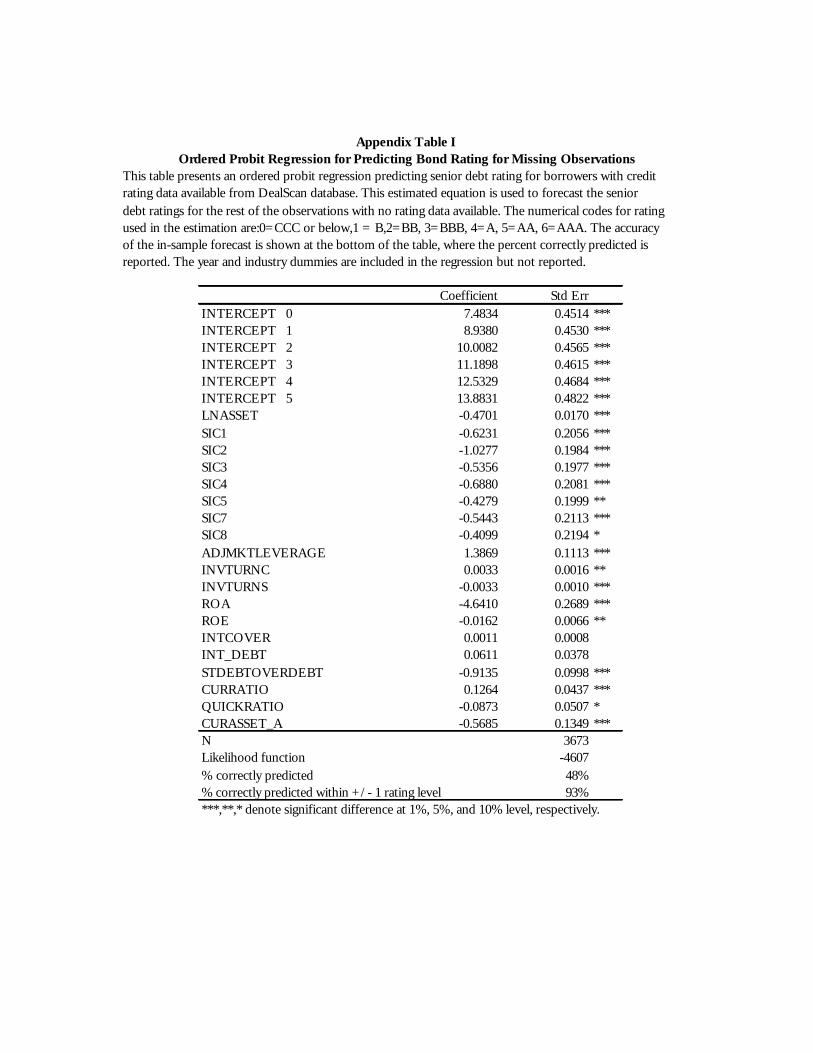
This table presents an ordered probit regression predicting senior debt rating for borrowers with credit rating data available from DealScan database. This estimated equation is used to forecast the senior debt ratings for the rest of the observations with no rating data available. The numerical codes for rating used in the estimation are:0=CCC or below,1 = B,2=BB, 3=BBB, 4=A, 5=AA, 6=AAA. The accuracy of the in-sample forecast is shown at the bottom of the table, where the percent correctly predicted is reported. The year and industry dummies are included in the regression but not reported.
Coefficient Std ErrINTERCEPT 0 7.4834 0.4514 ***INTERCEPT 1 8.9380 0.4530 ***INTERCEPT 2 10.0082 0.4565 ***INTERCEPT 3 11.1898 0.4615 ***INTERCEPT 4 12.5329 0.4684 ***INTERCEPT 5 13.8831 0.4822 ***LNASSET -0.4701 0.0170 ***SIC1 -0.6231 0.2056 ***SIC2 -1.0277 0.1984 ***SIC3 -0.5356 0.1977 ***SIC4 -0.6880 0.2081 ***SIC5 -0.4279 0.1999 **SIC7 -0.5443 0.2113 ***SIC8 -0.4099 0.2194 *ADJMKTLEVERAGE 1.3869 0.1113 ***INVTURNC 0.0033 0.0016 **INVTURNS -0.0033 0.0010 ***ROA -4.6410 0.2689 ***ROE -0.0162 0.0066 **INTCOVER 0.0011 0.0008INT_DEBT 0.0611 0.0378STDEBTOVERDEBT -0.9135 0.0998 ***CURRATIO 0.1264 0.0437 ***QUICKRATIO -0.0873 0.0507 *CURASSET_A -0.5685 0.1349 ***N 3673Likelihood function -4607% correctly predicted 48%% correctly predicted within +/- 1 rating level 93%***,**,* denote significant difference at 1%, 5%, and 10% level, respectively.
Ordered Probit Regression for Predicting Bond Rating for Missing ObservationsAppendix Table I

This example illustrates how we assign values to vectors of relationship dummy variables associated with events ina given financing windows (LDLEL window). Table 4 provides the definitions of these dummy variables.
Sequence of events Loan Debt Loan Equity Loan Single Lead Banker Bank A Bank B Bank A Bank B Bank BVariablesPL 0 1 1 1 1PD 0 0 1 1 1PE 0 0 0 0 1MPL 0 0 1 0 0MPD 0 0 0 1 1MPE 0 0 0 0 1SL 1 1 1 1 0SD 1 0 0 0 0SE 1 1 1 0 0MSL 1 1 0 1 0MSD 0 0 0 0 0MSE 0 1 0 0 0Obs Used in Regs r a r a a
This example illustrates how we assign values to vectors of relationship dummy variables associated with events ina given financing windows (LDL window) when there are multiple bankers in some deals and one dominant relationship.
Sequence of eventsJoint Lead Bankers Bank A Bank B Bank B Bank C Bank A Bank BVariablesPL 0 0 1 1 1 1PD 0 0 0 0 1 1PE 0 0 0 0 0 0MPL 0 0 1 0 1 1MPD 0 0 0 0 0 1MPE 0 0 0 0 0 0SL 1 1 1 1 0 0SD 1 1 0 0 0 0SE 0 0 0 0 0 0MSL 1 1 1 0 0 0MSD 0 1 0 0 0 0MSE 0 0 0 0 0 0Obs Used in Regs r a a r r a
Assigned Values
Appendix Table IIExamples of How Firm Financing and Bank Relationship Variables are Assigned
Example 2 Each Event has Multiple Bankers but One Dominant Relationship for the Window
Example 1 Each Event has Only One Banker
Assigned Values
Loan Debt Loan

This table provides a robustness check for Table VI in the text. Section 3 in the main text describes our approach in determining unique relationship within matched windows with multiple relationships. The clean subsample used for this table included only matched loans from the financial windows with unique relationship.
Coefficient Std Err Coefficient Std Err Coefficient Std Err Coefficient Std Err b0 7.079364 0.2686 25.31 <.0001 InterceptINTERCEPT 7.0794 0.2686 *** 7.1302 0.2712 *** a0 13.09970 1.9383 6.94 <.0001 InterceptINTERCEPT 13.0997 1.9383 *** 13.0777 1.8633 *** b1 0.055534 0.0224 1.24 0.2147 lnamtLNAMT 0.0555 0.0224 ** 0.0534 0.0215 ** a1 -1.40446 0.2561 -5.77 <.0001 lnspreadLNSPREAD -1.4045 0.2561 *** -1.4949 0.2514 *** b2 0.005308 0.0167 0.30 0.7605 PLPL 0.0053 0.0167 0.0043 0.0164 a2 -0.06874 0.0355 -1.90 0.0572 PLPL -0.0687 0.0355 * -0.0669 0.0375 * b3 -0.04555 0.0182 -2.49 0.0129 PDPD -0.0456 0.0182 ** -0.0445 0.0188 ** a3 -0.03799 0.0384 -0.96 0.3377 PDPD -0.0380 0.0384 -0.0419 0.0384 b4 -0.00044 0.0187 -0.02 0.9805 PEPE -0.0004 0.0187 -0.0014 0.0194 a4 0.243955 0.0361 6.59 <.0001 PEPE 0.2440 0.0361 *** 0.2386 0.0374 *** b5 0.016626 0.0124 1.35 0.1769 MPLMPL 0.0166 0.0124 0.0217 0.0128 * a5 -0.00124 0.0265 -0.05 0.9625 MPLMPL -0.0012 0.0265 -0.0016 0.0276 b6 0.004004 0.0230 0.17 0.8672 MPDMPD 0.0040 0.0230 -0.0003 0.0257 a6 -0.06075 0.0468 -1.31 0.1901 MPDMPD -0.0608 0.0468 -0.0828 0.0485 * b7 -0.04314 0.0205 -1.21 0.2252 MPEMPE -0.0431 0.0205 ** 0.0165 0.0524 a7 -0.27677 0.0696 -3.83 0.0001 MPEMPE -0.2768 0.0696 *** -0.2166 0.1104 ** b8 0.031441 0.0162 1.56 0.1186 SLSL 0.0314 0.0162 * 0.0330 0.0192 * a8 0.057270 0.0399 1.46 0.1448 SLSL 0.0573 0.0399 0.0598 0.0407 b9 -0.15317 0.0196 -7.81 <.0001 SDSD -0.1532 0.0196 *** -0.1587 0.0201 *** a9 -0.01612 0.0498 -0.32 0.7507 SDSD -0.0161 0.0498 -0.0219 0.0509 b10 0.043784 0.0255 2.01 0.0445 SESE 0.0438 0.0255 * 0.0443 0.0228 * a10 0.183623 0.0474 4.07 <.0001 SESE 0.1836 0.0474 *** 0.1859 0.0464 *** b11 0.011031 0.0153 0.77 0.4436 MSLMSL 0.0110 0.0153 0.0131 0.0151 a11 -0.07631 0.0316 -2.44 0.0146 MSLMSL -0.0763 0.0316 ** -0.0768 0.0325 ** b12 -0.02314 0.0192 -1.19 0.2344 MSDMSD -0.0231 0.0192 -0.0142 0.0214 a12 -0.06902 0.0401 -1.73 0.0838 MSDMSD -0.0690 0.0401 * -0.0493 0.0215 ** b13 0.092205 0.0385 2.51 0.0120 MSEMSE 0.0922 0.0385 ** 0.1622 0.0582 *** a13 -0.05924 0.0897 -0.66 0.5091 MSEMSE -0.0592 0.0897 -0.1146 0.1605 b14 0.069654 0.0194 2.10 0.0359 ibIB 0.0697 0.0194 *** 0.0819 0.0330 ** a14 0.152694 0.0386 3.83 0.0001 IBIB 0.1527 0.0386 *** 0.1038 0.0506 **
IB_PL 0.0093 0.0457 IB_PL 0.0141 0.0863IB_PD 0.0006 0.0617 IB_PD 0.1033 0.0952IB_PE 0.0088 0.0519 IB_PE -0.0114 0.0991IB_MPL -0.0751 0.0426 * IB_MPL 0.0378 0.0847IB_MPD 0.0471 0.0666 IB_MPD 0.0108 0.1109IB_MPE -0.0998 0.0244 *** IB_MPE -0.1155 0.1691IB_SL -0.0715 0.0562 IB_SL -0.0800 0.1114IB_SD 0.1293 0.0598 ** IB_SD 0.1230 0.1170IB_SE -0.0580 0.0507 IB_SE -0.1390 0.1137IB_MSL -0.0150 0.0562 IB_MSL 0.0751 0.1030IB_MSD -0.1358 0.0747 * IB_MSD -0.1897 0.1321IB_MSE -0.0450 0.0774 IB_MSE 0.2314 0.2057
b27 0.029119 0.1020 0.28 0.7819 multiplelenderMULTIPLELENDER 0.0291 0.1020 0.0290 0.1060 a38 0.069333 0.0326 1.64 0.1004 salegrowthSALEGROWTH 0.0693 0.0326 ** 0.0661 0.0316 ** b28 -0.01317 0.0034 -3.77 0.0002 lntotlendingLNTOTLENDING -0.0132 0.0034 *** -0.0138 0.0035 *** a39 0.001196 0.0001 9.20 <.0001 mve_bveMVE_BVE 0.0012 0.0001 *** 0.0008 0.0001 ***
A: No IB Interaction B: IB Interaction C: No IB Interaction D: IB Interaction
Appendix Table III GMM Estimates of Loan Pricing and Quantity Regressions - Only Observations from Clean Subsample
LNSPREAD Regressions LNAMT Regressions

Coefficient Std Err Coefficient Std Err Coefficient Std Err Coefficient Std Err b30 -0.11109 0.0237 -4.74 <.0001 lnmatureLNMATURE -0.1111 0.0237 *** -0.1159 0.0242 *** a27 1.358618 0.2361 6.07 <.0001 multiplelenderMULTIPLELENDER 1.3586 0.2361 *** 1.4828 0.2275 *** b31 0.143485 0.0343 4.37 <.0001 termBTERMB 0.1435 0.0343 *** 0.1484 0.0351 *** a28 -0.00454 0.0082 -0.55 0.5829 lntotlendingLNTOTLENDING -0.0045 0.0082 -0.0046 0.0085 b32 0.277365 0.0381 7.15 <.0001 termBsubTERMBSUB 0.2774 0.0381 *** 0.2715 0.0397 *** a30 0.015898 0.0514 0.31 0.7548 lnmatureLNMATURE 0.0159 0.0514 0.1776 0.1565 b33 -0.14385 0.0255 -5.37 <.0001 revolverREVOLVER -0.1439 0.0255 *** -0.1344 0.0248 *** a31 0.677054 0.0730 8.80 <.0001 termBTERMB 0.6771 0.0730 *** 0.6771 0.0730 *** b34 -0.33807 0.0421 -7.39 <.0001 strevolverSTREVOLVER -0.3381 0.0421 *** -0.3381 0.0420 *** a32 0.427030 0.1232 3.74 0.0002 termBsubTERMBSUB 0.4270 0.1232 *** 0.4513 0.1153 *** b35 -0.00699 0.0707 -0.10 0.9242 bridgeBRIDGE -0.0070 0.0707 -0.0102 0.0714 a33 0.227234 0.0508 4.33 <.0001 revolverREVOLVER 0.2272 0.0508 *** 0.2162 0.0540 *** b36 0.272344 0.0245 10.91 <.0001 combodealCOMBODEAL 0.2723 0.0245 *** 0.2708 0.0239 *** a34 0.031295 0.1096 0.28 0.7797 strevolverSTREVOLVER 0.0313 0.1096 0.0294 0.1152 b37 0.271871 0.0216 12.97 <.0001 secureSECURE 0.2719 0.0216 *** 0.2718 0.0205 *** a35 0.749632 0.1378 5.30 <.0001 bridgeBRIDGE 0.7496 0.1378 *** 0.7548 0.1486 *** b37p5 -0.03112 0.0167 -1.93 0.0531 perfprcPERFPRC -0.0311 0.0167 * -0.0324 0.0167 * a36 0.145162 0.0726 2.03 0.0428 combodealCOMBODEAL 0.1452 0.0726 ** 0.1443 0.0684 ** b38 0.805738 0.0966 8.43 <.0001 primePRIME 0.8057 0.0966 *** 0.7984 0.1017 *** a37 0.347932 0.0827 4.35 <.0001 secureSECURE 0.3479 0.0827 *** 0.3594 0.0816 *** b39 0.211257 0.0874 -2.49 0.0130 subordinateSUBORDINATE 0.2113 0.0874 ** -0.2082 0.0794 *** a37p5 0.155350 0.0313 5.17 <.0001 perfprcPERFPRC 0.1554 0.0313 *** 0.1594 0.0318 *** b40 -0.06695 0.0420 -1.63 0.1033 takeoverTAKEOVER -0.0670 0.0420 -0.0660 0.0407 a40 0.714449 0.0476 14.93 <.0001 takeoverTAKEOVER 0.7144 0.0476 *** 0.7155 0.0508 *** b41 -0.07857 0.0475 -1.64 0.1018 caprestrucCAPRESTRUC -0.0786 0.0475 * -0.0764 0.0470 a41 0.516006 0.0925 5.31 <.0001 caprestrucCAPRESTRUC 0.5160 0.0925 *** 0.5106 0.0974 *** b42 -0.23412 0.0255 -8.86 <.0001 cpbackupCPBACKUP -0.2341 0.0255 *** -0.2346 0.0261 *** a42 -0.02951 0.0702 -0.45 0.6511 cpbackupCPBACKUP -0.0295 0.0702 -0.0299 0.0680 b43 -0.06359 0.0247 -2.76 0.0058 debtrepayDEBTREPAY -0.0636 0.0247 ** -0.0686 0.0249 *** a43 0.248998 0.0462 5.48 <.0001 debtrepayDEBTREPAY 0.2490 0.0462 *** 0.2541 0.0445 *** b44 0.149568 0.0547 2.62 0.0089 buyoutBUYOUT 0.1496 0.0547 *** 0.1462 0.0551 *** a44 0.393084 0.1257 3.14 0.0017 buyoutBUYOUT 0.3931 0.1257 *** 0.3835 0.1312 *** b45 -0.01717 0.0263 -0.69 0.4928 WorkcapWORKCAP -0.0172 0.0263 -0.0180 0.0250 a45 0.142832 0.0562 2.57 0.0101 WorkcapWORKCAP 0.1428 0.0562 ** 0.1474 0.0584 ** b46 -0.08656 0.0255 -3.33 0.0009 lnassetLNASSET -0.0866 0.0255 *** -0.0887 0.0246 *** a46 0.497568 0.0212 24.42 <.0001 lnassetLNASSET 0.4976 0.0212 *** 0.4916 0.0214 *** b47 0.488742 0.0586 8.08 <.0001 adjmktleverageADJMKTLEVERAGE 0.4887 0.0586 *** 0.4666 0.0586 *** a47 1.803096 0.1682 10.89 <.0001 adjmktleverageADJMKTLEVERAGE 1.8031 0.1682 *** 1.8655 0.1714 *** b48 -1.94839 0.0671 -29.60 <.0001 aaaAAA -1.9484 0.0671 *** -1.9037 0.0649 *** a48 -2.12617 0.5029 -4.24 <.0001 aaaAAA -2.1262 0.5029 *** -2.0034 0.4945 *** b49 -1.74952 0.0661 -27.12 <.0001 aaAA -1.7495 0.0661 *** -1.8198 0.0648 *** a49 -1.48057 0.4262 -3.26 0.0011 aaAA -1.4806 0.4262 *** -1.4425 0.4394 *** b50 -1.38898 0.0622 -22.93 <.0001 aA -1.3890 0.0622 *** -1.4209 0.0588 *** a50 -1.20947 0.3464 -3.53 0.0004 aA -1.2095 0.3464 *** -1.1622 0.3578 *** b51 -0.75339 0.0522 -15.08 <.0001 bbbBBB -0.7534 0.0522 *** -0.7473 0.0523 *** a51 -0.58030 0.2087 -2.83 0.0047 bbbBBB -0.5803 0.2087 *** -0.5795 0.1997 *** b52 -0.27660 0.0446 -6.36 <.0001 bbBB -0.2766 0.0446 *** -0.2674 0.0427 *** a52 -0.13647 0.1078 -1.27 0.2058 bbBB -0.1365 0.1078 -0.1471 0.1103 b53 -0.08778 0.0439 -1.99 0.0466 bB -0.0878 0.0439 ** -0.0849 0.0423 ** a53 -0.21462 0.0906 -2.33 0.0200 bB -0.2146 0.0906 ** -0.2192 0.0899 ** b53p5 0.033735 0.0173 1.51 0.1318 rateforeRATEFORE 0.0337 0.0170 ** 0.0318 0.0167 * a53p5 -0.14387 0.0313 -5.39 <.0001 rateforeRATEFORE -0.1439 0.0313 *** -0.1563 0.0298 ***
N 12405 12405 N 12405 12405GMM Obj Fn 792.7 961.4 GMM Obj Fn 855.9 779.0
Specification Tests1. Overidentification test for validity of instruments (H0:instruments are exogenous) based on GMM Objective Function/N
jointly Chi-sq(2) 0.0639 0.0775 Chi-sq(2) 0.0690 0.0628
A: No IB Interaction B: IB Interaction C: No IB Interaction D: IB Interaction
Appendix Table III (continue)GMM Estimates of Loan Pricing and Quantity Regressions - Only Observations from Clean Subsample
LNSPREAD Regressions LNAMT Regressions

This table presents OLS regressions of log all-in-spread and log amount of all loans used in Table IV. Model A and C include IB dummy but does not interact with financing pattern and relationship variables. Model B and D allow IB interaction.
Coefficient Std Err Coefficient Std Err Coefficient Std Err Coefficient Std ErrINTERCEPT 7.2406 0.0935 *** 6.8370 0.0891 *** INTERCEPT 5.4740 0.1809 *** 5.6467 0.1852 ***LNAMT -0.1023 0.0040 *** -0.1010 0.0039 *** LNSPREAD -0.3871 0.0129 *** -0.3796 0.0123 ***PL 0.0096 0.0089 0.0089 0.0090 PL -0.0196 0.0164 -0.0188 0.0164PD -0.0478 0.0094 *** -0.0471 0.0098 *** PD -0.0354 0.0174 ** -0.0382 0.0183 **PE 0.0612 0.0090 *** 0.0605 0.0091 *** PE 0.2388 0.0174 *** 0.2460 0.0171 ***MPL 0.0071 0.0087 0.0110 0.0090 MPL -0.0266 0.0161 * -0.0306 0.0177 *MPD -0.0183 0.0200 -0.0206 0.0241 MPD -0.0743 0.0394 * -0.1057 0.0435 **MPE -0.0858 0.0376 ** -0.0112 0.0597 MPE -0.1788 0.0669 *** -0.1437 0.1118SL 0.0350 0.0094 *** 0.0389 0.0099 *** SL 0.0013 0.0177 -0.0002 0.0181SD -0.1623 0.0096 *** -0.1560 0.0096 *** SD 0.0967 0.0177 *** 0.0897 0.0177 ***SE 0.0253 0.0103 ** 0.0277 0.0098 *** SE 0.1543 0.0182 *** 0.1686 0.0181 ***MSL -0.0181 0.0094 * -0.0152 0.0096 MSL -0.0386 0.0175 ** -0.0467 0.0182 **MSD -0.0326 0.0197 * -0.0264 0.0200 MSD -0.0407 0.0368 -0.0356 0.0383MSE 0.0832 0.0396 ** 0.1357 0.0547 ** MSE -0.1426 0.0701 ** -0.1993 0.1075 *IB 0.0902 0.0160 *** 0.1442 0.0239 *** IB 0.1466 0.0283 *** 0.0769 0.0459 *IB_PL 0.0009 0.0404 IB_PL -0.0071 0.0721IB_PD -0.0359 0.0528 IB_PD 0.0752 0.0936IB_PE 0.0242 0.0479 IB_PE -0.0240 0.0865IB_MPL -0.0714 0.0410 * IB_MPL 0.0870 0.0739IB_MPD 0.0708 0.0600 IB_MPD 0.0474 0.1147IB_MPE -0.1382 0.0882 IB_MPE -0.0861 0.1525IB_SL -0.0747 0.0433 * IB_SL -0.0099 0.0790IB_SD 0.1148 0.0513 ** IB_SD 0.0952 0.0999IB_SE -0.0698 0.0511 IB_SE -0.1071 0.0997IB_MSL -0.0176 0.0444 IB_MSL 0.1304 0.0857IB_MSD -0.1209 0.0645 * IB_MSD -0.1432 0.1209IB_MSE -0.0125 0.0871 IB_MSE 0.1485 0.1647MULTIPLELENDER -0.0459 0.0176 *** -0.0439 0.0171 ** SALEGROWTH 0.0592 0.0172 *** 0.0560 0.0185 ***LNTOTLENDING -0.0104 0.0018 *** -0.0104 0.0019 *** MVE_BVE 0.0008 7.8333 0.0009 0.0001 ***
Appendix Table IV Loan Pricing and Quantity Regressions (OLS)
LNSPREAD Regressions LNAMT RegressionsC: No IB InteractionA: No IB Interaction B: IB Interaction D: IB Interaction

Coefficient Std Err Coefficient Std Err Coefficient Std Err Coefficient Std ErrLNMATURE -0.0859 0.0078 *** -0.0894 0.0074 *** MULTIPLELENDER 0.8778 0.0302 *** 0.8730 0.0312 ***TERMB 0.2884 0.0166 *** 0.3081 0.0162 *** LNTOTLENDING 0.0257 0.0035 *** 0.0254 0.0035 ***TERMBSUB 0.3966 0.0283 *** 0.3964 0.0291 *** LNMATURE 0.1664 0.0139 *** 0.1713 0.0134 ***REVOLVER -0.0150 0.0084 * -0.0147 0.0090 TERMB 0.3981 0.0298 *** 0.3767 0.0304 ***STREVOLVER -0.2161 0.0150 *** -0.2310 0.0141 *** TERMBSUB 0.0116 0.0571 0.0150 0.0568BRIDGE 0.1721 0.0260 *** 0.1774 0.0266 *** REVOLVER 0.3768 0.0152 *** 0.3700 0.0165 ***COMBODEAL 0.2330 0.0087 *** 0.2217 0.0086 *** STREVOLVER 0.3123 0.0265 *** 0.3372 0.0272 ***SECURE 0.3493 0.0080 *** 0.3428 0.0083 *** BRIDGE 0.7415 0.0484 *** 0.7784 0.0487 ***PERFPRC -0.1257 0.0220 *** -0.1316 0.0222 *** COMBODEAL -0.2965 0.0158 *** -0.2824 0.0170 ***PRIME 0.4768 0.0198 *** 0.4433 0.0191 *** SECURE 0.0399 0.0156 ** 0.0423 0.0167 **SUBORNINATE 0.1209 0.0612 ** 0.1250 0.0602 ** PERFPRC 0.0839 0.0421 ** 0.0809 0.0409 **TAKEOVER 0.0614 0.0111 *** 0.0636 0.0109 *** TAKEOVER 0.6945 0.0194 *** 0.7208 0.0192 ***CAPRESTRUC 0.0974 0.0219 *** 0.0998 0.0211 *** CAPRESTRUC 0.5209 0.0407 *** 0.5505 0.0396 ***CPBACKUP -0.2086 0.0110 *** -0.2154 0.0118 *** CPBACKUP 0.1649 0.0220 *** 0.1686 0.0200 ***DEBTREPAY -0.0152 0.0093 -0.0143 0.0093 DEBTREPAY 0.2693 0.0187 *** 0.2632 0.0187 ***BUYOUT 0.2333 0.0203 *** 0.2522 0.0215 *** BUYOUT 0.2651 0.0410 *** 0.2810 0.0405 ***WORKCAP 0.0058 0.0118 0.0057 0.0126 WORKCAP 0.1088 0.0224 *** 0.1034 0.0237 ***LNASSET 0.0278 0.0036 *** 0.0274 0.0038 *** LNASSET 0.5595 0.0056 *** 0.5764 0.0054 ***ADJMKTLEVERAGE 0.6780 0.0214 *** 0.6301 0.0224 *** ADJMKTLEVERAGE 1.5595 0.0400 *** 1.4977 0.0389 ***AAA -1.6768 0.0587 *** -1.7124 0.0556 *** AAA -0.2421 0.1039 ** -0.2305 0.1064 **AA -1.5424 0.0295 *** -1.4777 0.0285 *** AA 0.2668 0.0585 *** 0.2708 0.0584 ***A -1.1319 0.0243 *** -1.1004 0.0233 *** A 0.0443 0.0444 0.0436 0.0457BBB -0.5778 0.0205 *** -0.5642 0.0204 *** BBB 0.1035 0.0397 *** 0.1020 0.0397 **BB -0.1917 0.0195 *** -0.1883 0.0197 *** BB 0.1150 0.0380 *** 0.1201 0.0366 ***B -0.1022 0.0202 *** -0.0972 0.0203 *** B -0.1039 0.0369 *** -0.1081 0.0373 ***RATEFORE 0.0030 0.0088 0.0031 0.0088 RATEFORE -0.1787 0.0165 *** -0.1764 0.0160 ***Adj R-sq 0.8075 0.8097 Adj R-sq 0.8017 0.7968N 14439 14439 N 14439 14439
Appendix Table IV (continue)Loan Pricing and Quantity Regressions (OLS)
LNSPREAD Regressions LNAMT RegressionsC: No IB InteractionA: No IB Interaction B: IB Interaction D: IB Interaction
Related Documents