Relation between photospheric magnetic field and chromospheric emission

arX

iv:a

stro

-ph/

0701

896v

2 1

6 F

eb 2

007

Astronomy & Astrophysicsmanuscript no. aa2006˙7017 c© ESO 2013November 24, 2013

Relation between photospheric magnetic field and chromosph ericemission

R. Rezaei1, R. Schlichenmaier1, C.A.R. Beck1,2, J.H.M.J. Bruls1, and W. Schmidt1

1 Kiepenheuer-Institut fur Sonnenphysik, Schoneckstr. 6, 79 104 Freiburg, Germany2 Instituto de Astrofısica de Canarias (IAC), E 38 205, La Laguna, Espain

Received 22 December 2006/Accepted 25 January 2007

ABSTRACT

Aims. We investigate the relationship between the photospheric magnetic field and the emission of the mid chromosphere of the Sun.Methods. We simultaneously observed the Stokes parameters of the photospheric iron line pair at 630.2 nm and the intensity profileof the chromospheric CaiiH line at 396.8 nm in a quiet Sun region at a heliocentric angleof 53◦. Various line parameters havebeen deduced from the CaiiH line profile. The photospheric magnetic field vector has been reconstructed from an inversion of themeasured Stokes profiles. After alignment of the Ca and Fe maps, a common mask has been created to define network and inter-network regions. We perform a statistical analysis of network and inter-network properties. The H-index is the integrated emissionin a 0.1 nm band around the Ca core. We separate a non-magnetically, Hnon, and a magnetically, Hmag, heated component from anon-heated component, Hco in the H-index.Results. The average network and inter-network H-indices are equal to 12 and 10 pm, respectively. The emission in the network iscorrelated with the magnetic flux density, approaching a value of H ≈ 10 pm for vanishing flux. The inter-network magnetic field isdominated by weak field strengths with values down to 200 G andhas a mean absolute flux density of about 11 Mx cm−2.Conclusions. We find that a dominant fraction of the calcium emission caused by the heated atmosphere in the magnetic networkhas non-magnetic origin (Hmag ≈ 2 pm, Hnon ≈ 3 pm). Considering the effect of straylight, the contribution from an atmospherewith no temperature rise to the H-index (Hco ≈ 6 pm) is about half of the observed H-index in the inter-network. The H-index in theinter-network is not correlated to any property of the photospheric magnetic field, suggesting that magnetic flux concentrations havea negligible role in the chromospheric heating in this region. The height range of the thermal coupling between the photosphere andlow/mid chromosphere increases in presence of magnetic field. Inaddition, we demonstrate that a poor signal-to-noise levelin theStokes profiles leads to a significant over-estimation of themagnetic field strength.

Key words. Sun: photosphere – Sun: chromosphere – Sun: magnetic fields

1. Introduction

The dominant pattern covering the entire solar surface, exceptsunspots, is granulation, the top of small-scale convection cellswith diameters of 1-2 Mm. On a larger scale of∼20 Mm super-granulesare observed which show the same pattern as granu-lation: a horizontal flow from the center towards the boundaryof the cell. These large scale convection cells have a mean life-time of 20 h, much longer than the granular time-scale (some10 minutes). Thechromospheric networkforms at the boundaryof the supergranular cells. The network is presumably formedby the long–time advection of magnetic flux to the boundariesof the supergranules (Priest et al. 2002; Cattaneo et al. 2003).The interior of the network cells, theinter-network, has muchless magnetic field than the network (e.g., Keller et al. 1994).The magnetic and thermodynamic properties of the network andinter-network are different (e.g., Lites 2002).

The chromospheric heating mechanism is one of the mainchallenges of solar physics (Narain & Ulmschneider 1996, andreferences therein). The core emission of the CaiiH and K linesis an important source of radiative losses in the chromosphere.Moreover, this emission is an important tool to study the tem-perature stratification and the magnetic activity of the outer at-mosphere of the Sun and other stars (e.g., Schrijver & Zwaan2000). Most of the observational studies based on these lines use

Send offprint requests to: [email protected]

either the calcium intensity profile (e.g., Cram & Dame 1983;Lites et al. 1993) or combinations of calcium filtergrams andmagnetograms (e.g., Berger & Title 2001). From the observa-tion of the calcium spectrum alone, it is not possible to distin-guish between the magnetic and non-magnetic heating compo-nents. Combining calcium filtergrams with magnetograms al-lows to separate those components, but the spectral informa-tion is lost. Simultaneous observations that allow to reconstructthe magnetic field and record the spectrum for the CaiiH lineare rare (e.g., Lites et al. 1999) and only available at lowerspatial resolution. Therefore, it is not surprising that none ofthe present theories, mechanical and Joule heating, was con-firmed or rejected observationally (Fossum & Carlsson 2005;Socas-Navarro 2005).

Schrijver (1987) studied a sample of late-type stars and in-troduced the concept of thebasal flux to separate the non-magnetic heating from the magnetic one. The Sun is nota very active star, with a chromospheric radiative loss onthe order of the basal flux for Sun–like stars (Fawzy et al.2002b). Carlsson & Stein (1997) presented a semi–empiricalhydrodynamic model where enhanced chromospheric emissionis due to outward propagating acoustic waves. This modelwas criticized in subsequent investigations (e.g., Kalkofen et al.1999; Fossum & Carlsson 2005), which was partly due to dis-agreements on the temperature stratification in higher lay-ers (e.g., Ayres 2002; Wedemeyer-Bohm et al. 2005). In ad-

http://arxiv.org/abs/astro-ph/0701896v2

2 Rezaei et al.: Relation between photospheric magnetic field and chromospheric emission

dition, it is not clear whether high- or low-frequency acous-tic waves play the dominant role in the energy transportto higher layers (Fawzy et al. 2002a; Jefferies et al. 2006).While there are theoretical indications that the magnetic fill-ing factor discriminates between different regimes of heating(Solanki & Steiner 1990), there is no canonic model reproducingthermal, dynamical and magnetic properties of the solar chromo-sphere (Judge & Peter 1998; Rutten 1999).

The POlarimetric LIttrow Spectrograph (POLIS,Schmidt et al. 2003; Beck et al. 2005a) was designed toprovide co–temporal and co–spatial measurements of themagnetic field in the photosphere and the CaiiH intensityprofile. We use POLIS to address the question of the chro-mospheric heating mechanism, by comparing properties ofnetwork and inter-network in photosphere and chromospherebya statistical analysis. With the information on the photosphericfields, we separate the contributions of the magnetically andnon-magnetically heated component. For the first time westudy the correlation of the chromospheric emission with thecorresponding amplitude/area asymmetry and Stokes-V zero–crossing velocity at the corresponding photospheric position.We also investigate the magnetic field strength distributionof the inter-network to check whether it consists of weakfields (e.g., Faurobert et al. 2001; Collados 2001) or kilo-Gaussfields (e.g., Sanchez Almeida et al. 2003a,b).

Observations and data reduction are explained in Sects. 2 and3. Histograms of the obtained parameters are presented in Sect.4. Correlations between the chromospheric and photospheric pa-rameters are addressed in Sect. 5. The heating contributions areelaborated in Sect. 6. Discussion and conclusions are presentedin Sects. 7 and 8, respectively. Details of the magnetic fieldpa-rameters in the inter-network are discussed in Appendix A. Thestraylight contamination and calibration uncertainties for thePOLIS Ca channel are estimated in Appendix B. An overviewof some of our results also appears in Rezaei et al. (2007).

2. Observations

We observed a network area close to the active region NOAA10675 on September 27, 2004, with the POLIS instrument atthe German Vacuum Tower Telescope (VTT) in Tenerife. Theobservations were part of a coordinated observation campaignin the International Time Program, where also the SwedishSolar Telescope (SST), Dutch Open Telescope (DOT) and theTelescope Heliographique pour l’Etude du Magnetisme et desInstabilites Solaires (THEMIS) participated. Here we analyze aseries of thirteen maps of the same network region at a helio-centric angle of 53◦, taken during several hours. We achieved aspatial resolution of around 1.0 arcsec, estimated from thespa-tial power spectrum of the intensity maps.

All maps were recorded with a slit width of 0.5 arcsec, a slitheight of 47.5 arcsec, and an exposure time per slit positionof4.92 s. The scan extension for the first three maps was 40.5, 55.5,and 20.5 arcsec, while it was 25.5 arcsec for the remaining tenmaps.

The CaiiH line and the visible neutral iron lines at630.15nm, 630.25nm, and Tii 630.38nm were observed withthe blue (396.8nm) and red (630 nm) channels of POLIS. Thespatial sampling along the slit (y-axis in Fig. 1) was 0.29 arc-sec. The scanning step was 0.5 arcsec for all maps. The spectralsampling of 1.92 pm for the blue channel and 1.49 pm for the redchannel leads to a velocity dispersion of 1.45 and 0.7 km s−1 perpixel, respectively. The spectropolarimetric data of the red chan-

Table 1. The definition of the characteristic parameters of theCaiiH profile for the peak sample (upper part) and the band sam-ple (lower part) (see also Fig. 2). Wavelengths are in nm.

quantity: peak sample descriptionH3 core intensityH2v violet emission peakH2r red emission peakV/R H2v/H2r

emission strength H2v/H3

λ(H3) calcium core wavelengthλ(H2v) H2v wavelengthλ(H2r) H2r wavelength

quantity: band sample descriptionH-index 396.849± 0.050

H3 396.849± 0.008H2v 396.833± 0.008H2r 396.865± 0.008W1 outer wing: 396.632± 0.005W2 middle wing: 396.713± 0.010W3 inner wing: 396.774± 0.010

nel were corrected for instrumental effects and telescope polar-ization with the procedures described by Beck et al. (2005a,b).

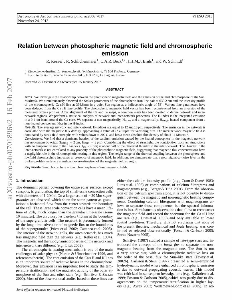
Figure 1 displays an overview of one of the thirteen mapsafter spatial alignment. The map (a) shows the Fei630 nm con-tinuum intensity normalized to the average quiet Sun intensity.The map (b) shows the CaiiH wing intensity, taken close to396.490nm (for a definition of line parameters see Fig. 2 andTable 1). These two maps were used for the spatial alignment ofthe red and blue channels. The next two maps (c and d) showthe intensities in the outer and inner wings (W1, respectively,W3). The inner wing samples a wavelength band close to thecore; hence, it is more influenced by the line–core emission andshows higher contrast of the network than the outer wing. Thenext map (e) is the H-index, i.e., the intensity of the calciumcore integrated over 0.1 nm (cf. Table 1). The network featuresappear broadest and show the highest contrast in this map. Themap (f) demonstrates network and inter-network masks (Sect.3.1). The map (g) shows the magnetic flux density obtained fromthe spectro-polarimetric data (Sect. 3.2).

3. Data analysis

In this section we discuss characteristic parameters of thecal-cium profile and the Fei 630 nm line pair. We briefly explain theinversion method that was used to infer the vector magnetic field.

3.1. Definition of network and inter-network

For each map, we created a mask to distinguish between the net-work and inter-network regions (Fig. 1f). This was done manu-ally on the basis of the magnetic flux and the H-index. We didnot use the black region in Fig. 1f which separates network frominter-network. To study structures in these two regions, wede-fine two statistical samples:

The peak sample: Each member of this sample has a reg-ular V profile and a double reversal in the calcium core. Forthis sample, we study quantities related to the CaiiH emissionpeaks (Table 1, upper part). The number of data points in the net-work and inter-network are 19509 and 1712, respectively. Weemphasize that the few inter-network points in this sample are

Rezaei et al.: Relation between photospheric magnetic fieldand chromospheric emission 3

Fig. 1. From left to right:a) the Fei630 nm continuum intensity, b) the calcium wing intensity at396.490nm which was calibratedto FTS data (Stenflo et al. 1984), c) the outer calcium wing intensity (W1), d) the inner calcium wing intensity (W3), e) theH-index, f) the masks which separate network (white) from the inter-network (gray), and g) the magnetic flux density obtained fromthe inversion. We did not use the black region between the network and inter-network. Each small tickmark is 1 arcsec. Note thatsampling in x and y directions are different.

396.4 396.5 396.6 396.7 396.8 396.9wavelength (nm)

0.0

0.1

0.2

0.3

0.4

0.5

norm

aliz

ed in

tens

ity

W1W2

W3

H2v H3 H2r

H-index

Fe I 396.451

Fe I 396.607

fit to FTSprofile

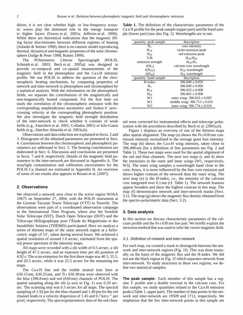
Fig. 2. Sample averaged calcium profile of one of the maps (theaverage profile is similar for all other maps). The bands are ex-plained in Table 1.

not distributed uniformly. They usually belong to small-scalemagnetic elements surrounded by large areas without magneticsignal above the noise level.

The band sample: All network and inter-network points,marked in the masks, are present in this sample. Since someof these profiles do not have two emission peaks in the cal-cium core, we use integrated intensities in a fixed spectralrange (Cram & Dame 1983) at the core and wing of the calciumprofile (Table 1, lower part). This definition retrieves reasonablechromospheric parameters. In total from all the maps, 24225points were selected as network (white in Fig. 1f) and 20855as inter-network positions (gray in Fig. 1f).

3.2. Analysis of Ca iiH profiles

We averaged profiles over a large area (including network) toob-tain an average profile for each map. These average profiles arethe mean of more than three thousand profiles each time; an ex-ample is shown in Fig. 2. We then normalized the intensity at theline wing at 396.490nm to the FTS profile (Stenflo et al. 1984).

The same normalization coefficient was applied to all profiles ofthe map. Hence, all profiles are normalized to the average con-tinuum intensity.

Table 1 lists the characteristic parameters we define for eachcalcium profile:

a) The intensity of the CaiiH core, H3, and the amplitudes ofthe emission peaks, H2v and H2r, and their respective posi-tions,λH3 , λH2v, andλH2r (peak sample).

b) Intensities in the outer (W1), middle (W2), and inner linewings (W3), which are integrated over spectral bands with afixedspectral range (band sample).

From these quantities we derive:

1. the ratio of the emission peaks, V/R = H2v/H2r, and2. the emission strength which is the intensity of the violet

emission peak divided by the core, H2v/H3.

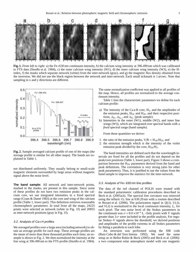
The band intensities are defined such that the wavelength in-tervals are fixed for all the profiles and do not depend on thepeak/core positions (Table 1, lower part). Figure 3 shows a com-parison between the H2v parameters derived from the band andpeak definitions. The correlation is very strong (also for otherpeak parameters). Thus, it is justified to use the values fromtheband sample to improve the statistics for the inter-network.

3.3. Analysis of Fe i 630 nm line profiles

The data of the red channel of POLIS were treated withthe standard polarimetric calibration procedures described inBeck et al. (2005a,b). The spectral line curvature was removedusing the telluric O2 line at 630.20nm with a routine describedin Rezaei et al. (2006). The polarization signal inQ(λ), U(λ),andV(λ) is normalized to the local continuum intensity,Ic, foreach pixel. The rms noise level of the Stokes parameters inthe continuum wasσ=8.0×10−4 Ic. Only pixels withV signalsgreater than 3σ were included in the profile analysis. For regu-lar Stokes–V signals above the threshold, we derived positionsand amplitudes of the profile extrema in all Stokes parametersby fitting a parabola to each lobe.

An inversion was performed using the SIR code(Ruiz Cobo & del Toro Iniesta 1992). We used the samesetup as in Bellot Rubio & Beck (2005) and Beck et al. (2006):a two–component solar atmosphere model with one magnetic


8 10 12 14 16H-index (pm)

0

2

4

6

8

freq

uenc

y(%

) (a)

1.0 1.5 2.0 2.5 3.0 3.5H2v (pm)

0

2

4

6

8

10

freq

uenc

y(%

) (b)

1.0 1.5 2.0 2.5 3.0 3.5H2r (pm)

0

2

4

6

8

10

freq

uenc

y(%

) (c)

2.2 2.4 2.6 2.8 3.0 3.2inner wing (pm)

0

2

4

6

8

freq

uenc

y(%

) (d)

2.8 3.0 3.2 3.4 3.6 3.8 4.0middle wing (pm)

0

2

4

6

8

freq

uenc

y(%

) (e)

2.0 2.2 2.4 2.6 2.8 3.0outer wing (pm)

0

2

4

6

8fr

eque

ncy(

%) (f)

0.30 0.35 0.40 0.45Ca wing

0

2

4

6

8

freq

uenc

y(%

) (g)

0.95 1.00 1.05Fe continuum

0

2

4

6

8

freq

uenc

y(%

) (h)

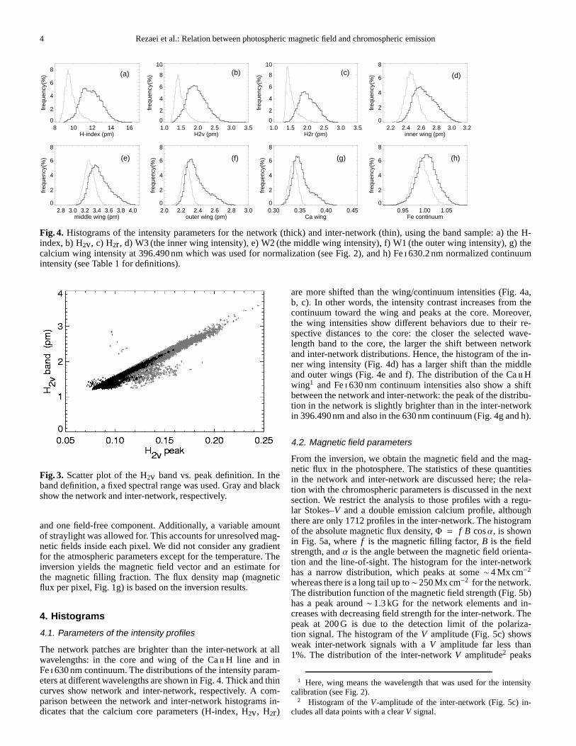
Fig. 4. Histograms of the intensity parameters for the network (thick) and inter-network (thin), using the band sample: a) the H-index, b) H2v, c) H2r, d) W3 (the inner wing intensity), e) W2 (the middle wing intensity), f) W1 (the outer wing intensity), g) thecalcium wing intensity at 396.490nm which was used for normalization (see Fig. 2), and h) Fei630.2 nm normalized continuumintensity (see Table 1 for definitions).

Fig. 3. Scatter plot of the H2v band vs. peak definition. In theband definition, a fixed spectral range was used. Gray and blackshow the network and inter-network, respectively.

and one field-free component. Additionally, a variable amountof straylight was allowed for. This accounts for unresolvedmag-netic fields inside each pixel. We did not consider any gradientfor the atmospheric parameters except for the temperature.Theinversion yields the magnetic field vector and an estimate forthe magnetic filling fraction. The flux density map (magneticflux per pixel, Fig. 1g) is based on the inversion results.

4. Histograms

4.1. Parameters of the intensity profiles

The network patches are brighter than the inter-network at allwavelengths: in the core and wing of the CaiiH line and inFei630 nm continuum. The distributions of the intensity param-eters at different wavelengths are shown in Fig. 4. Thick and thincurves show network and inter-network, respectively. A com-parison between the network and inter-network histograms in-dicates that the calcium core parameters (H-index, H2v, H2r)

are more shifted than the wing/continuum intensities (Fig. 4a,b, c). In other words, the intensity contrast increases fromthecontinuum toward the wing and peaks at the core. Moreover,the wing intensities show different behaviors due to their re-spective distances to the core: the closer the selected wave-length band to the core, the larger the shift between networkand inter-network distributions. Hence, the histogram of the in-ner wing intensity (Fig. 4d) has a larger shift than the middleand outer wings (Fig. 4e and f). The distribution of the CaiiHwing1 and Fei 630 nm continuum intensities also show a shiftbetween the network and inter-network: the peak of the distribu-tion in the network is slightly brighter than in the inter-networkin 396.490nm and also in the 630 nm continuum (Fig. 4g and h).

4.2. Magnetic field parameters

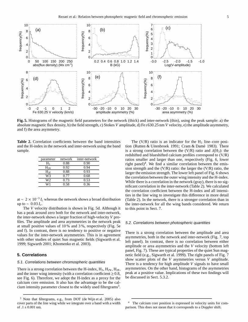
From the inversion, we obtain the magnetic field and the mag-netic flux in the photosphere. The statistics of these quantitiesin the network and inter-network are discussed here; the rela-tion with the chromospheric parameters is discussed in the nextsection. We restrict the analysis to those profiles with a regu-lar Stokes–V and a double emission calcium profile, althoughthere are only 1712 profiles in the inter-network. The histogramof the absolute magnetic flux density,Φ = f B cosα, is shownin Fig. 5a, wheref is the magnetic filling factor,B is the fieldstrength, andα is the angle between the magnetic field orienta-tion and the line-of-sight. The histogram for the inter-networkhas a narrow distribution, which peaks at some∼4 Mx cm−2

whereas there is a long tail up to∼ 250 Mx cm−2 for the network.The distribution function of the magnetic field strength (Fig. 5b)has a peak around∼ 1.3 kG for the network elements and in-creases with decreasing field strength for the inter-network. Thepeak at 200 G is due to the detection limit of the polariza-tion signal. The histogram of theV amplitude (Fig. 5c) showsweak inter-network signals with aV amplitude far less than1%. The distribution of the inter-networkV amplitude2 peaks

1 Here, wing means the wavelength that was used for the intensitycalibration (see Fig. 2).

2 Histogram of theV-amplitude of the inter-network (Fig. 5c) in-cludes all data points with a clearV signal.


0 50 100 150 200 250abs(flux density) (Mx cm-2)

0

2

4

6

8

10

freq

uenc

y(%

) (a)

0.2 0.4 0.6 0.8 1.0 1.2 1.4B (kG)

0

2

4

6

8

10

freq

uenc

y(%

) (b)

-3.0 -2.5 -2.0 -1.5 -1.0Log(V-amplitude)

01234567

freq

uenc

y(%

)

(c)

-3 -2 -1 0 1 2 Fe 630.25 V velocity (km/s)

0

2

4

6

8

freq

uenc

y(%

) (d)

-30 -20 -10 0 10 20 30amplitude asymmetry (%)

0

2

4

6

8

10

freq

uenc

y(%

) (e)

-30 -20 -10 0 10 20 30area asymmetry (%)

0

2

4

6

8

10

freq

uenc

y(%

) (f)

Fig. 5. Histograms of the magnetic field parameters for the network (thick) and inter-network (thin), using the peak sample: a) theabsolute magnetic flux density, b) the field strength, c) StokesV amplitude, d) Fei630.25nmV velocity, e) the amplitude asymmetry,and f) the area asymmetry.

Table 2. Correlation coefficients between the band intensitiesand the H-index in the network and inter-network using the bandsample.

parameter network inter-networkH3 0.88 0.90H2v 0.92 0.94H2r 0.88 0.93W3 0.77 0.68W2 0.73 0.53W1 0.58 0.36

at∼ 2 × 10−3 Ic whereas the network shows a broad distributionup to∼ 0.03 Ic.

TheV velocity distribution is shown in Fig. 5d. Although ithas a peak around zero both for the network and inter-network,the inter-network shows a larger fraction of high-velocityV pro-files. The amplitude and area asymmetries in the network peakat small positive values of 10 % and 3 %, respectively (Fig. 5eand f). In contrast, there is no tendency to positive or negativevalues for the inter-network asymmetries. This is in agreementwith other studies of quiet Sun magnetic fields (Sigwarth et al.1999; Sigwarth 2001; Khomenko et al. 2003).

5. Correlations

5.1. Correlations between chromospheric quantities

There is a strong correlation between the H-index, H3, H2v, H2r,and the inner wing intensity (with a correlation coefficient≥ 0.8,see Fig. 6). Therefore, we adopt the H-index as a proxy for thecalcium core emission. It also has the advantage to be the cal-cium intensity parameter closest to the widely used filtergrams3.

3 Note that filtergrams, e.g., from DOT (de Wijn et al. 2005) alsocover parts of the line wing while we integrate over a band with a widthof .1± 0.001 nm.

The (V/R) ratio is an indicator for the H3 line–core posi-tion (Rutten & Uitenbroek 1991; Cram & Dame 1983). Thereis a strong correlation between the (V/R) ratio andλ(H3): theredshifted and blueshifted calcium profiles correspond to (V/R)ratios smaller and larger than one, respectively (Fig. 6, lowerright panel)4. We find a similar correlation between the emis-sion strength and the (V/R) ratio: the larger the (V/R) ratio, thelarger the emission strength. The lower left panel of Fig. 6 showsthe correlation between the outer wing intensity and the H-index.While there is a correlation in the network (gray), there is no sig-nificant correlation in the inter-network (Table 2). We calculatedthe correlation coefficient between the H-index and all intensi-ties in the line wing to investigate this difference in more detail(Table 2). In the network, there is a stronger correlation than inthe inter-network for all the wing bands considered. We returnto this point in Sect. 7.

5.2. Correlations between photospheric quantities

There is a strong correlation between the amplitude and areaasymmetries, both in the network and inter-network (Fig. 7,topleft panel). In contrast, there is no correlation between eitheramplitude or area asymmetries and theV velocity (bottom leftpanel, Fig. 7). These are typical properties of the quiet Sunmag-netic field (e.g., Sigwarth et al. 1999). The right panels of Fig. 7show scatter plots of theV asymmetries versusV amplitude.There is a tendency for high amplitudeV signals to have smallasymmetries. On the other hand, histograms of the asymmetriespeak at a positive value. Implications of these two findings willbe discussed in Sect. 5.3.2.

4 The calcium core position is expressed in velocity units forcom-parison. This does not mean that it corresponds to a Doppler shift.


Fig. 6. Upper panels: correlation between the H2v and H2r basedon the peak sample and the H-index.Lower left: correlation be-tween W1 and the H-index.Lower right: correlation of the (V/R)ratio with the calcium core position. Gray and black show thenetwork and inter-network, respectively (for abbreviations, seeTable 1).

Fig. 7. Top left: scatter plot of the amplitude vs. area asymme-tries. Bottom left: scatter plot of the area asymmetry vs. theVvelocity. Right panels: scatter plots of the amplitude and areaasymmetries vs. the Fei630.25nmV amplitude. Gray and blackshow the network and inter-network, respectively.

5.3. Correlations between photospheric and chromosphericquantities

5.3.1. Calcium core emission vs. magnetic flux

The upper panel of Fig. 8 shows the relation between the pho-tospheric magnetic flux and the chromospheric emission for thenetwork. For lower flux values (<100 Mx cm−2 ), there is a clearincrease of emission with flux. However, for higher magneticflux densities, the H-index increases slowly. To reproduce theobserved relation, we utilize a power law fit to the data,

H = aΦb + c, (1)

whereΦ is the absolute magnetic flux density,H is the H-index,a is a constant coefficient, b is the power index, andc is thenon–magnetic contribution (see section 5.3.2). We use a variable

Fig. 8. Upper panel: Correlation between the H-index and theabsolute magnetic flux density. Gray is the original data andblack is the binned data: each point is average of 25 points. Themiddle curve shows a fit of a power law to the original data (Eq.1), the other two curves give the 1−σ error range of the fit.Lowerpanel:There is no correlation between the H-index and the mag-netic flux density in inter-network.

lower threshold of 0, 3, .., 20 Mx cm−2 (cf. Table 3) for the fit andneglect all data points with fluxes below this level. We find thatthe power exponent,b, depends strongly on the threshold. Thehigher the threshold, the better the fit curve resembles a straightline, as first reported by Skumanich et al. (1975). If we keep allthe points, including inter-network, we obtain a value for thepower exponentb of ≈ 0.2.

The calcium core emission in the inter-network does not cor-relate with the magnetic flux, at least with the concentratedmag-netic field within the Zeeman sensitivity (Fig. 8, lower panel).The value of the offset,c, of the fit to the network (Table 3)for low magnetic flux densities is around 10 pm, which is con-sistent with the average H-index value of all the inter-networkprofiles (10 pm for the peak sample). The value of thec param-eter changes for different thresholds of the flux density (Table3). Implications of this finding for the basal flux are discussed inSect. 7.

5.3.2. Calcium core emission vs. Stokes–V velocity and areaasymmetry

There are different behaviors for the network and inter-networkcalcium core emission with respect toV velocity and asymme-tries (Fig. 9). The core emission peaks at small positive ampli-tude/area symmetry in the network. This is caused by strong


Fig. 9. Correlation between the H-index and amplitude/area asymmetry andV velocity. Plusses and squares show network andinter-network, respectively. The binning method is similar to Fig. 8

Table 3. The parameters of the fit to Eq. 1 to the network data.The first column is the threshold for the magnetic flux den-sity (Mx cm−2 ). By increasing the threshold, we avoid the inter-network intrusions. For a comparison to the peak inter-networkflux density, see Appendix A.

cut a (pm) b c(pm)0 0.73± 0.05 0.28± 0.01 10.1± 0.13 0.71± 0.05 0.29± 0.01 10.1± 0.15 0.61± 0.04 0.31± 0.01 10.3± 0.110 0.22± 0.02 0.45± 0.02 11.0± 0.120 0.14± 0.06 0.51± 0.06 11.3± 0.2

V profiles that show small asymmetries (Fig. 7, right panels).The highest H-index in the network corresponds to almost zeroV velocity. In its diagram (Fig. 9), the slope of the left branch(blueshift) is smaller than the right one. Moreover for the strongupflow or downflow in the magnetic atmosphere in the network,the H-index decreases significantly. The H-index in the inter-network does not depend on any parameter of the Stokes–V pro-file (Fig. 9).

Considering the fact that the amplitude and area asymmetriesstrongly correlate with each other (top left panel, Fig. 7),a nat-ural consequence is that the left (right) branch of the scatter plotof the H-index vs. amplitude asymmetry corresponds to the left(right) branch of the scatter plot of the H-index vs. area asym-metry (Fig. 9). However, if we compare only negative or posi-tive branches of the scatter plots of the H-index vs.V velocityand asymmetries in the network, we realize that the left branchin the V velocity does notcorrespond to the similar branch inthe asymmetry plots. The left diagrams in Fig. 10 consider onlythe profiles with a negativeV velocity, while in the right pan-els profiles with a negative area asymmetry are shown. A pos-itive V velocity may thus correspond to a positive or negativearea asymmetry. There is no relation between the amplitude/areaasymmetries and theV signal in the inter-network (right panels,Fig. 7).

6. The magnetically and non-magnetically heatedcomponents

The H-index includes the H1 (the minima outside the emissionpeaks), H2, and H3 spectral regions. So its formation height ex-tends from the higher photosphere to the middle chromosphere.

The CaiiH & K lines are one of the main sources of the chro-mospheric radiative loss. We use the H-index as a proxy for

Fig. 10. In the left column diagrams, only the points with a neg-ativeV velocity are plotted. In the right panels, only points witha negative area asymmetry are plotted. Pluses and squares shownetwork and inter-network, respectively.

the emission in the low/mid chromosphere, and assume a linearrelation between the H-index and the chromospheric radiativeloss. To derive the contribution of magnetic fields to the chro-mospheric emission, we added the H-index of all points withmagnetic flux above a given flux threshold. Thefractional H-index, η, is then defined by normalizing this quantity to the totalH-index of all points in the field of view5:

η (Φ > Φ0) =∑

H (Φ > Φ0)∑

H (all maps).

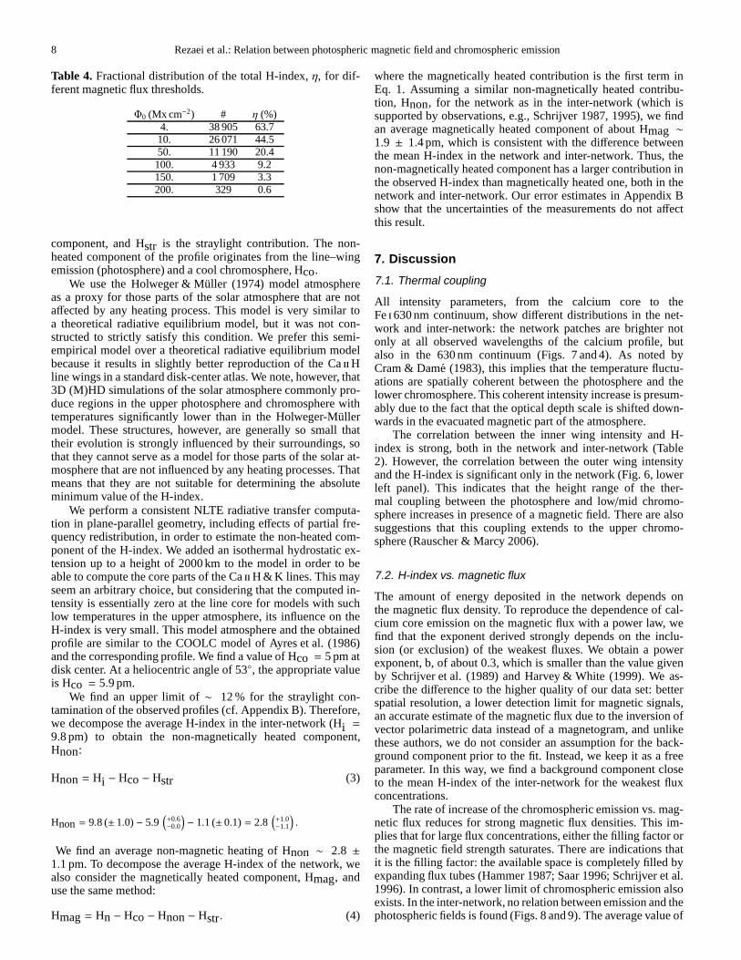
Table 4 lists the fractional H-index in different magnetic fluxthresholds. Some 20 % of the total H-index is provided by strongflux concentrations (Φ ≥ 50. Mx cm−2) while the remaining80 % of that is produced by the weak magnetic field and/or fieldfree regions.

The average H-index is 12.0 and 9.8 pm in the network andinter-network, respectively. However, it contains some contribu-tions from the photosphere (outside emission peaks) and a coolchromosphere (without temperature rise). Therefore, we decom-pose the observed calcium profiles in aheatedand anon-heatedcomponent,

Hi = Hco+ Hnon+ Hstr (2)

where Hi is the average H-index of the inter-network, Hco isthe non-heated component, Hnonis the non-magnetically heated

5 We use all data points in this part and do not use the mask definedin Sect. 3.


Table 4. Fractional distribution of the total H-index,η, for dif-ferent magnetic flux thresholds.

Φ0 (Mx cm−2) # η (%)4. 38 905 63.710. 26 071 44.550. 11 190 20.4100. 4 933 9.2150. 1 709 3.3200. 329 0.6

component, and Hstr is the straylight contribution. The non-heated component of the profile originates from the line–wingemission (photosphere) and a cool chromosphere, Hco.

We use the Holweger & Muller (1974) model atmosphereas a proxy for those parts of the solar atmosphere that are notaffected by any heating process. This model is very similar toa theoretical radiative equilibrium model, but it was not con-structed to strictly satisfy this condition. We prefer thissemi-empirical model over a theoretical radiative equilibrium modelbecause it results in slightly better reproduction of the CaiiHline wings in a standard disk-center atlas. We note, however, that3D (M)HD simulations of the solar atmosphere commonly pro-duce regions in the upper photosphere and chromosphere withtemperatures significantly lower than in the Holweger-Mullermodel. These structures, however, are generally so small thattheir evolution is strongly influenced by their surroundings, sothat they cannot serve as a model for those parts of the solar at-mosphere that are not influenced by any heating processes. Thatmeans that they are not suitable for determining the absoluteminimum value of the H-index.

We perform a consistent NLTE radiative transfer computa-tion in plane-parallel geometry, including effects of partial fre-quency redistribution, in order to estimate the non-heatedcom-ponent of the H-index. We added an isothermal hydrostatic ex-tension up to a height of 2000 km to the model in order to beable to compute the core parts of the CaiiH & K lines. This mayseem an arbitrary choice, but considering that the computedin-tensity is essentially zero at the line core for models with suchlow temperatures in the upper atmosphere, its influence on theH-index is very small. This model atmosphere and the obtainedprofile are similar to the COOLC model of Ayres et al. (1986)and the corresponding profile. We find a value of Hco = 5 pm atdisk center. At a heliocentric angle of 53◦, the appropriate valueis Hco = 5.9 pm.

We find an upper limit of∼ 12 % for the straylight con-tamination of the observed profiles (cf. Appendix B). Therefore,we decompose the average H-index in the inter-network (Hi =9.8 pm) to obtain the non-magnetically heated component,Hnon:

Hnon= Hi − Hco− Hstr (3)

Hnon= 9.8 (± 1.0)− 5.9(

+0.6−0.0

)

− 1.1 (± 0.1) = 2.8(

+1.0−1.1

)

.

We find an average non-magnetic heating of Hnon ∼ 2.8 ±1.1 pm. To decompose the average H-index of the network, wealso consider the magnetically heated component, Hmag, anduse the same method:

Hmag= Hn − Hco− Hnon− Hstr. (4)

where the magnetically heated contribution is the first terminEq. 1. Assuming a similar non-magnetically heated contribu-tion, Hnon, for the network as in the inter-network (which issupported by observations, e.g., Schrijver 1987, 1995), wefindan average magnetically heated component of about Hmag ∼1.9 ± 1.4 pm, which is consistent with the difference betweenthe mean H-index in the network and inter-network. Thus, thenon-magnetically heated component has a larger contribution inthe observed H-index than magnetically heated one, both in thenetwork and inter-network. Our error estimates in AppendixBshow that the uncertainties of the measurements do not affectthis result.

7. Discussion

7.1. Thermal coupling

All intensity parameters, from the calcium core to theFei630 nm continuum, show different distributions in the net-work and inter-network: the network patches are brighter notonly at all observed wavelengths of the calcium profile, butalso in the 630 nm continuum (Figs. 7 and 4). As noted byCram & Dame (1983), this implies that the temperature fluctu-ations are spatially coherent between the photosphere and thelower chromosphere. This coherent intensity increase is presum-ably due to the fact that the optical depth scale is shifted down-wards in the evacuated magnetic part of the atmosphere.

The correlation between the inner wing intensity and H-index is strong, both in the network and inter-network (Table2). However, the correlation between the outer wing intensityand the H-index is significant only in the network (Fig. 6, lowerleft panel). This indicates that the height range of the ther-mal coupling between the photosphere and low/mid chromo-sphere increases in presence of a magnetic field. There are alsosuggestions that this coupling extends to the upper chromo-sphere (Rauscher & Marcy 2006).

7.2. H-index vs. magnetic flux

The amount of energy deposited in the network depends onthe magnetic flux density. To reproduce the dependence of cal-cium core emission on the magnetic flux with a power law, wefind that the exponent derived strongly depends on the inclu-sion (or exclusion) of the weakest fluxes. We obtain a powerexponent, b, of about 0.3, which is smaller than the value givenby Schrijver et al. (1989) and Harvey & White (1999). We as-cribe the difference to the higher quality of our data set: betterspatial resolution, a lower detection limit for magnetic signals,an accurate estimate of the magnetic flux due to the inversionofvector polarimetric data instead of a magnetogram, and unlikethese authors, we do not consider an assumption for the back-ground component prior to the fit. Instead, we keep it as a freeparameter. In this way, we find a background component closeto the mean H-index of the inter-network for the weakest fluxconcentrations.

The rate of increase of the chromospheric emission vs. mag-netic flux reduces for strong magnetic flux densities. This im-plies that for large flux concentrations, either the filling factor orthe magnetic field strength saturates. There are indications thatit is the filling factor: the available space is completely filled byexpanding flux tubes (Hammer 1987; Saar 1996; Schrijver et al.1996). In contrast, a lower limit of chromospheric emissionalsoexists. In the inter-network, no relation between emissionand thephotospheric fields is found (Figs. 8 and 9). The average value of


the H-index in the inter-network of around 10 pm correspondstothe offset,c, Eq. 1. This reflects a constant contribution to the H-index which is present even without photospheric magnetic flux,in agreement with Schrijver (1987, 1995) who argued that thebasal flux does not depend on the magnetic activity. The basalflux contains two components: the non-heated (cf. Sect. 6) andthe non-magnetically heated contributions. The non-heated con-tribution depends on the temperature stratification, so that wespeculate that the non-magnetically heated component has an in-verse dependence on the temperature stratification.

Figure 8 (upper panel) shows that there is a variable lowerlimit for the H-index versus the magnetic flux density. In con-trast, the upper limit is less clearly defined, and would be inagreement with a constant maximum value independent of theamount of magnetic flux. There are also similar behaviors forthe upper and lower limits in the scatter plots of the H3, H2v,and H2r versus the magnetic flux density. This is similar to up-per and lower limits of the basal flux of stars vs. the color (B-V)where the lower boundary changes but the upper one is almostconstant (Fawzy et al. 2002b, their Fig. 2). The situation for theinter-network is different: both the upper and lower limits areindependent of the magnetic flux density.

7.3. Decomposing the Ca iiH profile

We interpret the solar CaiiH line profile as the superposition ofa cool chromospheric profile, the heated component and stray-light components. Oranje (1983) first applied this method toreproduce different observed Ca II K profiles from two “basic”profiles. Later, Solanki et al. (1991) used the same idea to de-compose the observed profiles by a combination of two theoret-ically calculated profiles. Our one-dimensional NLTE radiativetransfer calculations reveal that the H-index of a cool chromo-sphere is about 5.9 pm. Since the chromospheric emission of theSun as a star is slightly above the minimum among the Sun–like stars (Schrijver & Zwaan 2000), the average quiet Sun pro-file contains a heated component. Subtraction of the cool chro-mospheric component from the measured H-index (along withstraylight considerations) leads to an estimation of thepurenon-magnetically and magnetically heated components in the mea-sured H-index. The non-magnetically heated component is al-most 50 % larger than the magnetically heated component. Thepresence of a significant non-heated contribution in the H-indexindicates that not all of the chromospheric emission emergesfrom a hot chromosphere, in contrast to findings from, e.g.,Kalkofen et al. (1999). The minimum heated component in aCa profile provides evidence how cool the chromosphere maybe (e.g., Wedemeyer-Bohm et al. 2005). Moreover, it favorsthe-ories in which the non-magnetic heating plays the dominant rolein the chromospheric heating (Fawzy et al. 2002a).

The fact that the non-magnetic chromospheric heating con-tributes significantly to the chromospheric energy balanceis alsofound in the relative contributions of mainly field–free inter-network and network areas to the total emission in the field ofview. Magnetic flux densities above 50 Mx cm−2 add only 20 %to the total emission, which is also seen in the ratio of the meanH-index in the network and inter-network, 12.0/ 9.8≈1.2 (Table4) .

7.4. Uncertainties

The main uncertainty in the non-magnetically and magneticallyheated components is the presence of some heating in our cool

chromosphere profile. The Holweger & Muller (1974) model at-mosphere is close to an atmosphere in radiative equilibriumwithout non-magnetic or magnetic heating, so no heated com-ponent (cf. Sect. 6) is expected to be found on its Ca profile.Since there is no general agreement how cool the chromospheremay be (e.g., Kalkofen et al. 1999; Ayres 2002), the best answerwould be to use the observed calcium profile with the lowestH-index. However, Solanki et al. (1991) concluded that it isnotpossible to observe a low activity profile as presented by theCOOLC model of Ayres et al. (1986), which is similar to the oneemployed by us on base of the Holweger & Muller (1974) modelatmosphere. Thus, our cool profile can well serve as lower limitof the non-heated contribution to the H-index. Note that a largervalue for Hco would increase the contribution of the magneti-cally heated component, leading to a larger fractional contribu-tion for the magnetically heated to the total heated component.

There may be some mixed polarity fields below our polari-metric detection limit which may influence the ratio of the mag-netically heated to the non-magnetically heated component.

7.5. H-index vs. V asymmetries

From the relations of the chromospheric emission to quantitiesof the photospheric magnetic field in the network, we find thatthe chromospheric emission peaks at small positive values of theStokesV asymmetries and at zero StokesV velocity (Fig. 5). Itreflects the histograms of the respective photospheric fieldquan-tities which show similar distributions even at disk center(e.g.,Sigwarth et al. 1999). However, in combination with the depen-dence of the emission on the flux density it is inferred that thestronger flux concentrations mainly show small material flowsalong with non-zero asymmetries.

The magnetically heated component is related to StokesV profiles with non-zero area and amplitude asymmetries(Figs. 5 and 9). A possible explanation for this finding wouldbethe absorption of upward propagating acoustic waves, generatedby the turbulent convection, by the inclined fields of expand-ing flux tubes. This would imply that the energy is depositedat the outer boundary or in the canopy of flux concentrationsrather than in the central, more vertical, part. It is mainlybecausethe non-magnetic cutoff frequency is lowered at the boundary ofthe flux tubes, where the field lines are inclined. This was firstpredicted by Suematsu (1990) and recently achieved some ob-servational support (Hansteen et al. 2006; Jefferies et al. 2006).Figure 9 indicates that the maximum observed H-index has non-zeroV asymmetry. These asymmetricV profiles are consistentwith the case when the line of sight passes through the canopyof a magnetic element or through a flux tube axis (positive andnegative asymmetries respectively, Steiner 1999). Therefore ourfinding supports Suematsu (1990).

7.6. Inter-network field strength distribution

As a byproduct of our study on the relation between photo-spheric fields and chromospheric emission, we obtained distri-butions of field strength for network and inter-network regions.For the inter-network fields, for the first time an inversion of vis-ible spectral lines in the weak field limit led to the same distri-bution as results from the more sensitive infrared lines (Collados2001). This is discussed in Appendix A. Thus, we find that theinter-network magnetic field is dominated by field strengthsofthe weak field regime which ranges up to some 600 G. Thisrules out the argument that the inter-network is dominated by


a magnetic field with a strength of more than a kilo-Gauss (e.g.,Sanchez Almeida et al. 2003a).

8. Conclusions

There is no correlation between the H-index and magnetic fieldparameters in the inter-network. Therefore, we conclude that themagnetic field has a negligible role in the chromospheric heat-ing in the inter-network. On the other hand, the H-index is apower law function of the magnetic flux density in the networkwith a power index of 0.3. The average H-index observed in thenetwork and inter-network are∼ 10 and 12 pm, respectively. Wefind a non–magnetic component in the network (based on Eq.1) of about 10 pm which shows the consistency of our analysis:the non–magnetic part of the network H-index is equal to theH-index of the inter-network.

A NLTE radiative transfer calculation, using the Holweger–Muller model atmosphere, indicates that the non-heated com-ponent of the H-index, emerging from a cool chromosphere, isabout 5.9 pm. Comparison of this non-heated component and theaverage H-index in the inter-network has two implications:a)some of the observed chromospheric emission does not originatefrom a hot chromosphere, and b) the non-magnetically heatedcomponent is about 50 % larger than the magnetically heatedcomponent. From this, we conclude that the non-magneticallyheated component has a larger contribution in the chromosphericradiative loss than the magnetically heated component, both inthe network and inter-network.

In our statistical ensemble, spatial positions with strongmag-netic field (Φ ≥ 50 Mx cm−2) contribute about 20 % of the totalH-index. Correlations and histograms of the different intensitybands in the CaiiH spectrum indicate that above a magneticthreshold, photosphere and low/mid chromosphere are thermallycoupled. Moreover, our findings are consistent with the ideathatthe energy transfer in a flux tube has a skin effect: the energytransfer is more efficient in the flux tube boundary (canopy) thanat its center (axis).

For the first time, we find a magnetic field distribution in theinter-network using visible lines which is similar to results in-ferred from infrared lines with larger Zeeman splitting. The dis-tribution function increases with decreasing field strength. Thepeak at 200 G is due to the detection limit of the polarizationsignal. The average and distribution peak of the absolute fluxdensity (of magnetic profiles) in the inter-network are∼ 11 and4 Mx cm−2, respectively. We conclude that the combination ofhigh spatial resolution and polarimetric accuracy is sufficient toreconcile the different results on field strength found from in-frared and visible lines.

Acknowledgements.The principal investigator (PI) of the ITP observing cam-paign was P. Sutterlin, Utrecht, The Netherlands. We wish to thank ReinerHammer, Oskar Steiner, Thomas Kentischer, Wolfgang Rammacher, and HectorSocas-Navarro for useful discussions. The POLIS instrument has been ajoint development of the High Altitude Observatory (Boulder, USA) andthe Kiepenheuer-Institut. Part of this work was supported by the DeutscheForschungsgemeinschaft (SCHM 1168/8-1).

ReferencesAyres, T. R. 2002, ApJ, 575, 1104Ayres, T. R., Testerman, L., & Brault, J. W. 1986, ApJ, 304, 542Beck, C., Bellot Rubio, L., Schlichenmaier, R., & Sutterlin, P. 2006, A&A, sub-

mittedBeck, C., Schlichenmaier, R., Collados, M., Bellot Rubio, L., & Kentischer, T.

2005a, A&A, 443, 1047Beck, C., Schmidt, W., Kentischer, T., & Elmore, D. 2005b, A&A, 437, 1159

Bellot Rubio, L. R. & Beck, C. 2005, ApJ, 626, L125Bellot Rubio, L. R. & Collados, M. 2003, A&A, 406, 357Berger, T. E. & Title, A. M. 2001, ApJ, 553, 449Carlsson, M. & Stein, R. F. 1997, ApJ, 481, 500Cattaneo, F., Emonet, T., & Weiss, N. 2003, ApJ, 588, 1183Collados, M. 2001, in ASP Conf. Ser. 236: Advanced Solar Polarimetry –

Theory, Observation, and Instrumentation, ed. M. Sigwarth, 255Cram, L. E. & Dame, L. 1983, ApJ, 272, 355de Wijn, A. G., Rutten, R. J., Haverkamp, E. M. W. P., & Sutterlin, P. 2005,

A&A, 441, 1183Domınguez Cerdena, I., Almeida, J. S., & Kneer, F. 2006, ApJ, 646, 1421Faurobert, M., Arnaud, J., Vigneau, J., & Frisch, H. 2001, A&A, 378, 627Fawzy, D., Rammacher, W., Ulmschneider, P., Musielak, Z. E., & Stepien, K.

2002a, A&A, 386, 971Fawzy, D., Ulmschneider, P., Stepien, K., Musielak, Z. E., & Rammacher, W.

2002b, A&A, 386, 983Fossum, A. & Carlsson, M. 2005, Nature, 435, 919Hammer, R. 1987, LNP Vol. 292: Solar and Stellar Physics, 292, 77Hansteen, V. H., De Pontieu, B., Rouppe van der Voort, L., vanNoort, M., &

Carlsson, M. 2006, ApJ, 647, L73Harvey, K. L. & White, O. R. 1999, ApJ, 515, 812Holweger, H. & Muller, E. A. 1974, Sol. Phys., 39, 19Jefferies, S. M., McIntosh, S. W., Armstrong, J. D., et al. 2006, ApJ, 648, L151Judge, P. G. & Peter, H. 1998, Space Sci. Rev., 85, 187Kalkofen, W., Ulmschneider, P., & Avrett, E. H. 1999, ApJ, 521, L141Keller, C. U., Deubner, F.-L., Egger, U., Fleck, B., & Povel,H. P. 1994, A&A,

286, 626Khomenko, E. V., Collados, M., Solanki, S. K., Lagg, A., & Trujillo Bueno, J.

2003, A&A, 408, 1115Linsky, J. L. & Avrett, E. H. 1970, PASP, 82, 169Lites, B. W. 2002, ApJ, 573, 431Lites, B. W., Rutten, R. J., & Berger, T. E. 1999, ApJ, 517, 1013Lites, B. W., Rutten, R. J., & Kalkofen, W. 1993, ApJ, 414, 345Martınez Gonzalez, M. J., Collados, M., & Ruiz Cobo, B. 2006, A&A, 456, 1159Mullikin, J. C., van Vliet, L. J., Netten, H., et al. 1994, in Proc. SPIE Vol.

2173, Image Acquisition and Scientific Imaging Systems, ed.H. C. Titus &A. Waks, 73–84

Narain, U. & Ulmschneider, P. 1996, Space Sci. Rev., 75, 453Oranje, B. J. 1983, A&A, 124, 43Priest, E. R., Heyvaerts, J. F., & Title, A. M. 2002, ApJ, 576,533Rauscher, E. & Marcy, G. W. 2006, PASP, 118, 617Rezaei, R., Schlichenmaier, R., Beck, C. A. R., & Bellot Rubio, L. R. 2006,

A&A, 454, 975Rezaei, R., Schlichenmaier, R., Beck, C. A. R., & Schmidt, W.2007, in Modern

Solar Facilities-Advanced Solar Science, ed. F. Kneer, K. G. Puschmann, &A. D. Wittmann, in press.

Ruiz Cobo, B. & del Toro Iniesta, J. C. 1992, ApJ, 398, 375Rutten, R. J. 1999, in ASP Conf. Ser. 184: Third Advances in Solar

Physics Euroconference: Magnetic Fields and Oscillations, ed. B. Schmieder,A. Hofmann, & J. Staude, 181–200

Rutten, R. J. & Uitenbroek, H. 1991, Sol. Phys., 134, 15Saar, S. H. 1996, in IAU Symp. 176: Stellar Surface Structure, ed. K. G.

Strassmeier & J. L. Linsky, 237Sanchez Almeida, J., Domınguez Cerdena, I., & Kneer, F. 2003a, ApJ, 597, L177Sanchez Almeida, J., Emonet, T., & Cattaneo, F. 2003b, ApJ,585, 536Schmidt, W., Beck, C., Kentischer, T., Elmore, D., & Lites, B. 2003,

Astronomische Nachrichten, 324, 300Schrijver, C. 1995, A&A Rev., 6, 181Schrijver, C. J. 1987, A&A, 172, 111Schrijver, C. J., Cote, J., Zwaan, C., & Saar, S. H. 1989, ApJ,337, 964Schrijver, C. J., Shine, R. A., Hagenaar, H. J., et al. 1996, ApJ, 468, 921Schrijver, C. J. & Zwaan, C. 2000, Solar and Stellar MagneticActivity

(Cambridge University Press)Sigwarth, M. 2001, ApJ, 563, 1031Sigwarth, M., Balasubramaniam, K. S., Knolker, M., & Schmidt, W. 1999, A&A,

349, 941Skumanich, A., Smythe, C., & Frazier, E. N. 1975, ApJ, 200, 747Socas-Navarro, H. 2005, ApJ, 633, L57Solanki, S. K. & Steiner, O. 1990, A&A, 234, 519Solanki, S. K., Steiner, O., & Uitenbroeck, H. 1991, A&A, 250, 220Steiner, O. 1999, in ASP Conf. Ser. 184: Third Advances in Solar Physics

Euroconference: Magnetic Fields and Oscillations, ed. B. Schmieder,A. Hofmann, & J. Staude, 38–54

Steiner, O. 2003, in NATO Advanced Research Workshop: Turbulence, waves,and instabilities in the solar plasma, ed. R. Erdelyi & K. Petrovay, 181–200

Stenflo, J. O., Solanki, S., Harvey, J. W., & Brault, J. W. 1984, A&A, 131, 333Suematsu, Y. 1990, in LNP Vol. 367: Progress of Seismology ofthe Sun and

Stars, ed. Y. Osaki & H. Shibahashi, 211


0 10 20 30 40abs flux density (Mx cm-2)

0

2

4

6

8

10

freq

uenc

y(%

)

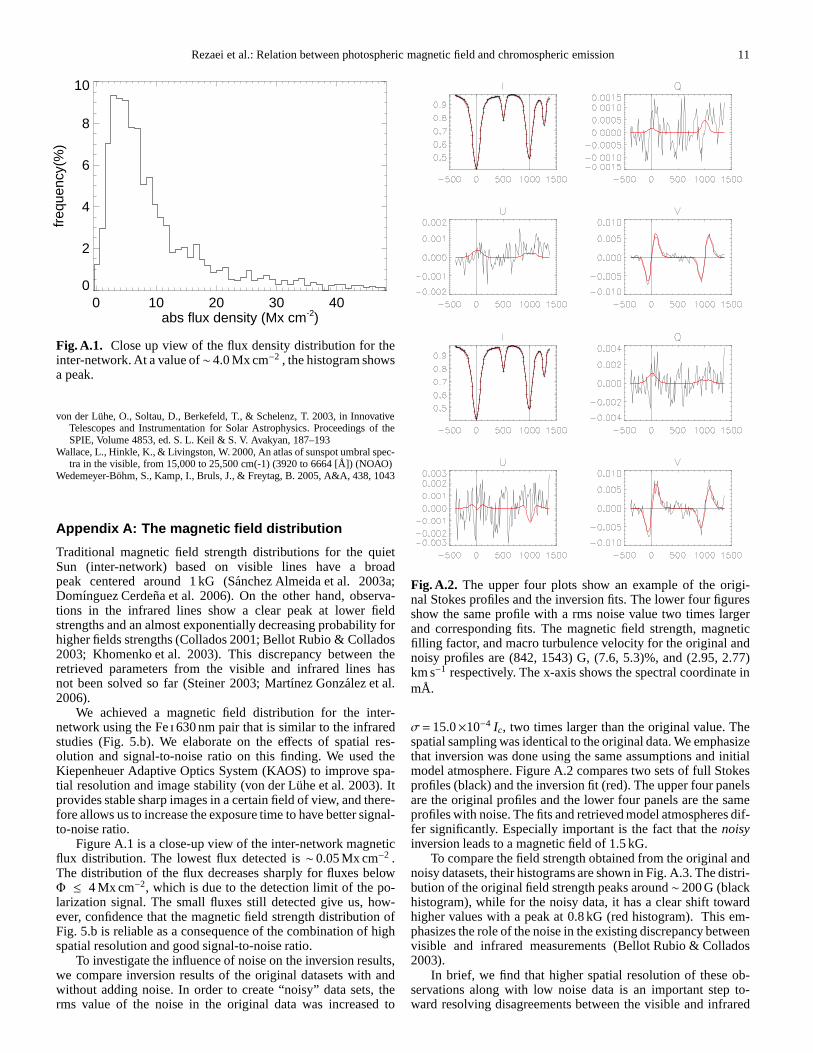
Fig. A.1. Close up view of the flux density distribution for theinter-network. At a value of∼4.0 Mx cm−2 , the histogram showsa peak.

von der Luhe, O., Soltau, D., Berkefeld, T., & Schelenz, T. 2003, in InnovativeTelescopes and Instrumentation for Solar Astrophysics. Proceedings of theSPIE, Volume 4853, ed. S. L. Keil & S. V. Avakyan, 187–193

Wallace, L., Hinkle, K., & Livingston, W. 2000, An atlas of sunspot umbral spec-tra in the visible, from 15,000 to 25,500 cm(-1) (3920 to 6664[Å]) (NOAO)

Wedemeyer-Bohm, S., Kamp, I., Bruls, J., & Freytag, B. 2005, A&A, 438, 1043

Appendix A: The magnetic field distribution

Traditional magnetic field strength distributions for the quietSun (inter-network) based on visible lines have a broadpeak centered around 1 kG (Sanchez Almeida et al. 2003a;Domınguez Cerdena et al. 2006). On the other hand, observa-tions in the infrared lines show a clear peak at lower fieldstrengths and an almost exponentially decreasing probability forhigher fields strengths (Collados 2001; Bellot Rubio & Collados2003; Khomenko et al. 2003). This discrepancy between theretrieved parameters from the visible and infrared lines hasnot been solved so far (Steiner 2003; Martınez Gonzalez etal.2006).

We achieved a magnetic field distribution for the inter-network using the Fei 630 nm pair that is similar to the infraredstudies (Fig. 5.b). We elaborate on the effects of spatial res-olution and signal-to-noise ratio on this finding. We used theKiepenheuer Adaptive Optics System (KAOS) to improve spa-tial resolution and image stability (von der Luhe et al. 2003). Itprovides stable sharp images in a certain field of view, and there-fore allows us to increase the exposure time to have better signal-to-noise ratio.

Figure A.1 is a close-up view of the inter-network magneticflux distribution. The lowest flux detected is∼ 0.05 Mx cm−2 .The distribution of the flux decreases sharply for fluxes belowΦ ≤ 4 Mx cm−2, which is due to the detection limit of the po-larization signal. The small fluxes still detected give us, how-ever, confidence that the magnetic field strength distribution ofFig. 5.b is reliable as a consequence of the combination of highspatial resolution and good signal-to-noise ratio.

To investigate the influence of noise on the inversion results,we compare inversion results of the original datasets with andwithout adding noise. In order to create “noisy” data sets, therms value of the noise in the original data was increased to

Fig. A.2. The upper four plots show an example of the origi-nal Stokes profiles and the inversion fits. The lower four figuresshow the same profile with a rms noise value two times largerand corresponding fits. The magnetic field strength, magneticfilling factor, and macro turbulence velocity for the original andnoisy profiles are (842, 1543) G, (7.6, 5.3)%, and (2.95, 2.77)km s−1 respectively. The x-axis shows the spectral coordinate inmÅ.

σ= 15.0×10−4 Ic, two times larger than the original value. Thespatial sampling was identical to the original data. We emphasizethat inversion was done using the same assumptions and initialmodel atmosphere. Figure A.2 compares two sets of full Stokesprofiles (black) and the inversion fit (red). The upper four panelsare the original profiles and the lower four panels are the sameprofiles with noise. The fits and retrieved model atmospheresdif-fer significantly. Especially important is the fact that thenoisyinversion leads to a magnetic field of 1.5 kG.

To compare the field strength obtained from the original andnoisy datasets, their histograms are shown in Fig. A.3. The distri-bution of the original field strength peaks around∼ 200 G (blackhistogram), while for the noisy data, it has a clear shift towardhigher values with a peak at 0.8 kG (red histogram). This em-phasizes the role of the noise in the existing discrepancy betweenvisible and infrared measurements (Bellot Rubio & Collados2003).

In brief, we find that higher spatial resolution of these ob-servations along with low noise data is an important step to-ward resolving disagreements between the visible and infrared


0.0 0.2 0.4 0.6 0.8 1.0 1.2 1.4B (kG)

0

1

2

3

4

5

freq

uenc

y (%

)

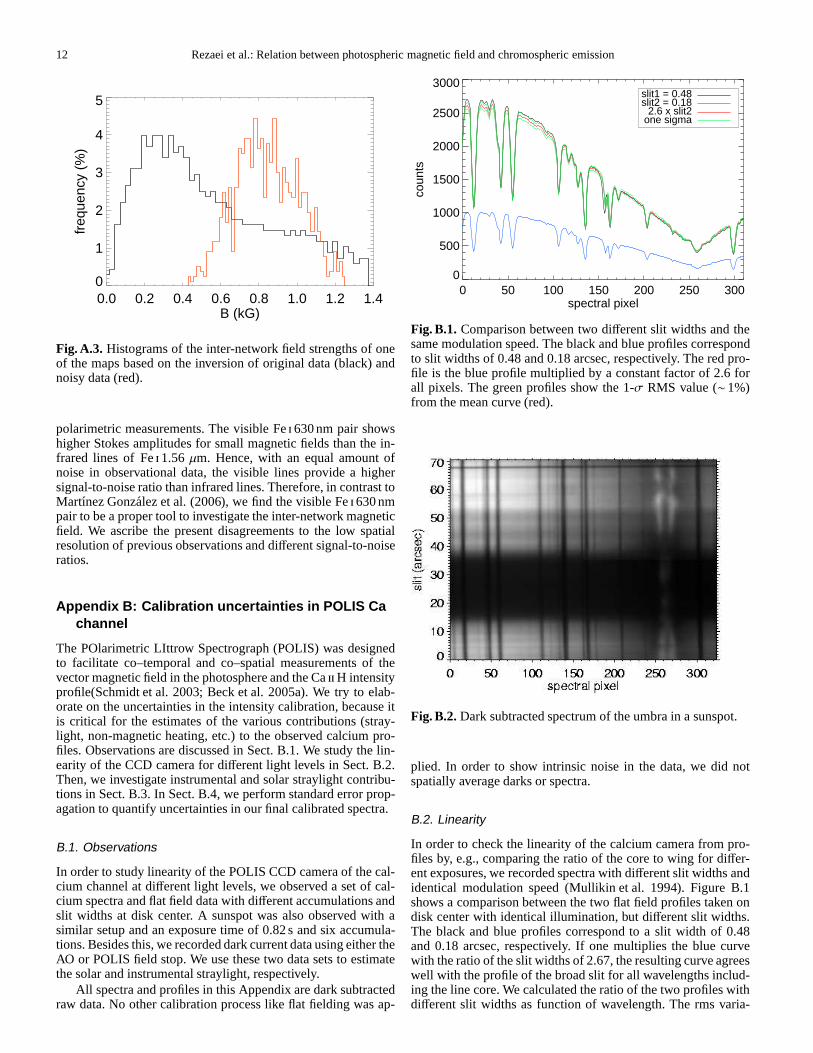
Fig. A.3. Histograms of the inter-network field strengths of oneof the maps based on the inversion of original data (black) andnoisy data (red).

polarimetric measurements. The visible Fei 630 nm pair showshigher Stokes amplitudes for small magnetic fields than the in-frared lines of Fei1.56 µm. Hence, with an equal amount ofnoise in observational data, the visible lines provide a highersignal-to-noise ratio than infrared lines. Therefore, in contrast toMartınez Gonzalez et al. (2006), we find the visible Fei630 nmpair to be a proper tool to investigate the inter-network magneticfield. We ascribe the present disagreements to the low spatialresolution of previous observations and different signal-to-noiseratios.

Appendix B: Calibration uncertainties in POLIS Cachannel

The POlarimetric LIttrow Spectrograph (POLIS) was designedto facilitate co–temporal and co–spatial measurements of thevector magnetic field in the photosphere and the CaiiH intensityprofile(Schmidt et al. 2003; Beck et al. 2005a). We try to elab-orate on the uncertainties in the intensity calibration, because itis critical for the estimates of the various contributions (stray-light, non-magnetic heating, etc.) to the observed calciumpro-files. Observations are discussed in Sect. B.1. We study the lin-earity of the CCD camera for different light levels in Sect. B.2.Then, we investigate instrumental and solar straylight contribu-tions in Sect. B.3. In Sect. B.4, we perform standard error prop-agation to quantify uncertainties in our final calibrated spectra.

B.1. Observations

In order to study linearity of the POLIS CCD camera of the cal-cium channel at different light levels, we observed a set of cal-cium spectra and flat field data with different accumulations andslit widths at disk center. A sunspot was also observed with asimilar setup and an exposure time of 0.82 s and six accumula-tions. Besides this, we recorded dark current data using either theAO or POLIS field stop. We use these two data sets to estimatethe solar and instrumental straylight, respectively.

All spectra and profiles in this Appendix are dark subtractedraw data. No other calibration process like flat fielding was ap-

0 50 100 150 200 250 300spectral pixel

0

500

1000

1500

2000

2500

3000

coun

ts

slit1 = 0.48slit2 = 0.18

2.6 x slit2one sigma

Fig. B.1. Comparison between two different slit widths and thesame modulation speed. The black and blue profiles correspondto slit widths of 0.48 and 0.18 arcsec, respectively. The redpro-file is the blue profile multiplied by a constant factor of 2.6 forall pixels. The green profiles show the 1-σ RMS value (∼1%)from the mean curve (red).

Fig. B.2. Dark subtracted spectrum of the umbra in a sunspot.

plied. In order to show intrinsic noise in the data, we did notspatially average darks or spectra.

B.2. Linearity

In order to check the linearity of the calcium camera from pro-files by, e.g., comparing the ratio of the core to wing for differ-ent exposures, we recorded spectra with different slit widths andidentical modulation speed (Mullikin et al. 1994). Figure B.1shows a comparison between the two flat field profiles taken ondisk center with identical illumination, but different slit widths.The black and blue profiles correspond to a slit width of 0.48and 0.18 arcsec, respectively. If one multiplies the blue curvewith the ratio of the slit widths of 2.67, the resulting curveagreeswell with the profile of the broad slit for all wavelengths includ-ing the line core. We calculated the ratio of the two profiles withdifferent slit widths as function of wavelength. The rms varia-


0 50 100 150 200 250 300spectral pixel

0

200

400

600

800

1000

coun

ts

quiet sunumbra

150 200 250 300spectral pixel

0

100

200

300

400

coun

ts

umbra (78 %)quiet sun12% quiet sun1 sigma (1%)

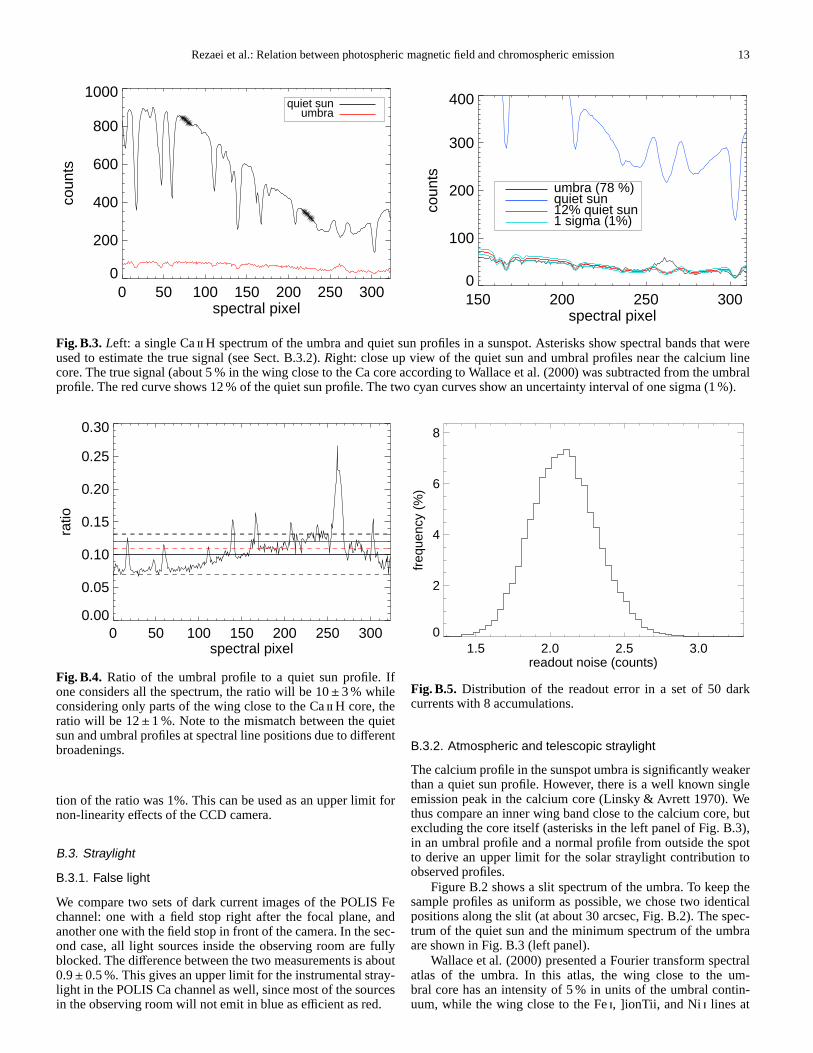
Fig. B.3. Left: a single CaiiH spectrum of the umbra and quiet sun profiles in a sunspot. Asterisks show spectral bands that wereused to estimate the true signal (see Sect. B.3.2).Right: close up view of the quiet sun and umbral profiles near the calcium linecore. The true signal (about 5 % in the wing close to the Ca coreaccording to Wallace et al. (2000) was subtracted from the umbralprofile. The red curve shows 12 % of the quiet sun profile. The two cyan curves show an uncertainty interval of one sigma (1 %).

0 50 100 150 200 250 300spectral pixel

0.00

0.05

0.10

0.15

0.20

0.25

0.30

ratio

Fig. B.4. Ratio of the umbral profile to a quiet sun profile. Ifone considers all the spectrum, the ratio will be 10± 3 % whileconsidering only parts of the wing close to the CaiiH core, theratio will be 12±1 %. Note to the mismatch between the quietsun and umbral profiles at spectral line positions due to differentbroadenings.

tion of the ratio was 1%. This can be used as an upper limit fornon-linearity effects of the CCD camera.

B.3. Straylight

B.3.1. False light

We compare two sets of dark current images of the POLIS Fechannel: one with a field stop right after the focal plane, andanother one with the field stop in front of the camera. In the sec-ond case, all light sources inside the observing room are fullyblocked. The difference between the two measurements is about0.9±0.5 %. This gives an upper limit for the instrumental stray-light in the POLIS Ca channel as well, since most of the sourcesin the observing room will not emit in blue as efficient as red.

1.5 2.0 2.5 3.0readout noise (counts)

0

2

4

6

8fr

eque

ncy

(%)

Fig. B.5. Distribution of the readout error in a set of 50 darkcurrents with 8 accumulations.

B.3.2. Atmospheric and telescopic straylight

The calcium profile in the sunspot umbra is significantly weakerthan a quiet sun profile. However, there is a well known singleemission peak in the calcium core (Linsky & Avrett 1970). Wethus compare an inner wing band close to the calcium core, butexcluding the core itself (asterisks in the left panel of Fig. B.3),in an umbral profile and a normal profile from outside the spotto derive an upper limit for the solar straylight contribution toobserved profiles.

Figure B.2 shows a slit spectrum of the umbra. To keep thesample profiles as uniform as possible, we chose two identicalpositions along the slit (at about 30 arcsec, Fig. B.2). The spec-trum of the quiet sun and the minimum spectrum of the umbraare shown in Fig. B.3 (left panel).

Wallace et al. (2000) presented a Fourier transform spectralatlas of the umbra. In this atlas, the wing close to the um-bral core has an intensity of 5 % in units of the umbral contin-uum, while the wing close to the Fei, ]ionTii, and Nii lines at


about 396.5 nm has an intensity of 38 %. In our umbral profile,this continuum has an intensity of about 80 counts (asterisks,Fig. B.3, left panel), whereas close to the core the profile hasabout 45 counts. Assuming no straylight in the atlas profile,only11 counts (∼22 % of the observed valued) should be measuredin the core. Thus, 78% of the observed signal have to be due tostraylight. To reproduce 78% of the umbral profile, a straylightcontribution of around 12 % is needed. If we assume that thereisno real calcium signal in the umbra (which is wrong) and take theobserved calcium profile of the umbra as pure scattered light, theratio changes from 12 % to 15 %. Therefore, uncertainties aboutthe scattered light in the atlas profile have minor importance.

A close-up view of the spectral region close to the calciumcore is shown in Fig. B.3 (right panel). For the reason mentionedabove, in the right panel of Fig. B.3, the umbral profile was la-beledumbra (78 %). The red curve shows 12 % of the quiet sunprofile. The two cyan curves also show an uncertainty interval ofone sigma (1 %). Figure B.4 shows the ratio of the umbra to thequiet sun profile. If we calculate mean and RMS of the wholespectrum, it gives a value of 10± 3 % while considering only onthe wing band close to the calcium core, we obtain 12± 1 %.We take this value as an upper limit for the total straylight inthe POLIS calcium channel. In Sect. B.3.1, we concluded thatthe instrumental straylight is about 1 %. Hence, most of the ob-tained straylight originates from the scattered solar light in thetelescope and the earth atmosphere.

B.4. Noise

There are three noise sources in a CCD camera (Mullikin et al.1994):

1. readout noise because of the pre-amplifier2. dark current noise which is influenced by the chip tempera-

ture3. photon noise due to the quantum nature of light which obeys

Poisson statistics.

The readout error of the camera was estimated by a set of50 consecutive dark frames with similar exposure and accumu-lations. Here, we compare the number of counts on each pixelin different images. We attribute the standard deviation of thecount value mainly to the readout error, and hence, obtain areadout error for each pixel separately. The distribution of thereadout errors is shown in Fig. B.5. The readout noise is aboutσreadout∼ 2 counts.

To investigate the thermal noise in the dark current, one hasto remove small systematic offsets between CCD columns (prob-ably due to thermal fluctuations of the AD system) before con-sidering statistical measures, e.g., rms, of a dark profile (a CCDrow). As it is shown in Fig. B.6, for a dark frame with 6 accumu-lations, the resulting rms (after removing systematics) isfar lessthan the standard deviation of the whole map including a large-scale variation. It provides an estimate for the thermal noise inthe camera. So the rms of the dark frame is aboutσthermal ∼ 3counts.

The total noise in the recorded data,σnoise, consists of threecomponents:

σnoise=√

σ2photon+ σ

2thermal+ σ

2readout (B.1)

where the photon noise originates from the Poisson fluctuationsof the number of photons counted. Assuming that nphotonis the

number of detected photons, the corresponding rms,σ2photon=

0 50 100 150 200 250 300spectral pixel

1200

1220

1240

1260

1280

coun

ts

0 50 100 150 200 250 300spectral pixel

-10

-5

0

5

10

coun

ts

RMS = 2.8 , RMS_map = 33.5

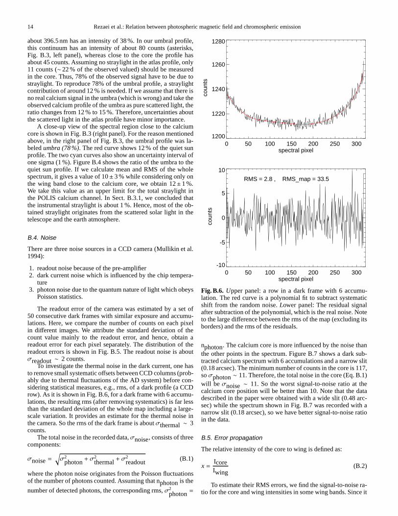
Fig. B.6. Upper panel: a row in a dark frame with 6 accumu-lation. The red curve is a polynomial fit to subtract systematicshift from the random noise.Lower panel: The residual signalafter subtraction of the polynomial, which is the real noise. Noteto the large difference between the rms of the map (excluding itsborders) and the rms of the residuals.

nphoton. The calcium core is more influenced by the noise thanthe other points in the spectrum. Figure B.7 shows a dark sub-tracted calcium spectrum with 6 accumulations and a narrow slit(0.18 arcsec). The minimum number of counts in the core is 117,soσphoton∼ 11. Therefore, the total noise in the core (Eq. B.1)will be σnoise ∼ 11. So the worst signal-to-noise ratio at thecalcium core position will be better than 10. Note that the datadescribed in the paper were obtained with a wide slit (0.48 arc-sec) while the spectrum shown in Fig. B.7 was recorded with anarrow slit (0.18 arcsec), so we have better signal-to-noise ratioin the data.

B.5. Error propagation

The relative intensity of the core to wing is defined as:

x =IcoreIwing

(B.2)

To estimate their RMS errors, we find the signal-to-noise ra-tio for the core and wing intensities in some wing bands. Since it


0 50 100 150 200 250 300spectral pixel

0

200

400

600

800

1000

coun

ts

Fig. B.7. A sample calcium profile. We use the calcium coreminimum counts to estimate the photon noise. In this case, thesignal-to-noise ratio at the calcium core is more than 10.

is not possible to use the core intensity to obtain the noise due tointrinsic changes, we use the average signal-to-noise of the leftand right wings close to the calcium core as the signal-to-noiseof the core. So the real signal-to-noise of the core is probablyworse than that. The S/N ratio of the core and wing vary from35 and 112 for two accumulations to 174 and 216 for twentyaccumulations. We use the worse S/N ratio corresponding to anexposure time of 1.64 s and obtain the following values for theRMS errors of the core and wing intensities:

σc

Icore∼

134∼ 3 % (B.3)

σw

Iwing∼

1112∼ 1 % (B.4)

So, we can obtain theσc as follows:

σx

x=

√

(σc

Icore)2 + (

σw

Iwing)2 ∼ 3 %. (B.5)

Error sources of the final calibrated data include uncertain-ties from the flat-field parameter, the straylight and the linearityof the detector. The straylight uncertainty was obtained about1 % in Sect. B.3. Assuming an upper limit for the uncertainty inthe flat-field to be 5 % and some 1 % uncertainty in linearity ofthe core to wing ratio,an upper limit for the uncertainty in thecalibrated spectrumwill be:

σr

r< 10 %.

Relation between photospheric magnetic field and chromospheric emission

Documents