Relation between geoidal undulation, deflection of the vertical and vertical gravity gradient revisited

1 23

Journal of GeodesyContinuation of Bulletin Géodésiqueand manuscripta geodaetica ISSN 0949-7714Volume 86Number 4 J Geod (2012) 86:287-304DOI 10.1007/s00190-011-0520-9

Relation between geoidal undulation,deflection of the vertical and verticalgravity gradient revisited

Johannes Bouman

1 23

Your article is protected by copyright and

all rights are held exclusively by Springer-

Verlag. This e-offprint is for personal use only

and shall not be self-archived in electronic

repositories. If you wish to self-archive your

work, please use the accepted author’s

version for posting to your own website or

your institution’s repository. You may further

deposit the accepted author’s version on a

funder’s repository at a funder’s request,

provided it is not made publicly available until

12 months after publication.

J Geod (2012) 86:287–304DOI 10.1007/s00190-011-0520-9

ORIGINAL ARTICLE

Relation between geoidal undulation, deflectionof the vertical and vertical gravity gradient revisited

Johannes Bouman

Received: 13 October 2010 / Accepted: 4 October 2011 / Published online: 2 November 2011© Springer-Verlag 2011

Abstract The vertical gradients of gravity anomaly andgravity disturbance can be related to horizontal first deriv-atives of deflection of the vertical or second derivativesof geoidal undulations. These are simplified relations ofwhich different variations have found application in satel-lite altimetry with the implicit assumption that the neglectedterms—using remove-restore—are sufficiently small. In thispaper, the different simplified relations are rigorously con-nected and the neglected terms are made explicit. The mainneglected terms are a curvilinear term that accounts for thedifference between second derivatives in a Cartesian sys-tem and on a spherical surface, and a small circle term thatstems from the difference between second derivatives on agreat and small circle. The neglected terms were comparedwith the dynamic ocean topography (DOT) and the require-ments on the GOCE gravity gradients. In addition, the signalroot-mean-square (RMS) of the neglected terms and ver-tical gravity gradient were compared, and the effect of aremove-restore procedure was studied. These analyses showthat both neglected terms have the same order of magnitudeas the DOT gradient signal and may be above the GOCErequirements, and should be accounted for when combiningaltimetry derived and GOCE measured gradients. The signalRMS of both neglected terms is in general small when com-pared with the signal RMS of the vertical gravity gradient,but they may introduce gradient errors above the sphericalapproximation error. Remove-restore with gravity field mod-els reduces the errors in the vertical gravity gradient, but itappears that errors above the spherical approximation errorcannot be avoided at individual locations. When computingthe vertical gradient of gravity anomaly from satellite altime-

J. Bouman (B)Deutsches Geodätisches Forschungsinstitut,Alfons-Goppel-Str. 11, 80359 Munich, Germanye-mail: [email protected]

ter data using deflections of the vertical, the small circle termis readily available and can be included. The direct compu-tation of the vertical gradient of gravity disturbance fromsatellite altimeter data is more difficult than the computationof the vertical gradient of gravity anomaly because in the for-mer case the curvilinear term is needed, which is not readilyavailable.

Keywords Vertical gravity gradient · Geoidal undulation ·Deflection of the vertical · Satellite altimetry

1 Introduction

The vertical gradient of the gravity anomaly can be relatedto the horizontal derivatives of the deflection of the verti-cal (Heiskanen and Moritz 1967; Hofmann-Wellenhof andMoritz 2005). This relation, however, is not exact as twoterms are neglected, one of which depends on the tangent ofthe latitude φ. It is stated in Heiskanen and Moritz (1967)and Hofmann-Wellenhof and Moritz (2005)—without ref-erence—that the two neglected terms are very small com-pared with the vertical gradient of gravity anomaly and needtherefore not to be considered. However, as tan φ tends to±∞ for φ going to ±π/2 (the North and South Pole), it isnot directly obvious that this term is negligible. Sandwelland Smith (1997, 2009) compute deflections of the verticalfrom Geosat and ERS-1 satellite altimeter data, and applya simplified relation similar to the one in Heiskanen andMoritz (1967) to compute the vertical gradient of gravitydisturbance.

The vertical gradient of the gravity anomaly can also berelated to the geoidal undulation N and its first and secondderivatives. This relation, however, may be less suited forpractical application as inaccuracies of N are greatly ampli-

123

Author's personal copy

288 J. Bouman

fied by forming the second derivatives (Heiskanen and Moritz1967; Hofmann-Wellenhof and Moritz 2005). Nonetheless,Rummel and Haagmans (1991) proposed to apply satellitealtimeter geoid profiles to compute gravity gradients alongsatellite altimeter ground tracks using smoothing splines andthey applied their method to SEASAT altimeter data in theNorth Atlantic. Despite the numerical challenges, it seemsworthwhile to revisit the geoid-gradient relation as todayhigh-resolution and highly accurate geoidal information isavailable, e.g. (Pavlis et al. 2008). Also the relation betweenthe along-track second derivatives from altimeter data andgravity gradients is a simplified one: a term is neglectedthat accounts for the difference between gravity gradientsin a Cartesian frame and on a curved surface (Bouman et al.2011a).

In this paper, the relation between geoidal undulations anddeflections of the vertical on the one hand, and the verticalgradient of gravity anomaly and gravity disturbance on theother hand is revisited. The gravity gradients along altim-eter ground tracks are explicitly connected to both verticalgradients of gravity anomaly and disturbance (Heiskanen andMoritz 1967). Alternative derivations of the relation betweengeoidal undulation and the vertical gradient of gravity dis-turbance are given, which provide additional insight in theindividual terms that are neglected in the simplified relations.The absolute and relative signal size of the neglected termsis evaluated with and without remove-restore and they arecompared with geophysical signals and the requirements onthe GOCE gravity gradients (ESA 1999).

The derivations in this paper are in spherical approxima-tion for a number of reasons. First of all, it is the startingpoint in Heiskanen and Moritz (1967) to derive the simplifiedrelation. Secondly, it allows the rigorous connection of thedifferent simplified relations. Thirdly, spherical approxima-tion allows the alternative derivations of the relation betweengeoidal undulation and the vertical gradient of gravity dis-turbance. A drawback of spherical approximation is that thederived relations have a relative error of up to 0.3%. However,the aim is to estimate the size of the different terms and to thisend spherical approximation suffices. In the Appendix it isindicated how the spherical approximation may be overcome.

This paper is organized as follows. In Sect. 2 both thevertical gradients of the gravity anomaly and disturbance arerelated to the geoidal undulation and its first and second deriv-atives with respect to geocentric coordinates, and the relationwith the gravity gradients from satellite altimetry is derived.In addition, the relations between the vertical gradients ofthe gravity anomaly and disturbance and the deflection ofthe vertical are given. In Sect. 3 alternative derivations areprovided for the relation between the vertical gradient ofthe gravity disturbance and the horizontal derivatives of thegeoidal undulation along satellite altimeter profiles as wellas parallels and meridians. Section 4 discusses the absolute

and relative signal sizes of the vertical gravity gradient andneglected terms based on EGM2008, and the latter are com-pared with dynamic ocean topography (DOT), earthquakesignal, and the GOCE gravity gradient requirements. The sig-nal and error reduction in a remove-restore procedure usingreference geoid models is discussed as well. Finally, Sect. 5contains the conclusions.

2 Vertical gravity gradients

2.1 Geoidal undulation

The derivation that connects the vertical gradient of grav-ity anomaly to the geoidal undulation and its first and sec-ond derivatives, given in (Heiskanen and Moritz 1967), isrepeated here for convenience and the equivalent derivationfor gravity disturbances is given as well. This is then con-nected to gravity gradients derived from altimetry.

The fundamental equation of physical geodesy is, in spher-ical approximation,

�g = −∂T

∂r− 2

rT (1)

where �g is the gravity anomaly at a certain point P, T theanomalous gravity potential and r the radius vector of pointP . Differentiation with respect to r gives

∂�g

∂r= −∂

2T

∂r2 − 2

r

∂T

∂r+ 2

r2 T . (2)

Laplace’s equation in spherical coordinates is

∂2T

∂r2 + 2

r

∂T

∂r− tan φ

r2

∂T

∂φ+ 1

r2

∂2T

∂φ2 + 1

r2 cos2 φ

∂2T

∂λ2 = 0

(3)

where φ and λ are geocentric latitude and longitude respec-tively. Adding (3) to (2) gives

∂�g

∂r= 2

r2 T − tan φ

r2

∂T

∂φ+ 1

r2

∂2T

∂φ2 + 1

r2 cos2 φ

∂2T

∂λ2 . (4)

Evaluating (4) at r = R and using T = γ N , with γ normalgravity and N geoidal undulation, we get (Heiskanen andMoritz 1967, Section 2-23; Hofmann-Wellenhof and Moritz2005, Section 2.20)

∂�g

∂r= 2γ

R2 N − γ

R2 tan φ∂N

∂φ+ γ

R2

∂2 N

∂φ2

+ γ

R2 cos2 φ

∂2 N

∂λ2 . (5)

Evaluation of Eq. (5) using numerical differentiation ofN requires very accurate and detailed geoidal information.Bouman et al. (2011a), for example, assess that a samplingof 700 m along satellite altimeter tracks is required when

123


geoidal undulation, deflection of the vertical and vertical gravity gradient 289

cubic splines are used to compute along-track gravity gra-dients directly from the altimeter data. We also see thatEq. (5) and similar equations throughout the paper are sin-gular at the two poles. The singularity can in principle beremoved through a transformation to four-dimensional coor-dinates (Gerstl 2008). In practical applications, however, thesingularity itself hardly plays a role, and three coordinatesare being used as usual.

The gravity disturbance δg is in spherical approximationrelated to the anomalous gravity potential T as

δg = −∂T

∂r(6)

and therefore

∂δg

∂r= −∂

2T

∂r2 . (7)

Adding Laplace’s equation (3) to the vertical gravity gradient(7) and again evaluating at r = R and using T = γ N gives

∂δg

∂r= 2

R

∂T

∂r− γ

R2 tan φ∂N

∂φ+ γ

R2

∂2 N

∂φ2 + γ

R2 cos2 φ

∂2 N

∂λ2 .

(8)

Thus Eqs. (5) and (8) relate the geoidal undulation to the ver-tical gradients of gravity anomaly and disturbance, respec-tively.

In spherical approximation, we may locally approximate asatellite altimeter ground track with a great circle. Considertwo crossing ground tracks with along-track parameters uand v respectively that are related to the great circle spheri-cal angles ψ(u) and ψ(v) as

u = Rψ(u), v = Rψ(v) (9)

where usually u is the parameter along ascending tracks andv along descending tracks. Along-track derivatives are com-puted with respect to these along-track parameters and Rum-mel and Haagmans (1991) derive that for two perpendicularground tracks at the crossover point the vertical gradient ofthe gravity disturbance is

∂δg

∂r= γ

(∂2 N

∂u2 + ∂2 N

∂v2

)(10)

and they propose to use smoothing splines to counteract thenoise amplification caused by the double differentiation.

The situation can be compared with Eq. (8) evaluated atthe equator because in that case both the meridian and theparallel (the equator) are great circles. Evaluation of (8) forφ = 0 gives

∂δg

∂r

∣∣∣∣φ=0

= 2

R

∂T

∂r+ γ

R2

∂2 N

∂φ2 + γ

R2

∂2 N

∂λ2 . (11)

Substitution of φ=ψ(u), λ=−ψ(v) and using du = Rdψ(u),dv = Rdψ(v) results in

∂δg

∂r

∣∣∣∣X,⊥

= 2

R

∂T

∂r+ γ

(∂2 N

∂u2 + ∂2 N

∂v2

). (12)

where X,⊥ denotes the crossover point of two perpendicularground tracks. In general, ground tracks are not perpendic-ular at crossover points and (12) needs to be modified, see(Bouman et al. 2011a).

The first term on the right in (12) is missing in (10). Rela-tion (10) is valid only if the along-track parameters u and vwould be coordinates of a local Cartesian system, which theyare not. The ∂T/∂r term can therefore be called curvilinearterm. An assessment based on EGM2008 gave a signal RMSof 0.2 E over the oceans (Bouman et al. 2011a). Comparedwith the total signal—the vertical gradient of gravity distur-bance—the curvilinear term is small, but may be above theGOCE requirements (ibid).

A similar derivation for gravity anomalies yields

∂�g

∂r

∣∣∣∣X,⊥

= 2γ

R2 N + γ

(∂2 N

∂u2 + ∂2 N

∂v2

). (13)

Note that the vertical gradient of gravity anomaly could bedirectly computed from altimeter geoid profiles using (13),whereas the vertical gradient of gravity disturbance or thevertical gravity gradient Trr cannot, because ∂T/∂r , neededin (12), cannot be derived directly from altimeter geoid pro-files.

2.2 Deflection of the vertical

In spherical approximation the deflections of the vertical arerelated to the geoidal undulation N as

ξ = − 1

R

∂N

∂φ, η = − 1

R cosφ

∂N

∂λ(14)

where ξ is the north-south deflection of the vertical and η theeast-west deflection of the vertical (Heiskanen and Moritz1967; Hofmann-Wellenhof and Moritz 2005). We thereforehave

∂N

∂φ= −Rξ,

∂N

∂λ= −Rη cosφ, (15)

so that

∂2 N

∂φ2 = −R∂ξ

∂φ,∂2 N

∂λ2 = −R∂η

∂λcosφ. (16)

Inserting (15) and (16) into (5) one finds

∂�g

∂r= 2γ

R2 N + γ

Rξ tan φ − γ

R

∂ξ

∂φ− γ

R cosφ

∂η

∂λ. (17)

Introducing

du = Rdφ, dv = R cosφ dλ (18)

123


290 J. Bouman

Eq. (17) becomes

∂�g

∂r= 2γ

R2 N + γ

Rξ tan φ − γ

(∂ξ

∂u+ ∂η

∂v

)(19)

where v indicates that it is a coordinate along a small cir-cle. According to (Heiskanen and Moritz 1967; Hofmann-Wellenhof and Moritz 2005) the first two terms on the rightare very small with respect to the third term and can beneglected:

∂�g

∂r= −γ

(∂ξ

∂u+ ∂η

∂v

)(20)

which will be assessed in Sect. 4. A similar derivation for thevertical gradient of gravity disturbance gives (also compare(12) with (13)):

∂δg

∂r= 2

R

∂T

∂r+ γ

Rξ tan φ − γ

(∂ξ

∂u+ ∂η

∂v

)(21)

with approximately

∂δg

∂r= −γ

(∂ξ

∂u+ ∂η

∂v

). (22)

Also when vertical gravity gradients are computed fromsatellite altimeter data, computing deflections of the verti-cal in a first step, the data need to be differentiated twice:first geoidal undulations are differentiated to obtain deflec-tions of the vertical, next these deflections are differentiatedto obtain the vertical gravity gradient in (22). The explicitdouble differentiation of (10) is therefore implicitly presentin this case as well, and filtering is needed.

2.3 Summary of simplified relations

Table 1 summarizes the simplified relations between the ver-tical gradients of gravity anomaly and disturbance on the onehand and geoidal undulations and deflections of the verticalon the other hand. The neglected terms are indicated, wherederivatives ∂ξ/∂u etc. are written as ξu etc.

In other words, the simplified relation (10) that relatesalong-track second derivatives of satellite altimeter profilesto the vertical gravity gradient Tzz = δgr neglects 2R−1Tr .The simplified relation (20) between the horizontal deriva-tives of the deflection of the vertical and the vertical gradient

Table 1 Simplified relations and neglected terms

Anomaly or Simplified Neglected termsdisturbance relation

2γ R−2 N 2R−1Tr γ R−1ξ tan φ

�gr = γ (Nuu + Nvv) Yes No Noδgr No Yes No

�gr = −γ (ξu + ηv) Yes No Yesδgr No Yes Yes

of the gravity anomaly neglects 2γ R−2 N + γ R−1ξ tan φ.The simplified relation (22) between the horizontal deriva-tives of the deflection of the vertical and the vertical gradientof the gravity disturbance neglects 2R−1Tr + γ R−1ξ tan φ.

3 Alternative derivations

Two alternative derivations are given for the relation betweenthe disturbing gravity potential and its second derivatives indifferent coordinate systems. First, the gravity gradient dis-turbances in a local Cartesian system are related to deriva-tives of the disturbing gravity potential along profiles on thesphere. Next, the gravity gradients in a local north-orientedCartesian system are related to derivatives of the disturbinggravity potential along parallels and meridians. The deriva-tions are possible when working in spherical approximationand should provide additional insight into the different termsthat are neglected in the simplified relations discussed inSect. 2. Section 3.3 discusses planar versus spherical approx-imation.

3.1 Cartesian and curvilinear system

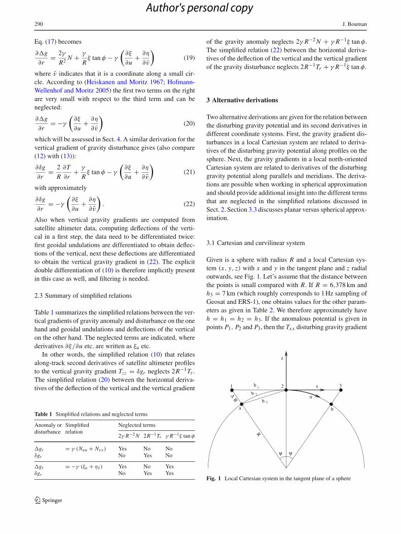
Given is a sphere with radius R and a local Cartesian sys-tem (x, y, z) with x and y in the tangent plane and z radialoutwards, see Fig. 1. Let’s assume that the distance betweenthe points is small compared with R. If R = 6,378 km andh3 = 7 km (which roughly corresponds to 1 Hz sampling ofGeosat and ERS-1), one obtains values for the other param-eters as given in Table 2. We therefore approximately haveh = h1 = h2 = h3. If the anomalous potential is given inpoints P1, P2 and P3, then the Txx disturbing gravity gradient

h 3

RΔ h 2

h1

ψψ

a b

R

2 31

u

x

z

Fig. 1 Local Cartesian system in the tangent plane of a sphere

123



Table 2 Parameters for Fig. 1

Parameter Derived from Value

R Given 6,378 km

h3 Given 7 km

ψ sin( 12ψ) = 1

2 h3R 1.1 × 10−3

h1 R tanψ h3 + 3.2 mm

h2 Rψ h3 + 0.4 mm

�R cosψ = RR+�R 3.84 m

in P2 may be approximated as

Txx (P2) ≈ T (P3)− 2T (P2)+ T (P1)

h2 . (23)

A satellite altimeter profile, however, provides disturbingpotential values in points Pa, P2 and Pb (in spherical approx-imation, assuming altimetry gives N and using T = γ N ).The disturbing gravity gradient Tuu is

Tuu(P2) ≈ T (Pb)− 2T (P2)+ T (Pa)

h2 . (24)

A Taylor expansion of T (Pa) at P1 yields

T (Pa) ≈ T (P1)− ∂T

∂r(P1)�R. (25)

Inserting this and the equivalent Taylor expansion for T (Pb)

in (24) gives

Tuu(P2)

≈ T (P3)− Tr (P3)�R − 2T (P2)+ T (P1)− Tr (P1)�R

h2

(26)

or

Tuu(P2) ≈ T (P3)− 2T (P2)+ T (P1)

h2

−�RTr (P3)+ Tr (P1)

h2 (27)

where the derivative of T with respect to r is denoted as Tr .Because h2

1+ R2 = (R +�R)2 and�R is small, we haveapproximately h2 = 2R�R. Inserting this in (27) and using(23) we get approximately

Tuu(P2) = Txx (P2)− 1

RTr (P2) (28)

as Tr (P2) ≈ (Tr (P1)+ Tr (P3))/2. Similarly we have for theorthogonal direction

Tvv(P2) = Tyy(P2)− 1

RTr (P2) (29)

φ

X

Z

R

zx

u

P

North Pole

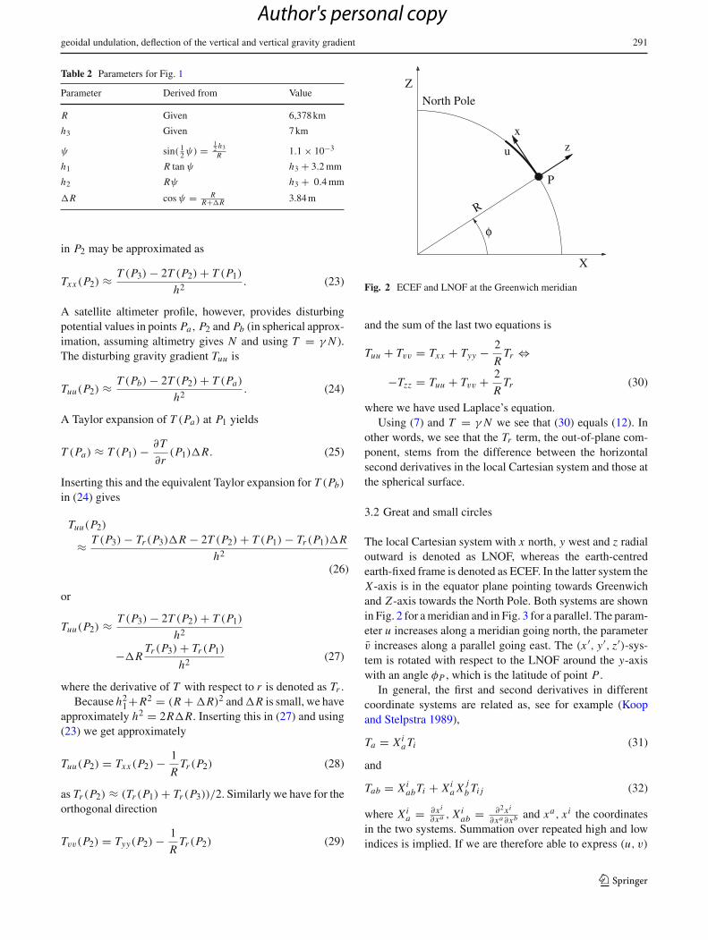
Fig. 2 ECEF and LNOF at the Greenwich meridian

and the sum of the last two equations is

Tuu + Tvv = Txx + Tyy − 2

RTr ⇔

−Tzz = Tuu + Tvv + 2

RTr (30)

where we have used Laplace’s equation.Using (7) and T = γ N we see that (30) equals (12). In

other words, we see that the Tr term, the out-of-plane com-ponent, stems from the difference between the horizontalsecond derivatives in the local Cartesian system and those atthe spherical surface.

3.2 Great and small circles

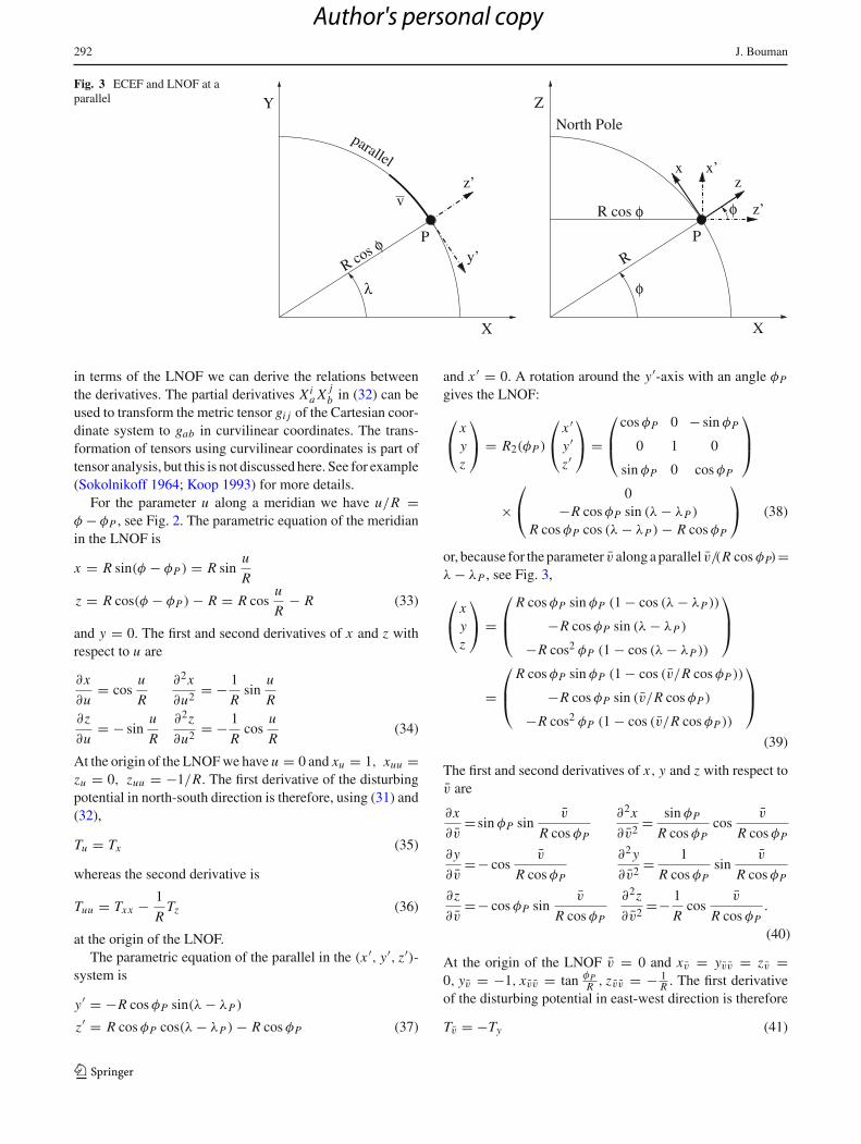
The local Cartesian system with x north, y west and z radialoutward is denoted as LNOF, whereas the earth-centredearth-fixed frame is denoted as ECEF. In the latter system theX -axis is in the equator plane pointing towards Greenwichand Z -axis towards the North Pole. Both systems are shownin Fig. 2 for a meridian and in Fig. 3 for a parallel. The param-eter u increases along a meridian going north, the parameterv increases along a parallel going east. The (x ′, y′, z′)-sys-tem is rotated with respect to the LNOF around the y-axiswith an angle φP , which is the latitude of point P .

In general, the first and second derivatives in differentcoordinate systems are related as, see for example (Koopand Stelpstra 1989),

Ta = XiaTi (31)

and

Tab = XiabTi + Xi

a X jb Ti j (32)

where Xia = ∂xi

∂xa , Xiab = ∂2xi

∂xa∂xb and xa, xi the coordinatesin the two systems. Summation over repeated high and lowindices is implied. If we are therefore able to express (u, v)

123


292 J. Bouman

Fig. 3 ECEF and LNOF at aparallel

X

Y

z’

λ

y’P

parallel

φR cos

v

φ

X

Z

R

z

North Pole

φ

x’

z’φ

x

P

R cos

in terms of the LNOF we can derive the relations betweenthe derivatives. The partial derivatives Xi

a X jb in (32) can be

used to transform the metric tensor gi j of the Cartesian coor-dinate system to gab in curvilinear coordinates. The trans-formation of tensors using curvilinear coordinates is part oftensor analysis, but this is not discussed here. See for example(Sokolnikoff 1964; Koop 1993) for more details.

For the parameter u along a meridian we have u/R =φ − φP , see Fig. 2. The parametric equation of the meridianin the LNOF is

x = R sin(φ − φP ) = R sinu

R

z = R cos(φ − φP )− R = R cosu

R− R (33)

and y = 0. The first and second derivatives of x and z withrespect to u are

∂x

∂u= cos

u

R

∂2x

∂u2 = − 1

Rsin

u

R∂z

∂u= − sin

u

R

∂2z

∂u2 = − 1

Rcos

u

R(34)

At the origin of the LNOF we have u = 0 and xu = 1, xuu =zu = 0, zuu = −1/R. The first derivative of the disturbingpotential in north-south direction is therefore, using (31) and(32),

Tu = Tx (35)

whereas the second derivative is

Tuu = Txx − 1

RTz (36)

at the origin of the LNOF.The parametric equation of the parallel in the (x ′, y′, z′)-

system is

y′ = −R cosφP sin(λ− λP )

z′ = R cosφP cos(λ− λP )− R cosφP (37)

and x ′ = 0. A rotation around the y′-axis with an angle φP

gives the LNOF:

⎛⎝ x

yz

⎞⎠ = R2(φP )

⎛⎝ x ′

y′z′

⎞⎠ =

⎛⎜⎝

cosφP 0 − sin φP

0 1 0

sin φP 0 cosφP

⎞⎟⎠

×⎛⎝ 0

−R cosφP sin (λ− λP )

R cosφP cos (λ− λP )− R cosφP

⎞⎠ (38)

or, because for the parameter v along a parallel v/(R cosφP)=λ− λP , see Fig. 3,

⎛⎝ x

yz

⎞⎠ =

⎛⎜⎝

R cosφP sin φP (1 − cos (λ− λP ))

−R cosφP sin (λ− λP )

−R cos2 φP (1 − cos (λ− λP ))

⎞⎟⎠

=⎛⎜⎝

R cosφP sin φP (1 − cos (v/R cosφP ))

−R cosφP sin (v/R cosφP )

−R cos2 φP (1 − cos (v/R cosφP ))

⎞⎟⎠

(39)

The first and second derivatives of x, y and z with respect tov are

∂x

∂v= sin φP sin

v

R cosφP

∂2x

∂v2 = sin φP

R cosφPcos

v

R cosφP

∂y

∂v=− cos

v

R cosφP

∂2 y

∂v2 = 1

R cosφPsin

v

R cosφP

∂z

∂v=− cosφP sin

v

R cosφP

∂2z

∂v2 =− 1

Rcos

v

R cosφP.

(40)

At the origin of the LNOF v = 0 and xv = yvv = zv =0, yv = −1, xvv = tan φP

R , zvv = − 1R . The first derivative

of the disturbing potential in east-west direction is therefore

Tv = −Ty (41)

123



whereas the east-west second derivative of the disturbinggravity potential then is

Tvv = Tyy + tan φ

RTx − 1

RTz = Tyy + tan φ

RTu − 1

RTr

(42)

where we used (35).The sum of Tuu and Tvv , Eqs. (36) and (42), yields Eq. (8)

using Laplace’s equation, Eq. (7), T = γ N and the relationsbetween (u, v) and (φ, λ), equation (18). As before, we seethat the Tr term stems from the difference between the hor-izontal second derivatives in the local Cartesian system andthose at spherical surface, whereas the tan φ term is due tothe fact that parallels are small circles.

3.3 Planar versus spherical approximation

Working with local rectangular coordinates is a planarapproximation. The reference surface remains the ellipsoid,but the evaluation and relation between different gravity fieldfunctionals is with respect to local Cartesian coordinates. Thenormals to the sphere and the local plane are the same, that is,∂∂r = ∂

∂z . Consequently, we have for the gravity disturbanceand gravity anomaly

δg = −∂T

∂r= −∂T

∂z,

�g = −∂T

∂r− 2

RT = −∂T

∂z− 2

RT . (43)

Also the horizontal first derivatives in spherical and planarapproximation are equal, see Eqs. (35) and (41). In contrast,the second derivatives in planar and spherical approximationare not equal, see Eqs. (36) and (42). This difference betweenfirst and second derivatives is caused by, loosely speaking,the fact that scalars have no sense of direction, but vectors do.Numerically, the horizontal first derivatives of T can be com-puted by taking the difference between two potential valuesdivided by the distance, see also Fig. 1. We have seen thatfor small spherical angles the planar and spherical distancesare almost equal (Table 2) and the numerical first derivativeswill therefore be the same.

Vectors, such as the first derivatives of the potential, arerelated to a given coordinate system, and second-order deriv-atives in arbitrary coordinates have to be computed by covari-ant differentiation. Covariant differentiation involves the sumof (i) first-order partial derivatives of the potential times theChristoffel symbols of the second kind, and (ii) the partialderivatives of the first-order potential derivatives (see, e.g.,Sokolnikoff 1964; Koop 1993). These Christoffel symbolsare zero in Cartesian coordinates and (i) is zero, but they arenon-zero in curvilinear coordinates. Terms with a first-orderderivative, such as γ R−1ξ tan φ and 2Tr R−1 can thereforenot occur in planar approximation.

Replacing the coordinate triplet {u, v, r} with {x, y, z} onesees that Eq. (10) is the Laplace equation in planar approx-imation of Eq. (12). Also note that when horizontal deriva-tives in the plane are given, the out-of-plane component Tzz

is immediately available, but on curved surfaces additionalinformation is needed, see e.g. Eq. (30). In planar approx-imation the vertical gradient of gravity anomaly (13) andvertical gradient of gravity disturbance (10) can hardly bedistinguished, because the first term on the right in (13) willprove to be very small (see next section). In spherical approxi-mation the difference between the vertical gradient of gravityanomaly and disturbance is

∂�g

∂r− ∂δg

∂r= −2

r

∂T

∂r+ 2

r2 T (44)

which can be compared with the difference between gravityanomalies and disturbances

�g − δg = −2

rT . (45)

The term on the right in (45) is, with γ = G M/r2, an approx-imation of

1

γ

∂γ

∂rT = ∂γ

∂rN (46)

which originates from the linear term of a Taylor expansionthat accounts for the difference in normal gravity at the geoidand ellipsoid (Heiskanen and Moritz 1967). Differentiationof (46) with respect to r gives

∂

∂r

(1

γ

∂γ

∂rT

)= γ−1 ∂γ

∂r

∂T

∂r+ γ−1 ∂

2γ

∂r2 T

+∂γ−1

∂r

∂γ

∂rT ≈ −2

r

∂T

∂r+ 2

r2 T (47)

Hence, in analogy to (45) the first term on the right in (44) isthe normal gravity gradient times the “distance” Tr , and thesecond term on the right is of second order.

4 Relative signal sizes

The signals of Tzz and the neglected terms 2Tr/R, γ R−1ξ

tan φ and 2Tr/R + γ R−1ξ tan φ are compared with eachother in Sect. 4.1. The neglected terms are compared withDOT and earthquake signal in Sect. 4.2 and with the GOCErequirements in Sect. 4.3. The effect of remove-restore isstudied in Sect. 4.4.

4.1 Signal RMS and signal ratio

The neglected terms are compared with the vertical gravitygradient in six regions: the Arctic, Antarctica, the Alps, theHimalaya, the South West Pacific and South Atlantic. Theglobal gravity field model EGM2008 to degree and order

123


294 J. Bouman

2,190 was used to synthesize the different quantities on a gridwith respect to the GRS80 reference ellipsoid. The bound-aries of each region are indicated in the figures below, thegrid size was chosen constant at 0.10.

The neglected term 2γ R−2 N will not be discussed indetail: using γ = 10 m/s2, R = 6,378 km and N = 100 m,one sees that the maximum of this term is about 50 mE(1 E is 10−9 s−2). Compared with Tzz this is very small:The maximum absolute value of the ratio of 2γ R−2 N toTzz is 5.6 × 10−6 for the Arctic, 1.3 × 10−6 for Antarc-tica, 3.1 × 10−8 for the Alps, 2.4 × 10−7 for the Himalayas,3.3 × 10−7 for the South West Pacific, and 7.0 × 10−8 forthe South Atlantic.

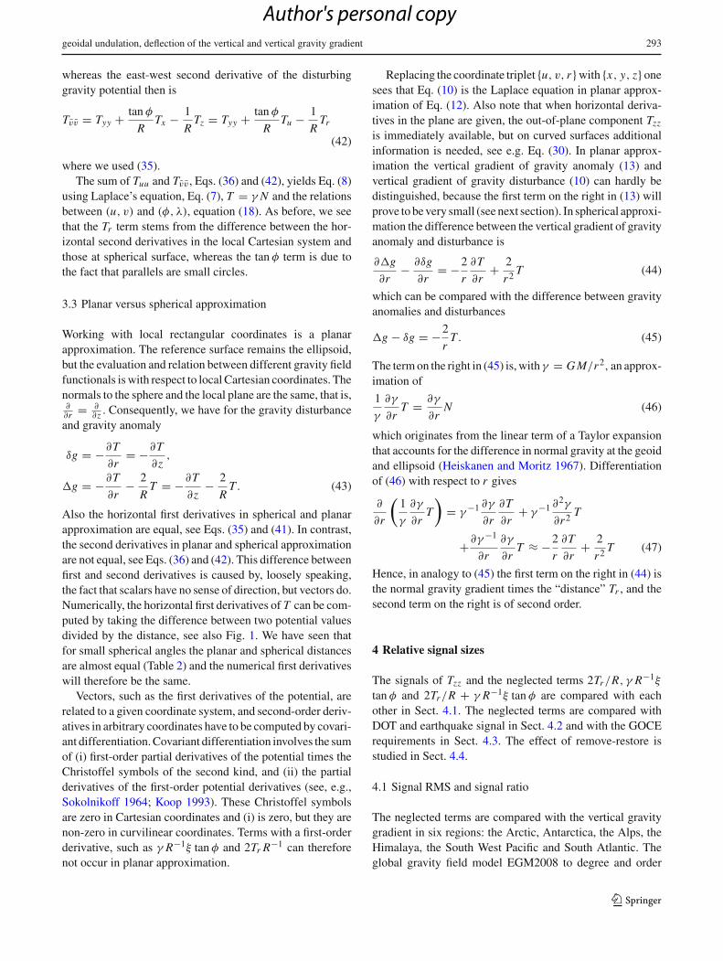
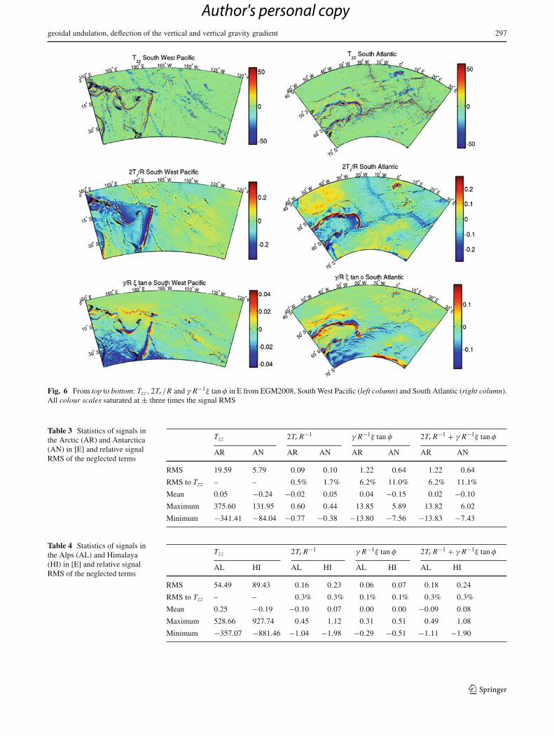
The vertical gravity gradient Tzz as well as 2Tr/R andγ R−1ξ tan φ are shown in Fig. 4 for the Arctic and Antarc-tica, in Fig. 5 for the Alps and the Himalayas, and in Fig. 6for the South West Pacific and South Atlantic. The statisticsof the signals are given in Tables 3, 4, and 5. The statistics ofγ R−1ξ tan φ have been computed excluding the North andSouth Pole because there the term becomes infinite in the-ory (∼ 1014 E in practice). The γ R−1ξ tan φ signal increasestowards the North and South Pole, as might be expected.

The Tzz signal RMS for Antarctica is much smaller thanin the Arctic, which is probably due to the lack of high-res-olution gravity field data on land in Antarctica. In the com-putation of EGM2008 only GRACE data were used overAntarctica and no terrestrial gravity data (Pavlis et al. 2008).This has, however, different consequences for different grav-ity field quantities. As an example, see Fig. 7 that displaysthe signal degree variances up to degree 720 for T, Tr andTzz computed with EGM2008. The maximum degree onecan resolve with GRACE is 150 or so and one sees thatabove degree 150 the Tzz degree variances are more or lessflat, whereas the Tr degree variances decrease for increasingdegree. In other words, the relative signal power loss overAntarctica is more pronounced for Tzz than for Tr or otherfirst derivatives.

The signal RMSs of 2Tr R−1, γ R−1ξ tan φ and their sumare in general small compared with the vertical gravity gra-dient. To judge whether these signals are also negligible,a reference is needed. The derivations in this paper are inspherical approximation, which introduces a maximum rel-ative error of 0.3% and this will serve as reference value. Inthe development of EGM2008, for example, the errors dueto spherical approximation were considered to be too largeand ellipsoidal harmonics were used. In the Appendix, it isbriefly discussed how the spherical approximation in Sect. 2may be overcome. The relative signal RMSs of the neglectedterms with respect to Tzz is in almost all cases greater thanor equal to 0.3% with the exception of γ R−1ξ tan φ in theAlps, Himalayas and South West Pacific. Thus applicationof the simplified relations may lead to systematic errors thatare greater than the errors introduced by spherical approx-

imation. The errors are systematic because they are signaldependent and not random.

A signal RMS is an average number and it is of interest tostudy as well the geographical distribution of the relative sig-nal sizes. For each point in Figs. 4, 5 and 6, the ratios of 2Tr/Rto Tzz , of γ R−1ξ tan φ to Tzz , and of (2Tr/R+γ R−1ξ tan φ)to Tzz were computed and these are summarized in Tables 6,7, and 8. Given is the percentage that falls within a certainratio range. A ratio ≥ 0.1, for example, indicates that at acertain location a neglected term is 10% or more of the Tzz

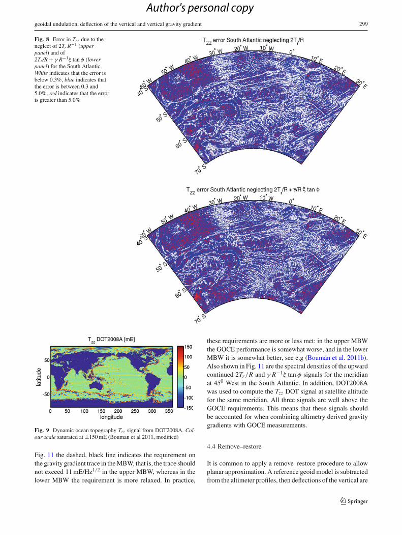
signal at that location. In this example, using the simplifiedrelations therefore locally introduces an error in Tzz of 10%or more. One sees that for all considered regions at a signifi-cant part of the locations the error in Tzz is larger than 0.3%.Figure 8 displays the geographic distribution of the errors inTzz in the South Atlantic if 2Tr/R or 2Tr/R + γ R−1ξ tan φis neglected.

4.2 Comparison with geophysical signals

One way to put the neglected terms in perspective is to com-pare their size with the size of relevant geophysical signals.Two examples are given here: the DOT and the change ingravity gradient signal caused by the 2004 Sumatra-And-aman earthquake.

The deviation between the sea level as observed by satel-lite altimetry and the geoid is called DOT. Maximum devi-ations of the DOT from an equipotential surface are in theorder of ±1 − 2 m, which is small compared with geoidalundulations of about 100 m. However, a proper use of satel-lite altimeter data in gravity field modelling requires that theDOT is accounted for. DOT2008A is a DOT model that wasestimated using the DNSC08B mean sea surface (Andersenet al. 2010) and the EGM2008 geoid model. DOT2008A hasbeen developed in spherical harmonic coefficients completeto degree and order 180. These coefficients were transformedinto dimensionless coefficients, which allow evaluating themodel also in terms of the vertical gravity gradient. Figure 9shows the Tzz DOT signal where the colour scale is satu-rated at ±0.15 E. Bouman et al. (2011a) computed that themaximum of the absolute Tzz DOT signal over the oceans is0.56 E with a signal RMS of 0.05 E. These values have thesame order of magnitude as the corresponding values of theneglected 2Tr/R and γ R−1ξ tan φ terms in the South WestPacific and South Atlantic (Table 5).

The 2004 Sumatra–Andaman earthquake caused crustaldeformations of several meters in the vicinity of the fault. Theassociated mass redistribution affected the gravity potentialthat has been observed by GRACE (Han et al. 2006). Broerseet al. (2011) computed a gravitationally self-consistent solu-tion for the co-seismic relative sea level, surface deformationand geoid height changes. From their geophysical modeling itis estimated that the co-seismic geoid changes are at cm level.

123



Fig. 4 From top to bottom: Tzz, 2Tr/R and γ R−1ξ tan φγ R−1ξ tan φin E from EGM2008, Arctic (left column) and Antarctica (right col-umn). Minimum latitude is 70◦ north and south, respectively. Colour

scales Tzz and 2Tr/R saturated at ± three times the signal RMS, colourscale γ R−1ξ tan φ saturated at one time the signal RMS

123


296 J. Bouman

Fig. 5 From top to bottom: Tzz, 2Tr/R and γ R−1ξ tan φ in E from EGM2008, Alps (left column) and Himalaya (right column). All colour scalessaturated at ± three times the signal RMS

123



Fig. 6 From top to bottom: Tzz, 2Tr/R and γ R−1ξ tan φ in E from EGM2008, South West Pacific (left column) and South Atlantic (right column).All colour scales saturated at ± three times the signal RMS

Table 3 Statistics of signals inthe Arctic (AR) and Antarctica(AN) in [E] and relative signalRMS of the neglected terms

Tzz 2Tr R−1 γ R−1ξ tan φ 2Tr R−1 + γ R−1ξ tan φ

AR AN AR AN AR AN AR AN

RMS 19.59 5.79 0.09 0.10 1.22 0.64 1.22 0.64

RMS to Tzz – – 0.5% 1.7% 6.2% 11.0% 6.2% 11.1%

Mean 0.05 −0.24 −0.02 0.05 0.04 −0.15 0.02 −0.10

Maximum 375.60 131.95 0.60 0.44 13.85 5.89 13.82 6.02

Minimum −341.41 −84.04 −0.77 −0.38 −13.80 −7.56 −13.83 −7.43

Table 4 Statistics of signals inthe Alps (AL) and Himalaya(HI) in [E] and relative signalRMS of the neglected terms


AL HI AL HI AL HI AL HI

RMS 54.49 89.43 0.16 0.23 0.06 0.07 0.18 0.24

RMS to Tzz – – 0.3% 0.3% 0.1% 0.1% 0.3% 0.3%

Mean 0.25 −0.19 −0.10 0.07 0.00 0.00 −0.09 0.08

Maximum 528.66 927.74 0.45 1.12 0.31 0.51 0.49 1.08

Minimum −357.07 −881.46 −1.04 −1.98 −0.29 −0.51 −1.11 −1.90

123


298 J. Bouman

Table 5 Statistics of signals inthe South West Pacific (SWP)and South Atlantic (SA) in [E]and relative signal RMS of theneglected terms


SWP SA SWP SA SWP SA SWP SA

RMS 18.60 18.71 0.11 0.09 0.01 0.06 0.11 0.11

RMS to Tzz – – 0.6% 0.5% 0.1% 0.3% 0.6% 0.6%

Mean 0.07 0.02 −0.03 −0.02 0.00 −0.01 −0.04 −0.03

Maximum 412.49 321.73 0.96 0.89 0.13 0.75 0.94 1.22

Minimum −165.37 −193.69 −1.41 −0.99 −0.22 −0.52 −1.37 −0.97

Fig. 7 Signal degree variances for Tzz, Tr and N (or T ) fromEGM2008

Table 6 Error in Tzz caused by neglecting terms

Error (%) 2Tr R−1 γ R−1ξ tan φ 2Tr R−1 + γ R−1ξ tan φ

AR AN AR AN AR AN

≤0.3 24.5 5.4 11.6 4.8 8.7 2.8

0.3–5 67.7 63.4 59.2 37.8 59.1 33.5

5–10 3.9 15.9 11.2 16.3 12.6 17.5

>10 3.9 15.3 18.0 41.1 19.6 46.2

Given is the percentage that falls within a certain error range in theArctic (AR) and Antarctica (AN)

The same modeling also allows estimating the correspondingvertical gravity gradient signal at the earth’s surface (Fig. 10),which has maximum amplitude of 0.09 E (Broerse 2011, per-sonal communication). Although it will probably challeng-ing to observe such changes with satellite altimeter data, thisexample shows that the geophysical signals one is aimingat with modern geodetic measurements are small. The max-imum amplitude of the neglected 2Tr/R and γ R−1ξ tan φterms is much larger (Figs. 4, 5, 6).



AL HI AL HI AL HI

≤0.3 28.7 32.7 68.7 70.2 28.9 31.5

0.3–5 64.6 57.1 29.2 27.7 64.2 57.6

5–10 3.6 5.1 1.0 1.0 3.7 5.4

>10 3.1 5.1 1.0 1.0 3.2 5.4

Given is the percentage that falls within a certain error range in the Alps(AL) and Himalaya (HI)



SWP SA SWP SA SWP SA

≤0.3 28.4 25.9 81.7 46.5 28.1 22.1

0.3–5 63.6 66.4 17.0 48.0 63.5 67.9

5–10 4.0 3.9 0.6 2.7 4.2 4.9

>10 4.0 3.9 0.6 2.8 4.2 5.1

Given is the percentage that falls within a certain error range in theSouth West Pacific (SWP) and South Atlantic (SA)

4.3 Comparison with GOCE measurement requirements

It may be of interest to combine vertical gravity gradientsderived from satellite altimeter data with gravity gradientsmeasured by GOCE (ESA 1999). The two sets of gravity gra-dients then need to be consistent, that is, the vertical gradientof gravity disturbance (7) is needed, which can in principlebe derived from (12) or (21). As mentioned above, a problemthen may be that the Tr term cannot be derived directly fromaltimeter profiles, which would mean that the gravity gradi-ents derived from altimetry and those measured by GOCEare not consistent. The question therefore is how large the Tr

term is in comparison with the GOCE measurement errorsand requirements.

The neglected terms are upward continued to GOCE alti-tude (about 260 km) and confronted with the GOCE require-ments. The measurement bandwidth (MBW) is the frequencyrange from 5 mHz–0.1 Hz in which the error for the GOCEdiagonal gravity gradients (Vxx , Vyy, Vzz) is minimal. In

123



Fig. 8 Error in Tzz due to theneglect of 2Tr R−1 (upperpanel) and of2Tr/R + γ R−1ξ tan φ (lowerpanel) for the South Atlantic.White indicates that the error isbelow 0.3%, blue indicates thatthe error is between 0.3 and5.0%, red indicates that the erroris greater than 5.0%

Fig. 9 Dynamic ocean topography Tzz signal from DOT2008A. Col-our scale saturated at ±150 mE (Bouman et al 2011, modified)

Fig. 11 the dashed, black line indicates the requirement onthe gravity gradient trace in the MBW, that is, the trace shouldnot exceed 11 mE/Hz1/2 in the upper MBW, whereas in thelower MBW the requirement is more relaxed. In practice,

these requirements are more or less met: in the upper MBWthe GOCE performance is somewhat worse, and in the lowerMBW it is somewhat better, see e.g (Bouman et al. 2011b).Also shown in Fig. 11 are the spectral densities of the upwardcontinued 2Tr/R and γ R−1ξ tan φ signals for the meridianat 450 West in the South Atlantic. In addition, DOT2008Awas used to compute the Tzz DOT signal at satellite altitudefor the same meridian. All three signals are well above theGOCE requirements. This means that these signals shouldbe accounted for when combining altimetry derived gravitygradients with GOCE measurements.

4.4 Remove–restore

It is common to apply a remove–restore procedure to allowplanar approximation. A reference geoid model is subtractedfrom the altimeter profiles, then deflections of the vertical are

123


300 J. Bouman

radial component gravity gradient (E)

85° 90° 95° 100°

−2°

0°

2°

4°

6°

8°

10°

12°

14°

16°

−0.06

−0.04

−0.02

0

0.02

0.04

0.06

0.08

Fig. 10 Modelled Tzz signal after the Sumatra 2004 earthquake in E(courtesy of T. Broerse)

10−3

10−2

10−1

10−2

10−1

100

Frequency [Hz]

Pow

er [E

/Hz1/

2 ]

Requirement2T

r/R

γ/R ξ tan φT

zz DOT

Fig. 11 Comparison of 2Tr R−1, γ R−1ξ tan φ and DOT Tzz withGOCE gravity gradient trace requirement for the meridian at 45◦ Westin the South Atlantic. All signals were de-trended and the mean hasbeen removed

computed and the same field is restored. Tests are performedhere with low-resolution models JGM-3 (Tapley et al. 1996)and EGM96 (Lemoine et al. 1998), but also with a high-res-olution model. Because EGM2008 is the baseline model inthis paper, using the model itself would yield too optimis-tic results. It can be argued that EGM2008 is the currentstate-of-the-art high-resolution global gravity field model,but there is for example concern that the relative weight-ing of the surface data has been sub-optimal (Förste et al.2009). In addition, two different sets of gravity anomaliesderived from satellite altimetry have been combined (NOAAand DNSC). Finally, there is continuous progress in satellitealtimeter data processing, e.g. through retracking (Andersen

Table 9 Statistics of 2Tr/R in the South Atlantic in [E] reduced withglobal gravity field models

2Tr R−1

JGM-3 EGM96 EGM08W

RMS 0.08 0.05 0.01

RMS to Tzz 0.4% 0.3% 0.03%

Mean 0.00 0.00 0.00

Maximum 0.81 0.48 0.07

Minimum −0.91 −0.58 −0.11

Table 10 Statistics of γ R−1ξ tan φ in the South Atlantic in [E] reducedwith global gravity field models

γ R−1ξ tan φ

JGM-3 EGM96 EGM08W

RMS 0.05 0.03 0.004

RMS to Tzz 0.3% 0.2% 0.02%

Mean 0.00 0.00 0.00

Maximum 0.72 0.34 0.05

Minimum −0.55 −0.47 −0.06

et al. 2010; Sandwell and Smith 2009) and it may therefore bethat EGM2008 is not fully consistent with the latest altimeterdata sets.

In order to account for the differences between EGM2008and altimeter data, a modified model has been created as fol-lows. The EGM2008 coefficients were tapered using a Wie-ner–Kolmogorov filter

K Wnm = c2

n

c2n + σ 2

nKnm (48)

where n,m are spherical harmonic degree and order, Knm

are the EGM2008 coefficients, c2n and σ 2

n are the EGM2008signal and error degree variances respectively, and K W

nm arethe tapered coefficients. The modified model is denotedas EGM08W. The differences between EGM2008 andEGM08W are thus governed by the formal EGM2008 coef-ficient error estimates and this should assess the non-perfectsignal reduction in the remove step.

All three reference models (JGM-3, EGM96 andEGM08W) were used to their maximum degree—70, 360and 2,190—to compute 2Tr R−1, γ R−1ξ tan φ and the sumof both for the South Atlantic. These values were then usedto reduce the original values computed with EGM2008. Thestatistics of the reduced signals are given in Tables 9, 10 and11. Comparing these values with the original EGM2008 val-ues in Table 5, one sees that the signal RMS slowly reduceswith increasing model resolution. It is only with the high-est resolution model that the signal RMS of the neglectedterms clearly becomes less than the spherical approximation

123



Table 11 Statistics of 2Tr/R + γ R−1ξ tan φ in the South Atlantic in[E] reduced with global gravity field models

2Tr R−1 + γ R−1ξ tan φ

JGM-3 EGM96 EGM08W

RMS 0.09 0.06 0.01

RMS to Tzz 0.5% 0.3% 0.04%

Mean 0.00 0.00 0.00

Maximum 1.11 0.54 0.12

Minimum −0.94 −0.74 −0.12

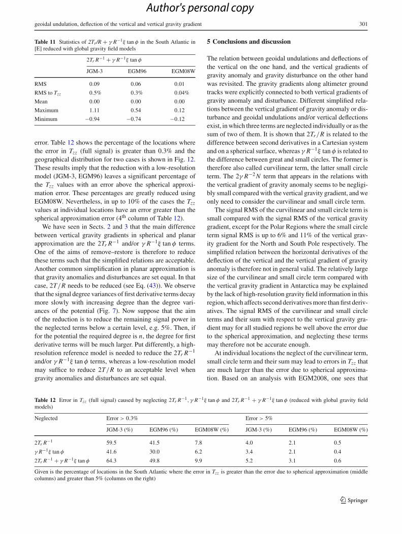
error. Table 12 shows the percentage of the locations wherethe error in Tzz (full signal) is greater than 0.3% and thegeographical distribution for two cases is shown in Fig. 12.These results imply that the reduction with a low-resolutionmodel (JGM-3, EGM96) leaves a significant percentage ofthe Tzz values with an error above the spherical approxi-mation error. These percentages are greatly reduced usingEGM08W. Nevertheless, in up to 10% of the cases the Tzz

values at individual locations have an error greater than thespherical approximation error (4th column of Table 12).

We have seen in Sects. 2 and 3 that the main differencebetween vertical gravity gradients in spherical and planarapproximation are the 2Tr R−1 and/or γ R−1ξ tan φ terms.One of the aims of remove–restore is therefore to reducethese terms such that the simplified relations are acceptable.Another common simplification in planar approximation isthat gravity anomalies and disturbances are set equal. In thatcase, 2T/R needs to be reduced (see Eq. (43)). We observethat the signal degree variances of first derivative terms decaymore slowly with increasing degree than the degree vari-ances of the potential (Fig. 7). Now suppose that the aimof the reduction is to reduce the remaining signal power inthe neglected terms below a certain level, e.g. 5%. Then, iffor the potential the required degree is n, the degree for firstderivative terms will be much larger. Put differently, a high-resolution reference model is needed to reduce the 2Tr R−1

and/or γ R−1ξ tan φ terms, whereas a low-resolution modelmay suffice to reduce 2T/R to an acceptable level whengravity anomalies and disturbances are set equal.

5 Conclusions and discussion

The relation between geoidal undulations and deflections ofthe vertical on the one hand, and the vertical gradients ofgravity anomaly and gravity disturbance on the other handwas revisited. The gravity gradients along altimeter groundtracks were explicitly connected to both vertical gradients ofgravity anomaly and disturbance. Different simplified rela-tions between the vertical gradient of gravity anomaly or dis-turbance and geoidal undulations and/or vertical deflectionsexist, in which three terms are neglected individually or as thesum of two of them. It is shown that 2Tr/R is related to thedifference between second derivatives in a Cartesian systemand on a spherical surface, whereas γ R−1ξ tan φ is related tothe difference between great and small circles. The former istherefore also called curvilinear term, the latter small circleterm. The 2γ R−2 N term that appears in the relations withthe vertical gradient of gravity anomaly seems to be negligi-bly small compared with the vertical gravity gradient, and weonly need to consider the curvilinear and small circle term.

The signal RMS of the curvilinear and small circle term issmall compared with the signal RMS of the vertical gravitygradient, except for the Polar Regions where the small circleterm signal RMS is up to 6% and 11% of the vertical grav-ity gradient for the North and South Pole respectively. Thesimplified relation between the horizontal derivatives of thedeflection of the vertical and the vertical gradient of gravityanomaly is therefore not in general valid. The relatively largesize of the curvilinear and small circle term compared withthe vertical gravity gradient in Antarctica may be explainedby the lack of high-resolution gravity field information in thisregion, which affects second derivatives more than first deriv-atives. The signal RMS of the curvilinear and small circleterms and their sum with respect to the vertical gravity gra-dient may for all studied regions be well above the error dueto the spherical approximation, and neglecting these termsmay therefore not be accurate enough.

At individual locations the neglect of the curvilinear term,small circle term and their sum may lead to errors in Tzz thatare much larger than the error due to spherical approxima-tion. Based on an analysis with EGM2008, one sees that

Table 12 Error in Tzz (full signal) caused by neglecting 2Tr R−1, γ R−1ξ tan φ and 2Tr R−1 + γ R−1ξ tan φ (reduced with global gravity fieldmodels)

Neglected Error > 0.3% Error > 5%

JGM-3 (%) EGM96 (%) EGM08W (%) JGM-3 (%) EGM96 (%) EGM08W (%)

2Tr R−1 59.5 41.5 7.8 4.0 2.1 0.5

γ R−1ξ tan φ 41.6 30.0 6.2 3.4 2.1 0.4

2Tr R−1 + γ R−1ξ tan φ 64.3 49.8 9.9 5.2 3.1 0.6

Given is the percentage of locations in the South Atlantic where the error in Tzz is greater than the error due to spherical approximation (middlecolumns) and greater than 5% (columns on the right)

123


302 J. Bouman

Fig. 12 Error in Tzz due to theneglect of 2Tr/R + γ R−1ξ tan φfor the South Atlantic afterreduction with EGM96 (upperpanel) and EGM08W (lowerpanel). White indicates that theerror is below 0.3%, blueindicates that the error isbetween 0.3 and 5.0%, redindicates that the error is greaterthan 5.0%

this is not only so for the Polar Regions (in 75–97% of thecases), where the small circle term is large, but also at inter-mediate and low latitudes, at the oceans (in 18–78% of thecases) and in mountainous areas (in 30–71% of the cases).A comparison of the curvilinear and small circle term withthe DOT induced gravity gradient signal shows that thesesignals have the same order of magnitude. All three signalsmay be well above the GOCE requirements and need to beaccounted for when combining GOCE and altimetry derivedgradients.

A reduction of the satellite altimeter data with a refer-ence geoid model decreases the signal RMS of the neglectedterms. However, as an example in the South Atlantic shows,it is only with a high-resolution model that the relative sig-nal RMS of the neglected terms becomes well below thespherical approximation error. Nevertheless, reduction with

a high-resolution model to minimize the effect of neglectingterms may at individual locations leave errors in Tzz that areabove the spherical approximation error (in up to 10% ofthe cases). When computing the vertical gradient of gravityanomaly using the horizontal derivatives of the deflectionsof the vertical the small circle term γ R−1ξ tan φ is readilyavailable and can be included. The direct computation of thevertical gradient of gravity disturbance from satellite altim-eter data is more difficult than the computation of the verti-cal gradient of gravity anomaly because in the former casethe curvilinear term is needed, which is not readily avail-able.

Acknowledgments I thank Taco Broerse for kindly providing the fig-ure on the gravity gradient signal after the Sumatra 2004 earthquake.This paper benefitted from the critical reviews by Roland Klees, ChrisJekeli and four anonymous referees.

123



Appendix: Abandoning the spherical approximation

The derivations in this paper are in spherical approximation,which should suffice to assess the size of the different sig-nals that are studied. Spherical approximation, however, maynot be sufficient using real data and the difference betweenthe normal directions of the sphere and ellipsoid needs to betaken into account.

Let the geodetic coordinates be (h, ϕ, λ)with h the heightabove the ellipsoid along the ellipsoidal normal and (ϕ, λ)geodetic latitude and longitude respectively. The for altim-etry relevant case with h = 0 is discussed here. Considerthe local ellipsoidal coordinate system (x, y, z) with thez-axis directed outwards, normal to the ellipsoid, the x-axis directed north, tangent to the ellipsoidal surface and they-axis directed west. This local Cartesian system differs fromthe LNOF (defined in Sect. 3) by a rotation around the y-axiswith angle ϕ − φ, where φ is the geocentric latitude. Thenorth-south gravity gradient Tx x expressed in geodetic coor-dinates at the surface of the ellipsoid is (Koop 1993)

Tx x = 1

MTh + 1

M2 Tϕϕ − 3e2 sin ϕ cosϕ

N M(1 − e2

) Tϕ (a)

with N = a(1 − e2 sin2 ϕ)−1/2,M = (1 − e2)N 3/a2, a isthe equatorial radius, and e is the first eccentricity. The east-west gravity gradient Ty y at the surface of the ellipsoid is

Ty y = 1

NTh + 1

N 2 cos2 ϕTλλ − tan ϕ

N MTϕ. (b)

Introducing the local coordinates du = Mdϕ and dv =N cosϕdλ one gets

Tx x = 1

MTh + Tuu − 3e2 sin ϕ cosϕ

N(1 − e2

) Tu

Ty y = 1

NTh + Tvv − tan ϕ

NTu (c)

where the multiplication factors in the first and last term onthe right of the north-south gravity gradient (c) are O(10−7)

and O(10−9), respectively.Evaluating the last term on the right of the north-south

gravity gradients (c) gave maximum amplitude of 3 mE and5 mE for the South West Pacific and South Atlantic respec-tively. Furthermore, we have seen that the terms with Th andTu are in general small with respect to the gravity gradientterms, and therefore spherical approximation for these termsis not as severe as for the gravity gradients themselves. Themaximum amplitude of the Th and Tu terms for the studiedareas in the South West Pacific and South Atlantic is approx-imately 1 E (Table 4), and a relative error of 0.3% thereforeleads to a maximum error of about 3 mE. Thus to this level

of approximation we have

Tx x = 1

RTr + Tuu

Ty y = 1

RTr + Tvv − tan ϕ

RTu (d)

and

− Tzz = Tx x + Ty y = 2

RTr − tan ϕ

RTu + Tuu + Tvv . (e)

This is, so to say, the ellipsoidal equivalent of Eqs. (8) and(21) with spherical approximations in the first derivativeterms. The last three terms on the ellipsoid in (e) can bedirectly derived from satellite altimeter data, and as for thespherical case, the Tr term cannot be directly computed.

References

Andersen O, Knudsen P, Berry P (2010) The DNSC08GRA globalmarine gravity field from double retracked satellite altimetry. JGeod 84:3. doi:10.1007/s00190-009-0355-9

Bouman J, Bosch W, Sebera J (2011a) Assessment of systematic errorsin the computation of gravity gradients from satellite altimeter data.Marine Geod 34:85–107. doi:10.1080/01490419.2010.518498

Bouman J, Fiorot S, Fuchs M, Gruber T, Schrama E, Tscherning CC,Veicherts M, Visser P (2011b) GOCE gravitational gradients alongthe orbit. J Geod. doi:10.1007/s00190-011-0464-0

Broerse DBT, Vermeersen LLA, Riva REM, van der Wal W (2011)Ocean contribution to co-seismic crustal deformation and geoidanomalies: application to the 2004 December 26 Sumatra-And-aman earthquake, Earth Planet. Sci. Lett. doi:10.1016/j.epsl.2011.03.011

ESA (1999) Gravity field and steady-state ocean circulation mission,Reports for mission selection; the four candidate earth explorercore missions, ESA SP-1233(1)

Förste C, Stubenvoll R, König R, Raimondo JC, Flechtner F, Barthel-mes F, Kusche J, Dahle C, Neumayer H, Biancale R, Lemoine JM,Bruinsma S (2009) Evaluation of EGM2008 by comparison withother recent global gravity field models. Newton’s Bull no 4, pp18–25

Gerstl M (2008) Computing the Earth gravity field with sphericalharmonics. In: Breitner MH, Denk G, Rentrop P (eds) Fromnano to space—applied mathematics inspired by Roland Bulirsch.Springer, Berlin pp 277–294

Han S, Shum C, Bevis M, Ji C, Kuo C (2006) Crustal dilation observedby GRACE after the 2004 Sumatra–Andaman earthquake. Science313(5787):658–662

Heiskanen WA, Moritz H (1967) Physical Geodesy. Freeman, San Fran-cisco

Hofmann-Wellenhof B, Moritz H (2005) Physical Geodesy. Springer,Berlin

Koop R (1993) Global gravity field modelling using satellite gravitygradiometry, Publications on geodesy, new series, no. 38, Nether-lands Geodetic Commission

Koop R, Stelpstra D (1989) On the computation of the gravitationalpotential and its first and second order derivatives. ManuscriptaGeodetica 14:373–382

Lemoine F, Kenyon S, Factor J, Trimmer R, Pavlis N, Chinn D, Cox C,Klosko S, Luthcke S, Torrence M, Wang Y, Williamson R, PavlisE, Rapp R, Olson T (1998) The Development of the Joint NASA

123


http://dx.doi.org/10.1007/s00190-009-0355-9

http://dx.doi.org/10.1080/01490419.2010.518498

http://dx.doi.org/10.1007/s00190-011-0464-0

http://dx.doi.org/10.1016/j.epsl.2011.03.011

http://dx.doi.org/10.1016/j.epsl.2011.03.011

304 J. Bouman

GSFC and National Imagery and Mapping Agency (NIMA) Geo-potential Model EGM96, NASA/TP-1998-206861

Pavlis N, Holmes S, Kenyon S, Factor J (2008) An Earth gravitationalmodel to degree 2160: EGM2008. Presented at the EGU GeneralAssembly 2008, Vienna, Austria

Rummel R, Haagmans R (1991) Gravity gradients from satellite altim-etry. Marine Geod 14:1–12

Sandwell DT, Smith WH (1997) Marine gravity anomaly from Geo-sat and ERS 1 satellite altimetry. J Geophys Res 102(B5):10039–10054

Sandwell DT, Smith WH (2009) Global marine gravity from retrackedGeosat and ERS-1 altimetry: Ridge segmentation versus spreadingrate. J Geophys Res 114:B01411. doi:10.1029/2008JB006008

Sokolnikoff I (1964) Tensor Analysis; Theory and Applications toGeometry and Mechanics of Continua. 2. Wiley, New York

Tapley B, Watkins M, Ries J, Davis G, Eanes R, Poole S, Rim H, SchutzB, Shum CK, Nerem RS, Lerch F, Marshall JA, Klosko S, PavlisN, Williamson R (1996) The joint gravity Model 3. J Geophys Res101(B12):28029–28049

123


http://dx.doi.org/10.1029/2008JB006008

Relation between geoidal undulation, deflection of the vertical and vertical gravity gradient revisited

Documents